TheAlgorithmicAutomationProblem: Prediction,Triage,and … › pdf › 1903.12220.pdf · 2019-04-01 · Maithra Raghu1; 2Katy Blumer Greg Corrado Jon Kleinberg1 Ziad Obermeyer3;4

The Algorithmic Automation Problem: Prediction, Triage, andHuman Effort

Maithra Raghu1,2∗ Katy Blumer2 Greg Corrado2Jon Kleinberg1 Ziad Obermeyer3,4 Sendhil Mullainathan5

1 Department of Computer Science, Cornell University2 Google Brain

3 UC Berkeley School of Public Health4 Center for Clinical Data Science, MGH

5 Chicago Booth School of Business

AbstractIn a wide array of areas, algorithms are matching and surpassing the performance of human experts,

leading to consideration of the roles of human judgment and algorithmic prediction in these domains.The discussion around these developments, however, has implicitly equated the specific task of predictionwith the general task of automation. We argue here that automation is broader than just a comparison ofhuman versus algorithmic performance on a task; it also involves the decision of which instances of thetask to give to the algorithm in the first place. We develop a general framework that poses this latterdecision as an optimization problem, and we show how basic heuristics for this optimization problem canlead to performance gains even on heavily-studied applications of AI in medicine. Our framework alsoserves to highlight how effective automation depends crucially on estimating both algorithmic and humanerror on an instance-by-instance basis, and our results show how improvements in these error estimationproblems can yield significant gains for automation as well.

1 IntroductionOn a variety of high-stakes tasks, machine learning algorithms are on the threshold of doing what humanexperts do with such high fidelity that we are contemplating using their predictions as a substitute for humanoutput. For example, convolutional neural networks are close to diagnosing pneumonia from chest X-raysbetter than radiologists can [14, 15]; examples like these underpin much of the widespread discussion ofalgorithmic automation in these tasks.

In assessing the potential for algorithms, however, the community has implicitly equated the specific taskof prediction with the general task of automation. We argue here that this implicit correspondence misses keyaspects of the automation problem; a broader conceptualization of automation can lead directly to concretebenefits in some of the key application areas where this process is unfolding.

We start from the premise that automation is more than just the replacement of human effort on a task; itis also the meta-decision of which instances of the task to automate. And it is here that algorithms distinguishthemselves from earlier technology used for automation, because they can actively take part in this decisionof what to automate. But as currently constructed, they are not set up to help with this second part of theproblem. The automation problem, then, should involve an algorithm that on any given instance both (i)produces a prediction output; and (ii) additionally also produces a triage judgment of its effectiveness relativeto the human effort it would replace on that instance.

∗Correspondence to [email protected]

1

arX

iv:1

903.

1222

0v1

[cs

.CV

] 2

8 M

ar 2

019

Viewed in this light, machine learning algorithms as currently constructed only solve the first problem;they do not pose or solve the second problem. In effect, currently when we contemplate automation usingthese algorithms, we are implicitly assuming that we will automate all instances or none. In this paper, weargue that when algorithms are built to solve both problems – prediction and triage – overall performance issignificantly higher. In fact, even on tasks where the algorithm significantly outperforms humans on averageper instance, the optimal solution is to automate only a fraction of the instances and to optimally divide upthe available human effort on the remaining ones. And correspondingly, even on tasks where an algorithmdoes not beat human experts, the optimal solution may still be to automate a subset of instances.

Now is the right time to ask these questions because the AI community is on the verge of translatingsome of its most successful algorithms into clinical practice. Notably, an influential line of work showedhow a well-constructed convolutional net trained on gold-standard consensus labels for diagnosing diabeticretinopathy (DR) outperforms ophthalmologists in aggregate, and these results have led to considerableoptimism about the role of algorithms in this setting [15]. But the community’s discussion around theseprospects has focused on the algorithms’ per-instance prediction performance without considering the problemof recognizing which instances to automate.

Using largely the same data, we build this additional, crucial component and find that, even in thiscontext where an algorithm outperforms human experts in the aggregate, the optimal level of triage is notfull automation. Instead significantly more accuracy can be had by triaging a fraction of the instances to thealgorithm and leaving the remaining fraction to the human experts. Specifically, full automation reduces theerror rate from roughly 5.5% by human doctors to 4% with an algorithm solving every instance; automationwith optimal triage, though, reduces the error further to roughly 3.5% – effectively adding a significant furtherfraction to the gains that were realized by algorithmically automating the task in the first place.

This gain occurs for two reasons: first the algorithm’s high average performance hides significant hetero-geneity in performance. For example, on roughly 40% of the instances the algorithm has zero errors. By thesame token, on a small set of instances, the algorithm makes far more errors than average and these instancescan be assigned to humans. Second, when the algorithm automates a fraction of the cases, that frees uphuman effort; reallocating that effort to the remaining cases can achieve further gains. In principle thesegains could come from a single doctor spending additional time on the instance, or from multiple doctorslooking at it; in our case, the available data allows us to explicitly quantify the gains arising from the secondof these effects, due to the fact that we have multiple doctor judgments on each instance.

These results empirically demonstrate the importance of the triage component for the automation problem.We show that the gains we demonstrate are unlikely to have fully tapped the potential gains to be hadthrough algorithmic triage: this neglected component deserves the kind of sustained effort from the machinelearning community that the prediction component has received to date. In fact, given the disparity in effortson these two problems, it is possible that the highest return to improving automation performance is throughsolving triage rather than further improving prediction.

2 General FrameworkIn a typical application where we consider using algorithmic effort in place of human effort, the goal is tolabel a set of instances of the problem with a positive or a negative label. For example, in a medical diagnosissetting, we may have a set of medical images, and the goal is to label each with a binary yes/no diagnosis.Let x be an instance of the labeling problem, and let a(x) be its ground truth value. For our purposes (as inthe example of a binary diagnosis), we will think of this ground truth value as taking a value of either 0 or 1,with a(x) = 0 corresponding to a negative label and a(x) = 1 corresponding to a positive label.

How do we approach this problem algorithmically? Given a set U of instances, we could train an algorithmto produce a numerical estimate m(x) ∈ [0, 1] with the goal of minimizing a loss function

∑x∈U L(a(x),m(x)),

where L(·, ·) increases with the distance between its two inputs. For notational convenience, we will writeg(x) for L(a(x),m(x)), the algorithmic error on instance x. The m(x) values are then converted into (binary)predictions, and we can evaluate the resulting error relative to ground truth. As a concrete example, oneoption is to threshold the m(x) to produce a 0 or 1 value, and evaluate agreement with a(x).

2

When a social planner considers the prospect of introducing algorithms into an existing task, we oftenimagine the question to be the following. The planner currently has human effort being devoted to instancesof the task; for an instance x ∈ U , we can imagine that there is a human output h(x), resulting in a lossf(x) = L(a(x), h(x)). The question of whether to automate the task could then be viewed as a comparisonbetween

∑x∈U g(x) and

∑x∈U f(x) — the loss from algorithmic effort relative to the loss from human effort.

Allocating Human Effort In order to think about the activity of automation in a richer sense, it is usefulto start from the realization that even in the absence of algorithms, the social planner is implicitly workingwith a larger space of choices than the simple picture above suggests. In particular, they have some availablebudget of total human effort, and they do not need to allocate it uniformly across instances: for an instancex, the planner can allocate k units of human effort for different possible values of k. There are multiplepossible interpretations for the meaning of k; for example, in the case of diagnosis we could think of k ascorresponding to the number of distinct doctors who look at the instance, or alternately to the total amountof time spent collectively by doctors on the instance. Thus, our functions h and f should more properlybe written as two-variable functions that take an instance x and a level of effort k: we say that h(x, k) isthe label provided as a result of k units of human effort on instance x, and f(x, k) = L(a(x), h(x, k)) is theresulting loss that we would like to minimize.

Note that as functions of effort k, it may be that f(x, k) and f(x′, k) are quite different for differentinstances x and x′. For example, instance x may be much harder than instance x′, and hence f(x, k) will bemuch larger than f(x′, k); similarly, instance x might not exhibit as much marginal benefit from additionaleffort as instance x′, and hence the growth of f(x, k) over increasing values of k might be much flatter thanthe growth of f(x′, k). The social planner might well not have precise quantitative estimates for values likef(x, k), but implicitly they are seeking to allocate human effort across the set of instances U so as to minimizethe total loss incurred. And indeed, a number of basic protocols — such as asking for second opinions —can be viewed as increasing the amount of effort spent on instances where there might be benefits for errorreduction.

2.1 Automation involving Algorithms and HumansWhen algorithms are introduced, the social planner has several new considerations to take into account. First,the full automation problem should be viewed more broadly than just a binary comparison of human andalgorithmic performance; it can involve decisions about the allocation of both human and algorithmic effort.The introduction of the algorithm need not be all-or-nothing: we can choose to apply it to some instances ina way that replaces human effort, thereby potentially freeing up this effort to be used on other instances. Theaverage overall comparison might even hide instances where the algorithm much more significantly under- (orout-) performs the human. Second, decisions about the allocation of human effort depend on the functionf(x, k), which can be challenging to reason about. Algorithms can potentially provide assistance in estimatingthese quantities f(x, k) to help even in the allocation of human effort.

The general problem can therefore be viewed as follows. We would like to select a subset S of instanceson which no human effort will be used (only the algorithm), and we will then optimally allocate human efforton the remaining instances T = U − S. Suppose that we have a budget B on the total number of units ofhuman effort that we can allocate, and we decide to allocate kx units of effort to each instance x ∈ T . Onsuch an instance x, we incur a loss of f(x, kx), using our notation above; and on the instances x ∈ S we incura loss of g(x) from the algorithmic prediction.

We thus have the following optimization problem.

Min∑x∈S

g(x) +∑x∈T

f(x, kx) (1)

subject to∑x∈T

kx ≤ B (2)

S ∪ T = U ; S ∩ T = φ (3)

3

Our earlier discussions about algorithms and humans in isolation are special cases of this optimizationproblem: full automation, when the algorithm substitutes completely for human effort, is the case in whichS = U ; and the social planner’s problem in the absence of an algorithm — which still involves decisions aboutthe effort variables kx — is the case in which T = U . Intermediate solutions can be viewed as performing akind of triage, a term we use here in a general sense for a process in which some instances go purely to analgorithm and others receive human attention.

By deliberately adopting a very general formulation, we can also get a clearer picture of the kinds ofinformation we would need in order to perform automation more effectively. Specifically,

(i) In addition to making algorithmic predictions m(x), the automation problem benefits from moreaccurate estimates of the algorithm’s instance-specific error rate g(x).

(ii) The allocation of human effort benefits from better models of human error rate, including error as afunction of effort spent f(x, k). As noted above, we can use an algorithm to help in estimating thishuman error rate.

(iii) Given estimates for the functions f and g, we can obtain further performance improvements purelythrough better allocations of human effort in the optimization problem (1).

We note that the notion of human error involves an additional set of complex design choices, which is howhumans decide to make use of algorithmic assistance on the instances (in the set T ) where they spend effort.In particular, if we imagine that algorithmic predictions are available on the instances in T , then the humansinvolved in the decision on x ∈ T may have the ability to incorporate the algorithmic prediction m(x) intotheir overall output h(x, kx), and this will have an effect on the error rate f(x, kx). In general, of course,it will be difficult to model a priori how this synthesis will work, although it is a very interesting question;we show that our results for the automation problem do not require assumptions about this aspect of theprocess, but we explore this question later in the paper.

2.2 Heuristics for AutomationIf we think of the social planner as the entity tasked with solving the automation problem in (1), they are nowfaced with a set of considerations: not simply the binary question of whether to use human or algorithmiceffort, but instead how to divide the instances between those (in S) that will be fully automated and those(in T ) that will involve human effort, and how to estimate the error rates g(x) and f(x, k) so as to solve theallocation problem effectively.

We will show that significant performance gains can be achieved over both algorithmic and human efforteven if we use only very simple heuristics for the different components of the allocation problem. Moreover,through a stronger benchmark based on ground truth, we will also show that much stronger gains are inprinciple achievable with improved approaches to the components.

We can describe the simplest level of heuristics in terms of sub-problems (i), (ii), and (iii) from earlier inthis section. The simplest heuristic for (i) is to use the functional form of the variance, m(x)(1−m(x)) as ameasure of the algorithm’s uncertainty in its prediction on x. A comparably natural predictor does not existfor (ii). We therefore design new algorithmic predictors to estimate the values of both (i) and (ii), and usethese to guide the allocation of algorithmic and human effort. We show that using separate predictors inthis way also strengthens the performance gains relative to the simpler heuristic based on m(x)(1−m(x)),although even this basic heuristic yields improvements over full automation.

Given these predictors for (i) and (ii), what does this suggest about simple strategies for approximating(iii), the allocation of human effort? First, we could restrict attention to solutions in which each instancein T receives the same amount of effort. Thus, if there are N total instances in U , we could choose a realnumber α ∈ [0, 1], perform full automation on a set S of αN instances, and divide the B units of humaneffort evenly across the remaining β = 1 − α fraction of the instances. This means that each instance inthe set receiving human effort gets B/βN units of effort. For simplicity, let us write B = cN , so that thehuman effort per instance in this remaining set is c/β. With this allocation of effort, the resulting loss is∑x∈S g(x) +

∑x∈T f(x, c/β).

4

This restriction on the set of possible solutions suggests the following heuristic. Consider any partitionof the instances into S and T , and suppose we use the algorithm on all the instances. Then we can writethe resulting loss in the following convenient way:

∑x∈S g(x) +

∑x∈T g(x). Subtracting from the loss

that results when we assign c/β units of human effort to each instance in T , we see that the difference is∑x∈T [f(x, c/β)− g(x)].Thus, for a given value of α (specifying the fraction of instances that we wish to assign to the algorithm),

it is sufficient to rank all instances x ∈ U by τα(x) = f(x, c/β) − g(x), and then choose the αN instanceswith the largest values of τα to put in the set S that we give to the algorithm. We can thus think of τα(x) asthe triage score of instance x, since it tells us the effect of algorithmic triage relative to human effort on theexpected error.

2.3 Overview of ResultsWe put these ideas together in the context of a widely studied medical application, concerned with thediagnosis of diabetic retinopathy, detailed in the next section. We rank instances by their triage score, usingsimple forms for the algorithmic loss g(x) and human loss f(x, c/β), and we then search over possible valuesof α, evaluating the performance at each. We find that there is range of values of α, and a way of choosingαN instances to give to the algorithm, so that the resulting performance exceeds either of the binary choicesof fully assigning the instances to the algorithm or to human effort.

As a scoping exercise, to see how strong the possible gains from our automation approach might be, weconsider what would happen if we ranked instances by a triage score derived from a ground-truth estimateof the individual human error on each instance. Such a benchmark indicates the power of the optimizationframework if we are able to get better approximations to the key quantities of interest — the functions f andg. We find large performance gains from this benchmark, and we also explore some stronger methods to workon closing the gap between our simple heuristics and this ideal.

Different Costs for Error. In many settings, a social planner may associate higher costs to errorscommitted by automated methods relative to errors committed by humans — for example, there may beconcern about the difficulty in identifying and correcting errors through automation, or the end users ofthe results may have a preference for human output. It is natural, therefore, to consider a version of theoptimization problem in which the objective (1) has an additional parameter λ specifying the relative cost oferror between algorithms and humans. This new objective function is

λ∑x∈S

g(x) +∑x∈T

f(x, kx). (4)

One might suppose that as λ grows large, the social planner would tend to favor purely human effort,given the relative cost of errors from automation. And indeed, the basic comparison that is typically madebetween

∑x∈U g(x) (for full automation) and

∑x∈U f(x, kx) (for purely human effort) would suggest that

this should be the case, since eventually λ will exceed the ratio between these two quantities. But ourmore detailed framework makes clear that these aggregate measures of performance can obscure large levelsof variability in difficulty across instances. And what we find in our application is that it is possible forthe algorithm to identify a large set of instances S on which it makes zero errors. Thus, even with strongpreferences for human effort over algorithmic effort, it may still be possible to find sizeable subsets of theproblem that should nevertheless be automated — a fact that is hidden by comparisons based purely onaggregate measures of performance.

3 Medical Preliminaries, Data and Experimental SetupWe first outline the details of the medical prediction problems, and describe the data and experimental setupused to design the automated decision making algorithm. As our primary goal is to study the interaction of

5

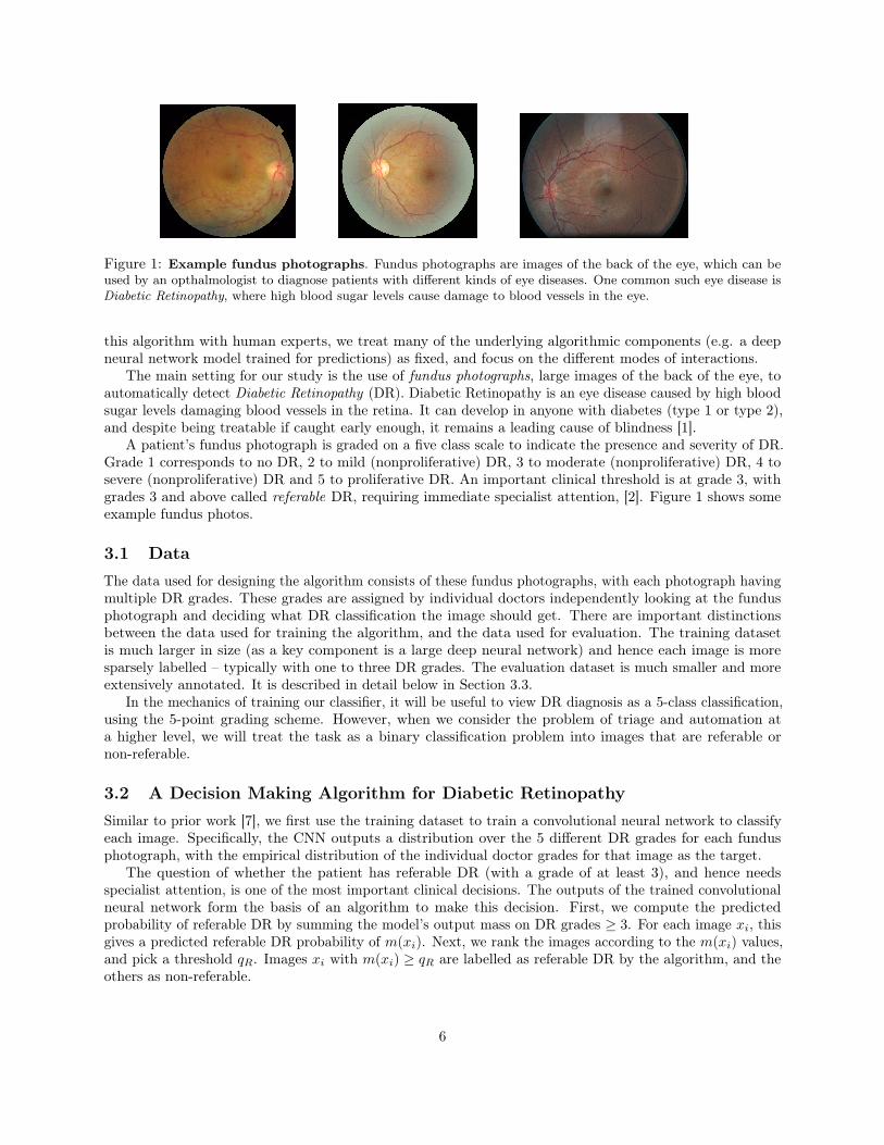
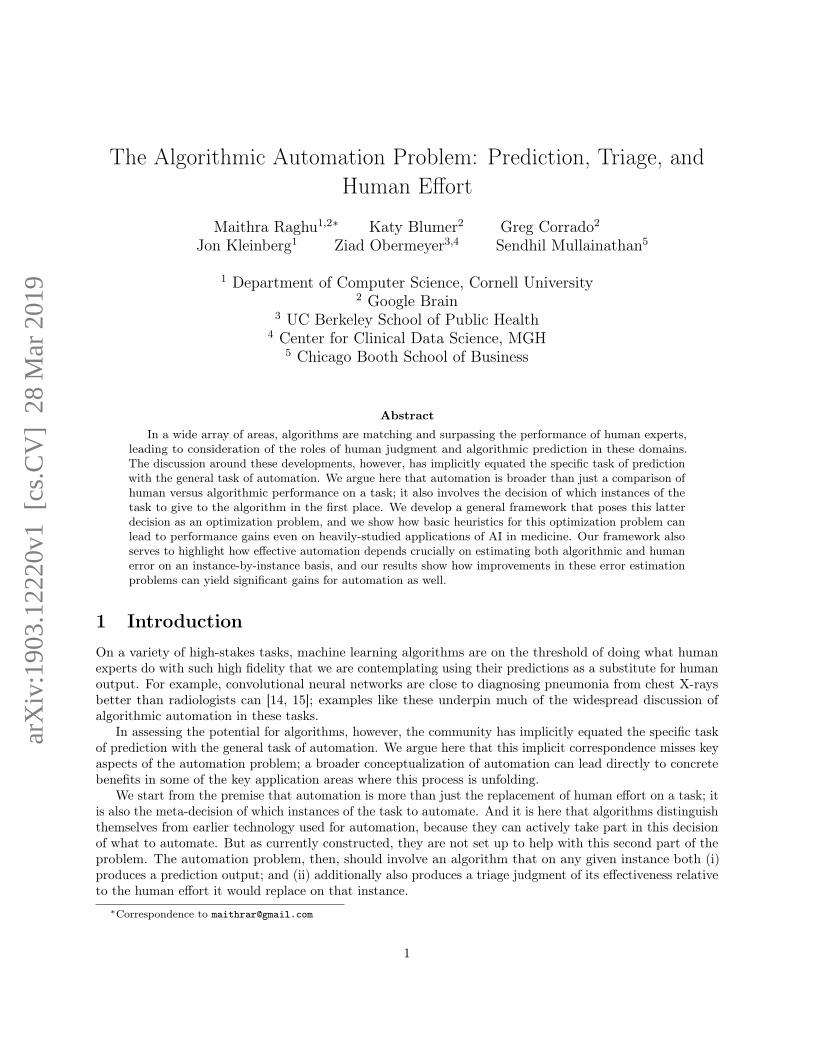
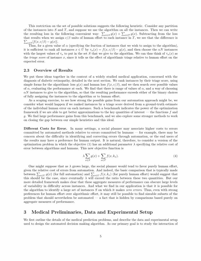
Figure 1: Example fundus photographs. Fundus photographs are images of the back of the eye, which can beused by an opthalmologist to diagnose patients with different kinds of eye diseases. One common such eye disease isDiabetic Retinopathy, where high blood sugar levels cause damage to blood vessels in the eye.

this algorithm with human experts, we treat many of the underlying algorithmic components (e.g. a deepneural network model trained for predictions) as fixed, and focus on the different modes of interactions.

The main setting for our study is the use of fundus photographs, large images of the back of the eye, toautomatically detect Diabetic Retinopathy (DR). Diabetic Retinopathy is an eye disease caused by high bloodsugar levels damaging blood vessels in the retina. It can develop in anyone with diabetes (type 1 or type 2),and despite being treatable if caught early enough, it remains a leading cause of blindness [1].

A patient’s fundus photograph is graded on a five class scale to indicate the presence and severity of DR.Grade 1 corresponds to no DR, 2 to mild (nonproliferative) DR, 3 to moderate (nonproliferative) DR, 4 tosevere (nonproliferative) DR and 5 to proliferative DR. An important clinical threshold is at grade 3, withgrades 3 and above called referable DR, requiring immediate specialist attention, [2]. Figure 1 shows someexample fundus photos.

3.1 DataThe data used for designing the algorithm consists of these fundus photographs, with each photograph havingmultiple DR grades. These grades are assigned by individual doctors independently looking at the fundusphotograph and deciding what DR classification the image should get. There are important distinctionsbetween the data used for training the algorithm, and the data used for evaluation. The training datasetis much larger in size (as a key component is a large deep neural network) and hence each image is moresparsely labelled – typically with one to three DR grades. The evaluation dataset is much smaller and moreextensively annotated. It is described in detail below in Section 3.3.

In the mechanics of training our classifier, it will be useful to view DR diagnosis as a 5-class classification,using the 5-point grading scheme. However, when we consider the problem of triage and automation ata higher level, we will treat the task as a binary classification problem into images that are referable ornon-referable.

3.2 A Decision Making Algorithm for Diabetic RetinopathySimilar to prior work [7], we first use the training dataset to train a convolutional neural network to classifyeach image. Specifically, the CNN outputs a distribution over the 5 different DR grades for each fundusphotograph, with the empirical distribution of the individual doctor grades for that image as the target.

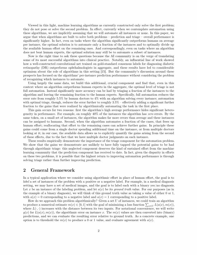
The question of whether the patient has referable DR (with a grade of at least 3), and hence needsspecialist attention, is one of the most important clinical decisions. The outputs of the trained convolutionalneural network form the basis of an algorithm to make this decision. First, we compute the predictedprobability of referable DR by summing the model’s output mass on DR grades ≥ 3. For each image xi, thisgives a predicted referable DR probability of m(xi). Next, we rank the images according to the m(xi) values,and pick a threshold qR. Images xi with m(xi) ≥ qR are labelled as referable DR by the algorithm, and theothers as non-referable.

6

Convolutional Neural Network

for 5-class

Classification of Diabetic

Retinopathy

Postprocess

m(xi) ≥ qR

o1

o2

o3

o4

o5

o3+ o4+ o5= m(xi)

Output

0 or 1

Input xi

Figure 2: Diagram of Algorithm for Diagnosing Diabetic Retinopathy (DR). The algorithm takes as inputa fundus photograph, which, with doctor grades as targets, is used to train a convolutional neural network to perform5 class classification of DR. For evaluation on an image i the output values of the convolutional neural networkon grades ≥ 3, o3, o4, o5, are summed to give m(xi), the total output mass on a referable diagnosis. m(xi) is thenthresholded with qR – the threshold for a referable diagnosis. This binary decision is output by the algorithm.

The choice of the threshold qR is made so that the total number of cases marked as referable by thealgorithm matches the total number of cases marked as referable when aggregating the human doctor grades.This ensures that the effort, resources, and expense needed to act upon the algorithmic decisions match thecurrent (feasible) effort resulting from the human decision making process. This is discussed in further detailin Section 3.4

The result of this process is an algorithm taking as input a patient’s fundus photograph, and outputting abinary 0/1 decision on whether the patient has non-referable/referable Diabetic Retinopathy. We illustratethe components of the DR algorithm in Figure 2. The full details of our algorithm development setup can befound in Appendix Section A.

3.3 EvaluationWe evaluate our decision-making algorithm on a special, gold-standard adjudicated dataset [10]. This datasetis much smaller than our training data, but is meticulously labelled. For every fundus photograph in thedataset, there are many individual doctor grades, and also a single adjudicated grade, given after multipledoctors discuss the appropriate diagnosis for the image. This adjudicated grade acts as a proxy for theground truth condition, and we use it to evaluate both the individual human doctors and the decision makingalgorithm. In Appendix Section E we carry out an additional evaluation of the methods on a different dataset,which exhibits the same results.

3.4 Aggregation and ThresholdingDuring evaluation and the triage process, we often have multiple (binary) grades per image. These gradesmight correspond to multiple different human doctors individually diagnosing the image, or the algorithm’sbinary decision along with human doctor grades. In all of these cases, for evaluation, we must typicallyaggregate these multiple grades into a concrete decision – a single summary binary grade. To do so, wecompute the mean grade and threshold by a value R. If the mean is greater than R, this corresponds to adecision of 1 (referable); otherwise the decision is 0 (non-referable).

The choice of the threshold R also affects the choice of qR which is used for the algorithm’s decision. Tocompute qR, we first aggregate the multiple doctor grades per image into a single grade by computing their

7

1.0 0.8 0.6 0.4 0.2 0.0 0.2 0.4 0.6 0.8(D Err - M Err)

10-3

10-2

10-1

100

Pro

port

ion o

f Im

ages

Log S

cale

Algorithm and Doctor Error Difference Log Scale

D Err = M Err

D Err < M Err

D Err > M Err

1.0 0.8 0.6 0.4 0.2 0.0 0.2 0.4 0.6 0.8(D Err - M Err)

0.00

0.01

0.02

0.03

0.04

0.05

0.06

0.07

0.08

Pro

port

ion o

f Im

ages

Algorithm and Doctor Error Difference

D Err < M Err

D Err > M Err

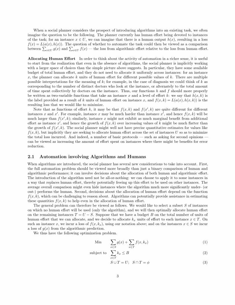
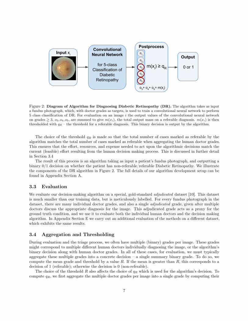
Figure 3: Histogram plot of Pr [Hi] − Pr [Mi] for instances i in the adjudicated evaluation dataset. Weshow a histogram of probability of human doctor error minus probability of model error over the examples in theadjudicated dataset. The orange bars correspond to examples where the human expert has a lower probability of errorthan the algorithm, the red where the probability of error is approximately equal, and the blue where the algorithm’sprobability of error is lower than the human expert’s. The left pane is a log plot, and the right is standard scaling(pictured without the red bar.) While the algorithm clearly has lower error probability than the human in more cases,there is a nontrivial mass ( 5%) where the human experts have lower error probability than the model.

mean and thresholding with R. This gives us the total number of patients marked as referable by the humandoctors, and we pick qR so that the algorithm matches this number.

In the main text, we give results for R = 0.5, which corresponds to the majority vote of the multiplegrades for an image. In the Appendix, we include results for R = 0.3, 0.4, which support the same conclusions.

4 The Triage Problem and Human Effort ReallocationThe performance of human experts and algorithmic decisions are typically summarized and compared via asingle number, such as average error, F1 score, or AUC. Seeing the algorithm outperform human expertsaccording to these metrics might suggest the hypothesis that the algorithm uniformly outperforms humanexperts on any given instance.

What we find instead, however, is significant diversity across instances in the performance of humans andalgorithms: for natural definitions of human and algorithmic error probability (formalized below), there areinstances in which human effort has lower error probability than the algorithm, and instances in which thealgorithm has lower error probability than human effort. Moreover, this diversity is partially predictable: wecan identify with non-trivial accuracy those instances on which one entity or the other will do better. Thisdiversity and its predictability is an important component of the automation framework, since it makes itpossible to divide instances between algorithms and humans so that each party is working on those instancesthat are best suited to it.

We first study this performance diversity, and then move on to the problem of allocating effort betweenhumans and algorithms across instances.

4.1 Per Instance Error Diversity of Humans and AlgorithmsIn order to look at the differences in performance between humans and algorithms on an instance-by-instancelevel, we want to define, for each instance xi in the adjudicated dataset, an error probability Pr [Hi] for thedoctors (human experts) and an error probability Pr [Mi] for the algorithm.

8

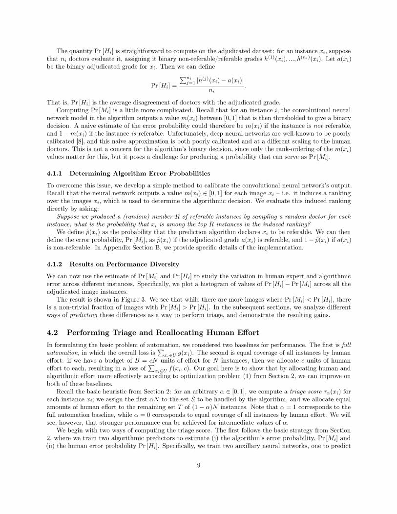
The quantity Pr [Hi] is straightforward to compute on the adjudicated dataset: for an instance xi, supposethat ni doctors evaluate it, assigning it binary non-referable/referable grades h(1)(xi), ..., h(ni)(xi). Let a(xi)be the binary adjudicated grade for xi. Then we can define

Pr [Hi] =

∑ni

j=1 |h(j)(xi)− a(xi)|ni

.

That is, Pr [Hi] is the average disagreement of doctors with the adjudicated grade.Computing Pr [Mi] is a little more complicated. Recall that for an instance i, the convolutional neural

network model in the algorithm outputs a value m(xi) between [0, 1] that is then thresholded to give a binarydecision. A naive estimate of the error probability could therefore be m(xi) if the instance is not referable,and 1−m(xi) if the instance is referable. Unfortunately, deep neural networks are well-known to be poorlycalibrated [8], and this naive approximation is both poorly calibrated and at a different scaling to the humandoctors. This is not a concern for the algorithm’s binary decision, since only the rank-ordering of the m(xi)values matter for this, but it poses a challenge for producing a probability that can serve as Pr [Mi].

4.1.1 Determining Algorithm Error Probabilities

To overcome this issue, we develop a simple method to calibrate the convolutional neural network’s output.Recall that the neural network outputs a value m(xi) ∈ [0, 1] for each image xi – i.e. it induces a rankingover the images xi, which is used to determine the algorithmic decision. We evaluate this induced rankingdirectly by asking:

Suppose we produced a (random) number R of referable instances by sampling a random doctor for eachinstance, what is the probability that xi is among the top R instances in the induced ranking?

We define p̃(xi) as the probability that the prediction algorithm declares xi to be referable. We can thendefine the error probability, Pr [Mi], as p̃(xi) if the adjudicated grade a(xi) is referable, and 1− p̃(xi) if a(xi)is non-referable. In Appendix Section B, we provide specific details of the implementation.

4.1.2 Results on Performance Diversity

We can now use the estimate of Pr [Mi] and Pr [Hi] to study the variation in human expert and algorithmicerror across different instances. Specifically, we plot a histogram of values of Pr [Hi]− Pr [Mi] across all theadjudicated image instances.

The result is shown in Figure 3. We see that while there are more images where Pr [Mi] < Pr [Hi], thereis a non-trivial fraction of images with Pr [Mi] > Pr [Hi]. In the subsequent sections, we analyze differentways of predicting these differences as a way to perform triage, and demonstrate the resulting gains.

4.2 Performing Triage and Reallocating Human EffortIn formulating the basic problem of automation, we considered two baselines for performance. The first is fullautomation, in which the overall loss is

∑xi∈U g(xi). The second is equal coverage of all instances by human

effort: if we have a budget of B = cN units of effort for N instances, then we allocate c units of humaneffort to each, resulting in a loss of

∑xi∈U f(xi, c). Our goal here is to show that by allocating human and

algorithmic effort more effectively according to optimization problem (1) from Section 2, we can improve onboth of these baselines.

Recall the basic heuristic from Section 2: for an arbitrary α ∈ [0, 1], we compute a triage score τα(xi) foreach instance xi; we assign the first αN to the set S to be handled by the algorithm, and we allocate equalamounts of human effort to the remaining set T of (1− α)N instances. Note that α = 1 corresponds to thefull automation baseline, while α = 0 corresponds to equal coverage of all instances by human effort. We willsee, however, that stronger performance can be achieved for intermediate values of α.

We begin with two ways of computing the triage score. The first follows the basic strategy from Section2, where we train two algorithmic predictors to estimate (i) the algorithm’s error probability, Pr [Mi] and(ii) the human error probability Pr [Hi]. Specifically, we train two auxillary neural networks, one to predict

9

Pr [Hi] and one to predict Pr [Mi]. To predict Pr [Hi], we build off of the work of [13] on direct prediction ofdoctor disagreement: we label each example with a 0 if there is agreement amongst the doctor grades, and 1otherwise, and train a small neural network to predict these agreement labels from the image embedding.A similar setup is employed for predicting Pr [Mi], where the binary label now corresponds to whether theoutput of the diagnostic 5-class convolutional neural network agrees with the doctor grades – i.e. does themodel make an error on that image. The full details of this process are described in Appendix B.

The second method of computing a triage score establishes an “ideal” benchmark on the potential powerof the optimization problem (1) using aspects of ground truth, sorting the instances by the true value ofPr [Hi] − Pr [Mi], since this divides the instances between humans and algorithms based on the relativestrength of each party on the respective instances.

In both cases, we determine the performance of the human effort using the average of a correspondingnumber of randomly sampled doctor grades from the data. This allows us to demonstrate improvementswithout any assumptions on how the doctors might use information from the algorithmic predictions on theseinstances. It is also reasonable, however, to imagine a scenario in which the algorithmic predictions are stillfreely available even on the instances that we assign to the human doctors, and to consider simple models forhow the doctor grades might be combined with these algorithmic predictions. We consider this case in theAppendix, which supports the same conclusions.

4.2.1 Triage Results

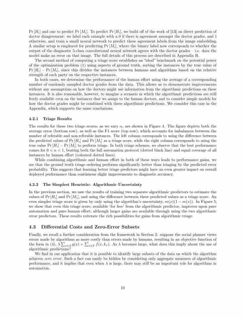
The results for these two triage scores, as we vary α, are shown in Figure 4. The figure depicts both theaverage error (bottom row), as well as the F1 score (top row), which accounts for imbalances between thenumber of referable and non-referable instances. The left column corresponds to using the difference betweenthe predicted values of Pr [Hi] and Pr [Mi] as a triage score, while the right column corresponds to using thetrue value Pr [Hi]− Pr [Mi] to perform triage. In both triage schemes, we observe that the best performancecomes for 0 < α < 1, beating both the full automation protocol (dotted black line) and equal coverage of allinstances by human effort (coloured dotted lines).

While combining algorithmic and human effort in both of these ways leads to performance gains, wesee that the ground truth triage ordering performs significantly better than triaging by the predicted errorprobability. This suggests that learning better triage predictors might have an even greater impact on overalldeployed performance than continuous slight improvements to diagnostic accuracy.

4.2.2 The Simplest Heuristic: Algorithmic Uncertainty

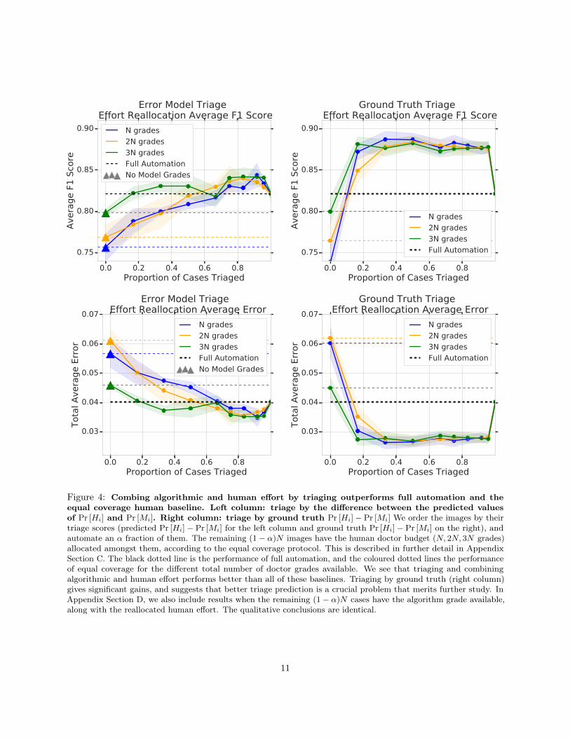
In the previous section, we saw the results of training two separate algorithmic predictors to estimate thevalues of Pr [Hi] and Pr [Mi], and using the difference between these predicted values as a triage score. Aneven simpler triage score is given by only using the algorithm’s uncertainty, m(x)(1−m(x)). In Figure 5,we show that even this triage score, available ‘for free’ from the algorithmic predictor, improves upon pureautomation and pure human effort, although larger gains are available through using the two algorithmicerror predictors. These results reiterate the rich possibilities for gains from algorithmic triage.

4.3 Differential Costs and Zero-Error SubsetsFinally, we recall a further consideration from the framework in Section 2: suppose the social planner viewserrors made by algorithms as more costly than errors made by humans, resulting in an objective function ofthe form in (4), λ

∑x∈S g(x) +

∑x∈T f(x, kx). As λ becomes large, what does this imply about the use of

algorithmic predictions?We find in our application that it is possible to identify large subsets of the data on which the algorithm

achieves zero error. Such a fact can easily be hidden by considering only aggregate measures of algorithmicperformance, and it implies that even when λ is large, there may still be an important role for algorithms inautomation.

10

0.0 0.2 0.4 0.6 0.8Proportion of Cases Triaged

0.75

0.80

0.85

0.90

Avera

ge F

1 S

core

Error Model Triage Effort Reallocation Average F1 Score

N grades

2N grades

3N grades

Full Automation

No Model Grades


0.75

0.80

0.85

0.90

Avera

ge F

1 S

core

Ground Truth Triage Effort Reallocation Average F1 Score

N grades

2N grades

3N grades

Full Automation


0.03

0.04

0.05

0.06

0.07

Tota

l A

vera

ge E

rror

Error Model Triage Effort Reallocation Average Error

N grades

2N grades

3N grades

Full Automation

No Model Grades


0.03

0.04

0.05

0.06

0.07

Tota

l A

vera

ge E

rror

Ground Truth Triage Effort Reallocation Average Error

N grades

2N grades

3N grades

Full Automation

Figure 4: Combing algorithmic and human effort by triaging outperforms full automation and theequal coverage human baseline. Left column: triage by the difference between the predicted valuesof Pr [Hi] and Pr [Mi]. Right column: triage by ground truth Pr [Hi]− Pr [Mi] We order the images by theirtriage scores (predicted Pr [Hi]− Pr [Mi] for the left column and ground truth Pr [Hi]− Pr [Mi] on the right), andautomate an α fraction of them. The remaining (1− α)N images have the human doctor budget (N, 2N, 3N grades)allocated amongst them, according to the equal coverage protocol. This is described in further detail in AppendixSection C. The black dotted line is the performance of full automation, and the coloured dotted lines the performanceof equal coverage for the different total number of doctor grades available. We see that triaging and combiningalgorithmic and human effort performs better than all of these baselines. Triaging by ground truth (right column)gives significant gains, and suggests that better triage prediction is a crucial problem that merits further study. InAppendix Section D, we also include results when the remaining (1− α)N cases have the algorithm grade available,along with the reallocated human effort. The qualitative conclusions are identical.

11


0.025

0.030

0.035

0.040

0.045

0.050

0.055

0.060

0.065

Tota

l A

vera

ge E

rror

Varying Triage Scores Effort Reallocation Average Error

Alg Uncertainty Triage

Predicted Errors Triage

Full Automation


0.74

0.76

0.78

0.80

0.82

0.84

0.86

Avera

ge F

1 S

core

Varying Triage Scores Effort Reallocation Average F1 Score

Alg Uncertainty Triage

Predicted Errors Triage

Full Automation

Figure 5: Even triaging by algorithm uncertainty leads to gains over pure algorithmic and pure humanperformance. Instead of the separate error prediction algorithms, we triage by the simple algorithm uncertainty:m(x)(1 −m(x)), which acts as a proxy for algorithm error probability (and no explicit modelling of human errorprobability.) The same qualitative conclusions hold with this simple triage score also (purple line), although largergains are achieved with the separate error prediction algorithms (blue line). These results are for N doctor grades, thesame conclusions hold for 2N, 3N grades.

To quantify this effect, we order the instances by a triage score as in our earlier analyses. We then look atthe average error of the algorithmic predictions on the first α fraction of images: for α varying between 0 and1, we plot

Merr(αN)

N

where Merr(αN) is the number of errors made by the model on the first αN instances.

4.3.1 Results

Figure 6 left pane shows the results of plotting this quantity. We triage the cases both by our predictionof Pr [Hi] − Pr [Mi] from the two error prediction algorithms as well as the simple algorithm uncertaintyterm, m(x)(1−m(x)). We evaluate the average error of the algorithmic predictions on the first α fraction ofimages, over three repetitions of training the diagnostic neural network component of the algorithm. We seethat even using the simple m9x)(1−m(x)) as a triage score, we can identify a zero-error subset that is 35%the size of the entire dataset. Similar to Section 4.2.2, further improvements are shown by predicting thevalue of Pr [Hi]− Pr [Mi]. The right pane of Figure 6 shows this result, where we can identify a zero-errorsubset of size 44%, again averaged over three repetitions.

5 Related WorkWith the successes of machine learning and particularly deep learning methodologies in modalities such asimaging, there have been numerous works comparing algorithmic performance to human performance inmedical tasks, albeit in frameworks that implicitly interpret automation as success in prediction. In thisprediction setting, the general comparison is between the case in which only the algorithm is used andthe case in which only human effort is used; such comparisons have been done for chest x-rays [14], forAlzheimer’s detection from PET scans [6], and for the setting we consider here based on diabetic retinopathy

12

0.0 0.2 0.4 0.6 0.8 1.0Fraction of Cases Triaged

0.00

0.01

0.02

0.03

0.04

0.05

0.06

Cum

ula

tive E

rror

Cumulative Error with Algorithm Uncertainty Triage

Cumulative Triaged Model Error

Total Average Model Error

Total Average Doctor Error

35% Triaged with Zero Error


0.00

0.01

0.02

0.03

0.04

0.05

0.06

Cum

ula

tive E

rror

Cumulative Error with Predicted Error Triage





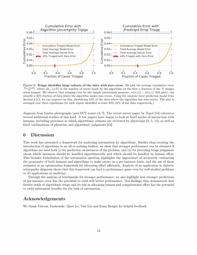
Figure 6: Triage identifies large subsets of the data with zero error. We plot the average cumulative errorMerr(αN)

N, where Merr(αN) is the number of errors made by the algorithm on the first α fraction of the N images

when triaged. We observe that triaging even by the simple uncertainty measure, m(xi)(1−m(xi)) (left plot), canidentify a 35% fraction of data where the algorithm makes zero errors. Using the separate error prediction model fromSection 4.2.2, we can improve on this, identifying 44% of the data where the algorithm has zero errors. The plot isaveraged over three repetitions (so each repeat identified at least 35%, 44% of the data respectively.)

diagnosis from fundus photographs (and OCT scans) [4, 7]. The recent survey paper by Topol [15] referencesseveral additional studies of this kind. A few papers have begun to look at fixed modes of interaction withhumans, including processes in which algorithmic outputs are reviewed by physicians [3, 5, 11], as well asfixed combinations of physician and algorithmic judgments [12].

6 DiscussionThis work has presented a framework for analyzing automation by algorithms. Rather than treating theintroduction of algorithms in an all-or-nothing fashion, we show that stronger performance can be obtained ifalgorithms are used both (i) for prediction on instances of the problem, and (ii) for providing triage judgmentsabout which instances should be handled algorithmically and which should be handled by human effort.This broader formulation of the automation question highlights the importance of accurately estimatingthe propensity of both humans and algorithms to make errors on a per-instance basis, and the use of theseestimates in an optimization framework for allocating effort efficiently. Analysis of an application in diabeticretinopathy diagnosis shows that this framework can lead to performance gains even for well-studied problemsin AI applications in medicine.

Through the analysis of benchmarks for stronger performance, we also highlight how stronger predictionsof per-instance error has the potential to yield still better performance. Our findings thus demonstrate howfurther study of algorithmic triage and its role in allocating human and computational effort has the potentialto yield substantial benefits for the task of automation.

AcknowledgementsWe thank Vincent Vanhoucke, Quoc Le, Yun Liu and Samy Bengio for helpful feedback.

13

References[1] Hasseb Ahsan. Diabetic retinopathy – biomolecules and multiple pathophysiology. Diabetes and Metabolic

Syndrome: Clincal Research and Review, pages 51–54, 2015.

[2] American Academy of Ophthalmology. International Clinical Diabetic Retinopathy Disease SeverityScale Detailed Table.

[3] Carrie J Cai, Emily Reif, Narayan Hegde, Jason Hipp, Been Kim, Daniel Smilkov, Martin Wattenberg,Fernanda Viegas, Greg S Corrado, Martin C Stumpe, et al. Human-centered tools for coping withimperfect algorithms during medical decision-making. arXiv preprint arXiv:1902.02960, 2019.

[4] Jeffrey De Fauw, Joseph R Ledsam, Bernardino Romera-Paredes, Stanislav Nikolov, Nenad Tomasev,Sam Blackwell, Harry Askham, Xavier Glorot, Brendan O’Donoghue, Daniel Visentin, et al. Clinicallyapplicable deep learning for diagnosis and referral in retinal disease. Nature medicine, 24(9):1342, 2018.

[5] Cem M Deniz, Siyuan Xiang, R Spencer Hallyburton, Arakua Welbeck, James S Babb, Stephen Honig,Kyunghyun Cho, and Gregory Chang. Segmentation of the proximal femur from mr images using deepconvolutional neural networks. Scientific reports, 8(1):16485, 2018.

[6] Yiming Ding, Jae Ho Sohn, Michael G Kawczynski, Hari Trivedi, Roy Harnish, Nathaniel W Jenkins,Dmytro Lituiev, Timothy P Copeland, Mariam S Aboian, Carina Mari Aparici, et al. A deep learningmodel to predict a diagnosis of alzheimer disease by using 18f-fdg pet of the brain. Radiology, 290(2):456–464, 2018.

[7] Varun Gulshan, Lily Peng, Marc Coram, Martin C Stumpe, Derek Wu, Arunachalam Narayanaswamy,Subhashini Venugopalan, Kasumi Widner, Tom Madams, Jorge Cuadros, Ramasamy Kim, Rajiv Raman,Philip Q Nelson, Jessica Mega, and Dale Webster. Development and validation of a deep learningalgorithm for detection of diabetic retinopathy in retinal fundus photographs. JAMA, 316(22):2402–2410,2016.

[8] Chuan Guo, Geoff Pleiss, Yu Sun, and Kilian Q. Weinberger. On calibration of modern neural networks.abs/1706.04599, 2017.

[9] Diederik P Kingma and Jimmy Ba. Adam: A method for stochastic optimization. arXiv preprintarXiv:1412.6980, 2014.

[10] Jonathan Krause, Varun Gulshan, Ehsan Rahimy, Peter Karth, Kasumi Widner, Gregory S. Corrado,Lily Peng, and Dale R. Webster. Grader variability and the importance of reference standards forevaluating machine learning models for diabetic retinopathy. abs/1710.01711, 2017.

[11] Yun Liu, Krishna Gadepalli, Mohammad Norouzi, George E Dahl, Timo Kohlberger, Aleksey Boyko,Subhashini Venugopalan, Aleksei Timofeev, Philip Q Nelson, Greg S Corrado, et al. Detecting cancermetastases on gigapixel pathology images. arXiv preprint arXiv:1703.02442, 2017.

[12] Aniruddh Raghu, Matthieu Komorowski, and Sumeetpal Singh. Model-based reinforcement learning forsepsis treatment. arXiv preprint arXiv:1811.09602, 2018.

[13] Maithra Raghu, Katy Blumer, Rory Sayres, Ziad Obermeyer, Sendhil Mullainathan, and Jon Kleinberg.Direct uncertainty prediction with applications to healthcare. arXiv preprint arXiv:1807.01771, 2018.

[14] Pranav Rajpurkar, Jeremy Irvin, Kaylie Zhu, Brandon Yang, Hershel Mehta, Tony Duan, Daisy Ding,Aarti Bagul, Curtis Langlotz, Katie Shpanskaya, Matthew P. Lungren, and Andrew Y. Ng. Chexnet:Radiologist-level pneumonia detection on chest x-rays with deep learning. abs/1711.05225, 2017.

[15] Eric Topol. High-performance medicine: the convergence of human and artificial intelligence. NatureMedicine, 25:44–56, 2019.

14

A Training Data and Models DetailsOur training dataset consists of fundus photographs with labels corresponding to individual doctor grades.There are 5 possible DR grades and hence 5 possible class labels. A subset of this data has fundus photographswith more than one doctor grade, corresponding to multiple doctors individually and independently decidingon the grade for the image. The label for these images is not a one-hot class label but the empirical distributionof grades. For example, if an image i has grades {2, 3, 3}, then its label would be [0, 1./3, 2./3, 0, 0].

On this data, we train a convolutional neural network, an Inception-v3 model with weights pretrainedfrom ImageNet and a new five class classification head. We train with the Adam optimizer [9] and an initiallearning rate of 0.005. To better calibrate the model, we retrain the very top of the network (from thePreLogits layer) on just the data with two or more doctor grades.

Training Error Probability Prediction Models For Figures 4, 5 and 6, we use separate error probabilityprediction algorithms to predict the values of Pr [Hi] and Pr [Mi]. The setup for predicting Pr [Mi] is asfollows: after training the main convolutional neural network on the train dataset, we train a small fullyconnected deep neural network to take the prelogit embeddings of a train image xi, and predict whether ornot the main convolutional neural network was correct on that image. The label for the image is binary:agree/disagree on whether the mass m(xi) put on referable by the convolutional neural network thresholdedat 0.5 equals the mass on referable by the human doctor grades, again thresholded at 0.5.

The setup for training Pr [Hi] builds off of [13]. First, we only select cases for which we have at leasttwo doctor grades. For these, we take the image embedding from the Prelogit layer of the large diagnosticconvolutional neural network as input, and the label as a binary target. This label is defined as follows: wesplit the available doctor grades into two evenly sized sets A and B. We aggregate all the grades in A into asingle referable/non-referable grade by averaging and thresholding at 0.5, and do the same for the grades inB. If these two aggregated grades agree, we label the image with 0 (agreement, low doctor error probability),if not, we label with 1 (disagreement, high doctor error probability.)

B Computing Pr [Mi]

In Section 4.1.1, we overviewed the method used to define a well calibrated error probability for the output ofthe convolutional neural network. In Algorithm , we give a step-by-step overview of the implementation ofthis method. In our experiments, we set C = 2000.

C Triage and Allocation AlgorithmWhen using triage to reallocate human effort, we first order the instances by their triage scores, and then fullyautomate the first αN of them. On the remainder (1− α)N images, we allocate the budget of cN humandoctor grades we have available. To allocate this set of cN grades, we use the equal coverage protocol: eachof the remaining (1− α)N cases gets cN/((1− α)N) grades. If this is a non-integer amount, with r sparegrades, the r cases identified as the hardest (according to the triage scores) get an additional grade. We thencompute the final binary decision by taking the mean grade (for each case) and thresholding by 0.5 (themajority vote.)

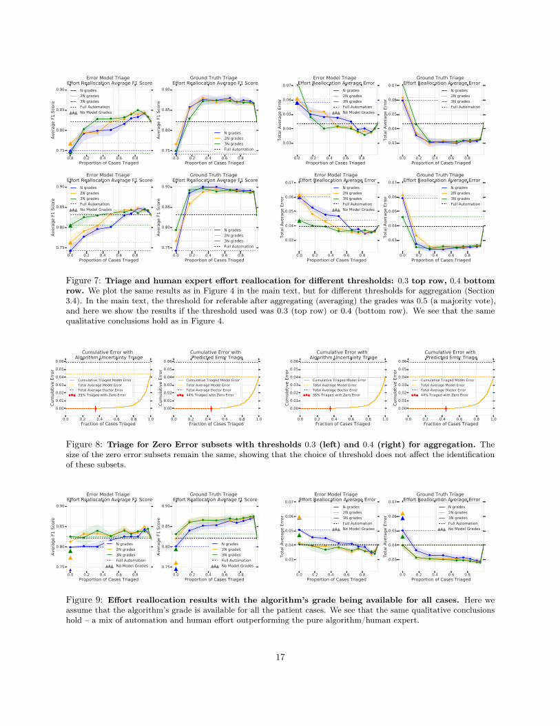
C.1 Results on other ThresholdsAs described in Section 3.4, at evaluation, for an instance with multiple grades we aggregate all the scores bytaking the mean and thresholding. In the main text, we pick this threshold to be 0.5, corresponding to themajority vote of all the grades. In Figure 7, we show the results corresponding to Figure 4 in the main text,but for when we take the thresholds to be 0.3 (top row) and 0.4 (bottom row). We see that the qualitativeconclusions remain the same – combining human and algorithmic effort beats the full allocation and equal

15

Algorithm 1: Model Error Probability Calibration1: Erri = 0 for i in instances.2: for (r = 0; r < C; r++) do . C is a sufficiently large constant.3: R = 04: for i in instances do . Sample a doctor grade and count number of referables.5: Sample doctor grade h(i)

6: if (h(i) ≥ 3) then7: R← R+ 18: end if9: end for

10: Rank instances i from highest to lowest m(xi)11: AR = {i : rank(i) ≤ R}12: for i in instances do . Assign binary grades to instances. Top R referable.13: if (i ∈ AR) then14: mi ← 115: else16: mi ← 017: end if18: Erri ← Erri + |mi − ai| . ai is the adjudicated grade19: end for20: end for21: return Pr [Mi] = Erri/C . Error probability by averaging over number of repetitions.

coverage protocols for both triage by the error prediction models and triage by the ground truth. We also seethe same significant gap between ground truth and triage by error predictions.

Note that this choice of threshold affects the choice of qR, which is chosen so that the number of casesmarked as referable by the model matches the number of cases marked as referable by the aggregated andthresholded grade of the human doctors, and could potentially affect the results of Figure 6. However, asshown in Figure 8, the choice of aggregation threshold does not affect the identification of zero error subsets.

D Triage and Human Effort Reallocation with Model GradesThe triage process for effort reallocation – Figures 4, 11 – assumes that the algorithm decision is not availablefor the (1−α)N cases that are not automated. This may be the situation if computing an algorithm decisionis expensive (less likely) or (more likely) the algorithm decision is purposefully not shown in cases where it isunsure, so as not to bias the human doctors. However, another equally likely scenario is that the algorithmdecision is also available ‘for free’ for the (1− α)N cases that are not fully automated. In Figure 9, we showthe effort reallocation results from triaging if the model grades were available for all the cases (compare toFigure 4 in the main text). We observe that all of the main conclusions – the optimal performance is througha combination of automation and human effort, which beats both full automation and the different equalcoverage baselines.

E Results on Additional Holdout DatasetThe results in the main text are on the adjudicated evaluation dataset, which, aside from multiple independentgrades by individual doctors, also have a consensus score, the adjudicated grade, which is used as a proxyfor ground truth. To further validate our result, we use an additional holdout set which doesn’t have anadjudicated grade, but does have many individual doctor grades. For each instance i, we use half of its gradesto compute a proxy ground truth grade, by aggregating and then thresholding the doctor grades. The other

16


0.75

0.80

0.85

0.90

Avera

ge F

1 S

core


N grades

2N grades

3N grades

Full Automation

No Model Grades


0.75

0.80

0.85

0.90

Avera

ge F

1 S

core


N grades

2N grades

3N grades

Full Automation


0.03

0.04

0.05

0.06

0.07

Tota

l A

vera

ge E

rror


N grades

2N grades

3N grades

Full Automation

No Model Grades


0.03

0.04

0.05

0.06

0.07

Tota

l A

vera

ge E

rror


N grades

2N grades

3N grades

Full Automation


0.75

0.80

0.85

0.90

Avera

ge F

1 S

core


N grades

2N grades

3N grades

Full Automation

No Model Grades


0.75

0.80

0.85

0.90

Avera

ge F

1 S

core


N grades

2N grades

3N grades

Full Automation


0.03

0.04

0.05

0.06

0.07

Tota

l A

vera

ge E

rror


N grades

2N grades

3N grades

Full Automation

No Model Grades


0.03

0.04

0.05

0.06

0.07

Tota

l A

vera

ge E

rror


N grades

2N grades

3N grades

Full Automation

Figure 7: Triage and human expert effort reallocation for different thresholds: 0.3 top row, 0.4 bottomrow. We plot the same results as in Figure 4 in the main text, but for different thresholds for aggregation (Section3.4). In the main text, the threshold for referable after aggregating (averaging) the grades was 0.5 (a majority vote),and here we show the results if the threshold used was 0.3 (top row) or 0.4 (bottom row). We see that the samequalitative conclusions hold as in Figure 4.


0.00

0.01

0.02

0.03

0.04

0.05

0.06

Cum

ula

tive E

rror







0.00

0.01

0.02

0.03

0.04

0.05

0.06

Cum

ula

tive E

rror







0.00

0.01

0.02

0.03

0.04

0.05

0.06

Cum

ula

tive E

rror







0.00

0.01

0.02

0.03

0.04

0.05

0.06

Cum

ula

tive E

rror






Figure 8: Triage for Zero Error subsets with thresholds 0.3 (left) and 0.4 (right) for aggregation. Thesize of the zero error subsets remain the same, showing that the choice of threshold does not affect the identificationof these subsets.


0.75

0.80

0.85

0.90

Avera

ge F

1 S

core


N grades

2N grades

3N grades

Full Automation

No Model Grades


0.75

0.80

0.85

0.90

Avera

ge F

1 S

core

Ground Truth Triage Effort Reallocation Average f1 Score

N grades

2N grades

3N grades

Full Automation

No Model Grades


0.03

0.04

0.05

0.06

0.07

Tota

l A

vera

ge E

rror


N grades

2N grades

3N grades

Full Automation

No Model Grades


0.03

0.04

0.05

0.06

0.07

Tota

l A

vera

ge E

rror


N grades

2N grades

3N grades

Full Automation

No Model Grades

Figure 9: Effort reallocation results with the algorithm’s grade being available for all cases. Here weassume that the algorithm’s grade is available for all the patient cases. We see that the same qualitative conclusionshold – a mix of automation and human effort outperforming the pure algorithm/human expert.

17

1.0 0.5 0.0 0.5 1.0(D Err - M Err)

10-4

10-3

10-2

10-1

100

Pro

port

ion o

f Im

ages

Log S

cale

Algorithm and Doctor Error Difference Log Scale

D Err = M Err

D Err < M Err

D Err > M Err

1.0 0.5 0.0 0.5 1.0(D Err - M Err)

0.00

0.02

0.04

0.06

0.08

0.10

0.12

0.14

Pro

port

ion o

f Im

ages

Algorithm and Doctor Error Difference

D Err < M Err

D Err > M Err

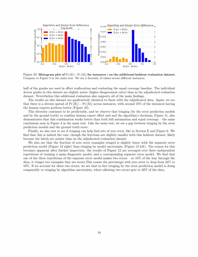
Figure 10: Histogram plot of Pr [Hi]−Pr [Mi] for instances i on the additional holdout evaluation dataset.Compare to Figure 3 in the main text. We see a diversity of values across different instances.

half of the grades are used in effort reallocation and evaluating the equal coverage baseline. The individualdoctor grades in this dataset are slightly noiser (higher disagreement rates) than in the adjudicated evaluationdataset. Nevertheless this additional evaluation also supports all of the main findings.

The results on this dataset are qualitatively identical to those with the adjudicated data. Again, we seethat there is a diverse spread of Pr [Hi]− Pr [Mi] across instances, with around 10% of the instances havingthe human experts perform better (Figure 10).

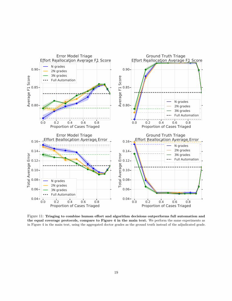
This diversity continues to be predictable, and we observe that triaging (by the error prediction modelsand by the ground truth) to combine human expert effort and and the algorithm’s decisions, Figure 11, alsodemonstrates that this combination works better than both full automation and equal coverage – the sameconclusions seen in Figure 4 in the main text. Like the main text, we see a gap between triaging by the errorprediction models and the ground truth score.

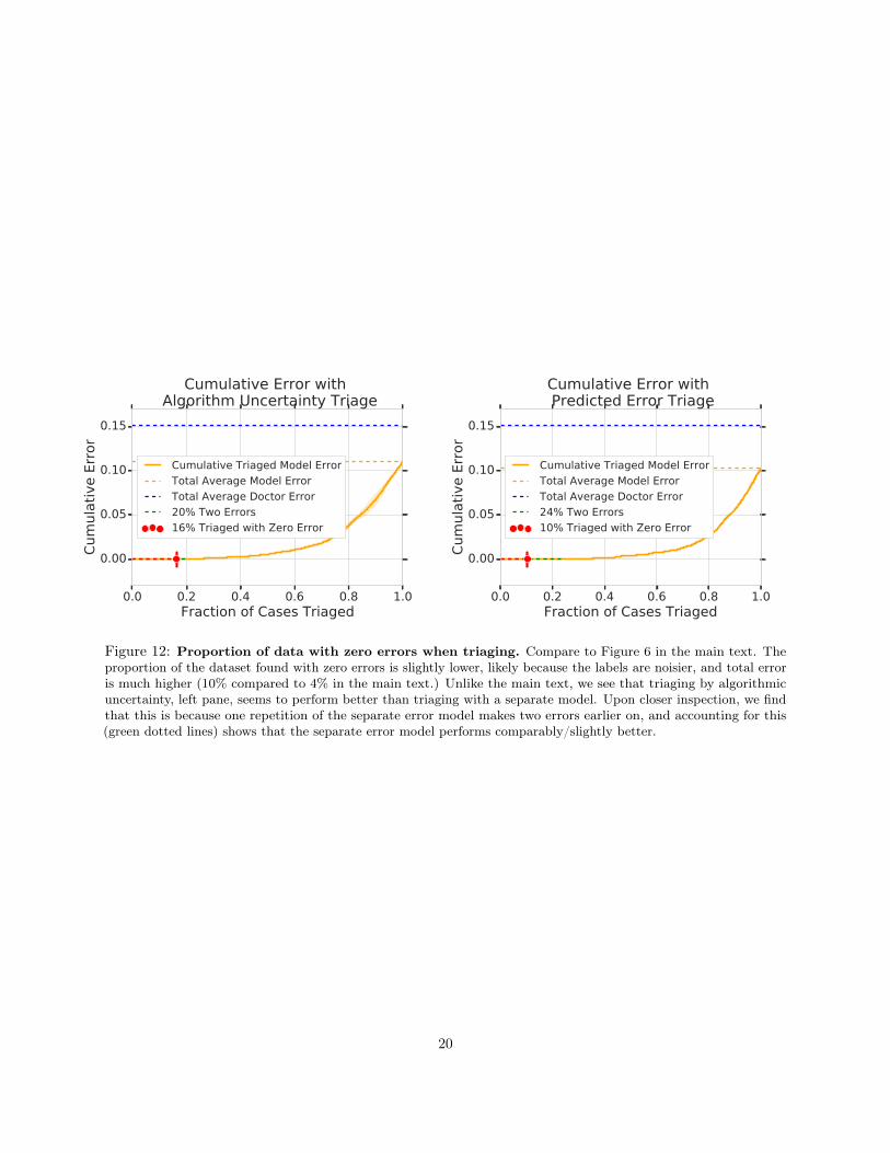
Finally, we also test to see if triaging can help find sets of zero error, like in Section E and Figure 6. Wefind that this is indeed the case, though the fractions are slightly smaller with this holdout dataset, likelybecause the labels are noisier than on the adjudicated evaluation dataset.

We also see that the fraction of zero error examples triaged is slightly lower with the separate errorprediction model (Figure 12 right) than triaging by model uncertainty (Figure 12 left). The reason for thisbecomes apparent after further inspection: the results of Figure 12 are averaged over three independentrepetitions of training a main diagnostic model, and a corresponding separate error model. We find thatone of the three repetitions of the separate error model makes two errors – at 10% of the way through thedata, it triages two examples that are errors.This causes the percentage with zero error to drop from 24% to10%. If we account for these two errors, we see that in fact triaging by the error prediction model is doingcomparably to triaging by algorithm uncertainty, where allowing two errors gets to 20% of the data.

18


0.80

0.85

0.90

Avera

ge F

1 S

core


N grades

2N grades

3N grades

Full Automation


0.80

0.85

0.90

Avera

ge F

1 S

core


N grades

2N grades

3N grades

Full Automation


0.04

0.06

0.08

0.10

0.12

0.14

0.16

Tota

l A

vera

ge E

rror


N grades

2N grades

3N grades

Full Automation


0.04

0.06

0.08

0.10

0.12

0.14

0.16

Tota

l A

vera

ge E

rror


N grades

2N grades

3N grades

Full Automation

Figure 11: Triaging to combine human effort and algorithm decisions outperforms full automation andthe equal coverage protocols, compare to Figure 4 in the main text. We perform the same experiments asin Figure 4 in the main text, using the aggregated doctor grades as the ground truth instead of the adjudicated grade.

19


0.00

0.05

0.10

0.15

Cum

ula

tive E

rror





20% Two Errors



0.00

0.05

0.10

0.15

Cum

ula

tive E

rror





24% Two Errors


Figure 12: Proportion of data with zero errors when triaging. Compare to Figure 6 in the main text. Theproportion of the dataset found with zero errors is slightly lower, likely because the labels are noisier, and total erroris much higher (10% compared to 4% in the main text.) Unlike the main text, we see that triaging by algorithmicuncertainty, left pane, seems to perform better than triaging with a separate model. Upon closer inspection, we findthat this is because one repetition of the separate error model makes two errors earlier on, and accounting for this(green dotted lines) shows that the separate error model performs comparably/slightly better.

20

Documents

TheAlgorithmicAutomationProblem: Prediction,Triage,and … › pdf › 1903.12220.pdf · 2019-04-01 · Maithra Raghu1; 2Katy Blumer Greg Corrado Jon Kleinberg1 Ziad Obermeyer3;4