TheGeneralized WarpDrive Concept in theEGRTheory - Zelmanov Journal

The Generalized Warp Drive Concept

in the EGR Theory

Patrick Marquet∗

Abstract: In this paper, we briefly review the basic theory of theAlcubierre drive, known as the Warp Drive Concept, and its subse-quent improvements. By using the Arnowitt-Deser-Misner formalismwe then re-formulate an extended extrinsic curvature which corre-sponds to the extra curvature of the Extended General Relativity(EGR). With this preparation, we are able to generalize the Alcu-bierre metric wherein the space-like hypersurfaces are Riemannian,and the characteristic Alcubierre function is associated with the EGRgeometry. This results in a reduced energy density tensor, whose formdisplays a potential ability to avoid the weak energy condition.

Contents:

Introduction . . . . . . . . . . . . . . . . . . . . . . . . . . . . . . . . . . . . . . . . . . . . . . . . . . . . 263

Chapter 1 Basics of Warp Drive Physics

§1.1 Description of the Alcubierre concept . . . . . . . . . . . . . . . . . . . 264

§1.1.1 Space-time bubble . . . . . . . . . . . . . . . . . . . . . . . . . . . . . . . 264

§1.1.2 Characteristics . . . . . . . . . . . . . . . . . . . . . . . . . . . . . . . . . . .265

§1.2 The physics that leads to Warp Drive . . . . . . . . . . . . . . . . . . . 265

§1.2.1 The (3+1) formalism: the Arnowitt-Deser-Misner(ADM) technique . . . . . . . . . . . . . . . . . . . . . . . . . . . . . . . . . . . . . . . 265

§1.2.2 Curvatures in the ADM formalism . . . . . . . . . . . . . . . 266

Chapter 2 The Alcubierre Warp Drive

§2.1 The Alcubierre metric . . . . . . . . . . . . . . . . . . . . . . . . . . . . . . . . . . 268

§2.2 Analyzing the “top hat” function . . . . . . . . . . . . . . . . . . . . . . . 268

§2.3 Eulerian observer . . . . . . . . . . . . . . . . . . . . . . . . . . . . . . . . . . . . . . . 269

§2.3.1 Definition. . . . . . . . . . . . . . . . . . . . . . . . . . . . . . . . . . . . . . . .269

§2.3.2 Specific characteristics . . . . . . . . . . . . . . . . . . . . . . . . . . . 270

§2.4 Negative energy requirement . . . . . . . . . . . . . . . . . . . . . . . . . . . . 271

§2.4.1 The Alcubierre-Einstein tensor . . . . . . . . . . . . . . . . . . . 271

§2.4.2 Negative energy . . . . . . . . . . . . . . . . . . . . . . . . . . . . . . . . . 273

Chapter 3 Causality

§3.1 Horizon formation . . . . . . . . . . . . . . . . . . . . . . . . . . . . . . . . . . . . . . 274

∗Postal address: 7, rue du 11 nov, 94350 Villiers/Marne, Paris, France. E-mail:[email protected]. Tel: (33) 1-49-30-33-42.

262 The Abraham Zelmanov Journal — Vol. 2, 2009

§3.2 Reducing the energy . . . . . . . . . . . . . . . . . . . . . . . . . . . . . . . . . . . . 275

§3.2.1 The ESAA metric . . . . . . . . . . . . . . . . . . . . . . . . . . . . . . . 276

§3.2.2 The required energy . . . . . . . . . . . . . . . . . . . . . . . . . . . . . 276

§3.3 Causally connected spaceship . . . . . . . . . . . . . . . . . . . . . . . . . . . 278

§3.3.1 The spaceship frame of reference . . . . . . . . . . . . . . . . . 278

§3.3.2 A remote frame of reference. . . . . . . . . . . . . . . . . . . . . .279

Chapter 4 The EGR-like Picture

§4.1 A particular extended Lie derivative . . . . . . . . . . . . . . . . . . . . 280

§4.2 The extended extrinsic curvature and associated energydensity . . . . . . . . . . . . . . . . . . . . . . . . . . . . . . . . . . . . . . . . . . . . . . . . . 282

Discussion and concluding remarks . . . . . . . . . . . . . . . . . . . . . . . . . . . . . . 283

Appendix Detailing a stellar round trip example according toAlcubierre . . . . . . . . . . . . . . . . . . . . . . . . . . . . . . . . . . . . . . . . . . . . . . 284

Notations:

To completely appreciate this article, it is imperative to define somenotations employed.

Indices. Throughout this paper, we adopt the Einstein summationconvention whereby a repeated index implies summation over all val-ues of this index:

4-tensor or 4-vector: small Latin indices a, b, . . . = 1, 2, 3, 4;

3-tensor or 3-vector: small Greek indices α, β, . . . = 1, 2, 3;

4-volume element: d4x;

3-volume element: d3x.

Signature of space-time metric:

(−+++) unless otherwise specified.

Operations:

Scalar function: U(xa);

Ordinary derivative: ∂aU ;

Covariant derivative in GR: ∇a;

Covariant derivative in EGR: Da or ′, (alternatively).

Newton’s constant:

G = c = 1.

Patrick Marquet 263

Introduction

The physical restriction related to the finite nature of the light velocityhas so far been a stumbling block to exploring the superluminal speedpossibility of long-term space journeys.

However, recent theoretical works have lent support to plausible in-terstellar hyperfast travels, without physiological human constraints.

How is this possible? The principle of space travel while locally “atrest”, is analogous to galaxies receding away from each other at extremevelocities due to the expansion (and contraction) of the Universe.

Instead of moving a spaceship from a planet A to a planet B, wemodify the space between them. The spaceship can be carried along bya local spacetime “singular region” and is thus “surfing” through spacewith a given velocity with respect to the rest of the Universe.

In 1994, a Mexican physicist Miguel Alcubierre [1], working at thePhysics and Astronomy Department of Cardiff University in Wales,Great Britain, published a short paper describing such a propulsionmode, known today under the name Warp Drive.

Based on this theory, a faster than light travel could be for the firsttime considered without violating the laws of relativity.

Many problems (open questions) remain to be investigated, amongwhich two major problems are reflected in the following statements:

a) Produce a sufficiently large negative energy to create a local spacedistortion without violating the energy conditions resulting fromthe laws of General Relativity [2];

b) Maintain contact (control) between the spaceship and the outsideof the distorsion (causality connection).

The problem a) can be avoided if one considers a non-Riemanniangeometry that governs the laws of our Universe [3] which could eliminatethe negative energy density required by the Alcubierre metric to sustaina realistic Warp Drive.

The difficulty b) may be theoretically circumvented by introducingcertain types of transformations which may allow us to use the warpedregions for the removal of the singularities or “event horizons”. Some ofthese transformations are briefly reviewed in the course of this study.

Pre-requisite: time-like unit four-vector

As is well known [4], the covariant derivative of a time-like vector field ua

(whose square is uaua =−1), may be expressed in an invariant mannerin terms of tensor fields which describe the kinematics of the congruenceof curves generated by the vector field ua.


One may write

ua;b = ςab + ωab +1

3(θhab) + uaub ,

where ua= ua;bub is the acceleration of the flow lines, τ is the proper

time, ωab = hcah

db u[c;d] is the vorticity tensor, hab = gab +uaub is the pro-

jection tensor, θab = hcah

db u(c;d) is the expansion tensor, θ=habθab =ua

;a

is the expansion scalar, ςab = θab − 13(habθ) is the shear tensor.

The kinematic quantities are completely orthogonal to ua, i.e.,

habub = ωabu

b = ςabub = 0 , uau

b = ωaub = 0 .

Physically, the time-like vector field ua is often taken to be the four-velocity of a fluid. The volume element expansion θ extracted fromthis decomposition can be thus seen as a hydrodynamic picture: it is ofmajor importance in the foregoing.

Chapter 1. Basics of Warp Drive Physics

§1.1. Description of the Alcubierre concept

§1.1.1 Space-time bubble

The Universe is approximated as a Minkowskian space: we choose anarbitrary curve and deform the space-time in the immediate vicinity insuch a way that the curve becomes a time-like geodesic somewhat likea “ripple”, in order to generate a perturbed or singular local region inwhich one may fit a spaceship and its occupants.

Let xs be the center of the region where the spaceship stays, and xany coordinate within this region so that x=xs for the spaceship.

Within an orthonormal coordinate frame, such a region, which isreferred to as a bubble, is transported forward with respect to distantobservers, along a given direction (x in this text).

With respect to the same distant observers, the apparent velocity ofthe bubble center is given by

vs(t) =dxs(t)

dt, (1.1)

where xs(t) is the trajectory of the region along the x-direction, and

rs(t) =

√

(x− xs(t))2+ y2 + z2 (1.2)

is the variable distance outward from the center of the spaceship untilℜ which may be called the radius of the singular region.

The spaceship is at rest inside the bubble and has no local velocity.

Patrick Marquet 265

§1.1.2. Characteristics

From these first elements, we must now select the exact form of a met-ric that will “push” the spaceship along a trajectory described by anarbitrary function of time (xs, t).

Furthermore, this trajectory should be a time-like geodesic, whatevervs(t). By substituting x=xs(t) in the new metric to be defined, weshould expect to find

dτ = dt . (1.3)

The proper time of the spaceship is equal to coordinate time whichis also the proper time of distant observers.

Since these observers are situated in the flat region, we concludethat the spaceship suffers no time dilation as it moves. It will be easyto prove that this spaceship moves along a time-like geodesic and itsproper acceleration is zero.

§1.2. The physics that leads to Warp Drive

§1.2.1. The (3+1) Formalism: the Arnowitt-Deser-Misner(ADM) technique

In 1960, Arnowitt, Deser, and Misner [5] suggested a technique basedon decomposing the space-time into a family of space-like hypersurfacesand parametrized by the value of an arbitrarily chosen time coordi-nate x4.

This “foilation” displays a proper-time element dτ between twonearby hypersurfaces labelled x4 = const and x4 + dx4 = const. Theproper-time element dτ must be proportional to dx4. Thus we write

dτ = N(

xα, x4)

dx4. (1.4)

In the ADM terminology, N is called the lapse function and morespecifically the time lapse.

Consider now the three-vector whose spatial coordinates xα are lyingin the hypersurface (x4 = const) and which is normal to it.

We want to evaluate this vector on the second hypersurface, whichis x4 + dx4 = const, where these coordinates now become Nαdx4. ThisNα vector is known as the shift vector.

The ADM four-metric tensor is decomposed into covariant compo-nents

(gab)ADM =

{

−N2 −NαNβ gαβ , Nβ ,

Nα , gαβ .(1.5)


The line element corresponding to the hypersurfaces’ separation istherefore written

(ds2)ADM = (gab)ADMdxadxb

or

(ds2)ADM = −N2(

dx4)2

+ gab(

Nαdx4 + dxα)(

Nβdx4 + dxβ)

=

=(

−N2 −NαNα)(

dx4)2

+ 2Nβ dx4dxβ + gαβ dx

αdxβ , (1.6)

where gαβ is the 3-metric tensor of the hypersurfaces.The ADM metric tensor has the contravariant components

(gab)ADM =

−N−2,Nβ

N2,

Nα

N2, gαβ −Nα Nβ

N2.

(1.7)

As a result, the hypersurfaces have a unit time-like normal vectorwith components

na = N−1 (1, −Nα) , na = (−N, 0) . (1.8)

When the fundamental three-tensor satisfies gαβ = δαβ the metric(1.6) becomes

ds2 = −(

N2 −NαNα)

dt2 − 2Nαdxdt+ dxαdxβ

ords2 = −N2dt2 − (dx+Nαdt)

2+ dy2 + dz2. (1.9)

§1.2.2. Curvatures in the ADM formalism

The Einstein action can be written in terms of the metric tensor (gab)ADM

(1.5) and (1.7), as [6]

SADM =

∫

R√−g d4x =

=

∫

dt

∫

N(

KαβKαβ −K2 + (3)R

)√−g d3x+

+ boundary terms(

KααK

ββ =K2

)

, (1.10)

where g= det ‖gαβ‖, while (3)R stands for the intrinsic curvature tensorof the hypersurface x4 = const

Kαβ = (2N)−1

(−Nα;β −Nβ;α + ∂t gαβ) . (1.11)

Patrick Marquet 267

The tensor (1.11) (in which ; refers to covariant differentiation withrespect to the three-metric), represents the extrinsic curvature, and assuch, describes the manner in which that surface is embedded in thesurrounding four-dimensional space-time.

The determinant (4)g of the four-metric is shown to be related to thedeterminant (3)g by

√

− (4)g = N√

(3)g .

The rate of change of the three-metric tensor gαβ with respect tothe time label can be decomposed into “normal” and “tangential” con-tributions:

• The normal change is proportional to the extrinsic curvature −2NKαβ

of the hypersurface;

• The tangential change is given by the Lie derivative of gαβ alongthe shift vector Nα, namely

LN

gαβ = 2N(α;β) . (1.12)

The main advantage of the ADM formalism is that the time deriva-tive is isolated and it can be used in further specific computations.Furthermore we verify that

Kαβ = −nα;β , (1.13)

which is sometimes called the second fundamental form of the three-space [7]. Six of the ten Einstein equations imply for Kα

β to evolveaccording to [8]

∂Kαβ

∂t+ L

N

Kαβ = ∇α∇β N +

+N[

Rαβ +Kα

αKαβ + 4π (T − C) δαβ − 8πTα

β

]

, (1.14)

where Rαβ is the three-Ricci tensor, and C =Tab n

anb is the materialenergy density in the rest frame of normal congruence (time-like vectorfield) with T =Tα

α .It is convenient to introduce the three-momentum current density

Iα =−nc Tcα. So the remaining four equations finally form the so-called

constraint equations

H =1

2

(

R−KαβK

βα +K2

)

− 8πC = 0 , (1.15)

Hβ = ∇α

(

Kαβ −Kδαβ

)

− 8πIβ = 0 . (1.16)

Equation (1.15) will be of central importance in the present theory.


Chapter 2. The Alcubierre Warp Drive

§2.1. The Alcubierre metric

In view of building a space warp progressing along the x-direction, onemay choose with Alcubierre

N = 1

N1 = − vs(t) f(rs, t)

N2 = N3 = 0

, (2.1)

we then have

(ds2)AL = − dt2 +[

dx− vs f(rs, t) dt]2

+ dy2 + dz2; (2.2)

this interval is known as the Alcubierre metric.The function f(rs, t) is so defined as to cause space-time to contract

on the forward edge and equally expanding on the trailing edge of thesingular region. It is often referred to as a “top hat” function.

Let us now write down the Alcubierre metric under the followingequivalent form

(ds2)AL = −[

1− v2s f2(rs, t)

]

dt2 − 2vsf dtdx+ dx2 + dy2 + dz2, (2.3)

which puts in evidence the covariant components of the Alcubierre met-ric tensor

(g44)AL = −[

1− v2s f2(rs, t)

]

(g41)AL = (g14)AL = − vs f(rs, t)

(g22)AL = (g33)AL = 1

. (2.4)

§2.2 Analyzing the “top hat” function

We now turn our attention to the “top hat” function f(rs, t) itself,which allows for the bubble to develop. Alcubierre originally chosen thefollowing form

f(rs, t) =tanh

[

σ (rs + ℜ)]

− tanh[

σ (rs −ℜ)]

2 tanh (σR), (2.5)

where ℜ> 0 is the “radius” of the “region”, while σ is a “bump” param-eter which can be used to “tune” the “wall” thickness of the singularregion.

Patrick Marquet 269

The larger this parameter, the greater the contained energy density,so its shell thickness decreases. Moreover, the absolute increase of σmeans a faster approach of the condition

limσ→∞

f(rs, t) =

{

1 for rs ∈ [−ℜ, ℜ ] ,

0 otherwise.(2.6)

Note that rs =0 at the center of the singular region (spaceship loca-tion). For rs >ℜ, the function f(rs, t) should rapidly verify f(rs, t)= 0and we recover the Minkowski space-time.

As outlined earlier, any function will suffice so long as the aboveconditions are fullfilled. For simplified calculations, it is convenient tointroduce the equivalent piecewise continuous function as establishedby Pfenning and Ford [9]

fp.c.(rs, t) =

1 for rs <ℜ− ∆2,

(

−1∆

)(

rs−ℜ− ∆2

)

for ℜ− ∆2<rs <ℜ+ ∆

2,

0 for rs >ℜ+ ∆2,

(2.7)

where the variable ∆ is the region shell “thickness”.Setting the slopes of the functions f(rs, t) and fp.c.(rs, t) to be equal

at rs =ℜ, leads to the following result

∆ =1 + tanh2 (σℜ)22σ [ tanh (σℜ)] . (2.8)

For large σℜ, one may admit the approximation

∆ ≈ 2

σ. (2.9)

§2.3. Eulerian observer

§2.3.1 Definition

With the choice of the three-vector Nα =0, we have a particular coordi-nate frame called normal coordinates, according to (1.8). Such a choiceof coordinates constitutes an “Eulerian” gauge.

In the Alcubierre formalism, N1 6=0 characterizes a special type ofobserver who “measures” the warped shell and the associated regionwhen they cross through.

His four-velocity is normal to the hypersurfaces. This observer, whoalso is referred to as Eulerian observer, is initially at rest. Just the front


wall of the disturbance reaches the observer, he begins to accelerate, inthe progressing direction of the singular region, relative to observerslocated at large distance from him.

Once during his “stay” inside the region, the Eulerian observer trav-els with a nearly constant velocity given by

dx(t)

dt= vs(tρ, ρ) f(ρ) , (2.10)

where tρ is the time measured at the coordinate

ρ =√

y2 + z2 . (2.11)

This velocity will always be less than the region’s velocity unlessρ=0, i.e. when the observer is at the center of the spaceship.

After reaching the region’s equator, the Eulerian observer deceler-ates, and is left at rest while going out of the rear edge of the “wall”.

If using the piecewise continuous function of Pfenning for rs<ℜ−∆2,

any observer moves along the singular region with the same speed. In-side the warped regions (“shells”), i.e. for

ℜ− ∆

2< ρ < ℜ+

∆

2,

we recover the conditions deduced from the “top hat” function (2.5),as viewed by the Eulerian observer. The singular regions have toroidalgeometry concentrated on either part of the longitudinal direction oftravel x, and are thus perpendicular to the plane defined by ρ.

§2.3.2. Specific characteristics

Following Alcubierre, such an observer has a four-velocity normal to thehypersurfaces t= const.

With the condition dτ = dt= ds, it is straightforward to show thatthis four-velocity has the following components

(ua)AL =[

1, vs f(rs, t), 0, 0]

(ua)AL =[

−1, 0, 0, 0]

}

. (2.12)

The Eulerian observer follows time-like geodesics orthogonal to theEuclidean hypersurfaces.

From the metric (2.2), inspection shows that the Eulerian observeris in free fall, i.e. his four-acceleration is zero

(ab)AL = (ua)AL (ub;a)AL = 0 ,

Patrick Marquet 271

which confirms the postulate of §1.1.2.In this case δαβ = gαβ , N =1, and (1.11) reduces to

Kαβ =1

2

(

∂αNβ + ∂βNα

)

.

The contracted tensor, which is defined by

θ = − traceKαβ , (2.13)

is the expansion scalar defined above; it means the expansion of thethree-volume element which, taking account of (2.1), is

θ = vsdf

(dx)AL

, (2.14)

where (x)AL = x−xs(t) is the single derivative variable.Hence, we find

θ = vs

(

df

drs

)[

drsd(x− xs)

]

(2.15)

and by using the classical derivative formula of functions of functions,it is not difficult to show that this last formula becomes

θ = vs

(

df

drs

)(

xs

rs

)

. (2.16)

Obviously, the shape of the function f , (2.5) induces both a volumecontraction and expansion ahead of, as well as behind, the singularregion.

§2.4. Negative energy requirement

§2.4.1. The Alcubierre-Einstein tensor

Before determining the form of the Alcubierre-Einstein tensor, we recallbriefly the so-called energy conditions.

Let us consider at a point p on the manifold (M, gab), an energy-momentum tensor T ab.

For any time-like vector ua ∈Tp (tangent space at p), one must havethe inequality

C = Tab ubub

> 0 , (2.17)

known as the weak energy condition.In addition, the “dominant” energy condition stipulates that for any

time-like four-vector ua> 0, the four-vector Qa=T ab u

b is a non-space-like vector.


By continuity, the weak energy condition implies the null energy

condition which asserts that for any null vector ka

Tabkakb > 0 .

Lastly, we consider the strong energy condition for any time-likefour-vector ua

(

Tab −1

2gab T

)

uaub> 0 .

Note: The dominant energy condition implies the weak energy con-dition and therefore the null energy condition, but not necessarily thestrong energy condition, which itself implies the null energy conditionbut not necessarily the weak energy condition.

From the components of the metric tensor (2.4), it is possible toform the contravariant components of the Ricci tensor (Rab)AL of theAlcubierre metric.

The resulting Einstein tensor

(Gab)AL = (Rab)AL −1

2(gab)ALR

contains the time component (R44)AL and

(G44)AL = −(

v2s4r2s

)

ρ2(

df

drs

)2

.

Using (G44)AL to define the energy density (T 44)AL, one finds

C =1

8π(G44)AL (u4u4)AL = − 1

32π

(

v2s ρ2

r2s

)(

df

drs

)2

. (2.18)

This formula is always negative as seen by the Eulerian observers,and therefore it is not compatible with the energy condition (2.17).

Another way of writing this equation is obtained by using the Gauss-Codazzi relations to form the Einstein tensor as a function of both theintrinsic and extrinsic curvatures, which eventually leads to [10]

C = Tab nanb =

1

16π

(

(3)R+K2 −KαβKαβ)

. (2.19)

By choosing N1 =−vs f(rs), N2 =N3 =0, and (3)R=0 the Alcu-bierre formulation is obtained again.

The energy density as measured by the Eulerian observer is given by

(C)AL =1

16π

(

K2 −KαβKαβ)

, (2.20)

Patrick Marquet 273

thus referring to (2.13), we find back

θ = − ∂1N1 = vs f

′(rs)x− xs

rs(2.21)

and

(C)AL=1

16π

[

(

∂1N1)2 −

(

∂1N1)2 −2

(

∂2N1

2

)2

−2

(

∂3N1

2

)2]

, (2.22)

(C)AL = − 1

32πv2s f

′2(rs)y2 + z2

r2s. (2.23)

§2.4.2. Negative energy

We now write down the form of the total negative energy required tosustain the Alcubierre metric.

Without loss of generality, we may simplify the case by assuminga constant velocity for the singular region, i.e.

x(t) = vs(t) (2.24)

at t=0, we havers(t = 0) ,

√

(xα)2 = r . (2.25)

Under these conditions, we must calculate the integral of the localenergy density over the proper volume d3x= dV (hypersurface)

E =

∫ √y T 44 dV, (2.26)

where y is the determinant of the spatial metric on the hypersurfacet= const, which, in our case, is y=1.

One finds

E = − 1

32πv2s

∫

ρ2

r2

[

df(rs, t)

dr

]2

dV. (2.27)

With the piecewise function of Pfenning (2.7), the energy is, in thespherical coordinates

E = − 1

12v2s

∫ ℜ+∆/2

ℜ−∆/2

r2(

− 1

∆

)2

dr. (2.28)

The contributions to the energy come only from the singular region’s“shell” areas.

We then see that one needs a special type of negative energy (matter)to travel faster than the speed of light by means of a Warp Drive. Suchan exotic matter has never been detected so far.


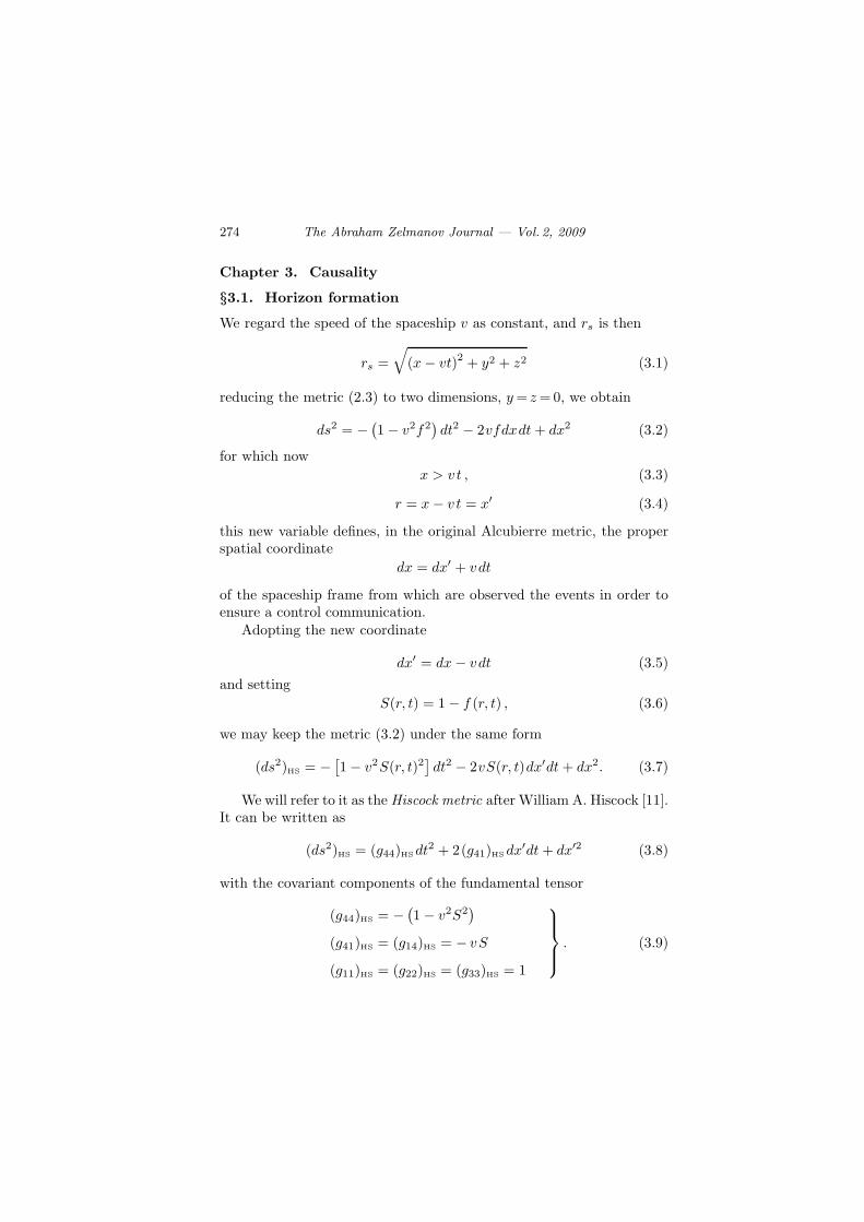
Chapter 3. Causality

§3.1. Horizon formation

We regard the speed of the spaceship v as constant, and rs is then

rs =

√

(x− vt)2 + y2 + z2 (3.1)

reducing the metric (2.3) to two dimensions, y= z=0, we obtain

ds2 = −(

1− v2f2)

dt2 − 2vfdxdt+ dx2 (3.2)

for which now

x > vt , (3.3)

r = x− v t = x′ (3.4)

this new variable defines, in the original Alcubierre metric, the properspatial coordinate

dx = dx′ + vdt

of the spaceship frame from which are observed the events in order toensure a control communication.

Adopting the new coordinate

dx′ = dx− vdt (3.5)

and setting

S(r, t) = 1− f (r, t) , (3.6)

we may keep the metric (3.2) under the same form

(ds2)HS = −[

1− v2S(r, t)2]

dt2 − 2vS(r, t)dx′dt+ dx2. (3.7)

We will refer to it as the Hiscock metric after William A. Hiscock [11].It can be written as

(ds2)HS = (g44)HSdt2 + 2(g41)HSdx

′dt+ dx′2 (3.8)

with the covariant components of the fundamental tensor

(g44)HS = −(

1− v2S2)

(g41)HS = (g14)HS = − vS

(g11)HS = (g22)HS = (g33)HS = 1

. (3.9)

Patrick Marquet 275

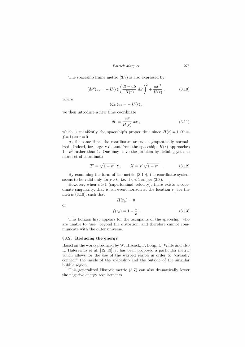
The spaceship frame metric (3.7) is also expressed by

(ds2)HS = −H(r)

(

dt− vS

H(r)dx′

)2

+dx′2

H(r), (3.10)

where(g44)HS = −H(r) ,

we then introduce a new time coordinate

dt′ =vS

H(r)dx′, (3.11)

which is manifestly the spaceship’s proper time since H(r)= 1 (thusf =1) as r=0.

At the same time, the coordinates are not asymptotically normal-ized. Indeed, for large r distant from the spaceship, H(r) approaches1− v2 rather than 1. One may solve the problem by defining yet onemore set of coordinates

T ′ =√

1− v2 t′ , X = x′√

1− v2 . (3.12)

By examining the form of the metric (3.10), the coordinate systemseems to be valid only for r > 0, i.e. if v < 1 as per (3.3).

However, when v > 1 (superluminal velocity), there exists a coor-dinate singularity, that is, an event horizon at the location r0 for themetric (3.10), such that

H(r0) = 0or

f(r0) = 1− 1

v. (3.13)

This horizon first appears for the occupants of the spaceship, whoare unable to “see” beyond the distortion, and therefore cannot com-municate with the outer universe.

§3.2. Reducing the energy

Based on the works produced byW. Hiscock, F. Loup, D. Waite and alsoE. Halerewicz et al. [12, 13], it has been proposed a particular metricwhich allows for the use of the warped region in order to “causallyconnect” the inside of the spaceship and the outside of the singularbubble region.

This generalized Hiscock metric (3.7) can also dramatically lowerthe negative energy requirements.


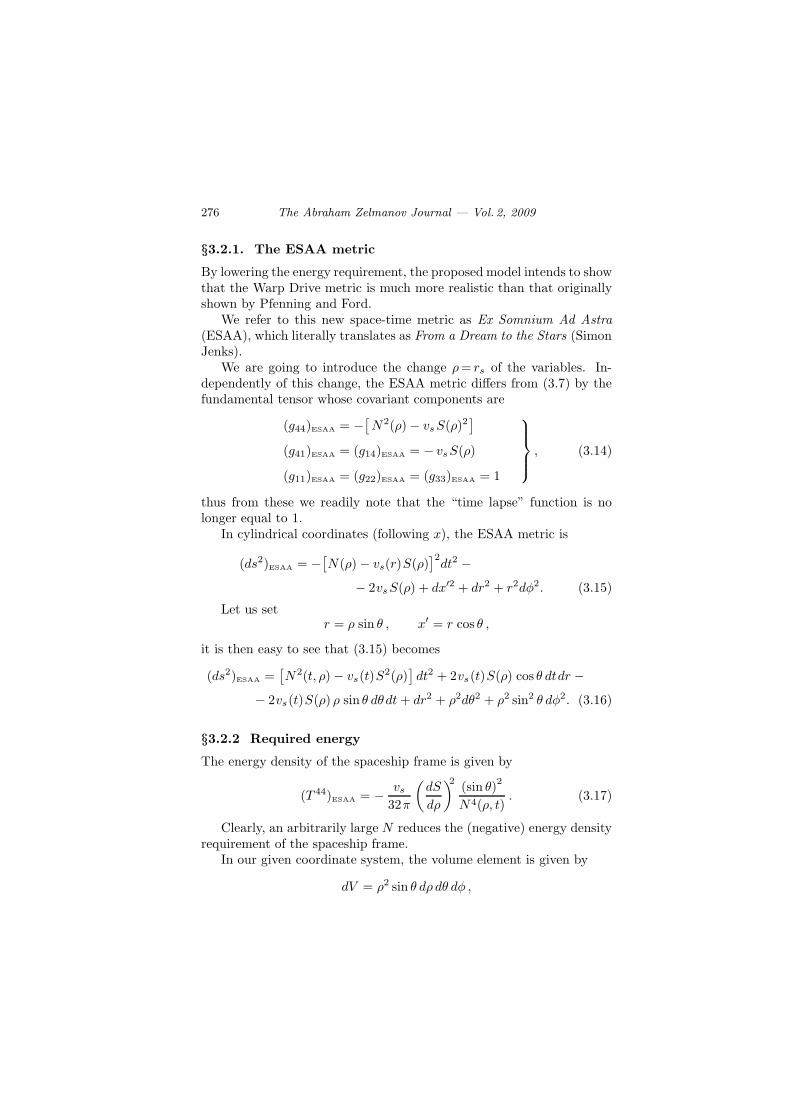
§3.2.1. The ESAA metric

By lowering the energy requirement, the proposed model intends to showthat the Warp Drive metric is much more realistic than that originallyshown by Pfenning and Ford.

We refer to this new space-time metric as Ex Somnium Ad Astra

(ESAA), which literally translates as From a Dream to the Stars (SimonJenks).

We are going to introduce the change ρ= rs of the variables. In-dependently of this change, the ESAA metric differs from (3.7) by thefundamental tensor whose covariant components are

(g44)ESAA = −[

N2(ρ)− vsS(ρ)2]

(g41)ESAA = (g14)ESAA = − vsS(ρ)

(g11)ESAA = (g22)ESAA = (g33)ESAA = 1

, (3.14)

thus from these we readily note that the “time lapse” function is nolonger equal to 1.

In cylindrical coordinates (following x), the ESAA metric is

(ds2)ESAA = −[

N(ρ)− vs(r)S(ρ)]2dt2 −

− 2vsS(ρ) + dx′2 + dr2 + r2dφ2. (3.15)

Let us setr = ρ sin θ , x′ = r cos θ ,

it is then easy to see that (3.15) becomes

(ds2)ESAA =[

N2(t, ρ)− vs(t)S2(ρ)

]

dt2 + 2vs(t)S(ρ) cos θ dtdr −− 2vs(t)S(ρ) ρ sin θ dθdt+ dr2 + ρ2dθ2 + ρ2 sin2 θ dφ2. (3.16)

§3.2.2 Required energy

The energy density of the spaceship frame is given by

(T 44)ESAA = − vs32π

(

dS

dρ

)2(sin θ)

2

N4(ρ, t). (3.17)

Clearly, an arbitrarily large N reduces the (negative) energy densityrequirement of the spaceship frame.

In our given coordinate system, the volume element is given by

dV = ρ2 sin θ dρ dθ dφ ,

Patrick Marquet 277

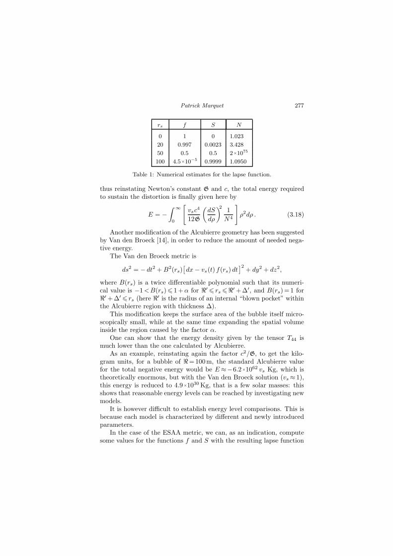
rs f S N

0 1 0 1.023

20 0.997 0.0023 3.428

50 0.5 0.5 2×1075

100 4.5×10−5 0.9999 1.0950

Table 1: Numerical estimates for the lapse function.

thus reinstating Newton’s constant G and c, the total energy requiredto sustain the distortion is finally given here by

E = −∫ ∞

0

[

vsc4

12G

(

dS

dρ

)21

N4

]

ρ2dρ . (3.18)

Another modification of the Alcubierre geometry has been suggestedby Van den Broeck [14], in order to reduce the amount of needed nega-tive energy.

The Van den Broeck metric is

ds2 = − dt2 +B2(rs)[

dx− vs(t) f(rs) dt]2

+ dy2 + dz2,

where B(rs) is a twice differentiable polynomial such that its numeri-cal value is −1<B(rs)6 1+α for ℜ′ 6 rs 6ℜ′ +∆′, and B(rs)= 1 forℜ′ +∆′ 6 rs (here ℜ′ is the radius of an internal “blown pocket” withinthe Alcubierre region with thickness ∆).

This modification keeps the surface area of the bubble itself micro-scopically small, while at the same time expanding the spatial volumeinside the region caused by the factor α.

One can show that the energy density given by the tensor T44 ismuch lower than the one calculated by Alcubierre.

As an example, reinstating again the factor c2/G, to get the kilo-gram units, for a bubble of ℜ=100m, the standard Alcubierre valuefor the total negative energy would be E≈−6.2×1062 vs Kg, which istheoretically enormous, but with the Van den Broeck solution (vs ≈ 1),this energy is reduced to 4.9×1030Kg, that is a few solar masses: thisshows that reasonable energy levels can be reached by investigating newmodels.

It is however difficult to establish energy level comparisons. This isbecause each model is characterized by different and newly introducedparameters.

In the case of the ESAA metric, we can, as an indication, computesome values for the functions f and S with the resulting lapse function


N , setting the initial values for the bump parameter as σ=0.1 andbubble radius ℜ=50m.

We first notice that in the warped regions (rs =ℜ), the lapse functionN takes on very large values, which appears as a severe drawback, butinterestingly, for rs >ℜ, the ESAA model yields back a lapse functionN → 1, which is in full accordance with the free fall condition (1.3).

§3.3. Causally connected spaceship

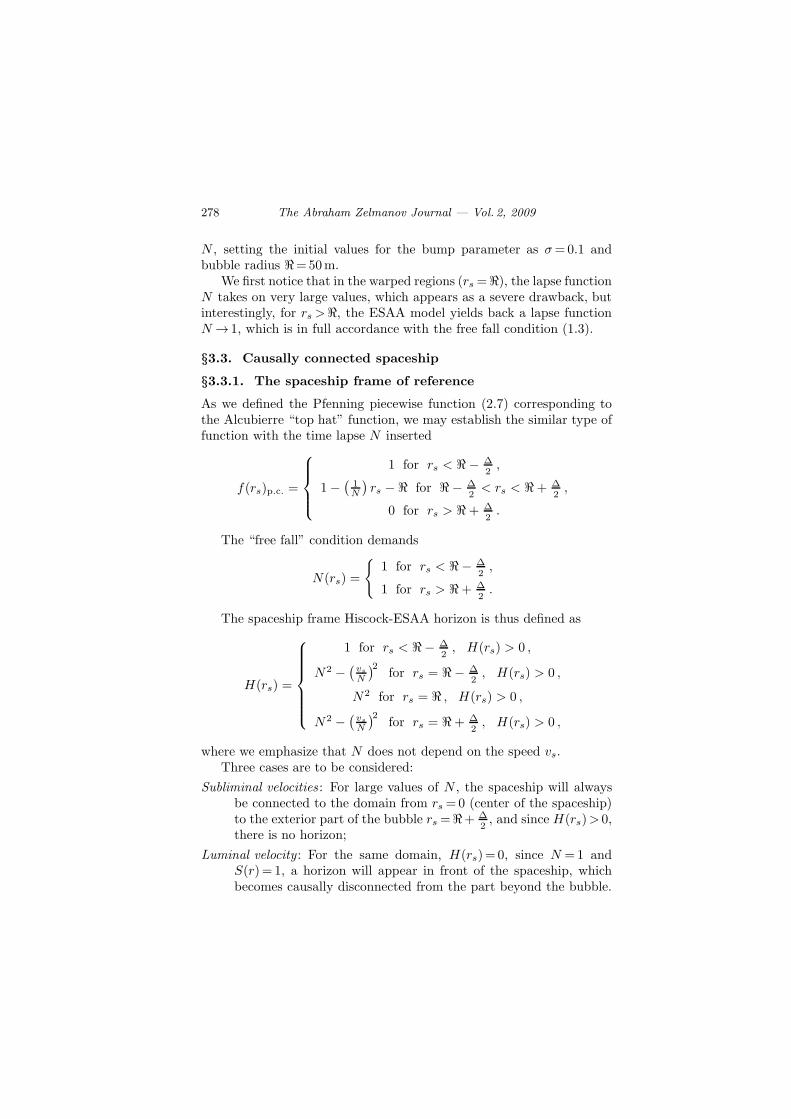
§3.3.1. The spaceship frame of reference

As we defined the Pfenning piecewise function (2.7) corresponding tothe Alcubierre “top hat” function, we may establish the similar type offunction with the time lapse N inserted

f(rs)p.c. =

1 for rs < ℜ − ∆2,

1−(

1N

)

rs −ℜ for ℜ − ∆2< rs < ℜ+ ∆

2,

0 for rs > ℜ+ ∆2.

The “free fall” condition demands

N(rs) =

{

1 for rs < ℜ− ∆2,

1 for rs > ℜ+ ∆2.

The spaceship frame Hiscock-ESAA horizon is thus defined as

H(rs) =

1 for rs < ℜ− ∆2, H(rs) > 0 ,

N2 −(

vsN

)2for rs = ℜ− ∆

2, H(rs) > 0 ,

N2 for rs = ℜ , H(rs) > 0 ,

N2 −(

vsN

)2for rs = ℜ+ ∆

2, H(rs) > 0 ,

where we emphasize that N does not depend on the speed vs.Three cases are to be considered:

Subliminal velocities : For large values of N , the spaceship will alwaysbe connected to the domain from rs =0 (center of the spaceship)to the exterior part of the bubble rs =ℜ+ ∆

2, and since H(rs)> 0,

there is no horizon;

Luminal velocity : For the same domain, H(rs)= 0, since N =1 andS(r)= 1, a horizon will appear in front of the spaceship, whichbecomes causally disconnected from the part beyond the bubble.

Patrick Marquet 279

Provided that N is not a function of the speed and has been en-

gineered at subluminal speeds, it is always connected to the space-

ship and the warped region∫ ℜ+∆/2

ℜ−∆/2 can be “controlled” by the

“astronauts”;

Superluminal velocities : The same argument applies here.

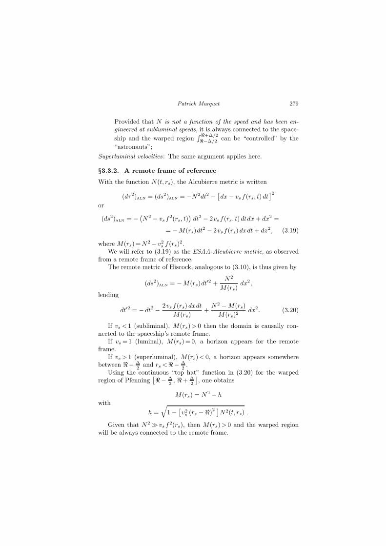
§3.3.2. A remote frame of reference

With the function N(t, rs), the Alcubierre metric is written

(dτ2)ALN = (ds2)ALN = −N2dt2 −[

dx − vs f(rs, t) dt]2

or

(ds2)ALN = −(

N2 − vs f2(rs, t)

)

dt2 − 2vs f(rs, t) dtdx + dx2 =

= −M(rs)dt2 − 2vs f(rs) dxdt + dx2, (3.19)

where M(rs)=N2 − v2s f(rs)2.

We will refer to (3.19) as the ESAA-Alcubierre metric, as observedfrom a remote frame of reference.

The remote metric of Hiscock, analogous to (3.10), is thus given by

(ds2)ALN = −M(rs)dt′2 +

N2

M(rs)dx2,

lending

dt′2 = − dt2 − 2vs f(rs) dxdt

M(rs)+

N2 −M(rs)

M(rs)2dx2. (3.20)

If vs < 1 (subliminal), M(rs)> 0 then the domain is causally con-nected to the spaceship’s remote frame.

If vs =1 (luminal), M(rs)= 0, a horizon appears for the remoteframe.

If vs > 1 (superluminal), M(rs)< 0, a horizon appears somewherebetween ℜ− ∆

2and rs <ℜ− ∆

2.

Using the continuous “top hat” function in (3.20) for the warpedregion of Pfenning

[

ℜ− ∆2, ℜ+ ∆

2

]

, one obtains

M(rs) = N2 − h

with

h =

√

1−[

v2s (rs −ℜ)2]

N2(t, rs) .

Given that N2 ≫ vs f2(rs), then M(rs)> 0 and the warped region

will be always connected to the remote frame.


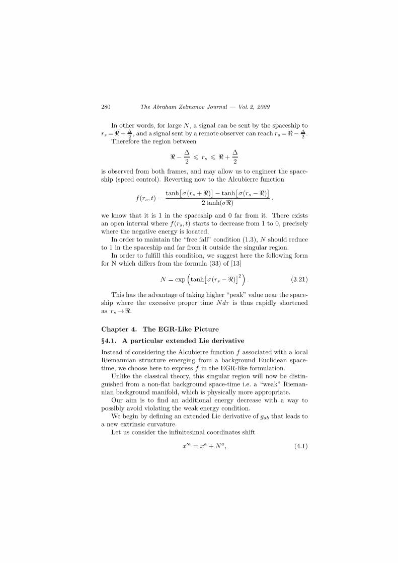
In other words, for large N , a signal can be sent by the spaceship tors =ℜ+ ∆

2, and a signal sent by a remote observer can reach rs =ℜ− ∆

2.

Therefore the region between

ℜ − ∆

26 rs 6 ℜ+

∆

2

is observed from both frames, and may allow us to engineer the space-ship (speed control). Reverting now to the Alcubierre function

f(rs, t) =tanh

[

σ(rs + ℜ)]

− tanh[

σ(rs −ℜ)]

2 tanh(σℜ) ,

we know that it is 1 in the spaceship and 0 far from it. There existsan open interval where f(rs, t) starts to decrease from 1 to 0, preciselywhere the negative energy is located.

In order to maintain the “free fall” condition (1.3), N should reduceto 1 in the spaceship and far from it outside the singular region.

In order to fulfill this condition, we suggest here the following formfor N which differs from the formula (33) of [13]

N = exp(

tanh[

σ(rs −ℜ)]2)

. (3.21)

This has the advantage of taking higher “peak” value near the space-ship where the excessive proper time Ndτ is thus rapidly shortenedas rs →ℜ.

Chapter 4. The EGR-Like Picture

§4.1. A particular extended Lie derivative

Instead of considering the Alcubierre function f associated with a localRiemannian structure emerging from a background Euclidean space-time, we choose here to express f in the EGR-like formulation.

Unlike the classical theory, this singular region will now be distin-guished from a non-flat background space-time i.e. a “weak” Rieman-nian background manifold, which is physically more appropriate.

Our aim is to find an additional energy decrease with a way topossibly avoid violating the weak energy condition.

We begin by defining an extended Lie derivative of gab that leads toa new extrinsic curvature.

Let us consider the infinitesimal coordinates shift

x′a = xa +Na, (4.1)

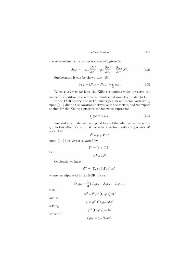
Patrick Marquet 281

the relevant metric variation is classically given by

δgab = − gac∂N c

∂xb− gcb

∂N c

∂xa− ∂gab

∂xcN c. (4.2)

Furthermore it can be shown that [15]

δgab = (Na;b +Nb;a) = LN

gab . (4.3)

When LN

gab=0, we have the Killing equations which preserve the

metric (a condition referred to as infinitesimal isometry) under (4.1).In the EGR theory, the metric undergoes an additional variation ζ

upon (4.1) due to the covariant derivative of the metric, and we expectto find for the Killing equations the following expression

LN

gab = ζ gab . (4.4)

We need now to define the explicit form of the infinitesimal variationζ. To this effect we will first consider a vector l with components Ai

such thatl2 = gik A

iAk

upon (4.1) this vector is varied by

l′2 = (1 + ζ) l2,

i.e.dl2 = ζ l2.

Obviously we have

dl2 = (Dc gik)AiAk dxc,

where, as stipulated in the EGR theory,

Dc gik =1

3

(

Jk gci + Ji gck − Jc gik)

,

thusdl2 = l2 gik (Dc gik) dx

c

and soζ = gik (Dc gik) dx

c

settinggik (Dc gik) = Bc

we writeζ gab = gabBcdx

c.


Within a sufficient approximation, we may set

dxc = N c,

hence we define the “extended Lie derivative” of gab as

LN′

gab ≡ LN

gab BcNc, (4.5)

where N ′ is the rescaled shift vector.At this stage, we want to stress that the assumed extension is here

always considered in a Riemannian scheme.The definition (4.5) formally holds for a Lie derivative of gab, pro-

vided the last term is “likened” to a Riemannian correction.Indeed a “non-Riemannian” Lie derivative (i.e. defined in the frame-

work of the EGR theory) is not applicable, due to the algebraic natureof this operation.

The EGR theory however provides a justification as to the origin ofthe extra term in (4.5).

§4.2. Extended extrinsic curvature and associated energydensity

We are now able to define the “extended” extrinsic curvature as

K ′

αβ = (2N ′)−1

(

∇α N ′

β +∇β N′

α +∂gαβ∂t

)

. (4.6)

Accordingly, we still consider the classical field equations as inferredfrom the Hilbert-Einstein action

S =

∫

R√−g d4x .

By doing so, we set forth a close one-to-one correspondence betweenthe EGR scalar curvature R=R− 1

3

(

∇eJe+ 1

2J2)

and the modifiedRiemannian scalar curvature R depicted in Riemannian geometry.

In this perspective, the equation (2.19) becomes here

C′ =1

6π

(

(3)R′ −K ′

αβK′αβ +K ′2

)

. (4.7)

Now we are going to generalize the Alcubierre metric by followingthe same pattern which has led to (2.20).

However, based on the extended formulation, we now choose

N ′1 = − vs f(rs) , (4.8)

Patrick Marquet 283

N ′2 = N2, N ′3 = N3 (4.9)and

(3)R′ = (3)R .

An immediate and important consequence appears when one ob-serves the form of the expression

(C′)AL=1

16π

[

(3)R−Kαβ(N′1, N)Kαβ(N ′1, N)+K2(N ′1, N)

]

. (4.10)

In contrast to the classical Alcubierre scheme, the non-vanishinginitial Riemannian scalar curvature of the hypersurfaces may have nowa significant impact on the negative energy density reduction.

In addition, the term K2, which should not cancel off here, con-tributes even further to lowering this energy.

Discussion and Concluding Remarks

First observation : The expansion of the volume element θ=−Kαα is

attached to the bubble which it generates and is thus a local prop-erty;

Second observation : The free fall condition (1.3) requires obviouslya flat space (flat Universe), instead of a Riemannian one.

However, in the EGR context, the non-vanishing scalar curvature(3)R may be also regarded here as sufficiently “local” with respect to the(quasi) Euclidean space as a whole, wherein the Eulerian observers aresituated.

Indeed, if the three-volume of each hypersurface t= const is ex-tremalized, the conditionK = const results (see Andre Lichnerowicz [16]and also subsequently maximum slicing conditions by Yvonne ChoquetBruhat [17]).

It is then possible to impose this condition, with respect to usingequation (1.16), to eliminate (3)R from the trace of equation (1.15): inthis case it is shown that the lapse function can be taken to be N → 1as an asymptotic boundary condition, which leads to an asymptoticallyflat space-time.

This condition is physically satisfied when one considers the scale ofdistances in our observable Universe as compared to the bubble warpingdimensions, so that (4.10) holds with an asymptotically flat universewherefrom the distant observers are located.

Hence, we can always imagine a situation where stellar massive ob-jects arranged in such a required configuration are coming into play, andwhere the influence of their curvature given by (3)R may then be used to


balance the negative energy, which renders the Warp Drive compatiblewith the weak energy condition.

With these two observations our theory tends to run counter to thezero expansion Warp Drive suggested by Jose Natario [18].

Needless to say, all arguments regarding the piecewise functioncausality constraints detailed above are equally valid in our extendedformulation.

Within the standard Alcubierre metric, it is however possible toavoid the problem of causally disconnecting the spaceship from the outeredge of the bubble.

A somewhat recent two dimensional metric concept has been pro-posed by Serge V. Krasnikov [19] in which the time for a round tripto a distant planet as measured by clocks located on the Earth can bemade arbitrarily short.

To connect the Earth to the planet, a space-time extension of thismetric leads to the creation of a “tube” wherein the space-time is flat,but the light cones are opened out so as to allow superluminal travel [20].

In some cases, these metrics are shown not to lead to the fatallyclosed time-like curves.

Appendix. Detailing a stellar round trip example accordingto Alcubierre

A1. Stellar journey

Consider two quasi-static planets A and B, which are apart from eachother at a distance D in the Euclidean space-time.

A spaceship starts off on its own (self-propulsion) from A at an initialmoment of time t= tA, with a subluminal velocity v < c.

At a distance d away from A, d≪D, the spaceship stops at a pointwhere the bubble is being created, which then drags the spaceship to-wards the planet B, thus inducing a coordinate three-acceleration a thatvaries rapidly from a=0 to a= const 6=0.

Halfway, between A and B, the bubble is controlled so as to invertthis acceleration from a to −a.

As the absolute values of acceleration and deceleration are assumedequal, the spaceship will eventually be at rest at a distance d away fromthe planet B at the time the disturbance will disappear (vs =0) and thejourney is further completed at a “physical” speed v < c.

The total coordinate time elapsed in the one-way trip from the planetA to the planet B is: T = tself-propulsion+ tbubble. Had the acceleration

Patrick Marquet 285

been constant along the distance (D− 2d), we would have

(D − 2d) =a t2bubble

2,

where

t2bubble =2 (D − 2d)

a.

In fact, during the accelerating stage of the bubble, we will have

(+)t2bubble =(D − 2d)

a

and during the decelerating stage

(−)t2bubble =(D − 2d)

a,

which in total yields

T = tself-propulsion +

√

2 (D − 2d)

athat is

T = 2

(

d

v+

√

(D − 2d)

2a

)

.

A2. Deceleration stage

Remember that we considered planets A and B as static in a quasi-flatspace. In this case dx= dy= dz=0. This means that their proper time

is equal to their coordinate time (reinstating c): t= τ = x4

c .The proper time τ measured in the spaceship, on the other hand,

must take into account the Lorentz transformations

τship = 2

(

d

γv+

√

(D − 2d)

2a

)

,

where

γ =1

√

1− v2/c2.

If the radius ℜ of the bubble satisfies, as it should, ℜ≪ d≪D, onemay admit the approximation

τ ≈ T ≈√

2D

a.


This clearly shows that T can be chosen as small as we like, byincreasing the value of a.

As outlined by Alcubierre, since a round trip will only take twice aslong, we can be back on the planet A after an arbitrarily short propertime, both from the point of view of an observer on board of the space-ship and from the point of view of an observer located on the planet.

The spaceship will then be able to travel much faster than the speedof light while remaining on a time-like trajectory (which is inside itslocal light-cone).

Submitted on December 10, 2009

1. Alcubierre M. The Warp Drive: hyper-fast travel within general relativity.Classical and Quantum Gravity, 1994, vol. 11, L73–L77.

2. Hawking S.W. The Large Scale Structure of Space-Time. Cambridge Univer-sity Press, Cambridge, 1973, p.88–92.

3. Marquet P. The EGR theory: an extended formulation of general relativity.The Abraham Zelmanov Journal, 2009, vol. 2, 148–170.

4. Kramer D., Stephani H., and Hertl E. Exact Solutions of Einstein’s FieldEquations. Cambridge University Press, Cambridge, 1980.

5. Arnowitt R. and Deser S. Quantum theory of gravitation: general formula-tion and linearized theory. Physical Review, 1959, vol. 113, no. 2, 745–750;Arnowitt R., Deser S., and Misner C. Dynamical structure and definition ofenergy in general relativity. Physical Review, 1959, vol. 116, no. 5, 1322–1330;Arnowitt R., Deser S., and Misner C. Canonical variables for general relativity.Physical Review, 1960, vol. 117, no. 6, 1595–1602.

6. Kuchar K. Canonical methods of quantization. Quantum Gravity 2. A Second

Oxford Symposium, Clarendon Press, Oxford, 1981, 329–374.

7. MacCallum M.A.H. Quantum cosmological models. Quantum Gravity. Pro-

ceedings of the Oxford Symposium. Clarendon Press, Oxford, 1975, 174–218.

8. Stewart J.M. Numerical relativity. In: Classical General Relativity, Cam-bridge University Press, Cambridge, 1982, 231–262.

9. Ford L. H. and Pfenning M.J. The unphysical nature of “warp drive”. Classical

and Quantum Gravity, 1997, vol. 14, no. 7, 1743–1751; Cornell UniversityarXiv: gr-qc/9702026.

10. Wald R. General Relativity. University of Chicago Press, Chicago, 1984.

11. Hiscock W.A. Quantum effects in the Alcubierre warp-drive spacetime. Clasi-

cal and Quantum Gravity, 1997, vol. 14, no. 11, L183–L188; Cornell UniversityarXiv: gr-qc/9707024.

12. Loup F., Waite D., and Halerewicz E. Reduced total energy requirement for amodified Alcubierre warp drive space-time. Cornell University arXiv: gr-qc/0107097.

13. Loup F., Held R., Waite D., Halerewicz E. Jr., Stabno M., Kuntzman M.,Sims R. A causally connected superluminal Warp Drive spacetime. CornellUniversity arXiv: gr-qc/0202021.

Patrick Marquet 287

14. Van den Broeck C. A “warp drive” with more reasonable total energy re-quirements. Classical and Quantum Gravity, 1999, vol. 16, no. 12, 3973–3979;Cornell University arXiv: gr-qc/9905084.

15. Landau L.D. et Lifshitz E.M. Theorie des Champs. Traduit du Russe parE. Gloukhian, Editions de la Paix, Moscou, 1964.

16. Lichnerowicz A. L’integration des equations de la gravitation relativiste et leprobleme des n corps. Journal de Mathematiques Pures et Appliquees, 1944,tome 23, 37–63.

17. Choquet-Bruhat Y. Maximal submanifolds and manifolds with constant meanextrinsic curvature of a Lorentzian manifold. Annali della Scuola Normale

Superiore di Pisa, Classe di Science, 1976, tome 3, no. 3, 373–375.

18. Natario J. Warp drive with zero expansion. Classical and Quantum Gravity,2002, vol. 19, no. 6, 1157–1165.

19. Krasnikov S.V. Hyperfast travel in general relativity. Physical Review D, 1998,vol. 57, no. 8, 4760–4766; Hyper fast interstellar travel in gneral relativity.Cornell University arXiv: gr-qc/9511068.

20. Everett A.E. and Roman T.A. Superluminal subway: the Krasnikov tube.Physical Review D, 1997, vol. 56, no. 4, 2100–2108.

Vol. 2, 2009 ISSN 1654-9163

THE

ABRAHAM ZELMANOV

JOURNALThe journal for General Relativity,gravitation and cosmology

TIDSKRIFTEN

ABRAHAM ZELMANOVDen tidskrift for allmanna relativitetsteorin,

gravitation och kosmologi

Editor (redaktor): Dmitri RabounskiSecretary (sekreterare): Indranu Suhendro

The Abraham Zelmanov Journal is a non-commercial, academic journal registeredwith the Royal National Library of Sweden. This journal was typeset using LATEXtypesetting system. Powered by Ubuntu Linux.

The Abraham Zelmanov Journal ar en ickekommersiell, akademisk tidskrift registr-erat hos Kungliga biblioteket. Denna tidskrift ar typsatt med typsattningssystemetLATEX. Utford genom Ubuntu Linux.

Copyright c© The Abraham Zelmanov Journal, 2009

All rights reserved. Electronic copying and printing of this journal for non-profit,academic, or individual use can be made without permission or charge. Any part ofthis journal being cited or used howsoever in other publications must acknowledgethis publication. No part of this journal may be reproduced in any form whatsoever(including storage in any media) for commercial use without the prior permissionof the publisher. Requests for permission to reproduce any part of this journal forcommercial use must be addressed to the publisher.

Eftertryck forbjudet. Elektronisk kopiering och eftertryckning av denna tidskrifti icke-kommersiellt, akademiskt, eller individuellt syfte ar tillaten utan tillstandeller kostnad. Vid citering eller anvandning i annan publikation ska kallan anges.Mangfaldigande av innehallet, inklusive lagring i nagon form, i kommersiellt syfte arforbjudet utan medgivande av utgivarna. Begaran om tillstand att reproducera delav denna tidskrift i kommersiellt syfte ska riktas till utgivarna.

Documents

TheGeneralized WarpDrive Concept in theEGRTheory - Zelmanov Journal