The Genus of Generalized Randomand Quasirandom Graphs

by

Yifan Jing

B.Sc. (Honors Program), University of Science and Technology of China, 2016

Thesis Submitted in Partial Fulfillment of theRequirements for the Degree of

Master of Science

in theDepartment of Mathematics

Faculty of Science

c© Yifan Jing 2018SIMON FRASER UNIVERSITY

Summer 2018

Copyright in this work rests with the author. Please ensure that anyreproduction or re-use is done in accordance with the relevant national

copyright legislation.

Approval

Name: Yifan Jing

Degree: Master of Science (Mathematics)

Title: The Genus of Generalized Random andQuasirandom Graphs

Examining Committee: Chair: Weiran SunAssistant Professor

Bojan MoharSenior SupervisorProfessor

Luis GoddynSupervisorProfessor

Matthew DeVosInternal ExaminerAssociate Professor

Date Defended: June 12, 2018

ii

Abstract

The genus of a graph G is the minimum integer h such that G has an embedding insome surface (closed compact 2-manifold) Sh of genus h. In this thesis, we will discussthe genus of generalized random and quasirandom graphs. First, by developing ageneral notion of random graphs, we determine the genus of generalized randomgraphs. Next, we approximate the genus of dense generalized quasirandom graphs.

Based on analysis of minimum genus embeddings of quasirandom graphs, we providean Efficient Polynomial-Time Approximation Scheme (EPTAS) for approximatingthe genus (and non-orientable genus) of dense graphs. More precisely, we provide analgorithm that for a given (dense) graph G of order n and given ε > 0, returns aninteger g such that G has an embedding into a surface of genus g, and this is ε-close toa minimum genus embedding in the sense that the minimum genus g(G) of G satisfies:g(G) ≤ g ≤ (1 + ε)g(G). The running time of the algorithm is O(f(ε)n2), where f(·)is an explicit function. Next, we extend this algorithm to also output an embedding(rotation system) of genus g. This second algorithm is an Efficient Polynomial-timeRandomized Approximation Scheme (EPRAS) and runs in time O(f1(ε)n2).

The last part of the thesis studies the genus of complete 3-uniform hypergraphs, whichis a special case of genus of random bipartite graphs, and also a natural generaliza-tion of Ringel–Youngs Theorem. Embeddings of a hypergraph H are defined as theembeddings of its associated Levi graph LH with vertex set V (H) t E(H), in whichv ∈ V (H) and e ∈ E(H) are adjacent if and only if v and e are incident in H. Theconstruction in the proof may be of independent interest as a design-type problem.

Keywords: graph embeddings (05C10); genus (57M15); Szemerédi regularity lemma(05C85); random graphs (05C80); hypergraphs (05C65)

iii

Acknowledgements

I would like to thank my supervisor, Bojan Mohar, for all his help and guidance thathe has given me, I have learned a great deal from him. It is my honor to be one of hisstudent. I want to thank all of my officemates, for their help and valuable discussionswith them. Last but not the least, I want to thank my parents and my girlfriend, fortheir love and support.

iv

Table of Contents

Approval ii

Abstract iii

Acknowledgements iv

Table of Contents v

List of Figures vii

1 Introduction 11.1 Motivation . . . . . . . . . . . . . . . . . . . . . . . . . . . . . . . . . 11.2 Structure of the Thesis . . . . . . . . . . . . . . . . . . . . . . . . . . 2

2 Embeddings of Graphs 42.1 Notation and Basic Definitions . . . . . . . . . . . . . . . . . . . . . . 42.2 Near Minimum Genus Embeddings . . . . . . . . . . . . . . . . . . . 5

3 Genus of Generalized Random Graphs 93.1 Introduction . . . . . . . . . . . . . . . . . . . . . . . . . . . . . . . . 93.2 Genus of Random Bipartite Graphs . . . . . . . . . . . . . . . . . . . 10

3.2.1 Random Bipartite Graphs G(n1, n2, p) . . . . . . . . . . . . . . 103.2.2 Bipartite Graphs with a Small Part . . . . . . . . . . . . . . . 18

3.3 Genus of Generalized Random Graphs . . . . . . . . . . . . . . . . . 233.3.1 H2-Random Graphs . . . . . . . . . . . . . . . . . . . . . . . . 23

4 Genus of Dense Quasirandom Graphs 304.1 Cut Metric and Quasirandomness . . . . . . . . . . . . . . . . . . . . 304.2 Genus of Quasirandom Graphs . . . . . . . . . . . . . . . . . . . . . . 334.3 Genus of Bipartite and Tripartite Quasirandom Graphs . . . . . . . . 384.4 Genus of Multipartite Quasirandom Graphs . . . . . . . . . . . . . . 44

v

5 Genus of Large Dense Graphs 485.1 Introduction . . . . . . . . . . . . . . . . . . . . . . . . . . . . . . . . 48

5.1.1 The Graph Genus Problem . . . . . . . . . . . . . . . . . . . . 485.1.2 Overview of the Algorithm . . . . . . . . . . . . . . . . . . . . 50

5.2 Algorithms and Analysis . . . . . . . . . . . . . . . . . . . . . . . . . 575.2.1 EPTAS for the Genus of Dense Graphs . . . . . . . . . . . . . 575.2.2 EPRAS for Embeddings of Dense Graphs . . . . . . . . . . . . 60

6 Genus of Complete 3-Uniform Hypergraphs 636.1 Embeddings of Hypergraphs . . . . . . . . . . . . . . . . . . . . . . . 636.2 Hypergraphs of Even Order . . . . . . . . . . . . . . . . . . . . . . . 64

6.2.1 Minimum Genus Embeddings of Hypergraphs . . . . . . . . . 646.2.2 Genus of Hypergraphs . . . . . . . . . . . . . . . . . . . . . . 686.2.3 Number of Non-Isomorphic Embeddings . . . . . . . . . . . . 736.2.4 Hypergraphs with Multiple Edges . . . . . . . . . . . . . . . . 75

6.3 Hypergraphs of Odd Order . . . . . . . . . . . . . . . . . . . . . . . . 77

Bibliography 79

vi

List of Figures

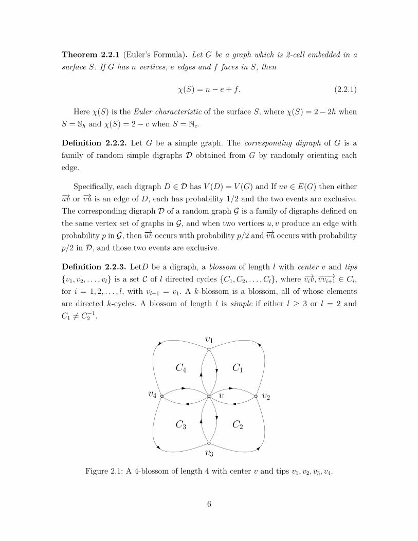
Figure 2.1 A 4-blossom of length 4 with center v and tips v1, v2, v3, v4. . . 6

Figure 6.1 Planar embeddings of K34 and its Levi graph L4. . . . . . . . . 64

Figure 6.2 A quadrilateral embedding around a vertex ijk ∈ Yn. The cho-sen clockwise rotation around vertices i, j, k is indicated by thedashed circular arcs. . . . . . . . . . . . . . . . . . . . . . . . 66

Figure 6.3 A minimum genus orientable embedding of K36 . . . . . . . . . 67

Figure 6.4 A non-orientable embedding of 2K34 on the Klein bottle. . . . 76

Figure 6.5 An optimal non-orientable embedding of K35 . . . . . . . . . . . 77

vii

Chapter 1

Introduction

1.1 Motivation

The study of topological graph theory dates back to the middle of the eighteenthcentury, start with the study of Euler characteristic for polyhedra. It took heightenedinterest in the latter part of the nineteenth century, with several map-coloring prob-lems. The object is to find the minimum number of colors needed to color all possiblemaps, where countries that share a border must be colored differently. Probably oneof the most famous conjectures in mathematics is Four Color Conjecture, that is, fourcolors are enough to color all possible maps drawn on the plane. The conjecture wasmade by Francis Guthrie [5, 47] in 1852. The first proof was published by Kempein 1878, but this contained an error which was found in 1890 [26] by Heawood, whoproved five colors are sufficient to color any map drawn on the plane. The conjecturewas finally confirmed in 1976 by Appel and Haken [3], after a century of false proofsand refinements of techniques.

The problem of coloring maps on the plane is equivalent to the problem on thesphere. Heawood Map-coloring Conjecture [26] generalizes the four color conjectureto every closed compact 2-manifold. We state the orientable case:

χ(Sh) =⌊7 +

√1 + 48h2

⌋, for h > 0,

where h is the genus of the closed compact 2-manifold Sh. The problem was open foralmost eight decades, and in 1965 it was given the place of honor for Tietze’s FamousProblems of Mathematics [68]. The problem was eventually reduced to the genuscomputation for complete graphs and was studied in a series of papers in the twentiethcentury. In 1968, Ringel and Youngs [53] determined the genus of all complete graphs,

1

which implies the final solution of the Heawood’s Conjecture. The complete proof wasfinally presented in the monograph [52]. Their proof is split in 12 cases, some of thecases were slightly simplified later, but for the most complicated cases, no short proofsare known.

Theorem 1.1.1 (Ringel–Youngs Theorem). If n ≥ 3 then

g(Kn) =⌈

(n− 3)(n− 4)12

⌉.

If n ≥ 5 and n 6= 7, then

g(Kn) =⌈

(n− 3)(n− 4)6

⌉.

Given a graph G, determine the genus of G is one of the central problems intopological graph theory. It is also a very hard problem in both mathematics andcomputer science, since Thomassen [65] proved that the problem is NP-complete. Onthe other hand, determine the genus of a graph is also very important, by Robertsonand Seymour’s graph minor theory.

Definition 1.1.2. Given two graphs H and G, we say H is a minor of G if H canbe obtained from G by deleting edges and vertices and by contracting edges.

The following generalized Kuratowski’s Theorem [56] tells us, the genus of a graphgives us a rough structure of the graph. Then many NP-complete algorithms becomeploynomial-time if we know the underlying graph has bounded genus.

Theorem 1.1.3 (Robertson and Seymour). Graphs with bounded genus have finitelymany forbidden minors.

The thesis is motived by the problem on approximating the genus of large densegraphs. After applying Szemerédi regularity lemma on graph G, we obtain a partitionP of V (G), and the induced subgraph between any two parts (except an ε-fraction) israndom-like. Therefore, the theories of the genus of random and quasirandom graphsare needed. Background of the graph genus problem is introduced in Chapter 5.1.1.

1.2 Structure of the Thesis

The thesis is organized as follows. In the second chapter, we introduce the basic defi-nitions in topological graph theory, and we also present the tools we use to construct

2

the minimum (or near minimum) genus embeddings of generalized random graphsand quasirandom graphs. In chapter three, we determine the genus of random bipar-tite graphs, and discuss the genus of H-random graphs. In chapter four, we approxi-mate the genus of dense quasirandom graphs. In chapter five, we provide an EfficientPolynomial-Time Approximation Scheme (EPTAS) for approximating the genus (andnon-orientable genus) of dense graphs, as well as an Efficient Polynomial-time Ran-domized Approximation Scheme (EPRAS) for the near optimal embeddings of densegraphs, based on the results in the previous chapters. In chapter six, we consider theminimum genus embeddings of complete 3-uniform hypergraphs, which is a specialcase of random bipartite graphs we discussed in chapter 3, and also a natural gen-eralization of Ringel–Youngs Theorem. We determine the genus (and non-orientablegenus) of K3

n when n is even, and discuss the genus when n is odd. Parts of the resultsin Chapters 3,4,5 and 6 are included in submitted papers [29, 30, 31]. Some of therest of the results in those chapters and some in-writing future work will be includedin [32, 33].

3

Chapter 2

Embeddings of Graphs

2.1 Notation and Basic Definitions

Through out the dissertation, We will use standard notation in graph theory, topolog-ical graph theory and graph limit theory as given in [16], [44] and [36], respectively.We fix the following notation.

• Denote by N the set of non-negative integers, and [n] is the set {1, . . . , n}.

• G is always a graph (1-complexes).

• Given a graph G, suppose X, Y ⊆ V (G). We use E(X, Y ) denote the set ofedges between X and Y , and e(X, Y ) = |E(X, Y )|. We also use e(G) to denote|E(G)|.

• For two sets X and Y , by X tY we denote the disjoint union of X and Y , andwe set X ⊕ Y = (X × Y ) ∪ (Y ×X).

• A(n) ∼ B(n) means limn→∞A(n)/B(n) = 1, and A(n) � B(n) means thatlimn→∞A(n)/B(n) = 0. If limn→∞A(n)/B(n) = c for some constant c, wedenote it by A(n) = Θ(B(n)). We say an event A(n) happens asymptoticallyalmost surely (abbreviated a.a.s.) if P(A(n))→ 1 as n→∞.

Now we give the definition of the genus of graphs, as a natural generalization ofplanar graphs.

Definition 2.1.1. Given a graph G, let g(G) be the genus of G, that is, the minimumh such that G embeds into the orientable surface Sh of genus h, and let g(G) be thenon-orientable genus of G which is the minimum c such that G embeds into the non-orientable surface Nc with crosscap number c. If orientability of a surface is not a

4

concern, we define the Euler genus as g(G) = min{2g(G), g(G)}. By a surface wemean a compact two-dimensional manifold without boundary.

For any surface S, we say G is 2-cell embedded in S if in that embedding, eachface of G is homeomorphic to an open disk. Similarly, a k-gon embedding of G is whenevery face is bounded by a cycle of length k. In particular, we say an embedding of Gis triangular if every face is bounded by a triangle, and an embedding is quadrangularif every face is bounded by a cycle of length 4.

Every 2-cell embedding (and thus also any minimum genus embedding) of G canbe represented combinatorially by using the corresponding rotation system π = {πv |v ∈ V (G)} where a local rotation πv at the vertex v is a cyclic permutation of theneighbours of v. In addition to this, we also add the signature, which is a mappingλ : E(G)→ {1,−1} and describes if the local rotations around the endvertices of anedge have been chosen consistently or not. The signature is needed only in the case ofnon-orientable surfaces; in the orientable case, we may always assume the signatureis trivial (all edges have positive signature). The pair (π, λ) is called the embeddingscheme for G. For more background on topological graph theory, we refer to [25, 44].

We say that two embeddings φ1, φ2 : G → S of a graph G into the same surfaceS are equivalent (or homeomorphic) if there exists a homeomorphism h : S → Ssuch that φ2 = hφ1. By [44, Corollary 3.3.2], (2-cell) embeddings are determined upto equivalence by their embedding scheme (π, λ), and two such embedding schemes(π, λ) and (π′, λ′) determine equivalent embeddings if and only if they are switchingequivalent. This means that there is a vertex-set U ⊆ V (G) such that (π′, λ′) isobtained from (π, λ) by replacing πu with π−1

u for each u ∈ U and by replacing λ(e)with −λ(e) for each edge e with one end in U and the other end in V (G) \ U .

2.2 Near Minimum Genus Embeddings

Given a graph G, determining the genus of G is one of the fundamental problemsin topological graph theory. Youngs [72] showed that the problem of determining thegenus of a connected graph G is the same as determining a 2-cell embedding of G withminimum genus. The same holds for the non-orientable genus [48]. That means, in thisthesis we only need to consider 2-cell embeddings of graphs. For 2-cell embeddingswe have the famous Euler’s Formula.

5

Theorem 2.2.1 (Euler’s Formula). Let G be a graph which is 2-cell embedded in asurface S. If G has n vertices, e edges and f faces in S, then

χ(S) = n− e+ f. (2.2.1)

Here χ(S) is the Euler characteristic of the surface S, where χ(S) = 2− 2h whenS = Sh and χ(S) = 2− c when S = Nc.

Definition 2.2.2. Let G be a simple graph. The corresponding digraph of G is afamily of random simple digraphs D obtained from G by randomly orienting eachedge.

Specifically, each digraph D ∈ D has V (D) = V (G) and If uv ∈ E(G) then either−→uv or −→vu is an edge of D, each has probability 1/2 and the two events are exclusive.The corresponding digraph D of a random graph G is a family of digraphs defined onthe same vertex set of graphs in G, and when two vertices u, v produce an edge withprobability p in G, then −→uv occurs with probability p/2 and −→vu occurs with probabilityp/2 in D, and those two events are exclusive.

Definition 2.2.3. LetD be a digraph, a blossom of length l with center v and tips{v1, v2, . . . , vl} is a set C of l directed cycles {C1, C2, . . . , Cl}, where −→viv,−−−→vvi+1 ∈ Ci,for i = 1, 2, . . . , l, with vl+1 = v1. A k-blossom is a blossom, all of whose elementsare directed k-cycles. A blossom of length l is simple if either l ≥ 3 or l = 2 andC1 6= C−1

2 .

v

v1

v2

v3

v4

C1

C2C3

C4

Figure 2.1: A 4-blossom of length 4 with center v and tips v1, v2, v3, v4.

6

Let C be a family of arc-disjoint closed trails in D∪D−1. We say that C is blossom-free if no subset of C forms a blossom centered at some vertex. The following lemmais a slight strengthening of [58, Lemma 2.1]; the proof is elementary and we omitdetails.

Lemma 2.2.4. Let G be a graph and let D be the corresponding digraph. Supposethat C1 and C2 is a set of arc-disjoint closed trails in D and D−1 (respectively) suchthat their union C1∪C2 is blossom-free in D∪D−1. Then there exist a rotation systemΠ of G such that every closed trail in C1 ∪ C2 is a face of Π.

For every ε > 0, an ε-near k-gon embedding Π is a rotation system of G such thatkfk(Π) ≥ 2(1− ε)|E(G)|, where fk(Π) is the number of faces of length k of Π.

The following result from [21] (see also [49, 58] where its current formulationappears) will be our main tool for constructing near-optimal embeddings of randomgraphs and quasirandom graphs.

Theorem 2.2.5. Let ε > 0 be a real number and d ≥ 2 be an integer. Then there exista positive real number δ and an integer N0 such that for every N ≥ N0 the followingholds. If ∆ is a real number and if H is a d-uniform hypergraph with |V (H)| = N

such that

1. |{x ∈ V (H) | (1− δ)∆ ≤ deg(x) ≤ (1 + δ)∆}| ≥ (1− δ)N ,

2. for every x, y ∈ V (H), |{e ∈ E(H) | x, y ∈ e}| < δ∆,

3. at most δN∆ hyperedges of H contain a vertex v ∈ V (H) with deg(v) > (1+δ)∆,

then H has a matching of size at least (1−ε)N/d. Moreover, for every matching M inH, there exists a matching M ′ in H with M ∩M ′ = ∅, and with |M ′| ≥ (1− ε)N/d.

Similarly as for undirected graphs (see [44, Lemma 5.4.2]), we have the followingproperty on digraphs.

Lemma 2.2.6. Let D(V,A) be a simple digraph and a, b ∈ A, a 6= b. Let f, g ∈ Z+.Then there exists a positive integer K = K(f, g), such that if D contains at leastK closed trails of length f containing both a and b, then there exist two verticesu, v ∈ V (D) and g internally disjoint directed paths from u to v, all of the samelength l, where 2 ≤ l ≤ f − 2.

7

Proof. Let x ∈ V be the head of a and let y ∈ V be the tail of b. We may assumex 6= y. The proof is by induction on f+g, with K(f, g) = ∏f−2

i=1 ((f−i)(f−i−1)g)2i−1 .In the base case when g = 0 there is nothing to prove, and when f = 3, the claimis easy, so we move to the induction step. Assume now we have K(f + 1, g) closedtrails of length f + 1 containing both a and b. Let −→Pxy be the set of paths from x

to y on these closed trails. Note that K(f + 1, g) = f(f − 1)gK(f, g)2. If one of theedges say −→az, is used on K(f, g) of the paths, we can consider the K(f, g) subpathsfrom z to y and apply induction. Otherwise, there is a subset

−→P ′xy of −→Pxy containing

f(f − 1)gK(f, g) paths, all of which start with different edges. Choose one path in−→P ′xy arbitrarily, call it P .

If at least fK(f, g) of our paths intersect P , there exists v ∈ V (P ) such that atleast K(f, g) paths pass though v. Contract all of those directed paths from a to v,we have K(f, g) closed trails of length at most f containing both a and b. For thoseclosed trails of length f ′ < f , we will add closed trails of length f − f ′ containing x.By induction, we obtain g internally disjoint directed paths.

Finally we suppose that we do not have fK(f, g) paths of−→P ′xy intersecting P . Since

P is arbitrary, we may assume the same holds for any P . Then at least (f−1)g of ourpaths of length at most f − 1 are internally disjoint. Therefore at least g internallydisjoint directed paths having the same length l, where l ≤ f − 1.

8

Chapter 3

Genus of Generalized RandomGraphs

3.1 Introduction

The random graph (Erdős-Rényi Model [17]) G(n, p) is a probability space whoseobjects are all (labelled) graphs defined on a vertex set V of cardinality n, and eachpossible edge occurs with probability p independently, i.e., a graph G = (V,E) ∈G(n, p) has probability p|E|(1 − p)(

n2)−|E|. There are thousands of papers studying

properties of random graphs; for more background about this fascinating area, see[2, 7].

Stahl [60] was the first to consider the genus (in fact, the average genus) of randomgraphs. Almost concurrently, Archdeacon and Grable [4] studied the genus of randomgraphs in G(n, p). They obtained the following result when p = p(n) is not too small.

Theorem 3.1.1 ([4]). Let ε > 0 and let 0 < p < 1 with p2(1 − p2) ≥ 8(lnn)4/n.Then almost every graph G in G(n, p) satisfies

(1− ε)pn2

12 ≤ g(G) ≤ (1 + ε)pn2

12

and(1− ε)pn

2

6 ≤ g(G) ≤ (1 + ε)pn2

6 .

They also conjectured that almost every graph in Gn,p has an ε-near k-gon embed-ding (in which all but an ε-fraction of edges lie on the boundary of two k-gonal faces)on some orientable surface and on some non-orientable surface. Rödl and Thomas[58] resolved their conjecture and extended Theorem 3.1.1 to an even broader rangeof edge-probabilities.

9

Theorem 3.1.2 ([58]). Let ε > 0, let i ≥ 1 be an integer and assume that n−i

i+1 �p� n−

i−1i . Then G ∈ G(n, p) almost surely satisfies

(1− ε) i

4(i+ 2)pn2 ≤ g(G) ≤ (1 + ε) i

4(i+ 2)pn2

and(1− ε) i

2(i+ 2)pn2 ≤ g(G) ≤ (1 + ε) i

2(i+ 2)pn2.

In this chapter, we will study the genus of a more general setting of random graphs.In the next section, we determine the genus of a general setting of random bipartitegraphs. In the rest of the chapter, we will discuss the genus of H-random graphs.

3.2 Genus of Random Bipartite Graphs

In this section, we define random bipartite graphs G(n1, n2, p) as the probability spaceof all bipartite graphs with (labelled) bipartition X t Y , |X| = n1, |Y | = n2, whereeach edge xy (x ∈ X, y ∈ Y ) appears independently with probability p. In this thesis,we will always assume n1 ≥ n2 for convenience.

3.2.1 Random Bipartite Graphs G(n1, n2, p)

Let us first consider the case when n1 and n2 have about the same magnitude.

Lemma 3.2.1. Let ε > 0 and G ∈ G(n1, n2, p) be a random bipartite graph on vertexset X t Y with |X| = n1 ≥ n2 = |Y |. If there exist a positive real number c and apositive integer i such that n1/n2 < c, and p � (n1n2)−

i2i+1 , then a.a.s. G has an

ε-near (2i+ 2)-gon embedding.

Proof. Choose 0 < ε1 < 12 , ε0 = 3i+4

1−ε1ε1, such that ε0 < 1/2 and ε ≥ 4ε0

1+ε0. Let

n = √n1n2. Then p � n−2i

2i+1 . Let us first assume that p � n− 2i−ε1

2i+1−ε1 . Let D ∈ Dbe the corresponding digraph of G(n1, n2, p). Consider the following hypergraph H,where V (H) is the edge set of D and E(H) is the set of closed trails of D of length2i+ 2. Let d = 2i+ 2, δ = ε1

1−ε1and ∆ = ni1n

i2(p2)2i+1. We claim that our hypergraph

H satisfies all three conditions in Theorem 2.2.5, a.a.s.To prove that condition (1) holds, let N = |V (H)|. We have

E(N) = n1n2p,

E(N2) = n1n2p(n1 − 1)(n2 − 1)p+O(n21n2p

2 + n22n1p

2).(3.2.1)

10

By Chebyshev’s inequality,

P(|N − E(N)| ≥ ε1n1n2p) ≤E(N2)− E2(N)

ε21E2(N) = O

(n1 + n2

n1n2

)= o(1). (3.2.2)

Therefore, we have a.a.s.

(1− ε1)n1n2p < N < (1 + ε1)n1n2p. (3.2.3)

For each pair of vertices (a, b) ∈ X ⊕ Y , let ρ(b, a) be the number of directed pathsin D from b to a of length 2i+ 1, and let U be the number of edges −→uv of D such thatthe number of directed paths from v to u of length 2i + 1 is at most (1 − δ)∆ or atleast (1 + δ)∆. Similarly as above we have

E(ρ(b, a)) =(n1 − 1i

)(n2 − 1i

)(i!)2

(p2)2i+1

,

E(ρ2(b, a)) =(n1 − 1i

)(n2 − 1i

)(n1 − 1− i

i

)(n2 − 1− i

i

)(i!)4

(p2)4i+2

+O(n2i1 n

2i−12 p4i+1 + n2i−1

1 n2i2 p

4i+1).

(3.2.4)

Using Chebyshev’s inequality, since |∆ − E(ρ(b, a))| = o(E(ρ(b, a))), for sufficientlylarge n,

P(|ρ(b, a)−∆| ≥ δ∆

)≤ P

(|ρ(b, a)− E(ρ(b, a))| ≥ ε1

2 E(ρ(b, a)))

≤ E(ρ2(b, a))− E2(ρ(b, a))( ε1

2 )2E2(ρ(b, a)) = O

(n1 + n2

n1n2p

)= o(1).

(3.2.5)

Also for U we have

E(U) = pn1n2P(|ρ(b, a)−∆| ≥ δ∆) ≤ O(n1 + n2). (3.2.6)

Hence by Markov’s inequality,

P(U ≥ ε1

p

2n1n2

)≤ E(U)ε1

p2n1n2

= O

(n1 + n2

n1n2p

)= o(1). (3.2.7)

This means, together with (3.2.3) and (3.2.5), a.a.s. at least N − ε1p2n1n2 > (1− δ)N

vertices of V (H) satisfy (1− δ)∆ ≤ deg(x) ≤ (1 + δ)∆, so condition (1) holds for H.

11

To verify (2), let e, f be two edges of D that together belong to at least δ∆hyperedges in H. This means that they are together in many closed trails of length2i + 2. By Lemma 2.2.6 there exists an integer K only depending on i, such that ifwe have more than K closed trails of length 2i + 2 containing both e and f , thereexist two vertices u and v, and at least 8i+ 2 internally disjoint directed paths fromu to v of length l, where 2 ≤ l ≤ 2i.

Let B be the number of vertex pairs (u, v) ∈ V (D)2 such that there exist 8i + 2internally disjoint directed paths from u to v of length l. Note that p� n

− 2i−ε12i+1−ε1 <

n−4i−14i+1 since ε1 < 1/2. We have

E(B) = O(n

(8i+2) l−12 +1

1 n(8i+2) l−1

2 +12 p(8i+2)l

)≤ o(n4l−8i) = o(1), when l ≡ 1 (mod 2);

E(B) = O(n

(8i+2) l2

1 n(8i+2) l−2

2 +22 p(8i+2)l

)≤ o(n2l

1 n2l−8i2 ) = o(1), when l ≡ 0 (mod 2).

(3.2.8)

By Markov’s inequality, P(B ≥ 1) ≤ o(1), that implies that no more than K closedtrails of D contain both e and f , for every e, f ∈ A(D), a.a.s. Therefore in ourhypergraph H, condition (2) holds for H when n is large enough.

Finally, let us consider condition (3) of Theorem 2.2.5. Let F be the number ofclosed trails of length 2i + 2 in D which contain at least one directed edge −→uv ∈ P δ,where P δ is the set of pairs of vertices (u, v) ∈ X⊕Y such that the number of directedtrails from v to u of length 2i+1 is at least (1+δ)∆. Each trail R = x1y1x2y2 · · · yi+1x1

contributing to F is determined by two sequences of vertices x1, x2, . . . , xi+1 ∈ X andy1, y2, . . . , yi+1 ∈ Y . Each such closed trail R has the same probability that it formsa trail contributing to F . There are 2i + 2 candidates for an edge of R being in P δ.This implies that

E(F ) ≤ ni+11 ni+1

2 (2i+ 2)P(R ⊆ A(D))P(−−→x1y1 ∈ P δ | R ⊆ A(D)). (3.2.9)

For j = 1, . . . , 2i − 1, let αj be the number of trails of length 2i + 1 from y1 tox1 that contain precisely j edges in R. Then α = ∑2i−1

j=1 αj is the number of trails oflength 2i + 1 from y1 to x1 different from R which contain at least one edge in R.

12

Since n2 = Θ(n1), we have

E(α | R ⊆ A(D)) =2i−1∑j=1

E(αj | R ⊆ A(D))

≤2i−1∑j=1

(2i+ 1j

)j!n2i−j

1

(p2)2i+1−j

≤ O(n2i−1p2i+1).

(3.2.10)

Now, by Markov’s inequality,

P(α ≥ 1 | R ⊆ A(D)) ≤ O(n2i−1p2i+1)� O(n−4i

4i+1 ) = o(1). (3.2.11)

In the next argument we will use the following events: Qδ is the event that thenumber of trails of length 2i + 1 from y1 to x1 that are different from R is at least(1 + δ)∆− 1; RE is the event that all edges in R appear in D, possibly with differentorientations. There are 22i+2 different orientations ω1, . . . , ω22i+2 of these edges. Wedenote by Rj

E the event that these edges are present and have orientation ωj. Clearly,different events Rj

E are mutually exclusive and RE is the union of all these events.Note that the following holds:

P(−−→x1y1 ∈ P δ, α = 0 | R ⊆ A(D)) = P(−−→x1y1 ∈ Qδ, α = 0 | R ⊆ A(D))

≤22i+2∑j=1

P(−−→x1y1 ∈ Qδ, α = 0 | RjE)

= 22i+1 P(−−→x1y1 ∈ Qδ, α = 0 | RE)

≤ 22i+1 P(−−→x1y1 ∈ Qδ, α = 0)

≤ 22i+1 P(−−→x1y1 ∈ Qδ).

We used the fact that α = 0 is less likely to happen under the condition that RE

holds and that −−→x1y1 ∈ Qδ is independent of RE when α = 0.Combining the above inequalities with (3.2.5), we get

P(−−→x1y1 ∈ P δ | R ⊆ A(D))

= P(−−→x1y1 ∈ P δ, α ≥ 1 | R ⊆ A(D)) + P(−−→x1y1 ∈ P δ, α = 0 | R ⊆ A(D))

≤ o(1) + 22i+1P(−−→x1y1 ∈ Qδ) = o(1).(3.2.12)

13

Now, together with (3.2.9), E(F ) ≤ o(ni+11 ni+1

2 p2i+2), and by Markov’s inequality,

P(F ≥ δN∆) ≤ 22i+1o(n2i+2p2i+2)δ(1− ε1)n2i+2p2i+2 = o(1). (3.2.13)

This means condition (3) holds for H a.a.s.We are now ready to apply Theorem 2.2.5. The theorem tells us that for sufficiently

large n, there exists a matching M of H of size at least (1 − ε1) N2i+2 . Therefore

M−1 = {H−1 | H ∈ M} is a matching on H−1 defined on D−1. Again, by Theorem2.2.5, we have another matching M ′ in H−1 of size at least (1 − ε1) N

2i+2 such thatM ′ ∩ M−1 = ∅. This implies that M ∪ M ′ does not have non-simple blossoms oflength 2.

Next we will argue that there is only a small number of simple blossoms. Considerthe digraph D ∪ D−1. Let 2 ≤ j ≤ 1

ε1be an integer, and let T (j) be the number of

simple (2i+ 2)-blossoms of length j in D ∪D−1. We have

E(T (j)) ≤ n1(nij1 nij2 pj+ij) + n2(nij1 nij2 pj+ij)

≤ 2n1(nij1 nij2 pj+ij) ≤ 2√cn1+2ijpj+2ij

< 2√c n2pn

1ε1

(2i−ε1)p

1ε1

(2i+1−ε1)

< 2√c n2pn

1ε1

(2i−ε1)n− 1

ε1(2i−ε1) = O(n2p).

(3.2.14)

Hence by Markov’s inequality,

P( 1/ε1∑j=2

T (j) ≥ ε1pn2)≤ P

(T (j) ≥ ε2

1pn2)≤ o(1). (3.2.15)

Therefore, a.a.s. the number of simple (2i + 2)-blossoms of length at most 1/ε1 inD ∪D−1 is at most ε1pn1n2 = ε1pn

2. Since M ∪M ′ has size at least 2(1− ε1) N2i+2 , it

has a subsetM1 without simple (2i+2)-blossom of length at most 1/ε1 after removingat most ε1pn

2 closed trails. By using (3) we have:

|M1| ≥ 2(1− ε1) N

2i+ 2 − ε1pn2

≥ (1− ε1) N

i+ 1 −ε1

1− ε1N

≥ (1− i+ 21− ε1

ε1) N

i+ 1 , a.a.s.

(3.2.16)

14

Now we consider the (2i+ 2)-blossoms of length at least 1/ε1 in M1. If C1 and C2 aretwo blossoms of M1 with center v, by the way we constructed M1 we could see thatthe tips of C1 and C2 cannot intersect. Therefore, if v has m neighbours in D, at mostε1m different (2i+ 2)-blossoms of length at least 1/ε1 have center v. Thus, the totalnumber of such blossoms is at most ∑v∈V (D) degG(v)/(1/ε1) = 2ε1N . By removingone of the trails from each such blossom we get a blossom-free subsetM0 ⊆M1 whichsatisfies

|M0| ≥ |M1| − 2ε1N

≥ (1− 3i+ 41− ε1

ε1) N

i+ 1 = (1− ε0) N

i+ 1 .(3.2.17)

Finally, using M0 we can obtain an ε0-near (2i + 2)-gon embedding of G by usingLemma 2.2.4. This completes the proof when p� n

− 2i−ε12i+1−ε1 .

For the case p ≥ Θ(n− 2i−ε1

2i+1−ε1), we use a similar argument as used in [58, Lemma

4.8]. Choose an integer t = t(n), such that n−2i

2i+1 � p/t � n− 2i−ε1

2i+1−ε1 . Let p1 = p/t.Now take a corresponding digraph D of G(n1, n2, p) and partition its edges into t

parts, putting each edge in one of the parts uniformly at random. Then each of theresulting digraphs D1, D2, . . . , Dt is a corresponding digraph of G(n1, n2, p1). By theabove, for every 1 ≤ j ≤ t, Dj ∪D−1

j has a collection of blossom-free directed (2i+2)-trails of size at least (1 − ε0) |A(Dj)|

i+1 a.a.s. That means, if we let q be the probabilitythat Dj ∪D−1

j does not have such set of trails, then q → 0 as n→∞.Let I ⊆ {1, 2, . . . , t} be the index set, containing all j, 1 ≤ j ≤ t, for which

Dj ∪ D−1j does not have a collection of directed blossom-free (2i + 2)-trails of size

at least (1 − ε0) |A(Dj)|i+1 . Then by Markov’s inequality, P(|I| ≥ √qt) ≤ √q. Hence for

sufficiently large n, |I| ≤ ε0t a.a.s.Similarly as in the proof of (3.2.3), we see that for each 0 ≤ j ≤ t a.a.s.

(1− ε0)12n

2p1 ≤ |A(Dj)| ≤ (1 + ε0)12n

2p1. (3.2.18)

15

Now let Γ be the union of collections of directed blossom-free (2i+ 2)-trails of size atleast (1− ε0) |A(Dj)|

i+1 for j /∈ I. We have:

|Γ| ≥ (1− ε0)∑j /∈I

|A(Dj)|i+ 1 ≥ (1− ε0)2t(1− ε0) p1n

2

2i+ 2

≥ (1− ε0)3 pn2

2i+ 2

≥ (1− ε)(1 + ε0)pn2

2 ≥ (1− ε) |A(D)|i+ 1 .

(3.2.19)

Since the directed closed trails of Γ that belong to any Dj (j /∈ I) are blossom-freeand any Dk and Dj are edge disjoint for k 6= j, Γ is blossom-free. By Lemma 2.2.4,we get a rotation system Π in which every closed trail in Γ is a face of Π. Let f2i+2

be the number of faces of length 2i+ 2 of Π. We have (2i+ 2)f2i+2 ≥ 2(1− ε)|E(G)|,thus Π is an ε-near (2i+ 2)-gon embedding.

The result of Lemma 3.2.1 has been proved under the assumption that n2 = Θ(n1).However, that assumption can be omitted as long as n2 � 1.

Lemma 3.2.2. Let ε > 0 and G ∈ G(n1, n2, p) be a random bipartite graph on vertexset X t Y with |X| = n1 ≥ n2 = |Y |. If p� n

− 2i2i+1

2 where i is a fixed positive integerand n2 � 1, then a.a.s. (as n2 →∞) G has an ε-near (2i+ 2)-gon embedding.

Proof. It is sufficient to consider the case n1/n2 � 1. Let t = bn1n2c, and let P =

{Xj}j∈J be the equitable partition of X into t parts, where J = [t]. Note that |Xj| =Nj is between n2 and 2n2, for every j ∈ J . Let Gj be the bipartite graph G[Xj t Y ]and let Dj be its corresponding digraph. Choose ε0 > 0 such that ε > 4ε0

1+ε0. By

Lemma 3.2.1 there exists a set Mj of closed trails of length 2i+ 2 in Dj ∪D−1j , such

that |Mj| ≥ (1− ε0) |A(Dj)|i+1 and Mj is blossom-free, for each j ∈ J a.a.s. That means,

if we let qj be the probability that Dj ∪D−1j does not have such set of closed trails,

we have qj → 0 when n2 → ∞. The probabilities qj are almost the same since |Xj|only take at most two different values. We let q = max{qj | j ∈ J}. Define theindex set I ⊆ J containing those j ∈ J , for which Dj ∪ D−1

j does not have a set ofclosed trails satisfying the conditions stated above. By Markov’s inequality, we haveP(|I| ≥ √qt) ≤ √q. Then, when n is large enough, |I| ≤ ε0t. Similarly as in the proofof (3.2.3) we have a.a.s.

(1− ε0)Njn2p ≤ |A(Dj)| ≤ (1 + ε0)Njn2p, ∀j ∈ J,

(1− ε0)n1n2p ≤ |E(G)| ≤ (1 + ε0)n1n2p.(3.2.20)

16

Let M = ⋃j∈J\IMj. Since each Mj (j ∈ J \ I) is blossom-free and the edge-sets of

different Dj are disjoint, M is also blossom-free. We also have:

|M | =∑j∈J\I

|Mj| ≥ t(1− ε0)(1− ε0) |A(Dj)|i+ 1

≥ t(1− ε0)3Njn2p

i+ 1 ≥ (1− ε0)3n1n2p

i+ 1

≥ (1 + ε0)(1− ε)n1n2p

i+ 1 ≥ (1− ε) |E(G)|i+ 1 .

(3.2.21)

Therefore, by Lemma 2.2.4 we get the desired ε-near (2i+ 2)-gon embedding Π a.a.s.

Now we are ready to compute the genus of random bipartite graphs.

Theorem 3.2.3. Let ε > 0 and G ∈ G(n1, n2, p) be a random bipartite graph andsuppose that i ≥ 2 is an integer. If p satisfies (n1n2)−

i2i+1 � p � (n1n2)−

i−12i−1 ,

n1/n2 < c and n2/n1 < c where c is a positive real number, then we have a.a.s.

(1− ε) i

2i+ 2pn1n2 ≤ g(G) ≤ (1 + ε) i

2i+ 2pn1n2

and(1− ε) i

i+ 1pn1n2 ≤ g(G) ≤ (1 + ε) i

i+ 1pn1n2.

Proof. To prove the lower bound, we count the number of closed trails of G of lengthat most 2i. Let C be the number of such closed trails. We have

E(C) ≤i∑

j=2nj1n

j2p

2j = o(n1n2p). (3.2.22)

Then by Markov’s inequality, a.a.s. at most 14(i−1)εpn1n2 closed trails of G have length

at most 2i. Similarly as in the proof of (3.2.3) we get |E(G)| ≥ (1− 12iε)pn1n2, a.a.s.

Let Π be a rotation system of G, and let f(Π) be the number of faces, and f ′ be thenumber of faces of Π with length at most 2i. Then 2|E(G)| ≥ (2i+2)(f(Π)−f ′)+4f ′ ≥

17

(2i+ 2)f(Π)− (2i− 2)f ′. By the above, f ′ ≤ 2C ≤ 12(2i−2)εpn1n2. Now we have a.a.s.

g(G,Π) = 12(|E(G)| − f(Π)− |V (G)|) + 1 ∼ 1

2(|E(G)| − f(Π))

≥ i

2i+ 2 |E(G)| − i− 12i+ 2f

′

≥(

1− 12iε

)i

2i+ 2pn1n2 −i− 12i+ 2

12(i− 1)εpn1n2

= (1− ε) i

2i+ 2pn1n2.

(3.2.23)

For the upper bound, by Lemma 3.2.1 we have an ε′-near (2i + 2)-gon embeddingΠ, with ε′ = iε

2+ε , and let f(Π) be the number of faces. Also, we have |E(G)| ≤(1 + 1

2ε)pn1n2. Therefore,

g(G,Π) = 12(|E(G)| − f(Π)− |V (G)|) + 1 ∼ 1

2(|E(G)| − f(Π))

≤ 12(|E(G)| − 2(1− ε′)

2i+ 2 |E(G)|)

≤(

1 + 12ε)i+ ε′

2i+ 2pn1n2 = (1 + ε) i

2i+ 2pn1n2.

(3.2.24)

This completes the proof for the orientable genus. The proof for g(G) is essentiallythe same, where the lower bound uses Euler’s Formula as in (3.2.23), while for theupper bound we just observe that g(G) ≤ 2g(G) + 1, see [44].

Theorem 3.2.4. Let ε > 0 and G ∈ G(n1, n2, p) be a random bipartite graph. Ifn1 ≥ n2 � 1 and p� n

− 23

2 , then we have a.a.s.

(1− ε)pn1n2

4 ≤ g(G) ≤ (1 + ε)pn1n2

4

and(1− ε)pn1n2

2 ≤ g(G) ≤ (1 + ε)pn1n2

2 .

Proof. The lower bound follows from [44, Proposition 4.4.4]. For the upper bound,we have the same proof as for (3.2.24), except that we use Lemma 3.2.2 (with i = 1)instead of Lemma 3.2.1.

3.2.2 Bipartite Graphs with a Small Part

Now we consider the case when G ∈ G(n1, n2, p) where n1 � 1 and n2 is a constant.We say S is a standard graph of G(n1, n2, p) if S is a bipartite graph on the vertex

18

set V (S) = X t Y with |X| ∼ n1 and |Y | = n2, and we have expected degreedistributions for G(n1, n2, p). This means, for every Y ′ ⊆ Y with |Y ′| = m, |{x ∈X | N(x) = Y ′}| = bpm(1 − p)n2−mn1c, where N(x) is the set of neighbours of x.Suppose that c is some constant. Then we say that an embedding Π of G is a neark-gon embedding (with respect to c) if 2|E(G)| − kfk(Π) ≤ c.

Lemma 3.2.5. Let S be the standard graph of G(n1, n2, p) where n1 � 1 and n2

is a constant. Suppose that p � n− 1

21 and let S ′ be the bipartite graph obtained by

removing all vertices of degree at most one in S. Then S ′ has a near 4-gon embeddingwith respect to the constant c = (4n2 + 14)2n2.

Proof. Let V (S) = X(S)tY (S). Note that n1− 2n2 ≤ |X(S)| ≤ n1 and |Y (S)| = n2.For every Y ′ ⊆ Y (S), let FS(Y ′) = {x ∈ X(S) | N(x) = Y ′}. Now consider all ofthe 2n2 subsets of Y (S), they give us a partition of X(S) = ⊔

Y ′⊆Y (S) FS(Y ′). Notethat S[Y ′ t FS(Y ′)] is a complete bipartite graph for every Y ′ ⊆ Y (S). If |Y ′| ≥ 2,by [51], we have a near 4-gon embedding of S[Y ′ tFS(Y ′)]. Moreover, there is alwaysa near 4-gon embedding with respect to the constant 14 since in the worst case, wemay have one 6-gon and one 8-gon apart from the 4-gons. Let C(Y ′) be the set of allfacial walks of length 4 in the optimal embedding of S[Y ′ t FS(Y ′)]. We can removefrom C(Y ′) a collection of at most |Y ′| closed trails to make C(Y ′) free of blossomswith center in Y ′. Therefore, we can remove at most 2n2n2 closed trails of length 4to make ⋃Y ′∈Y (S),|Y ′|≥2 C(Y ′) free of blossoms centered in Y ′. An obvious extension ofLemma 2.2.4 shows that the union of these sets for all Y ′ with |Y ′| ≥ 2 gives rise toa near 4-gon embedding of S ′ with respect to the constant c = (4n2 + 14)2n2 .

Lemma 3.2.6. Let S be the standard graph of G(n1, n2, p) where n1 � 1 and n2 is aconstant. Suppose that p� n

− 13

1 , then

g(S) ∼ n1n2p

4

n2−1∑i=2

i− 1i+ 1

(n2 − 1i

)(−p)i.

In particular, when n−13

1 � p� 1, g(S) = (1 + o(1))n1p3

4

(n23

).

19

Proof. Let Π be the rotation system of S ′ given by Lemma 3.2.5. Since this gives anear 4-gon embedding, we have

g(S ′) ∼ 12(2 + |E(S ′)| − f(Π)− |V (S ′)|)

∼ 12(|E(S ′)| − f(Π)− n1 + (1− p)n2n1 + (1− p)n2−1n1n2p)

∼ 12

(|E(S ′)|

2 − n1 + (1− p)n2n1 + (1− p)n2−1n1n2p

)

∼ 12

(n1n2p− (1− p)n2−1n1n2p

2 − n1 + (1− p)n2n1 + (1− p)n2−1n1n2p

)

= 12

(12n1n2p

n2−1∑i=1

(n2 − 1i

)(−p)i + n1

n2∑i=2

(n2

i

)(−p)i

)

= n1n2p

4

n2−1∑i=2

(n2 − 1i

)(−p)i i− 1

i+ 1 .

(3.2.25)

Since g(S) = g(S ′), this completes the proof.

Lemma 3.2.7. Let ε > 0 and G ∈ G(n1, n2, p) where n1 � 1 and n2 is a constant.If p� n

− 13

1 and S is the standard graph of G(n1, n2, p), we have a.a.s. (as n1 →∞)

(1− ε)g(S) ≤ g(G) ≤ (1 + ε)g(S).

Proof. Let V (G) = X(G) t Y (G) with |X(G)| = n1 and |Y (G)| = n2. For everyY ′ ⊆ Y (G), where |Y ′| = m ≥ 1, let FG(Y ′) = {x ∈ X(G) | N(x) = Y ′}. Then

E(|FG(Y ′)|) = pm(1− p)n2−mn1,

E(|FG(Y ′)|2) = p2m(1− p)2n2−2mn1(n1 − 1) + pm(1− p)n2−mn1.(3.2.26)

For every t > 0, by Chebyshev’s inequality, we have

P(∣∣∣|FG(Y ′)| − E(|FG(Y ′)|)

∣∣∣ ≥ tE(|FG(Y ′)|))≤ E(|FG(Y ′)|2)− E2(|FG(Y ′)|)

t2E2(|FG(Y ′)|)

∼ pm(1− p)n2−mn1

t2p2m(1− p)2n2−2mn21

= 1t2pm(1− p)n2−mn1

.

(3.2.27)

20

Suppose now that p � n− 1

31 and m ≥ 3. By taking t = ε

10n22n2 p3−m(1 − p)m−n2/2

in (3.2.27) we obtain that

P(∣∣∣|FG(Y ′)| − E(|FG(Y ′)|)

∣∣∣ ≥ ε10n22n2 p

3(1− p)n2/2n1)≤ 100n2

24n2

ε2p6−mn1≤ o(1). (3.2.28)

Let S be the standard graph of G(n1, n2, p) with V (S) = X(S) t Y (S). We mayassume that Y (S) = Y (G) = [n2]. Let G′ be the subgraph obtained from G bydeleting all vertices of degree at most 2 in X(G). Observe that deleting vertices ofdegree at most 1 does not change the genus and that vertices of degree 2 form (atmost)

(n22

)“parallel” classes, thus

g(G′) ≤ g(G) ≤ g(G′) +(n2

2

). (3.2.29)

For every Y ′ ⊆ Y (and |Y ′| ≥ 3), we consider FG′(Y ′) = FG(Y ′) and FS(Y ′). By(3.2.28), these two sets have almost the same cardinality (a.a.s.). More precisely, wehave a.a.s.∑

|Y ′|≥3

∣∣∣|FG(Y ′)| − |FS(Y ′)|∣∣∣ ≤ ∑

|Y ′|≥3

(∣∣∣|FG(Y ′)| − E(|FG(Y ′)|)∣∣∣+ 1

)

≤ 2n2(1 + 2n2ε

10n2p3(1− p)n2/2n1) ≤ 2n2 + ε

10n2p3n1.

(3.2.30)

If p � 1, then (3.2.30) implies, in particular, that S can be obtained from G′ byadding and deleting at most n22n2 + ε

10p3n1 edges a.a.s. Since adding an edge changes

the genus by at most 1, and by Lemma 3.2.6, g(S) > 15p

3n1 � 1 (if n1 is large), weobtain that (1 − 1

2ε)g(S) ≤ g(G′) ≤ (1 + 12ε)g(S) a.a.s. Together with (3.2.29) this

implies the lemma.Finally, suppose that p � n

−1/n21 . In this case we take t = εpΨ(p,n2)

15n22n2 in (3.2.27),where Ψ(p, n2) is defined in Theorem 3.2.8. Therefrom we conclude that with highprobability ∣∣∣|FG(Y ′)| − |FS(Y ′)|

∣∣∣ ≤ 2 + εpΨ(p, n2)15n22n2

|FS(Y ′)|.

Now we derive similarly as above that S can be obtained from G′ by adding andremoving less than 2n22n2 + ε

10 pΨ(p, n2)n1 edges a.a.s., which is less than ε5 pΨ(p, n2)n1

when n1 is sufficiently large. The same conclusion as above follows.

21

We have all tools to prove the last main statement.

Theorem 3.2.8. Let ε > 0 and G ∈ G(n1, n2, p) where n1 � 1 and n2 is a constant.

(a) If p� n− 1

31 we have a.a.s. (as n1 →∞)

(1− ε)n1n2p

4 Ψ(p, n2) ≤ g(G) ≤ (1 + ε)n1n2p

4 Ψ(p, n2)

and(1− ε)n1n2p

2 Ψ(p, n2) ≤ g(G) ≤ (1 + ε)n1n2p

2 Ψ(p, n2),

where Ψ(p, n2) = ∑n2−1i=2

i−1i+1

(n2−1i

)(−p)i.

(b) If n−12

1 � p� n− 1

31 , then a.a.s.

g(G) =⌈

(n2 − 3)(n2 − 4)12

⌉and g(G) =

⌈(n2 − 3)(n2 − 4)

6

⌉

with a single exception that g(G) = 3 when n2 = 7.

(c) If p� n− 1

21 , then a.a.s. g(G) = 0.

Proof. To prove part (a), we just combine Lemmas 3.2.5, 3.2.6 and 3.2.7.For case (b), when Y ′ ⊆ Y (G) with |Y ′| = m ≥ 3, we have

E(|FG(Y ′)|) = pm(1− p)n2−mn1 = o(1). (3.2.31)

Then by Markov’s inequality, P(|FG(Y ′)| ≥ 1) = o(1). For the sets Y2 ⊆ Y (G)with |Y2| = 2, by (3.2.27) we can see that for every t > 0, (1 − t)p2n1 ≤ |FG(Y2)| ≤(1+t)p2n1 a.a.s. That means if we remove all vertices with degree 1 inG, we will obtainthe complete graph Kn2 , in which each edge is replaced by roughly p2n1 internallydisjoint paths of length 2. By [53] we have g(G) = g(Kn2) =

⌈(n2−3)(n2−4)

12

⌉a.a.s. (and

similarly for g(G), where the exception occurs when n2 = 7). This proves part (b).To prove (c), note that when p� n

−1/21 , none of the subdivided edges of Kn2 from

case (b) will occur (a.a.s.), and with high probability, every vertex in X(G) will beof degree at most 1. Thus, g(G) = 0 a.a.s.

Note that in Theorem 3.2.8, when p = Θ(n− 13 ), a.a.s. the graph G will be the Levi

graph of mK3n1 , where mK

3n1 is the complete 3-uniform multi-hypergraph of order n1,

and each triple has m edges. This problem is hard and of independent interest as ageneralization of Ringel-Youngs Theorem. We will discuss it in Chapter 6.

22

3.3 Genus of Generalized Random Graphs

Now, we define a general notion of random graphs. Let Hm be a weighted completegraph with loops of order m, we may assume it has vertex set [m] and edge set [m]2.The vertex weights of Hm are c1, . . . , cm such that ∑m

i=1 ci = 1, and the edge weightsare pij, where 1 ≤ i ≤ j ≤ m. Let Hm(n) be a family of graphs which are the blow-upof Hm, that is, for every G ∈ Hm, |V (G)| = n, and there is a partition V1, . . . , Vm

of V (G) such that |Vi| = cin, and edge with end vertices in Vi and Vj occurs withprobability pij, for every 1 ≤ i ≤ j ≤ m.

We consider the genus of Hm-random graphs. Suppose m and ci are constants forevery 1 ≤ i ≤ m, and n is large enough. Since a significantly smaller pij does notcontribute a lot to the genus of G ∈ Hm(n) (actually it hides in the error term whenn is large enough), we may assume all non-zero pij have the same magnitude. Thatis, there is a function p(n) of n, and constants qij for every 1 ≤ i ≤ j ≤ m, such thatpij = qijp(n), i.e. the edges between Vi and Vj in G occur with probability qijp(n).

3.3.1 H2-Random Graphs

Random bipartite graphs are actually a special family of H2-random graphs, wherethe underlying complete graph H2 does not have loops. In this section, we deal witha more general random graphs. We assume c1 = c2 = 1/2 for the convenience.

Lemma 3.3.1. Let ε > 0, and G ∈ H2, where i+12 (q11 + q22) ≥ q12 and i is odd,

n−i

i+1 � p(n)� n−i−1

i . Then a.a.s. G has an ε-near (i+ 2)-gon embedding.

Proof. Note that we only need to consider the case when i is odd, or we can splitthe graph into a random bipartite graph G(n, n, q12p(n)), and two random graphsG(n, q11p(n)) and G(n, q22p(n)). We first consider the case i+1

2 (q11+q22) ≥ q12. Suppose0 < ε1 < 1/2 and ε0 = 4iε1+1

1−ε1. Assume first p(n) � n

− i−1−ε1i−ε1 . Let D ∈ D(H2) be the

corresponding digraph of H2. Now we partition the digraph D into two edge-disjointdigraphs D1 and D2. The second digraph D2 contains some edges in V1×V1∪V2×V2,

each of which picked uniformly at random with probability p =q11+q22−

2i+1 q12

q11+q22. Let

eD1(V1, V2) = N1, eD1(V1, V1) + eD1(V2, V2) = N2, eD2(V1, V1) = N3 and eD2(V2, V2) =

23

N4. Similarly as what we proved in Inequality (3.2.3), we have a.a.s.

(1− ε1)q12n2p(n) ≤ N1 ≤ (1 + ε1)q12n

2p(n),

(1− ε1) 1i+ 1q12n

2p(n) ≤ N2 ≤ (1 + ε1) 1i+ 1q12n

2p(n),

(1− ε1)12q11pn

2p(n) ≤ N3 ≤ (1 + ε1)12q11pn

2p(n),

(1− ε1)12q22pn

2p(n) ≤ N4 ≤ (1 + ε1)12q22pn

2p(n).

(3.3.1)

Let d = i + 2 and H1 be a d-uniform hypergraph, where V (H1) is the edge setof D1 and E(H1) is the set of directed closed trails of length d in D1, which satisfyevery edge in E(H1) contains one edge in e(V1, V1) or e(V2, V2).

For every pairs x, y ∈ V1 × V1 ∪ V2 × V2, let P be the number of directed trails oflength i+ 1 from y to x contains all edges in the set eD1(V1, V2). We have

E(P ) = 12i+1n

iqi+112 p(n)i+1,

Let ∆1 = 12i+1n

iqi+112 p(n)i+1 and δ = 2ε1

1−ε1, then by Chebyshev’s inequality, for suffi-

ciently large n we have,

P(|P −∆1| ≥ δ∆1) ≤ E(P 2)− E2(P )δ2E2(P ) = O

( 1np(n)2

)= o(1). (3.3.2)

Let U be the number of edges −→ab in eD1(V1, V1)∪ eD1(V2, V2) such that the numberof directed paths from b to a of length i+ 1 is at least (1 + δ)∆1 or at most (1− δ)∆1.Therefore,

E(U) = n2

2 q12p(n)P(|P −∆1| ≥ δ∆1) = O(

n

p(n)

).

Hence by Markov’s inequality,

P(U >

ε1

2 q12p(n)n2)≤ O

( 1np(n)2

)= o(1).

For every pair (x, y) ∈ V1 ⊕ V2, let P ′ be the number of directed paths from y tox of length i+ 1 in D1, and let U ′ be the number of directed edges −→ab in eD1(V1, V2)such that the number of directed paths from b to a of length i+1 is at least (1+δ)∆1

24

or at most (1− δ)∆1. Then similarly we get

P(|P ′ −∆1| ≥ δ∆1) ≤ E(P ′2)− E2(P ′)δ2E2(P ′) = O

( 1np(n)

)= o(1),

P(U ′ >

ε1

2 q12n2p(n)

)≤ O

( 1np(n)2

)= o(1).

Therefore, there exist V ′(H1) ⊆ V (H1) with |V ′(H1)| ≥ (1 − ε11−ε1

)N1 + (1 −2ε1

1−ε1)N2 ≥ (1 − δ)V (H1) such that for every v ∈ V ′(H1), we have (1 − δ)∆ ≤

degH1(x) ≤ (1 + δ)∆1.Condition (2) in Theorem 2.2.5 holds for H1 trivially. By a similar argument in

the proof of Lemma 4.2.3, condition (3) also holds for H1 a.s.s. By applying Theorem2.2.5, we obtain a matching M1 of H1 of size at least (1− ε1)N1+N2

i+2 . For H−11 defined

on D−11 , we have another large matching M ′

1 disjoint from M−11 has size at least

(1− ε1)N1+N2i+2 . Therefore, M1 ∪M ′

1 is a collection of directed triangles in D1 ∪D−11 of

size at least 2(1− ε1)N1+N2i+2 . Since M1 ∩M ′

1 = ∅, it does not contain any non-simpleblossoms of size two.

Let 2 ≤ j ≤ 1ε1

be an integer, and let B(j) be the number of simple (i + 2)-blossoms of length j in D1 ∪ D−1

1 , same as what we do in Lemma 3.2.1, for someinteger j/2 ≤ a ≤ j we have

E(B(j)) ≤ O(n1+jq2j

12p(n)2j(max(p1, p2)

p1 + p2

)a)≤ o(n2p(n)),

It follows by Markov’s inequality that the number of simple (i+2)-blossoms of lengthat most 1/ε1 where each triangle contains vertices in both V1 and V2 in D1 ∪D−1

1 isat most ε1p(n)n2, a.a.s.

Obviously at most 2ε1(N1 +N2) blossoms have length at least 1/ε1, by removingone triangle in each blossoms, we obtain a blossom-free set M ⊆M1 ∪M ′

1, such that

|M | ≥ 2(1− ε1)N1 +N2

i+ 2 − ε1q12n2 − 2ε1(N1 +N2)

= 2(1− 4iε1 + 11− ε1

)N1 +N2

i+ 2 ≥ 2(1− ε0)N1 +N2

i+ 2 .

Now consider the digraph D2, we view D2 as two disjoint corresponding digraphsD2[V1] and D2[V2] of G(n, p′1p(n)) and G(n, p′2p(n)), respectively, where p′1 = q11p andp′2 = q22p. Therefore, by [58, Lemma 1.3], there exists a blossom-free set M ′ of closedtrails of size at least 2(1− ε0)N3+N4

i+2 .

25

Since M and M ′ are edge disjoint, and both M and M ′ are blossom-free, M ∪M ′

is also blossom-free and it has size at least 2(1 − ε0)N1+N2+N3+N4i+2 = 2(1 − ε0) |E(G)|

i+2 .Note that when q11 + q22 = q12, we will only get digraph D1, then we will also get thelarge blossom-free set of triangles in D1 ∪D−1

1 .Next we choose a real number t = t(n) such that n−

ii+1 � p(n)/t� n

− i−ε1i+1−ε1 . By

the same argument in Lemma 3.2.1 and by Lemma 2.2.4, we get the desired rotationsystem Π.

Lemma 3.3.2. Let ε > 0, and G ∈ H2, where i+12 (q11 + q22) ≤ q12 and i is odd,

n−i

i+1 � p(n)� n−i−1

i . Then a.a.s. G has an embedding Π, such that

fi+2(Π) ≥ 2(1− ε)(e(V1, V1) + e(V2, V2)),

(i+ 3)fi+3(Π) ≥ 2(1− ε)(e(V1, V2)− (i+ 1)(e(V1, V1) + e(V2, V2))).(3.3.3)

Proof. For the same reason, we also only consider the case when i is odd. Let D ∈D(H2) be the corresponding digraph. Now we partition D into two edge disjointgraphs D1 and D2. D1 is obtained by removing edges between V1 and V2 uniformly at

random with probability p = q12−i+1

2 (q11+q22)q12

. Let N1 and N2 be the number of edgesin D1 and D2, respectively.

Let 0 < ε0 < 2 such that ε = 2ε0(2 − ε0). By Lemma 3.3.1 and Theorem 3.2.3,there exist two setsM1 andM2 with high probability, such thatM1 is a set of directedblossom-free closed trails of length i+ 2 in D1 ∪D−1

1 , and M2 is a set of blossom-freedirected closed trails of length i+3 in D2∪D−1

2 . They also satisfy |M1| ≥ 2(1−ε0) N1i+2

and |M2| ≥ 2(1−ε0) N2i+3 . Since D1 and D2 are edge disjoint,M = M1∪M2 is blossom-

free. By Lemma 2.2.4, M = M1 ∪M2 gives us a rotation system Π.By Chebyshev’s inequality, similarly as the proof of Inequality 3.2.3 we have

(1− ε0)i+ 22 n2(q11 + q22)p(n) ≤ N1 ≤ (1 + ε0)i+ 2

2 n2(q11 + q22)p(n),

(1− ε0)n2q12pp(n) ≤ N2 ≤ (1 + ε0)n2q12pp(n).

Let ε′ = ε2(1−ε) > 0, same as Inequalities 3.3.1 we have

(1− ε′)12q11n

2p(n) ≤ e(V1, V1) ≤ (1 + ε′)12q11n

2p(n),

(1− ε′)q12n2p(n) ≤ e(V1, V2) ≤ (1 + ε′)q12n

2p(n),

(1− ε′)12q22n

2p(n) ≤ e(V2, V2) ≤ (1 + ε′)12q22n

2p(n).

(3.3.4)

26

Therefore,

(i+ 2)fi+2(Π) = (i+ 2)|M1| ≥ 2(1− ε0)N1 ≥ 2(1− ε)(1 + ε′)i+ 22 n2(q11 + q22)p(n)

≥ 2(i+ 2)(1− ε)(e(V1, V1) + e(V2, V2)).

For faces of length i+ 3, we have

(i+ 3)fi+3(Π) = (i+ 3)|M2| ≥ 2(1− ε0)N2

≥ 2(1− ε)(1 + ε′)n2(q12 −i+ 1

2 (q11 + q22))p(n)

≥ 2(1− ε)(e(V1, V2)− (i+ 1)(e(V1, V1) + e(V2, V2))).

This completes the proof.

Next theorem will give us the minimum genus of H2.

Theorem 3.3.3. Let ε > 0, and G ∈ H2, where n−i

i+1 � p(n)� n−i−1

i . Then a.a.s.

1. if i is even or i is odd and i+12 (q11 + q22) ≥ q12, then

(1− ε) ip(n)4(i+ 2)n

2(q11 + q22 + 2q12) ≤ g(G) ≤ (1 + ε) ip(n)4(i+ 2)n

2(q11 + q22 + 2q12),

2. if i is odd and i+12 (q11 + q22) < q12, then

(1− ε)Fn2p(n) ≤ g(G) ≤ (1 + ε)Fn2p(n),

where F = i+12(i+3)q12 + i−1

4(i+3)(q11 + q22).

Proof. Note that we only need to consider the case when i is odd, or we can splitthe graph into a random bipartite graph G(n, n, q12p(n)), and two random graphsG(n, q11p(n)) and G(n, q22p(n)). Suppose i+1

2 (q11 + q22) ≥ q12 first. We can obtain thelower bound directly by [58]. To verify the upper bound, by Lemma 3.3.1, with highprobability, there exists an ε0-near (i + 2)-gon embedding Π of G, where we pickε0 <

iε2(2+ε) . By Inequalities 3.3.1, |E(G)| ≤ (1 + ε

2)12n

2(q11 + q22 + 2q12). By Euler’s

27

Formula,

g(G) ∼ 12(|E(G)| − f(Π)− |V (G)|)

≤ 12(|E(G)| − 2(1− ε0)

i+ 2 |E(G)|)

≤ 12(i+ 2)(i+ 2ε0)(1 + ε

2)12n

2(q11 + q22 + 2q12)

= (1 + ε) i

4(i+ 2)n2(q11 + q22 + 2q12).

For the case i+12 (q11 + q22) ≥ q12, pick ε0 > 0 small enough, apply Lemma 3.3.2

we obtain

g(G) ∼ 12(|E(G)| − f(Π)− |V (G)|)

≤ 12(e(V1, V1) + e(V2, V2) + e(V1, V2)− 2(1− ε0)(e(V1, V1) + e(V2, V2))

− 2i+ 3(1− ε0)(e(V1, V2)− (i+ 1)(e(V1, V1) + e(V2, V2))))

= ( i+ 12(i+ 3) + ε0

i+ 3)e(V1, V2) + ( i− 12(i+ 3) + 4ε0

i+ 3)(e(V1, V1) + e(V2, V2))

≤ ( i+ 12(i+ 3) + ε0

i+ 3)(1 + ε0)n2q12p(n)

+ ( i− 14(i+ 3) + 2ε0

i+ 3)(1− ε0)n2(q11 + q22)p(n)

≤ (1 + ε)( i+ 12(i+ 3)q12 + i− 1

4(i+ 3)(q11 + q22)n2p(n)) ≤ (1 + ε)Fn2p(n).

In order to verify the lower bound, let Π be an arbitrary embedding, f ′ is thenumber of faces of length i+ 2 of Π. Note that for a face of length i+ 2 of Π containsat least one edge in E(V1, V2), it has to contain at least one edge in E(V1, V1)∪E(V2, V2)since i is odd. Therefore,

f ′ ≤ 2(e(V1, V1) + e(V2, V2)).

Also, let f be the number of faces, we have

2|E(G)| ≥ (i+ 2)f ′ + (i+ 3)(f − f ′),

which implies f ≤ 2i+3 |E(G)|+ 1

i+3f′.

28

Then by Euler’s Formula,

g(G) ∼ 12(|E(G)| − f − |V (G)|)

≥ 12(i+ 1i+ 3 |E(G)| − 1

i+ 3f′)

≥ i+ 12(i+ 3)e(V1, V2) + i− 1

2(i+ 3)(e(V1, V1) + e(V2, V2))

≥ (1− ε)( i+ 12(i+ 3)q12 + i− 1

4(i+ 3)(q11 + q22)n2p(n)) ≥ (1− ε)Fn2p(n),

This completes the proof.

We have the following result for the non-orientable embeddings.

Theorem 3.3.4. Let ε > 0, and G ∈ H2, where n−i

i+1 � p(n)� n−i−1

i . Then a.a.s.

1. if i is even or i is odd and i+12 (q11 + q22) ≥ q12, then

(1− ε) ip(n)2(i+ 2)n

2(q11 + q22 + 2q12) ≤ g(G) ≤ (1 + ε) ip(n)2(i+ 2)n

2(q11 + q22 + 2q12),

2. if i is odd and i+12 (q11 + q22) < q12, then

2(1− ε)Fn2p(n) ≤ g(G) ≤ 2(1 + ε)Fn2p(n),

where F = i+12(i+3)q12 + i−1

4(i+3)(q11 + q22).

29

Chapter 4

Genus of Dense QuasirandomGraphs

4.1 Cut Metric and Quasirandomness

Szemerédi Regularity Lemma [61] is one of the most powerful tools in understandinglarge dense graphs. Szemerédi first used the lemma in his celebrated theorem onlong arithmetic progressions in dense subset of integers [62]. Nowadays, the regularitylemma has many connections to other areas of mathematics, for example, analysis,number theory and theoretical computer science. For an overview of applications, werefer to [38, 63]. Regularity Lemma gives us a structural characterization of graphs.Roughly speaking, it says that every large graph can be partitioned into a boundednumber of parts such that the graphs between almost every pair of parts is random-like. To make this precise we need some definitions.

Let G be a graph and X, Y ⊆ V (G). We define the edge density d(X, Y ) =e(X, Y )/(|X||Y |). We say the pair (X, Y ) is ε-regular if for all X ′ ⊆ X and Y ′ ⊆ Y

with |X ′| ≥ ε|X| and |Y ′| ≥ ε|Y |, we have |d(X ′, Y ′) − d(X, Y )| < ε. A vertexpartition P = {Vi}ki=1 is equitable if Vi ∩ Vj = ∅ for every 1 ≤ i < j ≤ k, and we have∣∣∣|Vi| − |Vj|∣∣∣ ≤ 1. An equitable vertex partition V1, . . . , VK with K parts is ε-regular ifall but εK2 pairs of parts (Vi, Vj) (1 ≤ i < j ≤ K) are ε-regular.

Theorem 4.1.1 (Szemerédi Regularity Lemma). For every ε > 0 and every integerm, there exists an integer M = M(m, ε) such that every graph G has an ε-regularpartition into K parts, where m ≤ K ≤M .

For ε > 0, a partition obtained from the regularity lemma is also called an ε-Szemerédi partition. In the original proof of the regularity lemma, the bound M onthe number of parts is a tower of twos (We define the tower function T (n) of height n

30

as follows: T (1) = 2, and T (n) = 2T (n−1) for n ≥ 2.) of height O(1/ε2). Unfortunately,this is not far away from the truth. Gowers [24] showed that such an enormous boundis indeed necessary. In this paper, we will always assume that m� 1/ε, so K � 1/εas well.

Recall that the cut metric d� between two (edge-weighted) graphs G and H onthe same vertex set V is defined by

d�(G,H) = maxU,W⊆V

|eG(U,W )− eH(U,W )||V |2

. (4.1.1)

Here eG(U,W ) denotes the total weight of the edges with one end vertex in U andthe other end vertex in W . When G and H are bipartite graphs defined on the vertexset X t Y , we can define the cut metric as

d�(G,H) = maxU⊆X,W⊆Y

|eG(U,W )− eH(U,W )||X||Y |

. (4.1.2)

If |X| ∼ |Y | is large, definitions (4.1.1) and (4.1.2) differ by a small constant factor.By using the language of cut metric, a weaker statement of the Szemerédi partition

P = {V1, . . . , VK} is that, for all but at most εK2 pairs of (Vi, Vj), we have d�(G[Vi tVj], K(Vi, Vj; pij)) < ε, where K(Vi, Vj; pij) is the complete bipartite graph defined onthe vertex set Vi t Vj with all edges weighted pij = dG(Vi, Vj).

The cut distance gives us a way to describe the similarity between two graphs,and it is widely used in graph limit theory [36]. Another widely used way to describethe similarity between two large graphs is comparing the homomorphism densitiesof small graphs. Let hom(F,G) denote the number of homomorphisms of F into G.Then we define the homomorphism density:

t(F,G) = hom(F,G)|V (G)||V (F )| .

To compare the cut distance and homomorphism densities, we have the followingfundamental relation. For the more general version to graphons, see [36, 37].

Lemma 4.1.2 (Counting Lemma). Let G and G′ be two graphs defined on the samevertex set. Then for any graph F ,

|t(F,G)− t(F,G′)| ≤ |E(F )|d�(G,G′).

31

Quasirandom graphs are graphs which share many properties with random graphs.The definition of quasirandomness was first introduced in a seminal paper by Chung,Graham and Wilson [13]. In that paper, they listed many equivalent definitions ofquasirandom graphs, but essentially, quasirandom graphs are graphs close to randomgraphs in the sense of cut distance. We will introduce a general form of quasirandom-ness. In order to avoid to use probability, we define the corresponding edge weightedcomplete graphs.

We will focus on a more general setting of quasirandom graphs. Let P be a m×msymmetric matrix with non-negative entries. Let K(n(m), P ) be the complete edgeweighted graph, which is defined on the vertex set V1t · · ·tVm, and for every i ∈ [m]we have |Vi| = n and the weight of edges between Vi and Vj is given by the (i, j)-entryof P . Although by using the same method, we can deal with more general graphs,for the convenience we only consider the case that each part of the graph has thesame size. We will always let the diagonal of P be 0 (then K(n(m), P ) is actually am-partite graph), and all the entries in P are between 0 and 1. We will use pij todenote the (i, j)-entry of P .

Recall [36] that a graphon is a symmetric measurable function W : [0, 1]2 → [0, 1].Let Km = Km(P ) be the quotient graph of K(n(m), P ), that is, Km has m vertices,and the weight of the edge ij is pij. Let Wm = Wm(P ) be a step function of Km,that means 〈Wm, [ i−1

m, im

]× [ j−1m, jm

]〉 = pij. We say a sequence of graphs {Gn} is Wm-quasirandom if Gn → Wm as n → ∞ where the convergence is in the cut-distancemetric.

Definition 4.1.3. Given a graph G of order mn, we say G is ε-Wm-quasirandom ifd�(G,K(n(m), P )) < ε, and we write G ∈ Q(n(m), P, ε) in such a case. If m = 1, wewrite just Q(n, p, ε).

Given a graph G of order n and an partition P = {V1, V2, . . . , Vk}, we say P isan ε-quasirandom partition if for every i ∈ [k] we have |Vi| = n/k, and for every1 ≤ i < j ≤ k, d�

(G[Vi ∪ Vj], K((n/k)(2), d(Vi, Vj))

)< ε. Clearly, one can obtain

an ε-quasirandom partition from an ε-Szemerédi partition P ′ = {V1, . . . , Vk}. Byremoving all the edges between irregular pairs, we obtain an ε-quasirandom partitionof the resulting graph.

To obtain a Szemerédi partition, there are many know results (for example,[1]), and recently Tao [64] provided a probabilistic algorithm which produces an ε-Szemerédi partition with high probability in constant time (depending on ε). In thispaper, we will use a more recent deterministic PTAS due to Fox et al. [19].

32

Theorem 4.1.4 ([19]). There exists an Oε,α,k(n2) time algorithm, which, given ε > 0,and 0 < α < 1, an integer k, and a graph G on n vertices that admits an ε-Szemerédipartition with k parts, outputs a (1 + α)ε-Szemerédi partition of G into k parts.

4.2 Genus of Quasirandom Graphs

Throughout this section, we will assume our graph is large enough, and ε is small.Given ε > 0, we consider a graph G ∈ Q(n, p, ε). Recall that this means thatd�(G,K(n, p)) < ε. Suppose that ε < p8/10. By the Counting lemma 4.1.2, wehave the following result.

Lemma 4.2.1. Suppose that we have ε > 0 and 0 ≤ p ≤ 1, and a simple graphG ∈ Q(n, p, ε). Then we have

2∑

uv∈E(G)|n(u, v)− p2n| ≤

√13ε n3.

Proof. By the Counting Lemma, we have

2∑

uv∈E(G)n(u, v) = hom(K3, G) ≥ (p3 − 3ε)n3.

Let K−4 be the graph obtained by K4 by deleting an edge. Let A be the adjacencymatrix of G, and aij the (i, j)-entry of A. Hence by Chauchy-Schwarz inequality,

(2

∑uv∈E(G)

|n(u, v)− p2n|)2

=( ∑u,v∈V (G)

|n(u, v)− p2n|auv)2

≤ n2 ∑u,v∈V (G)

∣∣∣n(u, v)− p2n∣∣∣2a2

uv

= n2(

2∑

uv∈E(G)n2(u, v)− 4p2n

∑uv∈E(G)

n(u, v) + 2p4n2|E(G)|)

∼ n2(hom(K−4 , G)− 4p2n

∑uv∈E(G)

n(u, v) + 2p4n2|E(G)|)

≤ n6(5ε+ 6εp2 + 2εp4) ≤ 13εn6.

This completes the proof.

Given an ε-quasirandom graph G ∈ Q(n, p, ε), we choose a real number t = t(n)such that n−1/2 � p/t � n−(1−ε)/(2−ε) (we will use this upper bound to limit the

33

number of short blossoms in the graph later). Let D ∈ D(G) be the correspondingdigraph of G, and we partition its edges into t parts, putting each edge in one of theparts uniformly at random. We call the resulting digraphs D1, . . . , Dt. Now for eachDi, let Hi be the 3-uniform hypergraph where V (Hi) is the edge set of Di, and E(Hi)is the set of directed triangles in Di. For convenience, we write p1 to denote p/t.

Lemma 4.2.2. Let ∆ = np21/4. Then there exists a real number δ > 0 such that

a.a.s.

|{x ∈ V (Hi) | (1− δ)∆ ≤ deg(x) ≤ (1 + δ)∆}| ≥ (1− δ)|V (Hi)|.

Proof. We first go back to the graph G. By Lemma 4.2.1, we have

2∑

uv∈E(G)|n(u, v)− np2| ≤

√13ε n3. (4.2.1)

Let λ2 =√

14εp2(p−2ε) . For every edge uv ∈ E(G), we say uv is unbalanced if there are

at least (1 + λ)np2 paths of length 2 between u and v, or at most (1− λ)np2 paths oflength 2 between them. Assume there are at least λ|E(G)| unbalanced edges. Then

2∑

uv∈E(G)|n(u, v)− np2| ≥ 2λ2|E(G)|np2

> λ2(n2p− 2εn2)np2 >√

13εn3,

which contradicts (4.2.1).We say an edge is balanced if it is not unbalanced in G. Let B be the set of edges

in G which are balanced. Since we create Di by selecting edges uniformly at randomfrom D, then for every ε > 0, we have

E(|B ∩ E(Di)|) = |B|t.

E(|B ∩ E(Di)|2) = |B|2 − |B|t2

.

Then by Chebyshev’s inequality,

P(∣∣∣|B ∩ E(Di)| − E(|B ∩ E(Di)|)

∣∣∣ > ε|B|t

)≤ |B|t2

t2ε2|B|2= 1ε2|B|

= o(1), (4.2.2)

which means a.a.s. that Di contains at least (1 − ε)|B|/t edges which are balancedin G. In the graph Di, for every e ∈ E(Di), let Ti(e) be the set of directed triangles

34

which contain e. Also in the graph G, let T (e) be the set of triangles which containe. Therefore,

E(|Ti(e)|) = TG(e)4t2 , E(|Ti(e)|2) = T

2G(e)− TG(e)

16t4 .

Then by Chebyshev’s inequality,

E(∣∣∣|Ti(e)| − E(|Ti(e)|)

∣∣∣ > εE(|Ti(e)|))≤ E2(|Ti(e)|)− E(|Ti(e)2|)

ε2E2(|Ti(e)|)= 1|TG(e)| = o(1).

This means at least (1−ε)2|B|/t edges in Di are contained in at least (1−ε)(1−λ)∆directed triangles and in at most (1 + ε)(1 + λ)∆ triangles.

Since |B|/t ≥ (1 − λ)|E(G)|/t, and a.a.s. |V (Hi)| < (1 + ε)|E(G)|/t (also byChebyshev’s inequality), we choose δ ≥ δ0 := max{λ+ε+ελ, ψ(ε, λ)}, where ψ(ε, λ) =λ(1−ε)2+ε(3−ε)

1+ε . Therefore,

(1 + ε)(1 + λ)∆ = (1 + λ+ ε+ ελ)∆ < (1 + δ)∆,

(1− ε)(1− λ)∆ = (1− λ− ε+ ελ)∆ > (1− δ)∆,

(1− ε)2 |B|t≥ (1− ε)2(1− λ) |V (Hi)|

1 + ε= (1− ψ(ε, λ))|V (Hi)| ≥ (1− δ)|V (Hi)|,

which completes the proof.

Now we fix the value ∆ in Lemma 4.2.2. The lemma shows that a.a.s. Hi satisfiescondition (1) of Theorem 2.2.5. Condition (2) holds trivially since for every a, b ∈V (Hi), at most one triangle of G contains both a and b as its edges. Condition (3)holds by the following lemma.

Lemma 4.2.3. Let Fi be the number of directed triangles in Di which contain at leastone directed edge −→uv ∈ P δ, where P δ is the set of pairs of vertices (u, v) ∈ V 2(Di) suchthat the number of directed paths from v to u of length 2 in Di is at least (1 + δ)∆.Then a.a.s. Fi < δ∆|V (Hi)|.

Proof. By using probabilistic method, we can almost pass the counting propertiesfrom G to Di, then it suffices to consider the dense graph G. Let F be the numberof triangles which contain at least one unbalanced edge in G. Since Di is constructedrandomly, if F < (1− ε)δnp2|E(G)|, then Fi < δ∆|V (Hi)| a.a.s.

35

By Lemma 4.2.1, we have

2∑

uv∈E(G)\Bn(u, v) <

√13ε n3 + 2

√13εδ

n3.

Therefore, we let δ > max{δ0, φ(ε)}, where φ(ε) =√

13ε+√

13ε+16p2√

13ε4p2(p−2ε)(1−ε) . Now Lemma

4.2.2 still holds, and we have the following quadratic function always positive forx ≥ δ:

q(x) = 2p2(p− 2ε)(1− ε)x2 −√

13εx+ 4p2.

This implies

F <∑

uv∈E(G)\Bn(u, v) < δn3p2(p− 2ε)(1− ε) < (1− ε)δnp2|E(G)|,

which completes the proof.

Now we are going to apply Theorem 2.2.5 to construct a large set of blossom-freetriangles. Using them together with Lemma 2.2.4, we will be able to obtain a neartriangular embedding. Specifically, we say that an embedding of a graph is ε-neartriangular (ε-near quadrangular) if all but at most 2ε|E(G)| edges of G belong to twotriangular (quadrangular) faces.

Theorem 4.2.4. For every ε > 0, every graph G ∈ Q(n, p, ε) admits a 9ε-neartriangular embedding of G.

Proof. Suppose that G ∈ Q(n, p, ε). We will use the notation introduced earlier. Forevery i ∈ [t], Hi satisfies conditions (1)–(3) in Theorem 2.2.5 a.a.s. That means, if q isthe probability that Hi does not satisfy all of the conditions, then q → 0 as n→∞.Let I ⊆ [t] be the index set, such that for every j ∈ I, Hj does not satisfy all theconditions listed in Theorem 2.2.5. By Markov’s inequality we obtain |I| ≤ εt a.a.s.Note that “a.a.s.” here comes from the way we construct Di, that means there exists aconstruction of Di for every i ∈ [t] such that |I| ≤ εt. For the convenience, we denoteJ = [t] \ I.

For every i ∈ J , apply Theorem 2.2.5. For sufficiently large n, there exists amatchingMi of Hi of size at least (1−ε) |E(Di)|

3 . Let H−1i be the 3-uniform hypergraph

defined on the digraph D−1, then M−1i is a large matching in H−1

i . Apply Theorem2.2.5 again, we obtain another matching M ′

i in H−1i which is disjoint with M−1

i , and

36

it has size at least (1− ε) |E(Di)|3 . Therefore, in the graph Di ∪D−1

i , Mi ∪M ′i has size

at least 2(1− ε) |E(Di)|3 , and does not have non-simple blossoms of length 2.

In order to apply Lemma 2.2.4 to obtain a rotation system and a surface embed-ding, we have to remove one of the cycles from each of the blossoms that appear inMi ∪M ′

i . We first consider short blossoms, that means, blossoms of length at most1/ε. We use −→Bj to denote 3-blossom-graphs of length j in D ∪D−1, and Bj is the un-derlying simple graph in G, where j is an integer such that 2 ≤ j ≤ 1/ε. By CountingLemma, we have

hom(Bj, G) ≤ nj+1p2j + 2jεnj+1.

By the way we construct Di, for every i ∈ [t], given a 3-blossom simple graph Bj,P(−→Bj ∈ Di ∪D−1

i ) = 12j−1t2j . Let Ni(j) denote the number of −→Bj in Di ∪D−1

i . Then byChebyshev’s inequality

Ni(j) < (1 + ε)(nj+1p2j

12j−1 + 2jεnj+1p2j

1p2j2j−1

)� n2p1, a.a.s.

That means ∑1/εj=1Ni(j) < ε(1 − ε)n2p1/2 < ε|E(Di)|, a.a.s. Then we can remove a

triangle from each blossom of length at most 1/ε, we obtain a subset of Mi ∪M ′i of

size at least 2(1− 3ε) |E(Di)|3 .

In the next step we will argue that there is only a small number of long blossoms.If B and B′ are two blossoms with center v inMi∪M ′

i , it is clear that the tips of B andB′ are disjoint. Therefore if v has l neighbours in Di, at most εl different 3-blossomsof length at least 1/ε have center v. Therefore, the total number of long blossomsis at most 2ε|E(Di)|. By removing one of the triangles from each long blossom, wefinally obtain a blossom-free subset Mi of Mi ∪M−1

i , such that

|Mi| ≥ 2(1− 3ε) |E(Di)|3 − 2ε|E(Di)| = 2(1− 6ε) |E(Di)|

3 .

Note that for every i ∈ J , by Chebyshev’s inequality, there exists a set J ′ ⊆ J

such that |J ′| ≥ (1− ε)|J | and for every i ∈ J ′,

(1− ε) |E(G)|t≤ |E(Di)| ≤ (1 + ε) |E(G)|

t.

Now we take the union of all Mi with i ∈ J ′, the union set is blossom-free sinceall pairs of the graphs Di and Dj with i 6= j are edge disjoint. Now, applying Lemma

37

2.2.4, we obtain an embedding Π from ⋃i∈J ′Mi such that

3f3(Π) ≥ 3∑i∈J ′|Mi| ≥ 2(1− 6ε)(1− ε)3|E(G)|

≥ 2(1− 9ε)|E(G)|,

which completes the proof.

Theorem 4.2.5. Suppose that ε > 0, and every G ∈ Q(n, p, ε/18). Then we have.

e(G)6 ≤ g(G) ≤ (1 + ε)e(G)

6

ande(G)

3 ≤ g(G) ≤ (1 + ε)e(G)3 .

Proof. By Theorem 4.2.4, G has an ε/2-near triangular embedding Π. Therefore,

g(G) ≤ g(G,Π) ∼ 12(e(G)− f(Π)) ≤ 1

2(e(G)− f3(Π))

≤ 12(e(G)− 2(1− ε

2)e(G)) ≤ (1 + ε)e(G)6 .

The lower bound for g(G) follows by [44, Proposition 4.4.4] directly, and the errorterm comes from Euler’s formula. For the non-orientable genus, since g(G) ≤ g(G)+1,we can just simply multiply by 2 the formula for the orientable genus.

4.3 Genus of Bipartite and Tripartite Quasiran-dom Graphs

Given ε > 0, we consider a graph G ∈ Q(n(2), p, ε). This means G is defined on thevertex set V1 t V2, each Vi of size n, and d�(G,K(n(2), p)) < ε. The following lemmais an analogous result to Lemma 4.2.1.

Lemma 4.3.1. Let ε > 0 and let G2 ∈ Q(n(2), P, ε). For every vertices u ∈ V1 andv ∈ V2, we have

2∑

uv∈E(G2)|p3(u, v)− n2p3| ≤

√17ε n4.

Proof. First by Counting Lemma, we have

2∑

uv∈E(G2)p3(u, v) = hom(C4, G2) ≥ (p4 − 4ε)n4.

38

Therefore, by Cauchy-Schwartz inequality,(

2∑

uv∈E(G2)|p3(u, v)− n2p3|

)2

≤ 2n2 ∑uv∈E(G2)

∣∣∣p3(u, v)− n2p3∣∣∣2

≤ n2(n6p7 + 8εn6 + n6p7 + εn6p6 − 2n6p7 + 8εn6p3)

< 17εn8,

and this proves the lemma.

Like what we did for quasirandom graphs in the proof of Theorem 4.2.4, in order tobound the number of short blossoms, we choose an integer t = t(n) and let p1 = p/t,such that n− 2

3 � p1 � n−2−ε3−ε . Let D ∈ D(G2) be the corresponding digraph of G2.

We partition its edges into t parts uniformly at random, the resulting edge disjointdigraphs are D1, . . . , Dt. For each Di, let Hi be the 4-uniform hypergraph such thatV (Hi) = E(Di) and the edge set of Hi is the set of directed closed trails of length 4.Now we are going to check condition (1) of Theorem 2.2.5.

Lemma 4.3.2. Let ∆2 = n2p31/8, then there exists a real number δ > 0 such that

a.a.s.

|{x ∈ V (Hi) | (1− δ)∆2 ≤ deg(x) ≤ (1 + δ)∆2}| ≥ (1− δ)|V (Hi)|.

Proof. Recall that p = tp1. Suppose λ2 =√

18εp3(p−ε) and uv is an edge in G2. We say uv

is balanced if p3(u, v) is at least (1− λ)n2p3 and at most (1 + λ)n2p3, otherwise it isunbalanced. Assume that at least λ|E(G2)| edges are unbalanced. Then we have

2∑

uv∈E(G2)|p3(u, v)− n2p3| ≥ λ2n2p3(n2p− εn2) ≥

√18ε n4,

which contradicts Lemma 4.3.1. Then in the graph G2, at least (1− λ)|E(G2)| edgesare balanced.

For the graph Di, by Chebyshev’s inequality, it satisfies

(1− ε) |E(G)|t≤ |E(Di)| ≤ (1 + ε) |E(G)|

t, a.a.s.

Let U be the number of balanced edges in G2. Then a.a.s. Di contains at least(1 − ε)U/t edges which are balanced in G2, and most of them are still in Di. To bemore precise, at least (1− ε)2U/t edges are contained in at least (1− ε)(1−λ)n2p3

1/8directed cycles of length 4, and are contained in at most (1+ε)(1+λ)n2p3

1/8 directed

39

cycles of length 4. Now we let δ ≥ max{λ+ ε+ ελ, ψ(ε, λ)}, where ψ(ε, λ) is given inLemma 4.2.2. We have a.a.s.

(1− ε)2U

t≥ (1− ε)2(1− λ) |E(G2)|

t

≥ (1− ε)2(1− λ)1 + ε

|V (Hi)| ≥ (1− δ)|V (Hi)|.

Also for the number of 4-cycles, we have 1+δ > (1+ε)(1+λ) and 1−δ < (1−ε)(1−λ).This completes the proof.

For the Condition (2) in Theorem 2.2.5, a.a.s. Di contains at most t2n cycles oflength 4 that contain two edges. Since t � n1/3, this is definitely less than δ∆2 =Θ(n2). In order to verify Condition (3), we have the following lemma. The proof issame as what we did in Lemma 4.2.3, and we omit the details.

Lemma 4.3.3. Let Fi be the number of directed cycles of length 4 in Di which containat least one directed edge −→uv ∈ P δ, where P δ is the set of pairs of vertices (u, v) ∈V1 ⊕ V2 such that the number of directed paths from v to u of length 3 is at least(1 + δ)∆2. Then with high probability, Fi < δ∆2|V (Hi)|.

Then for each Hi, it satisfies condition (1)–(3) a.a.s. Then we can apply Theorem2.2.5 to obtain a rotation system.

Theorem 4.3.4. Let ε > 0 and G2 ∈ Q(n(2), P, ε), then G2 has a 10ε-near quadran-gular embedding.

Proof. By the same argument as was used in the proof of Theorem 4.2.4, there existsa construction of D1, . . . , Dt by partitioning the edges uniformly at random from thecorresponding digraph D. By Markov’s inequality, we have |I| ≤ εt, where I ⊆ [t] isthe index set and every Hi with i ∈ I fails to satisfy some of the conditions listed inTheorem 2.2.5. We denote the set [t] \ I by J .

Then for every i ∈ J , there exists a matchingMi of Hi of size at least (1−ε) |E(Di)|4 ,

and another matching M ′i in H−1

i which is disjoint with M−1i , and it also has size at

least (1−ε) |E(Di)|4 . Then in the graph Di∪D−1

i ,Mi∪M ′i has size at least (1−ε) |E(Di)|

2 ,and does not have non-simple blossoms of length 2.

Now we proceed with removing all the blossoms inMi∪M ′i . For all of the blossoms

of length at most 1/ε, let −→Bj be the 4-blossom-graphs of length j in D ∪D−1, and Bjis the underlying simple graph in G, where 2 ≤ j ≤ 1/ε. Therefore,

hom(Bj, G) ≤ n2j+1p3j + 3jεn2j+1.

40

For every i ∈ [t], giving a 4-blossom simple graph Bj, P(−→Bj ∈ Di ∪D−1i ) = 1

2j−1t3j .Let Ni(j) be the number of −→Bj in Di ∪D−1

i . Then we have

Ni(j) < (1 + ε)(n2j+1p3j

122j−1 + 3jεn2j+1p3j

1p3j22j−1

)� n2p1, a.a.s.

That means ∑1/εj=1Ni(j) < ε(1− ε)n2p1 < ε|E(Di)|, a.a.s.

Now we are going to remove one cycle from each of the blossoms. Since the numberof 4-blossoms of length at least 1/ε is bounded by 2ε|E(Di)|, we obtain a blossom-freesubset of Mi ∪M ′

i of size at least (1 − 7ε) |E(Di)|2 , a.a.s. By Lemma 2.2.4 there exists

a construction of Di for every i ∈ [t], and (1 − ε)2t of them have almost the correctnumber of edges, and they give rise to a 7ε-near quadrangular embedding. Then Ghas an embedding Π such that

4f4(Π) ≥ 2(1− 7ε)(1− ε)3|E(G)| ≥ 2(1− 10ε)|E(G)|,

which completes the proof.

Now we are going to compute the genus of G2 ∈ Q(n2, p, ε).

Theorem 4.3.5. Let ε > 0, there exist a real number λ > 0 such that for everypositive number τ < λ and every G2 ∈ Q(n2, p, τ), we have.

e(G2)4 ≤ g(G2) ≤ (1 + ε)e(G2)

4 ,

ande(G2)

2 ≤ g(G2) ≤ (1 + ε)e(G2)2 .

Proof. It suffcies to consider the orientable genus. The lower bound follows by [44,Proposition 4.4.4]. For the upper bound, we use Theorem 4.3.4 which gives an ε/2-near quadrangular embedding Π. Therefore,

g(G2) ≤ g(G2,Π) ≤ 12(e(G2)− f4(Π)) ≤ (1 + ε)e(G)

4 ,

which completes the proof.

In the next case, we will focus on tripartite quasirandom graphs. We useQ(n(3), p, ε)to denote the family of quasirandom graphs defined on the vertex set V1 t V2 t V3

with |Vi| = n for every 1 ≤ i ≤ 3, and for every G ∈ Q(n(3), p, ε), we haved�(G,K(n(3), p)) < ε. We start with an analogous result to Lemma 4.2.1.

41

Lemma 4.3.6. Let ε > 0 and G3 ∈ Q(n(3), p, ε), where V (G3) = V1 t V2 t V3. Thenfor every i 6= j and u ∈ Vi, v ∈ Vj, we have

2∑

uv∈E(G3)|n(u, v)− np2| ≤

√13ε n3.

Proof. First apply the Counting Lemma,

2∑

uv∈E(G3)n(u, v) = hom(K3, G3) ≥ (6p3 − 3ε)n3.

Therefore,(

2∑

uv∈E(G3)|n(u, v)− np2|

)2

≤ 2n2 ∑uv∈E(G2)

∣∣∣n(u, v)− np2∣∣∣2

≤ n2((6p5 + 5ε)n4 + n2p4(6n2p+ εn2)− 2n2p(6p3n3 − 3εn3)

)≤ n6(5ε+ 2εp4 + 6ε) ≤ 13εn6,

and this proves the lemma.

Similarly as what we did before, we choose an integer t = t(n) and let p1 = p/t,such that n− 1

2 � p1 � n−1−ε2−ε . Let D ∈ D(G3) be the corresponding digraph of G3.

We partition the edge set of D into t parts uniformly at random, and the resultingedge disjoint digraphs are denoted by D1, . . . , Dt. For each Di, we define Hi be the3-uniform hypergraph for every i ∈ [t], such that V (Hi) = E(Di) and the edge set ofHi is the set of directed triangles in Di. The following lemma implies that Condition(1) in Theorem 2.2.5 holds a.a.s. in Hi.

Lemma 4.3.7. Let ∆3 = np21/4, then for every i ∈ [t] there exists a real number

δ > 0 such that a.a.s.

|{x ∈ V (Hi) | (1− δ)∆3 ≤ deg(x) ≤ (1 + δ)∆3}| ≥ (1− δ)|V (Hi)|.

Proof. Suppose λ2 =√

14εp2(3p−ε) . In order to use Counting Lemma, we go back to graph

G3. Suppose uv is an edge in G3. Similarly as what we did in quasirandom graphs, wesay uv is balanced if n(u, v) is at least (1 − λ)np2 and at most (1 + λ)np2, otherwiseit is unbalanced. Assume that at least λ|E(G2)| edges are unbalanced. Then we have

2∑

uv∈E(G2)|n(u, v)− np2| ≥ λ2np2(3n2p− εn2) ≥

√14ε n3,

42

which contradicts Lemma 4.3.6. This means that in the graph G3, at least (1 −λ)|E(G3)| edges are balanced.

Note that the graph Di has correct number of edges a.a.s. This means

(1− ε) |E(G3)|t

≤ |E(Di)| ≤ (1 + ε) |E(G3)|t

, a.a.s.

By a similar argument as we used before, we let U be the number of balancededges in G3. Then Di contains at least (1− ε)U/t balanced edges in G3, and at least(1−ε)2U/t edges are contained in at least (1−ε)(1−λ)np2

1/4 directed triangles and atmost (1+ε)(1+λ)np2

1/4 triangles inDi, a.a.s. Now we let δ ≥ max{λ+ε+ελ, ψ(ε, λ)},where ψ(ε, λ) is defined in Lemma 4.2.2. This completes the proof.

Since edges in Hi are triangles, Condition (2) in Theorem 2.2.5 holds trivially. ForCondition (3), we have the following lemma. The proof follows almost the same stepas were used in the proof of Lemma 4.2.3. We omit the details.

Lemma 4.3.8. Let Fi be the number of directed triangles in Di which contain at leastone directed edge −→uv ∈ P δ, where P δ is the set of pairs of vertices (u, v) ∈ Vi × Vjsuch that the number of directed paths from v to u of length 2 is at least (1 + δ)∆3,for every i 6= j. Then with high probability, Fi < δ∆3|V (Hi)|.

Now we are going to construct an embedding of G3 by using Lemma 2.2.4 andTheorem 2.2.5.

Theorem 4.3.9. Let ε > 0, and G3 ∈ Q(n(3), p, ε). Then G3 has a 9ε-near triangularembedding.

Proof. There exists a construction of D1, . . . , Dt such that set I ⊆ [t] containing allindices i for which Hi fails to satisfy conditions (1)–(3) of Theorem 2.2.5 is small,|I| < εt. Let J = [t] \ I.

Now we apply Theorem 2.2.5 for every Hi where i ∈ J . As before, there existsa matching Mi of Hi of size at least (1 − ε) |E(Di)|

3 , and another matching M ′i in

H−1i which is disjoing with M−1

i , and it also has size at least (1 − ε) |E(Di)|3 . Then in

the graph Di ∪D−1i , Mi ∪M ′

i has size at least 2(1 − ε) |E(Di)|3 , and does not contain

non-simple blossoms of length 2.As before, we are going to remove a cycle from each of the blossoms. For the short

blossoms of length at most 1/ε, we let −→Bj be the 3-blossom-graphs of length j inD ∪D−1, and let Bj be the underlying simple graph in G. Then,

hom(Bj, G) ≤ 3nj+1p2j + 2jεnj+1.

43

For every i ∈ [t], given a 3-blossom simple graph Bj, P(−→Bj ∈ Di ∪D−1i ) = 1

2j−1t2j . LetNi(j) be the number of−→Bj inDi∪D−1

i . Similarly as before we have a.a.s.Ni(j)� n2p1,which implies ∑1/ε

j=1Ni(j) < ε(1− ε)3n2p1 < ε|E(Di)|, a.a.s.Note that the number of blossoms of length at least 1/ε is bounded by 2ε|E(Di)|.

Therefore, we can obtain a blossom-free subset ofMi∪M ′i of size at least (1−6ε) |E(Di)|

2

a.a.s. By Lemma 2.2.4 there exists a construction of Di for every i ∈ [t], such that(1− ε)2t of them have almost the correct number of edges, and they admit a 6ε-neartriangular embedding. Then G has an embedding Π such that

3f3(Π) ≥ 2(1− 6ε)(1− ε)3|E(G)| ≥ 2(1− 9ε)|E(G)|,

which completes the proof.

We have the following consequence on the genus of G3 ∈ Q(n(3), p, ε).

Theorem 4.3.10. Let ε > 0, and G3 ∈ Q(n(3), p, ε/18). Then we have a.a.s.

(1− ε)e(G)6 ≤ g(G3) ≤ (1 + ε)e(G)

6

and(1− ε)e(G)

3 ≤ g(G3) ≤ (1 + ε)e(G)3 .

Proof. By using the same argument as in Theorem 4.2.5, the upper bound followsfrom Theorem 4.3.9, and the lower bound follows from [44, Proposition 4.4.4].

4.4 Genus of Multipartite Quasirandom Graphs

We first consider partition of quasirandom graphs into several quasirandom sub-graphs. We need this process throughout our approximation algorithm when we try toconstruct an embedding. Given a quasirandom graph G, the following lemma showsthat we can partition the graph into a number of edge disjoint graphs with prescribededge densities, each of which is also quasirandom.

Lemma 4.4.1. Let ε > 0 and G ∈ Q(n(2), p, ε). Suppose k is a constant andc1, c2, . . . , ck are positive real numbers such that ∑k

i=1 ci = 1. Then there exists anedge partition of G into k edge-disjoint graphs G1, G2, . . . , Gk, such that for everyi ∈ [k], Gi ∈ Q(n(2), cip, 3ciε).

44

Proof. We first consider a random partition, that is, for every edge e ∈ E(G), wehave P(e ∈ E(Gi)) = ci. Suppose G is defined on the vertex set V1 t V2. Then forevery X ⊆ V1 and Y ⊆ V2, by Chebyshev’s inequality, we have a.a.s.

(1− ε)cieG(X, Y ) ≤ eGi(X, Y ) ≤ (1 + ε)cieG(X, Y ).

That is

|eGi(X, Y )− eG(X, Y )ci| ≤ ciεn

2 + ciε2n2 + ciεeG(X, Y ) < 3ciεn2.

This implies d�(Gi, K(n(2), cip)) < 3ciε. Thus, if n is large enough, there exists arandom partition such that for every i ∈ [k], Gi ∈ Q(n(2), cip, 3ciε).

For any non-negative edge weighted simple graph H, let de be the weight of theedge e. Let T be the set of all triangles (of positive edge weight) in the graph H. Nowwe consider the following linear program with indeterminate {t(T ) | T ∈ T }:

ν(H) = max∑T∈T

t(T ),∑

T3e,T∈Tt(T ) ≤ de, for every edge e of H,

t(T ) ≥ 0, for every T ∈ T .

(4.4.1)

Given G ∈ Q(n(m), P, ε), let pij be the (i, j)-entry of P . Suppose G is defined onthe vertex set V1t· · ·tVm and let H be the quotient graph of G. That is, |V (H)| = m,and for every i, j ∈ V (H), the edge weight w(ij) = pij. With all tools in hand, wehave the following theorem on the genus of ε-Wm-quasirandom graphs. Suppose ν(H)is the maximum obtained from the linear program (4.4.1).

Theorem 4.4.2. Let ε > 0 and G ∈ Q(n(m), P, ε/30). Suppose H is the quotientgraph of G. Then

(1− ε)e(G)− ν(H)n2

4 ≤ g(G) < (1 + ε)e(G)− ν(H)n2

4 + nm2

and(1− ε)e(G)− ν(H)n2

2 ≤ g(G) < (1 + ε)e(G)− ν(H)n2

2 + 2nm2.

Proof. We first consider the upper bound. Suppose G is defined on the vertex setV1 t V2 t · · · t Vm. Suppose ν(H) is defined as above together with a set of triangles

45

{Tijk} for every 1 ≤ i < j < k ≤ m. Let dijk = t(Tijk). For every Vi and Vj, letbij = pij −

∑k 6=i,j dijk, where pij is the edge weight of edge ij in H. Now for every

1 ≤ i < j ≤ m, we randomly partition the edges between Vi and Vj into at most m−1parts Eij

1 , . . . , Eijm, E

ij0 , using probabilities dij1/pij, . . . , dijm/pij, bij/pij, respectively.

By Lemma 4.4.1 we partition the graph G into O(m2) ε/10-quasirandom bipartitegraphs and O(m3) ε/10-quasirandom tripartite graphs. That is, pick Vi, Vj and Vk,there exist a subgraph Gij

k defined on Vi∪Vj, a subgraph Gjki defined on Vj ∪Vk and a

subgraph Gikj defined on Vi∪Vk such that Gij

k , Gjki , G

ikj ∈ Q(n(2), dijk, ε/10). Combine

them together, we obtain a tripartite graph in Q(n(3), dijk, ε/10).Now we embed the graph G by the partition we constructed. For the tripartite

parts, we embed them as quasirandom tripartite graphs, and for the bipartite parts,we embed them as quasirandom bipartite graphs. By Theorems 4.3.5 and Theorem4.3.10 we obtain a rotation system Π for the disjoint union of these graphs whosegenus is

∑i

g(Gi) ≤ (1 + ε)(∑i<j

n2bij4 +

∑i<j<k

n2dijk2

)

= (1 + ε)(∑i<j

n2pij4 −

∑i<j<k

n2dijk4

)= (1 + ε)e(G)− ν(H)n2

4 .

To obtain an embedding of G we identify pairwise copies of the same vertex indifferent copies of the quasirandom subgraphs. Each identification can increase thegenus by at most 1, and the number of identification is at most m for each of thevertices. This justifies the added term nm2 in the upper bound.

Now we consider the lower bound for g(G). For any embedding Π of G, let T1(Π)and T2(Π) be the subsets of E(G) such that for every e ∈ Tl(Π), there exist ltriangular faces in Π that contain e (l = 1, 2). For every 1 ≤ i < j ≤ m, letElij = Tl(Π) ∩ EG(Vi, Vj), and let Tlijk be the triangles in Tl(Π) whose vertices liein Vi, Vj and Vk. Let kElij = Elij ∩ Tlijk, jElik = Elik ∩ Tlijk and iEljk = Eljk ∩ Tlijk, forevery 1 ≤ i < j < k ≤ m and l = 1, 2. Let

mijk = min{|kE2ij|+ |kE1

ij|/2, |iE2jk|+ |iE1

jk|/2, |jE2ik|+ |jE1

ik|/2}.

Then the number of triangles in T1ijk ∪ T2

ijk is at most 2mijk.Let us now consider the quotient graph H. For every triangle Tijk in H, where

1 ≤ i < j < k ≤ m, let t1(Tijk) = mijk)/n2. Then {t1(Tijk)} is an admissible solutionof the linear program (4.4.1), but it may not be optimal. Suppose all the {t1(Tijk)} we

46

obtained indeed give us the maximum solution in linear program (4.4.1), we define anew partition P ′ by keeping all the number of edges given in {t1(Tijk)}, but partitionit randomly. Then by Theorem 4.3.9, in each subgraph T1

ijk ∪ T2ijk, the number of

triangles is at least 2(1− ε)mijk. This implies the lower bound of g(G).

Let us observe that Theorem 4.4.2 also gives a formula for the genus of denseHm-random graphs mentioned in Chapter 3.

47

Chapter 5

Genus of Large Dense Graphs

5.1 Introduction

5.1.1 The Graph Genus Problem

The genus is a natural measure how far is G from being planar. Determining thegenus of a graph is one of fundamental problems in graph theory with wide range ofapplications in computing and design of algorithms. Algorithmic interest comes fromthe fact that graphs of bounded genus share many properties with planar graphs andthus admit efficient algorithms for many problems that are difficult for general graphs[14, 18, 15].

The genus of graphs played an important role in the developments of graph theorythrough its relationship to the Heawood problem asking what is the largest chromaticnumber of graphs embedded in a surface of genus g. This problem was eventuallyreduced to the genus computation for complete graphs and resolved by Ringel andYoungs in 1968, see [52]. Further importance of the genus became evident in thegraph minors theory of Robertson and Seymour with developments of structural graphtheory that plays an important role in stratification of complexity classes [15].

The genus problem is the computational task of deciding whether the genus of agiven graph G is smaller than a given integer k. The question about its computationalcomplexity was listed among the 12 open problems in the monograph by Garey andJohnson [23] in 1979. Half of these problems were resolved by 1981, three of them(including graph isomorphism) are still unresolved, while three of them have beenanswered with considerable delay. The genus problem was among the latter threeproblems. It was resolved in 1989 when Thomassen [65] proved that it is NP-complete.Later, Thomassen simplified his proof in [66] by showing that the question whetherG triangulates an (orientable) surface is NP-complete. In 1997 he also proved that

48

the genus problem for cubic graphs is NP-complete [67]. Mohar [43] proved that thegenus is NP-complete even if we restrict our attention to apex graphs, i.e. graphswhich become planar by removing a single vertex.

Measuring graphs by their genus is fixed parameter tractable. It follows from theRobertson and Seymour theory of graph minors (and their O(n3) algorithm for testingH-minor inclusion for any fixed graph H [54, 55]) that for every fixed k, there is anO(n3) algorithm for testing whether a given graph G has genus at most k. Thetime complexity in their cubic-time algorithm involves a huge constant depending onH, and the algorithm needs the list of the forbidden minors for genus k. Notably,this is “an impossible task" since the number of surface obstructions is huge (see,e.g., [46] for the up to date results about the surface of genus 1). Moreover, theRobertson–Seymour theory has a non-constructive element. The constants involvedin their estimates about forbidden minors are not computable through their results.This deficiency was repaired with the results of Mohar [41, 42], who found a linear-time algorithm for embedding graphs in any fixed surface. His result generalizes theseminal linear-time algorithms for planarity testing by Hopcroft and Tarjan [27] andby Booth and Lueker [8]. It also generalizes to any surface the linear time algorithmsthat actually construct an embedding in the plane [11] or find a Kuratowski subgraphwhen an embedding does not exist [71]. Mohar’s algorithm gives a constructive prooffor the finite number of forbidden minors for surface embeddability. The price paidfor this is that the algorithms are complicated and hard to implement. A differentlinear-time FPT algorithm based on structural graph theory (reducing a graph tohave bounded tree-width) has been found by Kawarabayashi, Mohar, and Reed [28].This algorithm includes as a subroutine a linear-time algorithm for computing thegenus of graph of bounded tree-width, which turned to be a difficult task by itself.

A large body of research has been done on approximating the genus by means ofpolynomial-time algorithms. Graphs whose genus is Θ(n) (n being the number of ver-tices) admit a constant factor approximation algorithm. This is an easy consequenceof Euler’s formula, see [10]. This case includes graphs whose (average) degree is atleast d for some d > 6.

For graphs of bounded degree, ∆ = ∆(G) ≤ ∆0, other approaches have beenfound. Chen et al. [10] describe a factor O(

√n) algorithm. Chekuri and Sidiropoulos

[9] found a polynomial-time algorithm that finds and embedding into a surface whoseEuler genus is at most (∆ g(G) log n)O(1). Here the approximation factor depends on∆, polylog factor in n and polynomial factor of the Euler genus itself.

49

Some other results give additional insight into approximating the genus when theaverage degree is bounded. For example, the aforementioned paper of Mohar [43]yields a polynomial-time constant factor approximation for the genus of apex graphs(whose maximum degree can be arbitrarily large, but their average degree is less than8). This result was extended to k-apex graphs in [35].

Kawarabayashi and Sidiropoulos [35] removed the dependence on the maximumdegree needed in Chekuri and Sidiropoulos approximation. With a very clever ap-proach they were able to design a polynomial-time algorithm that approximates theEuler genus of any graph within a factor of O(g255 log189 n). A corollary of their re-sult is that the genus can be approximated within factor O(n1−α) for some constantα > 0, see [35]. A predecessor to this result was published by Makarychev, Nayy-eri, and Sidiropoulos [39], who proved that for a graph G possessing a Hamiltonianpath (which, unfortunately, needs to be given as part of the input), one can effi-ciently approximate the Euler genus within factor (g(G) log n)O(1). Here the qualityof approximation depends on the orientable genus together with a polylog(n) factor.

5.1.2 Overview of the Algorithm

The main results of this paper provide a Efficient Polynomial-Time ApproximationScheme (EPTAS) for approximating the genus of dense graphs. A graph is α-denseif |E(G)| ≥ αn2. By saying a graph G is dense we mean it to be α-dense for somefixed α > 0. While a constant factor approximation is trivial for this class of graphs,approximations with factor arbitrarily close to 1 provided in this paper need a so-phisticated algorithm and complicated mathematical justification.

Given a (dense) graph G of order n and the allowed approximation error ε > 0,we want to find an integer g and an embedding of G into a surface of genus g whichis close to a minimum genus embedding, i.e. g(G) ≤ g ≤ (1 + ε)g(G). It is easy to seethat (after appropriate rescaling of ε) this problem is equivalent to the following one,where the assumption on density is left out.

Approximating Genus Dense.Input: A graph G of order n and a real number ε > 0.Output: An integer g and either a conclusion that g(G) ≤ g < εn2, or thatg(G) ≤ g ≤ (1 + ε)g(G).

In order to obtain EPTAS for the genus of dense graphs, we outline an algorithmwhose time complexity is O(f(ε)nO(1)), where f(·) is an arbitrary positive function.In fact, the polynomial dependence on n in our algorithm is quadratic.

50

Theorem 5.1.1. The problem Approximating Genus Dense can be solved intime O(f(ε)n2), where f(·) is an explicit positive function.

The dependence on ε−1 in the time complexity of our algorithms is super-exponen-tial. In fact, the value f(ε) is a tower of exponents of height O(ε−1). There are twosteps where non-polynomial dependence on ε−1 occurs. The main one is with “small”graphs, where n is considered small in terms of a huge function of ε−1. This casehas linear complexity in terms of n [41, 42], but it involves a large constant factorwhich is increasing super-exponentially fast with ε−1. This is where we are preventedof designing an FPTAS.

Our second computational result extends the previous one by constructing anembedding whose genus is close to the minimum genus. Formally, we consider theproblem:

Approximate Genus Embedding Dense.Input: A graph G of order n and a real number ε > 0.Output: Rotation system of a 2-cell embedding of G, whose genus g isclose to g(G): either g(G) ≤ g ≤ (1 + ε)g(G), or g(G) ≤ g < εn2.

As a solution we provide an Efficient Polynimial-time Randomized ApproximationScheme (EPRAS) [69].

Theorem 5.1.2. There is a randomized algorithm for Approximate Genus Em-bedding Dense which returns an embedding of the input graph G of genus g, suchthat either g(G) ≤ g ≤ (1 + ε)g(G), or g(G) ≤ g < εn2. The time spent by thealgorithm is O(f1(ε)n2), where f1(·) is an explicit positive function.

There are two parts in the embedding algorithm that are nondeterministic. Oneof them uses random partition of the edges of G. This part can be derandomized(yielding a cubic polynomial dependence on n), but for the other one we do notsee how to derandomize it. This part finds a large matching in a 3-uniform (or 4-uniform) hypergraph, and existence of a large matching and its construction relies onthe Lovász Local Lemma (for which one could use a randomized algorithm by Moserand Tardos [45]). We use another randomized solution using Rödl nibble [57] whichyields quadratic dependence on n.

Algorithms in Theorems 5.1.1 and 5.1.2 are based on analysis of minimum genusembeddings of quasirandom graphs. We partition the input graph into a boundednumber of quasirandom subgraphs, which are preselected in such a way that they

51

admit embeddings using as many triangles and quadrangles as faces as possible. Thestarting partition is obtained through an algorithmic version of the Szemerédi Regu-larity Lemma (due to Frieze and Kannan [22] and to Fox, Lovász, and Zhao [19, 20]).

We use the notion of quasirandomness inspired by the seminal paper of Chung,Graham, and Wilson [13] (see also [12]), and we need it in two special cases of bipartiteand tripartite graphs, respectively. In order to define it, we need some notation.

Let G be a graph, and X, Y ⊆ V (G). We define the edge density between X

and Y as the number d(X, Y ) = e(X, Y )/(|X||Y |), where e(X, Y ) is the number ofedges with one end in X and another end in Y . If G is a (large) bipartite graph withbalanced bipartition V (G) = V1 ∪ V2 (||V1| − |V2|| ≤ 1 and n = |V1| + |V2|), we saythat G is ε-quasirandom if for every X ⊆ V1 and every Y ⊆ V2, we have

|e(X, Y )− |X||Y |d(V1, V2)| ≤ ε|V1||V2|.

This is equivalent to saying that the number of 4-cycles with vertices in X∪Y is closeto what one would expect in a random bipartite graph with the same edge density,i.e. d4(V1, V2)|V1|2|V2|2, with an error of at most 4ε|V1|2|V2|2.

First we prove the following result.

Theorem 5.1.3. Suppose that G is a bipartite ε-quasirandom graph with edge densityd = d(V1, V2). If ε < d8/10 and n = |V (G)| ≥ Θ(ε−3/2), then

14(1− 10ε)e(G) ≤ g(G) ≤ 1

4(1 + 10ε)e(G).

The above theorem says, roughly speaking, that G admits an embedding in whichalmost all faces are quadrilaterals. More precisely, almost all edges are contained intwo quadrangular faces.

A similar result holds for tripartite ε-quasirandom graphs. Here we have threealmost equal parts V1, V2, V3, and the graph between any two of them is bipartiteε-quasirandom. Here we only need the corresponding embedding result when thedensities between the three parts are the same.

Theorem 5.1.4. Suppose that G is a tripartite ε-quasirandom graph with edge den-sities d = d(V1, V2) = d(V1, V3) = d(V2, V3). If ε < d8/10 and n = |V (G)| ≥ Θ(ε−3/2),then

16(1− 10ε)e(G) ≤ g(G) ≤ 1

6(1 + 10ε)e(G).

Similarly as for Theorem 5.1.3, the outcome of the above theorem is that G admitsan embedding in which almost all edges are contained in two triangular faces.

52

Theorems 5.1.3 and 5.1.4 have extensions to multipartite case with possibly non-equal edge densities and non-empty quasirandom graphs in the parts of the vertexpartition. For this extension see the main part of the paper.

Proofs of Theorems 5.1.3 and 5.1.4 build on the approach introduced by Archdea-con and Grable [4] and Rödl and Thomas [58]. The main ingredient is to find twodisjoint almost perfect matchings in a 3-uniform (or in a 4-uniform) hypergraph as-sociated with short cycles in G. One difference is that there may be too many shortcycles, in which case the matchings obtained from these hypergraphs may not forma set which could be realized as facial cycles of an embedding of the graph. This hasto be dealt with accordingly. The proof uses an old result of Frankl and Rödl [21].

From the above expressions about the genus of quasirandom graphs, there is justone major step left. We show that G can be partitioned into a constant number ofbipartite and tripartite ε-quasirandom subgraphs such that almost all triangles of Gbelong to the tripartite ε-quasirandom subgraphs in the partition. For each of theseε-quasirandom subgraphs, Theorem 5.1.4 or Theorem 5.1.3 can be applied. The mainresult is the following version of Szemerédi Regularity Lemma.

Theorem 5.1.5. There exists a computable function s : N × [0, 1] → N such thatthe following holds. For every ε > 0 and every positive integer m there is an integerK, where m ≤ K ≤ s(m, ε) such that every graph of order n ≥ m has an equitablepartition of its vertices V (G) = V1∪· · ·∪VK into K parts and G admits a partition intoO(K2) bipartite ε-quasirandom subgraphs Gij (1 ≤ i < j ≤ K) with V (Gij) = Vi∪Vj,and into O(K3) tripartite ε-quasirandom subgraphs Gijk (1 ≤ i < j < k ≤ K) withV (Gijk) = Vi ∪ Vj ∪ Vk with equal densities between their parts, and one additionalsubgraph G0 with at most εn2 edges. Moreover, the union of all bipartite constituentsGij is triangle-free.

To obtain such a partition V (G) = V1 ∪ · · · ∪ VK we start with an ε-regularpartition obtained from the Szemerédi Regularity Lemma. Such a partition can beconstructed in quadratic time by using an algorithm of Fox, Lovász, and Zhao [20].The edges in irregular pairs and all edges in subgraphs G[Vi] (1 ≤ i ≤ K) are putinto the subgraph G0. All the remaining edges belong to bipartite subgraphs joiningpairs Vi and Vj (1 ≤ i < j ≤ K). Let dij be the edge density for each such bipartitesubgraph. We represent the partition by a weighted graph H on vertices {1, . . . , K},where each edge ij has weight dij.

53

Let T be the set of all triangles in the quotient graph H (of positive edge weight).For every triangle T = abc ∈ T , let d(T ) = min{dab, dbc, dac}. Now we consider thefollowing linear program with indeterminates {t(T ) | T ∈ T }:

ν(H) = max∑T∈T

t(T ),∑

T3e,T∈Tt(T ) ≤ de, for every edge e of H,

t(T ) ≥ 0, for every T ∈ T .

(5.1.1)

We consider an optimum solution (t(T ) | T ∈ T ) of this linear program. For eachT = abc ∈ T we now define GT as a subgraph of G[Va∪Vb∪Vc] by taking a random setof edges with density t(T ) from each of the three bipartite graphs between Va, Vb, Vc.The edges between the sets Vi and Vj (1 ≤ i < j ≤ K) that remain after removingall tripartite subgraphs GT form bipartite quasirandom subgraphs.

From the Partition Theorem 5.1.5 it is not hard to see that

g(G) ≤∑i,j

g(Gij) +∑i,j,k

g(Gijk) + nK2 + εn2.

By using Theorems 5.1.3 and 5.1.4 we derive the main result:

Corollary 5.1.6. Let G be a graph that is partitioned as stated in Theorem 5.1.1, letν = ν(H) be the optimum value of the linear program (5.1.1), and let s : N×[0, 1]→ Nbe the function from Theorem 5.1.5. If n = |V (G)| ≥ Θ(s(4ε−1, ε) · ε−3/2), then thegenus of G satisfies:

(1− ε)14

(e(G)− νn2

K2

)≤ g(G) ≤ (1 + ε)1

4

(e(G)− νn2

K2

)+ nK2 + εn2.

Application of Theorems 5.1.3 and 5.1.4 requires that the densities are not toosmall. If this is not the case, we just add the edges to G0.

In order to apply the corollary to obtain an ε-approximation to the genus, we usethe corollary with the value 1

2ε playing the role of ε. If n ≥ Θ(s2(4ε−1, ε) · ε−1), thenthe last two terms in the corollary are bounded by 3

4εn2. Now, if ε is much smaller

than the lower bound α on the density of G, we get an ε-approximation of the genusof G.

54

Although we have not mentioned anything about the nonorientable genus before,the same results hold for the nonorientable genus, where all formulas about the genusneed to be multiplied by 2.

On a high level, our EPTAS for Approximating Genus Dense works as follows.

Phase 0. Check whether the graph is dense enough: If |E(G)| ≤ εn2, we returnthe information that g(G) < εn2 and stop.

Phase 1. Letm = 2ε−1 and letM = s(m, ε) where the function s is from Theorem5.1.5. If |G| = O(M2ε−1), we compute the genus of G exactly and return the result.Otherwise we proceed with the next step.

Phase 2. We find a Szemerédi partition of G into K parts, where m ≤ K ≤ M ,and according to Theorem 5.1.5 partitionG into edge-disjoint subgraphsG0, G1, . . . , GN ,where N = O(K3), each of them except G0 of order Θ(n/K) such that the followingholds:

(i) G0 has at most 12εn

2 edges.

(ii) All other subgraphs are either bipartite or tripartite ε-quasirandom.

(iii) The union of bipartite subgraphs contains no triangles.

Phase 3. Determine the densities dij, 1 ≤ i < j ≤ K, and solve the linearprogram (5.1.1). Let ν = ν(H) be the optimal value computed. Return the valueg = 1

4e(G)− νn2

4K2 .

The heart of the algorithm lies in Phase 2. However, Phase 3 is the mostchallenging mathematical part and has complicated justification. For the partition ofG into G0, G1, . . . , GN we could use algorithmic version of the Szemerédi RegularityLemma due to Frieze and Kannan [22]. But it is more convenient to use a recentstrengthening of Frieze-Kannan partitions due to Fox, Lovász, and Zhao [19]. Theirresult provides an ε-regular partition (in the sense of Szemerédi) of V (G) into setsV1, . . . , VK of size n/K (we neglect rounding of non-integral values as they are notimportant for the exposition) such that the majority of pairs (Vi, Vj) (1 ≤ i < j ≤ K)are ε-regular. Each such pair induces a bipartite ε-quasirandom graph. The edges inpairs that are not ε-regular can be added to G0 together with all edges in ⋃Ki=1G[Vi].So from now on, we assume that all edges of the graph are in ε-regular pairs (Vi, Vj)(1 ≤ i < j ≤ K).

The second, most difficult step, is to analyse the quotient graph determined by thepartition. In this step we use a linear programming approach to find for each triple T =

55

(i, j, k), 1 ≤ i < j < k ≤ K, the number t(T ) ≥ 0 and an ε-quasirandom subgraphGT ⊆ G[Vi ∪ Vj ∪ Vk] with t(T )(n/K)2 edges between each pair (Vi, Vj), (Vi, Vk), and(Vj, Vk). The graphs GT are then used to obtain as many triangular faces as possible(up to the allowed error) for the embedding of G. The edges that remain form quasi-random bipartite parts Gij between pairs (Vi, Vj) (1 ≤ i < j ≤ K). We use thoseto obtain as many quadrangular faces as possible (up to the allowed error) for theembedding of G.

Finally, the near-triangular embeddings of all GT and near-quadrangular embed-dings of all Gij are used to produce a near-optimal embedding of G. The descriptionof this part is in the main part of the paper.

Let us now comment on the main issues in the algorithmic part and in the theo-retical justification. First, we use known regularity partition results to find a partitionV1, . . . , VK . The algorithm runs in quadratic time with a decent (but superexponen-tial) dependence on 1/ε. The linear programming part to determine triangle densitiest(T ) is done on a constant size linear program and a rounding error of magnitudeO(ε) is allowed. Having gathered all the information about the required edge densi-ties in the partition, the partition of G into subgraphs GT and Gij uses a randomizedscheme, although derandomization is possible. For the computation of the approxi-mate value for the genus (Corollary 5.1.6), the partition is not needed. We just needto know that it exists, and we need to know the edge densities between the regularpairs of the partition. Thus this part is deterministic.

For the justification that the graphs GT and Gij admit almost triangular andalmost quadrangular embeddings, respectively, we use the quasirandomness condition.The proof is based on a theorem by Frankl and Rödl [21] giving a large matching in adense 3- or 4-uniform hypergraph (respectively). The hyperedges in the hypergraphcorrespond to cycles of length 3 and 4 (respectively) in the considered subgraph GT

or Gij. Two such matchings are needed in order to combine them into an embeddingof the graph, most of whose faces will be the triangles or quadrangles of the twohypergraph matchings. Quasirandomness is used to show that such matchings existsand that they have additional properties needed for them to give rise to an embedding.To obtain such a matching, we can follow the proof of Frankl and Rödl, but theproof uses the Lovasz Local Lemma. In order to make a construction, we may applythe algorithmic version of the Lovasz Local Lemma that was obtained by Moserand Tardos [45]. Alternatively, we may apply the randomized algorithm of Rödl andThoma [57] which uses the Rödl nibble method. A similar algorithm was obtained bySpencer [59]. Both of these latter algorithms use greedy selection and run in quadratic

56

time, but they are both randomized. This is the essential part where we are not ableto provide corresponding derandomized version.

5.2 Algorithms and Analysis

In this section, we will analyse properties on an large dense graph G. Section 5.4.1provides a deterministic EPTAS for the problem Approximating Genus Dense. Inthe Section 5.4.2, we will discuss how to construct a near minimum genus embeddingfor the problem Approximate Genus Embedding Dense.

5.2.1 EPTAS for the Genus of Dense Graphs

Suppose G has n vertices and suppose we have an equitable partition P of V (G) intoK parts, V (G) = V1 t · · · t VK . We use H = G/P denote an edge-weighted completegraph with K vertices, V (H) = {v1, . . . , vK}. The edge between vi and vj in H hasweight equal to the edge density dij = d(Vi, Vj) between Vi and Vj in G.

Theorem 5.2.1 (Szemerédi Regularity Lemma). There exists a computable functions : N × [0, 1] → N such that the following holds. For every ε > 0, every positiveinteger m, every graph G of order n ≥ m has an ε-Szemerédi partition P of itsvertices V (G) = V1 ∪ · · · ∪ VK into K parts, where m ≤ K ≤ s(m, ε).

Given a graph G, the following theorem shows the relation between the genus of Gand ν(H), where H is the quotient graph of G with respect to its Szemerédi partition.

Theorem 5.2.2. For every ε > 0, there exist a positive number ε′ > 0 and an ε′-Szemerédi partition P defined in Theorem 5.2.1. Suppose H = G/P be the quotientgraph, and ν(H) is an optimal solution of linear program (4.4.1). Then

(1− ε)e(G)− ν(H)n20

4 ≤ g(G) ≤ (1 + ε)e(G)− ν(H)n20

4 ,

and(1− ε)e(G)− ν(H)n2

02 ≤ g(G) ≤ (1 + ε)e(G)− ν(H)n2

02 ,

where n0 = n/K.

Proof. Take m = 4/ε and apply regularity lemma with ε′. We first remove all theedges in each G[Vi] for every i ∈ [K]. Let G′ be the resulting graph. Since genusproperty is edge-Lipschitz, we have that 0 ≤ g(G)− g(G′) ≤ 1

8εn2.

57

For the quotient graph H, by the linear program (4.4.1), we obtain a real numberν(H) and a set of triangles {Tijk} for every 1 ≤ i < j < k ≤ K. Let dijk = t(Tijk),where the function t(·) is defined as an optimal solution of the linear program. Forevery 1 ≤ i < j ≤ K, let bij = dij −

∑k 6=i,j dijk, where dij is the edge density between

Vi and Vj in G. We assume first that in the partition P , for every 1 ≤ i < j ≤ K,the graph induced on Vi and Vj is ε′-regular. Then we partition the edge set E(Vi, Vj)into at most K − 1 parts lEij for all l 6= i, j and Bij randomly, each with probabilitydij1/dij, . . . , dijK/dij, bij/dij. For convenience, we denote the graphs with vertex setVi∪Vj which has edge set lEij by lGij, and the graph with vertex set Vi∪Vj which hasedge set Bij by Gij. Then by Lemma 4.4.1, we have d�(lGij, K(n(2)

0 , dijl)) < 3ε′dijl/dijand d�(Gij, K(n(2)

0 , bij)) < 3ε′bij/dij. We also let Tijk be the graph defined on thevertex set Vi ∪ Vj ∪ Vk, with edge set iEjk ∪ jEik ∪ kEij, hence d�(Tijk, K(n(3)

0 , dijk)) <3ε′mijk, where mijk = max{dijk/dij, dijk/dik, dijk/djk}.

We are now going to compute the genus of G′. We construct an embedding Πsuch that all the Tijk (1 ≤ i < j < k ≤ K) embeds as tripartite quasirandom graphsand all the Bij embeds as bipartite quasirandom graphs. Apply Theorem 4.3.5 andTheorem 4.3.10 we have

g(G′,Π) ≤ (1 + 30ε′)( ∑

1≤i<j<k≤K

e(Tijk)6 +

∑1≤i<j≤K

e(Bij)4

)

≤ (1 + 30ε′)( ∑

1≤i<j<k≤K

3n20dijk + 27ε′mijkn

20

6 +∑

1≤i<j≤K

n20bij + 3ε′ bij

dijn2

0

4

).

To evaluate the error terms, we let p = max{dij} and q = min{dij : dij >√ε′} where

the maximum and minimum are taken over all i, j, 1 ≤ i < j ≤ K. We assume firstthat all positive dij in G′ are greater than

√ε′. Then,

g(G′,Π) ≤ (1 + 30ε′)( ∑

1≤i<j<k≤K

n20dijk2 +

∑1≤i<j≤K

n20bij4 + 21pε′n2

4q

)

= (1 + 30ε′)( ∑

1≤i<j≤K

n20dij4 −

∑1≤i<j<k≤K

n20dijk4 + 21pε′n2

4q

)

≤ (1 + 30ε′)(e(G′)− ν(H)n2

04 + 42p + q

8q ε′n2).

However, in the partition P of G′, not all the pairs (Vi, Vj) are ε′-regular, andsome of the densities dij can be very small (compared with

√ε′). By removing all the

edges between irregular pairs and edges with density less than√ε′, we obtain a new

58

graph G′′. We let H0 be the quotient graph G′′/P . Note that ν(H0) is also a solutionof H of the following system of linear inequalities:

µ(H) =∑T∈T

t(T ),∑

T3e,T∈Tt(T ) ≤ de, for every edge e of H0,

t(T ) ≥ 0, for every T ∈ T .

(5.2.1)

Clearly ν(H0) ≤ µ(H) ≤ ν(H). Therefore,

g(G) ≤ (1 + 30ε′)(e(G)− ν(H)n2

04 + 43

8√ε′n2

)+ ε′n2 +

√ε′

2 n2 + ε

8n2

≤ (1 + ε)(e(G)− ν(H)n2

04

).

(5.2.2)

For the lower bound, note that the lower bound on g(G′′) is also a lower boundon g(G), thus it suffices to consider the graph G′′. We first show that e(G′′)−ν(H0)

4 isalso a lower bound on g(G′′) (up to a constant factor (1 − o(1))). The proof uses asimilar argument as we used in the proof of Theorem 4.4.2.

For any embedding Π of G′′, let T1(Π) and T2(Π) be the subsets of E(G′′) suchthat for every e ∈ Tl(Π), there exist l triangular faces in Π that contain e. For every1 ≤ i < j ≤ K, we define Elij = Tl(Π) ∩ EG′′(Vi, Vj), and let Tlijk be the sets oftriangles in Tl(Π) whose vertices lie in Vi, Vj and Vk. We also define kElij = Elij ∩Tlijk,jElik = Elik ∩Tlijk and iEljk = Eljk ∩Tlijk, for every 1 ≤ i < j < k ≤ K and l = 1, 2. Let

mijk = min{|kE2ij|+ |kE1

ij|/2, |iE2jk|+ |iE1

jk|/2, |jE2ik|+ |jE1

ik|/2},

then Tijk contains at most 2mijk triangles.Now we consider the quotient graph H0. For every triangle Tijk in H0, let t(Tijk) =

mijk/n20. This is a solution of the linear inequalities (5.2.1) of H0. Under this random

partition (by the values of t(Tijk)), the number of trianglar faces in the subembeddingof G′′[Vi ∪ Vj ∪ Vk] is at least 2(1− 10ε′ t(Tijk)

dij)mijk. Therefore, by Theorem 4.3.5 and

4.3.10 we haveg(G′′) ≥ (1− 30ε′)

(e(G′′)− ν(H0)n20

4

).

In the next step, we will compare ν(H) and ν(H0). Clearly, H0 is obtained fromH be deleting edges between irregular pairs and edges with small weights. The total

59

weight of edges we delete is at most ε′K2 + K2

2

√ε′. Therefore,

ν(H0) + 3(ε′K2 + K2

2

√ε′)≤ ν(H).

Then we have

g(G) ≥ (1− 30ε′)(e(G)− 1

2Kn2 − ε′n2 −

√ε′

2 n2 − ν(H)n20 + 3

(ε′K2 + K2

2

√ε′)n2

0

4

)

≥ (1− 30ε′)(e(G)− ν(H)n2

04 +

n2(2ε′ +√ε′ − ε

8)4

)≥ (1− ε)

(e(G)− ν(H)n20

4

)(5.2.3)

Take ε′ be the solution of inequalities (5.2.2) and (5.2.3), this completes the proof.

With all tools in hand, we are going to provide the algorithm ApproximatingGenus Dense. Given ε > 0 and a graph G of order n, we do the following:

Step 1. Let τ = 3ε′/2, where ε′ is defined in Theorem 5.2.2. Pick α = 1/2,m = 4/ε and, apply the algorithm in Theorem 4.1.4 with integer k taking values fromm to s(τ,m). Then the algorithm will output an ε′-Szemerédi partition into K parts,where m ≤ K ≤ s(τ,m).

Step 2. Consider the quotient graph H = G/P . Solve the linear program (4.4.1)on H to obtain ν(H).

Step 3. Output g = (1 + ε) e(G)−ν(H)n20

4 , where n0 = n/K.

5.2.2 EPRAS for Embeddings of Dense Graphs

Now, we turn to our algorithm for Approximate Genus Embedding Dense wherethe added feature is to construct an embedding. Given ε > 0 and a graph G of ordern, we can apply Approximating Genus Dense to get g such that g(G) ≤ g ≤(1+ε)g(G). We are going to construct a rotation system Π of G, whose genus satisfiesthe same bound. Our algorithm proceeds as follows:

Step 1. Apply Approximating Genus Dense, we obtain an r(ε)-Szemerédipartition P into K parts, where r(ε) is the value of ε′ in Theorem 5.2.2. Determinethe quotient graph H and compute the value ν(H) as well as the family of trianglesT in H and their balanced edge densities t(T ), T ∈ T. We randomly partition thegraph into b = O(K2) bipartite graphs Bij and t = O(K3) tripartite graphs Tijk aswe defined in Theorem 5.2.2. Then with high probability, for any τ > 0, at least

60

(1−r(ε)− τ)b bipartite graphs are quasirandom and at least (1−r(ε)− τ)t tripartitegraphs are quasirandom. Note that r(ε) appears here because of the irregular pairs.

Step 2. Let t1 = n2−ε4−ε . For every 1 ≤ i < j < k ≤ K, we partition the edge set

of the graph Tijk into t1 parts uniformly at random. These t1 sets of edges give us t1graphs 1Tijk, . . . , t1Tijk. Then for any τ > 0, with high probability at least (1 − τ)t1graphs are still quasirandom. For every x ∈ [t1], let xDijk be the corresponding digraphof xTijk, and let xHijk be the hypergraph as defined in Section 3.

Step 3. Let t2 = n4−ε6−ε . For every 1 ≤ i < j ≤ K, we partition the edge set of the

graph Bij into t2 parts uniformly at random. These t2 sets of edges give us t2 graphs1Bij, . . . , t2Bij. Then for any τ > 0, with high probability at least (1− τ)t2 graphs arestill quasirandom. For every y ∈ [t2], let yDij be the corresponding digraph of yBij,and let yHij be the hypergraph as defined in Section 3. Let h be the total number ofhypergraphs.

Step 4. Apply random greedy algorithm [57] on 3-uniform hypergraphs xHijk forevery x ∈ [t1] and every 1 ≤ i < j < k ≤ K, and on 4-uniform hypergraphs yHij

for every y ∈ [t2] and every 1 ≤ i < j ≤ K. Note that the expected running timehere is still quadratic even though we need to run the algorithm t1 + t2 times. Thisis because the running time is linear on the number of vertices of the hypergraph,and with high probability, we have |V (xHijk)| = Θ(n2

t1) and |V (yHij)| = Θ(n2

t2). Then

for every τ > 0, with high probability the algorithm will output a τ -near perfectmatching in at least (1 − r(ε) − τ)h hypergraphs. Let M be the set of hyperedges(triangles and 4-cycles) such that for every e ∈ M, e is output by the algorithm asan element of a τ -near perfect matching in a hypergraph H.

Step 5. For each hypergraph H we defined in Step 4, consider H−1. Delete allthe edges contained in M (with inverse direction) from H−1. By [58, Theorem 3.3],the resulting hypergraph still satisfies Conditions (1)–(3) in Theorem 2.2.5. Applyrandom greedy algorithm again. For every τ > 0, with high probability the algorithmwill output a τ -near perfect matching in at least (1− r(ε)− τ)h hypergraphs. We alsoput edges in these near perfect matchings into M.

Step 6. Output the rotation Π = {πv | v ∈ V (G)} which is constructed asfollows. For every vertex v ∈ V (G), if there exists a hyperedge e such that v ∈ e ande ∈M, suppose v1 is one of the neighbours (in the graph G) of v in e, put v1 in therotation system πv. If there exists another edge e1 in M such that e1 contains bothv and v1, put the other neighbour of v in e1 into πv clockwise following v1, and do itrecursively. If at some point, we cannot find any other edges containing v in M, wemove to the other vertices. If vl is a neighbour of v, and when we try to add vl in πv,

61

the hyperedges in M we processed form a blossom, then remove this hypergraph fromM. By the proofs in Section 3, with high probability, there is only a small number ofblossoms. If for a vertex u ∈ V (G), there are some edges that have not been put inπu during this process, we put them in πu arbitrarily in order to obtain the rotationsystem πu. By Theorem 5.2.2, we have (1 + ε)g(G) ≥ g(G,Π).

62

Chapter 6

Genus of Complete 3-UniformHypergraphs

6.1 Embeddings of Hypergraphs

In this chapter, we will discuss the embeddings of complete 3-uniform hypergraphs,which is a natural generalization of Ringel-Youngs Theorem. The problem was firstdiscussed by Jungerman, Stahl and White [34]. The genus problems of hypergraphsare tightly related with the genus of bipartite graphs, 2-complexes, block designs andfinite geometry. We refer to [6, 50, 70] for more background.

LetH be a hypergraph. In order to study the embeddings ofH, let us first considerits associated Levi graph.

Definition 6.1.1. The associated Levi graph of a hypergraphH is the bipartite graphLH defined on the vertex set V (H) ∪ E(H), in which v ∈ V (H) and e ∈ E(H) areadjacent if and only if v and e are incident in H.

In this paper, we use K3n to denote the complete 3-uniform hypergraph of order n,

and we denote its Levi graph by Ln. The vertices of Ln corresponding to V (K3n) = [n]

will be denoted by Xn and the(n3

)vertices corresponding to the edges of K3

n will bedenoted by Yn. Following [70, Chapter 13], we define embeddings of a hypergraph Hin surfaces as the 2-cell embeddings of its Levi graph LH . That means we have thefollowing definition (See Figure 6.1 as an example).

Definition 6.1.2. Suppose H is a hypergraph, we define the genus g(H) (the non-orientable genus g(H), and the Euler genus g(H)) as the genus (non-orientable genus,and Euler genus, respectively) of LH .

Since LH is bipartite, we have the following simple corollary of Euler’s Formula(see [44, Proposition 4.4.4]):

63

1

2

3

4

1

2

3

4123

124

134

234

Figure 6.1: Planar embeddings of K34 and its Levi graph L4.

Lemma 6.1.3. Let H be a 3-uniform hypergraph with n vertices and e edges. Then

g(H) ≥ 12e− n+ 2. (6.1.1)

Moreover, equality holds in (6.1.1) if and only if the Levi graph LH admits a quadri-lateral embedding in some surface.

In the case of the complete 3-uniform hypergraphs we obtain:

Proposition 6.1.4. For every n ≥ 4 we have g(K3n) ≥

⌈(n−2)(n+3)(n−4)

12

⌉.

6.2 Hypergraphs of Even Order

In this section, we assume n ≥ 4 is an even integer.

6.2.1 Minimum Genus Embeddings of Hypergraphs

For each i (1 ≤ i ≤ n), let Kn − i be the labelled complete graph defined on thevertex set [n] \ {i}. Suppose Ti and T ′i are Eulerian circuits in Kn − i. If T ′i is thereverse of Ti, we denote it by T−1

i and view them to be equivalent. Two families F ,F ′

of circuits are equivalent if there is a bijection f : F → F ′ such that for each C ∈ Feither f(C) = C or f(C) = C−1.

Suppose Ti is an Eulerian circuit in Kn− i and Tj in Kn− j, where j 6= i. Define atransition through j in Ti as a subtrail of Ti consisting of two consecutive edges aj andjb, and we denote it simply by ajb (which may sometimes be written as a, j, b). Wesay that Ti and Tj are compatible if for every transition ajb in Ti, there is a transitionaib or bia in Tj, and Ti and Tj are strongly compatible if for every transition ajb inTi, there is the transition bia in Tj. Note that this gives a bijective correspondence

64

between n−22 transitions through j in Ti and n−2

2 transitions through i in Tj. We calla set of trails {T1, . . . , Tn} an embedding set if Ti is an Eulerian circuit in Kn − i foreach i = 1, . . . , n and any two of them are compatible. An embedding set is strong iffor every i 6= j, Ti and Tj are strongly compatible. In our construction of embeddings,we will use different rules when specifying Eulerian circuits for odd and even valuesof i, and we will say that i ∈ [n] is an odd vertex (or even vertex) when i is odd (oreven) viewed as an integer.

The following result is our main tool.

Theorem 6.2.1. Let n ≥ 4 be an even integer. There exists a bijection betweenequivalence classes of the (labelled) quadrilateral embeddings of the Levi graph Ln ofK3n and the equivalence classes of embedding sets of size n. Under this correspondence,

strong embedding sets correspond to orientable quadrilateral embeddings.

Proof. Suppose Π = {πv | v ∈ V (Ln)} is a quadrilateral embedding of Ln. Recall thatXn = [n] and Yn =

([n]3

)is the bipartition of Ln. For every vertex i ∈ Xn, consider

the local rotation πi around i. Note that the neighbors of i are all(n−1

2

)=: N triples

of elements of [n] which contain i, and all of them have degree 3 in Ln.Each pair of consecutive vertices (triples) in πi determines a 4-face with two ver-

tices in Xn, say i and j. Then both triples are adjacent to i and to j in Ln, so theyboth contain i and j. Let us now consider the two 4-faces containing the edge joiningi and a triple ijk. Since this triple is adjacent to vertices j and k in Ln, one of theneighbors of i preceding or succeeding ijk in the local rotation πi contains j and theother one contains k. Therefore there is a sequence a1, a2, . . . , aN such that aj is thecommon element between the jth and (j + 1)st neighbor of i in πi. Moreover, thejth neighbor of i is the triple iaj−1aj (where a0 = aN). Clearly, the cyclic sequenceTi = (a1a2 . . . aN) is an Eulerian circuit in Kn − i since the consecutive pairs aj−1aj

(1 ≤ j ≤ N) run over all pairs in [n] \ {i}.Suppose iaj and ijk are consecutive neighbors of the vertex i in πi and assume

iaj → ijk is clockwise. See Figure 6.2 for clarification. That means, ajk is a transitionin Ti. Now consider the local rotation πj. Clearly, iaj and ijk are consecutive verticesin πj. Moreover, assuming the local rotations around i and j are chosen consistentlywith the clockwise orientation in the face containing i, iaj, j, ijk, we have ijk → iaj

is clockwise. That means that Ti and Tj are compatible (strongly in the orientablecase). Therefore, {T1, . . . , Tn} form an embedding set (or strong embedding set).

This gives a correspondence (π, λ) 7→ {T1, . . . , Tn}. Let us first observe that equiv-alent embedding schemes (obtained by switching over a vertex-set U ⊆ V (Ln))

65

a

iaj

j

i k

ijk

c

b

ikb

jkcTi : . . . ajkb . . .

Tj : . . . ckia . . .

Tk : . . . b ijc . . .

Figure 6.2: A quadrilateral embedding around a vertex ijk ∈ Yn. The chosen clockwiserotation around vertices i, j, k is indicated by the dashed circular arcs.

correspond to changing the Eulerian circuits Tu with their inverse circuits T−1u for

u ∈ U ∩Xn. Thus the correspondence preserves equivalence.To see that the described correspondence is injective, consider two quadrilateral

embeddings with schemes Π1 = (π1, λ1) and Π2 = (π2, λ2), whose embedding set{T1, . . . , Tn} is the same. This in particular means that π1 and π2 agree on Xn.Clearly, this implies that the set of quadrangular faces is the same for both embeddings(for every π1

i -consecutive neighbors iaj → ijk the corresponding 4-face has verticesi, iaj, j, ijk). By [44, Corollary 3.3.2], this implies that Π1 and Π2 are equivalent.

In order to show the map is surjective, suppose E = {T1, . . . , Tn} is an embed-ding set. We have to show that there is a quadrilateral embedding of K3

n such thatthis embedding returns an equivalent embedding set under the correspondence de-scribed in the first part of the proof. The quadrilateral embedding will be given byan embedding scheme Π = (π, λ) which is determined as follows.

For i ∈ Xn, let Ti be the circuit a0a1a2 . . . aN , where a0 = aN . Then we define therotation πi around the vertex i as the cyclic permutation:

πi = (ia0a1, ia1a2, ia2a3, . . . , iaN−1aN).

For each triple ijk ∈ Yn (where i < j < k), set πijk = (i, j, k). Finally, define thesignature as follows. Given i < j < k, let e1, e2, and e3 be the edges joining ijk

with the vertex i, j, and k, respectively. We set λ(e1) = 1 if the edge jk appears inthe direction from j to k in Ti. Otherwise, set λ(e1) = −1. Similarly, set λ(e2) = 1

66

(λ(e3) = 1) if and only if the edge ki (ij) appears in Tj (Tk) in the direction fromk to i (from i to j). By these rules it is clear that equivalent embedding sets giveequivalent embedding schemes, and that Π will give back the same embedding set. Itremains to see that the embedding Π is quadrilateral. To see this, consider a tripleijk (i < j < k) and the faces around it. Figure 6.2 should help us to visualizethe situation. By changing the embedding set E to an equivalent embedding set (bypossibly changing Ti, Tj, Tk to their inverses), we may assume that Ti traverses jk inthe direction from j to k, Tj traverses ki from k to i, and Tk traverses ij from i towardsj. Then λ(e1) = λ(e2) = λ(e3) = 1. Let Ti : . . . ajkb . . . and Tj : . . . ckia . . . . Here weused compatibility condition to conclude that kia is a transition in Tj. Compatibilitycondition implies that Tk : . . . bijc . . . . This implies that the faces around ijk areprecisely as shown in the figure. Since ijk was arbitrary, we conclude that all facesare quadrilaterals, which we were to prove.

5 2 4 3 6 5

4

2

5

3

456456

3

5

4

6

1

a

a

b

b

c

c

d d

e

e

f

f

g

g

h

hi

i

j

j

Figure 6.3: A minimum genus orientable embedding of K36 .

Example 6.2.2. The genus of K36 is 3.

Here we give a construction of an optimal orientable embedding of K36 , see Figure

6.3. Identity the same number as end vertices in edges with same letter , we will get

67

an embedding on the triple torus. Its strong embedding set E6 is the following:

T1 = 3, 4, 2, 5, 3, 6, 4, 5, 6, 2;

T2 = 4, 3, 1, 6, 3, 5, 4, 6, 5, 1;

T3 = 1, 2, 4, 6, 1, 5, 2, 6, 5, 4;

T4 = 2, 1, 3, 5, 1, 6, 2, 5, 6, 3;

T5 = 6, 1, 4, 3, 6, 4, 2, 3, 1, 2;

T6 = 5, 2, 4, 1, 3, 4, 5, 3, 2, 1.

6.2.2 Genus of Hypergraphs

Next, we will construct minimum genus embeddings of K3n when n is even.

Theorem 6.2.3. If n ≥ 4 is even, then

g(K3n) = (n− 2)(n+ 3)(n− 4)

24 .

Proof. By Proposition 6.1.4, it suffies to show that g(K3n) ≤ (n−2)(n+3)(n−4)

24 . We willprove it by induction on n. The base case when n = 4 is clear from Figure 6.1, so weproceed with the induction step.

Assume Ln quadrangulates some orientable surface, and En = {T1, . . . , Tn} is thecorresponding strong embedding set, where Ti is an Eulerian trail in Kn− i (i ∈ [n]).Now we consider Ln+2 with two new vertices in Xn+2 = [n + 2]. For brevity we willwrite x = n + 1 and y = n + 2. For every odd vertex 1 ≤ i ≤ n− 1, Ti contains n−2

2

transitions of the form a, i + 1, b. We arbitrarily pick one of those transitions, anddenote it by ai, i + 1, bi. In the next step, we are going to insert a trail Ei betweeni+ 1 and bi in Ti to get a closed Eulerian trail in Kn+2− i. The new, longer trail willbe denoted by T ′i . For the trail Ti+1 in En, since ai, i + 1, bi is a transition in Ti, thetransition bi, i, ai is contained in Ti+1 by the strong compatibility condition. Similarlyas what we do for Ti, we will insert a trail Ei+1 between i and ai in Ti+1, and the newlonger trail we get is denoted by T ′i+1.

For every odd vertex 1 ≤ i ≤ n−1, let σi be the permutation of the set [n]\{i, i+1}that is obtained from the sequence 1, 2, . . . , n by removing i and i+1 and by switching

68

the pairs 2j − 1, 2j for j = 1, . . . , i−12 . Specifically:

σ1 = 3, 4, 5, 6, . . . , n− 1, n;

σ3 = 2, 1, 5, 6, . . . , n− 1, n;

· · ·

σi = 2, 1, 4, 3, . . . , i− 1, i− 2, i+ 2, i+ 3, i+ 4, . . . , n− 1, n;

· · ·

σn−1 = 2, 1, 4, 3, . . . , n− 2, n− 3.

We construct Ei as follows. We start with x, and then insert y and x consecutivelyin the interspace of numbers in σi, and add x, y, i+ 1 at the end, for every odd vertex1 ≤ i ≤ n− 1. For the case Ei+1, we start with y, insert x and y (alternating) in theinterspace of numbers in σi, and add y, x, i at the end. To be more precise, we get thefollowing:

E1 = x, 3, y, 4, x, 5, y, 6, . . . , x, n− 1, y, n, x, y, 2;

E2 = y, 3, x, 4, y, 5, x, 6, . . . , y, n− 1, x, n, y, x, 1;

· · ·

Ei = x, 2, y, 1, . . . , x, i− 1, y, i− 2, x, i+ 2, y, . . . , x, n− 1, y, n, x, y, i+ 1;

Ei+1 = y, 2, x, 1, . . . , y, i− 1, x, i− 2, y, i+ 2, x, . . . , y, n− 1, x, n, y, x, i;

· · ·

En−1 = x, 2, y, 1, x, 4, y, 3, . . . , x, n− 2, y, n− 3, x, y, n;

En = y, 2, x, 1, y, 4, x, 3, . . . , y, n− 2, x, n− 3, y, x, n− 1.

It is easy to see that T ′i and T ′i+1 are Eulerian trails in Kn+2− i and Kn+2− (i+1).To verify the strong compatibility of these Eulerian trails, note that our constructionpreserves almost all transitions in En, except for every odd i we break the transitionai, i+ 1, bi in Ti, and the transition bi, i, ai in Ti+1. That means we only need to checkthe strong compatibility of transitions in Ei. If j and i are both odd and j < i,this is true since x, i, y is a transition in Ej and y, j, x is a transition in Ei. Similarobservations hold in the other three cases depending on the parities of j and i. Thisshows that T ′a and T ′b are strongly compatible for every 1 ≤ a < b ≤ n.

In the final step, we will construct Eulerian trails T ′x and T ′y, such that En+2 ={T ′1, . . . , T ′n, T ′x, T ′y} is a strong embedding set. We have to fix some transitions in T ′x

69

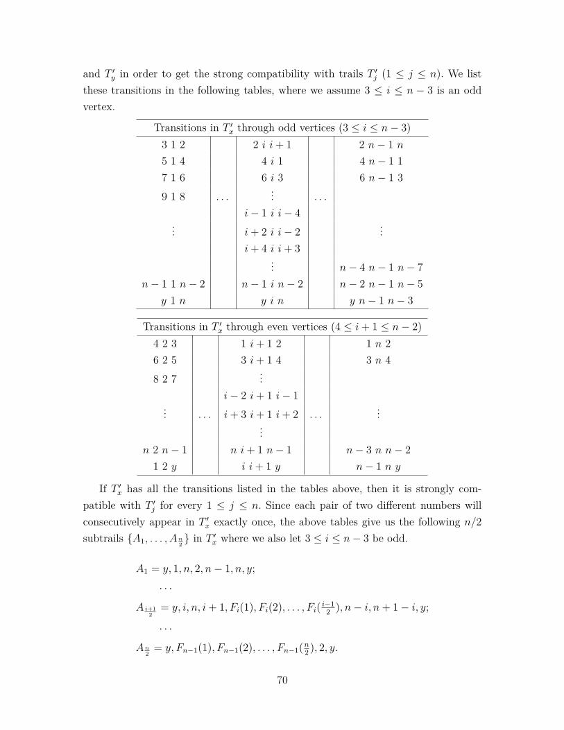
and T ′y in order to get the strong compatibility with trails T ′j (1 ≤ j ≤ n). We listthese transitions in the following tables, where we assume 3 ≤ i ≤ n − 3 is an oddvertex.

Transitions in T ′x through odd vertices (3 ≤ i ≤ n− 3)3 1 2 2 i i+ 1 2 n− 1 n5 1 4 4 i 1 4 n− 1 17 1 6 6 i 3 6 n− 1 39 1 8 . . .

... . . .

i− 1 i i− 4... i+ 2 i i− 2 ...

i+ 4 i i+ 3... n− 4 n− 1 n− 7

n− 1 1 n− 2 n− 1 i n− 2 n− 2 n− 1 n− 5y 1 n y i n y n− 1 n− 3

Transitions in T ′x through even vertices (4 ≤ i+ 1 ≤ n− 2)4 2 3 1 i+ 1 2 1 n 26 2 5 3 i+ 1 4 3 n 48 2 7 ...

i− 2 i+ 1 i− 1... . . . i+ 3 i+ 1 i+ 2 . . .

......

n 2 n− 1 n i+ 1 n− 1 n− 3 n n− 21 2 y i i+ 1 y n− 1 n y

If T ′x has all the transitions listed in the tables above, then it is strongly com-patible with T ′j for every 1 ≤ j ≤ n. Since each pair of two different numbers willconsecutively appear in T ′x exactly once, the above tables give us the following n/2subtrails {A1, . . . , An

2} in T ′x where we also let 3 ≤ i ≤ n− 3 be odd.

A1 = y, 1, n, 2, n− 1, n, y;

· · ·

A i+12

= y, i, n, i+ 1, Fi(1), Fi(2), . . . , Fi( i−12 ), n− i, n+ 1− i, y;

· · ·

An2

= y, Fn−1(1), Fn−1(2), . . . , Fn−1(n2 ), 2, y.

70

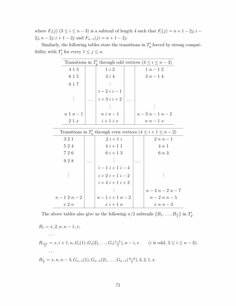
where Fi(j) (3 ≤ i ≤ n− 3) is a subtrail of length 4 such that Fi(j) = n+ 1− 2j, i−2j, n− 2j, i+ 1− 2j and Fn−1(j) = n+ 1− 2j.

Similarly, the following tables state the transitions in T ′y forced by strong compat-ibility with T ′j for every 1 ≤ j ≤ n.

Transitions in T ′y through odd vertices (3 ≤ i ≤ n− 3)4 1 3 1 i 2 1 n− 1 26 1 5 3 i 4 3 n− 1 48 1 7 ...

i− 2 i i− 1... . . . i+ 3 i i+ 2 . . .

... ...n 1 n− 1 n i n− 1 n− 3 n− 1 n− 22 1 x i+ 1 i x n n− 1 x

Transitions in T ′y through even vertices (4 ≤ i+ 1 ≤ n− 2)3 2 1 2 i+ 1 i 2 n n− 15 2 4 4 i+ 1 1 4 n 17 2 6 6 i+ 1 3 6 n 39 2 8 . . .

... . . .

i− 1 i+ 1 i− 4... i+ 2 i+ 1 i− 2 ...

i+ 4 i+ 1 i+ 3... n− 4 n− 2 n− 7

n− 1 2 n− 2 n− 1 i+ 1 n− 2 n− 2 n n− 5x 2 n x i+ 1 n x n n− 3

The above tables also give us the following n/2 subtrails {B1, . . . , Bn2} in T ′y.

B1 = x, 2, n, n− 1, x;

· · ·

B i+12

= x, i+ 1, n,Gi(1), Gi(2), . . . , Gi( i−12 ), n− i, x (i is odd, 3 ≤ i ≤ n− 3);

· · ·

Bn2

= x, n, n− 3, Gn−1(1), Gn−1(2), . . . , Gn−1(n−42 ), 3, 2, 1, x.

71

where Gi(j) (3 ≤ i ≤ n − 3) is a subtrail of length 4 such that Gi(j) = i − 2j, n +1 − 2j, i + 1 − 2j, n − 2j, and Gn−1(j) is a subtrail of length 3 where Gn−1(j) =n+ 1− 2j, n− 2j, n− 2j − 3.

Finally we are going to combine those subtrails of T ′x and T ′y. Note that anycombination will give us a closed Eulerian trail on Kn+2−x or Kn+2−y (respectively),since if ab (or ba) appears twice in the subtrails of T ′x, then either T ′a or T ′b is not anEulerian trail. We let T ′x = A1, A2, . . . , An

2and T ′y = B1, B2, . . . , Bn

2, that means the

construction is the following:

T ′x = y, 1, . . . , n, y, 3, . . . , n− 2, y, 5, . . . , 4, y, n− 1, . . . , 2;

T ′y = x, 2, . . . , n− 1, x, 4, . . . , 5, x, n− 2, . . . , 3, x, n, . . . , 1.

It remains to show that T ′x and T ′y are strongly compatible. This is true becausefor every odd vertex 3 ≤ i ≤ n − 1, we can see that n + 3 − i, y, i is a transition inT ′x and i, x, n + 3 − i is a transition in T ′y, as well as 2, y, 1 is a transition in T ′x and1, x, 2 is a transition in T ′y. This completes the proof.

Lemma 6.2.4. The non-orientable genus of K36 is 6.

Proof. By Lemma 6.1.3, we have g(K36) ≥ 6. Then it suffices to provide a construction

of an embedding of K36 in some non-orientable surfaces of genus 6. By Theorem 6.2.1,

we only need to construct an embedding set, but not a strong embedding set. Hereis the construction of the embedding set E6.

T1 = 4, 2, 5, 3, 6, 4, 5, 6, 2, 3;

T2 = 4, 6, 5, 1, 4, 3, 1, 6, 3, 5;

T3 = 1, 2, 4, 6, 1, 5, 2, 6, 5, 4;

T4 = 5, 1, 6, 2, 5, 6, 3, 2, 1, 3;

T5 = 6, 3, 4, 2, 3, 1, 2, 6, 4, 1;

T6 = 2, 1, 5, 3, 2, 5, 4, 3, 1, 4.

Note that 6, 3, 4 is a transition in T5 and 6, 5, 4 is a transition in T3, and also 2, 3, 1is a transition in T5 and 1, 5, 2 is a transition in T3. That means, neither T3 or T−1

3 isstrongly compatible with T5. It is not hard to see that the set E6 is compatible.

72

Theorem 6.2.5. If n ≥ 6 is even, then

g(K3n) = (n− 2)(n+ 3)(n− 4)

12 .

Proof. The proof follows the same inductive construction we used in the proof ofTheorem 6.2.3. Instead of using K3

4 as the base step, we use Lemma 6.2.4 as the basestep. Therefore, by the way we constructed the embedding set of K3

n, Eulerian trailsT3 and T5 will always be compatible, but they will never be strongly compatible.

6.2.3 Number of Non-Isomorphic Embeddings

We say that two embeddings φ1, φ2 : G → S are isomorphic if there is an automor-phism α of G such that the embeddings φ1 and φ2α are equivalent. In this section wewill show how to obtain many non-isomorphic optimal embeddings of K3

n when n iseven.

It is easy to see that the number of non-equivalent (2-cell) embeddings of K3n in

some surface is equal to

2(n3)23(n

3)(((

n

3

)− 1

)!)n

2−n = 2 12n

4 logn(1−o(1)).

The genera of all these embeddings take only O(n3) different values, but the majorityof them will have their genus much larger than the minimum possible genus. Thenumber of minimum genus embeddings is indeed much smaller as made explicit inthe following.

Lemma 6.2.6. The number of non-equivalent embeddings of K3n into a surface of

Euler genus 16(n− 2)(n+ 3)(n− 4) is at most 2 1

4n3 logn(1+o(1)), where the logarithm is

taken base 2.

Proof. We may assume that n is even since otherwise there are no such embeddings.By Theorem 6.2.1, optimal embeddings ofK3

n into surfaces of Euler genus 16(n−2)(n+

3)(n−4) are quadrilateral and are in a bijective correspondence with embedding sets.These are sets of Eulerian circuits satisfying compatibility conditions. Their numbercan be estimated as follows.

Suppose that compatible Eulerian circuits T1, . . . , Tk−1 are already chosen (1 ≤k ≤ n). To construct the next circuit Tk, we start by an arbitrary edge in Kn − k.If we come to a vertex i < k when following the last chosen edge, the transition isdetermined by compatibility with Ti. On the other hand if we come to a vertex i > k

73

for the rth time, there are (at most) n − 1 − 2r edges which can be chosen as thenext edge on the trail. All together, when passing through such a vertex i, we have atmost (n− 3)(n− 5)(n− 7) · · · 3 · 1 = (n− 3)!! choices. Therefore the number of waysto choose Tk is at most ((n− 3)!!)n−k. Thus the number of embedding sets is at most:

((n− 3)!!)(n−1)+(n−2)+···+1+0 = 2 14n

3 logn(1+o(1))

and this completes the proof.

Note that in the proof we are actually giving a bound on compatible closed traildecompositions. Nevertheless, this estimate may be rather tight, since the number ofEulerian circuits in Kn−1 is 2 1

2n2 logn(1+o(1)), see [40, Theorem 4].

Now we will turn to a lower bound on the number of non-isomorphic minimumgenus embeddings that can be obtained by a simple generalization of the constructionin our proofs of Theorems 6.2.3 and 6.2.5.

Theorem 6.2.7. If n is even, there exist at least 2 14n

2 logn(1−o(1)) non-isomorphicoptimal embeddings of K3

n in each, the orientable and the non-orientable surface ofEuler genus 1

6(n− 2)(n+ 3)(n− 4).

Proof. Let In be the number of non-isomorphic optimal embeddings of K3n. Here we

will only deal with the orientable case; for the non-orientable embeddings, argumentsare the same.

Recall that in the construction of the embedding set En = {T ′1, . . . , T ′n} of K3n, for

every odd vertex i ∈ [n− 2] we arbitrarily pick a transition ai, i + 1, bi in Ti ∈ En−2,and insert a subtrail Ei. Since i+ 1 appears exactly n−4

2 times in Ti, different choiceof transitions through i + 1 will give us different trails T ′i and T ′i+1. Also, the choiceof consecutive odd-even pairs i, i + 1 gives us a perfect matching of Kn−2. It is easyto see that any perfect matching of Kn−2 can be used as such a pairing and this willgive us different embedding sets En. Moreover, fixing a perfect matching, for example,i, i+ 1 for every odd i, we can exchange i and i+ 1 to get a new embedding set. Notethat x and y are symmetric in our construction, and can be exchanged.

Let In denote the resulting number of inequivalent embedding sets. Then we have:

In ≥12

(n− 4

2

)n−22

(n− 3)!! 2n−2

2 In−2.

74

Therefore,

log In ≥ logn−2

2∏k=2

(k − 1)k(2k − 1)!! 2k−1

≥ log(n−4

2 )!n−22 2n

2 ( n2−2)∏n−4

2k=2 k!∏n−6

2k=1 k!

= n(n− 4)4 log n− 4

2e +O(n2)

= 14n

2 log n (1− o(1)).

That means that there are at least 2 14n

2 logn (1+o(1)) inequivalent minimum genus em-beddings.

If φ1 and φ2 are non-equivalent but isomorphic embeddings, then there is an au-tomorphism α such that φ1 is equivalent with φ2α. Each such automorphism is deter-mined by the values α(1) and α(123), and by noting whether α preserves or reversesthe local rotation around the vertex 1. This means that the number of isomorphicembeddings is polynomial in n, and thus the number of isomorphism classes of em-beddings decreases by a factor that can be hidden in the o(1) term in the (1− o(1))factor. This completes the proof.

6.2.4 Hypergraphs with Multiple Edges

Now we are going to investigate the genus of complete 3-uniform graphs with multipleedges. These results will partially answer the question the authors asked in Theorem3.2.8. In that work, the genus of random bipartite graphs G(n1, n2, p) is considered,where n1 � 1 and n2 is a constant, and the edge probabilities are p = Θ(n−1/3

1 ). Inthat regime, the following hypergraph occurs. Let mK3

n be the complete 3-uniformhypergraph where each triple occurs m times, i.e., each edge of K3

n has multiplicitym. In this situation, each trail Tmi in the embedding set Emn is an Eulerian circuit inm(Kn− i). Similarly, we say two trails Ti and Tj are strongly compatible (compatible)if transitions ajb appear in Ti exactly t times, then transitions bia (aib or bia) appearin Tj exactly t times. It is easy to see that Theorem 6.2.1 is still true in this case, theproof is similar and we omit the details. Therefore, we have the following result.

Theorem 6.2.8. If n ≥ 4 is even and m ≥ 2, then g(mK3n) = (n−2)(mn(n−1)−12)

24 andg(mK3

n) = (n−2)(mn(n−1)−12)12 .

75

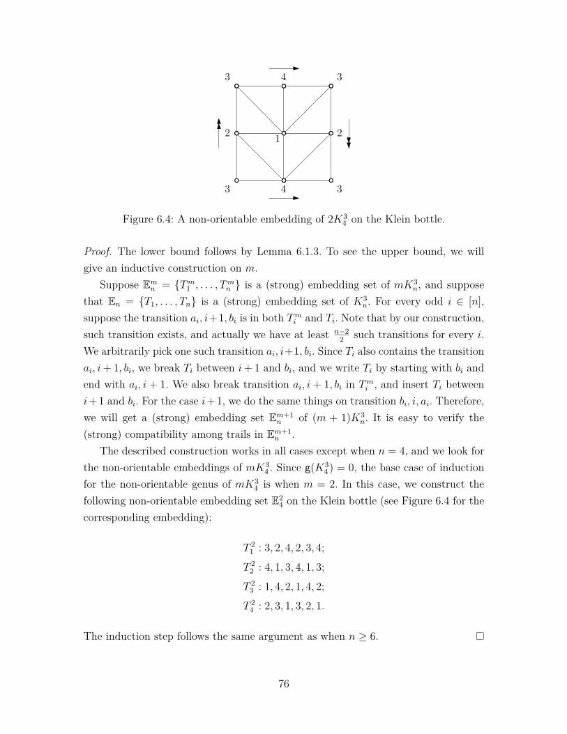
3 3

33

4

4

2 21

Figure 6.4: A non-orientable embedding of 2K34 on the Klein bottle.

Proof. The lower bound follows by Lemma 6.1.3. To see the upper bound, we willgive an inductive construction on m.

Suppose Emn = {Tm1 , . . . , Tmn } is a (strong) embedding set of mK3n, and suppose

that En = {T1, . . . , Tn} is a (strong) embedding set of K3n. For every odd i ∈ [n],

suppose the transition ai, i+1, bi is in both Tmi and Ti. Note that by our construction,such transition exists, and actually we have at least n−2

2 such transitions for every i.We arbitrarily pick one such transition ai, i+1, bi. Since Ti also contains the transitionai, i+ 1, bi, we break Ti between i+ 1 and bi, and we write Ti by starting with bi andend with ai, i + 1. We also break transition ai, i + 1, bi in Tmi , and insert Ti betweeni+ 1 and bi. For the case i+ 1, we do the same things on transition bi, i, ai. Therefore,we will get a (strong) embedding set Em+1

n of (m + 1)K3n. It is easy to verify the

(strong) compatibility among trails in Em+1n .

The described construction works in all cases except when n = 4, and we look forthe non-orientable embeddings of mK3

4 . Since g(K34) = 0, the base case of induction

for the non-orientable genus of mK34 is when m = 2. In this case, we construct the

following non-orientable embedding set E24 on the Klein bottle (see Figure 6.4 for the

corresponding embedding):

T 21 : 3, 2, 4, 2, 3, 4;

T 22 : 4, 1, 3, 4, 1, 3;

T 23 : 1, 4, 2, 1, 4, 2;

T 24 : 2, 3, 1, 3, 2, 1.

The induction step follows the same argument as when n ≥ 6.

76

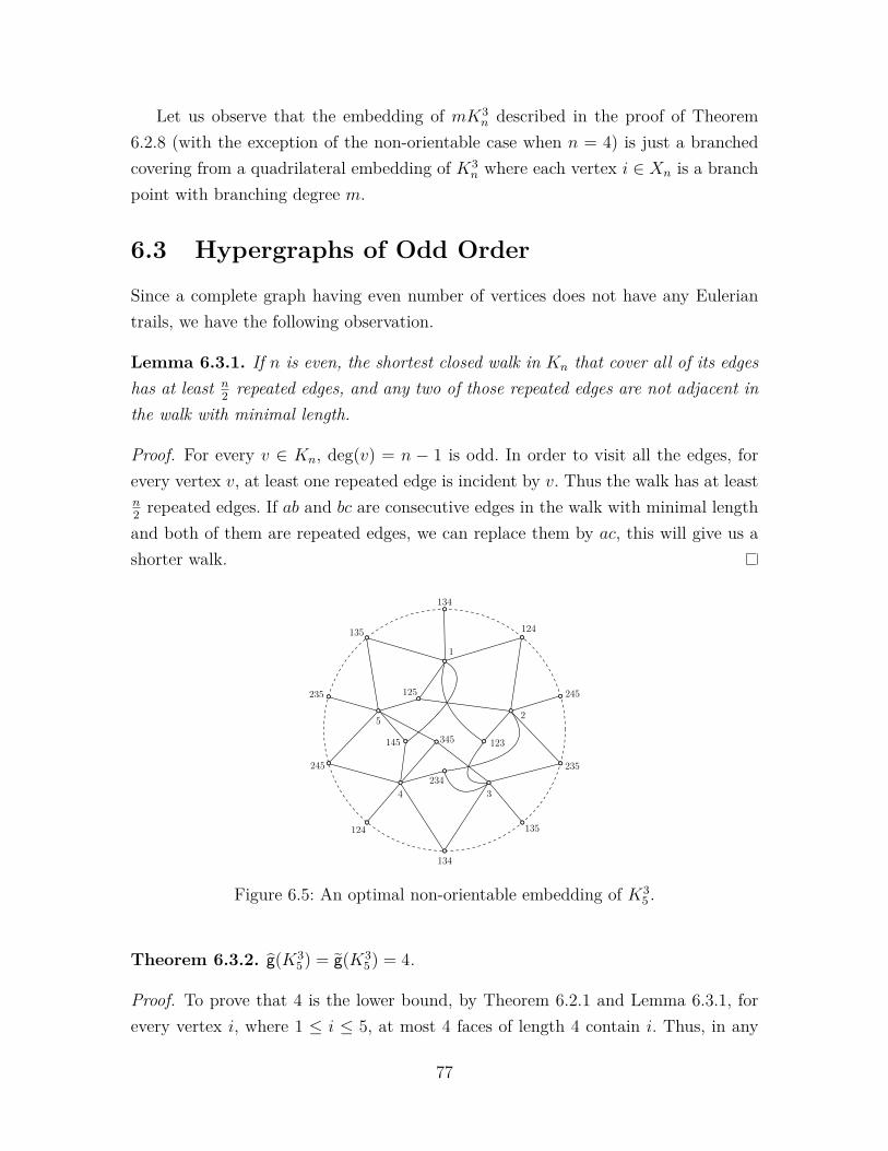
Let us observe that the embedding of mK3n described in the proof of Theorem

6.2.8 (with the exception of the non-orientable case when n = 4) is just a branchedcovering from a quadrilateral embedding of K3

n where each vertex i ∈ Xn is a branchpoint with branching degree m.

6.3 Hypergraphs of Odd Order

Since a complete graph having even number of vertices does not have any Euleriantrails, we have the following observation.

Lemma 6.3.1. If n is even, the shortest closed walk in Kn that cover all of its edgeshas at least n

2 repeated edges, and any two of those repeated edges are not adjacent inthe walk with minimal length.

Proof. For every v ∈ Kn, deg(v) = n − 1 is odd. In order to visit all the edges, forevery vertex v, at least one repeated edge is incident by v. Thus the walk has at leastn2 repeated edges. If ab and bc are consecutive edges in the walk with minimal lengthand both of them are repeated edges, we can replace them by ac, this will give us ashorter walk.

1

2

4 3

5

123

124

134

125

135

145

234

235 245

345

134

124

245 235

135

Figure 6.5: An optimal non-orientable embedding of K35 .

Theorem 6.3.2. g(K35) = g(K3

5) = 4.

Proof. To prove that 4 is the lower bound, by Theorem 6.2.1 and Lemma 6.3.1, forevery vertex i, where 1 ≤ i ≤ 5, at most 4 faces of length 4 contain i. Thus, in any

77

embedding of K35 , it has at most 10 faces of length 4. Since n(n− 1) is not divisible

by 3 when n = 5, the remaining faces cannot by all 6-gons. By Euler’s formula, wehave g(K3

5) ≤ 4.The proof of the upper bound is by construction, see Figure 6.5. The embedding

is on a projective plane together with 3 crosscaps, it has 10 faces of length 4, 2 facesof length 6 and one face of length 8.

Theorem 6.3.3. If n ≥ 5 is odd, then

g(K3n) ≥

⌈(n− 3)(n2 + n− 8)

12

⌉.

Proof. Recall that V (Ln) = XntYn where Xn = [n] and Yn =(

[n]3

). For every v ∈ Xn,

it has(n−1

2

)neighbors. By Lemma 6.3.1, at least n−1

2 pairs of them are contained inthe faces other than cycles of length 4. Therefore, suppose f be the number of facesin the minimum genus embeddings of K3

n, we have

f ≤n((

n−12

)− n−1

2

)2 + n(n− 1)

6

= 32

(n

3

)− 1

6

(n

2

).

Thus, by using Euler’s Formula, we obtain

g(K3n) ≥

⌈2− n−

(n

3

)− 3

2

(n

3

)+ 1

6

(n

2

)+ 3

(n

3

)⌉

=⌈

(n− 3)(n2 + n− 8)12

⌉,

which completes the proof.

78

Bibliography

[1] N. Alon, R. A. Duke, H. Lefmann, V. Rödl, and R. Yuster. The algorithmicaspects of the regularity lemma. J. Algorithms, 16(1):80–109, 1994.

[2] N. Alon and J. H. Spencer. The probabilistic method. Wiley Series in DiscreteMathematics and Optimization. John Wiley & Sons, Inc., Hoboken, NJ, fourthedition, 2016.

[3] K. Appel and W. Haken. Every planar map is four colorable. Bull. Amer. Math.Soc., 82(5):711–712, 1976.

[4] D. Archdeacon and D. A. Grable. The genus of a random graph. Discrete Math.,142(1-3):21–37, 1995.

[5] M. Behzad, G. Chartrand, and L. Lesniak-Foster. Graphs & digraphs. PWSPublishers, Boston, Mass., 1979.

[6] L. W. Beineke and R. J. Wilson, editors. Topics in topological graph theory,volume 128 of Encyclopedia of Mathematics and its Applications. CambridgeUniversity Press, Cambridge, 2009.

[7] B. Bollobás. Random graphs, volume 73 of Cambridge Studies in Advanced Math-ematics. Cambridge University Press, Cambridge, second edition, 2001.

[8] K. S. Booth and G. S. Lueker. Testing for the consecutive ones property, intervalgraphs, and graph planarity using PQ-tree algorithms. J. Comput. System Sci.,13(3):335–379, 1976. Working Papers presented at the ACM-SIGACT Sympo-sium on the Theory of Computing (Albuquerque, N. M., 1975).

[9] C. Chekuri and A. Sidiropoulos. Approximation algorithms for Euler genusand related problems. In 2013 IEEE 54th Annual Symposium on Foundationsof Computer Science—FOCS 2013, pages 167–176. IEEE Computer Soc., LosAlamitos, CA, 2013.

[10] J. Chen, S. P. Kanchi, and A. Kanevsky. A note on approximating graph genus.Inform. Process. Lett., 61(6):317–322, 1997.

[11] N. Chiba, T. Nishizeki, S. Abe, and T. Ozawa. A linear algorithm for embeddingplanar graphs using PQ-trees. J. Comput. System Sci., 30(1):54–76, 1985.

79

[12] F. Chung. From quasirandom graphs to graph limits and graphlets. Adv. inAppl. Math., 56:135–174, 2014.

[13] F. R. K. Chung, R. L. Graham, and R. M. Wilson. Quasi-random graphs. Com-binatorica, 9(4):345–362, 1989.

[14] É. Colin de Verdière. Computational topology of graphs on surfaces. CoRR,abs/1702.05358, 2017.

[15] M. Cygan, F. V. Fomin, Ł. Kowalik, D. Lokshtanov, D. Marx, M. Pilipczuk,M. Pilipczuk, and S. Saurabh. Parameterized algorithms. Springer, 2015.

[16] R. Diestel. Graph theory, volume 173 of Graduate Texts in Mathematics.Springer, Heidelberg, fourth edition, 2010.

[17] P. Erdős and A. Rényi. On random graphs. I. Publ. Math. Debrecen, 6:290–297,1959.

[18] J. Erickson, P. N. Klein, D. Marx, and C. Mathieu. Algorithms for Optimiza-tion Problems in Planar Graphs (Dagstuhl Seminar 16221). Dagstuhl Reports,6(5):94–116, 2016.

[19] J. Fox, L. M. Lovász, and Y. Zhao. On regularity lemmas and their algorithmicapplications. Combin. Probab. Comput., 26(4):481–505, 2017.

[20] J. Fox, L. M. Lovász, and Y. Zhao. A fast new algorithm for weak graph regu-larity. arXiv:1807.05031, 2018.

[21] P. Frankl and V. Rödl. Near perfect coverings in graphs and hypergraphs. Eu-ropean J. Combin., 6(4):317–326, 1985.

[22] A. Frieze and R. Kannan. Quick approximation to matrices and applications.Combinatorica, 19(2):175–220, 1999.

[23] M. R. Garey and D. S. Johnson. Computers and intractability. W. H. Freemanand Co., San Francisco, Calif., 1979. A guide to the theory of NP-completeness.

[24] W. T. Gowers. Lower bounds of tower type for Szemerédi’s uniformity lemma.Geom. Funct. Anal., 7(2):322–337, 1997.

[25] J. L. Gross and T. W. Tucker. Topological graph theory. Dover Publications, Inc.,Mineola, NY, 2001. Reprint of the 1987 original [Wiley, New York; MR0898434(88h:05034)] with a new preface and supplementary bibliography.

[26] P. J. Heawood. Map-colour theorem. Quart. J. Pure Appl. Math., 24(4):332–338,1890.

[27] J. Hopcroft and R. Tarjan. Efficient planarity testing. J. Assoc. Comput. Mach.,21:549–568, 1974.

80

[28] K. i. Kawarabayashi, B. Mohar, and B. Reed. A simpler linear time algorithm forembedding graphs into an arbitrary surface and the genus of graphs of boundedtree-width. In 49th Annual IEEE Symposium on Foundations of Computer Sci-ence (FOCS’08), pages 771–780, 2008.

[29] Y. Jing and B. Mohar. The genus of a random bipartite graph. arXiv:1712.09989,submitted, 2017.

[30] Y. Jing and B. Mohar. Efficient polynomial-time approximation scheme for thegenus of dense graphs. To appear in 2018 IEEE 59th Annual Symposium onFoundations of Computer Science—FOCS 2018, IEEE Computer Soc., Paris,France, 2018.

[31] Y. Jing and B. Mohar. The genus of complete 3-uniform hypergraphs.arXiv:1805.01557, submitted, 2018.

[32] Y. Jing and B. Mohar. The genus of complete 3-uniform hypergraphs. The oddcase. In preparation, 2018.

[33] Y. Jing and B. Mohar. On the genus of generalized random graphs. In prepara-tion, 2018.

[34] M. Jungerman, S. Stahl, and A. T. White. Imbeddings of hypergraphs. Congr.Numer., 29:545–557, 1980.

[35] K.-i. Kawarabayashi and A. Sidiropoulos. Beyond the Euler characteristic: ap-proximating the genus of general graphs [extended abstract]. In STOC’15—Proceedings of the 2015 ACM Symposium on Theory of Computing, pages 675–682. ACM, New York, 2015.

[36] L. Lovász. Large networks and graph limits, volume 60 of American MathematicalSociety Colloquium Publications. American Mathematical Society, Providence,RI, 2012.

[37] L. Lovász and B. Szegedy. Limits of dense graph sequences. J. Combin. TheorySer. B, 96(6):933–957, 2006.

[38] L. Lovász and B. Szegedy. Szemerédi’s lemma for the analyst. Geom. Funct.Anal., 17(1):252–270, 2007.

[39] Y. Makarychev, A. Nayyeri, and A. Sidiropoulos. A pseudo-approximation forthe genus of Hamiltonian graphs. In Approximation, randomization, and com-binatorial optimization, volume 8096 of Lecture Notes in Comput. Sci., pages244–259. Springer, Heidelberg, 2013.

[40] B. D. McKay and R. W. Robinson. Asymptotic enumeration of Eulerian circuitsin the complete graph. Combin. Probab. Comput., 7(4):437–449, 1998.

81

[41] B. Mohar. Embedding graphs in an arbitrary surface in linear time. In Proceed-ings of the Twenty-eighth Annual ACM Symposium on Theory of Computing,STOC ’96, pages 392–397, New York, NY, USA, 1996. ACM.

[42] B. Mohar. A linear time algorithm for embedding graphs in an arbitrary surface.SIAM J. Discrete Math., 12(1):6–26, 1999.

[43] B. Mohar. Face covers and the genus problem for apex graphs. J. Combin.Theory Ser. B, 82(1):102–117, 2001.

[44] B. Mohar and C. Thomassen. Graphs on surfaces. Johns Hopkins Studies in theMathematical Sciences. Johns Hopkins University Press, Baltimore, MD, 2001.

[45] R. A. Moser and G. Tardos. A constructive proof of the general Lovász locallemma. J. ACM, 57(2):Art. 11, 15, 2010.

[46] W. Myrvold and J. Woodcock. A large set of torus obstructions and how theywere discovered. Electron. J. Combin., 25:Paper 1.16, 2018.

[47] O. Ore. The four-color problem. Pure and Applied Mathematics, Vol. 27. Aca-demic Press, New York-London, 1967.

[48] T. D. Parsons, G. Pica, T. Pisanski, and A. G. S. Ventre. Orientably simplegraphs. Math. Slovaca, 37(4):391–394, 1987.

[49] N. Pippenger and J. Spencer. Asymptotic behavior of the chromatic index forhypergraphs. J. Combin. Theory Ser. A, 51(1):24–42, 1989.

[50] J. M. Rahn. The genus of a block design. In Proceedings of the Sundance con-ference on combinatorics and related topics (Sundance, Utah, 1985), volume 50,pages 255–268, 1985.

[51] G. Ringel. Das Geschlecht des vollständigen paaren Graphen. Abh. Math. Sem.Univ. Hamburg, 28:139–150, 1965.

[52] G. Ringel. Map color theorem. Springer-Verlag, New York-Heidelberg, 1974. DieGrundlehren der mathematischen Wissenschaften, Band 209.

[53] G. Ringel and J. W. T. Youngs. Solution of the Heawood map-coloring problem.Proc. Nat. Acad. Sci. U.S.A., 60:438–445, 1968.

[54] N. Robertson and P. Seymour. Graph minors. XIII. The disjoint paths problem.J. Combin. Theory Ser. B, 63(1):65–110, 1995.

[55] N. Robertson and P. Seymour. Graph minors. XXII. Irrelevant vertices in linkageproblems. J. Combin. Theory Ser. B, 102(2):530–563, 2012.

[56] N. Robertson and P. D. Seymour. Graph minors. VIII. A Kuratowski theoremfor general surfaces. J. Combin. Theory Ser. B, 48(2):255–288, 1990.

82

[57] V. Rödl and L. Thoma. Asymptotic packing and the random greedy algorithm.Random Structures Algorithms, 8(3):161–177, 1996.

[58] V. Rödl and R. Thomas. On the genus of a random graph. Random StructuresAlgorithms, 6(1):1–12, 1995.

[59] J. Spencer. Asymptotic packing via a branching process. Random StructuresAlgorithms, 7(2):167–172, 1995.

[60] S. Stahl. On the average genus of the random graph. J. Graph Theory, 20(1):1–18, 1995.

[61] E. Szemerédi. On sets of integers containing no k elements in arithmetic pro-gression. Acta Arith., 27:199–245, 1975. Collection of articles in memory ofJuriıVladimirovič Linnik.

[62] E. Szemerédi. Regular partitions of graphs. In Problèmes combinatoires et théoriedes graphes (Colloq. Internat. CNRS, Univ. Orsay, Orsay, 1976), volume 260 ofColloq. Internat. CNRS, pages 399–401. CNRS, Paris, 1978.

[63] T. Tao. Szemerédi’s regularity lemma revisited. Contrib. Discrete Math., 1(1):8–28, 2006.

[64] T. Tao. An epsilon of room, II. American Mathematical Society, Providence,RI, 2010. Pages from year three of a mathematical blog.

[65] C. Thomassen. The graph genus problem is NP-complete. J. Algorithms,10(4):568–576, 1989.

[66] C. Thomassen. Triangulating a surface with a prescribed graph. J. Combin.Theory Ser. B, 57(2):196–206, 1993.

[67] C. Thomassen. The genus problem for cubic graphs. J. Combin. Theory Ser. B,69(1):52–58, 1997.

[68] H. Tietze. Famous problems of mathematics. Solved and unsolved mathematicalproblems from antiquity to modern times. Authorized translation from the sec-ond (1959) revised German edition. Edited by B. K. Hofstadter and H. Komm.Graylock Press, New York, 1965.

[69] V. V. Vazirani. Approximation algorithms. Springer-Verlag, Berlin, 2001.

[70] A. T. White. Graphs of groups on surfaces, volume 188 of North-Holland Math-ematics Studies. North-Holland Publishing Co., Amsterdam, 2001. Interactionsand models.

[71] S. G. Williamson. Depth-first search and Kuratowski subgraphs. J. Assoc. Com-put. Mach., 31(4):681–693, 1984.

83

[72] J. W. T. Youngs. Minimal imbeddings and the genus of a graph. J. Math. Mech.,12:303–315, 1963.

84