The Lattice of N-Run Orthogonal Arrays

E. M. Rains and N. J. A. Sloane

Information Sciences Research CenterAT&T Shannon Lab

Florham Park, New Jersey 07932-0971

John StufkenDepartment of StatisticsIowa State UniversityAmes, IA 50011

April 20, 2000

ABSTRACT

If the number of runs in a (mixed-level) orthogonal array of strength 2 is specified, what numbers

of levels and factors are possible? The collection of possible sets of parameters for orthogonal arrays

with N runs has a natural lattice structure, induced by the “expansive replacement” construction

method. In particular the dual atoms in this lattice are the most important parameter sets, since

any other parameter set for an N -run orthogonal array can be constructed from them. To get

a sense for the number of dual atoms, and to begin to understand the lattice as a function of

N , we investigate the height and the size of the lattice. It is shown that the height is at most

bc(N − 1)c, where c = 1.4039 . . ., and that there is an infinite sequence of values of N for whichthis bound is attained. On the other hand, the number of nodes in the lattice is bounded above by

a superpolynomial function of N (and superpolynomial growth does occur for certain sequences of

values of N). Using a new construction based on “mixed spreads”, all parameter sets with 64 runs

are determined. Four of these 64-run orthogonal arrays appear to be new.

1

1. Introduction

Although mixed-level (or asymmetrical) orthogonal arrays have been the subject of a number of

papers in recent years (see Chapter 9 of Hedayat, Sloane and Stufken, 1999, for references), it seems

fair to say that we know much less about them than about fixed-level orthogonal arrays (in which

all factors have the same number of levels). For example, there is no analogue for mixed orthogonal

arrays of one of the most powerful construction methods for fixed-level arrays, that based on linear

codes (see Chapters 4 and 5 of Hedayat, Sloane and Stufken, 1999).

Again, there are many instances where the linear programming bound for fixed-level orthogonal

arrays gives the correct answer for the minimal number of runs needed for a specified number of

factors. There is a linear programming bound for mixed arrays (Sloane and Stufken, 1996), but it

is less effective than in the fixed-level case — it ignores too much of the combinatorial nature of the

problem (especially when the levels involve more than one prime number), and, though generally

stronger than the Rao bound, does not give correct answers as often as in the fixed-level case.

A mixed orthogonal array OA(N, sk11 sk22 · · · skvv , t) is an array of size N × k, where k = k1 +

k2 + · · · + kv is the total number of factors, in which the first k1 columns have symbols from{0, 1, . . . , s1 − 1}, the next k2 columns have symbols from {0, 1, . . . , s2 − 1}, and so on, with theproperty that in any N × t subarray every possible t-tuple of symbols occurs an equal number oftimes as a row. We usually assume 2 ≤ s1 < s2 < · · · and all ki ≥ 1. Except in Section 5, onlyarrays of strength 2 will be considered, and we will usually omit t from the symbol for the array.

We refer to (N, sk11 sk22 . . .) as the parameter set for an OA(N, s

k11 sk22 . . .). We also allow the

parameter set (N, 11), corresponding to the trivial array consisting of a single column of N 0’s.

In this paper we consider the question: if N is specified, how many different parameter sets are

possible?

Given an array A = OA(N, sk11 sk22 . . .), other N -run arrays can be obtained from it by the expan-

sive replacement method. Let S be one of the si occurring in A, and supposeB is an OA(S, tl11 tl22 . . .).

The expansive replacement method replaces a single column of A at S levels by the rows of B.

For example, if A = OA(16, 2344) and B = OA(4, 23), we obtain an OA(16, 2643). If B is a trivial

array OA(S, 11), we are simply deleting one of the S-level factors from A. E.g. taking S = 2,

an OA(24, 22041) trivially produces an OA(24, 21941). The expansive replacement method also in-

cludes replacing a factor at s levels by a factor at s′ levels, if s′ divides s. For further details about

the expansive replacement method see Chapter 9 of Hedayat, Sloane and Stufken, 1999.

Let A and B be parameter sets for orthogonal arrays with N runs. We say that B is dominated

2

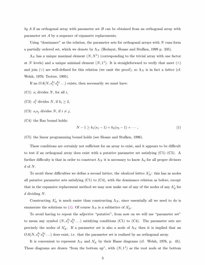
by A if an orthogonal array with parameter set B can be obtained from an orthogonal array with

parameter set A by a sequence of expansive replacements.

Using “dominance” as the relation, the parameter sets for orthogonal arrays with N runs form

a partially ordered set, which we denote by ΛN (Hedayat, Sloane and Stufken, 1999 p. 335).

ΛN has a unique maximal element (N,N1) (corresponding to the trivial array with one factor

at N levels) and a unique minimal element (N, 11). It is straightforward to verify that meet (∧)and join (∨) are well-defined for this relation (we omit the proof), so ΛN is in fact a lattice (cf.Welsh, 1976; Trotter, 1995).

If an OA(N, sk11 sk22 . . .) exists, then necessarily we must have:

(C1) si divides N , for all i,

(C2) s2i divides N , if ki ≥ 2,

(C3) sisj divides N , if i 6= j,

(C4) the Rao bound holds:

N − 1 ≥ k1(s1 − 1) + k2(s2 − 1) + · · · , (1)

(C5) the linear programming bound holds (see Sloane and Stufken, 1996).

These conditions are certainly not sufficient for an array to exist, and it appears to be difficult

to test if an orthogonal array does exist with a putative parameter set satisfying (C1)–(C5). A

further difficulty is that in order to construct ΛN it is necessary to know Λd for all proper divisors

d of N .

To avoid these difficulties we define a second lattice, the idealized lattice Λ ′N : this has as nodes

all putative parameter sets satisfying (C1) to (C4), with the dominance relation as before, except

that in the expansive replacement method we may now make use of any of the nodes of any Λ ′d for

d dividing N .

Constructing Λ′N is much easier than constructing ΛN , since essentially all we need to do is

enumerate the solutions to (1). Of course ΛN is a sublattice of Λ′N .

To avoid having to repeat the adjective “putative”, from now on we will use “parameter set”

to mean any symbol (N, sk11 sk22 . . .) satisfying conditions (C1) to (C4). The parameter sets are

precisely the nodes of Λ′N . If a parameter set is also a node of ΛN then it is implied that an

OA(N, sk11 sk22 . . .) does exist, i.e. that the parameter set is realized by an orthogonal array.

It is convenient to represent ΛN and Λ′N by their Hasse diagrams (cf. Welsh, 1976, p. 45).

These diagrams are drawn “from the bottom up”, with (N, 11) as the root node at the bottom

3

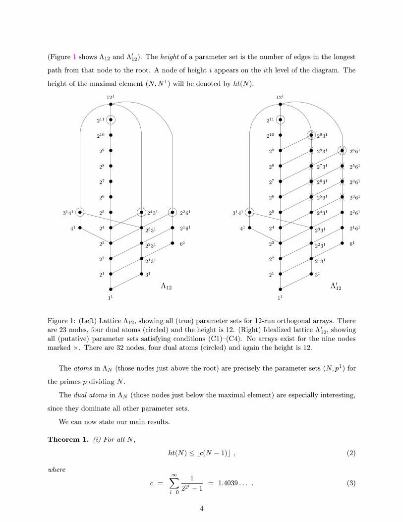
(Figure 1 shows Λ12 and Λ′12). The height of a parameter set is the number of edges in the longest

path from that node to the root. A node of height i appears on the ith level of the diagram. The

height of the maximal element (N,N 1) will be denoted by ht(N).

211

24

23

22

21

25

210

29

28

27

26

3141

26

25

24

23

27

Λ′12

211

210

29

28

22 2131

31

2261

2161

612231

21

3141

41

2431

2331

Λ12

2261

2161

61

121

31

41

2431

2331

2231

2131

121

2631

2361

2461

2561

2661

2531

11 11

2931

2831

2731

Figure 1: (Left) Lattice Λ12, showing all (true) parameter sets for 12-run orthogonal arrays. Thereare 23 nodes, four dual atoms (circled) and the height is 12. (Right) Idealized lattice Λ ′12, showingall (putative) parameter sets satisfying conditions (C1)–(C4). No arrays exist for the nine nodesmarked ×. There are 32 nodes, four dual atoms (circled) and again the height is 12.

The atoms in ΛN (those nodes just above the root) are precisely the parameter sets (N, p1) for

the primes p dividing N .

The dual atoms in ΛN (those nodes just below the maximal element) are especially interesting,

since they dominate all other parameter sets.

We can now state our main results.

Theorem 1. (i) For all N ,

ht(N) ≤ bc(N − 1)c , (2)

where

c =

∞∑

i=0

1

22i − 1 = 1.4039 . . . . (3)

4

(ii) If N = 22m

(m ≥ 0) then ht(N) = bc(N − 1)c.

Let T (N) (resp. T ′(N)) denote the total number of nodes in ΛN (resp. Λ′N ).

Theorem 2. If N = 2n,

1

4(log2N)

2(1 + o(1)) ≤ log2 T (N) ≤3

8(log2N)

2(1 + o(1)) . (4)

Theorem 3. There is a constant c1 such that for all N ,

ln lnT (N) ≤ c1lnN

ln lnN(1 + o(1)) . (5)

Remarks. (i) The bounds in (4) and (5) also apply to T ′(N).

(ii) Theorem 2 shows that when N = 2n, T (N) grows very roughly like N a log2N , for some

constant a between 14 and38 . This is a “superpolynomial” function of N , meaning that it grows

faster than any polynomial in N .

(iii) It appears (although we have not proved this) that the upper bound in (5) can be achieved

by taking N to be a certain product of powers of the first m primes, where m is about

1

2e

lnN

ln lnN

(see Section 7). In other words, it appears that there is an infinite sequence of values of N for

which T (N) grows very roughly like

exp(N c2/ ln lnN ) ,

where c2 is a constant. This is again a superpolynomial function of N , and is now close to being

an exponential function, since ln lnN grows slowly.

The above discussion has shown that there is an infinite sequence of values of N for which the

number of nodes in ΛN grows superpolynomially, while the height of ΛN grows at most linearly. It

follows that the size of the largest antichain must also grow superpolynomially. The data in Table

3 suggest the following conjecture.

Conjecture. There is an infinite sequence of values of N for which the number of dual atoms

grows superpolynomially in N .

In fact it seems likely that if N = 2n, a lower bound of the form in (4) (possibly with a different

constant) applies to the logarithm of the number of dual atoms, and that for some sequence of

values of N a lower bound similar to the upper bound on the right-hand side of (5) will hold.

However, at present these are only conjectures.

5

In order to construct the orthogonal arrays needed to establish the lower bound in Theorem 2

we make use of what we call “mixed spreads”, generalizing the notions of “spread” and “partial

spread” from projective geometry. Arrays that can be constructed in this way we call “geometric”.

Many familiar examples of orthogonal arrays, for example arrays constructed from linear codes,

are geometric. The construction is not restricted to strength 2 (and is one of the few general

constructions we know of for mixed arrays of strength greater than 2). The construction will be

described in Section 5.

In Section 6 we use this construction to determine the lattice Λ64, and in doing so we find tight

arrays with parameter sets

(64, 2541781), (64, 41483), (64, 2541084), (64, 4786),

which appear to be new.

When studying parameter sets of putative orthogonal arrays with N runs, it is convenient to

be able to say that if the number of degrees of freedom of the parameter set (N, sk11 sk22 . . .), that is,

k1(s1 − 1) + k2(s2 − 1) + · · · , (6)

is small compared with N − 1, then an orthogonal array certainly exists.To make this precise, we define the threshold function B(N) to be the maximum number b such

that every parameter set (satisfying conditions (C1) to (C4)) with at most b degrees of freedom is

realized by an orthogonal array, but some parameter set (again satisfying (C1) to (C4)) with b+ 1

degrees of freedom is not realized. If every parameter set satisfying (C1) to (C4) is realized, we set

B(N) = N − 1.Figure 1 shows that B(12) = 6, since there is no OA(12, 2531), but every parameter set with at

most 6 degrees of freedom is realized.

We are not aware of any earlier investigations of B(N).

Theorem 4. If N is a power of a prime then

N3/4 ≤ B(N) .

In words, if the number of degrees of freedom in the parameter set does not exceed N 3/4, then

an orthogonal array exists. This is certainly weak, but is enough to establish the lower bound of

Theorem 2. It would be nice to have more precise estimates for B(N).

A final remark. We could have considered the partially ordered set whose nodes are all the

inequivalent orthogonal arrays with N runs, rather than just their parameter sets. However, the

6

number of nodes then becomes unmanageably large, even for small values of N (furthermore, it

appears that “meet” and “join” are no longer well-defined, and so in general this partially ordered

set would not be a lattice).

Consider N = 28, for example. Using Kimura’s (1994a, 1994b) enumeration of the Hadamard

matrices of order 28, we have calculated1 that there are precisely 7570 inequivalent OA(28, 227)’s.

This would be merely a lower bound on the number of dual atoms. On the other hand we know

(see Table 1) that Λ28 has precisely four dual atoms, between 47 and 55 nodes, and height 28.

11

2131

31

11

p1

21

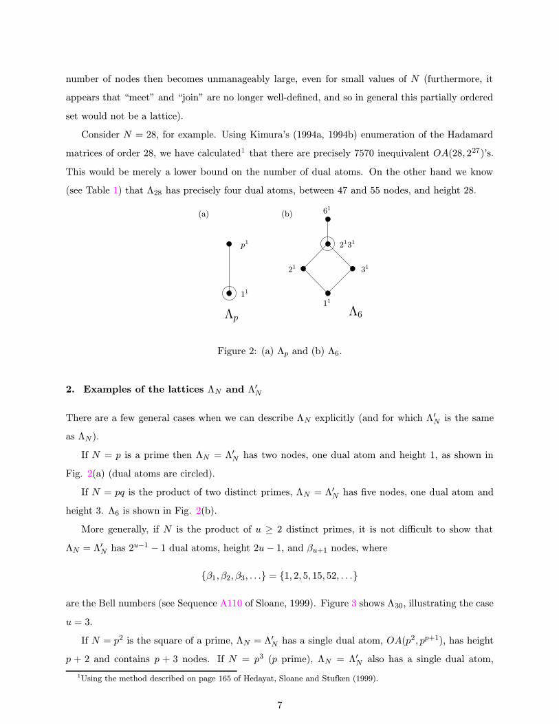
Λ6Λp

(b)(a) 61

Figure 2: (a) Λp and (b) Λ6.

2. Examples of the lattices ΛN and Λ′N

There are a few general cases when we can describe ΛN explicitly (and for which Λ′N is the same

as ΛN ).

If N = p is a prime then ΛN = Λ′N has two nodes, one dual atom and height 1, as shown in

Fig. 2(a) (dual atoms are circled).

If N = pq is the product of two distinct primes, ΛN = Λ′N has five nodes, one dual atom and

height 3. Λ6 is shown in Fig. 2(b).

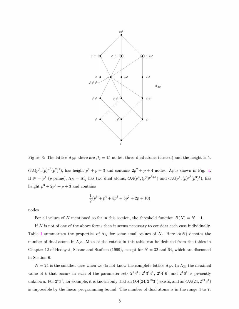
More generally, if N is the product of u ≥ 2 distinct primes, it is not difficult to show thatΛN = Λ

′N has 2

u−1 − 1 dual atoms, height 2u− 1, and βu+1 nodes, where

{β1, β2, β3, . . .} = {1, 2, 5, 15, 52, . . .}

are the Bell numbers (see Sequence A110 of Sloane, 1999). Figure 3 shows Λ30, illustrating the case

u = 3.

If N = p2 is the square of a prime, ΛN = Λ′N has a single dual atom, OA(p

2, pp+1), has height

p + 2 and contains p + 3 nodes. If N = p3 (p prime), ΛN = Λ′N also has a single dual atom,

1Using the method described on page 165 of Hedayat, Sloane and Stufken (1999).

7

5161

61

213151

2131

51

301

11

Λ30

101

3151

21

31101

2151

31

21151

151

Figure 3: The lattice Λ30: there are β4 = 15 nodes, three dual atoms (circled) and the height is 5.

OA(p3, (p)p2

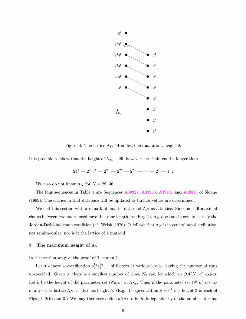
(p2)1), has height p2 + p + 3 and contains 2p2 + p + 4 nodes. Λ8 is shown in Fig. 4.

If N = p4 (p prime), ΛN = Λ′N has two dual atoms, OA(p

4, (p2)p2+1) and OA(p4, (p)p

3

(p3)1), has

height p3 + 2p2 + p+ 3 and contains

1

2(p5 + p4 + 5p3 + 5p2 + 2p+ 10)

nodes.

For all values of N mentioned so far in this section, the threshold function B(N) = N − 1.If N is not of one of the above forms then it seems necessary to consider each case individually.

Table 1 summarizes the properties of ΛN for some small values of N . Here A(N) denotes the

number of dual atoms in ΛN . Most of the entries in this table can be deduced from the tables in

Chapter 12 of Hedayat, Sloane and Stufken (1999), except for N = 32 and 64, which are discussed

in Section 6.

N = 24 is the smallest case when we do not know the complete lattice ΛN . In Λ24 the maximal

value of k that occurs in each of the parameter sets 2k31, 2k3141, 2k4161 and 2k61 is presently

unknown. For 2k31, for example, it is known only that an OA(24, 21631) exists, and an OA(24, 22131)

is impossible by the linear programming bound. The number of dual atoms is in the range 4 to 7.

8

2141

2241

2341

2441

81

41

25

26

27

Λ8

24

21

11

22

23

Figure 4: The lattice Λ8: 14 nodes, one dual atom, height 9.

It is possible to show that the height of Λ24 is 25, however: no chain can be longer than

241 — 22041 — 223 — 222 — 221 — · · · — 21 — 11 .

We also do not know ΛN for N = 28, 36, . . ..

The four sequences in Table 1 are Sequences A39927, A39930, A39931 and A48893 of Sloane

(1999). The entries in that database will be updated as further values are determined.

We end this section with a remark about the nature of ΛN as a lattice. Since not all maximal

chains between two nodes need have the same length (see Fig. 1), ΛN does not in general satisfy the

Jordan-Dedekind chain condition (cf. Welsh, 1976). It follows that ΛN is in general not distributive,

not semimodular, nor is it the lattice of a matroid.

3. The maximum height of ΛN

In this section we give the proof of Theorem 1.

Let σ denote a specification sk11 sk22 . . . of factors at various levels, leaving the number of runs

unspecified. Given σ, there is a smallest number of runs, N0 say, for which an OA(N0, σ) exists.

Let h be the height of the parameter set (N0, σ) in ΛN0 . Then if the parameter set (N,σ) occurs

in any other lattice ΛN , it also has height h. (E.g. the specification σ = 61 has height 3 in each of

Figs. 1, 2(b) and 3.) We may therefore define ht(σ) to be h, independently of the number of runs.

9

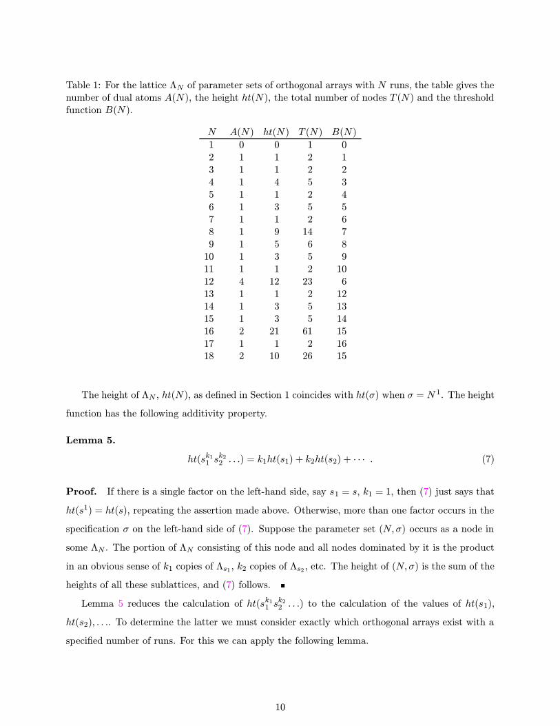
Table 1: For the lattice ΛN of parameter sets of orthogonal arrays with N runs, the table gives thenumber of dual atoms A(N), the height ht(N), the total number of nodes T (N) and the thresholdfunction B(N).

N A(N) ht(N) T (N) B(N)

1 0 0 1 02 1 1 2 13 1 1 2 24 1 4 5 35 1 1 2 46 1 3 5 57 1 1 2 68 1 9 14 79 1 5 6 810 1 3 5 911 1 1 2 1012 4 12 23 613 1 1 2 1214 1 3 5 1315 1 3 5 1416 2 21 61 1517 1 1 2 1618 2 10 26 15

The height of ΛN , ht(N), as defined in Section 1 coincides with ht(σ) when σ = N1. The height

function has the following additivity property.

Lemma 5.

ht(sk11 sk22 . . .) = k1ht(s1) + k2ht(s2) + · · · . (7)

Proof. If there is a single factor on the left-hand side, say s1 = s, k1 = 1, then (7) just says that

ht(s1) = ht(s), repeating the assertion made above. Otherwise, more than one factor occurs in the

specification σ on the left-hand side of (7). Suppose the parameter set (N,σ) occurs as a node in

some ΛN . The portion of ΛN consisting of this node and all nodes dominated by it is the product

in an obvious sense of k1 copies of Λs1 , k2 copies of Λs2 , etc. The height of (N,σ) is the sum of the

heights of all these sublattices, and (7) follows.

Lemma 5 reduces the calculation of ht(sk11 sk22 . . .) to the calculation of the values of ht(s1),

ht(s2), . . .. To determine the latter we must consider exactly which orthogonal arrays exist with a

specified number of runs. For this we can apply the following lemma.

10

Table 1 (cont.)

N A(N) ht(N) T (N) B(N)

19 1 1 2 1820 4 20 35 1121 1 3 5 2022 1 3 5 2123 1 1 2 2224 4− 7 25 119 − 133 18− 2225 1 7 8 2426 1 3 5 2527 1 15 25 2628 4 28 47 − 55 1529 1 1 2 2830 3 5 15 2931 1 1 2 3032 2 42 320 2933 1 3 5 3234 1 3 5 3335 1 3 5 34. . . . . . . . . . . . . . .64 7 86 3037 57. . . . . . . . . . . . . . .

Lemma 6.

ht(N) = 1 +max∑

i

kiht(si) , (8)

where the maximum is taken over all parameter sets (N, sk11 sk22 . . .) 6= (N,N 1) for which an orthog-

onal array exists.

Proof. The height of ΛN is one more than the maximal height among the dual atoms. (8) follows

by applying Lemma 5 to the parameter set of such a dual atom.

We can now use linear programming to obtain an upper bound on ht(N), by maximizing

1 +∑

i

kiht(si) (9)

over all choices of s1, k1, s2, k2, . . . that satisfy (C1) to (C4).

We first consider the case when N = 2n for some n.

The case N = 64 will illustrate the method. If there is a factor 321 then linear programming

shows that (9) is maximized by 232 321, giving height 75. If there is a factor 161 then there is

a unique parameter set that maximizes (9), 416161, giving height 86. Otherwise, if only factors

11

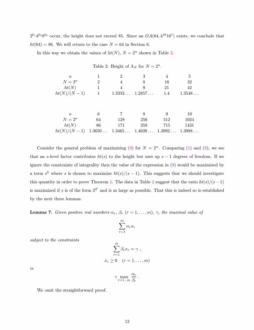
2k14k28k3 occur, the height does not exceed 85. Since an OA(64, 416161) exists, we conclude that

ht(64) = 86. We will return to the case N = 64 in Section 6.

In this way we obtain the values of ht(N), N = 2n shown in Table 2.

Table 2: Height of ΛN for N = 2n.

n 1 2 3 4 5N = 2n 2 4 8 16 32ht(N) 1 4 9 21 42

ht(N)/(N − 1) 1 1.3333 . . . 1.2857 . . . 1.4 1.3548 . . .

n 6 7 8 9 10N = 2n 64 128 256 512 1024ht(N) 86 171 358 715 1431

ht(N)/(N − 1) 1.3650 . . . 1.3465 . . . 1.4039 . . . 1.3992 . . . 1.3988 . . .

Consider the general problem of maximizing (9) for N = 2n. Comparing (1) and (9), we see

that an s-level factor contributes ht(s) to the height but uses up s − 1 degrees of freedom. If weignore the constraints of integrality then the value of the expression in (9) would be maximized by

a term sk where s is chosen to maximize ht(s)/(s − 1). This suggests that we should investigatethis quantity in order to prove Theorem 1. The data in Table 2 suggest that the ratio ht(s)/(s− 1)is maximized if s is of the form 22

i

and is as large as possible. That this is indeed so is established

by the next three lemmas.

Lemma 7. Given positive real numbers αr, βr (r = 1, . . . ,m), γ, the maximal value of

m∑

r=1

αrxr

subject to the constraintsm∑

r=1

βrxr = γ ,

xr ≥ 0 (r = 1, . . . ,m)

is

γ maxr=1...m

αrβr.

We omit the straightforward proof.

12

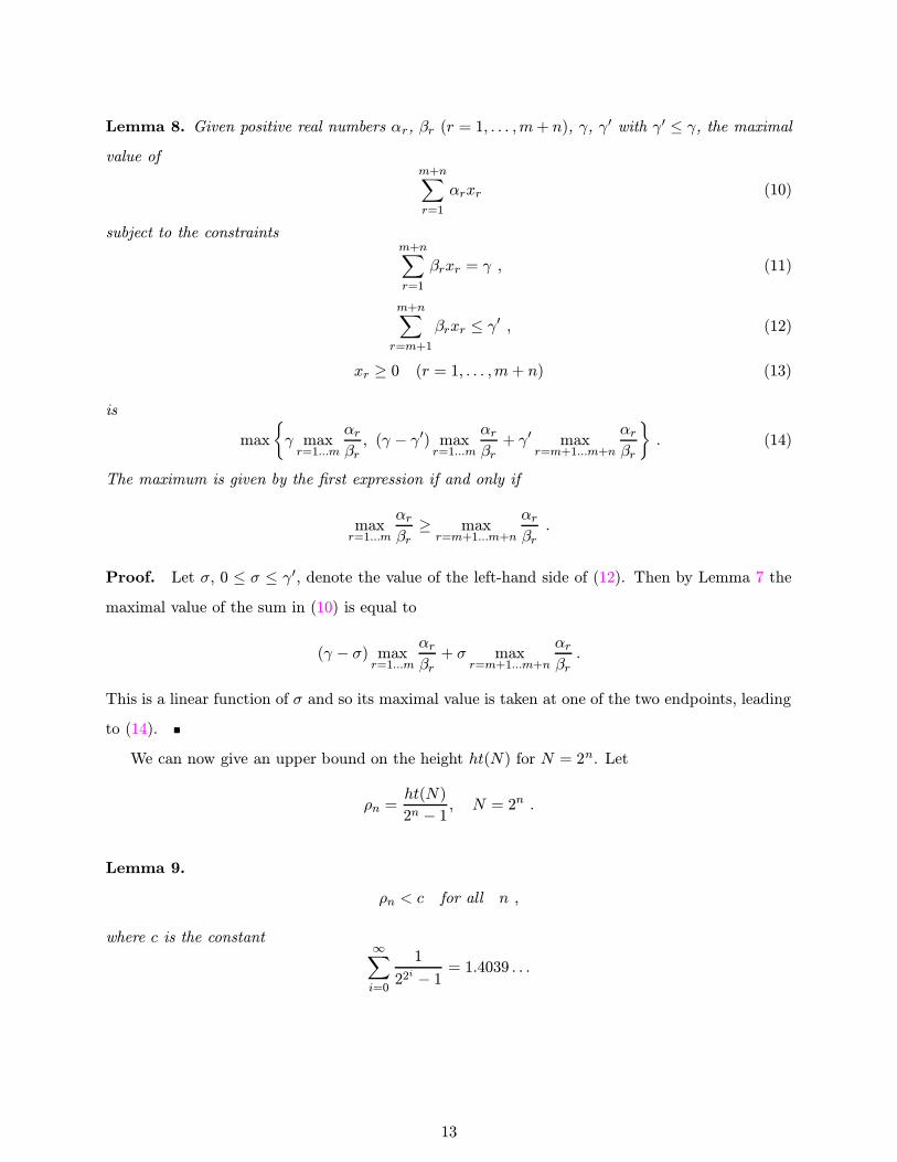
Lemma 8. Given positive real numbers αr, βr (r = 1, . . . ,m+ n), γ, γ′ with γ′ ≤ γ, the maximal

value ofm+n∑

r=1

αrxr (10)

subject to the constraintsm+n∑

r=1

βrxr = γ , (11)

m+n∑

r=m+1

βrxr ≤ γ′ , (12)

xr ≥ 0 (r = 1, . . . ,m+ n) (13)

is

max

{

γ maxr=1...m

αrβr, (γ − γ′) max

r=1...m

αrβr+ γ′ max

r=m+1...m+n

αrβr

}

. (14)

The maximum is given by the first expression if and only if

maxr=1...m

αrβr≥ maxr=m+1...m+n

αrβr.

Proof. Let σ, 0 ≤ σ ≤ γ ′, denote the value of the left-hand side of (12). Then by Lemma 7 themaximal value of the sum in (10) is equal to

(γ − σ) maxr=1...m

αrβr+ σ max

r=m+1...m+n

αrβr.

This is a linear function of σ and so its maximal value is taken at one of the two endpoints, leading

to (14).

We can now give an upper bound on the height ht(N) for N = 2n. Let

ρn =ht(N)

2n − 1 , N = 2n .

Lemma 9.

ρn < c for all n ,

where c is the constant∞∑

i=0

1

22i − 1 = 1.4039 . . .

13

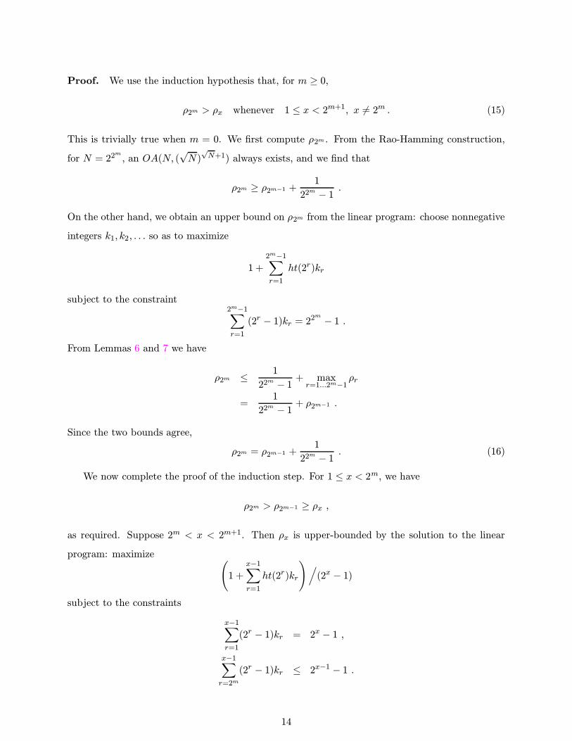
Proof. We use the induction hypothesis that, for m ≥ 0,

ρ2m > ρx whenever 1 ≤ x < 2m+1, x 6= 2m . (15)

This is trivially true when m = 0. We first compute ρ2m . From the Rao-Hamming construction,

for N = 22m

, an OA(N, (√N)√N+1) always exists, and we find that

ρ2m ≥ ρ2m−1 +1

22m − 1 .

On the other hand, we obtain an upper bound on ρ2m from the linear program: choose nonnegative

integers k1, k2, . . . so as to maximize

1 +2m−1∑

r=1

ht(2r)kr

subject to the constraint2m−1∑

r=1

(2r − 1)kr = 22m − 1 .

From Lemmas 6 and 7 we have

ρ2m ≤ 1

22m − 1 + maxr=1...2m−1

ρr

=1

22m − 1 + ρ2m−1 .

Since the two bounds agree,

ρ2m = ρ2m−1 +1

22m − 1 . (16)

We now complete the proof of the induction step. For 1 ≤ x < 2m, we have

ρ2m > ρ2m−1 ≥ ρx ,

as required. Suppose 2m < x < 2m+1. Then ρx is upper-bounded by the solution to the linear

program: maximize(

1 +

x−1∑

r=1

ht(2r)kr

)

/

(2x − 1)

subject to the constraints

x−1∑

r=1

(2r − 1)kr = 2x − 1 ,

x−1∑

r=2m

(2r − 1)kr ≤ 2x−1 − 1 .

14

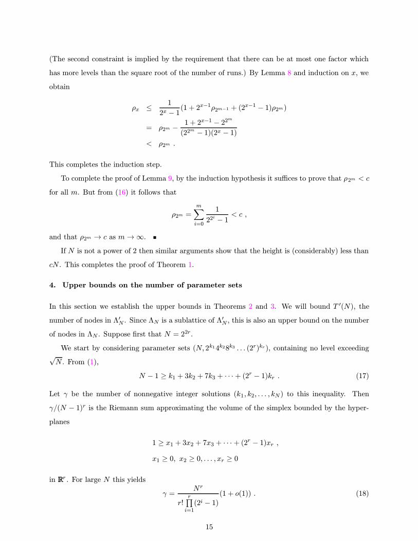
(The second constraint is implied by the requirement that there can be at most one factor which

has more levels than the square root of the number of runs.) By Lemma 8 and induction on x, we

obtain

ρx ≤1

2x − 1(1 + 2x−1ρ2m−1 + (2

x−1 − 1)ρ2m)

= ρ2m −1 + 2x−1 − 22m

(22m − 1)(2x − 1)< ρ2m .

This completes the induction step.

To complete the proof of Lemma 9, by the induction hypothesis it suffices to prove that ρ2m < c

for all m. But from (16) it follows that

ρ2m =m∑

i=0

1

22i − 1

< c ,

and that ρ2m → c as m→∞.If N is not a power of 2 then similar arguments show that the height is (considerably) less than

cN . This completes the proof of Theorem 1.

4. Upper bounds on the number of parameter sets

In this section we establish the upper bounds in Theorems 2 and 3. We will bound T ′(N), the

number of nodes in Λ′N . Since ΛN is a sublattice of Λ′N , this is also an upper bound on the number

of nodes in ΛN . Suppose first that N = 22r.

We start by considering parameter sets (N, 2k14k28k3 . . . (2r)kr), containing no level exceeding√N . From (1),

N − 1 ≥ k1 + 3k2 + 7k3 + · · · + (2r − 1)kr . (17)

Let γ be the number of nonnegative integer solutions (k1, k2, . . . , kN ) to this inequality. Then

γ/(N − 1)r is the Riemann sum approximating the volume of the simplex bounded by the hyper-planes

1 ≥ x1 + 3x2 + 7x3 + · · · + (2r − 1)xr ,

x1 ≥ 0, x2 ≥ 0, . . . , xr ≥ 0

in� r . For large N this yields

γ =N r

r!r∏

i=1(2i − 1)

(1 + o(1)) . (18)

15

The product in the denominator approaches c32r(r+1)/2, as r →∞, where c3 = 0.2887 . . ..

Now suppose the parameter set contains a factor at 2i levels, where r + 1 ≤ i ≤ 2r − 1. Therecan be at most one such factor, and the number of such parameter sets in each case is at most γ.

The total number of parameter sets is therefore at most rγ, and setting r = 12 log2N we find that

log2(rγ) ≤3

8(log2N)

2(1 + o(1)) .

This establishes the upper bound in Theorem 2 for N = 22r. It also implies the upper bound for

N = 22r+1, after noting that T ′(N) ≤ T ′(2N).We now give a sketch of the proof of Theorem 3, omitting many tedious details. To simplify

the analysis we will neglect terms on the right-hand side of (1) that correspond to factors with a

level greater than√N . Suppose first that N is a large number of the form 22a132a2 . Pretending

for the moment that a1 and a2 are allowed to be real numbers, not just integers, we may consider

what choice of a1 and a2 maximizes the number of solutions to (1) for a given value of N . The

number of terms on the right-hand side of (1) is now (a1 + 1)(a2 + 1)− 1. The arguments used toestablish the upper bound of Theorem 2 show that the number of solutions to (1) is maximized if

22a1 is approximately equal to 32a2 .

Now suppose that N is of the form

p2a11 p2a22 · · · p2amm , (19)

where p1 = 2, p2 = 3, . . . are the first m primes. We find that the number of solutions to (1) is

maximized when the numbers p2aii are all approximately equal, and we will therefore assume that

p2aii = N1

m(1+o(1)), i.e. that

ai =1

2m

lnN

ln pi(1 + o(1)), i = 1, . . . ,m .

The Rao bound contains a term for every possible level

s = pi11 pi22 · · · pimm

in which 0 ≤ iν ≤ aν , 1 ≤ ν ≤ m, where not all the iν are equal to 0. The number of such terms is

δ := (a1 + 1)(a2 + 1) · · · (am + 1)− 1 =1

(2m)m(lnN)m

m∏

j=1ln pj

(1 + o(1)) . (20)

The product of the coefficients of all the terms on the right-hand side of the Rao bound is

ζ := pa21a2...am/21 p

a1a22a3...am/22 · · · pa1...am−1a2m/2m (1 + o(1)) .

16

This implies

ln ζ =δ

4lnN(1 + o(1)) .

Again using γ to denote the number of solutions to the Rao inequality, we have

γ =N δ

δ!ζ(1 + o(1)) ,

hence

ln γ =3

4

(lnN)m+1

(2m)m(lnm)m(1+o(1))− 1

(2m)m(lnN)m

(lnm)m(1+o(1))(m ln lnN −m lnm)

+ smaller terms .

This expression is maximized if we take

m =1

2e

lnN

ln lnN(1 + o(1)) ,

and then we find that the leading term in the expression for ln γ is

3

4lnNN

1

2e

1

ln lnN .

We conclude that

ln ln γ ≤ 12e

lnN

ln lnN,

which establishes Theorem 3.

5. Geometric orthogonal arrays

We consider subspaces V of the vector space GF (q)n over GF (q), where q is a power of a prime.

By the dimension of V , dimV , we mean the vector space dimension over GF (q) (rather than the

projective dimension, which is one less). The following notion was suggested by the notions of

spread and partial spread in projective geometry (cf. Thas, 1995).

Definition. A mixed spread of strength t is a collection V = {V1, V2, . . . , Vk} of subspaces ofGF (q)n such that for all choices of τ ≤ t indices i1, i2, . . . , iτ (with 1 ≤ i1 < i2 < · · · < iτ ≤ k) thedimension of the span of Vi1 , . . . , Viτ is equal to dimVi1 + · · · + dimViτ .An equivalent condition is that the span of Vi1 , . . . , Viτ is the direct sum Vi1 ⊕ · · · ⊕ Viτ for all

choices of τ ≤ t indices i1, . . . , iτ with 1 ≤ i1 < · · · < iτ ≤ k.Any collection V of subspaces has strength 1. V has strength 2 if and only if every pair Vi,

Vj ∈ V, i 6= j, intersect just in the zero vector. V has strength 3 if and only if it has strength 2 andfor any triple of distinct subspaces each one meets the span of the other two just in the zero vector.

17

If V is a d-dimensional subspace of GF (q)n we denote by V ∗ the dual space, the space of linear

functionals on V (see for example Hoffman and Kunze, 1961), and we fix a labeling f0, f1, . . . , fqd−1

for the elements of V ∗.

Given a mixed spread of strength t, V = {V1, V2, . . . , Vk}, where the Vi are subspaces of GF (q)n,we obtain an orthogonal array OA(V) with qn runs as follows. The columns of the array are labeledV1, V2, . . . , Vk and the rows are labeled by the linear functionals f ∈ (GF (q)n)∗. If f restricted toVi, f |Vi , is the jth linear functional in V ∗i , the (f, Vi)-th entry in the array is j. The symbols incolumn i are therefore taken from {0, 1, . . . , qdimVi − 1}.We will say that an orthogonal array constructed in this way is geometric.

Theorem 10. The orthogonal array OA(V) has strength t if and only if the mixed spread V hasstrength t.

Proof. Suppose OA(V) has strength t. Consider for example the first t columns. In the projectionof the array onto these columns we see

t∏

i=1

qdimVi = q

t∑

i=1

dimVi

different t-tuples of symbols. Since these depend only on the restrictions of the f ∈ (GF (q)n)∗ tothe span of V1, . . . , Vt, the dimension of that space must be at least the sum of the dimensions of

V1, . . . , Vt, and clearly it cannot have a higher dimension. So V is a mixed spread of strength t.Conversely, suppose V is a mixed spread of strength t. We can write

GF (q)n = V1 ⊕ · · · ⊕ Vt ⊕X

where X is the complementary space to the Vi. Since the dual of a direct sum is canonically

isomorphic to the direct sum of the duals, we immediately find that as we run through the linear

functionals on GF (q)n, every tuple (f |V1 , . . . f |Vt , f |X) of restrictions occurs precisely once. Ignoringthe last component, we see that every tuple (f |V1 , . . . f |Vt) occurs precisely |X| times. Hence OA(V)has strength t.

Lemma 11. Any geometric array of strength 2 can always be extended to a tight array (i.e. one

meeting the Rao bound) by adding q-level factors.

Proof. We simply group any unused points into 1-dimensional subspaces.

18

Examples. (i) The 1-dimensional subspaces of GF (q)n form a mixed spread of strength 2. The

corresponding array is the familiar

OA(qn, qk), k = (qn − 1)/(q − 1) ,

of the Rao-Hamming construction.

(ii) More generally, a classical a-spread in PG(b, q) is a mixed spread of strength 2 in our sense.

This is a set of subspaces of PG(b, q) of projective dimension a which partitions PG(b, q) (Thas,

1995), and exists if and only if a+ 1 divides b+ 1. From Theorem 10 we obtain an

OA(qb+1, (qa+1)k), k = (qb+1 − 1)/(qa+1 − 1) ,

which of course is also given by the Rao-Hamming construction.

We could also have obtained example (ii) directly from example (i), by remarking that a mixed

spread of strength t over GF (q), q = pβ, is also a mixed spread of strength t over GF (q ′), q′ = pα,

if q′ divides q. The dimensions of the subspaces are multiplied by β/α.

(iii) Provided a ≥ b/2, there exists a mixed spread of strength 2 in GF (q)b consisting of a singlesubspace GF (q)a and a partitioning of the remaining points into qa subspaces GF (q)b−a. This

can be proved directly, or alternatively is equivalent to Lemma 2.1 of Eisfeld, Storme and Sziklai

(1999). From Theorem 10 we obtain a geometric

OA(qb, (qb−a)qa

(qa)1)

whenever a ≥ b/2. Orthogonal arrays with these parameters were already known from the dif-ference scheme construction (Hedayat, Sloane and Stufken, 1999, Example 9.19), but the present

construction also shows that they are geometric.

(iv) The classical “partial a-spread” constructed in Lemma 2.2 of Eisfeld, Storme and Sziklai

(1999) translates in our language into a mixed spread of strength 2 consisting of k b-dimensional

subspaces (b ≥ 2) of GF (q)n, where n = ib+ r, 0 ≤ r < b, and

k = qrqib − 1qb − 1 − q

r + 1 .

This produces a geometric OA(qn, (qb)k) (again arrays with these parameters were known from the

difference scheme construction), which by Lemma 11 can be extended to a tight

OA(qn, (q1)l(qb)k) , (21)

where l = qb(qr − 1)/(q − 1). The orthogonal arrays constructed by Wu (1989) are a special caseof (21), but in general these arrays may be new.

19

(v) Generalizing examples (i) and (ii), any orthogonal array formed from the codewords of a

projective linear code (one for which the columns of a generator matrix are nonzero and projectively

distinct) is geometric.

(vi) The OA(256, 216) of strength 5 formed from the Nordstrom-Robinson code (see Hedayat,

Sloane and Stufken, 1999, Section 5.10) is not geometric, and no geometric OA(256, 216) of strength

5 exists.

We shall see other examples in Section 6.

Remarks. An unmixed geometric orthogonal array is always linear, in the sense of Hedayat,

Sloane and Stufken (1999), Chapter 3. In general a mixed geometric orthogonal array is additive

but not necessarily linear2 over each of the fields involved.

If the strength is 2, the number of degrees of freedom in the parameter set for OA(V) is equalto the total number of nonzero points in all the subspaces Vi.

Finally, the following is a recipe for constructing the orthogonal array from a mixed spread

V = {V1, V2, . . . , Vk} of subspaces of GF (q)n in the case when q is a prime. Let v(i)1 , . . . , v(i)dibe a

basis for Vi, where di = dimVi, 1 ≤ i ≤ k. Let w0, . . . , wqn−1 be the vectors of GF (q)n. Then theith entry of the jth row of the orthogonal array, for 1 ≤ i ≤ k, 0 ≤ j ≤ qn − 1, is the number

di∑

r=1

wj · v(i)r qr−1 .

(This is a number in the range {0, . . . , qdi − 1}.)

6. If the number of runs is a power of 2

In this section we consider the case N = 2n, n = 1, 2, . . .. We have already discussed ht(N) in

Section 3 (see Table 2). With the assistance of Michele Colgan, we used a computer to determine

the number of dual atoms A′(N) and the total number of nodes T ′(N) in the idealized lattice Λ′N

for n ≤ 9. The results are shown in the second and third columns of Table 3. Note in particularthe extremely rapid growth from N = 256 to N = 512. We regard this as convincing evidence that

when N = 2n, A′(N) (and therefore presumably A(N)) grows faster than any polynomial in N .

As to the lattice ΛN itself, for n ≤ 4 this is covered by the results in Section 2. For N = 32there are precisely two parameter sets in Λ′32 which do not exist, (32, 4

10) and (32, 21410). These

can be ruled out either by the linear programming bound or by the Bose-Bush bound (Hedayat,

2For the distinction between additive and linear sets in the context of coding theory see Calderbank et al. (1998).

20

Table 3: Dual atoms and total number of nodes in idealized lattice Λ′N (A′(N) and T ′(N)) and in

lattice ΛN (A(N) and T (N)).

N A′(N) T ′(N) A(N) T (N)

1 0 1 0 12 1 2 1 24 1 5 1 58 1 14 1 1416 2 61 2 6132 3 322 2 32064 11 3058 7 3037128 21 33364256 72 789085512 144521 18614215

Sloane and Stufken, 1999, Theorem 2.8). All other parameter sets in Λ′32 are realized. It follows

that Λ32 contains exactly two dual atoms, OA(32, 216161) and OA(32, 4881).

Before considering Λ64 we give a lemma that will be used to construct new arrays.

Lemma 12. Suppose V1, V2, V3 are three r-dimensional subspaces of GF (2)2r such that Vi ∩ Vj =

{0}, i 6= j. Then their union can be replaced by 2r−1 two-dimensional subspaces, any pair of whichmeet just in the zero vector.

Proof. Since V1 ∩ V2 = {0}, V1 and V2 span the space GF (2)2r . Let π1, π2 be the associatedprojection maps from GF (2)2r to V1, V2 respectively. Then i1 = π1|V3 : V3 → V1 and i2 = π2|V3 :V3 → V2 are both isomorphisms. It follows that V3 is the set

{v + i(v) : v in V1}, i = i2i−11 .

But then we need simply take the planes {0, v, i(v), v + i(v)} for v ∈ V1 to establish the lemma.The lemma implies that if a geometric OA(22r, . . .) exists then so does the array obtained by

replacing (2r)3 in the parameter set by 4k, k = 2r − 1. In particular, in a geometric OA(64, . . .) wecan replace 83 by 47.

Theorem 13. The lattice Λ64 contains precisely seven dual atoms, with parameter sets

(64, 2541781), (64, 41483), (64, 2541084),

(64, 4786), (64, 89), (64, 416161), (64, 232321) . (22)

A geometric orthogonal array exists for each of these parameter sets.

21

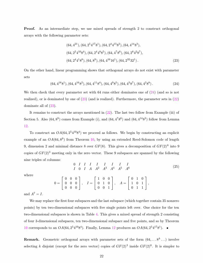
Proof. As an intermediate step, we use mixed spreads of strength 2 to construct orthogonal

arrays with the following parameter sets:

(64, 421), (64, 2541781), (64, 2441582), (64, 41483),

(64, 2541084), (64, 244885), (64, 4786), (64, 284287),

(64, 244188), (64, 89), (64, 416161), (64, 232321) . (23)

On the other hand, linear programming shows that orthogonal arrays do not exist with parameter

sets

(64, 41881), (64, 41682), (64, 41184), (64, 4985), (64, 4387), (64, 4288) . (24)

We then check that every parameter set with 64 runs either dominates one of (24) (and so is not

realized), or is dominated by one of (23) (and is realized). Furthermore, the parameter sets in (22)

dominate all of (23).

It remains to construct the arrays mentioned in (22). The last two follow from Example (iii) of

Section 5. Also (64, 89) comes from Example (i), and (64, 4786) and (64, 41483) follow from Lemma

12.

To construct an OA(64, 2541084) we proceed as follows. We begin by constructing an explicit

example of an OA(64, 89) from Theorem 10, by using an extended Reed-Solomon code of length

9, dimension 2 and minimal distance 8 over GF (8). This gives a decomposition of GF (2)6 into 9

copies of GF (2)3 meeting only in the zero vector. These 9 subspaces are spanned by the following

nine triples of columns:0 I I I I I I I II 0 I A A2 A3 A4 A5 A6

(25)

where

0 =

0 0 00 0 00 0 0

, I =

1 0 00 1 00 0 1

, A =

0 1 01 0 10 1 1

,

and A7 = I.

We may replace the first four subspaces and the last subspace (which together contain 35 nonzero

points) by ten two-dimensional subspaces with five single points left over. One choice for the ten

two-dimensional subspaces is shown in Table 4. This gives a mixed spread of strength 2 consisting

of four 3-dimensional subspaces, ten two-dimensional subspace and five points, and so by Theorem

10 corresponds to an OA(64, 2541084). Finally, Lemma 12 produces an OA(64, 2541781).

Remark. Geometric orthogonal arrays with parameter sets of the form (64, . . . 8k . . .) involve

selecting k disjoint (except for the zero vector) copies of GF (2)3 inside GF (2)6. It is simpler to

22

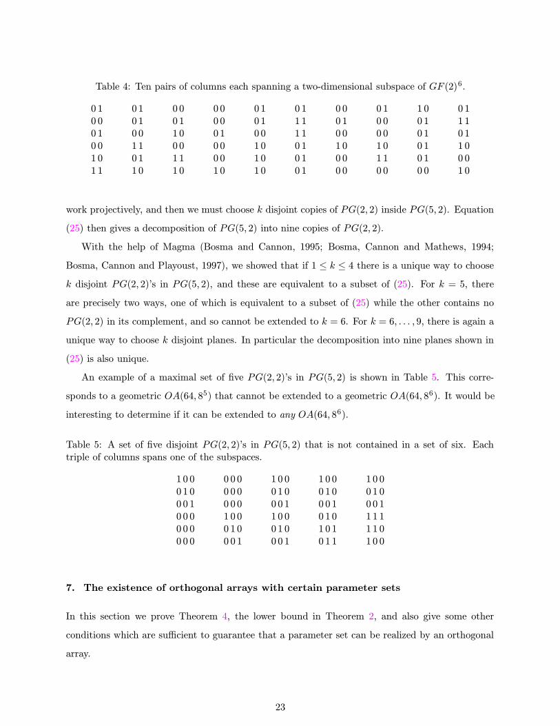
Table 4: Ten pairs of columns each spanning a two-dimensional subspace of GF (2)6.

0 10 00 10 01 01 1

0 10 10 01 10 11 0

0 00 11 00 01 11 0

0 00 00 10 00 01 0

0 10 10 01 01 01 0

0 11 11 10 10 10 1

0 00 10 01 00 00 0

0 10 00 01 01 10 0

1 00 10 10 10 10 0

0 11 10 11 00 01 0

work projectively, and then we must choose k disjoint copies of PG(2, 2) inside PG(5, 2). Equation

(25) then gives a decomposition of PG(5, 2) into nine copies of PG(2, 2).

With the help of Magma (Bosma and Cannon, 1995; Bosma, Cannon and Mathews, 1994;

Bosma, Cannon and Playoust, 1997), we showed that if 1 ≤ k ≤ 4 there is a unique way to choosek disjoint PG(2, 2)’s in PG(5, 2), and these are equivalent to a subset of (25). For k = 5, there

are precisely two ways, one of which is equivalent to a subset of (25) while the other contains no

PG(2, 2) in its complement, and so cannot be extended to k = 6. For k = 6, . . . , 9, there is again a

unique way to choose k disjoint planes. In particular the decomposition into nine planes shown in

(25) is also unique.

An example of a maximal set of five PG(2, 2)’s in PG(5, 2) is shown in Table 5. This corre-

sponds to a geometric OA(64, 85) that cannot be extended to a geometric OA(64, 86). It would be

interesting to determine if it can be extended to any OA(64, 86).

Table 5: A set of five disjoint PG(2, 2)’s in PG(5, 2) that is not contained in a set of six. Eachtriple of columns spans one of the subspaces.

1 0 00 1 00 0 10 0 00 0 00 0 0

0 0 00 0 00 0 01 0 00 1 00 0 1

1 0 00 1 00 0 11 0 00 1 00 0 1

1 0 00 1 00 0 10 1 01 0 10 1 1

1 0 00 1 00 0 11 1 11 1 01 0 0

7. The existence of orthogonal arrays with certain parameter sets

In this section we prove Theorem 4, the lower bound in Theorem 2, and also give some other

conditions which are sufficient to guarantee that a parameter set can be realized by an orthogonal

array.

23

Lemma 14. Suppose N = pm is a power of a prime and (N, sk11 sk22 . . .) is a parameter set with

k = Σiki factors. If k ≤ pb(m+1)/2c +1 then this parameter set is realized by a geometric orthogonalarray.

Proof. Suppose first that the parameter set contains a factor with s = pn >√N levels. If m is

even then a geometric OA(pm, (pm−n)pn

(pn)1) exists by Section 5, and pm−n is the largest number

of levels other factors can have if there is an s-level factor. Since there are pn factors with pm−n

levels, the existence of any array with one s-level factor and at most pm/2 factors with ≤ pm−n

levels follows immediately. The case that m is odd follows similarly.

We now assume that all si ≤√N . If m is even, N = p2r, then a geometric

OA(p2r, (pr)pr+1) (26)

exists by Section 5. Any parameter set with all si ≤ pr and k ≤ pr + 1 is dominated by (26) andso is realized. If m is odd, N = p2r+1, then a geometric

OA(p2r+1, (pr)pr+1+1) (27)

also exists by Section 5. Any parameter set with all si ≤ pr and k ≤ pr+1+1 is dominated by (27)and so is also realized.

Since the number of factors in a parameter set is less than or equal to the number of degrees of

freedom (6), Lemma 14 immediately implies that any parameter set (N = pm, sk11 sk22 . . .) with at

most pb(m+1)/2c + 1 degrees of freedom is realized by an orthogonal array. However, Theorem 4 is

much stronger.

Proof of Theorem 4. We will show that any parameter set (pm, pk1(p2)k2(p3)k3 . . .) satisfying

∑

i≥1ki(p

i − 1) ≤ p3m/4 (28)

is realized by a geometric orthogonal array, where p is any prime. To simplify the notation we

assume m = 4r is a multiple of 4. The arguments in the other three cases require only minor

modifications and are left to the reader.

From (28) we have

kr+1 + kr+2 + · · · + k4r−1 ≤ p2r + 1 , (29)

and so by Lemma 14 a geometric

OA(p4r, (pr+1)kr+1(pr+2)kr+2 . . . (p4r−1)k4r−1)

24

exists.

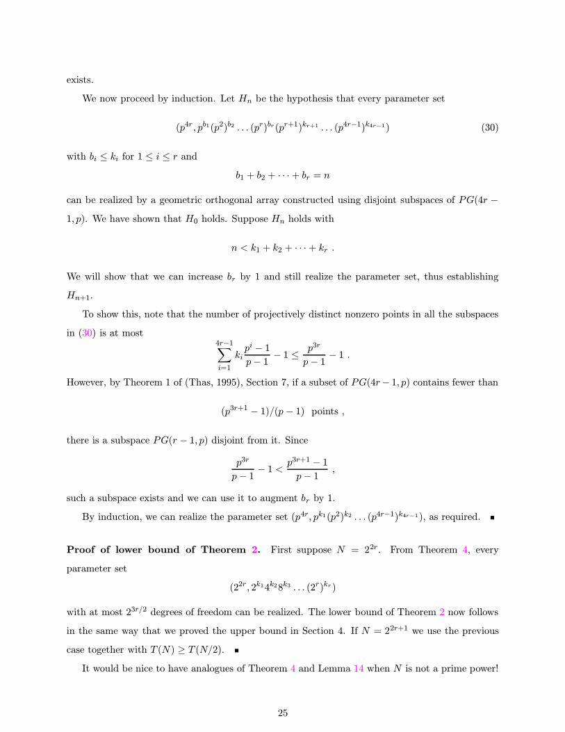
We now proceed by induction. Let Hn be the hypothesis that every parameter set

(p4r, pb1(p2)b2 . . . (pr)br(pr+1)kr+1 . . . (p4r−1)k4r−1) (30)

with bi ≤ ki for 1 ≤ i ≤ r andb1 + b2 + · · ·+ br = n

can be realized by a geometric orthogonal array constructed using disjoint subspaces of PG(4r −1, p). We have shown that H0 holds. Suppose Hn holds with

n < k1 + k2 + · · ·+ kr .

We will show that we can increase br by 1 and still realize the parameter set, thus establishing

Hn+1.

To show this, note that the number of projectively distinct nonzero points in all the subspaces

in (30) is at most4r−1∑

i=1

kipi − 1p− 1 − 1 ≤

p3r

p− 1 − 1 .

However, by Theorem 1 of (Thas, 1995), Section 7, if a subset of PG(4r− 1, p) contains fewer than

(p3r+1 − 1)/(p− 1) points ,

there is a subspace PG(r − 1, p) disjoint from it. Since

p3r

p− 1 − 1 <p3r+1 − 1p− 1 ,

such a subspace exists and we can use it to augment br by 1.

By induction, we can realize the parameter set (p4r, pk1(p2)k2 . . . (p4r−1)k4r−1), as required.

Proof of lower bound of Theorem 2. First suppose N = 22r. From Theorem 4, every

parameter set

(22r, 2k14k28k3 . . . (2r)kr)

with at most 23r/2 degrees of freedom can be realized. The lower bound of Theorem 2 now follows

in the same way that we proved the upper bound in Section 4. If N = 22r+1 we use the previous

case together with T (N) ≥ T (N/2).It would be nice to have analogues of Theorem 4 and Lemma 14 when N is not a prime power!

25

Acknowledgments

We thank Michele Colgan for computing the properties of the lattices Λ′N shown in Table 3. The

research of John Stufken was supported by NSF grant DMS-9803684.

26

References

Bosma, W. and Cannon, J. (1995). Handbook of Magma Functions, Sydney.

Bosma, W., Cannon, J. and Mathews, G. (1994). Programming with algebraic structures:

Design of the Magma language, in Proceedings of the 1994 International Symposium on Sym-

bolic and Algebraic Computation, M. Giesbrecht, Ed., Association for Computing Machinery,

52–57.

Bosma, W., Cannon, J. and Playoust, C. (1997). The Magma algebra system I: The user

language. J. Symb. Comp., 24, 235–265.

Calderbank, A. R., Rains, E. M., Shor, P. W. and Sloane, N. J. A. (1998). Quantum error

correction via codes over GF (4). IEEE Trans. Information Theory, 44, 1369–1387.

Eisfeld, J., Storme, L. and Sziklai, P. (1999). Maximal partial spreads in finite projective spaces,

preprint.

Hedayat, A. S., Sloane, N. J. A. and Stufken, J. (1999). Orthogonal Arrays: Theory and

Applications. New York: Springer-Verlag.

Hoffman, K. and Kunze, R. (1961). Linear Algebra, Engelewood Cliffs, NJ: Prentice-Hall.

Kimura, H. (1994a). Classification of Hadamard matrices of order 28 with Hall sets. Discrete

Math., 128, 257–268.

Kimura, H. (1994b). Classification of Hadamard matrices of order 28. Discrete Math., 133,

171–180.

Sloane, N. J. A. (1999). The On-Line Encyclopedia of Integer Sequences. Published electroni-

cally at http://www.research.att.com/∼njas/sequences/.

Sloane, N. J. A. and Stufken, J. (1996). A linear programming bound for orthogonal arrays

with mixed levels. J. Statist. Plann. Infer., 56, 295–305.

Thas, J. A. (1995). Projective geometries over a finite field, Chapter 7 of Handbook of Incidence

Geometry, edited by Buekenhout, F. Amsterdam: North-Holland.

Trotter, W. F. (1995). Partially ordered sets, Chapter 8 of Handbook of Combinatorics, edited

by Graham, R. L., Grotschel, M. and Lovasz, L. Amsterdam: North-Holland; Cambridge,

MA: MIT Press.

27

Welsh, D. J. A. (1976). Matroid Theory. London: Academic Press.

Wu, C. F. J. (1989). Construction of 2m4n designs via a grouping scheme. Annals Statist., 17,

1880–1885.

28