arX

iv:1

101.

0428

v1 [

cs.L

G]

2 J

an 2

011

The Local Optimality of Reinforcement Learning by

Value Gradients, and its Relationship to Policy

Gradient Learning

Michael Fairbank, Eduardo Alonso

Department of Computing, School of Informatics, City University London, London, UK

Abstract

In this theoretical paper we are concerned with the problem of learning avalue function by a smooth general function approximator, to solve a de-terministic episodic control problem in a large continuous state space. It isshown that learning the gradient of the value-function at every point alonga trajectory generated by a greedy policy is a sufficient condition for thetrajectory to be locally extremal, and often locally optimal, and we arguethat this brings greater efficiency to value-function learning. This contraststo traditional value-function learning in which the value-function must belearnt over the whole of state space.

It is also proven that policy-gradient learning applied to a greedy policyon a value-function produces a weight update equivalent to a value-gradientweight update, which provides a surprising connection between these twoalternative paradigms of reinforcement learning, and a convergence prooffor control problems with a value function represented by a general smoothfunction approximator.

Keywords:Reinforcement Learning, Control Problems, Value-gradient, Functionapproximators, Policy Gradient, Dual Heuristic Programming

Email addresses: michael.fairbank.1 ‘at’ city.ac.uk (Michael Fairbank),eduardo ‘at’ soi.city.ac.uk (Eduardo Alonso)

Preprint submitted to Arxiv January 4, 2011

1. Introduction

Reinforcement learning (RL) is the study of how an agent can learn ac-tions that maximise some given reward function. For example a typicalscenario is a robot (or agent) wandering around in an environment, suchthat at time t it has position (or state) vector ~xt. The robot moves in con-tinuous space and time, but we discretize time to enable modelling of themotion by a computer. Thus at each time t the robot chooses an action ~atwhich takes it to the next state according to the environment’s model func-tion ~xt+1 = f(~xt,~at), and gives it an immediate scalar reward rt, given bythe reward function rt = r(~xt,~at). The robot keeps moving until it reachesone of the designated terminal states. The RL problem is for the robot tolearn how to choose actions so as to maximise the total reward received, Σtrt.Specifically, the problem is to find a policy function π(~x, ~z) (where ~z is someparameter vector) that calculates which action ~a = π(~x, ~z) to take for anygiven state ~x, such that the total reward is maximised.

One key approach to tackle this RL problem is to assign a score to everypoint in state space that gives the best possible total reward attainable ifstarting from that state. This scoring function is called the optimal valuefunction, V ∗(~x). If this function was perfectly known then it would be easyfor the robot to behave optimally because at any instant it could considerall possible actions available and always choose the one that leads to thebest valued state, whilst also taking into account the immediate short-termreward in getting there. This way of acting is called the greedy policy onV ∗. So the objective of learning is to make a function approximator, V (~x, ~w)(e.g. a neural network with weight vector ~w), learn and represent the optimalvalue function, and then use a greedy policy on the approximated function.

However the optimal value function is not known at the start of learning.So for any given policy π(~x, ~z) we can define its value function V π(~x, ~z) to bethe real valued total reward that would be encountered if the robot startedat state ~x and followed that policy until termination. Bellman’s OptimalityCondition [1] shows that if V ≡ V π for all ~x in the state space S, where

π is the greedy policy on V , then that greedy policy is optimal. There isa circular interdependence here; V π depends on the greedy policy π, whichdepends on V , and we want V ≡ V π for all ~x.

If the state space was discrete and finite then Bellman’s condition couldbe met by dynamic programming which makes iterative sweeps through thewhole of state space, updating V incrementally. But in our problem the

2

state space is large and continuous so this is not possible. The RL methodsTD(0) and Q-learning [2, 3] can be used to update V along one trajectoryat a time, but these can be very slow since Bellman’s condition still needsmeeting over the entire state space for optimality. Even if Bellman’s conditionis perfectly satisfied along a single trajectory, performance can be extremelyfar from optimal if Bellman’s condition is not satisfied over the neighbouringtrajectories too. Hence it is well known in the RL community that constantexploration of the environment must be applied. This exploration could beprovided by stochastic model functions, a stochastic policy, or a stochasticstart point for each trajectory. The ability of RL algorithms to work instochastic environments is a virtue, but it is also a necessity for the abovereason, and it is a goal of this paper to define value-function learning methodsthat work in a deterministic environment.

TD(λ) [4] is a generalization to TD(0) which uses an extra parameterλ ∈ [0, 1] that can improve the speed of learning. The effect of λ is describedin detail in section 2.2, where we call it the “bootstrapping” parameter.

Although value function learning methods have produced successes inrobot control [5, 6], value function learning methods are problematic in thattheir theoretical convergence guarantees with function approximators are lim-ited. TD(λ) has been proven to converge [7] provided the function approx-

imator for V (~x, ~w) is linear in ~w, and the policy is fixed (i.e. that excludes

the greedy policy on V ). They are not proven to converge when a generalfunction approximator is used to represent the value function (e.g. a neuralnetwork) or when a greedy policy is used, such as is required by our robot RLproblem. Divergence examples exist for a non-linear function approximator[7], and where V is linear in ~w but where a greedy policy is used (divergingfor both λ = 0 and λ = 1; see section 4.3 of [8]).

One reason that these methods do not always converge is that changingthe approximated value function V at one point in state space will cause V

to change in other points of state space too, since the function approximatorthat represents V (~x, ~w) cannot be infinitely flexible. A second reason is thatin the Bellman condition, V π depends on π which in turn depends on V π, somaking progress in learning one of them can undo progress in learning theother. This second issue is highly relevant for RL control problems, sincethe ultimate objective is not just to learn a value function for some fixedpolicy, but is to improve a policy until it becomes optimal (or close enoughto optimal). Thus any successful convergence analysis for value function

3

learning must cope with the concurrent updating of V and the greedy policy,and there have been few insights into this problem by the RL literature—convergence proofs so far have generally treated one of these two componentsas fixed, or only treated the tabular case.

We address these issues by following the method of Dual Heuristic Pro-gramming (DHP) of Werbos [9] which tries to explicitly learn the gradientof the value function with respect to the state vector, i.e. it learns ∂V π

∂~xin-

stead of V π directly. We call this method value gradient learning (VGL),to distinguish it from the usual direct updates to the values of the valuefunction, which we refer to as value learning methods (VL). We extend Wer-bos’ method to include a bootstrapping parameter λ (just as Sutton did inextending TD(0) into TD(λ)), to give the algorithm we call VGL(λ).

The VGL method addresses the issue of the Bellman equation needingto be solved over the whole of state space, in that it turns out to be onlynecessary to learn the value gradient along a single trajectory for it to belocally optimal. This contrasts strongly with the VL methods which need tolearn the value function over all immediately neighbouring trajectories toofor local optimality, and so this is a significant efficiency gain for the VGLmethod. This optimality is an almost-immediate consequence of Pontryagin’smaximum principle [10], and this is proven in Section 3.

We address the difficulty of analysing the interdependence of simultane-ously updating V π and π by showing (in Lemma 7) that the dependency ofa greedy policy on a value function is primarily through the value-gradient.Hence a value-gradient analysis is necessary at some level to provide a theo-retical gateway to analysing the convergence properties of any value-functionweight update that uses a greedy policy; be it a VGL weight update or a VLweight update.

The dependency of the greedy policy on the value-gradient has alreadybeen exploited in an efficient policy [6], but the VGL method takes this onestep further by trying to explicitly learn the value-gradient.

There is an alternative paradigm of RL called policy gradient learning(PGL) which does not rely on learning a value function at all. We define PGLas algorithms that do gradient ascent on the total reward, and this definitionincludes methods of [11, 12, 13, 14]. These methods have natural convergenceguarantees since they are hill climbing strategies on a function with an upperbound, and have proved successful at robot control in continuous spaces [13].

In Section 4, we show a VGL weight update with λ = 1 is identicalto a PGL weight update, and this makes a theoretical connection between

4

these two different paradigms of RL, and provides a convergence proof forthis value function control problem with a general function approximator(provided λ = 1 and provided the policy is differentiable at every time stepof the trajectory).

In summary, the VGL methods in this paper lead to several benefits andinsights:

• They make a more direct approach to RL since it is the value-gradientthat affects the policy and so it makes sense that this is what shouldbe learned.

• It is only necessary to learn the value-gradient along a single trajectoryinstead of the whole of state space. This can lead to improved efficiencyfor VGL methods, since there is no need to explore locally (see Section3.1).

• They provide a theoretical insight and convergence result into the long-standing problem of proving convergence for value-function learningmethods with a function approximator, while providing a theoreticallink between value-function learning and PGL.

Another goal of this paper is to raise awareness in the RL community ofthe methods of [9].

The VGL method is a “model based” RL method in that it requiresthat the model functions f(~x,~a) and r(~x,~a) to be known. Knowledge of themodel functions (and their derivatives) delivers many of the above benefitsof the VGL method. Many researchers define RL specifically for the caseof unknown model functions. To answer this we would have to supplementthis VGL method with a separate learning system specifically to learn themodel functions, prior to trying to learn the policy. This is a commonlyused strategy for successful RL methods, for example in the recent successof maintaining the inverted flight of a helicopter [15], the model functionswere learned separately and prior to learning a policy. We also suggest thatmodel learning is the relatively straightforward part of the RL task, sinceit is a supervised learning problem, where the immediate answers are given.Also the model functions in a control problem are often simple known lawsof physics, and they do not change much from point to point, due to thecontinuous nature of the environment. [14] exploits this to successfully learnthe model functions, in real time, entirely while the robot is travelling along

5

one single trajectory. However we acknowledge that ideally, for a full RLlearning system, we would concurrently learn the model, the policy, and thevalue function while still ensuring convergence. In this paper we successfullyanalyse items two and three of this list in the case of λ = 1, but at theexpense of assuming the first is fixed and known.

We note that a third paradigm of RL exists called an actor-critic archi-tecture. In this architecture there is one function approximator to representV , and a second function approximator to represent the policy. The greedypolicy is not used. Successful theoretical results exist for the concurrent up-dating of the policy and V [16], and we discuss these results in comparisonto our own in section 4.1.

This paper is organised as follows. Section 2 defines the VGL(λ) algorithmand gives the definitions necessary to do this. Key concepts defined there arethe approximated value function and its target values; and the approximatedvalue gradient and its target. The next two sections give the two maintheoretical results: In Section 3 we prove the local optimality of the objectiveof VGL for a single trajectory and discuss the efficiency of the method. InSection 4 we demonstrate the connection between VGL and PGL, and hencegive the convergence proof for VGL with λ = 1, under certain conditions.Short discussions follow each of the two main theoretical results. Section 5presents the conclusions of our work.

2. Value Gradient Learning for Reinforcement Learning

This section defines the VGL algorithm. After some preliminary defini-tions are made in section 2.1, we describe target values which can be usedto define VL (in section 2.2). This definition of target values and VL isdone a concise way that differs from the conventional RL literature, and itallows us to define the VGL targets (in section 2.4) and the VGL algorithm(section 2.5). Both of these VGL concepts will be new to readers only expe-rienced with VL. A technical difficulty that needs dealing with on the wayare saturated actions, which are defined in section 2.3.

2.1. Preliminary Definitions

State space, trajectories and model functions. State Space, S, is asubset of ℜn. Each state in the state space is denoted by a column vector~x. The state space is large and continuous so that a function approximatoris necessary to represent the learned policy. A trajectory is a list of states

6

(~x0, ~x1, . . . , ~xF ) through state space starting at a given point ~x0. The trajec-tory is parameterised by actions ~at, chosen from an action space A, for timesteps t according to a model. The model is comprised of two known smoothdeterministic functions f(~x,~a) and r(~x,~a). The first model function f linksone state in the trajectory to the next, given action ~at, via the “Markovian”rule ~xt+1 = f(~xt,~at). The second model function, r, gives an immediatereal-valued reward rt = r(~xt,~at) on arriving at the next state ~xt+1.

Some states in S are designated as terminal states. Assume that eachtrajectory is guaranteed to reach a terminal state in some finite time (i.e. theproblem is episodic). For example, a scenario like this could be an aircraftwith limited fuel trying to land; or it could be a navigation problem withan imposed time limit. For a particular trajectory label the final time stept = F , so that ~xF is the terminal state of that trajectory. Note that for ageneral trajectory, F is dependent on the start point and the actions taken,so is not a global constant.Action vectors. The action vectors ~a can be real scalars or have severalreal components, one for each of the control dimensions of the agent. Forexample in a car, the action components might be accelerator pedal position,steering wheel angle, and brake pedal position. For a monorail train, theremight be just one scalar needed. Assume each action component (~at)

i is areal number that, for some problems, may be constrained to (~at)

i ∈ [−1, 1],and these constraints are imposed by the action space, such that ~at ∈ A forall t.1

Policy. A policy is a function π(~x, ~z), parameterised by a vector ~z, thatgenerates actions as a function of state. Thus for a given trajectory generatedby a given policy π, ~at = π(~xt, ~z). Since the policy is a pure function of ~x and~z, the policy is memoryless. The vector ~z holds the parameters of a smoothfunction approximator, for example it could be a concatenation in columnvector form of all of the weights of a neural network.Value Function. If a trajectory starts at state ~x0 and then follows a policyπ(~x, ~z) until reaching a terminal state, then the value function V π(~x0, ~z)

1The choice of the range [−1, 1] is arbitrary. The theoretical results of this paper wouldalso apply to any other finite range.

7

returns the total reward received:

V π(~x0, ~z) =

F−1∑

t=0

r(~xt, π(~xt, ~z))

= r(~x0, π(~x0, ~z)) + V π(f(~x0, π(~x0, ~z)), ~z) (1)

with V π(~xF , ~z) = 0.

Approximate Value Function. We define V (~x, ~w) to be the real-valuedoutput of a smooth function approximator with weight vector ~w and inputvector ~x. This is the approximate value function. It is the intention of mostVL algorithms to eventually find ~w such that V (~x, ~w) ≈ V ∗(~x) for all ~x, asdescribed earlier.Approximate Value-Gradient. The approximate value-gradient function

G(~x, ~w) is defined to be G(~x, ~w) = ∂V (~x,~w)∂~x

, and this is what the VGL al-

gorithms learn. Since V (~x, ~w) is defined to be smooth, the approximatevalue-gradient always exists.Greedy Policy. We define a greedy policy π(~x, ~w) on the approximate value

function V (~x, ~w) by:

π(~x, ~w) = argmax~a∈A

(r(~x,~a) + V (f(~x,~a), ~w)) (2)

The greedy policy is a one-step look-ahead that decides which actionto take, based only on the model and V . Since for a greedy policy, theactions are dependent on V (~x, ~w) and state, it follows that π = π(~x, ~w).This dependency on ~w distinguishes how we notate the greedy policy (i.e.π(~x, ~w)) from a general (non-greedy) policy (i.e. π(~x, ~z)). We extend thedefinition of the value function V π(~x, ~z) to also apply to the greedy policy,and we write this as V π(~x, ~w).Greedy Trajectory. A greedy trajectory is one that has been generated bythe greedy policy. Since the greedy policy depends upon the same weightvector as V (~x, ~w), any modification to the weight vector ~w will immediately

both change V (~x, ~w) and move all greedy trajectories. Hence we say V andthe greedy policy are tightly coupled; it is the same weight vector ~w used inV (~x, ~w) and the greedy policy π(~x, ~w).Trajectory Shorthand Notation. For a given trajectory through states(~x0, ~x1, . . . , ~xF ) with actions (~a0,~a1, . . . ,~aF−1), and for any function defined

on state space (e.g. including V (~x, ~w), G(~x, ~w), V π(~x, ~w), r(~x,~a) and the

8

functions defined later in the paper) we use a subscript of t on the functionto indicate that the function is being evaluated at (~xt,~at, ~w). For example,

rt = r(~xt,~at), Gt = G(~xt, ~w) and (V π)t=V π(~xt, ~w). Note that this shorthanddoes not mean that these functions are functions of t.Trajectory Shorthand Notation for Partial Derivatives. We usebrackets with a subscripted t to indicate that a partial derivative is to be

evaluated at time step t of a trajectory. For example,(

∂G∂ ~w

)

tis shorthand

for ∂G∂ ~w

∣∣∣(~xt, ~w)

, i.e. the function ∂G∂ ~w

evaluated at (~xt, ~w). Also, for example,(∂f

∂~a

)t= ∂f

∂~a

∣∣(~xt,~at)

; and similarly for other partial derivatives including(∂r∂~x

)t

and(∂V π

∂ ~w

)t.

Matrix-vector notation. Throughout this paper, a convention is used thatall defined vector quantities are columns, whether they are coordinates, orderivatives with respect to coordinates. Also any vector becomes transposed(becoming a row) if it appears in the numerator of a differential. Upperindices indicate the component of a vector or matrix. For example, ~xt is acolumn; ~w is a column; Gt is a column;

(∂V π

∂ ~w

)tis a column;

(∂f

∂~x

)tis a matrix

with element (i, j) equal to(

∂f(~x,~a)j

∂~xi

)

t;(

∂G∂ ~w

)

tis a matrix with element (i, j)

equal to(

∂Gj

∂ ~wi

)

t. An example product is

(∂f

∂~a

)tGt+1 =

∑i

(∂f i

∂~a

)

tGi

t+1. An

example second derivative of a scalar is(

∂2V∂ ~w∂~x

)ij=(

∂∂ ~w

∂V∂~x

)ij= ∂

∂ ~wi

∂V∂~xj =

∂Gj

∂ ~wi .Approximate Q Value function. Since the quantity in the right-hand sideof the greedy policy (eq. 2) comes up often, we define a function specificallyfor it. The approximate Q Value function [3] is defined as

Q(~x,~a, ~w) = r(~x,~a) + V (f(~x,~a), ~w) (3)

The greedy policy therefore maximises this quantity, i.e. the greedy policyis such that π(~x, ~w) = argmax~a∈A(Q(~x,~a, ~w)).

We will often also need the derivative ∂Q

∂awhich is

(∂Q

∂~a

)

t

=

(∂r

∂~a

)

t

+

(∂f

∂~a

)

t

Gt+1 (4)

2.2. Target ValuesThese are useful concepts for understanding value-learning, which we need

to define here because we will later differentiate them to make the targets

9

for the VGL algorithm.For a trajectory found by a greedy policy π(~x, ~w) on V (~x, ~w), we define

the “target-value function” V ′(~x, ~w) recursively as

V ′(~x, ~w) = r(~x, π(~x, ~w))+(λV ′(f(~x, π(~x, ~w)), ~w) + (1− λ)V (f(~x, π(~x, ~w)), ~w)

)

(5a)with V ′(~xF , ~w) = 0 and where λ ∈ [0, 1] is a fixed global constant (describedfurther below). To calculate V ′ for a particular point ~x0 in state space, itis necessary to run and cache a whole trajectory starting from ~x0 under thegreedy policy π(~x, ~w), and then work backwards along it applying the aboverecursion; thus V ′(~x, ~w) is defined for all points in state space.

For a given trajectory, using shorthand notation the above equation sim-plifies to

V ′t = rt +

(λV ′

t+1 + (1− λ)Vt+1

)(5b)

We refer to the values V ′t simply as the “target values” since the objective

of VL is to make Vt equal to V ′t for all t and along all greedy trajectories,

since then:

Vt = V ′t ∀~x0, ∀t

⇐⇒ Vt = rt + Vt+1 ∀~x0, ∀t by Eq. 5b

⇐⇒ V (~x, ~w) = r(~x, π(~x, ~w)) + V (f(~x, π(~x, ~w)), ~w) ∀~x

⇐⇒ V (~x, ~w) = V π(~x, ~w) ∀~x by Eq. 1

So when coupled with the greedy policy (Eq. 2), V satisfies Bellman’s Opti-mality Condition, and so the greedy policy will be an optimal policy.

We point out that since V ′ is dependent on the actions and on V (~x, ~w),

it is not a simple matter to attain the objective V ≡ V ′, since changing V

infinitesimally will immediately move the greedy trajectories (since they aretightly coupled), and therefore change V ′; these targets are moving ones. So

we should only try to move the values V slowly towards their targets. Forexample a VL function approximator weight update to do this could be:

∆~w = α

F−1∑

t=0

(∂V

∂ ~w

)

t

(V ′t − Vt) (6)

where α is a small positive constant.

10

The choice of the constant λ can be seen from Eq. 5b to affect thetargets and hence affect learning by Eq. 6. If λ = 0 then the recursionin Eq. 5b is not needed, and the weight update will force the estimateVt to move towards the estimate Vt+1. Updating an estimate based on anestimate like this is commonly called “bootstrapping”, and we call λ thebootstrapping parameter. If λ = 1 then the recursion in Eq. 5b is fully used,giving V ′(~x, ~w) ≡ V π(~x, ~w), and the estimate Vt will be updated to movetowards the actual total reward received until terminating. For other valuesof 0 ≤ λ ≤ 1 we get a smooth blending between these two cases as can beseen by Eq. 5b.

The function V ′ is identical to the “λ-Return” [17], as proven in Appendix A,but the V ′ recursive formula is more succinct. The weight update of Eq. 6 isa succinct statement of the TD(λ) algorithm in batch update mode, as alsoproven in Appendix A.

The use of V ′ greatly simplifies the analysis of value functions and value-gradients. Having it defined in this recursive form allows us to easily differ-entiate it to form the target value-gradient, and hence define the VGL algo-rithms. It would not be straightforward to define the VGL algorithms usingthe traditional formulation of the “λ-Return” described in Appendix A.

2.3. Saturated Actions

An extra complication arises if actions are bounded, e.g. if the constraints(~at)

i ∈ [−1, 1] are present for some action components. These need handlingcarefully to be able to differentiate the policy function later in this paper. Forexample if an action component represents the steering wheel of a car, thenwe say that action component is saturated when the steering wheel is rotatedto its full limit in either direction, with pressure being applied against thatlimit. Formally, for the greedy policy, when the constraints (~at)

i ∈ [−1, 1]are present for some action component (~at)

i, we say the action component

is saturated if |(~at)i| = 1 and

(∂Q

∂~ai

)t6= 0. If either of these conditions is not

met, or the constraints are not present, then the action component (~at)i is

not saturated.We sometimes want to refer to just the unsaturated components of action

vector ~a. We use the notation u(~a) to denote a vector of just the unsatu-rated components of ~a, i.e. this vector often has lower dimension than ~a

as any saturated components have been removed. If there are no saturatedcomponents then u(~a) = ~a.

11

We note some useful Lemmas about saturated actions and the greedypolicy.2

Lemma 1. If (~at)i is saturated, then, whenever they exist,

(∂πi

∂~x

)

t= 0 and

(∂πi

∂ ~w

)

t= 0.

This follows from the definition of saturated action components above: Imagine if thesteering wheel is fully turned to the right, with pressure applied. Because of the pressureapplied, any infinitesimal changes to the circumstances will not change the position of thesteering wheel.Note that

(∂π∂~x

)tand

(∂π∂ ~w

)tmay not exist, for example, if there are multiple joint maxima

in Q(~x,~a, ~w) with respect to ~a. Then an infinitesimal change to the Q function could causethe maximum to flip discontinuously from one of these maxima to the other.

Lemma 2. If an action component (~at)i chosen by a greedy policy is saturated, then

(~at)i = 1⇒

(∂Q∂~ai

)

t> 0; and (~at)

i = −1⇒(

∂Q∂~ai

)

t< 0.

The first of these two implications has to be true since for a saturated action(

∂Q∂~ai

)

t6= 0

by definition, and if(

∂Q∂~ai

)

t< 0 at (~at)

i = 1 then the maximum of Q would not be at

(~at)i = 1, which contradicts the greedy policy. The second implication is true for the same

reason with the situation reversed.

Lemma 3. If an action ~at chosen by a greedy policy has some unsaturated components,

then(

∂Q∂u(~a)

)

t= ~0 and

(∂2Q

∂u(~a)∂u(~a)

)

tis a negative semi-definite matrix.

The greedy policy has found an action somewhere in the middle of the vector space thatcontains u(~a). So this is an ordinary local maxima of a surface, hence possesses the claimedproperties.

Lemma 4. For any action ~at chosen by the greedy policy, regardless of whether any com-

ponents are saturated or not, whenever(∂π∂~x

)texists, we have

(∂π∂~x

)t

(∂Q∂~a

)

t= ~0.

Proof.(∂π∂~x

)t

(∂Q∂~a

)

t=∑

i

(∂πi

∂~x

)

t

(∂Q∂~ai

)

t. For each term of this sum, the greedy policy

implies either(

∂πi

∂~x

)

t= ~0 (in the case that action component (~at)

i is saturated and(

∂πi

∂~x

)

t

exists, by Lemma 1), or(

∂Q∂~ai

)

t= 0 (in the case that (~at)

i is not saturated, by Lemma 3).

Hence each term of the sum is zero, hence the sum is zero.

2These lemmas could be skipped on a first reading and just referred to as needed laterin the paper.

12

2.4. Target Value-Gradient, (G′t)

We now define the target vectors G′t that will be used as the VGL objec-

tive which is to achieve Gt = G′t for all t > 0 along a greedy trajectory. We

first define it for λ ∈ (0, 1] and afterwards extend the definition to includeλ = 0.

For λ ∈ (0, 1], we define the function G′(~x, ~w) = ∂V ′(~x,~w)∂~x

, which gives:

G′t =

(∂

∂~x

(r(~x, π(~x, ~w)) + λV ′(f(~x, π(~x, ~w)), ~w) + (1− λ)V (f(~x, π(~x, ~w)), ~w)

))

t

(by Eq. 5a)

=

((∂r

∂~x

)

t

+

(∂π

∂~x

)

t

(∂r

∂~a

)

t

)

+

((∂f

∂~x

)

t

+

(∂π

∂~x

)

t

(∂f

∂~a

)

t

)(λG′

t+1 + (1− λ)Gt+1

)(by chain rule)

(7)

with G′F = ~0, and assuming all derivatives in this equation exist (these

existence conditions are discussed further below).This recursive formula takes a known target value-gradient at the end

point of a trajectory (G′F = ~0), and works it backwards along the trajectory

rotating and incrementing it as appropriate, to give the target value-gradientat each time step.

For λ = 0, we modify the above definition slightly to make the definitionindependent of the existence of

(∂π∂~x

)t. We first note that in the special case

where λ = 0, Eq. 7 simplifies as follows:

G′t =

((∂r

∂~x

)

t

+

(∂π

∂~x

)

t

(∂r

∂~a

)

t

)+

((∂f

∂~x

)

t

+

(∂π

∂~x

)

t

(∂f

∂~a

)

t

)Gt+1 by Eq. 7

=

(∂r

∂~x

)

t

+

(∂f

∂~x

)

t

Gt+1 +

(∂π

∂~x

)

t

((∂r

∂~a

)

t

+

(∂f

∂~a

)

t

Gt+1

)

=

(∂r

∂~x

)

t

+

(∂f

∂~x

)

t

Gt+1 +

(∂π

∂~x

)

t

(∂Q

∂~a

)

t

by eq. 4

=

(∂r

∂~x

)

t

+

(∂f

∂~x

)

t

Gt+1 by Lemma 4

(8)

In this last line there was the assumption that(∂π∂~x

)texists, but for λ = 0

we simply define G′t to be equal to this last line. Thus G′

t is always defined

13

and exists for λ = 0. This matches the target value-gradient that Werbosuses in the algorithms DHP and GDHP (Eq. 28 of [18]).

In the special case of λ = 1, G′t becomes identical to

(∂V π

∂~x

)t(to see this,

remember that for λ = 1, we have V ′(~x, ~w) ≡ V π(~x, ~w)).All terms of Eq. 7 are obtainable from knowledge of the model functions

and the policy. For obtaining the term ∂π∂~x

it is usually preferable to havethe greedy policy written in analytical form (e.g. the policy used by [6]).Alternatively, using a derivation similar to that of Lemma 7, it can be shownthat, when it exists,

(∂π∂~x

)tis such that all saturated components satisfy(

∂πi

∂~x

)

t= ~0 and all unsaturated components satisfy:

(∂u(π)

∂~x

)

t

= −

(∂2Q

∂~x∂u(~a)

)

t

(∂2Q

∂u(~a)∂u(~a)

)−1

t

(9)

if(

∂2Q

∂u(~a)∂u(~a)

)−1

texists.

Existence conditions for the Target Value-Gradient The target value-gradient is a key concept of the VGL method, so we should check underwhich conditions it exists.

If λ = 0 then G′t is defined to always exist by Eq. 8. If λ > 0 and if

∂π∂~x

does not exist at some time step, t0, of the trajectory, then G′t is not

defined for all t ≤ t0. Conditions in which ∂π∂~x

might not exist are mentionedin Lemma 1 and Eq. 9.

It may be that in some problems the environment and model functionsmake it so that G′

t does not exist, even though the model functions aredesigned to be differentiable. For example, if an agent is at the boundarybetween a terminal state and a non-terminal state, and its velocity is zero,then depending on which way it goes next will determine whether the tra-jectory terminates or not. Hence the total reward could be vastly differentin those two cases, and so the function V π is not differentiable with respectto ~x at that point. These bifurcation points are hopefully rare in state spacein most problems.

The above rare occurrences of the non-existence of G′ do not affect thetwo main theoretical results of this paper (Sections 3 and 4), since bothresults talk about consequences of when the target value gradient does exist.

However certain problems would not be suitable for the VGL methodwithout their reformulation, for example if the total reward was defined to

14

be equal to the integer number of time-steps in a trajectory. This totalreward function is a step function, so does not give any useful derivative forlearning. Even though time needs to be discretized for simulation purposes, acalculation of the actual continuous value of time would be needed to make auseful differentiable total reward function. If the problem is modified so thatthe model functions more accurately reflect the underlying continuous timeprocess then the VGL method will work. As a rule of thumb, if a problem issuitable for PGL methods, then it will be suitable to work on VGL methods.

2.5. The VGL(λ) Learning Algorithm

The objective for any VGL algorithm is to attain Gt = G′t for all t >

0 along a greedy trajectory. It is proven in section 3 that this objectiveis sufficient to ensure the trajectory is locally extremal, and often locallyoptimal. As with the objective for learning the targets V ′, it should be notedthat the VGL objective is not straightforward to achieve since the targets G′

t

are moving ones and are highly dependent on ~w. Hence we must use a weightupdate to slowly move the approximated gradients towards their targets:

∆~w = α

F−1∑

t=0

(∂G

∂ ~w

)

t

Ωt(G′t − Gt) (10)

This equation defines the VGL(λ) algorithm. It is based on the GDHPand DHP algorithms [9, 18]. Our definition of G′ in Eq. 7 extends Werbos’methods which were defined for only λ = 0, to work with any λ. Twoimplementations of this algorithm are given in Appendix B.

The Ωt matrix is any positive definite matrix (as introduced by [18]),arbitrarily chosen by the experimenter. Ωt is included for generality, sincethe presence of any positive definite matrix here in the equation will forceevery component of Gt to move towards the corresponding component of G′

t

(in any basis). For simplicity Ωt is often just taken to be the identity matrixfor all t (as in Werbos’ algorithm DHP). One use for making Ωt arbitrarycould be for the experimenter to be able to compensate explicitly for anyrescalings of the state space axes.

It seems an inspired choice by Werbos to have included the matrix Ωt

at all, since in Section 4 it spontaneously appears in a PGL weight update,giving us an explicit formula we can use to specify Ωt when λ = 1. In thiscase it suffices for Ωt to be positive semi-definite.

15

Any VGL algorithm is going to involve using the matrices(

∂G∂ ~w

)

tand/or

∂G∂~x

which, for neural-networks, involves second order back-propagation. Thisis described in chapter 10 of [9].

3. The Local Optimality of the Value-Gradient Learning Objective

In this section we define locally optimal trajectories and prove that if theVGL objective is achieved, i.e. if G′

t = Gt for all t along a greedy trajectory,then that trajectory is locally extremal, and in certain situations, locallyoptimal.

We first define the total reward for a given trajectory that is irrespectiveof the policy that was used to find it. For any trajectory starting at state ~x0

and following actions (~a0,~a1, . . . ,~aF−1) until reaching a terminal state underthe given model, the total reward encountered is given by the function:

R(~x0,~a0,~a1, . . . ,~aF−1) =F−1∑

t=0

r(~xt,~at)

= r(~x0,~a0) +R(f(~x0,~a0),~a1,~a2, . . . ,~aF−1) (11)

with R(~xF ) = 0. Thus R is a function of the arbitrary starting state ~x0

and the actions. We extend the trajectory shorthand notation to include thefunction R, so that for any given trajectory, Rt ≡ R(xt,~at,~at+1, . . . ,~aF−1).This enables us to define the partial derivatives as

(∂R∂~x

)t= ∂Rt

∂~xtand

(∂R∂~a

)t=

∂Rt

∂~at.

Locally Optimal Trajectories. We define a trajectory parameterised byvalues (~x0,~a0,~a1,~a2, . . .) to be locally optimal if R(~x0,~a0,~a1,~a2, . . .) is at alocal maximum with respect to the parameters (~a0,~a1,~a2, . . .), subject to theconstraints (if present) that (~at)

i ∈ [−1, 1] for each action component i.Locally Extremal Trajectories (LET). We define a trajectory parame-terised by values (~x0,~a0,~a1,~a2, . . .) to be locally extremal if, for all t and allaction components i,

(∂R∂~ai

)t= 0 if (~at)

i is not saturated(∂R∂~ai

)t> 0 if (~at)

i is saturated and (~at)i = 1(

∂R∂~ai

)t< 0 if (~at)

i is saturated and (~at)i = −1.

(12)

16

In the case that all the actions are unbound, this criterion for a LET simplifiesto that of just requiring

(∂R∂~a

)t= ~0 for all t.

Having the possibility of bound actions introduces the extra complicationof saturated actions. The second condition in Eq. 12 can be understood bythe steering wheel analogy given before (in the definition of saturated actioncomponents); if the action component (~at)

i = 1 is saturated then the steeringwheel is fully turned to the right with pressure, implying we would like toturn the car even more in that direction if that were possible (even thoughit isn’t), which literally means that

(∂R∂~ai

)t> 0. The third condition in Eq.

12 is simply the reverse of this.In fact, in this definition R is locally optimal with respect to any sat-

urated actions. Consequently, if all of the actions are fully saturated (asituation known as bang-bang control), then this definition of a LET providesa sufficient condition for a locally optimal trajectory.

Lemma 5. For a greedy trajectory and any fixed λ ∈ [0, 1], if G′t = Gt for

all t then G′t = Gt =

(∂R∂~x

)tfor all t.

Proof. This is proven by induction. First we note that since Gt is defined toexist, then G′

t must also exist (since G′t = Gt for all t). Next, for λ ∈ (0, 1],

substituting G′t = Gt into eq. 7 gives,

Gt =

(∂π

∂~x

)

t

((∂r

∂~a

)

t

+

(∂f

∂~a

)

t

Gt+1

)+

(∂r

∂~x

)

t

+

(∂f

∂~x

)

t

Gt+1

=

(∂π

∂~x

)

t

(∂Q

∂~a

)

t

+

(∂r

∂~x

)

t

+

(∂f

∂~x

)

t

Gt+1 by eq. 4

=

(∂r

∂~x

)

t

+

(∂f

∂~x

)

t

Gt+1 by Lemma 4

where in the application of Lemma 4 we used the fact that(∂π∂~x

)texists since

G′t exists. For λ = 0, substituting G′

t = Gt into equation 8 gives the sameresult again, i.e.

Gt =

(∂r

∂~x

)

t

+

(∂f

∂~x

)

t

Gt+1 (13)

So Eq. 13 is valid for all λ ∈ [0, 1].

17

Also, differentiating Eq. 11 with respect to ~x gives

(∂R

∂~x

)

t

=

(∂r

∂~x

)

t

+

(∂f

∂~x

)

t

(∂R

∂~x

)

t+1

So(∂R∂~x

)tand Gt have the same recursive definition. Also their values at the

final time step t = F are the same, since(∂R∂~x

)F= GF = ~0. Therefore, by

induction, G′t = Gt =

(∂R∂~x

)tfor all t.

Theorem 1. Any greedy trajectory satisfying G′t = Gt (for all t) must be

locally extremal.

Proof. Since the greedy policy maximises Q(~xt,~at, ~w) with respect to ~at ateach time-step t, we know at each t and for each action component i,

(∂Q

∂~ai

)

t= 0 if (~at)

i is not saturated(

∂Q

∂~ai

)t> 0 if (~at)

i is saturated and (~at)i = 1

(∂Q

∂~ai

)

t< 0 if (~at)

i is saturated and (~at)i = −1.

(14)

These follow from Lemmas 3 and 2. Therefore since,

(∂R

∂~a

)

t

=

(∂r

∂~a

)

t

+

(∂f

∂~a

)

t

(∂R

∂~x

)

t+1

by differentiating eq. 11

=

(∂r

∂~a

)

t

+

(∂f

∂~a

)

t

Gt+1 by Lemma 5

=

(∂Q

∂~a

)

t

by eq. 4

we have(∂R∂~a

)t=(

∂Q

∂~a

)

tfor all t. Therefore the consequences of the greedy

policy (Eq. 14) become equivalent to the sufficient conditions for a LET (Eq.12), which implies the trajectory is a LET.

Corollary 1. If, in addition to the conditions of Theorem 1, all of the ac-tions are saturated (bang-bang control), then the trajectory is locally optimal.

This follows from the definitions given above of a LET.

18

Remark 1. According to the Bang-Bang Principle [19], bang-bang controloften arises in situations where the model functions are linear with respectto bound action vectors, or when the problem being solved is a time min-imisation problem. Hence it is often the case that all LETs found by thismethod are locally optimal.

Remark 2. If the VGL objective (i.e. G′t = Gt for all t) is achieved as the

fixed point of a weight update that is gradient ascent on the total reward(e.g. such as the weight update of Eq. 16 in Section 4), then the LET mustbe locally optimal, because the objective was arrived at by gradient ascenton the total reward.

Since the weight update of Eq. 16 is a special case of the VGL(λ) weightupdate (Eq. 10), it is speculated, but still an open question, that any timethe VGL objective is met by use of any instance of Eq. 10 (i.e. while usingany Ωt matrix, or any λ), it could always produce locally optimal trajectories.

Remark 3. We point out that the proof of Theorem 1 is highly related toPontryagin’s maximum principle (PMP), since Eq. 13 satisfies the PMP

equation for a “costate” vector. Therefore Gt is the costate vector of PMP,and the greedy policy (almost) forms the maximum condition of PMP (theonly difference being that PMP is defined for continuous time systems). Thiscompletes Pontryagin’s conditions to be a LET. However PMP still needssupplementing with Lemma 5 for it to be applicable for any λ ∈ [0, 1]. Wedid not use PMP explicitly because it only identifies LETs, and the way wehave formulated the proof allows us to derive the corollary’s extra conclusionfor bang-bang control producing locally optimal trajectories.

3.1. Discussion

This local optimality proof is valid for any λ ∈ [0, 1]. This optimalitycondition only needs satisfying over a single trajectory, whereas for VL thecorresponding optimality condition (V ′ = V ) needs satisfying over the wholeof state space. This implies that VGL methods have a much lesser require-ment for exploration than VL methods do, since the local part of explorationcomes for free with VGL methods. What we mean by this is that providedthe VGL learning algorithm makes progress towards achieving G′

t = Gt allalong a greedy trajectory, the trajectory will make progress in bending itselftowards a locally optimal shape, and this will happen without the need forany stochastic exploration. We argue that this leads to greater efficiency for

19

VGL compared to VL, and experiments confirm this in some simple problemdomains, by several orders of magnitude in most cases [8].

In comparison to VGL, the failure of VL without any exploration in adeterministic environment is dramatic and common, even when the value-function is perfectly learned along a single trajectory; examples are given insection 1.3 of [8].

A separate efficiency issue is the algorithmic complexity of VL and VGL,and these are both the same (O(dim(~w)) per time step) if Algorithm 1 isused, but VGL is slower (O(dim(~w)(dim(~x))2) per time step) if the on-lineimplementation of Algorithm 2 is used.

The requirement of our optimality proof for episodic problems could berelaxed by introducing a discount factor γ ∈ [0, 1] (see [2] for details), and theproof can then be extended by altering the terminal step of the induction ofLemma 5 to instead use the boundary condition limt→∞ γtG′

t = ~0. Howeverit is not yet clear how to extend the proof to an undiscounted non-episodicproblem.

The stochastic case for λ = 0 is considered by [18].

4. The Relationship of VGL to Policy-Gradient Learning

We now prove that the VGL(λ) weight update of Eq. 10, with λ = 1 anda carefully chosen Ωt matrix, is equivalent to PGL on a greedy policy.

PGL, sometimes also known as “direct” reinforcement learning, is definedto be gradient ascent on V π(~x0, ~z) with respect to the weight vector ~z ofa general policy, i.e. ∆~z = α

(∂V π

∂~z

)0for some small positive constant α.

PGL methods will naturally find local maxima of V π(~x0, ~z) and have goodconvergence properties.

A very direct and efficient method to calculate the policy gradient,(∂V π

∂~z

)0,

when the model functions are known is backpropagation through time (BPTT)[12] which we will follow here, and it is well suited to deterministic systems.However most studies of PGL in the RL literature [11, 13] are designed forstochastic environments and unknown model functions, and they form the

mean(

∂〈V π〉∂~z

)0after sampling many trajectories. [14] describes a rapid model

learning method that finds the policy gradient after just one trajectory.The required PGL gradient can be expanded as follows:

20

(∂V π

∂~z

)

t

=

(∂

∂~z(r(~x, π(~x, ~z)) + V π(f(~x, π(~x, ~z)), ~z))

)

t

(by Eq. 1)

=

(∂π

∂~z

)

t

((∂r

∂~a

)

t

+

(∂f

∂~a

)

t

(∂V π

∂~x

)

t+1

)+

(∂V π

∂~z

)

t+1

(by chain rule)

Expanding this recursion and substituting it into the gradient ascentequation gives,

∆~z =α∑

t≥0

(∂π

∂~z

)

t

((∂r

∂~a

)

t

+

(∂f

∂~a

)

t

(∂V π

∂~x

)

t+1

)

BPTT is merely an efficient implementation of this formula, often forcases where the policy π(~x, ~z) is provided by a neural-network [12], but alsodefined for a general differentiable policy. We note that although this equa-tion looks quite different from the more regularly used PGL equation of [11],the two are mathematically equivalent since it is proven in [11] that their

weight update is equal to ∂〈V π〉∂~z

The above weight update was derived for a general policy. We now switchto specifically consider PGL applied to a greedy policy, so that all instancesof the weight vector ~z will be now replaced by ~w:

∆~w =α∑

t≥0

(∂π

∂ ~w

)

t

((∂r

∂~a

)

t

+

(∂f

∂~a

)

t

(∂V π

∂~x

)

t+1

)(15)

The equivalence we will show only holds when the actions are unbound.If bound actions are required then they could be implemented indirectlyby applying an exponential cost function to the model function r(~x,~a) topenalise components of ~a that get close to their desired limits, prohibitingthe greedy policy from choosing actions beyond this range.

Initially we only consider the case where(∂V π

∂ ~w

)0exists for a greedy tra-

jectory, and also where hence(∂π∂ ~w

)texists for all t. The terms

(∂π∂ ~w

)tand(

∂r∂~a

)tcan be reinterpreted under the greedy policy:

Lemma 6. The greedy policy implies, for an unbound action,(∂r∂~a

)t= −

(∂f

∂~a

)tGt+1.

Proof. Substitute(

∂Q

∂~a

)t= ~0 (Lemma 3 for an unbound action) into Eq.

4.

21

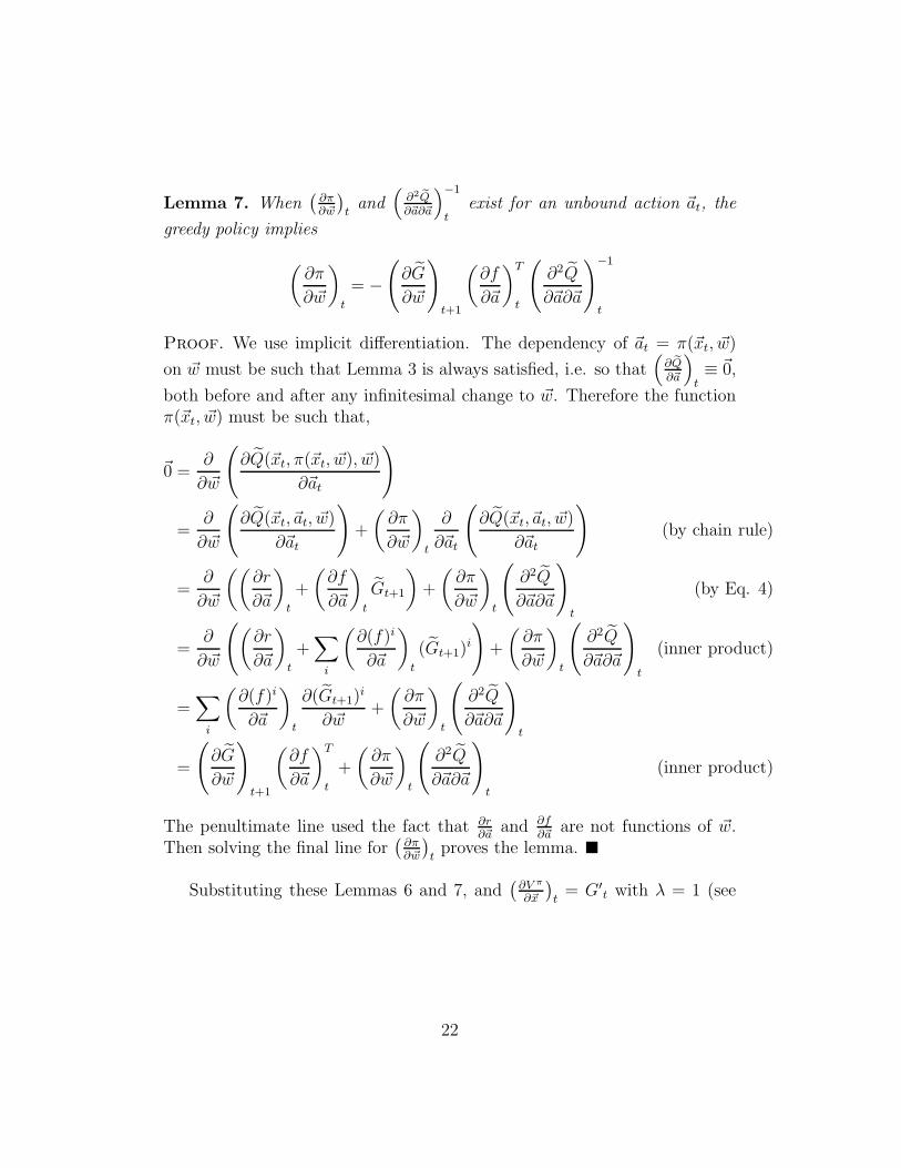
Lemma 7. When(∂π∂ ~w

)tand

(∂2Q

∂~a∂~a

)−1

texist for an unbound action ~at, the

greedy policy implies

(∂π

∂ ~w

)

t

= −

(∂G

∂ ~w

)

t+1

(∂f

∂~a

)T

t

(∂2Q

∂~a∂~a

)−1

t

Proof. We use implicit differentiation. The dependency of ~at = π(~xt, ~w)

on ~w must be such that Lemma 3 is always satisfied, i.e. so that(

∂Q

∂~a

)t≡ ~0,

both before and after any infinitesimal change to ~w. Therefore the functionπ(~xt, ~w) must be such that,

~0 =∂

∂ ~w

(∂Q(~xt, π(~xt, ~w), ~w)

∂~at

)

=∂

∂ ~w

(∂Q(~xt,~at, ~w)

∂~at

)+

(∂π

∂ ~w

)

t

∂

∂~at

(∂Q(~xt,~at, ~w)

∂~at

)(by chain rule)

=∂

∂ ~w

((∂r

∂~a

)

t

+

(∂f

∂~a

)

t

Gt+1

)+

(∂π

∂ ~w

)

t

(∂2Q

∂~a∂~a

)

t

(by Eq. 4)

=∂

∂ ~w

((∂r

∂~a

)

t

+∑

i

(∂(f)i

∂~a

)

t

(Gt+1)i

)+

(∂π

∂ ~w

)

t

(∂2Q

∂~a∂~a

)

t

(inner product)

=∑

i

(∂(f)i

∂~a

)

t

∂(Gt+1)i

∂ ~w+

(∂π

∂ ~w

)

t

(∂2Q

∂~a∂~a

)

t

=

(∂G

∂ ~w

)

t+1

(∂f

∂~a

)T

t

+

(∂π

∂ ~w

)

t

(∂2Q

∂~a∂~a

)

t

(inner product)

The penultimate line used the fact that ∂r∂~a

and ∂f

∂~aare not functions of ~w.

Then solving the final line for(∂π∂ ~w

)tproves the lemma.

Substituting these Lemmas 6 and 7, and(∂V π

∂~x

)t= G′

t with λ = 1 (see

22

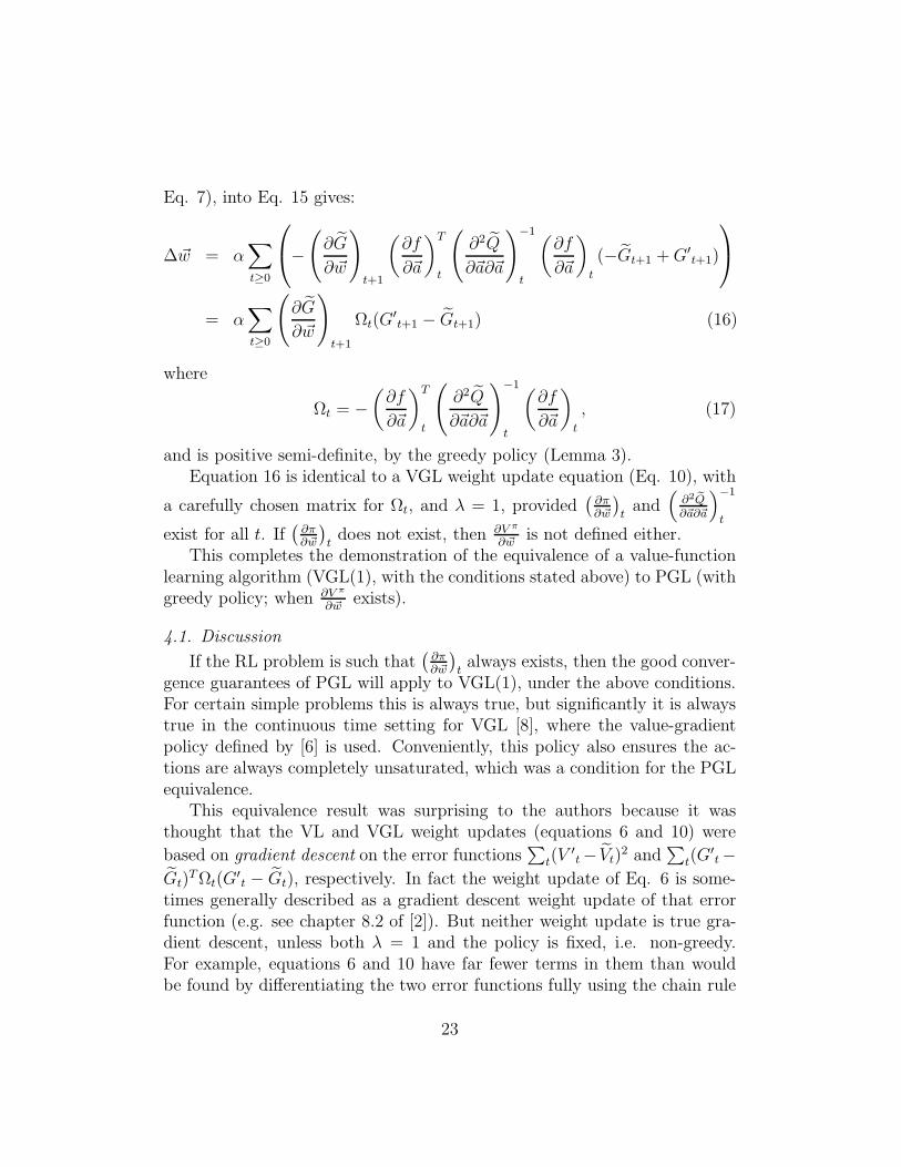
Eq. 7), into Eq. 15 gives:

∆~w = α∑

t≥0

−(∂G

∂ ~w

)

t+1

(∂f

∂~a

)T

t

(∂2Q

∂~a∂~a

)−1

t

(∂f

∂~a

)

t

(−Gt+1 +G′t+1)

= α∑

t≥0

(∂G

∂ ~w

)

t+1

Ωt(G′t+1 − Gt+1) (16)

where

Ωt = −

(∂f

∂~a

)T

t

(∂2Q

∂~a∂~a

)−1

t

(∂f

∂~a

)

t

, (17)

and is positive semi-definite, by the greedy policy (Lemma 3).Equation 16 is identical to a VGL weight update equation (Eq. 10), with

a carefully chosen matrix for Ωt, and λ = 1, provided(∂π∂ ~w

)tand

(∂2Q

∂~a∂~a

)−1

t

exist for all t. If(∂π∂ ~w

)tdoes not exist, then ∂V π

∂ ~wis not defined either.

This completes the demonstration of the equivalence of a value-functionlearning algorithm (VGL(1), with the conditions stated above) to PGL (withgreedy policy; when ∂V π

∂ ~wexists).

4.1. Discussion

If the RL problem is such that(∂π∂ ~w

)talways exists, then the good conver-

gence guarantees of PGL will apply to VGL(1), under the above conditions.For certain simple problems this is always true, but significantly it is alwaystrue in the continuous time setting for VGL [8], where the value-gradientpolicy defined by [6] is used. Conveniently, this policy also ensures the ac-tions are always completely unsaturated, which was a condition for the PGLequivalence.

This equivalence result was surprising to the authors because it wasthought that the VL and VGL weight updates (equations 6 and 10) were

based on gradient descent on the error functions∑

t(V′t− Vt)

2 and∑

t(G′t−

Gt)TΩt(G

′t − Gt), respectively. In fact the weight update of Eq. 6 is some-

times generally described as a gradient descent weight update of that errorfunction (e.g. see chapter 8.2 of [2]). But neither weight update is true gra-dient descent, unless both λ = 1 and the policy is fixed, i.e. non-greedy.For example, equations 6 and 10 have far fewer terms in them than wouldbe found by differentiating the two error functions fully using the chain rule

23

(e.g. [20] describes the missing terms for a fixed policy with VL and λ = 0;even more terms are missing if a tightly-coupled greedy policy is used, evenwhen λ = 1). Therefore learning progress as measured by either error func-tion is far from monotonic. So this PGL-VGL equivalence proof is surprisingbecause it shows these anomalies for VGL(1) are because the weight updateis actually gradient ascent on V π when Ωt is chosen carefully, and it neatlysolves the monotonic progress problem for a tightly-coupled greedy policy.

It was also surprising to learn that PGL and value-function weight up-dates are not as fundamentally different to each other as we first thought.It was not known that any PGL weight update, when applied to a greedypolicy on an approximate value function, would be doing the same thing asany value function weight update; even if both had λ = 1. Of course they areusually not the same, unless this particular choice of Ωt is chosen. The equiv-alence now creates a difficulty in distinguishing between PGL and VGL(1)with this particular Ωt. However, we describe the above weight update as aVGL update; it is of the same form as Eq. 10 which was defined by [18], i.e.prior to this equivalence being realised.

If λ = 1 is used then Eq. 17 is a good choice for Ωt, since it will ensuremonotonic progress with respect to V π, under the above conditions. HoweverEq. 17 means Ωt can sometimes be very small, which could slow learningdown. Alternative choices for Ωt (such as the identity matrix) may henceproduce an aggressive speed up of learning, but will do so at the expense ofmonotonic progress. A less aggressive speed up method for the gradient as-cent, such as conjugate gradients, could be used instead of using the identitymatrix for Ωt.

This analysis has been successful for a tightly-coupled greedy policy andvalue function, which is unusual since most RL analyses of value-functionupdates in the literature so far have only been applicable for a “fixed” policy.Interestingly, using a tightly-coupled value-function and greedy policy wasnecessary for the equivalence to hold.

[16] provides a related convergence result that also applies to the problem

of concurrently updating V and π. Their result applies to an actor-criticarchitecture, and since this does not use a greedy policy, they avoid the needfor considering ∂π

∂ ~wthrough Lemma 7. While our result compared to theirs

is disadvantaged in that it is only valid for λ = 1, some possible advantagesof our method over theirs are as follows: Their result is thought to applyonly when the function approximator for V is linear in the same features of

24

the state vector that the function approximator for the policy uses as input(see footnote 1 of [16]). Also the policy iteration algorithm that updates

both function approximators requires that the function approximator for Vis trained to completion, over all of state space, every time the policy changes,and this requirement is nested inside of the loop that updates the policy; sothe whole thing is quite computationally expensive. Finally, in order for thetraining process for V to have guaranteed convergence, it would have to belinear in ~w if λ < 1 [7].

5. Conclusions and Further Work

We have proven the local optimality of learning the target value gradientsalong a greedy trajectory (for any λ), argued the efficiency benefits of thatapproach, and have demonstrated the equivalence of VGL(1) to PGL. In thisresearch we have been interested in genuine theoretical challenges to under-standing value-function learning with a greedy policy, regardless of whetherby VL or VGL; particularly about how the greedy policy is affected by aweight update to V (~x, ~w) (as derived in Lemma 7), and particularly aboutwhat exactly is required for an optimal trajectory (Section 3).

In further work we would like to extend the optimality proof of Section3 to undiscounted non-episodic problems, and of course somehow work howto extend the convergence proof for λ = 1 to include λ < 1, which is unlikelywith the weight update in its current form since divergence examples for thisexist (e.g. section 4.3 of [8]).

Acknowledgements

We are very grateful to Peter Dayan, Paul Werbos, Csaba Szepesvari,Remi Coulom, Lucian Busoniu and the reviewers for their discussions, sug-gestions and pointers for research on this topic.

Appendix A. Equivalence of V ′ notation to the λ-Return

Although it was first discovered by Watkins [17], we use the definition

of the λ-Return given by [2]: Rλt = (1 − λ)

∑∞n=1 λ

n−1R(n)t with R

(n)t =∑n−1

k=0 rt+k + Vt+n. We aim to show that V ′t is identical to Rλ

t . Expanding

25

the definition of Rλt gives

Rλt = (1− λ)

∞∑

n=1

λn−1

(n−1∑

k=0

rt+k + Vt+n

)

= (1− λ)(λ0rt + λ1(rt + rt+1) + λ2(rt + rt+1 + rt+2) + . . .

)+ (1− λ)

∞∑

n=1

λn−1Vt+n

= (1− λ)

∞∑

n=0

(rt+n

∞∑

k=n

λk

)+ (1− λ)

∞∑

n=0

λnVt+n+1

=∞∑

n=0

(λnrt+n) + (1− λ)∞∑

n=0

λnVt+n+1

Expanding the definition of V ′ (Eq. 5b) gives

V ′t = rt +

(λV ′

t+1 + (1− λ)Vt+1

)

=∞∑

n=0

λn(rt+n + (1− λ)Vt+n+1

)

Thus V ′ is identical to Rλ. However since it uses a recursive notation,V ′ is easier to differentiate than Rλ, enabling us to define G′. The λ-Returnprovides an equivalent formulation for the algorithm TD(λ) known as the“forwards view of TD(λ)” [2]. This proves that Eq. 6 is equivalent to theTD(λ) weight update.

Appendix B. A batch mode implementation, and an on-line im-plementation of the VGL(λ) algorithm

We give two implementations of the VGL(λ) algorithm which produce anidentical weight update. Algorithm 1 is the faster of the two, but requiresstorage of a whole trajectory and is batch-mode only. Algorithm 2 can beused on-line and is more memory efficient since it does not store a wholetrajectory, but is slower since it requires the manipulation of an “eligibilitytrace” matrix.

Here we use a shorthand notation as DD~x≡ ∂

∂~x+ ∂π

∂~x∂∂~a. We let nw and nx

be the dimensions of ~w and ~x respectively. γ is a constant discount factor,where γ ∈ [0, 1].

26

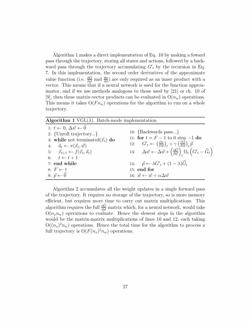
Algorithm 1 makes a direct implementation of Eq. 10 by making a fowardpass through the trajectory, storing all states and actions, followed by a back-ward pass through the trajectory accumulating G′

t by the recursion in Eq.7. In this implementation, the second order derivatives of the approximate

value function (i.e. ∂G∂ ~w

and ∂π∂~x) are only required as an inner product with a

vector. This means that if a neural network is used for the function approx-imator, and if we use methods analogous to those used by [21] or ch. 10 of[9], then these matrix-vector products can be evaluated in O(nw) operations.This means it takes O(Fnw) operations for the algorithm to run on a wholetrajectory.

Algorithm 1 VGL(λ). Batch-mode implementation.

1: t← 0, ∆~w ← ~02: Unroll trajectory...3: while not terminated(~xt) do4: ~at ← π(~xt, ~w)5: ~xt+1 ← f(~xt,~at)6: t← t + 17: end while8: F ← t

9: ~p← ~0

10: Backwards pass...11: for t = F − 1 to 0 step −1 do12: G′

t ←(DrD~x

)t+ γ

(Df

D~x

)t~p

13: ∆~w ← ∆~w+(

∂G∂ ~w

)tΩt

(G′

t − Gt

)

14: ~p← λG′t + (1− λ)Gt

15: end for16: ~w ← ~w + α∆~w

Algorithm 2 accumulates all the weight updates in a single forward passof the trajectory. It requires no storage of the trajectory, so is more memoryefficient, but requires more time to carry out matrix multiplications. This

algorithm requires the full ∂G∂ ~w

matrix which, for a neural network, would takeO(nxnw) operations to evaluate. Hence the slowest steps in the algorithmwould be the matrix-matrix multiplications of lines 10 and 12, each takingO((nx)

2nw) operations. Hence the total time for the algorithm to process afull trajectory is O(F (nx)

2nw) operations.

27

To derive this algorithm, we had to first rewrite Eq. 7 as follows:

G′t =

(Dr

D~x

)

t

+ γ

(Df

D~x

)

t

(λG′

t+1 + (1− λ)Gt+1

)

=

(Dr

D~x

)

t

+ γ

(Df

D~x

)

t

Gt+1 + λγ

(Df

D~x

)

t

(G′

t+1 − Gt+1

)

⇒ G′t − Gt =

((Dr

D~x

)

t

+ γ

(Df

D~x

)

t

Gt+1 − Gt

)+ λγ

(Df

D~x

)

t

(G′

t+1 − Gt+1

)

=~δt + λγ

(Df

D~x

)

t

(G′

t+1 − Gt+1

)(B.1)

where we define

~δt =

(Dr

D~x

)

t

+ γ

(Df

D~x

)

t

Gt+1 − Gt (B.2)

Unrolling the recursion in (G′t − Gt) of Eq. B.1 gives

G′t − Gt = ~δt + λγ

(Df

D~x

)

t

~δt+1 + λ2γ2

(Df

D~x

)

t

(Df

D~x

)

t+1

~δt+2 + . . .

Then substituting this into the VGL(λ) weight update equation (Eq. 10)and reordering the terms gives:

∆~w = α

F−1∑

t=0

(∂G

∂ ~w

)

t

Ωt

(~δt + λγ

(Df

D~x

)

t

~δt+1 + λ2γ2

(Df

D~x

)

t

(Df

D~x

)

t+1

~δt+2 + . . .

)

= α

F−1∑

t=0

(Et~δt

)(B.3)

where Et is a matrix defined to be

Et =

(∂G

∂ ~w

)

t

Ωt + λγ

(∂G

∂ ~w

)

t−1

Ωt−1

(Df

D~x

)

t−1

+ λ2γ2

(∂G

∂ ~w

)

t−2

Ωt−2

((Df

D~x

)

t−2

(Df

D~x

)

t−1

)

+ . . .+ λtγt

(∂G

∂ ~w

)

0

Ω0

((Df

D~x

)

0

(Df

D~x

)

1

. . .

(Df

D~x

)

t−2

(Df

D~x

)

t−1

)

28

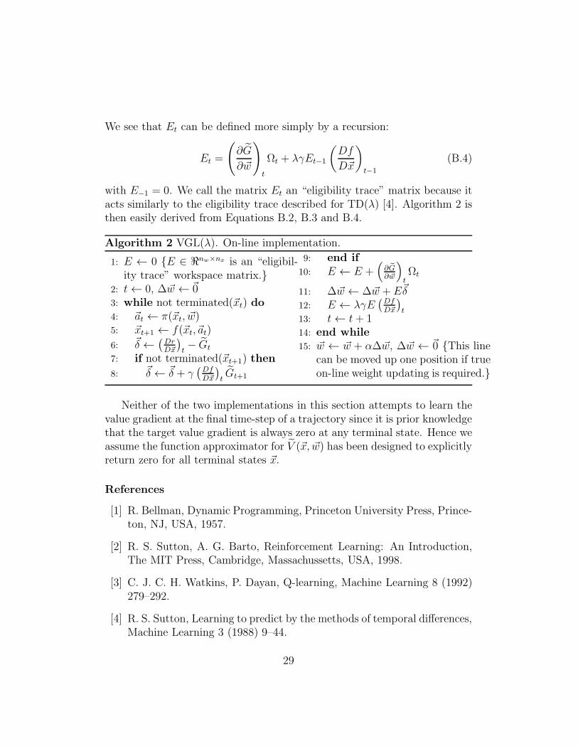
We see that Et can be defined more simply by a recursion:

Et =

(∂G

∂ ~w

)

t

Ωt + λγEt−1

(Df

D~x

)

t−1

(B.4)

with E−1 = 0. We call the matrix Et an “eligibility trace” matrix because itacts similarly to the eligibility trace described for TD(λ) [4]. Algorithm 2 isthen easily derived from Equations B.2, B.3 and B.4.

Algorithm 2 VGL(λ). On-line implementation.

1: E ← 0 E ∈ ℜnw×nx is an “eligibil-ity trace” workspace matrix.

2: t← 0, ∆~w ← ~03: while not terminated(~xt) do4: ~at ← π(~xt, ~w)5: ~xt+1 ← f(~xt,~at)

6: ~δ ←(DrD~x

)t− Gt

7: if not terminated(~xt+1) then

8: ~δ ← ~δ + γ(Df

D~x

)tGt+1

9: end if10: E ← E +

(∂G∂ ~w

)

tΩt

11: ∆~w ← ∆~w + E~δ

12: E ← λγE(Df

D~x

)t

13: t← t+ 114: end while15: ~w ← ~w + α∆~w, ∆~w ← ~0 This line

can be moved up one position if trueon-line weight updating is required.

Neither of the two implementations in this section attempts to learn thevalue gradient at the final time-step of a trajectory since it is prior knowledgethat the target value gradient is always zero at any terminal state. Hence weassume the function approximator for V (~x, ~w) has been designed to explicitlyreturn zero for all terminal states ~x.

References

[1] R. Bellman, Dynamic Programming, Princeton University Press, Prince-ton, NJ, USA, 1957.

[2] R. S. Sutton, A. G. Barto, Reinforcement Learning: An Introduction,The MIT Press, Cambridge, Massachussetts, USA, 1998.

[3] C. J. C. H. Watkins, P. Dayan, Q-learning, Machine Learning 8 (1992)279–292.

[4] R. S. Sutton, Learning to predict by the methods of temporal differences,Machine Learning 3 (1988) 9–44.

29

[5] C. Kwok, D. Fox, Reinforcement learning for sensing strategies, in: Pro-ceedings of the International Confrerence on Intelligent Robots and Sys-tems (IROS), 2004.

[6] K. Doya, Reinforcement learning in continuous time and space, NeuralComputation 12 (1) (2000) 219–245.

[7] J. N. Tsitsiklis, B. Van Roy, An analysis of temporal-difference learningwith function approximation, Tech. Rep. LIDS-P-2322 (1996).

[8] M. Fairbank, Reinforcement learning by value gradients, eprintarXiv:0803.3539v1 [cs.NE].URL http://arxiv.org/abs/0803.3539v1

[9] P. J. Werbos, Handbook of Intelligent Control, Van Nostrand, 1992.

[10] I. N. Bronshtein, K. A. Semendyayev, Handbook of Mathematics, 3rdEdition, Van Nostrand Reinhold Company, 1985, Ch. 3.2.2, pp. 372–382.

[11] R. J. Williams, Simple statistical gradient-following algorithms for con-nectionist reinforcement learning, Machine Learning 8 (1992) 229–356.

[12] P. J. Werbos, Backpropagation through time: What it does and how todo it, in: Proceedings of the IEEE, Vol. 78, No. 10, 1990, pp. 1550–1560.

[13] J. Peters, S. Schaal, Policy gradient methods for robotics, in: Proceed-ings of the IEEE/RSJ International Conference on Intelligent Robotsand Systems (IROS), 2006.

[14] R. Munos, Policy gradient in continuous time, Journal of Machine Learn-ing Research 7 (2006) 413–427.

[15] A. Y. Ng, H. J. Kim, M. I. Jordan, S. Sastry, Inverted autonomous he-licopter flight via reinforcement learning, in: International Symposiumon Experimental Robotics, MIT Press, 2004.

[16] R. S. Sutton, D. Mcallester, S. Singh, Y. Mansour, Policy gradient meth-ods for reinforcement learning with function approximation, in: Ad-vances in Neural Information Processing Systems 12, Vol. 12, 2000, pp.1057–1063.

30

[17] C. Watkins, Learning from delayed rewards, Ph.D. thesis, University ofCambridge, England (1989).

[18] P. J. Werbos, Stable adaptive control using new critic designs, eprintarXiv:adap-org/9810001.URL http://xxx.lanl.gov/html/adap-org/9810001

[19] L. Sonneborn, F. V. Vleck, The bang-bang principle for linear controlsystems, SIAM J. Control 2 (1965) 152–159.

[20] L. C. Baird, Residual algorithms: Reinforcement learning with functionapproximation, in: International Conference on Machine Learning, 1995,pp. 30–37.

[21] B. A. Pearlmutter, Fast exact multiplication by the Hessian, NeuralComputation 6 (1) (1994) 147–160.

31