Embed Size (px)
Citation preview

Thematic TutorialsRelease 9.1
The Sage Development Team
May 21, 2020

CONTENTS
1 Introduction to Sage 3
2 Introduction to Python 5
3 Calculus and Plotting 7
4 Algebra 9
5 Number Theory 11
6 Geometry 13
7 Combinatorics 15
8 Algebraic Combinatorics 17
9 Parents/Elements, Categories and Algebraic Structures 19
10 Numerical Computations 21
11 Advanced Programming 23
12 Documentation 25
Bibliography 483
i
ii

Thematic Tutorials, Release 9.1
Here you will find Sage demonstrations, quick reference cards, primers, and thematic tutorials,
• A quickref (or quick reference card) is a one page document with the essential examples, and pointers to themain entry points.
• A primer is a document meant for a user to get started by himself on a theme in a matter of minutes.
• A tutorial is more in-depth and could take as much as an hour or more to get through.
This documentation is licensed under a Creative Commons Attribution-Share Alike 3.0 License.
CONTENTS 1

Thematic Tutorials, Release 9.1
2 CONTENTS

CHAPTER
ONE
INTRODUCTION TO SAGE
• Logging on to a Sage Server and Creating a Worksheet (PREP)
• Introductory Sage Tutorial (PREP)
• Tutorial: Using the Sage notebook, navigating the help system, first exercises
• Sage’s main tutorial
3

Thematic Tutorials, Release 9.1
4 Chapter 1. Introduction to Sage
CHAPTER
TWO
INTRODUCTION TO PYTHON
• Tutorial: Sage Introductory Programming (PREP)
• Tutorial: Programming in Python and Sage
• Tutorial: Comprehensions, Iterators, and Iterables
• Tutorial: Objects and Classes in Python and Sage
• Functional Programming for Mathematicians
5

Thematic Tutorials, Release 9.1
6 Chapter 2. Introduction to Python

CHAPTER
THREE
CALCULUS AND PLOTTING
• Tutorial: Symbolics and Plotting (PREP)
• Tutorial: Calculus (PREP)
• Tutorial: Advanced-2D Plotting (PREP)
• Tutorial: Vector Calculus in Euclidean Spaces
7

Thematic Tutorials, Release 9.1
8 Chapter 3. Calculus and Plotting

CHAPTER
FOUR
ALGEBRA
• Group Theory and Sage
• Lie Methods and Related Combinatorics in Sage
• Tutorial: Using Free Modules and Vector Spaces
9

Thematic Tutorials, Release 9.1
10 Chapter 4. Algebra
CHAPTER
FIVE
NUMBER THEORY
• Number Theory and the RSA Public Key Cryptosystem
• Introduction to the p-adics
• Three Lectures about Explicit Methods in Number Theory Using Sage
11

Thematic Tutorials, Release 9.1
12 Chapter 5. Number Theory

CHAPTER
SIX
GEOMETRY
• Polyhedra
13

Thematic Tutorials, Release 9.1
14 Chapter 6. Geometry

CHAPTER
SEVEN
COMBINATORICS
• Introduction to combinatorics in Sage
• Coding Theory in Sage
• How to write your own classes for coding theory
15

Thematic Tutorials, Release 9.1
16 Chapter 7. Combinatorics

CHAPTER
EIGHT
ALGEBRAIC COMBINATORICS
• Algebraic Combinatorics in Sage
• Tutorial: Symmetric Functions
• Lie Methods and Related Combinatorics in Sage
• Tutorial: visualizing root systems
• Abelian Sandpile Model
17

Thematic Tutorials, Release 9.1
18 Chapter 8. Algebraic Combinatorics
CHAPTER
NINE
PARENTS/ELEMENTS, CATEGORIES AND ALGEBRAICSTRUCTURES
• How to implement new algebraic structures in Sage
• Elements, parents, and categories in Sage: a (draft of) primer
• Implementing a new parent: a (draft of) tutorial
• Tutorial: Implementing Algebraic Structures
19

Thematic Tutorials, Release 9.1
20 Chapter 9. Parents/Elements, Categories and Algebraic Structures

CHAPTER
TEN
NUMERICAL COMPUTATIONS
• Numerical Computing with Sage
• Linear Programming (Mixed Integer)
21

Thematic Tutorials, Release 9.1
22 Chapter 10. Numerical Computations

CHAPTER
ELEVEN
ADVANCED PROGRAMMING
• How to call a C code (or a compiled library) from Sage ?
• Profiling in Sage
23

Thematic Tutorials, Release 9.1
24 Chapter 11. Advanced Programming
CHAPTER
TWELVE
DOCUMENTATION
• Creating a Tutorial from a Worksheet
12.1 Thematic tutorial document tree
12.1.1 Algebraic Combinatorics in Sage
Author: Anne Schilling (UC Davis)
These notes provide some Sage examples for Stanley’s book:
A free pdf version of the book without exercises can be found on Stanley’s homepage.
Preparation of this document was supported in part by NSF grants DMS–1001256 and OCI–1147247.
I would like to thank Federico Castillo (who wrote a first version of the 𝑛-cube section) and Nicolas M. Thiery (whowrote a slightly different French version of the Tsetlin library section) for their help.
Walks in graphs
This section provides some examples on Chapter 1 of Stanley’s book [Stanley2013].
We begin by creating a graph with 4 vertices:
sage: G = Graph(4)sage: GGraph on 4 vertices
This graph has no edges yet:
sage: G.vertices()[0, 1, 2, 3]sage: G.edges()[]
Before we can add edges, we need to tell Sage that our graph can have loops and multiple edges.:
sage: G.allow_loops(True)sage: G.allow_multiple_edges(True)
Now we are ready to add our edges by specifying a tuple of vertices that are connected by an edge. If there are multipleedges, we need to add the tuple with multiplicity.:
25
Thematic Tutorials, Release 9.1
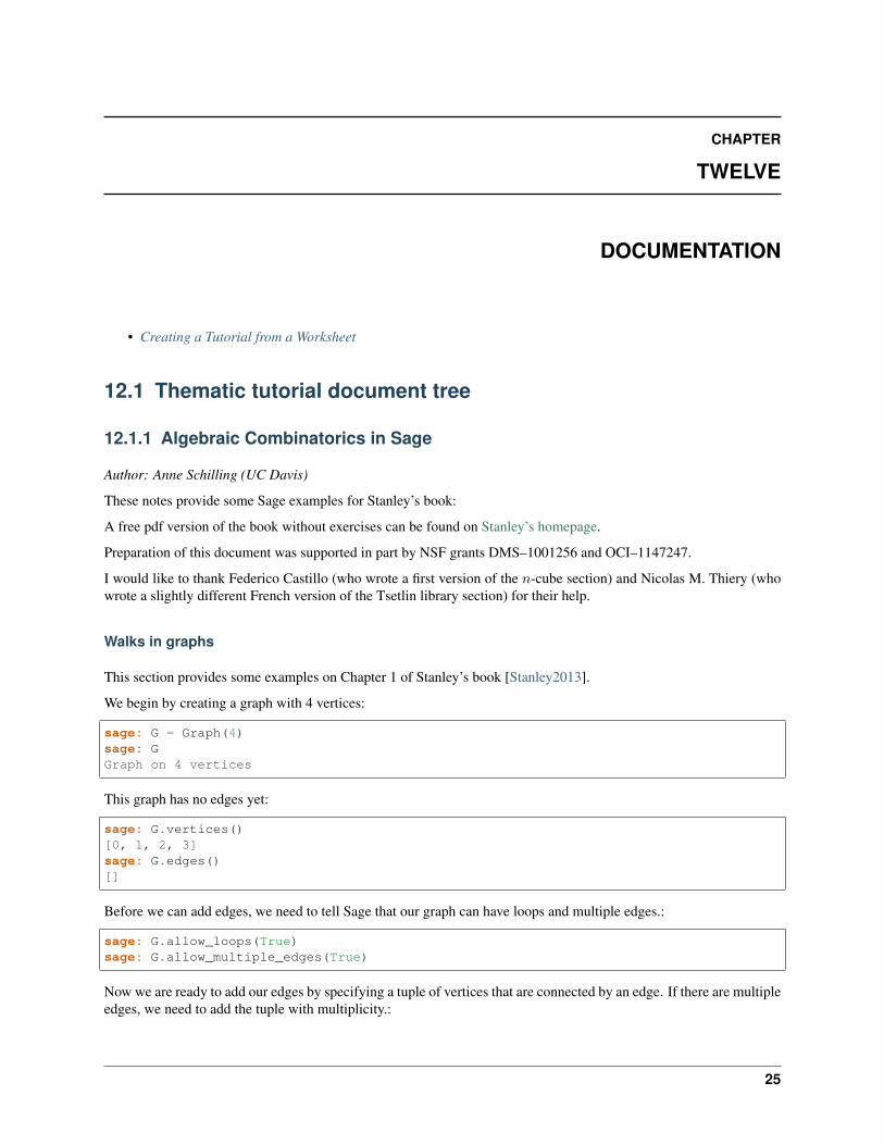
sage: G.add_edges([(0,0),(0,0),(0,1),(0,3),(1,3),(1,3)])
Now let us look at the graph!
sage: G.plot()Graphics object consisting of 11 graphics primitives
We can construct the adjacency matrix:
sage: A = G.adjacency_matrix()sage: A[2 1 0 1][1 0 0 2][0 0 0 0][1 2 0 0]
The entry in row 𝑖 and column 𝑗 of the ℓ-th power of 𝐴 gives us the number of paths of length ℓ from vertex 𝑖 to vertex𝑗. Let us verify this:
sage: A**2[6 4 0 4][4 5 0 1][0 0 0 0][4 1 0 5]
There are 4 paths of length 2 from vertex 0 to vertex 1: take either loop at 0 and then the edge (0, 1) (2 choices) ortake the edge (0, 3) and then either of the two edges (3, 1) (two choices):
sage: (A**2)[0,1]4
To count the number of closed walks, we can also look at the sum of the ℓ-th powers of the eigenvalues. Even thoughthe eigenvalues are not integers, we find that the sum of their squares is an integer:
sage: A.eigenvalues()[0, -2, 0.5857864376269049?, 3.414213562373095?]sage: sum(la**2 for la in A.eigenvalues())16.00000000000000?
We can achieve the same by looking at the trace of the ℓ-th power of the matrix:
sage: (A**2).trace()16
26 Chapter 12. Documentation
Thematic Tutorials, Release 9.1
𝑛-Cube
This section provides some examples on Chapter 2 of Stanley’s book [Stanley2013], which deals with 𝑛-cubes, theRadon transform, and combinatorial formulas for walks on the 𝑛-cube.
The vertices of the 𝑛-cube can be described by vectors in Z𝑛2 . First we define the addition of two vectors 𝑢, 𝑣 ∈ Z𝑛
2
via the following distance:
sage: def dist(u,v):....: h = [(u[i]+v[i])%2 for i in range(len(u))]....: return sum(h)
The distance function measures in how many slots two vectors in Z𝑛2 differ:
sage: u=(1,0,1,1,1,0)sage: v=(0,0,1,1,0,0)sage: dist(u,v)2
Now we are going to define the 𝑛-cube as the graph with vertices in Z𝑛2 and edges between vertex 𝑢 and vertex 𝑣 if
they differ in one slot, that is, the distance function is 1:
sage: def cube(n):....: G = Graph(2**n)....: vertices = Tuples([0,1],n)....: for i in range(2**n):....: for j in range(2**n):....: if dist(vertices[i],vertices[j]) == 1:....: G.add_edge(i,j)....: return G
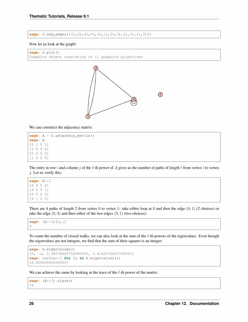
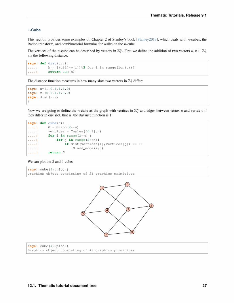
We can plot the 3 and 4-cube:
sage: cube(3).plot()Graphics object consisting of 21 graphics primitives
sage: cube(4).plot()Graphics object consisting of 49 graphics primitives
12.1. Thematic tutorial document tree 27
Thematic Tutorials, Release 9.1
Next we can experiment and check Corollary 2.4 in Stanley’s book, which states the 𝑛-cube has 𝑛 choose 𝑖 eigenvaluesequal to 𝑛− 2𝑖:
sage: G = cube(2)sage: G.adjacency_matrix().eigenvalues()[2, -2, 0, 0]
sage: G = cube(3)sage: G.adjacency_matrix().eigenvalues()[3, -3, 1, 1, 1, -1, -1, -1]
sage: G = cube(4)sage: G.adjacency_matrix().eigenvalues()[4, -4, 2, 2, 2, 2, -2, -2, -2, -2, 0, 0, 0, 0, 0, 0]
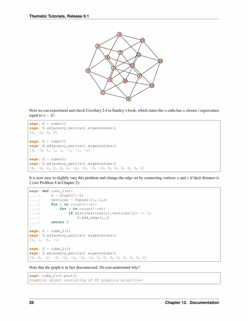
It is now easy to slightly vary this problem and change the edge set by connecting vertices 𝑢 and 𝑣 if their distance is2 (see Problem 4 in Chapter 2):
sage: def cube_2(n):....: G = Graph(2**n)....: vertices = Tuples([0,1],n)....: for i in range(2**n):....: for j in range(2**n):....: if dist(vertices[i],vertices[j]) == 2:....: G.add_edge(i,j)....: return G
sage: G = cube_2(2)sage: G.adjacency_matrix().eigenvalues()[1, 1, -1, -1]
sage: G = cube_2(4)sage: G.adjacency_matrix().eigenvalues()[6, 6, -2, -2, -2, -2, -2, -2, 0, 0, 0, 0, 0, 0, 0, 0]
Note that the graph is in fact disconnected. Do you understand why?
sage: cube_2(4).plot()Graphics object consisting of 65 graphics primitives
28 Chapter 12. Documentation
Thematic Tutorials, Release 9.1
The Tsetlin library
Introduction
In this section, we study a simple random walk (or Markov chain), called the Tsetlin library. It will give us theopportunity to see the interplay between combinatorics, linear algebra, representation theory and computer exploration,without requiring heavy theoretical background. I hope this encourages everyone to play around with this or similarsystems and investigate their properties! Formal theorems and proofs can be found in the references at the end of thissection.
It has been known for several years that the theory of group representations can facilitate the study of systems whoseevolution is random (Markov chains), breaking them down into simpler systems. More recently it was realized thatgeneralizing this (namely replacing the invertibility axiom for groups by other axioms) explains the behavior of otherparticularly simple Markov chains such as the Tsetlin library.
The Tsetlin library
Consider a bookshelf in a library containing 𝑛 distinct books. When a person borrows a book and then returns it, itgets placed back on the shelf to the right of all books. This is what we naturally do with our pile of shirts in the closet:after use and cleaning, the shirt is placed on the top of its pile. Hence the most popular books/shirts will more likelyappear on the right/top of the shelf/pile.
This type of organization has the advantage of being self-adaptive:
• The books most often used accumulate on the right and thus can easily be found.
• If the use changes over time, the system adapts.
In fact, this type of strategy is used not only in everyday life, but also in computer science. The natural questions thatarise are:
• Stationary distribution: To which state(s) does the system converge to? This, among other things, is used toevaluate the average access time to a book.
• The rate of convergence: How fast does the system adapt to a changing environment .
Let us formalize the description. The Tsetlin library is a discrete Markov chain (discrete time, discrete state space)described by:
• The state space Ω𝑛 is given by the set of all permutations of the 𝑛 books.
• The transition operators are denoted by 𝜕𝑖 : Ω𝑛 → Ω𝑛. When 𝜕𝑖 is applied to a permutation 𝜎, the number 𝑖 ismoved to the end of the permutation.
• We assign parameters 𝑥𝑖 ≥ 0 for all 1 ≤ 𝑖 ≤ 𝑛 with∑𝑛
𝑖=1 𝑥𝑖 = 1. The parameter 𝑥𝑖 indicates the probabilityof choosing the operator 𝜕𝑖.
12.1. Thematic tutorial document tree 29
Thematic Tutorials, Release 9.1
Transition graph and matrix
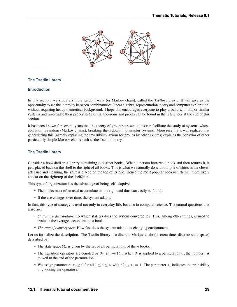
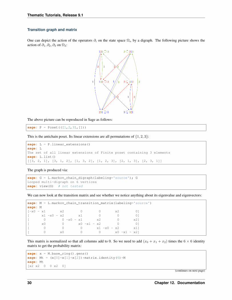
One can depict the action of the operators 𝜕𝑖 on the state space Ω𝑛 by a digraph. The following picture shows theaction of 𝜕1, 𝜕2, 𝜕3 on Ω3:
The above picture can be reproduced in Sage as follows:
sage: P = Poset(([1,2,3],[]))
This is the antichain poset. Its linear extensions are all permutations of 1, 2, 3:
sage: L = P.linear_extensions()sage: LThe set of all linear extensions of Finite poset containing 3 elementssage: L.list()[[3, 2, 1], [3, 1, 2], [1, 3, 2], [1, 2, 3], [2, 1, 3], [2, 3, 1]]
The graph is produced via:
sage: G = L.markov_chain_digraph(labeling='source'); GLooped multi-digraph on 6 verticessage: view(G) # not tested
We can now look at the transition matrix and see whether we notice anything about its eigenvalue and eigenvectors:
sage: M = L.markov_chain_transition_matrix(labeling='source')sage: M[-x0 - x1 x2 0 0 x2 0][ x1 -x0 - x2 x1 0 0 0][ 0 0 -x0 - x1 x2 0 x2][ x0 0 x0 -x1 - x2 0 0][ 0 0 0 x1 -x0 - x2 x1][ 0 x0 0 0 x0 -x1 - x2]
This matrix is normalized so that all columns add to 0. So we need to add (𝑥0 + 𝑥1 + 𝑥2) times the 6 × 6 identitymatrix to get the probability matrix:
sage: x = M.base_ring().gens()sage: Mt = (x[0]+x[1]+x[2])*matrix.identity(6)+Msage: Mt[x2 x2 0 0 x2 0]
(continues on next page)
30 Chapter 12. Documentation
Thematic Tutorials, Release 9.1
(continued from previous page)
[x1 x1 x1 0 0 0][ 0 0 x2 x2 0 x2][x0 0 x0 x0 0 0][ 0 0 0 x1 x1 x1][ 0 x0 0 0 x0 x0]
Since the 𝑥𝑖 are formal variables, we need to compute the eigenvalues and eigenvectors in the symbolic ring SR:
sage: Mt.change_ring(SR).eigenvalues()[x2, x1, x0, x0 + x1 + x2, 0, 0]
Do you see any pattern? In fact, if you start playing with bigger values of 𝑛 (the size of the underlying permutations),you might observe that there is an eigenvalue for every subset 𝑆 of 1, 2, . . . , 𝑛 and the multiplicity is given by aderangement number 𝑑𝑛−|𝑆|. Derangment numbers count permutations without fixed point. For the eigenvectors weobtain:
sage: Mt.change_ring(SR).eigenvectors_right()[(x2, [(1, 0, -1, 0, 0, 0)], 1),(x1, [(0, 1, 0, 0, -1, 0)], 1),(x0, [(0, 0, 0, 1, 0, -1)], 1),(x0 + x1 + x2,[(1,(x0 + x1)/(x0 + x2),x0/x1,(x0^2 + x0*x1)/(x1^2 + x1*x2),(x0^2 + x0*x1)/(x0*x2 + x2^2),(x0^2 + x0*x1)/(x1*x2 + x2^2))], 1),
(0, [(1, 0, -1, 0, -1, 1), (0, 1, -1, 1, -1, 0)], 2)]
The stationary distribution is the eigenvector of eigenvalues 1 = 𝑥0 + 𝑥1 + 𝑥2. Do you see a pattern?
Optional exercices: Study of the transition operators and graph
Instead of using the methods that are already in Sage, try to build the state space Ω𝑛 and the transition operators 𝜕𝑖yourself as follows.
1. For technical reasons, it is most practical in Sage to label the 𝑛 books in the library by 0, 1, · · · , 𝑛− 1, and torepresent each state in the Markov chain by a permutation of the set 0, . . . , 𝑛− 1 as a tuple. Construct thestate space Ω𝑛 as:
sage: list(map(tuple, Permutations(range(3))))[(0, 1, 2), (0, 2, 1), (1, 0, 2), (1, 2, 0), (2, 0, 1), (2, 1, 0)]
2. Write a function transition_operator(sigma, i) which implements the operator 𝜕𝑖 which takesas input a tuple sigma and integer 𝑖 ∈ 1, 2, . . . , 𝑛 and outputs a new tuple. It might be useful to extractsubtuples (sigma[i:j]) and concatentation.
3. Write a function tsetlin_digraph(n) which constructs the (multi digraph) as described as shownabove. This can be achieved using DiGraph.
4. Verify for which values of 𝑛 the digraph is strongly connected (i.e., you can go from any vertex to any othervertex by going in the direction of the arrow). This indicates whether the Markov chain is irreducible.
12.1. Thematic tutorial document tree 31
Thematic Tutorials, Release 9.1
Conclusion
The Tsetlin library was studied from the viewpoint of monoids in [Bidigare1997] and [Brown2000]. Precise statementsof the eigenvalues and the stationary distribution of the probability matrix as well as proofs of the statements are givenin these papers. Generalizations of the Tsetlin library from the antichain to arbitrary posets was given in [AKS2013].
Young’s lattice and the RSK algorithm
This section provides some examples on Young’s lattice and the RSK (Robinson-Schensted-Knuth) algorithm ex-plained in Chapter 8 of Stanley’s book [Stanley2013].
Young’s Lattice
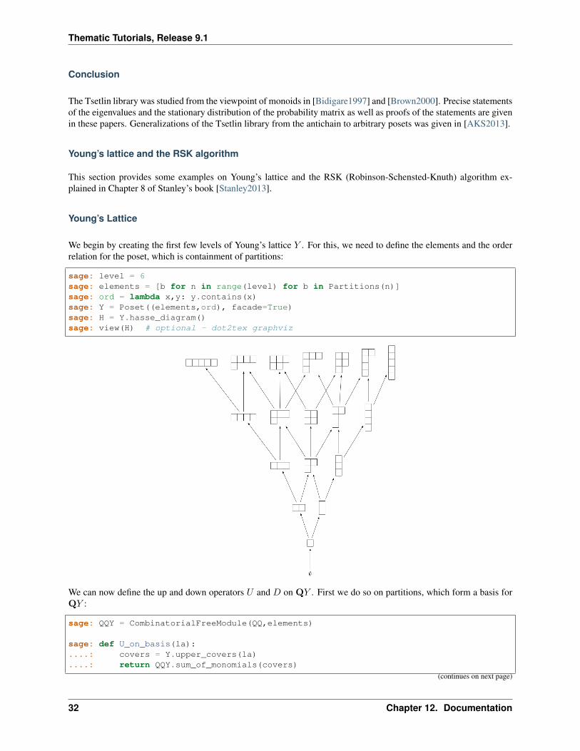
We begin by creating the first few levels of Young’s lattice 𝑌 . For this, we need to define the elements and the orderrelation for the poset, which is containment of partitions:
sage: level = 6sage: elements = [b for n in range(level) for b in Partitions(n)]sage: ord = lambda x,y: y.contains(x)sage: Y = Poset((elements,ord), facade=True)sage: H = Y.hasse_diagram()sage: view(H) # optional - dot2tex graphviz
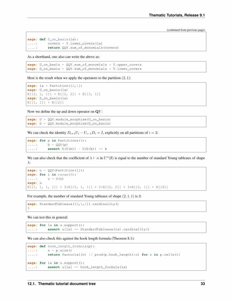
We can now define the up and down operators 𝑈 and 𝐷 on Q𝑌 . First we do so on partitions, which form a basis forQ𝑌 :
sage: QQY = CombinatorialFreeModule(QQ,elements)
sage: def U_on_basis(la):....: covers = Y.upper_covers(la)....: return QQY.sum_of_monomials(covers)
(continues on next page)
32 Chapter 12. Documentation
Thematic Tutorials, Release 9.1
(continued from previous page)
sage: def D_on_basis(la):....: covers = Y.lower_covers(la)....: return QQY.sum_of_monomials(covers)
As a shorthand, one also can write the above as:
sage: U_on_basis = QQY.sum_of_monomials * Y.upper_coverssage: D_on_basis = QQY.sum_of_monomials * Y.lower_covers
Here is the result when we apply the operators to the partition (2, 1):
sage: la = Partition([2,1])sage: U_on_basis(la)B[[2, 1, 1]] + B[[2, 2]] + B[[3, 1]]sage: D_on_basis(la)B[[1, 1]] + B[[2]]
Now we define the up and down operator on Q𝑌 :
sage: U = QQY.module_morphism(U_on_basis)sage: D = QQY.module_morphism(D_on_basis)
We can check the identity 𝐷𝑖+1𝑈𝑖 − 𝑈𝑖−1𝐷𝑖 = 𝐼𝑖 explicitly on all partitions of 𝑖 = 3:
sage: for p in Partitions(3):....: b = QQY(p)....: assert D(U(b)) - U(D(b)) == b
We can also check that the coefficient of 𝜆 ⊢ 𝑛 in 𝑈𝑛(∅) is equal to the number of standard Young tableaux of shape𝜆:
sage: u = QQY(Partition([]))sage: for i in range(4):....: u = U(u)sage: uB[[1, 1, 1, 1]] + 3*B[[2, 1, 1]] + 2*B[[2, 2]] + 3*B[[3, 1]] + B[[4]]
For example, the number of standard Young tableaux of shape (2, 1, 1) is 3:
sage: StandardTableaux([2,1,1]).cardinality()3
We can test this in general:
sage: for la in u.support():....: assert u[la] == StandardTableaux(la).cardinality()
We can also check this against the hook length formula (Theorem 8.1):
sage: def hook_length_formula(p):....: n = p.size()....: return factorial(n) // prod(p.hook_length(*c) for c in p.cells())
sage: for la in u.support():....: assert u[la] == hook_length_formula(la)
12.1. Thematic tutorial document tree 33
Thematic Tutorials, Release 9.1
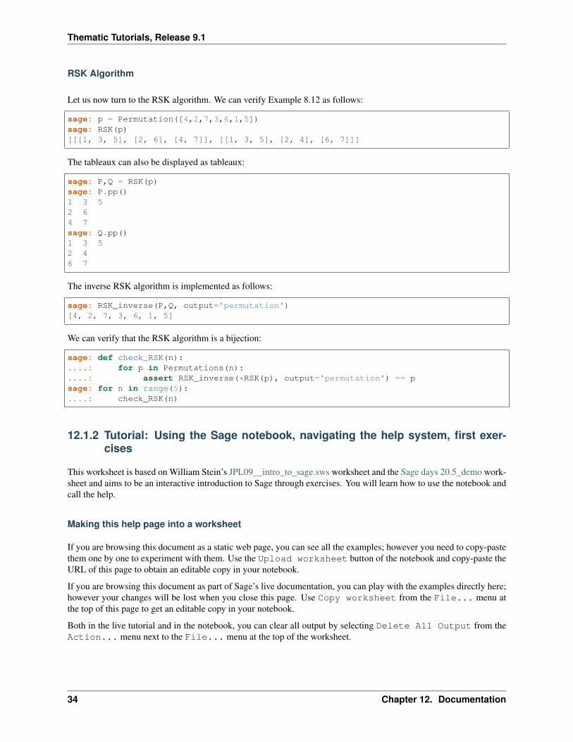
RSK Algorithm
Let us now turn to the RSK algorithm. We can verify Example 8.12 as follows:
sage: p = Permutation([4,2,7,3,6,1,5])sage: RSK(p)[[[1, 3, 5], [2, 6], [4, 7]], [[1, 3, 5], [2, 4], [6, 7]]]
The tableaux can also be displayed as tableaux:
sage: P,Q = RSK(p)sage: P.pp()1 3 52 64 7sage: Q.pp()1 3 52 46 7
The inverse RSK algorithm is implemented as follows:
sage: RSK_inverse(P,Q, output='permutation')[4, 2, 7, 3, 6, 1, 5]
We can verify that the RSK algorithm is a bijection:
sage: def check_RSK(n):....: for p in Permutations(n):....: assert RSK_inverse(*RSK(p), output='permutation') == psage: for n in range(5):....: check_RSK(n)
12.1.2 Tutorial: Using the Sage notebook, navigating the help system, first exer-cises
This worksheet is based on William Stein’s JPL09__intro_to_sage.sws worksheet and the Sage days 20.5_demo work-sheet and aims to be an interactive introduction to Sage through exercises. You will learn how to use the notebook andcall the help.
Making this help page into a worksheet
If you are browsing this document as a static web page, you can see all the examples; however you need to copy-pastethem one by one to experiment with them. Use the Upload worksheet button of the notebook and copy-paste theURL of this page to obtain an editable copy in your notebook.
If you are browsing this document as part of Sage’s live documentation, you can play with the examples directly here;however your changes will be lost when you close this page. Use Copy worksheet from the File... menu atthe top of this page to get an editable copy in your notebook.
Both in the live tutorial and in the notebook, you can clear all output by selecting Delete All Output from theAction... menu next to the File... menu at the top of the worksheet.
34 Chapter 12. Documentation
Thematic Tutorials, Release 9.1
Entering, Editing and Evaluating Input
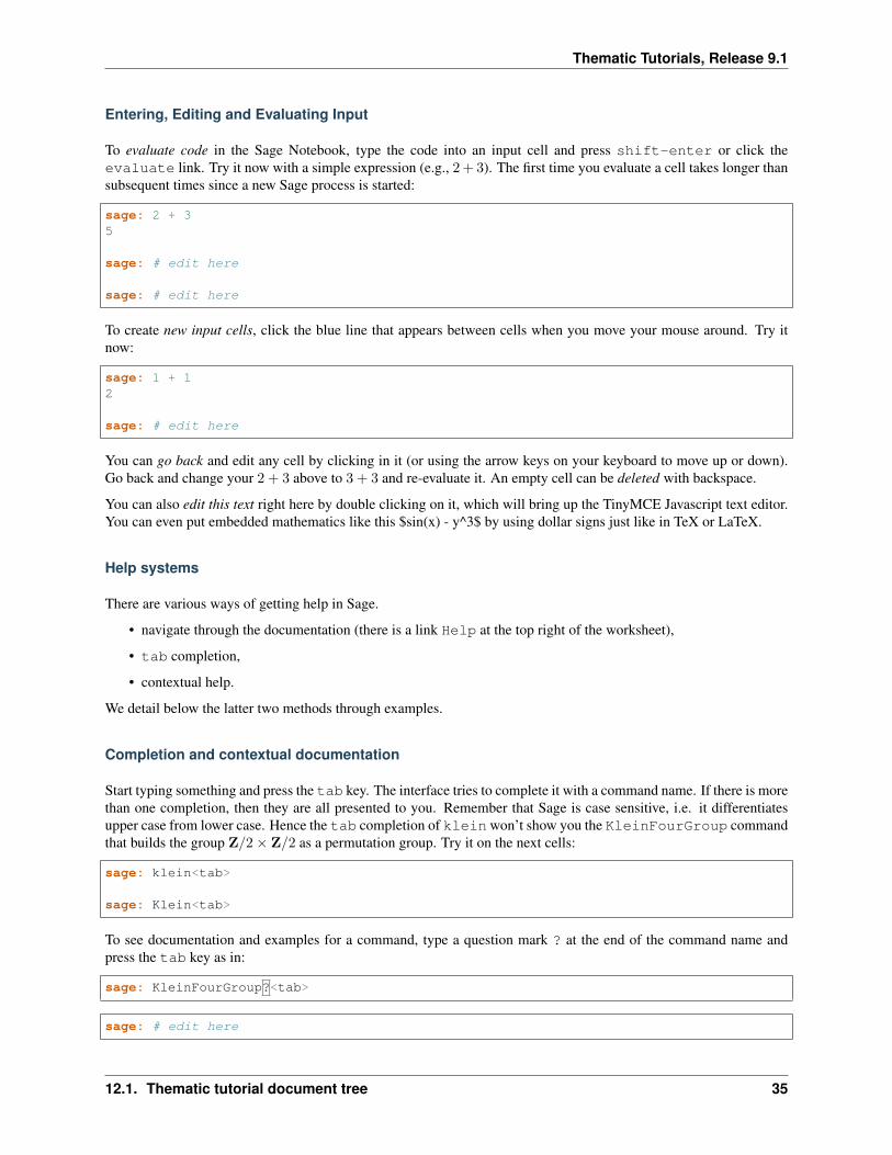
To evaluate code in the Sage Notebook, type the code into an input cell and press shift-enter or click theevaluate link. Try it now with a simple expression (e.g., 2 + 3). The first time you evaluate a cell takes longer thansubsequent times since a new Sage process is started:
sage: 2 + 35
sage: # edit here
sage: # edit here
To create new input cells, click the blue line that appears between cells when you move your mouse around. Try itnow:
sage: 1 + 12
sage: # edit here
You can go back and edit any cell by clicking in it (or using the arrow keys on your keyboard to move up or down).Go back and change your 2 + 3 above to 3 + 3 and re-evaluate it. An empty cell can be deleted with backspace.
You can also edit this text right here by double clicking on it, which will bring up the TinyMCE Javascript text editor.You can even put embedded mathematics like this $sin(x) - y^3$ by using dollar signs just like in TeX or LaTeX.
Help systems
There are various ways of getting help in Sage.
• navigate through the documentation (there is a link Help at the top right of the worksheet),
• tab completion,
• contextual help.
We detail below the latter two methods through examples.
Completion and contextual documentation
Start typing something and press the tab key. The interface tries to complete it with a command name. If there is morethan one completion, then they are all presented to you. Remember that Sage is case sensitive, i.e. it differentiatesupper case from lower case. Hence the tab completion of kleinwon’t show you the KleinFourGroup commandthat builds the group Z/2× Z/2 as a permutation group. Try it on the next cells:
sage: klein<tab>
sage: Klein<tab>
To see documentation and examples for a command, type a question mark ? at the end of the command name andpress the tab key as in:
sage: KleinFourGroup?<tab>
sage: # edit here
12.1. Thematic tutorial document tree 35
Thematic Tutorials, Release 9.1
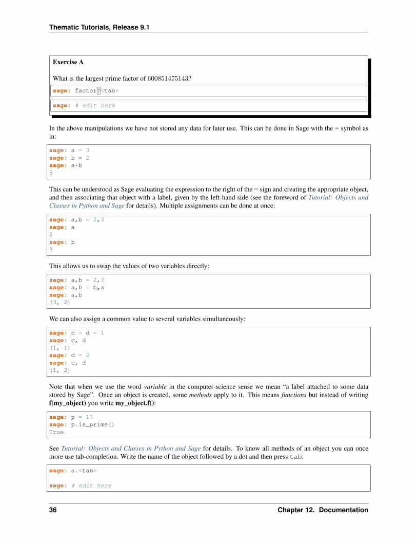
Exercise A
What is the largest prime factor of 600851475143?
sage: factor?<tab>
sage: # edit here
In the above manipulations we have not stored any data for later use. This can be done in Sage with the = symbol asin:
sage: a = 3sage: b = 2sage: a+b5
This can be understood as Sage evaluating the expression to the right of the = sign and creating the appropriate object,and then associating that object with a label, given by the left-hand side (see the foreword of Tutorial: Objects andClasses in Python and Sage for details). Multiple assignments can be done at once:
sage: a,b = 2,3sage: a2sage: b3
This allows us to swap the values of two variables directly:
sage: a,b = 2,3sage: a,b = b,asage: a,b(3, 2)
We can also assign a common value to several variables simultaneously:
sage: c = d = 1sage: c, d(1, 1)sage: d = 2sage: c, d(1, 2)
Note that when we use the word variable in the computer-science sense we mean “a label attached to some datastored by Sage”. Once an object is created, some methods apply to it. This means functions but instead of writingf(my_object) you write my_object.f():
sage: p = 17sage: p.is_prime()True
See Tutorial: Objects and Classes in Python and Sage for details. To know all methods of an object you can oncemore use tab-completion. Write the name of the object followed by a dot and then press tab:
sage: a.<tab>
sage: # edit here
36 Chapter 12. Documentation
Thematic Tutorials, Release 9.1
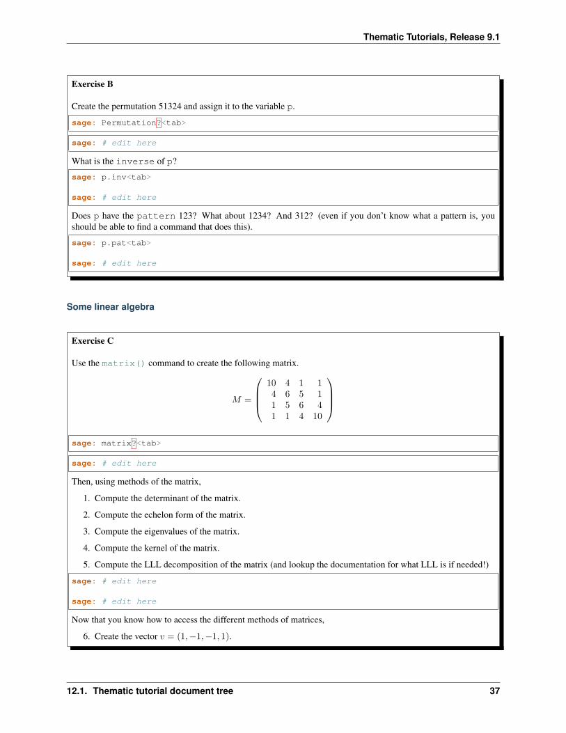
Exercise B
Create the permutation 51324 and assign it to the variable p.
sage: Permutation?<tab>
sage: # edit here
What is the inverse of p?
sage: p.inv<tab>
sage: # edit here
Does p have the pattern 123? What about 1234? And 312? (even if you don’t know what a pattern is, youshould be able to find a command that does this).
sage: p.pat<tab>
sage: # edit here
Some linear algebra
Exercise C
Use the matrix() command to create the following matrix.
𝑀 =
⎛⎜⎜⎝10 4 1 14 6 5 11 5 6 41 1 4 10
⎞⎟⎟⎠sage: matrix?<tab>
sage: # edit here
Then, using methods of the matrix,
1. Compute the determinant of the matrix.
2. Compute the echelon form of the matrix.
3. Compute the eigenvalues of the matrix.
4. Compute the kernel of the matrix.
5. Compute the LLL decomposition of the matrix (and lookup the documentation for what LLL is if needed!)
sage: # edit here
sage: # edit here
Now that you know how to access the different methods of matrices,
6. Create the vector 𝑣 = (1,−1,−1, 1).
12.1. Thematic tutorial document tree 37
Thematic Tutorials, Release 9.1
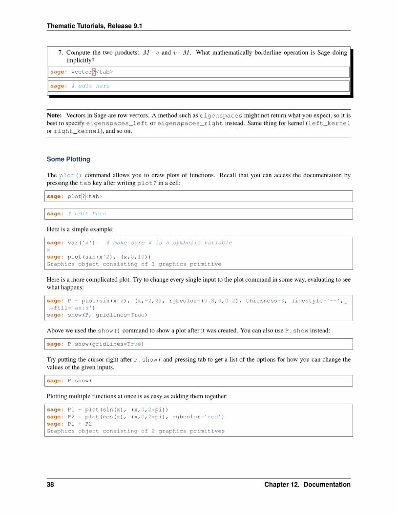
7. Compute the two products: 𝑀 · 𝑣 and 𝑣 · 𝑀 . What mathematically borderline operation is Sage doingimplicitly?
sage: vector?<tab>
sage: # edit here
Note: Vectors in Sage are row vectors. A method such as eigenspaces might not return what you expect, so it isbest to specify eigenspaces_left or eigenspaces_right instead. Same thing for kernel (left_kernelor right_kernel), and so on.
Some Plotting
The plot() command allows you to draw plots of functions. Recall that you can access the documentation bypressing the tab key after writing plot? in a cell:
sage: plot?<tab>
sage: # edit here
Here is a simple example:
sage: var('x') # make sure x is a symbolic variablexsage: plot(sin(x^2), (x,0,10))Graphics object consisting of 1 graphics primitive
Here is a more complicated plot. Try to change every single input to the plot command in some way, evaluating to seewhat happens:
sage: P = plot(sin(x^2), (x,-2,2), rgbcolor=(0.8,0,0.2), thickness=3, linestyle='--',→˓fill='axis')sage: show(P, gridlines=True)
Above we used the show() command to show a plot after it was created. You can also use P.show instead:
sage: P.show(gridlines=True)
Try putting the cursor right after P.show( and pressing tab to get a list of the options for how you can change thevalues of the given inputs.
sage: P.show(
Plotting multiple functions at once is as easy as adding them together:
sage: P1 = plot(sin(x), (x,0,2*pi))sage: P2 = plot(cos(x), (x,0,2*pi), rgbcolor='red')sage: P1 + P2Graphics object consisting of 2 graphics primitives
38 Chapter 12. Documentation
Thematic Tutorials, Release 9.1
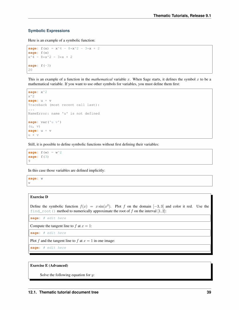
Symbolic Expressions
Here is an example of a symbolic function:
sage: f(x) = x^4 - 8*x^2 - 3*x + 2sage: f(x)x^4 - 8*x^2 - 3*x + 2
sage: f(-3)20
This is an example of a function in the mathematical variable 𝑥. When Sage starts, it defines the symbol 𝑥 to be amathematical variable. If you want to use other symbols for variables, you must define them first:
sage: x^2x^2sage: u + vTraceback (most recent call last):...NameError: name 'u' is not defined
sage: var('u v')(u, v)sage: u + vu + v
Still, it is possible to define symbolic functions without first defining their variables:
sage: f(w) = w^2sage: f(3)9
In this case those variables are defined implicitly:
sage: ww
Exercise D
Define the symbolic function 𝑓(𝑥) = 𝑥 sin(𝑥2). Plot 𝑓 on the domain [−3, 3] and color it red. Use thefind_root() method to numerically approximate the root of 𝑓 on the interval [1, 2]:
sage: # edit here
Compute the tangent line to 𝑓 at 𝑥 = 1:
sage: # edit here
Plot 𝑓 and the tangent line to 𝑓 at 𝑥 = 1 in one image:
sage: # edit here
Exercise E (Advanced)
Solve the following equation for 𝑦:
12.1. Thematic tutorial document tree 39
Thematic Tutorials, Release 9.1
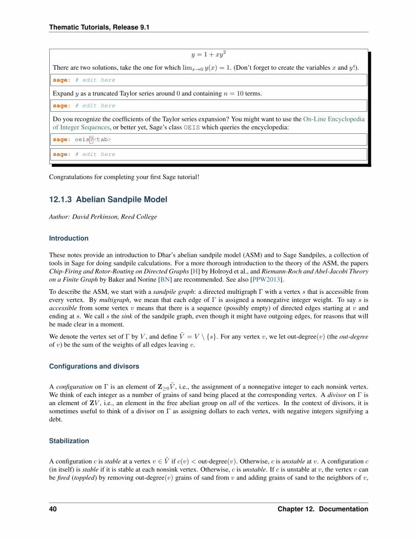
𝑦 = 1 + 𝑥𝑦2
There are two solutions, take the one for which lim𝑥→0 𝑦(𝑥) = 1. (Don’t forget to create the variables 𝑥 and 𝑦!).
sage: # edit here
Expand 𝑦 as a truncated Taylor series around 0 and containing 𝑛 = 10 terms.
sage: # edit here
Do you recognize the coefficients of the Taylor series expansion? You might want to use the On-Line Encyclopediaof Integer Sequences, or better yet, Sage’s class OEIS which queries the encyclopedia:
sage: oeis?<tab>
sage: # edit here
Congratulations for completing your first Sage tutorial!
12.1.3 Abelian Sandpile Model
Author: David Perkinson, Reed College
Introduction
These notes provide an introduction to Dhar’s abelian sandpile model (ASM) and to Sage Sandpiles, a collection oftools in Sage for doing sandpile calculations. For a more thorough introduction to the theory of the ASM, the papersChip-Firing and Rotor-Routing on Directed Graphs [H] by Holroyd et al., and Riemann-Roch and Abel-Jacobi Theoryon a Finite Graph by Baker and Norine [BN] are recommended. See also [PPW2013].
To describe the ASM, we start with a sandpile graph: a directed multigraph Γ with a vertex 𝑠 that is accessible fromevery vertex. By multigraph, we mean that each edge of Γ is assigned a nonnegative integer weight. To say 𝑠 isaccessible from some vertex 𝑣 means that there is a sequence (possibly empty) of directed edges starting at 𝑣 andending at 𝑠. We call 𝑠 the sink of the sandpile graph, even though it might have outgoing edges, for reasons that willbe made clear in a moment.
We denote the vertex set of Γ by 𝑉 , and define 𝑉 = 𝑉 ∖ 𝑠. For any vertex 𝑣, we let out-degree(𝑣) (the out-degreeof 𝑣) be the sum of the weights of all edges leaving 𝑣.
Configurations and divisors
A configuration on Γ is an element of Z≥0𝑉 , i.e., the assignment of a nonnegative integer to each nonsink vertex.We think of each integer as a number of grains of sand being placed at the corresponding vertex. A divisor on Γ isan element of Z𝑉 , i.e., an element in the free abelian group on all of the vertices. In the context of divisors, it issometimes useful to think of a divisor on Γ as assigning dollars to each vertex, with negative integers signifying adebt.
Stabilization
A configuration 𝑐 is stable at a vertex 𝑣 ∈ 𝑉 if 𝑐(𝑣) < out-degree(𝑣). Otherwise, 𝑐 is unstable at 𝑣. A configuration 𝑐(in itself) is stable if it is stable at each nonsink vertex. Otherwise, 𝑐 is unstable. If 𝑐 is unstable at 𝑣, the vertex 𝑣 canbe fired (toppled) by removing out-degree(𝑣) grains of sand from 𝑣 and adding grains of sand to the neighbors of 𝑣,
40 Chapter 12. Documentation
Thematic Tutorials, Release 9.1
determined by the weights of the edges leaving 𝑣 (each vertex 𝑤 gets as many grains as the weight of the edge (𝑣, 𝑤)is, if there is such an edge). Note that grains that are added to the sink 𝑠 are not counted (i.e., they “disappear”).
Despite our best intentions, we sometimes consider firing a stable vertex, resulting in a “configuration” with a negativeamount of sand at that vertex. We may also reverse-fire a vertex, absorbing sand from the vertex’s neighbors (includingthe sink).
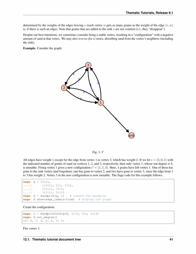
Example. Consider the graph:
Fig. 1: Γ
All edges have weight 1 except for the edge from vertex 1 to vertex 3, which has weight 2. If we let 𝑐 = (5, 0, 1) withthe indicated number of grains of sand on vertices 1, 2, and 3, respectively, then only vertex 1, whose out-degree is 4,is unstable. Firing vertex 1 gives a new configuration 𝑐′ = (1, 1, 3). Here, 4 grains have left vertex 1. One of these hasgone to the sink vertex (and forgotten), one has gone to vertex 2, and two have gone to vertex 3, since the edge from 1to 3 has weight 2. Vertex 3 in the new configuration is now unstable. The Sage code for this example follows.
sage: g = 0:,....: 1:0:1, 2:1, 3:2,....: 2:1:1, 3:1,....: 3:1:1, 2:1sage: S = Sandpile(g, 0) # create the sandpilesage: S.show(edge_labels=true) # display the graph
Create the configuration:
sage: c = SandpileConfig(S, 1:5, 2:0, 3:1)sage: S.out_degree()0: 0, 1: 4, 2: 2, 3: 2
Fire vertex 1:
12.1. Thematic tutorial document tree 41
Thematic Tutorials, Release 9.1
sage: c.fire_vertex(1)1: 1, 2: 1, 3: 3
The configuration is unchanged:
sage: c1: 5, 2: 0, 3: 1
Repeatedly fire vertices until the configuration becomes stable:
sage: c.stabilize()1: 2, 2: 1, 3: 1
Alternatives:
sage: ~c # shorthand for c.stabilize()1: 2, 2: 1, 3: 1sage: c.stabilize(with_firing_vector=true)[1: 2, 2: 1, 3: 1, 1: 2, 2: 2, 3: 3]
Since vertex 3 has become unstable after firing vertex 1, it can be fired, which causes vertex 2 to become unstable,etc. Repeated firings eventually lead to a stable configuration. The last line of the Sage code, above, is a list, the firstelement of which is the resulting stable configuration, (2, 1, 1). The second component records how many times eachvertex fired in the stabilization.
Since the sink is accessible from each nonsink vertex and never fires, every configuration will stabilize after a finitenumber of vertex-firings. It is not obvious, but the resulting stabilization is independent of the order in which unstablevertices are fired. Thus, each configuration stabilizes to a unique stable configuration.
Laplacian
Fix a total order on the vertices of Γ, thus leading to a labelling of the vertices by the numbers 1, 2, . . . , 𝑛 for some 𝑛(in the given order). The Laplacian of Γ is
𝐿 := 𝐷 −𝐴
where 𝐷 is the diagonal matrix of out-degrees of the vertices (i.e., the diagonal 𝑛 × 𝑛-matrix whose (𝑖, 𝑖)-th entry isthe out-degree of the vertex 𝑖) and𝐴 is the adjacency matrix whose (𝑖, 𝑗)-th entry is the weight of the edge from vertex𝑖 to vertex 𝑗, which we take to be 0 if there is no edge. The reduced Laplacian, , is the submatrix of the Laplacianformed by removing the row and column corresponding to the sink vertex. Firing a vertex of a configuration is thesame as subtracting the corresponding row of the reduced Laplacian.
Example. (Continued.)
sage: S.vertices() # the ordering of the vertices[0, 1, 2, 3]sage: S.laplacian()[ 0 0 0 0][-1 4 -1 -2][ 0 -1 2 -1][ 0 -1 -1 2]sage: S.reduced_laplacian()[ 4 -1 -2][-1 2 -1][-1 -1 2]
42 Chapter 12. Documentation
Thematic Tutorials, Release 9.1
The configuration we considered previously:
sage: c = SandpileConfig(S, [5,0,1])sage: c1: 5, 2: 0, 3: 1
Firing vertex 1 is the same as subtracting the corresponding row of the reduced Laplacian from the configuration(regarded as a vector):
sage: c.fire_vertex(1).values()[1, 1, 3]sage: S.reduced_laplacian()[0](4, -1, -2)sage: vector([5,0,1]) - vector([4,-1,-2])(1, 1, 3)
Recurrent elements
Imagine an experiment in which grains of sand are dropped one-at-a-time onto a graph, pausing to allow the con-figuration to stabilize between drops. Some configurations will only be seen once in this process. For example, formost graphs, once sand is dropped on the graph, no sequence of additions of sand and stabilizations will result in agraph empty of sand. Other configurations—the so-called recurrent configurations—will be seen infinitely often asthe process is repeated indefinitely.
To be precise, a configuration 𝑐 is recurrent if (i) it is stable, and (ii) given any configuration 𝑎, there is a configuration𝑏 such that 𝑐 = stab(𝑎+ 𝑏), the stabilization of 𝑎+ 𝑏.
The maximal-stable configuration, denoted 𝑐max, is defined by 𝑐max(𝑣) = out-degree(𝑣) − 1 for all nonsink vertices𝑣. It is clear that 𝑐max is recurrent. Further, it is not hard to see that a configuration is recurrent if and only if it has theform stab(𝑎+ 𝑐max) for some configuration 𝑎.
Example. (Continued.)
sage: S.recurrents(verbose=false)[[3, 1, 1], [2, 1, 1], [3, 1, 0]]sage: c = SandpileConfig(S, [2,1,1])sage: c1: 2, 2: 1, 3: 1sage: c.is_recurrent()Truesage: S.max_stable()1: 3, 2: 1, 3: 1
Adding any configuration to the max-stable configuration and stabilizing yields a recurrent configuration:
sage: x = SandpileConfig(S, [1,0,0])sage: x + S.max_stable()1: 4, 2: 1, 3: 1
Use & to add and stabilize:
sage: c = x & S.max_stable()sage: c1: 3, 2: 1, 3: 0sage: c.is_recurrent()True
12.1. Thematic tutorial document tree 43
Thematic Tutorials, Release 9.1
Note the various ways of performing addition and stabilization:
sage: m = S.max_stable()sage: (x + m).stabilize() == ~(x + m)Truesage: (x + m).stabilize() == x & mTrue
Burning Configuration
A burning configuration is a Z≥0-linear combination 𝑓 of the rows of the reduced Laplacian matrix having nonnegativeentries and such that every vertex is accessible from some vertex in the support of 𝑓 (in other words, for each vertex 𝑤,there is a path from some 𝑣 ∈ supp 𝑓 to 𝑤). The corresponding burning script gives the coefficients in the Z≥0-linearcombination needed to obtain the burning configuration. So if 𝑏 is a burning configuration, 𝜎 is its script, and is thereduced Laplacian, then 𝜎 = 𝑏. The minimal burning configuration is the one with the minimal script (each of itscomponents is no larger than the corresponding component of any other script for a burning configuration).
Given a burning configuration 𝑏 having script 𝜎, and any configuration 𝑐 on the same graph, the following are equiva-lent:
• 𝑐 is recurrent;
• 𝑐+ 𝑏 stabilizes to 𝑐;
• the firing vector for the stabilization of 𝑐+ 𝑏 is 𝜎.
The burning configuration and script are computed using a modified version of Speer’s script algorithm. This is ageneralization to directed multigraphs of Dhar’s burning algorithm.
Example.
sage: g = 0:,1:0:1,3:1,4:1,2:0:1,3:1,5:1,....: 3:2:1,5:1,4:1:1,3:1,5:2:1,3:1sage: G = Sandpile(g,0)sage: G.burning_config()1: 2, 2: 0, 3: 1, 4: 1, 5: 0sage: G.burning_config().values()[2, 0, 1, 1, 0]sage: G.burning_script()1: 1, 2: 3, 3: 5, 4: 1, 5: 4sage: G.burning_script().values()[1, 3, 5, 1, 4]sage: matrix(G.burning_script().values())*G.reduced_laplacian()[2 0 1 1 0]
Sandpile group
The collection of stable configurations forms a commutative monoid with addition defined as ordinary addition fol-lowed by stabilization. The identity element is the all-zero configuration. This monoid is a group exactly when theunderlying graph is a DAG (directed acyclic graph).
The recurrent elements form a submonoid which turns out to be a group. This group is called the sandpile group for Γ,denoted 𝒮(Γ). Its identity element is usually not the all-zero configuration (again, only in the case that Γ is a DAG).So finding the identity element is an interesting problem.
44 Chapter 12. Documentation
Thematic Tutorials, Release 9.1
Let 𝑛 = |𝑉 | − 1 and fix an ordering of the nonsink vertices. Let ℒ ⊂ Z𝑛 denote the column-span of 𝑡, the transposeof the reduced Laplacian. It is a theorem that
𝒮(Γ) ≈ Z𝑛/ℒ.
Thus, the number of elements of the sandpile group is det , which by the matrix-tree theorem is the number ofweighted trees directed into the sink.
Example. (Continued.)
sage: S.group_order()3sage: S.invariant_factors()[1, 1, 3]sage: S.reduced_laplacian().dense_matrix().smith_form()([1 0 0] [ 0 0 1] [3 1 4][0 1 0] [ 1 0 0] [4 1 6][0 0 3], [ 0 1 -1], [4 1 5])
Adding the identity to any recurrent configuration and stabilizing yields the same recurrent configuration:
sage: S.identity()1: 3, 2: 1, 3: 0sage: i = S.identity()sage: m = S.max_stable()sage: i & m == mTrue
Self-organized criticality
The sandpile model was introduced by Bak, Tang, and Wiesenfeld in the paper, Self-organized criticality: an expla-nation of 1/ƒ noise [BTW]. The term self-organized criticality has no precise definition, but can be loosely taken todescribe a system that naturally evolves to a state that is barely stable and such that the instabilities are described by apower law. In practice, self-organized criticality is often taken to mean like the sandpile model on a grid graph. Thegrid graph is just a grid with an extra sink vertex. The vertices on the interior of each side have one edge to the sink,and the corner vertices have an edge of weight 2. Thus, every nonsink vertex has out-degree 4.
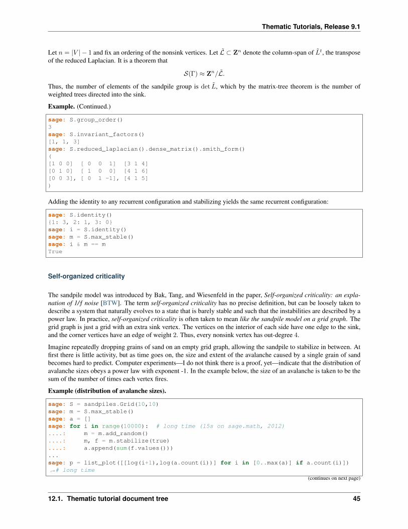
Imagine repeatedly dropping grains of sand on an empty grid graph, allowing the sandpile to stabilize in between. Atfirst there is little activity, but as time goes on, the size and extent of the avalanche caused by a single grain of sandbecomes hard to predict. Computer experiments—I do not think there is a proof, yet—indicate that the distribution ofavalanche sizes obeys a power law with exponent -1. In the example below, the size of an avalanche is taken to be thesum of the number of times each vertex fires.
Example (distribution of avalanche sizes).
sage: S = sandpiles.Grid(10,10)sage: m = S.max_stable()sage: a = []sage: for i in range(10000): # long time (15s on sage.math, 2012)....: m = m.add_random()....: m, f = m.stabilize(true)....: a.append(sum(f.values()))...sage: p = list_plot([[log(i+1),log(a.count(i))] for i in [0..max(a)] if a.count(i)])→˓# long time
(continues on next page)
12.1. Thematic tutorial document tree 45
Thematic Tutorials, Release 9.1
(continued from previous page)
sage: p.axes_labels(['log(N)','log(D(N))']) # long timesage: p # long timeGraphics object consisting of 1 graphics primitive
Fig. 2: Distribution of avalanche sizes
Note: In the above code, m.stabilize(true) returns a list consisting of the stabilized configuration and the firingvector. (Omitting true would give just the stabilized configuration.)
Divisors and Discrete Riemann surfaces
A reference for this section is Riemann-Roch and Abel-Jacobi theory on a finite graph [BN].
A divisor on Γ is an element of the free abelian group on its vertices, including the sink. Suppose, as above, that the𝑛 + 1 vertices of Γ have been ordered, and that ℒ is the column span of the transpose of the Laplacian. A divisor isthen identified with an element 𝐷 ∈ Z𝑛+1, and two divisors are linearly equivalent if they differ by an element of ℒ.A divisor 𝐸 is effective, written 𝐸 ≥ 0, if 𝐸(𝑣) ≥ 0 for each 𝑣 ∈ 𝑉 , i.e., if 𝐸 ∈ Z𝑛+1
≥0 . The degree of a divisor 𝐷 isdeg(𝐷) :=
∑𝑣∈𝑉 𝐷(𝑣). The divisors of degree zero modulo linear equivalence form the Picard group, or Jacobian
of the graph. For an undirected graph, the Picard group is isomorphic to the sandpile group.
The complete linear system for a divisor 𝐷, denoted |𝐷|, is the collection of effective divisors linearly equivalent to𝐷.
Riemann-Roch
To describe the Riemann-Roch theorem in this context, suppose that Γ is an undirected, unweighted graph. Thedimension, 𝑟(𝐷), of the linear system |𝐷| is−1 if |𝐷| = ∅, and otherwise is the greatest integer 𝑠 such that |𝐷−𝐸| = 0
46 Chapter 12. Documentation
Thematic Tutorials, Release 9.1
for all effective divisors 𝐸 of degree 𝑠. Define the canonical divisor by 𝐾 =∑
𝑣∈𝑉 (deg(𝑣)− 2)𝑣, and the genus by𝑔 = #(𝐸)−#(𝑉 ) + 1. The Riemann-Roch theorem says that for any divisor 𝐷,
𝑟(𝐷)− 𝑟(𝐾 −𝐷) = deg(𝐷) + 1− 𝑔.
Example.
sage: G = sandpiles.Complete(5) # the sandpile on the complete graph with 5 vertices
A divisor on the graph:
sage: D = SandpileDivisor(G, [1,2,2,0,2])
Verify the Riemann-Roch theorem:
sage: K = G.canonical_divisor()sage: D.rank() - (K - D).rank() == D.deg() + 1 - G.genus()True
The effective divisors linearly equivalent to 𝐷:
sage: D.effective_div(False)[[0, 1, 1, 4, 1], [1, 2, 2, 0, 2], [4, 0, 0, 3, 0]]
The nonspecial divisors up to linear equivalence (divisors of degree 𝑔 − 1 with empty linear systems):
sage: N = G.nonspecial_divisors()sage: [E.values() for E in N[:5]] # the first few[[-1, 0, 1, 2, 3],[-1, 0, 1, 3, 2],[-1, 0, 2, 1, 3],[-1, 0, 2, 3, 1],[-1, 0, 3, 1, 2]]
sage: len(N)24sage: len(N) == G.h_vector()[-1]True
Picturing linear systems
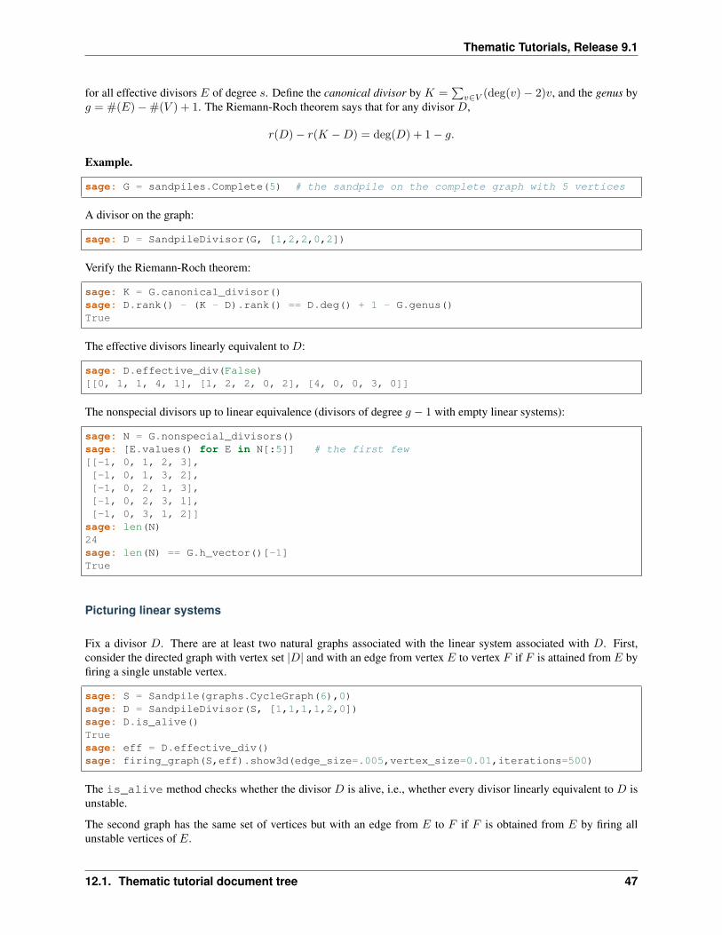
Fix a divisor 𝐷. There are at least two natural graphs associated with the linear system associated with 𝐷. First,consider the directed graph with vertex set |𝐷| and with an edge from vertex 𝐸 to vertex 𝐹 if 𝐹 is attained from 𝐸 byfiring a single unstable vertex.
sage: S = Sandpile(graphs.CycleGraph(6),0)sage: D = SandpileDivisor(S, [1,1,1,1,2,0])sage: D.is_alive()Truesage: eff = D.effective_div()sage: firing_graph(S,eff).show3d(edge_size=.005,vertex_size=0.01,iterations=500)
The is_alive method checks whether the divisor 𝐷 is alive, i.e., whether every divisor linearly equivalent to 𝐷 isunstable.
The second graph has the same set of vertices but with an edge from 𝐸 to 𝐹 if 𝐹 is obtained from 𝐸 by firing allunstable vertices of 𝐸.
12.1. Thematic tutorial document tree 47
Thematic Tutorials, Release 9.1
Fig. 3: Complete linear system for (1, 1, 1, 1, 2, 0) on 𝐶6: single firings
sage: S = Sandpile(graphs.CycleGraph(6),0)sage: D = SandpileDivisor(S, [1,1,1,1,2,0])sage: eff = D.effective_div()sage: parallel_firing_graph(S,eff).show3d(edge_size=.005,vertex_size=0.01,→˓iterations=500)
Note that in each of the examples above, starting at any divisor in the linear system and following edges, one iseventually led into a cycle of length 6 (cycling the divisor (1, 1, 1, 1, 2, 0)). Thus, D.alive() returns True. InSage, one would be able to rotate the above figures to get a better idea of the structure.
Algebraic geometry of sandpiles
Affine
Let 𝑛 = |𝑉 | − 1, and fix an ordering on the nonsink vertices of Γ. Let ℒ ⊂ Z𝑛 denote the column-span of 𝑡, thetranspose of the reduced Laplacian. Label vertex 𝑖 with the indeterminate 𝑥𝑖, and let C[Γ𝑠] = C[𝑥1, . . . , 𝑥𝑛]. (Here,𝑠 denotes the sink vertex of Γ.) The sandpile ideal or toppling ideal, first studied by Cori, Rossin, and Salvy [CRS]for undirected graphs, is the lattice ideal for ℒ:
𝐼 = 𝐼(Γ𝑠) := C[Γ𝑠] · 𝑥𝑢 − 𝑥𝑣 : 𝑢− 𝑣 ∈ ℒ ⊂ C[Γ𝑠],
where 𝑥𝑢 :=∏𝑛
𝑖=1 𝑥𝑢𝑖 for 𝑢 ∈ Z𝑛.
For each 𝑐 ∈ Z𝑛 define 𝑡(𝑐) = 𝑥𝑐+ − 𝑥𝑐− where 𝑐+𝑖 = max𝑐𝑖, 0 and 𝑐−𝑖 = max−𝑐𝑖, 0, so that 𝑐 = 𝑐+ − 𝑐−.
48 Chapter 12. Documentation
Thematic Tutorials, Release 9.1
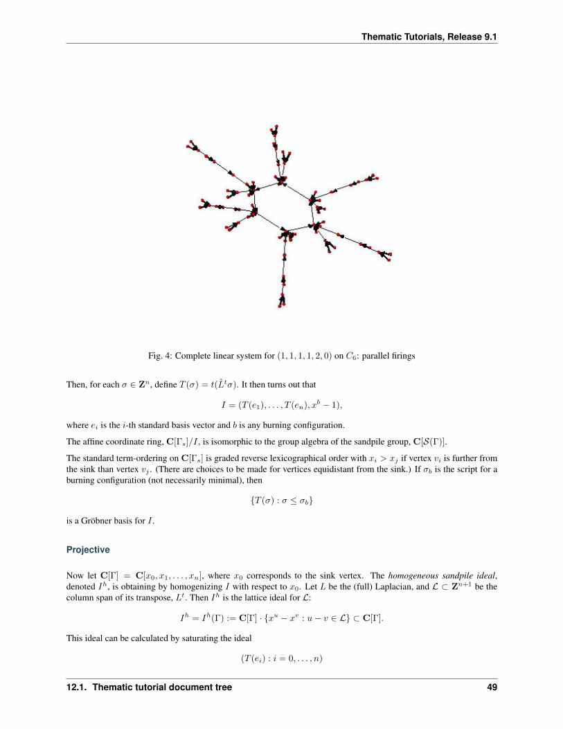
Fig. 4: Complete linear system for (1, 1, 1, 1, 2, 0) on 𝐶6: parallel firings
Then, for each 𝜎 ∈ Z𝑛, define 𝑇 (𝜎) = 𝑡(𝑡𝜎). It then turns out that
𝐼 = (𝑇 (𝑒1), . . . , 𝑇 (𝑒𝑛), 𝑥𝑏 − 1),
where 𝑒𝑖 is the 𝑖-th standard basis vector and 𝑏 is any burning configuration.
The affine coordinate ring, C[Γ𝑠]/𝐼, is isomorphic to the group algebra of the sandpile group, C[𝒮(Γ)].
The standard term-ordering on C[Γ𝑠] is graded reverse lexicographical order with 𝑥𝑖 > 𝑥𝑗 if vertex 𝑣𝑖 is further fromthe sink than vertex 𝑣𝑗 . (There are choices to be made for vertices equidistant from the sink.) If 𝜎𝑏 is the script for aburning configuration (not necessarily minimal), then
𝑇 (𝜎) : 𝜎 ≤ 𝜎𝑏
is a Gröbner basis for 𝐼 .
Projective
Now let C[Γ] = C[𝑥0, 𝑥1, . . . , 𝑥𝑛], where 𝑥0 corresponds to the sink vertex. The homogeneous sandpile ideal,denoted 𝐼ℎ, is obtaining by homogenizing 𝐼 with respect to 𝑥0. Let 𝐿 be the (full) Laplacian, and ℒ ⊂ Z𝑛+1 be thecolumn span of its transpose, 𝐿𝑡. Then 𝐼ℎ is the lattice ideal for ℒ:
𝐼ℎ = 𝐼ℎ(Γ) := C[Γ] · 𝑥𝑢 − 𝑥𝑣 : 𝑢− 𝑣 ∈ ℒ ⊂ C[Γ].
This ideal can be calculated by saturating the ideal
(𝑇 (𝑒𝑖) : 𝑖 = 0, . . . , 𝑛)
12.1. Thematic tutorial document tree 49
Thematic Tutorials, Release 9.1
with respect to the product of the indeterminates:∏𝑛
𝑖=0 𝑥𝑖 (extending the 𝑇 operator in the obvious way). A Gröbnerbasis with respect to the degree lexicographic order described above (with 𝑥0 the smallest vertex) is obtained byhomogenizing each element of the Gröbner basis for the non-homogeneous sandpile ideal with respect to 𝑥0.
Example.
sage: g = 0:,1:0:1,3:1,4:1,2:0:1,3:1,5:1,....: 3:2:1,5:1,4:1:1,3:1,5:2:1,3:1sage: S = Sandpile(g, 0)sage: S.ring()Multivariate Polynomial Ring in x5, x4, x3, x2, x1, x0 over Rational Field
The homogeneous sandpile ideal:
sage: S.ideal()Ideal (x2 - x0, x3^2 - x5*x0, x5*x3 - x0^2, x4^2 - x3*x1, x5^2 - x3*x0,x1^3 - x4*x3*x0, x4*x1^2 - x5*x0^2) of Multivariate Polynomial Ringin x5, x4, x3, x2, x1, x0 over Rational Field
The generators of the ideal:
sage: S.ideal(true)[x2 - x0,x3^2 - x5*x0,x5*x3 - x0^2,x4^2 - x3*x1,x5^2 - x3*x0,x1^3 - x4*x3*x0,x4*x1^2 - x5*x0^2]
Its resolution:
sage: S.resolution() # long time'R^1 <-- R^7 <-- R^19 <-- R^25 <-- R^16 <-- R^4'
and Betti table:
sage: S.betti() # long time0 1 2 3 4 5
------------------------------------------0: 1 1 - - - -1: - 4 6 2 - -2: - 2 7 7 2 -3: - - 6 16 14 4
------------------------------------------total: 1 7 19 25 16 4
The Hilbert function:
sage: S.hilbert_function()[1, 5, 11, 15]
and its first differences (which count the number of superstable configurations in each degree):
sage: S.h_vector()[1, 4, 6, 4]sage: x = [i.deg() for i in S.superstables()]sage: sorted(x)[0, 1, 1, 1, 1, 2, 2, 2, 2, 2, 2, 3, 3, 3, 3]
50 Chapter 12. Documentation
Thematic Tutorials, Release 9.1
The degree in which the Hilbert function starts equalling the Hilbert polynomial, the latter always being a constant inthe case of a sandpile ideal:
sage: S.postulation()3
Zeros
The zero set for the sandpile ideal 𝐼 is
𝑍(𝐼) = 𝑝 ∈ C𝑛 : 𝑓(𝑝) = 0 for all 𝑓 ∈ 𝐼,
the set of simultaneous zeros of the polynomials in 𝐼 . Letting 𝑆1 denote the unit circle in the complex plane, 𝑍(𝐼) is afinite subgroup of 𝑆1× · · ·×𝑆1 ⊂ C𝑛, isomorphic to the sandpile group. The zero set is actually linearly isomorphicto a faithful representation of the sandpile group on C𝑛.
Todo: The above is not quite true. 𝑍(𝐼) is neither finite nor a subgroup of 𝑆1 × · · · × 𝑆1 ⊂ C𝑛. What is probablymeant is that the subset of 𝑍(𝐼) in which the coordinate of 𝑝 corresponding to the sink is set to 1 is a finite subgroupof 𝑆1 × · · · × 𝑆1 ⊂ C𝑛−1.
Example. (Continued.)
sage: S = Sandpile(0: , 1: 2: 2, 2: 0: 4, 1: 1, 0)sage: S.ideal().gens()[x1^2 - x2^2, x1*x2^3 - x0^4, x2^5 - x1*x0^4]
Approximation to the zero set (setting x_0 = 1):
sage: S.solve()[[-0.707107 + 0.707107*I, 0.707107 - 0.707107*I],[-0.707107 - 0.707107*I, 0.707107 + 0.707107*I],[-I, -I],[I, I],[0.707107 + 0.707107*I, -0.707107 - 0.707107*I],[0.707107 - 0.707107*I, -0.707107 + 0.707107*I],[1, 1],[-1, -1]]sage: len(_) == S.group_order()True
The zeros are generated as a group by a single vector:
sage: S.points()[[(1/2*I + 1/2)*sqrt(2), -(1/2*I + 1/2)*sqrt(2)]]
Resolutions
The homogeneous sandpile ideal, 𝐼ℎ, has a free resolution graded by the divisors on Γ modulo linear equivalence.(See the section on Discrete Riemann Surfaces for the language of divisors and linear equivalence.) Let 𝑆 = C[Γ] =C[𝑥0, . . . , 𝑥𝑛], as above, and let S denote the group of divisors modulo rational equivalence. Then 𝑆 is graded by Sby letting deg(𝑥𝑐) = 𝑐 ∈ S for each monomial 𝑥𝑐. The minimal free resolution of 𝐼ℎ has the form
0← 𝐼ℎ ←⨁𝐷∈S
𝑆(−𝐷)𝛽0,𝐷 ←⨁𝐷∈S
𝑆(−𝐷)𝛽1,𝐷 ← · · · ←⨁𝐷∈S
𝑆(−𝐷)𝛽𝑟,𝐷 ← 0,
12.1. Thematic tutorial document tree 51
Thematic Tutorials, Release 9.1
where the 𝛽𝑖,𝐷 are the Betti numbers for 𝐼ℎ.
For each divisor class 𝐷 ∈ S, define a simplicial complex
∆𝐷 := 𝐼 ⊆ 0, . . . , 𝑛 : 𝐼 ⊆ supp(𝐸) for some 𝐸 ∈ |𝐷|.
The Betti number 𝛽𝑖,𝐷 equals the dimension over C of the 𝑖-th reduced homology group of ∆𝐷:
𝛽𝑖,𝐷 = dimC 𝑖(∆𝐷;C).
sage: S = Sandpile(0:,1:0: 1, 2: 1, 3: 4,2:3: 5,3:1: 1, 2: 1,0)
Representatives of all divisor classes with nontrivial homology:
sage: p = S.betti_complexes()sage: p[0][0: -8, 1: 5, 2: 4, 3: 1,Simplicial complex with vertex set (1, 2, 3) and facets (3,), (1, 2)]
The homology associated with the first divisor in the list:
sage: D = p[0][0]sage: D.effective_div()[0: 0, 1: 0, 2: 0, 3: 2, 0: 0, 1: 1, 2: 1, 3: 0]sage: [E.support() for E in D.effective_div()][[3], [1, 2]]sage: D.Dcomplex()Simplicial complex with vertex set (1, 2, 3) and facets (3,), (1, 2)sage: D.Dcomplex().homology()0: Z, 1: 0
The minimal free resolution:
sage: S.resolution()'R^1 <-- R^5 <-- R^5 <-- R^1'sage: S.betti()
0 1 2 3------------------------------
0: 1 - - -1: - 5 5 -2: - - - 1
------------------------------total: 1 5 5 1sage: len(p)11
The degrees and ranks of the homology groups for each element of the list p (compare with the Betti table, above):
sage: [[sum(d[0].values()),d[1].betti()] for d in p][[2, 0: 2, 1: 0],[3, 0: 1, 1: 1, 2: 0],[2, 0: 2, 1: 0],[3, 0: 1, 1: 1, 2: 0],[2, 0: 2, 1: 0],[3, 0: 1, 1: 1, 2: 0],[2, 0: 2, 1: 0],[3, 0: 1, 1: 1],
(continues on next page)
52 Chapter 12. Documentation
Thematic Tutorials, Release 9.1
(continued from previous page)
[2, 0: 2, 1: 0],[3, 0: 1, 1: 1, 2: 0],[5, 0: 1, 1: 0, 2: 1]]
Complete Intersections and Arithmetically Gorenstein toppling ideals
NOTE: in the previous section note that the resolution always has length 𝑛 since the ideal is Cohen-Macaulay.
To do.
Betti numbers for undirected graphs
To do.
Usage
Initialization
There are three main classes for sandpile structures in Sage: Sandpile, SandpileConfig, andSandpileDivisor. Initialization for Sandpile has the form
.. skip
sage: S = Sandpile(graph, sink)
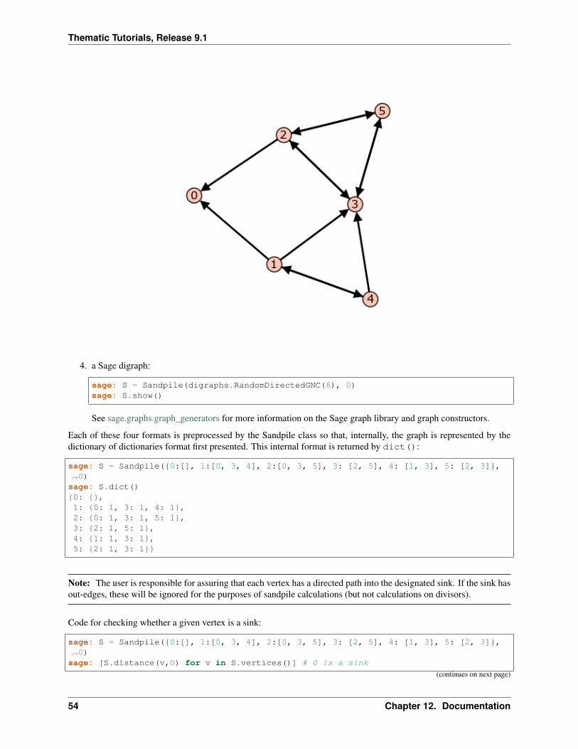
where graph represents a graph and sink is the key for the sink vertex. There are four possible forms for graph:
1. a Python dictionary of dictionaries:
sage: g = 0: , 1: 0: 1, 3: 1, 4: 1, 2: 0: 1, 3: 1, 5: 1,....: 3: 2: 1, 5: 1, 4: 1: 1, 3: 1, 5: 2: 1, 3: 1
Graph from dictionary of dictionaries.
Each key is the name of a vertex. Next to each vertex name 𝑣 is a dictionary consisting of pairs: vertex:weight. Each pair represents a directed edge emanating from 𝑣 and ending at vertex having (non-negativeinteger) weight equal to weight. Loops are allowed. In the example above, all of the weights are 1.
2. a Python dictionary of lists:
sage: g = 0: [], 1: [0, 3, 4], 2: [0, 3, 5],....: 3: [2, 5], 4: [1, 3], 5: [2, 3]
This is a short-hand when all of the edge-weights are equal to 1. The above example is for the same displayedgraph.
3. a Sage graph (of type sage.graphs.graph.Graph):
sage: g = graphs.CycleGraph(5)sage: S = Sandpile(g, 0)sage: type(g)<class 'sage.graphs.graph.Graph'>
To see the types of built-in graphs, type graphs., including the period, and hit TAB.
12.1. Thematic tutorial document tree 53
Thematic Tutorials, Release 9.1
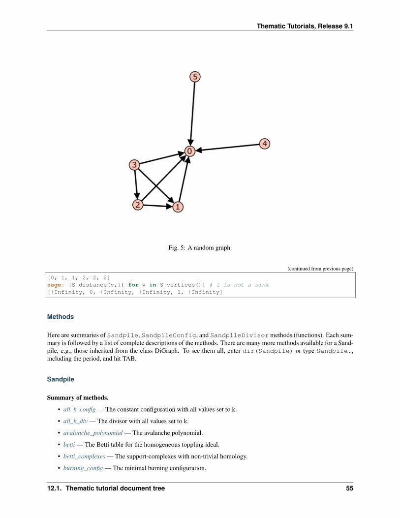
4. a Sage digraph:
sage: S = Sandpile(digraphs.RandomDirectedGNC(6), 0)sage: S.show()
See sage.graphs.graph_generators for more information on the Sage graph library and graph constructors.
Each of these four formats is preprocessed by the Sandpile class so that, internally, the graph is represented by thedictionary of dictionaries format first presented. This internal format is returned by dict():
sage: S = Sandpile(0:[], 1:[0, 3, 4], 2:[0, 3, 5], 3: [2, 5], 4: [1, 3], 5: [2, 3],→˓0)sage: S.dict()0: ,1: 0: 1, 3: 1, 4: 1,2: 0: 1, 3: 1, 5: 1,3: 2: 1, 5: 1,4: 1: 1, 3: 1,5: 2: 1, 3: 1
Note: The user is responsible for assuring that each vertex has a directed path into the designated sink. If the sink hasout-edges, these will be ignored for the purposes of sandpile calculations (but not calculations on divisors).
Code for checking whether a given vertex is a sink:
sage: S = Sandpile(0:[], 1:[0, 3, 4], 2:[0, 3, 5], 3: [2, 5], 4: [1, 3], 5: [2, 3],→˓0)sage: [S.distance(v,0) for v in S.vertices()] # 0 is a sink
(continues on next page)
54 Chapter 12. Documentation
Thematic Tutorials, Release 9.1
Fig. 5: A random graph.
(continued from previous page)
[0, 1, 1, 2, 2, 2]sage: [S.distance(v,1) for v in S.vertices()] # 1 is not a sink[+Infinity, 0, +Infinity, +Infinity, 1, +Infinity]
Methods
Here are summaries of Sandpile, SandpileConfig, and SandpileDivisor methods (functions). Each sum-mary is followed by a list of complete descriptions of the methods. There are many more methods available for a Sand-pile, e.g., those inherited from the class DiGraph. To see them all, enter dir(Sandpile) or type Sandpile.,including the period, and hit TAB.
Sandpile
Summary of methods.
• all_k_config — The constant configuration with all values set to k.
• all_k_div — The divisor with all values set to k.
• avalanche_polynomial — The avalanche polynomial.
• betti — The Betti table for the homogeneous toppling ideal.
• betti_complexes — The support-complexes with non-trivial homology.
• burning_config — The minimal burning configuration.
12.1. Thematic tutorial document tree 55
Thematic Tutorials, Release 9.1
• burning_script — A script for the minimal burning configuration.
• canonical_divisor — The canonical divisor.
• dict — A dictionary of dictionaries representing a directed graph.
• genus — The genus: (# non-loop edges) - (# vertices) + 1.
• groebner — A Groebner basis for the homogeneous toppling ideal.
• group_gens — A minimal list of generators for the sandpile group.
• group_order — The size of the sandpile group.
• h_vector — The number of superstable configurations in each degree.
• help — List of Sandpile-specific methods (not inherited from Graph).
• hilbert_function — The Hilbert function of the homogeneous toppling ideal.
• ideal — The saturated homogeneous toppling ideal.
• identity — The identity configuration.
• in_degree — The in-degree of a vertex or a list of all in-degrees.
• invariant_factors — The invariant factors of the sandpile group.
• is_undirected — Is the underlying graph undirected?
• jacobian_representatives — Representatives for the elements of the Jacobian group.
• laplacian — The Laplacian matrix of the graph.
• markov_chain — The sandpile Markov chain for configurations or divisors.
• max_stable — The maximal stable configuration.
• max_stable_div — The maximal stable divisor.
• max_superstables — The maximal superstable configurations.
• min_recurrents — The minimal recurrent elements.
• nonsink_vertices — The nonsink vertices.
• nonspecial_divisors — The nonspecial divisors.
• out_degree — The out-degree of a vertex or a list of all out-degrees.
• picard_representatives — Representatives of the divisor classes of degree d in the Picard group.
• points — Generators for the multiplicative group of zeros of the sandpile ideal.
• postulation — The postulation number of the toppling ideal.
• recurrents — The recurrent configurations.
• reduced_laplacian — The reduced Laplacian matrix of the graph.
• reorder_vertices — A copy of the sandpile with vertex names permuted.
• resolution — A minimal free resolution of the homogeneous toppling ideal.
• ring — The ring containing the homogeneous toppling ideal.
• show — Draw the underlying graph.
• show3d — Draw the underlying graph.
• sink — The sink vertex.
56 Chapter 12. Documentation
Thematic Tutorials, Release 9.1
• smith_form — The Smith normal form for the Laplacian.
• solve — Approximations of the complex affine zeros of the sandpile ideal.
• stable_configs — Generator for all stable configurations.
• stationary_density — The stationary density of the sandpile.
• superstables — The superstable configurations.
• symmetric_recurrents — The symmetric recurrent configurations.
• tutte_polynomial — The Tutte polynomial.
• unsaturated_ideal — The unsaturated, homogeneous toppling ideal.
• version — The version number of Sage Sandpiles.
• zero_config — The all-zero configuration.
• zero_div — The all-zero divisor.
Complete descriptions of Sandpile methods.
—
all_k_config(k)
The constant configuration with all values set to 𝑘.
INPUT:
k – integer
OUTPUT:
SandpileConfig
EXAMPLES:
sage: s = sandpiles.Diamond()sage: s.all_k_config(7)1: 7, 2: 7, 3: 7
—
all_k_div(k)
The divisor with all values set to 𝑘.
INPUT:
k – integer
OUTPUT:
SandpileDivisor
EXAMPLES:
sage: S = sandpiles.House()sage: S.all_k_div(7)0: 7, 1: 7, 2: 7, 3: 7, 4: 7
12.1. Thematic tutorial document tree 57
Thematic Tutorials, Release 9.1
—
avalanche_polynomial(multivariable=True)
The avalanche polynomial. See NOTE for details.
INPUT:
multivariable – (default: True) boolean
OUTPUT:
polynomial
EXAMPLES:
sage: s = sandpiles.Complete(4)sage: s.avalanche_polynomial()9*x0*x1*x2 + 2*x0*x1 + 2*x0*x2 + 2*x1*x2 + 3*x0 + 3*x1 + 3*x2 + 24sage: s.avalanche_polynomial(False)9*x0^3 + 6*x0^2 + 9*x0 + 24
Note: For each nonsink vertex 𝑣, let 𝑥𝑣 be an indeterminate. If (𝑟, 𝑣) is a pair consisting of a recurrent 𝑟 and nonsinkvertex 𝑣, then for each nonsink vertex 𝑤, let 𝑛𝑤 be the number of times vertex 𝑤 fires in the stabilization of 𝑟+ 𝑣. Let𝑀(𝑟, 𝑣) be the monomial
∏𝑤 𝑥
𝑛𝑤𝑤 , i.e., the exponent records the vector of 𝑛𝑤 as 𝑤 ranges over the nonsink vertices.
The avalanche polynomial is then the sum of 𝑀(𝑟, 𝑣) as 𝑟 ranges over the recurrents and 𝑣 ranges over the nonsinkvertices. If multivariable is False, then set all the indeterminates equal to each other (and, thus, only count thenumber of vertex firings in the stabilizations, forgetting which particular vertices fired).
—
betti(verbose=True)
The Betti table for the homogeneous toppling ideal. If verbose is True, it prints the standard Betti table, otherwise,it returns a less formatted table.
INPUT:
verbose – (default: True) boolean
OUTPUT:
Betti numbers for the sandpile
EXAMPLES:
sage: S = sandpiles.Diamond()sage: S.betti()
0 1 2 3------------------------------
0: 1 - - -1: - 2 - -2: - 4 9 4
------------------------------total: 1 6 9 4sage: S.betti(False)[1, 6, 9, 4]
—
betti_complexes()
58 Chapter 12. Documentation
Thematic Tutorials, Release 9.1
The support-complexes with non-trivial homology. (See NOTE.)
OUTPUT:
list (of pairs [divisors, corresponding simplicial complex])
EXAMPLES:
sage: S = Sandpile(0:,1:0: 1, 2: 1, 3: 4,2:3: 5,3:1: 1, 2: 1,0)sage: p = S.betti_complexes()sage: p[0][0: -8, 1: 5, 2: 4, 3: 1, Simplicial complex with vertex set (1, 2, 3) and facets→˓(3,), (1, 2)]sage: S.resolution()'R^1 <-- R^5 <-- R^5 <-- R^1'sage: S.betti()
0 1 2 3------------------------------
0: 1 - - -1: - 5 5 -2: - - - 1
------------------------------total: 1 5 5 1sage: len(p)11sage: p[0][1].homology()0: Z, 1: 0sage: p[-1][1].homology()0: 0, 1: 0, 2: Z
Note: A support-complex is the simplicial complex formed from the supports of the divisors in a linear system.
—
burning_config()
The minimal burning configuration.
OUTPUT:
dict (configuration)
EXAMPLES:
sage: g = 0:,1:0:1,3:1,4:1,2:0:1,3:1,5:1, \3:2:1,5:1,4:1:1,3:1,5:2:1,3:1
sage: S = Sandpile(g,0)sage: S.burning_config()1: 2, 2: 0, 3: 1, 4: 1, 5: 0sage: S.burning_config().values()[2, 0, 1, 1, 0]sage: S.burning_script()1: 1, 2: 3, 3: 5, 4: 1, 5: 4sage: script = S.burning_script().values()sage: script[1, 3, 5, 1, 4]sage: matrix(script)*S.reduced_laplacian()[2 0 1 1 0]
12.1. Thematic tutorial document tree 59
Thematic Tutorials, Release 9.1
Note: The burning configuration and script are computed using a modified version of Speer’s script algorithm. Thisis a generalization to directed multigraphs of Dhar’s burning algorithm.
A burning configuration is a nonnegative integer-linear combination of the rows of the reduced Laplacian matrixhaving nonnegative entries and such that every vertex has a path from some vertex in its support. The correspondingburning script gives the integer-linear combination needed to obtain the burning configuration. So if 𝑏 is the burningconfiguration, 𝜎 is its script, and is the reduced Laplacian, then 𝜎 · = 𝑏. The minimal burning configuration isthe one with the minimal script (its components are no larger than the components of any other script for a burningconfiguration).
The following are equivalent for a configuration 𝑐 with burning configuration 𝑏 having script 𝜎:
• 𝑐 is recurrent;
• 𝑐+ 𝑏 stabilizes to 𝑐;
• the firing vector for the stabilization of 𝑐+ 𝑏 is 𝜎.
—
burning_script()
A script for the minimal burning configuration.
OUTPUT:
dict
EXAMPLES:
sage: g = 0:,1:0:1,3:1,4:1,2:0:1,3:1,5:1,\3:2:1,5:1,4:1:1,3:1,5:2:1,3:1sage: S = Sandpile(g,0)sage: S.burning_config()1: 2, 2: 0, 3: 1, 4: 1, 5: 0sage: S.burning_config().values()[2, 0, 1, 1, 0]sage: S.burning_script()1: 1, 2: 3, 3: 5, 4: 1, 5: 4sage: script = S.burning_script().values()sage: script[1, 3, 5, 1, 4]sage: matrix(script)*S.reduced_laplacian()[2 0 1 1 0]
Note: The burning configuration and script are computed using a modified version of Speer’s script algorithm. Thisis a generalization to directed multigraphs of Dhar’s burning algorithm.
A burning configuration is a nonnegative integer-linear combination of the rows of the reduced Laplacian matrixhaving nonnegative entries and such that every vertex has a path from some vertex in its support. The correspondingburning script gives the integer-linear combination needed to obtain the burning configuration. So if 𝑏 is the burningconfiguration, 𝑠 is its script, and 𝐿red is the reduced Laplacian, then 𝑠 · 𝐿red = 𝑏. The minimal burning configurationis the one with the minimal script (its components are no larger than the components of any other script for a burningconfiguration).
The following are equivalent for a configuration 𝑐 with burning configuration 𝑏 having script 𝑠:
• 𝑐 is recurrent;
• 𝑐+ 𝑏 stabilizes to 𝑐;
60 Chapter 12. Documentation
Thematic Tutorials, Release 9.1
• the firing vector for the stabilization of 𝑐+ 𝑏 is 𝑠.
—
canonical_divisor()
The canonical divisor. This is the divisor with deg(𝑣)− 2 grains of sand on each vertex (not counting loops). Only forundirected graphs.
OUTPUT:
SandpileDivisor
EXAMPLES:
sage: S = sandpiles.Complete(4)sage: S.canonical_divisor()0: 1, 1: 1, 2: 1, 3: 1sage: s = Sandpile(0:[1,1],1:[0,0,1,1,1],0)sage: s.canonical_divisor() # loops are disregarded0: 0, 1: 0
Warning: The underlying graph must be undirected.
—
dict()
A dictionary of dictionaries representing a directed graph.
OUTPUT:
dict
EXAMPLES:
sage: S = sandpiles.Diamond()sage: S.dict()0: 1: 1, 2: 1,1: 0: 1, 2: 1, 3: 1,2: 0: 1, 1: 1, 3: 1,3: 1: 1, 2: 1
sage: S.sink()0
—
genus()
The genus: (# non-loop edges) - (# vertices) + 1. Only defined for undirected graphs.
OUTPUT:
integer
EXAMPLES:
sage: sandpiles.Complete(4).genus()3sage: sandpiles.Cycle(5).genus()1
12.1. Thematic tutorial document tree 61
Thematic Tutorials, Release 9.1
—
groebner()
A Groebner basis for the homogeneous toppling ideal. It is computed with respect to the standard sandpile ordering(see ring).
OUTPUT:
Groebner basis
EXAMPLES:
sage: S = sandpiles.Diamond()sage: S.groebner()[x3*x2^2 - x1^2*x0, x2^3 - x3*x1*x0, x3*x1^2 - x2^2*x0, x1^3 - x3*x2*x0, x3^2 - x0^2,→˓x2*x1 - x0^2]
—
group_gens(verbose=True)
A minimal list of generators for the sandpile group. If verbose is False then the generators are represented as listsof integers.
INPUT:
verbose – (default: True) boolean
OUTPUT:
list of SandpileConfig (or of lists of integers if verbose is False)
EXAMPLES:
sage: s = sandpiles.Cycle(5)sage: s.group_gens()[1: 1, 2: 1, 3: 1, 4: 0]sage: s.group_gens()[0].order()5sage: s = sandpiles.Complete(5)sage: s.group_gens(False)[[2, 2, 3, 2], [2, 3, 2, 2], [3, 2, 2, 2]]sage: [i.order() for i in s.group_gens()][5, 5, 5]sage: s.invariant_factors()[1, 5, 5, 5]
—
group_order()
The size of the sandpile group.
OUTPUT:
integer
EXAMPLES:
sage: S = sandpiles.House()sage: S.group_order()11
62 Chapter 12. Documentation
Thematic Tutorials, Release 9.1
—
h_vector()
The number of superstable configurations in each degree. Equivalently, this is the list of first differences of the Hilbertfunction of the (homogeneous) toppling ideal.
OUTPUT:
list of nonnegative integers
EXAMPLES:
sage: s = sandpiles.Grid(2,2)sage: s.hilbert_function()[1, 5, 15, 35, 66, 106, 146, 178, 192]sage: s.h_vector()[1, 4, 10, 20, 31, 40, 40, 32, 14]
—
help(verbose=True)
List of Sandpile-specific methods (not inherited from Graph). If verbose, include short descriptions.
INPUT:
verbose – (default: True) boolean
OUTPUT:
printed string
EXAMPLES:
sage: Sandpile.help()For detailed help with any method FOO listed below,enter "Sandpile.FOO?" or enter "S.FOO?" for any Sandpile S.
all_k_config -- The constant configuration with all values set to k.all_k_div -- The divisor with all values set to k.avalanche_polynomial -- The avalanche polynomial.betti -- The Betti table for the homogeneous toppling ideal.betti_complexes -- The support-complexes with non-trivial homology.burning_config -- The minimal burning configuration.burning_script -- A script for the minimal burning configuration.canonical_divisor -- The canonical divisor.dict -- A dictionary of dictionaries representing a directed→˓graph.genus -- The genus: (# non-loop edges) - (# vertices) + 1.groebner -- A Groebner basis for the homogeneous toppling ideal.group_gens -- A minimal list of generators for the sandpile group.group_order -- The size of the sandpile group.h_vector -- The number of superstable configurations in each degree.help -- List of Sandpile-specific methods (not inherited from→˓"Graph").hilbert_function -- The Hilbert function of the homogeneous toppling ideal.ideal -- The saturated homogeneous toppling ideal.identity -- The identity configuration.in_degree -- The in-degree of a vertex or a list of all in-degrees.invariant_factors -- The invariant factors of the sandpile group.is_undirected -- Is the underlying graph undirected?
(continues on next page)
12.1. Thematic tutorial document tree 63
Thematic Tutorials, Release 9.1
(continued from previous page)
jacobian_representatives -- Representatives for the elements of the Jacobian group.laplacian -- The Laplacian matrix of the graph.markov_chain -- The sandpile Markov chain for configurations or divisors.max_stable -- The maximal stable configuration.max_stable_div -- The maximal stable divisor.max_superstables -- The maximal superstable configurations.min_recurrents -- The minimal recurrent elements.nonsink_vertices -- The nonsink vertices.nonspecial_divisors -- The nonspecial divisors.out_degree -- The out-degree of a vertex or a list of all out-degrees.picard_representatives -- Representatives of the divisor classes of degree d in the→˓Picard group.points -- Generators for the multiplicative group of zeros of the→˓sandpile ideal.postulation -- The postulation number of the toppling ideal.recurrents -- The recurrent configurations.reduced_laplacian -- The reduced Laplacian matrix of the graph.reorder_vertices -- A copy of the sandpile with vertex names permuted.resolution -- A minimal free resolution of the homogeneous toppling→˓ideal.ring -- The ring containing the homogeneous toppling ideal.show -- Draw the underlying graph.show3d -- Draw the underlying graph.sink -- The sink vertex.smith_form -- The Smith normal form for the Laplacian.solve -- Approximations of the complex affine zeros of the→˓sandpile ideal.stable_configs -- Generator for all stable configurations.stationary_density -- The stationary density of the sandpile.superstables -- The superstable configurations.symmetric_recurrents -- The symmetric recurrent configurations.tutte_polynomial -- The Tutte polynomial of the underlying graph.unsaturated_ideal -- The unsaturated, homogeneous toppling ideal.version -- The version number of Sage Sandpiles.zero_config -- The all-zero configuration.zero_div -- The all-zero divisor.
—
hilbert_function()
The Hilbert function of the homogeneous toppling ideal.
OUTPUT:
list of nonnegative integers
EXAMPLES:
sage: s = sandpiles.Wheel(5)sage: s.hilbert_function()[1, 5, 15, 31, 45]sage: s.h_vector()[1, 4, 10, 16, 14]
—
ideal(gens=False)
The saturated homogeneous toppling ideal. If gens is True, the generators for the ideal are returned instead.
64 Chapter 12. Documentation
Thematic Tutorials, Release 9.1
INPUT:
gens – (default: False) boolean
OUTPUT:
ideal or, optionally, the generators of an ideal
EXAMPLES:
sage: S = sandpiles.Diamond()sage: S.ideal()Ideal (x2*x1 - x0^2, x3^2 - x0^2, x1^3 - x3*x2*x0, x3*x1^2 - x2^2*x0, x2^3 - x3*x1*x0,→˓ x3*x2^2 - x1^2*x0) of Multivariate Polynomial Ring in x3, x2, x1, x0 over Rational→˓Fieldsage: S.ideal(True)[x2*x1 - x0^2, x3^2 - x0^2, x1^3 - x3*x2*x0, x3*x1^2 - x2^2*x0, x2^3 - x3*x1*x0,→˓x3*x2^2 - x1^2*x0]sage: S.ideal().gens() # another way to get the generators[x2*x1 - x0^2, x3^2 - x0^2, x1^3 - x3*x2*x0, x3*x1^2 - x2^2*x0, x2^3 - x3*x1*x0,→˓x3*x2^2 - x1^2*x0]
—
identity(verbose=True)
The identity configuration. If verbose is False, the configuration are converted to a list of integers.
INPUT:
verbose – (default: True) boolean
OUTPUT:
SandpileConfig or a list of integers If verbose is False, the configuration are converted to a list of integers.
EXAMPLES:
sage: s = sandpiles.Diamond()sage: s.identity()1: 2, 2: 2, 3: 0sage: s.identity(False)[2, 2, 0]sage: s.identity() & s.max_stable() == s.max_stable()True
—
in_degree(v=None)
The in-degree of a vertex or a list of all in-degrees.
INPUT:
v – (optional) vertex name
OUTPUT:
integer or dict
EXAMPLES:
12.1. Thematic tutorial document tree 65
Thematic Tutorials, Release 9.1
sage: s = sandpiles.House()sage: s.in_degree()0: 2, 1: 2, 2: 3, 3: 3, 4: 2sage: s.in_degree(2)3
—
invariant_factors()
The invariant factors of the sandpile group.
OUTPUT:
list of integers
EXAMPLES:
sage: s = sandpiles.Grid(2,2)sage: s.invariant_factors()[1, 1, 8, 24]
—
is_undirected()
Is the underlying graph undirected? True if (𝑢, 𝑣) is and edge if and only if (𝑣, 𝑢) is an edge, each edge with thesame weight.
OUTPUT:
boolean
EXAMPLES:
sage: sandpiles.Complete(4).is_undirected()Truesage: s = Sandpile(0:[1,2], 1:[0,2], 2:[0], 0)sage: s.is_undirected()False
—
jacobian_representatives(verbose=True)
Representatives for the elements of the Jacobian group. If verbose is False, then lists representing the divisors arereturned.
INPUT:
verbose – (default: True) boolean
OUTPUT:
list of SandpileDivisor (or of lists representing divisors)
EXAMPLES:
For an undirected graph, divisors of the form s - deg(s)*sink as s varies over the superstables forms a distinctset of representatives for the Jacobian group.:
66 Chapter 12. Documentation
Thematic Tutorials, Release 9.1
sage: s = sandpiles.Complete(3)sage: s.superstables(False)[[0, 0], [0, 1], [1, 0]]sage: s.jacobian_representatives(False)[[0, 0, 0], [-1, 0, 1], [-1, 1, 0]]
If the graph is directed, the representatives described above may by equivalent modulo the rowspan of the Laplacianmatrix:
sage: s = Sandpile(0: 1: 1, 2: 2, 1: 0: 2, 2: 4, 2: 0: 4, 1: 2,0)sage: s.group_order()28sage: s.jacobian_representatives()[0: -5, 1: 3, 2: 2, 0: -4, 1: 3, 2: 1]
Let 𝜏 be the nonnegative generator of the kernel of the transpose of the Laplacian, and let 𝑡𝑎𝑢𝑠 be it sink component,then the sandpile group is isomorphic to the direct sum of the cyclic group of order 𝜏𝑠 and the Jacobian group. In theexample above, we have:
sage: s.laplacian().left_kernel()Free module of degree 3 and rank 1 over Integer RingEchelon basis matrix:[14 5 8]
Note: The Jacobian group is the set of all divisors of degree zero modulo the integer rowspan of the Laplacian matrix.
—
laplacian()
The Laplacian matrix of the graph. Its rows encode the vertex firing rules.
OUTPUT:
matrix
EXAMPLES:
sage: G = sandpiles.Diamond()sage: G.laplacian()[ 2 -1 -1 0][-1 3 -1 -1][-1 -1 3 -1][ 0 -1 -1 2]
Warning: The function laplacian_matrix should be avoided. It returns the indegree version of the Lapla-cian.
—
markov_chain(state, distrib=None)
The sandpile Markov chain for configurations or divisors. The chain starts at state. See NOTE for details.
INPUT:
• state – SandpileConfig, SandpileDivisor, or list representing one of these
12.1. Thematic tutorial document tree 67
Thematic Tutorials, Release 9.1
• distrib – (optional) list of nonnegative numbers summing to 1 (representing a prob. dist.)
OUTPUT:
generator for Markov chain (see NOTE)
EXAMPLES:
sage: s = sandpiles.Complete(4)sage: m = s.markov_chain([0,0,0])sage: next(m) # random1: 0, 2: 0, 3: 0sage: next(m).values() # random[0, 0, 0]sage: next(m).values() # random[0, 0, 0]sage: next(m).values() # random[0, 0, 0]sage: next(m).values() # random[0, 1, 0]sage: next(m).values() # random[0, 2, 0]sage: next(m).values() # random[0, 2, 1]sage: next(m).values() # random[1, 2, 1]sage: next(m).values() # random[2, 2, 1]sage: m = s.markov_chain(s.zero_div(), [0.1,0.1,0.1,0.7])sage: next(m).values() # random[0, 0, 0, 1]sage: next(m).values() # random[0, 0, 1, 1]sage: next(m).values() # random[0, 0, 1, 2]sage: next(m).values() # random[1, 1, 2, 0]sage: next(m).values() # random[1, 1, 2, 1]sage: next(m).values() # random[1, 1, 2, 2]sage: next(m).values() # random[1, 1, 2, 3]sage: next(m).values() # random[1, 1, 2, 4]sage: next(m).values() # random[1, 1, 3, 4]
Note: The closed sandpile Markov chain has state space consisting of the configurations on a sandpile. Ittransitions from a state by choosing a vertex at random (according to the probability distribution distrib), droppinga grain of sand at that vertex, and stabilizing. If the chosen vertex is the sink, the chain stays at the current state.
The open sandpile Markov chain has state space consisting of the recurrent elements, i.e., the state space isthe sandpile group. It transitions from the configuration 𝑐 by choosing a vertex 𝑣 at random according to distrib.The next state is the stabilization of 𝑐+ 𝑣. If 𝑣 is the sink vertex, then the stabilization of 𝑐+ 𝑣 is defined to be 𝑐.
Note that in either case, if distrib is specified, its length is equal to the total number of vertices (including the sink).
68 Chapter 12. Documentation
Thematic Tutorials, Release 9.1
REFERENCES:
—
max_stable()
The maximal stable configuration.
OUTPUT:
SandpileConfig (the maximal stable configuration)
EXAMPLES:
sage: S = sandpiles.House()sage: S.max_stable()1: 1, 2: 2, 3: 2, 4: 1
—
max_stable_div()
The maximal stable divisor.
OUTPUT:
SandpileDivisor (the maximal stable divisor)
EXAMPLES:
sage: s = sandpiles.Diamond()sage: s.max_stable_div()0: 1, 1: 2, 2: 2, 3: 1sage: s.out_degree()0: 2, 1: 3, 2: 3, 3: 2
—
max_superstables(verbose=True)
The maximal superstable configurations. If the underlying graph is undirected, these are the superstables of highestdegree. If verbose is False, the configurations are converted to lists of integers.
INPUT:
verbose – (default: True) boolean
OUTPUT:
tuple of SandpileConfig
EXAMPLES:
sage: s = sandpiles.Diamond()sage: s.superstables(False)[[0, 0, 0],[0, 0, 1],[1, 0, 1],[0, 2, 0],[2, 0, 0],[0, 1, 1],[1, 0, 0],[0, 1, 0]]
sage: s.max_superstables(False)
(continues on next page)
12.1. Thematic tutorial document tree 69
Thematic Tutorials, Release 9.1
(continued from previous page)
[[1, 0, 1], [0, 2, 0], [2, 0, 0], [0, 1, 1]]sage: s.h_vector()[1, 3, 4]
—
min_recurrents(verbose=True)
The minimal recurrent elements. If the underlying graph is undirected, these are the recurrent elements of least degree.If verbose is False, the configurations are converted to lists of integers.
INPUT:
verbose – (default: True) boolean
OUTPUT:
list of SandpileConfig
EXAMPLES:
sage: s = sandpiles.Diamond()sage: s.recurrents(False)[[2, 2, 1],[2, 2, 0],[1, 2, 0],[2, 0, 1],[0, 2, 1],[2, 1, 0],[1, 2, 1],[2, 1, 1]]
sage: s.min_recurrents(False)[[1, 2, 0], [2, 0, 1], [0, 2, 1], [2, 1, 0]]sage: [i.deg() for i in s.recurrents()][5, 4, 3, 3, 3, 3, 4, 4]
—
nonsink_vertices()
The nonsink vertices.
OUTPUT:
list of vertices
EXAMPLES:
sage: s = sandpiles.Grid(2,3)sage: s.nonsink_vertices()[(1, 1), (1, 2), (1, 3), (2, 1), (2, 2), (2, 3)]
—
nonspecial_divisors(verbose=True)
The nonspecial divisors. Only for undirected graphs. (See NOTE.)
INPUT:
verbose – (default: True) boolean
OUTPUT:
70 Chapter 12. Documentation
Thematic Tutorials, Release 9.1
list (of divisors)
EXAMPLES:
sage: S = sandpiles.Complete(4)sage: ns = S.nonspecial_divisors()sage: D = ns[0]sage: D.values()[-1, 0, 1, 2]sage: D.deg()2sage: [i.effective_div() for i in ns][[], [], [], [], [], []]
Note: The “nonspecial divisors” are those divisors of degree 𝑔−1 with empty linear system. The term is only definedfor undirected graphs. Here, 𝑔 = |𝐸| − |𝑉 | + 1 is the genus of the graph (not counting loops as part of |𝐸|). Ifverbose is False, the divisors are converted to lists of integers.
Warning: The underlying graph must be undirected.
—
out_degree(v=None)
The out-degree of a vertex or a list of all out-degrees.
INPUT:
v - (optional) vertex name
OUTPUT:
integer or dict
EXAMPLES:
sage: s = sandpiles.House()sage: s.out_degree()0: 2, 1: 2, 2: 3, 3: 3, 4: 2sage: s.out_degree(2)3
—
picard_representatives(d, verbose=True)
Representatives of the divisor classes of degree 𝑑 in the Picard group. (Also see the documentation forjacobian_representatives.)
INPUT:
• d – integer
• verbose – (default: True) boolean
OUTPUT:
list of SandpileDivisors (or lists representing divisors)
EXAMPLES:
12.1. Thematic tutorial document tree 71
Thematic Tutorials, Release 9.1
sage: s = sandpiles.Complete(3)sage: s.superstables(False)[[0, 0], [0, 1], [1, 0]]sage: s.jacobian_representatives(False)[[0, 0, 0], [-1, 0, 1], [-1, 1, 0]]sage: s.picard_representatives(3,False)[[3, 0, 0], [2, 0, 1], [2, 1, 0]]
—
points()
Generators for the multiplicative group of zeros of the sandpile ideal.
OUTPUT:
list of complex numbers
EXAMPLES:
The sandpile group in this example is cyclic, and hence there is a single generator for the group of solutions.
sage: S = sandpiles.Complete(4)sage: S.points()[[1, I, -I], [I, 1, -I]]
—
postulation()
The postulation number of the toppling ideal. This is the largest weight of a superstable configuration of the graph.
OUTPUT:
nonnegative integer
EXAMPLES:
sage: s = sandpiles.Complete(4)sage: s.postulation()3
—
recurrents(verbose=True)
The recurrent configurations. If verbose is False, the configurations are converted to lists of integers.
INPUT:
verbose – (default: True) boolean
OUTPUT:
list of recurrent configurations
EXAMPLES:
sage: r = Sandpile(graphs.HouseXGraph(),0).recurrents()sage: r[:3][1: 2, 2: 3, 3: 3, 4: 1, 1: 1, 2: 3, 3: 3, 4: 0, 1: 1, 2: 3, 3: 3, 4: 1]sage: sandpiles.Complete(4).recurrents(False)[[2, 2, 2],[2, 2, 1],
(continues on next page)
72 Chapter 12. Documentation
Thematic Tutorials, Release 9.1
(continued from previous page)
[2, 1, 2],[1, 2, 2],[2, 2, 0],[2, 0, 2],[0, 2, 2],[2, 1, 1],[1, 2, 1],[1, 1, 2],[2, 1, 0],[2, 0, 1],[1, 2, 0],[1, 0, 2],[0, 2, 1],[0, 1, 2]]
sage: sandpiles.Cycle(4).recurrents(False)[[1, 1, 1], [0, 1, 1], [1, 0, 1], [1, 1, 0]]
—
reduced_laplacian()
The reduced Laplacian matrix of the graph.
OUTPUT:
matrix
EXAMPLES:
sage: S = sandpiles.Diamond()sage: S.laplacian()[ 2 -1 -1 0][-1 3 -1 -1][-1 -1 3 -1][ 0 -1 -1 2]sage: S.reduced_laplacian()[ 3 -1 -1][-1 3 -1][-1 -1 2]
Note: This is the Laplacian matrix with the row and column indexed by the sink vertex removed.
—
reorder_vertices()
A copy of the sandpile with vertex names permuted. After reordering, vertex 𝑢 comes before vertex 𝑣 in the list ofvertices if 𝑢 is closer to the sink.
OUTPUT:
Sandpile
EXAMPLES:
sage: S = Sandpile(0:[1], 2:[0,1], 1:[2])sage: S.dict()0: 1: 1, 1: 2: 1, 2: 0: 1, 1: 1sage: T = S.reorder_vertices()
12.1. Thematic tutorial document tree 73
Thematic Tutorials, Release 9.1
The vertices 1 and 2 have been swapped:
sage: T.dict()0: 1: 1, 1: 0: 1, 2: 1, 2: 0: 1
—
resolution(verbose=False)
A minimal free resolution of the homogeneous toppling ideal. If verbose is True, then all of the mappings arereturned. Otherwise, the resolution is summarized.
INPUT:
verbose – (default: False) boolean
OUTPUT:
free resolution of the toppling ideal
EXAMPLES:
sage: S = Sandpile(0: , 1: 0: 1, 2: 1, 3: 4, 2: 3: 5, 3: 1: 1, 2: 1,0)sage: S.resolution() # a Gorenstein sandpile graph'R^1 <-- R^5 <-- R^5 <-- R^1'sage: S.resolution(True)[[ x1^2 - x3*x0 x3*x1 - x2*x0 x3^2 - x2*x1 x2*x3 - x0^2 x2^2 - x1*x0],
[ x3 x2 0 x0 0] [ x2^2 - x1*x0][-x1 -x3 x2 0 -x0] [-x2*x3 + x0^2][ x0 x1 0 x2 0] [-x3^2 + x2*x1][ 0 0 -x1 -x3 x2] [x3*x1 - x2*x0][ 0 0 x0 x1 -x3], [ x1^2 - x3*x0]]sage: r = S.resolution(True)sage: r[0]*r[1][0 0 0 0 0]sage: r[1]*r[2][0][0][0][0][0]
—
ring()
The ring containing the homogeneous toppling ideal.
OUTPUT:
ring
EXAMPLES:
sage: S = sandpiles.Diamond()sage: S.ring()Multivariate Polynomial Ring in x3, x2, x1, x0 over Rational Fieldsage: S.ring().gens()(x3, x2, x1, x0)
74 Chapter 12. Documentation
Thematic Tutorials, Release 9.1
Note: The indeterminate xi corresponds to the 𝑖-th vertex as listed my the method vertices. The term-orderingis degrevlex with indeterminates ordered according to their distance from the sink (larger indeterminates are furtherfrom the sink).
—
show(**kwds)
Draw the underlying graph.
INPUT:
kwds – (optional) arguments passed to the show method for Graph or DiGraph
EXAMPLES:
sage: S = Sandpile(0:[], 1:[0,3,4], 2:[0,3,5], 3:[2,5], 4:[1,1], 5:[2,4])sage: S.show()sage: S.show(graph_border=True, edge_labels=True)
—
show3d(**kwds)
Draw the underlying graph.
INPUT:
kwds – (optional) arguments passed to the show method for Graph or DiGraph
EXAMPLES:
sage: S = sandpiles.House()sage: S.show3d()
—
sink()
The sink vertex.
OUTPUT:
sink vertex
EXAMPLES:
sage: G = sandpiles.House()sage: G.sink()0sage: H = sandpiles.Grid(2,2)sage: H.sink()(0, 0)sage: type(H.sink())<... 'tuple'>
—
smith_form()
The Smith normal form for the Laplacian. In detail: a list of integer matrices 𝐷,𝑈, 𝑉 such that 𝑈𝐿𝑉 = 𝐷 where 𝐿 isthe transpose of the Laplacian, 𝐷 is diagonal, and 𝑈 and 𝑉 are invertible over the integers.
12.1. Thematic tutorial document tree 75
Thematic Tutorials, Release 9.1
OUTPUT:
list of integer matrices
EXAMPLES:
sage: s = sandpiles.Complete(4)sage: D,U,V = s.smith_form()sage: D[1 0 0 0][0 4 0 0][0 0 4 0][0 0 0 0]sage: U*s.laplacian()*V == D # laplacian symmetric => transpose not necessaryTrue
—
solve()
Approximations of the complex affine zeros of the sandpile ideal.
OUTPUT:
list of complex numbers
EXAMPLES:
sage: S = Sandpile(0: , 1: 2: 2, 2: 0: 4, 1: 1, 0)sage: S.solve()[[-0.707107 + 0.707107*I, 0.707107 - 0.707107*I], [-0.707107 - 0.707107*I, 0.707107 +→˓0.707107*I], [-I, -I], [I, I], [0.707107 + 0.707107*I, -0.707107 - 0.707107*I], [0.→˓707107 - 0.707107*I, -0.707107 + 0.707107*I], [1, 1], [-1, -1]]sage: len(_)8sage: S.group_order()8
Note: The solutions form a multiplicative group isomorphic to the sandpile group. Generators for this group aregiven exactly by points().
—
stable_configs(smax=None)
Generator for all stable configurations. If smax is provided, then the generator gives all stable configurations less thanor equal to smax. If smax does not represent a stable configuration, then each component of smax is replaced by thecorresponding component of the maximal stable configuration.
INPUT:
smax – (optional) SandpileConfig or list representing a SandpileConfig
OUTPUT:
generator for all stable configurations
EXAMPLES:
76 Chapter 12. Documentation
Thematic Tutorials, Release 9.1
sage: s = sandpiles.Complete(3)sage: a = s.stable_configs()sage: next(a)1: 0, 2: 0sage: [i.values() for i in a][[0, 1], [1, 0], [1, 1]]sage: b = s.stable_configs([1,0])sage: list(b)[1: 0, 2: 0, 1: 1, 2: 0]
—
stationary_density()
The stationary density of the sandpile.
OUTPUT:
rational number
EXAMPLES:
sage: s = sandpiles.Complete(3)sage: s.stationary_density()10/9sage: s = Sandpile(digraphs.DeBruijn(2,2),'00')sage: s.stationary_density()9/8
Note: The stationary density of a sandpile is the sum∑
𝑐(deg(𝑐) + deg(𝑠)) where deg(𝑠) is the degree of the sinkand the sum is over all recurrent configurations.
REFERENCES:
• [Levine2014]
—
superstables(verbose=True)
The superstable configurations. If verbose is False, the configurations are converted to lists of integers. Supersta-bles for undirected graphs are also known as G-parking functions.
INPUT:
verbose – (default: True) boolean
OUTPUT:
list of SandpileConfig
EXAMPLES:
sage: sp = Sandpile(graphs.HouseXGraph(),0).superstables()sage: sp[:3][1: 0, 2: 0, 3: 0, 4: 0, 1: 1, 2: 0, 3: 0, 4: 1, 1: 1, 2: 0, 3: 0, 4: 0]sage: sandpiles.Complete(4).superstables(False)[[0, 0, 0],[0, 0, 1],[0, 1, 0],
(continues on next page)
12.1. Thematic tutorial document tree 77
Thematic Tutorials, Release 9.1
(continued from previous page)
[1, 0, 0],[0, 0, 2],[0, 2, 0],[2, 0, 0],[0, 1, 1],[1, 0, 1],[1, 1, 0],[0, 1, 2],[0, 2, 1],[1, 0, 2],[1, 2, 0],[2, 0, 1],[2, 1, 0]]
sage: sandpiles.Cycle(4).superstables(False)[[0, 0, 0], [1, 0, 0], [0, 1, 0], [0, 0, 1]]
—
symmetric_recurrents(orbits)
The symmetric recurrent configurations.
INPUT:
orbits - list of lists partitioning the vertices
OUTPUT:
list of recurrent configurations
EXAMPLES:
sage: S = Sandpile(0: ,....: 1: 0: 1, 2: 1, 3: 1,....: 2: 1: 1, 3: 1, 4: 1,....: 3: 1: 1, 2: 1, 4: 1,....: 4: 2: 1, 3: 1)sage: S.symmetric_recurrents([[1],[2,3],[4]])[1: 2, 2: 2, 3: 2, 4: 1, 1: 2, 2: 2, 3: 2, 4: 0]sage: S.recurrents()[1: 2, 2: 2, 3: 2, 4: 1,1: 2, 2: 2, 3: 2, 4: 0,1: 2, 2: 1, 3: 2, 4: 0,1: 2, 2: 2, 3: 0, 4: 1,1: 2, 2: 0, 3: 2, 4: 1,1: 2, 2: 2, 3: 1, 4: 0,1: 2, 2: 1, 3: 2, 4: 1,1: 2, 2: 2, 3: 1, 4: 1]
Note: The user is responsible for ensuring that the list of orbits comes from a group of symmetries of the underlyinggraph.
—
tutte_polynomial()
The Tutte polynomial of the underlying graph. Only defined for undirected sandpile graphs.
OUTPUT:
78 Chapter 12. Documentation
Thematic Tutorials, Release 9.1
polynomial
EXAMPLES:
sage: s = sandpiles.Complete(4)sage: s.tutte_polynomial()x^3 + y^3 + 3*x^2 + 4*x*y + 3*y^2 + 2*x + 2*ysage: s.tutte_polynomial().subs(x=1)y^3 + 3*y^2 + 6*y + 6sage: s.tutte_polynomial().subs(x=1).coefficients() == s.h_vector()True
—
unsaturated_ideal()
The unsaturated, homogeneous toppling ideal.
OUTPUT:
ideal
EXAMPLES:
sage: S = sandpiles.Diamond()sage: S.unsaturated_ideal().gens()[x1^3 - x3*x2*x0, x2^3 - x3*x1*x0, x3^2 - x2*x1]sage: S.ideal().gens()[x2*x1 - x0^2, x3^2 - x0^2, x1^3 - x3*x2*x0, x3*x1^2 - x2^2*x0, x2^3 - x3*x1*x0,→˓x3*x2^2 - x1^2*x0]
—
version()
The version number of Sage Sandpiles.
OUTPUT:
string
EXAMPLES:
sage: Sandpile.version()Sage Sandpiles Version 2.4sage: S = sandpiles.Complete(3)sage: S.version()Sage Sandpiles Version 2.4
—
zero_config()
The all-zero configuration.
OUTPUT:
SandpileConfig
EXAMPLES:
sage: s = sandpiles.Diamond()sage: s.zero_config()1: 0, 2: 0, 3: 0
12.1. Thematic tutorial document tree 79
Thematic Tutorials, Release 9.1
—
zero_div()
The all-zero divisor.
OUTPUT:
SandpileDivisor
EXAMPLES:
sage: S = sandpiles.House()sage: S.zero_div()0: 0, 1: 0, 2: 0, 3: 0, 4: 0
—
SandpileConfig
Summary of methods.
• + — Addition of configurations.
• & — The stabilization of the sum.
• greater-equal — True if every component of self is at least that of other.
• greater — True if every component of self is at least that of other and the two configurations are not equal.
• ~ — The stabilized configuration.
• less-equal — True if every component of self is at most that of other.
• less — True if every component of self is at most that of other and the two configurations are not equal.
• * — The recurrent element equivalent to the sum.
• ^ — Exponentiation for the *-operator.
• - — The additive inverse of the configuration.
• - — Subtraction of configurations.
• add_random — Add one grain of sand to a random vertex.
• burst_size — The burst size of the configuration with respect to the given vertex.
• deg — The degree of the configuration.
• dualize — The difference with the maximal stable configuration.
• equivalent_recurrent — The recurrent configuration equivalent to the given configuration.
• equivalent_superstable — The equivalent superstable configuration.
• fire_script — Fire the given script.
• fire_unstable — Fire all unstable vertices.
• fire_vertex — Fire the given vertex.
• help — List of SandpileConfig methods.
• is_recurrent — Is the configuration recurrent?
• is_stable — Is the configuration stable?
80 Chapter 12. Documentation
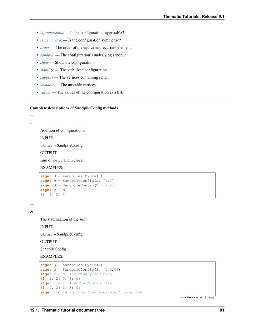
Thematic Tutorials, Release 9.1
• is_superstable — Is the configuration superstable?
• is_symmetric — Is the configuration symmetric?
• order — The order of the equivalent recurrent element.
• sandpile — The configuration’s underlying sandpile.
• show — Show the configuration.
• stabilize — The stabilized configuration.
• support — The vertices containing sand.
• unstable — The unstable vertices.
• values — The values of the configuration as a list.
Complete descriptions of SandpileConfig methods.
—
+
Addition of configurations.
INPUT:
other – SandpileConfig
OUTPUT:
sum of self and other
EXAMPLES:
sage: S = sandpiles.Cycle(3)sage: c = SandpileConfig(S, [1,2])sage: d = SandpileConfig(S, [3,2])sage: c + d1: 4, 2: 4
—
&
The stabilization of the sum.
INPUT:
other – SandpileConfig
OUTPUT:
SandpileConfig
EXAMPLES:
sage: S = sandpiles.Cycle(4)sage: c = SandpileConfig(S, [1,0,0])sage: c + c # ordinary addition1: 2, 2: 0, 3: 0sage: c & c # add and stabilize1: 0, 2: 1, 3: 0sage: c*c # add and find equivalent recurrent
(continues on next page)
12.1. Thematic tutorial document tree 81
Thematic Tutorials, Release 9.1
(continued from previous page)
1: 1, 2: 1, 3: 1sage: ~(c + c) == c & cTrue
—
>=
True if every component of self is at least that of other.
INPUT:
other – SandpileConfig
OUTPUT:
boolean
EXAMPLES:
sage: S = sandpiles.Cycle(3)sage: c = SandpileConfig(S, [1,2])sage: d = SandpileConfig(S, [2,3])sage: e = SandpileConfig(S, [2,0])sage: c >= cTruesage: d >= cTruesage: c >= dFalsesage: e >= cFalsesage: c >= eFalse
—
>
True if every component of self is at least that of other and the two configurations are not equal.
INPUT:
other – SandpileConfig
OUTPUT:
boolean
EXAMPLES:
sage: S = sandpiles.Cycle(3)sage: c = SandpileConfig(S, [1,2])sage: d = SandpileConfig(S, [1,3])sage: c > cFalsesage: d > cTruesage: c > dFalse
82 Chapter 12. Documentation
Thematic Tutorials, Release 9.1
—
~
The stabilized configuration.
OUTPUT:
SandpileConfig
EXAMPLES:
sage: S = sandpiles.House()sage: c = S.max_stable() + S.identity()sage: ~c == c.stabilize()True
—
<=
True if every component of self is at most that of other.
INPUT:
other – SandpileConfig
OUTPUT:
boolean
EXAMPLES:
sage: S = sandpiles.Cycle(3)sage: c = SandpileConfig(S, [1,2])sage: d = SandpileConfig(S, [2,3])sage: e = SandpileConfig(S, [2,0])sage: c <= cTruesage: c <= dTruesage: d <= cFalsesage: c <= eFalsesage: e <= cFalse
—
<
True if every component of self is at most that of other and the two configurations are not equal.
INPUT:
other – SandpileConfig
OUTPUT:
boolean
EXAMPLES:
12.1. Thematic tutorial document tree 83
Thematic Tutorials, Release 9.1
sage: S = sandpiles.Cycle(3)sage: c = SandpileConfig(S, [1,2])sage: d = SandpileConfig(S, [2,3])sage: c < cFalsesage: c < dTruesage: d < cFalsesage: S = Sandpile(graphs.CycleGraph(3), 0)sage: c = SandpileConfig(S, [1,2])sage: d = SandpileConfig(S, [2,3])sage: c < cFalsesage: c < dTruesage: d < cFalse
—
*
If other is an configuration, the recurrent element equivalent to the sum. If other is an integer, thesum of configuration with itself other times.
INPUT:
other – SandpileConfig or Integer
OUTPUT:
SandpileConfig
EXAMPLES:
sage: S = sandpiles.Cycle(4)sage: c = SandpileConfig(S, [1,0,0])sage: c + c # ordinary addition1: 2, 2: 0, 3: 0sage: c & c # add and stabilize1: 0, 2: 1, 3: 0sage: c*c # add and find equivalent recurrent1: 1, 2: 1, 3: 1sage: (c*c).is_recurrent()Truesage: c*(-c) == S.identity()Truesage: c1: 1, 2: 0, 3: 0sage: c*31: 3, 2: 0, 3: 0
—
^
The recurrent element equivalent to the sum of the configuration with itself 𝑘 times. If 𝑘 is negative, dothe same for the negation of the configuration. If 𝑘 is zero, return the identity of the sandpile group.
INPUT:
84 Chapter 12. Documentation
Thematic Tutorials, Release 9.1
k – SandpileConfig
OUTPUT:
SandpileConfig
EXAMPLES:
sage: S = sandpiles.Cycle(4)sage: c = SandpileConfig(S, [1,0,0])sage: c^31: 1, 2: 1, 3: 0sage: (c + c + c) == c^3Falsesage: (c + c + c).equivalent_recurrent() == c^3Truesage: c^(-1)1: 1, 2: 1, 3: 0sage: c^0 == S.identity()True
—
_
The additive inverse of the configuration.
OUTPUT:
SandpileConfig
EXAMPLES:
sage: S = sandpiles.Cycle(3)sage: c = SandpileConfig(S, [1,2])sage: -c1: -1, 2: -2
—
-
Subtraction of configurations.
INPUT:
other – SandpileConfig
OUTPUT:
sum of self and other
EXAMPLES:
sage: S = sandpiles.Cycle(3)sage: c = SandpileConfig(S, [1,2])sage: d = SandpileConfig(S, [3,2])sage: c - d1: -2, 2: 0
—
add_random(distrib=None)
12.1. Thematic tutorial document tree 85
Thematic Tutorials, Release 9.1
Add one grain of sand to a random vertex. Optionally, a probability distribution, distrib, may be placed on thevertices or the nonsink vertices. See NOTE for details.
INPUT:
distrib – (optional) list of nonnegative numbers summing to 1 (representing a prob. dist.)
OUTPUT:
SandpileConfig
EXAMPLES:
sage: s = sandpiles.Complete(4)sage: c = s.zero_config()sage: c.add_random() # random1: 0, 2: 1, 3: 0sage: c1: 0, 2: 0, 3: 0sage: c.add_random([0.1,0.1,0.8]) # random1: 0, 2: 0, 3: 1sage: c.add_random([0.7,0.1,0.1,0.1]) # random1: 0, 2: 0, 3: 0
We compute the “sizes” of the avalanches caused by adding random grains of sand to the maximal stable configurationon a grid graph. The function stabilize() returns the firing vector of the stabilization, a dictionary whose valuessay how many times each vertex fires in the stabilization.:
sage: S = sandpiles.Grid(10,10)sage: m = S.max_stable()sage: a = []sage: for i in range(1000):....: m = m.add_random()....: m, f = m.stabilize(True)....: a.append(sum(f.values()))sage: p = list_plot([[log(i+1),log(a.count(i))] for i in [0..max(a)] if a.count(i)])sage: p.axes_labels(['log(N)','log(D(N))'])sage: t = text("Distribution of avalanche sizes", (2,2), rgbcolor=(1,0,0))sage: show(p+t,axes_labels=['log(N)','log(D(N))'])
Note: If distrib is None, then the probability is the uniform probability on the nonsink vertices. Otherwise, thereare two possibilities:
(i) the length of distrib is equal to the number of vertices, and distrib represents a probability distribution onall of the vertices. In that case, the sink may be chosen at random, in which case, the configuration is unchanged.
(ii) Otherwise, the length of distrib must be equal to the number of nonsink vertices, and distrib represents aprobability distribution on the nonsink vertices.
Warning: If distrib != None, the user is responsible for assuring the sum of its entries is 1 and that itslength is equal to the number of sink vertices or the number of nonsink vertices.
—
burst_size(v)
The burst size of the configuration with respect to the given vertex.
86 Chapter 12. Documentation
Thematic Tutorials, Release 9.1
INPUT:
v – vertex
OUTPUT:
integer
EXAMPLES:
sage: s = sandpiles.Diamond()sage: [i.burst_size(0) for i in s.recurrents()][1, 1, 1, 1, 1, 1, 1, 1]sage: [i.burst_size(1) for i in s.recurrents()][0, 0, 1, 2, 1, 2, 0, 2]
Note: To define c.burst(v), if 𝑣 is not the sink, let 𝑐′ be the unique recurrent for which the stabilization of 𝑐′ + 𝑣is 𝑐. The burst size is then the amount of sand that goes into the sink during this stabilization. If 𝑣 is the sink, the burstsize is defined to be 1.
REFERENCES:
• [Levine2014]
—
deg()
The degree of the configuration.
OUTPUT:
integer
EXAMPLES:
sage: S = sandpiles.Complete(3)sage: c = SandpileConfig(S, [1,2])sage: c.deg()3
—
dualize()
The difference with the maximal stable configuration.
OUTPUT:
SandpileConfig
EXAMPLES:
sage: S = sandpiles.Cycle(3)sage: c = SandpileConfig(S, [1,2])sage: S.max_stable()1: 1, 2: 1sage: c.dualize()1: 0, 2: -1sage: S.max_stable() - c == c.dualize()True
12.1. Thematic tutorial document tree 87
Thematic Tutorials, Release 9.1
—
equivalent_recurrent(with_firing_vector=False)
The recurrent configuration equivalent to the given configuration. Optionally, return the corresponding firing vector.
INPUT:
with_firing_vector – (default: False) boolean
OUTPUT:
SandpileConfig or [SandpileConfig, firing_vector]
EXAMPLES:
sage: S = sandpiles.Diamond()sage: c = SandpileConfig(S, [0,0,0])sage: c.equivalent_recurrent() == S.identity()Truesage: x = c.equivalent_recurrent(True)sage: r = vector([x[0][v] for v in S.nonsink_vertices()])sage: f = vector([x[1][v] for v in S.nonsink_vertices()])sage: cv = vector(c.values())sage: r == cv - f*S.reduced_laplacian()True
Note: Let 𝐿 be the reduced Laplacian, 𝑐 the initial configuration, 𝑟 the returned configuration, and 𝑓 the firing vector.Then 𝑟 = 𝑐− 𝑓 · 𝐿.
—
equivalent_superstable(with_firing_vector=False)
The equivalent superstable configuration. Optionally, return the corresponding firing vector.
INPUT:
with_firing_vector – (default: False) boolean
OUTPUT:
SandpileConfig or [SandpileConfig, firing_vector]
EXAMPLES:
sage: S = sandpiles.Diamond()sage: m = S.max_stable()sage: m.equivalent_superstable().is_superstable()Truesage: x = m.equivalent_superstable(True)sage: s = vector(x[0].values())sage: f = vector(x[1].values())sage: mv = vector(m.values())sage: s == mv - f*S.reduced_laplacian()True
Note: Let 𝐿 be the reduced Laplacian, 𝑐 the initial configuration, 𝑠 the returned configuration, and 𝑓 the firing vector.Then 𝑠 = 𝑐− 𝑓 · 𝐿.
88 Chapter 12. Documentation
Thematic Tutorials, Release 9.1
—
fire_script(sigma)
Fire the given script. In other words, fire each vertex the number of times indicated by sigma.
INPUT:
sigma – SandpileConfig or (list or dict representing a SandpileConfig)
OUTPUT:
SandpileConfig
EXAMPLES:
sage: S = sandpiles.Cycle(4)sage: c = SandpileConfig(S, [1,2,3])sage: c.unstable()[2, 3]sage: c.fire_script(SandpileConfig(S,[0,1,1]))1: 2, 2: 1, 3: 2sage: c.fire_script(SandpileConfig(S,[2,0,0])) == c.fire_vertex(1).fire_vertex(1)True
—
fire_unstable()
Fire all unstable vertices.
OUTPUT:
SandpileConfig
EXAMPLES:
sage: S = sandpiles.Cycle(4)sage: c = SandpileConfig(S, [1,2,3])sage: c.fire_unstable()1: 2, 2: 1, 3: 2
—
fire_vertex(v)
Fire the given vertex.
INPUT:
v – vertex
OUTPUT:
SandpileConfig
EXAMPLES:
sage: S = sandpiles.Cycle(3)sage: c = SandpileConfig(S, [1,2])sage: c.fire_vertex(2)1: 2, 2: 0
—
help(verbose=True)
12.1. Thematic tutorial document tree 89
Thematic Tutorials, Release 9.1
List of SandpileConfig methods. If verbose, include short descriptions.
INPUT:
verbose – (default: True) boolean
OUTPUT:
printed string
EXAMPLES:
sage: SandpileConfig.help()Shortcuts for SandpileConfig operations:~c -- stabilizec & d -- add and stabilizec * c -- add and find equivalent recurrentc^k -- add k times and find equivalent recurrent
(taking inverse if k is negative)
For detailed help with any method FOO listed below,enter "SandpileConfig.FOO?" or enter "c.FOO?" for any SandpileConfig c.
add_random -- Add one grain of sand to a random vertex.burst_size -- The burst size of the configuration with respect to the→˓given vertex.deg -- The degree of the configuration.dualize -- The difference with the maximal stable configuration.equivalent_recurrent -- The recurrent configuration equivalent to the given→˓configuration.equivalent_superstable -- The equivalent superstable configuration.fire_script -- Fire the given script.fire_unstable -- Fire all unstable vertices.fire_vertex -- Fire the given vertex.help -- List of SandpileConfig methods.is_recurrent -- Is the configuration recurrent?is_stable -- Is the configuration stable?is_superstable -- Is the configuration superstable?is_symmetric -- Is the configuration symmetric?order -- The order of the equivalent recurrent element.sandpile -- The configuration's underlying sandpile.show -- Show the configuration.stabilize -- The stabilized configuration.support -- The vertices containing sand.unstable -- The unstable vertices.values -- The values of the configuration as a list.
—
is_recurrent()
Is the configuration recurrent?
OUTPUT:
boolean
EXAMPLES:
sage: S = sandpiles.Diamond()sage: S.identity().is_recurrent()True
(continues on next page)
90 Chapter 12. Documentation
Thematic Tutorials, Release 9.1
(continued from previous page)
sage: S.zero_config().is_recurrent()False
—
is_stable()
Is the configuration stable?
OUTPUT:
boolean
EXAMPLES:
sage: S = sandpiles.Diamond()sage: S.max_stable().is_stable()Truesage: (2*S.max_stable()).is_stable()Falsesage: (S.max_stable() & S.max_stable()).is_stable()True
—
is_superstable()
Is the configuration superstable?
OUTPUT:
boolean
EXAMPLES:
sage: S = sandpiles.Diamond()sage: S.zero_config().is_superstable()True
—
is_symmetric(orbits)
Is the configuration symmetric? Return True if the values of the configuration are constant over the vertices in eachsublist of orbits.
INPUT:
orbits – list of lists of vertices
OUTPUT:
boolean
EXAMPLES:
sage: S = Sandpile(0: ,....: 1: 0: 1, 2: 1, 3: 1,....: 2: 1: 1, 3: 1, 4: 1,....: 3: 1: 1, 2: 1, 4: 1,....: 4: 2: 1, 3: 1)sage: c = SandpileConfig(S, [1, 2, 2, 3])
(continues on next page)
12.1. Thematic tutorial document tree 91
Thematic Tutorials, Release 9.1
(continued from previous page)
sage: c.is_symmetric([[2,3]])True
—
order()
The order of the equivalent recurrent element.
OUTPUT:
integer
EXAMPLES:
sage: S = sandpiles.Diamond()sage: c = SandpileConfig(S,[2,0,1])sage: c.order()4sage: ~(c + c + c + c) == S.identity()Truesage: c = SandpileConfig(S,[1,1,0])sage: c.order()1sage: c.is_recurrent()Falsesage: c.equivalent_recurrent() == S.identity()True
—
sandpile()
The configuration’s underlying sandpile.
OUTPUT:
Sandpile
EXAMPLES:
sage: S = sandpiles.Diamond()sage: c = S.identity()sage: c.sandpile()Diamond sandpile graph: 4 vertices, sink = 0sage: c.sandpile() == STrue
—
show(sink=True, colors=True, heights=False, directed=None, **kwds)
Show the configuration.
INPUT:
• sink – (default: True) whether to show the sink
• colors – (default: True) whether to color-code the amount of sand on each vertex
• heights – (default: False) whether to label each vertex with the amount of sand
• directed – (optional) whether to draw directed edges
92 Chapter 12. Documentation
Thematic Tutorials, Release 9.1
• kwds – (optional) arguments passed to the show method for Graph
EXAMPLES:
sage: S = sandpiles.Diamond()sage: c = S.identity()sage: c.show()sage: c.show(directed=False)sage: c.show(sink=False,colors=False,heights=True)
—
stabilize(with_firing_vector=False)
The stabilized configuration. Optionally returns the corresponding firing vector.
INPUT:
with_firing_vector – (default: False) boolean
OUTPUT:
SandpileConfig or [SandpileConfig, firing_vector]
EXAMPLES:
sage: S = sandpiles.House()sage: c = 2*S.max_stable()sage: c._set_stabilize()sage: '_stabilize' in c.__dict__Truesage: S = sandpiles.House()sage: c = S.max_stable() + S.identity()sage: c.stabilize(True)[1: 1, 2: 2, 3: 2, 4: 1, 1: 2, 2: 2, 3: 3, 4: 3]sage: S.max_stable() & S.identity() == c.stabilize()Truesage: ~c == c.stabilize()True
—
support()
The vertices containing sand.
OUTPUT:
list - support of the configuration
EXAMPLES:
sage: S = sandpiles.Diamond()sage: c = S.identity()sage: c1: 2, 2: 2, 3: 0sage: c.support()[1, 2]
—
unstable()
The unstable vertices.
12.1. Thematic tutorial document tree 93
Thematic Tutorials, Release 9.1
OUTPUT:
list of vertices
EXAMPLES:
sage: S = sandpiles.Cycle(4)sage: c = SandpileConfig(S, [1,2,3])sage: c.unstable()[2, 3]
—
values()
The values of the configuration as a list. The list is sorted in the order of the vertices.
OUTPUT:
list of integers
boolean
EXAMPLES:
sage: S = Sandpile('a':['c','b'], 'b':['c','a'], 'c':['a'],'a')sage: c = SandpileConfig(S, 'b':1, 'c':2)sage: c'b': 1, 'c': 2sage: c.values()[1, 2]sage: S.nonsink_vertices()['b', 'c']
—
SandpileDivisor
Summary of methods.
• + — Addition of divisors.
• greater-equal — True if every component of self is at least that of other.
• greater — True if every component of self is at least that of other and the two divisors are not equal.
• less-equal — True if every component of self is at most that of other.
• less — True if every component of self is at most that of other and the two divisors are not equal.
• - — The additive inverse of the divisor.
• - — Subtraction of divisors.
• Dcomplex — The support-complex.
• add_random — Add one grain of sand to a random vertex.
• betti — The Betti numbers for the support-complex.
• deg — The degree of the divisor.
• dualize — The difference with the maximal stable divisor.
• effective_div — All linearly equivalent effective divisors.
94 Chapter 12. Documentation
Thematic Tutorials, Release 9.1
• fire_script — Fire the given script.
• fire_unstable — Fire all unstable vertices.
• fire_vertex — Fire the given vertex.
• help — List of SandpileDivisor methods.
• is_alive — Is the divisor stabilizable?
• is_linearly_equivalent — Is the given divisor linearly equivalent?
• is_q_reduced — Is the divisor q-reduced?
• is_symmetric — Is the divisor symmetric?
• is_weierstrass_pt — Is the given vertex a Weierstrass point?
• polytope — The polytope determining the complete linear system.
• polytope_integer_pts — The integer points inside divisor’s polytope.
• q_reduced — The linearly equivalent q-reduced divisor.
• rank — The rank of the divisor.
• sandpile — The divisor’s underlying sandpile.
• show — Show the divisor.
• simulate_threshold — The first unstabilizable divisor in the closed Markov chain.
• stabilize — The stabilization of the divisor.
• support — List of vertices at which the divisor is nonzero.
• unstable — The unstable vertices.
• values — The values of the divisor as a list.
• weierstrass_div — The Weierstrass divisor.
• weierstrass_gap_seq — The Weierstrass gap sequence at the given vertex.
• weierstrass_pts — The Weierstrass points (vertices).
• weierstrass_rank_seq — The Weierstrass rank sequence at the given vertex.
Complete descriptions of SandpileDivisor methods.
—
+
Addition of divisors.
INPUT:
other – SandpileDivisor
OUTPUT:
sum of self and other
EXAMPLES:
12.1. Thematic tutorial document tree 95
Thematic Tutorials, Release 9.1
sage: S = sandpiles.Cycle(3)sage: D = SandpileDivisor(S, [1,2,3])sage: E = SandpileDivisor(S, [3,2,1])sage: D + E0: 4, 1: 4, 2: 4
—
>=
True if every component of self is at least that of other.
INPUT:
other – SandpileDivisor
OUTPUT:
boolean
EXAMPLES:
sage: S = sandpiles.Cycle(3)sage: D = SandpileDivisor(S, [1,2,3])sage: E = SandpileDivisor(S, [2,3,4])sage: F = SandpileDivisor(S, [2,0,4])sage: D >= DTruesage: E >= DTruesage: D >= EFalsesage: F >= DFalsesage: D >= FFalse
—
>
True if every component of self is at least that of other and the two divisors are not equal.
INPUT:
other – SandpileDivisor
OUTPUT:
boolean
EXAMPLES:
sage: S = sandpiles.Cycle(3)sage: D = SandpileDivisor(S, [1,2,3])sage: E = SandpileDivisor(S, [1,3,4])sage: D > DFalsesage: E > DTruesage: D > EFalse
96 Chapter 12. Documentation
Thematic Tutorials, Release 9.1
—
<=
True if every component of self is at most that of other.
INPUT:
other – SandpileDivisor
OUTPUT:
boolean
EXAMPLES:
sage: S = sandpiles.Cycle(3)sage: D = SandpileDivisor(S, [1,2,3])sage: E = SandpileDivisor(S, [2,3,4])sage: F = SandpileDivisor(S, [2,0,4])sage: D <= DTruesage: D <= ETruesage: E <= DFalsesage: D <= FFalsesage: F <= DFalse
—
<
True if every component of self is at most that of other and the two divisors are not equal.
INPUT:
other – SandpileDivisor
OUTPUT:
boolean
EXAMPLES:
sage: S = sandpiles.Cycle(3)sage: D = SandpileDivisor(S, [1,2,3])sage: E = SandpileDivisor(S, [2,3,4])sage: D < DFalsesage: D < ETruesage: E < DFalse
—
-
The additive inverse of the divisor.
OUTPUT:
12.1. Thematic tutorial document tree 97
Thematic Tutorials, Release 9.1
SandpileDivisor
EXAMPLES:
sage: S = sandpiles.Cycle(3)sage: D = SandpileDivisor(S, [1,2,3])sage: -D0: -1, 1: -2, 2: -3
—
-
Subtraction of divisors.
INPUT:
other – SandpileDivisor
OUTPUT:
Difference of self and other
EXAMPLES:
sage: S = sandpiles.Cycle(3)sage: D = SandpileDivisor(S, [1,2,3])sage: E = SandpileDivisor(S, [3,2,1])sage: D - E0: -2, 1: 0, 2: 2
—
Dcomplex()
The support-complex. (See NOTE.)
OUTPUT:
simplicial complex
EXAMPLES:
sage: S = sandpiles.House()sage: p = SandpileDivisor(S, [1,2,1,0,0]).Dcomplex()sage: p.homology()0: 0, 1: Z x Z, 2: 0sage: p.f_vector()[1, 5, 10, 4]sage: p.betti()0: 1, 1: 2, 2: 0
Note: The “support-complex” is the simplicial complex determined by the supports of the linearly equivalent effectivedivisors.
—
add_random(distrib=None)
Add one grain of sand to a random vertex.
INPUT:
98 Chapter 12. Documentation
Thematic Tutorials, Release 9.1
distrib – (optional) list of nonnegative numbers representing a probability distribution on the vertices
OUTPUT:
SandpileDivisor
EXAMPLES:
sage: s = sandpiles.Complete(4)sage: D = s.zero_div()sage: D.add_random() # random0: 0, 1: 0, 2: 1, 3: 0sage: D.add_random([0.1,0.1,0.1,0.7]) # random0: 0, 1: 0, 2: 0, 3: 1
Warning: If distrib is not None, the user is responsible for assuring the sum of its entries is 1.
—
betti()
The Betti numbers for the support-complex. (See NOTE.)
OUTPUT:
dictionary of integers
EXAMPLES:
sage: S = sandpiles.Cycle(3)sage: D = SandpileDivisor(S, [2,0,1])sage: D.betti()0: 1, 1: 1
Note: The “support-complex” is the simplicial complex determined by the supports of the linearly equivalent effectivedivisors.
—
deg()
The degree of the divisor.
OUTPUT:
integer
EXAMPLES:
sage: S = sandpiles.Cycle(3)sage: D = SandpileDivisor(S, [1,2,3])sage: D.deg()6
—
dualize()
The difference with the maximal stable divisor.
12.1. Thematic tutorial document tree 99
Thematic Tutorials, Release 9.1
OUTPUT:
SandpileDivisor
EXAMPLES:: sage: S = sandpiles.Cycle(3) sage: D = SandpileDivisor(S, [1,2,3]) sage: D.dualize() 0: 0, 1: -1, 2:-2 sage: S.max_stable_div() - D == D.dualize() True
—
effective_div(verbose=True, with_firing_vectors=False)
All linearly equivalent effective divisors. If verbose is False, the divisors are converted to lists of integers. Ifwith_firing_vectors is True then a list of firing vectors is also given, each of which prescribes the vertices tobe fired in order to obtain an effective divisor.
INPUT:
• verbose – (default: True) boolean
• with_firing_vectors – (default: False) boolean
OUTPUT:
list (of divisors)
EXAMPLES:
sage: s = sandpiles.Complete(4)sage: D = SandpileDivisor(s,[4,2,0,0])sage: sorted(D.effective_div(), key=str)[0: 0, 1: 2, 2: 0, 3: 4,0: 0, 1: 2, 2: 4, 3: 0,0: 0, 1: 6, 2: 0, 3: 0,0: 1, 1: 3, 2: 1, 3: 1,0: 2, 1: 0, 2: 2, 3: 2,0: 4, 1: 2, 2: 0, 3: 0]
sage: sorted(D.effective_div(False))[[0, 2, 0, 4],[0, 2, 4, 0],[0, 6, 0, 0],[1, 3, 1, 1],[2, 0, 2, 2],[4, 2, 0, 0]]
sage: sorted(D.effective_div(with_firing_vectors=True), key=str)[(0: 0, 1: 2, 2: 0, 3: 4, (0, -1, -1, -2)),(0: 0, 1: 2, 2: 4, 3: 0, (0, -1, -2, -1)),(0: 0, 1: 6, 2: 0, 3: 0, (0, -2, -1, -1)),(0: 1, 1: 3, 2: 1, 3: 1, (0, -1, -1, -1)),(0: 2, 1: 0, 2: 2, 3: 2, (0, 0, -1, -1)),(0: 4, 1: 2, 2: 0, 3: 0, (0, 0, 0, 0))]
sage: a = _[2]sage: a[0].values()[0, 6, 0, 0]sage: vector(D.values()) - s.laplacian()*a[1](0, 6, 0, 0)sage: sorted(D.effective_div(False, True))[([0, 2, 0, 4], (0, -1, -1, -2)),([0, 2, 4, 0], (0, -1, -2, -1)),([0, 6, 0, 0], (0, -2, -1, -1)),([1, 3, 1, 1], (0, -1, -1, -1)),([2, 0, 2, 2], (0, 0, -1, -1)),([4, 2, 0, 0], (0, 0, 0, 0))]
(continues on next page)
100 Chapter 12. Documentation
Thematic Tutorials, Release 9.1
(continued from previous page)
sage: D = SandpileDivisor(s,[-1,0,0,0])sage: D.effective_div(False,True)[]
—
fire_script(sigma)
Fire the given script. In other words, fire each vertex the number of times indicated by sigma.
INPUT:
sigma – SandpileDivisor or (list or dict representing a SandpileDivisor)
OUTPUT:
SandpileDivisor
EXAMPLES:
sage: S = sandpiles.Cycle(3)sage: D = SandpileDivisor(S, [1,2,3])sage: D.unstable()[1, 2]sage: D.fire_script([0,1,1])0: 3, 1: 1, 2: 2sage: D.fire_script(SandpileDivisor(S,[2,0,0])) == D.fire_vertex(0).fire_vertex(0)True
—
fire_unstable()
Fire all unstable vertices.
OUTPUT:
SandpileDivisor
EXAMPLES:
sage: S = sandpiles.Cycle(3)sage: D = SandpileDivisor(S, [1,2,3])sage: D.fire_unstable()0: 3, 1: 1, 2: 2
—
fire_vertex(v)
Fire the given vertex.
INPUT:
v – vertex
OUTPUT:
SandpileDivisor
EXAMPLES:
12.1. Thematic tutorial document tree 101
Thematic Tutorials, Release 9.1
sage: S = sandpiles.Cycle(3)sage: D = SandpileDivisor(S, [1,2,3])sage: D.fire_vertex(1)0: 2, 1: 0, 2: 4
—
help(verbose=True)
List of SandpileDivisor methods. If verbose, include short descriptions.
INPUT:
verbose – (default: True) boolean
OUTPUT:
printed string
EXAMPLES:
sage: SandpileDivisor.help()For detailed help with any method FOO listed below,enter "SandpileDivisor.FOO?" or enter "D.FOO?" for any SandpileDivisor D.
Dcomplex -- The support-complex.add_random -- Add one grain of sand to a random vertex.betti -- The Betti numbers for the support-complex.deg -- The degree of the divisor.dualize -- The difference with the maximal stable divisor.effective_div -- All linearly equivalent effective divisors.fire_script -- Fire the given script.fire_unstable -- Fire all unstable vertices.fire_vertex -- Fire the given vertex.help -- List of SandpileDivisor methods.is_alive -- Is the divisor stabilizable?is_linearly_equivalent -- Is the given divisor linearly equivalent?is_q_reduced -- Is the divisor q-reduced?is_symmetric -- Is the divisor symmetric?is_weierstrass_pt -- Is the given vertex a Weierstrass point?polytope -- The polytope determining the complete linear system.polytope_integer_pts -- The integer points inside divisor's polytope.q_reduced -- The linearly equivalent q-reduced divisor.rank -- The rank of the divisor.sandpile -- The divisor's underlying sandpile.show -- Show the divisor.simulate_threshold -- The first unstabilizable divisor in the closed Markov chain.stabilize -- The stabilization of the divisor.support -- List of vertices at which the divisor is nonzero.unstable -- The unstable vertices.values -- The values of the divisor as a list.weierstrass_div -- The Weierstrass divisor.weierstrass_gap_seq -- The Weierstrass gap sequence at the given vertex.weierstrass_pts -- The Weierstrass points (vertices).weierstrass_rank_seq -- The Weierstrass rank sequence at the given vertex.
—
is_alive(cycle=False)
102 Chapter 12. Documentation
Thematic Tutorials, Release 9.1
Is the divisor stabilizable? In other words, will the divisor stabilize under repeated firings of all unstable vertices?Optionally returns the resulting cycle.
INPUT:
cycle – (default: False) boolean
OUTPUT:
boolean or optionally, a list of SandpileDivisors
EXAMPLES:
sage: S = sandpiles.Complete(4)sage: D = SandpileDivisor(S, 0: 4, 1: 3, 2: 3, 3: 2)sage: D.is_alive()Truesage: D.is_alive(True)[0: 4, 1: 3, 2: 3, 3: 2, 0: 3, 1: 2, 2: 2, 3: 5, 0: 1, 1: 4, 2: 4, 3: 3]
—
is_linearly_equivalent(D, with_firing_vector=False)
Is the given divisor linearly equivalent? Optionally, returns the firing vector. (See NOTE.)
INPUT:
• D – SandpileDivisor or list, tuple, etc. representing a divisor
• with_firing_vector – (default: False) boolean
OUTPUT:
boolean or integer vector
EXAMPLES:
sage: s = sandpiles.Complete(3)sage: D = SandpileDivisor(s,[2,0,0])sage: D.is_linearly_equivalent([0,1,1])Truesage: D.is_linearly_equivalent([0,1,1],True)(1, 0, 0)sage: v = vector(D.is_linearly_equivalent([0,1,1],True))sage: vector(D.values()) - s.laplacian()*v(0, 1, 1)sage: D.is_linearly_equivalent([0,0,0])Falsesage: D.is_linearly_equivalent([0,0,0],True)()
Note:
• If with_firing_vector is False, returns either True or False.
• If with_firing_vector is True then: (i) if self is linearly equivalent to 𝐷, returns a vector 𝑣 such thatself - v*self.laplacian().transpose() = D. Otherwise, (ii) if self is not linearly equivalentto 𝐷, the output is the empty vector, ().
—
12.1. Thematic tutorial document tree 103
Thematic Tutorials, Release 9.1
is_q_reduced()
Is the divisor 𝑞-reduced? This would mean that 𝑠𝑒𝑙𝑓 = 𝑐+ 𝑘𝑞 where 𝑐 is superstable, 𝑘 is an integer, and 𝑞 is the sinkvertex.
OUTPUT:
boolean
EXAMPLES:
sage: s = sandpiles.Complete(4)sage: D = SandpileDivisor(s,[2,-3,2,0])sage: D.is_q_reduced()Falsesage: SandpileDivisor(s,[10,0,1,2]).is_q_reduced()True
For undirected or, more generally, Eulerian graphs, 𝑞-reduced divisors are linearly equivalent if and only if they areequal. The same does not hold for general directed graphs:
sage: s = Sandpile(0:[1],1:[1,1])sage: D = SandpileDivisor(s,[-1,1])sage: Z = s.zero_div()sage: D.is_q_reduced()Truesage: Z.is_q_reduced()Truesage: D == ZFalsesage: D.is_linearly_equivalent(Z)True
—
is_symmetric(orbits)
Is the divisor symmetric? Return True if the values of the configuration are constant over the vertices in each sublistof orbits.
INPUT:
orbits – list of lists of vertices
OUTPUT:
boolean
EXAMPLES:
sage: S = sandpiles.House()sage: S.dict()0: 1: 1, 2: 1,1: 0: 1, 3: 1,2: 0: 1, 3: 1, 4: 1,3: 1: 1, 2: 1, 4: 1,4: 2: 1, 3: 1
sage: D = SandpileDivisor(S, [0,0,1,1,3])sage: D.is_symmetric([[2,3], [4]])True
—
104 Chapter 12. Documentation
Thematic Tutorials, Release 9.1
is_weierstrass_pt(v=’sink’)
Is the given vertex a Weierstrass point?
INPUT:
v – (default: sink) vertex
OUTPUT:
boolean
EXAMPLES:
sage: s = sandpiles.House()sage: K = s.canonical_divisor()sage: K.weierstrass_rank_seq() # sequence at the sink vertex, 0(1, 0, -1)sage: K.is_weierstrass_pt()Falsesage: K.weierstrass_rank_seq(4)(1, 0, 0, -1)sage: K.is_weierstrass_pt(4)True
Note: The vertex 𝑣 is a (generalized) Weierstrass point for divisor 𝐷 if the sequence of ranks 𝑟(𝐷 − 𝑛𝑣) for𝑛 = 0, 1, 2, . . . is not 𝑟(𝐷), 𝑟(𝐷)− 1, . . . , 0,−1,−1, . . ..
—
polytope()
The polytope determining the complete linear system.
OUTPUT:
polytope
EXAMPLES:
sage: s = sandpiles.Complete(4)sage: D = SandpileDivisor(s,[4,2,0,0])sage: p = D.polytope()sage: p.inequalities()(An inequality (-3, 1, 1) x + 2 >= 0,An inequality (1, 1, 1) x + 4 >= 0,An inequality (1, -3, 1) x + 0 >= 0,An inequality (1, 1, -3) x + 0 >= 0)
sage: D = SandpileDivisor(s,[-1,0,0,0])sage: D.polytope()The empty polyhedron in QQ^3
Note: For a divisor 𝐷, this is the intersection of (i) the polyhedron determined by the system of inequalities 𝐿𝑡𝑥 ≤ 𝐷where 𝐿𝑡 is the transpose of the Laplacian with (ii) the hyperplane 𝑥sink_vertex = 0. The polytope is thought of assitting in (𝑛− 1)-dimensional Euclidean space where 𝑛 is the number of vertices.
—
polytope_integer_pts()
12.1. Thematic tutorial document tree 105
Thematic Tutorials, Release 9.1
The integer points inside divisor’s polytope. The polytope referred to here is the one determining the divisor’s completelinear system (see the documentation for polytope).
OUTPUT:
tuple of integer vectors
EXAMPLES:
sage: s = sandpiles.Complete(4)sage: D = SandpileDivisor(s,[4,2,0,0])sage: sorted(D.polytope_integer_pts())[(-2, -1, -1),(-1, -2, -1),(-1, -1, -2),(-1, -1, -1),(0, -1, -1),(0, 0, 0)]
sage: D = SandpileDivisor(s,[-1,0,0,0])sage: D.polytope_integer_pts()()
—
q_reduced(verbose=True)
The linearly equivalent 𝑞-reduced divisor.
INPUT:
verbose – (default: True) boolean
OUTPUT:
SandpileDivisor or list representing SandpileDivisor
EXAMPLES:
sage: s = sandpiles.Complete(4)sage: D = SandpileDivisor(s,[2,-3,2,0])sage: D.q_reduced()0: -2, 1: 1, 2: 2, 3: 0sage: D.q_reduced(False)[-2, 1, 2, 0]
Note: The divisor 𝐷 is 𝑞𝑟𝑒𝑑𝑢𝑐𝑒𝑑𝑖𝑓 where 𝑐 is superstable, 𝑘 is an integer, and 𝑞 is the sink.
—
rank(with_witness=False)
The rank of the divisor. Optionally returns an effective divisor 𝐸 such that 𝐷 − 𝐸 is not winnable (has an emptycomplete linear system).
INPUT:
with_witness – (default: False) boolean
OUTPUT:
integer or (integer, SandpileDivisor)
EXAMPLES:
106 Chapter 12. Documentation
Thematic Tutorials, Release 9.1
sage: S = sandpiles.Complete(4)sage: D = SandpileDivisor(S,[4,2,0,0])sage: D.rank()3sage: D.rank(True)(3, 0: 3, 1: 0, 2: 1, 3: 0)sage: E = _[1]sage: (D - E).rank()-1
Riemann-Roch theorem::
sage: D.rank() - (S.canonical_divisor()-D).rank() == D.deg() + 1 - S.genus()True
Riemann-Roch theorem::
sage: D.rank() - (S.canonical_divisor()-D).rank() == D.deg() + 1 - S.genus()Truesage: S = Sandpile(0:[1,1,1,2],1:[0,0,0,1,1,1,2,2],2:[2,2,1,1,0],0) # multigraph
→˓with loopssage: D = SandpileDivisor(S,[4,2,0])sage: D.rank(True)(2, 0: 1, 1: 1, 2: 1)sage: S = Sandpile(0:[1,2], 1:[0,2,2], 2: [0,1],0) # directed graphsage: S.is_undirected()Falsesage: D = SandpileDivisor(S,[0,2,0])sage: D.effective_div()[0: 0, 1: 2, 2: 0, 0: 2, 1: 0, 2: 0]sage: D.rank(True)(0, 0: 0, 1: 0, 2: 1)sage: E = D.rank(True)[1]sage: (D - E).effective_div()[]
Note: The rank of a divisor 𝐷 is -1 if 𝐷 is not linearly equivalent to an effective divisor (i.e., the dollar gamerepresented by 𝐷 is unwinnable). Otherwise, the rank of 𝐷 is the largest integer 𝑟 such that 𝐷 − 𝐸 is linearlyequivalent to an effective divisor for all effective divisors 𝐸 with deg(𝐸) = 𝑟.
—
sandpile()
The divisor’s underlying sandpile.
OUTPUT:
Sandpile
EXAMPLES:
sage: S = sandpiles.Diamond()sage: D = SandpileDivisor(S,[1,-2,0,3])sage: D.sandpile()Diamond sandpile graph: 4 vertices, sink = 0
(continues on next page)
12.1. Thematic tutorial document tree 107
Thematic Tutorials, Release 9.1
(continued from previous page)
sage: D.sandpile() == STrue
—
show(heights=True, directed=None, **kwds)
Show the divisor.
INPUT:
• heights – (default: True) whether to label each vertex with the amount of sand
• directed – (optional) whether to draw directed edges
• kwds – (optional) arguments passed to the show method for Graph
EXAMPLES:
sage: S = sandpiles.Diamond()sage: D = SandpileDivisor(S,[1,-2,0,2])sage: D.show(graph_border=True,vertex_size=700,directed=False)
—
simulate_threshold(distrib=None)
The first unstabilizable divisor in the closed Markov chain. (See NOTE.)
INPUT:
distrib – (optional) list of nonnegative numbers representing a probability distribution on the vertices
OUTPUT:
SandpileDivisor
EXAMPLES:
sage: s = sandpiles.Complete(4)sage: D = s.zero_div()sage: D.simulate_threshold() # random0: 2, 1: 3, 2: 1, 3: 2sage: n(mean([D.simulate_threshold().deg() for _ in range(10)])) # random7.10000000000000sage: n(s.stationary_density()*s.num_verts())6.93750000000000
Note: Starting at self, repeatedly choose a vertex and add a grain of sand to it. Return the first unstabilizable divisorthat is reached. Also see the markov_chain method for the underlying sandpile.
—
stabilize(with_firing_vector=False)
The stabilization of the divisor. If not stabilizable, return an error.
INPUT:
with_firing_vector – (default: False) boolean
EXAMPLES:
108 Chapter 12. Documentation
Thematic Tutorials, Release 9.1
sage: s = sandpiles.Complete(4)sage: D = SandpileDivisor(s,[0,3,0,0])sage: D.stabilize()0: 1, 1: 0, 2: 1, 3: 1sage: D.stabilize(with_firing_vector=True)[0: 1, 1: 0, 2: 1, 3: 1, 0: 0, 1: 1, 2: 0, 3: 0]
—
support()
List of vertices at which the divisor is nonzero.
OUTPUT:
list representing the support of the divisor
EXAMPLES:
sage: S = sandpiles.Cycle(4)sage: D = SandpileDivisor(S, [0,0,1,1])sage: D.support()[2, 3]sage: S.vertices()[0, 1, 2, 3]
—
unstable()
The unstable vertices.
OUTPUT:
list of vertices
EXAMPLES:
sage: S = sandpiles.Cycle(3)sage: D = SandpileDivisor(S, [1,2,3])sage: D.unstable()[1, 2]
—
values()
The values of the divisor as a list. The list is sorted in the order of the vertices.
OUTPUT:
list of integers
boolean
EXAMPLES:
sage: S = Sandpile('a':['c','b'], 'b':['c','a'], 'c':['a'],'a')sage: D = SandpileDivisor(S, 'a':0, 'b':1, 'c':2)sage: D'a': 0, 'b': 1, 'c': 2sage: D.values()[0, 1, 2]
(continues on next page)
12.1. Thematic tutorial document tree 109
Thematic Tutorials, Release 9.1
(continued from previous page)
sage: S.vertices()['a', 'b', 'c']
—
weierstrass_div(verbose=True)
The Weierstrass divisor. Its value at a vertex is the weight of that vertex as a Weierstrass point. (SeeSandpileDivisor.weierstrass_gap_seq.)
INPUT:
verbose – (default: True) boolean
OUTPUT:
SandpileDivisor
EXAMPLES:
sage: s = sandpiles.Diamond()sage: D = SandpileDivisor(s,[4,2,1,0])sage: [D.weierstrass_rank_seq(v) for v in s][(5, 4, 3, 2, 1, 0, 0, -1),(5, 4, 3, 2, 1, 0, -1),(5, 4, 3, 2, 1, 0, 0, 0, -1),(5, 4, 3, 2, 1, 0, 0, -1)]
sage: D.weierstrass_div()0: 1, 1: 0, 2: 2, 3: 1sage: k5 = sandpiles.Complete(5)sage: K = k5.canonical_divisor()sage: K.weierstrass_div()0: 9, 1: 9, 2: 9, 3: 9, 4: 9
—
weierstrass_gap_seq(v=’sink’, weight=True)
The Weierstrass gap sequence at the given vertex. If weight is True, then also compute the weight of each gapvalue.
INPUT:
• v – (default: sink) vertex
• weight – (default: True) boolean
OUTPUT:
list or (list of list) of integers
EXAMPLES:
sage: s = sandpiles.Cycle(4)sage: D = SandpileDivisor(s,[2,0,0,0])sage: [D.weierstrass_gap_seq(v,False) for v in s.vertices()][(1, 3), (1, 2), (1, 3), (1, 2)]sage: [D.weierstrass_gap_seq(v) for v in s.vertices()][((1, 3), 1), ((1, 2), 0), ((1, 3), 1), ((1, 2), 0)]sage: D.weierstrass_gap_seq() # gap sequence at sink vertex, 0((1, 3), 1)
(continues on next page)
110 Chapter 12. Documentation
Thematic Tutorials, Release 9.1
(continued from previous page)
sage: D.weierstrass_rank_seq() # rank sequence at the sink vertex(1, 0, 0, -1)
Note: The integer 𝑘 is a Weierstrass gap for the divisor 𝐷 at vertex 𝑣 if the rank of 𝐷 − (𝑘 − 1)𝑣 does not equal therank of 𝐷− 𝑘𝑣. Let 𝑟 be the rank of 𝐷 and let 𝑘𝑖 be the 𝑖-th gap at 𝑣. The Weierstrass weight of 𝑣 for 𝐷 is the sum of(𝑘𝑖 − 𝑖) as 𝑖 ranges from 1 to 𝑟 + 1. It measure the difference between the sequence 𝑟, 𝑟 − 1, ..., 0,−1,−1, ... and therank sequence rank(𝐷), rank(𝐷 − 𝑣), rank(𝐷 − 2𝑣), . . .
—
weierstrass_pts(with_rank_seq=False)
The Weierstrass points (vertices). Optionally, return the corresponding rank sequences.
INPUT:
with_rank_seq – (default: False) boolean
OUTPUT:
tuple of vertices or list of (vertex, rank sequence)
EXAMPLES:
sage: s = sandpiles.House()sage: K = s.canonical_divisor()sage: K.weierstrass_pts()(4,)sage: K.weierstrass_pts(True)[(4, (1, 0, 0, -1))]
Note: The vertex 𝑣 is a (generalized) Weierstrass point for divisor 𝐷 if the sequence of ranks 𝑟(𝐷 − 𝑛𝑣) for𝑛 = 0, 1, 2, . . . is not 𝑟(𝐷), 𝑟(𝐷)− 1, . . . , 0,−1,−1, . . .
—
weierstrass_rank_seq(v=’sink’)
The Weierstrass rank sequence at the given vertex. Computes the rank of the divisor 𝐷 − 𝑛𝑣 starting with 𝑛 = 0 andending when the rank is −1.
INPUT:
v – (default: sink) vertex
OUTPUT:
tuple of int
EXAMPLES:
sage: s = sandpiles.House()sage: K = s.canonical_divisor()sage: [K.weierstrass_rank_seq(v) for v in s.vertices()][(1, 0, -1), (1, 0, -1), (1, 0, -1), (1, 0, -1), (1, 0, 0, -1)]
—
12.1. Thematic tutorial document tree 111
Thematic Tutorials, Release 9.1
Other
• firing_graph — The firing graph.
• parallel_firing_graph — The parallel-firing graph.
• random_DAG — A random directed acyclic graph.
• sandpiles — Some examples of sandpiles.
• wilmes_algorithm — Find matrix with the same integer row span as M that is the reduced Laplacian of a digraph.
Complete descriptions of methods.
firing_graph(S, eff)
Creates a digraph with divisors as vertices and edges between two divisors 𝐷 and 𝐸 if firing a singlevertex in 𝐷 gives 𝐸.
INPUT:
S – Sandpile eff – list of divisors
OUTPUT:
DiGraph
EXAMPLES:
sage: S = sandpiles.Cycle(6)sage: D = SandpileDivisor(S, [1,1,1,1,2,0])sage: eff = D.effective_div()sage: firing_graph(S,eff).show3d(edge_size=.005,vertex_size=0.01)
—
parallel_firing_graph(S,eff)
Creates a digraph with divisors as vertices and edges between two divisors D and E if firing all unstablevertices in D gives E.
INPUT:
S - Sandpile eff - list of divisors
OUTPUT:
DiGraph
EXAMPLES:
sage: S = Sandpile(graphs.CycleGraph(6),0)sage: D = SandpileDivisor(S, [1,1,1,1,2,0])sage: eff = D.effective_div()sage: parallel_firing_graph(S,eff).show3d(edge_size=.005,vertex_size=0.01)
—
random_DAG(num_verts,p=1/2,weight_max=1)
Returns a random directed acyclic graph with num_verts vertices. The method starts with the sinkvertex and adds vertices one at a time. Each vertex is connected only to only previously defined vertices,and the probability of each possible connection is given by the argument p. The weight of an edge is arandom integer between 1 and weight_max.
112 Chapter 12. Documentation
Thematic Tutorials, Release 9.1
INPUT:
• num_verts - positive integer
• p - number between 0 and 1
• weight_max – integer greater than 0
OUTPUT:
directed acyclic graph with sink 0
EXAMPLES:
sage: S = random_DAG(5, 0.3)
—
sandpiles
Some examples of sandpiles.
Here are the available examples; you can also type “sandpiles.” and hit tab to get a list:
• “Complete()”
• “Cycle()”
• “Diamond()”
• “Grid()”
• “House()”
EXAMPLES:
sage: s = sandpiles.Complete(4)sage: s.invariant_factors()[1, 4, 4]sage: s.laplacian()[ 3 -1 -1 -1][-1 3 -1 -1][-1 -1 3 -1][-1 -1 -1 3]
—
wilmes_algorithm(M)
Computes an integer matrix L with the same integer row span as M and such that L is the reduced laplacianof a directed multigraph.
INPUT:
M - square integer matrix of full rank
OUTPUT:
L - integer matrix
EXAMPLES:
sage: P = matrix([[2,3,-7,-3],[5,2,-5,5],[8,2,5,4],[-5,-9,6,6]])sage: wilmes_algorithm(P)[ 1642 -13 -1627 -1][ -1 1980 -1582 -397]
(continues on next page)
12.1. Thematic tutorial document tree 113
Thematic Tutorials, Release 9.1
(continued from previous page)
[ 0 -1 1650 -1649][ 0 0 -1658 1658]
NOTES:
The algorithm is due to John Wilmes.
Help
Documentation for each method is available through the Sage online help system:
sage: SandpileConfig.fire_vertex?Base Class: <type 'instancemethod'>String Form: <unbound method SandpileConfig.fire_vertex>Namespace: InteractiveFile: /usr/local/sage-4.7/local/lib/python2.6/site-packages/sage/sandpiles/→˓sandpile.pyDefinition: SandpileConfig.fire_vertex(self, v)Docstring:
Fire the vertex ``v``.
INPUT:
``v`` - vertex
OUTPUT:
SandpileConfig
EXAMPLES:
sage: S = Sandpile(graphs.CycleGraph(3), 0)sage: c = SandpileConfig(S, [1,2])sage: c.fire_vertex(2)1: 2, 2: 0
Note: An alternative to SandpileConfig.fire_vertex? in the preceding code example would be c.fire_vertex?, if c is any SandpileConfig.
Enter Sandpile.help(), SandpileConfig.help(), and SandpileDivisor.help() for lists of avail-able Sandpile-specific methods.
General Sage documentation can be found at http://doc.sagemath.org/html/en/.
Contact
Please contact [email protected] with questions, bug reports, and suggestions for additional features and other im-provements.
12.1.4 Group Theory and Sage
Author: Robert A. Beezer, University of Puget Sound
114 Chapter 12. Documentation
Thematic Tutorials, Release 9.1
This compilation collects Sage commands that are useful for a student in an introductory course on group theory. Itis not intended to teach Sage or to teach group theory. (There are many introductory texts on group theory and moreinformation on Sage can be found via www.sagemath.org) Rather, by presenting commands roughly in the order astudent would learn the corresponding mathematics they might be encouraged to experiment and learn more aboutmathematics and learn more about Sage. Not coincidentally, when Sage was the acronym SAGE, the “E” in Sagestood for “Experimentation.”
This guide is also distributed in PDF format and as a Sage worksheet. The worksheet version can be imported intothe Sage notebook environment running in a web browser, and then the displayed chunks of code may be executed bySage if one clicks on the small “evaluate” link below each cell, for a fully interactive experience. A PDF and Sageworksheet versions of this tutorial are available at http://abstract.ups.edu/sage-aata.html.
Table of contents
• Group Theory and Sage
– Basic properties of the integers
– Permutation groups
– Group functions
– Subgroups
– Symmetry groups
– Normal subgroups
– Conjugacy
– Sylow subgroups
– Groups of small order as permutation groups
– Acknowledgements
Changelog:
• 2009/01/30 Version 1.0, first complete release
• 2009/03/03 Version 1.1, added cyclic group size interact
• 2010/03/10 Version 1.3, dropped US on license, some edits.
Basic properties of the integers
Integer division
The command a % b will return the remainder upon division of 𝑎 by 𝑏. In other words, the value is the unique integer𝑟 such that:
1. 0 ≤ 𝑟 < 𝑏; and
2. 𝑎 = 𝑏𝑞 + 𝑟 for some integer 𝑞 (the quotient).
Then (𝑎− 𝑟)/𝑏 will equal 𝑞. For example:
sage: r = 14 % 3sage: q = (14 - r) / 3
(continues on next page)
12.1. Thematic tutorial document tree 115
Thematic Tutorials, Release 9.1
(continued from previous page)
sage: r, q(2, 4)
will return 2 for the value of r and 4 for the value of q. Note that the “/” is integer division, where any remainder iscast away and the result is always an integer. So, for example, 14 / 3 will again equal 4, not 4.66666.
Greatest common divisor
The greatest common divisor of 𝑎 and 𝑏 is obtained with the command gcd(a,b), where in our first uses, 𝑎 and 𝑏are integers. Later, 𝑎 and 𝑏 can be other objects with a notion of divisibility and “greatness,” such as polynomials. Forexample:
sage: gcd(2776, 2452)4
Extended greatest common divisor
The command xgcd(a, b) (“eXtended GCD”) returns a triple where the first element is the greatest commondivisor of 𝑎 and 𝑏 (as with the gcd(a, b) command above), but the next two elements are the values of 𝑟 and 𝑠such that 𝑟𝑎+ 𝑠𝑏 = gcd(𝑎, 𝑏). For example, xgcd(633, 331) returns (1, 194, -371). Portions of the triplecan be extracted using [ ] to access the entries of the triple, starting with the first as number 0. For example, thefollowing should return the result True (even if you change the values of a and b). Studying this block of code willgo a long way towards helping you get the most out of Sage’s output. (Note that “=” is how a value is assigned to avariable, while as in the last line, “==” is how we determine equality of two items.)
sage: a = 633sage: b = 331sage: extended = xgcd(a, b)sage: g = extended[0]sage: r = extended[1]sage: s = extended[2]sage: g == r*a + s*bTrue
Divisibility
A remainder of zero indicates divisibility. So (a % b) == 0 will return True if 𝑏 divides 𝑎, and will otherwisereturn False. For example, (9 % 3) == 0 is True, but (9 % 4) == 0 is False. Try predicting the outputof the following before executing it in Sage.
sage: answer1 = ((20 % 5) == 0)sage: answer2 = ((17 % 4) == 0)sage: answer1, answer2(True, False)
Factoring
As promised by the Fundamental Theorem of Arithmetic, factor(a) will return a unique expression for 𝑎 as aproduct of powers of primes. It will print in a nicely-readable form, but can also be manipulated with Python as a listof pairs (𝑝𝑖, 𝑒𝑖) containing primes as bases, and their associated exponents. For example:
116 Chapter 12. Documentation
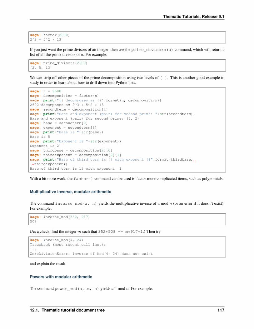
Thematic Tutorials, Release 9.1
sage: factor(2600)2^3 * 5^2 * 13
If you just want the prime divisors of an integer, then use the prime_divisors(a) command, which will return alist of all the prime divisors of 𝑎. For example:
sage: prime_divisors(2600)[2, 5, 13]
We can strip off other pieces of the prime decomposition using two levels of [ ]. This is another good example tostudy in order to learn about how to drill down into Python lists.
sage: n = 2600sage: decomposition = factor(n)sage: print(" decomposes as ".format(n, decomposition))2600 decomposes as 2^3 * 5^2 * 13sage: secondterm = decomposition[1]sage: print("Base and exponent (pair) for second prime: "+str(secondterm))Base and exponent (pair) for second prime: (5, 2)sage: base = secondterm[0]sage: exponent = secondterm[1]sage: print("Base is "+str(base))Base is 5sage: print("Exponent is "+str(exponent))Exponent is 2sage: thirdbase = decomposition[2][0]sage: thirdexponent = decomposition[2][1]sage: print("Base of third term is with exponent ".format(thirdbase,→˓thirdexponent))Base of third term is 13 with exponent 1
With a bit more work, the factor() command can be used to factor more complicated items, such as polynomials.
Multiplicative inverse, modular arithmetic
The command inverse_mod(a, n) yields the multiplicative inverse of 𝑎 mod 𝑛 (or an error if it doesn’t exist).For example:
sage: inverse_mod(352, 917)508
(As a check, find the integer 𝑚 such that 352*508 == m*917+1.) Then try
sage: inverse_mod(4, 24)Traceback (most recent call last):...ZeroDivisionError: inverse of Mod(4, 24) does not exist
and explain the result.
Powers with modular arithmetic
The command power_mod(a, m, n) yields 𝑎𝑚 mod 𝑛. For example:
12.1. Thematic tutorial document tree 117
Thematic Tutorials, Release 9.1
sage: power_mod(15, 831, 23)10
If 𝑚 = −1, then this command will duplicate the function of inverse_mod().
Euler 𝜑-function
The command euler_phi(n) will return the number of positive integers less than 𝑛 and relatively prime to 𝑛 (i.e.having greatest common divisor with 𝑛 equal to 1). For example:
sage: euler_phi(345)176
Experiment by running the following code several times:
sage: m = random_prime(10000)sage: n = random_prime(10000)sage: euler_phi(m*n) == euler_phi(m) * euler_phi(n)True
Feel a conjecture coming on? Can you generalize this result?
Primes
The command is_prime(a) returns True or False depending on if 𝑎 is prime or not. For example,
sage: is_prime(117371)True
while
sage: is_prime(14547073)False
since 14547073 = 1597 * 9109 (as you could determine with the factor() command).
The command random_prime(a, True) will return a random prime between 2 and 𝑎. Experiment with:
sage: p = random_prime(10^21, True)sage: is_prime(p)True
(Replacing True by False will speed up the search, but there will be a very small probability the result will not beprime.)
The command prime_range(a, b) returns an ordered list of all the primes from 𝑎 to 𝑏 − 1, inclusive. Forexample,
sage: prime_range(500, 550)[503, 509, 521, 523, 541, 547]
The commands next_prime(a) and previous_prime(a) are other ways to get a single prime number of adesired size. Give them a try.
118 Chapter 12. Documentation
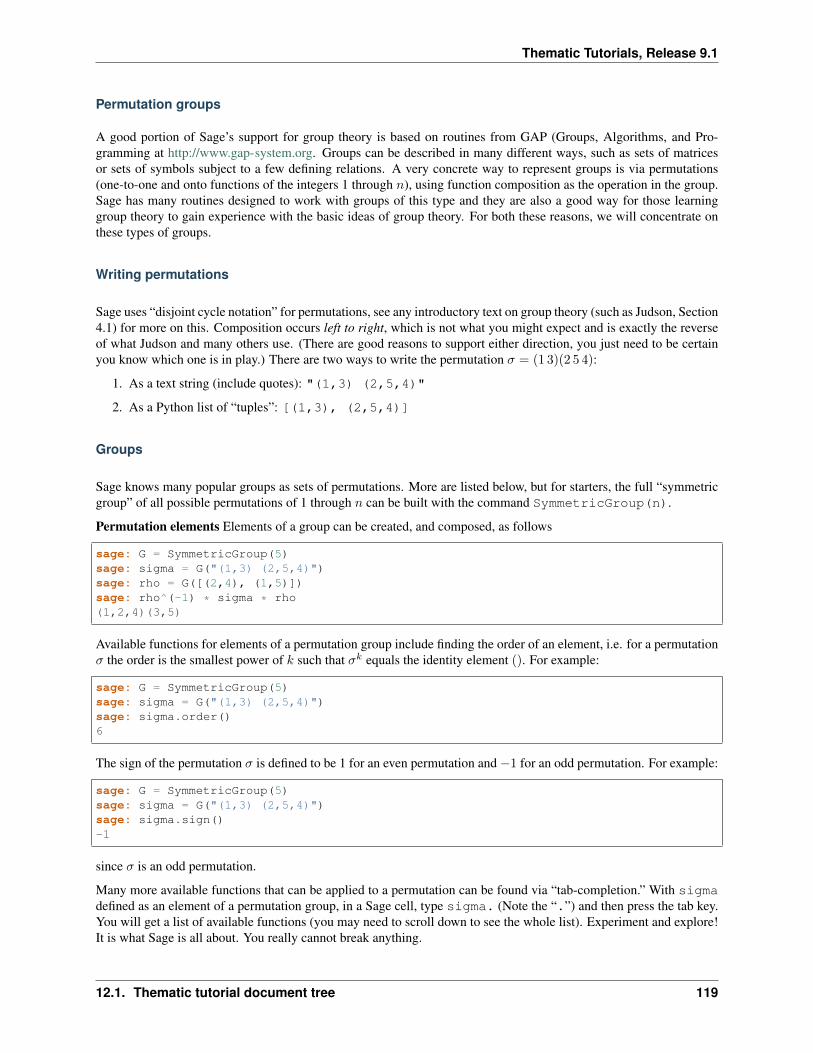
Thematic Tutorials, Release 9.1
Permutation groups
A good portion of Sage’s support for group theory is based on routines from GAP (Groups, Algorithms, and Pro-gramming at http://www.gap-system.org. Groups can be described in many different ways, such as sets of matricesor sets of symbols subject to a few defining relations. A very concrete way to represent groups is via permutations(one-to-one and onto functions of the integers 1 through 𝑛), using function composition as the operation in the group.Sage has many routines designed to work with groups of this type and they are also a good way for those learninggroup theory to gain experience with the basic ideas of group theory. For both these reasons, we will concentrate onthese types of groups.
Writing permutations
Sage uses “disjoint cycle notation” for permutations, see any introductory text on group theory (such as Judson, Section4.1) for more on this. Composition occurs left to right, which is not what you might expect and is exactly the reverseof what Judson and many others use. (There are good reasons to support either direction, you just need to be certainyou know which one is in play.) There are two ways to write the permutation 𝜎 = (1 3)(2 5 4):
1. As a text string (include quotes): "(1,3) (2,5,4)"
2. As a Python list of “tuples”: [(1,3), (2,5,4)]
Groups
Sage knows many popular groups as sets of permutations. More are listed below, but for starters, the full “symmetricgroup” of all possible permutations of 1 through 𝑛 can be built with the command SymmetricGroup(n).
Permutation elements Elements of a group can be created, and composed, as follows
sage: G = SymmetricGroup(5)sage: sigma = G("(1,3) (2,5,4)")sage: rho = G([(2,4), (1,5)])sage: rho^(-1) * sigma * rho(1,2,4)(3,5)
Available functions for elements of a permutation group include finding the order of an element, i.e. for a permutation𝜎 the order is the smallest power of 𝑘 such that 𝜎𝑘 equals the identity element (). For example:
sage: G = SymmetricGroup(5)sage: sigma = G("(1,3) (2,5,4)")sage: sigma.order()6
The sign of the permutation 𝜎 is defined to be 1 for an even permutation and−1 for an odd permutation. For example:
sage: G = SymmetricGroup(5)sage: sigma = G("(1,3) (2,5,4)")sage: sigma.sign()-1
since 𝜎 is an odd permutation.
Many more available functions that can be applied to a permutation can be found via “tab-completion.” With sigmadefined as an element of a permutation group, in a Sage cell, type sigma. (Note the “.”) and then press the tab key.You will get a list of available functions (you may need to scroll down to see the whole list). Experiment and explore!It is what Sage is all about. You really cannot break anything.
12.1. Thematic tutorial document tree 119
Thematic Tutorials, Release 9.1
Creating groups
This is an annotated list of some small well-known permutation groups that can be created simply in Sage. You canfind more in the source code file
SAGE_ROOT/src/sage/groups/perm_gps/permgroup_named.py
• SymmetricGroup(n): All 𝑛! permutations on 𝑛 symbols.
• DihedralGroup(n): Symmetries of an 𝑛-gon. Rotations and flips, 2𝑛 in total.
• CyclicPermutationGroup(n): Rotations of an 𝑛-gon (no flips), 𝑛 in total.
• AlternatingGroup(n): Alternating group on 𝑛 symbols having 𝑛!/2 elements.
• KleinFourGroup(): The non-cyclic group of order 4.
Group functions
Individual elements of permutation groups are important, but we primarily wish to study groups as objects on theirown. So a wide variety of computations are available for groups. Define a group, for example
sage: H = DihedralGroup(6)sage: HDihedral group of order 12 as a permutation group
and then a variety of functions become available.
After trying the examples below, experiment with tab-completion. Having defined H, type H. (note the “.”) and thenpress the tab key. You will get a list of available functions (you may need to scroll down to see the whole list). Asbefore, experiment and explore—it is really hard to break anything.
Here is another couple of ways to experiment and explore. Find a function that looks interesting, say is_abelian().Type H.is_abelian? (note the question mark) followed by the enter key. This will display a portion of the sourcecode for the is_abelian() function, describing the inputs and output, possibly illustrated with example uses.
If you want to learn more about how Sage works, or possibly extend its functionality, then you can start by examiningthe complete Python source code. For example, try H.is_abelian??, which will allow you to determine that theis_abelian() function is basically riding on GAP’s IsAbelian() command and asking GAP do the heavy-lifting for us. (To get the maximum advantage of using Sage it helps to know some basic Python programming, but itis not required.)
OK, on to some popular command for groups. If you are using the worksheet, be sure you have defined the group 𝐻as the dihedral group 𝐷6, since we will not keep repeating its definition below.
Abelian?
The command
sage: H = DihedralGroup(6)sage: H.is_abelian()False
will return False since 𝐷6 is a non-abelian group.
120 Chapter 12. Documentation
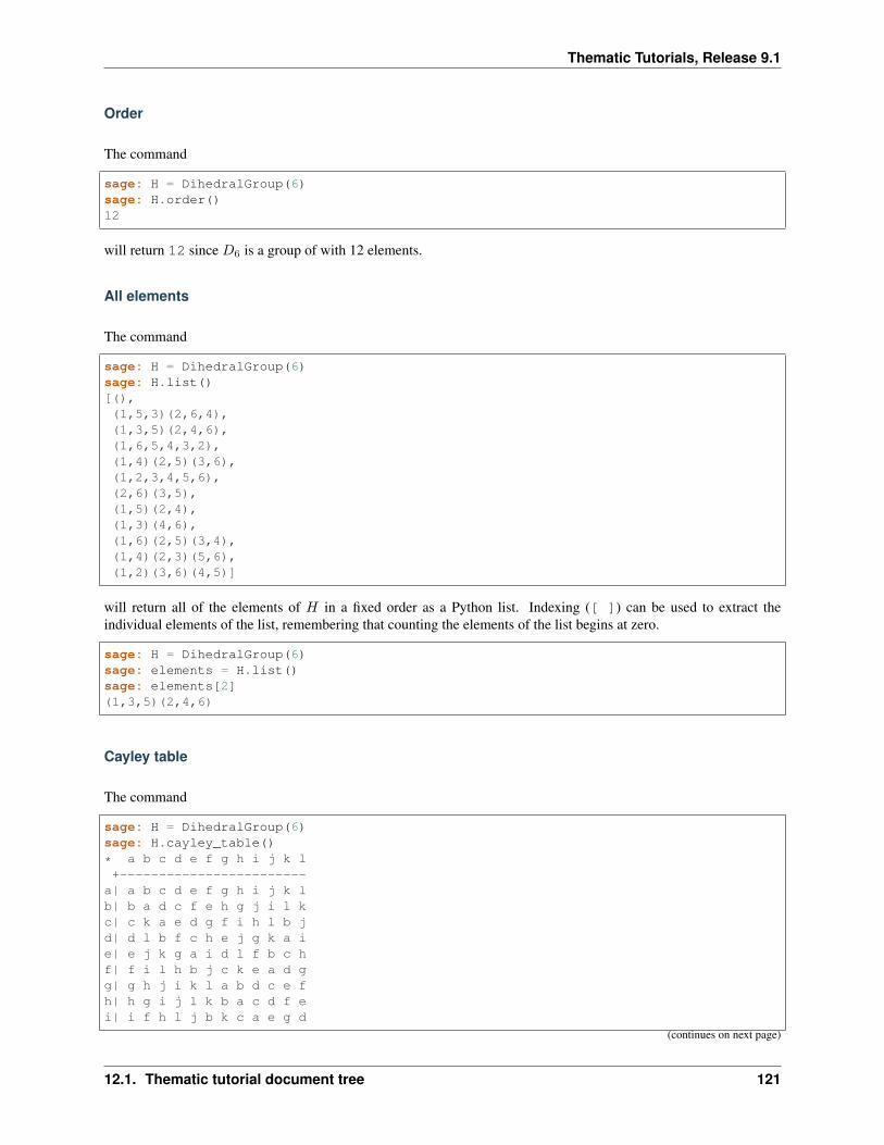
Thematic Tutorials, Release 9.1
Order
The command
sage: H = DihedralGroup(6)sage: H.order()12
will return 12 since 𝐷6 is a group of with 12 elements.
All elements
The command
sage: H = DihedralGroup(6)sage: H.list()[(),(1,5,3)(2,6,4),(1,3,5)(2,4,6),(1,6,5,4,3,2),(1,4)(2,5)(3,6),(1,2,3,4,5,6),(2,6)(3,5),(1,5)(2,4),(1,3)(4,6),(1,6)(2,5)(3,4),(1,4)(2,3)(5,6),(1,2)(3,6)(4,5)]
will return all of the elements of 𝐻 in a fixed order as a Python list. Indexing ([ ]) can be used to extract theindividual elements of the list, remembering that counting the elements of the list begins at zero.
sage: H = DihedralGroup(6)sage: elements = H.list()sage: elements[2](1,3,5)(2,4,6)
Cayley table
The command
sage: H = DihedralGroup(6)sage: H.cayley_table()
* a b c d e f g h i j k l+------------------------
a| a b c d e f g h i j k lb| b a d c f e h g j i l kc| c k a e d g f i h l b jd| d l b f c h e j g k a ie| e j k g a i d l f b c hf| f i l h b j c k e a d gg| g h j i k l a b d c e fh| h g i j l k b a c d f ei| i f h l j b k c a e g d
(continues on next page)
12.1. Thematic tutorial document tree 121
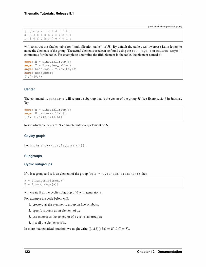
Thematic Tutorials, Release 9.1
(continued from previous page)
j| j e g k i a l d b f h ck| k c e a g d i f l h j bl| l d f b h c j e k g i a
will construct the Cayley table (or “multiplication table”) of 𝐻 . By default the table uses lowercase Latin letters toname the elements of the group. The actual elements used can be found using the row_keys() or column_keys()commands for the table. For example to determine the fifth element in the table, the element named e:
sage: H = DihedralGroup(6)sage: T = H.cayley_table()sage: headings = T.row_keys()sage: headings[4](1,3)(4,6)
Center
The command H.center() will return a subgroup that is the center of the group 𝐻 (see Exercise 2.46 in Judson).Try
sage: H = DihedralGroup(6)sage: H.center().list()[(), (1,4)(2,5)(3,6)]
to see which elements of 𝐻 commute with every element of 𝐻 .
Cayley graph
For fun, try show(H.cayley_graph()).
Subgroups
Cyclic subgroups
If G is a group and a is an element of the group (try a = G.random_element()), then
a = G.random_element()H = G.subgroup([a])
will create H as the cyclic subgroup of G with generator a.
For example the code below will:
1. create G as the symmetric group on five symbols;
2. specify sigma as an element of G;
3. use sigma as the generator of a cyclic subgroup H;
4. list all the elements of H.
In more mathematical notation, we might write ⟨(1 2 3)(4 5)⟩ = 𝐻 ⊆ 𝐺 = 𝑆5.
122 Chapter 12. Documentation
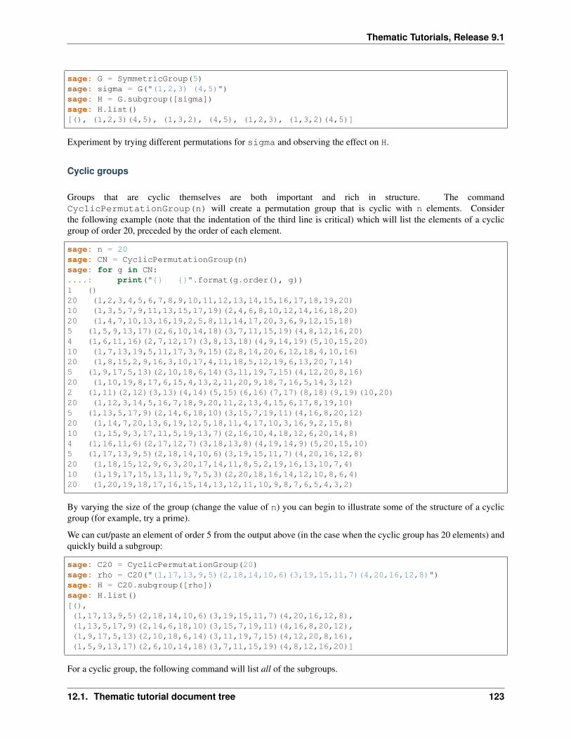
Thematic Tutorials, Release 9.1
sage: G = SymmetricGroup(5)sage: sigma = G("(1,2,3) (4,5)")sage: H = G.subgroup([sigma])sage: H.list()[(), (1,2,3)(4,5), (1,3,2), (4,5), (1,2,3), (1,3,2)(4,5)]
Experiment by trying different permutations for sigma and observing the effect on H.
Cyclic groups
Groups that are cyclic themselves are both important and rich in structure. The commandCyclicPermutationGroup(n) will create a permutation group that is cyclic with n elements. Considerthe following example (note that the indentation of the third line is critical) which will list the elements of a cyclicgroup of order 20, preceded by the order of each element.
sage: n = 20sage: CN = CyclicPermutationGroup(n)sage: for g in CN:....: print(" ".format(g.order(), g))1 ()20 (1,2,3,4,5,6,7,8,9,10,11,12,13,14,15,16,17,18,19,20)10 (1,3,5,7,9,11,13,15,17,19)(2,4,6,8,10,12,14,16,18,20)20 (1,4,7,10,13,16,19,2,5,8,11,14,17,20,3,6,9,12,15,18)5 (1,5,9,13,17)(2,6,10,14,18)(3,7,11,15,19)(4,8,12,16,20)4 (1,6,11,16)(2,7,12,17)(3,8,13,18)(4,9,14,19)(5,10,15,20)10 (1,7,13,19,5,11,17,3,9,15)(2,8,14,20,6,12,18,4,10,16)20 (1,8,15,2,9,16,3,10,17,4,11,18,5,12,19,6,13,20,7,14)5 (1,9,17,5,13)(2,10,18,6,14)(3,11,19,7,15)(4,12,20,8,16)20 (1,10,19,8,17,6,15,4,13,2,11,20,9,18,7,16,5,14,3,12)2 (1,11)(2,12)(3,13)(4,14)(5,15)(6,16)(7,17)(8,18)(9,19)(10,20)20 (1,12,3,14,5,16,7,18,9,20,11,2,13,4,15,6,17,8,19,10)5 (1,13,5,17,9)(2,14,6,18,10)(3,15,7,19,11)(4,16,8,20,12)20 (1,14,7,20,13,6,19,12,5,18,11,4,17,10,3,16,9,2,15,8)10 (1,15,9,3,17,11,5,19,13,7)(2,16,10,4,18,12,6,20,14,8)4 (1,16,11,6)(2,17,12,7)(3,18,13,8)(4,19,14,9)(5,20,15,10)5 (1,17,13,9,5)(2,18,14,10,6)(3,19,15,11,7)(4,20,16,12,8)20 (1,18,15,12,9,6,3,20,17,14,11,8,5,2,19,16,13,10,7,4)10 (1,19,17,15,13,11,9,7,5,3)(2,20,18,16,14,12,10,8,6,4)20 (1,20,19,18,17,16,15,14,13,12,11,10,9,8,7,6,5,4,3,2)
By varying the size of the group (change the value of n) you can begin to illustrate some of the structure of a cyclicgroup (for example, try a prime).
We can cut/paste an element of order 5 from the output above (in the case when the cyclic group has 20 elements) andquickly build a subgroup:
sage: C20 = CyclicPermutationGroup(20)sage: rho = C20("(1,17,13,9,5)(2,18,14,10,6)(3,19,15,11,7)(4,20,16,12,8)")sage: H = C20.subgroup([rho])sage: H.list()[(),(1,17,13,9,5)(2,18,14,10,6)(3,19,15,11,7)(4,20,16,12,8),(1,13,5,17,9)(2,14,6,18,10)(3,15,7,19,11)(4,16,8,20,12),(1,9,17,5,13)(2,10,18,6,14)(3,11,19,7,15)(4,12,20,8,16),(1,5,9,13,17)(2,6,10,14,18)(3,7,11,15,19)(4,8,12,16,20)]
For a cyclic group, the following command will list all of the subgroups.
12.1. Thematic tutorial document tree 123
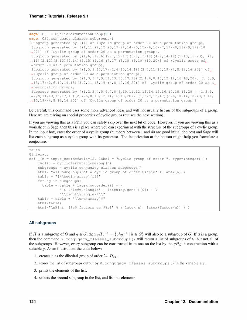
Thematic Tutorials, Release 9.1
sage: C20 = CyclicPermutationGroup(20)sage: C20.conjugacy_classes_subgroups()[Subgroup generated by [()] of (Cyclic group of order 20 as a permutation group),Subgroup generated by [(1,11)(2,12)(3,13)(4,14)(5,15)(6,16)(7,17)(8,18)(9,19)(10,→˓20)] of (Cyclic group of order 20 as a permutation group),Subgroup generated by [(1,6,11,16)(2,7,12,17)(3,8,13,18)(4,9,14,19)(5,10,15,20), (1,→˓11)(2,12)(3,13)(4,14)(5,15)(6,16)(7,17)(8,18)(9,19)(10,20)] of (Cyclic group of→˓order 20 as a permutation group),Subgroup generated by [(1,5,9,13,17)(2,6,10,14,18)(3,7,11,15,19)(4,8,12,16,20)] of→˓(Cyclic group of order 20 as a permutation group),Subgroup generated by [(1,3,5,7,9,11,13,15,17,19)(2,4,6,8,10,12,14,16,18,20), (1,5,9,→˓13,17)(2,6,10,14,18)(3,7,11,15,19)(4,8,12,16,20)] of (Cyclic group of order 20 as a→˓permutation group),Subgroup generated by [(1,2,3,4,5,6,7,8,9,10,11,12,13,14,15,16,17,18,19,20), (1,3,5,→˓7,9,11,13,15,17,19)(2,4,6,8,10,12,14,16,18,20), (1,5,9,13,17)(2,6,10,14,18)(3,7,11,→˓15,19)(4,8,12,16,20)] of (Cyclic group of order 20 as a permutation group)]
Be careful, this command uses some more advanced ideas and will not usually list all of the subgroups of a group.Here we are relying on special properties of cyclic groups (but see the next section).
If you are viewing this as a PDF, you can safely skip over the next bit of code. However, if you are viewing this as aworksheet in Sage, then this is a place where you can experiment with the structure of the subgroups of a cyclic group.In the input box, enter the order of a cyclic group (numbers between 1 and 40 are good initial choices) and Sage willlist each subgroup as a cyclic group with its generator. The factorization at the bottom might help you formulate aconjecture.
%auto@interactdef _(n = input_box(default=12, label = "Cyclic group of order:", type=Integer) ):
cyclic = CyclicPermutationGroup(n)subgroups = cyclic.conjugacy_classes_subgroups()html( "All subgroups of a cyclic group of order $%s$\n" % latex(n) )table = "$\\beginarrayll"for sg in subgroups:
table = table + latex(sg.order()) + \" & \\left\\langle" + latex(sg.gens()[0]) + \"\\right\\rangle\\\\"
table = table + "\\endarray$"html(table)html("\nHint: $%s$ factors as $%s$" % ( latex(n), latex(factor(n)) ) )
All subgroups
If 𝐻 is a subgroup of 𝐺 and 𝑔 ∈ 𝐺, then 𝑔𝐻𝑔−1 = 𝑔ℎ𝑔−1 | ℎ ∈ 𝐺 will also be a subgroup of 𝐺. If G is a group,then the command G.conjugacy_classes_subgroups() will return a list of subgroups of G, but not all ofthe subgroups. However, every subgroup can be constructed from one on the list by the 𝑔𝐻𝑔−1 construction with asuitable 𝑔. As an illustration, the code below:
1. creates K as the dihedral group of order 24, 𝐷12;
2. stores the list of subgroups output by K.conjugacy_classes_subgroups() in the variable sg;
3. prints the elements of the list;
4. selects the second subgroup in the list, and lists its elements.
124 Chapter 12. Documentation
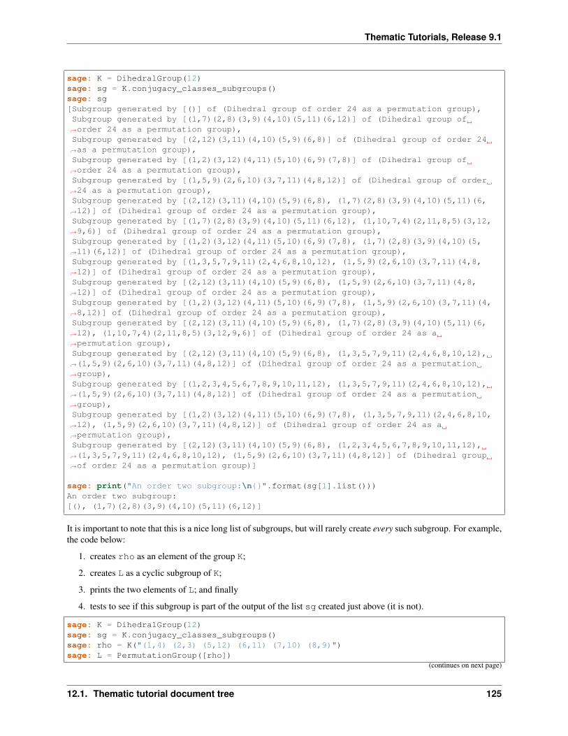
Thematic Tutorials, Release 9.1
sage: K = DihedralGroup(12)sage: sg = K.conjugacy_classes_subgroups()sage: sg[Subgroup generated by [()] of (Dihedral group of order 24 as a permutation group),Subgroup generated by [(1,7)(2,8)(3,9)(4,10)(5,11)(6,12)] of (Dihedral group of→˓order 24 as a permutation group),Subgroup generated by [(2,12)(3,11)(4,10)(5,9)(6,8)] of (Dihedral group of order 24→˓as a permutation group),Subgroup generated by [(1,2)(3,12)(4,11)(5,10)(6,9)(7,8)] of (Dihedral group of→˓order 24 as a permutation group),Subgroup generated by [(1,5,9)(2,6,10)(3,7,11)(4,8,12)] of (Dihedral group of order→˓24 as a permutation group),Subgroup generated by [(2,12)(3,11)(4,10)(5,9)(6,8), (1,7)(2,8)(3,9)(4,10)(5,11)(6,→˓12)] of (Dihedral group of order 24 as a permutation group),Subgroup generated by [(1,7)(2,8)(3,9)(4,10)(5,11)(6,12), (1,10,7,4)(2,11,8,5)(3,12,→˓9,6)] of (Dihedral group of order 24 as a permutation group),Subgroup generated by [(1,2)(3,12)(4,11)(5,10)(6,9)(7,8), (1,7)(2,8)(3,9)(4,10)(5,→˓11)(6,12)] of (Dihedral group of order 24 as a permutation group),Subgroup generated by [(1,3,5,7,9,11)(2,4,6,8,10,12), (1,5,9)(2,6,10)(3,7,11)(4,8,→˓12)] of (Dihedral group of order 24 as a permutation group),Subgroup generated by [(2,12)(3,11)(4,10)(5,9)(6,8), (1,5,9)(2,6,10)(3,7,11)(4,8,→˓12)] of (Dihedral group of order 24 as a permutation group),Subgroup generated by [(1,2)(3,12)(4,11)(5,10)(6,9)(7,8), (1,5,9)(2,6,10)(3,7,11)(4,→˓8,12)] of (Dihedral group of order 24 as a permutation group),Subgroup generated by [(2,12)(3,11)(4,10)(5,9)(6,8), (1,7)(2,8)(3,9)(4,10)(5,11)(6,→˓12), (1,10,7,4)(2,11,8,5)(3,12,9,6)] of (Dihedral group of order 24 as a→˓permutation group),Subgroup generated by [(2,12)(3,11)(4,10)(5,9)(6,8), (1,3,5,7,9,11)(2,4,6,8,10,12),→˓(1,5,9)(2,6,10)(3,7,11)(4,8,12)] of (Dihedral group of order 24 as a permutation→˓group),Subgroup generated by [(1,2,3,4,5,6,7,8,9,10,11,12), (1,3,5,7,9,11)(2,4,6,8,10,12),→˓(1,5,9)(2,6,10)(3,7,11)(4,8,12)] of (Dihedral group of order 24 as a permutation→˓group),Subgroup generated by [(1,2)(3,12)(4,11)(5,10)(6,9)(7,8), (1,3,5,7,9,11)(2,4,6,8,10,→˓12), (1,5,9)(2,6,10)(3,7,11)(4,8,12)] of (Dihedral group of order 24 as a→˓permutation group),Subgroup generated by [(2,12)(3,11)(4,10)(5,9)(6,8), (1,2,3,4,5,6,7,8,9,10,11,12),→˓(1,3,5,7,9,11)(2,4,6,8,10,12), (1,5,9)(2,6,10)(3,7,11)(4,8,12)] of (Dihedral group→˓of order 24 as a permutation group)]
sage: print("An order two subgroup:\n".format(sg[1].list()))An order two subgroup:[(), (1,7)(2,8)(3,9)(4,10)(5,11)(6,12)]
It is important to note that this is a nice long list of subgroups, but will rarely create every such subgroup. For example,the code below:
1. creates rho as an element of the group K;
2. creates L as a cyclic subgroup of K;
3. prints the two elements of L; and finally
4. tests to see if this subgroup is part of the output of the list sg created just above (it is not).
sage: K = DihedralGroup(12)sage: sg = K.conjugacy_classes_subgroups()sage: rho = K("(1,4) (2,3) (5,12) (6,11) (7,10) (8,9)")sage: L = PermutationGroup([rho])
(continues on next page)
12.1. Thematic tutorial document tree 125
Thematic Tutorials, Release 9.1
(continued from previous page)
sage: L.list()[(), (1,4)(2,3)(5,12)(6,11)(7,10)(8,9)]sage: L in sgFalse
Symmetry groups
You can give Sage a short list of elements of a permutation group and Sage will find the smallest subgroup that containsthose elements. We say the list “generates” the subgroup. We list a few interesting subgroups you can create this way.
Symmetries of an equilateral triangle
Label the vertices of an equilateral triangle as 1, 2 and 3. Then any permutation of the vertices will be a symmetry ofthe triangle. So either SymmetricGroup(3) or DihedralGroup(3) will create the full symmetry group.
Symmetries of an 𝑛-gon
A regular, 𝑛-sided figure in the plane (an 𝑛-gon) has 2𝑛 symmetries, comprised of 𝑛 rotations (including the trivialone) and 𝑛 “flips” about various axes. The dihedral group DihedralGroup(n) is frequently defined as exactly thesymmetry group of an 𝑛-gon.
Symmetries of a tetrahedron
Label the 4 vertices of a regular tetrahedron as 1, 2, 3 and 4. Fix the vertex labeled 4 and rotate the opposite facethrough 120 degrees. This will create the permutation/symmetry (1 2 3). Similarly, fixing vertex 1, and rotating theopposite face will create the permutation (2 3 4). These two permutations are enough to generate the full group of thetwelve symmetries of the tetrahedron. Another symmetry can be visualized by running an axis through the midpointof an edge of the tetrahedron through to the midpoint of the opposite edge, and then rotating by 180 degrees about thisaxis. For example, the 1–2 edge is opposite the 3–4 edge, and the symmetry is described by the permutation (1 2)(3 4).This permutation, along with either of the above permutations will also generate the group. So here are two ways tocreate this group:
sage: tetra_one = PermutationGroup(["(1,2,3)", "(2,3,4)"])sage: tetra_onePermutation Group with generators [(2,3,4), (1,2,3)]sage: tetra_two = PermutationGroup(["(1,2,3)", "(1,2)(3,4)"])sage: tetra_twoPermutation Group with generators [(1,2)(3,4), (1,2,3)]
This group has a variety of interesting properties, so it is worth experimenting with. You may also know it as the“alternating group on 4 symbols,” which Sage will create with the command AlternatingGroup(4).
Symmetries of a cube
Label vertices of one face of a cube with 1, 2, 3 and 4, and on the opposite face label the vertices 5, 6, 7 and 8 (5opposite 1, 6 opposite 2, etc.). Consider three axes that run from the center of a face to the center of the opposite face,and consider a quarter-turn rotation about each axis. These three rotations will construct the entire symmetry group.Use
126 Chapter 12. Documentation
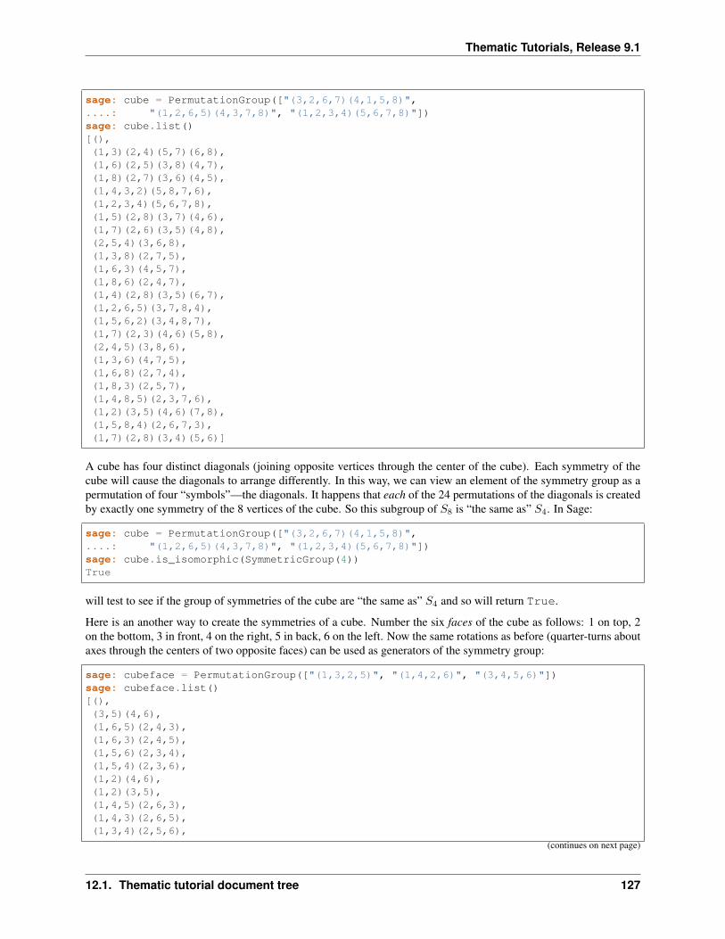
Thematic Tutorials, Release 9.1
sage: cube = PermutationGroup(["(3,2,6,7)(4,1,5,8)",....: "(1,2,6,5)(4,3,7,8)", "(1,2,3,4)(5,6,7,8)"])sage: cube.list()[(),(1,3)(2,4)(5,7)(6,8),(1,6)(2,5)(3,8)(4,7),(1,8)(2,7)(3,6)(4,5),(1,4,3,2)(5,8,7,6),(1,2,3,4)(5,6,7,8),(1,5)(2,8)(3,7)(4,6),(1,7)(2,6)(3,5)(4,8),(2,5,4)(3,6,8),(1,3,8)(2,7,5),(1,6,3)(4,5,7),(1,8,6)(2,4,7),(1,4)(2,8)(3,5)(6,7),(1,2,6,5)(3,7,8,4),(1,5,6,2)(3,4,8,7),(1,7)(2,3)(4,6)(5,8),(2,4,5)(3,8,6),(1,3,6)(4,7,5),(1,6,8)(2,7,4),(1,8,3)(2,5,7),(1,4,8,5)(2,3,7,6),(1,2)(3,5)(4,6)(7,8),(1,5,8,4)(2,6,7,3),(1,7)(2,8)(3,4)(5,6)]
A cube has four distinct diagonals (joining opposite vertices through the center of the cube). Each symmetry of thecube will cause the diagonals to arrange differently. In this way, we can view an element of the symmetry group as apermutation of four “symbols”—the diagonals. It happens that each of the 24 permutations of the diagonals is createdby exactly one symmetry of the 8 vertices of the cube. So this subgroup of 𝑆8 is “the same as” 𝑆4. In Sage:
sage: cube = PermutationGroup(["(3,2,6,7)(4,1,5,8)",....: "(1,2,6,5)(4,3,7,8)", "(1,2,3,4)(5,6,7,8)"])sage: cube.is_isomorphic(SymmetricGroup(4))True
will test to see if the group of symmetries of the cube are “the same as” 𝑆4 and so will return True.
Here is an another way to create the symmetries of a cube. Number the six faces of the cube as follows: 1 on top, 2on the bottom, 3 in front, 4 on the right, 5 in back, 6 on the left. Now the same rotations as before (quarter-turns aboutaxes through the centers of two opposite faces) can be used as generators of the symmetry group:
sage: cubeface = PermutationGroup(["(1,3,2,5)", "(1,4,2,6)", "(3,4,5,6)"])sage: cubeface.list()[(),(3,5)(4,6),(1,6,5)(2,4,3),(1,6,3)(2,4,5),(1,5,6)(2,3,4),(1,5,4)(2,3,6),(1,2)(4,6),(1,2)(3,5),(1,4,5)(2,6,3),(1,4,3)(2,6,5),(1,3,4)(2,5,6),
(continues on next page)
12.1. Thematic tutorial document tree 127
Thematic Tutorials, Release 9.1
(continued from previous page)
(1,3,6)(2,5,4),(1,4,2,6),(1,6)(2,4)(3,5),(1,3,2,5),(1,5,2,3),(1,2)(3,4)(5,6),(3,6,5,4),(1,6,2,4),(1,4)(2,6)(3,5),(1,5)(2,3)(4,6),(1,3)(2,5)(4,6),(3,4,5,6),(1,2)(3,6)(4,5)]
Again, this subgroup of 𝑆6 is “same as” the full symmetric group, 𝑆4:
sage: cubeface = PermutationGroup(["(1,3,2,5)", "(1,4,2,6)", "(3,4,5,6)"])sage: cubeface.is_isomorphic(SymmetricGroup(4))True
It turns out that in each of the above constructions, it is sufficient to use just two of the three generators (any two). Butone generator is not enough. Give it a try and use Sage to convince yourself that a generator can be sacrificed in eachcase.
Normal subgroups
Checking normality
The code below:
1. begins with the alternating group 𝐴4;
2. specifies three elements of the group (the three symmetries of the tetrahedron that are 180 degree rotations aboutaxes through midpoints of opposite edges);
3. uses these three elements to generate a subgroup; and finally
4. illustrates the command for testing if the subgroup H is a normal subgroup of the group A4.
sage: A4 = AlternatingGroup(4)sage: r1 = A4("(1,2) (3,4)")sage: r2 = A4("(1,3) (2,4)")sage: r3 = A4("(1,4) (2,3)")sage: H = A4.subgroup([r1, r2, r3])sage: H.is_normal(A4)True
Quotient group
Extending the previous example, we can create the quotient (factor) group of 𝐴4 by 𝐻 . The commands
sage: A4 = AlternatingGroup(4)sage: r1 = A4("(1,2) (3,4)")sage: r2 = A4("(1,3) (2,4)")
(continues on next page)
128 Chapter 12. Documentation
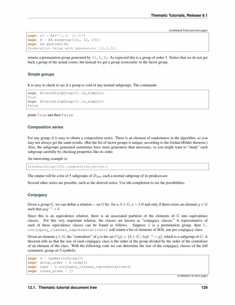
Thematic Tutorials, Release 9.1
(continued from previous page)
sage: r3 = A4("(1,4) (2,3)")sage: H = A4.subgroup([r1, r2, r3])sage: A4.quotient(H)Permutation Group with generators [(1,2,3)]
returns a permutation group generated by (1,2,3). As expected this is a group of order 3. Notice that we do not getback a group of the actual cosets, but instead we get a group isomorphic to the factor group.
Simple groups
It is easy to check to see if a group is void of any normal subgroups. The commands
sage: AlternatingGroup(5).is_simple()Truesage: AlternatingGroup(4).is_simple()False
prints True and then False.
Composition series
For any group, it is easy to obtain a composition series. There is an element of randomness in the algorithm, so youmay not always get the same results. (But the list of factor groups is unique, according to the Jordan-Hölder theorem.)Also, the subgroups generated sometimes have more generators than necessary, so you might want to “study” eachsubgroup carefully by checking properties like its order.
An interesting example is:
DihedralGroup(105).composition_series()
The output will be a list of 5 subgroups of 𝐷105, each a normal subgroup of its predecessor.
Several other series are possible, such as the derived series. Use tab-completion to see the possibilities.
Conjugacy
Given a group 𝐺, we can define a relation ∼ on 𝐺 by: for 𝑎, 𝑏 ∈ 𝐺, 𝑎 ∼ 𝑏 if and only if there exists an element 𝑔 ∈ 𝐺such that 𝑔𝑎𝑔−1 = 𝑏.
Since this is an equivalence relation, there is an associated partition of the elements of 𝐺 into equivalenceclasses. For this very important relation, the classes are known as “conjugacy classes.” A representative ofeach of these equivalence classes can be found as follows. Suppose G is a permutation group, then G.conjugacy_classes_representatives() will return a list of elements of $G$, one per conjugacy class.
Given an element 𝑔 ∈ 𝐺, the “centralizer” of 𝑔 is the set 𝐶(𝑔) = ℎ ∈ 𝐺 | ℎ𝑔ℎ−1 = 𝑔, which is a subgroup of 𝐺. Atheorem tells us that the size of each conjugacy class is the order of the group divided by the order of the centralizerof an element of the class. With the following code we can determine the size of the conjugacy classes of the fullsymmetric group on 5 symbols:
sage: G = SymmetricGroup(5)sage: group_order = G.order()sage: reps = G.conjugacy_classes_representatives()sage: class_sizes = []
(continues on next page)
12.1. Thematic tutorial document tree 129
Thematic Tutorials, Release 9.1
(continued from previous page)
sage: for g in reps:....: class_sizes.append(group_order / G.centralizer(g).order())...sage: class_sizes[1, 10, 15, 20, 20, 30, 24]
This should produce the list [1, 10, 15, 20, 20, 30, 24] which you can check sums to 120, the order ofthe group. You might be able to produce this list by counting elements of the group 𝑆5 with identical cycle structure(which will require a few simple combinatorial arguments).
Sylow subgroups
Sylow’s Theorems assert the existence of certain subgroups. For example, if 𝑝 is a prime, and 𝑝𝑟 divides the orderof a group 𝐺, then 𝐺 must have a subgroup of order 𝑝𝑟. Such a subgroup could be found among the output of theconjugacy_classes_subgroups() command by checking the orders of the subgroups produced. The map()command is a quick way to do this. The symmetric group on 7 symbols, 𝑆7, has order 7! = 5040 and is divisible by24 = 16. Let’s find one example of a subgroup of permutations on 4 symbols with order 16:
sage: G = SymmetricGroup(7)sage: subgroups = G.conjugacy_classes_subgroups()sage: list(map(order, subgroups))[1, 2, 2, 2, 3, 3, 4, 4, 4, 4, 4, 4, 4, 5, 6, 6, 6, 6, 6, 6, 6, 6, 7, 8, 8, 8, 8, 8,→˓8, 8, 9, 10, 10, 10, 12, 12, 12, 12, 12, 12, 12, 12, 12, 12, 12, 12, 12, 14, 16, 18,→˓ 18, 18, 20, 20, 20, 21, 24, 24, 24, 24, 24, 24, 24, 24, 24, 24, 24, 24, 24, 24, 36,→˓ 36, 36, 36, 40, 42, 48, 48, 48, 60, 60, 72, 72, 72, 72, 120, 120, 120, 120, 144,→˓168, 240, 360, 720, 2520, 5040]
The map(order, subgroups) command will apply the order() function to each of the subgroups in the listsubgroups. The output is thus a large list of the orders of many subgroups (96 to be precise). If you count carefully,you will see that the 49-th subgroup has order 16. You can retrieve this group for further study by referencing it assubgroups[48] (remember that counting starts at zero).
If 𝑝𝑟 is the highest power of 𝑝 to divide the order of 𝐺, then a subgroup of order 𝑝𝑟 is known as a “Sy-low 𝑝-subgroup.” Sylow’s Theorems also say any two Sylow 𝑝-subgroups are conjugate, so the output ofconjugacy_classes_subgroups() should only contain each Sylow 𝑝-subgroup once. But there is an eas-ier way, sylow_subgroup(p) will return one. Notice that the argument of the command is just the prime $p$, notthe full power 𝑝𝑟. Failure to use a prime will generate an informative error message.
Groups of small order as permutation groups
We list here constructions, as permutation groups, for all of the groups of order less than 16.
--------------------------------------------------------------------------------------→˓-------Size Construction Notes--------------------------------------------------------------------------------------→˓-------1 SymmetricGroup(1) Trivial2 SymmetricGroup(2) Also CyclicPermutationGroup(2)3 CyclicPermutationGroup(3) Prime order4 CyclicPermutationGroup(4) Cyclic4 KleinFourGroup() Abelian, non-cyclic5 CyclicPermutationGroup(5) Prime order
(continues on next page)
130 Chapter 12. Documentation
Thematic Tutorials, Release 9.1
(continued from previous page)
6 CyclicPermutationGroup(6) Cyclic6 SymmetricGroup(3) Non-abelian, also DihedralGroup(3)7 CyclicPermutationGroup(7) Prime order8 CyclicPermutationGroup(8) Cyclic8 D1 = CyclicPermutationGroup(4)
D2 = CyclicPermutationGroup(2)G = direct_product_permgroups([D1,D2]) Abelian, non-cyclic
8 D1 = CyclicPermutationGroup(2)D2 = CyclicPermutationGroup(2)D3 = CyclicPermutationGroup(2)G = direct_product_permgroups([D1,D2,D3]) Abelian, non-cyclic
8 DihedralGroup(4) Non-abelian8 QuaternionGroup() Quaternions, also DiCyclicGroup(2)9 CyclicPermutationGroup(9) Cyclic9 D1 = CyclicPermutationGroup(3)
D2 = CyclicPermutationGroup(3)G = direct_product_permgroups([D1,D2]) Abelian, non-cyclic
10 CyclicPermutationGroup(10) Cyclic10 DihedralGroup(5) Non-abelian11 CyclicPermutationGroup(11) Prime order12 CyclicPermutationGroup(12) Cyclic12 D1 = CyclicPermutationGroup(6)
D2 = CyclicPermutationGroup(2)G = direct_product_permgroups([D1,D2]) Abelian, non-cyclic
12 DihedralGroup(6) Non-abelian12 AlternatingGroup(4) Non-abelian, symmetries of→˓tetrahedron12 DiCyclicGroup(3) Non-abelian
Also semi-direct product $Z_3→˓\rtimes Z_4$13 CyclicPermutationGroup(13) Prime order14 CyclicPermutationGroup(14) Cyclic14 DihedralGroup(7) Non-abelian15 CyclicPermutationGroup(15) Cyclic--------------------------------------------------------------------------------------→˓--------
Acknowledgements
The construction of Sage is the work of many people, and the group theory portion is made possible by the extensivework of the creators of GAP. However, we will single out three people from the Sage team to thank for major con-tributions toward bringing you the group theory portion of Sage: David Joyner, William Stein, and Robert Bradshaw.Thanks!
12.1.5 Lie Methods and Related Combinatorics in Sage
Author: Daniel Bump (Stanford University), Ben Salisbury (Central Michigan University), and Anne Schilling (UCDavis)
These notes explain how to use the mathematical software Sage for Lie group computations. Sage also contains manycombinatorial algorithms. We will cover only some of these.
The Scope of this Document
12.1. Thematic tutorial document tree 131
Thematic Tutorials, Release 9.1
Lie groups and algebras
Sage can be used to do standard computations for Lie groups and Lie algebras. The following categories of represen-tations are equivalent:
• Complex representations of a compact, semisimple simply connected Lie group 𝐺.
• Complex representations of its Lie algebra g. This is a real Lie algebra, so representations are not required to becomplex linear maps.
• Complex representations of its complexified Lie algebra gC = C ⊗ g. This is a complex Lie algebra andrepresentations are required to be complex linear transformations.
• The complex analytic representations of the semisimple simply-connected complex analytic group 𝐺C havinggC as its Lie algebra.
• Modules of the universal enveloping algebra 𝑈(gC).
• Modules of the quantized enveloping algebra 𝑈𝑞(gC).
For example, we could take 𝐺 = 𝑆𝑈(𝑛), g = sl(𝑛,R), gC = sl(𝑛,C) and 𝐺C = 𝑆𝐿(𝑛,C). Because thesecategories are the same, their representations may be studied simultaneously. The above equivalences may be expandedto include reductive groups like 𝑈(𝑛) and 𝐺𝐿(𝑛) with a bit of care.
Here are some typical problems that can be solved using Sage:
• Decompose a module in any one of these categories into irreducibles.
• Compute the Frobenius-Schur indicator of an irreducible module.
• Compute the tensor product of two modules.
• If 𝐻 is a subgroup of 𝐺, study the restriction of modules for 𝐺 to 𝐻 . The solution to this problem is called abranching rule.
• Find the multiplicities of the weights of the representation.
In addition to its representations, which we may study as above, a Lie group has various related structures. Theseinclude:
• The Weyl Group 𝑊 .
• The Weight Lattice.
• The Root System
• The Cartan Type.
• The Dynkin diagram.
• The extended Dynkin diagram.
Sage contains methods for working with these structures.
If there is something you need that is not implemented, getting it added to Sage will likely be possible. You maywrite your own algorithm for an unimplemented task, and if it is something others will be interested in, it is probablypossible to get it added to Sage.
Combinatorics
Sage supports a great many related mathematical objects. Some of these properly belong to combinatorics. It isbeyond the scope of these notes to cover all the combinatorics in Sage, but we will try to touch on those combinatorialmethods which have some connection with Lie groups and representation theory. These include:
132 Chapter 12. Documentation
Thematic Tutorials, Release 9.1
• The affine Weyl group, an infinite group containing 𝑊 .
• Kashiwara crystals, which are combinatorial analogs of modules in the above categories.
• Coxeter group methods applicable to Weyl groups and the affine Weyl group, such as Bruhat order.
• The Iwahori Hecke algebras, which are deformations of the group algebras of 𝑊 and the affine Weyl group.
• Kazhdan-Lusztig polynomials.
Lie Group Basics
Goals of this section
Since we must be brief here, this is not really a place to learn about Lie groups or Lie algebras. Rather, the point ofthis section is to outline what you need to know to use Sage effectively for Lie computations, and to fix ideas andnotations.
Semisimple and reductive groups
If 𝑔 ∈ 𝐺𝐿(𝑛,C), then 𝑔 may be uniquely factored as 𝑔1𝑔2 where 𝑔1 and 𝑔2 commute, with 𝑔1 semisimple (diagonal-izable) and 𝑔2 unipotent (all its eigenvalues equal to 1). This follows from the Jordan canonical form. If 𝑔 = 𝑔1 then𝑔 is called semisimple and if 𝑔 = 𝑔2 then 𝑔 is called unipotent.
We consider a Lie group𝐺 and a class of representations such that if an element 𝑔 ∈ 𝐺 is unipotent (resp. semisimple)in one faithful representation from the class, then it is unipotent (resp. semisimple) in every faithful representation ofthe class. Thus the notion of being semisimple or unipotent is intrinsic. Examples:
• Compact Lie groups with continuous representations
• Complex analytic groups with analytic representations
• Algebraic groups over R with algebraic representations.
A subgroup of 𝐺 is called unipotent if it is connected and all its elements are unipotent. It is called a torus if it isconnected, abelian, and all its elements are semisimple. The group 𝐺 is called reductive if it has no nontrivial normalunipotent subgroup. For example, 𝐺𝐿(2,C) is reductive, but its subgroup:(
𝑎 𝑏𝑑
)is not since it has a normal unipotent subgroup (
1 𝑏1
).
A group has a unique largest normal unipotent subgroup, called the unipotent radical, so it is reductive if and only ifthe unipotent radical is trivial.
A Lie group is called semisimple it is reductive and furthermore has no nontrivial normal tori. For example 𝐺𝐿(2,C)is reductive but not semisimple because it has a normal torus:(
𝑎𝑎
).
The group 𝑆𝐿(2,C) is semisimple.
12.1. Thematic tutorial document tree 133
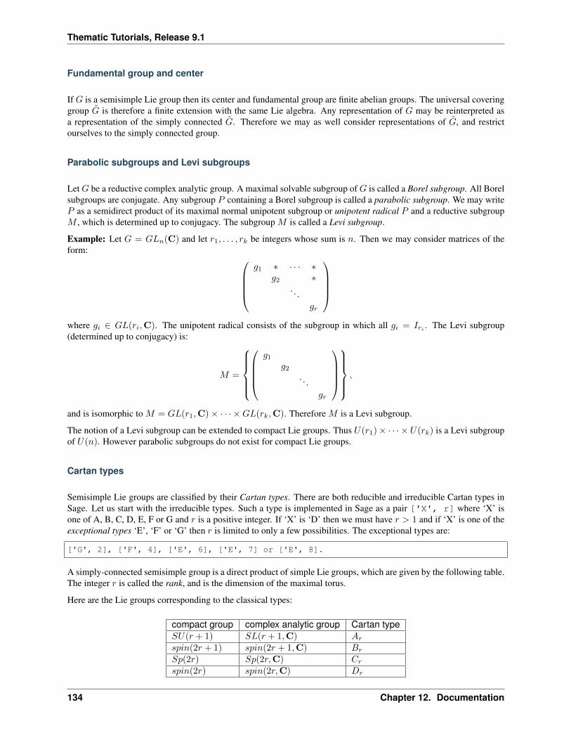
Thematic Tutorials, Release 9.1
Fundamental group and center
If 𝐺 is a semisimple Lie group then its center and fundamental group are finite abelian groups. The universal coveringgroup is therefore a finite extension with the same Lie algebra. Any representation of 𝐺 may be reinterpreted asa representation of the simply connected . Therefore we may as well consider representations of , and restrictourselves to the simply connected group.
Parabolic subgroups and Levi subgroups
Let𝐺 be a reductive complex analytic group. A maximal solvable subgroup of𝐺 is called a Borel subgroup. All Borelsubgroups are conjugate. Any subgroup 𝑃 containing a Borel subgroup is called a parabolic subgroup. We may write𝑃 as a semidirect product of its maximal normal unipotent subgroup or unipotent radical 𝑃 and a reductive subgroup𝑀 , which is determined up to conjugacy. The subgroup 𝑀 is called a Levi subgroup.
Example: Let 𝐺 = 𝐺𝐿𝑛(C) and let 𝑟1, . . . , 𝑟𝑘 be integers whose sum is 𝑛. Then we may consider matrices of theform: ⎛⎜⎜⎜⎝
𝑔1 * · · · *𝑔2 *
. . .𝑔𝑟
⎞⎟⎟⎟⎠where 𝑔𝑖 ∈ 𝐺𝐿(𝑟𝑖,C). The unipotent radical consists of the subgroup in which all 𝑔𝑖 = 𝐼𝑟𝑖 . The Levi subgroup(determined up to conjugacy) is:
𝑀 =
⎧⎪⎪⎪⎨⎪⎪⎪⎩⎛⎜⎜⎜⎝
𝑔1𝑔2
. . .𝑔𝑟
⎞⎟⎟⎟⎠⎫⎪⎪⎪⎬⎪⎪⎪⎭ ,
and is isomorphic to 𝑀 = 𝐺𝐿(𝑟1,C)× · · · ×𝐺𝐿(𝑟𝑘,C). Therefore 𝑀 is a Levi subgroup.
The notion of a Levi subgroup can be extended to compact Lie groups. Thus 𝑈(𝑟1)× · · · × 𝑈(𝑟𝑘) is a Levi subgroupof 𝑈(𝑛). However parabolic subgroups do not exist for compact Lie groups.
Cartan types
Semisimple Lie groups are classified by their Cartan types. There are both reducible and irreducible Cartan types inSage. Let us start with the irreducible types. Such a type is implemented in Sage as a pair ['X', r] where ‘X’ isone of A, B, C, D, E, F or G and 𝑟 is a positive integer. If ‘X’ is ‘D’ then we must have 𝑟 > 1 and if ‘X’ is one of theexceptional types ‘E’, ‘F’ or ‘G’ then 𝑟 is limited to only a few possibilities. The exceptional types are:
['G', 2], ['F', 4], ['E', 6], ['E', 7] or ['E', 8].
A simply-connected semisimple group is a direct product of simple Lie groups, which are given by the following table.The integer 𝑟 is called the rank, and is the dimension of the maximal torus.
Here are the Lie groups corresponding to the classical types:
compact group complex analytic group Cartan type𝑆𝑈(𝑟 + 1) 𝑆𝐿(𝑟 + 1,C) 𝐴𝑟
𝑠𝑝𝑖𝑛(2𝑟 + 1) 𝑠𝑝𝑖𝑛(2𝑟 + 1,C) 𝐵𝑟
𝑆𝑝(2𝑟) 𝑆𝑝(2𝑟,C) 𝐶𝑟
𝑠𝑝𝑖𝑛(2𝑟) 𝑠𝑝𝑖𝑛(2𝑟,C) 𝐷𝑟
134 Chapter 12. Documentation
Thematic Tutorials, Release 9.1
You may create these Cartan types and their Dynkin diagrams as follows:
sage: ct = CartanType("D5"); ct['D', 5]
Here "D5" is an abbreviation for ['D',5]. The group 𝑠𝑝𝑖𝑛(𝑛) is the simply-connected double cover of the orthog-onal group 𝑆𝑂(𝑛).
Dual Cartan types
Every Cartan type has a dual, which you can get from within Sage:
sage: CartanType("B4").dual()['C', 4]
Types other than𝐵𝑟 and𝐶𝑟 for 𝑟 > 2 are self-dual in the sense that the dual is isomorphic to the original type; howeverthe isomorphism of a Cartan type with its dual might relabel the vertices. We can see this as follows:
sage: CartanType("F4").dynkin_diagram()O---O=>=O---O1 2 3 4F4sage: CartanType("F4").dual()['F', 4] relabelled by 1: 4, 2: 3, 3: 2, 4: 1sage: CartanType("F4").dual().dynkin_diagram()O---O=>=O---O4 3 2 1F4 relabelled by 1: 4, 2: 3, 3: 2, 4: 1
Reducible Cartan types
If 𝐺 is a Lie group of finite index in 𝐺1 × 𝐺2, where 𝐺1 and 𝐺2 are Lie groups of positive dimension, then 𝐺 iscalled reducible. In this case, the root system of 𝐺 is the disjoint union of the root systems of 𝐺1 and 𝐺2, which lie inorthogonal subspaces of the ambient space of the weight space of 𝐺. The Cartan type of 𝐺 is thus reducible.
Reducible Cartan types are supported in Sage as follows:
sage: RootSystem("A1xA1")Root system of type A1xA1sage: WeylCharacterRing("A1xA1")The Weyl Character Ring of Type A1xA1 with Integer Ring coefficients
Low dimensional Cartan types
There are some isomorphisms that occur in low degree.
Cartan Type Group Equivalent Type Isomorphic Group𝐵2 𝑠𝑝𝑖𝑛(5) 𝐶2 𝑆𝑝(4)𝐷3 𝑠𝑝𝑖𝑛(6) 𝐴3 𝑆𝐿(4)𝐷2 𝑠𝑝𝑖𝑛(4) 𝐴1×𝐴1 𝑆𝐿(2)× 𝑆𝐿(2)𝐵1 𝑠𝑝𝑖𝑛(3) 𝐴1 𝑆𝐿(2)𝐶1 𝑆𝑝(2) 𝐴1 𝑆𝐿(2)
12.1. Thematic tutorial document tree 135
Thematic Tutorials, Release 9.1
Sometimes the redundant Cartan types such as 𝐷3 and 𝐷2 are excluded from the list of Cartan types. However Sageallows them since excluding them leads to exceptions having to be made in algorithms. A better approach, whichis followed by Sage, is to allow the redundant Cartan types, but to implement the isomorphisms explicitly as specialcases of branching rules. The utility of this approach may be seen by considering that the rank one group 𝑆𝐿(2) hasdifferent natural weight lattices realizations depending on whether we consider it to be 𝑆𝐿(2), 𝑠𝑝𝑖𝑛(2) or 𝑆𝑝(2):
sage: RootSystem("A1").ambient_space().simple_roots()Finite family 1: (1, -1)sage: RootSystem("B1").ambient_space().simple_roots()Finite family 1: (1)sage: RootSystem("C1").ambient_space().simple_roots()Finite family 1: (2)
Relabeled Cartan types
By default Sage uses the labeling of the Dynkin diagram from [Bourbaki46]. There is another labeling of the verticesdue to Dynkin. Most of the literature follows [Bourbaki46], though [Kac] follows Dynkin.
If you need to use Dynkin’s labeling, you should be aware that Sage does support relabeled Cartan types. See thedocumentation in sage.combinat.root_system.type_relabel for further information.
Standard realizations of the ambient spaces
These realizations follow the Appendix in [Bourbaki46]. See the Root system plot tutorial for how to visualize them.
Type A
For type 𝐴𝑟 we use an 𝑟 + 1 dimensional ambient space. This means that we are modeling the Lie group 𝑈(𝑟 + 1) or𝐺𝐿(𝑟 + 1,C) rather than 𝑆𝑈(𝑟 + 1) or 𝑆𝐿(𝑟 + 1,C). The ambient space is identified with Q𝑟+1:
sage: RootSystem("A3").ambient_space().simple_roots()Finite family 1: (1, -1, 0, 0), 2: (0, 1, -1, 0), 3: (0, 0, 1, -1)sage: RootSystem("A3").ambient_space().fundamental_weights()Finite family 1: (1, 0, 0, 0), 2: (1, 1, 0, 0), 3: (1, 1, 1, 0)sage: RootSystem("A3").ambient_space().rho()(3, 2, 1, 0)
The dominant weights consist of integer 𝑟 + 1-tuples 𝜆 = (𝜆1, . . . , 𝜆𝑟+1) such that 𝜆1 ≥ · · · ≥ 𝜆𝑟+1.
See SL versus GL for further remarks about Type A.
Type B
For the remaining classical Cartan types 𝐵𝑟, 𝐶𝑟 and 𝐷𝑟 we use an 𝑟-dimensional ambient space:
sage: RootSystem("B3").ambient_space().simple_roots()Finite family 1: (1, -1, 0), 2: (0, 1, -1), 3: (0, 0, 1)sage: RootSystem("B3").ambient_space().fundamental_weights()Finite family 1: (1, 0, 0), 2: (1, 1, 0), 3: (1/2, 1/2, 1/2)sage: RootSystem("B3").ambient_space().rho()(5/2, 3/2, 1/2)
136 Chapter 12. Documentation
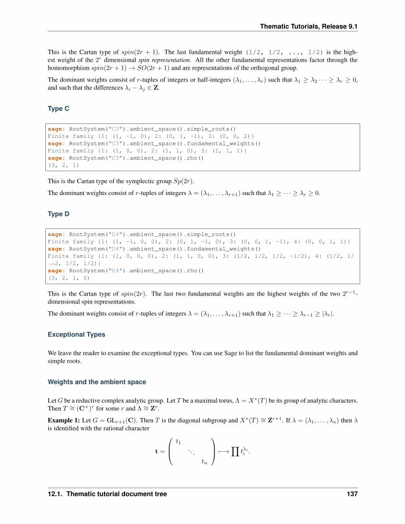
Thematic Tutorials, Release 9.1
This is the Cartan type of 𝑠𝑝𝑖𝑛(2𝑟 + 1). The last fundamental weight (1/2, 1/2, ..., 1/2) is the high-est weight of the 2𝑟 dimensional spin representation. All the other fundamental representations factor through thehomomorphism 𝑠𝑝𝑖𝑛(2𝑟 + 1)→ 𝑆𝑂(2𝑟 + 1) and are representations of the orthogonal group.
The dominant weights consist of 𝑟-tuples of integers or half-integers (𝜆1, . . . , 𝜆𝑟) such that 𝜆1 ≥ 𝜆2 · · · ≥ 𝜆𝑟 ≥ 0,and such that the differences 𝜆𝑖 − 𝜆𝑗 ∈ Z.
Type C
sage: RootSystem("C3").ambient_space().simple_roots()Finite family 1: (1, -1, 0), 2: (0, 1, -1), 3: (0, 0, 2)sage: RootSystem("C3").ambient_space().fundamental_weights()Finite family 1: (1, 0, 0), 2: (1, 1, 0), 3: (1, 1, 1)sage: RootSystem("C3").ambient_space().rho()(3, 2, 1)
This is the Cartan type of the symplectic group 𝑆𝑝(2𝑟).
The dominant weights consist of 𝑟-tuples of integers 𝜆 = (𝜆1, . . . , 𝜆𝑟+1) such that 𝜆1 ≥ · · · ≥ 𝜆𝑟 ≥ 0.
Type D
sage: RootSystem("D4").ambient_space().simple_roots()Finite family 1: (1, -1, 0, 0), 2: (0, 1, -1, 0), 3: (0, 0, 1, -1), 4: (0, 0, 1, 1)sage: RootSystem("D4").ambient_space().fundamental_weights()Finite family 1: (1, 0, 0, 0), 2: (1, 1, 0, 0), 3: (1/2, 1/2, 1/2, -1/2), 4: (1/2, 1/→˓2, 1/2, 1/2)sage: RootSystem("D4").ambient_space().rho()(3, 2, 1, 0)
This is the Cartan type of 𝑠𝑝𝑖𝑛(2𝑟). The last two fundamental weights are the highest weights of the two 2𝑟−1-dimensional spin representations.
The dominant weights consist of 𝑟-tuples of integers 𝜆 = (𝜆1, . . . , 𝜆𝑟+1) such that 𝜆1 ≥ · · · ≥ 𝜆𝑟−1 ≥ |𝜆𝑟|.
Exceptional Types
We leave the reader to examine the exceptional types. You can use Sage to list the fundamental dominant weights andsimple roots.
Weights and the ambient space
Let𝐺 be a reductive complex analytic group. Let 𝑇 be a maximal torus, Λ = 𝑋*(𝑇 ) be its group of analytic characters.Then 𝑇 ∼= (C×)𝑟 for some 𝑟 and Λ ∼= Z𝑟.
Example 1: Let 𝐺 = GL𝑟+1(C). Then 𝑇 is the diagonal subgroup and 𝑋*(𝑇 ) ∼= Z𝑟+1. If 𝜆 = (𝜆1, . . . , 𝜆𝑛) then 𝜆is identified with the rational character
t =
⎛⎜⎝ 𝑡1. . .
𝑡𝑛
⎞⎟⎠ ↦−→∏𝑡𝜆𝑖𝑖 .
12.1. Thematic tutorial document tree 137
Thematic Tutorials, Release 9.1
Example 2: Let𝐺 = SL𝑟+1(C). Again 𝑇 is the diagonal subgroup but now if 𝜆 ∈ ZΔ = (𝑑, · · · , 𝑑)|𝑑 ∈ Z ⊆ Z𝑟+1
then∏𝑡𝜆𝑖𝑖 = det(t)𝑑 = 1, so 𝑋*(𝑇 ) ∼= Z𝑟+1/ZΔ ∼= Z𝑟.
• Elements of Λ are called weights.
• If 𝜋 : 𝐺 → 𝐺𝐿(𝑉 ) is any representation we may restrict 𝜋 to 𝑇 . Then the characters of 𝑇 that occur in thisrestriction are called the weights of 𝜋.
• 𝐺 acts on its Lie algebra by conjugation (the adjoint representation).
• The nonzero weights of the adjoint representation are called roots.
• The ambient space of Λ is Q⊗ Λ.
The root system
As we have mentioned, 𝐺 acts on its complexified Lie algebra gC by the adjoint representation. The zero weight spacegC(0) is just the Lie algebra of 𝑇 itself. The other nonzero weights each appear with multiplicity one and form aninteresting configuration of vectors called the root system Φ.
It is convenient to partition Φ into two sets Φ+ and Φ− such that Φ+ consists of all roots lying on one side of ahyperplane. Often we arrange things so that 𝐺 is embedded in 𝐺𝐿(𝑛,C) in such a way that the positive weightscorrespond to upper triangular matrices. Thus if 𝛼 is a positive root, its weight space gC(𝛼) is spanned by a vector𝑋𝛼, and the exponential of this eigenspace in 𝐺 is a one-parameter subgroup of unipotent matrices. It is alwayspossible to arrange that this one-parameter subgroup consists of upper triangular matrices.
If 𝛼 is a positive root that cannot be decomposed as a sum of other positive roots, then 𝛼 is called a simple root. If 𝐺is semisimple of rank 𝑟, then 𝑟 is the number of positive roots. Let 𝛼1, . . . , 𝛼𝑟 be these.
The Weyl group
Let 𝐺 be a complex analytic group. Let 𝑇 be a maximal torus, and let 𝑁(𝑇 ) be its normalizer. Let 𝑊 = 𝑁(𝑇 )/𝑇be the Weyl group. It acts on 𝑇 by conjugation; therefore it acts on the weight lattice Λ and its ambient space. Theambient space admits an inner product that is invariant under this action. Let (𝑣|𝑤) denote this inner product. If 𝛼 isa root let 𝑟𝛼 denote the reflection in the hyperplane of the ambient space that is perpendicular to 𝛼. If 𝛼 = 𝛼𝑖 is asimple root, then we use the notation 𝑠𝑖 to denote 𝑟𝛼.
Then 𝑠1, . . . , 𝑠𝑟 generate 𝑊 , which is a Coxeter group. This means that it is generated by elements 𝑠𝑖 of order twoand that if 𝑚(𝑖, 𝑗) is the order of 𝑠𝑖𝑠𝑗 , then
𝑊 =⟨𝑠𝑖 | 𝑠2𝑖 = 1, (𝑠𝑖𝑠𝑗)
𝑚(𝑖,𝑗) = 1⟩
is a presentation. An important function ℓ : 𝑊 → Z is the length function, where ℓ(𝑤) is the length of the shortestdecomposition of 𝑤 into a product of simple reflections.
The dual root system
The coroots are certain linear functionals on the ambient space that also form a root system. Since the ambient spaceadmits a 𝑊 -invariant inner product ( | ), they may be identified with elements of the ambient space itself. Then theyare proportional to the roots, though if the roots have different lengths, long roots correspond to short coroots andconversely. The coroot corresponding to the root 𝛼 is
𝛼∨ =2𝛼
(𝛼|𝛼).
138 Chapter 12. Documentation
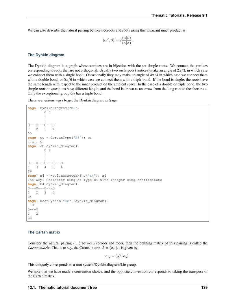
Thematic Tutorials, Release 9.1
We can also describe the natural pairing between coroots and roots using this invariant inner product as
⟨𝛼∨, 𝛽⟩ = 2(𝛼|𝛽)
(𝛼|𝛼).
The Dynkin diagram
The Dynkin diagram is a graph whose vertices are in bijection with the set simple roots. We connect the verticescorresponding to roots that are not orthogonal. Usually two such roots (vertices) make an angle of 2𝜋/3, in which casewe connect them with a single bond. Occasionally they may make an angle of 3𝜋/4 in which case we connect themwith a double bond, or 5𝜋/6 in which case we connect them with a triple bond. If the bond is single, the roots havethe same length with respect to the inner product on the ambient space. In the case of a double or triple bond, the twosimple roots in questions have different length, and the bond is drawn as an arrow from the long root to the short root.Only the exceptional group 𝐺2 has a triple bond.
There are various ways to get the Dynkin diagram in Sage:
sage: DynkinDiagram("D5")O 5||
O---O---O---O1 2 3 4D5sage: ct = CartanType("E6"); ct['E', 6]sage: ct.dynkin_diagram()
O 2||
O---O---O---O---O1 3 4 5 6E6sage: B4 = WeylCharacterRing("B4"); B4The Weyl Character Ring of Type B4 with Integer Ring coefficientssage: B4.dynkin_diagram()O---O---O=>=O1 2 3 4B4sage: RootSystem("G2").dynkin_diagram()
3O=<=O1 2G2
The Cartan matrix
Consider the natural pairing ⟨ , ⟩ between coroots and roots, then the defining matrix of this pairing is called theCartan matrix. That is to say, the Cartan matrix 𝐴 = (𝑎𝑖𝑗)𝑖𝑗 is given by
𝑎𝑖𝑗 = ⟨𝛼∨𝑖 , 𝛼𝑗⟩.
This uniquely corresponds to a root system/Dynkin diagram/Lie group.
We note that we have made a convention choice, and the opposite convention corresponds to taking the transpose ofthe Cartan matrix.
12.1. Thematic tutorial document tree 139
Thematic Tutorials, Release 9.1
Fundamental weights and the Weyl vector
There are certain weights 𝜔1, . . . , 𝜔𝑟 that:
⟨𝜔𝑗 , 𝛼𝑖⟩ = 2(𝛼𝑖|𝜔𝑗)
(𝛼𝑖|𝛼𝑖)= 𝛿𝑖𝑗 .
If 𝐺 is semisimple then these are uniquely determined, whereas if 𝐺 is reductive but not semisimple we may choosethem conveniently.
Let 𝜌 be the sum of the fundamental dominant weights. If 𝐺 is semisimple, then 𝜌 is half the sum of the positiveroots. In case 𝐺 is not semisimple, we have noted, the fundamental weights are not completely determined by theinner product condition given above. If we make a different choice, then 𝜌 is altered by a vector that is orthogonal toall roots. This is a harmless change for many purposes such as the Weyl character formula.
In Sage, this issue arises only for Cartan type 𝐴𝑟. See SL versus GL.
Representations and characters
Let 𝑇 be a maximal torus and Λ = 𝑋*(𝑇 ) be the group of rational characters. Then Λ ∼= Z𝑟.
• Recall that elements of Λ ∼= Z𝑟 are called weights.
• The Weyl group 𝑊 = 𝑁(𝑇 )/𝑇 acts on 𝑇 , hence on Λ and its ambient space by conjugation.
• The ambient space Q⊗𝑋*(𝑇 ) ∼= Q𝑟 has a fundamental domain 𝒞+ for the Weyl group 𝑊 called the positiveWeyl chamber. Weights in 𝒞+ are called dominant.
• Then 𝒞+ consists of all vectors such that (𝛼|𝑣) ≥ 0 for all positive roots 𝛼.
• It is useful to embed Λ in R𝑟 and consider weights as lattice points.
• If (𝜋, 𝑉 ) is a representation then restricting to 𝑇 , the module 𝑉 decomposes into a direct sum of weighteigenspaces 𝑉 (𝜇) with multiplicity 𝑚(𝜇) for weight 𝜇.
• There is a unique highest weight 𝜆 with respect to the partial order. We have 𝜆 ∈ 𝒞 and 𝑚(𝜆) = 1.
• 𝑉 ←→ 𝜆 gives a bijection between irreducible representations and weights 𝜆 in 𝒞+.
Assuming that 𝐺 is simply-connected (or more generally, reductive with a simply-connected derived group) everydominant weight 𝜆 is the highest weight of a unique irreducible representation 𝜋𝜆, and 𝜆 ↦→ 𝜋𝜆 gives a parametrizationof the isomorphism classes of irreducible representations of 𝐺 by the dominant weights.
The character of 𝜋𝜆 is the function 𝜒𝜆(𝑔) = 𝑡𝑟(𝜋𝜆(𝑔)). It is determined by its values on 𝑇 . If (𝑧) ∈ 𝑇 and 𝜇 ∈ Λ, letus write z𝜇 for the value of 𝜇 on z. Then the character:
𝜒𝜆(z) =∑𝜇∈Λ
𝑚(𝜇) z𝜆.
Sometimes this is written
𝜒𝜆 =∑𝜇∈Λ
𝑚(𝜇) 𝑒𝜆.
The meaning of 𝑒𝜆 is subject to interpretation, but we may regard it as the image of the additive group Λ in its groupalgebra. The character is then regarded as an element of this ring, the group algebra of Λ.
140 Chapter 12. Documentation
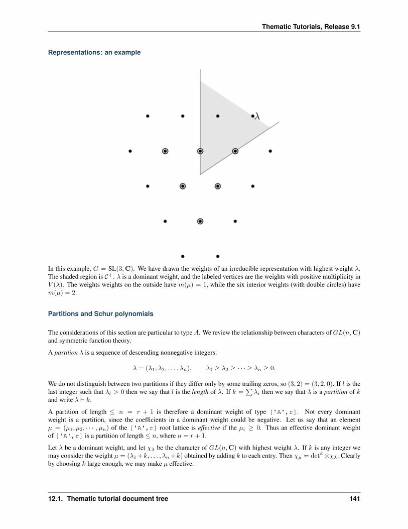
Thematic Tutorials, Release 9.1
Representations: an example
In this example, 𝐺 = SL(3,C). We have drawn the weights of an irreducible representation with highest weight 𝜆.The shaded region is 𝒞+. 𝜆 is a dominant weight, and the labeled vertices are the weights with positive multiplicity in𝑉 (𝜆). The weights weights on the outside have 𝑚(𝜇) = 1, while the six interior weights (with double circles) have𝑚(𝜇) = 2.
Partitions and Schur polynomials
The considerations of this section are particular to type𝐴. We review the relationship between characters of𝐺𝐿(𝑛,C)and symmetric function theory.
A partition 𝜆 is a sequence of descending nonnegative integers:
𝜆 = (𝜆1, 𝜆2, . . . , 𝜆𝑛), 𝜆1 ≥ 𝜆2 ≥ · · · ≥ 𝜆𝑛 ≥ 0.
We do not distinguish between two partitions if they differ only by some trailing zeros, so (3, 2) = (3, 2, 0). If 𝑙 is thelast integer such that 𝜆𝑙 > 0 then we say that 𝑙 is the length of 𝜆. If 𝑘 =
∑𝜆𝑖 then we say that 𝜆 is a partition of 𝑘
and write 𝜆 ⊢ 𝑘.
A partition of length ≤ 𝑛 = 𝑟 + 1 is therefore a dominant weight of type ['A',r]. Not every dominantweight is a partition, since the coefficients in a dominant weight could be negative. Let us say that an element𝜇 = (𝜇1, 𝜇2, · · · , 𝜇𝑛) of the ['A',r] root lattice is effective if the 𝜇𝑖 ≥ 0. Thus an effective dominant weightof ['A',r] is a partition of length ≤ 𝑛, where 𝑛 = 𝑟 + 1.
Let 𝜆 be a dominant weight, and let 𝜒𝜆 be the character of 𝐺𝐿(𝑛,C) with highest weight 𝜆. If 𝑘 is any integer wemay consider the weight 𝜇 = (𝜆1 +𝑘, . . . , 𝜆𝑛 +𝑘) obtained by adding 𝑘 to each entry. Then 𝜒𝜇 = det𝑘 ⊗𝜒𝜆. Clearlyby choosing 𝑘 large enough, we may make 𝜇 effective.
12.1. Thematic tutorial document tree 141
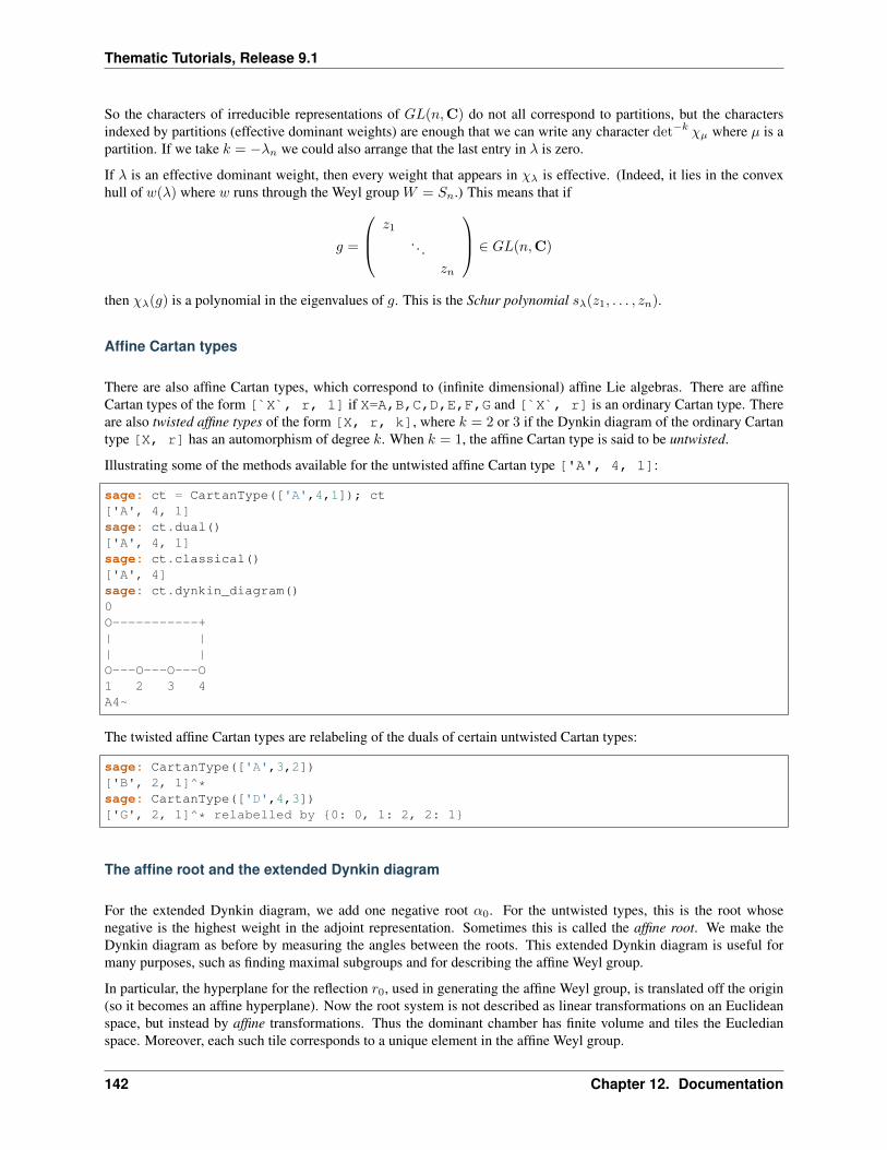
Thematic Tutorials, Release 9.1
So the characters of irreducible representations of 𝐺𝐿(𝑛,C) do not all correspond to partitions, but the charactersindexed by partitions (effective dominant weights) are enough that we can write any character det−𝑘 𝜒𝜇 where 𝜇 is apartition. If we take 𝑘 = −𝜆𝑛 we could also arrange that the last entry in 𝜆 is zero.
If 𝜆 is an effective dominant weight, then every weight that appears in 𝜒𝜆 is effective. (Indeed, it lies in the convexhull of 𝑤(𝜆) where 𝑤 runs through the Weyl group 𝑊 = 𝑆𝑛.) This means that if
𝑔 =
⎛⎜⎝ 𝑧1. . .
𝑧𝑛
⎞⎟⎠ ∈ 𝐺𝐿(𝑛,C)
then 𝜒𝜆(𝑔) is a polynomial in the eigenvalues of 𝑔. This is the Schur polynomial 𝑠𝜆(𝑧1, . . . , 𝑧𝑛).
Affine Cartan types
There are also affine Cartan types, which correspond to (infinite dimensional) affine Lie algebras. There are affineCartan types of the form [`X`, r, 1] if X=A,B,C,D,E,F,G and [`X`, r] is an ordinary Cartan type. Thereare also twisted affine types of the form [X, r, k], where 𝑘 = 2 or 3 if the Dynkin diagram of the ordinary Cartantype [X, r] has an automorphism of degree 𝑘. When 𝑘 = 1, the affine Cartan type is said to be untwisted.
Illustrating some of the methods available for the untwisted affine Cartan type ['A', 4, 1]:
sage: ct = CartanType(['A',4,1]); ct['A', 4, 1]sage: ct.dual()['A', 4, 1]sage: ct.classical()['A', 4]sage: ct.dynkin_diagram()0O-----------+| || |O---O---O---O1 2 3 4A4~
The twisted affine Cartan types are relabeling of the duals of certain untwisted Cartan types:
sage: CartanType(['A',3,2])['B', 2, 1]^*sage: CartanType(['D',4,3])['G', 2, 1]^* relabelled by 0: 0, 1: 2, 2: 1
The affine root and the extended Dynkin diagram
For the extended Dynkin diagram, we add one negative root 𝛼0. For the untwisted types, this is the root whosenegative is the highest weight in the adjoint representation. Sometimes this is called the affine root. We make theDynkin diagram as before by measuring the angles between the roots. This extended Dynkin diagram is useful formany purposes, such as finding maximal subgroups and for describing the affine Weyl group.
In particular, the hyperplane for the reflection 𝑟0, used in generating the affine Weyl group, is translated off the origin(so it becomes an affine hyperplane). Now the root system is not described as linear transformations on an Euclideanspace, but instead by affine transformations. Thus the dominant chamber has finite volume and tiles the Eucledianspace. Moreover, each such tile corresponds to a unique element in the affine Weyl group.
142 Chapter 12. Documentation
Thematic Tutorials, Release 9.1
The extended Dynkin diagram may be obtained as the Dynkin diagram of the corresponding untwisted affine type:
sage: ct = CartanType("E6"); ct['E', 6]sage: ct.affine()['E', 6, 1]sage: ct.affine() == CartanType(['E',6,1])Truesage: ct.affine().dynkin_diagram()
O 0||O 2||
O---O---O---O---O1 3 4 5 6E6~
The extended Dynkin diagram is also a method of the WeylCharacterRing:
sage: WeylCharacterRing("E7").extended_dynkin_diagram()O 2||
O---O---O---O---O---O---O0 1 3 4 5 6 7E7~
We note the following important distinctions from the classical cases:
• The affine Weyl groups are all infinite.
• Type 𝐴(1)1 has two anti-parallel roots with distinct reflections. The Dynkin diagram in this case is represented
by a double bond with arrows going in both directions.
Twisted affine root systems
For the construction of 𝛼0 in the twisted types, we refer the reader to Chapter 8 of [Kac]. As mentioned above, mosttwisted types can be constructed by taking the dual root system of an untwisted type. However the type 𝐴(2)
2𝑛 rootsystem can only be constructed by the twisting procedure defined in [Kac]. It has the following properties:
• The Dynkin diagram of type 𝐴(2)2 has a quadruple bond with an arrow pointing from the short root to the long
root.
• Type 𝐴(2)2𝑛 for 𝑛 > 1 has 3 different root lengths.
Further Generalizations
If a root system (on an Euclidean space) has only the angles 𝜋/2, 2𝜋/3, 3𝜋/4, 5𝜋/6 between its roots, then we call theroot system crystallographic (on Wikipedia article Root_system, this condition is called integrality since for any tworoots we have ⟨𝛽, 𝛼⟩ ∈ Z). So if we look at the reflection group generated by the roots (this is not a Weyl group), weget general Coxeter groups (with non-infinite labels) and non-crystallographic Coxeter groups are not connected withLie theory.
However we can generalize Dynkin diagrams (equivalently Cartan matrices) to have all its edges labelled by (𝑎, 𝑏)where 𝑎, 𝑏 ∈ Z>0 and corresponds to having 𝑎 arrows point one way and 𝑏 arrows pointing the other. For example in
12.1. Thematic tutorial document tree 143
Thematic Tutorials, Release 9.1
type 𝐴(1)1 , we have one edge of (2, 2), or in type 𝐴(2)
2 , we have one edge of (1, 4) (equivalently (4, 1)). These edgelabel between 𝑖 and 𝑗 corresponds to the entries 𝑎𝑖𝑗 and 𝑎𝑗𝑖 in the Cartan matrix. These are used to construct a classof (generally infinite dimensional) Lie algebras called Kac-Moody (Lie) algebras, which in turn are used to constructquantum groups. We refer the reader to [Kac] and [HongKang2002] for more information.
The Weyl Character Ring
Weyl character rings
The Weyl character ring is the representation ring of a compact Lie group. It has a basis consisting of the irreduciblerepresentations of 𝐺, or equivalently, their characters. The addition and multiplication in the Weyl character ringcorrespond to direct sum and tensor product of representations.
Methods of the ambient space
In Sage, many useful features of the Lie group are available as methods of the ambient space:
sage: S = RootSystem("B2").ambient_space(); SAmbient space of the Root system of type ['B', 2]sage: S.roots()[(1, -1), (1, 1), (1, 0), (0, 1), (-1, 1), (-1, -1), (-1, 0), (0, -1)]sage: S.fundamental_weights()Finite family 1: (1, 0), 2: (1/2, 1/2)sage: S.positive_roots()[(1, -1), (1, 1), (1, 0), (0, 1)]sage: S.weyl_group()Weyl Group of type ['B', 2] (as a matrix group acting on the ambient space)
Methods of the Weyl character ring
If you are going to work with representations, you may want to create a Weyl Character ring. Many methods of theambient space are available as methods of the Weyl character ring:
sage: B3 = WeylCharacterRing("B3")sage: B3.fundamental_weights()Finite family 1: (1, 0, 0), 2: (1, 1, 0), 3: (1/2, 1/2, 1/2)sage: B3.simple_roots()Finite family 1: (1, -1, 0), 2: (0, 1, -1), 3: (0, 0, 1)sage: B3.dynkin_diagram()O---O=>=O1 2 3B3
Other useful methods of the Weyl character ring include:
• cartan_type
• highest_root
• positive_root
• extended_dynkin_diagram
• rank
144 Chapter 12. Documentation
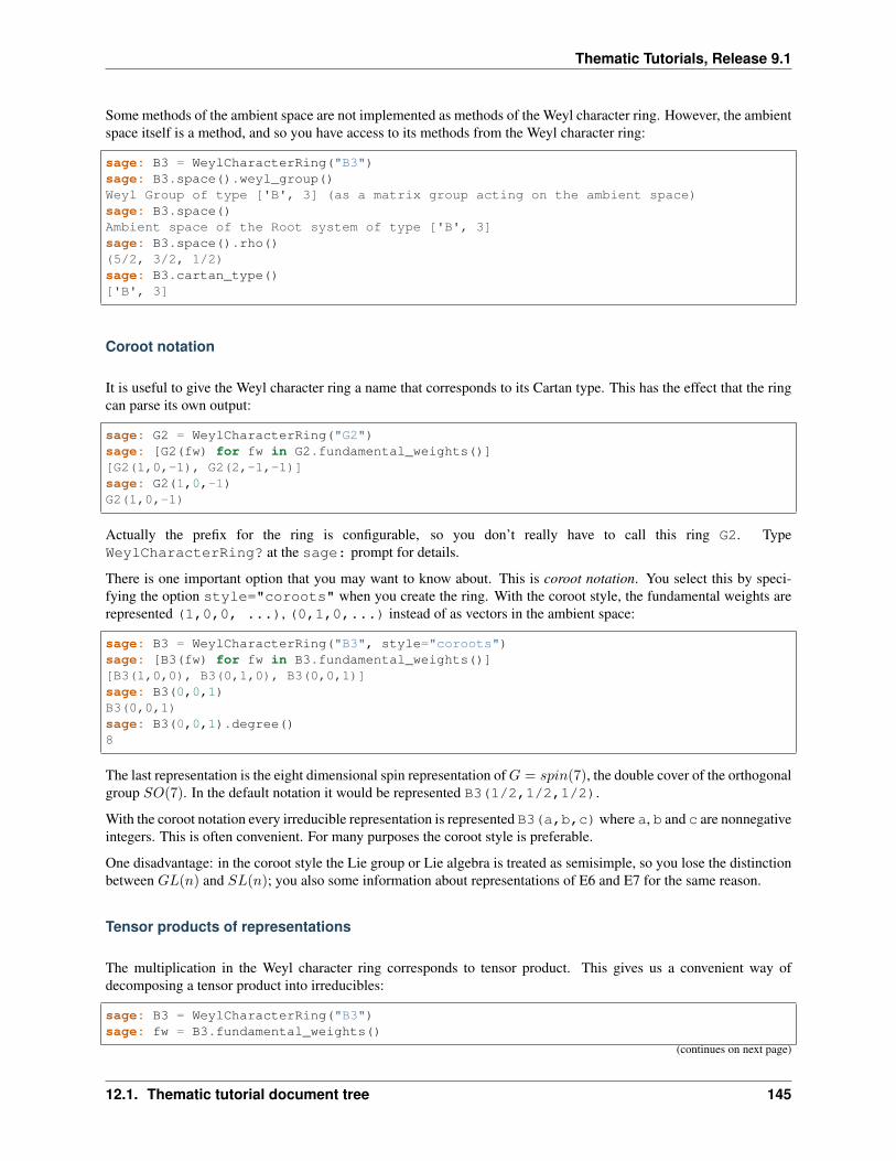
Thematic Tutorials, Release 9.1
Some methods of the ambient space are not implemented as methods of the Weyl character ring. However, the ambientspace itself is a method, and so you have access to its methods from the Weyl character ring:
sage: B3 = WeylCharacterRing("B3")sage: B3.space().weyl_group()Weyl Group of type ['B', 3] (as a matrix group acting on the ambient space)sage: B3.space()Ambient space of the Root system of type ['B', 3]sage: B3.space().rho()(5/2, 3/2, 1/2)sage: B3.cartan_type()['B', 3]
Coroot notation
It is useful to give the Weyl character ring a name that corresponds to its Cartan type. This has the effect that the ringcan parse its own output:
sage: G2 = WeylCharacterRing("G2")sage: [G2(fw) for fw in G2.fundamental_weights()][G2(1,0,-1), G2(2,-1,-1)]sage: G2(1,0,-1)G2(1,0,-1)
Actually the prefix for the ring is configurable, so you don’t really have to call this ring G2. TypeWeylCharacterRing? at the sage: prompt for details.
There is one important option that you may want to know about. This is coroot notation. You select this by speci-fying the option style="coroots" when you create the ring. With the coroot style, the fundamental weights arerepresented (1,0,0, ...), (0,1,0,...) instead of as vectors in the ambient space:
sage: B3 = WeylCharacterRing("B3", style="coroots")sage: [B3(fw) for fw in B3.fundamental_weights()][B3(1,0,0), B3(0,1,0), B3(0,0,1)]sage: B3(0,0,1)B3(0,0,1)sage: B3(0,0,1).degree()8
The last representation is the eight dimensional spin representation of𝐺 = 𝑠𝑝𝑖𝑛(7), the double cover of the orthogonalgroup 𝑆𝑂(7). In the default notation it would be represented B3(1/2,1/2,1/2).
With the coroot notation every irreducible representation is represented B3(a,b,c)where a, b and c are nonnegativeintegers. This is often convenient. For many purposes the coroot style is preferable.
One disadvantage: in the coroot style the Lie group or Lie algebra is treated as semisimple, so you lose the distinctionbetween 𝐺𝐿(𝑛) and 𝑆𝐿(𝑛); you also some information about representations of E6 and E7 for the same reason.
Tensor products of representations
The multiplication in the Weyl character ring corresponds to tensor product. This gives us a convenient way ofdecomposing a tensor product into irreducibles:
sage: B3 = WeylCharacterRing("B3")sage: fw = B3.fundamental_weights()
(continues on next page)
12.1. Thematic tutorial document tree 145
Thematic Tutorials, Release 9.1
(continued from previous page)
sage: spinweight = fw[3]; spinweight(1/2, 1/2, 1/2)sage: spin = B3(spinweight); spinB3(1/2,1/2,1/2)sage: spin.degree()8
The element 𝑠𝑝𝑖𝑛 of the WeylCharacterRing is the representation corresponding to the third highest weight represen-tation, the eight-dimensional spin representation of 𝑠𝑝𝑖𝑛(7). We could just as easily construct it with the command:
sage: spin = B3(1/2,1/2,1/2)
We may compute its tensor product with itself, using the multiplicative structure of the Weyl character ring:
sage: chi = spin*spin; chiB3(0,0,0) + B3(1,0,0) + B3(1,1,0) + B3(1,1,1)
We have taken the eight-dimensional spin representation and tensored with itself. We see that the tensor square splitsinto four irreducibles, each with multiplicity one.
The highest weights that appear here are available (with their coefficients) through the usual free module accessors:
sage: from pprint import pprintsage: list(chi) # random[((1, 1, 1), 1), ((0, 0, 0), 1), ((1, 0, 0), 1), ((1, 1, 0), 1)]sage: sorted(chi, key=str)[((0, 0, 0), 1), ((1, 0, 0), 1), ((1, 1, 0), 1), ((1, 1, 1), 1)]sage: pprint(dict(chi))(0, 0, 0): 1, (1, 0, 0): 1, (1, 1, 0): 1, (1, 1, 1): 1sage: M = sorted(chi.monomials(), key=lambda x: x.support()); M[B3(0,0,0), B3(1,0,0), B3(1,1,0), B3(1,1,1)]sage: sorted(chi.support())[(0, 0, 0), (1, 0, 0), (1, 1, 0), (1, 1, 1)]sage: chi.coefficients()[1, 1, 1, 1]sage: [r.degree() for r in M][1, 7, 21, 35]sage: sum(r.degree() for r in chi.monomials())64
Here we have extracted the individual representations, computed their degrees and checked that they sum up to 64.
Weight multiplicities
The weights of the character are available (with their coefficients) through the method weight_multiplicities.Continuing from the example in the last section:
sage: pprint(chi.weight_multiplicities())(0, 0, 0): 8, (-1, 0, 0): 4, (-1, -1, 0): 2, (-1, -1, -1): 1,(-1, -1, 1): 1, (-1, 1, 0): 2, (-1, 1, -1): 1, (-1, 1, 1): 1,(-1, 0, -1): 2, (-1, 0, 1): 2, (1, 0, 0): 4, (1, -1, 0): 2,(1, -1, -1): 1, (1, -1, 1): 1, (1, 1, 0): 2, (1, 1, -1): 1,(1, 1, 1): 1, (1, 0, -1): 2, (1, 0, 1): 2, (0, -1, 0): 4,(0, -1, -1): 2, (0, -1, 1): 2, (0, 1, 0): 4, (0, 1, -1): 2,(0, 1, 1): 2, (0, 0, -1): 4, (0, 0, 1): 4
146 Chapter 12. Documentation
Thematic Tutorials, Release 9.1
Each key of this dictionary is a weight, and its value is the multiplicity of that weight in the character.
Example
Suppose that we wish to compute the integral ∫𝑈(𝑛)
|𝑡𝑟(𝑔)|2𝑘 𝑑𝑔
for various 𝑛. Here 𝑈(𝑛) is the unitary group, which is the maximal compact subgroup of 𝐺𝐿(𝑛,C). The irreducibleunitary representations of 𝑈(𝑛) may be regarded as the basis elements of the WeylCharacterRing of type 𝐴𝑟, where𝑟 = 𝑛 − 1 so we might work in that ring. The trace 𝑡𝑟(𝑔) is then just the character of the standard representation.We may realize it in the WeylCharacterRing by taking the first fundamental weight and coercing it into the ring. Forexample, if 𝑘 = 5 and 𝑛 = 3 so 𝑟 = 2:
sage: A2 = WeylCharacterRing("A2")sage: fw = A2.fundamental_weights(); fwFinite family 1: (1, 0, 0), 2: (1, 1, 0)sage: tr = A2(fw[1]); trA2(1,0,0)
We may compute the norm square the character tr^5 by decomposing it into irreducibles, and taking the sum of thesquares of their multiplicities. By Schur orthogonality, this gives the inner product of the 𝑡𝑟(𝑔)5 with itself, that is, theintegral of |𝑡𝑟(𝑔)|10:
sage: sum(d^2 for d in (tr^5).coefficients())103
So far we have been working with 𝑛 = 3. For general 𝑛:
sage: def f(n,k):....: R = WeylCharacterRing(['A',n-1])....: tr = R(R.fundamental_weights()[1])....: return sum(d^2 for d in (tr^k).coefficients())sage: [f(n,5) for n in [2..7]][42, 103, 119, 120, 120, 120]
We see that the 10-th moment of 𝑡𝑟(𝑔) is just 5! when 𝑛 is sufficiently large. What if we fix 𝑛 and vary 𝑘?
sage: [f(2,k) for k in [1..10]][1, 2, 5, 14, 42, 132, 429, 1430, 4862, 16796]sage: [catalan_number(k) for k in [1..10]][1, 2, 5, 14, 42, 132, 429, 1430, 4862, 16796]
Frobenius-Schur indicator
The Frobeinus-Schur indicator of an irreducible representation of a compact Lie group 𝐺 with character 𝜒 is:∫𝐺
𝜒(𝑔2) 𝑑𝑔
The Haar measure is normalized so that 𝑣𝑜𝑙(𝐺) = 1. The Frobenius-Schur indicator equals 1 if the representation isreal (orthogonal),−1 if it is quaternionic (symplectic) and 0 if it is complex (not self-contragredient). This is a methodof weight ring elements corresponding to irreducible representations. Let us compute the Frobenius-Schur indicatorsof the spin representations of some odd spin groups:
12.1. Thematic tutorial document tree 147
Thematic Tutorials, Release 9.1
sage: def spinrepn(r):....: R = WeylCharacterRing(['B',r])....: return R(R.fundamental_weights()[r])....:sage: spinrepn(3)B3(1/2,1/2,1/2)sage: for r in [1..4]:....: print(" ".format(r, spinrepn(r).frobenius_schur_indicator()))1 -12 -13 14 1
Here we have defined a function that returns the spin representation of the group 𝑠𝑝𝑖𝑛(2𝑟 + 1) with Cartan type[′𝐵′, 𝑟], then computed the Frobenius-Schur indicators for a few values. From this experiment we see that the spinrepresentations of 𝑠𝑝𝑖𝑛(3) and 𝑠𝑝𝑖𝑛(5) are symplectic, while those of 𝑠𝑝𝑖𝑛(7) and 𝑠𝑝𝑖𝑛(9) are orthogonal.
Symmetric and exterior powers
Sage can compute symmetric and exterior powers of a representation:
sage: B3 = WeylCharacterRing("B3",style="coroots")sage: spin = B3(0,0,1); spin.degree()8sage: spin.exterior_power(2)B3(1,0,0) + B3(0,1,0)sage: spin.exterior_square()B3(1,0,0) + B3(0,1,0)sage: spin.exterior_power(5)B3(0,0,1) + B3(1,0,1)sage: spin.symmetric_power(5)B3(0,0,1) + B3(0,0,3) + B3(0,0,5)
The 𝑘-th exterior square of a representation is zero if 𝑘 is greater than the degree of the representation. However the𝑘-th symmetric power is nonzero for all 𝑘.
The tensor square of any representation decomposes as the direct sum of the symmetric and exterior squares:
sage: C4 = WeylCharacterRing("C4",style="coroots")sage: chi = C4(1,0,0,0); chi.degree()8sage: chi.symmetric_square()C4(2,0,0,0)sage: chi.exterior_square()C4(0,0,0,0) + C4(0,1,0,0)sage: chi^2 == chi.symmetric_square() + chi.exterior_square()True
Since in this example the exterior square contains the trivial representation we expect the Frobenius-Schur indicatorto be −1, and indeed it is:
sage: chi = C4(1,0,0,0)sage: chi.frobenius_schur_indicator()-1
This is not surprising since this is the standard representation of a symplectic group, which is symplectic by definition!
148 Chapter 12. Documentation
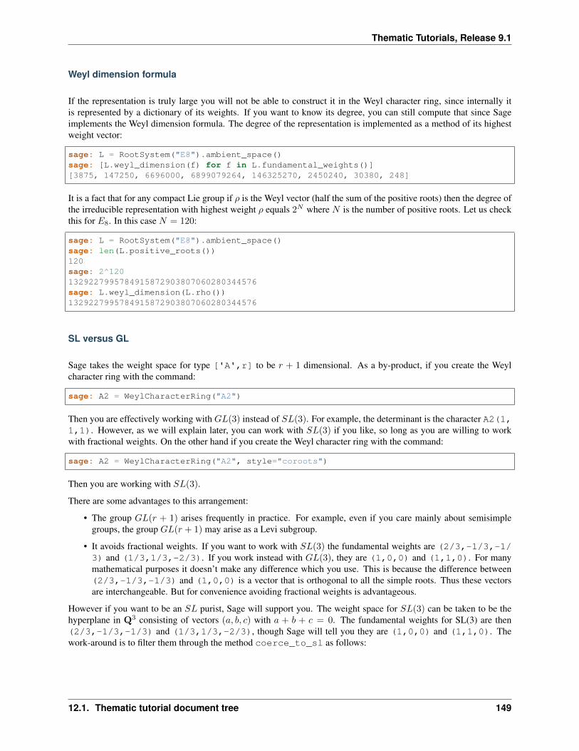
Thematic Tutorials, Release 9.1
Weyl dimension formula
If the representation is truly large you will not be able to construct it in the Weyl character ring, since internally itis represented by a dictionary of its weights. If you want to know its degree, you can still compute that since Sageimplements the Weyl dimension formula. The degree of the representation is implemented as a method of its highestweight vector:
sage: L = RootSystem("E8").ambient_space()sage: [L.weyl_dimension(f) for f in L.fundamental_weights()][3875, 147250, 6696000, 6899079264, 146325270, 2450240, 30380, 248]
It is a fact that for any compact Lie group if 𝜌 is the Weyl vector (half the sum of the positive roots) then the degree ofthe irreducible representation with highest weight 𝜌 equals 2𝑁 where 𝑁 is the number of positive roots. Let us checkthis for 𝐸8. In this case 𝑁 = 120:
sage: L = RootSystem("E8").ambient_space()sage: len(L.positive_roots())120sage: 2^1201329227995784915872903807060280344576sage: L.weyl_dimension(L.rho())1329227995784915872903807060280344576
SL versus GL
Sage takes the weight space for type ['A',r] to be 𝑟 + 1 dimensional. As a by-product, if you create the Weylcharacter ring with the command:
sage: A2 = WeylCharacterRing("A2")
Then you are effectively working with 𝐺𝐿(3) instead of 𝑆𝐿(3). For example, the determinant is the character A2(1,1,1). However, as we will explain later, you can work with 𝑆𝐿(3) if you like, so long as you are willing to workwith fractional weights. On the other hand if you create the Weyl character ring with the command:
sage: A2 = WeylCharacterRing("A2", style="coroots")
Then you are working with 𝑆𝐿(3).
There are some advantages to this arrangement:
• The group 𝐺𝐿(𝑟 + 1) arises frequently in practice. For example, even if you care mainly about semisimplegroups, the group 𝐺𝐿(𝑟 + 1) may arise as a Levi subgroup.
• It avoids fractional weights. If you want to work with 𝑆𝐿(3) the fundamental weights are (2/3,-1/3,-1/3) and (1/3,1/3,-2/3). If you work instead with 𝐺𝐿(3), they are (1,0,0) and (1,1,0). For manymathematical purposes it doesn’t make any difference which you use. This is because the difference between(2/3,-1/3,-1/3) and (1,0,0) is a vector that is orthogonal to all the simple roots. Thus these vectorsare interchangeable. But for convenience avoiding fractional weights is advantageous.
However if you want to be an 𝑆𝐿 purist, Sage will support you. The weight space for 𝑆𝐿(3) can be taken to be thehyperplane in Q3 consisting of vectors (𝑎, 𝑏, 𝑐) with 𝑎 + 𝑏 + 𝑐 = 0. The fundamental weights for SL(3) are then(2/3,-1/3,-1/3) and (1/3,1/3,-2/3), though Sage will tell you they are (1,0,0) and (1,1,0). Thework-around is to filter them through the method coerce_to_sl as follows:
12.1. Thematic tutorial document tree 149
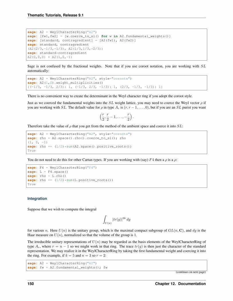
Thematic Tutorials, Release 9.1
sage: A2 = WeylCharacterRing("A2")sage: [fw1,fw2] = [w.coerce_to_sl() for w in A2.fundamental_weights()]sage: [standard, contragredient] = [A2(fw1), A2(fw2)]sage: standard, contragredient(A2(2/3,-1/3,-1/3), A2(1/3,1/3,-2/3))sage: standard*contragredientA2(0,0,0) + A2(1,0,-1)
Sage is not confused by the fractional weights. Note that if you use coroot notation, you are working with 𝑆𝐿automatically:
sage: A2 = WeylCharacterRing("A2", style="coroots")sage: A2(1,0).weight_multiplicities()(-1/3, -1/3, 2/3): 1, (-1/3, 2/3, -1/3): 1, (2/3, -1/3, -1/3): 1
There is no convenient way to create the determinant in the Weyl character ring if you adopt the coroot style.
Just as we coerced the fundamental weights into the 𝑆𝐿 weight lattice, you may need to coerce the Weyl vector 𝜌 ifyou are working with 𝑆𝐿. The default value for 𝜌 in type 𝐴𝑟 is (𝑟, 𝑟− 1, . . . , 0), but if you are an 𝑆𝐿 purist you want(𝑟
2,𝑟
2− 1, . . . ,−𝑟
2
).
Therefore take the value of 𝜌 that you get from the method of the ambient space and coerce it into 𝑆𝐿:
sage: A2 = WeylCharacterRing("A2", style="coroots")sage: rho = A2.space().rho().coerce_to_sl(); rho(1, 0, -1)sage: rho == (1/2)*sum(A2.space().positive_roots())True
You do not need to do this for other Cartan types. If you are working with (say) 𝐹4 then a 𝜌 is a 𝜌:
sage: F4 = WeylCharacterRing("F4")sage: L = F4.space()sage: rho = L.rho()sage: rho == (1/2)*sum(L.positive_roots())True
Integration
Suppose that we wish to compute the integral ∫𝑈(𝑛)
|𝑡𝑟(𝑔)|2𝑘 𝑑𝑔
for various 𝑛. Here 𝑈(𝑛) is the unitary group, which is the maximal compact subgroup of 𝐺𝐿(𝑛,C), and 𝑑𝑔 is theHaar measure on 𝑈(𝑛), normalized so that the volume of the group is 1.
The irreducible unitary representations of 𝑈(𝑛) may be regarded as the basis elements of the WeylCharacterRing oftype 𝐴𝑟, where 𝑟 = 𝑛 − 1 so we might work in that ring. The trace 𝑡𝑟(𝑔) is then just the character of the standardrepresentation. We may realize it in the WeylCharacterRing by taking the first fundamental weight and coercing it intothe ring. For example, if 𝑘 = 5 and 𝑛 = 3 so 𝑟 = 2:
sage: A2 = WeylCharacterRing("A2")sage: fw = A2.fundamental_weights(); fw
(continues on next page)
150 Chapter 12. Documentation
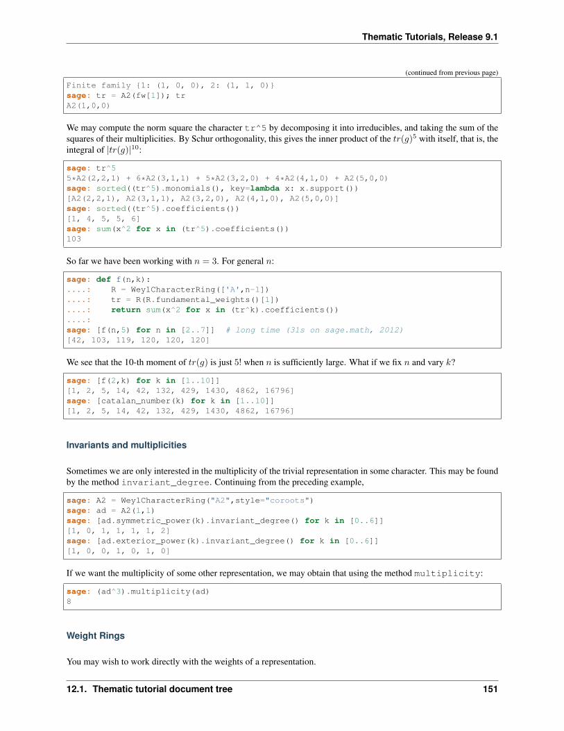
Thematic Tutorials, Release 9.1
(continued from previous page)
Finite family 1: (1, 0, 0), 2: (1, 1, 0)sage: tr = A2(fw[1]); trA2(1,0,0)
We may compute the norm square the character tr^5 by decomposing it into irreducibles, and taking the sum of thesquares of their multiplicities. By Schur orthogonality, this gives the inner product of the 𝑡𝑟(𝑔)5 with itself, that is, theintegral of |𝑡𝑟(𝑔)|10:
sage: tr^55*A2(2,2,1) + 6*A2(3,1,1) + 5*A2(3,2,0) + 4*A2(4,1,0) + A2(5,0,0)sage: sorted((tr^5).monomials(), key=lambda x: x.support())[A2(2,2,1), A2(3,1,1), A2(3,2,0), A2(4,1,0), A2(5,0,0)]sage: sorted((tr^5).coefficients())[1, 4, 5, 5, 6]sage: sum(x^2 for x in (tr^5).coefficients())103
So far we have been working with 𝑛 = 3. For general 𝑛:
sage: def f(n,k):....: R = WeylCharacterRing(['A',n-1])....: tr = R(R.fundamental_weights()[1])....: return sum(x^2 for x in (tr^k).coefficients())....:sage: [f(n,5) for n in [2..7]] # long time (31s on sage.math, 2012)[42, 103, 119, 120, 120, 120]
We see that the 10-th moment of 𝑡𝑟(𝑔) is just 5! when 𝑛 is sufficiently large. What if we fix 𝑛 and vary 𝑘?
sage: [f(2,k) for k in [1..10]][1, 2, 5, 14, 42, 132, 429, 1430, 4862, 16796]sage: [catalan_number(k) for k in [1..10]][1, 2, 5, 14, 42, 132, 429, 1430, 4862, 16796]
Invariants and multiplicities
Sometimes we are only interested in the multiplicity of the trivial representation in some character. This may be foundby the method invariant_degree. Continuing from the preceding example,
sage: A2 = WeylCharacterRing("A2",style="coroots")sage: ad = A2(1,1)sage: [ad.symmetric_power(k).invariant_degree() for k in [0..6]][1, 0, 1, 1, 1, 1, 2]sage: [ad.exterior_power(k).invariant_degree() for k in [0..6]][1, 0, 0, 1, 0, 1, 0]
If we want the multiplicity of some other representation, we may obtain that using the method multiplicity:
sage: (ad^3).multiplicity(ad)8
Weight Rings
You may wish to work directly with the weights of a representation.
12.1. Thematic tutorial document tree 151
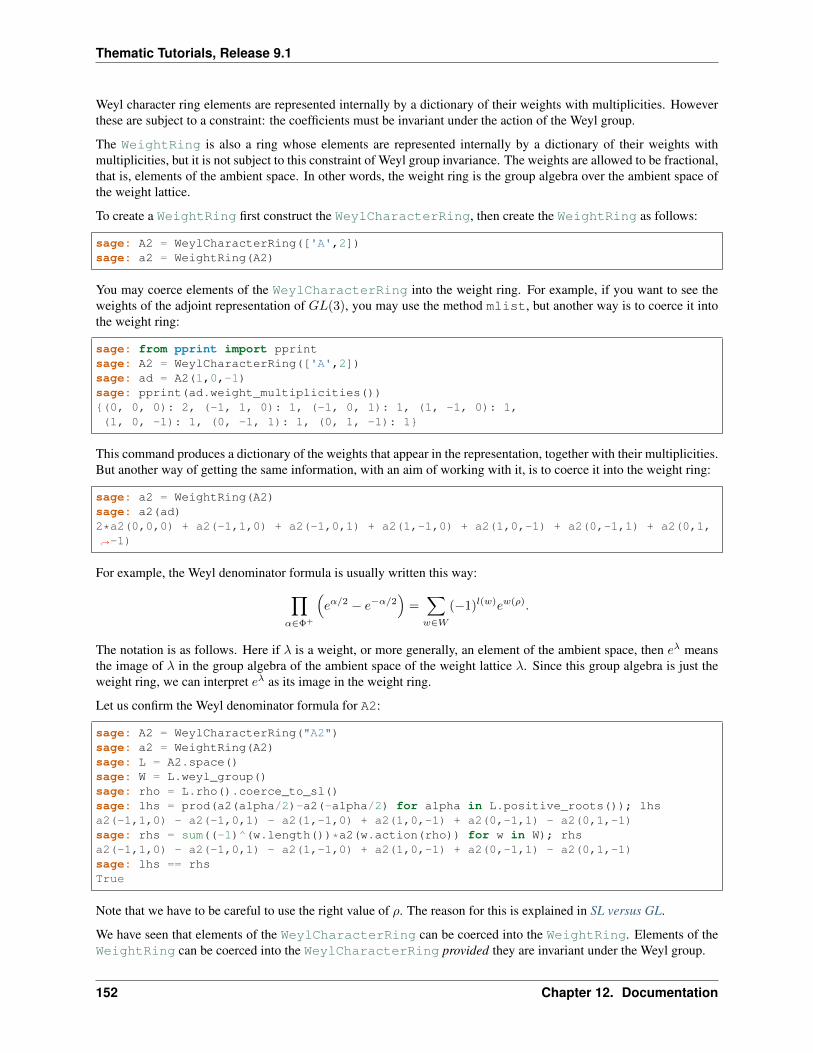
Thematic Tutorials, Release 9.1
Weyl character ring elements are represented internally by a dictionary of their weights with multiplicities. Howeverthese are subject to a constraint: the coefficients must be invariant under the action of the Weyl group.
The WeightRing is also a ring whose elements are represented internally by a dictionary of their weights withmultiplicities, but it is not subject to this constraint of Weyl group invariance. The weights are allowed to be fractional,that is, elements of the ambient space. In other words, the weight ring is the group algebra over the ambient space ofthe weight lattice.
To create a WeightRing first construct the WeylCharacterRing, then create the WeightRing as follows:
sage: A2 = WeylCharacterRing(['A',2])sage: a2 = WeightRing(A2)
You may coerce elements of the WeylCharacterRing into the weight ring. For example, if you want to see theweights of the adjoint representation of 𝐺𝐿(3), you may use the method mlist, but another way is to coerce it intothe weight ring:
sage: from pprint import pprintsage: A2 = WeylCharacterRing(['A',2])sage: ad = A2(1,0,-1)sage: pprint(ad.weight_multiplicities())(0, 0, 0): 2, (-1, 1, 0): 1, (-1, 0, 1): 1, (1, -1, 0): 1,(1, 0, -1): 1, (0, -1, 1): 1, (0, 1, -1): 1
This command produces a dictionary of the weights that appear in the representation, together with their multiplicities.But another way of getting the same information, with an aim of working with it, is to coerce it into the weight ring:
sage: a2 = WeightRing(A2)sage: a2(ad)2*a2(0,0,0) + a2(-1,1,0) + a2(-1,0,1) + a2(1,-1,0) + a2(1,0,-1) + a2(0,-1,1) + a2(0,1,→˓-1)
For example, the Weyl denominator formula is usually written this way:∏𝛼∈Φ+
(𝑒𝛼/2 − 𝑒−𝛼/2
)=
∑𝑤∈𝑊
(−1)𝑙(𝑤)𝑒𝑤(𝜌).
The notation is as follows. Here if 𝜆 is a weight, or more generally, an element of the ambient space, then 𝑒𝜆 meansthe image of 𝜆 in the group algebra of the ambient space of the weight lattice 𝜆. Since this group algebra is just theweight ring, we can interpret 𝑒𝜆 as its image in the weight ring.
Let us confirm the Weyl denominator formula for A2:
sage: A2 = WeylCharacterRing("A2")sage: a2 = WeightRing(A2)sage: L = A2.space()sage: W = L.weyl_group()sage: rho = L.rho().coerce_to_sl()sage: lhs = prod(a2(alpha/2)-a2(-alpha/2) for alpha in L.positive_roots()); lhsa2(-1,1,0) - a2(-1,0,1) - a2(1,-1,0) + a2(1,0,-1) + a2(0,-1,1) - a2(0,1,-1)sage: rhs = sum((-1)^(w.length())*a2(w.action(rho)) for w in W); rhsa2(-1,1,0) - a2(-1,0,1) - a2(1,-1,0) + a2(1,0,-1) + a2(0,-1,1) - a2(0,1,-1)sage: lhs == rhsTrue
Note that we have to be careful to use the right value of 𝜌. The reason for this is explained in SL versus GL.
We have seen that elements of the WeylCharacterRing can be coerced into the WeightRing. Elements of theWeightRing can be coerced into the WeylCharacterRing provided they are invariant under the Weyl group.
152 Chapter 12. Documentation
Thematic Tutorials, Release 9.1
Maximal Subgroups and Branching Rules
Branching rules
If 𝐺 is a Lie group and 𝐻 is a subgroup, one often needs to know how representations of 𝐺 restrict to 𝐻 . Irreduciblesusually do not restrict to irreducibles. In some cases the restriction is regular and predictable, in other cases it ischaotic. In some cases it follows a rule that can be described combinatorially, but the combinatorial description issubtle. The description of how irreducibles decompose into irreducibles is called a branching rule.
References for this topic:
• [FauserEtAl2006]
• [King1975]
• [HoweEtAl2005]
• [McKayPatera1981]
Sage can compute how a character of 𝐺 restricts to 𝐻 . It does so not by memorizing a combinatorial rule, butby computing the character and restricting the character to a maximal torus of 𝐻 . What Sage has memorized (ina series of built-in encoded rules) are the various embeddings of maximal tori of maximal subgroups of 𝐺. Themaximal subgroups of Lie groups were determined in [Dynkin1952]. This approach to computing branching rules hasa limitation: the character must fit into memory and be computable by Sage’s internal code in real time.
It is sufficient to consider the case where 𝐻 is a maximal subgroup of 𝐺, since if this is known then one may branchdown successively through a series of subgroups, each maximal in its predecessors. A problem is therefore to un-derstand the maximal subgroups in a Lie group, and to give branching rules for each, and a goal of this tutorial is toexplain the embeddings of maximal subgroups.
Sage has a class BranchingRule for branching rules. The function branching_rule returns elements of thisclass. For example, the natural embedding of 𝑆𝑝(4) into 𝑆𝐿(4) corresponds to the branching rule that we may createas follows:
sage: b=branching_rule("A3","C2",rule="symmetric"); bsymmetric branching rule A3 => C2
The name “symmetric” of this branching rule will be explained further later, but it means that 𝑆𝑝(4) is the fixedsubgroup of an involution of 𝑆𝑙(4). Here A3 and C2 are the Cartan types of the groups 𝐺 = 𝑆𝐿(4) and 𝐻 = 𝑆𝑝(4).
Now we may see how representations of 𝑆𝐿(4) decompose into irreducibles when they are restricted to 𝑆𝑝(4):
sage: A3=WeylCharacterRing("A3",style="coroots")sage: chi=A3(1,0,1); chi.degree()15sage: C2=WeylCharacterRing("C2",style="coroots")sage: chi.branch(C2,rule=b)C2(0,1) + C2(2,0)
Alternatively, we may pass chi to b as an argument of its branch method, which gives the same result:
sage: b.branch(chi)C2(0,1) + C2(2,0)
It is believed that the built-in branching rules of Sage are sufficient to handle all maximal subgroups and this is certainlythe case when the rank if less than or equal to 8.
However, if you want to branch to a subgroup that is not maximal you may not find a built-in branching rule. Wemay compose branching rules to build up embeddings. For example, here are two different embeddings of 𝑆𝑝(4) withCartan type C2 in 𝑆𝑝(8), with Cartan type C4. One embedding factors through 𝑆𝑝(4)×𝑆𝑝(4), while the other factors
12.1. Thematic tutorial document tree 153
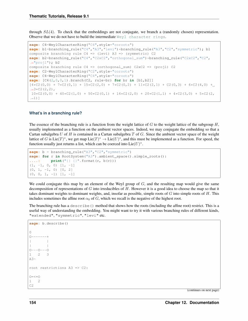
Thematic Tutorials, Release 9.1
through 𝑆𝐿(4). To check that the embeddings are not conjugate, we branch a (randomly chosen) representation.Observe that we do not have to build the intermediate Weyl character rings.
sage: C4=WeylCharacterRing("C4",style="coroots")sage: b1=branching_rule("C4","A3","levi")*branching_rule("A3","C2","symmetric"); b1composite branching rule C4 => (levi) A3 => (symmetric) C2sage: b2=branching_rule("C4","C2xC2","orthogonal_sum")*branching_rule("C2xC2","C2",→˓"proj1"); b2composite branching rule C4 => (orthogonal_sum) C2xC2 => (proj1) C2sage: C2=WeylCharacterRing("C2",style="coroots")sage: C4=WeylCharacterRing("C4",style="coroots")sage: [C4(2,0,0,1).branch(C2, rule=br) for br in [b1,b2]][4*C2(0,0) + 7*C2(0,1) + 15*C2(2,0) + 7*C2(0,2) + 11*C2(2,1) + C2(0,3) + 6*C2(4,0) +→˓3*C2(2,2),10*C2(0,0) + 40*C2(1,0) + 50*C2(0,1) + 16*C2(2,0) + 20*C2(1,1) + 4*C2(3,0) + 5*C2(2,→˓1)]
What’s in a branching rule?
The essence of the branching rule is a function from the weight lattice of 𝐺 to the weight lattice of the subgroup 𝐻 ,usually implemented as a function on the ambient vector spaces. Indeed, we may conjugate the embedding so that aCartan subalgebra 𝑈 of 𝐻 is contained in a Cartan subalgebra 𝑇 of 𝐺. Since the ambient vector space of the weightlattice of 𝐺 is Lie(𝑇 )*, we get map Lie(𝑇 )* → Lie(𝑈)*, and this must be implemented as a function. For speed, thefunction usually just returns a list, which can be coerced into Lie(𝑈)*.
sage: b = branching_rule("A3","C2","symmetric")sage: for r in RootSystem("A3").ambient_space().simple_roots():....: print(" ".format(r, b(r)))(1, -1, 0, 0) [1, -1](0, 1, -1, 0) [0, 2](0, 0, 1, -1) [1, -1]
We could conjugate this map by an element of the Weyl group of 𝐺, and the resulting map would give the samedecomposition of representations of 𝐺 into irreducibles of 𝐻 . However it is a good idea to choose the map so that ittakes dominant weights to dominant weights, and, insofar as possible, simple roots of 𝐺 into simple roots of 𝐻 . Thisincludes sometimes the affine root 𝛼0 of 𝐺, which we recall is the negative of the highest root.
The branching rule has a describe() method that shows how the roots (including the affine root) restrict. This is auseful way of understanding the embedding. You might want to try it with various branching rules of different kinds,"extended", "symmetric", "levi" etc.
sage: b.describe()
0O-------+| || |O---O---O1 2 3A3~
root restrictions A3 => C2:
O=<=O1 2C2
(continues on next page)
154 Chapter 12. Documentation
Thematic Tutorials, Release 9.1
(continued from previous page)
1 => 12 => 23 => 1
For more detailed information use verbose=True
The extended Dynkin diagram of 𝐺 and the ordinary Dynkin diagram of 𝐻 are shown for reference, and 3 => 1means that the third simple root 𝛼3 of 𝐺 restricts to the first simple root of 𝐻 . In this example, the affine root doesnot restrict to a simple roots, so it is omitted from the list of restrictions. If you add the parameter verbose=trueyou will be shown the restriction of all simple roots and the affine root, and also the restrictions of the fundamentalweights (in coroot notation).
Maximal subgroups
Sage has a database of maximal subgroups for every simple Cartan type of rank ≤ 8. You may access this with themaximal_subgroups method of the Weyl character ring:
sage: E7=WeylCharacterRing("E7",style="coroots")sage: E7.maximal_subgroups()A7:branching_rule("E7","A7","extended")E6:branching_rule("E7","E6","levi")A2:branching_rule("E7","A2","miscellaneous")A1:branching_rule("E7","A1","iii")A1:branching_rule("E7","A1","iv")A1xF4:branching_rule("E7","A1xF4","miscellaneous")G2xC3:branching_rule("E7","G2xC3","miscellaneous")A1xG2:branching_rule("E7","A1xG2","miscellaneous")A1xA1:branching_rule("E7","A1xA1","miscellaneous")A1xD6:branching_rule("E7","A1xD6","extended")A5xA2:branching_rule("E7","A5xA2","extended")
It should be understood that there are other ways of embedding 𝐴2 = SL(3) into the Lie group 𝐸7, but only oneway as a maximal subgroup. On the other hand, there are but only one way to embed it as a maximal subgroup.The embedding will be explained below. You may obtain the branching rule as follows, and use it to determine thedecomposition of irreducible representations of 𝐸7 as follows:
sage: b = E7.maximal_subgroup("A2"); bmiscellaneous branching rule E7 => A2sage: [E7,A2]=[WeylCharacterRing(x,style="coroots") for x in ["E7","A2"]]sage: E7(1,0,0,0,0,0,0).branch(A2,rule=b)A2(1,1) + A2(4,4)
This gives the same branching rule as just pasting line beginning to the right of the colon onto the command line:
sage:branching_rule("E7","A2","miscellaneous")miscellaneous branching rule E7 => A2
There are two distict embeddings of 𝐴1 = SL(2) into 𝐸7 as maximal subgroups, so the maximal_subgroupmethod will return a list of rules:
sage: WeylCharacterRing("E7").maximal_subgroup("A1")[iii branching rule E7 => A1, iv branching rule E7 => A1]
12.1. Thematic tutorial document tree 155
Thematic Tutorials, Release 9.1
The list of maximal subgroups returned by the maximal_subgroups method for irreducible Cartan types of rankup to 8 is believed to be complete up to outer automorphisms. You may want a list that is complete up to innerautomorphisms. For example, 𝐸6 has a nontrivial Dynkin diagram automorphism so it has an outer automorphism thatis not inner:
sage: [E6,A2xG2]=[WeylCharacterRing(x,style="coroots") for x in ["E6","A2xG2"]]sage: b=E6.maximal_subgroup("A2xG2"); bmiscellaneous branching rule E6 => A2xG2sage: E6(1,0,0,0,0,0).branch(A2xG2,rule=b)A2xG2(0,1,1,0) + A2xG2(2,0,0,0)sage: E6(0,0,0,0,0,1).branch(A2xG2,rule=b)A2xG2(1,0,1,0) + A2xG2(0,2,0,0)
Since as we see the two 27 dimensional irreducibles (which are interchanged by the outer automorphism) have differentbranching, the 𝐴2 × 𝐺2 subgroup is changed to a different one by the outer automorphism. To obtain the secondbranching rule, we compose the given one with this automorphism:
sage: b1=branching_rule("E6","E6","automorphic")*b; b1composite branching rule E6 => (automorphic) E6 => (miscellaneous) A2xG2
Levi subgroups
A Levi subgroup may or may not be maximal. They are easily classified. If one starts with a Dynkin diagram for 𝐺and removes a single node, one obtains a smaller Dynkin diagram, which is the Dynkin diagram of a smaller subgroup𝐻 .
For example, here is the A3 Dynkin diagram:
sage: A3 = WeylCharacterRing("A3")sage: A3.dynkin_diagram()O---O---O1 2 3A3
We see that we may remove the node 3 and obtain 𝐴2, or the node 2 and obtain 𝐴1 × 𝐴1. These correspond to theLevi subgroups 𝐺𝐿(3) and 𝐺𝐿(2)×𝐺𝐿(2) of 𝐺𝐿(4).
Let us construct the irreducible representations of𝐺𝐿(4) and branch them down to these down to𝐺𝐿(3) and𝐺𝐿(2)×𝐺𝐿(2):
sage: reps = [A3(v) for v in A3.fundamental_weights()]; reps[A3(1,0,0,0), A3(1,1,0,0), A3(1,1,1,0)]sage: A2 = WeylCharacterRing("A2")sage: A1xA1 = WeylCharacterRing("A1xA1")sage: [pi.branch(A2, rule="levi") for pi in reps][A2(0,0,0) + A2(1,0,0), A2(1,0,0) + A2(1,1,0), A2(1,1,0) + A2(1,1,1)]sage: [pi.branch(A1xA1, rule="levi") for pi in reps][A1xA1(1,0,0,0) + A1xA1(0,0,1,0),A1xA1(1,1,0,0) + A1xA1(1,0,1,0) + A1xA1(0,0,1,1),A1xA1(1,1,1,0) + A1xA1(1,0,1,1)]
Let us redo this calculation in coroot notation. As we have explained, coroot notation does not distinguish betweenrepresentations of 𝐺𝐿(4) that have the same restriction to 𝑆𝐿(4), so in effect we are now working with the groups𝑆𝐿(4) and its Levi subgroups 𝑆𝐿(3) and 𝑆𝐿(2)× 𝑆𝐿(2), which is the derived group of its Levi subgroup:
156 Chapter 12. Documentation
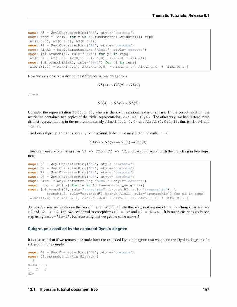
Thematic Tutorials, Release 9.1
sage: A3 = WeylCharacterRing("A3", style="coroots")sage: reps = [A3(v) for v in A3.fundamental_weights()]; reps[A3(1,0,0), A3(0,1,0), A3(0,0,1)]sage: A2 = WeylCharacterRing("A2", style="coroots")sage: A1xA1 = WeylCharacterRing("A1xA1", style="coroots")sage: [pi.branch(A2, rule="levi") for pi in reps][A2(0,0) + A2(1,0), A2(0,1) + A2(1,0), A2(0,0) + A2(0,1)]sage: [pi.branch(A1xA1, rule="levi") for pi in reps][A1xA1(1,0) + A1xA1(0,1), 2*A1xA1(0,0) + A1xA1(1,1), A1xA1(1,0) + A1xA1(0,1)]
Now we may observe a distinction difference in branching from
𝐺𝐿(4)→ 𝐺𝐿(2)×𝐺𝐿(2)
versus
𝑆𝐿(4)→ 𝑆𝐿(2)× 𝑆𝐿(2).
Consider the representation A3(0,1,0), which is the six dimensional exterior square. In the coroot notation, therestriction contained two copies of the trivial representation, 2*A1xA1(0,0). The other way, we had instead threedistinct representations in the restriction, namely A1xA1(1,1,0,0) and A1xA1(0,0,1,1), that is, det⊗1 and1⊗ det.
The Levi subgroup A1xA1 is actually not maximal. Indeed, we may factor the embedding:
𝑆𝐿(2)× 𝑆𝐿(2)→ 𝑆𝑝(4)→ 𝑆𝐿(4).
Therfore there are branching rules A3 -> C2 and C2 -> A2, and we could accomplish the branching in two steps,thus:
sage: A3 = WeylCharacterRing("A3", style="coroots")sage: C2 = WeylCharacterRing("C2", style="coroots")sage: B2 = WeylCharacterRing("B2", style="coroots")sage: D2 = WeylCharacterRing("D2", style="coroots")sage: A1xA1 = WeylCharacterRing("A1xA1", style="coroots")sage: reps = [A3(fw) for fw in A3.fundamental_weights()]sage: [pi.branch(C2, rule="symmetric").branch(B2, rule="isomorphic"). \
branch(D2, rule="extended").branch(A1xA1, rule="isomorphic") for pi in reps][A1xA1(1,0) + A1xA1(0,1), 2*A1xA1(0,0) + A1xA1(1,1), A1xA1(1,0) + A1xA1(0,1)]
As you can see, we’ve redone the branching rather circuitously this way, making use of the branching rules A3 ->C2 and B2 -> D2, and two accidental isomorphisms C2 = B2 and D2 = A1xA1. It is much easier to go in onestep using rule="levi", but reassuring that we get the same answer!
Subgroups classified by the extended Dynkin diagram
It is also true that if we remove one node from the extended Dynkin diagram that we obtain the Dynkin diagram of asubgroup. For example:
sage: G2 = WeylCharacterRing("G2", style="coroots")sage: G2.extended_dynkin_diagram()
3O=<=O---O1 2 0G2~
12.1. Thematic tutorial document tree 157
Thematic Tutorials, Release 9.1
Observe that by removing the 1 node that we obtain an 𝐴2 Dynkin diagram. Therefore the exceptional group 𝐺2
contains a copy of 𝑆𝐿(3). We branch the two representations of 𝐺2 corresponding to the fundamental weights to thiscopy of 𝐴2:
sage: G2 = WeylCharacterRing("G2", style="coroots")sage: A2 = WeylCharacterRing("A2", style="coroots")sage: [G2(f).degree() for f in G2.fundamental_weights()][7, 14]sage: [G2(f).branch(A2, rule="extended") for f in G2.fundamental_weights()][A2(0,0) + A2(0,1) + A2(1,0), A2(0,1) + A2(1,0) + A2(1,1)]
The two representations of 𝐺2, of degrees 7 and 14 respectively, are the action on the octonions of trace zero and theadjoint representation.
For embeddings of this type, the rank of the subgroup 𝐻 is the same as the rank of 𝐺. This is in contrast withembeddings of Levi type, where 𝐻 has rank one less than 𝐺.
Levi subgroups of 𝐺2
The exceptional group 𝐺2 has two Levi subgroups of type 𝐴1. Neither is maximal, as we can see from the extendedDynkin diagram: the subgroups 𝐴1 ×𝐴1 and 𝐴2 are maximal and each contains a Levi subgroup. (Actually 𝐴1 ×𝐴1
contains a conjugate of both.) Only the Levi subgroup containing the short root is implemented as an instance ofrule="levi". To obtain the other, use the rule:
sage: branching_rule("G2","A2","extended")*branching_rule("A2","A1","levi")composite branching rule G2 => (extended) A2 => (levi) A1
which branches to the 𝐴1 Levi subgroup containing a long root.
Orthogonal and symplectic subgroups of orthogonal and symplectic groups
If 𝐺 = SO(𝑛) then 𝐺 has a subgroup SO(𝑛 − 1). Depending on whether 𝑛 is even or odd, we thus have branchingrules ['D',r] to ['B',r-1] or ['B',r] to ['D',r]. These are handled as follows:
sage: branching_rule("B4","D4",rule="extended")extended branching rule B4 => D4sage: branching_rule("D4","B3",rule="symmetric")symmetric branching rule D4 => B3
If 𝐺 = SO(𝑟+ 𝑠) then 𝐺 has a subgroup SO(𝑟)× SO(𝑠). This lifts to an embedding of the universal covering groups
spin(𝑟)× spin(𝑠)→ spin(𝑟 + 𝑠).
Sometimes this embedding is of extended type, and sometimes it is not. It is of extended type unless 𝑟 and𝑠 are both odd. If it is of extended type then you may use rule="extended". In any case you may userule="orthogonal_sum". The name refer to the origin of the embedding 𝑆𝑂(𝑟) × 𝑆𝑂(𝑠) → 𝑆𝑂(𝑟 + 𝑠)from the decomposition of the underlying quadratic space as a direct sum of two orthogonal subspaces.
There are four cases depending on the parity of 𝑟 and 𝑠. For example, if 𝑟 = 2𝑘 and 𝑠 = 2𝑙 we have an embedding:
['D',k] x ['D',l] --> ['D',k+l]
This is of extended type. Thus consider the embedding D4xD3 -> D7. Here is the extended Dynkin diagram:
158 Chapter 12. Documentation
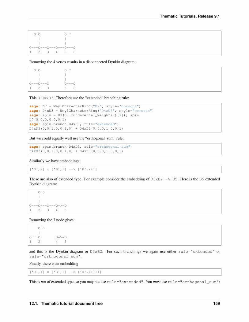
Thematic Tutorials, Release 9.1
0 O O 7| || |
O---O---O---O---O---O1 2 3 4 5 6
Removing the 4 vertex results in a disconnected Dynkin diagram:
0 O O 7| || |
O---O---O O---O1 2 3 5 6
This is D4xD3. Therefore use the “extended” branching rule:
sage: D7 = WeylCharacterRing("D7", style="coroots")sage: D4xD3 = WeylCharacterRing("D4xD3", style="coroots")sage: spin = D7(D7.fundamental_weights()[7]); spinD7(0,0,0,0,0,0,1)sage: spin.branch(D4xD3, rule="extended")D4xD3(0,0,1,0,0,1,0) + D4xD3(0,0,0,1,0,0,1)
But we could equally well use the “orthogonal_sum” rule:
sage: spin.branch(D4xD3, rule="orthogonal_sum")D4xD3(0,0,1,0,0,1,0) + D4xD3(0,0,0,1,0,0,1)
Similarly we have embeddings:
['D',k] x ['B',l] --> ['B',k+l]
These are also of extended type. For example consider the embedding of D3xB2 -> B5. Here is the B5 extendedDynkin diagram:
O 0||
O---O---O---O=>=O1 2 3 4 5
Removing the 3 node gives:
O 0|
O---O O=>=O1 2 4 5
and this is the Dynkin diagram or D3xB2. For such branchings we again use either rule="extended" orrule="orthogonal_sum".
Finally, there is an embedding
['B',k] x ['B',l] --> ['D',k+l+1]
This is not of extended type, so you may not use rule="extended". You must use rule="orthogonal_sum":
12.1. Thematic tutorial document tree 159
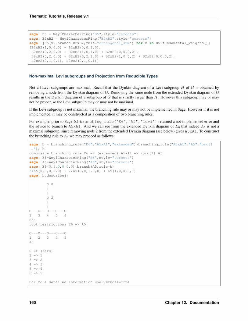
Thematic Tutorials, Release 9.1
sage: D5 = WeylCharacterRing("D5",style="coroots")sage: B2xB2 = WeylCharacterRing("B2xB2",style="coroots")sage: [D5(v).branch(B2xB2,rule="orthogonal_sum") for v in D5.fundamental_weights()][B2xB2(1,0,0,0) + B2xB2(0,0,1,0),B2xB2(0,2,0,0) + B2xB2(1,0,1,0) + B2xB2(0,0,0,2),B2xB2(0,2,0,0) + B2xB2(0,2,1,0) + B2xB2(1,0,0,2) + B2xB2(0,0,0,2),B2xB2(0,1,0,1), B2xB2(0,1,0,1)]
Non-maximal Levi subgroups and Projection from Reducible Types
Not all Levi subgroups are maximal. Recall that the Dynkin-diagram of a Levi subgroup 𝐻 of 𝐺 is obtained byremoving a node from the Dynkin diagram of 𝐺. Removing the same node from the extended Dynkin diagram of 𝐺results in the Dynkin diagram of a subgroup of 𝐺 that is strictly larger than 𝐻 . However this subgroup may or maynot be proper, so the Levi subgroup may or may not be maximal.
If the Levi subgroup is not maximal, the branching rule may or may not be implemented in Sage. However if it is notimplemented, it may be constructed as a composition of two branching rules.
For example, prior to Sage-6.1 branching_rule("E6","A5","levi") returned a not-implemented error andthe advice to branch to A5xA1. And we can see from the extended Dynkin diagram of 𝐸6 that indeed 𝐴5 is not amaximal subgroup, since removing node 2 from the extended Dynkin diagram (see below) gives A5xA1. To constructthe branching rule to 𝐴5 we may proceed as follows:
sage: b = branching_rule("E6","A5xA1","extended")*branching_rule("A5xA1","A5","proj1→˓"); bcomposite branching rule E6 => (extended) A5xA1 => (proj1) A5sage: E6=WeylCharacterRing("E6",style="coroots")sage: A5=WeylCharacterRing("A5",style="coroots")sage: E6(0,1,0,0,0,0).branch(A5,rule=b)3*A5(0,0,0,0,0) + 2*A5(0,0,1,0,0) + A5(1,0,0,0,1)sage: b.describe()
O 0||O 2||
O---O---O---O---O1 3 4 5 6E6~root restrictions E6 => A5:
O---O---O---O---O1 2 3 4 5A5
0 => (zero)1 => 13 => 24 => 35 => 46 => 5
For more detailed information use verbose=True
160 Chapter 12. Documentation
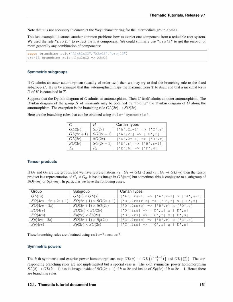
Thematic Tutorials, Release 9.1
Note that it is not necessary to construct the Weyl character ring for the intermediate group A5xA1.
This last example illustrates another common problem: how to extract one component from a reducible root system.We used the rule "proj1" to extract the first component. We could similarly use "proj2" to get the second, ormore generally any combination of components:
sage: branching_rule("A2xB2xG2","A2xG2","proj13")proj13 branching rule A2xB2xG2 => A2xG2
Symmetric subgroups
If 𝐺 admits an outer automorphism (usually of order two) then we may try to find the branching rule to the fixedsubgroup 𝐻 . It can be arranged that this automorphism maps the maximal torus 𝑇 to itself and that a maximal torus𝑈 of 𝐻 is contained in 𝑇 .
Suppose that the Dynkin diagram of 𝐺 admits an automorphism. Then 𝐺 itself admits an outer automorphism. TheDynkin diagram of the group 𝐻 of invariants may be obtained by “folding” the Dynkin diagram of 𝐺 along theautomorphism. The exception is the branching rule 𝐺𝐿(2𝑟)→ 𝑆𝑂(2𝑟).
Here are the branching rules that can be obtained using rule="symmetric".
𝐺 𝐻 Cartan Types𝐺𝐿(2𝑟) 𝑆𝑝(2𝑟) ['A',2r-1] => ['C',r]𝐺𝐿(2𝑟 + 1) 𝑆𝑂(2𝑟 + 1) ['A',2r] => ['B',r]𝐺𝐿(2𝑟) 𝑆𝑂(2𝑟) ['A',2r-1] => ['D',r]𝑆𝑂(2𝑟) 𝑆𝑂(2𝑟 − 1) ['D',r] => ['B',r-1]𝐸6 𝐹4 ['E',6] => ['F',4]
Tensor products
If 𝐺1 and 𝐺2 are Lie groups, and we have representations 𝜋1 : 𝐺1 → 𝐺𝐿(𝑛) and 𝜋2 : 𝐺2 → 𝐺𝐿(𝑚) then the tensorproduct is a representation of 𝐺1 ×𝐺2. It has its image in 𝐺𝐿(𝑛𝑚) but sometimes this is conjugate to a subgroup of𝑆𝑂(𝑛𝑚) or 𝑆𝑝(𝑛𝑚). In particular we have the following cases.
Group Subgroup Cartan Types𝐺𝐿(𝑟𝑠) 𝐺𝐿(𝑟)×𝐺𝐿(𝑠) ['A', rs-1] => ['A',r-1] x ['A',s-1]𝑆𝑂(4𝑟𝑠+ 2𝑟 + 2𝑠+ 1) 𝑆𝑂(2𝑟 + 1)× 𝑆𝑂(2𝑠+ 1) ['B',2rs+r+s] => ['B',r] x ['B',s]𝑆𝑂(4𝑟𝑠+ 2𝑠) 𝑆𝑂(2𝑟 + 1)× 𝑆𝑂(2𝑠) ['D',2rs+s] => ['B',r] x ['D',s]𝑆𝑂(4𝑟𝑠) 𝑆𝑂(2𝑟)× 𝑆𝑂(2𝑠) ['D',2rs] => ['D',r] x ['D',s]𝑆𝑂(4𝑟𝑠) 𝑆𝑝(2𝑟)× 𝑆𝑝(2𝑠) ['D',2rs] => ['C',r] x ['C',s]𝑆𝑝(4𝑟𝑠+ 2𝑠) 𝑆𝑂(2𝑟 + 1)× 𝑆𝑝(2𝑠) ['C',2rs+s] => ['B',r] x ['C',s]𝑆𝑝(4𝑟𝑠) 𝑆𝑝(2𝑟)× 𝑆𝑂(2𝑠) ['C',2rs] => ['C',r] x ['D',s]
These branching rules are obtained using rule="tensor".
Symmetric powers
The 𝑘-th symmetric and exterior power homomorphisms map 𝐺𝐿(𝑛) → 𝐺𝐿((
𝑛+𝑘−1𝑘
))and 𝐺𝐿
((𝑛𝑘
)). The cor-
responding branching rules are not implemented but a special case is. The 𝑘-th symmetric power homomorphism𝑆𝐿(2)→ 𝐺𝐿(𝑘 + 1) has its image inside of 𝑆𝑂(2𝑟 + 1) if 𝑘 = 2𝑟 and inside of 𝑆𝑝(2𝑟) if 𝑘 = 2𝑟 − 1. Hence thereare branching rules:
12.1. Thematic tutorial document tree 161
Thematic Tutorials, Release 9.1
['B',r] => A1['C',r] => A1
and these may be obtained using rule="symmetric_power".
Plethysms
The above branching rules are sufficient for most cases, but a few fall between the cracks. Mostly these involvemaximal subgroups of fairly small rank.
The rule rule="plethysm" is a powerful rule that includes any branching rule from types 𝐴, 𝐵, 𝐶 or 𝐷 as aspecial case. Thus it could be used in place of the above rules and would give the same results. However, it is mostuseful when branching from 𝐺 to a maximal subgroup 𝐻 such that 𝑟𝑎𝑛𝑘(𝐻) < 𝑟𝑎𝑛𝑘(𝐺)− 1.
We consider a homomorphism 𝐻 → 𝐺 where 𝐺 is one of 𝑆𝐿(𝑟 + 1), 𝑆𝑂(2𝑟 + 1), 𝑆𝑝(2𝑟) or 𝑆𝑂(2𝑟). The functionbranching_rule_from_plethysm produces the corresponding branching rule. The main ingredient is thecharacter 𝜒 of the representation of 𝐻 that is the homomorphism to 𝐺𝐿(𝑟 + 1), 𝐺𝐿(2𝑟 + 1) or 𝐺𝐿(2𝑟).
Let us consider the symmetric fifth power representation of 𝑆𝐿(2). This is implemented above byrule="symmetric_power", but suppose we want to use rule="plethysm". First we construct the homo-morphism by invoking its character, to be called chi:
sage: A1 = WeylCharacterRing("A1", style="coroots")sage: chi = A1([5])sage: chi.degree()6sage: chi.frobenius_schur_indicator()-1
This confirms that the character has degree 6 and is symplectic, so it corresponds to a homomorphism 𝑆𝐿(2)→ 𝑆𝑝(6),and there is a corresponding branching rule C3 -> A1:
sage: A1 = WeylCharacterRing("A1", style="coroots")sage: C3 = WeylCharacterRing("C3", style="coroots")sage: chi = A1([5])sage: sym5rule = branching_rule_from_plethysm(chi, "C3")sage: [C3(hwv).branch(A1, rule=sym5rule) for hwv in C3.fundamental_weights()][A1(5), A1(4) + A1(8), A1(3) + A1(9)]
This is identical to the results we would obtain using rule="symmetric_power":
sage: A1 = WeylCharacterRing("A1", style="coroots")sage: C3 = WeylCharacterRing("C3", style="coroots")sage: [C3(v).branch(A1, rule="symmetric_power") for v in C3.fundamental_weights()][A1(5), A1(4) + A1(8), A1(3) + A1(9)]
But the next example of plethysm gives a branching rule not available by other methods:
sage: G2 = WeylCharacterRing("G2", style="coroots")sage: D7 = WeylCharacterRing("D7", style="coroots")sage: ad = G2.adjoint_representation(); ad.degree()14sage: ad.frobenius_schur_indicator()1sage: for r in D7.fundamental_weights(): # long time (1.29s)....: print(D7(r).branch(G2, rule=branching_rule_from_plethysm(ad, "D7")))
(continues on next page)
162 Chapter 12. Documentation
Thematic Tutorials, Release 9.1
(continued from previous page)
G2(0,1)G2(0,1) + G2(3,0)G2(0,0) + G2(2,0) + G2(3,0) + G2(0,2) + G2(4,0)G2(0,1) + G2(2,0) + G2(1,1) + G2(0,2) + G2(2,1) + G2(4,0) + G2(3,1)G2(1,0) + G2(0,1) + G2(1,1) + 2*G2(3,0) + 2*G2(2,1) + G2(1,2) + G2(3,1) + G2(5,0) +→˓G2(0,3)G2(1,1)G2(1,1)
In this example, 𝑎𝑑 is the 14-dimensional adjoint representation of the exceptional group 𝐺2. Since the Frobenius-Schur indicator is 1, the representation is orthogonal, and factors through 𝑆𝑂(14), that is, 𝐷7.
We do not actually have to create the character (or for that matter its ambient WeylCharacterRing) in order to createthe branching rule:
sage: branching_rule("D4","A2.adjoint_representation()","plethysm")plethysm (along A2(1,1)) branching rule D4 => A2
The adjoint representation of any semisimple Lie group is orthogonal, so we do not need to compute the Frobenius-Schur indicator.
Miscellaneous other subgroups
Use rule="miscellaneous" for the following rules. Every maximal subgroup 𝐻 of an exceptional group 𝐺 areeither among these, or the five 𝐴1 subgroups described in the next section, or (if 𝐺 and 𝐻 have the same rank) isavailable using rule="extended".
𝐵3 → 𝐺2,
𝐸6 → 𝐴2,
𝐸6 → 𝐺2,
𝐹4 → 𝐺2 ×𝐴1,
𝐸6 → 𝐺2 ×𝐴2,
𝐸7 → 𝐺2 × 𝐶3,
𝐸7 → 𝐹4 ×𝐴1,
𝐸7 → 𝐴1 ×𝐴1,
𝐸7 → 𝐺2 ×𝐴1,
𝐸7 → 𝐴2
𝐸8 → 𝐺2 × 𝐹4.
𝐸8 → 𝐴2 ×𝐴1.
𝐸8 → 𝐵2
The first rule corresponds to the embedding of𝐺2 in SO(7) in its action on the trace zero octonions. The two branchingrules from 𝐸6 to 𝐺2 or 𝐴2 are described in [Testerman1989]. We caution the reader that Theorem G.2 of that paper,proved there in positive characteristic is false over the complex numbers. On the other hand, the assumption ofcharacteristic 𝑝 is not important for Theorems G.1 and A.1, which describe the torus embeddings, hence containenough information to compute the branching rule. There are other ways of embedding 𝐺2 or 𝐴2 into 𝐸6. These mayembeddings be characterized by the condition that the two 27-dimensional representations of 𝐸6 restrict irreduciblyto 𝐺2 or 𝐴2. Their images are maximal subgroups.
12.1. Thematic tutorial document tree 163
Thematic Tutorials, Release 9.1
The remaining rules come about as follows. Let 𝐺 be 𝐹4, 𝐸6, 𝐸7 or 𝐸8, and let 𝐻 be 𝐺2, or else (if 𝐺 = 𝐸7) 𝐹4. Weembed 𝐻 into 𝐺 in the most obvious way; that is, in the chain of subgroups
𝐺2 ⊂ 𝐹4 ⊂ 𝐸6 ⊂ 𝐸7 ⊂ 𝐸8
Then the centralizer of 𝐻 is 𝐴1, 𝐴2, 𝐶3, 𝐹4 (if 𝐻 = 𝐺2) or 𝐴1 (if 𝐺 = 𝐸7 and 𝐻 = 𝐹4). This gives us five of thecases. Regarding the branching rule 𝐸6 → 𝐺2 × 𝐴2, Rubenthaler [Rubenthaler2008] describes the embedding andapplies it in an interesting way.
The embedding of 𝐴1 × 𝐴1 into 𝐸7 is as follows. Deleting the 5 node of the 𝐸7 Dynkin diagram gives the Dynkindiagram of 𝐴4 × 𝐴2, so this is a Levi subgroup. We embed SL(2) into this Levi subgroup via the representation[4] ⊗ [2]. This embeds the first copy of 𝐴1. The other 𝐴1 is the connected centralizer. See [Seitz1991], particularlythe proof of (3.12).
The embedding if 𝐺2 × 𝐴1 into 𝐸7 is as follows. Deleting the 2 node of the 𝐸7 Dynkin diagram gives the 𝐴6
Dynkin diagram, which is the Levi subgroup SL(7). We embed 𝐺2 into SL(7) via the irreducible seven-dimensionalrepresentation of 𝐺2. The 𝐴1 is the centralizer.
The embedding if 𝐴2 ×𝐴1 into 𝐸8 is as follows. Deleting the 2 node of the 𝐸8 Dynkin diagram gives the 𝐴7 Dynkindiagram, which is the Levi subgroup SL(8). We embed 𝐴2 into SL(8) via the irreducible eight-dimensional adjointrepresentation of SL(2). The 𝐴1 is the centralizer.
The embedding 𝐴2 into 𝐸7 is proved in [Seitz1991] (5.8). In particular, he computes the embedding of the SL(3)torus in the 𝐸7 torus, which is what is needed to implement the branching rule. The embedding of 𝐵2 into 𝐸8 is alsoconstructed in [Seitz1991] (6.7). The embedding of the 𝐵2 Cartan subalgebra, needed to implement the branchingrule, is easily deduced from (10) on page 111.
Maximal A1 subgroups of Exceptional Groups
There are seven embeddings of 𝑆𝐿(2) into an exceptional group as a maximal subgroup: one each for 𝐺2 and 𝐹4, twononconjugate embeddings for𝐸7 and three for𝐸8 These are constructed in [Testerman1992]. Create the correspondingbranching rules as follows. The names of the rules are roman numerals referring to the seven cases of Testerman’sTheorem 1:
sage: branching_rule("G2","A1","i")i branching rule G2 => A1sage: branching_rule("F4","A1","ii")ii branching rule F4 => A1sage: branching_rule("E7","A1","iii")iii branching rule E7 => A1sage: branching_rule("E7","A1","iv")iv branching rule E7 => A1sage: branching_rule("E8","A1","v")v branching rule E8 => A1sage: branching_rule("E8","A1","vi")vi branching rule E8 => A1sage: branching_rule("E8","A1","vii")vii branching rule E8 => A1
The embeddings are characterized by the root restrictions in their branching rules: usually a simple root of the ambientgroup 𝐺 restricts to the unique simple root of 𝐴1, except for root 𝛼4 for rules iv, vi and vii, and the root 𝛼6 for root vii;this is essentially the way Testerman characterizes the embeddings, and this information may be obtained from Sageby employing the describe() method of the branching rule. Thus:
164 Chapter 12. Documentation
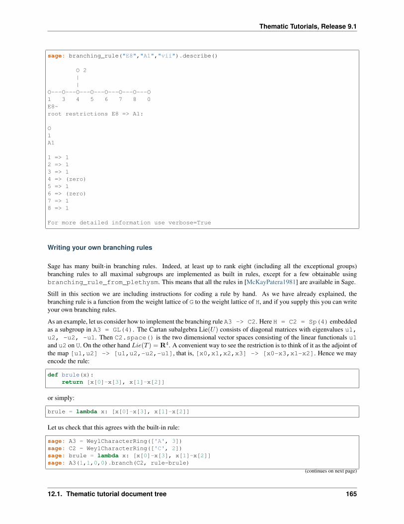
Thematic Tutorials, Release 9.1
sage: branching_rule("E8","A1","vii").describe()
O 2||
O---O---O---O---O---O---O---O1 3 4 5 6 7 8 0E8~root restrictions E8 => A1:
O1A1
1 => 12 => 13 => 14 => (zero)5 => 16 => (zero)7 => 18 => 1
For more detailed information use verbose=True
Writing your own branching rules
Sage has many built-in branching rules. Indeed, at least up to rank eight (including all the exceptional groups)branching rules to all maximal subgroups are implemented as built in rules, except for a few obtainable usingbranching_rule_from_plethysm. This means that all the rules in [McKayPatera1981] are available in Sage.
Still in this section we are including instructions for coding a rule by hand. As we have already explained, thebranching rule is a function from the weight lattice of G to the weight lattice of H, and if you supply this you can writeyour own branching rules.
As an example, let us consider how to implement the branching rule A3 -> C2. Here H = C2 = Sp(4) embeddedas a subgroup in A3 = GL(4). The Cartan subalgebra Lie(𝑈) consists of diagonal matrices with eigenvalues u1,u2, -u2, -u1. Then C2.space() is the two dimensional vector spaces consisting of the linear functionals u1and u2 on U. On the other hand 𝐿𝑖𝑒(𝑇 ) = R4. A convenient way to see the restriction is to think of it as the adjoint ofthe map [u1,u2] -> [u1,u2,-u2,-u1], that is, [x0,x1,x2,x3] -> [x0-x3,x1-x2]. Hence we mayencode the rule:
def brule(x):return [x[0]-x[3], x[1]-x[2]]
or simply:
brule = lambda x: [x[0]-x[3], x[1]-x[2]]
Let us check that this agrees with the built-in rule:
sage: A3 = WeylCharacterRing(['A', 3])sage: C2 = WeylCharacterRing(['C', 2])sage: brule = lambda x: [x[0]-x[3], x[1]-x[2]]sage: A3(1,1,0,0).branch(C2, rule=brule)
(continues on next page)
12.1. Thematic tutorial document tree 165
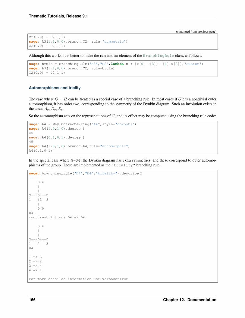
Thematic Tutorials, Release 9.1
(continued from previous page)
C2(0,0) + C2(1,1)sage: A3(1,1,0,0).branch(C2, rule="symmetric")C2(0,0) + C2(1,1)
Although this works, it is better to make the rule into an element of the BranchingRule class, as follows.
sage: brule = BranchingRule("A3","C2",lambda x : [x[0]-x[3], x[1]-x[2]],"custom")sage: A3(1,1,0,0).branch(C2, rule=brule)C2(0,0) + C2(1,1)
Automorphisms and triality
The case where 𝐺 = 𝐻 can be treated as a special case of a branching rule. In most cases if 𝐺 has a nontrivial outerautomorphism, it has order two, corresponding to the symmetry of the Dynkin diagram. Such an involution exists inthe cases 𝐴𝑟, 𝐷𝑟, 𝐸6.
So the automorphism acts on the representations of 𝐺, and its effect may be computed using the branching rule code:
sage: A4 = WeylCharacterRing("A4",style="coroots")sage: A4(1,0,1,0).degree()45sage: A4(0,1,0,1).degree()45sage: A4(1,0,1,0).branch(A4,rule="automorphic")A4(0,1,0,1)
In the special case where G=D4, the Dynkin diagram has extra symmetries, and these correspond to outer automor-phisms of the group. These are implemented as the "triality" branching rule:
sage: branching_rule("D4","D4","triality").describe()
O 4||
O---O---O1 |2 3
|O 0
D4~root restrictions D4 => D4:
O 4||
O---O---O1 2 3D4
1 => 32 => 23 => 44 => 1
For more detailed information use verbose=True
166 Chapter 12. Documentation
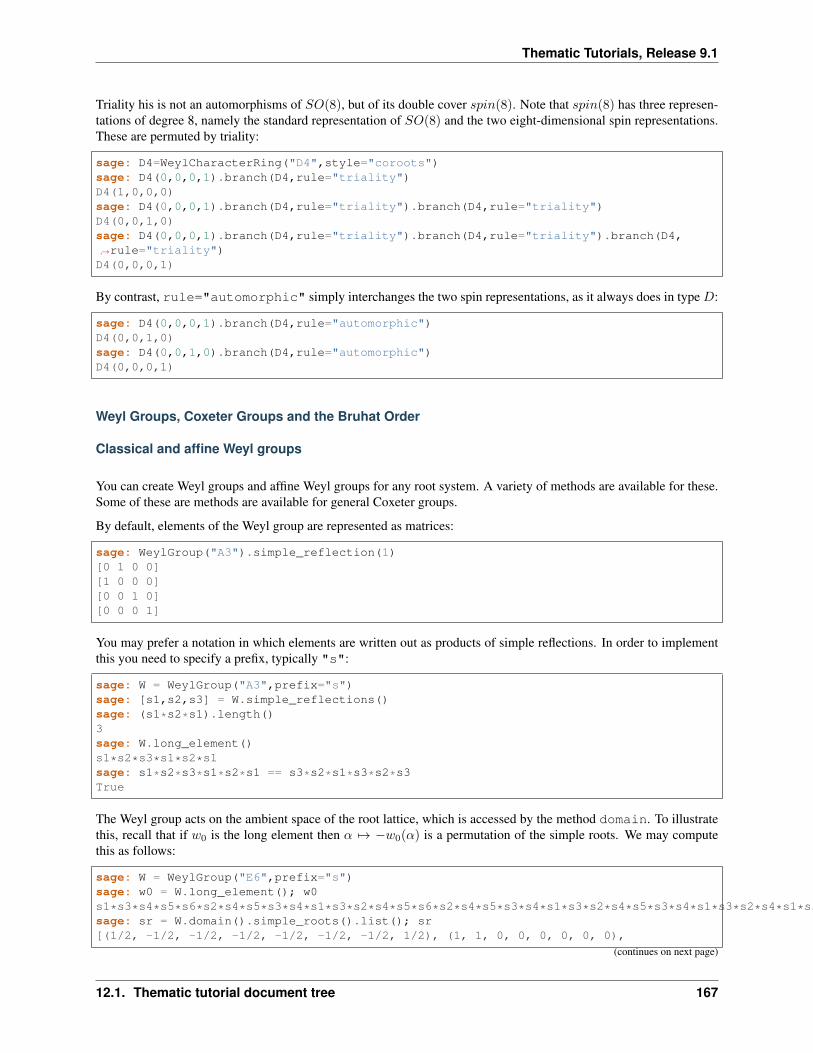
Thematic Tutorials, Release 9.1
Triality his is not an automorphisms of 𝑆𝑂(8), but of its double cover 𝑠𝑝𝑖𝑛(8). Note that 𝑠𝑝𝑖𝑛(8) has three represen-tations of degree 8, namely the standard representation of 𝑆𝑂(8) and the two eight-dimensional spin representations.These are permuted by triality:
sage: D4=WeylCharacterRing("D4",style="coroots")sage: D4(0,0,0,1).branch(D4,rule="triality")D4(1,0,0,0)sage: D4(0,0,0,1).branch(D4,rule="triality").branch(D4,rule="triality")D4(0,0,1,0)sage: D4(0,0,0,1).branch(D4,rule="triality").branch(D4,rule="triality").branch(D4,→˓rule="triality")D4(0,0,0,1)
By contrast, rule="automorphic" simply interchanges the two spin representations, as it always does in type 𝐷:
sage: D4(0,0,0,1).branch(D4,rule="automorphic")D4(0,0,1,0)sage: D4(0,0,1,0).branch(D4,rule="automorphic")D4(0,0,0,1)
Weyl Groups, Coxeter Groups and the Bruhat Order
Classical and affine Weyl groups
You can create Weyl groups and affine Weyl groups for any root system. A variety of methods are available for these.Some of these are methods are available for general Coxeter groups.
By default, elements of the Weyl group are represented as matrices:
sage: WeylGroup("A3").simple_reflection(1)[0 1 0 0][1 0 0 0][0 0 1 0][0 0 0 1]
You may prefer a notation in which elements are written out as products of simple reflections. In order to implementthis you need to specify a prefix, typically "s":
sage: W = WeylGroup("A3",prefix="s")sage: [s1,s2,s3] = W.simple_reflections()sage: (s1*s2*s1).length()3sage: W.long_element()s1*s2*s3*s1*s2*s1sage: s1*s2*s3*s1*s2*s1 == s3*s2*s1*s3*s2*s3True
The Weyl group acts on the ambient space of the root lattice, which is accessed by the method domain. To illustratethis, recall that if 𝑤0 is the long element then 𝛼 ↦→ −𝑤0(𝛼) is a permutation of the simple roots. We may computethis as follows:
sage: W = WeylGroup("E6",prefix="s")sage: w0 = W.long_element(); w0s1*s3*s4*s5*s6*s2*s4*s5*s3*s4*s1*s3*s2*s4*s5*s6*s2*s4*s5*s3*s4*s1*s3*s2*s4*s5*s3*s4*s1*s3*s2*s4*s1*s3*s2*s1sage: sr = W.domain().simple_roots().list(); sr[(1/2, -1/2, -1/2, -1/2, -1/2, -1/2, -1/2, 1/2), (1, 1, 0, 0, 0, 0, 0, 0),
(continues on next page)
12.1. Thematic tutorial document tree 167
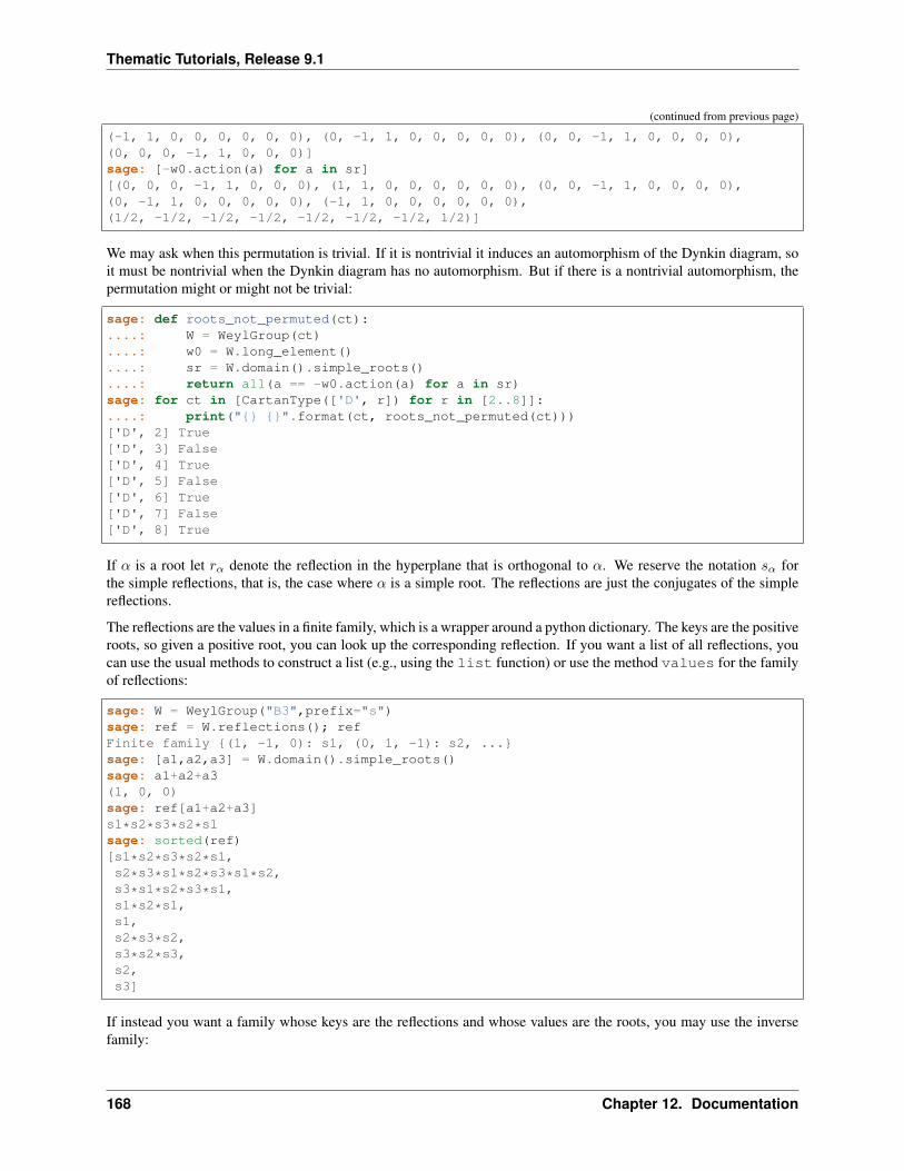
Thematic Tutorials, Release 9.1
(continued from previous page)
(-1, 1, 0, 0, 0, 0, 0, 0), (0, -1, 1, 0, 0, 0, 0, 0), (0, 0, -1, 1, 0, 0, 0, 0),(0, 0, 0, -1, 1, 0, 0, 0)]sage: [-w0.action(a) for a in sr][(0, 0, 0, -1, 1, 0, 0, 0), (1, 1, 0, 0, 0, 0, 0, 0), (0, 0, -1, 1, 0, 0, 0, 0),(0, -1, 1, 0, 0, 0, 0, 0), (-1, 1, 0, 0, 0, 0, 0, 0),(1/2, -1/2, -1/2, -1/2, -1/2, -1/2, -1/2, 1/2)]
We may ask when this permutation is trivial. If it is nontrivial it induces an automorphism of the Dynkin diagram, soit must be nontrivial when the Dynkin diagram has no automorphism. But if there is a nontrivial automorphism, thepermutation might or might not be trivial:
sage: def roots_not_permuted(ct):....: W = WeylGroup(ct)....: w0 = W.long_element()....: sr = W.domain().simple_roots()....: return all(a == -w0.action(a) for a in sr)sage: for ct in [CartanType(['D', r]) for r in [2..8]]:....: print(" ".format(ct, roots_not_permuted(ct)))['D', 2] True['D', 3] False['D', 4] True['D', 5] False['D', 6] True['D', 7] False['D', 8] True
If 𝛼 is a root let 𝑟𝛼 denote the reflection in the hyperplane that is orthogonal to 𝛼. We reserve the notation 𝑠𝛼 forthe simple reflections, that is, the case where 𝛼 is a simple root. The reflections are just the conjugates of the simplereflections.
The reflections are the values in a finite family, which is a wrapper around a python dictionary. The keys are the positiveroots, so given a positive root, you can look up the corresponding reflection. If you want a list of all reflections, youcan use the usual methods to construct a list (e.g., using the list function) or use the method values for the familyof reflections:
sage: W = WeylGroup("B3",prefix="s")sage: ref = W.reflections(); refFinite family (1, -1, 0): s1, (0, 1, -1): s2, ...sage: [a1,a2,a3] = W.domain().simple_roots()sage: a1+a2+a3(1, 0, 0)sage: ref[a1+a2+a3]s1*s2*s3*s2*s1sage: sorted(ref)[s1*s2*s3*s2*s1,s2*s3*s1*s2*s3*s1*s2,s3*s1*s2*s3*s1,s1*s2*s1,s1,s2*s3*s2,s3*s2*s3,s2,s3]
If instead you want a family whose keys are the reflections and whose values are the roots, you may use the inversefamily:
168 Chapter 12. Documentation
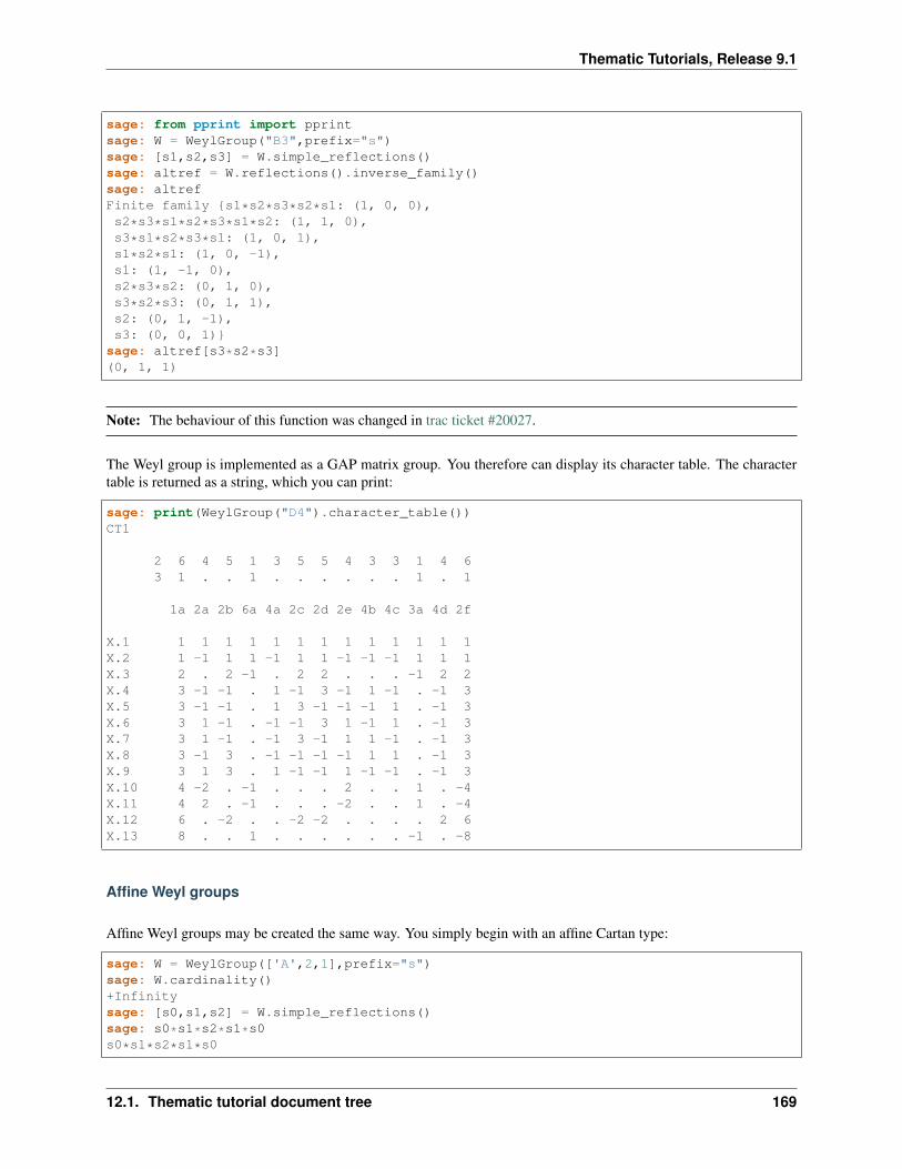
Thematic Tutorials, Release 9.1
sage: from pprint import pprintsage: W = WeylGroup("B3",prefix="s")sage: [s1,s2,s3] = W.simple_reflections()sage: altref = W.reflections().inverse_family()sage: altrefFinite family s1*s2*s3*s2*s1: (1, 0, 0),s2*s3*s1*s2*s3*s1*s2: (1, 1, 0),s3*s1*s2*s3*s1: (1, 0, 1),s1*s2*s1: (1, 0, -1),s1: (1, -1, 0),s2*s3*s2: (0, 1, 0),s3*s2*s3: (0, 1, 1),s2: (0, 1, -1),s3: (0, 0, 1)
sage: altref[s3*s2*s3](0, 1, 1)
Note: The behaviour of this function was changed in trac ticket #20027.
The Weyl group is implemented as a GAP matrix group. You therefore can display its character table. The charactertable is returned as a string, which you can print:
sage: print(WeylGroup("D4").character_table())CT1
2 6 4 5 1 3 5 5 4 3 3 1 4 63 1 . . 1 . . . . . . 1 . 1
1a 2a 2b 6a 4a 2c 2d 2e 4b 4c 3a 4d 2f
X.1 1 1 1 1 1 1 1 1 1 1 1 1 1X.2 1 -1 1 1 -1 1 1 -1 -1 -1 1 1 1X.3 2 . 2 -1 . 2 2 . . . -1 2 2X.4 3 -1 -1 . 1 -1 3 -1 1 -1 . -1 3X.5 3 -1 -1 . 1 3 -1 -1 -1 1 . -1 3X.6 3 1 -1 . -1 -1 3 1 -1 1 . -1 3X.7 3 1 -1 . -1 3 -1 1 1 -1 . -1 3X.8 3 -1 3 . -1 -1 -1 -1 1 1 . -1 3X.9 3 1 3 . 1 -1 -1 1 -1 -1 . -1 3X.10 4 -2 . -1 . . . 2 . . 1 . -4X.11 4 2 . -1 . . . -2 . . 1 . -4X.12 6 . -2 . . -2 -2 . . . . 2 6X.13 8 . . 1 . . . . . . -1 . -8
Affine Weyl groups
Affine Weyl groups may be created the same way. You simply begin with an affine Cartan type:
sage: W = WeylGroup(['A',2,1],prefix="s")sage: W.cardinality()+Infinitysage: [s0,s1,s2] = W.simple_reflections()sage: s0*s1*s2*s1*s0s0*s1*s2*s1*s0
12.1. Thematic tutorial document tree 169
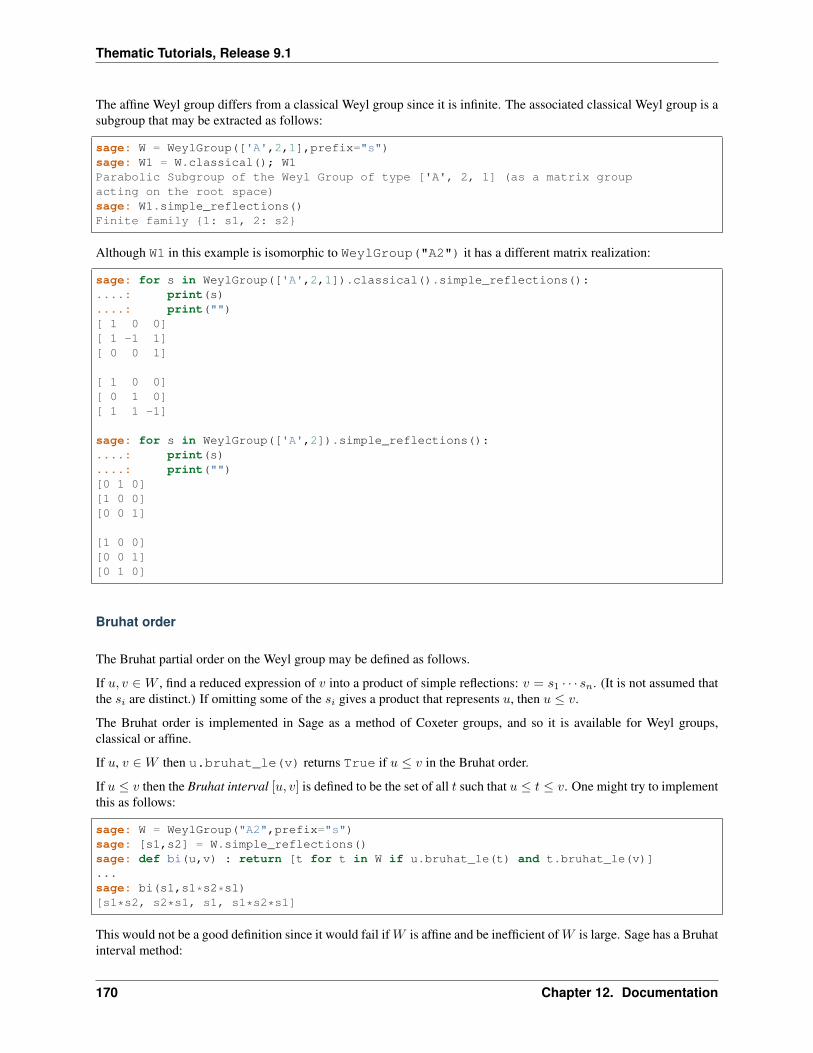
Thematic Tutorials, Release 9.1
The affine Weyl group differs from a classical Weyl group since it is infinite. The associated classical Weyl group is asubgroup that may be extracted as follows:
sage: W = WeylGroup(['A',2,1],prefix="s")sage: W1 = W.classical(); W1Parabolic Subgroup of the Weyl Group of type ['A', 2, 1] (as a matrix groupacting on the root space)sage: W1.simple_reflections()Finite family 1: s1, 2: s2
Although W1 in this example is isomorphic to WeylGroup("A2") it has a different matrix realization:
sage: for s in WeylGroup(['A',2,1]).classical().simple_reflections():....: print(s)....: print("")[ 1 0 0][ 1 -1 1][ 0 0 1]
[ 1 0 0][ 0 1 0][ 1 1 -1]
sage: for s in WeylGroup(['A',2]).simple_reflections():....: print(s)....: print("")[0 1 0][1 0 0][0 0 1]
[1 0 0][0 0 1][0 1 0]
Bruhat order
The Bruhat partial order on the Weyl group may be defined as follows.
If 𝑢, 𝑣 ∈ 𝑊 , find a reduced expression of 𝑣 into a product of simple reflections: 𝑣 = 𝑠1 · · · 𝑠𝑛. (It is not assumed thatthe 𝑠𝑖 are distinct.) If omitting some of the 𝑠𝑖 gives a product that represents 𝑢, then 𝑢 ≤ 𝑣.
The Bruhat order is implemented in Sage as a method of Coxeter groups, and so it is available for Weyl groups,classical or affine.
If 𝑢, 𝑣 ∈𝑊 then u.bruhat_le(v) returns True if 𝑢 ≤ 𝑣 in the Bruhat order.
If 𝑢 ≤ 𝑣 then the Bruhat interval [𝑢, 𝑣] is defined to be the set of all 𝑡 such that 𝑢 ≤ 𝑡 ≤ 𝑣. One might try to implementthis as follows:
sage: W = WeylGroup("A2",prefix="s")sage: [s1,s2] = W.simple_reflections()sage: def bi(u,v) : return [t for t in W if u.bruhat_le(t) and t.bruhat_le(v)]...sage: bi(s1,s1*s2*s1)[s1*s2, s2*s1, s1, s1*s2*s1]
This would not be a good definition since it would fail if𝑊 is affine and be inefficient of𝑊 is large. Sage has a Bruhatinterval method:
170 Chapter 12. Documentation
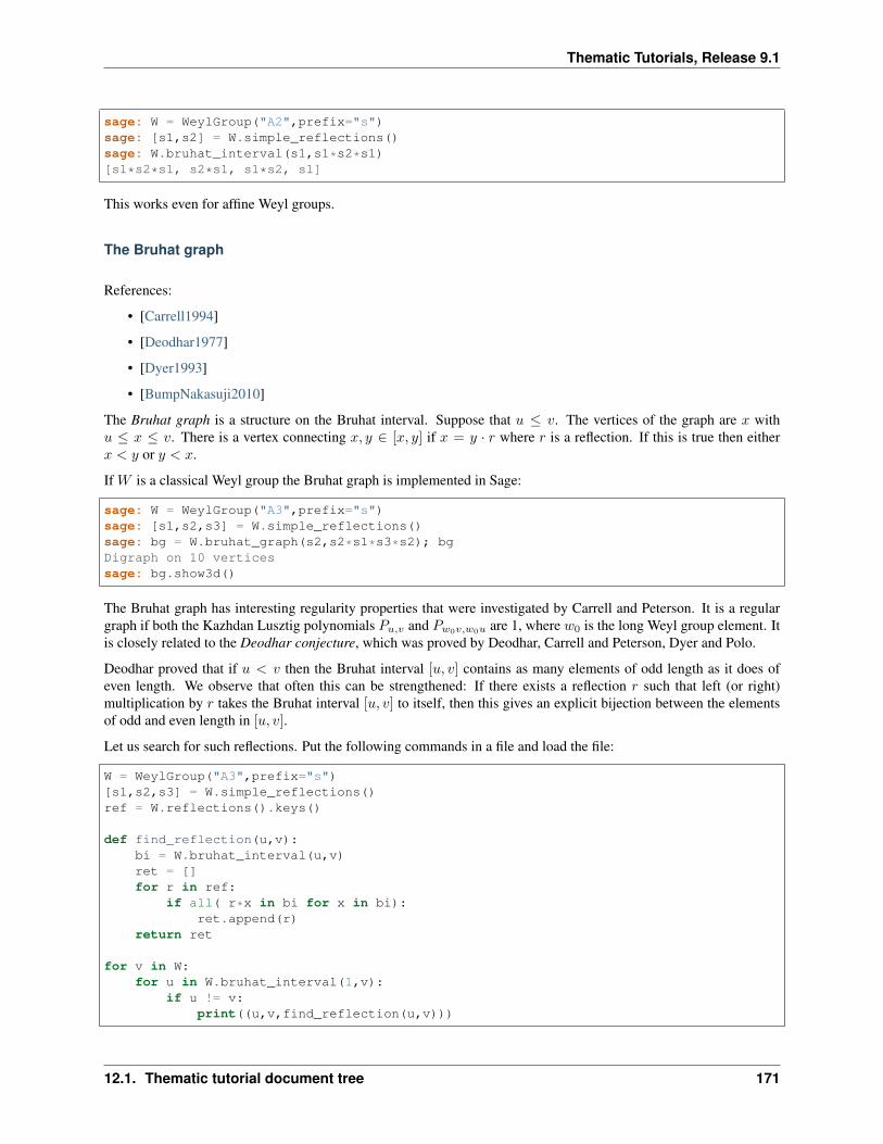
Thematic Tutorials, Release 9.1
sage: W = WeylGroup("A2",prefix="s")sage: [s1,s2] = W.simple_reflections()sage: W.bruhat_interval(s1,s1*s2*s1)[s1*s2*s1, s2*s1, s1*s2, s1]
This works even for affine Weyl groups.
The Bruhat graph
References:
• [Carrell1994]
• [Deodhar1977]
• [Dyer1993]
• [BumpNakasuji2010]
The Bruhat graph is a structure on the Bruhat interval. Suppose that 𝑢 ≤ 𝑣. The vertices of the graph are 𝑥 with𝑢 ≤ 𝑥 ≤ 𝑣. There is a vertex connecting 𝑥, 𝑦 ∈ [𝑥, 𝑦] if 𝑥 = 𝑦 · 𝑟 where 𝑟 is a reflection. If this is true then either𝑥 < 𝑦 or 𝑦 < 𝑥.
If 𝑊 is a classical Weyl group the Bruhat graph is implemented in Sage:
sage: W = WeylGroup("A3",prefix="s")sage: [s1,s2,s3] = W.simple_reflections()sage: bg = W.bruhat_graph(s2,s2*s1*s3*s2); bgDigraph on 10 verticessage: bg.show3d()
The Bruhat graph has interesting regularity properties that were investigated by Carrell and Peterson. It is a regulargraph if both the Kazhdan Lusztig polynomials 𝑃𝑢,𝑣 and 𝑃𝑤0𝑣,𝑤0𝑢 are 1, where 𝑤0 is the long Weyl group element. Itis closely related to the Deodhar conjecture, which was proved by Deodhar, Carrell and Peterson, Dyer and Polo.
Deodhar proved that if 𝑢 < 𝑣 then the Bruhat interval [𝑢, 𝑣] contains as many elements of odd length as it does ofeven length. We observe that often this can be strengthened: If there exists a reflection 𝑟 such that left (or right)multiplication by 𝑟 takes the Bruhat interval [𝑢, 𝑣] to itself, then this gives an explicit bijection between the elementsof odd and even length in [𝑢, 𝑣].
Let us search for such reflections. Put the following commands in a file and load the file:
W = WeylGroup("A3",prefix="s")[s1,s2,s3] = W.simple_reflections()ref = W.reflections().keys()
def find_reflection(u,v):bi = W.bruhat_interval(u,v)ret = []for r in ref:
if all( r*x in bi for x in bi):ret.append(r)
return ret
for v in W:for u in W.bruhat_interval(1,v):
if u != v:print((u,v,find_reflection(u,v)))
12.1. Thematic tutorial document tree 171
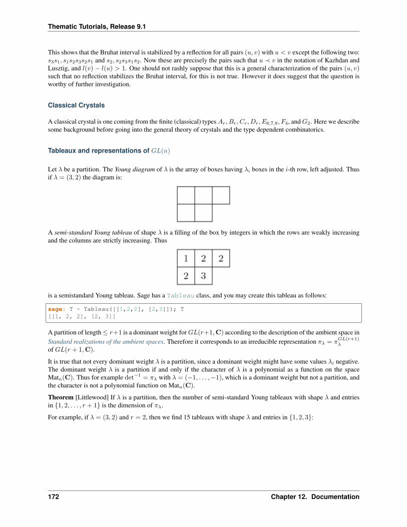
Thematic Tutorials, Release 9.1
This shows that the Bruhat interval is stabilized by a reflection for all pairs (𝑢, 𝑣) with 𝑢 < 𝑣 except the following two:𝑠3𝑠1, 𝑠1𝑠2𝑠3𝑠2𝑠1 and 𝑠2, 𝑠2𝑠3𝑠1𝑠2. Now these are precisely the pairs such that 𝑢 ≺ 𝑣 in the notation of Kazhdan andLusztig, and 𝑙(𝑣) − 𝑙(𝑢) > 1. One should not rashly suppose that this is a general characterization of the pairs (𝑢, 𝑣)such that no reflection stabilizes the Bruhat interval, for this is not true. However it does suggest that the question isworthy of further investigation.
Classical Crystals
A classical crystal is one coming from the finite (classical) types𝐴𝑟, 𝐵𝑟, 𝐶𝑟, 𝐷𝑟, 𝐸6,7,8, 𝐹4, and𝐺2. Here we describesome background before going into the general theory of crystals and the type dependent combinatorics.
Tableaux and representations of 𝐺𝐿(𝑛)
Let 𝜆 be a partition. The Young diagram of 𝜆 is the array of boxes having 𝜆𝑖 boxes in the 𝑖-th row, left adjusted. Thusif 𝜆 = (3, 2) the diagram is:
A semi-standard Young tableau of shape 𝜆 is a filling of the box by integers in which the rows are weakly increasingand the columns are strictly increasing. Thus
is a semistandard Young tableau. Sage has a Tableau class, and you may create this tableau as follows:
sage: T = Tableau([[1,2,2], [2,3]]); T[[1, 2, 2], [2, 3]]
A partition of length≤ 𝑟+1 is a dominant weight for𝐺𝐿(𝑟+1,C) according to the description of the ambient space inStandard realizations of the ambient spaces. Therefore it corresponds to an irreducible representation 𝜋𝜆 = 𝜋
𝐺𝐿(𝑟+1)𝜆
of 𝐺𝐿(𝑟 + 1,C).
It is true that not every dominant weight 𝜆 is a partition, since a dominant weight might have some values 𝜆𝑖 negative.The dominant weight 𝜆 is a partition if and only if the character of 𝜆 is a polynomial as a function on the spaceMat𝑛(C). Thus for example det−1 = 𝜋𝜆 with 𝜆 = (−1, . . . ,−1), which is a dominant weight but not a partition, andthe character is not a polynomial function on Mat𝑛(C).
Theorem [Littlewood] If 𝜆 is a partition, then the number of semi-standard Young tableaux with shape 𝜆 and entriesin 1, 2, . . . , 𝑟 + 1 is the dimension of 𝜋𝜆.
For example, if 𝜆 = (3, 2) and 𝑟 = 2, then we find 15 tableaux with shape 𝜆 and entries in 1, 2, 3:
172 Chapter 12. Documentation
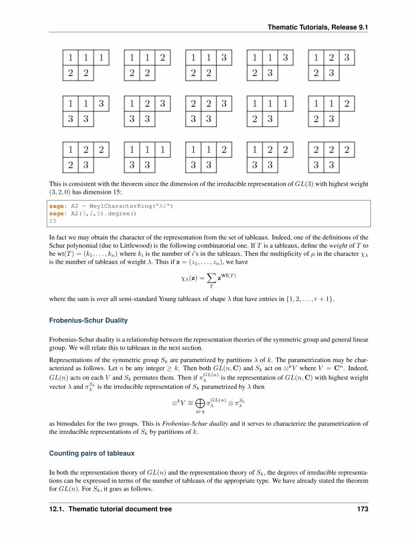
Thematic Tutorials, Release 9.1
This is consistent with the theorem since the dimension of the irreducible representation of𝐺𝐿(3) with highest weight(3, 2, 0) has dimension 15:
sage: A2 = WeylCharacterRing("A2")sage: A2(3,2,0).degree()15
In fact we may obtain the character of the representation from the set of tableaux. Indeed, one of the definitions of theSchur polynomial (due to Littlewood) is the following combinatorial one. If 𝑇 is a tableaux, define the weight of 𝑇 tobe wt(𝑇 ) = (𝑘1, . . . , 𝑘𝑛) where 𝑘𝑖 is the number of 𝑖’s in the tableaux. Then the multiplicity of 𝜇 in the character 𝜒𝜆
is the number of tableaux of weight 𝜆. Thus if z = (𝑧1, . . . , 𝑧𝑛), we have
𝜒𝜆(z) =∑𝑇
zwt(𝑇 )
where the sum is over all semi-standard Young tableaux of shape 𝜆 that have entries in 1, 2, . . . , 𝑟 + 1.
Frobenius-Schur Duality
Frobenius-Schur duality is a relationship between the representation theories of the symmetric group and general lineargroup. We will relate this to tableaux in the next section.
Representations of the symmetric group 𝑆𝑘 are parametrized by partitions 𝜆 of 𝑘. The parametrization may be char-acterized as follows. Let 𝑛 be any integer ≥ 𝑘. Then both 𝐺𝐿(𝑛,C) and 𝑆𝑘 act on ⊗𝑘𝑉 where 𝑉 = C𝑛. Indeed,𝐺𝐿(𝑛) acts on each 𝑉 and 𝑆𝑘 permutes them. Then if 𝜋𝐺𝐿(𝑛)
𝜆 is the representation of 𝐺𝐿(𝑛,C) with highest weightvector 𝜆 and 𝜋𝑆𝑘
𝜆 is the irreducible representation of 𝑆𝑘 parametrized by 𝜆 then
⊗𝑘𝑉 ∼=⨁𝜆⊢𝑘
𝜋𝐺𝐿(𝑛)𝜆 ⊗ 𝜋𝑆𝑘
𝜆
as bimodules for the two groups. This is Frobenius-Schur duality and it serves to characterize the parametrization ofthe irreducible representations of 𝑆𝑘 by partitions of 𝑘.
Counting pairs of tableaux
In both the representation theory of 𝐺𝐿(𝑛) and the representation theory of 𝑆𝑘, the degrees of irreducible representa-tions can be expressed in terms of the number of tableaux of the appropriate type. We have already stated the theoremfor 𝐺𝐿(𝑛). For 𝑆𝑘, it goes as follows.
12.1. Thematic tutorial document tree 173
Thematic Tutorials, Release 9.1
Let us say that a semistandard Young tableau 𝑇 of shape 𝜆 ⊢ 𝑘 is standard if 𝑇 contains each entry 1, 2, . . . , 𝑘 exactlyonce. Thus both rows and columns are strictly increasing.
Theorem [Young, 1927] The degree of 𝜋𝜆 is the number of standard tableaux of shape 𝜆.
Now let us consider the implications of Frobenius-Schur duality. The dimension of ⊗𝑘𝑉 is 𝑛𝑘. Therefore 𝑛𝑘 is equalto the number of pairs (𝑇1, 𝑇2) of tableaux of the same shape 𝜆 ⊢ 𝑘, where the first tableaux is standard (in thealphabet 1, 2, . . . , 𝑘), and the second the second semistandard (in the alphabet 1, 2, . . . , 𝑛).
The Robinson-Schensted-Knuth correspondence
The last purely combinatorial statement has a combinatorial proof, based on the Robinson-Schensted-Knuth (RSK)correspondence.
References:
• [Knuth1998], section “Tableaux and Involutions”.
• [Knuth1970]
• [Fulton1997]
• [Stanley1999]
The RSK correspondence gives bijections between pairs of tableaux of various types and combinatorial objects ofdifferent types. We will not review the correspondence in detail here, but see the references. We note that Schenstedinsertion is implemented as the method schensted_insertion of Tableau class in Sage.
Thus we have the following bijections:
• Pairs of tableaux 𝑇1 and 𝑇2 of shape 𝜆 where 𝜆 runs through the partitions of 𝑘 such that 𝑇1 is a standard tableauand 𝑇2 is a semistandard tableau in 1, 2, . . . , 𝑛 are in bijection with the 𝑛𝑘 words of length 𝑘 in 1, 2, . . . , 𝑛.
• Pairs of standard tableaux of the same shape 𝜆 as 𝜆 runs through the partitions of 𝑘 are in bijection with the 𝑘!elements of 𝑆𝑘.
• Pairs of tableaux 𝑇1 and 𝑇2 of the same shape 𝜆 but arbitrary size in 1, 2, 3, . . . , 𝑛 are in bijection with 𝑛 × 𝑛positive integer matrices.
• Pairs of tableaux 𝑇1 and 𝑇2 of conjugate shapes 𝜆 and 𝜆′ are in bijection with 𝑛×𝑛 matrices with entries 0 or 1.
The second of these four bijection gives a combinatorial proof of the fact explained above, that the number of pairs(𝑇1, 𝑇2) of tableaux of the same shape 𝜆 ⊢ 𝑘, where the first tableaux is standard (in the alphabet 1, 2, · · · , 𝑘), andthe second the second semistandard (in the alphabet 1, 2, · · · , 𝑛). So this second bijection is a combinatorial analogof Frobenius-Schur duality.
Analogies between representation theory and combinatorics
The four combinatorial bijections (variants of RSK) cited above have the following analogs in representation theory.
• The first combinatorial fact corresponds to Frobenius-Schur duality, as we have already explained.
• The second combinatorial fact also has an analog in representation theory. The group algebra C[𝑆𝑘] is an𝑆𝑘 × 𝑆𝑘 bimodule with of dimension 𝑘!. It decomposes as a direct sum of 𝜋𝑆𝑘
𝜆 ⊗ 𝜋𝑆𝑘
𝜆 .
Both the combinatorial fact and the decomposition of C[𝑆𝑘] show that the number of pairs of standard tableaux of size𝑘 and the same shape equals 𝑘!.
• The third combinatorial fact is analogous to the decomposition of the ring of polynomial functions on Mat(𝑛,C)on which 𝐺𝐿(𝑛,C) × 𝐺𝐿(𝑛,C) acts by (𝑔1, 𝑔2)𝑓(𝑋) = 𝑓(𝑡𝑔1𝑋𝑔2). The polynomial ring decomposes intothe direct sum of 𝜋𝐺𝐿(𝑛)
𝜆 ⊗ 𝜋𝐺𝐿(𝑛)𝜆 .
174 Chapter 12. Documentation
Thematic Tutorials, Release 9.1
Taking traces gives the Cauchy identity:∑𝜆
𝑠𝜆(𝑥1, · · · , 𝑥𝑛)𝑠𝜆(𝑦1, · · · , 𝑦𝑛) =∏𝑖,𝑗
(1− 𝑥𝑖𝑦𝑗)−1
where 𝑥𝑖 are the eigenvalues of 𝑔1 and 𝑦𝑗 are the eigenvalues of 𝑔2. The sum is over all partitions 𝜆.
• The last combinatorial fact is analogous to the decomposition of the exterior algebra over Mat(𝑛,C).
Taking traces gives the dual Cauchy identity:∑𝜆
𝑠𝜆(𝑥1, · · · , 𝑥𝑛)𝑠𝜆′(𝑦1, · · · , 𝑦𝑛) =∏𝑖,𝑗
(1 + 𝑥𝑖𝑦𝑗).
Again the sum is over partitions 𝜆 and here 𝜆′ is the conjugate partition.
Interpolating between representation theory and combinatorics
The theory of quantum groups interpolates between the representation theoretic picture and the combinatorial picture,and thereby explains these analogies. The representation 𝜋𝐺𝐿(𝑛)
𝜆 is reinterpreted as a module for the quantized en-veloping algebra 𝑈𝑞(gl𝑛(C)), and the representation 𝜋𝑆𝑘
𝜆 is reinterpreted as a module for the Iwahori Hecke algebra.Then Frobenius-Schur duality persists. See [Jimbo1986]. When 𝑞 → 1, we recover the representation story. When𝑞 → 0, we recover the combinatorial story.
Kashiwara crystals
References:
• [Kashiwara1995]
• [KashiwaraNakashima1994]
• [HongKang2002]
Kashiwara considered the highest weight modules of quantized enveloping algebras 𝑈𝑞(g) in the limit when 𝑞 → 0.The enveloping algebra cannot be defined when 𝑞 = 0, but a limiting structure can still be detected. This is the crystalbasis of the module.
Kashiwara’s crystal bases have a combinatorial structure that sheds light even on purely combinatorial constructionson tableaux that predated quantum groups. It gives a good generalization to other Cartan types (or more generally toKac-Moody algebras).
Let Λ be the weight lattice of a Cartan type with root system Φ. We now define a crystal of type Φ. Let ℬ be a set,and let 0 /∈ ℬ be an auxiliary element. For each index 1 ≤ 𝑖 ≤ 𝑟 we assume there given maps 𝑒𝑖, 𝑓𝑖 : ℬ −→ ℬ ∪ 0,maps 𝜀𝑖, 𝜙𝑖 : ℬ −→ Z and a map wt : ℬ −→ Λ satisfying certain assumptions, which we now describe. It is assumedthat if 𝑥, 𝑦 ∈ ℬ then 𝑒𝑖(𝑥) = 𝑦 if and only if 𝑓𝑖(𝑦) = 𝑥. In this case, it is assumed that
wt(𝑦) = wt(𝑥) + 𝛼𝑖, 𝜀𝑖(𝑥) = 𝜀𝑖(𝑦) + 1, 𝜙𝑖(𝑥) = 𝜙𝑖(𝑦)− 1.
Moreover, we assume that
𝜙𝑖(𝑥)− 𝜀𝑖(𝑥) = ⟨wt(𝑥), 𝛼∨𝑖 ⟩
for all 𝑥 ∈ ℬ.
We call a crystal regular if it satisfies the additional assumption that 𝜀𝑖(𝑣) is the number of times that 𝑒𝑖 may beapplied to 𝑣, and that 𝜑𝑖(𝑣) is the number of times that 𝑓𝑖 may be applied. That is, 𝜙𝑖(𝑥) = max𝑘|𝑓𝑘𝑖 𝑥 = 0 and𝜀𝑖(𝑥) = max𝑘|𝑒𝑘𝑖 (𝑥) = 0. Kashiwara also allows 𝜀𝑖 and 𝜙𝑖 to take the value −∞.
12.1. Thematic tutorial document tree 175
Thematic Tutorials, Release 9.1
Note: Most of the crystals that we are concerned with here are regular.
Given the crystal ℬ, the character 𝜒ℬ is: ∑𝑣∈ℬ
z𝑤𝑡(𝑣).
Given any highest weight 𝜆, constructions of Kashiwara and Nakashima, Littelmann and others produce a crystal 𝜒ℬ𝜆
such that 𝜒ℬ𝜆= 𝜒𝜆, where 𝜒𝜆 is the irreducible character with highest weight 𝜆, as in Representations and characters.
The crystal ℬ𝜆 is not uniquely characterized by the properties that we have stated so far. For Cartan types 𝐴,𝐷,𝐸(more generally, any simply-laced type) it may be characterized by these properties together with certain other Stem-bridge axioms. We will take it for granted that there is a unique “correct” crystal ℬ𝜆 and discuss how these areconstructed in Sage.
Installing dot2tex
Before giving examples of crystals, we digress to help you install dot2tex, which you will need in order to makelatex images of crystals.
dot2tex is an optional package of sage and the latest version can be installed via:
$ sage -i dot2tex
This also requires various LaTeX packages. The following command checks whether those are available:
sage: from sage.graphs.graph_latex import check_tkz_graphsage: check_tkz_graph() # random
Crystals of tableaux in Sage
All crystals that are currently in Sage can be accessed by crystals.<tab>.
For type 𝐴𝑟, Kashiwara and Nakashima put a crystal structure on the set of tableaux with shape 𝜆 in 1, 2, . . . , 𝑟 + 1,and this is a realization of ℬ𝜆. Moreover, this construction extends to other Cartan types, as we will explain. At themoment, we will consider how to draw pictures of these crystals.
Once you have dot2tex installed, you may make images pictures of crystals with a command such as this:
sage: fn = tmp_filename(ext=".tex")sage: crystals.Tableaux("A2", shape=[2,1]).latex_file(fn)
Here 𝜆 = (2, 1) = (2, 1, 0). The crystal C is ℬ𝜆. The character 𝜒𝜆 will therefore be the eight-dimensional irreduciblecharacter with this highest weight. Then you may run pdflatex on the file a2rho.tex. This can also be achievedwithout the detour of saving the latex file via:
sage: B = crystals.Tableaux(['A',2], shape=[2,1])sage: view(B, tightpage=True) # optional - dot2tex graphviz, not tested (opens→˓external window)
This produces the crystal graph:
176 Chapter 12. Documentation
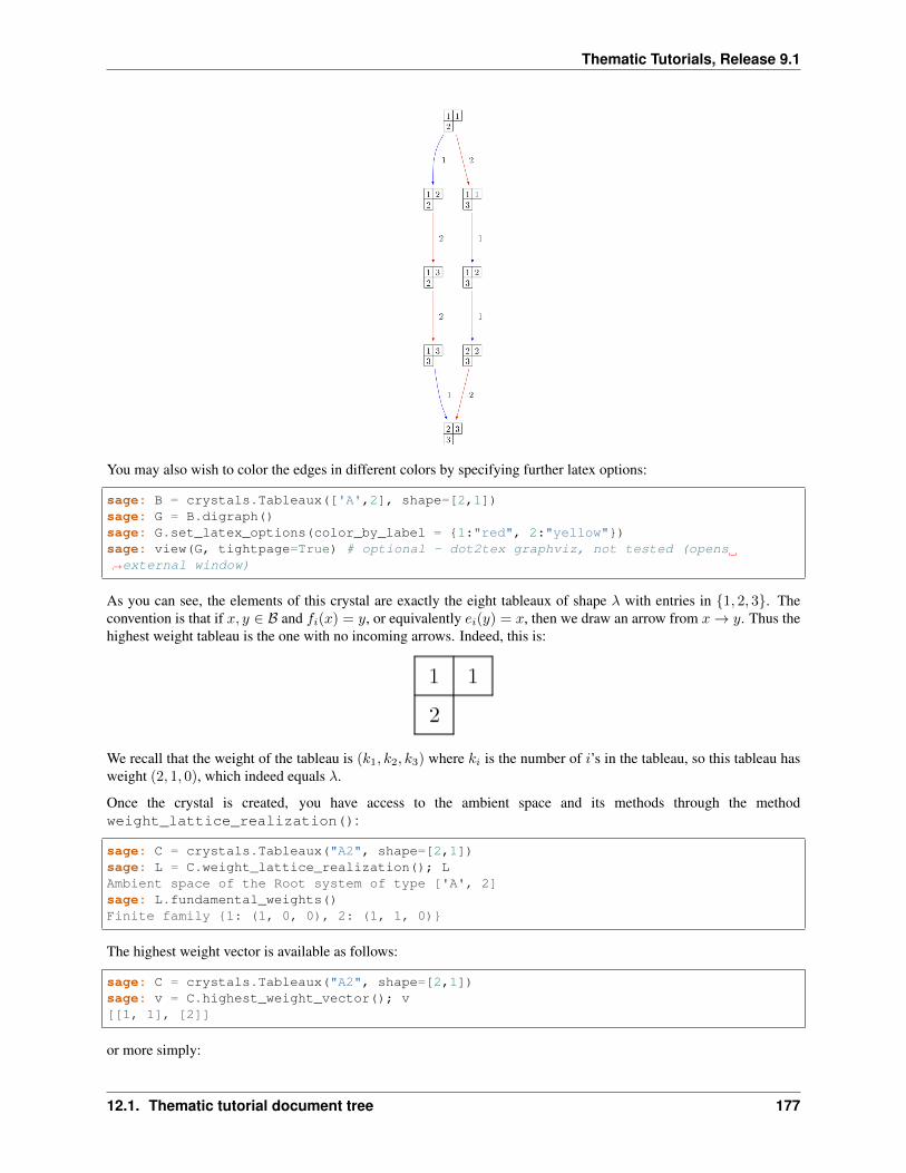
Thematic Tutorials, Release 9.1
You may also wish to color the edges in different colors by specifying further latex options:
sage: B = crystals.Tableaux(['A',2], shape=[2,1])sage: G = B.digraph()sage: G.set_latex_options(color_by_label = 1:"red", 2:"yellow")sage: view(G, tightpage=True) # optional - dot2tex graphviz, not tested (opens→˓external window)
As you can see, the elements of this crystal are exactly the eight tableaux of shape 𝜆 with entries in 1, 2, 3. Theconvention is that if 𝑥, 𝑦 ∈ ℬ and 𝑓𝑖(𝑥) = 𝑦, or equivalently 𝑒𝑖(𝑦) = 𝑥, then we draw an arrow from 𝑥→ 𝑦. Thus thehighest weight tableau is the one with no incoming arrows. Indeed, this is:
We recall that the weight of the tableau is (𝑘1, 𝑘2, 𝑘3) where 𝑘𝑖 is the number of 𝑖’s in the tableau, so this tableau hasweight (2, 1, 0), which indeed equals 𝜆.
Once the crystal is created, you have access to the ambient space and its methods through the methodweight_lattice_realization():
sage: C = crystals.Tableaux("A2", shape=[2,1])sage: L = C.weight_lattice_realization(); LAmbient space of the Root system of type ['A', 2]sage: L.fundamental_weights()Finite family 1: (1, 0, 0), 2: (1, 1, 0)
The highest weight vector is available as follows:
sage: C = crystals.Tableaux("A2", shape=[2,1])sage: v = C.highest_weight_vector(); v[[1, 1], [2]]
or more simply:
12.1. Thematic tutorial document tree 177
Thematic Tutorials, Release 9.1
sage: C = crystals.Tableaux("A2", shape=[2,1])sage: C[0][[1, 1], [2]]
Now we may apply the operators 𝑒𝑖 and 𝑓𝑖 to move around in the crystal:
sage: C = crystals.Tableaux("A2", shape=[2,1])sage: v = C.highest_weight_vector()sage: v.f(1)[[1, 2], [2]]sage: v.f(1).f(1)sage: v.f(1).f(1) is NoneTruesage: v.f(1).f(2)[[1, 3], [2]]sage: v.f(1).f(2).f(2)[[1, 3], [3]]sage: v.f(1).f(2).f(2).f(1)[[2, 3], [3]]sage: v.f(1).f(2).f(2).f(1) == v.f(2).f(1).f(1).f(2)True
You can construct the character if you first make a Weyl character ring:
sage: A2 = WeylCharacterRing("A2")sage: C = crystals.Tableaux("A2", shape=[2,1])sage: C.character(A2)A2(2,1,0)
Crystals of letters
For each of the classical Cartan types there is a standard crystal ℬstandard from which other crystals can be builtup by taking tensor products and extracting constituent irreducible crystals. This procedure is sufficient for Car-tan types 𝐴𝑟 and 𝐶𝑟. For types 𝐵𝑟 and 𝐷𝑟 the standard crystal must be supplemented with spin crystals. See[KashiwaraNakashima1994] or [HongKang2002] for further details.
Here is the standard crystal of type 𝐴𝑟.
You may create the crystal and work with it as follows:
sage: C = crystals.Letters("A6")sage: v0 = C.highest_weight_vector(); v01sage: v0.f(1)2sage: v0.f(1).f(2)3sage: [v0.f(1).f(2).f(x) for x in [1..6]][None, None, 4, None, None, None]sage: [v0.f(1).f(2).e(x) for x in [1..6]][None, 2, None, None, None, None]
Here is the standard crystal of type 𝐵𝑟.
178 Chapter 12. Documentation
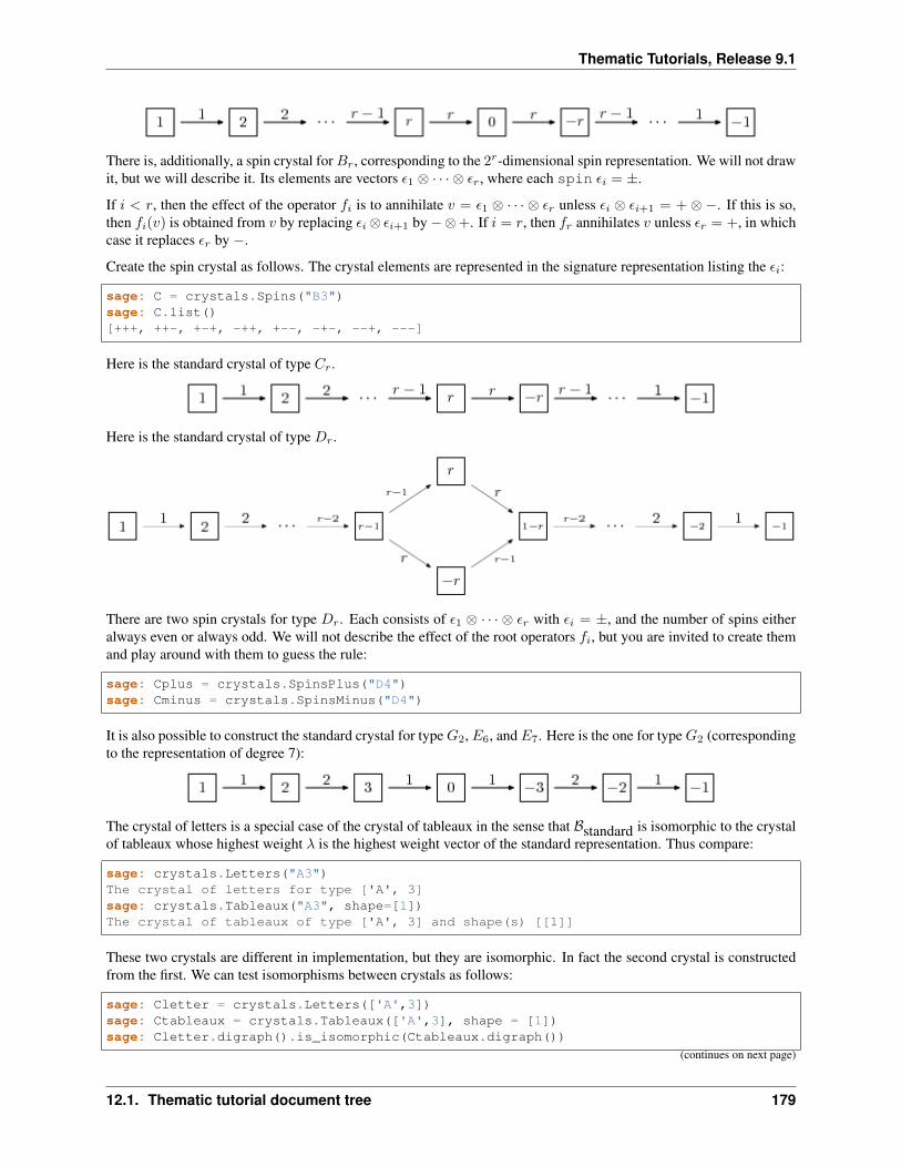
Thematic Tutorials, Release 9.1
There is, additionally, a spin crystal for𝐵𝑟, corresponding to the 2𝑟-dimensional spin representation. We will not drawit, but we will describe it. Its elements are vectors 𝜖1 ⊗ · · · ⊗ 𝜖𝑟, where each spin 𝜖𝑖 = ±.
If 𝑖 < 𝑟, then the effect of the operator 𝑓𝑖 is to annihilate 𝑣 = 𝜖1 ⊗ · · · ⊗ 𝜖𝑟 unless 𝜖𝑖 ⊗ 𝜖𝑖+1 = + ⊗ −. If this is so,then 𝑓𝑖(𝑣) is obtained from 𝑣 by replacing 𝜖𝑖⊗ 𝜖𝑖+1 by −⊗+. If 𝑖 = 𝑟, then 𝑓𝑟 annihilates 𝑣 unless 𝜖𝑟 = +, in whichcase it replaces 𝜖𝑟 by −.
Create the spin crystal as follows. The crystal elements are represented in the signature representation listing the 𝜖𝑖:
sage: C = crystals.Spins("B3")sage: C.list()[+++, ++-, +-+, -++, +--, -+-, --+, ---]
Here is the standard crystal of type 𝐶𝑟.
Here is the standard crystal of type 𝐷𝑟.
There are two spin crystals for type 𝐷𝑟. Each consists of 𝜖1 ⊗ · · · ⊗ 𝜖𝑟 with 𝜖𝑖 = ±, and the number of spins eitheralways even or always odd. We will not describe the effect of the root operators 𝑓𝑖, but you are invited to create themand play around with them to guess the rule:
sage: Cplus = crystals.SpinsPlus("D4")sage: Cminus = crystals.SpinsMinus("D4")
It is also possible to construct the standard crystal for type𝐺2, 𝐸6, and𝐸7. Here is the one for type𝐺2 (correspondingto the representation of degree 7):
The crystal of letters is a special case of the crystal of tableaux in the sense that ℬstandard is isomorphic to the crystalof tableaux whose highest weight 𝜆 is the highest weight vector of the standard representation. Thus compare:
sage: crystals.Letters("A3")The crystal of letters for type ['A', 3]sage: crystals.Tableaux("A3", shape=[1])The crystal of tableaux of type ['A', 3] and shape(s) [[1]]
These two crystals are different in implementation, but they are isomorphic. In fact the second crystal is constructedfrom the first. We can test isomorphisms between crystals as follows:
sage: Cletter = crystals.Letters(['A',3])sage: Ctableaux = crystals.Tableaux(['A',3], shape = [1])sage: Cletter.digraph().is_isomorphic(Ctableaux.digraph())
(continues on next page)
12.1. Thematic tutorial document tree 179
Thematic Tutorials, Release 9.1
(continued from previous page)
Truesage: Cletter.digraph().is_isomorphic(Ctableaux.digraph(), certificate = True)(True, 1: [[1]], 2: [[2]], 3: [[3]], 4: [[4]])
where in the last step the explicit map between the vertices of the crystals is given.
Crystals of letters have a special role in the theory since they are particularly simple, yet as Kashiwara and Nakashimashowed, the crystals of tableaux can be created from them. We will review how this works.
Tensor products of crystals
Kashiwara defined the tensor product of crystals in a purely combinatorial way. The beauty of this construction is thatit exactly parallels the tensor product of crystals of representations. That is, if 𝜆 and 𝜇 are dominant weights, thenℬ𝜆 ⊗ ℬ𝜇 is a (usually disconnected) crystal, which may contain multiple copies of ℬ𝜈 (for another dominant weight𝜈), and the number of copies of ℬ𝜈 is exactly the multiplicity of 𝜒𝜈 in 𝜒𝜆𝜒𝜇.
We will describe two conventions for the tensor product of crystals.
Kashiwara’s definition
As a set, the tensor product ℬ ⊗ 𝒞 of crystals ℬ and 𝒞 is the Cartesian product, but we denote the ordered pair (𝑥, 𝑦)with 𝑥 ∈ ℬ and 𝑦 ∈ 𝒞 by 𝑥⊗ 𝑦. We define wt(𝑥⊗ 𝑦) = wt(𝑥) + wt(𝑦). We define
𝑓𝑖(𝑥⊗ 𝑦) =
𝑓𝑖(𝑥)⊗ 𝑦 if 𝜙𝑖(𝑥) > 𝜀𝑖(𝑦),
𝑥⊗ 𝑓𝑖(𝑦) if 𝜙𝑖(𝑥) ≤ 𝜀𝑖(𝑦),
and
𝑒𝑖(𝑥⊗ 𝑦) =
𝑒𝑖(𝑥)⊗ 𝑦 if 𝜙𝑖(𝑥) ≥ 𝜀𝑖(𝑦),
𝑥⊗ 𝑒𝑖(𝑦) if 𝜙𝑖(𝑥) < 𝜀𝑖(𝑦).
It is understood that 𝑥⊗ 0 = 0⊗ 𝑥 = 0. We also define:
𝜙𝑖(𝑥⊗ 𝑦) = max(𝜙𝑖(𝑦), 𝜙𝑖(𝑥) + 𝜙𝑖(𝑦)− 𝜀𝑖(𝑦)),
𝜀𝑖(𝑥⊗ 𝑦) = max(𝜀𝑖(𝑥), 𝜀𝑖(𝑥) + 𝜀𝑖(𝑦)− 𝜙𝑖(𝑥)).
Alternative definition
As a set, the tensor product ℬ ⊗ 𝒞 of crystals ℬ and 𝒞 is the Cartesian product, but we denote the ordered pair (𝑦, 𝑥)with 𝑦 ∈ ℬ and 𝑥 ∈ 𝒞 by 𝑥⊗ 𝑦. We define wt(𝑥⊗ 𝑦) = wt(𝑦) + wt(𝑥). We define
𝑓𝑖(𝑥⊗ 𝑦) =
𝑓𝑖(𝑥)⊗ 𝑦 if 𝜙𝑖(𝑦) ≤ 𝜀𝑖(𝑥),
𝑥⊗ 𝑓𝑖(𝑦) if 𝜙𝑖(𝑦) > 𝜀𝑖(𝑥),
and
𝑒𝑖(𝑥⊗ 𝑦) =
𝑒𝑖(𝑥)⊗ 𝑦 if 𝜙𝑖(𝑦) < 𝜀𝑖(𝑥),
𝑥⊗ 𝑒𝑖(𝑦) if 𝜙𝑖(𝑦) ≥ 𝜀𝑖(𝑥).
It is understood that 𝑦 ⊗ 0 = 0⊗ 𝑦 = 0. We also define
𝜙𝑖(𝑥⊗ 𝑦) = max(𝜙𝑖(𝑥), 𝜙𝑖(𝑦) + 𝜙𝑖(𝑥)− 𝜀𝑖(𝑥)),
180 Chapter 12. Documentation
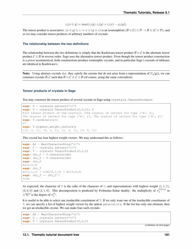
Thematic Tutorials, Release 9.1
𝜀𝑖(𝑥⊗ 𝑦) = max(𝜀𝑖(𝑦), 𝜀𝑖(𝑦) + 𝜀𝑖(𝑥)− 𝜙𝑖(𝑦)).
The tensor product is associative: (𝑥⊗ 𝑦)⊗ 𝑧 ↦→ 𝑥⊗ (𝑦 ⊗ 𝑧) is an isomorphism (ℬ ⊗ 𝒞)⊗𝒟 → ℬ ⊗ (𝒞 ⊗ 𝒟), andso we may consider tensor products of arbitrary numbers of crystals.
The relationship between the two definitions
The relationship between the two definitions is simply that the Kashiwara tensor product ℬ ⊗ 𝒞 is the alternate tensorproduct 𝒞 ⊗ ℬ in reverse order. Sage uses the alternative tensor product. Even though the tensor product constructionis a priori asymmetrical, both constructions produce isomorphic crystals, and in particular Sage’s crystals of tableauxare identical to Kashiwara’s.
Note: Using abstract crystals (i.e. they satisfy the axioms but do not arise from a representation of 𝑈𝑞(g)), we canconstruct crystals ℬ, 𝒞 such that ℬ ⊗ 𝒞 = 𝒞 ⊗ ℬ (of course, using the same convention).
Tensor products of crystals in Sage
You may construct the tensor product of several crystals in Sage using crystals.TensorProduct:
sage: C = crystals.Letters("A2")sage: T = crystals.TensorProduct(C,C,C); TFull tensor product of the crystals [The crystal of letters for type ['A', 2],The crystal of letters for type ['A', 2], The crystal of letters for type ['A', 2]]sage: T.cardinality()27sage: T.highest_weight_vectors()([1, 1, 1], [2, 1, 1], [1, 2, 1], [3, 2, 1])
This crystal has four highest weight vectors. We may understand this as follows:
sage: A2 = WeylCharacterRing("A2")sage: C = crystals.Letters("A2")sage: T = crystals.TensorProduct(C,C,C)sage: chi_C = C.character(A2)sage: chi_T = T.character(A2)sage: chi_CA2(1,0,0)sage: chi_TA2(1,1,1) + 2*A2(2,1,0) + A2(3,0,0)sage: chi_T == chi_C^3True
As expected, the character of T is the cube of the character of C, and representations with highest weight (1, 1, 1),(3, 0, 0) and (2, 1, 0). This decomposition is predicted by Frobenius-Schur duality: the multiplicity of 𝜋𝐺𝐿(𝑛)
𝜆 in⊗3C3 is the degree of 𝜋𝑆3
𝜆 .
It is useful to be able to select one irreducible constitutent of T. If we only want one of the irreducible constituents ofT, we can specify a list of highest weight vectors by the option generators. If the list has only one element, thenwe get an irreducible crystal. We can make four such crystals:
sage: A2 = WeylCharacterRing("A2")sage: C = crystals.Letters("A2")sage: T = crystals.TensorProduct(C,C,C)
(continues on next page)
12.1. Thematic tutorial document tree 181
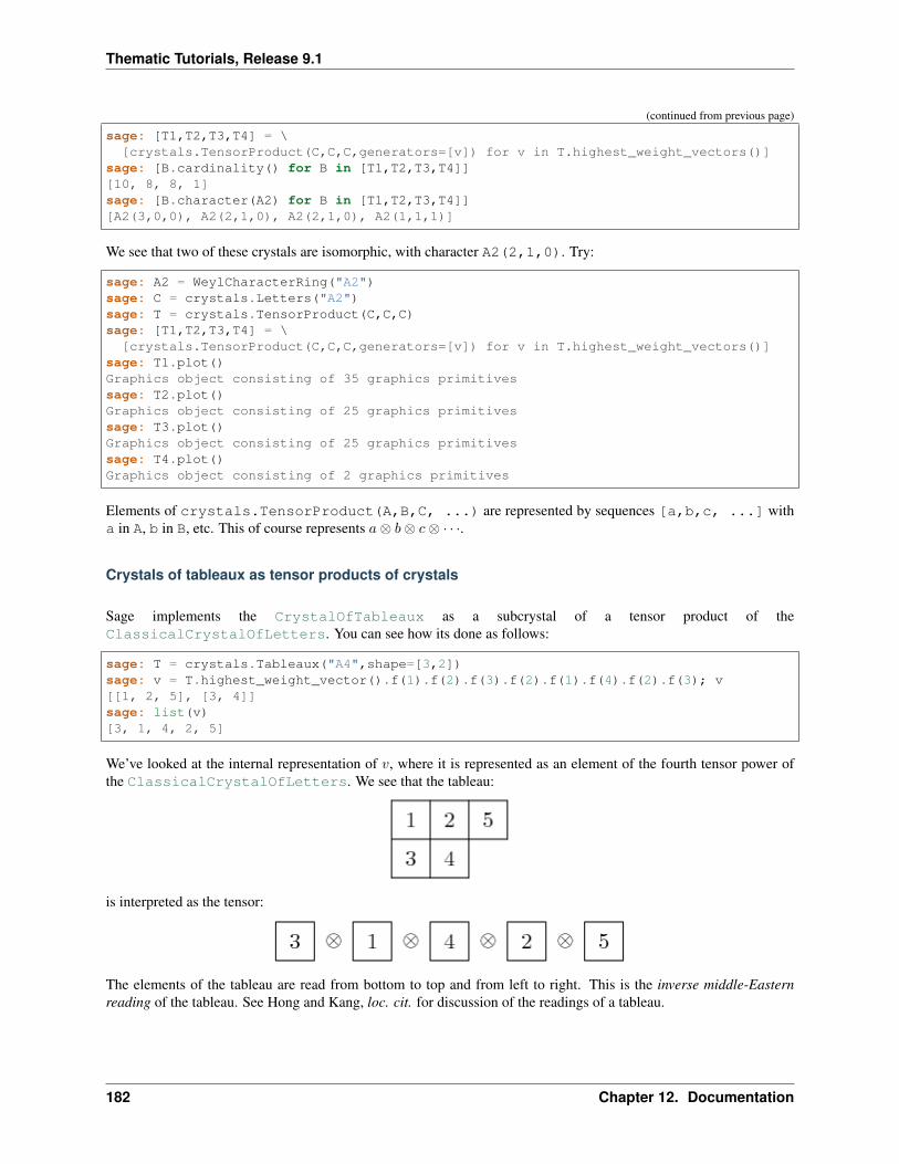
Thematic Tutorials, Release 9.1
(continued from previous page)
sage: [T1,T2,T3,T4] = \[crystals.TensorProduct(C,C,C,generators=[v]) for v in T.highest_weight_vectors()]
sage: [B.cardinality() for B in [T1,T2,T3,T4]][10, 8, 8, 1]sage: [B.character(A2) for B in [T1,T2,T3,T4]][A2(3,0,0), A2(2,1,0), A2(2,1,0), A2(1,1,1)]
We see that two of these crystals are isomorphic, with character A2(2,1,0). Try:
sage: A2 = WeylCharacterRing("A2")sage: C = crystals.Letters("A2")sage: T = crystals.TensorProduct(C,C,C)sage: [T1,T2,T3,T4] = \
[crystals.TensorProduct(C,C,C,generators=[v]) for v in T.highest_weight_vectors()]sage: T1.plot()Graphics object consisting of 35 graphics primitivessage: T2.plot()Graphics object consisting of 25 graphics primitivessage: T3.plot()Graphics object consisting of 25 graphics primitivessage: T4.plot()Graphics object consisting of 2 graphics primitives
Elements of crystals.TensorProduct(A,B,C, ...) are represented by sequences [a,b,c, ...] witha in A, b in B, etc. This of course represents 𝑎⊗ 𝑏⊗ 𝑐⊗ · · ·.
Crystals of tableaux as tensor products of crystals
Sage implements the CrystalOfTableaux as a subcrystal of a tensor product of theClassicalCrystalOfLetters. You can see how its done as follows:
sage: T = crystals.Tableaux("A4",shape=[3,2])sage: v = T.highest_weight_vector().f(1).f(2).f(3).f(2).f(1).f(4).f(2).f(3); v[[1, 2, 5], [3, 4]]sage: list(v)[3, 1, 4, 2, 5]
We’ve looked at the internal representation of 𝑣, where it is represented as an element of the fourth tensor power ofthe ClassicalCrystalOfLetters. We see that the tableau:
is interpreted as the tensor:
The elements of the tableau are read from bottom to top and from left to right. This is the inverse middle-Easternreading of the tableau. See Hong and Kang, loc. cit. for discussion of the readings of a tableau.
182 Chapter 12. Documentation
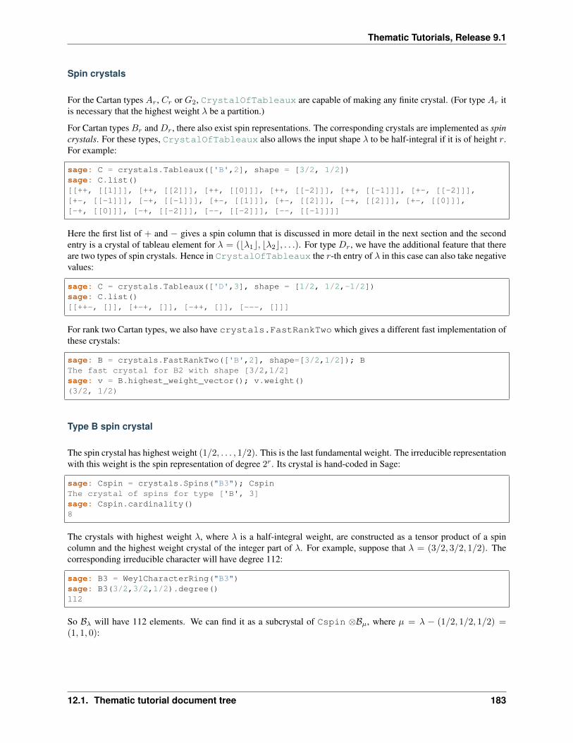
Thematic Tutorials, Release 9.1
Spin crystals
For the Cartan types 𝐴𝑟, 𝐶𝑟 or 𝐺2, CrystalOfTableaux are capable of making any finite crystal. (For type 𝐴𝑟 itis necessary that the highest weight 𝜆 be a partition.)
For Cartan types 𝐵𝑟 and 𝐷𝑟, there also exist spin representations. The corresponding crystals are implemented as spincrystals. For these types, CrystalOfTableaux also allows the input shape 𝜆 to be half-integral if it is of height 𝑟.For example:
sage: C = crystals.Tableaux(['B',2], shape = [3/2, 1/2])sage: C.list()[[++, [[1]]], [++, [[2]]], [++, [[0]]], [++, [[-2]]], [++, [[-1]]], [+-, [[-2]]],[+-, [[-1]]], [-+, [[-1]]], [+-, [[1]]], [+-, [[2]]], [-+, [[2]]], [+-, [[0]]],[-+, [[0]]], [-+, [[-2]]], [--, [[-2]]], [--, [[-1]]]]
Here the first list of + and − gives a spin column that is discussed in more detail in the next section and the secondentry is a crystal of tableau element for 𝜆 = (⌊𝜆1⌋, ⌊𝜆2⌋, . . .). For type 𝐷𝑟, we have the additional feature that thereare two types of spin crystals. Hence in CrystalOfTableaux the 𝑟-th entry of 𝜆 in this case can also take negativevalues:
sage: C = crystals.Tableaux(['D',3], shape = [1/2, 1/2,-1/2])sage: C.list()[[++-, []], [+-+, []], [-++, []], [---, []]]
For rank two Cartan types, we also have crystals.FastRankTwo which gives a different fast implementation ofthese crystals:
sage: B = crystals.FastRankTwo(['B',2], shape=[3/2,1/2]); BThe fast crystal for B2 with shape [3/2,1/2]sage: v = B.highest_weight_vector(); v.weight()(3/2, 1/2)
Type B spin crystal
The spin crystal has highest weight (1/2, . . . , 1/2). This is the last fundamental weight. The irreducible representationwith this weight is the spin representation of degree 2𝑟. Its crystal is hand-coded in Sage:
sage: Cspin = crystals.Spins("B3"); CspinThe crystal of spins for type ['B', 3]sage: Cspin.cardinality()8
The crystals with highest weight 𝜆, where 𝜆 is a half-integral weight, are constructed as a tensor product of a spincolumn and the highest weight crystal of the integer part of 𝜆. For example, suppose that 𝜆 = (3/2, 3/2, 1/2). Thecorresponding irreducible character will have degree 112:
sage: B3 = WeylCharacterRing("B3")sage: B3(3/2,3/2,1/2).degree()112
So ℬ𝜆 will have 112 elements. We can find it as a subcrystal of Cspin ⊗ℬ𝜇, where 𝜇 = 𝜆 − (1/2, 1/2, 1/2) =(1, 1, 0):
12.1. Thematic tutorial document tree 183
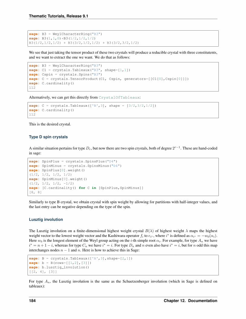
Thematic Tutorials, Release 9.1
sage: B3 = WeylCharacterRing("B3")sage: B3(1,1,0)*B3(1/2,1/2,1/2)B3(1/2,1/2,1/2) + B3(3/2,1/2,1/2) + B3(3/2,3/2,1/2)
We see that just taking the tensor product of these two crystals will produce a reducible crystal with three constitutents,and we want to extract the one we want. We do that as follows:
sage: B3 = WeylCharacterRing("B3")sage: C1 = crystals.Tableaux("B3", shape=[1,1])sage: Cspin = crystals.Spins("B3")sage: C = crystals.TensorProduct(C1, Cspin, generators=[[C1[0],Cspin[0]]])sage: C.cardinality()112
Alternatively, we can get this directly from CrystalOfTableaux:
sage: C = crystals.Tableaux(['B',3], shape = [3/2,3/2,1/2])sage: C.cardinality()112
This is the desired crystal.
Type D spin crystals
A similar situation pertains for type𝐷𝑟, but now there are two spin crystals, both of degree 2𝑟−1. These are hand-codedin sage:
sage: SpinPlus = crystals.SpinsPlus("D4")sage: SpinMinus = crystals.SpinsMinus("D4")sage: SpinPlus[0].weight()(1/2, 1/2, 1/2, 1/2)sage: SpinMinus[0].weight()(1/2, 1/2, 1/2, -1/2)sage: [C.cardinality() for C in [SpinPlus,SpinMinus]][8, 8]
Similarly to type B crystal, we obtain crystal with spin weight by allowing for partitions with half-integer values, andthe last entry can be negative depending on the type of the spin.
Lusztig involution
The Lusztig involution on a finite-dimensional highest weight crystal 𝐵(𝜆) of highest weight 𝜆 maps the highestweight vector to the lowest weight vector and the Kashiwara operator 𝑓𝑖 to 𝑒𝑖* , where 𝑖* is defined as 𝛼𝑖* = −𝑤0(𝛼𝑖).Here 𝑤0 is the longest element of the Weyl group acting on the 𝑖-th simple root 𝛼𝑖. For example, for type 𝐴𝑛 we have𝑖* = 𝑛+ 1− 𝑖, whereas for type 𝐶𝑛 we have 𝑖* = 𝑖. For type 𝐷𝑛 and 𝑛 even also have 𝑖* = 𝑖, but for 𝑛 odd this mapinterchanges nodes 𝑛− 1 and 𝑛. Here is how to achieve this in Sage:
sage: B = crystals.Tableaux(['A',3],shape=[2,1])sage: b = B(rows=[[1,2],[3]])sage: b.lusztig_involution()[[2, 4], [3]]
For type 𝐴𝑛, the Lusztig involution is the same as the Schuetzenberger involution (which in Sage is defined ontableaux):
184 Chapter 12. Documentation
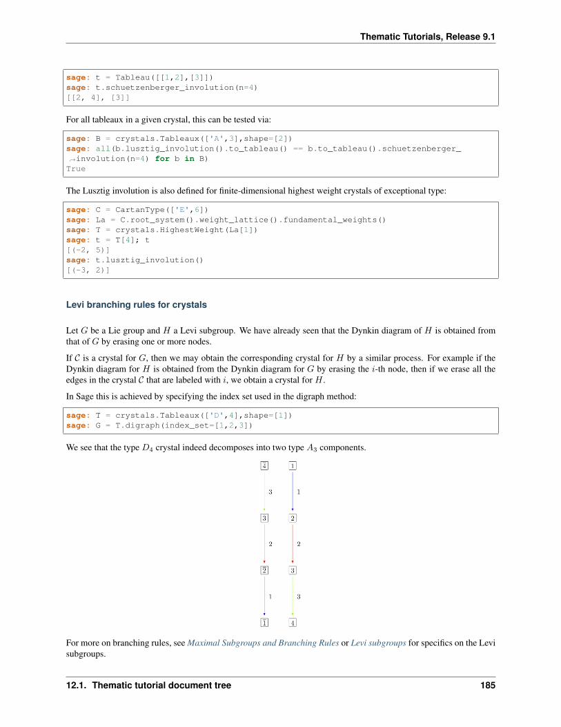
Thematic Tutorials, Release 9.1
sage: t = Tableau([[1,2],[3]])sage: t.schuetzenberger_involution(n=4)[[2, 4], [3]]
For all tableaux in a given crystal, this can be tested via:
sage: B = crystals.Tableaux(['A',3],shape=[2])sage: all(b.lusztig_involution().to_tableau() == b.to_tableau().schuetzenberger_→˓involution(n=4) for b in B)True
The Lusztig involution is also defined for finite-dimensional highest weight crystals of exceptional type:
sage: C = CartanType(['E',6])sage: La = C.root_system().weight_lattice().fundamental_weights()sage: T = crystals.HighestWeight(La[1])sage: t = T[4]; t[(-2, 5)]sage: t.lusztig_involution()[(-3, 2)]
Levi branching rules for crystals
Let 𝐺 be a Lie group and 𝐻 a Levi subgroup. We have already seen that the Dynkin diagram of 𝐻 is obtained fromthat of 𝐺 by erasing one or more nodes.
If 𝒞 is a crystal for 𝐺, then we may obtain the corresponding crystal for 𝐻 by a similar process. For example if theDynkin diagram for 𝐻 is obtained from the Dynkin diagram for 𝐺 by erasing the 𝑖-th node, then if we erase all theedges in the crystal 𝒞 that are labeled with 𝑖, we obtain a crystal for 𝐻 .
In Sage this is achieved by specifying the index set used in the digraph method:
sage: T = crystals.Tableaux(['D',4],shape=[1])sage: G = T.digraph(index_set=[1,2,3])
We see that the type 𝐷4 crystal indeed decomposes into two type 𝐴3 components.
For more on branching rules, see Maximal Subgroups and Branching Rules or Levi subgroups for specifics on the Levisubgroups.
12.1. Thematic tutorial document tree 185
Thematic Tutorials, Release 9.1
Subcrystals
Sometimes it might be desirable to work with a subcrystal of a crystal. For example, one might want to look at all2, 3, . . . , 𝑛 highest elements of a crystal and look at a particular such component:
sage: T = crystals.Tableaux(['D',4],shape=[2,1])sage: hw = [ t for t in T if t.is_highest_weight(index_set = [2,3,4]) ]; hw[[[1, 1], [2]],[[1, 2], [2]],[[2, -1], [-2]],[[2, -1], [-1]],[[1, -1], [2]],[[2, -1], [3]],[[1, 2], [3]],[[2, 2], [3]],[[1, 2], [-2]],[[2, 2], [-2]],[[2, 2], [-1]]]
sage: C = T.subcrystal(generators = [T(rows=[[2,-1],[3]])], index_set = [2,3,4])sage: G = T.digraph(subset = C, index_set=[2,3,4])
Affine Root System Basics
Among infinite-dimensional Lie algebras, Kac-Moody Lie algebras are generalizations of finite-dimensional simpleLie algebras. They include finite-dimensional simple Lie algebras as special cases but are usually infinite-dimensional.Many concepts and results from the representation theory of finite-dimensional Lie groups and Lie algebras extend toKac-Moody Lie algebras. This includes the root system, Weyl group, weight lattice, the parametrization of importantrepresentations (the integrable highest weight ones) by dominant weights and the Weyl character formula for theserepresentations.
Among Kac-Moody Lie algebras, affine Lie algebras are an important infinite-dimensional class, and their infinite-dimensional integrable highest-weight representations are an important class among their representations. In thissection many of the concepts are applicable to general Kac-Moody Lie algebras. However the code that we willdiscuss is mainly for the affine case. This is sufficiently different from the general case (and important) to meritspecial attention.
In this section we will review some of the Kac-Moody theory, taking [Kac] as our primary reference. We also recom-mend [KMPS]. This two volume set contains tables (in Volume 2) of quantities such as string functions and modularcharacteristics that you can now compute in Sage. Volume 1 contains an introduction to affine Lie algebras and theirrepresentations, including a valuable discussion of how they arise in string theory.
In this section and the next, we will also explain what facilities there are in Sage for computing with these. We willoften restrict ourselves to the case of affine Lie algebras.
Cartan Matrix
See [Kac] Chapter 1 for this topic.
The basic data defining a Kac-Moody Lie algebra is a (generalized) Cartan matrix. This is a square matrix 𝐴 = (𝑎𝑖𝑗)with diagonal entries equal to 2 and nonpositive off diagonal entries such that 𝑎𝑖𝑗 = 0 if and only if 𝑎𝑗𝑖 = 0. It isuseful to assume that it is indecomposable and symmetrizable. Indecomposable means that it cannot be arranged intotwo diagonal blocks by permuting the rows and columns; and symmetrizable means that 𝐷𝐴 is symmetric for someinvertible diagonal matrix 𝐷.
186 Chapter 12. Documentation
Thematic Tutorials, Release 9.1
Given a generalized Cartan matrix there is a vector space h containing vectors 𝛼∨𝑖 (called simple coroots) and vectors
𝛼𝑖 ∈ h* (called simple roots) such that ⟨𝛼∨𝑖 , 𝛼𝑗⟩ = 𝛼∨
𝑖 (𝛼𝑗) = 𝑎𝑖𝑗 . Moreover there exists a Kac-Moody Lie algebra gcontaining h as an abelian subalgebra that is generated by h and elements 𝑒𝑖 and 𝑓𝑖 such that
[𝑒𝑖, 𝑓𝑖] = 𝛿𝑖𝑗𝛼∨𝑖 , [ℎ, 𝑒𝑖] = 𝛼𝑖(ℎ)𝑒𝑖, [ℎ, 𝑓𝑖] = −𝛼𝑖(ℎ)𝑓𝑖.
(These conditions do not quite characterize g, but they do if supplemented by the Serre relations, which we will notneed or state.)
The significance of the diagonalizability assumption is that g admits an invariant symmetric bilinear form, and hencehas a Casimir operator and a good representation theory.
The transpose of 𝐴 is also a symmetrizable indecomposable generalized Cartan matrix, so there is a dual Cartan typein which the roots and coroots are interchanged.
In Sage, we may recover the Cartan matrix as follows:
sage: RootSystem(['B',2]).cartan_matrix()[ 2 -1][-2 2]sage: RootSystem(['B',2,1]).cartan_matrix()[ 2 0 -1][ 0 2 -1][-2 -2 2]
If det(𝐴) = 0 and its nullspace is one-dimensional, then g is an affine Lie algebra, as in the second example above.
Untwisted Affine Kac-Moody Lie Algebras
One realization of affine Lie algebras, described in Chapter 7 of [Kac] begins with a finite-dimensional simple Liealgebra g∘, with Cartan type 𝑋ℓ (['X',l] in Sage). Tensoring with the Laurent polynomial ring gives the loop Liealgebra g∘ ⊗ C[𝑡, 𝑡−1]. This is the Lie algebra of vector fields in g∘ on the circle. Then one may make a centralextension:
0→ C ·𝐾 → g′ → g∘ ⊗C[𝑡, 𝑡−1]→ 0.
After that, it is convenient to adjoin another basis element, which acts on g′ as a derivation 𝑑. If h∘ is a Cartansubalgebra of g∘, then we obtain a Cartan subalgebra h′ of g′ by adjoining the central element 𝐾, and then a Cartansubalgebra h by further adjoining the derivation 𝑑.
The resulting Lie algebra g is the untwisted affine Lie algebra. The Cartan type is designated to be 𝑋(1)ℓ in Kac’
notation, which is rendered as ['X',l,1] or "Xl~" in Sage. The Dynkin diagram of this Cartan type is theextended Dynkin-diagram of g∘:
sage: CartanType("E6~").dynkin_diagram()O 0||O 2||
O---O---O---O---O1 3 4 5 6E6~
From the Dynkin diagram, we can read off generators and relations for the affine Weyl group, which is a Coxetergroup with generators 𝑠𝑖 of order 2, that commute if 𝑖 and 𝑗 are not adjacent in the Dynkin diagram, and otherwise are
12.1. Thematic tutorial document tree 187
Thematic Tutorials, Release 9.1
subject to a braid relation. We can infer some Levi subalgebras of g, obtained by omitting one node from the Dynkindiagram; particularly omitting the “affine node” 0 gives 𝐸6, that is g∘.
The index set for the finite-dimensional Lie algebra g∘ is 𝐼 = 1, 2, . . . , ℓ. This means we label the roots, corootsetc. by 𝑖 ∈ 𝐼 . The index set for the affine Lie algebra g adds one index 0 for the affine root 𝛼0.
The subset of 𝜆 ∈ h* characterized by 𝜆(𝛼∨𝑖 ) ∈ Z for the coroots 𝛼∨
𝑖 is called the weight lattice 𝑃 . There are twoversions of the weight lattice, depending on whether we are working with g or g′. The weight lattice of g is called theextended weight lattice. We may create these as follows:
sage: RootSystem("A2~").weight_lattice()Weight lattice of the Root system of type ['A', 2, 1]sage: RootSystem("A2~").weight_lattice(extended=True)Extended weight lattice of the Root system of type ['A', 2, 1]
Referring to the extended lattice, the term lattice is a slight misnomer because 𝑃 is not discrete; it contains all complexmultiples of 𝛿, which is orthogonal to the coroots. However the image of 𝑃 in h*/C𝛿 is a bona fide lattice. Indeed,the fundamental weights are vectors Λ𝑖 ∈ h* such that Λ𝑖(𝛼
∨𝑗 ) = 𝛿𝑖𝑗 , and then
𝑃 = C𝛿 ⊕ℓ⨁
𝑖=0
ZΛ𝑖.
The Weyl vector 𝜌 is the sum of the fundamental weights. This plays the role as does the classical Weyl vector, whichalso equals half the sum of the positive roots, in the theory of finite semisimple Lie algebras. The weight lattice 𝑃contains the root lattice 𝑄, which is the lattice spanned by 𝛼0, 𝛼1, . . . , 𝛼ℓ.
Usually there is an advantage to working with g instead of g′. (Thus we prefer the extended weight lattice, though thisis not the default.) The reason for this is as follows. If 𝑉 is a representation of g then usually the weight spaces 𝑉𝜆, ina decomposition with respect to characters (weights) of h are finite-dimensional; but the corresponding weight spacesfor h′ would not be.
There are exceptions to this rule of preferring the extended weight lattice. In particular, we can construct non-trivialirreducible finite-dimensional representations of g′, and these cannot be lifted to g (although they do have infinite-dimensional analogs). These certain finite-dimensional representations have crystal bases, which include Kirillov-Reshetikhin crystals. Thus, for Kirillov-Reshetikhin crystals we prefer to use the non-extended weight lattice. SeeAffine Finite Crystals.
Twisted Types
There are also twisted types with Cartan type 𝑋(𝑚)ℓ or ['X',l,m] where 𝑚 is the order of an automorphism of the
Dynkin diagram of g∘. These are described in [Kac] Chapter 8. Alternative descriptions of the twisted types may befound in [Macdonald2003]. Examining the tables Aff1, Aff2 and Aff3 in Chapter 4 of Kac, you will see that eachtwisted type is dual to an untwisted type (except 𝐴(2)
2ℓ ). For example the twisted type ['E',6,2] (or 𝐸(2)6 ) in Aff2
is dual to the untwisted type ['F',4,1] (or 𝐹 (1)4 ).
Referring to the above Dynkin diagram for ['E',6,1], if we collapse the nodes 1 and 6 together, and the nodes 3and 5, we obtain the Dynkin diagram for ['E',6,2]:
sage: CartanType(['E',6,2]).dynkin_diagram()O---O---O=<=O---O0 1 2 3 4F4~*
We must explain why Sage calls this Cartan type F4~*. The Cartan type ['F',4,1] is obtained by adding oneDynkin node to the Cartan type “F4”:
188 Chapter 12. Documentation
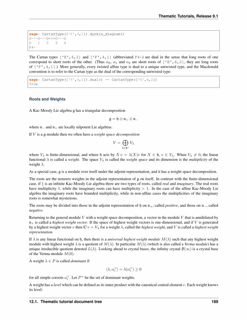
Thematic Tutorials, Release 9.1
sage: CartanType(['F',4,1]).dynkin_diagram()O---O---O=>=O---O0 1 2 3 4F4~
The Cartan types ['E',6,2] and ['F',4,1] (abbreviated F4~) are dual in the sense that long roots of onecorrespond to short roots of the other. (Thus 𝛼0, 𝛼1 and 𝛼2 are short roots of ['E',6,2], they are long rootsof ['F',4,1].) More generally, every twisted affine type is dual to a unique untwisted type, and the Macdonaldconvention is to refer to the Cartan type as the dual of the corresponding untwisted type:
sage: CartanType(['F',4,1]).dual() == CartanType(['E',6,2])True
Roots and Weights
A Kac-Moody Lie algebra g has a triangular decomposition
g = h⊕ n+ ⊕ n−
where n− and n+ are locally nilpotent Lie algebras.
If 𝑉 is a g-module then we often have a weight space decomposition
𝑉 =⨁𝜆∈h*
𝑉𝜆
where 𝑉𝜆 is finite-dimensional, and where h acts by 𝑋 𝑣 = 𝜆(𝑋)𝑣 for 𝑋 ∈ h, 𝑣 ∈ 𝑉𝜆. When 𝑉𝜆 = 0, the linearfunctional 𝜆 is called a weight. The space 𝑉𝜆 is called the weight space and its dimension is the multiplicity of theweight 𝜆.
As a special case, g is a module over itself under the adjoint representation, and it has a weight space decomposition.
The roots are the nonzero weights in the adjoint representation of g on itself. In contrast with the finite-dimensionalcase, if is an infinite Kac-Moody Lie algebra there are two types of roots, called real and imaginary. The real rootshave multiplicity 1, while the imaginary roots can have multiplicity > 1. In the case of the affine Kac-Moody Liealgebra the imaginary roots have bounded multiplicity, while in non-affine cases the multiplicities of the imaginaryroots is somewhat mysterious.
The roots may be divided into those in the adjoint representation of h on n+, called positive, and those on n−, callednegative.
Returning to the general module 𝑉 with a weight space decomposition, a vector in the module 𝑉 that is annihilated byn+ is called a highest weight vector. If the space of highest weight vectors is one-dimensional, and if 𝑉 is generatedby a highest weight vector 𝑣 then C 𝑣 = 𝑉𝜆 for a weight 𝜆, called the highest weight, and 𝑉 is called a highest weightrepresentation.
If 𝜆 is any linear functional on h, then there is a universal highest weight module 𝑀(𝜆) such that any highest weightmodule with highest weight 𝜆 is a quotient of 𝑀(𝜆). In particular 𝑀(𝜆) (which is also called a Verma module) has aunique irreducible quotient denoted 𝐿(𝜆). Looking ahead to crystal bases, the infinity crystal ℬ(∞) is a crystal baseof the Verma module 𝑀(0).
A weight 𝜆 ∈ 𝑃 is called dominant if
⟨𝜆, 𝛼∨𝑖 ⟩ = 𝜆(𝛼∨
𝑖 ) ≥ 0
for all simple coroots 𝛼∨𝑖 . Let 𝑃+ be the set of dominant weights.
A weight has a level which can be defined as its inner product with the canonical central element 𝑐. Each weight knowsits level:
12.1. Thematic tutorial document tree 189
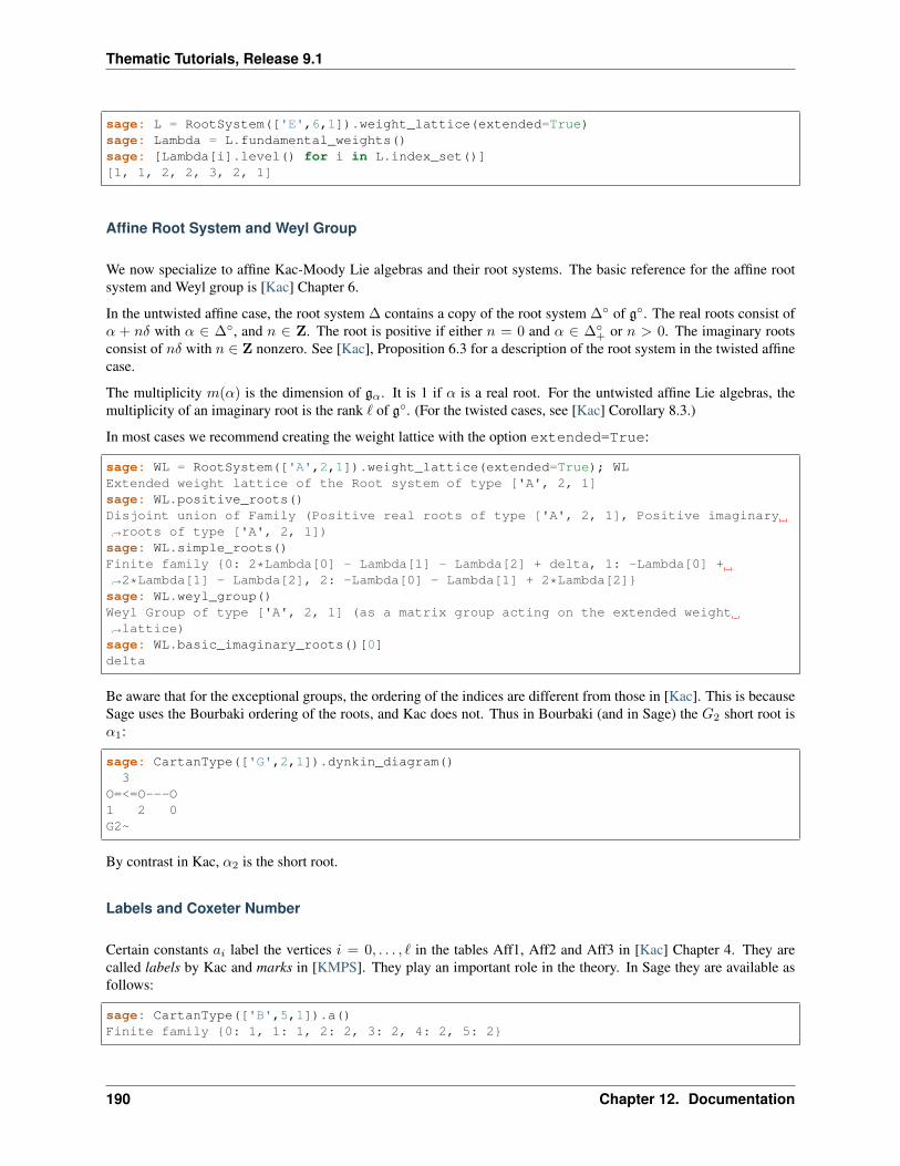
Thematic Tutorials, Release 9.1
sage: L = RootSystem(['E',6,1]).weight_lattice(extended=True)sage: Lambda = L.fundamental_weights()sage: [Lambda[i].level() for i in L.index_set()][1, 1, 2, 2, 3, 2, 1]
Affine Root System and Weyl Group
We now specialize to affine Kac-Moody Lie algebras and their root systems. The basic reference for the affine rootsystem and Weyl group is [Kac] Chapter 6.
In the untwisted affine case, the root system ∆ contains a copy of the root system ∆∘ of g∘. The real roots consist of𝛼 + 𝑛𝛿 with 𝛼 ∈ ∆∘, and 𝑛 ∈ Z. The root is positive if either 𝑛 = 0 and 𝛼 ∈ ∆∘
+ or 𝑛 > 0. The imaginary rootsconsist of 𝑛𝛿 with 𝑛 ∈ Z nonzero. See [Kac], Proposition 6.3 for a description of the root system in the twisted affinecase.
The multiplicity 𝑚(𝛼) is the dimension of g𝛼. It is 1 if 𝛼 is a real root. For the untwisted affine Lie algebras, themultiplicity of an imaginary root is the rank ℓ of g∘. (For the twisted cases, see [Kac] Corollary 8.3.)
In most cases we recommend creating the weight lattice with the option extended=True:
sage: WL = RootSystem(['A',2,1]).weight_lattice(extended=True); WLExtended weight lattice of the Root system of type ['A', 2, 1]sage: WL.positive_roots()Disjoint union of Family (Positive real roots of type ['A', 2, 1], Positive imaginary→˓roots of type ['A', 2, 1])sage: WL.simple_roots()Finite family 0: 2*Lambda[0] - Lambda[1] - Lambda[2] + delta, 1: -Lambda[0] +→˓2*Lambda[1] - Lambda[2], 2: -Lambda[0] - Lambda[1] + 2*Lambda[2]sage: WL.weyl_group()Weyl Group of type ['A', 2, 1] (as a matrix group acting on the extended weight→˓lattice)sage: WL.basic_imaginary_roots()[0]delta
Be aware that for the exceptional groups, the ordering of the indices are different from those in [Kac]. This is becauseSage uses the Bourbaki ordering of the roots, and Kac does not. Thus in Bourbaki (and in Sage) the 𝐺2 short root is𝛼1:
sage: CartanType(['G',2,1]).dynkin_diagram()3
O=<=O---O1 2 0G2~
By contrast in Kac, 𝛼2 is the short root.
Labels and Coxeter Number
Certain constants 𝑎𝑖 label the vertices 𝑖 = 0, . . . , ℓ in the tables Aff1, Aff2 and Aff3 in [Kac] Chapter 4. They arecalled labels by Kac and marks in [KMPS]. They play an important role in the theory. In Sage they are available asfollows:
sage: CartanType(['B',5,1]).a()Finite family 0: 1, 1: 1, 2: 2, 3: 2, 4: 2, 5: 2
190 Chapter 12. Documentation
Thematic Tutorials, Release 9.1
The column vector 𝑎 with these entries spans the nullspace of 𝐴:
sage: RS = RootSystem(['E',6,2]); RSRoot system of type ['F', 4, 1]^*sage: A=RS.cartan_matrix(); A[ 2 -1 0 0 0][-1 2 -1 0 0][ 0 -1 2 -2 0][ 0 0 -1 2 -1][ 0 0 0 -1 2]sage: ann = Matrix([[v] for v in RS.cartan_type().a()]); ann[1][2][3][2][1]sage: A*ann[0][0][0][0][0]
The nullroot 𝛿 =∑
𝑖∈𝐼 𝑎𝑖𝛼𝑖:
sage: WL = RootSystem('C3~').weight_lattice(extended=True); WLExtended weight lattice of the Root system of type ['C', 3, 1]sage: sum(WL.cartan_type().a()[i]*WL.simple_root(i) for i in WL.cartan_type().index_→˓set())delta
The number ℎ =∑
𝑖∈𝐼 𝑎𝑖 is called the Coxeter number. In the untwisted case it is the order of a Coxeter element ofthe finite Weyl group of g∘. The dual Coxeter number ℎ∨ is the Coxeter number of the dual root system. It appearsfrequently in representation theory. The Coxeter number and dual Coxeter number may be computed as follow:
sage: sum(CartanType(['F',4,1]).a()) # Coxeter number12sage: sum(CartanType(['F',4,1]).dual().a()) # Dual Coxeter number9
The Weyl Group
The ambient space of the root system comes with an (indefinite) inner product. The real roots have nonzero length butthe imaginary roots are isotropic. If 𝛼 is a real root we may define a reflection 𝑟𝛼 in the hyperplane orthogonal to 𝛼.In particular the ℓ+ 1 reflections 𝑠𝑖 with respect to the simple positive roots 𝛼𝑖 (𝑖 = 0, 1, 2, . . . , ℓ) generate a Coxetergroup. This is the Weyl group 𝑊 .
Illustrating how to use Sage to compute the action of 𝑊 on the weight lattice:
sage: L = RootSystem("A2~").weight_lattice(extended=True)sage: Lambda = L.fundamental_weights()sage: delta = L.null_root()sage: W = L.weyl_group(prefix="s")sage: s0,s1,s2 = W.simple_reflections()sage: [(s0*s1*s2*s1).action(x) - x for x in Lambda][-2*Lambda[0] + Lambda[1] + Lambda[2] - delta,
(continues on next page)
12.1. Thematic tutorial document tree 191
Thematic Tutorials, Release 9.1
(continued from previous page)
-2*Lambda[0] + Lambda[1] + Lambda[2] - 2*delta,-2*Lambda[0] + Lambda[1] + Lambda[2] - 2*delta]
sage: [s0.action(x) for x in Lambda][-Lambda[0] + Lambda[1] + Lambda[2] - delta, Lambda[1], Lambda[2]]sage: s0.action(delta)delta
The extended affine Weyl Group
The subgroup 𝑊 ∘ generated by 𝑠1, . . . , 𝑠ℓ is a finite Coxeter group that may be identified with the Weyl group of thefinite-dimensional simple Lie algebra g∘.
Geometrically, 𝑊 may be interpreted as the semidirect product of the finite Weyl group 𝑊 ∘ by a discrete group oftranslations 𝑄∨ isomorphic to the coroot lattice. A larger extended affine Weyl group is the semidirect product of 𝑊 ∘
by the coweight lattice 𝑃∨. If 𝑃∨ is strictly larger than 𝑄∨ this is not a Coxeter group but arises naturally in manyproblems. It may be constructed in Sage as follows:
sage: E = ExtendedAffineWeylGroup(["A",2,1]); EExtended affine Weyl group of type ['A', 2, 1]
See the documentation in extended_affine_weyl_group if you need this.
Integrable Highest Weight Representations of Affine Lie algebras
In this section g can be an arbitrary Kac-Moody Lie Algebra made with a symmetrizable, indecomposable Cartanmatrix.
Suppose that 𝑉 is a representation with a weight space decomposition as in Roots and Weights. Let 𝛼 be a real root,and let g𝛼 be the corresponding root space, that is, the one-dimensional weight space for 𝛼 in the adjoint representationof g on itself. Then −𝛼 is also a root. The two one-dimensional spaces g𝛼 and g−𝛼 generate a Lie algebra isomorphicto sl2. The module 𝑉 is called integrable if for each such 𝛼 the representation of sl2 obtained this way integratesto a representation of the Lie group SL2. Since this group contains an element that stabilizes h and induces thecorresponding simple reflection on the weight lattice, integrability implies that the weight multiplicities are invariantunder the action of the Weyl group.
If the Kac-Moody Lie algebra g is finite-dimensional then the integrable highest weight representations are just theirreducible finite-dimensional ones. For a general Kac-Moody Lie algebra the integrable highest weight representa-tions are the analogs of the finite-dimensional ones, that is, with WeylCharacterRing elements. Their theory hasmany aspects in common with the finite-dimensional representations of finite-dimensional simple Lie algebras, suchas the parametrization by dominant weights, and generalizations of the Weyl denominator and character formulas, dueto Macdonald and Kac respectively.
If Λ is a dominant weight, then the irreducible highest weight module 𝐿(Λ) defined in Roots and Weights is integrable.Moreover every highest weight integrable representation arises this way, so these representations are in bijection withthe cone 𝑃+ of dominant weights.
The affine case
Now we assume that g is affine. The integrable highest weight representations (and their crystals) are extremelyinteresting. Integrable highest weight representations of g arise in a variety of contexts, from string theory to themodular representation theory of the symmetric groups, and the theory of modular forms. The representation 𝐿(Λ0)is particularly ubiquitous and is called the basic representation.
192 Chapter 12. Documentation
Thematic Tutorials, Release 9.1
Therefore in [KMPS] (published in 1990) tabulated data for many of these representations. They wrote
We present a vast quantity of numerical data in tabular form, this being the only source for such infor-mation. The computations are tedious and not particularly straightforward when it is necessary to carrythem out individually. We hope the appearance of this book will spur interest in a field that has become,in barely 20 years, deeply rewarding and full of promise for the future. It would indeed be gratifyingif these tables were to appear to the scientists of 2040 as obsolete as the dust-gathering compilations oftranscendental functions appear for us today because of their availability on every pocket calculator.
As we will explain, Sage can reproduce the contents of these tables. Moreover the tables in [KMPS] are limited to theuntwisted types, but Sage also implements the twisted types.
Although Sage can reproduce the tables in the second volume of [KMPS], the work remains very useful. The firstvolume is a down-to-earth and very helpful exposition of the theory of integrable representations of affine Lie algebraswith explicit examples and explanations of the connections with mathematical physics and vertex operators.
The support of an integrable highest weight representation
Let Λ ∈ 𝑃+ and let 𝑉 = 𝐿(Λ) be the integrable representation with highest weight Λ. If 𝜇 is another weight, letmult(𝜇) denote the multiplicity of the weight 𝜇 in 𝐿(Λ). Define the support of the representation supp(𝑉 ) to be theset of 𝜇 such that mult(𝜇) > 0.
If mult(𝜇) > 0 then 𝜆−𝜇 is a linear combination of the simple roots with nonnegative integer coefficients. Moreoversupp(𝑉 ) is contained in the paraboloid
(Λ + 𝜌|Λ + 𝜌)− (𝜇+ 𝜌|𝜇+ 𝜌) ≥ 0
where ( | ) is the invariant inner product on the weight lattice and 𝜌 is the Weyl vector (Untwisted Affine Kac-MoodyLie Algebras). Moreover if 𝜇 ∈ supp(𝑉 ) then Λ− 𝜇 is an element of the root lattice 𝑄 ([Kac], Propositions 11.3 and11.4).
We organize the weight multiplicities into sequences called string functions or strings as follows. By [Kac], Proposi-tion 11.3 or Corollary 11.9, for fixed 𝜇 the function mult(𝜇 − 𝑘𝛿) of 𝑘 is an increasing sequence. We adjust 𝜇 by amultiple of 𝛿 to the beginning of the positive part of the sequence. Thus we define 𝜇 to be maximal if mult(𝜇) = 0but mult(𝜇+ 𝛿) = 0.
Since 𝛿 is fixed under the action of the affine Weyl group, and since the weight multiplicities are Weyl group invariant,the function 𝑘 ↦→ mult(𝜇 − 𝑘𝛿) is unchanged if 𝜇 is replaced by 𝑤(𝜇) for some Weyl group element 𝑤. Now everyWeyl orbit contains a dominant weight. Therefore in enumerating the string we may assume that the weight 𝜇 isdominant. There are only a finite number of dominant maximal weights. Thus there are only a finite number of suchstrings to be computed.
Modular Forms
Remarkably, [KacPeterson] showed that each string is the set of Fourier coefficients of a weakly holomorphic modularform; see also [Kac] Chapters 12 and 13. Here weakly holomorphic modular means that the form is allowed to havepoles at cusps.
To this end we define the modular characteristic
𝑚Λ =|Λ + 𝜌|2
2(𝑘 + ℎ∨)− |𝜌|
2
2ℎ∨.
Here 𝑘 = (Λ|𝛿) is the level of the representation and ℎ∨ is the dual Coxeter number (Labels and Coxeter Number). If𝜇 is a weight, define
𝑚Λ,𝜇 = 𝑚Λ −|𝜇|2
2𝑘.
12.1. Thematic tutorial document tree 193
Thematic Tutorials, Release 9.1
Let Λ be a weight, which we may assume maximal. Then Kac and Peterson defined the string function
𝑐Λ𝜇 = 𝑞𝑚Λ,𝜇
∑𝑛∈Z
mult(𝜇− 𝑛𝛿)𝑞𝑛.
Although these do arise as partition functions in string theory, the term “string” here does not refer to physical strings.
The string function 𝑐Λ𝜇 is a weakly holomorphic modular form, possibly of half-integral weight. See [Kac], Corollary13.10, or [KacPeterson]. It can have poles at infinity, but multiplying 𝑐Λ𝜇 by 𝜂(𝜏)dim g∘
gives a holomorphic modularform (for some level). Here 𝜂 is the Dedekind eta function:
𝜂(𝜏) = 𝑞1/24∞∏𝑘=1
(1− 𝑞𝑘), 𝑞 = 𝑒2𝜋𝑖𝜏 .
The weight of this modular form 𝜂(𝜏)dim g∘𝑐Λ𝜆 is the number of positive roots of g∘.
Sage methods for integrable representations
In this section we will show how to use Sage to compute with integrable highest weight representations of affine Liealgebras. For further documentation, see the reference manual IntegrableRepresentation.
In the following example, we work with the integrable representation with highest weight 2Λ0 for sl2, that is, 𝐴(1)1 .
First we create a dominant weight in the extended weight lattice, then create the IntegrableRepresentationclass. We compute the strings. There are two, since there are two dominant maximal weights. One of them is thehighest weight 2Λ0, and the other is 2Λ1 − 𝛿:
sage: L = RootSystem("A1~").weight_lattice(extended=True)sage: Lambda = L.fundamental_weights()sage: delta = L.null_root()sage: W = L.weyl_group(prefix="s")sage: s0, s1 = W.simple_reflections()sage: V = IntegrableRepresentation(2*Lambda[0])sage: V.strings()2*Lambda[0]: [1, 1, 3, 5, 10, 16, 28, 43, 70, 105, 161, 236],2*Lambda[1] - delta: [1, 2, 4, 7, 13, 21, 35, 55, 86, 130, 196, 287]
sage: mw1, mw2 = V.dominant_maximal_weights(); mw1, mw2(2*Lambda[0], 2*Lambda[1] - delta)
We see there are two dominant maximal weights, 2Λ0 and 2Λ1 − 𝛿. We obtain every maximal weight from theseby applying Weyl group elements. These lie inside the paraboloid described in The support of an integrable highestweight representation. Here are a few more maximal weights:
sage: pairs = [(s0*s1*s0, mw1), (s0*s1, mw2), (s0, mw1), (W.one(), mw2),....: (W.one(), mw1), (s1, mw2), (s1*s0, mw1), (s1*s0*s1, mw2)]sage: [w.action(mw) for (w, mw) in pairs][-6*Lambda[0] + 8*Lambda[1] - 8*delta,-4*Lambda[0] + 6*Lambda[1] - 5*delta,-2*Lambda[0] + 4*Lambda[1] - 2*delta,2*Lambda[1] - delta,2*Lambda[0],4*Lambda[0] - 2*Lambda[1] - delta,6*Lambda[0] - 4*Lambda[1] - 2*delta,8*Lambda[0] - 6*Lambda[1] - 5*delta]
We confirm that the string function for one in the Weyl orbit is the same as that for mw2, calculated above:
194 Chapter 12. Documentation
Thematic Tutorials, Release 9.1
sage: s1.action(mw2)4*Lambda[0] - 2*Lambda[1] - deltasage: [V.mult(s0.action(mw2)-k*delta) for k in [0..10]][1, 2, 4, 7, 13, 21, 35, 55, 86, 130, 196]
String functions of integrable representations often appear in the Online Encyclopedia of Integer Sequences:
sage: [oeis(x) for x in V.strings().values()] # optional - internet[0: A233758: Bisection of A006950 (the even part).,0: A233759: Bisection of A006950 (the odd part).]
Reading what the OEIS tells us about the sequence OEIS sequence A006950, we learn that the two strings are the oddand even parts of the series
∞∏𝑘=1
1 + 𝑞2𝑘−1
1− 𝑞2𝑘=
∞∏𝑘=1
1− 𝑞2𝑘
(1− 𝑞𝑘)(1− 𝑞4𝑘)= 𝑞1/8
𝜂(2𝜏)
𝜂(𝜏)𝜂(4𝜏)
This is not a modular form because of the factor 𝑞1/8 in front of the ratio of eta functions.
Let us confirm what the Online Encyclopedia tells us by computing the above product:
sage: PS.<q> = PowerSeriesRing(QQ)sage: prod([(1+q^(2*k-1))/(1-q^(2*k)) for k in [1..20]])1 + q + q^2 + 2*q^3 + 3*q^4 + 4*q^5 + 5*q^6 + 7*q^7 + 10*q^8+ 13*q^9 + 16*q^10 + 21*q^11 + 28*q^12 + 35*q^13 + 43*q^14+ 55*q^15 + 70*q^16 + 86*q^17 + 105*q^18 + 130*q^19 + O(q^20)
We see the values of the two strings interspersed in this product, with the 2Λ0 string values in the even positions andthe 2Λ1 − 𝛿 values in the odd positions.
To compute 𝑐2Λ0
𝜆 , which is guaranteed to be a modular form, we must compute the modular characteristics. We areinterested in the cases where 𝜆 is one of the two dominant maximal weights:
sage: [V.modular_characteristic(x) for x in [2*Lambda[0], 2*Lambda[1]-delta]][-1/16, 7/16]
This gives us the string functions
𝑐2Λ0
2Λ0= 𝑞−1/16(1 + 𝑞 + 3𝑞2 + 5𝑞3 + 10𝑞4 + 16𝑞5 + · · · ),
𝑐2Λ0
2Λ1−𝛿 = 𝑞7/16(1 + 2𝑞 + 4𝑞2 + 7𝑞3 + 13𝑞4 + 21𝑞5 + · · · ).
These are both weakly holomorphic modular forms. Any linear combination of these two is also a weakly holomorphicmodular form. For example we may replace 𝜏 by 𝜏/2 in our previous identity and get
𝑐2Λ0
2Λ0+ 𝑐2Λ0
2Λ1−𝛿 =𝜂(𝜏)
𝜂(𝜏/2)𝜂(2𝜏).
Many more examples may be found in [KacPeterson] and [KMPS].
Let 𝑉 be the integrable highest weight representation with highest weight Λ. If 𝜇 is in the support of 𝑉 then Λ− 𝜇 isof the form
∑𝑖 𝑛𝑖𝛼𝑖 where 𝛼𝑖 are the simple roots. Sage employs an internal representation of the weights as tuples
(𝑛0, 𝑛1, . . .). You can convert weights to and from this notation as follows:
sage: L = RootSystem(['E',6,2]).weight_lattice(extended=True)sage: Lambda = L.fundamental_weights()sage: delta = L.null_root()sage: V = IntegrableRepresentation(Lambda[0])
(continues on next page)
12.1. Thematic tutorial document tree 195
Thematic Tutorials, Release 9.1
(continued from previous page)
sage: V.strings()Lambda[0]: [1, 2, 7, 14, 35, 66, 140, 252, 485, 840, 1512, 2534]sage: V.to_weight((1,2,0,1,0))Lambda[0] - 3*Lambda[1] + 4*Lambda[2] - 2*Lambda[3] + Lambda[4] - deltasage: V.from_weight(Lambda[0] - 3*Lambda[1] + 4*Lambda[2] - 2*Lambda[3] + Lambda[4] -→˓delta)(1, 2, 0, 1, 0)sage: V.from_weight(Lambda[0]-delta)(1, 2, 3, 2, 1)
In reporting the strings, one may set the optional parameter depth to get more or fewer values. In certain cases eventhe first coefficient of the string is significant. See [JayneMisra2014] and [KimLeeOh2017].
Catalan numbers (OEIS sequence A000108):
sage: P = RootSystem(['A',12,1]).weight_lattice(extended=true)sage: Lambda = P.fundamental_weights()sage: IntegrableRepresentation(2*Lambda[0]).strings(depth=1) # long time2*Lambda[0]: [1],Lambda[1] + Lambda[12] - delta: [1],Lambda[2] + Lambda[11] - 2*delta: [2],Lambda[3] + Lambda[10] - 3*delta: [5],Lambda[4] + Lambda[9] - 4*delta: [14],Lambda[5] + Lambda[8] - 5*delta: [42],Lambda[6] + Lambda[7] - 6*delta: [132]
Catalan triangle numbers (OEIS sequence A000245):
sage: IntegrableRepresentation(Lambda[0]+Lambda[2]).strings(depth=1) # py2 long timeLambda[0] + Lambda[2]: [1],2*Lambda[1] - delta: [12],Lambda[3] + Lambda[12] - delta: [3],Lambda[4] + Lambda[11] - 2*delta: [9],Lambda[5] + Lambda[10] - 3*delta: [28],Lambda[6] + Lambda[9] - 4*delta: [90],Lambda[7] + Lambda[8] - 5*delta: [297]
sage: sorted(IntegrableRepresentation(Lambda[0]+Lambda[2]).strings(depth=1).values())→˓# long time[[1], [3], [9], [12], [28], [90], [297]]
Central binomial coefficients (OEIS sequence A001700, OEIS sequence A128015):
sage: P = RootSystem(['B',8,1]).weight_lattice(extended=true)sage: Lambda = P.fundamental_weights()sage: IntegrableRepresentation(Lambda[0]+Lambda[1]).strings(depth=1) # py2 long timeLambda[0] + Lambda[1]: [1],2*Lambda[0]: [1],2*Lambda[1] - delta: [1],Lambda[2] - delta: [3],Lambda[3] - delta: [3],Lambda[4] - 2*delta: [10],Lambda[5] - 2*delta: [10],Lambda[6] - 3*delta: [35],Lambda[7] - 3*delta: [35],2*Lambda[8] - 4*delta: [126]
sage: sorted(IntegrableRepresentation(Lambda[0]+Lambda[1]).strings(depth=1).values())→˓# long time
(continues on next page)
196 Chapter 12. Documentation
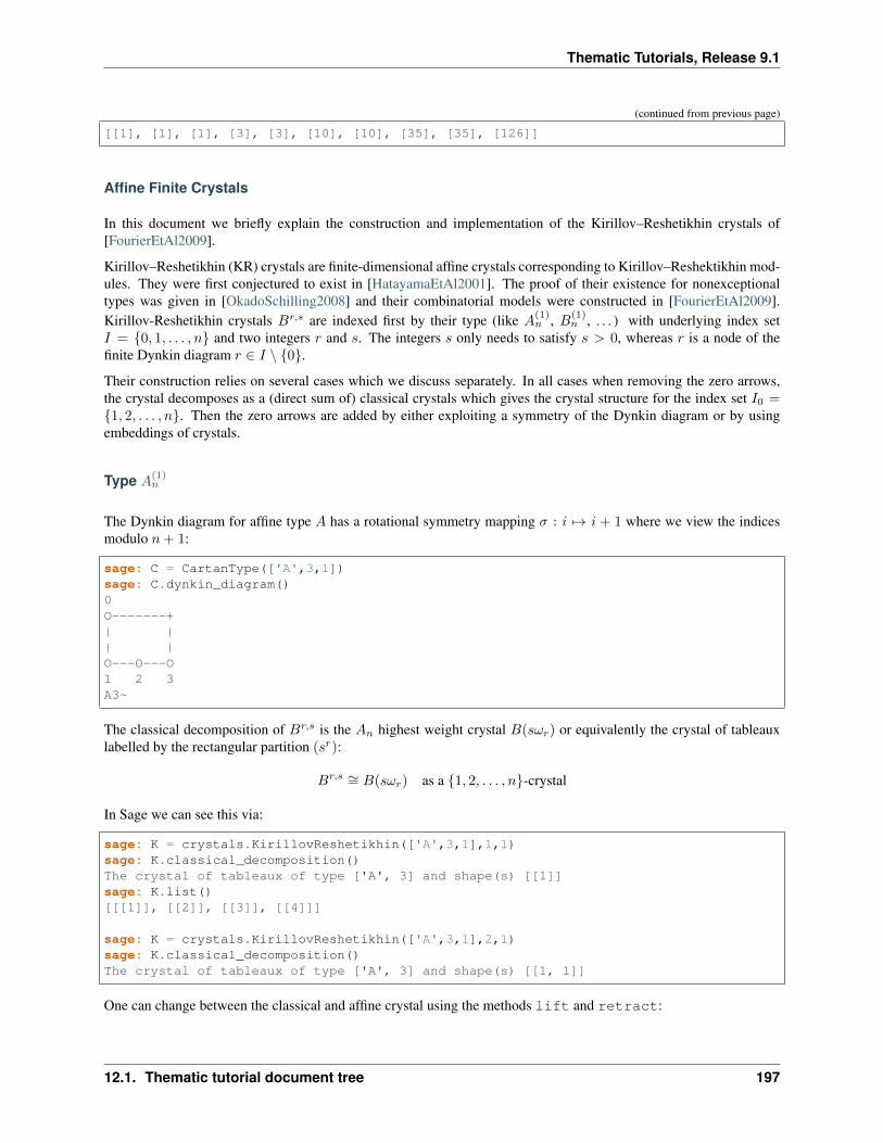
Thematic Tutorials, Release 9.1
(continued from previous page)
[[1], [1], [1], [3], [3], [10], [10], [35], [35], [126]]
Affine Finite Crystals
In this document we briefly explain the construction and implementation of the Kirillov–Reshetikhin crystals of[FourierEtAl2009].
Kirillov–Reshetikhin (KR) crystals are finite-dimensional affine crystals corresponding to Kirillov–Reshektikhin mod-ules. They were first conjectured to exist in [HatayamaEtAl2001]. The proof of their existence for nonexceptionaltypes was given in [OkadoSchilling2008] and their combinatorial models were constructed in [FourierEtAl2009].Kirillov-Reshetikhin crystals 𝐵𝑟,𝑠 are indexed first by their type (like 𝐴(1)
𝑛 , 𝐵(1)𝑛 , . . . ) with underlying index set
𝐼 = 0, 1, . . . , 𝑛 and two integers 𝑟 and 𝑠. The integers 𝑠 only needs to satisfy 𝑠 > 0, whereas 𝑟 is a node of thefinite Dynkin diagram 𝑟 ∈ 𝐼 ∖ 0.
Their construction relies on several cases which we discuss separately. In all cases when removing the zero arrows,the crystal decomposes as a (direct sum of) classical crystals which gives the crystal structure for the index set 𝐼0 =1, 2, . . . , 𝑛. Then the zero arrows are added by either exploiting a symmetry of the Dynkin diagram or by usingembeddings of crystals.
Type 𝐴(1)𝑛
The Dynkin diagram for affine type 𝐴 has a rotational symmetry mapping 𝜎 : 𝑖 ↦→ 𝑖 + 1 where we view the indicesmodulo 𝑛+ 1:
sage: C = CartanType(['A',3,1])sage: C.dynkin_diagram()0O-------+| || |O---O---O1 2 3A3~
The classical decomposition of 𝐵𝑟,𝑠 is the 𝐴𝑛 highest weight crystal 𝐵(𝑠𝜔𝑟) or equivalently the crystal of tableauxlabelled by the rectangular partition (𝑠𝑟):
𝐵𝑟,𝑠 ∼= 𝐵(𝑠𝜔𝑟) as a 1, 2, . . . , 𝑛-crystal
In Sage we can see this via:
sage: K = crystals.KirillovReshetikhin(['A',3,1],1,1)sage: K.classical_decomposition()The crystal of tableaux of type ['A', 3] and shape(s) [[1]]sage: K.list()[[[1]], [[2]], [[3]], [[4]]]
sage: K = crystals.KirillovReshetikhin(['A',3,1],2,1)sage: K.classical_decomposition()The crystal of tableaux of type ['A', 3] and shape(s) [[1, 1]]
One can change between the classical and affine crystal using the methods lift and retract:
12.1. Thematic tutorial document tree 197
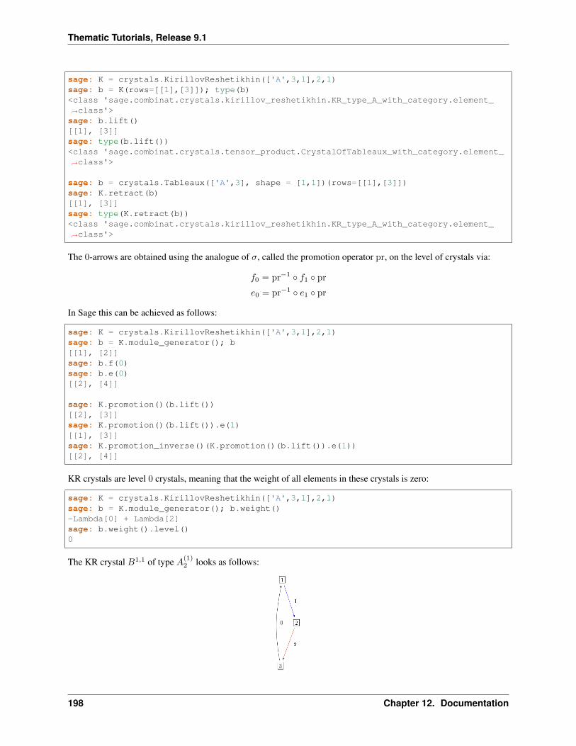
Thematic Tutorials, Release 9.1
sage: K = crystals.KirillovReshetikhin(['A',3,1],2,1)sage: b = K(rows=[[1],[3]]); type(b)<class 'sage.combinat.crystals.kirillov_reshetikhin.KR_type_A_with_category.element_→˓class'>sage: b.lift()[[1], [3]]sage: type(b.lift())<class 'sage.combinat.crystals.tensor_product.CrystalOfTableaux_with_category.element_→˓class'>
sage: b = crystals.Tableaux(['A',3], shape = [1,1])(rows=[[1],[3]])sage: K.retract(b)[[1], [3]]sage: type(K.retract(b))<class 'sage.combinat.crystals.kirillov_reshetikhin.KR_type_A_with_category.element_→˓class'>
The 0-arrows are obtained using the analogue of 𝜎, called the promotion operator pr, on the level of crystals via:
𝑓0 = pr−1 ∘ 𝑓1 ∘ pr
𝑒0 = pr−1 ∘ 𝑒1 ∘ pr
In Sage this can be achieved as follows:
sage: K = crystals.KirillovReshetikhin(['A',3,1],2,1)sage: b = K.module_generator(); b[[1], [2]]sage: b.f(0)sage: b.e(0)[[2], [4]]
sage: K.promotion()(b.lift())[[2], [3]]sage: K.promotion()(b.lift()).e(1)[[1], [3]]sage: K.promotion_inverse()(K.promotion()(b.lift()).e(1))[[2], [4]]
KR crystals are level 0 crystals, meaning that the weight of all elements in these crystals is zero:
sage: K = crystals.KirillovReshetikhin(['A',3,1],2,1)sage: b = K.module_generator(); b.weight()-Lambda[0] + Lambda[2]sage: b.weight().level()0
The KR crystal 𝐵1,1 of type 𝐴(1)2 looks as follows:
198 Chapter 12. Documentation
Thematic Tutorials, Release 9.1
In Sage this can be obtained via:
sage: K = crystals.KirillovReshetikhin(['A',2,1],1,1)sage: G = K.digraph()sage: view(G, tightpage=True) # optional - dot2tex graphviz, not tested (opens→˓external window)
Types 𝐷(1)𝑛 , 𝐵(1)
𝑛 , 𝐴(2)2𝑛−1
The Dynkin diagrams for types 𝐷(1)𝑛 , 𝐵(1)
𝑛 , 𝐴(2)2𝑛−1 are invariant under interchanging nodes 0 and 1:
sage: n = 5sage: C = CartanType(['D',n,1]); C.dynkin_diagram()
0 O O 5| || |
O---O---O---O1 2 3 4D5~sage: C = CartanType(['B',n,1]); C.dynkin_diagram()
O 0||
O---O---O---O=>=O1 2 3 4 5B5~sage: C = CartanType(['A',2*n-1,2]); C.dynkin_diagram()
O 0||
O---O---O---O=<=O1 2 3 4 5B5~*
The underlying classical algebras obtained when removing node 0 are type g0 = 𝐷𝑛, 𝐵𝑛, 𝐶𝑛, respectively. Theclassical decomposition into a g0 crystal is a direct sum:
𝐵𝑟,𝑠 ∼=⨁𝜆
𝐵(𝜆) as a 1, 2, . . . , 𝑛-crystal
where 𝜆 is obtained from 𝑠𝜔𝑟 (or equivalently a rectangular partition of shape (𝑠𝑟)) by removing vertical dominoes.This in fact only holds in the ranges 1 ≤ 𝑟 ≤ 𝑛− 2 for type 𝐷(1)
𝑛 , and 1 ≤ 𝑟 ≤ 𝑛 for types 𝐵(1)𝑛 and 𝐴(2)
2𝑛−1:
sage: K = crystals.KirillovReshetikhin(['D',6,1],4,2)sage: K.classical_decomposition()The crystal of tableaux of type ['D', 6] and shape(s)[[], [1, 1], [1, 1, 1, 1], [2, 2], [2, 2, 1, 1], [2, 2, 2, 2]]
For type 𝐵(1)𝑛 and 𝑟 = 𝑛, one needs to be aware that 𝜔𝑛 is a spin weight and hence corresponds in the partition
language to a column of height 𝑛 and width 1/2:
sage: K = crystals.KirillovReshetikhin(['B',3,1],3,1)sage: K.classical_decomposition()The crystal of tableaux of type ['B', 3] and shape(s) [[1/2, 1/2, 1/2]]
As for type 𝐴(1)𝑛 , the Dynkin automorphism induces a promotion-type operator 𝜎 on the level of crystals. In this case
in can however happen that the automorphism changes between classical components:
12.1. Thematic tutorial document tree 199
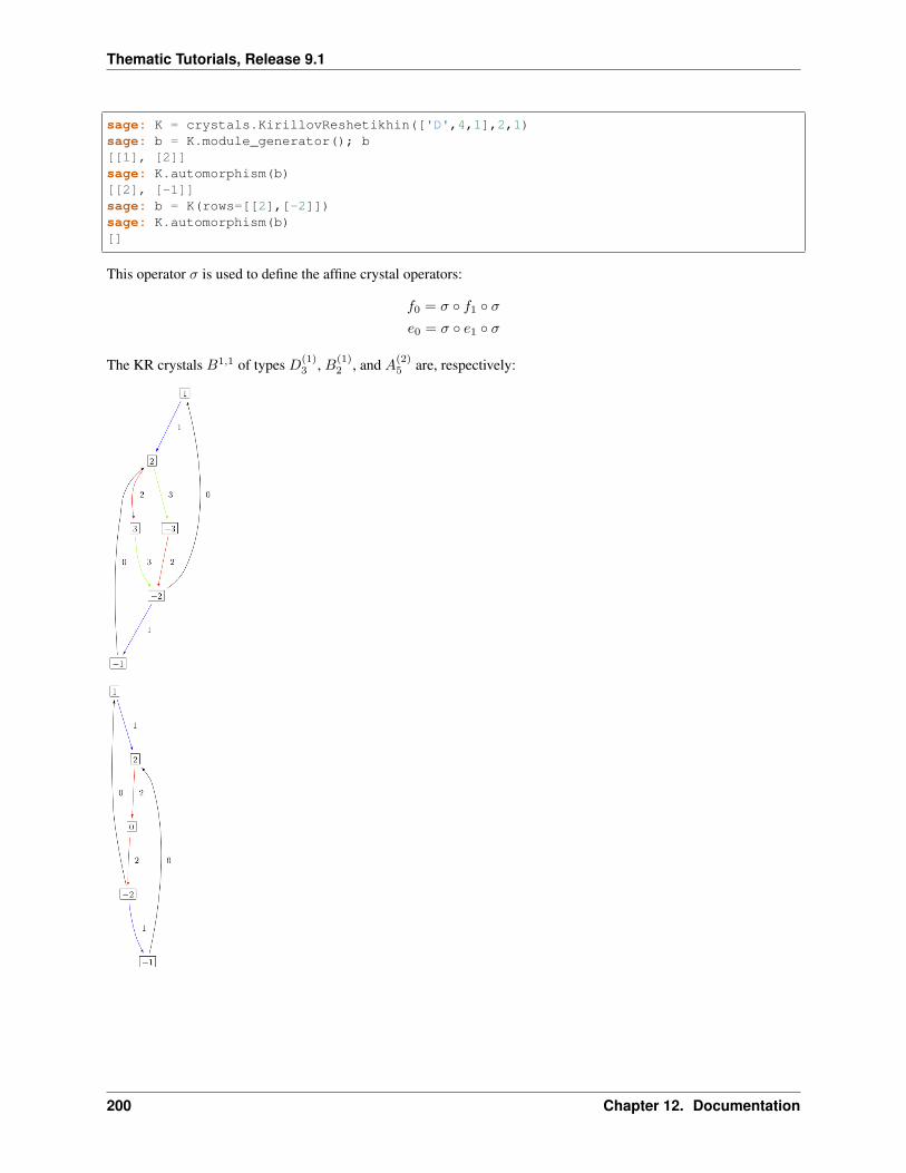
Thematic Tutorials, Release 9.1
sage: K = crystals.KirillovReshetikhin(['D',4,1],2,1)sage: b = K.module_generator(); b[[1], [2]]sage: K.automorphism(b)[[2], [-1]]sage: b = K(rows=[[2],[-2]])sage: K.automorphism(b)[]
This operator 𝜎 is used to define the affine crystal operators:
𝑓0 = 𝜎 ∘ 𝑓1 ∘ 𝜎𝑒0 = 𝜎 ∘ 𝑒1 ∘ 𝜎
The KR crystals 𝐵1,1 of types 𝐷(1)3 , 𝐵(1)
2 , and 𝐴(2)5 are, respectively:
200 Chapter 12. Documentation
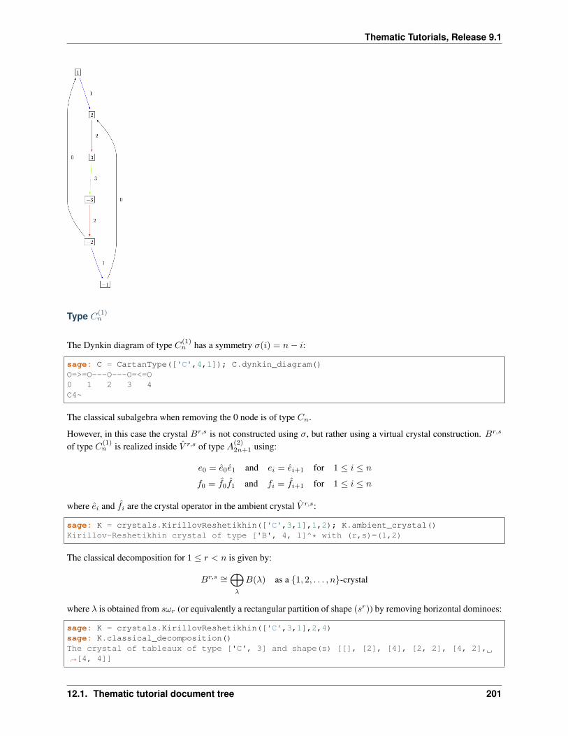
Thematic Tutorials, Release 9.1
Type 𝐶(1)𝑛
The Dynkin diagram of type 𝐶(1)𝑛 has a symmetry 𝜎(𝑖) = 𝑛− 𝑖:
sage: C = CartanType(['C',4,1]); C.dynkin_diagram()O=>=O---O---O=<=O0 1 2 3 4C4~
The classical subalgebra when removing the 0 node is of type 𝐶𝑛.
However, in this case the crystal 𝐵𝑟,𝑠 is not constructed using 𝜎, but rather using a virtual crystal construction. 𝐵𝑟,𝑠
of type 𝐶(1)𝑛 is realized inside 𝑉 𝑟,𝑠 of type 𝐴(2)
2𝑛+1 using:
𝑒0 = 𝑒0𝑒1 and 𝑒𝑖 = 𝑒𝑖+1 for 1 ≤ 𝑖 ≤ 𝑛
𝑓0 = 𝑓0𝑓1 and 𝑓𝑖 = 𝑓𝑖+1 for 1 ≤ 𝑖 ≤ 𝑛
where 𝑒𝑖 and 𝑓𝑖 are the crystal operator in the ambient crystal 𝑉 𝑟,𝑠:
sage: K = crystals.KirillovReshetikhin(['C',3,1],1,2); K.ambient_crystal()Kirillov-Reshetikhin crystal of type ['B', 4, 1]^* with (r,s)=(1,2)
The classical decomposition for 1 ≤ 𝑟 < 𝑛 is given by:
𝐵𝑟,𝑠 ∼=⨁𝜆
𝐵(𝜆) as a 1, 2, . . . , 𝑛-crystal
where 𝜆 is obtained from 𝑠𝜔𝑟 (or equivalently a rectangular partition of shape (𝑠𝑟)) by removing horizontal dominoes:
sage: K = crystals.KirillovReshetikhin(['C',3,1],2,4)sage: K.classical_decomposition()The crystal of tableaux of type ['C', 3] and shape(s) [[], [2], [4], [2, 2], [4, 2],→˓[4, 4]]
12.1. Thematic tutorial document tree 201
Thematic Tutorials, Release 9.1
The KR crystal 𝐵1,1 of type 𝐶(1)2 looks as follows:
Types 𝐷(2)𝑛+1, 𝐴(2)
2𝑛
The Dynkin diagrams of types 𝐷(2)𝑛+1 and 𝐴(2)
2𝑛 look as follows:
sage: C = CartanType(['D',5,2]); C.dynkin_diagram()O=<=O---O---O=>=O0 1 2 3 4C4~*
sage: C = CartanType(['A',8,2]); C.dynkin_diagram()O=<=O---O---O=<=O0 1 2 3 4BC4~
The classical subdiagram is of type 𝐵𝑛 for type 𝐷(2)𝑛+1 and of type 𝐶𝑛 for type 𝐴(2)
2𝑛 . The classical decomposition forthese KR crystals for 1 ≤ 𝑟 < 𝑛 for type 𝐷(2)
𝑛+1 and 1 ≤ 𝑟 ≤ 𝑛 for type 𝐴(2)2𝑛 is given by:
𝐵𝑟,𝑠 ∼=⨁𝜆
𝐵(𝜆) as a 1, 2, . . . , 𝑛-crystal
where 𝜆 is obtained from 𝑠𝜔𝑟 (or equivalently a rectangular partition of shape (𝑠𝑟)) by removing single boxes:
sage: K = crystals.KirillovReshetikhin(['D',5,2],2,2)sage: K.classical_decomposition()The crystal of tableaux of type ['B', 4] and shape(s) [[], [1], [2], [1, 1], [2, 1],→˓[2, 2]]
sage: K = crystals.KirillovReshetikhin(['A',8,2],2,2)sage: K.classical_decomposition()The crystal of tableaux of type ['C', 4] and shape(s) [[], [1], [2], [1, 1], [2, 1],→˓[2, 2]]
The KR crystals are constructed using an injective map into a KR crystal of type 𝐶(1)𝑛
𝑆 : 𝐵𝑟,𝑠 → 𝐵𝑟,2𝑠
𝐶(1)𝑛
such that 𝑆(𝑒𝑖𝑏) = 𝑒𝑚𝑖𝑖 𝑆(𝑏) and 𝑆(𝑓𝑖𝑏) = 𝑓𝑚𝑖
𝑖 𝑆(𝑏)
where
(𝑚0, . . . ,𝑚𝑛) = (1, 2, . . . , 2, 1) for type 𝐷(2)𝑛+1 and (1, 2, . . . , 2, 2) for type 𝐴(2)
2𝑛 .
202 Chapter 12. Documentation
Thematic Tutorials, Release 9.1
sage: K = crystals.KirillovReshetikhin(['D',5,2],1,2); K.ambient_crystal()Kirillov-Reshetikhin crystal of type ['C', 4, 1] with (r,s)=(1,4)sage: K = crystals.KirillovReshetikhin(['A',8,2],1,2); K.ambient_crystal()Kirillov-Reshetikhin crystal of type ['C', 4, 1] with (r,s)=(1,4)
The KR crystals 𝐵1,1 of type 𝐷(2)3 and 𝐴(2)
4 look as follows:
As you can see from the Dynkin diagram for type 𝐴(2)2𝑛 , mapping the nodes 𝑖 ↦→ 𝑛 − 𝑖 yields the same diagram, but
with relabelled nodes. In this case the classical subdiagram is of type 𝐵𝑛 instead of 𝐶𝑛. One can also construct theKR crystal 𝐵𝑟,𝑠 of type 𝐴(2)
2𝑛 based on this classical decomposition. In this case the classical decomposition is the sumover all weights obtained from 𝑠𝜔𝑟 by removing horizontal dominoes:
sage: C = CartanType(['A',6,2]).dual()sage: Kdual = crystals.KirillovReshetikhin(C,2,2)sage: Kdual.classical_decomposition()The crystal of tableaux of type ['B', 3] and shape(s) [[], [2], [2, 2]]
Looking at the picture, one can see that this implementation is isomorphic to the other implementation based on the𝐶𝑛 decomposition up to a relabeling of the arrows:
sage: C = CartanType(['A',4,2])sage: K = crystals.KirillovReshetikhin(C,1,1)sage: Kdual = crystals.KirillovReshetikhin(C.dual(),1,1)sage: G = K.digraph()
(continues on next page)
12.1. Thematic tutorial document tree 203
Thematic Tutorials, Release 9.1
(continued from previous page)
sage: Gdual = Kdual.digraph()sage: f = 1:1, 0:2, 2:0 sage: for u,v,label in Gdual.edges():....: Gdual.set_edge_label(u,v,f[label])sage: G.is_isomorphic(Gdual, edge_labels = True)True
Exceptional nodes
The KR crystals 𝐵𝑛,𝑠 for types 𝐶(1)𝑛 and 𝐷(2)
𝑛+1 were excluded from the above discussion. They are associated to theexceptional node 𝑟 = 𝑛 and in this case the classical decomposition is irreducible:
𝐵𝑛,𝑠 ∼= 𝐵(𝑠𝜔𝑛).
In Sage:
sage: K = crystals.KirillovReshetikhin(['C',2,1],2,1)sage: K.classical_decomposition()The crystal of tableaux of type ['C', 2] and shape(s) [[1, 1]]
sage: K = crystals.KirillovReshetikhin(['D',3,2],2,1)sage: K.classical_decomposition()The crystal of tableaux of type ['B', 2] and shape(s) [[1/2, 1/2]]
204 Chapter 12. Documentation
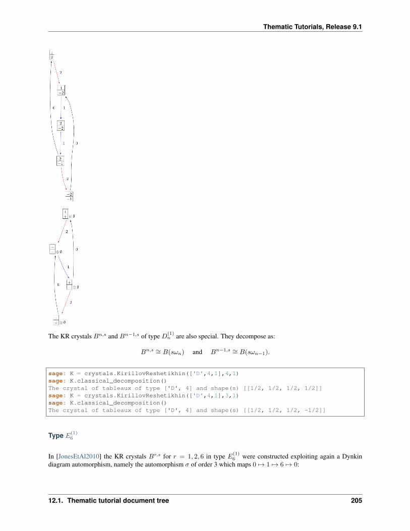
Thematic Tutorials, Release 9.1
The KR crystals 𝐵𝑛,𝑠 and 𝐵𝑛−1,𝑠 of type 𝐷(1)𝑛 are also special. They decompose as:
𝐵𝑛,𝑠 ∼= 𝐵(𝑠𝜔𝑛) and 𝐵𝑛−1,𝑠 ∼= 𝐵(𝑠𝜔𝑛−1).
sage: K = crystals.KirillovReshetikhin(['D',4,1],4,1)sage: K.classical_decomposition()The crystal of tableaux of type ['D', 4] and shape(s) [[1/2, 1/2, 1/2, 1/2]]sage: K = crystals.KirillovReshetikhin(['D',4,1],3,1)sage: K.classical_decomposition()The crystal of tableaux of type ['D', 4] and shape(s) [[1/2, 1/2, 1/2, -1/2]]
Type 𝐸(1)6
In [JonesEtAl2010] the KR crystals 𝐵𝑟,𝑠 for 𝑟 = 1, 2, 6 in type 𝐸(1)6 were constructed exploiting again a Dynkin
diagram automorphism, namely the automorphism 𝜎 of order 3 which maps 0 ↦→ 1 ↦→ 6 ↦→ 0:
12.1. Thematic tutorial document tree 205
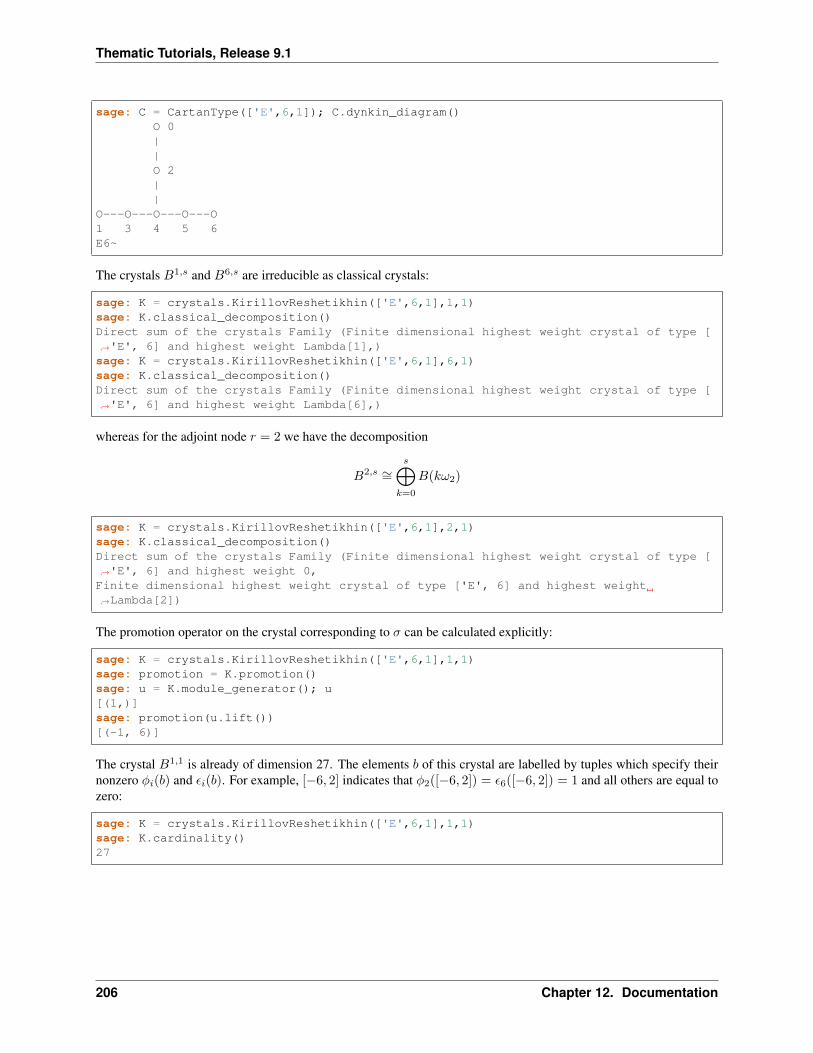
Thematic Tutorials, Release 9.1
sage: C = CartanType(['E',6,1]); C.dynkin_diagram()O 0||O 2||
O---O---O---O---O1 3 4 5 6E6~
The crystals 𝐵1,𝑠 and 𝐵6,𝑠 are irreducible as classical crystals:
sage: K = crystals.KirillovReshetikhin(['E',6,1],1,1)sage: K.classical_decomposition()Direct sum of the crystals Family (Finite dimensional highest weight crystal of type [→˓'E', 6] and highest weight Lambda[1],)sage: K = crystals.KirillovReshetikhin(['E',6,1],6,1)sage: K.classical_decomposition()Direct sum of the crystals Family (Finite dimensional highest weight crystal of type [→˓'E', 6] and highest weight Lambda[6],)
whereas for the adjoint node 𝑟 = 2 we have the decomposition
𝐵2,𝑠 ∼=𝑠⨁
𝑘=0
𝐵(𝑘𝜔2)
sage: K = crystals.KirillovReshetikhin(['E',6,1],2,1)sage: K.classical_decomposition()Direct sum of the crystals Family (Finite dimensional highest weight crystal of type [→˓'E', 6] and highest weight 0,Finite dimensional highest weight crystal of type ['E', 6] and highest weight→˓Lambda[2])
The promotion operator on the crystal corresponding to 𝜎 can be calculated explicitly:
sage: K = crystals.KirillovReshetikhin(['E',6,1],1,1)sage: promotion = K.promotion()sage: u = K.module_generator(); u[(1,)]sage: promotion(u.lift())[(-1, 6)]
The crystal 𝐵1,1 is already of dimension 27. The elements 𝑏 of this crystal are labelled by tuples which specify theirnonzero 𝜑𝑖(𝑏) and 𝜖𝑖(𝑏). For example, [−6, 2] indicates that 𝜑2([−6, 2]) = 𝜖6([−6, 2]) = 1 and all others are equal tozero:
sage: K = crystals.KirillovReshetikhin(['E',6,1],1,1)sage: K.cardinality()27
206 Chapter 12. Documentation
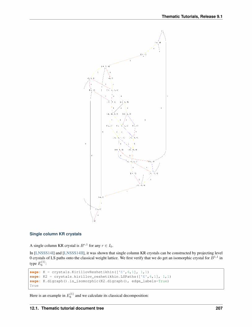
Thematic Tutorials, Release 9.1
Single column KR crystals
A single column KR crystal is 𝐵𝑟,1 for any 𝑟 ∈ 𝐼0.
In [LNSSS14I] and [LNSSS14II], it was shown that single column KR crystals can be constructed by projecting level0 crystals of LS paths onto the classical weight lattice. We first verify that we do get an isomorphic crystal for 𝐵1,1 intype 𝐸(1)
6 :
sage: K = crystals.KirillovReshetikhin(['E',6,1], 1,1)sage: K2 = crystals.kirillov_reshetikhin.LSPaths(['E',6,1], 1,1)sage: K.digraph().is_isomorphic(K2.digraph(), edge_labels=True)True
Here is an example in 𝐸(1)8 and we calculate its classical decomposition:
12.1. Thematic tutorial document tree 207
Thematic Tutorials, Release 9.1
sage: K = crystals.kirillov_reshetikhin.LSPaths(['E',8,1], 8,1)sage: K.cardinality()249sage: L = [x for x in K if x.is_highest_weight([1,2,3,4,5,6,7,8])]sage: [x.weight() for x in L][-2*Lambda[0] + Lambda[8], 0]
Applications
An important notion for finite-dimensional affine crystals is perfectness. The crucial property is that a crystal 𝐵 isperfect of level ℓ if there is a bijection between level ℓ dominant weights and elements in
𝐵min = 𝑏 ∈ 𝐵 | lev(𝜙(𝑏)) = ℓ .
For a precise definition of perfect crystals see [HongKang2002] . In [FourierEtAl2010] it was proven that for thenonexceptional types 𝐵𝑟,𝑠 is perfect as long as 𝑠/𝑐𝑟 is an integer. Here 𝑐𝑟 = 1 except 𝑐𝑟 = 2 for 1 ≤ 𝑟 < 𝑛 in type𝐶
(1)𝑛 and 𝑟 = 𝑛 in type 𝐵(1)
𝑛 .
Here we verify this using Sage for 𝐵1,1 of type 𝐶(1)3 :
sage: K = crystals.KirillovReshetikhin(['C',3,1],1,1)sage: Lambda = K.weight_lattice_realization().fundamental_weights(); LambdaFinite family 0: Lambda[0], 1: Lambda[1], 2: Lambda[2], 3: Lambda[3]sage: [w.level() for w in Lambda][1, 1, 1, 1]sage: Bmin = [b for b in K if b.Phi().level() == 1 ]; Bmin[[[1]], [[2]], [[3]], [[-3]], [[-2]], [[-1]]]sage: [b.Phi() for b in Bmin][Lambda[1], Lambda[2], Lambda[3], Lambda[2], Lambda[1], Lambda[0]]
As you can see, both 𝑏 = 1 and 𝑏 = −2 satisfy 𝜙(𝑏) = Λ1. Hence there is no bijection between the minimal elementsin 𝐵min and level 1 weights. Therefore, 𝐵1,1 of type 𝐶(1)
3 is not perfect. However, 𝐵1,2 of type 𝐶(1)𝑛 is a perfect
crystal:
sage: K = crystals.KirillovReshetikhin(['C',3,1],1,2)sage: Lambda = K.weight_lattice_realization().fundamental_weights()sage: Bmin = [b for b in K if b.Phi().level() == 1 ]sage: [b.Phi() for b in Bmin][Lambda[0], Lambda[3], Lambda[2], Lambda[1]]
Perfect crystals can be used to construct infinite-dimensional highest weight crystals and Demazure crystals using theKyoto path model [KKMMNN1992]. We construct Example 10.6.5 in [HongKang2002]:
sage: K = crystals.KirillovReshetikhin(['A',1,1], 1,1)sage: La = RootSystem(['A',1,1]).weight_lattice().fundamental_weights()sage: B = crystals.KyotoPathModel(K, La[0])sage: B.highest_weight_vector()[[[2]]]
sage: K = crystals.KirillovReshetikhin(['A',2,1], 1,1)sage: La = RootSystem(['A',2,1]).weight_lattice().fundamental_weights()sage: B = crystals.KyotoPathModel(K, La[0])sage: B.highest_weight_vector()[[[3]]]
(continues on next page)
208 Chapter 12. Documentation
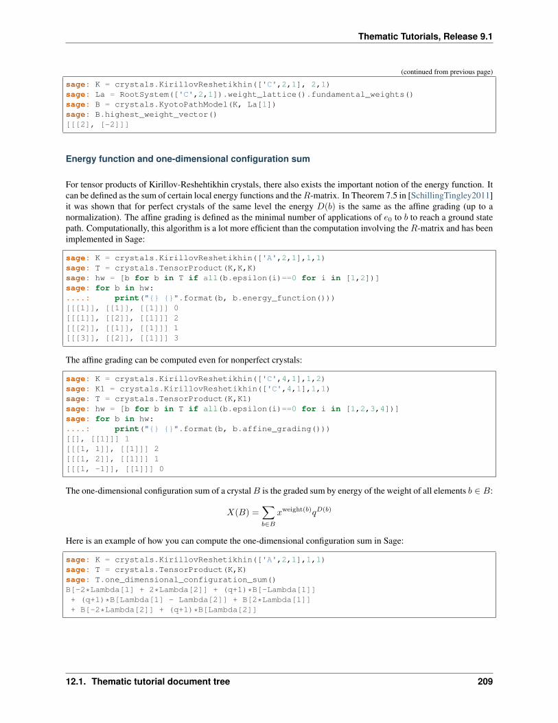
Thematic Tutorials, Release 9.1
(continued from previous page)
sage: K = crystals.KirillovReshetikhin(['C',2,1], 2,1)sage: La = RootSystem(['C',2,1]).weight_lattice().fundamental_weights()sage: B = crystals.KyotoPathModel(K, La[1])sage: B.highest_weight_vector()[[[2], [-2]]]
Energy function and one-dimensional configuration sum
For tensor products of Kirillov-Reshehtikhin crystals, there also exists the important notion of the energy function. Itcan be defined as the sum of certain local energy functions and the𝑅-matrix. In Theorem 7.5 in [SchillingTingley2011]it was shown that for perfect crystals of the same level the energy 𝐷(𝑏) is the same as the affine grading (up to anormalization). The affine grading is defined as the minimal number of applications of 𝑒0 to 𝑏 to reach a ground statepath. Computationally, this algorithm is a lot more efficient than the computation involving the 𝑅-matrix and has beenimplemented in Sage:
sage: K = crystals.KirillovReshetikhin(['A',2,1],1,1)sage: T = crystals.TensorProduct(K,K,K)sage: hw = [b for b in T if all(b.epsilon(i)==0 for i in [1,2])]sage: for b in hw:....: print(" ".format(b, b.energy_function()))[[[1]], [[1]], [[1]]] 0[[[1]], [[2]], [[1]]] 2[[[2]], [[1]], [[1]]] 1[[[3]], [[2]], [[1]]] 3
The affine grading can be computed even for nonperfect crystals:
sage: K = crystals.KirillovReshetikhin(['C',4,1],1,2)sage: K1 = crystals.KirillovReshetikhin(['C',4,1],1,1)sage: T = crystals.TensorProduct(K,K1)sage: hw = [b for b in T if all(b.epsilon(i)==0 for i in [1,2,3,4])]sage: for b in hw:....: print(" ".format(b, b.affine_grading()))[[], [[1]]] 1[[[1, 1]], [[1]]] 2[[[1, 2]], [[1]]] 1[[[1, -1]], [[1]]] 0
The one-dimensional configuration sum of a crystal𝐵 is the graded sum by energy of the weight of all elements 𝑏 ∈ 𝐵:
𝑋(𝐵) =∑𝑏∈𝐵
𝑥weight(𝑏)𝑞𝐷(𝑏)
Here is an example of how you can compute the one-dimensional configuration sum in Sage:
sage: K = crystals.KirillovReshetikhin(['A',2,1],1,1)sage: T = crystals.TensorProduct(K,K)sage: T.one_dimensional_configuration_sum()B[-2*Lambda[1] + 2*Lambda[2]] + (q+1)*B[-Lambda[1]]+ (q+1)*B[Lambda[1] - Lambda[2]] + B[2*Lambda[1]]+ B[-2*Lambda[2]] + (q+1)*B[Lambda[2]]
12.1. Thematic tutorial document tree 209
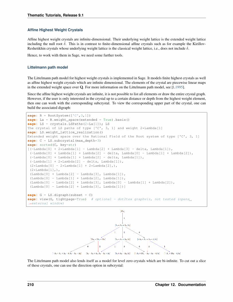
Thematic Tutorials, Release 9.1
Affine Highest Weight Crystals
Affine highest weight crystals are infinite-dimensional. Their underlying weight lattice is the extended weight latticeincluding the null root 𝛿. This is in contrast to finite-dimensional affine crystals such as for example the Kirillov-Reshetikhin crystals whose underlying weight lattice is the classical weight lattice, i.e., does not include 𝛿.
Hence, to work with them in Sage, we need some further tools.
Littelmann path model
The Littelmann path model for highest weight crystals is implemented in Sage. It models finite highest crystals as wellas affine highest weight crystals which are infinite dimensional. The elements of the crystal are piecewise linear mapsin the extended weight space over Q. For more information on the Littelmann path model, see [L1995].
Since the affine highest weight crystals are infinite, it is not possible to list all elements or draw the entire crystal graph.However, if the user is only interested in the crystal up to a certain distance or depth from the highest weight element,then one can work with the corresponding subcrystal. To view the corresponding upper part of the crystal, one canbuild the associated digraph:
sage: R = RootSystem(['C',3,1])sage: La = R.weight_space(extended = True).basis()sage: LS = crystals.LSPaths(2*La[1]); LSThe crystal of LS paths of type ['C', 3, 1] and weight 2*Lambda[1]sage: LS.weight_lattice_realization()Extended weight space over the Rational Field of the Root system of type ['C', 3, 1]sage: C = LS.subcrystal(max_depth=3)sage: sorted(C, key=str)[(-Lambda[0] + 2*Lambda[1] - Lambda[2] + Lambda[3] - delta, Lambda[1]),(-Lambda[0] + Lambda[1] + Lambda[2] - delta, Lambda[0] - Lambda[1] + Lambda[2]),(-Lambda[0] + Lambda[1] + Lambda[2] - delta, Lambda[1]),(-Lambda[1] + 2*Lambda[2] - delta, Lambda[1]),(2*Lambda[0] - 2*Lambda[1] + 2*Lambda[2],),(2*Lambda[1],),(Lambda[0] + Lambda[2] - Lambda[3], Lambda[1]),(Lambda[0] - Lambda[1] + Lambda[2], Lambda[1]),(Lambda[0] - Lambda[2] + Lambda[3], Lambda[0] - Lambda[1] + Lambda[2]),(Lambda[0] - Lambda[2] + Lambda[3], Lambda[1])]
sage: G = LS.digraph(subset = C)sage: view(G, tightpage=True) # optional - dot2tex graphviz, not tested (opens→˓external window)
The Littelmann path model also lends itself as a model for level zero crystals which are bi-infinite. To cut out a sliceof these crystals, one can use the direction option in subcrystal:
210 Chapter 12. Documentation
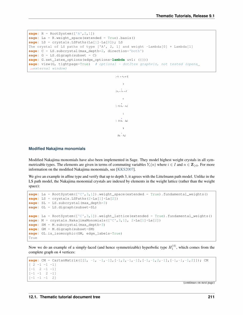
Thematic Tutorials, Release 9.1
sage: R = RootSystem(['A',2,1])sage: La = R.weight_space(extended = True).basis()sage: LS = crystals.LSPaths(La[1]-La[0]); LSThe crystal of LS paths of type ['A', 2, 1] and weight -Lambda[0] + Lambda[1]sage: C = LS.subcrystal(max_depth=2, direction='both')sage: G = LS.digraph(subset = C)sage: G.set_latex_options(edge_options=lambda uvl: ())sage: view(G, tightpage=True) # optional - dot2tex graphviz, not tested (opens→˓external window)
Modified Nakajima monomials
Modified Nakajima monomials have also been implemented in Sage. They model highest weight crystals in all sym-metrizable types. The elements are given in terms of commuting variables 𝑌𝑖(𝑛) where 𝑖 ∈ 𝐼 and 𝑛 ∈ Z≥0. For moreinformation on the modified Nakajima monomials, see [KKS2007].
We give an example in affine type and verify that up to depth 3, it agrees with the Littelmann path model. Unlike in theLS path model, the Nakajima monomial crystals are indexed by elements in the weight lattice (rather than the weightspace):
sage: La = RootSystem(['C',3,1]).weight_space(extended = True).fundamental_weights()sage: LS = crystals.LSPaths(2*La[1]+La[2])sage: SL = LS.subcrystal(max_depth=3)sage: GL = LS.digraph(subset=SL)
sage: La = RootSystem(['C',3,1]).weight_lattice(extended = True).fundamental_weights()sage: M = crystals.NakajimaMonomials(['C',3,1], 2*La[1]+La[2])sage: SM = M.subcrystal(max_depth=3)sage: GM = M.digraph(subset=SM)sage: GL.is_isomorphic(GM, edge_labels=True)True
Now we do an example of a simply-laced (and hence symmetrizable) hyperbolic type 𝐻(4)1 , which comes from the
complete graph on 4 vertices:
sage: CM = CartanMatrix([[2, -1, -1,-1],[-1,2,-1,-1],[-1,-1,2,-1],[-1,-1,-1,2]]); CM[ 2 -1 -1 -1][-1 2 -1 -1][-1 -1 2 -1][-1 -1 -1 2]
(continues on next page)
12.1. Thematic tutorial document tree 211
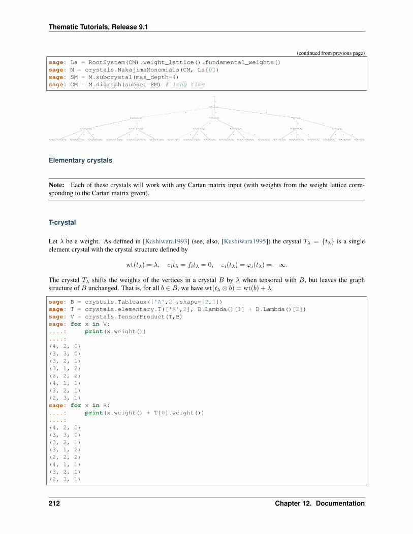
Thematic Tutorials, Release 9.1
(continued from previous page)
sage: La = RootSystem(CM).weight_lattice().fundamental_weights()sage: M = crystals.NakajimaMonomials(CM, La[0])sage: SM = M.subcrystal(max_depth=4)sage: GM = M.digraph(subset=SM) # long time
Elementary crystals
Note: Each of these crystals will work with any Cartan matrix input (with weights from the weight lattice corre-sponding to the Cartan matrix given).
T-crystal
Let 𝜆 be a weight. As defined in [Kashiwara1993] (see, also, [Kashiwara1995]) the crystal 𝑇𝜆 = 𝑡𝜆 is a singleelement crystal with the crystal structure defined by
wt(𝑡𝜆) = 𝜆, 𝑒𝑖𝑡𝜆 = 𝑓𝑖𝑡𝜆 = 0, 𝜀𝑖(𝑡𝜆) = 𝜙𝑖(𝑡𝜆) = −∞.
The crystal 𝑇𝜆 shifts the weights of the vertices in a crystal 𝐵 by 𝜆 when tensored with 𝐵, but leaves the graphstructure of 𝐵 unchanged. That is, for all 𝑏 ∈ 𝐵, we have wt(𝑡𝜆 ⊗ 𝑏) = wt(𝑏) + 𝜆:
sage: B = crystals.Tableaux(['A',2],shape=[2,1])sage: T = crystals.elementary.T(['A',2], B.Lambda()[1] + B.Lambda()[2])sage: V = crystals.TensorProduct(T,B)sage: for x in V:....: print(x.weight())....:(4, 2, 0)(3, 3, 0)(3, 2, 1)(3, 1, 2)(2, 2, 2)(4, 1, 1)(3, 2, 1)(2, 3, 1)sage: for x in B:....: print(x.weight() + T[0].weight())....:(4, 2, 0)(3, 3, 0)(3, 2, 1)(3, 1, 2)(2, 2, 2)(4, 1, 1)(3, 2, 1)(2, 3, 1)
212 Chapter 12. Documentation
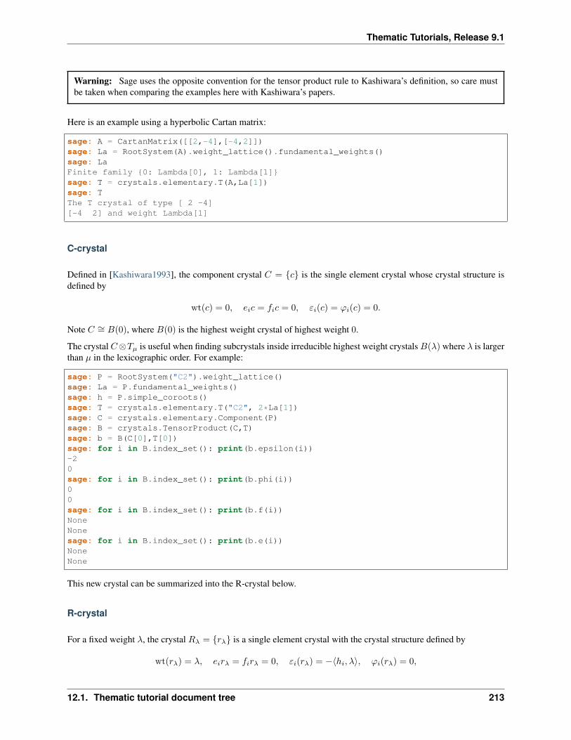
Thematic Tutorials, Release 9.1
Warning: Sage uses the opposite convention for the tensor product rule to Kashiwara’s definition, so care mustbe taken when comparing the examples here with Kashiwara’s papers.
Here is an example using a hyperbolic Cartan matrix:
sage: A = CartanMatrix([[2,-4],[-4,2]])sage: La = RootSystem(A).weight_lattice().fundamental_weights()sage: LaFinite family 0: Lambda[0], 1: Lambda[1]sage: T = crystals.elementary.T(A,La[1])sage: TThe T crystal of type [ 2 -4][-4 2] and weight Lambda[1]
C-crystal
Defined in [Kashiwara1993], the component crystal 𝐶 = 𝑐 is the single element crystal whose crystal structure isdefined by
wt(𝑐) = 0, 𝑒𝑖𝑐 = 𝑓𝑖𝑐 = 0, 𝜀𝑖(𝑐) = 𝜙𝑖(𝑐) = 0.
Note 𝐶 ∼= 𝐵(0), where 𝐵(0) is the highest weight crystal of highest weight 0.
The crystal 𝐶⊗𝑇𝜇 is useful when finding subcrystals inside irreducible highest weight crystals𝐵(𝜆) where 𝜆 is largerthan 𝜇 in the lexicographic order. For example:
sage: P = RootSystem("C2").weight_lattice()sage: La = P.fundamental_weights()sage: h = P.simple_coroots()sage: T = crystals.elementary.T("C2", 2*La[1])sage: C = crystals.elementary.Component(P)sage: B = crystals.TensorProduct(C,T)sage: b = B(C[0],T[0])sage: for i in B.index_set(): print(b.epsilon(i))-20sage: for i in B.index_set(): print(b.phi(i))00sage: for i in B.index_set(): print(b.f(i))NoneNonesage: for i in B.index_set(): print(b.e(i))NoneNone
This new crystal can be summarized into the R-crystal below.
R-crystal
For a fixed weight 𝜆, the crystal 𝑅𝜆 = 𝑟𝜆 is a single element crystal with the crystal structure defined by
wt(𝑟𝜆) = 𝜆, 𝑒𝑖𝑟𝜆 = 𝑓𝑖𝑟𝜆 = 0, 𝜀𝑖(𝑟𝜆) = −⟨ℎ𝑖, 𝜆⟩, 𝜙𝑖(𝑟𝜆) = 0,
12.1. Thematic tutorial document tree 213
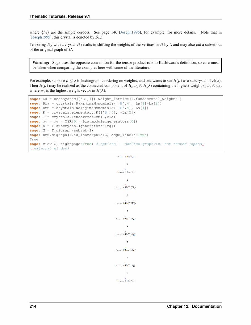
Thematic Tutorials, Release 9.1
where ℎ𝑖 are the simple coroots. See page 146 [Joseph1995], for example, for more details. (Note that in[Joseph1995], this crystal is denoted by 𝑆𝜆.)
Tensoring 𝑅𝜆 with a crystal 𝐵 results in shifting the weights of the vertices in 𝐵 by 𝜆 and may also cut a subset outof the original graph of 𝐵.
Warning: Sage uses the opposite convention for the tensor product rule to Kashiwara’s definition, so care mustbe taken when comparing the examples here with some of the literature.
For example, suppose 𝜇 ≤ 𝜆 in lexicographic ordering on weights, and one wants to see𝐵(𝜇) as a subcrystal of𝐵(𝜆).Then 𝐵(𝜇) may be realized as the connected component of 𝑅𝜇−𝜆 ⊗ 𝐵(𝜆) containing the highest weight 𝑟𝜇−𝜆 ⊗ 𝑢𝜆,where 𝑢𝜆 is the highest weight vector in 𝐵(𝜆):
sage: La = RootSystem(['B',4]).weight_lattice().fundamental_weights()sage: Bla = crystals.NakajimaMonomials(['B',4], La[1]+La[2])sage: Bmu = crystals.NakajimaMonomials(['B',4], La[1])sage: R = crystals.elementary.R(['B',4], -La[2])sage: T = crystals.TensorProduct(R,Bla)sage: mg = mg = T(R[0], Bla.module_generators[0])sage: S = T.subcrystal(generators=[mg])sage: G = T.digraph(subset=S)sage: Bmu.digraph().is_isomorphic(G, edge_labels=True)Truesage: view(G, tightpage=True) # optional - dot2tex graphviz, not tested (opens→˓external window)
214 Chapter 12. Documentation
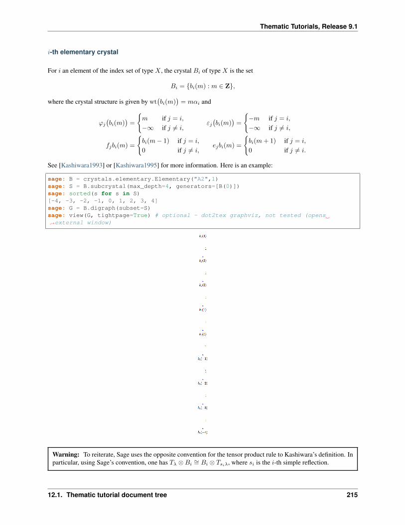
Thematic Tutorials, Release 9.1
𝑖-th elementary crystal
For 𝑖 an element of the index set of type 𝑋 , the crystal 𝐵𝑖 of type 𝑋 is the set
𝐵𝑖 = 𝑏𝑖(𝑚) : 𝑚 ∈ Z,
where the crystal structure is given by wt(𝑏𝑖(𝑚)
)= 𝑚𝛼𝑖 and
𝜙𝑗
(𝑏𝑖(𝑚)
)=
𝑚 if 𝑗 = 𝑖,
−∞ if 𝑗 = 𝑖,𝜀𝑗(𝑏𝑖(𝑚)
)=
−𝑚 if 𝑗 = 𝑖,
−∞ if 𝑗 = 𝑖,
𝑓𝑗𝑏𝑖(𝑚) =
𝑏𝑖(𝑚− 1) if 𝑗 = 𝑖,
0 if 𝑗 = 𝑖,𝑒𝑗𝑏𝑖(𝑚) =
𝑏𝑖(𝑚+ 1) if 𝑗 = 𝑖,
0 if 𝑗 = 𝑖.
See [Kashiwara1993] or [Kashiwara1995] for more information. Here is an example:
sage: B = crystals.elementary.Elementary("A2",1)sage: S = B.subcrystal(max_depth=4, generators=[B(0)])sage: sorted(s for s in S)[-4, -3, -2, -1, 0, 1, 2, 3, 4]sage: G = B.digraph(subset=S)sage: view(G, tightpage=True) # optional - dot2tex graphviz, not tested (opens→˓external window)
Warning: To reiterate, Sage uses the opposite convention for the tensor product rule to Kashiwara’s definition. Inparticular, using Sage’s convention, one has 𝑇𝜆 ⊗𝐵𝑖
∼= 𝐵𝑖 ⊗ 𝑇𝑠𝑖𝜆, where 𝑠𝑖 is the 𝑖-th simple reflection.
12.1. Thematic tutorial document tree 215
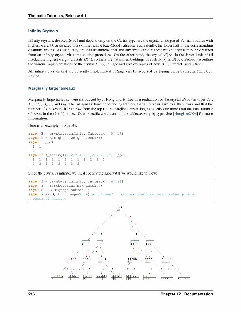
Thematic Tutorials, Release 9.1
Infinity Crystals
Infinity crystals, denoted ℬ(∞) and depend only on the Cartan type, are the crystal analogue of Verma modules withhighest weight 0 associated to a symmetrizable Kac-Moody algebra (equivalently, the lower half of the correspondingquantum group). As such, they are infinite-dimensional and any irreducible highest weight crystal may be obtainedfrom an infinity crystal via some cutting procedure. On the other hand, the crystal 𝐵(∞) is the direct limit of allirreducible highest weight crystals 𝐵(𝜆), so there are natural embeddings of each 𝐵(𝜆) in 𝐵(∞). Below, we outlinethe various implementations of the crystal 𝐵(∞) in Sage and give examples of how 𝐵(𝜆) interacts with 𝐵(∞).
All infinity crystals that are currently implemented in Sage can be accessed by typing crystals.infinity.<tab>.
Marginally large tableaux
Marginally large tableaux were introduced by J. Hong and H. Lee as a realization of the crystal 𝐵(∞) in types 𝐴𝑛,𝐵𝑛, 𝐶𝑛, 𝐷𝑛+1, and 𝐺2. The marginally large condition guarantees that all tableau have exactly 𝑛 rows and that thenumber of 𝑖-boxes in the 𝑖-th row from the top (in the English convention) is exactly one more than the total numberof boxes in the (𝑖 + 1)-st row. Other specific conditions on the tableaux vary by type. See [HongLee2008] for moreinformation.
Here is an example in type 𝐴2:
sage: B = crystals.infinity.Tableaux(['A',2])sage: b = B.highest_weight_vector()sage: b.pp()
1 12
sage: b.f_string([1,2,2,1,2,1,2,2,2,2,2]).pp()1 1 1 1 1 1 1 1 1 2 2 32 3 3 3 3 3 3 3
Since the crystal is infinite, we must specify the subcrystal we would like to view:
sage: B = crystals.infinity.Tableaux(['A',2])sage: S = B.subcrystal(max_depth=4)sage: G = B.digraph(subset=S)sage: view(G, tightpage=True) # optional - dot2tex graphviz, not tested (opens→˓external window)
216 Chapter 12. Documentation
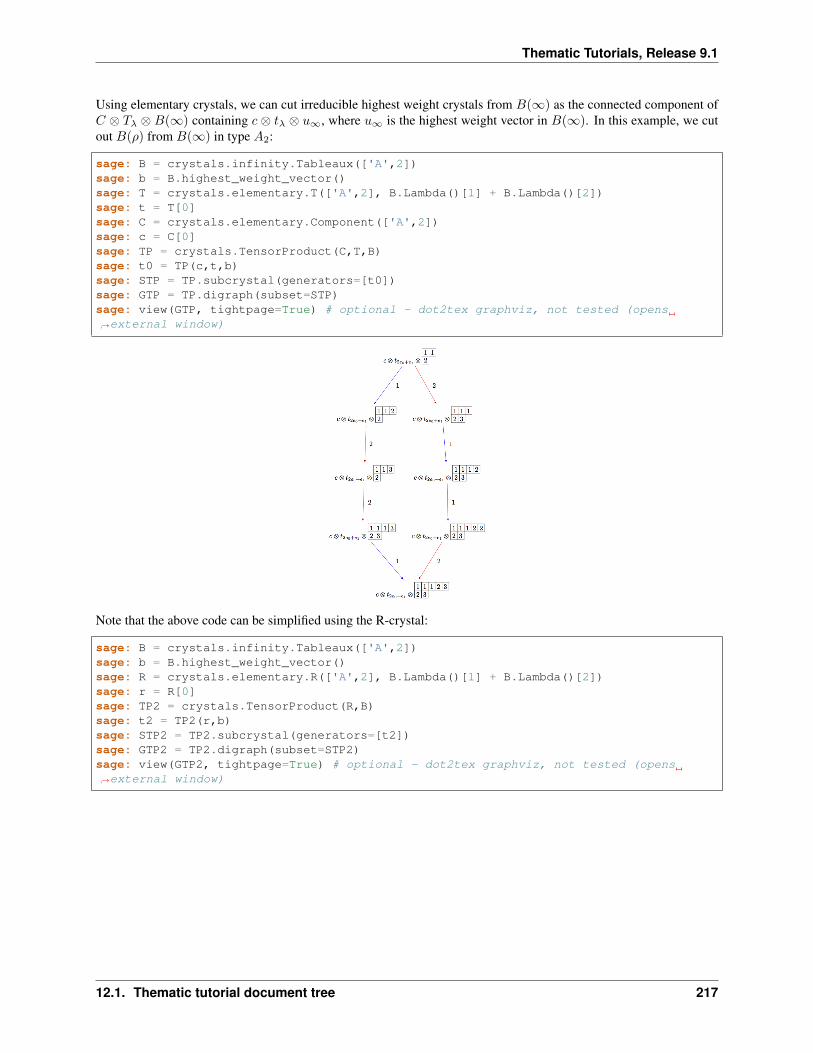
Thematic Tutorials, Release 9.1
Using elementary crystals, we can cut irreducible highest weight crystals from 𝐵(∞) as the connected component of𝐶 ⊗ 𝑇𝜆 ⊗ 𝐵(∞) containing 𝑐 ⊗ 𝑡𝜆 ⊗ 𝑢∞, where 𝑢∞ is the highest weight vector in 𝐵(∞). In this example, we cutout 𝐵(𝜌) from 𝐵(∞) in type 𝐴2:
sage: B = crystals.infinity.Tableaux(['A',2])sage: b = B.highest_weight_vector()sage: T = crystals.elementary.T(['A',2], B.Lambda()[1] + B.Lambda()[2])sage: t = T[0]sage: C = crystals.elementary.Component(['A',2])sage: c = C[0]sage: TP = crystals.TensorProduct(C,T,B)sage: t0 = TP(c,t,b)sage: STP = TP.subcrystal(generators=[t0])sage: GTP = TP.digraph(subset=STP)sage: view(GTP, tightpage=True) # optional - dot2tex graphviz, not tested (opens→˓external window)
Note that the above code can be simplified using the R-crystal:
sage: B = crystals.infinity.Tableaux(['A',2])sage: b = B.highest_weight_vector()sage: R = crystals.elementary.R(['A',2], B.Lambda()[1] + B.Lambda()[2])sage: r = R[0]sage: TP2 = crystals.TensorProduct(R,B)sage: t2 = TP2(r,b)sage: STP2 = TP2.subcrystal(generators=[t2])sage: GTP2 = TP2.digraph(subset=STP2)sage: view(GTP2, tightpage=True) # optional - dot2tex graphviz, not tested (opens→˓external window)
12.1. Thematic tutorial document tree 217
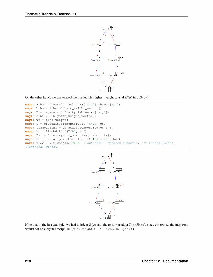
Thematic Tutorials, Release 9.1
On the other hand, we can embed the irreducible highest weight crystal 𝐵(𝜌) into 𝐵(∞):
sage: Brho = crystals.Tableaux(['A',2],shape=[2,1])sage: brho = Brho.highest_weight_vector()sage: B = crystals.infinity.Tableaux(['A',2])sage: binf = B.highest_weight_vector()sage: wt = brho.weight()sage: T = crystals.elementary.T(['A',2],wt)sage: TlambdaBinf = crystals.TensorProduct(T,B)sage: hw = TlambdaBinf(T[0],binf)sage: Psi = Brho.crystal_morphism(brho : hw)sage: BG = B.digraph(subset=[Psi(x) for x in Brho])sage: view(BG, tightpage=True) # optional - dot2tex graphviz, not tested (opens→˓external window)
Note that in the last example, we had to inject 𝐵(𝜌) into the tensor product 𝑇𝜆⊗𝐵(∞), since otherwise, the map Psiwould not be a crystal morphism (as b.weight() != brho.weight()).
218 Chapter 12. Documentation
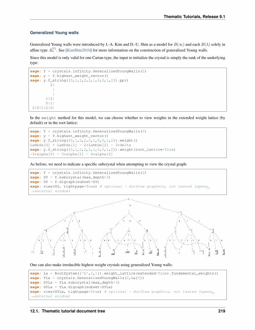
Thematic Tutorials, Release 9.1
Generalized Young walls
Generalized Young walls were introduced by J.-A. Kim and D.-U. Shin as a model for 𝐵(∞) and each 𝐵(𝜆) solely inaffine type 𝐴(1)
𝑛 . See [KimShin2010] for more information on the construction of generalized Young walls.
Since this model is only valid for one Cartan type, the input to initialize the crystal is simply the rank of the underlyingtype:
sage: Y = crystals.infinity.GeneralizedYoungWalls(2)sage: y = Y.highest_weight_vector()sage: y.f_string([0,1,2,2,2,1,0,0,1,2]).pp()
2|||
1|2|0|1|
2|0|1|2|0|
In the weight method for this model, we can choose whether to view weights in the extended weight lattice (bydefault) or in the root lattice:
sage: Y = crystals.infinity.GeneralizedYoungWalls(2)sage: y = Y.highest_weight_vector()sage: y.f_string([0,1,2,2,2,1,0,0,1,2]).weight()Lambda[0] + Lambda[1] - 2*Lambda[2] - 3*deltasage: y.f_string([0,1,2,2,2,1,0,0,1,2]).weight(root_lattice=True)-3*alpha[0] - 3*alpha[1] - 4*alpha[2]
As before, we need to indicate a specific subcrystal when attempting to view the crystal graph:
sage: Y = crystals.infinity.GeneralizedYoungWalls(2)sage: SY = Y.subcrystal(max_depth=3)sage: GY = Y.digraph(subset=SY)sage: view(GY, tightpage=True) # optional - dot2tex graphviz, not tested (opens→˓external window)
One can also make irreducible highest weight crystals using generalized Young walls:
sage: La = RootSystem(['A',2,1]).weight_lattice(extended=True).fundamental_weights()sage: YLa = crystals.GeneralizedYoungWalls(2,La[0])sage: SYLa = YLa.subcrystal(max_depth=3)sage: GYLa = YLa.digraph(subset=SYLa)sage: view(GYLa, tightpage=True) # optional - dot2tex graphviz, not tested (opens→˓external window)
12.1. Thematic tutorial document tree 219
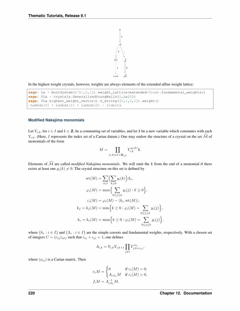
Thematic Tutorials, Release 9.1
In the highest weight crystals, however, weights are always elements of the extended affine weight lattice:
sage: La = RootSystem(['A',2,1]).weight_lattice(extended=True).fundamental_weights()sage: YLa = crystals.GeneralizedYoungWalls(2,La[0])sage: YLa.highest_weight_vector().f_string([0,1,2,0]).weight()-Lambda[0] + Lambda[1] + Lambda[2] - 2*delta
Modified Nakajima monomials
Let 𝑌𝑖,𝑘, for 𝑖 ∈ 𝐼 and 𝑘 ∈ Z, be a commuting set of variables, and let 1 be a new variable which commutes with each𝑌𝑖,𝑘. (Here, 𝐼 represents the index set of a Cartan datum.) One may endow the structure of a crystal on the set ℳ ofmonomials of the form
𝑀 =∏
(𝑖,𝑘)∈𝐼×Z≥0
𝑌𝑦𝑖(𝑘)𝑖,𝑘 1.
Elements of ℳ are called modified Nakajima monomials. We will omit the 1 from the end of a monomial if thereexists at least one 𝑦𝑖(𝑘) = 0. The crystal structure on this set is defined by
wt(𝑀) =∑𝑖∈𝐼
(∑𝑘≥0
𝑦𝑖(𝑘))
Λ𝑖,
𝜙𝑖(𝑀) = max ∑0≤𝑗≤𝑘
𝑦𝑖(𝑗) : 𝑘 ≥ 0,
𝜀𝑖(𝑀) = 𝜙𝑖(𝑀)− ⟨ℎ𝑖,wt(𝑀)⟩,
𝑘𝑓 = 𝑘𝑓 (𝑀) = min𝑘 ≥ 0 : 𝜙𝑖(𝑀) =
∑0≤𝑗≤𝑘
𝑦𝑖(𝑗),
𝑘𝑒 = 𝑘𝑒(𝑀) = max𝑘 ≥ 0 : 𝜙𝑖(𝑀) =
∑0≤𝑗≤𝑘
𝑦𝑖(𝑗),
where ℎ𝑖 : 𝑖 ∈ 𝐼 and Λ𝑖 : 𝑖 ∈ 𝐼 are the simple coroots and fundamental weights, respectively. With a chosen setof integers 𝐶 = (𝑐𝑖𝑗)𝑖 =𝑗 such that 𝑐𝑖𝑗 + 𝑐𝑗𝑖 = 1, one defines
𝐴𝑖,𝑘 = 𝑌𝑖,𝑘𝑌𝑖,𝑘+1
∏𝑗 =𝑖
𝑌𝑎𝑗𝑖
𝑗,𝑘+𝑐𝑗𝑖,
where (𝑎𝑖𝑗) is a Cartan matrix. Then
𝑒𝑖𝑀 =
0 if 𝜀𝑖(𝑀) = 0,
𝐴𝑖,𝑘𝑒𝑀 if 𝜀𝑖(𝑀) > 0,
𝑓𝑖𝑀 = 𝐴−1𝑖,𝑘𝑓
𝑀.
220 Chapter 12. Documentation
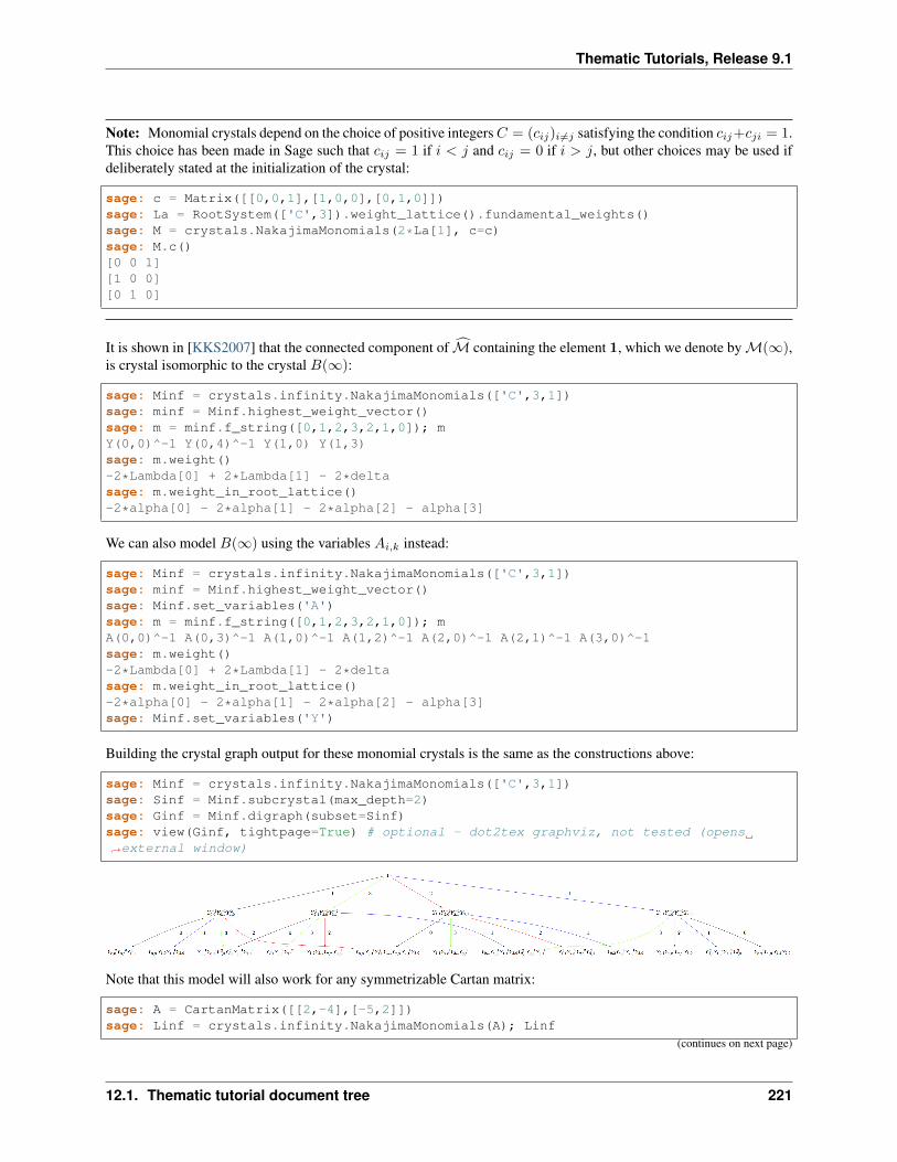
Thematic Tutorials, Release 9.1
Note: Monomial crystals depend on the choice of positive integers𝐶 = (𝑐𝑖𝑗)=𝑗 satisfying the condition 𝑐𝑖𝑗+𝑐𝑗𝑖 = 1.This choice has been made in Sage such that 𝑐𝑖𝑗 = 1 if 𝑖 < 𝑗 and 𝑐𝑖𝑗 = 0 if 𝑖 > 𝑗, but other choices may be used ifdeliberately stated at the initialization of the crystal:
sage: c = Matrix([[0,0,1],[1,0,0],[0,1,0]])sage: La = RootSystem(['C',3]).weight_lattice().fundamental_weights()sage: M = crystals.NakajimaMonomials(2*La[1], c=c)sage: M.c()[0 0 1][1 0 0][0 1 0]
It is shown in [KKS2007] that the connected component of ℳ containing the element 1, which we denote byℳ(∞),is crystal isomorphic to the crystal 𝐵(∞):
sage: Minf = crystals.infinity.NakajimaMonomials(['C',3,1])sage: minf = Minf.highest_weight_vector()sage: m = minf.f_string([0,1,2,3,2,1,0]); mY(0,0)^-1 Y(0,4)^-1 Y(1,0) Y(1,3)sage: m.weight()-2*Lambda[0] + 2*Lambda[1] - 2*deltasage: m.weight_in_root_lattice()-2*alpha[0] - 2*alpha[1] - 2*alpha[2] - alpha[3]
We can also model 𝐵(∞) using the variables 𝐴𝑖,𝑘 instead:
sage: Minf = crystals.infinity.NakajimaMonomials(['C',3,1])sage: minf = Minf.highest_weight_vector()sage: Minf.set_variables('A')sage: m = minf.f_string([0,1,2,3,2,1,0]); mA(0,0)^-1 A(0,3)^-1 A(1,0)^-1 A(1,2)^-1 A(2,0)^-1 A(2,1)^-1 A(3,0)^-1sage: m.weight()-2*Lambda[0] + 2*Lambda[1] - 2*deltasage: m.weight_in_root_lattice()-2*alpha[0] - 2*alpha[1] - 2*alpha[2] - alpha[3]sage: Minf.set_variables('Y')
Building the crystal graph output for these monomial crystals is the same as the constructions above:
sage: Minf = crystals.infinity.NakajimaMonomials(['C',3,1])sage: Sinf = Minf.subcrystal(max_depth=2)sage: Ginf = Minf.digraph(subset=Sinf)sage: view(Ginf, tightpage=True) # optional - dot2tex graphviz, not tested (opens→˓external window)
Note that this model will also work for any symmetrizable Cartan matrix:
sage: A = CartanMatrix([[2,-4],[-5,2]])sage: Linf = crystals.infinity.NakajimaMonomials(A); Linf
(continues on next page)
12.1. Thematic tutorial document tree 221
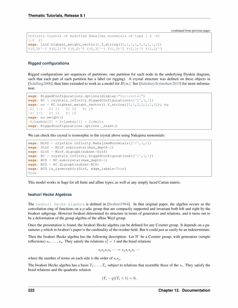
Thematic Tutorials, Release 9.1
(continued from previous page)
Infinity Crystal of modified Nakajima monomials of type [ 2 -4][-5 2]sage: Linf.highest_weight_vector().f_string([0,1,1,1,0,0,1,1,0])Y(0,0)^-1 Y(0,1)^9 Y(0,2)^5 Y(0,3)^-1 Y(1,0)^2 Y(1,1)^5 Y(1,2)^3
Rigged configurations
Rigged configurations are sequences of partitions, one partition for each node in the underlying Dynkin diagram,such that each part of each partition has a label (or rigging). A crystal structure was defined on these objects in[Schilling2006], then later extended to work as a model for 𝐵(∞). See [SalisburyScrimshaw2015] for more informa-tion:
sage: RiggedConfigurations.options(display="horizontal")sage: RC = crystals.infinity.RiggedConfigurations(['C',3,1])sage: nu = RC.highest_weight_vector().f_string([0,1,2,3,2,1,0]); nu-2[ ]-1 2[ ]1 0[ ]0 0[ ]0-2[ ]-1 2[ ]1 0[ ]0sage: nu.weight()-2*Lambda[0] + 2*Lambda[1] - 2*deltasage: RiggedConfigurations.options._reset()
We can check this crystal is isomorphic to the crystal above using Nakajima monomials:
sage: Minf = crystals.infinity.NakajimaMonomials(['C',3,1])sage: Sinf = Minf.subcrystal(max_depth=2)sage: Ginf = Minf.digraph(subset=Sinf)sage: RC = crystals.infinity.RiggedConfigurations(['C',3,1])sage: RCS = RC.subcrystal(max_depth=2)sage: RCG = RC.digraph(subset=RCS)sage: RCG.is_isomorphic(Ginf, edge_labels=True)True
This model works in Sage for all finite and affine types, as well as any simply laced Cartan matrix.
Iwahori Hecke Algebras
The Iwahori Hecke algebra is defined in [Iwahori1964]. In that original paper, the algebra occurs as theconvolution ring of functions on a 𝑝-adic group that are compactly supported and invariant both left and right by theIwahori subgroup. However Iwahori determined its structure in terms of generators and relations, and it turns out tobe a deformation of the group algebra of the affine Weyl group.
Once the presentation is found, the Iwahori Hecke algebra can be defined for any Coxeter group. It depends on a pa-rameter 𝑞 which in Iwahori’s paper is the cardinality of the residue field. But it could just as easily be an indeterminate.
Then the Iwahori Hecke algebra has the following description. Let 𝑊 be a Coxeter group, with generators (simplereflections) 𝑠1, . . . , 𝑠𝑛. They satisfy the relations 𝑠2𝑖 = 1 and the braid relations
𝑠𝑖𝑠𝑗𝑠𝑖𝑠𝑗 · · · = 𝑠𝑗𝑠𝑖𝑠𝑗𝑠𝑖 · · ·
where the number of terms on each side is the order of 𝑠𝑖𝑠𝑗 .
The Iwahori Hecke algebra has a basis 𝑇1, . . . , 𝑇𝑛 subject to relations that resemble those of the 𝑠𝑖. They satisfy thebraid relations and the quadratic relation
(𝑇𝑖 − 𝑞)(𝑇𝑖 + 1) = 0.
222 Chapter 12. Documentation
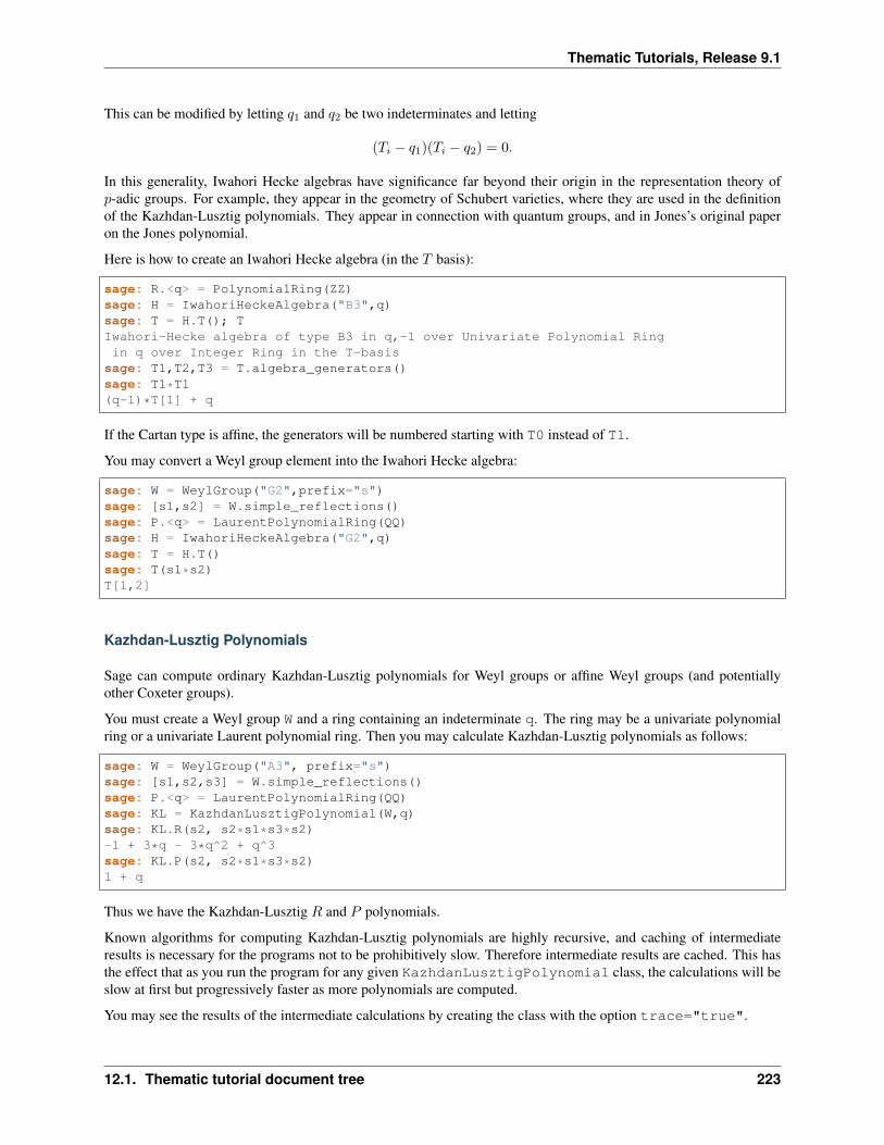
Thematic Tutorials, Release 9.1
This can be modified by letting 𝑞1 and 𝑞2 be two indeterminates and letting
(𝑇𝑖 − 𝑞1)(𝑇𝑖 − 𝑞2) = 0.
In this generality, Iwahori Hecke algebras have significance far beyond their origin in the representation theory of𝑝-adic groups. For example, they appear in the geometry of Schubert varieties, where they are used in the definitionof the Kazhdan-Lusztig polynomials. They appear in connection with quantum groups, and in Jones’s original paperon the Jones polynomial.
Here is how to create an Iwahori Hecke algebra (in the 𝑇 basis):
sage: R.<q> = PolynomialRing(ZZ)sage: H = IwahoriHeckeAlgebra("B3",q)sage: T = H.T(); TIwahori-Hecke algebra of type B3 in q,-1 over Univariate Polynomial Ringin q over Integer Ring in the T-basis
sage: T1,T2,T3 = T.algebra_generators()sage: T1*T1(q-1)*T[1] + q
If the Cartan type is affine, the generators will be numbered starting with T0 instead of T1.
You may convert a Weyl group element into the Iwahori Hecke algebra:
sage: W = WeylGroup("G2",prefix="s")sage: [s1,s2] = W.simple_reflections()sage: P.<q> = LaurentPolynomialRing(QQ)sage: H = IwahoriHeckeAlgebra("G2",q)sage: T = H.T()sage: T(s1*s2)T[1,2]
Kazhdan-Lusztig Polynomials
Sage can compute ordinary Kazhdan-Lusztig polynomials for Weyl groups or affine Weyl groups (and potentiallyother Coxeter groups).
You must create a Weyl group W and a ring containing an indeterminate q. The ring may be a univariate polynomialring or a univariate Laurent polynomial ring. Then you may calculate Kazhdan-Lusztig polynomials as follows:
sage: W = WeylGroup("A3", prefix="s")sage: [s1,s2,s3] = W.simple_reflections()sage: P.<q> = LaurentPolynomialRing(QQ)sage: KL = KazhdanLusztigPolynomial(W,q)sage: KL.R(s2, s2*s1*s3*s2)-1 + 3*q - 3*q^2 + q^3sage: KL.P(s2, s2*s1*s3*s2)1 + q
Thus we have the Kazhdan-Lusztig 𝑅 and 𝑃 polynomials.
Known algorithms for computing Kazhdan-Lusztig polynomials are highly recursive, and caching of intermediateresults is necessary for the programs not to be prohibitively slow. Therefore intermediate results are cached. This hasthe effect that as you run the program for any given KazhdanLusztigPolynomial class, the calculations will beslow at first but progressively faster as more polynomials are computed.
You may see the results of the intermediate calculations by creating the class with the option trace="true".
12.1. Thematic tutorial document tree 223
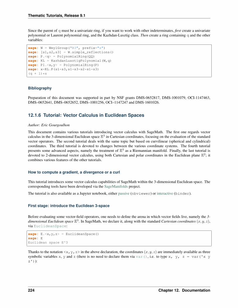
Thematic Tutorials, Release 9.1
Since the parent of q must be a univariate ring, if you want to work with other indeterminates, first create a univariatepolynomial or Laurent polynomial ring, and the Kazhdan-Lusztig class. Then create a ring containing q and the othervariables:
sage: W = WeylGroup("B3", prefix="s")sage: [s1,s2,s3] = W.simple_reflections()sage: P.<q> = PolynomialRing(QQ)sage: KL = KazhdanLusztigPolynomial(W,q)sage: P1.<x,y> = PolynomialRing(P)sage: x*KL.P(s1*s3,s1*s3*s2*s1*s3)(q + 1)*x
Bibliography
Preparation of this document was supported in part by NSF grants DMS-0652817, DMS-1001079, OCI-1147463,DMS–0652641, DMS–0652652, DMS–1001256, OCI–1147247 and DMS-1601026.
12.1.6 Tutorial: Vector Calculus in Euclidean Spaces
Author: Eric Gourgoulhon
This document contains various tutorials introducing vector calculus with SageMath. The first one regards vectorcalculus in the 3-dimensional Euclidean space E3 in Cartesian coordinates, focusing on the evaluation of the standardvector operators. The second tutorial deals with the same topic but based on curvilinear (spherical and cylindrical)coordinates. The third tutorial is devoted to changes between the various coordinate systems. The fourth tutorialpresents some advanced aspects, namely the treatment of E3 as a Riemannian manifold. Finally, the last tutorial isdevoted to 2-dimensional vector calculus, using both Cartesian and polar coordinates in the Euclidean plane E2; itcombines various features of the other tutorials.
How to compute a gradient, a divergence or a curl
This tutorial introduces some vector calculus capabilities of SageMath within the 3-dimensional Euclidean space. Thecorresponding tools have been developed via the SageManifolds project.
The tutorial is also available as a Jupyter notebook, either passive (nbviewer) or interactive (binder).
First stage: introduce the Euclidean 3-space
Before evaluating some vector-field operators, one needs to define the arena in which vector fields live, namely the 3-dimensional Euclidean space E3. In SageMath, we declare it, along with the standard Cartesian coordinates (𝑥, 𝑦, 𝑧),via EuclideanSpace:
sage: E.<x,y,z> = EuclideanSpace()sage: EEuclidean space E^3
Thanks to the notation <x,y,z> in the above declaration, the coordinates (𝑥, 𝑦, 𝑧) are immediately available as threesymbolic variables x, y and z (there is no need to declare them via var(), i.e. to type x, y, z = var('x yz')):
224 Chapter 12. Documentation
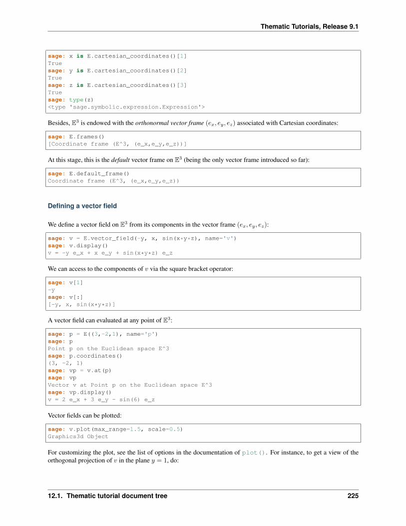
Thematic Tutorials, Release 9.1
sage: x is E.cartesian_coordinates()[1]Truesage: y is E.cartesian_coordinates()[2]Truesage: z is E.cartesian_coordinates()[3]Truesage: type(z)<type 'sage.symbolic.expression.Expression'>
Besides, E3 is endowed with the orthonormal vector frame (𝑒𝑥, 𝑒𝑦, 𝑒𝑧) associated with Cartesian coordinates:
sage: E.frames()[Coordinate frame (E^3, (e_x,e_y,e_z))]
At this stage, this is the default vector frame on E3 (being the only vector frame introduced so far):
sage: E.default_frame()Coordinate frame (E^3, (e_x,e_y,e_z))
Defining a vector field
We define a vector field on E3 from its components in the vector frame (𝑒𝑥, 𝑒𝑦, 𝑒𝑧):
sage: v = E.vector_field(-y, x, sin(x*y*z), name='v')sage: v.display()v = -y e_x + x e_y + sin(x*y*z) e_z
We can access to the components of 𝑣 via the square bracket operator:
sage: v[1]-ysage: v[:][-y, x, sin(x*y*z)]
A vector field can evaluated at any point of E3:
sage: p = E((3,-2,1), name='p')sage: pPoint p on the Euclidean space E^3sage: p.coordinates()(3, -2, 1)sage: vp = v.at(p)sage: vpVector v at Point p on the Euclidean space E^3sage: vp.display()v = 2 e_x + 3 e_y - sin(6) e_z
Vector fields can be plotted:
sage: v.plot(max_range=1.5, scale=0.5)Graphics3d Object
For customizing the plot, see the list of options in the documentation of plot(). For instance, to get a view of theorthogonal projection of 𝑣 in the plane 𝑦 = 1, do:
12.1. Thematic tutorial document tree 225
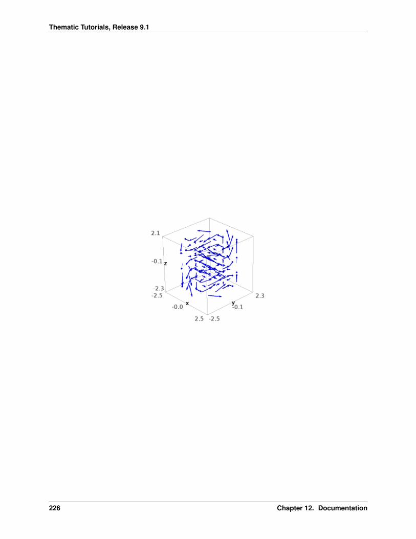
Thematic Tutorials, Release 9.1
226 Chapter 12. Documentation
Thematic Tutorials, Release 9.1
sage: v.plot(fixed_coords=y: 1, ambient_coords=(x,z), max_range=1.5,....: scale=0.25)Graphics object consisting of 81 graphics primitives
-1.5 -1 -0.5 0.5 1 1.5x
-1.5
-1
-0.5
0.5
1
1.5
z
We may define a vector field 𝑢 with generic components (𝑢𝑥, 𝑢𝑦, 𝑦𝑧):
sage: u = E.vector_field(function('u_x')(x,y,z),....: function('u_y')(x,y,z),....: function('u_z')(x,y,z),....: name='u')sage: u.display()u = u_x(x, y, z) e_x + u_y(x, y, z) e_y + u_z(x, y, z) e_zsage: u[:][u_x(x, y, z), u_y(x, y, z), u_z(x, y, z)]
Its value at the point 𝑝 is then:
sage: up = u.at(p)sage: up.display()u = u_x(3, -2, 1) e_x + u_y(3, -2, 1) e_y + u_z(3, -2, 1) e_z
How to compute various vector products
12.1. Thematic tutorial document tree 227
Thematic Tutorials, Release 9.1
Dot product
The dot (or scalar) product 𝑢 · 𝑣 of the vector fields 𝑢 and 𝑣 is obtained by the method dot_product(), whichadmits dot() as a shortcut alias:
sage: u.dot(v) == u[1]*v[1] + u[2]*v[2] + u[3]*v[3]True
𝑠 = 𝑢 · 𝑣 is a scalar field, i.e. a map E3 → R:
sage: s = u.dot(v)sage: sScalar field u.v on the Euclidean space E^3sage: s.display()u.v: E^3 --> R
(x, y, z) |--> -y*u_x(x, y, z) + x*u_y(x, y, z) + sin(x*y*z)*u_z(x, y, z)
It maps points of E3 to real numbers:
sage: s(p)-sin(6)*u_z(3, -2, 1) + 2*u_x(3, -2, 1) + 3*u_y(3, -2, 1)
Its coordinate expression is:
sage: s.expr()-y*u_x(x, y, z) + x*u_y(x, y, z) + sin(x*y*z)*u_z(x, y, z)
Norm
The norm ‖𝑢‖ of the vector field 𝑢 is defined in terms of the dot product by ‖𝑢‖ =√𝑢 · 𝑢:
sage: norm(u) == sqrt(u.dot(u))True
It is a scalar field on E3:
sage: s = norm(u)sage: sScalar field |u| on the Euclidean space E^3sage: s.display()|u|: E^3 --> R
(x, y, z) |--> sqrt(u_x(x, y, z)^2 + u_y(x, y, z)^2 + u_z(x, y, z)^2)sage: s.expr()sqrt(u_x(x, y, z)^2 + u_y(x, y, z)^2 + u_z(x, y, z)^2)
For 𝑣, we have:
sage: norm(v).expr()sqrt(x^2 + y^2 + sin(x*y*z)^2)
Cross product
The cross product 𝑢×𝑣 is obtained by the method cross_product(), which admits cross() as a shortcut alias:
228 Chapter 12. Documentation
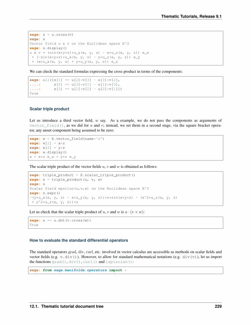
Thematic Tutorials, Release 9.1
sage: s = u.cross(v)sage: sVector field u x v on the Euclidean space E^3sage: s.display()u x v = (sin(x*y*z)*u_y(x, y, z) - x*u_z(x, y, z)) e_x+ (-sin(x*y*z)*u_x(x, y, z) - y*u_z(x, y, z)) e_y+ (x*u_x(x, y, z) + y*u_y(x, y, z)) e_z
We can check the standard formulas expressing the cross product in terms of the components:
sage: all([s[1] == u[2]*v[3] - u[3]*v[2],....: s[2] == u[3]*v[1] - u[1]*v[3],....: s[3] == u[1]*v[2] - u[2]*v[1]])True
Scalar triple product
Let us introduce a third vector field, 𝑤 say. As a example, we do not pass the components as arguments ofvector_field(), as we did for 𝑢 and 𝑣; instead, we set them in a second stage, via the square bracket opera-tor, any unset component being assumed to be zero:
sage: w = E.vector_field(name='w')sage: w[1] = x*zsage: w[2] = y*zsage: w.display()w = x*z e_x + y*z e_y
The scalar triple product of the vector fields 𝑢, 𝑣 and 𝑤 is obtained as follows:
sage: triple_product = E.scalar_triple_product()sage: s = triple_product(u, v, w)sage: sScalar field epsilon(u,v,w) on the Euclidean space E^3sage: s.expr()-(y*u_x(x, y, z) - x*u_y(x, y, z))*z*sin(x*y*z) - (x^2*u_z(x, y, z)+ y^2*u_z(x, y, z))*z
Let us check that the scalar triple product of 𝑢, 𝑣 and 𝑤 is 𝑢 · (𝑣 × 𝑤):
sage: s == u.dot(v.cross(w))True
How to evaluate the standard differential operators
The standard operators grad, div, curl, etc. involved in vector calculus are accessible as methods on scalar fields andvector fields (e.g. v.div()). However, to allow for standard mathematical notations (e.g. div(v)), let us importthe functions grad(), div(), curl() and laplacian():
sage: from sage.manifolds.operators import *
12.1. Thematic tutorial document tree 229
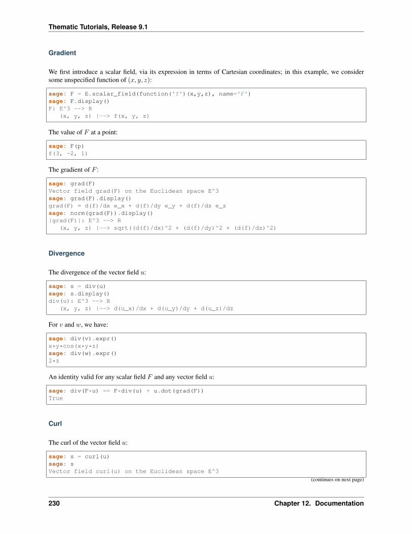
Thematic Tutorials, Release 9.1
Gradient
We first introduce a scalar field, via its expression in terms of Cartesian coordinates; in this example, we considersome unspecified function of (𝑥, 𝑦, 𝑧):
sage: F = E.scalar_field(function('f')(x,y,z), name='F')sage: F.display()F: E^3 --> R
(x, y, z) |--> f(x, y, z)
The value of 𝐹 at a point:
sage: F(p)f(3, -2, 1)
The gradient of 𝐹 :
sage: grad(F)Vector field grad(F) on the Euclidean space E^3sage: grad(F).display()grad(F) = d(f)/dx e_x + d(f)/dy e_y + d(f)/dz e_zsage: norm(grad(F)).display()|grad(F)|: E^3 --> R
(x, y, z) |--> sqrt((d(f)/dx)^2 + (d(f)/dy)^2 + (d(f)/dz)^2)
Divergence
The divergence of the vector field 𝑢:
sage: s = div(u)sage: s.display()div(u): E^3 --> R
(x, y, z) |--> d(u_x)/dx + d(u_y)/dy + d(u_z)/dz
For 𝑣 and 𝑤, we have:
sage: div(v).expr()x*y*cos(x*y*z)sage: div(w).expr()2*z
An identity valid for any scalar field 𝐹 and any vector field 𝑢:
sage: div(F*u) == F*div(u) + u.dot(grad(F))True
Curl
The curl of the vector field 𝑢:
sage: s = curl(u)sage: sVector field curl(u) on the Euclidean space E^3
(continues on next page)
230 Chapter 12. Documentation
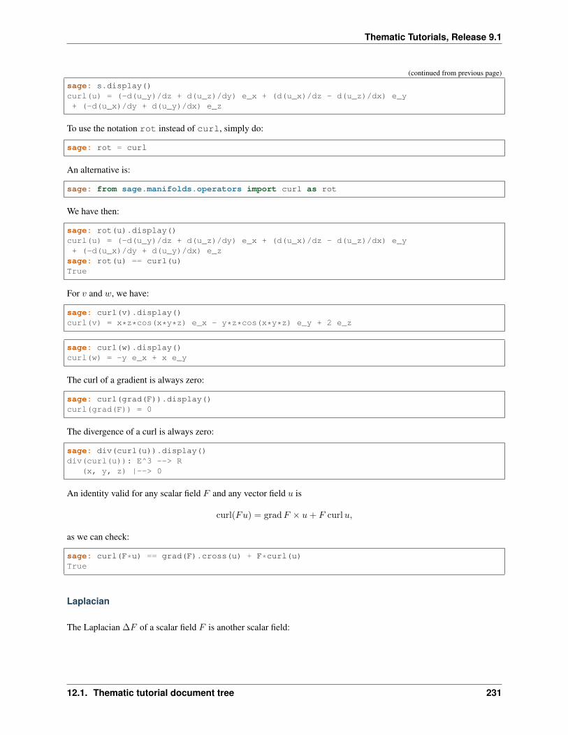
Thematic Tutorials, Release 9.1
(continued from previous page)
sage: s.display()curl(u) = (-d(u_y)/dz + d(u_z)/dy) e_x + (d(u_x)/dz - d(u_z)/dx) e_y+ (-d(u_x)/dy + d(u_y)/dx) e_z
To use the notation rot instead of curl, simply do:
sage: rot = curl
An alternative is:
sage: from sage.manifolds.operators import curl as rot
We have then:
sage: rot(u).display()curl(u) = (-d(u_y)/dz + d(u_z)/dy) e_x + (d(u_x)/dz - d(u_z)/dx) e_y+ (-d(u_x)/dy + d(u_y)/dx) e_z
sage: rot(u) == curl(u)True
For 𝑣 and 𝑤, we have:
sage: curl(v).display()curl(v) = x*z*cos(x*y*z) e_x - y*z*cos(x*y*z) e_y + 2 e_z
sage: curl(w).display()curl(w) = -y e_x + x e_y
The curl of a gradient is always zero:
sage: curl(grad(F)).display()curl(grad(F)) = 0
The divergence of a curl is always zero:
sage: div(curl(u)).display()div(curl(u)): E^3 --> R
(x, y, z) |--> 0
An identity valid for any scalar field 𝐹 and any vector field 𝑢 is
curl(𝐹𝑢) = grad𝐹 × 𝑢+ 𝐹 curl𝑢,
as we can check:
sage: curl(F*u) == grad(F).cross(u) + F*curl(u)True
Laplacian
The Laplacian ∆𝐹 of a scalar field 𝐹 is another scalar field:
12.1. Thematic tutorial document tree 231
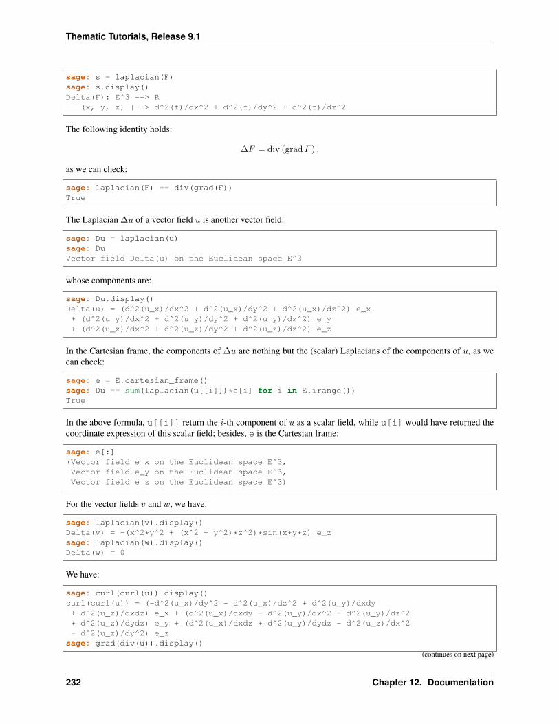
Thematic Tutorials, Release 9.1
sage: s = laplacian(F)sage: s.display()Delta(F): E^3 --> R
(x, y, z) |--> d^2(f)/dx^2 + d^2(f)/dy^2 + d^2(f)/dz^2
The following identity holds:
∆𝐹 = div (grad𝐹 ) ,
as we can check:
sage: laplacian(F) == div(grad(F))True
The Laplacian ∆𝑢 of a vector field 𝑢 is another vector field:
sage: Du = laplacian(u)sage: DuVector field Delta(u) on the Euclidean space E^3
whose components are:
sage: Du.display()Delta(u) = (d^2(u_x)/dx^2 + d^2(u_x)/dy^2 + d^2(u_x)/dz^2) e_x+ (d^2(u_y)/dx^2 + d^2(u_y)/dy^2 + d^2(u_y)/dz^2) e_y+ (d^2(u_z)/dx^2 + d^2(u_z)/dy^2 + d^2(u_z)/dz^2) e_z
In the Cartesian frame, the components of ∆𝑢 are nothing but the (scalar) Laplacians of the components of 𝑢, as wecan check:
sage: e = E.cartesian_frame()sage: Du == sum(laplacian(u[[i]])*e[i] for i in E.irange())True
In the above formula, u[[i]] return the 𝑖-th component of 𝑢 as a scalar field, while u[i] would have returned thecoordinate expression of this scalar field; besides, e is the Cartesian frame:
sage: e[:](Vector field e_x on the Euclidean space E^3,Vector field e_y on the Euclidean space E^3,Vector field e_z on the Euclidean space E^3)
For the vector fields 𝑣 and 𝑤, we have:
sage: laplacian(v).display()Delta(v) = -(x^2*y^2 + (x^2 + y^2)*z^2)*sin(x*y*z) e_zsage: laplacian(w).display()Delta(w) = 0
We have:
sage: curl(curl(u)).display()curl(curl(u)) = (-d^2(u_x)/dy^2 - d^2(u_x)/dz^2 + d^2(u_y)/dxdy+ d^2(u_z)/dxdz) e_x + (d^2(u_x)/dxdy - d^2(u_y)/dx^2 - d^2(u_y)/dz^2+ d^2(u_z)/dydz) e_y + (d^2(u_x)/dxdz + d^2(u_y)/dydz - d^2(u_z)/dx^2- d^2(u_z)/dy^2) e_z
sage: grad(div(u)).display()
(continues on next page)
232 Chapter 12. Documentation
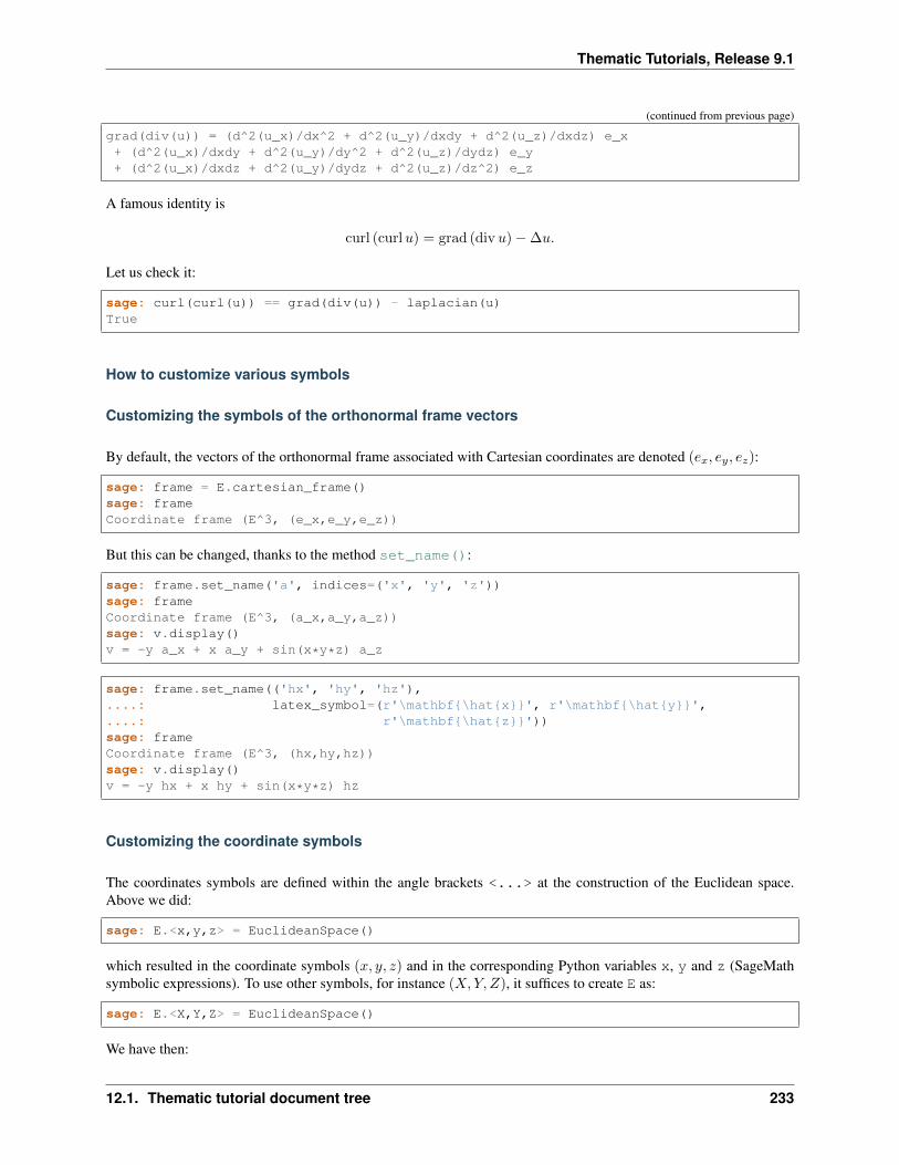
Thematic Tutorials, Release 9.1
(continued from previous page)
grad(div(u)) = (d^2(u_x)/dx^2 + d^2(u_y)/dxdy + d^2(u_z)/dxdz) e_x+ (d^2(u_x)/dxdy + d^2(u_y)/dy^2 + d^2(u_z)/dydz) e_y+ (d^2(u_x)/dxdz + d^2(u_y)/dydz + d^2(u_z)/dz^2) e_z
A famous identity is
curl (curl𝑢) = grad (div 𝑢)−∆𝑢.
Let us check it:
sage: curl(curl(u)) == grad(div(u)) - laplacian(u)True
How to customize various symbols
Customizing the symbols of the orthonormal frame vectors
By default, the vectors of the orthonormal frame associated with Cartesian coordinates are denoted (𝑒𝑥, 𝑒𝑦, 𝑒𝑧):
sage: frame = E.cartesian_frame()sage: frameCoordinate frame (E^3, (e_x,e_y,e_z))
But this can be changed, thanks to the method set_name():
sage: frame.set_name('a', indices=('x', 'y', 'z'))sage: frameCoordinate frame (E^3, (a_x,a_y,a_z))sage: v.display()v = -y a_x + x a_y + sin(x*y*z) a_z
sage: frame.set_name(('hx', 'hy', 'hz'),....: latex_symbol=(r'\mathbf\hatx', r'\mathbf\haty',....: r'\mathbf\hatz'))sage: frameCoordinate frame (E^3, (hx,hy,hz))sage: v.display()v = -y hx + x hy + sin(x*y*z) hz
Customizing the coordinate symbols
The coordinates symbols are defined within the angle brackets <...> at the construction of the Euclidean space.Above we did:
sage: E.<x,y,z> = EuclideanSpace()
which resulted in the coordinate symbols (𝑥, 𝑦, 𝑧) and in the corresponding Python variables x, y and z (SageMathsymbolic expressions). To use other symbols, for instance (𝑋,𝑌, 𝑍), it suffices to create E as:
sage: E.<X,Y,Z> = EuclideanSpace()
We have then:
12.1. Thematic tutorial document tree 233
Thematic Tutorials, Release 9.1
sage: E.atlas()[Chart (E^3, (X, Y, Z))]sage: E.cartesian_frame()Coordinate frame (E^3, (e_X,e_Y,e_Z))sage: v = E.vector_field(-Y, X, sin(X*Y*Z), name='v')sage: v.display()v = -Y e_X + X e_Y + sin(X*Y*Z) e_Z
By default the LaTeX symbols of the coordinate coincide with the letters given within the angle brackets. But this canbe adjusted through the optional argument symbols of the function EuclideanSpace, which has to be a string,usually prefixed by r (for raw string, in order to allow for the backslash character of LaTeX expressions). This stringcontains the coordinate fields separated by a blank space; each field contains the coordinate’s text symbol and possiblythe coordinate’s LaTeX symbol (when the latter is different from the text symbol), both symbols being separated by acolon (:):
sage: E.<xi,et,ze> = EuclideanSpace(symbols=r"xi:\xi et:\eta ze:\zeta")sage: E.atlas()[Chart (E^3, (xi, et, ze))]sage: v = E.vector_field(-et, xi, sin(xi*et*ze), name='v')sage: v.display()v = -et e_xi + xi e_et + sin(et*xi*ze) e_ze
How to perform vector calculus in curvilinear coordinates
This tutorial introduces some vector calculus capabilities of SageMath within the 3-dimensional Euclidean space. Thecorresponding tools have been developed via the SageManifolds project.
The tutorial is also available as a Jupyter notebook, either passive (nbviewer) or interactive (binder).
Using spherical coordinates
To use spherical coordinates (𝑟, 𝜃, 𝜑) within the Euclidean 3-space E3, it suffices to declare the latter with the keywordcoordinates='spherical':
sage: E.<r,th,ph> = EuclideanSpace(coordinates='spherical')sage: EEuclidean space E^3
Thanks to the notation <r,th,ph> in the above declaration, the coordinates (𝑟, 𝜃, 𝜑) are immediately available asthree symbolic variables r, th and ph (there is no need to declare them via var(), i.e. to type r, th, ph =var('r th ph')):
sage: r is E.spherical_coordinates()[1]Truesage: (r, th, ph) == E.spherical_coordinates()[:]Truesage: type(r)<type 'sage.symbolic.expression.Expression'>
Moreover, the coordinate LaTeX symbols are already set:
sage: latex(th)\theta
The coordinate ranges are:
234 Chapter 12. Documentation
Thematic Tutorials, Release 9.1
sage: E.spherical_coordinates().coord_range()r: (0, +oo); th: (0, pi); ph: [0, 2*pi] (periodic)
E3 is endowed with the orthonormal vector frame (𝑒𝑟, 𝑒𝜃, 𝑒𝜑) associated with spherical coordinates:
sage: E.frames()[Coordinate frame (E^3, (d/dr,d/dth,d/dph)),Vector frame (E^3, (e_r,e_th,e_ph))]
In the above output, (d/dr,d/dth,d/dph) =(
𝜕𝜕𝑟 ,
𝜕𝜕𝜃 ,
𝜕𝜕𝜑
)is the coordinate frame associated with (𝑟, 𝜃, 𝜑); it is
not an orthonormal frame and will not be used below. The default frame is the orthonormal one:
sage: E.default_frame()Vector frame (E^3, (e_r,e_th,e_ph))
Defining a vector field
We define a vector field on E3 from its components in the orthonormal vector frame (𝑒𝑟, 𝑒𝜃, 𝑒𝜑):
sage: v = E.vector_field(r*sin(2*ph)*sin(th)^2 + r,....: r*sin(2*ph)*sin(th)*cos(th),....: 2*r*cos(ph)^2*sin(th), name='v')sage: v.display()v = (r*sin(2*ph)*sin(th)^2 + r) e_r + r*cos(th)*sin(2*ph)*sin(th) e_th+ 2*r*cos(ph)^2*sin(th) e_ph
We can access to the components of 𝑣 via the square bracket operator:
sage: v[1]r*sin(2*ph)*sin(th)^2 + rsage: v[:][r*sin(2*ph)*sin(th)^2 + r, r*cos(th)*sin(2*ph)*sin(th), 2*r*cos(ph)^2*sin(th)]
A vector field can evaluated at any point of E3:
sage: p = E((1, pi/2, pi), name='p')sage: pPoint p on the Euclidean space E^3sage: p.coordinates()(1, 1/2*pi, pi)sage: vp = v.at(p)sage: vpVector v at Point p on the Euclidean space E^3sage: vp.display()v = e_r + 2 e_ph
We may define a vector field with generic components:
sage: u = E.vector_field(function('u_r')(r,th,ph),....: function('u_theta')(r,th,ph),....: function('u_phi')(r,th,ph),....: name='u')sage: u.display()u = u_r(r, th, ph) e_r + u_theta(r, th, ph) e_th + u_phi(r, th, ph) e_phsage: u[:][u_r(r, th, ph), u_theta(r, th, ph), u_phi(r, th, ph)]
12.1. Thematic tutorial document tree 235
Thematic Tutorials, Release 9.1
Its value at the point 𝑝 is then:
sage: up = u.at(p)sage: up.display()u = u_r(1, 1/2*pi, pi) e_r + u_theta(1, 1/2*pi, pi) e_th+ u_phi(1, 1/2*pi, pi) e_ph
Differential operators in spherical coordinates
The standard operators grad, div, curl, etc. involved in vector calculus are accessible as methods on scalar fields andvector fields (e.g. v.div()). However, to allow for standard mathematical notations (e.g. div(v)), let us importthe functions grad(), div(), curl() and laplacian():
sage: from sage.manifolds.operators import *
Gradient
We first introduce a scalar field, via its expression in terms of Cartesian coordinates; in this example, we consider aunspecified function of (𝑟, 𝜃, 𝜑):
sage: F = E.scalar_field(function('f')(r,th,ph), name='F')sage: F.display()F: E^3 --> R
(r, th, ph) |--> f(r, th, ph)
The value of 𝐹 at a point:
sage: F(p)f(1, 1/2*pi, pi)
The gradient of 𝐹 :
sage: grad(F)Vector field grad(F) on the Euclidean space E^3sage: grad(F).display()grad(F) = d(f)/dr e_r + d(f)/dth/r e_th + d(f)/dph/(r*sin(th)) e_phsage: norm(grad(F)).display()|grad(F)|: E^3 --> R
(r, th, ph) |--> sqrt((r^2*(d(f)/dr)^2 + (d(f)/dth)^2)*sin(th)^2+ (d(f)/dph)^2)/(r*sin(th))
Divergence
The divergence of a vector field:
sage: s = div(u)sage: s.display()div(u): E^3 --> R
(r, th, ph) |--> ((r*d(u_r)/dr + 2*u_r(r, th, ph)+ d(u_theta)/dth)*sin(th) + cos(th)*u_theta(r, th, ph)+ d(u_phi)/dph)/(r*sin(th))
sage: s.expr().expand()
(continues on next page)
236 Chapter 12. Documentation
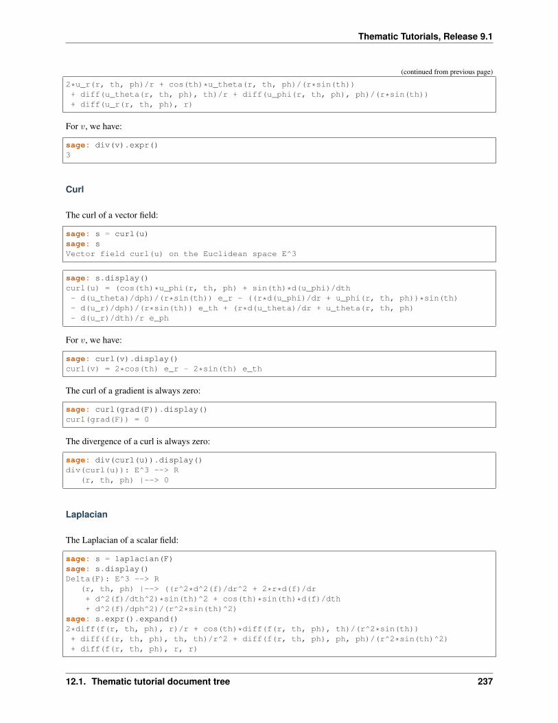
Thematic Tutorials, Release 9.1
(continued from previous page)
2*u_r(r, th, ph)/r + cos(th)*u_theta(r, th, ph)/(r*sin(th))+ diff(u_theta(r, th, ph), th)/r + diff(u_phi(r, th, ph), ph)/(r*sin(th))+ diff(u_r(r, th, ph), r)
For 𝑣, we have:
sage: div(v).expr()3
Curl
The curl of a vector field:
sage: s = curl(u)sage: sVector field curl(u) on the Euclidean space E^3
sage: s.display()curl(u) = (cos(th)*u_phi(r, th, ph) + sin(th)*d(u_phi)/dth- d(u_theta)/dph)/(r*sin(th)) e_r - ((r*d(u_phi)/dr + u_phi(r, th, ph))*sin(th)- d(u_r)/dph)/(r*sin(th)) e_th + (r*d(u_theta)/dr + u_theta(r, th, ph)- d(u_r)/dth)/r e_ph
For 𝑣, we have:
sage: curl(v).display()curl(v) = 2*cos(th) e_r - 2*sin(th) e_th
The curl of a gradient is always zero:
sage: curl(grad(F)).display()curl(grad(F)) = 0
The divergence of a curl is always zero:
sage: div(curl(u)).display()div(curl(u)): E^3 --> R
(r, th, ph) |--> 0
Laplacian
The Laplacian of a scalar field:
sage: s = laplacian(F)sage: s.display()Delta(F): E^3 --> R
(r, th, ph) |--> ((r^2*d^2(f)/dr^2 + 2*r*d(f)/dr+ d^2(f)/dth^2)*sin(th)^2 + cos(th)*sin(th)*d(f)/dth+ d^2(f)/dph^2)/(r^2*sin(th)^2)
sage: s.expr().expand()2*diff(f(r, th, ph), r)/r + cos(th)*diff(f(r, th, ph), th)/(r^2*sin(th))+ diff(f(r, th, ph), th, th)/r^2 + diff(f(r, th, ph), ph, ph)/(r^2*sin(th)^2)+ diff(f(r, th, ph), r, r)
12.1. Thematic tutorial document tree 237
Thematic Tutorials, Release 9.1
The Laplacian of a vector field:
sage: Du = laplacian(u)sage: Du.display()Delta(u) = ((r^2*d^2(u_r)/dr^2 + 2*r*d(u_r)/dr - 2*u_r(r, th, ph)+ d^2(u_r)/dth^2 - 2*d(u_theta)/dth)*sin(th)^2 - ((2*u_theta(r, th, ph)- d(u_r)/dth)*cos(th) + 2*d(u_phi)/dph)*sin(th) + d^2(u_r)/dph^2)/(r^2*sin(th)^2) e_r+ ((r^2*d^2(u_theta)/dr^2 + 2*r*d(u_theta)/dr + 2*d(u_r)/dth + d^2(u_theta)/dth^→˓2)*sin(th)^2+ cos(th)*sin(th)*d(u_theta)/dth - 2*cos(th)*d(u_phi)/dph - u_theta(r, th, ph)+ d^2(u_theta)/dph^2)/(r^2*sin(th)^2) e_th+ ((r^2*d^2(u_phi)/dr^2 + 2*r*d(u_phi)/dr+ d^2(u_phi)/dth^2)*sin(th)^2 + (cos(th)*d(u_phi)/dth + 2*d(u_r)/dph)*sin(th)+ 2*cos(th)*d(u_theta)/dph - u_phi(r, th, ph) + d^2(u_phi)/dph^2)/(r^2*sin(th)^2) e_→˓ph
Since this expression is quite lengthy, we may ask for a display component by component:
sage: Du.display_comp()Delta(u)^1 = ((r^2*d^2(u_r)/dr^2 + 2*r*d(u_r)/dr - 2*u_r(r, th, ph) + d^2(u_r)/dth^2- 2*d(u_theta)/dth)*sin(th)^2 - ((2*u_theta(r, th, ph) - d(u_r)/dth)*cos(th)+ 2*d(u_phi)/dph)*sin(th) + d^2(u_r)/dph^2)/(r^2*sin(th)^2)
Delta(u)^2 = ((r^2*d^2(u_theta)/dr^2 + 2*r*d(u_theta)/dr + 2*d(u_r)/dth+ d^2(u_theta)/dth^2)*sin(th)^2 + cos(th)*sin(th)*d(u_theta)/dth- 2*cos(th)*d(u_phi)/dph - u_theta(r, th, ph) + d^2(u_theta)/dph^2)/(r^2*sin(th)^2)
Delta(u)^3 = ((r^2*d^2(u_phi)/dr^2 + 2*r*d(u_phi)/dr + d^2(u_phi)/dth^2)*sin(th)^2+ (cos(th)*d(u_phi)/dth + 2*d(u_r)/dph)*sin(th) + 2*cos(th)*d(u_theta)/dph- u_phi(r, th, ph) + d^2(u_phi)/dph^2)/(r^2*sin(th)^2)
We may expand each component:
sage: for i in E.irange():....: s = Du[i].expand()sage: Du.display_comp()Delta(u)^1 = 2*d(u_r)/dr/r - 2*u_r(r, th, ph)/r^2- 2*cos(th)*u_theta(r, th, ph)/(r^2*sin(th)) + cos(th)*d(u_r)/dth/(r^2*sin(th))+ d^2(u_r)/dth^2/r^2 - 2*d(u_theta)/dth/r^2 - 2*d(u_phi)/dph/(r^2*sin(th))+ d^2(u_r)/dph^2/(r^2*sin(th)^2) + d^2(u_r)/dr^2
Delta(u)^2 = 2*d(u_theta)/dr/r + 2*d(u_r)/dth/r^2 + cos(th)*d(u_theta)/dth/(r^→˓2*sin(th))+ d^2(u_theta)/dth^2/r^2 - 2*cos(th)*d(u_phi)/dph/(r^2*sin(th)^2)- u_theta(r, th, ph)/(r^2*sin(th)^2) + d^2(u_theta)/dph^2/(r^2*sin(th)^2)+ d^2(u_theta)/dr^2
Delta(u)^3 = 2*d(u_phi)/dr/r + cos(th)*d(u_phi)/dth/(r^2*sin(th))+ d^2(u_phi)/dth^2/r^2 + 2*d(u_r)/dph/(r^2*sin(th))+ 2*cos(th)*d(u_theta)/dph/(r^2*sin(th)^2) - u_phi(r, th, ph)/(r^2*sin(th)^2)+ d^2(u_phi)/dph^2/(r^2*sin(th)^2) + d^2(u_phi)/dr^2
As a test, we may check that these formulas coincide with those of Wikipedia’s article Del in cylindrical and sphericalcoordinates.
Using cylindrical coordinates
The use of cylindrical coordinates (𝜌, 𝜑, 𝑧) in the Euclidean space E3 is on the same footing as that of sphericalcoordinates. To start with, one has simply to declare:
238 Chapter 12. Documentation
Thematic Tutorials, Release 9.1
sage: E.<rh,ph,z> = EuclideanSpace(coordinates='cylindrical')
The coordinate ranges are then:
sage: E.cylindrical_coordinates().coord_range()rh: (0, +oo); ph: [0, 2*pi] (periodic); z: (-oo, +oo)
The default vector frame is the orthonormal frame (𝑒𝜌, 𝑒𝜑, 𝑒𝑧) associated with cylindrical coordinates:
sage: E.default_frame()Vector frame (E^3, (e_rh,e_ph,e_z))
and one may define vector fields from their components in that frame:
sage: v = E.vector_field(rh*(1+sin(2*ph)), 2*rh*cos(ph)^2, z,....: name='v')sage: v.display()v = rh*(sin(2*ph) + 1) e_rh + 2*rh*cos(ph)^2 e_ph + z e_zsage: v[:][rh*(sin(2*ph) + 1), 2*rh*cos(ph)^2, z]
sage: u = E.vector_field(function('u_rho')(rh,ph,z),....: function('u_phi')(rh,ph,z),....: function('u_z')(rh,ph,z),....: name='u')sage: u.display()u = u_rho(rh, ph, z) e_rh + u_phi(rh, ph, z) e_ph + u_z(rh, ph, z) e_zsage: u[:][u_rho(rh, ph, z), u_phi(rh, ph, z), u_z(rh, ph, z)]
Differential operators in cylindrical coordinates
sage: from sage.manifolds.operators import *
The gradient:
sage: F = E.scalar_field(function('f')(rh,ph,z), name='F')sage: F.display()F: E^3 --> R
(rh, ph, z) |--> f(rh, ph, z)sage: grad(F)Vector field grad(F) on the Euclidean space E^3sage: grad(F).display()grad(F) = d(f)/drh e_rh + d(f)/dph/rh e_ph + d(f)/dz e_z
The divergence:
sage: s = div(u)sage: s.display()div(u): E^3 --> R
(rh, ph, z) |--> (rh*d(u_rho)/drh + rh*d(u_z)/dz + u_rho(rh, ph, z) + d(u_phi)/→˓dph)/rhsage: s.expr().expand()u_rho(rh, ph, z)/rh + diff(u_phi(rh, ph, z), ph)/rh + diff(u_rho(rh, ph, z), rh)+ diff(u_z(rh, ph, z), z)
12.1. Thematic tutorial document tree 239
Thematic Tutorials, Release 9.1
The curl:
sage: s = curl(u)sage: sVector field curl(u) on the Euclidean space E^3sage: s.display()curl(u) = -(rh*d(u_phi)/dz - d(u_z)/dph)/rh e_rh + (d(u_rho)/dz - d(u_z)/drh) e_ph+ (rh*d(u_phi)/drh + u_phi(rh, ph, z) - d(u_rho)/dph)/rh e_z
The Laplacian of a scalar field:
sage: s = laplacian(F)sage: s.display()Delta(F): E^3 --> R
(rh, ph, z) |--> (rh^2*d^2(f)/drh^2 + rh^2*d^2(f)/dz^2 + rh*d(f)/drh+ d^2(f)/dph^2)/rh^2
sage: s.expr().expand()diff(f(rh, ph, z), rh)/rh + diff(f(rh, ph, z), ph, ph)/rh^2+ diff(f(rh, ph, z), rh, rh) + diff(f(rh, ph, z), z, z)
The Laplacian of a vector field:
sage: Du = laplacian(u)sage: Du.display()Delta(u) = (rh^2*d^2(u_rho)/drh^2 + rh^2*d^2(u_rho)/dz^2 + rh*d(u_rho)/drh- u_rho(rh, ph, z) - 2*d(u_phi)/dph + d^2(u_rho)/dph^2)/rh^2 e_rh+ (rh^2*d^2(u_phi)/drh^2 + rh^2*d^2(u_phi)/dz^2 + rh*d(u_phi)/drh- u_phi(rh, ph, z) + d^2(u_phi)/dph^2 + 2*d(u_rho)/dph)/rh^2 e_ph+ (rh^2*d^2(u_z)/drh^2 + rh^2*d^2(u_z)/dz^2 + rh*d(u_z)/drh+ d^2(u_z)/dph^2)/rh^2 e_z
sage: for i in E.irange():....: s = Du[i].expand()sage: Du.display_comp()Delta(u)^1 = d(u_rho)/drh/rh - u_rho(rh, ph, z)/rh^2 - 2*d(u_phi)/dph/rh^2+ d^2(u_rho)/dph^2/rh^2 + d^2(u_rho)/drh^2 + d^2(u_rho)/dz^2
Delta(u)^2 = d(u_phi)/drh/rh - u_phi(rh, ph, z)/rh^2 + d^2(u_phi)/dph^2/rh^2+ 2*d(u_rho)/dph/rh^2 + d^2(u_phi)/drh^2 + d^2(u_phi)/dz^2
Delta(u)^3 = d(u_z)/drh/rh + d^2(u_z)/dph^2/rh^2 + d^2(u_z)/drh^2 + d^2(u_z)/dz^2
Again, we may check that the above formulas coincide with those of Wikipedia’s article Del in cylindrical and sphericalcoordinates.
Changing coordinates
Given the expression of a vector field in a given coordinate system, SageMath can compute its expression in anothercoordinate system, see the tutorial How to change coordinates
How to change coordinates
This tutorial introduces some vector calculus capabilities of SageMath within the 3-dimensional Euclidean space. Thecorresponding tools have been developed via the SageManifolds project.
The tutorial is also available as a Jupyter notebook, either passive (nbviewer) or interactive (binder).
240 Chapter 12. Documentation
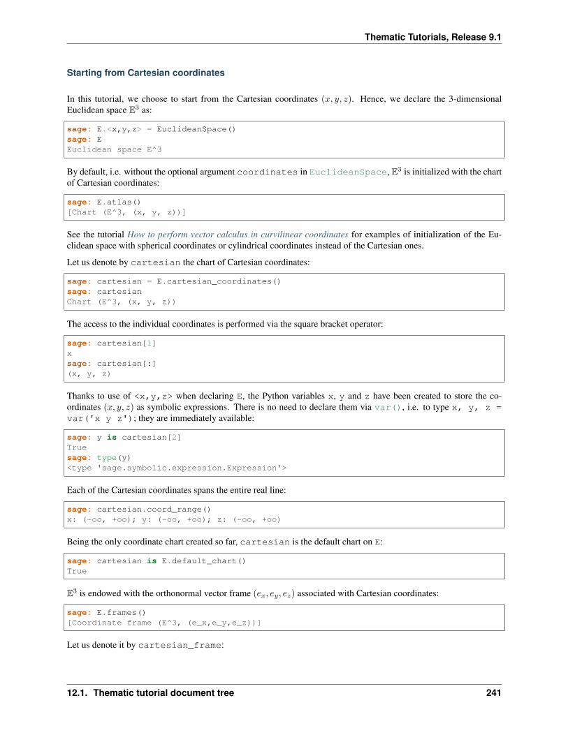
Thematic Tutorials, Release 9.1
Starting from Cartesian coordinates
In this tutorial, we choose to start from the Cartesian coordinates (𝑥, 𝑦, 𝑧). Hence, we declare the 3-dimensionalEuclidean space E3 as:
sage: E.<x,y,z> = EuclideanSpace()sage: EEuclidean space E^3
By default, i.e. without the optional argument coordinates in EuclideanSpace, E3 is initialized with the chartof Cartesian coordinates:
sage: E.atlas()[Chart (E^3, (x, y, z))]
See the tutorial How to perform vector calculus in curvilinear coordinates for examples of initialization of the Eu-clidean space with spherical coordinates or cylindrical coordinates instead of the Cartesian ones.
Let us denote by cartesian the chart of Cartesian coordinates:
sage: cartesian = E.cartesian_coordinates()sage: cartesianChart (E^3, (x, y, z))
The access to the individual coordinates is performed via the square bracket operator:
sage: cartesian[1]xsage: cartesian[:](x, y, z)
Thanks to use of <x,y,z> when declaring E, the Python variables x, y and z have been created to store the co-ordinates (𝑥, 𝑦, 𝑧) as symbolic expressions. There is no need to declare them via var(), i.e. to type x, y, z =var('x y z'); they are immediately available:
sage: y is cartesian[2]Truesage: type(y)<type 'sage.symbolic.expression.Expression'>
Each of the Cartesian coordinates spans the entire real line:
sage: cartesian.coord_range()x: (-oo, +oo); y: (-oo, +oo); z: (-oo, +oo)
Being the only coordinate chart created so far, cartesian is the default chart on E:
sage: cartesian is E.default_chart()True
E3 is endowed with the orthonormal vector frame (𝑒𝑥, 𝑒𝑦, 𝑒𝑧) associated with Cartesian coordinates:
sage: E.frames()[Coordinate frame (E^3, (e_x,e_y,e_z))]
Let us denote it by cartesian_frame:
12.1. Thematic tutorial document tree 241
Thematic Tutorials, Release 9.1
sage: cartesian_frame = E.cartesian_frame()sage: cartesian_frameCoordinate frame (E^3, (e_x,e_y,e_z))sage: cartesian_frame is E.default_frame()True
Each element of this frame is a unit vector field; for instance, we have 𝑒𝑥 · 𝑒𝑥 = 1:
sage: e_x = cartesian_frame[1]sage: e_xVector field e_x on the Euclidean space E^3sage: e_x.dot(e_x).expr()1
as well as 𝑒𝑥 · 𝑒𝑦 = 0:
sage: e_y = cartesian_frame[2]sage: e_x.dot(e_y).expr()0
Introducing spherical coordinates
Spherical coordinates are introduced by:
sage: spherical.<r,th,ph> = E.spherical_coordinates()sage: sphericalChart (E^3, (r, th, ph))
We have:
sage: spherical[:](r, th, ph)sage: spherical.coord_range()r: (0, +oo); th: (0, pi); ph: [0, 2*pi] (periodic)
E3 is now endowed with two coordinate charts:
sage: E.atlas()[Chart (E^3, (x, y, z)), Chart (E^3, (r, th, ph))]
The change-of-coordinate formulas have been automatically implemented during the above call E.spherical_coordinates():
sage: E.coord_change(spherical, cartesian).display()x = r*cos(ph)*sin(th)y = r*sin(ph)*sin(th)z = r*cos(th)sage: E.coord_change(cartesian, spherical).display()r = sqrt(x^2 + y^2 + z^2)th = arctan2(sqrt(x^2 + y^2), z)ph = arctan2(y, x)
These formulas are automatically used if we ask to plot the grid of spherical coordinates in terms of Cartesian coordi-nates:
242 Chapter 12. Documentation
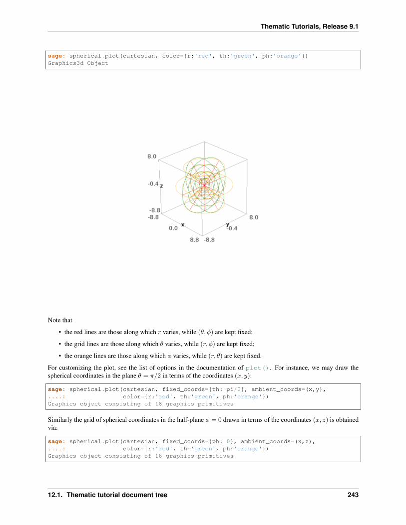
Thematic Tutorials, Release 9.1
sage: spherical.plot(cartesian, color=r:'red', th:'green', ph:'orange')Graphics3d Object
Note that
• the red lines are those along which 𝑟 varies, while (𝜃, 𝜑) are kept fixed;
• the grid lines are those along which 𝜃 varies, while (𝑟, 𝜑) are kept fixed;
• the orange lines are those along which 𝜑 varies, while (𝑟, 𝜃) are kept fixed.
For customizing the plot, see the list of options in the documentation of plot(). For instance, we may draw thespherical coordinates in the plane 𝜃 = 𝜋/2 in terms of the coordinates (𝑥, 𝑦):
sage: spherical.plot(cartesian, fixed_coords=th: pi/2, ambient_coords=(x,y),....: color=r:'red', th:'green', ph:'orange')Graphics object consisting of 18 graphics primitives
Similarly the grid of spherical coordinates in the half-plane 𝜑 = 0 drawn in terms of the coordinates (𝑥, 𝑧) is obtainedvia:
sage: spherical.plot(cartesian, fixed_coords=ph: 0, ambient_coords=(x,z),....: color=r:'red', th:'green', ph:'orange')Graphics object consisting of 18 graphics primitives
12.1. Thematic tutorial document tree 243
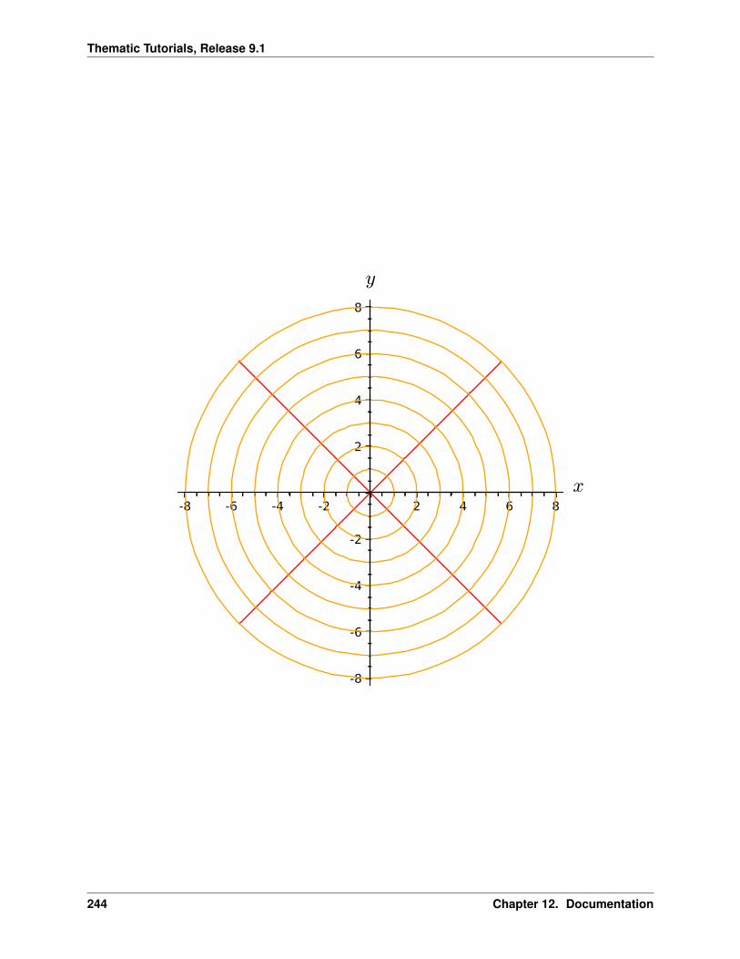
Thematic Tutorials, Release 9.1
-8 -6 -4 -2 2 4 6 8x
-8
-6
-4
-2
2
4
6
8
y
244 Chapter 12. Documentation
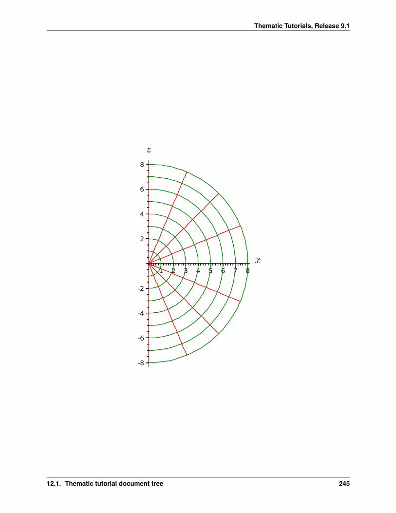
Thematic Tutorials, Release 9.1
1 2 3 4 5 6 7 8x
-8
-6
-4
-2
2
4
6
8
z
12.1. Thematic tutorial document tree 245
Thematic Tutorials, Release 9.1
Relations between the Cartesian and spherical vector frames
At this stage, E3 is endowed with three vector frames:
sage: E.frames()[Coordinate frame (E^3, (e_x,e_y,e_z)),Coordinate frame (E^3, (d/dr,d/dth,d/dph)),Vector frame (E^3, (e_r,e_th,e_ph))]
The second one is the coordinate frame(
𝜕𝜕𝑟 ,
𝜕𝜕𝜃 ,
𝜕𝜕𝜑
)of spherical coordinates, while the third one is the standard
orthonormal frame (𝑒𝑟, 𝑒𝜃, 𝑒𝜑) associated with spherical coordinates. For Cartesian coordinates, the coordinate frameand the orthonormal frame coincide: it is (𝑒𝑥, 𝑒𝑦, 𝑒𝑧). For spherical coordinates, the orthonormal frame is returned bythe method spherical_frame():
sage: spherical_frame = E.spherical_frame()sage: spherical_frameVector frame (E^3, (e_r,e_th,e_ph))
We may check that it is an orthonormal frame, i.e. that it obeys 𝑒𝑖 · 𝑒𝑗 = 𝛿𝑖𝑗 :
sage: es = spherical_framesage: [[es[i].dot(es[j]).expr() for j in E.irange()] for i in E.irange()][[1, 0, 0], [0, 1, 0], [0, 0, 1]]
Via the method display, we may express the orthonormal spherical frame in terms of the Cartesian one:
sage: for vec in spherical_frame:....: vec.display(cartesian_frame, spherical)e_r = cos(ph)*sin(th) e_x + sin(ph)*sin(th) e_y + cos(th) e_ze_th = cos(ph)*cos(th) e_x + cos(th)*sin(ph) e_y - sin(th) e_ze_ph = -sin(ph) e_x + cos(ph) e_y
The reverse is:
sage: for vec in cartesian_frame:....: vec.display(spherical_frame, spherical)e_x = cos(ph)*sin(th) e_r + cos(ph)*cos(th) e_th - sin(ph) e_phe_y = sin(ph)*sin(th) e_r + cos(th)*sin(ph) e_th + cos(ph) e_phe_z = cos(th) e_r - sin(th) e_th
We may also express the orthonormal frame (𝑒𝑟, 𝑒𝜃, 𝑒𝜑) in terms on the coordinate frame(
𝜕𝜕𝑟 ,
𝜕𝜕𝜃 ,
𝜕𝜕𝜑
)(the latter
being returned by the method frame() acting on the chart spherical):
sage: for vec in spherical_frame:....: vec.display(spherical.frame(), spherical)e_r = d/dre_th = 1/r d/dthe_ph = 1/(r*sin(th)) d/dph
Introducing cylindrical coordinates
Cylindrical coordinates are introduced in a way similar to spherical coordinates:
246 Chapter 12. Documentation
Thematic Tutorials, Release 9.1
sage: cylindrical.<rh,ph,z> = E.cylindrical_coordinates()sage: cylindricalChart (E^3, (rh, ph, z))
We have:
sage: cylindrical[:](rh, ph, z)sage: rh is cylindrical[1]Truesage: cylindrical.coord_range()rh: (0, +oo); ph: [0, 2*pi] (periodic); z: (-oo, +oo)
E3 is now endowed with three coordinate charts:
sage: E.atlas()[Chart (E^3, (x, y, z)), Chart (E^3, (r, th, ph)), Chart (E^3, (rh, ph, z))]
The transformations linking the cylindrical coordinates to the Cartesian ones are:
sage: E.coord_change(cylindrical, cartesian).display()x = rh*cos(ph)y = rh*sin(ph)z = zsage: E.coord_change(cartesian, cylindrical).display()rh = sqrt(x^2 + y^2)ph = arctan2(y, x)z = z
There are now five vector frames defined on E3:
sage: E.frames()[Coordinate frame (E^3, (e_x,e_y,e_z)),Coordinate frame (E^3, (d/dr,d/dth,d/dph)),Vector frame (E^3, (e_r,e_th,e_ph)),Coordinate frame (E^3, (d/drh,d/dph,d/dz)),Vector frame (E^3, (e_rh,e_ph,e_z))]
The orthonormal frame associated with cylindrical coordinates is (𝑒𝜌, 𝑒𝜑, 𝑒𝑧):
sage: cylindrical_frame = E.cylindrical_frame()sage: cylindrical_frameVector frame (E^3, (e_rh,e_ph,e_z))
We may check that it is an orthonormal frame:
sage: ec = cylindrical_framesage: [[ec[i].dot(ec[j]).expr() for j in E.irange()] for i in E.irange()][[1, 0, 0], [0, 1, 0], [0, 0, 1]]
and express it in terms of the Cartesian frame:
sage: for vec in cylindrical_frame:....: vec.display(cartesian_frame, cylindrical)e_rh = cos(ph) e_x + sin(ph) e_ye_ph = -sin(ph) e_x + cos(ph) e_ye_z = e_z
12.1. Thematic tutorial document tree 247
Thematic Tutorials, Release 9.1
The reverse is:
sage: for vec in cartesian_frame:....: vec.display(cylindrical_frame, cylindrical)e_x = cos(ph) e_rh - sin(ph) e_phe_y = sin(ph) e_rh + cos(ph) e_phe_z = e_z
Of course, we may express the orthonormal cylindrical frame in terms of the spherical one:
sage: for vec in cylindrical_frame:....: vec.display(spherical_frame, spherical)e_rh = sin(th) e_r + cos(th) e_the_ph = e_phe_z = cos(th) e_r - sin(th) e_th
along with the reverse transformation:
sage: for vec in spherical_frame:....: vec.display(cylindrical_frame, spherical)e_r = sin(th) e_rh + cos(th) e_ze_th = cos(th) e_rh - sin(th) e_ze_ph = e_ph
The orthonormal frame (𝑒𝜌, 𝑒𝜑, 𝑒𝑧) can be expressed in terms on the coordinate frame(
𝜕𝜕𝜌 ,
𝜕𝜕𝜑 ,
𝜕𝜕𝑧
)(the latter being
returned by the method frame() acting on the chart cylindrical):
sage: for vec in cylindrical_frame:....: vec.display(cylindrical.frame(), cylindrical)e_rh = d/drhe_ph = 1/rh d/dphe_z = d/dz
How to evaluate the coordinates of a point in various systems
Let us introduce a point 𝑝 ∈ E3 via the generic SageMath syntax for creating an element from its parent (here E3), i.e.the call operator (), with the coordinates of the point as the first argument:
sage: p = E((-1, 1,0), chart=cartesian, name='p')sage: pPoint p on the Euclidean space E^3
Actually, since the Cartesian coordinates are the default ones, the argument chart=cartesian can be omitted:
sage: p = E((-1, 1,0), name='p')sage: pPoint p on the Euclidean space E^3
The coordinates of 𝑝 in a given coordinate chart are obtained by letting the corresponding chart act on 𝑝:
sage: cartesian(p)(-1, 1, 0)sage: spherical(p)(sqrt(2), 1/2*pi, 3/4*pi)sage: cylindrical(p)(sqrt(2), 3/4*pi, 0)
248 Chapter 12. Documentation
Thematic Tutorials, Release 9.1
Here some example of a point defined from its spherical coordinates:
sage: q = E((4,pi/3,pi), chart=spherical, name='q')sage: qPoint q on the Euclidean space E^3
We have then:
sage: spherical(q)(4, 1/3*pi, pi)sage: cartesian(q)(-2*sqrt(3), 0, 2)sage: cylindrical(q)(2*sqrt(3), pi, 2)
How to express a scalar field in various coordinate systems
Let us define a scalar field on E3 from its expression in Cartesian coordinates:
sage: f = E.scalar_field(x^2+y^2 - z^2, name='f')
Note that since the Cartesian coordinates are the default ones, we have not specified them in the above definition.Thanks to the known coordinate transformations, the expression of 𝑓 in terms of other coordinates is automaticallycomputed:
sage: f.display()f: E^3 --> R
(x, y, z) |--> x^2 + y^2 - z^2(r, th, ph) |--> -2*r^2*cos(th)^2 + r^2(rh, ph, z) |--> rh^2 - z^2
We can limit the output to a single coordinate system:
sage: f.display(cartesian)f: E^3 --> R
(x, y, z) |--> x^2 + y^2 - z^2sage: f.display(cylindrical)f: E^3 --> R
(rh, ph, z) |--> rh^2 - z^2
The coordinate expression in a given coordinate system is obtained via the method expr():
sage: f.expr() # expression in the default chart (Cartesian coordinates)x^2 + y^2 - z^2sage: f.expr(spherical)-2*r^2*cos(th)^2 + r^2sage: f.expr(cylindrical)rh^2 - z^2
The values of 𝑓 at points 𝑝 and 𝑞 are:
sage: f(p)2sage: f(q)8
Of course, we may define a scalar field from its coordinate expression in a chart that is not the default one:
12.1. Thematic tutorial document tree 249
Thematic Tutorials, Release 9.1
sage: g = E.scalar_field(r^2, chart=spherical, name='g')
Instead of using the keyword argument chart, one can pass a dictionary as the first argument, with the chart as key:
sage: g = E.scalar_field(spherical: r^2, name='g')
The computation of the expressions of 𝑔 in the other coordinate systems is triggered by the method display():
sage: g.display()g: E^3 --> R
(x, y, z) |--> x^2 + y^2 + z^2(r, th, ph) |--> r^2(rh, ph, z) |--> rh^2 + z^2
How to express a vector field in various frames
Let us introduce a vector field on E3 by its components in the Cartesian frame. Since the latter is the default vectorframe on E3, it suffices to write:
sage: v = E.vector_field(-y, x, z^2, name='v')sage: v.display()v = -y e_x + x e_y + z^2 e_z
Equivalently, a vector field can be defined directly from its expansion on the Cartesian frame:
sage: ex, ey, ez = cartesian_frame[:]sage: v = -y*ex + x*ey + z^2*ezsage: v.display()-y e_x + x e_y + z^2 e_z
Let us provide v with some name, as above:
sage: v.set_name('v')sage: v.display()v = -y e_x + x e_y + z^2 e_z
The components of 𝑣 are returned by the square bracket operator:
sage: v[1]-ysage: v[:][-y, x, z^2]
The computation of the expression of 𝑣 in terms of the orthonormal spherical frame is triggered by the methoddisplay():
sage: v.display(spherical_frame)v = z^3/sqrt(x^2 + y^2 + z^2) e_r- sqrt(x^2 + y^2)*z^2/sqrt(x^2 + y^2 + z^2) e_th + sqrt(x^2 + y^2) e_ph
We note that the components are still expressed in the default chart (Cartesian coordinates). To have them expressedin the spherical chart, it suffices to pass the latter as a second argument to display():
sage: v.display(spherical_frame, spherical)v = r^2*cos(th)^3 e_r - r^2*cos(th)^2*sin(th) e_th + r*sin(th) e_ph
250 Chapter 12. Documentation
Thematic Tutorials, Release 9.1
Again, the components of 𝑣 are obtained by means of the square bracket operator, by specifying the vector frame asfirst argument and the coordinate chart as the last one:
sage: v[spherical_frame, 1]z^3/sqrt(x^2 + y^2 + z^2)sage: v[spherical_frame, 1, spherical]r^2*cos(th)^3sage: v[spherical_frame, :, spherical][r^2*cos(th)^3, -r^2*cos(th)^2*sin(th), r*sin(th)]
Similarly, the expression of 𝑣 in terms of the cylindrical frame is:
sage: v.display(cylindrical_frame, cylindrical)v = rh e_ph + z^2 e_zsage: v[cylindrical_frame, :, cylindrical][0, rh, z^2]
The value of the vector field 𝑣 at point 𝑝 is:
sage: vp = v.at(p)sage: vpVector v at Point p on the Euclidean space E^3sage: vp.display()v = -e_x - e_ysage: vp.display(spherical_frame.at(p))v = sqrt(2) e_phsage: vp.display(cylindrical_frame.at(p))v = sqrt(2) e_ph
The value of the vector field 𝑣 at point 𝑞 is:
sage: vq = v.at(q)sage: vqVector v at Point q on the Euclidean space E^3sage: vq.display()v = -2*sqrt(3) e_y + 4 e_zsage: vq.display(spherical_frame.at(q))v = 2 e_r - 2*sqrt(3) e_th + 2*sqrt(3) e_phsage: vq.display(cylindrical_frame.at(q))v = 2*sqrt(3) e_ph + 4 e_z
How to change the default coordinates and default vector frame
At any time, one may change the default coordinates by the method set_default_chart():
sage: E.set_default_chart(spherical)
Then:
sage: f.expr()-2*r^2*cos(th)^2 + r^2sage: v.display()v = -r*sin(ph)*sin(th) e_x + r*cos(ph)*sin(th) e_y + r^2*cos(th)^2 e_z
Note that the default vector frame is still the Cartesian one; to change to the orthonormal spherical frame, useset_default_frame():
12.1. Thematic tutorial document tree 251
Thematic Tutorials, Release 9.1
sage: E.set_default_frame(spherical_frame)
Then:
sage: v.display()v = r^2*cos(th)^3 e_r - r^2*cos(th)^2*sin(th) e_th + r*sin(th) e_phsage: v.display(cartesian_frame, cartesian)v = -y e_x + x e_y + z^2 e_z
Advanced aspects: the Euclidean space as a Riemannian manifold
This tutorial introduces some vector calculus capabilities of SageMath within the 3-dimensional Euclidean space. Thecorresponding tools have been developed via the SageManifolds project.
The tutorial is also available as a Jupyter notebook, either passive (nbviewer) or interactive (binder).
The Euclidean 3-space
Let us consider the 3-dimensional Euclidean space E3, with Cartesian coordinates (𝑥, 𝑦, 𝑧):
sage: E.<x,y,z> = EuclideanSpace()sage: EEuclidean space E^3
E3 is actually a Riemannian manifold (see pseudo_riemannian), i.e. a smooth real manifold endowed with apositive definite metric tensor:
sage: E.category()Category of smooth manifolds over Real Field with 53 bits of precisionsage: E.base_field() is RRTruesage: E.metric()Riemannian metric g on the Euclidean space E^3
Actually RR is used here as a proxy for the real field (this should be replaced in the future, see the discussion at#24456) and the 53 bits of precision play of course no role for the symbolic computations.
Let us introduce spherical and cylindrical coordinates on E3:
sage: spherical.<r,th,ph> = E.spherical_coordinates()sage: cylindrical.<rh,ph,z> = E.cylindrical_coordinates()
The user atlas of E3 has then three charts:
sage: E.atlas()[Chart (E^3, (x, y, z)), Chart (E^3, (r, th, ph)), Chart (E^3, (rh, ph, z))]
while there are five vector frames defined on E3:
sage: E.frames()[Coordinate frame (E^3, (e_x,e_y,e_z)),Coordinate frame (E^3, (d/dr,d/dth,d/dph)),Vector frame (E^3, (e_r,e_th,e_ph)),Coordinate frame (E^3, (d/drh,d/dph,d/dz)),Vector frame (E^3, (e_rh,e_ph,e_z))]
252 Chapter 12. Documentation
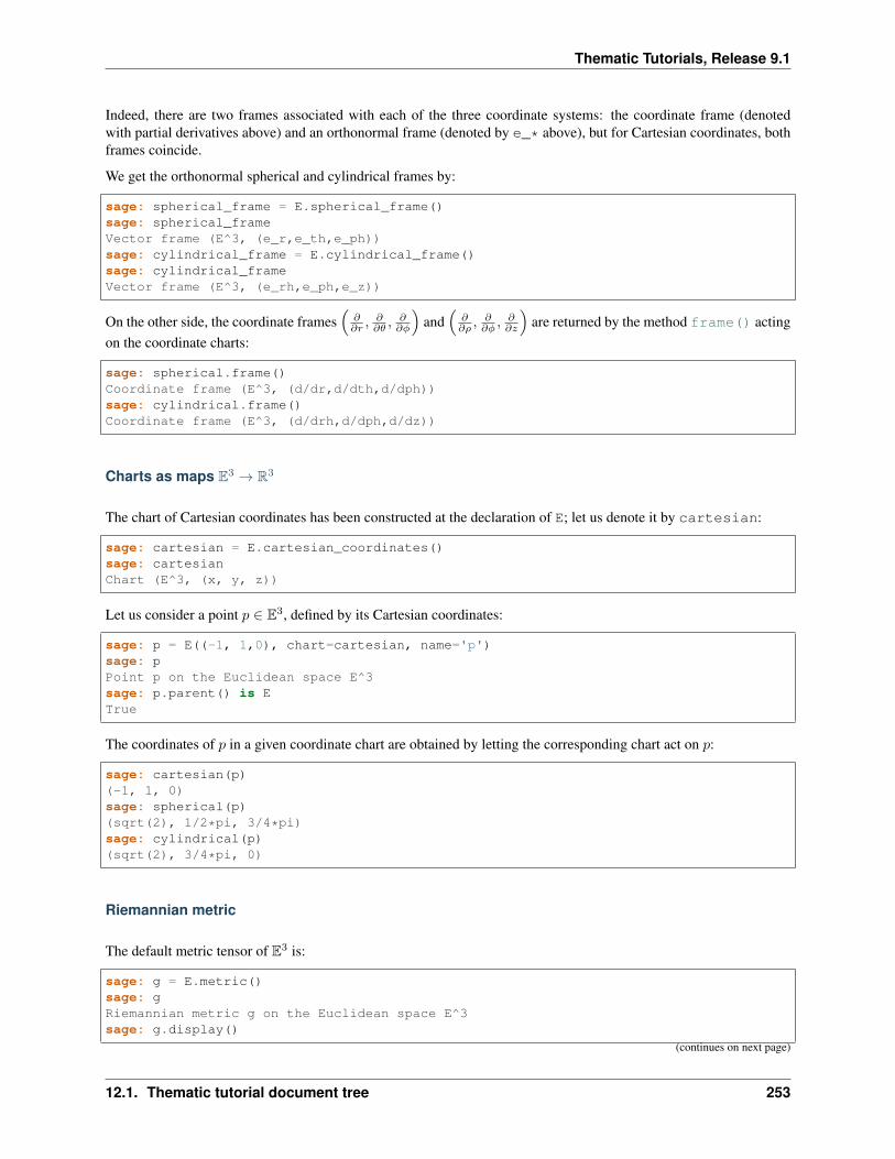
Thematic Tutorials, Release 9.1
Indeed, there are two frames associated with each of the three coordinate systems: the coordinate frame (denotedwith partial derivatives above) and an orthonormal frame (denoted by e_* above), but for Cartesian coordinates, bothframes coincide.
We get the orthonormal spherical and cylindrical frames by:
sage: spherical_frame = E.spherical_frame()sage: spherical_frameVector frame (E^3, (e_r,e_th,e_ph))sage: cylindrical_frame = E.cylindrical_frame()sage: cylindrical_frameVector frame (E^3, (e_rh,e_ph,e_z))
On the other side, the coordinate frames(
𝜕𝜕𝑟 ,
𝜕𝜕𝜃 ,
𝜕𝜕𝜑
)and
(𝜕𝜕𝜌 ,
𝜕𝜕𝜑 ,
𝜕𝜕𝑧
)are returned by the method frame() acting
on the coordinate charts:
sage: spherical.frame()Coordinate frame (E^3, (d/dr,d/dth,d/dph))sage: cylindrical.frame()Coordinate frame (E^3, (d/drh,d/dph,d/dz))
Charts as maps E3 → R3
The chart of Cartesian coordinates has been constructed at the declaration of E; let us denote it by cartesian:
sage: cartesian = E.cartesian_coordinates()sage: cartesianChart (E^3, (x, y, z))
Let us consider a point 𝑝 ∈ E3, defined by its Cartesian coordinates:
sage: p = E((-1, 1,0), chart=cartesian, name='p')sage: pPoint p on the Euclidean space E^3sage: p.parent() is ETrue
The coordinates of 𝑝 in a given coordinate chart are obtained by letting the corresponding chart act on 𝑝:
sage: cartesian(p)(-1, 1, 0)sage: spherical(p)(sqrt(2), 1/2*pi, 3/4*pi)sage: cylindrical(p)(sqrt(2), 3/4*pi, 0)
Riemannian metric
The default metric tensor of E3 is:
sage: g = E.metric()sage: gRiemannian metric g on the Euclidean space E^3sage: g.display()
(continues on next page)
12.1. Thematic tutorial document tree 253
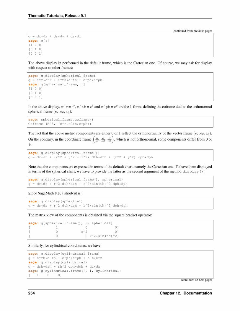
Thematic Tutorials, Release 9.1
(continued from previous page)
g = dx*dx + dy*dy + dz*dzsage: g[:][1 0 0][0 1 0][0 0 1]
The above display in performed in the default frame, which is the Cartesian one. Of course, we may ask for displaywith respect to other frames:
sage: g.display(spherical_frame)g = e^r*e^r + e^th*e^th + e^ph*e^phsage: g[spherical_frame, :][1 0 0][0 1 0][0 0 1]
In the above display, e^r = 𝑒𝑟, e^th = 𝑒𝜃 and e^ph = 𝑒𝜑 are the 1-forms defining the coframe dual to the orthonormalspherical frame (𝑒𝑟, 𝑒𝜃, 𝑒𝜑):
sage: spherical_frame.coframe()Coframe (E^3, (e^r,e^th,e^ph))
The fact that the above metric components are either 0 or 1 reflect the orthonormality of the vector frame (𝑒𝑟, 𝑒𝜃, 𝑒𝜑).
On the contrary, in the coordinate frame(
𝜕𝜕𝑟 ,
𝜕𝜕𝜃 ,
𝜕𝜕𝜑
), which is not orthonormal, some components differ from 0 or
1:
sage: g.display(spherical.frame())g = dr*dr + (x^2 + y^2 + z^2) dth*dth + (x^2 + y^2) dph*dph
Note that the components are expressed in terms of the default chart, namely the Cartesian one. To have them displayedin terms of the spherical chart, we have to provide the latter as the second argument of the method display():
sage: g.display(spherical.frame(), spherical)g = dr*dr + r^2 dth*dth + r^2*sin(th)^2 dph*dph
Since SageMath 8.8, a shortcut is:
sage: g.display(spherical)g = dr*dr + r^2 dth*dth + r^2*sin(th)^2 dph*dph
The matrix view of the components is obtained via the square bracket operator:
sage: g[spherical.frame(), :, spherical][ 1 0 0][ 0 r^2 0][ 0 0 r^2*sin(th)^2]
Similarly, for cylindrical coordinates, we have:
sage: g.display(cylindrical_frame)g = e^rh*e^rh + e^ph*e^ph + e^z*e^zsage: g.display(cylindrical)g = drh*drh + rh^2 dph*dph + dz*dzsage: g[cylindrical.frame(), :, cylindrical][ 1 0 0]
(continues on next page)
254 Chapter 12. Documentation
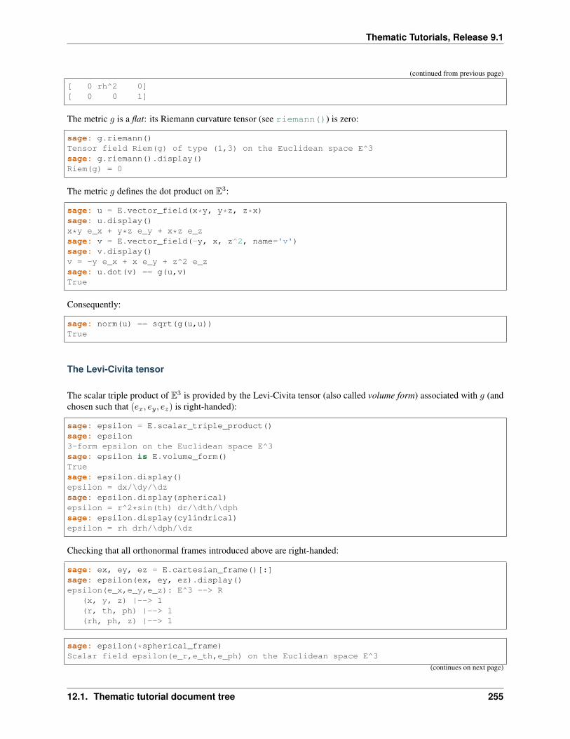
Thematic Tutorials, Release 9.1
(continued from previous page)
[ 0 rh^2 0][ 0 0 1]
The metric 𝑔 is a flat: its Riemann curvature tensor (see riemann()) is zero:
sage: g.riemann()Tensor field Riem(g) of type (1,3) on the Euclidean space E^3sage: g.riemann().display()Riem(g) = 0
The metric 𝑔 defines the dot product on E3:
sage: u = E.vector_field(x*y, y*z, z*x)sage: u.display()x*y e_x + y*z e_y + x*z e_zsage: v = E.vector_field(-y, x, z^2, name='v')sage: v.display()v = -y e_x + x e_y + z^2 e_zsage: u.dot(v) == g(u,v)True
Consequently:
sage: norm(u) == sqrt(g(u,u))True
The Levi-Civita tensor
The scalar triple product of E3 is provided by the Levi-Civita tensor (also called volume form) associated with 𝑔 (andchosen such that (𝑒𝑥, 𝑒𝑦, 𝑒𝑧) is right-handed):
sage: epsilon = E.scalar_triple_product()sage: epsilon3-form epsilon on the Euclidean space E^3sage: epsilon is E.volume_form()Truesage: epsilon.display()epsilon = dx/\dy/\dzsage: epsilon.display(spherical)epsilon = r^2*sin(th) dr/\dth/\dphsage: epsilon.display(cylindrical)epsilon = rh drh/\dph/\dz
Checking that all orthonormal frames introduced above are right-handed:
sage: ex, ey, ez = E.cartesian_frame()[:]sage: epsilon(ex, ey, ez).display()epsilon(e_x,e_y,e_z): E^3 --> R
(x, y, z) |--> 1(r, th, ph) |--> 1(rh, ph, z) |--> 1
sage: epsilon(*spherical_frame)Scalar field epsilon(e_r,e_th,e_ph) on the Euclidean space E^3
(continues on next page)
12.1. Thematic tutorial document tree 255
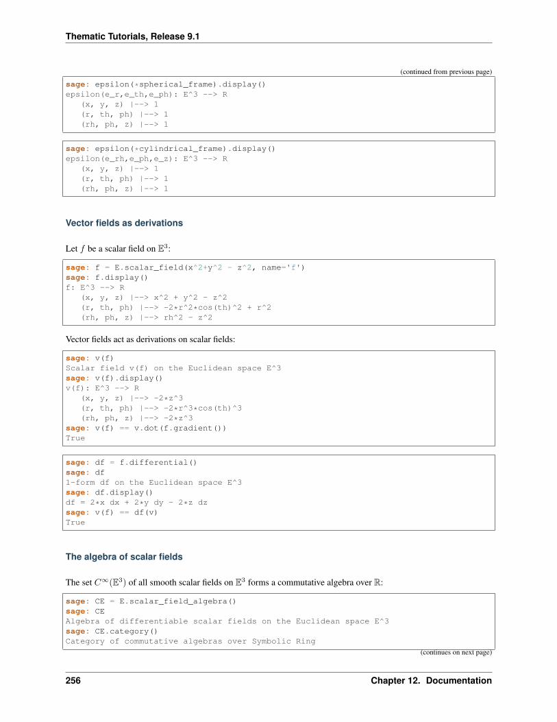
Thematic Tutorials, Release 9.1
(continued from previous page)
sage: epsilon(*spherical_frame).display()epsilon(e_r,e_th,e_ph): E^3 --> R
(x, y, z) |--> 1(r, th, ph) |--> 1(rh, ph, z) |--> 1
sage: epsilon(*cylindrical_frame).display()epsilon(e_rh,e_ph,e_z): E^3 --> R
(x, y, z) |--> 1(r, th, ph) |--> 1(rh, ph, z) |--> 1
Vector fields as derivations
Let 𝑓 be a scalar field on E3:
sage: f = E.scalar_field(x^2+y^2 - z^2, name='f')sage: f.display()f: E^3 --> R
(x, y, z) |--> x^2 + y^2 - z^2(r, th, ph) |--> -2*r^2*cos(th)^2 + r^2(rh, ph, z) |--> rh^2 - z^2
Vector fields act as derivations on scalar fields:
sage: v(f)Scalar field v(f) on the Euclidean space E^3sage: v(f).display()v(f): E^3 --> R
(x, y, z) |--> -2*z^3(r, th, ph) |--> -2*r^3*cos(th)^3(rh, ph, z) |--> -2*z^3
sage: v(f) == v.dot(f.gradient())True
sage: df = f.differential()sage: df1-form df on the Euclidean space E^3sage: df.display()df = 2*x dx + 2*y dy - 2*z dzsage: v(f) == df(v)True
The algebra of scalar fields
The set 𝐶∞(E3) of all smooth scalar fields on E3 forms a commutative algebra over R:
sage: CE = E.scalar_field_algebra()sage: CEAlgebra of differentiable scalar fields on the Euclidean space E^3sage: CE.category()Category of commutative algebras over Symbolic Ring
(continues on next page)
256 Chapter 12. Documentation
Thematic Tutorials, Release 9.1
(continued from previous page)
sage: f in CETrue
In SageMath terminology, 𝐶∞(E3) is the parent of scalar fields:
sage: f.parent() is CETrue
The free module of vector fields
The set X(E3) of all vector fields on E3 is a free module of rank 3 over the commutative algebra 𝐶∞(E3):
sage: XE = v.parent()sage: XEFree module X(E^3) of vector fields on the Euclidean space E^3sage: XE.category()Category of finite dimensional modules over Algebra of differentiablescalar fields on the Euclidean space E^3
sage: XE.base_ring()Algebra of differentiable scalar fields on the Euclidean space E^3sage: XE.base_ring() is CETruesage: rank(XE)3
The bases of the free module X(E3) are nothing but the vector frames defined on E3:
sage: XE.bases()[Coordinate frame (E^3, (e_x,e_y,e_z)),Coordinate frame (E^3, (d/dr,d/dth,d/dph)),Vector frame (E^3, (e_r,e_th,e_ph)),Coordinate frame (E^3, (d/drh,d/dph,d/dz)),Vector frame (E^3, (e_rh,e_ph,e_z))]
Tangent spaces
A vector field evaluated at a point $p$ is a vector in the tangent space 𝑇𝑝E3:
sage: pPoint p on the Euclidean space E^3sage: vp = v.at(p)sage: vpVector v at Point p on the Euclidean space E^3sage: vp.display()v = -e_x - e_y
sage: Tp = vp.parent()sage: TpTangent space at Point p on the Euclidean space E^3sage: Tp is E.tangent_space(p)Truesage: Tp.category()
(continues on next page)
12.1. Thematic tutorial document tree 257
Thematic Tutorials, Release 9.1
(continued from previous page)
Category of finite dimensional vector spaces over Symbolic Ringsage: dim(Tp)3sage: isinstance(Tp, FiniteRankFreeModule)True
The bases on 𝑇𝑝E3 are inherited from the vector frames of E3:
sage: Tp.bases()[Basis (e_x,e_y,e_z) on the Tangent space at Point p on the Euclidean space E^3,Basis (d/dr,d/dth,d/dph) on the Tangent space at Point p on the Euclidean space E^3,Basis (e_r,e_th,e_ph) on the Tangent space at Point p on the Euclidean space E^3,Basis (d/drh,d/dph,d/dz) on the Tangent space at Point p on the Euclidean space E^3,Basis (e_rh,e_ph,e_z) on the Tangent space at Point p on the Euclidean space E^3]
For instance, we have:
sage: spherical_frame.at(p)Basis (e_r,e_th,e_ph) on the Tangent space at Point p on theEuclidean space E^3
sage: spherical_frame.at(p) in Tp.bases()True
Levi-Civita connection
The Levi-Civita connection associated to the Euclidean metric 𝑔 is:
sage: nabla = g.connection()sage: nablaLevi-Civita connection nabla_g associated with the Riemannian metric gon the Euclidean space E^3
The corresponding Christoffel symbols with respect to Cartesian coordinates are identically zero: none of them ap-pear in the output of christoffel_symbols_display(), which by default displays only nonzero Christoffelsymbols:
sage: g.christoffel_symbols_display(cartesian)
On the contrary, some of the Christoffel symbols with respect to spherical coordinates differ from zero:
sage: g.christoffel_symbols_display(spherical)Gam^r_th,th = -rGam^r_ph,ph = -r*sin(th)^2Gam^th_r,th = 1/rGam^th_ph,ph = -cos(th)*sin(th)Gam^ph_r,ph = 1/rGam^ph_th,ph = cos(th)/sin(th)
By default, only nonzero and nonredundant values are displayed (for instance Γ𝜑𝜑𝑟 is skipped, since it can be deduced
from Γ𝜑𝑟𝜑 by symmetry on the last two indices).
Similarly, the nonzero Christoffel symbols with respect to cylindrical coordinates are:
258 Chapter 12. Documentation
Thematic Tutorials, Release 9.1
sage: g.christoffel_symbols_display(cylindrical)Gam^rh_ph,ph = -rhGam^ph_rh,ph = 1/rh
The Christoffel symbols are nothing but the connection coefficients in the corresponding coordinate frame:
sage: nabla.display(cylindrical.frame(), cylindrical, only_nonredundant=True)Gam^rh_ph,ph = -rhGam^ph_rh,ph = 1/rh
The connection coefficients with respect to the orthonormal (non-coordinate) frames are (again only nonzero valuesare displayed):
sage: nabla.display(spherical_frame, spherical)Gam^1_22 = -1/rGam^1_33 = -1/rGam^2_12 = 1/rGam^2_33 = -cos(th)/(r*sin(th))Gam^3_13 = 1/rGam^3_23 = cos(th)/(r*sin(th))sage: nabla.display(cylindrical_frame, cylindrical)Gam^1_22 = -1/rhGam^2_12 = 1/rh
The Levi-Civita connection∇𝑔 is the connection involved in the standard differential operators:
sage: from sage.manifolds.operators import *sage: grad(f) == nabla(f).up(g)Truesage: nabla(f) == grad(f).down(g)Truesage: div(u) == nabla(u).trace()Truesage: div(v) == nabla(v).trace()Truesage: laplacian(f) == nabla(nabla(f).up(g)).trace()Truesage: laplacian(u) == nabla(nabla(u).up(g)).trace(1,2)Truesage: laplacian(v) == nabla(nabla(v).up(g)).trace(1,2)True
Vector calculus in the Euclidean plane
This tutorial introduces some vector calculus capabilities of SageMath in the framework of the 2-dimensional Eu-clidean space. The corresponding tools have been developed via the SageManifolds project.
The tutorial is also available as a Jupyter notebook, either passive (nbviewer) or interactive (binder).
1. Defining the Euclidean plane
We define the Euclidean plane E2 as a 2-dimensional Euclidean space, with Cartesian coordinates (𝑥, 𝑦), via thefunction EuclideanSpace:
12.1. Thematic tutorial document tree 259
Thematic Tutorials, Release 9.1
sage: E.<x,y> = EuclideanSpace()sage: EEuclidean plane E^2
Thanks to the use of <x,y> in the above command, the Python variables x and y are assigned to the symbolicvariables 𝑥 and 𝑦 describing the Cartesian coordinates (there is no need to declare them via var(), i.e. to type x, y= var('x y')):
sage: type(y)<type 'sage.symbolic.expression.Expression'>
Instead of using the variables x and y, one may also access to the coordinates by their indices in the chart of Cartesiancoordinates:
sage: cartesian = E.cartesian_coordinates()sage: cartesianChart (E^2, (x, y))
sage: cartesian[1]xsage: cartesian[2]ysage: y is cartesian[2]True
Each of the Cartesian coordinates spans the entire real line:
sage: cartesian.coord_range()x: (-oo, +oo); y: (-oo, +oo)
2. Vector fields
The Euclidean plane E2 is canonically endowed with the vector frame associated with Cartesian coordinates:
sage: E.default_frame()Coordinate frame (E^2, (e_x,e_y))
Vector fields on E2 are then defined from their components in that frame:
sage: v = E.vector_field(-y, x, name='v')sage: v.display()v = -y e_x + x e_y
The access to individual components is performed by the square bracket operator:
sage: v[1]-ysage: v[:][-y, x]
A plot of the vector field 𝑣 (this is with the default parameters, see the documentation of plot() for the variousoptions):
sage: v.plot()Graphics object consisting of 80 graphics primitives
260 Chapter 12. Documentation
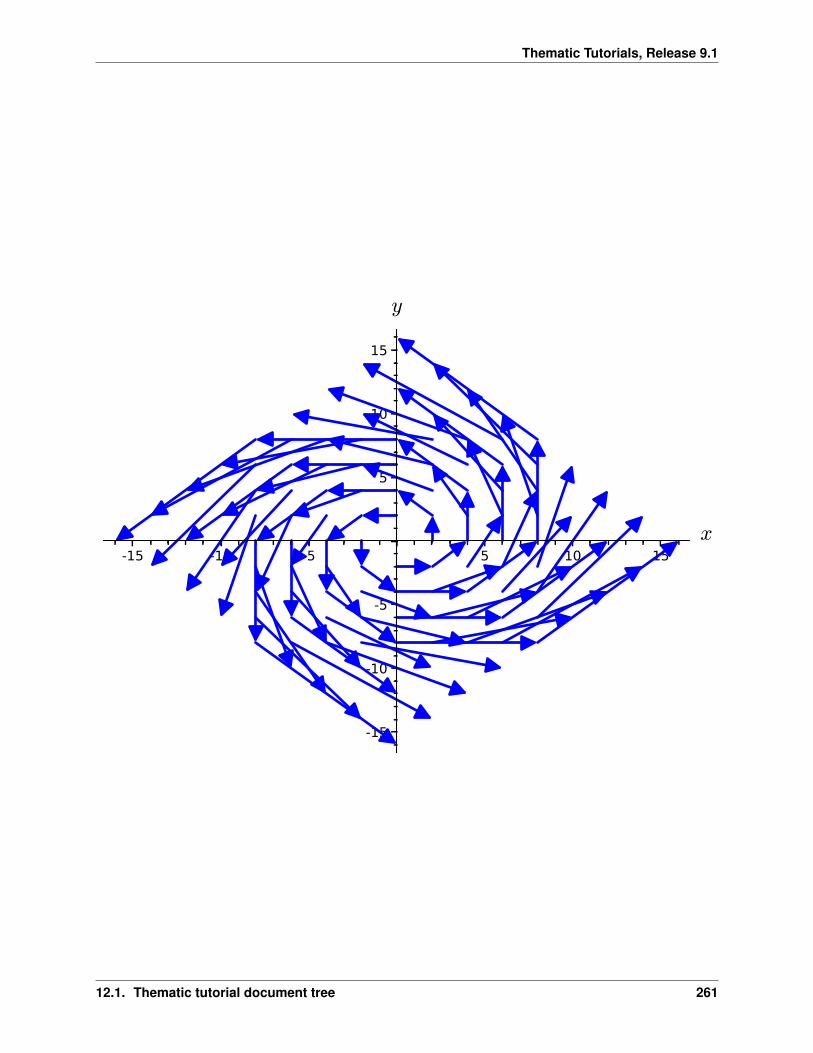
Thematic Tutorials, Release 9.1
-15 -10 -5 5 10 15x
-15
-10
-5
5
10
15
y
12.1. Thematic tutorial document tree 261
Thematic Tutorials, Release 9.1
One may also define a vector field by setting the components in a second stage:
sage: w = E.vector_field(name='w')sage: w[1] = function('w_x')(x,y)sage: w[2] = function('w_y')(x,y)sage: w.display()w = w_x(x, y) e_x + w_y(x, y) e_y
Note that in the above example the components of 𝑤 are unspecified functions of (𝑥, 𝑦), contrary to the componentsof 𝑣.
Standard linear algebra operations can be performed on vector fields:
sage: s = 2*v + x*wsage: s.display()(x*w_x(x, y) - 2*y) e_x + (x*w_y(x, y) + 2*x) e_y
Scalar product and norm
The dot (or scalar) product 𝑢 · 𝑣 of the vector fields 𝑢 and 𝑣 is obtained by the operator dot_product(); it givesrise to a scalar field on E2:
sage: s = v.dot_product(w)sage: sScalar field v.w on the Euclidean plane E^2
A shortcut alias of dot_product() is dot:
sage: s == v.dot(w)True
sage: s.display()v.w: E^2 --> R
(x, y) |--> -y*w_x(x, y) + x*w_y(x, y)
The symbolic expression representing the scalar field 𝑣 · 𝑤 is obtained by means of the method expr():
sage: s.expr()-y*w_x(x, y) + x*w_y(x, y)
The Euclidean norm of the vector field 𝑣 is a scalar field on E2:
sage: s = norm(v)sage: s.display()|v|: E^2 --> R
(x, y) |--> sqrt(x^2 + y^2)
Again, the corresponding symbolic expression is obtained via expr():
sage: s.expr()sqrt(x^2 + y^2)
sage: norm(w).expr()sqrt(w_x(x, y)^2 + w_y(x, y)^2)
We have of course ‖𝑣‖2 = 𝑣 · 𝑣
262 Chapter 12. Documentation
Thematic Tutorials, Release 9.1
sage: norm(v)^2 == v.dot(v)True
Values at a given point
We introduce a point 𝑝 ∈ E2 via the generic SageMath syntax for creating an element from its parent (here E2), i.e.the call operator (), with the Cartesian coordinates of the point as the first argument:
sage: p = E((-2,3), name='p')sage: pPoint p on the Euclidean plane E^2
The coordinates of 𝑝 are returned by the method coord():
sage: p.coord()(-2, 3)
or by letting the chart cartesian act on the point:
sage: cartesian(p)(-2, 3)
The value of the scalar field s = norm(v) at 𝑝 is:
sage: s(p)sqrt(13)
The value of a vector field at 𝑝 is obtained by the method at() (since the call operator () is reserved for the actionon scalar fields, see Vector fields as derivations below):
sage: vp = v.at(p)sage: vpVector v at Point p on the Euclidean plane E^2sage: vp.display()v = -3 e_x - 2 e_ysage: wp = w.at(p)sage: wp.display()w = w_x(-2, 3) e_x + w_y(-2, 3) e_ysage: s = v.at(p) + pi*w.at(p)sage: s.display()(pi*w_x(-2, 3) - 3) e_x + (pi*w_y(-2, 3) - 2) e_y
3. Differential operators
The standard operators grad, div, etc. involved in vector calculus are accessible as methods on scalar fields and vectorfields (e.g. v.div()). However, to use standard mathematical notations (e.g. div(v)), let us import the functionsgrad(), div(), and laplacian() in the global namespace:
sage: from sage.manifolds.operators import *
Divergence
The divergence of a vector field is returned by the function div(); the output is a scalar field on E2:
12.1. Thematic tutorial document tree 263
Thematic Tutorials, Release 9.1
sage: div(v)Scalar field div(v) on the Euclidean plane E^2sage: div(v).display()div(v): E^2 --> R
(x, y) |--> 0
In the present case, div 𝑣 vanishes identically:
sage: div(v) == 0True
On the contrary, the divergence of 𝑤 is:
sage: div(w).display()div(w): E^2 --> R
(x, y) |--> d(w_x)/dx + d(w_y)/dysage: div(w).expr()diff(w_x(x, y), x) + diff(w_y(x, y), y)
Gradient
The gradient of a scalar field, e.g. s = norm(v), is returned by the function grad(); the output is a vector field:
sage: s = norm(v)sage: grad(s)Vector field grad(|v|) on the Euclidean plane E^2sage: grad(s).display()grad(|v|) = x/sqrt(x^2 + y^2) e_x + y/sqrt(x^2 + y^2) e_ysage: grad(s)[2]y/sqrt(x^2 + y^2)
For a generic scalar field, like:
sage: F = E.scalar_field(function('f')(x,y), name='F')
we have:
sage: grad(F).display()grad(F) = d(f)/dx e_x + d(f)/dy e_ysage: grad(F)[:][d(f)/dx, d(f)/dy]
Of course, we may combine grad() and div():
sage: grad(div(w)).display()grad(div(w)) = (d^2(w_x)/dx^2 + d^2(w_y)/dxdy) e_x + (d^2(w_x)/dxdy + d^2(w_y)/dy^2)→˓e_y
Laplace operator
The Laplace operator ∆ is obtained by the function laplacian(); it acts on scalar fields:
264 Chapter 12. Documentation
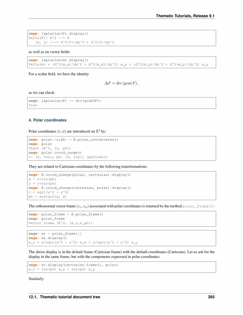
Thematic Tutorials, Release 9.1
sage: laplacian(F).display()Delta(F): E^2 --> R
(x, y) |--> d^2(f)/dx^2 + d^2(f)/dy^2
as well as on vector fields:
sage: laplacian(w).display()Delta(w) = (d^2(w_x)/dx^2 + d^2(w_x)/dy^2) e_x + (d^2(w_y)/dx^2 + d^2(w_y)/dy^2) e_y
For a scalar field, we have the identity
∆𝐹 = div (grad𝐹 ) ,
as we can check:
sage: laplacian(F) == div(grad(F))True
4. Polar coordinates
Polar coordinates (𝑟, 𝜑) are introduced on E2 by:
sage: polar.<r,ph> = E.polar_coordinates()sage: polarChart (E^2, (r, ph))sage: polar.coord_range()r: (0, +oo); ph: [0, 2*pi] (periodic)
They are related to Cartesian coordinates by the following transformations:
sage: E.coord_change(polar, cartesian).display()x = r*cos(ph)y = r*sin(ph)sage: E.coord_change(cartesian, polar).display()r = sqrt(x^2 + y^2)ph = arctan2(y, x)
The orthonormal vector frame (𝑒𝑟, 𝑒𝜑) associated with polar coordinates is returned by the method polar_frame():
sage: polar_frame = E.polar_frame()sage: polar_frameVector frame (E^2, (e_r,e_ph))
sage: er = polar_frame[1]sage: er.display()e_r = x/sqrt(x^2 + y^2) e_x + y/sqrt(x^2 + y^2) e_y
The above display is in the default frame (Cartesian frame) with the default coordinates (Cartesian). Let us ask for thedisplay in the same frame, but with the components expressed in polar coordinates:
sage: er.display(cartesian.frame(), polar)e_r = cos(ph) e_x + sin(ph) e_y
Similarly:
12.1. Thematic tutorial document tree 265
Thematic Tutorials, Release 9.1
sage: eph = polar_frame[2]sage: eph.display()e_ph = -y/sqrt(x^2 + y^2) e_x + x/sqrt(x^2 + y^2) e_ysage: eph.display(cartesian.frame(), polar)e_ph = -sin(ph) e_x + cos(ph) e_y
We may check that (𝑒𝑟, 𝑒𝜑) is an orthonormal frame:
sage: all([er.dot(er) == 1, er.dot(eph) == 0, eph.dot(eph) == 1])True
Scalar fields can be expressed in terms of polar coordinates:
sage: F.display()F: E^2 --> R
(x, y) |--> f(x, y)(r, ph) |--> f(r*cos(ph), r*sin(ph))
sage: F.display(polar)F: E^2 --> R
(r, ph) |--> f(r*cos(ph), r*sin(ph))
and we may ask for the components of vector fields in terms of the polar frame:
sage: v.display() # default frame and default coordinates (both Cartesian ones)v = -y e_x + x e_ysage: v.display(polar_frame) # polar frame and default coordinatesv = sqrt(x^2 + y^2) e_phsage: v.display(polar_frame, polar) # polar frame and polar coordinatesv = r e_ph
sage: w.display()w = w_x(x, y) e_x + w_y(x, y) e_ysage: w.display(polar_frame, polar)w = (cos(ph)*w_x(r*cos(ph), r*sin(ph)) + sin(ph)*w_y(r*cos(ph), r*sin(ph))) e_r+ (-sin(ph)*w_x(r*cos(ph), r*sin(ph)) + cos(ph)*w_y(r*cos(ph), r*sin(ph))) e_ph
Gradient in polar coordinates
Let us define a generic scalar field in terms of polar coordinates:
sage: H = E.scalar_field(polar: function('h')(r,ph), name='H')sage: H.display(polar)H: E^2 --> R
(r, ph) |--> h(r, ph)
The gradient of 𝐻 is then:
sage: grad(H).display(polar_frame, polar)grad(H) = d(h)/dr e_r + d(h)/dph/r e_ph
The access to individual components is achieved via the square bracket operator, where, in addition to the index, onehas to specify the vector frame and the coordinates if they are not the default ones:
sage: grad(H).display(cartesian.frame(), polar)grad(H) = (r*cos(ph)*d(h)/dr - sin(ph)*d(h)/dph)/r e_x + (r*sin(ph)*d(h)/dr
(continues on next page)
266 Chapter 12. Documentation
Thematic Tutorials, Release 9.1
(continued from previous page)
+ cos(ph)*d(h)/dph)/r e_ysage: grad(H)[polar_frame, 2, polar]d(h)/dph/r
Divergence in polar coordinates
Let us define a generic vector field in terms of polar coordinates:
sage: u = E.vector_field(function('u_r')(r,ph),....: function('u_ph', latex_name=r'u_\phi')(r,ph),....: frame=polar_frame, chart=polar, name='u')sage: u.display(polar_frame, polar)u = u_r(r, ph) e_r + u_ph(r, ph) e_ph
Its divergence is:
sage: div(u).display(polar)div(u): E^2 --> R
(r, ph) |--> (r*d(u_r)/dr + u_r(r, ph) + d(u_ph)/dph)/rsage: div(u).expr(polar)(r*diff(u_r(r, ph), r) + u_r(r, ph) + diff(u_ph(r, ph), ph))/rsage: div(u).expr(polar).expand()u_r(r, ph)/r + diff(u_ph(r, ph), ph)/r + diff(u_r(r, ph), r)
Using polar coordinates by default:
In order to avoid specifying the arguments polar_frame and polar in display(), expr() and [], we maychange the default values by means of set_default_chart() and set_default_frame():
sage: E.set_default_chart(polar)sage: E.set_default_frame(polar_frame)
Then we have:
sage: u.display()u = u_r(r, ph) e_r + u_ph(r, ph) e_phsage: u[1]u_r(r, ph)
sage: v.display()v = r e_phsage: v[2]r
sage: w.display()w = (cos(ph)*w_x(r*cos(ph), r*sin(ph)) + sin(ph)*w_y(r*cos(ph), r*sin(ph))) e_r + (-→˓sin(ph)*w_x(r*cos(ph), r*sin(ph)) + cos(ph)*w_y(r*cos(ph), r*sin(ph))) e_phsage: div(u).expr()(r*diff(u_r(r, ph), r) + u_r(r, ph) + diff(u_ph(r, ph), ph))/r
12.1. Thematic tutorial document tree 267
Thematic Tutorials, Release 9.1
5. Advanced topics: the Euclidean plane as a Riemannian manifold
E2 is actually a Riemannian manifold (see pseudo_riemannian), i.e. a smooth real manifold endowed with apositive definite metric tensor:
sage: E.category()Category of smooth manifolds over Real Field with 53 bits of precisionsage: E.base_field() is RRTrue
Actually RR is used here as a proxy for the real field (this should be replaced in the future, see the discussion at#24456) and the 53 bits of precision play of course no role for the symbolic computations.
The user atlas of E2 has two charts:
sage: E.atlas()[Chart (E^2, (x, y)), Chart (E^2, (r, ph))]
while there are three vector frames defined on E2:
sage: E.frames()[Coordinate frame (E^2, (e_x,e_y)),Coordinate frame (E^2, (d/dr,d/dph)),Vector frame (E^2, (e_r,e_ph))]
Indeed, there are two frames associated with polar coordinates: the coordinate frame ( 𝜕𝜕𝑟 ,
𝜕𝜕𝜑 ) and the orthonormal
frame (𝑒𝑟, 𝑒𝜑).
Riemannian metric
The default metric tensor of E2 is:
sage: g = E.metric()sage: gRiemannian metric g on the Euclidean plane E^2sage: g.display()g = e^r*e^r + e^ph*e^ph
In the above display, e^r = 𝑒𝑟 and e^ph = 𝑒𝜑 are the 1-forms defining the coframe dual to the orthonormal polarframe (𝑒𝑟, 𝑒𝜑), which is the default vector frame on E2:
sage: polar_frame.coframe()Coframe (E^2, (e^r,e^ph))
Of course, we may ask for some display with respect to frames different from the default one:
sage: g.display(cartesian.frame())g = dx*dx + dy*dysage: g.display(polar.frame())g = dr*dr + r^2 dph*dphsage: g[:][1 0][0 1]sage: g[polar.frame(),:][ 1 0][ 0 r^2]
268 Chapter 12. Documentation
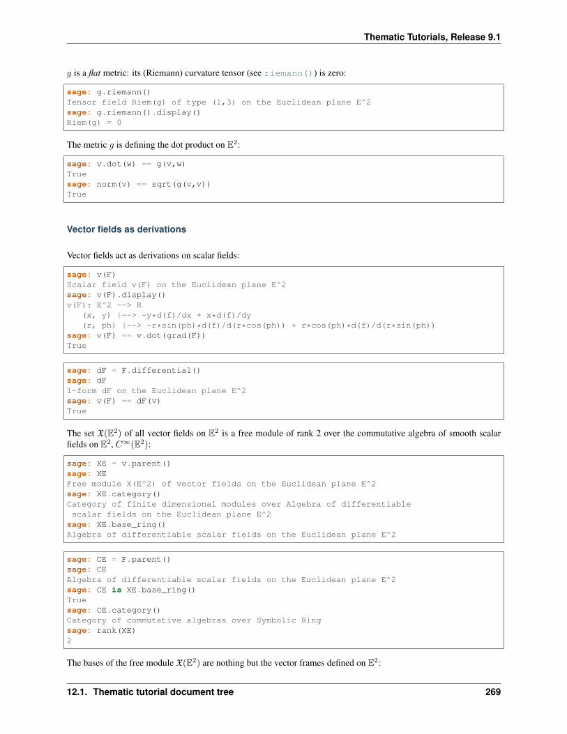
Thematic Tutorials, Release 9.1
𝑔 is a flat metric: its (Riemann) curvature tensor (see riemann()) is zero:
sage: g.riemann()Tensor field Riem(g) of type (1,3) on the Euclidean plane E^2sage: g.riemann().display()Riem(g) = 0
The metric 𝑔 is defining the dot product on E2:
sage: v.dot(w) == g(v,w)Truesage: norm(v) == sqrt(g(v,v))True
Vector fields as derivations
Vector fields act as derivations on scalar fields:
sage: v(F)Scalar field v(F) on the Euclidean plane E^2sage: v(F).display()v(F): E^2 --> R
(x, y) |--> -y*d(f)/dx + x*d(f)/dy(r, ph) |--> -r*sin(ph)*d(f)/d(r*cos(ph)) + r*cos(ph)*d(f)/d(r*sin(ph))
sage: v(F) == v.dot(grad(F))True
sage: dF = F.differential()sage: dF1-form dF on the Euclidean plane E^2sage: v(F) == dF(v)True
The set X(E2) of all vector fields on E2 is a free module of rank 2 over the commutative algebra of smooth scalarfields on E2, 𝐶∞(E2):
sage: XE = v.parent()sage: XEFree module X(E^2) of vector fields on the Euclidean plane E^2sage: XE.category()Category of finite dimensional modules over Algebra of differentiablescalar fields on the Euclidean plane E^2
sage: XE.base_ring()Algebra of differentiable scalar fields on the Euclidean plane E^2
sage: CE = F.parent()sage: CEAlgebra of differentiable scalar fields on the Euclidean plane E^2sage: CE is XE.base_ring()Truesage: CE.category()Category of commutative algebras over Symbolic Ringsage: rank(XE)2
The bases of the free module X(E2) are nothing but the vector frames defined on E2:
12.1. Thematic tutorial document tree 269
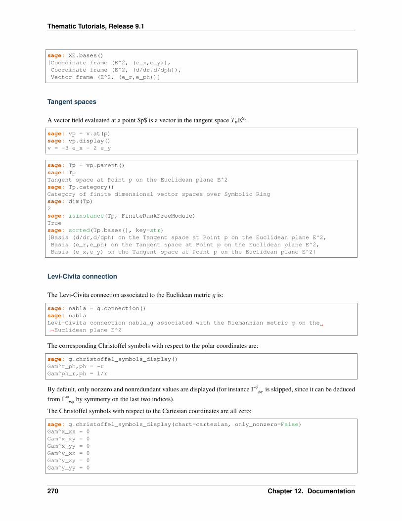
Thematic Tutorials, Release 9.1
sage: XE.bases()[Coordinate frame (E^2, (e_x,e_y)),Coordinate frame (E^2, (d/dr,d/dph)),Vector frame (E^2, (e_r,e_ph))]
Tangent spaces
A vector field evaluated at a point $p$ is a vector in the tangent space 𝑇𝑝E2:
sage: vp = v.at(p)sage: vp.display()v = -3 e_x - 2 e_y
sage: Tp = vp.parent()sage: TpTangent space at Point p on the Euclidean plane E^2sage: Tp.category()Category of finite dimensional vector spaces over Symbolic Ringsage: dim(Tp)2sage: isinstance(Tp, FiniteRankFreeModule)Truesage: sorted(Tp.bases(), key=str)[Basis (d/dr,d/dph) on the Tangent space at Point p on the Euclidean plane E^2,Basis (e_r,e_ph) on the Tangent space at Point p on the Euclidean plane E^2,Basis (e_x,e_y) on the Tangent space at Point p on the Euclidean plane E^2]
Levi-Civita connection
The Levi-Civita connection associated to the Euclidean metric 𝑔 is:
sage: nabla = g.connection()sage: nablaLevi-Civita connection nabla_g associated with the Riemannian metric g on the→˓Euclidean plane E^2
The corresponding Christoffel symbols with respect to the polar coordinates are:
sage: g.christoffel_symbols_display()Gam^r_ph,ph = -rGam^ph_r,ph = 1/r
By default, only nonzero and nonredundant values are displayed (for instance Γ𝜑𝜑𝑟 is skipped, since it can be deduced
from Γ𝜑𝑟𝜑 by symmetry on the last two indices).
The Christoffel symbols with respect to the Cartesian coordinates are all zero:
sage: g.christoffel_symbols_display(chart=cartesian, only_nonzero=False)Gam^x_xx = 0Gam^x_xy = 0Gam^x_yy = 0Gam^y_xx = 0Gam^y_xy = 0Gam^y_yy = 0
270 Chapter 12. Documentation
Thematic Tutorials, Release 9.1
∇𝑔 is the connection involved in differential operators:
sage: grad(F) == nabla(F).up(g)Truesage: nabla(F) == grad(F).down(g)Truesage: div(v) == nabla(v).trace()Truesage: div(w) == nabla(w).trace()Truesage: laplacian(F) == nabla(nabla(F).up(g)).trace()Truesage: laplacian(w) == nabla(nabla(w).up(g)).trace(1,2)True
12.1.7 Linear Programming (Mixed Integer)
This document explains the use of linear programming (LP) – and of mixed integer linear programming (MILP) – inSage by illustrating it with several problems it can solve. Most of the examples given are motivated by graph-theoreticconcerns, and should be understandable without any specific knowledge of this field. As a tool in Combinatorics, usinglinear programming amounts to understanding how to reformulate an optimization (or existence) problem throughlinear constraints.
This is a translation of a chapter from the book Calcul mathematique avec Sage.
Definition
Here we present the usual definition of what a linear program is: it is defined by a matrix 𝐴 : R𝑚 ↦→ R𝑛, along withtwo vectors 𝑏, 𝑐 ∈ R𝑛. Solving a linear program is searching for a vector 𝑥 maximizing an objective function andsatisfying a set of constraints, i.e.
𝑐𝑡𝑥 = max𝑥′ such that 𝐴𝑥′≤𝑏
𝑐𝑡𝑥′
where the ordering 𝑢 ≤ 𝑢′ between two vectors means that the entries of 𝑢′ are pairwise greater than the entries of 𝑢.We also write:
Max: 𝑐𝑡𝑥Such that: 𝐴𝑥 ≤ 𝑏
Equivalently, we can also say that solving a linear program amounts to maximizing a linear function defined overa polytope (preimage or 𝐴−1(≤ 𝑏)). These definitions, however, do not tell us how to use linear programming incombinatorics. In the following, we will show how to solve optimization problems like the Knapsack problem, theMaximum Matching problem, and a Flow problem.
Mixed integer linear programming
There are bad news coming along with this definition of linear programming: an LP can be solved in polynomial time.This is indeed bad news, because this would mean that unless we define LP of exponential size, we cannot expect LPto solve NP-complete problems, which would be a disappointment. On a brighter side, it becomes NP-complete tosolve a linear program if we are allowed to specify constraints of a different kind: requiring that some variables beintegers instead of real values. Such an LP is actually called a “mixed integer linear program” (some variables can beintegers, some other reals). Hence, we can expect to find in the MILP framework a wide range of expressivity.
12.1. Thematic tutorial document tree 271
Thematic Tutorials, Release 9.1
Practical
The MILP class
The MILP class in Sage represents a MILP! It is also used to solve regular LP. It has a very small number of methods,meant to define our set of constraints and variables, then to read the solution found by the solvers once computed. It isalso possible to export a MILP defined with Sage to a .lp or .mps file, understood by most solvers.
Let us ask Sage to solve the following LP:
Max: 𝑥+ 𝑦 + 3𝑧
Such that: 𝑥+ 2𝑦 ≤ 4
5𝑧 − 𝑦 ≤ 8
𝑥, 𝑦, 𝑧 ≥ 0
To achieve it, we need to define a corresponding MILP object, along with 3 variables x, y and z:
sage: p = MixedIntegerLinearProgram()sage: v = p.new_variable(real=True, nonnegative=True)sage: x, y, z = v['x'], v['y'], v['z']
Next, we set the objective function
sage: p.set_objective(x + y + 3*z)
And finally we set the constraints
sage: p.add_constraint(x + 2*y <= 4)sage: p.add_constraint(5*z - y <= 8)
The solve method returns by default the optimal value reached by the objective function
sage: round(p.solve(), 2)8.8
We can read the optimal assignation found by the solver for 𝑥, 𝑦 and 𝑧 through the get_values method
sage: round(p.get_values(x), 2)4.0sage: round(p.get_values(y), 2)0.0sage: round(p.get_values(z), 2)1.6
Variables
In the previous example, we obtained variables through v['x'], v['y'] and v['z']. This being said, largerLP/MILP will require us to associate an LP variable to many Sage objects, which can be integers, strings, or even thevertices and edges of a graph. For example:
sage: x = p.new_variable(real=True, nonnegative=True)
With this new object x we can now write constraints using x[1],...,x[15].
272 Chapter 12. Documentation
Thematic Tutorials, Release 9.1
sage: p.add_constraint(x[1] + x[12] - x[14] >= 8)
Notice that we did not need to define the “length” of x. Actually, x would accept any immutable object as a key, as adictionary would. We can now write
sage: p.add_constraint(x["I am a valid key"] +....: x[("a",pi)] <= 3)
And because any immutable object can be used as a key, doubly indexed variables 𝑥1,1, ..., 𝑥1,15, 𝑥2,1, ..., 𝑥15,15 canbe referenced by x[1,1],...,x[1,15],x[2,1],...,x[15,15]
sage: p.add_constraint(x[3,2] + x[5] == 6)
Typed variables and bounds
Types : If you want a variable to assume only integer or binary values, use the integer=True or binary=Truearguments of the new_variable method. Alternatively, call the set_integer and set_binary methods.
Bounds : If you want your variables to only take nonnegative values, you can say so when calling new_variablewith the argument nonnegative=True. If you want to set a different upper/lower bound on a variable, add aconstraint or use the set_min, set_max methods.
Basic linear programs
Knapsack
The Knapsack problem is the following: given a collection of items having both a weight and a usefulness, we wouldlike to fill a bag whose capacity is constrained while maximizing the usefulness of the items contained in the bag (wewill consider the sum of the items’ usefulness). For the purpose of this tutorial, we set the restriction that the bag canonly carry a certain total weight.
To achieve this, we have to associate to each object 𝑜 of our collection 𝐶 a binary variable taken[o], set to 1 whenthe object is in the bag, and to 0 otherwise. We are trying to solve the following MILP
Max:∑𝑜∈𝐿
usefulness𝑜 × taken𝑜
Such that:∑𝑜∈𝐿
weight𝑜 × taken𝑜 ≤ 𝐶
Using Sage, we will give to our items a random weight:
sage: C = 1
sage: L = ["pan", "book", "knife", "gourd", "flashlight"]
sage: L.extend(["random_stuff_" + str(i) for i in range(20)])
sage: weight = sage: usefulness =
12.1. Thematic tutorial document tree 273
Thematic Tutorials, Release 9.1
sage: set_random_seed(685474)sage: for o in L:....: weight[o] = random()....: usefulness[o] = random()
We can now define the MILP itself
sage: p = MixedIntegerLinearProgram()sage: taken = p.new_variable(binary=True)
sage: p.add_constraint(p.sum(weight[o] * taken[o] for o in L) <= C)
sage: p.set_objective(p.sum(usefulness[o] * taken[o] for o in L))
sage: p.solve() # abs tol 1e-63.1502766806530307sage: taken = p.get_values(taken)
The solution found is (of course) admissible
sage: sum(weight[o] * taken[o] for o in L) # abs tol 1e-60.6964959796619171
Should we take a flashlight?
sage: taken["flashlight"] # abs tol 1e-61.0
Wise advice. Based on purely random considerations.
Matching
Given a graph 𝐺, a matching is a set of pairwise disjoint edges. The empty set is a trivial matching. So we focus ourattention on maximum matchings: we want to find in a graph a matching whose cardinality is maximal. Computing themaximum matching in a graph is a polynomial problem, which is a famous result of Edmonds. Edmonds’ algorithm isbased on local improvements and the proof that a given matching is maximum if it cannot be improved. This algorithmis not the hardest to implement among those graph theory can offer, though this problem can be modeled with a verysimple MILP.
To do it, we need – as previously – to associate a binary variable to each one of our objects: the edges of our graph(a value of 1 meaning that the corresponding edge is included in the maximum matching). Our constraint on theedges taken being that they are disjoint, it is enough to require that, 𝑥 and 𝑦 being two edges and 𝑚𝑥,𝑚𝑦 theirassociated variables, the inequality 𝑚𝑥 +𝑚𝑦 ≤ 1 is satisfied, as we are sure that the two of them cannot both belongto the matching. Hence, we are able to write the MILP we want. However, the number of inequalities can be easilydecreased by noticing that two edges cannot be taken simultaneously inside a matching if and only if they have acommon endpoint 𝑣. We can then require instead that at most one edge incident to 𝑣 be taken inside the matching,which is a linear constraint. We will be solving:
Max:∑
𝑒∈𝐸(𝐺)
𝑚𝑒
Such that: ∀𝑣,∑
𝑒∈𝐸(𝐺)𝑣∼𝑒
𝑚𝑒 ≤ 1
Let us write the Sage code of this MILP:
274 Chapter 12. Documentation
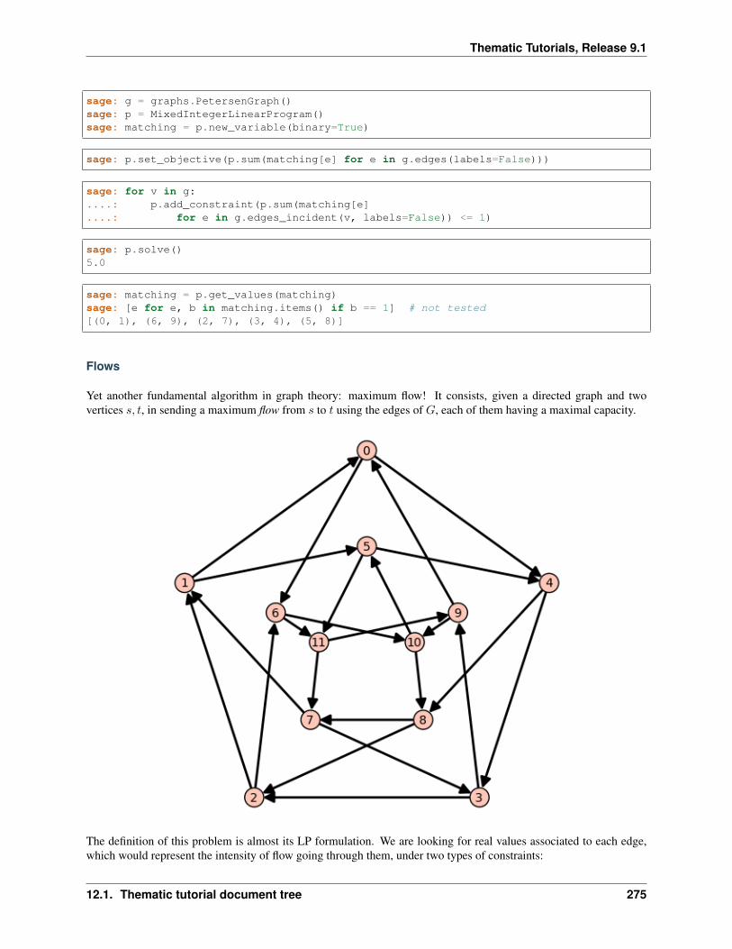
Thematic Tutorials, Release 9.1
sage: g = graphs.PetersenGraph()sage: p = MixedIntegerLinearProgram()sage: matching = p.new_variable(binary=True)
sage: p.set_objective(p.sum(matching[e] for e in g.edges(labels=False)))
sage: for v in g:....: p.add_constraint(p.sum(matching[e]....: for e in g.edges_incident(v, labels=False)) <= 1)
sage: p.solve()5.0
sage: matching = p.get_values(matching)sage: [e for e, b in matching.items() if b == 1] # not tested[(0, 1), (6, 9), (2, 7), (3, 4), (5, 8)]
Flows
Yet another fundamental algorithm in graph theory: maximum flow! It consists, given a directed graph and twovertices 𝑠, 𝑡, in sending a maximum flow from 𝑠 to 𝑡 using the edges of 𝐺, each of them having a maximal capacity.
The definition of this problem is almost its LP formulation. We are looking for real values associated to each edge,which would represent the intensity of flow going through them, under two types of constraints:
12.1. Thematic tutorial document tree 275
Thematic Tutorials, Release 9.1
• The amount of flow arriving on a vertex (different from 𝑠 or 𝑡) is equal to the amount of flow leaving it.
• The amount of flow going through an edge is bounded by the capacity of this edge.
This being said, we have to maximize the amount of flow leaving 𝑠: all of it will end up in 𝑡, as the other vertices aresending just as much as they receive. We can model the flow problem with the following LP
Max:∑𝑠𝑣∈𝐺
𝑓𝑠𝑣
Such that: ∀𝑣 ∈ 𝐺, 𝑣 =𝑠𝑣 =𝑡,
∑𝑣𝑢∈𝐺
𝑓𝑣𝑢 −∑𝑢𝑣∈𝐺
𝑓𝑢𝑣 = 0
∀𝑢𝑣 ∈ 𝐺, 𝑓𝑢𝑣 ≤ 1
We will solve the flow problem on an orientation of Chvatal’s graph, in which all the edges have a capacity of 1:
sage: g = graphs.ChvatalGraph()sage: g = g.minimum_outdegree_orientation()
sage: p = MixedIntegerLinearProgram()sage: f = p.new_variable(real=True, nonnegative=True)sage: s, t = 0, 2
sage: for v in g:....: if v != s and v != t:....: p.add_constraint(....: p.sum(f[v,u] for u in g.neighbors_out(v))....: - p.sum(f[u,v] for u in g.neighbors_in(v)) == 0)
sage: for e in g.edges(labels=False):....: p.add_constraint(f[e] <= 1)
sage: p.set_objective(p.sum(f[s,u] for u in g.neighbors_out(s)))
sage: p.solve() # rel tol 2e-112.0
276 Chapter 12. Documentation
Thematic Tutorials, Release 9.1
Solvers (backends)
Sage solves linear programs by calling specific libraries. The following libraries are currently supported:
• CBC: A solver from COIN-OR, provided under the Eclipse Public License (EPL), which is an open sourcelicense but incompatible with GPL. CBC and the Sage CBC backend can be installed using the shell command:
$ sage -i -c sage_numerical_backends_coin
• CPLEX: Proprietary, but available for free for researchers and students through IBM’s Academic Initiative.Since trac ticket #27790, only versions 12.8 and above are supported.
Install CPLEX according to the instructions on the website, which includes obtaining a license key.
Then find the installation directory of your ILOG CPLEX Studio installation, which contains subdirectoriescplex, doc, opl, etc. Set the environment variable CPLEX_HOME to this directory; for example using thefollowing shell command (on macOS):
$ export CPLEX_HOME=/Applications/CPLEX_Studio1210
or (on Linux):
12.1. Thematic tutorial document tree 277
Thematic Tutorials, Release 9.1
$ export CPLEX_HOME=/opt/ibm/ILOG/CPLEX_Studio1210
Now verify that the CPLEX binary that you will find in the subdirectory cplex/bin/ARCH-OS starts cor-rectly, for example:
$ $CPLEX_HOME/cplex/bin/x86-64_osx/cplexWelcome to IBM(R) ILOG(R) CPLEX(R) Interactive Optimizer...
This environment variable only needs to be set for the following step: Install the Sage CPLEX backend usingthe shell command:
$ sage -i -c sage_numerical_backends_cplex
• CVXOPT: an LP solver from Python Software for Convex Optimization, uses an interior-point method, alwaysinstalled in Sage.
Licensed under the GPL.
• GLPK: A solver from GNU
Licensed under the GPLv3. This solver is always installed, as the default one, in Sage.
• Gurobi: Proprietary, but available for free for researchers and students via Gurobi’s Academic Program.
Install Gurobi according to the instructions on the website, which includes obtaining a license key. The instal-lation should make the interactive Gurobi shell gurobi.sh available in your PATH. Verify this by typing theshell command gurobi.sh:
$ gurobi.shPython 3.7.4 (default, Aug 27 2019, 11:27:39)...Gurobi Interactive Shell (mac64), Version 9.0.0Copyright (c) 2019, Gurobi Optimization, LLCType "help()" for helpgurobi>
If this does not work, adjust your PATH or create symbolic links so that gurobi.sh is found.
Now install the Sage Gurobi backend using the shell command:
$ sage -i -c sage_numerical_backends_gurobi
• PPL: A solver from bugSeng.
This solver provides exact (arbitrary precision) computation, always installed in Sage.
Licensed under the GPLv3.
12.1.8 Number Theory and the RSA Public Key Cryptosystem
Author: Minh Van Nguyen <[email protected]>
This tutorial uses Sage to study elementary number theory and the RSA public key cryptosystem. A number of Sagecommands will be presented that help us to perform basic number theoretic operations such as greatest commondivisor and Euler’s phi function. We then present the RSA cryptosystem and use Sage’s built-in commands to encryptand decrypt data via the RSA algorithm. Note that this tutorial on RSA is for pedagogy purposes only. For furtherdetails on cryptography or the security of various cryptosystems, consult specialized texts such as [MenezesEtAl1996],[Stinson2006], and [TrappeWashington2006].
278 Chapter 12. Documentation
Thematic Tutorials, Release 9.1
Elementary number theory
We first review basic concepts from elementary number theory, including the notion of primes, greatest commondivisors, congruences and Euler’s phi function. The number theoretic concepts and Sage commands introduced willbe referred to in later sections when we present the RSA algorithm.
Prime numbers
Public key cryptography uses many fundamental concepts from number theory, such as prime numbers and greatestcommon divisors. A positive integer 𝑛 > 1 is said to be prime if its factors are exclusively 1 and itself. In Sage, wecan obtain the first 20 prime numbers using the command primes_first_n:
sage: primes_first_n(20)[2, 3, 5, 7, 11, 13, 17, 19, 23, 29, 31, 37, 41, 43, 47, 53, 59, 61, 67, 71]
Greatest common divisors
Let 𝑎 and 𝑏 be integers, not both zero. Then the greatest common divisor (GCD) of 𝑎 and 𝑏 is the largest positiveinteger which is a factor of both 𝑎 and 𝑏. We use gcd(𝑎, 𝑏) to denote this largest positive factor. One can extend thisdefinition by setting gcd(0, 0) = 0. Sage uses gcd(a, b) to denote the GCD of 𝑎 and 𝑏. The GCD of any twodistinct primes is 1, and the GCD of 18 and 27 is 9.
sage: gcd(3, 59)1sage: gcd(18, 27)9
If gcd(𝑎, 𝑏) = 1, we say that 𝑎 is coprime (or relatively prime) to 𝑏. In particular, gcd(3, 59) = 1 so 3 is coprime to59 and vice versa.
Congruences
When one integer is divided by a non-zero integer, we usually get a remainder. For example, upon dividing 23 by 5, weget a remainder of 3; when 8 is divided by 5, the remainder is again 3. The notion of congruence helps us to describethe situation in which two integers have the same remainder upon division by a non-zero integer. Let 𝑎, 𝑏, 𝑛 ∈ Z suchthat 𝑛 = 0. If 𝑎 and 𝑏 have the same remainder upon division by 𝑛, then we say that 𝑎 is congruent to 𝑏 modulo 𝑛 anddenote this relationship by
𝑎 ≡ 𝑏 (mod 𝑛)
This definition is equivalent to saying that 𝑛 divides the difference of 𝑎 and 𝑏, i.e. 𝑛 | (𝑎− 𝑏). Thus 23 ≡ 8 (mod 5)because when both 23 and 8 are divided by 5, we end up with a remainder of 3. The command mod allows us tocompute such a remainder:
sage: mod(23, 5)3sage: mod(8, 5)3
12.1. Thematic tutorial document tree 279
Thematic Tutorials, Release 9.1
Euler’s phi function
Consider all the integers from 1 to 20, inclusive. List all those integers that are coprime to 20. In other words, we wantto find those integers 𝑛, where 1 ≤ 𝑛 ≤ 20, such that gcd(𝑛, 20) = 1. The latter task can be easily accomplished witha little bit of Sage programming:
sage: L = []sage: for n in range(1, 21):....: if gcd(n, 20) == 1:....: L.append(n)sage: L[1, 3, 7, 9, 11, 13, 17, 19]
The above programming statements can be saved to a text file called, say, /home/mvngu/totient.sage, orga-nizing it as follows to enhance readability.
L = []for n in range(1, 21):
if gcd(n, 20) == 1:L.append(n)
L
We refer to totient.sage as a Sage script, just as one would refer to a file containing Python code as a Pythonscript. We use 4 space indentations, which is a coding convention in Sage as well as Python programming, instead oftabs.
The command load can be used to read the file containing our programming statements into Sage and, upon loadingthe content of the file, have Sage execute those statements:
load("/home/mvngu/totient.sage")[1, 3, 7, 9, 11, 13, 17, 19]
From the latter list, there are 8 integers in the closed interval [1, 20] that are coprime to 20. Without explicitly gener-ating the list
1 3 7 9 11 13 17 19
how can we compute the number of integers in [1, 20] that are coprime to 20? This is where Euler’s phi functioncomes in handy. Let 𝑛 ∈ Z be positive. Then Euler’s phi function counts the number of integers 𝑎, with 1 ≤ 𝑎 ≤ 𝑛,such that gcd(𝑎, 𝑛) = 1. This number is denoted by 𝜙(𝑛). Euler’s phi function is sometimes referred to as Euler’stotient function, hence the name totient.sage for the above Sage script. The command euler_phi implementsEuler’s phi function. To compute 𝜙(20) without explicitly generating the above list, we proceed as follows:
sage: euler_phi(20)8
How to keep a secret?
Cryptography is the science (some might say art) of concealing data. Imagine that we are composing a confidentialemail to someone. Having written the email, we can send it in one of two ways. The first, and usually convenient,way is to simply press the send button and not care about how our email will be delivered. Sending an email in thismanner is similar to writing our confidential message on a postcard and post it without enclosing our postcard inside anenvelope. Anyone who can access our postcard can see our message. On the other hand, before sending our email, wecan scramble the confidential message and then press the send button. Scrambling our message is similar to enclosing
280 Chapter 12. Documentation
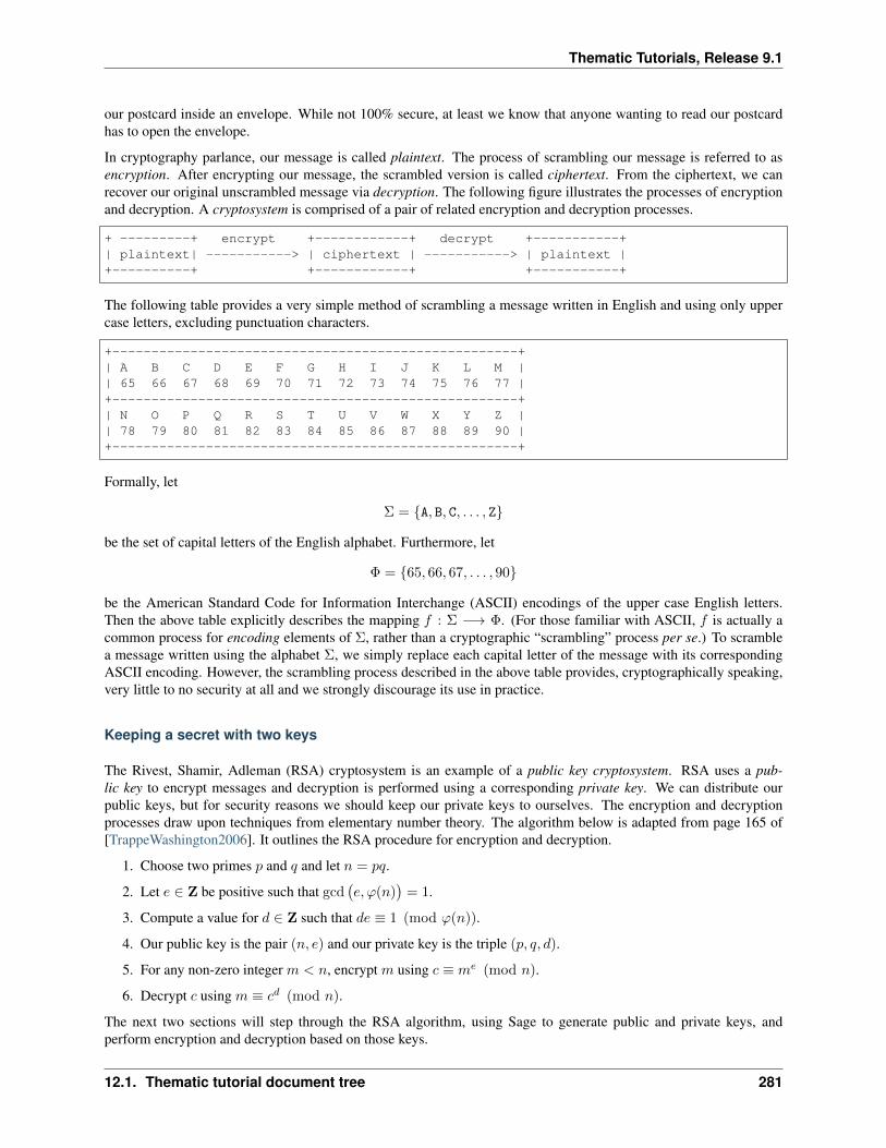
Thematic Tutorials, Release 9.1
our postcard inside an envelope. While not 100% secure, at least we know that anyone wanting to read our postcardhas to open the envelope.
In cryptography parlance, our message is called plaintext. The process of scrambling our message is referred to asencryption. After encrypting our message, the scrambled version is called ciphertext. From the ciphertext, we canrecover our original unscrambled message via decryption. The following figure illustrates the processes of encryptionand decryption. A cryptosystem is comprised of a pair of related encryption and decryption processes.
+ ---------+ encrypt +------------+ decrypt +-----------+| plaintext| -----------> | ciphertext | -----------> | plaintext |+----------+ +------------+ +-----------+
The following table provides a very simple method of scrambling a message written in English and using only uppercase letters, excluding punctuation characters.
+----------------------------------------------------+| A B C D E F G H I J K L M || 65 66 67 68 69 70 71 72 73 74 75 76 77 |+----------------------------------------------------+| N O P Q R S T U V W X Y Z || 78 79 80 81 82 83 84 85 86 87 88 89 90 |+----------------------------------------------------+
Formally, let
Σ = A, B, C, . . . , Z
be the set of capital letters of the English alphabet. Furthermore, let
Φ = 65, 66, 67, . . . , 90
be the American Standard Code for Information Interchange (ASCII) encodings of the upper case English letters.Then the above table explicitly describes the mapping 𝑓 : Σ −→ Φ. (For those familiar with ASCII, 𝑓 is actually acommon process for encoding elements of Σ, rather than a cryptographic “scrambling” process per se.) To scramblea message written using the alphabet Σ, we simply replace each capital letter of the message with its correspondingASCII encoding. However, the scrambling process described in the above table provides, cryptographically speaking,very little to no security at all and we strongly discourage its use in practice.
Keeping a secret with two keys
The Rivest, Shamir, Adleman (RSA) cryptosystem is an example of a public key cryptosystem. RSA uses a pub-lic key to encrypt messages and decryption is performed using a corresponding private key. We can distribute ourpublic keys, but for security reasons we should keep our private keys to ourselves. The encryption and decryptionprocesses draw upon techniques from elementary number theory. The algorithm below is adapted from page 165 of[TrappeWashington2006]. It outlines the RSA procedure for encryption and decryption.
1. Choose two primes 𝑝 and 𝑞 and let 𝑛 = 𝑝𝑞.
2. Let 𝑒 ∈ Z be positive such that gcd(𝑒, 𝜙(𝑛)
)= 1.
3. Compute a value for 𝑑 ∈ Z such that 𝑑𝑒 ≡ 1 (mod 𝜙(𝑛)).
4. Our public key is the pair (𝑛, 𝑒) and our private key is the triple (𝑝, 𝑞, 𝑑).
5. For any non-zero integer 𝑚 < 𝑛, encrypt 𝑚 using 𝑐 ≡ 𝑚𝑒 (mod 𝑛).
6. Decrypt 𝑐 using 𝑚 ≡ 𝑐𝑑 (mod 𝑛).
The next two sections will step through the RSA algorithm, using Sage to generate public and private keys, andperform encryption and decryption based on those keys.
12.1. Thematic tutorial document tree 281
Thematic Tutorials, Release 9.1
Generating public and private keys
Positive integers of the form 𝑀𝑚 = 2𝑚 − 1 are called Mersenne numbers. If 𝑝 is prime and 𝑀𝑝 = 2𝑝 − 1 is alsoprime, then 𝑀𝑝 is called a Mersenne prime. For example, 31 is prime and 𝑀31 = 231 − 1 is a Mersenne prime, ascan be verified using the command is_prime(p). This command returns True if its argument p is precisely aprime number; otherwise it returns False. By definition, a prime must be a positive integer, hence is_prime(-2)returns False although we know that 2 is prime. Indeed, the number 𝑀61 = 261 − 1 is also a Mersenne prime. Wecan use 𝑀31 and 𝑀61 to work through step 1 in the RSA algorithm:
sage: p = (2^31) - 1sage: is_prime(p)Truesage: q = (2^61) - 1sage: is_prime(q)Truesage: n = p * q ; n4951760154835678088235319297
A word of warning is in order here. In the above code example, the choice of 𝑝 and 𝑞 as Mersenne primes, and with somany digits far apart from each other, is a very bad choice in terms of cryptographic security. However, we shall usethe above chosen numeric values for 𝑝 and 𝑞 for the remainder of this tutorial, always bearing in mind that they havebeen chosen for pedagogy purposes only. Refer to [MenezesEtAl1996], [Stinson2006], and [TrappeWashington2006]for in-depth discussions on the security of RSA, or consult other specialized texts.
For step 2, we need to find a positive integer that is coprime to 𝜙(𝑛). The set of integers is implemented within theSage module sage.rings.integer_ring. Various operations on integers can be accessed via the ZZ.* familyof functions. For instance, the command ZZ.random_element(n) returns a pseudo-random integer uniformlydistributed within the closed interval [0, 𝑛− 1].
We can compute the value 𝜙(𝑛) by calling the sage function euler_phi(n), but for arbitrarily large prime numbers𝑝 and 𝑞, this can take an enormous amount of time. Indeed, the private key can be quickly deduced from the publickey once you know 𝜙(𝑛), so it is an important part of the security of the RSA cryptosystem that 𝜙(𝑛) cannot becomputed in a short time, if only 𝑛 is known. On the other hand, if the private key is available, we can compute𝜙(𝑛) = (𝑝− 1)(𝑞 − 1) in a very short time.
Using a simple programming loop, we can compute the required value of 𝑒 as follows:
sage: p = (2^31) - 1sage: q = (2^61) - 1sage: n = p * qsage: phi = (p - 1)*(q - 1); phi4951760152529835076874141700sage: e = ZZ.random_element(phi)sage: while gcd(e, phi) != 1:....: e = ZZ.random_element(phi)...sage: e # random1850567623300615966303954877sage: e < nTrue
As e is a pseudo-random integer, its numeric value changes after each execution of e = ZZ.random_element(phi).
To calculate a value for d in step 3 of the RSA algorithm, we use the extended Euclidean algorithm. By definition ofcongruence, 𝑑𝑒 ≡ 1 (mod 𝜙(𝑛)) is equivalent to
𝑑𝑒− 𝑘 · 𝜙(𝑛) = 1
282 Chapter 12. Documentation
Thematic Tutorials, Release 9.1
where 𝑘 ∈ Z. From steps 1 and 2, we already know the numeric values of 𝑒 and 𝜙(𝑛). The extended Euclideanalgorithm allows us to compute 𝑑 and −𝑘. In Sage, this can be accomplished via the command xgcd. Given twointegers 𝑥 and 𝑦, xgcd(x, y) returns a 3-tuple (g, s, t) that satisfies the Bézout identity 𝑔 = gcd(𝑥, 𝑦) =𝑠𝑥 + 𝑡𝑦. Having computed a value for d, we then use the command mod(d*e, phi) to check that d*e is indeedcongruent to 1 modulo phi.
sage: n = 4951760154835678088235319297sage: e = 1850567623300615966303954877sage: phi = 4951760152529835076874141700sage: bezout = xgcd(e, phi); bezout # random(1, 4460824882019967172592779313, -1667095708515377925087033035)sage: d = Integer(mod(bezout[1], phi)) ; d # random4460824882019967172592779313sage: mod(d * e, phi)1
Thus, our RSA public key is
(𝑛, 𝑒) = (4951760154835678088235319297, 1850567623300615966303954877)
and our corresponding private key is
(𝑝, 𝑞, 𝑑) = (2147483647, 2305843009213693951, 4460824882019967172592779313)
Encryption and decryption
Suppose we want to scramble the message HELLOWORLD using RSA encryption. From the above ASCII table, ourmessage maps to integers of the ASCII encodings as given below.
+----------------------------------------+| H E L L O W O R L D || 72 69 76 76 79 87 79 82 76 68 |+----------------------------------------+
Concatenating all the integers in the last table, our message can be represented by the integer
𝑚 = 72697676798779827668
There are other more cryptographically secure means for representing our message as an integer. The above process isused for demonstration purposes only and we strongly discourage its use in practice. In Sage, we can obtain an integerrepresentation of our message as follows:
sage: m = "HELLOWORLD"sage: m = [ord(x) for x in m]; m[72, 69, 76, 76, 79, 87, 79, 82, 76, 68]sage: m = ZZ(list(reversed(m)), 100) ; m72697676798779827668
To encrypt our message, we raise 𝑚 to the power of 𝑒 and reduce the result modulo 𝑛. The command mod(a^b, n)first computes a^b and then reduces the result modulo n. If the exponent b is a “large” integer, say with more than20 digits, then performing modular exponentiation in this naive manner takes quite some time. Brute force (or naive)modular exponentiation is inefficient and, when performed using a computer, can quickly consume a huge quantityof the computer’s memory or result in overflow messages. For instance, if we perform naive modular exponentiationusing the command mod(m^e, n), where m, n and e are as given above, we would get an error message similar tothe following:
12.1. Thematic tutorial document tree 283
Thematic Tutorials, Release 9.1
mod(m^e, n)Traceback (most recent call last)/home/mvngu/<ipython console> in <module>()/home/mvngu/usr/bin/sage-3.1.4/local/lib/python2.5/site-packages/sage/rings/integer.soin sage.rings.integer.Integer.__pow__ (sage/rings/integer.c:9650)()RuntimeError: exponent must be at most 2147483647
There is a trick to efficiently perform modular exponentiation, called the method of repeated squaring, cf. page 879 of[CormenEtAl2001]. Suppose we want to compute 𝑎𝑏 mod 𝑛. First, let 𝑑 := 1 and obtain the binary representationof 𝑏, say (𝑏1, 𝑏2, . . . , 𝑏𝑘) where each 𝑏𝑖 ∈ Z/2Z. For 𝑖 := 1, . . . , 𝑘, let 𝑑 := 𝑑2 mod 𝑛 and if 𝑏𝑖 = 1 then let 𝑑 := 𝑑𝑎mod 𝑛. This algorithm is implemented in the function power_mod. We now use the function power_mod toencrypt our message:
sage: m = 72697676798779827668sage: e = 1850567623300615966303954877sage: n = 4951760154835678088235319297sage: c = power_mod(m, e, n); c630913632577520058415521090
Thus 𝑐 = 630913632577520058415521090 is the ciphertext. To recover our plaintext, we raise c to the power ofd and reduce the result modulo n. Again, we use modular exponentiation via repeated squaring in the decryptionprocess:
sage: m = 72697676798779827668sage: c = 630913632577520058415521090sage: d = 4460824882019967172592779313sage: n = 4951760154835678088235319297sage: power_mod(c, d, n)72697676798779827668sage: power_mod(c, d, n) == mTrue
Notice in the last output that the value 72697676798779827668 is the same as the integer that represents our originalmessage. Hence we have recovered our plaintext.
Acknowledgements
1. 2009-07-25: Ron Evans (Department of Mathematics, UCSD) reported a typo in the definition of greatestcommon divisors. The revised definition incorporates his suggestions.
2. 2008-11-04: Martin Albrecht (Information Security Group, Royal Holloway, University of London), John Cre-mona (Mathematics Institute, University of Warwick) and William Stein (Department of Mathematics, Univer-sity of Washington) reviewed this tutorial. Many of their invaluable suggestions have been incorporated into thisdocument.
Bibliography
12.1.9 Coding Theory in Sage
Author: David Joyner and Robert Miller (2008), edited by Ralf Stephan for the initial version. David Lucas (2016)for this version.
This tutorial, designed for beginners who want to discover how to use Sage for their work (research, experimentation,teaching) on coding theory, will present several key features of Sage’s coding theory library and explain how to findclasses and methods you look for.
284 Chapter 12. Documentation
Thematic Tutorials, Release 9.1
During this tutorial, we will cover the following parts:
• what can you do with generic linear codes and associated methods,
• what can you do with structured code families,
• what can you do to encode and recover messages, correct errors and
• what can you do to easily add errors to codewords.
The goal of this tutorial is to give a quick overview of what can be done with the library and how to use the mainfunctionalities. It is neither a comprehensive description of all methods nor of specific classes. If one needs somespecific information on the behaviour of a class/method related to coding theory, one should check the documentationfor this class/method.
Table of contents
• Coding Theory in Sage
– I. Generic Linear codes and associated methods
– II. Structured code families and an overview of the encoding and decoding system
* II.1 Create specific codes in Sage
* II.2 Encode and decode in Sage
– III. A deeper view of the Encoder and Decoder structure
* III.1 Message spaces
* III.2 Generator matrices
* III.3 Decoders and messages
– IV. A deeper look at channels
* A channel for errors and erasures
– V. Conclusion - Afterword
I. Generic Linear codes and associated methods
Let us start with the most generic code one can build: a generic linear code without any specific structure.
To build such a code, one just need to provide its generator matrix, as follows:
sage: G = matrix(GF(3), [[1, 0, 0, 0, 1, 2, 1],....: [0, 1, 0, 0, 2, 1, 0],....: [0, 0, 1, 2, 2, 2, 2]])sage: C = LinearCode(G)
With these lines, you just created a linear code, congratulations! Note that if you pass a matrix which is not full rank,Sage will turn it into a full-rank matrix before building the code, as illustrated in the following example:
sage: G = matrix(GF(3), [[1, 0, 0, 0, 1, 2, 1],....: [0, 1, 0, 0, 2, 1, 0],....: [0, 0, 1, 2, 2, 2, 2],....: [1, 0, 1, 2, 0, 1, 0]]) #r3 = r0 + r2sage: C = LinearCode(G)sage: C.generator_matrix()
(continues on next page)
12.1. Thematic tutorial document tree 285
Thematic Tutorials, Release 9.1
(continued from previous page)
[1 0 0 0 1 2 1][0 1 0 0 2 1 0][0 0 1 2 2 2 2]
We now have a linear code. . . What can we do with it? As we can a lot of things, let us start with the basic function-alities.
In the example just above, we already asked for the code’s generator matrix. It is also possible to ask the code for itsbasic parameters: its length and dimension as illustrated therafter:
sage: C.length()7sage: C.dimension()3
It is also possible to ask for our code’s minimum distance:
sage: C.minimum_distance()3
Of course, as C is a generic linear code, an exhaustive search algorithm is run to find the minimum distance, whichwill be slower and slower as the code grows.
By just typing the name of our code, we get a sentence which briefly describes it and gives its parameters:
sage: C[7, 3] linear code over GF(3)
As the aim of this tutorial is not to give a comprehensive view of the methods, we won’t describe any other methods.
If one wants to get all methods that can be run on a linear code, one can:
• either check the manual page of the file Linear codes
• or type:
C.<tab>
in Sage to get a list of all available methods for C. Afterwards, typing:
C.method?
will show the manual page for method.
Note: Some generic methods require the installation of the optional package Guava for Gap. While some work isdone to always propose a default implementation which does not require an optional package, there exist some methodswhich are not up to date - yet. If you’re receiving an error message related to Gap, please check the documentation ofthe method to verify if Guava has to be installed.
II. Structured code families and an overview of the encoding and decoding system
II.1 Create specific codes in Sage
Now that we know how to create generic linear codes, we want to go deeper and create specific code families. In Sage,all codes families can be accessed by typing:
286 Chapter 12. Documentation
Thematic Tutorials, Release 9.1
codes.<tab>
Doing so, you will get the comprehensive list of all code families Sage can build.
For the rest of this section, we will illustrate specific functionalities of these code families by manipulating sage.coding.grs_code.GeneralizedReedSolomonCode.
So, for starters, we want to create a Generalized Reed-Solomon (GRS) code.
By clicking on the link provided above, or typing:
codes.GeneralizedReedSolomonCode?
one can access the documentation page for GRS codes, find a definition of these and learn what is needed to build onein Sage.
Here we choose to build a [12, 6] GRS code over F13. To do this, we need up to three elements:
• The list of evaluation points,
• the dimension of the code, and
• optionally, the list of column multipliers.
We build our code as follows:
sage: F = GF(13)sage: length, dimension = 12, 6sage: evaluation_pts = F.list()[:length]sage: column_mults = F.list()[1:length+1]sage: C = codes.GeneralizedReedSolomonCode(evaluation_pts, dimension, column_mults)
Our GRS code is now created. We can ask for its parameters, as we did in the previous section:
sage: C.length()12sage: C.dimension()6sage: C.base_ring()Finite Field of size 13
It is also possible to ask for the evaluation points and the column multipliers by calling sage.coding.grs_code.GeneralizedReedSolomonCode.evaluation_points() and sage.coding.grs_code.GeneralizedReedSolomonCode.column_multipliers().
Now, if you know some theory for GRS codes, you know that it’s especially easy to compute their minimum distance,which is: 𝑑 = 𝑛− 𝑘 + 1, where 𝑛 is the length of the code and 𝑘 is the dimension of the code.
Because Sage knows C is a GRS code, it will not run the exhaustive search algorithm presented in section I to find C’sminimum distance but use the operation introduced above. And you instantly get:
sage: C.minimum_distance()7
All these parameters are summarized inside the string representation of our code:
sage: C[12, 6, 7] Generalized Reed-Solomon Code over GF(13)
12.1. Thematic tutorial document tree 287
Thematic Tutorials, Release 9.1
Note: Writing proper classes for code families is a work in progress. Some constructions under codes.<tab>might thus be functions which build a generic linear code, and in that case are only able to use generic algorithms.Please refer to the documentation of a construction to check if it is a function or a class.
II.2 Encode and decode in Sage
In the previous part, we learnt how to find specific code families in Sage and create instances of these families.
In this part, we will learn how to encode and decode.
First of all, we want to generate a codeword to play with. There is two different ways to do that:
• It is possible to just generate a random element of our code, as follows:
sage: c = C.random_element()sage: c in CTrue
• Alternatively, we can create a message and then encode it into a codeword:
sage: msg = random_vector(C.base_field(), C.dimension())sage: c = C.encode(msg)sage: c in CTrue
Either way, we obtained a codeword. So, we might want to put some errors in it, and try to correct these errorsafterwards. We can obviously do it by changing the values at some random positions of our codeword, but we proposehere something more general: communication channels. sage.coding.channel.Channel objects are meant asabstractions for communication channels and for manipulation of data representation. In this case, we want to emulatea communication channel which adds some, but not too many, errors to a transmitted word:
sage: err = 3sage: Chan = channels.StaticErrorRateChannel(C.ambient_space(), err)sage: ChanStatic error rate channel creating 3 errors, of input and output space Vector space→˓of dimension 12 over Finite Field of size 13sage: r = Chan.transmit(c)sage: len((c-r).nonzero_positions())3
If you want to learn more on Channels, please refer to section IV of this tutorial.
Thanks to our channel, we got a “received word‘, r, as a codeword with errors on it. We can try to correct the errorsand recover the original codeword:
sage: c_dec = C.decode_to_code(r)sage: c_dec == cTrue
Perhaps we want the original message back rather than the codeword. All we have to do then is to unencode it back tothe message space:
sage: m_unenc = C.unencode(c_dec)sage: m_unenc == msgTrue
288 Chapter 12. Documentation
Thematic Tutorials, Release 9.1
It is also possible to perform the two previous operations (correct the errors and recover the original message) in oneline, as illustrated below:
sage: m_unenc2 = C.decode_to_message(r)sage: m_unenc2 == msgTrue
III. A deeper view of the Encoder and Decoder structure
In the previous section, we saw that encoding, decoding and unencoding a vector can be easily done using methodsdirectly on the code object. These methods are actually shortcuts, added for usability, for when one does not care morespecifically about how encoding and decoding takes place. At some point, however, one might need more control.
This section will thus go into details on the mechanism of Encoders and Decoders.
At the core, the three mentioned operations are handled by sage.coding.encoder.Encoder and sage.coding.decoder.Decoder. These objects possess their own methods to operate on words. When one calls(as seen above):
C.encode(msg)
one actually calls the method sage.coding.encoder.Encoder.encode() on the default encoder of C. Everycode object possess a list of encoders and decoders it can use. Let us see how one can explore this:
sage: C = codes.GeneralizedReedSolomonCode(GF(59).list()[:40], 12, GF(59).→˓list()[1:41])sage: C.encoders_available()['EvaluationPolynomial', 'EvaluationVector', 'Systematic']sage: C.decoders_available()['BerlekampWelch','ErrorErasure','Gao','GuruswamiSudan','InformationSet','KeyEquationSyndrome','NearestNeighbor','Syndrome']
We got a list of the available encoders and decoders for our GRS code. Rather than using the default ones as we didbefore, we can now ask for specific encoder and decoder:
sage: Evect = C.encoder("EvaluationVector")sage: EvectEvaluation vector-style encoder for [40, 12, 29] Generalized Reed-Solomon Code over→˓GF(59)sage: type(Evect)<class 'sage.coding.grs_code.GRSEvaluationVectorEncoder'>sage: msg = random_vector(GF(59), C.dimension()) #randomsage: c = Evect.encode(msg)sage: NN = C.decoder("NearestNeighbor")sage: NNNearest neighbor decoder for [40, 12, 29] Generalized Reed-Solomon Code over GF(59)
Calling:
C.encoder(encoder_name)
12.1. Thematic tutorial document tree 289
Thematic Tutorials, Release 9.1
is actually a short-hand for constructing the encoder manually, by calling the constructor for sage.coding.grs_code.EncoderGRSEvaluationVector yourself. If you don’t supply encoder_name to sage.coding.linear_code.AbstractLinearCode.encoder() you get the default encoder for the code.sage.coding.linear_code.AbstractLinearCode.encoder() also has an important side-effect: itcaches the constructed encoder before returning it. This means that each time one will access the sameEvaluationVector encoder for C, which saves construction time.
All the above things are similar for Decoders. This reinforces that Encoders and Decoders are rarely constructed butused many times, which allows them to perform expensive precomputation at construction or first use, for the benefitof future use.
This gives a good idea of how the elements work internally. Let us now go a bit more into details on specific points.
III.1 Message spaces
The point of an Encoder is to encode messages into the code. These messages are often just vectors over the basefield of the code and whose length matches the code’s dimension. But it could be anything: vectors over otherfields, polynomials, or even something quite different. Therefore, each Encoder has a sage.coding.encoder.Encoder.message_space(). For instance, we saw earlier that our GRS code has two possible encoders; let usinvestigate the one we left behind in the part just before:
sage: Epoly = C.encoder("EvaluationPolynomial")sage: EpolyEvaluation polynomial-style encoder for [40, 12, 29] Generalized Reed-Solomon Code→˓over GF(59)sage: Epoly.message_space()Univariate Polynomial Ring in x over Finite Field of size 59sage: msg_p = Epoly.message_space().random_element(degree=C.dimension()-1); msg_p→˓#random31*x^11 + 49*x^10 + 56*x^9 + 31*x^8 + 36*x^6 + 58*x^5 + 9*x^4 + 17*x^3 + 29*x^2 +→˓50*x + 46
Epoly reflects that GRS codes are often constructed as evaluations of polynomials, and that a natural way to considertheir messages is as polynomials of degree at most 𝑘 − 1, where 𝑘 is the dimension of the code. Notice that themessage space of Epoly is all univariate polynomials: message_space is the ambient space of the messages, andsometimes an Encoder demands that the messages are actually picked from a subspace hereof.
The default encoder of a code always has a vector space as message space, so when we call sage.coding.linear_code.AbstractLinearCode.decode_to_message() or sage.coding.linear_code.AbstractLinearCode.unencode() on the code itself, as illustrated on the first example, this will alwaysreturn vectors whose length is the dimension of the code.
III.2 Generator matrices
Whenever the message space of an Encoder is a vector space and it encodes using a linear map, the Encoder willpossess a generator matrix (note that this notion does not make sense for other types of encoders), which specifies thatlinear map.
Generator matrices have been placed on Encoder objects since a code has many generator matrices, and each of thesewill encode messages differently. One will also find sage.coding.linear_code.AbstractLinearCode.generator_matrix() on code objects, but this is again simply a convenience method which forwards the queryto the default encoder.
Let us see this in Sage, using the first encoder we constructed:
290 Chapter 12. Documentation
Thematic Tutorials, Release 9.1
sage: Evect.message_space()Vector space of dimension 12 over Finite Field of size 59sage: G = Evect.generator_matrix()sage: G == C.generator_matrix()True
III.3 Decoders and messages
As we saw before, any code has two generic methods for decoding, called decode_to_codeword anddecode_to_message. Every Decoder also has these two methods, and the methods on the code simply forwardthe calls to the default decoder of this code.
There are two reasons for having these two methods: convenience and speed. Convenience is clear: having bothmethods provides a useful shortcut depending on the user’s needs. Concerning speed, some decoders naturally de-code directly to a codeword, while others directly to a message space. Supporting both methods therefore avoidsunnecessary work in encoding and unencoding.
However, decode_to_message implies that there is a message space and an encoding from that space to the codebehind the scenes. A Decoder has methods message_space and connected_encoder to inform the user aboutthis. Let us illustrate that by a long example:
sage: C = codes.GeneralizedReedSolomonCode(GF(59).list()[1:41], 3, GF(59).→˓list()[1:41])sage: c = C.random_element()sage: c in CTrue
#Create two decoders: Syndrome and Gaosage: Syn = C.decoder("KeyEquationSyndrome")sage: Gao = C.decoder("Gao")
#Check their message spacessage: Syn.message_space()Vector space of dimension 3 over Finite Field of size 59sage: Gao.message_space()Univariate Polynomial Ring in x over Finite Field of size 59
#and now we unencodesage: Syn.decode_to_message(c) #random(55,9,43)
sage: Gao.decode_to_message(c) #random43*x^2 + 9*x + 55
IV. A deeper look at channels
In Section II, we briefly introduced the Channel objects as a way to put errors in a word. In this section, we will lookdeeper at their functionality and introduce a second Channel.
Note: Once again, we chose a specific class as a running example through all this section, as we donot want to make an exhaustive catalog of all channels. If one wants to get this list, one can access it bytyping:
12.1. Thematic tutorial document tree 291
Thematic Tutorials, Release 9.1
channels.<tab>
in Sage.
Consider again the sage.coding.channel.ChannelStaticErrorRate() from before. This is a channelthat places errors in the transmitted vector but within controlled boundaries. We can describe these boundaries in twoways:
• The first one was illustrated in Section II and consists in passing an integer, as shown below:
sage: C = codes.GeneralizedReedSolomonCode(GF(59).list()[:40], 12)sage: t = 14sage: Chan = channels.StaticErrorRateChannel(C.ambient_space(), t)sage: ChanStatic error rate channel creating 14 errors, of input and output space Vector→˓space of dimension 40 over Finite Field of size 59
• We can also pass a tuple of two integers, the first smaller than the second. Then each time a word is transmitted,a random number of errors between these two integers will be added:
sage: t = (1, 14)sage: Chan = channels.StaticErrorRateChannel(C.ambient_space(), t)sage: ChanStatic error rate channel creating between 1 and 14 errors, of input and output→˓space Vector space of dimension 40 over Finite Field of size 59
We already know that a channel has a sage.coding.channel.Channel.transmit() method which willperform transmission over the channel; in this case it will return the transmitted word with some errors in it. Thismethod will always check if the provided word belongs to the input space of the channel. In a case one is absolutelycertain that one’s word is in the input space, one might want to avoid this check, which is time consuming - espe-cially if one is simulating millions of transmissions. For this usage there is sage.coding.channel.Channel.transmit_unsafe() which does the same as sage.coding.channel.Channel.transmit() but with-out checking the input, as illustrated thereafter:
sage: c = C.random_element()sage: c in CTruesage: c_trans = Chan.transmit_unsafe(c)sage: c_trans in CFalse
Note there exists a useful shortcut for sage.coding.channel.Channel.transmit()
sage: r = Chan(c)sage: r in CFalse
A channel for errors and erasures
Let us introduce a new Channel object which adds errors and erasures. When it transmits a word, it both adds someerrors as well as it erases some positions:
292 Chapter 12. Documentation
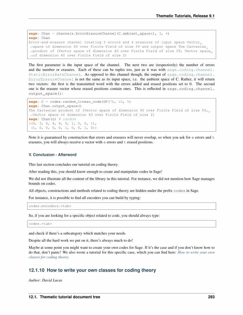
Thematic Tutorials, Release 9.1
sage: Chan = channels.ErrorErasureChannel(C.ambient_space(), 3, 4)sage: ChanError-and-erasure channel creating 3 errors and 4 erasures of input space Vector→˓space of dimension 40 over Finite Field of size 59 and output space The Cartesian→˓product of (Vector space of dimension 40 over Finite Field of size 59, Vector space→˓of dimension 40 over Finite Field of size 2)
The first parameter is the input space of the channel. The next two are (respectively) the number of errorsand the number or erasures. Each of these can be tuples too, just as it was with sage.coding.channel.StaticErrorRateChannel. As opposed to this channel though, the output of sage.coding.channel.ErrorErasureChannel is not the same as its input space, i.e. the ambient space of C. Rather, it will returntwo vectors: the first is the transmitted word with the errors added and erased positions set to 0. The secondone is the erasure vector whose erased positions contain ones. This is reflected in sage.coding.channel.output_space():
sage: C = codes.random_linear_code(GF(7), 10, 5)sage: Chan.output_space()The Cartesian product of (Vector space of dimension 40 over Finite Field of size 59,→˓Vector space of dimension 40 over Finite Field of size 2)sage: Chan(c) # random((0, 3, 6, 4, 4, 0, 1, 0, 0, 1),(1, 0, 0, 0, 0, 1, 0, 0, 1, 0))
Note it is guaranteed by construction that errors and erasures will never overlap, so when you ask for e errors and terasures, you will always receive a vector with e errors and t erased positions.
V. Conclusion - Afterword
This last section concludes our tutorial on coding theory.
After reading this, you should know enough to create and manipulate codes in Sage!
We did not illustrate all the content of the library in this tutorial. For instance, we did not mention how Sage managesbounds on codes.
All objects, constructions and methods related to coding theory are hidden under the prefix codes in Sage.
For instance, it is possible to find all encoders you can build by typing:
codes.encoders.<tab>
So, if you are looking for a specific object related to code, you should always type:
codes.<tab>
and check if there’s a subcategory which matches your needs.
Despite all the hard work we put on it, there’s always much to do!
Maybe at some point you might want to create your own codes for Sage. If it’s the case and if you don’t know how todo that, don’t panic! We also wrote a tutorial for this specific case, which you can find here: How to write your ownclasses for coding theory.
12.1.10 How to write your own classes for coding theory
Author: David Lucas
12.1. Thematic tutorial document tree 293
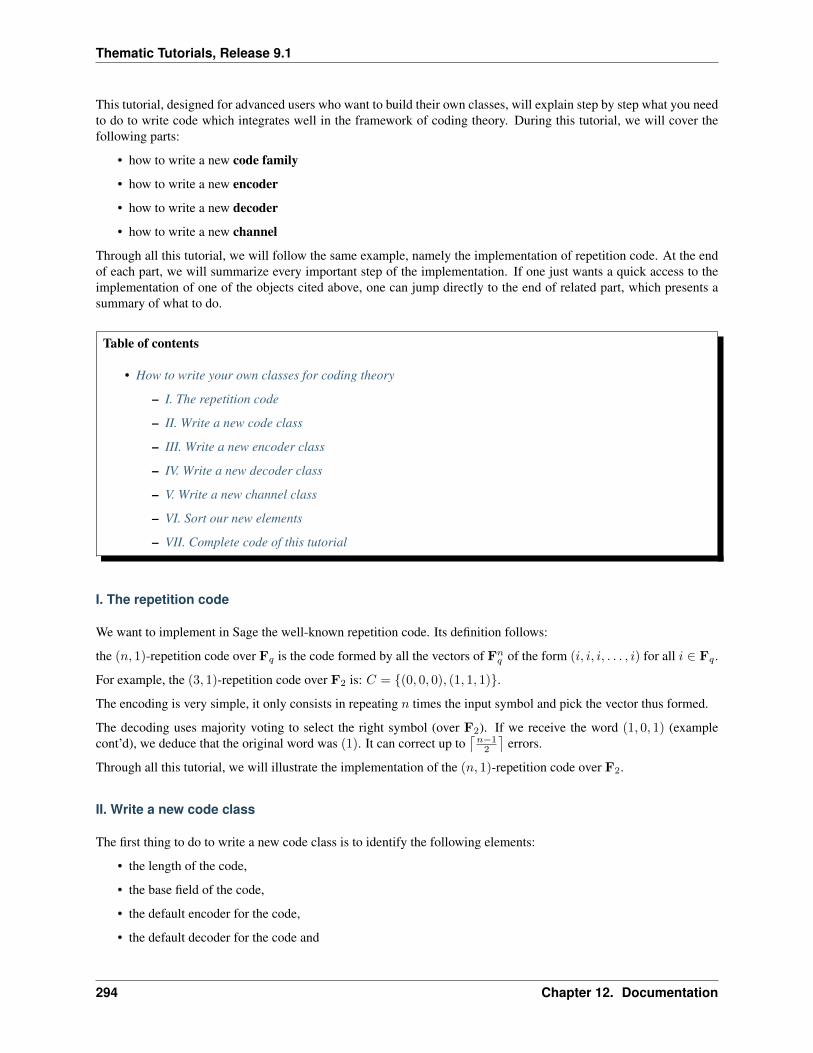
Thematic Tutorials, Release 9.1
This tutorial, designed for advanced users who want to build their own classes, will explain step by step what you needto do to write code which integrates well in the framework of coding theory. During this tutorial, we will cover thefollowing parts:
• how to write a new code family
• how to write a new encoder
• how to write a new decoder
• how to write a new channel
Through all this tutorial, we will follow the same example, namely the implementation of repetition code. At the endof each part, we will summarize every important step of the implementation. If one just wants a quick access to theimplementation of one of the objects cited above, one can jump directly to the end of related part, which presents asummary of what to do.
Table of contents
• How to write your own classes for coding theory
– I. The repetition code
– II. Write a new code class
– III. Write a new encoder class
– IV. Write a new decoder class
– V. Write a new channel class
– VI. Sort our new elements
– VII. Complete code of this tutorial
I. The repetition code
We want to implement in Sage the well-known repetition code. Its definition follows:
the (𝑛, 1)-repetition code over F𝑞 is the code formed by all the vectors of F𝑛𝑞 of the form (𝑖, 𝑖, 𝑖, . . . , 𝑖) for all 𝑖 ∈ F𝑞 .
For example, the (3, 1)-repetition code over F2 is: 𝐶 = (0, 0, 0), (1, 1, 1).
The encoding is very simple, it only consists in repeating 𝑛 times the input symbol and pick the vector thus formed.
The decoding uses majority voting to select the right symbol (over F2). If we receive the word (1, 0, 1) (examplecont’d), we deduce that the original word was (1). It can correct up to
⌈𝑛−12
⌉errors.
Through all this tutorial, we will illustrate the implementation of the (𝑛, 1)-repetition code over F2.
II. Write a new code class
The first thing to do to write a new code class is to identify the following elements:
• the length of the code,
• the base field of the code,
• the default encoder for the code,
• the default decoder for the code and
294 Chapter 12. Documentation
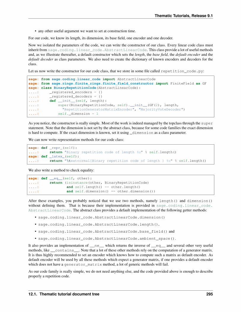
Thematic Tutorials, Release 9.1
• any other useful argument we want to set at construction time.
For our code, we know its length, its dimension, its base field, one encoder and one decoder.
Now we isolated the parameters of the code, we can write the constructor of our class. Every linear code class mustinherit from sage.coding.linear_code.AbstractLinearCode. This class provide a lot of useful methodsand, as we illustrate thereafter, a default constructor which sets the length, the base field, the default encoder and thedefault decoder as class parameters. We also need to create the dictionary of known encoders and decoders for theclass.
Let us now write the constructor for our code class, that we store in some file called repetition_code.py:
sage: from sage.coding.linear_code import AbstractLinearCodesage: from sage.rings.finite_rings.finite_field_constructor import FiniteField as GFsage: class BinaryRepetitionCode(AbstractLinearCode):....: _registered_encoders = ....: _registered_decoders = ....: def __init__(self, length):....: super(BinaryRepetitionCode, self).__init__(GF(2), length,....: "RepetitionGeneratorMatrixEncoder", "MajorityVoteDecoder")....: self._dimension = 1
As you notice, the constructor is really simple. Most of the work is indeed managed by the topclass through the superstatement. Note that the dimension is not set by the abstract class, because for some code families the exact dimensionis hard to compute. If the exact dimension is known, set it using _dimension as a class parameter.
We can now write representation methods for our code class:
sage: def _repr_(self):....: return "Binary repetition code of length %s" % self.length()sage: def _latex_(self):....: return "\textnormalBinary repetition code of length %s" % self.length()
We also write a method to check equality:
sage: def __eq__(self, other):....: return (isinstance(other, BinaryRepetitionCode)....: and self.length() == other.length()....: and self.dimension() == other.dimension())
After these examples, you probably noticed that we use two methods, namely length() and dimension()without defining them. That is because their implementation is provided in sage.coding.linear_code.AbstractLinearCode. The abstract class provides a default implementation of the following getter methods:
• sage.coding.linear_code.AbstractLinearCode.dimension()
• sage.coding.linear_code.AbstractLinearCode.length(),
• sage.coding.linear_code.AbstractLinearCode.base_field() and
• sage.coding.linear_code.AbstractLinearCode.ambient_space().
It also provides an implementation of __ne__ which returns the inverse of __eq__ and several other very usefulmethods, like __contains__. Note that a lot of these other methods rely on the computation of a generator matrix.It is thus highly recommended to set an encoder which knows how to compute such a matrix as default encoder. Asdefault encoder will be used by all these methods which expect a generator matrix, if one provides a default encoderwhich does not have a generator_matrix method, a lot of generic methods will fail.
As our code family is really simple, we do not need anything else, and the code provided above is enough to describeproperly a repetition code.
12.1. Thematic tutorial document tree 295
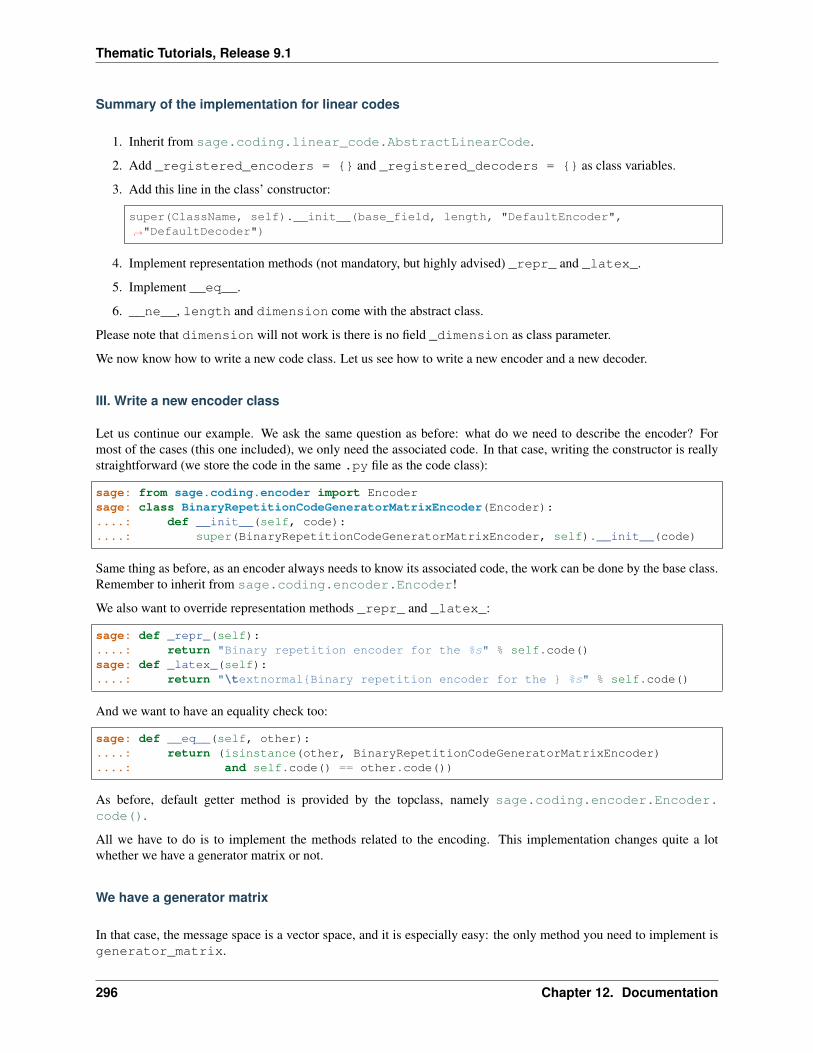
Thematic Tutorials, Release 9.1
Summary of the implementation for linear codes
1. Inherit from sage.coding.linear_code.AbstractLinearCode.
2. Add _registered_encoders = and _registered_decoders = as class variables.
3. Add this line in the class’ constructor:
super(ClassName, self).__init__(base_field, length, "DefaultEncoder",→˓"DefaultDecoder")
4. Implement representation methods (not mandatory, but highly advised) _repr_ and _latex_.
5. Implement __eq__.
6. __ne__, length and dimension come with the abstract class.
Please note that dimension will not work is there is no field _dimension as class parameter.
We now know how to write a new code class. Let us see how to write a new encoder and a new decoder.
III. Write a new encoder class
Let us continue our example. We ask the same question as before: what do we need to describe the encoder? Formost of the cases (this one included), we only need the associated code. In that case, writing the constructor is reallystraightforward (we store the code in the same .py file as the code class):
sage: from sage.coding.encoder import Encodersage: class BinaryRepetitionCodeGeneratorMatrixEncoder(Encoder):....: def __init__(self, code):....: super(BinaryRepetitionCodeGeneratorMatrixEncoder, self).__init__(code)
Same thing as before, as an encoder always needs to know its associated code, the work can be done by the base class.Remember to inherit from sage.coding.encoder.Encoder!
We also want to override representation methods _repr_ and _latex_:
sage: def _repr_(self):....: return "Binary repetition encoder for the %s" % self.code()sage: def _latex_(self):....: return "\textnormalBinary repetition encoder for the %s" % self.code()
And we want to have an equality check too:
sage: def __eq__(self, other):....: return (isinstance(other, BinaryRepetitionCodeGeneratorMatrixEncoder)....: and self.code() == other.code())
As before, default getter method is provided by the topclass, namely sage.coding.encoder.Encoder.code().
All we have to do is to implement the methods related to the encoding. This implementation changes quite a lotwhether we have a generator matrix or not.
We have a generator matrix
In that case, the message space is a vector space, and it is especially easy: the only method you need to implement isgenerator_matrix.
296 Chapter 12. Documentation
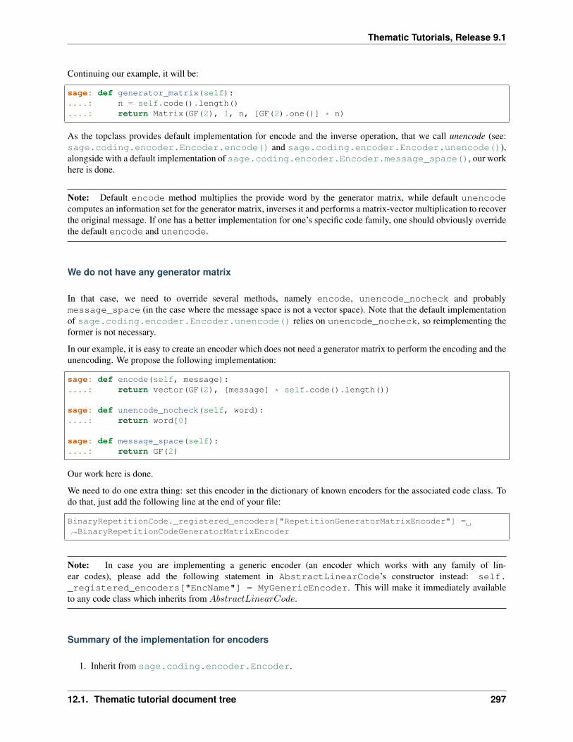
Thematic Tutorials, Release 9.1
Continuing our example, it will be:
sage: def generator_matrix(self):....: n = self.code().length()....: return Matrix(GF(2), 1, n, [GF(2).one()] * n)
As the topclass provides default implementation for encode and the inverse operation, that we call unencode (see:sage.coding.encoder.Encoder.encode() and sage.coding.encoder.Encoder.unencode()),alongside with a default implementation of sage.coding.encoder.Encoder.message_space(), our workhere is done.
Note: Default encode method multiplies the provide word by the generator matrix, while default unencodecomputes an information set for the generator matrix, inverses it and performs a matrix-vector multiplication to recoverthe original message. If one has a better implementation for one’s specific code family, one should obviously overridethe default encode and unencode.
We do not have any generator matrix
In that case, we need to override several methods, namely encode, unencode_nocheck and probablymessage_space (in the case where the message space is not a vector space). Note that the default implementationof sage.coding.encoder.Encoder.unencode() relies on unencode_nocheck, so reimplementing theformer is not necessary.
In our example, it is easy to create an encoder which does not need a generator matrix to perform the encoding and theunencoding. We propose the following implementation:
sage: def encode(self, message):....: return vector(GF(2), [message] * self.code().length())
sage: def unencode_nocheck(self, word):....: return word[0]
sage: def message_space(self):....: return GF(2)
Our work here is done.
We need to do one extra thing: set this encoder in the dictionary of known encoders for the associated code class. Todo that, just add the following line at the end of your file:
BinaryRepetitionCode._registered_encoders["RepetitionGeneratorMatrixEncoder"] =→˓BinaryRepetitionCodeGeneratorMatrixEncoder
Note: In case you are implementing a generic encoder (an encoder which works with any family of lin-ear codes), please add the following statement in AbstractLinearCode’s constructor instead: self._registered_encoders["EncName"] = MyGenericEncoder. This will make it immediately availableto any code class which inherits from 𝐴𝑏𝑠𝑡𝑟𝑎𝑐𝑡𝐿𝑖𝑛𝑒𝑎𝑟𝐶𝑜𝑑𝑒.
Summary of the implementation for encoders
1. Inherit from sage.coding.encoder.Encoder.
12.1. Thematic tutorial document tree 297
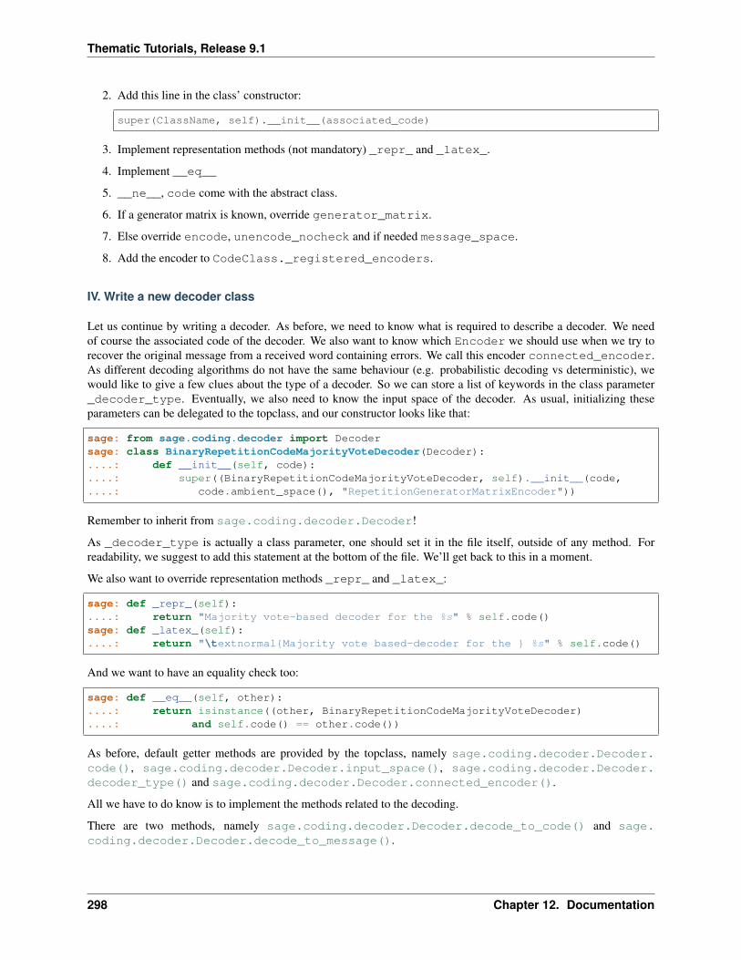
Thematic Tutorials, Release 9.1
2. Add this line in the class’ constructor:
super(ClassName, self).__init__(associated_code)
3. Implement representation methods (not mandatory) _repr_ and _latex_.
4. Implement __eq__
5. __ne__, code come with the abstract class.
6. If a generator matrix is known, override generator_matrix.
7. Else override encode, unencode_nocheck and if needed message_space.
8. Add the encoder to CodeClass._registered_encoders.
IV. Write a new decoder class
Let us continue by writing a decoder. As before, we need to know what is required to describe a decoder. We needof course the associated code of the decoder. We also want to know which Encoder we should use when we try torecover the original message from a received word containing errors. We call this encoder connected_encoder.As different decoding algorithms do not have the same behaviour (e.g. probabilistic decoding vs deterministic), wewould like to give a few clues about the type of a decoder. So we can store a list of keywords in the class parameter_decoder_type. Eventually, we also need to know the input space of the decoder. As usual, initializing theseparameters can be delegated to the topclass, and our constructor looks like that:
sage: from sage.coding.decoder import Decodersage: class BinaryRepetitionCodeMajorityVoteDecoder(Decoder):....: def __init__(self, code):....: super((BinaryRepetitionCodeMajorityVoteDecoder, self).__init__(code,....: code.ambient_space(), "RepetitionGeneratorMatrixEncoder"))
Remember to inherit from sage.coding.decoder.Decoder!
As _decoder_type is actually a class parameter, one should set it in the file itself, outside of any method. Forreadability, we suggest to add this statement at the bottom of the file. We’ll get back to this in a moment.
We also want to override representation methods _repr_ and _latex_:
sage: def _repr_(self):....: return "Majority vote-based decoder for the %s" % self.code()sage: def _latex_(self):....: return "\textnormalMajority vote based-decoder for the %s" % self.code()
And we want to have an equality check too:
sage: def __eq__(self, other):....: return isinstance((other, BinaryRepetitionCodeMajorityVoteDecoder)....: and self.code() == other.code())
As before, default getter methods are provided by the topclass, namely sage.coding.decoder.Decoder.code(), sage.coding.decoder.Decoder.input_space(), sage.coding.decoder.Decoder.decoder_type() and sage.coding.decoder.Decoder.connected_encoder().
All we have to do know is to implement the methods related to the decoding.
There are two methods, namely sage.coding.decoder.Decoder.decode_to_code() and sage.coding.decoder.Decoder.decode_to_message().
298 Chapter 12. Documentation
Thematic Tutorials, Release 9.1
By the magic of default implementation, these two are linked, as decode_to_message calls firstdecode_to_code and then unencode, while decode_to_code calls successively decode_to_messageand encode. So we only need to implement one of these two, and we choose to override decode_to_code:
sage: def decode_to_code(self, word):....: list_word = word.list()....: count_one = list_word.count(GF(2).one())....: n = self.code().length()....: length = len(list_word)....: F = GF(2)....: if count_one > length / 2:....: return vector(F, [F.one()] * n)....: elif count_one < length / 2:....: return vector(F, [F.zero()] * n)....: else:....: raise DecodingError("impossible to find a majority")
Note: One notices that if default decode_to_code calls default decode_to_message and defaultdecode_to_message calls default decode_to_code, if none is overriden and one is called, it will end upstuck in an infinite loop. We added a trigger guard against this, so if none is overriden and one is called, an exceptionwill be raised.
Only one method is missing: one to provide to the user the number of errors our decoder can decode. This is themethod sage.coding.decoder.Decoder.decoding_radius(), which we override:
sage: def decoding_radius(self):....: return (self.code().length()-1) // 2
As for some cases, the decoding might not be precisely known, its implementation is not mandatory in sage.coding.decoder.Decoder’s subclasses.
We need to do one extra thing: set this encoder in the dictionary of known decoders for the associated code class. Todo that, just add the following line at the end of your file:
BinaryRepetitionCode._registered_decoders["MajorityVoteDecoder"] =→˓BinaryRepetitionCodeMajorityVoteDecoder
Also put this line to set decoder_type:
BinaryRepetitionCode._decoder_type = "hard-decision", "unique"
Note: In case you are implementing a generic decoder (a decoder which works with any family of lin-ear codes), please add the following statement in AbstractLinearCode’s constructor instead: self._registered_decoders["DecName"] = MyGenericDecoder. This will make it immediately availableto any code class which inherits from 𝐴𝑏𝑠𝑡𝑟𝑎𝑐𝑡𝐿𝑖𝑛𝑒𝑎𝑟𝐶𝑜𝑑𝑒.
Summary of the implementation for decoders
1. Inherit from sage.coding.decoder.Decoder.
2. Add this line in the class’ constructor:
12.1. Thematic tutorial document tree 299
Thematic Tutorials, Release 9.1
super(ClassName, self).__init__(associated_code, input_space, connected_encoder_→˓name, decoder_type)
3. Implement representation methods (not mandatory) _repr_ and _latex_.
4. Implement __eq__.
5. __ne__, code, connected_encoder, decoder_type come with the abstract class.
6. Override decode_to_code or decode_to_message and decoding_radius.
7. Add the encoder to CodeClass._registered_decoders.
V. Write a new channel class
Alongside all these new structures directly related to codes, we also propose a whole new and shiny structure toexperiment on codes, and more specifically on their decoding.
Indeed, we implemented a structure to emulate real-world communication channels.
I’ll propose here a step-by-step implementation of a dummy channel for example’s sake.
We will implement a very naive channel which works only for words over F2 and flips as many bits as requested bythe user.
As channels are not directly related to code families, but more to vectors and words, we have a specific file, channel.py to store them.
So we will just add our new class in this file.
For starters, we ask ourselves the eternal question: What do we need to describe a channel? Well, we mandatorilyneed its input_space and its output_space. Of course, in most of the cases, the user will be able to providesome extra information on the channel’s behaviour. In our case, it will be the number of bits to flip (aka the number oferrors).
As you might have guess, there is an abstract class to take care of the mandatory arguments! Plus, in our case, as thischannel only works for vectors over F2, the input and output spaces are the same. Let us write the constructor of ournew channel class:
sage: from sage.coding.channel import Channelsage: class BinaryStaticErrorRateChannel(Channel):....: def __init__(self, space, number_errors):....: if space.base_ring() is not GF(2):....: raise ValueError("Provided space must be a vector space over GF(2)")....: if number_errors > space.dimension():....: raise ValueErrors("number_errors cannot be bigger than input space→˓'s dimension")....: super(BinaryStaticErrorRateChannel, self).__init__(space, space)....: self._number_errors = number_errors
Remember to inherit from sage.coding.channel.Channel!
We also want to override representation methods _repr_ and _latex_:
sage: def _repr_(self):....: return ("Binary static error rate channel creating %s errors, of input and→˓output space %s"....: % (format_interval(no_err), self.input_space()))
sage: def _latex_(self):
(continues on next page)
300 Chapter 12. Documentation
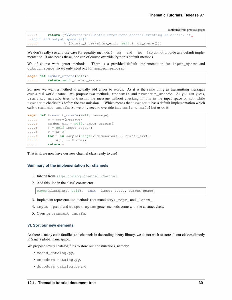
Thematic Tutorials, Release 9.1
(continued from previous page)
....: return ("\\textnormalStatic error rate channel creating %s errors, of→˓input and output space %s"....: % (format_interval(no_err), self.input_space()))
We don’t really see any use case for equality methods (__eq__ and __ne__) so do not provide any default imple-mentation. If one needs these, one can of course override Python’s default methods.
We of course want getter methods. There is a provided default implementation for input_space andoutput_space, so we only need one for number_errors:
sage: def number_errors(self):....: return self._number_errors
So, now we want a method to actually add errors to words. As it is the same thing as transmitting messagesover a real-world channel, we propose two methods, transmit and transmit_unsafe. As you can guess,transmit_unsafe tries to transmit the message without checking if it is in the input space or not, whiletransmit checks this before the transmission. . . Which means that transmit has a default implementation whichcalls transmit_unsafe. So we only need to override transmit_unsafe! Let us do it:
sage: def transmit_unsafe(self, message):....: w = copy(message)....: number_err = self.number_errors()....: V = self.input_space()....: F = GF(2)....: for i in sample(range(V.dimension()), number_err):....: w[i] += F.one()....: return w
That is it, we now have our new channel class ready to use!
Summary of the implementation for channels
1. Inherit from sage.coding.channel.Channel.
2. Add this line in the class’ constructor:
super(ClassName, self).__init__(input_space, output_space)
3. Implement representation methods (not mandatory) _repr_ and _latex_.
4. input_space and output_space getter methods come with the abstract class.
5. Override transmit_unsafe.
VI. Sort our new elements
As there is many code families and channels in the coding theory library, we do not wish to store all our classes directlyin Sage’s global namespace.
We propose several catalog files to store our constructions, namely:
• codes_catalog.py,
• encoders_catalog.py,
• decoders_catalog.py and
12.1. Thematic tutorial document tree 301
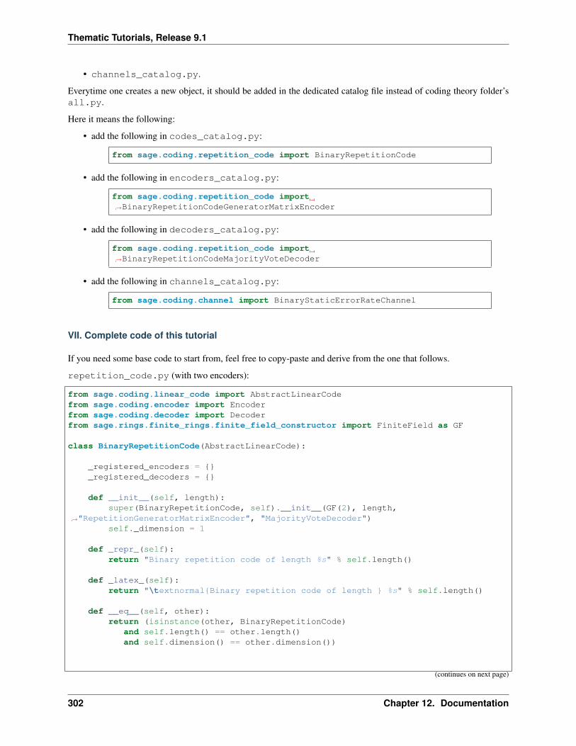
Thematic Tutorials, Release 9.1
• channels_catalog.py.
Everytime one creates a new object, it should be added in the dedicated catalog file instead of coding theory folder’sall.py.
Here it means the following:
• add the following in codes_catalog.py:
from sage.coding.repetition_code import BinaryRepetitionCode
• add the following in encoders_catalog.py:
from sage.coding.repetition_code import→˓BinaryRepetitionCodeGeneratorMatrixEncoder
• add the following in decoders_catalog.py:
from sage.coding.repetition_code import→˓BinaryRepetitionCodeMajorityVoteDecoder
• add the following in channels_catalog.py:
from sage.coding.channel import BinaryStaticErrorRateChannel
VII. Complete code of this tutorial
If you need some base code to start from, feel free to copy-paste and derive from the one that follows.
repetition_code.py (with two encoders):
from sage.coding.linear_code import AbstractLinearCodefrom sage.coding.encoder import Encoderfrom sage.coding.decoder import Decoderfrom sage.rings.finite_rings.finite_field_constructor import FiniteField as GF
class BinaryRepetitionCode(AbstractLinearCode):
_registered_encoders = _registered_decoders =
def __init__(self, length):super(BinaryRepetitionCode, self).__init__(GF(2), length,
→˓"RepetitionGeneratorMatrixEncoder", "MajorityVoteDecoder")self._dimension = 1
def _repr_(self):return "Binary repetition code of length %s" % self.length()
def _latex_(self):return "\textnormalBinary repetition code of length %s" % self.length()
def __eq__(self, other):return (isinstance(other, BinaryRepetitionCode)
and self.length() == other.length()and self.dimension() == other.dimension())
(continues on next page)
302 Chapter 12. Documentation
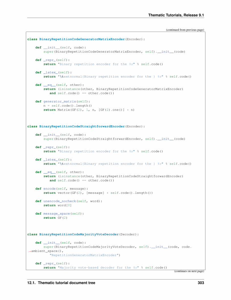
Thematic Tutorials, Release 9.1
(continued from previous page)
class BinaryRepetitionCodeGeneratorMatrixEncoder(Encoder):
def __init__(self, code):super(BinaryRepetitionCodeGeneratorMatrixEncoder, self).__init__(code)
def _repr_(self):return "Binary repetition encoder for the %s" % self.code()
def _latex_(self):return "\textnormalBinary repetition encoder for the %s" % self.code()
def __eq__(self, other):return (isinstance(other, BinaryRepetitionCodeGeneratorMatrixEncoder)
and self.code() == other.code())
def generator_matrix(self):n = self.code().length()return Matrix(GF(2), 1, n, [GF(2).one()] * n)
class BinaryRepetitionCodeStraightforwardEncoder(Encoder):
def __init__(self, code):super(BinaryRepetitionCodeStraightforwardEncoder, self).__init__(code)
def _repr_(self):return "Binary repetition encoder for the %s" % self.code()
def _latex_(self):return "\textnormalBinary repetition encoder for the %s" % self.code()
def __eq__(self, other):return (isinstance(other, BinaryRepetitionCodeStraightforwardEncoder)
and self.code() == other.code())
def encode(self, message):return vector(GF(2), [message] * self.code().length())
def unencode_nocheck(self, word):return word[0]
def message_space(self):return GF(2)
class BinaryRepetitionCodeMajorityVoteDecoder(Decoder):
def __init__(self, code):super(BinaryRepetitionCodeMajorityVoteDecoder, self).__init__(code, code.
→˓ambient_space(),"RepetitionGeneratorMatrixEncoder")
def _repr_(self):return "Majority vote-based decoder for the %s" % self.code()
(continues on next page)
12.1. Thematic tutorial document tree 303
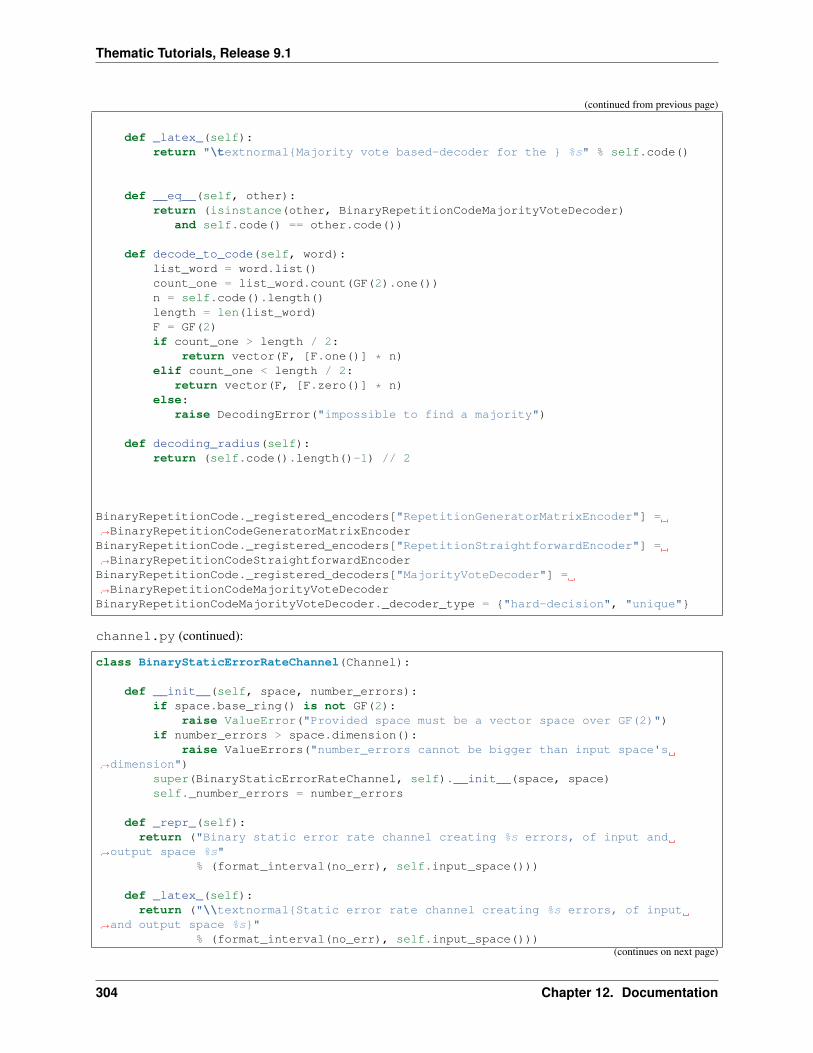
Thematic Tutorials, Release 9.1
(continued from previous page)
def _latex_(self):return "\textnormalMajority vote based-decoder for the %s" % self.code()
def __eq__(self, other):return (isinstance(other, BinaryRepetitionCodeMajorityVoteDecoder)
and self.code() == other.code())
def decode_to_code(self, word):list_word = word.list()count_one = list_word.count(GF(2).one())n = self.code().length()length = len(list_word)F = GF(2)if count_one > length / 2:
return vector(F, [F.one()] * n)elif count_one < length / 2:
return vector(F, [F.zero()] * n)else:
raise DecodingError("impossible to find a majority")
def decoding_radius(self):return (self.code().length()-1) // 2
BinaryRepetitionCode._registered_encoders["RepetitionGeneratorMatrixEncoder"] =→˓BinaryRepetitionCodeGeneratorMatrixEncoderBinaryRepetitionCode._registered_encoders["RepetitionStraightforwardEncoder"] =→˓BinaryRepetitionCodeStraightforwardEncoderBinaryRepetitionCode._registered_decoders["MajorityVoteDecoder"] =→˓BinaryRepetitionCodeMajorityVoteDecoderBinaryRepetitionCodeMajorityVoteDecoder._decoder_type = "hard-decision", "unique"
channel.py (continued):
class BinaryStaticErrorRateChannel(Channel):
def __init__(self, space, number_errors):if space.base_ring() is not GF(2):
raise ValueError("Provided space must be a vector space over GF(2)")if number_errors > space.dimension():
raise ValueErrors("number_errors cannot be bigger than input space's→˓dimension")
super(BinaryStaticErrorRateChannel, self).__init__(space, space)self._number_errors = number_errors
def _repr_(self):return ("Binary static error rate channel creating %s errors, of input and
→˓output space %s"% (format_interval(no_err), self.input_space()))
def _latex_(self):return ("\\textnormalStatic error rate channel creating %s errors, of input
→˓and output space %s"% (format_interval(no_err), self.input_space()))
(continues on next page)
304 Chapter 12. Documentation
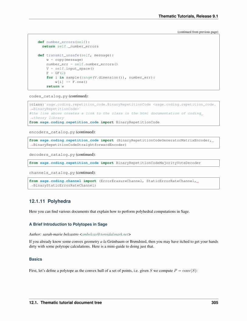
Thematic Tutorials, Release 9.1
(continued from previous page)
def number_errors(self):return self._number_errors
def transmit_unsafe(self, message):w = copy(message)number_err = self.number_errors()V = self.input_space()F = GF(2)for i in sample(range(V.dimension()), number_err):
w[i] += F.one()return w
codes_catalog.py (continued):
:class:`sage.coding.repetition_code.BinaryRepetitionCode <sage.coding.repetition_code.→˓BinaryRepetitionCode>`#the line above creates a link to the class in the html documentation of coding→˓theory libraryfrom sage.coding.repetition_code import BinaryRepetitionCode
encoders_catalog.py (continued):
from sage.coding.repetition_code import (BinaryRepetitionCodeGeneratorMatrixEncoder,→˓BinaryRepetitionCodeStraightforwardEncoder)
decoders_catalog.py (continued):
from sage.coding.repetition_code import BinaryRepetitionCodeMajorityVoteDecoder
channels_catalog.py (continued):
from sage.coding.channel import (ErrorErasureChannel, StaticErrorRateChannel,→˓BinaryStaticErrorRateChannel)
12.1.11 Polyhedra
Here you can find various documents that explain how to perform polyhedral computations in Sage.
A Brief Introduction to Polytopes in Sage
Author: sarah-marie belcastro <[email protected]>
If you already know some convex geometry a la Grünbaum or Brøndsted, then you may have itched to get your handsdirty with some polytope calculations. Here is a mini-guide to doing just that.
Basics
First, let’s define a polytope as the convex hull of a set of points, i.e. given 𝑆 we compute 𝑃 = conv(𝑆):
12.1. Thematic tutorial document tree 305
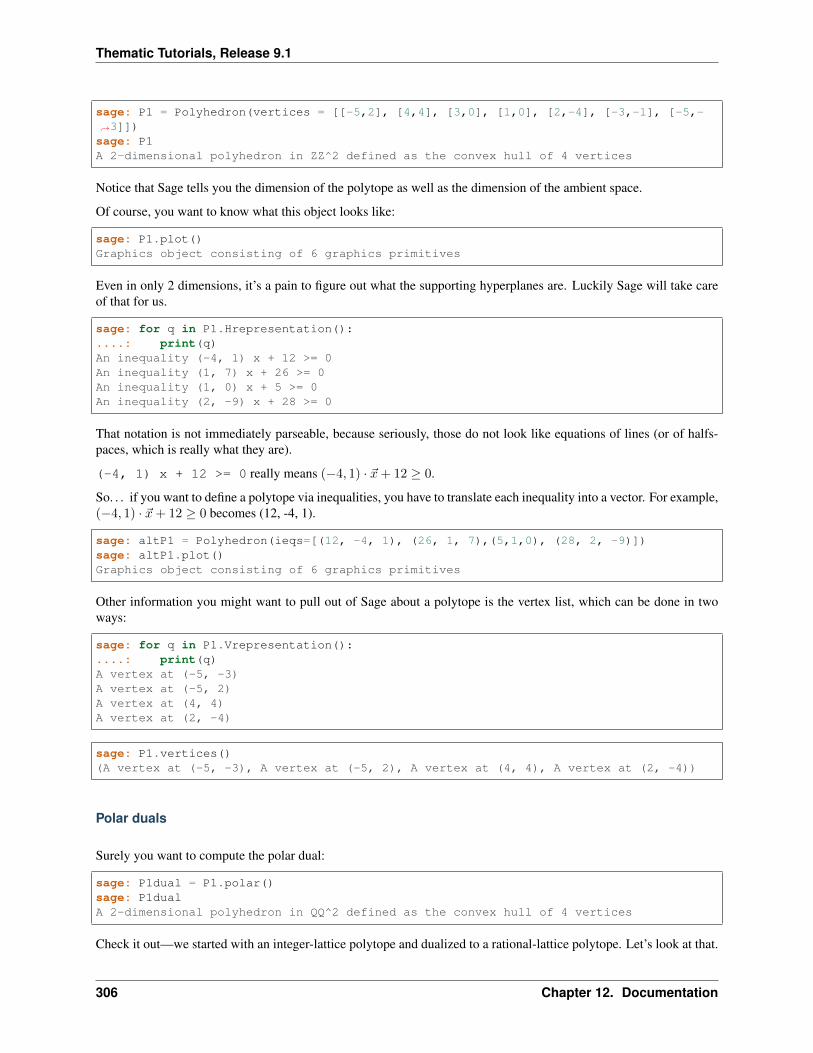
Thematic Tutorials, Release 9.1
sage: P1 = Polyhedron(vertices = [[-5,2], [4,4], [3,0], [1,0], [2,-4], [-3,-1], [-5,-→˓3]])sage: P1A 2-dimensional polyhedron in ZZ^2 defined as the convex hull of 4 vertices
Notice that Sage tells you the dimension of the polytope as well as the dimension of the ambient space.
Of course, you want to know what this object looks like:
sage: P1.plot()Graphics object consisting of 6 graphics primitives
Even in only 2 dimensions, it’s a pain to figure out what the supporting hyperplanes are. Luckily Sage will take careof that for us.
sage: for q in P1.Hrepresentation():....: print(q)An inequality (-4, 1) x + 12 >= 0An inequality (1, 7) x + 26 >= 0An inequality (1, 0) x + 5 >= 0An inequality (2, -9) x + 28 >= 0
That notation is not immediately parseable, because seriously, those do not look like equations of lines (or of halfs-paces, which is really what they are).
(-4, 1) x + 12 >= 0 really means (−4, 1) · + 12 ≥ 0.
So. . . if you want to define a polytope via inequalities, you have to translate each inequality into a vector. For example,(−4, 1) · + 12 ≥ 0 becomes (12, -4, 1).
sage: altP1 = Polyhedron(ieqs=[(12, -4, 1), (26, 1, 7),(5,1,0), (28, 2, -9)])sage: altP1.plot()Graphics object consisting of 6 graphics primitives
Other information you might want to pull out of Sage about a polytope is the vertex list, which can be done in twoways:
sage: for q in P1.Vrepresentation():....: print(q)A vertex at (-5, -3)A vertex at (-5, 2)A vertex at (4, 4)A vertex at (2, -4)
sage: P1.vertices()(A vertex at (-5, -3), A vertex at (-5, 2), A vertex at (4, 4), A vertex at (2, -4))
Polar duals
Surely you want to compute the polar dual:
sage: P1dual = P1.polar()sage: P1dualA 2-dimensional polyhedron in QQ^2 defined as the convex hull of 4 vertices
Check it out—we started with an integer-lattice polytope and dualized to a rational-lattice polytope. Let’s look at that.
306 Chapter 12. Documentation
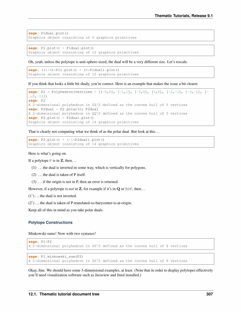
Thematic Tutorials, Release 9.1
sage: P1dual.plot()Graphics object consisting of 6 graphics primitives
sage: P1.plot() + P1dual.plot()Graphics object consisting of 12 graphics primitives
Oh, yeah, unless the polytope is unit-sphere-sized, the dual will be a very different size. Let’s rescale.
sage: ((1/4)*P1).plot() + (4*P1dual).plot()Graphics object consisting of 12 graphics primitives
If you think that looks a little bit shady, you’re correct. Here is an example that makes the issue a bit clearer.
sage: P2 = Polyhedron(vertices = [[-5,0], [-1,1], [-2,0], [1,0], [-2,-1], [-3,-1], [-→˓5,-1]])sage: P2A 2-dimensional polyhedron in ZZ^2 defined as the convex hull of 5 verticessage: P2dual = P2.polar(); P2dualA 2-dimensional polyhedron in QQ^2 defined as the convex hull of 5 verticessage: P2.plot() + P2dual.plot()Graphics object consisting of 14 graphics primitives
That is clearly not computing what we think of as the polar dual. But look at this. . .
sage: P2.plot() + (-1*P2dual).plot()Graphics object consisting of 14 graphics primitives
Here is what’s going on.
If a polytope P is in Z, then. . .
(1) . . . the dual is inverted in some way, which is vertically for polygons.
(2) . . . the dual is taken of P itself.
(3) . . . if the origin is not in P, then an error is returned.
However, if a polytope is not in Z, for example if it’s in Q or RDF, then. . .
(1’) . . . the dual is not inverted.
(2’) . . . the dual is taken of P-translated-so-barycenter-is-at-origin.
Keep all of this in mind as you take polar duals.
Polytope Constructions
Minkowski sums! Now with two syntaxes!
sage: P1+P2A 2-dimensional polyhedron in ZZ^2 defined as the convex hull of 8 vertices
sage: P1.minkowski_sum(P2)A 2-dimensional polyhedron in ZZ^2 defined as the convex hull of 8 vertices
Okay, fine. We should have some 3-dimensional examples, at least. (Note that in order to display polytopes effectivelyyou’ll need visualization software such as Javaview and Jmol installed.)
12.1. Thematic tutorial document tree 307
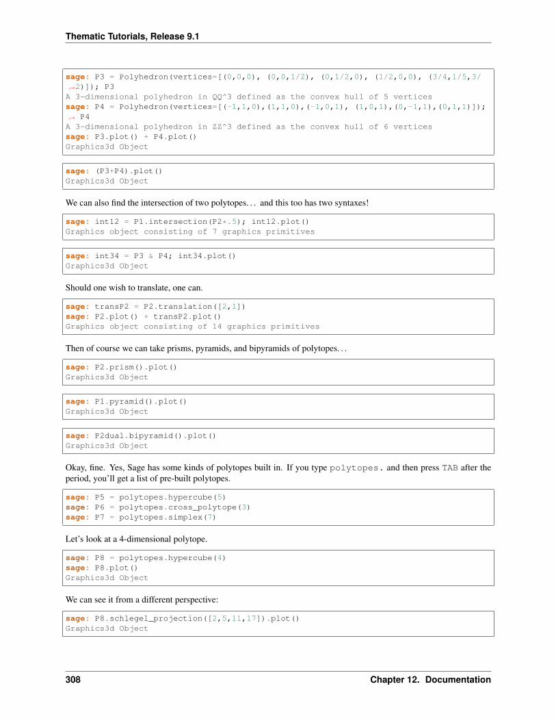
Thematic Tutorials, Release 9.1
sage: P3 = Polyhedron(vertices=[(0,0,0), (0,0,1/2), (0,1/2,0), (1/2,0,0), (3/4,1/5,3/→˓2)]); P3A 3-dimensional polyhedron in QQ^3 defined as the convex hull of 5 verticessage: P4 = Polyhedron(vertices=[(-1,1,0),(1,1,0),(-1,0,1), (1,0,1),(0,-1,1),(0,1,1)]);→˓ P4A 3-dimensional polyhedron in ZZ^3 defined as the convex hull of 6 verticessage: P3.plot() + P4.plot()Graphics3d Object
sage: (P3+P4).plot()Graphics3d Object
We can also find the intersection of two polytopes. . . and this too has two syntaxes!
sage: int12 = P1.intersection(P2*.5); int12.plot()Graphics object consisting of 7 graphics primitives
sage: int34 = P3 & P4; int34.plot()Graphics3d Object
Should one wish to translate, one can.
sage: transP2 = P2.translation([2,1])sage: P2.plot() + transP2.plot()Graphics object consisting of 14 graphics primitives
Then of course we can take prisms, pyramids, and bipyramids of polytopes. . .
sage: P2.prism().plot()Graphics3d Object
sage: P1.pyramid().plot()Graphics3d Object
sage: P2dual.bipyramid().plot()Graphics3d Object
Okay, fine. Yes, Sage has some kinds of polytopes built in. If you type polytopes. and then press TAB after theperiod, you’ll get a list of pre-built polytopes.
sage: P5 = polytopes.hypercube(5)sage: P6 = polytopes.cross_polytope(3)sage: P7 = polytopes.simplex(7)
Let’s look at a 4-dimensional polytope.
sage: P8 = polytopes.hypercube(4)sage: P8.plot()Graphics3d Object
We can see it from a different perspective:
sage: P8.schlegel_projection([2,5,11,17]).plot()Graphics3d Object
308 Chapter 12. Documentation
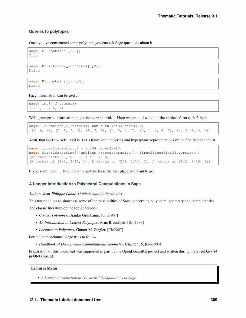
Thematic Tutorials, Release 9.1
Queries to polytopes
Once you’ve constructed some polytope, you can ask Sage questions about it.
sage: P1.contains([1,0])True
sage: P1.interior_contains([3,0])False
sage: P3.contains([1,0,0])False
Face information can be useful.
sage: int34.f_vector()(1, 8, 12, 6, 1)
Well, geometric information might be more helpful. . . Here we are told which of the vertices form each 2-face:
sage: [f.ambient_V_indices() for f in int34.faces(2)][(2, 6, 7), (0, 1, 3, 5), (1, 3, 4), (0, 5, 6, 7), (0, 1, 2, 4, 6), (2, 3, 4, 5, 7)]
Yeah, that isn’t so useful as it is. Let’s figure out the vertex and hyperplane representations of the first face in the list.
sage: first2faceofint34 = int34.faces(2)[0]sage: first2faceofint34.ambient_Hrepresentation(); first2faceofint34.vertices()(An inequality (0, 0, -1) x + 1 >= 0,)(A vertex at (2/3, 2/15, 1), A vertex at (3/8, 1/10, 1), A vertex at (1/2, 3/10, 1))
If you want more. . . Base class for polyhedra is the first place you want to go.
A Longer Introduction to Polyhedral Computations in Sage
Author: Jean-Philippe Labbé <[email protected]>
This tutorial aims to showcase some of the possibilities of Sage concerning polyhedral geometry and combinatorics.
The classic literature on the topic includes:
• Convex Polytopes, Branko Grünbaum, [Gru1967]
• An Introduction to Convex Polytopes, Arne Brøndsted, [Bro1983]
• Lectures on Polytopes, Günter M. Ziegler, [Zie2007]
For the nomenclature, Sage tries to follow:
• Handbook of Discrete and Computational Geometry, Chapter 15, [Goo2004]
Preparation of this document was supported in part by the OpenDreamKit project and written during the SageDays 84in Olot (Spain).
Lectures Menu
• A Longer Introduction to Polyhedral Computations in Sage
12.1. Thematic tutorial document tree 309
Thematic Tutorials, Release 9.1
– Lecture 0: Basic definitions and constructions
– Lecture 1: Representation objects
– Lecture 2: Backends for polyhedral computations
– Lecture 3: To every polyhedron, the proper parent class
– Lecture 4: A library of polytopes
– Bibliography
Lecture 0: Basic definitions and constructions
A real (𝑘× 𝑑)-matrix 𝐴 and a real vector 𝑏 in R𝑑 define a (convex) polyhedron 𝑃 as the set of solutions of the systemof linear inequalities:
𝐴 · 𝑥+ 𝑏 ≥ 0.
Each row of 𝐴 defines a closed half-space of R𝑑. Hence a polyhedron is the intersection of finitely many closed half-spaces in R𝑑. The matrix 𝐴 may contain equal rows, which may lead to a set of equalities satisfied by the polyhedron.If there are no redundant rows in the above definition, this definition is referred to as the H -representation of apolyhedron.
A maximal affine subspace 𝐿 contained in a polyhedron is a lineality space of 𝑃 . Fixing a point 𝑜 of the linealityspace 𝐿 to act as the origin, one can write every point 𝑝 inside a polyhedron as a combination
𝑝 = ℓ+
𝑛∑𝑖=1
𝜆𝑖𝑣𝑖 +
𝑚∑𝑖=1
𝜇𝑖𝑟𝑖,
where ℓ ∈ 𝐿 (using 𝑜 as the origin),∑𝑛
𝑖=1 𝜆𝑖 = 1, 𝜆𝑖 ≥ 0, 𝜇𝑖 ≥ 0, and 𝑟𝑖 = 0 for all 0 ≤ 𝑖 ≤ 𝑚 and the set of 𝑟𝑖 ‘sare positively independent (the origin is not in their positive span). For a given point 𝑝 there may be many equivalentways to write the above using different sets 𝑣𝑖𝑛𝑖=1 and 𝑟𝑖𝑚𝑖=1. Hence we require the sets to be inclusion minimalsets such that we can get the above property equality for any point 𝑝 ∈ 𝑃 .
The vectors 𝑣𝑖 are called the vertices of 𝑃 and the vectors 𝑟𝑖 are called the rays of 𝑃 . This way to represent apolyhedron is referred to as the V -representation of a polyhedron. The first sum represents the convex hull of thevertices 𝑣𝑖 ‘s and the second sum represents a pointed polyhedral cone generated by finitely many rays.
When the lineality space and the rays are reduced to a point (i.e. no rays and no lines) the object is often referred to asa polytope.
Note: As mentioned in the documentation of the constructor when typing Polyhedron?:
You may either define it with vertex/ray/line or inequalities/equations data, but not both. Redundant data will auto-matically be removed (unless “minimize=False”), and the complementary representation will be computed.
Here is the documentation for the constructor function of Polyhedra.
𝑉 -representation
First, let’s define a polyhedron object as the convex hull of a set of points and some rays.
310 Chapter 12. Documentation
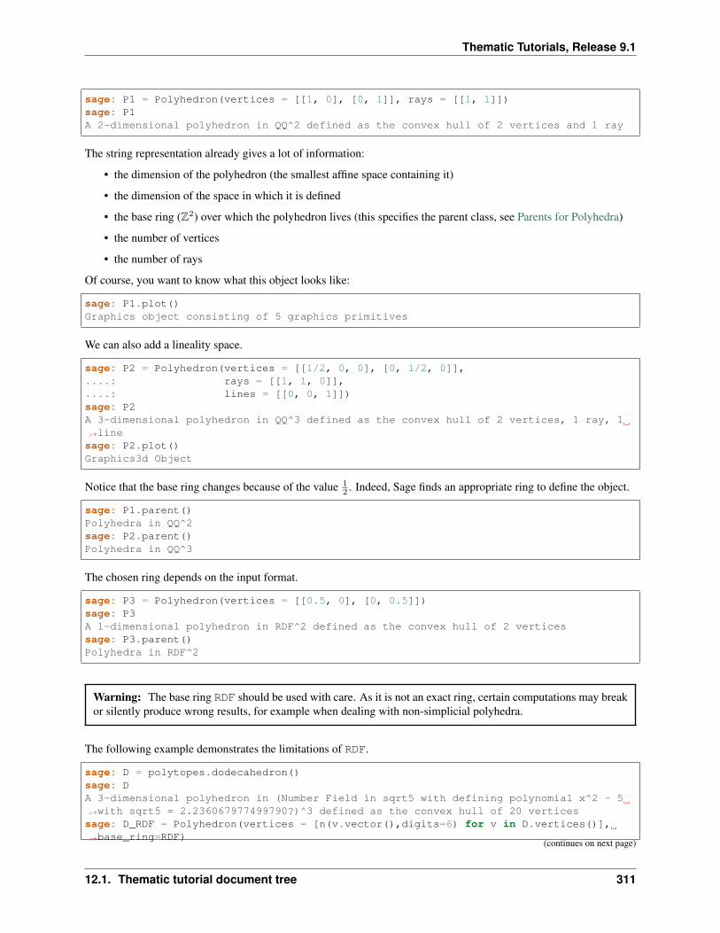
Thematic Tutorials, Release 9.1
sage: P1 = Polyhedron(vertices = [[1, 0], [0, 1]], rays = [[1, 1]])sage: P1A 2-dimensional polyhedron in QQ^2 defined as the convex hull of 2 vertices and 1 ray
The string representation already gives a lot of information:
• the dimension of the polyhedron (the smallest affine space containing it)
• the dimension of the space in which it is defined
• the base ring (Z2) over which the polyhedron lives (this specifies the parent class, see Parents for Polyhedra)
• the number of vertices
• the number of rays
Of course, you want to know what this object looks like:
sage: P1.plot()Graphics object consisting of 5 graphics primitives
We can also add a lineality space.
sage: P2 = Polyhedron(vertices = [[1/2, 0, 0], [0, 1/2, 0]],....: rays = [[1, 1, 0]],....: lines = [[0, 0, 1]])sage: P2A 3-dimensional polyhedron in QQ^3 defined as the convex hull of 2 vertices, 1 ray, 1→˓linesage: P2.plot()Graphics3d Object
Notice that the base ring changes because of the value 12 . Indeed, Sage finds an appropriate ring to define the object.
sage: P1.parent()Polyhedra in QQ^2sage: P2.parent()Polyhedra in QQ^3
The chosen ring depends on the input format.
sage: P3 = Polyhedron(vertices = [[0.5, 0], [0, 0.5]])sage: P3A 1-dimensional polyhedron in RDF^2 defined as the convex hull of 2 verticessage: P3.parent()Polyhedra in RDF^2
Warning: The base ring RDF should be used with care. As it is not an exact ring, certain computations may breakor silently produce wrong results, for example when dealing with non-simplicial polyhedra.
The following example demonstrates the limitations of RDF.
sage: D = polytopes.dodecahedron()sage: DA 3-dimensional polyhedron in (Number Field in sqrt5 with defining polynomial x^2 - 5→˓with sqrt5 = 2.236067977499790?)^3 defined as the convex hull of 20 verticessage: D_RDF = Polyhedron(vertices = [n(v.vector(),digits=6) for v in D.vertices()],→˓base_ring=RDF)
(continues on next page)
12.1. Thematic tutorial document tree 311
Thematic Tutorials, Release 9.1
(continued from previous page)
Traceback (most recent call last):...ValueError: *Error: Numerical inconsistency is found. Use the GMP exact arithmetic.
If the input of the polyhedron consists of python float, it automatically converts the data to RDF:
sage: Polyhedron(vertices=[[float(1.1)]])A 0-dimensional polyhedron in RDF^1 defined as the convex hull of 1 vertex
It is also possible to define polyhedron over algebraic numbers.
sage: sqrt_2 = AA(2)^(1/2)sage: cbrt_2 = AA(2)^(1/3)sage: timeit('Polyhedron(vertices = [[sqrt_2, 0], [0, cbrt_2]])') # random5 loops, best of 3: 43.2 ms per loopsage: P4 = Polyhedron(vertices = [[sqrt_2, 0], [0, cbrt_2]]); P4A 1-dimensional polyhedron in AA^2 defined as the convex hull of 2 vertices
There is another way to create a polyhedron over algebraic numbers:
sage: K.<a> = NumberField(x^2 - 2, embedding=AA(2)**(1/2))sage: L.<b> = NumberField(x^3 - 2, embedding=AA(2)**(1/3))sage: timeit('Polyhedron(vertices = [[a, 0], [0, b]])') # random5 loops, best of 3: 39.9 ms per loopsage: P5 = Polyhedron(vertices = [[a, 0], [0, b]]); P5A 1-dimensional polyhedron in AA^2 defined as the convex hull of 2 vertices
If the base ring is known it may be a good option to use the proper sage.rings.number_field.number_field.number_field.composite_fields():
sage: J = K.composite_fields(L)[0]sage: timeit('Polyhedron(vertices = [[J(a), 0], [0, J(b)]])') # random25 loops, best of 3: 9.8 ms per loopsage: P5_comp = Polyhedron(vertices = [[J(a), 0], [0, J(b)]]); P5_compA 1-dimensional polyhedron in (Number Field in ab with defining polynomial x^6 - 6*x^→˓4 - 4*x^3 + 12*x^2 - 24*x - 4 with ab = -0.1542925124782219?)^2 defined as the→˓convex hull of 2 vertices
Polyhedral computations with the Symbolic Ring are not implemented. It is not possible to define a polyhedronover it:
sage: sqrt_2s = sqrt(2)sage: cbrt_2s = 2^(1/3)sage: Polyhedron(vertices = [[sqrt_2s, 0], [0, cbrt_2s]])Traceback (most recent call last):...ValueError: no default backend for computations with Symbolic Ring
Similarly, it is not possible to create polyhedron objects over RR (no matter how many bits of precision).
sage: F45 = RealField(45)sage: F100 = RealField(100)sage: f = 1.1sage: Polyhedron(vertices=[[F45(f)]])Traceback (most recent call last):...
(continues on next page)
312 Chapter 12. Documentation
Thematic Tutorials, Release 9.1
(continued from previous page)
ValueError: the only allowed inexact ring is 'RDF' with backend 'cdd'sage: Polyhedron(vertices=[[F100(f)]])Traceback (most recent call last):...ValueError: the only allowed inexact ring is 'RDF' with backend 'cdd'
There is one exception, when the number of bits of precision is 53, then the base ring is converted to RDF:
sage: F53 = RealField(53)sage: Polyhedron(vertices=[[F53(f)]])A 0-dimensional polyhedron in RDF^1 defined as the convex hull of 1 vertexsage: type(Polyhedron(vertices=[[F53(f)]]))<class 'sage.geometry.polyhedron.parent.Polyhedra_RDF_cdd_with_category.element_class→˓'>
This behavior can be seen as wrong, but it allows the following to be acceptable by Sage:
sage: Polyhedron([(1.0, 2.3), (3.5, 2.0)])A 1-dimensional polyhedron in RDF^2 defined as the convex hull of 2 vertices
without having specified the base ring RDF by the user.
𝐻-representation
If a polyhedron object was constructed via a 𝑉 -representation, Sage can provide the 𝐻-representation of the object.
sage: for h in P1.Hrepresentation():....: print(h)An inequality (1, 1) x - 1 >= 0An inequality (1, -1) x + 1 >= 0An inequality (-1, 1) x + 1 >= 0
Each line gives a row of the matrix 𝐴 and an entry of the vector 𝑏. The variable 𝑥 is a vector in the ambient spacewhere P1 is defined. The 𝐻-representation may contain equations:
sage: P3.Hrepresentation()(An inequality (-2.0, 0.0) x + 1.0 >= 0,An inequality (1.0, 0.0) x + 0.0 >= 0,An equation (1.0, 1.0) x - 0.5 == 0)
The construction of a polyhedron object via its 𝐻-representation, requires a precise format. Each inequality(𝑎𝑖1, . . . , 𝑎𝑖𝑑) · 𝑥+ 𝑏𝑖 ≥ 0 must be written as [b_i,a_i1, ..., a_id].
sage: P3_H = Polyhedron(ieqs = [[1.0, -2, 0], [0, 1, 0]], eqns = [[-0.5, 1, 1]])sage: P3 == P3_HTruesage: P3_H.Vrepresentation()(A vertex at (0.0, 0.5), A vertex at (0.5, 0.0))
It is worth using the parameter eqns to shorten the construction of the object. In the following example, the first fourrows are the negative of the second group of four rows.
sage: H = [[0, 0, 0, 0, 0, 0, 0, 0, 1],....: [0, 0, 0, 0, 0, 0, 1, 0, 0],....: [-2, 1, 1, 1, 1, 1, 0, 0, 0],
(continues on next page)
12.1. Thematic tutorial document tree 313
Thematic Tutorials, Release 9.1
(continued from previous page)
....: [0, 0, 0, 0, 0, 0, 0, 1, 0],
....: [0, 0, 0, 0, 0, 0, 0, 0, -1],
....: [0, 0, 0, 0, 0, 0, -1, 0, 0],
....: [2, -1, -1, -1, -1, -1, 0, 0, 0],
....: [0, 0, 0, 0, 0, 0, 0, -1, 0],
....: [2, -1, -1, -1, -1, 0, 0, 0, 0],
....: [0, 0, 0, 0, 1, 0, 0, 0, 0],
....: [0, 0, 0, 1, 0, 0, 0, 0, 0],
....: [0, 0, 1, 0, 0, 0, 0, 0, 0],
....: [-1, 1, 1, 1, 1, 0, 0, 0, 0],
....: [1, 0, 0, -1, 0, 0, 0, 0, 0],
....: [0, 1, 0, 0, 0, 0, 0, 0, 0],
....: [1, 0, 0, 0, -1, 0, 0, 0, 0],
....: [1, 0, -1, 0, 0, 0, 0, 0, 0],
....: [1, -1, 0, 0, 0, 0, 0, 0, 0]]sage: timeit('Polyhedron(ieqs = H)') # random125 loops, best of 3: 5.99 ms per loopsage: timeit('Polyhedron(ieqs = H[8:], eqns = H[:4])') # random125 loops, best of 3: 4.78 ms per loopsage: Polyhedron(ieqs = H) == Polyhedron(ieqs = H[8:], eqns = H[:4])True
Of course, this is a toy example, but it is generally worth to preprocess the data before defining the polyhedron ifpossible.
Lecture 1: Representation objects
Many objects are related to the 𝐻- and 𝑉 -representations. Sage has classes implemented for them.
𝐻-representation
You can store the 𝐻-representation in a variable and use the inequalities and equalities as objects.
sage: P3_QQ = Polyhedron(vertices = [[0.5, 0], [0, 0.5]], base_ring=QQ)sage: HRep = P3_QQ.Hrepresentation()sage: H1 = HRep[0]; H1An equation (2, 2) x - 1 == 0sage: H2 = HRep[1]; H2An inequality (0, -2) x + 1 >= 0sage: H1.<tab> # not testedsage: H1.A()(2, 2)sage: H1.b()-1sage: H1.is_equation()Truesage: H1.is_inequality()Falsesage: H1.contains(vector([0,0]))Falsesage: H2.contains(vector([0,0]))Truesage: H1.is_incident(H2)True
314 Chapter 12. Documentation
Thematic Tutorials, Release 9.1
It is possible to obtain the different objects of the 𝐻-representation as follows.
sage: P3_QQ.equations()(An equation (2, 2) x - 1 == 0,)sage: P3_QQ.inequalities()(An inequality (0, -2) x + 1 >= 0, An inequality (0, 1) x + 0 >= 0)
Note: It is recommended to use equations or equation_generator (and similarly for inequalities) if onewants to iterate over them instead of equations_list.
𝑉 -representation
Similarly, you can access vertices, rays and lines of the polyhedron.
sage: VRep = P2.Vrepresentation(); VRep(A line in the direction (0, 0, 1),A vertex at (0, 1/2, 0),A vertex at (1/2, 0, 0),A ray in the direction (1, 1, 0))
sage: L = VRep[0]; LA line in the direction (0, 0, 1)sage: V = VRep[1]; VA vertex at (0, 1/2, 0)sage: R = VRep[3]; RA ray in the direction (1, 1, 0)sage: L.is_line()Truesage: L.is_incident(V)Truesage: R.is_incident(L)Falsesage: L.vector()(0, 0, 1)sage: V.vector()(0, 1/2, 0)
It is possible to obtain the different objects of the 𝑉 -representation as follows.
sage: P2.vertices()(A vertex at (0, 1/2, 0), A vertex at (1/2, 0, 0))sage: P2.rays()(A ray in the direction (1, 1, 0),)sage: P2.lines()(A line in the direction (0, 0, 1),)
sage: P2.vertices_matrix()[ 0 1/2][1/2 0][ 0 0]
Note: It is recommended to use vertices or vertex_generator (and similarly for rays and lines) if one wantsto iterate over them instead of vertices_list.
12.1. Thematic tutorial document tree 315
Thematic Tutorials, Release 9.1
Lecture 2: Backends for polyhedral computations
To deal with polyhedron objects, Sage currently has four backends available. These backends offer various function-alities and have their own specific strengths and limitations.
• The cdd backend for polyhedral computations
– The cdd and cddplus homepage
• The PPL (Parma Polyhedra Library) backend for polyhedral computations
– The Parma Polyhedra Library homepage
• The polymake backend for polyhedral computations
– The polymake project for convex geometry
• The Python backend
– This is a python backend that provides an implementation of polyhedron over irrational coordinates.
• The Normaliz backend for polyhedral computations, (requires the optional package pynormaliz)
– Normaliz Homepage
The default backend is ppl. Whenever one needs speed it is good to try out the different backends. The backendfield is not specifically designed for dealing with extremal computations but can do computations in exact coordi-nates.
The cdd backend
In order to use a specific backend, we specify the backend parameter.
sage: P1_cdd = Polyhedron(vertices = [[1, 0], [0, 1]], rays = [[1, 1]], backend='cdd')sage: P1_cddA 2-dimensional polyhedron in QQ^2 defined as the convex hull of 2 vertices and 1 ray
A priori, it seems that nothing changed, but . . .
sage: P1_cdd.parent()Polyhedra in QQ^2
The polyhedron P1_cdd is now considered as a rational polyhedron by the backend cdd. We can also check thebackend and the parent using type:
sage: type(P1_cdd)<class 'sage.geometry.polyhedron.parent.Polyhedra_QQ_cdd_with_category.element_class'>sage: type(P1)<class 'sage.geometry.polyhedron.parent.Polyhedra_QQ_ppl_with_category.element_class'>
We see
• the backend used (ex: backend_cdd)
• followed by a dot ‘.’
• the parent (ex: Polyhedra_QQ) followed again by the backend,
and you can safely ignore the rest for the purpose of this tutorial.
The cdd backend accepts also entries in RDF:
316 Chapter 12. Documentation
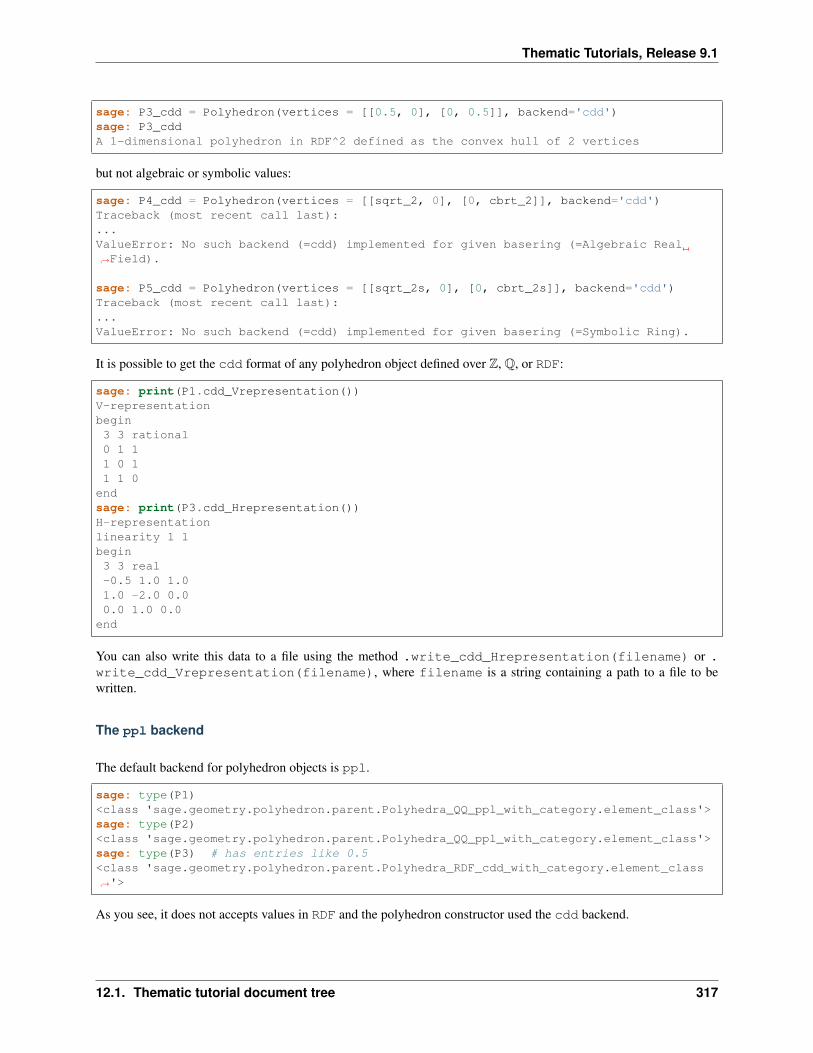
Thematic Tutorials, Release 9.1
sage: P3_cdd = Polyhedron(vertices = [[0.5, 0], [0, 0.5]], backend='cdd')sage: P3_cddA 1-dimensional polyhedron in RDF^2 defined as the convex hull of 2 vertices
but not algebraic or symbolic values:
sage: P4_cdd = Polyhedron(vertices = [[sqrt_2, 0], [0, cbrt_2]], backend='cdd')Traceback (most recent call last):...ValueError: No such backend (=cdd) implemented for given basering (=Algebraic Real→˓Field).
sage: P5_cdd = Polyhedron(vertices = [[sqrt_2s, 0], [0, cbrt_2s]], backend='cdd')Traceback (most recent call last):...ValueError: No such backend (=cdd) implemented for given basering (=Symbolic Ring).
It is possible to get the cdd format of any polyhedron object defined over Z, Q, or RDF:
sage: print(P1.cdd_Vrepresentation())V-representationbegin3 3 rational0 1 11 0 11 1 0
endsage: print(P3.cdd_Hrepresentation())H-representationlinearity 1 1begin3 3 real-0.5 1.0 1.01.0 -2.0 0.00.0 1.0 0.0
end
You can also write this data to a file using the method .write_cdd_Hrepresentation(filename) or .write_cdd_Vrepresentation(filename), where filename is a string containing a path to a file to bewritten.
The ppl backend
The default backend for polyhedron objects is ppl.
sage: type(P1)<class 'sage.geometry.polyhedron.parent.Polyhedra_QQ_ppl_with_category.element_class'>sage: type(P2)<class 'sage.geometry.polyhedron.parent.Polyhedra_QQ_ppl_with_category.element_class'>sage: type(P3) # has entries like 0.5<class 'sage.geometry.polyhedron.parent.Polyhedra_RDF_cdd_with_category.element_class→˓'>
As you see, it does not accepts values in RDF and the polyhedron constructor used the cdd backend.
12.1. Thematic tutorial document tree 317
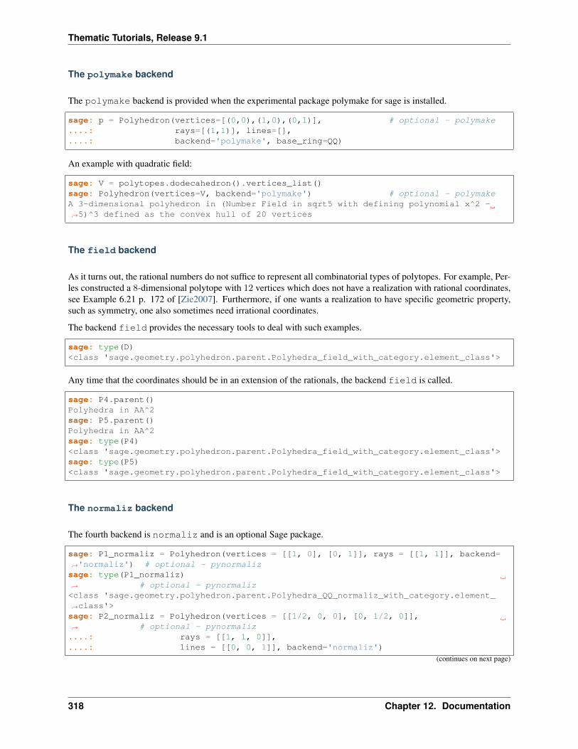
Thematic Tutorials, Release 9.1
The polymake backend
The polymake backend is provided when the experimental package polymake for sage is installed.
sage: p = Polyhedron(vertices=[(0,0),(1,0),(0,1)], # optional - polymake....: rays=[(1,1)], lines=[],....: backend='polymake', base_ring=QQ)
An example with quadratic field:
sage: V = polytopes.dodecahedron().vertices_list()sage: Polyhedron(vertices=V, backend='polymake') # optional - polymakeA 3-dimensional polyhedron in (Number Field in sqrt5 with defining polynomial x^2 -→˓5)^3 defined as the convex hull of 20 vertices
The field backend
As it turns out, the rational numbers do not suffice to represent all combinatorial types of polytopes. For example, Per-les constructed a 8-dimensional polytope with 12 vertices which does not have a realization with rational coordinates,see Example 6.21 p. 172 of [Zie2007]. Furthermore, if one wants a realization to have specific geometric property,such as symmetry, one also sometimes need irrational coordinates.
The backend field provides the necessary tools to deal with such examples.
sage: type(D)<class 'sage.geometry.polyhedron.parent.Polyhedra_field_with_category.element_class'>
Any time that the coordinates should be in an extension of the rationals, the backend field is called.
sage: P4.parent()Polyhedra in AA^2sage: P5.parent()Polyhedra in AA^2sage: type(P4)<class 'sage.geometry.polyhedron.parent.Polyhedra_field_with_category.element_class'>sage: type(P5)<class 'sage.geometry.polyhedron.parent.Polyhedra_field_with_category.element_class'>
The normaliz backend
The fourth backend is normaliz and is an optional Sage package.
sage: P1_normaliz = Polyhedron(vertices = [[1, 0], [0, 1]], rays = [[1, 1]], backend=→˓'normaliz') # optional - pynormalizsage: type(P1_normaliz)→˓ # optional - pynormaliz<class 'sage.geometry.polyhedron.parent.Polyhedra_QQ_normaliz_with_category.element_→˓class'>sage: P2_normaliz = Polyhedron(vertices = [[1/2, 0, 0], [0, 1/2, 0]],→˓ # optional - pynormaliz....: rays = [[1, 1, 0]],....: lines = [[0, 0, 1]], backend='normaliz')
(continues on next page)
318 Chapter 12. Documentation
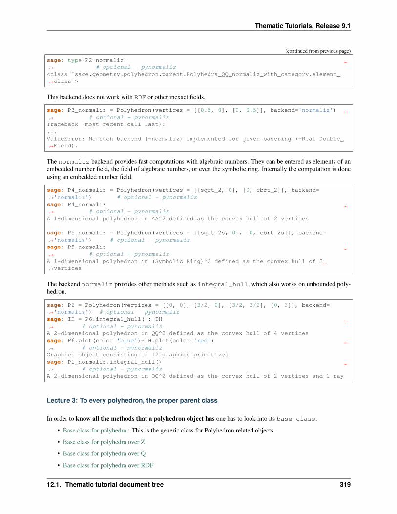
Thematic Tutorials, Release 9.1
(continued from previous page)
sage: type(P2_normaliz)→˓ # optional - pynormaliz<class 'sage.geometry.polyhedron.parent.Polyhedra_QQ_normaliz_with_category.element_→˓class'>
This backend does not work with RDF or other inexact fields.
sage: P3_normaliz = Polyhedron(vertices = [[0.5, 0], [0, 0.5]], backend='normaliz')→˓ # optional - pynormalizTraceback (most recent call last):...ValueError: No such backend (=normaliz) implemented for given basering (=Real Double→˓Field).
The normaliz backend provides fast computations with algebraic numbers. They can be entered as elements of anembedded number field, the field of algebraic numbers, or even the symbolic ring. Internally the computation is doneusing an embedded number field.
sage: P4_normaliz = Polyhedron(vertices = [[sqrt_2, 0], [0, cbrt_2]], backend=→˓'normaliz') # optional - pynormalizsage: P4_normaliz→˓ # optional - pynormalizA 1-dimensional polyhedron in AA^2 defined as the convex hull of 2 vertices
sage: P5_normaliz = Polyhedron(vertices = [[sqrt_2s, 0], [0, cbrt_2s]], backend=→˓'normaliz') # optional - pynormalizsage: P5_normaliz→˓ # optional - pynormalizA 1-dimensional polyhedron in (Symbolic Ring)^2 defined as the convex hull of 2→˓vertices
The backend normaliz provides other methods such as integral_hull, which also works on unbounded poly-hedron.
sage: P6 = Polyhedron(vertices = [[0, 0], [3/2, 0], [3/2, 3/2], [0, 3]], backend=→˓'normaliz') # optional - pynormalizsage: IH = P6.integral_hull(); IH→˓ # optional - pynormalizA 2-dimensional polyhedron in QQ^2 defined as the convex hull of 4 verticessage: P6.plot(color='blue')+IH.plot(color='red')→˓ # optional - pynormalizGraphics object consisting of 12 graphics primitivessage: P1_normaliz.integral_hull()→˓ # optional - pynormalizA 2-dimensional polyhedron in QQ^2 defined as the convex hull of 2 vertices and 1 ray
Lecture 3: To every polyhedron, the proper parent class
In order to know all the methods that a polyhedron object has one has to look into its base class:
• Base class for polyhedra : This is the generic class for Polyhedron related objects.
• Base class for polyhedra over Z
• Base class for polyhedra over Q
• Base class for polyhedra over RDF
12.1. Thematic tutorial document tree 319
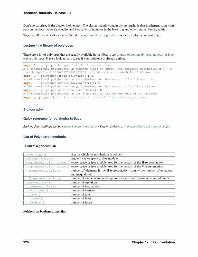
Thematic Tutorials, Release 9.1
Don’t be surprised if the classes look empty! The classes mainly contain private methods that implement some com-parison methods: to verify equality and inequality of numbers in the base ring and other internal functionalities.
To get a full overview of methods offered to you, Base class for polyhedra is the first place you want to go.
Lecture 4: A library of polytopes
There are a lot of polytopes that are readily available in the library, see Library of commonly used, famous, or inter-esting polytopes. Have a look at them to see if your polytope is already defined!
sage: A = polytopes.buckyball(); A # can take longA 3-dimensional polyhedron in (Number Field in sqrt5 with defining polynomial x^2 - 5→˓with sqrt5 = 2.236067977499790?)^3 defined as the convex hull of 60 verticessage: B = polytopes.cross_polytope(4); BA 4-dimensional polyhedron in ZZ^4 defined as the convex hull of 8 verticessage: C = polytopes.cyclic_polytope(3,10); CA 3-dimensional polyhedron in QQ^3 defined as the convex hull of 10 verticessage: E = polytopes.snub_cube(exact=False); EA 3-dimensional polyhedron in RDF^3 defined as the convex hull of 24 verticessage: polytopes.<tab> # not tested, to view all the possible polytopes
Bibliography
Quick reference for polyhedra in Sage
Author: Jean-Philippe Labbé <[email protected]> Vincent Delecroix <[email protected]>
List of Polyhedron methods
H and V-representation
base_ring() ring on which the polyhedron is definedambient_space() ambient vector space or free moduleHrepresentation_space() vector space or free module used for the vectors of the H-representationVrepresentation_space() vector space or free module used for the vectors of the V-representationn_Hrepresentation() number of elements in the H-representation (sum of the number of equations
and inequalities)n_Vrepresentation() number of elements in the V-representation (sum of vertices, rays and lines)n_equations() number of equationsn_inequalities() number of inequalitiesn_vertices() number of verticesn_rays() number of raysn_lines() number of linesn_facets() number of facets
Polyhedron boolean properties:
320 Chapter 12. Documentation
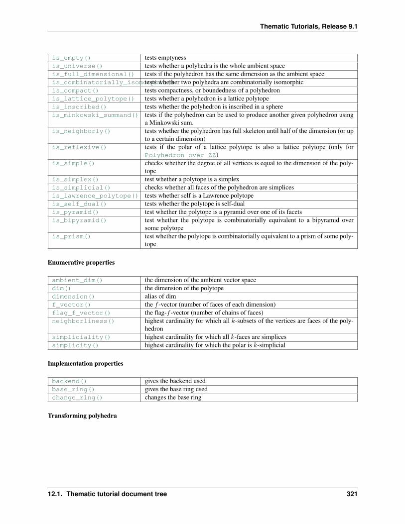
Thematic Tutorials, Release 9.1
is_empty() tests emptynessis_universe() tests whether a polyhedra is the whole ambient spaceis_full_dimensional() tests if the polyhedron has the same dimension as the ambient spaceis_combinatorially_isomorphic()tests whether two polyhedra are combinatorially isomorphicis_compact() tests compactness, or boundedness of a polyhedronis_lattice_polytope() tests whether a polyhedron is a lattice polytopeis_inscribed() tests whether the polyhedron is inscribed in a sphereis_minkowski_summand() tests if the polyhedron can be used to produce another given polyhedron using
a Minkowski sum.is_neighborly() tests whether the polyhedron has full skeleton until half of the dimension (or up
to a certain dimension)is_reflexive() tests if the polar of a lattice polytope is also a lattice polytope (only for
Polyhedron over ZZ)is_simple() checks whether the degree of all vertices is equal to the dimension of the poly-
topeis_simplex() test whether a polytope is a simplexis_simplicial() checks whether all faces of the polyhedron are simplicesis_lawrence_polytope() tests whether self is a Lawrence polytopeis_self_dual() tests whether the polytope is self-dualis_pyramid() test whether the polytope is a pyramid over one of its facetsis_bipyramid() test whether the polytope is combinatorially equivalent to a bipyramid over
some polytopeis_prism() test whether the polytope is combinatorially equivalent to a prism of some poly-
tope
Enumerative properties
ambient_dim() the dimension of the ambient vector spacedim() the dimension of the polytopedimension() alias of dimf_vector() the 𝑓 -vector (number of faces of each dimension)flag_f_vector() the flag-𝑓 -vector (number of chains of faces)neighborliness() highest cardinality for which all 𝑘-subsets of the vertices are faces of the poly-
hedronsimpliciality() highest cardinality for which all 𝑘-faces are simplicessimplicity() highest cardinality for which the polar is 𝑘-simplicial
Implementation properties
backend() gives the backend usedbase_ring() gives the base ring usedchange_ring() changes the base ring
Transforming polyhedra
12.1. Thematic tutorial document tree 321
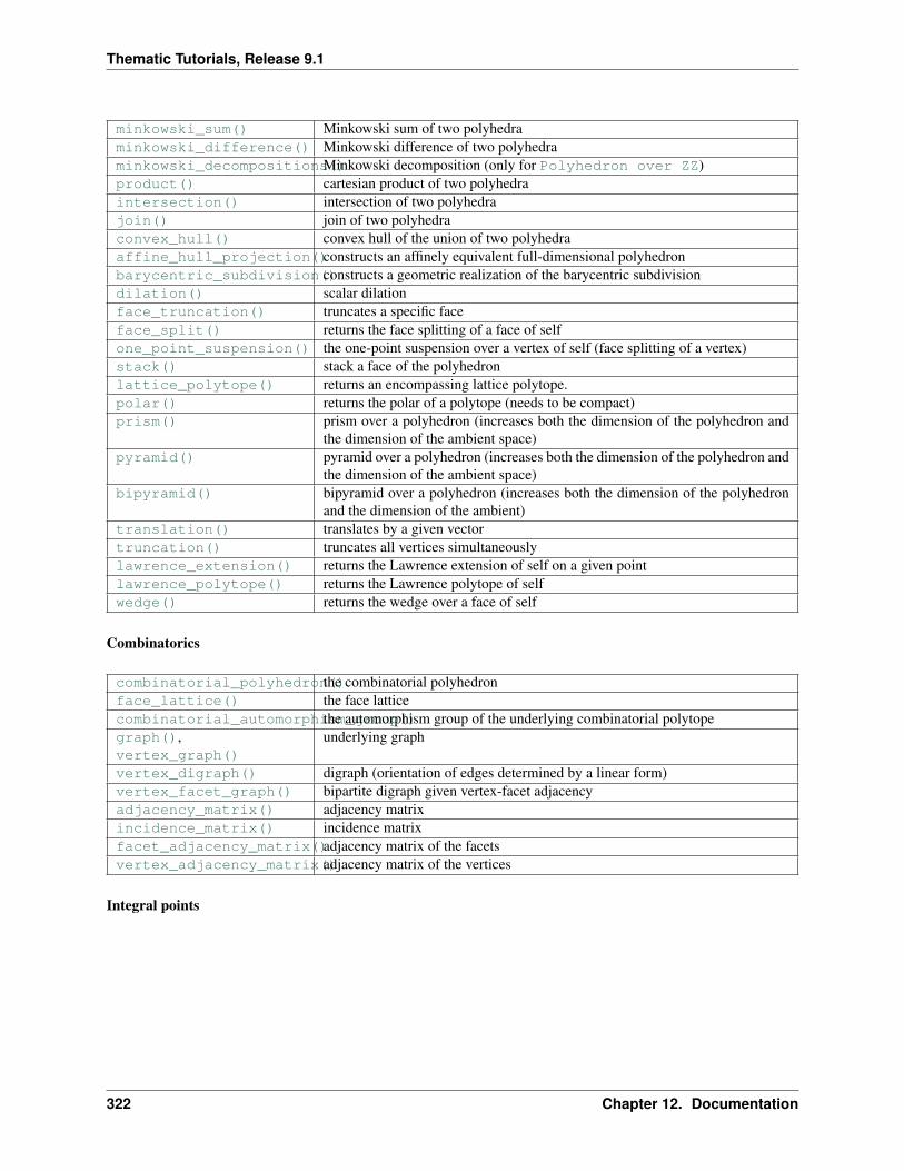
Thematic Tutorials, Release 9.1
minkowski_sum() Minkowski sum of two polyhedraminkowski_difference() Minkowski difference of two polyhedraminkowski_decompositions()Minkowski decomposition (only for Polyhedron over ZZ)product() cartesian product of two polyhedraintersection() intersection of two polyhedrajoin() join of two polyhedraconvex_hull() convex hull of the union of two polyhedraaffine_hull_projection()constructs an affinely equivalent full-dimensional polyhedronbarycentric_subdivision()constructs a geometric realization of the barycentric subdivisiondilation() scalar dilationface_truncation() truncates a specific faceface_split() returns the face splitting of a face of selfone_point_suspension() the one-point suspension over a vertex of self (face splitting of a vertex)stack() stack a face of the polyhedronlattice_polytope() returns an encompassing lattice polytope.polar() returns the polar of a polytope (needs to be compact)prism() prism over a polyhedron (increases both the dimension of the polyhedron and
the dimension of the ambient space)pyramid() pyramid over a polyhedron (increases both the dimension of the polyhedron and
the dimension of the ambient space)bipyramid() bipyramid over a polyhedron (increases both the dimension of the polyhedron
and the dimension of the ambient)translation() translates by a given vectortruncation() truncates all vertices simultaneouslylawrence_extension() returns the Lawrence extension of self on a given pointlawrence_polytope() returns the Lawrence polytope of selfwedge() returns the wedge over a face of self
Combinatorics
combinatorial_polyhedron()the combinatorial polyhedronface_lattice() the face latticecombinatorial_automorphism_group()the automorphism group of the underlying combinatorial polytopegraph(),vertex_graph()
underlying graph
vertex_digraph() digraph (orientation of edges determined by a linear form)vertex_facet_graph() bipartite digraph given vertex-facet adjacencyadjacency_matrix() adjacency matrixincidence_matrix() incidence matrixfacet_adjacency_matrix()adjacency matrix of the facetsvertex_adjacency_matrix()adjacency matrix of the vertices
Integral points
322 Chapter 12. Documentation
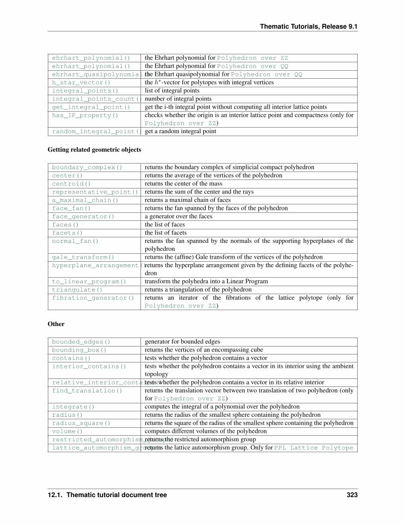
Thematic Tutorials, Release 9.1
ehrhart_polynomial() the Ehrhart polynomial for Polyhedron over ZZehrhart_polynomial() the Ehrhart polynomial for Polyhedron over QQehrhart_quasipolynomial()the Ehrhart quasipolynomial for Polyhedron over QQh_star_vector() the ℎ*-vector for polytopes with integral verticesintegral_points() list of integral pointsintegral_points_count() number of integral pointsget_integral_point() get the i-th integral point without computing all interior lattice pointshas_IP_property() checks whether the origin is an interior lattice point and compactness (only for
Polyhedron over ZZ)random_integral_point() get a random integral point
Getting related geometric objects
boundary_complex() returns the boundary complex of simplicial compact polyhedroncenter() returns the average of the vertices of the polyhedroncentroid() returns the center of the massrepresentative_point() returns the sum of the center and the raysa_maximal_chain() returns a maximal chain of facesface_fan() returns the fan spanned by the faces of the polyhedronface_generator() a generator over the facesfaces() the list of facesfacets() the list of facetsnormal_fan() returns the fan spanned by the normals of the supporting hyperplanes of the
polyhedrongale_transform() returns the (affine) Gale transform of the vertices of the polyhedronhyperplane_arrangement()returns the hyperplane arrangement given by the defining facets of the polyhe-
dronto_linear_program() transform the polyhedra into a Linear Programtriangulate() returns a triangulation of the polyhedronfibration_generator() returns an iterator of the fibrations of the lattice polytope (only for
Polyhedron over ZZ)
Other
bounded_edges() generator for bounded edgesbounding_box() returns the vertices of an encompassing cubecontains() tests whether the polyhedron contains a vectorinterior_contains() tests whether the polyhedron contains a vector in its interior using the ambient
topologyrelative_interior_contains()tests whether the polyhedron contains a vector in its relative interiorfind_translation() returns the translation vector between two translation of two polyhedron (only
for Polyhedron over ZZ)integrate() computes the integral of a polynomial over the polyhedronradius() returns the radius of the smallest sphere containing the polyhedronradius_square() returns the square of the radius of the smallest sphere containing the polyhedronvolume() computes different volumes of the polyhedronrestricted_automorphism_group()returns the restricted automorphism grouplattice_automorphism_group()returns the lattice automorphism group. Only for PPL Lattice Polytope
12.1. Thematic tutorial document tree 323
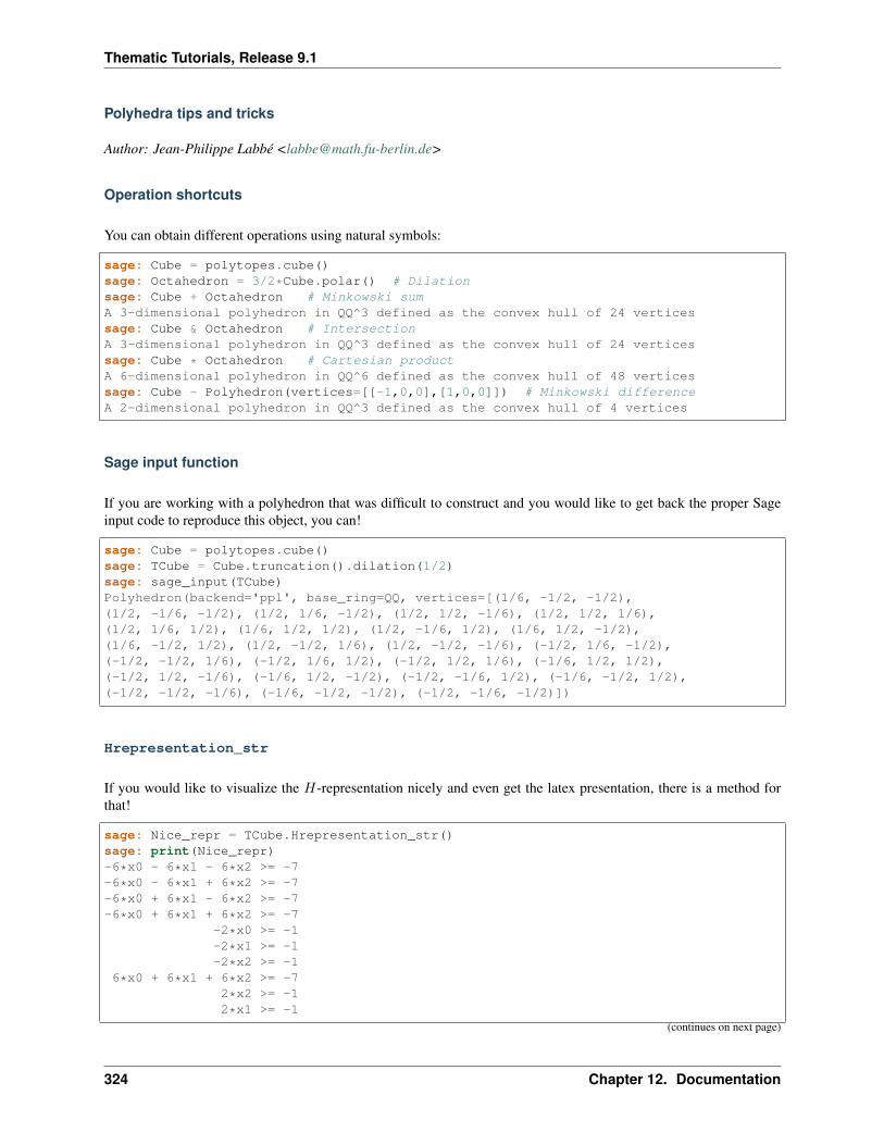
Thematic Tutorials, Release 9.1
Polyhedra tips and tricks
Author: Jean-Philippe Labbé <[email protected]>
Operation shortcuts
You can obtain different operations using natural symbols:
sage: Cube = polytopes.cube()sage: Octahedron = 3/2*Cube.polar() # Dilationsage: Cube + Octahedron # Minkowski sumA 3-dimensional polyhedron in QQ^3 defined as the convex hull of 24 verticessage: Cube & Octahedron # IntersectionA 3-dimensional polyhedron in QQ^3 defined as the convex hull of 24 verticessage: Cube * Octahedron # Cartesian productA 6-dimensional polyhedron in QQ^6 defined as the convex hull of 48 verticessage: Cube - Polyhedron(vertices=[[-1,0,0],[1,0,0]]) # Minkowski differenceA 2-dimensional polyhedron in QQ^3 defined as the convex hull of 4 vertices
Sage input function
If you are working with a polyhedron that was difficult to construct and you would like to get back the proper Sageinput code to reproduce this object, you can!
sage: Cube = polytopes.cube()sage: TCube = Cube.truncation().dilation(1/2)sage: sage_input(TCube)Polyhedron(backend='ppl', base_ring=QQ, vertices=[(1/6, -1/2, -1/2),(1/2, -1/6, -1/2), (1/2, 1/6, -1/2), (1/2, 1/2, -1/6), (1/2, 1/2, 1/6),(1/2, 1/6, 1/2), (1/6, 1/2, 1/2), (1/2, -1/6, 1/2), (1/6, 1/2, -1/2),(1/6, -1/2, 1/2), (1/2, -1/2, 1/6), (1/2, -1/2, -1/6), (-1/2, 1/6, -1/2),(-1/2, -1/2, 1/6), (-1/2, 1/6, 1/2), (-1/2, 1/2, 1/6), (-1/6, 1/2, 1/2),(-1/2, 1/2, -1/6), (-1/6, 1/2, -1/2), (-1/2, -1/6, 1/2), (-1/6, -1/2, 1/2),(-1/2, -1/2, -1/6), (-1/6, -1/2, -1/2), (-1/2, -1/6, -1/2)])
Hrepresentation_str
If you would like to visualize the 𝐻-representation nicely and even get the latex presentation, there is a method forthat!
sage: Nice_repr = TCube.Hrepresentation_str()sage: print(Nice_repr)-6*x0 - 6*x1 - 6*x2 >= -7-6*x0 - 6*x1 + 6*x2 >= -7-6*x0 + 6*x1 - 6*x2 >= -7-6*x0 + 6*x1 + 6*x2 >= -7
-2*x0 >= -1-2*x1 >= -1-2*x2 >= -1
6*x0 + 6*x1 + 6*x2 >= -72*x2 >= -12*x1 >= -1
(continues on next page)
324 Chapter 12. Documentation
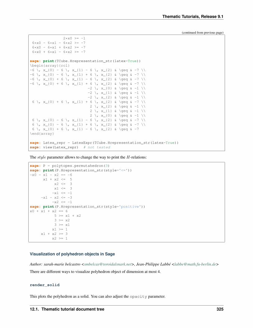
Thematic Tutorials, Release 9.1
(continued from previous page)
2*x0 >= -16*x0 - 6*x1 - 6*x2 >= -76*x0 - 6*x1 + 6*x2 >= -76*x0 + 6*x1 - 6*x2 >= -7
sage: print(TCube.Hrepresentation_str(latex=True))\beginarrayrcl-6 \, x_0 - 6 \, x_1 - 6 \, x_2 & \geq & -7 \\-6 \, x_0 - 6 \, x_1 + 6 \, x_2 & \geq & -7 \\-6 \, x_0 + 6 \, x_1 - 6 \, x_2 & \geq & -7 \\-6 \, x_0 + 6 \, x_1 + 6 \, x_2 & \geq & -7 \\
-2 \, x_0 & \geq & -1 \\-2 \, x_1 & \geq & -1 \\-2 \, x_2 & \geq & -1 \\
6 \, x_0 + 6 \, x_1 + 6 \, x_2 & \geq & -7 \\2 \, x_2 & \geq & -1 \\2 \, x_1 & \geq & -1 \\2 \, x_0 & \geq & -1 \\
6 \, x_0 - 6 \, x_1 - 6 \, x_2 & \geq & -7 \\6 \, x_0 - 6 \, x_1 + 6 \, x_2 & \geq & -7 \\6 \, x_0 + 6 \, x_1 - 6 \, x_2 & \geq & -7
\endarray
sage: Latex_repr = LatexExpr(TCube.Hrepresentation_str(latex=True))sage: view(Latex_repr) # not tested
The 𝑠𝑡𝑦𝑙𝑒 parameter allows to change the way to print the 𝐻-relations:
sage: P = polytopes.permutahedron(3)sage: print(P.Hrepresentation_str(style='<='))-x0 - x1 - x2 == -6
x1 + x2 <= 5x2 <= 3x1 <= 3
-x1 <= -1-x1 - x2 <= -3
-x2 <= -1sage: print(P.Hrepresentation_str(style='positive'))x0 + x1 + x2 == 6
5 >= x1 + x23 >= x23 >= x1
x1 >= 1x1 + x2 >= 3
x2 >= 1
Visualization of polyhedron objects in Sage
Author: sarah-marie belcastro <[email protected]>, Jean-Philippe Labbé <[email protected]>
There are different ways to visualize polyhedron object of dimension at most 4.
render_solid
This plots the polyhedron as a solid. You can also adjust the opacity parameter.
12.1. Thematic tutorial document tree 325
Thematic Tutorials, Release 9.1
sage: Cube = polytopes.cube()sage: Cube.render_solid(opacity=0.7)Graphics3d Object
render_wireframe
This plots the graph (with unbounded edges) of the polyhedron
sage: Cube.render_wireframe()Graphics3d Object
plot
The plot method draws the graph, the polygons and vertices of the polyhedron all together.
sage: Cube.plot()Graphics3d Object
show
This is similar to plot but does not return an object that you can manipulate.
schlegel_projection
It is possible to visualize 4-dimensional polytopes using a schlegel diagram.
sage: HC = polytopes.hypercube(4)sage: HC.schlegel_projection()The projection of a polyhedron into 3 dimensionssage: HC.schlegel_projection().plot()Graphics3d Object
We can see it from a different perspective:
sage: HC.schlegel_projection([2,5,11,17]).plot()Graphics3d Object
Draw polytopes in LaTeX using TikZ
Author: Jean-Philippe Labbé <[email protected]>
It is sometimes very helpful to draw 3-dimensional polytopes in a paper. TikZ is a very versatile tool to draw inscientific documents and Sage can deal easily with 3-dimensional polytopes. Finally sagetex makes everything worktogether nicely between Sage, TikZ and LaTeX. Since version 6.3 of Sage, there is a function for (projection of)polytopes to output a TikZ picture of the polytope. This short tutorial shows how it all works.
326 Chapter 12. Documentation
Thematic Tutorials, Release 9.1
Instructions
To put an image of a 3d-polytope in LaTeX using TikZ and Sage, simply follow the instructions:
• Install SageTex (optional but recommended!)
• Put \usepackagetikz in the preamble of your article
• Open Sage and change the directory to your article’s by the command cd /path/to/article
• Input your polytope, called P for example, to Sage
• Visualize the polytope P using the command P.show(aspect_ratio=1)
• This will open an interactive viewer named Jmol, in which you can rotate the polytope. Once the wished viewangle is found, right click on the image and select Console
• In the dialog box click the button State
• Scroll up to the line starting with moveto
• It reads something like moveto 0.0 x y z angle scale
• Go back to Sage and type Img = P.projection().tikz([x,y,z],angle)
• Img now contains a Sage object of type LatexExpr containing the raw TikZ picture of your polytope
Then, you can either copy-paste it to your article by typing Img in Sage or save it to a file, by doing
f = open('Img_poly.tex','w')f.write(Img)f.close()
Then in the pwd (present working directory of sage, the one of your article) you will have a file named Img_poly.tex containing the tikzpicture of your polytope.
Customization
You can customize the polytope using the following options in the command P.tikz()
• scale : positive number to scale the polytope,
• edge_color : string (default: blue!95!black) representing colors which tikz recognize,
• facet_color : string (default: blue!95!black) representing colors which tikz recognize,
• vertex_color : string (default: green) representing colors which tikz recognize,
• opacity : real number (default: 0.8) between 0 and 1 giving the opacity of the front facets,
• axis : Boolean (default: False) draw the axes at the origin or not.
Examples
Let’s say you want to draw the polar dual of the following (nice!) polytope given by the following list of vertices:
[[1,0,1],[1,0,0],[1,1,0],[0,0,-1],[0,1,0],[-1,0,0],[0,1,1],[0,0,1],[0,-1,0]]
In Sage, you type:
P = Polyhedron(vertices=[[1,0,1],[1,0,0],[1,1,0],[0,0,-1],[0,1,0],[-1,0,0],[0,1,1],[0,→˓0,1],[0,-1,0]]).polar()
12.1. Thematic tutorial document tree 327
Thematic Tutorials, Release 9.1
Then, you visualize the polytope by typing P.show(aspect_ratio=1)
When you found a good angle, follow the above procedure to obtain the values [674,108,-731] and angle=112, forexample.
Img = P.projection().tikz([674,108,-731],112)
Or you may want to customize using the command
Img = P.projection().tikz([674,108,-731],112,scale=2, edge_color='orange',facet_color=→˓'red',vertex_color='blue',opacity=0.4)
Further, you may want to edit deeper the style of the polytope, directly inside the tikzpicture. For example, line 6-9 inthe tikzpicture reads:
back/.style=loosely dotted, thin,edge/.style=color=orange, thick,facet/.style=fill=red,fill opacity=0.400000,vertex/.style=inner sep=1pt,circle,draw=blue!25!black,fill=blue!75!black,thick,→˓anchor=base]
It is also possible to replace it by the following 4 lines (and adding \usetikzlibraryshapes in the preamble)
back/.style=loosely dashed,line width=2pt,edge/.style=color=yellow, line width=2pt,facet/.style=fill=cyan,fill opacity=0.400000,vertex/.style=inner sep=4pt,star,star points=7,draw=blue!75!white,fill=blue!85!white,→˓thick,anchor=base]
Finally, you may want to tweak your picture my adding labels, elements on vertices, edges, facets, etc.
Automatize using SageTex
For this you need to put
\usepackagesagetex
in the preamble of your article
There are different ways to use sagetex and you may create your own. Here are some possibilities.
1) You can directly type in a sagestr in the article:
\sagestr(polytopes.permutahedron(4)).projection().tikz([4,5,6],45,scale=0.75, facet_→˓color='red',vertex_color='yellow',opacity=0.3)
2) You may create the following tex commands
\newcommand\polytopeimg[4]\sagestr(#1).projection().tikz(#2,#3,#4)\newcommand\polytopeimgopt[9]\sagestr(#1).projection().tikz(#2,#3,#4,#5,#6,#7,#8,→˓#9)
in your preamble and use them with a sagesilent in your article:
\beginsagesilentPolytope = polytopes.great_rhombicuboctahedron()\endsagesilent
328 Chapter 12. Documentation
Thematic Tutorials, Release 9.1
\polytopeimgPolytope[276,-607,-746]1021\polytopeimgoptPolytopeview=[-907,379,183]angle=129scale=2edge_color='red'→˓facet_color='yellow'vertex_color='blue'opacity=0.6axis=False
Then, run pdflatex, execute Sage on the file article_name.sagetex.sage and run pdflatex again.
For more information on SageTeX, see the tutorial http://doc.sagemath.org/html/en/tutorial/sagetex.html.
12.1.12 Tutorial: Programming in Python and Sage
Author: Florent Hivert <[email protected]>, Franco Saliola <[email protected]>, et al.
This tutorial is an introduction to basic programming in Python and Sage, for readers with elementary notions ofprogramming but not familiar with the Python language. It is far from exhaustive. For a more complete tutorial, havea look at the Python Tutorial. Also Python’s documentation and in particular the standard library can be useful.
A more advanced tutorial presents the notions of objects and classes in Python.
Here are further resources to learn Python:
• Learn Python in 10 minutes ou en français Python en 10 minutes
• Dive into Python is a Python book for experienced programmers. Also available in other languages.
• Discover Python is a series of articles published in IBM’s developerWorks technical resource center.
Data structures
In Python, typing is dynamic; there is no such thing as declaring variables. The function type() returns the typeof an object obj. To convert an object to a type typ just write typ(obj) as in int("123"). The commandisinstance(ex, typ) returns whether the expression ex is of type typ. Specifically, any value is an instanceof a class and there is no difference between classes and types.
The symbol = denotes the affectation to a variable; it should not be confused with == which denotes mathematicalequality. Inequality is !=.
The standard types are bool, int, list, tuple, set, dict, str.
• The type bool (booleans) has two values: True and False. The boolean operators are denoted by theirnames or, and, not.
• The Python types int and long are used to represent integers of limited size. To handle arbitrary large integerswith exact arithmetic, Sage uses its own type named Integer.
• A list is a data structure which groups values. It is constructed using brackets as in [1, 3, 4]. The range()function creates integer lists. One can also create lists using list comprehension:
[ <expr> for <name> in <iterable> (if <condition>) ]
For example:
sage: [ i^2 for i in range(10) if i % 2 == 0 ][0, 4, 16, 36, 64]
• A tuple is very similar to a list; it is constructed using parentheses. The empty tuple is obtained by () or bythe constructor tuple. If there is only one element, one has to write (a,). A tuple is immutable (one cannotchange it) but it is hashable (see below). One can also create tuples using comprehensions:
12.1. Thematic tutorial document tree 329
Thematic Tutorials, Release 9.1
sage: tuple(i^2 for i in range(10) if i % 2 == 0)(0, 4, 16, 36, 64)
• A set is a data structure which contains values without multiplicities or order. One creates it from a list (or anyiterable) with the constructor set. The elements of a set must be hashable:
sage: set([2,2,1,4,5])1, 2, 4, 5
sage: set([ [1], [2] ])Traceback (most recent call last):...TypeError: unhashable type: 'list'
• A dictionary is an association table, which associates values to keys. Keys must be hashable. One createsdictionaries using the constructor dict, or using the syntax:
key1 : value1, key2 : value2 ...
For example:
sage: age = 'toto' : 8, 'mom' : 27; age'mom': 27, 'toto': 8
• Quotes (simple ' ' or double " ") enclose character strings. One can concatenate them using +.
• For lists, tuples, strings, and dictionaries, the indexing operator is written l[i]. For lists, tuples, and stringsone can also uses slices as l[:], l[:b], l[a:], or l[a:b]. Negative indices start from the end.
• The len() function returns the number of elements of a list, a tuple, a set, a string, or a dictionary. One writesx in C to tests whether x is in C.
• Finally there is a special value called None to denote the absence of a value.
Control structures
In Python, there is no keyword for the beginning and the end of an instructions block. Blocks are delimited solely bymeans of indentation. Most of the time a new block is introduced by :. Python has the following control structures:
• Conditional instruction:
if <condition>:<instruction sequence>
[elif <condition>:<instruction sequence>]*
[else:<instruction sequence>]
• Inside expression exclusively, one can write:
<value> if <condition> else <value>
• Iterative instructions:
for <name> in <iterable>:<instruction sequence>
[else:<instruction sequence>]
330 Chapter 12. Documentation
Thematic Tutorials, Release 9.1
while <condition>:<instruction sequence>
[else:<instruction sequence>]
The else block is executed at the end of the loop if the loop is ended normally, that is neither by a break noran exception.
• In a loop, continue jumps to the next iteration.
• An iterable is an object which can be iterated through. Iterable types include lists, tuples, dictionaries, andstrings.
• An error (also called exception) is raised by:
raise <ErrorType> [, error message]
Usual errors include ValueError and TypeError.
Functions
Note: Python functions vs. mathematical functions
In what follows, we deal with functions is the sense of programming languages. Mathematical functions, as manip-ulated in calculus, are handled by Sage in a different way. In particular it doesn’t make sense to do mathematicalmanipulation such as additions or derivations on Python functions.
One defines a function using the keyword def as:
def <name>(<argument list>):<instruction sequence>
The result of the function is given by the instruction return. Very short functions can be created anonymously usinglambda (remark that there is no instruction return here):
lambda <arguments>: <expression>
Note: Functional programming
Functions are objects as any other objects. One can assign them to variables or return them. For details, see the tutorialon Functional Programming for Mathematicians.
Exercises
Lists
Creating Lists I: [Square brackets]
Example:
12.1. Thematic tutorial document tree 331
Thematic Tutorials, Release 9.1
sage: L = [3, Permutation([5,1,4,2,3]), 17, 17, 3, 51]sage: L[3, [5, 1, 4, 2, 3], 17, 17, 3, 51]
Exercise: Create the list [63, 12, -10, "a", 12], assign it to the variable L, and print the list.
sage: # edit here
Exercise: Create the empty list (you will often need to do this).
sage: # edit here
Creating Lists II: range
The range() function provides an easy way to construct a list of integers. Here is the documentation of therange() function:
range([start,] stop[, step]) -> list of integers
Return a list containing an arithmetic progression of integers.range(i, j) returns [i, i+1, i+2, ..., j-1]; start (!) defaults to 0.When step is given, it specifies the increment (or decrement). Forexample, range(4) returns [0, 1, 2, 3]. The end point is omitted!These are exactly the valid indices for a list of 4 elements.
Exercise: Use range() to construct the list [1, 2, . . . , 50].
sage: # edit here
Exercise: Use range() to construct the list of even numbers between 1 and 100 (including 100).
sage: # edit here
Exercise: The step argument for the range() command can be negative. Use range to construct the list[10, 7, 4, 1,−2].
sage: # edit here
See also:
• xrange(): returns an iterator rather than building a list, (only for Python2, replaced by range in Python 3).
• srange(): like range but with Sage integers; see below.
• xsrange(): like xrange but with Sage integers.
Creating Lists III: list comprehensions
List comprehensions provide a concise way to create lists from other lists (or other data types).
Example We already know how to create the list [1, 2, . . . , 16]:
sage: range(1,17) # py2[1, 2, 3, 4, 5, 6, 7, 8, 9, 10, 11, 12, 13, 14, 15, 16]
Using a list comprehension, we can now create the list [12, 22, 32, . . . , 162] as follows:
332 Chapter 12. Documentation
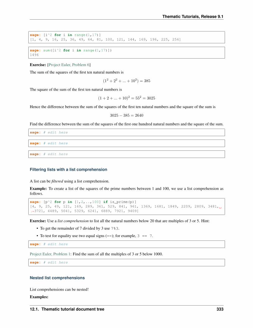
Thematic Tutorials, Release 9.1
sage: [i^2 for i in range(1,17)][1, 4, 9, 16, 25, 36, 49, 64, 81, 100, 121, 144, 169, 196, 225, 256]
sage: sum([i^2 for i in range(1,17)])1496
Exercise: [Project Euler, Problem 6]
The sum of the squares of the first ten natural numbers is
(12 + 22 + ...+ 102) = 385
The square of the sum of the first ten natural numbers is
(1 + 2 + ...+ 10)2 = 552 = 3025
Hence the difference between the sum of the squares of the first ten natural numbers and the square of the sum is
3025− 385 = 2640
Find the difference between the sum of the squares of the first one hundred natural numbers and the square of the sum.
sage: # edit here
sage: # edit here
sage: # edit here
Filtering lists with a list comprehension
A list can be filtered using a list comprehension.
Example: To create a list of the squares of the prime numbers between 1 and 100, we use a list comprehension asfollows.
sage: [p^2 for p in [1,2,..,100] if is_prime(p)][4, 9, 25, 49, 121, 169, 289, 361, 529, 841, 961, 1369, 1681, 1849, 2209, 2809, 3481,→˓3721, 4489, 5041, 5329, 6241, 6889, 7921, 9409]
Exercise: Use a list comprehension to list all the natural numbers below 20 that are multiples of 3 or 5. Hint:
• To get the remainder of 7 divided by 3 use 7%3.
• To test for equality use two equal signs (==); for example, 3 == 7.
sage: # edit here
Project Euler, Problem 1: Find the sum of all the multiples of 3 or 5 below 1000.
sage: # edit here
Nested list comprehensions
List comprehensions can be nested!
Examples:
12.1. Thematic tutorial document tree 333
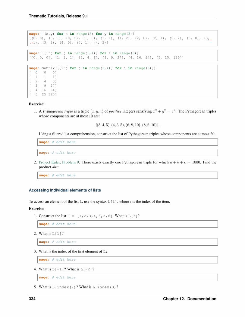
Thematic Tutorials, Release 9.1
sage: [(x,y) for x in range(5) for y in range(3)][(0, 0), (0, 1), (0, 2), (1, 0), (1, 1), (1, 2), (2, 0), (2, 1), (2, 2), (3, 0), (3,→˓1), (3, 2), (4, 0), (4, 1), (4, 2)]
sage: [[i^j for j in range(1,4)] for i in range(6)][[0, 0, 0], [1, 1, 1], [2, 4, 8], [3, 9, 27], [4, 16, 64], [5, 25, 125]]
sage: matrix([[i^j for j in range(1,4)] for i in range(6)])[ 0 0 0][ 1 1 1][ 2 4 8][ 3 9 27][ 4 16 64][ 5 25 125]
Exercise:
1. A Pythagorean triple is a triple (𝑥, 𝑦, 𝑧) of positive integers satisfying 𝑥2 + 𝑦2 = 𝑧2. The Pythagorean tripleswhose components are at most 10 are:
[(3, 4, 5), (4, 3, 5), (6, 8, 10), (8, 6, 10)] .
Using a filtered list comprehension, construct the list of Pythagorean triples whose components are at most 50:
sage: # edit here
sage: # edit here
2. Project Euler, Problem 9: There exists exactly one Pythagorean triple for which 𝑎 + 𝑏 + 𝑐 = 1000. Find theproduct 𝑎𝑏𝑐:
sage: # edit here
Accessing individual elements of lists
To access an element of the list L, use the syntax L[i], where 𝑖 is the index of the item.
Exercise:
1. Construct the list L = [1,2,3,4,3,5,6]. What is L[3]?
sage: # edit here
2. What is L[1]?
sage: # edit here
3. What is the index of the first element of L?
sage: # edit here
4. What is L[-1]? What is L[-2]?
sage: # edit here
5. What is L.index(2)? What is L.index(3)?
334 Chapter 12. Documentation
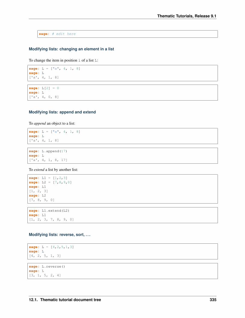
Thematic Tutorials, Release 9.1
sage: # edit here
Modifying lists: changing an element in a list
To change the item in position i of a list L:
sage: L = ["a", 4, 1, 8]sage: L['a', 4, 1, 8]
sage: L[2] = 0sage: L['a', 4, 0, 8]
Modifying lists: append and extend
To append an object to a list:
sage: L = ["a", 4, 1, 8]sage: L['a', 4, 1, 8]
sage: L.append(17)sage: L['a', 4, 1, 8, 17]
To extend a list by another list:
sage: L1 = [1,2,3]sage: L2 = [7,8,9,0]sage: L1[1, 2, 3]sage: L2[7, 8, 9, 0]
sage: L1.extend(L2)sage: L1[1, 2, 3, 7, 8, 9, 0]
Modifying lists: reverse, sort, . . .
sage: L = [4,2,5,1,3]sage: L[4, 2, 5, 1, 3]
sage: L.reverse()sage: L[3, 1, 5, 2, 4]
12.1. Thematic tutorial document tree 335
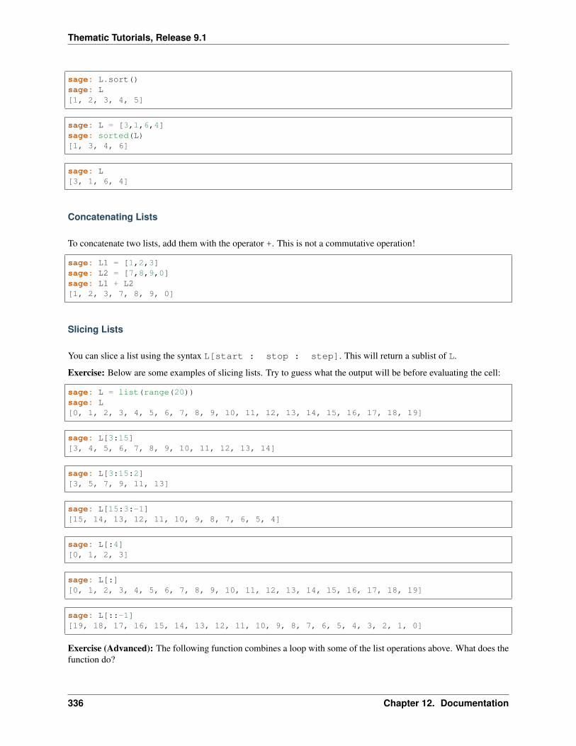
Thematic Tutorials, Release 9.1
sage: L.sort()sage: L[1, 2, 3, 4, 5]
sage: L = [3,1,6,4]sage: sorted(L)[1, 3, 4, 6]
sage: L[3, 1, 6, 4]
Concatenating Lists
To concatenate two lists, add them with the operator +. This is not a commutative operation!
sage: L1 = [1,2,3]sage: L2 = [7,8,9,0]sage: L1 + L2[1, 2, 3, 7, 8, 9, 0]
Slicing Lists
You can slice a list using the syntax L[start : stop : step]. This will return a sublist of L.
Exercise: Below are some examples of slicing lists. Try to guess what the output will be before evaluating the cell:
sage: L = list(range(20))sage: L[0, 1, 2, 3, 4, 5, 6, 7, 8, 9, 10, 11, 12, 13, 14, 15, 16, 17, 18, 19]
sage: L[3:15][3, 4, 5, 6, 7, 8, 9, 10, 11, 12, 13, 14]
sage: L[3:15:2][3, 5, 7, 9, 11, 13]
sage: L[15:3:-1][15, 14, 13, 12, 11, 10, 9, 8, 7, 6, 5, 4]
sage: L[:4][0, 1, 2, 3]
sage: L[:][0, 1, 2, 3, 4, 5, 6, 7, 8, 9, 10, 11, 12, 13, 14, 15, 16, 17, 18, 19]
sage: L[::-1][19, 18, 17, 16, 15, 14, 13, 12, 11, 10, 9, 8, 7, 6, 5, 4, 3, 2, 1, 0]
Exercise (Advanced): The following function combines a loop with some of the list operations above. What does thefunction do?
336 Chapter 12. Documentation
Thematic Tutorials, Release 9.1
sage: def f(number_of_iterations):....: L = [1]....: for n in range(2, number_of_iterations):....: L = [sum(L[:i]) for i in range(n-1, -1, -1)]....: return numerical_approx(2*L[0]*len(L)/sum(L), digits=50)
sage: # edit here
Tuples
A tuple is an immutable list. That is, it cannot be changed once it is created. This can be useful for code safety andforemost because it makes tuple hashable. To create a tuple, use parentheses instead of brackets:
sage: t = (3, 5, [3,1], (17,[2,3],17), 4)sage: t(3, 5, [3, 1], (17, [2, 3], 17), 4)
To create a singleton tuple, a comma is required to resolve the ambiguity:
sage: (1)1sage: (1,)(1,)
We can create a tuple from a list, and vice-versa.
sage: tuple(range(5))(0, 1, 2, 3, 4)
sage: list(t)[3, 5, [3, 1], (17, [2, 3], 17), 4]
Tuples behave like lists in many respects:
Operation Syntax for lists Syntax for tuplesAccessing a letter list[3] tuple[3]Concatenation list1 + list2 tuple1 + tuple2Slicing list[3:17:2] tuple[3:17:2]A reversed copy list[::-1] tuple[::-1]Length len(list) len(tuple)
Trying to modify a tuple will fail:
sage: t = (5, 'a', 6/5)sage: t(5, 'a', 6/5)
sage: t[1] = 'b'Traceback (most recent call last):...TypeError: 'tuple' object does not support item assignment
12.1. Thematic tutorial document tree 337
Thematic Tutorials, Release 9.1
Generators
“Tuple-comprehensions” do not exist. Instead, the syntax produces something called a generator. A generator allowsyou to process a sequence of items one at a time. Each item is created when it is needed, and then forgotten. This canbe very efficient if we only need to use each item once.
sage: (i^2 for i in range(5))<generator object <genexpr> at 0x...>
sage: g = (i^2 for i in range(5))sage: g[0]Traceback (most recent call last):...TypeError: 'generator' object ...
sage: [x for x in g][0, 1, 4, 9, 16]
g is now empty.
sage: [x for x in g][]
A nice ‘pythonic’ trick is to use generators as argument of functions. We do not need double parentheses for this:
sage: sum( i^2 for i in srange(100001) )333338333350000
Dictionaries
A dictionary is another built-in data type. Unlike lists, which are indexed by a range of numbers starting at 0, dictio-naries are indexed by keys, which can be any immutable objects. Strings and numbers can always be keys (becausethey are immutable). Dictionaries are sometimes called “associative arrays” in other programming languages.
There are several ways to define dictionaries. One method is to use braces, , with comma-separated entries given inthe form key:value:
sage: d = 3:17, 0.5:[4,1,5,2,3], 0:"goo", 3/2 : 17sage: d0: 'goo', 0.500000000000000: [4, 1, 5, 2, 3], 3/2: 17, 3: 17
A second method is to use the constructor dict which admits a list (or actually any iterable) of 2-tuples (key, value):
sage: dd = dict((i,i^2) for i in range(10))sage: dd0: 0, 1: 1, 2: 4, 3: 9, 4: 16, 5: 25, 6: 36, 7: 49, 8: 64, 9: 81
Dictionaries behave as lists and tuples for several important operations.
Operation Syntax for lists Syntax for dictionariesAccessing elements list[3] D["key"]Length len(list) len(D)Modifying L[3] = 17 D["key"] = 17Deleting items del L[3] del D["key"]
338 Chapter 12. Documentation
Thematic Tutorials, Release 9.1
sage: d[10]='a'sage: d0: 'goo', 0.500000000000000: [4, 1, 5, 2, 3], 3/2: 17, 3: 17, 10: 'a'
A dictionary can have the same value multiple times, but each key must only appear once and must be immutable:
sage: d = 3: 14, 4: 14sage: d3: 14, 4: 14
sage: d = 3: 13, 3: 14sage: d3: 14
sage: d = [1,2,3] : 12Traceback (most recent call last):...TypeError: unhashable type: 'list'
Another way to add items to a dictionary is with the update() method which updates the dictionary from anotherdictionary:
sage: d = sage: d
sage: d.update(10 : 'newvalue', 20: 'newervalue', 3: 14, 0.5:[1,2,3])sage: d0.500000000000000: [1, 2, 3], 3: 14, 10: 'newvalue', 20: 'newervalue'
We can iterate through the keys, or values, or both, of a dictionary. Note that, internally, there is no sorting of keysdone. In general, the order of keys/values will depend on memory locations can and will differ between differentcomputers and / or repeated runs on the same computer. However, Sage sort the dictionary entries by key whenprinting the dictionary specifically to make the docstrings more reproducible. However, the Python methods keys()and values() do not sort for you. If you want your output to be reproducable, then you have to sort it first just likein the examples below:
sage: d = 10 : 'newvalue', 20: 'newervalue', 3: 14, 0.5:(1,2,3)
sage: sorted([key for key in d])[0.500000000000000, 3, 10, 20]
sage: d.keys() # random order[0.500000000000000, 10, 3, 20]sage: sorted(d.keys())[0.500000000000000, 3, 10, 20]
sage: d.values() # random order[(1, 2, 3), 'newvalue', 14, 'newervalue']sage: set(d.values()) == set([14, (1, 2, 3), 'newvalue', 'newervalue'])True
sage: d.items() # random order[(0.500000000000000, (1, 2, 3)), (10, 'newvalue'), (3, 14), (20, 'newervalue')]
(continues on next page)
12.1. Thematic tutorial document tree 339
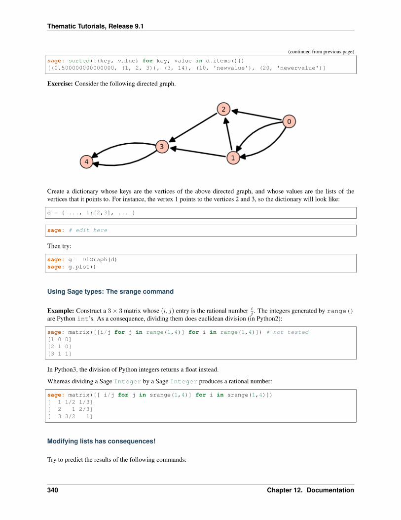
Thematic Tutorials, Release 9.1
(continued from previous page)
sage: sorted([(key, value) for key, value in d.items()])[(0.500000000000000, (1, 2, 3)), (3, 14), (10, 'newvalue'), (20, 'newervalue')]
Exercise: Consider the following directed graph.
Create a dictionary whose keys are the vertices of the above directed graph, and whose values are the lists of thevertices that it points to. For instance, the vertex 1 points to the vertices 2 and 3, so the dictionary will look like:
d = ..., 1:[2,3], ...
sage: # edit here
Then try:
sage: g = DiGraph(d)sage: g.plot()
Using Sage types: The srange command
Example: Construct a 3× 3 matrix whose (𝑖, 𝑗) entry is the rational number 𝑖𝑗 . The integers generated by range()
are Python int’s. As a consequence, dividing them does euclidean division (in Python2):
sage: matrix([[i/j for j in range(1,4)] for i in range(1,4)]) # not tested[1 0 0][2 1 0][3 1 1]
In Python3, the division of Python integers returns a float instead.
Whereas dividing a Sage Integer by a Sage Integer produces a rational number:
sage: matrix([[ i/j for j in srange(1,4)] for i in srange(1,4)])[ 1 1/2 1/3][ 2 1 2/3][ 3 3/2 1]
Modifying lists has consequences!
Try to predict the results of the following commands:
340 Chapter 12. Documentation
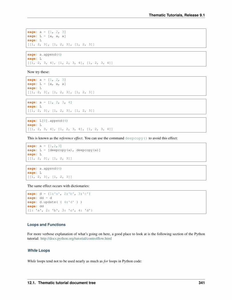
Thematic Tutorials, Release 9.1
sage: a = [1, 2, 3]sage: L = [a, a, a]sage: L[[1, 2, 3], [1, 2, 3], [1, 2, 3]]
sage: a.append(4)sage: L[[1, 2, 3, 4], [1, 2, 3, 4], [1, 2, 3, 4]]
Now try these:
sage: a = [1, 2, 3]sage: L = [a, a, a]sage: L[[1, 2, 3], [1, 2, 3], [1, 2, 3]]
sage: a = [1, 2, 3, 4]sage: L[[1, 2, 3], [1, 2, 3], [1, 2, 3]]
sage: L[0].append(4)sage: L[[1, 2, 3, 4], [1, 2, 3, 4], [1, 2, 3, 4]]
This is known as the reference effect. You can use the command deepcopy() to avoid this effect:
sage: a = [1,2,3]sage: L = [deepcopy(a), deepcopy(a)]sage: L[[1, 2, 3], [1, 2, 3]]
sage: a.append(4)sage: L[[1, 2, 3], [1, 2, 3]]
The same effect occurs with dictionaries:
sage: d = 1:'a', 2:'b', 3:'c'sage: dd = dsage: d.update( 4:'d' )sage: dd1: 'a', 2: 'b', 3: 'c', 4: 'd'
Loops and Functions
For more verbose explanation of what’s going on here, a good place to look at is the following section of the Pythontutorial: http://docs.python.org/tutorial/controlflow.html
While Loops
While loops tend not to be used nearly as much as for loops in Python code:
12.1. Thematic tutorial document tree 341
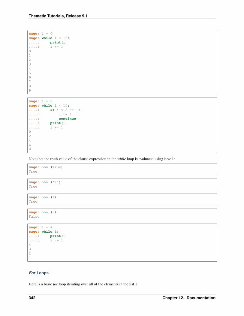
Thematic Tutorials, Release 9.1
sage: i = 0sage: while i < 10:....: print(i)....: i += 10123456789
sage: i = 0sage: while i < 10:....: if i % 2 == 1:....: i += 1....: continue....: print(i)....: i += 102468
Note that the truth value of the clause expression in the while loop is evaluated using bool:
sage: bool(True)True
sage: bool('a')True
sage: bool(1)True
sage: bool(0)False
sage: i = 4sage: while i:....: print(i)....: i -= 14321
For Loops
Here is a basic for loop iterating over all of the elements in the list l:
342 Chapter 12. Documentation
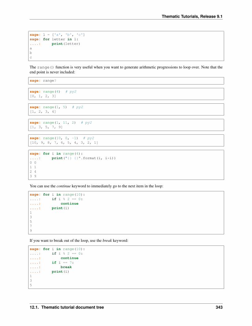
Thematic Tutorials, Release 9.1
sage: l = ['a', 'b', 'c']sage: for letter in l:....: print(letter)abc
The range() function is very useful when you want to generate arithmetic progressions to loop over. Note that theend point is never included:
sage: range?
sage: range(4) # py2[0, 1, 2, 3]
sage: range(1, 5) # py2[1, 2, 3, 4]
sage: range(1, 11, 2) # py2[1, 3, 5, 7, 9]
sage: range(10, 0, -1) # py2[10, 9, 8, 7, 6, 5, 4, 3, 2, 1]
sage: for i in range(4):....: print(" ".format(i, i*i))0 01 12 43 9
You can use the continue keyword to immediately go to the next item in the loop:
sage: for i in range(10):....: if i % 2 == 0:....: continue....: print(i)13579
If you want to break out of the loop, use the break keyword:
sage: for i in range(10):....: if i % 2 == 0:....: continue....: if i == 7:....: break....: print(i)135
12.1. Thematic tutorial document tree 343
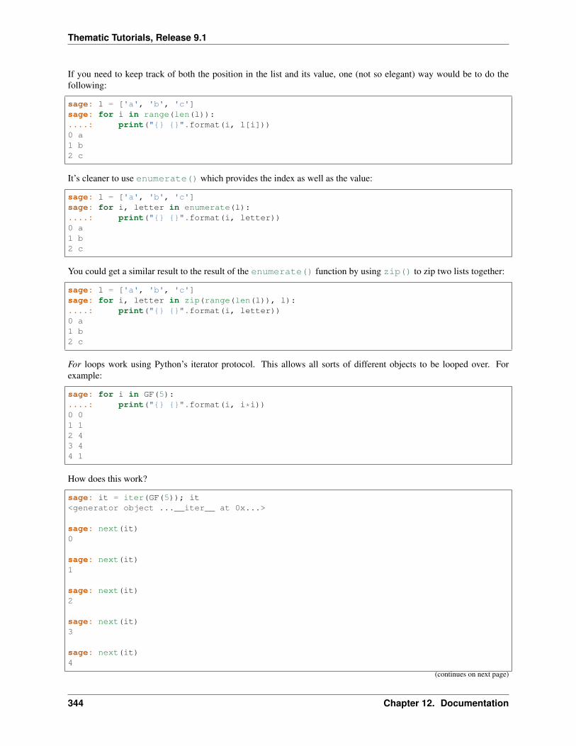
Thematic Tutorials, Release 9.1
If you need to keep track of both the position in the list and its value, one (not so elegant) way would be to do thefollowing:
sage: l = ['a', 'b', 'c']sage: for i in range(len(l)):....: print(" ".format(i, l[i]))0 a1 b2 c
It’s cleaner to use enumerate() which provides the index as well as the value:
sage: l = ['a', 'b', 'c']sage: for i, letter in enumerate(l):....: print(" ".format(i, letter))0 a1 b2 c
You could get a similar result to the result of the enumerate() function by using zip() to zip two lists together:
sage: l = ['a', 'b', 'c']sage: for i, letter in zip(range(len(l)), l):....: print(" ".format(i, letter))0 a1 b2 c
For loops work using Python’s iterator protocol. This allows all sorts of different objects to be looped over. Forexample:
sage: for i in GF(5):....: print(" ".format(i, i*i))0 01 12 43 44 1
How does this work?
sage: it = iter(GF(5)); it<generator object ...__iter__ at 0x...>
sage: next(it)0
sage: next(it)1
sage: next(it)2
sage: next(it)3
sage: next(it)4
(continues on next page)
344 Chapter 12. Documentation
Thematic Tutorials, Release 9.1
(continued from previous page)
sage: next(it)Traceback (most recent call last):...StopIteration
sage: R = GF(5)sage: R.__iter__??
The command yield provides a very convenient way to produce iterators. We’ll see more about it in a bit.
Exercises
For each of the following sets, compute the list of its elements and their sum. Use two different ways, if possible: witha loop, and using a list comprehension.
1. The first 𝑛 terms of the harmonic series:
𝑛∑𝑖=1
1
𝑖
sage: # edit here
2. The odd integers between 1 and 𝑛:
sage: # edit here
3. The first 𝑛 odd integers:
sage: # edit here
4. The integers between 1 and 𝑛 that are neither divisible by 2 nor by 3 nor by 5:
sage: # edit here
5. The first 𝑛 integers between 1 and 𝑛 that are neither divisible by 2 nor by 3 nor by 5:
sage: # edit here
Functions
Functions are defined using the def statement, and values are returned using the return keyword:
sage: def f(x):....: return x*x
sage: f(2)4
Functions can be recursive:
12.1. Thematic tutorial document tree 345
Thematic Tutorials, Release 9.1
sage: def fib(n):....: if n <= 1:....: return 1....: else:....: return fib(n-1) + fib(n-2)
sage: [fib(i) for i in range(10)][1, 1, 2, 3, 5, 8, 13, 21, 34, 55]
Functions are first class objects like any other. For example, they can be passed in as arguments to other functions:
sage: f<function f at 0x...>
sage: def compose(f, x, n): # computes f(f(...f(x)))....: for i in range(n):....: x = f(x) # this change is local to this function call!....: return x
sage: compose(f, 2, 3)256
sage: def add_one(x):....: return x + 1
sage: compose(add_one, 2, 3)5
You can give default values for arguments in functions:
sage: def add_n(x, n=1):....: return x + n
sage: add_n(4)5
sage: add_n(4, n=100)104
sage: add_n(4, 1000)1004
You can return multiple values from a function:
sage: def g(x):....: return x, x*x
sage: g(2)(2, 4)
sage: type(g)<... 'function'>
346 Chapter 12. Documentation
Thematic Tutorials, Release 9.1
sage: a,b = g(100)
sage: a100
sage: b10000
You can also take a variable number of arguments and keyword arguments in a function:
sage: def h(*args, **kwds):....: print(" ".format(type(args), args))....: print(" ".format(type(kwds), kwds))
sage: h(1,2,3,n=4)<... 'tuple'> (1, 2, 3)<... 'dict'> 'n': 4
Let’s use the yield instruction to make a generator for the Fibonacci numbers up to 𝑛:
sage: def fib_gen(n):....: if n < 1:....: return....: a = b = 1....: yield b....: while b < n:....: yield b....: a, b = b, b+a
sage: for i in fib_gen(50):....: print(i)112358132134
Exercises
1. Write a function is_even which returns True if n is even and False otherwise.
2. Write a function every_other which takes a list l as input and returns a list containing every other elementof l.
3. Write a generator every_other which takes an iterable l as input, and returns every other element of l, oneafter the other.
4. Write a function which computes the 𝑛-th Fibonacci number. Try to improve performance.
Todo:
12.1. Thematic tutorial document tree 347
Thematic Tutorials, Release 9.1
• Definition of hashable
• Introduction to the debugger.
12.1.13 Tutorial: Comprehensions, Iterators, and Iterables
Author: Florent Hivert <[email protected]> and Nicolas M. Thiéry <nthiery at users.sf.net>
List comprehensions
List comprehensions are a very handy way to construct lists in Python. You can use either of the following idioms:
[ <expr> for <name> in <iterable> ][ <expr> for <name> in <iterable> if <condition> ]
For example, here are some lists of squares:
sage: [ i^2 for i in [1, 3, 7] ][1, 9, 49]sage: [ i^2 for i in range(1,10) ][1, 4, 9, 16, 25, 36, 49, 64, 81]sage: [ i^2 for i in range(1,10) if i % 2 == 1][1, 9, 25, 49, 81]
And a variant on the latter:
sage: [i^2 if i % 2 == 1 else 2 for i in range(10)][2, 1, 2, 9, 2, 25, 2, 49, 2, 81]
Exercises
1. Construct the list of the squares of the prime integers between 1 and 10:
sage: # edit here
2. Construct the list of the perfect squares less than 100 (hint: use srange() to get a list of Sage integerstogether with the method i.sqrtrem()):
sage: # edit here
One can use more than one iterable in a list comprehension:
sage: [ (i,j) for i in range(1,6) for j in range(1,i) ][(2, 1), (3, 1), (3, 2), (4, 1), (4, 2), (4, 3), (5, 1), (5, 2), (5, 3), (5, 4)]
Warning: Mind the order of the nested loop in the previous expression.
If instead one wants to build a list of lists, one can use nested lists as in:
348 Chapter 12. Documentation
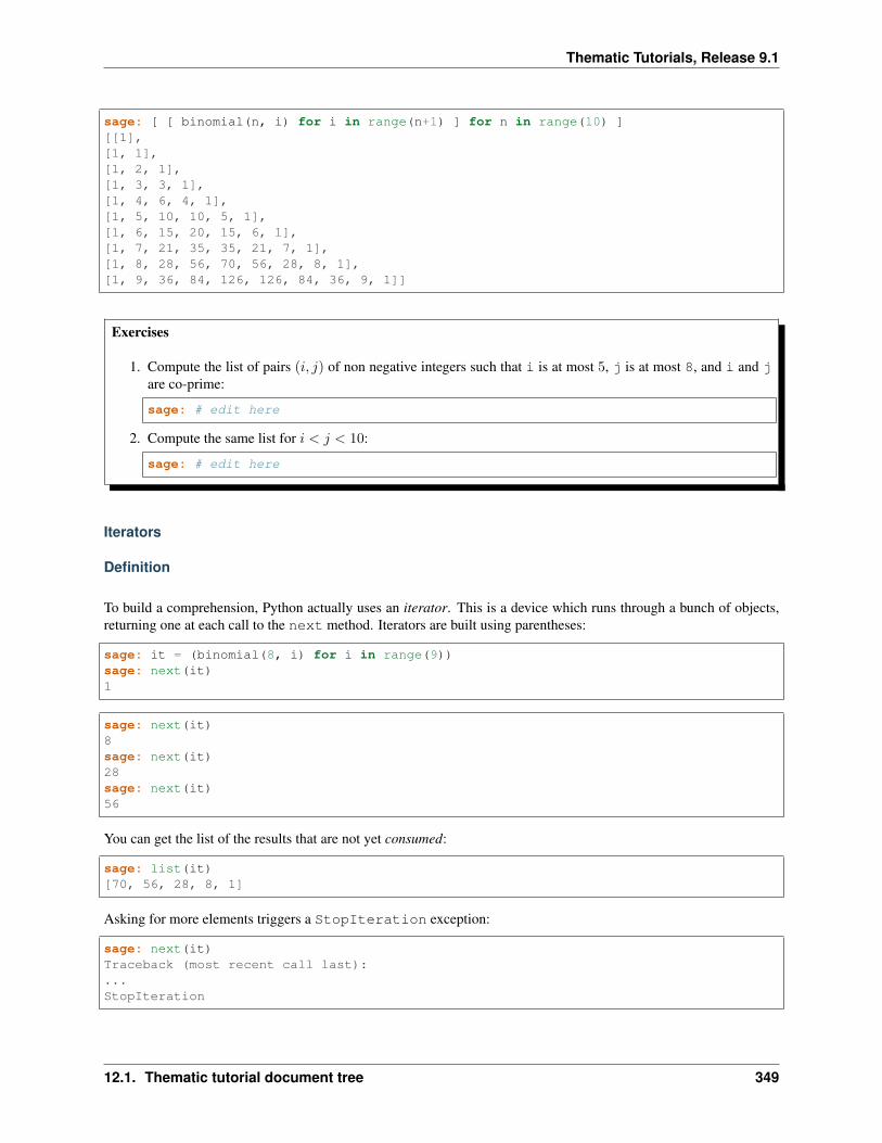
Thematic Tutorials, Release 9.1
sage: [ [ binomial(n, i) for i in range(n+1) ] for n in range(10) ][[1],[1, 1],[1, 2, 1],[1, 3, 3, 1],[1, 4, 6, 4, 1],[1, 5, 10, 10, 5, 1],[1, 6, 15, 20, 15, 6, 1],[1, 7, 21, 35, 35, 21, 7, 1],[1, 8, 28, 56, 70, 56, 28, 8, 1],[1, 9, 36, 84, 126, 126, 84, 36, 9, 1]]
Exercises
1. Compute the list of pairs (𝑖, 𝑗) of non negative integers such that i is at most 5, j is at most 8, and i and jare co-prime:
sage: # edit here
2. Compute the same list for 𝑖 < 𝑗 < 10:
sage: # edit here
Iterators
Definition
To build a comprehension, Python actually uses an iterator. This is a device which runs through a bunch of objects,returning one at each call to the next method. Iterators are built using parentheses:
sage: it = (binomial(8, i) for i in range(9))sage: next(it)1
sage: next(it)8sage: next(it)28sage: next(it)56
You can get the list of the results that are not yet consumed:
sage: list(it)[70, 56, 28, 8, 1]
Asking for more elements triggers a StopIteration exception:
sage: next(it)Traceback (most recent call last):...StopIteration
12.1. Thematic tutorial document tree 349
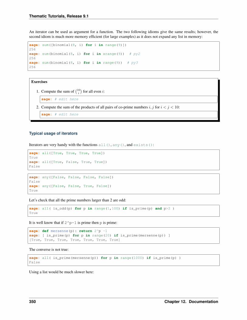
Thematic Tutorials, Release 9.1
An iterator can be used as argument for a function. The two following idioms give the same results; however, thesecond idiom is much more memory efficient (for large examples) as it does not expand any list in memory:
sage: sum([binomial(8, i) for i in range(9)])256sage: sum(binomial(8, i) for i in xrange(9)) # py2256sage: sum(binomial(8, i) for i in range(9)) # py3256
Exercises
1. Compute the sum of(10𝑖
)for all even 𝑖:
sage: # edit here
2. Compute the sum of the products of all pairs of co-prime numbers 𝑖, 𝑗 for 𝑖 < 𝑗 < 10:
sage: # edit here
Typical usage of iterators
Iterators are very handy with the functions all(), any(), and exists():
sage: all([True, True, True, True])Truesage: all([True, False, True, True])False
sage: any([False, False, False, False])Falsesage: any([False, False, True, False])True
Let’s check that all the prime numbers larger than 2 are odd:
sage: all( is_odd(p) for p in range(1,100) if is_prime(p) and p>2 )True
It is well know that if 2^p-1 is prime then p is prime:
sage: def mersenne(p): return 2^p -1sage: [ is_prime(p) for p in range(20) if is_prime(mersenne(p)) ][True, True, True, True, True, True, True]
The converse is not true:
sage: all( is_prime(mersenne(p)) for p in range(1000) if is_prime(p) )False
Using a list would be much slower here:
350 Chapter 12. Documentation
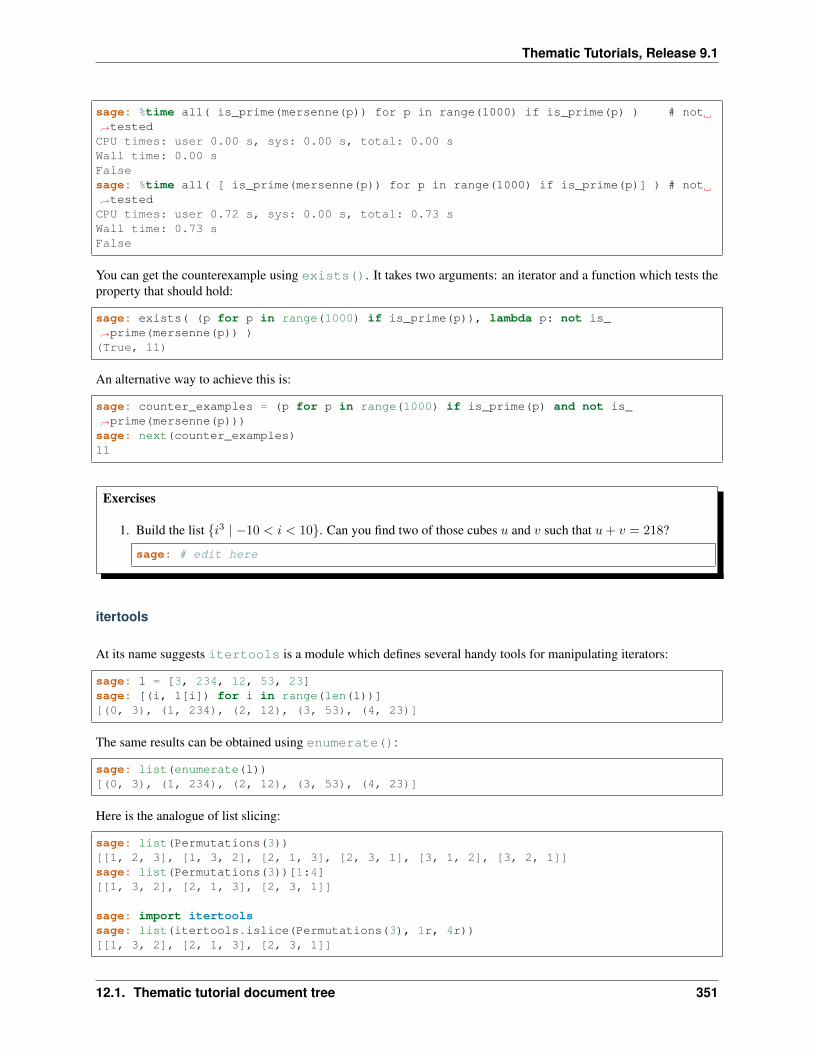
Thematic Tutorials, Release 9.1
sage: %time all( is_prime(mersenne(p)) for p in range(1000) if is_prime(p) ) # not→˓testedCPU times: user 0.00 s, sys: 0.00 s, total: 0.00 sWall time: 0.00 sFalsesage: %time all( [ is_prime(mersenne(p)) for p in range(1000) if is_prime(p)] ) # not→˓testedCPU times: user 0.72 s, sys: 0.00 s, total: 0.73 sWall time: 0.73 sFalse
You can get the counterexample using exists(). It takes two arguments: an iterator and a function which tests theproperty that should hold:
sage: exists( (p for p in range(1000) if is_prime(p)), lambda p: not is_→˓prime(mersenne(p)) )(True, 11)
An alternative way to achieve this is:
sage: counter_examples = (p for p in range(1000) if is_prime(p) and not is_→˓prime(mersenne(p)))sage: next(counter_examples)11
Exercises
1. Build the list 𝑖3 | −10 < 𝑖 < 10. Can you find two of those cubes 𝑢 and 𝑣 such that 𝑢+ 𝑣 = 218?
sage: # edit here
itertools
At its name suggests itertools is a module which defines several handy tools for manipulating iterators:
sage: l = [3, 234, 12, 53, 23]sage: [(i, l[i]) for i in range(len(l))][(0, 3), (1, 234), (2, 12), (3, 53), (4, 23)]
The same results can be obtained using enumerate():
sage: list(enumerate(l))[(0, 3), (1, 234), (2, 12), (3, 53), (4, 23)]
Here is the analogue of list slicing:
sage: list(Permutations(3))[[1, 2, 3], [1, 3, 2], [2, 1, 3], [2, 3, 1], [3, 1, 2], [3, 2, 1]]sage: list(Permutations(3))[1:4][[1, 3, 2], [2, 1, 3], [2, 3, 1]]
sage: import itertoolssage: list(itertools.islice(Permutations(3), 1r, 4r))[[1, 3, 2], [2, 1, 3], [2, 3, 1]]
12.1. Thematic tutorial document tree 351
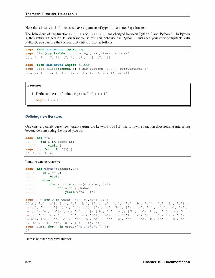
Thematic Tutorials, Release 9.1
Note that all calls to islice must have arguments of type int and not Sage integers.
The behaviour of the functions map() and filter() has changed between Python 2 and Python 3. In Python3, they return an iterator. If you want to use this new behaviour in Python 2, and keep your code compatible withPython3, you can use the compatibility library six as follows:
sage: from six.moves import mapsage: list(map(lambda z: z.cycle_type(), Permutations(3)))[[1, 1, 1], [2, 1], [2, 1], [3], [3], [2, 1]]
sage: from six.moves import filtersage: list(filter(lambda z: z.has_pattern([1,2]), Permutations(3)))[[1, 2, 3], [1, 3, 2], [2, 1, 3], [2, 3, 1], [3, 1, 2]]
Exercises
1. Define an iterator for the 𝑖-th prime for 5 < 𝑖 < 10:
sage: # edit here
Defining new iterators
One can very easily write new iterators using the keyword yield. The following function does nothing interestingbeyond demonstrating the use of yield:
sage: def f(n):....: for i in range(n):....: yield isage: [ u for u in f(5) ][0, 1, 2, 3, 4]
Iterators can be recursive:
sage: def words(alphabet,l):....: if l == 0:....: yield []....: else:....: for word in words(alphabet, l-1):....: for a in alphabet:....: yield word + [a]
sage: [ w for w in words(['a','b','c'], 3) ][['a', 'a', 'a'], ['a', 'a', 'b'], ['a', 'a', 'c'], ['a', 'b', 'a'], ['a', 'b', 'b'],→˓['a', 'b', 'c'], ['a', 'c', 'a'], ['a', 'c', 'b'], ['a', 'c', 'c'], ['b', 'a', 'a'],→˓ ['b', 'a', 'b'], ['b', 'a', 'c'], ['b', 'b', 'a'], ['b', 'b', 'b'], ['b', 'b', 'c→˓'], ['b', 'c', 'a'], ['b', 'c', 'b'], ['b', 'c', 'c'], ['c', 'a', 'a'], ['c', 'a',→˓'b'], ['c', 'a', 'c'], ['c', 'b', 'a'], ['c', 'b', 'b'], ['c', 'b', 'c'], ['c', 'c',→˓ 'a'], ['c', 'c', 'b'], ['c', 'c', 'c']]sage: sum(1 for w in words(['a','b','c'], 3))27
Here is another recursive iterator:
352 Chapter 12. Documentation
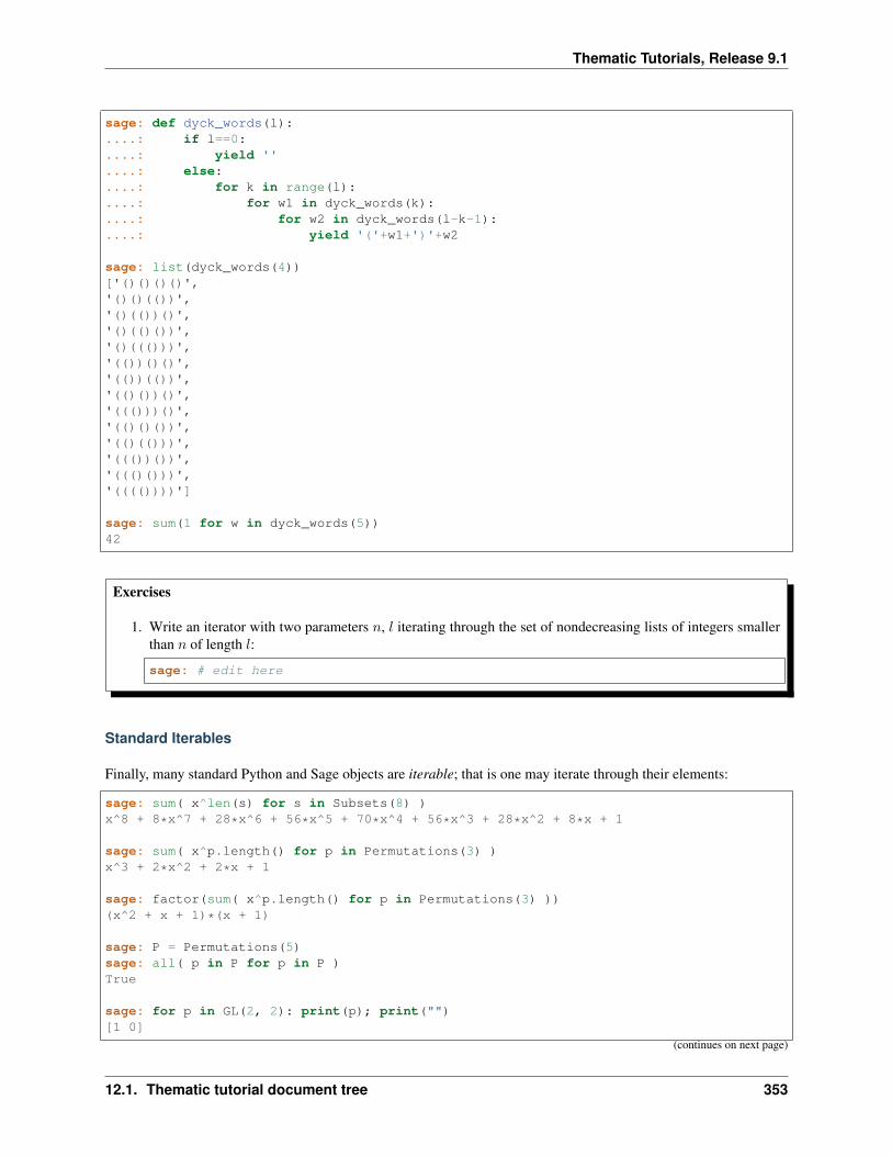
Thematic Tutorials, Release 9.1
sage: def dyck_words(l):....: if l==0:....: yield ''....: else:....: for k in range(l):....: for w1 in dyck_words(k):....: for w2 in dyck_words(l-k-1):....: yield '('+w1+')'+w2
sage: list(dyck_words(4))['()()()()','()()(())','()(())()','()(()())','()((()))','(())()()','(())(())','(()())()','((()))()','(()()())','(()(()))','((())())','((()()))','(((())))']
sage: sum(1 for w in dyck_words(5))42
Exercises
1. Write an iterator with two parameters 𝑛, 𝑙 iterating through the set of nondecreasing lists of integers smallerthan 𝑛 of length 𝑙:
sage: # edit here
Standard Iterables
Finally, many standard Python and Sage objects are iterable; that is one may iterate through their elements:
sage: sum( x^len(s) for s in Subsets(8) )x^8 + 8*x^7 + 28*x^6 + 56*x^5 + 70*x^4 + 56*x^3 + 28*x^2 + 8*x + 1
sage: sum( x^p.length() for p in Permutations(3) )x^3 + 2*x^2 + 2*x + 1
sage: factor(sum( x^p.length() for p in Permutations(3) ))(x^2 + x + 1)*(x + 1)
sage: P = Permutations(5)sage: all( p in P for p in P )True
sage: for p in GL(2, 2): print(p); print("")[1 0]
(continues on next page)
12.1. Thematic tutorial document tree 353
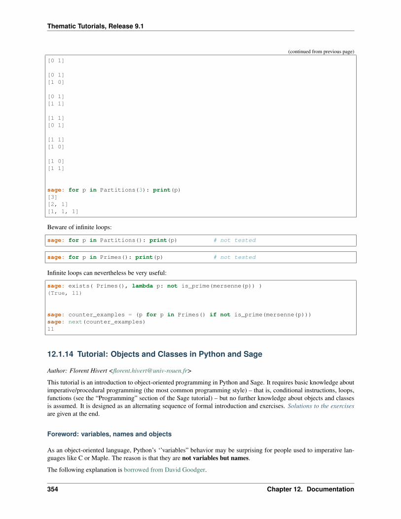
Thematic Tutorials, Release 9.1
(continued from previous page)
[0 1]
[0 1][1 0]
[0 1][1 1]
[1 1][0 1]
[1 1][1 0]
[1 0][1 1]
sage: for p in Partitions(3): print(p)[3][2, 1][1, 1, 1]
Beware of infinite loops:
sage: for p in Partitions(): print(p) # not tested
sage: for p in Primes(): print(p) # not tested
Infinite loops can nevertheless be very useful:
sage: exists( Primes(), lambda p: not is_prime(mersenne(p)) )(True, 11)
sage: counter_examples = (p for p in Primes() if not is_prime(mersenne(p)))sage: next(counter_examples)11
12.1.14 Tutorial: Objects and Classes in Python and Sage
Author: Florent Hivert <[email protected]>
This tutorial is an introduction to object-oriented programming in Python and Sage. It requires basic knowledge aboutimperative/procedural programming (the most common programming style) – that is, conditional instructions, loops,functions (see the “Programming” section of the Sage tutorial) – but no further knowledge about objects and classesis assumed. It is designed as an alternating sequence of formal introduction and exercises. Solutions to the exercisesare given at the end.
Foreword: variables, names and objects
As an object-oriented language, Python’s ‘’variables” behavior may be surprising for people used to imperative lan-guages like C or Maple. The reason is that they are not variables but names.
The following explanation is borrowed from David Goodger.
354 Chapter 12. Documentation
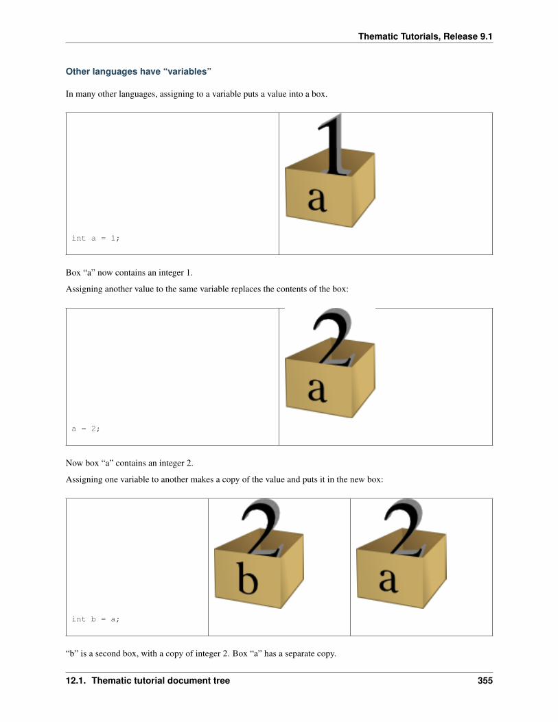
Thematic Tutorials, Release 9.1
Other languages have “variables”
In many other languages, assigning to a variable puts a value into a box.
int a = 1;
Box “a” now contains an integer 1.
Assigning another value to the same variable replaces the contents of the box:
a = 2;
Now box “a” contains an integer 2.
Assigning one variable to another makes a copy of the value and puts it in the new box:
int b = a;
“b” is a second box, with a copy of integer 2. Box “a” has a separate copy.
12.1. Thematic tutorial document tree 355
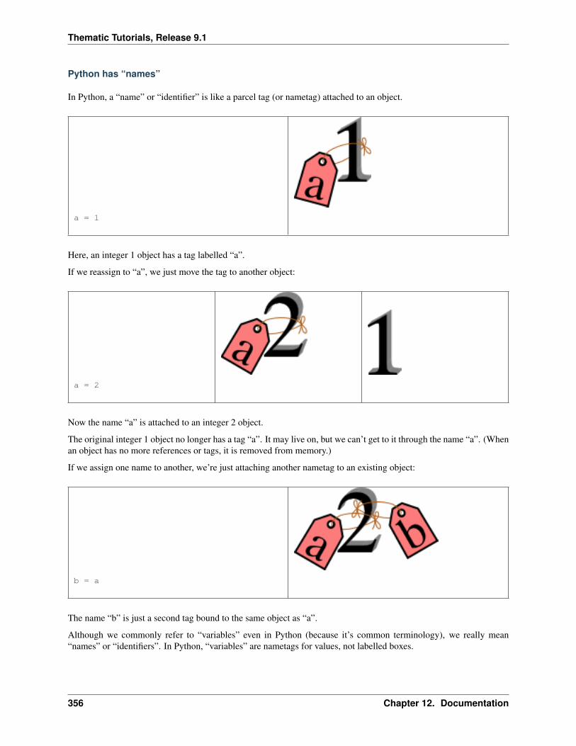
Thematic Tutorials, Release 9.1
Python has “names”
In Python, a “name” or “identifier” is like a parcel tag (or nametag) attached to an object.
a = 1
Here, an integer 1 object has a tag labelled “a”.
If we reassign to “a”, we just move the tag to another object:
a = 2
Now the name “a” is attached to an integer 2 object.
The original integer 1 object no longer has a tag “a”. It may live on, but we can’t get to it through the name “a”. (Whenan object has no more references or tags, it is removed from memory.)
If we assign one name to another, we’re just attaching another nametag to an existing object:
b = a
The name “b” is just a second tag bound to the same object as “a”.
Although we commonly refer to “variables” even in Python (because it’s common terminology), we really mean“names” or “identifiers”. In Python, “variables” are nametags for values, not labelled boxes.
356 Chapter 12. Documentation
Thematic Tutorials, Release 9.1
Warning: As a consequence, when there are two tags “a” and “b” on the same object, modifying the objecttagged “b” also modifies the object tagged “a”:
sage: a = [1,2,3]sage: b = asage: b[1] = 0sage: a[1, 0, 3]
Note that reassigning the tag “b” (rather than modifying the object with that tag) doesn’t affect the object tagged“a”:
sage: b = 7sage: b7sage: a[1, 0, 3]
Object-oriented programming paradigm
The object-oriented programming paradigm relies on the two following fundamental rules:
1. Anything of the real (or mathematical) world which needs to be manipulated by the computer is modeled by anobject.
2. Each object is an instance of some class.
At this point, those two rules are a little meaningless, so let’s give some more or less precise definitions of the terms:
object a portion of memory which contains the information needed to model the real world thing.
class defines the data structure used to store the objects which are instances of the class together with their behavior.
Let’s start with some examples: We consider the vector space over Q whose basis is indexed by permutations, and aparticular element in it:
sage: F = CombinatorialFreeModule(QQ, Permutations())sage: el = 3*F([1,3,2])+ F([1,2,3])sage: elB[[1, 2, 3]] + 3*B[[1, 3, 2]]
(For each permutation, say [1, 3, 2], the corresponding element in F is denoted by B[[1, 3, 2]] – in aCombinatorialFreeModule, if an element is indexed by x, then by default its print representation is B[x].)
In Python, everything is an object so there isn’t any difference between types and classes. One can get the class of theobject el by:
sage: type(el)<class 'sage.combinat.free_module.CombinatorialFreeModule_with_category.element_class→˓'>
As such, this is not very informative. We’ll come back to it later. The data associated to objects are stored in so-calledattributes. They are accessed through the syntax obj.attribute_name. For an element of a combinatorial freemodule, the main attribute is called _monomial_coefficients. It is a dictionary associating coefficients toindices:
12.1. Thematic tutorial document tree 357
Thematic Tutorials, Release 9.1
sage: el._monomial_coefficients[1, 2, 3]: 1, [1, 3, 2]: 3
Modifying the attribute modifies the objects:
sage: el._monomial_coefficients[Permutation([3,2,1])] = 1/2sage: elB[[1, 2, 3]] + 3*B[[1, 3, 2]] + 1/2*B[[3, 2, 1]]
Warning: as a user, you are not supposed to do such a modification by yourself (see note on private attributesbelow).
As an element of a vector space, el has a particular behavior:
sage: 2*el2*B[[1, 2, 3]] + 6*B[[1, 3, 2]] + B[[3, 2, 1]]sage: sorted(el.support())[[1, 2, 3], [1, 3, 2], [3, 2, 1]]sage: el.coefficient([1, 2, 3])1
The behavior is defined through methods (support, coefficient). Note that this is true even for equality,printing or mathematical operations. For example, the call a == b actually is translated to the method call a.__eq__(b). The names of those special methods which are usually called through operators are fixed by thePython language and are of the form __name__. Examples include __eq__ and __le__ for operators == and<=, __repr__ (see Sage specifics about classes) for printing, __add__ and __mult__ for operators + and *. Seehttp://docs.python.org/library/ for a complete list.
sage: el.__eq__(F([1,3,2]))Falsesage: el.__repr__()'B[[1, 2, 3]] + 3*B[[1, 3, 2]] + 1/2*B[[3, 2, 1]]'sage: el.__mul__(2)2*B[[1, 2, 3]] + 6*B[[1, 3, 2]] + B[[3, 2, 1]]
Note: We now create a custom Element class to explain the details of how attributes work in Python (you canignore the parent in the code below, that is not relevant here):
sage: from sage.structure.element import Elementsage: class MyElt(Element):....: def __init__(self, parent, val):....: super(MyElt, self).__init__(parent)....: self.value = valsage: el = MyElt(val=42, parent=ZZ)sage: elGeneric element of a structure
The class is stored in a particular attribute called __class__, and the normal attributes are stored in a dictionarycalled __dict__:
sage: el.__dict__'value': 42sage: el.__class__<class '__main__.MyElt'>
358 Chapter 12. Documentation
Thematic Tutorials, Release 9.1
Some particular actions modify the attributes of el:
sage: el.rename("bla")sage: elblasage: el.__dict__'__custom_name': 'bla', 'value': 42
Lots of Sage objects are not Python objects but compiled Cython objects. Python sees them as builtin objects and youdo not have access to some of their internal data structure. For example, the base class Element stores the parent ofel as a Cython attribute _parent but it does not appear in the __dict__ and we cannot access it from Python.
Some examples of Cython classes (technically, extension types) in Sage include integers and permutation group ele-ments. These do not have a __dict__ at all:
sage: e = Integer(9)sage: type(e)<type 'sage.rings.integer.Integer'>sage: e.__dict__Traceback (most recent call last):...AttributeError: 'sage.rings.integer.Integer' object has no attribute '__dict__'
sage: id4 = SymmetricGroup(4).one()sage: type(id4)<type 'sage.groups.perm_gps.permgroup_element.SymmetricGroupElement'>sage: id4.__dict__Traceback (most recent call last):...AttributeError: 'sage.groups.perm_gps.permgroup_element.SymmetricGroupElement' object→˓has no attribute '__dict__'
Note: Each object corresponds to a portion of memory called its identity in Python. You can get the identity usingid:
sage: el = Integer(9)sage: id(el) # random139813642977744sage: el1 = el; id(el1) == id(el)Truesage: el1 is elTrue
In Python (and therefore in Sage), two objects with the same identity will be equal, but the converse is not true ingeneral. Thus the identity function is different from mathematical identity:
sage: el2 = Integer(9)sage: el2 == el1Truesage: el2 is el1Falsesage: id(el2) == id(el)False
12.1. Thematic tutorial document tree 359
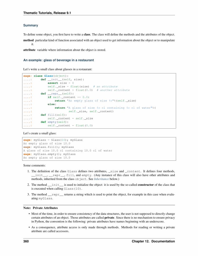
Thematic Tutorials, Release 9.1
Summary
To define some object, you first have to write a class. The class will define the methods and the attributes of the object.
method particular kind of function associated with an object used to get information about the object or to manipulateit.
attribute variable where information about the object is stored.
An example: glass of beverage in a restaurant
Let’s write a small class about glasses in a restaurant:
sage: class Glass(object):....: def __init__(self, size):....: assert size > 0....: self._size = float(size) # an attribute....: self._content = float(0.0) # another attribute....: def __repr__(self):....: if self._content == 0.0:....: return "An empty glass of size %s"%(self._size)....: else:....: return "A glass of size %s cl containing %s cl of water"%(....: self._size, self._content)....: def fill(self):....: self._content = self._size....: def empty(self):....: self._content = float(0.0)
Let’s create a small glass:
sage: myGlass = Glass(10); myGlassAn empty glass of size 10.0sage: myGlass.fill(); myGlassA glass of size 10.0 cl containing 10.0 cl of watersage: myGlass.empty(); myGlassAn empty glass of size 10.0
Some comments:
1. The definition of the class Glass defines two attributes, _size and _content. It defines four methods,__init__, __repr__, fill, and empty. (Any instance of this class will also have other attributes andmethods, inherited from the class object. See Inheritance below.)
2. The method __init__ is used to initialize the object: it is used by the so-called constructor of the class thatis executed when calling Glass(10).
3. The method __repr__ returns a string which is used to print the object, for example in this case when evalu-ating myGlass.
Note: Private Attributes
• Most of the time, in order to ensure consistency of the data structures, the user is not supposed to directly changecertain attributes of an object. Those attributes are called private. Since there is no mechanism to ensure privacyin Python, the convention is the following: private attributes have names beginning with an underscore.
• As a consequence, attribute access is only made through methods. Methods for reading or writing a privateattribute are called accessors.
360 Chapter 12. Documentation
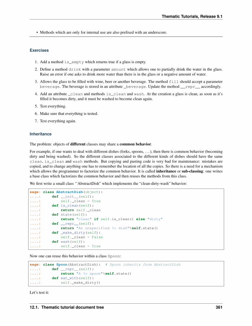
Thematic Tutorials, Release 9.1
• Methods which are only for internal use are also prefixed with an underscore.
Exercises
1. Add a method is_empty which returns true if a glass is empty.
2. Define a method drink with a parameter amount which allows one to partially drink the water in the glass.Raise an error if one asks to drink more water than there is in the glass or a negative amount of water.
3. Allows the glass to be filled with wine, beer or another beverage. The method fill should accept a parameterbeverage. The beverage is stored in an attribute _beverage. Update the method __repr__ accordingly.
4. Add an attribute _clean and methods is_clean and wash. At the creation a glass is clean, as soon as it’sfilled it becomes dirty, and it must be washed to become clean again.
5. Test everything.
6. Make sure that everything is tested.
7. Test everything again.
Inheritance
The problem: objects of different classes may share a common behavior.
For example, if one wants to deal with different dishes (forks, spoons, . . . ), then there is common behavior (becomingdirty and being washed). So the different classes associated to the different kinds of dishes should have the sameclean, is_clean and wash methods. But copying and pasting code is very bad for maintenance: mistakes arecopied, and to change anything one has to remember the location of all the copies. So there is a need for a mechanismwhich allows the programmer to factorize the common behavior. It is called inheritance or sub-classing: one writesa base class which factorizes the common behavior and then reuses the methods from this class.
We first write a small class ‘’AbstractDish” which implements the “clean-dirty-wash” behavior:
sage: class AbstractDish(object):....: def __init__(self):....: self._clean = True....: def is_clean(self):....: return self._clean....: def state(self):....: return "clean" if self.is_clean() else "dirty"....: def __repr__(self):....: return "An unspecified %s dish"%self.state()....: def _make_dirty(self):....: self._clean = False....: def wash(self):....: self._clean = True
Now one can reuse this behavior within a class Spoon:
sage: class Spoon(AbstractDish): # Spoon inherits from AbstractDish....: def __repr__(self):....: return "A %s spoon"%self.state()....: def eat_with(self):....: self._make_dirty()
Let’s test it:
12.1. Thematic tutorial document tree 361
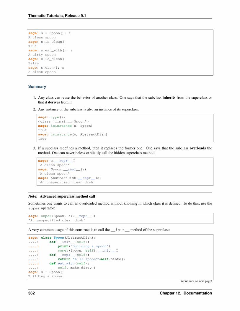
Thematic Tutorials, Release 9.1
sage: s = Spoon(); sA clean spoonsage: s.is_clean()Truesage: s.eat_with(); sA dirty spoonsage: s.is_clean()Falsesage: s.wash(); sA clean spoon
Summary
1. Any class can reuse the behavior of another class. One says that the subclass inherits from the superclass orthat it derives from it.
2. Any instance of the subclass is also an instance of its superclass:
sage: type(s)<class '__main__.Spoon'>sage: isinstance(s, Spoon)Truesage: isinstance(s, AbstractDish)True
3. If a subclass redefines a method, then it replaces the former one. One says that the subclass overloads themethod. One can nevertheless explicitly call the hidden superclass method.
sage: s.__repr__()'A clean spoon'sage: Spoon.__repr__(s)'A clean spoon'sage: AbstractDish.__repr__(s)'An unspecified clean dish'
Note: Advanced superclass method call
Sometimes one wants to call an overloaded method without knowing in which class it is defined. To do this, use thesuper operator:
sage: super(Spoon, s).__repr__()'An unspecified clean dish'
A very common usage of this construct is to call the __init__ method of the superclass:
sage: class Spoon(AbstractDish):....: def __init__(self):....: print("Building a spoon")....: super(Spoon, self).__init__()....: def __repr__(self):....: return "A %s spoon"%self.state()....: def eat_with(self):....: self._make_dirty()sage: s = Spoon()Building a spoon
(continues on next page)
362 Chapter 12. Documentation
Thematic Tutorials, Release 9.1
(continued from previous page)
sage: sA clean spoon
Exercises
1. Modify the class Glasses so that it inherits from Dish.
2. Write a class Plate whose instance can contain any meal together with a class Fork. Avoid as much aspossible code duplication (hint: you can write a factorized class ContainerDish).
3. Test everything.
Sage specifics about classes
Compared to Python, Sage has particular ways to handle objects:
• Any classes for mathematical objects in Sage should inherit from SageObject rather than from object.Most of the time, they actually inherit from a subclass such as Parent or Element.
• Printing should be done through _repr_ instead of __repr__ to allow for renaming.
• More generally, Sage-specific special methods are usually named _meth_ rather than __meth__. For exam-ple, lots of classes implement _hash_ which is used and cached by __hash__. In the same vein, elementsof a group usually implement _mul_, so that there is no need to take care about coercions as they are done in__mul__.
For more details, see the Sage Developer’s Guide.
Solutions to the exercises
1. Here is a solution to the first exercise:
sage: class Glass(object):....: def __init__(self, size):....: assert size > 0....: self._size = float(size)....: self.wash()....: def __repr__(self):....: if self._content == 0.0:....: return "An empty glass of size %s"%(self._size)....: else:....: return "A glass of size %s cl containing %s cl of %s"%(....: self._size, self._content, self._beverage)....: def content(self):....: return self._content....: def beverage(self):....: return self._beverage....: def fill(self, beverage = "water"):....: if not self.is_clean():....: raise ValueError("Don't want to fill a dirty glass")....: self._clean = False....: self._content = self._size....: self._beverage = beverage
(continues on next page)
12.1. Thematic tutorial document tree 363
Thematic Tutorials, Release 9.1
(continued from previous page)
....: def empty(self):
....: self._content = float(0.0)
....: def is_empty(self):
....: return self._content == 0.0
....: def drink(self, amount):
....: if amount <= 0.0:
....: raise ValueError("amount must be positive")
....: elif amount > self._content:
....: raise ValueError("not enough beverage in the glass")
....: else:
....: self._content -= float(amount)
....: def is_clean(self):
....: return self._clean
....: def wash(self):
....: self._content = float(0.0)
....: self._beverage = None
....: self._clean = True
2. Let’s check that everything is working as expected:
sage: G = Glass(10.0)sage: GAn empty glass of size 10.0sage: G.is_empty()Truesage: G.drink(2)Traceback (most recent call last):...ValueError: not enough beverage in the glasssage: G.fill("beer")sage: GA glass of size 10.0 cl containing 10.0 cl of beersage: G.is_empty()Falsesage: G.is_clean()Falsesage: G.drink(5.0)sage: GA glass of size 10.0 cl containing 5.0 cl of beersage: G.is_empty()Falsesage: G.is_clean()Falsesage: G.drink(5)sage: GAn empty glass of size 10.0sage: G.is_clean()Falsesage: G.fill("orange juice")Traceback (most recent call last):...ValueError: Don't want to fill a dirty glasssage: G.wash()sage: GAn empty glass of size 10.0sage: G.fill("orange juice")sage: G
(continues on next page)
364 Chapter 12. Documentation
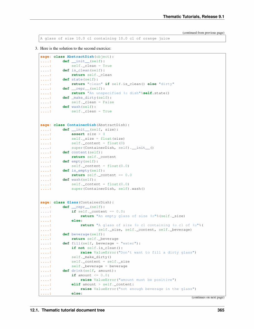
Thematic Tutorials, Release 9.1
(continued from previous page)
A glass of size 10.0 cl containing 10.0 cl of orange juice
3. Here is the solution to the second exercice:
sage: class AbstractDish(object):....: def __init__(self):....: self._clean = True....: def is_clean(self):....: return self._clean....: def state(self):....: return "clean" if self.is_clean() else "dirty"....: def __repr__(self):....: return "An unspecified %s dish"%self.state()....: def _make_dirty(self):....: self._clean = False....: def wash(self):....: self._clean = True
sage: class ContainerDish(AbstractDish):....: def __init__(self, size):....: assert size > 0....: self._size = float(size)....: self._content = float(0)....: super(ContainerDish, self).__init__()....: def content(self):....: return self._content....: def empty(self):....: self._content = float(0.0)....: def is_empty(self):....: return self._content == 0.0....: def wash(self):....: self._content = float(0.0)....: super(ContainerDish, self).wash()
sage: class Glass(ContainerDish):....: def __repr__(self):....: if self._content == 0.0:....: return "An empty glass of size %s"%(self._size)....: else:....: return "A glass of size %s cl containing %s cl of %s"%(....: self._size, self._content, self._beverage)....: def beverage(self):....: return self._beverage....: def fill(self, beverage = "water"):....: if not self.is_clean():....: raise ValueError("Don't want to fill a dirty glass")....: self._make_dirty()....: self._content = self._size....: self._beverage = beverage....: def drink(self, amount):....: if amount <= 0.0:....: raise ValueError("amount must be positive")....: elif amount > self._content:....: raise ValueError("not enough beverage in the glass")....: else:
(continues on next page)
12.1. Thematic tutorial document tree 365
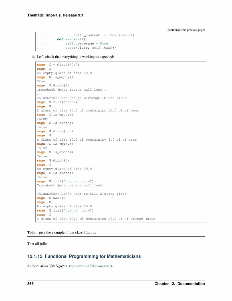
Thematic Tutorials, Release 9.1
(continued from previous page)
....: self._content -= float(amount)
....: def wash(self):
....: self._beverage = None
....: super(Glass, self).wash()
4. Let’s check that everything is working as expected:
sage: G = Glass(10.0)sage: GAn empty glass of size 10.0sage: G.is_empty()Truesage: G.drink(2)Traceback (most recent call last):...ValueError: not enough beverage in the glasssage: G.fill("beer")sage: GA glass of size 10.0 cl containing 10.0 cl of beersage: G.is_empty()Falsesage: G.is_clean()Falsesage: G.drink(5.0)sage: GA glass of size 10.0 cl containing 5.0 cl of beersage: G.is_empty()Falsesage: G.is_clean()Falsesage: G.drink(5)sage: GAn empty glass of size 10.0sage: G.is_clean()Falsesage: G.fill("orange juice")Traceback (most recent call last):...ValueError: Don't want to fill a dirty glasssage: G.wash()sage: GAn empty glass of size 10.0sage: G.fill("orange juice")sage: GA glass of size 10.0 cl containing 10.0 cl of orange juice
Todo: give the example of the class Plate.
That all folks !
12.1.15 Functional Programming for Mathematicians
Author: Minh Van Nguyen <[email protected]>
366 Chapter 12. Documentation
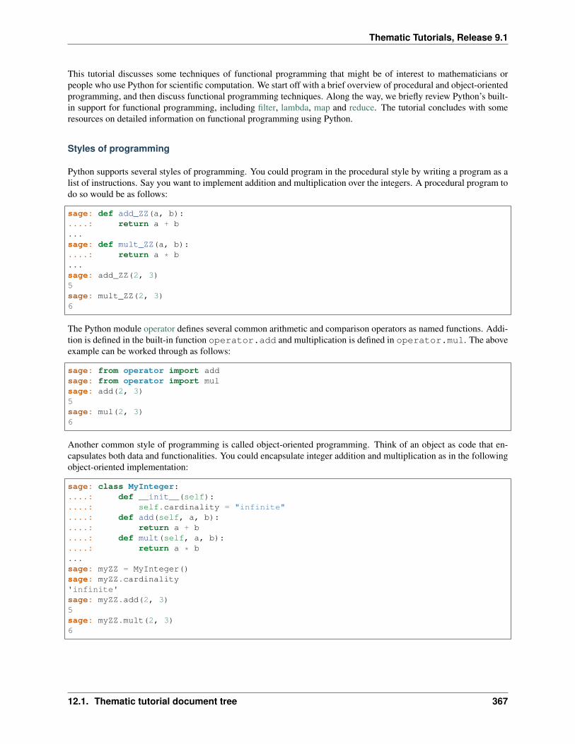
Thematic Tutorials, Release 9.1
This tutorial discusses some techniques of functional programming that might be of interest to mathematicians orpeople who use Python for scientific computation. We start off with a brief overview of procedural and object-orientedprogramming, and then discuss functional programming techniques. Along the way, we briefly review Python’s built-in support for functional programming, including filter, lambda, map and reduce. The tutorial concludes with someresources on detailed information on functional programming using Python.
Styles of programming
Python supports several styles of programming. You could program in the procedural style by writing a program as alist of instructions. Say you want to implement addition and multiplication over the integers. A procedural program todo so would be as follows:
sage: def add_ZZ(a, b):....: return a + b...sage: def mult_ZZ(a, b):....: return a * b...sage: add_ZZ(2, 3)5sage: mult_ZZ(2, 3)6
The Python module operator defines several common arithmetic and comparison operators as named functions. Addi-tion is defined in the built-in function operator.add and multiplication is defined in operator.mul. The aboveexample can be worked through as follows:
sage: from operator import addsage: from operator import mulsage: add(2, 3)5sage: mul(2, 3)6
Another common style of programming is called object-oriented programming. Think of an object as code that en-capsulates both data and functionalities. You could encapsulate integer addition and multiplication as in the followingobject-oriented implementation:
sage: class MyInteger:....: def __init__(self):....: self.cardinality = "infinite"....: def add(self, a, b):....: return a + b....: def mult(self, a, b):....: return a * b...sage: myZZ = MyInteger()sage: myZZ.cardinality'infinite'sage: myZZ.add(2, 3)5sage: myZZ.mult(2, 3)6
12.1. Thematic tutorial document tree 367
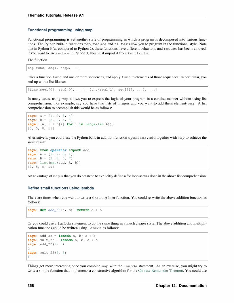
Thematic Tutorials, Release 9.1
Functional programming using map
Functional programming is yet another style of programming in which a program is decomposed into various func-tions. The Python built-in functions map, reduce and filter allow you to program in the functional style. Notethat in Python 3 (as compared to Python 2), these functions have different behaviors, and reduce has been removed:if you want to use reduce in Python 3, you must import it from functools.
The function
map(func, seq1, seq2, ...)
takes a function func and one or more sequences, and apply func to elements of those sequences. In particular, youend up with a list like so:
[func(seq1[0], seq2[0], ...), func(seq1[1], seq2[1], ...), ...]
In many cases, using map allows you to express the logic of your program in a concise manner without using listcomprehension. For example, say you have two lists of integers and you want to add them element-wise. A listcomprehension to accomplish this would be as follows:
sage: A = [1, 2, 3, 4]sage: B = [2, 3, 5, 7]sage: [A[i] + B[i] for i in range(len(A))][3, 5, 8, 11]
Alternatively, you could use the Python built-in addition function operator.add together with map to achieve thesame result:
sage: from operator import addsage: A = [1, 2, 3, 4]sage: B = [2, 3, 5, 7]sage: list(map(add, A, B))[3, 5, 8, 11]
An advantage of map is that you do not need to explicitly define a for loop as was done in the above list comprehension.
Define small functions using lambda
There are times when you want to write a short, one-liner function. You could re-write the above addition function asfollows:
sage: def add_ZZ(a, b): return a + b...
Or you could use a lambda statement to do the same thing in a much clearer style. The above addition and multipli-cation functions could be written using lambda as follows:
sage: add_ZZ = lambda a, b: a + bsage: mult_ZZ = lambda a, b: a * bsage: add_ZZ(2, 3)5sage: mult_ZZ(2, 3)6
Things get more interesting once you combine map with the lambda statement. As an exercise, you might try towrite a simple function that implements a constructive algorithm for the Chinese Remainder Theorem. You could use
368 Chapter 12. Documentation
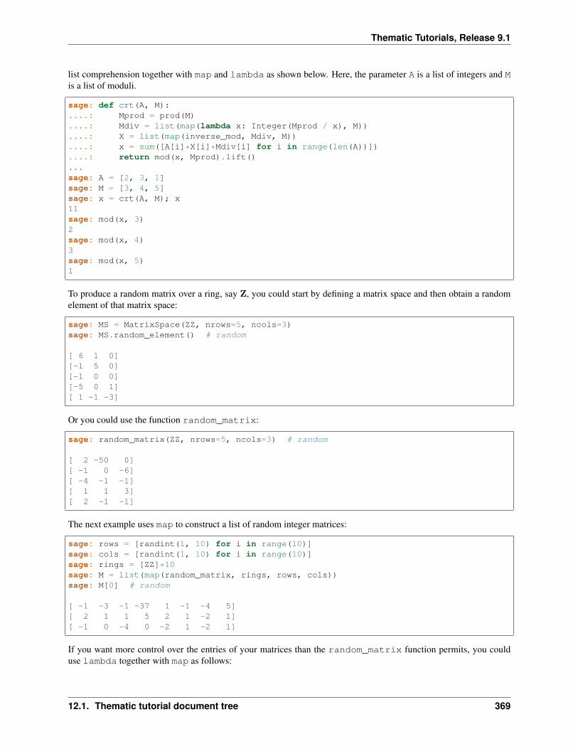
Thematic Tutorials, Release 9.1
list comprehension together with map and lambda as shown below. Here, the parameter A is a list of integers and Mis a list of moduli.
sage: def crt(A, M):....: Mprod = prod(M)....: Mdiv = list(map(lambda x: Integer(Mprod / x), M))....: X = list(map(inverse_mod, Mdiv, M))....: x = sum([A[i]*X[i]*Mdiv[i] for i in range(len(A))])....: return mod(x, Mprod).lift()...sage: A = [2, 3, 1]sage: M = [3, 4, 5]sage: x = crt(A, M); x11sage: mod(x, 3)2sage: mod(x, 4)3sage: mod(x, 5)1
To produce a random matrix over a ring, say Z, you could start by defining a matrix space and then obtain a randomelement of that matrix space:
sage: MS = MatrixSpace(ZZ, nrows=5, ncols=3)sage: MS.random_element() # random
[ 6 1 0][-1 5 0][-1 0 0][-5 0 1][ 1 -1 -3]
Or you could use the function random_matrix:
sage: random_matrix(ZZ, nrows=5, ncols=3) # random
[ 2 -50 0][ -1 0 -6][ -4 -1 -1][ 1 1 3][ 2 -1 -1]
The next example uses map to construct a list of random integer matrices:
sage: rows = [randint(1, 10) for i in range(10)]sage: cols = [randint(1, 10) for i in range(10)]sage: rings = [ZZ]*10sage: M = list(map(random_matrix, rings, rows, cols))sage: M[0] # random
[ -1 -3 -1 -37 1 -1 -4 5][ 2 1 1 5 2 1 -2 1][ -1 0 -4 0 -2 1 -2 1]
If you want more control over the entries of your matrices than the random_matrix function permits, you coulduse lambda together with map as follows:
12.1. Thematic tutorial document tree 369
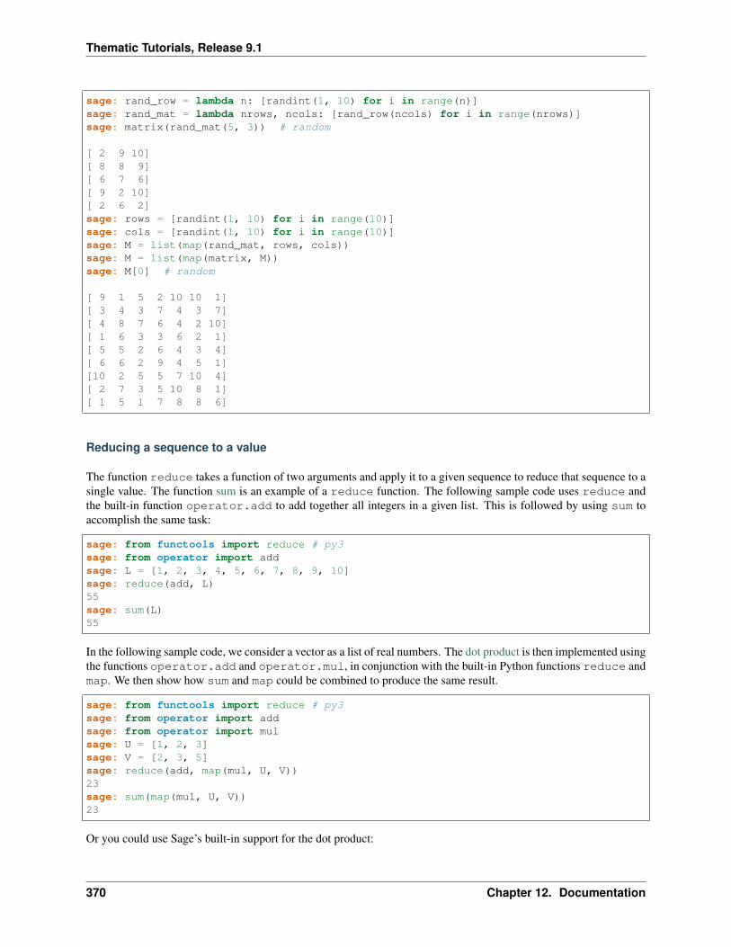
Thematic Tutorials, Release 9.1
sage: rand_row = lambda n: [randint(1, 10) for i in range(n)]sage: rand_mat = lambda nrows, ncols: [rand_row(ncols) for i in range(nrows)]sage: matrix(rand_mat(5, 3)) # random
[ 2 9 10][ 8 8 9][ 6 7 6][ 9 2 10][ 2 6 2]sage: rows = [randint(1, 10) for i in range(10)]sage: cols = [randint(1, 10) for i in range(10)]sage: M = list(map(rand_mat, rows, cols))sage: M = list(map(matrix, M))sage: M[0] # random
[ 9 1 5 2 10 10 1][ 3 4 3 7 4 3 7][ 4 8 7 6 4 2 10][ 1 6 3 3 6 2 1][ 5 5 2 6 4 3 4][ 6 6 2 9 4 5 1][10 2 5 5 7 10 4][ 2 7 3 5 10 8 1][ 1 5 1 7 8 8 6]
Reducing a sequence to a value
The function reduce takes a function of two arguments and apply it to a given sequence to reduce that sequence to asingle value. The function sum is an example of a reduce function. The following sample code uses reduce andthe built-in function operator.add to add together all integers in a given list. This is followed by using sum toaccomplish the same task:
sage: from functools import reduce # py3sage: from operator import addsage: L = [1, 2, 3, 4, 5, 6, 7, 8, 9, 10]sage: reduce(add, L)55sage: sum(L)55
In the following sample code, we consider a vector as a list of real numbers. The dot product is then implemented usingthe functions operator.add and operator.mul, in conjunction with the built-in Python functions reduce andmap. We then show how sum and map could be combined to produce the same result.
sage: from functools import reduce # py3sage: from operator import addsage: from operator import mulsage: U = [1, 2, 3]sage: V = [2, 3, 5]sage: reduce(add, map(mul, U, V))23sage: sum(map(mul, U, V))23
Or you could use Sage’s built-in support for the dot product:
370 Chapter 12. Documentation
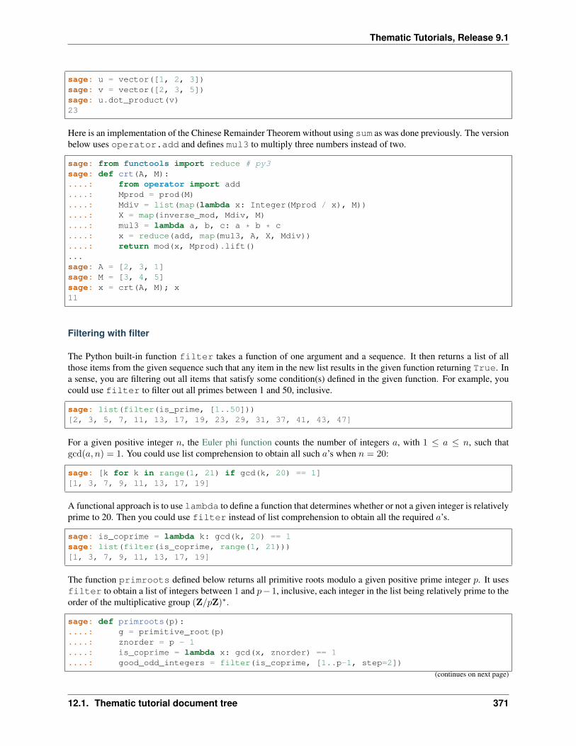
Thematic Tutorials, Release 9.1
sage: u = vector([1, 2, 3])sage: v = vector([2, 3, 5])sage: u.dot_product(v)23
Here is an implementation of the Chinese Remainder Theorem without using sum as was done previously. The versionbelow uses operator.add and defines mul3 to multiply three numbers instead of two.
sage: from functools import reduce # py3sage: def crt(A, M):....: from operator import add....: Mprod = prod(M)....: Mdiv = list(map(lambda x: Integer(Mprod / x), M))....: X = map(inverse_mod, Mdiv, M)....: mul3 = lambda a, b, c: a * b * c....: x = reduce(add, map(mul3, A, X, Mdiv))....: return mod(x, Mprod).lift()...sage: A = [2, 3, 1]sage: M = [3, 4, 5]sage: x = crt(A, M); x11
Filtering with filter
The Python built-in function filter takes a function of one argument and a sequence. It then returns a list of allthose items from the given sequence such that any item in the new list results in the given function returning True. Ina sense, you are filtering out all items that satisfy some condition(s) defined in the given function. For example, youcould use filter to filter out all primes between 1 and 50, inclusive.
sage: list(filter(is_prime, [1..50]))[2, 3, 5, 7, 11, 13, 17, 19, 23, 29, 31, 37, 41, 43, 47]
For a given positive integer 𝑛, the Euler phi function counts the number of integers 𝑎, with 1 ≤ 𝑎 ≤ 𝑛, such thatgcd(𝑎, 𝑛) = 1. You could use list comprehension to obtain all such 𝑎’s when 𝑛 = 20:
sage: [k for k in range(1, 21) if gcd(k, 20) == 1][1, 3, 7, 9, 11, 13, 17, 19]
A functional approach is to use lambda to define a function that determines whether or not a given integer is relativelyprime to 20. Then you could use filter instead of list comprehension to obtain all the required 𝑎’s.
sage: is_coprime = lambda k: gcd(k, 20) == 1sage: list(filter(is_coprime, range(1, 21)))[1, 3, 7, 9, 11, 13, 17, 19]
The function primroots defined below returns all primitive roots modulo a given positive prime integer 𝑝. It usesfilter to obtain a list of integers between 1 and 𝑝− 1, inclusive, each integer in the list being relatively prime to theorder of the multiplicative group (Z/𝑝Z)*.
sage: def primroots(p):....: g = primitive_root(p)....: znorder = p - 1....: is_coprime = lambda x: gcd(x, znorder) == 1....: good_odd_integers = filter(is_coprime, [1..p-1, step=2])
(continues on next page)
12.1. Thematic tutorial document tree 371
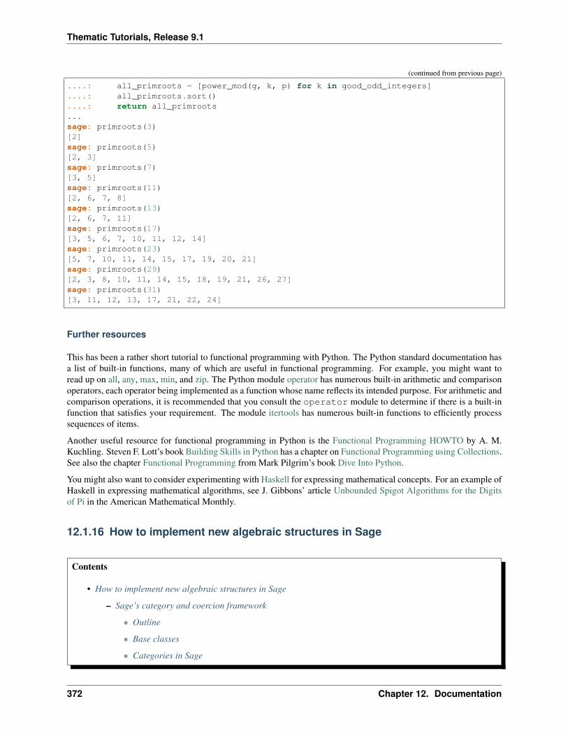
Thematic Tutorials, Release 9.1
(continued from previous page)
....: all_primroots = [power_mod(g, k, p) for k in good_odd_integers]
....: all_primroots.sort()
....: return all_primroots
...sage: primroots(3)[2]sage: primroots(5)[2, 3]sage: primroots(7)[3, 5]sage: primroots(11)[2, 6, 7, 8]sage: primroots(13)[2, 6, 7, 11]sage: primroots(17)[3, 5, 6, 7, 10, 11, 12, 14]sage: primroots(23)[5, 7, 10, 11, 14, 15, 17, 19, 20, 21]sage: primroots(29)[2, 3, 8, 10, 11, 14, 15, 18, 19, 21, 26, 27]sage: primroots(31)[3, 11, 12, 13, 17, 21, 22, 24]
Further resources
This has been a rather short tutorial to functional programming with Python. The Python standard documentation hasa list of built-in functions, many of which are useful in functional programming. For example, you might want toread up on all, any, max, min, and zip. The Python module operator has numerous built-in arithmetic and comparisonoperators, each operator being implemented as a function whose name reflects its intended purpose. For arithmetic andcomparison operations, it is recommended that you consult the operator module to determine if there is a built-infunction that satisfies your requirement. The module itertools has numerous built-in functions to efficiently processsequences of items.
Another useful resource for functional programming in Python is the Functional Programming HOWTO by A. M.Kuchling. Steven F. Lott’s book Building Skills in Python has a chapter on Functional Programming using Collections.See also the chapter Functional Programming from Mark Pilgrim’s book Dive Into Python.
You might also want to consider experimenting with Haskell for expressing mathematical concepts. For an example ofHaskell in expressing mathematical algorithms, see J. Gibbons’ article Unbounded Spigot Algorithms for the Digitsof Pi in the American Mathematical Monthly.
12.1.16 How to implement new algebraic structures in Sage
Contents
• How to implement new algebraic structures in Sage
– Sage’s category and coercion framework
* Outline
* Base classes
* Categories in Sage
372 Chapter 12. Documentation
Thematic Tutorials, Release 9.1
* Coercion—the basics
* Coercion—the advanced parts
* The test suites of the category framework
* Appendix: The complete code
Sage’s category and coercion framework
Author: Simon King, Friedrich–Schiller–Universität Jena, <[email protected]> © 2011/2013
The aim of this tutorial is to explain how one can benefit from Sage’s category framework and coercion model whenimplementing new algebraic structures. It is based on a worksheet created in 2011.
We illustrate the concepts of Sage’s category framework and coercion model by means of a detailed example, namelya toy implementation of fraction fields. The code is developed step by step, so that the reader can focus on one detailin each part of this tutorial. The complete code can be found in the appendix.
Outline
• Use existing base classes
For using Sage’s coercion system, it is essential to work with sub–classes of sage.structure.parent.Parent or sage.structure.element.Element, respectively. They provide default implementationsof many “magical” double-underscore Python methods, which must not be overridden. Instead, the actualimplementation should be in single underscore methods, such as _add_ or _mul_.
• Turn your parent structure into an object of a category
Declare the category during initialisation—Your parent structure will inherit further useful methods and consis-tency tests.
• Provide your parent structure with an element class
Assign to it an attribute called Element—The elements will inherit further useful methods from the category.In addition, some basic conversions will immediately work.
• Implement further conversions
Never override a parent’s __call__ method! Provide the method _element_constructor_ instead.
• Declare coercions
If a conversion happens to be a morphism, you may consider to turn it into a coercion. It will then implicitly beused in arithmetic operations.
• Advanced coercion: Define construction functors for your parent structure
Sage will automatically create new parents for you when needed, by the so–called sage.categories.pushout.pushout() construction.
• Run the automatic test suites
Each method should be documented and provide a doc test (we are not giving examples here). In addition, anymethod defined for the objects or elements of a category should be supported by a test method, that is executedwhen running the test suite.
12.1. Thematic tutorial document tree 373
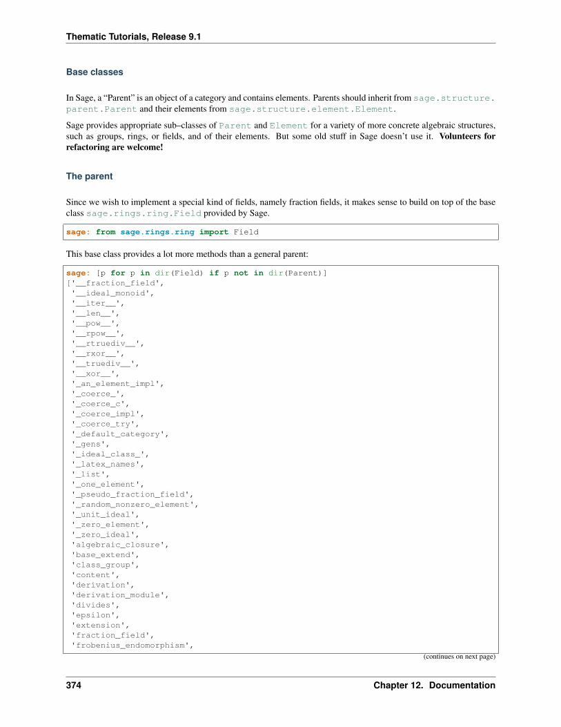
Thematic Tutorials, Release 9.1
Base classes
In Sage, a “Parent” is an object of a category and contains elements. Parents should inherit from sage.structure.parent.Parent and their elements from sage.structure.element.Element.
Sage provides appropriate sub–classes of Parent and Element for a variety of more concrete algebraic structures,such as groups, rings, or fields, and of their elements. But some old stuff in Sage doesn’t use it. Volunteers forrefactoring are welcome!
The parent
Since we wish to implement a special kind of fields, namely fraction fields, it makes sense to build on top of the baseclass sage.rings.ring.Field provided by Sage.
sage: from sage.rings.ring import Field
This base class provides a lot more methods than a general parent:
sage: [p for p in dir(Field) if p not in dir(Parent)]['__fraction_field','__ideal_monoid','__iter__','__len__','__pow__','__rpow__','__rtruediv__','__rxor__','__truediv__','__xor__','_an_element_impl','_coerce_','_coerce_c','_coerce_impl','_coerce_try','_default_category','_gens','_ideal_class_','_latex_names','_list','_one_element','_pseudo_fraction_field','_random_nonzero_element','_unit_ideal','_zero_element','_zero_ideal','algebraic_closure','base_extend','class_group','content','derivation','derivation_module','divides','epsilon','extension','fraction_field','frobenius_endomorphism',
(continues on next page)
374 Chapter 12. Documentation
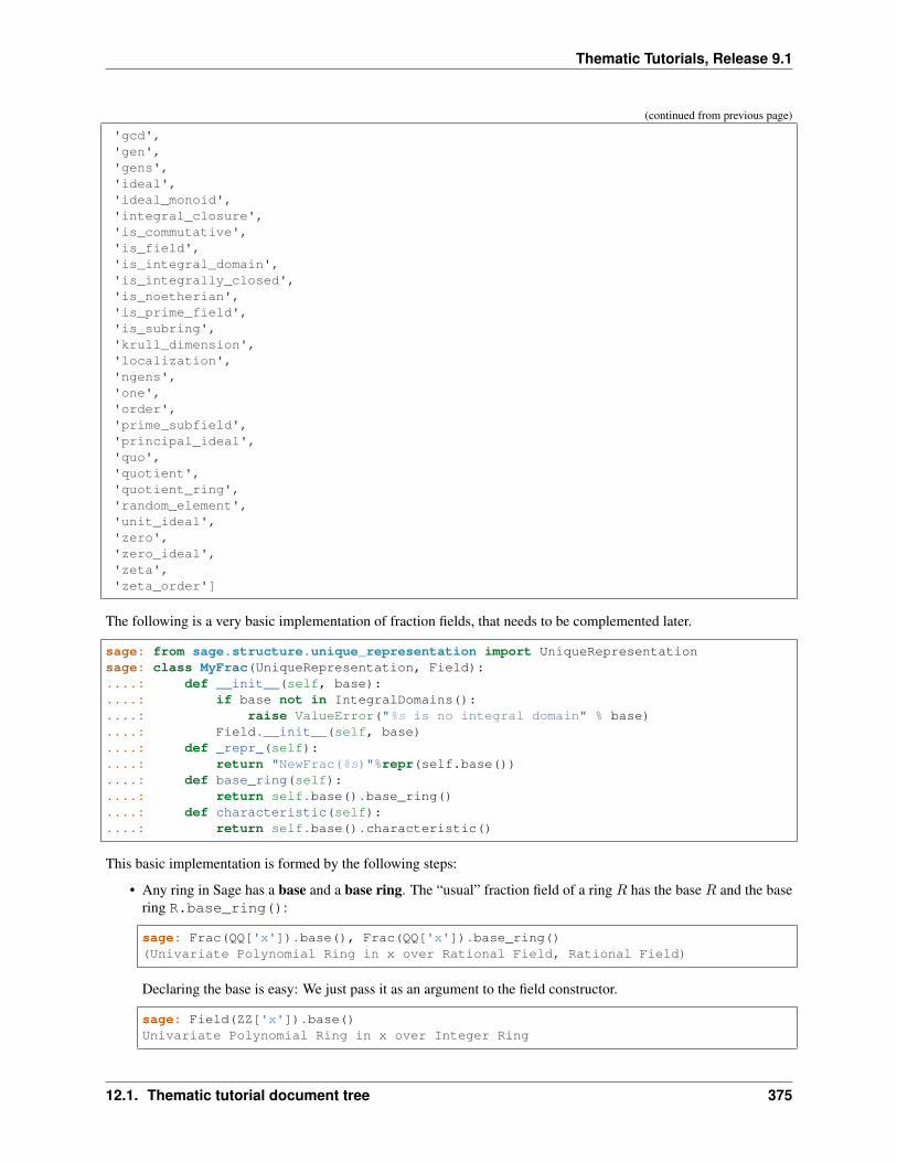
Thematic Tutorials, Release 9.1
(continued from previous page)
'gcd','gen','gens','ideal','ideal_monoid','integral_closure','is_commutative','is_field','is_integral_domain','is_integrally_closed','is_noetherian','is_prime_field','is_subring','krull_dimension','localization','ngens','one','order','prime_subfield','principal_ideal','quo','quotient','quotient_ring','random_element','unit_ideal','zero','zero_ideal','zeta','zeta_order']
The following is a very basic implementation of fraction fields, that needs to be complemented later.
sage: from sage.structure.unique_representation import UniqueRepresentationsage: class MyFrac(UniqueRepresentation, Field):....: def __init__(self, base):....: if base not in IntegralDomains():....: raise ValueError("%s is no integral domain" % base)....: Field.__init__(self, base)....: def _repr_(self):....: return "NewFrac(%s)"%repr(self.base())....: def base_ring(self):....: return self.base().base_ring()....: def characteristic(self):....: return self.base().characteristic()
This basic implementation is formed by the following steps:
• Any ring in Sage has a base and a base ring. The “usual” fraction field of a ring 𝑅 has the base 𝑅 and the basering R.base_ring():
sage: Frac(QQ['x']).base(), Frac(QQ['x']).base_ring()(Univariate Polynomial Ring in x over Rational Field, Rational Field)
Declaring the base is easy: We just pass it as an argument to the field constructor.
sage: Field(ZZ['x']).base()Univariate Polynomial Ring in x over Integer Ring
12.1. Thematic tutorial document tree 375
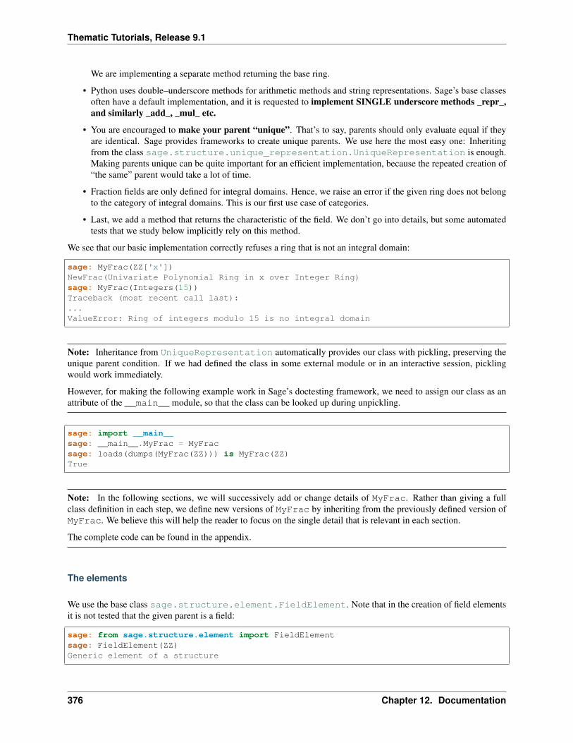
Thematic Tutorials, Release 9.1
We are implementing a separate method returning the base ring.
• Python uses double–underscore methods for arithmetic methods and string representations. Sage’s base classesoften have a default implementation, and it is requested to implement SINGLE underscore methods _repr_,and similarly _add_, _mul_ etc.
• You are encouraged to make your parent “unique”. That’s to say, parents should only evaluate equal if theyare identical. Sage provides frameworks to create unique parents. We use here the most easy one: Inheritingfrom the class sage.structure.unique_representation.UniqueRepresentation is enough.Making parents unique can be quite important for an efficient implementation, because the repeated creation of“the same” parent would take a lot of time.
• Fraction fields are only defined for integral domains. Hence, we raise an error if the given ring does not belongto the category of integral domains. This is our first use case of categories.
• Last, we add a method that returns the characteristic of the field. We don’t go into details, but some automatedtests that we study below implicitly rely on this method.
We see that our basic implementation correctly refuses a ring that is not an integral domain:
sage: MyFrac(ZZ['x'])NewFrac(Univariate Polynomial Ring in x over Integer Ring)sage: MyFrac(Integers(15))Traceback (most recent call last):...ValueError: Ring of integers modulo 15 is no integral domain
Note: Inheritance from UniqueRepresentation automatically provides our class with pickling, preserving theunique parent condition. If we had defined the class in some external module or in an interactive session, picklingwould work immediately.
However, for making the following example work in Sage’s doctesting framework, we need to assign our class as anattribute of the __main__ module, so that the class can be looked up during unpickling.
sage: import __main__sage: __main__.MyFrac = MyFracsage: loads(dumps(MyFrac(ZZ))) is MyFrac(ZZ)True
Note: In the following sections, we will successively add or change details of MyFrac. Rather than giving a fullclass definition in each step, we define new versions of MyFrac by inheriting from the previously defined version ofMyFrac. We believe this will help the reader to focus on the single detail that is relevant in each section.
The complete code can be found in the appendix.
The elements
We use the base class sage.structure.element.FieldElement. Note that in the creation of field elementsit is not tested that the given parent is a field:
sage: from sage.structure.element import FieldElementsage: FieldElement(ZZ)Generic element of a structure
376 Chapter 12. Documentation
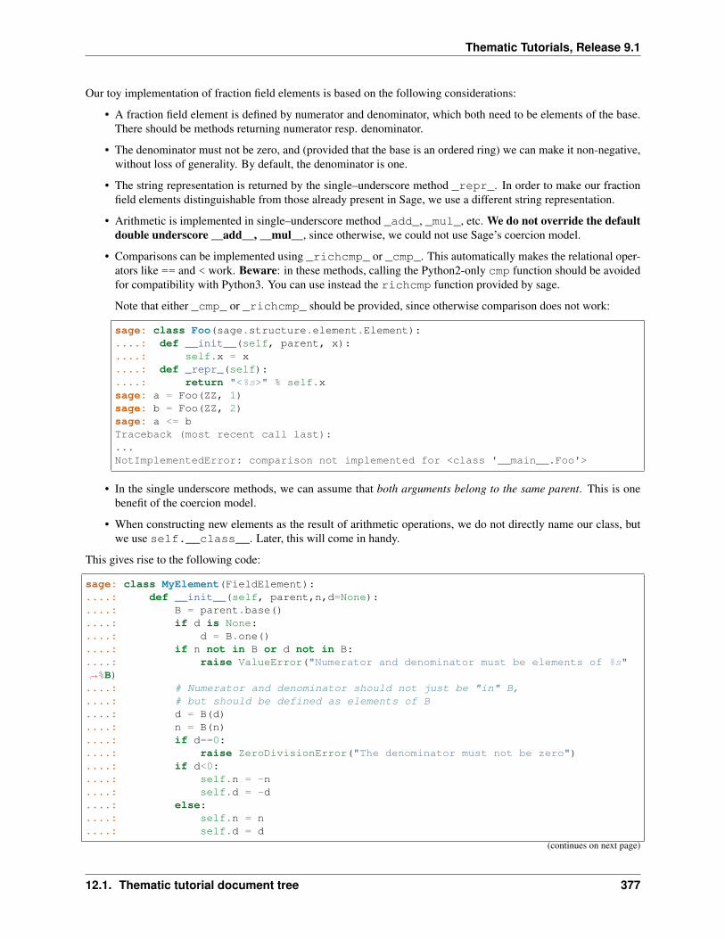
Thematic Tutorials, Release 9.1
Our toy implementation of fraction field elements is based on the following considerations:
• A fraction field element is defined by numerator and denominator, which both need to be elements of the base.There should be methods returning numerator resp. denominator.
• The denominator must not be zero, and (provided that the base is an ordered ring) we can make it non-negative,without loss of generality. By default, the denominator is one.
• The string representation is returned by the single–underscore method _repr_. In order to make our fractionfield elements distinguishable from those already present in Sage, we use a different string representation.
• Arithmetic is implemented in single–underscore method _add_, _mul_, etc. We do not override the defaultdouble underscore __add__, __mul__, since otherwise, we could not use Sage’s coercion model.
• Comparisons can be implemented using _richcmp_ or _cmp_. This automatically makes the relational oper-ators like == and < work. Beware: in these methods, calling the Python2-only cmp function should be avoidedfor compatibility with Python3. You can use instead the richcmp function provided by sage.
Note that either _cmp_ or _richcmp_ should be provided, since otherwise comparison does not work:
sage: class Foo(sage.structure.element.Element):....: def __init__(self, parent, x):....: self.x = x....: def _repr_(self):....: return "<%s>" % self.xsage: a = Foo(ZZ, 1)sage: b = Foo(ZZ, 2)sage: a <= bTraceback (most recent call last):...NotImplementedError: comparison not implemented for <class '__main__.Foo'>
• In the single underscore methods, we can assume that both arguments belong to the same parent. This is onebenefit of the coercion model.
• When constructing new elements as the result of arithmetic operations, we do not directly name our class, butwe use self.__class__. Later, this will come in handy.
This gives rise to the following code:
sage: class MyElement(FieldElement):....: def __init__(self, parent,n,d=None):....: B = parent.base()....: if d is None:....: d = B.one()....: if n not in B or d not in B:....: raise ValueError("Numerator and denominator must be elements of %s"→˓%B)....: # Numerator and denominator should not just be "in" B,....: # but should be defined as elements of B....: d = B(d)....: n = B(n)....: if d==0:....: raise ZeroDivisionError("The denominator must not be zero")....: if d<0:....: self.n = -n....: self.d = -d....: else:....: self.n = n....: self.d = d
(continues on next page)
12.1. Thematic tutorial document tree 377
Thematic Tutorials, Release 9.1
(continued from previous page)
....: FieldElement.__init__(self,parent)
....: def numerator(self):
....: return self.n
....: def denominator(self):
....: return self.d
....: def _repr_(self):
....: return "(%s):(%s)"%(self.n,self.d)
....: def _richcmp_(self, other, op):
....: from sage.structure.richcmp import richcmp
....: return richcmp(self.n*other.denominator(), other.numerator()*self.d, op)
....: def _add_(self, other):
....: C = self.__class__
....: D = self.d*other.denominator()
....: return C(self.parent(), self.n*other.denominator()+self.d*other.→˓numerator(), D)....: def _sub_(self, other):....: C = self.__class__....: D = self.d*other.denominator()....: return C(self.parent(), self.n*other.denominator()-self.d*other.→˓numerator(),D)....: def _mul_(self, other):....: C = self.__class__....: return C(self.parent(), self.n*other.numerator(), self.d*other.→˓denominator())....: def _div_(self, other):....: C = self.__class__....: return C(self.parent(), self.n*other.denominator(), self.d*other.→˓numerator())
Features and limitations of the basic implementation
Thanks to the single underscore methods, some basic arithmetics works, if we stay inside a single parent structure:
sage: P = MyFrac(ZZ)sage: a = MyElement(P, 3, 4)sage: b = MyElement(P, 1, 2)sage: a+b, a-b, a*b, a/b((10):(8), (2):(8), (3):(8), (6):(4))sage: a-b == MyElement(P, 1, 4)True
There is a default implementation of element tests. We can already do
sage: a in PTrue
since 𝑎 is defined as an element of 𝑃 . However, we can not verify yet that the integers are contained in the fractionfield of the ring of integers. It does not even give a wrong answer, but results in an error:
sage: 1 in PTraceback (most recent call last):...NotImplementedError: cannot construct elements of NewFrac(Integer Ring)
We will take care of this later.
378 Chapter 12. Documentation
Thematic Tutorials, Release 9.1
Categories in Sage
Sometimes the base classes do not reflect the mathematics: The set of 𝑚 × 𝑛 matrices over a field forms, in general,not more than a vector space. Hence, this set (called MatrixSpace) is not implemented on top of sage.rings.ring.Ring. However, if 𝑚 = 𝑛, then the matrix space is an algebra, thus, is a ring.
From the point of view of Python base classes, both cases are the same:
sage: MS1 = MatrixSpace(QQ,2,3)sage: isinstance(MS1, Ring)Falsesage: MS2 = MatrixSpace(QQ,2)sage: isinstance(MS2, Ring)False
Sage’s category framework can differentiate the two cases:
sage: Rings()Category of ringssage: MS1 in Rings()Falsesage: MS2 in Rings()True
And indeed, MS2 has more methods than MS1:
sage: import inspectsage: L1 = len([s for s in dir(MS1) if inspect.ismethod(getattr(MS1,s,None))])sage: L2 = len([s for s in dir(MS2) if inspect.ismethod(getattr(MS2,s,None))])sage: L1 < L2True
This is because the class of MS2 also inherits from the parent class for algebras:
sage: MS1.__class__.__bases__(<class 'sage.matrix.matrix_space.MatrixSpace'>,<class 'sage.categories.category.JoinCategory.parent_class'>)sage: MS2.__class__.__bases__(<class 'sage.matrix.matrix_space.MatrixSpace'>,<class 'sage.categories.category.JoinCategory.parent_class'>)
Below, we will explain how this can be taken advantage of.
It is no surprise that our parent 𝑃 defined above knows that it belongs to the category of fields, as it is derived fromthe base class of fields.
sage: P.category()Category of fields
However, we could choose a smaller category, namely the category of quotient fields.
Why should one choose a category?
One can provide default methods for all objects of a category, and for all elements of such objects. Hence, thecategory framework is a way to inherit useful stuff that is not present in the base classes. These default methods donot rely on implementation details, but on mathematical concepts.
12.1. Thematic tutorial document tree 379
Thematic Tutorials, Release 9.1
In addition, the categories define test suites for their objects and elements—see the last section. Hence, one also getsbasic sanity tests for free.
How does the category framework work?
Abstract base classes for the objects (“parent_class”) and the elements of objects (“element_class”) are provided byattributes of the category. During initialisation of a parent, the class of the parent is dynamically changed into asub–class of the category’s parent class. Likewise, sub–classes of the category’s element class are available for thecreation of elements of the parent, as explained below.
A dynamic change of classes does not work in Cython. Nevertheless, method inheritance still works, by virtue of a__getattr__ method.
Note: It is strongly recommended to use the category framework both in Python and in Cython.
Let us see whether there is any gain in choosing the category of quotient fields instead of the category of fields:
sage: QuotientFields().parent_class, QuotientFields().element_class(<class 'sage.categories.quotient_fields.QuotientFields.parent_class'>,<class 'sage.categories.quotient_fields.QuotientFields.element_class'>)
sage: [p for p in dir(QuotientFields().parent_class) if p not in dir(Fields().parent_→˓class)][]sage: [p for p in dir(QuotientFields().element_class) if p not in dir(Fields().→˓element_class)]['_derivative','denominator','derivative','numerator','partial_fraction_decomposition']
So, there is no immediate gain for our fraction fields, but additional methods become available to our fraction fieldelements. Note that some of these methods are place-holders: There is no default implementation, but it is required(respectively is optional) to implement these methods:
sage: QuotientFields().element_class.denominator<abstract method denominator at ...>sage: from sage.misc.abstract_method import abstract_methods_of_classsage: abstract_methods_of_class(QuotientFields().element_class)['optional']['_add_', '_mul_']sage: abstract_methods_of_class(QuotientFields().element_class)['required'] # py2['__nonzero__', 'denominator', 'numerator']sage: abstract_methods_of_class(QuotientFields().element_class)['required'] # py3['__bool__', 'denominator', 'numerator']
Hence, when implementing elements of a quotient field, it is required to implement methods returning the denominatorand the numerator, and a method that tells whether the element is nonzero, and in addition, it is optional (but certainlyrecommended) to provide some arithmetic methods. If one forgets to implement the required methods, the test suitesof the category framework will complain—see below.
Implementing the category framework for the parent
We simply need to declare the correct category by an optional argument of the field constructor, where we provide thepossibility to override the default category:
380 Chapter 12. Documentation
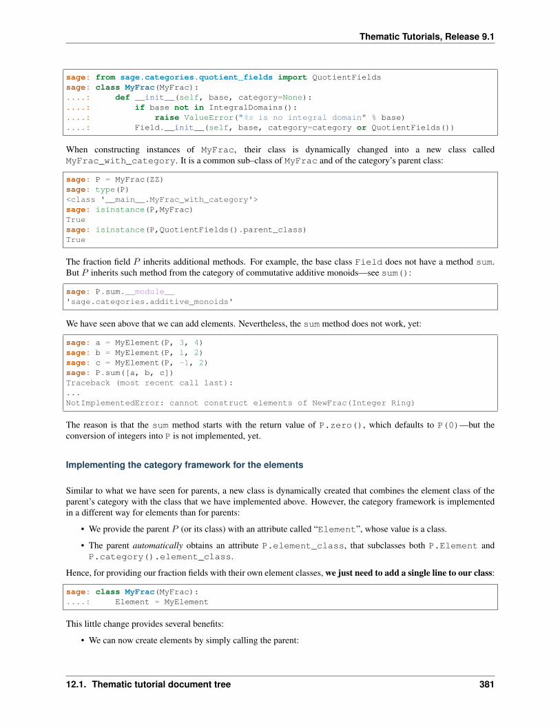
Thematic Tutorials, Release 9.1
sage: from sage.categories.quotient_fields import QuotientFieldssage: class MyFrac(MyFrac):....: def __init__(self, base, category=None):....: if base not in IntegralDomains():....: raise ValueError("%s is no integral domain" % base)....: Field.__init__(self, base, category=category or QuotientFields())
When constructing instances of MyFrac, their class is dynamically changed into a new class calledMyFrac_with_category. It is a common sub–class of MyFrac and of the category’s parent class:
sage: P = MyFrac(ZZ)sage: type(P)<class '__main__.MyFrac_with_category'>sage: isinstance(P,MyFrac)Truesage: isinstance(P,QuotientFields().parent_class)True
The fraction field 𝑃 inherits additional methods. For example, the base class Field does not have a method sum.But 𝑃 inherits such method from the category of commutative additive monoids—see sum():
sage: P.sum.__module__'sage.categories.additive_monoids'
We have seen above that we can add elements. Nevertheless, the sum method does not work, yet:
sage: a = MyElement(P, 3, 4)sage: b = MyElement(P, 1, 2)sage: c = MyElement(P, -1, 2)sage: P.sum([a, b, c])Traceback (most recent call last):...NotImplementedError: cannot construct elements of NewFrac(Integer Ring)
The reason is that the sum method starts with the return value of P.zero(), which defaults to P(0)—but theconversion of integers into P is not implemented, yet.
Implementing the category framework for the elements
Similar to what we have seen for parents, a new class is dynamically created that combines the element class of theparent’s category with the class that we have implemented above. However, the category framework is implementedin a different way for elements than for parents:
• We provide the parent 𝑃 (or its class) with an attribute called “Element”, whose value is a class.
• The parent automatically obtains an attribute P.element_class, that subclasses both P.Element andP.category().element_class.
Hence, for providing our fraction fields with their own element classes, we just need to add a single line to our class:
sage: class MyFrac(MyFrac):....: Element = MyElement
This little change provides several benefits:
• We can now create elements by simply calling the parent:
12.1. Thematic tutorial document tree 381
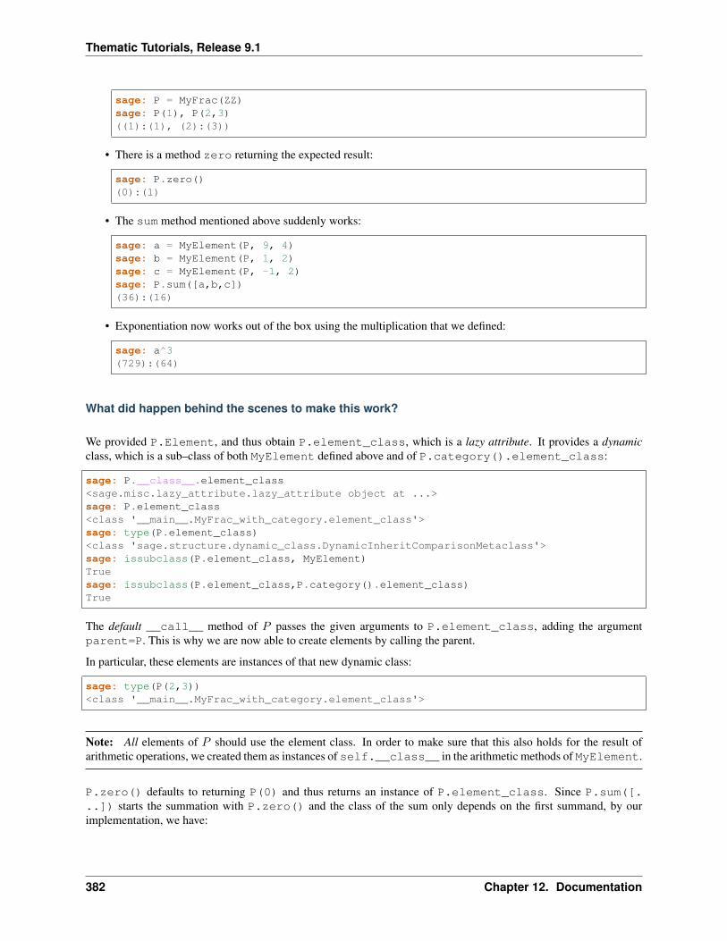
Thematic Tutorials, Release 9.1
sage: P = MyFrac(ZZ)sage: P(1), P(2,3)((1):(1), (2):(3))
• There is a method zero returning the expected result:
sage: P.zero()(0):(1)
• The sum method mentioned above suddenly works:
sage: a = MyElement(P, 9, 4)sage: b = MyElement(P, 1, 2)sage: c = MyElement(P, -1, 2)sage: P.sum([a,b,c])(36):(16)
• Exponentiation now works out of the box using the multiplication that we defined:
sage: a^3(729):(64)
What did happen behind the scenes to make this work?
We provided P.Element, and thus obtain P.element_class, which is a lazy attribute. It provides a dynamicclass, which is a sub–class of both MyElement defined above and of P.category().element_class:
sage: P.__class__.element_class<sage.misc.lazy_attribute.lazy_attribute object at ...>sage: P.element_class<class '__main__.MyFrac_with_category.element_class'>sage: type(P.element_class)<class 'sage.structure.dynamic_class.DynamicInheritComparisonMetaclass'>sage: issubclass(P.element_class, MyElement)Truesage: issubclass(P.element_class,P.category().element_class)True
The default __call__ method of 𝑃 passes the given arguments to P.element_class, adding the argumentparent=P. This is why we are now able to create elements by calling the parent.
In particular, these elements are instances of that new dynamic class:
sage: type(P(2,3))<class '__main__.MyFrac_with_category.element_class'>
Note: All elements of 𝑃 should use the element class. In order to make sure that this also holds for the result ofarithmetic operations, we created them as instances of self.__class__ in the arithmetic methods of MyElement.
P.zero() defaults to returning P(0) and thus returns an instance of P.element_class. Since P.sum([...]) starts the summation with P.zero() and the class of the sum only depends on the first summand, by ourimplementation, we have:
382 Chapter 12. Documentation
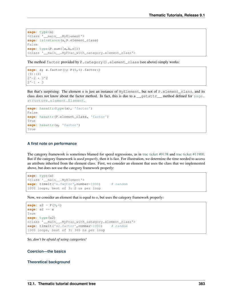
Thematic Tutorials, Release 9.1
sage: type(a)<class '__main__.MyElement'>sage: isinstance(a,P.element_class)Falsesage: type(P.sum([a,b,c]))<class '__main__.MyFrac_with_category.element_class'>
The method factor provided by P.category().element_class (see above) simply works:
sage: a; a.factor(); P(6,4).factor()(9):(4)2^-2 * 3^22^-1 * 3
But that’s surprising: The element 𝑎 is just an instance of MyElement, but not of P.element_class, and itsclass does not know about the factor method. In fact, this is due to a __getattr__ method defined for sage.structure.element.Element.
sage: hasattr(type(a), 'factor')Falsesage: hasattr(P.element_class, 'factor')Truesage: hasattr(a, 'factor')True
A first note on performance
The category framework is sometimes blamed for speed regressions, as in trac ticket #9138 and trac ticket #11900.But if the category framework is used properly, then it is fast. For illustration, we determine the time needed to accessan attribute inherited from the element class. First, we consider an element that uses the class that we implementedabove, but does not use the category framework properly:
sage: type(a)<class '__main__.MyElement'>sage: timeit('a.factor',number=1000) # random1000 loops, best of 3: 2 us per loop
Now, we consider an element that is equal to 𝑎, but uses the category framework properly:
sage: a2 = P(9,4)sage: a2 == aTruesage: type(a2)<class '__main__.MyFrac_with_category.element_class'>sage: timeit('a2.factor',number=1000) # random1000 loops, best of 3: 365 ns per loop
So, don’t be afraid of using categories!
Coercion—the basics
Theoretical background
12.1. Thematic tutorial document tree 383
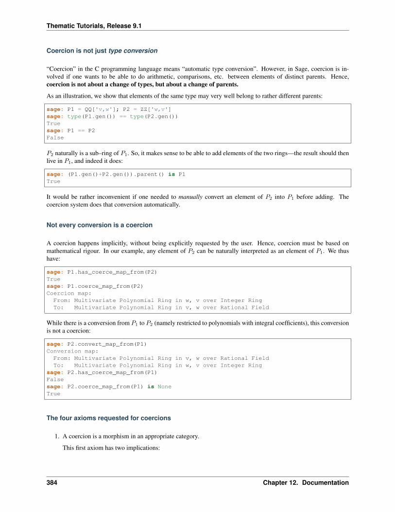
Thematic Tutorials, Release 9.1
Coercion is not just type conversion
“Coercion” in the C programming language means “automatic type conversion”. However, in Sage, coercion is in-volved if one wants to be able to do arithmetic, comparisons, etc. between elements of distinct parents. Hence,coercion is not about a change of types, but about a change of parents.
As an illustration, we show that elements of the same type may very well belong to rather different parents:
sage: P1 = QQ['v,w']; P2 = ZZ['w,v']sage: type(P1.gen()) == type(P2.gen())Truesage: P1 == P2False
𝑃2 naturally is a sub–ring of 𝑃1. So, it makes sense to be able to add elements of the two rings—the result should thenlive in 𝑃1, and indeed it does:
sage: (P1.gen()+P2.gen()).parent() is P1True
It would be rather inconvenient if one needed to manually convert an element of 𝑃2 into 𝑃1 before adding. Thecoercion system does that conversion automatically.
Not every conversion is a coercion
A coercion happens implicitly, without being explicitly requested by the user. Hence, coercion must be based onmathematical rigour. In our example, any element of 𝑃2 can be naturally interpreted as an element of 𝑃1. We thushave:
sage: P1.has_coerce_map_from(P2)Truesage: P1.coerce_map_from(P2)Coercion map:
From: Multivariate Polynomial Ring in w, v over Integer RingTo: Multivariate Polynomial Ring in v, w over Rational Field
While there is a conversion from 𝑃1 to 𝑃2 (namely restricted to polynomials with integral coefficients), this conversionis not a coercion:
sage: P2.convert_map_from(P1)Conversion map:
From: Multivariate Polynomial Ring in v, w over Rational FieldTo: Multivariate Polynomial Ring in w, v over Integer Ring
sage: P2.has_coerce_map_from(P1)Falsesage: P2.coerce_map_from(P1) is NoneTrue
The four axioms requested for coercions
1. A coercion is a morphism in an appropriate category.
This first axiom has two implications:
384 Chapter 12. Documentation
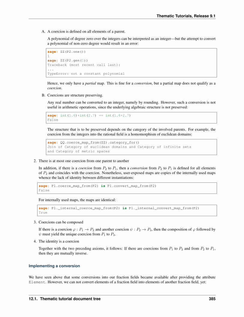
Thematic Tutorials, Release 9.1
A. A coercion is defined on all elements of a parent.
A polynomial of degree zero over the integers can be interpreted as an integer—but the attempt to converta polynomial of non-zero degree would result in an error:
sage: ZZ(P2.one())1sage: ZZ(P2.gen(1))Traceback (most recent call last):...TypeError: not a constant polynomial
Hence, we only have a partial map. This is fine for a conversion, but a partial map does not qualify as acoercion.
B. Coercions are structure preserving.
Any real number can be converted to an integer, namely by rounding. However, such a conversion is notuseful in arithmetic operations, since the underlying algebraic structure is not preserved:
sage: int(1.6)+int(2.7) == int(1.6+2.7)False
The structure that is to be preserved depends on the category of the involved parents. For example, thecoercion from the integers into the rational field is a homomorphism of euclidean domains:
sage: QQ.coerce_map_from(ZZ).category_for()Join of Category of euclidean domains and Category of infinite setsand Category of metric spaces
2. There is at most one coercion from one parent to another
In addition, if there is a coercion from 𝑃2 to 𝑃1, then a conversion from 𝑃2 to 𝑃1 is defined for all elementsof 𝑃2 and coincides with the coercion. Nonetheless, user-exposed maps are copies of the internally used mapswhence the lack of identity between different instantiations:
sage: P1.coerce_map_from(P2) is P1.convert_map_from(P2)False
For internally used maps, the maps are identical:
sage: P1._internal_coerce_map_from(P2) is P1._internal_convert_map_from(P2)True
3. Coercions can be composed
If there is a coercion 𝜙 : 𝑃1 → 𝑃2 and another coercion 𝜓 : 𝑃2 → 𝑃3, then the composition of 𝜙 followed by𝜓 must yield the unique coercion from 𝑃1 to 𝑃3.
4. The identity is a coercion
Together with the two preceding axioms, it follows: If there are coercions from 𝑃1 to 𝑃2 and from 𝑃2 to 𝑃1,then they are mutually inverse.
Implementing a conversion
We have seen above that some conversions into our fraction fields became available after providing the attributeElement. However, we can not convert elements of a fraction field into elements of another fraction field, yet:
12.1. Thematic tutorial document tree 385
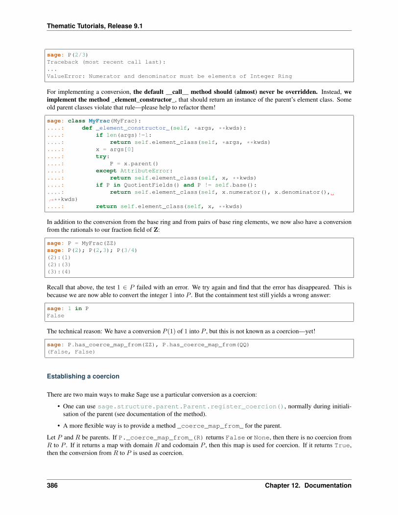
Thematic Tutorials, Release 9.1
sage: P(2/3)Traceback (most recent call last):...ValueError: Numerator and denominator must be elements of Integer Ring
For implementing a conversion, the default __call__ method should (almost) never be overridden. Instead, weimplement the method _element_constructor_, that should return an instance of the parent’s element class. Someold parent classes violate that rule—please help to refactor them!
sage: class MyFrac(MyFrac):....: def _element_constructor_(self, *args, **kwds):....: if len(args)!=1:....: return self.element_class(self, *args, **kwds)....: x = args[0]....: try:....: P = x.parent()....: except AttributeError:....: return self.element_class(self, x, **kwds)....: if P in QuotientFields() and P != self.base():....: return self.element_class(self, x.numerator(), x.denominator(),→˓**kwds)....: return self.element_class(self, x, **kwds)
In addition to the conversion from the base ring and from pairs of base ring elements, we now also have a conversionfrom the rationals to our fraction field of Z:
sage: P = MyFrac(ZZ)sage: P(2); P(2,3); P(3/4)(2):(1)(2):(3)(3):(4)
Recall that above, the test 1 ∈ 𝑃 failed with an error. We try again and find that the error has disappeared. This isbecause we are now able to convert the integer 1 into 𝑃 . But the containment test still yields a wrong answer:
sage: 1 in PFalse
The technical reason: We have a conversion 𝑃 (1) of 1 into 𝑃 , but this is not known as a coercion—yet!
sage: P.has_coerce_map_from(ZZ), P.has_coerce_map_from(QQ)(False, False)
Establishing a coercion
There are two main ways to make Sage use a particular conversion as a coercion:
• One can use sage.structure.parent.Parent.register_coercion(), normally during initiali-sation of the parent (see documentation of the method).
• A more flexible way is to provide a method _coerce_map_from_ for the parent.
Let 𝑃 and 𝑅 be parents. If P._coerce_map_from_(R) returns False or None, then there is no coercion from𝑅 to 𝑃 . If it returns a map with domain 𝑅 and codomain 𝑃 , then this map is used for coercion. If it returns True,then the conversion from 𝑅 to 𝑃 is used as coercion.
386 Chapter 12. Documentation
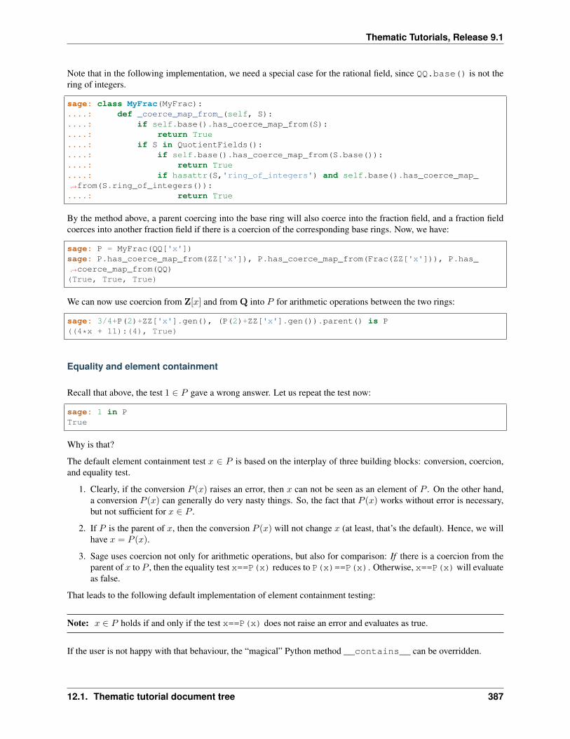
Thematic Tutorials, Release 9.1
Note that in the following implementation, we need a special case for the rational field, since QQ.base() is not thering of integers.
sage: class MyFrac(MyFrac):....: def _coerce_map_from_(self, S):....: if self.base().has_coerce_map_from(S):....: return True....: if S in QuotientFields():....: if self.base().has_coerce_map_from(S.base()):....: return True....: if hasattr(S,'ring_of_integers') and self.base().has_coerce_map_→˓from(S.ring_of_integers()):....: return True
By the method above, a parent coercing into the base ring will also coerce into the fraction field, and a fraction fieldcoerces into another fraction field if there is a coercion of the corresponding base rings. Now, we have:
sage: P = MyFrac(QQ['x'])sage: P.has_coerce_map_from(ZZ['x']), P.has_coerce_map_from(Frac(ZZ['x'])), P.has_→˓coerce_map_from(QQ)(True, True, True)
We can now use coercion from Z[𝑥] and from Q into 𝑃 for arithmetic operations between the two rings:
sage: 3/4+P(2)+ZZ['x'].gen(), (P(2)+ZZ['x'].gen()).parent() is P((4*x + 11):(4), True)
Equality and element containment
Recall that above, the test 1 ∈ 𝑃 gave a wrong answer. Let us repeat the test now:
sage: 1 in PTrue
Why is that?
The default element containment test 𝑥 ∈ 𝑃 is based on the interplay of three building blocks: conversion, coercion,and equality test.
1. Clearly, if the conversion 𝑃 (𝑥) raises an error, then 𝑥 can not be seen as an element of 𝑃 . On the other hand,a conversion 𝑃 (𝑥) can generally do very nasty things. So, the fact that 𝑃 (𝑥) works without error is necessary,but not sufficient for 𝑥 ∈ 𝑃 .
2. If 𝑃 is the parent of 𝑥, then the conversion 𝑃 (𝑥) will not change 𝑥 (at least, that’s the default). Hence, we willhave 𝑥 = 𝑃 (𝑥).
3. Sage uses coercion not only for arithmetic operations, but also for comparison: If there is a coercion from theparent of 𝑥 to 𝑃 , then the equality test x==P(x) reduces to P(x)==P(x). Otherwise, x==P(x) will evaluateas false.
That leads to the following default implementation of element containment testing:
Note: 𝑥 ∈ 𝑃 holds if and only if the test x==P(x) does not raise an error and evaluates as true.
If the user is not happy with that behaviour, the “magical” Python method __contains__ can be overridden.
12.1. Thematic tutorial document tree 387
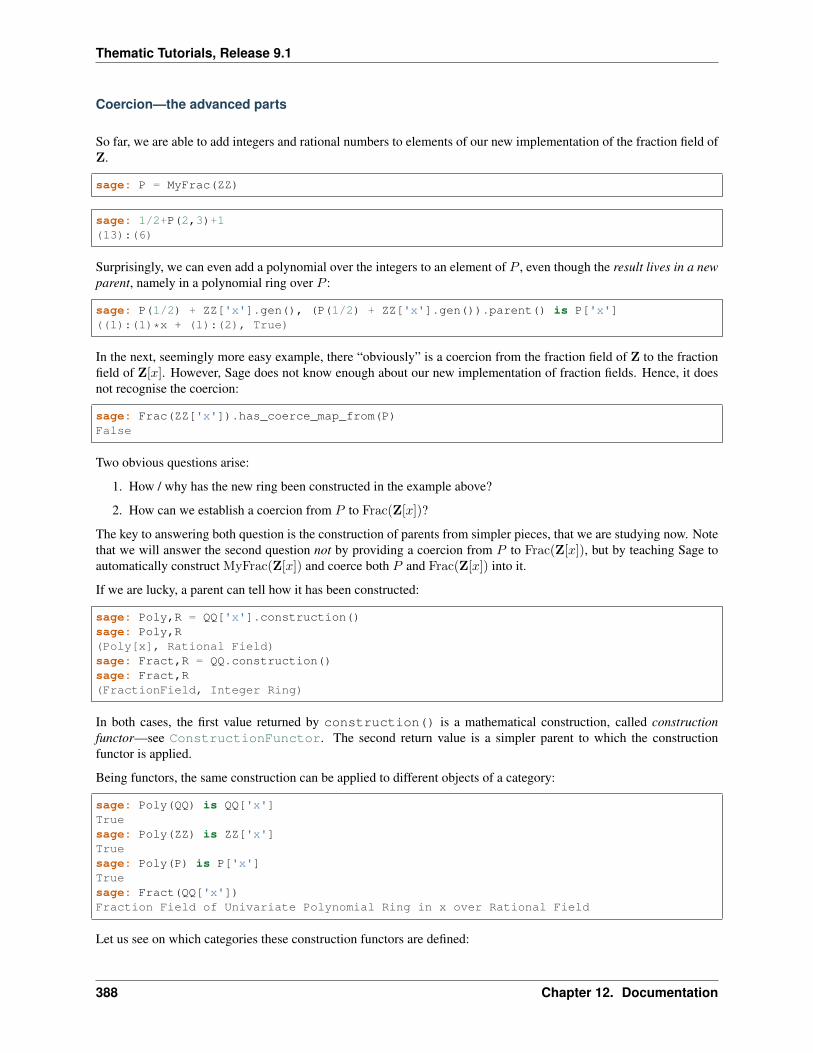
Thematic Tutorials, Release 9.1
Coercion—the advanced parts
So far, we are able to add integers and rational numbers to elements of our new implementation of the fraction field ofZ.
sage: P = MyFrac(ZZ)
sage: 1/2+P(2,3)+1(13):(6)
Surprisingly, we can even add a polynomial over the integers to an element of 𝑃 , even though the result lives in a newparent, namely in a polynomial ring over 𝑃 :
sage: P(1/2) + ZZ['x'].gen(), (P(1/2) + ZZ['x'].gen()).parent() is P['x']((1):(1)*x + (1):(2), True)
In the next, seemingly more easy example, there “obviously” is a coercion from the fraction field of Z to the fractionfield of Z[𝑥]. However, Sage does not know enough about our new implementation of fraction fields. Hence, it doesnot recognise the coercion:
sage: Frac(ZZ['x']).has_coerce_map_from(P)False
Two obvious questions arise:
1. How / why has the new ring been constructed in the example above?
2. How can we establish a coercion from 𝑃 to Frac(Z[𝑥])?
The key to answering both question is the construction of parents from simpler pieces, that we are studying now. Notethat we will answer the second question not by providing a coercion from 𝑃 to Frac(Z[𝑥]), but by teaching Sage toautomatically construct MyFrac(Z[𝑥]) and coerce both 𝑃 and Frac(Z[𝑥]) into it.
If we are lucky, a parent can tell how it has been constructed:
sage: Poly,R = QQ['x'].construction()sage: Poly,R(Poly[x], Rational Field)sage: Fract,R = QQ.construction()sage: Fract,R(FractionField, Integer Ring)
In both cases, the first value returned by construction() is a mathematical construction, called constructionfunctor—see ConstructionFunctor. The second return value is a simpler parent to which the constructionfunctor is applied.
Being functors, the same construction can be applied to different objects of a category:
sage: Poly(QQ) is QQ['x']Truesage: Poly(ZZ) is ZZ['x']Truesage: Poly(P) is P['x']Truesage: Fract(QQ['x'])Fraction Field of Univariate Polynomial Ring in x over Rational Field
Let us see on which categories these construction functors are defined:
388 Chapter 12. Documentation
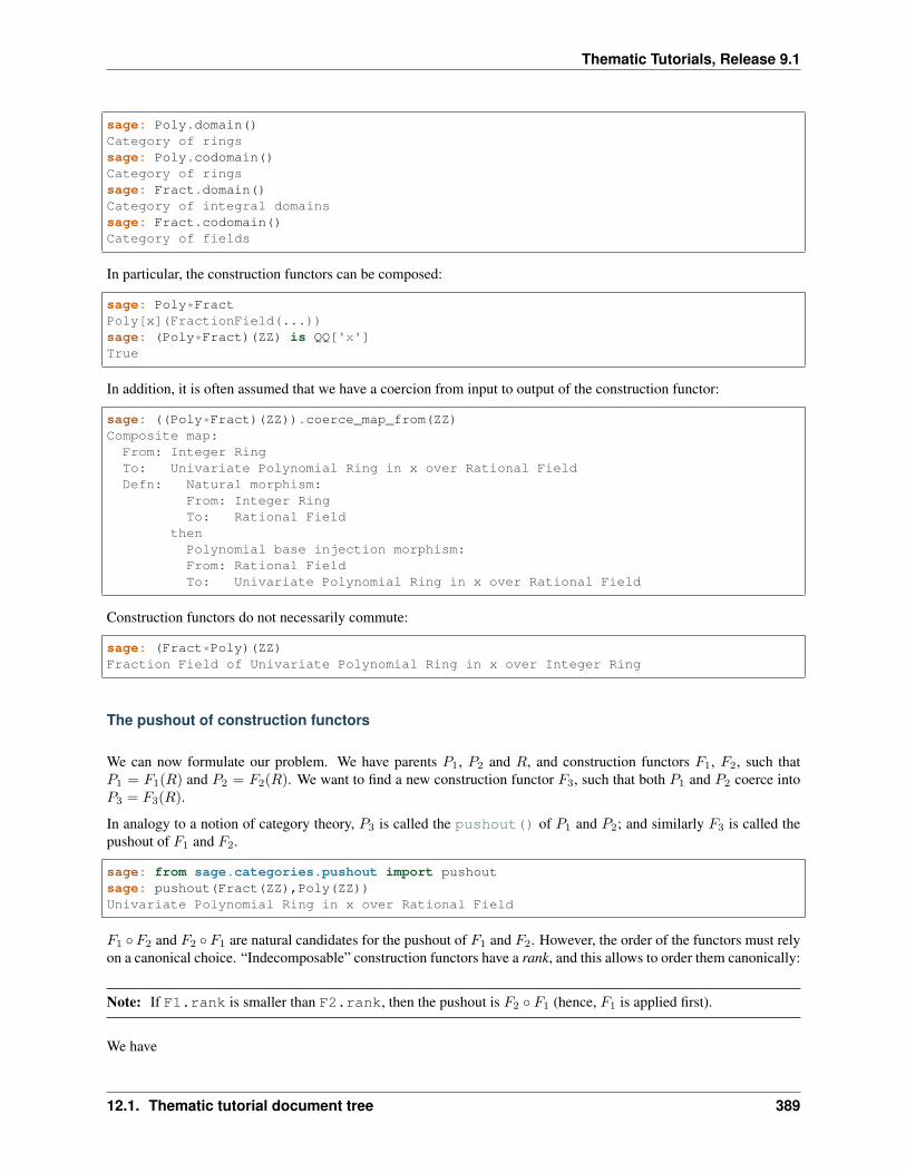
Thematic Tutorials, Release 9.1
sage: Poly.domain()Category of ringssage: Poly.codomain()Category of ringssage: Fract.domain()Category of integral domainssage: Fract.codomain()Category of fields
In particular, the construction functors can be composed:
sage: Poly*FractPoly[x](FractionField(...))sage: (Poly*Fract)(ZZ) is QQ['x']True
In addition, it is often assumed that we have a coercion from input to output of the construction functor:
sage: ((Poly*Fract)(ZZ)).coerce_map_from(ZZ)Composite map:
From: Integer RingTo: Univariate Polynomial Ring in x over Rational FieldDefn: Natural morphism:
From: Integer RingTo: Rational Field
thenPolynomial base injection morphism:From: Rational FieldTo: Univariate Polynomial Ring in x over Rational Field
Construction functors do not necessarily commute:
sage: (Fract*Poly)(ZZ)Fraction Field of Univariate Polynomial Ring in x over Integer Ring
The pushout of construction functors
We can now formulate our problem. We have parents 𝑃1, 𝑃2 and 𝑅, and construction functors 𝐹1, 𝐹2, such that𝑃1 = 𝐹1(𝑅) and 𝑃2 = 𝐹2(𝑅). We want to find a new construction functor 𝐹3, such that both 𝑃1 and 𝑃2 coerce into𝑃3 = 𝐹3(𝑅).
In analogy to a notion of category theory, 𝑃3 is called the pushout() of 𝑃1 and 𝑃2; and similarly 𝐹3 is called thepushout of 𝐹1 and 𝐹2.
sage: from sage.categories.pushout import pushoutsage: pushout(Fract(ZZ),Poly(ZZ))Univariate Polynomial Ring in x over Rational Field
𝐹1 ∘ 𝐹2 and 𝐹2 ∘ 𝐹1 are natural candidates for the pushout of 𝐹1 and 𝐹2. However, the order of the functors must relyon a canonical choice. “Indecomposable” construction functors have a rank, and this allows to order them canonically:
Note: If F1.rank is smaller than F2.rank, then the pushout is 𝐹2 ∘ 𝐹1 (hence, 𝐹1 is applied first).
We have
12.1. Thematic tutorial document tree 389
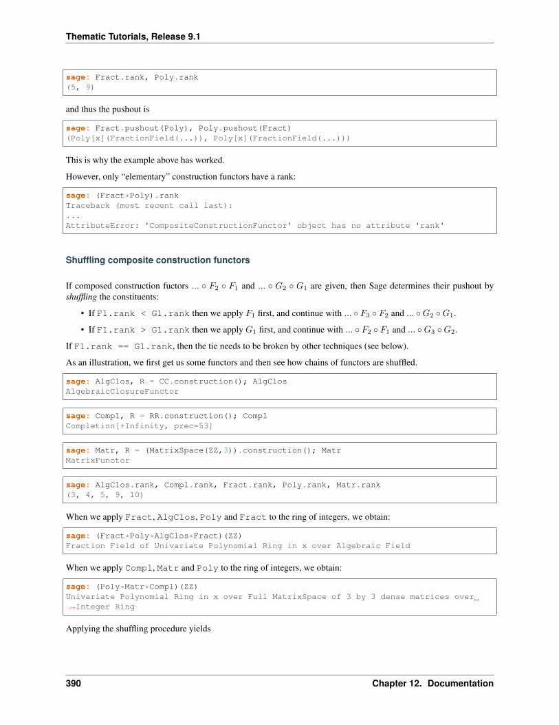
Thematic Tutorials, Release 9.1
sage: Fract.rank, Poly.rank(5, 9)
and thus the pushout is
sage: Fract.pushout(Poly), Poly.pushout(Fract)(Poly[x](FractionField(...)), Poly[x](FractionField(...)))
This is why the example above has worked.
However, only “elementary” construction functors have a rank:
sage: (Fract*Poly).rankTraceback (most recent call last):...AttributeError: 'CompositeConstructionFunctor' object has no attribute 'rank'
Shuffling composite construction functors
If composed construction fuctors ... ∘ 𝐹2 ∘ 𝐹1 and ... ∘ 𝐺2 ∘ 𝐺1 are given, then Sage determines their pushout byshuffling the constituents:
• If F1.rank < G1.rank then we apply 𝐹1 first, and continue with ... ∘ 𝐹3 ∘ 𝐹2 and ... ∘𝐺2 ∘𝐺1.
• If F1.rank > G1.rank then we apply 𝐺1 first, and continue with ... ∘ 𝐹2 ∘ 𝐹1 and ... ∘𝐺3 ∘𝐺2.
If F1.rank == G1.rank, then the tie needs to be broken by other techniques (see below).
As an illustration, we first get us some functors and then see how chains of functors are shuffled.
sage: AlgClos, R = CC.construction(); AlgClosAlgebraicClosureFunctor
sage: Compl, R = RR.construction(); ComplCompletion[+Infinity, prec=53]
sage: Matr, R = (MatrixSpace(ZZ,3)).construction(); MatrMatrixFunctor
sage: AlgClos.rank, Compl.rank, Fract.rank, Poly.rank, Matr.rank(3, 4, 5, 9, 10)
When we apply Fract, AlgClos, Poly and Fract to the ring of integers, we obtain:
sage: (Fract*Poly*AlgClos*Fract)(ZZ)Fraction Field of Univariate Polynomial Ring in x over Algebraic Field
When we apply Compl, Matr and Poly to the ring of integers, we obtain:
sage: (Poly*Matr*Compl)(ZZ)Univariate Polynomial Ring in x over Full MatrixSpace of 3 by 3 dense matrices over→˓Integer Ring
Applying the shuffling procedure yields
390 Chapter 12. Documentation
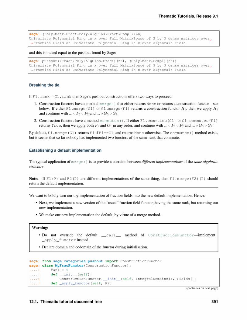
Thematic Tutorials, Release 9.1
sage: (Poly*Matr*Fract*Poly*AlgClos*Fract*Compl)(ZZ)Univariate Polynomial Ring in x over Full MatrixSpace of 3 by 3 dense matrices over→˓Fraction Field of Univariate Polynomial Ring in x over Algebraic Field
and this is indeed equal to the pushout found by Sage:
sage: pushout((Fract*Poly*AlgClos*Fract)(ZZ), (Poly*Matr*Compl)(ZZ))Univariate Polynomial Ring in x over Full MatrixSpace of 3 by 3 dense matrices over→˓Fraction Field of Univariate Polynomial Ring in x over Algebraic Field
Breaking the tie
If F1.rank==G1.rank then Sage’s pushout constructions offers two ways to proceed:
1. Construction functors have a method merge() that either returns None or returns a construction functor—seebelow. If either F1.merge(G1) or G1.merge(F1) returns a construction functor 𝐻1, then we apply 𝐻1
and continue with ... ∘ 𝐹3 ∘ 𝐹2 and ... ∘𝐺3 ∘𝐺2.
2. Construction functors have a method commutes(). If either F1.commutes(G1) or G1.commutes(F1)returns True, then we apply both 𝐹1 and 𝐺1 in any order, and continue with ... ∘ 𝐹3 ∘ 𝐹2 and ... ∘𝐺3 ∘𝐺2.
By default, F1.merge(G1) returns F1 if F1==G1, and returns None otherwise. The commutes() method exists,but it seems that so far nobody has implemented two functors of the same rank that commute.
Establishing a default implementation
The typical application of merge() is to provide a coercion between different implementations of the same algebraicstructure.
Note: If F1(P) and F2(P) are different implementations of the same thing, then F1.merge(F2)(P) shouldreturn the default implementation.
We want to boldly turn our toy implementation of fraction fields into the new default implementation. Hence:
• Next, we implement a new version of the “usual” fraction field functor, having the same rank, but returning ournew implementation.
• We make our new implementation the default, by virtue of a merge method.
Warning:
• Do not override the default __call__ method of ConstructionFunctor—implement_apply_functor instead.
• Declare domain and codomain of the functor during initialisation.
sage: from sage.categories.pushout import ConstructionFunctorsage: class MyFracFunctor(ConstructionFunctor):....: rank = 5....: def __init__(self):....: ConstructionFunctor.__init__(self, IntegralDomains(), Fields())....: def _apply_functor(self, R):
(continues on next page)
12.1. Thematic tutorial document tree 391
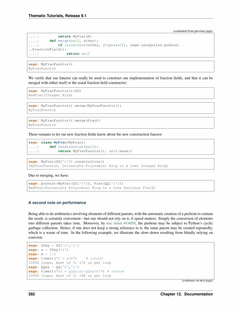
Thematic Tutorials, Release 9.1
(continued from previous page)
....: return MyFrac(R)
....: def merge(self, other):
....: if isinstance(other, (type(self), sage.categories.pushout.→˓FractionField)):....: return self
sage: MyFracFunctor()MyFracFunctor
We verify that our functor can really be used to construct our implementation of fraction fields, and that it can bemerged with either itself or the usual fraction field constructor:
sage: MyFracFunctor()(ZZ)NewFrac(Integer Ring)
sage: MyFracFunctor().merge(MyFracFunctor())MyFracFunctor
sage: MyFracFunctor().merge(Fract)MyFracFunctor
There remains to let our new fraction fields know about the new construction functor:
sage: class MyFrac(MyFrac):....: def construction(self):....: return MyFracFunctor(), self.base()
sage: MyFrac(ZZ['x']).construction()(MyFracFunctor, Univariate Polynomial Ring in x over Integer Ring)
Due to merging, we have:
sage: pushout(MyFrac(ZZ['x']), Frac(QQ['x']))NewFrac(Univariate Polynomial Ring in x over Rational Field)
A second note on performance
Being able to do arithmetics involving elements of different parents, with the automatic creation of a pushout to containthe result, is certainly convenient—but one should not rely on it, if speed matters. Simply the conversion of elementsinto different parents takes time. Moreover, by trac ticket #14058, the pushout may be subject to Python’s cyclicgarbage collection. Hence, if one does not keep a strong reference to it, the same parent may be created repeatedly,which is a waste of time. In the following example, we illustrate the slow–down resulting from blindly relying oncoercion:
sage: ZZxy = ZZ['x','y']sage: a = ZZxy('x')sage: b = 1/2sage: timeit("c = a+b") # random10000 loops, best of 3: 172 us per loopsage: QQxy = QQ['x','y']sage: timeit("c2 = QQxy(a)+QQxy(b)") # random10000 loops, best of 3: 168 us per loop
(continues on next page)
392 Chapter 12. Documentation
Thematic Tutorials, Release 9.1
(continued from previous page)
sage: a2 = QQxy(a)sage: b2 = QQxy(b)sage: timeit("c2 = a2+b2") # random100000 loops, best of 3: 10.5 us per loop
Hence, if one avoids the explicit or implicit conversion into the pushout, but works in the pushout right away, one canget a more than 10–fold speed–up.
The test suites of the category framework
The category framework does not only provide functionality but also a test framework. This section logically belongsto the section on categories, but without the bits that we have implemented in the section on coercion, our implemen-tation of fraction fields would not have passed the tests yet.
“Abstract” methods
We have already seen above that a category can require/suggest certain parent or element methods, that the usermust/should implement. This is in order to smoothly blend with the methods that already exist in Sage.
The methods that ought to be provided are called abstract_method(). Let us see what methods are needed forquotient fields and their elements:
sage: from sage.misc.abstract_method import abstract_methods_of_class
sage: abstract_methods_of_class(QuotientFields().parent_class)['optional'][]sage: abstract_methods_of_class(QuotientFields().parent_class)['required']['__contains__']
Hence, the only required method (that is actually required for all parents that belong to the category of sets) is anelement containment test. That’s fine, because the base class Parent provides a default containment test.
The elements have to provide more:
sage: abstract_methods_of_class(QuotientFields().element_class)['optional']['_add_', '_mul_']sage: abstract_methods_of_class(QuotientFields().element_class)['required'] # py2['__nonzero__', 'denominator', 'numerator']sage: abstract_methods_of_class(QuotientFields().element_class)['required'] # py3['__bool__', 'denominator', 'numerator']
Hence, the elements must provide denominator() and numerator() methods, and must be able to tell whetherthey are zero or not. The base class Element provides a default __nonzero__()method. In addition, the elementsmay provide Sage’s single underscore arithmetic methods (actually any ring element should provide them).
The _test_... methods
If a parent or element method’s name start with “_test_”, it gives rise to a test in the automatic test suite. For example,it is tested
• whether a parent 𝑃 actually is an instance of the parent class of the category of 𝑃 ,
• whether the user has implemented the required abstract methods,
12.1. Thematic tutorial document tree 393
Thematic Tutorials, Release 9.1
• whether some defining structural properties (e.g., commutativity) hold.
For example, if one forgets to implement required methods, one obtains the following error:
sage: class Foo(Parent):....: Element = sage.structure.element.Element....: def __init__(self):....: Parent.__init__(self, category=QuotientFields())sage: Bar = Foo()sage: bar = Bar.element_class(Bar)sage: bar._test_not_implemented_methods()Traceback (most recent call last):...AssertionError: Not implemented method: denominator
Here are the tests that form the test suite of quotient fields:
sage: [t for t in dir(QuotientFields().parent_class) if t.startswith('_test_')]['_test_additive_associativity','_test_an_element','_test_associativity','_test_cardinality','_test_characteristic','_test_characteristic_fields','_test_distributivity','_test_divides','_test_elements','_test_elements_eq_reflexive','_test_elements_eq_symmetric','_test_elements_eq_transitive','_test_elements_neq','_test_euclidean_degree','_test_fraction_field','_test_gcd_vs_xgcd','_test_one','_test_prod','_test_quo_rem','_test_some_elements','_test_zero','_test_zero_divisors']
We have implemented all abstract methods (or inherit them from base classes), we use the category framework, andwe have implemented coercions. So, we are confident that the test suite runs without an error. In fact, it does!
Note: The following trick with the __main__ module is only needed in doctests, not in an interactive session orwhen defining the classes externally.
sage: __main__.MyFrac = MyFracsage: __main__.MyElement = MyElementsage: P = MyFrac(ZZ['x'])sage: TestSuite(P).run()
Let us see what tests are actually performed:
sage: TestSuite(P).run(verbose=True)running ._test_additive_associativity() . . . pass
(continues on next page)
394 Chapter 12. Documentation
Thematic Tutorials, Release 9.1
(continued from previous page)
running ._test_an_element() . . . passrunning ._test_associativity() . . . passrunning ._test_cardinality() . . . passrunning ._test_category() . . . passrunning ._test_characteristic() . . . passrunning ._test_characteristic_fields() . . . passrunning ._test_distributivity() . . . passrunning ._test_divides() . . . passrunning ._test_elements() . . .
Running the test suite of self.an_element()running ._test_category() . . . passrunning ._test_eq() . . . passrunning ._test_new() . . . passrunning ._test_nonzero_equal() . . . passrunning ._test_not_implemented_methods() . . . passrunning ._test_pickling() . . . passpass
running ._test_elements_eq_reflexive() . . . passrunning ._test_elements_eq_symmetric() . . . passrunning ._test_elements_eq_transitive() . . . passrunning ._test_elements_neq() . . . passrunning ._test_eq() . . . passrunning ._test_euclidean_degree() . . . passrunning ._test_fraction_field() . . . passrunning ._test_gcd_vs_xgcd() . . . passrunning ._test_new() . . . passrunning ._test_not_implemented_methods() . . . passrunning ._test_one() . . . passrunning ._test_pickling() . . . passrunning ._test_prod() . . . passrunning ._test_quo_rem() . . . passrunning ._test_some_elements() . . . passrunning ._test_zero() . . . passrunning ._test_zero_divisors() . . . pass
Implementing a new category with additional tests
As one can see, tests are also performed on elements. There are methods that return one element or a list of someelements, relying on “typical” elements that can be found in most algebraic structures.
sage: P.an_element(); P.some_elements()(2):(1)[(2):(1)]
Unfortunately, the list of elements that is returned by the default method is of length one, and that single element couldalso be a bit more interesting. The method an_element relies on a method _an_element_(), so, we implementthat. We also override the some_elements method.
sage: class MyFrac(MyFrac):....: def _an_element_(self):....: a = self.base().an_element()....: b = self.base_ring().an_element()....: if (a+b)!=0:....: return self(a)**2/(self(a+b)**3)
(continues on next page)
12.1. Thematic tutorial document tree 395
Thematic Tutorials, Release 9.1
(continued from previous page)
....: if b != 0:
....: return self(a)/self(b)**2
....: return self(a)**2*self(b)**3
....: def some_elements(self):
....: return [self.an_element(),self(self.base().an_element()),self(self.base_→˓ring().an_element())]
sage: P = MyFrac(ZZ['x'])sage: P.an_element(); P.some_elements()(x^2):(x^3 + 3*x^2 + 3*x + 1)[(x^2):(x^3 + 3*x^2 + 3*x + 1), (x):(1), (1):(1)]
Now, as we have more interesting elements, we may also add a test for the “factor” method. Recall that the methodwas inherited from the category, but it appears that it is not tested.
Normally, a test for a method defined by a category should be provided by the same category. Hence, since factoris defined in the category of quotient fields, a test should be added there. But we won’t change source code here andwill instead create a sub–category.
Apparently, If 𝑒 is an element of a quotient field, the product of the factors returned by e.factor() should be equalto 𝑒. For forming the product, we use the prod method, that, no surprise, is inherited from another category:
sage: P.prod.__module__'sage.categories.monoids'
When we want to create a sub–category, we need to provide a method super_categories(), that returns a list ofall immediate super categories (here: category of quotient fields).
Warning: A sub–category 𝑆 of a category 𝐶 is not implemented as a sub–class of C.__class__! 𝑆 becomesa sub–category of 𝐶 only if S.super_categories() returns (a sub–category of) 𝐶!
The parent and element methods of a category are provided as methods of classes that are the attributesParentMethods and Element Methods of the category, as follows:
sage: from sage.categories.category import Categorysage: class QuotientFieldsWithTest(Category): # do *not* inherit from QuotientFields,→˓but .......: def super_categories(self):....: return [QuotientFields()] # ... declare QuotientFields as a super→˓category!....: class ParentMethods:....: pass....: class ElementMethods:....: def _test_factorisation(self, **options):....: P = self.parent()....: assert self == P.prod([P(b)**e for b,e in self.factor()])
We provide an instance of our quotient field implementation with that new category. Note that categorieshave a default _repr_ method, that guesses a good string representation from the name of the class:QuotientFieldsWithTest becomes “quotient fields with test”.
Note: The following trick with the __main__ module is only needed in doctests, not in an interactive session orwhen defining the classes externally.
396 Chapter 12. Documentation
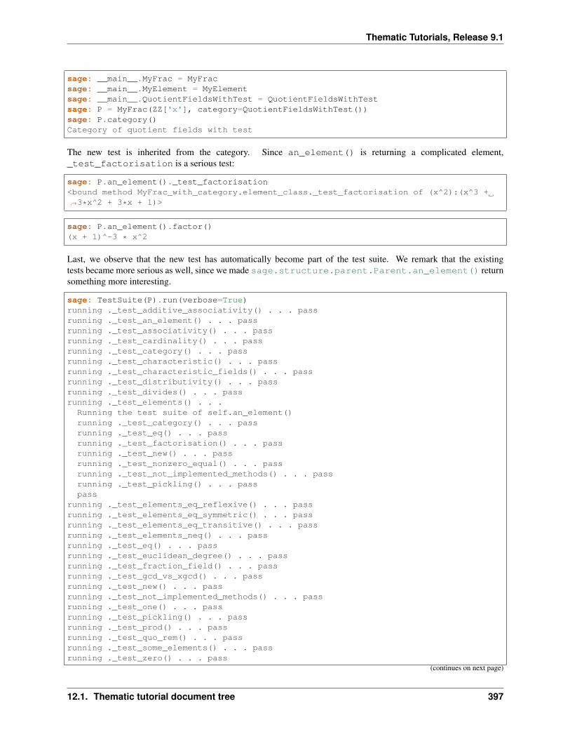
Thematic Tutorials, Release 9.1
sage: __main__.MyFrac = MyFracsage: __main__.MyElement = MyElementsage: __main__.QuotientFieldsWithTest = QuotientFieldsWithTestsage: P = MyFrac(ZZ['x'], category=QuotientFieldsWithTest())sage: P.category()Category of quotient fields with test
The new test is inherited from the category. Since an_element() is returning a complicated element,_test_factorisation is a serious test:
sage: P.an_element()._test_factorisation<bound method MyFrac_with_category.element_class._test_factorisation of (x^2):(x^3 +→˓3*x^2 + 3*x + 1)>
sage: P.an_element().factor()(x + 1)^-3 * x^2
Last, we observe that the new test has automatically become part of the test suite. We remark that the existingtests became more serious as well, since we made sage.structure.parent.Parent.an_element() returnsomething more interesting.
sage: TestSuite(P).run(verbose=True)running ._test_additive_associativity() . . . passrunning ._test_an_element() . . . passrunning ._test_associativity() . . . passrunning ._test_cardinality() . . . passrunning ._test_category() . . . passrunning ._test_characteristic() . . . passrunning ._test_characteristic_fields() . . . passrunning ._test_distributivity() . . . passrunning ._test_divides() . . . passrunning ._test_elements() . . .
Running the test suite of self.an_element()running ._test_category() . . . passrunning ._test_eq() . . . passrunning ._test_factorisation() . . . passrunning ._test_new() . . . passrunning ._test_nonzero_equal() . . . passrunning ._test_not_implemented_methods() . . . passrunning ._test_pickling() . . . passpass
running ._test_elements_eq_reflexive() . . . passrunning ._test_elements_eq_symmetric() . . . passrunning ._test_elements_eq_transitive() . . . passrunning ._test_elements_neq() . . . passrunning ._test_eq() . . . passrunning ._test_euclidean_degree() . . . passrunning ._test_fraction_field() . . . passrunning ._test_gcd_vs_xgcd() . . . passrunning ._test_new() . . . passrunning ._test_not_implemented_methods() . . . passrunning ._test_one() . . . passrunning ._test_pickling() . . . passrunning ._test_prod() . . . passrunning ._test_quo_rem() . . . passrunning ._test_some_elements() . . . passrunning ._test_zero() . . . pass
(continues on next page)
12.1. Thematic tutorial document tree 397
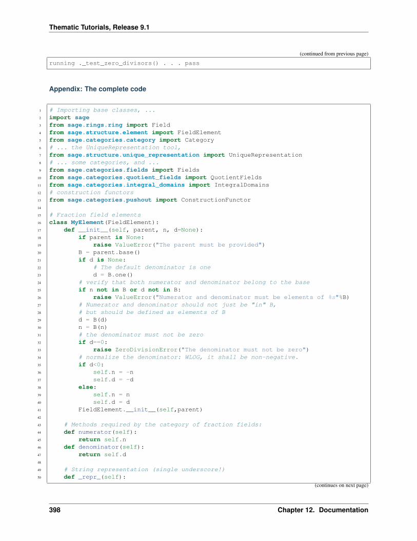
Thematic Tutorials, Release 9.1
(continued from previous page)
running ._test_zero_divisors() . . . pass
Appendix: The complete code
1 # Importing base classes, ...2 import sage3 from sage.rings.ring import Field4 from sage.structure.element import FieldElement5 from sage.categories.category import Category6 # ... the UniqueRepresentation tool,7 from sage.structure.unique_representation import UniqueRepresentation8 # ... some categories, and ...9 from sage.categories.fields import Fields
10 from sage.categories.quotient_fields import QuotientFields11 from sage.categories.integral_domains import IntegralDomains12 # construction functors13 from sage.categories.pushout import ConstructionFunctor14
15 # Fraction field elements16 class MyElement(FieldElement):17 def __init__(self, parent, n, d=None):18 if parent is None:19 raise ValueError("The parent must be provided")20 B = parent.base()21 if d is None:22 # The default denominator is one23 d = B.one()24 # verify that both numerator and denominator belong to the base25 if n not in B or d not in B:26 raise ValueError("Numerator and denominator must be elements of %s"%B)27 # Numerator and denominator should not just be "in" B,28 # but should be defined as elements of B29 d = B(d)30 n = B(n)31 # the denominator must not be zero32 if d==0:33 raise ZeroDivisionError("The denominator must not be zero")34 # normalize the denominator: WLOG, it shall be non-negative.35 if d<0:36 self.n = -n37 self.d = -d38 else:39 self.n = n40 self.d = d41 FieldElement.__init__(self,parent)42
43 # Methods required by the category of fraction fields:44 def numerator(self):45 return self.n46 def denominator(self):47 return self.d48
49 # String representation (single underscore!)50 def _repr_(self):
(continues on next page)
398 Chapter 12. Documentation
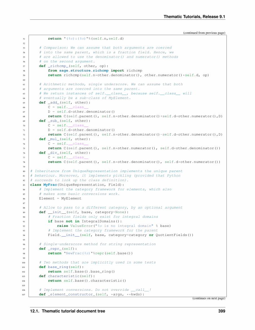
Thematic Tutorials, Release 9.1
(continued from previous page)
51 return "(%s):(%s)"%(self.n,self.d)52
53 # Comparison: We can assume that both arguments are coerced54 # into the same parent, which is a fraction field. Hence, we55 # are allowed to use the denominator() and numerator() methods56 # on the second argument.57 def _richcmp_(self, other, op):58 from sage.structure.richcmp import richcmp59 return richcmp(self.n*other.denominator(), other.numerator()*self.d, op)60
61 # Arithmetic methods, single underscore. We can assume that both62 # arguments are coerced into the same parent.63 # We return instances of self.__class__, because self.__class__ will64 # eventually be a sub-class of MyElement.65 def _add_(self, other):66 C = self.__class__67 D = self.d*other.denominator()68 return C(self.parent(), self.n*other.denominator()+self.d*other.numerator(),D)69 def _sub_(self, other):70 C = self.__class__71 D = self.d*other.denominator()72 return C(self.parent(), self.n*other.denominator()-self.d*other.numerator(),D)73 def _mul_(self, other):74 C = self.__class__75 return C(self.parent(), self.n*other.numerator(), self.d*other.denominator())76 def _div_(self, other):77 C = self.__class__78 return C(self.parent(), self.n*other.denominator(), self.d*other.numerator())79
80 # Inheritance from UniqueRepresentation implements the unique parent81 # behaviour. Moreover, it implements pickling (provided that Python82 # succeeds to look up the class definition).83 class MyFrac(UniqueRepresentation, Field):84 # Implement the category framework for elements, which also85 # makes some basic conversions work.86 Element = MyElement87
88 # Allow to pass to a different category, by an optional argument89 def __init__(self, base, category=None):90 # Fraction fields only exist for integral domains91 if base not in IntegralDomains():92 raise ValueError("%s is no integral domain" % base)93 # Implement the category framework for the parent94 Field.__init__(self, base, category=category or QuotientFields())95
96 # Single-underscore method for string representation97 def _repr_(self):98 return "NewFrac(%s)"%repr(self.base())99
100 # Two methods that are implicitly used in some tests101 def base_ring(self):102 return self.base().base_ring()103 def characteristic(self):104 return self.base().characteristic()105
106 # Implement conversions. Do not override __call__!107 def _element_constructor_(self, *args, **kwds):
(continues on next page)
12.1. Thematic tutorial document tree 399
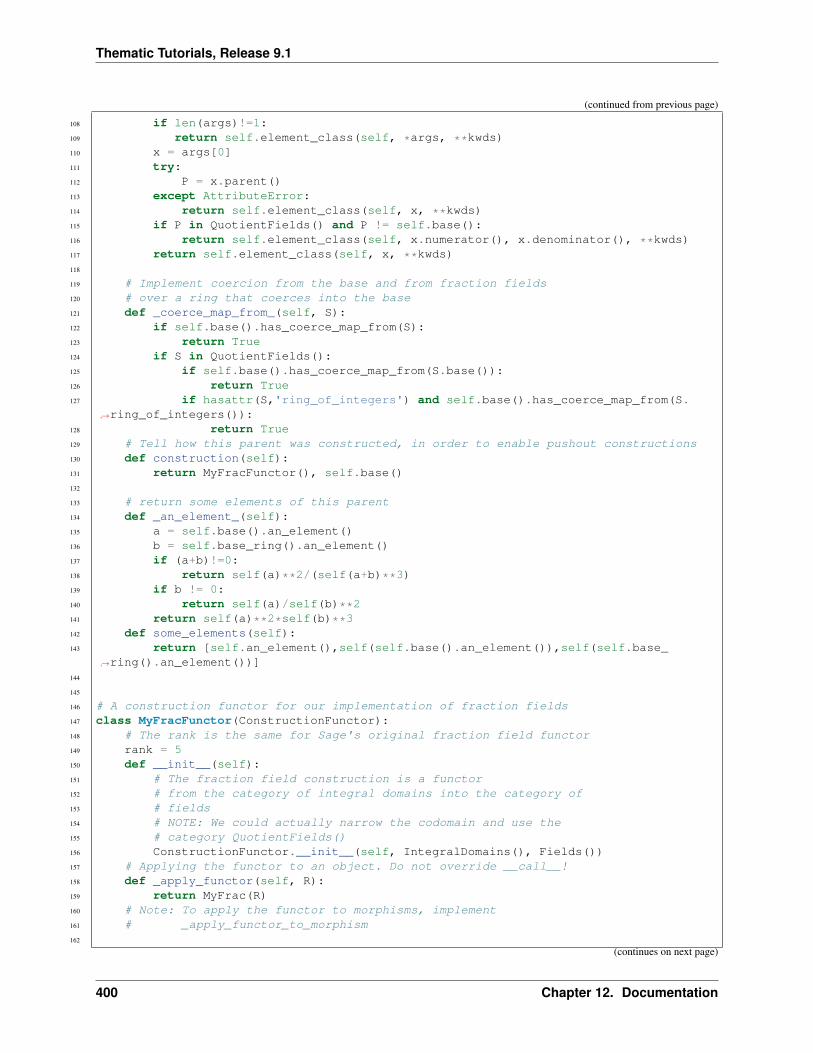
Thematic Tutorials, Release 9.1
(continued from previous page)
108 if len(args)!=1:109 return self.element_class(self, *args, **kwds)110 x = args[0]111 try:112 P = x.parent()113 except AttributeError:114 return self.element_class(self, x, **kwds)115 if P in QuotientFields() and P != self.base():116 return self.element_class(self, x.numerator(), x.denominator(), **kwds)117 return self.element_class(self, x, **kwds)118
119 # Implement coercion from the base and from fraction fields120 # over a ring that coerces into the base121 def _coerce_map_from_(self, S):122 if self.base().has_coerce_map_from(S):123 return True124 if S in QuotientFields():125 if self.base().has_coerce_map_from(S.base()):126 return True127 if hasattr(S,'ring_of_integers') and self.base().has_coerce_map_from(S.
→˓ring_of_integers()):128 return True129 # Tell how this parent was constructed, in order to enable pushout constructions130 def construction(self):131 return MyFracFunctor(), self.base()132
133 # return some elements of this parent134 def _an_element_(self):135 a = self.base().an_element()136 b = self.base_ring().an_element()137 if (a+b)!=0:138 return self(a)**2/(self(a+b)**3)139 if b != 0:140 return self(a)/self(b)**2141 return self(a)**2*self(b)**3142 def some_elements(self):143 return [self.an_element(),self(self.base().an_element()),self(self.base_
→˓ring().an_element())]144
145
146 # A construction functor for our implementation of fraction fields147 class MyFracFunctor(ConstructionFunctor):148 # The rank is the same for Sage's original fraction field functor149 rank = 5150 def __init__(self):151 # The fraction field construction is a functor152 # from the category of integral domains into the category of153 # fields154 # NOTE: We could actually narrow the codomain and use the155 # category QuotientFields()156 ConstructionFunctor.__init__(self, IntegralDomains(), Fields())157 # Applying the functor to an object. Do not override __call__!158 def _apply_functor(self, R):159 return MyFrac(R)160 # Note: To apply the functor to morphisms, implement161 # _apply_functor_to_morphism162
(continues on next page)
400 Chapter 12. Documentation
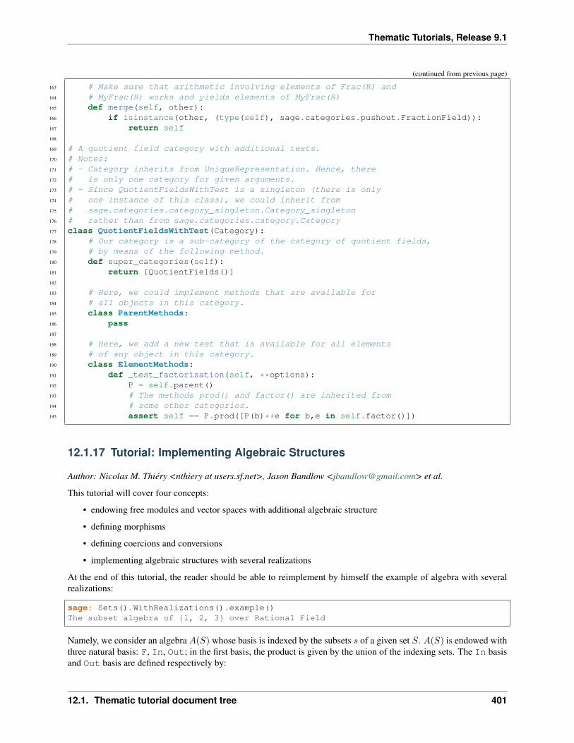
Thematic Tutorials, Release 9.1
(continued from previous page)
163 # Make sure that arithmetic involving elements of Frac(R) and164 # MyFrac(R) works and yields elements of MyFrac(R)165 def merge(self, other):166 if isinstance(other, (type(self), sage.categories.pushout.FractionField)):167 return self168
169 # A quotient field category with additional tests.170 # Notes:171 # - Category inherits from UniqueRepresentation. Hence, there172 # is only one category for given arguments.173 # - Since QuotientFieldsWithTest is a singleton (there is only174 # one instance of this class), we could inherit from175 # sage.categories.category_singleton.Category_singleton176 # rather than from sage.categories.category.Category177 class QuotientFieldsWithTest(Category):178 # Our category is a sub-category of the category of quotient fields,179 # by means of the following method.180 def super_categories(self):181 return [QuotientFields()]182
183 # Here, we could implement methods that are available for184 # all objects in this category.185 class ParentMethods:186 pass187
188 # Here, we add a new test that is available for all elements189 # of any object in this category.190 class ElementMethods:191 def _test_factorisation(self, **options):192 P = self.parent()193 # The methods prod() and factor() are inherited from194 # some other categories.195 assert self == P.prod([P(b)**e for b,e in self.factor()])
12.1.17 Tutorial: Implementing Algebraic Structures
Author: Nicolas M. Thiéry <nthiery at users.sf.net>, Jason Bandlow <[email protected]> et al.
This tutorial will cover four concepts:
• endowing free modules and vector spaces with additional algebraic structure
• defining morphisms
• defining coercions and conversions
• implementing algebraic structures with several realizations
At the end of this tutorial, the reader should be able to reimplement by himself the example of algebra with severalrealizations:
sage: Sets().WithRealizations().example()The subset algebra of 1, 2, 3 over Rational Field
Namely, we consider an algebra 𝐴(𝑆) whose basis is indexed by the subsets 𝑠 of a given set 𝑆. 𝐴(𝑆) is endowed withthree natural basis: F, In, Out; in the first basis, the product is given by the union of the indexing sets. The In basisand Out basis are defined respectively by:
12.1. Thematic tutorial document tree 401
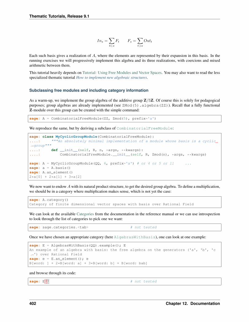
Thematic Tutorials, Release 9.1
𝐼𝑛𝑠 =∑𝑡⊂𝑠
𝐹𝑡 𝐹𝑠 =∑𝑡⊃𝑠
𝑂𝑢𝑡𝑡
Each such basis gives a realization of 𝐴, where the elements are represented by their expansion in this basis. In therunning exercises we will progressively implement this algebra and its three realizations, with coercions and mixedarithmetic between them.
This tutorial heavily depends on Tutorial: Using Free Modules and Vector Spaces. You may also want to read the lessspecialized thematic tutorial How to implement new algebraic structures.
Subclassing free modules and including category information
As a warm-up, we implement the group algebra of the additive group Z/5Z. Of course this is solely for pedagogicalpurposes; group algebras are already implemented (see ZMod(5).algebra(ZZ)). Recall that a fully functionalZ-module over this group can be created with the simple command:
sage: A = CombinatorialFreeModule(ZZ, Zmod(5), prefix='a')
We reproduce the same, but by deriving a subclass of CombinatorialFreeModule:
sage: class MyCyclicGroupModule(CombinatorialFreeModule):....: """An absolutely minimal implementation of a module whose basis is a cyclic→˓group"""....: def __init__(self, R, n, *args, **kwargs):....: CombinatorialFreeModule.__init__(self, R, Zmod(n), *args, **kwargs)
sage: A = MyCyclicGroupModule(QQ, 6, prefix='a') # or 4 or 5 or 11 ...sage: a = A.basis()sage: A.an_element()2*a[0] + 2*a[1] + 3*a[2]
We now want to endow𝐴with its natural product structure, to get the desired group algebra. To define a multiplication,we should be in a category where multiplication makes sense, which is not yet the case:
sage: A.category()Category of finite dimensional vector spaces with basis over Rational Field
We can look at the available Categories from the documentation in the reference manual or we can use introspectionto look through the list of categories to pick one we want:
sage: sage.categories.<tab> # not tested
Once we have chosen an appropriate category (here AlgebrasWithBasis), one can look at one example:
sage: E = AlgebrasWithBasis(QQ).example(); EAn example of an algebra with basis: the free algebra on the generators ('a', 'b', 'c→˓') over Rational Fieldsage: e = E.an_element(); eB[word: ] + 2*B[word: a] + 3*B[word: b] + B[word: bab]
and browse through its code:
sage: E?? # not tested
402 Chapter 12. Documentation
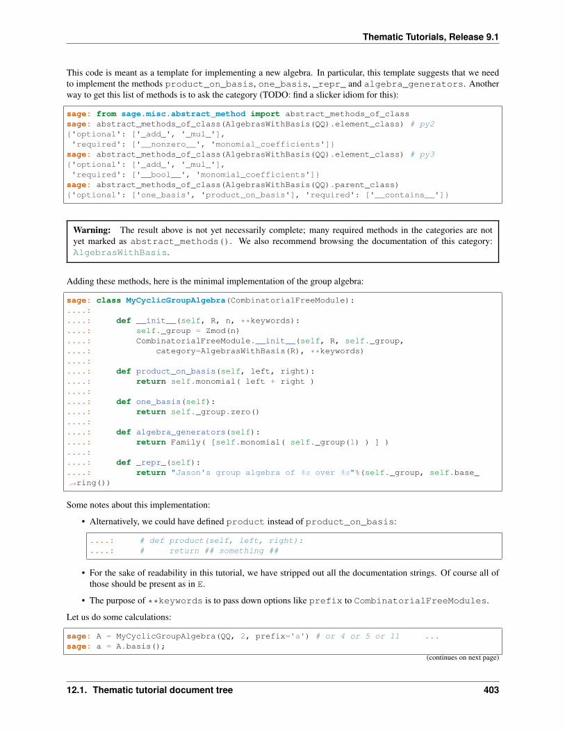
Thematic Tutorials, Release 9.1
This code is meant as a template for implementing a new algebra. In particular, this template suggests that we needto implement the methods product_on_basis, one_basis, _repr_ and algebra_generators. Anotherway to get this list of methods is to ask the category (TODO: find a slicker idiom for this):
sage: from sage.misc.abstract_method import abstract_methods_of_classsage: abstract_methods_of_class(AlgebrasWithBasis(QQ).element_class) # py2'optional': ['_add_', '_mul_'],'required': ['__nonzero__', 'monomial_coefficients']
sage: abstract_methods_of_class(AlgebrasWithBasis(QQ).element_class) # py3'optional': ['_add_', '_mul_'],'required': ['__bool__', 'monomial_coefficients']
sage: abstract_methods_of_class(AlgebrasWithBasis(QQ).parent_class)'optional': ['one_basis', 'product_on_basis'], 'required': ['__contains__']
Warning: The result above is not yet necessarily complete; many required methods in the categories are notyet marked as abstract_methods(). We also recommend browsing the documentation of this category:AlgebrasWithBasis.
Adding these methods, here is the minimal implementation of the group algebra:
sage: class MyCyclicGroupAlgebra(CombinatorialFreeModule):....:....: def __init__(self, R, n, **keywords):....: self._group = Zmod(n)....: CombinatorialFreeModule.__init__(self, R, self._group,....: category=AlgebrasWithBasis(R), **keywords)....:....: def product_on_basis(self, left, right):....: return self.monomial( left + right )....:....: def one_basis(self):....: return self._group.zero()....:....: def algebra_generators(self):....: return Family( [self.monomial( self._group(1) ) ] )....:....: def _repr_(self):....: return "Jason's group algebra of %s over %s"%(self._group, self.base_→˓ring())
Some notes about this implementation:
• Alternatively, we could have defined product instead of product_on_basis:
....: # def product(self, left, right):
....: # return ## something ##
• For the sake of readability in this tutorial, we have stripped out all the documentation strings. Of course all ofthose should be present as in E.
• The purpose of **keywords is to pass down options like prefix to CombinatorialFreeModules.
Let us do some calculations:
sage: A = MyCyclicGroupAlgebra(QQ, 2, prefix='a') # or 4 or 5 or 11 ...sage: a = A.basis();
(continues on next page)
12.1. Thematic tutorial document tree 403
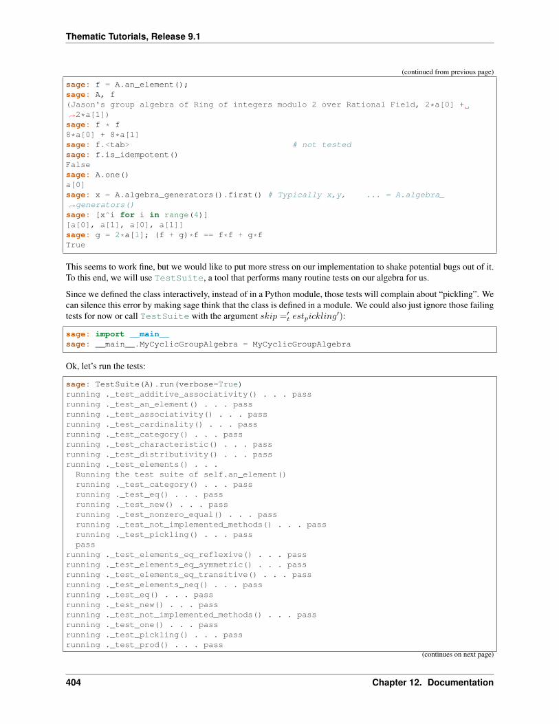
Thematic Tutorials, Release 9.1
(continued from previous page)
sage: f = A.an_element();sage: A, f(Jason's group algebra of Ring of integers modulo 2 over Rational Field, 2*a[0] +→˓2*a[1])sage: f * f8*a[0] + 8*a[1]sage: f.<tab> # not testedsage: f.is_idempotent()Falsesage: A.one()a[0]sage: x = A.algebra_generators().first() # Typically x,y, ... = A.algebra_→˓generators()sage: [x^i for i in range(4)][a[0], a[1], a[0], a[1]]sage: g = 2*a[1]; (f + g)*f == f*f + g*fTrue
This seems to work fine, but we would like to put more stress on our implementation to shake potential bugs out of it.To this end, we will use TestSuite, a tool that performs many routine tests on our algebra for us.
Since we defined the class interactively, instead of in a Python module, those tests will complain about “pickling”. Wecan silence this error by making sage think that the class is defined in a module. We could also just ignore those failingtests for now or call TestSuite with the argument 𝑠𝑘𝑖𝑝 =′
𝑡 𝑒𝑠𝑡𝑝𝑖𝑐𝑘𝑙𝑖𝑛𝑔′):
sage: import __main__sage: __main__.MyCyclicGroupAlgebra = MyCyclicGroupAlgebra
Ok, let’s run the tests:
sage: TestSuite(A).run(verbose=True)running ._test_additive_associativity() . . . passrunning ._test_an_element() . . . passrunning ._test_associativity() . . . passrunning ._test_cardinality() . . . passrunning ._test_category() . . . passrunning ._test_characteristic() . . . passrunning ._test_distributivity() . . . passrunning ._test_elements() . . .
Running the test suite of self.an_element()running ._test_category() . . . passrunning ._test_eq() . . . passrunning ._test_new() . . . passrunning ._test_nonzero_equal() . . . passrunning ._test_not_implemented_methods() . . . passrunning ._test_pickling() . . . passpass
running ._test_elements_eq_reflexive() . . . passrunning ._test_elements_eq_symmetric() . . . passrunning ._test_elements_eq_transitive() . . . passrunning ._test_elements_neq() . . . passrunning ._test_eq() . . . passrunning ._test_new() . . . passrunning ._test_not_implemented_methods() . . . passrunning ._test_one() . . . passrunning ._test_pickling() . . . passrunning ._test_prod() . . . pass
(continues on next page)
404 Chapter 12. Documentation
Thematic Tutorials, Release 9.1
(continued from previous page)
running ._test_some_elements() . . . passrunning ._test_zero() . . . pass
For more information on categories, see Elements, parents, and categories in Sage: a (draft of) primer:
sage: sage.categories.primer? # not tested
Review
We wanted to implement an algebra, so we:
1. Created the underlying vector space using CombinatorialFreeModule
2. Looked at sage.categories.<tab> to find an appropriate category
3. Loaded an example of that category, and used sage.misc.abstract_method.abstract_methods_of_class(), to see what methods we needed to write
4. Added the category information and other necessary methods to our class
5. Ran TestSuite to catch potential discrepancies
Exercises
1. Make a tiny modification to product_on_basis in “MyCyclicGroupAlgebra” to implement the dual of thegroup algebra of the cyclic group instead of its group algebra (so the product is now given by 𝑏𝑓𝑏𝑔 = 𝛿𝑓,𝑔𝑏𝑓 ).
Run the TestSuite tests (you may ignore the “pickling” errors). What do you notice?
Fix the implementation of one and check that the TestSuite tests now pass.
Add the Hopf algebra structure. Hint: look at the example:
sage: C = HopfAlgebrasWithBasis(QQ).example()
2. Given a set 𝑆, say:
sage: S = Set([1,2,3,4,5])
and a base ring, say:
sage: R = QQ
implement an 𝑅-algebra:
sage: F = SubsetAlgebraOnFundamentalBasis(S, R) # todo: not implemented
with a basis (b_s)_s\subset S indexed by the subsets of S:
sage: Subsets(S)Subsets of 1, 2, 3, 4, 5
and where the product is defined by 𝑏𝑠𝑏𝑡 = 𝑏𝑠∪𝑡.
12.1. Thematic tutorial document tree 405
Thematic Tutorials, Release 9.1
Morphisms
To better understand relationships between algebraic spaces, one wants to consider morphisms between them:
sage: A.module_morphism? # not testedsage: A = MyCyclicGroupAlgebra(QQ, 2, prefix='a')sage: B = MyCyclicGroupAlgebra(QQ, 6, prefix='b')sage: A, B(Jason's group algebra of Ring of integers modulo 2 over Rational Field, Jason's→˓group algebra of Ring of integers modulo 6 over Rational Field)
sage: def func_on_basis(g):....: r"""....: This function is the 'brain' of a (linear) morphism....: from A --> B.....: The input is the index of basis element of the domain (A).....: The output is an element of the codomain (B).....: """....: if g==1: return B.monomial(Zmod(6)(3))# g==1 in the range A....: else: return B.one()
We can now define a morphism that extends this function to 𝐴 by linearity:
sage: phi = A.module_morphism(func_on_basis, codomain=B)sage: f = A.an_element()sage: f2*a[0] + 2*a[1]sage: phi(f)2*b[0] + 2*b[3]
Exercise
Define a new free module In with basis indexed by the subsets of 𝑆, and a morphism phi from In to F defined by
𝜑(𝐼𝑛𝑠) =∑𝑡⊂𝑠
𝐹𝑡
Diagonal and Triangular Morphisms
We now illustrate how to specify that a given morphism is diagonal or triangular with respect to some order on thebasis, which means that the morphism is invertible and 𝑆𝑎𝑔𝑒 is able to compute the inverse morphism automatically.Currently this feature requires the domain and codomain to have the same index set (in progress . . . ).
sage: X = CombinatorialFreeModule(QQ, Partitions(), prefix='x'); x = X.basis();sage: Y = CombinatorialFreeModule(QQ, Partitions(), prefix='y'); y = Y.basis();
A diagonal module morphism takes as argument a function whose input is the index of a basis element of the domain,and whose output is the coefficient of the corresponding basis element of the codomain:
sage: def diag_func(p):....: if len(p)==0: return 1....: else: return p[0]....:
(continues on next page)
406 Chapter 12. Documentation
Thematic Tutorials, Release 9.1
(continued from previous page)
....:sage: diag_func(Partition([3,2,1]))3sage: X_to_Y = X.module_morphism(diagonal=diag_func, codomain=Y)sage: f = X.an_element();sage: f2*x[[]] + 2*x[[1]] + 3*x[[2]]sage: X_to_Y(f)2*y[[]] + 2*y[[1]] + 6*y[[2]]
Python fun fact: ~ is the inversion operator (but be careful with int’s!):
sage: ~21/2sage: ~(int(2)) # in python this is the bitwise complement: ~x = -x-1-3
Diagonal module morphisms are invertible:
sage: Y_to_X = ~X_to_Ysage: f = y[Partition([3])] - 2*y[Partition([2,1])]sage: f-2*y[[2, 1]] + y[[3]]sage: Y_to_X(f)-x[[2, 1]] + 1/3*x[[3]]sage: X_to_Y(Y_to_X(f))-2*y[[2, 1]] + y[[3]]
For triangular morphisms, just like ordinary morphisms, we need a function that accepts as input the index of a basiselement of the domain and returns an element of the codomain. We think of this function as representing the columnsof the matrix of the linear transformation:
sage: def triang_on_basis(p):....: return Y.sum_of_monomials(mu for mu in Partitions(sum(p)) if mu >= p)....:sage: triang_on_basis([3,2])y[[3, 2]] + y[[4, 1]] + y[[5]]sage: X_to_Y = X.module_morphism(triang_on_basis, triangular='lower',→˓unitriangular=True, codomain=Y)sage: f = x[Partition([1,1,1])] + 2*x[Partition([3,2])];sage: fx[[1, 1, 1]] + 2*x[[3, 2]]
sage: X_to_Y(f)y[[1, 1, 1]] + y[[2, 1]] + y[[3]] + 2*y[[3, 2]] + 2*y[[4, 1]] + 2*y[[5]]
Triangular module_morphisms are also invertible, even if X and Y are both infinite-dimensional:
sage: Y_to_X = ~X_to_Ysage: fx[[1, 1, 1]] + 2*x[[3, 2]]sage: Y_to_X(X_to_Y(f))x[[1, 1, 1]] + 2*x[[3, 2]]
For details, see ModulesWithBasis.ParentMethods.module_morphism() (and also sage.categories.modules_with_basis.TriangularModuleMorphism):
12.1. Thematic tutorial document tree 407
Thematic Tutorials, Release 9.1
sage: A.module_morphism? # not tested
Exercise
Redefine the morphism phi from the previous exercise as a morphism that is triangular with respect to inclusion ofsubsets and define the inverse morphism. You may want to use the following comparison key as key argument tomodules_morphism:
sage: def subset_key(s):....: """....: A comparison key on sets that gives a linear extension....: of the inclusion order.....:....: INPUT:....:....: - ``s`` -- set....:....: EXAMPLES::....:....: sage: sorted(Subsets([1,2,3]), key=subset_key)....: [, 1, 2, 3, 1, 2, 1, 3, 2, 3, 1, 2, 3]....: """....: return (len(s), list(s))
Coercions
Once we have defined a morphism from 𝑋 → 𝑌 , we can register it as a coercion. This will allow Sage to applythe morphism automatically whenever we combine elements of 𝑋 and 𝑌 together. See http://sagemath.com/doc/reference/coercion.html for more information. As a training step, let us first define a morphism 𝑋 to 𝑌 , and register itas a coercion:
sage: def triang_on_basis(p):....: return Y.sum_of_monomials(mu for mu in Partitions(sum(p)) if mu >= p)
sage: triang_on_basis([3,2])y[[3, 2]] + y[[4, 1]] + y[[5]]sage: X_to_Y = X.module_morphism(triang_on_basis, triangular='lower',→˓unitriangular=True, codomain=Y)sage: X_to_Y.<tab> # not testedsage: X_to_Y.register_as_coercion()
Now we can not only convert elements from 𝑋 to 𝑌 , but we can also do mixed arithmetic with these elements:
sage: Y(x[Partition([3,2])])y[[3, 2]] + y[[4, 1]] + y[[5]]sage: Y([2,2,1]) + x[Partition([2,2,1])]2*y[[2, 2, 1]] + y[[3, 1, 1]] + y[[3, 2]] + y[[4, 1]] + y[[5]]
Exercise
Use the inverse of phi to implement the inverse coercion from F to In. Reimplement In as an algebra, with a productmethod making it use phi and its inverse.
408 Chapter 12. Documentation
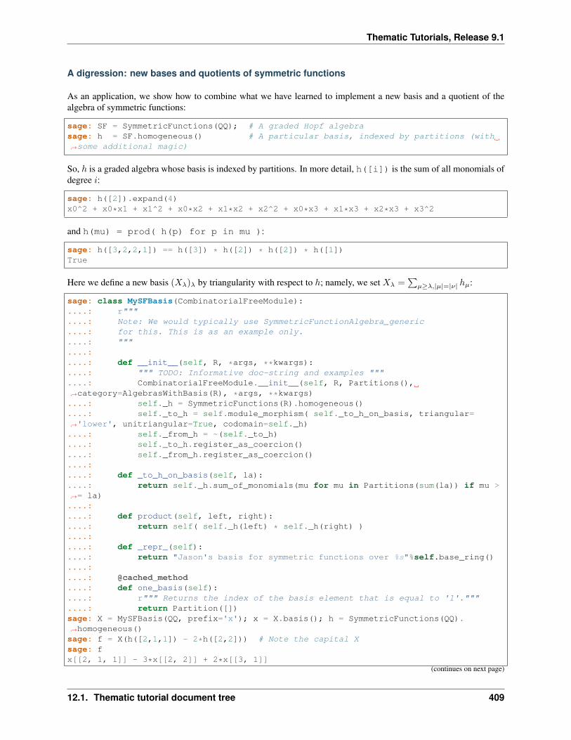
Thematic Tutorials, Release 9.1
A digression: new bases and quotients of symmetric functions
As an application, we show how to combine what we have learned to implement a new basis and a quotient of thealgebra of symmetric functions:
sage: SF = SymmetricFunctions(QQ); # A graded Hopf algebrasage: h = SF.homogeneous() # A particular basis, indexed by partitions (with→˓some additional magic)
So, ℎ is a graded algebra whose basis is indexed by partitions. In more detail, h([i]) is the sum of all monomials ofdegree 𝑖:
sage: h([2]).expand(4)x0^2 + x0*x1 + x1^2 + x0*x2 + x1*x2 + x2^2 + x0*x3 + x1*x3 + x2*x3 + x3^2
and h(mu) = prod( h(p) for p in mu ):
sage: h([3,2,2,1]) == h([3]) * h([2]) * h([2]) * h([1])True
Here we define a new basis (𝑋𝜆)𝜆 by triangularity with respect to ℎ; namely, we set 𝑋𝜆 =∑
𝜇≥𝜆,|𝜇|=|𝜈| ℎ𝜇:
sage: class MySFBasis(CombinatorialFreeModule):....: r"""....: Note: We would typically use SymmetricFunctionAlgebra_generic....: for this. This is as an example only.....: """....:....: def __init__(self, R, *args, **kwargs):....: """ TODO: Informative doc-string and examples """....: CombinatorialFreeModule.__init__(self, R, Partitions(),→˓category=AlgebrasWithBasis(R), *args, **kwargs)....: self._h = SymmetricFunctions(R).homogeneous()....: self._to_h = self.module_morphism( self._to_h_on_basis, triangular=→˓'lower', unitriangular=True, codomain=self._h)....: self._from_h = ~(self._to_h)....: self._to_h.register_as_coercion()....: self._from_h.register_as_coercion()....:....: def _to_h_on_basis(self, la):....: return self._h.sum_of_monomials(mu for mu in Partitions(sum(la)) if mu >→˓= la)....:....: def product(self, left, right):....: return self( self._h(left) * self._h(right) )....:....: def _repr_(self):....: return "Jason's basis for symmetric functions over %s"%self.base_ring()....:....: @cached_method....: def one_basis(self):....: r""" Returns the index of the basis element that is equal to '1'."""....: return Partition([])sage: X = MySFBasis(QQ, prefix='x'); x = X.basis(); h = SymmetricFunctions(QQ).→˓homogeneous()sage: f = X(h([2,1,1]) - 2*h([2,2])) # Note the capital Xsage: fx[[2, 1, 1]] - 3*x[[2, 2]] + 2*x[[3, 1]]
(continues on next page)
12.1. Thematic tutorial document tree 409
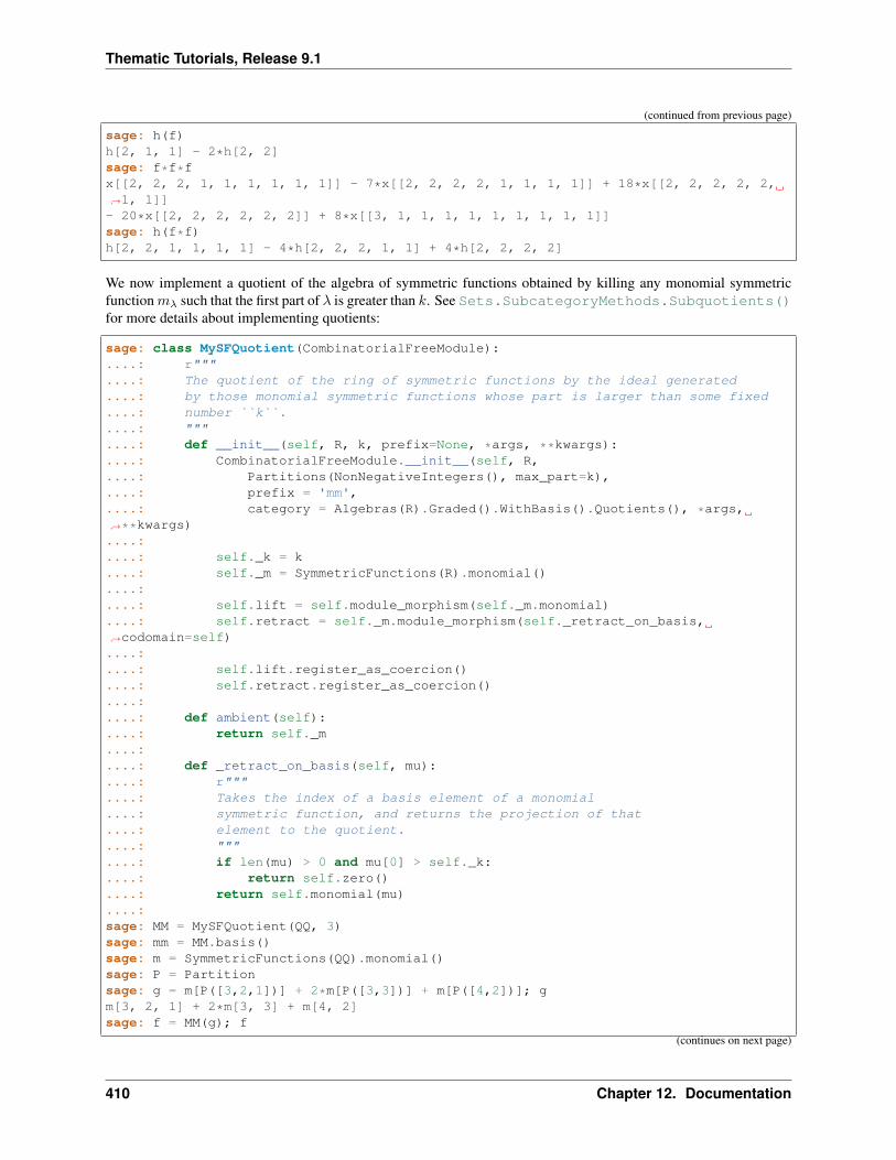
Thematic Tutorials, Release 9.1
(continued from previous page)
sage: h(f)h[2, 1, 1] - 2*h[2, 2]sage: f*f*fx[[2, 2, 2, 1, 1, 1, 1, 1, 1]] - 7*x[[2, 2, 2, 2, 1, 1, 1, 1]] + 18*x[[2, 2, 2, 2, 2,→˓1, 1]]- 20*x[[2, 2, 2, 2, 2, 2]] + 8*x[[3, 1, 1, 1, 1, 1, 1, 1, 1, 1]]sage: h(f*f)h[2, 2, 1, 1, 1, 1] - 4*h[2, 2, 2, 1, 1] + 4*h[2, 2, 2, 2]
We now implement a quotient of the algebra of symmetric functions obtained by killing any monomial symmetricfunction𝑚𝜆 such that the first part of 𝜆 is greater than 𝑘. See Sets.SubcategoryMethods.Subquotients()for more details about implementing quotients:
sage: class MySFQuotient(CombinatorialFreeModule):....: r"""....: The quotient of the ring of symmetric functions by the ideal generated....: by those monomial symmetric functions whose part is larger than some fixed....: number ``k``.....: """....: def __init__(self, R, k, prefix=None, *args, **kwargs):....: CombinatorialFreeModule.__init__(self, R,....: Partitions(NonNegativeIntegers(), max_part=k),....: prefix = 'mm',....: category = Algebras(R).Graded().WithBasis().Quotients(), *args,→˓**kwargs)....:....: self._k = k....: self._m = SymmetricFunctions(R).monomial()....:....: self.lift = self.module_morphism(self._m.monomial)....: self.retract = self._m.module_morphism(self._retract_on_basis,→˓codomain=self)....:....: self.lift.register_as_coercion()....: self.retract.register_as_coercion()....:....: def ambient(self):....: return self._m....:....: def _retract_on_basis(self, mu):....: r"""....: Takes the index of a basis element of a monomial....: symmetric function, and returns the projection of that....: element to the quotient.....: """....: if len(mu) > 0 and mu[0] > self._k:....: return self.zero()....: return self.monomial(mu)....:sage: MM = MySFQuotient(QQ, 3)sage: mm = MM.basis()sage: m = SymmetricFunctions(QQ).monomial()sage: P = Partitionsage: g = m[P([3,2,1])] + 2*m[P([3,3])] + m[P([4,2])]; gm[3, 2, 1] + 2*m[3, 3] + m[4, 2]sage: f = MM(g); f
(continues on next page)
410 Chapter 12. Documentation
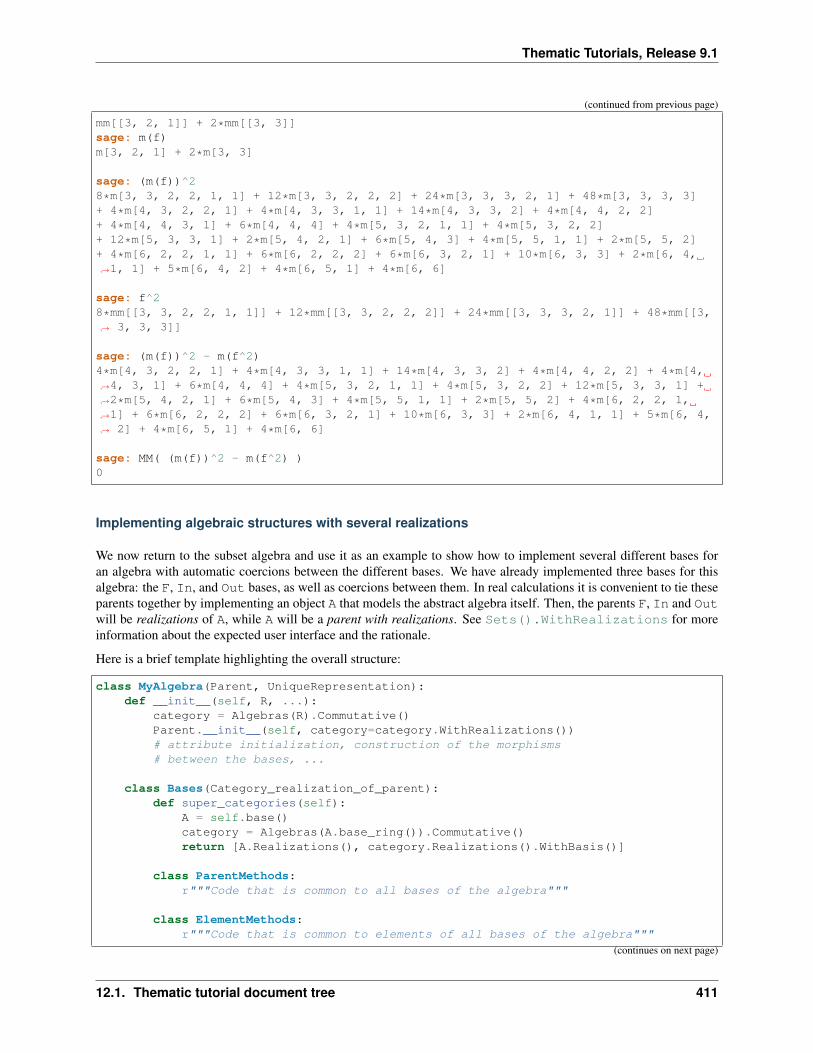
Thematic Tutorials, Release 9.1
(continued from previous page)
mm[[3, 2, 1]] + 2*mm[[3, 3]]sage: m(f)m[3, 2, 1] + 2*m[3, 3]
sage: (m(f))^28*m[3, 3, 2, 2, 1, 1] + 12*m[3, 3, 2, 2, 2] + 24*m[3, 3, 3, 2, 1] + 48*m[3, 3, 3, 3]+ 4*m[4, 3, 2, 2, 1] + 4*m[4, 3, 3, 1, 1] + 14*m[4, 3, 3, 2] + 4*m[4, 4, 2, 2]+ 4*m[4, 4, 3, 1] + 6*m[4, 4, 4] + 4*m[5, 3, 2, 1, 1] + 4*m[5, 3, 2, 2]+ 12*m[5, 3, 3, 1] + 2*m[5, 4, 2, 1] + 6*m[5, 4, 3] + 4*m[5, 5, 1, 1] + 2*m[5, 5, 2]+ 4*m[6, 2, 2, 1, 1] + 6*m[6, 2, 2, 2] + 6*m[6, 3, 2, 1] + 10*m[6, 3, 3] + 2*m[6, 4,→˓1, 1] + 5*m[6, 4, 2] + 4*m[6, 5, 1] + 4*m[6, 6]
sage: f^28*mm[[3, 3, 2, 2, 1, 1]] + 12*mm[[3, 3, 2, 2, 2]] + 24*mm[[3, 3, 3, 2, 1]] + 48*mm[[3,→˓ 3, 3, 3]]
sage: (m(f))^2 - m(f^2)4*m[4, 3, 2, 2, 1] + 4*m[4, 3, 3, 1, 1] + 14*m[4, 3, 3, 2] + 4*m[4, 4, 2, 2] + 4*m[4,→˓4, 3, 1] + 6*m[4, 4, 4] + 4*m[5, 3, 2, 1, 1] + 4*m[5, 3, 2, 2] + 12*m[5, 3, 3, 1] +→˓2*m[5, 4, 2, 1] + 6*m[5, 4, 3] + 4*m[5, 5, 1, 1] + 2*m[5, 5, 2] + 4*m[6, 2, 2, 1,→˓1] + 6*m[6, 2, 2, 2] + 6*m[6, 3, 2, 1] + 10*m[6, 3, 3] + 2*m[6, 4, 1, 1] + 5*m[6, 4,→˓ 2] + 4*m[6, 5, 1] + 4*m[6, 6]
sage: MM( (m(f))^2 - m(f^2) )0
Implementing algebraic structures with several realizations
We now return to the subset algebra and use it as an example to show how to implement several different bases foran algebra with automatic coercions between the different bases. We have already implemented three bases for thisalgebra: the F, In, and Out bases, as well as coercions between them. In real calculations it is convenient to tie theseparents together by implementing an object A that models the abstract algebra itself. Then, the parents F, In and Outwill be realizations of A, while A will be a parent with realizations. See Sets().WithRealizations for moreinformation about the expected user interface and the rationale.
Here is a brief template highlighting the overall structure:
class MyAlgebra(Parent, UniqueRepresentation):def __init__(self, R, ...):
category = Algebras(R).Commutative()Parent.__init__(self, category=category.WithRealizations())# attribute initialization, construction of the morphisms# between the bases, ...
class Bases(Category_realization_of_parent):def super_categories(self):
A = self.base()category = Algebras(A.base_ring()).Commutative()return [A.Realizations(), category.Realizations().WithBasis()]
class ParentMethods:r"""Code that is common to all bases of the algebra"""
class ElementMethods:r"""Code that is common to elements of all bases of the algebra"""
(continues on next page)
12.1. Thematic tutorial document tree 411
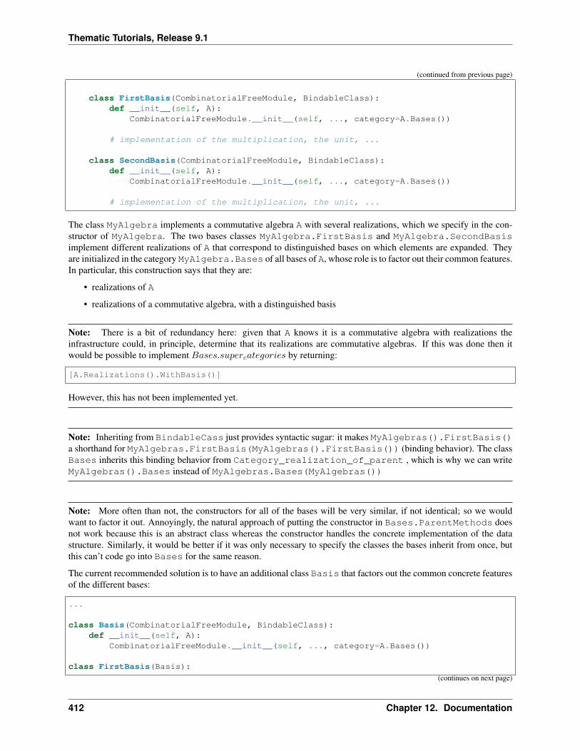
Thematic Tutorials, Release 9.1
(continued from previous page)
class FirstBasis(CombinatorialFreeModule, BindableClass):def __init__(self, A):
CombinatorialFreeModule.__init__(self, ..., category=A.Bases())
# implementation of the multiplication, the unit, ...
class SecondBasis(CombinatorialFreeModule, BindableClass):def __init__(self, A):
CombinatorialFreeModule.__init__(self, ..., category=A.Bases())
# implementation of the multiplication, the unit, ...
The class MyAlgebra implements a commutative algebra A with several realizations, which we specify in the con-structor of MyAlgebra. The two bases classes MyAlgebra.FirstBasis and MyAlgebra.SecondBasisimplement different realizations of A that correspond to distinguished bases on which elements are expanded. Theyare initialized in the category MyAlgebra.Bases of all bases of A, whose role is to factor out their common features.In particular, this construction says that they are:
• realizations of A
• realizations of a commutative algebra, with a distinguished basis
Note: There is a bit of redundancy here: given that A knows it is a commutative algebra with realizations theinfrastructure could, in principle, determine that its realizations are commutative algebras. If this was done then itwould be possible to implement 𝐵𝑎𝑠𝑒𝑠.𝑠𝑢𝑝𝑒𝑟𝑐𝑎𝑡𝑒𝑔𝑜𝑟𝑖𝑒𝑠 by returning:
[A.Realizations().WithBasis()]
However, this has not been implemented yet.
Note: Inheriting from BindableCass just provides syntactic sugar: it makes MyAlgebras().FirstBasis()a shorthand for MyAlgebras.FirstBasis(MyAlgebras().FirstBasis()) (binding behavior). The classBases inherits this binding behavior from Category_realization_of_parent , which is why we can writeMyAlgebras().Bases instead of MyAlgebras.Bases(MyAlgebras())
Note: More often than not, the constructors for all of the bases will be very similar, if not identical; so we wouldwant to factor it out. Annoyingly, the natural approach of putting the constructor in Bases.ParentMethods doesnot work because this is an abstract class whereas the constructor handles the concrete implementation of the datastructure. Similarly, it would be better if it was only necessary to specify the classes the bases inherit from once, butthis can’t code go into Bases for the same reason.
The current recommended solution is to have an additional class Basis that factors out the common concrete featuresof the different bases:
...
class Basis(CombinatorialFreeModule, BindableClass):def __init__(self, A):
CombinatorialFreeModule.__init__(self, ..., category=A.Bases())
class FirstBasis(Basis):(continues on next page)
412 Chapter 12. Documentation
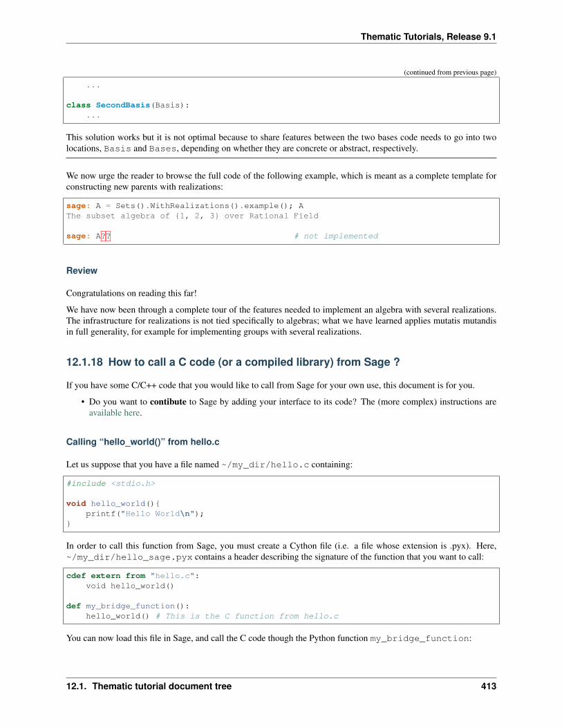
Thematic Tutorials, Release 9.1
(continued from previous page)
...
class SecondBasis(Basis):...
This solution works but it is not optimal because to share features between the two bases code needs to go into twolocations, Basis and Bases, depending on whether they are concrete or abstract, respectively.
We now urge the reader to browse the full code of the following example, which is meant as a complete template forconstructing new parents with realizations:
sage: A = Sets().WithRealizations().example(); AThe subset algebra of 1, 2, 3 over Rational Field
sage: A?? # not implemented
Review
Congratulations on reading this far!
We have now been through a complete tour of the features needed to implement an algebra with several realizations.The infrastructure for realizations is not tied specifically to algebras; what we have learned applies mutatis mutandisin full generality, for example for implementing groups with several realizations.
12.1.18 How to call a C code (or a compiled library) from Sage ?
If you have some C/C++ code that you would like to call from Sage for your own use, this document is for you.
• Do you want to contibute to Sage by adding your interface to its code? The (more complex) instructions areavailable here.
Calling “hello_world()” from hello.c
Let us suppose that you have a file named ~/my_dir/hello.c containing:
#include <stdio.h>
void hello_world()printf("Hello World\n");
In order to call this function from Sage, you must create a Cython file (i.e. a file whose extension is .pyx). Here,~/my_dir/hello_sage.pyx contains a header describing the signature of the function that you want to call:
cdef extern from "hello.c":void hello_world()
def my_bridge_function():hello_world() # This is the C function from hello.c
You can now load this file in Sage, and call the C code though the Python function my_bridge_function:
12.1. Thematic tutorial document tree 413
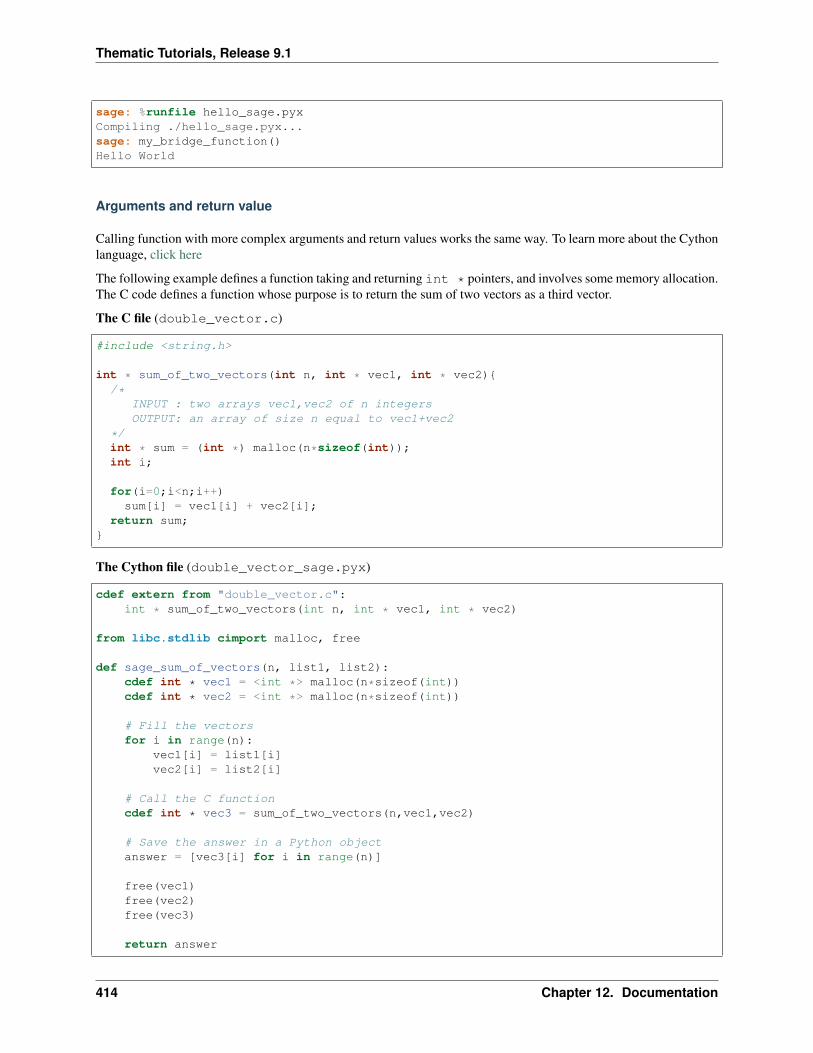
Thematic Tutorials, Release 9.1
sage: %runfile hello_sage.pyxCompiling ./hello_sage.pyx...sage: my_bridge_function()Hello World
Arguments and return value
Calling function with more complex arguments and return values works the same way. To learn more about the Cythonlanguage, click here
The following example defines a function taking and returning int * pointers, and involves some memory allocation.The C code defines a function whose purpose is to return the sum of two vectors as a third vector.
The C file (double_vector.c)
#include <string.h>
int * sum_of_two_vectors(int n, int * vec1, int * vec2)/*
INPUT : two arrays vec1,vec2 of n integersOUTPUT: an array of size n equal to vec1+vec2
*/int * sum = (int *) malloc(n*sizeof(int));int i;
for(i=0;i<n;i++)sum[i] = vec1[i] + vec2[i];
return sum;
The Cython file (double_vector_sage.pyx)
cdef extern from "double_vector.c":int * sum_of_two_vectors(int n, int * vec1, int * vec2)
from libc.stdlib cimport malloc, free
def sage_sum_of_vectors(n, list1, list2):cdef int * vec1 = <int *> malloc(n*sizeof(int))cdef int * vec2 = <int *> malloc(n*sizeof(int))
# Fill the vectorsfor i in range(n):
vec1[i] = list1[i]vec2[i] = list2[i]
# Call the C functioncdef int * vec3 = sum_of_two_vectors(n,vec1,vec2)
# Save the answer in a Python objectanswer = [vec3[i] for i in range(n)]
free(vec1)free(vec2)free(vec3)
return answer
414 Chapter 12. Documentation
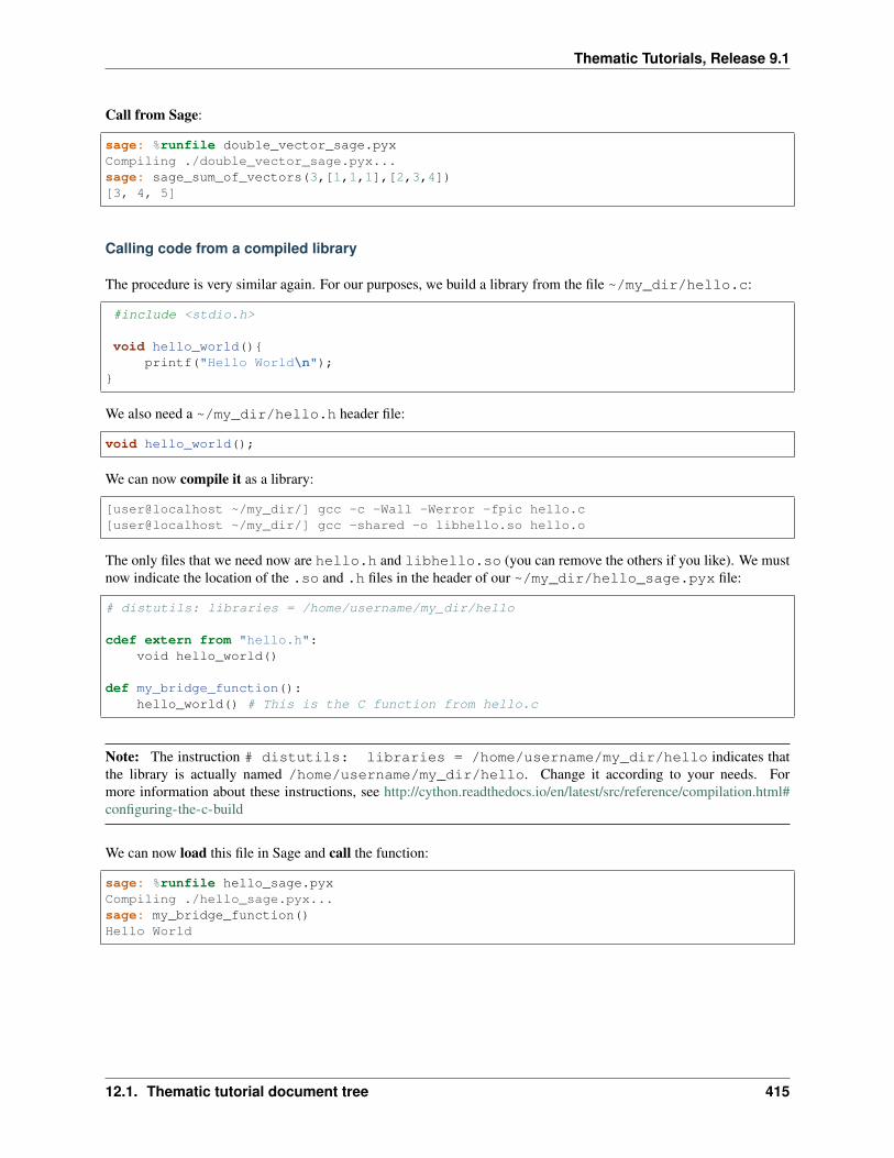
Thematic Tutorials, Release 9.1
Call from Sage:
sage: %runfile double_vector_sage.pyxCompiling ./double_vector_sage.pyx...sage: sage_sum_of_vectors(3,[1,1,1],[2,3,4])[3, 4, 5]
Calling code from a compiled library
The procedure is very similar again. For our purposes, we build a library from the file ~/my_dir/hello.c:
#include <stdio.h>
void hello_world()printf("Hello World\n");
We also need a ~/my_dir/hello.h header file:
void hello_world();
We can now compile it as a library:
[user@localhost ~/my_dir/] gcc -c -Wall -Werror -fpic hello.c[user@localhost ~/my_dir/] gcc -shared -o libhello.so hello.o
The only files that we need now are hello.h and libhello.so (you can remove the others if you like). We mustnow indicate the location of the .so and .h files in the header of our ~/my_dir/hello_sage.pyx file:
# distutils: libraries = /home/username/my_dir/hello
cdef extern from "hello.h":void hello_world()
def my_bridge_function():hello_world() # This is the C function from hello.c
Note: The instruction # distutils: libraries = /home/username/my_dir/hello indicates thatthe library is actually named /home/username/my_dir/hello. Change it according to your needs. Formore information about these instructions, see http://cython.readthedocs.io/en/latest/src/reference/compilation.html#configuring-the-c-build
We can now load this file in Sage and call the function:
sage: %runfile hello_sage.pyxCompiling ./hello_sage.pyx...sage: my_bridge_function()Hello World
12.1. Thematic tutorial document tree 415
Thematic Tutorials, Release 9.1
12.1.19 Numerical Computing with Sage
Warning: Beware that this document may be obsolete.
This document is designed to introduce the reader to the tools in Sage that are useful for doing numerical computation.By numerical computation we essentially mean machine precision floating point computations. In particular, thingssuch as optimization, numerical linear algebra, solving ODE’s or PDE’s numerically, etc.
In the first part of this document the reader is only assumed to be familiar with Python/Sage. In the second sectionon using compiled code, the computational prerequisites increase and I assume the reader is comfortable with writingprograms in C or Fortran. The third section is on mpi and parallel programming and only requires knowledge ofPython, though familiarity with mpi would be helpful.
In the current version of this document the reader is assumed to be familiar with the techniques of numerical analysis.The goal of this document is not to teach you numerical analysis, but to explain how to express your ideas in Sageand Python. Also this document is not meant to be comprehensive. Instead the goal is to be a road map and orient thereader to the packages relevant to numerical computation and to where they can find more information.
Numerical Tools
Sage has many different components that may be useful for numerical analysis. In particular three packages deservemention, they are numpy, SciPy, and cvxopt. Numpy is an excellent package that provides fast array facilities topython. It includes some basic linear algebra routines, vectorized math routines, random number generators, etc. Itsupports a programming style similar to one would use in matlab and most matlab techniques have an analogue innumpy. SciPy builds on numpy and provides many different packages for optimization, root finding, statistics, linearalgebra, interpolation, FFT and dsp tools, etc. Finally cvxopt is an optimization package which can solve linear andquadratic programming problems and also has a nice linear algebra interface. Now we will spend a bit more time oneach of these packages.
Before we start let us point out http://www.scipy.org/NumPy_for_Matlab_Users, which has a comparison betweenmatlab and numpy and gives numpy equivalents of matlab commands. If you’re not familiar with matlab, thats fine,even better, it means you won’t have any pre-conceived notions of how things should work. Also this http://www.scipy.org/Wiki/Documentation?action=AttachFile&do=get&target=scipy_tutorial.pdf is a very nice tutorial on SciPyand numpy which is more comprehensive than ours.
NumPy
NumPy is not imported into sage initially. To use NumPy, you first need to import it.
sage: import numpy
The basic object of computation in NumPy is an array. It is simple to create an array.
sage: l=numpy.array([1,2,3])sage: larray([1, 2, 3])
NumPy arrays can store any type of python object. However, for speed, numeric types are automatically converted tonative hardware types (i.e., int, float, etc.) when possible. If the value or precision of a number cannot be handledby a native hardware type, then an array of Sage objects will be created. You can do calculations on these arrays, butthey may be slower than using native types. When the numpy array contains Sage or python objects, then the data typeis explicitly printed as object. If no data type is explicitly shown when NumPy prints the array, the type is either ahardware float or int.
416 Chapter 12. Documentation
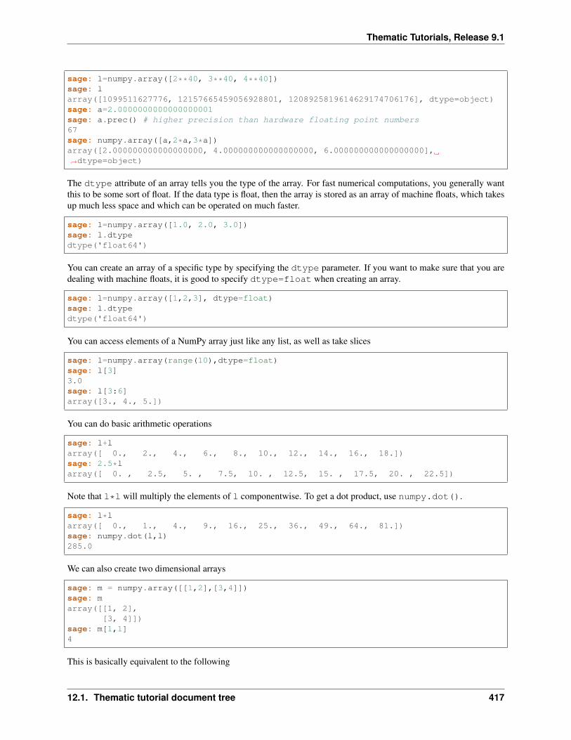
Thematic Tutorials, Release 9.1
sage: l=numpy.array([2**40, 3**40, 4**40])sage: larray([1099511627776, 12157665459056928801, 1208925819614629174706176], dtype=object)sage: a=2.0000000000000000001sage: a.prec() # higher precision than hardware floating point numbers67sage: numpy.array([a,2*a,3*a])array([2.000000000000000000, 4.000000000000000000, 6.000000000000000000],→˓dtype=object)
The dtype attribute of an array tells you the type of the array. For fast numerical computations, you generally wantthis to be some sort of float. If the data type is float, then the array is stored as an array of machine floats, which takesup much less space and which can be operated on much faster.
sage: l=numpy.array([1.0, 2.0, 3.0])sage: l.dtypedtype('float64')
You can create an array of a specific type by specifying the dtype parameter. If you want to make sure that you aredealing with machine floats, it is good to specify dtype=float when creating an array.
sage: l=numpy.array([1,2,3], dtype=float)sage: l.dtypedtype('float64')
You can access elements of a NumPy array just like any list, as well as take slices
sage: l=numpy.array(range(10),dtype=float)sage: l[3]3.0sage: l[3:6]array([3., 4., 5.])
You can do basic arithmetic operations
sage: l+larray([ 0., 2., 4., 6., 8., 10., 12., 14., 16., 18.])sage: 2.5*larray([ 0. , 2.5, 5. , 7.5, 10. , 12.5, 15. , 17.5, 20. , 22.5])
Note that l*l will multiply the elements of l componentwise. To get a dot product, use numpy.dot().
sage: l*larray([ 0., 1., 4., 9., 16., 25., 36., 49., 64., 81.])sage: numpy.dot(l,l)285.0
We can also create two dimensional arrays
sage: m = numpy.array([[1,2],[3,4]])sage: marray([[1, 2],
[3, 4]])sage: m[1,1]4
This is basically equivalent to the following
12.1. Thematic tutorial document tree 417
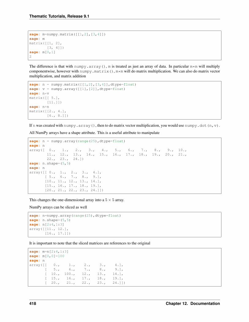
Thematic Tutorials, Release 9.1
sage: m=numpy.matrix([[1,2],[3,4]])sage: mmatrix([[1, 2],
[3, 4]])sage: m[0,1]2
The difference is that with numpy.array(), m is treated as just an array of data. In particular m*m will multiplycomponentwise, however with numpy.matrix(), m*m will do matrix multiplication. We can also do matrix vectormultiplication, and matrix addition
sage: n = numpy.matrix([[1,2],[3,4]],dtype=float)sage: v = numpy.array([[1],[2]],dtype=float)sage: n*vmatrix([[ 5.],
[11.]])sage: n+nmatrix([[2., 4.],
[6., 8.]])
If nwas created with numpy.array(), then to do matrix vector multiplication, you would use numpy.dot(n,v).
All NumPy arrays have a shape attribute. This is a useful attribute to manipulate
sage: n = numpy.array(range(25),dtype=float)sage: narray([ 0., 1., 2., 3., 4., 5., 6., 7., 8., 9., 10.,
11., 12., 13., 14., 15., 16., 17., 18., 19., 20., 21.,22., 23., 24.])
sage: n.shape=(5,5)sage: narray([[ 0., 1., 2., 3., 4.],
[ 5., 6., 7., 8., 9.],[10., 11., 12., 13., 14.],[15., 16., 17., 18., 19.],[20., 21., 22., 23., 24.]])
This changes the one-dimensional array into a 5× 5 array.
NumPy arrays can be sliced as well
sage: n=numpy.array(range(25),dtype=float)sage: n.shape=(5,5)sage: n[2:4,1:3]array([[11., 12.],
[16., 17.]])
It is important to note that the sliced matrices are references to the original
sage: m=n[2:4,1:3]sage: m[0,0]=100sage: narray([[ 0., 1., 2., 3., 4.],
[ 5., 6., 7., 8., 9.],[ 10., 100., 12., 13., 14.],[ 15., 16., 17., 18., 19.],[ 20., 21., 22., 23., 24.]])
418 Chapter 12. Documentation
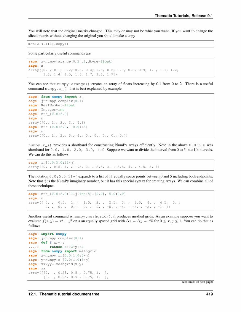
Thematic Tutorials, Release 9.1
You will note that the original matrix changed. This may or may not be what you want. If you want to change thesliced matrix without changing the original you should make a copy
m=n[2:4,1:3].copy()
Some particularly useful commands are
sage: x=numpy.arange(0,2,.1,dtype=float)sage: xarray([0. , 0.1, 0.2, 0.3, 0.4, 0.5, 0.6, 0.7, 0.8, 0.9, 1. , 1.1, 1.2,
1.3, 1.4, 1.5, 1.6, 1.7, 1.8, 1.9])
You can see that numpy.arange() creates an array of floats increasing by 0.1 from 0 to 2. There is a usefulcommand numpy.r_() that is best explained by example
sage: from numpy import r_sage: j=numpy.complex(0,1)sage: RealNumber=floatsage: Integer=intsage: n=r_[0.0:5.0]sage: narray([0., 1., 2., 3., 4.])sage: n=r_[0.0:5.0, [0.0]*5]sage: narray([0., 1., 2., 3., 4., 0., 0., 0., 0., 0.])
numpy.r_() provides a shorthand for constructing NumPy arrays efficiently. Note in the above 0.0:5.0 wasshorthand for 0.0, 1.0, 2.0, 3.0, 4.0. Suppose we want to divide the interval from 0 to 5 into 10 intervals.We can do this as follows
sage: r_[0.0:5.0:11*j]array([0. , 0.5, 1. , 1.5, 2. , 2.5, 3. , 3.5, 4. , 4.5, 5. ])
The notation 0.0:5.0:11*j expands to a list of 11 equally space points between 0 and 5 including both endpoints.Note that j is the NumPy imaginary number, but it has this special syntax for creating arrays. We can combine all ofthese techniques
sage: n=r_[0.0:5.0:11*j,int(5)*[0.0],-5.0:0.0]sage: narray([ 0. , 0.5, 1. , 1.5, 2. , 2.5, 3. , 3.5, 4. , 4.5, 5. ,
0. , 0. , 0. , 0. , 0. , -5. , -4. , -3. , -2. , -1. ])
Another useful command is numpy.meshgrid(), it produces meshed grids. As an example suppose you want toevaluate 𝑓(𝑥, 𝑦) = 𝑥2 + 𝑦2 on a an equally spaced grid with ∆𝑥 = ∆𝑦 = .25 for 0 ≤ 𝑥, 𝑦 ≤ 1. You can do that asfollows
sage: import numpysage: j=numpy.complex(0,1)sage: def f(x,y):....: return x**2+y**2sage: from numpy import meshgridsage: x=numpy.r_[0.0:1.0:5*j]sage: y=numpy.r_[0.0:1.0:5*j]sage: xx,yy= meshgrid(x,y)sage: xxarray([[0. , 0.25, 0.5 , 0.75, 1. ],
[0. , 0.25, 0.5 , 0.75, 1. ],
(continues on next page)
12.1. Thematic tutorial document tree 419
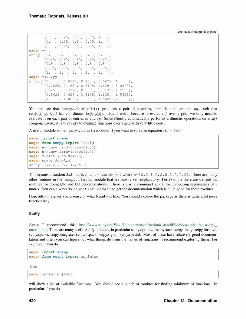
Thematic Tutorials, Release 9.1
(continued from previous page)
[0. , 0.25, 0.5 , 0.75, 1. ],[0. , 0.25, 0.5 , 0.75, 1. ],[0. , 0.25, 0.5 , 0.75, 1. ]])
sage: yyarray([[0. , 0. , 0. , 0. , 0. ],
[0.25, 0.25, 0.25, 0.25, 0.25],[0.5 , 0.5 , 0.5 , 0.5 , 0.5 ],[0.75, 0.75, 0.75, 0.75, 0.75],[1. , 1. , 1. , 1. , 1. ]])
sage: f(xx,yy)array([[0. , 0.0625, 0.25 , 0.5625, 1. ],
[0.0625, 0.125 , 0.3125, 0.625 , 1.0625],[0.25 , 0.3125, 0.5 , 0.8125, 1.25 ],[0.5625, 0.625 , 0.8125, 1.125 , 1.5625],[1. , 1.0625, 1.25 , 1.5625, 2. ]])
You can see that numpy.meshgrid() produces a pair of matrices, here denoted 𝑥𝑥 and 𝑦𝑦, such that(𝑥𝑥[𝑖, 𝑗], 𝑦𝑦[𝑖, 𝑗]) has coordinates (𝑥[𝑖], 𝑦[𝑗]). This is useful because to evaluate 𝑓 over a grid, we only need toevaluate it on each pair of entries in 𝑥𝑥, 𝑦𝑦. Since NumPy automatically performs arithmetic operations on arrayscomponentwise, it is very easy to evaluate functions over a grid with very little code.
A useful module is the numpy.linalg module. If you want to solve an equation 𝐴𝑥 = 𝑏 do
sage: import numpysage: from numpy import linalgsage: A=numpy.random.randn(5,5)sage: b=numpy.array(range(1,6))sage: x=linalg.solve(A,b)sage: numpy.dot(A,x)array([1., 2., 3., 4., 5.])
This creates a random 5x5 matrix A, and solves 𝐴𝑥 = 𝑏 where b=[0.0,1.0,2.0,3.0,4.0]. There are manyother routines in the numpy.linalg module that are mostly self-explanatory. For example there are qr and luroutines for doing QR and LU decompositions. There is also a command eigs for computing eigenvalues of amatrix. You can always do <function name>? to get the documentation which is quite good for these routines.
Hopefully this gives you a sense of what NumPy is like. You should explore the package as there is quite a bit morefunctionality.
SciPy
Again I recommend this http://www.scipy.org/Wiki/Documentation?action=AttachFile&do=get&target=scipy_tutorial.pdf. There are many useful SciPy modules, in particular scipy.optimize, scipy.stats, scipy.linalg, scipy.linsolve,scipy.sparse, scipy.integrate, scipy.fftpack, scipy.signal, scipy.special. Most of these have relatively good documen-tation and often you can figure out what things do from the names of functions. I recommend exploring them. Forexample if you do
sage: import scipysage: from scipy import optimize
Then
sage: optimize.[tab]
will show a list of available functions. You should see a bunch of routines for finding minimum of functions. Inparticular if you do
420 Chapter 12. Documentation
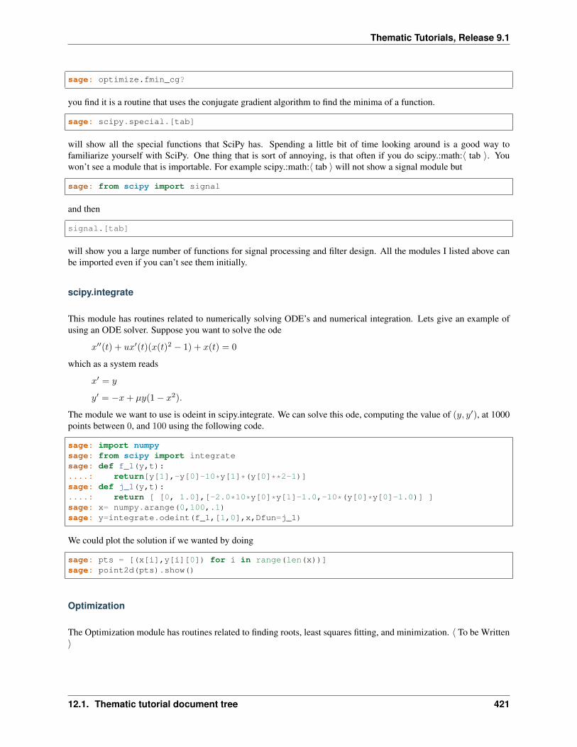
Thematic Tutorials, Release 9.1
sage: optimize.fmin_cg?
you find it is a routine that uses the conjugate gradient algorithm to find the minima of a function.
sage: scipy.special.[tab]
will show all the special functions that SciPy has. Spending a little bit of time looking around is a good way tofamiliarize yourself with SciPy. One thing that is sort of annoying, is that often if you do scipy.:math:⟨ tab ⟩. Youwon’t see a module that is importable. For example scipy.:math:⟨ tab ⟩ will not show a signal module but
sage: from scipy import signal
and then
signal.[tab]
will show you a large number of functions for signal processing and filter design. All the modules I listed above canbe imported even if you can’t see them initially.
scipy.integrate
This module has routines related to numerically solving ODE’s and numerical integration. Lets give an example ofusing an ODE solver. Suppose you want to solve the ode
𝑥′′(𝑡) + 𝑢𝑥′(𝑡)(𝑥(𝑡)2 − 1) + 𝑥(𝑡) = 0
which as a system reads
𝑥′ = 𝑦
𝑦′ = −𝑥+ 𝜇𝑦(1− 𝑥2).
The module we want to use is odeint in scipy.integrate. We can solve this ode, computing the value of (𝑦, 𝑦′), at 1000points between 0, and 100 using the following code.
sage: import numpysage: from scipy import integratesage: def f_1(y,t):....: return[y[1],-y[0]-10*y[1]*(y[0]**2-1)]sage: def j_1(y,t):....: return [ [0, 1.0],[-2.0*10*y[0]*y[1]-1.0,-10*(y[0]*y[0]-1.0)] ]sage: x= numpy.arange(0,100,.1)sage: y=integrate.odeint(f_1,[1,0],x,Dfun=j_1)
We could plot the solution if we wanted by doing
sage: pts = [(x[i],y[i][0]) for i in range(len(x))]sage: point2d(pts).show()
Optimization
The Optimization module has routines related to finding roots, least squares fitting, and minimization. ⟨ To be Written⟩
12.1. Thematic tutorial document tree 421
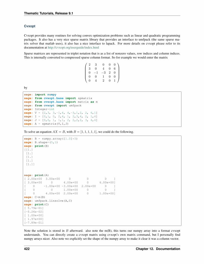
Thematic Tutorials, Release 9.1
Cvxopt
Cvxopt provides many routines for solving convex optimization problems such as linear and quadratic programmingpackages. It also has a very nice sparse matrix library that provides an interface to umfpack (the same sparse ma-trix solver that matlab uses), it also has a nice interface to lapack. For more details on cvxopt please refer to itsdocumentation at http://cvxopt.org/userguide/index.html
Sparse matrices are represented in triplet notation that is as a list of nonzero values, row indices and column indices.This is internally converted to compressed sparse column format. So for example we would enter the matrix⎛⎜⎜⎜⎜⎝
2 3 0 0 03 0 4 0 60 −1 −3 2 00 0 1 0 00 4 2 0 1
⎞⎟⎟⎟⎟⎠by
sage: import numpysage: from cvxopt.base import spmatrixsage: from cvxopt.base import matrix as msage: from cvxopt import umfpacksage: Integer=intsage: V = [2,3, 3,-1,4, 4,-3,1,2, 2, 6,1]sage: I = [0,1, 0, 2,4, 1, 2,3,4, 2, 1,4]sage: J = [0,0, 1, 1,1, 2, 2,2,2, 3, 4,4]sage: A = spmatrix(V,I,J)
To solve an equation 𝐴𝑋 = 𝐵, with 𝐵 = [1, 1, 1, 1, 1], we could do the following.
sage: B = numpy.array([1.0]*5)sage: B.shape=(5,1)sage: print(B)[[1.][1.][1.][1.][1.]]
sage: print(A)[ 2.00e+00 3.00e+00 0 0 0 ][ 3.00e+00 0 4.00e+00 0 6.00e+00][ 0 -1.00e+00 -3.00e+00 2.00e+00 0 ][ 0 0 1.00e+00 0 0 ][ 0 4.00e+00 2.00e+00 0 1.00e+00]sage: C=m(B)sage: umfpack.linsolve(A,C)sage: print(C)[ 5.79e-01][-5.26e-02][ 1.00e+00][ 1.97e+00][-7.89e-01]
Note the solution is stored in 𝐵 afterward. also note the m(B), this turns our numpy array into a format cvxoptunderstands. You can directly create a cvxopt matrix using cvxopt’s own matrix command, but I personally findnumpy arrays nicer. Also note we explicitly set the shape of the numpy array to make it clear it was a column vector.
422 Chapter 12. Documentation
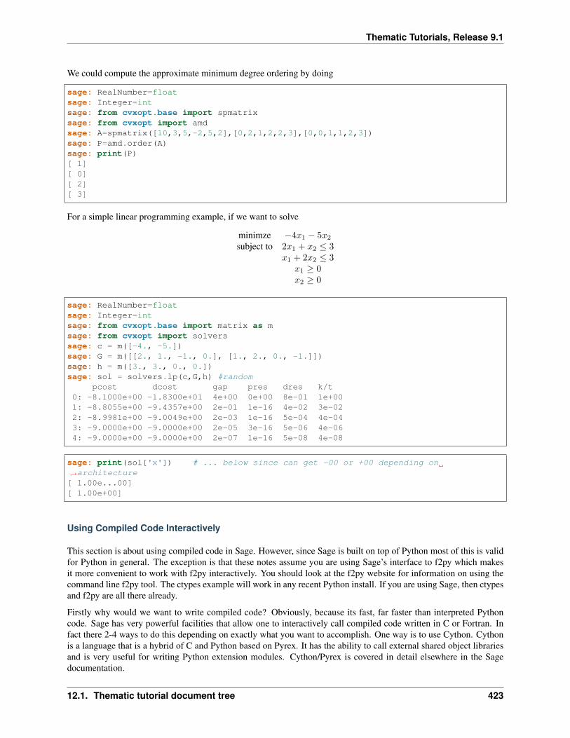
Thematic Tutorials, Release 9.1
We could compute the approximate minimum degree ordering by doing
sage: RealNumber=floatsage: Integer=intsage: from cvxopt.base import spmatrixsage: from cvxopt import amdsage: A=spmatrix([10,3,5,-2,5,2],[0,2,1,2,2,3],[0,0,1,1,2,3])sage: P=amd.order(A)sage: print(P)[ 1][ 0][ 2][ 3]
For a simple linear programming example, if we want to solve
minimze −4𝑥1 − 5𝑥2subject to 2𝑥1 + 𝑥2 ≤ 3
𝑥1 + 2𝑥2 ≤ 3𝑥1 ≥ 0𝑥2 ≥ 0
sage: RealNumber=floatsage: Integer=intsage: from cvxopt.base import matrix as msage: from cvxopt import solverssage: c = m([-4., -5.])sage: G = m([[2., 1., -1., 0.], [1., 2., 0., -1.]])sage: h = m([3., 3., 0., 0.])sage: sol = solvers.lp(c,G,h) #random
pcost dcost gap pres dres k/t0: -8.1000e+00 -1.8300e+01 4e+00 0e+00 8e-01 1e+001: -8.8055e+00 -9.4357e+00 2e-01 1e-16 4e-02 3e-022: -8.9981e+00 -9.0049e+00 2e-03 1e-16 5e-04 4e-043: -9.0000e+00 -9.0000e+00 2e-05 3e-16 5e-06 4e-064: -9.0000e+00 -9.0000e+00 2e-07 1e-16 5e-08 4e-08
sage: print(sol['x']) # ... below since can get -00 or +00 depending on→˓architecture[ 1.00e...00][ 1.00e+00]
Using Compiled Code Interactively
This section is about using compiled code in Sage. However, since Sage is built on top of Python most of this is validfor Python in general. The exception is that these notes assume you are using Sage’s interface to f2py which makesit more convenient to work with f2py interactively. You should look at the f2py website for information on using thecommand line f2py tool. The ctypes example will work in any recent Python install. If you are using Sage, then ctypesand f2py are all there already.
Firstly why would we want to write compiled code? Obviously, because its fast, far faster than interpreted Pythoncode. Sage has very powerful facilities that allow one to interactively call compiled code written in C or Fortran. Infact there 2-4 ways to do this depending on exactly what you want to accomplish. One way is to use Cython. Cythonis a language that is a hybrid of C and Python based on Pyrex. It has the ability to call external shared object librariesand is very useful for writing Python extension modules. Cython/Pyrex is covered in detail elsewhere in the Sagedocumentation.
12.1. Thematic tutorial document tree 423
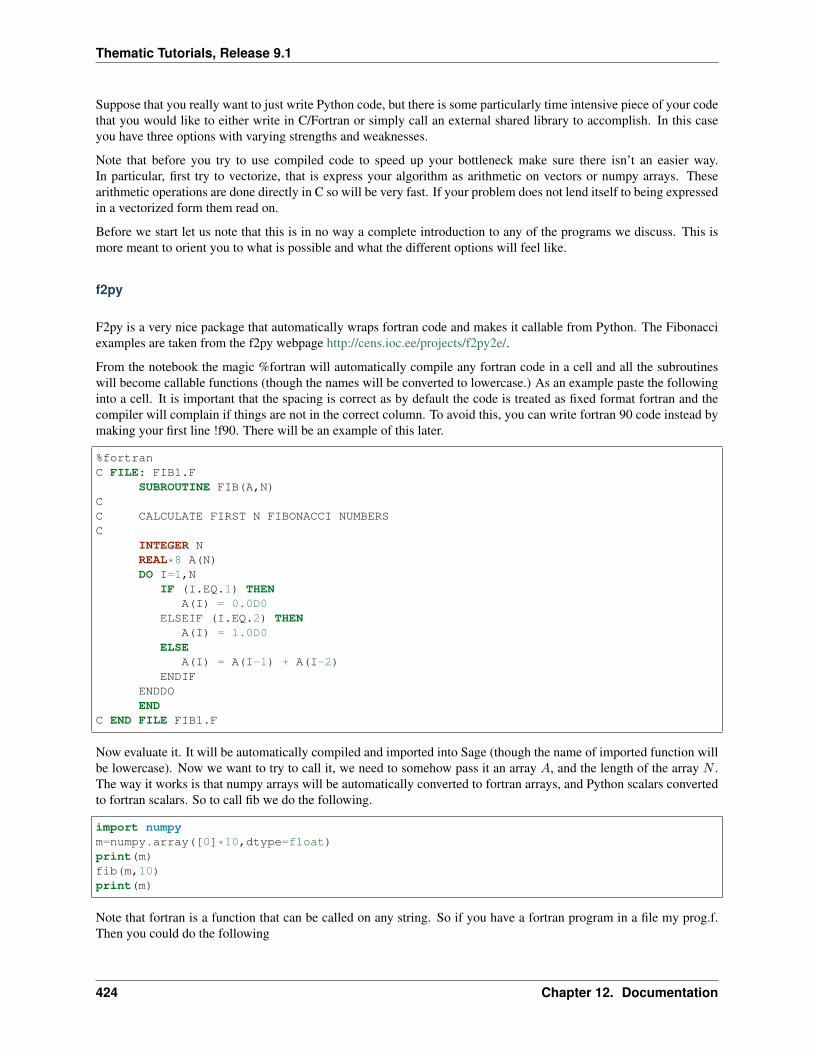
Thematic Tutorials, Release 9.1
Suppose that you really want to just write Python code, but there is some particularly time intensive piece of your codethat you would like to either write in C/Fortran or simply call an external shared library to accomplish. In this caseyou have three options with varying strengths and weaknesses.
Note that before you try to use compiled code to speed up your bottleneck make sure there isn’t an easier way.In particular, first try to vectorize, that is express your algorithm as arithmetic on vectors or numpy arrays. Thesearithmetic operations are done directly in C so will be very fast. If your problem does not lend itself to being expressedin a vectorized form them read on.
Before we start let us note that this is in no way a complete introduction to any of the programs we discuss. This ismore meant to orient you to what is possible and what the different options will feel like.
f2py
F2py is a very nice package that automatically wraps fortran code and makes it callable from Python. The Fibonacciexamples are taken from the f2py webpage http://cens.ioc.ee/projects/f2py2e/.
From the notebook the magic %fortran will automatically compile any fortran code in a cell and all the subroutineswill become callable functions (though the names will be converted to lowercase.) As an example paste the followinginto a cell. It is important that the spacing is correct as by default the code is treated as fixed format fortran and thecompiler will complain if things are not in the correct column. To avoid this, you can write fortran 90 code instead bymaking your first line !f90. There will be an example of this later.
%fortranC FILE: FIB1.F
SUBROUTINE FIB(A,N)CC CALCULATE FIRST N FIBONACCI NUMBERSC
INTEGER NREAL*8 A(N)DO I=1,N
IF (I.EQ.1) THENA(I) = 0.0D0
ELSEIF (I.EQ.2) THENA(I) = 1.0D0
ELSEA(I) = A(I-1) + A(I-2)
ENDIFENDDOEND
C END FILE FIB1.F
Now evaluate it. It will be automatically compiled and imported into Sage (though the name of imported function willbe lowercase). Now we want to try to call it, we need to somehow pass it an array 𝐴, and the length of the array 𝑁 .The way it works is that numpy arrays will be automatically converted to fortran arrays, and Python scalars convertedto fortran scalars. So to call fib we do the following.
import numpym=numpy.array([0]*10,dtype=float)print(m)fib(m,10)print(m)
Note that fortran is a function that can be called on any string. So if you have a fortran program in a file my prog.f.Then you could do the following
424 Chapter 12. Documentation
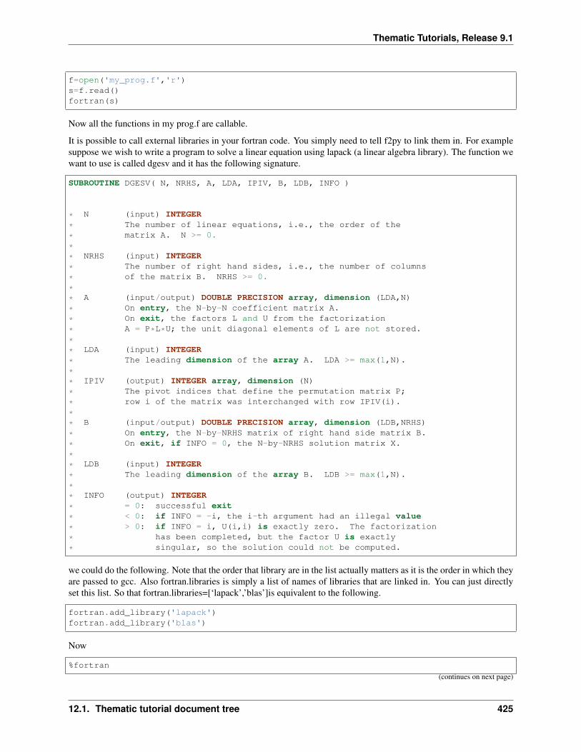
Thematic Tutorials, Release 9.1
f=open('my_prog.f','r')s=f.read()fortran(s)
Now all the functions in my prog.f are callable.
It is possible to call external libraries in your fortran code. You simply need to tell f2py to link them in. For examplesuppose we wish to write a program to solve a linear equation using lapack (a linear algebra library). The function wewant to use is called dgesv and it has the following signature.
SUBROUTINE DGESV( N, NRHS, A, LDA, IPIV, B, LDB, INFO )
* N (input) INTEGER
* The number of linear equations, i.e., the order of the
* matrix A. N >= 0.
** NRHS (input) INTEGER
* The number of right hand sides, i.e., the number of columns
* of the matrix B. NRHS >= 0.
** A (input/output) DOUBLE PRECISION array, dimension (LDA,N)
* On entry, the N-by-N coefficient matrix A.
* On exit, the factors L and U from the factorization
* A = P*L*U; the unit diagonal elements of L are not stored.
** LDA (input) INTEGER
* The leading dimension of the array A. LDA >= max(1,N).
** IPIV (output) INTEGER array, dimension (N)
* The pivot indices that define the permutation matrix P;
* row i of the matrix was interchanged with row IPIV(i).
** B (input/output) DOUBLE PRECISION array, dimension (LDB,NRHS)
* On entry, the N-by-NRHS matrix of right hand side matrix B.
* On exit, if INFO = 0, the N-by-NRHS solution matrix X.
** LDB (input) INTEGER
* The leading dimension of the array B. LDB >= max(1,N).
** INFO (output) INTEGER
* = 0: successful exit
* < 0: if INFO = -i, the i-th argument had an illegal value
* > 0: if INFO = i, U(i,i) is exactly zero. The factorization
* has been completed, but the factor U is exactly
* singular, so the solution could not be computed.
we could do the following. Note that the order that library are in the list actually matters as it is the order in which theyare passed to gcc. Also fortran.libraries is simply a list of names of libraries that are linked in. You can just directlyset this list. So that fortran.libraries=[‘lapack’,’blas’]is equivalent to the following.
fortran.add_library('lapack')fortran.add_library('blas')
Now
%fortran
(continues on next page)
12.1. Thematic tutorial document tree 425
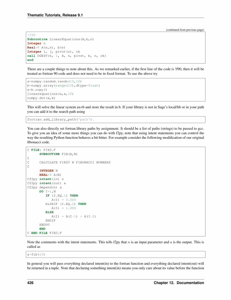
Thematic Tutorials, Release 9.1
(continued from previous page)
!f90Subroutine LinearEquations(A,b,n)Integer nReal*8 A(n,n), b(n)Integer i, j, pivot(n), okcall DGESV(n, 1, A, n, pivot, b, n, ok)end
There are a couple things to note about this. As we remarked earlier, if the first line of the code is !f90, then it will betreated as fortran 90 code and does not need to be in fixed format. To use the above try
a=numpy.random.randn(10,10)b=numpy.array(range(10),dtype=float)x=b.copy()linearequations(a,x,10)numpy.dot(a,x)
This will solve the linear system ax=b and store the result in b. If your library is not in Sage’s local/lib or in your pathyou can add it to the search path using
fortran.add_library_path('path').
You can also directly set fortran.library paths by assignment. It should be a list of paths (strings) to be passed to gcc.To give you an idea of some more things you can do with f2py, note that using intent statements you can control theway the resulting Python function behaves a bit bitter. For example consider the following modification of our originalfibonacci code.
C FILE: FIB3.FSUBROUTINE FIB(A,N)
CC CALCULATE FIRST N FIBONACCI NUMBERSC
INTEGER NREAL*8 A(N)
Cf2py intent(in) nCf2py intent(out) aCf2py depend(n) a
DO I=1,NIF (I.EQ.1) THEN
A(I) = 0.0D0ELSEIF (I.EQ.2) THEN
A(I) = 1.0D0ELSE
A(I) = A(I-1) + A(I-2)ENDIF
ENDDOEND
C END FILE FIB3.F
Note the comments with the intent statements. This tells f2py that 𝑛 is an input parameter and 𝑎 is the output. This iscalled as
a=fib(10)
In general you will pass everything declared intent(in) to the fortran function and everything declared intent(out) willbe returned in a tuple. Note that declaring something intent(in) means you only care about its value before the function
426 Chapter 12. Documentation

Thematic Tutorials, Release 9.1
is called not afterwards. So in the above n tells us how many fiboncci numbers to compute we need to specify thisas an input, however we don’t need to get n back as it doesn’t contain anything new. Similarly A is intent(out) so wedon’t need A to have an specific value beforehand, we just care about the contents afterwards. F2py generates a Pythonfunction so you only pass those declared intent(in) and supplies empty workspaces for the remaining arguments and itonly returns those that are intent(out). All arguments are intent(in) by default.
Consider now the following
%fortranSubroutine Rescale(a,b,n)Implicit noneInteger n,i,jReal*8 a(n,n), bdo i = 1,n
do j=1,na(i,j)=b*a(i,j)
end doend doend
You might be expecting Rescale(a,n) to rescale a numpy matrix a. Alas this doesn’t work. Anything you pass in isunchanged afterwards. Note that in the fibonacci example above, the one dimensional array was changed by the fortrancode, similarly the one dimensional vector b was replaced by its solution in the example where we called lapack whilethe matrix A was not changed even then dgesv says it modifies the input matrix. Why does this not happen with thetwo dimensional array. Understanding this requires that you are aware of the difference between how fortran and Cstore arrays. Fortran stores a matrices using column ordering while C stores them using row ordering. That is thematrix (
0 1 23 4 5
)is stored as
(0 1 2 3 4 5 ) in C
(0 3 1 4 2 5) in Fortran
One dimensional arrays are stored the same in C and Fortran. Because of this f2py allows the fortran code to operateon one dimensional vectors in place, so your fortran code will change one dimensional numpy arrays passed to it.However, since two dimensional arrays are different by default f2py copies the numpy array (which is stored in Cformat) into a second array that is in the fortran format (i.e. takes the transpose) and that is what is passed to thefortran function. We will see a way to get around this copying later. First let us point one way of writing the rescalefunction.
%fortran
Subroutine Rescale(a,b,n)Implicit noneInteger n,i,jReal*8 a(n,n), b
Cf2py intent(in,out) ado i = 1,n
do j=1,na(i,j)=b*a(i,j)
end doend doend
Note that to call this you would use
12.1. Thematic tutorial document tree 427
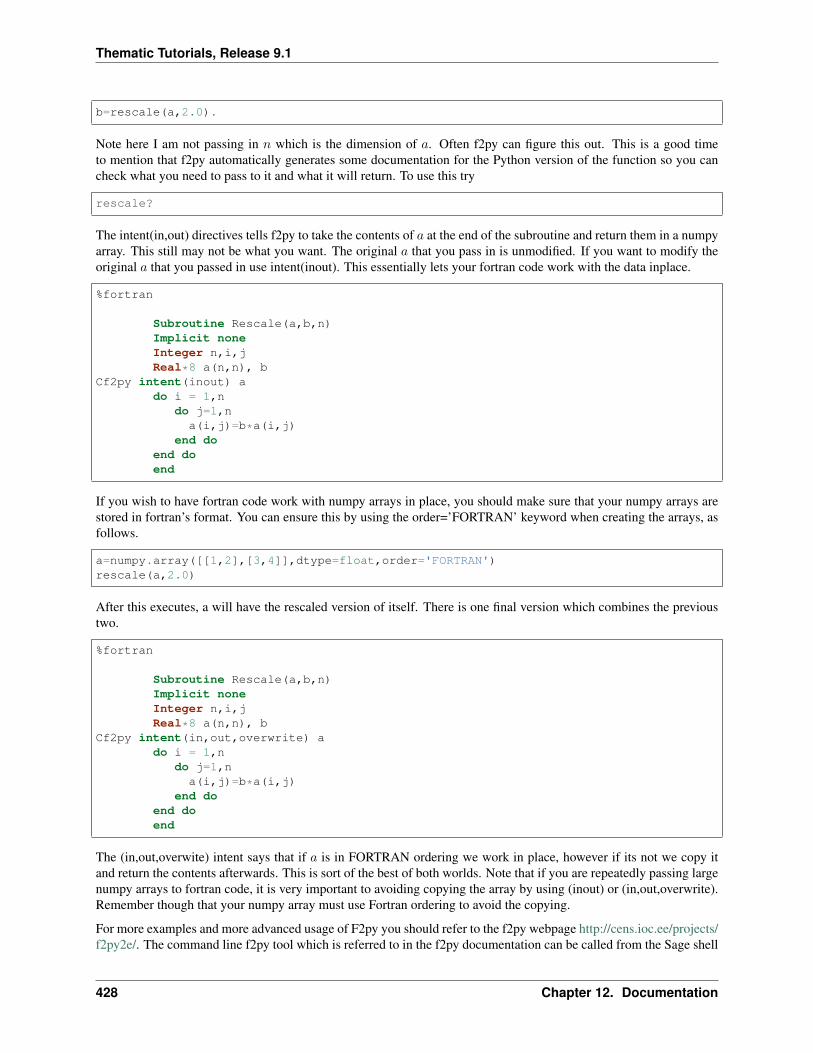
Thematic Tutorials, Release 9.1
b=rescale(a,2.0).
Note here I am not passing in 𝑛 which is the dimension of 𝑎. Often f2py can figure this out. This is a good timeto mention that f2py automatically generates some documentation for the Python version of the function so you cancheck what you need to pass to it and what it will return. To use this try
rescale?
The intent(in,out) directives tells f2py to take the contents of 𝑎 at the end of the subroutine and return them in a numpyarray. This still may not be what you want. The original 𝑎 that you pass in is unmodified. If you want to modify theoriginal 𝑎 that you passed in use intent(inout). This essentially lets your fortran code work with the data inplace.
%fortran
Subroutine Rescale(a,b,n)Implicit noneInteger n,i,jReal*8 a(n,n), b
Cf2py intent(inout) ado i = 1,n
do j=1,na(i,j)=b*a(i,j)
end doend doend
If you wish to have fortran code work with numpy arrays in place, you should make sure that your numpy arrays arestored in fortran’s format. You can ensure this by using the order=’FORTRAN’ keyword when creating the arrays, asfollows.
a=numpy.array([[1,2],[3,4]],dtype=float,order='FORTRAN')rescale(a,2.0)
After this executes, a will have the rescaled version of itself. There is one final version which combines the previoustwo.
%fortran
Subroutine Rescale(a,b,n)Implicit noneInteger n,i,jReal*8 a(n,n), b
Cf2py intent(in,out,overwrite) ado i = 1,n
do j=1,na(i,j)=b*a(i,j)
end doend doend
The (in,out,overwite) intent says that if 𝑎 is in FORTRAN ordering we work in place, however if its not we copy itand return the contents afterwards. This is sort of the best of both worlds. Note that if you are repeatedly passing largenumpy arrays to fortran code, it is very important to avoiding copying the array by using (inout) or (in,out,overwrite).Remember though that your numpy array must use Fortran ordering to avoid the copying.
For more examples and more advanced usage of F2py you should refer to the f2py webpage http://cens.ioc.ee/projects/f2py2e/. The command line f2py tool which is referred to in the f2py documentation can be called from the Sage shell
428 Chapter 12. Documentation
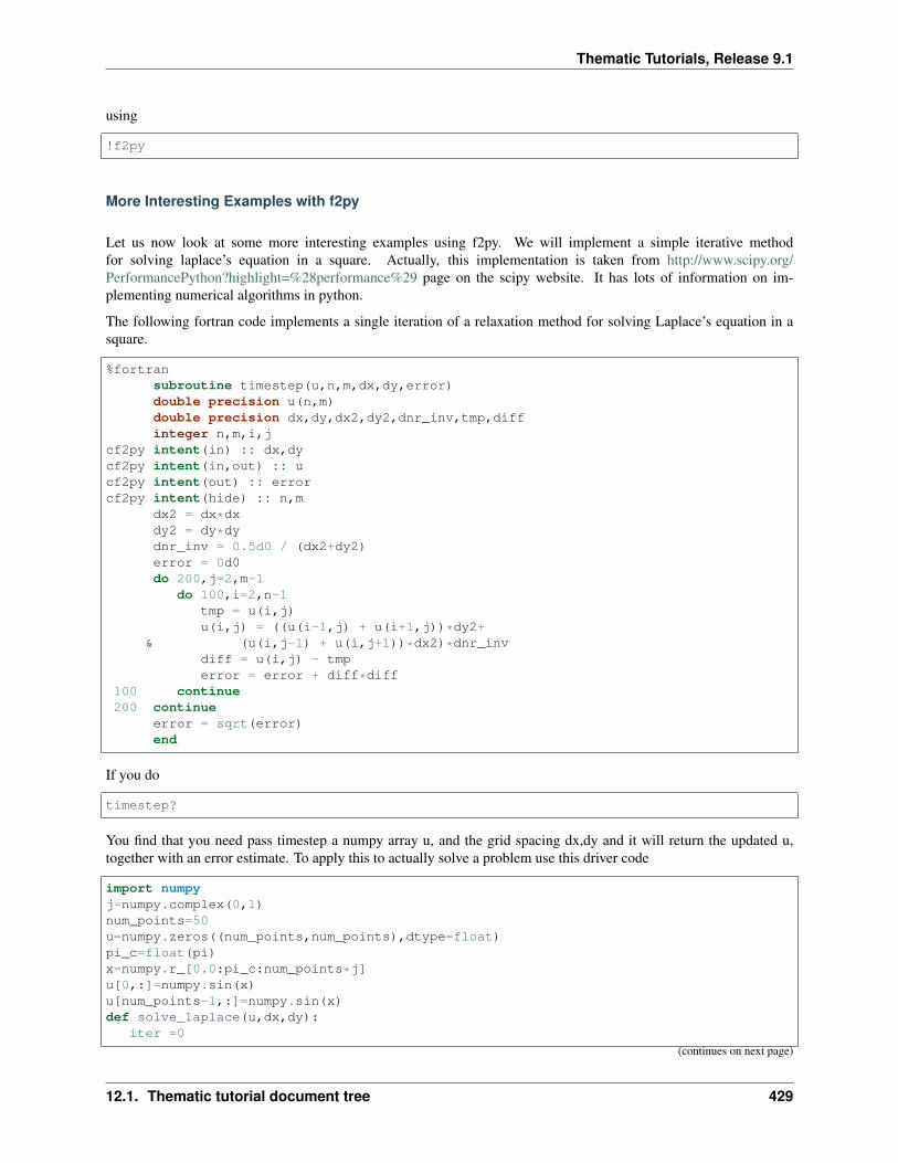
Thematic Tutorials, Release 9.1
using
!f2py
More Interesting Examples with f2py
Let us now look at some more interesting examples using f2py. We will implement a simple iterative methodfor solving laplace’s equation in a square. Actually, this implementation is taken from http://www.scipy.org/PerformancePython?highlight=%28performance%29 page on the scipy website. It has lots of information on im-plementing numerical algorithms in python.
The following fortran code implements a single iteration of a relaxation method for solving Laplace’s equation in asquare.
%fortransubroutine timestep(u,n,m,dx,dy,error)double precision u(n,m)double precision dx,dy,dx2,dy2,dnr_inv,tmp,diffinteger n,m,i,j
cf2py intent(in) :: dx,dycf2py intent(in,out) :: ucf2py intent(out) :: errorcf2py intent(hide) :: n,m
dx2 = dx*dxdy2 = dy*dydnr_inv = 0.5d0 / (dx2+dy2)error = 0d0do 200,j=2,m-1
do 100,i=2,n-1tmp = u(i,j)u(i,j) = ((u(i-1,j) + u(i+1,j))*dy2+
& (u(i,j-1) + u(i,j+1))*dx2)*dnr_invdiff = u(i,j) - tmperror = error + diff*diff
100 continue200 continue
error = sqrt(error)end
If you do
timestep?
You find that you need pass timestep a numpy array u, and the grid spacing dx,dy and it will return the updated u,together with an error estimate. To apply this to actually solve a problem use this driver code
import numpyj=numpy.complex(0,1)num_points=50u=numpy.zeros((num_points,num_points),dtype=float)pi_c=float(pi)x=numpy.r_[0.0:pi_c:num_points*j]u[0,:]=numpy.sin(x)u[num_points-1,:]=numpy.sin(x)def solve_laplace(u,dx,dy):
iter =0
(continues on next page)
12.1. Thematic tutorial document tree 429
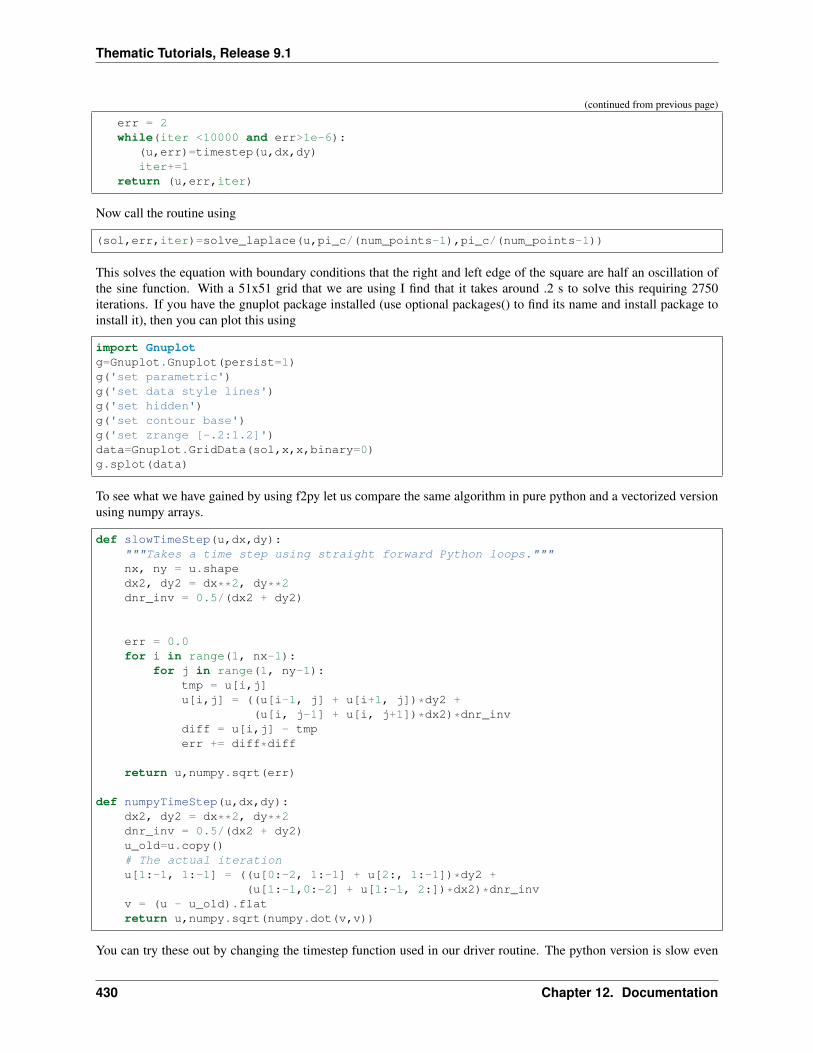
Thematic Tutorials, Release 9.1
(continued from previous page)
err = 2while(iter <10000 and err>1e-6):
(u,err)=timestep(u,dx,dy)iter+=1
return (u,err,iter)
Now call the routine using
(sol,err,iter)=solve_laplace(u,pi_c/(num_points-1),pi_c/(num_points-1))
This solves the equation with boundary conditions that the right and left edge of the square are half an oscillation ofthe sine function. With a 51x51 grid that we are using I find that it takes around .2 s to solve this requiring 2750iterations. If you have the gnuplot package installed (use optional packages() to find its name and install package toinstall it), then you can plot this using
import Gnuplotg=Gnuplot.Gnuplot(persist=1)g('set parametric')g('set data style lines')g('set hidden')g('set contour base')g('set zrange [-.2:1.2]')data=Gnuplot.GridData(sol,x,x,binary=0)g.splot(data)
To see what we have gained by using f2py let us compare the same algorithm in pure python and a vectorized versionusing numpy arrays.
def slowTimeStep(u,dx,dy):"""Takes a time step using straight forward Python loops."""nx, ny = u.shapedx2, dy2 = dx**2, dy**2dnr_inv = 0.5/(dx2 + dy2)
err = 0.0for i in range(1, nx-1):
for j in range(1, ny-1):tmp = u[i,j]u[i,j] = ((u[i-1, j] + u[i+1, j])*dy2 +
(u[i, j-1] + u[i, j+1])*dx2)*dnr_invdiff = u[i,j] - tmperr += diff*diff
return u,numpy.sqrt(err)
def numpyTimeStep(u,dx,dy):dx2, dy2 = dx**2, dy**2dnr_inv = 0.5/(dx2 + dy2)u_old=u.copy()# The actual iterationu[1:-1, 1:-1] = ((u[0:-2, 1:-1] + u[2:, 1:-1])*dy2 +
(u[1:-1,0:-2] + u[1:-1, 2:])*dx2)*dnr_invv = (u - u_old).flatreturn u,numpy.sqrt(numpy.dot(v,v))
You can try these out by changing the timestep function used in our driver routine. The python version is slow even
430 Chapter 12. Documentation
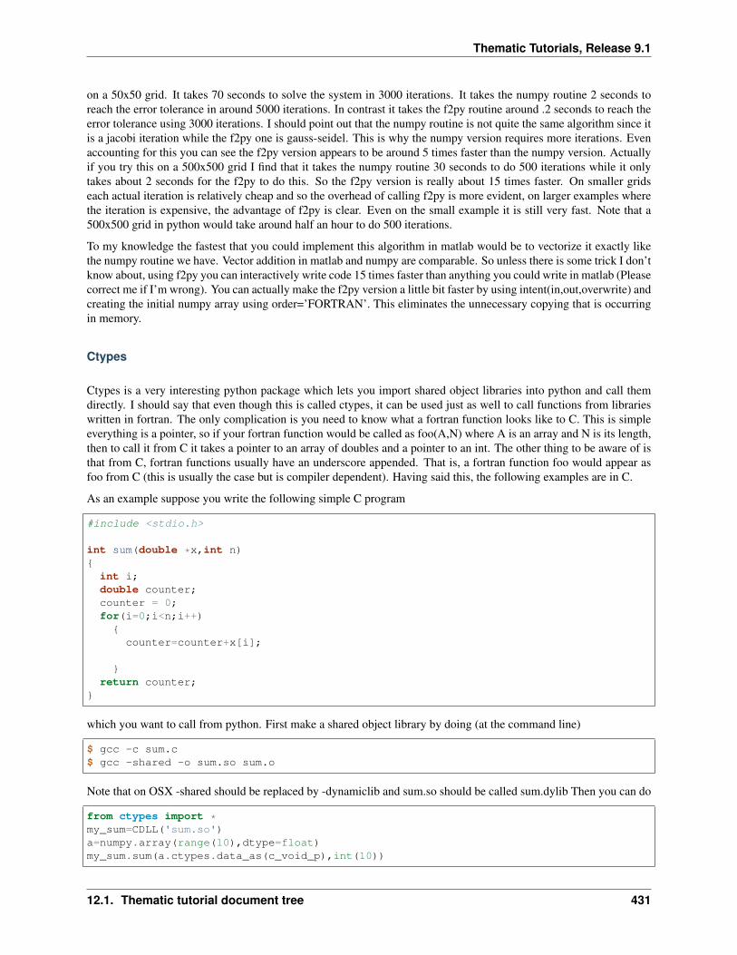
Thematic Tutorials, Release 9.1
on a 50x50 grid. It takes 70 seconds to solve the system in 3000 iterations. It takes the numpy routine 2 seconds toreach the error tolerance in around 5000 iterations. In contrast it takes the f2py routine around .2 seconds to reach theerror tolerance using 3000 iterations. I should point out that the numpy routine is not quite the same algorithm since itis a jacobi iteration while the f2py one is gauss-seidel. This is why the numpy version requires more iterations. Evenaccounting for this you can see the f2py version appears to be around 5 times faster than the numpy version. Actuallyif you try this on a 500x500 grid I find that it takes the numpy routine 30 seconds to do 500 iterations while it onlytakes about 2 seconds for the f2py to do this. So the f2py version is really about 15 times faster. On smaller gridseach actual iteration is relatively cheap and so the overhead of calling f2py is more evident, on larger examples wherethe iteration is expensive, the advantage of f2py is clear. Even on the small example it is still very fast. Note that a500x500 grid in python would take around half an hour to do 500 iterations.
To my knowledge the fastest that you could implement this algorithm in matlab would be to vectorize it exactly likethe numpy routine we have. Vector addition in matlab and numpy are comparable. So unless there is some trick I don’tknow about, using f2py you can interactively write code 15 times faster than anything you could write in matlab (Pleasecorrect me if I’m wrong). You can actually make the f2py version a little bit faster by using intent(in,out,overwrite) andcreating the initial numpy array using order=’FORTRAN’. This eliminates the unnecessary copying that is occurringin memory.
Ctypes
Ctypes is a very interesting python package which lets you import shared object libraries into python and call themdirectly. I should say that even though this is called ctypes, it can be used just as well to call functions from librarieswritten in fortran. The only complication is you need to know what a fortran function looks like to C. This is simpleeverything is a pointer, so if your fortran function would be called as foo(A,N) where A is an array and N is its length,then to call it from C it takes a pointer to an array of doubles and a pointer to an int. The other thing to be aware of isthat from C, fortran functions usually have an underscore appended. That is, a fortran function foo would appear asfoo from C (this is usually the case but is compiler dependent). Having said this, the following examples are in C.
As an example suppose you write the following simple C program
#include <stdio.h>
int sum(double *x,int n)
int i;double counter;counter = 0;for(i=0;i<n;i++)
counter=counter+x[i];
return counter;
which you want to call from python. First make a shared object library by doing (at the command line)
$ gcc -c sum.c$ gcc -shared -o sum.so sum.o
Note that on OSX -shared should be replaced by -dynamiclib and sum.so should be called sum.dylib Then you can do
from ctypes import *my_sum=CDLL('sum.so')a=numpy.array(range(10),dtype=float)my_sum.sum(a.ctypes.data_as(c_void_p),int(10))
12.1. Thematic tutorial document tree 431
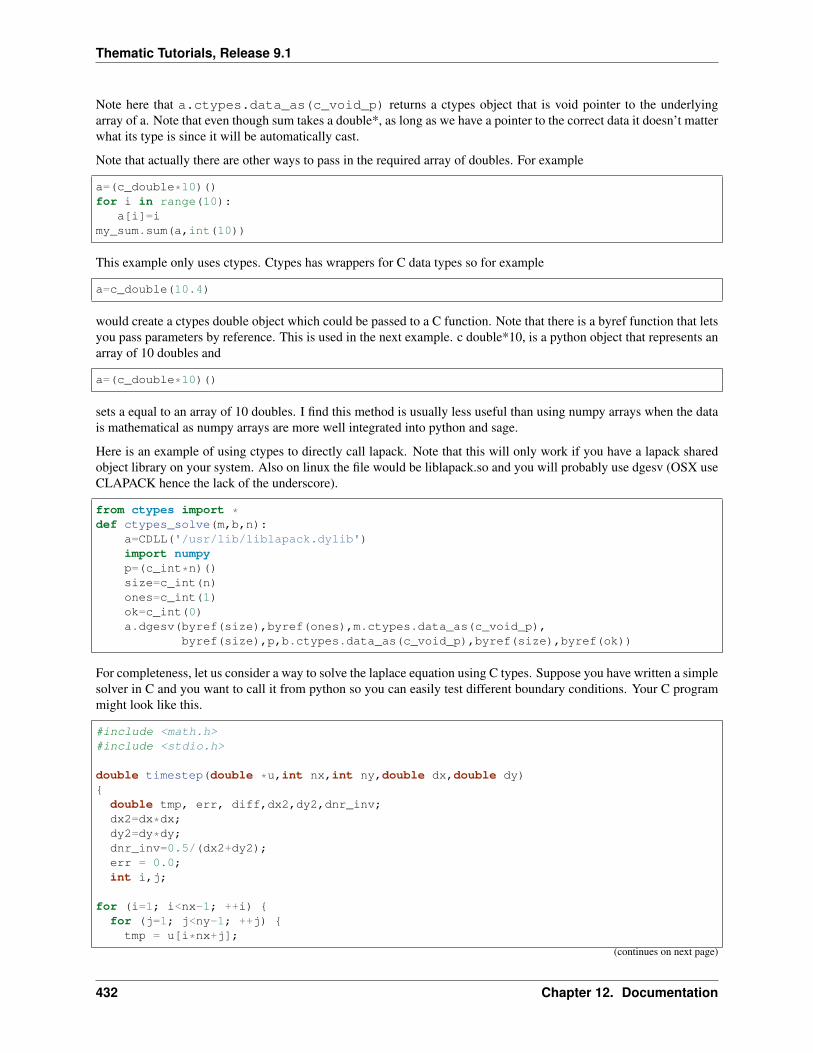
Thematic Tutorials, Release 9.1
Note here that a.ctypes.data_as(c_void_p) returns a ctypes object that is void pointer to the underlyingarray of a. Note that even though sum takes a double*, as long as we have a pointer to the correct data it doesn’t matterwhat its type is since it will be automatically cast.
Note that actually there are other ways to pass in the required array of doubles. For example
a=(c_double*10)()for i in range(10):
a[i]=imy_sum.sum(a,int(10))
This example only uses ctypes. Ctypes has wrappers for C data types so for example
a=c_double(10.4)
would create a ctypes double object which could be passed to a C function. Note that there is a byref function that letsyou pass parameters by reference. This is used in the next example. c double*10, is a python object that represents anarray of 10 doubles and
a=(c_double*10)()
sets a equal to an array of 10 doubles. I find this method is usually less useful than using numpy arrays when the datais mathematical as numpy arrays are more well integrated into python and sage.
Here is an example of using ctypes to directly call lapack. Note that this will only work if you have a lapack sharedobject library on your system. Also on linux the file would be liblapack.so and you will probably use dgesv (OSX useCLAPACK hence the lack of the underscore).
from ctypes import *def ctypes_solve(m,b,n):
a=CDLL('/usr/lib/liblapack.dylib')import numpyp=(c_int*n)()size=c_int(n)ones=c_int(1)ok=c_int(0)a.dgesv(byref(size),byref(ones),m.ctypes.data_as(c_void_p),
byref(size),p,b.ctypes.data_as(c_void_p),byref(size),byref(ok))
For completeness, let us consider a way to solve the laplace equation using C types. Suppose you have written a simplesolver in C and you want to call it from python so you can easily test different boundary conditions. Your C programmight look like this.
#include <math.h>#include <stdio.h>
double timestep(double *u,int nx,int ny,double dx,double dy)
double tmp, err, diff,dx2,dy2,dnr_inv;dx2=dx*dx;dy2=dy*dy;dnr_inv=0.5/(dx2+dy2);err = 0.0;int i,j;
for (i=1; i<nx-1; ++i) for (j=1; j<ny-1; ++j) tmp = u[i*nx+j];
(continues on next page)
432 Chapter 12. Documentation
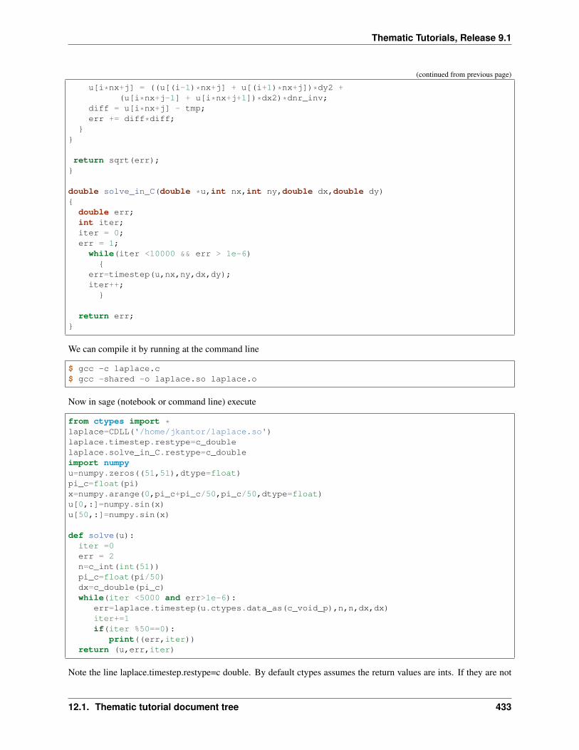
Thematic Tutorials, Release 9.1
(continued from previous page)
u[i*nx+j] = ((u[(i-1)*nx+j] + u[(i+1)*nx+j])*dy2 +(u[i*nx+j-1] + u[i*nx+j+1])*dx2)*dnr_inv;
diff = u[i*nx+j] - tmp;err += diff*diff;
return sqrt(err);
double solve_in_C(double *u,int nx,int ny,double dx,double dy)
double err;int iter;iter = 0;err = 1;while(iter <10000 && err > 1e-6)
err=timestep(u,nx,ny,dx,dy);iter++;
return err;
We can compile it by running at the command line
$ gcc -c laplace.c$ gcc -shared -o laplace.so laplace.o
Now in sage (notebook or command line) execute
from ctypes import *laplace=CDLL('/home/jkantor/laplace.so')laplace.timestep.restype=c_doublelaplace.solve_in_C.restype=c_doubleimport numpyu=numpy.zeros((51,51),dtype=float)pi_c=float(pi)x=numpy.arange(0,pi_c+pi_c/50,pi_c/50,dtype=float)u[0,:]=numpy.sin(x)u[50,:]=numpy.sin(x)
def solve(u):iter =0err = 2n=c_int(int(51))pi_c=float(pi/50)dx=c_double(pi_c)while(iter <5000 and err>1e-6):
err=laplace.timestep(u.ctypes.data_as(c_void_p),n,n,dx,dx)iter+=1if(iter %50==0):
print((err,iter))return (u,err,iter)
Note the line laplace.timestep.restype=c double. By default ctypes assumes the return values are ints. If they are not
12.1. Thematic tutorial document tree 433
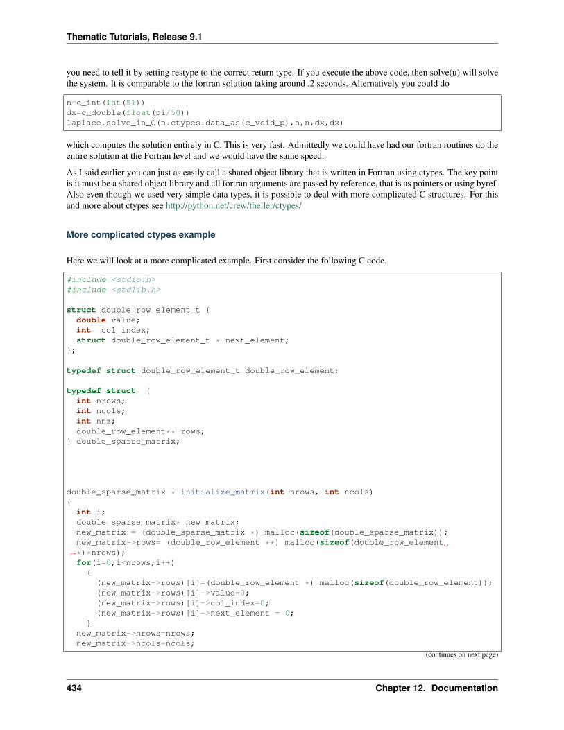
Thematic Tutorials, Release 9.1
you need to tell it by setting restype to the correct return type. If you execute the above code, then solve(u) will solvethe system. It is comparable to the fortran solution taking around .2 seconds. Alternatively you could do
n=c_int(int(51))dx=c_double(float(pi/50))laplace.solve_in_C(n.ctypes.data_as(c_void_p),n,n,dx,dx)
which computes the solution entirely in C. This is very fast. Admittedly we could have had our fortran routines do theentire solution at the Fortran level and we would have the same speed.
As I said earlier you can just as easily call a shared object library that is written in Fortran using ctypes. The key pointis it must be a shared object library and all fortran arguments are passed by reference, that is as pointers or using byref.Also even though we used very simple data types, it is possible to deal with more complicated C structures. For thisand more about ctypes see http://python.net/crew/theller/ctypes/
More complicated ctypes example
Here we will look at a more complicated example. First consider the following C code.
#include <stdio.h>#include <stdlib.h>
struct double_row_element_t double value;int col_index;struct double_row_element_t * next_element;
;
typedef struct double_row_element_t double_row_element;
typedef struct int nrows;int ncols;int nnz;double_row_element** rows;
double_sparse_matrix;
double_sparse_matrix * initialize_matrix(int nrows, int ncols)
int i;double_sparse_matrix* new_matrix;new_matrix = (double_sparse_matrix *) malloc(sizeof(double_sparse_matrix));new_matrix->rows= (double_row_element **) malloc(sizeof(double_row_element
→˓*)*nrows);for(i=0;i<nrows;i++)
(new_matrix->rows)[i]=(double_row_element *) malloc(sizeof(double_row_element));(new_matrix->rows)[i]->value=0;(new_matrix->rows)[i]->col_index=0;(new_matrix->rows)[i]->next_element = 0;
new_matrix->nrows=nrows;new_matrix->ncols=ncols;
(continues on next page)
434 Chapter 12. Documentation
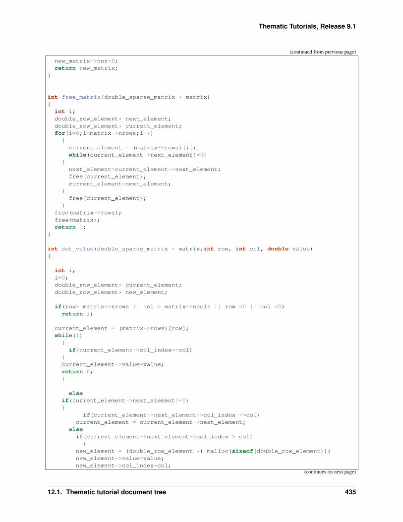
Thematic Tutorials, Release 9.1
(continued from previous page)
new_matrix->nnz=0;return new_matrix;
int free_matrix(double_sparse_matrix * matrix)
int i;double_row_element* next_element;double_row_element* current_element;for(i=0;i<matrix->nrows;i++)
current_element = (matrix->rows)[i];while(current_element->next_element!=0)
next_element=current_element->next_element;free(current_element);current_element=next_element;
free(current_element);
free(matrix->rows);free(matrix);return 1;
int set_value(double_sparse_matrix * matrix,int row, int col, double value)
int i;i=0;double_row_element* current_element;double_row_element* new_element;
if(row> matrix->nrows || col > matrix->ncols || row <0 || col <0)return 1;
current_element = (matrix->rows)[row];while(1)
if(current_element->col_index==col)current_element->value=value;return 0;
elseif(current_element->next_element!=0)
if(current_element->next_element->col_index <=col)current_element = current_element->next_element;
elseif(current_element->next_element->col_index > col)
new_element = (double_row_element *) malloc(sizeof(double_row_element));new_element->value=value;new_element->col_index=col;
(continues on next page)
12.1. Thematic tutorial document tree 435
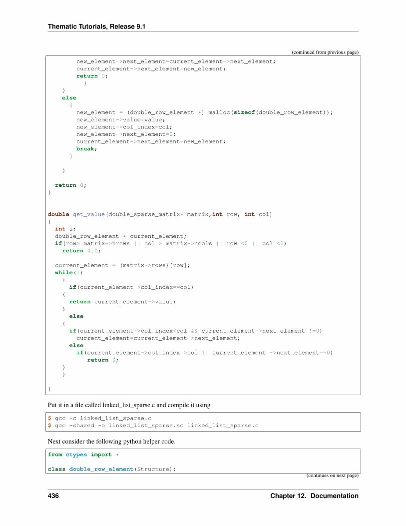
Thematic Tutorials, Release 9.1
(continued from previous page)
new_element->next_element=current_element->next_element;current_element->next_element=new_element;return 0;
else
new_element = (double_row_element *) malloc(sizeof(double_row_element));new_element->value=value;new_element->col_index=col;new_element->next_element=0;current_element->next_element=new_element;break;
return 0;
double get_value(double_sparse_matrix* matrix,int row, int col)
int i;double_row_element * current_element;if(row> matrix->nrows || col > matrix->ncols || row <0 || col <0)return 0.0;
current_element = (matrix->rows)[row];while(1)
if(current_element->col_index==col)
return current_element->value;
else
if(current_element->col_index<col && current_element->next_element !=0)current_element=current_element->next_element;
elseif(current_element->col_index >col || current_element ->next_element==0)
return 0;
Put it in a file called linked_list_sparse.c and compile it using
$ gcc -c linked_list_sparse.c$ gcc -shared -o linked_list_sparse.so linked_list_sparse.o
Next consider the following python helper code.
from ctypes import *
class double_row_element(Structure):(continues on next page)
436 Chapter 12. Documentation
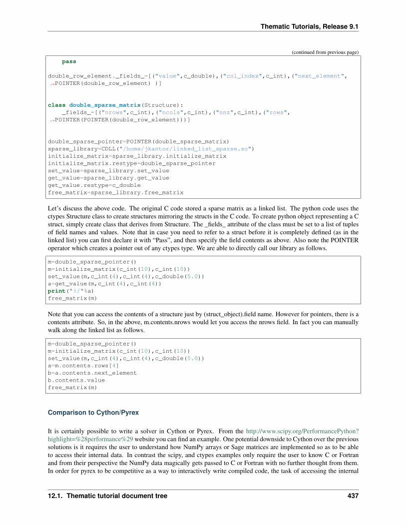
Thematic Tutorials, Release 9.1
(continued from previous page)
pass
double_row_element._fields_=[("value",c_double),("col_index",c_int),("next_element",→˓POINTER(double_row_element) )]
class double_sparse_matrix(Structure):_fields_=[("nrows",c_int),("ncols",c_int),("nnz",c_int),("rows",
→˓POINTER(POINTER(double_row_element)))]
double_sparse_pointer=POINTER(double_sparse_matrix)sparse_library=CDLL("/home/jkantor/linked_list_sparse.so")initialize_matrix=sparse_library.initialize_matrixinitialize_matrix.restype=double_sparse_pointerset_value=sparse_library.set_valueget_value=sparse_library.get_valueget_value.restype=c_doublefree_matrix=sparse_library.free_matrix
Let’s discuss the above code. The original C code stored a sparse matrix as a linked list. The python code uses thectypes Structure class to create structures mirroring the structs in the C code. To create python object representing a Cstruct, simply create class that derives from Structure. The _fields_ attribute of the class must be set to a list of tuplesof field names and values. Note that in case you need to refer to a struct before it is completely defined (as in thelinked list) you can first declare it with “Pass”, and then specify the field contents as above. Also note the POINTERoperator which creates a pointer out of any ctypes type. We are able to directly call our library as follows.
m=double_sparse_pointer()m=initialize_matrix(c_int(10),c_int(10))set_value(m,c_int(4),c_int(4),c_double(5.0))a=get_value(m,c_int(4),c_int(4))print("%f"%a)free_matrix(m)
Note that you can access the contents of a structure just by (struct_object).field name. However for pointers, there is acontents attribute. So, in the above, m.contents.nrows would let you access the nrows field. In fact you can manuallywalk along the linked list as follows.
m=double_sparse_pointer()m=initialize_matrix(c_int(10),c_int(10))set_value(m,c_int(4),c_int(4),c_double(5.0))a=m.contents.rows[4]b=a.contents.next_elementb.contents.valuefree_matrix(m)
Comparison to Cython/Pyrex
It is certainly possible to write a solver in Cython or Pyrex. From the http://www.scipy.org/PerformancePython?highlight=%28performance%29 website you can find an example. One potential downside to Cython over the previoussolutions is it requires the user to understand how NumPy arrays or Sage matrices are implemented so as to be ableto access their internal data. In contrast the scipy, and ctypes examples only require the user to know C or Fortranand from their perspective the NumPy data magically gets passed to C or Fortran with no further thought from them.In order for pyrex to be competitive as a way to interactively write compiled code, the task of accessing the internal
12.1. Thematic tutorial document tree 437
Thematic Tutorials, Release 9.1
structure of NumPy arrays or Sage matrices needs to be hidden.
Parallel Computation
mpi4py
MPI which stands for message passing interface is a common library for parallel programming. There is a packagempi4py that builds on the top of mpi, and lets arbitrary python objects be passed between different processes. Thesepackages are not part of the default sage install. To install them do
sage: optional_packages()
Find the package name openmpi-* and mpi4py-*and do
sage: install_package('openmpi-*')sage: install_package('mpi4py-*')
Note that openmpi takes a while to compile (15-20 minutes or so). Openmpi can be run on a cluster, however thisrequires some set up so that processes on different machines can communicate (though if you are on a cluster this isprobably already set up). The simplest case is if you are on a shared memory or multicore system where openmpi willjust work with no configuration from you. To be honest, I have never tried to run mpi4py on a cluster, though there ismuch information about these topics online.
Now, the way that mpi works is you start a group of mpi processes, all of the processes run the same code. Eachprocess has a rank, that is a number that identifies it. The following pseudocode indicates the general format of MPIprograms.
....
if my rank is n:do some computation ...send some stuff to the process of rank jreceive some data from the process of rank k
else if my rank is n+1:....
Each processes looks for what it’s supposed to do (specified by its rank) and processes can send data and receive data.Lets give an example. Create a script with the following code in a file mpi_1.py
from mpi4py import MPIcomm = MPI.COMM_WORLDprint("hello world")print("my rank is: %d"%comm.rank)
To run it you can do (from the command line in your sage directory)
./local/bin/mpirun -np 5 ./sage -python mpi_1.py
The command mpirun -np 5 starts 5 copies of a program under mpi. In this case we have 5 copies of sage in purepython mode run the script mpi_1.py. The result should be 5 “hello worlds” plus 5 distinct ranks. The two mostimportant mpi operations are sending and receiving. Consider the following example which you should put in a scriptmpi_2.py
438 Chapter 12. Documentation
Thematic Tutorials, Release 9.1
from mpi4py import MPIimport numpycomm = MPI.COMM_WORLDrank=comm.ranksize=comm.sizev=numpy.array([rank]*5,dtype=float)comm.send(v,dest=(rank+1)%size)data=comm.recv(source=(rank-1)%size)print("my rank is %d"%rank)print("I received this:")print(data)
The same command as above with mpi_1.py replaced by mpi_2.py will produce 5 outputs and you will see eachprocess creates an array and then passes it to the next guy (where the last guy passes to the first.) Note that MPI.sizeis the total number of mpi processes. MPI.COMM WORLD is the communication world.
There are some subtleties regarding MPI to be aware of. Small sends are buffered. This means if a process sendsa small object it will be stored by openmpi and that process will continue its execution and the object it sent willbe received whenever the destination executes a receive. However, if an object is large a process will hang until itsdestination executes a corresponding receive. In fact the above code will hang if [rank]*5 is replaced by [rank]*500.It would be better to do
from mpi4py import MPIimport numpycomm = MPI.COMM_WORLDrank=comm.ranksize=comm.sizev=numpy.array([rank]*500,dtype=float)if comm.rank==0:
comm.send(v,dest=(rank+1)%size)if comm.rank > 0:
data=comm.recv(source=(rank-1)%size)comm.send(v,dest=(rank+1)%size)
if comm.rank==0:data=comm.recv(source=size-1)
print("my rank is %d"%rank)print("I received this:")print(data)
Now the first process initiates a send, and then process 1 will be ready to receive and then he will send and process 2will be waiting to receive, etc. This will not lock regardless of how large of an array we pass.
A common idiom is to have one process, usually the one with rank 0 act as a leader. That processes sends data outto the other processes and processes the results and decides how further computation should proceed. Consider thefollowing code
from mpi4py import MPIimport numpysendbuf=[]root=0comm = MPI.COMM_WORLDif comm.rank==0:
m=numpy.random.randn(comm.size,comm.size)print(m)sendbuf=m
(continues on next page)
12.1. Thematic tutorial document tree 439
Thematic Tutorials, Release 9.1
(continued from previous page)
v=comm.scatter(sendbuf,root)
print("I got this array:")print(v)
The scatter command takes a list and evenly divides it amongst all the processes. Here the root process creates amatrix (which is viewed as a list of rows) and then scatters it to everybody (roots sendbuf is divided equally amongstthe processes). Each process prints the row it got. Note that the scatter command is executed by everyone, but whenroot executes it, it acts as a send and a receive (root gets one row from itself), while for everyone else it is just a receive.
There is a complementary gather command that collects results from all the processes into a list. The next exampleuses scatter and gather together. Now the root process scatters the rows of a matrix, each process then squares theelements of the row it gets. Then the rows are all gathered up again by the root process who collects them into a newmatrix.
from mpi4py import MPIimport numpycomm = MPI.COMM_WORLDsendbuf=[]root=0if comm.rank==0:
m=numpy.array(range(comm.size*comm.size),dtype=float)m.shape=(comm.size,comm.size)print(m)sendbuf=m
v=comm.scatter(sendbuf,root)print("I got this array:")print(v)v=v*vrecvbuf=comm.gather(v,root)if comm.rank==0:
print(numpy.array(recvbuf))
There is also a broadcast command that sends a single object to every process. Consider the following small extension.This is the same as before, but now at the end the root process sends everyone the string “done”, which is printed out.
v=MPI.COMM_WORLD.scatter(sendbuf,root)print("I got this array:")print(v)v=v*vrecvbuf=MPI.COMM_WORLD.gather(v,root)if MPI.COMM_WORLD.rank==0:
print(numpy.array(recvbuf))
if MPI.COMM_WORLD.rank==0:sendbuf="done"
recvbuf=MPI.COMM_WORLD.bcast(sendbuf,root)print(recvbuf)
MPI programming is difficult. It is “schizophrenic programming” in that you are writing a single programming withmultiple threads of execution “many voices in one head”.
440 Chapter 12. Documentation
Thematic Tutorials, Release 9.1
Parallel Laplace Solver
The following code solves Laplace’s equation in parallel on a grid. It divides a square into 𝑛 parallel strips where 𝑛 isthe number of processes and uses jacobi-iteration. The way the code works is that the root process creates a matrix anddistributes the pieces to the other processes. At each iteration each process passes its upper row to the process aboveand its lower row to the process below since they need to know the values at neighboring points to do the iteration.Then they iterate and repeat. Every 500 iterations the error estimates from the processes are collected using Gather.you can compare the output of this with the solver we wrote in the section on f2py.
from mpi4py import MPIimport numpysize=MPI.sizerank=MPI.ranknum_points=500sendbuf=[]root=0dx=1.0/(num_points-1)from numpy import r_j=numpy.complex(0,1)rows_per_process=num_points/sizemax_iter=5000num_iter=0total_err=1
def numpyTimeStep(u,dx,dy):dx2, dy2 = dx**2, dy**2dnr_inv = 0.5/(dx2 + dy2)u_old=u.copy()# The actual iterationu[1:-1, 1:-1] = ((u[0:-2, 1:-1] + u[2:, 1:-1])*dy2 +
(u[1:-1,0:-2] + u[1:-1, 2:])*dx2)*dnr_invv = (u - u_old).flatreturn u,numpy.sqrt(numpy.dot(v,v))
if MPI.rank==0:print("num_points: %d"%num_points)print("dx: %f"%dx)print("row_per_procss: %d"%rows_per_process)m=numpy.zeros((num_points,num_points),dtype=float)pi_c=numpy.pix=r_[0.0:pi_c:num_points*j]m[0,:]=numpy.sin(x)m[num_points-1,:]=numpy.sin(x)l=[ m[i*rows_per_process:(i+1)*rows_per_process,:] for i in range(size)]sendbuf=l
my_grid=MPI.COMM_WORLD.Scatter(sendbuf,root)
while num_iter < max_iter and total_err > 10e-6:
if rank==0:MPI.COMM_WORLD.Send(my_grid[-1,:],1)
if rank > 0 and rank< size-1:
(continues on next page)
12.1. Thematic tutorial document tree 441
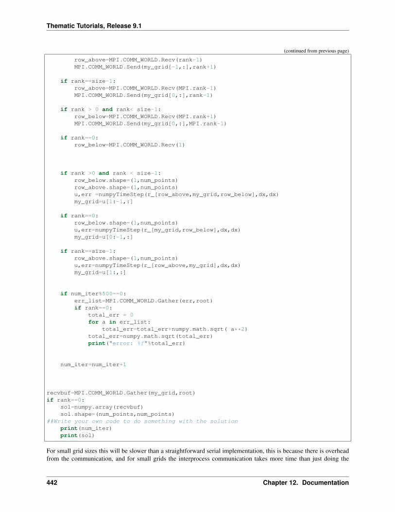
Thematic Tutorials, Release 9.1
(continued from previous page)
row_above=MPI.COMM_WORLD.Recv(rank-1)MPI.COMM_WORLD.Send(my_grid[-1,:],rank+1)
if rank==size-1:row_above=MPI.COMM_WORLD.Recv(MPI.rank-1)MPI.COMM_WORLD.Send(my_grid[0,:],rank-1)
if rank > 0 and rank< size-1:row_below=MPI.COMM_WORLD.Recv(MPI.rank+1)MPI.COMM_WORLD.Send(my_grid[0,:],MPI.rank-1)
if rank==0:row_below=MPI.COMM_WORLD.Recv(1)
if rank >0 and rank < size-1:row_below.shape=(1,num_points)row_above.shape=(1,num_points)u,err =numpyTimeStep(r_[row_above,my_grid,row_below],dx,dx)my_grid=u[1:-1,:]
if rank==0:row_below.shape=(1,num_points)u,err=numpyTimeStep(r_[my_grid,row_below],dx,dx)my_grid=u[0:-1,:]
if rank==size-1:row_above.shape=(1,num_points)u,err=numpyTimeStep(r_[row_above,my_grid],dx,dx)my_grid=u[1:,:]
if num_iter%500==0:err_list=MPI.COMM_WORLD.Gather(err,root)if rank==0:
total_err = 0for a in err_list:
total_err=total_err+numpy.math.sqrt( a**2)total_err=numpy.math.sqrt(total_err)print("error: %f"%total_err)
num_iter=num_iter+1
recvbuf=MPI.COMM_WORLD.Gather(my_grid,root)if rank==0:
sol=numpy.array(recvbuf)sol.shape=(num_points,num_points)
##Write your own code to do something with the solutionprint(num_iter)print(sol)
For small grid sizes this will be slower than a straightforward serial implementation, this is because there is overheadfrom the communication, and for small grids the interprocess communication takes more time than just doing the
442 Chapter 12. Documentation
Thematic Tutorials, Release 9.1
iteration. However, on a 1000x1000 grid I find that using 4 processors, the parallel version takes only 6 seconds whilethe serial version we wrote earlier takes 20 seconds.
Excercise: Rewrite the above using f2py, so that each process compiles a fortran function and uses that, how fast canyou get this?
12.1.20 Three Lectures about Explicit Methods in Number Theory Using Sage
This article is about using the mathematical software Sage to do computations with number fields and modu-lar forms. It was written for the October 2008 Bordeaux meeting on explicit methods in number theory (http://www.math.u-bordeaux.fr/gtem2008/). It assumes no prior knowledge about Sage, but assumes a graduate levelbackground in algebraic number theory.
Introduction
What is Sage?
Sage (see http://sagemath.org) is a comprehensive mathematical software system for computations in many areas ofpure and applied mathematics. We program Sage using the mainstream programming language Python (see http://python.org), or its compiled variant Cython. It is also very easy to efficiently use code written in C/C++ from Sage.
The author of this article started the Sage project in 2005.
Sage is free and open source, meaning you can change any part of Sage and redistribute the result without having topay any license fees, and Sage can also leverage the power of commercial mathematical software such as Magma andMathematica, if you happen to have access to those closed source commercial systems.
This document assumes no prior knowledge of either Python or Sage. Our goal is to help number theorists do compu-tations involving number fields and modular forms using Sage.
TODO: Overview of Article
As you read this article, please try every example in Sage, and make sure things works as I claim, and do all of theexercises. Moreover, you should experiment by typing in similar examples and checking that the output you get agreeswith what you expect.
Using Sage
To use Sage, install it on your computer, and use either the command line or use the notebook by starting Sage assage -n.
We show Sage sessions as follows:
sage: factor(123456)2^6 * 3 * 643
This means that if you type factor(123456) as input to Sage, then you’ll get 2^6 * 3 * 643 as output. Ifyou’re using the Sage command line, you type factor(123456) and press enter; if you’re using the Sage notebookvia your web browser, you type factor(123456) into an input cell and press shift-enter; in the output cell you’llsee 2^6 * 3 * 643.
After trying the factor command in the previous paragraph (do this now!), you should try factoring some othernumbers.
12.1. Thematic tutorial document tree 443
Thematic Tutorials, Release 9.1
Note: What happens if you factor a negative number? a rational number?
You can also draw both 2d and 3d pictures using Sage. For example, the following input plots the number of primedivisors of each positive integer up to 500.
sage: line([(n, len(factor(n))) for n in [1..500]])Graphics object consisting of 1 graphics primitive
And, this example draws a similar 3d plot:
sage: import warningssage: warnings.simplefilter('ignore', UserWarning)sage: v = [[len(factor(n*m)) for n in [1..15]] for m in [1..15]]sage: list_plot3d(v, interpolation_type='clough')Graphics3d Object
The Sage-Pari-Magma Ecosystem
• The main difference between Sage and Pari is that Sage is vastly larger than Pari with a much wider range offunctionality, and has many more data types and much more structured objects. Sage in fact includes Pari, anda typical Sage install takes nearly a gigabyte of disk space, whereas a typical Pari install is much more nimble,using only a few megabytes. There are many number-theoretic algorithms that are included in Sage, whichhave never been implemented in Pari, and Sage has 2d and 3d graphics which can be helpful for visualizingnumber theoretic ideas, and a graphical user interface. Both Pari and Sage are free and open source, whichmeans anybody can read or change anything in either program, and the software is free.
• The biggest difference between Sage and Magma is that Magma is closed source, not free, and difficult for usersto extend. This means that most of Magma cannot be changed except by the core Magma developers, sinceMagma itself is well over two million lines of compiled C code, combined with about a half million lines ofinterpreted Magma code (that anybody can read and modify). In designing Sage, we carried over some of theexcellent design ideas from Magma, such as the parent, element, category hierarchy.
• Any mathematician who is serious about doing extensive computational work in algebraic number theory andarithmetic geometry is strongly urged to become familiar with all three systems, since they all have their pros andcons. Pari is sleek and small, Magma has much unique functionality for computations in arithmetic geometry,and Sage has a wide range of functionality in most areas of mathematics, a large developer community, andmuch unique new code.
Number Fields
Introduction to Number Fields
In Sage, we can create the number field Q( 3√
2) as follows.
sage: K.<alpha> = NumberField(x^3 - 2)
The above creates two Sage objects, 𝐾 and 𝛼. Here 𝐾 “is” (isomorphic to) the number field Q( 3√
2), as we confirmbelow:
sage: KNumber Field in alpha with defining polynomial x^3 - 2
444 Chapter 12. Documentation
Thematic Tutorials, Release 9.1
and 𝛼 is a root of 𝑥3 − 2, so 𝛼 is an abstract choice of 3√
2 (no specific embedding of the number field 𝐾 into C ischosen by default in Sage-3.1.2):
sage: alpha^32sage: (alpha+1)^33*alpha^2 + 3*alpha + 3
The variable 𝑥
Note that we did not define 𝑥 above before using it. You could “break” the above example by redefining 𝑥 to besomething funny:
sage: x = 1sage: K.<alpha> = NumberField(x^3 - 2)Traceback (most recent call last):...TypeError: polynomial (=-1) must be a polynomial.
The Traceback above indicates that there was an error. Potentially lots of detailed information about the error (a “trace-back”) may be given after the word Traceback and before the last line, which contains the actual error messages.
Note: Important: whenever you use Sage and get a big error, look at the last line for the actual error, and only lookat the rest if you are feeling adventurous. In the notebook, the part indicated by ... above is not displayed; to see it,click just to the left of the word Traceback and the traceback will appear.
If you redefine 𝑥 as above, but need to define a number field using the indeterminate 𝑥, you have several options. Youcan reset 𝑥 to its default value at the start of Sage, you can redefine 𝑥 to be a symbolic variable, or you can define 𝑥 tobe a polynomial indeterminate (a polygen):
sage: reset('x')sage: xxsage: x = 1sage: x = var('x')sage: xxsage: x = 1sage: x = polygen(QQ, 'x')sage: xxsage: x = 1sage: R.<x> = PolynomialRing(QQ)sage: xx
Using tab completion to get the methods of an object
One you have created a number field 𝐾, type K.[tab key] to see a list of functions. Type, e.g., K.minkowski_embedding?[tab key] to see help on the minkowski_embedding command. To see sourcecode, type K.minkowski_embedding??[tab key].
12.1. Thematic tutorial document tree 445
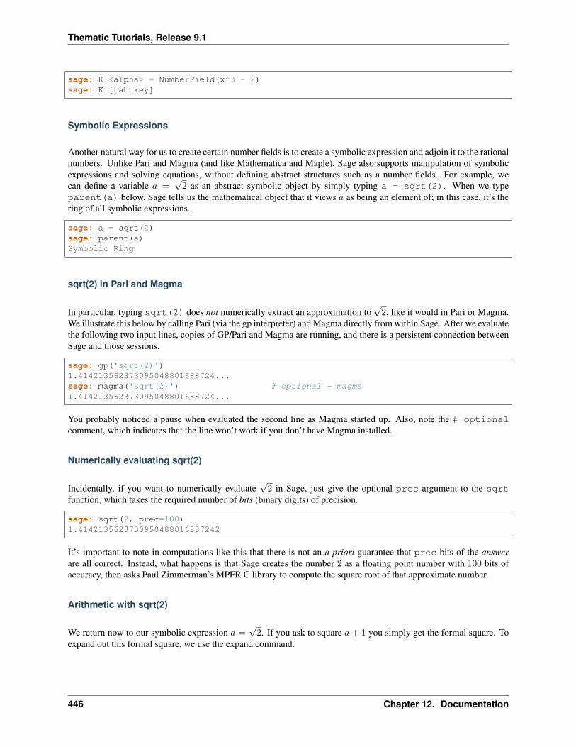
Thematic Tutorials, Release 9.1
sage: K.<alpha> = NumberField(x^3 - 2)sage: K.[tab key]
Symbolic Expressions
Another natural way for us to create certain number fields is to create a symbolic expression and adjoin it to the rationalnumbers. Unlike Pari and Magma (and like Mathematica and Maple), Sage also supports manipulation of symbolicexpressions and solving equations, without defining abstract structures such as a number fields. For example, wecan define a variable 𝑎 =
√2 as an abstract symbolic object by simply typing a = sqrt(2). When we type
parent(a) below, Sage tells us the mathematical object that it views 𝑎 as being an element of; in this case, it’s thering of all symbolic expressions.
sage: a = sqrt(2)sage: parent(a)Symbolic Ring
sqrt(2) in Pari and Magma
In particular, typing sqrt(2) does not numerically extract an approximation to√
2, like it would in Pari or Magma.We illustrate this below by calling Pari (via the gp interpreter) and Magma directly from within Sage. After we evaluatethe following two input lines, copies of GP/Pari and Magma are running, and there is a persistent connection betweenSage and those sessions.
sage: gp('sqrt(2)')1.414213562373095048801688724...sage: magma('Sqrt(2)') # optional - magma1.414213562373095048801688724...
You probably noticed a pause when evaluated the second line as Magma started up. Also, note the # optionalcomment, which indicates that the line won’t work if you don’t have Magma installed.
Numerically evaluating sqrt(2)
Incidentally, if you want to numerically evaluate√
2 in Sage, just give the optional prec argument to the sqrtfunction, which takes the required number of bits (binary digits) of precision.
sage: sqrt(2, prec=100)1.4142135623730950488016887242
It’s important to note in computations like this that there is not an a priori guarantee that prec bits of the answerare all correct. Instead, what happens is that Sage creates the number 2 as a floating point number with 100 bits ofaccuracy, then asks Paul Zimmerman’s MPFR C library to compute the square root of that approximate number.
Arithmetic with sqrt(2)
We return now to our symbolic expression 𝑎 =√
2. If you ask to square 𝑎 + 1 you simply get the formal square. Toexpand out this formal square, we use the expand command.
446 Chapter 12. Documentation
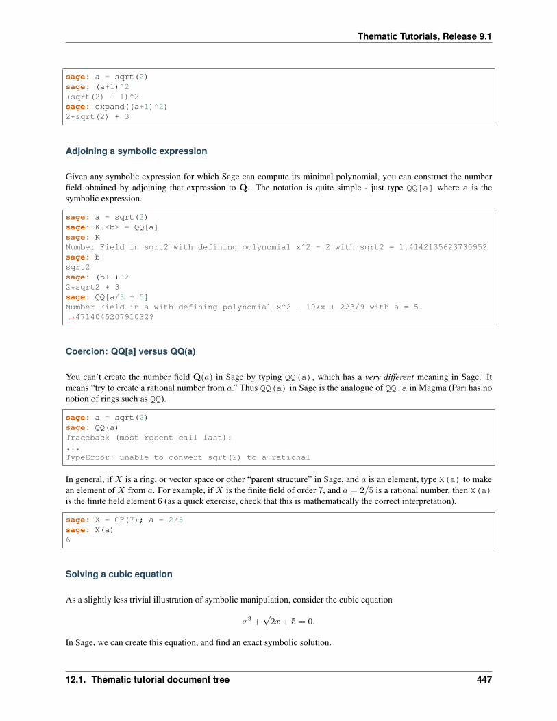
Thematic Tutorials, Release 9.1
sage: a = sqrt(2)sage: (a+1)^2(sqrt(2) + 1)^2sage: expand((a+1)^2)2*sqrt(2) + 3
Adjoining a symbolic expression
Given any symbolic expression for which Sage can compute its minimal polynomial, you can construct the numberfield obtained by adjoining that expression to Q. The notation is quite simple - just type QQ[a] where a is thesymbolic expression.
sage: a = sqrt(2)sage: K.<b> = QQ[a]sage: KNumber Field in sqrt2 with defining polynomial x^2 - 2 with sqrt2 = 1.414213562373095?sage: bsqrt2sage: (b+1)^22*sqrt2 + 3sage: QQ[a/3 + 5]Number Field in a with defining polynomial x^2 - 10*x + 223/9 with a = 5.→˓471404520791032?
Coercion: QQ[a] versus QQ(a)
You can’t create the number field Q(𝑎) in Sage by typing QQ(a), which has a very different meaning in Sage. Itmeans “try to create a rational number from 𝑎.” Thus QQ(a) in Sage is the analogue of QQ!a in Magma (Pari has nonotion of rings such as QQ).
sage: a = sqrt(2)sage: QQ(a)Traceback (most recent call last):...TypeError: unable to convert sqrt(2) to a rational
In general, if 𝑋 is a ring, or vector space or other “parent structure” in Sage, and 𝑎 is an element, type X(a) to makean element of 𝑋 from 𝑎. For example, if 𝑋 is the finite field of order 7, and 𝑎 = 2/5 is a rational number, then X(a)is the finite field element 6 (as a quick exercise, check that this is mathematically the correct interpretation).
sage: X = GF(7); a = 2/5sage: X(a)6
Solving a cubic equation
As a slightly less trivial illustration of symbolic manipulation, consider the cubic equation
𝑥3 +√
2𝑥+ 5 = 0.
In Sage, we can create this equation, and find an exact symbolic solution.
12.1. Thematic tutorial document tree 447
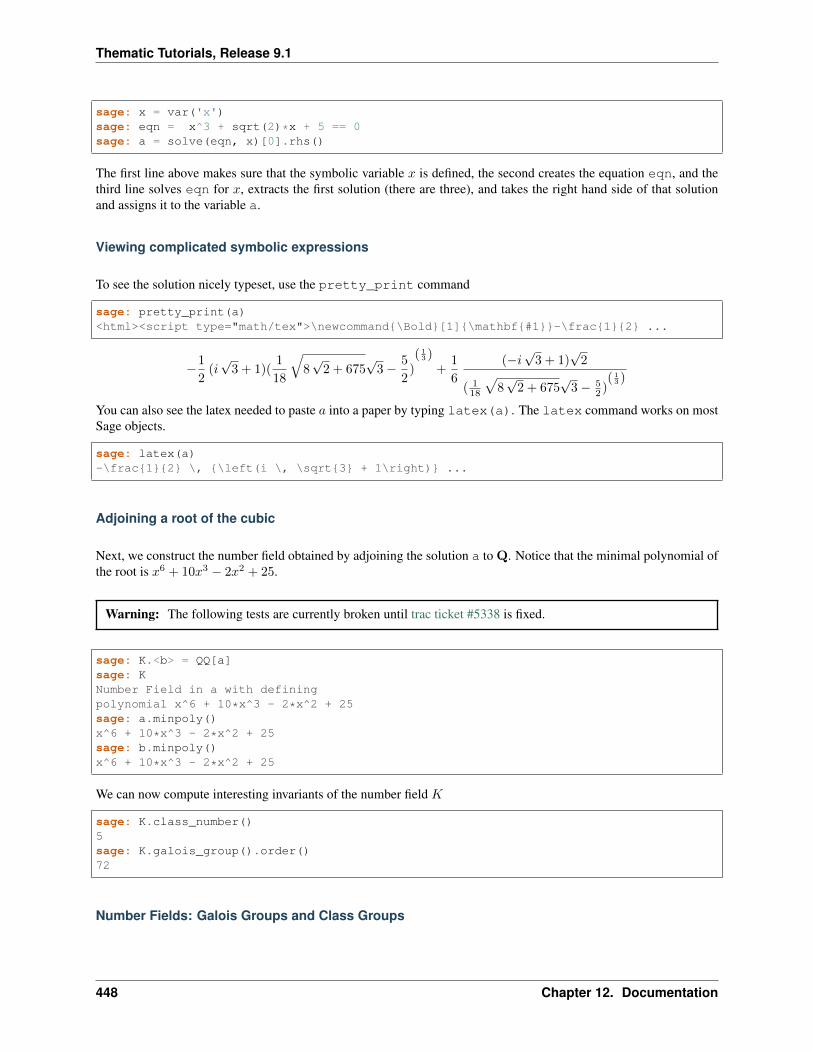
Thematic Tutorials, Release 9.1
sage: x = var('x')sage: eqn = x^3 + sqrt(2)*x + 5 == 0sage: a = solve(eqn, x)[0].rhs()
The first line above makes sure that the symbolic variable 𝑥 is defined, the second creates the equation eqn, and thethird line solves eqn for 𝑥, extracts the first solution (there are three), and takes the right hand side of that solutionand assigns it to the variable a.
Viewing complicated symbolic expressions
To see the solution nicely typeset, use the pretty_print command
sage: pretty_print(a)<html><script type="math/tex">\newcommand\Bold[1]\mathbf#1-\frac12 ...
−1
2(𝑖√
3 + 1)(1
18
√8√
2 + 675√
3− 5
2)( 1
3 )+
1
6
(−𝑖√
3 + 1)√
2
( 118
√8√
2 + 675√
3− 52 )
( 13 )
You can also see the latex needed to paste 𝑎 into a paper by typing latex(a). The latex command works on mostSage objects.
sage: latex(a)-\frac12 \, \left(i \, \sqrt3 + 1\right) ...
Adjoining a root of the cubic
Next, we construct the number field obtained by adjoining the solution a to Q. Notice that the minimal polynomial ofthe root is 𝑥6 + 10𝑥3 − 2𝑥2 + 25.
Warning: The following tests are currently broken until trac ticket #5338 is fixed.
sage: K.<b> = QQ[a]sage: KNumber Field in a with definingpolynomial x^6 + 10*x^3 - 2*x^2 + 25sage: a.minpoly()x^6 + 10*x^3 - 2*x^2 + 25sage: b.minpoly()x^6 + 10*x^3 - 2*x^2 + 25
We can now compute interesting invariants of the number field 𝐾
sage: K.class_number()5sage: K.galois_group().order()72
Number Fields: Galois Groups and Class Groups
448 Chapter 12. Documentation
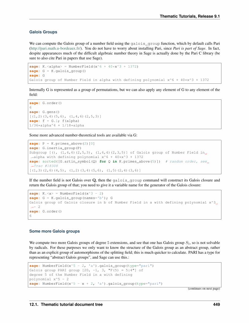
Thematic Tutorials, Release 9.1
Galois Groups
We can compute the Galois group of a number field using the galois_group function, which by default calls Pari(http://pari.math.u-bordeaux.fr/). You do not have to worry about installing Pari, since Pari is part of Sage. In fact,despite appearances much of the difficult algebraic number theory in Sage is actually done by the Pari C library (besure to also cite Pari in papers that use Sage).
sage: K.<alpha> = NumberField(x^6 + 40*x^3 + 1372)sage: G = K.galois_group()sage: GGalois group of Number Field in alpha with defining polynomial x^6 + 40*x^3 + 1372
Internally G is represented as a group of permutations, but we can also apply any element of G to any element of thefield:
sage: G.order()6sage: G.gens()[(1,2)(3,4)(5,6), (1,4,6)(2,5,3)]sage: f = G.1; f(alpha)1/36*alpha^4 + 1/18*alpha
Some more advanced number-theoretical tools are available via G:
sage: P = K.primes_above(2)[0]sage: G.inertia_group(P)Subgroup [(), (1,4,6)(2,5,3), (1,6,4)(2,3,5)] of Galois group of Number Field in→˓alpha with defining polynomial x^6 + 40*x^3 + 1372sage: sorted([G.artin_symbol(Q) for Q in K.primes_above(5)]) # random order, see→˓Trac #18308[(1,3)(2,6)(4,5), (1,2)(3,4)(5,6), (1,5)(2,4)(3,6)]
If the number field is not Galois over Q, then the galois_group command will construct its Galois closure andreturn the Galois group of that; you need to give it a variable name for the generator of the Galois closure:
sage: K.<a> = NumberField(x^3 - 2)sage: G = K.galois_group(names='b'); GGalois group of Galois closure in b of Number Field in a with defining polynomial x^3→˓- 2sage: G.order()6
Some more Galois groups
We compute two more Galois groups of degree 5 extensions, and see that one has Galois group 𝑆5, so is not solvableby radicals. For these purposes we only want to know the structure of the Galois group as an abstract group, ratherthan as an explicit group of automorphisms of the splitting field; this is much quicker to calculate. PARI has a type forrepresenting “abstract Galois groups”, and Sage can use this.:
sage: NumberField(x^5 - 2, 'a').galois_group(type="pari")Galois group PARI group [20, -1, 3, "F(5) = 5:4"] ofdegree 5 of the Number Field in a with definingpolynomial x^5 - 2sage: NumberField(x^5 - x + 2, 'a').galois_group(type="pari")
(continues on next page)
12.1. Thematic tutorial document tree 449
Thematic Tutorials, Release 9.1
(continued from previous page)
Galois group PARI group [120, -1, 5, "S5"] of degree 5 ofthe Number Field in a with defining polynomial x^5 - x + 2
Magma’s Galois group command
Recent versions of Magma have an algorithm for computing Galois groups that in theory applies when the inputpolynomial has any degree. There are no open source implementation of this algorithm (as far as I know). Ifyou have Magma, you can use this algorithm from Sage by calling the galois_group function and giving thealgorithm='magma' option. The return value is one of the groups in the GAP transitive groups database.
sage: K.<a> = NumberField(x^3 - 2)sage: K.galois_group(type="gap", algorithm='magma') # optional - magmaGalois group Transitive group number 2 of degree 3 ofthe Number Field in a with defining polynomial x^3 - 2
We emphasize that the above example should not work if you don’t have Magma.
Computing complex embeddings
You can also enumerate all complex embeddings of a number field:
sage: K.complex_embeddings()[Ring morphism:
From: Number Field in a with defining polynomial x^3 - 2To: Complex Field with 53 bits of precisionDefn: a |--> -0.629960524947437 - 1.09112363597172*I,
Ring morphism:From: Number Field in a with defining polynomial x^3 - 2To: Complex Field with 53 bits of precisionDefn: a |--> -0.629960524947437 + 1.09112363597172*I,
Ring morphism:From: Number Field in a with defining polynomial x^3 - 2To: Complex Field with 53 bits of precisionDefn: a |--> 1.25992104989487
]
Class Numbers and Class Groups
The class group 𝐶𝐾 of a number field 𝐾 is the group of fractional ideals of the maximal order 𝑅 of 𝐾 modulo thesubgroup of principal fractional ideals. One of the main theorems of algebraic number theory asserts that 𝐶𝐾 is afinite group. For example, the quadratic number field Q(
√−23) has class number 3, as we see using the Sage class
number command.
sage: L.<a> = NumberField(x^2 + 23)sage: L.class_number()3
450 Chapter 12. Documentation
Thematic Tutorials, Release 9.1
Quadratic imaginary fields with class number 1
There are only 9 quadratic imaginary field Q(√𝐷) that have class number 1:
𝐷 = −3,−4,−7,−8,−11,−19,−43,−67,−163
To find this list using Sage, we first experiment with making lists in Sage. For example, typing [1..10] makes thelist of integers between 1 and 10.
sage: [1..10][1, 2, 3, 4, 5, 6, 7, 8, 9, 10]
We can also make the list of odd integers between 1 and 11, by typing [1,3,..,11], i.e., by giving the second termin the arithmetic progression.
sage: [1,3,..,11][1, 3, 5, 7, 9, 11]
Applying this idea, we make the list of negative numbers from −1 down to −10.
sage: [-1,-2,..,-10][-1, -2, -3, -4, -5, -6, -7, -8, -9, -10]
Enumerating quadratic imaginary fields with class number 1
The first two lines below makes a list 𝑣 of every 𝐷 from −1 down to −200 such that 𝐷 is a fundamental discriminant(the discriminant of a quadratic imaginary field).
Note: Note that you will not see the . . . in the output below; this . . . notation just means that part of the output isomitted below.
sage: w = [-1,-2,..,-200]sage: v = [D for D in w if is_fundamental_discriminant(D)]sage: v[-3, -4, -7, -8, -11, -15, -19, -20, ..., -195, -199]
Finally, we make the list of 𝐷 in our list 𝑣 such that the quadratic number field Q(√𝐷) has class number 1. Notice
that QuadraticField(D) is a shorthand for NumberField(x^2 - D).
sage: [D for D in v if QuadraticField(D,'a').class_number()==1][-3, -4, -7, -8, -11, -19, -43, -67, -163]
Of course, we have not proved that this is the list of all negative 𝐷 so that Q(√𝐷) has class number 1.
Class number 1 fields
A frustrating open problem is to prove that there are infinitely many number fields with class number 1. It is quite easyto be convinced that this is probably true by computing a bunch of class numbers of real quadratic fields. For example,over 58 percent of the real quadratic number fields with discriminant 𝐷 < 1000 have class number 1!
12.1. Thematic tutorial document tree 451
Thematic Tutorials, Release 9.1
sage: w = [1..1000]sage: v = [D for D in w if is_fundamental_discriminant(D)]sage: len(v)302sage: len([D for D in v if QuadraticField(D,'a').class_number() == 1])176sage: 176.0/3020.582781456953642
For more intuition about what is going on, read about the Cohen-Lenstra heuristics.
Class numbers of cyclotomic fields
Sage can also compute class numbers of extensions of higher degree, within reason. Here we use the shorthandCyclotomicField(n) to create the number field Q(𝜁𝑛).
sage: CyclotomicField(7)Cyclotomic Field of order 7 and degree 6sage: for n in [2..15]:....: print(" ".format(n, CyclotomicField(n).class_number()))2 13 1...15 1
In the code above, the notation for n in [2..15]: ... means “do . . . for 𝑛 equal to each of the integers2, 3, 4, . . . , 15.”
Note: Exercise: Compute what is omitted (replaced by . . . ) in the output of the previous example.
Assuming conjectures to speed computations
Computations of class numbers and class groups in Sage is done by the Pari C library, and unlike in Pari, by defaultSage tells Pari not to assume any conjectures. This can make some commands vastly slower than they might be directlyin Pari, which does assume unproved conjectures by default. Fortunately, it is easy to tell Sage to be more permissiveand allow Pari to assume conjectures, either just for this one call or henceforth for all number field functions. Forexample, with proof=False it takes only a few seconds to verify, modulo the conjectures assumed by Pari, that theclass number of Q(𝜁23) is 3.
sage: CyclotomicField(23).class_number(proof=False)3
Note: Exercise: What is the smallest 𝑛 such that Q(𝜁𝑛) has class number bigger than 1?
Class group structure
In addition to computing class numbers, Sage can also compute the group structure and generators for class groups. Forexample, the quadratic field Q(
√−30) has class group 𝐶 = (Z/2Z)⊕2, with generators the ideal classes containing
(5,√−30) and (3,
√−30).
452 Chapter 12. Documentation
Thematic Tutorials, Release 9.1
sage: K.<a> = QuadraticField(-30)sage: C = K.class_group()sage: CClass group of order 4 with structure C2 x C2 of Number Field in a with defining→˓polynomial x^2 + 30 with a = 5.477225575051661?*Isage: category(C)Category of finite enumerated commutative groupssage: C.gens()(Fractional ideal class (2, a), Fractional ideal class (3, a))
Arithmetic in the class group
In Sage, the notation C.i means “the 𝑖𝑡ℎ generator of the object 𝐶,” where the generators are indexed by numbers0, 1, 2, . . .. Below, when we write C.0 \* C.1, this means “the product of the 0th and 1st generators of the classgroup 𝐶.”
sage: K.<a> = QuadraticField(-30)sage: C = K.class_group()sage: C.0Fractional ideal class (2, a)sage: C.0.ideal()Fractional ideal (2, a)sage: I = C.0 * C.1sage: IFractional ideal class (5, a)
Next we find that the class of the fractional ideal (2,√−30 + 4/3) is equal to the ideal class 𝐶.0.
sage: A = K.ideal([2, a+4/3])sage: J = C(A)sage: JFractional ideal class (2/3, 1/3*a)sage: J == C.0True
Unfortunately, there is currently no Sage function that writes a fractional ideal class in terms of the generators for theclass group.
Orders and Relative Extensions
Orders in Number Fields
An order in a number field 𝐾 is a subring of 𝐾 whose rank over Z equals the degree of 𝐾. For example, if 𝐾 =Q(√−1), then Z[7𝑖] is an order in 𝐾. A good first exercise is to prove that every element of an order is an algebraic
integer.
sage: K.<I> = NumberField(x^2 + 1)sage: R = K.order(7*I)sage: ROrder in Number Field in I with defining polynomial x^2 + 1sage: R.basis()[1, 7*I]
Using the discriminant command, we compute the discriminant of this order
12.1. Thematic tutorial document tree 453
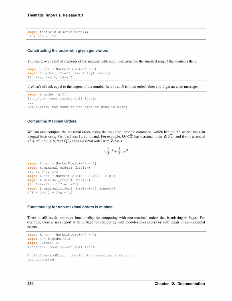
Thematic Tutorials, Release 9.1
sage: factor(R.discriminant())-1 * 2^2 * 7^2
Constructing the order with given generators
You can give any list of elements of the number field, and it will generate the smallest ring 𝑅 that contains them.
sage: K.<a> = NumberField(x^4 + 2)sage: K.order([12*a^2, 4*a + 12]).basis()[1, 4*a, 4*a^2, 16*a^3]
If 𝑅 isn’t of rank equal to the degree of the number field (i.e., 𝑅 isn’t an order), then you’ll get an error message.
sage: K.order([a^2])Traceback (most recent call last):...ValueError: the rank of the span of gens is wrong
Computing Maximal Orders
We can also compute the maximal order, using the maxima order command, which behind the scenes finds anintegral basis using Pari’s nfbasis command. For example, Q( 4
√2) has maximal order Z[ 4
√2], and if 𝛼 is a root of
𝑥3 + 𝑥2 − 2𝑥+ 8, then Q(𝛼) has maximal order with Z-basis
1,1
2𝑎2 +
1
2𝑎, 𝑎2.
sage: K.<a> = NumberField(x^4 + 2)sage: K.maximal_order().basis()[1, a, a^2, a^3]sage: L.<a> = NumberField(x^3 + x^2 - 2*x+8)sage: L.maximal_order().basis()[1, 1/2*a^2 + 1/2*a, a^2]sage: L.maximal_order().basis()[1].minpoly()x^3 - 2*x^2 + 3*x - 10
Functionality for non-maximal orders is minimal
There is still much important functionality for computing with non-maximal orders that is missing in Sage. Forexample, there is no support at all in Sage for computing with modules over orders or with ideals in non-maximalorders.
sage: K.<a> = NumberField(x^3 + 2)sage: R = K.order(3*a)sage: R.ideal(5)Traceback (most recent call last):...NotImplementedError: ideals of non-maximal orders notyet supported.
454 Chapter 12. Documentation
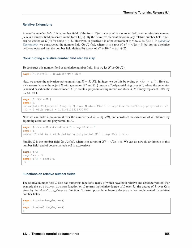
Thematic Tutorials, Release 9.1
Relative Extensions
A relative number field 𝐿 is a number field of the form 𝐾(𝛼), where 𝐾 is a number field, and an absolute numberfield is a number field presented in the form Q(𝛼). By the primitive element theorem, any relative number field 𝐾(𝛼)can be written as Q(𝛽) for some 𝛽 ∈ 𝐿. However, in practice it is often convenient to view 𝐿 as 𝐾(𝛼). In SymbolicExpressions, we constructed the number field Q(
√2)(𝛼), where 𝛼 is a root of 𝑥3 +
√2𝑥 + 5, but not as a relative
field–we obtained just the number field defined by a root of 𝑥6 + 10𝑥3 − 2𝑥2 + 25.
Constructing a relative number field step by step
To construct this number field as a relative number field, first we let 𝐾 be Q(√
2).
sage: K.<sqrt2> = QuadraticField(2)
Next we create the univariate polynomial ring 𝑅 = 𝐾[𝑋]. In Sage, we do this by typing R.<X> = K[]. Here R.<X> means “create the object 𝑅 with generator 𝑋” and K[] means a “polynomial ring over 𝐾”, where the generatoris named based on the aformentioned 𝑋 (to create a polynomial ring in two variables 𝑋,𝑌 simply replace R.<X> byR.<X,Y>).
sage: R.<X> = K[]sage: RUnivariate Polynomial Ring in X over Number Field in sqrt2 with defining polynomial x^→˓2 - 2 with sqrt2 = 1.414213562373095?
Now we can make a polynomial over the number field 𝐾 = Q(√
2), and construct the extension of 𝐾 obtained byadjoining a root of that polynomial to 𝐾.
sage: L.<a> = K.extension(X^3 + sqrt2*X + 5)sage: LNumber Field in a with defining polynomial X^3 + sqrt2*X + 5...
Finally, 𝐿 is the number field Q(√
2)(𝛼), where 𝛼 is a root of 𝑋3 +√
2𝛼 + 5. We can do now do arithmetic in thisnumber field, and of course include
√2 in expressions.
sage: a^3-sqrt2*a - 5sage: a^3 + sqrt2*a-5
Functions on relative number fields
The relative number field 𝐿 also has numerous functions, many of which have both relative and absolute version. Forexample the relative_degree function on 𝐿 returns the relative degree of 𝐿 over 𝐾; the degree of 𝐿 over Q isgiven by the absolute_degree function. To avoid possible ambiguity degree is not implemented for relativenumber fields.
sage: L.relative_degree()3sage: L.absolute_degree()6
12.1. Thematic tutorial document tree 455
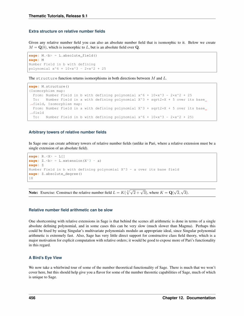
Thematic Tutorials, Release 9.1
Extra structure on relative number fields
Given any relative number field you can also an absolute number field that is isomorphic to it. Below we create𝑀 = Q(𝑏), which is isomorphic to 𝐿, but is an absolute field over Q.
sage: M.<b> = L.absolute_field()sage: MNumber Field in b with definingpolynomial x^6 + 10*x^3 - 2*x^2 + 25
The structure function returns isomorphisms in both directions between 𝑀 and 𝐿.
sage: M.structure()(Isomorphism map:
From: Number Field in b with defining polynomial x^6 + 10*x^3 - 2*x^2 + 25To: Number Field in a with defining polynomial X^3 + sqrt2*X + 5 over its base
→˓field, Isomorphism map:From: Number Field in a with defining polynomial X^3 + sqrt2*X + 5 over its base
→˓fieldTo: Number Field in b with defining polynomial x^6 + 10*x^3 - 2*x^2 + 25)
Arbitrary towers of relative number fields
In Sage one can create arbitrary towers of relative number fields (unlike in Pari, where a relative extension must be asingle extension of an absolute field).
sage: R.<X> = L[]sage: Z.<b> = L.extension(X^3 - a)sage: ZNumber Field in b with defining polynomial X^3 - a over its base fieldsage: Z.absolute_degree()18
Note: Exercise: Construct the relative number field 𝐿 = 𝐾(3√√
2 +√
3), where 𝐾 = Q(√
2,√
3).
Relative number field arithmetic can be slow
One shortcoming with relative extensions in Sage is that behind the scenes all arithmetic is done in terms of a singleabsolute defining polynomial, and in some cases this can be very slow (much slower than Magma). Perhaps thiscould be fixed by using Singular’s multivariate polynomials modulo an appropriate ideal, since Singular polynomialarithmetic is extremely fast. Also, Sage has very little direct support for constructive class field theory, which is amajor motivation for explicit computation with relative orders; it would be good to expose more of Pari’s functionalityin this regard.
A Bird’s Eye View
We now take a whirlwind tour of some of the number theoretical functionality of Sage. There is much that we won’tcover here, but this should help give you a flavor for some of the number theoretic capabilities of Sage, much of whichis unique to Sage.
456 Chapter 12. Documentation
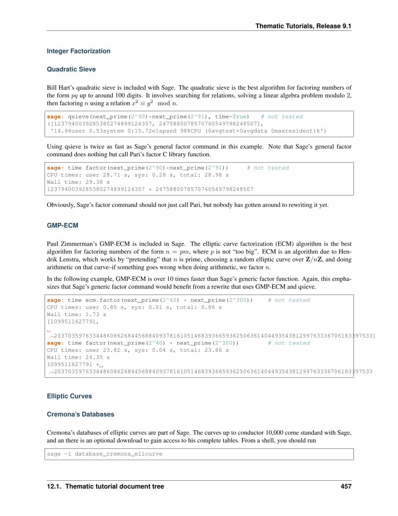
Thematic Tutorials, Release 9.1
Integer Factorization
Quadratic Sieve
Bill Hart’s quadratic sieve is included with Sage. The quadratic sieve is the best algorithm for factoring numbers ofthe form 𝑝𝑞 up to around 100 digits. It involves searching for relations, solving a linear algebra problem modulo 2,then factoring 𝑛 using a relation 𝑥2 ≡ 𝑦2 mod 𝑛.
sage: qsieve(next_prime(2^90)*next_prime(2^91), time=True) # not tested([1237940039285380274899124357, 2475880078570760549798248507],'14.94user 0.53system 0:15.72elapsed 98%CPU (0avgtext+0avgdata 0maxresident)k')
Using qsieve is twice as fast as Sage’s general factor command in this example. Note that Sage’s general factorcommand does nothing but call Pari’s factor C library function.
sage: time factor(next_prime(2^90)*next_prime(2^91)) # not testedCPU times: user 28.71 s, sys: 0.28 s, total: 28.98 sWall time: 29.38 s1237940039285380274899124357 * 2475880078570760549798248507
Obviously, Sage’s factor command should not just call Pari, but nobody has gotten around to rewriting it yet.
GMP-ECM
Paul Zimmerman’s GMP-ECM is included in Sage. The elliptic curve factorization (ECM) algorithm is the bestalgorithm for factoring numbers of the form 𝑛 = 𝑝𝑚, where 𝑝 is not “too big”. ECM is an algorithm due to Hen-drik Lenstra, which works by “pretending” that 𝑛 is prime, choosing a random elliptic curve over Z/𝑛Z, and doingarithmetic on that curve–if something goes wrong when doing arithmetic, we factor 𝑛.
In the following example, GMP-ECM is over 10 times faster than Sage’s generic factor function. Again, this empha-sizes that Sage’s generic factor command would benefit from a rewrite that uses GMP-ECM and qsieve.
sage: time ecm.factor(next_prime(2^40) * next_prime(2^300)) # not testedCPU times: user 0.85 s, sys: 0.01 s, total: 0.86 sWall time: 1.73 s[1099511627791,
→˓2037035976334486086268445688409378161051468393665936250636140449354381299763336706183397533]sage: time factor(next_prime(2^40) * next_prime(2^300)) # not testedCPU times: user 23.82 s, sys: 0.04 s, total: 23.86 sWall time: 24.35 s1099511627791 *→˓2037035976334486086268445688409378161051468393665936250636140449354381299763336706183397533
Elliptic Curves
Cremona’s Databases
Cremona’s databases of elliptic curves are part of Sage. The curves up to conductor 10,000 come standard with Sage,and an there is an optional download to gain access to his complete tables. From a shell, you should run
sage -i database_cremona_ellcurve
12.1. Thematic tutorial document tree 457
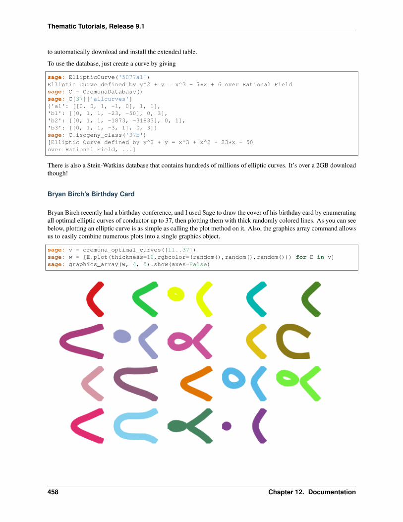
Thematic Tutorials, Release 9.1
to automatically download and install the extended table.
To use the database, just create a curve by giving
sage: EllipticCurve('5077a1')Elliptic Curve defined by y^2 + y = x^3 - 7*x + 6 over Rational Fieldsage: C = CremonaDatabase()sage: C[37]['allcurves']'a1': [[0, 0, 1, -1, 0], 1, 1],'b1': [[0, 1, 1, -23, -50], 0, 3],'b2': [[0, 1, 1, -1873, -31833], 0, 1],'b3': [[0, 1, 1, -3, 1], 0, 3]sage: C.isogeny_class('37b')[Elliptic Curve defined by y^2 + y = x^3 + x^2 - 23*x - 50over Rational Field, ...]
There is also a Stein-Watkins database that contains hundreds of millions of elliptic curves. It’s over a 2GB downloadthough!
Bryan Birch’s Birthday Card
Bryan Birch recently had a birthday conference, and I used Sage to draw the cover of his birthday card by enumeratingall optimal elliptic curves of conductor up to 37, then plotting them with thick randomly colored lines. As you can seebelow, plotting an elliptic curve is as simple as calling the plot method on it. Also, the graphics array command allowsus to easily combine numerous plots into a single graphics object.
sage: v = cremona_optimal_curves([11..37])sage: w = [E.plot(thickness=10,rgbcolor=(random(),random(),random())) for E in v]sage: graphics_array(w, 4, 5).show(axes=False)
458 Chapter 12. Documentation
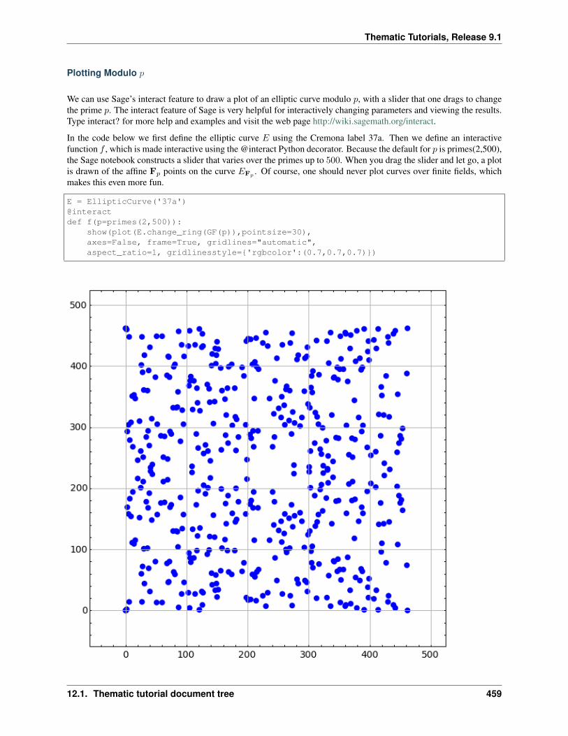
Thematic Tutorials, Release 9.1
Plotting Modulo 𝑝
We can use Sage’s interact feature to draw a plot of an elliptic curve modulo 𝑝, with a slider that one drags to changethe prime 𝑝. The interact feature of Sage is very helpful for interactively changing parameters and viewing the results.Type interact? for more help and examples and visit the web page http://wiki.sagemath.org/interact.
In the code below we first define the elliptic curve 𝐸 using the Cremona label 37a. Then we define an interactivefunction 𝑓 , which is made interactive using the @interact Python decorator. Because the default for 𝑝 is primes(2,500),the Sage notebook constructs a slider that varies over the primes up to 500. When you drag the slider and let go, a plotis drawn of the affine F𝑝 points on the curve 𝐸F𝑝
. Of course, one should never plot curves over finite fields, whichmakes this even more fun.
E = EllipticCurve('37a')@interactdef f(p=primes(2,500)):
show(plot(E.change_ring(GF(p)),pointsize=30),axes=False, frame=True, gridlines="automatic",aspect_ratio=1, gridlinesstyle='rgbcolor':(0.7,0.7,0.7))
12.1. Thematic tutorial document tree 459
Thematic Tutorials, Release 9.1
Schoof-Elkies-Atkin Point Counting
Sage includes sea.gp, which is a fast implementation of the SEA (Schoff-Elkies-Atkin) algorithm for counting thenumber of points on an elliptic curve over F𝑝.
We create the finite field 𝑘 = F𝑝, where 𝑝 is the next prime after 1020. The next prime command uses Pari’s nextprimefunction, but proves primality of the result (unlike Pari which gives only the next probable prime after a number). Sagealso has a next probable prime function.
sage: k = GF(next_prime(10^20))
compute its cardinality, which behind the scenes uses SEA.
sage: E = EllipticCurve_from_j(k.random_element())sage: E.cardinality() # less than a second99999999999371984255
To see how Sage chooses when to use SEA versus other methods, type E.cardinality?? and read the source code. Asof this writing, it simply uses SEA whenever 𝑝 > 1018.
𝑝-adic Regulators
Sage has the world’s best code for computing 𝑝-adic regulators of elliptic curves, thanks to work of David Harveyand Robert Bradshaw. The 𝑝-adic regulator of an elliptic curve 𝐸 at a good ordinary prime 𝑝 is the determinantof the global 𝑝-adic height pairing matrix on the Mordell-Weil group 𝐸(Q). (This has nothing to do with local orArchimedean heights.) This is the analogue of the regulator in the Mazur-Tate-Teitelbaum 𝑝-adic analogue of theBirch and Swinnerton-Dyer conjecture.
In particular, Sage implements Harvey’s improvement on an algorithm of Mazur-Stein-Tate, which builds on KiranKedlaya’s Monsky-Washnitzer approach to computing 𝑝-adic cohomology groups.
We create the elliptic curve with Cremona label 389a, which is the curve of smallest conductor and rank 2. We thencompute both the 5-adic and 997-adic regulators of this curve.
sage: E = EllipticCurve('389a')sage: E.padic_regulator(5, 10)5^2 + 2*5^3 + 2*5^4 + 4*5^5 + 3*5^6 + 4*5^7 + 3*5^8 + 5^9 + O(5^11)sage: E.padic_regulator(997, 10)740*997^2 + 916*997^3 + 472*997^4 + 325*997^5 + 697*997^6
+ 642*997^7 + 68*997^8 + 860*997^9 + 884*997^10 + O(997^11)
Before the new algorithm mentioned above, even computing a 7-adic regulator to 3 digits of precision was a nontrivialcomputational challenge. Now in Sage computing the 100003-adic regulator is routine:
sage: E.padic_regulator(100003,5) # a couple of seconds42582*100003^2 + 35250*100003^3 + 12790*100003^4 + 64078*100003^5 + O(100003^6)
𝑝-adic 𝐿-functions
𝑝-adic 𝐿-functions play a central role in the arithmetic study of elliptic curves. They are 𝑝-adic analogues of complexanalytic 𝐿-function, and their leading coefficient (at 0) is the analogue of 𝐿(𝑟)(𝐸, 1)/Ω𝐸 in the 𝑝-adic analogue of theBirch and Swinnerton-Dyer conjecture. They also appear in theorems of Kato, Schneider, and others that prove partialresults toward 𝑝-adic BSD using Iwasawa theory.
460 Chapter 12. Documentation
Thematic Tutorials, Release 9.1
The implementation in Sage is mainly due to work of myself, Christian Wuthrich, and Robert Pollack. We use Sageto compute the 5-adic 𝐿-series of the elliptic curve 389a of rank 2.
sage: E = EllipticCurve('389a')sage: L = E.padic_lseries(5)sage: L5-adic L-series of Elliptic Curve definedby y^2 + y = x^3 + x^2 - 2*x over Rational Fieldsage: L.series(3)O(5^5) + O(5^2)*T + (4 + 4*5 + O(5^2))*T^2 +(2 + 4*5 + O(5^2))*T^3 + (3 + O(5^2))*T^4 + O(T^5)
Bounding Shafarevich-Tate Groups
Sage implements code to compute numerous explicit bounds on Shafarevich-Tate Groups of elliptic curves. Thisfunctionality is only available in Sage, and uses results Kolyvagin, Kato, Perrin-Riou, etc., and unpublished papers ofWuthrich and me.
sage: E = EllipticCurve('11a1')sage: E.sha().bound() # so only 2 could divide sha[2]sage: E = EllipticCurve('37a1') # so only 2 could divide shasage: E.sha().bound()([2], 1)sage: E = EllipticCurve('389a1')sage: E.sha().bound()(0, 0)
The (0, 0) in the last output above indicates that the Euler systems results of Kolyvagin and Kato give no informationabout finiteness of the Shafarevich-Tate group of the curve 𝐸. In fact, it is an open problem to prove this finiteness,since 𝐸 has rank 2, and finiteness is only known for elliptic curves for which 𝐿(𝐸, 1) = 0 or 𝐿′(𝐸, 1) = 0.
Partial results of Kato, Schneider and others on the 𝑝-adic analogue of the BSD conjecture yield algorithms for bound-ing the 𝑝-part of the Shafarevich-Tate group. These algorithms require as input explicit computation of 𝑝-adic 𝐿-functions, 𝑝-adic regulators, etc., as explained in Stein-Wuthrich. For example, below we use Sage to prove that 5 and7 do not divide the Shafarevich-Tate group of our rank 2 curve 389a.
sage: E = EllipticCurve('389a1')sage: sha = E.sha()sage: sha.p_primary_bound(5) # iwasawa theory ==> 5 doesn't divide sha0sage: sha.p_primary_bound(7) # iwasawa theory ==> 7 doesn't divide sha0
This is consistent with the Birch and Swinnerton-Dyer conjecture, which predicts that the Shafarevich-Tate group istrivial. Below we compute this predicted order, which is the floating point number 1.000000 to some precision. Thatthe result is a floating point number helps emphasize that it is an open problem to show that the conjectural order ofthe Shafarevich-Tate group is even a rational number in general!
sage: E.sha().an()1.00000000000000
12.1. Thematic tutorial document tree 461
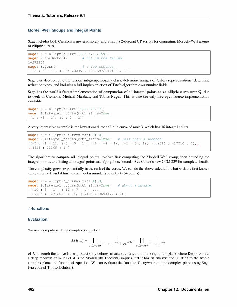
Thematic Tutorials, Release 9.1
Mordell-Weil Groups and Integral Points
Sage includes both Cremona’s mwrank library and Simon’s 2-descent GP scripts for computing Mordell-Weil groupsof elliptic curves.
sage: E = EllipticCurve([1,2,5,17,159])sage: E.conductor() # not in the Tables10272987sage: E.gens() # a few seconds[(-3 : 9 : 1), (-3347/3249 : 1873597/185193 : 1)]
Sage can also compute the torsion subgroup, isogeny class, determine images of Galois representations, determinereduction types, and includes a full implementation of Tate’s algorithm over number fields.
Sage has the world’s fastest implementation of computation of all integral points on an elliptic curve over Q, dueto work of Cremona, Michael Mardaus, and Tobias Nagel. This is also the only free open source implementationavailable.
sage: E = EllipticCurve([1,2,5,7,17])sage: E.integral_points(both_signs=True)[(1 : -9 : 1), (1 : 3 : 1)]
A very impressive example is the lowest conductor elliptic curve of rank 3, which has 36 integral points.
sage: E = elliptic_curves.rank(3)[0]sage: E.integral_points(both_signs=True) # less than 3 seconds[(-3 : -1 : 1), (-3 : 0 : 1), (-2 : -4 : 1), (-2 : 3 : 1), ...(816 : -23310 : 1),→˓(816 : 23309 : 1)]
The algorithm to compute all integral points involves first computing the Mordell-Weil group, then bounding theintegral points, and listing all integral points satisfying those bounds. See Cohen’s new GTM 239 for complete details.
The complexity grows exponentially in the rank of the curve. We can do the above calculation, but with the first knowncurve of rank 4, and it finishes in about a minute (and outputs 64 points).
sage: E = elliptic_curves.rank(4)[0]sage: E.integral_points(both_signs=True) # about a minute[(-10 : 3 : 1), (-10 : 7 : 1), ...(19405 : -2712802 : 1), (19405 : 2693397 : 1)]
𝐿-functions
Evaluation
We next compute with the complex 𝐿-function
𝐿(𝐸, 𝑠) =∏
𝑝|Δ=389
1
1− 𝑎𝑝𝑝−𝑠 + 𝑝𝑝−2𝑠·
∏𝑝|Δ=389
1
1− 𝑎𝑝𝑝−𝑠
of 𝐸. Though the above Euler product only defines an analytic function on the right half plane where Re(𝑠) > 3/2,a deep theorem of Wiles et al. (the Modularity Theorem) implies that it has an analytic continuation to the wholecomplex plane and functional equation. We can evaluate the function 𝐿 anywhere on the complex plane using Sage(via code of Tim Dokchitser).
462 Chapter 12. Documentation
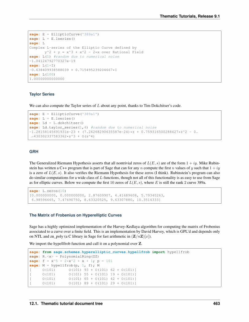
Thematic Tutorials, Release 9.1
sage: E = EllipticCurve('389a1')sage: L = E.lseries()sage: LComplex L-series of the Elliptic Curve defined by
y^2 + y = x^3 + x^2 - 2*x over Rational Fieldsage: L(1) #random due to numerical noise-1.04124792770327e-19sage: L(1+I)-0.638409938588039 + 0.715495239204667*Isage: L(100)1.00000000000000
Taylor Series
We can also compute the Taylor series of 𝐿 about any point, thanks to Tim Dokchitser’s code.
sage: E = EllipticCurve('389a1')sage: L = E.lseries()sage: Ld = L.dokchitser()sage: Ld.taylor_series(1,4) #random due to numerical noise-1.28158145691931e-23 + (7.26268290635587e-24)*z + 0.759316500288427*z^2 - 0.→˓430302337583362*z^3 + O(z^4)
GRH
The Generalized Riemann Hypothesis asserts that all nontrivial zeros of 𝐿(𝐸, 𝑠) are of the form 1 + 𝑖𝑦. Mike Rubin-stein has written a C++ program that is part of Sage that can for any 𝑛 compute the first 𝑛 values of 𝑦 such that 1 + 𝑖𝑦is a zero of 𝐿(𝐸, 𝑠). It also verifies the Riemann Hypothesis for these zeros (I think). Rubinstein’s program can alsodo similar computations for a wide class of 𝐿-functions, though not all of this functionality is as easy to use from Sageas for elliptic curves. Below we compute the first 10 zeros of 𝐿(𝐸, 𝑠), where 𝐸 is still the rank 2 curve 389a.
sage: L.zeros(10)[0.000000000, 0.000000000, 2.87609907, 4.41689608, 5.79340263,6.98596665, 7.47490750, 8.63320525, 9.63307880, 10.3514333]
The Matrix of Frobenius on Hyperelliptic Curves
Sage has a highly optimized implementation of the Harvey-Kedlaya algorithm for computing the matrix of Frobeniusassociated to a curve over a finite field. This is an implementation by David Harvey, which is GPL’d and depends onlyon NTL and zn_poly (a C library in Sage for fast arithmetic in (Z/𝑛Z)[𝑥]).
We import the hypellfrob function and call it on a polynomial over Z.
sage: from sage.schemes.hyperelliptic_curves.hypellfrob import hypellfrobsage: R.<x> = PolynomialRing(ZZ)sage: f = x^5 + 2*x^2 + x + 1; p = 101sage: M = hypellfrob(p, 1, f); M[ O(101) O(101) 93 + O(101) 62 + O(101)][ O(101) O(101) 55 + O(101) 19 + O(101)][ O(101) O(101) 65 + O(101) 42 + O(101)][ O(101) O(101) 89 + O(101) 29 + O(101)]
12.1. Thematic tutorial document tree 463
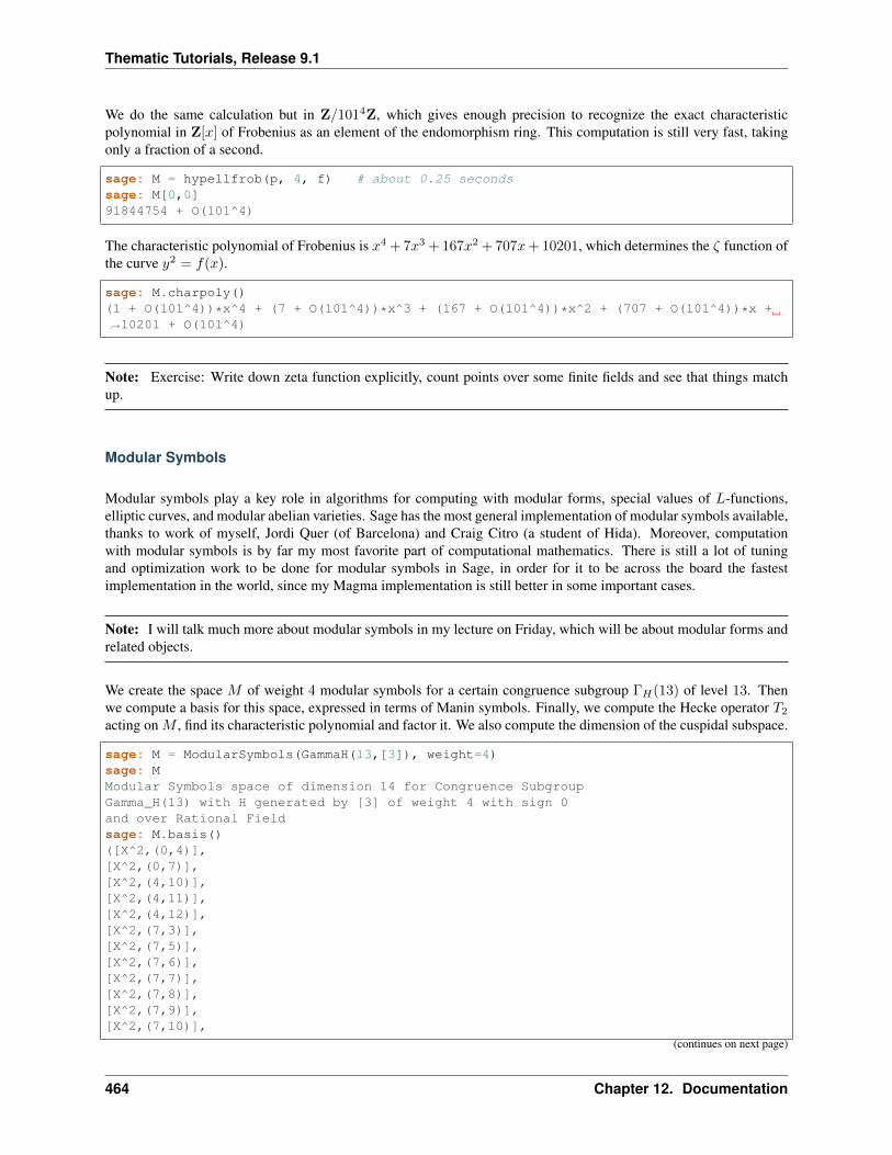
Thematic Tutorials, Release 9.1
We do the same calculation but in Z/1014Z, which gives enough precision to recognize the exact characteristicpolynomial in Z[𝑥] of Frobenius as an element of the endomorphism ring. This computation is still very fast, takingonly a fraction of a second.
sage: M = hypellfrob(p, 4, f) # about 0.25 secondssage: M[0,0]91844754 + O(101^4)
The characteristic polynomial of Frobenius is 𝑥4 + 7𝑥3 + 167𝑥2 + 707𝑥+ 10201, which determines the 𝜁 function ofthe curve 𝑦2 = 𝑓(𝑥).
sage: M.charpoly()(1 + O(101^4))*x^4 + (7 + O(101^4))*x^3 + (167 + O(101^4))*x^2 + (707 + O(101^4))*x +→˓10201 + O(101^4)
Note: Exercise: Write down zeta function explicitly, count points over some finite fields and see that things matchup.
Modular Symbols
Modular symbols play a key role in algorithms for computing with modular forms, special values of 𝐿-functions,elliptic curves, and modular abelian varieties. Sage has the most general implementation of modular symbols available,thanks to work of myself, Jordi Quer (of Barcelona) and Craig Citro (a student of Hida). Moreover, computationwith modular symbols is by far my most favorite part of computational mathematics. There is still a lot of tuningand optimization work to be done for modular symbols in Sage, in order for it to be across the board the fastestimplementation in the world, since my Magma implementation is still better in some important cases.
Note: I will talk much more about modular symbols in my lecture on Friday, which will be about modular forms andrelated objects.
We create the space 𝑀 of weight 4 modular symbols for a certain congruence subgroup Γ𝐻(13) of level 13. Thenwe compute a basis for this space, expressed in terms of Manin symbols. Finally, we compute the Hecke operator 𝑇2acting on 𝑀 , find its characteristic polynomial and factor it. We also compute the dimension of the cuspidal subspace.
sage: M = ModularSymbols(GammaH(13,[3]), weight=4)sage: MModular Symbols space of dimension 14 for Congruence SubgroupGamma_H(13) with H generated by [3] of weight 4 with sign 0and over Rational Fieldsage: M.basis()([X^2,(0,4)],[X^2,(0,7)],[X^2,(4,10)],[X^2,(4,11)],[X^2,(4,12)],[X^2,(7,3)],[X^2,(7,5)],[X^2,(7,6)],[X^2,(7,7)],[X^2,(7,8)],[X^2,(7,9)],[X^2,(7,10)],
(continues on next page)
464 Chapter 12. Documentation
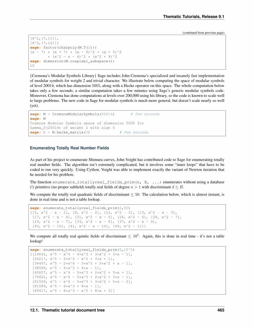
Thematic Tutorials, Release 9.1
(continued from previous page)
[X^2,(7,11)],[X^2,(7,12)])sage: factor(charpoly(M.T(2)))(x - 7) * (x + 7) * (x - 9)^2 * (x + 5)^2
* (x^2 - x - 4)^2 * (x^2 + 9)^2sage: dimension(M.cuspidal_subspace())10
Cremona’s Modular Symbols Library Sage includes John Cremona’s specialized and insanely fast implementationof modular symbols for weight 2 and trivial character. We illustrate below computing the space of modular symbolsof level 20014, which has dimension 5005, along with a Hecke operator on this space. The whole computation belowtakes only a few seconds; a similar computation takes a few minutes using Sage’s generic modular symbols code.Moreover, Cremona has done computations at levels over 200,000 using his library, so the code is known to scale wellto large problems. The new code in Sage for modular symbols is much more general, but doesn’t scale nearly so well(yet).
sage: M = CremonaModularSymbols(20014) # few secondssage: MCremona Modular Symbols space of dimension 5005 forGamma_0(20014) of weight 2 with sign 0sage: t = M.hecke_matrix(3) # few seconds
Enumerating Totally Real Number Fields
As part of his project to enumerate Shimura curves, John Voight has contributed code to Sage for enumerating totallyreal number fields. The algorithm isn’t extremely complicated, but it involves some “inner loops” that have to becoded to run very quickly. Using Cython, Voight was able to implement exactly the variant of Newton iteration thathe needed for his problem.
The function enumerate_totallyreal_fields_prim(n, B, ...) enumerates without using a database(!) primitive (no proper subfield) totally real fields of degree 𝑛 > 1 with discriminant 𝑑 ≤ 𝐵.
We compute the totally real quadratic fields of discriminant ≤ 50. The calculation below, which is almost instant, isdone in real time and is not a table lookup.
sage: enumerate_totallyreal_fields_prim(2,50)[[5, x^2 - x - 1], [8, x^2 - 2], [12, x^2 - 3], [13, x^2 - x - 3],[17, x^2 - x - 4], [21, x^2 - x - 5], [24, x^2 - 6], [28, x^2 - 7],[29, x^2 - x - 7], [33, x^2 - x - 8], [37, x^2 - x - 9],[40, x^2 - 10], [41, x^2 - x - 10], [44, x^2 - 11]]
We compute all totally real quintic fields of discriminant ≤ 105. Again, this is done in real time - it’s not a tablelookup!
sage: enumerate_totallyreal_fields_prim(5,10^5)[[14641, x^5 - x^4 - 4*x^3 + 3*x^2 + 3*x - 1],[24217, x^5 - 5*x^3 - x^2 + 3*x + 1],[36497, x^5 - 2*x^4 - 3*x^3 + 5*x^2 + x - 1],[38569, x^5 - 5*x^3 + 4*x - 1],[65657, x^5 - x^4 - 5*x^3 + 2*x^2 + 5*x + 1],[70601, x^5 - x^4 - 5*x^3 + 2*x^2 + 3*x - 1],[81509, x^5 - x^4 - 5*x^3 + 3*x^2 + 5*x - 2],[81589, x^5 - 6*x^3 + 8*x - 1],[89417, x^5 - 6*x^3 - x^2 + 8*x + 3]]
12.1. Thematic tutorial document tree 465
Thematic Tutorials, Release 9.1
Bernoulli Numbers
Mathematica and Pari
From the Mathematica website:
“Today We Broke the Bernoulli Record: From the Analytical Engine to Mathematica April 29, 2008Oleksandr Pavlyk, Kernel Technology A week ago, I took our latest development version of Mathematica,and I typed BernoulliB[10^7]. And then I waited. Yesterday–5 days, 23 hours, 51 minutes, and 37seconds later–I got the result!”
Tom Boothby did that same computation in Sage, which uses Pari’s bernfrac command that uses evaluation of 𝜁 andfactorial to high precision, and it took 2 days, 12 hours.
David Harvey’s bernmm
Then David Harvey came up with an entirely new algorithm that parallelizes well. He gives these timings for comput-ing 𝐵107 on his machine (it takes 59 minutes, 57 seconds on my 16-core 1.8ghz Opteron box):
PARI: 75 h, Mathematica: 142 h
bernmm (1 core) = 11.1 h, bernmm (10 cores) = 1.3 h
“Running on 10 cores for 5.5 days, I [David Harvey] computed [the Bernoulli number] 𝐵𝑘 for 𝑘 = 108,which I believe is a new record. Essentially it’s the multimodular algorithm I suggested earlier on thisthread, but I figured out some tricks to optimise the crap out of the computation of 𝐵𝑘mod𝑝.”
So now Sage is the fastest in the world for large Bernoulli numbers. The timings below are on a 24-core 2.66GhzXeon box.
sage: w1 = bernoulli(100000, num_threads=16) # 0.9 seconds wall timesage: w2 = bernoulli(100000, algorithm='pari') # long time (6s on sage.math, 2011)sage: w1 == w2 # long timeTrue
Polynomial Arithmetic
FLINT: Univariate Polynomial Arithmetic
Sage uses Bill Hart and David Harvey’s GPL’d Flint C library for arithmetic in Z[𝑥]. Its main claim to fame is thatit is the world’s fastest for polynomial multiplication, e.g., in the benchmark below it is faster than NTL and Magmaon some systems (though such benchmarks of course change as software improves). Behind the scenes Flint containssome carefully tuned discrete Fourier transform code.
sage: Rflint = PolynomialRing(ZZ, 'x')sage: f = Rflint([ZZ.random_element(2^64) for _ in [1..32]])sage: g = Rflint([ZZ.random_element(2^64) for _ in [1..32]])sage: timeit('f*g') # random output625 loops, best of 3: 105 microseconds per loopsage: Rntl = PolynomialRing(ZZ, 'x', implementation='NTL')sage: f = Rntl([ZZ.random_element(2^64) for _ in [1..32]])sage: g = Rntl([ZZ.random_element(2^64) for _ in [1..32]])sage: timeit('f*g') # random output625 loops, best of 3: 310 microseconds per loop
(continues on next page)
466 Chapter 12. Documentation
Thematic Tutorials, Release 9.1
(continued from previous page)
sage: ff = magma(f); gg = magma(g) #optional - magmasage: s = 'time v := [%s * %s : i in [1..10^5]];'%(ff.name(), gg.name()) #optional -→˓magmasage: magma.eval(s) #optional - magma'Time: ...'
Singular: Multivariate Polynomial Arithmetic
Multivariate polynomial arithmetic in many cases uses Singular in library mode (due to Martin Albrecht), which isquite fast. For example, below we do the Fateman benchmark over the finite field of order 32003, and compare thetiming with Magma.
sage: P.<x,y,z> = GF(32003)[]sage: p = (x+y+z+1)^10sage: q = p+1sage: timeit('p*q') # random output125 loops, best of 3: 1.53 ms per loop
sage: p = (x+y+z+1)^20sage: q = p+1sage: timeit('p*q') # not tested - timeout if SAGE_DEBUG=yes5 loops, best of 3: 384 ms per loop
sage: pp = magma(p); qq = magma(q) #optional - magmasage: s = 'time w := %s*%s;'%(pp.name(),qq.name()) #optional - magmasage: magma.eval(s) #optional - magma'Time: ...'
Modular Forms
This section is about computing with modular forms, modular symbols, and modular abelian varieties. Most of theSage functionality we describe below is new code written for Sage by myself, Craig Citro, Robert Bradshaw, and JordiQuer in consultation with John Cremona. It has much overlap in functionality with the modular forms code in Magma,which I developed during 1998-2004.
Modular Forms and Hecke Operators
Congruence subgroups
Definition
A congruence subgroup is a subgroup of the group SL2(Z) of determinant ±1 integer matrices that contains
Γ(𝑁) = Ker(SL2(Z)→ SL2(Z/𝑁Z))
for some positive integer 𝑁 . Since Γ(𝑁) has finite index in SL2(Z), all congruence subgroups have finite index. Theconverse is not true, though in many other settings it is true (see [paper of Serre]).
The inverse image Γ0(𝑁) of the subgroup of upper triangular matrices in SL2(Z/𝑁Z) is a congruence subgroup, asis the inverse image Γ1(𝑁) of the subgroup of matrices of the form ( 1 *
0 1 ). Also, for any subgroup 𝐻 ⊂ (Z/𝑁Z)*, the
12.1. Thematic tutorial document tree 467
Thematic Tutorials, Release 9.1
inverse image Γ𝐻(𝑁) of the subgroup of SL2(Z/𝑁Z) of all elements of the form ( 𝑎 *0 𝑑 ) with 𝑑 ∈ 𝐻 is a congruence
subgroup.
We can create each of the above congruence subgroups in Sage, using the Gamma0, Gamma1, and GammaH com-mands.
sage: Gamma0(8)Congruence Subgroup Gamma0(8)sage: Gamma1(13)Congruence Subgroup Gamma1(13)sage: GammaH(11,[3])Congruence Subgroup Gamma_H(11) with H generated by [3]
The second argument to the GammaH command is a list of generators of the subgroup 𝐻 of (Z/𝑁Z)*.
Generators
Sage can compute a list of generators for these subgroups. The algorithm Sage uses is a straightforward genericprocedure that uses coset representatives for the congruence subgroup (which are easy to enumerate) to obtain a list ofgenerators [[ref my modular forms book]].
The list of generators Sage computes is unfortunately large. Improving this would be an excellent Sage developmentproject, which would involve much beautiful mathematics.
UPDATE (March 2012): The project referred to above has been carried out (by several people, notably HartmutMonien, building on earlier work of Chris Kurth). Sage now uses a much more advanced algorithm based on Fareysymbols which calculates a minimal set of generators.
sage: Gamma0(2).gens()([1 1] [ 1 -1][0 1], [ 2 -1])sage: Gamma0(2).gens(algorithm="todd-coxeter") # the old implementation([1 1] [-1 0] [ 1 -1] [ 1 -1] [-1 1][0 1], [ 0 -1], [ 0 1], [ 2 -1], [-2 1])sage: len(Gamma1(13).gens())15
Modular Forms
Definition
A modular form on a congruence subgroup Γ of integer weight 𝑘 is a holomorphic function 𝑓(𝑧) on the upper halfplane
h* = 𝑧 ∈ C : ℑ(𝑧) > 0 ∪Q ∪ 𝑖∞
such that for every matrix(𝑎 𝑏𝑐 𝑑
)∈ Γ, we have
𝑓
(𝑎𝑧 + 𝑏
𝑐𝑧 + 𝑑
)= (𝑐𝑧 + 𝑑)𝑘𝑓(𝑧).
468 Chapter 12. Documentation
Thematic Tutorials, Release 9.1
A cusp form is a modular form that vanishes at all of the cusps Q ∪ 𝑖∞.
If Γ contains Γ1(𝑁) for some 𝑁 , then ( 1 10 1 ) ∈ Γ, so the modular form condition implies that 𝑓(𝑧) = 𝑓(𝑧 + 1). This,
coupled with the holomorphicity condition, implies that 𝑓(𝑧) has a Fourier expansion
𝑓(𝑧) =
∞∑𝑛=0
𝑎𝑛𝑒2𝜋𝑖𝑛𝑧
with 𝑎𝑛 ∈ C. We let 𝑞 = 𝑒2𝜋𝑖𝑧 , and call 𝑓 =∑∞
𝑛=0 𝑎𝑛𝑞𝑛 the 𝑞-expansion of 𝑓 .
Creation in Sage
Henceforth we assume that Γ is either Γ1(𝑁), Γ0(𝑁), or Γ𝐻(𝑁) for some 𝐻 and 𝑁 . The complex vector space𝑀𝑘(Γ) of all modular forms of weight 𝑘 on Γ is a finite dimensional vector space.
We create the space 𝑀𝑘(Γ) in Sage by typing ModularForms(G, k) where 𝐺 is the congruence subgroup and 𝑘is the weight.
sage: ModularForms(Gamma0(25), 4)Modular Forms space of dimension 11 for ...sage: S = CuspForms(Gamma0(25),4, prec=15); SCuspidal subspace of dimension 5 of Modular Forms space ...sage: S.basis()[q + q^9 - 8*q^11 - 8*q^14 + O(q^15),q^2 - q^7 - q^8 - 7*q^12 + 7*q^13 + O(q^15),q^3 + q^7 - 2*q^8 - 6*q^12 - 5*q^13 + O(q^15),q^4 - q^6 - 3*q^9 + 5*q^11 - 2*q^14 + O(q^15),q^5 - 4*q^10 + O(q^15)]
Dimension Formulas
Sage computes the dimensions of all these spaces using simple arithmetic formulas instead of actually computingbases for the spaces in question. In fact, Sage has the most general collection of modular forms dimension formulas ofany software; type help(sage.modular.dims) to see a list of arithmetic functions that are used to implementthese dimension formulas.
sage: ModularForms(Gamma1(949284), 456).dimension()11156973844800sage: a = [dimension_cusp_forms(Gamma0(N),2) for N in [1..25]]; a[0, 0, ..., 1, 0, 0, 1, 1, 0, 1, 0, 1, 1, 1, 2, 2, 1, 0]sage: oeis(a) # optional - internet0: A001617: Genus of modular group Gamma_0(n). Or, genus of modular curve X_0(n).
Sage doesn’t have simple formulas for dimensions of spaces of modular forms of weight 1, since such formulasperhaps do not exist.
Diamond Bracket Operators
The space 𝑀𝑘(Γ1(𝑁)) is equipped with an action of (Z/𝑁Z)* by diamond bracket operators ⟨𝑑⟩, and this induces adecomposition
𝑀𝑘(Γ1(𝑁)) =⨁
𝜀:(Z/𝑁Z)*→C*
𝑀𝑘(𝑁, 𝜀),
12.1. Thematic tutorial document tree 469
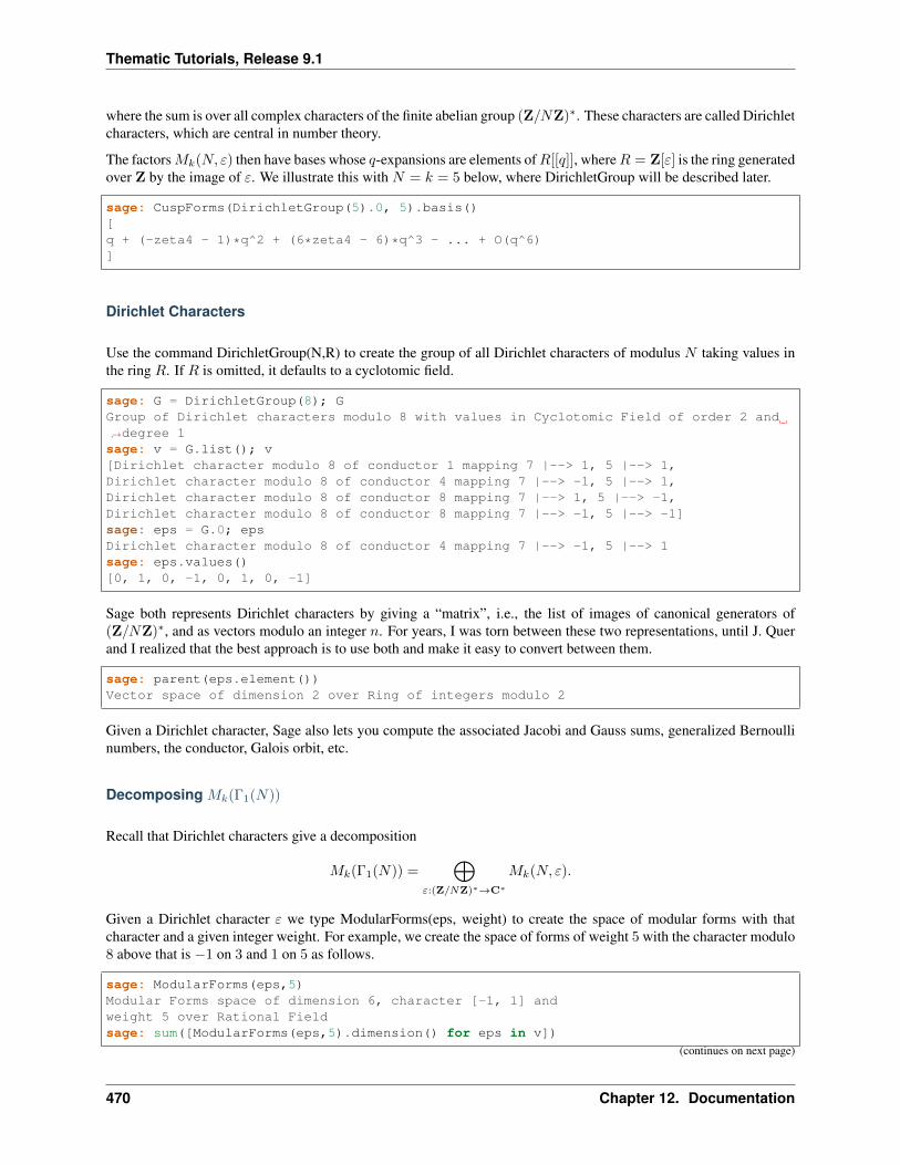
Thematic Tutorials, Release 9.1
where the sum is over all complex characters of the finite abelian group (Z/𝑁Z)*. These characters are called Dirichletcharacters, which are central in number theory.
The factors𝑀𝑘(𝑁, 𝜀) then have bases whose 𝑞-expansions are elements of𝑅[[𝑞]], where𝑅 = Z[𝜀] is the ring generatedover Z by the image of 𝜀. We illustrate this with 𝑁 = 𝑘 = 5 below, where DirichletGroup will be described later.
sage: CuspForms(DirichletGroup(5).0, 5).basis()[q + (-zeta4 - 1)*q^2 + (6*zeta4 - 6)*q^3 - ... + O(q^6)]
Dirichlet Characters
Use the command DirichletGroup(N,R) to create the group of all Dirichlet characters of modulus 𝑁 taking values inthe ring 𝑅. If 𝑅 is omitted, it defaults to a cyclotomic field.
sage: G = DirichletGroup(8); GGroup of Dirichlet characters modulo 8 with values in Cyclotomic Field of order 2 and→˓degree 1sage: v = G.list(); v[Dirichlet character modulo 8 of conductor 1 mapping 7 |--> 1, 5 |--> 1,Dirichlet character modulo 8 of conductor 4 mapping 7 |--> -1, 5 |--> 1,Dirichlet character modulo 8 of conductor 8 mapping 7 |--> 1, 5 |--> -1,Dirichlet character modulo 8 of conductor 8 mapping 7 |--> -1, 5 |--> -1]sage: eps = G.0; epsDirichlet character modulo 8 of conductor 4 mapping 7 |--> -1, 5 |--> 1sage: eps.values()[0, 1, 0, -1, 0, 1, 0, -1]
Sage both represents Dirichlet characters by giving a “matrix”, i.e., the list of images of canonical generators of(Z/𝑁Z)*, and as vectors modulo an integer 𝑛. For years, I was torn between these two representations, until J. Querand I realized that the best approach is to use both and make it easy to convert between them.
sage: parent(eps.element())Vector space of dimension 2 over Ring of integers modulo 2
Given a Dirichlet character, Sage also lets you compute the associated Jacobi and Gauss sums, generalized Bernoullinumbers, the conductor, Galois orbit, etc.
Decomposing 𝑀𝑘(Γ1(𝑁))
Recall that Dirichlet characters give a decomposition
𝑀𝑘(Γ1(𝑁)) =⨁
𝜀:(Z/𝑁Z)*→C*
𝑀𝑘(𝑁, 𝜀).
Given a Dirichlet character 𝜀 we type ModularForms(eps, weight) to create the space of modular forms with thatcharacter and a given integer weight. For example, we create the space of forms of weight 5 with the character modulo8 above that is −1 on 3 and 1 on 5 as follows.
sage: ModularForms(eps,5)Modular Forms space of dimension 6, character [-1, 1] andweight 5 over Rational Fieldsage: sum([ModularForms(eps,5).dimension() for eps in v])
(continues on next page)
470 Chapter 12. Documentation
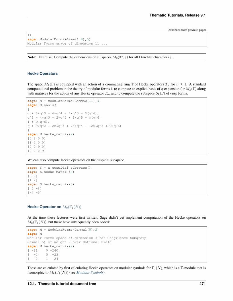
Thematic Tutorials, Release 9.1
(continued from previous page)
11sage: ModularForms(Gamma1(8),5)Modular Forms space of dimension 11 ...
Note: Exercise: Compute the dimensions of all spaces 𝑀2(37, 𝜀) for all Dirichlet characters 𝜀.
Hecke Operators
The space 𝑀𝑘(Γ) is equipped with an action of a commuting ring T of Hecke operators 𝑇𝑛 for 𝑛 ≥ 1. A standardcomputational problem in the theory of modular forms is to compute an explicit basis of 𝑞-expansion for 𝑀𝑘(Γ) alongwith matrices for the action of any Hecke operator 𝑇𝑛, and to compute the subspace 𝑆𝑘(Γ) of cusp forms.
sage: M = ModularForms(Gamma0(11),4)sage: M.basis()[q + 3*q^3 - 6*q^4 - 7*q^5 + O(q^6),q^2 - 4*q^3 + 2*q^4 + 8*q^5 + O(q^6),1 + O(q^6),q + 9*q^2 + 28*q^3 + 73*q^4 + 126*q^5 + O(q^6)]sage: M.hecke_matrix(2)[0 2 0 0][1 2 0 0][0 0 9 0][0 0 0 9]
We can also compute Hecke operators on the cuspidal subspace.
sage: S = M.cuspidal_subspace()sage: S.hecke_matrix(2)[0 2][1 2]sage: S.hecke_matrix(3)[ 3 -8][-4 -5]
Hecke Operator on 𝑀𝑘(Γ1(𝑁))
At the time these lectures were first written, Sage didn’t yet implement computation of the Hecke operators on𝑀𝑘(Γ1(𝑁)), but these have subsequently been added:
sage: M = ModularForms(Gamma1(5),2)sage: MModular Forms space of dimension 3 for Congruence SubgroupGamma1(5) of weight 2 over Rational Fieldsage: M.hecke_matrix(2)[ -21 0 -240][ -2 0 -23][ 2 1 24]
These are calculated by first calculating Hecke operators on modular symbols for Γ1(𝑁), which is a T-module that isisomorphic to 𝑀𝑘(Γ1(𝑁)) (see Modular Symbols).
12.1. Thematic tutorial document tree 471
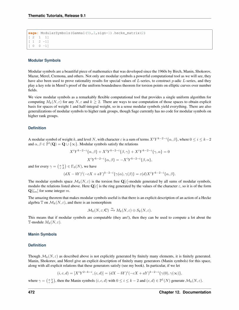
Thematic Tutorials, Release 9.1
sage: ModularSymbols(Gamma1(5),2,sign=1).hecke_matrix(2)[ 2 1 1][ 1 2 -1][ 0 0 -1]
Modular Symbols
Modular symbols are a beautiful piece of mathematics that was developed since the 1960s by Birch, Manin, Shokorov,Mazur, Merel, Cremona, and others. Not only are modular symbols a powerful computational tool as we will see, theyhave also been used to prove rationality results for special values of 𝐿-series, to construct 𝑝-adic 𝐿-series, and theyplay a key role in Merel’s proof of the uniform boundedness theorem for torsion points on elliptic curves over numberfields.
We view modular symbols as a remarkably flexible computational tool that provides a single uniform algorithm forcomputing 𝑀𝑘(𝑁, 𝜀) for any 𝑁, 𝜀 and 𝑘 ≥ 2. There are ways to use computation of those spaces to obtain explicitbasis for spaces of weight 1 and half-integral weight, so in a sense modular symbols yield everything. There are alsogeneralizations of modular symbols to higher rank groups, though Sage currently has no code for modular symbols onhigher rank groups.
Definition
A modular symbol of weight 𝑘, and level𝑁 , with character 𝜀 is a sum of terms𝑋𝑖𝑌 𝑘−2−𝑖𝛼, 𝛽, where 0 ≤ 𝑖 ≤ 𝑘−2and 𝛼, 𝛽 ∈ P1(Q) = Q ∪ ∞. Modular symbols satisfy the relations
𝑋𝑖𝑌 𝑘−2−𝑖𝛼, 𝛽+𝑋𝑖𝑌 𝑘−2−𝑖𝛽, 𝛾+𝑋𝑖𝑌 𝑘−2−𝑖𝛾, 𝛼 = 0
𝑋𝑖𝑌 𝑘−2−𝑖𝛼, 𝛽 = −𝑋𝑖𝑌 𝑘−2−𝑖𝛽, 𝛼,and for every 𝛾 =
(𝑎 𝑏𝑐 𝑑
)∈ Γ0(𝑁), we have
(𝑑𝑋 − 𝑏𝑌 )𝑖(−𝑐𝑋 + 𝑎𝑌 )𝑘−2−𝑖𝛾(𝛼), 𝛾(𝛽) = 𝜀(𝑑)𝑋𝑖𝑌 𝑘−2−𝑖𝛼, 𝛽.
The modular symbols space ℳ𝑘(𝑁, 𝜀) is the torsion free Q[𝜀]-module generated by all sums of modular symbols,modulo the relations listed above. Here Q[𝜀] is the ring generated by the values of the character 𝜀, so it is of the formQ[𝜁𝑚] for some integer 𝑚.
The amazing theorem that makes modular symbols useful is that there is an explicit description of an action of a Heckealgebra T onℳ𝑘(𝑁, 𝜀), and there is an isomorphism
ℳ𝑘(𝑁, 𝜀;C)≈−→𝑀𝑘(𝑁, 𝜀)⊕ 𝑆𝑘(𝑁, 𝜀).
This means that if modular symbols are computable (they are!), then they can be used to compute a lot about theT-module 𝑀𝑘(𝑁, 𝜀).
Manin Symbols
Definition
Thoughℳ𝑘(𝑁, 𝜀) as described above is not explicitly generated by finitely many elements, it is finitely generated.Manin, Shokoruv, and Merel give an explicit description of finitely many generators (Manin symbols) for this space,along with all explicit relations that these generators satisfy (see my book). In particular, if we let
(𝑖, 𝑐, 𝑑) = [𝑋𝑖𝑌 2−𝑘−𝑖, (𝑐, 𝑑)] = (𝑑𝑋 − 𝑏𝑌 )𝑖(−𝑐𝑋 + 𝑎𝑌 )𝑘−2−𝑖𝛾(0), 𝛾(∞),
where 𝛾 =(𝑎 𝑏𝑐 𝑑
), then the Manin symbols (𝑖, 𝑐, 𝑑) with 0 ≤ 𝑖 ≤ 𝑘 − 2 and (𝑐, 𝑑) ∈ P1(𝑁) generateℳ𝑘(𝑁, 𝜀).
472 Chapter 12. Documentation
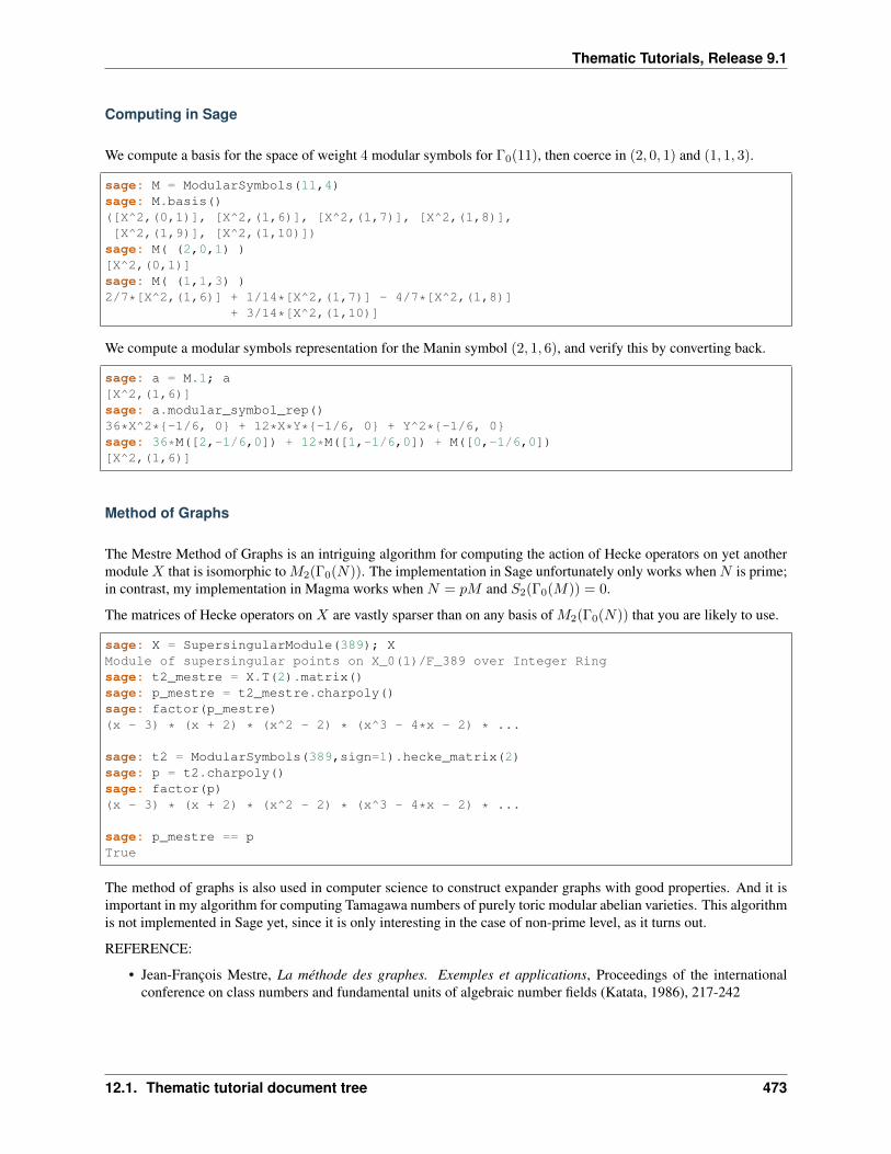
Thematic Tutorials, Release 9.1
Computing in Sage
We compute a basis for the space of weight 4 modular symbols for Γ0(11), then coerce in (2, 0, 1) and (1, 1, 3).
sage: M = ModularSymbols(11,4)sage: M.basis()([X^2,(0,1)], [X^2,(1,6)], [X^2,(1,7)], [X^2,(1,8)],[X^2,(1,9)], [X^2,(1,10)])
sage: M( (2,0,1) )[X^2,(0,1)]sage: M( (1,1,3) )2/7*[X^2,(1,6)] + 1/14*[X^2,(1,7)] - 4/7*[X^2,(1,8)]
+ 3/14*[X^2,(1,10)]
We compute a modular symbols representation for the Manin symbol (2, 1, 6), and verify this by converting back.
sage: a = M.1; a[X^2,(1,6)]sage: a.modular_symbol_rep()36*X^2*-1/6, 0 + 12*X*Y*-1/6, 0 + Y^2*-1/6, 0sage: 36*M([2,-1/6,0]) + 12*M([1,-1/6,0]) + M([0,-1/6,0])[X^2,(1,6)]
Method of Graphs
The Mestre Method of Graphs is an intriguing algorithm for computing the action of Hecke operators on yet anothermodule𝑋 that is isomorphic to𝑀2(Γ0(𝑁)). The implementation in Sage unfortunately only works when𝑁 is prime;in contrast, my implementation in Magma works when 𝑁 = 𝑝𝑀 and 𝑆2(Γ0(𝑀)) = 0.
The matrices of Hecke operators on 𝑋 are vastly sparser than on any basis of 𝑀2(Γ0(𝑁)) that you are likely to use.
sage: X = SupersingularModule(389); XModule of supersingular points on X_0(1)/F_389 over Integer Ringsage: t2_mestre = X.T(2).matrix()sage: p_mestre = t2_mestre.charpoly()sage: factor(p_mestre)(x - 3) * (x + 2) * (x^2 - 2) * (x^3 - 4*x - 2) * ...
sage: t2 = ModularSymbols(389,sign=1).hecke_matrix(2)sage: p = t2.charpoly()sage: factor(p)(x - 3) * (x + 2) * (x^2 - 2) * (x^3 - 4*x - 2) * ...
sage: p_mestre == pTrue
The method of graphs is also used in computer science to construct expander graphs with good properties. And it isimportant in my algorithm for computing Tamagawa numbers of purely toric modular abelian varieties. This algorithmis not implemented in Sage yet, since it is only interesting in the case of non-prime level, as it turns out.
REFERENCE:
• Jean-François Mestre, La méthode des graphes. Exemples et applications, Proceedings of the internationalconference on class numbers and fundamental units of algebraic number fields (Katata, 1986), 217-242
12.1. Thematic tutorial document tree 473
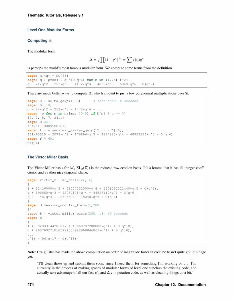
Thematic Tutorials, Release 9.1
Level One Modular Forms
Computing ∆
The modular form
∆ = 𝑞∏
(1− 𝑞𝑛)24 =∑
𝜏(𝑛)𝑞𝑛
is perhaps the world’s most famous modular form. We compute some terms from the definition.
sage: R.<q> = QQ[[]]sage: q * prod( 1-q^n+O(q^6) for n in (1..5) )^24q - 24*q^2 + 252*q^3 - 1472*q^4 + 4830*q^5 - 6048*q^6 + O(q^7)
There are much better ways to compute ∆, which amount to just a few polynomial multiplications over Z.
sage: D = delta_qexp(10^5) # less than 10 secondssage: D[:10]q - 24*q^2 + 252*q^3 - 1472*q^4 + ...sage: [p for p in primes(10^5) if D[p] % p == 0][2, 3, 5, 7, 2411]sage: D[2411]4542041100095889012sage: f = eisenstein_series_qexp(12,6) - D[:6]; f691/65520 + 2073*q^2 + 176896*q^3 + 4197825*q^4 + 48823296*q^5 + O(q^6)sage: f % 691O(q^6)
The Victor Miller Basis
The Victor Miller basis for 𝑀𝑘(SL2(Z)) is the reduced row echelon basis. It’s a lemma that it has all integer coeffi-cients, and a rather nice diagonal shape.
sage: victor_miller_basis(24, 6)[1 + 52416000*q^3 + 39007332000*q^4 + 6609020221440*q^5 + O(q^6),q + 195660*q^3 + 12080128*q^4 + 44656110*q^5 + O(q^6),q^2 - 48*q^3 + 1080*q^4 - 15040*q^5 + O(q^6)]sage: dimension_modular_forms(1,200)17sage: B = victor_miller_basis(200, 18) #5 secondssage: B[1 + 79288314420681734048660707200000*q^17 + O(q^18),q + 2687602718106772837928968846869*q^17 + O(q^18),...q^16 + 96*q^17 + O(q^18)]
Note: Craig Citro has made the above computation an order of magnitude faster in code he hasn’t quite got into Sageyet.
“I’ll clean those up and submit them soon, since I need them for something I’m working on . . . I’mcurrently in the process of making spaces of modular forms of level one subclass the existing code, andactually take advantage of all our fast 𝐸𝑘 and ∆ computation code, as well as cleaning things up a bit.”
474 Chapter 12. Documentation
Thematic Tutorials, Release 9.1
Half Integral Weight Forms
Basmaji’s Algorithm
Basmaji (page 55 of his Essen thesis, “Ein Algorithmus zur Berechnung von Hecke-Operatoren und Anwendungenauf modulare Kurven”, http://wstein.org/scans/papers/basmaji/).
Let 𝑆 = 𝑆𝑘+1(𝜀) be the space of cusp forms of even integer weight 𝑘 + 1 and character 𝜀 = 𝜒𝜓(𝑘+1)/2, where 𝜓 isthe nontrivial mod-4 Dirichlet character. Let 𝑈 be the subspace of 𝑆 × 𝑆 of elements (𝑎, 𝑏) such that Θ2𝑎 = Θ3𝑏.Then 𝑈 is isomorphic to 𝑆𝑘/2(𝜒) via the map (𝑎, 𝑏) ↦→ 𝑎/Θ3.
This algorithm is implemented in Sage. I’m sure it could be implemented in a way that is much faster than the currentimplementation. . .
sage: half_integral_weight_modform_basis(DirichletGroup(16,QQ).1, 3, 10)[]sage: half_integral_weight_modform_basis(DirichletGroup(16,QQ).1, 5, 10)[q - 2*q^3 - 2*q^5 + 4*q^7 - q^9 + O(q^10)]sage: half_integral_weight_modform_basis(DirichletGroup(16*7).0^2,3,30)[q - 2*q^2 - q^9 + 2*q^14 + 6*q^18 - 2*q^21 - 4*q^22 - q^25 + O(q^30),q^2 - q^14 - 3*q^18 + 2*q^22 + O(q^30),q^4 - q^8 - q^16 + q^28 + O(q^30), q^7 - 2*q^15 + O(q^30)]
Generators for Rings of Modular Forms
Computing Generators
For any congruence subgroup Γ, the direct sum
𝑀(Γ) =⨁𝑘≥0
𝑀𝑘(Γ)
is a ring, since the product of modular forms 𝑓 ∈ 𝑀𝑘(Γ) and 𝑔 ∈ 𝑀𝑘′(Γ) is an element 𝑓𝑔 ∈ 𝑀𝑘+𝑘′(Γ). Sage cancompute likely generators for rings of modular forms, but currently doesn’t prove any of these results.
We verify the statement proved in Serre’s “A Course in Arithmetic” that 𝐸4 and 𝐸6 generate the space of level onemodular forms.
sage: ModularFormsRing(SL2Z).generators(prec=4)[(4, 1 + 240*q + 2160*q^2 + 6720*q^3 + O(q^4)),(6, 1 - 504*q - 16632*q^2 - 122976*q^3 + O(q^4))]
Have you ever wondered which forms generate the ring 𝑀(Γ0(2))? It turns out that one form of weight 2 and oneform of weight 4 suffice.
sage: ModularFormsRing(Gamma0(2)).generators(prec=12)[(2, 1 + 24*q + 24*q^2 + 96*q^3 + 24*q^4 + 144*q^5 + 96*q^6 + 192*q^7 + 24*q^8 +→˓312*q^9 + 144*q^10 + 288*q^11 + O(q^12)),(4, 1 + 240*q^2 + 2160*q^4 + 6720*q^6 + 17520*q^8 + 30240*q^10 + O(q^12))]
Here’s generators for 𝑀(Γ0(3)). Notice that elements of weight 6 are now required, in addition to weights 2 and 4.
sage: ModularFormsRing(Gamma0(3)).generators()[(2, 1 + 12*q + 36*q^2 + 12*q^3 + 84*q^4 + 72*q^5 + 36*q^6 + 96*q^7 + 180*q^8 + 12*q^→˓9 + O(q^10)),
(continues on next page)
12.1. Thematic tutorial document tree 475
Thematic Tutorials, Release 9.1
(continued from previous page)
(4, 1 + 240*q^3 + 2160*q^6 + 6720*q^9 + O(q^10)),(6, 1 - 504*q^3 - 16632*q^6 - 122976*q^9 + O(q^10))]
(Note: As of 2012, updates to the code mean that the output of this test is not quite the same as it was in 2008, but ofcourse there are multiple equally valid answers.)
We can also handle rings of modular forms for odd congruence subgroups, but with the usual caveat that we can’tcalculate forms of weight 1. So these are elements generating the graded ring of forms of weight 0 or ≥ 2.
sage: ModularFormsRing(Gamma1(3)).generators()[(2, 1 + 12*q + 36*q^2 + 12*q^3 + 84*q^4 + 72*q^5 + 36*q^6 + 96*q^7 + 180*q^8 + 12*q^→˓9 + O(q^10)),(3, 1 + 54*q^2 + 72*q^3 + 432*q^5 + 270*q^6 + 918*q^8 + 720*q^9 + O(q^10)),(3, q + 3*q^2 + 9*q^3 + 13*q^4 + 24*q^5 + 27*q^6 + 50*q^7 + 51*q^8 + 81*q^9 + O(q^→˓10)),(4, 1 + 240*q^3 + 2160*q^6 + 6720*q^9 + O(q^10))]
𝐿-series
𝐿-series of ∆
Thanks to wrapping work of Jennifer Balakrishnan of M.I.T., we can compute explicitly with the 𝐿-series of themodular form ∆. Like for elliptic curves, behind these scenes this uses Dokchitsers 𝐿-functions calculation Pariprogram.
sage: L = delta_lseries(); LL-series of conductor 1 and weight 12sage: L(1)0.0374412812685155
𝐿-series of a Cusp Form
In some cases we can also compute with 𝐿-series attached to a cusp form.
sage: f = CuspForms(2,8).newforms()[0]sage: L = f.lseries()sage: L(1)0.0884317737041015sage: L(0.5)0.0296568512531983
𝐿-series of a General Newform is Not Implemented
Unfortunately, computing with the 𝐿-series of a general newform is not yet implemented.
sage: S = CuspForms(23,2); SCuspidal subspace of dimension 2 of Modular Forms space ofdimension 3 for Congruence Subgroup Gamma0(23) of weight2 over Rational Fieldsage: f = S.newforms('a')[0]; fq + a0*q^2 + (-2*a0 - 1)*q^3 + (-a0 - 1)*q^4 + 2*a0*q^5 + O(q^6)
476 Chapter 12. Documentation
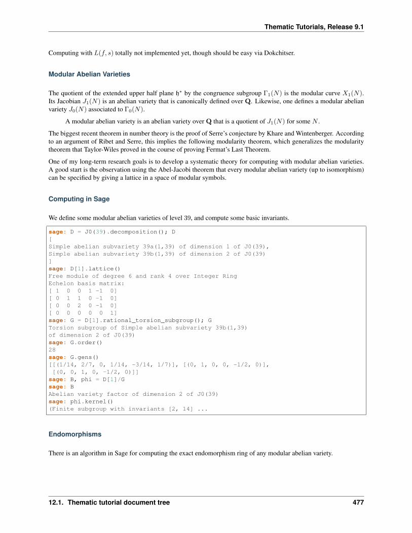
Thematic Tutorials, Release 9.1
Computing with 𝐿(𝑓, 𝑠) totally not implemented yet, though should be easy via Dokchitser.
Modular Abelian Varieties
The quotient of the extended upper half plane h* by the congruence subgroup Γ1(𝑁) is the modular curve 𝑋1(𝑁).Its Jacobian 𝐽1(𝑁) is an abelian variety that is canonically defined over Q. Likewise, one defines a modular abelianvariety 𝐽0(𝑁) associated to Γ0(𝑁).
A modular abelian variety is an abelian variety over Q that is a quotient of 𝐽1(𝑁) for some 𝑁 .
The biggest recent theorem in number theory is the proof of Serre’s conjecture by Khare and Wintenberger. Accordingto an argument of Ribet and Serre, this implies the following modularity theorem, which generalizes the modularitytheorem that Taylor-Wiles proved in the course of proving Fermat’s Last Theorem.
One of my long-term research goals is to develop a systematic theory for computing with modular abelian varieties.A good start is the observation using the Abel-Jacobi theorem that every modular abelian variety (up to isomorphism)can be specified by giving a lattice in a space of modular symbols.
Computing in Sage
We define some modular abelian varieties of level 39, and compute some basic invariants.
sage: D = J0(39).decomposition(); D[Simple abelian subvariety 39a(1,39) of dimension 1 of J0(39),Simple abelian subvariety 39b(1,39) of dimension 2 of J0(39)]sage: D[1].lattice()Free module of degree 6 and rank 4 over Integer RingEchelon basis matrix:[ 1 0 0 1 -1 0][ 0 1 1 0 -1 0][ 0 0 2 0 -1 0][ 0 0 0 0 0 1]sage: G = D[1].rational_torsion_subgroup(); GTorsion subgroup of Simple abelian subvariety 39b(1,39)of dimension 2 of J0(39)sage: G.order()28sage: G.gens()[[(1/14, 2/7, 0, 1/14, -3/14, 1/7)], [(0, 1, 0, 0, -1/2, 0)],[(0, 0, 1, 0, -1/2, 0)]]
sage: B, phi = D[1]/Gsage: BAbelian variety factor of dimension 2 of J0(39)sage: phi.kernel()(Finite subgroup with invariants [2, 14] ...
Endomorphisms
There is an algorithm in Sage for computing the exact endomorphism ring of any modular abelian variety.
12.1. Thematic tutorial document tree 477
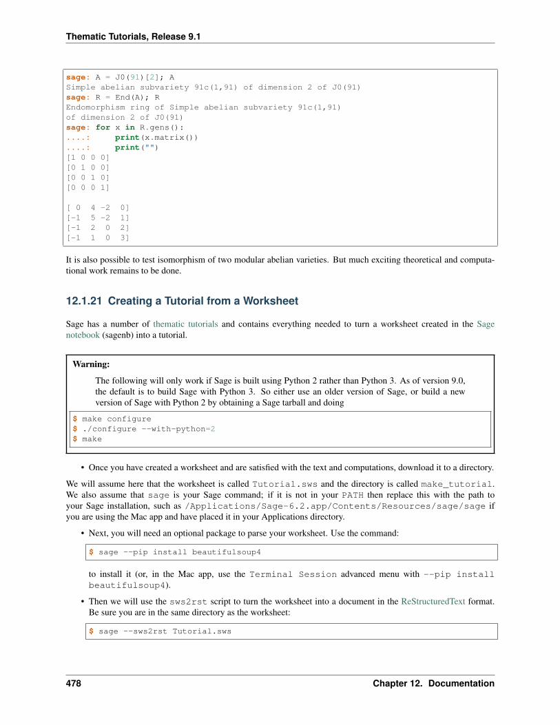
Thematic Tutorials, Release 9.1
sage: A = J0(91)[2]; ASimple abelian subvariety 91c(1,91) of dimension 2 of J0(91)sage: R = End(A); REndomorphism ring of Simple abelian subvariety 91c(1,91)of dimension 2 of J0(91)sage: for x in R.gens():....: print(x.matrix())....: print("")[1 0 0 0][0 1 0 0][0 0 1 0][0 0 0 1]
[ 0 4 -2 0][-1 5 -2 1][-1 2 0 2][-1 1 0 3]
It is also possible to test isomorphism of two modular abelian varieties. But much exciting theoretical and computa-tional work remains to be done.
12.1.21 Creating a Tutorial from a Worksheet
Sage has a number of thematic tutorials and contains everything needed to turn a worksheet created in the Sagenotebook (sagenb) into a tutorial.
Warning:
The following will only work if Sage is built using Python 2 rather than Python 3. As of version 9.0,the default is to build Sage with Python 3. So either use an older version of Sage, or build a newversion of Sage with Python 2 by obtaining a Sage tarball and doing
$ make configure$ ./configure --with-python=2$ make
• Once you have created a worksheet and are satisfied with the text and computations, download it to a directory.
We will assume here that the worksheet is called Tutorial.sws and the directory is called make_tutorial.We also assume that sage is your Sage command; if it is not in your PATH then replace this with the path toyour Sage installation, such as /Applications/Sage-6.2.app/Contents/Resources/sage/sage ifyou are using the Mac app and have placed it in your Applications directory.
• Next, you will need an optional package to parse your worksheet. Use the command:
$ sage --pip install beautifulsoup4
to install it (or, in the Mac app, use the Terminal Session advanced menu with --pip installbeautifulsoup4).
• Then we will use the sws2rst script to turn the worksheet into a document in the ReStructuredText format.Be sure you are in the same directory as the worksheet:
$ sage --sws2rst Tutorial.sws
478 Chapter 12. Documentation
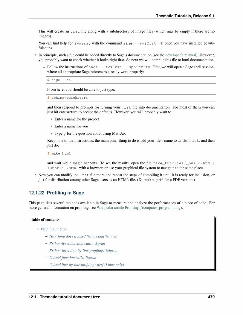
Thematic Tutorials, Release 9.1
This will create an .rst file along with a subdirectory of image files (which may be empty if there are noimages).
You can find help for sws2rst with the command sage --sws2rst -h once you have installed beauti-fulsoup4.
• In principle, such a file could be added directly to Sage’s documentation (see the developer’s manual). However,you probably want to check whether it looks right first. So next we will compile this file to html documentation.
– Follow the instructions of sage --sws2rst --sphinxify. First, we will open a Sage shell session,where all appropriate Sage references already work properly:
$ sage --sh
From here, you should be able to just type:
$ sphinx-quickstart
and then respond to prompts for turning your .rst file into documentation. For most of them you canjust hit enter/return to accept the defaults. However, you will probably want to
* Enter a name for the project
* Enter a name for you
* Type y for the question about using MathJax
Keep note of the instructions; the main other thing to do is add your file’s name to index.rst, and thenjust do:
$ make html
and wait while magic happens. To see the results, open the file make_tutorial/_build/html/Tutorial.html with a browser, or use your graphical file system to navigate to the same place.
• Now you can modify the .rst file more and repeat the steps of compiling it until it is ready for inclusion, orjust for distribution among other Sage users as an HTML file. (Do make pdf for a PDF version.)
12.1.22 Profiling in Sage
This page lists several methods available in Sage to measure and analyze the performances of a piece of code. Formore general information on profiling, see Wikipedia article Profiling_(computer_programming).
Table of contents
• Profiling in Sage
– How long does it take? %time and %timeit
– Python-level function calls: %prun
– Python-level line-by-line profiling: %lprun
– C-level function calls: %crun
– C-level line-by-line profiling: perf (Linux only)
12.1. Thematic tutorial document tree 479
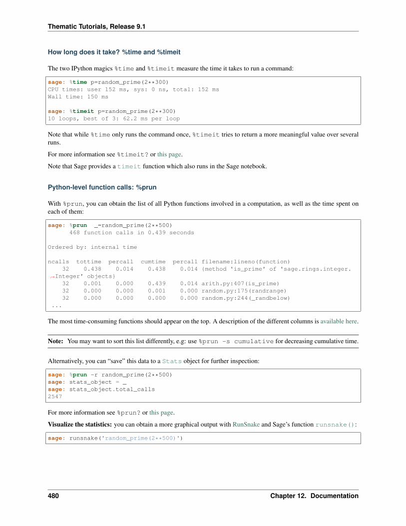
Thematic Tutorials, Release 9.1
How long does it take? %time and %timeit
The two IPython magics %time and %timeit measure the time it takes to run a command:
sage: %time p=random_prime(2**300)CPU times: user 152 ms, sys: 0 ns, total: 152 msWall time: 150 ms
sage: %timeit p=random_prime(2**300)10 loops, best of 3: 62.2 ms per loop
Note that while %time only runs the command once, %timeit tries to return a more meaningful value over severalruns.
For more information see %timeit? or this page.
Note that Sage provides a timeit function which also runs in the Sage notebook.
Python-level function calls: %prun
With %prun, you can obtain the list of all Python functions involved in a computation, as well as the time spent oneach of them:
sage: %prun _=random_prime(2**500)468 function calls in 0.439 seconds
Ordered by: internal time
ncalls tottime percall cumtime percall filename:lineno(function)32 0.438 0.014 0.438 0.014 method 'is_prime' of 'sage.rings.integer.
→˓Integer' objects32 0.001 0.000 0.439 0.014 arith.py:407(is_prime)32 0.000 0.000 0.001 0.000 random.py:175(randrange)32 0.000 0.000 0.000 0.000 random.py:244(_randbelow)
...
The most time-consuming functions should appear on the top. A description of the different columns is available here.
Note: You may want to sort this list differently, e.g: use %prun -s cumulative for decreasing cumulative time.
Alternatively, you can “save” this data to a Stats object for further inspection:
sage: %prun -r random_prime(2**500)sage: stats_object = _sage: stats_object.total_calls2547
For more information see %prun? or this page.
Visualize the statistics: you can obtain a more graphical output with RunSnake and Sage’s function runsnake():
sage: runsnake('random_prime(2**500)')
480 Chapter 12. Documentation
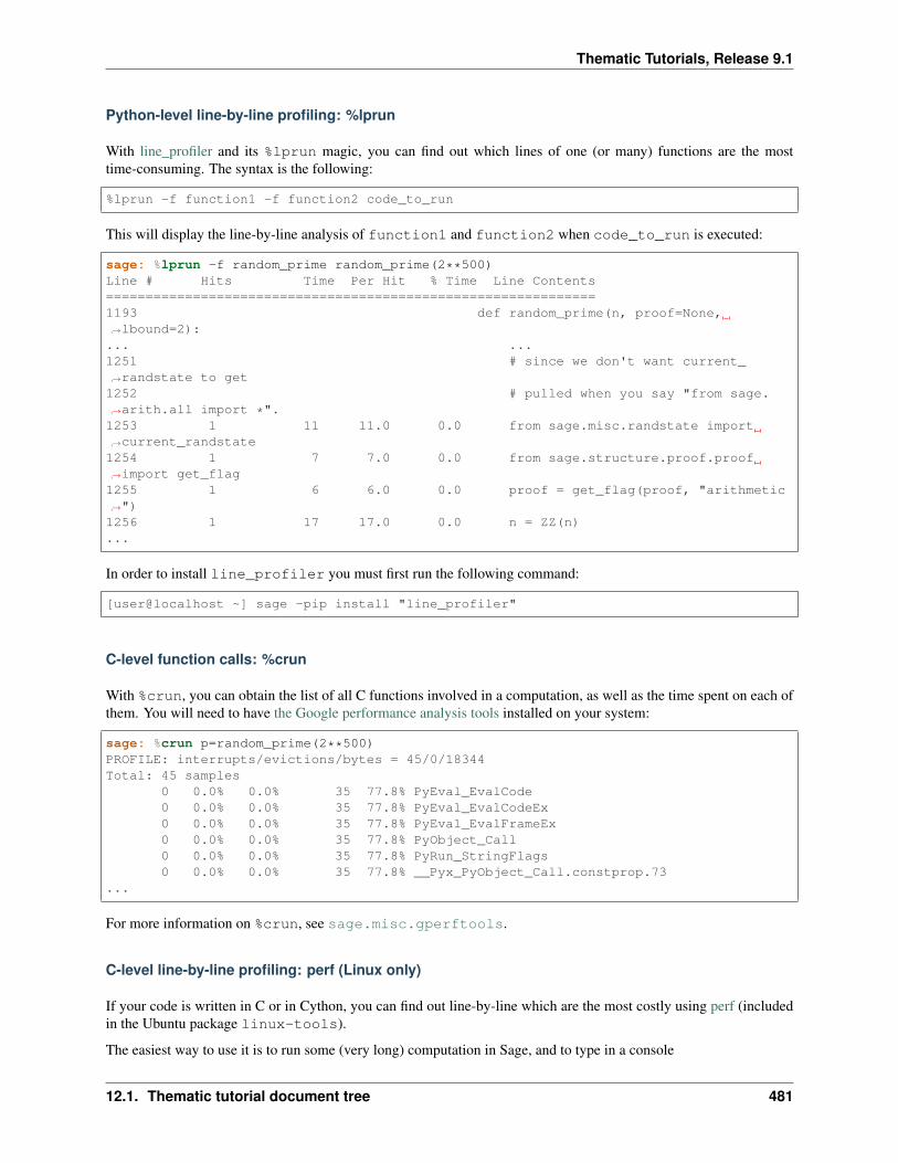
Thematic Tutorials, Release 9.1
Python-level line-by-line profiling: %lprun
With line_profiler and its %lprun magic, you can find out which lines of one (or many) functions are the mosttime-consuming. The syntax is the following:
%lprun -f function1 -f function2 code_to_run
This will display the line-by-line analysis of function1 and function2 when code_to_run is executed:
sage: %lprun -f random_prime random_prime(2**500)Line # Hits Time Per Hit % Time Line Contents==============================================================1193 def random_prime(n, proof=None,→˓lbound=2):... ...1251 # since we don't want current_→˓randstate to get1252 # pulled when you say "from sage.→˓arith.all import *".1253 1 11 11.0 0.0 from sage.misc.randstate import→˓current_randstate1254 1 7 7.0 0.0 from sage.structure.proof.proof→˓import get_flag1255 1 6 6.0 0.0 proof = get_flag(proof, "arithmetic→˓")1256 1 17 17.0 0.0 n = ZZ(n)...
In order to install line_profiler you must first run the following command:
[user@localhost ~] sage -pip install "line_profiler"
C-level function calls: %crun
With %crun, you can obtain the list of all C functions involved in a computation, as well as the time spent on each ofthem. You will need to have the Google performance analysis tools installed on your system:
sage: %crun p=random_prime(2**500)PROFILE: interrupts/evictions/bytes = 45/0/18344Total: 45 samples
0 0.0% 0.0% 35 77.8% PyEval_EvalCode0 0.0% 0.0% 35 77.8% PyEval_EvalCodeEx0 0.0% 0.0% 35 77.8% PyEval_EvalFrameEx0 0.0% 0.0% 35 77.8% PyObject_Call0 0.0% 0.0% 35 77.8% PyRun_StringFlags0 0.0% 0.0% 35 77.8% __Pyx_PyObject_Call.constprop.73
...
For more information on %crun, see sage.misc.gperftools.
C-level line-by-line profiling: perf (Linux only)
If your code is written in C or in Cython, you can find out line-by-line which are the most costly using perf (includedin the Ubuntu package linux-tools).
The easiest way to use it is to run some (very long) computation in Sage, and to type in a console
12.1. Thematic tutorial document tree 481
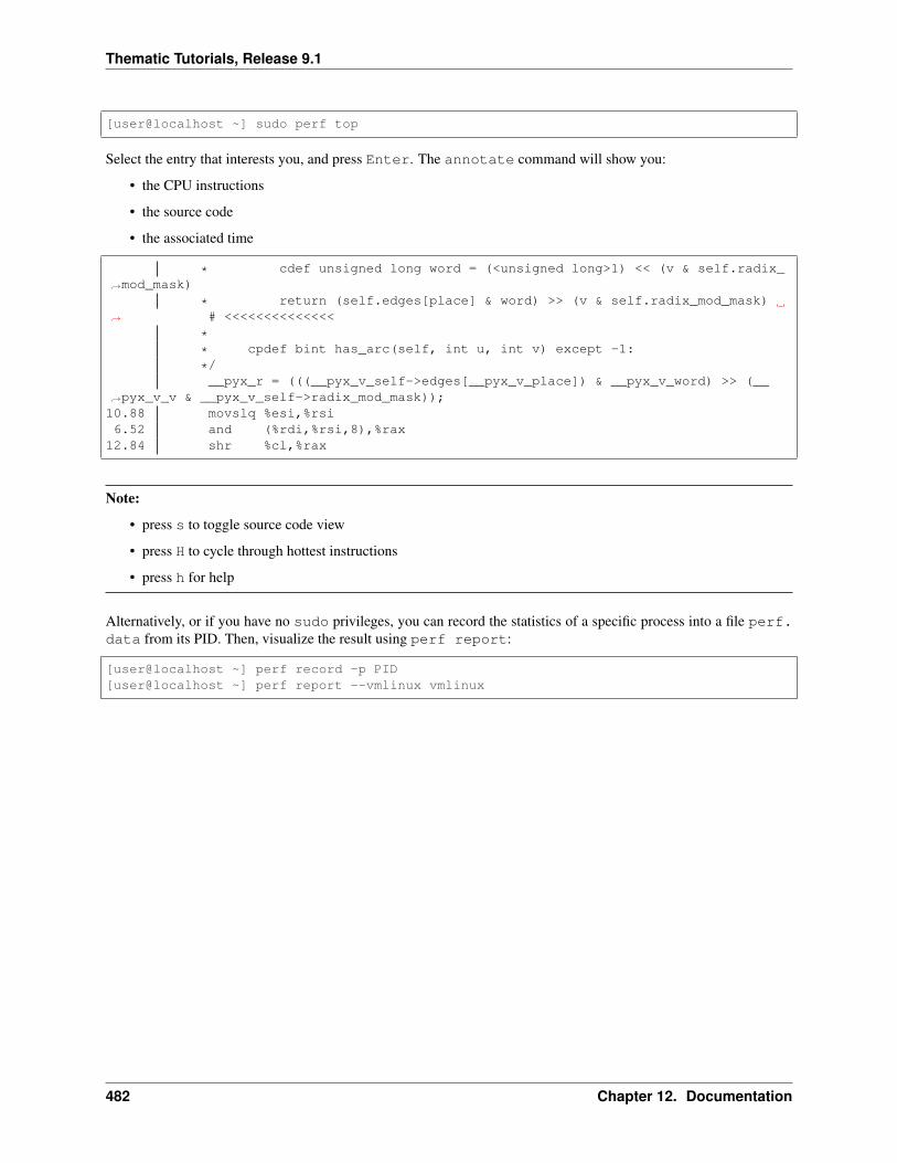
Thematic Tutorials, Release 9.1
[user@localhost ~] sudo perf top
Select the entry that interests you, and press Enter. The annotate command will show you:
• the CPU instructions
• the source code
• the associated time
* cdef unsigned long word = (<unsigned long>1) << (v & self.radix_→˓mod_mask)
* return (self.edges[place] & word) >> (v & self.radix_mod_mask)→˓ # <<<<<<<<<<<<<<
** cpdef bint has_arc(self, int u, int v) except -1:
*/__pyx_r = (((__pyx_v_self->edges[__pyx_v_place]) & __pyx_v_word) >> (__
→˓pyx_v_v & __pyx_v_self->radix_mod_mask));10.88 movslq %esi,%rsi6.52 and (%rdi,%rsi,8),%rax
12.84 shr %cl,%rax
Note:
• press s to toggle source code view
• press H to cycle through hottest instructions
• press h for help
Alternatively, or if you have no sudo privileges, you can record the statistics of a specific process into a file perf.data from its PID. Then, visualize the result using perf report:
[user@localhost ~] perf record -p PID[user@localhost ~] perf report --vmlinux vmlinux
482 Chapter 12. Documentation
BIBLIOGRAPHY
[Stanley2013] Richard Stanley. Algebraic Combinatorics: walks, trees, tableaux and more, Springer, first edition,2013.
[Bidigare1997] Thomas Patrick Bidigare. Hyperplane arrangement face algebras and their associated Markov chains.ProQuest LLC, Ann Arbor, MI, 1997. Thesis (Ph.D.) University of Michigan.
[Brown2000] Kenneth S. Brown. Semigroups, rings, and Markov chains. J. Theoret. Probab., 13(3):871-938, 2000.
[AKS2013] Arvind Ayyer, Steven Klee, Anne Schilling. Combinatorial Markov chains on linear extensions J. Alge-braic Combinatorics, doi:10.1007/s10801-013-0470-9, arXiv 1205.7074.
[Levine2014] Lionel Levine. Threshold state and a conjecture of Poghosyan, Poghosyan, Priezzhev and Ruelle, Com-munications in Mathematical Physics. arXiv 1402.3283
[BN] Matthew Baker, Serguei Norine, Riemann-Roch and Abel-Jacobi Theory on a Finite Graph, Advances inMathematics 215 (2007), 766–788.
[BTW] Per Bak, Chao Tang and Kurt Wiesenfeld (1987). Self-organized criticality: an explanation of 1/f noise,Physical Review Letters 60: 381–384; Wikipedia article Bak-Tang-Wiesenfeld_sandpile.
[CRS] Robert Cori, Dominique Rossin, and Bruno Salvy, Polynomial ideals for sandpiles and their Gröbnerbases, Theoretical Computer Science, 276 (2002) no. 1–2, 1–15.
[H] Alexander E. Holroyd, Lionel Levine, Karola Meszaros, Yuval Peres, James Propp, David B. Wilson,Chip-Firing and Rotor-Routing on Directed Graphs, arXiv 0801.3306. An older version of this paperappears in In and out of Equilibrium II, Eds. V. Sidoravicius, M. E. Vares, in the Series Progress inProbability, Birkhauser (2008).
[PPW2013] D. Perkinson, J. Perlman, and J. Wilmes. Primer for the algebraic geometry of sandpiles. Tropical andNon-Archimedean Geometry, Contemp. Math., 605, Amer. Math. Soc., Providence, RI, 2013. arXiv1112.6163.
[Bourbaki46] Nicolas Bourbaki. Lie Groups and Lie Algebras: Chapters 4-6. Springer, reprint edition, 1998.
[BumpNakasuji2010] D. Bump and M. Nakasuji. Casselman’s basis of Iwahori vectors and the Bruhat order. arXiv1002.2996, arXiv 1002.2996.
[BumpSchilling2017] D. Bump and A. Schilling, Crystal bases: representations and combinatorics, World Scientific,2017.
[Carrell1994] J. B. Carrell. The Bruhat graph of a Coxeter group, a conjecture of Deodhar, and rational smoothness ofSchubert varieties. In Algebraic Groups and Their Generalizations: Classical Methods, AMS Proceedingsof Symposia in Pure Mathematics, 56, 53–61, 1994.
[Deodhar1977] V. V. Deodhar. Some characterizations of Bruhat ordering on a Coxeter group and determination ofthe relative Moebius function. Inventiones Mathematicae, 39(2):187–198, 1977.
483
Thematic Tutorials, Release 9.1
[Dyer1993] M. J. Dyer. The nil Hecke ring and Deodhar’s conjecture on Bruhat intervals. Inventiones Mathematicae,111(1):571–574, 1993.
[Dynkin1952] E. B. Dynkin, Semisimple subalgebras of semisimple Lie algebras. (Russian) Mat. Sbornik N.S.30(72):349–462, 1952.
[FauserEtAl2006] B. Fauser, P. D. Jarvis, R. C. King, and B. G. Wybourne. New branching rules induced by plethysm.Journal of Physics A. 39(11):2611–2655, 2006.
[Fulton1997] W. Fulton. Young Tableaux. Cambridge University Press, 1997.
[FourierEtAl2009] G. Fourier, M. Okado, A. Schilling. Kirillov–Reshetikhin crystal for nonexceptional types. Ad-vances in Mathematics, 222:1080–1116, 2009.
[FourierEtAl2010] G. Fourier, M. Okado, A. Schilling. Perfectness of Kirillov-Reshetikhin crystals for nonexcep-tional types. Contemp. Math., 506:127–143, 2010.
[HatayamaEtAl2001] G. Hatayama, A. Kuniba, M. Okado, T. Takagi, Z. Tsuboi. Paths, crystals and fermionic for-mulae. in MathPhys Odyssey 2001, in : Prog. Math. Phys., vol 23, Birkhauser Boston, Boston, MA 2002,pp. 205–272.
[HainesEtAl2009] T. J. Haines, R. E. Kottwitz, and A. Prasad. Iwahori-Hecke Algebras. arXiv math/0309168.
[HongKang2002] J. Hong and S.-J. Kang. Introduction to Quantum Groups and Crystal Bases. AMS Graduate Studiesin Mathematics, American Mathematical Society, 2002.
[HongLee2008] J. Hong and H. Lee. Young tableaux and crystal 𝐵(∞) for finite simple Lie algebras. J. Algebra,320:3680–3693, 2008.
[HoweEtAl2005] R. Howe, E.-C.Tan, and J. F. Willenbring. Stable branching rules for classical symmetric pairs.Transactions of the American Mathematical Society, 357(4):1601–1626, 2005.
[Iwahori1964] N. Iwahori. On the structure of a Hecke ring of a Chevalley group over a finite field. J. Fac. Sci. Univ.Tokyo Sect. I, 10:215–236, 1964.
[JayneMisra2014] R. Jayne and K. Misra, On multiplicities of maximal weights of 𝑠𝑙(𝑛)-modules. Algebr. Represent.Theory 17 (2014), no. 4, 1303–1321. arXiv 1309.4969.
[Jimbo1986] M. A. Jimbo. 𝑞-analogue of 𝑈(gl(𝑁 + 1)), Hecke algebra, and the Yang-Baxter equation. Lett. Math.Phys, 11(3):247–252, 1986.
[JonesEtAl2010] B. Jones, A. Schilling. Affine structures and a tableau model for E_6 crystals J. Algebra, 324:2512-2542, 2010.
[Joseph1995] A. Joseph. Quantum Groups and Their Primitive Ideals. Springer-Verlag, 1995.
[Kac] Victor G. Kac. Infinite Dimensional Lie algebras, Cambridge University Press, third edition, 1994.
[KacPeterson] Kac and Peterson. Infinite-dimensional Lie algebras, theta functions and modular forms. Adv. in Math.53 (1984), no. 2, 125-264.
[KKMMNN1992] S-J. Kang, M. Kashiwara, K. C. Misra, T. Miwa, T. Nakashima, A. Nakayashiki. Affine crystalsand vertex models. Int. J. Mod. Phys. A 7 (suppl. 1A): 449–484, 1992.
[KKS2007] S.-J. Kang, J.-A. Kim, and D.-U. Shin. Modified Nakajima monomials and the crystal 𝐵(∞). J. Algebra,308 (2007), 524-535.
[Kashiwara1993] M. Kashiwara. The crystal base and Littelmann’s refined Demazure character formula. Duke Math.J., 71(3):839–858, 1993.
[Kashiwara1995] M. Kashiwara. On crystal bases. Representations of groups (Banff, AB, 1994), 155–197, CMSConference Proceedings, 16, American Mathematical Society, Providence, RI, 1995.
[KashiwaraNakashima1994] M. Kashiwara and T. Nakashima. Crystal graphs for representations of the 𝑞-analogueof classical Lie algebras. Journal Algebra, 165(2):295–345, 1994.
484 Bibliography
Thematic Tutorials, Release 9.1
[KMPS] Kass, Moody, Patera and Slansky, Affine Lie algebras, weight multiplicities, and branching rules. Vols. 1,2. University of California Press, Berkeley, CA, 1990.
[KimShin2010] J.-A. Kim and D.-U. Shin. Generalized Young walls and crystal bases for quantum affine algebra oftype 𝐴. Proc. Amer. Math. Soc., 138(11):3877–3889, 2010.
[KimLeeOh2017] Jang Soo Kim, Kyu-Hwan Lee and Se-Jin Oh, Weight multiplicities and Young tableaux throughaffine crystals. arXiv 1703.10321 (2017).
[King1975] R. C. King. Branching rules for classical Lie groups using tensor and spinor methods. Journal of PhysicsA, 8:429–449, 1975.
[Knuth1970] D. Knuth. Permutations, matrices, and generalized Young tableaux. Pacific Journal of Mathematics,34(3):709–727, 1970.
[Knuth1998] D. Knuth. The Art of Computer Programming. Volume 3. Sorting and Searching. Addison Wesley Long-man, 1998.
[LNSSS14I] C. Lenart, S. Naito, D. Sagaki, A. Schilling, and M. Shimozono. A uniform model for for Kirillov-Reshetikhin crystals I: Lifting the parabolic quantum Bruhat graph. (2014) arXiv 1211.2042
[LNSSS14II] C. Lenart, S. Naito, D. Sagaki, A. Schilling, and M. Shimozono. A uniform model for for Kirillov-Reshetikhin crystals II: Alcove model, path model, and 𝑃 = 𝑋 . (2014) arXiv 1402.2203
[L1995] P. Littelmann. Paths and root operators in representation theory. Ann. of Math. (2) 142 (1995), no. 3,499-525.
[Macdonald2003] I. Macdonald. Affine Hecke algebras and orthogonal polynomials, Cambridge, 2003.
[McKayPatera1981] W. G. McKay and J. Patera. Tables of Dimensions, Indices and Branching Rules for Representa-tions of Simple Lie Algebras. Marcel Dekker, 1981.
[OkadoSchilling2008] M. Okado, A.Schilling. Existence of crystal bases for Kirillov–Reshetikhin crystals for nonex-ceptional types. Representation Theory 12:186–207, 2008.
[Seitz1991] G. Seitz, Maximal subgroups of exceptional algebraic groups. Mem. Amer. Math. Soc. 90 (1991), no.441.
[Rubenthaler2008] H. Rubenthaler, The (A2,G2) duality in E6, octonions and the triality principle. Trans. Amer.Math. Soc. 360 (2008), no. 1, 347–367.
[SalisburyScrimshaw2015] B. Salisbury and T. Scrimshaw. A rigged configuration model for 𝐵(∞). J. Combin. The-ory Ser. A, 133:29–57, 2015.
[Schilling2006] A. Schilling. Crystal structure on rigged configurations. Int. Math. Res. Not., Volume 2006. (2006)Article ID 97376. Pages 1-27.
[SchillingTingley2011] A. Schilling, P. Tingley. Demazure crystals, Kirillov-Reshetikhin crystals, and the energyfunction. preprint arXiv 1104.2359
[Stanley1999] R. P. Stanley. Enumerative Combinatorics, Volume 2. Cambridge University Press, 1999.
[Testerman1989] Testerman, Donna M. A construction of certain maximal subgroups of the algebraic groups E6 andF4. J. Algebra 122 (1989), no. 2, 299–322.
[Testerman1992] Testerman, Donna M. The construction of the maximal A1’s in the exceptional algebraic groups.Proc. Amer. Math. Soc. 116 (1992), no. 3, 635–644.
[CormenEtAl2001] T. H. Cormen, C. E. Leiserson, R. L. Rivest, and C. Stein. Introduction to Algorithms. The MITPress, USA, 2nd edition, 2001.
[MenezesEtAl1996] A. J. Menezes, P. C. van Oorschot, and S. A. Vanstone. Handbook of Applied Cryptography.CRC Press, Boca Raton, FL, USA, 1996.
Bibliography 485
Thematic Tutorials, Release 9.1
[Stinson2006] D. R. Stinson. Cryptography: Theory and Practice. Chapman & Hall/CRC, Boca Raton, USA, 3rdedition, 2006.
[TrappeWashington2006] W. Trappe and L. C. Washington. Introduction to Cryptography with Coding Theory. Pear-son Prentice Hall, Upper Saddle River, New Jersey, USA, 2nd edition, 2006.
[Bro1983] Brondsted, A., An Introduction to Convex Polytopes, volume 90 of Graduate Texts in Mathematics.Springer-Verlag, New York, 1983. ISBN 978-1-4612-7023-2
[Goo2004] J.E. Goodman and J. O’Rourke, editors, CRC Press LLC, Boca Raton, FL, 2004. ISBN 978-1584883012(65 chapters, xvii + 1539 pages).
[Gru1967] Grünbaum, B., Convex polytopes, volume 221 of Graduate Texts in Mathematics. Springer-Verlag, NewYork, 2003. ISBN 978-1-4613-0019-9
[Zie2007] Ziegler, G. M., Lectures on polytopes, volume 152 of Graduate Texts in Mathematics. Springer-Verlag,New York, 2007. ISBN 978-0-387-94365-7
486 Bibliography