Themicroscopicmodellingofhydrodynamicsin ...jos/pbl/ces56p2495.pdf · crystalliserdimensions, modesof operationor types of crystalliser, these models therefore require di!erent modelparameters

*Correspondence address. Laboratory Kramers Laboratorium voorFysische Technology, Delft University of Technology, Leeghwater-straat 44, 2628 CA, Delft, The Netherlands.

Chemical Engineering Science 56 (2001) 2495}2509

The microscopic modelling of hydrodynamics inindustrial crystallisers

A. ten Cate��*, J. J. Derksen�, H. J. M. Kramer�, G. M. van Rosmalen�,H. E. A. Van den Akker�

�Kramers Laboratorium voor Fysische Technologie, Delft University of Technology, Prins Bernhardlaan 6, 2628 BW Delft, The Netherlands�Laboratory for Process Equipment, Delft University of Technology, Leeghwaterstraat 44, 2628 CA, Delft, The Netherlands

�Process Systems Engineering, DelftChemTech, Delft University of Technology, Julianalaan 136, 2628 BL, Delft, The Netherlands

Abstract

In this contribution a method for the calculation of crystal}crystal collisions in the #ow "eld of an industrial crystalliser is proposed.The method consists of two steps. The "rst step is to simulate the internal #ow of the crystalliser as a whole. For this purpose, thesimulation of the internal #ow of an 1100 l draft tube ba%ed crystalliser at a Reynolds number of 240,000 is presented. This simulationwas done with a lattice-Boltzmann scheme with a Smagorinsky sub-grid-scale turbulence model (c

�was 0.11) on approximately

35.5�10� grid nodes. The second step of the method consists of simulating individual crystals in a fully periodic box with turbulentconditions that represent the conditions in a point of the crystalliser. Thus collision frequencies and intensities of the crystals under thelocal hydrodynamic regime can be obtained. In this contribution a feasibility study of this second step is described. A theoreticalframework is established to identify the key parameters that determine the relationship between the crystalliser #ow and the boxsimulations. Based on this framework, conditions for box simulations representing three monitor points in the simulated crystalliserare calculated. Finally, to demonstrate the method of predicting the motion of individual particles, sedimentation and consecutivecollision of a single sphere with a solid wall is simulated. � 2001 Elsevier Science Ltd. All rights reserved.

Keywords: Crystallisation; Lattice-Boltzmann; Collision rate; Large eddy simulation; Discrete particle simulation; Turbulence

1. Introduction

The design and scale-up of industrial crystallisers re-quires predictive models that describe the evolutionof the crystal size distribution (CSD) as a function ofprocess conditions, crystalliser layout and type of crys-tallisation process. Generally, these models are based onpopulation balances, mass balances and energy balancesand treat the crystalliser as a single ideally mixed vessel(MSMPRmodels). For evaporation crystallisation, thesemodels generally contain strongly nonlinear kinetic ex-pressions for crystal growth, secondary or contact nu-cleation and agglomeration (Gahn &Mersmann, 1999b).Themodel parameters are based on the volume-averagedbehaviour of the entire crystalliser. However, an indus-trial crystalliser is far from homogeneous in terms of the

physical and thermodynamic conditions. With varyingcrystalliser dimensions, modes of operation or types ofcrystalliser, these models therefore require di!erentmodel parameters.A detailed approach to modelling crystallisation pro-

cesses should be able to capture the geometry of thecrystalliser on the one hand and contain geometry-inde-pendent kinetic models on the other. This approach hasbeen presented by Kramer, Bermingham, and Van Ros-malen (1999) who propose to divide the crystalliser intoa number of well-de"ned regions in which supersatura-tion, rate of energy dissipation, solids concentration andCSD are more or less uniformly distributed. With suchan approach, kinetic parameters for these models can beobtained from lab-scale experiments or can be estimatedfrom simulation techniques while model simulations onindustrial scale are able to predict the performance of thefull-scale crystallisation process.One of the key aspects in the (dynamic) behaviour

of a crystallisation process is the role of hydrodynamics.On a macroscopic scale the hydrodynamic conditions

0009-2509/01/$ - see front matter � 2001 Elsevier Science Ltd. All rights reserved.PII: S 0 0 0 9 - 2 5 0 9 ( 0 0 ) 0 0 4 3 3 - 4

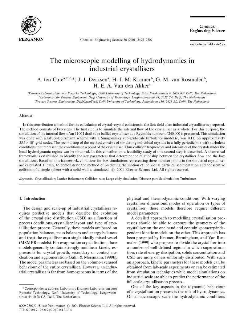
Fig. 1. Two scales of #uid motion. The macroscopic scale (crystalliser)and microscopic scale (individual particles).

control the crystal residence time and circulation time inthe crystalliser. On a microscopic scale, key processessuch as crystal collisions (source for secondary nuclea-tion and agglomeration) and mass transfer for crystalgrowth are largely determined by the smallest scale #owphenomena. One of the main di$culties in correctlycapturing the e!ect of the crystalliser hydrodynamics onthe evolution of the crystal product is that the length andtime scales in a crystallisation process vary widely. Atone end of the spectrum there are the crystalliser lengthand time scales, which lie in ranges of metres and hours.At the other end, one can consider the individual crystalsin the turbulent #ow "eld. Here dominating length scalesare in the range of 100}1000 �m for the crystals and10}100 �m for the smallest #uid eddies. Time scales are ofthe order of milliseconds. The main question is how tointegrate these widely varying scales and formulatea consistent method for estimating the in#uence of thesmall-scale phenomena on the overall performance of thecrystalliser.In this paper a method is proposed to solve part of the

above posed question. The crystal}crystal collision rate isan important parameter in describing both agglomer-ation and the formation of attrition fragments and thusplays an important role in the crystalliser behaviour.The crystal motion is directly related to the localhydrodynamic conditions. Therefore, a relationship be-tween the macroscopic and microscopic hydrodynamicconditions needs to be established to predict collisionrates in the crystalliser accurately. In this contribution,a two-step method is proposed.The "rst step of our method is to perform computa-

tional #uid dynamics (CFD) simulations of a given crys-tallisation process. From these simulations, characteristic#ow data are obtained that describe the local hy-drodynamic conditions of the crystalliser. The #uid phase(typically containing 10}20 vol% solids) is treated asa single phase with a homogeneous density and viscosity,characteristic for the crystal slurry. This approach limitsthe method. It can only be applied to simulations ofcrystalliser #ow with a virtually homogeneous slurryconcentration, i.e. to crystallisers at lab to pilot scale athigh Reynolds numbers. This assumption can be relievedby taking into account the particle transport, for instanceby solving a particle dispersion equation (e.g. Liu, 1999)and coupling back of the particle concentration to a sub-grid-scale model that locally modi"es the #uid viscosity,comparable to sub-grid-scale turbulence modelling. Typ-ical parameters that are obtained from these simulationsare rates of energy dissipation, turbulent kinetic energyand #uid velocity. These parameters are obtained at theresolution of the CFD simulation, which is at least oneorder of magnitude larger than the particle size of thecrystallisation process.The second step of our method is to focus on the

individual crystals in the crystalliser. A transition is made

from a pseudo-single-phase simulation to an explicittwo-phase simulation and thus, a transition is made fromcrystalliser #ow simulations to highly detailed CFDsimulations of individually suspended particles (seeFig. 1). The simulated particles are implemented at highresolution with respect to the CFD grid and thereforetypically occupy a number of grid nodes. The crystalliserslurry consists of high-inertia particles (i.e. particles thatdo not follow the streamlines of the turbulent #uidmotion) at high volume concentrations. CFD simula-tions of colliding particles under turbulent #uid motionare reported by, for instance, Sundaram and Collins(1997) and Chen, Kontomaris, and McLaughlin (1998),but these systems are typically investigated at (very) lowparticle volume concentrations which do not requirea coupling between the particle and #uid motion. At highvolume concentrations, particles will continuously hin-der each other. Therefore, in order to accurately simulatethe particle motion, a direct coupling between the #uidmotion and the particle motion is required.The basic concept to resolve the second step is to

design a box with fully periodic boundaries that containsa large number of particles. In this box turbulence isgenerated by forcing the #uid motion on the large scales.The turbulent #ow is simulated up to the smallest occur-ring scales (i.e. direct numerical simulation (DNS) of theturbulent #ow). The conditions in this periodic box arerelated to the crystalliser #ow via a number of key para-meters. These parameters are the turbulence character-istics obtained from the crystalliser CFD and the slurrycharacteristics (particle size, viscosity and density). Fromthese so-called box simulations, the collision frequencyand energy can be monitored. Collision data obtained inthis way can be used in models predicting the rate ofsecondary nucleation and attrition (Gahn & Mersmann,1999a) or agglomeration in crystallisers. Since the #uidphase in the crystalliser is currently assumed to be ahomogeneous slurry, no back-coupling of the resultsfrom the microscopic particle simulations (e.g. streakformation of particles and turbulence modi"cation) tothe macroscopic crystalliser simulations is taken intoaccount.

2496 A. ten Cate et al. / Chemical Engineering Science 56 (2001) 2495}2509

The numerical method chosen to simulate both thefull-scale crystalliser #ow and the suspended particles isthe lattice-Boltzmann method. This method is chosenbecause it has a number of favourable properties. First,the method is e$cient and numerically stable. Second, ithas an excellent performance on parallel computers. Thisis an important feature, because both the equipment #owsimulations and the discrete particle simulations requirelarge computational resources. Third, the method is in-herently time dependent, which makes it suitable for theimplementation of a sub-grid-scale (SGS) turbulencemodel for large eddy simulations (LES). Turbulencemodelling is required for simulation of the highly turbu-lent crystalliser #ow. Fourth, the method can treat arbit-rarily shaped boundaries which makes it suited forsimulating #uid #ow in irregular-shaped geometries suchas a crystalliser or a cluster of moving particles. Simula-tions of generated isotropic turbulence are frequentlydone with spectral methods. Turbulence in the lattice-Boltzmann schemes can be generated by agitating the#uid at varying time and length scales with #uctuatingforce "elds. In Section 2 the background of the lattice-Boltzmann method is discussed along with the imple-mentation of the LES model and the treatment of theboundary conditions.The main objective of this contribution is to establish

the relationship between the two steps of the simulationmethodology and to investigate the feasibility of theproposed method. For the "rst step, in Section 3, theCFD simulation of a pilot scale 1100 l draft tube ba%edcrystalliser is reported and results are presented. Then, inSection 4 an analysis is given of the hydrodynamic lengthand time scales that occur in the turbulent crystalliser#ow and that characterise the crystalliser #ow at themicroscopic scale. These parameters are then used toexplain how to calculate the parameters that set the scenefor a representative box simulation. It is shown what therequirements of box simulations that represent threechosen monitor points in the crystalliser will be withrespect to computational parameters such as the domainsize and computational time for a given particle size. Thebox simulations are currently still under constructionand therefore no results of these simulations are reportedhere. However, as a "rst example of a detailed suspendedparticle simulation, the lattice-Boltzmann simulation ofa single particle settling towards and colliding witha solid wall is presented in Section 5. In Section 6 con-clusions are drawn regarding the obtained framework.

2. The lattice-Boltzmann method

The lattice-Boltzmann method has been developedduring the last decade and stems from the lattice gascellular automata techniques that date back to the 1970sand 1980s. The concept of the lattice-Boltzmann method

is based on the premise that the mesoscopic (continuum)behaviour of a #uid is determined by the behaviour of theindividual molecules at the microscopic level. In thelattice-Boltzmann approach, the #uid is represented by#uid mass placed on the nodes of an equidistant grid(lattice). At each time cycle, a number of steps are ex-ecuted; from each grid node, #uid mass moves to thesurrounding grid nodes and conversely mass arrives ateach grid node. In this way conservation of mass isguaranteed. Arriving mass collides, while collision rulesare applied that guarantee conservation of momentum.After the collision step, the mass is redistributed anda cycle is "nished. One of the elegant features of themethod is that although the collision rules describe the#uid behaviour locally on a grid node, the continuityequation and incompressible Navier}Stokes equationsare recovered (Rothman & Zaleski, 1997; Chen &Doolen, 1998). A number of recent developments in theapplication of the lattice-Boltzmannmethod clearly dem-onstrate its versatility. In this contribution a methodo-logy is presented to simulate turbulent slurry #ow whileresolving the complete hydrodynamic environment of theparticles. The "rst publications in which this approach toslurry #ow is described are from Ladd, who applied themethod to simulate slurry #ow at the most detailed level(Ladd, 1994a,b) and calculated sedimentation with upto 32,000 individual particles (Ladd, 1997). Anothercontribution in this "eld is given by Heemels (1999).Multi-phase problems have also been addressed byRothman and Zaleski (1997) (liquid}liquid) or bySankaranarayanan, Shan, Kevrekidis, and Sundaresan(1999) (liquid}gas). Examples of lattice-Boltzmannstudies in which complex and dynamic geometries arecombined with mass transfer are simulations of coralgrowth (Kaandorp, Lowe, Frenkel, & Sloot, 1996) andbio"lm growth (Picioreanu, Loosdrecht, & Heijnen,1999; Picioreanu, 1999). The internal #ow of a crystalliseris highly turbulent and requires the incorporation of anSGS turbulence model. Examples in which the method isused to investigate the turbulent #uid #ow in a stirredtank are given by Eggels (1996) and Derksen and Vanden Akker (1999). A review on the lattice-Boltzmannmethod is found in Chen and Doolen (1998).

2.1. The lattice-Boltzmann equation

Although di!erent types of lattice-Boltzmann schemeshave been developed, the di!erent methods all stem fromthe evaluation of the same lattice-Boltzmann equation(LBE):

f�(x#c

�, t#1)"f

�(x, t)#�

�( f

�(x, t)). (1)

This equation states that at a position x and time t, anamount �

�is added to f

�and transported to the position

x#c�at time t#1. The subscript indicator i represents

the direction of propagation and is determined by the

A. ten Cate et al. / Chemical Engineering Science 56 (2001) 2495}2509 2497

type of grid, c�is the discrete velocity at which mass

travels from one node to the other, ��is the collision

operator which determines the post-collision distributionof mass over the M directions on a grid node. The massdensity function f

�and the collision operator �

�have the

following universal properties:

� summation of f�over the M directions of the chosen

lattice gives the #uid density at position x and summa-tion of f

�c�gives the momentum vector:

��

f�(x, t)"�, (2)

��

f�(x, t)c

�"�u, (3)

� conservation of mass and momentum is guaranteed bythe following equations:

��

��(x, t)"0, (4)

��

�c�"f(x, t). (5)

For the two applications discussed in this paper, twodi!erent schemes for solution of the LBE equation wereused. The simulation of the internal #ow of an 1100 lDTB crystalliser is based on the method of Somers(1993). Based on this method, a 3D code for LES wasdeveloped by Derksen and Van den Akker (1999). Forthe simulation of settling particles, a single relaxationtime scheme is used (Qian, d'Humieres, & Lallemand,1992). Both schemes obtain the same continuity equation

��#� ) �u"0 (6)

and momentum equation

��u#� ) �uu"!�P#� ) �[�(�u)#(�(�u))�]#f. (7)

In the compressible limit (i.e. �u��u�) Eq. (7) corresponds

to the incompressible Navier}Stokes equation. Thelattice-Boltzmann method is inherently dimensionless.Length scales are treated as lattice units (equal to the gridspacing �) and time is represented in time steps.

2.2. Large eddy simulation

For the simulation of #ows at industrially relevantReynolds numbers (i.e. at turbulent conditions) directsimulation of the #ow is not feasible and turbulencemodelling is required. The time-dependent character ofthe lattice-Boltzmann method makes it suitable for theimplementation of an SGS model. In this way large-scalemotions are explicitly solved, while all small-scale

motions, typically smaller than two times the grid spac-ing, are "ltered out. This approach is usually referred toas LES. The "ltering of small-scale motion is based onthe assumption that the motion of the smallest scales isisotropic in nature and that the SGS energy is dissipatedvia an inertial subrange that has a geometry-independentcharacter. Thus, the turbulent #ow at the SGS can berepresented by an SGS eddy viscosity (�

�). The LES

model applied in this research is a standard Smagorinskymodel (Smagorinsky, 1963) where the eddy viscosity isrelated to the local rate of deformation:

��"l�

��S�, (8)

where l��

is the mixing length of the sub-grid motion.The rate of deformation S� is calculated by

S�"1

2��u��x�

#

�u��x�

!

2

3�� ) u�

�(9)

with �� the Kronecker delta. The Smagorinsky constantc�is de"ned as the ratio between the mixing length and

the grid spacing and thus also determines the cut-o!length l

�of the applied LES model (Eggels, 1994):

l��

"c��"0.0825l

�. (10)

Implementation of this LES model into the lattice-Boltzmann framework is rather straightforward, becausethe gradients required for the rate of deformation (Eq. (9))are essentially contained within the method. A local totalviscosity (�#�

�) is calculated and applied in the collision

step.

2.3. Boundary conditions

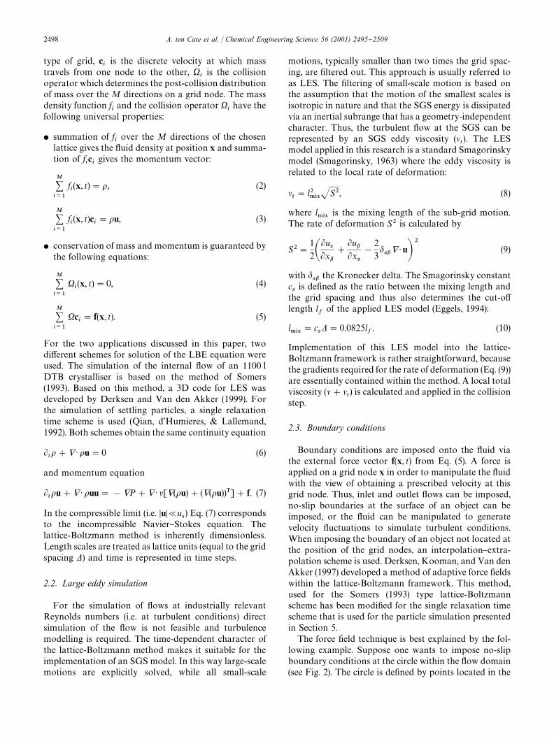
Boundary conditions are imposed onto the #uid viathe external force vector f(x, t) from Eq. (5). A force isapplied on a grid node x in order to manipulate the #uidwith the view of obtaining a prescribed velocity at thisgrid node. Thus, inlet and outlet #ows can be imposed,no-slip boundaries at the surface of an object can beimposed, or the #uid can be manipulated to generatevelocity #uctuations to simulate turbulent conditions.When imposing the boundary of an object not located atthe position of the grid nodes, an interpolation}extra-polation scheme is used. Derksen, Kooman, and Van denAkker (1997) developed a method of adaptive force "eldswithin the lattice-Boltzmann framework. This method,used for the Somers (1993) type lattice-Boltzmannscheme has been modi"ed for the single relaxation timescheme that is used for the particle simulation presentedin Section 5.The force "eld technique is best explained by the fol-

lowing example. Suppose one wants to impose no-slipboundary conditions at the circle within the #ow domain(see Fig. 2). The circle is de"ned by points located in the


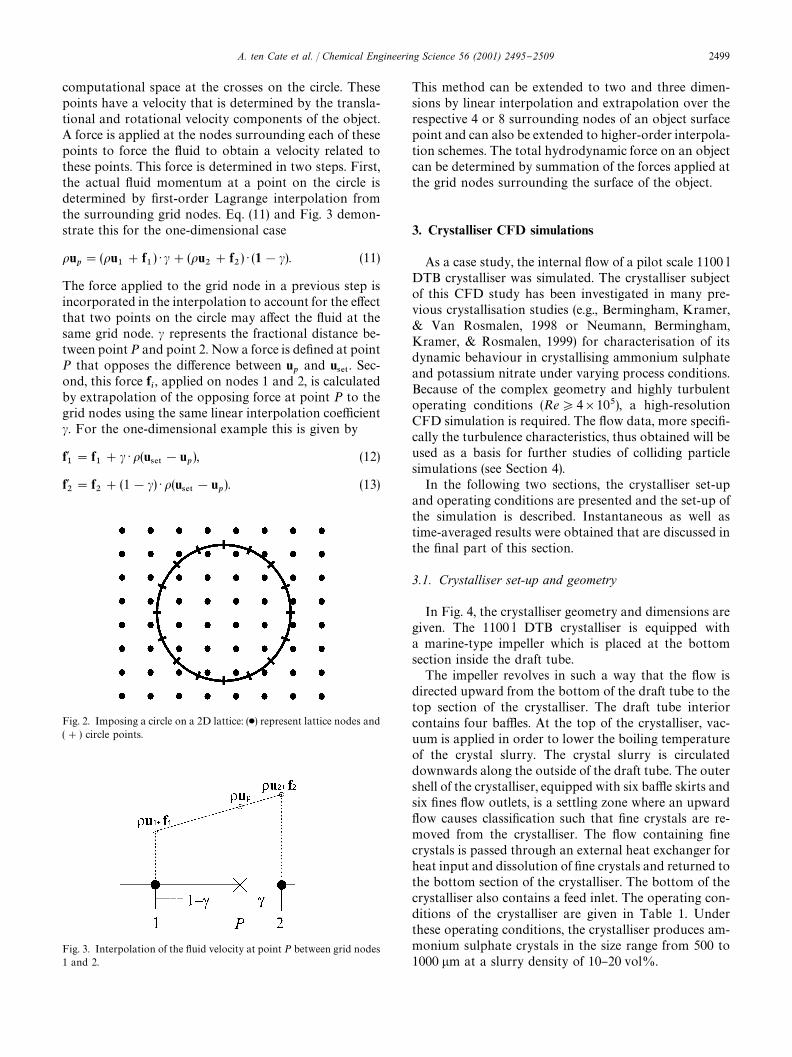
Fig. 3. Interpolation of the #uid velocity at point P between grid nodes1 and 2.

Fig. 2. Imposing a circle on a 2D lattice: (�) represent lattice nodes and(#) circle points.

computational space at the crosses on the circle. Thesepoints have a velocity that is determined by the transla-tional and rotational velocity components of the object.A force is applied at the nodes surrounding each of thesepoints to force the #uid to obtain a velocity related tothese points. This force is determined in two steps. First,the actual #uid momentum at a point on the circle isdetermined by "rst-order Lagrange interpolation fromthe surrounding grid nodes. Eq. (11) and Fig. 3 demon-strate this for the one-dimensional case

�u�"(�u

�#f

�) ) �#(�u

�#f

�) ) (1!�). (11)

The force applied to the grid node in a previous step isincorporated in the interpolation to account for the e!ectthat two points on the circle may a!ect the #uid at thesame grid node. � represents the fractional distance be-tween pointP and point 2. Now a force is de"ned at pointP that opposes the di!erence between u

�and u

��. Sec-

ond, this force f�, applied on nodes 1 and 2, is calculated

by extrapolation of the opposing force at point P to thegrid nodes using the same linear interpolation coe$cient�. For the one-dimensional example this is given by

f��"f

�#� ) �(u

��!u

�), (12)

f��"f

�#(1!�) ) �(u

��!u

�). (13)

This method can be extended to two and three dimen-sions by linear interpolation and extrapolation over therespective 4 or 8 surrounding nodes of an object surfacepoint and can also be extended to higher-order interpola-tion schemes. The total hydrodynamic force on an objectcan be determined by summation of the forces applied atthe grid nodes surrounding the surface of the object.

3. Crystalliser CFD simulations

As a case study, the internal #ow of a pilot scale 1100 lDTB crystalliser was simulated. The crystalliser subjectof this CFD study has been investigated in many pre-vious crystallisation studies (e.g., Bermingham, Kramer,& Van Rosmalen, 1998 or Neumann, Bermingham,Kramer, & Rosmalen, 1999) for characterisation of itsdynamic behaviour in crystallising ammonium sulphateand potassium nitrate under varying process conditions.Because of the complex geometry and highly turbulentoperating conditions (Re*4�10�), a high-resolutionCFD simulation is required. The #ow data, more speci"-cally the turbulence characteristics, thus obtained will beused as a basis for further studies of colliding particlesimulations (see Section 4).In the following two sections, the crystalliser set-up

and operating conditions are presented and the set-up ofthe simulation is described. Instantaneous as well astime-averaged results were obtained that are discussed inthe "nal part of this section.

3.1. Crystalliser set-up and geometry

In Fig. 4, the crystalliser geometry and dimensions aregiven. The 1100 l DTB crystalliser is equipped witha marine-type impeller which is placed at the bottomsection inside the draft tube.The impeller revolves in such a way that the #ow is

directed upward from the bottom of the draft tube to thetop section of the crystalliser. The draft tube interiorcontains four ba%es. At the top of the crystalliser, vac-uum is applied in order to lower the boiling temperatureof the crystal slurry. The crystal slurry is circulateddownwards along the outside of the draft tube. The outershell of the crystalliser, equipped with six ba%e skirts andsix "nes #ow outlets, is a settling zone where an upward#ow causes classi"cation such that "ne crystals are re-moved from the crystalliser. The #ow containing "necrystals is passed through an external heat exchanger forheat input and dissolution of "ne crystals and returned tothe bottom section of the crystalliser. The bottom of thecrystalliser also contains a feed inlet. The operating con-ditions of the crystalliser are given in Table 1. Underthese operating conditions, the crystalliser produces am-monium sulphate crystals in the size range from 500 to1000 �m at a slurry density of 10}20 vol%.


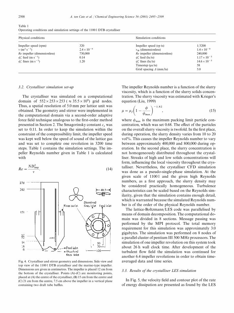
Table 1Operating conditions and simulation settings of the 1100 l DTB crystalliser

Physical conditions Simulation conditions

Impeller speed (rpm) 320 Impeller speed (rp ts) 1/3200� (m� s��) 2.4�10��

��(dimensionless) 1.4�10�

Re impeller (dimensionless) 730,000 Re impeller (dimensionless) 240,000�feed (m s��) 0.14 �

feed (lu/ts) 1.17�10�

�"nes (m s��) 1.20 �

"nes (lu/ts) 14.6�10�

Timestep (�s/ts) 58Grid spacing � (mm/lu) 5.0

Fig. 4. Crystalliser and stirrer geometry and dimensions. Side view andtop view of the 1100 l DTB crystalliser and the marine-type impeller.Dimensions are given in centimetres. The impeller is placed 12 cm fromthe bottom of the crystalliser. Points (A)}(C) are monitoring points,placed at (A) the centre of the crystalliser, (B) 15 cm from the centre and(C) 21 cm from the centre, 7.5 cm above the impeller in a vertical planecontaining two draft tube ba%es.

3.2. Crystalliser simulation set-up

The crystalliser was simulated on a computationaldomain of 552�253�253 (+35.5�10�) grid nodes.Thus, a spatial resolution of 5.0 mm per lattice unit wasobtained. The geometry and stirrer were implemented inthe computational domain via a second-order adaptiveforce "eld technique analogous to the "rst-order methodpresented in Section 2. The Smagorinsky constant c

�was

set to 0.11. In order to keep the simulation within theconstraint of the compressibility limit, the impeller speedwas kept well below the speed of sound of the lattice gasand was set to complete one revolution in 3200 timesteps. Table 1 contains the simulation settings. The im-peller Reynolds number given in Table 1 is calculatedwith

Re"

ND��

�. (14)

The impeller Reynolds number is a function of the slurryviscosity, which is a function of the slurry solids concen-tration. The slurry viscosity was estimated with Krieger'sequation (Liu, 1999)

"��1!

�

��

��, (15)

where ��

is the maximum packing limit particle con-centration, which was set 0.68. The e!ect of the particleson the overall slurry viscosity is twofold. In the "rst place,during operation, the slurry density varies from 10 to 20vol%. This causes the impeller Reynolds number to varybetween approximately 400,000 and 800,000 during op-eration. In the second place, the slurry concentration isnot homogeneously distributed throughout the crystal-liser. Streaks of high and low solids concentrations willform, in#uencing the local viscosity throughout the crys-talliser. Nevertheless, the crystalliser CFD simulationwas done as a pseudo-single-phase simulation. At thegiven scale of 1100 l and the given high Reynoldsnumbers, as a "rst approach, the slurry density maybe considered practically homogeneous. Turbulencecharacteristics can be scaled based on the Reynolds sim-ilarity, given that the simulation contains enough detail,which is warranted because the simulated Reynolds num-ber is of the order of the physical Reynolds number.The lattice-Boltzmann/LES code was parallelised by

means of domain decomposition. The computational do-main was divided in 8 sections. Message passing wasperformed by the MPI protocol. The total memoryrequirement for this simulation was approximately 3.0gigabytes. The simulation was performed on 8 nodes ofa parallel cluster of pentium III 500 MHz processors. Thesimulation of one impeller revolution on this system tookabout 26 h wall clock time. After development of theturbulent #ow "eld the simulation was continued foranother 6.4 impeller revolutions in order to obtain time-averaged data and time series.

3.3. Results of the crystalliser LES simulation

In Fig. 5, the velocity "eld and contour plot of the rateof energy dissipation are presented as found by the LES


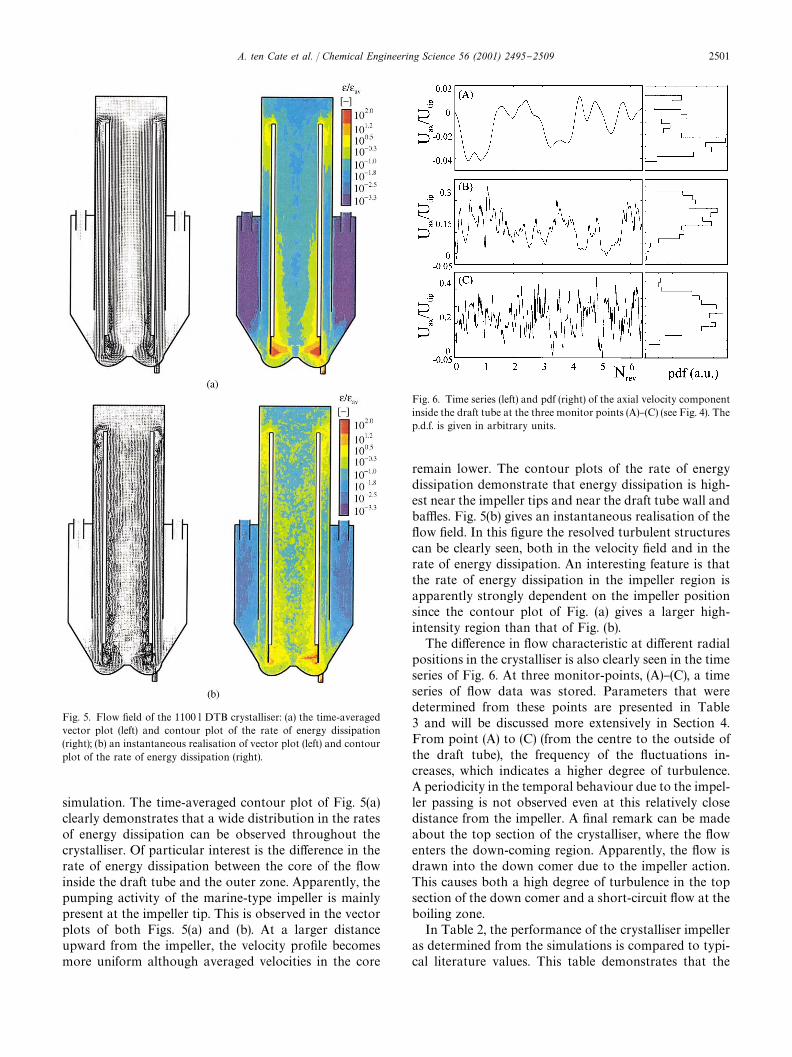
Fig. 5. Flow "eld of the 1100 l DTB crystalliser: (a) the time-averagedvector plot (left) and contour plot of the rate of energy dissipation(right); (b) an instantaneous realisation of vector plot (left) and contourplot of the rate of energy dissipation (right).

Fig. 6. Time series (left) and pdf (right) of the axial velocity componentinside the draft tube at the three monitor points (A)}(C) (see Fig. 4). Thep.d.f. is given in arbitrary units.

simulation. The time-averaged contour plot of Fig. 5(a)clearly demonstrates that a wide distribution in the ratesof energy dissipation can be observed throughout thecrystalliser. Of particular interest is the di!erence in therate of energy dissipation between the core of the #owinside the draft tube and the outer zone. Apparently, thepumping activity of the marine-type impeller is mainlypresent at the impeller tip. This is observed in the vectorplots of both Figs. 5(a) and (b). At a larger distanceupward from the impeller, the velocity pro"le becomesmore uniform although averaged velocities in the core

remain lower. The contour plots of the rate of energydissipation demonstrate that energy dissipation is high-est near the impeller tips and near the draft tube wall andba%es. Fig. 5(b) gives an instantaneous realisation of the#ow "eld. In this "gure the resolved turbulent structurescan be clearly seen, both in the velocity "eld and in therate of energy dissipation. An interesting feature is thatthe rate of energy dissipation in the impeller region isapparently strongly dependent on the impeller positionsince the contour plot of Fig. (a) gives a larger high-intensity region than that of Fig. (b).The di!erence in #ow characteristic at di!erent radial

positions in the crystalliser is also clearly seen in the timeseries of Fig. 6. At three monitor-points, (A)}(C), a timeseries of #ow data was stored. Parameters that weredetermined from these points are presented in Table3 and will be discussed more extensively in Section 4.From point (A) to (C) (from the centre to the outside ofthe draft tube), the frequency of the #uctuations in-creases, which indicates a higher degree of turbulence.A periodicity in the temporal behaviour due to the impel-ler passing is not observed even at this relatively closedistance from the impeller. A "nal remark can be madeabout the top section of the crystalliser, where the #owenters the down-coming region. Apparently, the #ow isdrawn into the down comer due to the impeller action.This causes both a high degree of turbulence in the topsection of the down comer and a short-circuit #ow at theboiling zone.In Table 2, the performance of the crystalliser impeller

as determined from the simulations is compared to typi-cal literature values. This table demonstrates that the


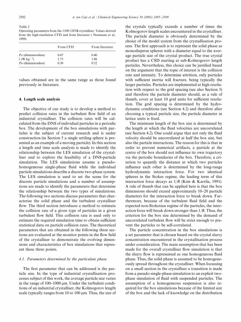
Table 2Operating parameters from the 1100 l DTB crystalliser. Values derivedfrom the high-resolution CFD and from literature ( Neumann et al.,1999)

From CFD From literature

Po (dimensionless) 0.47 0.40�� (W kg��) 1.73 1.96Pu (dimensionless) 0.30 0.32

values obtained are in the same range as those foundpreviously in literature.

4. Length scale analysis

The objective of our study is to develop a method topredict collision rates in the turbulent #ow "eld of anindustrial crystalliser. The collision rates will be cal-culated from the DNS of individual particles in a periodicbox. The development of the box simulations with par-ticles is the subject of current research and is underconstruction (in Section 5 a single settling sphere is pre-sented as an example of a moving particle). In this sectiona length and time scale analysis is made to identify therelationship between the LES simulation of the crystal-liser and to explore the feasibility of a DNS-particlesimulation. The LES simulations assume a pseudo-homogeneous single-phase #uid while the individualparticle simulations describe a discrete two-phase system.The LES simulation is used to set the scene for thediscrete particle simulations and a number of assump-tions are made to identify the parameters that determinethe relationship between the two types of simulations.The following two sections discuss parameters that char-acterise the solid phase and the turbulent crystalliser#ow. The third section introduces a method to estimatethe collision rate of a given type of particles in a giventurbulent #ow "eld. This collision rate is used only toestimate the required simulation time to obtain su$cientstatistical data on particle collision rates. The theoreticalparameters that are obtained in the following three sec-tions are evaluated at the monitor points in the #ow "eldof the crystalliser to demonstrate the evolving dimen-sions and characteristics of box simulations that repres-ent these three points.

4.1. Parameters determined by the particulate phase

The "rst parameter that can be addressed is the par-ticle size. In the type of industrial crystallisation pro-cesses subject of this work, the average particle size variesin the range of 100}1000 �m. Under the turbulent condi-tions of an industrial crystalliser, the Kolmogorov lengthscale typically ranges from 10 to 100 �m. Thus, the size of

the crystals typically exceeds a number of times theKolmogorov length scales encountered in the crystalliser.The particle diameter is obviously determined by thechoice of the model system from the crystallisation pro-cess. The "rst approach is to represent the solid phase asmonodisperse spheres with a diameter equal to the aver-age particle size of the crystal product. The true crystalproduct has a CSD starting at sub-Kolmogorov lengthparticles. Nevertheless, this choice can be justi"ed basedon the argument that the topic of interest is the collisionrate and intensity. To determine attrition, only particleswith su$cient inertia will fracture, being typically thelarger particles. Particles are implemented at high resolu-tion with respect to the grid spacing (see also Section 5)and therefore the particle diameter should, as a rule ofthumb, cover at least 10 grid units for su$cient resolu-tion. The grid spacing is determined by the hydro-dynamic conditions (see Section 4.2) and therefore afterchoosing a typical particle size, the particle diameter inlattice units is "xed.The minimum length of the box size is determined by

the length at which the #uid velocities are uncorrelated(see Section 4.2). One could argue that not only the #uidvelocity should be uncorrelated at half the box size, butalso the particle interactions. The reason for this is that inorder to prevent numerical artifacts, a particle at thecentre of the box should not in#uence its own trajectoryvia the periodic boundaries of the box. Therefore, a cri-terion to quantify the distance at which two particlesin#uence each other is determined by the long-rangehydrodynamic interaction force. For two identicalspheres in the Stokes regime, the leading term of thisinteraction force decays as 1/R (Kim & Karrila, 1991).A rule of thumb that can be applied here is that the boxdimensions should exceed approximately 10}20 particlediameters for the interaction force to break down. Fur-thermore, because of the turbulent #uid "eld and theexpected non-Stokesian regime of the particles, the inter-action force will break down stronger than 1/R. Thus, thecriterion for the box size determined by the demand ofuncorrelated turbulent #ow will be strict enough to pre-vent the particles to be self-correlated.The particle concentration in the box simulations is

a set parameter that is chosen based on the crystal slurryconcentration encountered in the crystallisation processunder consideration. The main assumption that has beenmade for the overall crystalliser #ow simulation is thatthe slurry #ow is represented as one homogeneous #uidphase. Thus, the solid phase is assumed to be homogene-ously spread throughout the crystalliser. When focussingon a small section in the crystalliser a transition is madefrom a pseudo-single-phase simulation to an explicit two-phase simulation of #uid with suspended particles. Theassumption of a homogeneous suspension is also re-quired for the box simulations because of the limited sizeof the box and the lack of knowledge on the distribution


of the crystals throughout the crystalliser. This is war-ranted by the fully periodic boundary conditions of thebox for both the #uid phase and the particulate phase.Because of the limited size of the box and the limitednumber of contained particles, at any position inside thebox any particle will experience a practically homogene-ous and constant particle concentration.The particle inertia can be characterised with the par-

ticle relaxation time �which is a measure of the response

time of a particle subject to external accelerations. ForStokesian particles this relaxation time is given by

�"

(2��#�

�)d�

�36

. (16)

Two particles coming from two uncorrelated eddies willcollide if their inertia is large enough to make themdeviate from the streamlines. The relaxation time of theparticles can be used as a measure to determine whichturbulent scales need to be investigated. The large-scalemotion of the turbulent #uid #ow will cause all particlesin a cluster to move simultaneously in the same directionwithout e!ective relative motion and thus the contribu-tion of the largest scales to collisions will be small. On theother hand, the smallest scale motion (i.e. at the Kol-mogorov length scale) is typically one order of magnitudesmaller than the average particle size and thus the netcontribution of this motion to particle collisions will alsobe negligible. The scales of #uid motion that contributemost to the particle collisions are probably the scales thatare identi"ed with a time scale of the same order ofmagnitude as the particle relaxation time.

4.2. Turbulence length and time scales

In order to have a consistent method to translate theGS and SGS turbulent #uid motion of the crystalliser toa DNS of the #uid #ow in a periodic box, the assump-tions that are made for LES modelling need to be investi-gated and the key parameters that characterise the #owconditions at both the GS and the SGS need to bedetermined.As discussed in Section 2.2, the LES modelling ap-

proach is based on the assumption that the turbulentmotion at the SGS is isotropic. The kinetic energy con-tained at the grid scale is transported via a cascade ofeddies to the smallest length scale or dissipation scalewhere it is dissipated. The energy spectrum of the cascadeof large to small eddies is assumed to behave according tothe k�� law that characterises the inertial subrange(Eggels, 1994) and can be taken as (Tennekes & Lumney,1972)

E(k)"�� k�� , (17)

where �is the Kolmogorov constant with an approxim-

ate value of 1.6. Thus, the SGS motion of the LES

simulation is characterised by the energy that is con-tained at the GS and SGS and the rate at which energy islocally dissipated. From the LES simulations, the rate ofenergy dissipation (�) and the energy that is contained bythe motion at the GS and the SGS turbulence, E

��and

E��

, are calculated according to the following equations:

�"��S�, (18)

E��

"��(u��#v��#w��), (19)

where u�, v� and w� are the root-mean-square values of thex, y and z components of the resolved velocity #uctu-ations. Finally, an equation for E

��(Eggels, 1994)

E��

"

��

0.27l��

"

l��

S�

0.27. (20)

The total turbulent kinetic energy � is given by

�"E��

#E��

. (21)

A mean square velocity related to the kinetic energy ofa scale i can be calculated with

;��,�

E�. (22)

From the LES simulations a number of characteristiclength and time scales can be determined that need to beresolved by the temporal and spatial resolution of a DNSof the turbulent #ow. The dissipation scale or Kol-mogorov length scale is the smallest length scale encoun-tered in the turbulent #ow. This length scale and the timescale associated with this length scale are given by

�"��

� , (23)

"�

��

� �. (24)

A criterion for good representation of the microscopiclength scales is given by the demand that the grid spacingwave number times the occurring Kolmogorov length isgreater than unity, i.e. the grid spacing is at approxi-mately less than six times the Kolmogorov length(Sundaram & Collins, 1997).A criterion that should be satis"ed and determines

a minimum box dimension is that the #uid velocities areuncorrelated over a distance of at least half the boxlength.With the assumption of the existence of an inertialsubrange, the correlation coe$cient f

��(r) can be used to

estimate this length. This coe$cient describes the cor-relation of #uid velocities along a line joining two pointsand for the inertial subrange is given by the followingequation (Abrahamson, 1975):

f��(r)"1!

0.9�� r�

;��

. (25)


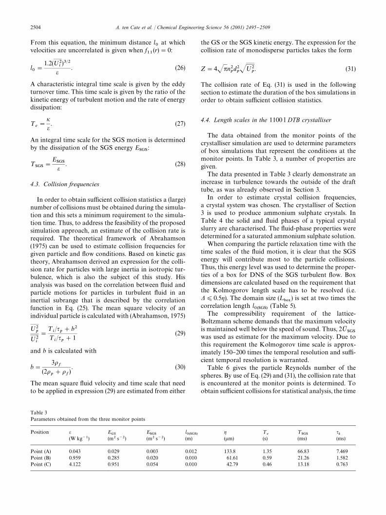
Table 3Parameters obtained from the three monitor points

Position � E��

E��

l��

� ¹�

¹��

(W kg��) (m� s��) (m� s��) (m) (�m) (s) (ms) (ms)

Point (A) 0.043 0.029 0.003 0.012 133.8 1.35 66.83 7.469Point (B) 0.959 0.285 0.020 0.010 61.61 0.59 21.26 1.582Point (C) 4.122 0.951 0.054 0.010 42.79 0.46 13.18 0.763

From this equation, the minimum distance l�at which

velocities are uncorrelated is given when f��(r)"0:

l�"

1.2(;��) �

�. (26)

A characteristic integral time scale is given by the eddyturnover time. This time scale is given by the ratio of thekinetic energy of turbulent motion and the rate of energydissipation:

¹�"

��. (27)

An integral time scale for the SGS motion is determinedby the dissipation of the SGS energy E

��:

¹��

"

E��

. (28)

4.3. Collision frequencies

In order to obtain su$cient collision statistics a (large)number of collisions must be obtained during the simula-tion and this sets a minimum requirement to the simula-tion time. Thus, to address the feasibility of the proposedsimulation approach, an estimate of the collision rate isrequired. The theoretical framework of Abrahamson(1975) can be used to estimate collision frequencies forgiven particle and #ow conditions. Based on kinetic gastheory, Abrahamson derived an expression for the colli-sion rate for particles with large inertia in isotropic tur-bulence, which is also the subject of this study. Hisanalysis was based on the correlation between #uid andparticle motions for particles in turbulent #uid in aninertial subrange that is described by the correlationfunction in Eq. (25). The mean square velocity of anindividual particle is calculated with (Abrahamson, 1975)

;��;�

�

"

¹�/

�#b�

¹�/

�#1

(29)

and b is calculated with

b"

3��

(2��#�

�). (30)

The mean square #uid velocity and time scale that needto be applied in expression (29) are estimated from either

the GS or the SGS kinetic energy. The expression for thecollision rate of monodisperse particles takes the form

Z"4��n��d��;�

�. (31)

The collision rate of Eq. (31) is used in the followingsection to estimate the duration of the box simulations inorder to obtain su$cient collision statistics.

4.4. Length scales in the 1100 l DTB crystalliser

The data obtained from the monitor points of thecrystalliser simulation are used to determine parametersof box simulations that represent the conditions at themonitor points. In Table 3, a number of properties aregiven.The data presented in Table 3 clearly demonstrate an

increase in turbulence towards the outside of the drafttube, as was already observed in Section 3.In order to estimate crystal collision frequencies,

a crystal system was chosen. The crystalliser of Section3 is used to produce ammonium sulphate crystals. InTable 4 the solid and #uid phases of a typical crystalslurry are characterised. The #uid-phase properties weredetermined for a saturated ammonium sulphate solution.When comparing the particle relaxation time with the

time scales of the #uid motion, it is clear that the SGSenergy will contribute most to the particle collisions.Thus, this energy level was used to determine the proper-ties of a box for DNS of the SGS turbulent #ow. Boxdimensions are calculated based on the requirement thatthe Kolmogorov length scale has to be resolved (i.e.�)0.5�). The domain size (¸

��) is set at two times the

correlation length l��

(Table 5).The compressibility requirement of the lattice-

Boltzmann scheme demands that the maximum velocityis maintained well below the speed of sound. Thus, 2;M

��was used as estimate for the maximum velocity. Due tothis requirement the Kolmogorov time scale is approx-imately 150}200 times the temporal resolution and su$-cient temporal resolution is warranted.Table 6 gives the particle Reynolds number of the

spheres. By use of Eq. (29) and (31), the collision rate thatis encountered at the monitor points is determined. Toobtain su$cient collisions for statistical analysis, the time


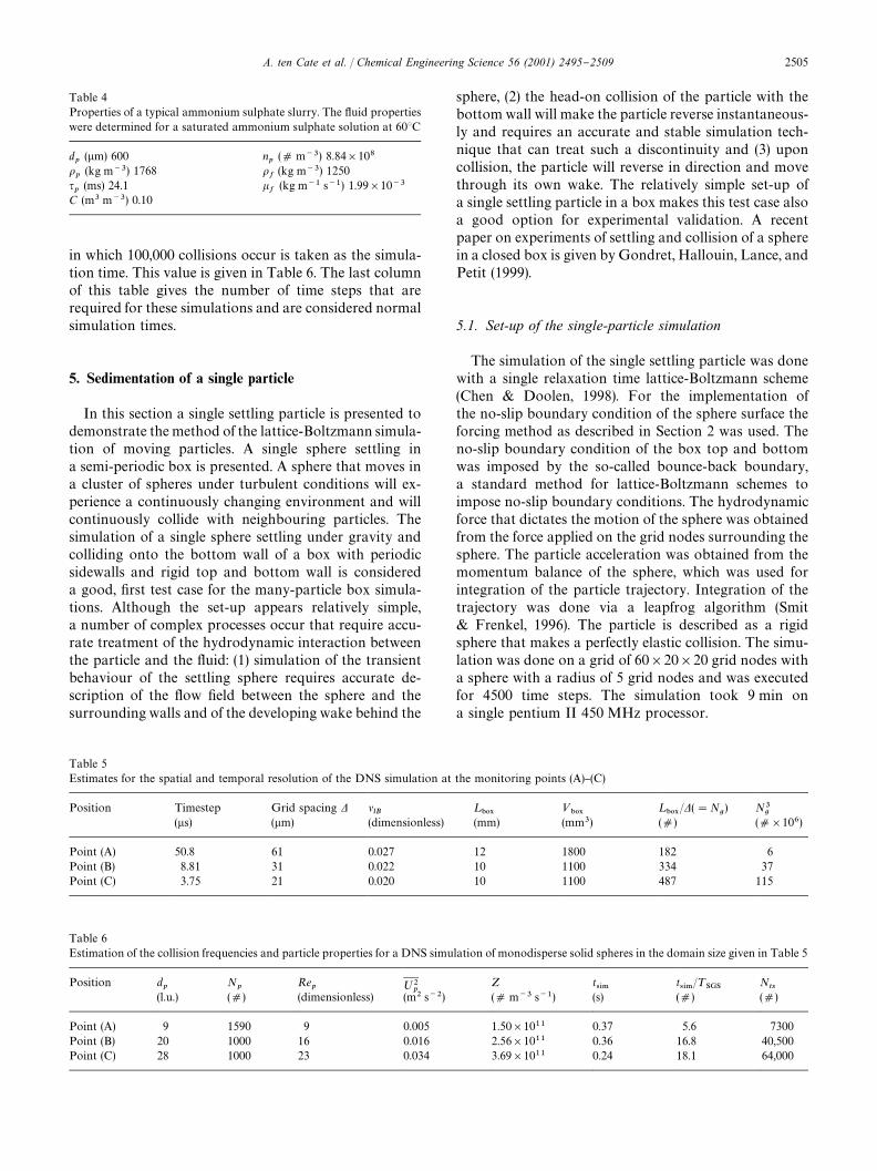
Table 4Properties of a typical ammonium sulphate slurry. The #uid propertieswere determined for a saturated ammonium sulphate solution at 603C

d�(�m) 600 n

�(� m�) 8.84�10�

��(kg m�) 1768 �

�(kg m�) 1250

�(ms) 24.1

�(kg m�� s��) 1.99�10�

C (m m�) 0.10

Table 6Estimation of the collision frequencies and particle properties for a DNS simulation of monodisperse solid spheres in the domain size given in Table 5

Position d�

N�

Re� ;�

�Z t

��t��

/¹��

N��

(l.u.) (�) (dimensionless) (m� s��) (� m� s��) (s) (�) (�)

Point (A) 9 1590 9 0.005 1.50�10�� 0.37 5.6 7300Point (B) 20 1000 16 0.016 2.56�10�� 0.36 16.8 40,500Point (C) 28 1000 23 0.034 3.69�10�� 0.24 18.1 64,000

Table 5Estimates for the spatial and temporal resolution of the DNS simulation at the monitoring points (A)}(C)

Position Timestep Grid spacing � ��

¸��

<��

¸��

/�("N�) N

�(�s) (�m) (dimensionless) (mm) (mm) (�) (��10�)

Point (A) 50.8 61 0.027 12 1800 182 6Point (B) 8.81 31 0.022 10 1100 334 37Point (C) 3.75 21 0.020 10 1100 487 115

in which 100,000 collisions occur is taken as the simula-tion time. This value is given in Table 6. The last columnof this table gives the number of time steps that arerequired for these simulations and are considered normalsimulation times.

5. Sedimentation of a single particle

In this section a single settling particle is presented todemonstrate themethod of the lattice-Boltzmann simula-tion of moving particles. A single sphere settling ina semi-periodic box is presented. A sphere that moves ina cluster of spheres under turbulent conditions will ex-perience a continuously changing environment and willcontinuously collide with neighbouring particles. Thesimulation of a single sphere settling under gravity andcolliding onto the bottom wall of a box with periodicsidewalls and rigid top and bottom wall is considereda good, "rst test case for the many-particle box simula-tions. Although the set-up appears relatively simple,a number of complex processes occur that require accu-rate treatment of the hydrodynamic interaction betweenthe particle and the #uid: (1) simulation of the transientbehaviour of the settling sphere requires accurate de-scription of the #ow "eld between the sphere and thesurrounding walls and of the developing wake behind the

sphere, (2) the head-on collision of the particle with thebottomwall will make the particle reverse instantaneous-ly and requires an accurate and stable simulation tech-nique that can treat such a discontinuity and (3) uponcollision, the particle will reverse in direction and movethrough its own wake. The relatively simple set-up ofa single settling particle in a box makes this test case alsoa good option for experimental validation. A recentpaper on experiments of settling and collision of a spherein a closed box is given by Gondret, Hallouin, Lance, andPetit (1999).

5.1. Set-up of the single-particle simulation

The simulation of the single settling particle was donewith a single relaxation time lattice-Boltzmann scheme(Chen & Doolen, 1998). For the implementation ofthe no-slip boundary condition of the sphere surface theforcing method as described in Section 2 was used. Theno-slip boundary condition of the box top and bottomwas imposed by the so-called bounce-back boundary,a standard method for lattice-Boltzmann schemes toimpose no-slip boundary conditions. The hydrodynamicforce that dictates the motion of the sphere was obtainedfrom the force applied on the grid nodes surrounding thesphere. The particle acceleration was obtained from themomentum balance of the sphere, which was used forintegration of the particle trajectory. Integration of thetrajectory was done via a leapfrog algorithm (Smit& Frenkel, 1996). The particle is described as a rigidsphere that makes a perfectly elastic collision. The simu-lation was done on a grid of 60�20�20 grid nodes witha sphere with a radius of 5 grid nodes and was executedfor 4500 time steps. The simulation took 9 min ona single pentium II 450 MHz processor.


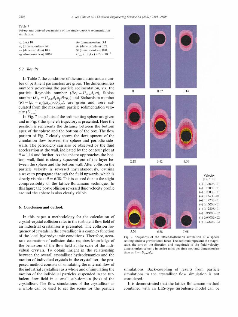
Table 7Set-up and derived parameters of the single-particle sedimentationsimulation

d�(l.u.) 10 Re (dimensionless) 3.4

��(dimensionless) 540 Ri (dimensionless) 0.22

��(dimensionless) 10.8 St (dimensionless) 38.0

��

(dimensionless) 0.067 ;��

(1.u./t.s.) 2.28�10��

Fig. 7. Snapshots of the lattice-Boltzmann simulation of a spheresettling under a gravitational force. The contours represent the magni-tude, the arrows the direction and magnitude of the #uid velocity;dimensionless velocity in lattice units per time step and dimensionlesstime as �"t;

��/d

�.

5.2. Results

In Table 7, the conditions of the simulation and a num-ber of pertinent parameters are given. The dimensionlessnumbers governing the particle sedimentation, viz. theparticle Reynolds number (Re

�";

��d�/�), Stokes

number (St�";

��d��/9��

�) and Richardson number

(Ri"(��!�

�)gd

�/�

�;�

��), are given and were cal-

culated from the maximum particle sedimentation velo-city (;

��).

In Fig. 7 snapshots of the sedimenting sphere are givenand in Fig. 8 the sphere's trajectory is presented. Here theposition h represents the distance between the bottomapex of the sphere and the bottom of the box. The #owpattern of Fig. 7 clearly shows the development of thecirculation #ow between the sphere and periodic side-walls. The periodicity can also be observed by the #uidacceleration at the wall, indicated by the contour plot at�"1.14 and further. As the sphere approaches the bot-tom wall, #uid is clearly squeezed out of the layer be-tween the sphere and the bottom wall. After collision theparticle velocity is reversed instantaneously, causinga wave to propagate through the #uid upwards, which isclearly visible at �"6.38. This is caused due to the slightcompressibility of the lattice-Boltzmann technique. Inthis "gure the post-collision reversed #uid velocity pro"learound the sphere is also clearly visible.

6. Conclusion and outlook

In this paper a methodology for the calculation ofcrystal}crystal collision rates in the turbulent #ow "eld ofan industrial crystalliser is presented. The collision fre-quency of crystals in the crystalliser is a complex functionof the local hydrodynamic conditions. Therefore, accu-rate estimation of collision data requires knowledge ofthe behaviour of the #ow "eld at the scale of the indi-vidual crystals. To obtain insight in the relationshipbetween the overall crystalliser hydrodynamics and themotion of individual crystals in the crystalliser, the pro-posed method consists of simulating the internal #ow ofthe industrial crystalliser as a whole and of simulating themotion of the individual particles suspended in the tur-bulent #ow "eld in a small sub-domain (box) of thecrystalliser. The #ow simulations of the crystalliser asa whole can be used to set the scene for the particle

simulations. Back-coupling of results from particlesimulations to the crystalliser #ow simulation is notconsidered.It is demonstrated that the lattice-Boltzmann method

combined with an LES-type turbulence model can be


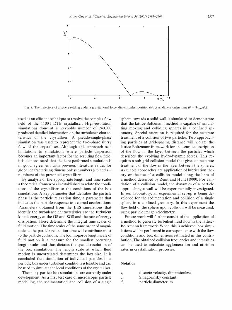
Fig. 8. The trajectory of a sphere settling under a gravitational force: dimensionless position (h/d�) vs. dimensionless time (�"t;

��/d

�).

used as an e$cient technique to resolve the complex #ow"eld of the 1100 l DTB crystalliser. High-resolutionsimulations done at a Reynolds number of 240,000produced detailed information on the turbulence charac-teristics of the crystalliser. A pseudo-single-phasesimulation was used to represent the two-phase slurry#ow of the crystalliser. Although this approach setslimitations to simulations where particle dispersionbecomes an important factor for the resulting #ow "eld,it is demonstrated that the here performed simulation isin good agreement with previous literature values forglobal characterising dimensionless numbers (Po and Punumbers) of the presented crystalliser.By analysis of the appropriate length and time scales

a theoretical framework is established to relate the condi-tions of the crystalliser to the conditions of the boxsimulations. A key parameter that identi"es the particlephase is the particle relaxation time, a parameter thatindicates the particle response to external accelerations.Parameters obtained from the LES simulations thatidentify the turbulence characteristics are the turbulentkinetic energy at the GS and SGS and the rate of energydissipation. These determine the integral time scales of#uid motion. The time scales of the same order of magni-tude as the particle relaxation time will contribute mostto the particle collisions. The Kolmogorov length scale of#uid motion is a measure for the smallest occurringlength scales and thus dictates the spatial resolution ofthe box simulation. The length scale at which #uidmotion is uncorrelated determines the box size. It isconcluded that simulation of individual particles in aperiodic box under turbulent conditions is feasible and canbe used to simulate the local conditions of the crystalliser.The many-particle box simulations are currently under

development. As a "rst test case of microscopic particlemodelling, the sedimentation and collision of a single

sphere towards a solid wall is simulated to demonstratethat the lattice-Boltzmann method is capable of simula-ting moving and colliding spheres in a con"ned ge-ometry. Special attention is required for the accuratetreatment of a collision of two particles. Two approach-ing particles at grid-spacing distance will violate thelattice-Boltzmann framework for an accurate descriptionof the #ow in the layer between the particles whichdescribes the evolving hydrodynamic forces. This re-quires a sub-grid collision model that gives an accuratetreatment of the #ow in the layer between the spheres.Available approaches are application of lubrication the-ory or the use of a collision model along the lines ofa method described by Zenit and Hunt (1999). For vali-dation of a collision model, the dynamics of a particleapproaching a wall will be experimentally investigated.In our laboratory, an experimental set-up is being de-veloped for the sedimentation and collision of a singlesphere in a con"ned geometry. In this experiment the#ow "eld of the sphere upon collision will be measured,using particle image velocimetry.Future work will further consist of the application of

a method to generate turbulent #uid #ow in the lattice-Boltzmann framework. When this is achieved, box simu-lations will be performed in correspondence with the #owconditions and box dimensions estimated in this contri-bution. The obtained collision frequencies and intensitiescan be used to calculate agglomeration and attritionrates in crystallisation processes.

Notation

c�

discrete velocity, dimensionlessc�

Smagorinsky constantd�

particle diameter, m


D��

impeller diameter, mE energy, m� s��

f�

mass density function, dimensionlessf��

velocity correlation function, dimensionlessf force vector, dimensionlessh z-coordinate, mk wave number, m��

l��

mixing length, ml�

cut-o! length, ml�

zero correlation length, mM lattice directions, dimensionlessn�

particle number concentration, � m�

N impeller speed, rev s��

N�

number of particles, � m�

N�

number of gridcells, �N

��number of timesteps, �

P pressure, Par distance, mS rate of deformation, s��

t time, s¹ integral time scale, su, v,w velocity components, m s��

u�

speed of sound, m s��

u velocity vector, m s��

x position vector, dimensionlessZ collision rate, � m� s��

Greek letters� grid spacing, m�� average energy dissipation rate, m� s�

� energy dissipation rate, m� s�

� Kolmogorov length scale, m� length ratio, dimensionless� turbulent kinetic energy, m� s��

� dimensionless time, dimensionless dynamic viscosity, Pa s�

dynamic viscosity of pure liquid, Pa s� kinematic viscosity, m� s��

��

turbulent kinematic viscosity, m� s��

��

kinematic viscosity of lB scheme, dimension-less

��

collision operator, dimensionless� density, kg m�

Kolmogorov time scale, s �

particle relaxation time, s� volume fraction, dimensionless�

volume #ux, m s��

Dimensionless numbersPo power numberPu pumping numberRe Reynolds numberRi Richardson numberSt Stokes number

AcronymsCFD computational #uid dynamicsCSD crystal size distributionDNS direct numerical simulationDTB draft tube ba%e crystallizerGS grid scaleLES large eddy simulationSGS sub-grid scale

References

Abrahamson, J. (1975). Collision rates of small particles in a vigorouslyturbulent #uid. Chemical Engineering Science, 30, 1371}1379.

Bermingham, S. K., Kramer, H., & Van Rosmalen, G. M. (1998).Towards on-scale crystalliser design using compartmental models.Computers & Chemical Engineering, 22, S355}S362.

Chen, M., Kontomaris, K., & McLaughlin, J. (1998). Directnumerical simulation of droplet collisions in a turbulent channel#ow. Part ii: Collision rates. Journal of Multiphase Flow, 24(11),1105}1138.

Chen, S., & Doolen, G. (1998). Lattice boltzmann method for #uid#ows. Annual Review of Fluid Mechanics, 30, 329}364.

Derksen, J., Kooman, J., & Van den Akker, H. (1997). Parallel yuid yowsimulation by means of a lattice-boltzmann scheme. Lecture Notes inComputer Science, vol. 1225 (p. 524). Berlin: Springer.

Derksen, J., & Van den Akker, H. (1999). Large eddy simulationson the #ow driven by a rushton turbine. A.I.Ch.E. Journal, 45(2),209}221.

Eggels, J. (1994). Direct and large Eddy simulation of turbulent yowin a cylindrical pipe geometry. Ph.D. thesis, Laboratory forAero- and Hydro-dynamics, Delft University of Technology,The Netherlands.

Eggels, J. (1996). Direct and large-eddy simulations of turbulent #uid#ow using the lattice-boltzmann scheme. International Journal ofHeat Fluid Flow, 17, 307.

Gahn, C., & Mersmann, A. (1999a). Brittle fracture in crystallizationprocesses. Part a: Attrition and abrasion of brittle solids. ChemicalEngineering Science, 54, 1273}1282.

Gahn, C., & Mersmann, A. (1999b). Brittle fracture in crystallizationprocesses. Part b: Growth of fragments and scale-up of suspensioncrystallizers. Chemical Engineering Science, 54, 1283}1292.

Gondret, P., Hallouin, E., Lance, M., & Petit, L. (1999). Experiments onthe motion of a solid sphere toward a wall: From viscous dissipationto elastohydrodynamic bouncing. Physics of Fluids, 11(9),2803}2805.

Heemels, M. (1999). Computer simulations of colloidal suspensions usingan improved lattice-Boltzmann scheme. Ph.D. thesis, Delft Universityof Technology.

Kaandorp, J. A., Lowe, C. P., Frenkel, D., & Sloot, P. M. A. (1996).E!ect of nutrient di!usion and #ow on coral morphology. PhysicalReview Letters, 77(11), 2328}2331.

Kim, S., & Karrila, S.J. (1991). Microhydrodynamics: Principles andselected applications. Butterworth-Heinemann Series in ChemicalEngineering. London: Butterworth-Heinemann.

Kramer, H., Bermingham, S. K., & Van Rosmalen, G.M. (1999). Designof industrial crystallisers for a required product quality. Journal ofCrystal Growth, 198/199, 729}737.

Ladd, A. J. (1994a). Numerical simulations of particulate suspensionsvia a discretized boltzmann equation. Part 1: Theoretical founda-tion. Journal of Fluid Mechanics, 271, 285}309.

Ladd, A. J. (1994b). Numerical simulations of particulate suspensionsvia a discretized boltzmann equation. Part 2: Numerical results.Journal of Fluid Mechanics, 271, 311}339.


Ladd, A. J. (1997). Sedimentation of homogeneous suspensions ofnon-brownian spheres. Physics of Fluids, 9(3), 491}499.

Liu, S. (1999). Particle dispersion for suspension #ow. Chemical Engin-eering Science, 54, 873}891.

Neumann, A. M., Bermingham, S. K., Kramer, H. J., & Rosmalen, G.M., v. (1999). Modeling industrial crystallizers of di!erent scale andtype. Proceedings of the 14th international symposium on industrialcrystallization.

Picioreanu, C. (1999). Multidimensional modeling of bioxlm structure.Ph.D. thesis, Delft University of Technology.

Picioreanu, C., Loosdrecht, M. v., & Heijnen, J. (1999). Discrete-di!er-ential modelling of bio"lm structure. Water Science Technology,39(7), 115}122.

Qian, Y., d'Humieres, D., & Lallemand, P. (1992). Lattice bgkmodels for navier-stokes equation. Europhysics Letters, 17(6),479}484.

Rothman, D. H., & Zaleski, S. (1997). Lattice-gas cellular automata (1sted.). Cambridge: Cambridge University Press.

Sankaranarayanan, K., Shan, X., Kevrekidis, I., & Sundaresan, S.(1999). Bubble #ow simulations with the lattice-boltzmann method.Chemical Engineering Science, 54(21), 4817.

Smagorinsky, J. (1963). General circulation experiments with the primi-tive equations. 1: The basic experiment.Monthly Weather Review, 91,99}164.

Smit, B., & Frenkel, D. (1996). Understanding molecular simulation. NewYork: Academic Press.

Somers, J. (1993). Direct simulation of #uid #ow with cellular automataand the lattice-boltzmann equation. Applied Science Research, 51,127}133.

Sundaram, S., & Collins, L. R. (1997). Collision statistics in an isotropicparticle-laden turbulent suspension. Part 1: Direct numerical simu-lations. Journal of Fluid Mechanics, 335, 75}109.

Tennekes, H., & Lumney, J. L. (1972). A xrst course in turbulence.Cambridge, MA: The MIT Press.

Zenit, R., & Hunt, M. L. (1999). Mechanics of immersed particlecollisions. Journal of Fluids Engineering, 121, 179}184.


Documents

Themicroscopicmodellingofhydrodynamicsin ...jos/pbl/ces56p2495.pdf · crystalliserdimensions, modesof operationor types of crystalliser, these models therefore require di!erent modelparameters