Theoretical and Experimental Investigations for … · MEMOIRE PRESENTE A L'UNIVERSITÉ DU QUÉBEC À CHICOUTIMI COMME EXIGENCE PARTIELLE ... This Master study deals with the development

UNIVERSITE DU QUEBEC

MEMOIRE PRESENTE AL'UNIVERSITÉ DU QUÉBEC À CHICOUTIMI COMME

EXIGENCE PARTIELLEDE LA MAÎTRISE EN INGÉNIERIE

Par

MANDANA JAVAN-MASHMOOL

Theoretical and Experimental Investigations forMeasuring Interfacial Bonding Strength between Ice

and Substrate

NOVEMBRE 2005

Mise en garde/Advice

Afin de rendre accessible au plus grand nombre le résultat des travaux de recherche menés par ses étudiants gradués et dans l'esprit des règles qui régissent le dépôt et la diffusion des mémoires et thèses produits dans cette Institution, l'Université du Québec à Chicoutimi (UQAC) est fière de rendre accessible une version complète et gratuite de cette œuvre.

Motivated by a desire to make the results of its graduate students' research accessible to all, and in accordance with the rules governing the acceptation and diffusion of dissertations and theses in this Institution, the Université du Québec à Chicoutimi (UQAC) is proud to make a complete version of this work available at no cost to the reader.

L'auteur conserve néanmoins la propriété du droit d'auteur qui protège ce mémoire ou cette thèse. Ni le mémoire ou la thèse ni des extraits substantiels de ceux-ci ne peuvent être imprimés ou autrement reproduits sans son autorisation.

The author retains ownership of the copyright of this dissertation or thesis. Neither the dissertation or thesis, nor substantial extracts from it, may be printed or otherwise reproduced without the author's permission.

Dedication

I dedicate this thesis in loving memory of my parents who have always been very

supportive, understanding and encouraging through my study.

Ill

Abstract

This Master study deals with the development of a mechanical technique for measuring

interfacial bonding strength of atmospheric ice, using embedded piezoelectric film (PVDF)

sensors at the ice/substrate interface. The substrate is an aluminum beam on which PVDF

piezoelectric sensors are bonded. The composite beam, formed by an aluminum beam and a

deposited ice layer, is submitted to sinusoidal stress at the interface by an electromagnetic

shaker on which one end of the beam is clamped. The ice layer is deposited artificially on

the aluminium beam from sprayed supercooled water droplets in order to simulate

atmospheric icing on structures.

The piezoelectric charge coefficient is used to predict the electric charge density

induced on the piezoelectric (PVDF) film which enables us to develop a macroscopic and

direct measurement technique for determining mechanical stresses at the atmospheric-

ice/substrate interface. All tests have been performed for a frequency close to the natural

resonance frequency of the aluminum beam. The tests were carried out on two series of

aluminum beams with two different finishes and on Plexiglas.

It may be observed that, in all test series, with an increase in displacement amplitude of

the clamped end, the interface stress increases approximately linear until delamination or

IV

ice de-bonding occurrence at the film position. At this specific moment a drastic change in

the interface stress occurred resulting from a local redistribution of the bending and shear

stress. Hence, the interface stress obtained at this specific moment corresponds to the stress

required to de-bond the ice from its substrate (ice adhesion strength). The obtained

empirical results demonstrate that ice adhesion strength depends on the surface finish, as it

is more finished the adhesion strength is less. The experimental results prove that ice

adhesion strength significantly depends on substrate type as the adhesion strength on

Plexiglas surface was 100 times less than on the aluminum surface. Within the limitations

of the experimental conditions, it was possible using this approach to estimate ice adhesion

strengths in accordance with those obtained in literature. This demonstrates the feasibility

of this simple ice adhesion testing method.

Résumé

Cette étude porte sur le développement d'une technique mécanique pour mesurer la

force d'adhérence de la glace atmosphérique à l'aide d'un film polymère piézoélectrique

(PVDF) inséré à l'interface glace/substrat. Dans le cas présent, le substrat est une poutre

d'aluminium sur laquelle l'élément piézoélectrique PVDF est collé et sur laquelle la glace

atmosphérique est déposée artificiellement à partir de gouttelettes d'eau surfondues. La

poutre composite ainsi formée, qui est encastrée à une extrémité au niveau de

l'aluminium et libre de l'autre, est soumise à une flexion simple par une excitation

mécanique sinusoïdale appliquée sur l'extrémité encastrée dans le plan vertical en

utilisant un pot vibrant.

Le coefficient piézoélectrique de charge est utilisé afin de mesurer la charge

électrique induite par le film PVDF qui est directement proportionnelle à la contrainte

mécanique générée à l'interface glace/poutre, résultante de la contribution de la

contrainte en flexion et de cisaillement. Ce principe permet ainsi de développer une

méthode de mesure macroscopique et directe afin de déterminer des contraintes

mécaniques à l'interface de glace atmosphérique/substrat. Tous les essais ont été réalisés

à une fréquence proche de la fréquence de résonance de la poutre composite.

VI

Après avoir étalonné la méthode par une modélisation numérique et dynamique de la

poutre en aluminium seule, trois séries d'essais ont été effectuées dont deux avec des

poutres en aluminium de rugosités différentes et la troisième avec une poutre identique

géométriquement mais constituée de plexiglas. Les résultats obtenus avec des dépôts de

glace de quatre millimètres d'épaisseur montrent que la contrainte d'interface augmente

linéairement avec l'augmentation de l'amplitude de la contrainte d'excitation jusqu'au

décollement de la glace, résultant d'un délaminage progressif initié à l'encastrement et

qui se propage vers le milieu de la poutre composite. L'instant où le délaminage atteint le

film PVDF est facilement détectable par la lecture du signal délivré par ce dernier qui

permet ainsi de déterminer la contrainte mécanique nécessaire pour détacher la glace du

substrat. Les résultats obtenus à partir des trois séries montrent que la méthode proposée

est valide puisque les valeurs des forces d'adhérence obtenues dépendent de la rugosité

du substrat dont l'augmentation entraîne une augmentation de la force d'adhérence et les

force d'adhésion dépendent aussi du matériau constituant le substrat avec une force

d'adhésion sur l'aluminium environ cent fois plus grande que pour le plexiglas. De plus,

les résultats obtenus sont en accord avec les ordres de grandeurs des forces d'adhérence

de la littérature.

Ainsi, une méthode simple et originale, basée sur l'utilisation de films polymères

piézoélectriques PVDF et permettant des mesures directes de la force d'adhérence de la

glace a été développée et validée. Cette méthode a permis de tester différents matériaux

pour des épaisseurs de glace de 4 mm. Cependant, l'épaisseur du dépôt de glace n'est pas

Vil

une limitation mais l'influence de cette dernière sur la force d'adhérence reste encore à

être démontrée.

vin

Acknowledgements

This Masters' research was carried out within the framework of the Industrial Chair on

Atmospheric Icing of Power Network Equipment (CIGELE) and the Canada Research

Chair on Engineering of Power Network Atmospheric Icing (INGIVRE) at University of

Quebec in Chicoutimi (UQAC).

I would like to thank hearty Prof. M. FARZANEH, my director for his support,

supervision, guidance, encouragement, motivation and patience in this endeavor. I will

forever be indebted to you for showing your interest, generous help during my Masters'

studies, and providing me the opportunity to work in 'Pavillon de Recherche sur le

Givrage', the grandest research laboratory on the atmospheric icing in the world. Special

thanks to Dr. C. VOLAT, my co-director and mentor for his patience and guidance. I am

particularly grateful for all of your time and help during last two years. I would like to

thank Prof. Y. TEISSEYRE from 'École Supérieure d'Ingénieurs d'Annecy' for showing

his interest, time and help during the experiments. I would like to show my deepest

appreciations to all of my friends and collaborators who provided assistance in CIGELE

Laboratory and other labs of the University of Quebec at Chicoutimi (UQAC). Special

thanks to technicians, for all their collaborations. I would like to thank my family,

especially my parents for all of their love and support through the years, you have

IX

always encouraged me to challenge myself, and I enjoy sharing my accomplishments

with you.

Finally, I would like to thank Jalil Farzaneh-Dehkordi my spouse. Thank you for your

true love and endurance support. I look forward to my future with you and to more great

moments.

Table of Contents

Dedication ii

Abstract in

Résumé. v

Acknowledgements viii

Table of Contents x

List of Figures xiii

List of Tables xvii

List of Symbols xviii

CHAPTER! 1

Introduction 2

1.1 General 2

1.2 Overview of the Problem 3

1.3 Research Objectives 7

CHAPTER 2 10

Review of Literature 11

2.1 Introduction 11

2.2 Adhesion Theory and Mechanism 122.2.1 Mechanism of Adhesion 122.2.2 Three Main Adhesion Forces 162.2.3 Factors that Influence Adhesion Strength 17

2.3 Ice adhesion Tests 19

2.4 Conclusion 32

CHAPTER 3 34

Piezoelectric sensors. 35

3.1 Introduction 35

3.2 Piezoelectric Films Properties 38

3.3 Piezoelectric Film as Source Capacitance 42

3.4 The Fundamental Piezoelectric Equations 44

XI

3.5 Conclusion 48

CHAPTER 4 50

Theory and Calibration 51

4.1 Introduction 51

4.2 Analytical Modeling of Beam and its Deflection 534.2.1 Beam Modeling 534.2.2 Determination of Neutral Plane Position 584.2.3 Determination of Deflection (Bending Displacement) 604.2.4 Determination of Bending Stress in order to Calibrate the Piezo Film Response 65

4.3 Calibration of Accelerometer 68

4.4 Calibration of Piezo Film Response 69

4.5 Determination of adequate frequency exercised to electromagnetic shaker 71

4.6 Theoretical Modeling of Bending and Shear Stress in Presence of Ice at Interface 764.6.1 Modeling of Bending Stress 76

4.6.2 Modeling of Shear stress 80

CHAPTER 5 85

Experimental Set-up, Facilities and Tests Procedure 865.1 Introduction 865.2 Laboratory Facilities 86

5.2.1 Ice deposition in climate room 865.2.2 Water droplet generator 885.2.3 Cooling system 895.2.4 Data acquisition system 905.2.5 Glues 905.2.6 Accelerometer 925.2.7 Aluminum Beam and Piezoelectric Film 925.2.8 Charge Amplifier Circuit 935.2.9 Beam preparation and icing 96

5.3 Experimental Set-up 98

5.4 Tests Procedure 99

CHAPTER 6 103

Experimental results 104

CHAPTER 7. 112

Conclusions and Recommendations. 113

7.1 Conclusions 113

7.2 Recommendations 115

REFERENCES 123

APPENDIX 128

Xll

A. Stress 129A.1 Normal Stress 129A.2 Shear Stress 130

B. Strain 135B.I Normal Strain 135B.2 Shear Strain 136

C. Strain-Displacement Relation 138

D. Stress - Strain Relationships (Constitutive Relations) 139

E. Poisson Ratio 146

F. Engineering Stress-Strain Diagrams 147

Xll l

List of Figures

Figure 1.1 : A Street in Elora after an ice storm - frozen utility lines are pulled over 4

Figure 2.1: Electrostatic attraction due to electron transfer 13

Figure 2.2: The illustration of diffusion on the surface 13

Figure 2.3 : Two different materials adhere due to chemical bonds 14

Figure 2.4: Forming of an interlocking system 15

Figure 2.5 : Illustration of adsorption of molecules by a substrate 16

Figure 2.6: Shear strength as a function of Temperature 18

Figure 2.7: Lap shear Tests 20

Figure 2.8: Tensile Test 21

Figure 2.9: Torsion Test 22

Figure 2.10: Peel Tests.... 23

Figure 2.11: Impact Tests 24

Figure 2.12: Laser Spallation Technique 25

Figure 2.13: Electromagnetic Tensile Test 26

Figure 2.14: Blister Test 27

Figure 2.15: Cylinder Torsion Shear Test 28

XIV

Figure 2.16: Axial Cylinder Shear Test 29

Figure 2.17: Cone test 30

Figure 3.1 : Like water from a sponge, piezoelectric materials generate charge

when squeezed, making an ideal strain gage 37

Figure 3.2: Piezo also changes dimension with applied voltage for high

fidelity transmission 37

Figure 3.3: Temperature coefficient for d3l and g3l constants for PVDF film 41

Figure 3.4: Piezoelectric film as a simple voltage generator 43

Figure 3.5: Equivalent circuit as a charge generator 44

Figure 3.6: Classification of Piezoelectric axes 45

Figure 3.7: Dimensions of film with length of e width of b and thickness of t 47

Figure 4.1 : A composite beam, composed of an ice layer deposited on an aluminum

beam, clamped onto an electromagnetic shaker at one end 54

Figure 4.2: Bending stress repartition 57

Figure 4.3: Aluminum/ice interface behavior under composite beam bending 57

Figure 4.4: Aluminum clamped-free beam 62

Figure 4.5: Bending stress as a function of frequency, for a given position

and acceleration 74

XV

Figure 4.6: Bending stress as a function of position, for a given frequency

and acceleration 75

Figure 4.7: Coordinates of modeling, z, demonstrates the neutral axis position 78

Figure 4.8: z . is the vertical distance from the centroid of the cross section

to the centroid of A* 82

Figure 5.1 : Beams placed on the stand exposed to artificial ice deposition 87

Figure 5.2: Flat Spray Standard Nozzle, H1/4W2501 89

Figure 5.3: Practical exhibition of glues 91

Figure 5.4: Homemade Charge Amplifier 94

Figure 5.5: Top view of 'TL061CP' package 95

Figure 5.6: Schematic illustration of homemade charge amplifier 96

Figure 5.7: Ice layer obtained at the end of the atmospheric ice accretion process 97

Figure 5.8: Experimental setup 98

Figure 5.9: Measured stress for Al (180) 101

Figure 5.10: Measured stress for Al (400) 102

Figure 6.1: Temporal evolution of the resulting ice/aluminum interface stress

obtained from the PVDF embedded sensor (finished AL 180) 105

Figure 6.2: Temporal evolution of the resulting ice/aluminum interface stress

XVI

obtained from the PVDF embedded sensor (finished AL 400) 106

Figure 6.3: Induced stress distribution at interface as the contribution of both shear and

bending stresses, when ice is thicker I l l

Figure 6.4: Induced stress distribution at interface as the contribution of both shear and

bending stresses, when substrate is thicker I l l

Figure 7.1: Insulating and protecting The PVDF film 121

Figure A. 1 : Demonstration of three normal stresses and six shear stresses 131

Figure A.2: All of the stress forces act on the infinitesimal element 133

Figure A.3: Calculating the stress in a particular direction 134

Figure A.4: Simple illustration of normal strain forms as elongation and contraction 136

Figure A.5: Engineering shear strain 137

Figure A.6: Uni-axially loaded rod undergoing longitudinal and transverse deformation. 141

Figure A.7: Stress versus longitudinal strain 141

Figure A.8: Transverse strain versus longitudinal strain 147

Figure A.9: Engineering Stress-strain diagrams [29] 148

XV11

List of Tables

Table 3.1: Typical properties of Piezo film 48

Table 4.1: Dimensions of PVDF strip 70

Table 4.2: Physical characteristics of the aluminum beam 72

Table 5.1: Constant Parameters used for atmospheric ice accretion 88

Table 5.2: Dimensions of the aluminum beam and PVDF strip 93

Table 6.1 : Ice Adhesion test results 107

XVlll

List of Symbols

Latin Symbols

A

a

b

C

CIGELE

D

d

do

<*3.

DAS

e

E

F

f(x,t)

Cross section area

Acceleration of the Clamped end

Film Width

Capacitance of PVDF film

The Industrial Chair on Atmospheric Icing of PowerNetwork Equipment

Charge density developed on P VDF film

Sinusoidal displacement

Amplitude of Sinusoidal displacement

Piezoelectric coefficient in charge mode

Data acquisition system

Film length

Young's modulus

Young's modulus of ice

Young's modulus of substrate

Force

External lateral force per unit area

XIX

G Shear modulus

g3l Piezoelectric coefficient in voltage mode

hs Substrate Thickness

ht Ice thickness

I Second moment of area of beam cross section about theneutral axis

INGIVRE Canada Research Chair on Engineering of Power NetworkAtmospheric Icing

K The adjusting coefficient in DAS

k The amplification coefficient (amplifier gain)

L Beam Length; in Appendix: the current gage length

Lo The initial gage length

Lf The final gage length

AL The increment of elongation or contraction

Mg Global bending moment

MB Bending moment

N.A. Neutral axis

P Load

p Permittivity

Q Charge on PVDF film

Q* First moment of area about neutral axis

t Film Thickness

XX

T Stress induced on PVDF film

V Shear force

Vout The output voltage of Piezo film

V ' The output voltage of amplifier

W(x) Bending displacement (The solution of spatial equation)

w(x,t) Bending displacement along z axis

zB Bottom position of composite beam along z axis

z,. Neutral axis position along z axis with respect to

ice/substrate interface

z r Top position of composite beam along z axis

Greek Symbols

fi Flexural wave number

a Electrical Permittivity

s (. Normal strain ( i = x, y, z )

sL Longitudinal strain

sT Transverse strain

\£} Strain matrix

y Pulsation of the temporal solution

XXI

y y Shear strain ( i, j = x,y,z)

v Poisson's ratio

v,. Poisson's ratio of ice

vs Poisson's ratio of substrate

(M , v ) Displacement vector

o Normal stress (in Appendix)

ox Bending stress in x direction

{o} Stress matrix

p Mass density

6 The solution of temporal equation

T Shear stress

� Pulsation of electromagnetic shaker

CHAPTER 1INTRODUCTION

Chapter 1Introduction

1.1 General

In cold climate regions, power lines and communication towers are subjected to

damage following freezing rain storms. The January 1998 icing event in Quebec, Ontario

and the Maritimes clearly illustrates the disastrous socio-economic consequences of

damage to power systems, a catastrophe that highlighted the brittleness of electrical

networks against such weather events [1]. For high voltage overhead power transmission,

the atmospheric ice accretion on wires and structural members combined with wind causes

serious failures as mechanical and electrical breakdowns. Indeed, ice accretion on surfaces

can affect the operation of critical systems as aircrafts, hydroelectric intakes,

communication and power delivery systems, and many other services. Repair costs after a

severe storm can be hundreds of millions of dollars for power transmission companies,

such as Hydro-One and Hydro-Quebec [1] . In addition electrical outages may depress

residents and businesses of heat, water, and power for extended periods. These concerns

and problems led relevant Canadian companies and scientific institutions to become aware

of the need for developing effective ice accumulation prevention methods. Obviously the

need for reliable transmission networks in severe icing conditions highlights the importance

of ice adhesion studies. To the best of our knowledge, few publications are dedicated to

icing and de-icing processes and applicable techniques for overhead power lines [2]. That is

why the emergence of research in the field of the prevention of ice accumulations seemed

necessary and, consequently, the creation of the Canada Research Chair on Engineering of

Power Network Atmospheric Icing (INGIVRE)1, at University of Quebec in Chicoutimi

(UQAC) in January 2003. This will generate new opportunities for researchers, in order to

achieve better understandings of the problems related to ice accumulation and adherence,

and the development of innovative methods to protect electrical networks against

atmospheric icing and its impacts.

1.2 Overview of the Problem

While efforts to develop mechanical ice removal techniques have received the most

attention, few studies have focused on understanding the basic mechanism of ice adhesion

because of its high sensibility to test conditions, e.g., ice type, substrate structure,

temperature and test techniques [3]. When water freezes on solid bodies like car

windscreens, power cables or aircrafts it is very difficult to remove except by melting. This

strong adhesion of ice to other materials is a property of the ice-solid interface. There have

been attempts to reduce it but fundamental physics of the adhesion of ice is not yet well

understood. Following photo shows frozen utility lines after an ice storm occurred between

1 NSERC/Hydro-Quebec/UQAC Industrial Chair on Atmospheric Icing of Power Network Equipment(CIGELE) and Canada Research Chair on Engineering of Power Network Atmospheric Icing (INGIVRE),Université du Québec à Chicoutimi, 555 boulevard de l'Université, Chicoutimi, Qc, Canada, G7H 2B1

1900 and 1919. Evidently after one century of technological progress, the problem of ice

adhesion on structures has not yet been solved!

Figure 1.1 : A Street in Elora after an ice storm - frozen utility lines are pulled over (photographer unknown)

The removal of ice deposits using anti-icing or icephobic materials which would yield

zero ice adhesion on an unheated surface has not yet been achieved. A coating cannot

prevent ice from adhering to structures. Ice sticks to everything but probably an 'icephobic'

coating can reduce the adhesion of ice, and then the ice can be more easily removed (deiced

with less force, i.e. wind or natural vibrations). Despite the considerable number of studies

no material has been identified as efficient to assure protection against ice accretion. In fact

none holds the two main qualities of a true icephobic substance: 1. high effect of reducing

ice adhesion, 2. long life-time [4]. The development of new techniques for thawing ice,

anti-icing, and the optimization of the existing techniques require an increased knowledge

of the physical-mechanical phenomena at the ice/material interface. Make an effort to

improve our understanding of properties of the ice/solid interface, the physics and

mechanism of the ice adhesion is still a controversial subject. These studies are

complementary to any step in the development of effective techniques to prevent ice

accumulation. Some efforts have been put into research for commercial icephobic

materials; too, little has been regarded to understand icing processes as applied to power

lines.

There is no doubt that a greater effort should go in the direction of obtaining a better

understanding of icing processes e.g., ice adhesion force instead of waiting for the

development of efficient ice repellent materials. The determination of adhesion forces

between ice and various surfaces is definitely important for analysis of a number of

processes, as it would allow for the selection of more efficient and economical de-icing

techniques. Developing an effective method in order to determine adhesion strength will

allow us to quantify necessary mechanical energy at the interface for removal of ice.

However, the review of literature shows that few measurement techniques make it possible

to macroscopically determine the mechanical stresses at the ice/material interface [5].

The adhesion force is equal to the force needed to separate the ice from the substrate in

adhesive failure. Ice adhesion has been measured in a variety of ways but the results are

relatively scattered and difficult to compare because adhesion strength is highly sensible to

differences in test conditions, e.g., ice type, substrate structure, temperature and test

technique.

In the next section, Review of literature, it can be seen that in majority of known

techniques, the increasing rate of applied load is instantaneous that means the failure can

not be incremental, then cohesive failure2 is more probable which is undesirable. In some

of the methods the load is applied directly on the ice which has a brittle structure.

Generally, these methods quantify indirectly the mechanical adhesion forces of ice

[3] [4] [6] [7] [8] [9] [10] .Moreover, the majority of the suggested methods are usable only for

ice formed by simple freezing, i.e., ordinary ice or oceanic ice. Very few of these methods

are applicable to atmospheric ice, which is formed from spraying super-cooled water

droplets [9] [10]. Consequently, under these conditions, additional studies are necessary in

Cohesive Failure: Failure occurs within ice itself, not at the ice/material interface

order to quantify directly and macroscopically the mechanical stresses that are generated at

atmospheric ice/material interface.

1.3 Research Objectives

This research will focus on theoretical and particularly experimental investigations that

lead to the development of a macroscopic and direct measurement method for determining

interfacial bonding strength at the atmospheric ice/substrate interface using piezoelectric

sensors. A method in which the adhesive failure is certain and incremental, which means

the failure does not occur within ice and the failure is not instantaneous in all over,

respectively. As we all know ice is not strong under vertical and direct load. In other words,

in the direct force application on the ice the surface molecules are more susceptible to

break than bulk and interface molecules, which means cohesive failure is more probable.

One of the advantages of this method is that load is applied indirectly on the ice/material

interface.

Developing a macroscopic and direct method has many advantages in order to measure

ice adhesion force in different situations, and for many applications. This is made possible

by using integrated piezoelectric sensors, which have been utilized more and more in

composite materials, in order to sense mechanical stress at the atmospheric ice/substrate

interface during experimental tests. Moreover, it is related to the multi-layer materials

technology and properties of their interfaces with regard to a substrate on which a layer of

atmospheric ice has been deposited. The preliminary results show that adhesive failure is

obtained for a frequency close to the natural resonance frequency of the aluminum beam.

Within the limitations of the experimental conditions, it is possible using this approach to

obtain ice adhesion strengths in accordance with those in literature. This demonstrates the

feasibility of this simple ice adhesion testing method. The challenging objectives of this

research can be divided into six stages, as follows:

� A comprehensive review of literature of ice adhesion measurement techniques

� The design of a new and innovative experimental set-up

� The development of a mathematical and analytical model in order to calibrate and

to explain the mechanical behavior at ice/solid interface in this particular set-up

� The construction of the experimental assembly and installation

Obviously, the accuracy of the results depends on the conditions under which the

experiments are carried out. This stage relates primarily to establish experimental

requirements and the choice of proper configuration, based on the analytical

calculations, which must respect certain constraints enumerated previously, e.g., to

increase the degree of reproducibility of the experiments. It is also related to

piezoelectric sensors integrated into the acquisition system that measure ice

adhesion strength. The specific experimental set-up is described in detail in chapter

4. This set-up allows us to measure contribution of both shear and bending stresses

everywhere along the prototype.

� The calibration of the laboratory set-up

This stage primarily consists in calibrating the measurements of mechanical stress

at the aluminum surface, without ice accretion, using the piezoelectric elements,

which could be done by comparing between the experimental results and the results

of analytical modeling.

� The validation of ice adhesion measurements

After calibration, measurements of atmospheric-ice adhesion were carried out and

results are compared with the results of literature. This was done for various types

of substrates (metallic and Plexiglas) and depending on substrate, different rates of

load are applied. The proposed technique is relatively simple and does not require

the use of sophisticated equipment, yet allowing measurement of interfacial

bonding strength of atmospheric ice.

CHAPTER 2REVIEW OF LITERATURE

11

Chapter 2Review of Literature

2.1 Introduction

Some of the earliest studies of the properties of ice concerned the adhesion of ice to

itself which is not in the scope of this work. Experiments to measure the adhesion of ice to

other materials can be of various kinds. Few mechanical methods make it possible to

measure the mechanical adhesion force of ice on different materials [5]. hi the range of

ordinary forces, ice is a brittle material and its cohesion force is weaker than its adhesion

force, therefore the cohesive failure3 is more likely than adhesive failure4. Thus, the known

methods in the field of adhesion measurement are difficult to apply for ice. A simple tensile

test with the stress normal to the interface frequently results in fracture within the ice,

known as 'cohesive break'. An 'adhesive break' at the interface itself is often observed

when a shear stress is applied in the plane of the interface and this geometry is therefore

more commonly used for studying the adhesion of ice [5]. It has been found that the

adhesive strength depends on the rate of the loading, the surface finish, and the type of

material.

3 Cohesive failure: failure characterized by rupture within the adhesive, e.g. ice4 Adhesive failure: failure of the bond between the adhesive and substrate surface

12

2.2 Adhesion Theory and Mechanism

2.2.1 Mechanism of Adhesion

The mechanisms of adhesion on substrate are not unique. They depend on the substrate and

adhesive material, e.g., ice, and the interactions between them. Several theories of adhesion

have been presented [11], they are divided into five categories:

1 Electrostatic, when two materials are placed in contact, negatively charged

electrons are transferred from the surface of one material to the surface of the other

material. Therefore materials in intimate contact can adhere due to a transfer of

electrical charge between them. Which material loses electrons and which gains

electrons will depend on the nature of the two materials. The material that loses

electrons becomes positively charged, while the material that gains electrons is

negatively charged. This is shown in Figure 2.1. Electrostatic attraction theory is

based on Coulomb's law and donor-acceptor interactions such as hydrogen bond5.

The transfer of electrons across the interface results in positive and negative charges

that interact together.

The interaction between an electron-deficient hydrogen atom with a centre of relative electron excess, e.g.,electronegative atoms such as F, N, or O

13

MaterialContact

ElectronTransfer

Material "A"-3+3

Net = O

Material-3

43Net = O

"B"

Net

Material "A"-243

= +1

Material "B"-4+3

Net = -1

Figure 2.1: Electrostatic attraction dueto electron transfer [12]

2 Diffusion, Materials adhere because molecules at the surface of one adherent

diffuse across the interface into the matrix (lattice) of the other as shown in Figure

2.2, subsequently.

Figure 2.2: The illustration of diffusion on the surface [13]

14

3 Chemical, Materials adhere because chemical bonds are formed between them; in

any specific case, a number of different types of bonds can be formed with a single

substrate. In Figure 2.3 a chemical bond is schematically illustrated.

Figure 2.3: Two different materials adhere due to chemical bonds [14]

4 Mechanical,

I) Mechanical Interlocking: In macroscopic scale, when the substrate surface

contains pores, the interlocking of the solidified adhesive with the roughness and

irregularities create a mechanical anchor, seen in Figure 2.4. An adhesive sticks

to a substrate because it penetrates into microscopic pores of the substrate and

cures thereby forming an interlocking system. In the case of ice adhesion, a water

droplet, solidifies and therefore expands and pushes apart the sides of the pore.

15

WaterDroplet Solid

Mechanical Interlock

Figure 2.4: Forming of an interlocking system [11]

II) Another type of Mechanical theory of ice adhesion based on a liquid-like

transition layer at the ice/air interface and at the ice/substrate interface. The

properties of this layer are influenced by the nature of the substrate. The

observation of the shear strength at ice/material interface has been interpreted due

to sliding on a quasi-liquid layer in the interface [11].

5 Adsorption is a process by which a molecule is adsorbed by a substrate,

schematically shown in Figure 2.5. It is the result of Van der Waals forces, dipole-

dipole or donor-acceptor interactions between the molecule and substrate. The

forces of Van der Waals operate between each pair of materials, which is

quantitatively small. Polar interactions between ice and aluminum oxide are likely.

16

Figure 2.5: Illustration of adsorption of molecules by a substrate [15]

It is found that among these five theories of adhesion, three of them, i.e., adsorption,

electrostatic and mechanical interlock interfere in ice adhesion to aluminum [11].

2.2.2 Three Main Adhesion Forces

Intermolecular forces, the attractive forces between molecules, have three types:

Dipole-Dipole forces, London dispersion forces (the weakest), Hydrogen bonding (the

strongest one). Dipole-Dipole Forces are intermolecular forces that exist between polar

molecules. They are active only when the molecules are close together. The strengths of

intermolecular attractions increase when polarity increases. The London Dispersion Force

is a temporary attractive force that results when the electrons in two adjacent atoms occupy

positions that make the atoms form temporary dipoles. Dispersion Forces are present

between any two molecules (even polar molecules) when they are almost touching. The

London Dispersion Forces are one component of the intermolecular Van der Waals Forces

that govern the interactions between two non-covalently bound atoms or molecules [12].

17

Hydrogen bonding is unusually strong dipole-dipole attractions that occur among

molecules in which hydrogen is bonded to a highly electronegative atom.

The force always observed at a surface is the London Dispersion Force and in many

instances hydrogen bonds are also found. The generated adhesive force can be very large

from a practical viewpoint because of the presence of the hydrogen bonds [16].

2.2.3 Factors that Influence Adhesion Strength

Ice adhesion and its strength are really sensible to test conditions. They are very

dependent on temperature, rate of loading, characteristics of the substrate, i.e., its Young

modulus and its cohesive strength, type of ice, how the load is applied, surface energy (in

microscopic range), and in micro-scales techniques fractures at the interfacial region. For

example in the case of its dependence on temperature it is found a linear increase of shear

strength with decreasing temperature till -13°C but the shear stress required for adhesive

failure become approximately constant with more falling temperature as shown in Figure

2.6 [18].

18

-30 -20Temperature (°C)

Figure 2.6: Shear strength as a function of Temperature [6]

The problem is further complicated by the fact that deformation and failure depend on the

type of the ice and its structure, e.g. ice grain size [12]. Surface energy and adhesion are

interrelated. In other words ice on surfaces with low energy has low adhesion.

The other important factor that significantly influences the ice adhesion strength is the

rate of load applied in adhesion measurement techniques. Indeed the strength of ice is a

function of loads and strain states. Ice exhibits ductile and viscoelastic behavior at low

strain rates with no sign of damage or micro-crack formation [5]. At high strain rates, it

appears to be brittle, a ductile to brittle transition6 was observed at intermediate strain rates.

6 Engineering strain-stress diagram and transition from ductile to brittle is explained in detail in Appendix I.

19

The structure of ice similar to other materials is not ideal. The rates of loading encountered

in practice cover the full range of ductile and brittle behavior. This implies that the viscous

or plastic behavior of ice must be taken into consideration for some problems, whereas

elastic theory is adequate for others, hi its crystalline structure, flaws and cracks are

generally observed. In the brittle range, cracks are also created by applying load, and they

propagate easily until failure. It is remarkable that cracks and other concentrations play a

vital role in the strength and deformation and fracture processes of ice [19]. The fracture is

generally initiated by the formation of a crack or the growth of an existing crack, which

then spreads through the specimen. The number of cracks and their size increase when a

load is applied. However the fracture of ice depends on its grain size, effective surface

energy, and elastic constant. Other kinds of defects such as vacancy also exist within the

crystal structure. The voids eventually join together to produce large cavities, which lead to

the fracture of the structure [16].

As has been indicated, different results may be anticipated using different methods.

Hence adhesion force depends on the test techniques which will be applied for ice adhesion

measurement.

2.3 Ice adhesion Tests

hi the following, a review of various methods to determine ice adhesion strength has been

done. This review of different adhesion tests reflects the multifaceted efforts by including

new methods.

20

1. Lap Shear Tests [20], where two blocks are pulled apart by tensile

stress parallel to the adhesive plane as shown in Figure 2.7. This

sandwich configuration makes stress application symmetrical to a

central block with two side blocks and two adhesive planes and also

some peeling action due to distortion should be avoided. In the second

figure with ice as central block it might shatter if pulled but might

withstand pushing. Or layers of ice on either side of a central strong

block might work. This shear system should require a large total stress

for instantaneous overall failure that means the failure can not be

incremental.

ICE

SUBSTRATESUBSTRATE

SUBSTRATE

(a)

IlllllllliiiiffllliÊi;iiii:i;i:i:i:i:i;;;ii;iii;:;r* :'��.'�:'��.'��.'�:'�:'��.'��.'��.'��.'��.'�:'�:'�:'�

ICE

(b)

Figure 2.7: Lap shear Tests [21]

21

2. Pure Tensile Tests [20], where two adhered blocks are pulled apart

perpendicularly to the adhesive plane. This may result in cohesive

failure in substrate, since in most cases a well- made adhered joint is

stronger than the substrate. This type of adhesion test with ice on low-

adhesion surfaces might be useful. This method entail instantaneous

parting over which may result in high gross failure loads compared to

some of the methods where failure is incremental.

Figure 2.8: Tensile Test [21]

22

3. Different types of Torsion Shear Tests [20], for example in one

version the adhesive layer is formed between a fixed plate and a flat disk

or annulus, which is then rotated, with measurement of force for failure.

In this case intensity of stress or magnitude of strain will vary radially.

This may help initiate failure cracks at the periphery, resulting in

incremental failure at lower stress which overcomes some of the above

problems.

Adhesiveor ice

Plate

Figure 2.9: Torsion Test [21]

23

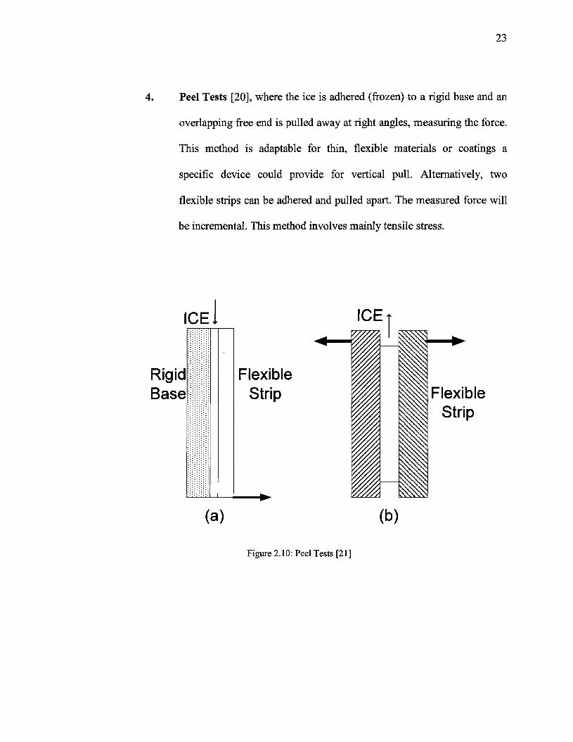
4. Peel Tests [20], where the ice is adhered (frozen) to a rigid base and an

overlapping free end is pulled away at right angles, measuring the force.

This method is adaptable for thin, flexible materials or coatings a

specific device could provide for vertical pull. Alternatively, two

flexible strips can be adhered and pulled apart. The measured force will

be incremental. This method involves mainly tensile stress.

ICE

RigidBase

FlexibleStrip

(a)

FlexibleStrip

(b)

Figure 2.10: Peel Tests [21]

24

5. Impact Tests [16], where the impact is a load which is applied suddenly

or with a shock. It always produces a peak stress higher than that

produced by a load of the same magnitude if it is applied slowly. The

apparatus shown in Figure 2.11 consists of a semi cylindrical bar which

is placed with the rounded portion in contact with the ice surface being

held firmly in place with U-shaped end pieces. The weight in the tube is

raised to a specific height and allowed to drop onto the flat, horizontal

upper face of the bar. This is repeated until all the ice is detached. The

impact energy is the sum of the energy represented by each impact.

Figure 2.11: Impact Tests [17]

25

6. Laser Spallation Technique [10] is an experimental method for

measuring the tensile strength of ice coating to structural surfaces. As

shown in Figure 2.12, a laser-induced stress pulse travels through the

substrate disc that has a layer of ice grown on its front face. The

compressive stress pulse reflects into a tensile wave from the free

surface of the ice and pulls the ice/interface apart, given sufficient

amplitude. The interface strength was calculated at the interface using a

finite-difference elastic wave mechanic simulation. This method shows

that the adhesion strength of very thin layers of ice decreases by

polishing the substrate surface and by decreasing the temperature. This

decrement in the tensile strength can be directly related to the existence

of a liquid-like layer that is known to exist on the surface of solid ice till

-30° C.

computer digitizer

M2 3M2*

constraining substratematerial """"�̂ X

Nd: YAG laser

photo-diode

mirror

energy absorbing^ coatingfilm

mirror w/hole in center

Figure 2.12: Laser Spallation Technique [10]

26

7. Atomic Force Microscopy Technique [21]: this new method using a

Nanoscope Atomic Force (AFM) Microscope is employed to determine the

adhesion force between an individual particle and a solid surface in order to

determine the average value for the adhesion. Micro/Nano scale tests using

AFM or Nano indentation instruments can be used to estimate the nature and

surface energy, too.

8. Electromagnetic Tensile Tests [22], where the interaction of an external

magnetic field with an electric current in the coating produces a normal force

on the coating and therefore provides a means of measuring the adhesion of

the film to its substrate, without requiring any mechanical attachment. This

technique is not applicable for ice because of heat generation due to pass the

test current. It is designed for adhesion measurement of thin film.

Figure 2.13: Electromagnetic Tensile Test [23]

27

9. Blister test [20], as shown in Figure 2.14, in which air pressure is applied at

the center of the adhered interface, the upper (thinner, more flexible) member

of which is thereby debond blister-fashion. Forces involved are mainly tensile.

In this technique the forces are incremental. Indeed, this method permits a

series of measurements on one specimen by interruption of the pressure and

noting each debonds location.

Adhesiveor Ice

\Flexible Cover

Rigid Base

ir Pressure

Figure 2.14: Blister Test [21]

10. Scratch Tests [23] in which a smoothly rounded diamond tip is drawn across

the coating surface and a vertical load, applied to the point, is gradually

increased until the coating is completed removed. This method is not usable

for ice which has a brittle structure.

28

11. Cylinder Torsion Shear Test [20], where an adhesive layer (ice) is formed

between a hollow cylinder and central core, one of which is rotated and the

torque measured. Here stress should be uniform and symmetrical at all points.

The failure occurs instantaneous in all over.

Adhesive or ice{thin .annulus)

Biock

Test Cooting Applied on either Core or Stock

Figure 2.15: Cylinder Torsion Shear Test [20]

12. Combined Mode Tests [20], for example combined shear and tensile force

might be useful. This could be done by applying a fixed load in one mode

while increasing the other till failure. The fixed-variable stress combination

should aid in initiation and propagation of cracks to failure.

29

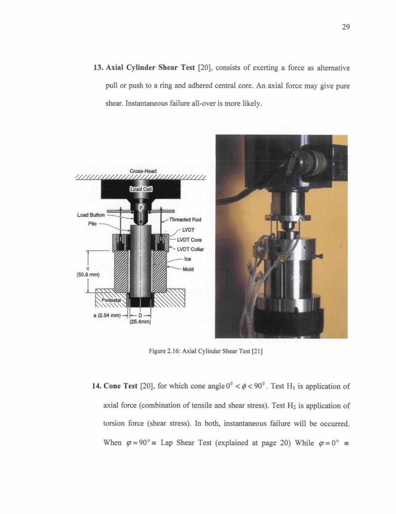
13. Axial Cylinder Shear Test [20], consists of exerting a force as alternative

pull or push to a ring and adhered central core. An axial force may give pure

shear. Instantaneous failure all-over is more likely.

Threaded Rod

LVDT

LVDT Core

LVDT Collar

a {2.54 irnn) H H P(25.4mm)

Figure 2.16: Axial Cylinder Shear Test [21]

14. Cone Test [20], for which cone angle 0° < tp< 90c. Test H] is application of

axial force (combination of tensile and shear stress). Test H2 is application of

torsion force (shear stress). In both, instantaneous failure will be occurred.

When $?=90° = Lap Shear Test (explained at page 20) While <p = 0° =

30

Cylinder Torsion Test (torsion force) and Axial Cylinder Shear Test (axial

force).

_QH

Figure2.17: Cone test [21]

Another simpler method, in theory, uses a beam on which the ice is deposited [4]. A

bending moment is applied to the beam by a mechanical impulse which leads to the ice

separation. The ice thickness is chosen in order to induce the maximum value of shear

stress at the interface which is indirectly deduced from the measurement of the applied

force and the displacement of the beam. Since in this method the thickness of the ice

coating is selected to the value for which the neutral axis locate at vicinity of the

ice/aluminum interface that will be a limiting method. The disadvantages like yielding an

indirect value of adhesion force and high sensitivity to the thickness of ice can lead into

31

some inaccuracies. In addition, this method is not sensitive enough to measure weak

adhesion forces, as in the case of ice-phobic materials.

As has been seen the most of these tests are macroscopic and mechanical

measurements. In the majority of methods a pulling or pushing force was exercised on the

ice to debond it from its substrate. Different results may be anticipated using different

methods. For an example, the review of literature [20] shows that in contrast to shear

experiments, tensile experiments showed that the adhesive strength under tension is at least

15 times larger than the adhesive strength obtained from shear experiments. This large

discrepancy was explained by the assumption of a liquid-like layer between ice and solid

interface. In the case of tension, this layer is held together by surface tension forces

whereas in shear only fractional forces, which are of much smaller magnitude, have to be

overcome [18]. Another note is that the ice solidification is accompanied by expansion.

This could affect some of the test schemes, as an example, the temperature of the ice

sample must be held constant during the experiment. Also the stress should not be applied

during freezing. Because ice is brittle and not strong in either tensile or compressive mode,

the stress developed on freezing might cause cracking, producing a cohesive breaking

before adhesive failure.

The intention is to measure the force to separate the ice from its substrate in adhesion

failure, in other words, the force needed to overcome the adhesion between coating and

substrate. In practice however, the cohesive strength of the coating, e.g., ice, and of the

32

substrate both have an effect on how easy it is to remove the coating. In the case of ice,

cohesion force is lesser than adhesion that means the cohesion failure is more likely.

Moreover, among the methods used for ice adhesion tests some can only be used for

ordinary ice and excludes atmospheric ice formed by the freezing of the super-cooled water

drops in contact with structures.

2.4 Conclusion

In conclusion, the basic of an adhesion test involves a load applied to

adhesive/substrate system until failure occurs. Shear mode tests, i.e. "Lap Shear Test" or,

"Torsion Shear Test" are more common, hi the Torsion Shear Test the adhesive layer is

formed between a fixed plate and a flat disk, which is rotated, with measurement of force

for failure. In "Cylinder Torsion Shear Test" the ice freezes between a hollow cylinder and

central core, one of which is rotated and the torque measured. In "Axial Cylinder Shear

Test", for which the ice is deposited between a hollow cylinder and central core, the

applied force is axial. There are other techniques like "Tensile Tests" and "Peel Tests"

where the ice is frozen onto a rigid base and an overlapping free end is pulled away at right

angles, measuring the force. In "Impact Test" a load is applied suddenly on the surface of

deposited ice till ice detachment. In "Blister Test" a pressure applied at the center of the

adhering interface, the thinner and more flexible member of which is thereby debond in

blister-fashion with measuring the adhesion force. Another method uses an instantaneous

pressure is applied to the ice deposited beam by a mechanical impulse which leads to ice

33

separation. Ice thickness is chosen in order to induce the maximum value of shear stress at

the interface. The high sensitivity to the thickness of ice and insensitivity to measure weak

adhesion forces, as in the case of ice-phobic materials, can lead into some inaccuracies.

Most of known methods have many difficulties and defects that would not yield to

desired results, e.g. in some of the enumerated techniques increasing rate of applied load is

instantaneous, the load is applied directly on the ice which has a brittle structure, the

adhesion force is quantified indirectly, the technique is not applicable for atmospheric ice

and occurring the adhesive failure is not obvious.

CHAPTER 3PIEZOELECTRIC SENSORS

35

Chapter 3Piezoelectric sensors

3.1 Introduction

Piezoelectricity, Greek word for "pressure" electricity was discovered by the Curies

brothers more than 100 years ago [24]. They found that quartz changed its dimensions

when subjected to an electrical field, and conversely generated electrical charge when

mechanically deformed. By the I960's researchers had discovered a weak piezoelectric

effect in whale bone and tendon. This began an intense search for other organic materials

that might exhibit piezoelectricity. In 1969, Kawai [25] found very high Piezo-activity in

the polarized Fluoropolymer, Polyvinylindene Fluoride (PVDF). While other materials like

PVC exhibit the effect, none are as highly piezoelectric as PVDF. Today piezoelectric

polymer sensors are among the fastest growing of the technologies within the sensor

market and there have been an extraordinary number of applications [24].

The most important uses of active/smart material, e.g., piezoelectric, are application as

transducer, means sensor and actuator, based on their electromechanical coupling effects,

which also constitute a major subject of current research regarding so-called smart

materials and structures. Smart structures are being used in a wide range of products. The

36

Hubble Space Telescope contains smart materials for correcting optical efficiencies, and

chip fabrication equipment includes PZT actuators to cancel undesirable vibrations. Smart

materials that incorporates 'sensors (nerves), actuators (muscles), and computers (brains)'

can be thought of something that takes input energy in one form and converts it to output

energy in another form. Depending on the behavior of different smart materials, they may

be more suitable for one application or another [26] [25].

Nowadays, Piezoelectric Fluoropolymer Film, or Piezo Film, is an enabling sensor

technology with unique capabilities. Piezo Film produces voltage in proportional response

to compressive or tensile mechanical stress or strain, making it an ideal dynamic strain

gage as shown schematically in Figure 3.1. Successful applications have been developed

across a vast dynamic range from sensing nanostrains to measuring explosive-level forces

(Mbar). Piezo Film's stress constant (voltage output per stress input) is about 10 times

higher than other piezoelectric materials such as ceramics and quartz. It makes a highly

reliable vibration sensor, accelerometer and switch element [24].

37

Figure 3.1: Like water from a sponge, piezoelectric materials generate charge when squeezed, making anideal strain gage [14]

Conversely, Piezo material undergoes a proportional change in dimension under the

influence of an applied electric field at frequencies from DC to 100 MHz as schematically

seen in Figure 3.2. This property, as well as the film's low impedance, makes Piezo ideally

suited for high fidelity transducers operating throughout the high audio (>lKHz) and

ultrasonic (up to 100MHz) ranges.

Figure 3.2: Piezo also changes dimension with applied voltage for high fidelitj transmission^ 14]

38

Piezo Film is robust, thin, with low weight and low mass, so it doesn't attenuate vibrations

in the material to which it is attached. Piezo can be formed into cable (available in spools

up to 1 mile in length) for applications such as perimeter security. Piezo Film and Piezo

Cable can withstand storage and operating temperatures from -40° C to 85° C.

3.2 Piezoelectric Films Properties

Piezoelectric films are light, flexible, and available in wide variety of thicknesses and

large areas. They have high sensitivity to mechanical load and small variation in it, flat

response over a wide frequency area, and they have also wide frequency range of

application from 0.001 Hz to 109 Hz [24]. Their output voltage is 10 times higher than

Piezo ceramics for the same force input. Due to their low mechanical impedance a number

of piezoelectric films can be placed along structure without drastically affecting its

mechanical properties. Other characteristics are high mechanical strength and impact

resistant, stability confronting chemical components. They are especially interesting due to

their high sensitivities to small variations in applied loads. They can be easily manufactured

into desired shapes and unusual designs, miniaturized, mounted on, and integrated into the

main structures and can be also glued with the commercial adhesive as we have done in our

set-up. When extruded into thin film piezoelectric polymers can be directly attached to a

structure without disturbing its mechanical motion. Piezo film is well suited to strain

sensing application requiring high sensitivity. As mentioned before, operating properties of

Piezoelectric materials can be divided into two branches depending of application as

39

actuator or sensor: Electrical to Mechanical Conversion; i.e., actuator applications and

Mechanical to Electrical Conversion; i.e., sensor applications.

In actuator applications many researchers have shown that the vibration control of a

structure can be realized by applying an adjustable electric field to a piezoelectric

integrated with the structure. As a simple example of this method is sensing and

suppressing vibrations of special tables on which very sensible microscopes have been

installed. Indeed the application of piezoelectric as an actuator seems an active control of

vibration of structures. In fact the active vibration control of flexible structures using

piezoelectric materials has been a great interest to many researchers due to their higher

potential for shape control, vibration suppression, noise attenuation and damage detection

in the past decades as it may be one of the major aircraft designs aspects, which is out of

the scope of this study.

hi application as a sensor studying the Mechanical to Electrical Conversion is more

interesting. Indeed, the sensitivity of Piezo film as a receiver of mechanical work input is

awesome. In its simplest mode the film behaves like a dynamic strain gauge except that it

requires no external power source and generates signals greater than those from strain

gauge after amplification. This extreme sensitivity is largely due to its format. The low

thickness of the film makes in turn a very small cross-sectional area, thus relatively small

longitudinal forces create very large stresses within the material. This aspect enhances the

sensitivity parallel to mechanical axis of the piezoelectric film, which is defined in section

40

3.4. Some sensor applications of Piezo film are enumerated as in musical instruments,

traffic sensors, accelerometers, medical probes, speakers, microphones, impact sensors; i.e.,

impact printers and sport scoring, switches; i.e., switches for automated process, panel

switches, door closure switches, beam switches, and snap-action switches.

If the smart materials are to be used as sensors, they must be integral with the structural

material whose strain is of interest such as this project. For an example of an application as

a sensor, one applies polyvinylindene fluoride (PVDF) for designing very large,

extremely low weight optical sensing systems in space. The primary component of the

system is an unsupported laminated reflector consisting of two layers of piezoelectric

film, such as PVDF in a bimorph configuration and a single layer of shape memory alloy

(SMA), such as Nitinol. The structure will be coated with a reflective surface on one side

to function as the primary reflector of a large telescope. The shape of the structure will

be controlled in space by scanning an electron beam across the piezoelectric surface,

causing local deformations at places where electron charges are deposited. Upon

deployment in space, the Sun's heat will activate the Nitinol causing the membrane to

deploy to its final configuration with minimal surface wrinkles. An electron beam will be

made responsive to an optical figure sensor, observing the shape of the structure, and

will stimulate the PVDF layers to correct surface wrinkles and control the curvature of

the reflector.

41

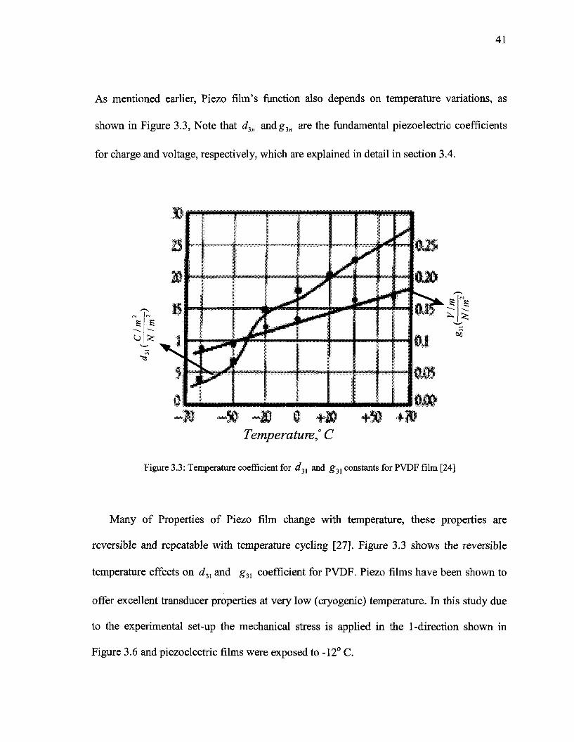
As mentioned earlier, Piezo film's function also depends on temperature variations, as

shown in Figure 3.3, Note that d2n andg3n are the fundamental piezoelectric coefficients

for charge and voltage, respectively, which are explained in detail in section 3.4.

-» -10Temperature,0 C

Figure 3.3: Temperature coefficient for d3l and g3l constants for PVDF film [24]

Many of Properties of Piezo film change with temperature, these properties are

reversible and repeatable with temperature cycling [27]. Figure 3.3 shows the reversible

temperature effects on d31 and gn coefficient for PVDF. Piezo films have been shown to

offer excellent transducer properties at very low (cryogenic) temperature. In this study due

to the experimental set-up the mechanical stress is applied in the 1-direction shown in

Figure 3.6 and piezoelectric films were exposed to -12° C.

42

Figure 3.6 and piezoelectric films were exposed to -12° C.

3.3 Piezoelectric Film as Source Capacitance

Perhaps the most important characteristic after the piezoelectric property is Piezo film's

capacitance. Capacitance is a measure of any component's ability to store electrical charge

and is always present when two conductive plates are brought close together. In case of

piezoelectric films the conductive plates are the electrode metallized onto each surface of

the film7. PVDF has a high dielectric constant compared with most polymers, with value

about "12" relative to the permittivity of free space. Obviously the capacitance of the

element will increase as its plate area is increases. Capacitance also increases as the film

thickness decreases. These factors are formally related in the following equation:

j Eq.3.1

where Co is the capacitance of the film, p is the permittivity, A is the overlap area of the

film's electrodes, and t is the film thickness.

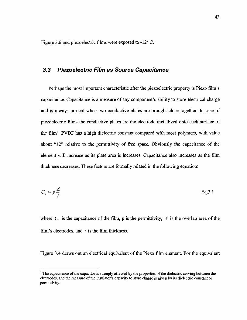
Figure 3.4 draws out an electrical equivalent of the Piezo film element. For the equivalent

7 The capacitance of the capacitor is strongly affected by the properties of the dielectric serving between theelectrodes, and the measure of the insulator's capacity to store charge is given by its dielectric constant orpermittivity.

43

circuit, there are two models- one is a voltage source in series with a capacitance, the other

a charge generator in parallel with a capacitance.

Figure 3.4: Piezoelectric film as a simple voltage generator

Figure 3.4 demonstrates the voltage source which is more common in circuit analysis.

The dashed line represents the "contents" of the Piezo film component. The voltage source

Vs is the piezoelectric generator itself, and this source is directly proportional to the

applied pressure or strain. Our purpose is not to elaborate further calculations. The main

point is that this source voltage will absolutely follow the applied pressure, on other words,

piezoelectric film is a "perfect" source, a great advantage as a sensor. Note, the film's

capacitance, Co is always present and connected when the "output" of the film at the

electrodes is monitored, the node X can never be accessed, and Vo is open circuit voltage.

Note, the voltage source amplitude is equal to the open circuit voltage of Piezo fihn and

varies from micro volts to 100's of volts, depending on the excitation magnitude.

44

Figure 3.5 shows an equivalent circuit as a charge generator. This equivalent circuit has

film capacitance Cf and internal film resistanceRf. The induced charge Q is linearly

proportional to the applied force as described earlier. As in this study, in low frequency

applications, the internal film resistance is very high and can be ignored. The open circuit

output voltage can be found from the film capacitance; i.e. V � � .

ChargeGenerator

Figure 3.5: Equivalent circuit as a charge generator

3.4 The Fundamental Piezoelectric Equations

The amplitude of the signal generated by the piezoelectric film is directly proportional

to mechanical deformation. The resulting deformation causes a change in the surface

charge density of the material so that a voltage appears between the electroded surfaces. It

seems necessary to introduce the fundamental piezoelectric coefficients for charge and

voltage, d3n and g3n, respectively. They predict the charge density (charge per unit area)

45

and voltage field (voltage per unit thickness) developed by the Piezo film, respectively.

Piezoelectric charge and voltage coefficients are each assigned two subscripts: one refers to

the electrical axis, the other to the mechanical axis as shown in Figure 3.6. Because Piezo

film is thin the electrodes are applied to the top and bottom film surfaces. The electrical

axis is always "3" as the charge or voltage is always transferred through the thickness of

the film.

(THICKNESS)

2

1(LENGTH)

Figure 3.6: Classification of Piezoelectric axes [24]

The mechanical strain can be measured on 1, 2 or 3 since the stress can be applied to any of

these axes. It is concluded that piezoelectric materials are anisotropic that its mechanical

response differs depending upon the axis of applied mechanical stress. Hence a particular

attention seems necessary for taking into account the directionality.

46

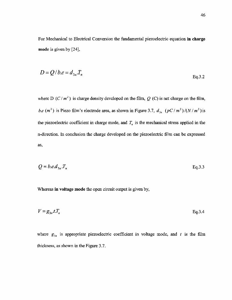
For Mechanical to Electrical Conversion the fundamental piezoelectric equation in charge

mode is given by [24],

Eq.3.2

where D (C / m2) is charge density developed on the film, Q (C) is net charge on the film,

b.e (m2) is Piezo film's electrode area, as shown in Figure 3.7, d3n (pCI m2 ) I{NI m2)is

the piezoelectric coefficient in charge mode, and Tn is the mechanical stress applied in the

n-direction. In conclusion the charge developed on the piezoelectric film can be expressed

as,

Q = b.e.d3n.Tn Eq.3.3

Whereas in voltage mode the open circuit output is given by,

Eq.3.4

where g3n is appropriate piezoelectric coefficient in voltage mode, and t is the film

thickness, as shown in the Figure 3.7.

47

Figure 3.7: Dimensions of film with length of e width of b and thickness of t

Hereafter in this research, for measurement purpose, piezoelectric film is used to assess the

adhesion force at the ice/substrate interface. In the following Table almost all typical

physical characteristics of PVDF films are shown [24].

48

Table 3.1: Typical properties of Piezo film [24]

Symbol

t

<*3.

^33

# 3 1

# 3 3

cY

£

£/£0

Pm

Parameter

Thickness

Piezo Strain constant

Piezo Stress constant

Capacitance

Young Modulus

Permittivity

Relative Permittivity

Mass Density

Temperature Range

PVDF

28

23

-33

216

-330

380

2-4

106-113

12-13

1.78

-40 to 80

Units

jum (micron)

io-12 c/m2

N/m2

10-3 VimN/m2

pF/cm2@ 1kHz

\09N/m2

10"12F/m

103 kg/m3

°C

3.5 Conclusion

As it is mentioned later, piezoelectric film, in sensor application, develops an electrical

charge proportional to a change in mechanical stress. In conclusion some of the most

49

important characteristics of PVDF film for which it has been selected in this study are

enumerated below:

1 Small thickness in micron order

2 Lightness

3 Flexibility (it can be easily manufactured into desired shapes, miniaturized,

mounted on, and integrated into the main structures)

4 Excellent mechanical strength

5 High sensitivity to mechanical load

6 High sensitivity to small variation in mechanical load

7 Low mechanical impedance (because of this property a number of PVDF films

can be placed along the structure without dramatically affecting its mechanical

properties.)

8 In this study it can allow a direct measurement of ice adhesion at ice/substrate

interface, and

9 It can allow applying any ice thickness, by measuring the contribution of shear

and bending stress simultaneously.

CHAPTER 4THEORY AND CALIBRATION

51

Chapter 4Theory and Calibration

4.1 Introduction

In order to describe the stress-strain behavior of ice under loading, physically based

models can be used not only as predictive tools, but also as calibration tools for the

experimental set-up. The successful development of physically based model is contingent

on our understanding of the mechanisms underlying the mechanical properties of ice.

The physical principle of the work is that the ice adhesion strength is equal to the

substrate surface stress subjecting to ice at ice/material interface at the time of ice adhesive

failure. Different mechanical methods for measuring ice adhesion as well as factors

influencing such measurements are briefly reviewed earlier in chapter 2. The purpose of

this research is focusing on the development of a mechanical, macroscopic, and direct

technique for measuring this strength at ice/material interface. This goal is achieved by

using embedded piezoelectric film sensors at the ice/substrate interface. Indeed, a similar

technique was previously used successfully for the measurement of interfacial energy and

shear stress in composite material [28].

52

One of the main advantages of this configuration is that the thickness of ice or substrate

is not confined by the position of the neutral axis, as in the case of the presented method in

[4]. In this configuration, adhesive failure is more likely, because of the creation of the

shear stress at interface. The rate of applied load is incremental and the load is applied on

the substrate surface not on the ice directly which has a brittle structure. Ice is not strong

under the direct load, due to its open chemical structure. If the load is applied directly to the

surface of the sample the molecules on the surface are more susceptible to breaking than

bulk and interface molecules, therefore cohesive failure is more probable.

The aim of this chapter is to present theoretical investigations and the experimental set-

up of this technique and calibration of piezoelectric response. In theoretical approach, the

analytical solution of an aluminum beam, driven into harmonic vibration is obtained.

Theoretical equations of the bending stress due to a vibrating load in a cantilever beam are

derived. A set of presumptions and criteria has been established and used to evaluate a

suitable set-up for empirical studies. Prototype configuration has been constructed in

CIGELE laboratory. Methodology presented later, has been established particularly for

measuring ice adhesion strength. Detailed measurements were carried out and comparisons

made between the experimental results and literature.

In order to calibrate our set-up and also enter the proper coefficient in the program of data

acquisition system, first a few tests for measuring the stress induced on the beam surface

53

with the help of PVDF films were performed, of course without ice. Then a comparison

was done between:

� The calculated value of theoretical bending stress at the beam surface and,

� The practical tests.

4.2 Analytical Modeling of Beam and its Deflection

4.2.1 Beam Modeling

Figure 4.1 shows the configuration used for modeling. The proposed technique for

measuring ice adhesion is based on the bending vibrations of a beam composed of an

aluminum substrate and an ice layer deposited on it. As illustrated in Figure 4.1, one end is

free to move and the clamped end is fixed onto an electromagnetic shaker in order to

produce a desired sinusoidal displacement. Since ice is a brittle material, only the

aluminum beam is clamped.

54

Ice layer

^Electromagnetic shaker

Aluminiumbeam

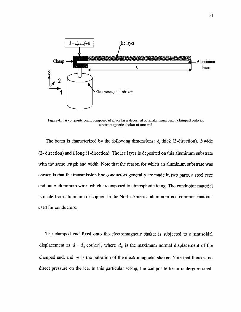
Figure 4.1 : A composite beam, composed of an ice layer deposited on an aluminum beam, clamped onto anelectromagnetic shaker at one end

The beam is characterized by the following dimensions: hs thick (3-direction), b wide

(2- direction) and L long (1-direction). The ice layer is deposited on this aluminum substrate

with the same length and width. Note that the reason for which an aluminum substrate was

chosen is that the transmission line conductors generally are made in two parts, a steel core

and outer aluminum wires which are exposed to atmospheric icing. The conductor material

is made from aluminum or copper. In the North America aluminum is a common material

used for conductors.

The clamped end fixed onto the electromagnetic shaker is subjected to a sinusoidal

displacement as d = d0 cos(cot), where d0 is the maximum normal displacement of the

clamped end, and a is the pulsation of the electromagnetic shaker. Note that there is no

direct pressure on the ice. hi this particular set-up, the composite beam undergoes small

55

deflections in its linearly elastic region. As a result of the sinusoidal displacement, the

composite beam is subjected to both shear8 and bending9 stress. Figure 4.2 represents the

bending stress repartition in aluminium and ice considering their Young moduli. Figure

4.3 illustrates both shear and bending stress. Note in reality they are not in the same plane

as illustrated in this figure. The shear stress is in yz plane while the bending stress is in

xz plane, which illustrated clearly in Appendix, Figure A.2. The Piezoelectric films can

be placed on the aluminum surface before ice deposition. The piezoelectric film thickness

(28 jum ) is very thin compared to the substrate and ice thickness. As stress distribution

varies along the beam and is a function of 1 -direction, x, then the piezoelectric films

length is set relatively small in order to sense homogenous stress while their width is the

same as the beam. Moreover, due to low mechanical impedance of piezoelectric films, the

placement of many of them along the substrate has no influence on the mechanical

properties of the structure. Hence, the mechanical influence of the piezoelectric film is not

taken into account.

In stress analysis terminology, this problem was considered as a static, linear,

temperature-independent problem, isotropic as well as homogeneity of beam. The shear

stress is considered to be constant all along the neutral axis. Initial strains may have various

causes, including temperature change and swelling due to moisture and radiation, however

8 Shear Stress tends to deform the material without changing its volume, usually by "sliding" forces - torqueby transversely-acting forces. The shape change is evaluated by measuring the change of the angle'smagnitude (shear strain).9 Bending Stress: Force per unit area acting at a point along the length of a member resulting from thebending moment applied at that point.

56

they are not taken into account. It is assumed that the composite beam width b is small

compared to its length L. The stress, T2 and the deformation in the 2-direction normal to the

(13) plane seen in Figure 4.3, u2 are considered to be equal to zero. Similarly, the

composite beam thickness hi + hs is small compared to its length L . The stress, T3 and

the deformation, 113, in the 3-direction normal to the (12) plane, shown in Figure 4.3, are

considered respectively to be equal to zero. However the local deformation, U3, of the beam

is zero in the 3-direction but the beam deflection W(x) in this direction is not zero. Note that

the beam vibrates in relatively small finite amplitude. Indeed, when a sinusoidal

displacement, d, is set in motion at the clamped end of the composite beam, a bending

moment, MB, is induced and lead to the appearance of a stress, Tx, at the ice/aluminium

interface. This stress is the result of the contribution of the shear and bending stresses.

From Figure 4.3, it can be observed that the resulted stress at the ice/ aluminium interface is

directly linked with the position of the neutral axis10 (N.A.) and, consequently, with the

thickness of the ice layer. Along the neutral axis the bending stress is equal to zero whereas

the shear stress has its maximum value. This beam transmits a shear force and a bending

moment. Note that the x axis must be replaced from the plane of interface and located

along the undeformed neutral axis of the beam. Therefore the first step is determining the

neutral plane position.

1 Definition and formulation of neutral axis is explained in section 4.2.2

57

Neutral Axis

STRESS

\

Figure 4.2: Bending stress repartition

Neutral Axis

Bending Stress Shear Stress

Figure 4.3: Aluminum/ice interface behavior under composite beam bending (applied case in tests)

58

4.2.2 Determination of Neutral Plane Position

When a beam is bent, one side narrows and the other side lengthens. Between the two,

there is a neutral plane for which the bending stress is equal to zero and shear stress has its

maximum value. The coordinate origin, the x axis, must be located at the neutral plane

position in order to have the right value of z for calculating both bending and shear stress.

The neutral plane position can be calculated using the moment equilibrium of the structure.

It is carried out by calculating the stress in a cross section of the bimorph. The neutral plane

is located at an unknown distance zi from the interface as it is showed in Figure 4.2. In

each material, the bending stress variation versus the z coordinate is linear and the element

equilibrium requires the sum of normal forces to go to zero [29],

Fx=JTxdA = 0 Eq.4.1

where Tx is the bending stress. Considering a section made of two different materials with

Young's modulus Ei and Es as shown in Figure 4.2, then

I*' ThdA + fr TsxdA = 0 Eq.4.2J-zB Jz,

59

Since Tx= , by consideration zmax

=c we have, 7̂ =77mm� by substituting in

above equation,

E, F (£ Sm W + Es p (- Smax )dA = 0 Eq.4.3

where S1^ is the maximum strain at surfaces as shown in Figure 4.2 Ei and Es are the

Young's modulus of ice and substrate. After simplification,

z2B={\-EJEt)zf + (E, IE,)z2

T Eq.4.4

Depending on ice thickness the neutral axis can be located within ice or substrate. This

discrepancy is well shown in Figures 4.2 and 4.3. Assuming the neutral axis is located

within the ice (as in experimental test, Figure 4.3); the ice and substrate thicknesses are

known, then substitution of zB =hs + zi and zT = A,. - z;. in Eq.4.4 gives,

2h,+2(E, IE,)h,

60

where ht is ice thickness and hs is substrate thickness. Subscripts B and T refer to bottom

and top of the composite beam, respectively. If the obtained value for z, is negative, it

means that the NA is located in substrate. As it was expected in the case of having one

material the NA is located at the mid plane. The coordinate origin, z axis will now be

located at distance z, from the ice/material interface.

4.2.3 Determination of Deflection (Bending Displacement)

In order to calibrate the Piezo film response a numerical model for our particular set-up

was developed for studying the dynamic behavior of an aluminum beam, without ice,

subjected to sinusoidal displacement. The neutral axis in this case is located at the middle

thickness of the aluminum beam. Assuming that along the beam, the elastic modulus,

inertia, and cross section area are constant and there is no ice deposition- for calibration of

the Piezo response, there is no need for presence of ice as shown in Figure 4.4. A sinusoidal

displacement d = d0 cos(cot) is applied at the clamped end of beam. Assuming that the

beam undergoes small deflections in the linearly elastic region, and has a uniform cross-

section then the differential equation of motion for the bending displacement of the beam is

known and is described later. Rotary inertia effects have not been considered. The bending

displacement is obtained from the moment equilibrium in the structure. Assuming the

deformation to be small enough such that the shear deformation is much smaller than

bending displacement, w(x,t), i.e., so that the sides of the element dx do not bend. This

61

planar beam, i.e., where all forces are exerted in the same plane, is a system of two internal

stress components, shear and bending stresses.

According to Euler-Bernoulli Beam theory for a beam subjected to a transverse vibration11

the differential equation of motion for the bending displacement of the beam is given by

[30][31][32][33],

Eq.4.6ôx dt

where E is the Young's modulus, / is the second moment of area of the beam cross

section about the neutral axis (El is so-called flexural rigidity), w(x,t) I2is deflection of the

structure, p is the mass density of the beam, A is the cross section area of the aluminum

beam, and f(x,t) is the external lateral force per unit length [34]. A separation of variables

is assumed of the form w(x,t) = W(x)6(t) where the solution of spatial equation is

W(x) and 6 if) is the solution of temporal equation [33].

11 Transverse Vibration: vibration of the beam in the direction perpendicular to its length

12 For this modeling, two important assumptions are made. First the beam thickness is supposed to be verysmall compared to its length, so that strain and stress along the 3-axis are equal to zero. Second, the structurewidth is assumed small compared to its length, hence strain and stress along the 2-direction is also equal tozero. So the bending displacement or deflection w(x, y, z, t) reduces to w(x, t).

62

Clamp

Figure 4.4: Aluminum clamped-free beam

The solution of temporal equation gives,

6(t)-6l cos(ft) + 62 sin(yt)

N.A.

Eq.4.7

where the y is the pulsation. The coefficients 6X and 62 can be calculated only if two

initial conditions (initial deflection and velocity) are specified. In this study we do not need

to have the temporal answer.

The homogeneous spatial equation comes [32],

dx

d*W

dx*

Eq.4.8

Eq.4.9

63

where fi is the flexural wave number given by

fi*=pAco2/EI Eq.4.10

The general solution to Eq.4.9 leads to,

W{x) = kx cosh/ft:+k2 sinh/fc:+£3 cos/fe:+k4 sia/k Eq.4.11

where the coefficients kl, k2, k3, k4 are determined using four boundary conditions of

cantilever beam as follows:

� At clamped end, the deflection is equal to d0 and its first derivative is equal to zero

at X =

U at x =dx

By means of accelerometer, which is fixed at the clamed end of the set-up, the acceleration

of the forced end is measurable, therefore for a given frequency, maximum displacement

d0 at the clamped end is known as,

d0=a/co2 Eq.4.13

where a is acceleration expressed in (m/s2), and � in (rad/s).

64

At the free end, the bending moment and the transverse shearing force are equal to zero.

= 0 at X =dx Eq.4.14

El r^- = 0 at x = Ldx3

Finally, making use of boundary conditions, four coefficients of bending displacement are

determined as:

k _d0cosfiL-k2Al Eq.4.15A2

_ dQ.(A-i cos flL + A^ sin fiL)

lr � � k

where the three coefficients AX,A2, A3 are given as,

A = sin BL + smhBL � . . ,1 ^ ^ Eq.4.16

A2 = cos ySZ + cosh /3L

A3 = sinh flL - sin J3L

In order to calibrate the Piezo film response we should calculate the stress induced at the

aluminium beam surface. When there is no ice on the beam, the neutral axis is located at

65

the middle thickness of the aluminium beam zi = �, thus shear stress at the surface is

equal to zero while bending stress is equal to zero at neutral axis and it increases linearly to

a maximum at the surface.

4.2.4 Determination of Bending Stress in order to Calibrate the Piezo

Film Response

By knowing the fonctionality of bending displacement along 1-direction or x, it is possible

to calculate bending stress on the surface of the aluminium beam as a fonction of bending

moment. Thus, the following equation can be used [34],

Eq.4.17

where M is the bending moment, / is the area moment of inertia about the z axis, and z is

distance from the neutral axis. The bending moment is the result of bending stress of

structure and is given by [29],

M = -jzTxdA Eq.4.18

66

According to primary assumptions and simplification of Hook's law, the longitudinal stress

is given by,

Eq.4.191-v2

where v is Poisson' s ratio, E is the Young modulus, and £xis the longitudinal strain. For

such a cantilever beam the longitudinal strain is expressed as [29],

d2W

dx

Substitution of Eq.4.20 into Eq.4.19 yields,

E d2W

dx2

According to Euler-Bernoulli beam theory, bending moment as a function of bending

displacement is given by,

� ^ Eq.4.22dx

67

Eq.4.22 expresses bending moment as a function of deflection, W(x). Substituting this

equation in Eq.4.17, and considering z = � (hs is the thickness of the beam) results,

T 2 Tãx l Eq.4.23

Note, here the denominator 1-v2 in equation 4.21 is close to unity, since Poisson ratio

of aluminium according to Table 4.2 is 0.33 then,

l-(0.33)2 =0.90 = 1

Thus bending stress as a function of bending displacement at the surface of the beam is

bh3

obtained. Consequently, having beam dimensions, i.e., L, A (A = b.h, I = ) , its mass

density p , and Young's modulus E, frequency and the acceleration at the clamped end, the

exact theoretical value of bending stress induced at the surface along the beam is

computable.

68

4.3 Calibration of Accelerometer

The output voltage of charge amplifier is

V' = knmnQ Eq.4.24amp. �*--� i

where hamp is the amplification coefficient (gain of amplifier) which is calculated in this

section for accelerometer calibration, F'is the output voltage of amplifier measured by

means of an oscilloscope, and Q was measured by means of a charge amplifier type 4370

(Brûel & Kjaer Co.). Indeed this charge amplifier measures the acceleration in(ms'2), then

by multiplying this acceleration in accelerometer coefficient (transformation coefficient)

that is 10.00 (pCI ms~2 ) , the resulted charge was obtained in (pC).

Moreover the Eq.4.24 can be shown as,

kamn =� Eq.4.25amp. s-. 1

By measuring the output voltage of amplifier and charge on accelerometer by means of a

charge amplifier, the amplification coefficient (gain of amplifier) is calculated. In this study

69

considering the homemade piezoelectric film amplifier the value of amplification

coefficient was 1.1 * 109 (V/C).

4.4 Calibration of Piezo Film Response

The stress induced on the film can be expressed as,

1 KEq.4.26

where K(Vm2 /AT)is the adjusting coefficient in Data Acquisition Program which must be

calculated for calibrating Piezoelectric film response, Vout is the output voltage of the

Piezo film after amplification measured by means of an oscilloscope (or Data Acquisition

System during performing the tests with ice). Therefore for calibrating the Piezo film

response, the adjusting coefficient, K, must be calculated. For this purpose consider Eq.3.3,

which expresses Q as a function of Piezo film physical properties and induced stress,

Q = b.e.d3VTl Eq.4.27

13 Note that V is the output voltage of amplifier itself without Piezo film where Vout is the output voltage13

of the Piezo film after amplification, thus they are not equal

70

where bis the film width, eis the film length, as illustrated in Table 4.1, d3l is the

piezoelectric coefficient (Piezo strain constant) with a value of 23 * 1(T12 � � - , and Tx isNlm2

the stress induced on the piezoelectric film.

Table.4.1: Dimensions of PVDF strip

\

PVDF

Strip

Tested Length or e

(mm)

4

Width o r e

(mm)

26

Thickness

(mm)

0.028

On the other hand it was seen in Eq.4.25 for accelerometer calibration that,

V' = k Q => 0 =amp.*-- *-.

V

amp.

Eq.4.28

where kamp is the amplification coefficient (gain of amplifier) with a value of

1.1 *109 (V/C) that was calculated for accelerometer calibration, F'is the output voltage of

amplifier measured by means of an oscilloscope. Thereafter measured voltage is output

voltage of Piezo film and Q is the charge induced on the film. Therefore stress induced on

the film as a function of output voltage is given by,

71

= � Voul Eq.4.29K

K is a known coefficient, thus the relation between the resulting stress r,(Pa) and the

output voltage of film, Vout (V), becomes:

Tl = 0.3S*l06*Vout E q A 3 0

Equation 4.30 was used to determine the magnitude of the stress at the location of the

PVDF film; of course the known coefficient K was entered before into the Data

acquisition program in order to calculate directly the induced stress during ice adhesion

test.

4.5 Determination of adequate frequency exercised toelectromagnetic shaker

As can be seen in Eq.4.10, fi is a function of pulsation m, which expresses the applied

frequency of sinusoidal displacement (co - 2nf). Hence determining the appropriate

frequency for set-up is essential. According to theory in this set-up the first and second

resonance frequencies were calculated as demonstrated in Eq.4.33 and Eq.4.34.

72

Table 4.2: Physical characteristics of the aluminum beam

Length

(mm)

280

Width (b)

(mm)

25.4

Thickness (h)

(mm)

3.1

Young modulus ( E )

(GPa)

66.8

Poisson ratio (V )

0.33

Mass density ( p )

(gr/cm3)

2.712

/ , which is the area moment of inertia about the z axis, by using Table 4.2 can be

calculated as,

12 12<2 t Eq.4.31

A, which is the cross section area of the aluminum beam, is given by,

=78.74*1(T (m2) Eq.4.32

Therefore, the first and the second resonance frequencies of the aluminum beam are [34].

Eq.4.33

Eq.4.34

73

d2W(x) h d2W(x)Eq.4.23, Tx = -E r ^ � expresses T as a function of j - ^ - , where W{x) is given

dx 2 dx

by Eq.4.11, which depends on fi,kj(i = 1,2,3,4), and x. In addition according to Eq.4.10

fi is a function of ÛJ or applied frequency f(co = 27if). Considering Eq.4.15 which

expresses kt coefficients as functions of d0, maximum displacement,

_dü cos pL-k2.Ax _do(A3 cos fiL + A2 sin fiL)x - - ,K2 - � - �^ , « 3 � « 0

A2 AXA3 � A2

Because of d0 =alco2, W{x) is a function of acceleration, too. In conclusion the bending

stress is a function of applied frequency, acceleration as well as position. Figure 4.5 depicts

bending stress as a function of frequency, for a given position (30 mm from the clamped

end) and for a constant acceleration(\0m.s~2).

74

x i o '

50 10D 150 200 250 300 350 400 450 500Frequency of displacement (Hz)

Figure 4.5: Bending stress as a function of frequency, for a given position and acceleration

It can be seen that maximum bending stress appears at first resonance frequency. Indeed

bending stress, at the first resonance frequency, has the same order as ice adhesion strength

in literature [4]. Therefore it seems more interesting selecting and working around first

resonance frequency of the beam, between 30-34 Hz.

For more assurance, we illustrate bending stress as a function of position along the beam,

for a given acceleration(l0m.s~2 ) and the supposed frequency (30 Hz).

75

x10°

O 0 02 0.04 0 06 0 0B 0.1 0.12 0.14 0.16 0 18 0.2Position along the beam (m)

Figure 4.6: Bending stress as a function of position, for a given frequency and acceleration

Figure 4.6 shows the functionality of bending stress along the beam at 30 Hz. In fact

bending stress, about frequency of 30 Hz, has the same order as ice adhesion strength in

literature [4]. Figure 4.6 also shows that at low frequency, the distribution of bending stress

is approximately linear and the maximum stress value is obtained at the clamped end.

It is more attractive working close to the first resonance frequency of the beam in order

to induce the maximum resulting stress at the ice/aluminium interface. Moreover, adhesion

failure should be initially induced much closer to the clamped end of the aluminium beam,

where the stress has its maximum value. Consequently, the frequency of sinusoidal

displacement is appropriately chosen close to the first resonance frequency, it means 30 Hz.

Figure 4.6 reveals it is preferable that the PVDF film sensor be located close to the clamped

76

end of the beam (30 mm) because the bending stress increases by approaching to clamped

end while near the free end (see Figure 4.6), it is more likely that the bending stress do not

be sufficient for ice detachment, thus the piezoelectric film may not pick up the detachment

strength.

4.6 Theoretical Modeling of Bending and Shear Stress inPresence of Ice at Interface

4.6.1 Modeling of Bending Stress

Hereafter, theoretical calculations for determination of bending and shear stresses, in

presence of atmospheric ice layer on the substrate, at ice/material interface are presented.

Obviously the only way to be insured of having reasonable and feasible modeling is to

compare the practical results with the theoretical superposition of bending and shear

stresses at interface. Unfortunately any model, measurement or particular experimental

equipments do not exist in order to measure the exact value of Young modulus and Poisson

ratio of atmospheric ice which is certainly different from the ordinary ice. Indeed ordinary

ice results from water solidified in low temperature. Surely its physical and mechanical

characteristics differ from atmospheric ice which forms from precipitation in nature or

spraying supercooled water droplets in laboratory tests.

77

However it seems interesting to study the theoretical approach since there is similar

approach in composite materials [28]. The determination of neutral axis plane has yet

explained in detail in section 4.2.2. hi order to determine bending displacement (deflection)

of bimorph, Eq.4.8 was renewal,

-pAco2W(x) = 0 Eq.4.35dx

where El is the global flexural rigidity, which is given by [25], and p is the total density

pA = pibhi +psbhs where pi and ps are ice and substrate densities, respectively, and A is

the cross section area, A = b * (hl;+ hs ) . The next step is determining the bending moment

of the bimorph, referring to Eq.4.18 and Eq.4.21,

d2W

Note this equation is not apparently equal to Eq.4.23 which is obtained in order to calibrate

the set-up without ice. Because in presence of ice the neutral plane is not located at

aluminum midplane, z{ is given by Eq.4.5. In addition in theoretical analysis the

denominator is maintained. For the case of a section made of two different materials as

shown in Figure 4.7, the integral is divided into two parts, one for each elastic material

78

M = -d2W

dx2O z ,

Eq.4.37

where v(. and vs are Poisson's ratio of ice and substrate, £;. and Es are Ice and substrate

Young modulus, respectively. The terms inside the parentheses represent the moment of

inertia of the section about the neutral axis,

z

E..

E.

X

Figure 4.7: Coordinates of modeling, zi demonstrates the neutral axis position

The global bending moment is,

M = - d2wHx1 � H Eq.4.38

79

The previous relation can be seen from Euler-Bernoulli Beam Theory [34],which expresses

bending moment as a function of deflection. The global bending moment can also be

written as,

Eq.4.39

where El is the global flexural rigidity of the structure,

T FTi ^^ Eq.4.40l-v, 1-v,

Finally solving the moment equation for stress gives us the bending stress within the ice

[33]

T =-^2-z Eq.4.41XI j I *

where MG is the global bending moment, zi is the distance from the neutral axis within the

ice, and / is the moment of inertia of the section about the neutral axis of non-

homogeneous beam which can be expressed as,

Eq.4.42

80

Substituting Eq.4.39 into Eq.4.41 gives the bending stress of ice as a function of bending

displacement,

dx1

The bending stress of the substrate is expressed as,

Eq.4.43

Eq.4.44

where zs is the distance from the neutral axis within the substrate.

4.6.2 Modeling of Shear stress

For this particular set-up, in addition to bending stress which develops in a loaded

beam, e.g., ice covered beam there is also shear stress which develops at ice/substrate

interface, including both a vertical shear stress and horizontal (longitudinal) shear stress. It

can be shown that at any given point in the beam, the values of vertical shear stress and the

horizontal shear stress must be equal at that point for static equilibrium [29]. As a result it

is usual to discuss and calculate the horizontal shear stress in a beam. Thus, the formula for

81

the horizontal shear stress was derived. In this study, the value of shear stress was not

considered for calibration; however it will be complementary to mention its related

equations and calculations for a iced covered beam for having an idea about the values of

horizontal and vertical shear stresses at interface, theoretically. It is remarkable that in this

research the value of the contribution of both shear and bending stresses was

simultaneously measured and no separation or distinction between two different stresses is

practically possible.

Assuming the bimorph (aluminum beam and ice layer deposited on it) undergoes small

deflections in the linearly elastic region, and has a uniform cross-section. According to

Euler-Bernoulli Beam theory shear force can be expressed as the third derivative of

transverse deflection,

õ3w(x,t) dW(x\

^ P Eq.4.45= W(x)0(t) X

The shear stress z generated from the shear force can now be calculated as [34][35],

VQ*�~ Eq.4.46

ID

where Q* is the first moment of the area about the neutral axis. For composite areas, i.e.,

82

ice and substrate, the first moment of area can be calculated for each part and then added

together. The equation for Q in this case is

Eq.4.47

where A- is the area of the part of the cross section that is considered, 2C* is the vertical

distance from the centroid of the cross section to the centroid of A- as shown in Figure 4.8

and / is the moment of inertia of the section about the neutral axis.

Neutral Axis

Figure 4.8: z , is the vertical distance from the centroid of the cross section to the centroid of A* [29]c

Substituting Eq.4.45 in Eq.4.46 gives the shear stress as a function of bending

displacement,

83

$-% Eq.4.48b cb?

Assuming that before ice detachment, in the linearly elastic region, the displacement and

the strain tensor are the same for both substrate and ice at interface, because they are

closely linked.

It is remarkable that inertia forces of ice accretion are negligible in comparison with shear

and bending forces acting at the interface. The bending displacement of the beam is very

small, around 4 mm for the free extremity of the composite beam. The maximum inertia

force due to the beam acceleration can be expressed as a function of the bending

displacement as follow:

where W{x,t) = W{x).em is the bending displacement with W(x)14, which represents the

spatial part of the bending displacement.

õ2W(x t)Hence, as j ^ - = -co2W(x,t) and with a small ice masse m (around 28 g), the

inertia force induced by the ice deposit is around 1.15 N. This correspond to a normal

14 which will be described later

84

stress of 161 Pa applied to the center of gravity of ice deposit. In this context, the

contribution of the inertia force of the acceleration of ice deposit in the process of ice de-

bonding can be neglected in comparison of the range mentioned in literature [4] means

about 0.2 MPa, required to ice de-bonding.

CHAPTER 5EXPERIMENTAL SETUP, FACILITIES AND

TESTS PROCEDURE

86

Chapter 5Experimental Set-up, Facilities and Tests

Procedure

5.1 Introduction

In order to achieve the objectives, an experimental study was systematically carried out

in the laboratory of CIGELE/INGIVRE in Université du Québec à Chicoutimi. For this

purpose, the atmospheric icing conditions were simulated by spraying super cooled water

droplets on the prototypes. This chapter introduces laboratory facilities, the experimental

set-up and the test procedure used in this particular technique of measuring ice adhesion

strength.

5.2 Laboratory Facilities

5.2.1 Ice deposition in climate room

Scientific tests should be repeatable and comparable. Therefore, the tests were carried

out in a chamber that makes it possible to control precisely the environmental conditions,

such as temperature, wind velocity, and ice-thickness deposited on beams. In this study, all

the adhesion tests were performed in one climate rooms at CIGELE that is equipped with a

water droplet generator (nozzle) and a cooling system, which makes it possible to form an

87

ice layer on the surface of the beam. Then> beams were placed on a stand shown in Figure

5,1, with a constant slope angle of 47° and constant distance from the nozzle, inside the

climatic chamber where exposed to atmospheric ice accretion obtained from spraying

cooled water droplets under the experimental conditions presented in Table 5.1 In order to

have isothermal conditions for beams in the chamber, they were exposed about two hours

to dry air before beginning ice deposition.

Figure 5.1: Beams placed on the stand exposed to artificial ice deposition

88

Table 5.1: Constant Parameters used for atmospheric ice accretion

Test Parameters

Air temperature (°C)

Freezing water temperature (°C)

Water droplet size (|im)

Precipitation rate(mm/hr)

Wind Speed(m/s)

Water Pressure(psi)

Ice thickness(mm)

Parameters values

-12(±0.2)

3

around 80

18

3.3

60

3-4

5.2.2 Water droplet generator

The water droplet generator is comprised of an oscillating nozzle with 30 Hz frequency of

oscillation, in all tests. The type of flat spray standard nozzle- VeeJet spray nozzle with

small capacity of 0.12 gallon per minute at 60 psi-is H1/4W2501 shown in Figure 5.2. It

is located in front of the 1.5-meter-height stand with 1.9 meter horizontal distance and 2.9

meter height. The spray angle at 60 psi was set at 30° C.

89

As we all know, glaze adhesion is the most dangerous to the power systems; therefore

glaze adhesion is more interesting to measure. For that reason by adjusting the water

pressure fed into the nozzle to 60 psi, the water droplet size is adjusted to 80 ju m in order

to particularly have the glaze ice type. Wind velocity, as another important factor affecting

the ice type, was set to 3.3m/s.

Figure5.2: Flat Spray Standard Nozzle, H1/4W2501

5.2.3 Cooling system

To simulate cold atmospheric icing conditions, our laboratory is equipped with an ammonia

cooling system. This system is made up of a compressor and computer-controlled

regulators, which allow to very rapidly reach air temperatures as low as -30°C ± 0.2°C.

The accuracy of temperature control is 0.1°C. In order to produce the glaze in this study,

the environmental temperature was adjusted to -12°C during the ice accretion period. The

90

water conductivity was set to its minimum about 5-8 jus I cm in order to minimize the

probability of affecting charge induced on the piezoelectric film while tap water

conductivity is about 80 jus I cm. The humidity of the room, which has an important role in

ice adhesion value, was measured by a Hygro-Thermo anemometer (HHF710) as

5.2.4 Data acquisition system

The test data, including the stress and acceleration were monitored and recorded by a data

acquisition system, which consists of a PC-compatible, high-speed data acquisition card

developed in MATLAB environment.

5.2.5 Glues

For this study, as shown in Figure 5.3, two kinds of glues were necessary;

� Insulated glue that was applied between piezoelectric film

and aluminium beam

� Conductor glue that was applied between piezoelectric film

and electrical wires

This value shows relative humidity which defines as the percent of saturation humidity [38],R.H.= (actual vapor density/saturation vapor density) * 100. Saturation vapor density depends on

temperature, for example in � 10° C it is 2.36 gm/m3

91

In order to have an insulated and vibration resistant contact a special epoxy, named

EPOXY RESIN RBC # 3215, was used. Weighing the desired amount of resin and

hardener into a clean container, mixing thoroughly and potting it in 60 C for 4 hour, gives

the best result. It is remarkable that this epoxy bonds well to aluminium, polypropylene and

glass and its operating temperature range is -55° to 100° C, thus applicable for many types

of substrates and for icing condition.

Conductor glue, epoxy modelled EE129-4, makes an excellent electrical contact

between two piezoelectric electrodes and electrical wires. Wires which were used here

were insulated, varnished winding wires from copper. Their diameter was rather fine about

0.1 mm. It is remarkable that for each prepared prototype the contact resistance was

checked in order to ensure that the electrical contacts are all right.

Insulatedcontact

Eléctricacontact

Figure 5.3: Practical exhibition of glues

92

5.2.6 Accelerometer

A charge accelerometer, type 4370 (Brûel & Kjaer Co.), is mounted on the clamped end in

order to measure the acceleration of the beam during the test, however accelerometer is not

principally used to measure acceleration but to determine the displacement of the clamped

end, seen in Eq.4.13. The accelerometer was calibrated by a charge amplifier named

"Measuring Amplifier Type 2525" made by Brûel & Kjaer. The accelerometer was used to

calibrate the charge amplifier, too. Note that the amplitude of sinusoidal displacement was

increased manually that is not ideal for having a good ramp. As one of future works,

developing a software for automating of amplitude command seems necessary.

5.2.7 Aluminum Beam and Piezoelectric Film

The aluminum beam that was used in ice adhesion tests was 'Alcoa Alloy 6061-T6511 '. Its

general characteristics are excellent joining, good acceptance of applied coatings, combines

relatively high strength, good workability and high resistance to corrosion. Transmission

lines conductors are generally are made in two parts, core and conductor. The envelope

wires are made from aluminum or copper. In the North America aluminum is a common

material used for conductors. Its Young modulus E = 66.8GPa , its Poisson ratio, v = 0.33,

its mass density p = 2.112gr/cm3 axe known exactly. In this study two different surface

93

finishes (roughness) was applied. The first series of prototypes were polished by aluminum

oxide sandpaper no. 180, following by a cleaning step using acetone. The second series

were polished by sandpaper no.400 following by a cotton polishing wheel, in order to have

a more finished surface. In Table 5.2 dimensions of both types of aluminum beams and also

piezoelectric films glued on the aluminum surface, is given. The PVDF film used has a d3l

"1charge coefficient value of 23.10"1 ((pc I m2 ) /(NI m2 )).

Table 5.2: Dimensions of the aluminum beam and PVDF strip

Beam (no. 180)

Beam (no. 400)

PVDF

Strip

Tested Length

(mm)

280

280

4

Width

(mm)

25.4

25.4

26

Thickness

(mm)

3.1

3.1

0.028

5.2.8 Charge Amplifier Circuit

As shown in Figure 5.4 a homemade charge amplifier was prepared in order to cancel

environmental noise and reinforce piezoelectric film signals. The charge amplifier gives a

voltage output which is directly proportional to the charge induced on the piezoelectric

94

film. Hence, the output voltage of the charge amplifier is directly proportional to the

resulting stress measured at the ice/aluminum interface. Amplifier input comes from

piezoelectric film and accelerometer and its output goes to the data acquisition system and

a PC in order to record simultaneously the total charge and acceleration in all the moments

and then to calculate the stress induced on the beam by means of a special MATLAB

Programming.

Figure5.4: Homemade Charge Amplifier

The transistor selected for this charge amplifier was low-power J-FET operational amplifier

named as 4TL061CP\ It features high input impedance; wide bandwidth, high slew rate,

and low input offset and input bias currents. Figure 5.5 illustrates top view of 'TL061CP'

package.

95

we| V C C +

I OUT| OFFSET

Figure5.5: Top view of 'TL061CP' package

Figure 5.6 shows the charge amplifier circuit used in this research. Note for each

piezoelectric film an equivalent charge amplifier circuit is needed. Moreover a charge

amplifier circuit was considered for accelerometer.

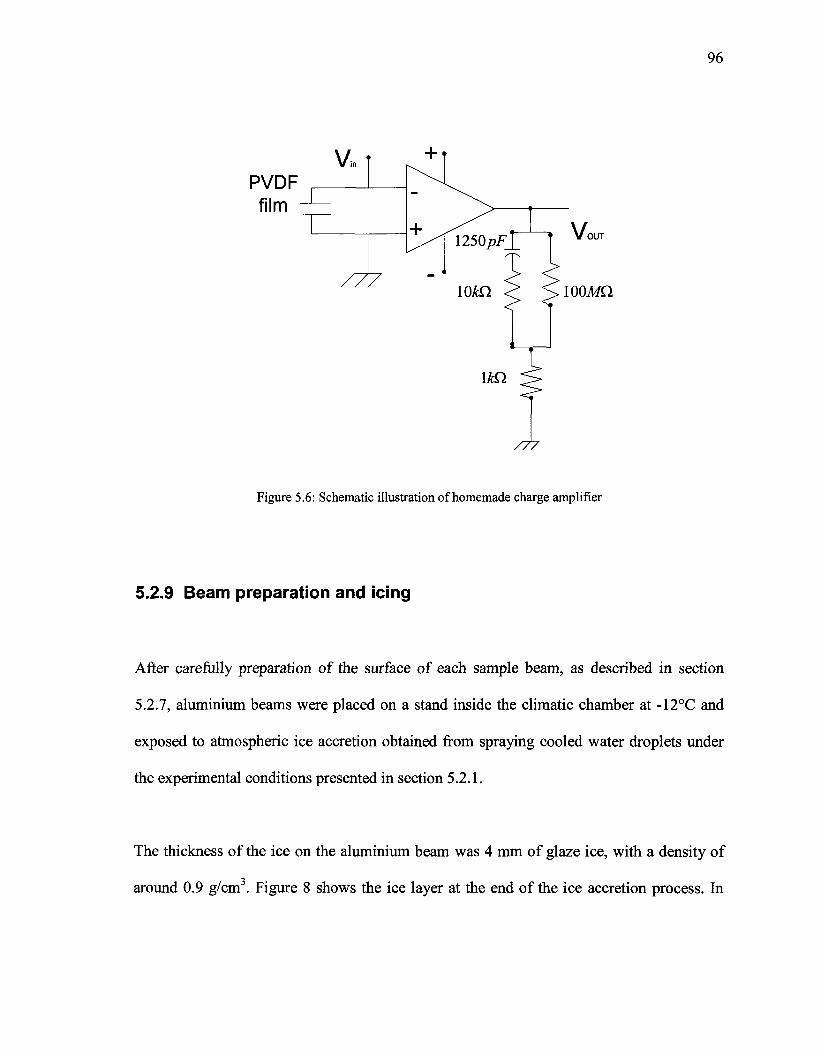
96

PVDFfilm

OUT

100MQ

/77

Figure 5.6: Schematic illustration of homemade charge amplifier

5.2.9 Beam preparation and icing

After carefully preparation of the surface of each sample beam, as described in section

5.2.7, aluminium beams were placed on a stand inside the climatic chamber at -12°C and

exposed to atmospheric ice accretion obtained from spraying cooled water droplets under

the experimental conditions presented in section 5.2.1.

The thickness of the ice on the aluminium beam was 4 mm of glaze ice, with a density of

around 0.9 g/cm3. Figure 8 shows the ice layer at the end of the ice accretion process. In

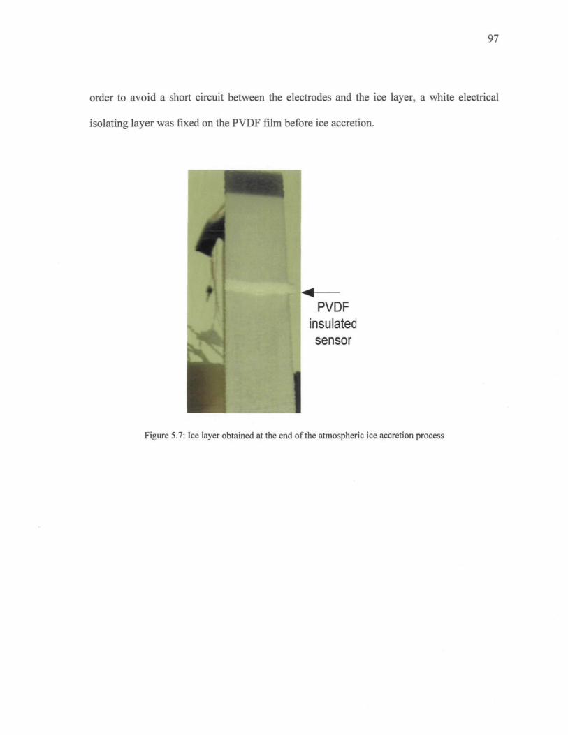
97

order to avoid a short circuit between the electrodes and the ice layer, a white electrical

isolating layer was fixed on the PVDF film before ice accretion.

PVDFinsulatedsensor

Figure 5.7: Ice layer obtained at the end of the atmospheric ice accretion process

98

5.3 Experimental Set-up

An electromagnetic shaker and frequency generator were used in order to induce the

necessary sinusoidal displacement to the aluminium beam at the clamped end. Note ice is a

brittle material, only the aluminum beam is clamped. Figure 5.8 shows the experimental

setup of the method developed.

Accelerometer

Clamp PVDF Strip

ElectromagneticShaker

Figure 5.8: Experimental setup

99

The clamp is directly fixed to the moving part of the electromagnetic shaker in order to

provide the sinusoidal normal displacement d0 cos(cot) which is measured with the

accelerometer fixed on the top of the clamp (see Figure 5.8). The PVDF strips bonded to

the aluminum beam are larger than the beam width in order to properly carry out the

electrical contact on the PVDF electrodes, as illustrated in Figure 5.8. This also ensures a

rigid mechanical bond between the PVDF strips and the substrate.

5.4 Tests Procedure

Hereafter all the exact tests procedure is explained systematically. The calibrations of

accelerometer and piezoelectric film had been performed before the tests commencement.

1. Prepared beams (finished beams with glued piezoelectric film) are weighed

before icing.

2. Ice thickness is measured after icing.

3. Beams are weighed following icing in order to calculate ice density.

4. After icing, the composite beam is clamped onto the electromagnetic shaker

inside the cold room.

100

5. The PVDF film sensor and accelerometer are connected to the Data

Acquisition System (DAS).

6. The frequency of the electromagnetic shaker is set to 30Hz.

7. As explained before, for a frequency of about the resonance frequency of the

structure (30 Hz for aluminum beam) and constantly increasing amplitude.

Note that the strain rate must be suitable.

8. Afterwards the commencement of DAS recording, the amplitude of the

displacement d is constantly and progressively increased from zero until the

ice de-bonding.

9. Piezoelectric cells pick up the ice detachment force.

10. The collected data by Data Acquisition System contain the exact moment,

and stress value of ice detachment with tracing the variation in received

signals from the piezoelectric films during the test, as specimens shown in

Figure 5.9 and Figure 5.10.

11. The results are analyzed in terms of surface roughness.

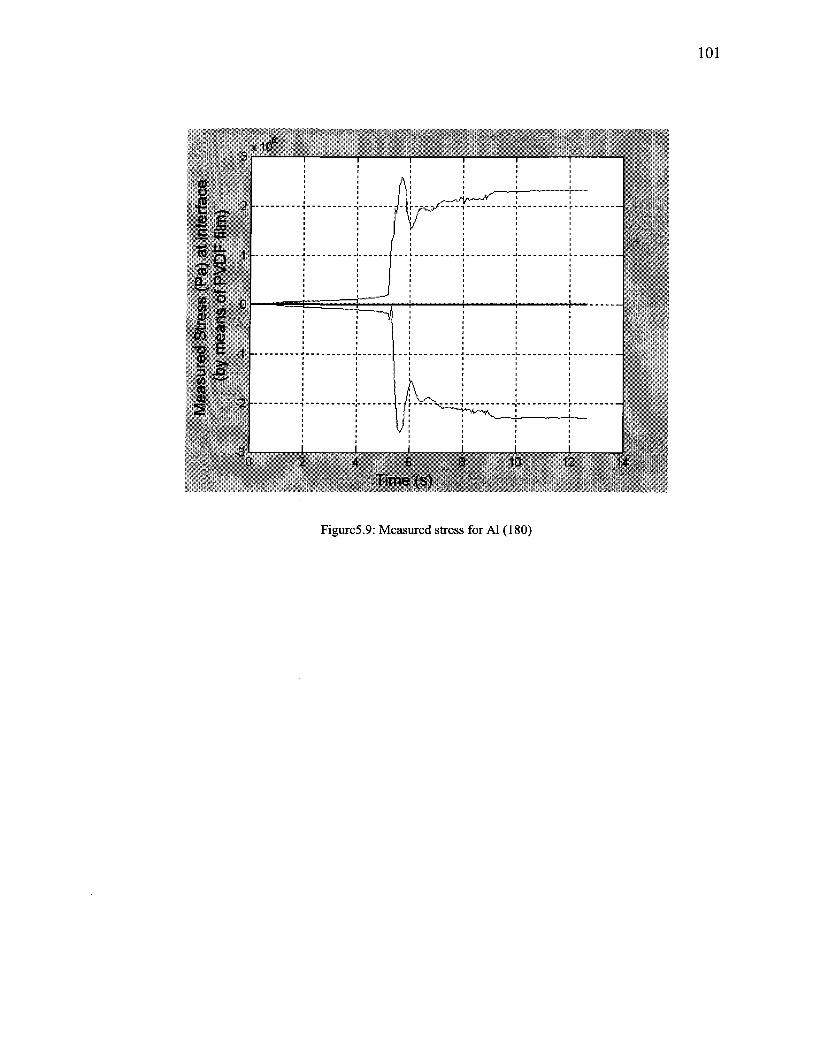
101

x10u

a>o�g&�sID"

ïSîS?3(0CO

LJL

O

�s(ACta

J2

2 �

- 1 �

-2

-3

__

i

t.J\

1

r

4 6

Time (s)10 12 14

Figure5.9: Measured stress for Al (180)

102

4 6 8

Time (s)

Figure5.7: Measured stress for Al (400)

10 12

In next chapter we will discuss more about the resulted graphs and the value obtained for

ice adhesion strength.

CHAPTER 6EXPERIMENTAL RESULTS

104

Chapter 6Experimental results

1.1 Introduction

After the completion of many preliminary tests, a series of four tests were performed

under the same conditions with a PVDF film sensor placed at 30 mm from the clamped end

at a constant temperature of-12°C. The temporal evolution of the resulting stress measured

by the PVDF film at the ice/aluminium interface is presented in Figure 6.1 and Figure 6.2.

Each graph corresponds to the positive and negative envelope of the sinusoidal signal

obtained from PVDF films. The results of Figure 6.1 show the evolution of the stress

magnitude on the aluminium surface less finished (polished by sandpaper no. 180) as

measured by the PVDF film. Figure 6.2 demonstrates the stress magnitude on the

aluminium surface more finished (polished by sandpaper no.400 following a cotton

polishing wheel). Thus the experimental results were affected by surface roughness. The

obtained empirically results demonstrate that ice adhesion strength depends on the surface

finish, as it is more finished the adhesion strength is less, which can be explained by

mechanical interlocking mechanism16. Evidently mechanical interlocking plays a more

important role when a surface is less finished. It may be observed that, in all test series,

16 Which is explained precisely in chapter 2

105

with an increase in the displacement amplitude of the clamped end, the interface stress

increases quite linearly until delamination or ice de-bonding occurs at the film position. At

this specific moment a drastic change in the interface stress occurred resulting from a local

redistribution of the bending and shear stress. Hence, the interface stress obtained at this

specific moment corresponds to the stress needed to de-bond the ice from its substrate (ice

adhesion strength). The ice adherence force obtained for each test series are presented in

Table 6.1.

x10°

8

|(O O

88sto S

to "�'

1 ..

-1 -

-2

-3

- T ^ ; -

Ice-debondi

i

( \

� �

/

V

r

1

4 6 8

Time (s)10 12 14

Figure 6.1: Temporal evolution of the resulting ice/aluminum interface stress obtained from the PVDF embeddedsensor (finished AL 180)

106

1.5x10u

8� § -SE£ .«= 0.5 -

£ê

8 "SCO d>

(0(0

-0.5 -

-1 -

-1.5

deIce-

bonding\

��-_

\/

\\

V17^

� � � - .��_- 1

4 6

Time (s)10 12

Figure 6.2: Temporal evolution of the resulting ice/aluminum interface stress obtained from the PVDF embeddedsensor (finished AL 400)

In the Table 6.1 the resulting interface stress in MPa are expressed for Aluminium

finished by sand paper no. 180 and 400 and Plexiglas. The same method, technique and

constraints have been used for carrying out tests using Plexiglas. The obtained empirically

results demonstrate that ice adhesion strength depends on the surface finish. Otherwise the

adhesion strength increases when the substrate surface roughness is increased. As can be

seen in Table 6.1, the experimental results prove that ice adhesion strength depends

significantly on substrate type as the adhesion strength on Plexiglas surface was 100 times

less than on the aluminum surface. This can be explained that electrostatic attractions

107

between ice/Plexiglas are significantly less than ice/Aluminum. The Plexiglas surface is

also more finished than the aluminum surface.

Table 6.1: Ice Adhesion test results

Beam#l

Beam #2

Beam #3

Beam #4

Beam #5

Beam #6

Mean valueof measured

stress

Position ofthe PVDFfilm fromthe clamp

(mm)

28

28

28

28

28

28

ResultingInterface stress

(MPa)AL Beam

Roughness(400)

1.2

1.5

1.7

1.6

1.4

1.7

1.5 ±0.06

ResultingInterface stress

(MPa)ALBeamRoughness

(180)

2.5

2.6

3.0

2.9

2.8

3.2

2.8 ±0.09

ResultingInterface

stress (MPa)Plexiglas

0.04

0.03

0.06

0.08

0.04

0.06

0.05 + 0.002

On the basis of the results of Table 6.1, the mean value obtained for the adhesive strength

of the ice on aluminium finished by sand paper no.400 was, 1.5 ±0.06 MPa on aluminium

finished by sand paper no. 180 were 2.8 ±0.09 MPa, and on Plexiglas was 0.0515 ± 0.215

108

On the basis of the results of Table 6.1, the mean value obtained for the adhesive strength

of the ice on aluminium finished by sand paper no.400 was, 1.5 ±0.06 MPa on aluminium

finished by sand paper no. 180 were 2.8 ±0.09 MPa, and on Plexiglas was 0.0515 ± 0.215

MPa. These results are in the same order of magnitude as those reported in literature review

as 0.2 MPa to 2 MPa or as results found for shear adhesive strength reported in literature

which varies from 0.2 MPa to 1.0 MPa [13]. This value is the result of the contribution of

the bending and shear forces generated at the ice/beam interface due to clamped end's

sinusoidal displacement.

Before conducting the ice adhesion measurement, several preliminary tests were

performed with different ice thicknesses, at constant temperature of -10°C. These tests

verified if adhesive failure was definitely obtained at the previously determined frequency.

In particular for each test, as the amplitude of the sinusoidal displacement increased, ice

was observed to detach itself from the beam starting at the clamped end and propagating

along the beam with the increase of d. In many cases, the propagation of this ice de-

bonding or delamination occurred without any visual crack until it reached about at the

middle length of the beam17. At this moment, many cracks perpendicular to the beam

length were produced, leading to ice shedding from the beam.

One of the main advantages of this experimental set-up is that this technique is not

confined by the thickness of the ice or substrate nor by the position of the neutral axis, as in

17 However this is not exactly measured

109

the case of the presented in the last technique in review of literature [4]. This particular

condition was used in the ice adhesion measurement method developed by [4] based on the

flexion of an ice/composite substrate beam. In the latter method, ice thickness is chosen in

order to induce the maximum value of shear stress at the interface which is indirectly

deduced from measuring the applied force and beam displacement. This technique is very

sensible to neutral axis position consequently it is very sensible to ice thickness, it means

by a little and unwanted change of ice thickness, the measurement is not reliable.

From Figure 6.3 and Figure 6.4, it can be observed that the magnitude of the stress at

the aluminium/ice interface is directly linked with the position of the neutral axis (N.A.)

and, consequently, the magnitude of stress induced at the interface depends directly on the

thickness of the ice layer and substrate. Along the neutral axis the bending stress is equal to

zero whereas the shear stress is maximum. As it is shown in Figure 6.318 when the neutral

axis is located within the ice, the bending stress direction is not the same as that of the

shear stress at the aluminium/ice interface. Similarly from Figure 6.4 it is remarkable that

when the neutral axis placed within the substrate the direction of bending stress is the same

as that of the shear stress; however they are never in the same plane. Note as mentioned

before shear stress and bending stress do not act in the same plane, however paying

attention to the vector direction of shear and bending stresses is more tangible. However it

does not mean that for all different ice or substrate thicknesses the magnitude of the stress

induced at the interface is the same. The magnitude of stress at the interface has different

' For more clearance both of the figures are shown at the same page (111).

110

values depending on the ice and substrate thicknesses [4]. Although in present study a

comparison between the two possibilities shown in Figure 6.3 and Figure 6.4 have not been

done. In this study the configuration of Figure 6.3 is tested since the aluminium beam

thickness is 3.1 mm and the deposited ice thickness is 4mm.Apparently using Table 4.2 and

Eq.4.5 yields the neutral axis position in this set-up. However knowing the exact Young

modulus of artificially deposited atmospheric ice seems necessary for obtaining more

precise result. It would be a great interest as a future work to study the influence of ice and

substrate thicknesses in experimental results (the variation of stress induced at the

interface).

I l l

Neutral Axis

Interface


Figure 6.3: Induced stress distribution at interface as the contribution of both shear and bending stresses, when ice isthicker

Interface


Figure 6.4: Induced stress distribution at interface as the contribution of both shear and bending stresses, whensubstrate is thicker

CHAPTER 7CONCLUSIONS AND RECOMMENDATIONS

113

Chapter 7Conclusions and Recommendations

7.1 Conclusions

As demonstrated in previous six chapters, this study was dedicated to introduce a new

mechanical, macroscopic and direct technique for estimating atmospheric ice adhesion

strength on structures. The great advantages of the proposed method compared to existing

methods can be enumerated as follows,

1 The apparatus was designed using the principle of a Cantilever Beam

2 The increasing rate of applied load is not instantaneous as exist in 'impact test'.

3 The load is applied directly on substrate surface not directly on the ice which

has a brittle structure, contrary to many techniques mentioned in chapter 2 as

'cylinder torsion shear tests' or 'axial cylinder shear test'.

4 This technique can quantify the adhesion strength of very thin ice layers, too.

114

5 The adhesion strength can be quantified directly. Almost all techniques

reviewed in chapter 2 quantify the value of adhesion force indirectly, which

increases the probability of errors and decreases the certitude of the result.

6 The presented technique is applicable for atmospheric ice which has completely

different characteristics as well as structure from the ordinary ice.

7 Laboratory observations revealed that in all performed tests failures occurred on

the beam, were 'adhesive failure' that is desired in adhesion tests.

8 In order that the increasing rate of applied load is not instantaneous, the failure

is not instantaneous, too. The Propagation of ice delamination starts from the

clamped end to the free end gradually by appearance of cracks along the

prototype. This progression is even visible by naked eyes as a color change of

ice.

9 The method makes it possible to measure the contribution of both shear and

bending stresses anywhere along the beam.

10 The technique can be carried out on various types of substrate by adjusting all

proper parameters, provided their mechanical properties are known.

11 The originality of the study is application of Piezoelectric Films in order to

sense and to measure directly adhesion strength in situ. As explained before in

chapter 3 piezoelectric materials have many advantages as sensors and their

115

applications in sensing domain are more and more interesting. In the present

research advantages as their small thickness, lightness, easy handling and high

sensitivity to mechanical load were considered the most.

12 The presented technique is highly sensitive as experimental results were

affected by surface roughness.

13 The obtained empirically results demonstrate that ice adhesion strength depends

on the surface finish, as it is more finished the adhesion strength is less.

14 The experimental results prove that ice adhesion strength depends significantly

on substrate type as the adhesion strength on Plexiglas surface was 100 times

less than on the aluminum surface

7.2 Recommendations

Since this work was the one of the first works in this domain in CIGELE laboratory,

some recommendations are presented in order to improve and ameliorate test conditions

as well as to examine the adhesion strength value under different experimental

conditions. Hereafter a list of suggestions is represented for more future works.

116

1 Investigating the influence of electric field on ice adhesion

Several studies carried out on ice accretion on conductors [1] show that the physical

appearance of ice is related to electric field strength and to the polarity of applied

voltage. It is likely that atmospheric ice formed under impression of various electric

fields exhibit different ice adhesion values. This effect can be a field of interest to

investigate.

2 Determining the effects of existing fractures in the interfacial region

Micro-cracks are always present in the interfacial region. The presence of any type

of defect at interface would reduce the adhesive strength. Real adhesive joints

contain flaws that greatly reduce the practical strength of the adhesive/substrate

[19]. Depending on the level of loading, these defects can be the starting point of

the creep processes or crack propagation in the interface [36]. In our experimental

considerations, the effect of fractures is not taken into account regarding to lack of

the necessary experimental equipments. However this aspect seems marginal but it

may be interesting in order to attain a better knowledge for producing icephobic

materials.

3 Developing a software for automating of amplitude command

In experimental procedure during the test the amplitude of sinusoidal displacement

of electromagnetic shaker was increased manually that not ideal for having a good

117

ramp. It sounds to be great developing particular software in order to control and to

increase automatically the amplitude of vibration for desired slope.

4 Studying the ice adhesion on the Phase Change Materials [39]

Briefly Phase Change Materials (PCMs) are 'latent' thermal storage materials. They

used chemical bonds to store and release heat. The thermal energy transfer occurs

when a material changes from a solid to a liquid or from a liquid to a solid. It would

be of great benefit studying the possibility of their application for de-icing

purposes; therefore the first thing that seems necessary is researching the ice

adhesion strength on them and if the released energy would be adequate for de-

icing or not.

5 Trying to measure roughness value empirically for different surfacefinishes

In order to have the best results and comparisons it is of interest to measure the

precise roughness value for different metal surface before tests by means of a

profilometer. This gives a clearer image of what happens at the interface.

6 Testing ice adhesion on more different types of materials

It would be of interest carrying out this technique to determine atmospheric ice

adhesion strength on various substrates or paintings that are more applicable for

instance in aircraft industry, etc.

118

7 Developing constitutive laws of atmospheric ice

It would be wise if constitutive laws of atmospheric ice are developed to describe

theoretically the strain-stress behavior of the atmospheric ice under loading in order

to have more knowledge about the physical-mechanical process at interface and to

better confront the problem of de-icing.

8 Developing a software to determine automatically the moment of ice de-bonding

Finally, specific software can be developed, using PVDF film signals to

automatically detect the precise de-bonding moment and to return the

corresponding ice adhesion strength value.

9 Fixing the amplitude of vibration at various level and letting the beamvibrate until failure occurs

The proposed technique involves vibrating a beam which producing an alternating

stress at the ice/substrate interface. As shown by experimental studies [37] the loads

that do not cause fracture in a single application can result in fracture when applied

repeatedly for many cycles (cyclic loading). The phenomenon of fracture under

cyclic loading is referred to as Fatigue [29]. This failure apparently results from the

fact there are regions usually on the surface or at the interface, where the localized

stress is much greater than the average stress acting over the cross section. As this

higher stress is cycled, it leads to the initiation of fatigue cracks. Once a fatigue

119

cracks is initiated, additional cycles of loading cause a further propagation of that

crack into the material. Eventually the cross-sectional area of the structure is

reduced to some critical size, when the load can no longer be sustained, and as a

result sudden fracture occurs [29]. During the cyclic loading fracture of material

may occur after a few cycles (low-cycle fatigue) or after millions of cycles (high-

cycle fatigue). The number of cycles required to initiate a fatigue crack is called

fatigue-initiation life. The period of fatigue-crack growth from initiation to failure is

called the fatigue-propagation life. Thus, the total fatigue life is defined as the sum

of two lives and it strongly influenced by

� The quality of the surface finish

� The possible residual stress within the member

� The presence of fabrication imperfections such as cracks and defects

� The presence of stress concentrations

� The chemical nature of the environment

� The nature of material itself

It is well-known that the fatigue strength of any material or bond is much less than

the static strength and it depends on the number of cycles. The endurance limit is

the maximum stress where a bond will not fail after an infinite number of cycles.It

may be of great interest studying that using this new technique what strength are

measuring One way to test this is to fix the amplitude of vibration at various levels

and let the beam vibrate until failure occurs. One can then establish a fatigue curve

for the ice/material interface i.e., stress at failure versus number of cycles.

120

10 Performing the same experiments with de-aired water, distilled, de-ionizedand taps water

In this study for all tests the water conductivity was set to its minimum about 5-

8 jus I cm in order to minimize the probability of affecting charge induced on the

piezoelectric film while tap water conductivity is about 80 jus I cm. It may be

interesting to perform the same tests with

� De-aired water, which is expected to lead to more adhesion strength;

� Distilled water and de-ionized water in order to eliminate free ions resulted from

probable dissolved salts. It can lead to reduce the probability of electrostatic

attraction at the interface, thus to reduce the adhesion strength;

� Tap water that is more realistic

11 Carrying out some tests in order to study the influence of ice and substratethicknesses on stress induced at the interface

As discussed before in chapters 4 and 6 the magnitude of the stress at the

aluminium/ice interface is directly linked with the position of the neutral axis

(N.A.) and, consequently, it depends directly on the thickness of the ice layer and

substrate, as shown in Figure 7.1. Consequently for different ice or substrate

thicknesses the magnitude of stress induced at the interface is the not the same. It

121

can be very interesting to carry out some tests for various thicknesses and

comparing two possibilities.

12 Searching a better method for insulating and protecting the PVDF film

In this research in order to avoid a short circuit between the electrodes and the ice

layer, a white electrical isolating layer was fixed on the PVDF film before ice

accretion, however finding a better technique for PVDF film insulation and

protection, in order to have more reliable results, seems necessary

PVDFinsulatecsensor

Figure 7.1: Insulating and protecting The PVDF film

122

13 Considering the effect of temperature

In this study all tests were performed at constant temperature. For future work one

can carry out tests at different temperatures in order to study the influence of

temperature.

123

REFERENCES

[1]. Farzaneh, M., "Ice Accretions on High-Voltage Conductors and Insulators and

related phenomena", Philosophical Transactions of the Royal Society, Vol. 358,

No. 1776, pp. 297-3005, November 2000.

[2]. CEA, « De-Icing Techniques Before, during, and Following Ice Storms », mars

2002.

[3]. http://w\vw.crrel.usace.army.mil/welcome/facilities/Ice_Adhesion_Lab.html

[4]. C. Blakburn, C. Laforte et J.L. Laforte, "Apparatus for Measuring the Adhesion

Force of an Thin Ice Sheet on a Substrate", Proceedings of the 9th International

Workshop on Atmospheric Icing of Structures, Chester, Royaume-Uni, juin 2000

[5]. Kasaai, M.R.,Farzaneh, M. "A critical evaluation methods of ice adhesion strength

on the surface of materials", In Press, Proceedings of OMAE04, 23r International

Conference on Offshore Mechanics and Arctic Engineering, June 20-25, 2004,

Vancouver, BC, Canada

[6]. Petrenko, V.F., and Whitworth, R.W., 1999, Physics of Ice, Oxford University

Press, Oxford.

124

[7]. B. Pittenger, D. J. Cook, R. Slaugtherbeck and S. C. Fain, "Investigation of ice-

solid interfaces by force microscopy: plastic flow and adhesive forces", J. Vac. Sci.

Techno. A16(3), pp. 1832-1837, May/June 1998.

[8]. L. Makkonen, L., and E. Lehmus, "Studies on adhesion strength of saline ice."

Proceeding of 9th International Conference on Port and Ocean Engineering Under

Arctic Conditions, POAC'87, 1987.

[9]. M. Yoshida, T. Ohichi ,K. Konno, "Adhesion of Ice to Various Materials", Cold

Regions Technologies Conference, 29-31 octobre 91, Sapporo, Japon.

[10]. Archer P. Gupta V., "Measurement and control of Ice Adhesion to Aluminium 6061

Alloy", J. Mech. Phys. Solids, Vol. 46, No. 10, pp. 1745-1771, 1998.

[11]. Landy, M., and Freiberger, A. 1967, "Studies of Ice Adhesion, 1: Adhesion of Ice to

Plastics", Journal of Colloid and Interface Science, 25,pp.231-244

[12]. www.unisem.com.my/productreliabilitv8 .html

[13]. www.ematerials.Ensiacet.fr/diffusion/diffusion.html

[14]. www.people.ku.edu/~alamgir/cnews.htm

[15]. www.freedrinkingwater.com/water-education/quality-water-filtration-method.htm

[16]. Croutch,V. K., and Hartely, R.A., 1992, "Adhesion of Ice to Coatings and the

Performance of Ice release Coatings", journal of Coatings Technology, 64, pp.41-

53.

[17]. Hobbs, P.V., 1974, Ice Physics, Clarendon Press,Oxford

125

[18].Jellinek, H. H. G., 1962, "Ice Adhesion", Canadian Journal of Physics, 40,pp. 1294-

1309

[19]. Gold, L.W., 1970, "Process of Failure in Ice" Canadian Geotechnological Journal,

7, pp. 405-413

[20]. J. M. Sayward, "Seeking low ice adhesion", US Army Regions Research and

Engineering Laboratory, New Hamsphire, Special Report AD-A071-040,1979

[21]. Padeletti, G., Pergolin, S., Montesperelli, M., Alessandra, A. D., Campoli, F., and

Maltese, P., 2000, "Evaluation of Structural and Adhesive Properties of Nylon 6

and PTFE Alignment Films by Means of Atomic Force Microscopy", Applied

Physics, A.71,pp. 571-576

[22]. Krongelb, S., 1978, "Electromagnetic Tensile Adhesion Tests Methods", In

Adhesion Measurements of Thin Films, Thick Films and Bulk Coatings, K.L.,

Mittal, éd., ASTM, Philadelphia, PA, pp. 107-121

[23]. Ahn, J., Mittal, K.L., and McQueen, R.H., 1978, "Hardness and Adhesion of

Filmed Structures as Determined by the Scratch Techniques", In: Adhesion

Measurement of Thin Films, Thick Films and Bulk Coatings, K.L., mittal, éd.,

ASTM, Philadelphia, PA., pp. 134-157

[24]. Piezo Film Sensors Technical Manual, electronic Hardware AG, Measurements

Specialties, August 1998

[25]. Ueberschlag, "PVDF Piezoelectric Polymer", Sensor Review, Vol. 21, No. 2, April

2001, pp. 118-126

126

[26]. Loewy, Robert G., "Recent developments in smart structures with aeronautical

applications", Review Article, Smart Material structure 6 1997

[27]. L. Ngalamou, N. Noury, E. Chamberod, Ph. Benech "Analysis of sensitivity and the

temperature influence of a static force sensor based on a PVDF resonator", Sensors

and Actuators A 57 (1996) , pp.173-177

[28]. Yan, Y.J, Yam, L.H. 2003. Mechanical interaction issues in piezoelectric composite

structures. Composite Structures. No.59: 61-65.

[29]. Popov E. P. "Engineering mechanics of solids" New Jersey: Prentice Hall, 1998

[30]. S. Timoshenko, Théorie des vibrations, Béranger, 1945

[31]. Y. Jullien, Vibration des systèmes continues, GALF, 1971

[32]. D. V. Bambill, S. J. Escanes, C.A. Rossit, "Forced vibration of a clamped free beam

with a mass at the free end with an external periodic disturbance acting on the mass

with application in ships' structures" Ocean Engineering, vol. 30, pp. 1065-1077,

2003

[33]. D.J. Inman Engineering vibration New Jersey: Prentice Hall, 1994

[34]. Braun, S.; Ewins, D.;Rao, S.S., "Encyclopedia of Vibration" San Diego: Academic

Press,V.l, pp.137, 2002

[35]. L. Ngalamou, N. Noury, E. Chamberod, Ph. Benech "Analysis of sensitivity and the

temperature influence of a static force sensor based on a PVDF resonator", Sensors

and Actuators A, vol.57, pp.173-177, 1996

127

[36]. Raraty, L.W., and Tabor, D., 1958, "The Adhesion and Strength Properties of Ice"

Proceeding of Royal society of London, series A, Mathematical and Physical

Sciences, London, Vol. 245, pp. 184-201

[37]. Collins, J.A, "Failures of Materials in Mechanical Design" New York, John Wiley

&Sons,1981

[38]. http://hvperphysics.phv-astr.gsu.edu/hbase/kinetic/relhum.html

[39]. Anderson, J.C., Leaver, K.D., Leavers P., Rawlings, R.D., " Material Science for

Engineering" 5th edition, CRC Press, 2003

APPENDIX

129

Appendix19

A. Stress

A.I Normal Stress

If the internal sectioned area is subdivided into smaller and smaller areas, ÁA, two

important assumptions must be made regarding to the material: it is continuous and it is

cohesive. Thus, as the subdivided area is reduced to infinitesimal size, the distribution of

internal forces acting over the entire sectioned area will consist of an infinite number of

forces each acting on an element, A A, as a very small force A F. The ratio of incremental

AFforce to incremental area on which the force acts such that: lim � is the stress that can be

further defined as the intensity of the internal force on a specific plane (area), passing

through a point.

Stress has two components, one acting perpendicular to the plane of the area and the

other acting parallel to the area. Mathematically, the former component is expressed as a

normal stress that is the intensity of the internal force acting normal to an incremental area

such that,

1 This Appendix is derived from [29]

130

G = hmA4 E q .A . !

Where + a i s tensile stress, i.e., "pulling" stress, and -o is compressive stress, i.e.,

"pushing" stress.

A.2 Shear Stress

The other stress component is expressed as shear stress, which is the intensity of the

internal force acting tangent to an incremental area such that:

= hmA4 Eq.A.2

The general state of stress is one that includes all the internal stresses acting on an

incremental element, hi particular, the most general state of stress must include normal

stresses in each of the three Cartesian axes, and six corresponding shear stresses.

Note that for the general state of stress that + o acts normal to a positive face in the

positive coordinate direction and an +1 acts tangent to a positive face in a positive

coordinate direction. For example, o^(or justox) acts normal to the positive x face in the

positive x direction andr^ acts tangent to the positive x face in the positive y-direction.

131

Although in the general stress state, there are three normal stress component and six shear

stress components, by summing forces and summing moments it can be shown

=Txy;txz = tzx',Tzy =?yz, which is out of the scope of this study.

Figure A.1: Demonstration of three normal stresses and six shear stresses

Therefore the complete state of stress contains six independent stress components (three

normal stresses o x in x-direction, cry in y-direction and o2 in z-direction as well as three

shear stresses T^ ; ryz andrzx ) which uniquely describe the stress state for each particular

orientation. This complete state of stress can be written in vector form as following,

[ax Eq.A.3

132

Otherwise, in matrix form it can be written as

Eq.A.4

A particular set of coordinates exist that diagnolize the stress tensor as following

0

0

0

0

0

0

Eq.A.5

The stress vector depends on the location of the point as well as the orientation of the

surface through the point. This figure shows all of the stress forces that act on the

infinitesimal element (more details about these forces in Equilibrium equations section).

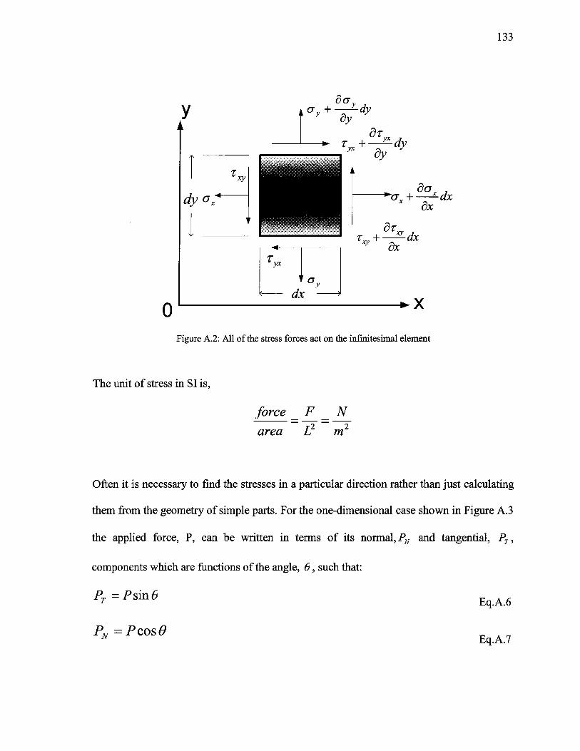
O

133

ôay

ôy

xy

Ôy

ôx

ôx

Figure A.2: All of the stress forces act on the infinitesimal element

The unit of stress in SI is,

force F _ Narea Û m2

Often it is necessary to find the stresses in a particular direction rather than just calculating

them from the geometry of simple parts. For the one-dimensional case shown in Figure A.3

the applied force, P, can be written in terms of its normal,/^ and tangential, PT,

components which are functions of the angle, 6, such that:

PT =Psin6

PN =Pcosô

Eq.A.6

Eq.A.7

134

A = Aacos6

Figure A.3: Calculating the stress in a particular direction

The areaAe, on which PNand PT act can also be written in terms of the area, A, normal to

the applied load P, and the angle 6,

Ae = A/cos6 Eq.A.8

The normal and shear stress relation acting on any area oriented at angle, 6 relative to the

original applied force, P are:

PN Pcosé PN

A0 Al cos 6 A= � cos 6 = G cos 6

AEq.A.9

�^- = = �

Ae AlcosB A Eq.A.10

where o is the applied unidirectional normal stress.

135

B. Strain

Whenever a force is applied to a body, it will tend to change the body's shape and size.

There changes are referred to as deformation. Size changes are known as dilatation

(volumetric changes) and are due to normal stresses. Shape changes are known as distortion

and are due to shear stresses. In order to describe the deformation in length of line

segments and the changes in angles between them, the concept of strain is used. Therefore,

strain is defined as normalized deformations within a body exclusive of rigid body

displacements.

These are two types of strain, one producing size changes by elongation or contraction

named as normal strain and the other producing shape changes by angular distortion named

as shear strain.

B.1 Normal Strain

Normal strain is the elongation or contraction of a line segment per unit length resulting in

a volume change such that:

, . AW-ABs = lim- L° Eq.A.ll

where all the parameters are determined by Figure A.4,

136

A : B

B'A' " " " ^ ~ � ~ " ~

Elongation

* 'Contraction

Figure A.4: Simple illustration of normal strain forms as elongation and contraction

where + a is tensile strain or elongation and - s is compressive strain or contraction.

B.2 Shear Strain

/

Shear strain is the angle change between two line segments resulting in a shape change as

shown in Figure A. 5, thus

= 6 > = y - # ' « � (For small angles) Eq.A. 12

where +? occurs if � >& and -y occurs if �< 9r 2 r 2

137

Figure A. 5: Engineering shear strain, y = £ + Sxy xy yx

The complete state of strain has six independent strain components (three normal

strains sx, sy and ez as well as three engineering shear strains, y^ ; yyz ; y ̂ ) which uniquely

describe the strain state for each particular orientation. This complete state of strain can be

written in vector form as,

Yx

Alternatively, the complete state of strain can be written in matrix form as,

Eq.A.13

138

£x Y xy

Y*y Sy

y y y* Eq.A.14

length L mThe unit of strain in SI is r = � = �

length L m

C. Strain-Displacement Relation

A displacement field describes how a body deforms as well as how it displaces. Strain-

displacement relations extract the strain field contained in a displacement field. The

definition of strain is considered to obtain this field,

� Normal strain is change in length divided by original length, Shear strain is the

amount of change in a right angle.

� X-direction displacement u as well as Y-direction displacement v are functions of

coordinates; u=u(x, y, z) andv = v(x,y, z).

Therefore two-dimensional strain-displacement relations are as,

139

ou ôv ou ôvp = � p � � y � I

ox ôy ôy ôx Eq.A.15

In matrix operator format, the strain-displacement relations are:

ô_ôx

0

d

oô_ôyô

ôy ôx

«=[*} Eq.A.16

D. Stress - Strain Relationships (Constitutive Relations)

If deformation and strain are the response of the body to an applied force or stress, then

there must be some type of relations, which allow the strain to be predicted from stress.

This relation is called constitutive model of a material and conveys the most important

mechanical properties of a material during a loading process. The constitutive model of a

material is based on results from experiments performed under very simple loading

conditions. When a constitutive relation is combined with the equilibrium and compatibility

equations, general structural behavior can be predicted.

During uni-axial loading by load, P, of a rod with uniform cross sectional area, A, and

length, L, the applied stress, o is simply calculated as,

140

Pcr = �

Eq.A.17

The resulting normal strain,^ in the longitudinal direction can be calculated from the

deformation response, A/ along the L direction:

AL

L Eq.A.18

The normal strain, sr in the transverse direction can be calculated from the deformation

response, AD along the D direction:

AD£T~~D Eq.A.19

There is a constant of proportionality between stress and strain in the elastic region such

that

b=>o=Ee E q A 2 0

141

where E = is known as the elastic modulus or Young's modulus and above equation isAs

known as unidirectional Hook's law.

Figure A.6: Uni-axially loaded rod undergoing longitudinal and transverse deformation

O

E

Longitudinal Strain

Figure A.7: Stress versus longitudinal strain

142

A plot of aT vs. sL shows a constant of proportionality between transverse and longitudinal

strains in the elastic region such that

~ V&L Eq.A.21

where v = � - is known as Poisson's ratio (which will be explained after).

For the results for three different uni-axial stresses applied separately, x, y and z can give

the general relations between normal stress and normal strain known as generalized Hook's

law if the strain components for each of the stress conditions are superposed:

o,Eq.A.22

£y=-{cTy-v(c7x+CTz))

Since shear stresses are decoupled (i.e., unaffected) by stresses in other directions the

relations for shear stress-shear strain are:

143

y*?

yxz

i~~GTxy

1-�*xz

1

~~GTyz

Eq.A.23

r. AT Ewhere the shear modulus is G =

2(1 + v)

144

Generalized Hook's law is usually written in matrix form such that:

rxyrxz

1E

-vE

-v

-vE1E

-v

-vE

� vE1

E

0

0

0

E

0

0

0

E

0

0

0

0

0

J_~G

0

0 0

0 0

0

0

0

_L_

~G

0

0

0

0

0

0

1

~G_

°x°y

°z<T*y

TXZ

Tyz

Eq.A.24

Therefore,

E

l + v1 i v

l -2v_vE E

(l + vXl-2v) l + vvE

(l + vXl-2v) (l +

vEvXl-2v)t _ v

l - 2 v .v^:

vYl-2v)

v£

v£

l + v

V

l - 2 v

0

0

0

0

0

0

0

0

0

0

0

G

0

0

0

0

0

0

G

0

0

0

0

0

0

G

£y

7*z

Eq.A.25

145

Generalized Hook's law can be simplified somewhat for the special case of plane stress in

the x-y plane since oz =0. Being orthogonal to the x-y plane, since o z is an also a principal

stress by definition, all the shear stresses associated with the z-direction are also zero. Thus,

the stress-strain relations for plane stress in the x-y plane become,

crcr

vE

0

vE 0

o

O G

y {o}=[E]{s}Eq.A.26

For the special case of plane stress, although o z =0, the strain in the z-direction is not zero

but instead can be determined such that

Plane stress: o z = 0,

Similarly for the special case of plane strain, although, ez = 0, the stress in the z-direction

is not zero but instead can be determined such that

Plane strain: sz = 0 , <JZ * 0 = v[<7x +<Jy)

146

Experiments, mainly tension or compression tests, provide basic information on the

mechanical behavior of materials under load. In these experiments, the macroscopic

(overall) response of specimens to the applied load is observed in order to determine force-

deformation relationships.

E. Poisson Ratio

In addition to the deformation of materials in the direction of applied force , another

property can be observed in all solid materials namely, that at right angles to the applied

uni-axial force, a certain amount of lateral ( transverse ) expansion or contraction takes

place. If a solid body is subjected to an axial tension, it contracts laterally; on the other

hand, if it is compressed, the material "squashes out" sideways. For a general theory, it is

preferable to refer to those lateral deformations based on deformation per unit of length of

the transverse dimension. These relative unit lateral deformations are termed lateral strains.

Moreover, it is known from experiments that lateral strain bear a constant relationship to

the longitudinal or axial strains caused by axial force, provided a material remains elastic,

homogenous, and isotropic. This property is called Poisson's Ratio and it is defined as

follows:

v =lateral strain

axial strain

lateral _ strain

axial strainEq.A.27

147

The value of v fluctuates for different materials over a relatively narrow range. Generally,

it is in order of 0.25 to 0.35.

"sw

CO

II - V

Longitudinal Strain

Figure A. 8: Transverse strain versus longitudinal strain

F. Engineering Stress-Strain Diagrams

In the experimental study of the mechanical properties of materials, it is customary to

plot diagrams of the relationship between stress and strain in a particular test. The stress-

strain diagrams are independent of the size of the specimen. The general shape of stress-

strain diagram for a ductile steel specimen loaded in tension or failure for a monotonically

increasing load is shown in the following figure (the normal stress versus engineering

strain). This figure can be subdivided into four well-defined regions:

148

1. the linear elastic region

2. the yield plateau

3. the strain-hardening region

4. the post ultimate stress or strain-softening region

Yield plateauStrath-hardening 'region JPostyllimatei strew region

Ultimate stress,

. Upper yield

Linear elastic region \

0.02 0.04 0-06 O.08Strain Unfm)

0.1 0.12

Figure A.9: Engineering Stress-strain diagrams [29]

This diagram is very important in engineering since it provides the means for obtaining

various mechanical properties of a material without regard to its physical size or shape, hi

some engineering applications, the strain may be large. For such purposes the total strain

will be defined as a sum of incremental strains; thus

149

Z - v AL

Eq.A.28

where L is the current gage length when the increment of elongation or contraction AL

occurs. If Lo is the initial gage of the specimen, then in the limit asAL�»0 strain

corresponding to the gage length Lf can be defined by the following integral:

Eq.A.29

This strain, obtained by adding up the increments of strains, is called logarithmic strain

or true strain During plastic strain of a uniform specimen subjected to axial tension

(compression), the cross-section area gets smaller (larger) as the specimen elongates

(shortens). A more accurate description of the actual stress experienced by the specimen

can be given by the true stress concept. The true stress is related to instantaneous cross-

sectional area and the applied force as

- F(7 = �

A Eq.A.30

Since plastic strain involves no volume change, that is, -A0L0 = AL and L = Lo (l + s)

� ( l + ff)=cr(l

150

Eq.A.31

Documents

Theoretical and Experimental Investigations for … · MEMOIRE PRESENTE A L'UNIVERSITÉ DU QUÉBEC À CHICOUTIMI COMME EXIGENCE PARTIELLE ... This Master study deals with the development