Embed Size (px)
Citation preview
Theoretical and Experimental Study
of AM and FM Molecular
Communications
Final Year Project
by
Ivan Pérez Laka
Universitat Politècnica de Catalunya
New Jersey Institute of Technology
Advisor: Raquel Pérez Castillejos


4
Acknowledgment
I would like to take the opportunity to thank to all the people who have helped me
during the development of this project. During this time I have grown as researcher but
especially I have grown as person.
First of all, I would like to thank my family for their support during all these years of
degree and because of understand my decision to travel so far from the beginning.
Without them none of this would have been possible. I would also like to mention all the
colleagues that I have been meeting during my period in UPC with who I spent a great
time.
Especial gratitude to my advisor Raquel Pérez Castillejos, who always had time to
help me and who after one year became a very good friend. Her support has been really
helpful to carry out this project. I would also like to thank to all the people of the The
Tissue Models Lab group of NJIT who helped me when I needed. They form a fantastic
group and I will always remember the awesome time that we spent together; Anil B.
Shrirao, Isabel Burdallo, Neha Jain and Olga Ordeig, part of this thesis has been possible
thanks to you.
For their financial support I would like to thank Fundación Vodafone España,
Generalitat de Cataluña, Universitat Politècnica de Catalunya and Obra Social Bancaja.
Finally I want to thank to Escola Tècnica Superior d’Enginyeria de Telecumincació de
Barcelona (ETSETB) and New Jersey Institute of Technology for their institutional support
and for give me the opportunity to do this unforgettable journey.
Thanks to all of you.

5
6
Table of Contents
1 MOTIVATIONS AND OBJECTIVES...................................................................................................................... 8
2 BACKGROUND INFORMATION ...................................................................................................................... 10
2.1 CELL COMMUNICATIONS FUNDAMENTALS .................................................................................................................. 12 2.1.1 Basic concept of cell communication .......................................................................................................... 12 2.1.2 Forms of intercellular signaling ..................................................................................................................... 13 2.1.3 Each cell responds to a specific extracellular signal molecules .......................................................... 15 2.1.4 Intracellular signal pathways ......................................................................................................................... 17
2.2 MOLECULAR COMMUNICATION SYSTEM ..................................................................................................................... 19 2.2.1 Nanotechnology ................................................................................................................................................. 19 2.2.2 Overview of nanomachines ............................................................................................................................ 20 2.2.3 Overview of nanonetworks ............................................................................................................................. 22 2.2.4 Communications among nanomachines .................................................................................................... 23 2.2.5 Nanonetwork components ............................................................................................................................. 26 2.2.6 Communication systems using calcium signaling ................................................................................... 28 2.2.7 Communication systems using other methods ........................................................................................ 32 2.2.8 Conclusion and research challenges ............................................................................................................ 34
2.3 MICROFLUIDICS FUNDAMENTALS ................................................................................................................................. 34 2.3.1 Low Reynolds number ....................................................................................................................................... 35 2.3.2 Velocity profile in microchannels .................................................................................................................. 36 2.3.3 Fick's laws of diffusion ...................................................................................................................................... 39 2.3.4 Micorfabrication ................................................................................................................................................. 41
3 THEORETICAL ANALYSIS OF MOLECULAR COMMUNICATION SYSTEMS ............................................... 44
3.1 INTRODUCTION .............................................................................................................................................................. 46 3.2 CLOSED SOLUTION FOR THE DIFFUSION EQUATION .................................................................................................... 46
3.2.1 Discharge conditions ......................................................................................................................................... 48 3.2.2 Charge conditions .............................................................................................................................................. 53 3.2.3 Complete solution .............................................................................................................................................. 55
3.3 FREQUENTIAL ANALYSIS ................................................................................................................................................ 56 3.3.1 Discharge conditions ......................................................................................................................................... 56 3.3.2 Charge conditions .............................................................................................................................................. 58
3.4 STABILITY........................................................................................................................................................................ 60 3.4.1 Non-minimum phase systems ........................................................................................................................ 60 3.4.2 Discharge conditions ......................................................................................................................................... 61 3.4.3 Charge conditions .............................................................................................................................................. 63
3.5 RESULTS AND DISCUSSIONS .......................................................................................................................................... 68
4 FABRICATION AND CHARACTERIZATION OF A MICROFLUIDIC DEVICE ................................................. 74
4.1 T-SENSOR .................................................................................................................................................................... 76 4.2 DESIGN ........................................................................................................................................................................... 77 4.3 FABRICATION ................................................................................................................................................................. 78
4.3.1 Required materials............................................................................................................................................. 79 4.3.2 Fabrication process ............................................................................................................................................ 79
4.4 CHARACTERIZATION ....................................................................................................................................................... 82 4.4.1 Data acquisition and image processing ..................................................................................................... 86
4.5 RESULTS AND DISCUSSIONS .......................................................................................................................................... 87
5 SIMULATION OF A T-SENSOR ......................................................................................................................... 89
5.1 INTRODUCTION .............................................................................................................................................................. 91
7
5.2 SIMULATION USING NUMERICAL METHODS................................................................................................................ 92 5.2.1 Finite difference method .................................................................................................................................. 92
5.3 1-DIMENSIONAL SIMULATION ...................................................................................................................................... 95 5.3.1 Stability in finite difference 1-D ..................................................................................................................... 99
5.4 2-DIMENSIONAL SIMULATION ................................................................................................................................... 100 5.4.1 Butterfly effect ................................................................................................................................................. 104 5.4.2 Stability in finite difference 2-D .................................................................................................................. 105
5.5 RESULTS AND DISCUSSIONS ........................................................................................................................................ 106 5.5.1 Simulator validation with theoretical results ........................................................................................ 107 5.5.2 Simulator validation with experimental results .................................................................................... 110
6 SIMULATION OF MOLECULAR COMMUNICATION SYSTEMS ................................................................. 114
6.1 INTRODUCTION ........................................................................................................................................................... 116 6.2 T-SENSOR SIMULATION: ENTRANCE WITH VARIABLE CONCENTRATION ................................................................. 117 6.3 CELL COMMUNICATIONS SIMULATION ...................................................................................................................... 121 6.4 RESULTS AND DISCUSSIONS ........................................................................................................................................ 126
6.4.1 Comparison with theoretical results ......................................................................................................... 128
7 CONCLUSIONS ................................................................................................................................................. 132
APPENDIX A .............................................................................................................................................................. 138
APPENDIX B ............................................................................................................................................................... 142
APPENDIX C ............................................................................................................................................................... 150
APPENDIX D .............................................................................................................................................................. 155
APPENDIX E ............................................................................................................................................................... 159
APPENDIX F ............................................................................................................................................................... 163
8 REFERENCES .................................................................................................................................................... 167
Study of AM and FM Molecular Communications ETSETB
8
1 MOTIVATIONS AND OBJECTIVES
Molecular communications are defined as those that use molecules as information
carriers between transmitter and receiver. This type of communications is the one used
by biological cells either in intra-cell communications or in inter-cell communications. In
recent years there has been a growing interest by this type of communications driven by
the development of nanotechnologies. Molecular communications is essential to
communicate nodes and devices in networks at nanometric scale.
Molecular communications are a new investigation field with applications in
biomedicine and in the development of technology at nano-level. For example a new
treatment in the cure for cancer, specifically the metastases of it, is based on
angiogenesis processes [1], which are based basically on molecular communications.
Likewise, the future of the technology goes through the miniaturization of devices
beyond the current micrometric scale. The next step is the nanotechnology, and a
communication system that controls all devices of these sizes is needed. The current
communication technologies such as electromagnetism or optics cannot be used on
these scales; however molecular communications are intrinsically designed to this kind
of sizes.
One of the motivations of this work is the interdisciplinary nature of molecular
communications that includes fields such as biology, chemistry, microfluidics,
electronics or telecommunications. Cellular communications are a perfect example of
how molecular communication systems work, so that a study of them is essential for
understanding these systems. The encoding and decoding information is done by
chemical reactions that must be understood on order to characterize and optimize
communication processes. The fabrication of devices for the practical study of these
systems is based on microelectronic fabrication technologies as well as in microfluidic
technologies. They allow the monitorization of the evolution of biocellular parameters
needed in the study of communications. Finally telecommunications provide a
background for understanding all bio-chemical processes from a perspective of
information theory that can be applied in different situations such as networks with
nanometric sizes.
It has been demonstrated that cells are able to encode the information transmitted
using modulations in amplitude (AM) or in frequency (FM) [2] using molecules as
information carriers. This type of molecular modulations allows the use of the same
communications channel to transmit different communications at the same time and
Study of AM and FM Molecular Communications ETSETB
9
provides a better noise immunity. The application of molecular modulations is essential
in the development of technologies at nanometric scale.
Although this is a field currently being investigated, actually a general model for
molecular communications that describes this communication process is still needed.
The purpose of this project is getting a mathematical model that describes
molecular communications based on diffusion processes of particles. With this model
the behavior of this type of communications will be studied according to the physical
parameters that determine it.
Also, this model will be used to study the modulation processes, either amplitude or
frequency modulation and will establish a criterion for which decide under what
situations biological cells decide to encode the information using one form or the other.
This report is structured in seven sections. Firstly, in Chapter 2, the basic
fundamentals of bio-cell communications, molecular communication systems and a
briefly introduction of microfluidics are presented in order to clarify some concepts of
systems that are based on molecular communications. The concepts defined in this
section are fundamental to understand the next sections.
Once this new scenario has been presented, in Chapter 3, the mathematical model
for molecular communication systems is calculated and analyzed. The behavior of these
systems is discussed and the stability issues that the model has are studied.
Since molecular communications are based on diffusion processes in Chapter 4, a
microfluidic device, whose operating principle is the diffusion of particles, is presented,
the T-SENSOR. In this section a T-Sensor is designed, fabricated and characterized in
order to study the diffusion experimentally.
The goal of Chapters 5 and 6 is getting a simulator able to predict the behavior of
communications between transmitter and receiver using molecular communications.
This simulator solves the issues that the mathematical model presented in Chapter 3
has. Chapter 5 is based in the programming of a T-Sensor simulator. This device is based
on the same principles as molecular communications. The simulator presented in this
chapter is validated using the experimental results got in Chapter 4.
Chapter 6 presents the molecular communications simulator and compares the
results using this simulator and the results using the mathematical model. The criterion
of decision for amplitude and frequency modulations is determined. This simulator is
obtained from the T-Sensor simulator with a previous modification that is also
presented in this chapter.
Finally the conclusions of this work are stated in Chapter 7
Study of AM and FM Molecular Communications ETSETB
10
2 BACKGROUND INFORMATION
In this section the basic concepts necessary to understand how molecular
communications work is presented. The chapter is divided in three different sections. An
overview of cell communications is explained in the first one that provides a biological
perspective of molecular communications. The second section presents a point of view
more technological, explaining the new field of nanonetworks that are strongly
dependent on molecular communications. Finally in the last section it is presented a
briefly explanation about microfluidics, a science that will be needed in further chapters
because of its intrinsic features for diffusion of particles.

Study of AM and FM Molecular Communications ETSETB
11
Study of AM and FM Molecular Communications ETSETB
12
2.1 Cell Communications Fundamentals
2.1.1 Basic concept of cell communication
Unicellular organisms have been present in the earth since long before multicellular
organisms. The complexity of the mechanisms needed for the interaction in multicellular
organisms is probably one of the reasons of their slow evolution. The cells have to be
able to communicate with one other in a complex ways if they want to control their own
behavior for the benefit of the unique organism.
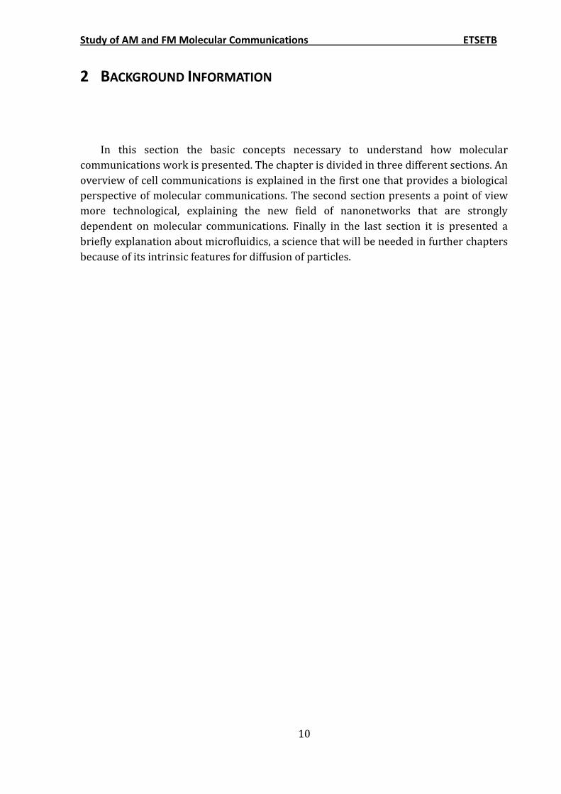
The extracellular signal molecules are the fundamental piece in these
communications. They are produced by cells which want to communicate with their
neighbors or with cells further away. And also, an elaborate system of proteins that each
cell contains enables it to react to a particular set of these signals in a specific way. Some
of these proteins are the cell-surface receptor proteins, which bind the signal molecule;
or the intracellular signaling proteins that distribute the signal to different parts in the
cell. This distribution takes place through different intracellular signaling pathways, and
at the end of each one there are target proteins, which react when the pathway is active
changing the cell's behavior.
Fig. 2.1 Intracellular signaling pathway activated by extracellular signal.
Some unicellular organisms are able to communicate by secreting a few kinds of
small peptides, but in higher multicellular organism communicate using hundreds of
kinds of molecules. In most of the cases the signaling cell secretes the molecules to the
Study of AM and FM Molecular Communications ETSETB
13
extracellular space by exocytosis (process by which a cell directs the contents of
secretory vesicles out of the cell membrane). In other cases the molecules are released
by diffusion through the plasma membrane, and in some others they are exposed to the
extracellular space while remaining tightly bound to the signaling cell's surface.
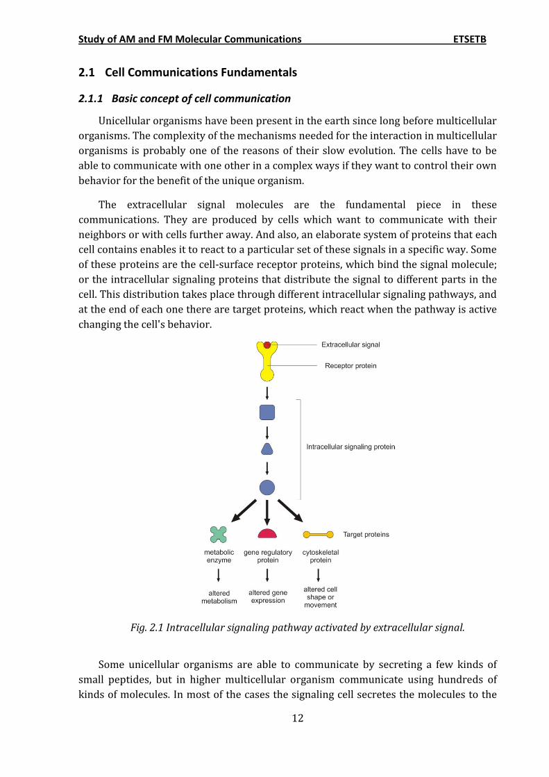
The target cell detects the signal by means of receptors [3], a protein which binds
specifically the signal molecule and this binding starts the reaction in the target cell. The
extracellular signal molecules usually act at very low concentration and the receptor
that detects them bind them with high affinity. In most cases this receptor proteins are
on the target cell surface. The signal molecules (ligand) which are hydrophilic and then
are unable to cross the plasma membrane directly, bind to cell-surface receptors, which
in turn generate one or more signals inside the target cell that alter the behavior of the
cell. Some small signal molecules can diffuse across the plasma membrane and bind to
receptors inside the cell. This requires that the signal molecules be hydrophobic and
sufficiently insoluble in aqueous solutions.
Fig. 2.2 The binding of extracellular signal molecules to either cell surface receptors
(on the left) or intracellular receptors (on the right).
2.1.2 Forms of intercellular signaling
Cells have different ways to communicate [3]. In multicellular organism, the most
"public" style of communication is the endocrine signaling. The signal molecules (called
hormones in animal's cells) are secreted into the blood stream, which carries the
information to the whole body. The cells that produce hormones are called endocrine
cells. For example, part of the pancreas is an endocrine gland that produces the hormone
insulin, which regulates glucose uptake in cells all over the body.
Study of AM and FM Molecular Communications ETSETB
14
Fig. 2.3 Endocrine signaling.
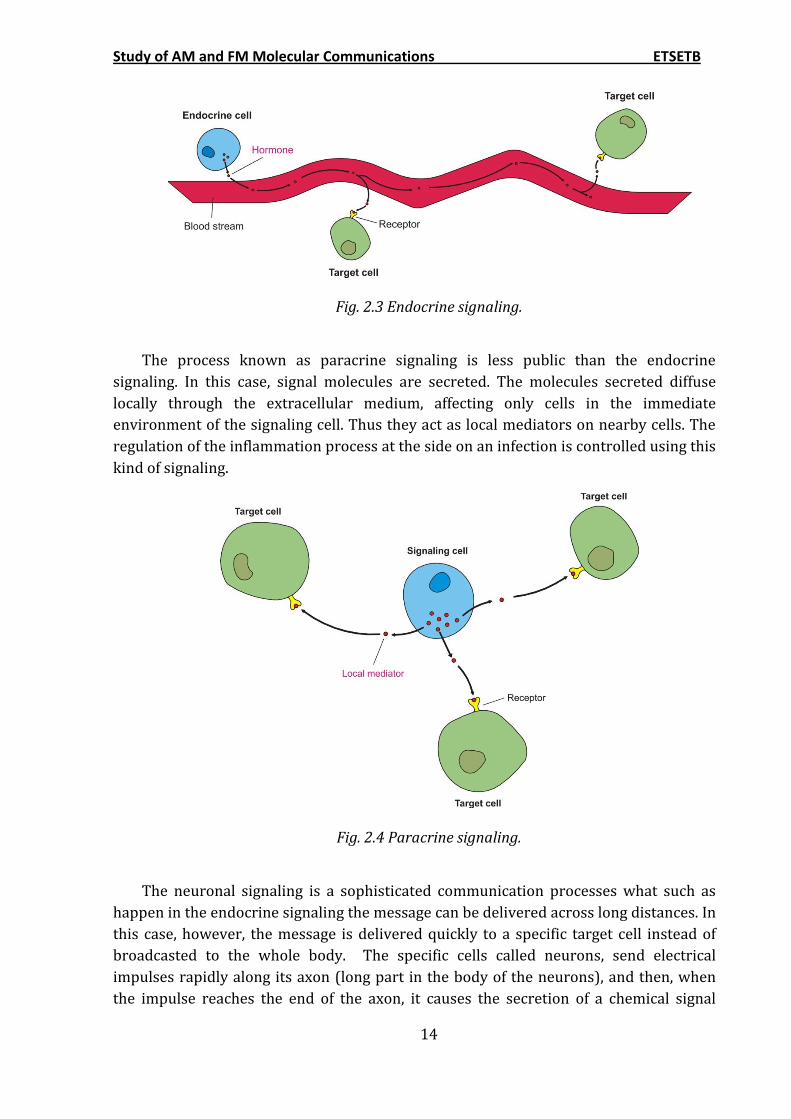
The process known as paracrine signaling is less public than the endocrine
signaling. In this case, signal molecules are secreted. The molecules secreted diffuse
locally through the extracellular medium, affecting only cells in the immediate
environment of the signaling cell. Thus they act as local mediators on nearby cells. The
regulation of the inflammation process at the side on an infection is controlled using this
kind of signaling.
Fig. 2.4 Paracrine signaling.
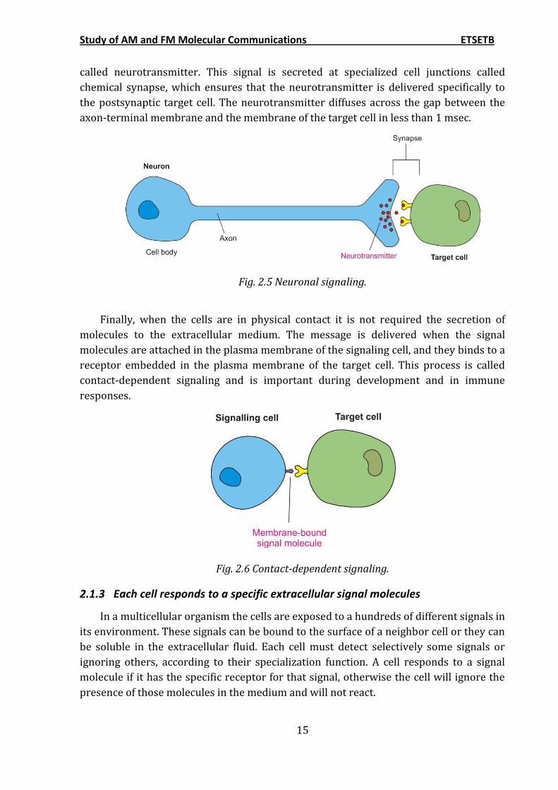
The neuronal signaling is a sophisticated communication processes what such as
happen in the endocrine signaling the message can be delivered across long distances. In
this case, however, the message is delivered quickly to a specific target cell instead of
broadcasted to the whole body. The specific cells called neurons, send electrical
impulses rapidly along its axon (long part in the body of the neurons), and then, when
the impulse reaches the end of the axon, it causes the secretion of a chemical signal
Study of AM and FM Molecular Communications ETSETB
15
called neurotransmitter. This signal is secreted at specialized cell junctions called
chemical synapse, which ensures that the neurotransmitter is delivered specifically to
the postsynaptic target cell. The neurotransmitter diffuses across the gap between the
axon-terminal membrane and the membrane of the target cell in less than 1 msec.
Fig. 2.5 Neuronal signaling.
Finally, when the cells are in physical contact it is not required the secretion of
molecules to the extracellular medium. The message is delivered when the signal
molecules are attached in the plasma membrane of the signaling cell, and they binds to a
receptor embedded in the plasma membrane of the target cell. This process is called
contact-dependent signaling and is important during development and in immune
responses.
Fig. 2.6 Contact-dependent signaling.
2.1.3 Each cell responds to a specific extracellular signal molecules
In a multicellular organism the cells are exposed to a hundreds of different signals in
its environment. These signals can be bound to the surface of a neighbor cell or they can
be soluble in the extracellular fluid. Each cell must detect selectively some signals or
ignoring others, according to their specialization function. A cell responds to a signal
molecule if it has the specific receptor for that signal, otherwise the cell will ignore the
presence of those molecules in the medium and will not react.
Study of AM and FM Molecular Communications ETSETB
16
The cells restrict the amount of molecules that they can detect by producing a
limited set of receptors out of the thousands that are possible. But even with this limited
set of receptors, those signals are able to control the cell’s behavior in a complex way.
One signal binding to one receptor can cause many different effects in the target cell
such as the movement of the cell or the alteration of the cell’s shape. At the same time
the cell’s receptors can bind more than one molecule, and these signals, by acting
together, can produce reactions that are more than the combination of the effects caused
of each signals by their own. The intracellular transmission systems for the different
signals interact, so the presence of one signal changes the reaction to another [3]. A cell
may be programmed to respond to one combination of signals by differentiating, to
another combination by multiplying, and to by doing a specialized task such as secretion
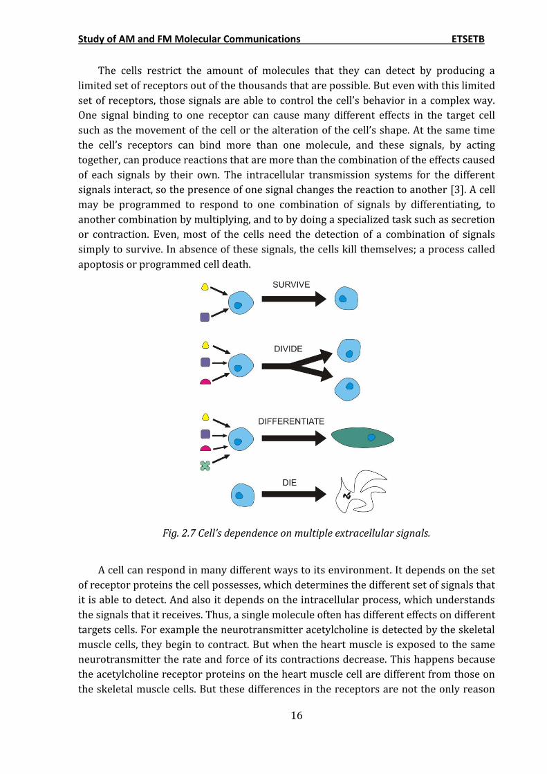
or contraction. Even, most of the cells need the detection of a combination of signals
simply to survive. In absence of these signals, the cells kill themselves; a process called
apoptosis or programmed cell death.
Fig. 2.7 Cell’s dependence on multiple extracellular signals.
A cell can respond in many different ways to its environment. It depends on the set
of receptor proteins the cell possesses, which determines the different set of signals that
it is able to detect. And also it depends on the intracellular process, which understands
the signals that it receives. Thus, a single molecule often has different effects on different
targets cells. For example the neurotransmitter acetylcholine is detected by the skeletal
muscle cells, they begin to contract. But when the heart muscle is exposed to the same
neurotransmitter the rate and force of its contractions decrease. This happens because
the acetylcholine receptor proteins on the heart muscle cell are different from those on
the skeletal muscle cells. But these differences in the receptors are not the only reason
Study of AM and FM Molecular Communications ETSETB
17
this success. It is perfectly possible that the same signal molecules binds to the same
receptor proteins in two different types of target cell, and yet produce a very different
responses. The receptor protein in the salivary gland is similar to the receptor protein
presents in the heart muscle cells, but in this case, the gland secretes components of
saliva instead of decrease the contraction.
2.1.4 Intracellular signal pathways
When a signal molecule binds with a receptor protein the signal reception begins.
The receptor does the first transduction; it receives an external signal and generates a
new intracellular response [4]. This is the first step in a chain in which the message
passes from one intracellular signal to another, activating and generating the next
intracellular signal, until arrive to a metabolic enzyme which execute some action, or to
a gen regulatory protein, or to a cytoskeletal protein, changing the cell’s configuration.
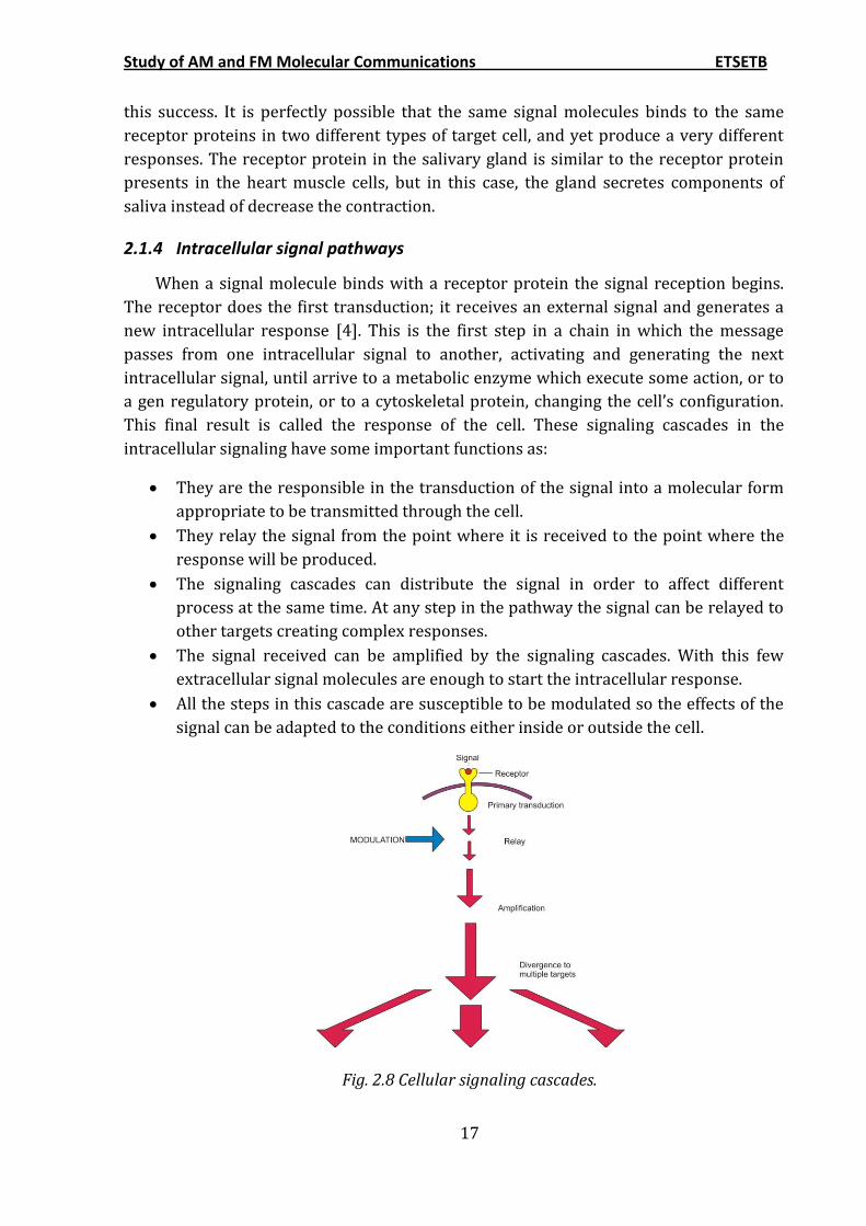
This final result is called the response of the cell. These signaling cascades in the
intracellular signaling have some important functions as:
They are the responsible in the transduction of the signal into a molecular form
appropriate to be transmitted through the cell.
They relay the signal from the point where it is received to the point where the
response will be produced.
The signaling cascades can distribute the signal in order to affect different
process at the same time. At any step in the pathway the signal can be relayed to
other targets creating complex responses.
The signal received can be amplified by the signaling cascades. With this few
extracellular signal molecules are enough to start the intracellular response.
All the steps in this cascade are susceptible to be modulated so the effects of the
signal can be adapted to the conditions either inside or outside the cell.
Fig. 2.8 Cellular signaling cascades.
Study of AM and FM Molecular Communications ETSETB
18
Signaling pathways are usually long and with a lot of branches. Therefore, many
intracellular parts are affected by the information received by the receptors at the cell
surfaces. In these cases the molecules are too large or too hydrophilic to cross the
plasma membrane of the target cell. Because of this they have to bind on the receptors at
the cell surface to relay the message across the membrane. But it is also true that some
signal pathways are more direct. This happens when the molecules are small enough
and hydrophobic enough, they are able to cross the plasma membrane directly; Fig. 2.2.
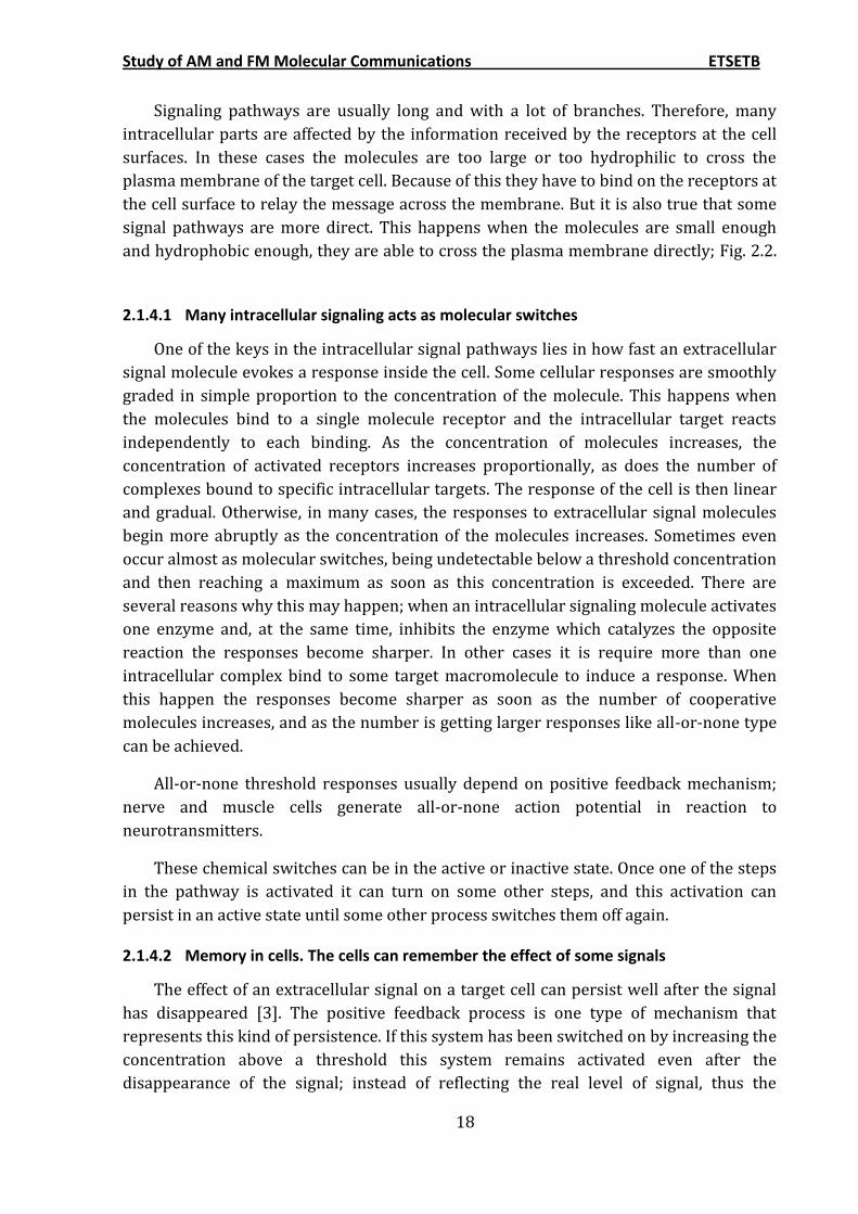
2.1.4.1 Many intracellular signaling acts as molecular switches
One of the keys in the intracellular signal pathways lies in how fast an extracellular
signal molecule evokes a response inside the cell. Some cellular responses are smoothly
graded in simple proportion to the concentration of the molecule. This happens when
the molecules bind to a single molecule receptor and the intracellular target reacts
independently to each binding. As the concentration of molecules increases, the
concentration of activated receptors increases proportionally, as does the number of
complexes bound to specific intracellular targets. The response of the cell is then linear
and gradual. Otherwise, in many cases, the responses to extracellular signal molecules
begin more abruptly as the concentration of the molecules increases. Sometimes even
occur almost as molecular switches, being undetectable below a threshold concentration
and then reaching a maximum as soon as this concentration is exceeded. There are
several reasons why this may happen; when an intracellular signaling molecule activates
one enzyme and, at the same time, inhibits the enzyme which catalyzes the opposite
reaction the responses become sharper. In other cases it is require more than one
intracellular complex bind to some target macromolecule to induce a response. When
this happen the responses become sharper as soon as the number of cooperative
molecules increases, and as the number is getting larger responses like all-or-none type
can be achieved.
All-or-none threshold responses usually depend on positive feedback mechanism;
nerve and muscle cells generate all-or-none action potential in reaction to
neurotransmitters.
These chemical switches can be in the active or inactive state. Once one of the steps
in the pathway is activated it can turn on some other steps, and this activation can
persist in an active state until some other process switches them off again.
2.1.4.2 Memory in cells. The cells can remember the effect of some signals
The effect of an extracellular signal on a target cell can persist well after the signal
has disappeared [3]. The positive feedback process is one type of mechanism that
represents this kind of persistence. If this system has been switched on by increasing the
concentration above a threshold this system remains activated even after the
disappearance of the signal; instead of reflecting the real level of signal, thus the
Study of AM and FM Molecular Communications ETSETB
19
response system displays memory. Some of these changes can even persist for the rest
of the life of the organism. They usually depend on self-activating memory mechanisms
that operate in the last steps in the signaling pathway, at the level of gene transcription.
For example, the signals that determine if a cell has to become a muscle cell turn on a
series of muscle-specific gene regulatory proteins which produce many other muscle cell
proteins. In this way, the decision to become a cell muscle is made permanent.
2.2 Molecular Communication System
2.2.1 Nanotechnology
The cell communication system exposed in the chapter above is one of the solutions
for nano-scale communications scenarios. These systems based on the molecular
signaling may be one of the keys for the development of the nanotechnologies. In this
new situation appears the figure of the nanomachine, which is, at nano-scale, the most
basic functional unit. Nanomachines represent tiny devices consisting in a group of
molecules which are able to perform simple tasks such as computation, sensing or
actuation. The interconnection between these nanomachines makes possible their
cooperation and the exchange of information increasing the capabilities of a single
nanomachine. Molecular communication provides a mechanism for one nanomachine to
encode or decode the information into molecules and to send information to other
nanomachines.
The interconnection of these nanomachines becomes in nanonetworks, and they
improve their capacities in the following ways:
Provides a larger workspace to the nanomachines, which is extremely limited for
a single one. Nanonetworks will allow dens deployments of interconnected
nanomachines. Thus, larger applications scenarios will be enabled.
Allows the connection over large areas where the control of a specific
nanomachine is difficult because of its small size. By means of broadcasting and
multihopping nanonetworks can interact with remote nanomachines
Nanomachines such as nano-valves, nano switches or nano memories, cannot
execute complex task by themselves. The network performed by the connection
between these nanomachines will allow them to work in a cooperative manner
achieving more complex tasks.
Nanomachines cannot be built yet, but they exist in the nature in the form of
biological cells and the chemical processes within those cells. The bionanotechnology is
advancing quickly, until the actual point where engineering of biological systems is
possible. It has been demonstrated [5] that the modification of the DNA can give a new
functionality to a cell. As the bionanotechnology becomes more mature, the study of the
molecular communications can be applied in the design of more complex nanomachine
systems.
Study of AM and FM Molecular Communications ETSETB
20
2.2.2 Overview of nanomachines
A nanomachine is defines as a device consisting of nanometer-scale components
that performs a useful function at nano-level, such as communicating, data storing,
sensing and actuation or computing. The tasks that a single nanomachine can achieve
are very simple because of its low complexity and small size.
As it has said before, the fabrication of these nanomachines is still a very promising
field in research, but with the exception of the found in the nature, it is not possible to
built artificial nanomachines yet. There are three different approaches for their
development; the top-down approach in which the nanomachines are developed by
means of downscaling the already existing microelectronic technologies. The bottom-up
approach consists in the design of nanomachines from molecular components, which are
assembled using chemical principles of molecular recognition. Recently has appeared a
third approach called bio-hybrid that is based on the use of existing biological
nanomachines as models or components for the development of new nanomachines.
2.2.2.1 Nanomachine architecture
The architecture of a nanomachine depends strongly on its complexity. It can be
from simple molecular switches up to complete nanorobots. In general a regular
nanomachine should include the following architecture components [6]:
Control unit. The control unit executes the instructions to perform the intended
tasks, and all the components of the nanomachines can be controlled by this unit
in order to achieve this purpose.
Communications unit. The communications unit is a transceiver capable of
transmitting and receiving messages at nano-scale.
Power unit. The goal of the power unit is supply all the components of the
nanomachine, by obtaining energy from external sources such as light or
temperature and store it for a later distribution and consumption.
Sensor and actuators. In the same way as the communications unit the sensors
and actuators acts as interfaces between the environment and the nanomachine.
Reproduction unit. In many applications the capability of replicate the
nanomachine using external elements may be very useful. This is the aim of the
reproduction unit. It fabricates each component of the architecture using external
elements, and then assembles them to replicate it.
Currently such complex nanomachine cannot be built. However, systems found in
the nature like living cells have similar architectures. According to the bio-hybrid
approach, the biological cells have served as a template from which we are learning to
build nanomachines. Similar to the architecture of a nanomachine, a cell contains the
following components:
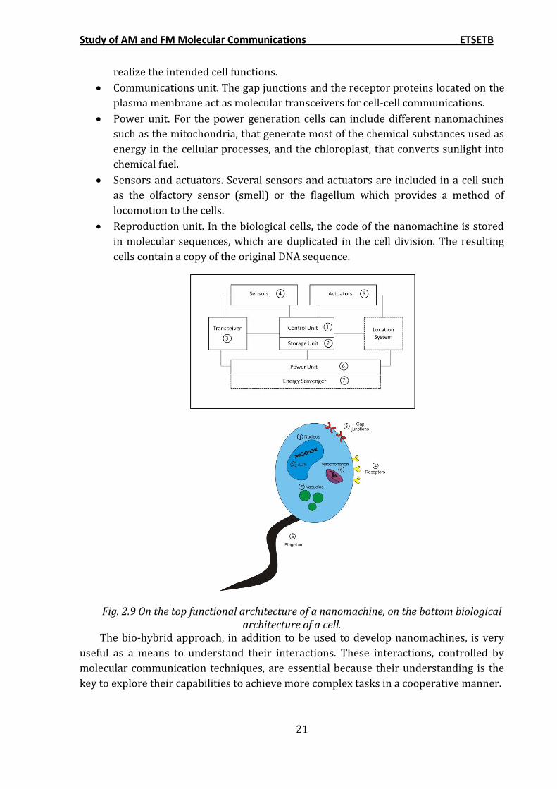
Control unit. The chromosome within the nucleus contains all the instructions to
Study of AM and FM Molecular Communications ETSETB
21
realize the intended cell functions.
Communications unit. The gap junctions and the receptor proteins located on the
plasma membrane act as molecular transceivers for cell-cell communications.
Power unit. For the power generation cells can include different nanomachines
such as the mitochondria, that generate most of the chemical substances used as
energy in the cellular processes, and the chloroplast, that converts sunlight into
chemical fuel.
Sensors and actuators. Several sensors and actuators are included in a cell such
as the olfactory sensor (smell) or the flagellum which provides a method of
locomotion to the cells.
Reproduction unit. In the biological cells, the code of the nanomachine is stored
in molecular sequences, which are duplicated in the cell division. The resulting
cells contain a copy of the original DNA sequence.
Fig. 2.9 On the top functional architecture of a nanomachine, on the bottom biological architecture of a cell.
The bio-hybrid approach, in addition to be used to develop nanomachines, is very
useful as a means to understand their interactions. These interactions, controlled by
molecular communication techniques, are essential because their understanding is the
key to explore their capabilities to achieve more complex tasks in a cooperative manner.
Study of AM and FM Molecular Communications ETSETB
22
2.2.2.2 Desirable features of nanomachines
As we have seen desirable features of nanomachines are presents in living cells. For
example, nanomachines will have a set of instructions or code to realize specific tasks
embedded in their molecular structure, or they will be able to read them from another
molecular structure in which the instruction set is stored. The ability of a nanomachine
could make a copy of itself would be interesting. In order to achieve this goal, a
nanomachine would need the features of self-assembly and self-replication. Self-
assembly is defined as the process in which several disordered elements form an
organized structure without external intervention. A nano-level this happens naturally
due to the molecular affinities between two different elements. Self-replication is
defined as the process in which a device makes a copy of itself using external elements.
Self-maintenance is another feature very interesting to be considered as well as the
locomotion, which would provide the ability to move from one place to another at a
nanomachine. Communication among nanomachines is one of the most desired features.
It is required to realize more complex tasks in a cooperative manner, and also a nano-to-
macro interface with which to access and control the nanomachine.
From the point of view of communication, cells act as multi-interface devices. Cells
have hundreds of receivers and are able to communicate using multiple unique channel
access techniques such as ligand-recptors or gap junctions. Besides, the cells can be
using these mechanisms simultaneously. All cells have a very sensitive transducing
signal mechanism. The signal is detected by the receptor, which amplify the signal,
integrate the signal with the input received by other receptors, and transmit the
resulting signal to the cell. Therefore, a nanomachine should have these features that
characterize signal transduction [7]:
Specificity. Specificity is the ability to detect and react to a specific signal. The
signal and the receptor are complementary. The specificity quantifies the
precision with which a molecule fits in a complementary receptor, where other
signals do not fit.
Amplification. Amplification is the ability to increase the magnitude of a signal.
Amplification by enzyme cascades can amplify a signal in several orders of
magnitude within milliseconds.
Desensitization. Desensitization is the ability to remove the molecules of the
signal once this is received.
Integration. Integration is defined as the ability of a system to receive multiple
signals and integrate them into only one, producing the suitable response of the
nanomachine.
2.2.3 Overview of nanonetworks
Nanonetworks are communication networks which exist mostly at nano-level scale.
The nanonetworks achieve the functionally and performance as the macro-scale
networks using nodes of nanometers and channels physically separated by up to
Study of AM and FM Molecular Communications ETSETB
23
hundreds or thousands of nanometers. Besides, nodes are supposed to be rapidly
deployable and mobile, and also are assumed to be self-powered.
Nanonetworks, such as all the other networks have all the features analogous
communication networks. The information must be collected, coded, transmitted,
received, decoded and delivered to the appropriate target. Thereby, all the concepts
presented in the information theory apply in nanonetworks including bandwidth,
compression, error detection and correction.
2.2.4 Communications among nanomachines
Since nanonetworks provides to the nanomachines a support on which establish a
communication system, two different bidirectional scenarios appear:
Communications between two or more nanomachines.
Communications between a nanomachine and a larger system such as electronic
micro-device.
Different communication technologies have been proposed to approach each
scenario [8] electromagnetic, acoustic or molecular.
The electromagnetic waves have been used for communications since long time, and
actually are the most common technique to interconnect microelectronic devices. The
losses for these waves are minimal along wires or through air. However, in the nano-
scale scenario, wiring large quantity of nano-machines is unfeasible. In this case,
wireless technology could be an alternative. In order to establish bidirectional
communication, a radiofrequency transceiver would have to be integrated in the
nanomachine. Nano-scale antennas can be built for very high frequency
communications, but due to the size and the complexity of the transceivers, they cannot
be easily integrated in nanomachines yet. In addition, even if this integration could be
realized, the nanomachine could not have enough output power to establish a
bidirectional communication. Because of that, electromagnetic communication could be
used to transmit information from a micro-device to a nanomachine, but not in the
opposite direction.
Acoustic communications are based in the transmission if ultrasonic waves, air
pressure waves. In the same way to the electromagnetic communications, the acoustic
communication would need the integration of ultrasonic transducers in the
nanomachines. These transducers are obviously needed to sense the variations of
pressure produced by the ultrasonic waves and also to emit acoustic signals. The issue in
this case is exactly the same that in the previous case, the size of these transducers
makes impossible their integration in the nanomachines.
Molecular communication is established when the information is encoded using
molecules. Molecular communication is a new and interdisciplinary field which includes
knowledge in nano, bio and communication technologies. Unlike previous
Study of AM and FM Molecular Communications ETSETB
24
communication techniques, in this case the integration of transceivers in the
nanomachine is not an issue because of the intrinsic size of the molecular transceivers.
These transceivers are nanomachines which are able to react to specific molecules, and
to release others as a response to an internal command. Molecular communications can
be used to interconnect different nanomachines, resulting in nanonetworks which
increase the capabilities of a single nanomachine.
2.2.4.1 Features of molecular communication
The nanonetworks, as it has said previously, expand the capabilities of a single
nanomachine, but in addition, represent a potential solution for some applications
where the current communication networks are not suitable. Compared to actual
communication network technologies, nanonetworks have the following advantages [7]:
Biocompatibility: This is defined as the capacity of a device to operate in
biological environments without affecting them negatively. Inserting
nanomachines into the human body for medical applications requires
nanomachines that are biologically friendly. Functions as receiving, interpreting,
and releasing molecules would provide to biological nanomachines a mechanism
to interface directly with natural processes. Thus, it would not be necessary to
include harmful inorganic chemicals. In addition, nanomachines and molecular
messages may also be programmed to be broken down after use to avoid
procedures for removal or cleanup of devices
Scale: The reduced size of the nanomachines and the resulting nanonetwork
components are a very interesting goal in systems where the dimensions of the
system are critic.
Information representation: Molecules can represent the information using
different ways, such as their chemical structure, relative positioning or
concentration. Thus, molecular information provides different methods for
manipulating and interacting with the information since operation performed are
non-binary.
Energy efficiency: In terms of energy consumption, chemical reactions are highly
efficient. These reactions could power nanonetwork nodes and processes. In
addition, chemical reaction can represent computation and decision processes,
which usually take multiple operations.
2.2.4.2 Traditional communication networks and nanonetworks
The emergence of nanonetworks has implied the development of a new paradigm
which is much more complex than a simple extension of the traditional communication
networks. Especially due to the size, most of the communication processes are
inspired by biological systems found in nature and because of that there are some
differences between nanonetworks and traditional communication networks [6]:
In nanonetworks the message is encoded using molecules instead of
Study of AM and FM Molecular Communications ETSETB
25
electromagnetic, acoustic or optical signals which are used by the traditional
communication networks. There are two different and complementary
techniques to encode the information in nanonetworks. The first, called
molecular encoding, uses internal parameters of the molecule -such as chemical
structure, polarization or relative positioning- to encode the information. In this
case the receiver has to be able to detect these parameters in order to decode the
information. This technique is similar to the use of encrypted messages, in which
only the specific receivers are able to decode the information. The second
technique uses temporal sequences to encode the information, such as the
temporal concentration of a specific molecule in the medium. Depending on the
concentration, the receiver decodes the information in one way or another. This
technique is similar to those used in traditional communication where the
information is encoded in time-varying sequences.
Most of the processes in nanonetworks are chemical reactions with low power
consumption. In traditional networks, the communication processes consume
electrical power which comes from batteries or from external sources such as
electromagnetic induction.
In traditional communication networks, the noise is known as an unwanted
perturbation overlapped with the wanted signals. In nanonetworks, according to
the molecular encoding techniques the noise can be described in two different
ways. The first, as occurs in traditional communication systems, is an overlapping
of the molecule signal with some other molecules of the same type. This means,
another source emits the same molecules used to encode the message, affecting
the concentration sensed by the receiver. The second source of noise in
nanonetworks can be understood as undesirable reaction between the
information molecules and other molecules present in the medium. Those
reactions can modify the structure of the information molecules and then the
receiver would not be able to detect the message.
The propagation speed of signals used in traditional communication networks is
much faster than the propagation of molecular messages. In nanonetworks, the
information molecules have to be physically transported from the transmitter to
the receiver. In addition, molecules can be subjected to random diffusion
processes and environmental conditions, such as temperature, that affects the
propagation of the molecular message.
Study of AM and FM Molecular Communications ETSETB
26
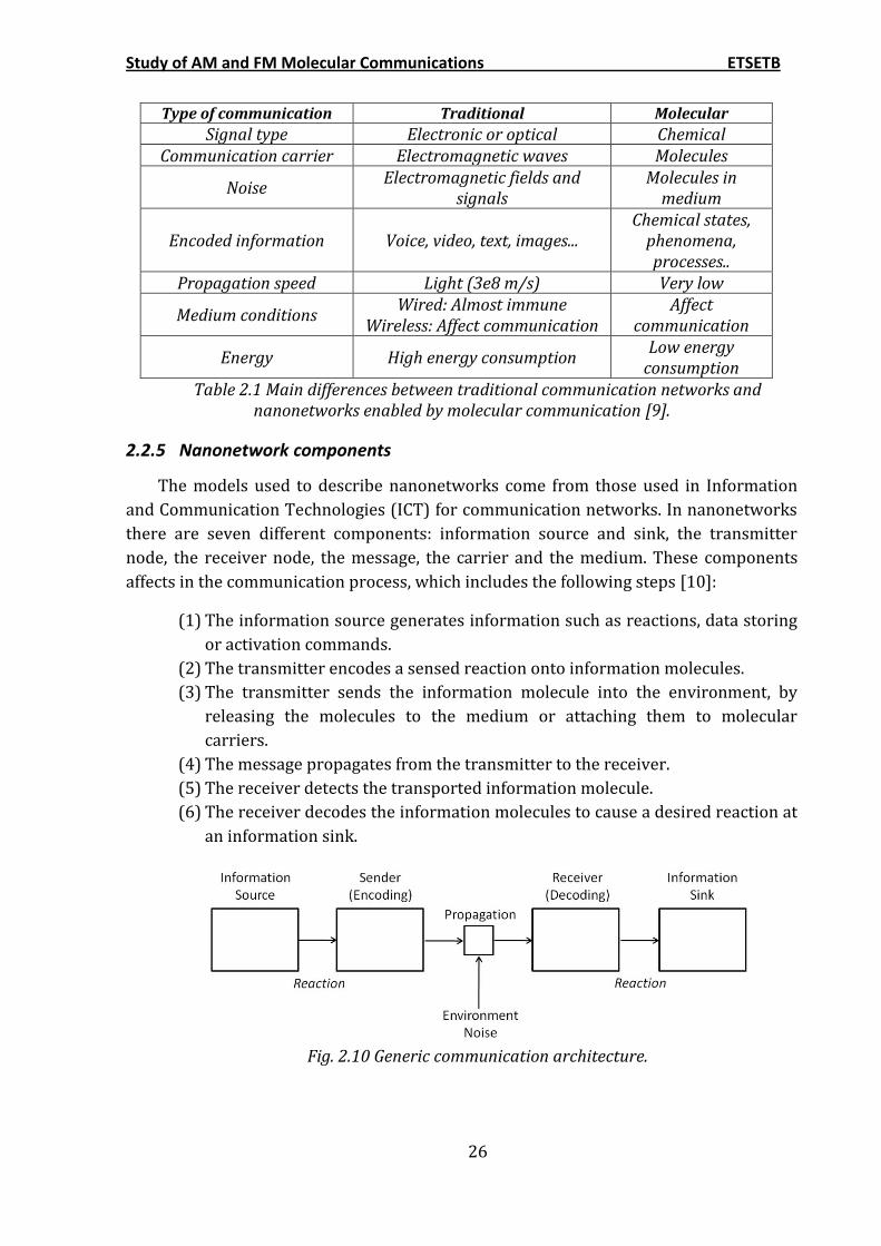
Type of communication Traditional Molecular Signal type Electronic or optical Chemical
Communication carrier Electromagnetic waves Molecules
Noise Electromagnetic fields and
signals Molecules in
medium
Encoded information Voice, video, text, images... Chemical states,
phenomena, processes..
Propagation speed Light (3e8 m/s) Very low
Medium conditions Wired: Almost immune
Wireless: Affect communication Affect
communication
Energy High energy consumption Low energy
consumption Table 2.1 Main differences between traditional communication networks and
nanonetworks enabled by molecular communication [9].
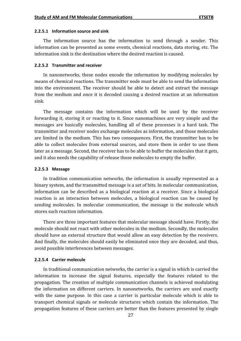
2.2.5 Nanonetwork components
The models used to describe nanonetworks come from those used in Information
and Communication Technologies (ICT) for communication networks. In nanonetworks
there are seven different components: information source and sink, the transmitter
node, the receiver node, the message, the carrier and the medium. These components
affects in the communication process, which includes the following steps [10]:
(1) The information source generates information such as reactions, data storing
or activation commands.
(2) The transmitter encodes a sensed reaction onto information molecules.
(3) The transmitter sends the information molecule into the environment, by
releasing the molecules to the medium or attaching them to molecular
carriers.
(4) The message propagates from the transmitter to the receiver.
(5) The receiver detects the transported information molecule.
(6) The receiver decodes the information molecules to cause a desired reaction at
an information sink.
Fig. 2.10 Generic communication architecture.
Study of AM and FM Molecular Communications ETSETB
27
2.2.5.1 Information source and sink
The information source has the information to send through a sender. This
information can be presented as some events, chemical reactions, data storing, etc. The
information sink is the destination where the desired reaction is caused.
2.2.5.2 Transmitter and receiver
In nanonetworks, these nodes encode the information by modifying molecules by
means of chemical reactions. The transmitter node must be able to send the information
into the environment. The receiver should be able to detect and extract the message
from the medium and once it is decoded causing a desired reaction at an information
sink.
The message contains the information which will be used by the receiver
forwarding it, storing it or reacting to it. Since nanomachines are very simple and the
messages are basically molecules, handling all of these processes is a hard task. The
transmitter and receiver nodes exchange molecules as information, and those molecules
are limited in the medium. This has two consequences. First, the transmitter has to be
able to collect molecules from external sources, and store them in order to use them
later as a message. Second, the receiver has to be able to buffer the molecules that it gets,
and it also needs the capability of release those molecules to empty the buffer.
2.2.5.3 Message
In tradition communication networks, the information is usually represented as a
binary system, and the transmitted message is a set of bits. In molecular communication,
information can be described as a biological reaction at a receiver. Since a biological
reaction is an interaction between molecules, a biological reaction can be caused by
sending molecules. In molecular communication, the message is the molecule which
stores such reaction information.
There are three important features that molecular message should have. Firstly, the
molecule should not react with other molecules in the medium. Secondly, the molecules
should have an external structure that would allow an easy detection by the receivers.
And finally, the molecules should easily be eliminated once they are decoded, and thus,
avoid possible interferences between messages.
2.2.5.4 Carrier molecule
In traditional communication networks, the carrier is a signal in which is carried the
information to increase the signal features, especially the features related to the
propagation. The creation of multiple communication channels is achieved modulating
the information on different carriers. In nanonetworks, the carriers are used exactly
with the same purpose. In this case a carrier is particular molecule which is able to
transport chemical signals or molecule structures which contain the information. The
propagation features of these carriers are better than the features presented by single
Study of AM and FM Molecular Communications ETSETB
28
information molecules by themselves, protecting the information from noise sources
and allowing the system to create multiple independent channels using the same
medium.
The use of molecules as information carriers has been observed in biological
systems; identifying two different carriers in which modulate the information. Molecular
motors [10], and calcium ions [11]. Molecular motors are proteins that can generate
movement using chemical energy. These proteins transport the information molecule
from the transmitter to the receiver [12]. The second types of carriers are calcium ions.
In this case the transmitter can modulate the information in the concentration of these
ions -modulation of amplitude- or it can do it encoding the information in the frequency
at which the transmitter sends these ions -frequency modulation-.
2.2.5.5 Medium
The medium is the space in which the message goes from the transmitter to the
receiver. In molecular communication the medium can be wet or dry, and the
propagation depends strongly on the medium conditions. In addition, the presence of
physical obstacles can hinder the propagation of the message.
2.2.6 Communication systems using calcium signaling
Cell-cell communication based on calcium signaling is one of the most important
molecular techniques [13, 14]. It is responsible for many coordinated cellular task, such
as, contraction, secretion or fertilization. This signaling process is used in two different
scenarios, when two cells are in physical contact, or when there is not this physical
dependence.
The propagation of the signal is driven by a chemo-signal pathway, in which one
messenger transports the information until certain point in the pathway where the
information is transferred to another messenger. This transmission from one messenger
to another continues until the information reaches its destination. This process is
explained in more detail in the previous chapter “Intracellular signal pathways”. As it is
presented there, this system has some important advantages, especially the possibility
to amplify the information at different levels of the chemo-signal pathway. The ligand-
receptor binding principle is the most important process in this information transfer
between messengers. As it is explained before this process consists in the bounding
between to molecules (the information molecule, or ligand, and the protein receptor)
resulting in a local reaction, which in turn can trigger other process.
When cells are physically separated the information molecule binds to the receptors
placed on the cell membrane. This binding generates an internal signal which can be
decoded by cell components.
Study of AM and FM Molecular Communications ETSETB
29
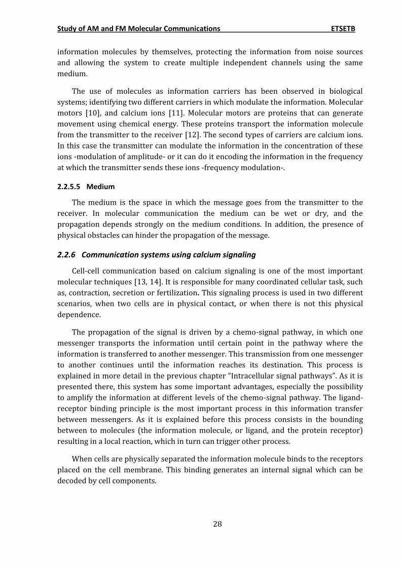
Fig. 2.11 Signal propagation in calcium signaling communication systems by diffusion.
In this case the information molecule is considered as the first messenger, while the
internal signal is considered as the second messenger. The first messenger in the signal
that transports the information outside the cell while the second messenger is the signal
which transports the information inside the cell. Membrane receptors transforms first
messenger into second messengers by chemical reactions.
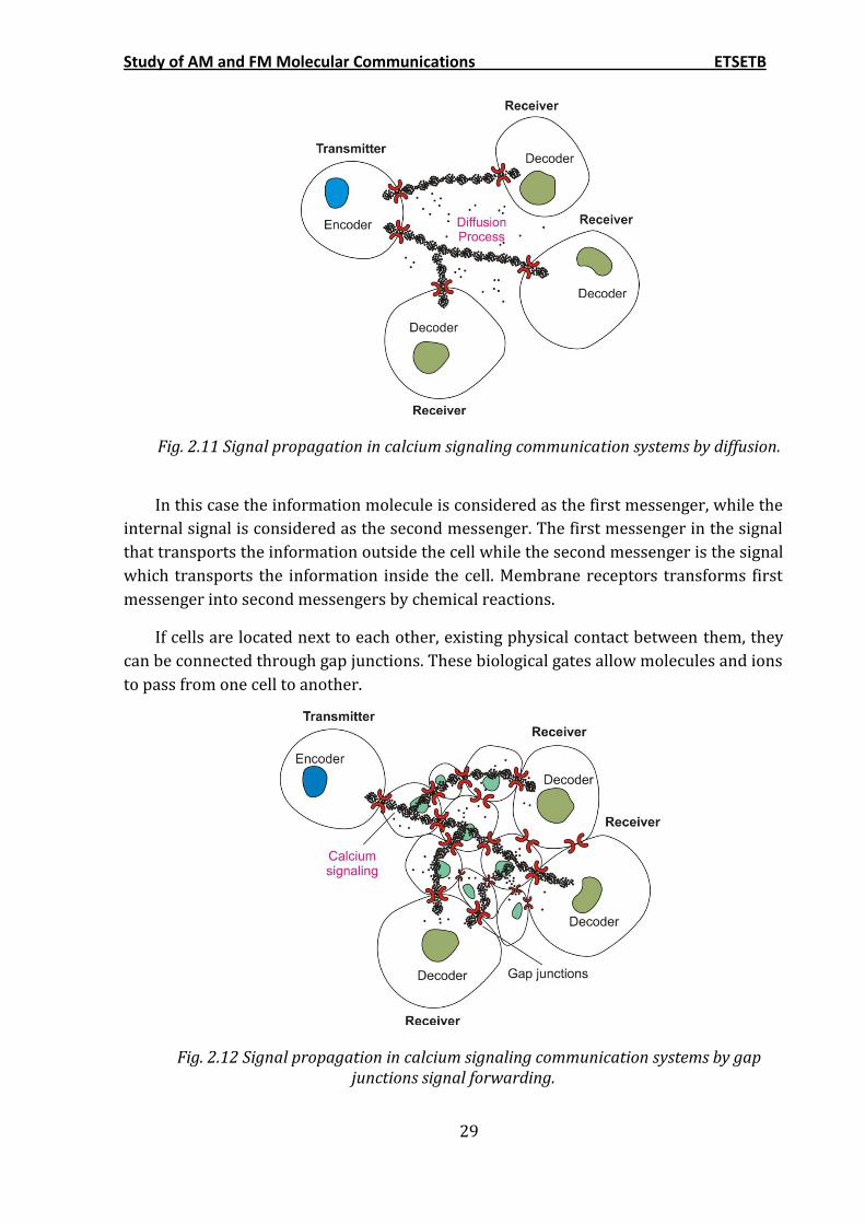
If cells are located next to each other, existing physical contact between them, they
can be connected through gap junctions. These biological gates allow molecules and ions
to pass from one cell to another.
Fig. 2.12 Signal propagation in calcium signaling communication systems by gap junctions signal forwarding.
Study of AM and FM Molecular Communications ETSETB
30
In this case the information travels along cells using only second messengers such
IP3 (inistor 1,4,5-triphosphate) without intervention of first messengers. IP3 is a
messenger that propitiates the secretion of calcium ions (Ca2+) by cell organelles.
Therefore, diffusion of IP3 through gap junctions propagates waves of Ca2+ along the
interconnected cells.
The propagation of Ca2+ is very complex task in which several cell components
participate in order to make this signal propagation possible. Ca2+ buffers or reservoirs
are needed inside the cell when it needs to release molecules to the medium, or when it
is passing those molecules through the gap junctions to the next cell. These buffers can
be certain proteins of the cytoplasm and organelles such as the endoplasmatinc
reticulum. Also ion channels located on the cell membrane are involved in this process,
maintaining this finite resource.
Calcium signaling provides a method to maintain neighboring cells interconnected.
Using calcium signaling surrounding nanomachines can receive a message sent it only
from one nanomachine, in a similar way that is done in traditional communication
networks in processes such as multicasting or broadcasting.
2.2.6.1 Communication features
Calcium signaling would be used in communications over short-range (nm up to
µm) among nanomachines [11]. Similar to natural models, this method would be used by
nanomachines when these placed near each other. Following natural models, the
propagation of the information can be performed in two different ways depending on
the deployment of the nanomachines:
Direct access. In this case, nanomachines should have to be physically
connected. Thereby, Ca2+ signals would travel from one nanomachine to another
through the gates in a similar way that is shown in the figure Fig. 2.12. These
gates would act as gap junctions allowing the flux of calcium waves from one
nano-machine to the interior of the next.
Indirect access. For indirect access, nanomachines should have to be separated,
and the transmitter should be able to release molecules to the medium as a first
messenger in the chemical pathway. These information molecules would move to
the destination following a diffusion process. There, they would be detected by
the receptors and the second messengers would be produced inside the
nanomachine. The transmitters should be able to encode the information varying
the concentration of the first messenger. Biological systems can encode the
information on frequency and amplitude of concentration changes, usually
referred to as Ca2+ oscillation and Ca2+ spikes.
These two propagation methods enable the formation of networks supporting
multicast or broadcasting transmission mechanisms.
Study of AM and FM Molecular Communications ETSETB
31
2.2.6.2 Communication process using calcium signaling
The communication process is set of steps for which the message travels from the
transmitter to the receiver. Usually this process consists of the following steps:
encoding, transmission, signal propagation, reception and decoding. These steps may
present differences for direct access or indirect access.
2.2.6.2.1 Direct access communication process
In this scenario there is one transmitter and many other cells or nanomachines that
are able to propagate the message. As it is said above these components are located one
next to each other, existing physical contact between them, and they are interconnected
through gap junctions or functional gates. In this case, the target cell or nanomachine
can be any of those components of the network.
Encoding. This step generates the information molecules. When the
nanomachines are used to propagate the signal, the transmitter encodes the
information using Ca2+. These calcium waves are encoded varying the
concentration of the ions in amplitude or frequency. These encoding methods are
known as amplitude modulation (AM) or frequency modulation (FM), and they
can be understood in a similar way to the conventional radio-electric
modulations.
Transmission. This task refers to the signaling initiation. The transmitter
stimulates neighboring nanomachines and then the signaling process starts. The
signaling generates the initiation of propagation of Ca2+ waves. IP3 generated by
the transmitter, starts flowing into neighboring nanomachines through the gates,
and therefore, neighboring nanomachines release more Ca2+ driven by the
presence of IP3 substance.
Signal propagation. IP3 transmitted to neighboring nanomachines induces the
release of Ca2+ from the Ca2+ stores which are sensitive to this substance. The
diffusion of IP3 continues to the next nanomachine inducing again the release of
Ca2+ on this nanomachine. Because of this chain reaction, the concentration of
Ca2+ increases, and as a result, the Ca2+ wave propagates along the networked
nodes affected by IP3. This propagation can be controlled changing the
permeability of the function gates.
Reception. Receiver nanomachine is connected to their neighbors through the
gap junctions and perceives the Ca2+concentration waves from inside them. Once
the message is received, receiver nanomachine closes its gates, and thus, it stops
the propagation of IP3.
Decoding. The receiver nanomachine reacts to the internal concentration of Ca2+.
The signal can be encoded in amplitude or frequency enabling the activation of
different processes. The difference between the receiver and all of the
participating components in the propagation is the capacity to decode the
message. The other nanomachines just receive the signal and forward it to the
next component.
Study of AM and FM Molecular Communications ETSETB
32
2.2.6.2.2 Indirect access communication process
The indirect scenario is formed by nanomachines deployed separately and where
the signals propagate along the medium where the nanomachines are deployed.
Encoding. The transmitter encodes the information in the molecule to be used as
a first messenger. The first messenger can also be encoded using AM of FM
techniques.
Transmission. Transmitter initiates signaling by releasing calcium to the
environment.
Signal propagation. In indirect access, the signal diffuse along the medium to
reach with the receiver. This scenario is much more sensitive to the medium
conditions than the direct access. Transmitter nanomachines should consider the
medium conditions to ensure that the signal will arrive to the receiver.
Reception. The receptors placed on the receiver have to translate the
information molecule into internal Ca2+ signals. A nanomachine needs several
different receptors in order to be able to detect many different information
molecules. This could be used to establish many parallel communications
channels using the same medium.
Decoding. The receiver nanomachine reacts to the internal concentration of Ca2+.
This depends on the bindings between information molecules and nanomachine
receptors. Again the information can be encoded in AM or FM and the only
nanomachine which is able to decode the information is the receiver, while other
nanomachines only forward the signal. Since calcium signaling can be considered
as a broadcast scheme, multiple receivers can decode the same message.
2.2.7 Communication systems using other methods
There are so many communication systems which are used in the nature depending
on the distance between transmitter and receiver. Because the main work in this thesis
is based on calcium signaling using indirect access, this system has been explained in
more detail. Now the intention is present some other communication systems more
briefly which are use by biological cells in different scenarios.
2.2.7.1 Molecular motors
Similar to the calcium signaling, the communication systems based on molecular
motors are used in tiny scenarios. They cover the necessities in short-ranges from nm to
a few µm. Molecular motors are used in most of the intra-cellular communications and
they are proteins that converts chemical energy into mechanical work at nano-scale
[15].
The information molecule is carried on the motor, in this move directionally along
cytoskeletal tracks. Inside the cells, molecular motors are aimed to transport molecules
Study of AM and FM Molecular Communications ETSETB
33
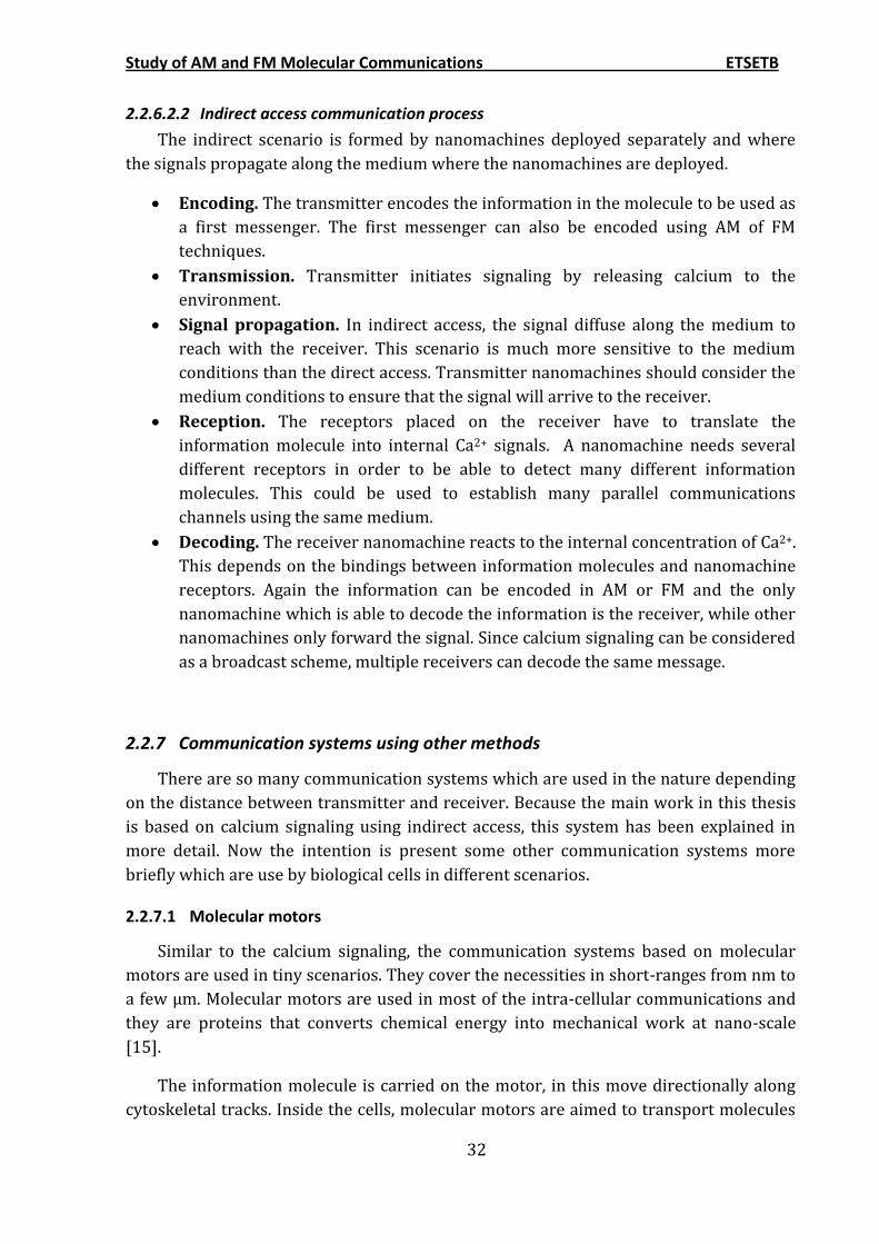
among organelles. They travel along molecular rails performs a complete railway
network inside the cell for intra-cell substance transportation.
Fig. 2.13 System components in molecular motors communication systems.
This communication system includes one transmitter and only one receiver. The
ability to move molecules makes molecular motors a feasible way to transport
information packets. But this system applied in nanonetworks should be able to adapt to
more complex scenarios. In this case techniques as multihoping would be needed and
because of that the nanomachines should be able to amplify, decode and redirect the
information.
2.2.7.2 Pheromones
Pheromones are a system very useful when the distance between transmitter and
receiver nanomachines ranges from mm up to km. Nanonetworks in long-range scenario
are also inspired in biological systems found in nature. Many animals such as butterflies,
bees, many mammals or ants use pheromones in their communications. Butterflies use
pheromones and molecular messages can reach the range of a few kilometers [7].
Communication using pheromones is similar to the techniques based on the release
molecules that can be detected by a receiver. Once the molecules are released to the
medium, they can be affected by factors, temperature, medium flow, antagonist agents,
and the can be considered as noise sources.
Probably, the most important feature in this kind of log-range communication
system is the coding system. In the nature only the animals of the same species can
detect the pheromones in the air. While in traditional communication networks, the
information is usually encoded in a binary system, in pheromone systems the
information is encoded in the molecule itself. The messages can be encoded using
different molecules which imply more combinations to encode the information.
Study of AM and FM Molecular Communications ETSETB
34
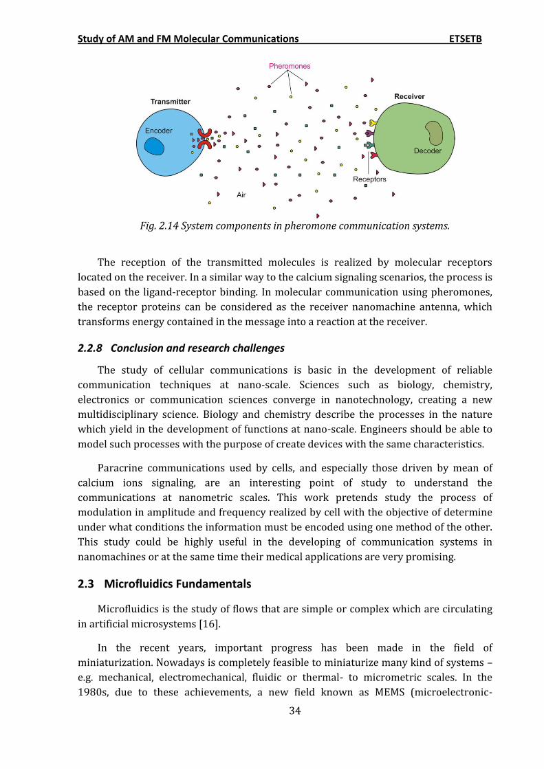
Fig. 2.14 System components in pheromone communication systems.
The reception of the transmitted molecules is realized by molecular receptors
located on the receiver. In a similar way to the calcium signaling scenarios, the process is
based on the ligand-receptor binding. In molecular communication using pheromones,
the receptor proteins can be considered as the receiver nanomachine antenna, which
transforms energy contained in the message into a reaction at the receiver.
2.2.8 Conclusion and research challenges
The study of cellular communications is basic in the development of reliable
communication techniques at nano-scale. Sciences such as biology, chemistry,
electronics or communication sciences converge in nanotechnology, creating a new
multidisciplinary science. Biology and chemistry describe the processes in the nature
which yield in the development of functions at nano-scale. Engineers should be able to
model such processes with the purpose of create devices with the same characteristics.
Paracrine communications used by cells, and especially those driven by mean of
calcium ions signaling, are an interesting point of study to understand the
communications at nanometric scales. This work pretends study the process of
modulation in amplitude and frequency realized by cell with the objective of determine
under what conditions the information must be encoded using one method of the other.
This study could be highly useful in the developing of communication systems in
nanomachines or at the same time their medical applications are very promising.
2.3 Microfluidics Fundamentals
Microfluidics is the study of flows that are simple or complex which are circulating
in artificial microsystems [16].
In the recent years, important progress has been made in the field of
miniaturization. Nowadays is completely feasible to miniaturize many kind of systems –
e.g. mechanical, electromechanical, fluidic or thermal- to micrometric scales. In the
1980s, due to these achievements, a new field known as MEMS (microelectronic-
Study of AM and FM Molecular Communications ETSETB
35
mechanical systems) showed up. Later in 1990s these systems began to be used in many
different fields, being manufactured MEMS for chemical, biological and biomedical
applications. These systems utilized fluid flows operating in unusual and unexplored
conditions, which inevitable led to the creation of a new discipline
known as microfluidics.
In microfluidics the systems manipulate small amounts of liquids, from 10-18 to 10-
9 liters, using channels with dimensions of tens to hundreds of micrometers [17]. It
takes advantage of its most obvious characteristic, small size, but also it exploits a less
obvious characteristic of fluid in microchannels, the laminar flow.
Microfluidics offers a number of interesting capabilities such as the ability to use
very small quantities of samples, low cost or short time of analysis which are very useful
in analysis applications. It offers fundamentally new capabilities in the control of
concentration of molecules in space and time.
2.3.1 Low Reynolds number
In fluid mechanics, the Reynolds number is the ratio between the inertial forces and
the viscous forces, and quantifies the relative importance between these two types of
forces.
2
vInertial
d
(2.1)
2
vViscous
d
(2.2)
Where ρ is the density of the fluid (kg/m3), v is the mean velocity of the fluid (m/s),
d is the characteristic length of the flow (m) and μ is the dynamic viscosity of the fluid
(kg/m·s).
This dimensionless number can be used to characterize different flow regimes, such
as laminar flow or turbulent flow. For low values of the Reynolds number (less than
2300 [18])the fluid flows in a laminar way, on the other hand for large values of this
number (more than 10000 [18]) the behavior of the fluid is turbulent. Laminar flow is
characterized by smooth, constant fluid motion. The motion of the particles of fluid is
very orderly with all particles moving in straight lines parallel to the pipe walls [19],
while turbulent flow tend to create vortices, chaotic eddies and other flow instabilities.
Revd vd
(2.3)
Where υ is the kinematic viscosity (m2/s). The characteristic length of closed
channel flow is the hydraulic diameter of the channel:
Study of AM and FM Molecular Communications ETSETB
36
4h
Ad
P
(2.4)
Where A is the cross-sectional area and P is the wetted perimeter, the perimeter of
the channel which is wetted by the fluid.
In microfluidic systems, typical fluid velocities do not exceed a centimeter per
second and widths of canal are on the order of tens to hundreds of micrometers;
therefore, in general, Reynolds number in microfluidic systems do not exceed 10e-1. In
fact, we can say that a microfluidic system whose channels have one of the three
dimensions (height, width or depth) lower than 100μm, always will work in laminar
regime.
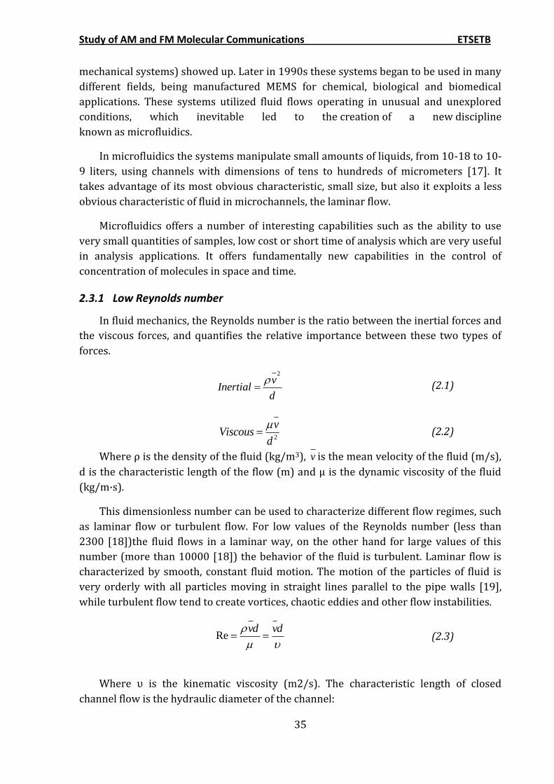
2.3.2 Velocity profile in microchannels
In the situation of two parallel planes close together filled with fluid the gap space
between them. In fluid dynamics there are two ways of provoke movement in the fluid
between the planes: by applying shear stress through the channel or by a playing a
pressure gradient along the channel [20].
Fig. 2.15 On the left velocity profile applying shear stress of the superior plane. On the
right, velocity profile applying a pressure gradient along the channel.
The second one, which is called Poiseuille flow, is the most common situation in
microfluidic systems because in these systems the walls are usually resting in the same
position.
The flow forced by a hydrodynamic pressure gradient is called Pressure-Driven
Flow (PDF) and it is conditioned by the velocity of the channel walls. As it has been said
before, in pressure-driven flow the walls are at rest forcing the velocity of the fluid at the
channels walls is zero. On the other hand, the pressure applied to the fluid volume
generates a uniform force over the whole cross-sectional area of the channel. The
combination of the no-slip condition at the walls and the uniform force applied to the
entrance provokes a parabolic velocity profile of the flow, that is, zero velocity at the
walls and maximum a velocity at the center of the channel.
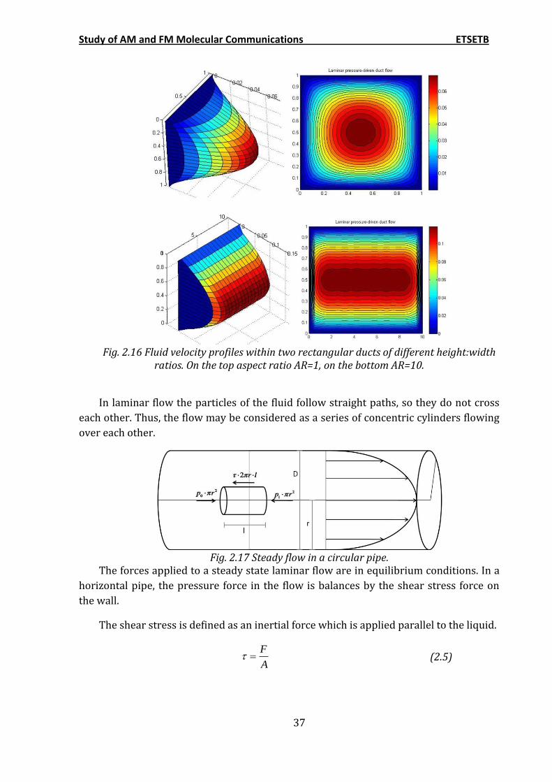
Study of AM and FM Molecular Communications ETSETB
37
Fig. 2.16 Fluid velocity profiles within two rectangular ducts of different height:width
ratios. On the top aspect ratio AR=1, on the bottom AR=10.
In laminar flow the particles of the fluid follow straight paths, so they do not cross
each other. Thus, the flow may be considered as a series of concentric cylinders flowing
over each other.
Fig. 2.17 Steady flow in a circular pipe.
The forces applied to a steady state laminar flow are in equilibrium conditions. In a
horizontal pipe, the pressure force in the flow is balances by the shear stress force on
the wall.
The shear stress is defined as an inertial force which is applied parallel to the liquid.
F
A
(2.5)
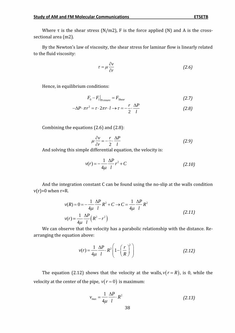
Study of AM and FM Molecular Communications ETSETB
38
Where τ is the shear stress (N/m2), F is the force applied (N) and A is the cross-
sectional area (m2).
By the Newton’s law of viscosity, the shear stress for laminar flow is linearly related
to the fluid viscosity:
v
r
(2.6)
Hence, in equilibrium conditions:
0 1 Pr ShearessureF F F
(2.7)
2 22
r PP r r l
l
(2.8)
Combining the equations (2.6) and (2.8):
2
v r P
r l
(2.9)
And solving this simple differential equation, the velocity is:
21( )
4
Pv r r C
l
(2.10)
And the integration constant C can be found using the no-slip at the walls condition
v(r)=0 when r=R.
2 2
2 2
1 1( ) 0
4 4
1( )
4
P Pv R R C C R
l l
Pv r R r
l
(2.11)
We can observe that the velocity has a parabolic relationship with the distance. Re-
arranging the equation above:
2
21( ) 1
4
P rv r R
l R
(2.12)
The equation (2.12) shows that the velocity at the walls, v r R , is 0, while the
velocity at the center of the pipe, 0v r is maximum:
2
max
1
4
Pv R
l
(2.13)
Study of AM and FM Molecular Communications ETSETB
39
Similar to the Poiseuille flow, the velocity profile in a pipe is also parabolic. Actually,
the three dimensional flow has a velocity profile which a form of a paraboloid, having its
maximum at the axis of the pipe, and its zeros at the walls. For non-circular three
dimensional channels, the solution is not analytical so microfluidic devices have to be
studied through simulation tools.
2.3.3 Fick's laws of diffusion
In microfluidics is very common to find situations where the particles in the liquid
move inside it following diffusion processes.
Molecular diffusion is the thermal motion of all molecules at temperatures above
absolute zero. This principle establishes that when in a certain point exists a non-
uniform distribution of particles, then they tend to diffuse away in order to reach
uniform concentration through all the space [21]. Molecular diffusion can be also
considered a specific case of random walk or Brownian motion, which is used to model
the movement of particles suspended in a fluid.
Molecular diffusion is typically described using the Fick's laws of diffusion.
Fick's first law: The Fick's first law permits relate the net flux of particles to the concentration of
particles, establishing that the flux goes from regions of high concentration to regions of
low concentration, with a value proportional to the concentration gradient.
, ,J x t D C x t
(2.14)
J represents the net flux of particles in a specific position x and at a specific time t
(mol/m2·s). C is the concentration of particles (mol/m3) and D is the diffusion
coefficient or diffusivity (m2/s). The diffusion coefficient is a parameter which specifies
how "easy" is for a particle to move in a fluid. It provides the idea of the speed at which
the particles move from positions with high concentration to positions with low
concentrations. This coefficient depends strongly on the size of the particles. Small
particles have high values of diffusivity while big particles provide low values of this
parameter.
Fick's second law: The Fick's second law predicts how diffusion causes the change of the concentration
with the time. This law depends on the combination of the Fick's first law and the law of
conservation of mass. The law of conservation of mass states that the particles cannot be
created or destroyed, and thus, all the particles entering or leaving the global system
must be the same.
In a first approximation, the variation of the particles concentration in time must be
opposite to the gradient of the particle flux in the same location.
Study of AM and FM Molecular Communications ETSETB
40
Hence:
,,
C x tJ x t
t
(2.15)
And then, substituting the expression of the first Fick's law (2.14) into the law of
conservation of mass (2.15) the Fick's second law is obtained:
2
,,
C x tD C x t
t
(2.16)
A more detailed expression for the Fick’s second law takes into account two more
terms that can affect in the ratio of appearance of disappearance of particles in the
system.
The four terms are [22]:
Rate of increase of particles per unit volume:
,C x t
t
(2.17)
Net rate of addition of particles per unit volume by convection:
,v C x t
(2.18)
Rate of addition of particles per unit volume by diffusion:
2, ,J x t D C x t
(2.19)
Rate of production or elimination of particles per unit volume by reactions:
,R x t
(2.20)
Then, the variation of particles concentration is the result of the addition of
molecules by convection, by diffusion or by reaction:
,, , ,
C x tv C x t J x t R x t
t
(2.21)
Arranging the previous equation and assuming the simplification that the diffusion
coefficient is constant [22]:
Study of AM and FM Molecular Communications ETSETB
41
2
,, , ,
C x tv C x t D C x t R x t
t
(2.22)
Where v is the velocity and R is the production or elimination (source or sink) of
particles. There are two important: when the velocity is zero, then, the system works in
a pure diffusion mode, while if the velocity is not zero, then, is the system is produces
the dispersion phenomena.
The equation (2.22) is also known as the Diffusion Equation. It provides the value
of the future concentration of particles in one point if the concentration in that point and
in its vicinities is known.
2.3.4 Micorfabrication
The most common technique of microfabrication of microfluidic systems is the one
known as Soft-Lithography. It is based in two steps, the fabrication of a master using
lithography techniques, and the replica of this master by casting of some plastics or
polymers.
The use of microelectronic techniques such as photolithography over silicon wafer
to fabricate the master is especially due to two reasons. The first one is that the
microelectronic fabrication techniques are a very well known source of knowledge in
the fabrication of all kind of devices at micrometric scale. The second one is because of
the low roughness of the silicon wafers (around 2nm [23]), which is essential in the
replication of structures. The use of glass substrates is being used more frequently due
to its characteristics of softness and its lower cost.
2.3.4.1 Photolithography
One process that plays a central role in microfabrication is photolithography. It
consists in the exposition of a photosensitive resist through a mask, which has been
deposited on a substrate.
The photolithography masks are generally plates of quartz on which deposits of
chrome form the pattern that is desired to replicate. Obviously is not possible to
fabricate objects with geometric precision superior to that of the mask. These masks are
often made using electron beams with a precision on the order of a fraction a
micrometer. When this high precision is not required methods like high quality printout
on a transparency can be used.
The mold will appear when the light through the mask cure the photosensitive
resist. This resist is deposited in a thin layer on a solid substrate of silicon or glass. The
deposit is made using a spin coater.
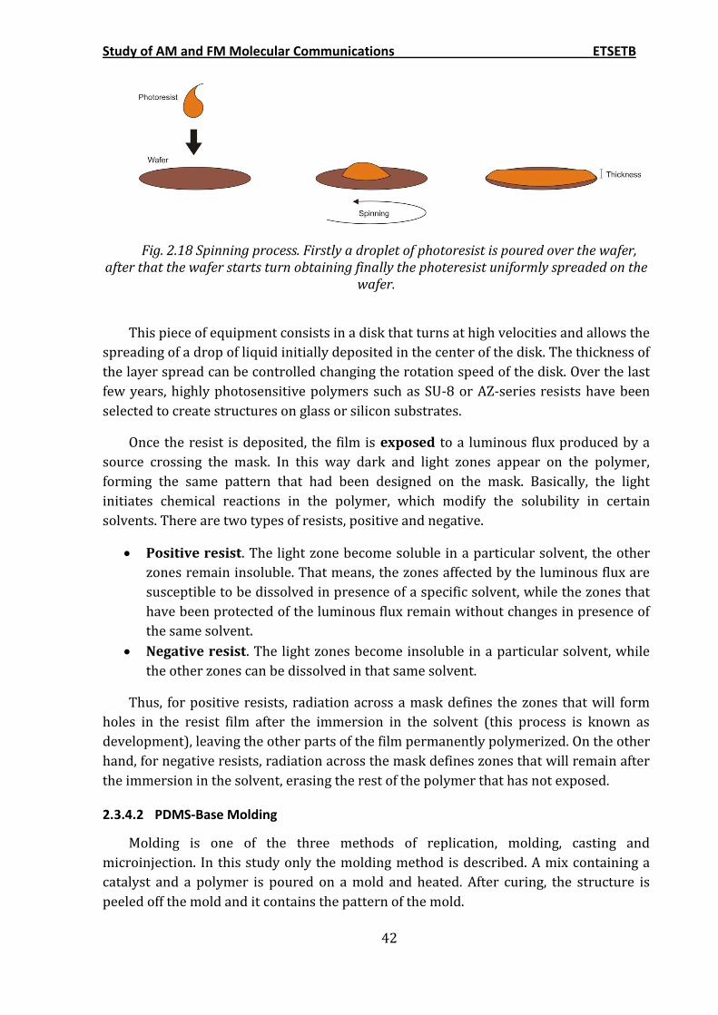
Study of AM and FM Molecular Communications ETSETB
42
Fig. 2.18 Spinning process. Firstly a droplet of photoresist is poured over the wafer, after that the wafer starts turn obtaining finally the photeresist uniformly spreaded on the
wafer.
This piece of equipment consists in a disk that turns at high velocities and allows the
spreading of a drop of liquid initially deposited in the center of the disk. The thickness of
the layer spread can be controlled changing the rotation speed of the disk. Over the last
few years, highly photosensitive polymers such as SU-8 or AZ-series resists have been
selected to create structures on glass or silicon substrates.
Once the resist is deposited, the film is exposed to a luminous flux produced by a
source crossing the mask. In this way dark and light zones appear on the polymer,
forming the same pattern that had been designed on the mask. Basically, the light
initiates chemical reactions in the polymer, which modify the solubility in certain
solvents. There are two types of resists, positive and negative.
Positive resist. The light zone become soluble in a particular solvent, the other
zones remain insoluble. That means, the zones affected by the luminous flux are
susceptible to be dissolved in presence of a specific solvent, while the zones that
have been protected of the luminous flux remain without changes in presence of
the same solvent.
Negative resist. The light zones become insoluble in a particular solvent, while
the other zones can be dissolved in that same solvent.
Thus, for positive resists, radiation across a mask defines the zones that will form
holes in the resist film after the immersion in the solvent (this process is known as
development), leaving the other parts of the film permanently polymerized. On the other
hand, for negative resists, radiation across the mask defines zones that will remain after
the immersion in the solvent, erasing the rest of the polymer that has not exposed.
2.3.4.2 PDMS-Base Molding
Molding is one of the three methods of replication, molding, casting and
microinjection. In this study only the molding method is described. A mix containing a
catalyst and a polymer is poured on a mold and heated. After curing, the structure is
peeled off the mold and it contains the pattern of the mold.
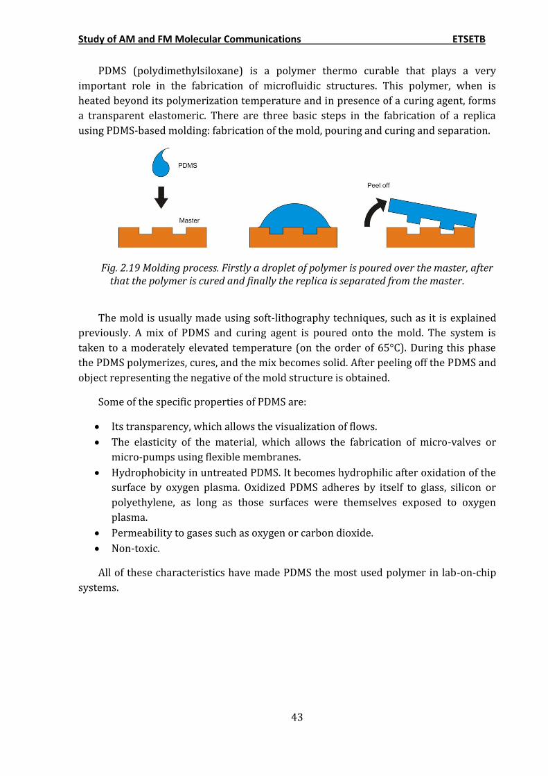
Study of AM and FM Molecular Communications ETSETB
43
PDMS (polydimethylsiloxane) is a polymer thermo curable that plays a very
important role in the fabrication of microfluidic structures. This polymer, when is
heated beyond its polymerization temperature and in presence of a curing agent, forms
a transparent elastomeric. There are three basic steps in the fabrication of a replica
using PDMS-based molding: fabrication of the mold, pouring and curing and separation.
Fig. 2.19 Molding process. Firstly a droplet of polymer is poured over the master, after that the polymer is cured and finally the replica is separated from the master.
The mold is usually made using soft-lithography techniques, such as it is explained
previously. A mix of PDMS and curing agent is poured onto the mold. The system is
taken to a moderately elevated temperature (on the order of 65°C). During this phase
the PDMS polymerizes, cures, and the mix becomes solid. After peeling off the PDMS and
object representing the negative of the mold structure is obtained.
Some of the specific properties of PDMS are:
Its transparency, which allows the visualization of flows.
The elasticity of the material, which allows the fabrication of micro-valves or
micro-pumps using flexible membranes.
Hydrophobicity in untreated PDMS. It becomes hydrophilic after oxidation of the
surface by oxygen plasma. Oxidized PDMS adheres by itself to glass, silicon or
polyethylene, as long as those surfaces were themselves exposed to oxygen
plasma.
Permeability to gases such as oxygen or carbon dioxide.
Non-toxic.
All of these characteristics have made PDMS the most used polymer in lab-on-chip
systems.
Study of AM and FM Molecular Communications ETSETB
44
3 THEORETICAL ANALYSIS OF MOLECULAR COMMUNICATION SYSTEMS
Previously the concept of molecular modulation has been presented. Cells are able
to encode the information using amplitude modulation or frequency modulation
depending on the requirements of the communication. Understand which are the
criteria that cells use to decide whether the communication should be modulated in
amplitude or frequency is a key point to design future communication systems for
nanonetworks.
In this section a mathematical model for a paracrine communication system is
calculated. Whit it, the behavior of these system is predicted and it allows us to find a
criterion for which the information shod be encoded using amplitude or frequency
modulation.

Study of AM and FM Molecular Communications ETSETB
45
Study of AM and FM Molecular Communications ETSETB
46
3.1 Introduction
In the previous chapters, molecular communications systems based on the diffusion
of particles in the medium have been presented, such as paracrine signaling or contact-
dependent signaling. In these systems the particles move through the medium following
diffusion processes and the concentration of these particles can be predicted using the
diffusion equation (2.22).
Usually in partial differential equations, such as the diffusion equation, it is not
possible to find an analytical closed solution, but sometimes when the geometry of the
region where the equation applies is simple and the initials and boundary conditions
permit it, it is possible to find a closed solution.
3.2 Closed Solution for the Diffusion Equation
We suppose a biological scenario where a cell cultivated in a cuvette is secreting
molecules to the medium and these molecules diffuse until reach to their targets. If we
restrict this system to a one dimensional situation where the molecules only can diffuse
in one direction, and we assume that the fluid in which the cells are immersed is at rest
and the molecules do not react with others, then, the equation (2.22) can be simplified
to:
2
2
, ,
0
0 final
C x t C x tD
t x
x H
t T
(3.23)
In some cases cells send information by secretion of spikes of molecules
periodically. For this case, we assume a simplification of that. A cell secretes a constant
concentration of molecules for a period of time and then forces zero concentration of
molecules around it. Thus, the concentration of molecules around the cell follows a
square function between maximum and zero concentration.
The intention is to solve the equation (3.23) under the situation that the
concentration at x=0 is changing from maximum to minimum periodically, following a
square function.
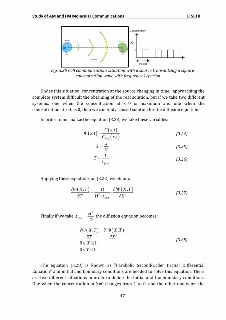
Study of AM and FM Molecular Communications ETSETB
47
Fig. 3.20 Cell communications situation with a source transmitting a square
concentration wave with frequency 1/period.
Under this situation, concentration at the source changing in time, approaching the
complete system difficult the obtaining of the real solution, but if we take two different
systems, one when the concentration at x=0 is maximum and one when the
concentration at x=0 is 0, then we can find a closed solution for the diffusion equation.
In order to normalize the equation (3.23) we take these variables:
max
,,
,
C x tx t
C x t
(3.24)
xX
H
(3.25)
final
tT
T
(3.26)
Applying these equations on (3.23) we obtain:
2
2 2
, ,
final
X T X TD
T H t X
(3.27)
Finally if we take 2
final
HT
D the diffusion equation becomes:
2
2
, ,
0 1
0 1
X T X T
T X
X
T
(3.28)
The equation (3.28) is known as "Parabolic Second-Order Partial Differential
Equation" and initial and boundary conditions are needed to solve this equation. There
are two different situations in order to define the initial and the boundary conditions.
One when the concentration at X=0 changes from 1 to 0, and the other one when the
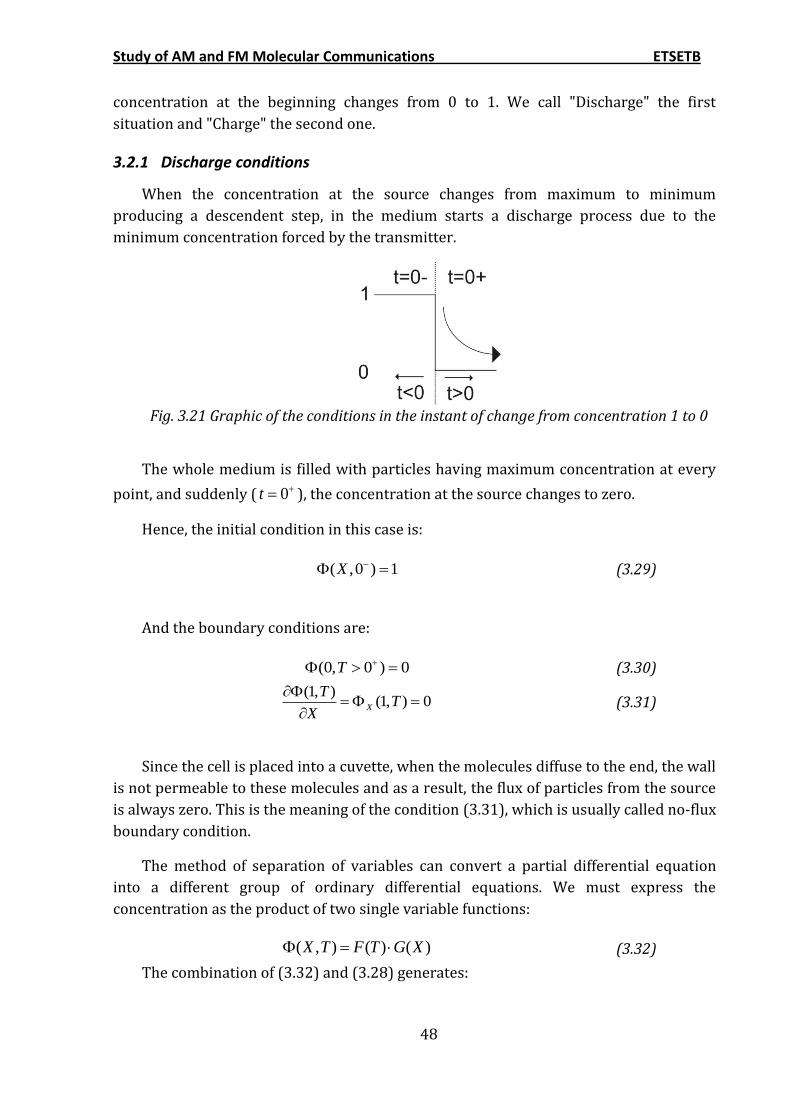
Study of AM and FM Molecular Communications ETSETB
48
concentration at the beginning changes from 0 to 1. We call "Discharge" the first
situation and "Charge" the second one.
3.2.1 Discharge conditions
When the concentration at the source changes from maximum to minimum
producing a descendent step, in the medium starts a discharge process due to the
minimum concentration forced by the transmitter.
Fig. 3.21 Graphic of the conditions in the instant of change from concentration 1 to 0
The whole medium is filled with particles having maximum concentration at every
point, and suddenly ( 0t ), the concentration at the source changes to zero.
Hence, the initial condition in this case is:
( ,0 ) 1X (3.29)
And the boundary conditions are:
(0, 0 ) 0T (3.30)
(1, )(1, ) 0X
TT
X
(3.31)
Since the cell is placed into a cuvette, when the molecules diffuse to the end, the wall
is not permeable to these molecules and as a result, the flux of particles from the source
is always zero. This is the meaning of the condition (3.31), which is usually called no-flux
boundary condition.
The method of separation of variables can convert a partial differential equation
into a different group of ordinary differential equations. We must express the
concentration as the product of two single variable functions:
( , ) ( ) ( )X T F T G X (3.32)
The combination of (3.32) and (3.28) generates:
Study of AM and FM Molecular Communications ETSETB
49
2
2
1 1F G
T F X G
(3.33)
Because ( )F T and ( )G X depend on different variables, the equation (3.33) must be
equal to an arbitrary constant:
2
2
1 1F Gk
T F X G
(3.34)
The partial differential equation (3.28) has become in two different ordinary
differential equation:
FF k
T
(3.35)
2
2
GG k
X
(3.36)
The solution of the equation (3.35) is:
( ) kTF T e (3.37)
For positive values of k, the equation (3.37) becomes monotically increasing and
would be infinite at infinite values of T which is impossible. So the constant k must be
negative:
2
0
k
(3.38)
The solution for the equation (3.36) is:
( ) cos( ) sin( )G X A X B X (3.39)
Therefore the combination of (3.37) and (3.39) provides the complete solution:
2
( , ) cos( ) sin( ) TX T A X B X e C
(3.40)
Where C is a constant that disappears when the concentration equation is
derivative.
Now the boundary and the initial conditions will be used in order to find the
constants A, B, C and λ.
The substitution of the first boundary condition in (3.40) gives the equation (3.41):
2
(0, ) 1 0 0TT A B e C
(3.41)
Study of AM and FM Molecular Communications ETSETB
50
Because 0 does not have any time dependence:
0A (3.42)
And then:
0C (3.43)
Using the second boundary condition in (3.40):
2
(1, ) cos( 1) 0T
X T B e (3.44)
The equation (3.44) has infinite solutions:
(2 1)2
0
n n
n
(3.45)
Adding all the possible solutions we obtain the general solution of the diffusion
equation (superposition principle):
2
1
( , ) sin( ) n T
n n
n
X T B X e
(3.46)
2
(2 1)2
1
( , ) sin((2 1) )2
n T
n
n
X T B n X e
(3.47)
Finally to find the last constant B, we use the last information that we know, the
initial condition. So using (3.29) in (3.47):
2 0
1 1
( ,0) sin( ) sin( ) 1n
n n n n
n n
X B X e B X
(3.48)
Using the concept of orthogonal functions, taking f(x) as:
1
( ) sin( )n n
n
f X B X
We can say:
1 1
10 0
( ) sin( ) sin( ) sin( )m n n m
n
f X X dX B X X dX
(3.49)
Because the operator integral is linear:
1
1 0
sin( ) sin( )n n m
n
B X X dX
(3.50)
Arranging the product of sinus we obtain:
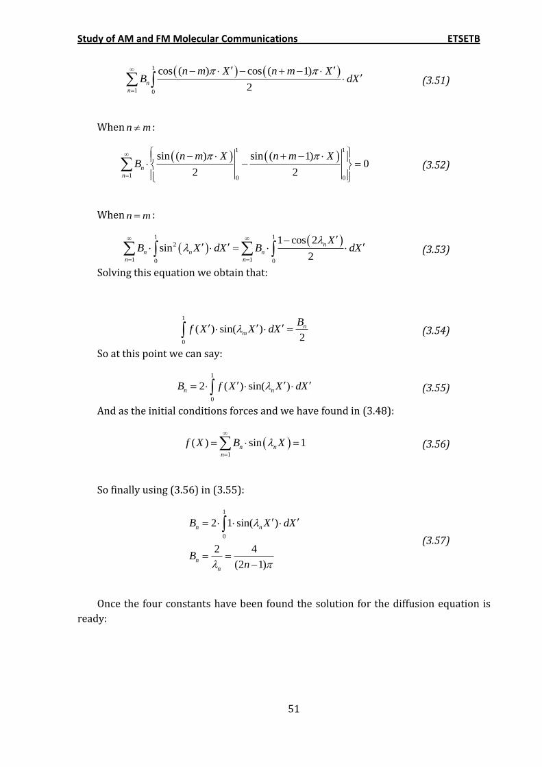
Study of AM and FM Molecular Communications ETSETB
51
1
1 0
cos ( ) cos ( 1)
2n
n
n m X n m XB dX
(3.51)
When n m :
1 1
1 0 0
sin ( ) sin ( 1)0
2 2n
n
n m X n m XB
(3.52)
When n m :
1 1
2
1 10 0
1 cos 2sin
2
n
n n n
n n
XB X dX B dX
(3.53)
Solving this equation we obtain that:
1
0
( ) sin( )2
nm
Bf X X dX
(3.54)
So at this point we can say:
1
0
2 ( ) sin( )n nB f X X dX
(3.55)
And as the initial conditions forces and we have found in (3.48):
1
( ) sin 1n n
n
f X B X
(3.56)
So finally using (3.56) in (3.55):
1
0
2 1 sin( )
2 4
(2 1)
n n
n
n
B X dX
Bn
(3.57)
Once the four constants have been found the solution for the diffusion equation is
ready:
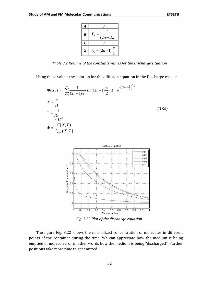
Study of AM and FM Molecular Communications ETSETB
52
A 0
B 4
(2 1)nB
n
C 0
λ (2 1)2
n n
Table 3.2 Resume of the constants values for the Discharge situation
Using these values the solution for the diffusion equation in the Discharge case is:
2
(2 1)2
1
2
max
4( , ) sin((2 1) )
(2 1) 2
,
,
n T
n
X T n X en
xX
H
tT
DH
C X T
C X T
(3.58)
Fig. 3.22 Plot of the discharge equation.
The figure Fig. 3.22 shows the normalized concentration of molecules in different
points of the container during the time. We can appreciate how the medium is being
emptied of molecules, or in other words how the medium is being “discharged”. Further
positions take more time to get emitted.
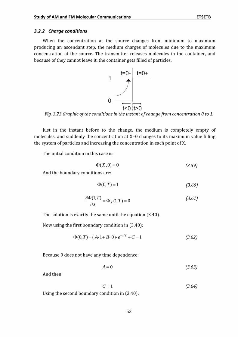
Study of AM and FM Molecular Communications ETSETB
53
3.2.2 Charge conditions
When the concentration at the source changes from minimum to maximum
producing an ascendant step, the medium charges of molecules due to the maximum
concentration at the source. The transmitter releases molecules in the container, and
because of they cannot leave it, the container gets filled of particles.
Fig. 3.23 Graphic of the conditions in the instant of change from concentration 0 to 1.
Just in the instant before to the change, the medium is completely empty of
molecules, and suddenly the concentration at X=0 changes to its maximum value filling
the system of particles and increasing the concentration in each point of X.
The initial condition in this case is:
( ,0) 0X (3.59)
And the boundary conditions are:
The solution is exactly the same until the equation (3.40).
Now using the first boundary condition in (3.40):
2
(0, ) 1 0 1TT A B e C
(3.62)
Because 0 does not have any time dependence:
0A (3.63)
And then:
1C (3.64)
Using the second boundary condition in (3.40):
(0, ) 1T (3.60)
(1, )
(1, ) 0X
TT
X
(3.61)
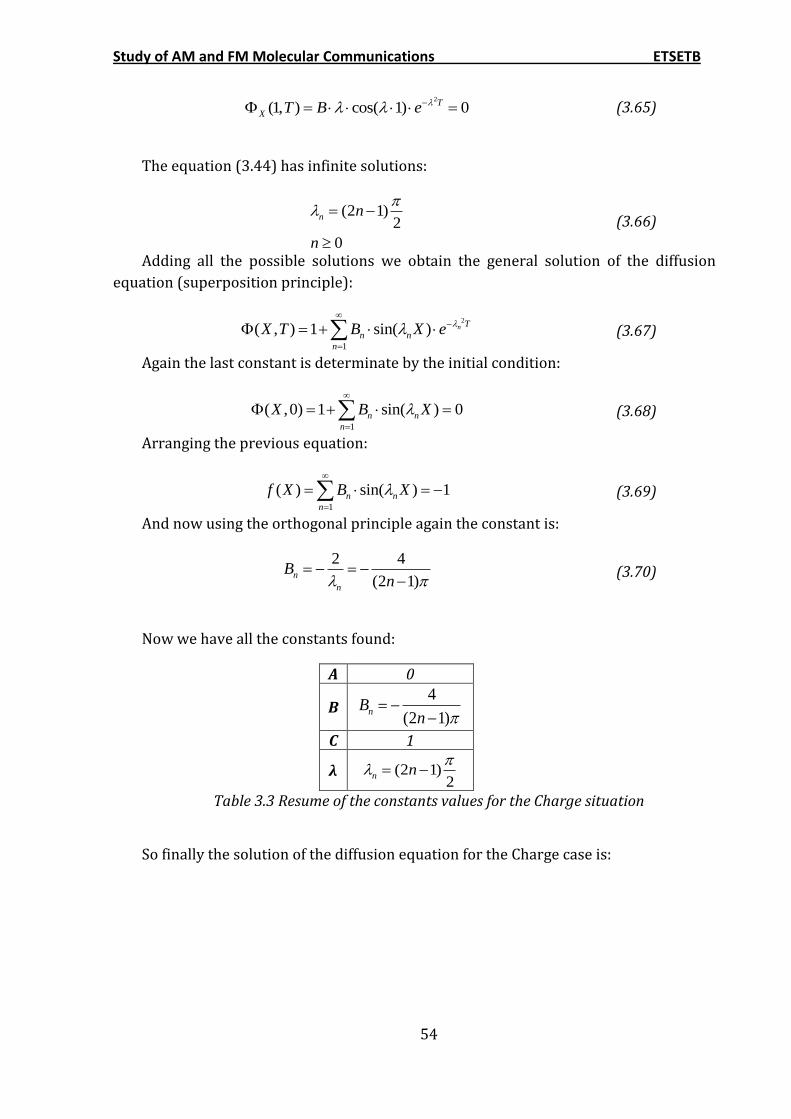
Study of AM and FM Molecular Communications ETSETB
54
2
(1, ) cos( 1) 0T
X T B e (3.65)
The equation (3.44) has infinite solutions:
(2 1)2
0
n n
n
(3.66)
Adding all the possible solutions we obtain the general solution of the diffusion
equation (superposition principle):
2
1
( , ) 1 sin( ) n T
n n
n
X T B X e
(3.67)
Again the last constant is determinate by the initial condition:
1
( ,0) 1 sin( ) 0n n
n
X B X
(3.68)
Arranging the previous equation:
1
( ) sin( ) 1n n
n
f X B X
(3.69)
And now using the orthogonal principle again the constant is:
2 4
(2 1)n
n
Bn
(3.70)
Now we have all the constants found:
A 0
B 4
(2 1)nB
n
C 1
λ (2 1)2
n n
Table 3.3 Resume of the constants values for the Charge situation
So finally the solution of the diffusion equation for the Charge case is:
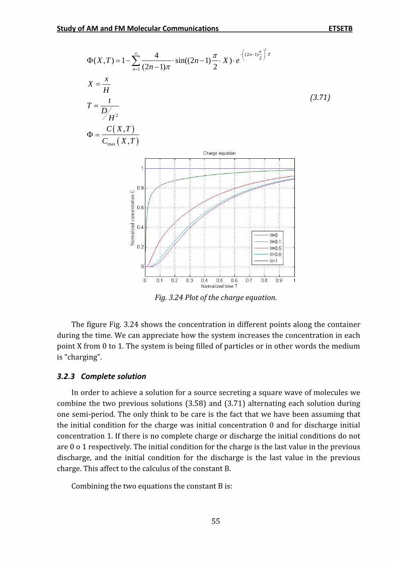
Study of AM and FM Molecular Communications ETSETB
55
2
(2 1)2
1
2
max
4( , ) 1 sin((2 1) )
(2 1) 2
,
,
n T
n
X T n X en
xX
H
tT
DH
C X T
C X T
(3.71)
Fig. 3.24 Plot of the charge equation.
The figure Fig. 3.24 shows the concentration in different points along the container
during the time. We can appreciate how the system increases the concentration in each
point X from 0 to 1. The system is being filled of particles or in other words the medium
is “charging”.
3.2.3 Complete solution
In order to achieve a solution for a source secreting a square wave of molecules we
combine the two previous solutions (3.58) and (3.71) alternating each solution during
one semi-period. The only think to be care is the fact that we have been assuming that
the initial condition for the charge was initial concentration 0 and for discharge initial
concentration 1. If there is no complete charge or discharge the initial conditions do not
are 0 o 1 respectively. The initial condition for the charge is the last value in the previous
discharge, and the initial condition for the discharge is the last value in the previous
charge. This affect to the calculus of the constant B.
Combining the two equations the constant B is:
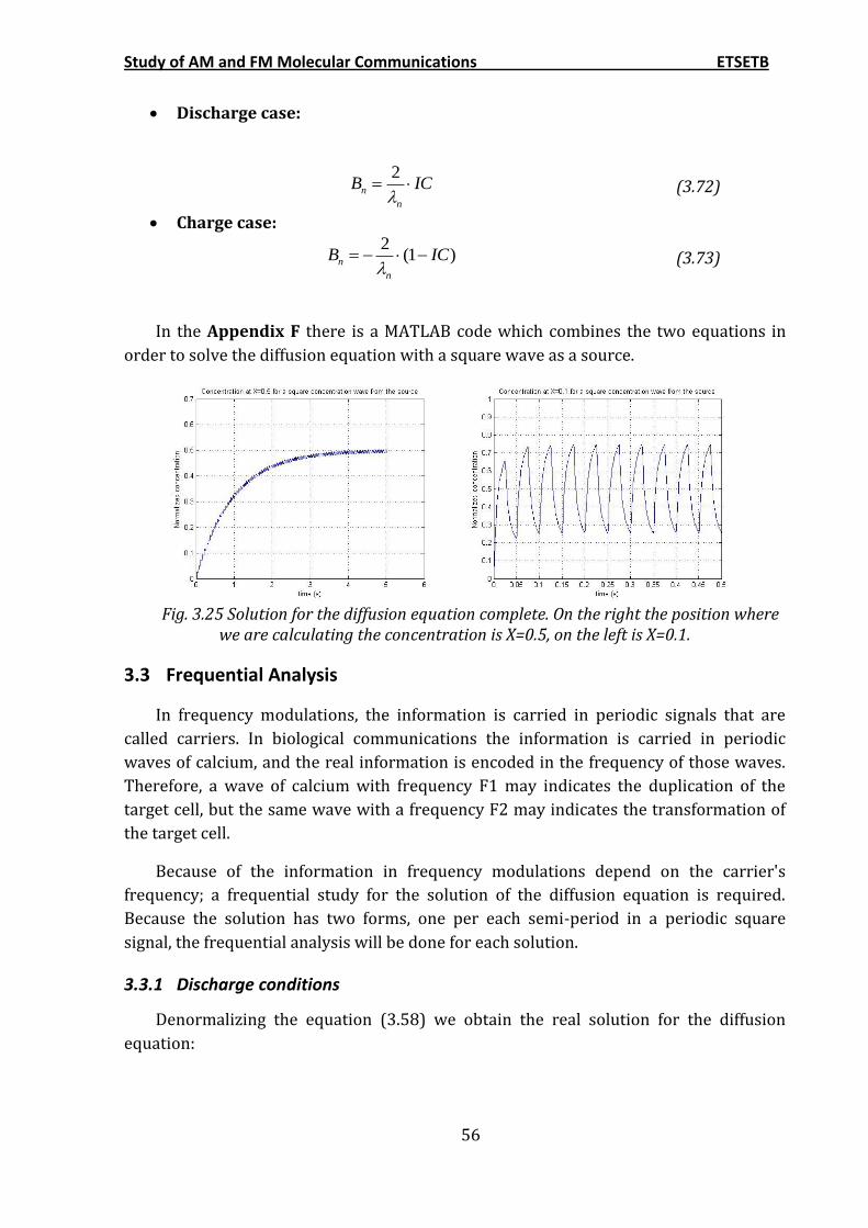
Study of AM and FM Molecular Communications ETSETB
56
Discharge case:
2n
n
B IC
(3.72)
Charge case: 2
(1 )n
n
B IC
(3.73)
In the Appendix F there is a MATLAB code which combines the two equations in
order to solve the diffusion equation with a square wave as a source.
Fig. 3.25 Solution for the diffusion equation complete. On the right the position where
we are calculating the concentration is X=0.5, on the left is X=0.1.
3.3 Frequential Analysis
In frequency modulations, the information is carried in periodic signals that are
called carriers. In biological communications the information is carried in periodic
waves of calcium, and the real information is encoded in the frequency of those waves.
Therefore, a wave of calcium with frequency F1 may indicates the duplication of the
target cell, but the same wave with a frequency F2 may indicates the transformation of
the target cell.
Because of the information in frequency modulations depend on the carrier's
frequency; a frequential study for the solution of the diffusion equation is required.
Because the solution has two forms, one per each semi-period in a periodic square
signal, the frequential analysis will be done for each solution.
3.3.1 Discharge conditions
Denormalizing the equation (3.58) we obtain the real solution for the diffusion
equation:
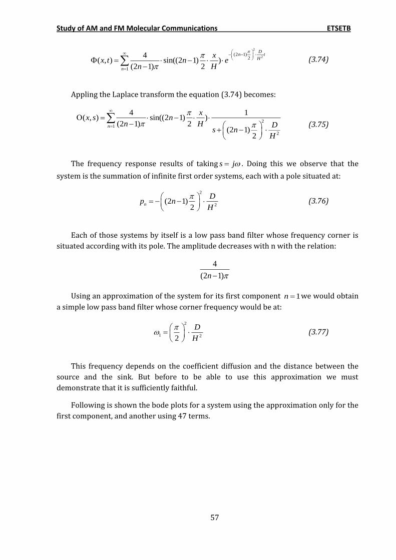
Study of AM and FM Molecular Communications ETSETB
57
2
2(2 1)
2
1
4( , ) sin((2 1) )
(2 1) 2
Dn t
H
n
xx t n e
n H
(3.74)
Appling the Laplace transform the equation (3.74) becomes:
21
2
4 1( , ) sin((2 1) )
(2 1) 2(2 1)
2
n
xx s n
n H Ds n
H
(3.75)
The frequency response results of taking s j . Doing this we observe that the
system is the summation of infinite first order systems, each with a pole situated at:
2
2(2 1)
2n
Dp n
H
(3.76)
Each of those systems by itself is a low pass band filter whose frequency corner is
situated according with its pole. The amplitude decreases with n with the relation:
4
(2 1)n
Using an approximation of the system for its first component 1n we would obtain
a simple low pass band filter whose corner frequency would be at:
2
1 22
D
H
(3.77)
This frequency depends on the coefficient diffusion and the distance between the
source and the sink. But before to be able to use this approximation we must
demonstrate that it is sufficiently faithful.
Following is shown the bode plots for a system using the approximation only for the
first component, and another using 47 terms.
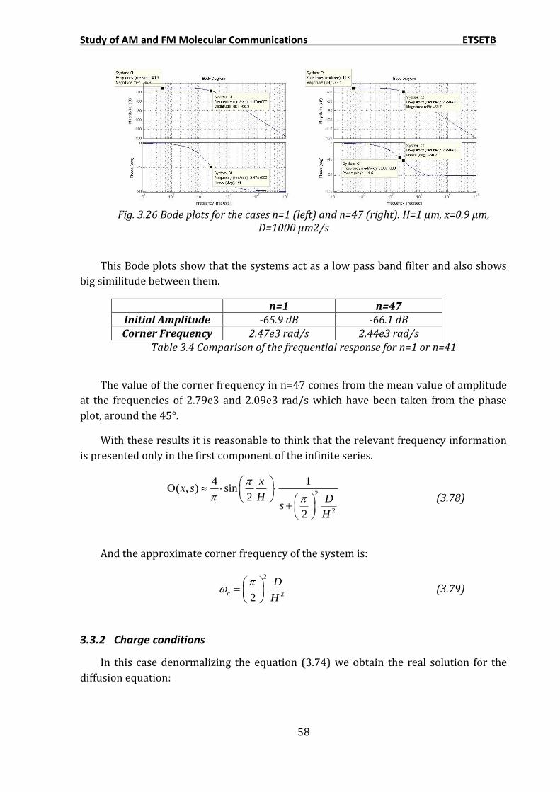
Study of AM and FM Molecular Communications ETSETB
58
Fig. 3.26 Bode plots for the cases n=1 (left) and n=47 (right). H=1 µm, x=0.9 µm,
D=1000 µm2/s
This Bode plots show that the systems act as a low pass band filter and also shows
big similitude between them.
n=1 n=47 Initial Amplitude -65.9 dB -66.1 dB Corner Frequency 2.47e3 rad/s 2.44e3 rad/s
Table 3.4 Comparison of the frequential response for n=1 or n=41
The value of the corner frequency in n=47 comes from the mean value of amplitude
at the frequencies of 2.79e3 and 2.09e3 rad/s which have been taken from the phase
plot, around the 45°.
With these results it is reasonable to think that the relevant frequency information
is presented only in the first component of the infinite series.
2
2
4 1( , ) sin
2
2
xx s
H Ds
H
(3.78)
And the approximate corner frequency of the system is:
2
22c
D
H
(3.79)
3.3.2 Charge conditions
In this case denormalizing the equation (3.74) we obtain the real solution for the
diffusion equation:
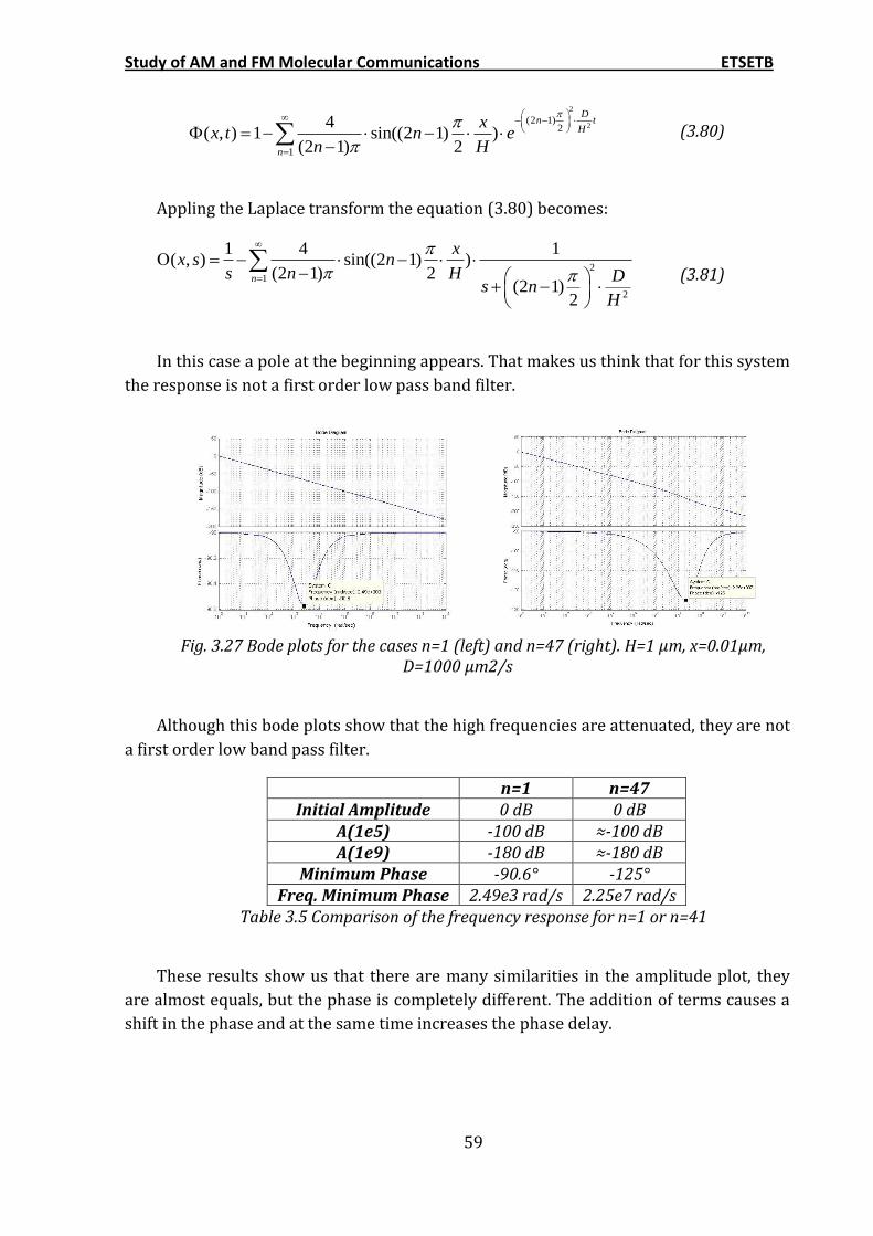
Study of AM and FM Molecular Communications ETSETB
59
2
2(2 1)
2
1
4( , ) 1 sin((2 1) )
(2 1) 2
Dn t
H
n
xx t n e
n H
(3.80)
Appling the Laplace transform the equation (3.80) becomes:
21
2
1 4 1( , ) sin((2 1) )
(2 1) 2(2 1)
2
n
xx s n
s n H Ds n
H
(3.81)
In this case a pole at the beginning appears. That makes us think that for this system
the response is not a first order low pass band filter.
Fig. 3.27 Bode plots for the cases n=1 (left) and n=47 (right). H=1 µm, x=0.01µm,
D=1000 µm2/s
Although this bode plots show that the high frequencies are attenuated, they are not
a first order low band pass filter.
n=1 n=47 Initial Amplitude 0 dB 0 dB
A(1e5) -100 dB ≈-100 dB A(1e9) -180 dB ≈-180 dB
Minimum Phase -90.6° -125° Freq. Minimum Phase 2.49e3 rad/s 2.25e7 rad/s
Table 3.5 Comparison of the frequency response for n=1 or n=41
These results show us that there are many similarities in the amplitude plot, they
are almost equals, but the phase is completely different. The addition of terms causes a
shift in the phase and at the same time increases the phase delay.
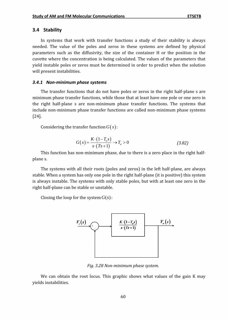
Study of AM and FM Molecular Communications ETSETB
60
3.4 Stability
In systems that work with transfer functions a study of their stability is always
needed. The value of the poles and zeros in these systems are defined by physical
parameters such as the diffusivity, the size of the container H or the position in the
cuvette where the concentration is being calculated. The values of the parameters that
yield instable poles or zeros must be determined in order to predict when the solution
will present instabilities.
3.4.1 Non-minimum phase systems
The transfer functions that do not have poles or zeros in the right half-plane s are
minimum phase transfer functions, while those that at least have one pole or one zero in
the right half-plane s are non-minimum phase transfer functions. The systems that
include non-minimum phase transfer functions are called non-minimum phase systems
[24].
Considering the transfer function G s :
10
1
a
a
K T sG s T
s Ts
(3.82)
This function has non-minimum phase, due to there is a zero place in the right half-
plane s.
The systems with all their roots (poles and zeros) in the left half-plane, are always
stable. When a system has only one pole in the right half-plane (it is positive) this system
is always instable. The systems with only stable poles, but with at least one zero in the
right half-plane can be stable or unstable.
Closing the loop for the system ( )G s :
Fig. 3.28 Non-minimum phase system.
We can obtain the root locus. This graphic shows what values of the gain K may
yields instabilities.
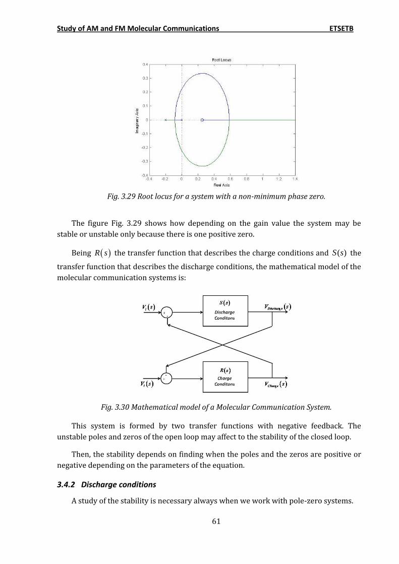
Study of AM and FM Molecular Communications ETSETB
61
Fig. 3.29 Root locus for a system with a non-minimum phase zero.
The figure Fig. 3.29 shows how depending on the gain value the system may be
stable or unstable only because there is one positive zero.
Being R s the transfer function that describes the charge conditions and ( )S s the
transfer function that describes the discharge conditions, the mathematical model of the
molecular communication systems is:
Fig. 3.30 Mathematical model of a Molecular Communication System.
This system is formed by two transfer functions with negative feedback. The
unstable poles and zeros of the open loop may affect to the stability of the closed loop.
Then, the stability depends on finding when the poles and the zeros are positive or
negative depending on the parameters of the equation.
3.4.2 Discharge conditions
A study of the stability is necessary always when we work with pole-zero systems.
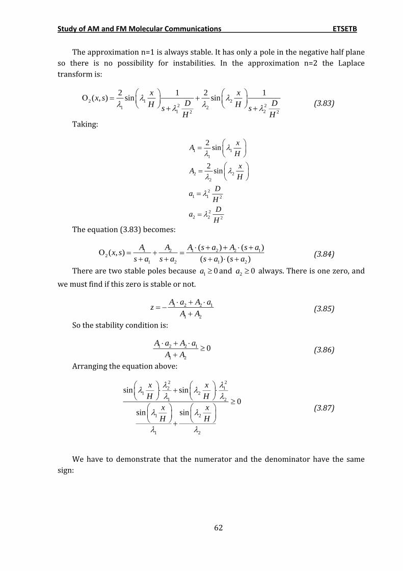
Study of AM and FM Molecular Communications ETSETB
62
The approximation n=1 is always stable. It has only a pole in the negative half plane
so there is no possibility for instabilities. In the approximation n=2 the Laplace
transform is:
2 1 22 21 2
1 22 2
2 1 2 1( , ) sin sin
x xx s
D DH Hs s
H H
(3.83)
Taking:
1 1
1
2 2
2
2
1 1 2
2
2 2 2
2sin
2sin
xA
H
xA
H
Da
H
Da
H
The equation (3.83) becomes:
1 2 1 2 2 12
1 2 1 2
( ) ( )( , )
( ) ( )
A A A s a A s ax s
s a s a s a s a
(3.84)
There are two stable poles because 1 0a and 2 0a always. There is one zero, and
we must find if this zero is stable or not.
1 2 2 1
1 2
A a A az
A A
(3.85)
So the stability condition is:
1 2 2 1
1 2
0A a A a
A A
(3.86)
Arranging the equation above:
2 2
2 11 2
1 2
1 2
1 2
sin sin
0
sin sin
x x
H H
x x
H H
(3.87)
We have to demonstrate that the numerator and the denominator have the same
sign:
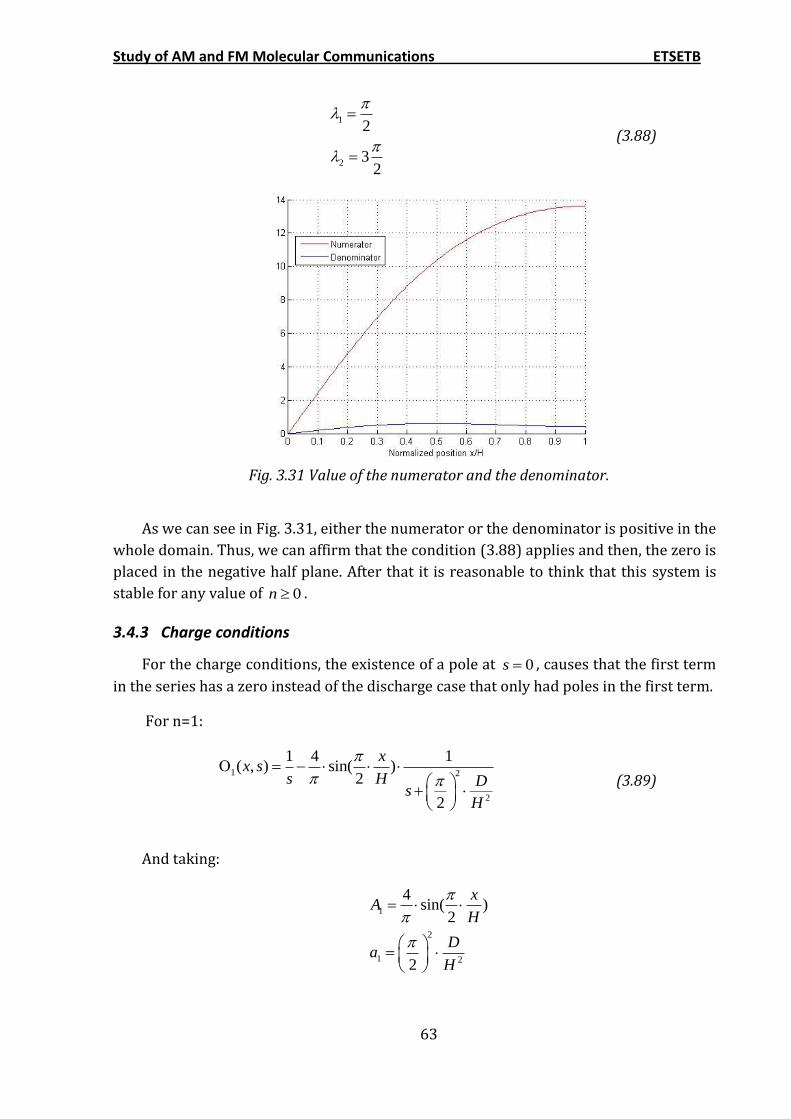
Study of AM and FM Molecular Communications ETSETB
63
1
2
2
32
(3.88)
Fig. 3.31 Value of the numerator and the denominator.
As we can see in Fig. 3.31, either the numerator or the denominator is positive in the
whole domain. Thus, we can affirm that the condition (3.88) applies and then, the zero is
placed in the negative half plane. After that it is reasonable to think that this system is
stable for any value of 0n .
3.4.3 Charge conditions
For the charge conditions, the existence of a pole at 0s , causes that the first term
in the series has a zero instead of the discharge case that only had poles in the first term.
For n=1:
1 2
2
1 4 1( , ) sin( )
2
2
xx s
s H Ds
H
(3.89)
And taking:
1
2
1 2
4sin( )
2
2
xA
H
Da
H
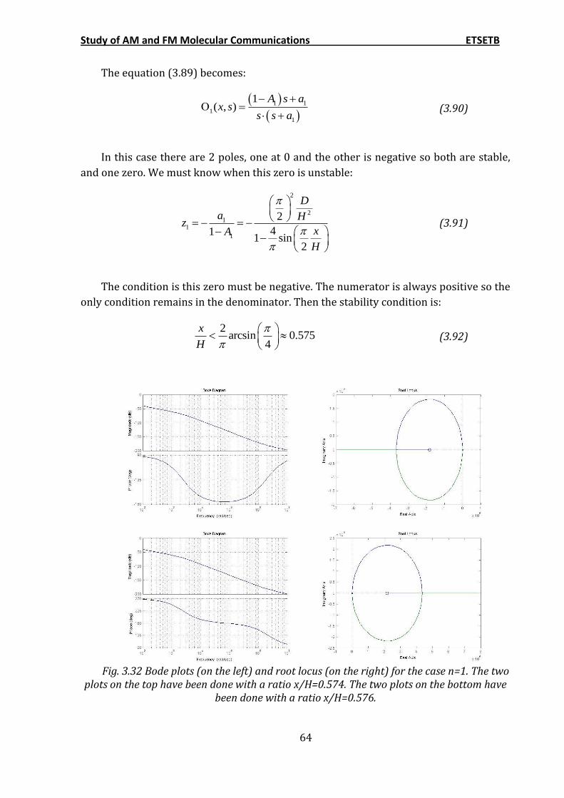
Study of AM and FM Molecular Communications ETSETB
64
The equation (3.89) becomes:
1 1
1
1
1( , )
A s ax s
s s a
(3.90)
In this case there are 2 poles, one at 0 and the other is negative so both are stable,
and one zero. We must know when this zero is unstable:
2
21
1
1
2
411 sin
2
D
a Hz
xA
H
(3.91)
The condition is this zero must be negative. The numerator is always positive so the
only condition remains in the denominator. Then the stability condition is:
2arcsin 0.575
4
x
H
(3.92)
Fig. 3.32 Bode plots (on the left) and root locus (on the right) for the case n=1. The two
plots on the top have been done with a ratio x/H=0.574. The two plots on the bottom have been done with a ratio x/H=0.576.
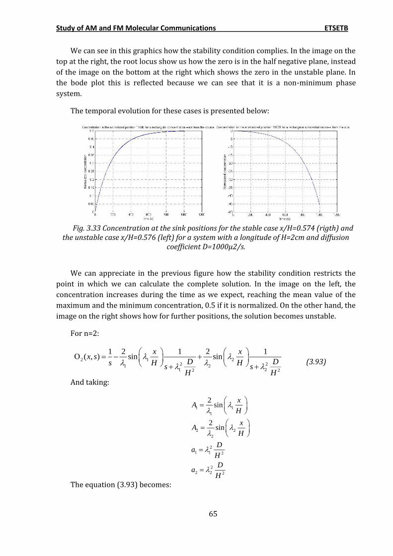
Study of AM and FM Molecular Communications ETSETB
65
We can see in this graphics how the stability condition complies. In the image on the
top at the right, the root locus show us how the zero is in the half negative plane, instead
of the image on the bottom at the right which shows the zero in the unstable plane. In
the bode plot this is reflected because we can see that it is a non-minimum phase
system.
The temporal evolution for these cases is presented below:
Fig. 3.33 Concentration at the sink positions for the stable case x/H=0.574 (rigth) and
the unstable case x/H=0.576 (left) for a system with a longitude of H=2cm and diffusion coefficient D=1000µ2/s.
We can appreciate in the previous figure how the stability condition restricts the
point in which we can calculate the complete solution. In the image on the left, the
concentration increases during the time as we expect, reaching the mean value of the
maximum and the minimum concentration, 0.5 if it is normalized. On the other hand, the
image on the right shows how for further positions, the solution becomes unstable.
For n=2:
2 1 22 21 2
1 22 2
1 2 1 2 1( , ) sin sin
x xx s
D Ds H Hs s
H H
(3.93)
And taking:
1 1
1
2 2
2
2
1 1 2
2
2 2 2
2sin
2sin
xA
H
xA
H
Da
H
Da
H
The equation (3.93) becomes:
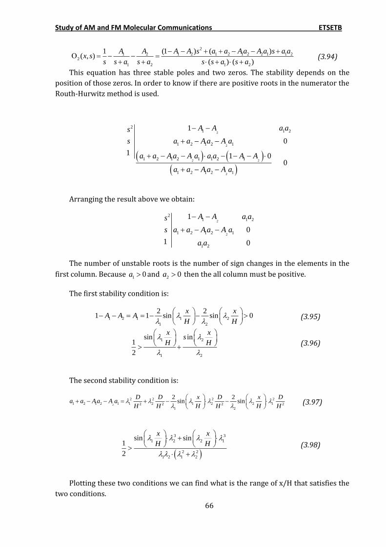
Study of AM and FM Molecular Communications ETSETB
66
2
1 2 1 2 1 2 1 2 2 1 1 22
1 2 1 2
(1 ) ( )1( , )
( ) ( )
A A A A s a a Aa A a s a ax s
s s a s a s s a s a
(3.94)
This equation has three stable poles and two zeros. The stability depends on the
position of those zeros. In order to know if there are positive roots in the numerator the
Routh-Hurwitz method is used.
2
2
2 2
2
21 1 2
1 2 1 2 1
1 2 1 2 1 1 2 1
1 2 1 2 1
1
0
1 1 00
A A a as
s a a A a A a
a a A a A a a a A A
a a A a A a
Arranging the result above we obtain:
2
2
21 1 2
1 2 1 2 1
1 2
1
0
1 0
A A a as
s a a A a A a
a a
The number of unstable roots is the number of sign changes in the elements in the
first column. Because 1 0a and 2 0a then the all column must be positive.
The first stability condition is:
1 2 1 1 2
1 2
2 21 1 sin sin 0
x xA A A
H H
(3.95)
1 2
1 2
sin in1
2
x xs
H H
(3.96)
The second stability condition is:
2
2 2 2 2
1 2 1 2 1 1 2 1 2 2 12 2 2 2
1 2
2 2sin sin 0
D D x D x Da a Aa A a
H H H H H H
(3.97)
3 3
1 2 2 1
2 2
1 2 1 2
sin sin1
2
x x
H H
(3.98)
Plotting these two conditions we can find what is the range of x/H that satisfies the
two conditions.

Study of AM and FM Molecular Communications ETSETB
67
Fig. 3.34 Stabilities conditions for n=2.
As we can see in the figure above the range of stability is 0 0.3x
H
Fig. 3.35 Bode plots (on the left) and root locus (on the right) for the case n=2. The two
plots on the top have been done with a ratio x/H=0.29. The two plots on the bottom have been done with a ratio x/H=0.31.
We can see the position of the zeros depending on the stability condition. Below is
shown the temporal effects for these conditions:
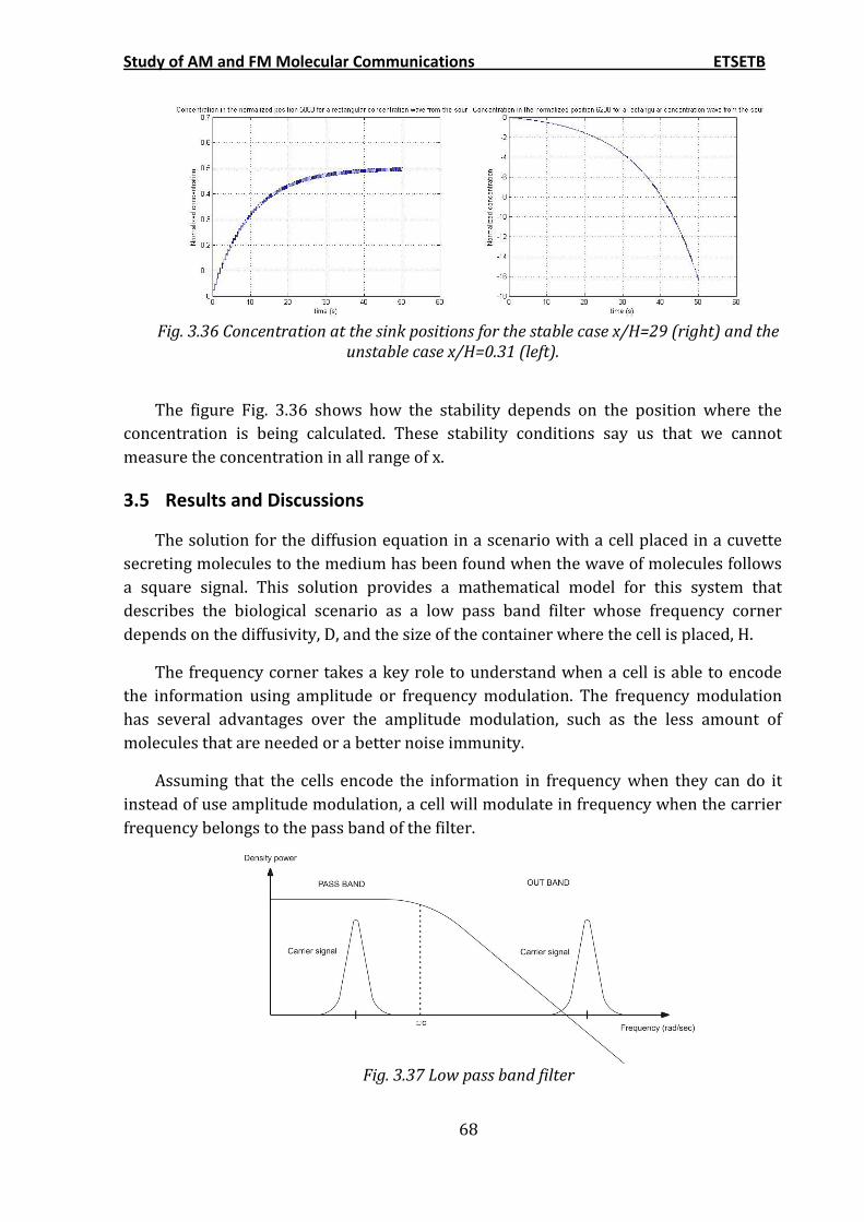
Study of AM and FM Molecular Communications ETSETB
68
Fig. 3.36 Concentration at the sink positions for the stable case x/H=29 (right) and the
unstable case x/H=0.31 (left).
The figure Fig. 3.36 shows how the stability depends on the position where the
concentration is being calculated. These stability conditions say us that we cannot
measure the concentration in all range of x.
3.5 Results and Discussions
The solution for the diffusion equation in a scenario with a cell placed in a cuvette
secreting molecules to the medium has been found when the wave of molecules follows
a square signal. This solution provides a mathematical model for this system that
describes the biological scenario as a low pass band filter whose frequency corner
depends on the diffusivity, D, and the size of the container where the cell is placed, H.
The frequency corner takes a key role to understand when a cell is able to encode
the information using amplitude or frequency modulation. The frequency modulation
has several advantages over the amplitude modulation, such as the less amount of
molecules that are needed or a better noise immunity.
Assuming that the cells encode the information in frequency when they can do it
instead of use amplitude modulation, a cell will modulate in frequency when the carrier
frequency belongs to the pass band of the filter.
Fig. 3.37 Low pass band filter
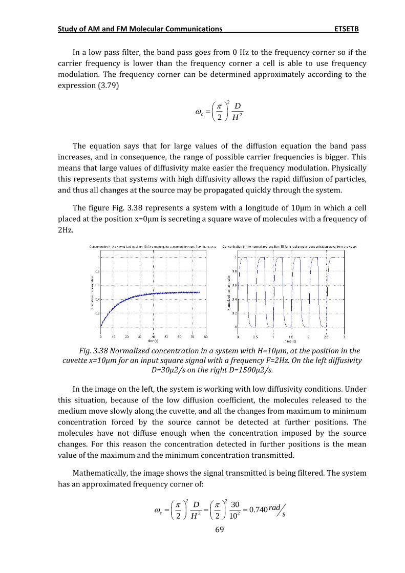
Study of AM and FM Molecular Communications ETSETB
69
In a low pass filter, the band pass goes from 0 Hz to the frequency corner so if the
carrier frequency is lower than the frequency corner a cell is able to use frequency
modulation. The frequency corner can be determined approximately according to the
expression (3.79)
2
22c
D
H
The equation says that for large values of the diffusion equation the band pass
increases, and in consequence, the range of possible carrier frequencies is bigger. This
means that large values of diffusivity make easier the frequency modulation. Physically
this represents that systems with high diffusivity allows the rapid diffusion of particles,
and thus all changes at the source may be propagated quickly through the system.
The figure Fig. 3.38 represents a system with a longitude of 10μm in which a cell
placed at the position x=0μm is secreting a square wave of molecules with a frequency of
2Hz.
Fig. 3.38 Normalized concentration in a system with H=10μm, at the position in the
cuvette x=10μm for an input square signal with a frequency F=2Hz. On the left diffusivity D=30µ2/s on the right D=1500μ2/s.
In the image on the left, the system is working with low diffusivity conditions. Under
this situation, because of the low diffusion coefficient, the molecules released to the
medium move slowly along the cuvette, and all the changes from maximum to minimum
concentration forced by the source cannot be detected at further positions. The
molecules have not diffuse enough when the concentration imposed by the source
changes. For this reason the concentration detected in further positions is the mean
value of the maximum and the minimum concentration transmitted.
Mathematically, the image shows the signal transmitted is being filtered. The system
has an approximated frequency corner of:
2 2
2 2
300.740
2 2 10c
D radsH
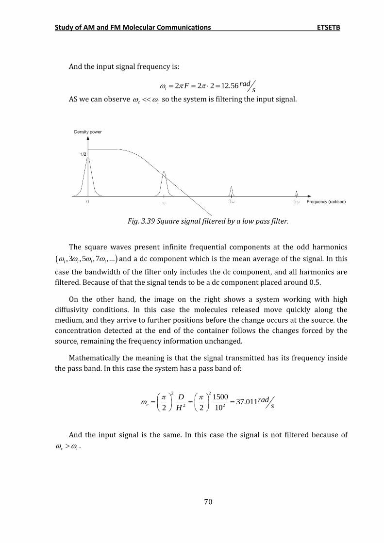
Study of AM and FM Molecular Communications ETSETB
70
And the input signal frequency is:
2 2 2 12.56iradF
s
AS we can observe c i so the system is filtering the input signal.
Fig. 3.39 Square signal filtered by a low pass filter.
The square waves present infinite frequential components at the odd harmonics
,3 ,5 ,7 ,...i i i i and a dc component which is the mean average of the signal. In this
case the bandwidth of the filter only includes the dc component, and all harmonics are
filtered. Because of that the signal tends to be a dc component placed around 0.5.
On the other hand, the image on the right shows a system working with high
diffusivity conditions. In this case the molecules released move quickly along the
medium, and they arrive to further positions before the change occurs at the source. the
concentration detected at the end of the container follows the changes forced by the
source, remaining the frequency information unchanged.
Mathematically the meaning is that the signal transmitted has its frequency inside
the pass band. In this case the system has a pass band of:
2 2
2 2
150037.011
2 2 10c
D radsH
And the input signal is the same. In this case the signal is not filtered because of
c i .
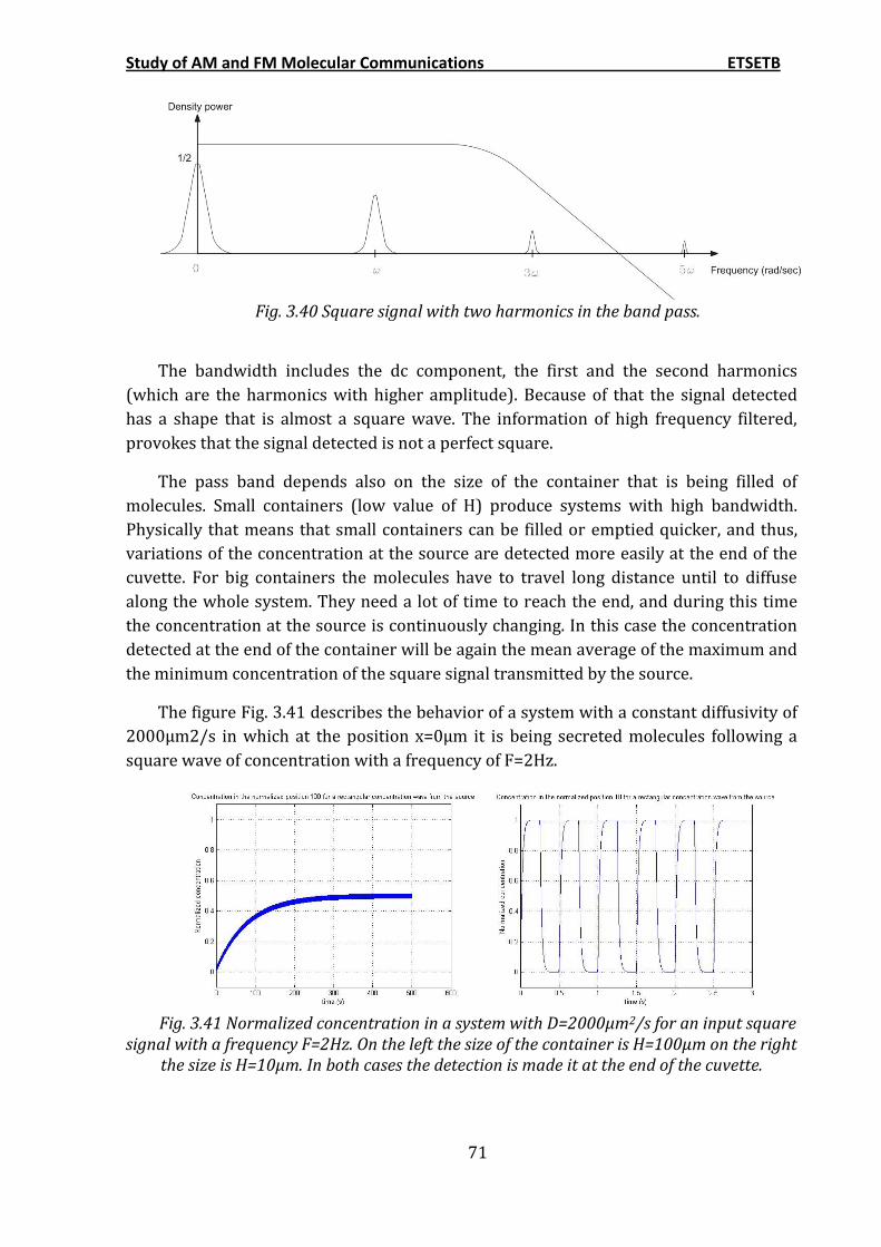
Study of AM and FM Molecular Communications ETSETB
71
Fig. 3.40 Square signal with two harmonics in the band pass.
The bandwidth includes the dc component, the first and the second harmonics
(which are the harmonics with higher amplitude). Because of that the signal detected
has a shape that is almost a square wave. The information of high frequency filtered,
provokes that the signal detected is not a perfect square.
The pass band depends also on the size of the container that is being filled of
molecules. Small containers (low value of H) produce systems with high bandwidth.
Physically that means that small containers can be filled or emptied quicker, and thus,
variations of the concentration at the source are detected more easily at the end of the
cuvette. For big containers the molecules have to travel long distance until to diffuse
along the whole system. They need a lot of time to reach the end, and during this time
the concentration at the source is continuously changing. In this case the concentration
detected at the end of the container will be again the mean average of the maximum and
the minimum concentration of the square signal transmitted by the source.
The figure Fig. 3.41 describes the behavior of a system with a constant diffusivity of
2000µm2/s in which at the position x=0µm it is being secreted molecules following a
square wave of concentration with a frequency of F=2Hz.
Fig. 3.41 Normalized concentration in a system with D=2000μm2/s for an input square
signal with a frequency F=2Hz. On the left the size of the container is H=100µm on the right the size is H=10μm. In both cases the detection is made it at the end of the cuvette.
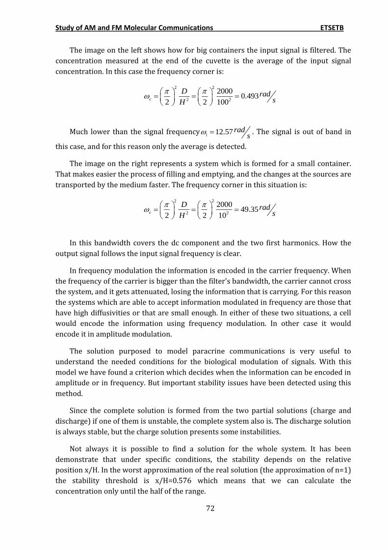
Study of AM and FM Molecular Communications ETSETB
72
The image on the left shows how for big containers the input signal is filtered. The
concentration measured at the end of the cuvette is the average of the input signal
concentration. In this case the frequency corner is:
2 2
2 2
20000.493
2 2 100c
D radsH
Much lower than the signal frequency 12.57irad
s . The signal is out of band in
this case, and for this reason only the average is detected.
The image on the right represents a system which is formed for a small container.
That makes easier the process of filling and emptying, and the changes at the sources are
transported by the medium faster. The frequency corner in this situation is:
2 2
2 2
200049.35
2 2 10c
D radsH
In this bandwidth covers the dc component and the two first harmonics. How the
output signal follows the input signal frequency is clear.
In frequency modulation the information is encoded in the carrier frequency. When
the frequency of the carrier is bigger than the filter's bandwidth, the carrier cannot cross
the system, and it gets attenuated, losing the information that is carrying. For this reason
the systems which are able to accept information modulated in frequency are those that
have high diffusivities or that are small enough. In either of these two situations, a cell
would encode the information using frequency modulation. In other case it would
encode it in amplitude modulation.
The solution purposed to model paracrine communications is very useful to
understand the needed conditions for the biological modulation of signals. With this
model we have found a criterion which decides when the information can be encoded in
amplitude or in frequency. But important stability issues have been detected using this
method.
Since the complete solution is formed from the two partial solutions (charge and
discharge) if one of them is unstable, the complete system also is. The discharge solution
is always stable, but the charge solution presents some instabilities.
Not always it is possible to find a solution for the whole system. It has been
demonstrate that under specific conditions, the stability depends on the relative
position x/H. In the worst approximation of the real solution (the approximation of n=1)
the stability threshold is x/H=0.576 which means that we can calculate the
concentration only until the half of the range.

Study of AM and FM Molecular Communications ETSETB
73
For this reason a tool able to simulate the paracrine communication system will be
programmed. The intention is, once the mathematical model has been described, to
design a simulator based on numerical methods which provides an approximate
solution of the diffusion equation. With this simulator the concentration at every point
in the system will be known solving all the stability issues that the real solution
presents.

Study of AM and FM Molecular Communications ETSETB
74
4 FABRICATION AND CHARACTERIZATION OF A MICROFLUIDIC DEVICE
The aim of this chapter is to fabricate a microfluidic device known as T-SENSOR
whose operating principle is basically the same of the one that governs the molecular
communication systems. With this device we can study the diffusion process in a more
experimental way, and also doing experiments with this device we will get experimental
data that will be used to validate the simulator of diffusion.

Study of AM and FM Molecular Communications ETSETB
75
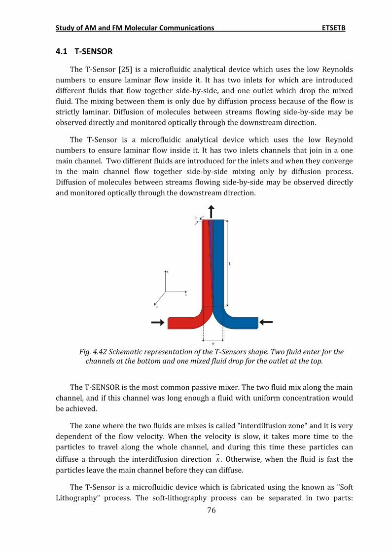
Study of AM and FM Molecular Communications ETSETB
76
4.1 T-SENSOR
The T-Sensor [25] is a microfluidic analytical device which uses the low Reynolds
numbers to ensure laminar flow inside it. It has two inlets for which are introduced
different fluids that flow together side-by-side, and one outlet which drop the mixed
fluid. The mixing between them is only due by diffusion process because of the flow is
strictly laminar. Diffusion of molecules between streams flowing side-by-side may be
observed directly and monitored optically through the downstream direction.
The T-Sensor is a microfluidic analytical device which uses the low Reynold
numbers to ensure laminar flow inside it. It has two inlets channels that join in a one
main channel. Two different fluids are introduced for the inlets and when they converge
in the main channel flow together side-by-side mixing only by diffusion process.
Diffusion of molecules between streams flowing side-by-side may be observed directly
and monitored optically through the downstream direction.
Fig. 4.42 Schematic representation of the T-Sensors shape. Two fluid enter for the
channels at the bottom and one mixed fluid drop for the outlet at the top.
The T-SENSOR is the most common passive mixer. The two fluid mix along the main
channel, and if this channel was long enough a fluid with uniform concentration would
be achieved.
The zone where the two fluids are mixes is called "interdiffusion zone" and it is very
dependent of the flow velocity. When the velocity is slow, it takes more time to the
particles to travel along the whole channel, and during this time these particles can
diffuse a through the interdiffusion direction x . Otherwise, when the fluid is fast the
particles leave the main channel before they can diffuse.
The T-Sensor is a microfluidic device which is fabricated using the known as "Soft
Lithography" process. The soft-lithography process can be separated in two parts:
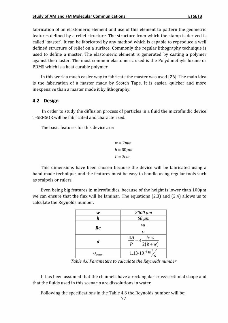
Study of AM and FM Molecular Communications ETSETB
77
fabrication of an elastomeric element and use of this element to pattern the geometric
features defined by a relief structure. The structure from which the stamp is derived is
called 'master'. It can be fabricated by any method which is capable to reproduce a well
defined structure of relief on a surface. Commonly the regular lithography technique is
used to define a master. The elastomeric element is generated by casting a polymer
against the master. The most common elastomeric used is the Polydimethylsiloxane or
PDMS which is a heat curable polymer.
In this work a much easier way to fabricate the master was used [26]. The main idea
is the fabrication of a master made by Scotch Tape. It is easier, quicker and more
inexpensive than a master made it by lithography.
4.2 Design
In order to study the diffusion process of particles in a fluid the microfluidic device
T-SENSOR will be fabricated and characterized.
The basic features for this device are:
2
60
3
w mm
h µm
L cm
This dimensions have been chosen because the device will be fabricated using a
hand-made technique, and the features must be easy to handle using regular tools such
as scalpels or rulers.
Even being big features in microfluidics, because of the height is lower than 100μm
we can ensure that the flux will be laminar. The equations (2.3) and (2.4) allows us to
calculate the Reynolds number.
w 2000 μm h 60 μm
Re vd
d
44
2
A h w
P h w
water 2
61.13 10 ms
Table 4.6 Parameters to calculate the Reynolds number
It has been assumed that the channels have a rectangular cross-sectional shape and
that the fluids used in this scenario are dissolutions in water.
Following the specifications in the Table 4.6 the Reynolds number will be:
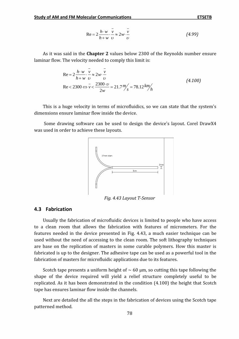
Study of AM and FM Molecular Communications ETSETB
78
Re 2 2h w v v
wh w
(4.99)
As it was said in the Chapter 2 values below 2300 of the Reynolds number ensure
laminar flow. The velocity needed to comply this limit is:
Re 2 2
2300Re 2300 21.7 78.12
2
h w v vw
h w
m kmvs hw
(4.100)
This is a huge velocity in terms of microfluidics, so we can state that the system's
dimensions ensure laminar flow inside the device.
Some drawing software can be used to design the device's layout. Corel DrawX4
was used in order to achieve these layouts.
Fig. 4.43 Layout T-Sensor
4.3 Fabrication
Usually the fabrication of microfluidic devices is limited to people who have access
to a clean room that allows the fabrication with features of micrometers. For the
features needed in the device presented in Fig. 4.43, a much easier technique can be
used without the need of accessing to the clean room. The soft lithography techniques
are base on the replication of masters in some curable polymers. How this master is
fabricated is up to the designer. The adhesive tape can be used as a powerful tool in the
fabrication of masters for microfluidic applications due to its features.
Scotch tape presents a uniform height of ~ 60 µm, so cutting this tape following the
shape of the device required will yield a relief structure completely useful to be
replicated. As it has been demonstrated in the condition (4.100) the height that Scotch
tape has ensures laminar flow inside the channels.
Next are detailed the all the steps in the fabrication of devices using the Scotch tape
patterned method.
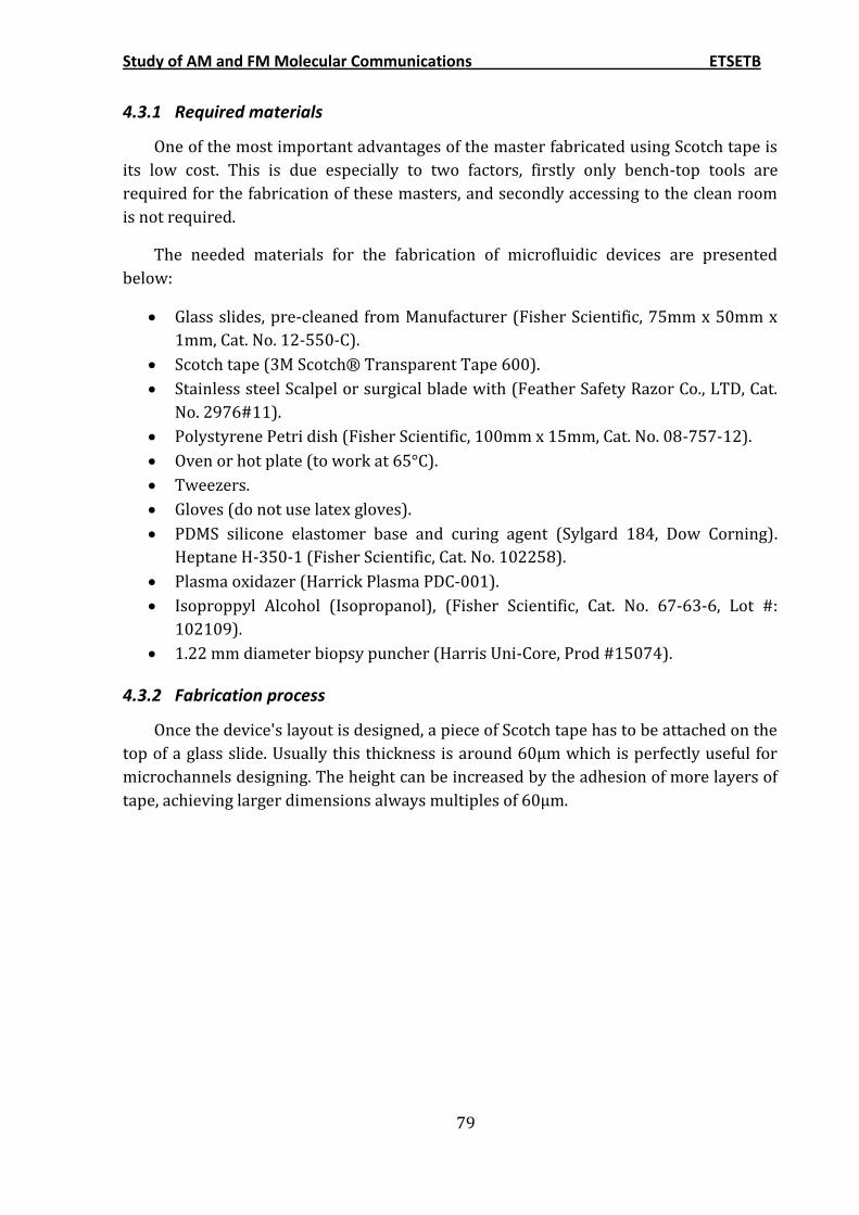
Study of AM and FM Molecular Communications ETSETB
79
4.3.1 Required materials
One of the most important advantages of the master fabricated using Scotch tape is
its low cost. This is due especially to two factors, firstly only bench-top tools are
required for the fabrication of these masters, and secondly accessing to the clean room
is not required.
The needed materials for the fabrication of microfluidic devices are presented
below:
Glass slides, pre-cleaned from Manufacturer (Fisher Scientific, 75mm x 50mm x
1mm, Cat. No. 12-550-C).
Scotch tape (3M Scotch® Transparent Tape 600).
Stainless steel Scalpel or surgical blade with (Feather Safety Razor Co., LTD, Cat.
No. 2976#11).
Polystyrene Petri dish (Fisher Scientific, 100mm x 15mm, Cat. No. 08-757-12).
Oven or hot plate (to work at 65°C).
Tweezers.
Gloves (do not use latex gloves).
PDMS silicone elastomer base and curing agent (Sylgard 184, Dow Corning).
Heptane H-350-1 (Fisher Scientific, Cat. No. 102258).
Plasma oxidazer (Harrick Plasma PDC-001).
Isoproppyl Alcohol (Isopropanol), (Fisher Scientific, Cat. No. 67-63-6, Lot #:
102109).
1.22 mm diameter biopsy puncher (Harris Uni-Core, Prod #15074).
4.3.2 Fabrication process
Once the device's layout is designed, a piece of Scotch tape has to be attached on the
top of a glass slide. Usually this thickness is around 60μm which is perfectly useful for
microchannels designing. The height can be increased by the adhesion of more layers of
tape, achieving larger dimensions always multiples of 60μm.
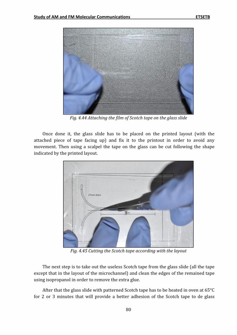
Study of AM and FM Molecular Communications ETSETB
80
Fig. 4.44 Attaching the film of Scotch tape on the glass slide
Once done it, the glass slide has to be placed on the printed layout (with the
attached piece of tape facing up) and fix it to the printout in order to avoid any
movement. Then using a scalpel the tape on the glass can be cut following the shape
indicated by the printed layout.
Fig. 4.45 Cutting the Scotch tape according with the layout
The next step is to take out the useless Scotch tape from the glass slide (all the tape
except that in the layout of the microchannel) and clean the edges of the remained tape
using isopropanol in order to remove the extra glue.
After that the glass slide with patterned Scotch tape has to be heated in oven at 65°C
for 2 or 3 minutes that will provide a better adhesion of the Scotch tape to de glass
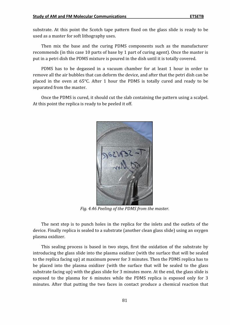
Study of AM and FM Molecular Communications ETSETB
81
substrate. At this point the Scotch tape pattern fixed on the glass slide is ready to be
used as a master for soft lithography uses.
Then mix the base and the curing PDMS components such as the manufacturer
recommends (in this case 10 parts of base by 1 part of curing agent). Once the master is
put in a petri dish the PDMS mixture is poured in the dish until it is totally covered.
PDMS has to be degassed in a vacuum chamber for at least 1 hour in order to
remove all the air bubbles that can deform the device, and after that the petri dish can be
placed in the oven at 65°C. After 1 hour the PDMS is totally cured and ready to be
separated from the master.
Once the PDMS is cured, it should cut the slab containing the pattern using a scalpel.
At this point the replica is ready to be peeled it off.
Fig. 4.46 Peeling of the PDMS from the master.
The next step is to punch holes in the replica for the inlets and the outlets of the
device. Finally replica is sealed to a substrate (another clean glass slide) using an oxygen
plasma oxidizer.
This sealing process is based in two steps, first the oxidation of the substrate by
introducing the glass slide into the plasma oxidizer (with the surface that will be sealed
to the replica facing up) at maximum power for 3 minutes. Then the PDMS replica has to
be placed into the plasma oxidizer (with the surface that will be sealed to the glass
substrate facing up) with the glass slide for 3 minutes more. At the end, the glass slide is
exposed to the plasma for 6 minutes while the PDMS replica is exposed only for 3
minutes. After that putting the two faces in contact produce a chemical reaction that
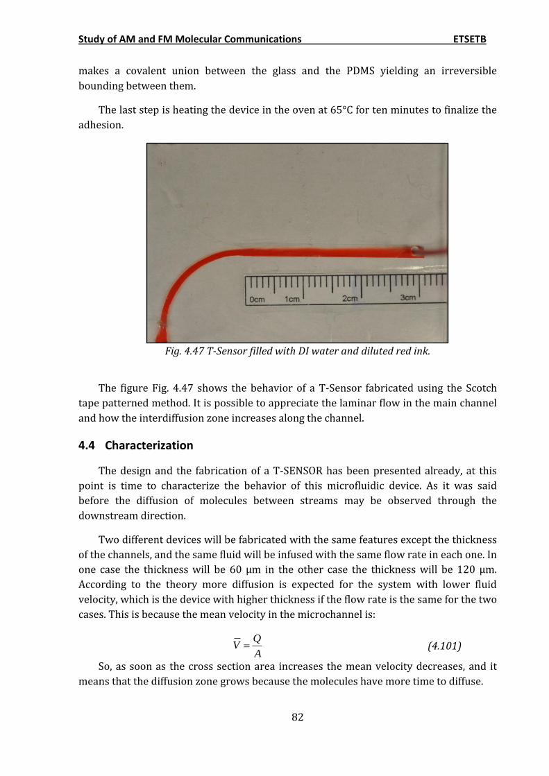
Study of AM and FM Molecular Communications ETSETB
82
makes a covalent union between the glass and the PDMS yielding an irreversible
bounding between them.
The last step is heating the device in the oven at 65°C for ten minutes to finalize the
adhesion.
Fig. 4.47 T-Sensor filled with DI water and diluted red ink.
The figure Fig. 4.47 shows the behavior of a T-Sensor fabricated using the Scotch
tape patterned method. It is possible to appreciate the laminar flow in the main channel
and how the interdiffusion zone increases along the channel.
4.4 Characterization
The design and the fabrication of a T-SENSOR has been presented already, at this
point is time to characterize the behavior of this microfluidic device. As it was said
before the diffusion of molecules between streams may be observed through the
downstream direction.
Two different devices will be fabricated with the same features except the thickness
of the channels, and the same fluid will be infused with the same flow rate in each one. In
one case the thickness will be 60 µm in the other case the thickness will be 120 µm.
According to the theory more diffusion is expected for the system with lower fluid
velocity, which is the device with higher thickness if the flow rate is the same for the two
cases. This is because the mean velocity in the microchannel is:
QV
A
(4.101)
So, as soon as the cross section area increases the mean velocity decreases, and it
means that the diffusion zone grows because the molecules have more time to diffuse.
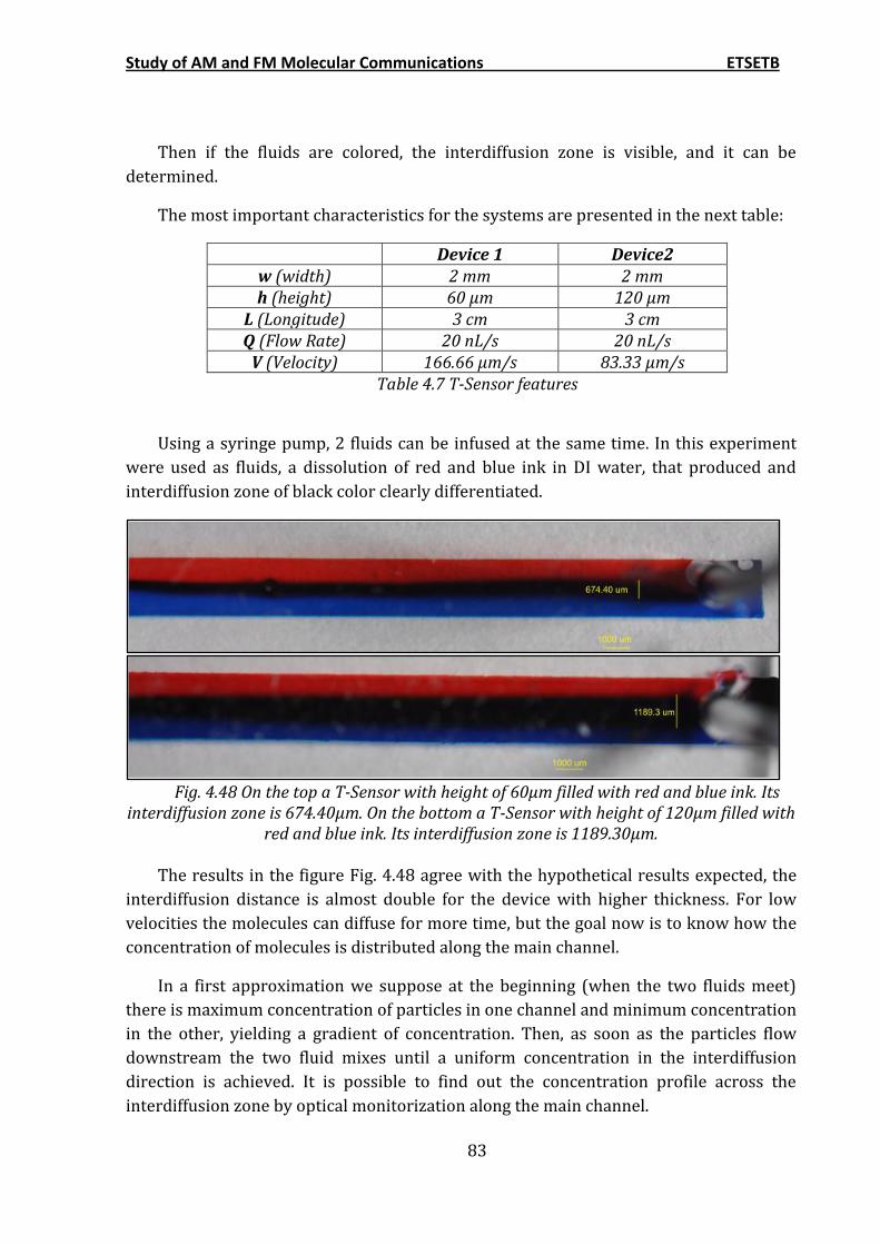
Study of AM and FM Molecular Communications ETSETB
83
Then if the fluids are colored, the interdiffusion zone is visible, and it can be
determined.
The most important characteristics for the systems are presented in the next table:
Device 1 Device2 w (width) 2 mm 2 mm h (height) 60 µm 120 µm
L (Longitude) 3 cm 3 cm Q (Flow Rate) 20 nL/s 20 nL/s
V (Velocity) 166.66 µm/s 83.33 µm/s Table 4.7 T-Sensor features
Using a syringe pump, 2 fluids can be infused at the same time. In this experiment
were used as fluids, a dissolution of red and blue ink in DI water, that produced and
interdiffusion zone of black color clearly differentiated.
Fig. 4.48 On the top a T-Sensor with height of 60µm filled with red and blue ink. Its
interdiffusion zone is 674.40µm. On the bottom a T-Sensor with height of 120µm filled with red and blue ink. Its interdiffusion zone is 1189.30µm.
The results in the figure Fig. 4.48 agree with the hypothetical results expected, the
interdiffusion distance is almost double for the device with higher thickness. For low
velocities the molecules can diffuse for more time, but the goal now is to know how the
concentration of molecules is distributed along the main channel.
In a first approximation we suppose at the beginning (when the two fluids meet)
there is maximum concentration of particles in one channel and minimum concentration
in the other, yielding a gradient of concentration. Then, as soon as the particles flow
downstream the two fluid mixes until a uniform concentration in the interdiffusion
direction is achieved. It is possible to find out the concentration profile across the
interdiffusion zone by optical monitorization along the main channel.
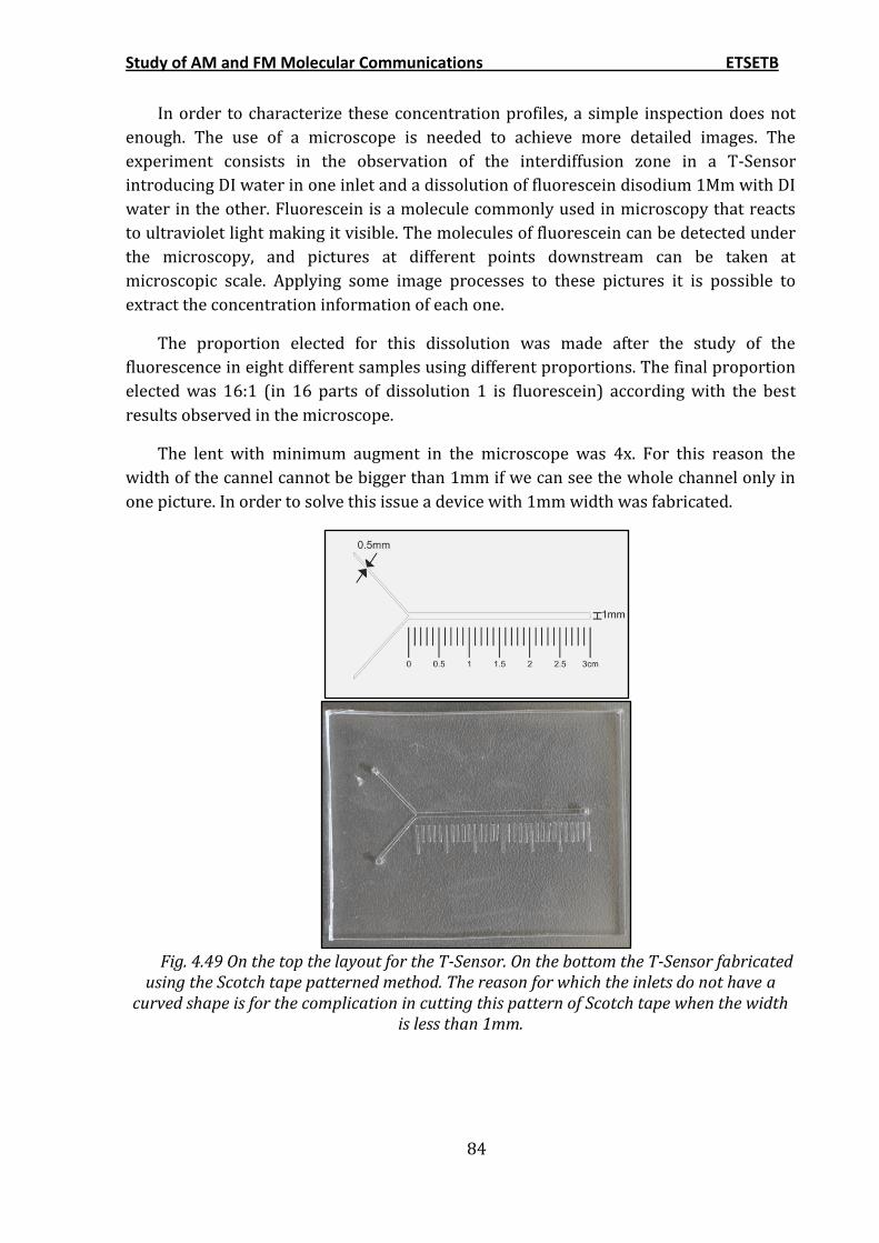
Study of AM and FM Molecular Communications ETSETB
84
In order to characterize these concentration profiles, a simple inspection does not
enough. The use of a microscope is needed to achieve more detailed images. The
experiment consists in the observation of the interdiffusion zone in a T-Sensor
introducing DI water in one inlet and a dissolution of fluorescein disodium 1Mm with DI
water in the other. Fluorescein is a molecule commonly used in microscopy that reacts
to ultraviolet light making it visible. The molecules of fluorescein can be detected under
the microscopy, and pictures at different points downstream can be taken at
microscopic scale. Applying some image processes to these pictures it is possible to
extract the concentration information of each one.
The proportion elected for this dissolution was made after the study of the
fluorescence in eight different samples using different proportions. The final proportion
elected was 16:1 (in 16 parts of dissolution 1 is fluorescein) according with the best
results observed in the microscope.
The lent with minimum augment in the microscope was 4x. For this reason the
width of the cannel cannot be bigger than 1mm if we can see the whole channel only in
one picture. In order to solve this issue a device with 1mm width was fabricated.
Fig. 4.49 On the top the layout for the T-Sensor. On the bottom the T-Sensor fabricated
using the Scotch tape patterned method. The reason for which the inlets do not have a curved shape is for the complication in cutting this pattern of Scotch tape when the width
is less than 1mm.
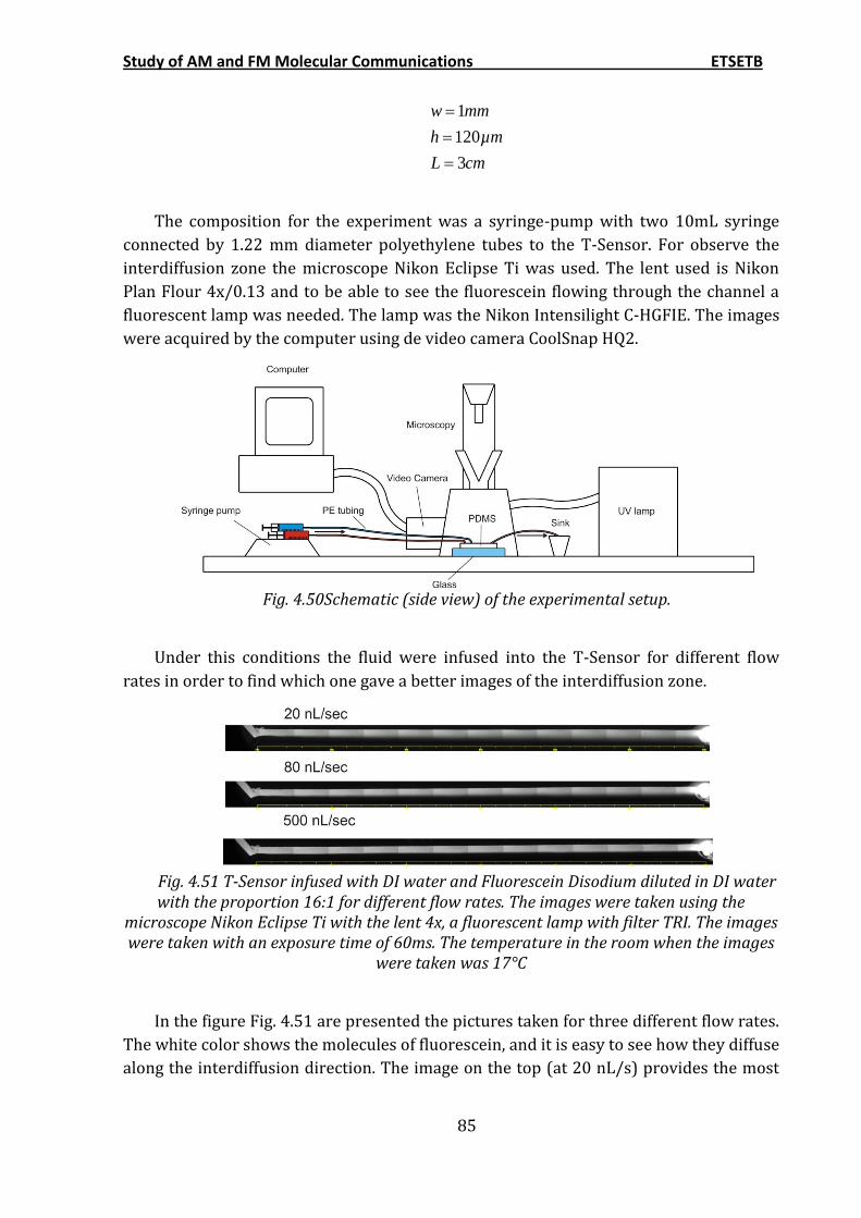
Study of AM and FM Molecular Communications ETSETB
85
1
120
3
w mm
h µm
L cm
The composition for the experiment was a syringe-pump with two 10mL syringe
connected by 1.22 mm diameter polyethylene tubes to the T-Sensor. For observe the
interdiffusion zone the microscope Nikon Eclipse Ti was used. The lent used is Nikon
Plan Flour 4x/0.13 and to be able to see the fluorescein flowing through the channel a
fluorescent lamp was needed. The lamp was the Nikon Intensilight C-HGFIE. The images
were acquired by the computer using de video camera CoolSnap HQ2.
Fig. 4.50Schematic (side view) of the experimental setup.
Under this conditions the fluid were infused into the T-Sensor for different flow
rates in order to find which one gave a better images of the interdiffusion zone.
Fig. 4.51 T-Sensor infused with DI water and Fluorescein Disodium diluted in DI water with the proportion 16:1 for different flow rates. The images were taken using the
microscope Nikon Eclipse Ti with the lent 4x, a fluorescent lamp with filter TRI. The images were taken with an exposure time of 60ms. The temperature in the room when the images
were taken was 17°C
In the figure Fig. 4.51 are presented the pictures taken for three different flow rates.
The white color shows the molecules of fluorescein, and it is easy to see how they diffuse
along the interdiffusion direction. The image on the top (at 20 nL/s) provides the most
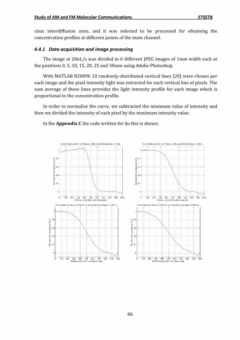
Study of AM and FM Molecular Communications ETSETB
86
clear interdiffusion zone, and it was selected to be processed for obtaining the
concentration profiles at different points of the main channel.
4.4.1 Data acquisition and image processing
The image at 20nL/s was divided in 6 different JPEG images of 1mm width each at
the positions 0, 5, 10, 15, 20, 25 and 30mm using Adobe Photoshop.
With MATLAB R2009b 10 randomly-distributed vertical lines [20] were chosen per
each image and the pixel intensity light was extracted for each vertical line of pixels. The
sum average of these lines provides the light intensity profile for each image which is
proportional to the concentration profile.
In order to normalize the curve, we subtracted the minimum value of intensity and
then we divided the intensity of each pixel by the maximum intensity value.
In the Appendix C the code written for do this is shown.
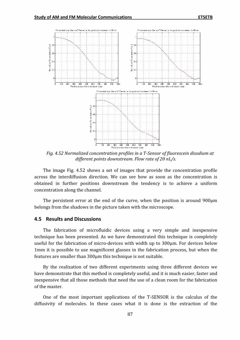
Study of AM and FM Molecular Communications ETSETB
87
Fig. 4.52 Normalized concentration profiles in a T-Sensor of fluorescein disodium at
different points downstream. Flow rate of 20 nL/s. The image Fig. 4.52 shows a set of images that provide the concentration profile
across the interdiffusion direction. We can see how as soon as the concentration is
obtained in further positions downstream the tendency is to achieve a uniform
concentration along the channel.
The persistent error at the end of the curve, when the position is around 900µm
belongs from the shadows in the picture taken with the microscope.
4.5 Results and Discussions
The fabrication of microfluidic devices using a very simple and inexpensive
technique has been presented. As we have demonstrated this technique is completely
useful for the fabrication of micro-devices with width up to 300μm. For devices below
1mm it is possible to use magnificent glasses in the fabrication process, but when the
features are smaller than 300μm this technique is not suitable.
By the realization of two different experiments using three different devices we
have demonstrate that this method is completely useful, and it is much easier, faster and
inexpensive that all those methods that need the use of a clean room for the fabrication
of the master.
One of the most important applications of the T-SENSOR is the calculus of the
diffusivity of molecules. In these cases what it is done is the extraction of the

Study of AM and FM Molecular Communications ETSETB
88
concentration profiles of these molecules such as it has been done before. After that a
simulator can be used to find out which is the diffusion coefficient that fits better with
the experimental results.
In the following chapters a simulator of the diffusion will be programmed, and the
results that we have got before will be use to verify the reliability of that simulator.
The T-SENSOR is a microfluidic device that allows the study of the diffusion of
particles. It may provide us a better understanding of this phenomenon, and utilize this
knowledge in the study of molecular communication based on diffusion processes.
Study of AM and FM Molecular Communications ETSETB
89
5 SIMULATION OF A T-SENSOR
As it was commented in previous section, the analytical solution of molecular
communication systems presents instability issues. For this reasons a simulator of this
process has to be programmed.
In this chapter firstly we discuss about numerical methods and specifically we
present the method of "Finite Differences". Using this method we find a simulator able to
predict the theoretical behavior of a T-Sensor. This simulator is done in 1 and 2
dimensions and is validated using the experimental data got in Chapter 4.
Using this simulator as model, in future sections the molecular communication
simulator is programmed.

Study of AM and FM Molecular Communications ETSETB
90
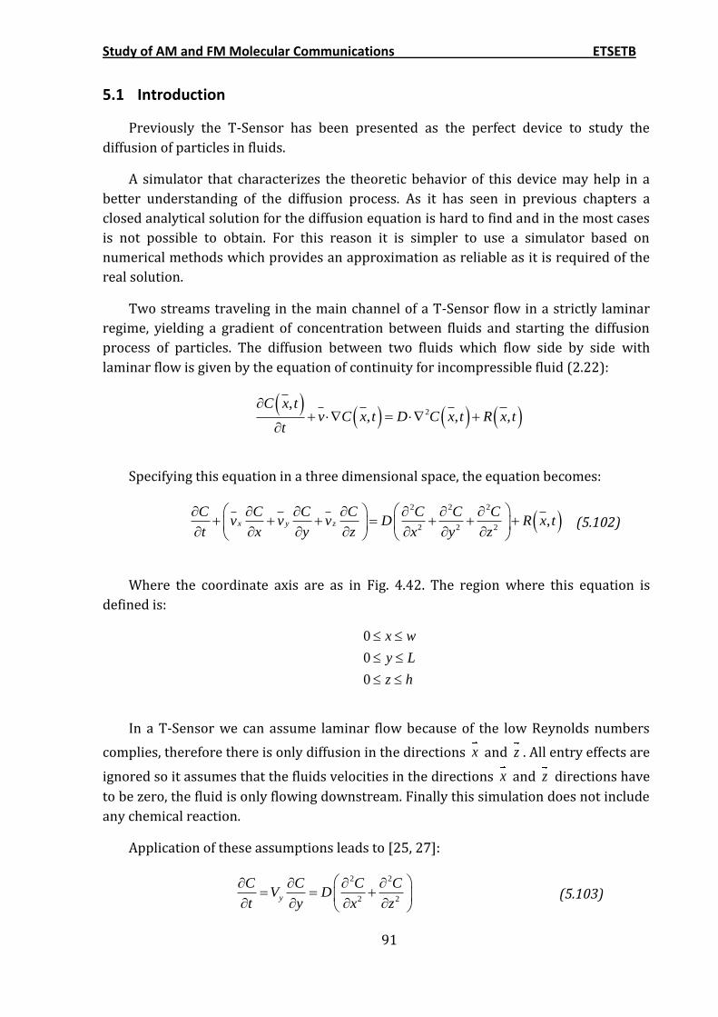
Study of AM and FM Molecular Communications ETSETB
91
5.1 Introduction
Previously the T-Sensor has been presented as the perfect device to study the
diffusion of particles in fluids.
A simulator that characterizes the theoretic behavior of this device may help in a
better understanding of the diffusion process. As it has seen in previous chapters a
closed analytical solution for the diffusion equation is hard to find and in the most cases
is not possible to obtain. For this reason it is simpler to use a simulator based on
numerical methods which provides an approximation as reliable as it is required of the
real solution.
Two streams traveling in the main channel of a T-Sensor flow in a strictly laminar
regime, yielding a gradient of concentration between fluids and starting the diffusion
process of particles. The diffusion between two fluids which flow side by side with
laminar flow is given by the equation of continuity for incompressible fluid (2.22):
2
,, , ,
C x tv C x t D C x t R x t
t
Specifying this equation in a three dimensional space, the equation becomes:
2 2 2
2 2 2,x y z
C C C C C C Cv v v D R x t
t x y z x y z
(5.102)
Where the coordinate axis are as in Fig. 4.42. The region where this equation is
defined is:
0
0
0
x w
y L
z h
In a T-Sensor we can assume laminar flow because of the low Reynolds numbers
complies, therefore there is only diffusion in the directions x and z . All entry effects are
ignored so it assumes that the fluids velocities in the directions x and z directions have
to be zero, the fluid is only flowing downstream. Finally this simulation does not include
any chemical reaction.
Application of these assumptions leads to [25, 27]:
2 2
2 2y
C C C CV D
t y x z
(5.103)
Study of AM and FM Molecular Communications ETSETB
92
This equation is a three dimensional parabolic differential equation and it can be
solved a numerical method known as "finite differences".
5.2 Simulation Using Numerical Methods
The science and the technology describe real phenomena by mathematical models.
The study of these models allows large in-depth knowledge of the phenomenon as well
as its future evolution. Unfortunately, applying classic analytical methods to obtain these
mathematical models is not always possible. This can be due to different reasons:
They do not fit to the particular model. The analytical solution is so complicated, and
makes impossible further interpretations. Their application is excessively complicated.
It does not exist any analytical method able to provide solutions to the problem.
In these cases numerical methods are useful. They provide approximate solutions
which are always numerical. These methods depend on a very large number of calculi,
and their use requires computational devices.
In the field of partial differential equations one of the most well known numerical
methods is the "Finite Difference Method".
5.2.1 Finite difference method
In mathematics, finite difference methods are numerical methods approximating the
solutions to differential equations using finite differences equations to approximate
derivatives.
The first derivative of a function is defined by:
0lim
f a f af x
(5.104)
Then a reasonable approximation for that derivative when ε has a small value would
be:
f a f a
f x
(5.105)
Using this and similar formula to replace derivative expressions in differential
equations, it is possible to approximate their solutions without the need for calculus.
The main idea for this method is discretize the continuous domain in a finite
number of points, building a two dimensional mesh.
Being ,f x t a function defined in the domain 0 x X and 0 t T , this function
can be approximated in a limited number of points discretizating its domain.
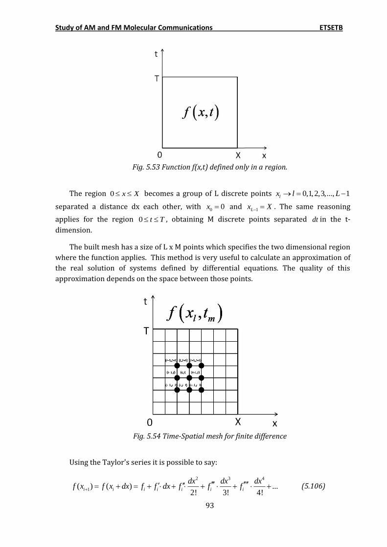
Study of AM and FM Molecular Communications ETSETB
93
Fig. 5.53 Function f(x,t) defined only in a region.
The region 0 x X becomes a group of L discrete points 0,1,2,3,..., 1lx l L
separated a distance dx each other, with 0 0x and 1Lx X . The same reasoning
applies for the region 0 t T , obtaining M discrete points separated dt in the t-
dimension.
The built mesh has a size of L x M points which specifies the two dimensional region
where the function applies. This method is very useful to calculate an approximation of
the real solution of systems defined by differential equations. The quality of this
approximation depends on the space between those points.
Fig. 5.54 Time-Spatial mesh for finite difference
Using the Taylor's series it is possible to say:
2 3 4
1( ) ( ) ...2! 3! 4!
i i i i i i i
dx dx dxf x f x dx f f dx f f f
(5.106)
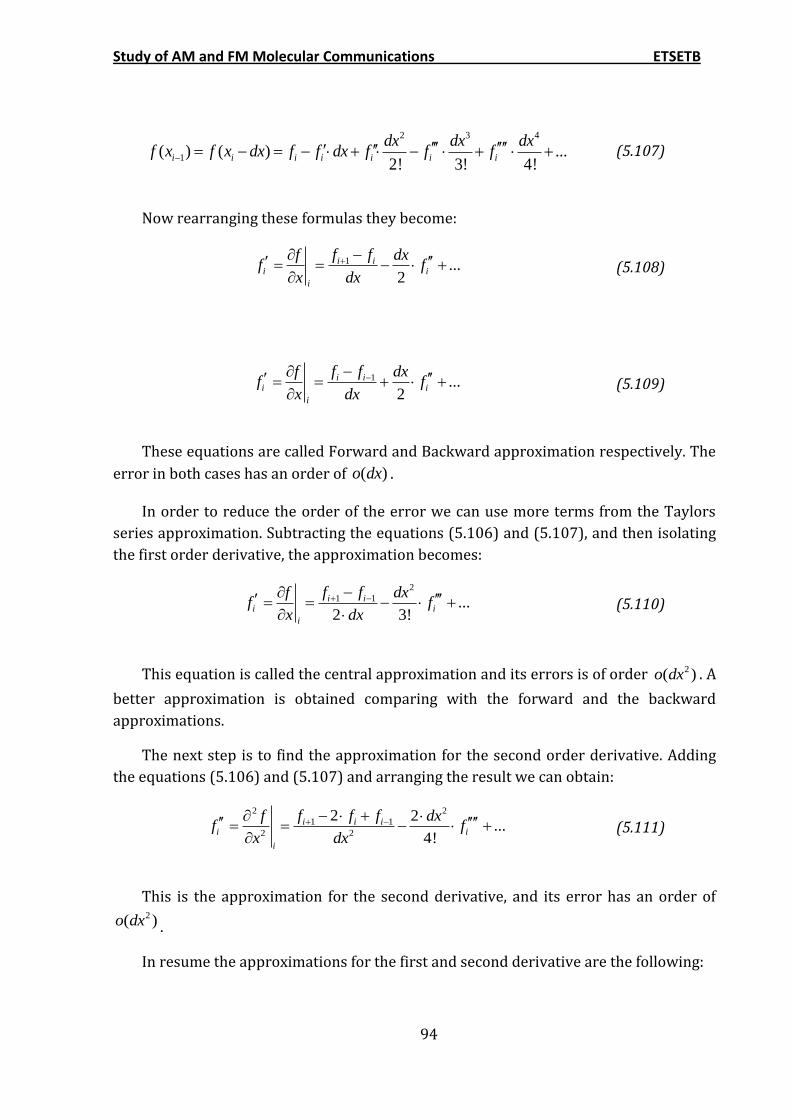
Study of AM and FM Molecular Communications ETSETB
94
2 3 4
1( ) ( ) ...2! 3! 4!
i i i i i i i
dx dx dxf x f x dx f f dx f f f
(5.107)
Now rearranging these formulas they become:
1 ...2
i ii i
i
f ff dxf f
x dx
(5.108)
1 ...2
i ii i
i
f ff dxf f
x dx
(5.109)
These equations are called Forward and Backward approximation respectively. The
error in both cases has an order of ( )o dx .
In order to reduce the order of the error we can use more terms from the Taylors
series approximation. Subtracting the equations (5.106) and (5.107), and then isolating
the first order derivative, the approximation becomes:
2
1 1 ...2 3!
i ii i
i
f ff dxf f
x dx
(5.110)
This equation is called the central approximation and its errors is of order 2( )o dx . A
better approximation is obtained comparing with the forward and the backward
approximations.
The next step is to find the approximation for the second order derivative. Adding
the equations (5.106) and (5.107) and arranging the result we can obtain:
2 2
1 1
2 2
2 2...
4!
i i ii i
i
f f ff dxf f
x dx
(5.111)
This is the approximation for the second derivative, and its error has an order of2( )o dx .
In resume the approximations for the first and second derivative are the following:
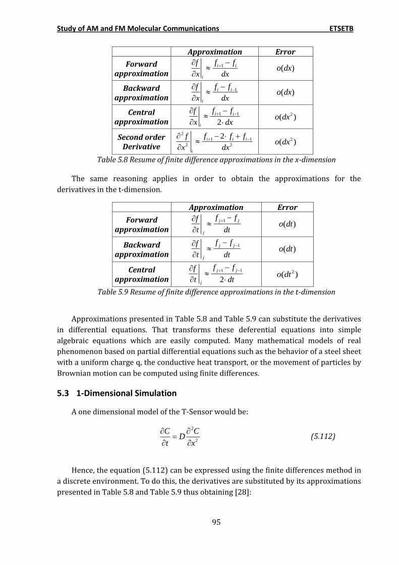
Study of AM and FM Molecular Communications ETSETB
95
Approximation Error
Forward approximation
1i i
i
f ff
x dx
( )o dx
Backward approximation
1i i
i
f ff
x dx
( )o dx
Central approximation
1 1
2
i i
i
f ff
x dx
2( )o dx
Second order Derivative
2
1 1
2 2
2i i i
i
f f ff
x dx
2( )o dx
Table 5.8 Resume of finite difference approximations in the x-dimension
The same reasoning applies in order to obtain the approximations for the
derivatives in the t-dimension.
Approximation Error
Forward approximation
1j j
j
f ff
t dt
( )o dt
Backward approximation
1j j
j
f ff
t dt
( )o dt
Central approximation
1 1
2
j j
j
f ff
t dt
2( )o dt
Table 5.9 Resume of finite difference approximations in the t-dimension
Approximations presented in Table 5.8 and Table 5.9 can substitute the derivatives
in differential equations. That transforms these deferential equations into simple
algebraic equations which are easily computed. Many mathematical models of real
phenomenon based on partial differential equations such as the behavior of a steel sheet
with a uniform charge q, the conductive heat transport, or the movement of particles by
Brownian motion can be computed using finite differences.
5.3 1-Dimensional Simulation
A one dimensional model of the T-Sensor would be:
2
2
C CD
t x
(5.112)
Hence, the equation (5.112) can be expressed using the finite differences method in
a discrete environment. To do this, the derivatives are substituted by its approximations
presented in Table 5.8 and Table 5.9 thus obtaining [28]:
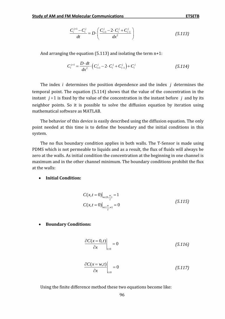
Study of AM and FM Molecular Communications ETSETB
96
1
1 1
2
2j j j j j
i i i i iC C C C CD
dt dx
(5.113)
And arranging the equation (5.113) and isolating the term n+1:
1
1 122j j j j j
i i i i i
D dtC C C C C
dx
(5.114)
The index i determines the position dependence and the index j determines the
temporal point. The equation (5.114) shows that the value of the concentration in the
instant 1j is fixed by the value of the concentration in the instant before j and by its
neighbor points. So it is possible to solve the diffusion equation by iteration using
mathematical software as MATLAB.
The behavior of this device is easily described using the diffusion equation. The only
point needed at this time is to define the boundary and the initial conditions in this
system.
The no flux boundary condition applies in both walls. The T-Sensor is made using
PDMS which is not permeable to liquids and as a result, the flux of fluids will always be
zero at the walls. As initial condition the concentration at the beginning in one channel is
maximum and in the other channel minimum. The boundary conditions prohibit the flux
at the walls:
Initial Condition:
(0, )2
( , )2
( , 0) 1
( , 0) 0
wx
wx w
C x t
C x t
(5.115)
Boundary Conditions:
0
( 0, )0
t
C x t
x
(5.116)
0
( , )0
t
C x w t
x
(5.117)
Using the finite difference method these two equations become like:
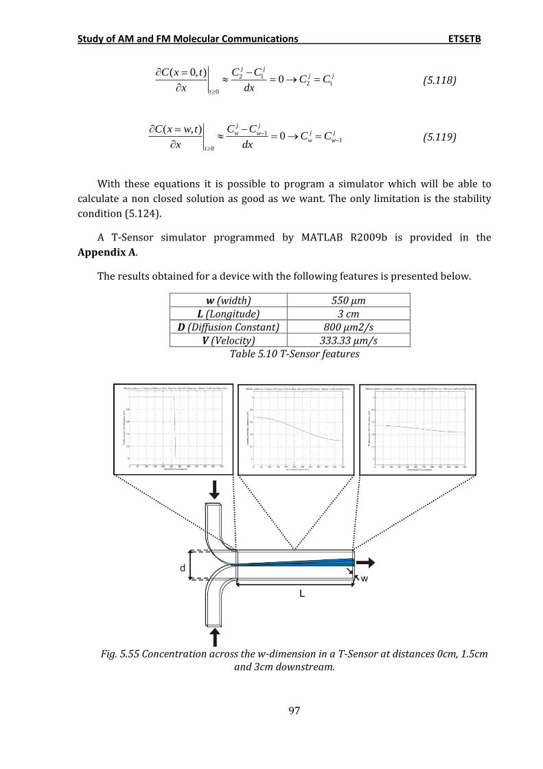
Study of AM and FM Molecular Communications ETSETB
97
2 12 1
0
( 0, )0
j jj j
t
C CC x tC C
x dx
(5.118)
11
0
( , )0
j jj jw w
w w
t
C CC x w tC C
x dx
(5.119)
With these equations it is possible to program a simulator which will be able to
calculate a non closed solution as good as we want. The only limitation is the stability
condition (5.124).
A T-Sensor simulator programmed by MATLAB R2009b is provided in the
Appendix A.
The results obtained for a device with the following features is presented below.
w (width) 550 µm L (Longitude) 3 cm
D (Diffusion Constant) 800 µm2/s V (Velocity) 333.33 µm/s
Table 5.10 T-Sensor features
Fig. 5.55 Concentration across the w-dimension in a T-Sensor at distances 0cm, 1.5cm
and 3cm downstream.
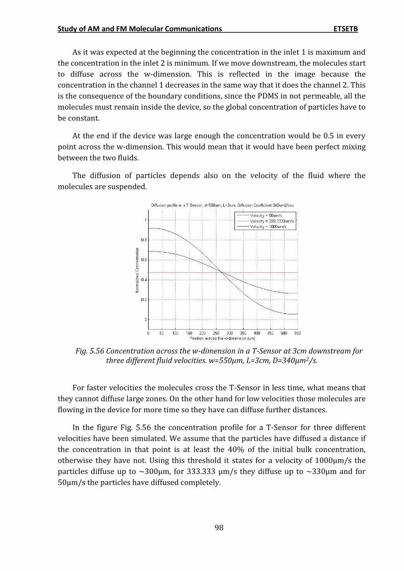
Study of AM and FM Molecular Communications ETSETB
98
As it was expected at the beginning the concentration in the inlet 1 is maximum and
the concentration in the inlet 2 is minimum. If we move downstream, the molecules start
to diffuse across the w-dimension. This is reflected in the image because the
concentration in the channel 1 decreases in the same way that it does the channel 2. This
is the consequence of the boundary conditions, since the PDMS in not permeable, all the
molecules must remain inside the device, so the global concentration of particles have to
be constant.
At the end if the device was large enough the concentration would be 0.5 in every
point across the w-dimension. This would mean that it would have been perfect mixing
between the two fluids.
The diffusion of particles depends also on the velocity of the fluid where the
molecules are suspended.
Fig. 5.56 Concentration across the w-dimension in a T-Sensor at 3cm downstream for
three different fluid velocities. w=550μm, L=3cm, D=340μm2/s.
For faster velocities the molecules cross the T-Sensor in less time, what means that
they cannot diffuse large zones. On the other hand for low velocities those molecules are
flowing in the device for more time so they have can diffuse further distances.
In the figure Fig. 5.56 the concentration profile for a T-Sensor for three different
velocities have been simulated. We assume that the particles have diffused a distance if
the concentration in that point is at least the 40% of the initial bulk concentration,
otherwise they have not. Using this threshold it states for a velocity of 1000μm/s the
particles diffuse up to ~300μm, for 333.333 μm/s they diffuse up to ~330μm and for
50μm/s the particles have diffused completely.
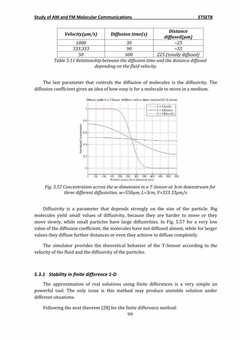
Study of AM and FM Molecular Communications ETSETB
99
Velocity(μm/s) Diffusion time(s) Distance
diffused(μm) 1000 30 ~25
333.333 90 ~55 50 600 225 (totally diffused)
Table 5.11 Relationship between the diffusion time and the distance diffused depending on the fluid velocity.
The last parameter that controls the diffusion of molecules is the diffusivity. The
diffusion coefficient gives an idea of how easy is for a molecule to move in a medium.
Fig. 5.57 Concentration across the w-dimension in a T-Sensor at 3cm downstream for
three different diffusivities. w=550μm, L=3cm, V=333.33μm/s.
Diffusivity is a parameter that depends strongly on the size of the particle. Big
molecules yield small values of diffusivity, because they are harder to move or they
move slowly, while small particles have large diffusivities. In Fig. 5.57 for a very low
value of the diffusion coefficient, the molecules have not diffused almost, while for larger
values they diffuse further distances or even they achieve to diffuse completely.
The simulator provides the theoretical behavior of the T-Sensor according to the
velocity of the fluid and the diffusivity of the particles.
5.3.1 Stability in finite difference 1-D
The approximation of real solutions using finite differences is a very simple an
powerful tool. The only issue is this method may produce unstable solution under
different situations.
Following the next theorem [28] for the finite difference method:
Study of AM and FM Molecular Communications ETSETB
100
1
1 1
j j j j
i i i iC A C B C C C
(5.120)
If an equation as (5.120) is obtained using finite difference, then the scheme is
stable and the errors die out when A, B, and C are positive and 1A B C . In the case
above:
Taking 2
D dt
dx
then (5.114) can be written as:
1
1 1(1 2 )j j j j
i i i iC C C C
(5.121)
And comparing with (5.120):
2
D dtA C
dx
(5.122)
21 2 1 2
D dtB
dx
(5.123)
Is easy to see that 1A B C is always true:
(1 2 ) 1
A and C are always positive constants, so the only term which affects in the stability
is B.
11 2 0
2B
2
2
1
2 2
D dt dxdt
dx D
(5.124)
(5.124) is the stability condition to solve the diffusion equation using finite
difference.
The practical explanation is that, given a spatial resolution and the velocity by which
the molecules diffuse away, the temporal resolution has to be enough to "see" without
mistake the evolution of all the particles.
5.4 2-Dimensional Simulation
A two dimension model of the T-Sensor is presented in the equation (5.103). This
system is defined by a three dimensional grid which comprehend the two spatial
dimension x and z , ant the temporal dimension t .
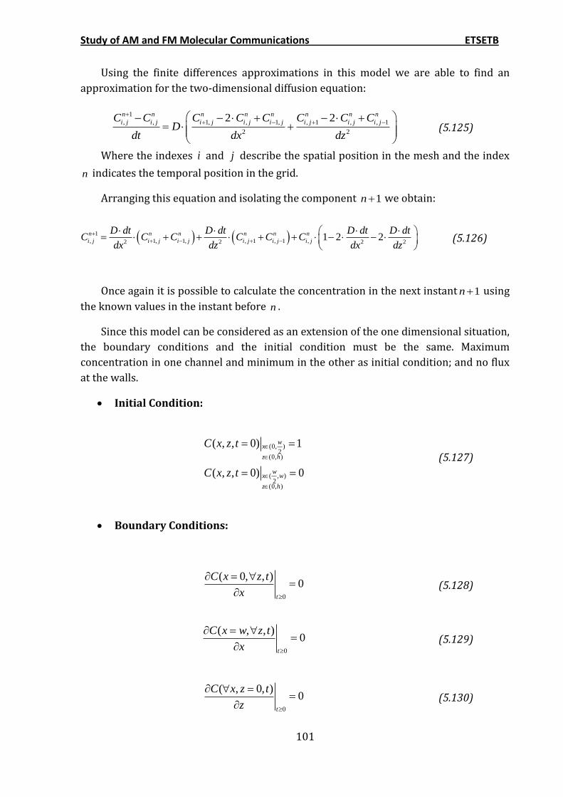
Study of AM and FM Molecular Communications ETSETB
101
Using the finite differences approximations in this model we are able to find an
approximation for the two-dimensional diffusion equation:
1
, , 1, , 1, , 1 , , 1
2 2
2 2n n n n n n n n
i j i j i j i j i j i j i j i jC C C C C C C CD
dt dx dz
(5.125)
Where the indexes i and j describe the spatial position in the mesh and the index
n indicates the temporal position in the grid.
Arranging this equation and isolating the component 1n we obtain:
1
, 1, 1, , 1 , 1 ,2 2 2 21 2 2n n n n n n
i j i j i j i j i j i j
D dt D dt D dt D dtC C C C C C
dx dz dx dz
(5.126)
Once again it is possible to calculate the concentration in the next instant 1n using
the known values in the instant before n .
Since this model can be considered as an extension of the one dimensional situation,
the boundary conditions and the initial condition must be the same. Maximum
concentration in one channel and minimum in the other as initial condition; and no flux
at the walls.
Initial Condition:
(0, )2
(0, )
( , )2
(0, )
( , , 0) 1
( , , 0) 0
wx
z h
wx w
z h
C x z t
C x z t
(5.127)
Boundary Conditions:
0
( 0, , )0
t
C x z t
x
(5.128)
0
( , , )0
t
C x w z t
x
(5.129)
0
( , 0, )0
t
C x z t
z
(5.130)

Study of AM and FM Molecular Communications ETSETB
102
0
( , , )0
t
C x z h t
z
(5.131)
Fig. 5.58 Distribution of the boundary conditions in the device
Using finite difference the boundary conditions become:
2, 1,
2, 1,
0
( 0, , )0 0
n n
j j n n
j j
t
C CC x z tC C
x dx
(5.132)
, 1,
, 1,
0
( , , )0 0
n n
w j w j n n
w j w j
t
C CC x w z tC C
x dx
(5.133)
,2 ,1
,2 ,1
0
( , 0, )0 0
n n
i i n n
i i
t
C CC x z tC C
y dz
(5.134)
, , 1
, , 1
0
( , , )0 0
n n
i h i h n n
i h i h
t
C CC x z h tC C
y dz
(5.135)
A T-Sensor simulator programmed by MATLAB R2009b is provided in the
Appendix B. The results obtained for a device characterized in the following table will
be presented below.
w (width) 550 µm h (height) 60 µm
L (Longitude) 3 mm D (Diffusion Constant) 320 µm2/s
Q (Flow Rate) 11 nL/s V (Velocity) 333.33 µm/s
Table 5.12 T-Sensor features
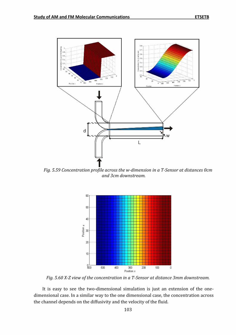
Study of AM and FM Molecular Communications ETSETB
103
Fig. 5.59 Concentration profile across the w-dimension in a T-Sensor at distances 0cm
and 3cm downstream.
Fig. 5.60 X-Z view of the concentration in a T-Sensor at distance 3mm downstream.
It is easy to see the two-dimensional simulation is just an extension of the one-
dimensional case. In a similar way to the one dimensional case, the concentration across
the channel depends on the diffusivity and the velocity of the fluid.
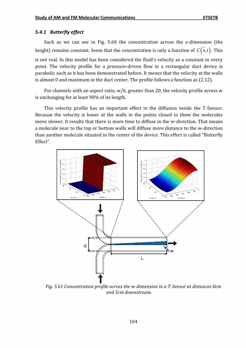
Study of AM and FM Molecular Communications ETSETB
104
5.4.1 Butterfly effect
Such as we can see in Fig. 5.60 the concentration across the z-dimension (the
height) remains constant. Seem that the concentration is only a function of ,C x t . This
is not real. In this model has been considered the fluid's velocity as a constant in every
point. The velocity profile for a pressure-driven flow in a rectangular duct device is
parabolic such as it has been demonstrated before. It means that the velocity at the walls
is almost 0 and maximum in the duct center. The profile follows a function as (2.12).
For channels with an aspect ratio, w/h, greater than 20, the velocity profile across w
is unchanging for at least 90% of its length.
This velocity profile has an important effect in the diffusion inside the T-Sensor.
Because the velocity is lower at the walls in the points closed to them the molecules
move slower. It results that there is more time to diffuse in the w-direction. That means
a molecule near to the top or bottom walls will diffuse more distance to the w-direction
than another molecule situated in the center of the device. This effect is called "Butterfly
Effect".
Fig. 5.61 Concentration profile across the w-dimension in a T-Sensor at distances 0cm
and 3cm downstream.
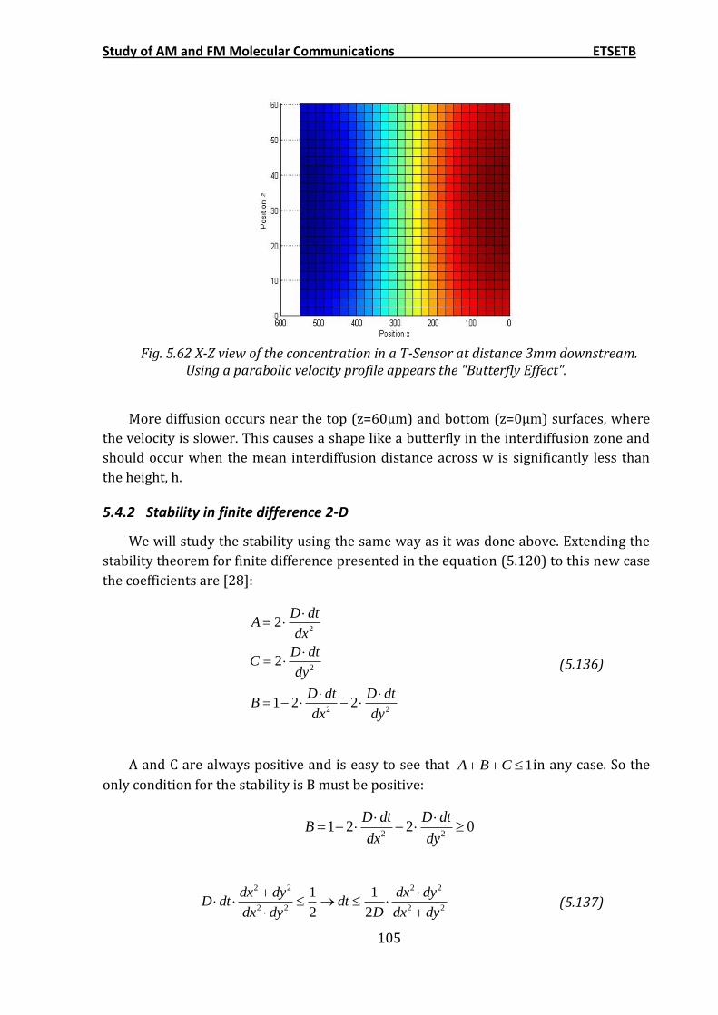
Study of AM and FM Molecular Communications ETSETB
105
Fig. 5.62 X-Z view of the concentration in a T-Sensor at distance 3mm downstream.
Using a parabolic velocity profile appears the "Butterfly Effect".
More diffusion occurs near the top (z=60μm) and bottom (z=0μm) surfaces, where
the velocity is slower. This causes a shape like a butterfly in the interdiffusion zone and
should occur when the mean interdiffusion distance across w is significantly less than
the height, h.
5.4.2 Stability in finite difference 2-D
We will study the stability using the same way as it was done above. Extending the
stability theorem for finite difference presented in the equation (5.120) to this new case
the coefficients are [28]:
2
2
2 2
2
2
1 2 2
D dtA
dx
D dtC
dy
D dt D dtB
dx dy
(5.136)
A and C are always positive and is easy to see that 1A B C in any case. So the
only condition for the stability is B must be positive:
2 21 2 2 0
D dt D dtB
dx dy
2 2 2 2
2 2 2 2
1 1
2 2
dx dy dx dyD dt dt
dx dy D dx dy
(5.137)
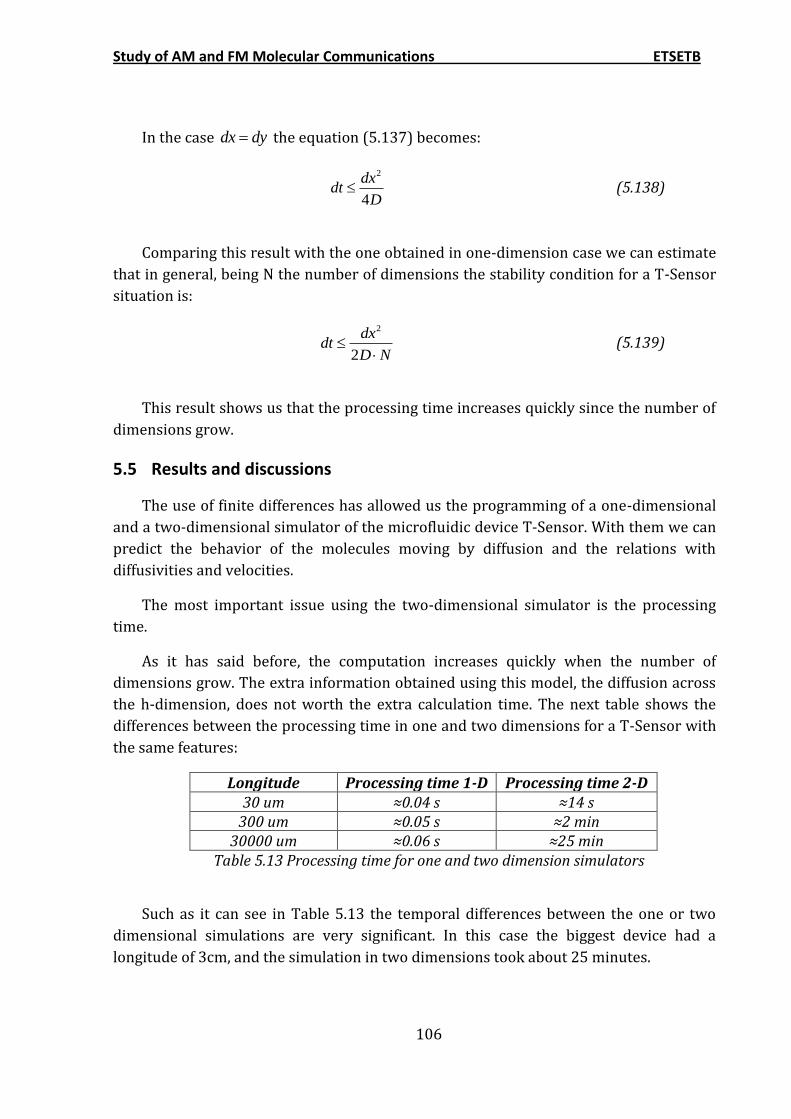
Study of AM and FM Molecular Communications ETSETB
106
In the case dx dy the equation (5.137) becomes:
2
4
dxdt
D
(5.138)
Comparing this result with the one obtained in one-dimension case we can estimate
that in general, being N the number of dimensions the stability condition for a T-Sensor
situation is:
2
2
dxdt
D N
(5.139)
This result shows us that the processing time increases quickly since the number of
dimensions grow.
5.5 Results and discussions
The use of finite differences has allowed us the programming of a one-dimensional
and a two-dimensional simulator of the microfluidic device T-Sensor. With them we can
predict the behavior of the molecules moving by diffusion and the relations with
diffusivities and velocities.
The most important issue using the two-dimensional simulator is the processing
time.
As it has said before, the computation increases quickly when the number of
dimensions grow. The extra information obtained using this model, the diffusion across
the h-dimension, does not worth the extra calculation time. The next table shows the
differences between the processing time in one and two dimensions for a T-Sensor with
the same features:
Longitude Processing time 1-D Processing time 2-D 30 um ≈0.04 s ≈14 s
300 um ≈0.05 s ≈2 min 30000 um ≈0.06 s ≈25 min
Table 5.13 Processing time for one and two dimension simulators
Such as it can see in Table 5.13 the temporal differences between the one or two
dimensional simulations are very significant. In this case the biggest device had a
longitude of 3cm, and the simulation in two dimensions took about 25 minutes.
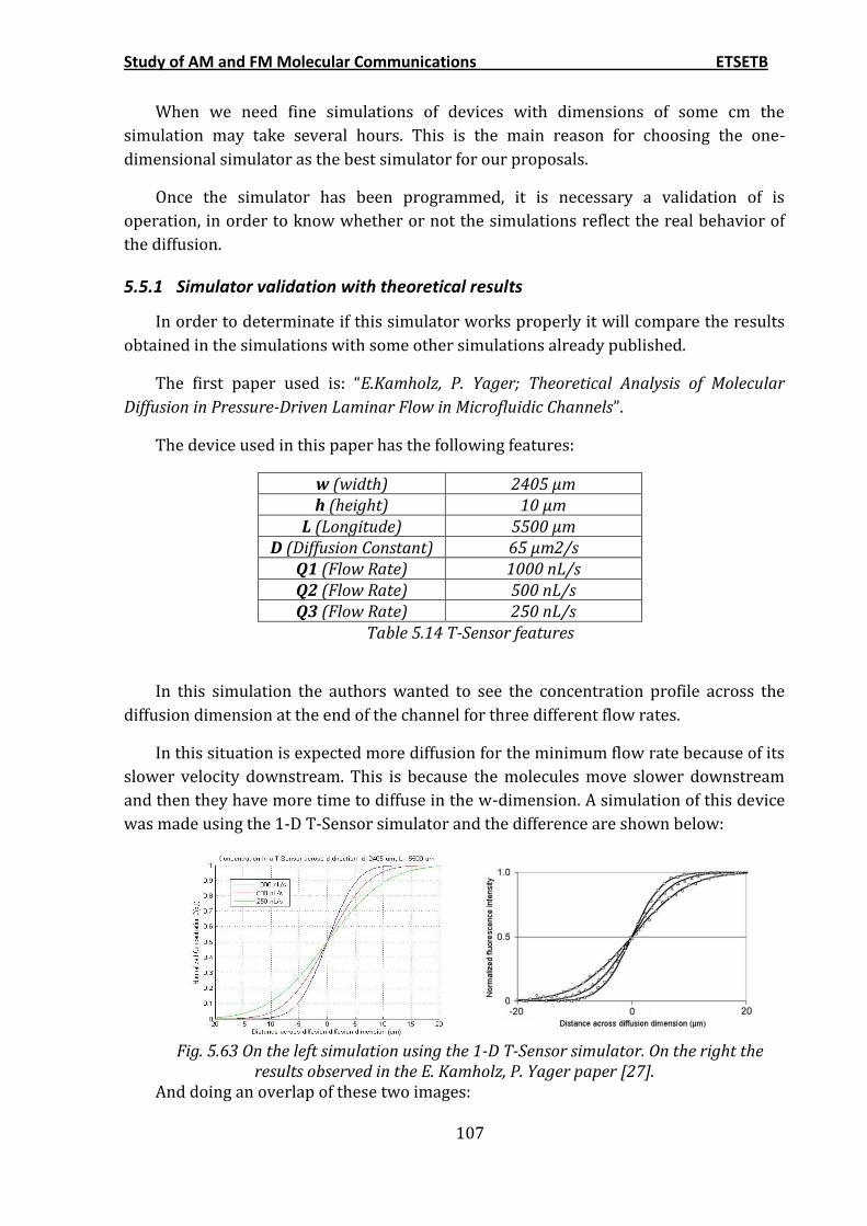
Study of AM and FM Molecular Communications ETSETB
107
When we need fine simulations of devices with dimensions of some cm the
simulation may take several hours. This is the main reason for choosing the one-
dimensional simulator as the best simulator for our proposals.
Once the simulator has been programmed, it is necessary a validation of is
operation, in order to know whether or not the simulations reflect the real behavior of
the diffusion.
5.5.1 Simulator validation with theoretical results
In order to determinate if this simulator works properly it will compare the results
obtained in the simulations with some other simulations already published.
The first paper used is: “E.Kamholz, P. Yager; Theoretical Analysis of Molecular
Diffusion in Pressure-Driven Laminar Flow in Microfluidic Channels”.
The device used in this paper has the following features:
w (width) 2405 µm h (height) 10 µm
L (Longitude) 5500 µm D (Diffusion Constant) 65 µm2/s
Q1 (Flow Rate) 1000 nL/s Q2 (Flow Rate) 500 nL/s Q3 (Flow Rate) 250 nL/s
Table 5.14 T-Sensor features
In this simulation the authors wanted to see the concentration profile across the
diffusion dimension at the end of the channel for three different flow rates.
In this situation is expected more diffusion for the minimum flow rate because of its
slower velocity downstream. This is because the molecules move slower downstream
and then they have more time to diffuse in the w-dimension. A simulation of this device
was made using the 1-D T-Sensor simulator and the difference are shown below:
Fig. 5.63 On the left simulation using the 1-D T-Sensor simulator. On the right the
results observed in the E. Kamholz, P. Yager paper [27]. And doing an overlap of these two images:
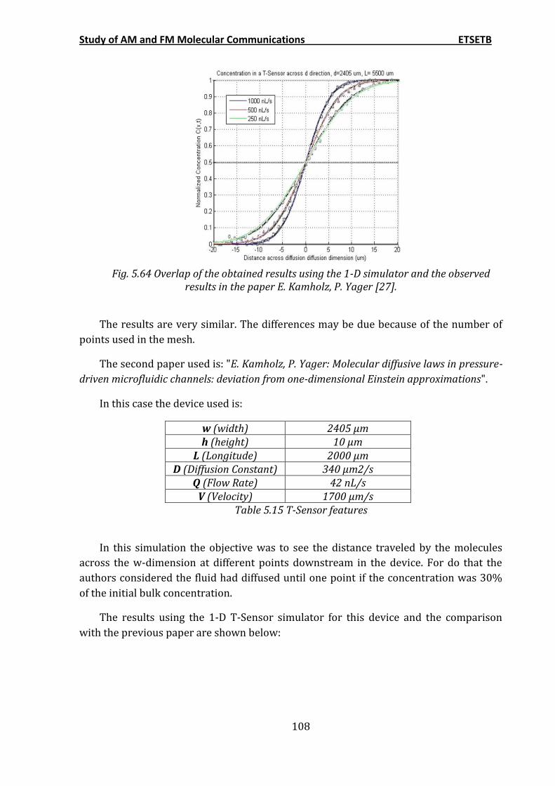
Study of AM and FM Molecular Communications ETSETB
108
Fig. 5.64 Overlap of the obtained results using the 1-D simulator and the observed
results in the paper E. Kamholz, P. Yager [27].
The results are very similar. The differences may be due because of the number of
points used in the mesh.
The second paper used is: "E. Kamholz, P. Yager: Molecular diffusive laws in pressure-
driven microfluidic channels: deviation from one-dimensional Einstein approximations".
In this case the device used is:
w (width) 2405 µm h (height) 10 µm
L (Longitude) 2000 µm D (Diffusion Constant) 340 µm2/s
Q (Flow Rate) 42 nL/s V (Velocity) 1700 µm/s
Table 5.15 T-Sensor features
In this simulation the objective was to see the distance traveled by the molecules
across the w-dimension at different points downstream in the device. For do that the
authors considered the fluid had diffused until one point if the concentration was 30%
of the initial bulk concentration.
The results using the 1-D T-Sensor simulator for this device and the comparison
with the previous paper are shown below:
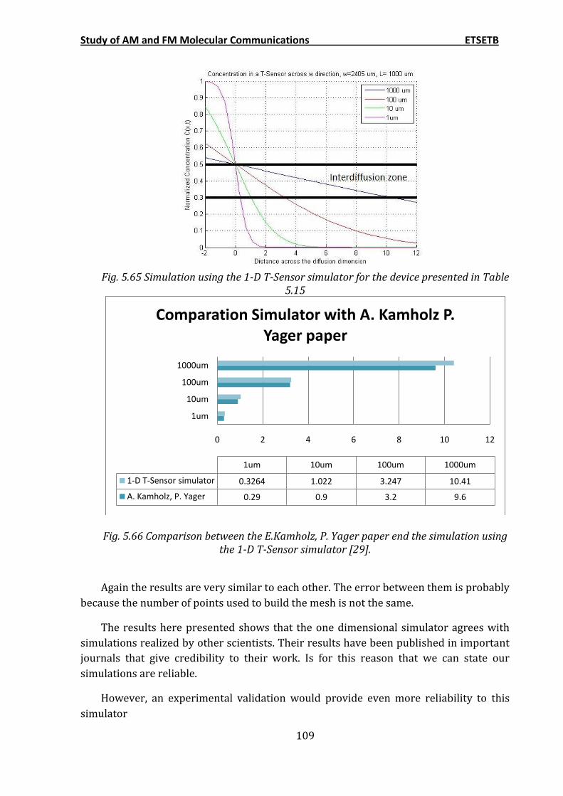
Study of AM and FM Molecular Communications ETSETB
109
Fig. 5.65 Simulation using the 1-D T-Sensor simulator for the device presented in Table
5.15
Fig. 5.66 Comparison between the E.Kamholz, P. Yager paper end the simulation using the 1-D T-Sensor simulator [29].
Again the results are very similar to each other. The error between them is probably
because the number of points used to build the mesh is not the same.
The results here presented shows that the one dimensional simulator agrees with
simulations realized by other scientists. Their results have been published in important
journals that give credibility to their work. Is for this reason that we can state our
simulations are reliable.
However, an experimental validation would provide even more reliability to this
simulator
0 2 4 6 8 10 12
1um
10um
100um
1000um
1um 10um 100um 1000um
1-D T-Sensor simulator 0.3264 1.022 3.247 10.41
A. Kamholz, P. Yager 0.29 0.9 3.2 9.6
Comparation Simulator with A. Kamholz P. Yager paper
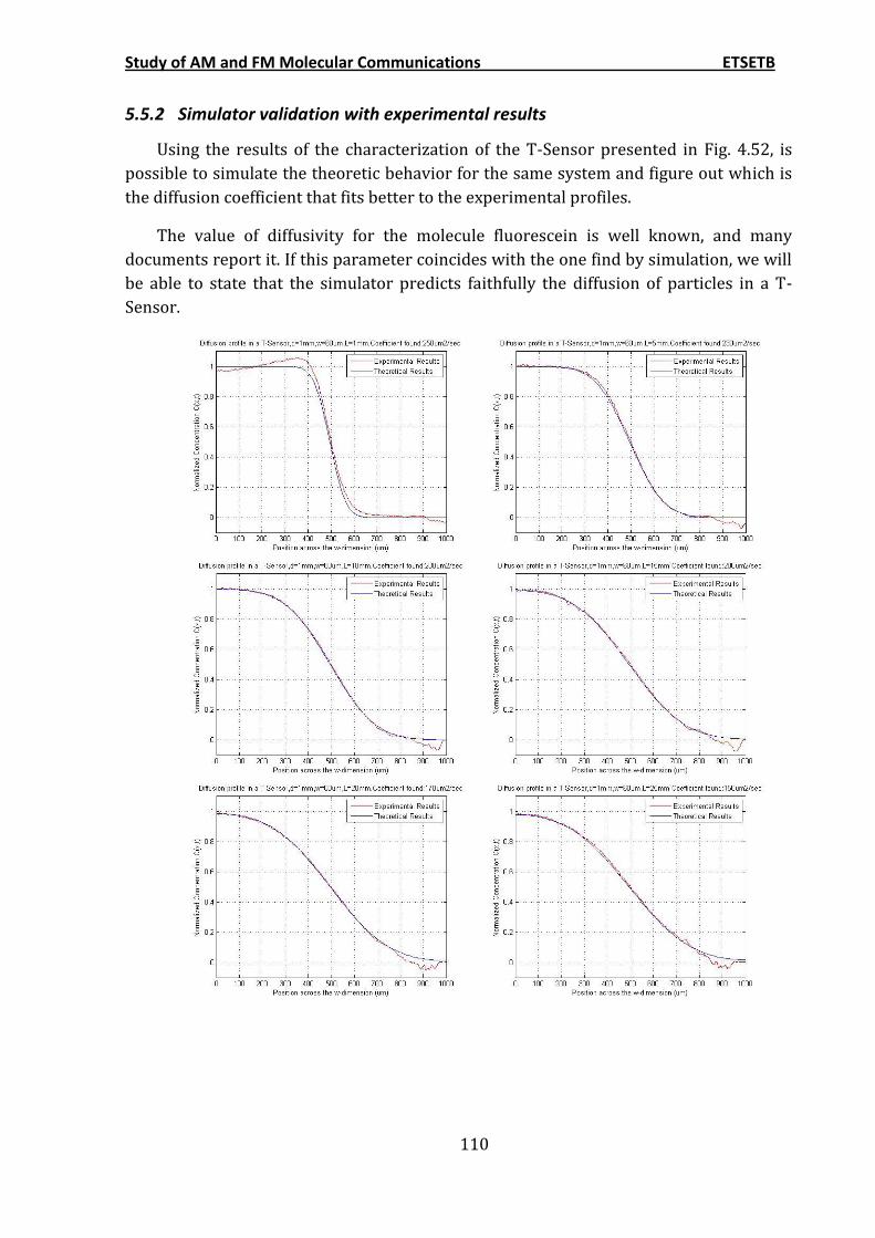
Study of AM and FM Molecular Communications ETSETB
110
5.5.2 Simulator validation with experimental results
Using the results of the characterization of the T-Sensor presented in Fig. 4.52, is
possible to simulate the theoretic behavior for the same system and figure out which is
the diffusion coefficient that fits better to the experimental profiles.
The value of diffusivity for the molecule fluorescein is well known, and many
documents report it. If this parameter coincides with the one find by simulation, we will
be able to state that the simulator predicts faithfully the diffusion of particles in a T-
Sensor.
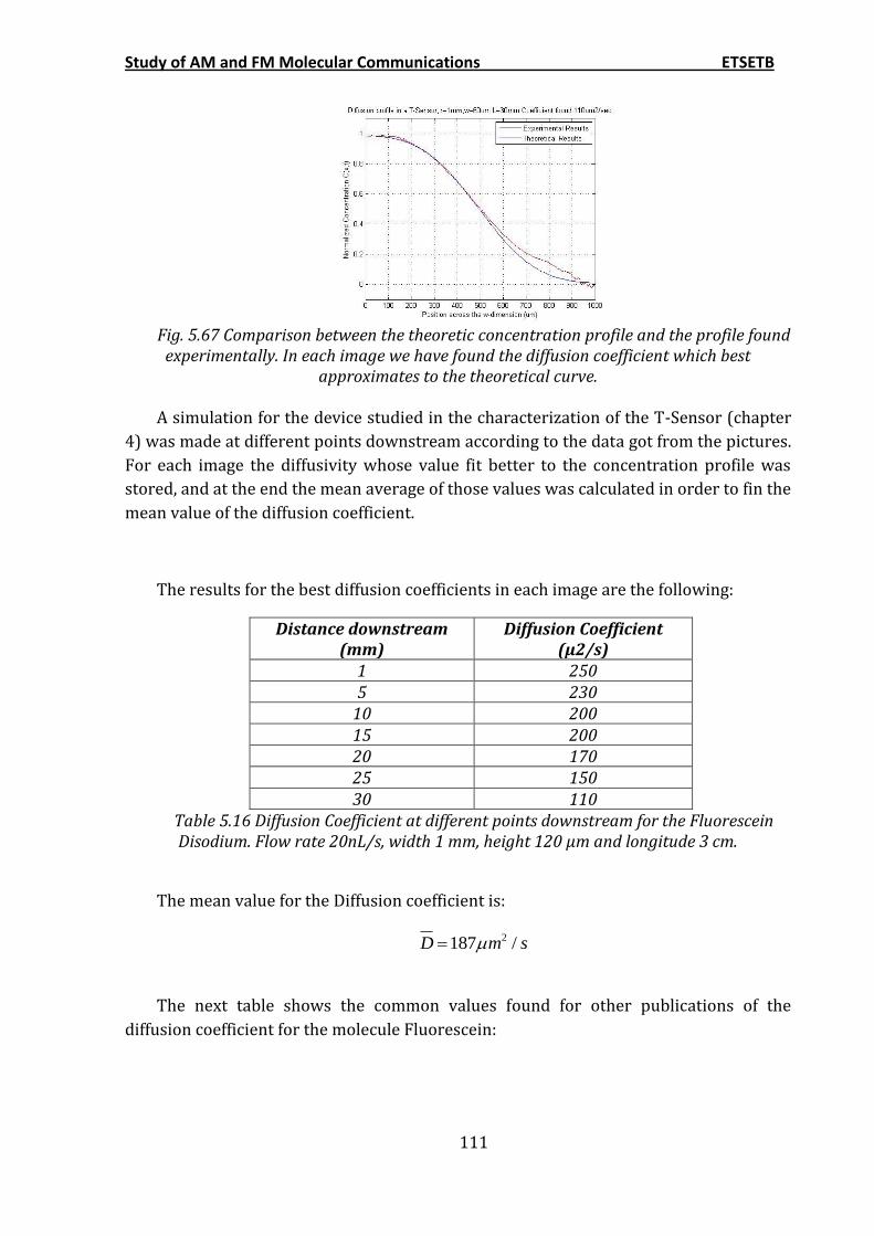
Study of AM and FM Molecular Communications ETSETB
111
Fig. 5.67 Comparison between the theoretic concentration profile and the profile found
experimentally. In each image we have found the diffusion coefficient which best approximates to the theoretical curve.
A simulation for the device studied in the characterization of the T-Sensor (chapter
4) was made at different points downstream according to the data got from the pictures.
For each image the diffusivity whose value fit better to the concentration profile was
stored, and at the end the mean average of those values was calculated in order to fin the
mean value of the diffusion coefficient.
The results for the best diffusion coefficients in each image are the following:
Distance downstream (mm)
Diffusion Coefficient (µ2/s)
1 250 5 230
10 200 15 200 20 170 25 150 30 110
Table 5.16 Diffusion Coefficient at different points downstream for the Fluorescein Disodium. Flow rate 20nL/s, width 1 mm, height 120 µm and longitude 3 cm.
The mean value for the Diffusion coefficient is:
2187 /D m s
The next table shows the common values found for other publications of the
diffusion coefficient for the molecule Fluorescein:
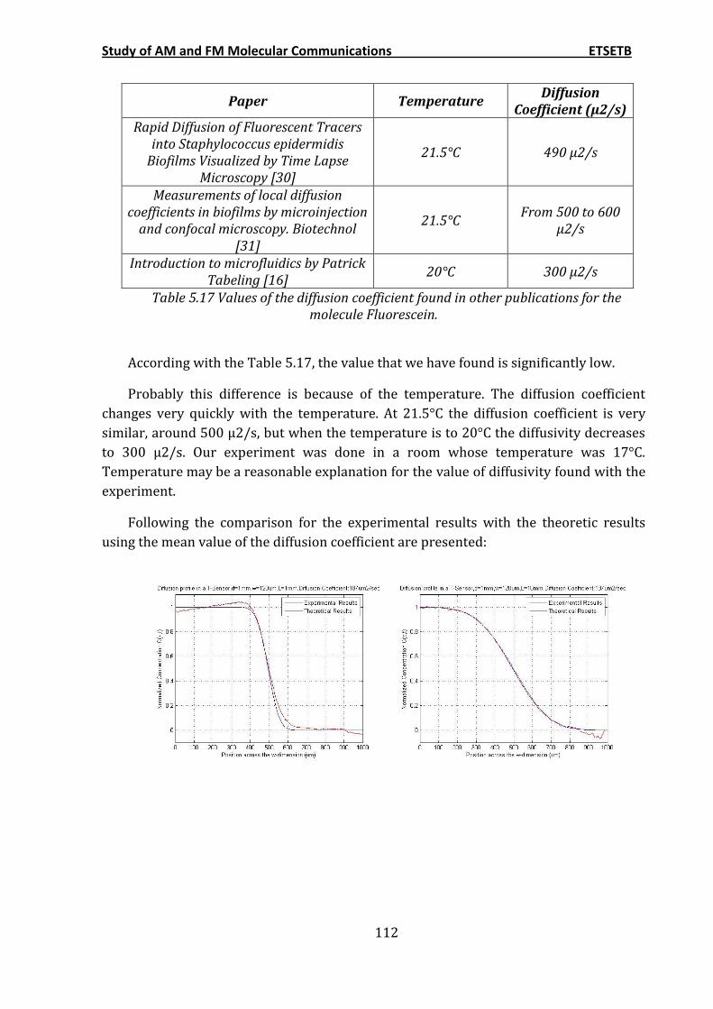
Study of AM and FM Molecular Communications ETSETB
112
Paper Temperature Diffusion
Coefficient (µ2/s) Rapid Diffusion of Fluorescent Tracers
into Staphylococcus epidermidis Biofilms Visualized by Time Lapse
Microscopy [30]
21.5°C 490 µ2/s
Measurements of local diffusion coefficients in biofilms by microinjection
and confocal microscopy. Biotechnol [31]
21.5°C From 500 to 600
µ2/s
Introduction to microfluidics by Patrick Tabeling [16]
20°C 300 µ2/s
Table 5.17 Values of the diffusion coefficient found in other publications for the molecule Fluorescein.
According with the Table 5.17, the value that we have found is significantly low.
Probably this difference is because of the temperature. The diffusion coefficient
changes very quickly with the temperature. At 21.5°C the diffusion coefficient is very
similar, around 500 µ2/s, but when the temperature is to 20°C the diffusivity decreases
to 300 µ2/s. Our experiment was done in a room whose temperature was 17°C.
Temperature may be a reasonable explanation for the value of diffusivity found with the
experiment.
Following the comparison for the experimental results with the theoretic results
using the mean value of the diffusion coefficient are presented:
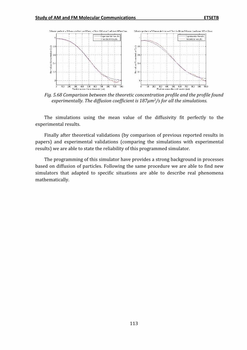
Study of AM and FM Molecular Communications ETSETB
113
Fig. 5.68 Comparison between the theoretic concentration profile and the profile found
experimentally. The diffusion coefficient is 187μm2/s for all the simulations.
The simulations using the mean value of the diffusivity fit perfectly to the
experimental results.
Finally after theoretical validations (by comparison of previous reported results in
papers) and experimental validations (comparing the simulations with experimental
results) we are able to state the reliability of this programmed simulator.
The programming of this simulator have provides a strong background in processes
based on diffusion of particles. Following the same procedure we are able to find new
simulators that adapted to specific situations are able to describe real phenomena
mathematically.

Study of AM and FM Molecular Communications ETSETB
114
6 SIMULATION OF MOLECULAR COMMUNICATION SYSTEMS
In this section the molecular communication simulator is programmed using as a
model the T-Sensor simulator done in previous chapters. The concept of signals with
variable concentration is presented, achieving the possibility of study the diffusion of
this type of signals in a T-Sensor. A simulator that includes this possibility is also
programmed.

Study of AM and FM Molecular Communications ETSETB
115
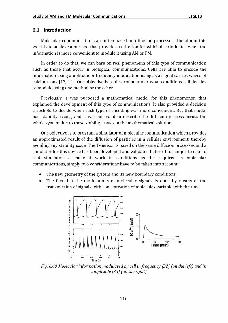
Study of AM and FM Molecular Communications ETSETB
116
6.1 Introduction
Molecular communications are often based on diffusion processes. The aim of this
work is to achieve a method that provides a criterion for which discriminates when the
information is more convenient to module it using AM or FM.
In order to do that, we can base on real phenomena of this type of communication
such as those that occur in biological communications. Cells are able to encode the
information using amplitude or frequency modulation using as a signal carries waves of
calcium ions [13, 14]. Our objective is to determine under what conditions cell decides
to module using one method or the other.
Previously it was purposed a mathematical model for this phenomenon that
explained the development of this type of communications. It also provided a decision
threshold to decide when each type of encoding was more convenient. But that model
had stability issues, and it was not valid to describe the diffusion process across the
whole system due to these stability issues in the mathematical solution.
Our objective is to program a simulator of molecular communication which provides
an approximated result of the diffusion of particles in a cellular environment, thereby
avoiding any stability issue. The T-Sensor is based on the same diffusion processes and a
simulator for this device has been developed and validated before. It is simple to extend
that simulator to make it work in conditions as the required in molecular
communications, simply two considerations have to be taken into account:
The new geometry of the system and its new boundary conditions.
The fact that the modulations of molecular signals is done by means of the
transmission of signals with concentration of molecules variable with the time.
Fig. 6.69 Molecular information modulated by cell in frequency [32] (on the left) and in
amplitude [33] (on the right).
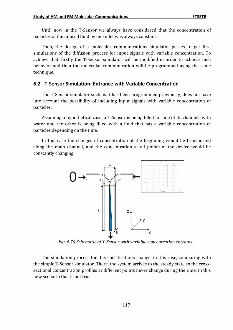
Study of AM and FM Molecular Communications ETSETB
117
Until now in the T-Sensor we always have considered that the concentration of
particles of the infused fluid by one inlet was always constant
Then, the design of a molecular communications simulator passes to get first
simulations of the diffusion process for input signals with variable concentration. To
achieve that, firstly the T-Sensor simulator will be modified in order to achieve such
behavior and then the molecular communication will be programmed using the same
technique.
6.2 T-Sensor Simulation: Entrance with Variable Concentration
The T-Sensor simulator such as it has been programmed previously, does not have
into account the possibility of including input signals with variable concentration of
particles.
Assuming a hypothetical case, a T-Sensor is being filled for one of its channels with
water and the other is being filled with a fluid that has a variable concentration of
particles depending on the time.
In this case the changes of concentration at the beginning would be transported
along the main channel, and the concentration at all points of the device would be
constantly changing.
Fig. 6.70 Schematic of T-Sensor with variable concentration entrance.
The simulation process for this specifications change, in this case, comparing with
the simple T-Sensor simulator. There, the system arrives to the steady state so the cross-
sectional concentration profiles at different points never change during the time. In this
new scenario that is not true.
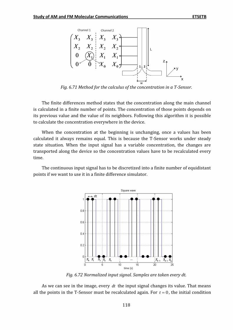
Study of AM and FM Molecular Communications ETSETB
118
Fig. 6.71 Method for the calculus of the concentration in a T-Sensor.
The finite differences method states that the concentration along the main channel
is calculated in a finite number of points. The concentration of those points depends on
its previous value and the value of its neighbors. Following this algorithm it is possible
to calculate the concentration everywhere in the device.
When the concentration at the beginning is unchanging, once a values has been
calculated it always remains equal. This is because the T-Sensor works under steady
state situation. When the input signal has a variable concentration, the changes are
transported along the device so the concentration values have to be recalculated every
time.
The continuous input signal has to be discretized into a finite number of equidistant
points if we want to use it in a finite difference simulator.
Fig. 6.72 Normalized input signal. Samples are taken every dt.
As we can see in the image, every dt the input signal changes its value. That means
all the points in the T-Sensor must be recalculated again. For 0t , the initial condition
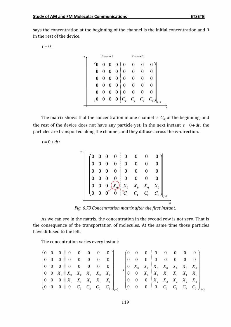
Study of AM and FM Molecular Communications ETSETB
119
says the concentration at the beginning of the channel is the initial concentration and 0
in the rest of the device.
0t :
The matrix shows that the concentration in one channel is 0C at the beginning, and
the rest of the device does not have any particle yet. In the next instant 0t dt , the
particles are transported along the channel, and they diffuse across the w-direction.
0t dt :
Fig. 6.73 Concentration matrix after the first instant.
As we can see in the matrix, the concentration in the second row is not zero. That is
the consequence of the transportation of molecules. At the same time those particles
have diffused to the left.
The concentration varies every instant:
0 0 0 0 0 0 0
0 1 1 1 1 10 0 0 0 0 0
2 2 2 2 21 1 1 1 1
3 3 3 32 2 2 2 2 3
0 0 0 0 0 0 0 00 0 0 0 0 0 0 0
0 0 0 0 0 0 0 00 0 0 0 0 0 0 0
00 0 0 0 0 0 0 0
0 00 0
0 0 00 0 0
0 0 0 00 0 0 0j j
X X X X X X X
X X X X X XX X X X X X
X X X X XX X X X X
C C C CC C C C
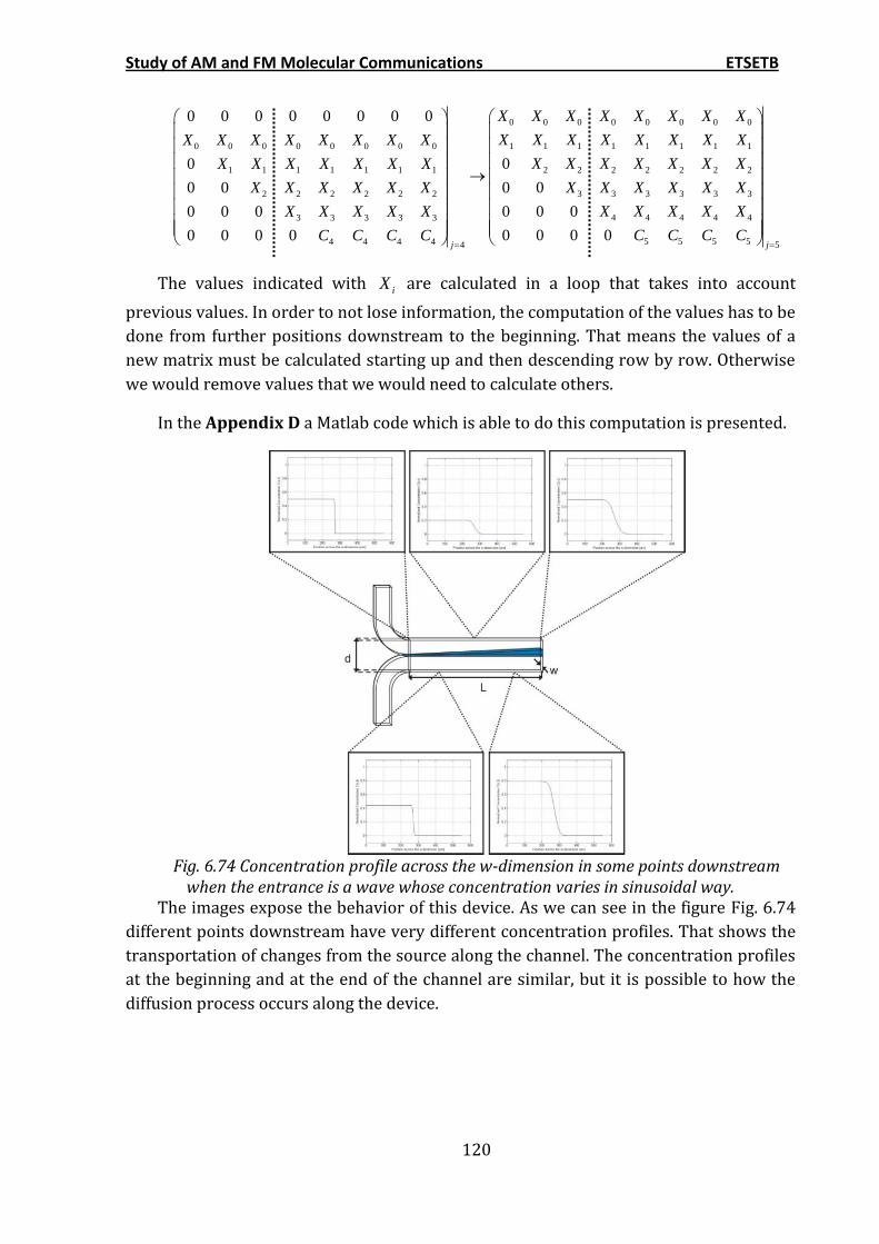
Study of AM and FM Molecular Communications ETSETB
120
0 0 0 0 0 0 0 0
1 1 1 1 1 1 1 10 0 0 0 0 0 0 0
2 2 2 2 2 2 21 1 1 1 1 1 1
3 3 3 3 3 32 2 2 2 2 2
4 4 4 4 43 3 3 3 3
5 5 5 54 4 4 4 4
0 0 0 0 0 0 0 0
00
0 00 0
0 0 00 0 0
0 0 0 00 0 0 0j
X X X X X X X X
X X X X X X X XX X X X X X X X
X X X X X X XX X X X X X X
X X X X X XX X X X X X
X X X X XX X X X X
C C C CC C C C
5j
The values indicated with iX are calculated in a loop that takes into account
previous values. In order to not lose information, the computation of the values has to be
done from further positions downstream to the beginning. That means the values of a
new matrix must be calculated starting up and then descending row by row. Otherwise
we would remove values that we would need to calculate others.
In the Appendix D a Matlab code which is able to do this computation is presented.
Fig. 6.74 Concentration profile across the w-dimension in some points downstream
when the entrance is a wave whose concentration varies in sinusoidal way. The images expose the behavior of this device. As we can see in the figure Fig. 6.74
different points downstream have very different concentration profiles. That shows the
transportation of changes from the source along the channel. The concentration profiles
at the beginning and at the end of the channel are similar, but it is possible to how the
diffusion process occurs along the device.
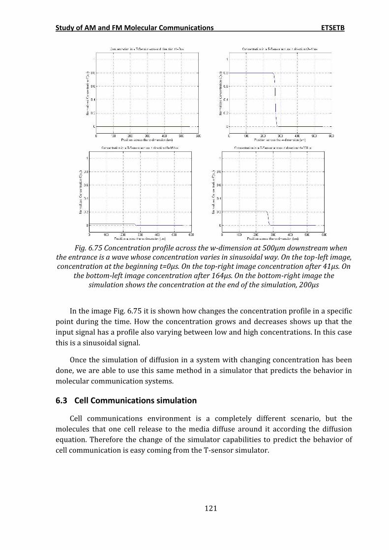
Study of AM and FM Molecular Communications ETSETB
121
Fig. 6.75 Concentration profile across the w-dimension at 500μm downstream when
the entrance is a wave whose concentration varies in sinusoidal way. On the top-left image, concentration at the beginning t=0μs. On the top-right image concentration after 41μs. On
the bottom-left image concentration after 164μs. On the bottom-right image the simulation shows the concentration at the end of the simulation, 200μs
In the image Fig. 6.75 it is shown how changes the concentration profile in a specific
point during the time. How the concentration grows and decreases shows up that the
input signal has a profile also varying between low and high concentrations. In this case
this is a sinusoidal signal.
Once the simulation of diffusion in a system with changing concentration has been
done, we are able to use this same method in a simulator that predicts the behavior in
molecular communication systems.
6.3 Cell Communications simulation
Cell communications environment is a completely different scenario, but the
molecules that one cell release to the media diffuse around it according the diffusion
equation. Therefore the change of the simulator capabilities to predict the behavior of
cell communication is easy coming from the T-sensor simulator.
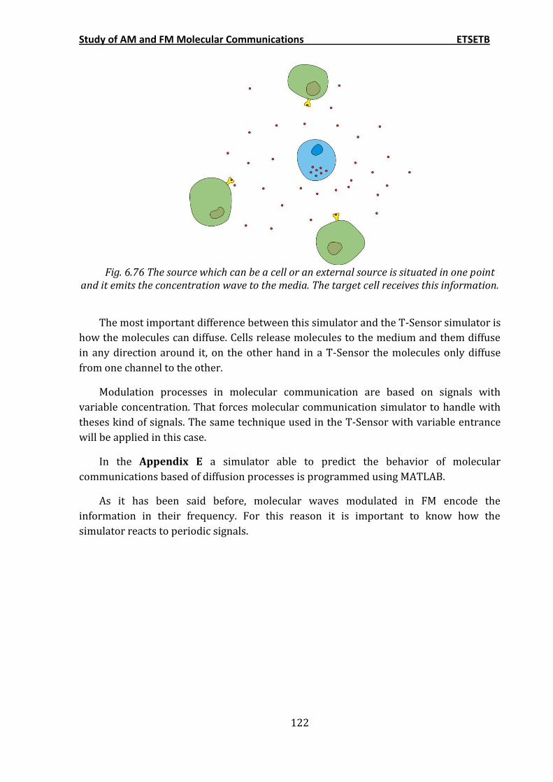
Study of AM and FM Molecular Communications ETSETB
122
Fig. 6.76 The source which can be a cell or an external source is situated in one point
and it emits the concentration wave to the media. The target cell receives this information.
The most important difference between this simulator and the T-Sensor simulator is
how the molecules can diffuse. Cells release molecules to the medium and them diffuse
in any direction around it, on the other hand in a T-Sensor the molecules only diffuse
from one channel to the other.
Modulation processes in molecular communication are based on signals with
variable concentration. That forces molecular communication simulator to handle with
theses kind of signals. The same technique used in the T-Sensor with variable entrance
will be applied in this case.
In the Appendix E a simulator able to predict the behavior of molecular
communications based of diffusion processes is programmed using MATLAB.
As it has been said before, molecular waves modulated in FM encode the
information in their frequency. For this reason it is important to know how the
simulator reacts to periodic signals.
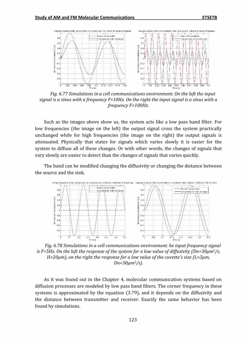
Study of AM and FM Molecular Communications ETSETB
123
Fig. 6.77 Simulations in a cell communications environment. On the left the input
signal is a sinus with a frequency F=10Hz. On the right the input signal is a sinus with a frequency F=100Hz.
Such as the images above show us, the system acts like a low pass band filter. For
low frequencies (the image on the left) the output signal cross the system practically
unchanged while for high frequencies (the image on the right) the output signals is
attenuated. Physically that states for signals which varies slowly it is easier for the
system to diffuse all of these changes. Or with other words, the changes of signals that
vary slowly are easier to detect than the changes of signals that varies quickly.
The band can be modified changing the diffusivity or changing the distance between
the source and the sink.
Fig. 6.78 Simulations in a cell communications environment. he input frequency signal
is F=5Hz. On the left the response of the system for a low value of diffusivity (Dn=30μm2/s, H=20μm), on the right the response for a low value of the cuvette's size (L=3μm,
Dn=30μm2/s).
As it was found out in the Chapter 4, molecular communication systems based on
diffusion processes are modeled by low pass band filters. The corner frequency in these
systems is approximated by the equation (3.79), and it depends on the diffusivity and
the distance between transmitter and receiver. Exactly the same behavior has been
found by simulations.
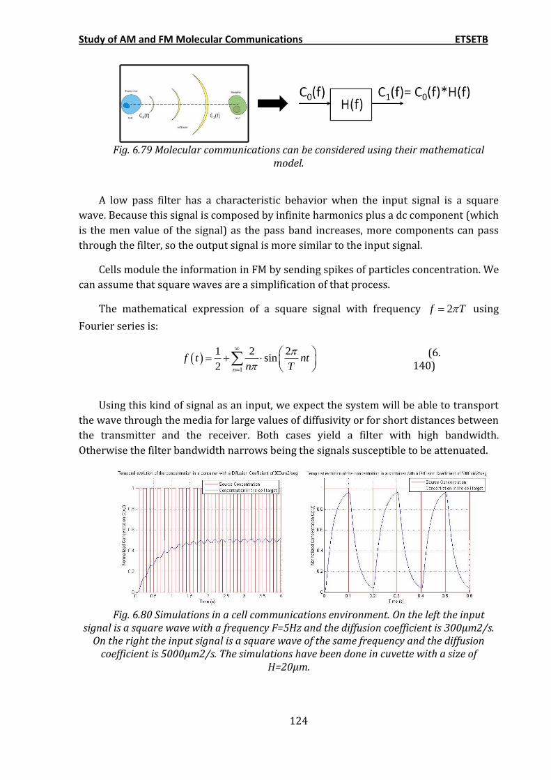
Study of AM and FM Molecular Communications ETSETB
124
Fig. 6.79 Molecular communications can be considered using their mathematical
model.
A low pass filter has a characteristic behavior when the input signal is a square
wave. Because this signal is composed by infinite harmonics plus a dc component (which
is the men value of the signal) as the pass band increases, more components can pass
through the filter, so the output signal is more similar to the input signal.
Cells module the information in FM by sending spikes of particles concentration. We
can assume that square waves are a simplification of that process.
The mathematical expression of a square signal with frequency 2f T using
Fourier series is:
1
1 2 2sin
2 n
f t ntn T
(6.
140)
Using this kind of signal as an input, we expect the system will be able to transport
the wave through the media for large values of diffusivity or for short distances between
the transmitter and the receiver. Both cases yield a filter with high bandwidth.
Otherwise the filter bandwidth narrows being the signals susceptible to be attenuated.
Fig. 6.80 Simulations in a cell communications environment. On the left the input
signal is a square wave with a frequency F=5Hz and the diffusion coefficient is 300µm2/s. On the right the input signal is a square wave of the same frequency and the diffusion
coefficient is 5000µm2/s. The simulations have been done in cuvette with a size of H=20μm.
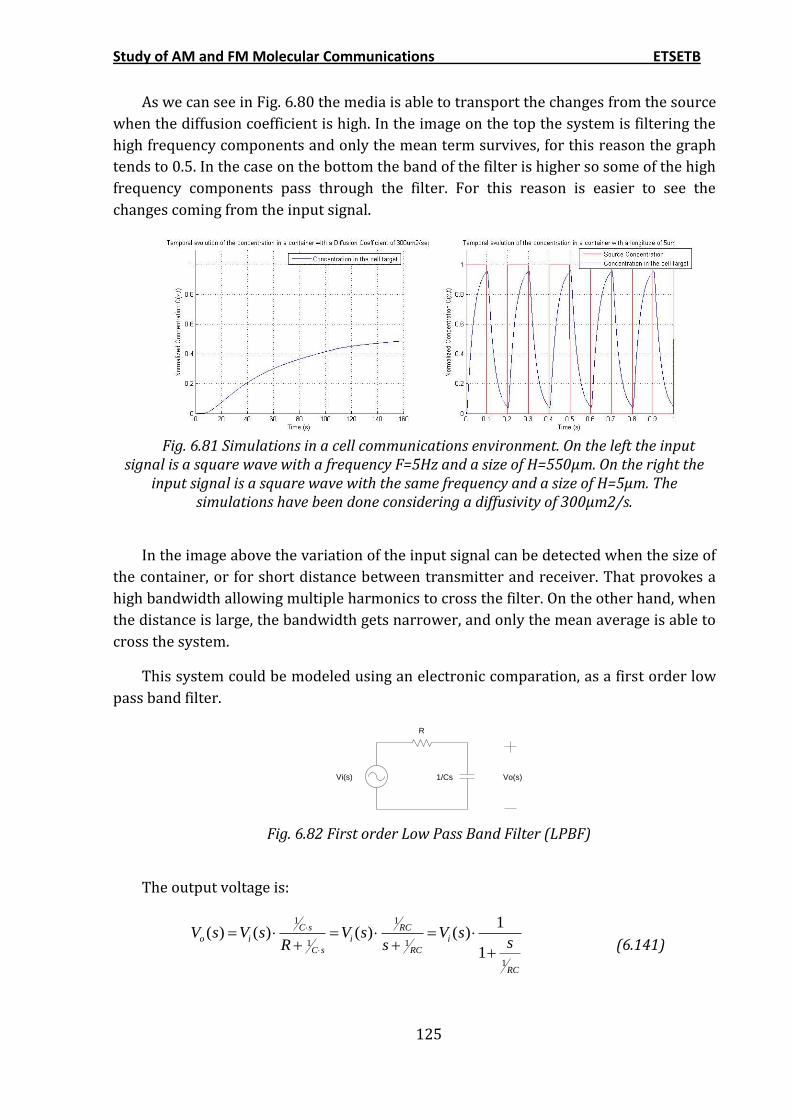
Study of AM and FM Molecular Communications ETSETB
125
As we can see in Fig. 6.80 the media is able to transport the changes from the source
when the diffusion coefficient is high. In the image on the top the system is filtering the
high frequency components and only the mean term survives, for this reason the graph
tends to 0.5. In the case on the bottom the band of the filter is higher so some of the high
frequency components pass through the filter. For this reason is easier to see the
changes coming from the input signal.
Fig. 6.81 Simulations in a cell communications environment. On the left the input
signal is a square wave with a frequency F=5Hz and a size of H=550µm. On the right the input signal is a square wave with the same frequency and a size of H=5µm. The
simulations have been done considering a diffusivity of 300µm2/s.
In the image above the variation of the input signal can be detected when the size of
the container, or for short distance between transmitter and receiver. That provokes a
high bandwidth allowing multiple harmonics to cross the filter. On the other hand, when
the distance is large, the bandwidth gets narrower, and only the mean average is able to
cross the system.
This system could be modeled using an electronic comparation, as a first order low
pass band filter.
R
1/CsVi(s) Vo(s)
Fig. 6.82 First order Low Pass Band Filter (LPBF)
The output voltage is:
1 1
1 1
1
1( ) ( ) ( ) ( )
1
C s RC
o i i i
C s RC
RC
V s V s V s V ssR s
(6.141)
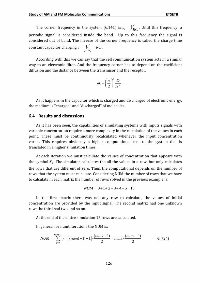
Study of AM and FM Molecular Communications ETSETB
126
The corner frequency in the system (6.141) is 1c RC
. Until this frequency, a
periodic signal is considered inside the band. Up to this frequency the signal is
considered out of band. The inverse of the corner frequency is called the charge time
constant capacitor charging 1c
RC
.
According with this we can say that the cell communication system acts in a similar
way to an electronic filter. And the frequency corner has to depend on the coefficient
diffusion and the distance between the transmisor and the receptor.
2
22c
D
H
As it happens in the capacitor which is charged and discharged of electronic energy,
the medium is "charged" and "discharged" of molecules.
6.4 Results and discussions
As it has been seen, the capabilities of simulating systems with inputs signals with
variable concentration require a more complexity in the calculation of the values in each
point. These must be continuously recalculated whenever the input concentration
varies. This requires obviously a higher computational cost to the system that is
translated in a higher simulation times.
At each iteration we must calculate the values of concentration that appears with
the symbol iX . The simulator calculates the all the values in a row, but only calculates
the rows that are different of zero. Thus, the computational depends on the number of
rows that the system must calculate. Considering NUM the number of rows that we have
to calculate in each matrix the number of rows solved in the previous example is:
0 1 2 3 4 5 15NUM
In the first matrix there was not any row to calculate, the values of initial
concentration are provided by the input signal. The second matrix had one unknown
row; the third had two and so on.
At the end of the entire simulation 15 rows are calculated.
In general for numt iterations the NUM is:
1
0
( 1) ( 1)( 1) 1
2 2
numt
j
numt numtNUM j numt numt
(6.142)
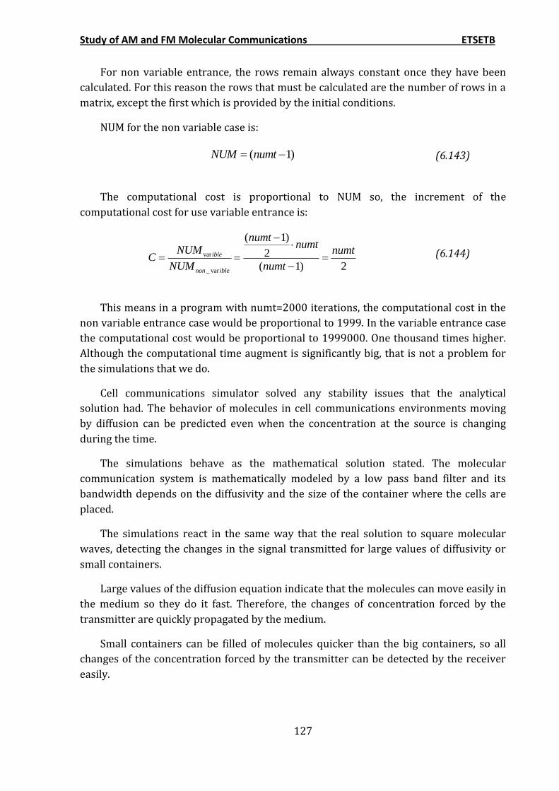
Study of AM and FM Molecular Communications ETSETB
127
For non variable entrance, the rows remain always constant once they have been
calculated. For this reason the rows that must be calculated are the number of rows in a
matrix, except the first which is provided by the initial conditions.
NUM for the non variable case is:
( 1)NUM numt (6.143)
The computational cost is proportional to NUM so, the increment of the
computational cost for use variable entrance is:
var
_ var
( 1)
2
( 1) 2
ible
non ible
numtnumt
NUM numtC
NUM numt
(6.144)
This means in a program with numt=2000 iterations, the computational cost in the
non variable entrance case would be proportional to 1999. In the variable entrance case
the computational cost would be proportional to 1999000. One thousand times higher.
Although the computational time augment is significantly big, that is not a problem for
the simulations that we do.
Cell communications simulator solved any stability issues that the analytical
solution had. The behavior of molecules in cell communications environments moving
by diffusion can be predicted even when the concentration at the source is changing
during the time.
The simulations behave as the mathematical solution stated. The molecular
communication system is mathematically modeled by a low pass band filter and its
bandwidth depends on the diffusivity and the size of the container where the cells are
placed.
The simulations react in the same way that the real solution to square molecular
waves, detecting the changes in the signal transmitted for large values of diffusivity or
small containers.
Large values of the diffusion equation indicate that the molecules can move easily in
the medium so they do it fast. Therefore, the changes of concentration forced by the
transmitter are quickly propagated by the medium.
Small containers can be filled of molecules quicker than the big containers, so all
changes of the concentration forced by the transmitter can be detected by the receiver
easily.
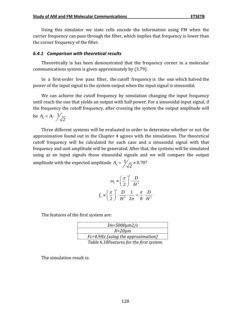
Study of AM and FM Molecular Communications ETSETB
128
Using this simulator we state cells encode the information using FM when the
carrier frequency can pass through the filter, which implies that frequency is lower than
the corner frequency of the filter.
6.4.1 Comparison with theoretical results
Theoretically is has been demonstrated that the frequency corner in a molecular
communications system is given approximately by (3.79).
In a first-order low pass filter, the cutoff frequency is the one which halved the
power of the input signal to the system output when the input signal is sinusoidal.
We can achieve the cutoff frequency by simulation changing the input frequency
until reach the one that yields an output with half power. For a sinusoidal input signal, if
the frequency the cutoff frequency, after crossing the system the output amplitude will
be 12
o iA A
Three different systems will be evaluated in order to determine whether or not the
approximation found out in the Chapter 4 agrees with the simulations. The theoretical
cutoff frequency will be calculated for each case and a sinusoidal signal with that
frequency and unit amplitude will be generated. After that, the systems will be simulated
using as an input signals those sinusoidal signals and we will compare the output
amplitude with the expected amplitude 1 0.7072
oA
2
22c
D
H
2
2 2
1
2 2 8c
D Df
H H
The features of the first system are:
Dn=5000µm2/s H=20µm
Fc=4.9Hz (using the approximation) Table 6.18Features for the first system.
The simulation result is:
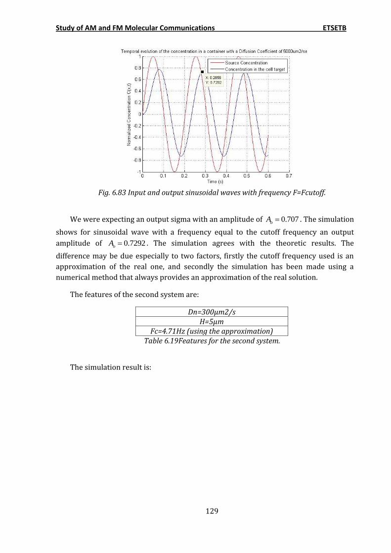
Study of AM and FM Molecular Communications ETSETB
129
Fig. 6.83 Input and output sinusoidal waves with frequency F=Fcutoff.
We were expecting an output sigma with an amplitude of 0.707oA . The simulation
shows for sinusoidal wave with a frequency equal to the cutoff frequency an output
amplitude of 0.7292oA . The simulation agrees with the theoretic results. The
difference may be due especially to two factors, firstly the cutoff frequency used is an
approximation of the real one, and secondly the simulation has been made using a
numerical method that always provides an approximation of the real solution.
The features of the second system are:
Dn=300µm2/s H=5µm
Fc=4.71Hz (using the approximation) Table 6.19Features for the second system.
The simulation result is:
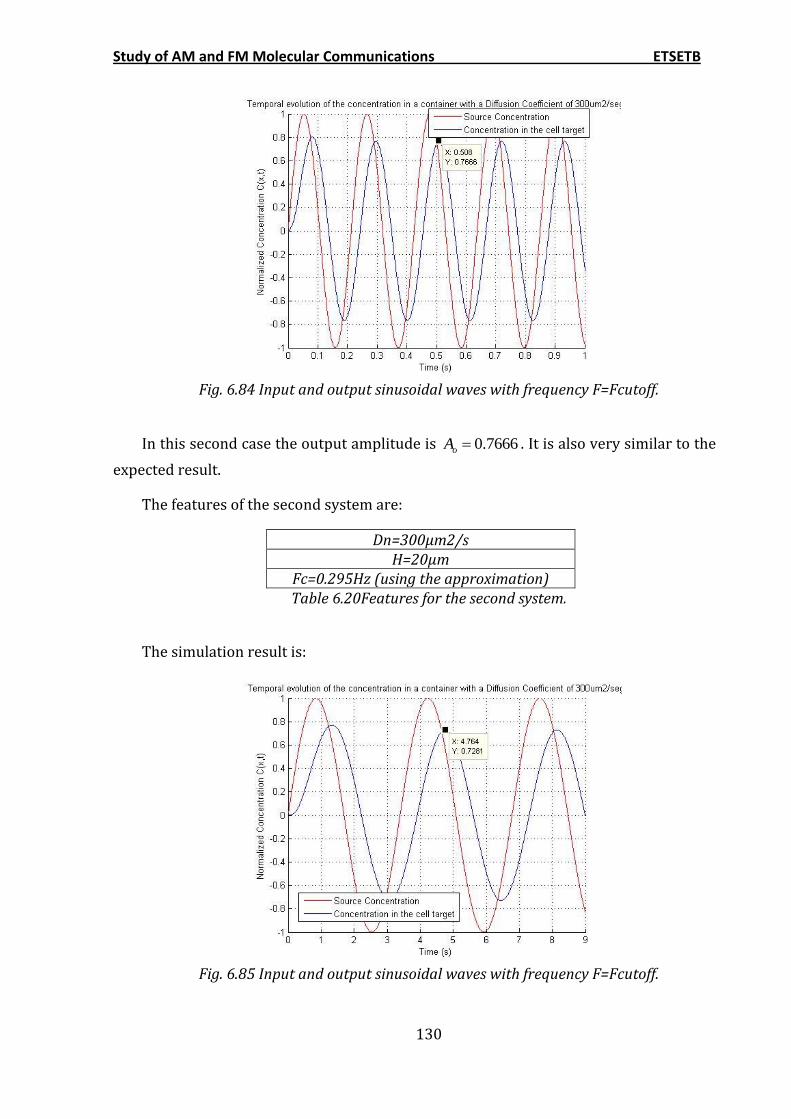
Study of AM and FM Molecular Communications ETSETB
130
Fig. 6.84 Input and output sinusoidal waves with frequency F=Fcutoff.
In this second case the output amplitude is 0.7666oA . It is also very similar to the
expected result.
The features of the second system are:
Dn=300µm2/s H=20µm
Fc=0.295Hz (using the approximation) Table 6.20Features for the second system.
The simulation result is:
Fig. 6.85 Input and output sinusoidal waves with frequency F=Fcutoff.
Study of AM and FM Molecular Communications ETSETB
131
One more time the simulation agrees with the theoretical results.
The values of the corner frequency were obtained by simulation searching what
values gave the exact output amplitude 0 0.707A .
The next table shows the comparison of the theoretical and simulated values of the
cutoff frequency:
System Theoretic Frequency
(Hz) Simulated Frequency
(Hz) 1 4.9 5.22 2 4.71 5.1 3 0.295 0.315
Table 6.21 Comparison of the theoretical and simulated values of the corner frequency in the three systems
The results here presented demonstrate the value of the frequency corner can be
calculated either by using the molecular communication simulator or using the
analytical solution. This cutoff frequency can be used as the threshold that determines if
the information must be encoded amplitude or frequency modulation.
A simple formula for this parameter is given by the equation (3.79) which has been
obtained by the resolution of the diffusion equation in a cellular environment. That
solution provides practical information of how molecular communication systems work,
but it is not useful to achieve a prediction of the concentration in the whole system. In
these cases the simulator here presented provides a stable solution that approximates
the reality with veracity.

Study of AM and FM Molecular Communications ETSETB
132
7 CONCLUSIONS

Study of AM and FM Molecular Communications ETSETB
133
Study of AM and FM Molecular Communications ETSETB
134
Communication at nanometric scale is one of the challenges in the near future and
molecular communication is considered the most promising option for this matter.
In this project it has been modeled a molecular communication system base on
diffusion processes of particles. One of the contributions of this work is obtaining a
parameter that allows us to decide if the information should be encoded using amplitude
or frequency modulation.
To achieve this goal, it started from the Fick’s second law, and it was particularized
to a specific case of molecular communications. The transmitter sent a variable
concentration wave with a square shape to the receptor, and applying the needed
boundary conditions the system was solved finding an analytical solution. This model
describes the behavior of the molecular communication systems according to their
physical parameters, the diffusivity and the distance between transmitter and receiver.
The model that was obtained presented in Chapter 3 by the equations (3.58) and
(3.71), shows a system that behaves as a first order low pass band filter whose cutoff
frequency is approximately described by the equation (3.79). The pass band of this filter
depends on the diffusion coefficient of the diffusing molecule and the dimensions of the
container of the fluidic medium.
In Chapter 3 is demonstrated that this model presents instabilities under certain
conditions, so even providing a qualitative explanation of the behavior of such systems,
it is useless to describe the communication process in the whole system. To solve this
issue it was decided to program a simulator that provided an approximate numerical
solution of this process. The combination of the analytical model and the simulator
becomes a powerful tool to describe and understand molecular communication systems.
Before programming this simulator a microfluidic device called T-SENSOR, whose
operating principle is based on the same process of diffusion of particles, was fabricated.
With this system the diffusion process was studied in a practical way, and experimental
results were got in order to validate the simulator programmed using numerical
methods. The device was fabricated using a new process known as “Scotch Tape
Patterned Method” that presents the same features as the methods based on lithography
being much more inexpensive and simple. It was found that this method is useful until
sizes that can be treated with bench top tools, around 300 μm.
In order to determine whether or not numerical methods based on finite differences
achieved a reliable approximation of particles diffusion processes, such as molecular
communication systems, firstly a T-SENSOR simulator was programmed. We obtained 1-
dimensional and 2-dimensional simulators, providing more information about the
diffusion the second one. But the longer computation time made us to decide that the 1-
dimensional simulator was more useful for our purposes. This simulator was validated
with theoretical and experimental results that we got in the experiments performed
with the microfluidic device.
Study of AM and FM Molecular Communications ETSETB
135
Once the diffusion of particles was studied using the T-SENSOR simulator, the
possibility to add the capability of simulating systems with variable concentration input
signals was studied. This is what happens in cellular communications, and the T-SENSOR
simulator did not reflect this possibility. This new capability adds a strong
computational workload to the simulator, but it does not affect to the simulations done
in this work. So, the T-SENSOR simulator was extended to a simulator with variable
concentration signals and the behavior under this situation was studied. A continuous
change of concentration was observed in these systems, being transported all changes
from the beginning of the channel to the outlet.
The molecular communications simulator was programmed from the T-SENSOR
simulator with variable concentration inputs. With this simulator the instability issues
that the analytical solution are solved, besides exposing the system to all types of inputs
with variable concentration is possible without having the recalculate the model for
each entrance.
Using this simulator the value of the cutoff frequency found in Chapter 3 was
proven, and it was established this parameter as a decision criterion to choose the type
of modulation. Assuming that the information is encoded using FM when is possible, due
to the advantages that this modulation presents over AM, the cutoff frequency
establishes a decision threshold of the kind of modulation. As long as the frequency of
the carrier signal is able to cross the filter without being filtered the information will be
modulated using FM, otherwise it will be modulated using AM. This, we state that the
decision of the way of modulation is determined by the physical parameter of diffusivity
and the dimensions of the container of the fluidic medium.
With this decision threshold can be understood why ions of calcium are used as
information carriers in FM modulation in cell communications. Information (changes in
the concentration of molecules secreted by the cell) can be modulated using FM for large
values of the diffusion coefficient, which result in a larger cutoff frequency. The diffusion
coefficient is a function of the size of the carrier molecule and therefore, one would
expect larger cutoff frequencies for smaller molecules, such as Ca2+.
Information can also be modulated using FM when diffusion occurs in small
containers, which yields higher cutoff frequencies. This may be the reason why FM
modulation of Ca2+ has been found in intracellular communications. A common size of a
cell is around 10 μm, subtracting the volume of the nucleolus and the organelles; the size
of this container is a few microns which agree with the simulations presented in Chapter
6.
At the beginning, the aim of this work was to achieve a mathematical model that
described the behavior of molecular communications based on diffusion processes, as
well as establishing a threshold able to differentiate when the encoding should be done
using amplitude or frequency modulation. At the end we can conclude that the analytical
model with the simulator based on numerical methods provide a sturdy model of the

Study of AM and FM Molecular Communications ETSETB
136
behavior of these communications. In the same way, it has succeeded providing a
criterion that depends on the physical parameters that allow us to understand different
events in nature, such as the reason of using ions of calcium as molecular carriers of
information and the reason why the FM modulation usually occurs in intra-cell
communications.

Study of AM and FM Molecular Communications ETSETB
137
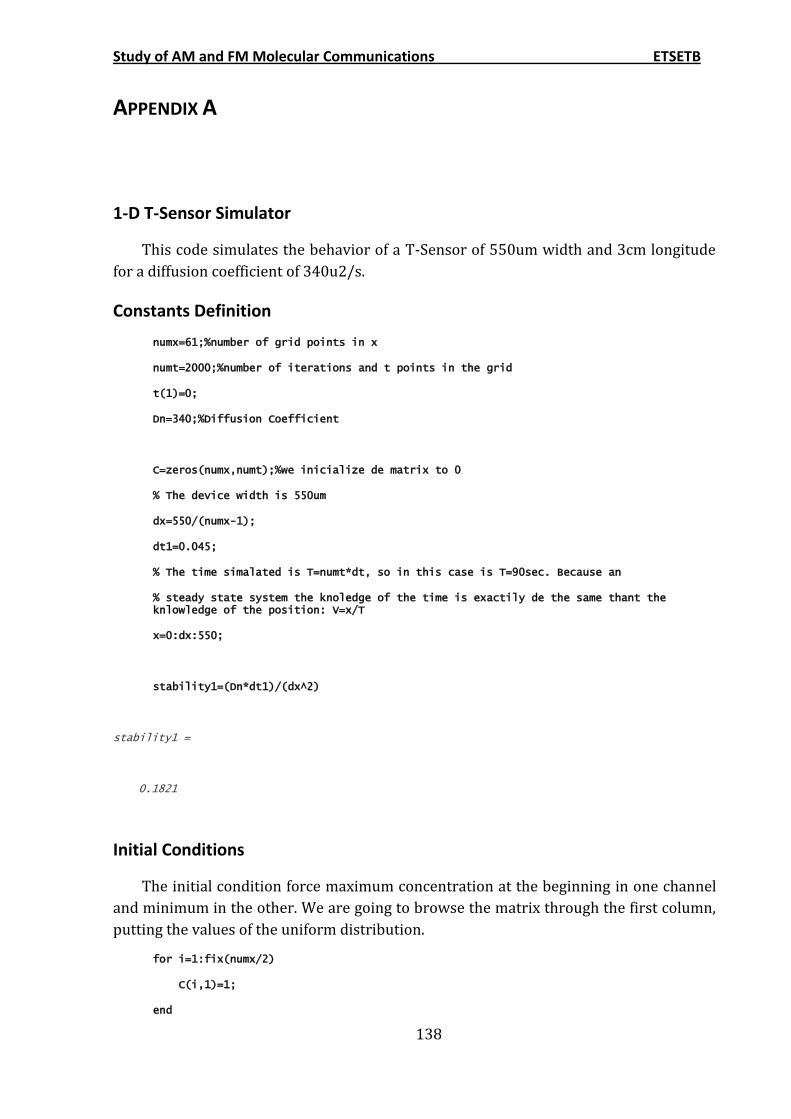
Study of AM and FM Molecular Communications ETSETB
138
APPENDIX A
1-D T-Sensor Simulator
This code simulates the behavior of a T-Sensor of 550um width and 3cm longitude
for a diffusion coefficient of 340u2/s.
Constants Definition
numx=61;%number of grid points in x
numt=2000;%number of iterations and t points in the grid
t(1)=0;
Dn=340;%Diffusion Coefficient
C=zeros(numx,numt);%we inicialize de matrix to 0
% The device width is 550um
dx=550/(numx-1);
dt1=0.045;
% The time simalated is T=numt*dt, so in this case is T=90sec. Because an
% steady state system the knoledge of the time is exactily de the same thant the knlowledge of the position: V=x/T
x=0:dx:550;
stability1=(Dn*dt1)/(dx^2)
stability1 =
0.1821
Initial Conditions
The initial condition force maximum concentration at the beginning in one channel
and minimum in the other. We are going to browse the matrix through the first column,
putting the values of the uniform distribution.
for i=1:fix(numx/2)
C(i,1)=1;
end
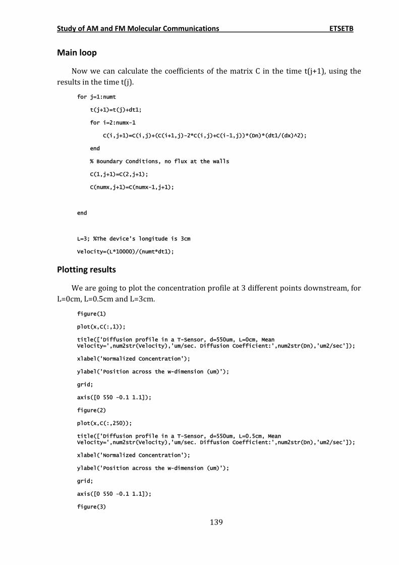
Study of AM and FM Molecular Communications ETSETB
139
Main loop
Now we can calculate the coefficients of the matrix C in the time t(j+1), using the
results in the time t(j).
for j=1:numt
t(j+1)=t(j)+dt1;
for i=2:numx-1
C(i,j+1)=C(i,j)+(C(i+1,j)-2*C(i,j)+C(i-1,j))*(Dn)*(dt1/(dx)^2);
end
% Boundary Conditions, no flux at the walls
C(1,j+1)=C(2,j+1);
C(numx,j+1)=C(numx-1,j+1);
end
L=3; %The device's longitude is 3cm
Velocity=(L*10000)/(numt*dt1);
Plotting results
We are going to plot the concentration profile at 3 different points downstream, for
L=0cm, L=0.5cm and L=3cm.
figure(1)
plot(x,C(:,1));
title(['Diffusion profile in a T-Sensor, d=550um, L=0cm, Mean Velocity=',num2str(Velocity),'um/sec. Diffusion Coefficient:',num2str(Dn),'um2/sec']);
xlabel('Normalized Concentration');
ylabel('Position across the w-dimension (um)');
grid;
axis([0 550 -0.1 1.1]);
figure(2)
plot(x,C(:,250));
title(['Diffusion profile in a T-Sensor, d=550um, L=0.5cm, Mean Velocity=',num2str(Velocity),'um/sec. Diffusion Coefficient:',num2str(Dn),'um2/sec']);
xlabel('Normalized Concentration');
ylabel('Position across the w-dimension (um)');
grid;
axis([0 550 -0.1 1.1]);
figure(3)
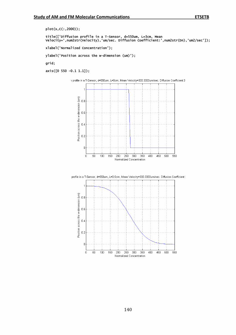
Study of AM and FM Molecular Communications ETSETB
140
plot(x,C(:,2000));
title(['Diffusion profile in a T-Sensor, d=550um, L=3cm, Mean Velocity=',num2str(Velocity),'um/sec. Diffusion Coefficient:',num2str(Dn),'um2/sec']);
xlabel('Normalized Concentration');
ylabel('Position across the w-dimension (um)');
grid;
axis([0 550 -0.1 1.1]);
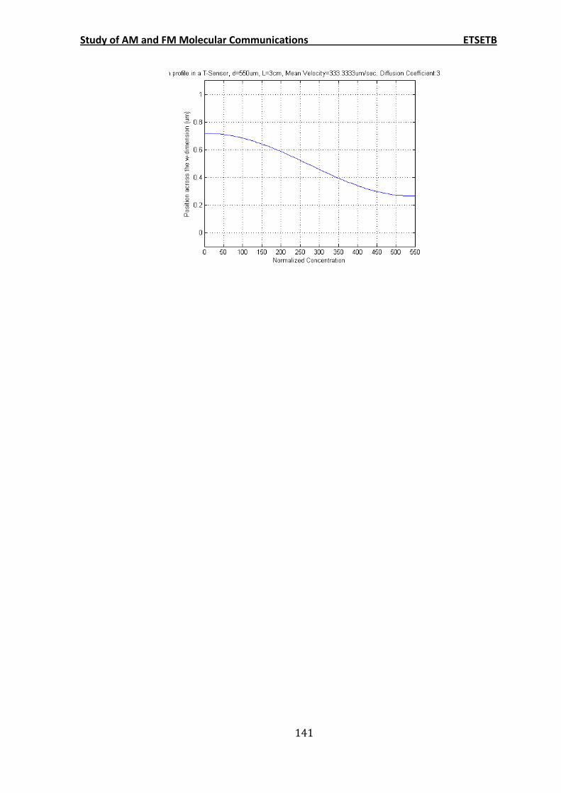
Study of AM and FM Molecular Communications ETSETB
141
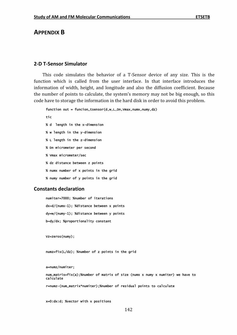
Study of AM and FM Molecular Communications ETSETB
142
APPENDIX B
2-D T-Sensor Simulator
This code simulates the behavior of a T-Sensor device of any size. This is the
function which is called from the user interface. In that interface introduces the
information of width, height, and longitude and also the diffusion coefficient. Because
the number of points to calculate, the system’s memory may not be big enough, so this
code have to storage the information in the hard disk in order to avoid this problem.
function out = funcion_tsensor(d,w,L,Dn,Vmax,numx,numy,dz)
tic
% d length in the x-dimension
% w length in the y-dimension
% L length in the z-dimension
% Dn micrometer per second
% Vmax micrometer/sec
% dz distance between z points
% numx number of x points in the grid
% numy number of y points in the grid
Constants declaration
numiter=7000; %number of iterations
dx=d/(numx-1); %distance between x points
dy=w/(numy-1); %distance between y points
b=dy/dx; %proportionality constant
Vz=zeros(numy);
numz=fix(L/dz); %number of z points in the grid
a=numz/numiter;
num_matrix=fix(a);%number of matrix of size (numx x numy x numiter) we have to calculate
r=numz-(num_matrix*numiter);%number of residual points to calculate
x=0:dx:d; %vector with x positions
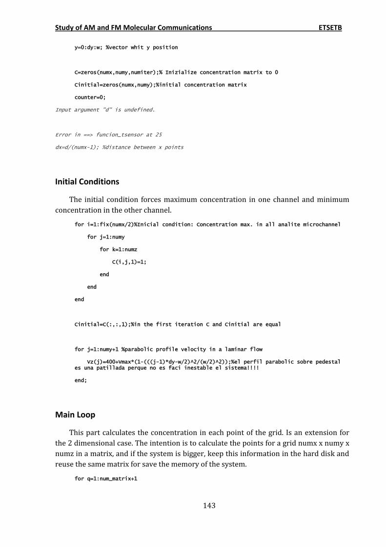
Study of AM and FM Molecular Communications ETSETB
143
y=0:dy:w; %vector whit y position
C=zeros(numx,numy,numiter);% Inizialize concentration matrix to 0
Cinitial=zeros(numx,numy);%initial concentration matrix
counter=0;
Input argument "d" is undefined.
Error in ==> funcion_tsensor at 25
dx=d/(numx-1); %distance between x points
Initial Conditions
The initial condition forces maximum concentration in one channel and minimum
concentration in the other channel.
for i=1:fix(numx/2)%Inicial condition: Concentration max. in all analite microchannel
for j=1:numy
for k=1:numz
C(i,j,1)=1;
end
end
end
Cinitial=C(:,:,1);%in the first iteration C and Cinitial are equal
for j=1:numy+1 %parabolic profile velocity in a laminar flow
Vz(j)=400+Vmax*(1-(((j-1)*dy-w/2)^2/(w/2)^2));%el perfil parabolic sobre pedestal es una patillada perque no es faci inestable el sistema!!!!
end;
Main Loop
This part calculates the concentration in each point of the grid. Is an extension for
the 2 dimensional case. The intention is to calculate the points for a grid numx x numy x
numz in a matrix, and if the system is bigger, keep this information in the hard disk and
reuse the same matrix for save the memory of the system.
for q=1:num_matrix+1
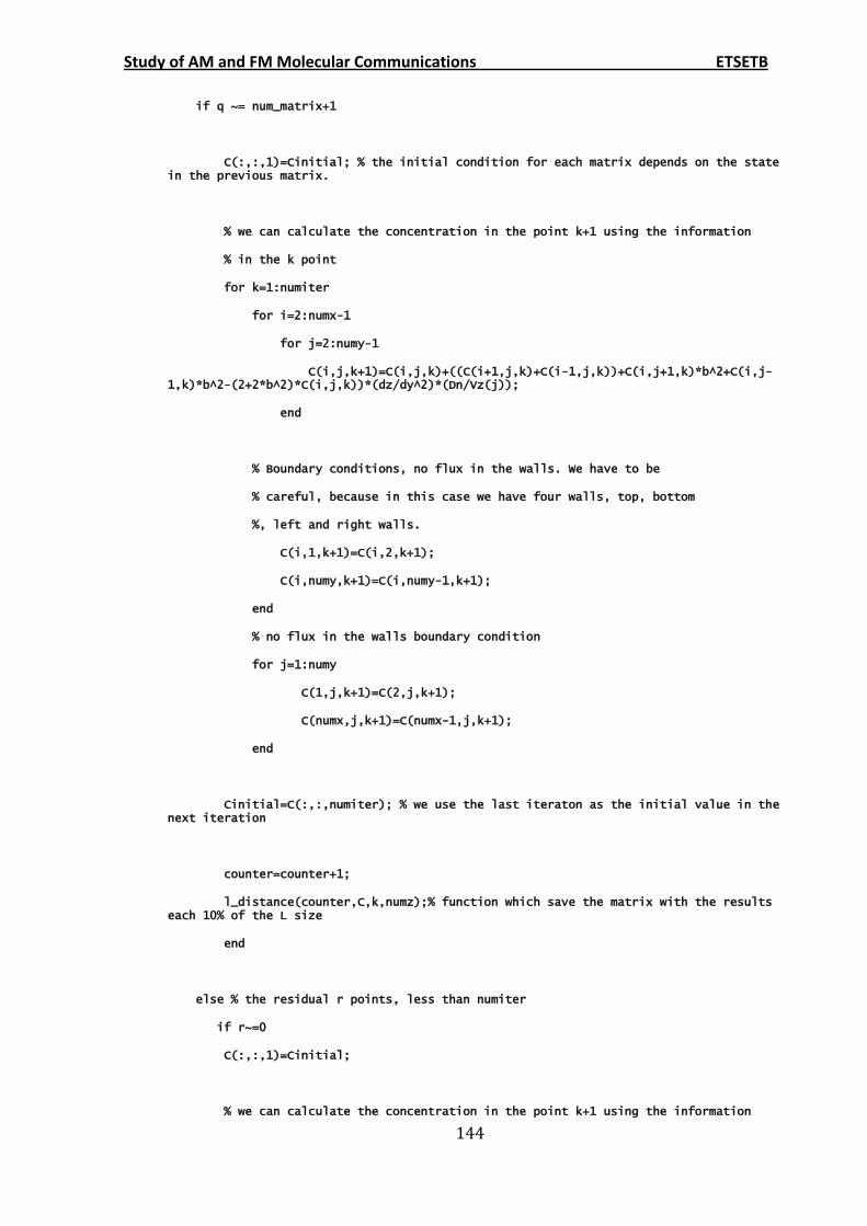
Study of AM and FM Molecular Communications ETSETB
144
if q ~= num_matrix+1
C(:,:,1)=Cinitial; % the initial condition for each matrix depends on the state in the previous matrix.
% we can calculate the concentration in the point k+1 using the information
% in the k point
for k=1:numiter
for i=2:numx-1
for j=2:numy-1
C(i,j,k+1)=C(i,j,k)+((C(i+1,j,k)+C(i-1,j,k))+C(i,j+1,k)*b^2+C(i,j-1,k)*b^2-(2+2*b^2)*C(i,j,k))*(dz/dy^2)*(Dn/Vz(j));
end
% Boundary conditions, no flux in the walls. We have to be
% careful, because in this case we have four walls, top, bottom
%, left and right walls.
C(i,1,k+1)=C(i,2,k+1);
C(i,numy,k+1)=C(i,numy-1,k+1);
end
% no flux in the walls boundary condition
for j=1:numy
C(1,j,k+1)=C(2,j,k+1);
C(numx,j,k+1)=C(numx-1,j,k+1);
end
Cinitial=C(:,:,numiter); % we use the last iteraton as the initial value in the next iteration
counter=counter+1;
l_distance(counter,C,k,numz);% function which save the matrix with the results each 10% of the L size
end
else % the residual r points, less than numiter
if r~=0
C(:,:,1)=Cinitial;
% we can calculate the concentration in the point k+1 using the information
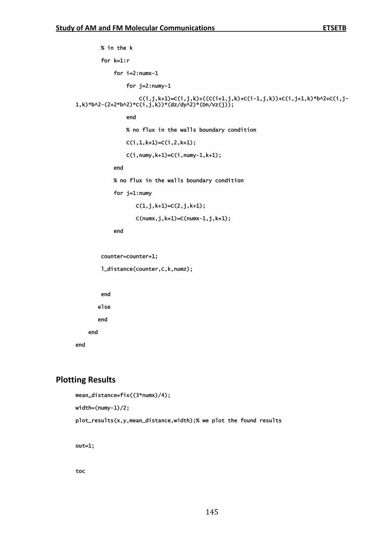
Study of AM and FM Molecular Communications ETSETB
145
% in the k
for k=1:r
for i=2:numx-1
for j=2:numy-1
C(i,j,k+1)=C(i,j,k)+((C(i+1,j,k)+C(i-1,j,k))+C(i,j+1,k)*b^2+C(i,j-1,k)*b^2-(2+2*b^2)*C(i,j,k))*(dz/dy^2)*(Dn/Vz(j));
end
% no flux in the walls boundary condition
C(i,1,k+1)=C(i,2,k+1);
C(i,numy,k+1)=C(i,numy-1,k+1);
end
% no flux in the walls boundary condition
for j=1:numy
C(1,j,k+1)=C(2,j,k+1);
C(numx,j,k+1)=C(numx-1,j,k+1);
end
counter=counter+1;
l_distance(counter,C,k,numz);
end
else
end
end
end
Plotting Results
mean_distance=fix((3*numx)/4);
width=(numy-1)/2;
plot_results(x,y,mean_distance,width);% we plot the found results
out=1;
toc
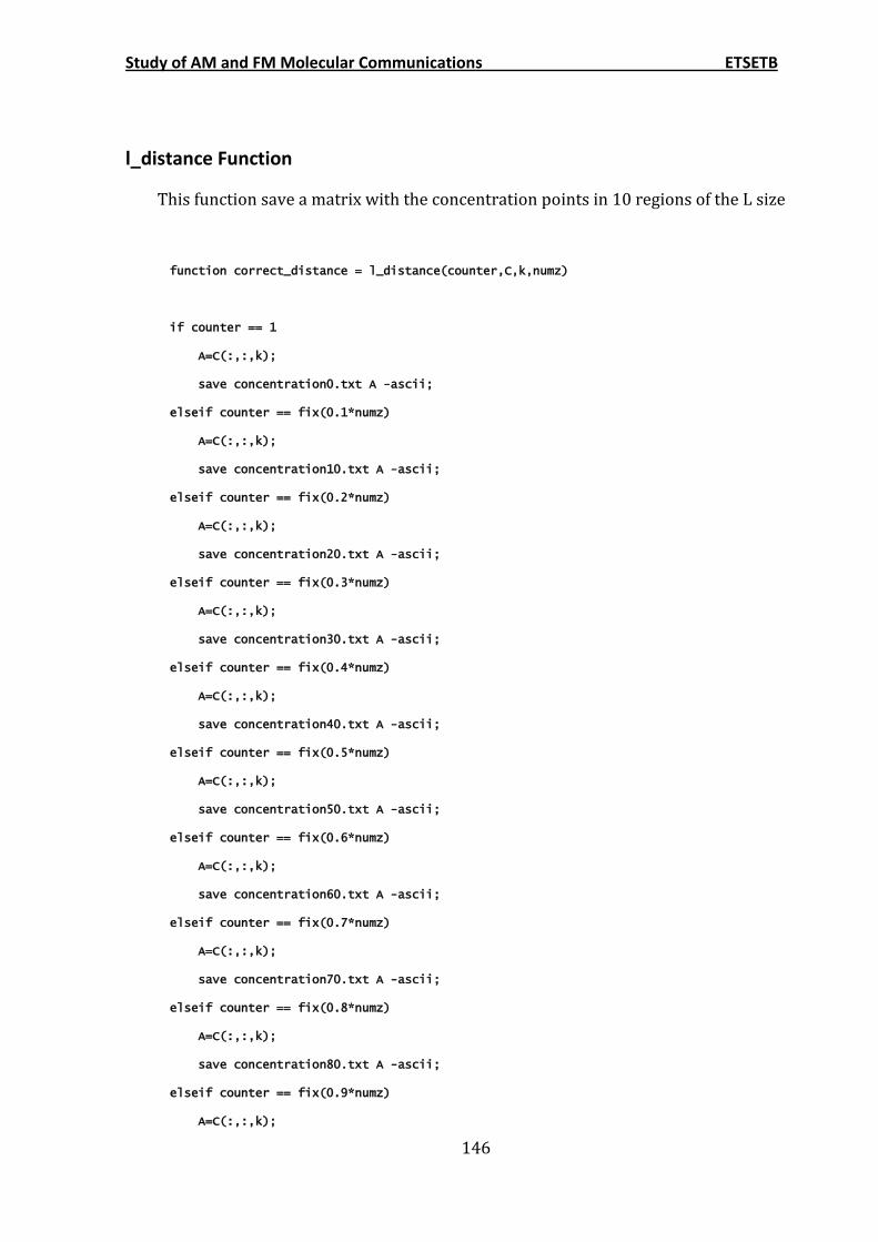
Study of AM and FM Molecular Communications ETSETB
146
l_distance Function
This function save a matrix with the concentration points in 10 regions of the L size
function correct_distance = l_distance(counter,C,k,numz)
if counter == 1
A=C(:,:,k);
save concentration0.txt A -ascii;
elseif counter == fix(0.1*numz)
A=C(:,:,k);
save concentration10.txt A -ascii;
elseif counter == fix(0.2*numz)
A=C(:,:,k);
save concentration20.txt A -ascii;
elseif counter == fix(0.3*numz)
A=C(:,:,k);
save concentration30.txt A -ascii;
elseif counter == fix(0.4*numz)
A=C(:,:,k);
save concentration40.txt A -ascii;
elseif counter == fix(0.5*numz)
A=C(:,:,k);
save concentration50.txt A -ascii;
elseif counter == fix(0.6*numz)
A=C(:,:,k);
save concentration60.txt A -ascii;
elseif counter == fix(0.7*numz)
A=C(:,:,k);
save concentration70.txt A -ascii;
elseif counter == fix(0.8*numz)
A=C(:,:,k);
save concentration80.txt A -ascii;
elseif counter == fix(0.9*numz)
A=C(:,:,k);
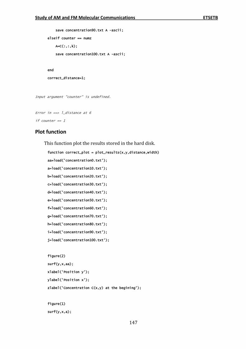
Study of AM and FM Molecular Communications ETSETB
147
save concentration90.txt A -ascii;
elseif counter == numz
A=C(:,:,k);
save concentration100.txt A -ascii;
end
correct_distance=1;
Input argument "counter" is undefined.
Error in ==> l_distance at 6
if counter == 1
Plot function
This function plot the results stored in the hard disk.
function correct_plot = plot_results(x,y,distance,width)
aa=load('concentration0.txt');
a=load('concentration10.txt');
b=load('concentration20.txt');
c=load('concentration30.txt');
d=load('concentration40.txt');
e=load('concentration50.txt');
f=load('concentration60.txt');
g=load('concentration70.txt');
h=load('concentration80.txt');
i=load('concentration90.txt');
j=load('concentration100.txt');
figure(2)
surf(y,x,aa);
xlabel('Position y');
ylabel('Position x');
zlabel('Concentration C(x,y) at the begining');
figure(1)
surf(y,x,a);
Study of AM and FM Molecular Communications ETSETB
148
xlabel('Position y');
ylabel('Position x');
zlabel('Concentration C(x,y) at the end');
% figure(3)
% surf(y,x,b);
% xlabel('Position y');
% ylabel('Position x');
% zlabel('Concentration C(x,y) in 20% of L');
%
% figure(4)
% surf(y,x,e);
% xlabel('Position y');
% ylabel('Position x');
% zlabel('Concentration C(x,y) in 50% of L');
%
% figure(5)
% surf(y,x,h);
% xlabel('Position y');
% ylabel('Position x');
% zlabel('Concentration C(x,y) in 80% of L');
%
% figure(6)
% surf(y,x,j);
% xlabel('Position y');
% ylabel('Position x');
% zlabel('Concentration C(x,y) in 100% of L');
%
% figure(7)
% title('Diffusion in d dimension');
% hold on
% plot(x,a(:,width),'b');
% plot(x,b(:,width),'r');
% plot(x,c(:,width),'r');
% plot(x,d(:,width),'r');
% plot(x,e(:,width),'r');
% plot(x,f(:,width),'r');

Study of AM and FM Molecular Communications ETSETB
149
% plot(x,g(:,width),'r');
% plot(x,h(:,width),'r');
% plot(x,i(:,width),'r');
% plot(x,j(:,width),'b');
% xlabel('Position x');
% ylabel('Concentration C(x)');
correct_plot=1;

Study of AM and FM Molecular Communications ETSETB
150
APPENDIX C
Image processing
This code pretends to extract the concentration profile from a .jpg image and
compare this profile with the theoretical in order to find what the best diffusion
coefficient is
Get image
[name,path]=uigetfile('*.jpg','Select the input JPG file');
fullname=strcat(path,name)
image2=imread(fullname);
image=rgb2gray(image2);
image=double(image);
[row,col]=size(image);
fullname =
D:\Lab\Probes imatges\Tratamiento de las imagenes del microscopio\20nlsec\15mm.jpg
Diffusion coefficient
%The key is to change this value until find the theretical caoncentration
%which most agree with the experimental results
Dn=200;
Obtaining the concentration information from the image
I take 10 random columns from the image and I extract the light intensity from each
pixel. Then I average the 10 different curves.
pixel=1:1:row;
pixel=pixel';
for i=1:10
x1(i)=random('unid',col);

Study of AM and FM Molecular Communications ETSETB
151
end
X=zeros(row,10);
for i=1:10
X(:,i)=image(:,x1(i));
end
A=zeros(row,1);
for j=1:row
for i=1:10
A(j)=A(j)+X(j,i);
end
end
A=A/10;
The calculus of the max and min average for normalize the curve
In order to normalize the concentration profile, the maximum and the minimum
values are obtained averaging the first points, where the curve has a maximum value
and the lasts points where the concentration is minimum.
%Firstly a manual way to do that for any imatge it is shown.
% plot(pixel,A);
%
% msgbox('Insert in the prompt in the pixels at max concetration','Max concentration','help');
% start1=input('First Pixel: ');
% start2=input('Second Pixel: ');
% msgbox('Insert in the prompt in the pixels at min concetration','Min Concentration','help');
% eend1=input('First pixel: ');
% eend2=input('Second pixel: ');
% But for the images used in this work all of those point have been found
% and they are the following
% 1mm
Study of AM and FM Molecular Communications ETSETB
152
% start1=240;
% start2=300;
% eend1=685;
% eend2=1040;
% position=1;
% limit=236;
% %5mm
% start1=193;
% start2=313;
% eend1=701;
% eend2=1040;
% position=5;
% limit=260;
% %10mm
% start1=208;
% start2=252;
% eend1=712;
% eend2=1040;
% position=10;
% limit=268;
%15mm
start1=215;
start2=261;
eend1=721;
eend2=1040;
position=15;
limit=266;
% %20mm
% start1=197;
% start2=256;
% eend1=729;
% eend2=1040;
% position=20;
Study of AM and FM Molecular Communications ETSETB
153
% limit=271;
%25mm
% start1=241;
% start2=248;
% eend1=741;
% eend2=1040;
% position=25;
% limit=262;
% %30mm
% start1=280;
% start2=310;
% eend1=745;
% eend2=1040;
% position=30;
% limit=247;
% minavg=mean(A(eend1:eend2));
% B=A-(minavg);
% maxavg=mean(B(start1:start2));
% B=B/maxavg;
% plot(pixel,B);
Theoretical profile
“tensor” is the function which calculates the theoretical concentration curve. It
returns the maximum and the minimum concentration value because they are needed to
normalize the concentration profile coming from the image.
[inipoint endpoint]=tsensor(Dn,position);
% This is true only in the cases when the concentration at the walls are 1
% or 0. As the boundary conditions permit this no happen always, sometime a
% correction in the normalization is required. The values at the walls can
% be found using the simulator.
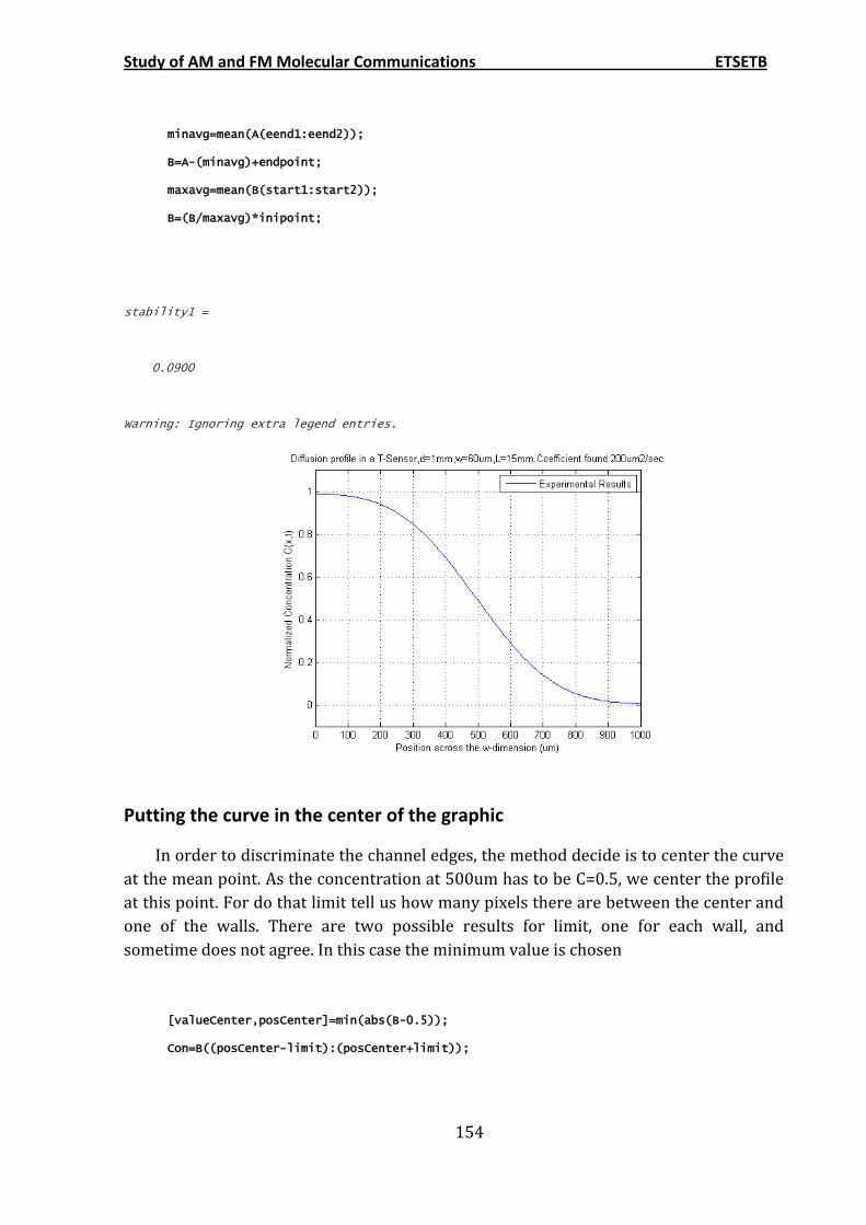
Study of AM and FM Molecular Communications ETSETB
154
minavg=mean(A(eend1:eend2));
B=A-(minavg)+endpoint;
maxavg=mean(B(start1:start2));
B=(B/maxavg)*inipoint;
stability1 =
0.0900
Warning: Ignoring extra legend entries.
Putting the curve in the center of the graphic
In order to discriminate the channel edges, the method decide is to center the curve
at the mean point. As the concentration at 500um has to be C=0.5, we center the profile
at this point. For do that limit tell us how many pixels there are between the center and
one of the walls. There are two possible results for limit, one for each wall, and
sometime does not agree. In this case the minimum value is chosen
[valueCenter,posCenter]=min(abs(B-0.5));
Con=B((posCenter-limit):(posCenter+limit));
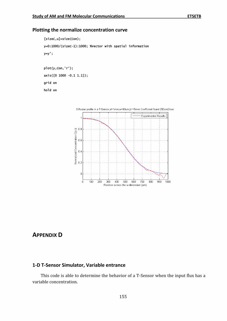
Study of AM and FM Molecular Communications ETSETB
155
Plotting the normalize concentration curve
[sizeC,u]=size(Con);
y=0:1000/(sizeC-1):1000; %Vector with spatial information
y=y';
plot(y,Con,'r');
axis([0 1000 -0.1 1.1]);
grid on
hold on
APPENDIX D
1-D T-Sensor Simulator, Variable entrance
This code is able to determine the behavior of a T-Sensor when the input flux has a
variable concentration.
Study of AM and FM Molecular Communications ETSETB
156
%tic
Constants declaration
numx=101;%number of grid points in x
numt=500;%number of iterations
Dn=455;
C=zeros(numx,numt);%we inicialize de matrix to 0
dx=550/(numx-1);
dt1=4.1e-4;
x=0:dx:550; %vector of x values
stability1=(Dn*dt1)/(dx^2)
stability1 =
0.0062
Initial Conditions
In this case the initial condition is maxim concentration at the beginning in one
channel and minimum in the order channel, but only the first iteration. Then at the
beginning the concentration changes according with the variable VecCon.
% we are going to browse the matrix throght the first column, putting the values of the uniform distribution
C(1:fix(numx/2),1)=1;
%Concetration at the begining in each instant: Sinusioidal variation
W=0:2*pi/numt:2*pi;
VecCon=(0.5*sin(W))+0.5;
Study of AM and FM Molecular Communications ETSETB
157
Main Loop
%Now we can calculate the coefficients of the matrix C in the time t(j+1), using the results in the time t(j)
for j=1:numt
for k=(j+1):-1:1
if k~=1 %Is not the beginig
for i=2:numx-1
C(i,k)=C(i,k-1)+(C(i+1,k-1)-2*C(i,k-1)+C(i-1,k-1))*(Dn)*(dt1/(dx)^2);
end
C(1,k)=C(2,k);
C(numx,k)=C(numx-1,k);
else
for i=1:fix(numx/2)
C(i,1)=VecCon(j+1);
end
end
end
end
Plotting
figure(1)
hold on;
plot(x,C(:,1));
plot(x,C(:,10));
plot(x,C(:,100));
plot(x,C(:,200));
plot(x,C(:,300));
plot(x,C(:,400));
plot(x,C(:,500));
xlabel('Position across the w-dimension (um)');
ylabel('Normalized Concentration C(x,t)');
title('Concentration in a T-Sensor across d direction,w=550um,L=5000um,D=455um2/s');
grid on;
%toc
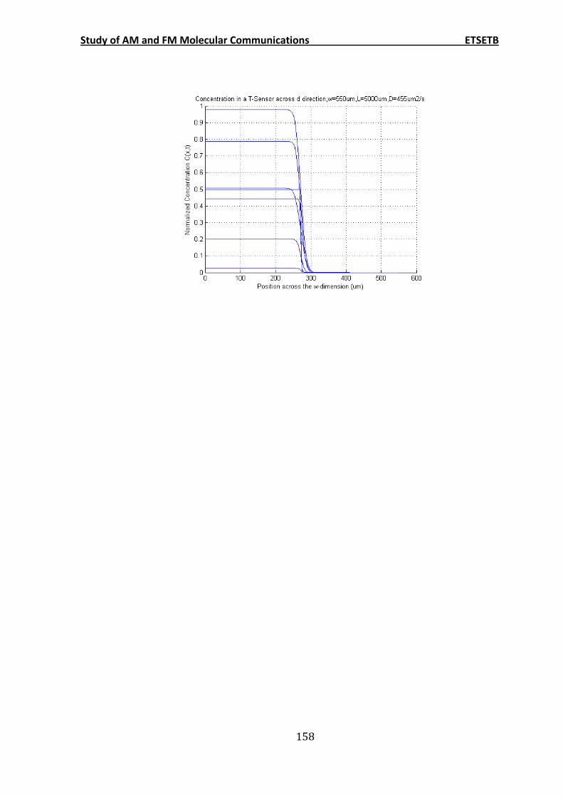
Study of AM and FM Molecular Communications ETSETB
158
Study of AM and FM Molecular Communications ETSETB
159
APPENDIX E
Cell system
This code pretends to simulate the behavior of cell communications system. The
idea is that in one pint there is a source which can be a cell or an external source that is
infusing molecules in the media. This system calculates the concentration in the sink
point where the target cell is placed.
Constants definition
numx=51;%number of grid points in x
numt=1000;%number of iterations
F=0.5; % frequency of the input signal
Dn=100;
C=zeros(numx,numt);%we inicialize de matrix to 0
dx=550/(numx-1);
dt1=0.5;
x=0:dx:550; %vector of x values
t=0:dt1:numt*dt1;
stability1=(Dn*dt1)/(dx^2)
stability1 =
0.4132
Initial condition
In this case the initial condition is that the source has maximum concentration at the
beginning. But only in the first iteration, after that the concentration at the sources
follows the value stored in VeCon.
Study of AM and FM Molecular Communications ETSETB
160
posIniCell=2; % source position in the mesh
posDetectionCell=5; % sink position in the mesh
C(posIniCell,1)=1;
%Concetration at the begining in each instant
VecCon=0.5*square(2*pi*F*t)+0.5; %square case
% VecCon=sin(2*pi*F*t); %sinusioidal case
Main loop
%Now we can calculate the coefficients of the matrix C in the time t(j+1), using the results in the time t(j)
for j=1:numt
for k=(j+1):-1:1
if k~=1 %Is not the beginig
for i=posIniCell-1:-1:2
C(i,k)=C(i,k-1)+(C(i+1,k-1)-2*C(i,k-1)+C(i-1,k-1))*(Dn)*(dt1/(dx)^2);
end
for i=posIniCell+1:numx-1
C(i,k)=C(i,k-1)+(C(i+1,k-1)-2*C(i,k-1)+C(i-1,k-1))*(Dn)*(dt1/(dx)^2);
end
%Boundary conditions
C(numx,k)=C(numx-1,k);
else
C(posIniCell,j+1)=VecCon(j+1);
end
end
end
Ctarget=C(posDetectionCell,:);
positionSource=posIniCell*dx;
positionTarget=posDetectionCell*dx;
Study of AM and FM Molecular Communications ETSETB
161
Plotting
figure(1)
hold on;
plot(x,C(:,1),'r');
plot(x,C(:,10));
plot(x,C(:,100));
xlabel('Position x');
ylabel('Normalizated Concentration C(x,t)');
title(['Molecule diffusion for a cell situated in the position ',num2str(positionSource),'um']);
grid on;
figure(2)
ax(1)=subplot(2,1,1);
plot(t,VecCon);
grid
xlim([0 t(numt)]);
ylim([0 1.2]);
ylabel('Normalizated Concentration C(x,t)');
xlabel('Time (s)');
title('Variable concentration from the source');
ax(2)=subplot(2,1,2);
plot(t,Ctarget);
grid
ylabel('Normalizated Concentration C(x,t)');
xlabel('Time (s)');
title(['Temporal evolution of the concentration in the point ',num2str(positionTarget),'um in a device of 550um of longitude']);
linkaxes(ax,'xy');
% figure(3)
% hold on
% grid on
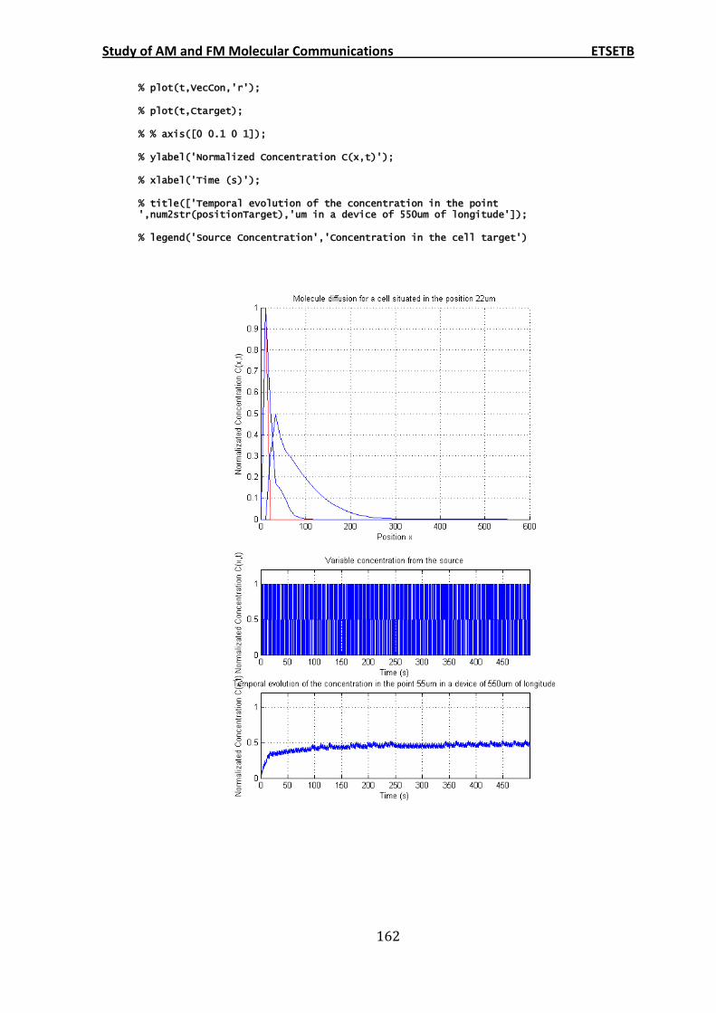
Study of AM and FM Molecular Communications ETSETB
162
% plot(t,VecCon,'r');
% plot(t,Ctarget);
% % axis([0 0.1 0 1]);
% ylabel('Normalized Concentration C(x,t)');
% xlabel('Time (s)');
% title(['Temporal evolution of the concentration in the point ',num2str(positionTarget),'um in a device of 550um of longitude']);
% legend('Source Concentration','Concentration in the cell target')
Study of AM and FM Molecular Communications ETSETB
163
APPENDIX F
Solution for the diffusion equation
This code has programmed the solution for the diffusion equation. In this script the
idea is to call the functions "gasificacion.m" and "degasificacion.m" alternately. Each call
is one half-period in the periodic square wave at the beginning.
position=0.5; %position from the domain 0<X<1 where we are calculating the result
P=0.05; %periode
F=1/P; %frequency
DC=0.5; %duty cicle
cicles=100; %number of cicles simulated
Main Loop
concentration=gasificacion(position,0,P*DC); %calcul of the first half period
%the solution is calculated in each half period, cicles is the number of
%cicles that is being calculated
for i=1:cicles
[row col]=size(concentration);
%the initial condition in the next half period depends on the last
%value in the period before, this value is keep in concentration(col)
aux=degasificacion(position,concentration(col),P*DC);
%the concentration array is made concatenating the different half
%periods
concentration=horzcat(concentration,aux);
[row col]=size(concentration);
%the initial condition in the next half period depends on the last
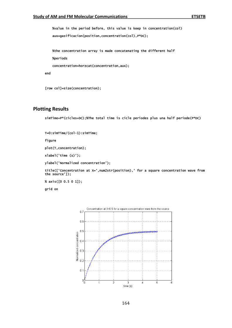
Study of AM and FM Molecular Communications ETSETB
164
%value in the period before, this value is keep in concentration(col)
aux=gasificacion(position,concentration(col),P*DC);
%the concentration array is made concatenating the different half
%periods
concentration=horzcat(concentration,aux);
end
[row col]=size(concentration);
Plotting Results
simTime=P*(cicles+DC);%The total time is cicle periodes plus una half periode(P*DC)
T=0:simTime/(col-1):simTime;
figure
plot(T,concentration);
xlabel('time (s)');
ylabel('Normalized concentration');
title(['Concentration at X=',num2str(position),' for a square concentration wave from the source']);
% axis([0 0.5 0 1]);
grid on
Study of AM and FM Molecular Communications ETSETB
165
Gasificacion Function
This function calculates the concentration using the charge equation
function [concentration] = gasificacion(position,IC,halfP)
T=0:0.001:halfP;
sum=0;
X=position;
for n=1:1:10000
Wn=((2*n)-1)*(pi/2);
Bn=(2*(1-IC))/Wn;
sum=Bn*(sin(Wn*X))*(exp(-Wn^2*T))+sum;
end
concentration=1-sum;
Degasificacion Function
This function calculets the concentration using the discharge equation
function [concentration] = degasificacion(position,IC,halfP)
T=0:0.001:halfP;
sum=0;
X=position;
for n=1:1:10000
Wn=((2*n)-1)*(pi/2);
Bn=(2*IC)/Wn;
sum=Bn*(sin(Wn*X))*(exp(-Wn^2*T))+sum;
end
concentration=sum;

Study of AM and FM Molecular Communications ETSETB
166
Input argument "halfP" is undefined.
Error in ==> degasificacion at 4
T=0:0.001:halfP;
Study of AM and FM Molecular Communications ETSETB
167
8 REFERENCES
[1] P. Carmeliet and R. K. Jain, "Angiogenesis in cancer and other diseases," Nature, vol. 407, pp. 249-257, 2000.
[2] M. J. Berridge, "The AM and FM of calcium signaling," Nature, vol. 386, pp. 759-760, 1997.
[3] B. Alberts, et al., Molecular Biology of the Cell, 2002.
[4] A. R. Asthagiri and D. A. Lauffenburger, "Bioengineering models of cell signaling," Annual Review of Biomedical Engineering, vol. 2, pp. 31-53, 2000.
[5] R. Weiss, et al., "Genetic circuit building blocks for cellular computation, communications, and signal processing," Natural Computing, vol. 2, pp. 47-84, 2003.
[6] S. F. Bush, Nanoscale Communication Networks, 2010.
[7] I. F. Akyildiz, et al., "Nanonetworks: A new communication paradigm," Computer Networks, vol. 52, pp. 2260-2279, 2008.
[8] R. A. Freitas, Nanomedicine, Volume I: Basic Capabilities, 1999.
[9] S. Hiyama, et al., "Molecular Communication," in Proceedings of the 2005 NSTI Nanotechnology Conference, 2005, pp. 391 - 394.
[10] M. Moore, et al., "A design of a molecular communication system for nanomachines using molecular motors," Fourth Annual IEEE International Conference on Pervasive Computing and Communications Workshops, Proceedings, pp. 554-559, 2006.
[11] T. Nakano, et al., "Molecular communication for nanomachines using intercellular calcium signaling," in Nanotechnology, 2005. 5th IEEE Conference on, 2005, pp. 478-481 vol. 2.
[12] Y. Moritani, et al., "Molecular communication for health care applications," in Pervasive Computing and Communications Workshops, 2006. PerCom Workshops 2006. Fourth Annual IEEE International Conference on, 2006, pp. 5 pp.-553.
Study of AM and FM Molecular Communications ETSETB
168
[13] E. Carafoli, "Calcium signaling: A tale for all seasons," Proceedings of the National Academy of Sciences of the United States of America, vol. 99, pp. 1115-1122, February 5, 2002 2002.
[14] W. D. Kepseu and P. Woafo, "Intercellular waves propagation in an array of cells coupled through paracrine signaling: A computer simulation study," Physical Review E, vol. 73, 2006.
[15] C. Bustamante, et al., "Mechanical processes in biochemestry," Annual Review of Biochemistry, vol. 73, pp. 705-748, 2004.
[16] P. Tabeling, Introduction to Microfluidics, 2003.
[17] G. M. Whitesides, "The origins and the future of microfluidics," Nature, vol. 442, pp. 368-373, 2006.
[18] J. P. Abraham, et al., "Heat transfer in all pipe flow regimes: laminar, transitional/intermittent, and turbulent," International Journal of Heat and Mass Transfer, vol. 52, pp. 557-563, 2009.
[19] C. Noakes and A. Sleigh, An Introduction to Fluid Mechanics, 2009.
[20] A. P. Wong, et al., "Partitioning microfluidic channels with hydrogel to construct tunable 3-D cellular microenvironments," Biomaterials, vol. 29, pp. 1853-1861, 2008.
[21] J. Philibert, "One and a Half Century of Diffusion: Fick, Einstein, Before and Beyond," Diffusion Fundamentals, vol. 4, pp. 1-19, 2006.
[22] R. B. Bird, et al., Transport Phenomena, 2001.
[23] Z. Zhenrong, et al., "Roughness characterization of well-polished surfaces by measurements of light scattering distribution," Optica Applicata, vol. 40, pp. 811-818, 2010.
[24] K. Ogata, Modern Control Engineering, 1996.
[25] A. E. Kamholz, et al., "Quantitative analysis of molecular interaction in a microfluidic channel: The T-sensor," Analytical Chemistry, vol. 71, pp. 5340-5347, 1999.
[26] A. B. Shrirao and R. Perez-Castillejos, "Simple fabrication of microfluidic devices by replicating Scotch-tape masters," Lab on a Chip: Chips and Tips, 2010.
Study of AM and FM Molecular Communications ETSETB
169
[27] A. E. Kamholz and P. Yager, "Theoretical analysis of molecular diffusion in pressure-driven laminar flow in microfluidic channels," Biophysical Journal, vol. 80, pp. 155-160, 2001.
[28] B. A. Finlayson, Nonlinear analysis in chemical engineering, 1980
[29] A. E. Kamholz and P. Yager, "Molecular diffusive scaling laws in pressure-driven microfluidic channels: deviation from one-dimensional Einstein approximations," Sensors and Actuators B-Chemical, vol. 82, pp. 117-121, 2002.
[30] S. A. Rani, et al., "Rapid diffusion of fluorescent tracers into Staphylococcus epidermidis biofilms visualized by time lapse microscopy," Antimicrobial Agents and Chemotherapy, vol. 49, pp. 728-732, 2005.
[31] D. deBeer, et al., "Measurement of local diffusion coefficients in biofilms by microinjection and confocal microscopy," Biotechnology and Bioengineering, vol. 53, pp. 151-158, 1997.
[32] A. Goldbeter, et al., "Minimal model for signal-induced Ca2+ oscillations and for their frequency encoding through protein phosphorylation," Proceedings of the National Academy of Sciences, vol. 87, pp. 1461-1465, February 1, 1990 1990.
[33] R. E. Dolmetsch, et al., "Differential activation of transcription factors induced by Ca2+ response amplitude and duration," Nature, vol. 386, pp. 855-858 24 April 1997 1997.

Study of AM and FM Molecular Communications ETSETB
170