Theoretical comparison of three X-ray phase-contrast …discovery.ucl.ac.uk/1345033/1/1345033_Diemoz_OE_2012.pdfand D. Sayers, “Diffraction enhanced x-ray imaging,” Phys. Med

$Page 1: Theoretical comparison of three X-ray phase-contrast …discovery.ucl.ac.uk/1345033/1/1345033_Diemoz_OE_2012.pdfand D. Sayers, “Diffraction enhanced x-ray imaging,” Phys. Med$
Theoretical comparison of three X-ray

phase-contrast imaging techniques:

propagation-based imaging, analyzer-based

imaging and grating interferometry

P.C. Diemoz,1,2,*

A. Bravin,2 and P. Coan

1,3

1 Faculty of Physics, Ludwig-Maximilians-University München, 85748 Garching, Germany 2 European Synchrotron Radiation Facility, 38043 Grenoble, France

3 Faculty of Medicine, Ludwig-Maximilians-University München, 81377 Munich, Germany

*[email protected]

Abstract: Various X-ray phase-contrast imaging techniques have been

developed and applied over the last twenty years in different domains, such

as material sciences, biology and medicine. However, no comprehensive

inter-comparison exists in the literature. We present here a theoretical study

that compares three among the most used techniques: propagation-based

imaging (PBI), analyzer-based imaging (ABI) and grating interferometry

(GI). These techniques are evaluated in terms of signal-to-noise ratio, figure

of merit and spatial resolution. Both area and edge signals are considered.

Dependences upon the object properties (absorption, phase shift) and the

experimental acquisition parameters (energy, system point-spread function

etc.) are derived and discussed. The results obtained from this analysis can

be used as the reference for determining the most suitable technique for a

given application.

©2011 Optical Society of America

OCIS codes: (110.7440) X-ray imaging; (110.2990) Image formation theory; (100.2960) Image

analysis; (110.4980) Partial coherence in imaging.

References and links

1. M. Born and E. Wolf, Principles of Optics: Electromagnetic Theory of Propagation, Interference and

Diffraction of Light (Cambridge University Press, Cambridge, 1999). 2. U. Bonse and M. Hart, “An X-ray interferometer,” Appl. Phys. Lett. 6(8), 155–156 (1965).

3. A. Momose, T. Takeda, Y. Itai, and K. Hirano, “Phase-contrast X-ray computed tomography for observing

biological soft tissues,” Nat. Med. 2(4), 473–475 (1996). 4. A. Snigirev, I. Snigireva, V. Kohn, S. Kuznetsov, and I. Schelokov, “On the possibility of x-ray phase contrast

microimaging by coherent high-energy synchrotron radiation,” Rev. Sci. Instrum. 66(12), 5486–5492 (1995).

5. S. W. Wilkins, T. E. Gureyev, D. Gao, A. Pogany, and A. W. Stevenson, “Phase-contrast imaging using polychromatic hard X-rays,” Nature 384(6607), 335–338 (1996).

6. E. Förster, K. Goetz, and P. Zaumseil, “Double crystal diffractometry for the characterization of targets for laser

fusion experiments,” Krist. Tech. 15(8), 937–945 (1980). 7. D. Chapman, W. Thomlinson, R. E. Johnston, D. Washburn, E. Pisano, N. Gmur, Z. Zhong, R. Menk, F. Arfelli,

and D. Sayers, “Diffraction enhanced x-ray imaging,” Phys. Med. Biol. 42(11), 2015–2025 (1997).

8. A. Bravin, “Exploiting the X-ray refraction contrast with an analyser: the state of the art,” J. Phys. D Appl. Phys. 36(10A), A24–A29 (2003).

9. C. David, B. Nöhammer, H. Solak, and E. Ziegler, “Differential X-ray phase contrast imaging using a shearing

interferometer,” Appl. Phys. Lett. 81(17), 3287–3289 (2002). 10. T. Weitkamp, A. Diaz, C. David, F. Pfeiffer, M. Stampanoni, P. Cloetens, and E. Ziegler, “X-ray phase imaging

with a grating interferometer,” Opt. Express 13(16), 6296–6304 (2005).

11. F. Pfeiffer, T. Weitkamp, O. Bunk, and C. David, “Phase retrieval and differential phase-contrast imaging with low-brilliance X-ray sources,” Nat. Phys. 2(4), 258–261 (2006).

12. A. Olivo, K. Ignatyev, P. R. T. Munro, and R. D. Speller, “Noninterferometric phase-contrast images obtained

with incoherent x-ray sources,” Appl. Opt. 50(12), 1765–1769 (2011). 13. E. Castelli, M. Tonutti, F. Arfelli, R. Longo, E. Quaia, L. Rigon, D. Sanabor, F. Zanconati, D. Dreossi, A.

Abrami, E. Quai, P. Bregant, K. Casarin, V. Chenda, R. H. Menk, T. Rokvic, A. Vascotto, G. Tromba, and M. A.

#156604 - $15.00 USD Received 17 Oct 2011; accepted 30 Nov 2011; published 23 Jan 2012(C) 2012 OSA 30 January 2012 / Vol. 20, No. 3 / OPTICS EXPRESS 2789

Cova, “Mammography with synchrotron radiation: first clinical experience with phase-detection technique,”

Radiology 259(3), 684–694 (2011). 14. P. Coan, F. Bamberg, P. C. Diemoz, A. Bravin, K. Timpert, E. Mützel, J. G. Raya, S. Adam-Neumair, M. F.

Reiser, and C. Glaser, “Characterization of osteoarthritic and normal human patella cartilage by computed

tomography X-ray phase-contrast imaging: a feasibility study,” Invest. Radiol. 45(7), 437–444 (2010). 15. G. Schulz, T. Weitkamp, I. Zanette, F. Pfeiffer, F. Beckmann, C. David, S. Rutishauser, E. Reznikova, and B.

Mueller, “High-resolution tomographic imaging of a human cerebellum: comparison of absorption and grating-

based phase contrast,” J. R. Soc. Interface 7(53), 1665–1676 (2010). 16. E. Pagot, S. Fiedler, P. Cloetens, A. Bravin, P. Coan, K. Fezzaa, J. Baruchel, J. Härtwig, K. von Smitten, M.

Leidenius, M. L. Karjalainen-Lindsberg, and J. Keyriläinen, “Quantitative comparison between two phase

contrast techniques: diffraction enhanced imaging and phase propagation imaging,” Phys. Med. Biol. 50(4), 709–724 (2005).

17. M. R. Teague, “Irradiance moments - their propagation and use for unique retrieval of phase,” J. Opt. Soc. Am.

72(9), 1199–1209 (1982). 18. T. E. Gureyev, Y. I. Nesterets, A. W. Stevenson, P. R. Miller, A. Pogany, and S. W. Wilkins, “Some simple rules

for contrast, signal-to-noise and resolution in in-line x-ray phase-contrast imaging,” Opt. Express 16(5), 3223–

3241 (2008). 19. P. Coan, E. Pagot, S. Fiedler, P. Cloetens, J. Baruchel, and A. Bravin, “Phase-contrast X-ray imaging combining

free space propagation and Bragg diffraction,” J. Synchrotron Radiat. 12(2), 241–245 (2005).

20. Y. I. Nesterets, P. Coan, T. E. Gureyev, A. Bravin, P. Cloetens, and S. W. Wilkins, “On qualitative and quantitative analysis in analyser-based imaging,” Acta Crystallogr. A 62(4), 296–308 (2006).

21. T. E. Gureyev and S. W. Wilkins, “Regimes of X-ray phase-contrast imaging with perfect crystals,” Nuovo

Cimento D 19(2-4), 545–552 (1997). 22. K. M. Pavlov, T. E. Gureyev, D. Paganin, Y. I. Nesterets, M. J. Morgan, and R. A. Lewis, “Linear systems with

slowly varying transfer functions and their application to x-ray phase-contrast imaging,” J. Phys. D Appl. Phys.

37(19), 2746–2750 (2004). 23. R. Tanuma and M. Ohsawa, “Submicron-resolved X-ray topography using asymmetric-reflection magnifiers,”

Spectrochim. Acta, Part B 59(10-11), 1549–1555 (2004). 24. P. C. Diemoz, P. Coan, I. Zanette, A. Bravin, S. Lang, C. Glaser, and T. Weitkamp, “A simplified approach for

computed tomography with an X-ray grating interferometer,” Opt. Express 19(3), 1691–1698 (2011).

25. A. L. Evans, The Evaluation of Medical Images (Adam Hilger Ltd, Bristol, 1981). 26. F. Arfelli, V. Bonvicini, A. Bravin, G. Cantatore, E. Castelli, L. Dalla Palma, M. Di Michiel, R. Longo, A.

Olivo, S. Pani, D. Pontoni, P. Poropat, M. Prest, A. Rashevsky, G. Tromba, and A. Vacchi, “Mammography of a

phantom and breast tissue with synchrotron radiation and a linear-array silicon detector,” Radiology 208(3), 709–715 (1998).

27. S. Webb, The Physics of Medical Imaging (Institute of Physics Publishing, Bristol, 1988).

28. J. M. Boone, K. K. Lindfors, V. N. Cooper 3rd, and J. A. Seibert, “Scatter/primary in mammography: comprehensive results,” Med. Phys. 27(10), 2408–2416 (2000).

29. J. Persliden and G. A. Carlsson, “Scatter rejection by air gaps in diagnostic radiology. Calculations using a

Monte Carlo collision density method and consideration of molecular interference in coherent scattering,” Phys. Med. Biol. 42(1), 155–175 (1997).

30. M. Sanchez del Rio, C. Ferrero, and V. Mocella, “Computer simulations of bent perfect crystal diffraction

profiles,” Proc. SPIE 3152, 312–323 (1997), http://www.esrf.eu/UsersAndScience/Experiments/TBS/ SciSoft/xop2.3.

31. T. Matsushita and H. Hashizume, “X-Ray monochromators,” in Handbook on Synchrotron Radiation, E. Koch,

ed. (North Holland Publishing Company, New York, 1983), pp. 261–314.

1. Introduction

In conventional X-ray imaging, the contrast is generated by variations of the X-ray

attenuation that arise from differences in the thickness, composition and density of the imaged

object. These variations, however, can be very tiny when imaging samples composed by low

Z elements like soft biological tissues. Moreover, in the case of clinical or in-vivo imaging,

the radiation dose (and therefore the photon fluence) has to be kept as low as possible. As a

result, the obtained image contrast may be not sufficient for the complete discrimination and

characterization of the healthy and diseased tissues in a given sample/patient.

With the aim of overcoming the intrinsic limitations of attenuation-based X-ray imaging,

a number of phase-contrast techniques have been developed and applied over the last twenty

years. Unlike conventional X-ray methods, these techniques are not only sensitive to the

attenuation, but also to the phase shift that X-rays, as all electromagnetic waves, experience

when passing through the matter. The propagation of X-rays in matter can be mathematically

described in terms of the complex index of refraction 1n iδ β= − + , whose real part δ and


imaginary part β are related to the phase shift and to the X-ray attenuation in the object,

respectively [1]. Since δ is orders of magnitude higher than β in the hard X-rays range, the

phase shift can be significant even for small details characterized by a weak amplitude

modulation (i.e. attenuation). Therefore, the achievable contrast for soft biological tissues can

be greatly increased.

Various techniques have been developed to exploit the phase contrast in the X-ray regime.

They can be classified into five main categories: the interferometric methods based on the use

of crystals [2, 3], the propagation-based imaging (PBI) methods [4, 5], the analyzer-based

imaging (ABI) methods [6–8], the grating interferometric (GI) [9–11] and the grating non-

interferometric methods [12].

In this article, we will focus on PBI, ABI and GI, the most largely presented techniques in

the literature in the past years. These methods differ not only for their experimental setup and

requirements in terms of the X-ray beam spatial and temporal coherence, but also for the

nature and amplitude of the provided image signal, and for the amount of radiation dose that

is delivered to the sample. These phase-contrast modalities (in particular PBI and ABI) have

been extensively investigated in preclinical and clinical trials to access their potential for

biomedical imaging, in subjects as diverse as mammography [13], cartilage imaging [14] and

brain imaging [15]. Despite the large number of publications in the field of phase contrast,

very few attempts have been made to compare these different methods [16], and a complete

qualitative and quantitative comparison is still missing in the literature.

We here present a theoretical comparison of PBI, ABI and GI by examining key

parameters as the spatial resolution, the signal-to-noise ratio, the delivered radiation dose and

the figure-of-merit. The advantages and drawbacks of each method and the consequences in

biomedical applications will be also discussed.

In the next section, the main features, formulas and experimental requirements of the PBI,

ABI and GI techniques are briefly reviewed. In section 2.1 the various contributions to spatial

resolution are summarized. In section 3, the notions of signal-to-noise ratio (SNR) and figure-

of-merit (FoM) for area and edge signals are introduced, and general expressions for these

quantities derived. Simple expressions that relate the FoM with the acquisition parameters for

each of the considered techniques are finally obtained and compared in section 4.

2. Brief description of PBI, ABI and GI techniques

In order to simplify the description, we will consider only the case of monochromatic

radiation, characterized by a definite wavelength λ, and the typical 1-dimensional (1-D)

implementation of ABI and GI; extension of the formalism to the 2-D case is straightforward.

1. Propagation-based imaging (PBI) is the method with the simplest experimental setup.

It requires that the sample is irradiated with highly spatially coherent radiation and

that the detector is positioned at a sufficient distance r from the sample; no optical

elements are needed between the sample and the detector. Thanks to Fresnel

diffraction, the differences in phase shift introduced by the object onto the beam lead

to a measurable intensity modulation onto the detector [1]. This intensity can be

expressed, in the near-field diffraction regime, by the transport of intensity equation

(TIE) [17]. The near-field regime approximation is valid for sufficiently small

propagation distances and for objects introducing a slowly varying phase shift in the

plane (x,y) transversal to the optical axis z [18]. In the case of additional slowly

varying object absorption, the TIE can be written as (for sake of simplicity the

spatial variables are omitted):

2 2

0 12

PBI

dI M I T

λφ

π−

⊥= − ∇

(1)


where ( )M r l l= + , with l being the source-to-sample distance, is the magnification factor,

which takes into account the beam divergence; I0 indicates the intensity incident onto the

object; ( )expobj

T dz µ= −∫ is the object transmission and µ is the linear attenuation

coefficient; /=d r M is the so-called defocusing distance and φ is the phase shift introduced

by the object. Under these approximations, the intensity modulation is thus proportional to the

Laplacian of the phase shift. As an example, a typical PBI intensity profile corresponding to a

pure phase object (Fig. 1(a)) is plotted in Fig. 1(b).

As shown by Wilkins and associates [5], PBI is relatively insensitive to broad beam

polychromaticity. However, a high degree of spatial coherence is required, otherwise the

interference fringes are rapidly smeared out.

Imax

Imin

Imax

Integral signal

IbackIback

Integral signal

(a)

(b) (c)

PBI ABI - GI

Fig. 1. (a) Profile of a pure phase object. (b) Typical corresponding PBI signal that can be

calculated from Eq. (1). (c) Typical ABI / GI signal that can be calculated from Eqs. (4 and 6). Values have been normalized by the average background intensity Iback. Poissonian noise has

been added to the theoretical profiles. Maximum (Imax) and minimum (Imin) values for the

intensity at the edge, as well as the integral of the edge signal, are also drawn in the figure.

2. Analyzer-based imaging (ABI) makes use of a quasi-monochromatic and quasi-parallel

beam (typically produced by diffraction from a perfect crystal, called the

monochromator) irradiating the sample and of a perfect “analyzer” crystal placed

between the sample and the detector. The analyzer acts as an angular filter of the

radiation refracted and scattered by the sample. In a typical ABI setup the sample-to-

detector distance is small, so that the propagation phase contrast can be neglected

[19]. The general expression for the intensity recorded on the detector [20] can be

greatly simplified under the geometrical optics approximation [21], which is valid if

the phase of the wave incident onto the crystal is a slowly varying function over the

length scales on the order of the crystal extinction length [22]. In this case the

intensity for each detector pixel can then be expressed, if the crystal diffraction plane

is assumed to be parallel to the (y,z) plane, as:

( )2

0ABI asym an yI M M I T R θ θ−= + ∆ (2)


where M accounts for the image magnification due to beam divergence and Masym for that

arising in the case of an asymmetrically-cut analyzer crystal [23], which affects only the

direction y parallel to the diffraction plane. θan is the angular deviation of the crystal from the

Bragg angle and 2∆ = − ∂ ∂y

yθ λ π φ is the component of the refraction angle that is parallel

to the diffraction plane. R is the so-called rocking curve (RC), defined as the ratio between the

intensity diffracted by the analyzer crystal and the intensity incident on it, and whose

expression is given by:

( )( ) ( ) ( )

( )

' ' ' '

' '

M AN

M

d f R RR

d R

θ

θ

θ θ θ θ θθ

θ θ

−=∫

∫ (3)

where RM and RAN are the reflectivity curves of the monochromator (M) and analyzer (AN)

crystals respectively, and f(θ’) is the angular distribution of photons incident onto the

monochromator. If the object refraction angles are small compared to the full-width at half

maximum (FWHM) of the RC, Eq. (2) can be rewritten by using a first-order Taylor

approximation of the RC [7]:

( ) ( )2

0 'ABI asym an an yI M M I T R Rθ θ θ− + ∆ ≃ (4)

where ( )′anR θ denotes the first derivative of the RC. In case of small refraction angles,

therefore, the intensity modulation in ABI is proportional to the refraction angle itself. As an

example, a typical ABI signal for a pure phase object is plotted in Fig. 1(c).

In ABI, X-rays incident on the sample must be almost parallel and monochromatic with a

typical energy bandwidth, ∆E/E, of a perfect crystal (10−4

). Due to the unavoidable loss of

photons occurring in the monochromatization/collimation process in the first crystal, sources

providing highly collimated and intense X-rays, like synchrotron radiation facilities, are

particularly advantageous for ABI.

3. The grating interferometry (GI) technique consists in illuminating the imaged object

with highly spatially coherent X-rays, and in analyzing the radiation transmitted

through the object by using a pair of gratings [10]. The first is generally a phase

grating, of period p1, which introduces a periodic phase shift onto the beam but

negligible absorption. A second absorption grating of period p2 is then placed

downstream at one of the so-called fractional Talbot distances dTalbot, where the

interference fringes created by the first grating give rise to the so-called self-imaging

effect.

Let us assume the grating lines to be perpendicular to the axis y, and let us denote with yG the

relative position of the two gratings in this direction. The intensity incident on each detector

pixel can in general be approximated by [24]:

( )0

2 2

0

2

2 21 sin ;

GI GR G y GR G yI M I T T V y M I T T G y

p S

π πψ θ θ− −= + + + ∆ = ∆

(5)

where TGR indicates the average intensity transmission through the gratings, ψ is the shift of

the sinusoidal fringe profile measured with no object in the beam, and 2

=Talbot

S p d is the

angle corresponding to one grating period; V indicates the fringe visibility, defined as

( ) ( )max min max min

V I - I I + I≡ , where Imin and Imax are respectively the minimum and maximum

intensities on the fringe profile.

In the case of small refraction angles, such that 4∆ ≪y

Sθ , the function G can be well

approximated, in analogy with the ABI case, with a first-order Taylor expansion [24]:


( ) ( )2

0 'GI GR G G yI M I T T G y G y θ− + ∆ ≃ (6)

where ( )G

G y′ denotes the first derivative of the function G with respect to the refraction

angle. The similarity of the signals in the GI and ABI techniques is evident from Eqs. (2-6):

both techniques are sensitive to the refraction angle (more precisely to its component along

one direction), and in both cases the signal is proportional to the refraction angle if this is

sufficiently small. A typical GI signal is plotted in Fig. 1(c), in the case of a simple pure

phase object.

Differently from ABI, GI works efficiently even with relatively broad-band radiation [11]

but requires a high degree of spatial coherence. It was shown that the technique can also be

applied to normal X-ray tubes delivering spatially incoherent radiation if an appropriate third

grating is added close to the source [11]. This comes however at the expenses of the available

photon flux (and therefore of the time required to acquire an image), since the source grating

introduces a considerable filtration of the incoming radiation.

2.1. Spatial resolution

In a real case, the here-considered techniques are characterized by a finite spatial resolution

whose value depends on the experimental acquisition parameters. The imaging system point-

spread function (PSF) can be approximated as the product of two one-dimensional Gaussian

functions:

( ) 1 2 2 2 2

, , , ,2 exp 2 2−

= − − sys sys x sys y sys x sys yP x yπσ σ σ σ (7)

where 2

,syst xσ and 2

,syst yσ represent the PSF variances referred to the object plane, in the x and

y directions. Equation (7) takes into account that the spatial resolution can be significantly

different in the two image directions. In the case of PBI, the PSF variances can be written as

[18]:

( )22 2 2 2 2

, , , , det, ,1

− −= − +sys PBI x y src x y x y

M M Mσ σ σ (8)

where , ,src x yσ indicates the source size and det, ,x yσ the width of the detector PSF, respectively

in the directions x and y. The first term in Eq. (8) is predominant for large values of the

magnification factor ( ,sys PBI srcσ σ≈ if M → ∞ ), while the second term is more important

when the magnification is small ( ,PBI sys detσ σ≈ if 1M → ). There is therefore a limit for the

spatial resolution in PBI, depending on the particular value of the magnification factor. In the

general case, the resolution is also limited by the width of the first Fresnel zone but in the

near-field diffraction regime, as shown by Gureyev and associates [18], the latter is much

smaller than the width of the system PSF.

Equation (8) is also valid for GI. However, it has to be noted that in this case there is a

low limit in the size of the detector pixels: they are required to be at least the size of an entire

period of the second grating, at least in the direction y perpendicular to the grating lines.

The PSF variances for ABI in the x and y directions can be written instead as:

( )22 2 2 2 2

, , det,1sys ABI x src x xM M Mσ σ σ− −= − + (9)

( )22 2 2 2 2 2 2 2 2

, , det, ,1

sys ABI y src y asym y asym an yM M M M M Mσ σ σ σ− − − − −= − + + (10)

where an additional source of spatial resolution degradation, due to the intrinsic PSF of the

analyzer crystal, is present in the direction y parallel to the diffraction plane. The blurring


introduced by the analyzer can be essentially attributed to the finite penetration length of X-

rays in the crystal, and its width can have values of up to a few micrometers. This blurring

can however be reduced (to values in the submicrometre range) with the use of

asymmetrically-cut crystals, characterized by a magnification factor 1>asymM [23].

3. Definition of signal-to-noise ratio and figure-of-merit

3.1 Area signal

In the case of an area signal (typical of conventional absorption imaging), the signal-to-noise

ratio (SNR) of a detail with respect to the surrounding region (considered as the background)

is usually defined as [25]:

( )

( ) ( )

( )2 2

obj back obj back

area

obj backobj back

A I I A I ISNR

I Istd I std I

− −≡

++≃ (11)

where obj objI N A= and

back backI N A= are the mean intensity values in a given area A

respectively in the object/detail and in the background, with Nobj and Nback being the number

of counts on the detector in these two regions; std(Iobj) and std(Iback) indicate their standard

deviations.

The right-hand side of Eq. (11) can be derived under the conditions of a Poisson noise, for

which ( )std N N= ; in this latter expression we have implicitly assumed that each detected

photon produces one count on the digital detector. We will also consider, for sake of

simplicity, a detection efficiency of 100%. These assumptions are however not stringent and

the following formulas can be easily extended to more general cases.

The SNR is strongly dependent on the incoming X-ray flux (see Eq. (11)) and, in the

presence of pure Poissonian noise, it can be shown to be proportional to the square root of the

number of incident photons. Therefore, if images acquired with different photon fluxes need

to be compared, the SNR does not represent an appropriate parameter. In order to evaluate the

quality of an image independently of the delivered dose used to obtain that image it is

convenient to introduce the Figure of Merit (FoM) [26]:

SNR

FoMD

≡ (12)

The FoM is independent of the number of photons because the dose, D, is directly

proportional to the X-ray flux for a given sample and energy [27]:

0doseD K I= (13)

where I0 indicates the beam intensity before the sample and Kdose is a constant that depends in

a complicated way on both the imaging system (X-rays energy, irradiation geometry..) and

the object (shape, dimensions, composition etc.). Note that in general Kdose cannot be

calculated analytically but only through Monte Carlo simulations. By combining Eqs. (11-

13), the following expression for the area FoM can be obtained:

( )( )0

obj back

area

dose obj back

A I IFoM

K I I I

−=

+ (14)


3.2 Edge signal

In addition to the absorption signal specific of homogeneous regions within the object, phase-

contrast images are characterized by a peculiar signal generated at the interfaces (edges)

between regions with different refractive indexes (see Fig. 1). Following [16, 19] and in

analogy with Eq. (11), it is possible to extend the definition of the SNR to the case of an edge

signal as:

( )

( )( )max min max min

2 22edge peak

backback

A I I A I ISNR

Istd I

− −≡ ≃ (15)

where Imin and Imax are the minimum and maximum intensities of a mean intensity profile

across the edge, obtained by averaging the signal over a certain number n of pixel rows in the

direction parallel to the edge; A is the area defined as = ⋅A np p , where p is the pixel size in

each dimension; Iback is the average intensity in the background (outside the edge). In Eq. (15)

we have again assumed a pure Poissonian noise (like in Eq. (11)).

We will refer to the quantity defined in Eq. (15) as the “peak edge” SNR. The

corresponding figure of merit can be expressed, by using Eqs. (12-13), as:

( )max min

02edge peak

dose back

A I IFoM

K I I

−= (16)

The previous definitions of peak edge SNR and FoM do not actually consider the width of

the edge. The latter parameter, however, can be important with respect to the detail visibility.

For this reason, an alternative definition for the edge signal has been introduced by Gureyev

and associates [18]; it takes into account not only the maximum and minimum intensity

values but the integral of all the values across the edge (see Fig. 1).

Supposing an edge extended on the x direction (perpendicular to the sensitivity direction

of ABI and GI techniques), the integral edge SNR and FoM for the three here studied phase-

contrast methods can be written as:

( )1

0

1

0

int .

,

2

a x

backa x

edgea x

backa x

dy dx I x y I

SNR

dy dxI

+

−

+

−

−≡∫ ∫

∫ ∫ (17)

( )1

0

1

0

int .

0

,

2

a x

backa x

edgea x

dose backa x

dy dx I x y I

FoM

K I dy dxI

+

−

+

−

−=∫ ∫

∫ ∫ (18)

where 2a represents the edge width (in the y direction) and 1 0= −xL x x the width, in the

direction parallel to the edge, considered for calculating the average edge profile. We will

henceforth refer to the above-defined quantities as the “integral edge” SNR and FoM.


4. Calculation of figure of merit

In the following, analytical expressions for the FoM will be derived for the PBI, ABI and GI

techniques, respectively. Both area and edge signals will be analyzed. For sake of simplicity,

the effect of magnification will be here neglected.

4.1 Calculation of area FoM

In addition to the phase effects at the edges of an object/detail, phase-contrast images also

show a signal due to X-ray attenuation, similar to that encountered in conventional X-ray

imaging. This signal gives rise to an area contrast, visible in the bulk region of objects, which

provides complementary information to the phase signal.

In order to derive the FoM for the area signal in PBI, we consider a region in the object

where the phase signal is absent. By inserting Eq. (1) into Eq. (14), the following expression

can be obtained:

( ) ( )( ) ( )( )

( )( )

,

exp exp

exp exp 2

obj back back obj

PBI abs

dose obj back dose back obj

A dz dz A dz dzFoM

K dz dz K dz dz

µ µ µ µ

µ µ µ µ

− − − −= ≈

− + − − −

∫ ∫ ∫ ∫∫ ∫ ∫ ∫

(19)

The approximation on the right side of Eq. (19) is valid only in the case of small

absorption, such that 1dzµ∫ ≪ . It can be noted that Eq. (19) is similar to the FoM that one

would obtain in absorption imaging. The important difference is that in the latter case the

Compton-scattered X-rays can blur the detected signal and can introduce additional noise in

the image (a well-known problem in conventional radiology [28]). In PBI instead, thanks to

the propagation distance r between the sample and the detector, the X-rays scattered at a

sufficiently large angle will not reach the detector, and the blurring due to Compton scattering

can be largely reduced (analogously to the scatter rejection method by air gaps which can

used in conventional diagnostic radiology [29]).

From Eq. (19) we can remark that the FoM (in the case of dominant Poissonian noise) is

independent of the photon flux I0 incident on the sample. This confirms that the FoM is an

appropriate quantity for comparing the quality of images acquired with different incoming

photon fluxes (or, equivalently, at different doses to the sample).

The area FoM in ABI can be calculated from Eqs. (2) and (14), by considering a region

where the refraction angle ∆θy is equal to zero. It can be easily shown that:

( ), ,ABI abs an PBI absFoM R FoMθ= (20)

1( )an

R θ < , thus the value of the area FoM for a pure absorbing object is smaller than in the

case of PBI. This is a direct result of the filtration introduced by the analyzer crystal, which

reduces the number of photons impinging on the detector. This means that, for the same

number of photons exiting the sample, in ABI the photon statistics recorded on the detector is

reduced and the relative contribution of noise is more important. An advantage of ABI,

however, is the total rejection of the Compton-scattered X-rays by the analyzer.

A similar expression for the area FoM can be obtained for the GI technique from Eqs. (6)

and (14):

( ), ,GI abs GR G PBI absFoM T G y FoM= (21)

Like in ABI, there exists in GI a considerable photon filtration due to the absorption in the

two gratings (particularly in the second one, which is usually made of highly absorbing

stripes with duty cycle ~0.5). This fact results in an unavoidable reduction in the FoM values


for the attenuation signal. Furthermore, it can be noted that, in GI, the beam intensity on the

detector depends also, through the function ( )G

G y , on the considered working point yG.

Compton-scattered photons are mostly rejected in GI because of the non-zero distance

between the sample and the detector, and the beam filtration operated by the gratings.

4.2 Calculation of peak edge signal FoM

In PBI the peak edge FoM can be derived by simply combining the general equation for the

peak edge FoM (Eq. (16)) with that for the intensity incident onto the detector in the near-

field regime (Eq. (1)):

( )2 2

, max min2 2

PBI peak

dose

d AFoM

K

λφ φ

π− ∇ −∇≃ (22)

In the near-field regime the FoM is thus proportional to the difference between the values

of the phase Laplacian at the two sides of the object/detail edge, and to the defocusing

distance (if the validity conditions for TIE are still satisfied).

Another important aspect to be considered is the dependence upon the energy (E). In good

approximation, the phase shift can be assumed to be inversely proportional to E [1]. As a

consequence, the , 0 ,PBI peak dose PBI peakSNR I K FoM= is proportional to 1/E

2. For the FoM, the

energy dependence is instead more complex and cannot be univocally determined: the

coefficient Kdose depends on both E and the sample geometry and composition, and the two

dependencies are correlated.

Under the assumption of refraction angles small compared to the FWHM of the RC, the

peak edge FoM for ABI can be derived by combining Eqs. (4) and 16):

( )( )

,2

' an

ABI peak y

dose an

RAFoM

K R

θθ

θ∆≃ (23)

The FoM is therefore proportional to the refraction angle. The factor ( ) ( )an an

R Rθ θ′

that appears in Eq. (23) strongly depends on the chosen analyzer position. This means that,

for a given experimental setup, the sensitivity of the technique (and the values of FoM) can be

varied and optimized by selecting specific positions of the analyzer along its RC.

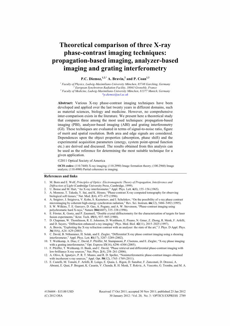
Figures 2(a,b,c) show example profiles of the RC, its derivative and the quantity

( ) ( )an an

R Rθ θ′ , respectively. They were calculated by considering an X-ray energy of 26

keV and the (111) reflection for both a silicon monochromator and a silicon crystal analyzer

[30]. Figure 2(b) shows that the first derivative of the RC varies slowly along the two RC

slopes for a relatively large range of angles, and reaches its maximum at around ± 10 µrad

(close to the end of the two slopes, where the RC is approximately 10% of its peak value).

The ( ) ( )an an

R Rθ θ′ function, instead, is not constant at the RC slopes but is strongly peaked

around ± 10 µrad (Fig. 2(c)). This implies that, for refraction angles sufficiently small for the

linear approximation of the RC to hold, the sensitivity is maximized at these points.

Evidently, the crystal material and the used reflection also have a strong influence on the

sensitivity: configurations with narrower RC will determine increased SNR and FoM.

The dependence of , 0 ,ABI peak dose ABI peak

SNR I K FoM= upon the X-ray energy can be derived

from Eq. (23), considering that: i) the Darwin width of the crystal is inversely proportional to

E, and thus the RC first derivative is approximately proportional to E [31]; (ii) the refraction

angle goes as 1/E2. It follows then that the SNR is inversely proportional to E. As pointed out


in the case of PBI, also for ABI the FoM dependence on the energy is non-trivial due to the

complicated energy dependence of Kdose.

-0,16

-0,08

0,00

0,08

0,16

-40 -30 -20 -10 0 10 20 30 40

Analyzer position (μrad)

Series2

-0,08

-0,04

0,00

0,04

0,08

-40 -30 -20 -10 0 10 20 30 40


Series1

0,0

0,2

0,4

0,6

0,8

-40 -30 -20 -10 0 10 20 30 40


Series2

(a)

(b) (c)

−′ µ 1R ( rad )

R

−′µ 1R

( rad )R

Fig. 2. (a) Profile of the theoretical RC, in the case of monochromator and analyzer in Si(111)

Bragg reflection geometry, (b) profile of its first derivative, and (c) ratio between the first derivative and the square root of the RC. All quantities have been calculated with XOP [30] for

an X-ray energy of 26 keV.

Finally, an expression that relates the peak edge FoM in GI to the object and setup

parameters can be derived by inserting Eq. (6) for the intensity incident on the detector into

Eq. (16), which leads to:

( )( )

2

,

2

2

2cos

; 02

2 ; 0 21 sin

' G

GR G y GR Talbot

GI peak y y

dosedose G y

G

yAT G y AT Vd p

FoMK pK G y

yp

πψ

θθ π θ

θ πψ

+∆ =

∆ = ∆∆ =

+ +

≃ (24)

Similarly to ABI, under the hypothesis of small refraction angles with respect to S/4 (with

2/

TalbotS p d= being the angle corresponding to one fringe period), the FoM is proportional to

∆θy. This also implies that, if all the other parameters are unchanged,

, 0 ,GI peak dose GI peakSNR I K FoM= is inversely proportional to the square of the energy, i.e.

2

,1 /

GI peakSNR E∝ . Furthermore, the SNR and FoM are also inversely proportional to S, thus

they are expected to improve with increasing distances dTalbot. However, the visibility V will

also decrease with increasing dTalbot because the X-ray beam will never be perfectly coherent.

The optimal distance dTalbot corresponding to the maximum value of the FoM is therefore a

function of the degree of coherence of the beam.

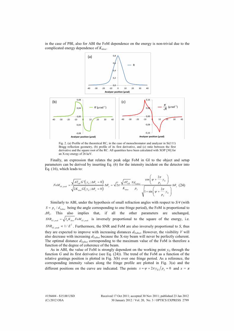
As in ABI, the value of FoM is strongly dependent on the working point yG through the

function G and its first derivative (see Eq. (24)). The trend of the FoM as a function of the

relative gratings position is plotted in Fig. 3(b) over one fringe period. As a reference, the

corresponding intensity values along the fringe profile are plotted in Fig. 3(a) and the

different positions on the curve are indicated. The points 22 0= + =Gx y pψ π and x = π


represent the positions in the middle of the positive and negative slopes, respectively, while

the points x = -π/2 and x = + π/2 indicate respectively the bottom and the top of the fringe

profile. The highest theoretical FoM is achieved at a point that is very close to the half slope

where G’ is maximized. The choice of the working point is thus very important to optimize

the sensitivity in a given setup.

-1

-0,8

-0,6

-0,4

-0,2

0

0,2

0,4

0,6

0,8

1

-0,5 0 0,5 1 1,5

No

rma

lize

d F

oM

(a

.u.)

ψ+2πyG/p2 (π units)

0,5

0,6

0,7

0,8

0,9

1

1,1

1,2

1,3

1,4

-2 -1 0 1 2

No

rma

lize

d i

nte

nsi

ty (

a.u

.)

ψ+2πyG/p2 (π units)

“top” position

“right slope”

position

“left slope”

position

“bottom”

position

“top”

position

“right slope”

position

“left slope”

position

“bottom”

position

(a)

(b)

Fig. 3. (a) Intensity profile in GI as a function of the gratings relative displacement, for a

visibility of 30%, (b) Normalized FoM values calculated by using Eq. (24) in the range [–π/2,

3/2π] for the quantity ψ + 2πyG/p2. The different positions on the fringe profile are indicated.

From Eqs. (23-24), we can notice that the ABI and GI techniques are sensitive to a

different physical quantity compared to PBI. SNR and FoM in PBI are to first approximation

(for small propagation distances and small beam curvature) proportional to the Laplacian of

the phase (or, more correctly, to the difference between the values of the phase Laplacian at

the two sides of the object/detail edge). In ABI and GI, the SNR and FoM are (for small

refraction angles) proportional to the component of the refraction angle on the diffraction

plane (ABI) and on the plane perpendicular to the grating lines (GI), respectively.

A direct consequence of the dependence of the PBI signal on the Laplacian of the phase is

that this technique is more sensitive to high object frequencies, while ABI and GI are more

sensitive to low spatial frequencies, as experimentally shown by Pagot and associates [16].

The comparison of the FoM in ABI and GI is straightforward, because the two techniques

are sensitive to the same physical quantity. In the hypothesis that the same object is imaged

using the two techniques, from Eqs. (23-24) we can obtain that the ratio of the FoMs is equal

to:

( )( )

( )( )

,

,

; 0'

; 0'

G yABI peak an

GI peak G y GRan

G yFoM R

FoM G y TR

θθ

θθ

∆ ==

∆ = (25)


Using Eq. (25), for each pair of ABI and GI experimental setups the relative sensitivity of

the two methods can be calculated.

Finally, it is noteworthy to remark the different dependence of the three phase-contrast

techniques upon the X-ray energy. As we have calculated, 21 /SNR E∝ in PBI and GI, while

1 /SNR E∝ in ABI: this means that ABI is particularly favoured at high energies with respect

to the other methods. This different dependence directly follows from the fact that the Darwin

width of the crystal is inversely proportional to E, thus the crystal sensitivity is increased at

higher energies.

4.3 Calculation of integral edge signal FoM

We will here follow the approach used by Gureyev and associates [18] to calculate the

integral edge SNR for PBI, and extend it to the calculation of the FoM in PBI, ABI and GI

techniques.

Let us consider the case of an object edge parallel to the x direction, i.e. perpendicular to

the direction of sensitivity of ABI and GI techniques. Under the assumption that the recorded

intensity is independent of x, Eq. (18) for the FoM can be rewritten as:

( )

int .

04

a

x backa

edge

dose back

L dy I y IFoM

K aI I

+

−−

=∫

(26)

Let us further assume that the phase profile across the edge can be expressed as:

( )( )obj stepH P yφ φ= ∗ (27)

where H is the Heavyside step function, φstep is the total step of the phase shift across the

edge, and ( ) 1/ 22 2 2

, ,2 exp 2

obj obj y obj yP yπσ σ

−= − is a normalized Gaussian function that

expresses the smoothness of the object edge.

If we take into account the effect of the system PSF on the recorded intensity (Eqs. (7-8)),

the PBI TIE equation for slowly varying absorption (Eq. (1)) becomes:

( ) ( ) ( )2

0 , ,2

back sys PBI

dI y I I y P x y

λφ

π ⊥− ≈ − ∇ ∗ (28)

By using the expression for the phase profile in Eq. (27) and knowing that the derivative

of the Heavyside function is the Dirac delta function, the convolution in Eq. (28) can be

written as:

( ) ( ) ( ) 12 2 2 3

,exp 2 2

sys PBI step y obj sys step PBI PBIP y P P y yφ φ δ φ σ σ π

−

⊥∇ ∗ = ∗ ∂ ∗ = − − (29)

where 2 2 2

,PBI obj sys PBI yσ σ σ≡ + . Finally, by inserting Eqs. (28-29) into Eq. (26), and after tedious

calculations, we obtain:

2

,int . 2

11 exp

22 2

x

PBI edge step

PBIPBI dose

d L aFoM

K a

λφ

σπσ π= − −

(30)

It can be shown numerically that the quantity in Eq. (30) is maximized if 2.16PBI

a σ≃ . A

good choice for the value of the integration parameter a in Eq. (26) is 2PBI

a σ= , which is

approximately equal to the width of the first Fresnel fringes in the TIE regime. Equation (30)

then becomes:


2

,int . 3.88 10x

PBI edge step

PBI PBI dose

d LFoM

K

λφ

σ σ−⋅≃ (31)

The corresponding expression for ABI can be similarly obtained. Using a linear

approximation for the RC (Eq. (4)), and considering the finite PSF of the imaging system

(Eqs. (7, 9 and 10)), we can write:

( ) ( )( )

( )0 ,, ,

2'

back an sys ABI

yI x y I I R P x y

y

φλθ

π

∂− = ∗

∂ (32)

The convolution in Eq. (32) can then be analytically calculated, in a similar way to the

case of PBI (with the difference that here the first derivative of the phase needs to be

considered):

( ) ( ) ( ) 12 2

, 2 exp 2sys ABI step obj sys step ABI ABIP y P P yy

φφ δ φ πσ σ

−∂∗ = ⋅ ∗ ∗ = ⋅ −

∂ (33)

where 2 2 2

,ABI obj sys ABI yσ σ σ≡ + . If Eqs. (32-33) are then inserted into Eq. (26), for the integral

edge FoM we get:

( )

( )( ) 1

2 2

,int .

12 exp 2

4

' ax an step

ABI edge ABI ABI

adose an

L RFoM y

aK R

λ θ φπσ σ

π θ

+ −

−

= −

∫ (34)

In analogy with PBI, we will choose the value 2ABI

a σ= for the integration parameter a.

The Gaussian integral is then equal to about 0.95 and the quantity in the parenthesis is about

0.67. It follows that:

( )( )

2

,int . 5.37 10'x an

ABI edge step

ABI dose an

L RFoM

K R

λ θφ

σ θ−⋅≃ (35)

Since the expression for the intensity in GI has mathematically the same form as the ABI

one, the same procedure for the calculation of the integral edge FoM can be applied. We

obtain then:

( )( )

2

,int . 5.37 10'x GR G

GI edge step

GI dose G

L T G yFoM

K G y

λφ

σ−⋅≃ (36)

with 2 2 2

,GI obj sys GI yσ σ σ≡ + .

We now compare the results for the integral edge FoM obtained for the three techniques,

by focusing on the different dependences upon the experimental parameters.

Expressions derived for ABI (Eq. (35) and GI (Eq. (36)) are very similar. In the

hypothesis that the same object is imaged using the two techniques the ratio between the two

FoMs is easily found to be:

( )( )

( )( )

,int .

,int .

'

'

ABI edge GanGI

GI edge ABI GR Gan

FoM G yR

FoM T G yR

θσ

σ θ= (37)

From Eq. (37) and Eq. (25), one can infer that the relative sensitivity of the ABI and GI

techniques is the same as that calculated by considering the peak edge signal, apart from the


dependence upon the square root of /GI ABI

σ σ . The latter, however, does not generally play

an important role since the spatial resolutions in the two systems do not differ considerably in

typical experimental setups.

As we will see in the following, the formulas derived for the integral edge FoM allow a

direct comparison of the ABI and GI signals with the PBI one. To do so, let us consider, for

instance, the ratio between the ABI and PBI FoMs:

( )( )

,int .

,int .

11.38

'ABI edge PBI PBIan

PBI edge ABIan

FoM R

FoM dR

σ σθ

σθ≃ (38)

This ratio increases with the X-ray energy, since ( )an

R θ′ is proportional to E.

Furthermore, the explicit dependence upon the spatial resolution allows drawing some

important considerations on the relative strength of PBI and ABI (or GI) signals. In particular,

it can be seen from Eq. (38) that the ABI technique (as well as GI) provides a better FoM than

PBI in the case of large values of the PSF width, while PBI is advantageous for small values

of this parameter.

To make this comparison even more explicit, let us assume that the same object edge is

imaged in two ABI and PBI setups that use the same detector, and that the spatial resolution is

dominated by the detector PSF (σdet). Under these hypotheses, detPBI ABI

σ σ σ= = and therefore

the ratio in Eq. (38) is proportional to the detector PSF. This means that the relative strength

of PBI and ABI signals can be completely reversed by just changing the pixel size: small

pixel sizes will provide better values for PBI, larger ones for ABI. Note that a similar

situation arises when the total value of the spatial resolution is dominated by the object

smoothness σobj (i.e. PBI ABI objσ σ σ= = ): PBI will provide better sensitivity for very sharp

details while ABI for smoother ones.

Intuitively, the fact that the signal in PBI is much more dependent on spatial resolution

than in ABI and GI (cf. Equations (31, 35-36)) can be explained as follows. In ABI and GI, an

edge between two materials with different refractive indexes is characterized by a signal that

is either positive or negative. In other words, only one peak (positive or negative) is present at

the edge (Fig. 1(c)). In the case of PBI, instead, a positive as well as a negative peaks are

always encountered, if the spatial resolution is sufficiently good to allow distinguishing them

(Fig. 1(b)). When the ideal edge profile is convolved by the system PSF, the two peaks may

rapidly cancel out each other. On the contrary, in ABI and GI, the convolution with the PSF

only results in the signal being spread out, but the total integral value under the peak remains

the same.

Even if this property was already experimentally known, this concept had not been yet

derived and formalized in the literature.

The expressions for the peak edge FoM and the integral edge FoM that have been

obtained for the three considered phase-contrast techniques are summarized in Table 1.


Table 1. Peak edge FoM and integral edge FoM calculated in PBI, ABI and GI

techniques.

FoMpeak edge FoMint.edge

Propagation-

based imaging

(PBI) ( )2 2

max min

2 2dose

d A

K

λφ φ

π− ∇ − ∇

23.88 10

−⋅step

PBI PBI dose

xd L

K

λφ

σ σ

Analyzer-

based imaging

(ABI) ( )

( )

'

2

an

y

dose an

RA

K R

θθ

θ∆

( )

( )2

5.37 10'

x an

step

ABI dose an

L R

K R

λ θφ

σ θ

−⋅

Grating

interferometry

(GI) ( )( )

; 0

2 ; 0

'GR G y

y

dose G y

AT G y

K G y

θθ

θ

∆ =∆

∆ =

( )

( )2

5.37 10'x GR G

step

GI dose G

L T G y

K G y

λφ

σ

−⋅

5. Conclusions

We have theoretically compared the signals provided by the PBI, ABI and GI phase-contrast

techniques. The spatial resolutions obtainable by the three methods have been evaluated and

compared, as a function of the setup and acquisition parameters, like the source size, the

magnification factor and the detector point-spread function (PSF). Additionally, the spatial

resolution was also shown to be affected in ABI by the PSF of the analyzer crystal, while in

GI it is limited to at least the size of an entire grating period.

Definitions for the signal-to-noise ratio (SNR) and for the figure of merit (FoM) have

been provided in both the cases of area and edge signals. FoM has been shown to be the most

appropriate quantity when comparing images obtained with different amounts of radiation

dose delivered to the sample, because it is independent of the incoming photon flux.

For each of the here-considered techniques, we have obtained analytical expressions that

relate in a simple way the FoM to quantities depending on the object and on the experimental

setup and acquisition conditions.

We proved that the FoM values for the absorption signal in phase contrast images are

different from those that would be obtained in conventional imaging for the same object. The

attenuation of the beam between the sample and the detector introduced by the gratings (in

GI) or by the analyzer crystal (in ABI) reduces the number of counts on the detector and

accordingly the FoM values. On the other hand, the complete and partial Compton scattering

rejection in ABI and in GI and PBI, respectively, eliminates or reduces a source of noise

typical of conventional absorption imaging.

Two different definitions for the edge FoM have been introduced: the so-called peak edge

FoM takes into account only the maximum and minimum intensity of the signal from an edge,

while the integral edge FoM considers the sum of all intensity values across the edge. The

two quantities are complementary. The first definition is more suitable when the edge of the

detail is large with respect to the imaging system spatial resolution (smooth edge) and when

different edges overlap each other. The second definition is more convenient in the cases in

which the effect of the finite spatial resolution of the imaging system is important and /or an

isolated edge in considered.

The expressions obtained for the peak edge and integral FoMs differ considerably in the

PBI technique with respect to ABI and GI. This arises from the different nature of the signals:

in PBI the signal is proportional to the phase Laplacian (in the near-field regime

approximation), while in ABI and GI it is proportional to the refraction angle (in the

approximation of small refraction angles). As a consequence, PBI is expected to have


maximum sensitivity for higher object spatial frequencies than ABI and GI do. We also

showed that PBI is more affected by the system finite spatial resolution than the other

techniques: it provides higher FoM when the width of the PSF is very small, but when the

PSF width is increased the positive and negative peaks across the edge cancel each other and

the FoM values rapidly decrease.

Important analogies exist between the signal in the ABI and GI techniques. In both cases

the peak edge FoM is to first approximation proportional to the refraction angle. The peak

edge and integral FoMs are also proportional to the first derivative of the rocking curve (in

ABI) and of the function G (in GI). Therefore, the sensitivity is maximized around the slopes

of these functions, where their first derivative is maximum, and reaches the lowest values at

the top and bottom positions, where the derivative is equal to zero.

We have demonstrated that the sensitivities of the three here-considered techniques

present a different dependence upon the energy. The SNR is inversely proportional to the

square of the energy (SNR∝ 1/E2) in PBI and GI, while it is inversely proportional to the

energy (SNR∝ 1/E) in ABI. This means that ABI is particularly favoured with respect to the

other techniques if high energies are used.

In this study, the PBI, ABI and GI methods have been compared for the first time in the

literature, and a comprehensive analysis of the different area and edge SNR and FoM has

been carried out. We believe that the here presented formalism involving three of the most

used phase-contrast imaging techniques may find widespread applications. On the one hand,

the different definitions that have been given for the SNR and the FoM can be used to

quantitatively compare images obtained with different setups and/or experimental parameters.

On the other hand, the theoretical expressions that have been obtained for the SNR and FoM

are useful in the setting up of experiments, allowing choosing the best technique and

experimental parameters according to the properties of the object to be imaged and the

experimental requirements (such as dose constraints, the needed spatial resolution etc.).

Acknowledgments

The authors acknowledge support through the DFG - Cluster of Excellence Munich-Centre

for Advanced Photonics.


Documents

Theoretical comparison of three X-ray phase-contrast …discovery.ucl.ac.uk/1345033/1/1345033_Diemoz_OE_2012.pdfand D. Sayers, “Diffraction enhanced x-ray imaging,” Phys. Med