Theoretical Physics Seminar

From the Manhatten Project to Number Theory:How Nuclear Physics helps us understand primes

Steven J. Miller

Brown University

Providence, April12th, 2006http://www.math.brown.edu/∼sjmiller

Acknowledgements

Random Matrices (with Peter Sarnak, Eduardo Dueñez)

• Rebecca Lehman

• Yi-Kai Liu

• Chris Hammond

• Adam Massey

• Inna Zakharevich

Random Graphs (with Peter Sarnak, Yakov Sinai)

• Dustin Steinhauer

• Randy Qian

• Felice Kuan

• Leo Goldmakher

1

Fundamental Problem: Spacing Between Events

General Formulation:Studying system, observe values att1, t2, t3, . . . .

Question:what rules govern the spacings between theti?

Examples:

• Spacings b/w Energy Levels of Nuclei.

• Spacings b/w Eigenvalues of Matrices.

• Spacings b/w Primes.

• Spacings b/w Zeros of Functions.

2

Goals of the Talk

• Determine correct scale to study spacings.

• See similar behavior in different systems.

• Discuss tools / techniques needed to prove the results.

3

PART I

NORMALIZED SPACINGS

4

Normalized Spacing

Example: Fractional Parts

Forα 6∈ Q, setxn = nα mod 1.

Orderx1, . . . , xN : 0 ≤ y1 ≤ · · · ≤ yN ≤ 1.

Expect spacings between adjacenty’s of size 1N .

Should studyyn+1−yn1/N

.

5

PART II

RANDOM MATRIX THEORY

6

Origins of Random Matrix Theory

Classical Mechanics:3 Body Problem Intractable.

Heavy nuclei like Uranium (200+ protons / neutrons) even worse!

Get some info by shooting high-energy neutrons into nucleus, see what comes out.

Fundamental Equation:

Hψn = Enψn

H : matrix, entries depend on systemEn : energy levelsψn : energy eigenfunctions

7

Origins (continued)

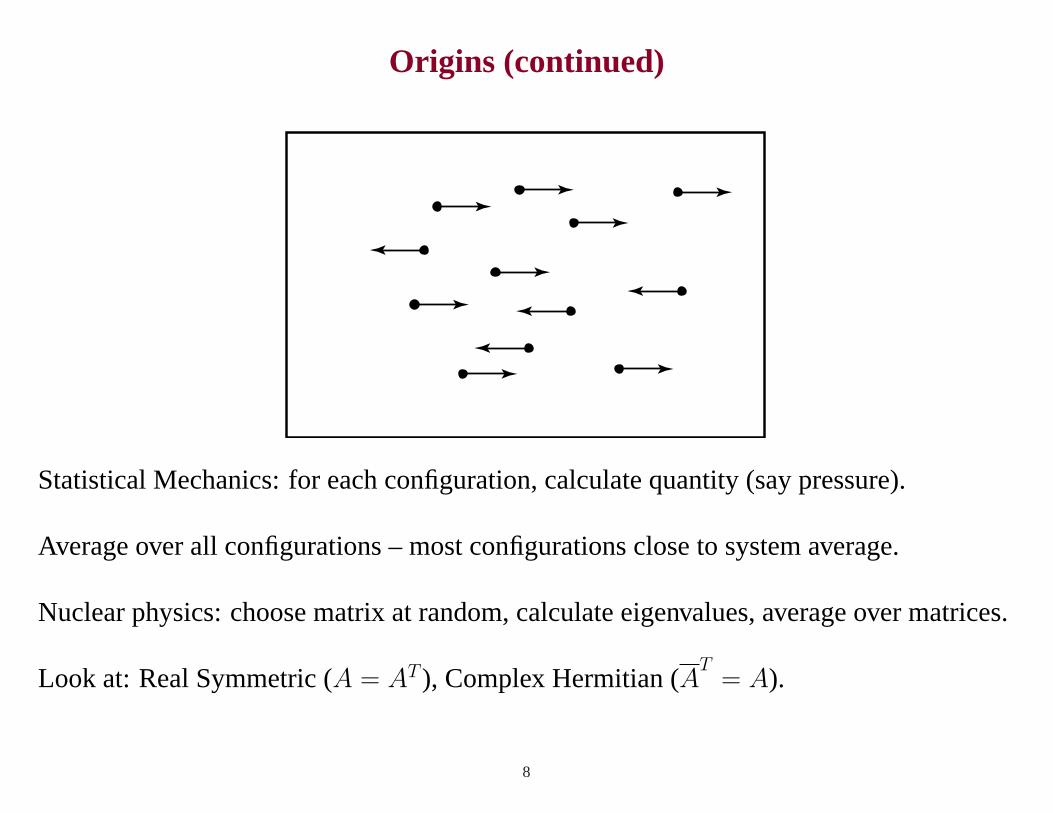
Statistical Mechanics: for each configuration, calculate quantity (say pressure).

Average over all configurations – most configurations close to system average.

Nuclear physics: choose matrix at random, calculate eigenvalues, average over matrices.

Look at: Real Symmetric (A = AT ), Complex Hermitian (AT

= A).

8

Random Matrix Ensembles

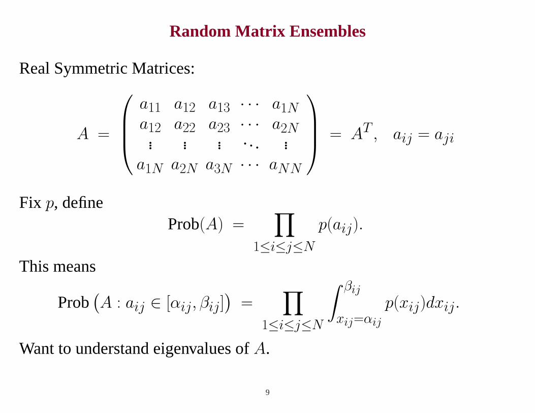
Real Symmetric Matrices:

A =

a11 a12 a13 · · · a1Na12 a22 a23 · · · a2N... ... ... ... ...

a1N a2N a3N · · · aNN

= AT , aij = aji

Fix p, defineProb(A) =

∏

1≤i≤j≤N

p(aij).

This means

Prob(A : aij ∈ [αij, βij]

)=

∏

1≤i≤j≤N

∫ βij

xij=αij

p(xij)dxij.

Want to understand eigenvalues ofA.

9

Eigenvalue Distribution

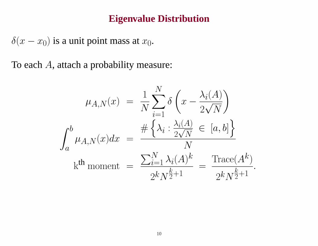
δ(x− x0) is a unit point mass atx0.

To eachA, attach a probability measure:

µA,N (x) =1

N

N∑

i=1

δ

(x− λi(A)

2√

N

)

∫ b

aµA,N (x)dx =

#{

λi :λi(A)

2√

N∈ [a, b]

}

N

kth moment =

∑Ni=1 λi(A)k

2kNk2+1

=Trace(Ak)

2kNk2+1

.

10

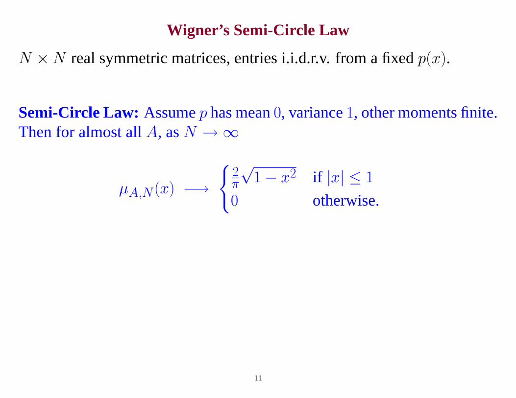
Wigner’s Semi-Circle Law

N ×N real symmetric matrices, entries i.i.d.r.v. from a fixedp(x).

Semi-Circle Law: Assumep has mean0, variance1, other moments finite.Then for almost allA, asN →∞

µA,N (x) −→{

2π

√1− x2 if |x| ≤ 1

0 otherwise.

11

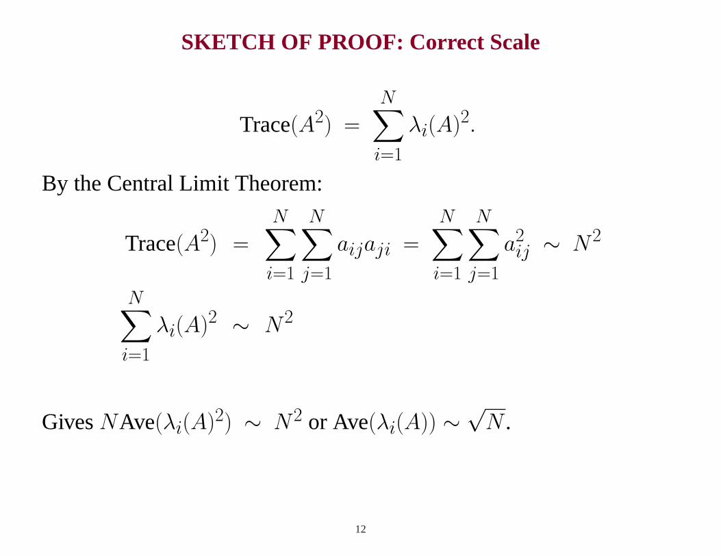
SKETCH OF PROOF: Correct Scale

Trace(A2) =

N∑

i=1

λi(A)2.

By the Central Limit Theorem:

Trace(A2) =

N∑

i=1

N∑

j=1

aijaji =

N∑

i=1

N∑

j=1

a2ij ∼ N2

N∑

i=1

λi(A)2 ∼ N2

GivesNAve(λi(A)2) ∼ N2 or Ave(λi(A)) ∼ √N .

12

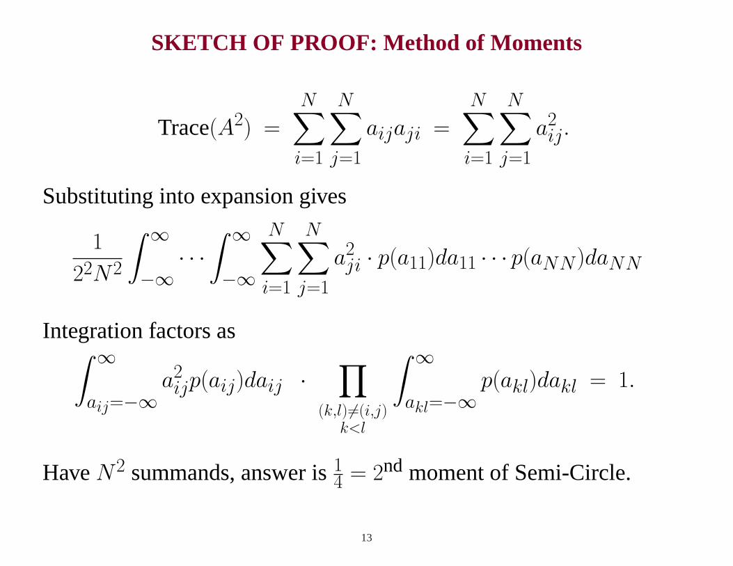
SKETCH OF PROOF: Method of Moments

Trace(A2) =

N∑

i=1

N∑

j=1

aijaji =

N∑

i=1

N∑

j=1

a2ij.

Substituting into expansion gives

1

22N2

∫ ∞

−∞· · ·

∫ ∞

−∞

N∑

i=1

N∑

j=1

a2ji · p(a11)da11 · · · p(aNN )daNN

Integration factors as∫ ∞

aij=−∞a2ijp(aij)daij ·

∏

(k,l) 6=(i,j)k<l

∫ ∞

akl=−∞p(akl)dakl = 1.

HaveN2 summands, answer is14 = 2nd moment of Semi-Circle.

13

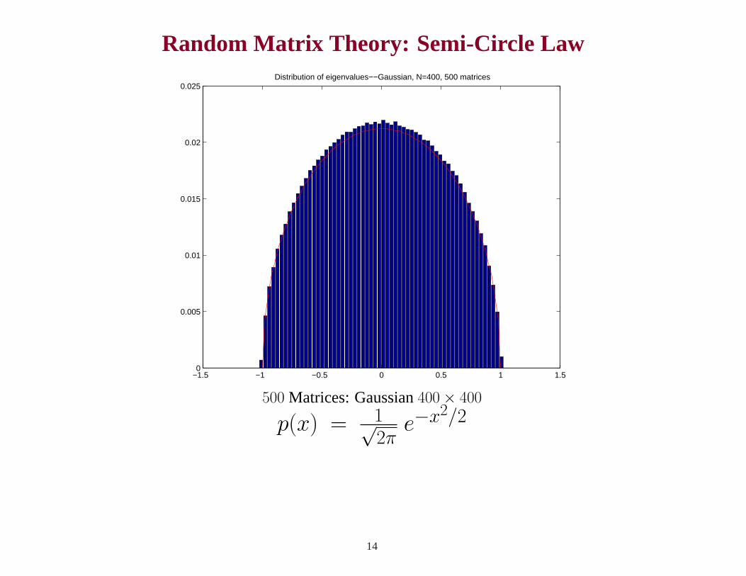
Random Matrix Theory: Semi-Circle Law

−1.5 −1 −0.5 0 0.5 1 1.50

0.005

0.01

0.015

0.02

0.025Distribution of eigenvalues−−Gaussian, N=400, 500 matrices

500 Matrices: Gaussian400× 400

p(x) = 1√2π

e−x2/2

14

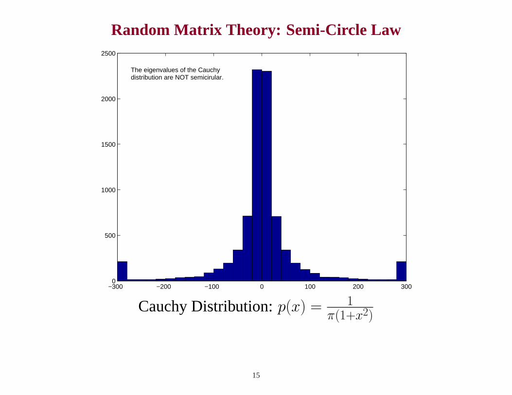
Random Matrix Theory: Semi-Circle Law

−300 −200 −100 0 100 200 3000

500

1000

1500

2000

2500

The eigenvalues of the Cauchydistribution are NOT semicirular.

Cauchy Distribution:p(x) = 1π(1+x2)

15

GOE Conjecture

GOE Conjecture: As N →∞, the probability density of the spacing b/wconsecutive normalized eigenvalues approaches a limit independent ofp.

Only known ifp is a Gaussian.

GOE(x) ≈ Axe−Bx2.

16

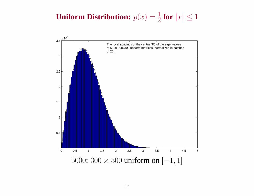
Uniform Distribution: p(x) = 12 for |x| ≤ 1

0 0.5 1 1.5 2 2.5 3 3.5 4 4.5 50

0.5

1

1.5

2

2.5

3

3.5x 10

4

The local spacings of the central 3/5 of the eigenvaluesof 5000 300x300 uniform matrices, normalized in batchesof 20.

5000: 300× 300 uniform on[−1, 1]

17

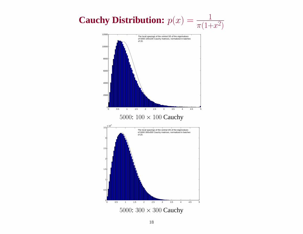
Cauchy Distribution: p(x) = 1π(1+x2)

0 0.5 1 1.5 2 2.5 3 3.5 4 4.5 50

2000

4000

6000

8000

10000

12000

The local spacings of the central 3/5 of the eigenvaluesof 5000 100x100 Cauchy matrices, normalized in batchesof 20.

5000: 100× 100 Cauchy

0 0.5 1 1.5 2 2.5 3 3.5 4 4.5 50

0.5

1

1.5

2

2.5

3

3.5x 10

4

The local spacings of the central 3/5 of the eigenvaluesof 5000 300x300 Cauchy matrices, normalized in batchesof 20.

5000: 300× 300 Cauchy

18

Fat Thin Families

Need a family F A T enough to do averaging.

Need a family THIN enough so that everything isn’t averaged out.

Real Symmetric Matrices haveN(N+1)2 independent entries.

19

Random Graphs 1

23

4

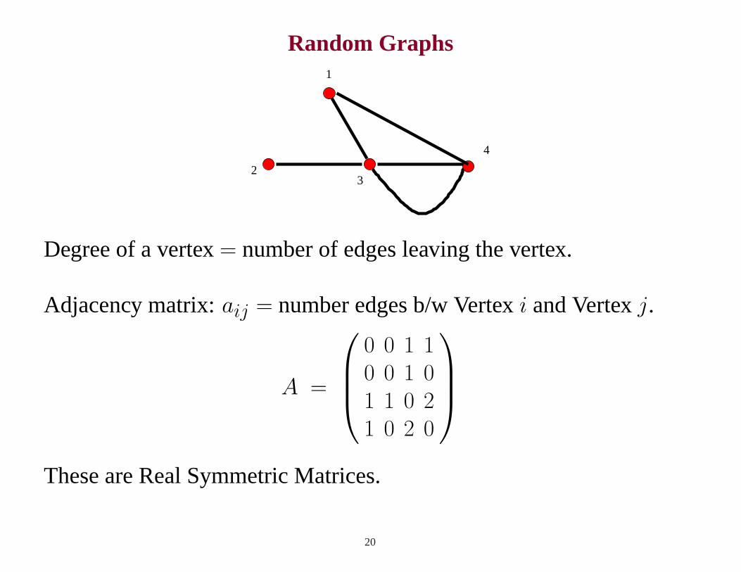
Degree of a vertex= number of edges leaving the vertex.

Adjacency matrix:aij = number edges b/w Vertexi and Vertexj.

A =

0 0 1 10 0 1 01 1 0 21 0 2 0

These are Real Symmetric Matrices.

20

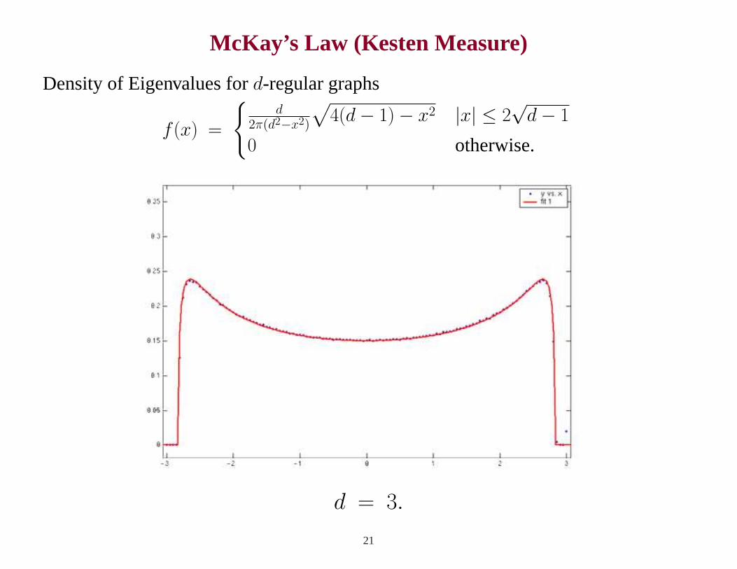
McKay’s Law (Kesten Measure)

Density of Eigenvalues ford-regular graphs

f (x) =

{d

2π(d2−x2)

√4(d− 1)− x2 |x| ≤ 2

√d− 1

0 otherwise.

d = 3.

21

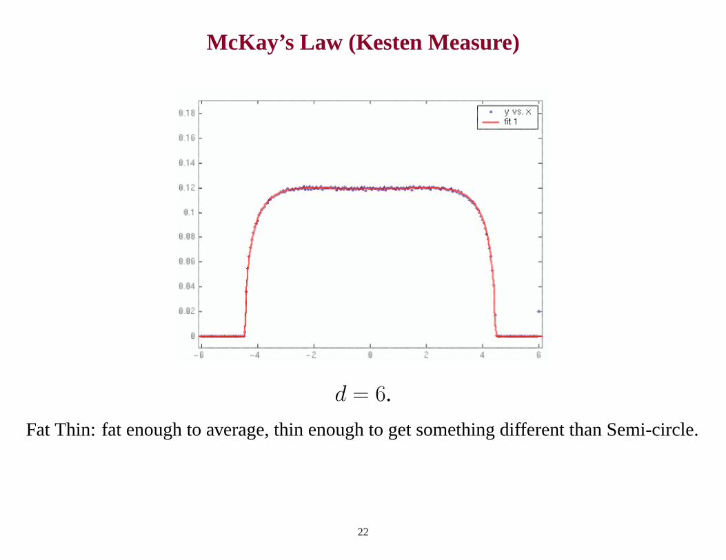
McKay’s Law (Kesten Measure)

d = 6.

Fat Thin: fat enough to average, thin enough to get something different than Semi-circle.

22

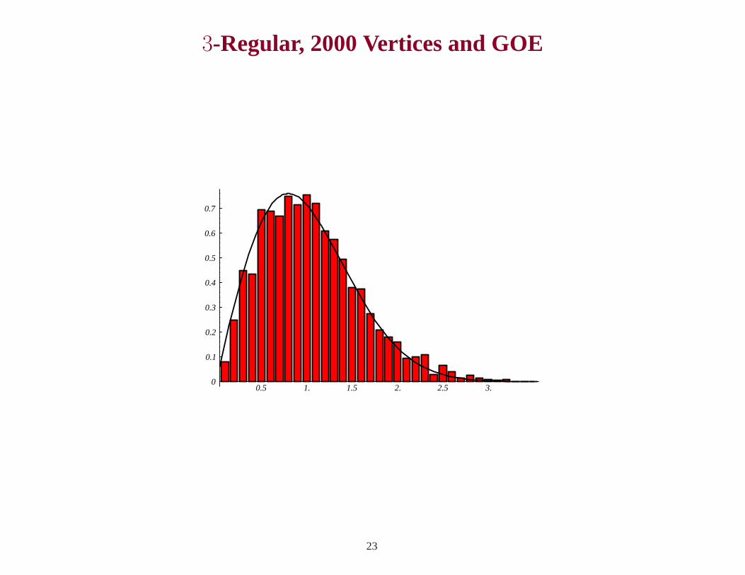
3-Regular, 2000 Vertices and GOE

0.5 1. 1.5 2. 2.5 3.0

0.1

0.2

0.3

0.4

0.5

0.6

0.7

23

PART III

NUMBER THEORY

24

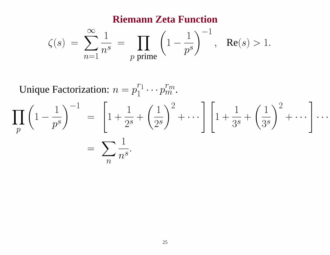
Riemann Zeta Function

ζ(s) =

∞∑

n=1

1

ns =∏

p prime

(1− 1

ps

)−1

, Re(s) > 1.

Unique Factorization:n = pr11 · · · prm

m .

∏p

(1− 1

ps

)−1

=

[1 +

1

2s +

(1

2s

)2

+ · · ·][

1 +1

3s +

(1

3s

)2

+ · · ·]· · ·

=∑n

1

ns.

25

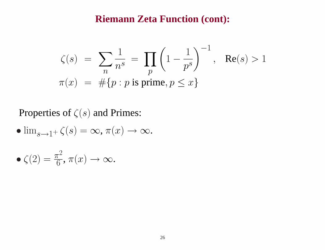
Riemann Zeta Function (cont):

ζ(s) =∑n

1

ns =∏p

(1− 1

ps

)−1

, Re(s) > 1

π(x) = #{p : p is prime, p ≤ x}

Properties ofζ(s) and Primes:

• lims→1+ ζ(s) = ∞, π(x) →∞.

• ζ(2) = π2

6 , π(x) →∞.

26

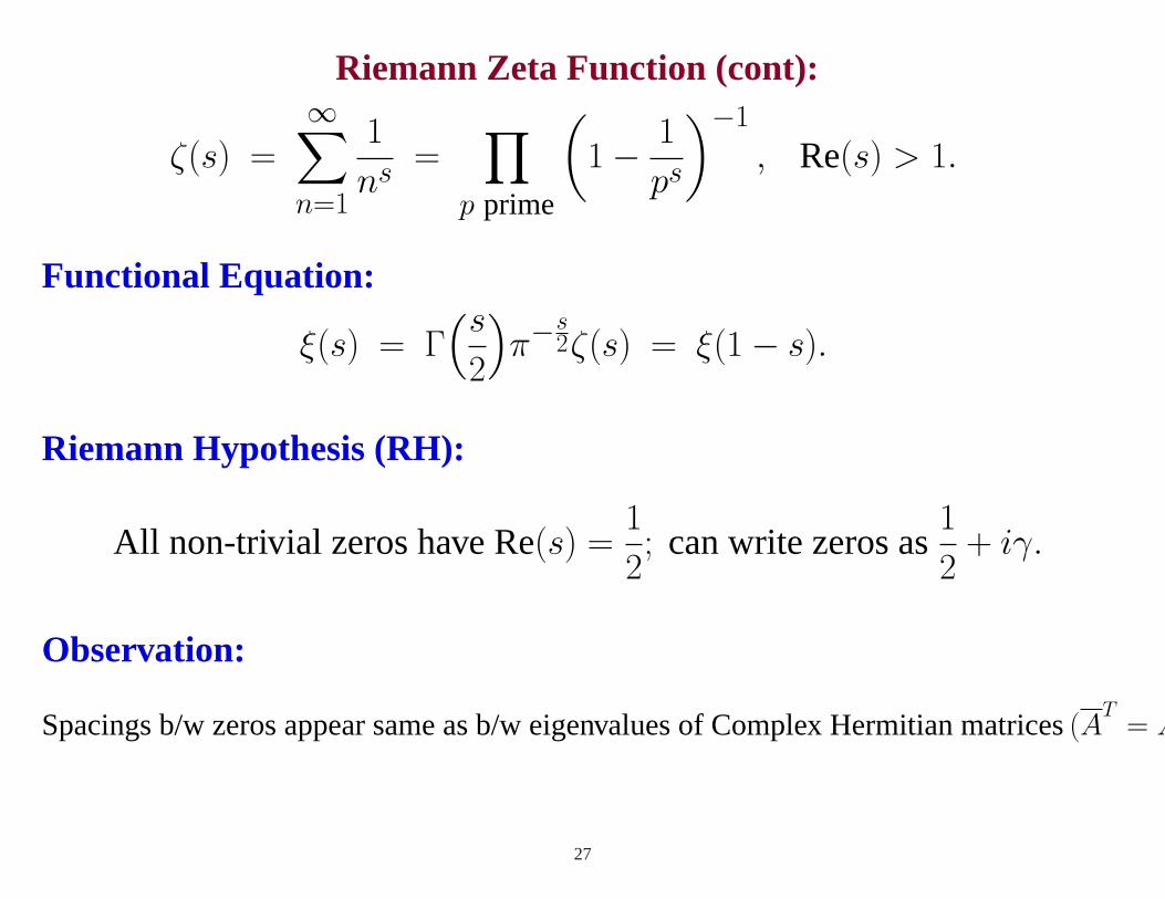
Riemann Zeta Function (cont):

ζ(s) =

∞∑

n=1

1

ns =∏

p prime

(1− 1

ps

)−1

, Re(s) > 1.

Functional Equation:

ξ(s) = Γ(s

2

)π−

s2ζ(s) = ξ(1− s).

Riemann Hypothesis (RH):

All non-trivial zeros have Re(s) =1

2; can write zeros as

1

2+ iγ.

Observation:

Spacings b/w zeros appear same as b/w eigenvalues of Complex Hermitian matrices(AT

= A).

27

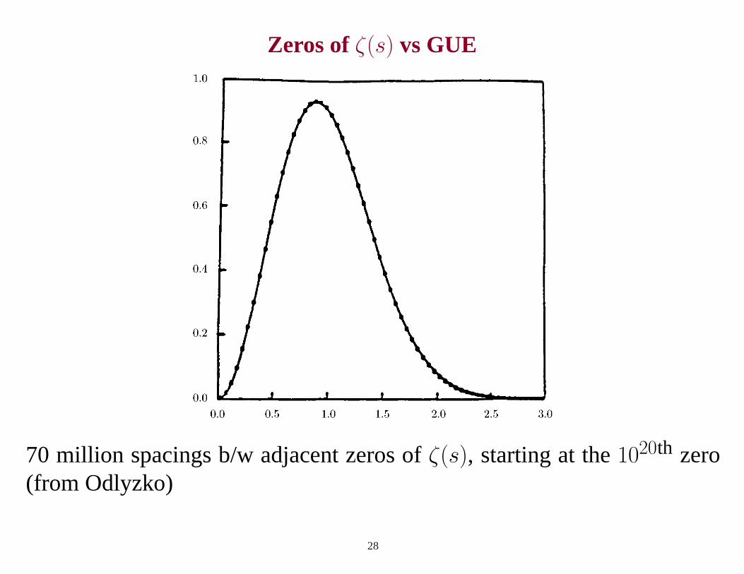
Zeros of ζ(s) vs GUE

70 million spacings b/w adjacent zeros ofζ(s), starting at the1020th zero(from Odlyzko)

28

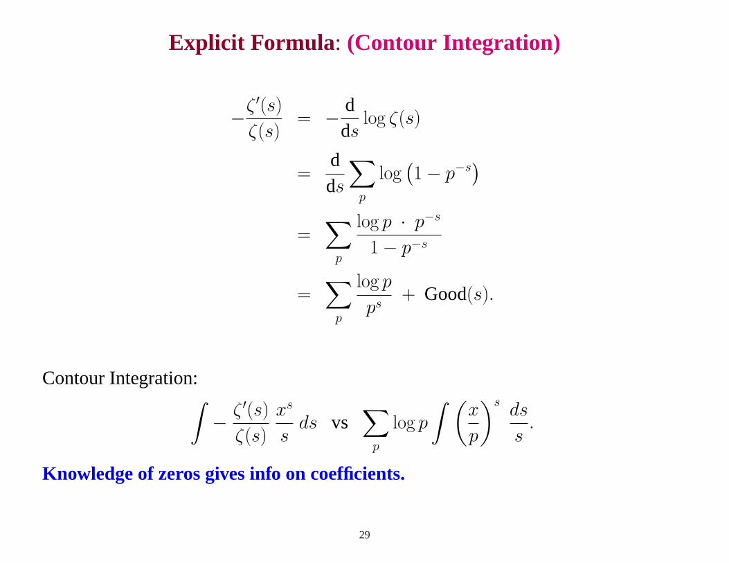
Explicit Formula : (Contour Integration)

−ζ ′(s)

ζ(s)= − d

dslog ζ(s)

=dds

∑p

log(1− p−s

)

=∑

p

log p · p−s

1− p−s

=∑

p

log p

ps+ Good(s).

Contour Integration:∫− ζ ′(s)

ζ(s)

xs

sds vs

∑p

log p

∫ (x

p

)sds

s.

Knowledge of zeros gives info on coefficients.

29

PART IV

ELLIPTIC CURVES

30

Elliptic Curves:

Et : y2 = x3 + A(T )x + B(T ), A(T ), B(T ) ∈ Z(T ).

at(p) = −∑

x mod p

(x3 + A(t)x + B(t)

p

)= at+mp(p)

L(E, s) =

∞∑n=1

aE(n)

ns=

∏p

Lp(E, s).

By GRH: All zeros on the critical line.

Rational solutions:E(Q) = Zr ⊕T .

Birch and Swinnerton-Dyer Conjecture:Geometric rankr = analytic rank (order of vanishing at central point).

31

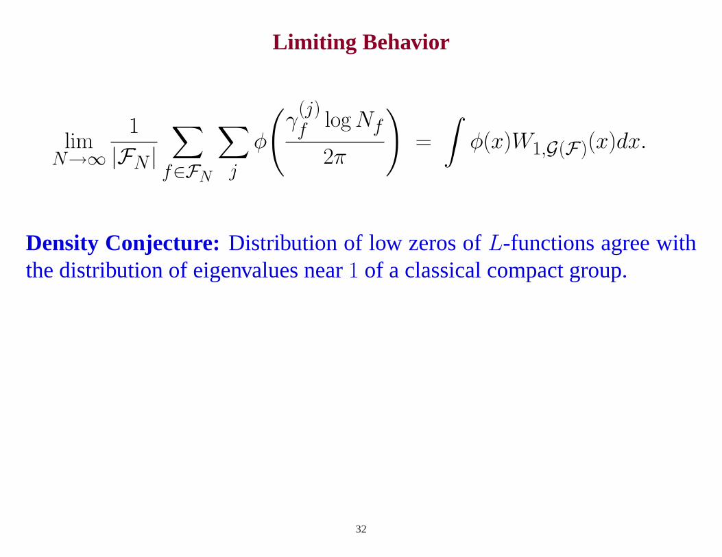
Limiting Behavior

limN→∞

1

|FN |∑

f∈FN

∑

j

φ

(γ

(j)f log Nf

2π

)=

∫φ(x)W1,G(F)(x)dx.

Density Conjecture: Distribution of low zeros ofL-functions agree withthe distribution of eigenvalues near1 of a classical compact group.

32

Tools to Study Low Zeros

• explicit formularelating zeros and Fourier coeffs;

¦ Analogue of Eigenvalue Trace Lemma

• averaging formulasfor the family;

¦ Analogue of integration formulas forTrace(Ak).

33

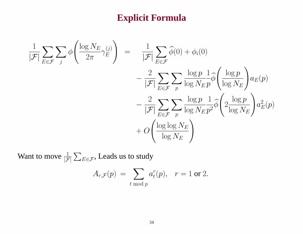
Explicit Formula

1

|F|∑

E∈F

∑j

φ

(log NE

2πγ

(j)E

)=

1

|F|∑

E∈Fφ̂(0) + φi(0)

− 2

|F|∑

E∈F

∑p

log p

log NE

1

pφ̂

(log p

log NE

)aE(p)

− 2

|F|∑

E∈F

∑p

log p

log NE

1

p2φ̂

(2

log p

log NE

)a2

E(p)

+ O

(log log NE

log NE

)

Want to move 1|F|

∑E∈F , Leads us to study

Ar,F(p) =∑

t mod p

art(p), r = 1 or 2.

34

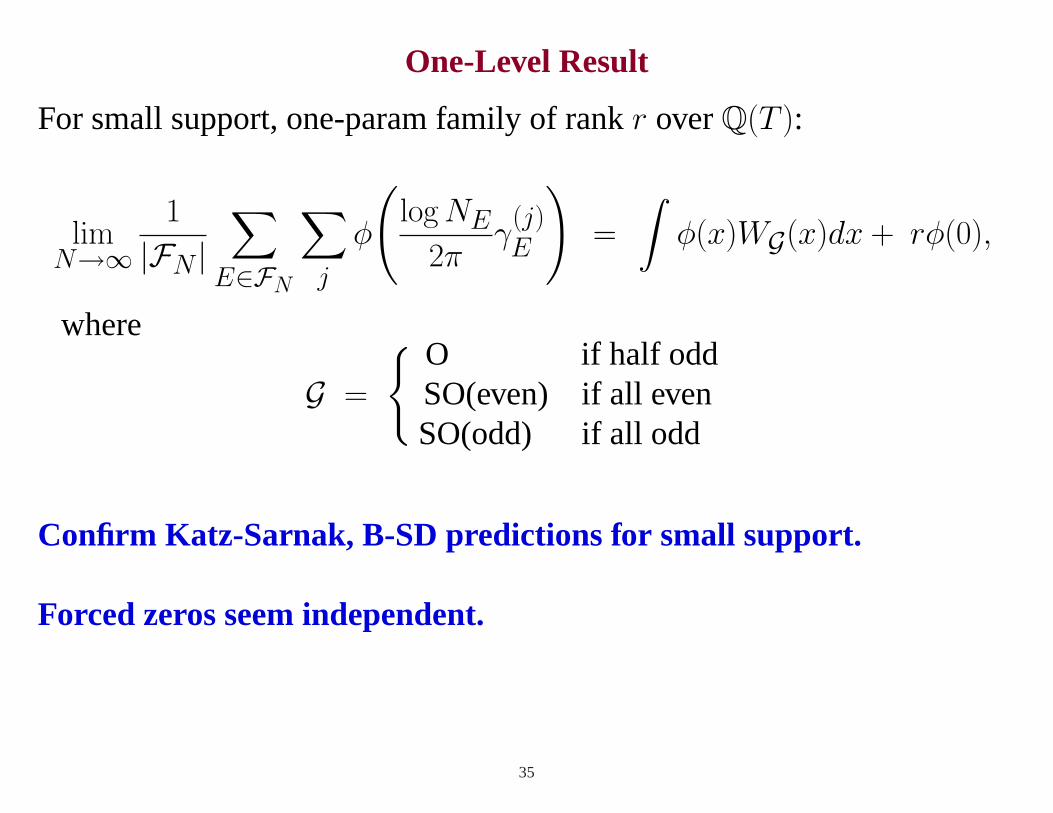
One-Level Result

For small support, one-param family of rankr overQ(T ):

limN→∞

1

|FN |∑

E∈FN

∑

j

φ

(log NE

2πγ

(j)E

)=

∫φ(x)WG(x)dx + rφ(0),

where

G =

{ O if half oddSO(even) if all evenSO(odd) if all odd

Confirm Katz-Sarnak, B-SD predictions for small support.

Forced zeros seem independent.

35

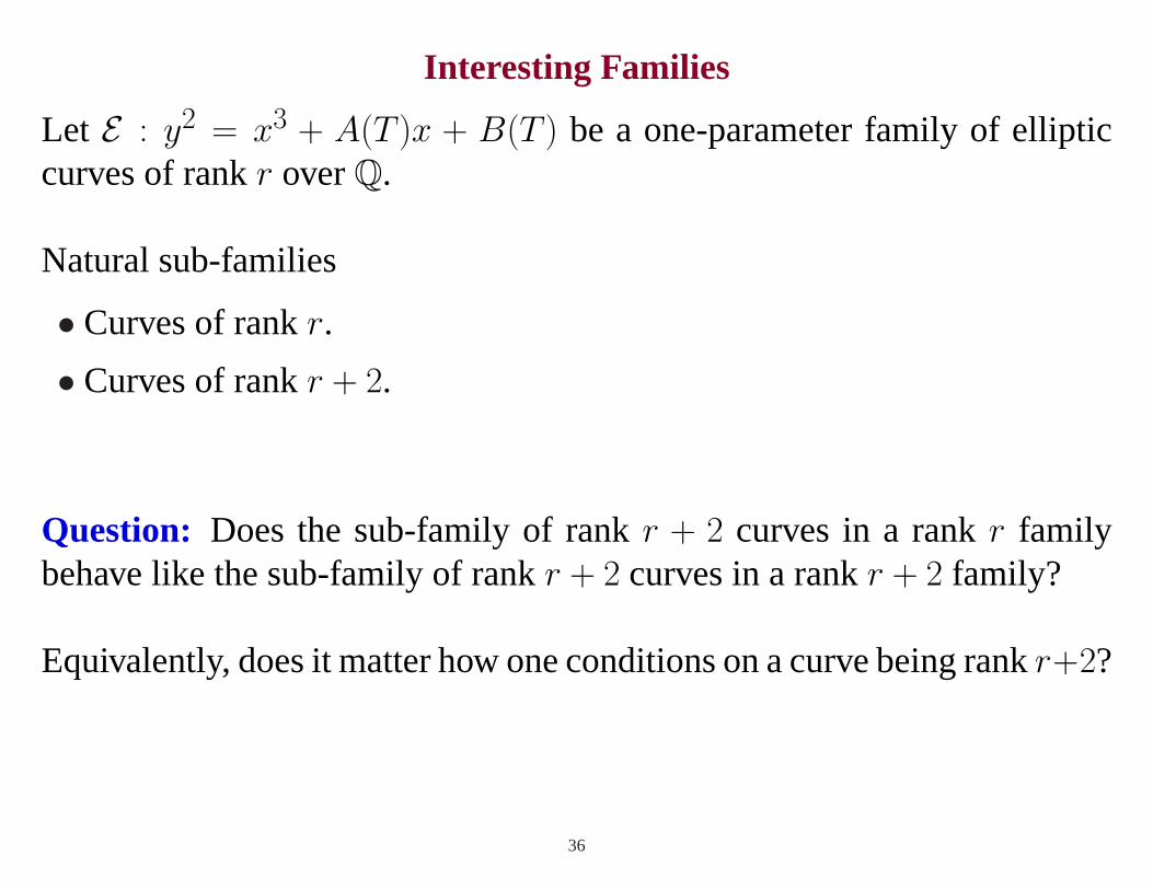
Interesting Families

Let E : y2 = x3 + A(T )x + B(T ) be a one-parameter family of ellipticcurves of rankr overQ.

Natural sub-families

• Curves of rankr.

• Curves of rankr + 2.

Question: Does the sub-family of rankr + 2 curves in a rankr familybehave like the sub-family of rankr + 2 curves in a rankr + 2 family?

Equivalently, does it matter how one conditions on a curve being rankr+2?

36

Orthogonal Random Matrix Models

RMT: 2N eigenvalues, in pairse±iθj, probability measure on[0, π]N :

dε0(θ) ∝∏

j<k

(cos θk − cos θj)2∏

j

dθj.

Independent Model:

A2N,2r =

{(I2r×2r

g

): g ∈ SO(2N − 2r)

}.

Interaction Model:Sub-ensemble ofSO(2N) with the last2r of the2N eigenvalues equal+1:

dε2r(θ) ∝∏

j<k

(cos θk − cos θj)2∏

j

(1− cos θj)2r

∏j

dθj,

with 1 ≤ j, k ≤ N − r.

37

Comparing the RMT Models

Small support, one-parameter families agree withρr,Indep and notρr,Inter.

CurveE, conductorNE, expect first zero12 + iγ(1)E with γ

(1)E ≈ 1

log NE.

r zeros at central point, if repulsion of zeros is of sizecrlog NE, can detect in

1

|FN |∑

E∈FN

∑

j

φ

(γ

(j)E log NE

2π

).

Corrections of size

φ (x0 + cr)− φ(x0) ≈ φ′ (x(x0, cr)) · cr.

38

Testing Random Matrix Theory Predictions

First (Normalized) Zero above Central Point: Do extra zeros at the cen-tral point affect the distribution of zeros near the central point?

39

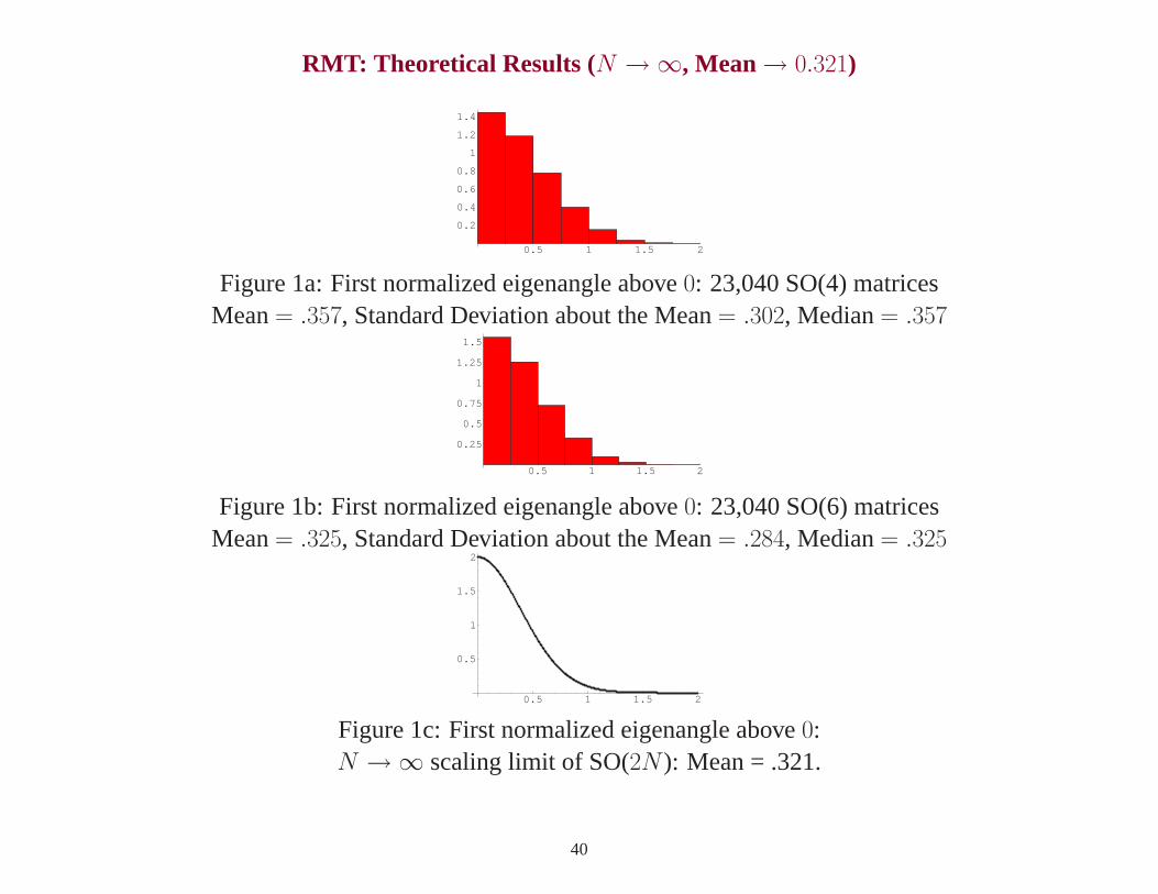
RMT: Theoretical Results (N →∞, Mean→ 0.321)

0.5 1 1.5 2

0.2

0.4

0.6

0.8

1

1.2

1.4

Figure 1a: First normalized eigenangle above0: 23,040 SO(4) matricesMean= .357, Standard Deviation about the Mean= .302, Median= .357

0.5 1 1.5 2

0.25

0.5

0.75

1

1.25

1.5

Figure 1b: First normalized eigenangle above0: 23,040 SO(6) matricesMean= .325, Standard Deviation about the Mean= .284, Median= .325

0.5 1 1.5 2

0.5

1

1.5

2

Figure 1c: First normalized eigenangle above0:N →∞ scaling limit of SO(2N ): Mean = .321.

40

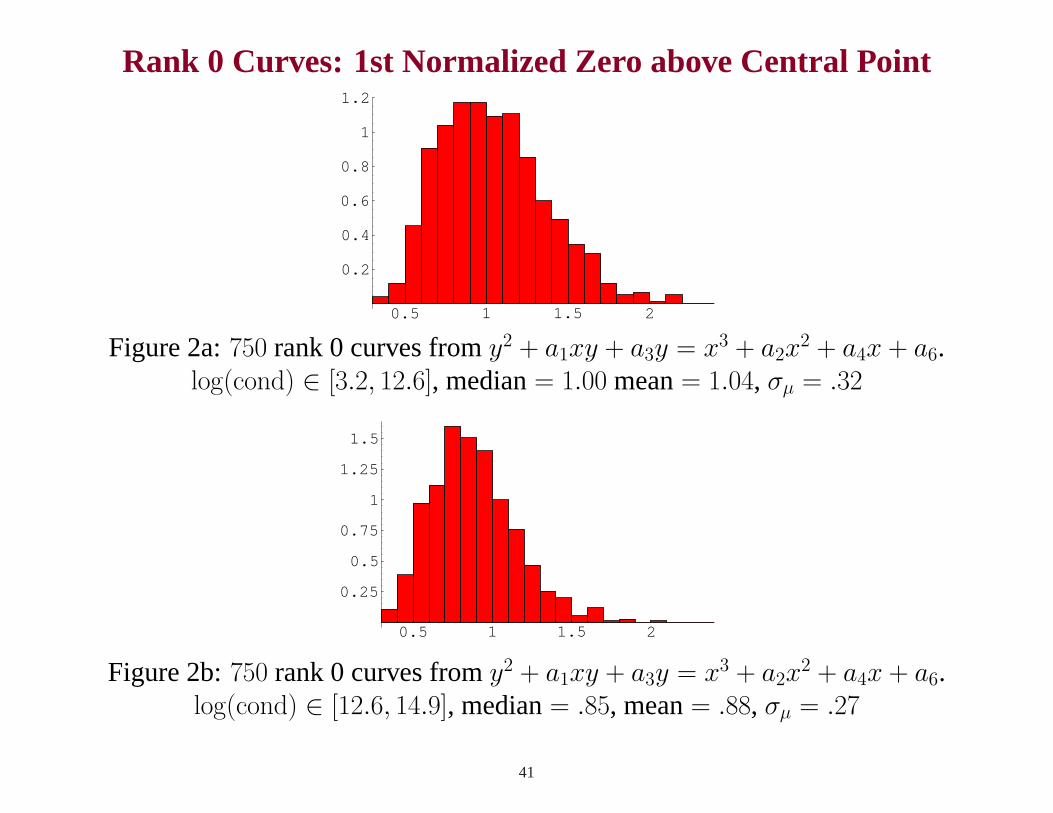
Rank 0 Curves: 1st Normalized Zero above Central Point

0.5 1 1.5 2

0.2

0.4

0.6

0.8

1

1.2

Figure 2a:750 rank 0 curves fromy2 + a1xy + a3y = x3 + a2x2 + a4x + a6.

log(cond) ∈ [3.2, 12.6], median= 1.00 mean= 1.04, σµ = .32

0.5 1 1.5 2

0.25

0.5

0.75

1

1.25

1.5

Figure 2b:750 rank 0 curves fromy2 + a1xy + a3y = x3 + a2x2 + a4x + a6.

log(cond) ∈ [12.6, 14.9], median= .85, mean= .88, σµ = .27

41

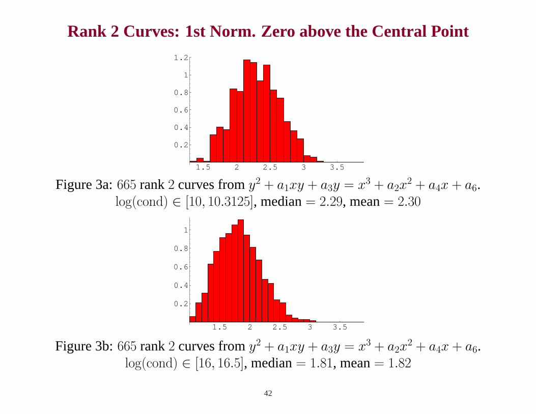
Rank 2 Curves: 1st Norm. Zero above the Central Point

1.5 2 2.5 3 3.5

0.2

0.4

0.6

0.8

1

1.2

Figure 3a:665 rank2 curves fromy2 + a1xy + a3y = x3 + a2x2 + a4x + a6.

log(cond) ∈ [10, 10.3125], median= 2.29, mean= 2.30

1.5 2 2.5 3 3.5

0.2

0.4

0.6

0.8

1

Figure 3b:665 rank2 curves fromy2 + a1xy + a3y = x3 + a2x2 + a4x + a6.

log(cond) ∈ [16, 16.5], median= 1.81, mean= 1.82

42

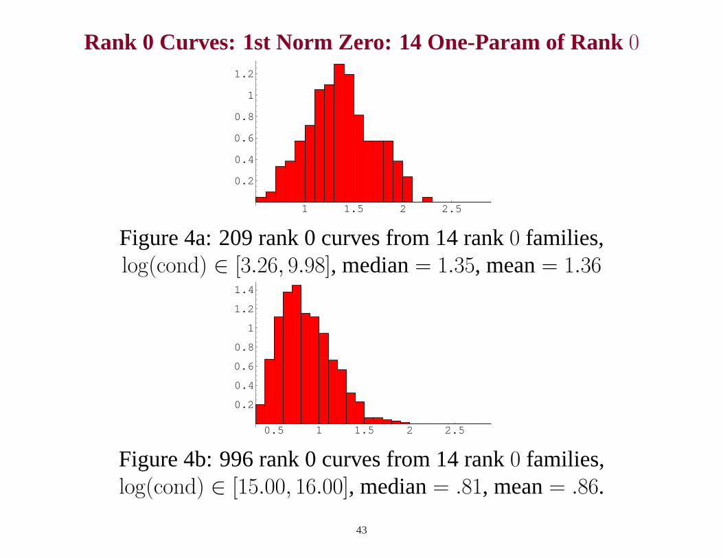
Rank 0 Curves: 1st Norm Zero: 14 One-Param of Rank0

1 1.5 2 2.5

0.2

0.4

0.6

0.8

1

1.2

Figure 4a: 209 rank 0 curves from 14 rank0 families,log(cond) ∈ [3.26, 9.98], median= 1.35, mean= 1.36

0.5 1 1.5 2 2.5

0.2

0.4

0.6

0.8

1

1.2

1.4

Figure 4b: 996 rank 0 curves from 14 rank0 families,log(cond) ∈ [15.00, 16.00], median= .81, mean= .86.

43

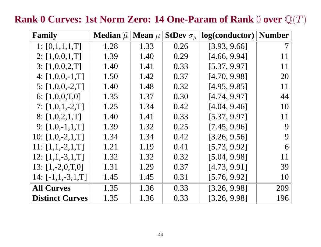
Rank 0 Curves: 1st Norm Zero: 14 One-Param of Rank0 overQ(T )

Family Median µ̃ Mean µ StDevσµ log(conductor) Number1: [0,1,1,1,T] 1.28 1.33 0.26 [3.93, 9.66] 72: [1,0,0,1,T] 1.39 1.40 0.29 [4.66, 9.94] 113: [1,0,0,2,T] 1.40 1.41 0.33 [5.37, 9.97] 114: [1,0,0,-1,T] 1.50 1.42 0.37 [4.70, 9.98] 205: [1,0,0,-2,T] 1.40 1.48 0.32 [4.95, 9.85] 116: [1,0,0,T,0] 1.35 1.37 0.30 [4.74, 9.97] 447: [1,0,1,-2,T] 1.25 1.34 0.42 [4.04, 9.46] 108: [1,0,2,1,T] 1.40 1.41 0.33 [5.37, 9.97] 119: [1,0,-1,1,T] 1.39 1.32 0.25 [7.45, 9.96] 9

10: [1,0,-2,1,T] 1.34 1.34 0.42 [3.26, 9.56] 911: [1,1,-2,1,T] 1.21 1.19 0.41 [5.73, 9.92] 612: [1,1,-3,1,T] 1.32 1.32 0.32 [5.04, 9.98] 1113: [1,-2,0,T,0] 1.31 1.29 0.37 [4.73, 9.91] 3914: [-1,1,-3,1,T] 1.45 1.45 0.31 [5.76, 9.92] 10All Curves 1.35 1.36 0.33 [3.26, 9.98] 209Distinct Curves 1.35 1.36 0.33 [3.26, 9.98] 196

44

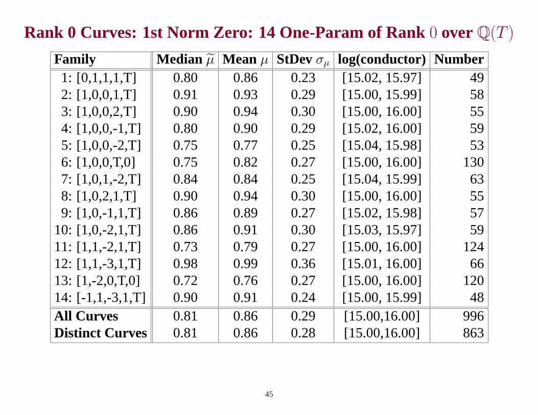
Rank 0 Curves: 1st Norm Zero: 14 One-Param of Rank0 overQ(T )

Family Median µ̃ Mean µ StDevσµ log(conductor) Number1: [0,1,1,1,T] 0.80 0.86 0.23 [15.02, 15.97] 492: [1,0,0,1,T] 0.91 0.93 0.29 [15.00, 15.99] 583: [1,0,0,2,T] 0.90 0.94 0.30 [15.00, 16.00] 554: [1,0,0,-1,T] 0.80 0.90 0.29 [15.02, 16.00] 595: [1,0,0,-2,T] 0.75 0.77 0.25 [15.04, 15.98] 536: [1,0,0,T,0] 0.75 0.82 0.27 [15.00, 16.00] 1307: [1,0,1,-2,T] 0.84 0.84 0.25 [15.04, 15.99] 638: [1,0,2,1,T] 0.90 0.94 0.30 [15.00, 16.00] 559: [1,0,-1,1,T] 0.86 0.89 0.27 [15.02, 15.98] 57

10: [1,0,-2,1,T] 0.86 0.91 0.30 [15.03, 15.97] 5911: [1,1,-2,1,T] 0.73 0.79 0.27 [15.00, 16.00] 12412: [1,1,-3,1,T] 0.98 0.99 0.36 [15.01, 16.00] 6613: [1,-2,0,T,0] 0.72 0.76 0.27 [15.00, 16.00] 12014: [-1,1,-3,1,T] 0.90 0.91 0.24 [15.00, 15.99] 48All Curves 0.81 0.86 0.29 [15.00,16.00] 996Distinct Curves 0.81 0.86 0.28 [15.00,16.00] 863

45

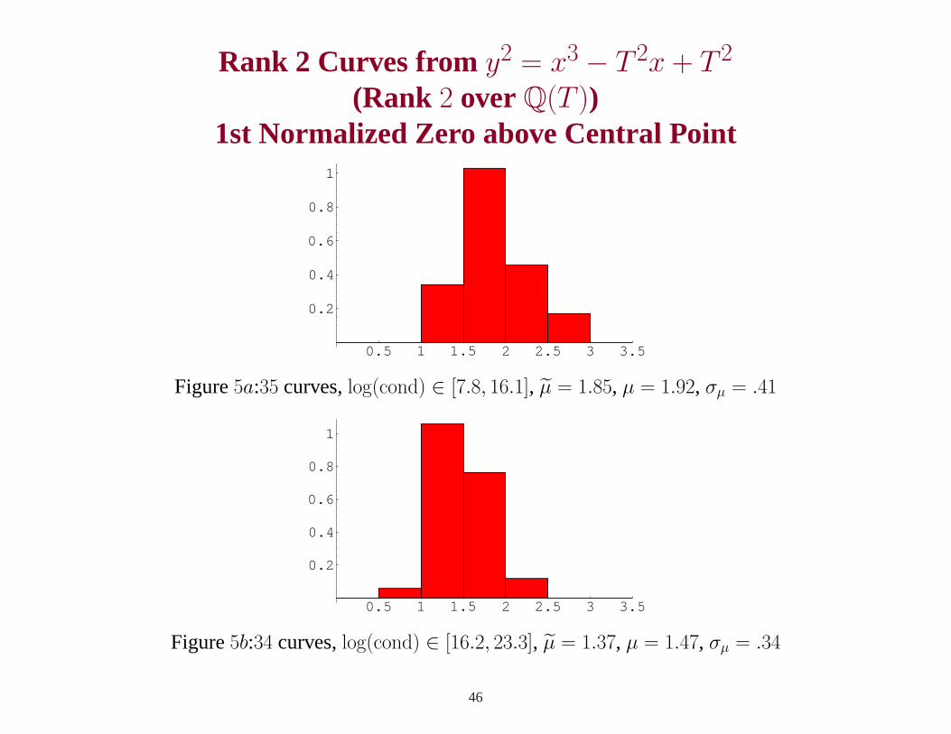
Rank 2 Curves from y2 = x3 − T 2x + T 2

(Rank 2 overQ(T ))1st Normalized Zero above Central Point

0.5 1 1.5 2 2.5 3 3.5

0.2

0.4

0.6

0.8

1

Figure5a:35 curves,log(cond) ∈ [7.8, 16.1], µ̃ = 1.85, µ = 1.92, σµ = .41

0.5 1 1.5 2 2.5 3 3.5

0.2

0.4

0.6

0.8

1

Figure5b:34 curves,log(cond) ∈ [16.2, 23.3], µ̃ = 1.37, µ = 1.47, σµ = .34

46

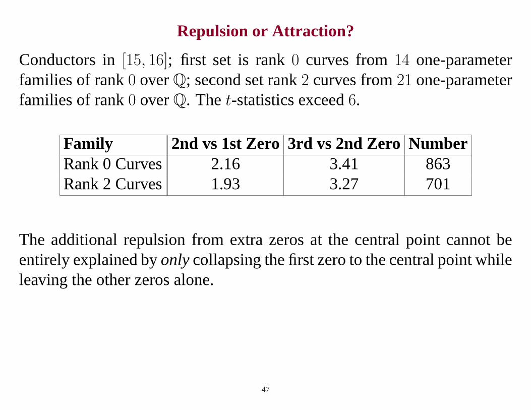
Repulsion or Attraction?

Conductors in[15, 16]; first set is rank0 curves from14 one-parameterfamilies of rank0 overQ; second set rank2 curves from21 one-parameterfamilies of rank0 overQ. Thet-statistics exceed6.

Family 2nd vs 1st Zero 3rd vs 2nd Zero NumberRank 0 Curves 2.16 3.41 863Rank 2 Curves 1.93 3.27 701

The additional repulsion from extra zeros at the central point cannot beentirely explained byonlycollapsing the first zero to the central point whileleaving the other zeros alone.

47

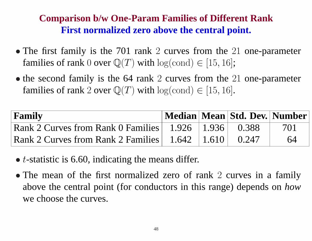
Comparison b/w One-Param Families of Different RankFirst normalized zero above the central point.

• The first family is the 701 rank2 curves from the21 one-parameterfamilies of rank0 overQ(T ) with log(cond) ∈ [15, 16];

• the second family is the 64 rank2 curves from the21 one-parameterfamilies of rank2 overQ(T ) with log(cond) ∈ [15, 16].

Family Median Mean Std. Dev. NumberRank 2 Curves from Rank 0 Families1.926 1.936 0.388 701Rank 2 Curves from Rank 2 Families1.642 1.610 0.247 64

• t-statistic is 6.60, indicating the means differ.

• The mean of the first normalized zero of rank2 curves in a familyabove the central point (for conductors in this range) depends onhowwe choose the curves.

48

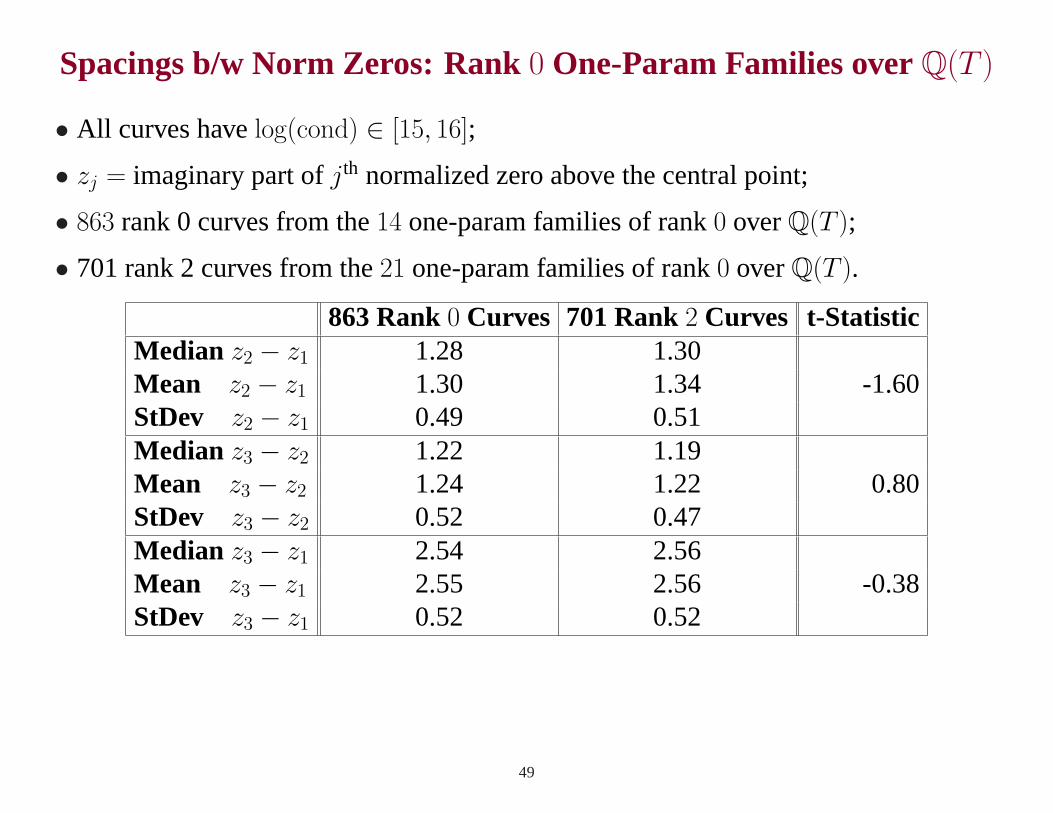
Spacings b/w Norm Zeros: Rank0 One-Param Families overQ(T )

• All curves havelog(cond) ∈ [15, 16];

• zj = imaginary part ofjth normalized zero above the central point;

• 863 rank 0 curves from the14 one-param families of rank0 overQ(T );

• 701 rank 2 curves from the21 one-param families of rank0 overQ(T ).

863 Rank0 Curves 701 Rank2 Curves t-StatisticMedian z2 − z1 1.28 1.30Mean z2 − z1 1.30 1.34 -1.60StDev z2 − z1 0.49 0.51Median z3 − z2 1.22 1.19Mean z3 − z2 1.24 1.22 0.80StDev z3 − z2 0.52 0.47Median z3 − z1 2.54 2.56Mean z3 − z1 2.55 2.56 -0.38StDev z3 − z1 0.52 0.52

49

Spacings b/w Norm Zeros: Rank0 One-Param Families overQ(T )

•While the normalized zeros are repelled from the central point (and bydifferent amounts for the two sets), thedifferencesbetween the nor-malized zeros are statistically independent of this repulsion (t-statistics< 2).

•While for a given range of log-conductors the average second normal-ized zero of a rank0 curve is close to the average first normalized zeroof a rank2 curve, they are not the same and the additional repulsionfrom extra zeros at the central point cannot be entirely explained byonlycollapsing the first zero to the central point while leaving the otherzeros alone.

50

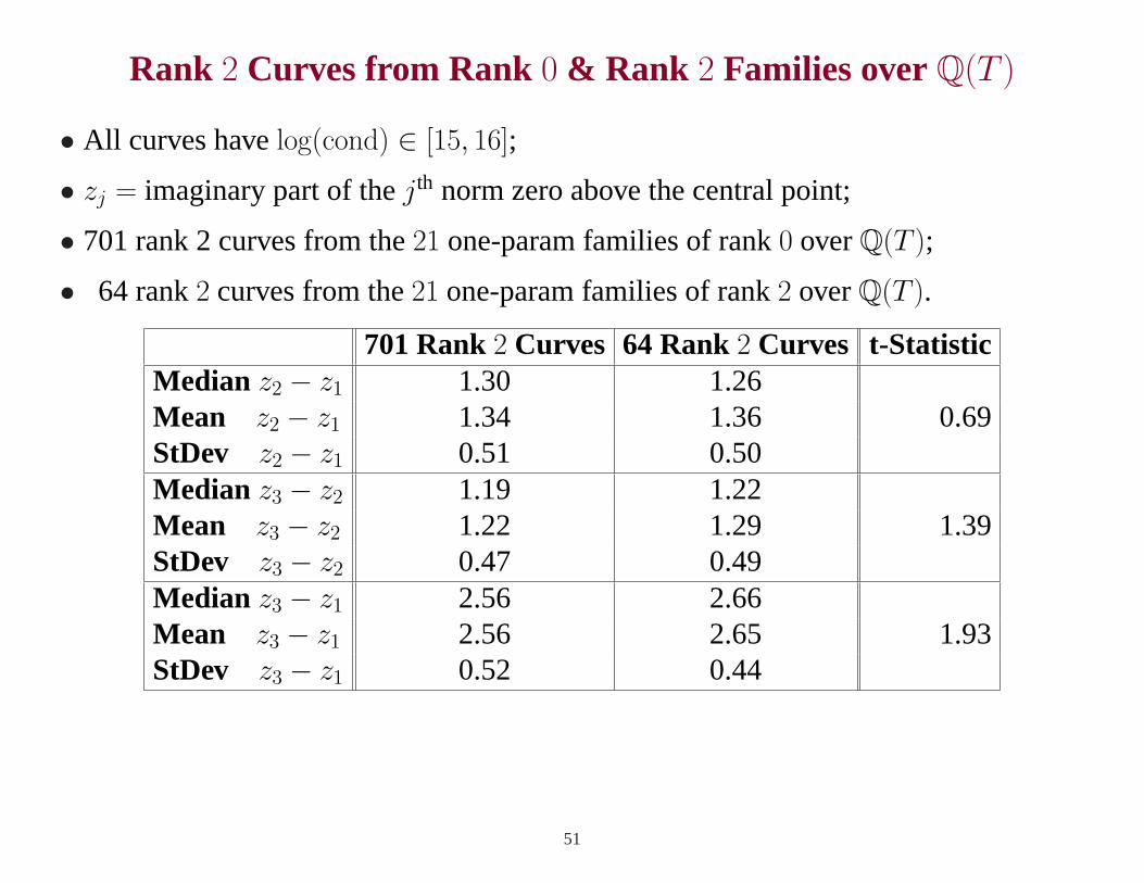
Rank 2 Curves from Rank 0 & Rank 2 Families overQ(T )

• All curves havelog(cond) ∈ [15, 16];

• zj = imaginary part of thejth norm zero above the central point;

• 701 rank 2 curves from the21 one-param families of rank0 overQ(T );

• 64 rank2 curves from the21 one-param families of rank2 overQ(T ).

701 Rank2 Curves 64 Rank2 Curves t-StatisticMedian z2 − z1 1.30 1.26Mean z2 − z1 1.34 1.36 0.69StDev z2 − z1 0.51 0.50Median z3 − z2 1.19 1.22Mean z3 − z2 1.22 1.29 1.39StDev z3 − z2 0.47 0.49Median z3 − z1 2.56 2.66Mean z3 − z1 2.56 2.65 1.93StDev z3 − z1 0.52 0.44

51

PART V

CONCLUSIONS

52

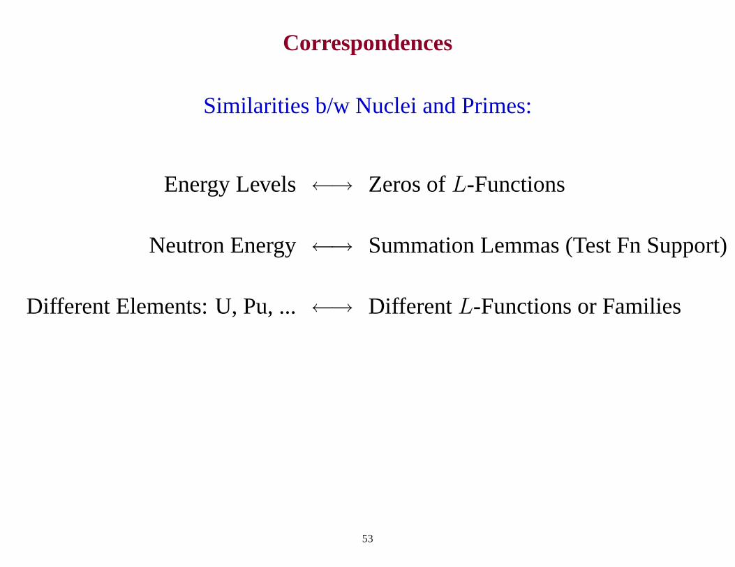
Correspondences

Similarities b/w Nuclei and Primes:

Energy Levels←→ Zeros ofL-Functions

Neutron Energy←→ Summation Lemmas (Test Fn Support)

Different Elements: U, Pu, ...←→ DifferentL-Functions or Families

53

Summary

• Similar behavior in different systems.

• Find correct scale.

• Average over similar elements.

• Need a Trace Lemma.

• Thin subsets can exhibit very different behavior.

54

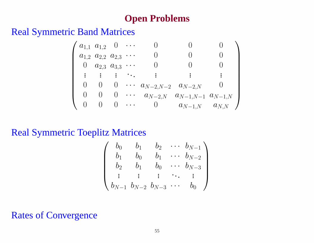
Open ProblemsReal Symmetric Band Matrices

a1,1 a1,2 0 · · · 0 0 0a1,2 a2,2 a2,3 · · · 0 0 00 a2,3 a3,3 · · · 0 0 0... ... ... ... ... ... ...0 0 0 · · · aN−2,N−2 aN−2,N 00 0 0 · · · aN−2,N aN−1,N−1 aN−1,N

0 0 0 · · · 0 aN−1,N aN,N

Real Symmetric Toeplitz Matrices

b0 b1 b2 · · · bN−1

b1 b0 b1 · · · bN−2

b2 b1 b0 · · · bN−3... ... ... ... ...

bN−1 bN−2 bN−3 · · · b0

Rates of Convergence

55