Theory and simulation of micropolar fluid dynamics

Theory and simulation of micropolar fluid dynamicsJ Chen*, C Liang, and J D Lee

Department of Mechanical and Aerospace Engineering, The George Washington University, Washington, DC, USA

The manuscript was received on 29 October 2010 and was accepted after revision for publication on 21 January 2011.

DOI: 10.1177/1740349911400132

Abstract: This paper reviews the fundamentals of micropolar fluid dynamics (MFD), and pro-poses a numerical scheme integrating Chorin’s projection method and time-centred splitmethod (TCSM) for solving unsteady forms of MFD equations. It has been known thatNavier–Stokes equations are incapable of explaining the phenomena at micro and nanoscales. On the contrary, MFD can naturally pick up the physical phenomena at micro andnano scales owingto its additional degrees of freedom for gyration. In this study, the analyti-cal and exact solutions of Couette and Hagen–Poiseuille flow are provided. Though this studyis limited to the steady flow cases, the unsteady term in the MFD has been taken intoaccount. This present work initiates the development of a general-purpose code of computa-tional micropolar fluid dynamics (CMFD). The discretization scheme in space is demon-strated with nearly second-order accuracy on multiple meshes.

Keywords: micropolar fluid dynamics (MFD), microfluidics, computational micropolar fluid

dynamics (CMFD), finite difference method, projection method, time-centre split method

(TCSM)

1 INTRODUCTION

Research activities aiming to explore fluid physics

at nano and micro scales have been increasing over

the past 20 years. There are existing literatures that

have analysed fluid mechanics in microchannels

and micromachined fluid systems (e.g. pumps and

valves) using Navier–Stokes equations [1]. Fluid

flow moves differently in the micro scale than that

in the macro scale. There are situations in which

the Navier–Stokes equations, derived from classical

continuum, become incapable of explaining the

micro scale fluid transport phenomena [2]. The

reason is that when the channel size is comparable

to the molecular size, the spinning of molecules,

which have been observed in molecular dynamics

(MD) simulations [3, 4], affects significantly the

flow field. This effect of molecular spin is not taken

into account in the Navier–Stokes equations. A

novel approach, microcontinuum theory, consisting

of micropolar, microstretch, and micromorphic

(3M) theories, developed by Eringen [5–8] and Lee

et al. [9], offers a mathematical foundation to cap-

ture such motions. In 3M theories, each particle has

a finite size and contains a microstructure that can

rotate and deform independently, regardless of the

motion of the centroid of the particle. The formula-

tion of the micropolar theory has additional degrees

of freedom – gyration – to determine the rotation of

the microstructure. Hence, the balance law of angu-

lar momentum are given for solving gyration. This

equation introduces a mechanism to take into

account the effect of molecular spin. The micropo-

lar theory thus represents a promising alternative

approach to numerically solving micro scale fluid

dynamics that can be much more computationally

efficient than the MD simulations.

Papautsky [10] was the first one to adopt the

micropolar fluid model to explain the experimental

observation of volume flow rate reduction for the

flow in a rectangular microchannel. In addition,

Gad-El-Hak [11] explicitly states that microscale

flows are essentially different from flows in the

*Corresponding author: Department of Mechanical and

Aerospace Engineering, The George Washington University,

Washington, DC, 20052, USA

email: [email protected]

31

Proc. IMechE Vol. 224 Part N: J. Nanoengineering and Nanosystems

macroscale. The Navier–Stokes description is inca-

pable of explaining the observed effects. The calcu-

lated hydrodynamic quantities for a fluid as

a classical continuous medium (from Navier–Stokes

equations) differ significantly from those obtained

experimentally, and the difference increases with

the decrease of the channel diameter in the flow

through narrow channels.

There are many recent developments of micro-

polar theory that have focused on numerical analy-

sis of Hagen–Poiseuille flow and its applications on

nano- and microfluidics, including Papautsky [10],

Ye [12], and Hansen [13]. However, all of the stud-

ies considered only a steady state solution and did

not solve for pressure. Their methods are therefore

unable to solve unsteady flow problems.

In this work, a numerical scheme for solving the

unsteady form of micropolar fluid dynamics (MFD)

is developed. A detailed explanation for the physical

meaning of all coefficients is provided. Analytical

and exact solutions for flat-plate Hagen–Poiseuille

flow and flat-plate Couette flow are discussed

against numerical solutions. As a numerical exam-

ple, lid-driven cavity flow is simulated by solving

the micropolar equations. Nomenclature can be

found in the Appendix section.

2 MICROPOLAR FLUID THEORY

In microcontinuum field theories, the material points

of the fluid are considered to be small deformable

particles. The macromotion and micromotion of the

material particles are expressed by [5–9]

xk5xk X ; tð Þ; k51;2;3 (1)

jk5xkK X ; tð Þ�K ; K 51;2;3 (2)

Since the material particles are considered to be

geometrical points with mass and inertia, xkK X ; tð Þhere represents the three deformable directors

attached to the material particles.

For a material body called a micropolar contin-

uum, the micromotion is further reduced to a rota-

tion. In other words, its directors are orthonormal

and rigid, that is

xkK xlK ¼ dkl; xkK xkL ¼ dKL (3)

For fluid flow, deformation-rate tensors are cru-

cial to the characterization of the viscous resistance.

Deformation-rate tensors may be deduced by

simply calculating the material time-rates of the

spatial deformation tensors. For micropolar fluid,

two objective deformation-rate tensors are [5–8]

akl ¼ vl;k1elkmvm; bkl ¼ vk;l (4)

vm is the gyration vector, which is the addi-

tional rotating degree of freedom for a particle.

Because the mean free path of fluid is larger than

solid, each fluid molecule has more space to move

around. When a group of fluid molecules or

a single fluid molecule spins, the effect of the

gyration vector appears and cannot be observed in

classical continuum theory. Therefore, the gy

ration vector is a good candidate for determining

the physics at the micro scale while adopting the

continuum assumption.

The balance laws of the micropolar continuum

can be expressed as [5, 6]:

Conservation of mass

_r1rvl;l ¼ 0 (5)

Balance of momentum

tkl;k1rðfl � _vlÞ ¼ 0 (6)

Balance of angular momentum

mkl;k1elmntmn1rðll � i _vlÞ ¼ 0 (7)

Conservation of energy

r _e � tklðvl;k1elkrvrÞ �mklvl;k 1 qk;k � rh ¼ 0 (8)

Clausius–Duhem inequality

� rð _c1h _uÞ1tklakl1mblblk �qk

uu;k � 0 (9)

The linear constitutive equations for Cauchy

stress, moment stress, and heat flux are derived to

be [5, 6]

tkl5� pdkl1l tr amnð Þdkl1 m1kð Þakl1malk

[� pdkl1Dtkl

mkl5a

ueklmu;m1a tr bmnð Þdkl1bbkl1gblk

qk5K

uu;k1aeklmvm;l (10)

Substitute the constitutive equations into all the

balance laws, and the governing field equations of

MFD can be rewritten as [5–8]:

Conservation of mass

_r1rvl;l ¼ 0 (11)

32 J Chen, C Liang, and J D Lee


Balance of momentum

�rp1ðl1mÞrr � v1ðm1kÞr2v

1kr3v1rf ¼ r _v(12)

Balance of angular momentum

ða1bÞrr �v1gr2v1kðr3v � 2vÞ1rl ¼ ri _v (13)

Conservation of energy

r _e � Dt : aT�m : b1r � q � rh ¼ 0 (14)

The microinertia is defined as

i [ 2jkjkh i

5 2

Rr0jkjkdv0R

r0dv0

[ l2

(15)

and l represents a hidden length scale, which can be

at the level of molecular scale, Kolmogorov micro

scale, or Taylor micro scale. These small-scale activi-

ties can possibly be measured experimentally using

Largragian velocities of tracer particles [14,15].

3 CONNECTION WITH NAVIER–STOKES

EQUATIONS

Vorticity is considered as the circulation per unit

area at a point in a fluid flow field. It is a common

practice in general vector analysis to describe

a vector function of a position having zero curl as

irrotational in view of the connection between

r 3 v and the local rotation of the fluid [16]. It has

another physical interpretation: vorticity measures

the solid-body-like rotation of a material point P’

adjacent to the primary material point P [17].

In micropolar fluid dynamics, gyration has a simi-

lar concept. One can interpret the motion in MFD

using the earth motion as an example. In the

motion of the earth, it not only revolves around the

sun, which results in seasons, but also spins on its

own axis, which makes days. A micropolar contin-

uum is considered as a continuous collection of

finite-size particles. The translation of finite-size

fluid particles can be imagined as the earth revolu-

tion with, the gyration being similar to the spin of

the earth.

The material time rates of spatial deformation

tensors can be obtained as

D

Dtðxk;K Þ ¼ vk;lxl;K

D

DtðxkK Þ ¼ vklxlK (16)

If the micromotion equals the macromotion, that

is, xl,K = xlK, this leads to

vk;l ¼ vkl (17)

In micropolar theory, the gyration tensor is anti-

symmetric, that is

vkl ¼ �eklmvm (18)

This leads to

vm ¼1

2elkmvk;l (19)

The physical picture of equation (19) is similar to

the motion of the moon; it always faces the Earth

with the same side while revolving around the Earth.

Substitute equation (19) into equation (12) and

one can obtain

�rp1ðl1m�Þrr � v1m�r2v1rf ¼ r _v (20)

where m� ¼ m11=2k. It is identical to Navier–Stokes

equations derived from Newtonian fluid. At this

point, the MFD formulation has been clearly shown

as more general than Navier–Stokes equations.

4 NUMERICAL SCHEME

The time-centre split method (TCSM) was first devel-

oped by Fu and Hodges in 2009 for unsteady advec-

tion problems [18]. Here the TCSM is further

extended for incompressible MFD. The incompress-

ible fluid implies r � v ¼ 0 and hence the pressure p

becomes the Lagrange multiplier. The condition

r � v ¼ 0 must be enforced and indeed it is used to

calculate the Lagrange multiplier. The Chorin’s pro-

jection method is incorporated with TCSM to update

the pressure gradient term for solving the Poisson

equation. Also, it is noted that the effect of thermo-

mechanical coupling is not considered.

The projection method was originally introduced

to solve time-dependent incompressible Navier–

Stokes fluid-flow problems by Chorin [19]. In

Chorin’s original version of the projection method,

the intermediate velocity v* is explicitly computed

Theory and simulation of micropolar fluid dynamics 33


using the momentum equations, ignoring the pres-

sure gradient term

v� � vn

ðt� � tnÞ ¼ �vn � rvn1mr2vn(21)

where vn is the velocity at the nth time step. In the

next step, the velocity is updated with

vn11 � v�

ðtn11 � t�Þ ¼ �1

rrpn11 (22)

In order to guarantee that vn11 satisfies the conti-

nuity equation, taking divergence on both sides of

equation (22) leads to

r � vn11 �r � v� ¼ � ðtn11 � t�Þ

rr2pn11 (23)

Thus, a Poisson equation for pn11 is obtained as

r2pn11 ¼ r

ðtn11 � t�Þr � v�

(24)

A distinguished feature of Chorin’s projection

method is that the velocity field is forced to satisfy

the continuity equation at the end of each time

step.

In this paper, a new method is proposed. It

incorporates TCSM into Chorin’s projection method

for MFD equations and enforces the continuity

equation to be satisfied in the middle and at the

end of each time step. The procedures of this

method are listed as follows.

1. Neglect the pressure effect and update the

velocity from tn to t* while dealing with the con-

vective term as v � rv = vn � rv*

rv� � vn

t� � tnð Þ1vn � rv��

¼ m1kð Þr2v�1kr3vn

(25)

2. Solve

r2p�� ¼ r

ðt�� t�Þr � v�

3. March time from t* to t**and update velocity as

v�� ¼ v� � ðt�� t�Þ

rrp��

which guarantees velocity divergence free at t**.

4. Solve gyration v** at t** using velocity field v**

riv�� vn

t�� tnð Þ1v�� rv��

¼

a1bð Þrr �v��1gr2v��1k r3v�� 2v��ð Þ1rl(26)

5. Neglect the pressure effect and update velocity

from t** to t*** while dealing with the convective

term as v � rv = v** � rv**

rv�� v��

t�� t��ð Þ1v�� rv��

¼

ðm1kÞr2v��1kr3v��(27)

6. Solve

r2pn11 ¼ r

tn11 � t��ð Þr � v��

7. March time from t*** to tn11 and update velocity

using

vn11 ¼ v�� tn11 � t��

rrpn11:vn11

to satisfy the continuity equation at tn11.

8. Solve gyration vn11 at tn11 using the velocity

field nn11

rivn11 �v��

tn11 � t��ð Þ1vn11 � rvn11

� �¼

ða1bÞrr �vn111gr2vn111

kðr3vn11 � 2vn11Þ1rl

(28)

The procedures from step 1 to step 8 complete

a physical step of time marching. The advantage of

this algorithm is to avoid the non-linear terms in

the equations and to provide a set of linear equa-

tions with a second-order accuracy in time evolving

[18].

For the viscous terms of velocity and gyration,

they are discretized using the central difference

method, for example

r2vx ¼vxðx11; y; zÞ � 2vxðx; y; zÞ1vxðx � 1; y; zÞ

�x2

� �

1vxðx; y11; zÞ � 2vxðx; y; zÞ1vxðx; y � 1; zÞ

�y2

� �

1vxðx; y; z11Þ � 2vxðx; y; zÞ1vxðx; y; z � 1Þ

�z2

� �

(29)



r2vx ¼vxðx11; y; zÞ � 2vxðx; y; zÞ1vxðx � 1; y; zÞ

�x2

� �

1vxðx; y11; zÞ � 2vxðx; y; zÞ1vxðx; y � 1; zÞ

�y2

� �

1vxðx; y; z11Þ � 2vxðx; y; zÞ1vxðx; y; z � 1Þ

�z2

� �

(30)

For the convective terms, v � rv and v � rv, an

upwind scheme is adopted due to the stability

issue. For example, at step 1 in the time marching

algorithm, the convective terms in momentum

equations can be discretized as

vxvj;x )

vnx x;y;zð Þ

v�j x;y;zð Þ � v�j x � 1;y;zð Þ�x

if vnx x;y;zð Þ. 0

vnx x;y;zð Þ

v�j x11;y;zð Þ � v�j x;y;zð Þ�x

if vnx x;y;zð Þ\0

8>>>>>>>><>>>>>>>>:

(31)

where j can be x, y, or z. However at step 5, v*** is

unknown, so the upwind scheme is chosen based

on v**

vxvj;x )

v��x ðx; y; zÞv��x ðx; y; zÞ � v��x ðx � 1; y; zÞ

�x

if v��x ðx; y; zÞ. 0

v��x ðx; y; zÞv��x ðx11; y; zÞ � v��x ðx; y; zÞ

�x

if v��x ðx; y; zÞ\0

8>>>>>>>>><>>>>>>>>>:

(32)

where j can be x, y, or z. At steps 4 and 8, the con-

vective terms in the angular momentum equations

are discretized as

vxvj;x )

v�xðx; y; zÞv�j ðx; y; zÞ � v�j ðx � 1; y; zÞ

�x

if v�xðx; y; zÞ. 0

v�xðx; y; zÞv�j ðx11; y; zÞ � v�j ðx; y; zÞ

�x

if v�xðx; y; zÞ\0

8>>>>>>>><>>>>>>>>:

(33)

vxvj;x )

vn11x ðx; y; zÞ

vn11j ðx; y; zÞ � vn11

j ðx � 1; y; zÞ�x

if vn11x ðx; y; zÞ. 0

vn11x ðx; y; zÞ

vn11j ðx11; y; zÞ � vn11

j ðx; y; zÞ�x

if vn11x ðx; y; zÞ\0

8>>>>>>>><>>>>>>>>:

(34)

where j can be x or y or z. The central difference

method is also employed to discretize the curl of

velocity and gyration.

∂vx

∂y� ∂vy

∂x5

vx x;y11;zð Þ � vx x;y � 1;zð Þ2�y

� vy x11;y;zð Þ � vy x � 1;y;zð Þ2�x

∂vx

∂y� ∂vy

∂x5

vx x;y11;zð Þ � vx x;y � 1;zð Þ2�y

� vy x11;y;zð Þ � vy x � 1;y;zð Þ2�x (35)

5 ANALYTICAL AND EXACT SOLUTIONS OFCOUETTE FLOW

Consider an incompressible fluid with a top plate in

height h moving with a velocity U0, a bottom plate

fixed, and the following assumptions: (a) no velocity

in the y- and z-directions, (b) no gyration in the x-

and y-directions, (c) fully developed flow (i.e. both

x-direction velocity and z-direction gyration are

functions of y only), and (d) no body force.

The steady solution for micropolar fluid is

vx ¼�k

Mðm1kÞ C2eMy�C3e�My� �

12ðC_21C_3Þy1C4

vz ¼ C2eMy1C3e�My � m1k

2m1kC1

(36)

where

M25k 2m1kð Þg m1kð Þ

C152m1k

m1kC21C3ð Þ

C25U0

2 k 1�eMhð ÞM m1kð Þ 1 e�Mh�eMh

e�Mh�1

� �h

� �

C351� eMh

e�Mh � 1C2

C45k

M m1kð Þ C2 � C3ð Þ(37)

The steady solution of Newtonian fluid is

vx ¼y

hU0

�vz ¼ �1

2

∂vx

∂y¼ �U0

2h

(38)

Taking into account that g is the viscosity coeffi-

cient, which tends to stop the rotation of the finite



size particles, one can also define the internal char-

acteristic length l

l ¼ g

k� m1k

2m1k

� �12

(39)

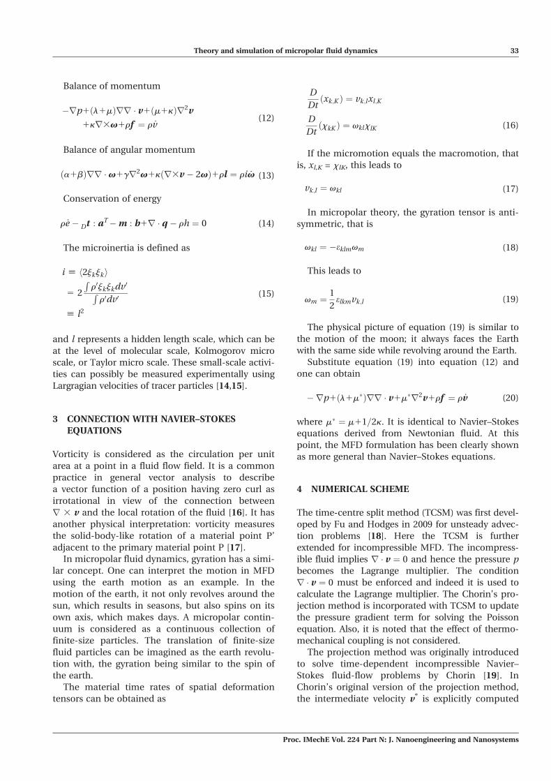
Note that g = 0 leads to l = 0. Figure 1 shows the

gyration plot with the change of l. It can be

observed that as g decreases, the gyration effect

intensifies. It should be mentioned that the gyration

is normalized by the angular velocity solved from

Navier–Stokes equations.

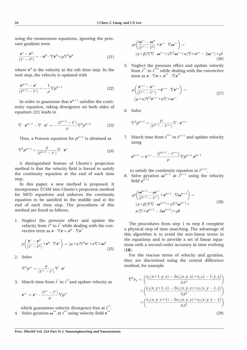
Utilizing the proposed numerical method, the

transient process of Couette flow can now be tack-

led. The fluid is initially at rest. The time step is set

as 2 31023 and the result is output every 100 steps.

Figure 2 shows the time evolution of the velocity

profile in Couette flow

6 ANALYTICAL AND EXACT SOLUTIONS OFPOISEUILLE FLOW

Consider an incompressible fluid in a channel with

a uniform pressure gradient 2G and half channel

height h. The steady state solution for micropolar

fluid is

vx5G

2m1kð Þ h2 � y2� �

1kC2

M m1kð Þ eMh1e�Mh� �

� eMy1e�My� ��

vz5Gy

2m1kð Þ1C2 eMy � e�My� �

(40)

where

M2 ¼ kð2m1kÞgðm1kÞ ; C2 ¼

�Gh

ðeMh � e�MhÞð2m1kÞ (41)

The steady solution of Newtonian fluid is

vx ¼G

2m�ðh2 � y2Þ

�vz ¼ �1

2

∂vx

∂y¼ Gy

2m�

(42)

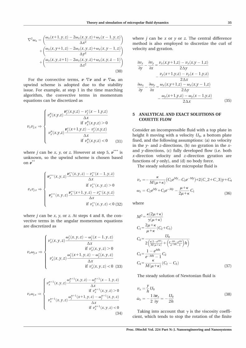
It can be observed that k is the connection

between velocity and gyration, which indicates the

strength of the coupling effect. In Figs 3 and 4, m1k

keeps constant while k is changing. It is obvious that

when k is dominating in m1k, the coupling effect is

so strong that the centre velocity of MFD is quite dif-

ferent from the velocity obtained from the Navier–

Stokes equations. The plot of gyration and centre

Fig. 1 The comparison of angular velocity in Navier–Stokes equations and microgyration in MFD(Couette flow)

Fig. 2 Time evolution of velocity in Couette flow. Thearrow indicates the transient process as timemarches on

Fig. 3 The comparison of velocity profiles in Navier–Stokes equations and MFD (Poiseuille flow)



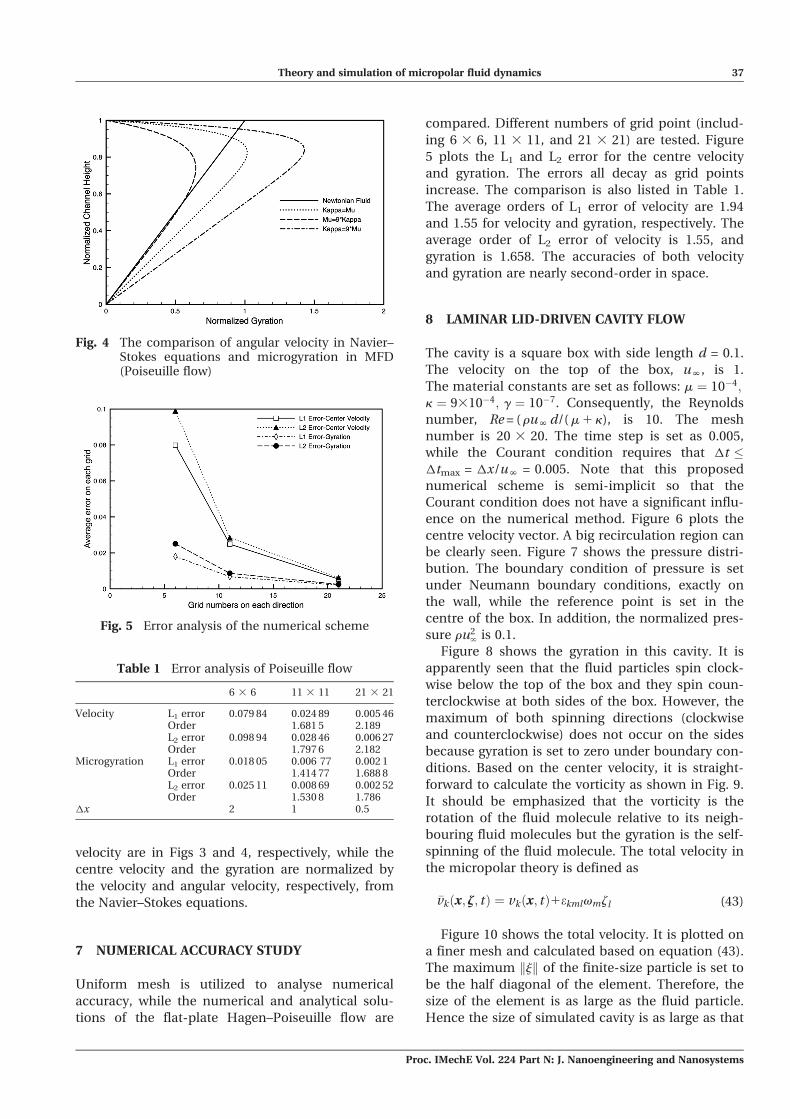
velocity are in Figs 3 and 4, respectively, while the

centre velocity and the gyration are normalized by

the velocity and angular velocity, respectively, from

the Navier–Stokes equations.

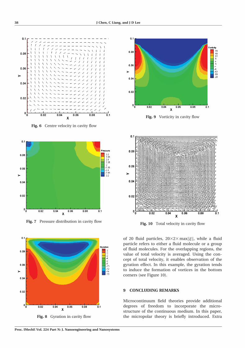
7 NUMERICAL ACCURACY STUDY

Uniform mesh is utilized to analyse numerical

accuracy, while the numerical and analytical solu-

tions of the flat-plate Hagen–Poiseuille flow are

compared. Different numbers of grid point (includ-

ing 6 3 6, 11 3 11, and 21 3 21) are tested. Figure

5 plots the L1 and L2 error for the centre velocity

and gyration. The errors all decay as grid points

increase. The comparison is also listed in Table 1.

The average orders of L1 error of velocity are 1.94

and 1.55 for velocity and gyration, respectively. The

average order of L2 error of velocity is 1.55, and

gyration is 1.658. The accuracies of both velocity

and gyration are nearly second-order in space.

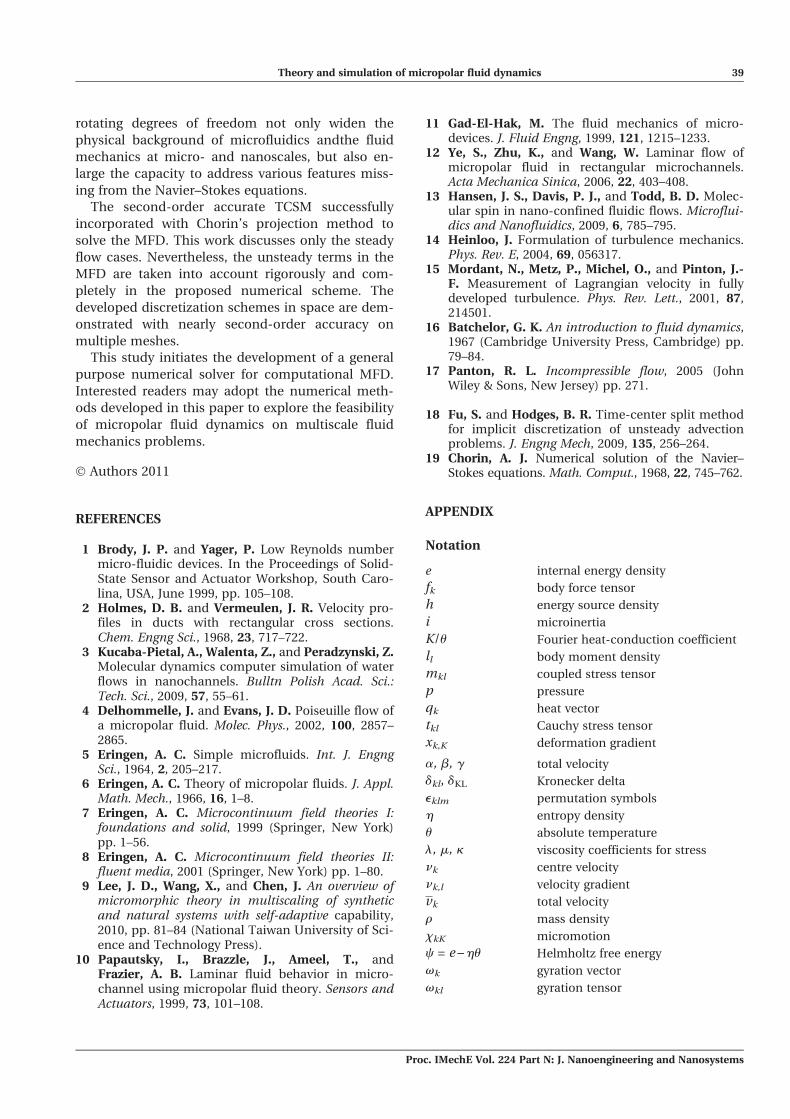
8 LAMINAR LID-DRIVEN CAVITY FLOW

The cavity is a square box with side length d = 0.1.

The velocity on the top of the box, uN, is 1.

The material constants are set as follows: m ¼ 10�4;

k ¼ 9310�4; g ¼ 10�7. Consequently, the Reynolds

number, Re = ( ruN d/( m 1 k), is 10. The mesh

number is 20 3 20. The time step is set as 0.005,

while the Courant condition requires that �t ��tmax = �x/uN = 0.005. Note that this proposed

numerical scheme is semi-implicit so that the

Courant condition does not have a significant influ-

ence on the numerical method. Figure 6 plots the

centre velocity vector. A big recirculation region can

be clearly seen. Figure 7 shows the pressure distri-

bution. The boundary condition of pressure is set

under Neumann boundary conditions, exactly on

the wall, while the reference point is set in the

centre of the box. In addition, the normalized pres-

sure ru2‘ is 0.1.

Figure 8 shows the gyration in this cavity. It is

apparently seen that the fluid particles spin clock-

wise below the top of the box and they spin coun-

terclockwise at both sides of the box. However, the

maximum of both spinning directions (clockwise

and counterclockwise) does not occur on the sides

because gyration is set to zero under boundary con-

ditions. Based on the center velocity, it is straight-

forward to calculate the vorticity as shown in Fig. 9.

It should be emphasized that the vorticity is the

rotation of the fluid molecule relative to its neigh-

bouring fluid molecules but the gyration is the self-

spinning of the fluid molecule. The total velocity in

the micropolar theory is defined as

�vkðx; z; tÞ ¼ vkðx; tÞ1ekmlvmzl (43)

Figure 10 shows the total velocity. It is plotted on

a finer mesh and calculated based on equation (43).

The maximum jk k of the finite-size particle is set to

be the half diagonal of the element. Therefore, the

size of the element is as large as the fluid particle.

Hence the size of simulated cavity is as large as that

Fig. 4 The comparison of angular velocity in Navier–Stokes equations and microgyration in MFD(Poiseuille flow)

Fig. 5 Error analysis of the numerical scheme

Table 1 Error analysis of Poiseuille flow

6 3 6 11 3 11 21 3 21

Velocity L1 error 0.079 84 0.024 89 0.005 46Order 1.681 5 2.189L2 error 0.098 94 0.028 46 0.006 27Order 1.797 6 2.182

Microgyration L1 error 0.018 05 0.006 77 0.002 1Order 1.414 77 1.688 8L2 error 0.025 11 0.008 69 0.002 52Order 1.530 8 1.786

�x 2 1 0.5



of 20 fluid particles, 20323 max jk k, while a fluid

particle refers to either a fluid molecule or a group

of fluid molecules. For the overlapping regions, the

value of total velocity is averaged. Using the con-

cept of total velocity, it enables observation of the

gyration effect. In this example, the gyration tends

to induce the formation of vortices in the bottom

corners (see Figure 10).

9 CONCLUDING REMARKS

Microcontinuum field theories provide additional

degrees of freedom to incorporate the micro-

structure of the continuous medium. In this paper,

the micropolar theory is briefly introduced. Extra

Fig. 6 Centre velocity in cavity flow

Fig. 10 Total velocity in cavity flowFig. 7 Pressure distribution in cavity flow

Fig. 8 Gyration in cavity flow

Fig. 9 Vorticity in cavity flow



rotating degrees of freedom not only widen the

physical background of microfluidics andthe fluid

mechanics at micro- and nanoscales, but also en-

large the capacity to address various features miss-

ing from the Navier–Stokes equations.

The second-order accurate TCSM successfully

incorporated with Chorin’s projection method to

solve the MFD. This work discusses only the steady

flow cases. Nevertheless, the unsteady terms in the

MFD are taken into account rigorously and com-

pletely in the proposed numerical scheme. The

developed discretization schemes in space are dem-

onstrated with nearly second-order accuracy on

multiple meshes.

This study initiates the development of a general

purpose numerical solver for computational MFD.

Interested readers may adopt the numerical meth-

ods developed in this paper to explore the feasibility

of micropolar fluid dynamics on multiscale fluid

mechanics problems.

� Authors 2011

REFERENCES

1 Brody, J. P. and Yager, P. Low Reynolds numbermicro-fluidic devices. In the Proceedings of Solid-State Sensor and Actuator Workshop, South Caro-lina, USA, June 1999, pp. 105–108.

2 Holmes, D. B. and Vermeulen, J. R. Velocity pro-files in ducts with rectangular cross sections.Chem. Engng Sci., 1968, 23, 717–722.

3 Kucaba-Pietal, A., Walenta, Z., and Peradzynski, Z.Molecular dynamics computer simulation of waterflows in nanochannels. Bulltn Polish Acad. Sci.:Tech. Sci., 2009, 57, 55–61.

4 Delhommelle, J. and Evans, J. D. Poiseuille flow ofa micropolar fluid. Molec. Phys., 2002, 100, 2857–2865.

5 Eringen, A. C. Simple microfluids. Int. J. EngngSci., 1964, 2, 205–217.

6 Eringen, A. C. Theory of micropolar fluids. J. Appl.Math. Mech., 1966, 16, 1–8.

7 Eringen, A. C. Microcontinuum field theories I:foundations and solid, 1999 (Springer, New York)pp. 1–56.

8 Eringen, A. C. Microcontinuum field theories II:fluent media, 2001 (Springer, New York) pp. 1–80.

9 Lee, J. D., Wang, X., and Chen, J. An overview ofmicromorphic theory in multiscaling of syntheticand natural systems with self-adaptive capability,2010, pp. 81–84 (National Taiwan University of Sci-ence and Technology Press).

10 Papautsky, I., Brazzle, J., Ameel, T., andFrazier, A. B. Laminar fluid behavior in micro-channel using micropolar fluid theory. Sensors andActuators, 1999, 73, 101–108.

11 Gad-El-Hak, M. The fluid mechanics of micro-devices. J. Fluid Engng, 1999, 121, 1215–1233.

12 Ye, S., Zhu, K., and Wang, W. Laminar flow ofmicropolar fluid in rectangular microchannels.Acta Mechanica Sinica, 2006, 22, 403–408.

13 Hansen, J. S., Davis, P. J., and Todd, B. D. Molec-ular spin in nano-confined fluidic flows. Microflui-dics and Nanofluidics, 2009, 6, 785–795.

14 Heinloo, J. Formulation of turbulence mechanics.Phys. Rev. E, 2004, 69, 056317.

15 Mordant, N., Metz, P., Michel, O., and Pinton, J.-F. Measurement of Lagrangian velocity in fullydeveloped turbulence. Phys. Rev. Lett., 2001, 87,214501.

16 Batchelor, G. K. An introduction to fluid dynamics,1967 (Cambridge University Press, Cambridge) pp.79–84.

17 Panton, R. L. Incompressible flow, 2005 (JohnWiley & Sons, New Jersey) pp. 271.

18 Fu, S. and Hodges, B. R. Time-center split methodfor implicit discretization of unsteady advectionproblems. J. Engng Mech, 2009, 135, 256–264.

19 Chorin, A. J. Numerical solution of the Navier–Stokes equations. Math. Comput., 1968, 22, 745–762.

APPENDIX

Notation

e internal energy density

fk body force tensor

h energy source density

i microinertia

K/u Fourier heat-conduction coefficient

ll body moment density

mkl coupled stress tensor

p pressure

qk heat vector

tkl Cauchy stress tensor

xk,K deformation gradient

a, b, g total velocity

dkl, dKL Kronecker delta

eklm permutation symbols

h entropy density

u absolute temperature

l, m, k viscosity coefficients for stress

nk centre velocity

nk,l velocity gradient

vk total velocity

r mass density

xkK micromotion

c = e – hu Helmholtz free energy

vk gyration vector

vkl gyration tensor



Documents

Theory and simulation of micropolar fluid dynamics