Embed Size (px)
Citation preview

Theory I Algorithm Design and Analysis
(8 – Dynamic tables)

Dynamic Tables
Problem: Maintenance of a table under the operations insert and delete such that
• the table size can be adjusted to the number of elements
• a fixed portion of the table is always filled with elements
• the costs for n insert or delete operations are in O(n).
Organisation of the table: hash table, heap, stack, etc.
Load factor αT : fraction of table spaces of T which are occupied.
Cost model:
Insertion or deletion of an element causes cost 1, if the table is not filled yet. If the table size is changed, all elements must be copied.

Initialisation
class dynamicTable {
private int [] table;
private int size; private int num;
dynamicTable () {
table = new int [1]; // initialize empty table size = 1; num = 0; }

Expansion strategy: insert
Double the table size whenever an element is inserted in the fully occupied table!
public void insert (int x) { if (num == size) { int[] newTable = new int[2*size]; for (int i=0; i < size; i++) insert table[i] in newTable; table = newTable; size = 2*size; } insert x in table; num = num + 1; }

insert operations in an initially empty table
ti = cost of the i-th insert operation
Worst case:
ti = 1, if the table was not full before operation i
ti = (i – 1) + 1, if the table was full before operation i
Hence, n insert operations require costs of at most
€
ii=1
n
∑ =O(n2)
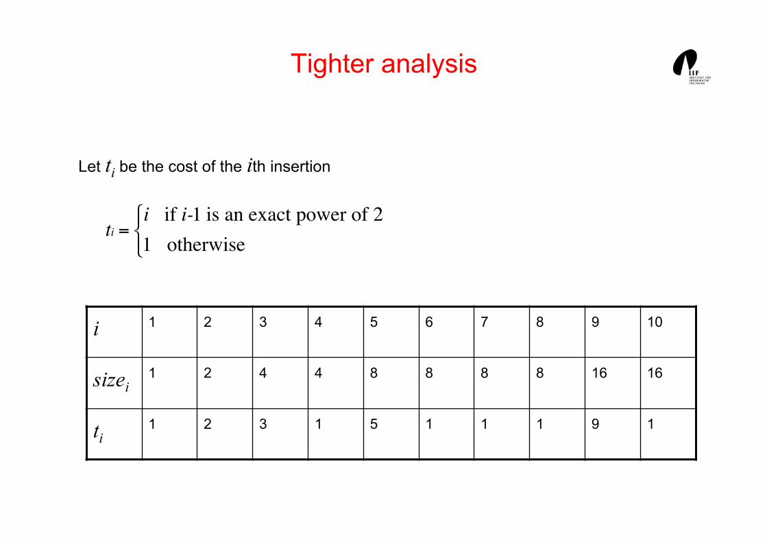
Tighter analysis
Let ti be the cost of the ith insertion
€
ti =i if i-1 is an exact power of 21 otherwise
i 1 2 3 4 5 6 7 8 9 10
sizei 1 2 4 4 8 8 8 8 16 16
ti 1 2 3 1 5 1 1 1 9 1

Tighter analysis
Let ti be the cost of the i th insertion
€
ti =i if i -1 is an exact power of 21 otherwise
i 1 2 3 4 5 6 7 8 9 10
sizei 1 2 4 4 8 8 8 8 16 16
ti 1 1+1 1+2 1 1+4 1 1 1 1+8 1

Tighter analysis
Cost of the n insertions
Thus the average cost of each dynamic table operation is 3.

Amortized analysis
• An amortized analysis is any strategy for analyzing a sequence of operations to show that the average cost per operation is small, even though a single operation within the sequence might be expensive.
• Even though we’re taking averages, however, probability is not involved!
• An amortized analysis guarantees the average performance of each operation in the worst case.

Types of amortized analysis
Three common amortization arguments:
– The aggregate method,
– The accounting method,
– The potential method.
We’ve just seen an aggregate analysis.
• The aggregate method, though simple, lacks the precision of the other two methods. In particular, the accounting and potential methods allow a specific amortized cost to be allocated to each operation.

Accounting method
• Charge i-th operation a fictitious amortized cost ai, where $1 pays for 1 unit of work (i.e., time). This fee is consumed to perform the operation.
• Any amount not immediately consumed is stored in the bank for use by subsequent operations. The bank balance must not go negative!
• We must ensure that for all n,
Thus, the total amortized costs provide an upper bound on the total true costs.
€
tii=1
n
∑ ≤ aii=1
n
∑

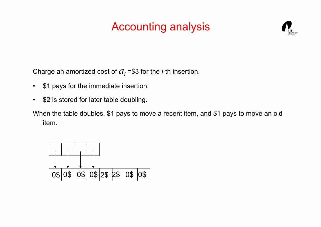
Accounting analysis
Charge an amortized cost of ai =$3 for the i-th insertion.
• $1 pays for the immediate insertion.
• $2 is stored for later table doubling.
When the table doubles, $1 pays to move a recent item, and $1 pays to move an old item.
0$ 0$ 0$ 0$

Accounting analysis
Charge an amortized cost of ai =$3 for the i-th insertion.
• $1 pays for the immediate insertion.
• $2 is stored for later table doubling.
When the table doubles, $1 pays to move a recent item, and $1 pays to move an old item.
0$ 0$ 2$ 0$

Accounting analysis
Charge an amortized cost of ai =$3 for the i-th insertion.
• $1 pays for the immediate insertion.
• $2 is stored for later table doubling.
When the table doubles, $1 pays to move a recent item, and $1 pays to move an old item.
0$ 0$ 2$ 2$

Accounting analysis
Charge an amortized cost of ai =$3 for the i-th insertion.
• $1 pays for the immediate insertion.
• $2 is stored for later table doubling.
When the table doubles, $1 pays to move a recent item, and $1 pays to move an old item.
0$ 0$ 0$ 0$ 0$ 0$ 0$ 0$
overflow

Accounting analysis
Charge an amortized cost of ai =$3 for the i-th insertion.
• $1 pays for the immediate insertion.
• $2 is stored for later table doubling.
When the table doubles, $1 pays to move a recent item, and $1 pays to move an old item.
0$ 0$ 0$ 0$ 2$ 0$ 0$ 0$
Accounting analysis
Charge an amortized cost of ai =$3 for the i-th insertion.
• $1 pays for the immediate insertion.
• $2 is stored for later table doubling.
When the table doubles, $1 pays to move a recent item, and $1 pays to move an old item.
0$ 0$ 0$ 0$ 2$ 2$ 0$ 0$

Accounting analysis
Charge an amortized cost of ai =$3 for the i-th insertion.
• $1 pays for the immediate insertion.
• $2 is stored for later table doubling.
When the table doubles, $1 pays to move a recent item, and $1 pays to move an old item.
0$ 0$ 0$ 0$ 2$ 2$ 2$ 0$

Accounting analysis
Charge an amortized cost of ai =$3 for the i-th insertion.
• $1 pays for the immediate insertion.
• $2 is stored for later table doubling.
When the table doubles, $1 pays to move a recent item, and $1 pays to move an old item.
0$ 0$ 0$ 0$ 2$ 2$ 2$ 2$
overflow

Accounting analysis
Charge an amortized cost of ai =$3 for the i-th insertion.
• $1 pays for the immediate insertion.
• $2 is stored for later table doubling.
When the table doubles, $1 pays to move a recent item, and $1 pays to move an old item.
overflow
0$ 0$ 0$ 0$ 0$ 0$ 0$ 0$ 0$ 0$ 0$ 0$ 0$ 0$ 0$ 0$

Potential method
IDEA: View the bank account as the potential energy of the dynamic set.
Framework:
• Start with an initial data structure D0.
• Operation i transforms Di–1 to Di.
• The cost of operation i is ti.
• Define a potential function Φ: {Di} →R, such that Φ(D0 ) = 0 and Φ(Di) ≥ 0 for all
i.
The amortized cost ai with respect to Φ is defined to be ai = ti + Φ(Di) – Φ(Di–1 ).

Potential method
ai = ti + Φ(Di) – Φ(Di–1 ).
Φ(Di) – Φ(Di–1 ) is called potential difference.
• If Φ(Di) – Φ(Di–1 ) > 0, operation i stores work in the data structure for later use.
• If Φ(Di) – Φ(Di–1 ) < 0, the data structure delivers up stored work to help pay for
operation i.
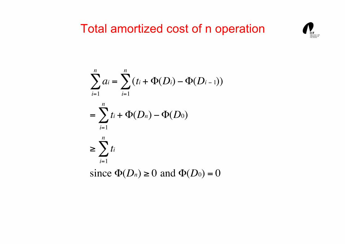
Total amortized cost of n operation
€
aii=1
n
∑ = (tii=1
n
∑ +Φ(Di) −Φ(Di − 1))
= tii=1
n
∑ +Φ(Dn) −Φ(D0)
≥ tii=1
n
∑
since Φ(Dn) ≥ 0 and Φ(D0) = 0

Potential method
T table with
• k = T.num elements and
• s = T.size spaces
Potential function
φ (T) = 2 k – s
φ (T) = 2 *7– 8 = 6
0$ 0$ 0$ 0$ 2$ 2$ 2$ Accounting method

Properties of the potential function
Properties • φ0 = φ(T0) = φ (empty table) = 0
• For all i ≥ 1 : φi = φ (Ti) ≥ 0
Since φn - φ0 ≥ 0, Σ ai is an upper bound for Σ ti
• Directly before an expansion, k = s,
hence φ(T) = k = s.
• Directly after an expansion, k = s/2,
hence φ(T) = 2k – s = 0.

Amortized cost of insert (1)
ki = # elements in T after the i-th operation
si = table size of T after the i-th operation
Case 1: [ i-th operation does not trigger an expansion]
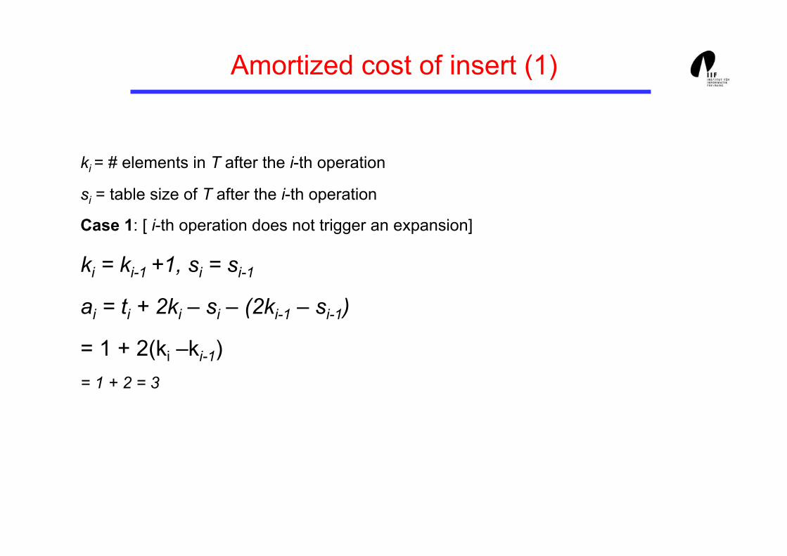
Amortized cost of insert (1)
ki = # elements in T after the i-th operation
si = table size of T after the i-th operation
Case 1: [ i-th operation does not trigger an expansion]
ki = ki-1 +1, si = si-1
ai = ti + 2ki – si – (2ki-1 – si-1)
= 1 + 2(ki –ki-1) = 1 + 2 = 3

Case 2: [ i-th operation triggers an expansion]
si = 2*si-1, ki = ki-1 +1,
ai = ti + 2ki –si –(2ki-1-si-1)
= si-1+1 + 2 – 2si-1 + si-1
=3
Amortized cost of insert (2)

Insertion and deletion of elements
Now: contract table, if the load is too small!
Goals:
(1) Load factor is always bounded below by a constant
(2) Amortized cost of a single insert or delete operation is constant.
First attempt:
• Expansion: same as before
• Contraction: halve the table size as soon as table is less than ½ occupied (after the deletion)!

„Bad“ sequence of insert and delete operations
Cost
n/2 times insert
(table fully occupied) 3 n/2
I: expansion n/2 + 1
D, D: contraction n/2 + 1
I, I : expansion n/2 + 1
D, D: contraction
Total cost of the sequence In/2,I,D,D,I,I,D,D,... of length n:

Second attempt
Expansion: (as before) double the table size, if an element is inserted in the full table.
Contraction: As soon as the load factor is below ¼, halve the table size.
Hence:
At least ¼ of the table is always occupied, i.e.
¼ ≤ α(T) ≤ 1
Cost of a sequence of insert and
delete operations?

Analysis: insert and delete
k = T.num, s = T.size, α = k/s
Potential function φ
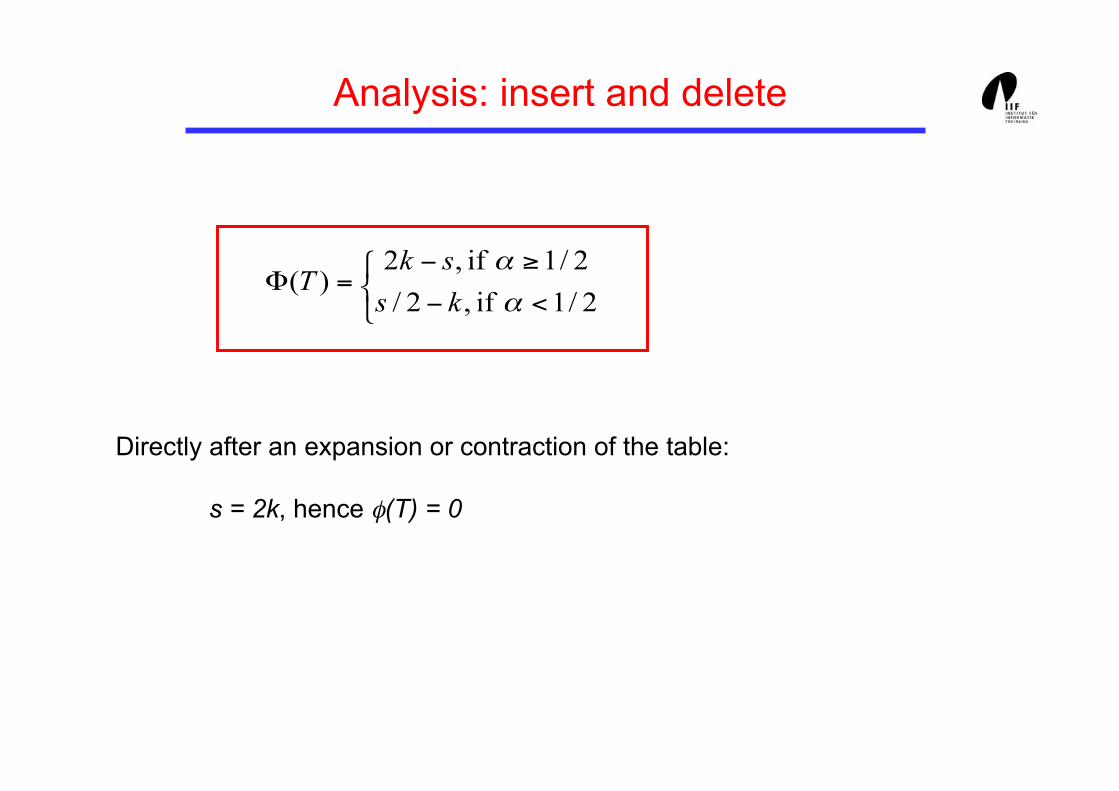
Analysis: insert and delete
Directly after an expansion or contraction of the table:
s = 2k, hence φ(T) = 0

insert
i-th operation: ki = ki-1 + 1
Case 1: αi-1 ≥ ½
Case 2: αi-1 < ½
Case 2.1: αi < ½
Case 2.2: αi ≥ ½

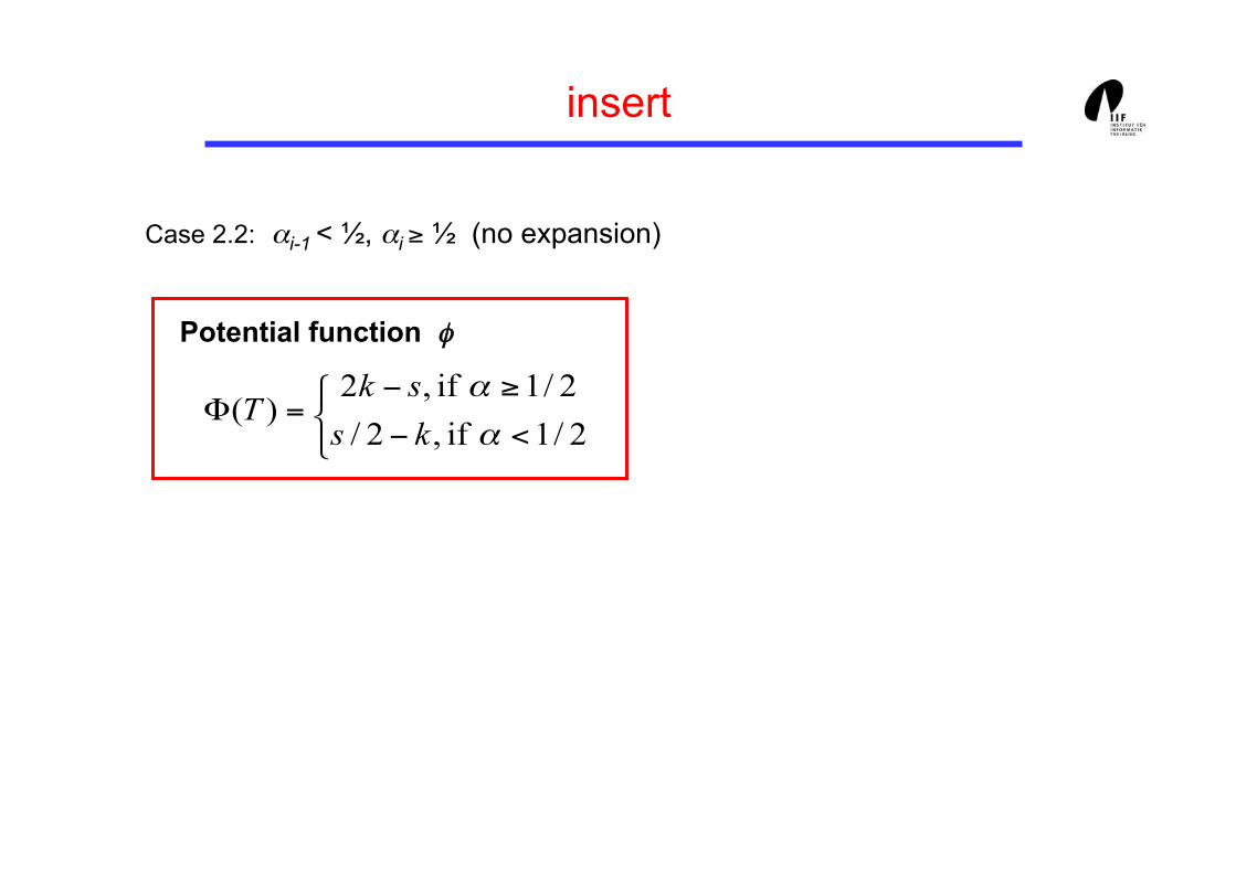
insert
Case 2.1: αi-1 < ½, αi < ½ (no expansion)
Potential function φ

insert
Case 2.1: αi-1 < ½, αi < ½ (no expansion)
Potential function φ
ai = ti + si /2 –ki – (si-1/2 –ki-1 )
si = si-1, ki = ki-1 +1
ai = 1 + ki-1 – ki
ai = 0
insert
Case 2.2: αi-1 < ½, αi ≥ ½ (no expansion)
Potential function φ

insert
Case 2.2: αi-1 < ½, αi ≥ ½ (no expansion)
Potential function φ
ai = ti + 2ki – si – (si-1/2 –ki-1 )
ai = 1 – (ki –ki-1)
ai = 0
si=si-1 ki=1+ki-1
si=2ki

delete
ki = ki-1 - 1
Case 1: αi-1 < ½
Case 1.1: deletion causes no contraction si = si-1
Potential function φ

delete
Case 1.2: αi-1 < ½ deletion causes a contraction 2si = si –1
ki-1 = si-1/4
ki = ki-1 - 1
Case 1: αi-1 < ½
Potential function φ

delete
Case 2: αi-1 ≥ ½ no contraction
si = si –1 ki = ki-1 - 1
Case 2.1: αi-1 ≥ ½
Potential function φ

delete
Case 2: αi-1 ≥ ½ no contraction
si = si –1 ki = ki-1 - 1
Case 2.2: αi < ½
Potential function φ

![Introduction to Algorithm Analysis - Nanjing Universitycs.nju.edu.cn/algorithm/slides/01.pdfIntroduction to Algorithm Analysis Algorithm : Design & Analysis [1] As soon as an Analytical](https://img.pdfslide.net/doc/110x75/5b336a807f8b9adf6c8cd516/introduction-to-algorithm-analysis-nanjing-to-algorithm-analysis-algorithm-design.jpg)