Theory of a two-mode micromaser simultaneously pumped by one- and two-photon atomic

transitions

This article has been downloaded from IOPscience. Please scroll down to see the full text article.

1999 J. Phys. B: At. Mol. Opt. Phys. 32 4405

(http://iopscience.iop.org/0953-4075/32/18/302)

Download details:

IP Address: 139.91.197.95

The article was downloaded on 25/08/2013 at 15:10

Please note that terms and conditions apply.

View the table of contents for this issue, or go to the journal homepage for more

Home Search Collections Journals About Contact us My IOPscience

J. Phys. B: At. Mol. Opt. Phys.32 (1999) 4405–4423. Printed in the UK PII: S0953-4075(99)03397-0

Theory of a two-mode micromaser simultaneously pumped byone- and two-photon atomic transitions

David Petrosyan†‡ and P Lambropoulos†§† Foundation for Research and Technology Hellas, Institute of Electronic Structure and Laser,PO Box 1527, Heraklion 71110, Crete, Greece‡ Institute for Physical Research, Armenian National Academy of Sciences, Ashtarak-2, 378410,Armenia§ Department of Physics, University of Crete, GreeceandMax-Planck-Institut fur Quantenoptik, Hans-Kopfermann-Straße 1, D-85748 Garching, Germany

Received 6 April 1999, in final form 20 July 1999

Abstract. We formulate the theory of a micromaser operating simultaneously on a one- and atwo-photon atomic transition. Departing from the complete microscopic Hamiltonian for thiscomposite ‘atom plus field’ system, we derive the equations governing its behaviour in thesemiclassical approximation and also the fully quantum mechanical master equation. Usingparameters corresponding to existing realizations of the one- and two-photon micromaser, weobtain illustrative examples of some novel aspects of this system in the steady state as well as indynamical evolution.

1. Introduction

A rather serious experimental limitation in realizing a two-photon laser in the opticalwavelength range stems from the difficulty in constructing a cavity possessing the properfinesse. The requirement is that no cavity mode is near resonance with a single-photontransition from the upper (pumped) state to an intermediate one lying between the two statesconnected by the desired two-photon transition. If that requirement is not satisfied, an atomicsystem tuned to a cavity mode on resonance with a two-photon transition will most likely laseinto an adjacent mode near resonance with the single-photon transition. Thus a two-photonlaser may more often than not lase simultaneously into two modes, one pumped througha single-photon transition and another pumped by the desired two-photon one. We haveaddressed this issue in a recent paper [1] where we have developed the theory of this unusualtwo-mode laser in which one of the modes is pumped by the two-photon transition.

This has motivated us to study the same problem in the context of the micromaser.Micromasers pumped by either one- or two-photon transitions have been studied quiteextensively experimentally as well as theoretically [2–6]. This of course is not the placefor a review of the vast literature on these topics which can be found in [7]. The difficulty withthe finesse in the optical wavelength range discussed above does not arise in the two-photonmicromaser because the wavelength allows the design of the appropriate cavity. For the samereason, one can envision designing a cavity which does have a second mode near resonancewith the single-photon transition to an intermediate Rydberg state. It may even be possible totune such a resonance. A further degree of flexibility in adjusting the detuning comes from

0953-4075/99/184405+19$30.00 © 1999 IOP Publishing Ltd 4405

4406 D Petrosyan and P Lambropoulos

the possibility of choosing slightly different Rydberg states. In other words, one can tune boththe cavity as well as the atomic system. That is the problem we have studied in this paper; amicromaser pumped by two- and one-photon atomic transitions at the same time. Given recentprogress in microcavities, one may also envision the implementation of such a system even inthe context of the microlaser [8]. It is not a (micro)maser (laser) operating in two modes, butrather a (micro)maser (laser) operating in two modes one of which is inherently nonlinear.

The theory of a two- or multi-mode laser is of course a mature topic but the issue here isdifferent in a rather fundamentally significant way. In the standard two-mode single-photonlaser, the two competing modes feed on the same gain curve but each of them alone and wellbelow threshold represents a linear process. In the present context, one of the modes exhibits anonlinear dependence on the respective field down to zero intensity. Moreover, the two modesnow feed on two different gain curves. As for the micromaser case, the issue has never beenconsidered as it can be avoided, while for the laser, it is most often an inconvenient fact ofreality. Our purpose then is to explore, in a controlled setting, the fundamental features of theresulting phenomena.

This paper is organized as follows. In section 2 we derive the effective Hamiltonian of thesystem, which is then used in section 3 for the analysis of the interaction of a single atom withthe pure state of the cavity field. The more general master equation approach is discussed insection 4, and the formalism developed there is applied to the exploration of the semiclassicalbehaviour of the system in section 5, as well as its quantum-mechanical evolution in section 6.The paper is closes with the conclusions outlined in section 7.

2. Derivation of the effective Hamiltonian

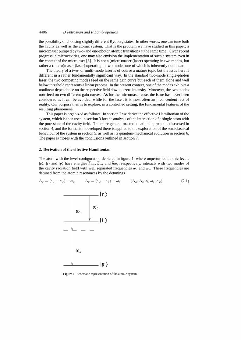
The atom with the level configuration depicted in figure 1, where unperturbed atomic levels|e〉, |i〉 and |g〉 have energies ¯hωe, hωi and hωg, respectively, interacts with two modes ofthe cavity radiation field with well separated frequenciesωa andωb. These frequencies aredetuned from the atomic resonances by the detunings

1a = (ωi − ωg)− ωa 1b = (ωe − ωi)− ωb (1a,1b � ωa, ωb) (2.1)

Figure 1. Schematic representation of the atomic system.

Theory of a two-mode micromaser 4407

and for simplicity we assume that modea is in perfect two-photon resonance with the atomictransition|e〉 → |g〉, so that(ωe − ωi)− ωa = −1a.

We begin with the complete microscopic Hamiltonian of the combined system ‘atom pluscavity field’, which, in the electric dipole and rotating-wave approximations, can be written as

H = HA +HF +Hint (2.2)

whereHA,HF andHint are, respectively, the atom, field and interaction terms:

HA = hωe|e〉〈e| + hωi |i〉〈i| + hωg|g〉〈g| (2.3)

HF = hωa(a†a + 1

2

)+ hωb

(b†b + 1

2

)(2.4)

Hint = hk(a)ei (a|e〉〈i| + a†|i〉〈e|) + hk(b)ei (b|e〉〈i| + b†|i〉〈e|)+hk(a)ig (a|i〉〈g| + a†|g〉〈i|) + hk(b)ig (b|i〉〈g| + b†|g〉〈i|). (2.5)

In these equations, the field modesa andb are described, respectively, by the creation andannihilation operatorsa†, a andb†, b. The quantityk(a)ei is, for instance, the coupling strengthof modea with the atomic transition|e〉 → |i〉, etc:

k(a,b)ei = −〈e|D|i〉Ea,b

h(2.6)

k(a,b)ig = −〈i|D|g〉Ea,b

h(2.7)

where 〈e|D|i〉 and 〈i|D|g〉 are the matrix elements of the electric dipole operatorD,Ea,b = (hωa,b/2ε0V )

1/2 is the field per photon for the corresponding mode, andV is thecavity volume. Taking into account the fact thatωa − ωb = 1a +1b � ωa,b, we can neglectthe difference betweenEa andEb and drop the superscript in the coupling constantsk. Thissimplification has practically no impact on the generality of the discussion and results whichcan be easily adapted to the case of two different coupling constantsk(a), k(b), if that werenecessary. Consistently with our model (figure 1), we assume that|1a| � |1b|, kei, kigthroughout this paper.

In the number state representation for both modes of the cavity field, the Hamiltonian(2.2) has non-vanishing matrix elements only between the following six states of the combinedatom + field system:|e, na, nb〉, |i, na + 1, nb〉, |i, na, nb + 1〉, |g, na + 2, nb〉, |g, na + 1, nb + 1〉and|g, na, nb +2〉, where the first element in the kets represents the state of the atom, while thesecond and the third elements indicate the state of the modea andb, respectively, containingthe corresponding number of photons. We assume that a single atom initially prepared in theexcited level|e〉 enters the cavity whose two modes under consideration, prior to the interactionwith the atom, are in the pure number states|na〉 and|nb〉, respectively. Thus, the initial stateof the system is|ψ(0)〉 = |e, na, nb〉. For the moment, we assume that both cavity modesare not dumped (later on in the derivation of the master equation of the field we discuss thevalidity of such an assumption), which allows us to describe the system evolution using theSchrodinger equation

ihd|ψ(t)〉

dt= H |ψ(t)〉. (2.8)

The state of the system at a subsequent timet will be represented by the linear combinationof the six basis states, with the complex probability amplitudes determined by (2.8).

The differential equations for the complex probability amplitudes of the states|i, na +1, nb〉, |g, na + 1, nb + 1〉 and|g, na, nb + 2〉 are of the form (in the interaction picture)

idy

dt= 2y +B(t) (2.9)

4408 D Petrosyan and P Lambropoulos

where2 is such that|2| � B(t) (in our case2 contains1a). Equation (2.9) can be writtenin an integral form as

y(t) = −i∫ t

0dt ′ exp[i2(t ′ − t)]B(t ′). (2.10)

For time intervalst sufficiently short, so thatB(t ′) does not change much but the exponent in(2.10) experiences many oscillations overt ′ ∈ [0 : t ], we can integrate this equation makingthe slowly varying envelope approximation forB(t) and, after performing the time averaging,we obtain〈y(t)〉 = B(t)/2.

Following the above procedure we obtain a set of algebraic equations for the complexprobability amplitudes of the states|i, na + 1, nb〉, |g, na + 1, nb + 1〉 and |g, na, nb + 2〉.Expressing these amplitudes through the probability amplitudesA1,A2 andA3 of the remainingthree states|e, na, nb〉, |i, na, nb + 1〉 and|g, na + 2, nb〉, respectively, we substitute them intothe equations forA1, A2 andA3 found from (2.8). The result is

idA1

dt= −k

2ei(na + 1)

1a

A1 +

(kei√nb + 1− keik

2ig

√(na + 1)2(nb + 1)

1a(1a +1b)

)A2

−keikig√(na + 1)(na + 2)

1a

A3 (2.11)

idA2

dt=(kei√nb + 1− keik

2ig

√(na + 1)2(nb + 1)

1a(1a +1b)

)A1

+

(−1b +

k2ig(nb + 2)

2(1a +1b)+k2ig(na + 1)

1a +1b

)A2 −

k3ig

√(na + 1)(na + 2)(nb + 1)

1a(1a +1b)A3

(2.12)

idA3

dt= −keikig

√(na + 1)(na + 2)

1a

A1−k3ig

√(na + 1)(na + 2)(nb + 1)

1a(1a +1b)A2 −

k2ig(na + 2)

1a

A3

(2.13)

where we have dropped the termk2ig(nb+1)/(1a+1b) in the non-resonant denominators, since

it is negligible in comparison with1a. Now consider the physical meaning of the various termsof the above equations: first of all, we note that the terms proportional tok3/1a(1a +1b) areresponsible for certain three-photon couplings between the atomic levels. Their contributioncan be neglected in comparison with the first- (�b) and the second- (�a) order couplings

�a(na) = −keikig√(na + 1)(na + 2)

1a

(2.14)

�b(nb) = kei√nb + 1 (2.15)

since the number of photonsna, nb is not expected, in this context, to be so large as to violatethe hierarchy of the orders of perturbation theory. This we have also checked quantitativelyin detail using parameters typical for the two-photon micromaser experiments (listed later insection 5). As long asna andnb are not larger than 100, these terms can be safely neglected.The termsk2

ei(na + 1)/1a in (2.11),k2ig(nb + 2)/2(1a +1b) + k2

ig(na + 1)/(1a +1b) in (2.12)andk2

ei(na + 2)/1a in (2.13) represent the shift of the corresponding level; then-dependentpart of each term gives the Stark shift of the atomic level, whereas the remaining constant ispart of the vacuum shift, which must be assumed to be incorporated into the energy of theatomic level. Under the conditionkei = kig ≡ k, the differential Stark shift of the atomic

Theory of a two-mode micromaser 4409

levels|e〉 and|g〉 vanishes and equations (2.11)–(2.13) can be greatly simplified:

idA1

dt= �b(nb)A2 +�a(na)A3 (2.16)

idA2

dt= �b(nb)A1 +1(na, nb)A2 (2.17)

idA3

dt= �a(na)A1 (2.18)

where

1(na, nb) = −1b +k2(4na + nb)

2(1a +1b)(2.19)

is the effective detuning of the modeb from the atomic transition|e〉 → |i〉.Equations (2.16)–(2.18) imply the effective Hamiltonian

Heff = hk(b|e〉〈i| + b†|i〉〈e|) + hµ(a2|e〉〈g| + a†2|g〉〈e|) (2.20)

combined with the fact that the detuning1(na, nb) is a function of the number of photons inboth modes,a andb, of the cavity field. (In equation (2.20) the parameterµ = −k2/1a is thecoupling strength of the two-photon process.) Thus, the problem is reduced to the three-levelsystem, and the state vector|ψ(t)〉 can be expanded at anyt > 0 as

|ψ(t)〉 = A1(t) |e, na, nb〉 +A2(t) |i, na, nb + 1〉 +A3(t) |g, na + 2, nb〉 (2.21)

with the initial conditionsA1(0) = 1,A2(0) = A3(0) = 0.

3. The energy exchange between atom and field

To find the complex probability amplitudesAj(t) (j = 1, 2, 3), we take the Laplace transformof the equations of motion (2.16)–(2.18). The resulting system of algebraic equations can besolved exactly, but for an arbitrary value of1(na, nb) the procedure involves solving a cubic.In the special case of1(na, nb) = 0, this cubic factorizes and the inverse Laplace transformgives

A1(t) = cos(√�2a +�2

b t)

(3.1)

A2(t) = −i�b√�2a +�2

b

sin(√�2a +�2

b t)

(3.2)

A3(t) = −i�a√�2a +�2

b

sin(√�2a +�2

b t). (3.3)

This shows that the population|A1(t)|2 of the atomic level|e〉 experiences Rabi oscillations

with the frequency√�2a +�2

b. Thus, there is a periodic exchange of energy between the atom

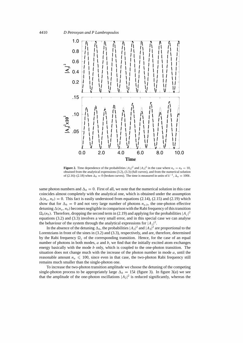
and both cavity modes. The quantity|A2(t)|2 represents the probability of adding one photoninto modeb which containednb photons att = 0. Similarly, |A3(t)|2 gives the probabilityfor modea to gain two photons, since each transition|e〉 → |g〉 leads to the emission of twophotons. In figure 2 we plot the time dependence of the probabilities|A2(t)|2 and|A3(t)|2 forthe case when the cavity contains initiallyna = 10 andnb = 10 photons, using the analyticalexpressions (3.2) and (3.3). For comparison we plot in the same graph the probabilities|A2(t)|2 and|A3(t)|2 obtained from the numerical solution of equations (2.16)–(2.18) for the

4410 D Petrosyan and P Lambropoulos

Figure 2. Time dependence of the probabilities|A2|2 and|A3|2 in the case wherena = nb = 10,obtained from the analytical expressions (3.2), (3.3) (full curves), and from the numerical solutionof (2.16)–(2.18) when1b = 0 (broken curves). The time is measured in units ofk−1,1a = 100k.

same photon numbers and1b = 0. First of all, we note that the numerical solution in this casecoincides almost completely with the analytical one, which is obtained under the assumption1(na, nb) = 0. This fact is easily understood from equations (2.14), (2.15) and (2.19) whichshow that for1b = 0 and not very large number of photonsna,b, the one-photon effectivedetuning1(na, nb)becomes negligible in comparison with the Rabi frequency of this transition�b(nb). Therefore, dropping the second term in (2.19) and applying for the probabilities|Aj |2equations (3.2) and (3.3) involves a very small error, and in this special case we can analysethe behaviour of the system through the analytical expressions for|Aj |2.

In the absence of the detuning1b, the probabilities|A2|2 and|A3|2 are proportional to theLorentzians in front of the sines in (3.2) and (3.3), respectively, and are, therefore, determinedby the Rabi frequency�j of the corresponding transition. Hence, for the case of an equalnumber of photons in both modes,a andb, we find that the initially excited atom exchangesenergy basically with the modeb only, which is coupled to the one-photon transition. Thesituation does not change much with the increase of the photon number in modea, until thereasonable amountna 6 100, since even in that case, the two-photon Rabi frequency stillremains much smaller than the single-photon one.

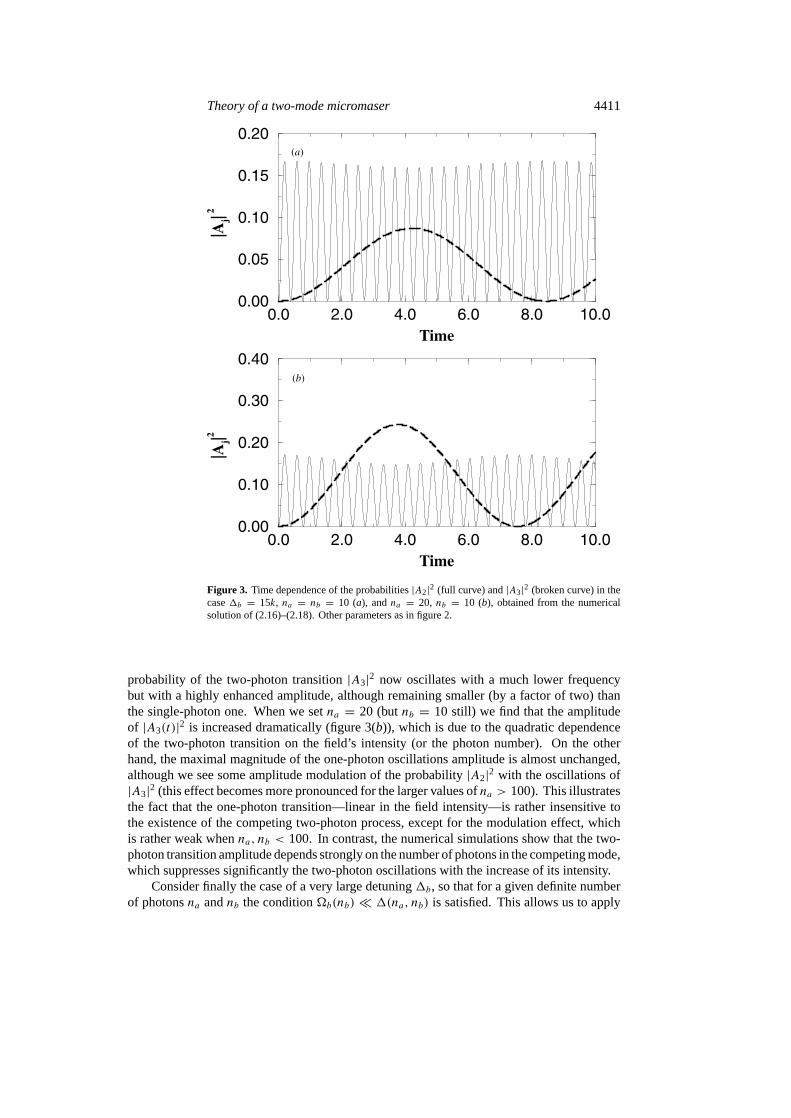
To increase the two-photon transition amplitude we choose the detuning of the competingsingle-photon process to be appropriately large1b = 15k (figure 3). In figure 3(a) we seethat the amplitude of the one-photon oscillations|A2|2 is reduced significantly, whereas the

Theory of a two-mode micromaser 4411

Figure 3. Time dependence of the probabilities|A2|2 (full curve) and|A3|2 (broken curve) in thecase1b = 15k, na = nb = 10 (a), andna = 20, nb = 10 (b), obtained from the numericalsolution of (2.16)–(2.18). Other parameters as in figure 2.

probability of the two-photon transition|A3|2 now oscillates with a much lower frequencybut with a highly enhanced amplitude, although remaining smaller (by a factor of two) thanthe single-photon one. When we setna = 20 (butnb = 10 still) we find that the amplitudeof |A3(t)|2 is increased dramatically (figure 3(b)), which is due to the quadratic dependenceof the two-photon transition on the field’s intensity (or the photon number). On the otherhand, the maximal magnitude of the one-photon oscillations amplitude is almost unchanged,although we see some amplitude modulation of the probability|A2|2 with the oscillations of|A3|2 (this effect becomes more pronounced for the larger values ofna > 100). This illustratesthe fact that the one-photon transition—linear in the field intensity—is rather insensitive tothe existence of the competing two-photon process, except for the modulation effect, whichis rather weak whenna, nb < 100. In contrast, the numerical simulations show that the two-photon transition amplitude depends strongly on the number of photons in the competing mode,which suppresses significantly the two-photon oscillations with the increase of its intensity.

Consider finally the case of a very large detuning1b, so that for a given definite numberof photonsna andnb the condition�b(nb) � 1(na, nb) is satisfied. This allows us to apply

4412 D Petrosyan and P Lambropoulos

to equation (2.17) the same procedure as for equation (2.9), obtaining

A2 = �b(nb)A1

1(na, nb)' A1

�b(nb)

1b

� 1. (3.4)

Then the solution for the remaining two complex probability amplitudesA1 andA3 is foundfrom equations (2.16) and (2.18) to be

A1(t) = cos(�at) (3.5)

A3(t) = −i sin(�at) (3.6)

which describes the ordinary two-photon Rabi oscillations between the levels|e〉 and |g〉,practically unaffected by the presence of the competing modeb.

4. The master equation

In this section, we derive the general master equations for both modes of the cavity field. Forthis purpose, we adopt the standard micromaser assumptions [3, 4]; namely, a monoenergeticbeam of excited atoms crosses the two-mode cavity at a flux low enough that, at most, oneatom at a time is present inside the resonator. Letti be the arrival time of theith atom andtint the time spend by the atom inside the cavity. Then the assumption above implies thattint 6 ti+1 − ti , which allows us to neglect the atom–atom interaction inside the cavity andconsider the contribution of each atom independently. We also suppose that the cavity dampingrateγa,b on both frequenciesωa andωb is small enough in order for the excited atoms to beable to build up the field with large number of photons:γ−1

a,b � ti+1− ti . Combined with theprevious inequality, this givestint � γ−1

a,b and the field’s relaxation process can be neglectedduring the time of interactiontint with the single atom. With these approximations, we canadopt the standard procedure in micromaser theory [9, 10] for the derivation of the masterequation of our system.

Consider first the single-atom incremental contribution to the state of the cavity field.Prior to interaction with the atom, att = 0, the initial state of each mode of the cavity fieldcan be represented quite generally as

ρ(j)(0) =∑nj ,mj

ρ(j)nj ,mj (0)|nj 〉〈mj | j = a, b. (4.1)

The state of the atom at this moment of time is

ρ(at)(0) = |e〉〈e| (4.2)

and the total density operator of the atom + field system is just a tensor product of (4.1) and(4.2):

ρ(0) = ρ(at)(0)⊗ ρ(a)(0)⊗ ρ(b)(0)=

∑na,ma;nb,mb

ρ(a)na,ma (0)ρ(b)nb,mb

(0)|e, na, nb〉〈e,ma,mb| (4.3)

where|e, na, nb〉 ≡ |e〉 ⊗ |na〉 ⊗ |nb〉.After the interaction, att = tint, the system evolves to the state

ρ(tint) =∑

na,ma;nb,mbρ(a)na,ma (0) ρ

(b)nb,mb

(0) |ψna,nb (tint)〉〈ψma,mb (tint)| (4.4)

Theory of a two-mode micromaser 4413

where|ψna,nb (t)〉 is given by equation (2.21). The state of each mode of the field at this momentof time is described by the reduced density operator

ρ(a)(tint) = Trb[Trat [ρ(tint)]] ≡ Pa(tint)ρ(a)(0) (4.5)

ρ(b)(tint) = Tra[Trat [ρ(tint)]] ≡ Pb(tint)ρ(b)(0). (4.6)

The pump operatorPj (tint) of modej contains the change of the density operatorρ(j) of thecorresponding mode due to the interaction with one single atom. Thus, ifr atoms have passedthrough the cavity during timet , the density operator of each mode of the cavity is given by

ρ(j)(t) = [Pj ]rρ(j)(0). (4.7)

Equation (4.7) describes a so-called regularly pumped micromaser in the absence of decay ofthe cavity field. More generally, however, in the time interval between the entrance of twosuccessive atoms in the cavity, both cavity modes decay with the corresponding ratesγa,btowards thermal equilibrium with mean numbers of thermal photonsNa,b present in the cavitydue to its coupling to the environment having a finite temperature. This process is describedby the standard [9, 10] master equation

d

dtρ(a) = Lρ(a) = 1

2γa(Na + 1)(2aρ(a)a†− a†aρ(a) − ρ(a)a†a)

+12γaNa(2a

†ρ(a)a − aa†ρ(a) − ρ(a)aa†) (4.8)

and the analogous equation forρ(b), with the replacementa ↔ b. Moreover, if the time intervalti+1 − ti between the two subsequent atoms fluctuates, equation (4.7) becomes inapplicable.Let the arrival times of the incoming atoms obey a Poisson distribution, which implies thatthe probability for an excited atom to enter the cavity betweent and t + δt is R δt , whereR = 〈(ti+1− ti)−1〉 is the average injection rate. Then, each mode of the field at timet + δt ismade up of a mixture of states corresponding to atomic excitation and no atomic excitation:

ρ(j)(t + δt) = R δtPjρ(j)(t) + (1− R δt)ρ(j)(t) (4.9)

which yields, in the limitδt → 0,

d

dtρ(j) = R[Pjρ

(j)(t)− ρ(j)(t)]. (4.10)

Also including the relaxation process, we obtain, finally, the master equations governing thetime evolution of both cavity modes:

d

dtρ(j) = Lρ(j)(t) +R[Pjρ

(j)(t)− ρ(j)(t)] j = a, b (4.11)

with Lρ(j)(t) given by equation (4.8). With the help of equations (4.5), (4.6) and (4.4), in thenumber state representation of the field, the master equations (4.11), in component form, canbe written as

d

dtρ(a)na,ma = −Rρ(a)na,ma

[1−

∑nb

ρ(b)nb,nb

∑z=1,2

Az(na, nb, tint) A∗z(ma, nb, tint)

]+Rρ(a)na−2,ma−2

∑nb

ρ(b)nb,nbA3(na − 2, nb, tint) A∗3(ma − 2, nb, tint)

− 12γa[na +ma + 2Na(na +ma + 1)] ρ(a)na,ma

+γa(Na + 1)√(na + 1)(ma + 1) ρ(a)na+1,ma+1 + γaNa

√nama ρ

(a)na−1,ma−1 (4.12)

4414 D Petrosyan and P Lambropoulos

for modea, and

d

dtρ(b)nb,mb = −Rρ(b)nb,mb

[1−

∑na

ρ(a)na,na

∑z=1,3

Az(na, nb, tint)A∗z(na,mb, tint)

]+Rρ(b)nb−1,mb−1

∑na

ρ(a)na,naA2(na, nb − 1, tint) A∗2(na,mb − 1, tint)

− 12γb[nb +mb + 2Nb(nb +mb + 1)] ρ(b)nb,mb

+γb(Nb + 1)√(nb + 1)(mb + 1) ρ(b)nb+1,mb+1 + γbNb

√nbmb ρ

(b)nb−1,mb−1 (4.13)

for modeb.These equations imply that the interaction timetint is fixed, i.e. all atoms pass through

the cavity with the same speed. The generalization to the case when there is a distribution ofatomic velocities is straightforward [4], but for the sake of simplicity, from now on we assumethattint = constant.

Equations (4.12) and (4.13) are the central equations of this paper. They are similar to thoseone obtains for the ordinary one- and two-photon micromasers and lasers with one importantnew aspect: each of these equations includes the averaging over the state of the other mode.

In the following section, from equations (4.12) and (4.13) we will obtain the semiclassicalevolution of the system, as well as analyse the dynamics of the photon number distribution insection 6.

5. The semiclassical evolution

Denoting byp(a)na ≡ ρ(a)na,na andp(b)nb ≡ ρ(b)nb,nb the diagonal elements of the density operator ofthe corresponding mode of the field, from equations (4.12) and (4.13) we obtain

dp(a)nadt= −Rp(a)na

∑nb

p(b)nb |A3(na, nb)|2 +Rp(a)na−2

∑nb

p(b)nb |A3(na − 2, nb)|2

−γa[na +Na(2na + 1)]p(a)na + γa(Na + 1)(na + 1)p(a)na+1 + γaNanap(a)na−1 (5.1)

dp(b)nbdt= −Rp(b)nb

∑na

p(a)na |A2(na, nb)|2 +Rp(b)nb−1

∑na

p(a)na |A2(na, nb − 1)|2

−γb[nb +Nb(2nb + 1)]p(b)nb + γb(Nb + 1)(nb + 1)p(b)nb+1 + γbNbnbp(b)nb−1 (5.2)

where the explicit dependence of the probabilities|Aj |2 on tint has been omitted, because, asmentioned above,tint is fixed.

The mean value of any physical quantityf (n), which is the function of the photonnumbern, is given by〈f (n)〉 =∑n pnf (n). The semiclassical approximation is obtained byassuming that the photon number distribution is highly peaked around some largen, so that〈f (n)〉 ' f (〈n〉).

Multiplying both sides of (5.1) and (5.2) byna andnb, respectively, and summing overnaandnb, we obtain, in the semiclassical approximation, the equations of motion for the meanphoton numbers in both modesa andb:

dnadt=∑na

nap(a)na= 2R|A3(na, nb)|2 − γa(na −Na) (5.3)

dnbdt=∑nb

nbp(b)nb= R|A2(na, nb)|2 − γb(nb −Nb). (5.4)

Theory of a two-mode micromaser 4415

In these equations the first terms on the right-hand side represent the gain ofna and nb dueto the downward transitions|e〉 → |g〉 and|e〉 → |i〉 of the excited atoms, respectively. Thefactor of 2 in (5.3) comes from the fact that each transition|e〉 → |g〉 causes the emission oftwo photons. The second terms in equations (5.3) and (5.4) are responsible for the relaxationof na and nb to the mean thermal photon numbersNa andNb inside the cavity. If, ideally,every atom leaves the cavity in level|i〉, from equation (5.4) we find that the steady-state valuefor the photon number in modeb would benb = R/γb (providingNb = 0). Similarly, fromequation (5.3), in the steady state, for the maximal possible number of photons in modea weobtainna = 2R/γa (Na = 0).

The reader who is familiar with the theory of the homogeneously broadened two-modelaser (see, for example, [10], chapter 6) will notice a difference between the differentialequations governing the intensities in that case and our equations (5.3) and (5.4). IfI1 andI2denote the intensities in the two modes, those equations have the form

I1 = 2I1(a1− β1I1− θ12I2)− γ1I1 (5.5)

I2 = 2I2(a2 − β2I2 − θ21I1)− γ2I2 (5.6)

wherea1,2 are the linear gain constants,β1,2 the self-saturation coefficients,θ1,2, θ2,1 the cross-saturation coefficients andγ1,2 the damping rate of the corresponding mode. These equationsallow the two modes to oscillate independently even ifI1 ' I2 providedθ1,2, θ2,1 < β1, β2. Itappears that our equations (5.3) and (5.4) do not allow for such a case (when�a ' �b) exceptfor very short times, as can be seen by examining the form ofA2 andA3 in equations (3.2) and

(3.3) for smallt , so that√�2a +�2

b t � 1. This seems to be a rather fundamental differencebetween the two systems. Of course one needs to keep in mind that atomic line broadeningdoes not occur in the micromaser; but it is doubtful that this is the only reason for the abovedifference in behaviour.

Before proceeding further, let us examine the relevance of the conditions established atthe beginning of section 4 to real experiments performed for the micromaser [2, 4, 6]. In amicrowave cavity, with the quality factorQ ' 108–109 for both modes of the cavity field, wehave for the damping ratesγa,b ' 102–103 s−1. Choosing a pump rateR � γa,b ensures thatmany atoms pass through the cavity during its damping time; letR = 105 atom/s. In orderfor the atoms to be sufficiently dilute (tint 6 R−1) we settint = 10−5 s, which is consistentwith the experimental situation when atoms with thermal velocityv ' 102–103 m s−1 crossa cavity having a transverse dimension of about a few mm. Since the coupling constantk forRydberg atoms is ordinarily equal to 105–106 s−1, even for not very large numbers of photonsna, nb 6 102 present in the cavity, atoms undergo many cycles of Rabi oscillations duringthe interaction timetint. To be definite, we choose furtherγa,b = 10−2R, tint = 10k−1 and1a = 100k as before.

Consider first the case of the exact one- and two-photon resonances of modesb andawith the atomic transitions|e〉 → |i〉 and|e〉 → |g〉, respectively. It was shown in section 3,in the discussion of figure 2, that in this case during the interaction time with the cavityfield, a single-atom exchanges energy primarily with modeb, so that the amplitude of theoscillations of|A2|2 is close to 1, whereas the amplitude of the oscillations of|A3|2 is afew orders of magnitude weaker, which is due to the smallness of the two-photon couplingconstantµ in comparison to the one-photon matrix elementk. This actually means thatin equation (5.4) the gain term has a high probability to take large positive values, whichdepend, for fixedtint, practically only on the photon number in modeb, as is easily seenfrom equation (3.2) taking into account that�a(na) � �b(nb). For the same reason, withthe help of equation (3.3), we deduce that, for givenR, the gain term in equation (5.3) isterribly small and the only possible steady state for modea is na = Na. Hence, in the case

4416 D Petrosyan and P Lambropoulos

of 1b = 0, we recover the ordinary one-photon micromaser [3] with all its characteristicattributes.

The other limiting case, that of the pure two-photon oscillations of the system [4], canbe realized in a microcavity for which the condition�b(nb) � 1b is satisfied, as was shownat the end of section 3. This condition requires that if the detuning1b is not very large,i.e. there is a mode in the microcavity close to the atomic resonance|e〉 → |i〉, the qualityfactor of the cavity on this mode should be sufficiently low. Then the maximal (possible)amount of photons in this modenb = R/γb would be a small number, so that the one-photonRabi frequency�b = k

√nb + 1 is small too. Increasing the quality factor of the cavity (and

consequently decreasingγb), to keep the above condition satisfied, one should increase thedetuning1b as well, making it actually very large whenγa = γb.

It is thus interesting to consider the intermediate range of detunings1b, when one wouldexpect to observe processes caused by a real competition between modesa andb inside thecavity. For the illustration of the basic behaviour of the system in this intermediate regime,

Figure 4. Diagram of the values ofna andnb for which ˙na = 0 (a) and˙nb = 0 (b). The areas markedwith ‘+’ (‘ −’) in (a) and (b) correspond to the positive (negative) values ofFa andFb, respectively.The mean thermal photon numbersNa = Nb = 0.1, and the cavity widthγa = γb = 10−2R; otherparameters are given in the text (section 5).

Theory of a two-mode micromaser 4417

we choose once again1b = 15k (as in section 3), since it is a rather convenient value of thesingle-photon process detuning.

One can formally associate the right-hand side of equations (5.3) and (5.4) with the classicalforce

Fa(na, nb) ≡ 2R|A3(na, nb)|2 − γa(na −Na) (5.7)

Fb(na, nb) ≡ R|A2(na, nb)|2 − γb(nb −Nb) (5.8)

the positive (negative) ‘force’ leads to the increase (decrease) of the photon number in thecorresponding mode. In figure 4 we plot the diagram of the values of photon numbers inmodesa andb for which ˙na = 0 (figure 4(a)), and ˙nb = 0 (figure 4(b)), i.e. the force forthe corresponding mode turns to zero. We see that there are well contoured regions of thevalues ofna andnb where the corresponding force has a definite sign. Obviously, with thedecrease of the ratio of the pumping rateR to the decay rateγa and/orγb, the areas occupiedby the zones of ‘positive force’ in the corresponding mode decrease as well, with simultaneousdisappearance of the zones located around the largest values ofna and/ornb, respectively. Themagnitude ofR/γj for which the last positive zone in the corresponding modej disappears(for a fixed number of photons in the other mode) can be viewed as the lasing threshold of thismode, which is, in fact, also depends on the number of photons in the competing mode.

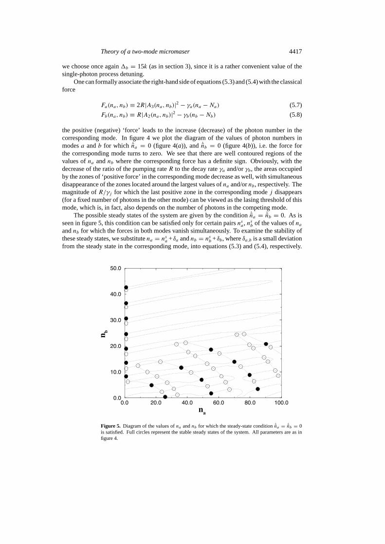
The possible steady states of the system are given by the condition˙na = ˙nb = 0. As isseen in figure 5, this condition can be satisfied only for certain pairsnsa, n

sb of the values ofna

andnb for which the forces in both modes vanish simultaneously. To examine the stability ofthese steady states, we substitutena = nsa +δa andnb = nsb +δb, whereδa,b is a small deviationfrom the steady state in the corresponding mode, into equations (5.3) and (5.4), respectively.

Figure 5. Diagram of the values ofna andnb for which the steady-state condition˙na = ˙nb = 0is satisfied. Full circles represent the stable steady states of the system. All parameters are as infigure 4.

4418 D Petrosyan and P Lambropoulos

Applying the linearization in the parametersδa andδb, yields

δa = αaδa + βaδb (5.9)

δb = αbδb + βbδa (5.10)

where

αa = 2R∂|A3(n

sa, n

sb)|2

∂na− γa βa = 2R

∂|A3(nsa, n

sb)|2

∂nb(5.11)

αb = R∂|A2(nsa, n

sb)|2

∂nb− γb βb = R∂|A2(n

sa, n

sb)|2

∂na. (5.12)

The steady-state solutionsnsa, nsb are stable if, and only if, all eigenvalues of the matrix of

coefficients of equations (5.9) and (5.10) have negative real parts:

Re(λ±) < 0 λ± = 12

[αa + αb ±

√(αa − αb)2 + 4βaβb

]. (5.13)

Such stable operational points of the system are plotted differently (full circles) in figure 5. Ofcourse, if one varies the detuning1b (and also, the ratio of the pumping rateR to the decays

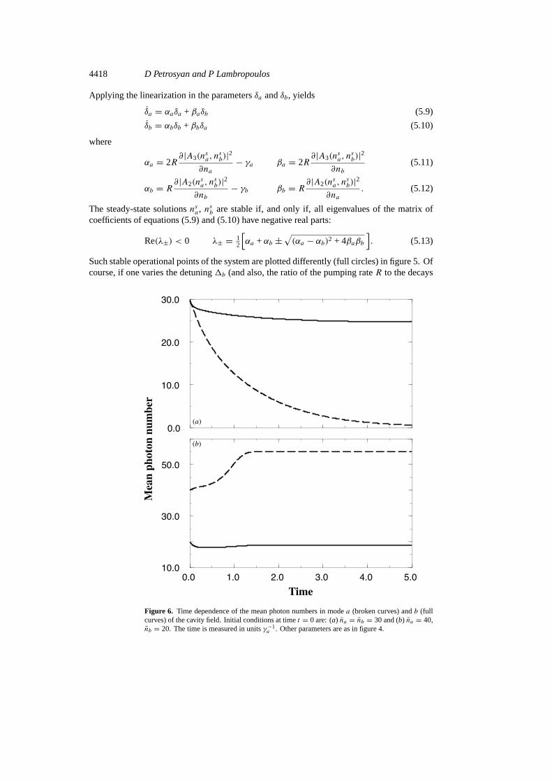
Figure 6. Time dependence of the mean photon numbers in modea (broken curves) andb (fullcurves) of the cavity field. Initial conditions at timet = 0 are: (a) na = nb = 30 and (b) na = 40,nb = 20. The time is measured in unitsγ−1

a . Other parameters are as in figure 4.

Theory of a two-mode micromaser 4419

γa,b) one obtains different stable operational points. Within a certain range of parameters,however, the general picture of the system’s behaviour remains similar, gradually tendingto the appropriate limits of the limiting cases discussed above; namely, with the decreaseof 1b the stable points tend to be located around lower values ofna, reaching in the limit1b → 0 thenb-axis in figure 5 (one-photon maser), and vice versa for1b � k (two-photonmaser).

Finally, in figure 6, we present the semiclassical time-dependent behaviour of the systemfor two different ‘triggering’ values of the mean photon numbers in modesa andb. We seethat depending on the initial conditions forna andnb the system evolves towards the nearestreachable stable steady state (see figure 5). We will compare this result with the time evolutionof the photon number distribution in the following section, where we present a more rigoroustreatment of the system’s dynamics.

6. The quantum-mechanical evolution

In this section, we present further discussion of the features of the system in terms of an exactquantum-mechanical time-dependent dynamics of the photon number distributions in modesa

andb, obtained through numerical solution of equations (5.1) and (5.2).

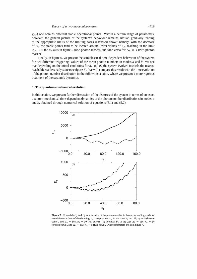
Figure 7. PotentialsUa andUb as a function of the photon number in the corresponding mode fortwo different values of the detuning1b: (a) potentialUa in the case1b = 15k, nb = 5 (brokencurve), and1b = 10k, nb = 30 (full curve). (b) PotentialUb in the case1b = 15k, na = 50(broken curve), and1b = 10k, na = 5 (full curve). Other parameters are as in figure 4.

4420 D Petrosyan and P Lambropoulos

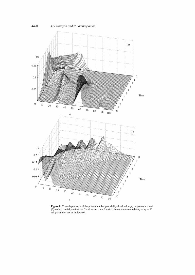
Figure 8. Time dependence of the photon number probability distributionpn in (a) modea and(b) modeb. Initially at timet = 0 both modesa andbare in coherent states centred atna = nb = 30.All parameters are as in figure 6.

Theory of a two-mode micromaser 4421

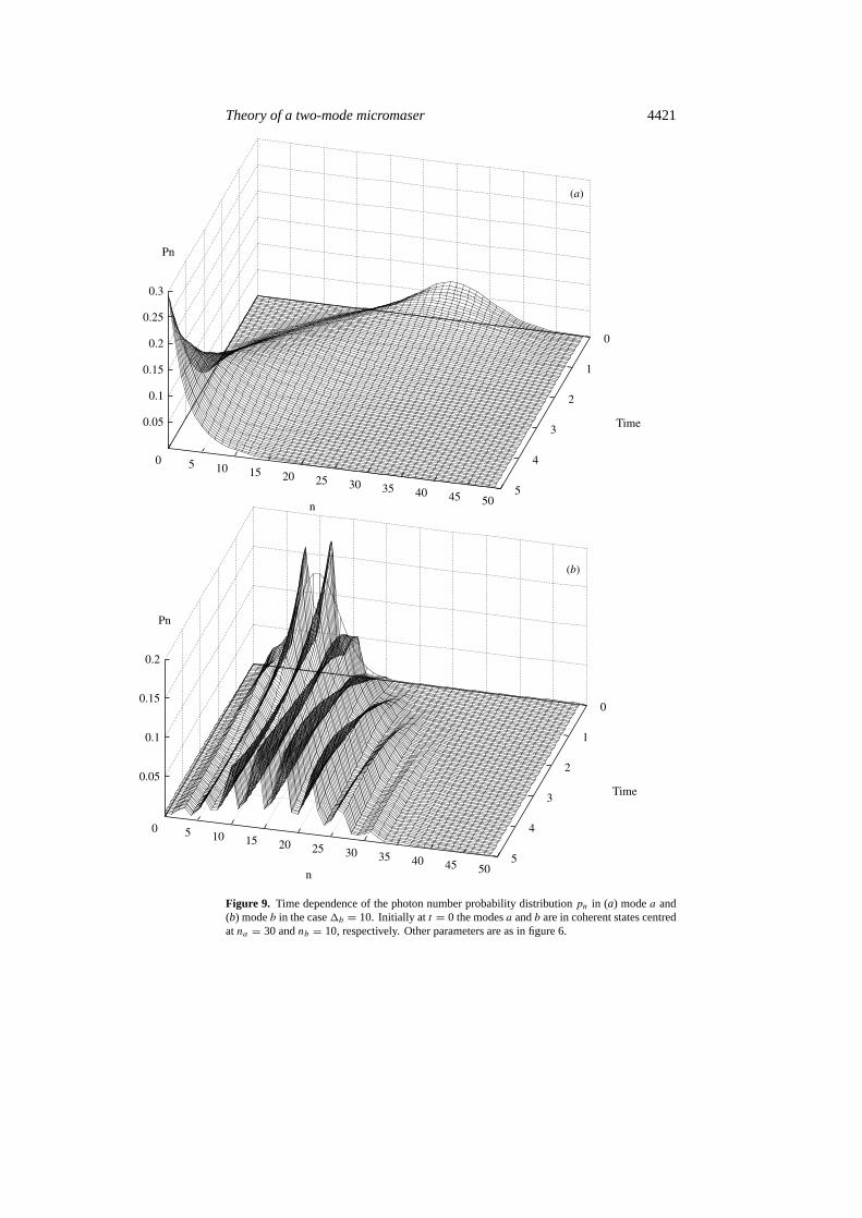
Figure 9. Time dependence of the photon number probability distributionpn in (a) modea and(b) modeb in the case1b = 10. Initially at t = 0 the modesa andb are in coherent states centredatna = 30 andnb = 10, respectively. Other parameters are as in figure 6.

4422 D Petrosyan and P Lambropoulos

We have introduced in equations (5.7) and (5.8) the force for the corresponding mode. Itis straightforward, thus, to define the potentials

Ua(na, nb) = −∫Fa(na, nb) dna (6.1)

Ub(na, nb) = −∫Fb(na, nb) dnb (6.2)

which will allow us an easier interpretation of the dynamics of the system. In equation (6.1),the quantitynb must be viewed as a parameter corresponding to the (fixed) number of photonsin modeb, and similarly in equation (6.2) the parameterna reflects the number of photons inmodea. Numerical integration of equations (6.1) and (6.2) shows that the potentialUb of themodeb depends weakly on the parameterna, within the rangena ∈ [0:150] where the two-photon Rabi frequency is much weaker than the single-photon one, whereas the dependenceof Ua on nb is very strong. Physically, this means that modeb does not feel the presenceof the competing two-photon transition (unless it is weak), and the behaviour of this modeis determined almost solely by its own parameters, i.e. detuning1b, coupling strengthk andthe ratio of the pump to decayR/γb. The two-photon transition, in turn, apart from thesystem’s parameters, also depends on the photon number in the one-photon modeb (see alsothe discussion of figure 3 in section 3). In figure 7, we plot the potentialsUa andUb for twodifferent values of the detuning1b. Comparison with figure 6 shows that, in the semiclassicalpicture, the mean photon numbersna and nb tend to occupy the nearest ‘potential wells’ ofUa andUb, respectively. Quantum mechanically, however, although on a short time scalethe evolution of the system is consistent with that given by semiclassical considerations, forlonger times deviations from the latter become significant (figure 8). Apart from the localdeterministic movement, the probabilitiesp(a) andp(b) experience a ‘diffusion’ through thepotential barriers into the neighbouring potential minima; the lower the potential barrier, thehigher the speed of this diffusion. This fact is illustrated in figures 8 and 9, which also showthat the peaks of the probabilitiesp(a) andp(b) are located around the potential wells ofUa andUb in figure 7. We can now specify that the time scale mentioned above refers to a diffusiontime which, unlike the single-mode laser where a diffusion constant is well defined, here mustbe understood in reference to the results depicted in the figures. This is because an effectivediffusion constant in one mode depends on the state of the other. Obviously, the diffusionintensity must be higher in the direction of the lowering of the mean potential. Thus forsufficiently long time, the photon distributionsp(a) andp(b) will flow into the deepest well(global minimum) of the corresponding potential, where the steady state is reached.

7. Conclusion

In conclusion, we have explored the traditional two-photon micromaser scheme [4], in a newsetting where the excited atoms pass through a cavity having two well separated modes whichconnect the excited atomic level to a lower level by a two-photon transition and, in addition,to an intermediate level by a single-photon one. In particular, we have explored the influenceof the various parameters of the system on the probability of the amplification or suppressionof the oscillations in one or the other mode of the cavity.

We have presented the derivation of the effective Hamiltonian of the system, by means ofwhich we have illustrated the features of the interaction of the atom with the pure state of thecavity field. Further analysis of the system was carried out within the framework of the moregeneral master equation approach through which we investigated the semiclassical behaviourof the system, as well as its quantum-mechanical evolution.

Theory of a two-mode micromaser 4423

As we anticipated, this system exhibits some novel features in comparison with either thesingle- or the two-photon version alone. The multiple-well structure of the effective potentialsassociated with the forces appearing in the semiclassical analysis is one of these novel features.A number of further questions occurring in studies of the micromaser can also be explored inthis new richer context with perhaps some surprises. For example, in our treatment we haveseen that the effective potential for either mode is parametrically dependent on the numberof photons in the other mode. It would thus be interesting to explore in this model a two-dimensional Fokker–Planck equation which would also allow for a better understanding ofthe diffusion of probabilities discussed in the previous section. It is also worth examining thecross-correlations between the two modes which are fed from the same upper level. Someindications of such correlations can be discerned in figure 3 and noted in the relevant discussion.We hope to report on such issues in a forthcoming paper. Finally, possible experimental studiesof this system may provide valuable insight into possibilities for the optical wavelength range.

Acknowledgment

The work of one of us (DP) has been supported in part by the Republic of Armenia (scientificproject no 96-770).

References

[1] Petrosyan D and Lambropoulos P 1999Phys. Rev.A 60398[2] Meschede D, Walther H and Muller G 1985Phys. Rev. Lett.54551[3] Filipowicz P, Javanainen J and Meystre P 1986Phys. Rev.A 343077[4] Brune M, Raimond J M and Haroche S 1987Phys. Rev.A 35154

Davidovich L, Raimond J M, Brune M and Haroche S 1987Phys. Rev.A 363771[5] Laughlin D W G and Swain S1991Quantum Opt.3 77[6] Walther H 1996Usp. Fiz. Nauk.166777[7] Haroche S and Raimond J M 1985Adv. At. Mol. Phys.20350

Raithel G, Wagner C, Walther H, Narducci L M and Scully M O 1994Cavity Quantum ElectrodynamicsedP R Bergman (Boston, MA: Academic)

[8] Feld M S and An K 1998Sci. Am.27941An K, Dasari R R and Feld M S 1996SPIE Proc.279914

[9] Walls D F and Milburn G J 1994Quantum Opt.(Berlin: Springer)[10] Meystre P and Sargent M III 1991Elements of Quantum Optics2nd edn (Berlin: Springer)