Embed Size (px)
Citation preview
The Pennsylvania State University
The Graduate School
SECURITY AND PRIVACY SUPPORT FOR MOBILE SENSING
A Dissertation in
Computer Science and Engineering
by
Qinghua Li
c© 2013 Qinghua Li
Submitted in Partial Fulfillment
of the Requirements
for the Degree of
Doctor of Philosophy
August 2013

The dissertation of Qinghua Li was reviewed and approved∗ by the following:
Guohong Cao
Professor of Computer Science and Engineering
Dissertation Advisor, Chair of Committee
Thomas F. La Porta
William E. Leonhard Professor
Director of Networking and Security Research Center
Sencun Zhu
Associate Professor of Computer Science and Engineering
Aylin Yener
Professor of Electrical Engineering
Lee Coraor
Associate Professor of Computer Science and Engineering
Graduate Officer
∗Signatures are on file in the Graduate School.

Abstract
The proliferation and ever-increasing capabilities of mobile devices such as smartphones give rise to a variety of mobile sensing systems, which collect data from theembedded sensors of mobile devices to make sophisticated inferences about peopleand their surroundings. Mobile sensing can be applied to environmental moni-toring, traffic monitoring, healthcare, etc. However, the large-scale deploymentof mobile sensing applications is hindered by several challenges, including privacyleakage from sensing data, the lack of incentives for mobile device users to partici-pate, and the lack of security mechanisms for data collection when communicationinfrastructure is unavailable.
The specific goal of this dissertation is to provide security and privacy sup-port for mobile sensing. We achieve this goal by devising techniques to addressthe aforementioned challenges. First, to provide incentives for users to participateand at the same time preserve privacy, we propose two credit-based privacy-awareincentive schemes for mobile sensing. These schemes reward users with credits fortheir contributed data without exposing who contributes the data. They also en-sure that dishonest users cannot abuse the system to earn unlimited credits. Onescheme relies on a trusted third party to protect privacy. The other scheme re-moves the assumption of trusted third party, and provides unconditional privacy bycombining blind signature, partially blind signature, and commitment techniques.Second, for a broad class of applications that need to periodically collect usefulaggregate statistics of sensing data, we propose a privacy-preserving aggregationprotocol for the Sum aggregate, which can provide differential privacy–a strong andprovable privacy guarantee. To perform private and efficient aggregation, we designa novel HMAC-based encryption scheme which allows the aggregator to get thesum of all users’ data but nothing else, and a novel ring-based overlapped group-ing technique to efficiently deal with dynamic joins and leaves of users. We alsoextend the aggregation scheme for Sum to derive Max/Min and other aggregate s-
iii

tatistics. Third, for mobile devices without communication infrastructure support,opportunistic mobile networking techniques are used to connect these devices. Weaddress three security issues that may degrade the performance of sensing datacollection in opportunistic mobile networks: social selfishness, flood attacks, androuting misbehavior. Specifically, we propose a Social Selfishness Aware Rout-ing (SSAR) protocol which allows users to behave in the socially selfish way butimproves routing performance by considering user selfishness into relay selection;we employ rate limiting to defend against flood attacks and design a distributedscheme which can probabilistically detect the violation of rate limit; to mitigaterouting misbehavior, we devise a distributed scheme to detect packet dropping inopportunistic mobile networks and an algorithm to reduce the amount of packetsforwarded to misbehaving users.
iv

Table of Contents
List of Figures x
List of Tables xiv
Acknowledgments xvi
Chapter 1Introduction 11.1 Challenges . . . . . . . . . . . . . . . . . . . . . . . . . . . . . . . . 21.2 Focus of This Dissertation . . . . . . . . . . . . . . . . . . . . . . . 3
1.2.1 Providing Privacy-Aware Incentives . . . . . . . . . . . . . . 41.2.2 Efficient and Privacy-Preserving Stream Aggregation . . . . 41.2.3 Secure Opportunistic Mobile Networking for Data Collection 5
1.3 Organization . . . . . . . . . . . . . . . . . . . . . . . . . . . . . . 8
Chapter 2Providing Privacy-Aware Incentives 92.1 Introduction . . . . . . . . . . . . . . . . . . . . . . . . . . . . . . . 92.2 Preliminaries . . . . . . . . . . . . . . . . . . . . . . . . . . . . . . 10
2.2.1 System and Incentive Model . . . . . . . . . . . . . . . . . . 102.2.2 Adversary and Trust Model . . . . . . . . . . . . . . . . . . 132.2.3 Our Goals . . . . . . . . . . . . . . . . . . . . . . . . . . . . 142.2.4 Cryptographic Primitives . . . . . . . . . . . . . . . . . . . . 14
2.3 An Overview of our Approach . . . . . . . . . . . . . . . . . . . . . 152.3.1 Basic Approach . . . . . . . . . . . . . . . . . . . . . . . . . 152.3.2 Scheme Overview . . . . . . . . . . . . . . . . . . . . . . . . 16
2.4 A TTP-based Scheme . . . . . . . . . . . . . . . . . . . . . . . . . . 17
v

2.4.1 The Basic Scheme . . . . . . . . . . . . . . . . . . . . . . . . 182.4.2 Dealing with Dynamic Joins and Leaves . . . . . . . . . . . 202.4.3 Addressing Timing Attacks . . . . . . . . . . . . . . . . . . 212.4.4 Commitment Removal . . . . . . . . . . . . . . . . . . . . . 222.4.5 Security Analysis . . . . . . . . . . . . . . . . . . . . . . . . 222.4.6 Cost Analysis . . . . . . . . . . . . . . . . . . . . . . . . . . 23
2.5 A TTP-Free Scheme . . . . . . . . . . . . . . . . . . . . . . . . . . 242.5.1 The Scheme . . . . . . . . . . . . . . . . . . . . . . . . . . . 242.5.2 Dealing with Dynamic Joins and Leaves . . . . . . . . . . . 272.5.3 Credential Removal . . . . . . . . . . . . . . . . . . . . . . . 282.5.4 Security Analysis . . . . . . . . . . . . . . . . . . . . . . . . 282.5.5 Cost Analysis . . . . . . . . . . . . . . . . . . . . . . . . . . 29
2.6 Evaluations . . . . . . . . . . . . . . . . . . . . . . . . . . . . . . . 292.7 Discussions . . . . . . . . . . . . . . . . . . . . . . . . . . . . . . . 312.8 Related Work . . . . . . . . . . . . . . . . . . . . . . . . . . . . . . 322.9 Summary . . . . . . . . . . . . . . . . . . . . . . . . . . . . . . . . 32
Chapter 3Efficient and Privacy-Preserving Stream Aggregation 333.1 Introduction . . . . . . . . . . . . . . . . . . . . . . . . . . . . . . . 333.2 Related Work . . . . . . . . . . . . . . . . . . . . . . . . . . . . . . 363.3 Preliminaries . . . . . . . . . . . . . . . . . . . . . . . . . . . . . . 38
3.3.1 Problem Definition . . . . . . . . . . . . . . . . . . . . . . . 383.3.2 Threat and Trust Model . . . . . . . . . . . . . . . . . . . . 393.3.3 Building Blocks . . . . . . . . . . . . . . . . . . . . . . . . . 40
3.3.3.1 Homomorphic Encryption . . . . . . . . . . . . . . 403.3.3.2 Data Perturbation . . . . . . . . . . . . . . . . . . 41
3.3.4 Overview of Solution . . . . . . . . . . . . . . . . . . . . . . 423.4 Basic Encryption Scheme . . . . . . . . . . . . . . . . . . . . . . . . 43
3.4.1 Scheme Overview . . . . . . . . . . . . . . . . . . . . . . . . 433.4.2 A Straw-man Construction for Key Generation . . . . . . . 443.4.3 Our Construction for Key Generation . . . . . . . . . . . . . 47
3.5 Dealing with Dynamic Joins and Leaves . . . . . . . . . . . . . . . 523.5.1 Naive Grouping . . . . . . . . . . . . . . . . . . . . . . . . . 533.5.2 Overlapped Grouping . . . . . . . . . . . . . . . . . . . . . . 53
3.5.2.1 Basic Idea . . . . . . . . . . . . . . . . . . . . . . . 533.5.2.2 Security Condition . . . . . . . . . . . . . . . . . . 54
3.5.3 Ring-based Overlapped Grouping . . . . . . . . . . . . . . . 563.5.3.1 Ring-based Group Structure . . . . . . . . . . . . . 563.5.3.2 Properties . . . . . . . . . . . . . . . . . . . . . . . 57
vi

3.5.3.3 Group Management . . . . . . . . . . . . . . . . . 593.5.3.4 Communication Cost Analysis . . . . . . . . . . . . 67
3.6 Aggregation Protocol for Sum . . . . . . . . . . . . . . . . . . . . . 683.6.1 Encryption Method . . . . . . . . . . . . . . . . . . . . . . . 683.6.2 Data Perturbation . . . . . . . . . . . . . . . . . . . . . . . 683.6.3 Dealing with Dynamic Joins and Leaves . . . . . . . . . . . 693.6.4 Analysis . . . . . . . . . . . . . . . . . . . . . . . . . . . . . 70
3.6.4.1 Aggregation Error . . . . . . . . . . . . . . . . . . 703.6.4.2 Communication Cost . . . . . . . . . . . . . . . . . 71
3.7 Evaluations . . . . . . . . . . . . . . . . . . . . . . . . . . . . . . . 713.7.1 Communication Cost . . . . . . . . . . . . . . . . . . . . . . 723.7.2 Aggregation Error . . . . . . . . . . . . . . . . . . . . . . . 733.7.3 Computation Cost and Running Time . . . . . . . . . . . . 74
3.8 Extensions and Discussions . . . . . . . . . . . . . . . . . . . . . . . 763.8.1 Aggregation Protocol for Min . . . . . . . . . . . . . . . . . 76
3.8.1.1 Basic Min Aggregation . . . . . . . . . . . . . . . . 763.8.1.2 Low-cost Min Aggregation . . . . . . . . . . . . . . 783.8.1.3 Practical Performances . . . . . . . . . . . . . . . . 79
3.8.2 More Aggregate Statistics . . . . . . . . . . . . . . . . . . . 813.8.3 Honest-but-Curious Key Dealer . . . . . . . . . . . . . . . . 813.8.4 Dealing with Node Failures . . . . . . . . . . . . . . . . . . 82
3.9 Summary . . . . . . . . . . . . . . . . . . . . . . . . . . . . . . . . 83
Chapter 4Secure Opportunistic Mobile Networking for Data Collection 844.1 Social Selfishness Aware Routing . . . . . . . . . . . . . . . . . . . 85
4.1.1 Introduction . . . . . . . . . . . . . . . . . . . . . . . . . . . 854.1.2 SSAR Overview . . . . . . . . . . . . . . . . . . . . . . . . . 87
4.1.2.1 Design for User . . . . . . . . . . . . . . . . . . . . 874.1.2.2 Network Model . . . . . . . . . . . . . . . . . . . . 874.1.2.3 Willingness Table . . . . . . . . . . . . . . . . . . . 884.1.2.4 The Architecture . . . . . . . . . . . . . . . . . . . 894.1.2.5 The Protocol . . . . . . . . . . . . . . . . . . . . . 914.1.2.6 Forwarding Strategy . . . . . . . . . . . . . . . . . 92
4.1.3 Detailed Design . . . . . . . . . . . . . . . . . . . . . . . . . 924.1.3.1 Packet Priority . . . . . . . . . . . . . . . . . . . . 924.1.3.2 Delivery Probability Estimation . . . . . . . . . . . 944.1.3.3 Forwarding Set Optimization . . . . . . . . . . . . 97
4.1.4 Performance Evaluations . . . . . . . . . . . . . . . . . . . . 994.1.4.1 Experiment Setup . . . . . . . . . . . . . . . . . . 99
vii

4.1.4.2 Routing Algorithms . . . . . . . . . . . . . . . . . 1034.1.4.3 Metrics . . . . . . . . . . . . . . . . . . . . . . . . 1044.1.4.4 Results . . . . . . . . . . . . . . . . . . . . . . . . 104
4.1.5 Related Work . . . . . . . . . . . . . . . . . . . . . . . . . . 1104.1.6 Summary . . . . . . . . . . . . . . . . . . . . . . . . . . . . 112
4.2 Defending Against Flood Attacks . . . . . . . . . . . . . . . . . . . 1134.2.1 Introduction . . . . . . . . . . . . . . . . . . . . . . . . . . . 1134.2.2 Motivation . . . . . . . . . . . . . . . . . . . . . . . . . . . . 1154.2.3 Overview . . . . . . . . . . . . . . . . . . . . . . . . . . . . 117
4.2.3.1 Problem Definition . . . . . . . . . . . . . . . . . . 1174.2.3.2 Models and Assumptions . . . . . . . . . . . . . . 1194.2.3.3 Basic Idea: Claim-Carry-and-Check . . . . . . . . . 120
4.2.4 Our Scheme . . . . . . . . . . . . . . . . . . . . . . . . . . . 1224.2.4.1 Claim Construction . . . . . . . . . . . . . . . . . 1224.2.4.2 Inconsistency Caused by Attack . . . . . . . . . . . 1234.2.4.3 Protocol . . . . . . . . . . . . . . . . . . . . . . . . 1234.2.4.4 Local Data Structures . . . . . . . . . . . . . . . . 1254.2.4.5 Inconsistency Check . . . . . . . . . . . . . . . . . 1264.2.4.6 Alarm . . . . . . . . . . . . . . . . . . . . . . . . . 1274.2.4.7 Efficient T-claim Authentication . . . . . . . . . . 1284.2.4.8 Dealing with Different Rate Limits . . . . . . . . . 1294.2.4.9 Replica Flood Attacks in Quota-based Protocols . . 129
4.2.5 Meta Data Exchange . . . . . . . . . . . . . . . . . . . . . . 1304.2.5.1 Sampling . . . . . . . . . . . . . . . . . . . . . . . 1314.2.5.2 Redirection . . . . . . . . . . . . . . . . . . . . . . 1324.2.5.3 The Exchange Process . . . . . . . . . . . . . . . . 1324.2.5.4 Meta Data Deletion . . . . . . . . . . . . . . . . . 133
4.2.6 Analysis . . . . . . . . . . . . . . . . . . . . . . . . . . . . . 1334.2.6.1 Detection Probability . . . . . . . . . . . . . . . . 1334.2.6.2 Cost . . . . . . . . . . . . . . . . . . . . . . . . . . 1364.2.6.3 Parameter Selection . . . . . . . . . . . . . . . . . 1374.2.6.4 Collusion . . . . . . . . . . . . . . . . . . . . . . . 138
4.2.7 Performance Evaluations . . . . . . . . . . . . . . . . . . . . 1384.2.7.1 Experiment Setup . . . . . . . . . . . . . . . . . . 1384.2.7.2 Routing Algorithms and Metrics . . . . . . . . . . 1394.2.7.3 Analysis Verification . . . . . . . . . . . . . . . . . 1404.2.7.4 Detection Rate . . . . . . . . . . . . . . . . . . . . 1404.2.7.5 Detection delay . . . . . . . . . . . . . . . . . . . . 1434.2.7.6 Flooded Replicas under Collusion . . . . . . . . . . 1434.2.7.7 Cost . . . . . . . . . . . . . . . . . . . . . . . . . . 143
viii

4.2.8 Related Work . . . . . . . . . . . . . . . . . . . . . . . . . . 1464.2.9 Summary . . . . . . . . . . . . . . . . . . . . . . . . . . . . 147
4.3 Mitigating Routing Misbehavior . . . . . . . . . . . . . . . . . . . . 1474.3.1 Introduction . . . . . . . . . . . . . . . . . . . . . . . . . . . 1474.3.2 Preliminaries . . . . . . . . . . . . . . . . . . . . . . . . . . 149
4.3.2.1 Network and Routing Model . . . . . . . . . . . . . 1494.3.2.2 Security Model . . . . . . . . . . . . . . . . . . . . 1494.3.2.3 Overview of Our Approach . . . . . . . . . . . . . 1504.3.2.4 Terms and Notations . . . . . . . . . . . . . . . . . 151
4.3.3 Packet Dropping Detection: A Basic Scheme . . . . . . . . . 1514.3.3.1 Basic Idea . . . . . . . . . . . . . . . . . . . . . . . 1514.3.3.2 Contact Record and Record Summary . . . . . . . 1534.3.3.3 Packet Dropping Detection . . . . . . . . . . . . . 1544.3.3.4 Misreporting Detection . . . . . . . . . . . . . . . . 155
4.3.4 Dealing with Collusions . . . . . . . . . . . . . . . . . . . . 1564.3.4.1 Misreporting with Collusion . . . . . . . . . . . . . 1574.3.4.2 Forge-Buffer . . . . . . . . . . . . . . . . . . . . . . 1584.3.4.3 Forge-Inactive . . . . . . . . . . . . . . . . . . . . . 1594.3.4.4 Record and Summary Deletion . . . . . . . . . . . 1604.3.4.5 Discussion . . . . . . . . . . . . . . . . . . . . . . . 161
4.3.5 Analysis of Misreporting Detection . . . . . . . . . . . . . . 1614.3.6 Routing Misbehavior Mitigation . . . . . . . . . . . . . . . . 165
4.3.6.1 FP Maintenance . . . . . . . . . . . . . . . . . . . 1674.3.6.2 Dealing with Packet Dropping . . . . . . . . . . . . 168
4.3.7 Performance Evaluations . . . . . . . . . . . . . . . . . . . . 1694.3.7.1 Experiment Setup . . . . . . . . . . . . . . . . . . 1694.3.7.2 Routing Algorithms . . . . . . . . . . . . . . . . . 1694.3.7.3 Metrics . . . . . . . . . . . . . . . . . . . . . . . . 1704.3.7.4 Experimental Results . . . . . . . . . . . . . . . . 170
4.3.8 Related Work . . . . . . . . . . . . . . . . . . . . . . . . . . 1754.3.9 Summary . . . . . . . . . . . . . . . . . . . . . . . . . . . . 176
4.4 Chapter Summary . . . . . . . . . . . . . . . . . . . . . . . . . . . 176
Chapter 5Conclusions and Future Work 1785.1 Conclusions . . . . . . . . . . . . . . . . . . . . . . . . . . . . . . . 1785.2 Future Directions . . . . . . . . . . . . . . . . . . . . . . . . . . . . 180
Bibliography 182
ix

List of Figures
2.1 System model. . . . . . . . . . . . . . . . . . . . . . . . . . . . . . . 10
3.1 System model. . . . . . . . . . . . . . . . . . . . . . . . . . . . . . . 393.2 The intuition behind the straw-man construction. The aggregator
computes the sum of a set of random numbers as the decryptionkey. These numbers are secretly allocated to the nodes, and eachnode computes the sum of its allocated numbers as the encryptionkey. The aggregator cannot know any node’s encryption key sinceit does not know the mapping between the numbers and the nodes. 45
3.3 The intuition behind our construction in comparison with the straw-man construction. . . . . . . . . . . . . . . . . . . . . . . . . . . . . 48
3.4 The basic idea of overlapped grouping. In this example, groups G1and G2 share node A. A is assigned secrets from both G1 and G2. Asets kA = h(fs1(t)) + h(fs4(t)). B only receives secrets from groupG1, and it sets kB = h(fs2(t)) − h(fs1(t)). Other nodes set theirkeys similarly. The aggregator sets k0 =
∑i={2,3,5,6,8,9} h(fsi(t)).
The aggregator can only get the sum of all nodes. . . . . . . . . . . 543.5 Ring-based overlapped grouping. In this example, the nodes form
eight groups, four disjoint groups in the outer ring (G1–G4) and fourdisjoint groups in the inner ring (G ′1–G ′4). Groups on different ringsmay overlap. Group G1 and G ′1 overlap, and they share node 1 and 2. 56
3.6 Segment representation of groups. . . . . . . . . . . . . . . . . . . . 573.7 The two patterns that two groups G and A may overlap where
|G| ≥ |A|. G and A are in different virtual rings. In (b) and (c), Goverlaps with the left and right part of A, respectively. . . . . . . . 58
3.8 The regrouping (in Algorithm 2) when a node joins G and A whichoverlap in Pattern I. G is split into G1 and G2 if it has too manynodes. . . . . . . . . . . . . . . . . . . . . . . . . . . . . . . . . . . 60
3.9 The regrouping (in Alg. 3) when a node joins G andA which overlapin Pattern II. B is the neighbor of A; it overlaps with G in PatternI or II. . . . . . . . . . . . . . . . . . . . . . . . . . . . . . . . . . . 61
x

3.10 The regrouping in Alg. 4 and 5 when a node leaves G and A whichoverlap in Pattern I and II, respectively. . . . . . . . . . . . . . . . 64
3.11 The communication cost of ring-based overlapped grouping. . . . . 733.12 Comparisons between our scheme and other schemes in the com-
munication cost of dynamic joins and leaves (log-log scale). Fordynamic leaves, the communication cost of Binary and JK is zeroand thus not shown in the log-log plot. . . . . . . . . . . . . . . . . 73
3.13 An example of sum based on extended and concatenated derivativedata. . . . . . . . . . . . . . . . . . . . . . . . . . . . . . . . . . . . 77
3.14 An example of the process that obtains an approximate Min. . . . . 80
4.1 SSAR architecture and an example contact between node N and M.The dashed rectangles enclose the information exchanged in step 2and step 3 (Sec. 4.1.2.5). . . . . . . . . . . . . . . . . . . . . . . . . 89
4.2 An example of willingness-aware forwarding. . . . . . . . . . . . . . 914.3 Heuristics used to estimate buffer overflow dropping probability
Pover. Triangles and squares are historical samples. . . . . . . . . . 964.4 An example of social network graph generation in the 4 basic steps. 1004.5 Comparison of algorithms in the forwarding mode. The Reality
trace and contact-dependent graph are used. . . . . . . . . . . . . . 1044.6 Comparison of algorithms in the forwarding mode. The Reality
trace and random graph are used. . . . . . . . . . . . . . . . . . . . 1054.7 Comparison of algorithms in the forwarding mode. The Infocom05
trace and contact-dependent graph are used. . . . . . . . . . . . . . 1054.8 Comparison of algorithms in the replication mode. The Reality
trace and contact-dependent graph are used. . . . . . . . . . . . . . 1074.9 Comparison of algorithms on the Reality trace when nodes have
different buffer sizes. The forwarding mode and contact-dependentgraph are used. . . . . . . . . . . . . . . . . . . . . . . . . . . . . . 108
4.10 Comparison of algorithms on the Reality trace when nodes havedifferent average numbers of social ties. The replication mode andcontact-dependent graph are used. . . . . . . . . . . . . . . . . . . . 108
4.11 The effects of willingness awareness in SSAR. The forwarding modeand contact-dependent graph are used over the Reality trace. . . . . 109
4.12 The accuracy of our KNN-plus-Kcenter algorithm in estimating thebuffer overflow dropping probability of the packets that fall into 10priority intervals with the ith interval being [0.1 · (i−1), 0.1 · i]. Theforwarding mode and contact-dependent graph are used over theReality trace. . . . . . . . . . . . . . . . . . . . . . . . . . . . . . . 109
xi

4.13 Comparison of algorithms in selfishness satisfaction over the Realitytrace. The forwarding mode is used. . . . . . . . . . . . . . . . . . . 111
4.14 Comparison of algorithms in selfishness satisfaction over the Info-com05 trace. The forwarding mode is used. . . . . . . . . . . . . . . 111
4.15 The effect of flood attacks on packet delivery ratio. In AbsentNode, attackers are simply removed from the network. Attackersare selectively deployed to high-connectivity nodes. . . . . . . . . . 116
4.16 The effect of flood attacks on wasted transmission. Attackers arerandomly deployed. . . . . . . . . . . . . . . . . . . . . . . . . . . . 117
4.17 The basic idea of flood attack detection. cp and ct are packet countand transmission count, respectively. The arrows mean the trans-mission of packet or meta data which happens when the two endnodes contact. . . . . . . . . . . . . . . . . . . . . . . . . . . . . . 119
4.18 The conceptual structure of a packet and the changes made at eachhop of the forwarding path. . . . . . . . . . . . . . . . . . . . . . . 123
4.19 The Merkle hash tree constructed upon eight T-claims TC1,...,TC8.In the tree, Hi is the hash of TCi, and an inner node is the hashof its child nodes. The signature of TC1 includes H2, H34, H58 andSIG. . . . . . . . . . . . . . . . . . . . . . . . . . . . . . . . . . . . 129
4.20 The idea of redirection which is used to mitigate the stealthy attack. 1314.21 (a) The basic attack considered for detection probability analysis.
Attacker S floods packets to A and then to B. (b) The scenariowhen the lower bound detection probability can be obtained. (c)The scenario when the upper bound detection probability can beobtained. . . . . . . . . . . . . . . . . . . . . . . . . . . . . . . . . . 133
4.22 Verification of analysis results on the synthetic trace. Spray-and-Wait is used as the routing protocol. Each attacker launches thebasic attack once. . . . . . . . . . . . . . . . . . . . . . . . . . . . . 141
4.23 The detection rate under different conditions. In (d), Forward isused as the routing protocol. . . . . . . . . . . . . . . . . . . . . . . 141
4.24 The detection delay compared with the routing delay of Propagation. 1434.25 The effect of undetected replicas on wasted transmissions when at-
tackers collude to launch replica flood attacks. . . . . . . . . . . . . 1444.26 The computation cost of our scheme. . . . . . . . . . . . . . . . . . 1454.27 The communication cost of our scheme. . . . . . . . . . . . . . . . . 1454.28 The effects of routing misbehavior when SimBet and Delegation are
used as the routing algorithms. . . . . . . . . . . . . . . . . . . . . 1494.29 An overview of our approach. . . . . . . . . . . . . . . . . . . . . . 150
xii

4.30 Examples of packet dropping detection and misreporting detection.In (b), M reports the same contact record to N2 and N3 as its“previous” record, and then it has to assign the same sequencenumber to the contact with N2 and N3, which violates consistencyrules. . . . . . . . . . . . . . . . . . . . . . . . . . . . . . . . . . . . 152
4.31 Two colluding nodes M and M ′ try to hide the dropping of packetm by forging a contact (via the out-band channel) and reportingthe forged contact record. The forged record may show that M hasnot received m, M has forwarded m to M ′, etc. . . . . . . . . . . . 156
4.32 A decision-tree based exploration of misreporting . . . . . . . . . . 1574.33 Examples of report window when r = 2. A node is required to
report the records of the contacts in its current report window tothe next contacted node. . . . . . . . . . . . . . . . . . . . . . . . . 159
4.34 Numerical results on misreporting detection where 20% of nodes aremisbehaving (i.e., q = 0.2). (a) Detection probability when eachmisbehaving node misreports once. (b) The minimum w requiredto detect each misreporting node with probability not less than 0.95when n = 1000. . . . . . . . . . . . . . . . . . . . . . . . . . . . . . 164
4.35 Comparison results when misbehaving nodes are selectively de-ployed to high-connectivity nodes which drop all received packets.The Reality trace is used. . . . . . . . . . . . . . . . . . . . . . . . 168
4.36 Comparison results when misbehaving nodes are randomly deployedand they only drop part of the received packets. The Reality traceis used, and the fraction of misbehaving nodes is fixed at 30%. . . . 172
4.37 Comparison of analysis and simulation results on the detectionprobability and detection delay of a single misreporting instance.The synthetic trace is used. . . . . . . . . . . . . . . . . . . . . . . 172
4.38 The detection rate of our scheme in the Reality trace. . . . . . . . . 1734.39 The detection delay compared with the packet delivery delay. . . . . 173
xiii

List of Tables
2.1 Notations . . . . . . . . . . . . . . . . . . . . . . . . . . . . . . . . 182.2 The running time of our schemes when M = 1000 and cmax = 5 . . 302.3 The power consumption of our schemes on a smartphone . . . . . . 31
3.1 Comparison between existing schemes and our scheme. . . . . . . . 343.2 Notations . . . . . . . . . . . . . . . . . . . . . . . . . . . . . . . . 433.3 Security levels of the straw-man construction when γ = 0.1. . . . . 463.4 The minimum values of c for 80-bit security in the straw-man con-
struction. . . . . . . . . . . . . . . . . . . . . . . . . . . . . . . . . 473.5 The security level of our construction when γ = 0.1. . . . . . . . . . 503.6 The values of c for 80-bit security in our construction. . . . . . . . . 503.7 The values of q for 80-bit security in our construction. . . . . . . . . 503.8 The security and cost of our construction and the straw-man con-
struction. For computation cost, the value is the cost per timeperiod. . . . . . . . . . . . . . . . . . . . . . . . . . . . . . . . . . . 52
3.9 The computation cost of our construction and the straw-man con-struction for 80-bit security when γ = 0.1. . . . . . . . . . . . . . . 52
3.10 The values of x and d for 80-bit security. . . . . . . . . . . . . . . . 593.11 An example of Algorithm 6 . . . . . . . . . . . . . . . . . . . . . . 693.12 The mean and standard deviation of aggregation error . . . . . . . 743.13 The analytical computation cost of different schemes . . . . . . . . 753.14 The running time of different schemes . . . . . . . . . . . . . . . . . 763.15 The relative error and cost of the basic Min aggregation scheme and
the low-cost scheme. . . . . . . . . . . . . . . . . . . . . . . . . . . 793.16 The running time of our Min aggregation protocol and SCRCS-min
when the relative error is smaller than 1%. . . . . . . . . . . . . . . 813.17 The running time of our Min aggregation protocol and SCRCS-min
when the relative error is smaller than 0.1%. . . . . . . . . . . . . . 81
4.1 The summary of the two traces used for evaluation . . . . . . . . . 1004.2 The default parameters used in the simulation . . . . . . . . . . . . 102
xiv

4.3 Variables used in the analysis . . . . . . . . . . . . . . . . . . . . . 1344.4 The storage (KB) used for claims and data packets . . . . . . . . . 1464.5 The average communication overhead per contact . . . . . . . . . . 1744.6 The average storage overhead per node . . . . . . . . . . . . . . . . 174
xv

Acknowledgments
I would like to thank all the people who have helped me during my Ph.D. study.
First of all, I would like to express my sincere gratitude to my advisor ProfessorGuohong Cao. Without his consistent supervision and support, this dissertationwould not be possible. During my doctoral study, he has spent a lot of time andeffort in training me to be a more matured researcher. He has kindly and unre-servedly advised me in doing research, publishing papers, and performing profes-sional services. It was because of his unreserved assistance and kind encouragementthat I could go through many difficult times in my Ph.D study; it was because ofhis inspirational guidance and patient training that I could find my path in theresearch community. His spirit, attitude, and passion have profoundly influencedme, and will influence my future growth as a researcher and educator in computerscience.
My gratitude also goes to other members of my dissertation committee, includ-ing Prof. Thomas La Porta, Prof. Sencun Zhu, and Prof. Aylin Yener. Theirinsightful comments for my dissertation have significantly helped me improve it.Besides, Prof. Thomas La Porta and Prof. Sencun Zhu influenced much of myearly work on opportunistic mobile networks. Both of them have consistently pro-vided me with valuable advice and support throughout my doctoral study. It ismy great honor to have all these wonderful professors in my committee.
In addition to the committee members, I would like to thank my co-authorsWei Gao, Xuejun Zhuo, Eve M. Schooler, and Jianqing Zhang. I have been verylucky to collaborate with these great people on different research projects. Theconversations and discussions with them have always been inspiring. Especially,thanks are given to Eve M. Schooler and Jianqing Zhang who served as my mentorsduring my summer internship at Intel Labs and provided insightful suggestions on
xvi

my research.
I also wish to thank the many unnamed fellow students in the MCN lab and atPenn State University for encouraging me on my research and providing friendship.They make my years of study at Penn State University a joyful journey.
Finally, I express my deepest gratitude to my family for their unconditionallove. I am indebted to my parents who have always supported me in my life andencouraged me to do my best; I am also indebted to my wife for her persistent faithin me and sacrifices made during my candidature. Without their love, support,and encouragement, I would not be where I am.
xvii

Dedication
To my parents and my wife.
xviii

Chapter 1Introduction
Today smartphones are proliferating, with more than one billion units installed
worldwide by the third quarter of 2012 [1]. As these smartphones have matured
as computing platforms, they are also acquiring richer functionality with the in-
troduction of various sensors. For example, the Apple iPhone 5 includes eight
different sensors: accelerometer, GPS, ambient light, dual microphones, proximity
sensor, dual cameras, compass, and gyroscope. Besides smartphones, other mobile
devices such as tablets, personal medical devices, and environmental monitoring
devices are usually also equipped with various embedded sensors. For instance,
BodyMedia FIT Armband [2] has sensors to measure galvanic skin response, skin
temperature, heat flux, and acceleration, and RTI International’s MicroPEM [3]
has sensors to measure air pollution levels. These sensors are very useful in pro-
viding location-based services, as well as gathering data about people and their
environments. For example, GPS enables new location-based applications includ-
ing location search, navigation, and mobile social networks; cameras are used to
take pictures or videos of the surroundings; microphones are used to record sounds
of the surroundings. More recently, these embedded sensors have been used for
mobile sensing research such as activity recognition, where people’s activity such
as walking, driving, sitting, talking, etc. can be identified, and have been applied
to support more advanced applications in healthcare [4, 5], public safety, environ-
mental monitoring [6], traffic monitoring [7], etc.
Mobile sensing applications can be divided into two categories: local sensing
in which the sensing data collected on a mobile device are consumed by third

2
party applications on the same device, and participatory sensing in which the
sensing data on multiple mobile devices are collected and consumed by remote
data collectors. In this dissertation, we focus on participatory sensing, which
is lately seeing many interesting applications [8, 9], e.g., assessing neighborhood
safety, and developing citizen science and journalism [10, 11]. Other applications
include tracking the spread of disease across a city [12], building a noise map [13],
a pollution map [14, 15], identifying traffic congestions on city roads [7], etc.
1.1 Challenges
Although mobile sensing is very useful, several challenges impede the collection of
sensing data, as summarized in the following.
The first challenge is privacy leakage. Data from sensors may be exploited to
obtain private information about mobile device users. For example, to build a
noise map for a city, a server may request each user to continuously upload his
current location and the noise level at this location. However, from the location
data, the server can learn where the user has been and possibly infer his activities,
e.g., if he has gone to a hospital recently. There are also other well-known location
tracking attacks [16, 17, 18]. For another example, to monitor the propagation
of a new flu, a server will collect information on who have been infected by this
flu. However, a patient may not want to provide such information if he is not
sure whether the information will be abused by the server. Such possible privacy
leakage may prevent users from contributing sensing data. Thus, it is critical to
preserve privacy in mobile sensing applications.
The second challenge is the lack of incentives for users to participate. To
participate, a user has to trigger his sensors to measure data (e.g., to obtain GPS
locations), which may consume much power of his smartphone. For example,
reading GPS consumes much power of a smartphone. Also, the user needs to
upload data to a server which may consume much of his 3G data quota (e.g.,
when the data is photos or video clips). Moreover, the user may have to move to a
specific location to sense the required data. Considering these efforts and resources
required from the user, an incentive scheme is strongly desired for mobile sensing
applications to proliferate.

3
The third challenge is the lack of pervasive and secure network connectivity.
Collection of sensing data relies on some kind of network connectivity between mo-
bile devices and remote data collectors. Although 3G and 4G are widely deployed
today, such communication infrastructures do not cover every location, and are not
always available (e.g., in disaster recovery scenarios). They are also not supported
by all mobile devices. For instance, some tablets may not have 3G service, and
some pollution sensing devices (e.g., MicroPEM by RTI International) do not sup-
port 3G communications at all. For mobile devices without infrastructure support
and for circumstances of unavailable or cost-inefficient infrastructures, the lack of
network connectivity is a key challenge to sensing data collection. Although oppor-
tunistic mobile networks (which employ the mobility of users and the short-range
radios of their devices for communications) can be used to collect sensing data,
data forwarding in such networks represents a challenge due to user selfishness and
various security attacks.
To address these challenges, we also need to consider that mobile devices are
resource-constrained. They usually have limited computing resources, which sets
a stringent requirement on the computation cost of any solution to the above three
challenges. Typically powered by batteries, mobile devices also have limited energy
resources. Thus, energy consumption should always be a concern in the design of
security and privacy solutions. In addition, communication and storage overhead
should be kept low whenever possible.
1.2 Focus of This Dissertation
The goal of this dissertation is to provide security and privacy support for mobile
sensing, and consequently facilitate the proliferation of mobile sensing applications.
For this purpose, we devise techniques to address the challenges elaborated in
Chapter 1.1. In particular, we focus on three important aspects, i.e., privacy-
aware incentives, efficient and privacy-preserving stream aggregation, and secure
opportunistic mobile networking techniques for sensing data collection. We briefly
explain them in the following three subsections.

4
1.2.1 Providing Privacy-Aware Incentives
As discussed in Chapter 1.1, the large-scale deployment of mobile sensing applica-
tions is hindered by the lack of incentives for users to participate and the concerns
on possible privacy leakage. Although incentive and privacy have been addressed
separately in mobile sensing [19, 20, 21, 22], it is still an open problem to provide
incentives while simultaneously protect privacy.
To address the problem of providing privacy-aware incentives for mobile sens-
ing, we adopt a credit-based approach which allows each user to earn credits by
contributing data without leaking what data it has contributed [23]. The ap-
proach also ensures that dishonest users cannot abuse the system to earn unlim-
ited amount of credits. Following this approach, we propose two privacy-aware
incentive schemes. The first scheme is designed for scenarios where a trusted third
party (TTP) is available. It relies on the TTP to protect user privacy, and thus
has very low computation and storage cost at each user. The second scheme con-
siders scenarios where no TTP is available. It applies blind signature, partially
blind signature and commitment techniques to protect privacy. To the best of
our knowledge, they are the first privacy-preserving incentive schemes for mobile
sensing. Implementation-based measurements on smartphones show that these
schemes have short running time and low power consumption.
1.2.2 Efficient and Privacy-Preserving Stream Aggregation
In many monitoring applications, aggregate statistics need to be periodically com-
puted from a stream of data contributed by a group of users [24], in order to
identify interesting phenomena or track important patterns. For example, the av-
erage amount of daily exercises (which can be measured by motion sensors [5]) can
be used to infer public health conditions. The average or maximum level of air pol-
lution and pollen concentration is useful for people to plan their outdoor activities.
Other statistics of interests include the lowest gasoline price in a city, the highest
moving speed of road traffic during rush hour, etc. For these applications, it is
important to allow an untrusted collector to obtain the desired aggregate statistics
without knowing the content of each user’s data. This problem is very challenging
considering that the collector may have auxiliary information obtained elsewhere

5
(e.g., from the Internet), as recent studies [25, 26] have shown that such auxiliary
information may help the collector to obtain private information about users from
aggregate statistics. Existing approaches [27, 28, 29, 30] provide privacy guarantee
by adding noise to each user’s data and allowing the aggregator to get a noisy sum
aggregate. However, these approaches either have high computation cost, high
communication overhead when users join and leave, or accumulate a large noise in
the sum aggregate which means high aggregation error.
To address these problems, we propose a scheme for privacy-preserving ag-
gregation of time-series data in presence of untrusted aggregator [31, 32], which
provides differential privacy [25, 26] for the sum aggregate. It provides provable
guarantees that negligible information about individual users will be leaked from
the aggregate statistic, even if the collector has arbitrary auxiliary information.
Our scheme relies on a novel encryption technique to conceal the content of the
user’s data from the collector, but still allows the collector to get the sum of all
users’ data. This technique is purely built upon light-weight symmetric-key cryp-
tography, and hence has very low computation overhead. Our scheme also leverages
a novel ring-based overlapped grouping technique to efficiently deal with dynamic
joins and leaves. When a user joins or leaves, only a small number of users need to
update their cryptographic keys. Our scheme has very low aggregation error. The
users only collectively add some necessary noise to the sum to ensure differential
privacy, which is O(1) with respect to the number of users. In addition, we extend
the aggregation scheme for sum to derive Max/Min and other aggregate statistics.
Evaluations show that our scheme is orders of magnitude faster than existing
solutions. Also, only a small number of users need to be communicated for each
join or leave, irrespective of the total number of users that the system has. In
addition, the aggregation error of our scheme is only 2-3 times of the minimum
required for differential privacy.
1.2.3 Secure Opportunistic Mobile Networking for Data
Collection
For mobile devices without infrastructure support and for circumstances of un-
available or cost-inefficient infrastructures, securely collecting data from mobile

6
nodes1 is challenging. To broaden the scope of mobile sensing to these scenarios,
we propose to use opportunistic mobile networks for data collection. Opportunis-
tic mobile networks employ the mobility of users and the short-range radios (e.g.,
Bluetooth and WiFi) of their devices to provide communication support. Specif-
ically, two users forward data to each other during an opportunistic contact (i.e.,
when they move into the wireless communication range of their devices). Through
multiple-hop forwarding, sensing data can be delivered to remote collectors. Such
mobility-assisted forwarding is especially helpful for delay-tolerant data collection.
For example, pollution studies that collect pollution data for archival purposes may
not be very sensitive to the delay of data collection. However, data forwarding in
such networks is challenging due to unpredictable mobility, user selfishness, and
attacks on security.
Effective data delivery relies on users to cooperatively forward data for each
other. In practice, however, users are socially selfish. They are willing to forward
data for those with whom they have social ties, but not others. Most existing rout-
ing protocols [33, 34, 35, 36, 37, 38] proposed for opportunistic mobile networks
assume that each node is willing to relay packets for everyone else. They may
not work well since some packets are forwarded to nodes unwilling to relay, and
will be dropped. A couple of works [39, 40] have studied the selfishness problem,
but they go to another extreme and assume that users do not forward packets for
anyone else. Thus, they miss the opportunity of using social ties for data forward-
ing. Different from them, we propose a Social Selfishness Aware Routing (SSAR)
algorithm to allow user selfishness and provide better routing performance in an
efficient way [41, 42]. To select a forwarding node, SSAR considers both users’
willingness to forward and their contact opportunity, resulting in a better forward-
ing strategy than purely contact-based approaches. Trace-driven simulations show
that SSAR allows users to maintain selfishness and achieves better routing per-
formance with low transmission cost. Our work is the first to incorporate both
social and selfish aspects of users’ natures into forwarding decisions, and study
correlations between users’ social selfishness and performance of data forwarding
in opportunistic mobile networks.
Due to the limitation in network resources such as contact opportunity and
1In this dissertation, we use node and user interchangeably when the context is clear.

7
buffer space, opportunistic mobile networks are vulnerable to flood attacks in which
attackers send as much sensing data as possible to the network, in order to deplete
or overuse the limited network resources. Unfortunately, little work has been done
to address flood attacks. In this dissertation, we employ rate limiting [43] to
defend against flood attacks [44], such that each node has a limit over the number
of packets that it can generate in each time interval and a limit over the number
of replicas that it can generate for each packet. We propose a distributed scheme
to detect if a node has violated its rate limits. To address the challenge that
it is difficult to count all the packets or replicas sent by a node due to lack of
communication infrastructure, our detection adopts claim-carry-and-check : Each
node itself counts the number of packets or replicas that it has sent and claims the
count to other nodes; the receiving nodes carry the claims when they move, and
cross-check if their carried claims are inconsistent when they contact. The claim
structure uses the pigeonhole principle to guarantee that an attacker will make
inconsistent claims which may lead to detection. We provide rigorous analysis on
the probability of detection, and evaluate the effectiveness and efficiency of our
scheme with extensive trace-driven simulations.
Besides launching flood attacks, malicious nodes may also drop received data
packets. Such routing misbehavior prevents sensing data from being delivered
and wastes system resources such as power and bandwidth. Although techniques
have been proposed to mitigate routing misbehavior in mobile ad hoc networks
[45, 46, 47, 48, 49], they cannot be directly applied to opportunistic mobile networks
because of the intermittent connectivity between nodes. To address the problem,
we propose a distributed scheme to detect packet dropping in opportunistic mobile
networks [50]. In our scheme, a node is required to keep a few signed contact records
of its previous contacts, based on which the next contacted node can detect if
the node has dropped any packet. Since misbehaving nodes may misreport their
contact records to avoid being detected, a small part of each contact record is
disseminated to a certain number of witness nodes, which can collect appropriate
contact records and detect the misbehaving nodes. We also propose a scheme
to mitigate routing misbehavior by limiting the number of packets forwarded to
the misbehaving nodes [50]. Trace-driven simulations show that our solutions are
efficient and can effectively mitigate routing misbehavior.
8
1.3 Organization
The remainder of the dissertation is organized as follows. Chapter 2 presents our
privacy-aware incentives schemes. Chapter 3 focuses on our schemes for differ-
entially private aggregation of stream data. Chapter 4 introduces secure mobile
networking techniques for sensing data collection, and describes our approaches
for addressing user selfishness, flood attacks, and routing misbehavior. Chapter 5
concludes this dissertation and discusses future work.

Chapter 2Providing Privacy-Aware Incentives
2.1 Introduction
Although the data contributed by mobile users is very useful, currently most mobile
sensing applications rely on a small number of volunteers to contribute data, and
hence the amount of collected data is limited. There are two factors that hinder
the large-scale deployment of mobile sensing applications. First, there is a lack
of incentives for users to participate in mobile sensing. To participate, a user has
to trigger his sensors to measure data (e.g., to obtain GPS locations), which may
consume much power of his smart phone. Also, the user needs to upload data to
a server which may consume much of his 3G data quota (e.g., when the data is
photos). Moreover, the user may have to move to a specific location to sense the
required data. Considering these efforts and resources required from the user, an
incentive scheme is strongly desired for mobile sensing applications to proliferate.
Second, in many cases the data from individual user is privacy-sensitive. For
instance, to monitor the propagation of a new flu, a server will collect information
on who have been infected by this flu. However, a patient may not want to provide
such information if he is not sure whether the information will be abused by the
server.
Several schemes [19, 20, 21] have been proposed to protect user privacy in
mobile sensing, but they do not provide incentives for users to participate. A
recent work [22] designs incentives based on gaming and auction theories, but it
does not consider privacy. Thus, it is still an open problem to provide incentives

10
ServiceProvider
Mobile Node(MN)
1: Query
Querier5: Answer
2: Task3: Data Report
4: Pseudo-Credit
6: Credit Token
CreditAccounts
7: Update
Figure 2.1. System model.
for mobile sensing without privacy leakage.
In this chapter, we address the problem of providing privacy-aware incentives
for mobile sensing. We adopt a credit-based approach which allows each user to
earn credits by contributing his data without leaking which data he has contribut-
ed. At the same time, the approach ensures that dishonest users cannot abuse the
system to earn unlimited amount of credits. Following this approach, we propose
two privacy-aware incentive schemes. The first scheme is designed for scenarios
where a trusted third party (TTP) is available. It relies on the TTP to protect
user privacy, and thus has very low computation and storage cost at each user.
The second scheme considers scenarios where no TTP is available. It applies blind
signature, partially blind signature and commitment techniques to protect privacy.
2.2 Preliminaries
2.2.1 System and Incentive Model
Figure 2.1 shows our system model. The system mainly consists of a dynamic
set of mobile nodes (MNs), a mobile sensing Service Provider (SP), and a set of
queriers. MNs are mobile devices with sensing, computation and communication
capabilities, e.g., smart phones. MNs are carried by people or mounted to vehicles
and other objects. They have (possibly intermittent) Internet access via 3G, WiFi
or other available networks. Queriers use the mobile sensing service. They send
queries to the SP to request the desired statistics and context information, e.g.,
“What is the pollen level in Central Park?” The SP collects sensor readings from
MNs and answers the queries based on the collected data.
The SP pays credits to the carrier of a MN for the sensing data that it con-

11
tributes1. The credits earned by a MN can be used to buy mobile sensing service
from the SP, exchanged for discount of the MN’s 3G service, or converted to other
real-world rewards. Thus, MNs are incentivized to participate.
The basic workflow is as follows. A querier sends a query to the SP. To answer
the query, the SP transforms the query into one or more tasks and adds them
into a task queue. A task specifies what sensor readings to report, and when and
where to sense. The task also specifies an expiration time, after which it should be
deleted. When a MN has network access, it (using a random pseudonym generated
by itself) polls the SP to retrieve tasks. After retrieving a task, the MN decides
whether to accept the task based on certain criteria (e.g., if it has the required
sensing capability). If the MN accepts the task, it will collect its sensor data at the
time and location specified by the task, and generate one report. Then it submits
the report to the SP using a new pseudonym in a new communication session.
In the same communication session, the SP pays a certain number of credits to
the reporting MN. Since it does not know the real identity of the MN, it issues
pseudo-credits to the MN which will be used to generate real credit tokens. After
the SP collects enough reports for a task, it deletes the task from the task queue.
It aggregates the reported data to obtain the answer for the appropriate query, and
sends the answer back to the querier. When the MN receives the pseudo-credits, it
transforms them into credit tokens. After a random time (to avoid timing attacks),
it deposits each credit token to the SP with its real identity. The SP updates the
MN’s credit account accordingly. Cashing a pseudo-credit for a credit token relies
on a secret which is only known by the MN, such that the SP cannot link the
credit token to the pseudo-credit and hence does not know the report from which
the credit was earned.
When a MN retrieves tasks, the SP sends a random subset of tasks (e.g., 100
tasks) in the queue to the MN2. Since there may be many tasks, delivering a
subset of them can reduce the communication cost. In this approach, a MN may
repeatedly retrieve the same tasks. Here performance is sacrificed for privacy. If
1The carrier of a MN is the person that carries the MN, or the owner of the vehicle where theMN is mounted. In this chapter, we use MN and carrier interchangeably.
2In future work, we will consider other methods to determine which subset of tasks the SPshould send. For example, it may send recently created tasks. Also, a MN may specify certainattributes that retrieved tasks should satisfy, on condition that the revealed attributes do notcause much privacy leakage.

12
the MN reveals the tasks that it retrieved before, it is easier for the SP to link the
tasks accepted by the MN. Although the MN may retrieve a task multiple times, it
accepts the task at most once. To mitigate timing attacks, the MN waits a random
time between successive task retrievals.
Among the tasks that a MN retrieves in the same communication session with
the SP, at most one task will be accepted by the MN. Here we sacrifice performance
for privacy. If the MN accepts multiple tasks retrieved in the same session and
the SP does not send these tasks to other MNs, the SP knows that the collected
reports must be submitted by the same MN. Such knowledge can help the SP to
infer the real identity of the MN.
The amount of credits paid for different reports may be different. It depends
on the type of sensor reading to report and the amount of effort needed to submit
the report. For example, suppose it requires the carrier to take a high-definition
photograph to generate a report. Since the generation process needs user inter-
vention and the submission of the report causes much network traffic, more credits
should be paid for the report. In contrast, if a report just needs an accelerator
reading which can be obtained without human intervention and does not induce
much communication cost, less credits can be paid for it. Let c denote the number
of credits paid for a report. The value of c is set by the SP. A MN may not accept
a task if the amount of credits paid for the task is less than its expectation. Thus,
the SP should set an appropriate c for each task (e.g., higher values for more chal-
lenging tasks). We assume that c has integer values ranging from 1 to a certain
maximum cmax. We expect that cmax is not large in practice, e.g., cmax = 5.
The SP may charge queriers fees for using its service. The fee charged for a
query is more than the amount of credits that the SP pays for the reports collected
to answer the query, such that the SP can make a profit. To control the cost of
answering queries, the SP needs to control the number of reports that each MN
can submit for each task. In this chapter, we assume that each task allows one
report from each MN.
In practice, many queries can be answered by a single report containing the
required sensor reading, e.g., What is the temperature in Central Park? Other
queries that need a series of reports can be answered by creating multiple tasks
each of which only needs one report. For a query that requires periodical sensor

13
readings (e.g., What is the hourly pollen level in Central Park?), the SP can create
one single-report task in every period. For a query that requires event-driven
reports (e.g., What is your location when you drive over a pothole?), the SP can
ensure that there is always a single-report task for this query in the task queue,
such that MNs can always retrieve it. We will explore more efficient techniques to
support such queries in future work.
2.2.2 Adversary and Trust Model
Threats to Incentive MNs may want to earn as many credits as possible. To
achieve this goal, a MN may submit a lot of reports for each task (using a different
pseudonym to submit each report), and try to obtain more than c credit tokens
for the task. A number of MNs may collude. A malicious MN may compromise
some other MNs, and steal their credentials to earn more credits. For example, it
steals their credit tokens and deposits these tokens to its own credit account.
With respect to incentive, we assume that the SP behaves honestly. It will
not repudiate valid credit tokens deposited by MNs, since this will discourage the
MNs from contributing sensing data in the future. As discussed in Chapter 2.2.1,
the SP may make profits from providing mobile sensing service, and thus it is not
of interest for the SP to discourage MNs from participation. Also, the SP will
not manipulate any MN’s credit account (e.g., reducing the credits without its
approval).
Malicious MNs may submit false sensor readings to prevent the SP from ob-
taining correct answers. Such data pollution attacks are outside the scope of this
chapter. However, the effect of false readings can be mitigated by using an anony-
mous reputation scheme (e.g., IncogniSense [21]) to filter the reports submitted by
the MNs with low reputations.
Threats to Privacy The SP is curious about which tasks a MN has accepted,
and what reports the MN has submitted.
The SP may craft a task which targets a narrow set of MNs and thus makes it
easier to identify the MNs accepting this task. For example, the crafted task only
allows the faculty members of a university to report their data. For such a task,
even a single report may leak the reporter’s affiliation. This problem is not unique

14
to our scenario, and it can be addressed as follows [19]: A registration authority
is used to verify that no task targets a narrow set of MNs, and only verified tasks
with the authority’s signature can be published by the SP. In this chapter, we
do not consider tasks that target a narrow set of MNs, but the aforementioned
solution to this problem can be easily applied to our approach.
Trust Model We assume that the SP and each MN have a pair of public and
private keys, which can be used to authenticate each other. These keys are issued
by a (possibly offline) certificate authority. An adversary may compromise a MN
and know its keys, but the adversary cannot bind the compromised MN to a new
pair of authentication keys. Similar to [19], we assume that the communications
between MNs and the SP are anonymized (e.g., with IP and MAC address recycling
techniques and Mix Networks).
2.2.3 Our Goals
With respect to incentive, we ensure that no MN can earn more credits than allowed
by the SP. More formally, suppose the SP is willing to pay c credits for one report
of a task. Then each MN can earn at most c credits by submitting reports for
this task. We have two goals in preserving privacy. First, given a report, the SP
cannot tell which MN has submitted this report. Second, given multiple reports
submitted by the same MN, the SP cannot tell if these reports are submitted by
the same MN.
2.2.4 Cryptographic Primitives
Blind Signature A blind signature scheme [51] enables a user to obtain a sig-
nature from a signer on a message, such that the signer learns nothing about the
message being signed. More formally, to obtain a signature on message m, the
user first blinds the content of m with a random blinding factor, and then sends
the blinded message m′ to the signer. The signer signs on m′ using a standard
signing algorithm (e.g., RSA), and passes the signature σ′ back to the user. The
user removes the blinding factor from σ′, and obtains a signature σ on m which
can be verified using the signer’s public key. This process satisfies two properties.
The first property is blindness, which ensures that the signer cannot link 〈m, σ〉

15
to m′ or σ′. The second property is unforgeability, which ensures that from σ′ the
user cannot obtain a valid signature for any other message m′′ �= m.
We use the blind RSA signature scheme [52] due to its simplicity. However,
our approach can be easily adapted to other schemes as well. The blind RSA
signature scheme works as follows. Let Q denote the public modulus of RSA, e
denote the signer’s public key and d denote the signer’s private key. To obtain a
blind signature on message m, the user selects a random value z which is relatively
prime to Q, and computes m′ = mze mod Q. The signer computes the signature
σ′ = (m′)d mod Q. From σ′, the user obtains the signature for m by computing
σ = (σ′ · z−1) mod Q.
Partially Blind Signature A partially blind signature scheme (e.g., [53]) is
quite similar to a blind signature scheme in that it also allows a user to obtain a
signature from a signer on a message, without revealing the content of the message
to the signer. The only difference is that it allows the signer to explicitly include
some common information (e.g., date of issue), which is under agreement with the
user, in the signature. If the common information is attached to many signatures,
the signer cannot link a signature to the secret message. Our approach does not
assume any specific partially blind signature scheme. We simply use PBSK(p,m)
to denote a partially blind signature, where K is the signing key, m is the secret
message and p is the common information attached to the signature. Note that
the signer cannot link the signature to the communication session in which the
signature is generated.
2.3 An Overview of our Approach
2.3.1 Basic Approach
To achieve the incentive goal that each MN can earn at most c credits from each
task, our approach satisfies three conditions: (i) each MN can accept a task at
most once, (ii) the MN can submit at most one report for each accepted task, and
(iii) the MN can earn c credits from a report. To satisfy the first condition, the
basic idea is to issue one request token for each task to each MN. The MN consumes
the token when it accepts the task. Since it does not have more tokens for the

16
task, it cannot accept the task again. Similarly, to satisfy the second condition,
each MN will be given one report token for each task. It consumes the token when
it submits a report for the task and thus cannot submit more reports. To satisfy
the last condition, when the SP receives a report, it issues pseudo-credits to the
reporting MN which can be transformed to c credit tokens. The MN will deposit
these tokens to its credit account.
To achieve the privacy goals, all tokens are constructed in a privacy-preserving
way, such that a request (report) token cannot be linked to a MN and a credit
token cannot be linked to the task and report from which the token is earned.
Thus, our approach precomputes privacy-preserving tokens for MNs which are
used to process future tasks. To ensure that MNs will use the tokens appropriately
(i.e., they will not abuse the tokens), commitments to the tokens are also precom-
puted such that each request (report) token is committed to a specific task and
each credit token is committed to a specific MN.
2.3.2 Scheme Overview
Following the aforementioned approach, we propose two schemes. The first scheme
assumes a trusted third party (TTP), and uses the TTP to generate tokens for
each MN and their commitments. This scheme relies on the TTP to protect each
MN’s privacy, and thus has very low computation and storage cost at each MN.
The second scheme does not assume any TTP. Each MN generates its tokens and
commitments in cooperation with the SP using blind signature and partially blind
signature techniques. The use of blind and partially blind signatures protects the
MN’s privacy against attacks by any third party. Certainly, such unconditional
privacy is not free: each MN has higher computation and storage overhead.
Both schemes work in five phases as follows.
Setup In this phase, the tokens and their commitments that each MN and
the SP will use to process the next M (which is a system parameter) tasks are
precomputed, and distributed to each MN and the SP. The distribution process
ensures that each MN cannot get the report token for a task unless it is approved
by the SP to accept the task, and it cannot get the credit tokens for a task unless
it submits a report for the task.

17
Task assignment Suppose a MN has retrieved a task i from the SP via an
anonymous communication session. If the MN decides to accept this task, it sends
a request to the SP. The request includes the MN’s request token. The SP verifies
that the token has been committed for task i in the setup phase. If the SP allows
the MN to accept this task, it returns an approval message to the MN. From the
approval message, the MN can compute a report token for task i. However, the
MN cannot derive a valid report token without the approval message.
Report submission After the MN generates a report for task i, it submits the
report via another anonymous communication session. The MN’s report token for
task i is also submitted. The SP verifies that the report token has been committed
for task i, and then sends pseudo-credits to the MN. From the pseudo-credits, the
MN computes c credit tokens, where c is the number of credits paid for each report
of task i. It cannot obtain any credit token without the pseudo-credits.
Credit deposit After the MN gets a credit token, it deposits the token to
the SP after a random period of time to mitigate timing attacks. The SP verifies
that the token has been committed for the MN, and then increases the MN’s credit
account by one.
Token and commitment renewal When the previous M tasks have been
processed, the tokens and their commitments for the next M tasks should be
precomputed and distributed similar to the setup phase.
Note that in the setup, credit deposit and token renewal phases, each MN
communicates with the SP using its real identity. However, in the task assignment
and report submission phases, each MN uses a random pseudonym generated by
itself to communicate with the SP. The pseudonym cannot be linked to the real
identity of the MN.
The notations used in this chapter are summarized in Table 2.1.
2.4 A TTP-based Scheme
This scheme assumes the existence of a TTP which always has Internet access.

18
Table 2.1. NotationsM The num. of tasks for which credentials are precomputedN, V The num. of real MNs and virtual MNs in the systemci ∈ [1, cmax] The number of credits paid for each report of task iτ, δ, ε Request token, report token, credit tokenr, r1, r2, r3 The secrets assigned to a MNK0, ...,K3 The private keys of the SP to generate signaturese, d The SP’s public and private key for blind RSA signaturesk The secret key assigned to the SPNID,PID The real identity and pseudonym of a MNH A cryptographic hash function
2.4.1 The Basic Scheme
Setup In this phase, the TTP precomputes and distributes the tokens and com-
mitments that will be used to process the next M tasks. Without loss of generality,
suppose the IDs of these tasks are 1, 2, ...,M .
The TTP assigns and delivers a secret r to each MN and a secret key sk to the
SP. The secrets for different MNs are different. The TTP also generates a nonce ρ
to identify this set of secrets, and sends it to each MN and the SP. If a new set of
secrets are assigned to the SP and MNs later, a new nonce will be generated. The
TTP computes other credentials using the set of secrets and the nonce.
We first describe how to generate the tokens and commitments for a single MN.
Let r denote the secret of this MN. From r and the nonce ρ, the TTP derives three
other secrets r1 = H(r|ρ|1), r2 = H(r|ρ|2) and r3 = H(r|ρ|3). Then it generates
the tokens and commitments in three steps.
Step 1. The TTP computes M request tokens for the MN. Each token will be
used for one task. The token for task i (i ∈ [1,M ]) is τi = H(0|H i(r1)). Here, the
one-wayness of hash chain is exploited to calculate τi (see explanations in Chapter
2.4.2). The commitment to τi is 〈H(τi), i〉.Step 2. The TTP computes M report tokens for the MN, with each token
used for one task. The token for task i is δi = HMACr2(i|HMACsk(ρ|τi)). Its
commitment is 〈H(δi), i〉.Step 3. The TTP computes M · cmax credit tokens. Since at this time the
TTP does not know the number of credits that the SP will pay for each task, it
generates the maximum possible number of credit tokens for each task. The tokens
for task i are computed as εij = HMACr3(j|i|(s′ ⊕Hj(s′′))) for j = 0, ..., cmax − 1,

19
where s′ = HMACsk(0|ρ|δi) and s′′ = HMACsk(1|ρ|δi). The commitment of εij is
〈H(εij), NID〉, where NID is the MN’s real identity.
Following these steps, the TTP can also generate the tokens and commitments
for other MNs. The TTP randomly shuffles each category of commitments and
sends them to the SP.
At the end of this phase, each MN gets one secret and one nonce. The SP gets
one secret key, one nonce, N · M commitments for request (report) tokens and
N ·M · cmax commitments for credit tokens. The TTP stores the secret key of the
SP, the secret of each MN and the nonce.
Task Assignment Suppose a MN has retrieved a task i. If it decides to accept this
task, it sends a request to the SP using a pseudonym PID1. The request contains
its request token for this task, which is τi = H(0|H i(r1)) where r1 = H(r|ρ|1).
MN→ SP: PID1, i, τi (2.1)
The SP verifies that 〈H(τi), i〉 is a valid commitment and deletes this commitment
to avoid token reuse. Then it sends an approval message to the MN:
SP→ MN: HMACsk(ρ|τi) (2.2)
From this message, the MN computes its report token for task i, i.e.,
δi = HMACr2(i|HMACsk(ρ|τi)) where r2 = H(r|ρ|2).Report Submission When the MN, using a pseudonym PID2, submits a report
for task i, it also submits its report token δi for this task:
MN→ SP: PID2, i, δi, report (2.3)
The SP verifies that 〈H(δi), i〉 is a valid commitment and deletes this commitment
to avoid token reuse. Then it computes s′ = HMACsk(0|ρ|δi), s′′ = HMACsk(1|ρ|δi)and s′′′ = Hcmax−ci(s′′) and sends the following back to the MN.
SP→ MN: s′, s′′′ (2.4)
Using s′ and s′′′, the MN computes ci credit tokens

20
εj = HMACr3(j|i|(s′ ⊕ Hj(s′′′))) = HMACr3(j|i|(s′ ⊕ Hcmax−ci+j(s′′))) for j =
0, ..., ci−1. Due to the one-way property of H , the MN cannot obtain other credit
tokens.
Credit Deposit After the MN gets a credit token ε, it waits a length of time
randomly selected from (0, T ] to mitigate timing attacks (see Chapter 2.4.3) and
then deposits the token using its real identity NID:
MN→ SP: NID, ε (2.5)
The SP verifies that 〈H(ε), NID〉 is a valid commitment and deletes this commit-
ment to avoid token reuse. Then it increases the MN’s credit account by one.
Commitment Renewal When the first M tasks have been processed, the SP
should communicate with the TTP again to obtain another set of commitments
for the next M tasks. The commitments for the previous M tasks will be deleted
later as discussed in Chapter 2.4.4. The SP’s secret key, each MN’s secret and the
nonce are not changed.
2.4.2 Dealing with Dynamic Joins and Leaves
Join In the setup phase, the TTP assumes the existence of V (a system parameter)
virtual MNs besides the N real MNs. It generates the tokens and commitments
for both real and virtual MNs. Also, it sends the commitments to the request and
report tokens of the virtual MNs, mixed with the commitments for the real MNs,
to the SP.
When a new MN joins, the TTP maps it to an unused virtual MN and sends
the virtual MN’s secret r to it. Also, the TTP generates the credit tokens for the
new MN (i.e., the mapped virtual MN) and sends their commitments to the SP.
Afterward, it tags the mapped virtual MN as used.
If there is no available unused virtual MN when the new MN joins, the TTP
reruns the setup phase again in which a new set of secrets are issued to the SP and
all the current MNs as well as a new set of virtual MNs. Some MNs may not have
network access during the setup phase and hence cannot receive the new nonce
and their new secrets. To address this problem, whenever a MN retrieves tasks
from the SP, it checks if it has the same nonce ρ with the SP. Note that the SP
21
always has the latest version of nonce. If the MN’s nonce is out of date, it means
that the MN has missed the previous setup phase and its secret is also out of date.
In this case, the MN connects to the TTP to update its secret and nonce.
In practice, the value of parameter V can be adjusted according to churn rate.
If the churn rate is high (i.e., new MNs join frequently), a larger V can be used
to reduce the number of reruns of the expensive setup phase, at the cost of higher
storage at the SP. If the churn rate is low, a smaller V can be used to reduce the
storage overhead at the SP.
Leave When a MN leaves, its request tokens for future tasks should be invalidated
at the SP. Note that if the request token for a future task is invalidated, the report
token and credit tokens for the same task are also invalidated automatically, since
the the leaving MN will not be able to compute them. Let r denote the leaving
MN’s secret, ρ denote the current nonce and r1 = H(r|ρ|1). The TTP releases
λ = H i(r1) to the SP, where i is the next task to be published. From λ, the SP can
compute the request tokens of the leaving MN for future tasks. For example, the
token for a future task i + j is H(0|Hj(λ)). The SP will invalidate these tokens.
However, due to the one-way property of H , the SP cannot derive the tokens that
the leaving MN used in previous tasks. No changes are made to other MNs.
2.4.3 Addressing Timing Attacks
If a MN deposits a credit token earned from a report immediately after it submits
the report, since it uses its real identity to deposit the token, the SP may be able
to link the report to it via timing analysis. Thus, the MN should wait some time
before it deposits the credit token. Specially, after a MN gets a credit token, it
waits a length of time randomly selected from (0, T ] and then deposits the token.
The parameter T is large enough (e.g., one month) such that, in each time
interval T , many tasks can be created and most MNs have chances to connect to
the SP. The SP will store the commitments to the credit tokens for a time period
of at least 2T (see Chapter 2.4.4), such that most MNs can deposit their credit
tokens before the commitments are deleted. If a MN (e.g., with very infrequent
network access) wants to deposit some credit tokens after their commitments are
deleted, the SP can check the validity of these tokens with the TTP, and update

22
the MN’s credit account accordingly.
2.4.4 Commitment Removal
The SP removes the commitments to the previous M tasks as follows. Note that
part of commitments are removed to avoid token reuse immediately after the corre-
sponding tokens are verified. Since not all MNs accept all tasks, some commitments
may remain after the previous M tasks have been processed. Let texp denote the
maximum time at which each of the previous M tasks will expire. Note that all
reports for the M tasks are submitted before texp and all credit tokens paid for
these reports are sent to MNs before texp. Thus, the SP can remove the remain-
ing commitments to request and report tokens after time texp. To allow MNs to
deposit their earned credit tokens, the SP stores the remaining commitments to
credit tokens for another time period of 2T (as discussed in Chapter 2.4.3), and
removes them after time texp + 2T .
2.4.5 Security Analysis
Attacks on Incentive Without loss of generality, let us consider a task i which
is paid at a rate of c credits per report.
Our scheme ensures that each MN can earn at most c credits from the task by
satisfying three conditions. First, the MN can only obtain one request token for
the task and hence can only be approved by the SP once to report for the task.
Second, from the approval message sent by the SP, the MN can only get one report
token and thus can submit at most one report for the task. Third, after submitting
a report, the MN can only obtain c credit tokens.
Also, if a MN is not approved by the SP to accept the task, it cannot obtain the
report token and thus cannot submit a report for the task. Without submitting a
report, it cannot obtain the credit tokens and thus cannot earn credits from the
task.
A dishonest MN may forge tokens, but the forged tokens cannot pass the com-
mitment check. The MN may use the request token of task j (i.e., τj) to request
for task i, but this will fail since the commitment to τj (i.e., 〈H(τj), j〉) has boundτj to j. Similarly, the MN cannot use the report token of one task to another task.

23
A dishonest MN may have compromised a number of other MNs and obtained
their secrets. It may use the request token of a compromised MN to request for
task i, use the report token of the compromised MN to submit a report and obtain
some credit tokens. However, the obtained credit tokens have been bound to the
compromised MN by their commitments, and thus cannot be deposited to the
dishonest MN’s credit account. If the dishonest MN is not approved to report for
task i but those compromised MNs are, it may submit its own tokens from one
compromised MN and earn c credits. However, it still cannot increase its credits
using the tokens of the compromised MNs. Thus, the dishonest MN cannot earn
more than c credits from task i no matter how many MNs it compromises.
Attacks on Privacy Since each MN uses pseudonyms to retrieve tasks, request
tasks and submits reports, the SP cannot know the MN that has submitted a
specific report from whom it is communicating with. Also, the SP cannot know
the information from the request and report tokens, since the tokens have been
randomized (i.e., anonymized) by each MN’s secrets that the SP does not know.
For similar reasons, the SP cannot link multiple reports submitted by the same
MN.
The SP can link a credit token to a MN, since the MN uses its real identity
to deposit the credit token. However, the SP cannot link the credit token to the
report and task (or the report token and request token) from which the credit is
earned, since the connection between them has been anonymized using the MN’s
secret r3. Thus, linking a credit token to a MN does not help the SP to break the
MN’s privacy.
2.4.6 Cost Analysis
Each MN only stores one secret and one nonce. The TTP stores the secret key
of the SP, the secret of each MN and the nonce. It can be seen that the storage
at each MN and the TTP is low. The SP mainly stores M(N + V )(2cmax + 1)
commitments for the next M tasks, where N (V ) is the number of real (virtual)
MNs. It also stores (N + V )cmax credit token commitments for each task created
in the past time window 2T . Let us consider a simple case. Suppose N = 10000,
V = 1000, M = 1000, cmax = 5, T = 30 days and 1000 tasks are generated per

24
day. Also, suppose SHA-256 is used as the hash function H , and each task ID or
node ID has 8 bytes. Then the storage at the SP is about 137GB. We expect that
such storage cost is not an issue for modern servers.
For each task (throughout the setup, task assignment, report submission and
credit deposit phases), each MN computes at most cmax + 2 hashes and cmax + 1
HMACs, the SP computes at most 2N(cmax +1) hashes and 3N HMACs, and the
TTP computes (N + V )(3cmax + 4) hashes and (N + V )(cmax + 4) HMACs. Since
hash and HMAC are extremely efficient, the computation cost is low.
Since each message that a MN sends and receives mainly contains one or two
hash values, the communication cost is about two hundred bytes per task for each
MN, which is low.
2.5 A TTP-Free Scheme
To provide privacy-aware incentives for the scenarios where no TTP is available,
we design a TTP-free scheme. It uses blind signature and partially blind signature
to generate tokens and commitments for MNs in a privacy-preserving way.
2.5.1 The Scheme
The SP has three private keys K1, K2 and K3 which are used to generate partially
blind signatures, and another private key K0 which is used to generate traditional
digital signatures. The SP also has a private key d and public key e which are used
to generate blind RSA signatures. These keys are assigned by a (possibly offline)
certificate authority. Besides, the SP has a secret key sk generated by itself, and
each MN has three secrets r1, r2 and r3 generated by itself.
Setup Each MN communicates with the SP with its real identity to obtain the
tokens and commitments for the first M tasks. Suppose these tasks’ identifier are
1, 2, ...,M .
For each task i (i = 1, 2, ...,M), the MN computes cmax random values mij =
H(i|j|H i(r1)) where j = 1, 2, ..., cmax. Each value and the SP’s RSA signature over
the value constitute one credit token, which is εij = 〈mij , SIGd(mij)〉. However,
the MN cannot obtain the RSA signature until it submits a report for this task.

25
To commit to credit token εij , the MN sends H(mij) and its real identity NID
to the SP. The SP signs on 〈H(mij), NID〉 with key K0 and returns the signature
SIGK0(H(mij)|NID). Then the MN obtains the commitment to εij , which is
〈H(mij), NID, SIGK0(H(mij)|NID)〉. To reduce the computation cost, the SP
can build a Merkle hash tree [54] over all 〈H(εij), NID〉 of the same MN, and
generates just one digital signature for all of them. The SP ensures that no two
H(mij) (of the same MN or different MNs) are identical. Since each mij is a
result of the hash function H , the probability of generating two identical mij (and
H(mij)) is negligible.
For each mij , the MN generates a random blinding factor zij = H(i|j|H i(r2)|x),where x is the smallest positive integer such that zij is relatively prime to the pubic
modulus Q of the RSA signature. From each pair of mij and zij , the MN computes
μij = mij · zeij mod Q. Then it computes cmax report token components for task i
which are bij = H(μi1|μi2|...|μij|i|j) where j = 1, 2, ..., cmax. Each bij and the SP’s
partially blind signature PBSK2(i, bij) over it constitute one possible report token
for task i, which is δij = 〈bij , PBSK2(i, bij)〉. However, the MN cannot obtain the
signature until it is approved by the SP to accept this task. Only one report token
for task i will be obtained by each MN.
To commit to report token δij , the MN obtains a partially blind signature
PBSK3(i, bij) from the SP. However, the SP does not send this signature to the
MN in plaintext. It encrypts the signature with key kij = H(sk|i|j), and sends
the ciphertext Ekij (PBSK3(i, bij)) to the MN. Given i and j, the SP uses the same
encryption key kij for all MNs.
For each task i, the MN generates a request token τi = H(0|H i(r3)). Similar
to the TTP-based scheme, hash chain is used to calculate τi. To commit to token
τi, it obtains a partially blind signature PBSK1(i, τi) from the SP.
In the end, each MN obtains M commitments to request tokens, M · cmax
encrypted commitments to report tokens, and M · cmax commitments to credit
tokens. The tokens τi, δij , and εij can be stored for later use or generated on the
fly.
Since bij is committed, μi1, μi2, ..., μij are also committed due to the one-way
property of H . Considering that mij is committed, the random blinding factor zij
is fixed. Thus, each MN cannot change its credentials after the setup phase.

26
Task Assignment When the SP publishes task i, it also publishes ci, which is
the number of credits paid for each report of task i. In the following, we omit the
subscript and refer to the number as c for simplicity. The SP also publishes a key
k′ = kic = H(sk|i|c). Note that in the setup phase, each MN generated cmax report
token components for task i and obtained an encrypted commitment for each of
them. From c, each MN knows that the report token component it should use for
task i is bic = H(μi1|μi2|...|μic|i|c). Using key k′, it can decrypt the commitment
to bic, which is PBSK3(i, bic).
Suppose a MN has retrieved a task i. If it decides to accept task i, it sends
a request to the SP using a pseudonym PID1. The request includes the MN’s
request token τi and its commitment PBSK1(i, τi).
MN→ SP: PID1, i, τi, PBSK1(i, τi) (2.6)
The SP verifies the signature PBSK1(i, τi), and knows that token τi has been com-
mitted for task i. Then the MN obtains a partially blind signature PBSK2(i, bic)
on bic from the SP via a standard partially blind signature scheme. Conceptually,
the SP delivers the signature in an approval message:
SP→ MN: PBSK2(i, bic) (2.7)
Now the MN obtains a report token for task i, which is δic = 〈bic, PBSK2(i, bic)〉.Report Submission When the MN, using a pseudonym PID2, submits a report
for task i, it also submits its report token for this task and the commitment:
MN→ SP:PID2, i, bic, PBSK2(i, bic), PBSK3(i, bic), μi1, μi2, ..., μic, report (2.8)
Signature PBSK2(i, bic) ensures that the MN has been approved by the SP to
report for task i, and signature PBSK3(i, bic) ensures that bic has been committed
for task i. If the two signatures are valid, the SP can issue c pseudo-credits to the
MN. Specifically, the SP first verifies that bic ≡ H(μi1|μi2|...|μic|i|c). Due to the
one-way property of H , the SP knows that each μij (j = 1, 2, ..., c) has also been
committed for task i. Then it signs each μij with the private key d and sends the

27
signatures to the MN.
SP→ MN: SIGd(μi1), SIGd(μi2), ..., SIGd(μic) (2.9)
From each signature SIGd(μij), the MN removes the blinding factor zeij mod Q
and gets a blind RSA signature for mij which is SIGd(mij). Then it obtains c
credit tokens εij = 〈mij, SIGd(mij)〉 (j = 1, 2, ..., c).
Credit Deposit After the MN gets a credit token ε = 〈m,SIGd(m)〉, it waits
a length of time randomly selected from (0, T ] to mitigate timing attacks (see
Chapter 2.4.3) and then deposits the token using its real identity NID:
MN→ SP: NID,m, SIGd(m), SIGK0(H(m)|NID) (2.10)
The second signature means that the credit token has been committed to this MN.
The SP verifies the two signature and then increases the MN’s credit account by
one.
Token and Commitment Renewal When the first M tasks have finished
or expired, each MN should communicate with the SP to obtain a new set of
commitments (as done in the setup phase) for the next M tasks whose identifiers
are M + 1,M + 2, ..., 2M . The keys used by each MN and the SP do not change.
Similarly, renewal is needed for every task group [k ·M + 1, (k + 1)M ] (k ≥ 0).
The SP may launch isolation attacks, in which it only issues the commitments
for the next M tasks to one MN. When the MN submits reports for these tasks,
the SP can link the reports to it. To address this attack, each MN generates a
signature over the task ID range (i.e., the smallest and largest ID) of the next M
tasks. Before submitting a report for a task, each MN makes sure that the SP has
collected signatures from a large-enough number of MNs (e.g., half of the MNs).
2.5.2 Dealing with Dynamic Joins and Leaves
Let i denote identifier of the most recently created task. Suppose k ·M ≤ i <
(k + 1)M . When a new MN joins, it obtains the commitments for the tasks in
range [i + 1, (k + 1)M ] from the SP, as done in the setup phase. When a node
leaves, its credentials for the tasks in range [i + 1, (k + 1)M ] should be revoked.

28
Let r1, r2 and r3 denote its secrets. The MN releases H i+1(0|r1), H i+1(0|r2) andH i+1(0|r3) to the SP. From them, the SP can compute the leaving MN’s tokens and
commitments for those tasks, and invalidate them. Due to the one-way property
of hash function H , the SP cannot derive the credentials that the leaving MN used
for previous tasks.
2.5.3 Credential Removal
A MN removes the credentials for a task if it decides not to accept the task. For
the tasks that it accepted, the tokens and commitments can be removed after they
are submitted or deposited to the SP.
2.5.4 Security Analysis
Attacks on Incentive Similar to the analysis in Chapter 2.4.5, the TTP-free
scheme also ensures that each MN can earn at most c credits from a task.
A dishonest MN may forge tokens but these tokens will fail the commitment
check. Since the commitment to each request (report) token binds the token to a
task identifier, the MN cannot use the request (report) token of one task to process
another task.
A dishonest MN may compromise a number of other MNs but it still cannot
earn more than c credits from a task. Since the commitment of each credit token
binds the token to a specific MN, the dishonest MN cannot deposit the credit
tokens of the compromised MNs to its own account. It may use the report tokens
of a compromised MN to submit reports, but the obtained credit tokens have been
committed to the compromised MN. This is because, given bij , the μi1, ..., μij used
to generate bij are determined due to the one-wayness of hash function H . Due to
the unforgeability of blind signature, the mi1, ..., mij are also determined. In the
next token renewal phase, the dishonest MN may want to bind the credit tokens
of the compromised MNs (in addition to its own credit tokens) to its own identity,
but the binding of more than one set of credit tokens to the same MN will be
detected by the SP.
Attacks on Privacy Since each request and report token (as well as its commit-
ment) is constructed using a partially blind signature, the SP cannot know the MN

29
that has submitted a specific report, and cannot link multiple reports submitted
by the same MN. Although the SP can link a credit token to a MN, since the con-
nection between the credit token and its corresponding report token is anonymized
using a blind RSA signature (i.e., the connection between mij and μij is blinded
with the random factor zij), the SP cannot link the credit token to the report from
which the credit is earned. Thus, linking a credit token to a MN does not lead to
any privacy leakage.
2.5.5 Cost Analysis
Each MN mainly stores M(2cmax + 1) commitments for the next M tasks. It also
stores the credit tokens earned during the past time interval T . Let us consider
a simple case. Suppose the parameters are the same as in Chapter 2.4.6, and
a MN accepts 100 tasks per day. Also, suppose RSA (1024-bit) is used as the
digital signature scheme and partially blind RSA [55] is used as the partially blind
signature scheme. Then the storage at each MN is about 2.7MB. The cost is not
an issue for modern smart phones with many gigabytes of storage.
For the whole life cycle of each task, each MN mainly performs one modular
exponentiation and participates in the generation of cmax + 2 partially blind sig-
natures. In the setup phase, the SP generates N ·M · cmax digital signatures and
NM(cmax+1) partially blind signatures. Later on, when the SP receives a request,
report or credit token, it generates at most cmax signatures and verifies at most
two signatures.
Each message mainly contains at most cmax signatures or hashes. Since ex-
pectedly cmax is not large in practice, the communication cost is low. Under the
aforementioned parameter settings, it is about 4.5KB per task. Considering that
setup and credit deposit can run when the MN has WiFi access, the remaining
cost is about 1.4KB per task.
2.6 Evaluations
To study the feasibility of our solution, we have built a prototype and implemented
our schemes in Java. The prototype has three components: a MN, a SP and a

30
Table 2.2. The running time of our schemes when M = 1000 and cmax = 5Setup Task Report Credit
Assignment Submission DepositTTP 45ms* - - -
TTP-basedSP - 4μs 8μs 4μsMN - 0.56ms 2.4ms -
TTP-freeSP 32s* 4.1ms 8.2ms 0.2msMN 37s 6.3ms 0.5ms -
* The time is needed to generate credentials for each MN.
TTP. The MN is implemented on Android Nexus S Phone, which is equipped
with 1GHz CPU, 512MB RAM, running Android 4.0.4 OS. The SP and TTP
are implemented on a Windows laptop with 2.6GHz CPU and 4GB RAM. For
simplicity, our prototype uses RSA as the digital signature scheme and partially
blind RSA [55] as the partially blind signature scheme. SHA-256 is used as the
hash function.
Table 2.2 shows the running time of our schemes when M = 1000 and cmax = 5.
In the TTP-based scheme, every phase can be finished within tens of milliseconds,
which means the computation cost is very low. In the TTP-free scheme, the
task assignment, report submission and credit deposit phases only take several
milliseconds. The running time of the setup phase is long (around half a minute)
for both the MN and the SP, which means high computation cost. However, such
cost is amortized among 1000 tasks. Also, the running time can be significantly
reduced if other more efficient signature schemes are used instead of RSA. Using
other native libs (e.g., OpenSSL) in combination with Java can also reduce the
running time. Moreover, the SP can be implemented on more powerful high-end
servers to further shorten the running time. Lastly, since the setup phase for
certain tasks is run before these tasks are created, the running time is not a big
issue even for tasks with real-time requirements.
We also measure the power consumption of the smartphone. In the experi-
ment, the smartphone iteratively runs the whole life cycle of one task (setup, task
retrieval & assignment, report submission, and credit deposit) for 2500 (500) tasks
in the TTP-based (TTP-free) scheme. The smartphone communicates with the
laptop using TCP connections via WiFi, and it initiates a new TCP connection
for each phase. In this process, we use Agilent E3631A Power Supply to power
the smartphone at a constant voltage and program it to capture the current of the

31
Table 2.3. The power consumption of our schemes on a smartphoneScheme TTP-based TTP-free
Power (W) 0.363 0.349Energy cost per task (J) 0.05 0.22
Num. of Tasks per Battery (3.7V, 1500mAh) 399600 90818
smartphone. From the voltage and current, the power consumption can be easily
calculated. Table 2.3 shows the results. The TTP-based scheme only consumes
0.05 joules to process each task. The TTP-free scheme consumes a little more
energy, which is 0.22 joules, due to the use of computation expensive cryptogra-
phy. However, the power consumption of both schemes is low. For example, a
fully-charged standard battery for a Nexus S phone (3.7V, 1500 mAh) can support
400 (90) thousand tasks when the TTP-based (TTP-free) scheme is used.
2.7 Discussions
The SP may infer if a MN has accepted a task from the number of credits that the
MN has earned, and then cause privacy leakage. For instance, suppose the SP has
published 100 tasks, each of which is paid at a rate of one credit per report. If a
participant Bob has earned 100 credits, the SP can infer that Bob has submitted
a report for every task. If one of the tasks is “Report the temperature at 10:00
AM in Central Park,” the SP knows that Bob is in Central Park at 10:00 AM. To
launch this attack, the SP may create multiple tasks that require the MN to appear
at close-by times (e.g., 10:01 AM) and locations. In the above example, suppose
51 tasks require a temperature reading near Central Park around 10:00AM. If Bob
has earned 50 credits, at least one credit is earned from those 51 tasks. Thus the
SP knows that Bob is near Central Park around 10:00 AM.
To address this attack, each MN should carefully select the tasks that it will
accept and limit the number of accepted tasks. One possible approach is as follows.
Among the tasks that it is able to report for, the MN identifies the “similar” tasks
which may reveal the same privacy information about it (e.g., its location around a
certain time). For each group of similar tasks, it accepts one of them with a certain
probability (e.g., 0.5). This ensures that the number of its accepted tasks does not
exceed the number of similar-task groups. From the number of credits earned
32
by a MN, the SP does not know which tasks the MN has reported for, and thus
cannot infer any private information about the MN. Since each MN intentionally
omits some tasks, this approach sacrifices some chances of earning credits for better
privacy. We plan to explore this topic in future work.
2.8 Related Work
Many schemes [19, 20, 21, 56, 57, 58, 59, 60, 61, 31] have been proposed to protect
user privacy in mobile sensing. AnonySense [19] and PEPSI [20] enable anonymous
data collection from mobile users. DeCristofaro et al [62] considered scenarios
where external entities query specific users’ sensing data and proposed a scheme
to hide which user matches a query. Gilbert et al [63] proposed to use TPM to
secure user data. Privacy-aware data aggregation in mobile sensing has also been
studied by several works [64, 65, 32]. However, these schemes cannot provide
incentives for users to participate. Christin et al [21] proposed a privacy-aware
reputation scheme for mobile sensing which uses reputation to filter incorrect sensor
readings, but their solution does not address incentive either. Recently, Yang et al
[22] proposed incentive schemes for mobile sensing based on gaming and auction
theories, but their work does not consider the protection of user privacy. Privacy-
aware incentives designed for other applications (e.g., publish-subscribe systems)
[66] cannot be directly applied here since they do not consider the requirements of
mobile sensing.
2.9 Summary
To facilitate large-scale deployment of mobile sensing applications, we proposed
two credit-based privacy-aware incentive schemes to promote user participation,
corresponding to scenarios with and without a TTP respectively. Based on hash
and HMAC functions, the TTP-based scheme has very low computation and stor-
age cost at each MN. Based on blind and partially blind signatures, the TTP-free
scheme has higher overhead at each MN but it ensures that no third party can
break the MN’s privacy. Both schemes can efficiently support dynamic joins and
leaves.

Chapter 3Efficient and Privacy-Preserving
Stream Aggregation
3.1 Introduction
In many scenarios, stream data from the mobile users over time can be collected,
aggregated, and mined for obtaining or identifying useful patterns or statistics
over a population [24]. In applications such as CarTel [67] and N-SMARTS [68],
participants generate time-series data such as their location, speed, the pollution
density and noise level in their surroundings, etc. These data can be aggregated
to obtain the traffic pattern and pollution map. For another example, the average
amount of exercise (which can be measured by motion sensors on smartphones [5])
that people do in every day can be used to infer public health conditions.
Although aggregation statistics computed from time-series data is very useful,
in many scenarios, the data from individual user may be privacy-sensitive, and
users do not trust any single third-party aggregator to see their data in cleartext.
For instance, to monitor the propagation of a new flu, the aggregator will count
the number of users infected by this flu. However, a user may not want to directly
provide his true status (“1” if being infected and “0” otherwise) if he is not sure
whether the information will be abused by the aggregator. Accordingly, systems
that collect users’ true data values and compute aggregate statistics over them may
not meet users’ privacy requirement [24]. Thus, an important challenge is how to

34
Table 3.1. Comparison between existing schemes and our scheme.Scheme Comm. Comm. Aggregation Dynamic Comm. Cryptography
per model error join & per joininterval leave & leave
[27] O(n) N ↔ A O(1) No - Public-key[28] O(n) N → A O(1) No O(n) Public-key
[29] O(n logn) N → A O((log n)32 ) Yes O(1) Public-key
[30] O(n) N → A O(1) Yes O(1) Public-keyOur O(n) N → A O(1) Yes O(d) Symmetric-key
schemeN → A: node-to-aggregator uni-directional.N ↔ A: interactive between node and aggregator.n: number of nodes. d: a parameter of our scheme (smaller than 100 in most settings).
protect the users’ privacy in mobile sensing, especially when the aggregator is
untrusted.
Recently, the problem of privacy-preserving aggregation of time-series data in
presence of untrusted aggregator has been studied by Rastogi et al. [27] and Shi et
al. [28]. They combine differential privacy [25, 26] and cryptography techniques to
provide distributed differential privacy, such that only negligible information about
the node can be leaked even if the aggregator has arbitrary auxiliary information.
In these schemes, each node independently adds appropriate noise to his data
before aggregation, and the aggregator gets a noisy sum instead of the accurate
sum. A large enough noise is accumulated in the aggregate to achieve differential
privacy. These schemes also rely on a special encryption technique where each node
encrypts its noisy data with a key, sends the encrypted data to the aggregator which
can decrypt the sum of the nodes’ noisy data without learning anything else.
However, these schemes cannot efficiently support dynamic joins and leaves.
For example, in [28], when a node joins or leaves, the encryption keys of all n-
odes are updated, which means high communication overhead in a large system.
Thus, they are not suitable for mobile sensing applications with many nodes and
high churn rate. Also, they have high computation overhead due to the use of
asymmetric-key cryptography. For example, for an application in which the plain-
text space of sensing data can reach 1041 and the system scale reach one million
nodes, the construction in [28] requires 30 seconds to decrypt the sum on a modern
1For instance, carbon dioxide levels can range from 350 ppm outdoors to over 10000 ppm inindustrial workplaces [69]. In applications that monitor the carbon dioxide levels that people areexposed to [70, 71], the plaintext space can reach 104.

35
64-bit desktop PC. Hence, they are inefficient for an aggregator to run realtime
monitoring applications with short aggregation intervals and to collect multiple
aggregate statistics simultaneously. Chan et al. [29] propose a binary interval tree
technique which can reduce the communication cost for joins and leaves, but their
scheme has high aggregation error (i.e., the difference between the noisy sum and
the accurate sum), which means poor utility of the aggregate. A recent scheme
[30] can efficiently support dynamic joins and leaves, but it still has high com-
putation overhead due to the use of public-key cryptography. Moreover, none of
these existing schemes considers the Min aggregate (i.e., the minimum value) of
time-series data, which is also important in many mobile sensing applications.
In this chapter, we propose a new differentially private protocol for mobile
sensing to obtain the sum aggregate of time-series data in the presence of an
untrusted aggregator. Different from previous works which use computationally
expensive asymmetric-key cryptography (see Table 3.1), our protocol is purely built
upon computationally efficient symmetric-key cryptography (i.e., HMAC). Hence,
it has very low computation cost. The second nice property of our protocol is that
it can efficiently deal with dynamic joins and leaves. Specifically, when a node joins
or leaves, only a small number of nodes need to update their encryption keys, which
is in the order of tens in most practical settings irrespective of the total number
of nodes. Another nice property is that our protocol has low aggregation error.
All nodes only collectively add O(1) noise (required for differential privacy) to the
sum aggregate. These salient properties make our protocol more appropriate for
application scenarios with resource-constrained mobile devices, high aggregation
loads, and high node dynamics.
Our aggregation protocol for Sum relies on two novel techniques. The first
technique is an efficient HMAC-based encryption scheme (see Chapter 3.4), which
allows the aggregator to obtain the sum of all nodes’ data but nothing else (e.g.,
any individual node’s data or intermediate result). In this scheme, each node (the
aggregator) only needs to compute a very small number of HMACs to encrypt his
data (decrypt the sum), which is very efficient in computation. Also, this scheme
only needs to add a small amount of noise to the sum aggregate, leading to low
aggregation error. The second technique is overlapped grouping (see Chapter 3.5),
which is devised to efficiently deal with dynamic joins and leaves. Specifically, we

36
design a novel ring-based overlapped grouping construction, which divides nodes
into groups of smaller size such that at most three (four) groups of nodes need to
be updated for each join (leave).
Based on the sum aggregation protocol, we also propose a protocol to obtain
the Min aggregate. To our best knowledge, this is the first privacy-preserving
solution to obtain the Min of time-series data in mobile sensing with just one
round of node-to-aggregator communication. Our protocols for Sum and Min can
be easily adapted to derive many other aggregate statistics such as Count, Average
and Max.
3.2 Related Work
Many works have addressed various security and privacy issues in mobile sensing
networks and systems (e.g., [23, 58, 20, 44]), but they do not consider data aggre-
gation. There are a lot of existing works (e.g., [72, 73, 74, 75]) on security and
privacy-preserving data aggregation, but most of them assume a trusted aggrega-
tor and cannot protect user privacy against untrusted aggregators. For example,
in [74], the aggregator knows the encryption key used by each participant and thus
can know the data of any individual user. Yang et al. [76] proposed an encryp-
tion scheme that allows an untrusted aggregator to obtain the sum of multiple
nodes’s data without knowing any specific node’s data. However, their scheme
requires expensive re-keying operations to support multiple time steps, and thus
may not work for time-series data. Secure multiparty computation techniques [77]
can be used for sum aggregation, but they require interactions among nodes and
the computational overhead will be significantly increased as the number of nodes
increases.
Shi et al. [65] proposed a privacy-preserving data aggregation scheme based on
data slicing and mixing techniques. However, their scheme relies on peer-to-peer
communications among nodes, which is nontrivial in mobile sensing scenarios due
to the high mobility of nodes. Also, their scheme does not work well for time-series
data, since each node may need to select a new set of peers in each aggregation
interval due to mobility. Besides, their scheme for non-additive aggregates (e.g.,
Max/Min) requires multiple rounds of bi-directional communications between the

37
aggregator and mobile nodes which means long delays. In contrast, our scheme
obtains those aggregates with just one round of uni-directional communication
from nodes to the aggregator.
To achieve privacy-preserving sum aggregation of time-series data, Rastogi and
Nath [27] designed an encryption scheme based on threshold Paillier cryptosystem
[78], where the decryption key is divided into portions and distributed to the n-
odes. The aggregator collects the ciphertexts of nodes, multiplies them together
and sends the aggregate ciphertext to all nodes. Each node decrypts a share of
the sum aggregate. The aggregator collects all the shares and gets the final sum.
However, their scheme requires an extra round of interaction between the aggrega-
tor and nodes in every aggregation period, which means high communication cost.
Moreover, it requires all nodes to be online until decryption is completed, which
may not be practical in many mobile sensing scenarios due to node mobility and
the heterogeneity of node connectivity.
Based on an efficient additive homomorphic encryption scheme, Rieffel et al.
[79] proposed a construction that does not require an extra round of interaction
between the aggregator and the nodes. In their scheme, the computation and
storage cost is roughly equal to the number of colluding nodes that the system
can tolerate. Thus, their scheme has high overhead to achieve good resistance to
collusion, especially when the system is large and a large number of nodes collude.
In contrast, our scheme tolerates a high fraction of colluding nodes (e.g., 30%)
with very small cost even when the system is large. Acs and Castelluccia [80] also
proposed a scheme based on additive homomorphic encryption, but in their scheme
each node shares a pairwise key with any other node.
Shi et al. [28] proposed a construction for sum aggregation based on the as-
sumption that the Decisional Diffie-Hellman problem is hard over finite cyclic
groups. In their construction, each node sends his ciphertext to the aggregator
and no communication is needed from the aggregator to the nodes. To decrypt
the sum, however, their construction needs to traverse the possible plaintext space
of sum, and thus it is not efficient for a large system with large plaintext spaces.
Also, their scheme redistributes encryption keys to all nodes when a node joins or
leaves, which means high communication overhead. Two other schemes [80, 81]
proposed for smart metering and cognitive radio networks also cannot efficiently

38
support dynamic joins and leaves.
To efficiently deal with dynamic joins and leaves, Chan et al. [29] extend the
construction in [28] with a binary interval tree technique which reduces expensive
rekeying operations. However, in their scheme, since each node’s data is aggregated
into multiple sums, a large noise is added to each node’s data to provide differential
privacy, which leads to high aggregation error. Recent designs [82, 83] employ an
honest-but-curious proxy server to tolerate the churn of a small fraction of nodes,
but it is unknown how they work when many nodes leave.
Jawurek and Kerschbaum [30] proposed a fault-tolerant scheme which provides
differential privacy for sum, but it employs Paillier cryptosystem which is very
expensive in computation.
Grouping has been recently used for differentially-private publication of graph
topologies [84, 85]. These solutions divide a dataset into disjoint groups, which is
different from our overlapped grouping technique.
3.3 Preliminaries
3.3.1 Problem Definition
Our system model is shown in Figure 3.1. An aggregator wants to get the sum
aggregate of n mobile nodes periodically. Let x(t)i (x
(t)i ∈ {0, 1, ...,Δ}) denote the
data of node i in aggregation period t (t = 1, 2, 3, ...). Then the sum aggregate
for time period t is∑n
i=1 x(t)i . Since the accurate sum may leak node privacy in
presence of side information [25, 26], the aggregator is only allowed to obtain a
noisy sum (i.e., the accurate sum plus some noise). In each time period t, each
node i adds noise r(t)i to his data x
(t)i , encrypts the noisy data x
(t)i = x
(t)i + r
(t)i with
his key k(t)i and sends the ciphertext to the aggregator. The aggregator uses the
capability k(t)0 to decrypt the noisy sum
∑ni=1(x
(t)i +r
(t)i ). Here, k
(t)i and k
(t)0 change
in every time period. In the following, when we describe our solution, we usually
focus on the aggregation scheme in one time period. For simplicity, we omit the
superscript t and write xi, ri, ki and k0 instead.
Each mobile node communicates with the aggregator via 3G, WiFi, or other
available access networks. Peer-to-peer communication among the nodes is not

39
1 c1 = Enc(k1; x1 + r1)
2 c2 = Enc(k2; x2 + r2)
n cn = Enc(kn; xn + rn)
Dec(k0; c1; :::; cn) P(xi + ri)
data noise
nodes aggregator
Figure 3.1. System model.
required, because nodes may not know each other for privacy reasons and such
communication is nontrivial due to the mobility of nodes in mobile sensing. We
assume that time is synchronized among nodes. In mobile sensing, mobile de-
vices (e.g., smartphones) usually have embedded GPS receivers, which can easily
synchronize time without communications among them.
There are three requirements regarding privacy. First, the aggregator only
learns the noisy sum but nothing else (e.g., intermediate results). Second, a party
without the aggregator capability learns nothing. This is aggregator obliviousness
[28]. The third requirement is differential privacy. Intuitively, the sum obtained
by the aggregator is roughly the same no matter if a specific node is in the system
or not.
3.3.2 Threat and Trust Model
The aggregator is untrusted. A number of nodes may collude with the aggregator
and reveal their data and noise values. We refer to these nodes as compromised
nodes and refer to others as good nodes. We assume that the fraction of compro-
mised nodes that collude is at most γ (0 ≤ γ < 1), and nodes are equally likely
to collude. Similar to [28], we assume that the system has an a priori estimate
over the upper bound of γ, and uses it in our protocol. The aggregator may eaves-
drop all messages sent to/from every node. Also, all entities are computationally
bounded.
We also assume a key dealer which issues keys to the nodes and the aggregator
via a secure channel. For now, we assume that the key dealer is trusted, and

40
we relax this assumption in Chapter 3.8.3. Malicious nodes may also perform
data pollution attacks in which they provide false data values in order to sway
the final aggregate statistics. Data pollution attacks are outside the scope of this
chapter, and their influence can be bounded if each node uses a non-interactive
zero-knowledge proof to prove that his data lies in a valid range.
3.3.3 Building Blocks
3.3.3.1 Homomorphic Encryption
One building block of our solution is the additive homomorphic encryption scheme
proposed by Castelluccia et al. [86, 74]. This scheme works as follows.
Encryption:
1. Represent message m as an integer within range [0,M − 1] where M is a
large integer.
2. Let k be a randomly generated key, k ∈ {0, 1}λ, where λ is a security param-
eter.
3. Output ciphertext c = (m+ h(fk(r))) mod M , where fk is a pseudorandom
function (PRF) that uses k as a parameter, h is a length-matching hash
function (see details below) and r is a nonce for this message.
Decryption:
1. Output plaintext m = (c− h(fk(r))) mod M .
fk is a function of the PRF family Fλ = {fk : {0, 1}λ → {0, 1}λ}k∈{0,1}λ indexed
by k. Since provably secure PRFs are usually computationally expensive, Castel-
luccia et al. [74] advocate using keyed hash functions (e.g., HMAC) as PRFs.
HMAC is a PRF if the underlying compression function of the hash function in
use is a PRF [87]. When HMAC is used, fk(r) is the HMAC of r with k as the
key.
The purpose of h is to shorten a long bit string. It maps the output of fk to
a shorter bit string of length α, where α is the modulus size of M (i.e., α = |M |).h is not required to be collision-consistent, but its output should be uniformly

41
distributed over {0, 1}α. An example construction for h is to truncate the output
of fk into shorter bit strings of length α, take exclusive-OR on all these strings and
use it as the output of h. This scheme is proved to be semantically secure [74].
This scheme allows additive homomorphic encryption. Given two ciphertexts
c1 = (m1 + h(fk(r))) mod M and c2 = (m2 + h(fk′(r))) mod M , an individual
that knows k and k′ can compute the sum ofm1 andm2 directly from the aggregate
ciphertext c = c1 + c2:
m = m1 +m2 = (c− h(fk(r))− h(fk′(r))) mod M.
To correctly compute the sum of n messages m1, m2, ..., mn, M must be larger
than∑n
i=1mi. In practice, M should be selected as M = 2�log2 (max(mi)·n)�.
3.3.3.2 Data Perturbation
Another building block of our solution is the data perturbation method proposed
in [28]. To achieve differential privacy for the Sum aggregate of time-series data,
that method adds a noise that follows diluted geometric distribution to each node’s
data.
Definition 1. Geometric Distribution. Let α > 1. Geom(α) denotes the symmet-
ric geometric distribution with parameter α. Its probability mass function at k
(k = 0,±1,±2, ...) is α−1α+1· α−|k|.
Definition 2. Diluted Geometric Distribution. Let α > 1 and 0 < β ≤ 1. A
random variable follows β-diluted Geometric distribution Geomβ(α) if it is sampled
from Geom(α) with probability β, and is set to 0 with probability 1− β.
Specifically, in time period t, node i generates a noise ri from Geomβ(α)
and computes xi = xi + ri. Parameters α and β are set as α = eεΔ and β =
min( 1(1−γ)n
ln 1δ, 1), where ε and δ are privacy parameters. Given that the encryp-
tion method is aggregator oblivious (i.e., the aggregator only learns the noisy sum
but nothing else), the data perturbation procedure achieves (ε,δ)-differential pri-
vacy [28]:
Theorem 1. Let 0 < δ < 1, ε > 0, α = eεΔ and β = min( 1
(1−γ)nln 1
δ, 1), where
γ is the maximum fraction of nodes compromised. If each node adds diluted Geo-

42
metric noise Geomβ(α), the above perturbation procedure achieves (ε,δ)-distributed
differential privacy2.
With this data perturbation method, roughly one copy of geometric noise
Geom(α) is added to the sum, which is required to ensure ε-differential privacy
[88].
3.3.4 Overview of Solution
Our solution to Sum aggregation has two components. The first component is
an encryption method, which allows the aggregator to obtain the sum of all n-
odes’ noisy data but nothing else. The second component is a data perturbation
method, which adds an appropriate amount of noise to each node’s data to achieve
differential privacy. For data perturbation, our solution uses the method described
in Chapter 3.3.3.2 due to its simplicity. Then we focus on devising an encryption
method that is efficient in computation and can efficiently support dynamic joins
and leaves.
To derive such an encryption method, we first propose a basic encryption
scheme which has very low computation overhead (see Chapter 3.4). Since this
scheme has high communication cost when a node joins or leaves, we then propose
an overlapped grouping scheme which can effectively reduce the communication
cost of dealing with dynamic joins and leaves (see Chapter 3.5).
By combining these two schemes and the data perturbation method, we obtain
our aggregation protocol for Sum (see Chapter 3.6). Strictly speaking, our pro-
tocol achieves differential privacy against polynomial-time adversaries, since the
encryption method is secure against polynomial-time adversaries.
We note that our overlapped grouping technique can also be applied upon other
aggregator oblivious encryption schemes (e.g., [79, 28]) with different tradeoffs.
Table 3.2 summarizes the notations used in this chapter.
2If each node is compromised independently with probability γ, the data perturbation proce-dure is proved to achieve (ε,δ)-computational differential privacy [29].

43
Table 3.2. Notationsn The number of nodesγ The maximum fraction of compromised nodesxi The data of node iri The noise that node i adds to his dataxi The noisy data of node i with xi = xi + riΔ Each node’s data is from {0, 1, ...,Δ}c Number of secrets assigned to each node in the aggregation scheme for Sumq Number of secrets assigned to the aggregator in the aggregation scheme for Sum
M M = 2�log2 (nΔ)�
Fλ Fλ = {fs : {0, 1}λ→ {0, 1}λ}s∈{0,1}λ is a family of pesudorandom functions indexedby key s
h A length-matching hash function, h : {0, 1}λ → {0, 1}α, where α = log2 (nΔ)�ε, δ Parameters of differential privacyα, β Parameters used to generate noised, x Parameters of our proposed schemeg The number of groups in Naive Grouping and our schemek0 The capability used by the aggregator to decrypt noisy sumki The encryption key used by node il The required security level is l-bit, e.g., l = 80
3.4 Basic Encryption Scheme
In this section, we propose a basic encryption scheme which allows the aggregator
to get the sum of all nodes’ data but nothing else.
3.4.1 Scheme Overview
Setup: The trusted authority assigns a set of secret values (secrets for short) to
each node and the aggregator.
Enc: In each time period, node i (i ∈ [1, n]) generates encryption key ki using the
secrets that it is assigned. It encrypts its noisy data xi by computing
ci = (ki + xi) mod M (3.1)
where M = 2�log2 (nΔ)�. Then it sends the ciphertext ci to the aggregator.
AggrDec: In each time period, the aggregator generates decryption key k0 using
the secrets that it is assigned, and decrypts the sum aggregate S =∑n
i=1 xi by
computing
S = (
n∑i=1
ci − k0) mod M. (3.2)

44
The keys are generated using a PRF family and a length-matching hash function
(see later). According to [86], the aggregator can get the correct sum so long as
the following equation holds:
k0 = (n∑
i=1
ki) mod M. (3.3)
In our protocol, the setup phase only runs once. After the setup phase, the
trusted authority does not need to distribute secrets to the nodes and the aggre-
gator again. In addition, the nodes and the aggregator do not have to synchronize
their key generations with communications in every time period. These restrictions
make it challenging for the nodes and the aggregator to generate their keys such
that Equation 3.3 holds in every time period and the encryption (decryption) key
used by each node (the aggregator) cannot be learned by any other party besides
the trusted authority.
We propose a construction for key generations which preserves the privacy of
each node and the Sum aggregate efficiently. Before presenting our construction,
we first discuss a straw-man construction which is very efficient for the nodes but
not efficient for the aggregator. Then we extend this straw-man scheme to derive
our construction.
Both constructions include three processes, which are secret setup, encryption
key generation and decryption key generation. They proceed in the Setup phase,
Enc phase and AggrDec phase of the aggregation protocol, respectively.
3.4.2 A Straw-man Construction for Key Generation
Intuition Figure 4.17 shows the intuition of the straw-man construction. Suppose
there are nc random numbers. The aggregator has access to all the numbers, and
it computes the sum of these numbers as the decryption key k0. These numbers
are divided into n random disjoint subsets, each of size c. These n subsets are
assigned to the n nodes, where each node has access to one subset of numbers.
node i computes the sum of the numbers assigned to it as the encryption key ki.
Clearly, Equation 3.3 holds. The aggregator cannot know any node’s encryp-
tion key since it does not know the mapping between the random numbers and

45
random numbersknown to the aggregator
secret allocation ofrandom numbers to nodes
k1 kn
sum
sum
k2
sumsum
node 1 node 2 node n
aggregatork0
Figure 3.2. The intuition behind the straw-man construction. The aggregator computesthe sum of a set of random numbers as the decryption key. These numbers are secretlyallocated to the nodes, and each node computes the sum of its allocated numbers as theencryption key. The aggregator cannot know any node’s encryption key since it does notknow the mapping between the numbers and the nodes.
the nodes. When c is large enough, it is infeasible for the aggregator to guess the
numbers assigned to a particular node with a brute-force method. The aggrega-
tor’s decryption key cannot be revealed by any node since no node knows all the
numbers.
Construction The construction is as follows:
Secret Setup: The trusted authority generates nc random and different secrets s1,
..., snc. It divides these secrets into n random disjoint subsets, with c secrets in
each subset. Let S denote the set of all secrets, and let Si denote the ith subset.
Clearly, S =⋃n
i=1 Si and ∀i �= j,Si⋂Sj = φ. The trusted authority sends the
secrets in subset Si to node i and sends all the secrets in S to the aggregator.
Encryption Key Generation: In time period t ∈ N, node i generates its encryption
key as follows:
ki = (∑s′∈Si
h(fs′(t))) mod M. (3.4)
Decryption Key Generation: In time period t ∈ N, the aggregator generates the
decryption key as follows:
k0 = (∑s′∈S
h(fs′(t))) mod M. (3.5)

46
Table 3.3. Security levels of the straw-man construction when γ = 0.1.n = 102 c 10 11 12 13 14
pb 2−76.3 2−84.1 2−92.0 2−99.9 2−107.7
n = 103 c 6 7 8 9 10pb 2−64.9 2−76.0 2−87.2 2−98.4 2−109.6
n = 104 c 4 5 6 7 8pb 2−56.0 2−70.4 2−84.8 2−99.3 2−113.8
n = 105 c 3 4 5 6 7pb 2−51.5 2−69.2 2−87.0 2−104.8 2−122.6
n = 106 c 2 3 4 5 6pb 2−40.6 2−61.5 2−82.5 2−103.6 2−124.7
In Equation 3.4, since each h(fs′(t)) is uniformly distributed over {0, 1}α, kiis also uniformly distributed over {0, 1}α. Thus, the encryption keys satisfy the
security requirement of the underlying cryptosystem. Equation 3.3 also holds since
n∑i=1
ki = (
n∑i=1
∑s′∈Si
h(fs′(t))) mod M
= (∑s′∈S
h(fs′(t))) mod M
= k0 mod M.
Security level If the aggregator knows the c secrets used by a node, it can obtain
the encryption key of the node. We can derive the probability that the aggregator
finds the c secrets used by a node. Let pb denote the probability that in a single
trial the aggregator can successfully guess the secrets assigned to the node. Recall
that γ is the maximal fraction of nodes that collude with the aggregator. In the
worst case, the aggregator knows the γnc secrets assigned to the colluding nodes,
but it does not know how the remaining (1 − γ)nc secrets are assigned to other
nodes. There are((1−γ)nc
c
)possible secret assignments for each node. Hence we
have:
pb =1(
(1−γ)ncc
) . (3.6)
With a smaller pb, better security can be achieved. Table 3.3 shows the values of pb
for varying parameters n and c. As c increases, the security level increases quickly.
Given the number of nodes n and an estimate of γ, we can derive the minimum
value of c to achieve a certain required security level. (c is minimized to minimize

47
Table 3.4. The minimum values of c for 80-bit security in the straw-man construction.n 102 103 104 105 106
γ = 0, 0.1, 0.2, 0.3 11 8 6 5 4
the cost.) For l-bit security (e.g., l = 80), c should be selected as the minimum
value that satisfies pb ≤ 2−l. Table 3.4 shows the values of c for 80-bit security.
A fraction of nodes may collude against the aggregator to reveal the aggregate.
To achieve this goal, they need to obtain all the secrets that the aggregator has.
However, each participant only knows a subset of the secrets. So long as not all
nodes collude, they cannot obtain all the secrets.
Cost In each time period, each node computes c PRFs and the aggregator com-
putes nc PRFs. Since c is small as shown in Table 3.4, the computation cost at
each node is very low. However, when the number of nodes n is very large, the
computation cost at the aggregator is high.
3.4.3 Our Construction for Key Generation
Our construction extends the straw-man construction to reduce the computation
overhead at the aggregator.
Intuition Consider an equation:
a1 + a2 + · · ·+ anc = a1 + a2 + · · ·+ anc. (3.7)
If we remove nc− q summands from the right side and subtract them from the left
side, the derived equation
a1 + · · ·+ anc + (−a1) + · · ·+ (−anc−q) = anc−q+1 + · · ·+ anc (3.8)
is equivalent to the original equation.
To meet the requirement of Equation 3.3, the straw-man construction essen-
tially mimics Equation 3.7, i.e., the nodes collectively generate the summands on
the left side and add them to the aggregate, while the aggregator alone generates
the summands on the right side and subtracts them from the perturbed aggregate
(see Figure 3.3(a)). Each summand is generated from a secret. Since Equation
3.7 and 3.8 are equivalent, we can remove some summands from the aggregator

48
integersderived fromsecretsdecryption
keyencryptionkeys
k0
k1
k2
kn
addition
(a) Straw-man construction
additionsubtraction
integersderived fromsecretsdecryption
keyencryptionkeys
k0
k1
k2
kn
(b) Our construction
Figure 3.3. The intuition behind our construction in comparison with the straw-manconstruction.
side and subtract them from the node side without violating Equation 3.3. Now
the aggregator has less computation overhead since it needs to generate less sum-
mands. The reduced computation does not come for free, as it is amortized among
the nodes such that each node generates more summands (see Figure 3.3(b)). A
nice property is that it is now more difficult to guess the summands generated by
each node and thus each node has better security.
Construction The construction is as follows:
Secret Distribution: The trusted authority generates nc random and different se-
crets s1, ..., snc. Let S denote the set composed of all the secrets. The trusted
authority divides these secrets into n random disjoint subsets, with c secrets in
each subset. For convenience, we call these subsets additive subsets. Let Si denotethe ith additive subset. Clearly, S =
⋃ni=1 Si.
Out of the nc secrets, the trusted authority randomly selects q secrets and
assigns them to the aggregator. Let S denote the set of secrets assigned to the
aggregator. The trusted authority divides the remaining nc− q secrets evenly into
n random disjoint subsets. Among them, (nc−q)−n�nc−qn� subsets have �nc−q
n�+1
secrets each, and the other n(1+ �nc−qn�)−nc+ q subsets have �nc−q
n� secrets each.
For convenience, we call these subsets subtractive subsets. Let Si denote the ith
subtractive subset. Clearly, S = (⋃n
i=1 Si)⋃ S. The trusted authority assigns the
secrets in the additive subset Si and subtractive subset Si to node i.

49
Encryption Key Generation: In time period t ∈ N, node i generates its encryption
key by computing
ki = (∑s′∈Si
h(fs′(t))−∑s′∈Si
h(fs′(t))) mod M. (3.9)
Decryption Key Generation: In time period t ∈ N, the aggregator generates the
decryption key by computing
k0 = (∑s′∈S
h(fs′(t))) mod M. (3.10)
The requirement in Equation 3.3 is satisfied since
n∑i=1
ki = (n∑
i=1
(∑s′∈Si
h(fs′(t))−∑s′∈Si
h(fs′(t)))) mod M
= (∑s′∈S
h(fs′(t))−∑
s′∈⋃ni=1 Si
h(fs′(t))) mod M
= (∑s′∈S
h(fs′(t))) mod M
= k0.
Security level The aggregator cannot learn any node’s encryption key since it
does not know the additive secrets (i.e., secrets in the additive subset) and the
subtractive secrets (i.e., secrets in the subtractive subset) assigned to this node.
Each node has c additive secrets and at least �nc−qn� subtractive secrets. The
aggregator may know the secrets assigned to itself and those to its γn colluders,
but there are still (1−γ)nc additive secrets and at least (1−γ)n�nc−qn� subtractive
secrets that the aggregator does not know how they are assigned to the good nodes.
There are at least((1−γ)nc
c
) ·((1−γ)n�nc−qn
��nc−q
n�
)possible secret assignments for each good
node. Thus,
pb ≤ 1((1−γ)nc
c
) · ((1−γ)n�nc−qn
��nc−q
n�
) . (3.11)
pb decreases (i.e., the security for the nodes is better) when n and c increase, but
pb increases when γ increases.

50
Table 3.5. The security level of our construction when γ = 0.1.n = 102 c 4 5 6 7 8
pb 2−51.0 2−66.5 2−82.1 2−97.7 2−113.3
n = 103 c 3 4 5 6 7pb 2−52.2 2−74.3 2−96.4 2−118.7 2−140.9
n = 104 c 2 3 4 5 6pb 2−40.4 2−68.8 2−97.5 2−126.3 2−155.2
n = 105 c 1 2 3 4 5pb 2−16.5 2−50.4 2−85.5 2−120.8 2−156.2
n = 106 c 1 2 3 4 5pb 2−19.8 2−60.3 2−102.1 2−144.0 2−186.1
Table 3.6. The values of c for 80-bit security in our construction.n 102 103 104 105 106
γ = 0, 0.1, 0.2 6 5 4 3 3γ = 0.3 7 5 4 3 3
Under the same total computation cost, the smaller q is, the more subtractive
secrets the nodes are assigned and the better security the nodes have. However, if q
is too small, the secrets (and hence the decryption key) used by the aggregator may
be learned by a number of colluding nodes in the brute-force way. We can derive
the minimum value of q to make it infeasible for γ fraction of nodes to collusively
obtain the decryption key. These colluders know at most γnc subtractive secrets,
but they do not know which q of the remaining (1 − γ)nc secrets the aggregator
has. There are((1−γ)nc
q
)possible secret assignments for the aggregator. Let pc
denote the probability that the q secrets assigned to the aggregator can be guessed
in a single trial. We have
pc ≤ 1((1−γ)nc
q
) . (3.12)
When q increases, pc decreases which means better security for the aggregator.
Practical considerations To achieve l-bit security for each node and the aggre-
gator, it is required that pb ≤ 2−l and pc ≤ 2−l respectively. Given parameters n
Table 3.7. The values of q for 80-bit security in our construction.n 102 103 104 105 106
γ = 0 12 8 6 5 4γ = 0.1 13 8 6 5 4γ = 0.2 13 8 6 5 4γ = 0.3 13 9 7 5 5

51
and γ, large-enough values should be set for c and q to meet these requirements.
Since the values of c and q depend on each other, which can be seen from
Equation 3.11 and 3.12, they can be set as follows. First, we assume q ∈ (0, n].
Under this assumption, Equation 3.11 can be rewritten as:
pb ≤ 1((1−γ)nc
c
) · ((1−γ)n(c−1)c−1
) . (3.13)
We can derive the minimum value of c that makes the right-hand side of Equation
3.13 smaller than 2−l. Then we apply the derived value of c to Equation 3.12, and
obtain the minimum value of q that makes the right-hand side of Equation 3.12
smaller than 2−l. If the obtained value of q falls into the assumed range (0, n], the
values of c and q are accepted. Otherwise, we can increase the value of c, until the
minimum value of q that makes the right-hand side of Equation 3.12 smaller than
2−l is not larger than n.
This method of setting c and q ensures that q ≤ n, and thus pb is given in
Equation 3.13. Table 3.5 shows the values of pb when n and c change. Table 3.6
and Table 3.7 show the values of c and q respectively for 80-bit security. It can be
seen that both c and q are very small.
Cost Since the setup phase is run only once, we analyze the cost of our construc-
tion in each aggregation period. The computation cost is measured by the number
of PRFs computed, since the length-matching hash function (which mainly con-
sists of exclusive-OR operations) and arithmetic addition are much less expensive
in computation.
In each time period, each node computes 2c − qnPRFs on average, while the
aggregator computes q PRFs. As for the storage cost, the trusted authority stores
nc secrets as well as 2nc mappings between the secrets and the nodes/aggregator.
Each node stores 2c− qnsecrets on average, while the aggregator stores q secrets.
Besides sending the encrypted data to the aggregator, each node does not make
any extra communications.
Comparisons with the Straw-man Construction Table 3.8 compares our
construction to the straw-man construction in security and cost. When the total
computation cost (for nodes and the aggregator) is the same, our construction
achieves better security. Also, it has smaller computation cost at the aggregator.

52
Table 3.8. The security and cost of our construction and the straw-man construction.For computation cost, the value is the cost per time period.
Straw-man Ourspb
1((1− γ)nc
c
) 1((1− γ)nc
c
)·((1 − γ)n(c− 1)
c− 1
)Comp. (total) 2nc 2ncComp. (node) c 2c− q
n
Comp. nc q(q < n)(aggregator)
Storage (node) c 2c− qStorage nc q
(aggregator)
Table 3.9. The computation cost of our construction and the straw-man constructionfor 80-bit security when γ = 0.1.
n 102 103 104 105 106
node Straw-man 11 8 6 5 4Ours 12 10 8 6 6
Aggregator Straw-man 1100 8000 6 · 104 5 · 105 4 · 106Ours 13 8 6 5 4
Upon initial inspection, our construction may seem to double the computation cost
at each node (i.e., from c to roughly 2c). In practice, however, it can use a smaller
c to achieve the same security level. Table 3.9 shows the computation cost of the
two constructions at the same security level. For a wide range of n (102 − 106),
the computation cost at each node is slightly higher (i.e., one or two PRFs) in our
construction, but the computation cost at the aggregator is orders of magnitude
smaller.
3.5 Dealing with Dynamic Joins and Leaves
In the basic encryption scheme (see Chapter 3.4), when a node joins or leaves, the
key dealer must issue a new set of secrets to every node and the aggregator to ensure
security. This induces high communication overhead and makes it impractical
for large-scale mobile sensing applications with high churn rate. Thus, efficient
techniques should be proposed to deal with dynamic joins and leaves.

53
3.5.1 Naive Grouping
Intuitively, we can apply grouping on top of the basic encryption scheme to reduce
the communication cost of dynamic joins and leaves.
Naive Grouping. The n nodes are divided into g disjoint groups of equal size,
and the basic encryption scheme is applied to each group independently. The
aggregator has the capability to decrypt the sum of each group. To provide differ-
ential privacy, one copy of geometric noise is added to the sum of each group, using
the data perturbation method described in Chapter 3.3.3.2. As some positive and
negative noises cancel out, the accumulated noise in the final aggregate is O(√g)
with high probability. When a node joins or leaves a group, only the ngnodes in
this group are redistributed secrets.
The problem with Naive Grouping is that it cannot achieve both low commu-
nication cost for dynamic joins and leaves and low aggregation error, since these
two goals require the parameter g to be tuned in reverse directions. Thus, it is
nontrivial to use grouping to achieve both churn resilience and low aggregation
error.
3.5.2 Overlapped Grouping
Although grouping can be used to reduce the communication overhead of dynamic
joins and leaves, the naive grouping scheme has high aggregation error since it adds
one independent copy of geometric noise to each group. To address this problem,
we propose to use a new technique called overlapped grouping. This technique
allows the aggregator to obtain the sum of all nodes’ data but nothing else, and
thus all nodes only need to collectively add one copy of geometric noise to the sum,
resulting in low aggregation error.
3.5.2.1 Basic Idea
The basic idea is to divide the nodes into overlapped groups, where each group
shares some nodes with other groups. In the setup phase, an independent set
of secrets are assigned to each group of nodes and the aggregator similarly as
that in the basic encryption scheme. For each group, the aggregator does not
know the secrets assigned to each member of the group. A node that belongs to

54
G1
A
DE
BC
FGG2 G3
G1 : SAfs1g; ¹SAfg;SBfs2g; ¹SBfs1g;SCfs3g; ¹SCfg SAgg = fs2; s3gG2 : SAfs4g; ¹SAfg;SDfs5g; ¹SDfs4g;SEfs6g; ¹SEfg SAgg = fs5; s6gG3 : SCfs7g; ¹SCfg;SFfs8g; ¹SFfs7g;SGfs9g; ¹SGfg SAgg = fs8; s9g
Figure 3.4. The basic idea of overlapped grouping. In this example, groups G1 and G2share nodeA. A is assigned secrets from both G1 and G2. A sets kA = h(fs1(t))+h(fs4(t)).B only receives secrets from group G1, and it sets kB = h(fs2(t)) − h(fs1(t)). Othernodes set their keys similarly. The aggregator sets k0 =
∑i={2,3,5,6,8,9} h(fsi(t)). The
aggregator can only get the sum of all nodes.
multiple groups will receive secrets from each group it belongs to. Each node (the
aggregator) uses the union of the secrets that it receives to derive its encryption
key (decryption capability). The encryption (decryption) process is the same as
the basic encryption scheme. Clearly the aggregator can decrypt the sum.
Overlapped grouping guarantees that the aggregator cannot learn the sum of
any individual group or the sum of any subset of (not all) nodes (see the example
below), and thus the nodes can collectively add just one copy of geometric noise
to the aggregate, minimizing the aggregation error. When a node joins or leaves
a group, the key dealer runs the setup phase again for this group only. Thus the
communication cost is low.
We use the example in Figure 3.4 to show how overlapped grouping provides
that guarantee. Seven nodes are divided into three overlapped groups, where group
G1 shares node A with G2 and shares C with G3. The secrets assigned to each node
and the aggregator are shown in the figure. Suppose the aggregator tries to get
the sum of group G2, i.e., xA + xD + xE . From A’s, D’s and E’s ciphertexts
xA + h(fs1(t)) + h(fs4(t)), xD + h(fs5(t)) − h(fs4(t)) and xE + h(fs6(t)), it sums
them and gets (xA+ xD+ xE)+h(fs1(t))+h(fs5(t))+h(fs6(t)). Although it knows
SAgg = {s5, s6} and can get h(fs5(t)) + h(fs6(t)), it does not know s1 (i.e., the
secrets assigned to A in group G1) and hence cannot get the sum of G2. Similarly,
it cannot get the sum of G1, G3 or any other strict and non-empty subset of nodes.
3.5.2.2 Security Condition
When nodes may be compromised, overlapped grouping should satisfy the following
security condition.

55
Condition 1: Let S denote an arbitrary strict and non-empty subset of groups.
There exists a good node N , group G ∈ S and group G ′ �∈ S, such that N ∈ G and
N ∈ G ′.The following theorem explains why Condition 1 is needed.
Theorem 2. In overlapped grouping, the aggregator cannot obtain the sum of any
strict and nonempty subset of good nodes if and only if Condition 1 is satisfied.
Proof. The necessity of Condition 1 can be seen from a counterexample in Fig. 3.4.
Suppose S = {G2} is the subset of groups in consideration, which only shares node
A with the outside world. If A is compromised (which violates Condition 1) and
A reveals s1, the aggregator will be able to get the sum of G2.Proof of sufficiency. Since the aggregator knows the secret of each compromised
node, without loss generality, we shrink each group by removing the compromised
nodes. Suppose the aggregator aims to obtain the sum of a strict and nonempty
subset (denoted by S) of good nodes. There are four cases. Case 1: S is a strict
subset of a group G (e.g., S = {D} in Fig. 3.4). Since the encryption basic scheme
is applied to G, the aggregator does not know the secrets assigned to any good node
in G (or S), and thus it cannot get the sum aggregate of S. Case 2: S contains
the same nodes as a group G (e.g., S = {A,D,E} in Fig. 3.4). The aggregator
knows how to offset the effect of the secrets assigned to group G. However, due toCondition 1, S shares at least one good node with another group G ′. This node
uses not only the secrets received from group G but also the secrets received from
G ′ to encrypt its data. Since the aggregator does not the secrets that the node
receives from G ′, it cannot get the sum of S. Case 3: S is the union of a number
of overlapped groups (e.g., S = {A,B,C,D,E} in Fig. 3.4). The proof is quite
similar to Case 2. Case 4: S is an arbitrary combination of the above three cases
(e.g., S = {A,B,C,D, F} in Fig. 3.4). The proofs for the above three cases can
be easily generalized to this case.
According to Theorem 2, any specific overlapped grouping scheme needs to
and only needs to satisfy Condition 1. Thus, Condition 1 can be used to guide the
construction of overlapped grouping schemes. In the next section, we present such
a scheme based on a ring structure.

56
12
3
4
G1
G2G3
G4
G01
G02
G03
G04
5
Figure 3.5. Ring-based overlapped grouping. In this example, the nodes form eightgroups, four disjoint groups in the outer ring (G1–G4) and four disjoint groups in theinner ring (G′1–G′4). Groups on different rings may overlap. Group G1 and G′1 overlap,and they share node 1 and 2.
3.5.3 Ring-based Overlapped Grouping
For overlapped grouping, it is nontrivial to satisfy Condition 1. With a total of g
groups, there are about 2g possible subsets of groups. Unless g is very small, it is
infeasible to adjust each possible subset to satisfy the condition. In this section, we
present a novel overlapped grouping construction which addresses this challenge
with a ring structure.
3.5.3.1 Ring-based Group Structure
As shown in Figure 3.5, the nodes are arranged into a node ring, which is mirrored
to two virtual rings, the outer ring and inner ring. Each virtual ring is partitioned
into segments, and the nodes in a segment form a group. Each node belongs to two
groups, one in each virtual ring. Groups in the same virtual ring are disjoint, but
groups in different virtual rings may overlap (i.e., they share at least one node). A
group in the inner (outer) ring will overlap with one or more groups in the outer
(inner) ring.
The Basic Structure Since the node ring and the two virtual rings are identical,
we use “the ring” to refer to the structure when the context is clear. Suppose there
are n (n ≥ 2d) nodes in the ring indexed from 0 to n − 1 in the clockwise order.
For convenience, we use a directed segment to represent a group, say G (see Fig.

57
G
l’ l’+1 r-1 r
G:left G:right
(a) Group with nodes l′, ..., r
L R
L:right R:left
(b) Two neighbor groups
Figure 3.6. Segment representation of groups.
3.6(a)). The direction from left to right corresponds to the clockwise order in
the ring. Let l′ and r denote the indexes of the leftmost and rightmost node in
G. Then the left and right boundary of G are defined as G.left = l′ − 0.5 and
G.right = r+ 0.5, respectively. Let |G| denote the number of nodes in G. We have
|G| = (G.right− G.left) mod n.
Suppose L and R are two neighbor groups in the same virtual ring, and
L.right = R.left (see Fig. 3.6(b)). L.right (or R.left) is the border between Land R. Term “move L.right to the right by y” means that L.right and R.left areincreased by y mod n, i.e., the leftmost y nodes ofR are moved to L. Term “move
R.left to the left by y” is interpreted similarly.
Overlap patterns Two groups in different virtual rings can overlap in two pat-
terns (see Figure 3.7). In Pattern I, one group is a strict subset of the other group.
In Pattern II, the two groups have nodes in common, but each group also has some
nodes that the other group does not have.
3.5.3.2 Properties
To satisfy Condition 1 and reduce the communication cost of dealing with dynamic
joins and leaves, the ring-based group structure has the following properties:
Overlap Property: Any two groups that overlap share at least x nodes. x is large
enough to make it infeasible (i.e., with probability smaller than 2−l) that none of
the shared nodes is good (see later).
Interleave Property: If two neighboring nodes in the ring belong to two neighboring
groups in one virtual ring, they belong to the same group in the other virtual ring.
Group Size Property: Each group has d (d > 2x) to 2d− 1 nodes.
An example of the interleave property is shown in Figure 3.5. Two neighboring
nodes 4 and 5 belong to neighboring groups G1 and G2 in the outer ring, and they
are in the same group G ′2 in the inner ring. The group size property is required by

58
GA
(a) Pattern I
GA
(b) Pattern II
GA
(c) Pattern II
Figure 3.7. The two patterns that two groups G and A may overlap where |G| ≥ |A|.G and A are in different virtual rings. In (b) and (c), G overlaps with the left and rightpart of A, respectively.
our group adjustment algorithms.
Theorem 3. In ring-based overlapped grouping, the overlap and interleave property
ensure that Condition 1 is satisfied.
Proof. Let us consider the set that consists of all groups. Let S denote an arbitrary
strict and non-empty subset of groups, and S denote its complement. It is sufficient
to prove that S shares at least x nodes with S. Since S is a strict subset, there must
be at least one node i in S who has one neighbor node j that belongs to S. We can
find two groups G1 and G2, which satisfy that (i) i ∈ G1, (ii) j ∈ G2, and (iii) G1and G2 are neighbors in one virtual ring and they belong to S and S respectively.
Due to the interleave property, i and j belong to one group (denoted by G3) in the
other virtual ring. G3 overlaps with both G1 and G2, and it shares at least x nodes
with them according to the overlap property. Since G1 and G2 belong to S and S
respectively, no matter which subset G3 belongs to, the number of shared nodes
between S and S is at least x, and there is at least one shared good node. Thus,
Condition 1 is satisfied.
Comments: Due to Theorem 2 and 3, the ring-based construction guarantees
that the aggregator cannot obtain the sum of any strict and nonempty subset of good
nodes. For convenience, we say the ring-based grouping is secure if the overlap,
interleave and group size property hold.
Practical Considerations In practice, the value of x should be sufficiently
large such that for any two groups that overlap, with a high probability (denoted by
ps) at least one of their shared nodes is good. Since each node can be compromised
with the same probability, with standard combinatorial techniques, we can derive
that ps = 1 − (γnx
)/(nx
). When n is large, ps � 1 − γx. Parameter x can be set as
the minimum value that satisfies ps > 1− 2−l:

59
Table 3.10. The values of x and d for 80-bit security.γ 0 0.01 0.05 0.1 0.15 0.2x 1 13 19 25 30 35d 3 27 39 51 61 71
x = −l logγ 2�. (3.14)
To minimize the communication cost of dynamic joins and leaves (see later), pa-
rameter d can be set as the minimum value that satisfies d > 2x, i.e., d = 2x+ 1.
Table 3.10 shows the values of x and d for 80-bit security.
Algorithm 1 initGroup(): Group initialization.Require: Nodes 0,...,n− 1. Without loss of generality, n is divisible by d.Ensure: 2n
d groups G1, ..., Gnd, G′1, ..., G′n
d, each of size d.
1: for i from 1 to nd do
2: Add nodes (i − 1)nd , (i− 1)nd + 1, ..., (i− 1)nd + d− 1 to group Gi3: Add nodes (i− 1)nd + d
2 mod n, (i− 1)nd + d2 +1 mod n, ..., (i− 1)nd + d
2 + d− 1 mod nto group G′i
4: end for
3.5.3.3 Group Management
Suppose initially there are n nodes. Algorithm 1 initializes them into 2nd
groups.
Figure 3.5 shows an instance of initialized groups for n = 16 and d = 4. Clearly,
each group overlaps with two other groups and shares d2nodes with each overlap-
ping group. It is easy to verify that the grouping is secure.
When a new node joins, it is inserted to a random location in the ring, and
added to the two groups that cover the location of insertion. The two changed
groups may violate the group size property (i.e., having more than 2d− 1 nodes).
Similarly, when a node leaves, it is removed from the ring and from the two groups
it belonged to, which may violate the group size property and overlap property. In
these cases, the nodes should be regrouped so that the three properties still hold.
Algorithm 2-5 show the group adjustment algorithms. Suppose the grouping
is secure before the node joins or leaves. Lemma 1-4 show that these algorithms
make the grouping secure. Their proofs can be found in Appendix.
Lemma 1. Suppose a node joins two groups which overlap in Pattern I. After
Algorithm 2 is run, the grouping is secure.

60
Algorithm 2 adjust(JOIN, I): Re-grouping after a node joins two groups whichoverlap in pattern I (see Fig. 3.8).Require: G, A: The two groups that the node joins, |G| > |A|.1: if |G| < 2d then2: return;3: else4: Split G in the middle into two groups, each of size d;5: end if
GA
u zv w
B C
G1 G2split
Figure 3.8. The regrouping (in Algorithm 2) when a node joins G and A which overlapin Pattern I. G is split into G1 and G2 if it has too many nodes.
Proof. Algorithm 2 only affects groups G, A, and the two neighbors of A (see
Figure 3.8). Thus it is sufficient to prove that for these groups the group size
property, overlap property and interleave property still hold. According to the
ways that Algorithm 2 will be executed, the proof proceeds in two cases.
Case I: |G| < 2d (line 1-2). After the participant joins, |G| and |A| increases by
1. Since |G| < 2d and |A| < |G|, the group size property is satisfied. The overlap
between G and A increases, the overlap between G and B (C) does not change.
Hence the overlap property holds.
Case II: |G| = 2d (line 3-4): After G is split, clearly the group size property is
satisfied. The overlap between G1 and B after the split is the same as the overlap
between G and B before the split. Thus, u = |G1⋂B| ≥ x. Similarly, z =
|G2⋂ C| ≥ x. Let v = |G1
⋂A| and w = |G2⋂A|. w = |A|−v = |A|− (|G1|−u) =
|A|+u−|G1| ≥ d+x− d = x. Similarly, v ≥ x. Thus, the overlap property holds.
Clearly, in both cases the interleave property holds.
Lemma 2. Suppose a node joins two groups which overlap in Pattern II. After
Algorithm 3 is run, the grouping is secure.
Proof. Algorithm 3 only affects groups G, A, B and possibly the right neighbor of
B (see Figure 3.9). It is sufficient to prove that these groups satisfy the group size

61
Algorithm 3 adjust(JOIN, II): Re-grouping after a node joins two groups whichoverlap in pattern II (see Fig. 3.9(a)).Require: G, A: the two groups that the node joins, |G| ≥ |A|.Require: B: A’s neighbor group which also overlaps with G.Require: Without loss of generality, G overlaps with the right part of A, i.e., G.left > A.left andG.right > A.right. In this case, B is the right neighbor of A. See Figure 3.9(a).
1: if |G| < 2d then2: return;3: else4: Split G in the middle into two groups, each of size d;5: Move A.right to the position P = max{G.left + x,A.left + d};6: if |B| < 2d then7: return;8: else9: Create a group C, with C.left = A.right and C.right = C.left+ d;10: B.left← C.right;11: end if12: end if
A BG
.
possible B:right
(a) Groups before join
A B
v zw y
G1 G2
u
DP
(b) Before join, B.right <G.right: Split G to G1, G2; moveA.right.
A B
v w
G1 G2
u
P
(c) Before join, B.right >G.right. After splitting G andmoving A.right, |B| < 2d.
A B
v zw y
G1 G2
u
CP P+d
(d) Before join, B.right >G.right. After splitting G andmovingA.right, |B| = 2d. Thus,C is created.
Figure 3.9. The regrouping (in Alg. 3) when a node joins G and A which overlap inPattern II. B is the neighbor of A; it overlaps with G in Pattern I or II.

62
property, overlap property and interleave property. According to the ways that
Algorithm 3 will be executed, the proof proceeds in three cases.
Case I: Line 1-2 are run. The proof is similar to the proof of Lemma 1.
Case II: Line 3-7 are run. Suppose G is split into G1 and G2, each of size d (see
Figure 3.9(b)). First, we prove that the group size property holds. Clearly, G1, G2and B satisfy the condition. Since |A| = A.right−A.left = max{G.left+x,A.left+d} − A.left ≥ (A.left+ d)−A.left = d, A also satisfies the group size property.
Then we prove that the overlap property holds. v = |A⋂G1| = A.right −G1.left = max{G.left+x,A.left+d}−G1.left ≥ (G1.left+x)−G1.left = x. Since the
overlap property holds before the join, u ≥ x. v = max{G1.left+ x,A.left + d} −G1.left ≤ max{G1.left+ x,G1.left− u+ d}−G1.left = max{x, d− u} ≤ max{x, d−x} = d− x. Then we have w = |B⋂G1| = |G1| − v = d− v ≥ d− (d− x) = x. For
the overlap between B and G2, there are two cases:
• If B overlaps with G in Pattern I before G splits, i.e., B.right < G2.right (seeFigure 3.9(b)), y = |B⋂G2| = |B|+v−|G1| ≥ d+x−d = x; also, the overlap
between G2 and the right neighbor of B is identical to the overlap between Gand the right neighbor of B before the join, which means z ≥ x.
• If B overlaps with G in Pattern II before G splits, i.e., B.right > G2.right (seeFigure 3.9(c)), |B⋂G2| = |G2| = d > x.
Thus the overlap property holds.
Case III: Line 3-5, 8-10 are run. Suppose G is split into G1 and G2 (see Figure
3.9(d)). In this case, B.right > G2.right. First we prove that the group size property
holds. Similar as in Case II, G1, G2, A and C satisfy the group size property. The
distance between B.right and A.left is equal to the size of B plus the size of B before
group C is created. Hence we have B.right−A.left ≤ ((2d−1)+1)+(2d−1) = 4d−1.|B| = B.right−A.left− |A| − C ≤ 4d− 1− d− d = 2d− 1.
Then we prove that the overlap property holds. Similar as in Case II, x ≤ v ≤d−x. Since w = |G1|−v = d−v, x ≤ w ≤ d−x. Similarly, since y = |C|−w = d−wand z = |G2| − y = d− y, we get x ≤ y ≤ d− x and x ≤ z ≤ d− x.
Clearly in these cases the interleave property holds.

63
Algorithm 4 adjust(LEAVE, I): Re-grouping after a node leaves two groupswhich overlap in pattern I (see Fig. 3.10(a)).Require: G, A: the two groups that the node leaves, with |G| < |A|.Require: C, E : the right neighbor of G and A, respectively. See Figure 3.10(a).1: if |G| ≥ d then2: return;3: else if |C| = d then4: Merge G and C;5: else6: u← |C⋂A|;7: if u ≥ x+ 1 then8: Move G.right to the right by 1;9: else if u = x and |C| ≥ d+ 2x then10: Move G.right to the right by 2x;11: else if u = x and |C| < d+ 2x then12: Move both G.right and A.right to the right by 1;13: end if14: end if
Lemma 3. Suppose a node leaves two groups which overlap in Pattern I. After
Algorithm 4 is run, the grouping is secure.
Proof. Algorithm 4 only affects groups G, A and their right neighbors (see Figure
3.10(a)). Thus we prove that these groups satisfy the group size property, overlap
property and interleave property. According to the ways that Algorithm 4 will be
executed, the proof proceeds in four cases:
Case I: |G| ≥ d (line 1-2). Since |A| > |G|, |A| > d. The group size property holds.
Since |G⋂A| = |G| ≥ d > x, the overlap property is also satisfied.
Case II: |G| = d − 1, |C| = d (line 3-4). Since |A| > |G|, |A| ≥ d. Let G ′denote the group derived from the merge of G and C; i.e., G ′.left = G.left and
G ′.right = C.right. Clearly, |G ′| = 2d − 1. Thus the group size property holds.
|G ′ ⋂A| ≥ |G| = d − 1 > x. Because the overlap property holds before the leave,
|C⋂ E| ≥ x. Then |G ′ ⋂ E| = |C⋂ E| ≥ x. Hence the overlap property holds.
Case III: |G| = d− 1, |C| ≥ d+ 1 (line 5-12). Let u = |C⋂A|.• Subcase 1: u ≥ x + 1 (line 7-8). Similar as in case II, |A| ≥ d. Clearly,
|G| = (d − 1) + 1 = d and |C| ≥ (d + 1) − 1 = d. The group size property
holds. After the move of G.right, |G⋂A| = d > x and |A⋂ C| = u− 1 ≥ x.
Hence, the overlap property holds.
• Subcase 2: u = x and |C| ≥ d + 2x (line 9-10). Similar as in Subcase 1,

64
GA
CE
u
(a) Regrouping in Alg. 4
GA B
EDF
u wv
(b) Regrouping in Alg. 5
Figure 3.10. The regrouping in Alg. 4 and 5 when a node leaves G and A which overlapin Pattern I and II, respectively.
|A| ≥ d. |G| = (d − 1) + 2x. Since x < d2, d < |G| < 2d − 1. |C| ≥
(d+2x)− 2x = d. The group size property holds. After the move of G.right,|G⋂A| = d − 1 + x > x, |G⋂ E| = x, and |C⋂ E| ≥ d − x > x. Hence, the
overlap property holds.
• Subcase 3: u = x and |C| < d + 2x (line 11-12). The participant’s leave
decreases the size of A and G by one, but the move (see line 11) increases
their size by one. As a result, their size is the same as before the join.
Clearly, |C| ≥ d. Before the participant joins, |E| ≥ d + 1. This is because
if |E| = d (which means E .right < C.right), the overlap between C and the
right neighbor of E satisfies that |C| − |E| − u < (d + 2x) − d − x = x,
which violates the assumption that the overlap property holds before the
participant joins. Then after the move |E| ≥ (d+ 1)− 1 = d. Therefore, the
group size property holds. It is easy to see that |A⋂G| = d, |A⋂C| = x,
and |E⋂ C| = |C| − u ≥ d− x > x. Hence, the overlap property holds.
Clearly in these cases the interleave property holds.
Lemma 4. Suppose a node leaves two groups which overlap in Pattern II. After
Algorithm 5 is run, the grouping is secure.
Proof. Algorithm 5 only affects groups G, A and their neighbors (see Figure
3.10(b)). Thus we prove that these groups satisfy the group size property, overlap
property and interleave property. According to the ways that Algorithm 5 will be
executed, the proof proceeds in eight cases. Let u = |G⋂A|.Case I: u ≥ x, |G| ≥ d, |A| ≥ d (line 2-4). Clearly, the group size property and
the overlap property are satisfied.
Case II: u ≥ x, |G| = d− 1, |A| ≥ d (line 5-11).

65
Algorithm 5 adjust(LEAVE, II): Re-grouping after a node leaves two groupswhich overlap in pattern II (see Fig. 3.10(b)).Require: G, A: the two groups that the node leaves.Require: D, E : G’s neighbors. D overlaps with A; E does not.Require: B, F : A’s neighbors. B overlaps with G; F does not.Require: Without loss of generality, suppose G.left > A.left and G.right > A.right (see Fig.
3.10(b)).1: if |G⋂A| ≥ x then2: if |G| ≥ d and |A| ≥ d then3: return;4: end if5: if |G| = d− 1 then6: if |E| = d then7: Merge G and E ;8: else9: Move G.right to the right by 1;10: end if11: end if12: if |A| = d− 1 then13: if |F| = d then14: Merge A and F ;15: else16: Move A.left to the left by 1;17: end if18: end if19: else20: if |G| ≥ d and |A| ≥ d then21: if |B| ≥ d+ 1 then22: Move A.right to the right by 1;23: else if |D| ≥ d+ 1 then24: Move G.left to the left by 1;25: else26: Move D.right to the right by 2x− 1;27: end if28: end if29: if |G| = d− 1 then30: if |D| = d then31: Merge G and D;32: else33: Move G.left to the left by 1;34: end if35: end if36: if |A| = d− 1 then37: if |B| = d then38: Merge A and B;39: else40: Move A.right to the right by 1;41: end if42: end if43: end if

66
• Subcase 1: |E| = d (line 6-7). The proof is similar to Case II in the proof of
Lemma 3.
• Subcase 2: |E| ≥ d + 1 (line 8-9). After the move, |G| = d and |E| ≥ d.
The group size property holds. The overlap between G and B increases, and
thus they still satisfy the overlap property. The overlap between B and Edecreases. If B.right > E .right, |B⋂ E| = |E| ≥ d > x; if B.right < E .right asshown in Figure 3.10(b), w = |B⋂ E| = |B|+u− |G| ≥ d+ x− d = x. Thus,
the overlap property holds.
Case III: u ≥ x, |G| ≥ d, |A| = d− 1 (line 12-18). The proof is similar to Case II.
Case IV: u ≥ x, |G| = d− 1, |A| = d − 1 (line 5-18). The proof simply combines
the proofs of Case II and Case III together.
Case V: u = x− 1, |G| ≥ d, |A| ≥ d (line 20-28).
• Subcase 1: |B| ≥ d + 1 (line 21-22): The participant’s leave decreases the
size of A by one, but the move increases it by one. Thus, A’s size is the same
as before the participant joins. After the move, the size of B decreases by
one, but |B| ≥ (d + 1)− 1 = d. The group size property holds. It is easy to
see that |A⋂G| = (x− 1) + 1 = x, and |B⋂G| ≥ d− |A⋂G| = d− x ≥ x.
Thus, the overlap property holds.
• Subcase 2: |B| = d, |D| ≥ d+1 (line 23-24): The proof is similar to Subcase
1.
• Subcase 3: |B| = d and |D| = d (line 25-26): It can be proved that |G| ≥ d+
2x−1 before the move. We first prove that G.right > B.right by contradiction.Assume G.right < B.right. Let w = |B⋂ E|. The participant’s leave does notaffect w. w = |B| + u − |G| ≤ d + (x − 1) − d = x − 1, which violates the
assumption that the overlap property holds before the leave. Thus, G.right >B.right. Then we can see that |G| ≥ u+ |B|+ x ≥ d+ 2x− 1.
The move increases (decreases) the size of D (G) by 2x− 1. After the move,
|D| = d + 2x − 1 < 2d − 1, and |G| ≥ (d + 2x − 1) − (2x − 1) = d. The
group size property holds. Since |D⋂A| = |A| ≥ d > x, |D⋂B| = x, and
|G⋂B| = |B| − x = d− x > x, the overlap property holds.

67
Case VI: u = x− 1, |G| = d− 1, |A| ≥ d (line 29-35). The proof is similar to Case
II.
Case VII: u = x − 1, |G| ≥ d, |A| = d − 1 (line 36-42). The proof is similar to
Case III.
Case VIII: u = x − 1, |G| = d − 1, |A| = d − 1 (line 29-42). The proof is similar
to Case IV.
Clearly, in these cases the interleave property holds.
3.5.3.4 Communication Cost Analysis
We measure the communication cost of dynamic joins and leaves by the number
of nodes that the key dealer should reissue secrets to (number of updated nodes for
short). The communication cost of ring-based overlapped grouping is given in the
following theorem.
Theorem 4. In ring-based overlapped grouping, when a node joins (leaves), at
most three (four) existing groups are updated and the number of updated nodes has
an upper bound 4d (6d).
Proof. When a node joins, if Alg. 2 is run, at most two groups (G and A in Fig.
3.8) are updated, and the number of updated nodes is bounded by 2d, including
the joining node. If Alg. 3 is run, at most three existing groups are updated
(G, A and B in Fig. 3.9(a)). The number of updated nodes is max{G.right −A.left,B.right−A.left} < 4d.
When a node leaves, if Alg. 4 is run (see Fig. 3.10(a)), at most four groups
are updated, and the number of updated nodes is max{E .right− A.left, C.right −A.left} < 4d. If Alg. 5 is run, at most four groups are updated. They are G, E , Aand F (line 5-18 in Alg. 5) or G, D, A and B (line 22-31). The first case happens
when |G| = |A| = d, and the number of updated nodes is |E| + |F| + (G.right −A.left) < 2d + 2d + 2d = 6d. The second case also happens when |G| = |A| = d,
and the number of updated nodes is smaller than |B|+|A|+|D| < 2d+d+2d = 5d.
Hence, the number of updated nodes is bounded by 6d.
This theorem indicates that the communication cost of ring-based overlapped
grouping depends on parameter d, which in turn depends on parameter γ (see
68
Table 3.10), the maximum fraction of compromised nodes. According to Table
3.10, the value of d is not large when γ is not too high. Thus, the communication
cost is low. Note that the cost does not change with the number of nodes in the
system.
3.6 Aggregation Protocol for Sum
In this section, we combine the basic encryption scheme in Chapter 3.4 and the
ring-based overlapped grouping scheme in Chapter 3.5 to derive our privacy-
preserving aggregation protocol for Sum.
3.6.1 Encryption Method
Setup: The key dealer divides the nodes into groups using Alg. 1, and indepen-
dently assigns secrets for each group as done in the basic encryption scheme. Each
node i gets secrets from the two groups that it is in. Let Si1 and Si1 denote the setsof secrets received from one group, and Si2 and Si2 denote the sets of secrets re-
ceived from the other group. The node merges the secrets as follows: Si = Si1⋃Si2
and Si = Si1⋃ Si2. Let g denote the number of groups generated by Alg. 1. The
aggregator obtains S1, ..., Sg, where each Sj is the decryption capability of one
group. It sets the overall decryption capability as S =⋃g
i=j Sj .Encryption: The same as in the basic encryption scheme.
Decryption: The same as in the basic encryption scheme.
Due to the guarantee provided by ring-based overlapped grouping, the aggre-
gator can only decrypt the noisy sum but nothing else.
3.6.2 Data Perturbation
The perturbation algorithm is the same as in Chapter 3.3.3.2, except that param-
eter β is set differently (see below).

69
Table 3.11. An example of Algorithm 6step operation u1 u2 u3 u4 u5 u6 n0 initialize 3 3 4 4 - - 41 Node 5 joins 3 5 4 4 5 - 52 Node 6 joins 6 5 4 4 5 6 63 Node 2 leaves 5 - 4 4 5 3 54 Node 1 leaves - - 4 4 3 3 4
3.6.3 Dealing with Dynamic Joins and Leaves
When a node joins or leaves, the key dealer runs Algorithm 2-5 to adjust grouping.
For each adjusted group, it reruns the setup phase to distribute a new set of
secrets to the nodes of the group and to the aggregator. In this process, it only
communicates with the nodes in the adjusted groups, which constitute only a small
portion of all nodes.
In the data perturbation algorithm presented in Chapter 3.3.3.2, each node
uses the number of nodes n to set parameter β (i.e., β = min( 1(1−γ)n
ln 1δ, 1)), such
that all nodes collectively add just one copy of geometric noise to the aggregate.
However, it requires communications with all nodes upon every join and leave to
send the exact value of n to them. Obviously, it nullifies the benefits of grouping
in reducing the communication cost. To address this issue, we relax the accuracy
requirement on the value of n such that n does not have to be updated to every
node upon every join and leave. As a tradeoff, a little more noise is added.
Specifically, each node records the value of n according to its knowledge. Let u
denote the value recorded by the node. u may not always reflect n, which is the real
number of nodes. Each node uses u to set parameter β for data perturbation, i.e.,
β = min( 1(1−γ)u
ln 1δ, 1). The smaller u is, the more noise is added. u should not be
larger than n to ensure that at least one copy of geometric noise is added to provide
differential privacy, but u cannot be too small to avoid too much aggregation error.
Thus, the values of u at the nodes should be updated appropriately upon dynamic
joins or leaves. The challenge is how to update u without incurring too much
communication cost.
We propose Alg. 6 to address this challenge. Table 3.11 shows a running
example of it.

70
3.6.4 Analysis
3.6.4.1 Aggregation Error
Theorem 5. Algorithm 6 guarantees that ∀i, ui ∈ (n2, n].
Proof. By induction, we prove that the sorted values of u always follow one of the
following two patterns:
n is even: �n2�+ 1, �n
2�+ 1, �n
2� + 2, �n
2� + 2, ..., n, n
n is odd: �n2�+ 1, �n
2�+ 2, �n
2�+ 2, ..., n, n.
Clearly, the statement is true for the initial values of u. In the induction step,
we prove that the statement is still true after a participant joins or leaves. The
induction step proceeds in four cases.
First, the initial pattern is �n2� + 1, �n
2� + 1, �n
2� + 2, �n
2� + 2, ..., n, n, and a
participant joins. After the join, the pattern becomes �n2� + 1, �n
2� + 2, �n
2� + 2,
..., n + 1, n + 1, and the number of participants becomes n + 1. Since n is even,
�n2�+ 1 = �n+1
2�+ 1. Thus, the statement is still true.
Second, the initial pattern is �n2� + 1, �n
2� + 1, �n
2� + 2, �n
2� + 2, ..., n, n, and
a participant leaves. No matter which participant leaves, the pattern becomes
�n−12�+1, �n
2�+1, �n
2�+1, ..., n−1, n−1 and the number of participants becomes
n− 1. The statement is still true.
Third, the initial pattern is �n2� + 1, �n
2� + 2, �n
2� + 2, ..., n, n, and a participant
joins. After the join, �n2� + 1 changes to n + 1, and the pattern becomes �n
2� + 2,
�n2�+2, ..., n+1, n+1. Note that the number of participants becomes n+1. The
statement is still true.
Fourth, the initial pattern is �n2�+ 1, �n
2�+ 2, �n
2�+ 2, ..., n, n, and a participant
leaves. After the leave, the pattern becomes �n−12�+ 1, �n
2�+ 1, �n
2�+ 2, �n
2�+ 2,
..., n− 1, n− 1. Since n is odd, the pattern is equivalent to �n−12�+ 1, �n−1
2�+ 1,
�n−12�+2, �n−1
2�+2, ..., n−1, n−1. Note that the number of participants becomes
n+ 1. The statement is still true.
Comments: Since u ≤ n, at least one copy of geometric noise is added to the
sum aggregate to provide differential privacy; since u > n2, at most one more copy
of geometric noise is added. Thus, the average aggregation error is roughly within
twice of the geometric noise required for differential privacy.

71
3.6.4.2 Communication Cost
Alg. 6 only incurs very small communication cost. When a node joins, the joining
node and another node with the minimum u are updated; when a node leaves, (at
most) two remaining nodes with the maximum u are updated. Thus, the u of at
most two nodes are updated for each join or leave. Considering this property and
Theorem 4, the overall communication cost is as follows.
Corollary 1. When a node joins (leaves), our scheme communicates with at most
4d+ 2 (6d+ 2) nodes to update their secret keys and their values of u.
Algorithm 6 Procedures run by the key dealer to manage the values of u fornodes.Require: n: the real number of nodesRequire: ui: the number of nodes that node i uses to set parameter β1: Initialization:2: if n is even then3: u1, u2, ..., un ← �n2 �+ 1, �n2 �+ 1, �n2 �+ 2, �n2 �+ 2, ..., n, n;4: else5: u1, u2, ..., un ← �n2 �+ 1, �n2 �+ 2, �n2 �+ 2, ..., n, n;6: end if7:8: Join:9: if Node i joins then10: n← n+ 1;11: ui ← n;12: Find a node j with uj = min{u1, u2, ..., un};13: uj ← n;14: end if15:16: Leave:17: if Node i leaves then18: n← n− 1;19: Find a node j with uj = max{u1, u2, ..., un};20: if There exists another node m with um = uj then21: um ← ui;22: end if23: uj ← �n2 �+ 1;24: end if
3.7 Evaluations
This section evaluates the communication cost (measured by the number of up-
dated nodes per join or leave) and the aggregation error of our solution through

72
simulations, and evaluates the computation cost via implementation-based mea-
surements. We compare our solution against four other schemes: the scheme pro-
posed in [28] (denoted by SCRCS), the Binary scheme [29], the scheme proposed in
[30] (denoted by JK), and the Naive Grouping scheme presented in Chapter 3.5.1.
3.7.1 Communication Cost
We first evaluate the communication cost of ring-based overlapped grouping, and
study how it is affected by parameter γ (i.e., the maximum fraction of nodes com-
promised). We set x and d according to Table 3.10. To measure the communication
cost of join (leave), we first generate a random initial grouping structure that in-
cludes 2000 (102,000) nodes, and then simulate 105 joins (leaves) over it, resulting
in 102,000 (2000) nodes in the end. We compute the mean and standard deviation
over the 105 measurements.
Figure 3.11 shows the simulation results as well as the analytical upper bound
(see Theorem 4). As γ increases, the communication cost increases. This is because
x is larger (see Eq. 3.14) and the group size is larger. However, only 170 nodes
are updated even when 20% of nodes are compromised. Also, we found that the
communication cost of our scheme is roughly half of the analytical upper bound.
We also simulated the communication cost under a mix of joins and leaves.
The results do not deviate much from the cost of pure joins and leaves.
We then compare our solution against the other four schemes in communication
cost. In Naive Grouping, parameter g is set such that our scheme and Naive
Grouping have the same average aggregation error. In our scheme, γ = 0.05. We
vary the number of nodes n. For each value of n, we compute the mean and
standard deviation over 10000 runs.
Figure 3.12 shows the results. Clearly, the communication cost of our scheme is
much smaller than SCRCS and Naive Grouping, and is close to Binary and JK. This
is because the ring-based overlapped grouping can effectively reduce the number
of nodes that should be updated for dynamic joins and leaves. Also, the commu-
nication cost of our scheme does not change with parameter n, and hence it can
scale to large systems. Interestingly, our scheme has much smaller communication
cost than Naive Grouping with the same aggregation error, which demonstrates
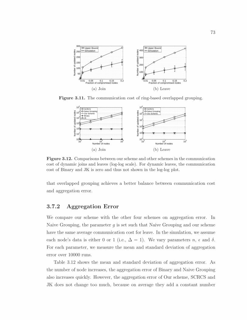
73
0.01 0.05 0.1 0.15 0.20
50
100
150
200
250
300
Fraction of compromised nodes
Num
ber
of u
pdat
ed n
odes
Upper BoundSimulation
(a) Join
0.01 0.05 0.1 0.15 0.20
100
200
300
400
Fraction of compromised nodes
Num
ber
of u
pdat
ed n
odes
Upper BoundSimulation
(b) Leave
Figure 3.11. The communication cost of ring-based overlapped grouping.
103
104
10510
0
101
102
103
104
105
106
Number of nodes
Num
ber
of u
pdat
ed n
odes
SCRCSNaive GroupingOur SchemeBinaryJK
(a) Join
103
104
10510
1
102
103
104
105
106
Number of nodes
Num
ber
of u
pdat
ed n
odes
SCRCSNaive GroupingOur Scheme
(b) Leave
Figure 3.12. Comparisons between our scheme and other schemes in the communicationcost of dynamic joins and leaves (log-log scale). For dynamic leaves, the communicationcost of Binary and JK is zero and thus not shown in the log-log plot.
that overlapped grouping achieves a better balance between communication cost
and aggregation error.
3.7.2 Aggregation Error
We compare our scheme with the other four schemes on aggregation error. In
Naive Grouping, the parameter g is set such that Naive Grouping and our scheme
have the same average communication cost for leave. In the simulation, we assume
each node’s data is either 0 or 1 (i.e., Δ = 1). We vary parameters n, ε and δ.
For each parameter, we measure the mean and standard deviation of aggregation
error over 10000 runs.
Table 3.12 shows the mean and standard deviation of aggregation error. As
the number of node increases, the aggregation error of Binary and Naive Grouping
also increases quickly. However, the aggregation error of Our scheme, SCRCS and
JK does not change too much, because on average they add a constant number
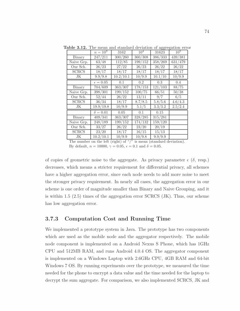
74
Table 3.12. The mean and standard deviation of aggregation errorn = 103 3162 104 31623 105
Binary 247/211 300/260 360/308 386/333 439/381Naive Grp. 63/48 112/85 199/152 358/269 631/479Our Sch. 26/23 27/22 26/23 26/22 26/22SCRCS 18/17 18/17 18/17 18/17 18/17JK 9.9/9.8 10.2/10.1 10/9.9 10.1/10 10/9.9
ε = 0.05 0.1 0.2 0.3 0.4Binary 704/609 363/307 178/153 121/103 88/75
Naive Grp. 398/301 199/152 100/75 66/51 50/38Our Sch. 52/44 26/22 13/11 9/7 6/5SCRCS 36/34 18/17 8.7/8.5 5.8/5.6 4.6/4.3JK 19.9/19.8 10/9.9 5.1/5 3.3/3.2 2.5/2.4
δ = 0.01 0.05 0.1 0.15Binary 409/341 363/307 328/285 315/281
Naive Grp. 248/189 199/152 174/132 159/120Our Sch. 33/27 26/22 23/20 20/19SCRCS 23/20 18/17 16/15 15/13JK 10.2/10.1 10/9.9 10/9.8 9.9/9.9
The number on the left (right) of “/” is mean (standard deviation).By default, n = 10000, γ = 0.05, ε = 0.1 and δ = 0.05.
of copies of geometric noise to the aggregate. As privacy parameter ε (δ, resp.)
decreases, which means a stricter requirement for differential privacy, all schemes
have a higher aggregation error, since each node needs to add more noise to meet
the stronger privacy requirement. In nearly all cases, the aggregation error in our
scheme is one order of magnitude smaller than Binary and Naive Grouping, and it
is within 1.5 (2.5) times of the aggregation error SCRCS (JK). Thus, our scheme
has low aggregation error.
3.7.3 Computation Cost and Running Time
We implemented a prototype system in Java. The prototype has two components
which are used as the mobile node and the aggregator respectively. The mobile
node component is implemented on a Android Nexus S Phone, which has 1GHz
CPU and 512MB RAM, and runs Android 4.0.4 OS. The aggregator component
is implemented on a Windows Laptop with 2.6GHz CPU, 4GB RAM and 64-bit
Windows 7 OS. By running experiments over the prototype, we measured the time
needed for the phone to encrypt a data value and the time needed for the laptop to
decrypt the sum aggregate. For comparison, we also implemented SCRCS, JK and

75
Table 3.13. The analytical computation cost of different schemesMobile Node Aggregator
Our Scheme 4c PRFs 2nqd PRFs
2 Paillier encryptions & 2 Paillier decryptions &JK 1 signature generation 2n mod. multiplications & n sig. verifications
SCRCS 2 mod. exp.√nΔ mod. exp.
Binary 2(�log2 n�+ 1) mod. exp.√nΔ mod. exp.
Binary and measured their running time. As to the JK scheme, the data consumer
and the key manager (see [30]) are implemented together as the aggregator.
Table 3.13 shows the computation overhead of these schemes (see [32, 28, 29, 30]
for details). In the implementation, HMAC-SHA256 is used as the PRF of our
scheme. For JK, the Paillier cryptosystem uses a 1024-bit modulus, and RSA
(1024-bit) is used as the digital signature algorithm. For SCRCS and Binary, the
high-speed elliptic curve “curve25519” is used for modular exponentiation.
Table 3.14 shows the running time of these schemes. Compared with JK, our
scheme is two orders of magnitude faster in both encryption and decryption. This is
because JK uses the Paillier cryptosystem which is very expensive in computation,
but our scheme is based on HMAC which is very efficient. Compared with SCRCS
(Binary), our scheme is one (two) order(s) of magnitude faster in encryption, and
two or three orders of magnitude faster in decryption when the plaintext space is
1000 or larger. SCRCS and Binary are very slow in decryption because they need
to traverse the possible plaintext space to decrypt sum, computing one modular
exponentiation for each possible value. Thus, our scheme is the most efficient in
computation.
Comments. Our scheme’s high efficiency in computation makes it a better
choice for large-scale mobile sensing applications with large plaintext spaces, high
aggregation loads (e.g., many parallel aggregation tasks per node or per aggrega-
tor, short aggregation period), resource-constraint mobile devices (e.g., personal
healthcare devices besides smartphones) and rich statistics.

76
Table 3.14. The running time of different schemesEnc. Decryption- n = 103 104 105 106
Our Scheme 3.4ms 1.2ms 12ms 0.12s 1.2sJK 236ms 175ms 1.5s 15s 150s
SCRCS (Δ = 103) 45ms 5.6s 18s 56s 177sSCRCS (Δ = 104) 45ms 18s 56s 177s 560sSCRCS (Δ = 105) 45ms 56s 177s 560s 1770sBinary (Δ = 103) 0.5∼0.9s 5.6s 18s 56s 177sBinary (Δ = 104) 0.5∼0.9s 18s 56s 177s 560sBinary (Δ = 105) 0.5∼0.9s 56s 177s 560s 1770sThe encryption time of Binary depends on n, and range [0.5, 0.9] isobtained for n ∈ [103, 106]. In our scheme, γ = 0.2.
3.8 Extensions and Discussions
3.8.1 Aggregation Protocol for Min
The Min aggregate is defined as the minimum value of the nodes’ data. This
section presents a protocol which employs the Sum aggregate to get Min.
3.8.1.1 Basic Min Aggregation
This scheme gets the Min aggregate of each time period using Δ+ 1 parallel Sum
aggregates in the same time period. The sums used to obtain Min are based on a
number of 1-bit derivative data (denoted by d) derived from the nodes’ raw data
x. Without loss of generality, we assume that Δ is a power of two.
The scheme works as follows. In each time period, each node generates Δ + 1
derivative data d[0], d[1], ..., d[Δ], where each derivative data corresponds to one
possible data value in the plaintext space. For each j ∈ [0,Δ], the node assigns
1 to d[j] if its raw data value is equal to j and assigns 0 otherwise. For each
j ∈ [0,Δ], the aggregator can obtain the Sum aggregate of d[j] using the sum
aggregation protocol presented in Chapter 3.4. Then Min is the smallest j that
returns a positive sum.
In each time period, each node involves in Δ + 1 sum aggregates over Δ + 1
derivative data. Note that in the sum aggregation protocol each node computes 2c
PRFs to encrypt his data. It is inefficient to compute 2c PRFs for each derivative
data. Since these data are independent, we use a more efficient technique that
concatenates multiple data together and encrypts them as a whole.

77
011
1 0 0
0000
0 0Sum 2 01 0
d[1] d[2] d[3] d[4]
321
User Derivative data
(a) Original derivative data
100
0 0 0
0000
0 0
0 00 1
000
0 0 0
0010
0 1
0 01 0
d[1]
Sum
321
d[2] d[3] d[4]User Derivative data
(b) Extended and concatenated data
Figure 3.13. An example of sum based on extended and concatenated derivative data.
This technique extends each derivative data from one bit to log (n+ 1)� bits byadding log (n+ 1)�−1 0’s on the left, and then concatenates all extended deriva-
tive data into a single bit string. The sum of the concatenated string (interpreted
as an integer) is obtained using the sum aggregation protocol. The obtained sum is
considered as a bit string, and split into substrings of log (n + 1)� bits each. Eachsubstring, when interpreted as an integer, represents the sum of one derivative
data. Note that these substrings do not affect each other (i.e., no carries among
them), since the sum of each derivative data does not exceed n. Figure 3.13 shows
an example of this process.
Clearly, the concatenated data has (Δ + 1) log (n+ 1)� bits. The ciphertext
generated by each node has α = (Δ + 1) log (n+ 1)� bits. If α is larger than H ,
which is the size of the output generated by the PRF (i.e., an HMAC), we can
divide the derivative data into (Δ+1)�log (n+1)�H
groups and apply the above technique
to each group. Thus, (Δ+1)�log (n+1)�H
instances of the sum aggregation protocol are
needed in each time period. For example, when n = 1000, Δ = 10000 and SHA-
512 is used as the hash function of HMAC, 196 instances of the sum aggregation
protocol are needed.
Each node uses just one set of secrets for all instances of the sum aggregation
protocol. For instance j, it uses h(fs′(j|t)) to generate the encryption key instead of
using h(fs′(t)) in the original protocol (see Equation 3.9). Similarly, the aggregator
also uses just one set of secrets.
Since the sum aggregation protocol does not leak the derivative data of any
node, the aggregator cannot know the data value of any specific node.

78
3.8.1.2 Low-cost Min Aggregation
When the plaintext space is large, the cost of the basic Min aggregation scheme
is high. In some application scenarios, it may not be necessary to get the exact
Min, but an approximate answer is good enough. For such scenarios, the basic
Min aggregation scheme can be extended to get an approximate Min with much
smaller cost.
Specifically, we wish to obtain an approximate Min where the relative error
(defined as |Exact Min−Approximate Min|max{Exact Min,1} ) is required to be lower than 1
2ε(ε ≥ 0). To
meet this requirement, the exact value of Min should be obtained if Min is smaller
than or equal to 2ε, and the ε-bit segment of Min (when Min is interpreted as a
bit string) that starts from the first ‘1’ bit should be obtained if Min is larger than
2ε. For example, suppose Min is 42 (00101010) out of 8-bit data. To make the
relative error smaller than 123, it is sufficient to know that Min has the bit pattern
00101xxx. Then we can set the bit that follows the known bits as 1 and set other
bits as 0. The obtained approximate Min is 00101100, which is 44. The relative
error is 121, which is smaller than the required 1
23.
To obtain the approximate Min, each node appends ε + 1 padding bits to its
raw data. If the data value is zero, the first padding bit is 1 and the others are
0; otherwise, all the padding bits are 0. The padded data has logΔ + ε + 2 bits
and at least one bit is 1. The first ‘1’ bit of Min may appear in any of the first
logΔ + 2 bits of the padded data. In the case it appears at the first padding bit,
Min is zero.
Suppose in the binary representation of data value, the weight of bit decreases
from the left to the right. Let δ (δ ∈ [1, logΔ + 2]) denote the location (indexed
from the left) of the first ‘1’ bit of Min. Smaller δ means larger Min. Let σ
denote the value of the (ε − 1)-bit segment of Min that follows δ. When δ is the
same, a larger σ means larger Min. Clearly, there are 2ε−1(logΔ + 2) possible
combinations of 〈δ, σ〉. We map these combinations to an auxiliary plaintext space
0, 1, ..., 2ε−1(logΔ+ 2)− 1, such that if one combination means smaller Min than
another combination, it is mapped to a smaller value in the auxiliary plaintext
space than that combination. Let v[δ, σ] denote the value that combination 〈δ, σ〉maps to.
In each time period, each node converts its padded raw data to a value x′ in

79
Table 3.15. The relative error and cost of the basic Min aggregation scheme and thelow-cost scheme.
Basic Low-costRelative error 0 ≤ 1
2ε
Encryption (PRFs) 2c(Δ+1)�log (n+1)�H
2εc(logΔ+2)H
Decryption (PRFs) q(Δ+1)�log (n+1)�H
2ε−1q(logΔ+2)H
Ciphertext size (bit) (Δ + 1) log (n+ 1)� 2ε−1(logΔ + 2)H is the size of the output generated by the PRF.
the auxiliary plaintext space as follows: if in its padded raw data the first ‘1’ bit
appears at δ′ and the value of the (ε− 1)-bit segment that follows the first ‘1’ bit
is σ′, it sets x′ = v[δ′, σ′]. The aggregator can get the Min of x′ using the basic
Min aggregation scheme, and reversely map the Min of x′ to a pair of 〈δ, σ〉. It
knows that the first ‘1’ bit of the Min aggregate over padded raw data appears at
location δ, and the (ε − 1)-bit segment that follows the first ‘1’ bit is σ. Then it
sets the bit that follows the (ε − 1)-bit segment as 1, and sets the remaining bits
as 0. This derives the Min aggregate over padded raw data, which has the form
{0}δ−1{1}1{0, 1}ε−1{1}1{0}logΔ+2−δ. From this bit string, the last ε + 1 padding
bits are removed and then the approximate Min of nodes’ raw data is obtained.
Figure 3.14 shows a running example of this process. In this example, Δ = 4
and ε = 3. The four nodes’ auxiliary data values are x′1 = 12, x′
2 = 12, x′3 = 10
and x′4 = 4. The Min of the auxiliary data is 4, and it is reversely mapped to
〈δ, σ〉 = 〈3, 00〉. Thus, the approximate Min of padded raw data is 0010010. After
the last four padding bits are removed, the output is 001.
In total, this scheme uses 2ε−1(logΔ + 2) Sum aggregates of 1-bit derivative
data. Thus, 2ε−1(logΔ+2)H
instances of the sum aggregation protocol are needed in
each time period. For example, when Δ = 104, SHA-512 is used as the hash
function of HMAC and it is required to limit the relative error to 1% (i.e., ε = 7),
only 2 instances are needed.
Table 3.15 summarizes the relative error and cost of the basic Min aggregation
scheme and the low-cost scheme.
3.8.1.3 Practical Performances
Our low-cost Min aggregation scheme derives Min from 2ε−1(logΔ+2) parallel Sum
aggregates of 1-bit data, where each sum is obtained using our Sum aggregation

80
1 0 0 00
11
1 0 0
0010
0 0
00
00
x1=4
Raw data
00
00
x[1] x[2] x[3] x[4] x[5] x[6]
x4=1x3=3x2=4
Padding bits
00
00
x[7]
(a) Padded raw data
0 0 0 10
00
0 0 1
0000
0 0
x1=4
11 10 01 00
x4=1x3=3x2=4
1
0 0 0 00
00
0 0 0
0010
0 0
2
0 0 0 00
00
0 0 0
1000
0 0
3
0 0 0 00
00
0 0 0
0000
0 0
4
11 10 01 00 11 10 01 00 11 10 01 00
Sum 0 20 0 0 00 1 0 10 0 0 00 0
±
¾
15 14 13 12 11 10 9 8 7 6 5 4 3 2 1 0v[±; ¾]
(b) Derivative data
Figure 3.14. An example of the process that obtains an approximate Min.
protocol. Here, each sum can also be obtained using SCRCS, and we refer to the
Min aggregation scheme that uses SCRCS as a building block as SCRCS-Min. In
SCRCS-Min, each node computes 2ε(logΔ+2) modular exponentiations to encrypt
his data, and the aggregator computes 2ε−1√n(logΔ+2) modular exponentiations
to decrypt the Min.
According to the bench-marking data reported by eBACS [89], it takes roughly
0.3 ms to compute a modular exponentiation using high-speed elliptic curves such
as “curve25519” on a 64-bit desktop PC, and it takes roughly 0.26 μs3 to compute
an HMAC when SHA-512 is used as the hash function.
Based on these numbers, Table 3.16 and 3.17 show the running time of our Min
aggregation protocol and SCRCS-min at different levels of relative error. Here,
the plaintext space is set as Δ = 104. The parameters of our protocol are set
according to Table 3.6 and Table 3.7 when γ = 0.2. In all the shown cases,
our protocol is at least five (six) orders of magnitude faster than SCRCS-min in
encryption (decryption). Especially, as the system scale increases, the running time
of decryption in SCRCS-min increases quickly which shows the poor scalability of
SCRCS-min, but the running time of our protocol decreases and is always very
3According to eBACS, it takes 0.13 μs to compute one SHA-512. Since one HMAC mainlycomputes two hashes, we simply double this time to get the running time of HMAC.

81
Table 3.16. The running time of our Min aggregation protocol and SCRCS-min whenthe relative error is smaller than 1%.
Encryption Decryptionn = 103 104 105 106 103 104 105 106
SCRCS-min 587ms 587ms 587ms 587ms 9.3s 29s 93s 294sOurs 5μs 4μs 3μs 3μs 4μs 3μs 2.5μs 2μs
Table 3.17. The running time of our Min aggregation protocol and SCRCS-min whenthe relative error is smaller than 0.1%.
Encryption Decryptionn = 103 104 105 106 103 104 105 106
SCRCS-min 4.7s 4.7s 4.7s 4.7s 74s 235s 743s 2348sOurs 40μs 32μs 24μs 24μs 32μs 24μs 20μs 16μs
low, which shows that our protocol is scalable.
3.8.2 More Aggregate Statistics
From Sum and Min, many other aggregate statistics can be easily derived, such as
Count (i.e., the number of nodes that satisfy certain predicate), Average (which is
derivable from Sum and Count), and Max (which can be obtained from the Min
of Δ− x).
Also, in the basic aggregation scheme for Min presented in Chapter 3.8.1.1,
the aggregator can actually get the number of times that each possible data value
appears, and derive the accurate distribution of the nodes’ data in the plaintext
space [0,Δ]. From the distribution, other aggregate statistics such as Median,
Percentile and Histogram can be obtained. In this process, the aggregator knows
nothing about each individual node’s data.
3.8.3 Honest-but-Curious Key Dealer
The assumption of trusted key dealer can be relaxed. Instead, we can assume an
honest-but-curious key dealer that does not collude with the aggregator. It follows
our protocol as specified, but may attempt to infer the data value of nodes from
the the protocol transcript and from eavesdropping all communications. Under
this semi-honest model, the only adaptation that should be made to our protocol
is adding one more encryption/decryption to the data that each node submits to
the aggregator. Specifically, each node first encrypts its noisy data as previously

82
specified with the secrets received from the key dealer, deriving an intermediate
result c, and then encrypts c using a pre-shared key shared with the aggregator.
It sends the final ciphertext to the aggregator. The aggregator first decrypts each
node’s intermediate result c using the pre-shared key, and then decrypts the noisy
sum as previously specified. So long as the key dealer does not collude with the
aggregator, it cannot get any node’s intermediate result c, and thus cannot get the
node’s data value. In future work, we will explore how to completely remove the
key dealer.
3.8.4 Dealing with Node Failures
Fault tolerance is not the major focus of this chapter, but our solution can be
adapted in the following way such that, when some nodes fail, the aggregator can
still obtain the aggregate over the remaining nodes.
Since the key dealer knows the secrets assigned to every node, if some nodes
fail to submit data, the aggregator asks the dealer to submit data on behalf of
those failed nodes. The dealer sets the data value as zero, adds a large-enough
(see below) noise r to it, encrypts the noisy data with the secrets of all those failed
nodes, and submits the obtained ciphertext to the aggregator. The aggregator
can decrypt the sum over the functioning nodes’ data. This method incurs a
round trip communication between the key dealer and the aggregator. The overall
communication cost is still O(n).
Even if all nodes are functioning, the aggregator may dishonestly claim the
failure of a subset S of nodes. (It can only claim one subset per aggregation
period.) Then it can obtain two independent noisy sums, S =∑
i(xi + ri) and
S ′ =∑
i ∈S(xi + ri) + r. It is easy to see that each node is included in at most
two sums. Roughly speaking, to provide differential privacy, it suffices to add two
copies of geometric noise to each sum. Thus, all nodes collectively add two copies
of geometric noise to S and the key dealer itself adds two copies of geometric noise
to S ′. Considering that Alg. 6 may at most double the noise added to S, the
final aggregation error is less than six copies of geometric noise when there is node
failure, and less than four copies without node failure. Obviously, this method
maintains O(1) aggregation error.

83
If a node has failed for a long time, it can be removed from the system as a
“leave”. The recovery of a failed node can be processed as a “join”.
In this method, the key dealer needs to be online, but it only makes online
communications when there is node failure. In future work, we will study other
solutions for fault tolerance, e.g., by exploring the direction pointed out in [29].
3.9 Summary
To facilitate the collection of useful aggregate statistics in mobile sensing without
infringing mobile users’ privacy, we proposed a new differentially private proto-
col to obtain the Sum aggregate of time-series data. The protocol utilizes a novel
HMAC-based encryption scheme to perform computationally efficient aggregation,
and a novel ring-based overlapped grouping technique to efficiently deal with dy-
namic joins and leaves of users. Implementation-based measurements show that
operations at user and aggregator in our protocol are orders of magnitude faster
than existing work. Also, our solution achieves O(1) aggregation error irrespective
of the number of nodes in the system. More importantly, it has very low com-
munication overhead for dynamic joins and leaves. Simulation results show that
only a small number of nodes need to be updated for each join or leave when on
average 20% of nodes are compromised, irrespective of the system scale. Thus, our
protocol can be applied to a wide range of mobile sensing systems with various
scales, plaintext spaces, aggregation loads and resource constraints.
Based on the Sum aggregation protocol, we also proposed two schemes to derive
the Min aggregate of time-series data. One scheme can obtain the accurate Min
while the other one can obtain an approximate Min with provable error guarantee
at much lower cost.

Chapter 4Secure Opportunistic Mobile
Networking for Data Collection
For mobile devices without infrastructure support (e.g., a tablet without 3G ser-
vice) and for circumstances of unavailable or cost-inefficient infrastructures (e.g.,
in disaster recovery scenarios), the lack of network connectivity is a key challenge
to sensing data collection. To address this challenge, we observe that the mobility
of users and the short-range radios of their devices can be used to form an Oppor-
tunistic Mobile Network, and sensing data can be delivered to remote collectors in
this network.
Opportunistic mobile networks consist of mobile nodes carried by human be-
ings [90, 91], vehicles [34, 92], etc. In these networks, due to lack of consistent
connectivity, two nodes can only exchange data when they move into the trans-
mission range of each other (which is called a contact between them). These
contact opportunities can be employed for data forwarding with “store-carry-and-
forward”; i.e., when a node receives some data packets, it stores these packets in
its buffer, carries them around until it contacts another node, and then forwards
them. Such a node with data is called a relay. Opportunistic mobile networks
are also known as Delay/Disruption Tolerant Networks [93] or Pocket Switched
Networks [90].
Opportunistic mobile networks can deliver sensing data in the following way.
Due to mobility, nodes of mobile sensing systems only have opportunistic and
intermittent network connectivity to access points and to each other. If a node

85
has connectivity to an access point, it can directly upload sensing data, assuming
that data collectors are accessible via the Internet. If a node does not have such
connectivity, it delivers sensing data using store-carry-and-forward. Specifically, it
forwards its sensing data to another node (i.e., a relay). The relay may forward the
data to another relay when they contact. The data is eventually delivered when
some relay moves into the physical vicinity of an access point.
The effectiveness of opportunistic mobile networks relies on nodes to cooper-
atively forward packets for each other, and make best use of the limited network
resources (e.g., contact opportunities) for data forwarding. However, several secu-
rity issues make it challenging to deliver sensing data using such networks. Users
are selfish, and they may not forward packets for everyone else. Misbehaving nodes
may drop all received packets, causing sensing data undelivered. Malicious nodes
may also flood their sensing data to the network in order to increase their chance
of being delivered or deplete network resources. If these issues are not well dealt
with, performances of data delivery will degrade. In the following, we address these
problems, i.e., user selfishness, flood attacks, and misbehavior that drop received
packets.
4.1 Social Selfishness Aware Routing
4.1.1 Introduction
Since routing in opportunistic mobile networks relies on mobile nodes to forward
packets for each other, the routing performance (e.g., the number of packets deliv-
ered to their destinations) depends on if nodes are willing to forward for others.
In the real world, most people are socially selfish. As being social, they are
willing to forward packets for others with whom they have social ties1 such as
family members and friends even at the cost of their own resources. Also, they
give different preferences to those with social ties, i.e., they will provide better
service to those with stronger ties than to those with weaker ties, especially when
there are resource constraints. As being selfish, they are unwilling to forward
1In this section, a social tie means an interpersonal tie that falls into the strong or weakcategory defined by Granovetter [94].

86
packets for those with whom they have no social ties in order to save their own
storage and power resources. For convenience, the above social and selfish behavior
will be referred to as social selfishness.
As far as we know, social selfishness has not been addressed before. Although
many routing algorithms [33, 34, 35, 36, 37, 38] have been proposed for opportunis-
tic mobile networks, most of them do not consider users’ willingness and implicitly
assume that a node is willing to forward packets for all others. They may not
work well since some packets are forwarded to nodes unwilling to relay, and will
be dropped. A few recent studies [39, 40] have considered the selfish side of user-
s, where selfish nodes are stimulated to forward packets for all other nodes to
maintain high performance. However, these schemes go to another extreme; i.e.,
they assume that a node is not willing to forward packets for anyone else. For
convenience, such selfishness is called individual selfishness.
In this section, we aim to answer the following question: How to design a routing
protocol for opportunistic mobile networks composed of socially selfish users? From
the network’s point of view, the protocol should force every node to forward packets
for all others, since this can achieve the highest network performance. However,
this solution does not consider the users’ willingness and users cannot behave as
they are willing to. Different from it, our philosophy is “design for user”, i.e.,
we take social selfishness as a user demand and allow nodes to be socially selfish.
Following this philosophy, we propose a Social Selfishness Aware Routing (SSAR)
protocol, in which a node only forwards packets for those with social ties, and it
gives priority to packets received from those with stronger social ties when there
are not enough resources.
Since each node only forwards packets for part of the nodes, it is important to
know how this will affect the routing performance. To achieve high performance,
SSAR considers both user willingness and contact opportunity when selecting re-
lays. It combines the two factors through mathematical modeling and machine
learning techniques, and obtains a new metric to measure the forwarding capa-
bility of a relay. With SSAR, a packet will most likely be forwarded to the relay
that has strong willingness to forward as well as high direct or indirect/transitive
contact opportunity with the destination. To further improve performance, SSAR
formulates the forwarding process as a Multiple Knapsack Problem with Assign-

87
ment Restrictions (MKPAR). It provides a heuristic-based solution that forwards
the most effective packets for social selfishness and routing performance. Extensive
trace-driven simulations show that SSAR can achieve good routing performance
with low transmission cost.
4.1.2 SSAR Overview
In this section, we first introduce our design philosophy and then discuss our models
and assumptions. Finally, we give an overview of SSAR and explain how it works.
4.1.2.1 Design for User
Existing work in mobile ad hoc networks and opportunistic mobile networks has
focused on addressing individual selfishness using reputation-based [95], credit-
based [96], or game-theory based [39] approaches to stimulate users to cooperate
and forward packets for others. If the nodes cooperate with others, they will be
able to get help from others; if not, they will be punished, e.g., being deprived of
access to the network.
These incentive-based schemes may not be directly applied to deal with social
selfishness, since they do not consider social selfishness. In these schemes, every
node has to provide service to others no matter there is a social tie or not. Thus,
social selfishness is not allowed. In essence, these approaches follow the philosophy
of “design for network” because they sacrifice the user’s requirement for selfishness
(i.e., resource saving) to achieve high performance.
We address this problem from a different point of view. We allow social self-
ishness but also try to maintain good routing performance under social selfish
behavior. Our underlying philosophy is that social selfishness is a kind of user
demand that should be satisfied. It should be treated as a new design dimension
that measures the user satisfaction, similar to other traditional dimensions such as
performance. Such design philosophy is referred to as “design for user”.
4.1.2.2 Network Model
In opportunistic mobile networks, nodes have limited bandwidth and computa-
tional capability. As in other studies [34], we assume each node has unlimited

88
buffer space for its own packets, but limited buffer space for packets received from
other nodes. We also assume each packet has a certain lifetime denoted by T-
TL. A packet becomes useless and should be dropped after it expires. We further
assume bidirectional links, which can be provided by some MAC layer protocols,
e.g., IEEE 802.11.
4.1.2.3 Willingness Table
Each node maintains a table that contains its willingness values for other nodes in
the network. In this table, each item has the format 〈nodeID, value〉. The value
of willingness is a real number within [0, 1], where 0 means unwilling to forward
and 1 means the most willing to forward. A node’s willingness value for another
node depends on the social tie between them. The stronger the social tie is, the
larger the willingness is.
Each user manages his willingness table in an off-line style through some user
interface provided by the mobile device (e.g., the keypad of a smart phone). Note
that a user does not need to know all other users in the network. He only needs
to set his willingness value via the user interface for each other user with whom he
has a social tie, and set a default willingness value (e.g., 0) for all other (possibly
unknown) users without any social tie. Thus, most likely, the willingness table has
one item for each node with a social tie and an additional item for all other nodes.
A user only needs to manually configure his willingness table when he joins the
network or migrates to a new mobile device, and update the table when he has
new social ties or his old social ties have changed.
Sociological studies have found that the number of social ties a human being
may have is only a few hundred (150 and 290 according to Dunbar [97] and McCarty
et al. [98], resp.) and social ties are usually stable over time [99]. This means
that the update of willingness table is quite infrequent. Thus, only a low manual
intervention from the user is required, and the usability will not be affected much.
Actually, the maintenance of willingness table is comparable to the maintenance
of address book in a cell phone, which can be well handled by users.
Here, one concern is whether users can quantify the strength of their social
ties into the range of [0, 1]. This has been shown to be feasible by a recent study
which requires users to quantitatively rate their friendships [100]. To be more user-

89
Delivery Probability Estimator
Forwarding Set Manager
Expiration Dropping Estimator
Buffer Overflow Dropping Estimator
Packet Priority Manager
Packet Priority Manager
Buffer Manager
Buffer Manager
Forwarding Set Manager
Expiration Dropping Estimator
Buffer Overflow Dropping Estimator
N MSource,
Destination,
Available buffer size
Delivery probability
Delivery Probability Estimator
Expiration timeNew priority
Step 2
Step 3
Priority,
Figure 4.1. SSAR architecture and an example contact between node N and M. Thedashed rectangles enclose the information exchanged in step 2 and step 3 (Sec. 4.1.2.5).
friendly, the user interface can even provide several preset willingness levels for the
user to choose from, and convert each chosen willingness level into numerical values
in the background. For example, with six preset willingness levels “very strong”,
“strong”, “average”, “weak”, “very weak” and “none”, they can be converted into
1.0, 0.8, 0.6, 0.4, 0.2 and 0, respectively.
4.1.2.4 The Architecture
Figure 4.1 shows the architecture of SSAR. In the following we introduce the
components and their functions.
Packet priority manager: A node assigns a priority between 0 and 1 to each
buffered packet based on its willingness for the source node and the previous hop.
The priority of a packet measures the social importance of this packet for this
node. More details on priority calculation will be given in Sec. 4.1.3.1.
Buffer manager: A node manages buffers based on packet priority: (i) Packets
with priority 0 will not be buffered; (ii) When buffer overflows, packets of low
priority are dropped first. The second rule indicates that a new incoming packet
can preempt the buffer occupied by a lower-priority packet. The buffer policy
together with the priority assignment method allows nodes to be socially selfish
(see Sec. 4.1.3.1).
Delivery probability estimator: It estimates a node’s delivery probability for a

90
packet, which is used to measure the node’s forwarding capability for that packet.
When two nodes are in contact, each packet is forwarded from the node with a
lower delivery probability to the node with a higher delivery probability.
Traditionally, the quality of a relay is measured solely based on contact op-
portunity, which can be the relay’s direct contact opportunity to the destination
node or the transitive contact opportunity provided by the relay’s contacted n-
odes or both. SSAR measures the delivery probability of a node based on both
of its contact opportunity to the destination and its willingness to forward. It is
straightforward that a node with a low contact opportunity should not be a relay.
Interestingly, a node with a high contact opportunity but low willingness should
not be a relay either. This is illustrated in Figure 4.2. Suppose S has a packet
m1 to send to D, and its contact opportunity with D within the packet lifetime is
low (0.3). Suppose S successively meets A, C, and B. If only contact opportunity
is considered, it will forward m1 to A whose contact opportunity is 0.9. Unfortu-
nately, A will drop m1 since it is unwilling to forward for S (the willingness is 0).
SSAR will avoid such forwarding. Although C has a higher contact opportunity
and it is willing to forward m1 for S, its willingness is so low that m1 may suffer a
high risk of being dropped, so SSAR will also avoid such forwarding. As a result,
B is the optimal forwarder for m1 in this scenario, since it has high willingness to
forward and a high contact opportunity.
Our approach to deriving delivery probability includes the mathematical model-
ing of the probability that a packet will be dropped due to expiration with Markov’s
Inequality and the estimation of the probability that the packet will be dropped
due to buffer overflow with a machine learning technique that combines two known
classification algorithms from the literature. More details will be provided in Chap-
ter 4.1.3.2.
Forwarding set manager: After a node determines a set of packets that should
be forwarded to a better relay, existing protocols (e.g., [36]) greedily transmit them
no matter the receiver has enough buffer to hold these packets or not. Obviously,
bandwidth will be wasted if the transmitted packets are dropped due to buffer
overflow. To address this issue, the forwarding set manager decides which packet
to transmit by solving an MKPAR (Multiple Knapsack Problem with Assignment
Restrictions). It considers the buffer constraint and transmits the packets that are

91
msg priority
P{contact D}
m1 1.0
Willingness for S
msg prioritym3 1.0
msg prioritym2 1.0
P{contact D}0.3
0.90
P{contact D}Willingness for S
0.70.1
P{contact D}Willingness for S
0.71.0
Willingness for S’ 0.5Willingness for S” 0
Figure 4.2. An example of willingness-aware forwarding.
the most effective for social selfishness and routing performance.
4.1.2.5 The Protocol
We use an example (Fig. 4.1) to illustrate how SSAR works in the following five
steps:
1. After neighbor discovery, node N and M deliver packets destined to each
other in the decreasing order of priority.
2. Suppose M still buffers some other packets. Then M sends N a summary
list of 〈source ID, destination ID, expiration time, priority〉 for these packets.
3. From the source ID and priority information, N calculates the new priority
value for each packet in the list (Sec. 4.1.3.1). Based on the new priority,
the destination ID and expiration time, N calculates its delivery probability
(Sec. 4.1.3.2) and available buffer size (Sec. 4.1.3.3) for each packet, and
returns them to M .
4. M determines a candidate set of packets for which N has higher delivery
probabilities.
5. Considering the available buffer size information, M further decides which
candidates to transmit by solving the MKPAR (Sec. 4.1.3.3) formulation.
In Step 3, if the new priority of a packet is zero, N ’s delivery probability and
available buffer size for it are also zero. In this case, N does not need to go

92
through the procedures in Sec. 4.1.3.2 and 4.1.3.3. Without loss of generality,
in the last four steps we only describe how node M determines which packets to
transfer to N . Node N does so in similar ways.
Sometimes a node may be in contact with multiple neighbors at the same time.
Then it would be very difficult to extend the MKPAR formulation to the whole
neighborhood. As a simple solution, the node interacts with its neighbors one by
one.
4.1.2.6 Forwarding Strategy
SSAR can work in two modes, forwarding mode and replication mode. In the for-
warding mode, a node deletes its own copy after it transmits a packet to its neighbor
(which has a higher delivery probability). Thus, any packet can simultaneously
have at most one copy in the network. In the replication mode, however, the node
keeps its own copy after transmitting the packet. Therefore, the packet may have
many replicas in the network. The number of replicas depends on the mobility
pattern and is non-deterministic. Generally speaking, the replication mode can
deliver more packets than the forwarding mode but it also requires more resources
such as buffer and bandwidth. Which mode to use should be application-specific.
4.1.3 Detailed Design
This section describes the detailed design of the packet priority calculation, the
delivery probability estimation, and the forwarding set optimization.
4.1.3.1 Packet Priority
When a node receives a packet from a previous hop, it assigns a priority to the
packet. The priority determines if this node will relay the packet (i.e., the priority
is positive) or not (i.e., the priority is zero). To be socially selfish, the node only
forwards the packet if it is from a node with a social tie. There are two cases. First,
the source of the packet has a social tie with this node, and hence forwarding the
packet means helping the source. Second, the previous hop has a social tie with
this node, no matter the source has a social tie or not. In this case, the previous
hop has taken over the responsibility (probably from its own social tie) to deliver

93
the packet. Thus, even if the source does not have a social tie with this node,
this node should still relay the packet to help the previous hop. Actually, this is
motivated by the real-world phenomenon that people usually would like to help
a friend’s friend. The priority should also measure the social importance of the
packet to this node. For example, when other conditions are the same, packets
from the node with a stronger social tie should have a higher priority.
Let pcurr denote the new priority of a packet in the current hop, and pprev denote
the old priority of the packet in its previous hop. Let ωsrc and ωprev denote the
current hop’s willingness for the packet source and the previous hop, respectively.
Then the current hop calculates the new priority in the following ways (Note that
the initial priority of a packet is set as 1 by the source node.): (1) If neither the
source nor the previous hop has a social tie with the current hop, then pcurr = 0.
(2) If the source has a social tie but the previous hop does not, then pcurr = ωsrc.
(3) If the previous hop has a social tie but the source does not, then pcurr =
pprev · ωprev. This calculation method borrows the idea of transitive trust [101]
from the reputation system literature. (4) If both the source and the previous
hop have a social tie with the current hop, pcurr = max{ωsrc, pprev · ωprev}. The
calculation method can be summarized as:
pcurr =
⎧⎪⎪⎪⎪⎨⎪⎪⎪⎪⎩
0 ωsrc = 0, ωprev = 0
ωsrc ωsrc > 0, ωprev = 0
pprev · ωprev ωsrc = 0, ωprev > 0
max{ωsrc, pprev · ωprev} ωsrc > 0, ωprev > 0
(4.1)
The priority assignment method and the buffer management policy can enforce
social selfishness. Packets that traverse different social links will receive different
forwarding service. As shown in Figure 4.2, although m1, m2, and m3 have the
same priority in the source, they will receive different service at relay B after being
transmitted to B. That is, m3 will not receive any forwarding service, and m1 will
receive better service than m2.
The priority of a packet does not consider the destination of the packet due
to the following reason. If a node forwards all the packets destined to its social
ties no matter where these packets are from, a malicious source can exploit this
vulnerability to send unsolicited packets (e.g., advertisement) via this node to its

94
social ties, although the source has no social tie with this node or its social ties. We
note that the malicious source can launch attacks (e.g., source address forgery) to
achieve similar goals, but these security issues are out of the scope of this section.
4.1.3.2 Delivery Probability Estimation
Suppose each packet has some expiration time, the question is: at a given time t,
how to estimate node N ’s probability of delivering packet m to its destination D
before its expiration time texp?
Overall Delivery Probability We assume N can deliver m when it contacts D
if it still buffers m at the time of contact. Then m will either be dropped before
N contacts D or delivered when N contacts D. There are two cases of dropping.
First, m expires before N contacts D and is then dropped. This dropping is due
to N ’s insufficient contact opportunity with D. Second, N drops m in order to
allocate the buffer space originally occupied by m to other newly received packets
which have a higher priority. This dropping happens because m’s priority is too
low and N does not have sufficient buffers for it.
Suppose the next contact between N and D happens at time tc, and N has to
drop m due to buffer overflow at time tover. Further denote the overall delivery
probability by Pdelivery. Then the probabilities of the first and second type of
dropping are given by P{texp ≤ tc} and P{tover ≤ tc}, respectively. Note that the
temporal order of tc and texp is determined by system parameters and the mobility
pattern of N and D, while the time of buffer overflow depends on N ’s traffic load.
Thus we assume that the two dropping events are independent. We integrate them
to get the delivery probability:
Pdelivery = (1− P{texp ≤ tc})(1− P{tover ≤ tc}) (4.2)
In opportunistic mobile networks with unpredictable connectivity, when N
makes such estimation it is impossible to know the exact tc, and thus it is impossi-
ble to compute the r.h.s of Eq. 4.2. Thus, we have to make some approximations.
When texp > tc, P{tover ≤ tc} ≤ P{tover ≤ texp} because the probability density
function of tover is nonnegative. After inserting this inequation into Eq. 4.2, we
get a conservative estimation:

95
Pdelivery ≥ (1− P{texp ≤ tc})(1− P{tover ≤ texp}) (4.3)
The above estimation of Pdelivery can be seen as determined by two independent
droppings, {texp ≤ tc} and {tover ≤ texp}. The first one means that the packet
expires before N ’s next contact with D, so we call it expiration dropping. The
second one means that the packet overflows before expiration, so we call it buffer
overflow dropping. Let Pexp and Pover denote the expiration dropping probability
and buffer overflow dropping probability, respectively. Next, we describe how to
estimate them.
Expiration Dropping Probability To estimate Pexp, we adopt an approach sim-
ilar to that in [39]. Let random variable X denote the inter-contact time between
N and the destination D. Assume that each inter-contact time is independent,
then by Markov’s Inequality:
Pexp = P{X > texp − t} ≤ E(X)/(texp − t) (4.4)
where E(X) is the mean of X and t is the most recent contact time between N
and D before the estimation time t. E(X) can be approximated by the average
of historical inter-contact times. The value of Pexp should be bounded by 1. Eq.
4.4 intuitively means that nodes with a lower average inter-contact time (i.e., a
higher contact frequency) with the destination have a lower expiration dropping
probability.
Buffer Overflow Dropping Probability The most important factor that affects
Pover is m’s priority value p due to the buffer policy. Two other minor factors are
the current empty buffer size L0 and the residual time tr = texp−t before expiration.L0 is positively related to how long m can stay before being removed. But tr is
negatively related: the longer tr is, the more likely it will be dropped due to buffer
overflow.
Without clear knowledge of how these factors interact, it is extremely hard
to theoretically model Pover. Therefore we turn to machine learning techniques
and model it as a supervised learning problem. Whenever N drops or forwards a
packet, it generates a record < p, L0, tr, β >. With machine learning terminology,
each record is called a sample, p, L0, and tr are called feature dimensions and β is

96
m1
m2
Packet priority (p)
Emptybuffersize(L0)
dropped due tobuffer overflow
others
Figure 4.3. Heuristics used to estimate buffer overflow dropping probability Pover.Triangles and squares are historical samples.
called class label. β = 1 if N drops the packet due to buffer overflow and β = 0 if
N does not drop it or drops it due to expiration.
Our basic heuristic is that the probability that m will be dropped is similar
to some historical packets which have similar feature values when they enter N ’s
buffer. Suppose we match m to a set S of similar packets, and within S the subset
of packets being dropped due to buffer overflow is Sdrop. Then Pover is estimated
as:
Pover = |Sdrop|/|S| (4.5)
Figure 4.3 illustrates the idea in a two-dimensional space < p, L0 >, where the
historical packets in the dashed circle are the matched ones. In this example, the
estimated Pover of m1 and m2 are 5/6 = 0.83 and 1/4 = 0.25, respectively.
To match m to similar packets, we choose the K-Nearest-Neighbor (KNN)[102]
algorithm from the machine learning literature, which identifies the K packets that
have the shortest distance to m in the feature space. However, KNN traverses all
samples during matching, which induces high online computation cost, and leaves
less contact duration time for data transmission. Although some techniques [103]
have been proposed to improve its online matching time, they are too complex to
be applied to mobile nodes. To address this problem, we combine KNN with the
Kcenter algorithm [104] to propose a two-phase solution:
• In the offline phase (when not in contact with others), nodes use the Kcenter
algorithm to cluster samples into K clusters around K points in the feature

97
space2.
• In the online phase, nodes scan the K points in the increasing order of their
distance with m’s feature vector until K samples are included in the scanned
clusters.
Based on previous work in this area [105], we set K =√n, where n is the
number of samples. We also set K =√n. Simulations show that they perform
well. The time and space complexity of offline clustering is O(n√n) and O(n).
The time complexity of online matching is O(√n log n), which is much smaller
than that of naive KNN (i.e., O(n√n)). To reduce the computation cost, the
offline phase does not have to be run whenever a packet is dropped or forwarded;
it can be run when a certain number of packets have been dropped or forwarded
since the last run.
Both the online and offline phase need to compute the distance between two
feature vectors. When doing so, L0 is normalized to [0, 1] based on the total
buffer size of N , and tr is normalized to [0, 1] based on the packet TTL. Moreover,
since Euclidean distance performs poorly when samples are sparse in the feature
space, we propose a distance metric by assigning different weights to different
feature dimensions. We observe that if dropped samples spread narrowly in one
feature dimension, this dimension is sensitive and should be highly weighted and
vice versa. Suppose m1 and m2 are two feature vectors. Then their distance
is D(m1, m2) =√∑3
i=1σi
2
σ2i(mi
1 −mi2)
2, where σ2i and σi
2 denote the variance of
feature i in dropped samples and all samples, respectively.
4.1.3.3 Forwarding Set Optimization
In this subsection, we solve the following problem: suppose a node M contacts N ,
and M has determined a candidate packet set C for which N has higher delivery
probabilities. Since N ’s buffer may be inadequate to accept all packets in C, weneed to find out how to determine a subset of C to transmit.
We follow two principles. First, M will not forward a packet to N if N does
not have sufficient buffers for that packet. According to the buffer management
rule, N ’s available buffer size Lm for m is:
2We refer to the original paper for details.

98
Algorithm 7 : Greedy algorithm for forwarding set selection, pseudo-code for M1: Compute the selfish gain g for each packet in C2: Sort C in the decreasing order of g/l (Let i denote the ith packet in C)3: for Packet i from 1 to |C| do4: if N is not in contact with M anymore then5: break6: end if7: if Li ≥ li then8: Forward i to N9: for Packet j from i+ 1 to |C| do10: Lj− = li11: end for12: else13: continue14: end if15: end for
Lm = L0 +∑
{k|pk<p}lk (4.6)
where L0 denotes N ’s empty buffer size, {k|pk < p} denotes the packets in N ’s
buffer whose priority is smaller than that of m (i.e., p), and lk denotes the size of
packet k. Second, M tries to maximize its selfish gain through this contact, which
is defined as follows.
Definition 1 (Selfish Gain) The selfish gain g that M achieves by forward-
ing m to N is the product of m’s priority p in M and the increment of delivery
probability, i.e., g = p ·ΔPdelivery.
Both factors in the definition are related to selfishness. p means how socially
important the packet is. The larger p is, the more selfishness is gained. ΔPdelivery
means how much this forwarding can increase the packet’s probability to be de-
livered. The larger ΔPdelivery is, the more help is provided. So their product is a
natural representation of the gained selfishness.
Suppose all the packets in C are sorted by priority in the increasing order. Then
we can simply use i to denote the ith packet. Let Xi denote if packet i is selected to
be transmitted (Xi = 1) or not (Xi = 0). According to the above two principles,
the problem can be formulated as:
max∑i∈C
giXi s.t. ∀i∑j≤i
Xjlj ≤ Li (4.7)

99
In a special case that all candidate packets have the same priority, Eq. 4.7
becomes a standard Knapsack problem. Thus, Eq. 4.7 is a variant of the Knapsack
problem. Next we show that it can be converted into an MKPAR [106], where each
item can only be assigned to a subset of the knapsacks. Suppose the original buffer
is divided into |C|+1 knapsacks such that the first knapsack has size S1 = L1, the
jth (j ∈ {2, ..., |C|}) one has size Sj = Lj −Lj−1, and the (|C|+1)th one consists of
buffers that cannot be preempted by any packet in C. Then packet i can only be
packed into knapsacks indexed smaller than or equal to i. Let Xij denote if packet
i is packed into knapsack j (Xij = 1) or not (Xij = 0). Then Xij = 0 when i < j.
Eq. 4.7 can be rewritten as:
max
|C|∑i=1
|C|∑j=1
giXij s.t. ∀i∑j
Xij ≤ 1, ∀j∑i
Xijli ≤ Sj (4.8)
Since the problem is NP-hard, we give a greedy algorithm, which ranks the
packets in the decreasing order of selfish gain weighted by packet size, and packs
them one by one until no more packets can be packed. The details are shown in
Algorithm 7. The time complexity of this algorithm is O(|C|2), which is acceptable
because most handsets have such computing capability.
4.1.4 Performance Evaluations
In this section, we evaluate the performance of SSAR and compare it to other
routing algorithms.
4.1.4.1 Experiment Setup
We evaluate SSAR over two traces collected from real-world opportunistic mo-
bile networks: Haggle Infocom05 [107] and MIT Reality [108]. Both are available
from the CRAWDAD project in Dartmouth [109]. These traces record contacts
among users carrying Bluetooth devices, which periodically discover peer devices
and record contacts between them. The chosen traces cover a diversity of environ-
ments, from college campuses (Reality) to conference sites (Infocom05), and with
experimental periods from several days (Infocom05) to several months (Reality).
Table 4.1 summarizes their main characteristics.

100
Table 4.1. The summary of the two traces used for evaluationTrace Infocom05 Reality
Network type Bluetooth BluetoothNumber of devices 41 97Number of contacts 22 thousand 110 thousand
Duration 3 days 9 monthsGranularity 120 seconds 300 seconds
A B C D
degree=3 degree=2 degree=1 degree=1
(a) Generate node degrees
A B C D
degree=2 degree=1 degree=1
0.70.4
0.9 0.5
degree=3
0.8
0.5
0.3
(b) Generate edge weights
AC D
degree=2 degree=1 degree=1
0.70.4
0.9 0.5B
degree=3
0.8
0.5
0.3
(c) Assign degrees to nodes
AC
DB
0.8
0.3
0.5
0.70.4
0.5 0.9
(d) Connect edges
Figure 4.4. An example of social network graph generation in the 4 basic steps.
Since the traces do not have the accurate social relationship information among
participants (i.e., nodes), we need to construct a weighted directed social network
graph upon them. In the graph, a vertex denotes a node in the trace, and an edge
denotes a social tie between nodes. Edge weight means the strength of the social
tie, and it also means the willingness to forward. For instance, the weight of edge−−→NM is node N ’s willingness to forward packets for M . The weight of edge
−−→NM
and that of−−→MN may be different.
Several measurement studies (e.g., [110]) have empirically found that in real-
world social networks node degrees follow power-law distributions. Also, in one
recent study [100] participants rate the strength of their friendships nearly uni-
formly between 0 and 1, which is the best empirical data we can find about the
distribution of social tie strength. Thus, we try to ensure that the constructed
social network graph have these two basic properties.
Our construction process involves four steps as illustrated in Fig. 4.4. Step 1 :

101
Generate power-law distributed node degrees. Since the degree of a node means
the number of edges emitted from this node, we denote a degree d with d arrows
in Fig. 4.4. Step 2 : Generate weights for these arrows (which will become edges
in the finished graph) that follow the uniform distribution between 0 and 1. Step
3 : Assign those degrees to nodes. When this step is complete, each node has a
number of edges emitting from it. Step 4 : Connect each of these edges to another
node.
To better evaluate SSAR, we generate two types of social network graphs which
differ in the last two steps. The first type is contact-dependent graph, where the
contact frequency between nodes probabilistically determines how degrees are as-
signed to nodes and how edges are connected. It is based on the following heuristic
which has been verified by sociology studies [94]. The stronger tie two individuals
have, the more likely they contact frequently. Individuals with more social ties
are more likely to meet other people. Let f∗ denote the overall contact frequen-
cy of the whole trace, fN denote node N ’s overall contact frequency, and fNM
denote the contact frequency between N and M . Then the last two steps for
contact-dependent graph are as follows:
• Step 3 : Repeatedly assign node degrees to nodes, i.e., assign the largest
degree to a node in such a way that node N ’s probability to be selected is
fN/f∗, and repeat this for the remaining degrees and nodes.
• Step 4 : For each node N , connect its edges to other nodes. First connect
the edge with the highest weight to another node in a way that node M ’s
probability to be connected is fNM/fN , and repeat this for the other edges
and nodes that have not been connected to N . In the end, for any ordered
node pair NM that has not been connected yet, the willingness of N for M
is set 0.
The second type of graph is random graph. To construct it, in the third and fourth
step we simply assign degrees to random nodes and connect each edge of a node
to another random node. Though we believe random graph is less realistic than
contact-dependent graph, we still use it in order to evaluate SSAR under diversified
social graphs.
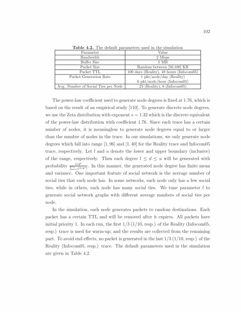
102
Table 4.2. The default parameters used in the simulationParameter ValueBandwidth 2 MbpsBuffer Size 5 MBPacket Size Random between [50,100] KBPacket TTL 100 days (Reality), 48 hours (Infocom05)
Packet Generation Rate 1 pkt/node/day (Reality)6 pkt/node/hour (Infocom05)
Avg. Number of Social Ties per Node 25 (Reality), 8 (Infocom05)
The power-law coefficient used to generate node degrees is fixed at 1.76, which is
based on the result of an empirical study [110]. To generate discrete node degrees,
we use the Zeta distribution with exponent s = 1.32 which is the discrete equivalent
of the power-law distribution with coefficient 1.76. Since each trace has a certain
number of nodes, it is meaningless to generate node degrees equal to or larger
than the number of nodes in the trace. In our simulations, we only generate node
degrees which fall into range [1, 96] and [1, 40] for the Reality trace and Infocom05
trace, respectively. Let l and u denote the lower and upper boundary (inclusive)
of the range, respectively. Then each degree l ≤ d ≤ u will be generated with
probability 1/ds∑ua=l(1/a
s). In this manner, the generated node degree has finite mean
and variance. One important feature of social network is the average number of
social ties that each node has. In some networks, each node only has a few social
ties; while in others, each node has many social ties. We tune parameter l to
generate social network graphs with different average numbers of social ties per
node.
In the simulation, each node generates packets to random destinations. Each
packet has a certain TTL and will be removed after it expires. All packets have
initial priority 1. In each run, the first 1/3 (1/10, resp.) of the Reality (Infocom05,
resp.) trace is used for warm-up, and the results are collected from the remaining
part. To avoid end-effects, no packet is generated in the last 1/3 (1/10, resp.) of the
Reality (Infocom05, resp.) trace. The default parameters used in the simulation
are given in Table 4.2.

103
4.1.4.2 Routing Algorithms
We compare SSAR with two other benchmark algorithms, PROPHET [33] and
SimBet [35]. PROPHET is a standard non-oblivious benchmark that has been
used to compare against several previous works [37]. It calculates a metric, delivery
predictability, based on contact histories, and relays a packet to a node with higher
delivery predictability. We use the same parameters as in [33]. SimBet has also
been used as a benchmark in several works [38]. It calculates a simbet metric using
two social measures (similarity and betweenness). A packet is forwarded to a node
if that node has a higher simbet metric than the current one. We use the same
parameters as in [35].
Since the original algorithms do not define the order of packets to be trans-
mitted during a contact, we adopt the transmission order used in RAPID [36].
Because this order has been shown to be the most effective, we believe such re-
finement does not favor SSAR in comparison. Since the original algorithm either
assumes infinite buffer (SimBet) or assumes finite buffer but does not specify the
packet dropping policy (PROPHET), we apply three policies (drop-tail, random
drop, and minimum-utility-drop-first) in simulation, and only present the results
of the best policy here, i.e., minimum-utility-drop-first. Since it is impossible to
traverse all dropping policies and choose the optimal one, we tried our best to
impose the minimum influence on the original algorithms.
PROPHET and SimBet are designed without considering social selfishness. For
fair comparison, we modified them so that they have some basic selfishness aware-
ness. That is, nodes do not forward packets to others who are not willing to forward
for them, and avoid immediate droppings caused by selfishness. However, when
nodes forward packets to others who are willing to forward for them, they still
follow the aforementioned transmission order and buffer policy. To show the effect
of such selfishness-awareness, we also include the basic PROPHET in our simula-
tions. For convenience, we label the selfishness-aware PROPHET PROPHET-2,
and label the basic one PROPHET-1.
We evaluate SSAR and these algorithms under the forwarding mode and repli-
cation mode introduced in Sec. 4.1.2.6.

104
0 10 25 50 75 1000
0.1
0.2
0.3
0.4
0.5
Packet TTL (Day)
Pac
ket D
eliv
ery
Rat
io
SSARSimBetPROPHET−2PROPHET−1
(a) Performance
0 10 25 50 75 1000
1
2
3
4
5
6
7
8
Packet TTL (Day)
Pac
ket D
eliv
ery
Cos
t
SSARSimBetPROPHET−2PROPHET−1
(b) Cost
0 10 25 50 75 1000
5
10
15
20
25
Packet TTL (Day)
Pac
ket D
eliv
ery
Del
ay (
Day
)
SSARSimBetPROPHET−2PROPHET−1
(c) Delay
Figure 4.5. Comparison of algorithms in the forwarding mode. The Reality trace andcontact-dependent graph are used.
4.1.4.3 Metrics
We use the following metrics to evaluate these algorithms: 1) Packet delivery
ratio: The proportion of packets that are delivered to their destinations out of
the total unique packets generated. 2) Packet delivery cost: The total number
transmissions divided by the number of unique packets generated. 3) Packet
delivery delay: From the time a packet is generated to the time the packet is
delivered. In the results, we plot the average delay of all delivered packets. 4)
Selfishness satisfaction (SS): A node’s SS is defined as the ratio of the average
priority of the packets it forwards or delivers over the average priority of the packets
it drops. SS reflects how much the user is satisfied with the network, because a
larger SS indicates more important messages are served. In the results, we plot
the average SS of all nodes.
4.1.4.4 Results
The Effects of TTL We first evaluate the algorithms when the forwarding mode
(see Sec. 4.1.2.6) is used, i.e., each packet has only one copy in the network, so
that the effect of packet replication can be separated. Figure 4.5 shows the results
over the Reality trace when the contact-dependent graph is used.
Figure 4.5(a) compares the algorithms in packet delivery ratio. When the T-
TL increases all algorithms deliver more packets to the destinations. However, as
the TTL becomes large the increment in packet delivery ratio becomes marginal,
because at that time the forwarding capacity of the network becomes the perfor-
mance bottleneck. Among all algorithms, SSAR has the highest packet delivery

105
0 10 25 50 75 1000
0.1
0.2
0.3
0.4
0.5
Packet TTL (Day)
Pac
ket D
eliv
ery
Rat
io
SSARSimBetPROPHET−2PROPHET−1
(a) Performance
0 10 25 50 75 1000
0.5
1
1.5
2
2.5
3
Packet TTL (Day)
Pac
ket D
eliv
ery
Cos
t
SSARSimBetPROPHET−2PROPHET−1
(b) Cost
0 10 25 50 75 1000
5
10
15
20
25
30
Packet TTL (Day)
Pac
ket D
eliv
ery
Del
ay (
Day
)
SSARSimBetPROPHET−2PROPHET−1
(c) Delay
Figure 4.6. Comparison of algorithms in the forwarding mode. The Reality trace andrandom graph are used.
0 12 24 36 48 600
0.1
0.2
0.3
0.4
0.5
0.6
0.7
Packet TTL (Hour)
Pac
ket D
eliv
ery
Rat
io
SSARSimBetPROPHET−2PROPHET−1
(a) Performance
0 12 24 36 48 600
5
10
15
20
Packet TTL (Hour)
Pac
ket D
eliv
ery
Cos
t
SSARSimBetPROPHET−2PROPHET−1
(b) Cost
0 12 24 36 48 600
2
4
6
8
10
12
Packet TTL (Hour)
Pac
ket D
eliv
ery
Del
ay (
Hou
r)
SSARSimBetPROPHET−2PROPHET−1
(c) Delay
Figure 4.7. Comparison of algorithms in the forwarding mode. The Infocom05 traceand contact-dependent graph are used.
ratio. For example, when the TTL is 100 days it outperforms PROPHET-2, Sim-
Bet and PROPHET-1 by 80%, 120% and 300%, respectively. This is because SSAR
incorporates user willingness, buffer constraint, and contact opportunity into relay
selection. It avoids low-willingness nodes or overloaded hot spots when selecting
relays, and has much less packet dropping caused by these nodes. In contrast,
PROPHET and SimBet cannot avoid those nodes since they only consider contact
opportunity when selecting relays. Another reason is that the MKPAR formula-
tion of SSAR does not forward a packet to the next hop whose buffer is insufficient
to hold this packet, but PROPHET and SimBet may make such transmissions and
result in packet dropping. PROPHET-1 performs much worse than PROPHET-2
because PROPHET-1 is not selfishness-aware. It forwards many packets to those
who are unwilling to forward, and those packets are dropped.
Figure 4.5(b) compares the algorithms in packet delivery cost. As the TTL in-
creases, all algorithms have more transmissions, because packets stay longer in the
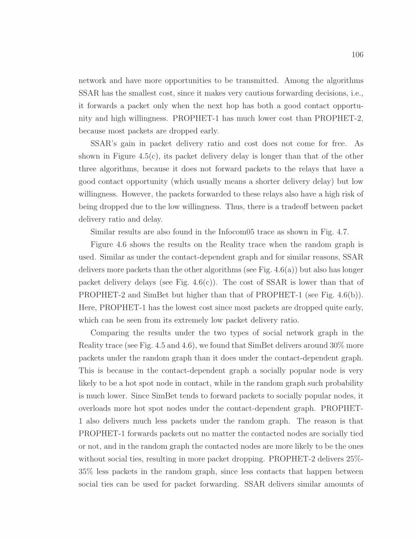
106
network and have more opportunities to be transmitted. Among the algorithms
SSAR has the smallest cost, since it makes very cautious forwarding decisions, i.e.,
it forwards a packet only when the next hop has both a good contact opportu-
nity and high willingness. PROPHET-1 has much lower cost than PROPHET-2,
because most packets are dropped early.
SSAR’s gain in packet delivery ratio and cost does not come for free. As
shown in Figure 4.5(c), its packet delivery delay is longer than that of the other
three algorithms, because it does not forward packets to the relays that have a
good contact opportunity (which usually means a shorter delivery delay) but low
willingness. However, the packets forwarded to these relays also have a high risk of
being dropped due to the low willingness. Thus, there is a tradeoff between packet
delivery ratio and delay.
Similar results are also found in the Infocom05 trace as shown in Fig. 4.7.
Figure 4.6 shows the results on the Reality trace when the random graph is
used. Similar as under the contact-dependent graph and for similar reasons, SSAR
delivers more packets than the other algorithms (see Fig. 4.6(a)) but also has longer
packet delivery delays (see Fig. 4.6(c)). The cost of SSAR is lower than that of
PROPHET-2 and SimBet but higher than that of PROPHET-1 (see Fig. 4.6(b)).
Here, PROPHET-1 has the lowest cost since most packets are dropped quite early,
which can be seen from its extremely low packet delivery ratio.
Comparing the results under the two types of social network graph in the
Reality trace (see Fig. 4.5 and 4.6), we found that SimBet delivers around 30%more
packets under the random graph than it does under the contact-dependent graph.
This is because in the contact-dependent graph a socially popular node is very
likely to be a hot spot node in contact, while in the random graph such probability
is much lower. Since SimBet tends to forward packets to socially popular nodes, it
overloads more hot spot nodes under the contact-dependent graph. PROPHET-
1 also delivers much less packets under the random graph. The reason is that
PROPHET-1 forwards packets out no matter the contacted nodes are socially tied
or not, and in the random graph the contacted nodes are more likely to be the ones
without social ties, resulting in more packet dropping. PROPHET-2 delivers 25%-
35% less packets in the random graph, since less contacts that happen between
social ties can be used for packet forwarding. SSAR delivers similar amounts of

107
0 10 25 50 750
0.1
0.2
0.3
0.4
0.5
0.6
0.7
0.8
Packet TTL (Day)
Pac
ket D
eliv
ery
Rat
io
SSARSimBetPROPHET−2PROPHET−1
(a) Performance
0 10 25 50 750
50
100
150
200
250
300
Packet TTL (Day)
Pac
ket D
eliv
ery
Cos
t
SSARSimBetPROPHET−2PROPHET−1
(b) Cost
0 10 25 50 750
5
10
15
20
25
Packet TTL (Day)
Pac
ket D
eliv
ery
Del
ay (
Day
)
SSARSimBetPROPHET−2PROPHET−1
(c) Delay
Figure 4.8. Comparison of algorithms in the replication mode. The Reality trace andcontact-dependent graph are used.
packets under the two types of social network graph. The cost of all algorithms
is lower in the random graph since fewer contacts happen between socially tied
nodes. Packet delivery delay does not change much in the two graphs.
Next we evaluate the algorithms when the replication mode (see Sec. 4.1.2.6) is
used over the Reality trace. The packet generation rate is 0.1 packets per node per
day. As shown in Fig. 4.8(a), all algorithms have a similar packet delivery ratio;
however, SSAR achieves such performance at much lower cost (see Fig. 4.8(b)).
For example, when TTL is 75 days, the cost in SSAR is only 8%-13% of that in
the other three algorithms. Again, this is because SSAR makes very cautious but
effective transmissions. If a packet has a high probability to be dropped by the next
hop, most likely SSAR will not replicate the packet. In contrast, the other three
algorithms are more greedy in replication. Many replicas only play a marginal role
in packet delivery, and very likely such transmissions are wasted. In addition, the
MKPAR formulation of SSAR also avoids many useless transmissions. As shown
in Fig. 4.8(c), all algorithms have similar packet delivery delays.
The Effects of Buffer Size To evaluate how SSAR performs when nodes
have different storage resources, we change the buffer size of each node from 1MB to
10MB over the Reality trace and show the results in Fig. 4.9. When the buffer size
increases, all the three metrics (packet delivery ratio, cost and delay) also increase.
SSAR delivers much more packets than the other three algorithms at lower cost
but it also has a longer packet delivery delay for aforementioned reasons.
The Effects of the Average Number of Social Ties per Node Fig. 4.10
shows the results on the Reality trace when each node generates 0.1 packets per

108
0 1 2.5 5 7.5 100
0.1
0.2
0.3
0.4
0.5
Buffer Size (MB)
Pac
ket D
eliv
ery
Rat
io
SSARSimBetPROPHET−2PROPHET−1
(a) Performance
0 1 2.5 5 7.5 100
2
4
6
8
10
12
Buffer Size (MB)
Pac
ket D
eliv
ery
Cos
t
SSARSimBetPROPHET−2PROPHET−1
(b) Cost
0 1 2.5 5 7.5 100
5
10
15
20
25
30
Buffer Size (MB)
Pac
ket D
eliv
ery
Del
ay (
Day
)
SSARSimBetPROPHET−2PROPHET−1
(c) Delay
Figure 4.9. Comparison of algorithms on the Reality trace when nodes have differentbuffer sizes. The forwarding mode and contact-dependent graph are used.
5 10 15 20 250
0.1
0.2
0.3
0.4
0.5
0.6
0.7
0.8
Average Number of Social Ties per Node
Pac
ket D
eliv
ery
Rat
io
SSARSimBetPROPHET−2PROPHET−1
(a) Performance
5 10 15 20 250
50
100
150
200
250
300
350
Average Number of Social Ties per Node
Pac
ket D
eliv
ery
Cos
t
SSARSimBetPROPHET−2PROPHET−1
(b) Cost
5 10 15 20 250
5
10
15
20
25
30
35
Average Number of Social Ties per Node
Pac
ket D
eliv
ery
Del
ay (
Day
)
SSARSimBetPROPHET−2PROPHET−1
(c) Delay
Figure 4.10. Comparison of algorithms on the Reality trace when nodes have differentaverage numbers of social ties. The replication mode and contact-dependent graph areused.
day and the TTL is 50 days. When nodes have more social ties the packet delivery
ratio of all algorithms increases. The packet delivery cost of SSAR, SimBet and
PROPHET-2 also increases. Obviously, the increment in packet delivery ratio and
cost is because more nodes can be used for relays and packets have more chances
to be transmitted. SSAR achieves similar performance with other algorithms at
much lower cost, and these algorithms have very similar delays that do not change
much with the average number of social ties.
The Effects of Willingness-aware Forwarding Fig. 4.11 compares SSAR
with its variant where willingness is not considered in relay selection (i.e., only
contact opportunity is considered). The Reality trace is used and the buffer size
is 1MB. As shown in Fig. 4.11(a) and 4.11(b), SSAR achieves a higher packet
delivery ratio at lower cost than its variant that does not consider willingness, and
their difference is more significant when the workload is higher. This is because
willingness significantly affects the probability that a packet will be dropped by a

109
0.25 0.5 1 20.2
0.25
0.3
0.35
0.4
0.45
0.5
0.55
Packet Generation Rate (Packet/Node/Day)
Pac
ket D
eliv
ery
Rat
io
Willingness ConsideredWillingness Not Considered
(a) Performance
0.25 0.5 1 21
1.5
2
2.5
3
Packet Generation Rate (Packet/Node/Day)
Pac
ket D
eliv
ery
Cos
t
Willingness ConsideredWillingness Not Considered
(b) Cost
0.25 0.5 1 218
19
20
21
22
23
24
Packet Generation Rate (Packet/Node/Day)
Pac
ket D
eliv
ery
Del
ay (
Day
)
Willingness ConsideredWillingness Not Considered
(c) Delay
Figure 4.11. The effects of willingness awareness in SSAR. The forwarding mode andcontact-dependent graph are used over the Reality trace.
1 2 3 4 5 6 7 8 9 100
0.2
0.4
0.6
0.8
1
Packet Priority Interval i
Avg. Estimated Dropping ProbabilityReal Dropping Rate
Figure 4.12. The accuracy of our KNN-plus-Kcenter algorithm in estimating the bufferoverflow dropping probability of the packets that fall into 10 priority intervals with theith interval being [0.1 · (i−1), 0.1 · i]. The forwarding mode and contact-dependent graphare used over the Reality trace.
node, especially when the workload is high. For instance, when each node generates
only 0.25 packets per day, SSAR outperforms its variant by 10% in packet delivery
ratio with 7% lower cost. However, when each node generates 2 packets per day,
SSAR outperforms its variant by 31% in packet delivery ratio at 23% lower cost.
When delay is considered (see Fig. 4.11(c)), SSAR and its variant has a small
difference which is only 4%-7%. Thus, willingness-aware forwarding is effective.
Estimation Accuracy Now we evaluate the accuracy of our KNN-plus-
Kcenter algorithm in estimating the probability that a packet will be dropped
due to buffer overflow. Since packet priority is the major factor that affects this
probability, we divide the packets into 10 groups whose priority falls into 10 in-
tervals evenly spanned in [0, 1], i.e., the ith priority interval is [0.1 · (i− 1), 0.1 · i](1 ≤ i ≤ 10). We compare the average estimated dropping probability of each

110
group of packets with the real dropping rate of the same group in Fig. 4.12, where
SSAR works in the forwarding mode over the Reality trace and the buffer size
is 1MB. As shown in Fig. 4.12, the estimation result of our algorithm is close to
the real dropping rate, and our algorithm can correctly predict that low-priority
packets are more likely to be dropped than high-priority packets. Thus, it helps
direct packets to those relays with high willingness to forward.
Allowed Selfishness To compare SSAR with other algorithms on how much
selfishness is allowed, we plot the SS metric in Fig. 4.13 and 4.14. The buffer size
is 1MB and 5MB in the Reality and Infocom05 trace, respectively. The two figures
show that SSAR allows better selfishness than the other three algorithms. This
is because SSAR’s buffer management policy satisfies social selfishness. Also, due
to the selfish gain metric and the MKPAR formulation, high-priority packets are
more likely to be forwarded than low-priority ones. In contrast, the other three
algorithms manage buffers without selfishness information and forward packets
purely based on contact opportunity, so they perform much worse. We noted that
the SS in SSAR drops as the packet generation rate increases. This is because
when the workload is higher more packets are dropped. Thus, the average priority
of dropped packets increases and SS decreases. In the extreme, if the workload is
so high that nearly all packets are dropped, the SS will be close to 1.
4.1.5 Related Work
Many algorithms have been proposed for routing and data dissemination in oppor-
tunistic mobile networks, and they vary in what information is used to evaluate a
node’s forwarding capability and make forwarding decisions. Earlier works [33, 34]
evaluate the forwarding capability of a node by the historic contact information,
while more recent studies [35, 37, 111, 112] employ the social property (e.g., be-
tweenness and centrality) of nodes or transient contact patterns [113] for relay
selection. Gao and Cao [114] also propose a social centrality metric that consid-
ers the social contact patterns and interests of mobile users simultaneously and
achieves effective relay selection. However, these approaches do not consider the
social willingness of users to forward packets for others, and implicitly assume
nodes are fully willing to forward packets for each other, which may not be al-

111
0.25 0.33 0.5 1.0 1.50
2
4
6
8
10
12
Packet Generation Rate (Packet/Node/Day)
Sel
fishn
ess
Sat
isfa
ctio
n
SSARSimBetPROPHET−2PROPHET−1
(a) Contact-dependent Graph
0.25 0.33 0.5 1.0 1.50
2
4
6
8
10
12
Packet Generation Rate (Packet/Node/Day)
Sel
fishn
ess
Sat
isfa
ctio
n
SSARSimBetPROPHET−2PROPHET−1
(b) Random Graph
Figure 4.13. Comparison of algorithms in selfishness satisfaction over the Reality trace.The forwarding mode is used.
6 9 12 150
2
4
6
8
10
Packet Generation Rate (Packet/Node/Hour)
Sel
fishn
ess
Sat
isfa
ctio
n
SSARSimBetPROPHET−2PROPHET−1
(a) Contact-dependent Graph
6 9 12 150
2
4
6
8
10
Packet Generation Rate (Packet/Node/Hour)
Sel
fishn
ess
Sat
isfa
ctio
n
SSARSimBetPROPHET−2PROPHET−1
(b) Random Graph
Figure 4.14. Comparison of algorithms in selfishness satisfaction over the Infocom05trace. The forwarding mode is used.
ways true in reality. Algorithms [115, 116] have also been proposed for finding the
right relays for data forwarding in vehicular ad hoc networks, but they consider a
different scenario from this work.
Hui et al. [117] study the impact of altruistic behavior on the communication
throughput of mobile social networks. The “altruism” concept in their work is
similar to the willingness concept in this work in that altruism also describes if a
node will forward packets for other nodes. However, there is important difference
between the two. Altruism is used in an absolute sense and it denotes the prob-
ability that a node will forward a received packet. On the contrast, willingness
is used in a relative sense, and it takes effect only when multiple packets contend
for shared limited resource (e.g., buffer and bandwidth). More importantly, their
focus is the impact of altruism on opportunistic communication but our focus is
to design an effective and efficient routing protocol that considers user willingness.

112
Thus, this work and their work are complementary to each other.
Most existing routing algorithms explicitly or implicitly assume unlimited buffer
(e.g., delegation forwarding [38]) which is unrealistic. Though some algorithm-
s [36, 34] consider the buffer constraint in design, their attention is limited to
which packets to drop when buffer overflows. However, SSAR integrates the buffer
constraint into relay selection and takes it as a factor of delivery probability. Some
work (e.g., RAPID [36]) has addressed in which order candidate packets should be
transmitted to a better relay during a contact, but existing approaches ignore that
the forwarded packets may be immediately dropped by the relay due to the buffer
constraint. SSAR uses MKPAR to determine both which subset of candidate pack-
ets to forward and in what order to forward them. The formulation is different
from the Knapsack formulation in [112] and [111]. Recently, Thompson et al [118]
propose a congestion control scheme for opportunistic mobile networks which us-
es the local dropping information to control packet replications. Their scheme is
different from SSAR since it controls a node’s overall amount of replications but
does not determine which node is a better relay.
Individual selfishness has been widely studied in mobile ad hoc networks [96, 95]
and even in opportunistic mobile networks [40, 39]. The solutions proposed so far
fall into three categories, credit-based approaches (e.g., [96, 40]), reputation-based
approaches (e.g., [95]) and gaming-based approaches (e.g., [39]). The principle
idea is to stimulate users to forward packets for others. As discussed in Chapter
4.1.2.1, they cannot be directly applied to the social selfishness problem.
4.1.6 Summary
In this section, we investigated the social selfishness problem in opportunistic mo-
bile networks, and proposed a routing protocol SSAR for sensing data delivery
which allows users to behave in the socially selfish way. Different from existing
routing protocols that only consider contact opportunity when selecting relays,
SSAR considers both user willingness and contact opportunity to measure the
quality of relay, which is a better strategy for socially selfish networks. We de-
signed novel machine learning techniques to incorporate user willingness into relay
selection. To make better use of the limited contact opportunities, we modeled
113
the data forwarding process as an MKPAR, and gave a heuristic solution. Exten-
sive simulations on the MIT Reality trace and Infocom05 trace show that SSAR
can maintain social selfishness and achieve very good routing performance in an
efficient way.
4.2 Defending Against Flood Attacks
4.2.1 Introduction
In opportunistic mobile networks, since the contacts between nodes are oppor-
tunistic and the duration of a contact may be short because of mobility, the usable
bandwidth which is only available during the opportunistic contacts is a limited
resource. Also, mobile nodes may have limited buffer space.
Due to the limitation in bandwidth and buffer space, opportunistic mobile
networks are vulnerable to flood attacks. In flood attacks, maliciously or selfishly
motivated attackers inject as many packets as possible into the network, or instead
of injecting different packets the attackers forward replicas of the same packet
to as many nodes as possible. For convenience, we call the two types of attack
packet flood attack and replica flood attack, respectively. Flooded packets and
replicas can waste the precious bandwidth and buffer resources, prevent benign
packets from being forwarded and thus degrade the network service provided to
good nodes. Moreover, mobile nodes spend much energy on transmitting/receiving
flooded packets and replicas which may shorten their battery life. Therefore, it is
urgent to secure opportunistic mobile networks against flood attacks.
Although many schemes have been proposed to defend against flood attacks
on the Internet [119] and in wireless sensor networks [120], they assume persistent
connectivity and cannot be directly applied to opportunistic mobile networks that
have intermittent connectivity. In opportunistic mobile networks, little work has
been done on flood attacks, despite the many works on routing [35, 34, 41], data
dissemination [112, 121], blackhole attack [122], wormhole attack [123] and selfish
dropping behavior [39, 124]. We noted that the packets flooded by outsider at-
tackers (i.e., the attackers without valid cryptographic credentials) can be easily
filtered with authentication techniques (e.g., [125]). However, authentication alone

114
does not work when insider attackers (i.e., the attackers with valid cryptographic
credentials) flood packets and replicas with valid signatures. Thus, it is still an
open problem is to address flood attacks in opportunistic mobile networks.
In this section, we employ rate limiting [43] to defend against flood attacks in
opportunistic mobile networks. In our approach, each node has a limit over the
number of packets that it, as a source node, can send to the network in each time
interval. Each node also has a limit over the number of replicas that it can generate
for each packet (i.e., the number of nodes that it can forward each packet to). The
two limits are used to mitigate packet flood and replica flood attacks respectively.
If a node violates its rate limits, it will be detected and its data traffic will be
filtered. In this way, the amount of flooded traffic can be controlled.
Our main contribution is a technique to detect if a node has violated its rate
limits. Although it is easy to detect the violation of rate limit on the Internet
and in telecommunication networks where the egress router and base station can
account each user’s traffic, it is challenging in opportunistic mobile networks due
to lack of communication infrastructure and consistent connectivity. Since a node
moves around and may send data to any contacted node, it is very difficult to
count the number of packets or replicas sent out by this node. Our basic idea of
detection is claim-carry-and-check. Each node itself counts the number of packets
or replicas that it has sent out, and claims the count to other nodes; the receiving
nodes carry the claims around when they move, exchange some claims when they
contact, and cross-check if these claims are inconsistent. If an attacker floods
more packets or replicas than its limit, it has to use the same count in more than
one claim according to the pigeonhole principle3, and this inconsistency may lead
to detection. Based on this idea, we use different cryptographic constructions to
detect packet flood and replica flood attacks.
Because the contacts in opportunistic mobile networks are opportunistic in
nature, our approach provides probabilistic detection. The more traffic an attacker
floods, the more likely it will be detected. The detection probability can be flexibly
adjusted by system parameters that control the amount of claims exchanged in
a contact. We provide a lower and upper bound of detection probability and
3The pigeonhole principle states that if α items are put into β pigeonholes with α > β, thenat least one pigeonhole must contain more than one item.
115
investigate the problem of parameter selection to maximize detection probability
under a certain amount of exchanged claims. The effectiveness and efficiency of
our scheme are evaluated with extensive trace-driven simulations.
4.2.2 Motivation
The Potential Prevalence of Flood Attacks Many nodes may launch flood
attacks for malicious or selfish purposes. Malicious nodes, which can be the nodes
deliberately deployed by the adversary or subverted by the adversary via mobile
phone worms [126], launch attacks to congest the network and waste the resources
of other nodes.
Selfish nodes may also exploit flood attacks to increase their communication
throughput. In opportunistic mobile networks, a single packet usually can only be
delivered to the destination with a probability smaller than 1 due to the oppor-
tunistic connectivity. If a selfish node floods many replicas of its own packet, it
can increase the likelihood of its packet being delivered, since the delivery of any
replica means successful delivery of the packet. With packet flood attacks, selfish
nodes can also increase their throughput, albeit in a subtler manner. For example,
suppose Alice wants to send a packet to Bob. Alice can construct 100 variants of
the original packet which only differ in one unimportant padding byte, and send
the 100 variants to Bob independently. When Bob receives any one of the 100
variants, he throws away the padding byte and gets the original packet.
The Effect of Flood Attacks To study the effect of flood attacks on routing
and motivate our work, we run simulations on the MIT Reality trace [108] (see
more details about this trace in Chapter 4.2.7).
We consider three general routing strategies. 1) Single-copy routing (e.g., [42,
35]): After forwarding a packet out, a node deletes its own copy of the packet.
Thus, each packet only has one copy in the network. 2) Multi-copy routing (e.g.,
[127]): The source node of a packet sprays a certain number of copies of the packet
to other nodes and each copy is individually routed using the single-copy strategy.
The maximum number of copies that each packet can have is fixed. 3) Propagation
routing (e.g., [108, 33, 128]): When a node finds it appropriate (according to the
routing algorithm) to forward a packet to another encountered node, it replicates

116
0 0.05 0.1 0.15 0.20
0.1
0.2
0.3
0.4
0.5
0.6
0.7
Fraction of Attackers within Network
Pac
ket D
eliv
ery
Rat
io
Absent NodePacket Flood AttackReplica Flood Attack
(a) Single-copy Routing
0 0.05 0.1 0.15 0.20
0.1
0.2
0.3
0.4
0.5
0.6
0.7
Fraction of Attackers within Network
Pac
ket D
eliv
ery
Rat
io
Absent NodePacket Flood AttackReplica Flood Attack
(b) Multi-copy Routing
0 0.05 0.1 0.15 0.20
0.2
0.4
0.6
0.8
1
Fraction of Attackers within Network
Pac
ket D
eliv
ery
Rat
io
Absent NodePacket Flood AttackReplica Flood Attack
(c) Propagation Routing
Figure 4.15. The effect of flood attacks on packet delivery ratio. In Absent Node,attackers are simply removed from the network. Attackers are selectively deployed tohigh-connectivity nodes.
that packet to the encountered node and keeps its own copy. There is no preset
limit over the number of copies a packet can have. In our simulations, SimBet [35],
Spray-and-Focus [127] (3 copies allowed for each packet) and Propagation are used
as representatives of the three routing strategies respectively. In Propagation, a
node replicates a packet to another encountered node if the latter has more frequent
contacts with the destination of the packet.
Two metrics are used, The first metric is packet delivery ratio, which is defined
as the fraction of packets delivered to their destinations out of all the unique
packets generated. The second metric is the fraction of wasted transmissions (i.e.,
the transmissions made by good nodes for flooded packets). The higher fraction of
wasted transmissions, the more network resources are wasted. We noticed that the
effect of packet flood attacks on packet delivery ratio has been studied by Burgess
et al [129] using a different trace [34]. Their simulations show that packet flood
attacks significantly reduce the packet delivery ratio of single-copy routing but do
not affect propagation routing much. However, they do not study replica flood
attacks and the effect of packet flood attacks on wasted transmissions.
In our simulations, a packet flood attacker floods packets destined to random
good nodes in each contact until the contact ends or the contacted node’s buffer
is full. A replica flood attacker replicates the packets it has generated to every
encountered node that does not have a copy. Each good node generates thirty
packets on the 121st day of the Reality trace, and each attacker does the same in
replica flood attacks. Each packet expires in 60 days. The buffer size of each node
is 5MB, bandwidth is 2Mbps and packet size is 10KB.
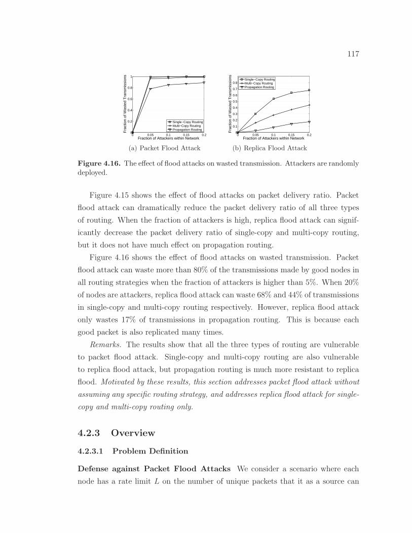
117
0 0.05 0.1 0.15 0.20
0.2
0.4
0.6
0.8
1
Fraction of Attackers within Network
Fra
ctio
n of
Was
ted
Tra
nsm
issi
ons
Single−Copy RoutingMulti−Copy RoutingPropagation Routing
(a) Packet Flood Attack
0 0.05 0.1 0.15 0.20
0.1
0.2
0.3
0.4
0.5
0.6
0.7
0.8
Fraction of Attackers within Network
Fra
ctio
n of
Was
ted
Tra
nsm
issi
ons
Single−Copy RoutingMulti−Copy RoutingPropagation Routing
(b) Replica Flood Attack
Figure 4.16. The effect of flood attacks on wasted transmission. Attackers are randomlydeployed.
Figure 4.15 shows the effect of flood attacks on packet delivery ratio. Packet
flood attack can dramatically reduce the packet delivery ratio of all three types
of routing. When the fraction of attackers is high, replica flood attack can signif-
icantly decrease the packet delivery ratio of single-copy and multi-copy routing,
but it does not have much effect on propagation routing.
Figure 4.16 shows the effect of flood attacks on wasted transmission. Packet
flood attack can waste more than 80% of the transmissions made by good nodes in
all routing strategies when the fraction of attackers is higher than 5%. When 20%
of nodes are attackers, replica flood attack can waste 68% and 44% of transmissions
in single-copy and multi-copy routing respectively. However, replica flood attack
only wastes 17% of transmissions in propagation routing. This is because each
good packet is also replicated many times.
Remarks. The results show that all the three types of routing are vulnerable
to packet flood attack. Single-copy and multi-copy routing are also vulnerable
to replica flood attack, but propagation routing is much more resistant to replica
flood. Motivated by these results, this section addresses packet flood attack without
assuming any specific routing strategy, and addresses replica flood attack for single-
copy and multi-copy routing only.
4.2.3 Overview
4.2.3.1 Problem Definition
Defense against Packet Flood Attacks We consider a scenario where each
node has a rate limit L on the number of unique packets that it as a source can

118
generate and send into the network within each time interval T . The time intervals
start from time 0, T , 2T , etc. The packets generated within the rate limit are
deemed legitimate, but the packets generated beyond the limit are deemed flooded
by this node. To defend against packet flood attacks, our goal is to detect if a node
as a source has generated and sent more unique packets into the network than its
rate limit L per time interval.
A node’s rate limit L does not depend on any specific routing protocol, but
it can be determined by a service contract between the node and the network
operator as discussed later. Different nodes can have different rate limits and their
rate limits can be dynamically adjusted.
The length of time interval should be set appropriately. If the interval is too
long, rate limiting may not be very effective against packet flood attacks. If the
interval is too short, the number of contacts that each node has during one interval
may be too nondeterministic and thus it is difficult to set an appropriate rate
limit. Generally speaking, the interval should be short under the condition that
most nodes can have a significant number of contacts with other nodes within
one interval, but the appropriate length depends on the contact patterns between
nodes in the specific deployment scenario.
Defense against Replica Flood Attacks As motivated in Chapter 4.2.2, the
defense against replica flood considers single-copy and multi-copy routing proto-
cols. These protocols require that, for each packet that a node buffers no matter
if this packet has been generated by the node or forwarded to it, there is a limit l
on the number of times that the node can forward this packet to other nodes. The
values of l may be different for different buffered packets. Our goal is to detect if
a node has violated the routing protocol and forwarded a packet more times than
its limit l for the packet.
A node’s limit l for a buffered packet is determined by the routing protocol. In
multi-copy routing, l = L′ (where L′ is a parameter of routing) if the node is the
source of the packet, and l = 1 if the node is an intermediate hop (i.e., it received
the packet from another node). In single-copy routing, l = 1 no matter if the node
is the source or an intermediate hop. Note that the two limits L and l do not
depend on each other.
We discuss how to defend against replica flood attacks for quota-based routing

119
S
A
m1,S, c
p=1, t=1
B
C
D
m2, S, cp=2, t=2
m3, S, cp=3, t=3m4, S, cp=3, t=4
E
m3, S, cp=3, t=3
S, H(m4
), cp=3,
t=4
packet meta data
Detection
attacker good node
(a) Packet flood (L = 3)
S
A
B
C
S, A, m,
ct=1, t=1
S, B, m, ct=2,t=2
S, C, m, ct=2, t=3 S,C,H(m), ct=2, t=3
Detection
(b) Replica flood by the source(l = 2)
R
A
B
R, A,m, ct=
1, t=1
R, B, m, ct=1, t=2
R, B, H(m),ct=1, t=2
Detection
(c) Replica flood by a relay(l = 1)
Figure 4.17. The basic idea of flood attack detection. cp and ct are packet count andtransmission count, respectively. The arrows mean the transmission of packet or metadata which happens when the two end nodes contact.
[130, 127, 131] in Chapter 4.2.4.9.
Setting the Rate Limit L One possible method is to set L in a request-approve
style. When a user joins the network, he requests for a rate limit from a trusted
authority which acts as the network operator. In the request, this user specifies
an appropriate value of L based on prediction of his traffic demand. If the trusted
authority approves this request, it issues a rate limit certificate to this user, which
can be used by the user to prove to other nodes the legitimacy of his rate limit.
To prevent users from requesting unreasonably large rate limits, a user pays an
appropriate amount of money or virtual currency (e.g., the credits that he earns
by forwarding data for other users [40]) for his rate limit. When a user predicts an
increase (decrease) of his demand, he can request for a higher (lower) rate limit.
The request and approval of rate limit may be done offline. The flexibility of rate
limit leaves legitimate users’ usage of the network unhindered. This process can be
similar to signing a contract between a smartphone user and a 3G service provider:
the user selects a data plan (e.g., 200MB/month) and pays for it; he can upgrade
or downgrade the plan when needed.
4.2.3.2 Models and Assumptions
Network Model In opportunistic mobile networks, since contact durations may
be short, a large data item is usually split into smaller packets (or fragments) to
facilitate data transfer. For simplicity, we assume that all packets have the same
predefined size. Although in opportunistic mobile networks the allowed delay of
packet delivery is usually long, it is still impractical to allow unlimited delays.

120
Thus, we assume that each packet has a lifetime. The packet becomes meaningless
after its lifetime ends and will be discarded.
We assume that every packet generated by nodes is unique. This can be im-
plemented by including the source node ID and a locally unique sequence number,
which is assigned by the source for this packet, in the packet header.
We also assume that time is loosely synchronized, such that any two nodes are
in the same time slot at any time. Since the inter-contact time in opportunistic
mobile networks is usually at the scale of minutes or hours, the time slot can be
at the scale of one minute. Such loose time synchronization is not hard to achieve.
Adversary Model There are a number of attackers in the network. An attacker
can flood packets and/or replicas. When flooding packets, the attacker acts as a
source node. It creates and injects more packets into the network than its rate
limit L. When flooding replicas, the attacker forwards its buffered packets (which
can be generated by itself or received from other nodes) more times than its limit
l for them. The attackers may be insiders with valid cryptographic keys. Some
attackers may collude and communicate via out-band channels.
Trust Model We assume that a public-key cryptography system is available. For
example, Identity-Based Cryptography (IBC) [132] has been shown to be practical
for opportunistic mobile networks [133]. In IBC, only an offline Key Generation
Center (KGC) is needed. KGC generates a private key for each node based on
the node’s id, and publishes a small set of public security parameters to the node.
Except the KGC, no party can generate the private key for a node id. With such
a system, an attacker cannot forge a node id and private key pair. Also, attackers
do not know the private key of a good node (not attacker).
Each node has a rate limit certificate obtained from a trusted authority. The
certificate includes the node’s ID, its approved rate limit L, the validation time of
this certificate and the trusted authority’s signature. The rate limit certificate can
be merged into the public key certificate or stand alone.
4.2.3.3 Basic Idea: Claim-Carry-and-Check
Packet Flood Detection To detect the attackers that violate their rate limit
L, we must count the number of unique packets that each node as a source has
generated and sent to the network in the current interval. However, since the node

121
may send its packets to any node it contacts at any time and place, no other node
can monitor all of its sending activities. To address this challenge, our idea is to
let the node itself count the number of unique packets that it, as a source, has
sent out, and claim the up-to-date packet count (together with a little auxiliary
information such as its ID and a timestamp) in each packet sent out. The node’s
rate limit certificate is also attached to the packet, such that other nodes receiving
the packet can learn its authorized rate limit L. If an attacker is flooding more
packets than its rate limit, it has to dishonestly claim a count smaller than the real
value in the flooded packet, since the real value is larger than its rate limit and
thus a clear indicator of attack. The claimed count must have been used before
by the attacker in another claim, which is guaranteed by the pigeonhole principle,
and these two claims are inconsistent. The nodes which have received packets from
the attacker carry the claims included in those packets when they move around.
When two of them contact, they check if there is any inconsistency between their
collected claims. The attacker is detected when an inconsistency is found.
Let us look at an example in Fig. 4.17(a). S is an attacker that successively
sends out four packets to A, B, C and D, respectively. Since L = 3, if S claims the
true count 4 in the fourth packet m4, this packet will be discarded by D. Thus, S
dishonestly claims the count to be 3, which has already been claimed in the third
packet m3. m3 (including the claim) is further forwarded to node E. When D
and E contact, they exchange the count claims included in m3 and m4, and check
that S has used the same count value in two different packets. Thus, they detect
that S as an attacker.
Replica Flood Detection Claim-carry-and-check can also be used to detect the
attacker that forwards a buffered packet more times than its limit l. Specifically,
when the source node of a packet or an intermediate hop transmits the packet to
its next hop, it claims a transmission count which means the number of times it
has transmitted this packet (including the current transmission). Based on if the
node is the source or an intermediate node and which routing protocol is used, the
next hop can know the node’s limit l for the packet, and ensure that the claimed
count is within the correct range [1, l]. Thus, if an attacker wants to transmit the
packet more than l times, it must claim a false count which has been used before.
Similarly as in packet flood attacks, the attacker can be detected. Examples are

122
given in Fig. 4.17(b) and 4.17(c).
4.2.4 Our Scheme
Our scheme uses two different cryptographic constructions to detect packet flood
and replica flood attacks independently. When our scheme is deployed to propa-
gation routing protocols, the detection of replica flood attacks is deactivated.
The detection of packet flood attacks works independently for each time inter-
val. Without loss of generality, we only consider one time interval when describing
our scheme. For convenience, we first describe our scheme assuming that all nodes
have the same rate limit L, and relax this assumption in Chapter 4.2.4.8. In the
following, we use SIGi(∗) to denote node i’s signature over the content in the
brackets.
4.2.4.1 Claim Construction
Two pieces of meta data are added to each packet (see Fig. 4.18), Packet Count
Claim (P-claim) and Transmission Count Claim (T-claim). P-claim and T-claim
are used to detect packet flood and replica flood attacks, respectively.
P-claim is added by the source and transmitted to later hops along with the
packet. T-claim is generated and processed hop-by-hop. Specifically, the source
generates a T-claim and appends it to the packet. When the first hop receives this
packet, it peels off the T-claim; when it forwards the packet out, it appends a new
T-claim to the packet. This process continues in later hops. Each hop keeps the
P-claim of the source and the T-claim of its previous hop to detect attacks.
P-claim When a source node S sends a new packet m (which has been generated
by S and not sent out before) to a contacted node, it generates a P-claim as follows:
P-claim: S, cp, t, H(m), SIGS(H(H(m)|S|cp|t)) (4.9)
Here, t is the current time. cp (cp ∈ [1, L]) is the packet count of S, which means
that this is the cthp new packet S has created and sent to the network in the current
time interval. S increases cp by one after sending m out.
The P-claim is attached to packet m as a header field, and will always be
forwarded along with the packet to later hops. When the contacted node receives

123
S A Bm P-claim
of ST-claimof S m P-claim
of ST-claimof A
A’s collected claims
B’s collected claims
Figure 4.18. The conceptual structure of a packet and the changes made at each hopof the forwarding path.
this packet, it verifies the signature in the P-claim, and checks the value of cp. If
cp is larger than L, it discards this packet; otherwise, it stores this packet and the
P-claim.
T-claim When node A transmits a packet m to node B, it appends a T-claim to
m. The T-claim includes A’s current transmission count ct for m (i.e., the number
of times it has transmitted m out) and the current time t. The T-claim is:
T-claim: A,B,H(m), ct, t, SIGA(H(A|B|H(m)|ct|t)) (4.10)
B checks if ct is in the correct range based on if A is the source of m. If ct has a
valid value, B stores this T-claim.
In single-copy and multi-copy routing, after forwarding m for enough times, A
deletes its own copy of m and will not forward m again.
4.2.4.2 Inconsistency Caused by Attack
In a dishonest P-claim, an attacker uses a smaller packet count than the real value.
(We do not consider the case where the attacker uses a larger packet count than
the real value, since it makes no sense for the attacker.) However, this packet
count must have been used in another P-claim generated earlier. This causes an
inconsistency called count reuse, which means the use of the same count in two
different P-claims generated by the same node. For example in Fig. 4.17(a) the
count value 3 is reused in the P-claims of packet m3 and m4. Similarly, count
reuse is also caused by dishonest T-claims.
4.2.4.3 Protocol
Suppose two nodes contact and they have a number of packets to forward to each
other. Then our protocol is sketched in Algorithm 8.

124
When a node forwards a packet, it attaches a T-claim to the packet. Since
many packets may be forwarded in a contact and it is expensive to sign each T-
claim separately, an efficient signature construction is proposed in Chapter 4.2.4.7.
The node also attaches a P-claim to the packets that are generated by itself and
have not been sent to other nodes before (called new packet in line 3, Algorithm 8).
When a node receives a packet, it gets the P-claim and T-claim included in the
packet. It checks them against the claims that it has already collected to detect
if there is any inconsistency (see Sec. 4.2.4.5). Only the P-claims generated in the
same time interval (which can be determined by the time tag) are cross-checked.
If no inconsistency is detected, this node stores the P-claim and T-claim locally
(see Sec. 4.2.4.4).
To better detect flood attacks, the two nodes also exchange a small number
of the recently collected P-claims and T-claims and check them for inconsistency.
This meta data exchange process is separately presented in Sec. 4.2.5.
When a node detects an attacker, it adds the attacker into a blacklist and will
not accept packets originated from or forwarded by the attacker. The node also
disseminates an alarm against the attacker to other nodes (see Sec. 4.2.4.6).
Algorithm 8 : The protocol run by each node in a contact1: Meta data (P-claim and T-claim) exchange and attack detection2: if Have packets to send then3: For each new packet, generate a P-claim;4: For all packets, generate their T-claims and sign them with a hash tree;5: Send every packet with the P-claim and T-claim attached;6: end if7: if Receive a packet then8: if Signature verification fails or the count value in its P-claim or T-claim is invalid then9: Discard this packet;10: end if11: Check the P-claim against those locally collected and generated in the same time interval
to detect inconsistency;12: Check the T-claim against those locally collected for inconsistency;13: if Inconsistency is detected then14: Tag the signer of the P-claim (T-claim, resp.) as an attacker and add it into a blacklist;15: Disseminate an alarm against the attacker to the network;16: else17: Store the new P-claim (T-claim, resp.);18: end if19: end if

125
4.2.4.4 Local Data Structures
Each node collects P-claims and T-claims from the packets that it has received
and stores them locally to detect flood attacks. Let us look at a received packet
m and the P-claim and T-claim included in this packet. Initially, this pair of P-
claim and T-claim are stored in full with all the components shown in Formula
4.9 and 4.10. When this node removes m from its buffer (e.g., after m is delivered
to the destination or dropped due to expiration), it compacts this pair of claims
to reduce the storage cost. If this pair of claims have been sampled for meta
data exchange, they will be stored in full until the exchange process ends and be
compacted afterward.
Compact P-claim Storage Suppose node W stores a P-claim
CP = {S, cp, t, H(m), SIGS}. It compacts the P-claim as follows. Using the times-
tamp t, W gets the index i of the time interval that t belongs to. The signature is
discarded since it has been verified. The compacted P-claim is:
S, i, cp, H8 (4.11)
where H8 is a 8-bit string called hash remainder. It is obtained by concatenating 8
random bits of the packet hash H(m). The indices of these 8 bits in the hash are
determined by 8 locators. The locators are randomly and independently generated
by W for S at the beginning of the ith interval, and are shared by all the P-claims
issued by S in the ith interval. Each locator only has log2 h bits where h denotes
the size of a hash (e.g., 256 for SHA-256). W keeps these locators secret.
Suppose node W has collected n P-claims generated by S in interval i. For all
these claims, only one source node ID and interval index is stored. Also, instead of
directly storing the packet count values cp included in these P-claims, the compact
structure uses a L-bit long bit vector to store them. If value c appears in these
P-claims, the cth bit of the vector is set. Let CiS denote the compact structure of
these P-claims. Then:
CiS = S, i, bit-vector, locators, [H81 , H82, ..., H8n ] (4.12)
Compact T-claim Storage Suppose node W stores a T-claim

126
CT = {R,W,H(m), ct, t, SIGR} issued by node R. The signature is discarded since
it has been verified. W does not need to store its own ID and t is not useful for
inconsistency check. Then the compacted T-claim is:
R, ct, H32 (4.13)
where H32 is a 32-bit hash remainder defined similarly as H8. Suppose W has
collected n T-claims generated by R. Then the compact structure of these T-
claims is:
CR = R, locators, [H321 , ct1 ], ..., [H32n , ctn ] (4.14)
The locators are randomly and independently generated by W for R, and are
shared by all the T-claims issued by R.
4.2.4.5 Inconsistency Check
Suppose node W wants to check a pair of P-claim and T-claim against its local
collections to detect if there is any inconsistency. The inconsistency check against
full claims is trivial: W simply compares the pair of claims with those collected. In
the following, we describe the inconsistency check against compactly stored claims.
Inconsistency Check with P-claim From the P-claim node W gets: the source
node ID S, packet count cp, timestamp t and packet hash H . To check inconsis-
tency, W first uses S and t to map the P-claim to the structure CiS (see Eq. 4.12).
Then it reconstructs the hash remainder of H using the locators in CiS. If the bit
indexed by the packet count cp is set in the bit-vector but the hash remainder is
not included in CiS , count reuse is detected and S is an attacker.
The inconsistency check based on compact P-claims does not cause false posi-
tive, since a good node never reuses any count value in different packets generated
in the same interval. The inconsistency check may cause false negative if the two
inconsistent P-claims have the same hash remainder. However, since the attacker
does not know which bits constitute the hash remainder, the probability of false
negative is only 2−8. Thus, it has minimal effect on the overall detection probabil-
ity.

127
Inconsistency Check with T-claim From the T-claim node W gets: the sender
ID R, receiver ID Q and transmission count ct. If Q is W itself (which is possible
if the T-claim has been sent out by W but returned by an attacker), W takes no
action. Otherwise, it uses R to map the T-claim to the structure CR (see Eq. 4.14).
If there is a 2-tuple [H ′32, c
′t] in CR that satisfies 1) H ′
32 is the same as the remainder
of H , and 2) c′t = ct, then the issuer of the T-claim (i.e., R) is an attacker.
The inconsistency check based on compact T-claims does not cause extra false
negative. False positive is possible but it can be kept low as follows. Node W
may falsely detect a good node R as an attacker if it has received two T-claims
generated by R that satisfy two conditions: (i) they are generated for two different
packets, and (ii) they have the same hash remainder. For 32-bit hash remainder,
the probability that each pair of T-claims lead to false detection is 2−32. In most
cases, we expect that the number of T-claims generated by R and received by W
is not large due to the opportunistic contacts, and thus the probability of false
detection is low. As W receives more T-claims generated by R, it can use a longer
(e.g., 64-bit) hash remainder for R to keep the probability of false detection low.
Moreover, such false detection is limited to W only, since W cannot convince other
nodes to accept the detection with compact T-claim.
4.2.4.6 Alarm
Suppose in a contact a node receives a claim Cr from a forwarded data packet or
from the meta data exchange process (see Sec. 4.2.5.3) and it detects inconsistency
between Cr and a local claim Cl that the node has collected. Cr is a full claim
as shown in Formula 4.9 (or 4.10), but Cl may be stored as a full claim or just a
compact structure shown in Formula 4.11 (or 4.13).
If Cl is a full claim, the node can broadcast (via Epidemic routing [134]) a
global alarm to all the other nodes to speed up the attacker detection process. The
alarm includes the two full claims Cl and Cr. When a node receives an alarm, it
verifies the inconsistency between the two included claims and their signatures. If
the verification succeeds, it adds the attacker into its blacklist and broadcasts the
alarm further; otherwise, it discards the alarm. The node also discards the alarm
if it has broadcast another alarm against the same attacker.
If the detecting node stores Cl as a compact structure, it cannot convince other

128
nodes to trust the detection since the compact structure does not have the at-
tacker’s signature. Thus it cannot broadcast a global alarm. However, since the
attacker may have reused the count value of Cr to other claims besides Cl, the
detecting node can disseminate a local alarm that only contains Cr to its contact-
ed nodes who have received those claims. These contacted nodes can verify the
inconsistency between Cr and their collected claims, and also detect the attacker.
If any of these nodes still stores a full claim inconsistent with Cr, it can broadcast a
global alarm as done in the previous case; otherwise, it disseminates a local alarm.
As this iterative process proceeds, the attacker can be quickly detected by many
nodes. Each node only disseminates one local alarm for each detected attacker.
A local alarm and a global alarm against the same attacker may be disseminated
in parallel. If a node receives the global alarm first and then receives the local
alarm, it discards the local alarm. If it receives the local alarm first, when it
receives the global alarm later, it discards the local alarm and keeps the global
alarm.
An attacker may falsify an alarm against a good node. However, since it does
not have the node’s private key (as our assumption), it cannot forge the node’s
signatures for the claims included in the alarm. Thus, the alarm will be discarded
by other nodes and this attack fails.
4.2.4.7 Efficient T-claim Authentication
The T-claims of all the packets transmitted in a contact should be signed by
the transmitting node. Since the contact may end at any unpredictable time,
each received T-claim must be individually authenticated. A naive approach is
to protect each T-claim with a separate public-key signature, but it has high
computation cost in signature operations.
Our scheme uses Merkle hash tree [54] to amortize the computation cost of
public-key based signature on all the T-claims that the node sends out in a contact.
Specifically, after a node generates the T-claims (without signature) for all the
packets it want to send, it constructs a hash tree upon these partial T-claims, and
signs the root of the tree with a public-key based signature. Then the signature of a
T-claim includes this root signature and a few elements of the tree. Fig. 4.19 shows
the hash tree constructed upon eight T-claims and the tree elements included in

129
H12
TC1
H14
H34
TC2 TC3 TC4 TC5 TC6 TC7 TC8
H1 H2 H3 H4 H5 H6 H7 H8
H18
H56
H58
H78
hash
SIG
Figure 4.19. The Merkle hash tree constructed upon eight T-claims TC1,...,TC8. Inthe tree, Hi is the hash of TCi, and an inner node is the hash of its child nodes. Thesignature of TC1 includes H2, H34, H58 and SIG.
the signature of the first T-claim. We refer to the original paper [54] for details. In
this way, for all the T-claims sent by the sender in a contact, only one public-key
based signature is generated by the sender and verified by the receiver.
4.2.4.8 Dealing with Different Rate Limits
Previously we have assumed that all nodes have the same rate limit L. When
nodes have different rate limits, for our detection scheme to work properly, each
intermediate node that receives a packet needs to know the rate limit L of the
source of the packet, such that it can check if the packet count is in the correct
range 1, 2, ..., L. To do so, when a source node sends out a packet, it attaches its
rate limit certificate to the packet. The intermediate nodes receiving this packet
can learn the node’s authorized rate limit from the attached certificate.
4.2.4.9 Replica Flood Attacks in Quota-based Protocols
Our scheme to detect replica flood attacks can also be adapted to quota-based
routing protocols [130, 127, 131].
Quota-based routing works as follows. Each node has a quota for each packet
that it buffers, and the quota specifies the number of replicas into which the current
packet is allowed to be split. When a source node creates a packet, its quota for the
packet is L′ replicas, where L′ is a system parameter. When the source contacts a
relay node, it can split multiple replicas to the relay according to the quality of the
relay. After the split, the relay’s quota for the packet is the number of replicas split
to it, and the source node’s quota is reduced by the same amount. This procedure
continues recursively, and each node carrying the packet can split out a number of

130
replicas less than its current quota for the packet. It can be seen that each packet
can simultaneously have at most L′ replicas in the network.
In quota-based routing, replica flood attacks (where an attacker sends out more
replicas of a packet than its quota) can be detected by our approach as follows.
First, we observe that quota-based routing (with the total quota determined
at the source) can be emulated by single-copy routing if different replicas of the
same packet appear different to intermediate nodes and each replica is forwarded
in a similar way as single-copy routing. A node can split multiple replicas of a
packet to another node, but it can only send each replica out once. For instance,
if a node has forwarded Replica 1 to one relay, it must remove Replica 1 from its
local buffer, and it cannot forward this replica again to another relay.
To differentiate replicas, the source assigns a unique index to each replica as a
header field, and signs the replica to prevent intermediate nodes from modifying the
index. The index value should be in range [1, L′], and replicas with invalid index
will be discarded. In this way, a node’s local quota for a packet is represented
by the number of replicas (with different indices) that it buffers. Note that an
intermediate node cannot increase its quota by forging replicas since it does not
have the source node’s key to generate a valid signature.
To prevent a node from abusing its quota, we need to ensure that the node only
forwards each replica once. T-claim can be used to achieve this goal. Particularly,
when a node splits multiple replicas of a packet to another node, it generates a T-
claim for each replica. The inconsistency check (see Chapter IV.E) can be applied
here to detect the attackers that transmit the same replica more than once.
4.2.5 Meta Data Exchange
When two nodes contact they exchange their collected P-claims and T-claims to
detect flood attacks. If all claims are exchanged, the communication cost will be
too high. Thus, our scheme uses sampling techniques to keep the communication
cost low. To increase the probability of attack detection, one node also stores a
small portion of claims exchanged from its contacted node, and exchanges them
to its own future contacts. This is called redirection.

131
S
A
S, m1, cp=
1
B
S, m2, cp=1
C
E
D
S, H(m2), cp=1
S, H(m1),
cp=1
S, H(m1), cp=1
S, H(m1),cp=1
Detection
Detection
Contacted nodeset of B
Contacted nodeset of A
packet
exchanged claims
redirected claims
Figure 4.20. The idea of redirection which is used to mitigate the stealthy attack.
4.2.5.1 Sampling
Since P-claims and T-claims are sampled together (i.e., when a P-claim is sampled
the T-claim of the same packet is also sampled), in the following we only consider
P-claims.
A node may receive a number of packets (each with a P-claim) in a contact. It
randomly samples Z (a system parameter) of the received P-claims, and exchanges
the sampled P-claims to the next K (a system parameter) different nodes it will
contact, excluding the sources of the P-claims and the previous hop from which
these P-claims are received.
However, a vulnerability to tailgating attack should be addressed. In tailgating
attack, one or more attackers tailgate a good node to create a large number (say, d)
of frequent contacts with this node, and send Z packets (not necessarily generated
by the attackers) to it in each contact. If this good node sends the Zd P-claims
of these contacts to the next K good nodes it contacts, much effective bandwidth
between these good nodes will be wasted, especially in a large network where K is
not small.
To address this attack, the node uses an inter-contact sampling technique to
determine which P-claims sampled in historical contacts should be exchanged in the
current contact. Let SK denote a set of contacts. This set includes the minimum
number of most recent contacts between this node and at least K other different
nodes. Within this set, all the contacts with the same node are taken as one single
contact and a total of Z P-claims are sampled out of these contacts. This technique
is not vulnerable to the tailgating attack since the number of claims exchanged in
each contact is bounded by a constant.

132
4.2.5.2 Redirection
There is a stealthy attack to flood attack detection. For replica flood attacks, the
condition of detection is that at least two nodes carrying inconsistent T-claims
can contact. However, suppose the attacker knows that two nodes A and B never
contact. Then, it can send some packets to A, and invalidly replicate these packets
to B. In this scenario, this attacker cannot be detected since A and B never
contact. Similarly, the stealthy attack is also harmful for some routing protocols
like Spray-and-Wait [127] in which each packet is forwarded from the source to a
relay and then directly delivered from the relay to the destination.
To address the stealthy attack, our idea is to add one level of indirection. A
node redirects the Z P-claims and T-claims sampled in the current contact to one
of the next K nodes it will contact, and this contacted node will exchange (but
not redirect again) these redirected claims in its own subsequent contacts. Look at
the example in Fig. 4.20. Suppose attacker S sends mutually inconsistent packets
to two nodes A and B which will never contact. Suppose A and B redirect their
sampled P-claims to node C and D, respectively. Then so long as C and B or D
and A or C and D can contact, the attack has a chance to be detected. Thus, the
successful chance of stealthy attack is significantly reduced.
4.2.5.3 The Exchange Process
Each node maintains two separate sets of P-claims (T-claims, resp. in the follow-
ing) for meta data exchange, a sampled set which includes the P-claims sampled
from the most recent contacts with K different nodes (i.e., SK in Chapter 4.2.5.1),
and a redirected set which includes the P-claims redirected from those contacts.
Both sets include Z P-claims obtained in each of those contacts.
When two nodes A and B contact, they first select KZ P-claims from each
set with the inter-contact sampling technique (see Sec. 4.2.5.1), and then send
these P-claims to each other. When A receives a P-claim, it checks if this P-claim
is inconsistent with any of its collected P-claims using the method described in
Sec 4.2.4.5. If the received P-claim is inconsistent with a locally collected one and
the signature of the received P-claim is valid, A detects that the issuer (or signer)
of the received P-claim is an attacker.

133
S
A
Flooded &
normal pkt.
B
Flooded &normal pkt.
C
DRedirected claims
Redirected claims
(a) Considered basic attack
A
C
B
D
time
detection window
(b) Lower bound scenario
A
C
B
D
time
detection window and its ith contact
1 2 K
1 2 K
2 3 K1
i
1 2 K
(c) Upper bound scenario.
Figure 4.21. (a) The basic attack considered for detection probability analysis. At-tacker S floods packets to A and then to B. (b) The scenario when the lower bounddetection probability can be obtained. (c) The scenario when the upper bound detectionprobability can be obtained.
Out of all the P-claims received from B, A randomly selects Z of the P-claims
from the sampled set of B, and stores them to A’s redirected set. All other P-claims
received from B are discarded after inconsistency check.
4.2.5.4 Meta Data Deletion
A node stores the P-claims and T-claims collected from received data packets
for a certain time denoted by τ and deletes them afterward. It deletes the claims
redirected from other nodes immediately after it has exchanged them toK different
nodes.
4.2.6 Analysis
This section presents rigorous analysis over the security and cost of our scheme,
and discusses the optimal parameter to maximize the effectiveness of flood attack
detection under a certain amount of exchanged meta data per contact.
4.2.6.1 Detection Probability
The following analysis assumes uniform and independent contacts between nodes,
i.e., at any time each node’s next contacted node can be any other node with the
same probability. This assumption holds for mobility models such as RandomWay-
point where the contacts between all node pairs can be modeled as i.i.d. Poisson
processes [135]. When analyzing the detection probability, we assume that each
attacker acts alone. The case of collusion is analyzed separately in Chapter 4.2.6.4.

134
Table 4.3. Variables used in the analysisSi The K nodes that node i (i ∈ {A,B,C,D}) exchanges its
sampled or redirected claims to.ei A boolean event which means if node i (i ∈ {A,B}) has sampled
at least one flooded packet (ei = TRUE) or not (ei = FALSE)eAB A boolean event which means if node A and B have sampled at
least one pair of inconsistent packets (eAB = TRUE) or notPs The probability that event eA = TRUE (or eB = TRUE, resp.)Povp The conditional probability that if eA = eB = TRUE then
eAB = TRUE.Pd The probability that S is detected.P ld The lower-bound of Pd.
Pud The upper-bound of Pd.N The number of nodes in the network.M The number of attackers in the network.r The proportion of good nodes, i.e., r = N−M
N .K The number of nodes that a claim is exchanged to. K � N .a The number of flooded packets sent to A and B.n The total number of packets sent to A and B.y The proportion of flooded packets sent to A and B, i.e., y = a
n .
The Basic Attack First we consider a basic attack (see Fig. 4.21(a)) in which
an attacker S floods two sets of mutually inconsistent packets to two good nodes
A and B, respectively. Each flooded packet received by A is inconsistent with
one of the flooded packets received by B. In the contacts with A and B, S also
forwards some normal, not flooded, packets to A and B to make the attack harder
to detect. Let y denote the proportion of flooded packets among those sent by
S. For simplicity, we assume y is the same in both contacts. Suppose A and B
redirect the claims sampled in the contact with S to C and D, respectively.
To consider the worst-case performance, suppose the flooded packets are not
forwarded fromA and B to other nodes (which is the case in Spray-and-Wait [127]),
i.e., only A and B have the inconsistent claims. Note that the analysis also applies
to the detection of replica flood attacks.
For convenience, we define node A’s (or B’s) detection window as from the time
it receives the flooded packets to the time it exchanges the sampled claims to K
nodes, and node C’s (or D’s) detection window as from the time it receives the
redirected claims to the time it exchanges them to K nodes. The attacker has a
chance to be detected if node pairs 〈A,B〉, 〈A,D〉, 〈C,B〉 and 〈C,D〉 can contact
within their detection windows. Table 4.3 shows the variables used in the analysis.
Lower Bound The lower bound of detection probability is obtained in the

135
following scenario (see Fig. 4.21(b)): When B receives the packets from S, both
A and C have finished their detection window. Due to the effect of sampling, the
attacker can be detected 1) by A if A ∈ SB and eB = TRUE; or 2) by A if D is
a good node, A ∈ SD and eB = TRUE; or 3) by C if C is a good node, C ∈ SBand eAB = TRUE; or 4) by C if both C and D are good nodes, C ∈ SD and
eAB = TRUE.
Since each of A and B exchanges the sampled claims to K nodes other than
itself, and C (D) exchanges the redirected claims to K nodes other than A (B),
according to the uniform contact assumption, we have:
Pd =Ps[1− (1− K
N − 1) · (1− r
K
N − 2)·
(1− rK
N − 1PsPovp) · (1− r2
K
N − 2PsPovp)]
(4.15)
The expected number of flooded packets that A or B can sample is yZ. Since
Z is typically small while a is not that small (which we believe realistic), Povp is
negligible. Considering that K � N , Pd is approximated as follows:
Pd ≈ Ps[1− (1− K
N − 1)(1− r
K
N − 2)] ≈ Ps
1 + r
NK
Since random sampling is used, it is trivial to get:
Ps =1− n− a
n
n− a− 1
n− 1· · · n− a− Z + 1
n− Z + 1
≥ 1− (1− a/n)Z = 1− (1− y)Z
Thus, we have Pd ≥ K 1+rN
(1 − (1 − y)Z), and a lower bound of the detection
probability is:
P ld = K
1 + r
N(1− (1− y)Z) (4.16)
Upper Bound The upper bound of detection probability is obtained in the
following scenario (see Fig. 4.21(c)): D receives the redirected claims from B not
later than the time C receives the redirected claims from A, and they are the first
node that A and B encounter after the contact with S. Besides the four cases that
we discussed when deriving the lower bound, the attacker can also be detected 1)

136
by B if B ∈ SA and eA = TRUE; or 2) by B if C is a good node, B ∈ SC and
eA = TRUE; or 3) by D if D is a good node, D ∈ SA and eAB = TRUE; or 4) by
D if both C and D are good nodes, D ∈ SC and eAB = TRUE.
Similarly as in the lower bound case, we can obtain that the detection proba-
bility is Pd ≈ 2K 1+rN
Ps. Since Ps ≤ 1, an upper bound of the detection probability
is:
P ud =
2K(1 + r)
N(4.17)
Stronger Attacks We use the number of times that a count value is reused to
represent the strength of an attack. Intuitively, if each count value is used many
times, the attacker floods a lot of packets or replicas. Let X denote the number of
times a count value is reused. We want to derive the relation between X and the
probability that the attacker will be detected.
The stronger attacks we consider extends the basic attack as follows. Suppose
the attacker has sent a set of packets to a good node G0, and then it successively
sends the same number of packets (reusing the count values of the packets sent to
G0) to X good nodes G1, ..., GX . All other parameters in the basic analysis apply
here. From a global point of view, a total of X(X+1)2
node pairs have inconsistent
packets, and each pair can detect the attacker independently as in the basic attack.
Then the attacker will be detected by at least one node pair with a probability:
PXd = 1− (1− Pd)
X(X+1)2 (4.18)
We can see that the stronger the attack is, the more likely the attacker will be
detected.
4.2.6.2 Cost
Communication The communication cost mainly has two parts. One part is
the P-claim and T-claim transmitted with each packet, and the other part is the
partial claims transmitted during meta data exchange. As to the latter, at most
4ZK P-claims and 4ZK T-claims are exchanged in each contact, with one half for
sampled and the other half for redirected claims.
Computation As to signature generation, a node generates one signature for
each newly generated packet. It also generates one signature for all its T-claims as

137
a whole sent in a contact. As to signature verification, a node verifies the signature
of each received packet. It also verifies one signature for all the T-claims as a whole
received in one contact.
Storage Most P-claims and T-claims are compacted when the packets are
forwarded. The Z sampled P-claims and T-claims are stored in full until the
packets are forwarded or have been exchanged to K nodes, whichever is later, and
then compacted. For each received packet, less than 20 bytes of compact claims
are stored for time duration τ .
4.2.6.3 Parameter Selection
We study the following question: If we fix the communication cost of meta da-
ta exchange (note that little can be done with the transmission of claims within
packets), then how should we set parameter K and Z to maximize the detection
probability? Note that the communication cost of meta data exchange is propor-
tional to ZK. As to detection probability, we consider the lower-bound detection
probability for the basic attack which can be written as Pd = cK(1− (1− y)Z).
Lemma 5. If the communication cost of meta data exchange is fixed at ZK = C,
then Pd is maximized at K = C and Z = 1.
Proof. Pd can be rewritten as Pd = cC 1−(1−y)Z
Z. The derivative of Pd over Z is:
P ′d(Z) =
cC
Z2[(1− y)Z(1− ln (1− y)Z)− 1] (4.19)
Let u = (1 − y)Z (0 < u ≤ 1), then P ′d(Z) = cC
Z2 (u − u lnu − 1). Let g(u) =
u−u ln u−1. Then g′(u) = − ln u ≥ 0, which means g(u) monotonically increases.
Since g(1) = 0, g(u) ≤ 0 when 0 < u ≤ 1. Therefore, P ′d(Z) ≤ 0, which means
Pd monotonically decreases with Z. Thus, to maximize Pd, Z should be set the
minimum value 1.
Remarks In this parameter setting, the lower-bound detection probability can
be written as Pd = yK 1+rN
. Suppose the attacker launches attacks independently.
Then it can be detected after NyK(1+r)
attacks. If the attacker wants to stay unde-
tected for a longer time, it should maintain a smaller y, which means the attack
effect is weaker; if it wants to make a big attack impact, it should maintain a high

138
y, but this means it will be detected in a shorter time. From another point of
view, since the attacker only uses y proportion its capacity for flood attack, it is
equivalent that the attacker can attack at full capacity for only NK(1+r)
contacts.
Thus, the attacks can be effectively mitigated.
4.2.6.4 Collusion
Packet Flood Attack One attacker may send a packet with a dishonest packet
count to its colluder, which will forward the packet to the network. Certainly,
the colluder will not exchange the dishonest P-claim with its contacted nodes.
However, so long as the colluder forwards this packet to a good node, this good
node has a chance to detect the dishonest claim as well as the attacker. Thus, the
detection probability is not affected by this type of collusion.
Replica Flood AttackWhen attackers collude, they can inject invalid replicas
of a packet without being detected, but the number of flooded replicas is effectively
limited in our scheme. More specifically, in our scheme for a unique packet all the
M colluders as a whole can flood a total of M − 1 invalid replicas without being
detected. To the contrast, when there is no defense, a total of N − M invalid
replicas can be injected by the colluders for each unique packet. Since the number
of colluders is not very large, our scheme can still effectively mitigate the replica
flood attack. This will be further evaluated in Sec. 4.2.7.
4.2.7 Performance Evaluations
4.2.7.1 Experiment Setup
To evaluate the performance and cost of our scheme, we run simulations on a
synthetic trace generated by the Random Waypoint (RWP) [135] mobility model
and on the MIT Reality trace [108] collected from the real world.
In our synthetic trace, 97 nodes move in a 500 × 500 square area with the
RWP model. The moving speed is randomly selected from [1, 1.6] to simulate the
speed of walking, and the transmission range of each node is 10 to simulate that
of Bluetooth. Each simulation lasts 5× 10⁵ time units.
The Reality trace has been shown [136, 37] to have social community struc-
tures. 97 smartphones are carried by students and staff at MIT over 10 months.

139
These phones run Bluetooth device discovery every five minutes and log about 110
thousand contacts. Each contact includes the two contact parties, the start time
and duration of the contact.
In the simulations, 20% of nodes are deployed as attackers. They are randomly
deployed or selectively deployed to high-connectivity nodes. The buffer size of each
node is 5MB, the Drop Tail policy is used when buffer overflows. The bandwidth
is 2Mbps. Each node generates packets of 10KB with random destinations at a
uniform rate. Parameter Z = 1.
4.2.7.2 Routing Algorithms and Metrics
We use the following routing protocols in evaluations:
• Forward A single-copy routing protocol where a packet is forwarded to a
relay if the relay has more frequent contacts with the destination.
• SimBet [35] A single-copy routing protocol where a packet is forwarded to
a relay if the relay has a higher simbet metric, which is calculated from two
social measures (similarity and betweenness).
• Spray-and-Wait [127] A multi-copy protocol, where the source replicates
a packet to L′ = 3 relays and each relay directly delivers its copy to the
destination when they contact.
• Spray-and-Focus [127] It is similar to Spray-and-Wait, but each packet
copy is individually routed to the destination with Forward.
• Propagation A packet is replicated to a relay if the relay has more frequent
contacts with the destination.
We use the following performance evaluation metrics:
• Detection rate The proportion of attackers that are detected out of all the
attackers.
• Detection delay From the time the first invalid packet is sent to the time
the attacker is detected.

140
• Computation cost The average number of signature generations and ver-
ifications per contact.
• Communication cost The number of P-claim/T-claim pairs transmitted
into the air, normalized by the number of packets transmitted.
• Storage cost The time-averaged kilobytes stored for P-claims and T-claims
per node.
4.2.7.3 Analysis Verification
We use the synthetic trace to verify our analysis results given in Chapter 4.2.6,
since in this trace the contacts between node pairs are i.i.d. [135] which conforms
to our assumption for the analysis. We divide the trace into 10 segments, each with
5× 10⁴ time units, and run simulations on each of the 3rd − 7th segments 3 times
with different random seeds. Each data point is averaged over the individual runs.
Spray-and-Wait is used as the routing protocol to consider the worst case of packet
flood detection (see Sec. 4.2.6.1). Here we only verify the detection probability
for the basic attack, since the detection probability for the strong attack can be
derived from it in a straightforward way. In this group of simulations, each attacker
launches the basic attack once. It sends out two sets of packets to two good nodes
with 10 packets in each set (i.e., n = 10), and these two sets contain mutually
inconsistent packets. We first fix parameter y = 1.0 (see Table 4.3) but change
parameter K from 0 to 10, and then we fix parameter K = 10 but change y from
0 to 1.0. The results are shown in Fig. 4.22(a) and 4.22(b), respectively. It can be
seen that the simulation results are between the analytical lower bound and upper
bound, which verifies the correctness of our analysis.
4.2.7.4 Detection Rate
The Reality trace is used. We divide the trace into segments of one month, and run
simulations on each of the 3rd− 7th segments 3 times with different random seeds.
Each data point is averaged over the individual runs. By default, each attacker
launches the basic attack once, and it floods one packet out (i.e., n = 1, y = 1.0).
By default, attackers are selectively deployed to high-connectivity nodes.
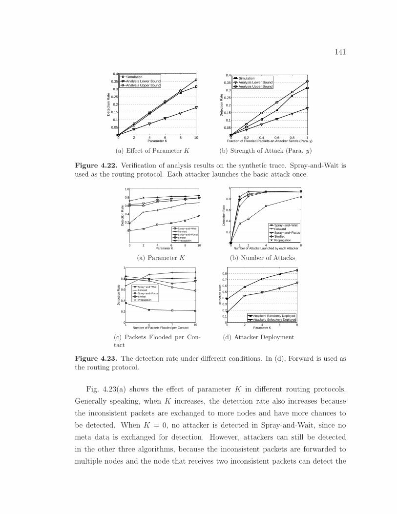
141
0 2 4 6 8 100
0.05
0.1
0.15
0.2
0.25
0.3
0.35
0.4
Parameter K
Det
ectio
n R
ate
SimulationAnalysis Lower BoundAnalysis Upper Bound
(a) Effect of Parameter K
0 0.2 0.4 0.6 0.8 10
0.05
0.1
0.15
0.2
0.25
0.3
0.35
0.4
Fraction of Flooded Packets an Attacker Sends (Para. y)
Det
ectio
n R
ate
SimulationAnalysis Lower BoundAnalysis Upper Bound
(b) Strength of Attack (Para. y)
Figure 4.22. Verification of analysis results on the synthetic trace. Spray-and-Wait isused as the routing protocol. Each attacker launches the basic attack once.
0 2 4 6 8 10
0
0.2
0.4
0.6
0.8
1.0
Parameter K
Det
ectio
n R
ate
Spray−and−WaitForwardSpray−and−FocusSimBetPropagation
(a) Parameter K
0 1 2 4 80
0.2
0.4
0.6
0.8
1
Number of Attacks Launched by each Attacker
Det
ectio
n R
ate
Spray−and−WaitForwardSpray−and−FocusSimBetPropagation
(b) Number of Attacks
1 4 7 100
0.2
0.4
0.6
0.8
1
Number of Packets Flooded per Contact
Det
ectio
n R
ate
Spray−and−WaitForwardSpray−and−FocusSimBetPropagation
(c) Packets Flooded per Con-tact
0 2 4 6 80
0.1
0.2
0.3
0.4
0.5
0.6
0.7
0.8
Parameter K
Det
ectio
n R
ate
Attackers Randomly DeployedAttackers Selectively Deployed
(d) Attacker Deployment
Figure 4.23. The detection rate under different conditions. In (d), Forward is used asthe routing protocol.
Fig. 4.23(a) shows the effect of parameter K in different routing protocols.
Generally speaking, when K increases, the detection rate also increases because
the inconsistent packets are exchanged to more nodes and have more chances to
be detected. When K = 0, no attacker is detected in Spray-and-Wait, since no
meta data is exchanged for detection. However, attackers can still be detected
in the other three algorithms, because the inconsistent packets are forwarded to
multiple nodes and the node that receives two inconsistent packets can detect the

142
attacker. Among these protocols, Propagation achieves the highest detection rate
since it replicates inconsistent packets the most number of times. Between the two
single-copy routing protocols, SimBet has a higher detection rate than Forward.
This is because SimBet tends to forward packets to the more socially connected
nodes and thus these nodes are more likely to collect inconsistent packets.
Fig. 4.23(b) shows the results when each attacker launches the basic attack
independently for a varying number of times. As the attackers launch more attacks,
the detection rate quickly increases for obvious reasons.
Fig. 4.23(c) shows the effect of the number of packets that an attacker floods
in each contact (i.e., parameter n). As an attacker floods more packets in each
contact, the detection rate decreases in Spray-and-Wait and SimBet, increases in
Forward and does not change much in Spray-and-focus and Propagation. The
opposite trends are due to two factors that affect the detection rate reversely. On
the one hand, sampling decreases detection rate. To explain this more clearly,
let us look at the basic attack scenario in Fig. 4.21(a) for Spray-and-Wait. Since
Z = 1, A (B, resp.) only samples one packet out of all the packets received from
the attacker and redirects it to C (D, resp.). When n = 1, C and D will receive
mutually inconsistent claims, which means in Equation 4.15 Povp = 1.0. However,
when n is larger than 1, C and D may not receive a pair of inconsistent claims
due to the independent sampling by A and B. As n increases, Povp decreases
and thus the detection rate also decreases. On the other hand, for the routing
protocols where each packet is forwarded in multiple hops, when an attacker sends
more attack packets in each contact, it is more likely that one pair of inconsistent
packets are forwarded to the same intermediate node and lead to detection.
Fig. 4.23(d) shows the effect of attacker deployment. The detection rate is lower
when attackers are selectively deployed to high-connectivity nodes. This is because
when attackers are selectively deployed they have more contacts with good nodes.
The probability that a good node exchanges its sampled claims to attackers rather
than to other good nodes is higher, but attackers do not run detection against each
other.

143
0 10 20 30 40 50 60 70 800
0.1
0.2
0.3
0.4
0.5
0.6
0.7
0.8
0.9
1
Day
Cum
ulat
ive
Dis
trib
utio
n F
unct
ion
(CD
F)
Detection DelayRouting Delay
Figure 4.24. The detection delay compared with the routing delay of Propagation.
4.2.7.5 Detection delay
Fig. 4.24 shows the CDF of detection delay when Propagation is used as the routing
protocol on the Reality trace. For comparison, the CDF of routing delay (i.e., from
the time a packet is generated to the time it is delivered) is also plotted. Here, no
lifetime is set for packets. It can be seen that 90% of the attacks can be detected
by our scheme within 10 days. On the contrary, within 10 days only 60% of data
packets can be delivered by the routing protocol. Hence, the detection delay of
our scheme is much lower than the routing delay.
4.2.7.6 Flooded Replicas under Collusion
As mentioned in Sec. 4.2.6.4, colluders can flood a small number of replicas without
being detected. To evaluate their effect, we run simulations on the Reality trace
when all attackers collude. The simulation settings are the same as in Chapter
4.2.2. We compare our scheme with the case of no defense. As shown in Fig. 4.25,
even when 20% of nodes are attackers and collude, our scheme can still limit the
percentage of wasted transmissions to 14% in single-copy routing (SimBet) and
6% in multi-copy routing (Spray-and-Focus), which is only 1/7-1/5 of the wasted
transmissions when there is no defense.
4.2.7.7 Cost
To evaluate the cost of our scheme in a steady state (i.e., all attackers have been
detected), no attackers are deployed in this group of simulations. The Reality
trace is used. Packets are generated between the 61st and 120th day of the trace,
and statistics are collected from the 91th day. By default, each node generates 2

144
0 0.05 0.1 0.15 0.20
0.1
0.2
0.3
0.4
0.5
0.6
0.7
0.8
Fraction of Attackers within Network
Fra
ctio
n of
Was
ted
Tra
nsm
issi
ons
SimBet UnsecuredSpray−and−Focus UnsecuredSimBet SecuredSpray−and−Focus Secured
Figure 4.25. The effect of undetected replicas on wasted transmissions when attackerscollude to launch replica flood attacks.
packets per day, parameter τ (i.e., the time a claim is stored) is 30 days and K
is 10. In a contact, a node may receive some packets but then immediately drop
them due to buffer overflow. In such cases, the transmission of the claims attached
to these packets is counted into the communication overhead, and the signature
generations for these claims are counted into the computation overhead. Since the
receiver does not buffer these packets, it does not store these claims or verify their
signatures.
We first evaluate the computation cost of our scheme, and Fig. 4.26 shows the
results. When Forward is used as the routing protocol (see Fig. 4.26(a)), as the
packet generation rate increases, the computation cost also increases since more
packets need to be signed and verified. But the cost is still low, less than 20 signa-
ture generations and verifications, when each node generates 10 packets per day.
Also, it can be seen that there are less signature generations than verifications.
This is because in each contact our scheme only signs P-claims for the newly gen-
erated packets (which constitute a very small portion of the packets transmitted),
and it generates only one signature in total for the T-claims of all forwarded pack-
ets due to the use of authentication tree. When Propagation is used as the routing
protocol (see Fig. 4.26(b)), similar trends hold. When the packet generation rates
crosses 1, the signature verification cost turns to decrease. This is because when
the traffic load is high many received packets are dropped due to buffer overflow.
Then we evaluate the communication cost. The communication overhead main-
ly comes from two sources, the transmission of claims attached to data packets,
and the transmission of claims in meta data exchange. The total communication
cost and the two components are shown in Fig. 4.27. When K increases from 2

145
0.1 0.5 1 2 5 102
4
6
8
10
12
14
16
18
Packet Generation Rate (pkt/node/day)
Com
puta
tion
Cos
t
Signature GenerationSignature VerificationSignature Generation + Verification
(a) Forward
0.1 0.5 1 2 5 102
4
6
8
10
12
14
16
18
Packet Generation Rate (pkt/node/day)
Com
puta
tion
Cos
t
Signature GenerationSignature VerificationSignature Generation + Verification
(b) Propagation
Figure 4.26. The computation cost of our scheme.
2 4 6 8 100
0.5
1
1.5
2
Parameter K
Num
ber
of P
−cl
aim
/T−
clai
m P
airs
Tra
nsm
itted
TotalTransmitted with PacketMeta Data Exchange
(a)
0.5 1 2 5 100
2
4
6
8
10
Packet Generation Rate (pkt/node/day)
Num
ber
of P
−cl
aim
/T−
clai
m P
airs
Tra
nsm
itted
Total
Transmitted with Packet
Meta Data Exchange
(b)
Figure 4.27. The communication cost of our scheme.
to 10 (see Fig. 4.27(a)), the cost caused by meta data exchange increases linear-
ly since each sampled claim is transmitted more times. The cost caused by the
transmission of claims attached to packets is always 1 due to the normalization.
In total, less than 2 pairs of P-claim/T-claim are transmitted per transmission of
data packet. When the packet generation rate increases (see Fig. 4.27(b)), the
total normalized communication cost decreases, because more data packets are
transmitted in each contact but the number of claims transmitted for meta data
exchange in each contact does not change with the traffic load. When the packet
generation rate is larger than 1, the communication cost is smaller than 3. When
the packet generation rate is 0.5, the communication cost is higher (i.e., 10). How-
ever, at this point the number of packet transmissions is very small, and hence the
communication overhead is not an issue. Moreover, since the claims are small in
size, they can be attached to and transmitted with data packets and will not incur
extra transmissions. Thus, the communication overhead is low.
Finally, we evaluate the storage cost of our scheme against two factors, the time
a claim is stored (parameter τ) and the packet generation rate. The results are

146
Table 4.4. The storage (KB) used for claims and data packetsτ (days) 10 20 30 40 50 -Claims 67 101 125 139 145 -Packets 3330 3301 3321 3336 3316 -
Pkt. Generation Rate 0.1 0.5 1 2 5 10(pkt/node/day)
Claims 65 93 113 125 124 114Packets 334 1572 2596 3321 3716 3808
shown in Table 4.4. We can see that the storage space used for claims is low, only
less than 150 kilobytes per node. This is due to the compact structures we use to
store P-claims and T-claims. We noticed that the storage cost does not increase
after the packet generation rate reaches 2 packets per node per day, because when
the traffic load is high many received packets are dropped due to buffer overflow.
4.2.8 Related Work
Our scheme bears some similarity with previous approaches (e.g., [137]) that detect
node clone attacks in sensor networks. Both rely on the identification of some
kind of inconsistency to detect the attacker. However, their approaches assumes
consistent connectivity between nodes which is unavailable in opportunistic mobile
networks. Also, they do not handle the long delays of detection.
A few recent works [122, 40, 39, 123, 124] also address security issues in op-
portunistic mobile networks. Li et al. [122] studied the blackhole attack in which
malicious nodes forge routing metrics to attract packets and drop all received pack-
ets. Their approach uses a primitive called encounter ticket to prove the existence
of contacts and prevent the forgery of routing metrics, but encounter ticket cannot
be used to address flood attacks. Li and Cao [124] also proposed a distributed
scheme to mitigate packet drop attacks, which works no matter if the attackers
forge routing metrics or not. Ren et al. [123] studied wormhole attacks in oppor-
tunistic mobile networks. Chen and Choon [40] proposed a credit-based approach
and Shevade et al. proposed a gaming-based approach [39] to provide incentives for
packet forwarding. Privacy issues have also be addressed [58, 32]. However, these
work do not address flood attacks. Other works (e.g., Sprite [96]) deter abuse by
correlating the amount of network resources that a node can use with the node’s
contributions to the network in terms of forwarding. This approach has been pro-

147
posed for mobile ad hoc networks, but it is still not clear how the approach can be
applied to opportunistic mobile networks, where nodes are disconnected most of
the time. Zhu et al. [125] proposed a batch authentication protocol which verifies
multiple packet signatures in an aggregated way. Their work is complementary to
ours, and their protocol can be used in our scheme to further reduce the cost of
authentication.
Parallel to our work, Natarajan et al. [138] also proposed a scheme to detect
resource misuse in opportunistic mobile networks. In their scheme, the gateway of
an opportunistic mobile network monitors the activities of nodes and detects an
attack if there is deviation from expected behavior. Different from their work, our
scheme works in a totally distributed manner and requires no special gateway.
4.2.9 Summary
In this section, we employed rate limiting to mitigate flood attacks in opportunis-
tic mobile networks, and proposed a scheme which exploits claim-carry-and-check
to probabilistically detect the violation of rate limit in mobile environments. Our
scheme uses efficient constructions and sampling techniques to keep the computa-
tion, communication and storage cost low. Also, we analyzed the lower bound and
upper bound of detection probability. Extensive trace-driven simulations showed
that our scheme is effective to detect flood attacks and it achieves such effective-
ness in an efficient way. Our scheme works in a distributed manner, not relying on
any online central authority or infrastructure, which well fits opportunistic mobile
networks. Besides, it can tolerate a small number of attackers to collude.
4.3 Mitigating Routing Misbehavior
4.3.1 Introduction
In opportunistic mobile networks, a node may misbehave by dropping packets
even when it has sufficient buffers. Routing misbehavior can be caused by selfish
nodes that are unwilling to spend resources such as power and buffer on forwarding
packets of others, or caused by malicious nodes that drop packets to launch attacks.
148
Routing misbehavior will significantly reduce the packet delivery ratio and
waste the resources of the mobile nodes that have carried and forwarded the
dropped packets. To demonstrate this, we simulate the effects of routing mis-
behavior in two popular routing algorithms SimBet [35] and Delegation [38] based
on the Reality trace [108]. SimBet is a forwarding-based algorithm where a packet
only has one replica. Delegation is a replication-based algorithm where a packet
may have multiple replicas. As shown in Figure 4.28, when 30% of the nodes with
higher connectivity are misbehaving, SimBet only delivers 3% of the packets where-
as Delegation only delivers 40%. Moreover, 95% of the transmissions in SimBet
and 80% in Delegation are wasted since the packets are finally dropped by misbe-
having nodes. Although Burgess et al. [129] studied the effects of packet dropping
on packet delivery ratio, they did not consider the wasted transmission (band-
width) caused by dropping. Therefore, it is extremely important to detect packet
dropping and mitigate routing misbehavior in opportunistic mobile networks.
Routing misbehavior has been widely studied in mobile ad hoc networks [45, 46,
47, 48, 49]. These works use neighborhood monitoring [45, 46, 47] or acknowledge-
ment (ACK) [48, 49] to detect packet dropping, and avoid the misbehaving nodes
in path selection. However, they do not consider the intermittent connectivity in
opportunistic mobile networks and cannot be directly applied to such networks.
In this section, we address routing misbehavior in opportunistic mobile net-
works by answering two questions: how to detect packet dropping and how to
limit the traffic flowing to the misbehaving nodes. We first propose a scheme
which detects packet dropping in a distributed manner. In this scheme, a node is
required to keep previous signed contact records such as the buffered packets and
the packets sent or received, and report them to the next contact node which can
detect if the node has dropped packets based on the reported records. Misbehav-
ing nodes may falsify some records to avoid being detected, but this will violate
some consistency rules. To detect such inconsistency, a small part of each con-
tact record is disseminated to some selected nodes which can collect appropriate
contact records and detect the misbehaving nodes with certain probability. Then
we propose a scheme to mitigate routing misbehavior by limiting the number of
packets forwarded to the misbehaving nodes.

149
0 10% 20% 30%0
0.1
0.2
0.3
0.4
0.5
0.6
0.7
0.8
Percentage of Misbehaving Nodes within Network
Pac
ket D
eliv
ery
Rat
io
SimBet Delegation
(a)
0 10% 20% 30%0
0.2
0.4
0.6
0.8
1
Percentage of Misbehaving Nodes within Network
Fra
ctio
n of
Was
ted
Tra
nsm
issi
ons
SimBet Delegation
(b)
Figure 4.28. The effects of routing misbehavior when SimBet and Delegation are usedas the routing algorithms.
4.3.2 Preliminaries
4.3.2.1 Network and Routing Model
Similar to many other works (e.g., [34]), we assume each node has two separate
buffers. One has unlimited space and is used to store its own packets; the other
one has limited space and is used to store packets received from other nodes.
We assume the network is loosely synchronized; i.e., any two nodes should be
in the same time slot at any time. Since the inter-contact time is usually at the
scale of minutes or hours, the time slot can be at the scale of one minute. Thus,
such loose time synchronization is not hard to achieve.
4.3.2.2 Security Model
There are two types of nodes: misbehaving node and normal node. A misbehaving
node drops the received packets even if it has available buffers4, but it does not drop
its own packets. It may also drop the control messages of our detection scheme. We
assume a small number of misbehaving nodes may collude to avoid being detected,
and they may synchronize their actions via out-band communication channels.
A normal node may drop packets when its buffer overflows, but it follows our
protocol.
In some applications, each packet has a certain lifetime, and then expired pack-
ets should be dropped no matter there is buffer space or not. Such dropping can be
identified if the expiration time of the packet is signed by the source. Such dropping
4In the rest of this section, when we mention “buffer” we mean the buffer that is used to storethe packets received from other nodes.

150
A
M isbehavingnode
ContactRecord
R
B
Record
URecord
Sum m ary
ofR
W
Sum m aryofR
VSum m aryof
Sum m
aryof
M isreportingdetected by WM
W itnessnodesselected byA forRthatrun m isreportingdetection
W itnessnodesselected byB forthatrun m isreportingdetection
Nodescontacted byMthatrun dropping detection
(a) Packet Dropping Detection. Misbehaving node Mreports two forged contact records R and R′ which areinconsistent.
droppingdetection
m isreportingdetection
PacketDroppingDetection
m isbehaviorm itigation
blacklisting
RoutingMisbehaviorMitigation
misbehavingnode
drop & reporttrue contact
record
drop &misreport
(b) Misbehavior Mitigation
Figure 4.29. An overview of our approach.
is not a misbehavior, and will not be considered in the following presentations.
We assume a public-key authentication service is available. For example, Hi-
erarchical Identity-Based Cryptography [132] has been shown to be practical in
opportunistic mobile networks [133]. In identity-based authentication, only the
offline trusted Private Key Generator can generate a public/private key pair, so
a misbehaving node itself cannot forge node identifiers (e.g., to launch Sybil at-
tacks). Generally speaking, a node’s private key is only known by itself; however,
colluding nodes may know each other’s private key.
4.3.2.3 Overview of Our Approach
Our approach consists of a packet dropping detection scheme and a routing misbe-
havior mitigation scheme. Fig. 4.29(a) illustrates our basic approach for misbehav-
ior detection. The misbehaving node (M in Fig. 4.29(a)) is required to generate
a contact record during each contact and report its previous contact records to

151
the contacted node (A and B in Fig. 4.29(a)). Based on the reported contact
records, the contacted node detects if the misbehaving node has dropped packets.
The misbehaving node may misreport (i.e., report forged contact records) to hide
its misbehavior, but forged records cause inconsistencies which make misreporting
detectable. To detect misreporting, the contacted node also randomly selects a
certain number of witness nodes for the reported records and sends a summary
of each reported record to them when it contacts them. The witness node (W in
Fig. 4.29(a)) that collects two inconsistent contact records can detect the misre-
porting node.
Fig. 4.29(b) illustrates our approach for routing misbehavior mitigation. It
reduces the data traffic that flows into misbehaving nodes in two ways: 1) If
a misbehaving node misreports, it will be blacklisted (after the misreporting is
detected) and will not receive any packet from other nodes; 2) if it reports its
contact records honestly, its dropping behavior can be monitored by its contacted
nodes, and it will receive much less packets from them.
4.3.2.4 Terms and Notations
We use N , Ni, Nj, etc. to denote a node, and use M or M ′ to denote a misbe-
having node. We use SIG{∗} to denote a node’s signature over the content in the
bracket. H(∗) denotes a cryptographically strong hash function (e.g., SHA-1), and
“|” denotes the concatenation operation.
4.3.3 Packet Dropping Detection: A Basic Scheme
This section presents our basic packet dropping detection scheme. We first intro-
duce the basic idea and then describe how to detect packet dropping and how to
detect misreporting. Collusions will not be considered in this section, and will be
addressed in Chapter 4.3.4.
4.3.3.1 Basic Idea
When two nodes contact, they generate a contact record which shows when this
contact happens, which packets are in their buffers before data exchange, and what
packets they send or receive during the data exchange. The record also includes

152
M
N1
m1
M
Buffer: m1
Send: null
Recv: m2
Contact: N2My Seq: 11
M
N3
Previous record
M
N2
m2
M
drop m2
m1 m2
movement
direction
packet
forwarding
record
reporting
m1 packets buffered by M during movement
m1m1
(a) Dropping Detection
R
N5
N5
N4R
Detection!
record summary transmission
N2
M
N3
Buffer: null
Send: null
Recv: m1
Contact: N1My Seq: 10
prev. record
: 11Contact: N2...
between N2 and M
N2
N3
Contact record R
between N3 and M
: 11Contact: N3...
(b) Misreporting Detection
Figure 4.30. Examples of packet dropping detection and misreporting detection. In(b), M reports the same contact record to N2 and N3 as its “previous” record, and thenit has to assign the same sequence number to the contact with N2 and N3, which violatesconsistency rules.
the unique sequence number that each of them assigns for this contact. The record
is signed by both nodes for integrity protection.
A node is required to carry the record of its previous contact, and report the
record to its next contacted node, which will detect if it has dropped packets since
the previous contact. We illustrate this with an example shown in Fig. 4.30(a). M
buffers packet m1 before the contact with node N2 and it receives m2 from N2 in
the contact. Such information is included in the contact record that M reports to
its next contacted node N3. From the record N3 can deduce that M should still
buffer m1 and m2 at the current time. If M has dropped m2 after the contact
with N2, N3 will detect the dropping when it exchanges the buffer state with M .
A misbehaving node may report a false record to hide the dropping from being
detected. However, misreporting will result in inconsistent contact records gen-
erated by the misbehaving node. To detect misreporting, for each contact record
that a normal node generates with (or receives from) other nodes, the normal node

153
selects w witness nodes and transmits the record summary to them. The summary
only includes a part of the record necessary for detecting the inconsistency caused
by misreporting. With some probability, the summaries of two inconsistent con-
tact records will reach a common witness node which will detect the misreporting
node.
We use the example in Fig. 4.30(b) to show how misreporting causes incon-
sistency and how it can be detected. After dropping m2, M does not report the
contact record with N2 to N3, but it dishonestly reports the contact record with
N1 as the “previous” record to N3 as if it did not contact N2. Based on this record
N3 cannot detect the dropping of m2. Since this record is reported to both N2
and N3, M has to assign the same sequence number to the contact with N2 and
N3, which is one plus the sequence number it assigned to the reported “previous”
record. Since the same sequence number should not be assigned to two different
contacts, the two records that M generates with N2 and N3 are inconsistent. Sup-
pose both N2 and N3 have selected N5 as the witness node for their contact record.
When N5 receives the summaries of the two inconsistent records from N2 and N3,
it will detect the misreporting of M .
4.3.3.2 Contact Record and Record Summary
Suppose a contact happens between node Ni and Nj at time t. Without loss of
generality, suppose i < j. Let BVi and BVj denote the vector of packets buffered by
Ni and Nj before this contact, respectively. Let RVi and RVj denote the identifiers
of the packets received by Ni and Nj during this contact, respectively. Then the
record of this contact that Ni will store and report is as follows:
R = Ni, sni, Nj, snj , t, BVi, RVi, RVj, sig1i , sig
1j , sig
2i , sig
2j
sig1i,j = SIGi,j{H(Ni|sni|Nj|snj|t|BVi)}sig2i,j = SIGi,j{H(Ni|sni|Nj|snj|t|H(RVi)|H(RVj))}
(4.20)
sni and snj are the sequence numbers assigned by Ni and Nj for this contact,
respectively. A node assigns sequence number 1 to its first contact, and increases
the number by one after each contact. The sequence number is large enough (e.g.
32 bits) so that a node will not use the same number twice. The summary of this

154
record is:
S = Ni, sni, Nj, snj , t, H(RVi), H(RVj), sig2i , sig
2j (4.21)
The size of record summary is constant, no matter how many packets are buffered
before or exchanged during the contact. Note that the record of this contact that
Nj will store and report is similar to that by Ni except that BVi is replaced with
BVj .
If the two nodes contact each other several times without contacting any other
node, the transactions in the second and later contacts can be seen as an extension
of the transaction of the first contact. Then, only one record is generated in the
first contact, and its RV and the appropriate signature components are updated
in later contacts.
4.3.3.3 Packet Dropping Detection
In a contact, each of the two contacting nodes reports its previous contact record
(see Eq. 4.20) to the other node. In this contact the two nodes also exchange
their current vector of buffered packets (as a step of contact record generation).
In this way, one node knows the two sets of packets the other node buffers at the
beginning of the previous contact and the beginning of the current contact, which
are denoted by Sbgn and Send, respectively. It also knows the two sets of packets
the other node sends and receives in the previous contact, which are denoted by
Ssnd and Srcv, respectively. If forwarding-based routing is used, the other node has
dropped packets iff:
∃ m ∈ Sbgn ∪ Srcv, m /∈ Send and m /∈ Ssnd (4.22)
If replication-based routing is used, the other node has dropped packets iff:
∃ m ∈ Sbgn ∪ Srcv, m /∈ Send (4.23)
A misbehaving node may drop a packet but keep the packet ID, pretending that
it still buffers the packet. However, the next contacted node may be a better relay
for the dropped packet according to the routing protocol, which can be determined
when the two exchange the destination (included in packet ID) of the buffered

155
packets. In this case, the misbehaving node should forward the packet to the next
contacted node, but it cannot since it has dropped the packet. Thus, the next
contacted node can easily detect this misbehavior and will not forward packets to
this misbehaving node.
4.3.3.4 Misreporting Detection
Suppose a misbehaving node M has dropped some packets. To hide the dropping
from being detected by the next contacted node, M will not report the true record
of the previous contact. However, when there is no collusion, M cannot modify the
true record since it is signed by the previous contacted node. Also, M cannot forge
a contact record because it does not know the private key of any other node. Thus,
the only misreporting it can perform is to replay an old record generated before the
previous contact as illustrated in Fig. 4.30(b). This misreporting is referred to as
replay-record. Note that other types of misreporting are possible when collusions
exist, and we will address them in Chapter 4.3.4.
Consistency rules There exist two simple rules which are obeyed by normal
nodes but violated by misreporting nodes:
• Rule 1: Use a unique sequence number in each contact.
• Rule 2: For two records signed by the same node, the record with a smaller
contact time also has a smaller sequence number.
With replay-record, the misreporting node violates Rule 1 and/or Rule 2. In
the example shown in Fig. 4.30(b), M replays the record that it has reported to
N2 when it contacts N3, and it has to assign the same sequence number (i.e., 11)
for the contacts with N2 and N3, which means Rule 1 is violated. If M replays
an earlier record, the sequence number it assigns for the contact with N3 will be
smaller than the number it assigns for the contact with N2, which means Rule 2
is violated. For a special case where the misbehaving node does not report any
previous record pretending that it has not had any contact, every time it does
so, it has to claim that the current contact is its first contact and assign 1 as its
sequence number. Then, Rule 1 is violated.
Detection To detect the inconsistency caused by misreporting, for each contact
record generated and received in a contact, a node selects w random nodes as the

156
M M
N2
M
N1
m
M
drop m
m
M
Reportforged record
forged contact
with colluder
Figure 4.31. Two colluding nodes M and M ′ try to hide the dropping of packet m byforging a contact (via the out-band channel) and reporting the forged contact record.The forged record may show that M has not received m, M has forwarded m to M ′, etc.
witness nodes of this record, and transmits the summary of this record to them
when it contacts them. It selects the witness nodes from the nodes that it has
directly contacted. Here, the nodes contacted a long time ago are not used since
they may have left the network.
In this manner, each node can collect some record summaries for which it
is a witness. When it receives a new summary, it checks the summary against
the already collected summaries signed by the same node to see if the signer has
violated any of the two consistency rules. If a violation is detected, it further
verifies the signatures included in the inconsistent summaries. If the signature
verification succeeds, the signer is detected as misreporting.
Alarm After detection, the witness node floods an alarm (via Epidemic rout-
ing [134]) to all other nodes. The alarm includes the two inconsistent summaries.
When a node receives this alarm it verifies the inconsistency between the included
summaries and the signature of the summaries. If the verification succeeds, this
node adds the appropriate misreporting node into a blacklist and will not send any
packets to it. If the verification fails, the alarm is discarded and will not be further
propagated. A misreporting node will be kept in the blacklist for a certain time
before being deleted.
4.3.4 Dealing with Collusions
This section extends the basic scheme presented in Chapter 4.3.3 to address the
collusions among misbehaving nodes.

157
forge-buffer
m included inforged record?
colluderactive?
No
Yes
forge-inactive
forge-transaction
No
Yes
Start
Figure 4.32. A decision-tree based exploration of misreporting
4.3.4.1 Misreporting with Collusion
Suppose a misbehaving node M drops a packet. If M reports the true record of
its previous contact to the next contacted (normal) node, the dropping can be
detected. To hide the dropping, M can forge a contact with its colluder M ′ after
dropping the packet, and report the falsified contact record to the next contacted
node, as illustrated in Fig. 4.31.
The two colluding nodes can hide the dropping in several ways. We use a deci-
sion tree to describe the possible collusions, as shown in Fig. 4.32. The following
explanations are based on the the example shown in Fig. 4.31.
M and M ′ first need to decide if the forged record lists the dropped packet
m as being buffered by M . If not, M will tell N2 that it did not receive m, and
N2 cannot detect the dropping of m. This misreporting behavior is referred to as
forge-buffer.
If the forged record lists m as being buffered by M , then to hide the dropping,
the forged record should also show that M has forwarded m to M ′ in a forged
contact. M is safe to report this record to N2 without being detected, but if M ′
reports this record to its next contacted (normal) node, M ′ will be detected as
having dropped m. Thus, M ′ cannot report such a record.
There are two choices for M ′ to avoid being detected. 1) M ′ does not report
any record to non-colluding nodes in the future. Then, it has to keep inactive, e.g.,
turning off its wireless transmitter. This misreporting behavior is referred to as
forge-inactive. 2) M ′ keeps active and it reports a record of the forged contact to
its next contacted node, but the record reported by M ′ is different from the one
reported by M . This means that M and M ′ generate two different records for the
same forged contact. This misreporting behavior is referred to as forge-transaction.

158
In forge-transaction, two different records are generated for the same forged
contact. Thus, forge-transaction violates Rule 1 and can be detected by the basic
scheme presented in Chapter 4.3.3. In the following, we address other collusions.
4.3.4.2 Forge-Buffer
Forge-buffer can hide packet dropping because the normal nodes contacted by the
misbehaving node and its colluder cannot see a long-enough contact history of
them. To address this problem, the basic scheme is extended such that each node
is required to report more than one previous record in its contact. The number of
records the node needs to report is determined by its current report window.
Let r (r ≥ 2) denote the number of colluding nodes. The report window of a
node includes the minimum number of its most recent contacts so that it includes
at least r different nodes. As shown in Fig. 4.33 (r = 2), when contacting N2,
M ’s report window includes the contact with N0 and the contact with N1 since
these two contacts are with two different nodes. However, when contacting N4,
M ’s report window includes the contact with N2 and the two contacts with N3.
Due to the opportunistic nature of contacts, the average size of the report window
is usually close to r. For the Reality trace [108], the average window size is 2.34
when r = 2.
During a contact, the two contacting nodes exchange records of the contacts in
their report window. In this way, a node knows more history information about the
packets that the contacting node buffers, sends and receives. Then it can detect if
the other node has dropped packets during the report window similar to that in the
basic scheme (see Chapter 4.3.3.3). Since the contacts in a report window happen
successively, a node does not need to report the vector of its buffered packets in the
intermediate contacts of the window, which can reduce the communication cost.
In forge-buffer, since the misreporting node is required to report the recent
records with at least r distinct nodes but it only has r − 1 colluders, the record
of its previous real contact has to be reported. Then it is trivial for the contacted
node to detect the packet dropping, and forge-buffer fails.

159
M
N1
M
N2
M
N3
M
N3
M
N4
when it contacts N2
M
N0
when it contacts N4
Figure 4.33. Examples of report window when r = 2. A node is required to report therecords of the contacts in its current report window to the next contacted node.
4.3.4.3 Forge-Inactive
To address forge-inactive, a forwarding rule is added which requires that packets
can only be forwarded to an active node, which is defined as the node that contacts
at least r different nodes within the recent time interval Tactive5.
To support the forwarding rule, each node maintains an activeness table which
includes the active nodes it knows from local knowledge. Each table entry has three
elements, the identifier of an active node, the most recent time this active node
has proved to be active, and the activeness proof. The activeness proof contains
part of the active node’s most recent r contact records with r different nodes. An
entry expires when Tactive has passed since the time given by the second element.
Then the entry is deleted and the active node is tagged as inactive.
The activeness of a node can be easily proved by the recent contact records it
reports to other nodes. During a contact one node is supposed to be able to obtain
the contacted node’s most recent contact records with r nodes. Based on these
records, it updates its activeness table entry for the contacted node. If it has some
packets to the contacted node, it forwards them only when the contacted node is
active. Even if the contacted node is inactive, the two nodes still generate a record
for this contact although the packet is not forwarded. This will help newly joined
nodes quickly accumulate contact records and quickly become a packet forwarder.
The two nodes also check if anyone has broken the rule and forwarded packets
to inactive nodes. Suppose from the reported contact records Ni knows that Nj
has forwarded packets to node Nk. If Nk is not active from the local knowledge
of Ni, then Nj should show Ni the activeness proof of Nk. If Nj cannot provide a
5The packets destined to a node which can only contact r−1 other nodes can still be deliveredto it.

160
valid proof, Ni knows that Nj has invalidly forwarded packets to an inactive node,
and it adds Nj into the blacklist.
In forge-inactive, M ′ becomes inactive after the forged contact. Although M
can still “forward” packets to M ′ within the next Tactive, it cannot continue to do
so after Tactive due to the forwarding rule. Then forge-inactive becomes useless to
M .
The forwarding rule has a side effect: packets will not be forwarded to the
nodes which are not able to contact more than r − 1 other nodes. Since these
nodes’ forwarding capability cannot be exploited, packet delivery ratio may be
reduced. However, when r is small, these nodes have limited forwarding capability
and probably there are not too many of them. Thus, the side effect on packet
delivery ratio should be marginal.
4.3.4.4 Record and Summary Deletion
A node deletes the record that it generates in a contact after the contact has
been purged out of its report window, probably after a few contacts. It deletes
the records received from the contacted node right after this contact, since these
received records are only used to check if the contacted node has dropped packets
recently.
The witness node should keep its collected record summaries for a long enough
time to detect misreporting. For simplicity, our scheme uses a time-to-live param-
eter Tdelete, which denotes the time for the collected summaries to be stored before
being deleted.
In forge-inactive, the colluder M ′ may become active again after being inactive
for some time, and then perform forge-transaction. If the inactive time is longer
than Tdelete, this misreporting may not be detected, since the record reported by M
which is inconsistent with the record reported by M ′ may have been deleted by the
witness nodes. Considering this problem, a witness node can keep the most recent
r record summaries generated by each inactive node even if these summaries have
expired. The witness nodes that receive the summary of the record reported by
M will keep the summary and (with certain probability) detect the misreporting
when M ′ becomes active again.

161
4.3.4.5 Discussion
After M tells the next contacted node that it has forwarded the dropped packet m
to the colluder M ′, M ′ may tell its own next contacted node that it has forwarded
m to M or another colluder M ′′. This is equivalent to the case that M ′ has
dropped m and it wants to hide the dropping with the help of M or M ′′. Such
fake forwarding can continue among the colluding nodes.
When only two nodes collude (r = 2), this phenomenon can be easily detected
with report window. Since the forged contacts between the two colluding nodes
are within their report window, their next contacted node can detect that m is
forwarded back-and-forth between the two colluding nodes.
However, report window may not work when three or more nodes collude be-
cause a report window may not include all the colluding nodes in the chain of fake
forwarding. A more generic solution is needed. Since the number of colluders is
limited and small, the chain of fake forwarding cannot extend forever and it will
loop back. In the above example, suppose there are only three colluders. Then M ′′
will have to claim that it has forwarded m back to M or M ′. This means that at
least one colluding node in the chain will “receive” m twice or more. However, in
most routing protocols a normal node will not receive the same packet more than
once. Therefore, repeated receiving of the same packet can be used to detect such
fake forwarding. From the reported contact records, nodes can monitor each other
on the packets they have received, and raise an alarm when repeated receiving of
the same packet is detected.
4.3.5 Analysis of Misreporting Detection
In our scheme, a misreporting node can be detected when a witness node receives
two inconsistent summaries generated by this misreporting node. Due to the op-
portunistic nature of contacts, the detection is also opportunistic. In this section,
we analyze the probability of detection and the detection delay. We also analyze
the cost of the detection scheme.
Models and Notations For simplicity, we base our analysis on the mobility
models such as Random Waypoint and Random Direction where the contacts be-
tween node pairs can be modeled as i.i.d. Poisson processes [135]. Then a node

162
will encounter any other node in its next contact with the same probability. Pois-
son contact model has been experimentally validated by [139, 112, 140] to fit well
to realistic traces. In the analysis, we assume a node can disseminate a record
summary to its selected witness nodes, and the witness nodes store the summary
for a long enough time.
Let n denote the number of nodes in the network, and q denote the proportion
of misbehaving nodes. Without loss of generality, the following analysis considers
forge-transaction in which misreporting node M and its colluder M ′ generate two
inconsistent contact records R and R′. M reports R to its next two contacted
nodes which constitute a set S, and M ′ reports R′ to its next two contacted nodes
which constitute a set S′.
For convenience, we define function Po(x, y) as the probability that two ran-
domly and independently selected sets of nodes with size x and y (x, y < n) have
at least one common node. It is trivial to get Po(x, y) = 1− (n−xy
)/(ny
).
Detection Probability We first analyze the probability Pd that a single misre-
porting instance can be detected. If S overlaps with S′ and the overlapping node
is a normal node, the attack can be detected by the overlapping node. This prob-
ability is given by Po(2, 2) =4n−6n(n−1)
. Since n is usually large, it is negligible. In
the following, we consider the case where S and S′ do not overlap.
The detection succeeds when: (i) there is at least one normal node in S and
S′; (ii) the normal nodes in S and those in S′ select one or more common witness
nodes for the two records; and (iii) at least one common witness is a normal node.
Obviously, the three conditions hold independently. The probability that the first
two conditions hold depends on how many nodes in S and S′ are normal. In the
case that both the two nodes in S (S′) are normal, the probability that they select
a common witness for R (R′) is given by Po(w,w), which is small since w � n.
For simplicity, in this case we assume their selected witness nodes do not overlap,
i.e., they select 2w witness nodes for R (R′). Then the probability that the first
two conditions hold is given by:
Po(w,w) · [2q(1− q)]2 + Po(w, 2w) · [4q(1− q)(1− q)2] +
Po(2w, 2w) · (1− q)4
163
Since the third condition holds with probability not smaller than 1−q, the detectionprobability has a lower bound:
Pd = Po(w,w) · 4q2(1− q)3
+Po(w, 2w) · 4q(1− q)4 + Po(2w, 2w) · (1− q)5
Numerical results on Pd are shown in Fig. 4.34(a). Pd increases as the number of
witness nodes w increases, and it is higher than 0.5 even when w is smaller than
the square root of n.
If a high Pd is required, w is not very small. However, in reality, it may not
be necessary to detect each misreporting instance (which requires a high Pd). A
misbehaving node needs to drop packets many times to make a reasonable impact
and misreport many times to hide its misbehavior. A good-enough security can
be provided if the misbehaving node can be detected with a high probability after
a reasonably small number of misreporting instances. Suppose a misbehaving
node launches k misreporting instances independently. Then the node will be
detected with probability P ′ = 1 − (1 − Pd)k, which is much higher than Pd
when k > 1. Given a certain required probability P ′ (e.g., 0.95), we can find the
minimum w with which the misbehaving node can be detected with probability
not less than P ′ after it misreports for k times. Fig. 4.34(b) shows the minimum
w required to detect misbehaving nodes with probability not less than 0.95 when
different numbers of misreporting instance k can be tolerated. Basically, w will be
significantly reduced if k increases.
Detection Delay Detection delay (Td) is defined as the elapsed time from when
R and R′ have been reported to the nodes in set S and S′ respectively, to the time
when the misreporting instance is detected by a witness node. Detection delay is
meaningful only when misreporting can be detected.
If a misreporting is detected, there is at least one witness node which receives
the summary of both R and R′. When there is only one such witness node, the
detection delay is the time needed for the summary of R and R′ to be transmitted
to this witness node; when there are multiple witness nodes, detection delay is
the time needed for the summary of R and R′ to be transmitted to any of these
witness nodes. Since the contact patterns between different node pairs are i.i.d.,

164
0 5 10 15 20 25 300
0.1
0.2
0.3
0.4
0.5
0.6
0.7
0.8
w
Pd
n=500 n=1000
(a)
5 10 15 20
9
11
13
17
Number of mireports per misbehaving node
Min
. w to
ach
ieve
det
ectio
n pr
ob. 0
.95
(b)
Figure 4.34. Numerical results on misreporting detection where 20% of nodes aremisbehaving (i.e., q = 0.2). (a) Detection probability when each misbehaving nodemisreports once. (b) The minimum w required to detect each misreporting node withprobability not less than 0.95 when n = 1000.
the expected delay is longer in the former case. Let T ′d denote the detection delay
in that case. We derive the expectation of T ′d to obtain an upper bound of the
expected Td.
Let λ denote the Poisson contact rate. Then the cumulative distribution func-
tion (CDF) of inter-contact time between any node pair is Fc(t) = 1 − exp(−λt).Since the witness node receives the summary of R and R′ independently, the CDF
of T ′d is:
Fd(t) = (1− exp(−λt))2,
and the probability density function (PDF) of T ′d is:
fd(t) = F ′d(t) = 2λ(1− exp(−λt)) exp(−λt).
Then the expectation of T ′d is:
E(T ′d) =
∫ +∞
0
2λt(1− exp(−λt)) exp(−λt)dt = 3
2λ
Now we have an upper bound for the expected detection delay:
E(Td) ≤ 3
2λ
False Positive Our misreporting detection scheme does not have false positive
when detecting replay-record and forge-transaction. This is because normal nodes

165
do not violate any of the consistency rules.
An attacker may spoof another normal node and insert new inconsistent con-
tact records or record summaries on behalf the normal node, so that when the
witness receives the inconsistent record summaries it detects the normal node as
a misreporting attacker. However, in our scheme both contact record and record
summary are protected by the signature of the node that generates them. Since
the attacker do not know the private key of any normal node (as our assumption),
it cannot forge a valid contact record or record summary.
Cost We analyze the computation cost per contact in terms of signature gen-
erations and verifications. In each contact, the two nodes invocate six signature
generations and verifications to generate the contact record. The reported records
require 8r signature verifications in total (assuming one report window contains r
contacts). To enforce the forwarding rule each node in the worst case verifies 2r
signatures (i.e., 4r in total). Also, the summary of each contact is disseminated
to 4w witness nodes. Note that the witness nodes verify the signatures of the
summary only when some violation is detected. If there is no misreporting node,
there is no signature verification. To sum up, each contact requires 6 signature
generations and at most 12r+6 signature verifications. This cost is low considering
that signature verification is usually much faster than signature generation.
For the communication cost, in each contact, the buffer states of the two nodes
are exchanged, a few contact records are reported, and a few activeness proofs
may be transmitted. Each of the contacting nodes transmits the two reported
summaries for at most w times. Since only meta data is transmitted and for very
limited time, the communication overhead is low. The storage cost mainly comes
from the record summaries. Since each summary only has around 100 bytes (see
the setting in Chapter 4.3.7 and Equation 4.21) and will be deleted later, the
storage cost is also low.
4.3.6 Routing Misbehavior Mitigation
To mitigate routing misbehavior, we try to reduce the number of packets sent to
the misbehaving nodes. If a node is detected to be misreporting, it should be
blacklisted and should not receive packets from others. However, if a misbehaving

166
Algorithm 9 : FP Update (run by Ni when it contacts Nj)Require: The gauge list GL that Ni maintains form Nj
Require: The r nodes Nx (1 ≤ x ≤ r) contacted by Nj in its report windowRequire: drop=FALSE, receive=FALSE, forward=FALSERequire: 0 < δ < 1, 0 ≤ ρ < 11: Delete the two oldest elements of GL2: Insert Nx (1 ≤ x ≤ r) into GL3: if Nx is the most-frequent element of GL but not Ni itself then4: Tag Nx as special5: else6: Tag Nx as plain7: end if8: if Nj has dropped packets in the report window then9: drop=TRUE10: end if11: if Nj has received packets from a plain node (Nx) then12: receive=TRUE13: end if14: if Nj has forwarded packets to a plain node (Nx) then15: forward=TRUE16: end if17: if drop==TRUE then18: γ = γ · ρ19: else if receive==TRUE or forward==TRUE then20: γ = min{γ + δ, 1}21: else22: γ = max{γ − δ, 0}23: end if
node does not misreport, we cannot simply blacklist it because it is dropping
packets, since a normal node may also drop packets due to buffer overflow. In
the following we focus on how to mitigate routing misbehavior without affecting
normal nodes too much when misbehaving nodes do not misreport.
Our basic idea is to maintain a metric Forwarding Probability (FP) for each
node based on if the node has dropped, received and forwarded packets in recent
contacts, which can be derived from its reported contact records. The nodes that
frequently drop packets but seldom forward packets will have a small FP and will
receive few packets from others. Our scheme borrows ideas from congestion control
to update FP. More specifically, it combines additive increase, additive decrease
and multiplicative decrease to differentiate misbehaving nodes from normal nodes.

167
4.3.6.1 FP Maintenance
Each node maintains a FP for every other node it has contacted based on the
local knowledge obtained from previous contacts, and updates the FP with new
contacts. Let γ (0 ≤ γ ≤ 1) denote the FP that node Ni maintains for Nj . When
Ni contacts Nj , it obtains the recent contact records of Nj which are used to derive
if Nj has dropped, received and forwarded packets in the report window. If Nj has
dropped packets, Ni decreases γ by a multiplicative factor ρ (0 ≤ ρ < 1). If Nj
has not dropped packets, there will be two subcases. If Nj has received packets or
forwarded packets out, Ni knows that Nj has contributed its buffer or bandwidth
to the network, and it increases γ by an additive amount δ (0 < δ < 1). If Nj has
not received or forwarded any packets, it can either be a misbehaving node or a
normal node. For security concerns, Ni conservatively takes Nj as misbehaving,
and decreases γ by δ.
A misbehaving node may “forward” packets to or “receive” packets from its
colluder via the out-band channel, to deceive its contacted nodes to increase the
FP for it. To address this problem, node Ni keeps a gauge list for every other node
Nj it has contacted, which includes the nodes contacted by Nj that Ni observes
in the recent c contacts with Nj. If Nj frequently launches the above collusion
behavior, its colluder will appear frequently in the gauge list. When Ni observes
that Nj has forwarded (received) packets in the report window, Ni checks if the
packets are forwarded to (received from) the top r − 1 nodes which appear most
frequently in the gauge list. If this is true, it is very likely that Nj has “forwarded”
packets to (“received” packets from) its colluder, and Ni will not increase the FP
for Nj . Here, r is the number of colluders. When r is small, we use c = 10.
The initial value of FP is recommended to be set smaller than 1, which means
a node from the start does not fully trust other nodes but it gradually builds the
trust on them. We set the initial FP as 0.6. Experimentally, we found out that a
lower ρ which means a fast decrement, coupled with a low δ which means a slow
increment can result in good performances. We use ρ = 0.1 and δ = 0.1. The
Pseudo-code of FP update is shown in Alg. 9.

168
0 10% 20% 30%0
0.1
0.2
0.3
0.4
0.5
0.6
Percentage of Misbehaving Nodes
Pac
ket D
eliv
ery
Rat
io
No−DefenseOptimalOur scheme
(a) SimBet
0 10% 20% 30%0
0.5
1
1.5
2
2.5x 10
4
Percentage of Misbehaving Nodes
Num
ber
of W
aste
d T
rans
mis
sion
s
No−DefenseOptimalOur scheme
(b) SimBet
0 10% 20% 30%0.2
0.3
0.4
0.5
0.6
0.7
0.8
Percentage of Misbehaving Nodes
Pac
ket D
eliv
ery
Rat
io
No−DefenseOptimalOur scheme
(c) Delegation
0 10% 20% 30%0
1
2
3
4
5
6x 10
4
Percentage of Misbehaving Nodes
Num
ber
of W
aste
d T
rans
mis
sion
s
No−DefenseOptimalOur scheme
(d) Delegation
Figure 4.35. Comparison results when misbehaving nodes are selectively deployed tohigh-connectivity nodes which drop all received packets. The Reality trace is used.
4.3.6.2 Dealing with Packet Dropping
Suppose node Ni has selected a set of packets (according to the routing algorithm)
to forward to its contacted node Nj . Let Sopt denote this set of packets. Then Ni
forwards them with the following policy:
For m ∈ Sopt, forward m with probability γ
Our scheme can effectively mitigate routing misbehavior, since if a node is
misbehaving and frequently drops packets, it will be assigned a low FP by its
contacted nodes and receive few packets from them. Our scheme has the minimal
(or no) effect on the normal nodes that seldom or never drop packets. For the
“hot spot” normal nodes that receive many packets from others and frequently
drop them due to buffer overflow, our scheme will reduce the amount of packets
forwarded to them, and thus relieve the congestion at these nodes.
169
4.3.7 Performance Evaluations
4.3.7.1 Experiment Setup
We evaluate our solutions both on a synthetic trace generated by the Random
Waypoint (RWP) model [135] and on the MIT Reality trace [108] collected from
the real world.
In the synthetic trace, 97 nodes move in a 500 × 500 area with the RWP
model. The moving speed is randomly selected from [1, 1.6] to simulate the speed
of walking, and the transmission range is 10m to simulate that of Bluetooth. Each
simulation lasts 5× 10⁵ time units.
In the Reality trace, 97 phones are carried by students and staff at MIT over
ten months. These phones run Bluetooth device discovery every five minutes and
log about 110 thousand contacts with each other. Each logged contact includes
the two contact parties, the start-time, and the contact duration. We use these
contacts to generate trace-driven simulations.
In our simulations, misbehaving nodes are either randomly deployed or selec-
tively deployed. In the latter case, they are the high-connectivity nodes which have
the most frequent contacts with others. Misbehaving nodes drop all or part of the
packets they receive from others. In default, each normal node generates one pack-
et (with size 10KB) every day to a random destination. A misbehaving node does
not generate packets as done in [129] and [122]. Each node has buffer size 5MB
and bandwidth 2Mbps. Results are averaged over 10 runs with different random
seeds.
4.3.7.2 Routing Algorithms
SimBet [35]: a forwarding-based routing algorithm. It calculates a metric using
two social measures (similarity and betweenness), and a packet is forwarded to a
node if that node has higher metric than the current one.
Delegation [38]: a replication-based routing algorithm, where the receiving
node replicates the packet to a neighbor if the neighbor has the highest utility it
has seen. We use the contact frequency with the destination as the utility metric.

170
4.3.7.3 Metrics
• Packet delivery ratio The percentage of packets delivered to their desti-
nations out of all generated packets.
• Number of wasted transmissions In forwarding-based routing, a trans-
mission is wasted if the transmitted packet is dropped by misbehaving nodes
before reaching the destination; in replication-based routing, a transmission
is wasted if it directly transmits a packet to a misbehaving node that drop-
s the packet. Here, we only count the wasted packets dropped by routing
misbehavior.
• Detection rate The percentage of misreporting nodes detected by normal
nodes.
• Detection delay The time needed for misreporting to be detected.
• Bytes transmitted per contact The number of bytes transmitted in a
contact for control.
• Bytes stored per node The number of bytes stored at a node for control.
4.3.7.4 Experimental Results
We compare our scheme to two solutions: one is called No-Defense, which does not
deal with routing misbehavior; the other one is the optimal scheme, which assumes
that all misbehaving nodes are known and no packet will be forwarded to them.
Routing Misbehavior Mitigation We first evaluate the case where misbehaving
nodes drop all received packets. Fig. 4.35 shows the comparison results on the
Reality trace. Generally speaking, our scheme performs much better than No-
Defense. For SimBet where the routing performance is the major concern, our
scheme is close to the optimal in terms of packet delivery ratio; for Delegation
where the reduction of wasted transmission is the major concern, our scheme is
close to the optimal in terms of wasted transmissions.
When SimBet is used as the routing algorithm, as shown in Fig. 4.35(a), the
packet delivery ratio of all three schemes decreases as the percentage of misbe-
having nodes increases, because fewer nodes can be used for packet forwarding.

171
However, our scheme still delivers much more packets than No-Defense, since it
can effectively limit the number of packets forwarded to misbehaving nodes. For
similar reasons, our scheme has a much lower number of wasted transmissions than
No-Defense, as shown in Fig. 4.35(b). In No-Defense, the number of wasted trans-
missions first increases and then decreases as the percentage of misbehaving nodes
increases. This is because with more misbehaving nodes, more packets are dropped
but the average number of hops traversed by each dropped packet is smaller. As
a result, the maximum is reached at some middle point.
When Delegation is used as the routing algorithm, again, our scheme delivers
more packets than No-Defense. As shown in Fig. 4.35(c), when 30% of nodes
are misbehaving, our scheme delivers 46% of packets which is 24% higher than
that of No-Defense. No-Defense performs worse due to the following reason. In
Delegation, although replicating a packet to a misbehaving node does not decrease
the probability of other replicas carried by normal nodes to reach the destination,
it can reduce the probability of the packet to be further replicated. As a result,
fewer replicas are created and the overall probability of reaching the destination
is reduced. For the number of wasted transmissions as shown Fig. 4.35(d), our
scheme performs much better than No-Defense.
Then we evaluate the case where misbehaving nodes only drop part of the
received packets. Figure 4.36 shows the comparison results when SimBet is used
as the routing algorithm on the Reality trace. When misbehaving nodes only
drop part of the received packets, optimal does not necessarily perform the best
since some packets can be delivered by misbehaving nodes. Thus, optimal is not
compared here. As shown in Figure 4.36(a), the packet delivery ratio of No-
Defense decreases from 59% to 22% as the percentage of received packets that a
misbehaving node drops increases from 0% to 100%, because more packets are
dropped. The packet delivery ratio of our scheme is much higher than that of No-
Defense. For example, when misbehaving nodes drop 60% of the received packets,
our scheme delivers 50% of the generated packets, and it outperforms No-Defense
by 80%. This shows that our scheme can still effectively limit the number of
packets forwarded to misbehaving nodes. For the number of wasted transmissions
as shown in Figure 4.36(b), our scheme performs much better than No-Defense.
Misreporting Detection In this group of simulations 10 pairs of misbehaving

172
0 20% 60% 100%0
0.1
0.2
0.3
0.4
0.5
0.6
Percentage of Packets a Misbehaving Node Drops
Pac
ket D
eliv
ery
Rat
io
No−DefenseOur scheme
(a)
0 20% 60% 100%0
2000
4000
6000
8000
10000
12000
14000
16000
Percentage of Packets a Misbehaving Node Drops
Num
ber
of W
aste
d T
rans
mis
sion
s
No−DefenseOur scheme
(b)
Figure 4.36. Comparison results when misbehaving nodes are randomly deployed andthey only drop part of the received packets. The Reality trace is used, and the fractionof misbehaving nodes is fixed at 30%.
0 2 4 6 8 100
0.2
0.4
0.6
0.8
1
w
Pd
Analytical Lower BoundSimulation
(a) Detection Probability
2 4 6 8 100
1000
2000
3000
4000
5000
6000
7000
8000
Number of Witness Nodes (Para. w)
Det
ectio
n D
elay
(se
cond
)
Analytical Upper BoundSimulation
(b) Detection Delay
Figure 4.37. Comparison of analysis and simulation results on the detection probabilityand detection delay of a single misreporting instance. The synthetic trace is used.
nodes (i.e., 20 in total) launch forge-transaction independently.
First of all, we verify our analysis results on the detection probability and
detection delay of a single misreporting instance (i.e., Pd and Td in Sec. 4.3.5). The
synthetic trace is used since it is accordant to the mobility assumption in Sec. 4.3.5.
In each run, 200 misreporting events are generated and detected independently.
As shown in Fig. 4.37, the detection probability in the simulations is higher than
the analytical lower bound, but the difference is small which means the analytical
result is a good approximation. The detection delay in the simulations is lower
than the analytical upper bound6.
Then we evaluate the detection rate of our scheme on the Reality trace. As
shown in Fig. 4.38(a), the detection rate increases as the number of witness nodes
for each record summary increases. When misbehaving nodes are randomly de-
6In Random Waypoint model, λ ≈ 8ωrvπS [135], where ω ≈ 1.3683, r is the transmission range
of node, v is the moving speed of node (we use the average moving speed 1.3), and S is the sizeof the simulation area.

173
0 2 4 6 8 100
0.1
0.2
0.3
0.4
0.5
0.6
0.7
Number of Witness Nodes (Para. w)
Det
ectio
n R
ate
Analytical Lower BoundRandom Misbehaving NodesSelective Misbehaving Nodes
(a) Each collusion pair misre-ports once
1 5 10 15 200
0.2
0.4
0.6
0.8
1
Number of Misreports Per Colluding Pair
Det
ectio
n R
ate
(b) Parameter w = 10
Figure 4.38. The detection rate of our scheme in the Reality trace.
0 20 40 60 80 1000
0.2
0.4
0.6
0.8
1
Time (day)
CD
F
Detection DelayPacket Delivery Delay
Figure 4.39. The detection delay compared with the packet delivery delay.
ployed, the detection rate is close to the analytical result, which implies that the
set of witness nodes randomly selected from a node’s local view can be roughly
seen as a random subset of the global node set. However, when misbehaving nodes
are selectively deployed, the detection rate is much lower since misbehaving nodes
contact normal nodes less frequently and a forged record has less chances to be
disseminated by a normal node. Despite this, our scheme can still effectively detect
the selectively deployed misbehaving nodes when they launch more misreporting
instances. As shown in Fig. 4.38(b), when each colluding pair misreports 20 times,
96% of them are detected.
Next we evaluate the detection delay of our scheme on the Reality trace. To
better evaluate the delay caused by node mobility, we set Tdelete as infinity in this
group of simulations. Fig. 4.39 shows the CDF of detection delay compared with
packet delivery delay when Delegation is used in the Reality trace. It shows that
80% of misreporting instances are detected within 20 days, but it needs 40 days
to deliver 80% of the packets. Thus, the detection delay is much shorter than the
packet delivery delay.
Cost The size of record and summary is set as follows: node ID, sequence number

174
Table 4.5. The average communication overhead per contactw 2 4 6 8 10
Communication (KB) 10.3 10.5 10.8 11.3 11.5Pkt. Generation Rate 0.5 1 2 4 8
(pkt/node/day)Communication (KB) 6.7 10.5 14.7 20.6 27.5
Table 4.6. The average storage overhead per nodew 2 4 6 8 10
Storage (KB) 47 71 89 108 127Tdelete (days) 20 30 40 50 60Storage (KB) 45 71 92 126 170
Pkt. Generation Rate 0.5 1 2 4 8(pkt/node/day)Storage (KB) 70 71 72 74 79
and timestamp has 4B each; a hash has 16B; a signature has 40B [141]. In default
w = 4 and Tdelete = 30 days. Delegation is used and all nodes are normal.
The communication cost of our scheme is given in Table 4.5. We can see that
the communication overhead increases with the parameter w, but very slowly. This
is because w only affects how many times a record summary is transmitted. Since
only one record summary is generated per contact, the transmission of summaries
is only a minor source of communication. On the contrast, the major source
of communication overhead comes from the reporting of contact records which
include the vector of buffered packets. For this reason, when the packet generation
rate increases, the communication overhead increases significantly as shown in
Table 4.5. However, the overall communication overhead is still low, e.g., less than
30KB when each node generates 10 packets per day.
The storage cost of our scheme is shown in Table 4.6. The storage overhead
increases significantly with the parameter w and Tdelete since record summaries
are stored at more nodes and for a longer time. However, the storage overhead
only increases slowly with the packet generation rate. This is because the major
source of storage overhead is record summaries which are stored for a relatively
long time, not contact records which are deleted soon, and the number of generated
record summaries only depends on the number of contacts, not on the traffic load.
Generally, the storage overhead of our scheme is low, less than 200KB at each
node.

175
4.3.8 Related Work
In mobile ad hoc networks, much work has been done to detect packet dropping
and mitigate routing misbehavior. To detect packet dropping, Marti et al. [45]
proposed watchdog based solutions in which the sending node operates in promis-
cuous mode and overhears the medium to check if the packet is really sent out by
its neighbor. Some follow up works [46, 47] have used this neighborhood monitor-
ing approach to detect packet dropping. However, neighborhood monitoring relies
on a connected link between the sender and its neighbor, which most likely will
not exist in opportunistic mobile networks. In opportunistic mobile networks, a
node may move away right after forwarding the packet to its neighbor, and thus
cannot overhear if the neighbor forwards the packet.
Another line of work uses the acknowledgement (ACK) packet [48, 142, 49] sent
from the downstream node along the routing path to confirm if the packet has been
forwarded by the next hop. Liu et al. [48] proposed a 2ACK scheme in which the
sending node waits for an ACK from the next hop of its neighbor to confirm that
the neighbor has forwarded the data packet. However, this technique is vulnerable
to collusions, i.e., the neighbor can forward the packet to a colluder which drops
the packet. Although end-to-end ACK schemes [142] are resistent to such colluding
attacks, the ACK packets may be lost due to the opportunistic data delivery in
opportunistic mobile networks. Moreover, in routing protocols [34, 37, 38] where
each packet has multiple replicas, it is difficult for the source to verify which replica
is acknowledged since there is no persistent routing path between the source and
destination in opportunistic mobile networks.
To mitigate routing misbehavior, existing works [45, 48, 142] in mobile ad hoc
networks reduce the traffic flowing to the misbehaving nodes by avoiding them in
path selection. However, they cannot be directly applied to opportunistic mobile
networks due to the lack of persistent path.
In opportunistic mobile networks, one serious routing misbehavior is the black-
hole attack, in which a blackhole node advertises itself as a perfect relay for all
destinations, but drops the packets received from others. Li et al. [122] proposed
an approach that prevents the forgery of routing metrics. However, if the blackhole
node indeed has a good routing metric for many destinations, their approach will
not work, but our approach still works by limiting the number of packets forwarded

176
to the blackhole node. Another related attack is the wormhole attack, which has
been recently addressed by Ren et al. [123].
To address selfish behaviors, Shevade et al. proposed a gaming-based approach
[39] and Chen et al. [40] proposed a credit-based approach which provide incentives
for selfish nodes to forward packets. Li et al. [42, 41] proposed a social selfish-
ness aware routing algorithm to allow user selfishness and provide better routing
performance in an efficient way. Our work is complementary since besides dealing
with selfish routing we also consider the misbehavior of malicious nodes whose goal
is not to maximize their own benefits but to launch attacks.
Our solution has some similarity with previous work (e.g., [137]) on detecting
node clone attacks in sensor networks, since both detect the attacker by identifying
some inconsistency. However, our work relies on a different kind of inconsistency,
and opportunistic mobile networks do not have the reliable link connection used
in existing solutions for node clone attacks.
4.3.9 Summary
In this section, we presented a scheme to detect packet dropping in opportunistic
mobile networks. The detection scheme works in a distributed way; i.e., each node
detects packet dropping locally based on the collected information. Moreover, the
detection scheme can effectively detect misreporting even when some nodes collude.
Analytical results on detection probability and detection delay were also presented.
Based on our packet dropping detection scheme, we then proposed a scheme to
mitigate routing misbehavior in opportunistic mobile networks. The proposed
scheme is very generic and it does not rely on any specific routing algorithm.
Trace-driven simulations show that our solutions are efficient and can effectively
mitigate routing misbehavior.
4.4 Chapter Summary
In this chapter, we explored using opportunistic mobile networks for sensing da-
ta delivery when no communication infrastructure is available. Specifically, we
addressed three security issues that may degrade the performance of sensing da-

177
ta delivery, which are social selfishness, flood attacks, and routing misbehavior.
To deal with social selfishness, we proposed a routing protocol SSAR which al-
lows users to behave in the socially selfish way. SSAR improves performance by
considering both user willingness and contact opportunity when selecting relays.
Extensive simulations on the MIT Reality trace and Infocom05 trace showed that
SSAR can maintain social selfishness and achieve very good routing performance
in an efficient way. To defend against flood attacks, we adopted the approach of
rate limiting, and proposed a distributed scheme which exploits claim-carry-and-
check to probabilistically detect the violation of rate limit in opportunistic mobile
networks. Extensive trace-driven simulations showed that this scheme is effective
to detect flood attacks and it has very low cost. To mitigate routing misbehav-
ior, we proposed a distributed scheme to detect packet dropping in opportunistic
mobile networks, and designed techniques to detect misreporting caused by col-
luders. Based on the dropping detection scheme, we then devised a scheme which
mitigates routing misbehavior by reducing the packets forwarded to misbehav-
ing nodes. Trace-driven simulations show that our solutions are efficient and can
effectively mitigate routing misbehavior.

Chapter 5Conclusions and Future Work
5.1 Conclusions
In this dissertation, we proposed a comprehensive set of techniques to provide
security and privacy support for mobile sensing, and ultimately facilitate the pro-
liferation of mobile sensing applications. These techniques are summarized as
follows.
In Chapter 2, we addressed the problem of providing privacy-aware incentives
for mobile sensing, so as to facilitate large-scale deployment of sensing applications.
Specifically, we proposed two credit-based privacy-aware incentive schemes, corre-
sponding to the scenarios with and without a TTP respectively. These schemes
reward users with credits for their contributed data, and simultaneously provide
anonymity for users. The first scheme relies on a TTP to provide anonymity
and prevent abuse attacks. Purely built upon cryptographic hash functions, this
scheme has very low computation and storage cost at each mobile node. The second
scheme does not rely on any TTP for privacy protection, but employs blind signa-
ture, partially blind signatures, and commitment techniques to achieve anonymity
and security. This scheme ensures that no third party can break any node’s pri-
vacy. We implemented these schemes on Nexus S smartphones. Measurements
based on the implementation show that these schemes have low computation cost
and power consumption. To our best knowledge, they are the first privacy-aware
incentive schemes for mobile sensing.
In Chapter 3, we addressed the problem of providing privacy support for aggre-

179
gation of time-series data in mobile sensing. Specifically, we proposed a protocol
to obtain the Sum aggregate of time-series data, which can achieve differential
privacy–a strong privacy guarantee. To construct the protocol, we first designed
a novel HMAC-based encryption scheme which allows the aggregator to obtain
the sum of all users’ data but nothing else, and then devised a novel ring-based
overlapped grouping technique to efficiently deal with dynamic joins and leaves of
users. Compared to prior works, our protocol is the first purely based on computa-
tionally efficient symmetric-key cryptography. Thus, it has very low computation
cost. Due to the overlapped grouping technique, our protocol also has very low
communication overhead for dynamic joins and leaves. Besides, it achieves differ-
ential privacy with only O(1) aggregation error. Based on the Sum aggregation
protocol, we also proposed two schemes to obtain the Min aggregate of time-series
data. One scheme obtains the accurate Min while the other one obtains an approx-
imate Min with provable error guarantee at much lower cost. Evaluations show
that our protocol runs orders of magnitude faster than existing work, and only
a small number of nodes need to be updated for each join or leave when 20% of
nodes are compromised. Due to low computation and communication cost, our
protocol can be applied to a wide range of mobile sensing systems with various
scales, aggregation loads and resource constraints.
In Chapter 4, we addressed the problem of providing secure networking support
for mobile sensing when no communication infrastructure is available. For mobile
devices without infrastructure support and for circumstances of unavailable or
cost-inefficient infrastructures, we proposed to use opportunistic mobile networks
for sensing data delivery, and addressed three security issues (i.e., social selfish-
ness, flood attacks, and routing misbehavior) that may degrade the performance of
sensing data delivery. We first addressed social selfishness by proposing a routing
protocol SSAR. SSAR allows users to behave in the socially selfish way, but im-
proves performance by considering both user willingness and contact opportunity
when selecting relays. Trace-driven simulations showed that SSAR can maintain
social selfishness and achieve good routing performance with low cost. We then
adopted the approach of rate limiting to defend against flood attacks. To enforce
rate limiting in opportunistic mobile networks, we proposed a distributed scheme
which can probabilistically detect the violation of rate limit. Evaluations showed

180
that this scheme can effectively detect flood attacks in an efficient way. Lastly, we
designed a distributed scheme to detect packet dropping in opportunistic mobile
networks, and provided analytical results on detection probability as well as detec-
tion delay. To mitigate the effect of routing misbehavior, we also devised a scheme
which reduces the amount of packets forwarded to misbehaving nodes. Evaluations
showed that our solutions can effectively mitigate routing misbehavior at low cost.
5.2 Future Directions
Secure and privacy-ware mobile sensing is an emerging area. This dissertation has
provided a series of solutions for security and privacy of mobile sensing, but there
are still many other issues that deserve in-depth investigation. In the following,
we outline several interesting directions that could be further explored.
• Usable privacy: As the producer of data, users must decide what data to
share. For example, should a user share his location when he is at home,
in office, and in a shopping mall? However, making such decisions requires
a deep understanding of the interactions between the user’s desired level of
privacy, the methods for sharing data, and the scope of that sharing. Based
on the observation that the potential for privacy leakage can be mitigated
by controlling the quality of shared sensing data (e.g., the accuracy of GPS
reading and the sampling rate of an accelerometer), one future direction is to
investigate the correlation between the quality of sensor data and the degree
of privacy leakage. In particular, it is interesting to investigate the correlation
under the assumption of strong attackers that have auxiliary information
obtained elsewhere (e.g., from the Internet). Challenges include how to model
the privacy level achieved by a scheme or protocol. Differential privacy is a
good privacy model defined for numeric data, but it is still unknown how to
define similar concepts for more general data. Based on the investigation, a
further step is to derive context-aware models that enable the data source to
automatically control what data to be shared, when to be shared, and how
to be shared according to a required privacy level.
• Trustworthy data collection: Mobile sensing systems usually run in un-

181
trusted environments. Some mobile users may manipulate sensing data for
economic benefits or malicious disruptions. For the data collector, data cred-
ibility is probably the most important requirement. Here, data credibility
means that the sensors’ data is indeed collected from the claimed device
and in the claimed environment. Unfortunately, little work has been done
to address data credibility. In mobile sensing, ensuring data credibility is
a challenge due to the lack of a trust infrastructure and the use of priva-
cy enhancing technologies. Thus, it deserves further exploration to achieve
privacy-aware and trustworthy data collection. Possible directions of inves-
tigation include designing anonymous reputation systems which allow the
collector to evaluate the credibility of data based on the reputation of the
user generating the data, and devising cross-validation techniques which rely
on colocated users to validate each other’s data.
• Empirical study: A lot of mobile sensing systems have been developed (see
a recent survey of these systems in [9]). Current mobile sensing systems pri-
marily focus on providing new sensing functions, but not enhancing security
and privacy. We are developing a prototype system, which implements the
security enhancements presented in this dissertation on Samsung Nexus S
smartphones. Plans include distributing these smartphones among students
at Penn State University, and evaluating how our security enhancements
work in the real world. The project provides unique opportunities to empiri-
cally study the interactions among incentive, privacy, user participation, and
trustworthy data in the context of mobile sensing.

Bibliography
[1] Bicheno, S. (2012), “Global Smartphone Installed Base Fore-cast by Operating System for 88 Countries: 2007 to 2017,”http://www.strategyanalytics.com/default.aspx?mod=reportabstractviewer&a0=7834.
[2] BodyMedia, “FIT Armband,” http://www.bodymedia.com/Support-Help/BodyMedia-FIT-Advantage.
[3] International, R., “MicroPEM,” http://www.rti.org/page.cfm?objectid=E19BDB1B-A77F-E4A3-F83126CB83065E76.
[4] Consolvo, S., D. W. McDonald, T. Toscos, M. Y. Chen,J. Froehlich, B. Harrison, P. Klasnja, A. LaMarca, L. LeGrand,R. Libby, I. Smith, and J. A. Landay (2008) “Activity sensing in thewild: a field trial of ubifit garden,” in Proc. CHI, pp. 1797–1806.
[5] Lane, N. D., M. Mohammod, M. Lin, X. Yang, H. Lu, S. Ali, A. Do-
ryab, E. Berke, T. Choudhury, and A. Campbell (2011) “BeWell: ASmartphone Application to Monitor, Model and Promote Wellbeing,” in Intl.ICST Conf. on Pervasive Computing Technologies for Healthcare.
[6] Mun, M., S. Reddy, K. Shilton, N. Yau, J. Burke, D. Estrin,M. Hansen, E. Howard, R. West, and P. Boda (2009) “PEIR, thepersonal environmental impact report, as a platform for participatory sens-ing systems research,” in Proc. ACM MobiSys, pp. 55–68.
[7] Thiagarajan, A., L. Ravindranath, K. LaCurts, S. Madden,H. Balakrishnan, S. Toledo, and J. Eriksson (2009) “VTrack: ac-curate, energy-aware road traffic delay estimation using mobile phones,” inProc. SenSys, pp. 85–98.

183
[8] Lane, N. D., E. Miluzzo, H. Lu, D. Peebles, T. Choudhury, andA. T. Campbell (2010) “A survey of mobile phone sensing,” IEEE Comm.Mag., 48(9), pp. 140–150.
[9] Khan, W. Z., Y. Xiang, M. Y. Aalsalem, and Q. Arshad (2013)“Mobile Phone Sensing Systems: A Survey,” IEEE COMMUNICATIONSSURVEYS & TUTORIALS, 15(1), pp. 402–427.
[10] iReport, “http://www.ireport.com/,” .
[11] Paulos, E., M. Foth, C. Satchell, Y. Kim, P. Dourish, and J. H.
jeong Choi (2008) “Ubiquitous sustainability: Citizen science and activis-m,” in In UbiComp Workshops.
[12] “App Games. Swine Flu Tracker Map iPhone Game, 2000.” .
[13] Bilandzic, M., M. Banholzer, D. Peev, V. Georgiev, F. Balagtas-
Fernandez, and A. De Luca (2008) “Laermometer: a mobile noise map-ping application,” in Proceedings of the 5th Nordic conference on Human-computer interaction: building bridges, NordiCHI ’08, pp. 415–418.
[14] Honicky, R., E. Paulos, E. Brewer, and R. White (2008) “N-SMARTS: Networked Suite of Mobile Atmospheric Real-time Sensors,” inIn NSDR.
[15] Ramanathan, N., S. Reddy, J. Burke, and D. Estrin (2007) “Par-ticipatory Sensing for Surya,” in In SenSys 2007 Workshop on Sensing onEveryday Mobile Phones in Support of Participatory Research.
[16] Golle, P. and K. Partridge (2009) “On the Anonymity of Home/WorkLocation Pairs,” in Proceedings of the 7th International Conference on Per-vasive Computing, Pervasive ’09, Springer-Verlag, Berlin, Heidelberg, pp.390–397.
[17] Hoh, B., M. Gruteser, H. Xiong, and A. Alrabady (2006) “Enhanc-ing Security and Privacy in Traffic-Monitoring Systems,” IEEE PervasiveComputing, 5, pp. 38–46.
[18] Krumm, J. (2007) “Inference attacks on location tracks,” in Proceedings ofthe 5th international conference on Pervasive computing, PERVASIVE’07,Springer-Verlag, Berlin, Heidelberg, pp. 127–143.
[19] Cornelius, C., A. Kapadia, D. Kotz, D. Peebles, M. Shin, andN. Triandopoulos (2008) “Anonysense: privacy-aware people-centricsensing,” in Proceedings of the 6th international conference on Mobile sys-tems, applications, and services (MobiSys), ACM, pp. 211–224.

184
[20] Cristofaro, E. D. and C. Soriente (2011) “Short paper: PEPSI—privacy-enhanced participatory sensing infrastructure,” in Proc. ACMWiSec, pp. 23–28.
[21] Christin, D., C. Rosskopf, M. Hollick, L. A. Martucci, and S. S.
Kanhere “IncogniSense: An anonymity-preserving reputation frameworkfor participatory sensing applications,” in Proc. IEEE PerCom.
[22] Yang, D., G. Xue, X. Fang, and J. Tang (2012) “Crowdsourcing toSmartphones: Incentive Mechanism Design for Mobile Phone Sensing,” inProc. ACM MobiCom.
[23] Li, Q. and G. Cao (2013) “Providing Privacy-Aware Incentives for MobileSensing,” in Proc. IEEE PerCom.
[24] Hicks, J., N. Ramanathan, D. Kim, M. Monibi, J. Selsky,M. Hansen, and D. Estrin (2010) “AndWellness: an open mobile systemfor activity and experience sampling,” in Proc. Wireless Health, pp. 34–43.
[25] Dwork, C. (2006) “Differential Privacy,” Invited talk at ICALP.
[26] Dwork, C., F. McSherry, K. Nissim, andA. Smith (2006) “Calibratingnoise to sensitivity in private data analysis,” TCC.
[27] Rastogi, V. and S. Nath (2010) “Differentially Private Aggregation ofDistributed Time-Series with Transformation and Encryption,” ACM SIG-MOD.
[28] Shi, E., T.-H. H. Chan, E. Rieffel, R. Chow, and D. Song (2011)“Privacy-Preserving Aggregation of Time-Series Data,” Network and Dis-tributed System Security Symposium (NDSS).
[29] Chan, T.-H. H., E. Shi, and D. Song (2012) “Privacy-Preserving StreamAggregation with Fault Tolerance,” Financial Cryptography and Data Secu-rity (FC).
[30] Jawurek, M. and F. Kerschbaum (2012) “Fault-Tolerant Privacy-Preserving Statistics,” in The 12th Privacy Enhancing Technologies Sym-posium (PETS).
[31] Li, Q. andG. Cao (2013) “Efficient Privacy-Preserving Stream Aggregationin Mobile Sensing with Low Aggregation Error,” Proceedings of the 13thPrivacy Enhancing Technologies Symposium (PETS).
[32] ——— (2012) “Efficient and Privacy-Preserving Data Aggregation in MobileSensing,” in Proc. IEEE ICNP, pp. 1–10.

185
[33] Lindgren, A., A. Doria, and O. Schelen (2003) “Probabilistic routingin intermittently connected networks,” ACM SIGMOBILE CCR, 7(3), pp.19–20.
[34] Burgess, J., B. Gallagher, D. Jensen, and B. Levine (2006) “Max-Prop: Routing for Vehicle-Based Disruption-Tolerant Networks,” Proc. IN-FOCOM.
[35] Daly, E. and M. Haahr (2007) “Social network analysis for routing indisconnected delay-tolerant MANETs,” Proc. MobiHoc, pp. 32–40.
[36] Balasubramanian, A., B. N. Levine, and A. Venkataramani (2007)“DTN Routing as a Resource Allocation Problem,” Proc. ACM SIGCOMM.
[37] Hui, P., J. Crowcroft, and E. Yoneki (2008) “Bubble rap: social-basedforwarding in delay tolerant networks,” Proc. MobiHoc, pp. 241–250.
[38] Erramilli, V., A. Chaintreau, M. Crovella, and C. Diot (2008)“Delegation Forwarding,” Proc. MobiHoc.
[39] Shevade, U., H. Song, L. Qiu, and Y. Zhang (2008) “Incentive-AwareRouting in DTNs,” IEEE ICNP.
[40] Chen, B. and C. Choon (2010) “MobiCent: A Credit-Based IncentiveSystem for Disruption Tolerant Network,” Proc. IEEE INFOCOM.
[41] Li, Q., W. Gao, S. Zhu, and G. Cao (2012) “A Routing Protocol for So-cially Selfish Delay Tolerant Networks,” Ad Hoc Networks, 10(8), pp. 1619–1632.
[42] Li, Q., S. Zhu, and G. Cao (2010) “Routing in Socially Selfish DelayTolerant Networks,” in Proc. IEEE INFOCOM, pp. 1–9.
[43] Raghavan, B., K. Vishwanath, S. Ramabhadran, K. Yocum, andA. Snoeren (2007) “Cloud Control with Distributed Rate Limiting,” Proc.ACM SIGCOMM.
[44] Li, Q., W. Gao, S. Zhu, and G. Cao (2013) “To Lie or to Comply:Defending against Flood Attacks in Disruption Tolerant Networks,” IEEETransactions on Dependable and Secure Computing, 10(3), pp. 168–182.
[45] Marti, S., T. J. Giuli, K. Lai, andM. Baker (2000) “Mitigating routingmisbehavior in mobile ad hoc networks,” Proc. IEEE MobiCom, pp. 255–265.
[46] Yang, H., J. Shu, X. Meng, and S. Lu (2006) “SCAN: self-organizednetwork-layer security in mobile ad hoc networks,” IEEE JSAC, 24(2).

186
[47] Buchegger, S. and J.-Y. L. Boudec (2002) “Performance analysis of theCONFIDANT protocol (cooperation of nodes: Fairness in dynamic ad-hocnetworks),” Proc. MobiHoc, pp. 226–236.
[48] Liu, K., J. Deng, P. K. Varshney, and K. Balakrishnan (2007) “AnAcknowledgment-Based Approach for the Detection of Routing Misbehaviorin MANETs,” IEEE Transactions on Mobile Computing, 6(5).
[49] Awerbuch, B., D. Holmer, C.-N. Rotaru, and H. Rubens (2002) “AnOn-Demand Secure Routing Protocol Resilient to Byzantine Failures,” WiSe.
[50] Li, Q. and G. Cao (2012) “Mitigating Routing Misbehavior in Disrup-tion Tolerant Networks,” IEEE Transactions on Information Forensics andSecurity, 7(2), pp. 664–675.
[51] Chaum, D. (1982) “Blind signatures for untraceable payments,” in Advancesin Cryptology: Proceedings of CRYPTO ’82, Plenum.
[52] ——— (1983) “Blind Signature System,” in Advances in Cryptology: Pro-ceedings of CRYPTO ’83, Plenum.
[53] Abe, M. and T. Okamoto (2000) “Provably Secure Partially Blind Signa-tures,” in Proc CRYPTO, pp. 271–286.
[54] Merkle, R. (1980) “Protocols for public key cryptosystems,” IEEE S&P.
[55] Abe, M. and E. Fujisaki (1996) “How to Date Blind Signatures,” in Proc.ASIACRYPT, pp. 244–251.
[56] Pidcock, S., R. Smits, U. Hengartner, and I. Goldberg (2011) “No-tiSense: An Urban Sensing Notification System To Improve Bystander Pri-vacy,” in PhoneSense.
[57] Shao, M., Y. Yang, S. Zhu, and G. Cao (2008) “Towards StatisticallyStrong Source Anonymity for Sensor Networks,” in Proc. IEEE INFOCOM.
[58] Zhu, Z. and G. Cao (2011) “APPLAUS: A Privacy-Preserving LocationProof Updating System for Location-based Services,” in Proc. IEEE INFO-COM.
[59] Huang, K. L., S. S. Kanhere, and W. Hu (2009) “Towards privacy-sensitive participatory sensing,” in The 5th International Workshop on Sen-sor Networks and Systems for Pervasive Computing.
[60] Shao, M., S. Zhu, W. Zhang, and G. Cao (2009) “pDCS: Security andPrivacy Support for Data-Centric Sensor Networks,” IEEE Transactions onMobile Computing, 8(8), pp. 1023–1038.

187
[61] Yang, Y., M. Shao, S. Zhu, B. Urgaonkar, and G. Cao (2008) “To-wards Event Source Unobservability with Minimum Network Traffic in SensorNetworks,” in Proc. ACM WiSec.
[62] De Cristofaro, E. and R. Di Pietro (2012) “Preserving query privacyin urban sensing systems,” in Proc. of the 13th intl. conf. on DistributedComputing and Networking (ICDCN), Springer-Verlag, pp. 218–233.
[63] Gilbert, P., L. P. Cox, J. Jung, and D. Wetherall (2010) “Towardtrustworthy mobile sensing,” in Proc. ACM HotMobile, pp. 31–36.
[64] Ganti, R. K., N. Pham, Y.-E. Tsai, and T. F. Abdelzaher (2008)“PoolView: stream privacy for grassroots participatory sensing,” in ProcACM SenSys, pp. 281–294.
[65] Shi, J., R. Zhang, Y. Liu, and Y. Zhang (2010) “Prisense: privacy-preserving data aggregation in people-centric urban sensing systems,” inProc. IEEE INFOCOM, pp. 758–766.
[66] Ion, M., G. Russello, and B. Crispo (2010) “Supporting publicationand subscription confidentiality in pub/sub networks,” in SecureComm.
[67] Hull, B., V. Bychkovsky, Y. Zhang, K. Chen, M. Goraczko,A. Miu, E. Shih, H. Balakrishnan, and S. Madden (2006) “Cartel:a distributed mobile sensor computing system,” in SenSys.
[68] Honicky, R., E. A. Brewer, E. Paulos, and R. White (2008) “N-smarts: networked suite of mobile atmospheric real-time sensors,” in NSDR.
[69] MNDOLI, “MNOSHA Permissible Exposure Limits,” Available athttp://www.dli.mn.gov/OSHA/PDF/pels.pdf.
[70] Eisenman, S. B., E. Miluzzo, N. D. Lane, R. A. Peterson, G.-S.
Ahn, and A. T. Campbell (2007) “The BikeNet mobile sensing system forcyclist experience mapping,” in Proceedings of the 5th international confer-ence on Embedded networked sensor systems (SenSys), pp. 87–101.
[71] Apte, M. G., W. J. Fisk, and J. M. Daisey (2000) “Indoor Carbon Diox-ide Concentrations and SBS in Office Workers,” in Proceedings of HealthyBuildings, pp. 133–138.
[72] Bonet, D., E.-J. Goh, andK. Nissim (2005) “Evaluating 2-DNF formulason ciphertexts,” TCC.
[73] Gentry, C. (2009) “Fully homomorphic encryption using ideal lattices,” inACM symposium on Theory of computing (STOC), pp. 169–178.

188
[74] Castelluccia, C., A. C.-F. Chan, E. Mykletun, and G. Tsudik
(2009) “Efficient and provably secure aggregation of encrypted data in wire-less sensor networks,” ACM Transactions on Sensor Networks (TOSN), 5(3),pp. 20:1–20:36.
[75] Yang, Y., X. Wang, S. Zhu, and G. Cao (2008) “SDAP: A Secure Hop-by-Hop Data Aggregation Protocol for Sensor Networks,” ACM Transactionson Information and System Security (TISSEC), 11(4).
[76] Yang, Z., S. Zhong, and R. N. Wright (2005) “Privacy-Preserving Clas-sification of Customer Data without Loss of Accuracy,” in SIAM SDM, pp.21–23.
[77] Goldreich, O. “Secure multi-party computation,”http://www.wisdom.weizmann.ac.il/ oded/PS/prot.ps.
[78] Fouque, P.-A., G. Poupard, and J. Stern (2000) “Sharing Decryptionin the Context of Voting or Lotteries,” in Proceedings of the 4th InternationalConference on Financial Cryptography, FC ’00, pp. 90–104.
[79] Rieffel, E. G., J. Biehl,W. van Melle, andA. J. Lee (2010) “Securedhistories: computing group statistics on encrypted data while preservingindividual privacy.” In submission.
[80] Acs, G. and C. Castelluccia (2011) “I have a DREAM!: differentiallyprivate smart metering,” in Proc. IH, pp. 118–132.
[81] Li, S., H. Zhu, Z. Gao, X. Guan, K. Xing, , and X. S. Shen (2012)“Location Privacy Preservation in Collaborative Spectrum Sensing,” in Proc.IEEE INFOCOM.
[82] Goetz, M. and S. Nath (2011) Privacy-Aware Personalization for MobileAdvertising, Tech. rep., No. MSR-TR-2011-92.
[83] Chen, R., A. Reznichenko, P. Francis, and J. Gehrke (2012) “To-wards Statistical Queries over Distributed Private User Data,” in Proc. ofNSDI.
[84] Proserpio, D., S. Goldberg, and F. McSherry (2012) “A workflowfor differentially-private graph synthesis,” in Proc. ACM workshop on onlinesocial networks (WOSN), pp. 13–18.
[85] Sala, A., X. Zhao, C. Wilson, H. Zheng, and B. Y. Zhao (2011)“Sharing graphs using differentially private graph models,” in Proc. ACMIMC, pp. 81–98.

189
[86] Castelluccia, C. (2005) “Efficient aggregation of encrypted data in wire-less sensor networks,” in In MobiQuitous, IEEE Computer Society, pp. 109–117.
[87] Bellare, M. (2006) “New proofs for NMAC and HMAC: security withoutcollision-resistance,” in Proceedings of the 26th annual international confer-ence on Advances in Cryptology, CRYPTO’06, Springer-Verlag, pp. 602–619.
[88] Ghosh, A., T. Roughgarden, and M. Sundararajan (2009) “Univer-sally utility-maximizing privacy mechanisms,” in ACM symposium on Theoryof computing (STOC), pp. 351–360.
[89] Bernstein, D. J. and T. L. (editors) “eBACS: ECRYPT Benchmarkingof Cryptographic Systems,” http://bench.cr.yp.to, accessed 11 Feb 2012.
[90] Hui, P., A. Chaintreau, J. Scott, R. Gass, J. Crowcroft, andC. Diot (2005) “Pocket Switched Networks and Human Mobility in Con-ference Environments,” SIGCOMM Workshops.
[91] Motani, M., V. Srinivasan, and P. Nuggehalli (2005) “PeopleNet:engineering a wireless virtual social network,” Proc. MobiCom, pp. 243–257.
[92] Grid Computing Center, S. J. T. U. “Shanghai Taxi Trace Data,”http://wirelesslab.sjtu.edu.cn/.
[93] Fall, K. (2003) “A delay-tolerant network architecture for challenged in-ternets,” Proc. SIGCOMM, pp. 27–34.
[94] Granovetter, M. (1973) “The Strength of Weak Ties,” The AmericanJournal of Sociology, 78(6).
[95] Jaramillo, J. J. and R. Srikant (2007) “DARWIN: Distributed andAdaptive Reputation mechanism for WIreless ad-hoc Networks,” Proc. Mo-biCom.
[96] Zhong, S., J. Chen, and Y. R. Yang (2003) “Sprite: A simple, cheat-proof, credit-based system for mobile ad-hoc networks,” Proc. IEEE INFO-COM, 3, pp. 1987–1997.
[97] Dunbar, R. (1992) “Neocortex size as a constraint on group size in pri-mates,” Journal of Human Evolution, 22, pp. 469–493.
[98] McCarty, C., P. Killworth, H. Bernard, E. Johnsen, andG.Shelley (1992) “Comparing Two Methods for Estimating Network Size,”Human Organization, 60, pp. 28–39.

190
[99] Degirmencioglu, S., K. Urberg, J. Tolson, and P. Richard (1998)“Adolescent Friendship Networks: Continuity and Change Over the SchoolYear,” Merrill-Palmer Quarterly, 44, pp. 313–337.
[100] Gilbert, E. and K. Karahalios (2009) “Predicting Tie Strength WithSocial Media,” Proc. CHI.
[101] Josang, A. and S. Pope (2005) “Semantic Constraints for Trust Tansi-tivity,” Proceedings of the Asia-Pacific Conference of Conceptual Modelling(APCCM) (Volume 43 of Conferences in Research and Practice in Informa-tion Technology).
[102] Mclachlan, G. (1992) Discriminant Analysis and Statistical PatternRecognition, Wiley.
[103] Friedman, J. H., J. L. Bentler, and R. A. Finkel (1977) “An Al-gorithm for Finding Best Matches in Logrithmic Expected Time,” ACMTransactions on Mathimatical Software, 3(3), pp. 209–226.
[104] Gonzalez, T. (1985) “Clustering to minimize the maximum inter-clusterdistance,” Theoret. Comput. Sci., 38, pp. 293–306.
[105] Loftsgaarden, D. . and C. P. Quesenberry (1965) “A nonparametricestimate of a multivariate density function,” Ann. Math. Statist., 36.
[106] Dawande, M., J. Kalagnanam, P. Keskinocak, R. Ravi, andF. Salman (2000) “Approximation Algorithms for the Multiple KnapsackProblem with Assignment Restrictions,” Journal of Combinatorial Optimiza-tion, 4, pp. 171–186.
[107] Chaintreau, A., P. Hui, J. Crowcroft, C. Diot, R. Gass, and J. S-
cott (2007) “Impact of Human Mobility on Opportunistic Forwarding Al-gorithms,” IEEE Trans. on Mobile Computing, pp. 606–620.
[108] Eagle, N. and A. Pentland (2006) “Reality mining: sensing complexsocial systems,” Personal and Ubiquitous Computing, 10(4), pp. 255–268.
[109] community resource for archiving wireless data at Dartmouth,
A., “http://crawdad.cs.dartmouth.edu/data.php,” .
[110] Mislove, A., M. Marcon, K. P. Gummadi, Druschel, and Bhat-
tacharjee (2007) “Measurement and Analysis of Online Social Networks,”Proc. IMC.
[111] Boldrini, C., M. Conti, and A. Passarella (2008) “ContentPlace:Social-aware Data Dissemination in Opportunistic Networks,” Proc. M-SWiM.

191
[112] Gao, W., Q. Li, B. Zhao, and G. Cao (2009) “Multicasting in DelayTolerant Networks: A Social Network Perspective,” Proc. ACM MobiHoc.
[113] Gao, W. and G. Cao (2010) “On Exploiting Transient Contact Patternsfor Data Forwarding in Delay Tolerant Networks,” Proc. IEEE ICNP, pp.193–202.
[114] ——— (2011) “User-Centric Data Dissemination in Disruption Tolerant Net-works,” Proc. IEEE INFOCOM.
[115] Zhao, J. and G. Cao (2006) “VADD: Vehicle-Assisted Data Delivery inVehicular Ad Hoc Networks,” Proc. IEEE INFOCOM.
[116] Zhang, Y., J. Zhao, and G. Cao (2009) “Roadcast: A Popularity AwareContent Sharing Scheme in VANETs,” IEEE International Conference onDistributed Computing Systems (ICDCS).
[117] Hui, P., K. Xu, V. O. Li, J. Crowcroft, V. Latora, and P. Lio (2009)“Selfishness, Altruism and Message Spreading in Mobile Social Networks,”Proceeding of First IEEE International Workshop on Network Science ForCommunication Networks (NetSciCom09).
[118] Thompson, N., S. C. Nelson, M. Bakht, T. Abdelzaher,and R. Kravets (2010) “Retiring Replicants: Congestion Control forIntermittently-Connected Networks,” Proc. IEEE INFOCOM.
[119] Mirkovic, J., S. Dietrich, D. Dittrich, and P. Reiher (2005) “Inter-net Denial of Service: Attack and Defense Mechanisms,” Prentice Hall.
[120] Karlof, C. and D. Wagner (2003) “Secure routing in wireless sensor net-works: Attacks and countermeasures,” First IEEE International Workshopon Sensor Network Protocols and Applications.
[121] Gao, W., G. Cao, M. Srivatsa, and A. Iyengar (2012) “Distribut-ed Maintenance of Cache Freshness in Opportunistic Mobile Networks,” inIEEE International Conference on Distributed Computing Systems (ICDCS).
[122] Li, F., A. Srinivasan, and J. Wu (2009) “Thwarting Blackhole Attack-s in Distruption-Tolerant Networks using Encounter Tickets,” Proc. IEEEINFOCOM.
[123] Ren, Y., M. C. Chuah, J. Yang, and Y. Chen (2010) “Detecting Worm-hole Attacks in Delay Tolerant Networks,” IEEE Wireless CommunicationsMagazine (IEEE WCM), 17(5).
[124] Li, Q. and G. Cao (2011) “Mitigating Routing Misbehavior in DisruptionTolerant Networks,” IEEE Trans. on Information Forensics and Security.

192
[125] Zhu, H., X. Lin, R. Lu, X. S. Shen, D. Xing, and Z. Cao (2010) “Anopportunistic Batch Bundle Authentication Scheme for Energy ConstrainedDTNs,” IEEE INFOCOM.
[126] F-SECURE “F-secure malware information pages: Smswor-m:symbos/feak,” http://www.f-secure.com/v-descs/smsworm symbosfeak.shtml.
[127] Spyropoulos, T., K. Psounis, and C. S. Raghavendra (2007) “Effi-cient Routing in Intermittently Connected Mobile Networks: The Multiple-Copy Case,” IEEE/ACM Trans. on Networking (ToN), 16(1), pp. 77–90.
[128] Gao, W. and G. Cao (2010) “On Exploiting Transient Contact Patternsfor Data Forwarding in Delay Tolerant Networks,” Proc. IEEE ICNP.
[129] Burgess, J., G. D. Bissias, M. Corner, and B. N. Levine (2007) “Sur-viving Attacks on Disruption-Tolerant Networks without Authentication,”Proc. ACM MobiHoc.
[130] Nelson, S. C., M. Bakht, and R. Kravets (2009) “Encounter-BasedRouting in DTNs,” Proc. IEEE INFOCOM, pp. 846–854.
[131] Spyropoulos, T., K. Psounis, and C. Raghavendra (2005) “Sprayand wait: an efficient routing scheme for intermittently connected mobilenetworks,” in Proceedings of 2005 ACM SIGCOMM workshop on Delay-tolerant networking, pp. 252–259.
[132] Gentry, C. and A. Silverberg (2002) “Hierarchical ID-Based Cryptog-raphy,” Proc. International Conference on the Theory and Application ofCryptography and Information Security.
[133] Seth, A., D. Kroeker, M. Zaharia, S. Guo, and S. Keshav (2006)“Lowcost Communication for Rural Internet Kiosks Using Mechanical Back-haul,” ACM Proc. of Mobicom.
[134] Vahdat, A. and D. Becker (2000) “Epidemic routing for partially con-nected ad hoc networks,” Technical Report CS-200006, Duke University.
[135] Groenevelt, R. (2006) “Stochastic Models in Mobile Ad Hoc Networks,”Technical report, University of Nice, Sophia Antipolis, INRIA.
[136] Chaintreau, A., A. Mtibaa, L. Massoulie, and C. Diot (2007) “Thediameter of opportunistic mobile networks,” Proc. ACM CoNEXT.
[137] Parno, B., A. Perrig, and V. Gligor (2005) “Distributed Detection ofNode Replication Attacks in Sensor Networks,” Proc. IEEE S&P.

193
[138] Natarajan, V., Y. Yang, and S. Zhu (2011) “Resource-Misuse AttackDetection in Delay-Tolerant Networks,” Proceedings of International Perfor-mance Computing and Communications Conference (IPCCC).
[139] Conan, V., J. Leguay, and T. Friedman (2007) “Characterizing Pair-wise Intercontact Patterns in Delay Tolerant Networks,” ACM Autonomics.
[140] Zhu, H., L. Fu, G. Xue, Y. Zhu, M. Li, and L. Ni (2010) “RecognizingExponential Inter-Contact Time in VANETs,” IEEE Proc. of INFOCOM,pp. 101–105.
[141] Cha, J. C. and J. H. Cheon (2003) “An identity-based signature form gapDiffie-Hellman groups,” Proc. of PKC.
[142] Xue, Y. and K. Nahrstedt (2004) “Providing Fault-Tolerant Ad-HocRouting Service in Adversarial Environments,” Wireless Personal Comm.,29(3-4).
Vita
Qinghua Li
Qinghua Li received his B.E. degree from Xi’an Jiaotong University, Xi’an,China, in 2004, and M.S. degree from Tsinghua University, Beijing, China, in2007. He enrolled in the Ph.D. program in Computer Science and Engineering atThe Pennsylvania State University in August 2007. He is a student member ofIEEE.
Publications during the Ph.D. study:
• Qinghua Li, Wei Gao, Sencun Zhu, and Guohong Cao, “To Lie Or To Com-ply: Defending against Flood Attacks in Disruption Tolerant Networks,”IEEE Transactions on Dependable and Secure Computing (TDSC), Vol. 10,No. 3, pp. 168-182, 2013.
• Qinghua Li and Guohong Cao, “Efficient Privacy-Preserving Stream Aggre-gation in Mobile Sensing with Low Aggregation Error,” The 13th PrivacyEnhancing Technologies Symposium (PETS), 2013.
• Qinghua Li and Guohong Cao, “Providing Privacy-Aware Incentives for Mo-bile Sensing,” IEEE International Conference on Pervasive Computing andCommunications (PerCom), 2013.
• Qinghua Li and Guohong Cao, “Efficient and Privacy-Preserving Data Ag-gregation in Mobile Sensing,” IEEE International Conference on NetworkProtocols (ICNP), 2012.
• Qinghua Li and Guohong Cao, “Mitigating Routing Misbehavior in Disrup-tion Tolerant Networks,” IEEE Transactions on Information Forensics andSecurity (TIFS), Vol. 7, No. 2, pp. 664-675, 2012.
• Qinghua Li, Wei Gao, Sencun Zhu, and Guohong Cao, “A Routing Protocolfor Socially Selfish Delay Tolerant Networks,” Ad Hoc Networks, Vol. 10,No. 8, pp. 1619-1632, 2012.
• Qinghua Li, Sencun Zhu, and Guohong Cao, “Routing in Socially SelfishDelay Tolerant Networks,” IEEE Conference on Computer Communications(INFOCOM), 2010.