Embed Size (px)
Citation preview
Universidade de Lisboa Faculdade de Ciências
Departamento de Biologia Animal
Thermal Tolerance and Sensitivity of
Amphibian Larvae from Paleartic and
Neotropical Communities
Marco Jacinto Katzenberger Baptista Novo
Mestrado em Biologia da Conservação
2009
i
Universidade de Lisboa Faculdade de Ciências
Departamento de Biologia Animal
Thermal Tolerance and Sensitivity of
Amphibian Larvae from Paleartic and
Neotropical communities
Marco Jacinto Katzenberger Baptista Novo
Mestrado em Biologia da Conservação
2009
Dissertação orientada por
Dr. Miguel Tejedo
Department of Evolutionary Ecology, Doñana Biological Station, CSIC
e
Prof. Rui Rebelo
Departamento de Biologia Animal, Faculdade de Ciências, Universidade de
Lisboa

ii
To Maria, Jacinto and Manuela
Thank you for making my life such a wonderful and exciting ride!
Rhinella schneideri, (Werner, 1894) On the cover – Rhinella granulosa, (Spix, 1824)

iii
“All over the world the wildlife that I write about is in grave danger. It is
being exterminated by what we call the progress of civilization. (…) Does a creature have to be of direct material use to mankind in order to exist? By
and large, by asking the question "what use is it?" you are asking the animal to justify its existence without having justified your own.”
Gerald Durrell
“We can't leave people in abject poverty, so we need to raise the standard of living for 80% of the world's people, while bringing it down considerably
for the 20% who are destroying our natural resources.”
Jane Goodall
iv
ABSTRACT
Amphibians across the world are threatened by climate change. This work deals
with the analysis of thermal tolerance and sensitivity and their latitudinal variation at
the community level, with the intent of examining the prediction that tropical
amphibians are at higher risk of extinction due to global warming than temperate
species since their environmental temperatures are closer to their upper thermal
limits.
To test this prediction, two larval amphibian communities were selected from
contrasting latitudes: subtropical (Argentina) and temperate Mediterranean (Iberian
Peninsula) climates. In both locations, the following key parameters were obtained: 1)
environmental pond temperatures (Thab), by monitoring ponds at different locations
using water dataloggers; 2) critical thermal maximum, using a dynamic method called
CTmax or knockdown temperature, to assess how close environmental temperatures
are from their upper thermal limit; and 3) optimum temperature (Topt), by analysing
tadpole’s maximum swimming speed at different temperatures and building thermal
performance curves (TPCs), to determine how changes in environmental temperatures
will affect the ability to perform ecologically relevant functions and therefore their
general fitness.
Warming Tolerance (WT) (WT=CTmax-Thab) and Thermal Safety Margins (TSM)
(TSM=Topt-Thab) were also calculated for all species.
Analyses of CTmax and optimal performance temperature indicate that species
have adapted their critical and optimal temperatures to cope with environmental
conditions. Species exposed to higher maximum or average temperatures usually have
higher CTmax or optimum temperatures, respectively. In addition, there is a significant
positive correlation between these traits.
Results also show that Argentinean subtropical species, although having higher
CTmax and optimum temperature values, have lower WT and narrower TSM.
Therefore, these species generally appear to be in greater extinction risk than
temperate species from the Iberian Peninsula, under predicted scenarios of rising
temperatures and climate change.
Keywords: thermal tolerance, thermal sensitivity, performance, global warming,
amphibian decline.

v
RESUMO
Este trabalho aborda a questão de como os organismos irão lidar com a ameaça
do aquecimento global. Seleccionaram-se os anfíbios como objecto de estudo por
estes serem o grupo de vertebrados terrestres mais ameaçado e por potencialmente
serem altamente sensíveis aos efeitos da subida da temperatura. A sua ectotermia,
fase larvar aquática e mobilidade limitada poderão aumentar o impacto que o
aquecimento global terá nos anfíbios e nas suas populações. Pretendeu-se abordar
esta complexa questão através de uma análise de duas comunidades, procurando
desvendar se espécies de anfíbios sujeitas a regimes térmicos distintos, por exemplo
comunidades de anfíbios tropicais “versus” temperadas, diferem no risco de extinção
face aos desafios impostos pelos cenários previstos de mudança climática.
Analisaram-se a tolerância e a sensibilidade térmicas, ao nível específico e de
toda a comunidade, e a sua variação latitudinal. Examinou-se a previsão de que os
anfíbios tropicais se encontram sujeitos a um risco de extinção mais elevado devido ao
aquecimento global do que as espécies temperadas, uma vez que as temperaturas
ambientais a que estão sujeitos estão mais perto dos seus limites térmicos superiores.
De modo a testar esta previsão, seleccionaram-se duas comunidades de larvas
de anfíbios, abrangendo os climas subtropical (Argentina) e temperado mediterrânico
(Península Ibérica). Para cada comunidade, foram obtidos os seguintes parâmetros-
chave: temperaturas ambientais das charcas; temperatura crítica máxima (CTmax) de
uma selecção de espécies, para determinar a proximidade do seu limite térmico
máximo às temperaturas ambientais; e curvas de “performance” térmica (TPCs)
durante a fase larvar, de modo a perceber como as temperaturas ambientais afectam
a sua capacidade de realizar funções ecologicamente relevantes e, portanto, a sua
“fitness” geral.
Para a comunidade subtropical, seleccionaram-se áreas de estudo no norte da
Argentina. Foram incluídas charcas da região do “El Gran Chaco”, províncias de
Formosa e Chaco, e também da parte norte da província de Corrientes, abragendo
uma área geográfica entre 24-27ºS e 58-61ºW. Estas regiões caracterizam-se por um
regime sazonal de precipitação, concentrada durante o verão austral, o que condiciona
os anfíbios a reproduzirem-se num período especialmente quente e húmido. O “El
Gran Chaco” é , inclusive, uma das regiões mais quentes da América do Sul.
As áreas de estudo para a comunidade temperada de anfíbios situaram-se na
Península Ibérica, onde os girinos foram recolhidos em Portugal e Espanha, cobrindo
uma distribuição norte-sul desde Oviedo, Astúrias (43ºN), até Doñana, Andaluzia
(37ºN), e uma distribuição este-oeste desde Granada, Andaluzia (3ºW), até Verdizela,
na costa portuguesa (9ºW). A maioria dos anfíbios da Península Ibérica reproduz-se
com temperaturas mais frias, durante o Outono, Inverno e/ou Primavera; apenas as
espécies que vivem a altitudes mais elevadas se reproduzem no início do Verão.
De modo a estimar a tolerância ao aquecimento e as margens de segurança
térmicas, são necessários dados ambientais sobre a temperatura da água das charcas.
vi
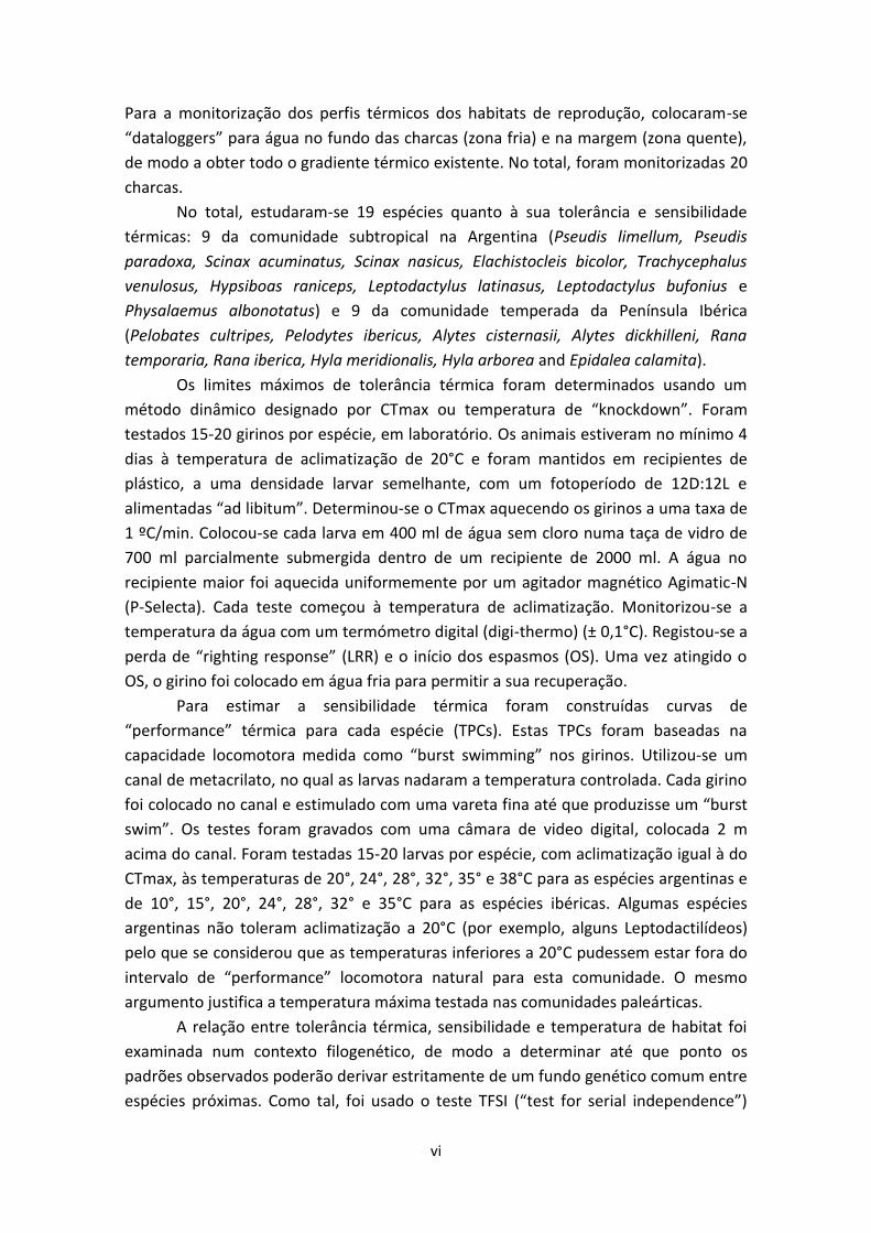
Para a monitorização dos perfis térmicos dos habitats de reprodução, colocaram-se
“dataloggers” para água no fundo das charcas (zona fria) e na margem (zona quente),
de modo a obter todo o gradiente térmico existente. No total, foram monitorizadas 20
charcas.
No total, estudaram-se 19 espécies quanto à sua tolerância e sensibilidade
térmicas: 9 da comunidade subtropical na Argentina (Pseudis limellum, Pseudis
paradoxa, Scinax acuminatus, Scinax nasicus, Elachistocleis bicolor, Trachycephalus
venulosus, Hypsiboas raniceps, Leptodactylus latinasus, Leptodactylus bufonius e
Physalaemus albonotatus) e 9 da comunidade temperada da Península Ibérica
(Pelobates cultripes, Pelodytes ibericus, Alytes cisternasii, Alytes dickhilleni, Rana
temporaria, Rana iberica, Hyla meridionalis, Hyla arborea and Epidalea calamita).
Os limites máximos de tolerância térmica foram determinados usando um
método dinâmico designado por CTmax ou temperatura de “knockdown”. Foram
testados 15-20 girinos por espécie, em laboratório. Os animais estiveram no mínimo 4
dias à temperatura de aclimatização de 20°C e foram mantidos em recipientes de
plástico, a uma densidade larvar semelhante, com um fotoperíodo de 12D:12L e
alimentadas “ad libitum”. Determinou-se o CTmax aquecendo os girinos a uma taxa de
1 ºC/min. Colocou-se cada larva em 400 ml de água sem cloro numa taça de vidro de
700 ml parcialmente submergida dentro de um recipiente de 2000 ml. A água no
recipiente maior foi aquecida uniformemente por um agitador magnético Agimatic‐N
(P‐Selecta). Cada teste começou à temperatura de aclimatização. Monitorizou-se a
temperatura da água com um termómetro digital (digi‐thermo) (± 0,1°C). Registou-se a
perda de “righting response” (LRR) e o início dos espasmos (OS). Uma vez atingido o
OS, o girino foi colocado em água fria para permitir a sua recuperação.
Para estimar a sensibilidade térmica foram construídas curvas de
“performance” térmica para cada espécie (TPCs). Estas TPCs foram baseadas na
capacidade locomotora medida como “burst swimming” nos girinos. Utilizou-se um
canal de metacrilato, no qual as larvas nadaram a temperatura controlada. Cada girino
foi colocado no canal e estimulado com uma vareta fina até que produzisse um “burst
swim”. Os testes foram gravados com uma câmara de video digital, colocada 2 m
acima do canal. Foram testadas 15-20 larvas por espécie, com aclimatização igual à do
CTmax, às temperaturas de 20°, 24°, 28°, 32°, 35° e 38°C para as espécies argentinas e
de 10°, 15°, 20°, 24°, 28°, 32° e 35°C para as espécies ibéricas. Algumas espécies
argentinas não toleram aclimatização a 20°C (por exemplo, alguns Leptodactilídeos)
pelo que se considerou que as temperaturas inferiores a 20°C pudessem estar fora do
intervalo de “performance” locomotora natural para esta comunidade. O mesmo
argumento justifica a temperatura máxima testada nas comunidades paleárticas.
A relação entre tolerância térmica, sensibilidade e temperatura de habitat foi
examinada num contexto filogenético, de modo a determinar até que ponto os
padrões observados poderão derivar estritamente de um fundo genético comum entre
espécies próximas. Como tal, foi usado o teste TFSI (“test for serial independence”)
vii
para caracteres contínuos e o método de PIC (“phylogenetically independent
contrasts”) para determinar se cada caracter estava significativamente associado à sua
história filogenética e para corrigir as correlações encontradas tendo em conta a sua
filogenia.
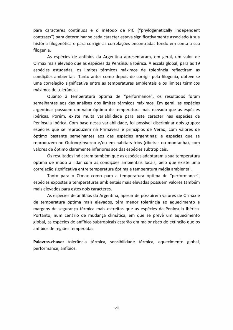
As espécies de anfíbios da Argentina apresentaram, em geral, um valor de
CTmax mais elevado que as espécies da Pensínsula Ibérica. À escala global, para as 19
espécies estudadas, os limites térmicos máximos de tolerância reflectiram as
condições ambientais. Tanto antes como depois de corrigir pela filogenia, obteve-se
uma correlação significativa entre as temperaturas ambientais e os limites térmicos
máximos de tolerância.
Quanto à temperatura óptima de “performance”, os resultados foram
semelhantes aos das análises dos limites térmicos máximos. Em geral, as espécies
argentinas possuem um valor óptimo de temperatura mais elevado que as espécies
ibéricas. Porém, existe muita variabilidade para este caracter nas espécies da
Península Ibérica. Com base nessa variabilidade, foi possível discriminar dois grupos:
espécies que se reproduzem na Primavera e princípios de Verão, com valores de
óptimo bastante semelhantes aos das espécies argentinas; e espécies que se
reproduzem no Outono/Inverno e/ou em habitats frios (ribeiras ou montanha), com
valores de óptimo claramente inferiores aos das espécies subtropicais.
Os resultados indicaram também que as espécies adaptaram a sua temperatura
óptima de modo a lidar com as condições ambientais locais, pelo que existe uma
correlação significativa entre temperatura óptima e temperatura média ambiental.
Tanto para o Ctmax como para a temperatura óptima de “performance”,
espécies expostas a temperaturas ambientais mais elevadas possuem valores também
mais elevados para estes dois caracteres.
As espécies de anfíbios da Argentina, apesar de possuírem valores de CTmax e
de temperatura óptima mais elevados, têm menor tolerância ao aquecimento e
margens de segurança térmica mais estreitas que as espécies da Península Ibérica.
Portanto, num cenário de mudança climática, em que se prevê um aquecimento
global, as espécies de anfíbios subtropicais estarão em maior risco de extinção que os
anfíbios de regiões temperadas.
Palavras-chave: tolerância térmica, sensibilidade térmica, aquecimento global,
performance, anfíbios.
viii
INDEX
1. Introduction 1
1.1. State of the art 1
1.2. Objectives and study organisms 4
1.3. Thermal tolerance studies 7
1.4. Thermal sensitivity studies 8
2. Methodology 10
2.1. Field work 10
2.1.1. Study areas 10
2.1.2. Monitoring environmental temperatures 11
2.2. Comparative evaluation of the upper thermal maxima and
Warming Tolerance 12
2.3. Evaluation of thermal sensitivity of locomotor performance and
Thermal Safety Margins 14
2.4. Phylogenetic analyses 15
3. Results 17
3.1. Monitoring environmental temperatures 17
3.2. Upper thermal maxima and Warming Tolerance 20
3.3. Thermal sensitivity and Thermal Safety Margins 24
3.4. CTmax vs Optimum Temperature and Warming Tolerance vs
Thermal Safety Margins 30
4. Discussion 33
4.1. Thermal tolerance 33
4.2. Thermal sensitivity 34
4.3. Evaluating vulnerability to warming temperatures 35
5. Acknowledgments 38
6. References 40
7. Annexes 47
Annexe I. Monitored ponds 47
Annexe II. Phylogenetic trees 48
Annexe III. CTmax 50
Annexe IV. Thermal performance curves 51
- 1 -
1. INTRODUCTION
1.1. State of the art
Temperature affects virtually all physiological processes. It determines both
rates of chemical reactions (Hochochka and Somero, 2002) and many ecological
interactions (Dunson and Travis, 1991). Therefore, it is expected that environmental
temperature changes associated with global warming will have broad ecological
consequences for species and communities (Southward et al., 1995; Pearson and
Dawson, 2003; Case et al., 2005). Recent reports, using meta‐analyses, have presented
comprehensive synthesis of the impact of climate change on a range of species
(Parmesan and Yohe, 2003; Root et al., 2003). However, extensive debate still exists on
whether the observed biological changes can be conclusively linked to an
anthropogenic effect on climate or contrarily it may be better attributed simply to
sampling bias (Jensen, 2003).
To assess how climate change will really impact organims, deep knowledge is
required on three main key issues: a) the current conditions and future climatic
scenarios; b) how close organisms are to their thermal tolerance in nature; and c) to
know the degree to which organisms are able to adjust or acclimatize their thermal
sensitivity (Stillman, 2003; Gilman et al., 2006). One can expect that organisms with
the greatest risk of extinction from rapid climatic change are those with a low
tolerance to warming, limited acclimation ability and reduced dispersal, incapacitating
them to avoid/adjust to new challenging conditions.
Ectotherms comprise most of the terrestrial biodiversity and are expected to be
especially vulnerable to global warming since their basic physiological functions,
development and behaviour are strongly affected by temperature. In these organisms,
most physiological processes proceed rapidly over a range of body temperatures
defining a thermal performance curve or TPC (Huey and Stevenson, 1979). This
thermal sensitivity curve rises gradually from a minimum critical temperature (CTmin),
to an optimum temperature (Topt), and then falls rapidly to a critical thermal
maximum (CTmax). Critical thermal limits define the thermal tolerance range of an
organism. Temperatures either below or above the range of tolerance result in
impaired physiological function (Hillman et al., 2009).
Impacts of global warming on biodiversity are often assumed to be
geographically dependent, being predicted to be smaller in the tropics relatively to
those in temperate regions (Root et al., 2003; Parmesan, 2007) because the projected
rate of climate warming in the tropics is lower than the one expected for higher
latitudes (IPCC, 2007a). However, this prediction based on absolute temperature
change may be misleading due to several factors associated with behaviour, physiology
and ecology of organisms.
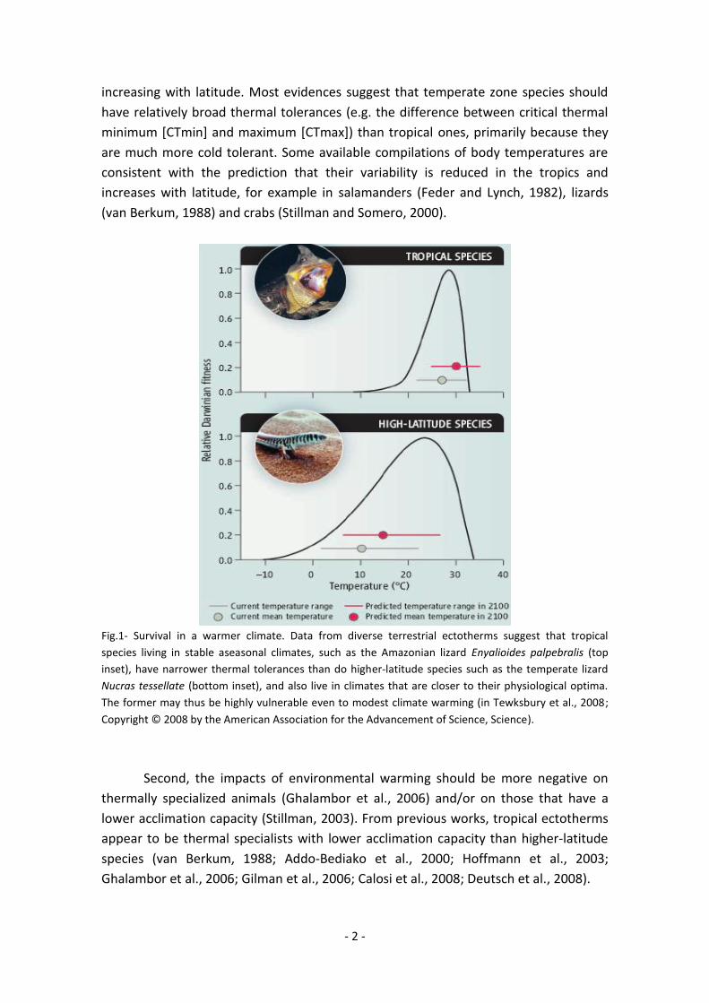
First, there are wide indications that thermal tolerance in different groups of
ectotherms is related to the magnitude of temperature variation they normally
experience (Janzen, 1969; Addo‐Bediako et al., 2000; Ghalambor et al., 2006), thereby
- 2 -
increasing with latitude. Most evidences suggest that temperate zone species should
have relatively broad thermal tolerances (e.g. the difference between critical thermal
minimum [CTmin] and maximum [CTmax]) than tropical ones, primarily because they
are much more cold tolerant. Some available compilations of body temperatures are
consistent with the prediction that their variability is reduced in the tropics and
increases with latitude, for example in salamanders (Feder and Lynch, 1982), lizards
(van Berkum, 1988) and crabs (Stillman and Somero, 2000).
Fig.1- Survival in a warmer climate. Data from diverse terrestrial ectotherms suggest that tropical
species living in stable aseasonal climates, such as the Amazonian lizard Enyalioides palpebralis (top
inset), have narrower thermal tolerances than do higher-latitude species such as the temperate lizard
Nucras tessellate (bottom inset), and also live in climates that are closer to their physiological optima.
The former may thus be highly vulnerable even to modest climate warming (in Tewksbury et al., 2008;
Copyright © 2008 by the American Association for the Advancement of Science, Science).
Second, the impacts of environmental warming should be more negative on
thermally specialized animals (Ghalambor et al., 2006) and/or on those that have a
lower acclimation capacity (Stillman, 2003). From previous works, tropical ectotherms
appear to be thermal specialists with lower acclimation capacity than higher‐latitude
species (van Berkum, 1988; Addo‐Bediako et al., 2000; Hoffmann et al., 2003;
Ghalambor et al., 2006; Gilman et al., 2006; Calosi et al., 2008; Deutsch et al., 2008).
- 3 -
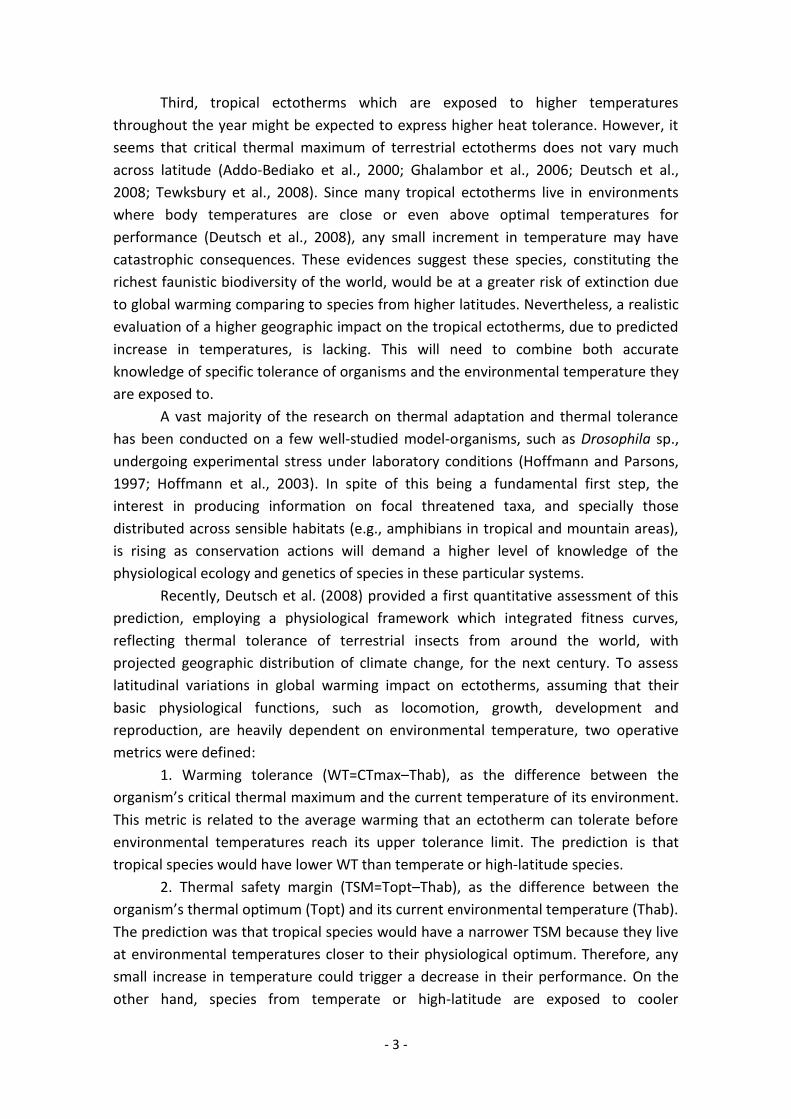
Third, tropical ectotherms which are exposed to higher temperatures
throughout the year might be expected to express higher heat tolerance. However, it
seems that critical thermal maximum of terrestrial ectotherms does not vary much
across latitude (Addo‐Bediako et al., 2000; Ghalambor et al., 2006; Deutsch et al.,
2008; Tewksbury et al., 2008). Since many tropical ectotherms live in environments
where body temperatures are close or even above optimal temperatures for
performance (Deutsch et al., 2008), any small increment in temperature may have
catastrophic consequences. These evidences suggest these species, constituting the
richest faunistic biodiversity of the world, would be at a greater risk of extinction due
to global warming comparing to species from higher latitudes. Nevertheless, a realistic
evaluation of a higher geographic impact on the tropical ectotherms, due to predicted
increase in temperatures, is lacking. This will need to combine both accurate
knowledge of specific tolerance of organisms and the environmental temperature they
are exposed to.
A vast majority of the research on thermal adaptation and thermal tolerance
has been conducted on a few well‐studied model‐organisms, such as Drosophila sp.,
undergoing experimental stress under laboratory conditions (Hoffmann and Parsons,
1997; Hoffmann et al., 2003). In spite of this being a fundamental first step, the
interest in producing information on focal threatened taxa, and specially those
distributed across sensible habitats (e.g., amphibians in tropical and mountain areas),
is rising as conservation actions will demand a higher level of knowledge of the
physiological ecology and genetics of species in these particular systems.
Recently, Deutsch et al. (2008) provided a first quantitative assessment of this
prediction, employing a physiological framework which integrated fitness curves,
reflecting thermal tolerance of terrestrial insects from around the world, with
projected geographic distribution of climate change, for the next century. To assess
latitudinal variations in global warming impact on ectotherms, assuming that their
basic physiological functions, such as locomotion, growth, development and
reproduction, are heavily dependent on environmental temperature, two operative
metrics were defined:
1. Warming tolerance (WT=CTmax–Thab), as the difference between the
organism’s critical thermal maximum and the current temperature of its environment.
This metric is related to the average warming that an ectotherm can tolerate before
environmental temperatures reach its upper tolerance limit. The prediction is that
tropical species would have lower WT than temperate or high‐latitude species.
2. Thermal safety margin (TSM=Topt–Thab), as the difference between the
organism’s thermal optimum (Topt) and its current environmental temperature (Thab).
The prediction was that tropical species would have a narrower TSM because they live
at environmental temperatures closer to their physiological optimum. Therefore, any
small increase in temperature could trigger a decrease in their performance. On the
other hand, species from temperate or high‐latitude are exposed to cooler
- 4 -
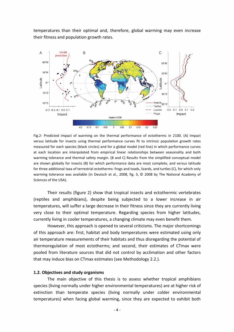
temperatures than their optimal and, therefore, global warming may even increase
their fitness and population growth rates.
Fig.2- Predicted impact of warming on the thermal performance of ectotherms in 2100. (A) Impact
versus latitude for insects using thermal performance curves fit to intrinsic population growth rates
measured for each species (black circles) and for a global model (red line) in which performance curves
at each location are interpolated from empirical linear relationships between seasonality and both
warming tolerance and thermal safety margin. (B and C) Results from the simplified conceptual model
are shown globally for insects (B) for which performance data are most complete, and versus latitude
for three additional taxa of terrestrial ectotherms: frogs and toads, lizards, and turtles (C), for which only
warming tolerance was available (in Deutsch et al., 2008, fig. 3, © 2008 by The National Academy of
Sciences of the USA).
Their results (figure 2) show that tropical insects and ectothermic vertebrates
(reptiles and amphibians), despite being subjected to a lower increase in air
temperatures, will suffer a large decrease in their fitness since they are currently living
very close to their optimal temperature. Regarding species from higher latitudes,
currently living in cooler temperatures, a changing climate may even benefit them.
However, this approach is opened to several criticisms. The major shortcomings
of this approach are: first, habitat and body temperatures were estimated using only
air temperature measurements of their habitats and thus disregarding the potential of
thermoregulation of most ectotherms; and second, their estimates of CTmax were
pooled from literature sources that did not control by acclimation and other factors
that may induce bias on CTmax estimates (see Methodology 2.2.).
1.2. Objectives and study organisms
The main objective of this thesis is to assess whether tropical amphibians
species (living normally under higher environmental temperatures) are at higher risk of
extinction than temperate species (living normally under colder environmental
temperatures) when facing global warming, since they are expected to exhibit both
- 5 -
lower warming tolerance (WT=CTmax–Thab) and narrower thermal safety margins
(TSM=Topt–Thab).
Amphibians are considered the most endangered group of vertebrates since
near one third of all extant species are threatened with extinction (Stuart et al., 2004).
They have a number of physiological, ecological and life‐history characteristics that
make them highly susceptible to environmental change such as ectothermy,
permeable skin and complex life‐cycles (with metamorphosis), the last one presumed
to be an adaptation to the sequential occupation of temporary wetlands and terrestrial
environments (Wells, 2007). All of these traits also determine an important
dependence on environmental factors and, in addition, can explain the geographic
pattern of amphibian species richness. The tropics hold much higher species richness,
containing more than 85 % of the current amphibian species (Duellmann, 1999; Wells,
2007; Stuart et al., 2008). Particularly, the Neotropical realm of Central and South
America alone concentrates the highest diversity of amphibians on earth with 2916
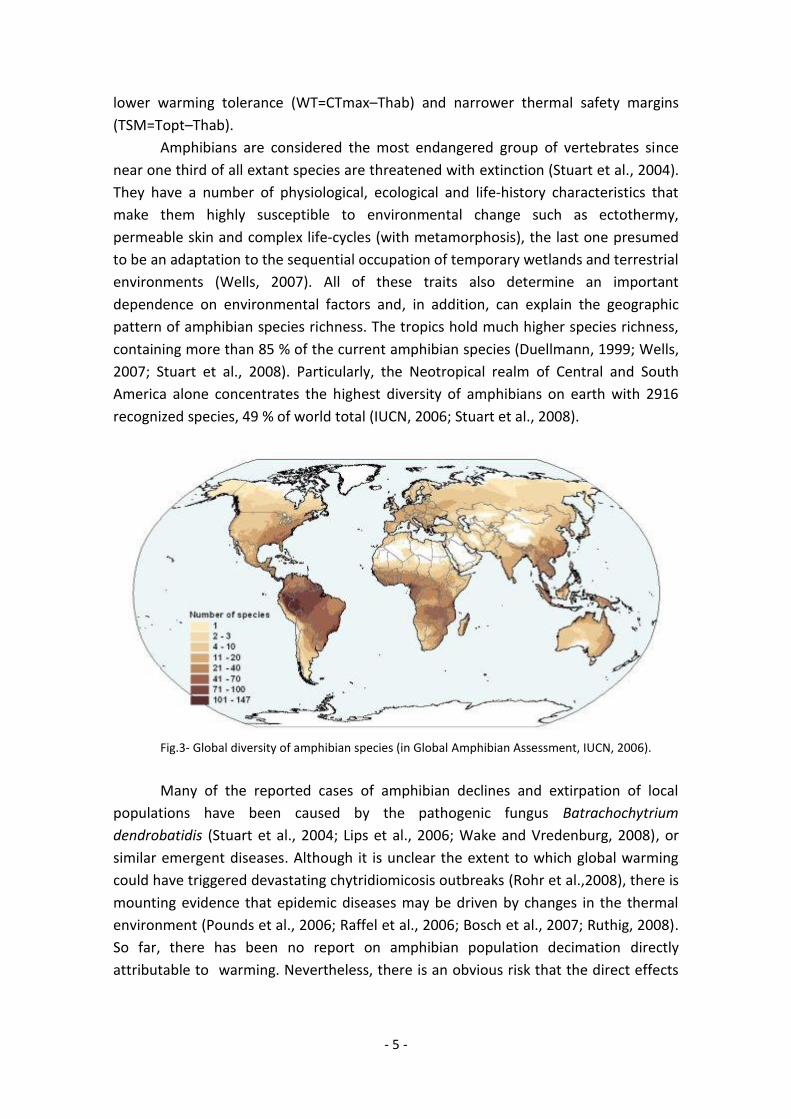
recognized species, 49 % of world total (IUCN, 2006; Stuart et al., 2008).
Fig.3- Global diversity of amphibian species (in Global Amphibian Assessment, IUCN, 2006).
Many of the reported cases of amphibian declines and extirpation of local
populations have been caused by the pathogenic fungus Batrachochytrium
dendrobatidis (Stuart et al., 2004; Lips et al., 2006; Wake and Vredenburg, 2008), or
similar emergent diseases. Although it is unclear the extent to which global warming
could have triggered devastating chytridiomicosis outbreaks (Rohr et al.,2008), there is
mounting evidence that epidemic diseases may be driven by changes in the thermal
environment (Pounds et al., 2006; Raffel et al., 2006; Bosch et al., 2007; Ruthig, 2008).
So far, there has been no report on amphibian population decimation directly
attributable to warming. Nevertheless, there is an obvious risk that the direct effects
- 6 -
of increasing temperatures and other manifestations of climate change can cause a
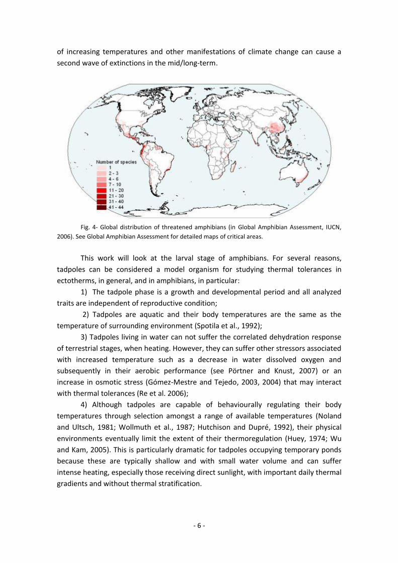
second wave of extinctions in the mid/long‐term.
Fig. 4- Global distribution of threatened amphibians (in Global Amphibian Assessment, IUCN,
2006). See Global Amphibian Assessment for detailed maps of critical areas.
This work will look at the larval stage of amphibians. For several reasons,
tadpoles can be considered a model organism for studying thermal tolerances in
ectotherms, in general, and in amphibians, in particular:
1) The tadpole phase is a growth and developmental period and all analyzed
traits are independent of reproductive condition;
2) Tadpoles are aquatic and their body temperatures are the same as the
temperature of surrounding environment (Spotila et al., 1992);
3) Tadpoles living in water can not suffer the correlated dehydration response
of terrestrial stages, when heating. However, they can suffer other stressors associated
with increased temperature such as a decrease in water dissolved oxygen and
subsequently in their aerobic performance (see Pörtner and Knust, 2007) or an
increase in osmotic stress (Gómez‐Mestre and Tejedo, 2003, 2004) that may interact
with thermal tolerances (Re et al. 2006);
4) Although tadpoles are capable of behaviourally regulating their body
temperatures through selection amongst a range of available temperatures (Noland
and Ultsch, 1981; Wollmuth et al., 1987; Hutchison and Dupré, 1992), their physical
environments eventually limit the extent of their thermoregulation (Huey, 1974; Wu
and Kam, 2005). This is particularly dramatic for tadpoles occupying temporary ponds
because these are typically shallow and with small water volume and can suffer
intense heating, especially those receiving direct sunlight, with important daily thermal
gradients and without thermal stratification.

- 7 -
Fig.5- Tadpole of Pseudis paradoxa, (Linnaeus, 1758). Foto by Ricardo Reques.
In ponds located in tropical environments with a wet summer breeding season,
tadpoles may be exposed to temperatures over 40°C. During heating waves, tadpoles
may not be able to escape from dangerous temperatures before ponds dry completely,
even though they are capable of behavioural thermoregulation (Wells, 2007), unless
they can reach metamorphosis and jump to land. Here, a wider range of microhabitats
can be found and possibly they will be able to select a more thermally favourable
microclimate (Navas et al, 2007). The expected increase in global mean temperature,
together with more frequent extreme hot events, such as heat waves, will accentuate
this condition (IPCC, 2007b). On the other hand, global warming is predicted to shorten
pond hydroperiods in many areas such as Central America and Australia due to parallel
shortage in rainfalls (IPCC, 2007b) which may potentially increase local extinction of
amphibian populations.
Most of the literature concerning temperature effects and responses has
focused groups of ectothermic vertebrates other than amphibians (fish and reptiles).
However, thermal physiology research in amphibians, in spite of seminal contributions
in the 50s ‐ 70s (Brattstrom, 1959, 1962 and 1968; Lillywhite, 1970; Hutchison, 1961;
Heatwole et al., 1965; Mahoney and Hutchison, 1969), has been intensively developed
specially in later decades (see reviews in Rome et al., 1992; Hutchison and Dupré,
1992; Ultsch et al., 1999; Wells, 2007; Navas et al., 2008; Hillman et al., 2009).
1.3. Thermal tolerance studies
The analysis of thermal tolerances in amphibians was initially developed by
Brattstrom (1968) in anurans, and Hutchison (1961), in salamanders. Interestingly,
Brattstrom’s study included comparative data of CTmax for 53 species of frogs from a
latitudinal and altitudinal gradient in North and Central America. He found that CTmax
varied both at the species and population levels.
For most anuran larvae, CTmax was determined to fall between 38°C and 42°C
(Ultsch et al., 1999). The differences in CTmax among populations may be a response
- 8 -
to interdemic thermal habitat through local genetic adaptation in thermal tolerance. A
number of studies have demonstrated within species variation in heat tolerance (e.g.,
Hutchison, 1961; Brattstrom, 1968 and 1970; Delson and Whitford, 1973; Miller and
Packard, 1977; Hoppe, 1978; Hertz et al., 1979; Garland and Adolph, 1991; Meffe et al.,
1995; Schwarzkopf, 1998; Gvoždík and Castilla, 2001; Winne and Keck, 2005; Huang
and Tu, 2008). However, few studies have performed common garden experiments
designed to distinguish between genetic and acclimation induced differences in
physiology (Garland and Adolph, 1991). In amphibians some evidences have been
reported that CTmax may adaptively differ between populations (Skelly and
Freidenburg, 2000; Chen et al., 2001; Wu and Kam 2005; C. Navas, unpublished data).
Other factors should be taken into account. Ontogeny may affect CTmax, which
drops 3°C‐4°C when larvae are close to metamorphic climax (Floyd, 1983), requiring
deeper analysis of maximum heating during this risk‐sensitive phase. Acclimation to
higher temperatures may affect the estimate of CTmax, increasing its value up to 4°C
(Brattstrom, 1968; Navas et al., 2008). It is recognized that CTmax exhibits a
phylogenetic signal and differences between amphibian lineages can be found both in
adult stages (Navas et al., 2008), and tadpoles, (H. Duarte and J.P. do Amaral,
unpublished data).
Finally, some controversy exists whether CTmax is dependent on latitude.
Analysis on insects revealed no geographical trend (Addo‐Bediako et al., 2000). In
amphibians, the analysis of Brattstrom (1968) data set is inconclusive: Snyder and
Weathers (1975) found a significant decline in CTmax with increasing latitude (r=0,70;
p<0,05) whereas the re‐analysis of Ghalambor et al. (2006) showed that the trend was
not significant (p >0,70).
Since estimates of CTmax are susceptible to error due to several factors,
including variations in end‐points (Lutterschmidt and Hutchison, 1997), acclimation
temperature (Navas et al., 2008), or even differences in researcher perceptions, it is
top-priority to standardize all the measurements in order to provide testable
comparisons.
1.4. Thermal sensitivity studies
The study of thermal sensitivity and optimal temperature in locomotor
performance has been largely developed in ectotherms in general (e.g. Bauwens et al.,
1995; Claussen et al., 2000) and in amphibians in particular (Rome et al., 1992;
Whitehead et al., 1989; Tejedo et al., 2000; Wilson, 2001; Gomes et al., 2002).
Maximum sprint speed is an ecologically relevant index of organismal performance
capacity and has been employed as a good proxy to estimate optimal temperatures in
ectotherms since it may correlate with fitness (Jayne and Bennett, 1990; Le Galliard et
al., 2004; Husak, 2006).
Two hypotheses have been suggested to explain the evolution of thermal
sensitivity using thermal performance curves. The ‘‘warmer is better’’ (or
- 9 -
‘‘thermodynamic constraint’’) hypothesis states that the maximal performance of
organisms with high optimal temperatures should be higher than that of organisms
with low optimal temperatures (Huey and Kingsolver, 1989; Savage et al., 2004). The
‘‘Jack‐of all‐temperatures is a master of none’’ (Huey and Hertz, 1984) hypothesis
assumes a trade‐off between maximal performance and the breadth of the
performance curve (Levins, 1968; Huey and Slatkin, 1976). Few interespecific analyses
have tested these hypotheses and also whether generalist/specialist species
predominate either in tropical or temperate communities.
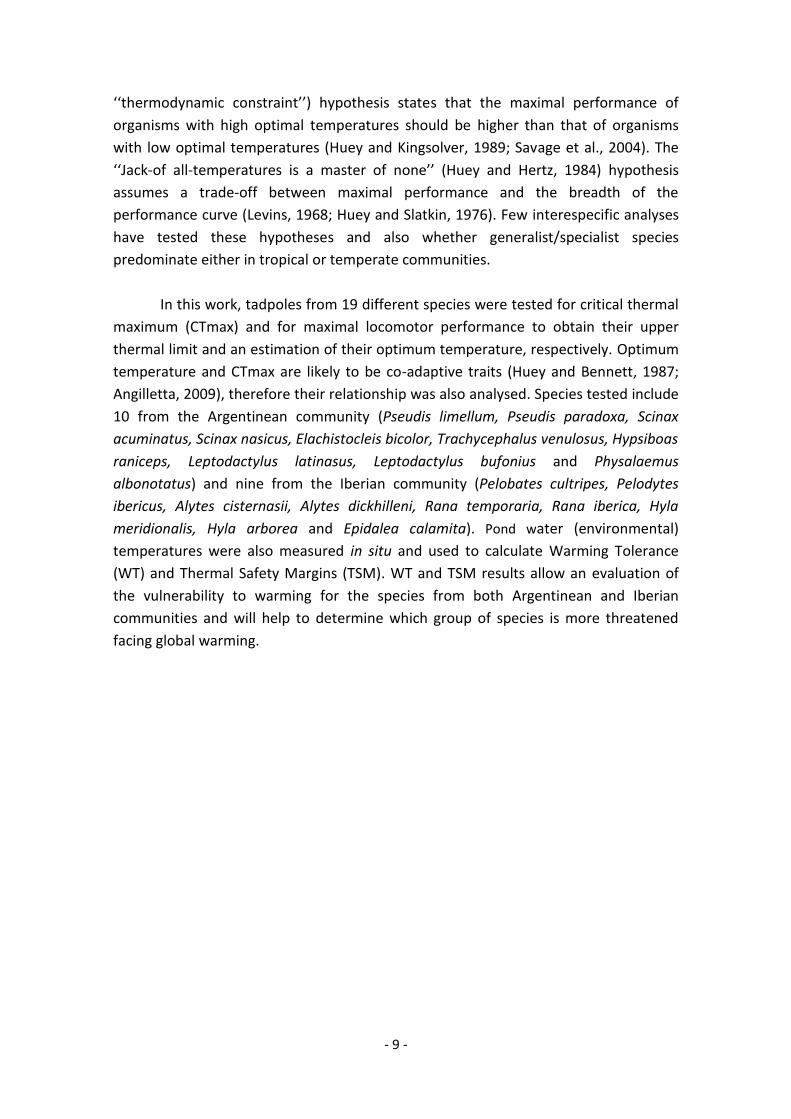
In this work, tadpoles from 19 different species were tested for critical thermal
maximum (CTmax) and for maximal locomotor performance to obtain their upper
thermal limit and an estimation of their optimum temperature, respectively. Optimum
temperature and CTmax are likely to be co-adaptive traits (Huey and Bennett, 1987;
Angilletta, 2009), therefore their relationship was also analysed. Species tested include
10 from the Argentinean community (Pseudis limellum, Pseudis paradoxa, Scinax
acuminatus, Scinax nasicus, Elachistocleis bicolor, Trachycephalus venulosus, Hypsiboas
raniceps, Leptodactylus latinasus, Leptodactylus bufonius and Physalaemus
albonotatus) and nine from the Iberian community (Pelobates cultripes, Pelodytes
ibericus, Alytes cisternasii, Alytes dickhilleni, Rana temporaria, Rana iberica, Hyla
meridionalis, Hyla arborea and Epidalea calamita). Pond water (environmental)
temperatures were also measured in situ and used to calculate Warming Tolerance
(WT) and Thermal Safety Margins (TSM). WT and TSM results allow an evaluation of
the vulnerability to warming for the species from both Argentinean and Iberian
communities and will help to determine which group of species is more threatened
facing global warming.
- 10 -
2. METHODOLOGY
2.1. Field work
2.1.1. Study areas
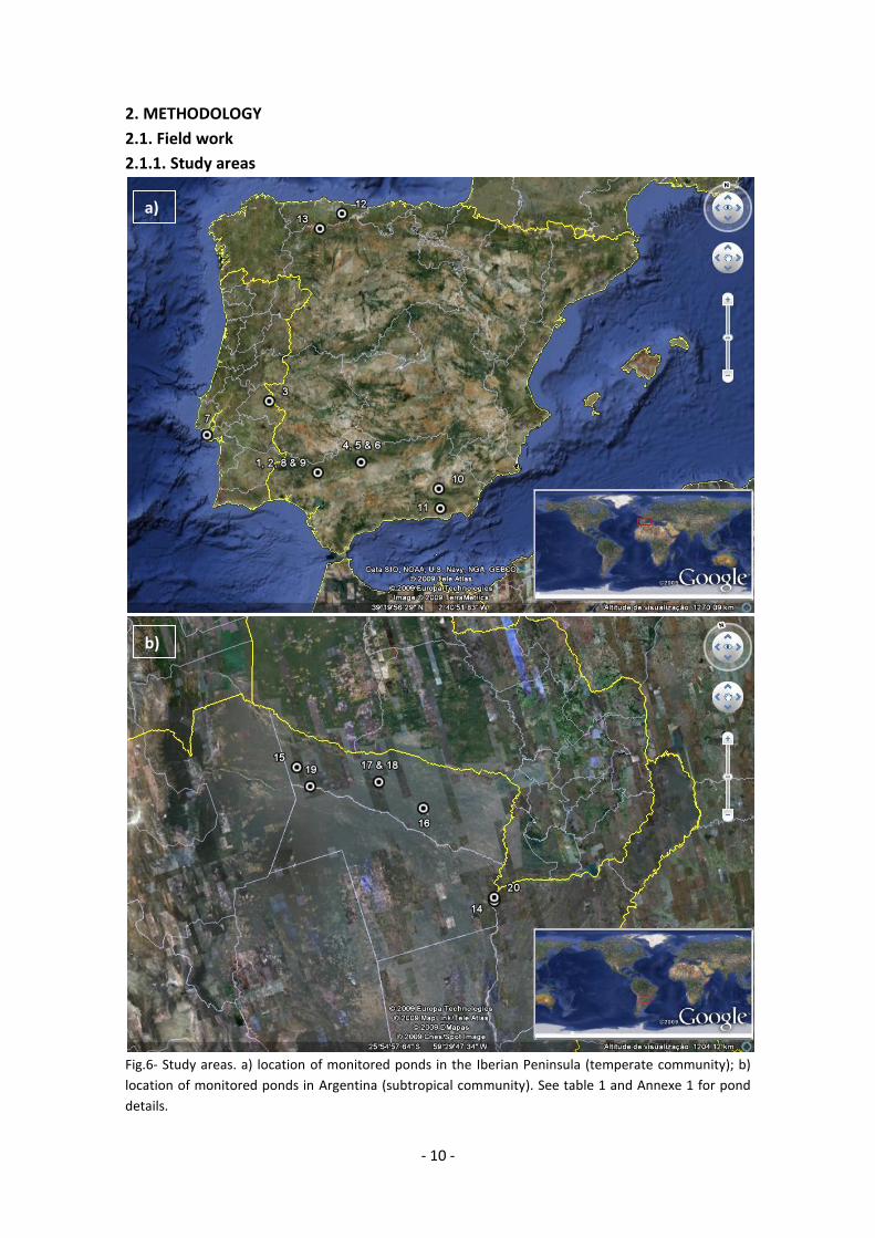
Fig.6- Study areas. a) location of monitored ponds in the Iberian Peninsula (temperate community); b)
location of monitored ponds in Argentina (subtropical community). See table 1 and Annexe 1 for pond
details.
a)
b)
- 11 -
Regarding the subtropical community from northern Argentina, sampled ponds
were located in the El Gran Chaco region, in the provinces of Formosa and Chaco, and
also in the northern part of the province of Corrientes, ranging from 24ºS to 27ºS and
58ºW to 61ºW (see figure 6). The El Gran Chaco region is one of the warmest areas of
South America, characterized by a seasonal regimen of precipitation concentrated
during the austral summer, thus, amphibians from this region breed in a hot humid
season.
The study area for the temperate amphibian community was situated in the
Iberian Peninsula (see figure 6). Sampled populations were spread throughout
Portugal and Spain, spanning a north-south distribution from Oviedo, Asturias (43ºN),
to Doñana, Andalusia (37ºN), and an east-west distribution from Granada, Andalusia
(3ºW) to the Portuguese coast, at Verdizela (9ºW). Amphibian species from the Iberian
Peninsula (temperate community) differ from the subtropical species because they
breed at cooler environmental temperatures, during autumn, winter and/or spring;
only species living in higher mountain areas breed in the early summer.
2.1.2. Monitoring environmental temperatures
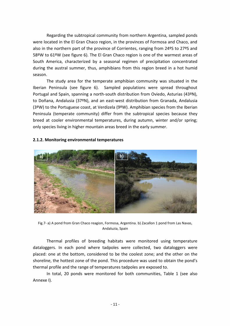
Fig.7- a) A pond from Gran Chaco reagion, Formosa, Argentina. b) Zacallon 1 pond from Las Navas,
Andaluzia, Spain
Thermal profiles of breeding habitats were monitored using temperature
dataloggers. In each pond where tadpoles were collected, two dataloggers were
placed: one at the bottom, considered to be the coolest zone; and the other on the
shoreline, the hottest zone of the pond. This procedure was used to obtain the pond’s
thermal profile and the range of temperatures tadpoles are exposed to.
In total, 20 ponds were monitored for both communities, Table 1 (see also
Annexe I).
a) b)
- 12 -
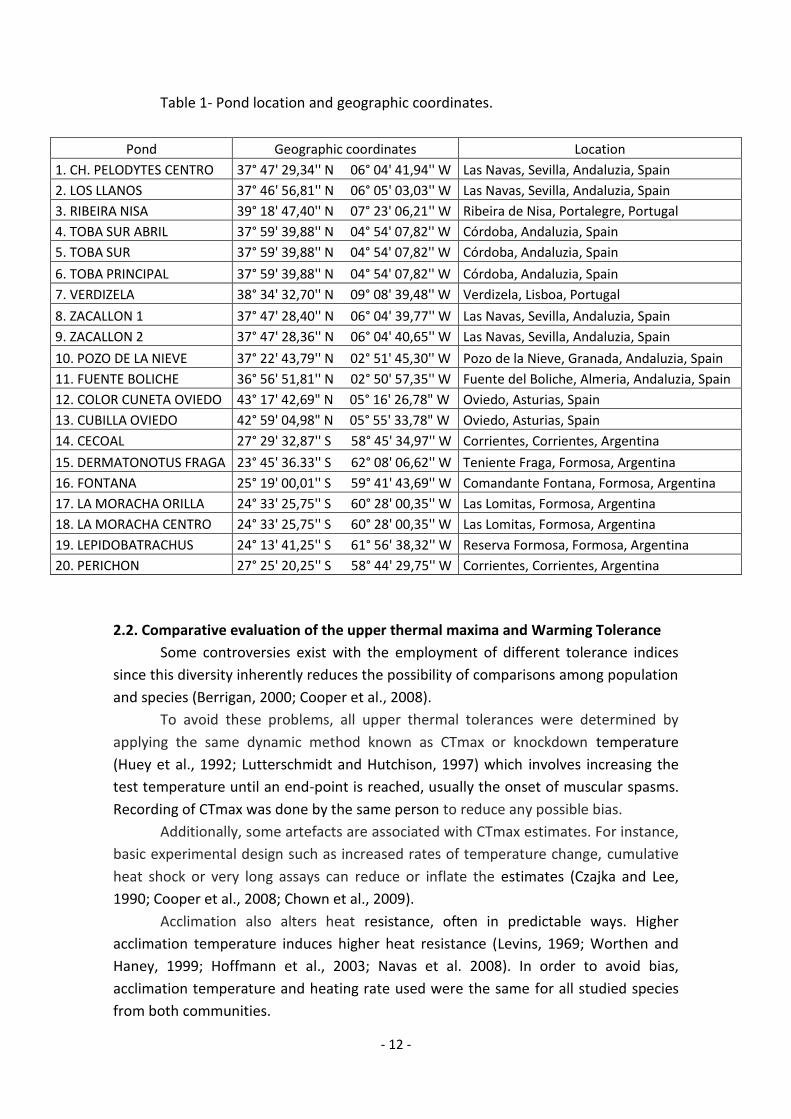
Table 1- Pond location and geographic coordinates.
Pond Geographic coordinates Location
1. CH. PELODYTES CENTRO 37° 47' 29,34'' N 06° 04' 41,94'' W Las Navas, Sevilla, Andaluzia, Spain
2. LOS LLANOS 37° 46' 56,81'' N 06° 05' 03,03'' W Las Navas, Sevilla, Andaluzia, Spain
3. RIBEIRA NISA 39° 18' 47,40'' N 07° 23' 06,21'' W Ribeira de Nisa, Portalegre, Portugal
4. TOBA SUR ABRIL 37° 59' 39,88'' N 04° 54' 07,82'' W Córdoba, Andaluzia, Spain
5. TOBA SUR 37° 59' 39,88'' N 04° 54' 07,82'' W Córdoba, Andaluzia, Spain
6. TOBA PRINCIPAL 37° 59' 39,88'' N 04° 54' 07,82'' W Córdoba, Andaluzia, Spain
7. VERDIZELA 38° 34' 32,70'' N 09° 08' 39,48'' W Verdizela, Lisboa, Portugal
8. ZACALLON 1 37° 47' 28,40'' N 06° 04' 39,77'' W Las Navas, Sevilla, Andaluzia, Spain
9. ZACALLON 2 37° 47' 28,36'' N 06° 04' 40,65'' W Las Navas, Sevilla, Andaluzia, Spain
10. POZO DE LA NIEVE 37° 22' 43,79'' N 02° 51' 45,30'' W Pozo de la Nieve, Granada, Andaluzia, Spain
11. FUENTE BOLICHE 36° 56' 51,81'' N 02° 50' 57,35'' W Fuente del Boliche, Almeria, Andaluzia, Spain
12. COLOR CUNETA OVIEDO 43° 17' 42,69" N 05° 16' 26,78" W Oviedo, Asturias, Spain
13. CUBILLA OVIEDO 42° 59' 04,98" N 05° 55' 33,78" W Oviedo, Asturias, Spain
14. CECOAL 27° 29' 32,87'' S 58° 45' 34,97'' W Corrientes, Corrientes, Argentina
15. DERMATONOTUS FRAGA 23° 45' 36.33'' S 62° 08' 06,62'' W Teniente Fraga, Formosa, Argentina
16. FONTANA 25° 19' 00,01'' S 59° 41' 43,69'' W Comandante Fontana, Formosa, Argentina
17. LA MORACHA ORILLA 24° 33' 25,75'' S 60° 28' 00,35'' W Las Lomitas, Formosa, Argentina
18. LA MORACHA CENTRO 24° 33' 25,75'' S 60° 28' 00,35'' W Las Lomitas, Formosa, Argentina
19. LEPIDOBATRACHUS 24° 13' 41,25'' S 61° 56' 38,32'' W Reserva Formosa, Formosa, Argentina
20. PERICHON 27° 25' 20,25'' S 58° 44' 29,75'' W Corrientes, Corrientes, Argentina
2.2. Comparative evaluation of the upper thermal maxima and Warming Tolerance
Some controversies exist with the employment of different tolerance indices
since this diversity inherently reduces the possibility of comparisons among population
and species (Berrigan, 2000; Cooper et al., 2008).
To avoid these problems, all upper thermal tolerances were determined by
applying the same dynamic method known as CTmax or knockdown temperature
(Huey et al., 1992; Lutterschmidt and Hutchison, 1997) which involves increasing the
test temperature until an end-point is reached, usually the onset of muscular spasms.
Recording of CTmax was done by the same person to reduce any possible bias.
Additionally, some artefacts are associated with CTmax estimates. For instance,
basic experimental design such as increased rates of temperature change, cumulative
heat shock or very long assays can reduce or inflate the estimates (Czajka and Lee,
1990; Cooper et al., 2008; Chown et al., 2009).
Acclimation also alters heat resistance, often in predictable ways. Higher
acclimation temperature induces higher heat resistance (Levins, 1969; Worthen and
Haney, 1999; Hoffmann et al., 2003; Navas et al. 2008). In order to avoid bias,
acclimation temperature and heating rate used were the same for all studied species
from both communities.
- 13 -
A random sample of 15 tadpoles per species was analyzed, with larval
developmental stages between 25-39 Gosner’s (Gosner, 1960). Acclimation
temperature was set to 20ºC, for a minimum of 4 days. Acclimated individuals were
maintained in plastic containers, at a similar larval density, with 12D:12L photoperiod
and fed ad libitum.
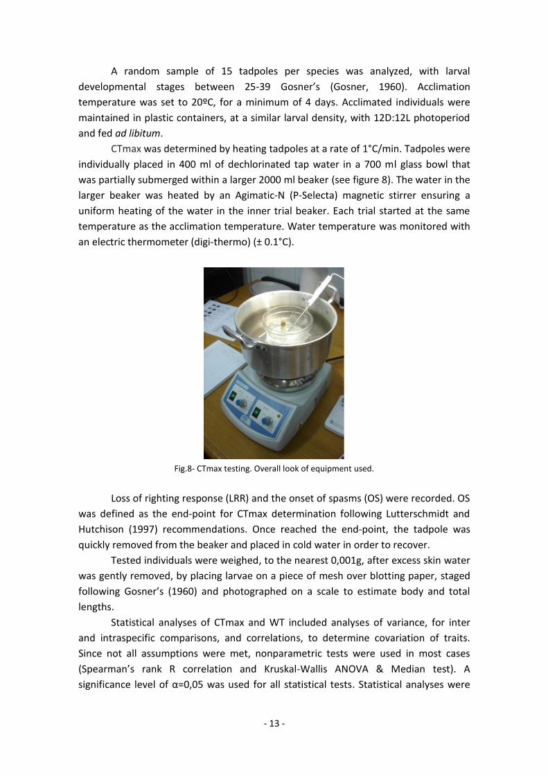
CTmax was determined by heating tadpoles at a rate of 1°C/min. Tadpoles were
individually placed in 400 ml of dechlorinated tap water in a 700 ml glass bowl that
was partially submerged within a larger 2000 ml beaker (see figure 8). The water in the
larger beaker was heated by an Agimatic‐N (P‐Selecta) magnetic stirrer ensuring a
uniform heating of the water in the inner trial beaker. Each trial started at the same
temperature as the acclimation temperature. Water temperature was monitored with
an electric thermometer (digi‐thermo) (± 0.1°C).
Fig.8- CTmax testing. Overall look of equipment used.
Loss of righting response (LRR) and the onset of spasms (OS) were recorded. OS
was defined as the end‐point for CTmax determination following Lutterschmidt and
Hutchison (1997) recommendations. Once reached the end‐point, the tadpole was
quickly removed from the beaker and placed in cold water in order to recover.
Tested individuals were weighed, to the nearest 0,001g, after excess skin water
was gently removed, by placing larvae on a piece of mesh over blotting paper, staged
following Gosner’s (1960) and photographed on a scale to estimate body and total
lengths.
Statistical analyses of CTmax and WT included analyses of variance, for inter
and intraspecific comparisons, and correlations, to determine covariation of traits.
Since not all assumptions were met, nonparametric tests were used in most cases
(Spearman’s rank R correlation and Kruskal-Wallis ANOVA & Median test). A
significance level of α=0,05 was used for all statistical tests. Statistical analyses were

- 14 -
computed using STATISTICA 7.0 software (StatSoft 2000). All data appear as means ± 1
SE or SD.
2.3. Evaluation of thermal sensitivity of locomotor performance and Thermal Safety
Margins
Thermal performance curves (TPCs) were obtained in order to estimate thermal
sensitivity. TPCs were based on maximal locomotor performance by measuring
tadpoles maximal burst swimming speed. Locomotor performance is considered to be
a proxy, representing maximum physiological performance, and a critical variable in
fleeing from predators (e.g. Feder, 1983; Werner and McPeek, 1994; Watkins 1996).
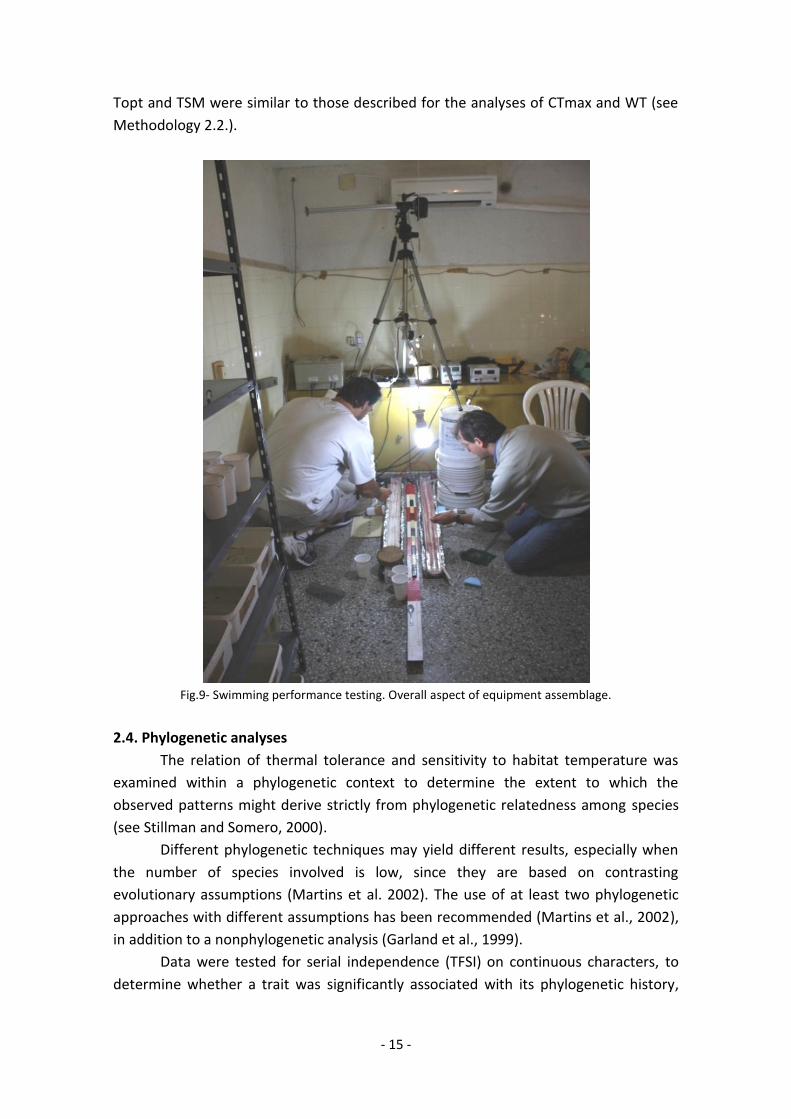
To determine maximum swimming speed, burst swimming of tadpoles was
estimated. Tadpoles were placed on a thermally controlled and opened cross section
methacrylate tube and gently prodded with a thin stick to stimulate swimming. Each
trial was recorded using a digital camera installed around 2 m above the tube (see
figure 9). Tadpoles were acclimated for at least 4 days at 20°C and 9-38 individuals per
species were tested (see table 5).
TPCs were defined using 6-7 temperatures within the natural range recorded in
the ponds (see Annexe I). For Argentinean species, the test temperatures were 20°,
24°, 28°, 32°, 35° and 38°C and for the Iberian species 10°, 15°, 20°, 24°, 28°, 32° and
35°C. Temperatures were randomized and tadpoles were tested on consecutive days,
one temperature per day. Prior to swimming, tadpoles were submitted for half an hour
to the test temperature.
Previous analysis with a Chacoan frog community (northern Argentina)
revealed that a few species could not tolerate acclimation at 20°C (some Leptodactilids
from the Cavicola group, Leptodactylus sp.). This situation matched the thermal
profiles measured in the ponds so temperatures lower than 20°C were considered to
be out of the natural thermal range for the subtropical Argentinean community. A
similar argument was used to select the maximum temperature tested for the Iberian
community.
Swimming recordings were analyzed with software Measurement in Motion
v3.1 (http://www.motion.com/products/measurement/index.html) that provided
tadpole swimming speed at each video recording frame.
After the swimming trials, all tested tadpoles were staged and wet weighed to
the nearest 0,001 g. Dorsal and lateral pictures were taken and digitized for
morphometric measurements of total length, head‐body length, head‐body height, tail
muscle height, total tail height, total tail area, tail muscle area, head‐body width, and
tail muscle width (see Dayton et al., 2005) to conduct further morphofunctional
analyses, not included in this thesis.
A simple Gaussian model was applied to the data (Angilletta, 2006) in order to
estimate optimum temperatures for swimming performance. Statistical analyses of
- 15 -
Topt and TSM were similar to those described for the analyses of CTmax and WT (see
Methodology 2.2.).
Fig.9- Swimming performance testing. Overall aspect of equipment assemblage.
2.4. Phylogenetic analyses
The relation of thermal tolerance and sensitivity to habitat temperature was
examined within a phylogenetic context to determine the extent to which the
observed patterns might derive strictly from phylogenetic relatedness among species
(see Stillman and Somero, 2000).
Different phylogenetic techniques may yield different results, especially when
the number of species involved is low, since they are based on contrasting
evolutionary assumptions (Martins et al. 2002). The use of at least two phylogenetic
approaches with different assumptions has been recommended (Martins et al., 2002),
in addition to a nonphylogenetic analysis (Garland et al., 1999).
Data were tested for serial independence (TFSI) on continuous characters, to
determine whether a trait was significantly associated with its phylogenetic history,
- 16 -
using the software Phylogenetic Independence v2.0 (Abouheif, 1999; see also
http://www.biology.mcgill.ca/faculty/abouheif/protocols.html).
Diagnosis was based on a measurement of the autocorrelation of each trait
across phylogeny, in the form of a C‐statistic, resulting from similarity between
adjacent phylogenetic observations. Topology and associated numerator distribution
were randomized 1,000 times and the C‐statistic was calculated for each randomized
topology to build the null hypothesis. Observed C‐statistic was compared to the
randomized distribution to calculate its level of significance.
If the former analyses revealed that examined traits (CTmax, Topt and Thab)
exhibited significant phylogenetic autocorrelation, the coevolution of all traits will
require a correction for phylogeny since data is not independent. In order to avoid this
bias, correlations between traits were obtained using the method of phylogenetically
independent contrasts (PIC) as described by Felsenstein (1985), with PDTREE module
(PDAP package by Midford et al., 2003) for Mesquite (v. 2.6) software (Maddison and
Maddison, 2009).
PIC is a method of correcting for phylogeny. It requires that both the tree
topology and the branch lengths are known, and that characters are allowed to be
modelled by Brownian motion on a linear scale. Given these conditions, the phylogeny
specifies a set of contrasts among species, contrasts that are statistically independent
and can be used in regression or correlation studies (Felsenstein, 1985).
Using independent contrasts, PDTREE also allows the estimation of ancestral
states (values at internal nodes or at any point along a branch) and their standard
errors (Garland et al., 1999). In most cases, PIC is mathematically and statistically
equivalent to generalized least-squares (GLS) models (Garland et al., 2005).
Previous works have used similar analysis to evaluate evolutionary trends
amongst traits in amphibians (see Gvozdik and van Damme, 2008, for an example with
European newts).
For these analyses, three phylogenetic trees were constructed based on Frost
et al (2006), including only the studied species: one for each community and one
combining all species from both communities (see Annexe II). All branch lengths were
set equal to one.
- 17 -
3. RESULTS
3.1. Monitoring environmental temperatures
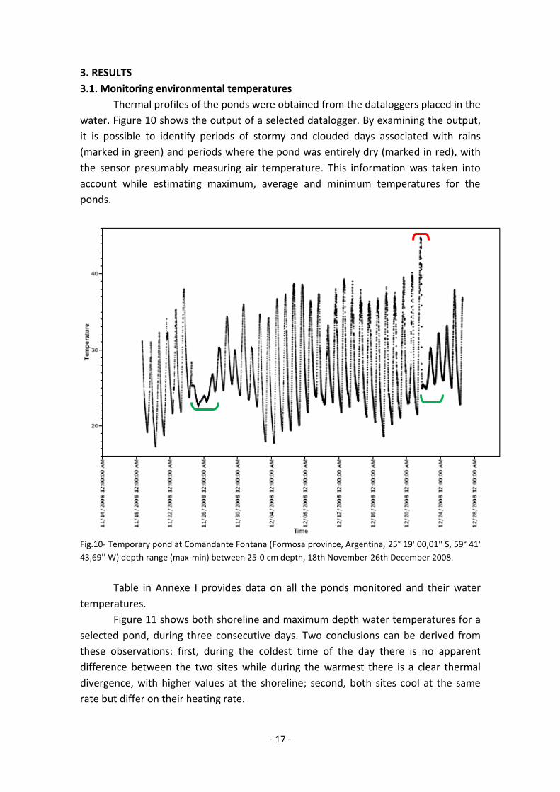
Thermal profiles of the ponds were obtained from the dataloggers placed in the
water. Figure 10 shows the output of a selected datalogger. By examining the output,
it is possible to identify periods of stormy and clouded days associated with rains
(marked in green) and periods where the pond was entirely dry (marked in red), with
the sensor presumably measuring air temperature. This information was taken into
account while estimating maximum, average and minimum temperatures for the
ponds.
Fig.10- Temporary pond at Comandante Fontana (Formosa province, Argentina, 25° 19' 00,01'' S, 59° 41'
43,69'' W) depth range (max‐min) between 25‐0 cm depth, 18th November‐26th December 2008.
Table in Annexe I provides data on all the ponds monitored and their water
temperatures.
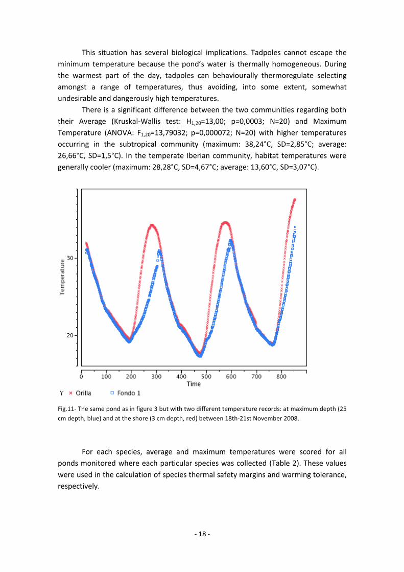
Figure 11 shows both shoreline and maximum depth water temperatures for a
selected pond, during three consecutive days. Two conclusions can be derived from
these observations: first, during the coldest time of the day there is no apparent
difference between the two sites while during the warmest there is a clear thermal
divergence, with higher values at the shoreline; second, both sites cool at the same
rate but differ on their heating rate.
- 18 -
This situation has several biological implications. Tadpoles cannot escape the
minimum temperature because the pond’s water is thermally homogeneous. During
the warmest part of the day, tadpoles can behaviourally thermoregulate selecting
amongst a range of temperatures, thus avoiding, into some extent, somewhat
undesirable and dangerously high temperatures.
There is a significant difference between the two communities regarding both
their Average (Kruskal-Wallis test: H1,20=13,00; p=0,0003; N=20) and Maximum
Temperature (ANOVA: F1,20=13,79032; p=0,000072; N=20) with higher temperatures
occurring in the subtropical community (maximum: 38,24°C, SD=2,85°C; average:
26,66°C, SD=1,5°C). In the temperate Iberian community, habitat temperatures were
generally cooler (maximum: 28,28°C, SD=4,67°C; average: 13,60°C, SD=3,07°C).
Fig.11- The same pond as in figure 3 but with two different temperature records: at maximum depth (25
cm depth, blue) and at the shore (3 cm depth, red) between 18th‐21st November 2008.
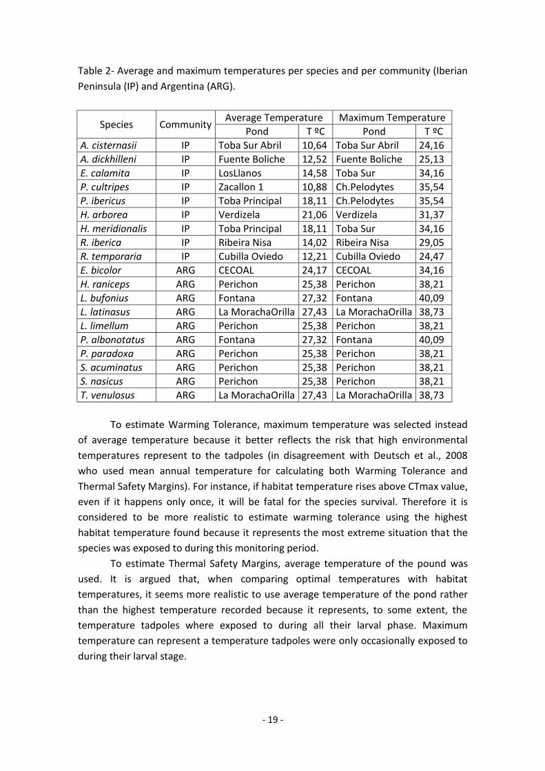
For each species, average and maximum temperatures were scored for all
ponds monitored where each particular species was collected (Table 2). These values
were used in the calculation of species thermal safety margins and warming tolerance,
respectively.
- 19 -
Table 2- Average and maximum temperatures per species and per community (Iberian
Peninsula (IP) and Argentina (ARG).
Species Community Average Temperature Maximum Temperature
Pond T ºC Pond T ºC
A. cisternasii IP Toba Sur Abril 10,64 Toba Sur Abril 24,16
A. dickhilleni IP Fuente Boliche 12,52 Fuente Boliche 25,13
E. calamita IP LosLlanos 14,58 Toba Sur 34,16
P. cultripes IP Zacallon 1 10,88 Ch.Pelodytes 35,54
P. ibericus IP Toba Principal 18,11 Ch.Pelodytes 35,54
H. arborea IP Verdizela 21,06 Verdizela 31,37
H. meridionalis IP Toba Principal 18,11 Toba Sur 34,16
R. iberica IP Ribeira Nisa 14,02 Ribeira Nisa 29,05
R. temporaria IP Cubilla Oviedo 12,21 Cubilla Oviedo 24,47
E. bicolor ARG CECOAL 24,17 CECOAL 34,16
H. raniceps ARG Perichon 25,38 Perichon 38,21
L. bufonius ARG Fontana 27,32 Fontana 40,09
L. latinasus ARG La MorachaOrilla 27,43 La MorachaOrilla 38,73
L. limellum ARG Perichon 25,38 Perichon 38,21
P. albonotatus ARG Fontana 27,32 Fontana 40,09
P. paradoxa ARG Perichon 25,38 Perichon 38,21
S. acuminatus ARG Perichon 25,38 Perichon 38,21
S. nasicus ARG Perichon 25,38 Perichon 38,21
T. venulosus ARG La MorachaOrilla 27,43 La MorachaOrilla 38,73
To estimate Warming Tolerance, maximum temperature was selected instead
of average temperature because it better reflects the risk that high environmental
temperatures represent to the tadpoles (in disagreement with Deutsch et al., 2008
who used mean annual temperature for calculating both Warming Tolerance and
Thermal Safety Margins). For instance, if habitat temperature rises above CTmax value,
even if it happens only once, it will be fatal for the species survival. Therefore it is
considered to be more realistic to estimate warming tolerance using the highest
habitat temperature found because it represents the most extreme situation that the
species was exposed to during this monitoring period.
To estimate Thermal Safety Margins, average temperature of the pound was
used. It is argued that, when comparing optimal temperatures with habitat
temperatures, it seems more realistic to use average temperature of the pond rather
than the highest temperature recorded because it represents, to some extent, the
temperature tadpoles where exposed to during all their larval phase. Maximum
temperature can represent a temperature tadpoles were only occasionally exposed to
during their larval stage.
- 20 -
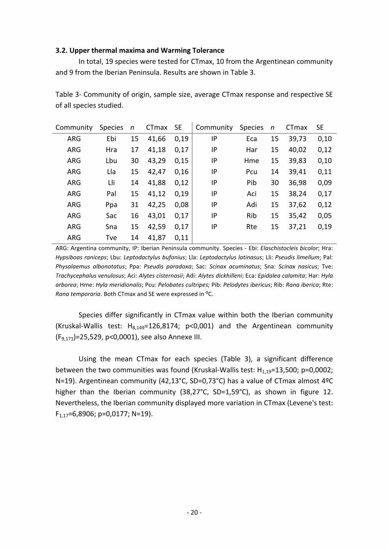
3.2. Upper thermal maxima and Warming Tolerance
In total, 19 species were tested for CTmax, 10 from the Argentinean community
and 9 from the Iberian Peninsula. Results are shown in Table 3.
Table 3- Community of origin, sample size, average CTmax response and respective SE
of all species studied.
Community Species n CTmax SE Community Species n CTmax SE
ARG Ebi 15 41,66 0,19 IP Eca 15 39,73 0,10
ARG Hra 17 41,18 0,17 IP Har 15 40,02 0,12
ARG Lbu 30 43,29 0,15 IP Hme 15 39,83 0,10
ARG Lla 15 42,47 0,16 IP Pcu 14 39,41 0,11
ARG Lli 14 41,88 0,12 IP Pib 30 36,98 0,09
ARG Pal 15 41,12 0,19 IP Aci 15 38,24 0,17
ARG Ppa 31 42,25 0,08 IP Adi 15 37,62 0,12
ARG Sac 16 43,01 0,17 IP Rib 15 35,42 0,05
ARG Sna 15 42,59 0,17 IP Rte 15 37,21 0,19
ARG Tve 14 41,87 0,11
ARG: Argentina community, IP: Iberian Peninsula community. Species - Ebi: Elaschistocleis bicolor; Hra:
Hypsiboas raniceps; Lbu: Leptodactylus bufonius; Lla: Leptodactylus latinasus; Lli: Pseudis limellum; Pal:
Physalaemus albonotatus; Ppa: Pseudis paradoxa; Sac: Scinax acuminatus; Sna: Scinax nasicus; Tve:
Trachycephalus venulosus; Aci: Alytes cisternasii; Adi: Alytes dickhilleni; Eca: Epidalea calamita; Har: Hyla
arborea; Hme: Hyla meridionalis; Pcu: Pelobates cultripes; Pib: Pelodytes ibericus; Rib: Rana iberica; Rte:
Rana temporaria. Both CTmax and SE were expressed in :C.
Species differ significantly in CTmax value within both the Iberian community
(Kruskal-Wallis test: H8,149=126,8174; p<0,001) and the Argentinean community
(F9,171)=25,529, p<0,0001), see also Annexe III.
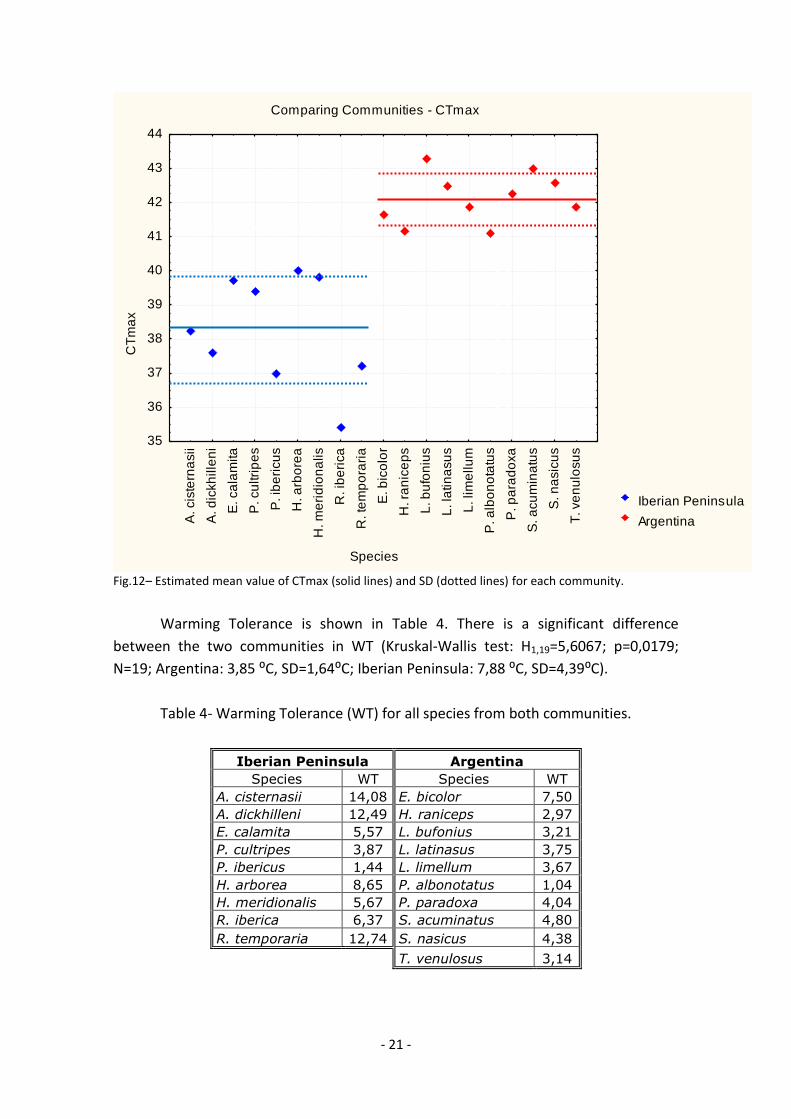
Using the mean CTmax for each species (Table 3), a significant difference
between the two communities was found (Kruskal-Wallis test: H1,19=13,500; p=0,0002;
N=19). Argentinean community (42,13°C, SD=0,73°C) has a value of CTmax almost 4ºC
higher than the Iberian community (38,27°C, SD=1,59°C), as shown in figure 12.
Nevertheless, the Iberian community displayed more variation in CTmax (Levene's test:
F1,17=6,8906; p=0,0177; N=19).
- 21 -
Comparing Communities - CTmax
Species
CT
ma
x
Iberian Peninsula
ArgentinaA. cis
tern
asii
A. d
ickh
ille
ni
E. ca
lam
ita
P. cu
ltri
pe
s
P. ib
eri
cu
s
H. a
rbo
rea
H. m
eri
dio
na
lis
R. ib
eri
ca
R. te
mp
ora
ria
E. b
ico
lor
H. ra
nic
ep
s
L. b
ufo
niu
s
L. la
tin
asu
s
L. lim
ellu
m
P. a
lbo
no
tatu
s
P. p
ara
do
xa
S. a
cu
min
atu
s
S. n
asic
us
T. ve
nu
losu
s
35
36
37
38
39
40
41
42
43
44
Fig.12– Estimated mean value of CTmax (solid lines) and SD (dotted lines) for each community.
Warming Tolerance is shown in Table 4. There is a significant difference
between the two communities in WT (Kruskal-Wallis test: H1,19=5,6067; p=0,0179;
N=19; Argentina: 3,85 :C, SD=1,64:C; Iberian Peninsula: 7,88 :C, SD=4,39:C).
Table 4- Warming Tolerance (WT) for all species from both communities.
Iberian Peninsula Argentina
Species WT Species WT
A. cisternasii 14,08 E. bicolor 7,50
A. dickhilleni 12,49 H. raniceps 2,97
E. calamita 5,57 L. bufonius 3,21
P. cultripes 3,87 L. latinasus 3,75
P. ibericus 1,44 L. limellum 3,67
H. arborea 8,65 P. albonotatus 1,04
H. meridionalis 5,67 P. paradoxa 4,04
R. iberica 6,37 S. acuminatus 4,80
R. temporaria 12,74 S. nasicus 4,38
T. venulosus 3,14
- 22 -
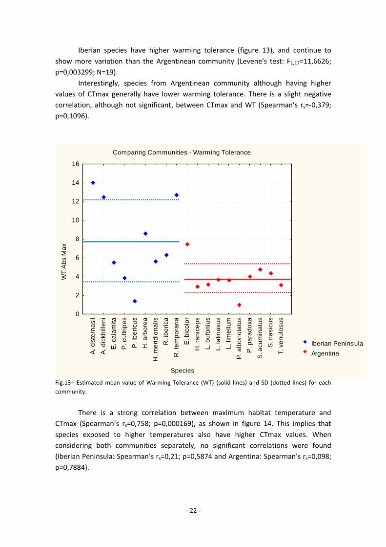
Iberian species have higher warming tolerance (figure 13), and continue to
show more variation than the Argentinean community (Levene's test: F1,17=11,6626;
p=0,003299; N=19).
Interestingly, species from Argentinean community although having higher
values of CTmax generally have lower warming tolerance. There is a slight negative
correlation, although not significant, between CTmax and WT (Spearman’s rs=-0,379;
p=0,1096).
Comparing Communities - Warming Tolerance
Species
WT
Ab
s M
ax
Iberian Peninsula
ArgentinaA. cis
tern
asii
A. d
ickh
ille
ni
E. ca
lam
ita
P. cu
ltri
pe
s
P. ib
eri
cu
s
H. a
rbo
rea
H. m
eri
dio
na
lis
R. ib
eri
ca
R. te
mp
ora
ria
E. b
ico
lor
H. ra
nic
ep
s
L. b
ufo
niu
s
L. la
tin
asu
s
L. lim
ellu
m
P. a
lbo
no
tatu
s
P. p
ara
do
xa
S. a
cu
min
atu
s
S. n
asic
us
T. ve
nu
losu
s
0
2
4
6
8
10
12
14
16
Fig.13– Estimated mean value of Warming Tolerance (WT) (solid lines) and SD (dotted lines) for each
community.
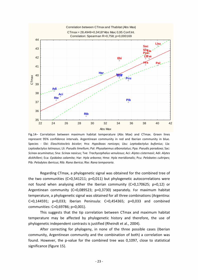
There is a strong correlation between maximum habitat temperature and
CTmax (Spearman’s rs=0,758; p=0,000169), as shown in figure 14. This implies that
species exposed to higher temperatures also have higher CTmax values. When
considering both communities separately, no significant correlations were found
(Iberian Peninsula: Spearman’s rs=0,21; p=0,5874 and Argentina: Spearman’s rs=0,098;
p=0,7884).
- 23 -
Correlation between CTmax and Thabitat (Abs Max)
CTmax = 28,4949+0,3418*Abs Max; 0,95 Conf.Int.
Correlation: Spearman R=0,758; p=0,000169
Adi
Aci
EcaPcu
Pib
HarHme
Rib
Rte
Ebi
Hra
Lbu
Lla
Lli
Pal
Ppa
Sac
Sna
Tve
22 24 26 28 30 32 34 36 38 40 42
Abs Max
35
36
37
38
39
40
41
42
43
44
CT
ma
x
Fig.14– Correlation between maximum habitat temperature (Abs Max) and CTmax. Green lines
represent 95% confidence intervals. Argentinean community in red and Iberian community in blue.
Species - Ebi: Elaschistocleis bicolor; Hra: Hypsiboas raniceps; Lbu: Leptodactylus bufonius; Lla:
Leptodactylus latinasus; Lli: Pseudis limellum; Pal: Physalaemus albonotatus; Ppa: Pseudis paradoxa; Sac:
Scinax acuminatus; Sna: Scinax nasicus; Tve: Trachycephalus venulosus; Aci: Alytes cisternasii; Adi: Alytes
dickhilleni; Eca: Epidalea calamita; Har: Hyla arborea; Hme: Hyla meridionalis; Pcu: Pelobates cultripes;
Pib: Pelodytes ibericus; Rib: Rana iberica; Rte: Rana temporaria.
Regarding CTmax, a phylogenetic signal was obtained for the combined tree of
the two communities (C=0,541211; p=0,011) but phylogenetic autocorrelations were
not found when analysing either the Iberian community (C=0,170625; p=0,12) or
Argentinean community (C=0,089523; p=0,3730) separately. For maximum habitat
temperature, a phylogenetic signal was obtained for all three combinations (Argentina:
C=0,144591; p=0,033; Iberian Peninsula: C=0,454365; p=0,033 and combined
communities: C=0,69786; p=0,001).
This suggests that the tip correlation between CTmax and maximum habitat
temperature may be affected by phylogenetic history and therefore, the use of
phylogenetic independent contrasts is justified (Rheindt et al., 2004).
After correcting for phylogeny, in none of the three possible cases (Iberian
community, Argentinean community and the combination of both) a correlation was
found. However, the p-value for the combined tree was 0,1097, close to statistical
significance (figure 15).

- 24 -
Fig.15– Plot of contrasts vs. positivized contrasts for combined tree for both Argentina and Iberian
Peninsula communities (CTmax, Thabitat). Number of contrasts: 18; Pearson Product-Moment
Correlation Coefficient: 0,379; Two tailed p-value: 0,10977; Regression lines through origin: Black is
ordinary least squares (OLS), Green is major axis (MA) and Red is reduced major axis.
3.3. Thermal sensitivity and Thermal Safety Margins In total, 18 species were tested for thermal sensitivity, 9 from the Argentinean
community and 9 from the Iberian Peninsula. Results are shown in Table 5.
Table 5- Community origin, sample size, estimated optimum temperature (Opt) and
temperature of highest performance (T) of all species studied.
Community Species n Opt T Community Species n Opt T
ARG Ebi 19 31,02 28 IP Eca 20 35,61 35
ARG Hra 18 36,14 35 IP Har 14 36,09 35
ARG LEP 9 38,04 35 IP Hme 15 37,64 35
ARG Lli 16 33,09 28 IP Pcu 20 37,98 35
ARG Pal 18 36,17 38 IP Pib 38 26,93 24
ARG Ppa 21 30,56 28 IP Aci 20 22,82 24
ARG Sac 19 35,81 38 IP Adi 19 23,00 24
ARG Sna 20 35,03 38 IP Rib 14 26,64 28
ARG Tve 20 39,09 38 IP Rte 14 23,70 24
ARG: Argentina community, IP: Iberian Peninsula community. Species - Ebi: Elaschistocleis bicolor; Hra:
Hypsiboas raniceps; LEP: Leptodactylus sp.; Lli: Pseudis limellum; Pal: Physalaemus albonotatus; Ppa:
Pseudis paradoxa; Sac: Scinax acuminatus; Sna: Scinax nasicus; Tve: Trachycephalus venulosus; Aci:
Alytes cisternasii; Adi: Alytes dickhilleni; Eca: Epidalea calamita; Har: Hyla arborea; Hme: Hyla
meridionalis; Pcu: Pelobates cultripes; Pib: Pelodytes ibericus; Rib: Rana iberica; Rte: Rana temporaria.
Both Topt and T are expressed in :C.

- 25 -
The symbol “T” shown in Table 5 refers to the treatment temperature at which
tadpoles had the best overall swimming performance and Topt is the estimated
optimum temperature (see also figure 16 and Annexe IV).
Alytes cisternasii
Vertical bars denote 0,95 confidence intervals
10 15 20 24 28 32
Temperature (ºC)
0,30
0,35
0,40
0,45
0,50
0,55
0,60
0,65
0,70
0,75
0,80
0,85
0,90
Sp
ee
d (
m/s
)
Fig.16–Swimming speed of Alytes cisternasii (blue), by treatment temperature. Best overall swimming
performance (red circle) and estimated Optimum temperature and performance curve (green circle and
line).
Optimum temperatures were higher in the Argentinean community, although
not statistically different from those of the Iberian Peninsula community (Kruskal-
Wallis test: H1,18=2,387914; p=0,1223; N=18; Argentina: 34,99:C, SD=2,93:C; Iberian
Peninsula: 30,05:C, SD=6,63:C), as shown in figure 17. Variance in optimum
temperature was higher for the Iberian community (Levene’s test: F1,16=22,12609;
p=0,000239; N=18).
If the comparison is made using T temperature (from Table 5), a significant
difference is found (Kruskal-Wallis test: H=4,421337; p=0,0355; N=18) which confirms
the tendency found in the previous test.
Interestingly, Iberian species Topt values can be differentiated into two groups:
a cool Topt group that encompases Alytes cisternasii, Alytes dickhilleni, Pelodytes
ibericus, Rana iberica and Rana temporaria; and a warm Topt group, containing
Epidalea calamita, Pelobates cultripes, Hyla arborea and Hyla meridionalis.
Covariate means:
Weight: 0,885 g
- 26 -
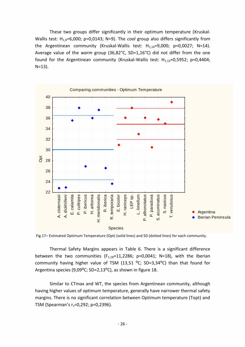
These two groups differ significantly in their optimum temperature (Kruskal-
Wallis test: H1,9=6,000; p=0,0143; N=9). The cool group also differs significantly from
the Argentinean community (Kruskal-Wallis test: H1,14=9,000; p=0,0027; N=14).
Average value of the warm group (36,82°C, SD=1,16°C) did not differ from the one
found for the Argentinean community (Kruskal-Wallis test: H1,13=0,5952; p=0,4404;
N=13).
Comparing communities - Optimum Temperature
Species
Op
t
Argentina
Iberian PeninsulaA. cis
tern
asii
A. d
ickh
ille
ni
E. ca
lam
ita
P. cu
ltri
pe
s
P. ib
eri
cu
s
H. a
rbo
rea
H. m
eri
dio
na
lis
R. ib
eri
ca
R. te
mp
ora
ria
E. b
ico
lor
H. ra
nic
ep
s
LE
P s
p.
L. lim
ellu
m
P. a
lbo
no
tatu
s
P. p
ara
do
xa
S. a
cu
min
atu
s
S. n
asic
us
T. ve
nu
losu
s
22
24
26
28
30
32
34
36
38
40
Fig.17– Estimated Optimum Temperature (Opt) (solid lines) and SD (dotted lines) for each community.
Thermal Safety Margins appears in Table 6. There is a significant difference
between the two communities (F1,18=11,2286; p=0,0041; N=18), with the Iberian
community having higher value of TSM (13,51 :C; SD=3,34:C) than that found for
Argentina species (9,09:C; SD=2,13:C), as shown in figure 18.
Similar to CTmax and WT, the species from Argentinean community, although
having higher values of optimum temperature, generally have narrower thermal safety
margins. There is no significant correlation between Optimum temperature (Topt) and
TSM (Spearman’s rs=0,292; p=0,2396).

- 27 -
Table 6- Thermal Safety Margins (TSM) for all species from both communities.
Iberian Peninsula Argentina
Species TSM Species TSM
A. cisternasii 12,18 E. bicolor 6,85
A. dickhilleni 10,48 H. raniceps 10,76
E. calamita 14,55 Leptodactylus sp. 10,72
P. cultripes 16,93 L. limellum 7,71
P. ibericus 8,82 P. albonotatus 8,85
H. arborea 15,03 P. paradoxa 5,18
H. meridionalis 19,53 S. acuminatus 10,43
R. iberica 12,62 S. nasicus 9,65
R. temporaria 11,49 T. venulosus 11,66
Comparing communities - Thermal Safety Margins (TSM)
Species
TS
M (
ca
lcu
late
d w
ith
Op
t)
Community: ARG
Community: IPA. cis
tern
asii
A. d
ickh
ille
ni
E. ca
lam
ita
P. cu
ltri
pe
s
P. ib
eri
cu
s
H. a
rbo
rea
H. m
eri
dio
na
lis
R. ib
eri
ca
R. te
mp
ora
ria
E. b
ico
lor
H. ra
nic
ep
s
LE
P s
p.
L. lim
ellu
m
P. a
lbo
no
tatu
s
P. p
ara
do
xa
S. a
cu
min
atu
s
S. n
asic
us
T. ve
nu
losu
s
4
6
8
10
12
14
16
18
20
22
Fig.18– Thermal Safety Margins (TSM) (solid lines) and SD (dotted lines) for each community, using
estimated optimum temperature.
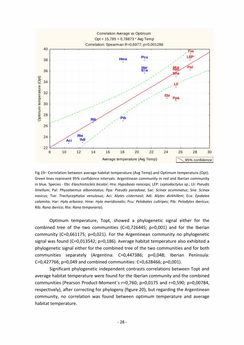
Average habitat temperature and optimum temperature exhibit a strong
correlation (Spearman’s rs=0,6977; p=0,001286, figure 19). This suggests that species
exposed to higher average temperatures have a higher optimum temperature.
Considering both communities separately, there was also a significant correlation
(Iberian Peninsula: Spearman’s rs=0,857; p=0,00314 and Argentina: Spearman’s rs
=0,853; p=0,00344).
- 28 -
Correlation Average vs Optimum
Opt = 15,785 + 0,78873 * Avg Temp
Correlation: Spearman R=0,6977; p=0,001286
Aci Adi
Eca
Pcu
Pib
Har
Hme
Rib
Rte
Ebi
Hra
LEP
Lli
Pal
Ppa
SacSna
Tve
8 10 12 14 16 18 20 22 24 26 28 30
Average temperature (Avg Temp)
22
24
26
28
30
32
34
36
38
40
Op
tim
um
te
mp
era
ture
(O
pt)
95% confidence
Fig.19– Correlation between average habitat temperature (Avg Temp) and Optimum temperature (Opt).
Green lines represent 95% confidence intervals. Argentinean community in red and Iberian community
in blue. Species - Ebi: Elaschistocleis bicolor; Hra: Hypsiboas raniceps; LEP: Leptodactylus sp.; Lli: Pseudis
limellum; Pal: Physalaemus albonotatus; Ppa: Pseudis paradoxa; Sac: Scinax acuminatus; Sna: Scinax
nasicus; Tve: Trachycephalus venulosus; Aci: Alytes cisternasii; Adi: Alytes dickhilleni; Eca: Epidalea
calamita; Har: Hyla arborea; Hme: Hyla meridionalis; Pcu: Pelobates cultripes; Pib: Pelodytes ibericus;
Rib: Rana iberica; Rte: Rana temporaria).
Optimum temperature, Topt, showed a phylogenetic signal either for the
combined tree of the two communities (C=0,726445; p=0,001) and for the Iberian
community (C=0,661175; p=0,021). For the Argentinean community no phylogenetic
signal was found (C=0,013542; p=0,186). Average habitat temperature also exhibited a
phylogenetic signal either for the combined tree of the two communities and for both
communities separately (Argentina: C=0,447386; p=0,048; Iberian Peninsula:
C=0,427766; p=0,049 and combined communities: C=0,628466; p=0,001).
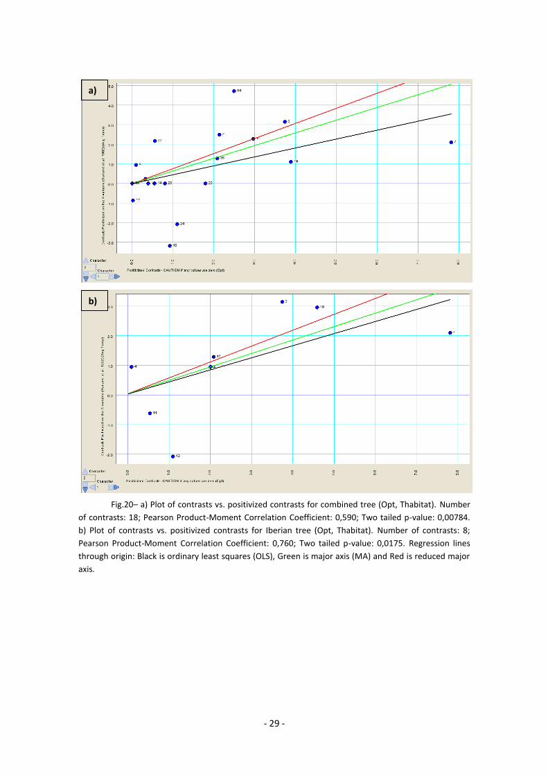
Significant phylogenetic independent contrasts correlations between Topt and
average habitat temperature were found for the Iberian community and the combined
communities (Pearson Product-Moment´s r=0,760; p=0,0175 and r=0,590; p=0,00784,
respectively), after correcting for phylogeny (figure 20), but regarding the Argentinean
community, no correlation was found between optimum temperature and average
habitat temperature.
- 29 -
Fig.20– a) Plot of contrasts vs. positivized contrasts for combined tree (Opt, Thabitat). Number
of contrasts: 18; Pearson Product-Moment Correlation Coefficient: 0,590; Two tailed p-value: 0,00784.
b) Plot of contrasts vs. positivized contrasts for Iberian tree (Opt, Thabitat). Number of contrasts: 8;
Pearson Product-Moment Correlation Coefficient: 0,760; Two tailed p-value: 0,0175. Regression lines
through origin: Black is ordinary least squares (OLS), Green is major axis (MA) and Red is reduced major
axis.
a)
b)

- 30 -
3.4. CTmax vs Optimum Temperature and Warming Tolerance vs Thermal Safety Margins
Following the previous results, CTmax and Optimum Temperature were tested
to see if there was any relation between these two characters. Leptodactylus bufonios
and Leptodactylus latinasus were considered to have the same optimum temperature,
also when calculating TSM.
Comparing CTmax and Optimum Temperature
Ctmax = 30,641 + 0,29453 * Opt est
Correlation: Spearman R=0,543; p=0,016233
Aci
Adi
EcaPcu
Pib
HarHme
Rib
Rte
Ebi
Hra
Lbu
Lla
Lli
Pal
Ppa
Sac
Sna
Tve
22 24 26 28 30 32 34 36 38 40
Optimum Temperature (Opt)
35
36
37
38
39
40
41
42
43
44
CT
ma
x
95% confidence
Fig.21– Correlation between Optimum Temperature (Opt) and CTmax. Argentinean community in red
and Iberian community in blue. Species - Ebi: Elaschistocleis bicolor; Hra: Hypsiboas raniceps; Lbu:
Leptodactylus bufonius; Lla: Leptodactylus latinasus; Lli: Pseudis limellum; Pal: Physalaemus albonotatus;
Ppa: Pseudis paradoxa; Sac: Scinax acuminatus; Sna: Scinax nasicus; Tve: Trachycephalus venulosus; Aci:
Alytes cisternasii; Adi: Alytes dickhilleni; Eca: Epidalea calamita; Har: Hyla arborea; Hme: Hyla
meridionalis; Pcu: Pelobates cultripes; Pib: Pelodytes ibericus; Rib: Rana iberica; Rte: Rana temporaria).
A significant tip correlation was found (Spearman’s rs=0,543; p=0,016233),
figure 21. This correlation suggests that a species with higher optimum temperature
also have higher CTmax. However, for both Argentinean and Iberian communities
separately, no correlation was found (Spearman’s R=0,061; p=0,8675 and R=0,567;
p=0,1116 respectively).
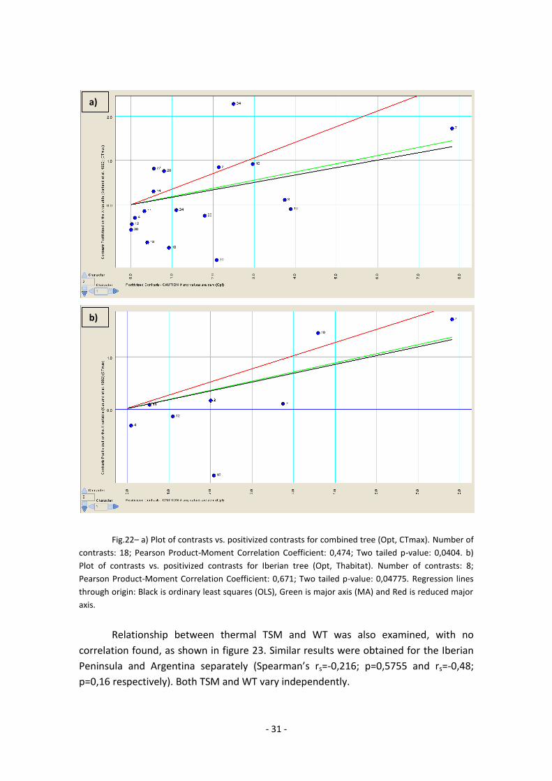
PIC correlations for both the Iberian community and the combined
communities were found to be significant (figure 22), whereas no correlation was
found between CTmax and optimum temperature for the Argentinean community.
- 31 -
Fig.22– a) Plot of contrasts vs. positivized contrasts for combined tree (Opt, CTmax). Number of
contrasts: 18; Pearson Product-Moment Correlation Coefficient: 0,474; Two tailed p-value: 0,0404. b)
Plot of contrasts vs. positivized contrasts for Iberian tree (Opt, Thabitat). Number of contrasts: 8;
Pearson Product-Moment Correlation Coefficient: 0,671; Two tailed p-value: 0,04775. Regression lines
through origin: Black is ordinary least squares (OLS), Green is major axis (MA) and Red is reduced major
axis.
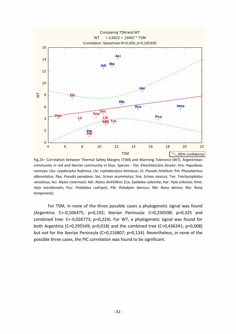
Relationship between thermal TSM and WT was also examined, with no
correlation found, as shown in figure 23. Similar results were obtained for the Iberian
Peninsula and Argentina separately (Spearman’s rs=-0,216; p=0,5755 and rs=-0,48;
p=0,16 respectively). Both TSM and WT vary independently.
a)
b)
- 32 -
Comparing TSM and WT
WT = 3,5622 + ,19467 * TSM
Correlation: Spearman R=0,450; p=0,165305
Aci
Adi
Eca
Pcu
Pib
Har
HmeRib
Rte
Ebi
HraLbuLlaLli
Pal
Ppa
SacSna
Tve
4 6 8 10 12 14 16 18 20 22
TSM
0
2
4
6
8
10
12
14
16
WT
95% confidence
Fig.23– Correlation between Thermal Safety Margins (TSM) and Warming Tolerance (WT). Argentinean
community in red and Iberian community in blue. Species - Ebi: Elaschistocleis bicolor; Hra: Hypsiboas
raniceps; Lbu: Lepdactylus bufonius; Lla: Leptodactylus latinasus; Lli: Pseudis limellum; Pal: Physalaemus
albonotatus; Ppa: Pseudis paradoxa; Sac: Scinax acuminatus; Sna: Scinax nasicus; Tve: Trachycephalus
venulosus; Aci: Alytes cisternasii; Adi: Alytes dickhilleni; Eca: Epidalea calamita; Har: Hyla arborea; Hme:
Hyla meridionalis; Pcu: Pelobates cultripes; Pib: Pelodytes ibericus; Rib: Rana iberica; Rte: Rana
temporaria).
For TSM, in none of the three possible cases a phylogenetic signal was found
(Argentina: C=-0,106475; p=0,192; Iberian Peninsula: C=0,250598; p=0,325 and
combined tree: C=-0,026773; p=0,224). For WT, a phylogenetic signal was found for
both Argentina (C=0,295549; p=0,018) and the combined tree (C=0,436341; p=0,008)
but not for the Iberian Peninsula (C=0,216807; p=0,134). Nevertheless, in none of the
possible three cases, the PIC correlation was found to be significant.
- 33 -
4. DISCUSSION
4.1. Thermal tolerance
CTmax values were clearly higher for the summer-breeding subtropical
Argentinean species than for the Iberian species, which breed at much cooler water
temperatures. This suggests the hypothesis that tolerance to heating may have
evolved through thermal selection.
Results also revealed that CTmax is correlated with maximum habitat
temperature at the tip level. Since both CTmax and Thab showed phylogenetic
autocorrelation, a phylogenetic control was mandatory (Rheindt et al. 2004). However,
the non-significant PIC correlation revealed that these traits have not coevolved.
Differences between species and contrast correlations are likely to be of biological
significance and, in this case, where traits are correlated and their phylogenetic
contrasts are not, it points at a correlated evolution only during an early adaptive
radiation in the history of a clade and not later (Price, 1997). Nevertheless, the p-
value’s proximity to statistical significance can be alternatively explained by a low
statistical power (type II error) since the addition of more species from the present
analysed communities, and also from Sweden, revealed that the PIC analysis’ outcome
exhibits a positive and highly significant p-value (H. Duarte, M. Tejedo and M.
Katzenberger, unpublished data).
Summarizing, maximal thermal tolerance limits reflected habitat conditions and
differences found in CTmax between communities and species should be more related
to local adaptation to habitat temperatures than to their phylogenetic history. Similar
results were found in crabs inhabiting temperate and tropical waters (Stillman and
Somero, 2000).
Janzen (1967) stated that it can be assumed that animals and plants are
evolutionarily adapted to, and/or have the ability to acclimate to, the temperatures
normally encountered in their temporal and geographic habitat (microhabitat). Since
environmental temperatures vary with latitude, traits that have evolved as adaptations
to habitat temperatures, such as CTmax, should also depend on latitude. This theory is
still controversial.
Previous works, such as Addo‐Bediako et al. (2000, on insects) and Ghalambor
et al. (2006, re-analysis of Brattstrom (1968) data set on amphibians) revealed no
geographical trend on thermal tolerance. However, our results tend to agree with
Snyder and Weathers (1975) re-analysis of Brattstrom (1968) data set which found a
significant decline in CTmax with increasing latitude, since CTmax values were higher
for Argentinean species than for Iberian species. Recent data from a Swedish
community of amphibians (around 60:N) indicate that these species exhibit the lowest
CTmax values when compared to both the Argentinean and the Iberian species (H.
Duarte, M. Tejedo and M. Katzenberger, unpublished data), thus supporting the
hypothesis that CTmax is negatively related to latitude.

- 34 -
4.2. Thermal sensitivity
When comparing both communities for their optimum temperature, no
significant differences were found, although the mean was higher for the subtropical
Argentine community. The lack of differences is the result of the high heterogeneity in
optimal thermal values for the Iberian species. Within the Iberian community, two
groups were found: one comprising species with cool optimum temperatures (Aci, Adi,
Rte, Rib and Pib) and a second group that displayed warmer optimal temperatures
(Eca, Hme, Har, Pcu) that did not differ from the values expressed in the subtropical
community.
These groups of Iberian species largely differ in their breeding phenology and
aquatic habitats. The cold species group includes species living at cool ponds
represented by both autumn-winter breeders (Aci, Pib) and species that breed either
at high mountains (Adi, Rte) or at cool streams (Rib). The high temperature group
included species that either develop at warm pond environments, with the breeding
season occurring at mid-late Winter or early Spring (Eca, Hme, Har) or that, although
breeding in Autumn or Winter, have a very long larval period reaching metamorphosis
at mid or late Spring and therefore exposed to higher temperatures (Pcu), (Ferrand de
Almeida et al., 2001; Malkmus, 2004; García-París et al., 2004).
Argentinean species included in this work breed during austral summer and
they all came from pond habitats around the same altitudinal level (despite being in
different regions). Rainfall is low (750-900 mm annually) and concentrated in a short
rainy season during the austral summer (Duellman, 1999), the period in which most of
the Chacoan amphibians breed (Cei, 1980). Chacoan wetlands inhabited by amphibians
include basically temporary ponds and low flooded rivers and streams. Therefore,
Argentinean breeding sites were less variable in thermal regimen than breeding
habitats from the Iberian Peninsula.
Our results indicate that habitat is acting as a selective force and species have
adapted their optimum temperature to cope with environmental temperatures. Both
Argentine and warm-breeders from the Iberian community have evolved a higher
thermal optimum. Species with lower optimum temperature values tend to have lower
TSM values. In the Iberian Peninsula, species with cool optimum temperatures (Aci,
Adi, Rte, Rib and Pib) might be more affected by rising temperatures than species with
warmer optimal temperatures (Eca, Hme, Har, Pcu). In the Argentinean community,
species with lower optimum temperature (e.g. Pseudis sp.) seem to be more
vulnerable to rising temperatures. In the future, community structure of the Iberian
Peninsula could change and be constituted only by average and warm optimum
temperatures species. Argentinean’s community structure could also change and only
be composed by warm optimum temperature species. To determine if this predicted
shifts in community structure, regarding hot-cold species, will also be accompanied by
changes in the proportions of specialist/generalist species still requires further
research.
- 35 -
It is still unclear whether there are cold optimum temperature species in the
subtropical Chacoan community. Recently, some additional results on CTmax and
habitat temperature have been reported for two species of Melanophryniscus sp.
(species not included in this work), winter stream-breeding species from Misiones
province, nearby the Grand Chaco region, in North Eastern Argentina, where rains are
distributed evenly throughout the year. Both species show much lower CTmax values
(M. krauczuki, 39,93°C and M. devincenzii, 39,16°C) and cooler environmental
temperature (around 18°C of average habitat temperature) than the studied Chacoan
summer-breeding species (mean 42,13:C) (F. Marangoni, unpublished data).
Optimum temperature is positively correlated with CTmax (this study and Huey,
2009) and with average habitat temperature (this study). These results are in
agreement with previous works which state that optimum temperature and CTmax are
likely to be co-adaptive traits (Huey and Bennett, 1987; Angilletta, 2009). Presumably,
Argentinean winter-breeding species may have lower values for optimum
temperature. If so, they should fall between the group of cold-breeding Iberian species
and the Argentinean summer-breeding species, regarding their CTmax and optimum
temperature values.
Assuming that cool breeders from the tropical areas have lower Topt, we can
expect more variation in Topt and CTmax in the tropics than our results with the
summer breeder species reveal. Independently of the community of origin, there
should be a strong influence of species breeding periods (seasonality) in both CTmax
and optimum temperature values. This would be consistent with theoretical
expectations (Janzen, 1967; Ghalambor et al., 2006) and with Deutsch et al. (2008)
results which consider seasonality a strong predictor of Warming Tolerance (WT) and
also of Thermal Safety Margins (TSM). Future research on these species could confirm
this suggestion.
4.3. Evaluating vulnerability to warming temperatures
Having a high value for CTmax or optimum temperature does not necessarily
reflect a high warming tolerance (WT) or broader thermal safety margins (TSM),
respectively. Argentinean species have higher CTmax values and higher optimum
temperature, in general, but they have lower WT and narrower TSM. This is due to the
already high environmental temperatures they experience. Nevertheless, groups of
species that differ in habitat and breeding phenology can have similar values of TSM
and WT (Huey et al, 2009) and phylogenetic signal was very weak for both WT and
TSM.
For evaluating species’ vulnerability to warming, the plot WT vs TSM (figure 23)
provides valuable information. Species with low WT and narrower (lower value) TSM
are expected to be more threatened than species with high WT, broader TSM or both.
- 36 -
All species from Argentina have WT lower than 8°C and TSM lower than 12°C. Only one
species from the Iberian Pensisula, Pelodytes ibericus, has values within this range.
Based on this information, subtropical taxa, or at least summer-breeding
subtropical species of amphibians (which includes most amphibian species from the
Chaco region), would be subjected to higher risk of extinction under a scenario of
rising temperatures in the upcoming years. This can also be true for species from all
seasonal lowlands of South America and possibly other tropical and subtropical species
of Africa and Australia, which breed during the wet season, in the austral Summer
(Cogger, 1983; Lambiris, 1989; Channing and Howell, 2006).
Whether global warming will also affect these species more negatively or not,
there is still limited information. Global warming is more than just rising temperatures;
it also implies deep changes in rainfall amount, expected to be reduced in large areas
of Central America, Mediterranean basin, South and Central Africa and Australia (IPCC,
2007a, b). Increase in temperature, and correlated raise in evapotranspiration, can be
accompanied by a reduction in the amount of rain determining shorter pond
hydroperiods. Therefore, the outcome pattern will be a strong reduction in pond
durability and thus species with long larval period or low developmental plasticity will
have to shift their breeding habitats to more permanent ones (see Newman, 1992;
Wells, 2007).
Although results may give a first idea of how changes in temperature will affect
these species, further information about traits with important relation to pond
duration is required. For instance, in many cases, the key question may be not what
temperature can species tolerate but how fast can they develop and metamorph to
escape from the water before ponds dry. This is true, for example, for species that
breed in temporary and ephemeral ponds.
Some species from Chaco that breed in ephemeral ponds (habitats with high
environmental temperatures) already have high development and growth rates.
Considering that temperatures will rise and pond duration may be reduced, what is
their physiological limit to their development and growth rates or, in other words,
what is the minimum amount of time required to reach metamorphosis and survive?
Larval amphibian growth and differentiation are largely dependent on
temperature (Smith-Gill and Berven, 1979). Size and time to metamorphosis are
considered fitness related traits and there is a strong selection on both. Size at
metamorphosis determines differential survival at the terrestrial stage and shorter
larval period in desiccating ponds may help to avoid catastrophic mortalities (Reques
and Tejedo, 1997; Altweeg and Reyer, 2003). Alternatively, selection may favour
phenotypic plasticity due to the heterogeneity of pond environments (Tejedo and
Reques, 1994; Laurila et al., 2006). The analysis of temperature‐induced plasticities in
development and growth rates is badly needed (see Kaplan and Phillips, 2006).
- 37 -
Species may be forced to change their breeding seasonality to be able to cope
with expected climate changes. In the Iberian Peninsula, species breeding in late Spring
may be forced to advance reproduction to early Spring or even to late winter,
depending on the extent of habitat changes, because their current breeding season
will be too hot and/or dry for them. The situation in tropical regions may be more
critical because wet season coincides with Summer. Opportunities for breeding will
occur on a much lesser regular basis than they currently occur. If they are able to shift
their reproductive season, or at least their reproductive habits (changing breeding
locations from ephemeral and temporary to permanent ponds), species may have
overlapping breeding periods which would mean high density of tadpoles on the
ponds, resulting in a stronger competition for resources and increased predation
pressure (more predators are found in permanent pond, e.g. Wellborn et al, 1996).
Another way of predicting what will happen is to understand what occurred in
similar periods of Earth’s history, when climate was warmer than it currently is. It
would be interesting to know what happened in the interglacial periods, during the
Pleistocene.
In the Eemian period (third interglacial period in Northern Europe), ranging
from around 130,000 to 114,000 years ago, temperatures were 3ºC to 5ºC higher than
they are today and it is the nearest time known that matches temperatures expected
for the next 100 or 200 years (Larsen, 2009). Mammalian fauna such as the Common
Hippopotamus (Hippopotamus amphibius, Linnaeus, 1758), a species whose current
distribution only embraces tropical reagions, reached as far as Northwestern and
Central Europe (van Kolfschoten, 2000). This raises the question: if there was tropical
fauna inhabiting modern temperate reagions during the interglacial periods, what
happened in the current tropical reagions during those periods? Unfortunately, there
is currently no sufficient information for the tropic regions to make predictions based
on paleontological records.
As mentioned, at a given time, Earth already had temperature values similar to
those predicted to be reached in the next 100 or 200 years. The magnitude of the
changes is really important but so is the time they take to occur. Species have the
capability of coping with changes through adaptive evolution, plasticity, migration (less
likely or even inexistent in most amphibians) and habitat niche shift (Parmesan, 2006).
Expected rate of current global warming can be too high for species to evolve
accordingly. Therefore, if neither the plasticity of important traits such as CTmax,
optimum temperature, development and growth rates or habitat niches shift cannot
buffer the effect of rising temperatures, species could be facing extinction during the
next couple of centuries. The biodiversity loss would be huge if tropical amphibian
species are confirmed to be more threatened than temperate species.
- 38 -
5. ACKNOWLEDGMENTS
I’m still giving my first steps in the scientific world and this thesis is one of
them. The whole process of gathering data and writing was a constant test to my
capability as a young scientist and this work allowed my skills as a researcher to
flourish while also learning new things. On a personal level, all the travelling I did to
accomplish this work and all the people I met along the way really helped me to get a
bigger picture of the world we all share. The possibility of meeting different people
and cultures, together with the passion and admiration for wildlife and the natural
world, makes my life meaningful and, in particular, made this thesis such an
enrichening experience.
For these reasons, I want to especially thank:
Miguel Tejedo, for the wonderful opportunity he presented when he accepted me as
his student and included me in this project. You have been a pleasure to work with
(bueno, entonces nada!).
Helder Duarte, for all the ideas, debates and comments and for all the work we
developed together. We are just at the beginning of the road, next stop PhD!
Federico Marangoni, who was always there when needed, for helping with sampling
and experiments and providing useful comments. Thank you for the unforgettable
asado we had on our last field day in the wilderness of Chaco, Argentina.
Juan José Neiff, for his cooperation and for offering us everything I could ask for to do
lab and field work, during my stay in Argentina.
Rui Rebelo, for providing good insight on my work and for helping with the
writing/correction process.
Mónica Costa, for her help on video analysis and data collection.
Juan Francisco Beltrán and Ricardo Reques, for their cooperation and support.
Alfredo Nicieza, Maribel Benítez and Manolo Chirosa, for helping with sampling.
Eduardo Schaefer, Rodrigo Cajade, Marta Duré and Arturo Kehr for their cooperation
and hospitality, while I was in Argentina.
At last but not the least, a very special thanks to Mili García, Lety Monzón and
all of Federico’s family for making me feel at home. You were my family when I could
not be with my own, especially during Christmas time. I will always treasure the
moments we spent together and I cannot wait to return to Argentina!
To all of my friends, thank you for your understanding and support. Life would
not be the same without you!
- 39 -
I also want to thank the following institutions that, in so many ways,
contributed to this work:
- 40 -
6. REFERENCES
Abouheif, E.; 1999. A method to test the assumption of phylogenetic independence in comparative data. Evolutionary Ecology Research, 1:895-909.
Addo‐Bediako, A. S.; Chown, S. L. and Gaston, K. J.; 2000. Thermal tolerance, climatic variability and latitude. Proceedings of the Royal Society of London, B 267:739–745.
Altwegg, R. and Reyer, H‐U.; 2003. Patterns of natural selection on size at metamorphosis in water frogs. Evolution, 57(4):872–882.
Alvarez, D. and Nicieza, A.; 2002. Effects of induced variation in anuran larval development on postmetamorphic energy reserves and locomotion. Oecologia, 131:186–195.
Angilletta, M.J.; 2009. Thermal adaptation: a theoretical and empirical synthesis. Oxford University Press.
Angilletta, M.J.Jr.; 2006. Estimating and comparing thermal performance curves. Journal of Thermal Biology, 31:541–545.
Bauwens, D.; Garland Jr.; T., Castilla, A.M. and Van Damme, R.; 1995. Evolution of sprint speed in lacertid lizards: morphological, physiological, and behavioral covariation. Evolution, 49:848–863.
Berrigan, D.; 2000. Correlations between measures of thermal stress resistance within and between species. Oikos, 89:301–304.
Bosch, J.; Carrascal, L.M.; Durán, L.; Walker, S. and Fisher, M.C.; 2007. Climate change and outbreaks of amphibian chytridiomycosis in a montane area of central Spain; is there a link? Proceedings of the Royal Society, B 274:53‐260.
Brattstrom, B.H.; 1959. The role of evaporative cooling as a thermoregulatory device in tropical amphibians. Year b. American Philosophical Society, 225–226.
Brattstrom, B.H.; 1962. A preliminary review of the thermal requirements of amphibians. Ecology, 44:238–255.
Brattstrom, B.H.; 1968. Thermal acclimation in anuran amphibians as a function of latitude and altitude. Comparative Biochemistry and Physiology, 24:93–111.
Brattstrom, B.H.; 1970. Thermal acclimation in Australian amphibians. Comparative Biochemestry and Physiology, 35:69–103.
Calosi, P.; Bilton, D.T. and Spicer, J.I.; 2008. Thermal tolerance, acclimatory capacity and vulnerability to global climate change. Biology Letters, 4:99‐102.
Case, T.J.; Holt, R.D.; McPeek, M.A. and Keitt, T.H.; 2005. The community context of species’ borders: ecological and evolutionary perspectives. Oikos 108:28‐46.
Cei, J.M.; 1980. Amphibians of Argentina. Monitore Zoologico Italiana (N.S.). 243 Monografia 2:1-609.
Channing, A. and Howell, K.M.; 2006. Amphibians of East Africa. Cornell University Press.
Chen, T.C.; Kam, C. and Lin, Y.S.; 2001. Thermal physiology and reproductive phenology of Buergeria japonica (Rhacophoridae) breeding in a stream and a geothermal hot spring in Taiwan. Zoological Science, 18:591–596.
Chown, S.L.; Jumbam, K.R.; Sørensen, J.G. and Terblanche, J.S.; 2009. Phenotypic variance, plasticity and heritability estimates of critical thermal limits depend on methodological context. Functional Ecology, 23:133–140.
Claussen, D.L.; Hopper, R.A. and Sanker, A.M.; 2000. The effects of temperature, body size, and hydration state on the terrestrial locomotion of the crayfish Orconectes rusticus. Journal of Crustacean Biology, 20(2):218–223.
Cogger, H.C.; 1983. Reptiles and Amphibians of Australia. Reed (3rdedition). Sydney. 660 pp.
Cooper, B.S.; Williams, B.H. and Angiletta, M.J. Jr.; 2008. Unifying indices of heat tolerance in ectotherms. Journal of Thermal Biology, 33:320–323.

- 41 -
Czajka, M.C. and Lee, R.E.; 1990. A rapid cold‐hardening response protecting against cold shock injury in Drosophila melanogaster. Journal of Experimental Biology, 148:245–254.
Dayton, G.H.; Saenz, D.; Baum, K.A.; Langerhans, R.B. and DeWitt, T.J.; 2005. Body shape, burst speed and escape behavior of larval anurans. Oikos, 111:582–591.
Delson, J. and Whitford, W.G.; 1973. Critical thermal maxima in several life history stages in desert and montane populations of Ambystoma tigrinum. Herpetology, 29:352–355.
Deutsch, C. A.; Tewksbury, J. J.; Huey, R. B.; Sheldon, K. S.; Ghalambor, C. K.; Haak, D.C. and Martin, P.R.; 2008. Impact of climate warming on terrestrial ectotherms across latitude. PNAS, 105: 6668–6672.
Duellman ,W.E.; 1999. Patterns of distribution of amphibians. A global perspective. Ed. Duellman, W.D. Baltimore: John Hopkins University Press.
Dunson, W.A.; Travis, J.; 1991. The role of abiotic factors in community organization. American Naturalist, 138:1067–1091.
Feder, M. E. and Lynch, J. F.; 1982. Effects of latitude, season, elevation, and microhabitat on field body temperatures of neotropical and temperate zone salamanders. Ecology, 63:1657–1664.
Feder, M. E.; 1983. The relation of air breathing and locomotion to predation on tadpoles, Rana berlandieri, by turtles. Physiological Zoology, 56:522–531.
Felsentein, J.; 1985. Phylogenies and the comparative method. American Naturalist, 125:1‐13.
Ferrand de Almeida, N.; Ferrand de Almeida, P.; Gonçalves, H.; Sequeira, F.; Teixeira, J. and Ferrand de Almeida, F.; 2001. Guia FAPAS Anfibios e Répteis de Portugal. FAPAS - Câmara Municipal de Porto. Porto.
Floyd, R.B.; 1983. Ontogenetic change in the temperature tolerance of larval Bufo marinus (Anura:Bufonidae). Comparative Biochemistry and Physiology, 75A:267‐271.
Frost, D.R.; Grant, T.; Faivovich, J.; Bain, R.H.; Haas, A.; Haddad, C.F.B.; de Sá, R.O.; Channing, A.; Wilkinson, M.; Donnellan, S.C.; Raxworthy, C.J.; Campbell, J.A.; Blottto, B.L.; Moler, P.; Drewes, R.C.; Nussbaum, R.A.; Lynch, J.D.; Green, D.M. and Wheeler, W.C.; 2006. The amphibian tree of life. Bulletin of the American Museum of Natural History. 297:1–291.
García-París, M; Montori, A. and Herrero, P.; 2004. Amphibia, Lissamphibia.In: Fauna Ibérica, vol. 24. Ramos et al. (Eds.). Museo Nacional de Ciencias Naturales. CSIC. Madrid. 640 pp.
Garland, T. and Adolph, S.C.; 1991. Physiological differentiation of vertebrate populations. Annual Review of Ecology and Systematic, 22:193– 228.
Garland, T.Jr.; Bennett, A.F.; and Rezende, E.L.; 2005. Phylogenetic approaches in comparative physiology. Journal of Experimental Biology, 208:3015-3035.
Garland, T.Jr.; Midford, P.E. and Ives, A.R.; 1999. An introduction to phylogenetically based statistical methods, with a new method for confidence intervals on ancestral states. American Zoologist, 39:374-388.
Ghalambor, C.; Huey, R.B.; Martin, P.R.; Tewksbury, J.J. and Wang, G; 2006. Are mountain passes higher in the tropics? Janzen’s hypothesis revisited. Integrative and Comparative Biology, 46:5‐17.
Gilman, S.E.; Wethey, D.S. and Helmuth, B.; 2006. Variation in the sensitivity of organismal body temperature to climate change over local and geographic scales. PNAS, 103:9560‐9565.
Gomes, F. R.; Bevier, C. and Navas, C. A.; 2002. Environmental and physiological factors influence antipredator behavior in Scinax hiemalis (Anura: Hylidae). Copeia, 2002(4):994‐1005.
Gomez‐Mestre, I. and Tejedo, M.; 2003. Local adaptation of an anuran amphibian to osmotically stressful environments. Evolution, 57: 1889–1899.
Gomez‐Mestre, I. and Tejedo, M.; 2004. Contrasting patterns of quantitative and neutral genetic variation in locally adapted populations of the natterjack toad, Bufo calamita. Evolution, 58:2343–2352.
- 42 -
Gosner, K.L.; 1960. A simplified table for staging anuran embryos and larvae with notes on identification. Herpetologica, 16:183–190.
Gvoždík, L. and Castilla, A.M.; 2001. A comparative study of preferred body temperatures and critical thermal tolerance limits among populations of Zootoca vivipara (Squamata: Lacertidae) along an altitudinal gradient. Journal of Herpetology, 35:486– 492.
Gvoždík, L. and Van Damme, R.; 2006. Triturus newts defy the running-swimming dilemma. Evolution, 60:2110–2121.
Heatwole, H.; Mercado, N. and Ortiz, E.; 1965. Comparison of critical thermal maxima of two species of Puerto Rican frogs of the genus Eleutherodactylus. Physiological Zoology. 38:1–8.
Hertz, P.E.; 1979. Sensitivity to high temperatures in three West Indian grass anoles (Sauria, Igaunidae), with a review of heat sensitivity in the genus Anolis. Comparative Biochemistry and Physiology, A 63:217–222.
Hillman, S.S.; Withers, P. C.; Drewes, R.C. and Hillyard, S.D.; 2009. Ecological and environmental physiology of amphibians. Oxford University Press.
Hochochka, P.W.; Somero, G.N.; 2002. Biochemical Adaptation. Oxford University Press, Oxford.
Hoffmann, A.A. and Parsons, P.A.; 1997. Extreme Environmental Change and Evolution. Cambridge University Press.
Hoffmann, A.A.; Hallas, R.J.; Dean, J.A. and Schiffer, M.; 2003. Low potential for climatic stress adaptation in a rainforest Drosophila species. Science, 301:100‐102.
Hoffmann, A.A.; Sørensen, J.G. and Loeschcke, V.; 2003. Adaptation of Drosophila to temperature extremes: bringing together quantitative and molecular approaches. Journal of Thermal Biology, 28:175‐216.
Hoppe, D.M.; 1978. Thermal tolerance in tadpoles of the chorus frog Pseudacris triseriata. Herpetologica, 34:318– 321.
Huang, S‐P. and Tu, M‐C.; 2008. Heat tolerance and altitudinal distribution of a mountainous lizard Takydromus hsuehshanensis, in Taiwan. Journal of Thermal Biology, 33:48‐56.
Huey, R.B. and Bennett, A.F.; 1987. Phylogenetic studies of coadaptation: preferred temperatures versus optimal performance temperatures of lizards. Evolution, 41:1098–1115.
Huey, R.B. and Hertz, P.E.; 1984. Is a jack‐of‐all‐temperatures a master of none? Evolution, 38:441–444.
Huey, R.B. and Kingsolver, J.G.; 1989. Evolution of thermal sensitivity of ectotherm performance. Trends in Ecology and Evolution, 4:131–135.
Huey, R.B. and Slatkin, M.; 1976. Cost and benefits of lizard thermoregulation. The Quarterly Review of Biology. 51:363–384.
Huey, R.B. and Stevenson, R.D.; 1979. Integrating physiology and ecology of ectotherms: a discussion of approaches. American Zoologist, 19:357–366.
Huey, R.B.; 1974. Behavioral thermoregulation in lizards: importance of associated cost. Science, 184:1001–1003.
Huey, R.B.; Crill, W.D.; Kingsolver, J.G. and Weber, K.E.; 1992. A method for rapid measurement of heat or cold resistance of small insects. Functional Ecology, 6:489–494.
Huey, R.B.; Deutsch, C.A.; Tewksbury, J.J.; Vitt, L.J.; Hertz, P.E.; Álvarez Pérez, H.J. and Garland, Jr, T.; 2009. Why tropical forest lizards are vulnerable to climate warming. Proceeding of The Royal Society B Biological Sciences, 276:1939-1948.
Husak, J.F.; 2006. Does speed help you survive? A test with collared lizards of different ages. Functional Ecology, 20:174–179.
Hutchison, V.H. and Dupré, R.K.; 1992. Thermoregulation. In: Ferder, M.E., Burggren, W.M. (Eds.), Environmental Physiology of the Amphibians. The University of Chicago Press, Chicago, pp. 206‐249.
Hutchison, V.H.; 1961. Critical thermal maxima in salamanders. Physiological Zoology, 34:92–125.
- 43 -
IPCC; 2007a. Intergovernmental Panel on Climate Change (IPCC), Climate Change 2007: The Physical Science Basis. Working Group I Contribution to the Fourth Assessment.
IPCC; 2007b. Climate Change 2007: Synthesis Report. S. Solomon et al., Eds. (Cambridge University Press, Cambridge, 2007).
IUCN, 2006. Conservation International and NatureServe. Global Amphibian Assessment.
Janzen, D. H.; 1967. Why mountain passes are higher in the tropics? American Naturalist, 101:233–249.
Jayne, B.C. and Bennett, A.F.; 1990. Selection on locomotor performance capacity in a natural population of garter snakes. Evolution, 44:1204–1229.
Jensen, M.; 2003. Consensus on Ecological Impacts Remains Elusive. Science, 299:38.
Kaplan, R.H. and Phillips, P.C.; 2006. Ecological and developmental context of natural selection: Maternal effects and thermally induced plasticity in the frog Bombina orientalis. Evolution, 60:142-156.
Lambiris, A.J.L.; 1989. Monografia X – The Frogs of Zimbabwe. Museo Regionale di Scienze Naturali. Torino. 248 pp.
Larsen, L.B.; 2009. In: Lewis Smith - Scientists drill deep into Greenland ice for global warming clues from Eemian Period. The Times.
http://www.timesonline.co.uk/tol/news/environment/article5955880.ece
Laurila, A; Pakkasmaa, S. and Merilä, J.; 2006. Population divergence in growth rate and antipredator defences in Rana arvalis. Oecologia, 147:585‐595.
Le Galliard, J.‐F.; Clobert, J. and Ferrière, R.; 2004. Physical performance and darwinian fitness in lizards. Nature, 432:502–505.
Levins, R.; 1968. Evolution in Changing Environments. Princeton University Press, Princeton, NJ.
Levins, R.; 1969. Thermal acclimation and heat resistance in Drosophila species. American Naturalist, 103:483–499.
Lillywhite, H.B.; 1970. Behavioral temperature regulation in the bullfrog, Rana catesbeiana. Copeia, 158–168.
Lips, K.R.; Brem, F.; Brenes, R.; Reeve, J.D.; Alford, R.A.; Voyles, J.; Carey, C.; Livo, L.; Pessier, A.P. and Collins, J.P.; 2006. Emerging infectious disease and the loss of biodiversity in a Neotropical amphibian community. PNAS, 103:3165‐3170.
Lutterschmidt, W.I. and Hutchison, V.H.; 1997. The critical thermal maximum: history and critique. Canadian Journal of Zoology, 75:1561–1574.
Maddison, W.P. and Maddison, D.R.; 2009. Mesquite: A modular system for evolutionary analysis. Version 2.6. http://mesquiteproject.org.
Mahoney, J.J. and Hutchison, V.H.; 1969. Photoperiod acclimation and 24‐hour variations on the critical thermal maxima of a tropical and a temperate frog. Oecologia, 2:143–161.
Malkmus, R.; 2004. Amphibians and Reptiles of Portugal, Madeira and the Azores Archipelago – distribution and natural history notes. A.R.G. Gantner Verlag K.G..
Martins, E.P.; Diniz-Filho, J.A.F. and Housworth ,E.A.; 2002. Adaptive constraints and the phylogenetic comparative method: a computer simulation test. Evolution, 56:1–13.
Marvin, G.A.; 2003a. Effects of acute temperature and thermal acclimation on aquatic and terrestrial locomotor performance of the three‐lined salamander, Eurycea guttolineata. Journal of Thermal Biology, 28:251–259.
Marvin, G.A.; 2003b. Aquatic and terrestrial locomotor performance in a semiaquatic plethodontid salamander (Pseudotriton ruber): influence of acute temperature, thermal acclimation, and body size. Copeia, 2003: 704–713.
Meffe, G.K.; Weeks, S.C.; Mulvey, M. and Kandl, K.L.; 1995. Genetic differences in thermal tolerance of eastern mosquitofish (Gambusia holbrooki; Poeciliidae) from ambient and thermal ponds. Canadian Journal of Fisheries and Aquatic Sciences, 52:2704– 2711.
Midford, P. E., Garland Jr. T. and Maddison, W.P.; 2003. PDAP Package.
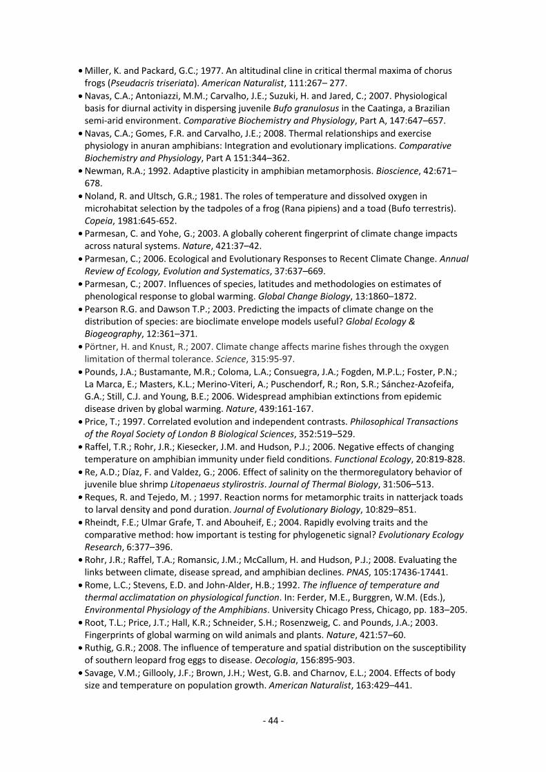
- 44 -
Miller, K. and Packard, G.C.; 1977. An altitudinal cline in critical thermal maxima of chorus frogs (Pseudacris triseriata). American Naturalist, 111:267– 277.
Navas, C.A.; Antoniazzi, M.M.; Carvalho, J.E.; Suzuki, H. and Jared, C.; 2007. Physiological basis for diurnal activity in dispersing juvenile Bufo granulosus in the Caatinga, a Brazilian semi-arid environment. Comparative Biochemistry and Physiology, Part A, 147:647–657.
Navas, C.A.; Gomes, F.R. and Carvalho, J.E.; 2008. Thermal relationships and exercise physiology in anuran amphibians: Integration and evolutionary implications. Comparative Biochemistry and Physiology, Part A 151:344–362.
Newman, R.A.; 1992. Adaptive plasticity in amphibian metamorphosis. Bioscience, 42:671–678.
Noland, R. and Ultsch, G.R.; 1981. The roles of temperature and dissolved oxygen in microhabitat selection by the tadpoles of a frog (Rana pipiens) and a toad (Bufo terrestris). Copeia, 1981:645‐652.
Parmesan, C. and Yohe, G.; 2003. A globally coherent fingerprint of climate change impacts across natural systems. Nature, 421:37–42.
Parmesan, C.; 2006. Ecological and Evolutionary Responses to Recent Climate Change. Annual Review of Ecology, Evolution and Systematics, 37:637–669.
Parmesan, C.; 2007. Influences of species, latitudes and methodologies on estimates of phenological response to global warming. Global Change Biology, 13:1860–1872.
Pearson R.G. and Dawson T.P.; 2003. Predicting the impacts of climate change on the distribution of species: are bioclimate envelope models useful? Global Ecology & Biogeography, 12:361–371.
Pörtner, H. and Knust, R.; 2007. Climate change affects marine fishes through the oxygen limitation of thermal tolerance. Science, 315:95‐97.
Pounds, J.A.; Bustamante, M.R.; Coloma, L.A.; Consuegra, J.A.; Fogden, M.P.L.; Foster, P.N.; La Marca, E.; Masters, K.L.; Merino‐Viteri, A.; Puschendorf, R.; Ron, S.R.; Sánchez‐Azofeifa, G.A.; Still, C.J. and Young, B.E.; 2006. Widespread amphibian extinctions from epidemic disease driven by global warming. Nature, 439:161‐167.
Price, T.; 1997. Correlated evolution and independent contrasts. Philosophical Transactions of the Royal Society of London B Biological Sciences, 352:519–529.
Raffel, T.R.; Rohr, J.R.; Kiesecker, J.M. and Hudson, P.J.; 2006. Negative effects of changing temperature on amphibian immunity under field conditions. Functional Ecology, 20:819‐828.
Re, A.D.; Díaz, F. and Valdez, G.; 2006. Effect of salinity on the thermoregulatory behavior of juvenile blue shrimp Litopenaeus stylirostris. Journal of Thermal Biology, 31:506–513.
Reques, R. and Tejedo, M. ; 1997. Reaction norms for metamorphic traits in natterjack toads to larval density and pond duration. Journal of Evolutionary Biology, 10:829–851.
Rheindt, F.E.; Ulmar Grafe, T. and Abouheif, E.; 2004. Rapidly evolving traits and the comparative method: how important is testing for phylogenetic signal? Evolutionary Ecology Research, 6:377–396.
Rohr, J.R.; Raffel, T.A.; Romansic, J.M.; McCallum, H. and Hudson, P.J.; 2008. Evaluating the links between climate, disease spread, and amphibian declines. PNAS, 105:17436‐17441.
Rome, L.C.; Stevens, E.D. and John‐Alder, H.B.; 1992. The influence of temperature and thermal acclimatation on physiological function. In: Ferder, M.E., Burggren, W.M. (Eds.), Environmental Physiology of the Amphibians. University Chicago Press, Chicago, pp. 183–205.
Root, T.L.; Price, J.T.; Hall, K.R.; Schneider, S.H.; Rosenzweig, C. and Pounds, J.A.; 2003. Fingerprints of global warming on wild animals and plants. Nature, 421:57–60.
Ruthig, G.R.; 2008. The influence of temperature and spatial distribution on the susceptibility of southern leopard frog eggs to disease. Oecologia, 156:895‐903.
Savage, V.M.; Gillooly, J.F.; Brown, J.H.; West, G.B. and Charnov, E.L.; 2004. Effects of body size and temperature on population growth. American Naturalist, 163:429–441.
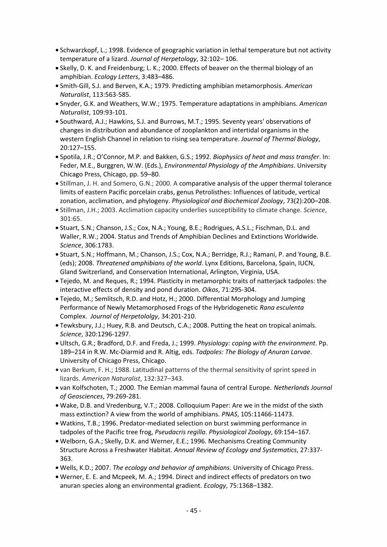
- 45 -
Schwarzkopf, L.; 1998. Evidence of geographic variation in lethal temperature but not activity temperature of a lizard. Journal of Herpetology, 32:102– 106.
Skelly, D. K. and Freidenburg; L. K.; 2000. Effects of beaver on the thermal biology of an amphibian. Ecology Letters, 3:483–486.
Smith-Gill, S.J. and Berven, K.A.; 1979. Predicting amphibian metamorphosis. American Naturalist, 113:563-585.
Snyder, G.K. and Weathers, W.W.; 1975. Temperature adaptations in amphibians. American Naturalist, 109:93-101.
Southward, A.J.; Hawkins, S.J. and Burrows, M.T.; 1995. Seventy years' observations of changes in distribution and abundance of zooplankton and intertidal organisms in the western English Channel in relation to rising sea temperature. Journal of Thermal Biology, 20:127–155.
Spotila, J.R.; O’Connor, M.P. and Bakken, G.S.; 1992. Biophysics of heat and mass transfer. In: Feder, M.E., Burggren, W.W. (Eds.), Environmental Physiology of the Amphibians. University Chicago Press, Chicago, pp. 59–80.
Stillman, J. H. and Somero, G.N.; 2000. A comparative analysis of the upper thermal tolerance limits of eastern Pacific porcelain crabs, genus Petrolisthes: Influences of latitude, vertical zonation, acclimation, and phylogeny. Physiological and Biochemical Zoology, 73(2):200–208.
Stillman, J.H.; 2003. Acclimation capacity underlies susceptibility to climate change. Science, 301:65.
Stuart, S.N.; Chanson, J.S.; Cox, N.A.; Young, B.E.; Rodrigues, A.S.L.; Fischman, D.L. and Waller, R.W.; 2004. Status and Trends of Amphibian Declines and Extinctions Worldwide. Science, 306:1783.
Stuart, S.N.; Hoffmann, M.; Chanson, J.S.; Cox, N.A.; Berridge, R.J.; Ramani, P. and Young, B.E. (eds); 2008. Threatened amphibians of the world. Lynx Editions, Barcelona, Spain, IUCN, Gland Switzerland, and Conservation International, Arlington, Virginia, USA.
Tejedo, M. and Reques, R.; 1994. Plasticity in metamorphic traits of natterjack tadpoles: the interactive effects of density and pond duration. Oikos, 71:295‐304.
Tejedo, M.; Semlitsch, R.D. and Hotz, H.; 2000. Differential Morphology and Jumping Performance of Newly Metamorphosed Frogs of the Hybridogenetic Rana esculenta Complex. Journal of Herpetololgy, 34:201‐210.
Tewksbury, J.J.; Huey, R.B. and Deutsch, C.A.; 2008. Putting the heat on tropical animals. Science, 320:1296‐1297.
Ultsch, G.R.; Bradford, D.F. and Freda, J.; 1999. Physiology: coping with the environment. Pp. 189–214 in R.W. Mc‐Diarmid and R. Altig, eds. Tadpoles: The Biology of Anuran Larvae. University of Chicago Press, Chicago.
van Berkum, F. H.; 1988. Latitudinal patterns of the thermal sensitivity of sprint speed in lizards. American Naturalist, 132:327–343.
van Kolfschoten, T.; 2000. The Eemian mammal fauna of central Europe. Netherlands Journal of Geosciences, 79:269-281.
Wake, D.B. and Vredenburg, V.T.; 2008. Colloquium Paper: Are we in the midst of the sixth mass extinction? A view from the world of amphibians. PNAS, 105:11466‐11473.
Watkins, T.B.; 1996. Predator‐mediated selection on burst swimming performance in tadpoles of the Pacific tree frog, Pseudacris regilla. Physiological Zoology, 69:154–167.
Welborn, G.A.; Skelly, D.K. and Werner, E.E.; 1996. Mechanisms Creating Community Structure Across a Freshwater Habitat. Annual Review of Ecology and Systematics, 27:337-363.
Wells, K.D.; 2007. The ecology and behavior of amphibians. University of Chicago Press.
Werner, E. E. and Mcpeek, M. A.; 1994. Direct and indirect effects of predators on two anuran species along an environmental gradient. Ecology, 75:1368–1382.
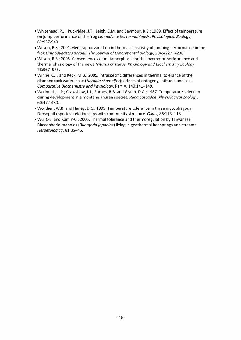
- 46 -
Whitehead, P.J.; Puckridge, J.T.; Leigh, C.M. and Seymour, R.S.; 1989. Effect of temperature on jump performance of the frog Limnodynastes tasmaniensis. Physiological Zoology, 62:937‐949.
Wilson, R.S.; 2001. Geographic variation in thermal sensitivity of jumping performance in the frog Limnodynastes peronii. The Journal of Experimental Biology, 204:4227–4236.
Wilson, R.S.; 2005. Consequences of metamorphosis for the locomotor performance and thermal physiology of the newt Triturus cristatus. Physiology and Biochemistry Zoology, 78:967–975.
Winne, C.T. and Keck, M.B.; 2005. Intraspecific differences in thermal tolerance of the diamondback watersnake (Nerodia rhombifer): effects of ontogeny, latitude, and sex. Comparative Biochemistry and Physiology, Part A, 140:141–149.
Wollmuth, L.P.; Crawshaw, L.I.; Forbes, R.B. and Grahn, D.A.; 1987. Temperature selection during development in a montane anuran species, Rana cascadae. Physiological Zoology, 60:472‐480.
Worthen, W.B. and Haney, D.C.; 1999. Temperature tolerance in three mycophagous Drosophila species: relationships with community structure. Oikos, 86:113–118.
Wu, C‐S. and Kam Y‐C.; 2005. Thermal tolerance and thermoregulation by Taiwanese Rhacophorid tadpoles (Buergeria japonica) living in geothermal hot springs and streams. Herpetologica, 61:35–46.
- 47 -
7.ANNEXES
Annexe I. Monitored ponds
Information about monitored ponds, including measured temperatures and number of
days sampled.
Pond Days Maximum Overall
Mean Minimum
Abs Mean Abs Mean
1. CH. PELODYTES CENTRO 98 35,54 17,45 12,42 4,73 9,20
2. LOS LLANOS 80 28,36 21,05 14,58 5,04 9,86
3. RIBEIRA NISA 43 29,05 16,92 14,02 10,26 12,23
4. TOBA SUR ABRIL 138 24,16 13,05 10,64 1,44 8,68
5. TOBA SUR 176 34,16 16,18 13,45 1,44 11,30
6. TOBA PRINCIPAL 12 31,98 25,99 18,11 9,97 12,25
7. VERDIZELA 8 31,37 28,94 21,06 13,27 14,60
8. ZACALLON 1 191 33,74 12,80 10,88 2,09 9,28
9. ZACALLON 2 223 23,97 13,08 11,84 2,84 10,76
10. POZO DE LA NIEVE 92 21,90 14,92 10,28 0,00 6,93
11. FUENTE BOLICHE 345 25,13 13,62 12,52 2,33 11,43
12. COLOR CUNETA OVIEDO 200 23,84 16,39 14,76 6,84 13,58
13. CUBILLA OVIEDO 120 24,47 15,62 12,21 3,32 9,31
14. CECOAL 13 34,16 30,13 24,17 18,05 20,37
15. DERMATONOTUS FRAGA 7 41,36 37,21 27,69 21,29 23,22
16. FONTANA 34 40,09 35,01 27,32 17,23 21,98
17. LA MORACHA ORILLA 3 38,73 35,96 27,43 19,84 21,52
18. LA MORACHA CENTRO 14 34,60 30,66 26,14 15,08 22,41
19. LEPIDOBATRACHUS 19 40,57 33,90 28,51 20,32 24,73
20. PERICHON 46 38,21 32,10 25,38 12,49 21,75
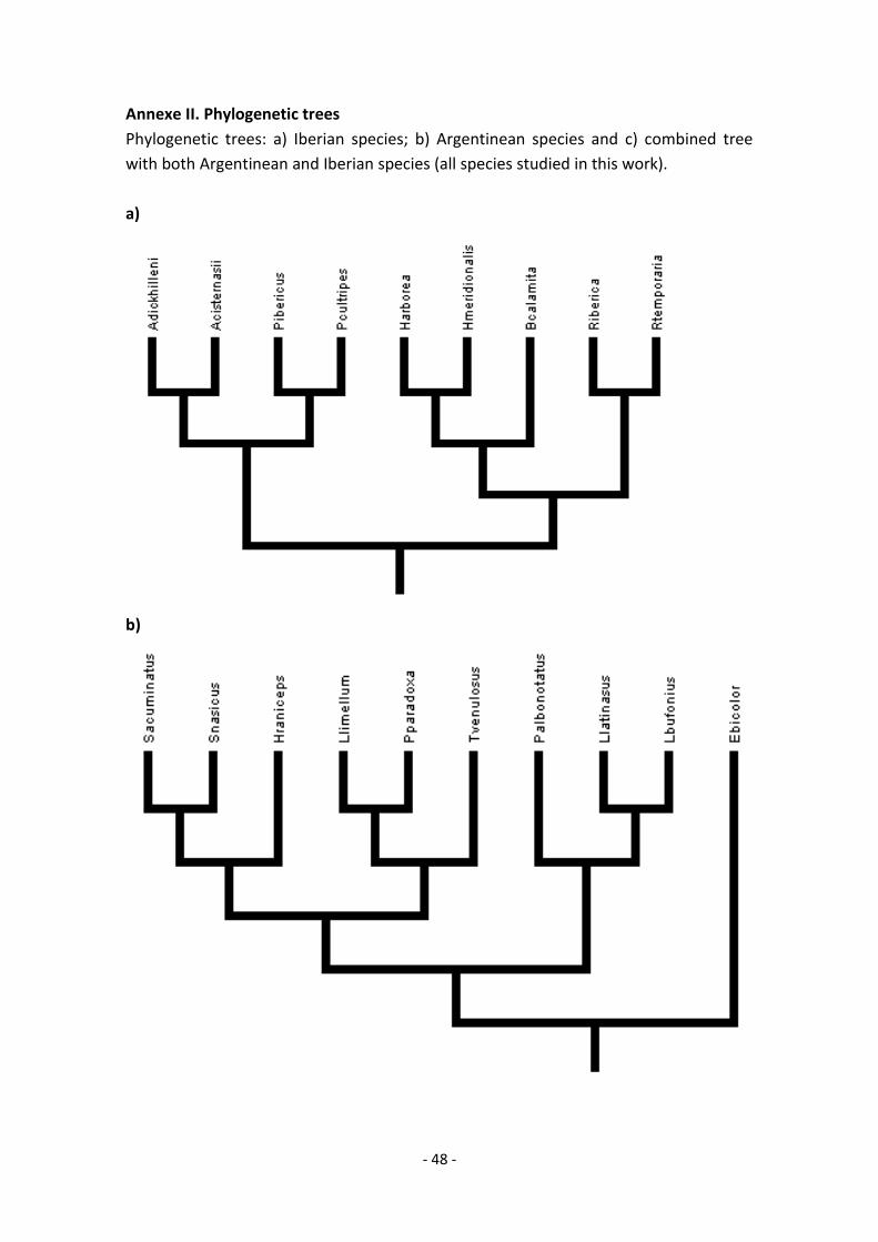
- 48 -
Annexe II. Phylogenetic trees
Phylogenetic trees: a) Iberian species; b) Argentinean species and c) combined tree
with both Argentinean and Iberian species (all species studied in this work).
a)
b)
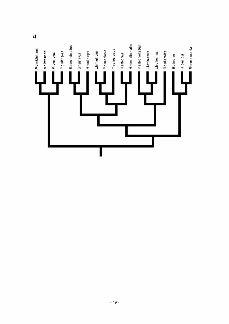
- 49 -
c)
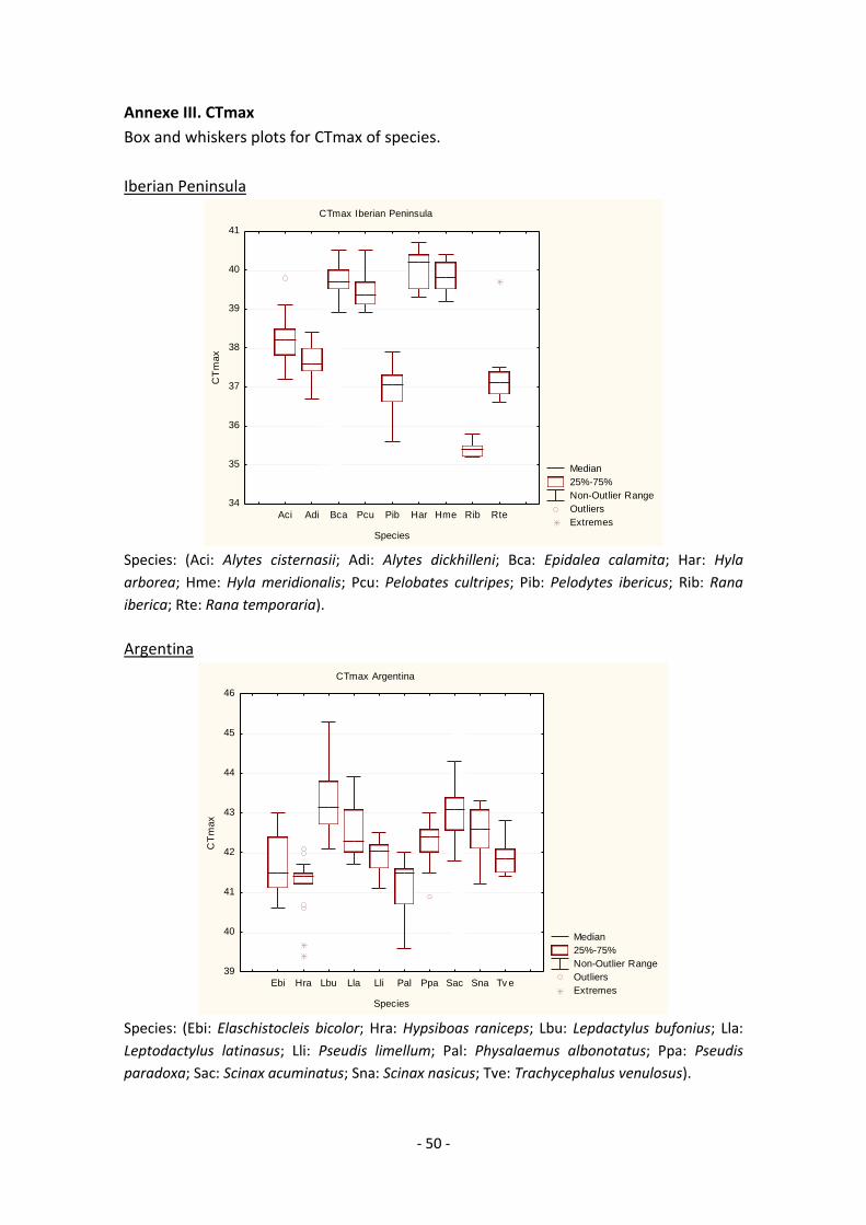
- 50 -
Annexe III. CTmax
Box and whiskers plots for CTmax of species.
Iberian Peninsula
CTmax Iberian Peninsula
Median
25%-75%
Non-Outlier Range
Outliers
ExtremesAci Adi Bca Pcu Pib Har Hme Rib Rte
Species
34
35
36
37
38
39
40
41
CT
max
Species: (Aci: Alytes cisternasii; Adi: Alytes dickhilleni; Bca: Epidalea calamita; Har: Hyla
arborea; Hme: Hyla meridionalis; Pcu: Pelobates cultripes; Pib: Pelodytes ibericus; Rib: Rana
iberica; Rte: Rana temporaria).
Argentina
CTmax Argentina
Median
25%-75%
Non-Outlier Range
Outliers
ExtremesEbi Hra Lbu Lla Lli Pal Ppa Sac Sna Tv e
Species
39
40
41
42
43
44
45
46
CT
ma
x
Species: (Ebi: Elaschistocleis bicolor; Hra: Hypsiboas raniceps; Lbu: Lepdactylus bufonius; Lla:
Leptodactylus latinasus; Lli: Pseudis limellum; Pal: Physalaemus albonotatus; Ppa: Pseudis
paradoxa; Sac: Scinax acuminatus; Sna: Scinax nasicus; Tve: Trachycephalus venulosus).
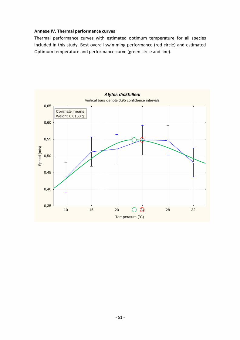
- 51 -
Annexe IV. Thermal performance curves
Thermal performance curves with estimated optimum temperature for all species
included in this study. Best overall swimming performance (red circle) and estimated
Optimum temperature and performance curve (green circle and line).
Alytes dickhilleni
Vertical bars denote 0,95 confidence intervals
10 15 20 24 28 32
Temperature (ºC)
0,35
0,40
0,45
0,50
0,55
0,60
0,65
Sp
ee
d (
m/s
)
Covariate means:
Weight: 0,6153 g
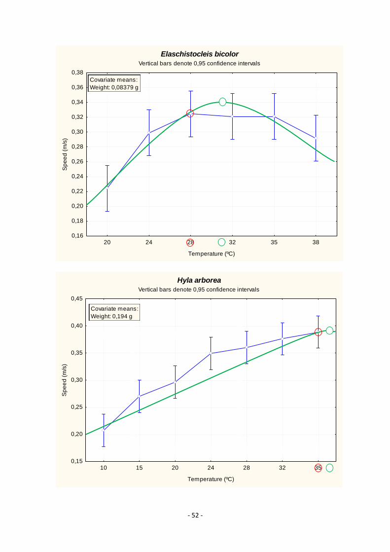
- 52 -
Elaschistocleis bicolor
Vertical bars denote 0,95 confidence intervals
20 24 28 32 35 38
Temperature (ºC)
0,16
0,18
0,20
0,22
0,24
0,26
0,28
0,30
0,32
0,34
0,36
0,38
Sp
ee
d (
m/s
)
Covariate means:
Weight: 0,08379 g
Hyla arborea
Vertical bars denote 0,95 confidence intervals
10 15 20 24 28 32 35
Temperature (ºC)
0,15
0,20
0,25
0,30
0,35
0,40
0,45
Sp
ee
d (
m/s
)
Covariate means:
Weight: 0,194 g
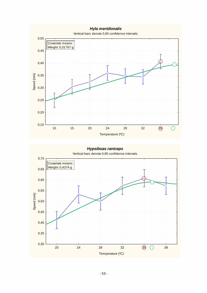
- 53 -
Hyla meridionalis
Vertical bars denote 0,95 confidence intervals
10 15 20 24 28 32 35
Temperature (ºC)
0,15
0,20
0,25
0,30
0,35
0,40
0,45
0,50
Sp
ee
d (
m/s
)
Covariate means:
Weight: 0,31767 g
Hypsiboas raniceps
Vertical bars denote 0,95 confidence intervals
20 24 28 32 35 38
Temperature (ºC)
0,30
0,35
0,40
0,45
0,50
0,55
0,60
0,65
0,70
Sp
ee
d (
m/s
)
Covariate means:
Weight: 0,4374 g
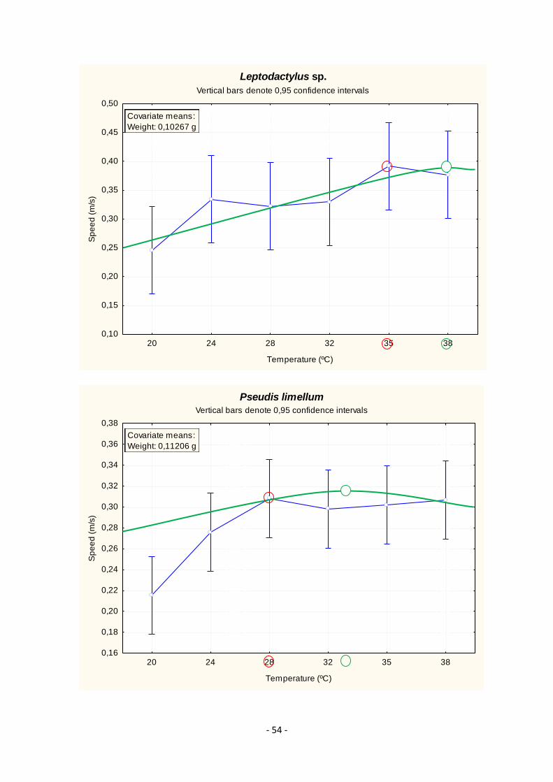
- 54 -
Leptodactylus sp.
Vertical bars denote 0,95 confidence intervals
20 24 28 32 35 38
Temperature (ºC)
0,10
0,15
0,20
0,25
0,30
0,35
0,40
0,45
0,50
Sp
ee
d (
m/s
)
Covariate means:
Weight: 0,10267 g
Pseudis limellum
Vertical bars denote 0,95 confidence intervals
20 24 28 32 35 38
Temperature (ºC)
0,16
0,18
0,20
0,22
0,24
0,26
0,28
0,30
0,32
0,34
0,36
0,38
Sp
ee
d (
m/s
)
Covariate means:
Weight: 0,11206 g
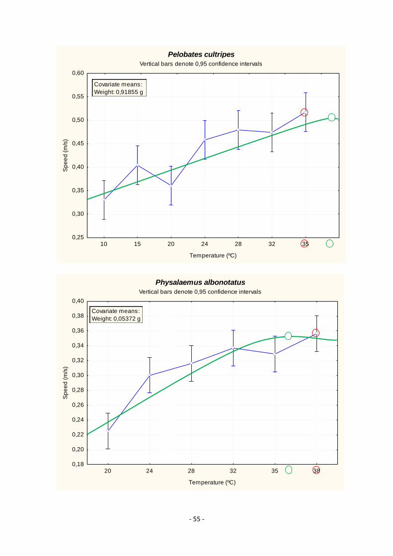
- 55 -
Pelobates cultripes
Vertical bars denote 0,95 confidence intervals
10 15 20 24 28 32 35
Temperature (ºC)
0,25
0,30
0,35
0,40
0,45
0,50
0,55
0,60
Sp
ee
d (
m/s
)
Covariate means:
Weight: 0,91855 g
Physalaemus albonotatus
Vertical bars denote 0,95 confidence intervals
20 24 28 32 35 38
Temperature (ºC)
0,18
0,20
0,22
0,24
0,26
0,28
0,30
0,32
0,34
0,36
0,38
0,40
Sp
ee
d (
m/s
)
Covariate means:
Weight: 0,05372 g
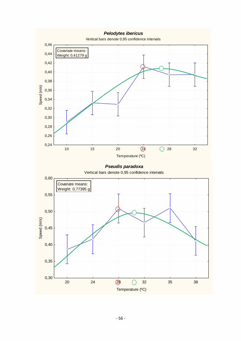
- 56 -
Pelodytes ibericus
Vertical bars denote 0,95 confidence intervals
10 15 20 24 28 32
Temperature (ºC)
0,24
0,26
0,28
0,30
0,32
0,34
0,36
0,38
0,40
0,42
0,44
0,46
Sp
ee
d (
m/s
)
Covariate means:
Weight: 0,41279 g
Pseudis paradoxa
Vertical bars denote 0,95 confidence intervals
20 24 28 32 35 38
Temperature (ºC)
0,30
0,35
0,40
0,45
0,50
0,55
0,60
Speed (
m/s
)
Covariate means:
Weight: 0,77395 g

- 57 -
Rana iberica
Vertical bars denote 0,95 confidence intervals
10 15 20 24 28 32
Temperature (ºC)
0,25
0,30
0,35
0,40
0,45
0,50
0,55
0,60
0,65
Sp
ee
d (
m/s
)
Covariate means:
Weight: 0,27857 g
Rana temporaria
Vertical bars denote 0,95 confidence intervals
10 15 20 24 28 32 35
Temperature (ºC)
0,16
0,18
0,20
0,22
0,24
0,26
0,28
0,30
0,32
0,34
0,36
Sp
ee
d (
m/s
)
Covariate means:
Weight: 0,21093 g
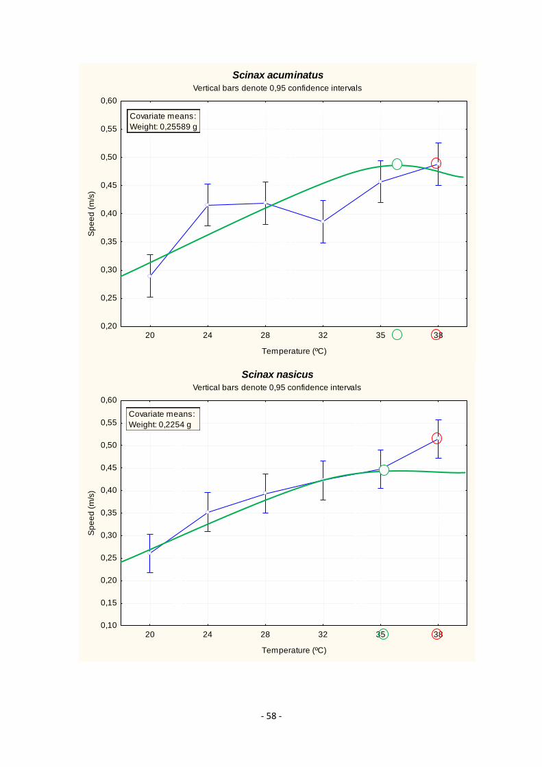
- 58 -
Scinax acuminatus
Vertical bars denote 0,95 confidence intervals
20 24 28 32 35 38
Temperature (ºC)
0,20
0,25
0,30
0,35
0,40
0,45
0,50
0,55
0,60
Sp
ee
d (
m/s
)
Covariate means:
Weight: 0,25589 g
Scinax nasicus
Vertical bars denote 0,95 confidence intervals
20 24 28 32 35 38
Temperature (ºC)
0,10
0,15
0,20
0,25
0,30
0,35
0,40
0,45
0,50
0,55
0,60
Sp
ee
d (
m/s
)
Covariate means:
Weight: 0,2254 g
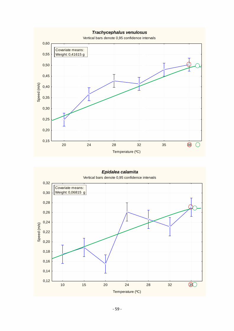
- 59 -
Trachycephalus venulosus
Vertical bars denote 0,95 confidence intervals
20 24 28 32 35 38
Temperature (ºC)
0,15
0,20
0,25
0,30
0,35
0,40
0,45
0,50
0,55
0,60
Sp
ee
d (
m/s
)
Covariate means:
Weight: 0,41615 g
Epidalea calamita
Vertical bars denote 0,95 confidence intervals
10 15 20 24 28 32 35
Temperature (ºC)
0,12
0,14
0,16
0,18
0,20
0,22
0,24
0,26
0,28
0,30
0,32
Sp
ee
d (
m/s
)
Covariate means:
Weight: 0,06815 g