Thermische Ermüdung - Werkstoffmodellierung

Thermal Fatigue – Materials Modeling

D. Siegele (1), J. Fingerhuth (1), M. Mrovec (1), X. Schuler (2), S. Utz (2), M. Fischaleck (3), A. Scholz (3), M. Oechsner (3), M. Vormwald (4), K. Bauerbach (4),

T. Schlitzer (4), J. Rudolph (5), A. Willuweit (5)

(1) Fraunhofer Institut für Werkstoffmechanik (IWM), Freiburg (2) MPA Universität Stuttgart

(3) Institut für Werkstoffkunde (IfW), TU Darmstadt (4) Institut für Stahlbau und Werkstoffmechanik (IFSW), TU Darmstadt

(5) AREVA NP GmbH, Erlangen

38th MPA-Seminar October 1 and 2, 2012 in Stuttgart

106

Abstract

In the framework of the ongoing joint research project “Thermal Fatigue - Basics of the system-, outflow- and material-characteristics of piping under thermal fatigue“

funded by the German Federal Ministry of Education and Research (BMBF) fundamental numerical and experimental investigations on the material behavior under transient thermal-mechanical stress conditions (high cycle fatigue – HCF and low cycle fatigue - LCF) are carried out. The primary objective of the research is the further development of simulation methods applied in safety evaluations of nuclear power plant components. In this context the modeling of crack initiation and growth inside the material structure induced by varying thermal loads are of particular interest. Therefore, three scientific working groups organized in three sub-projects of the joint research project are dealing with numerical modeling and simulation at different levels ranging from atomistic to micromechanics and continuum mechanics, and in addition corresponding experimental data for the validation of the numerical results and identification of the parameters of the associated material models are provided.

The present contribution is focused on the development and experimental validation of material models and methods to characterize the damage evolution and the life cycle assessment as a result of thermal cyclic loading. The individual purposes of the subprojects are as following:

Material characterization, Influence of temperature and surface roughness on fatigue endurances, biaxial thermo-mechanical behavior, experiments on structural behavior of cruciform specimens and scatter band analysis (IfW Darmstadt)

Life cycle assessment with micromechanical material models (MPA Stuttgart)

Life cycle assessment with atomistic and damage-mechanical material models associated with material tests under thermal fatigue (Fraunhofer IWM, Freiburg)

Simulation of fatigue crack growth, opening and closure of a short crack under thermal cyclic loading conditions, developing methods for the damage assessment based on the cyclic J-integral (IFSW Darmstadt, AREVA)

Further development of plasticity models (IFSW Darmstadt, AREVA)

Within this paper the various investigations and the main results are presented.

107

1 Introduction

Thermal loads are of significant relevance in the assessment of most components of nuclear or conventional power plants. Thermal loads are present for instance at start-up or shutdown, operational loading conditions such as typical spray events or at emergency cooling conditions as well as in case of stratification of fluids (e.g. feedwater nozzle of steam generator in PWR) or steam in pipings or thermal fluctuation due to fluid mixing. In any case, the thermal loading can produce high local stresses with the possibility of material damage or initiation of postulated defects.

Further applications of thermally loaded components are the integrity assessment of reactor pressure vessels under loss of coolant accident (LOCA) conditions or the leak-before-break (LBB) assessment of pipings under combined thermal stratification and internal pressure. In general, such assessments are performed under the assumption of thermal loads as primary loads and without consideration of the influence of the loading history on the crack initiation behavior.

A general refinement of the calculation and evaluation methods constitutes the focus of this contribution.

2 Material characterization, Influence of temperature and surface roughness on fatigue endurances, biaxial thermo-mechanical behavior, experiments on structural behavior of cruciform specimens and scatter band analysis

2.1 Pre-characterization

For the materials characterization, multiple heats of material of the type X6 CrNiNb 18-10 were available to the Institut für Werkstoffkunde (Institute for Material Science). Heat 1 and Heat 2 were processed from the same melt to various semi-finished products. Heat 1 is present in the form of round stock with a diameter of 15 mm. Heat 2 is a sheet metal of the thickness t=20 mm measuring 2000 x 1000 mm. This was hot rolled. Charge 3 is present as round stock with a diameter of 106 mm. The chemical composition was analyzed by means of optical spark emission spectrometry (OES) and tested for conformity to KTA 3201.1[1].

108

Table 2.1: Chemical composition of the heats in the project

C Si Mn P S Co Cr Mo Nb Ni Ti

KTA 3201.1

min - - - - - - 17 - 10xC 9 -

max. 0.04 1 2 0.04 0.02 0.2 19 - 0.65 12 -

Heats 1 & 2 <0.01 0.27 1.6 0.01 <0.01 0.02 18.5 <0.01 0.39 11.1 <0.01

Heat 3 0.03 0.35 2 0.02 <0.01 0.03 18.1 0.07 0.46 9.91 <0.01

In the quasi-static tensile tests, the mechanical-technological characteristic values show significant differences between Heat 3 in contrast to Heats 1 and 2. This may be due to the presence of increased processing forces during production of the semi-finished material. In preliminary tests, an altered cyclic behavior was also evident. It was possible, however, to neutralize this effect for the most part through a repeated solution annealing at 1050°C for 2 hours. Further preliminary tests have shown that similar behavior was established in the context of a narrow scatterband.

2.2 Cyclic Behavior

The characterization of the material X6 CrNiNb 18-10 essentially consists of several logically self-contained partial test programs. The test temperatures are derived from temperature ranges typical for nuclear facilities. Ambient temperature (AT, German RT), symbolizes the cold power station status and/or cooling and emergency systems. 200°C corresponds to a typical warm-start temperature, and 350°C to the maximum operating temperature of pressurized water reactors plus a 10-15% safety margin. At each temperature, polished, grinded and rough specimens were examined.

Test procedures were oriented to ASME practice. To this end, specimens described as relatively small (d < 10 mm) with a polished surface were used. Without exception, the experiments were conducted under strain control. Tests with polished surface were documented at low cycle 3 times, at high cycle 1 to 3 times. Low cycle (εA > 0.3%) was tested at constant test speed (dε/dt = 0.1 1/s); high cycle, at constant test frequency (2Hz). Tests for influence of various test speeds had shown no effects on the strain rate in the range of 0.1 1/s to 2.15 1/s. Incipient crack frequency and tension level differed in the context of the usual scattering; special tendencies could not be determined.

109

2.3 Behavior of the Ambient Temperature

The material X6 CrNiNb 18-10 belongs to the category of the austenites. Both the classification in the Schäffler-diagram as well as metallographic sections evidence an austenitic microstructure which is traversed in a linear fashion with 3-5% δ-ferrite (see Figure 2.1).

Figure 2.1: Illustration of longitudinal section with ferrite lines in typical austenitic basic matrix with polygonal grains and strong twinning tendency

Figure 2.2: Overview of results from the ambient temperature experiments on cylindrical specimens with polished surface in strain tests; up to 0.3% at constant test speed, below this value at constant test frequency 2Hz

Stra

in ra

nge

e

l,

pl,

g

es, [

%]

Cycles to failure N [-]

110

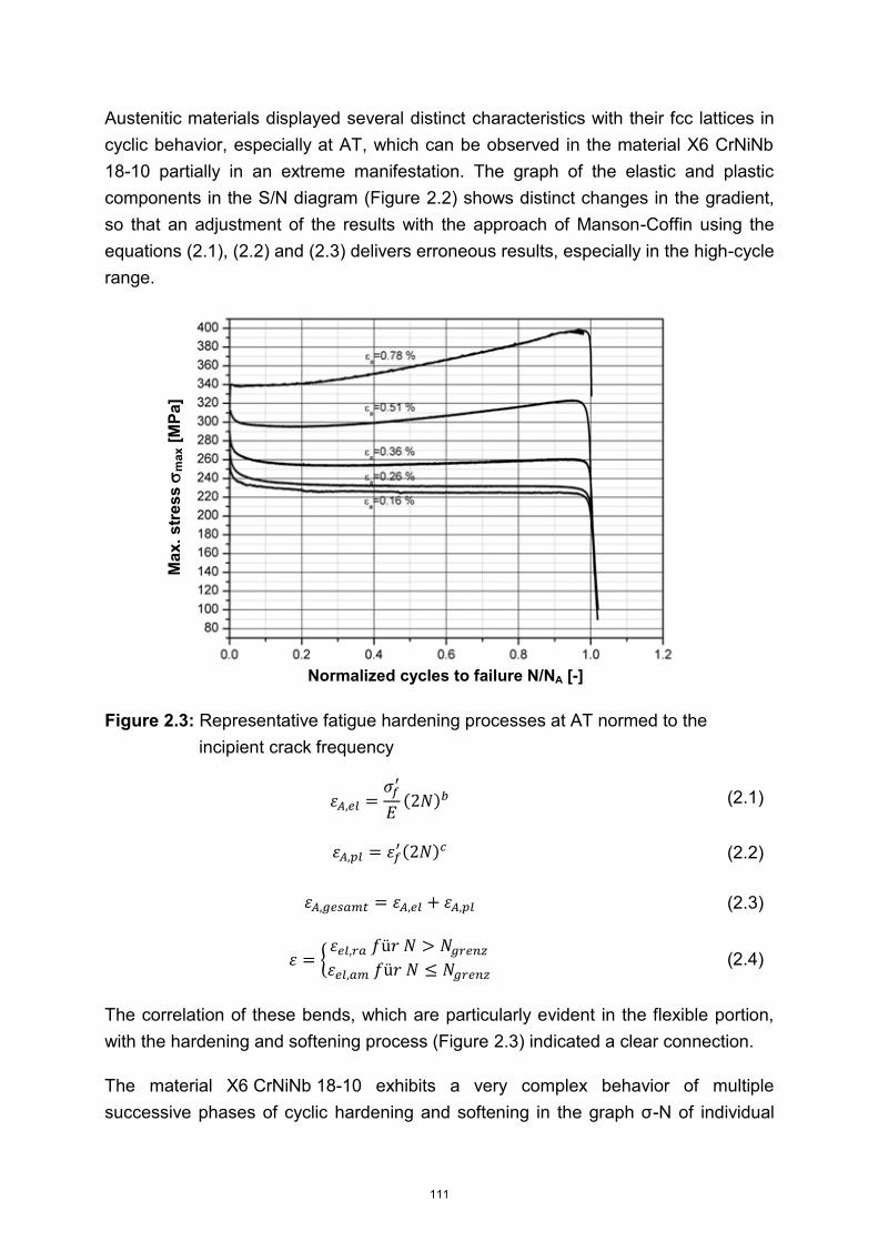
Austenitic materials displayed several distinct characteristics with their fcc lattices in cyclic behavior, especially at AT, which can be observed in the material X6 CrNiNb 18-10 partially in an extreme manifestation. The graph of the elastic and plastic components in the S/N diagram (Figure 2.2) shows distinct changes in the gradient, so that an adjustment of the results with the approach of Manson-Coffin using the equations (2.1), (2.2) and (2.3) delivers erroneous results, especially in the high-cycle range.

Figure 2.3: Representative fatigue hardening processes at AT normed to the incipient crack frequency

( ) (2.1)

( ) (2.2)

(2.3)

{

(2.4)

The correlation of these bends, which are particularly evident in the flexible portion, with the hardening and softening process (Figure 2.3) indicated a clear connection.

The material X6 CrNiNb 18-10 exhibits a very complex behavior of multiple successive phases of cyclic hardening and softening in the graph σ-N of individual

Max

. str

ess

m

ax [M

Pa]

Normalized cycles to failure N/NA [-]

111

experiments. Above a critical load εgrenz, experiments can principally be divided into the phases of the primary hardening (approx. 10-20 cycles); a softening phase (to approx. 12 -20% of the lifespan) and a final secondary hardening phase. Below εgrenz the secondary hardening phase is not applicable. This is due to a deformation-induced transformation of γ-austenite to ε- and α-martensite. If the introduced mechanical load is adequate, the fcc lattice of the austenite transforms into bcc martensite with repeated cyclic loading. This behavior is attributed to all austenitic materials as a rule. However, it is especially pronounced with the present Nb-stabilized material. Similar materials such as the Ti-stabilized material 1.4541 show a less pronounced secondary hardening capacity and thus also a weaker stress increase [2][3].

The break point observed in the flexible pitch line in the S/N diagram can be clearly correlated to the onset of the secondary hardening and thus to the martensitic transformation, so that an explicit critical load εgrenz can be designated for which the martensitic transformation must be considered in the materials specification. This was carried out for the Manson-Coffin approach using equation (4). The flexible line was divided up sectionally into a purely austenitic and an austenitic-martensitic portion. This step increased considerably the forecast accuracy of lifespan in the high-cycle phase and reduced the scatter band to a factor of approx. 1.8.

2.4 Behavior at Increased Temperature

Until recently it was assumed that the influence of increased temperatures did not greatly affect fatigue behavior. This assertion is based in particular on experiments on austenites of the 1960’s. At that time, however, no small strain load tests were

conducted. It was only possible to confirm this assumption for the low-cycle range.

In particular at high cycles, a clearly different behavior is evident, Figure 2.4. In the investigated series, there was no clear break of slope point towards increased lifespans. During evaluation of the elastic and plastic strain process, a definite displacement towards the right of the intersection of the two lines was observed. Therefore it is assumed that the elbow point exists nonetheless; however, it would lie at a level below εA=0.1 %.

112

Figure 2.4: Comparison of all fatigue tests at varying temperatures with polished surfaces

Figure 2.5: Hardening process at 200°C representative for tests at increased temperature

In the hardening and softening processes, the secondary hardening is almost completely inapplicable, Figure 2.5. Primary hardening and the following softening are not negatively affected by the increased temperature.

2.5 Influence of Surface Roughness

Three cases of differing surface roughness as depicted by Figure 2.6 were examined. The surface roughness in Figure 2.6 corresponds to the assumed

Normalized cycles to failure, N/NA [-]

Max

. str

ess

m

ax [M

Pa]

Number of cycles until 5% load drop [-]

Stra

in a

mpl

itude

a [

%]

113

maximum value of a milled surface or casting skin as described in the established body of rules and standards such as AD-Merkblatt S2 or DIN EN 13445.

a) polished Rz=0.6 µm b) grinded Rz=2.4 µm c) rough Rz=200 µm

Figure 2.6: Types of surfaces tested

In Figure 2.7, the test results for all of the surface states at 200°C are centrally displayed. The tests on polished surfaces are also shown for purposes of classification.

Figure 2.7: Fatigue behavior of the various surface states. T=200°C

In the extreme low-cycle range, the results of grinded and polished surfaces harmonize with relatively good agreement. The increase of the Rz value from 0.6 µm to 2.4 µm by a factor of 4 was probably not high enough to result in a significant influence on the surface. Thus it can also be concluded that experiments involving varying surface roughnesses whose differences do not exceed a factor of 4 to 5 can be summarized in a scatter band, and the experimental results from tests using polished surfaces can be adopted without further adjustment of technical surfaces.

Number of cycles until 5% load drop [-]

Stra

in a

mpl

itude

a [

%]

114

It is notable that the experiments within the high-cycle range under a εA value of approx. 0.2% show a tendency towards longer lifespans. This tendency is not substantial enough in the case of Rz=2.0 µm for them to leave the usual scatter band range of a factor of 2. This behavior is also clearly recognizable in the course of the Δεel-N and Δεpl-N curves.

During the plotting of the results on the rough material in the S/N diagram, it is apparent in the LCF range that the reduction manifests approx. a factor of 3 in relation to the lifespan. With such a deviation, which is outside a usual scatter band range with a factor of 2 and shows a definite tendency towards shorter lifespans, the influence of such a degree of roughness can be assumed to be significant. The reduction ratio is not constant over the entire tested spectrum; rather, at a critical load of approx. εA=0.5 %, an intersection of the polished and rough S/N diagram is set. A lifespan-increasing effect can be seen at increased temperature and extreme surface below a certain strain limit due to the surface roughness.

This finding contradicts the current established reductive efforts in cases of deviation of a theoretically ideal surface, as they are recorded in the current body of regulations AD-S2 or DIN EN 13445 with the fo and fs factors.

An explicit clarification of this effect has not been possible so far. It is, however, assumed that the material in the notch root begins early to flow plastically due to the high local strain and undergoes a not insignificant primary hardening process (creation of dislocation and slip dislocation until resistance is encountered). It is possible for this material, sheared in this manner, to be able to create higher tensile strain simultaneously with smaller portions of plastic flow. In the LCF range this would be more likely to have a negative impact due to a higher strain amplitude, but in the HCF range it is advantageous. In the HCF range, the elastic strains are dominant, which in the case of ambient temperature causes the bending toward higher lifespans. This assertion is supported by the observation of the polished material. The minimally sheared Heat 3 shows a slight tendency to shorter test run times in the LCF range, whereas in the HCF range the tendency toward longer test runs dominates. Nonetheless, the difference is too small to consider it significant or to warrant a separate evaluation.

2.6 TMF Tests (uni- and biaxial)

In addition to the isothermic test program, TMF tests on polished round stock and multiaxial cruciform specimens in a plane stress state were conducted. All experiments were based on a heating and cooling rate of 10°C/s. The temperature

115

rise consists of 190°C from a minimum of 50°C to 240°C peak temperature. The mechanical load on the specimen results from a cycle similar to an operational cycle such as that in a nuclear facility. The evaluation of the results and the assessment are still ongoing. It is assumed that the biaxial loading causes a considerable reduction of lifespan.

3 Life cycle assessment with micromechanical material models

3.1 Basic characterization of the initial material characteristics

The used austenitic niobium-stabilized chromium-nickel steel X6CrNiNb18-10 (material number 1.4550) was fabricated according to the current nuclear standard KTA 3201.1, Table 3.1. At the MPA University of Stuttgart the microstructural characterization of the test material (plate material, rod Ø 15 mm, rod Ø 106 mm) before thermal loading was performed, Figure 3.1 to 3.3. This steel is mainly used in nuclear piping due to its high resistance to corrosion and its high plastic deformation capacity. Due to the high content of chromium (Cr) of 18%, this steel is rust and acid resistant. The nickel content (Ni) of 10% stabilizes the fcc structure (austenite) to room temperature and provides an increase in strength through Fe-Ni solid solution formation. The added niobium (Nb) in the alloy binds the carbon as NbC, thus preventing the precipitation of chromium carbides. As a result, this steel is resistant to intergranular corrosion (IC). The chemical composition and the mechanical properties are summarized in Table 3.2 and Table 3.3.

Table 3.1: Manufacturing and heat treatment of X6CrniNb18-10

Table 3.2: Chemical composition according to melt-analysis

Table 3.3: Mechanical properties according to manufacturer’s certificate

element C Si Mn P S Cr Ni Nb Co

massfraction

% 0,023 0,34 1,86 0,019 0,002 18,1 10,1 0,45 0,037

Rp0,2/RT Rp1,0/RT Rm/RT A5/RT ZRT KVRT

MPa MPa MPa % % J

251 294 562 57 77 261

116

Figure 3.1: Microstructure of X6crNiNb18-10 in undeformed state (optical microscope)

Dislocation density: 214m102,06,0 after heat treatment (undeformed).

Figure 3.2: TEM-investigations (extraction replica, thin metal foil)

117

Figure 3.3: Size distribution of niobium-carbides in undeformed state.

3.2 Development of a testing device for the investigation of high cyclic thermo-mechanical loading

Thermal strains in piping systems are induced by thermal transient or thermal shock loadings. The frequency of these loadings e.g. in mixing zones might be quite high. Thermal loadings on the inner surface of piping components induce biaxial stresses with more or less steep gradients in thickness direction. Therefore for the development of an appropriate testing device, preliminary numerical investigations on the temperature and stress distribution were necessary and have been carried out for different specimen types.

Here, firstly water-cooled hollow samples with constant and variable outer diameter ("hourglass" sample) were subjected to alternating thermal cyclic loading. At a frequency of 1 Hz, temperature stress ranges of 200 K in the range between 200°C and 400°C could be realized.

Secondly, multiple geometry variations of specimen with a double-sided, hemispherical cavity were calculated. These specimens with double sided hemispherical cavities were subjected with an alternating heat input to the surface (inductive) and air cooling on both sides. At a frequency of 0.5 Hz, temperature amplitudes of 100-150 K with respect to a maximum temperature of 350 ° C could be realized.

Based on these numerical studies appropriate specimen type and test equipment have been developed.

The final specimen design is shown in Figure 3.4. The heating of the sample takes place via an induction coil, which is controlled via a high-frequency generator. The

118

testing device is shown in Figure 3.5. The surface temperature at the center of the sample is determined via two pyrometers. To determine the temperature distribution on the specimen surface, it can be recorded during the experimental procedure on the opposite side to the coil by using a thermal imaging camera. To measure the induced thermal strains an optical strain measurement system (ARAMIS) is used.

Figure 3.4: Final design of the specimen geometry

The greatest temperature gradients and thus greatest stresses and strains are induced in the center of the specimen. Thereby, the greatest damage, and thus a possible fatigue crack initiation can be expected in the center of the specimen. The specimen holder is designed in such a way, that the thermal expansion of the specimen is not restraint. So that the material in the initial state has minimal residual stresses or other material changes by cold working, the samples are spark eroded and then polished. The initial state of the sample surface is documented metallographically in detail.

3.3 Experimental and numerical investigation of the temperature distribution

The first heating begins at room temperature. Thereby the difference in temperature during the first heating phase is greater than in the later cycles. To keep the temperature gradients and the resulting stresses during this heating phase as low as possible so that they have no influence on the subsequent test results, the generator output is reduced to 30%.

119

Figure 3.5: Testing device with induction heating system

After the heating step, the temperature is kept constant at 300°C until the specimen reaches a constant temperature. Then the alternating load at full generator capacity starts with temperature cycles between 150°C and 320°C.

Figure 3.6: Temperature distribution and function of time at the specimen center

The temperature distribution over the surface of the specimen was recorded during the experiment with a thermal imaging camera, Figure 3.6 (left). During the test, the temperature, which is measured with the two pyrometers in the center of the

120

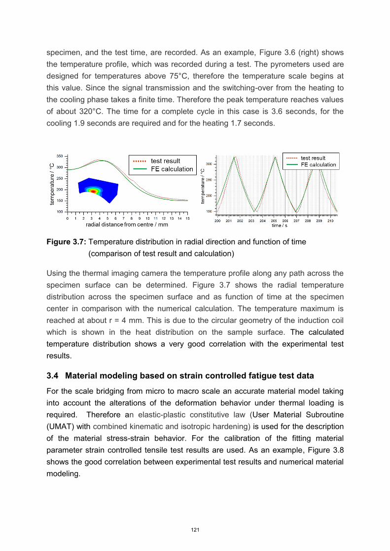
specimen, and the test time, are recorded. As an example, Figure 3.6 (right) shows the temperature profile, which was recorded during a test. The pyrometers used are designed for temperatures above 75°C, therefore the temperature scale begins at this value. Since the signal transmission and the switching-over from the heating to the cooling phase takes a finite time. Therefore the peak temperature reaches values of about 320°C. The time for a complete cycle in this case is 3.6 seconds, for the cooling 1.9 seconds are required and for the heating 1.7 seconds.

Figure 3.7: Temperature distribution in radial direction and function of time (comparison of test result and calculation)

Using the thermal imaging camera the temperature profile along any path across the specimen surface can be determined. Figure 3.7 shows the radial temperature distribution across the specimen surface and as function of time at the specimen center in comparison with the numerical calculation. The temperature maximum is reached at about r = 4 mm. This is due to the circular geometry of the induction coil which is shown in the heat distribution on the sample surface. The calculated temperature distribution shows a very good correlation with the experimental test results.

3.4 Material modeling based on strain controlled fatigue test data

For the scale bridging from micro to macro scale an accurate material model taking into account the alterations of the deformation behavior under thermal loading is required. Therefore an elastic-plastic constitutive law (User Material Subroutine (UMAT) with combined kinematic and isotropic hardening) is used for the description of the material stress-strain behavior. For the calibration of the fitting material parameter strain controlled tensile test results are used. As an example, Figure 3.8 shows the good correlation between experimental test results and numerical material modeling.

121

Figure 3.8: Cyclic stress-strain modeling (comparison of test result and calculation)

The stress and strain distributions in the specimen under cyclic loading result from the specimen geometry and materials microstructure on the nano- and micro-levels. These both influencing factors will be taken into account in the modelling. Through the submodelling-technique combined with the boundary conditions extracted from the former model the impact of the geometry (e.g. concave specimen shape) can be transferred to the micro-model. The application of the self-developed user subroutine (UMAT) will ensure an accurate description of the stress and strain pattern in the material in course of the thermal loading. The initiation of fatigue cracks is expected in the areas with highest stress/strain distributions. The validation of the simulation model will be done by the comparison between experiment and simulations results.

3.5 Experimental results and comparison with uniaxial mechanical fatigue test data

First indications for surface cracks were detected after about 22,000 thermo cycles. Figure 3.9 shows the crack pattern and the deformations in the vicinity of the crack tip at the specimen surface after 23,000 cycles. This crack pattern is typical for cyclic thermal shock loadings.

To compare these test result with uniaxial mechanical loaded fatigue tests, the equivalent strain amplitude has to be determined. For this purpose the procedure according to 2010 ASME Boiler & Pressure Vessel Code, Section III, Division 1 – NH was applied. The equivalent strain range for each point (i) in time is calculated according to the following equation:

2/12i,xi,z

2i,zi,y

2i,yi,x

i,equiv 2i,zx

2i,yz

2i,xy2

3*122

where 5,0* when using inelastic analysis 3,0* when using elastic analysis

122

Figure 3.9: SEM investigation – Surface crack pattern and crack tip

The largest strain range occurs in the center of the specimen. The maximum strain range on this position is 0.706% respectively the value of the maximum strain amplitude is v,a = 0,353%. This value lies within the scatter band of the uniaxial mechanical loaded fatigue test data, Figure 3.10.

Figure 3.10: Comparison of the test result with the German data base for stabilized austenitic stainless steels at elevated temperature

3.6 Further micromechanical investigations

The microstructure of the X6CrNiNb18-10 before thermal loading consists of the austenitic grains with several twins, uniformly distributed fine NbC and a small amount of delta-ferrite. The further investigations of the microstructure after thermal

0,01

0,10

1,00

10,00

1,0E+00 1,0E+02 1,0E+04 1,0E+06 1,0E+08 1,0E+10

Stra

in A

mpl

itude

a

(%)

Load Cycle N

≈2,3·104

a=0,353 %

DatabaseT = 200°C … 350°C

123

loading are in progress. The focus lies currently on the TEM analysis of dislocations arrangements and their interactions with NbC. From the former BMWi-Project [4] is known that deformation induced martensitic transformation under mechanical cyclic loading at room temperature takes place. The formed bcc martensite controls the growth of fatigue cracks. According to the authors state of knowledge no martensitic transformation can be expected at the thermal loading performed within this project. Therefore the main fatigue damage mechanism might be the formation of extrusions and intrusions at the specimen surface. The TEM and analyses should clear this issue. Moreover, the impact of the grain orientations as well as the interfaces (grain and phase boundaries) will be investigated by Electron Backscatter Diffraction (EBSD) in SEM. This is important in connection with the reduction of the yielding stress of the fcc X6CrNiNb18-10 at higher temperatures.

Figure 3.11 shows the FE-simulation of the formation of extrusions and intrusion in a model-fcc-material under mechanical cyclic loading. In the FE-model the dislocation rich areas (veins-like) alternate with the dislocation poor areas and form “two-phase”

microstructure on the micro-level. The heterogeneity on this level gives rise to the formation of the surface roughness and possible crack initiation sites in the soft areas between dislocation rich veins.

Figure 3.11: Formation of extrusions and intrusions under mechanical cyclic loading in the fcc model-material [4].

The FE-model (Figure 3.11) with experimentally determined dislocation arrangements of X6CrNiNb18-10 after thermal loading will be adapted to further sophisticate numerical models in which damage relevant microstructural details will be included.

1

2

1 2

124

4 Life cycle assessment with atomistic and damage-mechanical material models associated with material tests under thermal fatigue

4.1 Damage Mechanism Based Material Modeling

4.1.1 Experimental Results

To allow validation of mechanism based material modeling of thermal fatigue (TF), an experimental setup was developed and thermal fatigue experiments carried out.

Experimental setup

For investigation of thermal fatigue an experimental setup was constructed, which allows the application of a large number of sufficiently damaging thermal load cycles in a reasonable amount of time. Also, the setup permits variation of temperature differences and frequencies in the load cycles. In the setup, a specimen is heated inductively and cyclically cooled by a spray of water mist (see Figure 4.1). Frequencies up to 3 Hz are possible, but only up to 1 Hz they are considered to be useful due to the otherwise very small depth of thermal loading. To allow for free thermal expansion, the specimen is only fixed at the bottom end. The shape of the sprayed area on the specimen surface is determined by the shape of slit placed between the nozzle and the specimen. For the current investigation we used a slit with a size of 10mmx2mm, the long direction oriented parallel to the axis of the specimen. Due to the axially elongated shape of the sprayed area we expect cracks to be parallel and oriented normal to the axis of the sample. To produce a more network-like pattern of cracks a more biaxial stress state should be aimed at by using a more circular aperture to form the sprayed area. The intensity of the cooling can be varied by diverse settings of the nozzle and by the distance of nozzle and specimen. The inductive heating is controlled using a thermocouple which is placed above, but close to the sprayed region. Before each experiment the settings for the desired experimental conditions are fixed using a calibration specimen with thermocouples in the center and outside of the sprayed region. The temperature differences set once at the beginning of the experiment proofed to be sufficiently stable during the whole experiment.

Experimental results

A detailed characterization of the austenitic steel used for the experiments is given in chapter 2, where the material is labeled as heat 3 or aRH. The thermal fatigue specimens are cylindrical dog bone specimens with a diameter of 10mm in the gauge length. The surfaces were plasma polished like in all other parts of the cooperation.

125

Figure 4.1: Experimental setup for thermal fatigue experiments. An inductively heated specimen is cyclically cooled by a water mist.

The experimental setup is used to perform thermal fatigue experiments with temperature differences between 50°C and 300°C and frequencies in the range of 0.1Hz to 1Hz. Some experiments are performed with interruptions to take replicas, so that later the development of the crack pattern on the surface can be tracked; others are stopped after specific numbers of TF cycles to investigate the development of the crack depths with cycle number. In each category, frequencies and temperature differences are varied.

(a) (b)

Figure 4.2: (a) Cracks observed by light microscopy on the surface of a specimen thermally fatigued with ∆T=200°C, 0.2Hz for 100k cycles. The axis of the sample is horizontal in the figure, the cracks extend in vertical direction. (b) Detail of a crack (SEM).

126

On all surfaces that were not obscured by brass deposit from a valve, marks of plastic deformation like slip bands and extrusions are observed. Some surfaces show cracks or slip band markings connected to fine cracks extending over several grains. On the surface of a specimen loaded for 100k cycles with ∆T=200°C and a frequency of 0.2Hz a multitude of cracks can be clearly seen (Figure 4.2). The cracks extend in circumferential direction and cover all the width of the sprayed area. The distances of cracks are usually in between 300µm and 500µm (with a few as close as 100µm and a few as distant as 900µm).

The depths of cracks and the correlation of depths with a specimen that was thermally fatigued for 500k cycles with ∆T=200°C and frequency 1Hz was investigated (Figure 4.3). An axial micrograph through the center of the sprayed area shows nine cracks with depths between 300µm and 550µm, in between which often some shorter cracks are found. The deeper cracks in most cases have a larger distance to their neighbors than shorter cracks. A second micrograph, 0.19mm off the center, showed cracks of similar lengths at similar positions. A systematic investigation of the correlation of experimental conditions (temperature difference, frequency, number of TF cycles) and the observed crack lengths, depths and distances is in progress.

(a) (b)

Figure 4.3: (a) Pattern of crack depths obtained from a micrograph through the center of the sprayed area of a specimen thermally fatigued with ∆T=200°C, 1Hz for 500k cycles. (b) Example of three cracks (300µm, 140µm and 100µm deep) in a micrograph 0.19mm off the center.

4.1.2 Lifetime modeling

For prediction of thermal fatigue a mechanism based model for thermo-mechanical fatigue commonly used at the Fraunhofer IWM, consisting of a cyclic plasticity model

127

of Chaboche type and the damage parameter DTMF1, is applied. A detailed description

of the models and its application is given e.g. in [5]. The lifetime model is based on the observation that the crack growth rate da/dN is proportional to the crack tip opening displacement ∆CTOD:

da/dN = β ∆CTOD (4.1)

Under conditions detailed e.g. in [6], the crack tip opening displacement can be estimated analytically by

(

√ )

(4.2)

Here, dn’ depends on the hardening behaviour of the material, σcy is the cyclic yield strength, ∆σeff=σmax-σop is the effective stress range considering crack closure, E is Young’s modulus, ∆σ the stress range, ∆εpl the plastic strain range and n’ is the cyclic

analogue of the Ramberg-Osgood hardening exponent.

On the other hand, eq. (4.1) can be integrated to yield the relation

Nf = A / (dnZD/σcy) (4.3)

between lifetime Nf and damage parameter dnZD/σcy. Here, the constant A = ln(af/a0)/β results from crack length at the beginning and at failure. Often, the addition of an exponent B

Nf = A / (dnZD/σcy)B (4.4)

allows a better description of experimental data.

To customize the lifetime model and cyclic plasticity model for the current material, LCF tests at temperatures between room temperature and 350°C, as well as TMF tests were performed with plasma polished specimens cut from the same raw material as the TF specimens. Also, experiments from the investigations of chapter 2 (materials aRF and aRH) were used to fit the parameters of the models. Calculation of damage parameters from experimental hysteresis loops showed that lifetimes of LCF, HCF and low cycle TMF experiments at temperatures between 100°C and 350°C can be described together by one power law according to eq. (4.4) within a scatter band of factor 2 (see Figure 4.4a). Room temperature experiments cannot be described by the same law, but are not needed for the prediction of the lifetimes of

1 As in the temperature range of interest creep does not play a significant role, the damage parameter DTMF reduces to dnZD/σcy.

128

thermal fatigue experiments in the temperature range between 100°C and 350°C. The same holds for damage parameters calculated from hysteresis loops modelled with the cyclic plasticity model (not shown). A comparison of experimental lifetimes and lifetimes calculated with the cyclic plasticity and lifetime model (Figure 4.4b) shows a good agreement in the aforementioned temperature range. We therefore expect being able to describe with that model also thermal fatigue in the range between 100°C and 350°C. To validate the model for TF experiments, it will be used in FE simulations reflecting the temperature changes in the experiments. The spatial distribution of cycles to failure will be compared to the experimentally observed crack patterns and depths.

(a) (b)

Figure 4.4: (a) Power law relationship between damage parameter dnZD/σcy extracted from experimental hysteresis loops and cycles to failure. (b) Comparison of modeled and experimental cycles to failure.

4.2 Atomistic Modeling

Computer modeling has become an indispensable part of every branch of today’s

materials research. It serves as an invaluable tool for testing the validity of models and underlying theories by comparing the results of simulations with experiments, as well as a predictive tool in studies of mechanical, physical and chemical properties. Behavior of materials is nowadays investigated from the theoretical point of view by various computational methods and on length scales spanning many orders of magnitude. The enormous advancement of computer hardware in the last two decades allowed us to handle problems which would be inconceivable to tackle some twenty years ago, and assuming a similar pace of technological evolution we can anticipate even broader application of computer modeling in the near future.

129

The mechanical behavior of materials is ultimately determined by events occurring at the atomic scale. The onset of plastic yield corresponds to triggering of dislocation motion. Subsequent hardening is mainly controlled by interaction of gliding dislocations with other lattice defects such as forest dislocations, grain boundaries, interfaces and surfaces. Finally, material failure is influenced by processes at the tip of a crack propagating in a crystal lattice. A thorough understanding of all these phenomena rests ultimately on the knowledge of the underlying atomic processes that occur within a few nanometers from the interacting defects. Unfortunately, experimental observations of such complicated nano-scale phenomena are difficult to perform even with modern techniques. For this reason, part of our work focused on investigations of the microscopic origins of plastic behavior in iron using atomic level computer modeling.

Efforts to model Fe-based materials at the atomic level have been growing rapidly in the last years not only to gain a better fundamental understanding but also to facilitate the design of advanced materials such as modern high-strength twinning- or transformation-induced-plasticity (TWIP/TRIP) steels. First-principles calculations, which require only few fundamental physical properties as input parameters, are able to provide trustworthy predictions for small atomic ensembles. However, the development of accurate models of interatomic interactions that could capture subtleties of chemical bonding and still be applicable in large-scale atomistic studies of lattice defects presents a significant challenge.

The absence of reliable and computationally efficient models of interatomic interactions for iron stems from a difficulty to describe appropriately and simultaneously two key ingredients of its atomic bonding: (1) the unsaturated directional covalent bonds and (2) the magnetic effects. Most existing interatomic potentials for Fe cannot provide a proper description of directional bonds, and almost none contains a physically-based treatment of magnetic interactions. These potentials are therefore neither able to describe the broad variety of magnetic phases of iron nor provide any information about local magnetic phenomena in the vicinity of crystal defects.

Within this project, we developed a novel magnetic bond-order potential (BOP) [7][8] that is able to provide a correct description of both directional covalent bonds and magnetic interactions in iron. This potential, based on the tight binding approximation and the Stoner model of itinerant magnetism, forms a direct bridge between the electronic structure and the atomistic modeling hierarchies. Even though BOP calculations are computationally more demanding than those using common

130

empirical potentials, the formalism can be used for studies of complex defect configurations in large atomic ensembles exceeding 105 atoms. Our studies of dislocations in α-Fe (Figure 4.4) and other body-centered cubic transition metals [9][10] demonstrate that correct descriptions of directional covalent bonds and magnetism are crucial for a reliable modeling of these defects.

In addition to these studies, we developed a new methodology [11] that enables construction of advanced BOP models for binary systems directly from quantum-mechanical calculations. This method has so far been applied to Ti-C and Ti-N systems [12] and will be used in the future for construction of BOP models for iron compounds and alloys such as Fe-C, Fe-H, Fe-Nb, etc.

(a) (b) (c) (d)

Figure 4.5: Core structures of ½<111> screw (a) and edge (b), and <100> screw (c) and edge (d) dislocations in α-Fe. The coloring shows decrease of magnetic moments of atoms in the vicinity of the cores.

131

5 Simulation of fatigue crack growth, opening and closure of a short crack under thermal cyclic loading conditions, developing methods for the damage assessment based on the cyclic J-integral

For the numerical simulation of crack opening and closure we used the system of a thick walled tube similar to the system used in [13]. However, the 3D-model is not suitable for the problem at hand. To reduce the computational cost of three-dimensional FEM calculations and represent a tube of arbitrary length the numerical simulations were carried out for a completely axially symmetric torus similar to the system described in [14]. Given that the radius of this torus is large enough the stress-strain state on the appropriate location of the inside wall of this torus is the same as in a tube of arbitrary length. For the numerical calculations a torus with a primary radius of 4000 mm has been modeled. Here the primary radius is the distance from the center axis of rotation to the center of the cross-section of the torus. To further utilize symmetry only the upper half of an axially symmetric torus cross-section has been modeled resulting in the finite element model seen in Figure 5.1. The inner radius of the tube is 95 mm and the wall thickness is 40 mm. The inner wall of this tube is subjected to a constant internal pressure and to different time dependent temperature transients with the temperature ranging from 50°C to 350°C. The temperature dependent thermal and mechanical material parameters for the Niobium stabilized austenitic stainless steel 1.4550 (X6CrNiNb18-10, AISI 347) – typical grade in German nuclear power plants - are taken from the KTA rule [1], the research report [15] and the technical report [16]. The temperature range for the material parameters given in these reports covers the temperature load range described above.

To describe the cyclic elastic-plastic material behavior in the FEM simulations the Chaboche plasticity model [17] has been used. In a further step, the Ohno&Wang model [18] is implemented as a user routine in the ANSYS® finite elements software [19] (see paragraph 6) and is used for the simulation of the transient cyclic plasticity behavior. In all the calculations we used 4-Node elements with linear shape functions. Figure 5.2 shows a magnification of the refined mesh on the inside wall. The elements in this area are nearly quadratic with an edge length of 10 μm. The

thermal and structural results are in very good agreement with results obtained using the FE model described in [13].

In the first step of the numerical simulations the temperature profiles caused by the thermal transients have been determined. The analyses for the temperature

132

distribution and all subsequent structural calculations have been done in two steps re-using the results of the thermal simulation. This load transfer method leads to a unidirectionally coupled-field solution. For the first structural calculation the constant pressure on the inside wall along with the temperature solution has been applied as a load to determine the deformations and the resulting stresses and strains. For this calculation displacement boundary conditions were set along the symmetry line of the torus cross-section to prevent circumferential displacement of the respective nodes. This means that for all nodes with Cartesian coordinate y=0 in Figure 5.2 the boundary condition uy=0 was imposed.

Figure 5.1: Global finite elements mesh of cracked structure

Figure 5.2: Mesh detail of the cracked zone

This calculation has been carried out for several cycles with repeated application of the temperature profile to obtain quasi-stabilized hysteresis solutions. This system will be referred to as the non-cracked configuration. To model crack opening and closure we modified the above model to obtain a pre-cracked configuration. This has been done by removing the boundary constraints on the nodes on the horizontal

133

symmetry axis thus pre-determining the crack geometry and orientation. For a crack length of 10 μm only the node on the inside wall has been released whereas a crack

length of 50 μm required 5 nodes to be unconstrained. The temperature solution

obtained from the very first FE simulation and the pressure on the inside wall were then again applied to this model as loads. To numerically describe crack closure and capture the effects of contact of the crack flanks contact elements have been used. The contact boundary conditions have been defined along the symmetry line of the torus cross-section thus allowing the released nodes displacement in positive y-direction only. The contact elements are located at the nodes of the refined mesh along the symmetry line of the cross-section. The contact elements remain at these nodes and their displacement is determined by the displacement of the structural elements the contact elements are sharing the respective nodes with. In this model self penetration would occur as a displacement of these nodes below the horizontal axis of symmetry and self contact would occur whenever an unconstrained node is on this horizontal symmetry line. Appropriate contact boundary conditions ensure that self contact is allowed but self penetration is prevented.

Each of the simulations for pre-cracked geometry has been done separately and no explicit crack growth has been modeled here. To overcome plasticity induced stabilization and saturation effects each of these calculations comprised 10 cycles. From the simulations of the pre-cracked configurations merely the time information of the crack opening and closure points has been extracted. The sought-after crack opening stress and strain values are then determined by taking the stresses and strains of the non-cracked configuration at the times of crack opening and closure extracted from the simulation of the pre-cracked configurations.

For the damage assessment of hysteresis loops the appropriate consideration of crack closure effects is a key element as discussed above. The damage contributing parts of the hysteresis loop are considered to be the phase when the flanks of the crack are not in contact and the crack is open. To determine the crack opening stress for uniaxial mechanical loading Newman’s proposal [20] is widely accepted. To compare the crack opening stresses determined from the numerical simulations described in the previous section with an analytical solution obtained from Newman type equations a modified set of equations is used.

Since can be easily determined on the ascending part of the hysteresis this allows to identify the crack closure stress on the descending part of the loop. Knowing the opening stress for the hysteresis loop of interest the opening and closure points can be identified as it is shown schematically in Figure 5.3.

opx,

134

For the application of the Newman equations to the hysteresis loops caused by thermal cyclic loading the temperature influence has to be considered when calculating the crack opening stress .

Figure 5.3: Crack closure relevant hysteresis parameters

To account for the temperature dependent yield stress the set of Newman equations has to be evaluated repeatedly to determine the crack opening stress. Knowing the temperature distribution for the whole hysteresis at each FEM computed data point every discrete data point of the hysteresis loop can be related to a temperature on the inside wall. The crack opening stress is obtained by scanning the ascending branch of the hysteresis loop. Starting with the point of minimum stress the equations are evaluated for every data point until the condition for crack opening is met. As a first step is evaluated for the temperature associated with the current data point. This value of is then used to determine a crack opening stress . If this stress is less than or equal to the stress of the currently investigated data point the crack is assumed to be open and the point of crack opening is found. Since for this method crack opening and closure are assumed to occur at the same strain level the point of crack closure is identified by scanning the descending hysteresis branch for the data point with the strain value corresponding to the previously identified point of crack opening. The crack closure stress is then the stress value of this data point.

Crack closure simulations were carried out based on the algorithm described above.

opx,

'

F

opx,'

F

clx,

135

Fifty hysteresis loops were analyzed in order to achieve an approximately stabilized stress strain hysteresis loop and to consider appropriately the influence of the cyclic plasticity behavior on the cracked structure.

The hysteresis loop in figure 5.4 represents the un-cracked configuration. The analysis of the cracked configuration of different crack lengths delivers the information about the crack opening and crack closure stresses and strains. Obviously, the precision of determination depends on the discretization of data points. Iterative refinement is possible. Figure 5.4 reveals a more refined set of data points for the descending branch compared to the ascending branch. Consequently, crack closure stresses and strains can be determined more precisely than crack opening stresses and strains in this case.

Figure 5.4: Hysteresis loop for inner surface

Figure 5.5: Opening and closure strains (transient 1)

-300

-200

-100

0

100

200

300

-0,40 -0,30 -0,20 -0,10 0,00 0,10 0,20

Strain in [%]

Stre

ss in

[MPa

]

-0,244

-0,242

-0,24

-0,238

-0,236

-0,234

-0,232

-0,23

-0,228

-0,2260 5 10 15 20 25 30 35 40 45 50

Crack length in [mm]

Cra

ck o

peni

ng a

nd c

losu

re s

trai

n in

[%]

Closure

Opening

136

Exemplarily, resulting opening and closure strains as mean values between two data points are shown in Figure 5.5 (transient 1).

Analytical expressions are derived for the determination of the essential crack opening and crack closure stresses and strains. In connection with approximation formulae for the J-integral they constitute essential parts of an engineering algorithm. A more detailed description is out of the scope of this paper.

6 Further development of plasticity models

The applied plasticity model has to be capable of simulating the local (at the crack tip) multiaxial stress-strain-relations for typical thermal cyclic or thermal mechanical loading conditions. This includes the correct determination of the crack opening and crack closure levels. In the case of cyclically stabilized material behavior the standard implementations of material models such as the Besseling or the Chaboche model within commercial finite element codes are applicable in principle. However, this does not hold true for the simulation of complex phenomena of cyclic plasticity such as particularly the possible cycle by cycle accumulation of plastic strain increments (ratcheting). Possible incremental plasticity laws for a more realistic description of the opening and closing behavior of short cracks are the models proposed by Ohno & Wang (given in [18] and [21]) which belong to the group of plasticity laws with Armstrong Frederick type nonlinear kinematic hardening rules such as the classic model of Chaboche [22].

6.1 General relations of elasto-plastic material behavior

The models are formulated in the small strain regime, therefore the total strain can be additively composed into a reversible elastic part , an irreversible plastic part and a reversible thermal part (see [23], chapter 23 for example), expressed as

(6.1) The thermal strains are purely volumetric (no distortion of shape) and are calculated using the common relationship

(6.2)

using the instantaneous coefficient of thermal expansion , the difference of the actual temperature relative to a reference temperature and the 2nd order unit

137

tensor . The elastic part is governed by the linear isotropic elasticity law (Hooke's law)

(6.3)

with the two (in general temperature dependent) elasticity constants (Lamé-constants) and .

Furthermore, the existence of a specific strain energy density function is postulated. The free energy is a function of so-called external and internal variables which characterize the momentary local material state. Observable external variables are the total strain and the temperature . The type and number of the internal variables is caused by the phenomenological aspects to be considered in the plastic material model. A necessary internal variable for describing plastic material behaviour are the plastic strains . The strain energy density

(6.4)

consists of a thermoelastic part , a plastic part and a purely thermal part . The specific parts of are functions of the thermoelastic strains of strain valued second order tensors which characterize the kinematic hardening of the material. The third term of equation (6.4) represents the dependence on the temperature .

The actual stress and the j-th backstress tensor can be derived using the relationships

(6.5)

(r is the density of the material) and

(6.6)

respectively.

The conjugated thermodynamic force represents the j-th partial backstress tensor describing one kinematic hardening mechanism. The total backstress

(6.7)

is defined as the sum of the partial backstresses. The yield function is taken as a von-Mises type yield function written as

138

(6.8)

The plastic strain increment is governed by the associated flow rule

(6.9)

with the scalar plastic multiplier .

6.2 The nonlinear kinematic rule of Ohno & Wang (Model II)

According to [18] (see eq. (21) and (22) there) for the plastic part of the strain energy the quadratic potential

(6.10)

is chosen. Inserting eq. (6.10) into eq. (6.6) yields the linear relationship

(6.11)

between each partial back-stress and its corresponding strain valued kinematic tensor .

One obtains the kinematic hardening model proposed by Ohno & Wang [18] as Model II by choosing

(6.12)

for the dynamic recovery parts of the kinematic hardening equations. In these rate equations

(6.13)

are the norm of the j-th backstress , the normalized back-stress and the MacAuley-bracket, respectively. , and are temperature-dependent material parameters in general. The motivation for choosing the dynamic recovery parts in such a way is explained in [18]. Using eq. (6.11) and (6.12) the kinematic hardening equations

(6.14)

for each partial backstress is obtained finally. In eq. (6.14) the abbrevation for the derivative relative to the temperature is introduced. Substituting by in eq. (6.14) by using the linear relationship (6.11) together with the abbreviations (6.13) the nonlinear kinematic rate equations (6.14) can be rewritten as

139

(6.15)

where the in equations (6.13)1,2 have to be substituted by the linear relationship (6.11). The rate equations (6.15) are equivalent to (6.14). Nevertheless, the form (6.15) is useful for integrating the model using an elastic-predictor/plastic-corrector algorithm because the temperature rate dependent term does not appear explicitly and hence has not to be integrated separately in an elastic predictor step.

The ratcheting rates predicted by the model can be controlled mainly by the appropriate determination of the exponents within the range of . With increasing values of the hardening law (6.14) tends to a linear hardening law for each partial backstress and the overall ratcheting rate decreases. The term reduces the value of the non-linear term in eq. (6.14), especially under non-proportional loadings resulting in an additional reduction of the ratcheting rate.

In the sense of a finite elements implementation the governing equations describing the material behavior have to be discretized and solved. The implicit (backward) Euler method is often applied in the framework of plasticity because of its unconditionally stable time integration scheme and ease of implementation. To solve the equations which describe the material model numerically an operator split method consisting of two parts was used. In the elastic predictor step it is checked if the material is in elastic or plastic state. In the plastic corrector step the discretization of the elasto-plastic parts of the equations is done with an implicit Euler step yielding a system of nonlinear algebraic equations which is solved using a multidimensional Newton-Raphson algorithm.

Figure 6.1: Comparison of ratcheting experiments [24] and simulation

0

0,5

1

1,5

2

2,5

3

3,5

4

4,5

5

0 50 100 150 200 250 300 350 400

Cycles

Tota

l Str

ain

[%]

Simulation V7 Experiment V7 (30/210)Simulation V8 Experiment V8 (30/230)Simulation V9 Experiment V9 (30/250)

140

The performance of the Ohno & Wang material model with respect to the simulation of ratcheting is shown exemplarily in Figure 6.1 by comparing simulation results with experiments reported in [24].

In the framework of the joint research project described here the parameters of the Ohno&Wang material model are optimized based on the uniaxial and biaxial material characterization done by IfW Darmstadt (see paragraph 2). The description of the optimization procedures chosen is beyond the scope of this paper.

7 Conclusion

Fatigue and cyclic deformation behaviour of the Niobium stabilized type 347 austenitic stainless steel was investigated at a fundamental level. Experimental data were generated at operational temperature levels of Nuclear Power Plants under thermo-mechanical stress-strain conditions. Research was focused on generating data for parameter identification, improvement and development of advanced nonlinear kinematic material models, and experimental validation of these models.

Investigations over a wide spectrum of fatigue loading parameters deal with fatigue behaviour at ambient temperatures and elevated temperatures, varying surface roughness conditions, and the presence of mean stress and strain. Metallographic examinations show an effect of transition from austenite to (deformation induced) martensite. Uniaxial experiments show both a significant influence of temperature and a significant influence of extreme surface roughness on the fatigue properties (strain life curve).

Further uniaxial TMF-loading experiments at elevated temperature contribute to a reduction of fatigue endurances. Start-up and shut-down as well as operational conditions have also been simulated experimentally on cruciform specimens. This kind of specimens can be considered as a bridge between uniaxially loaded laboratory specimens and real components. These complex experiments are input for parameter identification and validation of complex elastic-plastic material models, respectively. At biaxial cruciform loading, the reduction is even more significant.

In order to investigate the fatigue behaviour under thermal loading (TF) testing facilities were developed which allow for introducing cyclic thermal loads on the specimen surface. Dependent on the amplitude and the frequency of the temperature changes at the surface of the specimen a crack pattern could be generated with crack depths up to 500µm. Further investigations with varying frequency, temperature amplitudes and number of cycles are in progress.

141

Using self-developed user-subroutines based on the Chaboche material model for cyclic deformation behavior of the tested material and the DTMF-parameter as damage parameter, the fatigue tests at constant temperature and tests under thermo-mechanical loading with slow heating and cooling of the specimen in the LCF regime could be described quite well. The only exception are tests at room temperature with low stress range (high number of cycles). Here, the DTMF-Parameter results in smaller lifetimes as observed for elevated temperatures. The evaluation of the TF-tests that requires the full matching of the temperature field from the experiments to the simulation is still in progress. On the atomistic level, a new methodology was developed that enables the construction of advanced bond-order potential (BOP) models for binary systems directly from quantum-mechanical calculations.

In a further step, the short crack fracture mechanics based damage parameter PJ was qualified for thermo-cyclic loading conditions. This part of the investigations focused on typical low cycle operational transients as loading input requiring a realistic description of the local (at the crack tip) multiaxial cyclic stress-strain behavior. For this purpose, the non-linear kinematic Ohno&Wang material model was further developed considering particularly the thermal part of the describing equations. Material parameters were determined based on optimization procedures and by using the uniaxial and biaxial experimental data as essential input. The short crack approach essentially has to answer the question at which stress and strain states the short crack opens and closes and how the crack driving force (e.g. the cyclic effective J-integral Jeff) can be calculated for thermal cyclic loading and which engineering approximation can be used. Finally, the results of systematic detailed elasto-plastic finite element analyses of the cracked structure are used for the derivation of analytical approximation formulae for the determination of the crack opening and crack closure stresses and strains as well as the J-integral as essential parts of an engineering algorithm.

8 Literature

[1] KTA 3201.1, 1998. Components of the Reactor Coolant Pressure Boundary of Light Water Reactors Part 1: Materials and Product Forms. Kerntechnischer Ausschuss (KTA)

[2] Schloß, V.: Martensitische Umwandlung und Ermüdung austenitischer Edelstähle, Gefügeveränderungen und Möglichkeiten der Früherkennung von

142

Ermüdungsschädigungen, Disstertation Technische Universität Bergakademie Freiberg, 2001

[3] Mauerauch, E., Mayr, P.: Strukturmechanische Grundlagern der Werkstoffermüdung, Zeitschrift für Werkstofftechnik, 1977, 213 - 248

[4] Final report “Micromechanical and atomistic modelling of crack initiation and crack development in fatigued steels”. BMWi-Project-No. 1501353, MPA Universität Stuttgart (2011).

[5] G. Maier, M. Möser, H. Riedel, T. Seifert, D. Siegele, J. Klöwer, R. Mohrmann: High Temperature Plasticity and Damage Mechanisms of the Nickel Alloy 617B, Proceedings of the 36th MPA-Seminar “Materials and Components Behaviour

in Energy & Plant Technology”, October 7-8 (2010), University of Stuttgart, Germany.

[6] C. Schweizer, T. Seifert, B. Nieweg, P. von Hartrott, H. Riedel: Mechanisms and modelling of fatigue crack growth under combined low and high cycle fatigue loading. Int. J. Fat. 33 (2011) 194-202.

[7] M. Mrovec, D. Nguyen-Manh, C. Elsässer, P. Gumbsch, Phys. Rev. Lett. 106, 246402 (2011).

[8] L. Pastewka, M. Mrovec, M. Moseler, P. Gumbsch, MRS Bull. 37, 493 (2012).

[9] Z. M. Chen, M. Mrovec, and P. Gumbsch, Modelling Simul. Mater. Sci. Eng. 19, 074002 (2011).

[10] M. Mrovec, C. Elsässer, P. Gumbsch, Int. J. Refractory Metals and Hard Mater. 28, 698 (2010).

[11] A. Urban, M. Reese, M. Mrovec, C. Elsässer, B. Meyer, Phys. Rev. B 84, 155119 (2011).

[12] E.R. Margine, A. Kolmogorov, M. Reese, M. Mrovec, C. Elsässer, B. Meyer, R. Drautz, D.G. Pettifor, Phys. Rev. B 84, 155120 (2011).

[13] Bauerbach, K.; Vormwald, M.; Rudolph, J.: Fatigue assessment of nuclear power plant components subjected to thermal cyclic loading. PVP2009-77450, Proceedings of PVP2009, 2009 ASME Pressure Vessels and Piping Division Conference July 26-30, 2009, Prague, Czech Republic

[14] Herz, E.; Thumser, R.; Bergmann, J.W.; Vormwald, M.: Endurance limit of autofrettaged Diesel-engine injection tubes with defects. Engineering Fracture Mechanics 73 (2006), S. 3/21

143

[15] O.Hertel and M. Vormwald, 2007. Zyklische Werkstoffversuche und Parameteridentifikation für die Plastizitätsmodelle nach Chaboche und Ohno-Wang. Work Report FI–145/2007, Institut für Stahlbau und Werkstoffmechanik, TU Darmstadt.

[16] Sester, M.; Chauvot, C.; Westerheide, R.; Heilmann, A.; Lengnick, M.; Hoffmeyer, J. and Seeger, T.: Erfassung und Bewertung von Schädigungsmechanismen in austenitischen Kraftwerkskomponenten unter mechanischer und thermozyklischer Belastung. Reaktorsicherheitsforschung - Vorhaben-Nr. 1501091, IWM-Bericht Nr. T 12/2000. Tech. rep.

[17] Chaboche, J.: Constitutive equations for cyclic plasticity and cyclic viskoplasticity”.International Journal of Plasticity 5 (1989), pp. 247–302.

[18] Ohno, N.; Wang, J.-D.: Kinematic hardening rules with critical state of dynamic recovery, part I: Formulation and basic features for ratchetting behavior, part II: Application to experiments of ratchetting behavior. International Journal of Plasticity 9 (1993), pp. 375/390 (part I), pp. 391/403 (part II)

[19] Willuweit, A.: Implementierung der Materialmodelle von Chaboche und Ohno/Wang in ANSYS zur Simulation von mechanisch- und thermomechanisch induzierter fortschreitender plastischer Deformation (Ratcheting). Proceedings of the ANSYS Conference & 27th CADFEM Users’ Meeting, Leipzig, November

18-20, 2009 Congress Center Leipzig

[20] Newman Jr., J.C.: A crack opening stress equation for fatigue crack growth. Int. J. Fract. 24 (1984), S. R131/R135

[21] Ohno, N. and Wang, J.-D. (1995). On modelling of kinematic hardening for ratcheting behaviour. Nuclear Engineering and Design 153 (2-3), 205-212.

[22] Chaboche, J.L., Dang-Van, K. and Cordier, G. (1979). Modelization of the strain memory effect on the cyclic hardening of 316 stainless steel. SMIRT-5, Division L. Berlin

[23] Ottosen, N.S., Ristinmaa, M. (2005). The Mechanics of Constitutive Modeling. Elsevier, Ltd., 1. Edition

[24] Haupt, A. and Schinke, B. (1996). Experiments on the Ratcheting Beaviour of AISI 316L(N) Austenitic Steel at Room Temperature. Journal of Engineering

Materials and Technology 118, 281-284.

144