NASA / TM---2002-211507

Thermocouple Calibration and Accuracy

in a Materials Testing Laboratory

B.A. Lerch and M.V. Nathal

Glenn Research Center, Cleveland, Ohio

D.J. Keller

Real World Quality Systems, Cleveland, Ohio

April 2002

https://ntrs.nasa.gov/search.jsp?R=20020061400 2018-08-29T11:33:45+00:00Z

The NASA STI Program Office ... in Profile

Since its founding, NASA has been dedicated to the advancement of aeronautics and space science. The NASA Scientific and Technical Information (STI) Program Office plays a key part in helping NASA maintain this important role.

The NASA STI Program Office is operated by Langley Research Center, the Lead Center for NASA's scientific and technical information. The NASA STI Program Office provides access to the NASA STI Database, the largest collection of aeronautical and space science STI in the world. The Program Office is also NASA's institutional mechanism for disseminating the results of its research and development activities. These results are published by NASA in the NASA STI Report Series~ which includes the following report types:

• TECHNICAL PUBliCATION. Reports of completed research or a major significant phase of research that present the results of NASA programs and include extensive data or theoretical analysis. Includes compilations of significant scientific and technical data and information deemed to be of continuing reference value. NASA's counterpart of peer­reviewed formal professional papers but has less stringent limitations on manuscript length and extent of graphic presentations.

• TECHNICAL MEMORANDUM. Scientific and technical findings that are preliminary or of specialized interest, e.g., quick release reports, working papers, and bibliographies that contain minimal annotation. Does not contain extensive analysis.

• CONTRACTOR REPORT. Scientific and technical findings by NASA-sponsored contractors and grantees.

• CONFERENCE PUBliCATION. Collected papers from scientific and technical conferences, symposia, seminars, or other meetings sponsored or cosponsored by NASA.

• SPECIAL PUBliCATION. Scientific, technical, or historical information from NASA programs, projects, and missions, often concerned with subjects having substantial public interest.

• TECHNICAL TRANSLATION. English­language translations of foreign scientific and technical material pertinent to NASA's mission.

Specialized services that complement the STI Program Office's diverse offerings include creating custom thesauri, building customized -data bases, organizing and publishing research results ... even providing videos.

For more information about the NASA STI Program Office, see the following:

• Access the NASA STI Program Home Page at http://www.sti.nasa.gov

• E-mail your question via the Internet to help@sti.nasa.gov

• Fax your question to the NASA Access Help Desk at 301-621-0134

• Telephone the NASA Access Help Desk at 301-621-0390

• Write to: NASA Access Help Desk NASA Center for AeroSpace Information 7121 Standard Drive Hanover, MD 21076

NASA / TM--2002-211507

Thermocouple Calibration and Accuracy

in a Materials Testing Laboratory

B.A. Lerch and M.V. Nathal

Glenn Research Center, Cleveland, Ohio

D.J. Keller

Real World Quality S_ystems, Cleveland, Ohio

National Aeronautics and

Space Administration

Glenn Research Center

April 2002

Acknowledgments

We greatly appreciate the technical advice and critical review of the manuscript by R. Park of

Marlin Manufacturing Corporation. We would also like to thank the diligence of various people who

performed the calibration experiments and collected the data: Larry Huse, Eva Horvat, Bill Karpinski,and Sharon Thomas.

Trade names or manufacturers' names are used in this report foridentification only. This usage does not constitute an official

endorsement, either expressed or implied, by the National

Aeronautics and Space Administration.

NASA Center for Aerospace Information7121 Standard Drive

Hanover, MD 21076

Available from

National Technical Information Service

5285 Port Royal Road

Springfield, VA 22100

Available electronically at h_://gltrs.grc.nasa.gov/GLTRS

Thermocouple Calibration and Accuracy in a Materials Testing Laboratory

B.A. Lerch and M.V. Nathal

National Aeronautics and Space AdministrationGlenn Research Center

Cleveland, Ohio 4413 5

D.J. Keller

Real World Quality Systems

Cleveland, Ohio 44116

Introduction

Temperature measurement is a critical element in numerous experimental programs for

aerospace propulsion and power applications. Typically, thermocouples (TCs) are used

for temperature measurements and it is important to ensure that the TCs are accurate and

give reliable readings. In the Structures and Materials Divisions, TCs are used for many

processes such as furnace control for heat treating, material processing and mechanical

and component testing. Most of these processes have stringent requirements on

temperature accuracy and stability, as well as on thermal gradients within the test object.

These requirements areusually defined in various, standards such as those given by

ASTM. The purpose of this report is to develop and document TC calibration methods

that are suitable for most of the Divisions' needs. The literature [ 1-3] provides

recommended practices and expected results on reproducibility and uncertainties for

given methods of calibration. However, there were three shortcomings in these

references. The descriptions of the experimental setups are not sufficient for easy

replication in the lab. Secondly, some of the steps recommended would be very time

consuming. Finally, the statistical analyses to determine the quoted uncertainties in

measurements were not provided. Therefore, the documentation of the accuracy.

associated with specific steps in the calibration process will enable decisions on whether

the improved accuracy of a given step is worth the cost. This report also provides a

complete statistically-rigorous documentation of the experimental results including theuncertainties assigned to subsequent calibration measurements.

This paper documents the procedure recommended for calibrating longer TCs and TCs

made from spools of wire to accuracies similar to those reported in refs. 1-3. It treats the

most commonly used TCs, types R and K, in the two Divisions. The bulk of this work

was performed with type R (Pt/Pt-13%Rh) TCs. Other types can be calibrated using

these procedures as long as the equipment is compatible with those specific types. Also,

these pi'ocesses were conducted in air so TCs containing easily oxidized metals (e.g.,tungsten) cannot be used in these processes.

Both sheathed and unsheathed TCs were tested. Sheathed TCs are constructed by placingthe TC wire, including the beaded hot junction, within an enclosed tube of either ceramic

or metal. This tube protects the TC from handling damage, which can affect its accuracy

NASA/TM_2002-211507 1

[1,2]. Likewise,thesheathreducesenvironmentalcontaminationthatcandegradeTCperformance.However,dueto theinsulativepropertiesof particularly the ceramic tube

and the f'mite distance between the TC bead and the point of interest, sheaths mayintroduce some small temperature errors. In addition, sheathed TCs have a slowerthermal response than an unsheathed TC.

Additionally this paper presents in Appendix A, a history of previously attempted

procedures, together with their shortcomings. A description of the statistical methods

used in analyzing the data is presented in Appendices B-D. It is recognized that much of

the content of this report is probably a duplication of numerous investigations over the

last 50 years. Nevertheless, we had difficulty finding the data we needed to make

recommendations and decided that documentation of all of these experiments in a singlereport would provide some value.

Experimental Procedure

The basic procedure described in the article uses the comparison method of calibrating

TCs, in which unknown TCs are compared to a known, secondary standard. In this

case, the hot junctions are placed in close proximity to one another to ensure similar

temperatures. The TC used as the secondary standard has been previously calibrated bythe manufacturer and is traceable to NIST.

Experiments were conducted in a Lindberg tube furnace (model 54433) capable of

temperatures up to 1500 °C. The 3 in. diameter by 36 in. long alumina tube had a wall

thickness of 0.13 in. A temperature controller (Eurotherm #818) with 1 °C resolution

was used to control the fin'nace. The controller was set to the adaptive tuning mode. Thefurnace temperature was controlled using a type R TC inserted into the radial center of

the alumina tube from the rear of the fin'nace. Its hot junction was placed at the midpointof the fimaace length. It was found that furnace control using a TC in the sidewall of the

furnace and outside the alumina tube was unsuitable for accurate and stable temperature

control of the hot zone. Care is also required in insulating the ends of the furnace tubeconsistently from run to run.

The TCs used the appropriate type TC mini-connectors. Four feet of TC extension wire

was used between the TC and the data acquisition system. The data acquisition system

was a Fluke HydraSeries II, which contained an electronic reference point junction. Thedata acquisition system was calibrated by the NASA-GRC Calibration Lab. It was also

spot-checked against a calibrated digital voltmeter that had 1 IuV resolution. Data from

various TCs were periodically collected and then routed either to a printer or a personal

computer for a permanent copy. The setup is shown in Figure 1. Conventional methods

were employed to minimize electromagnetic interference (EMI) from the furnace.

However at the higher temperatures, EMI still caused some fluctuations (a few tenths of a

degree at 1100 °C) in the digital temperature readings.

NASA/TM_2002-211507 2

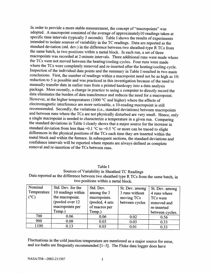
In order to provide a more stable measurement, the concept of"macropoints" was

adopted. A macropoint consisted of the average of approximately10 readings taken at

specific time intervals (typically 5 seconds). Table I shows the results of experiments

intended to isolate sources of variability in the TC readings. Data are reported as the

standard deviation (std. dev.) in the difference between two sheathed-type R TCs from

the same batch, in two positions within a metal block. In each run, a set of three

macropoints was recorded at 2-minute intervals. Three additional rtms were made where

the TCs were not moved between the heating/cooling cycles. Four runs were made

where the TCs were completely removed and re-inserted after the heating/cooling cycle.Inspection of the individual data points and the summary in Table I resulted in two main

conclusions. First, the number of readings within a macropoint need not be as high as 10:

reduction to 5 is possible and was practiced in this investigation because of the need to

manually transfer data in earlier runs from a printed hardcopy into a data analysis

package. More recently, a change in practice to using a computer to directly record the

data eliminates the burden of data transference and reduces the need for a macropoint.

However, at the higher temperatures (1000 °C and higher) where the effects of

electromagnetic interference are more noticeable, a 10-reading macropoint is still

recommended. Secondly, the variations (i.e., standard deviations) between macropoints

and between runs where the TCs are not physically disturbed are very small. Hence, only

a single macropoint is needed to characterize a temperature in a given run. Comparing

the standard deviations in Table I clearly shows that a major source for the increase in

standard deviation from less than ~0.1 °C to ~0.5 °C or more can be traced to slightdifferences in the physical positions of the TCs each time they are inserted within the

metal block and within the fumace. In subsequent sections, the standard deviations and

confidence intervals will be reported where repeats are always defined as completeremoval and re-insertion of the TCs between runs.

Table I

Sources of Variability in Sheathed TC Readings

Data reported as the difference between two sheathed type R TCs from the same batch, in

two positions within a metal block.

Nominal

Temperature

(oc)

700

900

1100

Std. Dev. for the

10 readings within

the macropoim.

(pooled over 12

macropoints per

Temp.)

0.06

0.08

0.13

Std. Dev.

among the 3

macropoints.

(pooled, 4 sets

of macros per

Temp.)

0.06

0.03

0.03

St. Dev. among3 runs without

moving TCs

between cycles

0.02

0.03

0.01

St. Dev. among4 runs where

TCs were

removed and

re-inserted

between cycles.

0.56

0.33

0.33

Fluctuations in the cold junction temperature are mentioned as a major source for error,

and ice-baths are frequently recommended [ 1-3]. The Fluke data logger does have

NASA/TM_2002-211507 3

electronicroomtemperaturecompensation,which shouldalleviatethisproblem. Thecompensationfor differencesbetweenthethermocouplewire endsandthedataloggerinputis accomplishedby severalelementsof the circuit, includingthe connectors,extensionwire,andinput circuit to thedatalogger. Theeffectivenessof thoseelementswasinvestigatedthroughselectiveheatingof thevariouscomponentsby meansof aheatgun. Thetemperatureof thecomponentschangedfrom 23 °Cto 40 °CandthechangeintheTC readingat 700 °Cwasrecorded.TheTC connectorplugs,theextensionwires,andtheinput cardfor the dataacquisitionsystemwereeachheatedindependently.Therewasamaximumof 0.3 °Cchangein thedisplayedtemperature,which occurredonlywhentheinput cardwasheated.Thechangeswere smallerwhentheothercomponentswerewarmed. Sincetypical fluctuationsin theambienttemperaturearesignificantlysmallerthanthosecausedby theheatgun,this setupcanbeconsideredstable.

Results and Discussion

A. Sheathed Thermocouples

The final and accepted setup for calibrating sheathed TCs is shown in Figure 2, and is

known as a solid block comparison method [2]. To minimize differences in the

temperature of the TC junctions, a solid metal block with holes drilled for individual TCs

is employed. A 2 in. diameter by 3 in. long cylinder of Haynes 188 (Co-22Cr-23Ni-

14W) was chosen for the block material due to its excellent oxidation resistance up to

1100 °C [4]. Seven 9/32 in. x 1.5 in. deep diameter holes were bored into the block.

They were located at the 12, 2, 4, 6, 8 and 10 o'clock positions and the 7th TC was

placed in the center of the block. For calibrating unknown TCs with this setup, the

unknowns were placed in the outer holes and the standard TC was placed in the centerposition. Care must be taken to be sure that all TCs are bottomed-out. The holes were

numbered as shown in Figure 2 and will henceforth be called positions. The block was

placed on two ceramic boats that elevated the block such that it was approximately

centered within the 3 in. diameter furnace tube (Fig. 2). The block and boats were

pushed into the tube until they were centered with respect to the furnace length.

Before TCs could be calibrated, potential errors due to positional bias within the block

had to be determined. ("Bias" is the statistical term defined as the offset value attributed

to a specific factor.) The positional bias can be added to or subtracted from any

difference between a TC in the block and the secondary standard TC to yield the true

thermocouple bias (- calibration offset). To determine the positional bias, seven

secondary standard TCs which were sheathed in 18 in. long alumina tubes were used.

These TCs were made from 20 gauge, type R wire taken from the same wire lot. A lot

calibration with NIST traceability was performed by the TC manufacturer [5]. The

manufacturer claims that variability within a lot is exceedingly small, which was

confirmed in our lab. As described in Section B.3, four TCs from the same lot were

welded together to form a common junction, and the temperature difference among the

four was only 0.06 °C. Thus all of the TCs from the same lot were treated as identical,

and any difference between the positional and the center readings was assigned aspositional bias.

NASA/TM_2002-211507 4

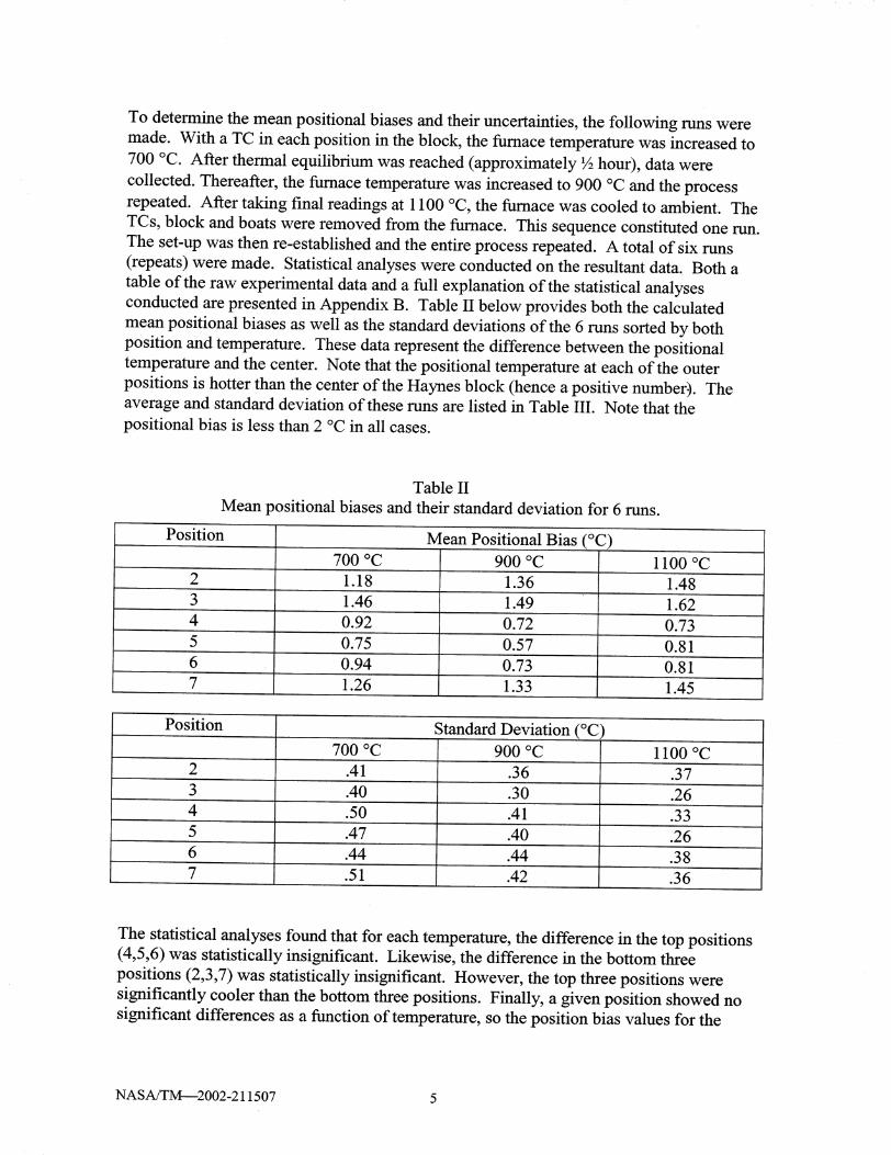
To determine the mean positional biases and their uncertainties, the following runs were

made. With a TC in each position in the block, the fumace temperature was increased to

700 °C. After thermal equilibrium was reached (approximately 1Ahour), data were

collected. Thereafter, the fumace temperature was increased to 900 °C and the process

repeated. After taking final readings at 1100 °C, the fumace was cooled to ambient. The

TCs, block and boats were removed from the fumace. This sequence constituted one ran.

The set-up was then re-established and the entire process repeated. A total of six runs

(repeats) were made. Statistical analyses were conducted on the resultant data. Both a

table of the raw experimental data and a full explanation of the statistical analyses

conducted are presented in Appendix B. Table II below provides both the calculated

mean positional biases as well as the standard deviations of the 6 runs sorted by both

position and temperature. These data represent the difference between the positional

temperature and the center. Note that the positional temperature at each of the outer

positions is hotter than the center of the Haynes block (hence a positive number). Theaverage and standard deviation of these runs are listed in Table III. Note that the

positional bias is less than 2 °C in all cases.

Table II

Mean positional biases and their standard deviation for 6 runs.

PositionMean Positional Bias (°C)

700 °C 900 °C 1100 °C

1.18 1.36 1.48

3 1.46 1.49 1.62

4 0.92 0.72 0.73

5 0.75 0.57 0.81

6 0.94 0.73 0.81

7 1.26 1.33 1.45

Position

700 °C

Standard Deviation (°C)

900 °C 1100 °C

.37

3 .40 .30 .26

4 .50 .41 .33

5 .47 .40 .26

6 .44 .44 .38

7 .51 .42 .36

The statistical analyses found that for each temperature, the difference in the top positions(4,5,6) was statistically insignificant. Likewise, the difference in the bottom three

positions (2,3,7) was statistically insignificant. However, the top three positions were

significantly cooler than the bottom three positions. Finally, a given position showed no

significant differences as a function of temperature, so the position bias values for the

NASA/TM_2002-211507 5

threetemperaturescouldbepooledinto a singlenumbercoveringtheentiretemperaturerange.

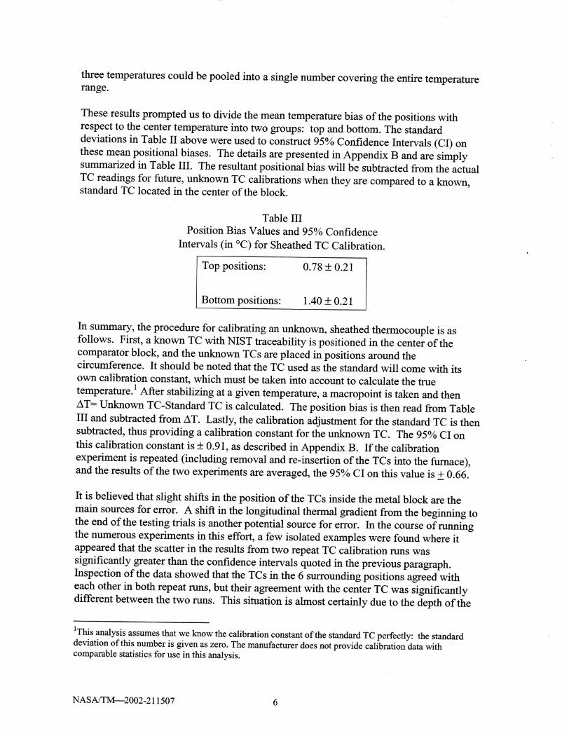
Theseresultspromptedusto divide themeantemperaturebias of thepositionswithrespectto thecentertemperatureinto two groups" topandbottom.Thestandarddeviationsin TableII abovewereusedto construct95%ConfidenceIntervals(CI) onthesemeanpositionalbiases.Thedetailsarepresentedin Appendix B andaresimplysummarizedin TableIII. Theresultantpositionalbiaswill be subtractedfrom theactualTC readingsfor future,unknownTC calibrationswhentheyarecomparedto a known,standardTC locatedin the center of the block.

Table III

Position Bias Values and 95% Confidence

Intervals (in °C) for Sheathed TC Calibration.

Top positions" 0.78 _+0.21

Bottom positions" 1.40 _+0.21

In summary, the procedure for calibrating an unknown, sheathed thermocouple is as

follows. First, a known TC with NIST traceability is positioned in the center of the

comparator block, and the unknown TCs are placed in positions around the

circumference. It should be noted that the TC used as the standard will come with its

own calibration constant, which must be taken into account to calculate the true

temperature. _ After stabilizing at a given temperature, a macropoint is taken and then

AT= Unknown TC-Standard TC is calculated. The position bias is then read from Table

III and subtracted from AT. Lastly, the calibration adjustment for the standard TC is then

subtracted, thus providing a calibration constant for the unknown TC. The 95% CI on

this calibration constant is + 0.91, as described in Appendix B. If the calibration

experiment is repeated (including removal and re-insertion of the TCs into the furnace),

and the results of the two experiments are averaged, the 95% CI on this value is + 0.66.

It is believed that slight shifts in the position of the TCs inside the metal block are the

main sources for error. A shift in the longitudinal thermal gradient from the beginning to

the end of the testing trials is another potential source for error. In the course of runningthe numerous experiments in this effort, a few isolated examples were found where it

appeared that the scatter in the results from two repeat TC calibration runs was

significantly greater than the confidence intervals quoted in the previous paragraph.

Inspection of the data showed that the TCs in the 6 surrounding positions agreed with

each other in both repeat runs, but their agreement with the center TC was significantly

different between the two runs. This situation is almost certainly due to the depth of the

1This analysis assumes that we know the calibration constant of the standard TC perfectly: the standard

deviation of this number is given as zero. The manufacturer does not provide calibration data withcomparable statistics for use in this analysis.

NASA/TM_2002-211507 6

center TC within the metal block having shifted more than usual in one of the runs.

Thus, the center TC, which is the standard against which all the unknowns are compared,is equally likely to suffer from errors due to slight differences in how the TC is inserted

within the metal block. Because of this effect, it is recommended that a second standard

TC be used in a calibration run, placing it in one of the outside TC positions, to act as a

double check of the calibration run. The two standard TCs must agree with each otherfor the run to be valid.

B. Unsheathed Thermocouples

B. 1 Metal Block Method

In principle, the same exact setup used for sheathed TCs can be used for unsheathed TCs.

Despite the fact that we have not run any confirmation experiments, we recommend that

the data in Table III be used to calculate the calibration constant for an unknown,

unsheathed TC if the setup described in Section B is used. However, several additional

options were explored for the case of unsheathed TCs. The first and most important is

that a different tube furnace was used in order to match the most commonly used

unsheathed TCs in the Materials Division mechanical testing labs. In these labs, shorter,

15 in. long type R TCs are frequently used in conjunction with 16 in. long, 2.75 in.

internal diameter furnaces. In order to minimize the extent of immersion error in the

determination of a calibration shift, a smaller tube furnace that matched the mechanical

testing furnaces was used. Others [6] have shown that with type R TCs after extended use

during creep testing, apparent calibration shifts can be mostly attributed to immersioneffects, rather than a true shift in the TC wire.

Since this particular tube furnace was equipped with a 1.25 in. diameter quartz tube, a1 in. diameter metal block with smaller 1/8 in. diameter holes was used to better match

the dimensions of both the furnace and the unsheathed TCs. The positions for all

experiments with this block were slightly different than for the sheathed block, as shown

in Fig. 2. In order to maximize furnace life, all experiments were limited to 1000 °C. To

produce more data in a given run, experiments were started at 600 °C and incremented in

100 °C steps. In all other details, the data recording protocol using macropoints wasidentical to that used previously.

The statistical analysis for these experiments is contained in Appendix C. It was found

that the behavior of this new fiarnace/TC combination showed subtle differences

compared to the sheathed experiments. First, the position bias of the TC holes was not a

simple vertical gradient through the cross section of the metal block, as it was for the

sheathed experiments. Rather, the position bias showed a slanted gradient with the two

upper fight positions being slightly cooler than the two lower left positions. This gradientis apparently the result of the clamshell furnace design. Second, while the mean values

for the position bias were still independent of temperature, the standard deviations

attached to these positions increased as temperature increased, as shown in Table CIII of

Appendix C. Recall that the experiments on the sheathed TCs exhibited standard

deviations that were constant over the temperature range.

NASA/TM_2002-211507 7

In summary,theprocedurefor calibratinganunknown,unsheathedthermocoupleis asfollows. A known TC with NIST traceability is positioned in the center of the

comparator block, and the unknown TCs are placed in positions around the

circumference. It should be noted that the TC used as the standard will come with its

own calibration constant, which must be taken into account to calculate the true

temperature. As mentioned in Section A, a second standard TC placed in one of the

circumferential positions adds another degree of confidence in data interpretation. After

stabilizing at a given temperature, a macropoint is taken and then AT= Unknown TC-

Standard TC is calculated. The position bias is then read from Table CIV in Appendix C

and subtracted from AT. Lastly, the calibration adjustment for the standard TC is then

subtracted, thus providing a calibration constant for the unknown TC. The 95% CI on

this calibration constant is + 0.56 at 600 °C and + 1.35 at 1000 °C, as described in

Table CV in Appendix C. If the calibration experiment is repeated (including removal

and re-insertion of the TCs into the furnace), and the results of the two experiments are

averaged, the 95% CI on this calibration constant is + 0.32 at 600 °C and + 0.76 at

1000 °C. Note that compared to the CI's measured with the sheathed TCs, this method

produced better results at 600 °C but was slightly worse at 1000 °C.

B.2 Tying Method

An alternate method of tying the hot junctions of the unknown TCs to a standard TC was

also investigated. This was done to eliminate position bias and still be able to calibrate

multiple TCs in one run. Tying was best accomplished by threading a loop of wire (we

used 0.012 in. diameter type K TC wire) through one leg of the TCs and twist-tying the

TCs moderately tight. A second loop of wire was then wrapped around the hot junction

beads to ensure tight contact between the unknown TCs and the standard TCs (see

Figure 3). After tying, care was taken to make sure the individual wires of each TC were

not touching each other away from the bead. Some degree of skill and practice is

required to perform the tying adequately. If the tying is too loose, or the TC wires are

touching in undesirable locations, more data scatter occurs. If the tying is too tight,damage to the TC is likely. By tying TCs together an electrical connection can be made

at areas other than the bead and this can create a source of error in the measurements.

Since the length of exposed wire (i.e., the distance between the bead and the first ceramic

insulator) is small (approximately 1/8 in.), it is assumed that the temperature is isothermal

over this distance and the error is negligible, but is a consequence of trying to maximize

efficiency by calibrating many thermocouples simultaneously.

The smaller furnace and the identical TCs used in Section B. 1 were used for the

calibration experiments. Because of the concern that operator skill would influence the

results, three operators performed five repeat runs (2 runs each by 2 operators, and 1 run

by the third), and the results were combined. The complete statistical analysis is

presented in Appendix D. With the tying method, there is no Position Bias that needs to

be calculated, thus making the results easier to analyze. As was the case for the metal

block experiments described in Section B. 1, the standard deviations characterizing the

scatter in these experiments increased as the nominal temperature increased. In summary,

NASA/TM_2002-211507 8

theprocedurefor calibratinganunknown,unsheathedthermocoupleis asfollows. First, aknown TC with NIST traceabilityis tied to asmanyasthreeunknownTCs. It shouldbenotedthattheTC usedasthestandardwill comewith its own calibration constant, which

must be taken into account to calculate the true temperature. After stabilizing at a given

temperature, a macropoint is taken and then AT= Unknown TC-Standard TC is

calculated. The calibration adjustment for the standard TC is then subtracted, thus

providing a calibration constant for the unknown TC. The 95% CI on this calibration

constant is + 0.56 at 600 °C and +1.11 at 1000 °C, as described in Table DIV in

Appendix D. If the calibration experiment is repeated (including removal, untying, andre-tying the TCs),. and the two experiments are averaged, the 95% CI on this value is

+ 0.39 at 600 °C and + 0.77 at 1000 °C. Note that compared to the CI's measured with

the sheathed TCs, this method produced a better CI at 600 °C but a slightly worse CI at

1000 °C. The results are virtually identical to the metal block experiments with the same

small furnace described in Section B. 1. Again, it is believed that slight differences in the

tying of the TCs are the main source for error. A shift in the longitudinal thermal

gradient from the beginning to the end of the testing trials is another potential source forerror.

B.3 Welding Method

References 1 to 3 also discuss a method of welding the unknoWn TCs to the standard TC

in order to enhance the thermal homogeneity between the TCs. Such intimate contact

would eliminate the errors associated with shifting positions within a metal block or the

reproducibility of tying the TCs together. There is a common misperception that the act

of welding a hot junction bead, cutting the bead off, and re-welding the bead can affect

the calibration constant of the TC. This concern is counter to the recommendations in

refs. [ 1-3] and private communications with representatives from NIST and ASTM.

However, the disadvantage remains that continued welding and cutting beads will serve

to shorten the available wire. For this reason, our efforts in investigating this method

were limited to a single trial of welding 4 TCs from a single batch. The four TCs

exhibited extremely good agreement with each other, producing a standard deviation of

only 0.06 *C at all temperatures between 600 and 1000 *C. This value is smaller than the

standard deviation obtained by tying the same 4 TCs by about a factor of 3. Assuming

that this ratio would be maintained if a full series of repeat experiments were conducted,

a CI of approximately + 0.2 °C for a single calibration run and approximately + 0.1 °C

for a duplicate run would be expected. These results represent the best accuracy and

precision obtained in this laboratory. In fact, at this level of error, we may be testing the

variability of some other part of our experimental setup, such as electromagneticinterference, the recording devices or the extension wires.

C. Summary and Verification of Type R Thermocouple Calibration Experiments.

A summary of the calibration experiments and the statistical uncertainties (expressed as

95% CI's) expected from these experiments is displayed in Figure 4. The least accurate

method of knowing a thermocouple's true value is relying on the manufacturer's

tolerance, which is given as + 3 at 600 °C and as + 5 at 1000 *C [2]. Figure 5 shows

NASA/TM--2002-211507

calibrationresultsfor 6 separatebatchesof new TCspurchasedover a 2 year period. The

range of data covers approximately + 1 °C at 600 °C and + 2 °C at 1000 °C, which is

much tighter than the quoted ranges shown in Figure 4. Thus, the quoted ranges are

clearly conservative and the risk of relying on such data appears minimal. However, the

benefit of tighter confidence intervals from calibration is seen in Figure 4. Using

comparison methods for calibration, ref. [2] quotes CI = + 1.2 °C (at 600 °C) as the

uncertainty to be expected using good practice, whereas ASTM E220 quotes CI =

+ 0.6 °C at the same temperature [3]. R. Park, a member of the ASTM committee

responsible for TC calibrations, recommended [7] that the CI = + 1.2 °C value quoted in

ref. [2] be used, because it is more recent than the current version of ASTM E220, which

was written in 1986. He also mentioned that more statistically rigorous values for

uncertainties will be available in a new revision of ASTM E220, which is due to be

released in the near future. Further improvements in accuracy and precision can be

obtained by calibrating against the melting point of pure metals [2]. Also shown in

Figure 4 are the CI's that resulted from the experiments described in Sections A and B.

These values are comparable to what is expected from the literature.

The final set of bars in Figure 4 describes another set of experiments where new

unsheathed TCs were tested in identical experiments as a "verification run" to see if the

standard deviations in practice were consistent with the initial "baseline" runs. First, two

batches of 3 TCs each were calibrated in 5 repeat experiments, producing a CI =

+ 1.47 °C at 600C °C and + 2.81 °C at 1000 °C. These values were greater than the

baseline data described in Section B. This change may be due to either a change in

operators or a shift in the longitudinal temperature gradient in the tube fumaces, since it

was found after the experiments were completed that both fumaces had heating elements

that had degraded. More positively, one of the TC batches was independently calibrated

by the manufacturer [5], and the results from the two labs agreed within experimental

scatter. Another batch of new TCs were calibrated by the tying method, and a batch of

used TCs from the Materials Division Creep Lab were calibrated via the metal block

method. Both of these batches had similar CI results as the first batch. The results of

these "verification" runs are somewhat equivocal. The larger CI values of the

verification rims compared to the baseline runs were clearly undesirable, but the

differences were borderline in terms of statistical significance. Furthermore, the

agreement with the extemal lab, and the still relatively small values for scatter, would

seem to make the calibration testing worth the effort, certainly compared to themanufacturer's tolerance.

To check on the stability of the metal block calibration method and the position biases

over time, the tube fumace used for the unsheathed TC experiments was repaired and

after a twelve month waiting period, a new set of calibrations were run. First, seven new

TCs from a single batch were used to recalculate the position biases using the small metal

block. The standard deviation among these 4 runs was equivalent to the initial baseline

runs, thus confirming that accuracy of better than + 1 °C is achievable. However, the

position biases showed considerable shifts, of up to 2 °C from the baseline values in two

of the six positions, compared to the other four where the position bias remained within

approximately + 0.5 °C. At first glance, these shifts in position bias couldbe attributed to

NASA/TM_2002-211507 10

thefact thatnewheatingelementswereinstalledduringthe fumacerepair. However,closeinspectionof the individual dataonspecificTCsleadusto the conclusionthatthedifferencein positionbiasbetweenthenew runsandthebaselinewereduetoexperimentalscatterratherthanatruechangein thermalgradient. If aTC wasplacedinoneof thefour 'morestable'positions,its calibrationconstantwaswithin + 1 °C of that

determined 12 months earlier, and also close to the data supplied by the manufacturer.

However, if the TC was placed in one of the two 'unstable' positions, the calibration

constant differed from the prior data by + 2 °C (i.e., subtracting the position bias did not

produce consistent results with the baseline).

Therefore, it appears that there is still a source of variability that occurs sporadically and

causes data to occasionally fall outside the statistical confidence limits defined in sections

A and B and Figure 4. Thus, the presumed benefit of improved accuracy from specific

calibration runs may be illusory. Determining the true size of the variability would

require several repeat runs that might not be worth the cost. The entire focus of this work

was to establish methods for simultaneous calibration of multiple TCs in order to

minimize cost. The number of repeat rims necessary to ensure accuracy appears tonegate any efficiencies in these multiple TC runs. We therefore conclude that the

welding method is the most accurate and cost effective method for calibrating multiple

TCs in a single run. If unsheathed TCs are to be used, the tying method with a small

number of TCs is likely to be accomplished with the accuracy exhibited in Figure 4,

provided that a specific operator has been properly trained and passed qualification

standards. For sheathed TCs, the only choice appears to be the metal block comparison

method, but achieving the accuracy quoted in Figure 4 appears torequire attention to

exact detail in experimental setup; additionally, a check for any shift of the position bias

values from the baseline should be performed immediately prior to calibrating.

D. Type K Thermocouples.

Type K thermocouples can be used in air (for short periods) up to 1250 °C [2]. For

extended periods there is a much lower temperature limit, and this limit also depends on

the wire diameter. These thermocouples are subject to errors induced by oxidation or byC,_, " 99 , ,

short range ordering. Both of these effects cause an accumulative drift in the EMF

output of the TC over time. The effect of short range ordering is seen up to 600 °C, and

can cause changes up to 3 °C [2]. At temperatures above 1000 °C, the drift due to

oxidation can be greater than ~10 °C after a few 100's of hours [8]. The low cost and

moderate stability of type K thermocouples usually imply that these thermocouples

should be discarded rather than recalibrated. The recommended standard practice is that

any portion of the thermocouple that is exposed to elevated temperatures during the test

should be removed at the end of the test and a new measurement junction made.

Calibration experiments were performed on TCs made from type K wire (0.012 in.

diameter) taken from a spool in the Structures Division Fatigue Lab and calibrated

against a type R TC by the tying method. Calibrations were performed on five TCs and a

CI = + 1.3 at 600 °C was determined. The calibration constant of-l.4 °C is valid for the

entire spool, although periodic crosschecks will be performed as the spool is consumed.

NASA/TM_2002-211507 11

Comparedto themanufacturer'stolerancesof + 10°C [2], thevalueof performingthecalibration on the spool of wire is obvious.

Because stability data on the exact wire diameter used in the mechanical testing labs were

not found, individual experiments were necessary to quantify the calibration drift to be

expected in our labs. Experiments were performed by tying unsheathed, 0.012 in. wire

diameter, type K TCs to a type R standard and exposing them in a tube furnace in air.

The data from Dahl [8] in Figure 6 shows that calibration drift is negligible at

temperatures below about 600 °C. Our own experiments at 300 and 500 °C confirmed

this finding. Very little evidence for calibration drift due to short range ordering was

found in this lower temperature range:, if the effect was present, its magnitude was less

than a degree and its duration was confined to the first few hours of the test. Apparently,

the different thermal responses of the TCs, and the difficulty in achieving a stabletemperature in this low temperature region masked the effect.

Our data from higher temperature exposures are shown in Figure 7. At all 3

temperatures, there is a transient period where the calibration drift changes by about 2 °C

during the first few hours of exposure. After this transient the TC was very stable at

700 °C. The TC continued to drift at 800 °C and 900 °C, reaching a total calibration shift

after 1000 hours of 5 °C and 6 °C, respectively. Comparison of our data to that of Dahl's

is not straightforward because of different wire diameters and exposure temperatures.

The closest match is shown in Fig. 8, where Dahl's data at 871 °C is compared to our

data at 800 and 900 °C. Figure 8 shows that both data sets are consistent with each

other. There are general trends of larger calibration shifts exhibited by either higher

temperatures or thinner wires, as would be expected for an oxidation mechanism. The

reproducibility between two runs at 800 °C is also shown to be within 1 °C after 1000hours.

The above experiments all reflect isothermal conditions. Dahl [8] showed abundant data

that the effects of oxidation can cause calibration shifts that are dependent on

temperature. For example, aging 0.026 in. diameter wire at 871 °C for 1000 hours caused

a calibration shift of 4 ° at 871 °C. The same 871 °C exposure resulted in calibration

shifts of 5 ° at 300 °C and only 1o at 550 °C.

Several stability experiments were run with metal-sheathed TCs to determine if they

provide any advantage by protecting the TC wires from oxidation. Two separate

sheathed geometries were examined: 1) 0.05 in. diameter wire sheathed in a 0.25 in.

diameter Inconel 600 TM tube, where the TC was not grounded to the sheath and was

separated from the sheath by MgO insulation; and 2) a 0.005 in. diameter wire sheathed

inside a 0.032 in. diameter 304 stainless steel tube, where the hot junction was grounded,

indicating intimate contact with the sheath. Figure 9a shows that at 800 °C, the larger

sheathed TC did indeed stabilize at a slightly smaller calibration shift, but the effect was

not very pronounced. More surprising was the behavior of the smaller sheathed TC,

which showed no evidence of stabilization even after 1350 hours. This behavior was

confirmed in a second run, Figure 9b, and is caused by diffusion in the fine wire diameter

in the grounded TC. At 900 °C, the effect is even more pronounced, and the unsheathed

NASAJTM_2002-211507 12

TC is clearlymorestabledueto its largerwire diameterthanthesmall-sheathed,groundeddesign(Fig. 10). Additional experimentswererunwith ungroundedTCshaving0.040in. and0.062in. diametersheathsand0.010in. diameterwire. Theyshowedcalibrationshiftsof 3 and 4 °C, respectively throughout the 1000 hours exposure

at 1100 °C. These calibration shifts were accumulated gradually throughout the exposure

with no evidence of stabilization at longer times. Hence, the choice of wire diameter for

any type of TC is important.

Comparisons between type R and type K TCs are summarized in Figure 11. The

manufacturer's tolerances for type R TCs are clearly superior to type K at both at 700 and

900 °C, so type R would be the choice using this criterion. However, a spool (or batch)

calibration brings the uncertainty levels achievable in the two TC types to more

comparable levels. The next criterion to consider is thermal stability. It appears from the

data in Figures 6-9 that 700 °C is a reliable, conservative upper limit for the use of type

K TCs in air. This temperature is dependent on wire diameter, but it is certainly valid forwire diameters at least as small as 0.010 in. If one uses the calibration constant after

about 1-2 hours of exposure, the stability of the type K TC is excellent. Although the

type R TC is also excellent, it can suffer from calibration shift due to cold work [1-3, 6].Evidence for the magnitude of this shift was supplied by testing six used TCs from a

Materials Division creep lab. The temperature and duration of the exposure given tothese TCs is unknown, although it is known that at least one TC was used for

10,000 hours at 980 °C. The calibration shifts measured on these TCs are given by the

data points in Figure 11 and ranged up to 4 °C. Unfortunately, it is difficult to separate a

true calibration shift from the effects of immersion, as is made strikingly clear byDesvaux [6]. The TC must be cleaned and annealed and then recalibrated in order to see

if a chemical composition change in the TC wires was causing the measured drift.

Furthermore, it is not clear whether all or parts of a calibration shift due to cold work is

actually affecting the temperature measurement in-situ in the creep-testing machine. In

principle, all the cold work should be located in the ~50 mm flexible portion of the TC,

which is exposed in the nearly isothermal section of the creep machine fumace. Our

recommendation would be that in-situ calibration is probably the easiest way of

addressing these concems. In an in-situ calibration, one fresh TC is placed near the used

TCs in the same location in the testing fumace, rather than removing the TCs and placingthem in a separate 'calibration' fumace.

This discussion indicates that if the calibration shifts of 1--4 °C are critical to the success

of an experiment, recalibration of type R TCs should be carefully considered. A

measurement of calibration drift with sufficient accuracy appears to be quite difficult and

certainly has hindered our efforts to come up with an inexpensive standardized method.

An extensive database provided from a series of in-situ calibrations would be needed

before a final recommendation can be reached. The type K TCs have an advantage in

that they are used only once and the calibration constant from the spool is valid for all

tests below about 700 °C or up to ~900 °C for times less than 20 hours, again dependingon wire diameter.

NASA/TM_2002-211507 13

Conclusions

This paper has provided a consolidation of information that can be used to define

procedures for enhancing and maintaining accuracy in temperature measurements in

materials testing laboratories. These studies were restricted to type R and K

thermocouples (TCs) tested in air. Thermocouple accuracies, as influenced by calibration

methods, thermocouple stability, and manufacturer's tolerances were all quantified in

terms of statistical confidence intervals. By calibrating specific TCs the benefits in

accuracy can be as great as 6 °C or 5X better compared to relying on manufacturer's

tolerances. The results emphasize strict reliance on the defined testing protocol and onthe need to establish recalibration frequencies in order to maintain these levels of

accuracy. Type K TCs are best utilized when discarded after a single use. A limited

number of calibrations on individual TCs are sufficient to characterize the entire spool of

TC wire. After some initial transients during the first hour or two of exposure, Type _K

TCs are stable for thousands of hours below 700 °C but only for about 20 hours at and

above 900 °C, though the exact temperatures are highly dependent on wire diameter.

Type R TCs are more stable at the higher temperatures, but may need periodic re-

calibration as accumulating cold work during use causes calibration shifts. However,

recalibration is complicated by immersion .errors and it may be more efficient to replace

the TCs with new ones. Although an extensive effort was made in using the metal block

and tying variants of the comparison method for TC calibration, the welding method

clearly exhibited the best reproducibility and accuracy. Finally, a consideration of in-situcalibration appears to be compelling.

NASA/TM_2002-211507 14

Appendix A

Attempted Methods of Calibration

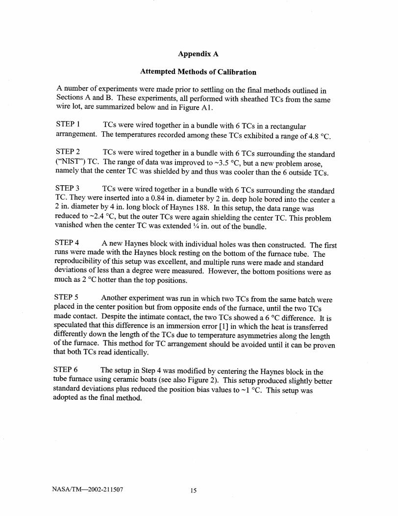
A number of experiments were made prior to settling on the final methods outlined in

Sections A and B. These experiments, all performed with sheathed TCs from the same

wire lot, are summarized below and in Figure A1.

STEP 1 TCs were wired together in a bundle with 6 TCs in a rectangular

arrangement. The temperatures recorded among these TCs exhibited a range of 4.8 °C.

STEP 2 TCs were wired together in a bundle with 6 TCs surrounding the standard

("NIST") TC. The range of data was improved to ~3.5 °C, but a new problem arose,

namely that the center TC was shielded by and thus was cooler than the 6 outside TCs.

STEP 3 TCs were wired together in a bundle with 6 TCs surrounding the standard

TC. They were inserted into a 0.84 in. diameter by 2 in. deep hole bored into the center a

2 in. diameter by 4 in. long block of Haynes 188. In this setup, the data range was

reduced to ~2.4 °C, but the outer TCs were again shielding the center TC. This problemvanished when the center TC was extended ¼ in. out of the bundle.

STEP 4 A new Haynes block with individual holes was then constructed. The first

runs were made with the Haynes block resting on the bottom of the furnace tube. The

reproducibility of this setup was excellent, and multiple runs were made and standard

deviations of less than a degree were measured. However, the bottom positions were as

much as 2 °C hotter than the top positions.

STEP 5 Another experiment was run in which two TCs from the same batch were

placed in the center position but from opposite ends of the furnace, until the two TCs

made contact. Despite the intimate contact, the two TCs showed a 6 °C difference. It is

speculated that this difference is an immersion error [1] in which the heat is transferred

differently down the length of the TCs due to temperature asymmetries along the length

of the furnace. This method for TC arrangement should be avoided until it can be proventhat both TCs read identically.

STEP 6 The setup in Step 4 was modified by centering the Haynes block in the

tube furnace using ceramic boats (see also Figure 2). This setup produced slightly better

standard deviations plus reduced the position bias values to ~ 1 °C. This setup wasadopted as the final method.

NASA/TM_2002-211507 15

Page intentionally left blank

Appendix B

Statistical Analyses of Data from the Metal Block Method of Calibrating

Sheathed Thermocouples

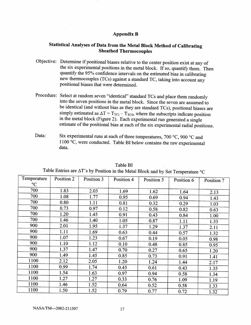
Objective: Determine if positional biases relative to the center position exist at any of

the six experimental positions in the metal block. If so, quantify them. Then

quantify the 95% confidence intervals on the estimated bias in calibrating

new thermocouples (TCs) against a standard TC, taking into account anypositional biases that were determined.

Procedure" Select at random seven "identical" standard TCs and place them randomlyinto the seven positions in the metal block. Since the seven are assumed to

be identical (and without bias as they are standard TCs), positional biases are

simply estimated as AT = TTci- TTC0, where the subscripts indicate position

in the metal block (Figure 2). Each experimental run generated a single

estimate of the positional bias at each of the six experimental radial positions.

Data: Six experimemal runs at each of three temperatures, 700 °C, 900 °C and

1100 °C, were conducted. Table BI below contains the raw experimentaldata.

Table BI

Table Entries are AT's by Position in the Metal Block and by Set Temperature °C

Temperature

°C

700

700

700

700

700

700

900

900

900.....

900

900

900

1100

1100

1100

1100

1100

1100

Position 2

1.83

1.08

0.80

0.73

1.20

1.46

2.01

1.11

1.07

1.10

1.37

1.49

2.12

0.99

1.54

1.27

1.46

1.50

Position 3

2.03

1.77

1.11

0.97

1.45

1.40

1.95

1.69

1.23

1.12

1.47

1.45

2.05

1.74

1.63

Position 4

1.69

0.95

0.81

0.12

0.91

1.05

1.37

0.63

0.67

0.10

0.70

0.85

1.20

0.45

0.97

1.27 0.33

1.52 0.64

1.52 0.79

Position 5

1.62

0.69

0.32

0.58

0.43

0.87

1.29

Position 6

1.64

0.94

0.29

0.82

0.84

1.11

1.37

0.44 0.57

0.19 0.05

0.48 0.85

0.27

0.73

1.24

0.61

0.94

0.76

0.52

0.77

0.65

0.91

1.44

0.43

0.58

1.09

0.58

0.72

Position 7

2.13

1.43

1.03

0.63

1.00

1.33

2.11

1.32

0.98

0.95

1.20

1.41

2.17

1.35

1.34

1.19

1.33

1.32

NASA/TM_2002-211507 17

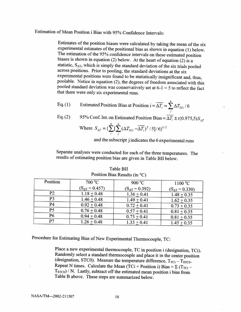
Estimationof Mean Position i Bias with 95% Confidence Intervals:

Estimates of the position biases were calculated by taking the mean of the six

experimental estimates of the positional bias as shown in equation (1) below.

The estimation of the 95% confidence intervals on these estimated position

biases is shown in equation (2) below. At the heart of equation (2) is a

statistic, SaT, which is simply the standard deviation of the six trials pooledacross positions. Prior to pooling, the standard deviations at the six

experimental positions were found to be statistically insignificant and, thus,poolable. Notice in equation (2), the degrees of freedom associated with this

pooled standard deviation was conservatively set at 6-1 = 5 to reflect the fact

that there were only six experimental runs.

Eq. (1)

Eq. (2)

6

Estimated Position Bias at Position i - AT,. - _ ATvc _/ 6j

95% Conf. Int. on Estimated Position Bias - _ + t(0.975,5)S_r6 6

Where S_r - {_[_(ATro. -AT,.) 2/5]/6} 1/2i j

and the subscript j indicates the 6 experimental runs

Separate analyses were conducted for each of the three temperatures. The

results of estimating position bias are given in Table BII below.

Table BII

Position Bias Results (in °C)

Position

P2

P3

P4

P5

P6

P7

700 °C

(SaT = 0.457)1.18 + 0.48

1.46 + 0.48

0.92 + 0.48

0.76 + 0.48

0.94 + 0.48,,

1.26 + 0.48

900 °C

(SAT -- 0.392)

1.36 + 0.41

1.49 + 0.41

0.72 + 0.41

0.57 + 0.41

0.73 + 0.41

1.33 + 0.41

1100 °C

(SaT = 0.330)1.48 + 0.35

1.62 + 0.35

0.73 + 0.35

0.81 + 0.35

0.81 +0.35

1.45 + 0.35

Procedure for Estimating Bias of New Experimental Thermocouple, TC"

Place a new experimental thermocouple, TC in position i (designation, TCi).

Randomly select a standard thermocouple and place it in the center position

(designation, STC0). Measure the temperature difference, TTCi- TSTC0.

Repeat N times. Calculate the Mean (TCi + Position i) Bias = Z (TTci-

TsTc0) / N. Lastly, subtract off the estimated mean position i bias from

Table B above. These steps are summarized below.

NASA/TM_2002-211507 18

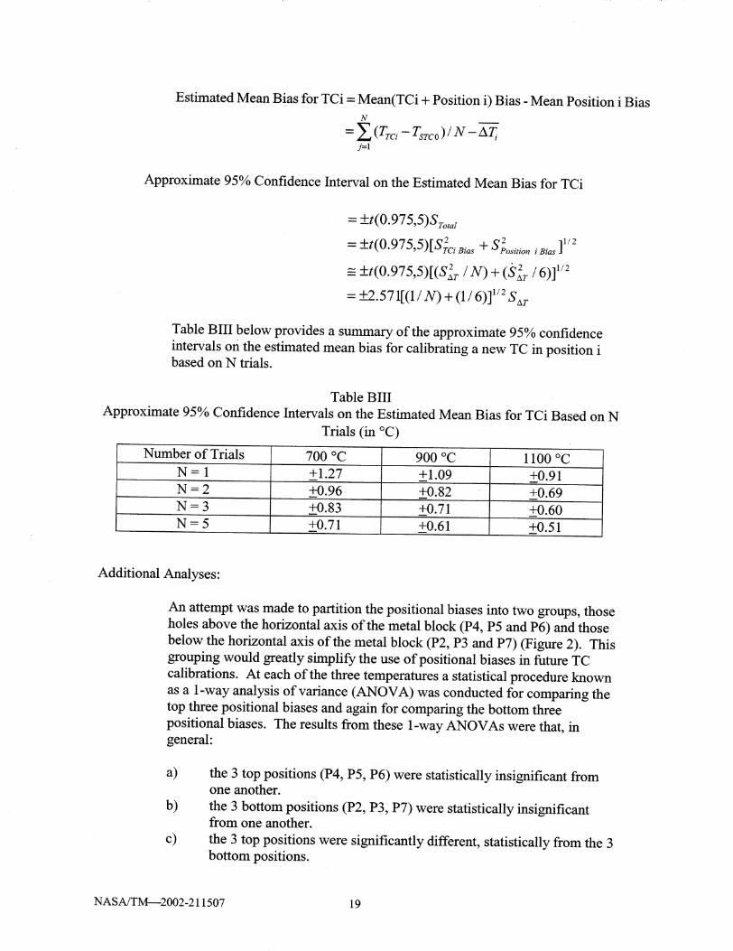
Estimated Mean Bias for TCi - Mean(TCi + Position i) Bias - Mean Position i Bias

N

= Z (Trc_ - Tsrco ) / N - AT_j=l

Approximate 95% Confidence Interval on the Estimated Mean Bias for TCi

= +t(O.975,5)STo_a _

= +t(0"975,5)[S_c_ B_s + S2 ]1/2Position i Bias

= +t(0.975,5)[(sZr / N) + (S_r / 6)] 1/2

= _+2.571[(1/N) + (1/6)] 1/2 S_T

Table BIII below provides a summary of the approximate 95% confidence

intervals on the estimated mean bias for calibrating a new TC in position ibased on N trials.

Table BIII

Approximate 95% Confidence Intervals on the Estimated Mean Bias for TCi Based on N

Trials (in °C)

Number oflrials

N=I

700 °C

+1.27

900 °C

+1.09

1100 °C

+0.91

N = 2 +0.96 +0.82 +0.69

N = 3 +0.83 +0.71 +0.60

N = 5 +0.71 +0.61 +0.51

Additional Analyses:

An attempt was made to partition the positional biases into two groups, those

holes above the horizontal axis of the metal block (P4, P5 and P6) and those

below the horizontal axis of the metal block (P2, P3 and P7) (Figure 2). This

grouping would greatly simplify the use of positional biases in future TC

calibrations. At each of the three temperatures a statistical procedure known

as a 1-way analysis of variance (ANOVA) was conducted for comparing the

top three positional biases and again for comparing the bottom three

positional biases. The results from these 1-way ANOVAs were that, ingeneral:

a)

b)

c)

the 3 top positions (P4, P5, P6) were statistically insignificant fromone another.

the 3 bottom positions (P2, P3, P7) were statistically insignificantfrom one another.

the 3 top positions were significantly different, statistically from the 3

bottom positions.

NASA/TM_2002-211507 19

It wasassumedthattherewereno statisticaldifferencesacrossthethreetemperatures.Hence,thedatawerepooledacrossthethreetemperaturesandthenbrokeninto twoparts,thetop positionsandthebottompositions. Then,a 2-wayANOVA (with factorsTemperatureandPosition)wasconductedforeachsetof positions,top andbottom,separately.Theresultsof eachof theseanalysesfoundthattheTemperatureeffectandthePositioneffectandtheTemperature-x-Positioninteractionwerenot statisticallysignificant. Theseresultssupportedtheconjecturethattherewereno differencesacrossthethreetemperatures.Theresultantestimatedmeanbiasfor thetoppositionswas0.78andtheestimatedmeanbiasfor thebottompositionswas1.40.

A components-of-variationanalysiswasconductedfor eachsetof positions

separately to quantify the variability in the response, AT, pooled over all

three temperatures and all three positions within a group. The resultant SaT

statistic was statistically insignificant between the top and bottom positions

and could themselves be pooled. The resultant grand pooled standard

deviation of the response, AT, was SaT - 0.416 with 15 degrees of freedom.

(Note- Even though there were 54 data points in each of the top and bottom

pooled data sets, there were only six true repeats at each temperature

resulting in five degrees of freedom for each of three temperatures. When

pooled over the three temperatures, the total becomes 15 degrees of freedom.The results are summarized in Table BIV below.

Table BIV

Estimation of Mean Position Bias with 95% Confidence

Intervals = ATi + t(0.975,15)Sax/(181/2)

Position Mean Bias with 95% Confidence Interval

'lop (P4, P5, P6) 0.78 + 0.21

Bottom (P2, P3, P7) 1.40 + 0.21

Estimating Bias of New Experimental Thermocouple, TC"

The logic described above also applies here except that the formulas changeslightly.

Estimated Mean Bias for TCi - Mean(TCi + Position i) Bias - Mean Position i Bias

N

- Z (Trc_ - Tsrco) / N - ATe,j=l

where, A_ -0.775 (Top)or 1.402 (Bottom)

NASA/TM_2002-211507 20

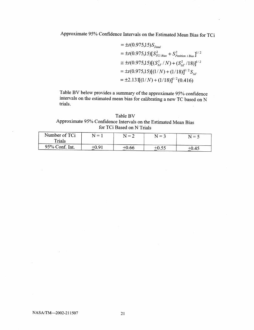
Approximate95%ConfidenceImervalson the Estimated Mean Bias for TCi

= +t(0.975,15)Svota ,

= +t(0.975,15)[$2c; Bias q" $2 ]1/2Position i Bias

= +.t(0.975,15)[(sJv/N) + (sZv/18)] 1/2

= +_t(O.975,15)[(1/N) + (1/18)]I/2SAT

= _+2.131[(1 / N) + (1 / 18)] 1/2 (0.416)

Table BV below provides a summary of the approximate 95% confidence

intervals on the estimated mean bias for calibrating a new TC based on Ntrials.

Table BV

Approximate 95% Confidence Intervals on the Estimated Mean Bias

for TCi Based on N Trials

Number ofl'Ci

Trials

95% Conf. Int.

N=I

+0.91

N=2

+0.66

N=3

+0.55

N=5

NASA/TM--2002-211507 21

Page intentionally left blank

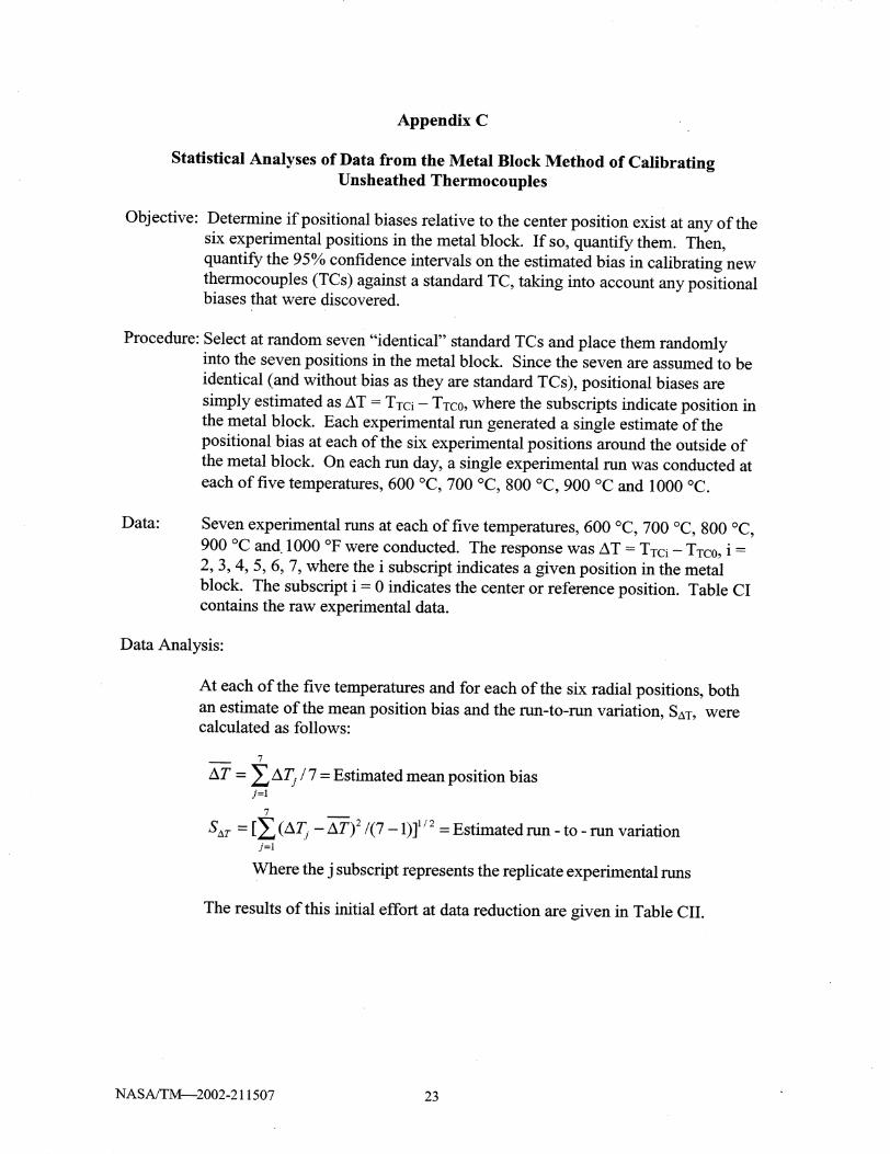
Appendix C

Statistical Analyses of Data from the Metal Block Method of Calibrating

Unsheathed Thermocouples

Objective: Determine if positional biases relative to the center position exist at any of the

six experimental positions in the metal block. If so, quantify them. Then,

quantify the 95% confidence intervals on the estimated bias in calibrating new

thermocouples (TCs) against a standard TC, taking into account any positionalbiases that were discovered.

Procedure: Select at random seven "identical" standard TCs and place them randomlyinto the seven positions in the metal block. Since the seven are assumed to be

identical (and without bias as they are standard TCs), positional biases are

simply estimated as AT = TTCi- TTC0, where the subscripts indicate position in

the metal block. Each experimental run generated a single estimate of the

positional bias at each of the six experimental positions around the outside of

the metal block. On each nm day, a single experimental run was conducted at

each of five temperatures, 600 °C, 700 °C, 800 °C, 900 °C and 1000 °C.

Data: Seven experimental runs at each of five temperatures, 600 °C, 700 °C, 800 °C,

900 °C and 1000 °F were conducted. The response was AT = TTCi- TTC0, i --

2, 3, 4, 5, 6, 7, where the i subscript indicates a given position in the metal

block. The subscript i - 0 indicates the center or reference position. Table CIcontains the raw experimental data.

Data Analysis:

At each of the five temperatures and for each of the six radial positions, both

an estimate of the mean position bias and the run-to-ran variation, SAT, werecalculated as follows:

7

AT = _ AT:. / 7 - Estimated mean position biasj=l

7

Sat - [_ (ATj - _--_)2/(7 - 1)] 1/2 - Estimated run- to- run variationj=l

Where the j subscript represents the replicate experimental runs

The results of this initial effort at data reduction are given in Table CII.

NASAJTM_2002-211507 23

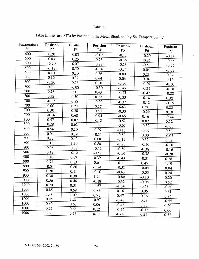
TableCI

TableEntriesareAT's by Position in the Metal Block and by Set Temperature °C

Temperature

°C

600

600

600

600

600

600

600

700

700

700

700

700

700

700

800

800

800

800

800

800

800

900

900

900

900

900

900

900

1000

1000

1000

1000

1000

1000

1000

Position

P2

0.20

0.03

-0.20

0.10

0.16

-0.20

0.03

0.28

0.32

-0.17

0.00

0.30

0.57

0.28

0.54

0.04

0.23

1.10

0.06

0.48

0.18

0.91

0.20

0.30

0.56

0.20

0.85

1.43

0.05

0.60

0.22

0.56

Position

P3

0.03

0.25

0.07

0.20

0.32

0.12

0.30

0.58

0.27

0.20

0.68

0.07

0.02

0.20

0.39

0.42

1.10

0.08

-0.12

0.07

0.83

0.66

0.11

0.30

0.44

0.31

0.59

1.09

1.22

0.66

0.66

0.39

Position

P4

0.28

0.26

0.64

0.10

0.43

0.22

0.27

0.60

-0.18

0.38

0.29

-0.31

0.08

0.80

-0.12

-0.57

0.39

0.64

0.86

0.71

0.06

0.12

0.17

Position

P5

0.00

0.06

Position

P6

0.16

0.02

_.J

0.47 0.36

0.23

0.73

-0.32

0.27

Position

P7

-0.14

-0.45

-0.27

-0.08

0.32

0.16

-0.10

-0.18

-0.28

0.32

-0.15

0.28

0.10

0.12

-O.O5

0.57

-0.03

0.32

-0.10

-0.16

0.28

1.19

0.04

0.24

0.20

0.52

-0.60

0.61

0.86

-0.55

0.20

0.66

0.52

NASA/TM_2002-211507 24

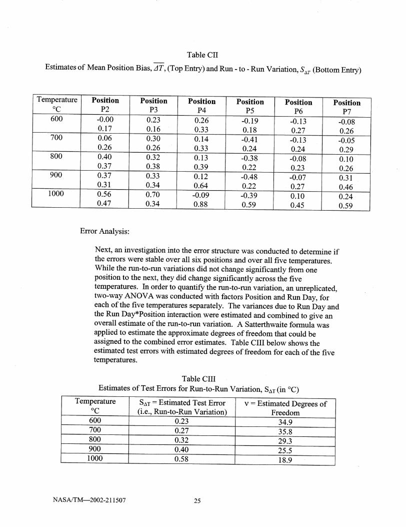
TableCII

Estimatesof MeanPositionBias,A T, (Top Entry) and Run - to - Run Variation, Sat (Bottom Entry)

Temperature

°C

600

700

800

900

1000

Position

P2

-0.00

0.17

0'06

0.26

0.40

0.37

0.37

0.31

0.56

0.47

Position

P3

0.23

0.16

0.30

0.26

0.32

0.38

0.33

0.34

0.70

0.34

Position

P4

0.26

0.33

0.14

0.33

0.13

0.39

0.12

0.64

Position

P5

Position

P6

0.10

0.45

Position

P7

0.10

0.26

0.31

0.46

0.24

0.59

Error Analysis:

Next, an investigation into the error structure was conducted to determine if

the errors were stable over all six positions and over all five temperatures.

While the rtm-to-run variations did not change significantly from one

position to the next, they did change significantly across the five

temperatures. In order to quantify the ran-to-run variation, an unreplicated,

two-way ANOVA was conducted with factors Position and Run Day, for

each of the five temperatures separately. The variances due to Run Day and

the Run Day*Position interaction were estimated and combined to give anoverall estimate of the run-to-run variation. A Satterthwaite formula was

applied to estimate the approximate degrees of freedom that could be

assigned to the combined error estimates. Table CIII below shows the

estimated test errors with estimated degrees of freedom for each of the five

temperatures.

Table CIII

Estimates of Test Errors for Run-to-Run Variation, SaT (in °C)

Temperature

°CSaT = Estimated Test Error

(i.e., Run-to-Run Variation)v = Estimated Degrees of

Freedom

600 0.23 34.9

700 0.27 35.8

800 0.32 29.3

900 0.40 25.5

1000 0.58 18.9i

NASA/TM_2002-211507 25

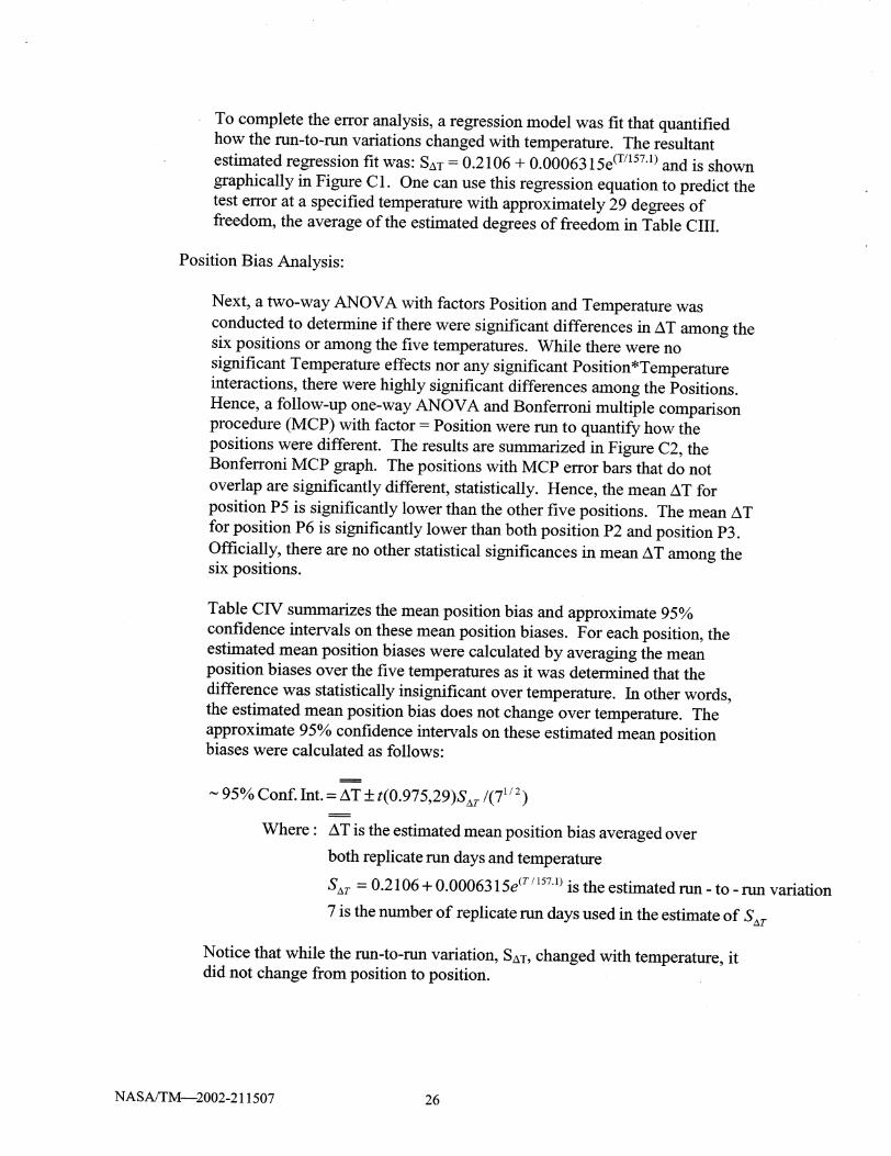
To completetheerroranalysis,aregressionmodelwas fit thatquantifiedhowtherun-to-ranvariationschangedwith temperature.Theresultantestimatedregressionfit was"SzxT= 0.2106+ 0.0006315e(T/157"1) and is shown

graphically in Figure C 1. One can use this regression equation to predict the

test error at a specified temperature with approximately 29 degrees of

freedom, the average of the estimated degrees of freedom in Table CIII.

Position Bias Analysis:

Next, a two-way ANOVA with factors Position and Temperature was

conducted to determine if there were significant differences in AT among thesix positions or among the five temperatures. While there were no

significant Temperature effects nor any significant Position*Temperature

interactions, there were highly significant differences among the Positions.

Hence, a follow-up one-way ANOVA and Bonferroni multiple comparison

procedure (MCP) with factor = Position were run to quantify how the

positions were different. The results are summarized in Figure C2, the

Bonferroni MCP graph. The positions with MCP error bars that do not

overlap are significantly different, statistically. Hence, the mean AT for

position P5 is significantly lower than the other five positions. The mean AT

for position P6 is significantly lower than both position P2 and position P3.

Officially, there are no other statistical significances in mean AT among thesix positions.

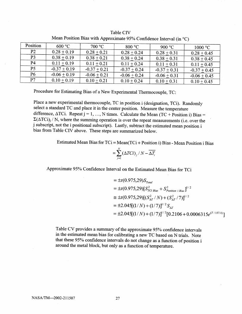
Table CIV summarizes the mean position bias and approximate 95%

confidence intervals on these mean position biases. For each position, the

estimated mean position biases were calculated by averaging the mean

position biases over the five temperatures as it was determined that the

difference was statistically insignificant over temperature. In other words,

the estimated mean position bias does not change over temperature. The

approximate 95% confidence intervals on these estimated mean positionbiases were calculated as follows:

~ 95% Conf. Int.- AT + t(0.975,29)Sar/(71/2)

Where" AT is the estimated mean position bias averaged over

both replicate nm days and temperature

S_r - 0.2106 + 0.0006315e (r / 157.1)is the estimated run - to - run variation

7 is the number of replicate run days used in the estimate of Sat

Notice that while the run-to-ran variation, Sax, changed with temperature, itdid not change from position to position.

NASA/TM_2002-211507 26

Position

TableCIVMeanPositionBiaswith Approximate95%ConfidenceInterval (in °C)

600 °C 700 °CP2 0.28+ 0.19 0.28+ 0.21P3 0.38+ 0.19 0.38+ 0.21P4 0.11+ 0.19 0.11+ 0.21P5P6P7

-0.37+ 0.19-0.06+ 0.190.10+0.19

-0.37+ 0.21-0.06+ 0.210.10+ 0.21

800°C0.28+ 0.24

900°C 1000°C0.28+ 0.31 0.28+ 0.45

0.38+ 0.24 0.38+ 0.310.11+0.24 0.11+0.31-0.37+ 0.24 -0.37+ 0.31-0.06+ 0.240.10+ 0.24

-0.06+ 0.310.10+0.31

0.38+ 0.450.11+0.45-0.37+ 0.45-0.06+ 0.450.10+0.45

Procedurefor EstimatingBiasof aNew ExperimentalThermocouple,TC:

Placeanewexperimentalthermocouple,TC in position i (designation,TCi). Randomlyselecta standardTC andplaceit in thecenterposition. Measurethetemperaturedifference,ATCi. Repeat j = 1, ..., N times. Calculate the Mean (TC + Position i) Bias =

Z(ATCi)j / N, where the summing operation is over the repeat measurements (i.e. over the

j subscript, not the i positional subscript). Lastly, subtract the estimated mean position i

bias from Table CIV above.. These steps are summarized below.

Estimated Mean Bias for TCi - Mean(TCi + Position i) Bias - Mean Position i Bias

N

- _ (ATCi)j / N- ,ST_j=l

Approximate 95% Confidence Interval on the Estimated Mean Bias for TCi

= +_t(O.975,29)STot_ _

2 ]1/2= +t(0"975,29)[$2c_ Bias "_- SpositioniBias

= +t(O.975,29)[(S2r / N) + (S2r / 7)] 1/2

= +_2.045[(1/N) + (1 / 7)] 1/2 SaT

= +_2.045[(1/N) + (1 / 7)] 1/2[0.2106 + 0.0006315e (z /157.1)]

Table CV provides a summary of the approximate 95% confidence intervals

in the estimated mean bias for calibrating a new TC based on N trials. Note

that these 95% confidence intervals do not change as a function of position i

around the metal block, but only as a function of temperature.

NASA/TM_2002-211507 27

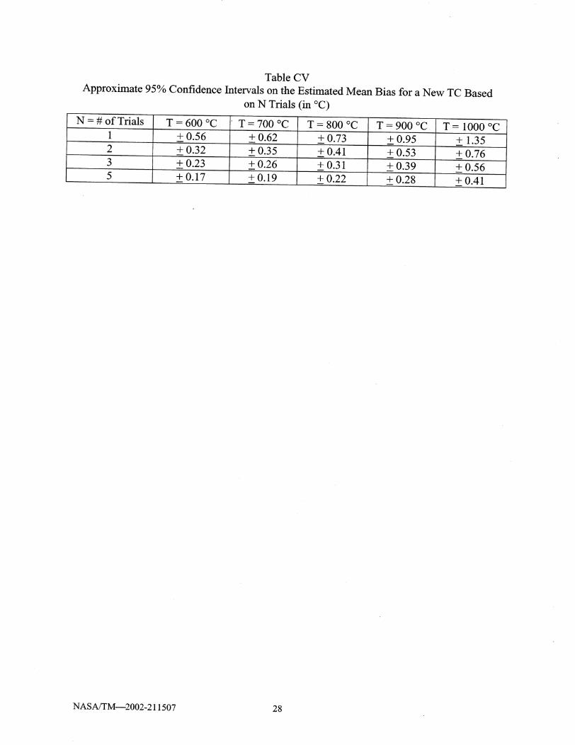
Table CV

Approximate 95% Confidence Intervals on the Estimated Mean Bias for a New TC Based

on N Trials (in °C)

N # of Trials T= 600 °C

+ 0.56

+ 0.32

+ 0.23

+0.17

[ T = 700 °C

+ 0.62

+ 0.35

+ 0.26

+0.19

T = 800 °C

+0.73

+ 0.41

+0.31

+ 0.22

T = 900 °C

+ 0.95

+ 0.53

+ 0.39

+ 0.28

T = 1000 °C

+ 1.35

+0.76

+0.56

+0.41

NASA/TM_2002-211507 28

Appendix D

Statistical Analyses of Data from the Tying Method of Calibrating Unsheathed

Thermocouples

Objective: Quantify the 95% confidence intervals on the estimated bias in calibrating

new unsheathed thermocouples (TCs) against a standard TC using the tyingmethod of calibration.

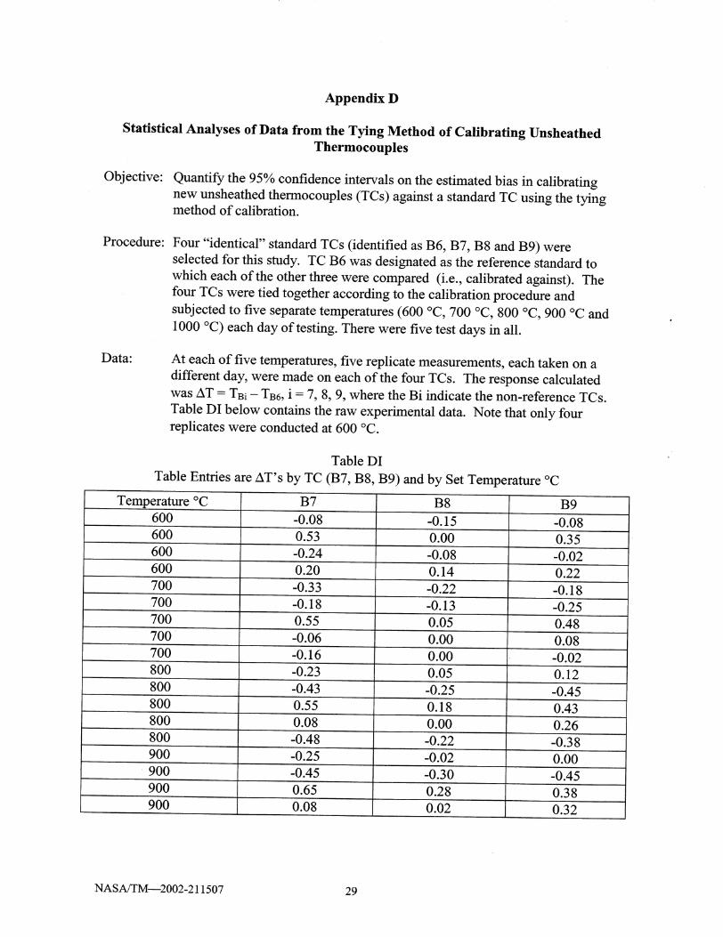
Procedure: Four "identical" standard TCs (identified as B6, B7, B8 and B9) were

selected for this study. TC B6 was designated as the reference standard to

which each of the other three were compared (i.e., calibrated against). The

four TCs were tied together according to the calibration procedure and

subjected to five separate temperatures (600 °C, 700 °C, 800 °C, 900 °C and

1000 °C) each day of testing. There were five test days in all.

Data: At each of five temperatures, five replicate measurements, each taken on a

different day, were made on each of the four TCs. The response calculated

was AT - TBi- TB6, i = 7, 8, 9, where the Bi indicate the non-reference TCs.

Table DI below contains the raw experimental data. Note that only four

replicates were conducted at 600 °C.

Table DI

Table Entries are AT's by TC (B7, B8, B9) and by Set Temperature °Cm

l'emperature oC600

600

600

600

700

700

700

700

700

800

800

800

800

800

900

900

900

900

B7

-0.08

0.53

-0.24

0.20

0.55

0.55

0.08

-0.48

-0.25

0.65

0.08

B8

-0.15

0.00

-0.08

0.14

0.05

0.00

0.00

0.05

0.18

0.00

-0.22

-0.02

0.28

0.02

B9

-0.08

0.35

-0.02

0.22

-0.18

-0.25

0.48

0.08

-0.02

0.12

-0.45

0.43

0.26

-0.38

0.00

-0.45

0.38

0.32

NASA/TM_2002-211507 29

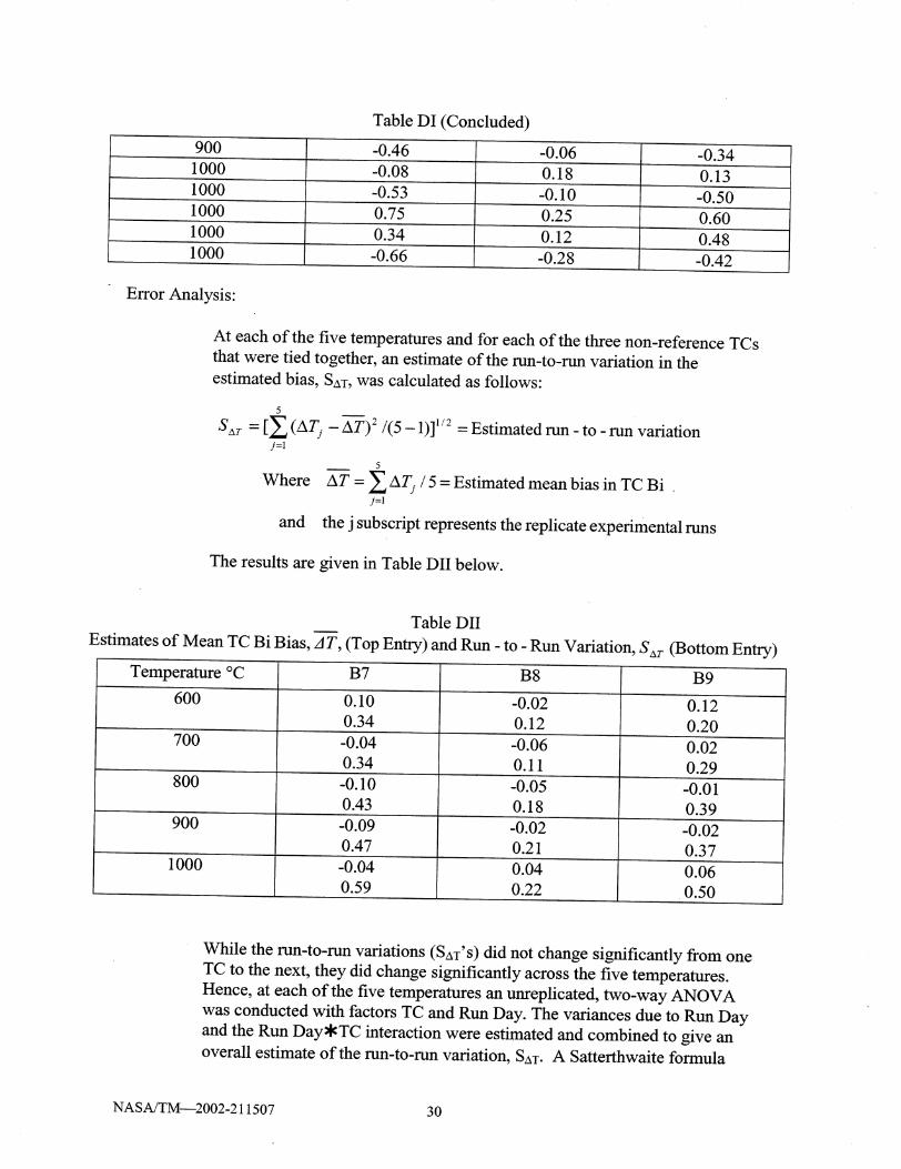
TableDI (Concluded)90010001000100010001000

0.750.34

0.18

0.250.12

-0.340.13-0.500.600.48

Error Analysis"

At eachof thefive temperaturesandfor eachof thethreenon-referenceTCsthatweretied together,anestimateof therun-to-rtmvariationin theestimatedbias,SaT,wascalculatedasfollows:

5

S_xr - [_ (,,XTj - _--f) 2/(5 - 1)] _/2j=l

Where

and

- Estimated run - to - run variation

j=l

ATj / 5 - Estimated mean bias in TC Bi

the j subscript represents the replicate experimental runs

The results are given in Table DII below.

Table DII

Estimates of Mean TC Bi Bias, AT, (Top Entry) and Run - to - Run Variation, Sat (Bottom Entry)

T emp erature ° C B 7 B 8 B 9

600

700

800

900

1000

0.10

0.34

0.04

0.22

0.12

0.20

0.02

0.29

0.06

0.50

While the run-to-ran variations (SAT'S) did not change significantly from one

TC to the next, they did change significantly across the five temperatures.

Hence, at each of the five temperatures an unreplicated, two-way ANOVA

was conducted with factors TC and Run Day. The variances due to Run Day

and the Run Day_TC interaction were estimated and combined to give an

overall estimate of the run-to-ran variation, SAT. A Satterthwaite formula

NASA/TM_2002-211507 30

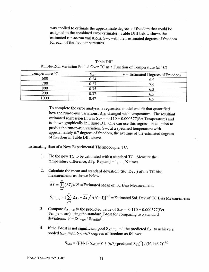
was applied to estimate the approximate degrees of freedom that could be

assigned to the combined error estimates. Table DIII below shows the

estimated ran-to-run variations, SaT, with their estimated degrees of freedom

for each of the five temperatures.

Table DIII

Run-to-Run Variation Pooled Over TC as a Function of Temperature (in °C)

Temperature °C

600

700

800

900

1000

SAT

0.24

0.27

0.35

0.37

0.47

v = Estimated Degrees of Freedom

To complete the error analysis, a regression model was fit that quantified

how the run-to-ran variations, SaT, changed with temperature. The resultant

estimated regression fit was SaT = -0.110 + 0.000577(Set Temperature) and

is shown graphically in Figure D 1. One can use this regression equation to

predict the run-to-rim variation, Sa_, at a specified temperature with

approximately 6.7 degrees of freedom, the average of the estimated degreesof freedom in Table DIII above.

Estimating Bias of a New Experimental Thermocouple, TC:

lo Tie the new TC to be calibrated with a standard TC. Measure the

temperature difference, ATj. Repeat j = 1, ..., N times.

o Calculate the mean and standard deviation (Std. Dev.) of the TC biasmeasurements as shown below.

N

AT - _ (AT:)/N = Estimated Mean of TC Bias Measurementsj=l

N

Sar_r c = [__, (ATj. - A--T):/(N - 1)] 1/2 - Estimated Std. Dev. of TC Bias Measurementsj=l

3. Compare SzxT_Tcto the predicted value of SzxT= -0.110 + 0.000577(Set

Temperature) using the standard F-test for comparing two standard

deviations: F = (SLarger / SSmaller)2.

4. If the F-test is not significant, pool SzxT_Tcand the predicted SaT to achieve a

pooled SaTp with N-1 +6.7 degrees of freedom as follows"

SATp -" { [(N- 1)(SAT_TC)2 -k- (6.7)(predicted SAT) 2] / (N- 1+6.7) } 1/2

NASA/TM_2002-211507 31

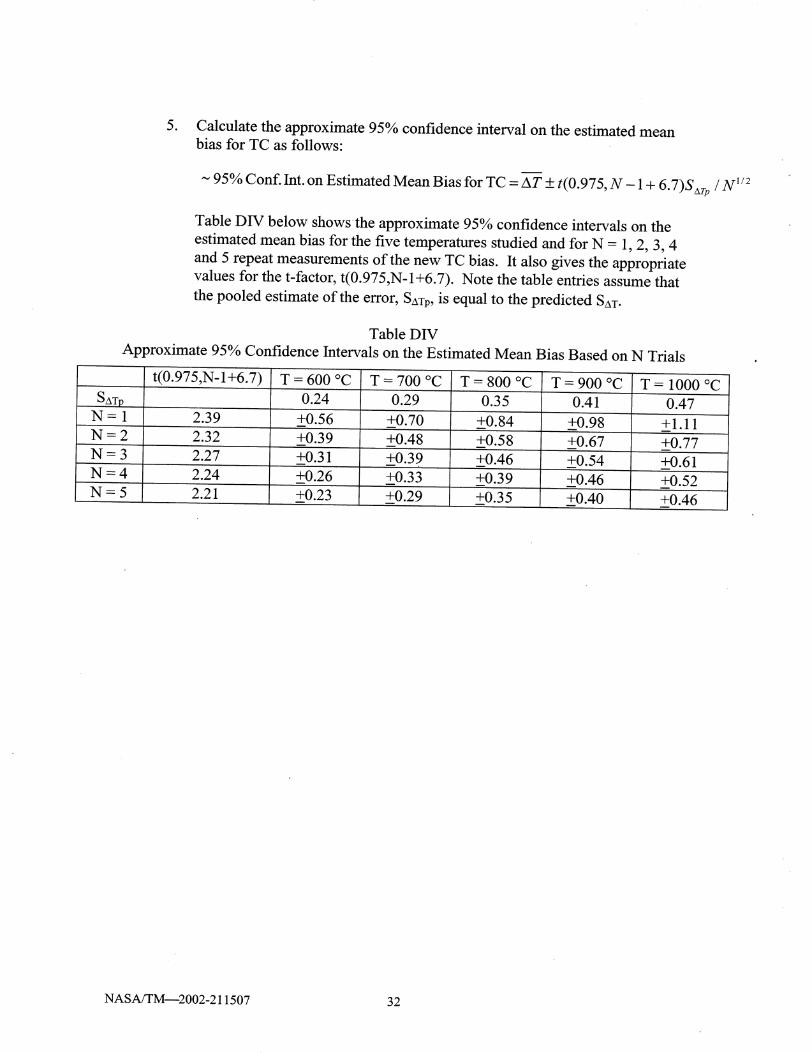
° Calculate the approximate 95% confidence interval on the estimated meanbias for TC as follows:

~ 95% Conf. Int. on Estimated Mean Bias for TC - A----T+ t(0.975, N - 1 + 6.7)Sat p / N 1/2

Table DIV below showsthe approximate 95% confidence intervals on the

estimated mean bias for the five temperatures studied and for N = 1, 2, 3, 4

and 5 repeat measurements of the new TC bias. It also gives the appropriatevalues for the t-factor, t(0.975,N-1 +6.7). Note the table entries assume that

the pooled estimate of the error, SaTp, is equal to the predicted SaT.

Ap

SATp

N-1

N=2

N=3

N=4

N=5

Table DIV

_roximate 95% Confidence Intervals on the Estimated Mean Bias Based on N Trials

t(0.975,N-l+6.7)

2.39

2.32

2.27

2.24

2.21

T = 600 °C

0.24

+0.56

+0.39

+0.31

+0.26

+0.23

T = 700 °C

0.29

+0.70

+0.48

+0.39

+0.33

+0.29

T = 800 °C

0.35

+0.84

+0.58

+0.46

+0.39

+0.35

T = 900 °C

0.41

+0.98

+0.67....

+0.54

+0.46

+0.40

T = 1000 °C

0.47

+1.11

+0.77

+0.61

+0.52

+0.46

NASA/TM_2002-211507 32

References

1. Traceable Temperatures, J.V. Nicholas and D.R. White, John Wiley and Sons,NY, 1994.

2. Manual on the Use of Thermocouples in Temperature Measurement, ASTM,Philadelphia, PA, 1993.

3. Standard Test Method for Calibration of Thermocouple by Comparison

Techniques, E220, Annual Book of ASTM Standards, Volume 14.03,2001,pp. 98-109.

4. J.D. Whittenberger, J. Materials Eng. and Performance, Vol. 1(4), 1992, p. 469.

5. Marlin Manufacturing Corp., 12404 Triskett Road, Cleveland OH, 44111.

6. M.P.E. Desvaux, in Measurement of High Temperature Mechanical Properties of

Materials, eds. M.S. Loveday, M.F. Day, and B.F. Dyson, Her Majesty'sStationary Office, London, 1981, p. 96.

7. Private communication with R. Park, Marlin Manufacturing Corp, 2000.

8. A.I. Dahl, in Temperature, its Measurement and Control in Science and Industry,

Vol. 1, Reinhold Publishing Corp., NY, 1941, p. 1238.

NASA/TM_2002-211507 33

Page intentionally left blank

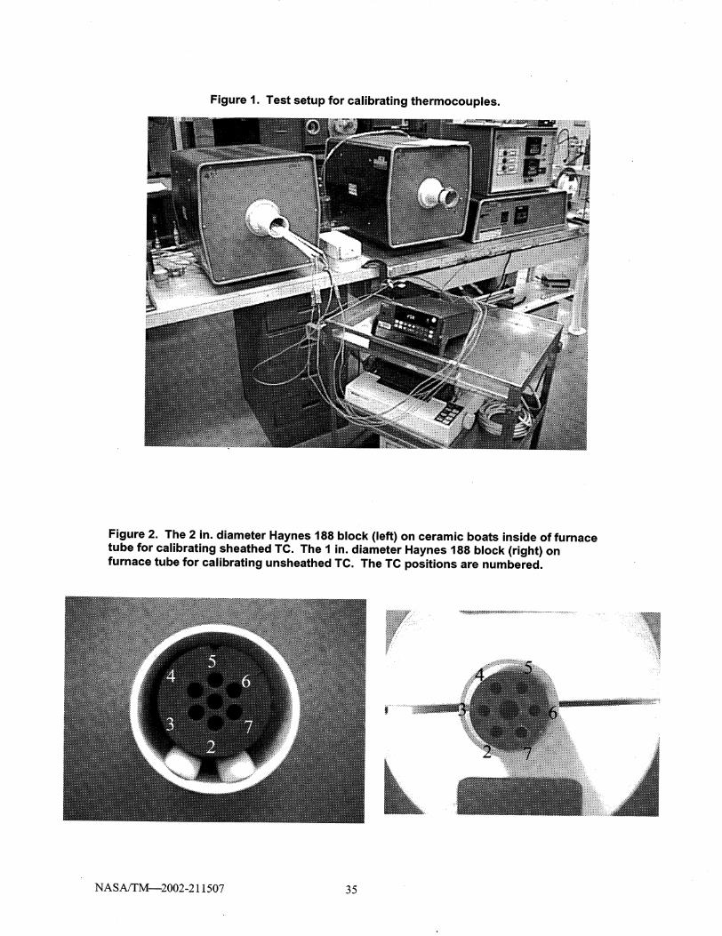
Figure 1. Test setup for calibrating thermocouples.

Figure 2. The 2 in. diameter Haynes 188 block (left) on ceramic boats inside of furnace

tube for calibrating sheathed TC. The 1 in. diameter Haynes 188 block (right) onfurnace tube for calibrating unsheathed TC. The TC positions are numbered,

NASA/TM_2002-211507 35

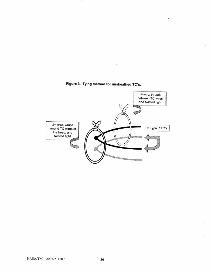
Figure 3. Tying method for unsheathed TC's.

1st wire, threadsbetween TC wires

and twisted tight

2 nd wire, wrapsaround TC wires at

the bead, and

twisted tigh_

. ..

2. Type R TC's I

NASA/TM_2002-211507 36

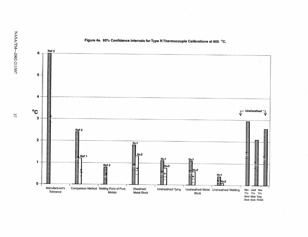
Z>rj3

Ref 2

Figure 4a. 95% Confidence Intervals for Type R Thermocouple Calibrations at 600 °C.

o

L_o-..3

..j

ocUnsheathed --_

Manufacturer's

Tolerance

Ref 2

_ef 1

_il! Ref 2

Comparison Method Melting Point of Pure

1---

N=I

N=2

N=I N=I

_._i-I. =_,N=2_i- 2

__ - i

]-_ 1---

MetalsSheathed/ Unsheathed/TyingMetal Block

N=I

V--- 1_

Unsheathed/Metal Unsheathed/WeldingBlock

N_

7New Used NewTCs TCs TCs

MetalMetalTyingBlock Block RT-600

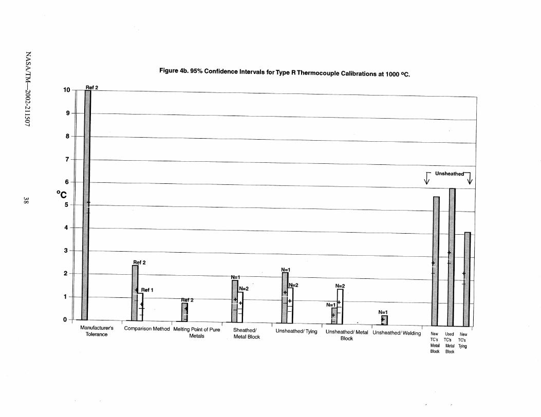
Z>

(Ji

,.,..I

OO

10

oc

Figure 4b. 95% Confidence Intervals for Type R Thermocouple Calibrations at 1000 oc.

Ref 2

Manufacturer's

Tolerance

Ref 2

Ref 2

N=I

N=i

N=2 _=2 N=2I

F'-

Sheathed/ Unsheathed/TyingMetal Block

__Ref 1

Comparison Method Melting Point of Pure

Metals

N=I

Unsheathed/Metal Unsheathed/WeldingBlock

_" Unsheathed_

h

r

:iiii_ii'_:_:_:_:_:

iii........

- ii!i_:!iiiii_

_::iiiiiii

_iiiiii!i_:i_:iii!i.:.:.:.:,iiiii_i_::

-- iiiil-........

, !iji!_i_

New Used New

TC's TC's TC's

Metal Metal TyingBlock Block

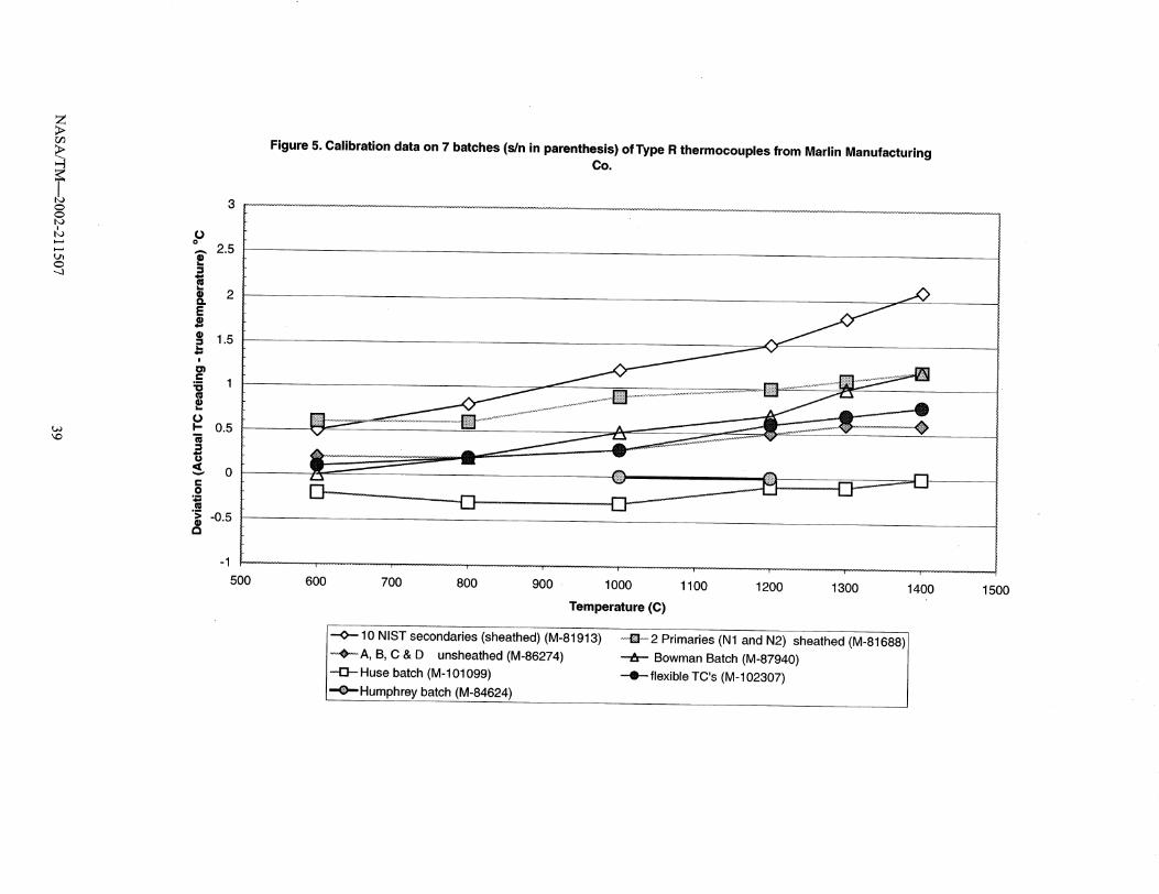
Z>rj_

.fFigure 5. Calibration data on 7 batches (s/n in parenthesis) of Type R thermocouples from Marlin Manufacturing

Co,

h_

u_

--4

u,)

P2.5

L_

• 2Q.E

1.5L_

c_5 1t_

¢_

oP. 0.5J(g

,-_ 0cO

.,...,i.i

• -0.5C_

"1 .... -................ :---- ........... ""i

500 600i "i i T'' ......... --" ......... :''" ....... i f i"" ........ "--'"- ......... --- ........ '"i

700 800 900 - 1000 1100 1200 1300 1400

Temperature (C)

15OO

-<>- 10 NIST secondaries (sheathed) (M-81913)

•--_)----A,B, C & D unsheathed (M-86274)

Huse batch (M-101099)

_Humphrey batch (M-84624)

.........Q........2 Primaries (N1 and N2) sheathed (M-81688)

Bowman Batch (M-87940)

flexible TC's (M-102307)

>

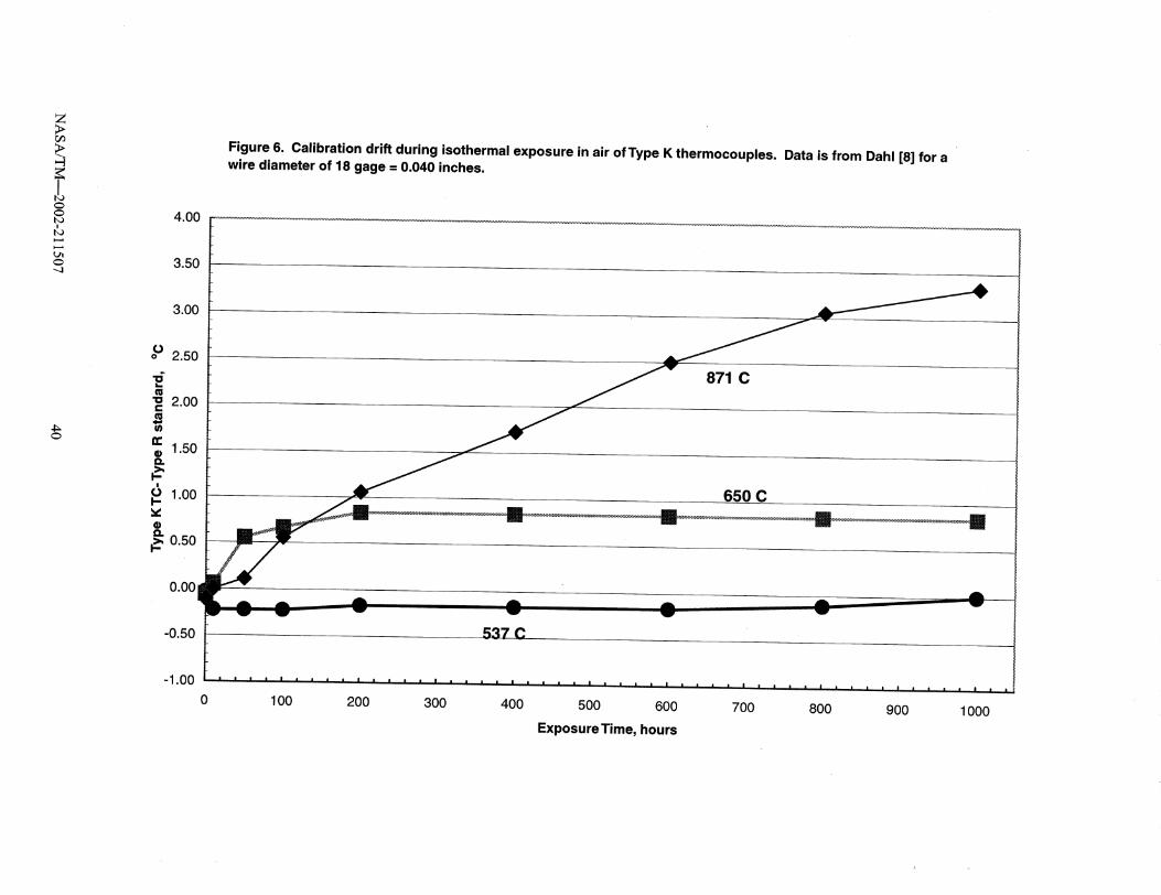
l,o

O...3

Figure 6. Calibration drift during isothermal exposure in air of Type K thermocouples. Data is from Dahl [8] for awire diameter of 18 gage = 0.040 inches.

3.50

3.00

0o 2.50

871 C

650 C

0.00

-1.00

0 1O0 200 300 400 500 600

Exposure Time, hours

700 800 900 1000

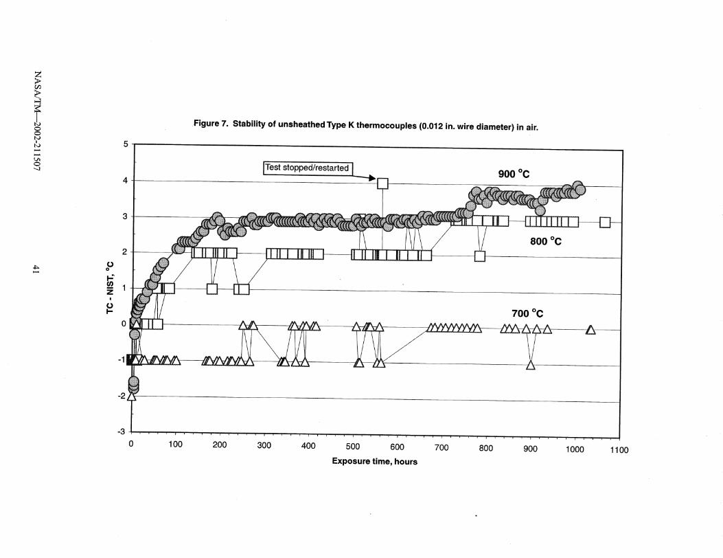
:Z>

Figure 7. Stability of unsheathed Type K thermocouples (0.012 in. wire diameter) in air.

"--3 Imeststopped/restarted L 900 °C

k--.*

800 °C

700 °C

A

-3

0 100 200 300 400 500 600 700 800 900 1000 1100

Exposure time, hours

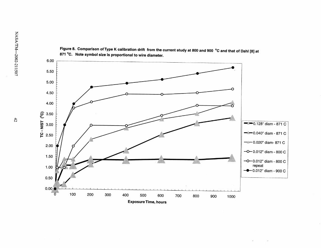
>rj3

-,4

4_bo

6.00

5.50

5.00

4.50

4.00

2.00

1.50

1.00

0.50

Figure 8. Comparison of Type K calibration drift from the current study at 800 and 900 °C and that of Dahl [8] at871 °C. Note symbol size is proportional to wire diameter.

_iii_O. 128" diam - 871 C

mi_ilmO.040 '' diam - 871 C

--_i!_,_0.020'' diam- 871 C

--0-- 0.012" diam - 800 C

--0-- 0.012" diam - 800 Crepeat

0.012" diam - 900 C

0.00

100 200 300 400 500 600

Exposure Time, hours

7O0 8OO 900 1000

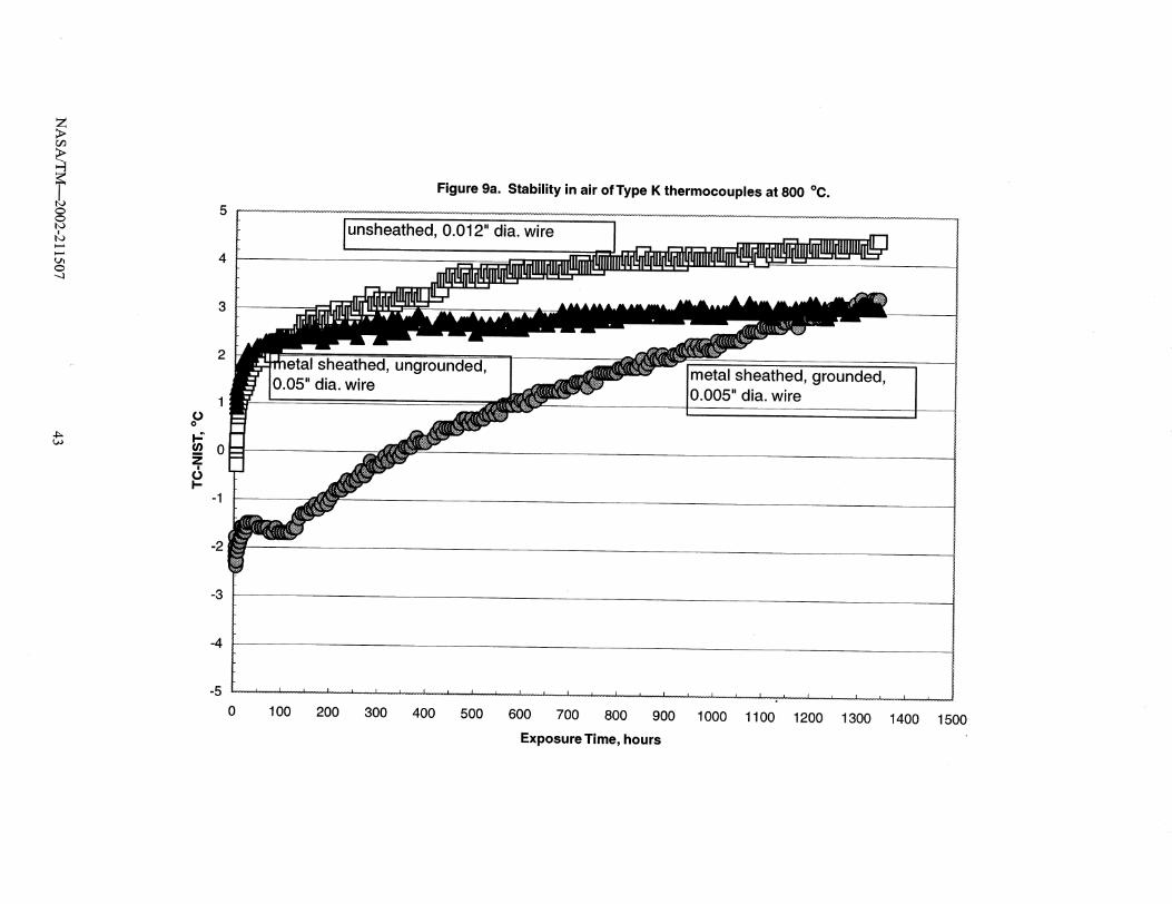
Z>rj9

bJ

u_

...j

4_L_

o0

p:

Z

(3I-

-2

-3

Figure 9a. Stability in air of Type K thermocouples at 800 °C....... ._H.,

unsheathed, 0.012" dia. wire

etal sheathed, ungrounded,0.05" dia. wire metal sheathed, grounded,

0.005" dia. wire

-4

-5....... i ........ 1 __ i ......... I .__ 1 ...... i........ I i ........ I _ • ! ..... I l 1..... i _ _ I t...... 1 ...... i ] ........ i l ....... i I ...i ....

0 100 200 300 400 500 600 700 800 900 1000 1100 1200 1300 1400 1500

Exposure Time, hours

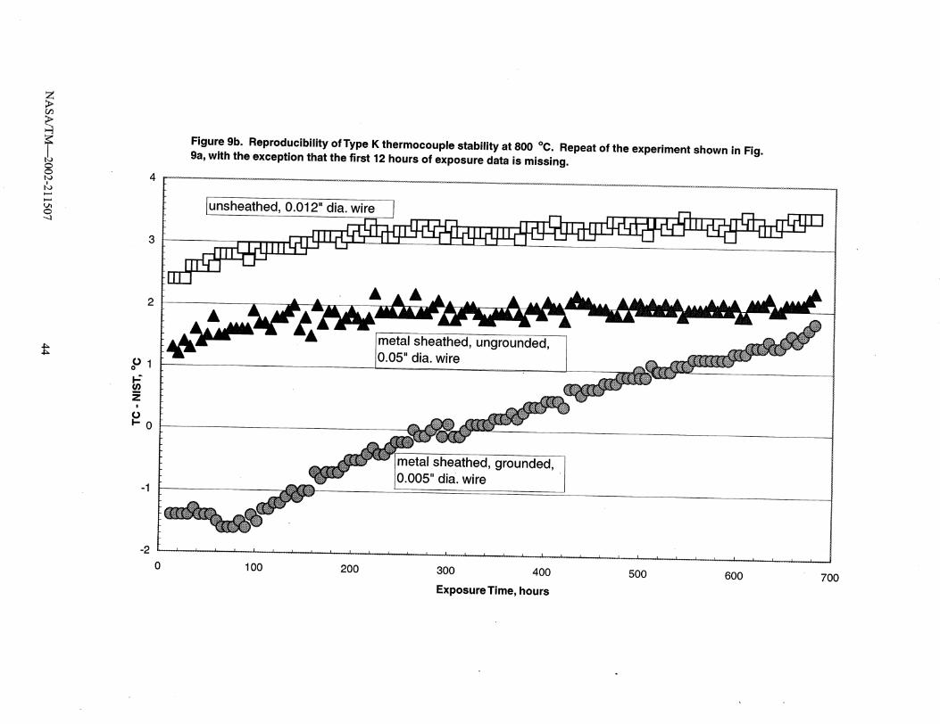
Z>

Figure 9b. Reproducibility of Type K thermocouple stability at 800 °C, Repeat of the experiment shown in Fig.9a, with the exception that the first 12 hours of exposure data is missing,

t_

,-..I

4_

l..unsheathed, 0.012" dia. wire 1

U.Lj- A A

A

. [005"dia "

d___metal sheathed, grounded,

• _ 10.005" dia. wire '

1oo 200300 400 500 600 700

Exposure Time, hours

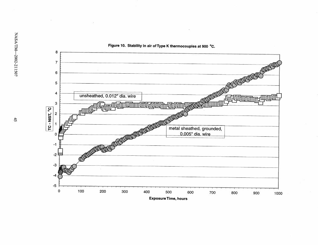
sJnoq'etU!.LeJnsodx3

000i.006oog00/_.00900_001700800_O0I.0

...............L.__._..L........|........J................j........j........±.......±................[....._-_!........I........I...........___._J........•.......I........t........[........,........,........I.......J.......J.......I.......-.......I........,........I.......l........J.......J.....J.I.±.[.I..i

........................................................ic3.

eJiM"e!p,,c300"0'pepunoJB'peq_eeqsle_euJ

Mh

M3

Cq

"0o006_eseldnoootuJeqlHedAlJOJleu!_l!l!qels"OLeJn61:l

<Z

>

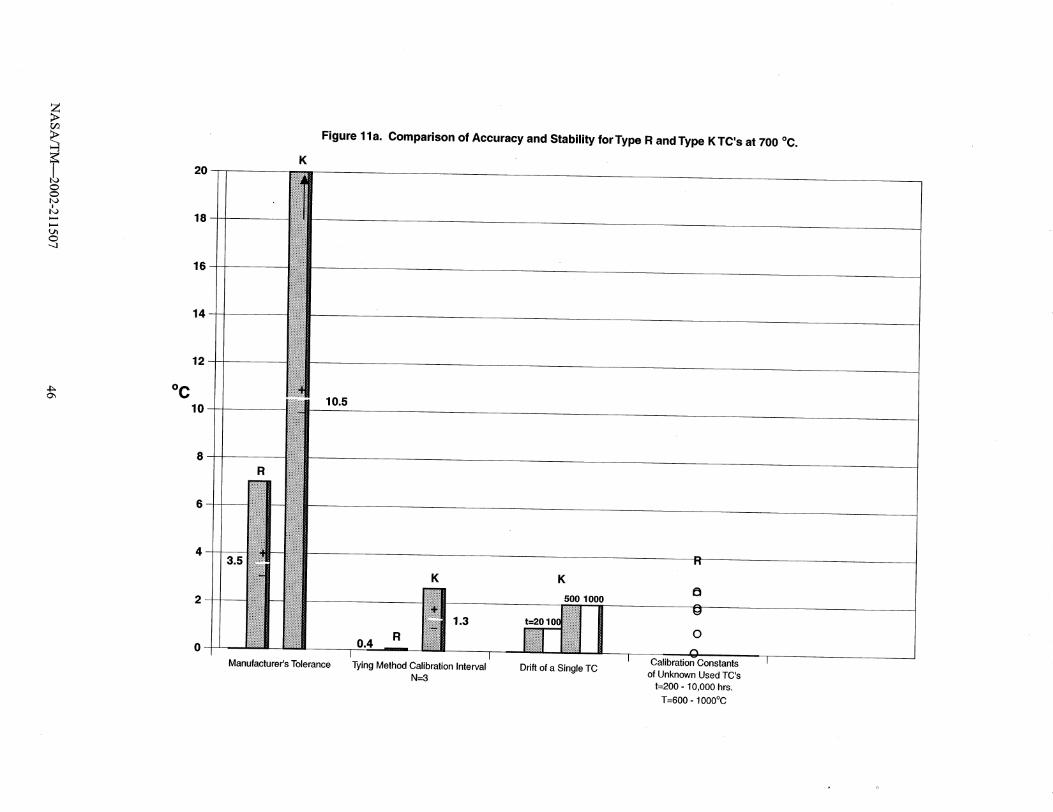
L_

....j

O_ oc

20

18

16

14

12

10

K

iiiiiii#

Figure 1la, Comparison of Accuracy and Stability for Type R and Type K TC's at 700 °C,

i

10.5

3.5

Manufacturer's Tolerance

R

K K

500 1000

_g

1,3 ..o

_1--_ Calibration Constants TTying Method Calibration Interval Drift of a Single TC

N=3 of Unknown Used TC's

t=200 - 10,000 hrs.

T=600 - 1000°C

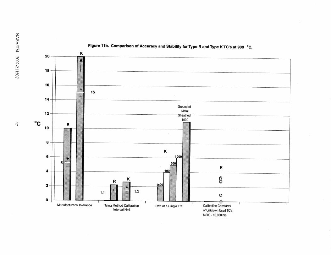
Z

5/9

O

FO

_h

"--.,I

4_"-,..I oc

2O

18

16

14

12

10

Figure 11b. Comparison of Accuracy and Stability for Type R and Type K TC's at 900 °C.

K

::_::-:-:_:,:.:.:.:.:.:,

.......

22=2:2:2:.:;

:::::::::_

K

15

GroundedMetal

Sheathed1000

K

1000

100 _

1.1 1.3

Tying Method Calibration

Interval N=3Drift of a Single TC

8

O

OCalibrationConstantsofUnknownUsedTC's

t=200- 10,000hrs.

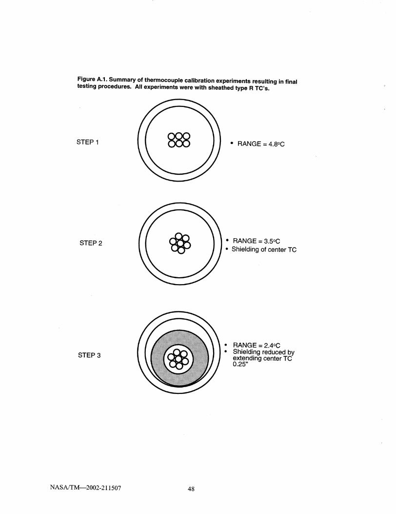
Figure A.1. Summary of thermocouple calibration experiments resulting in finaltesting procedures. All experiments were with sheathed type R TC's.

STEP 1 • RANG E = 4.8oC

STEP 2 • RANGE = 3.5oC

° Shielding of center TC

STEP 3

° RANGE = 2.4oC• Shielding reduced by

extending center TC0.25"

NASA/TM_2002-211507 48

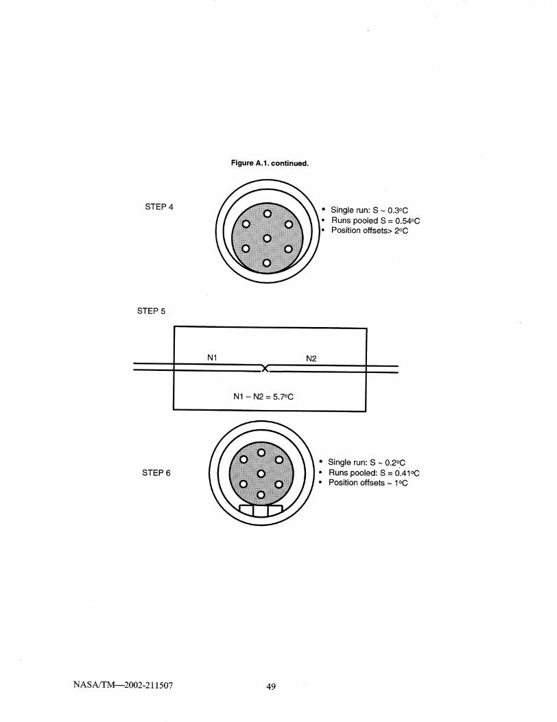
Figure A.1. continued.

STEP 4• Single run" S ~ 0.3oC• Runs pooled S = 0.54oC• Position offsets> 2oC

STEP 5

N1

X

N1 - N2 = 5.7°C

N2

STEP 6• Single run" S ~ 0.2oC

• Runs pooled: S = 0.41oC• Position offsets ~ 1oC

NASA/TM_2002-211507 49

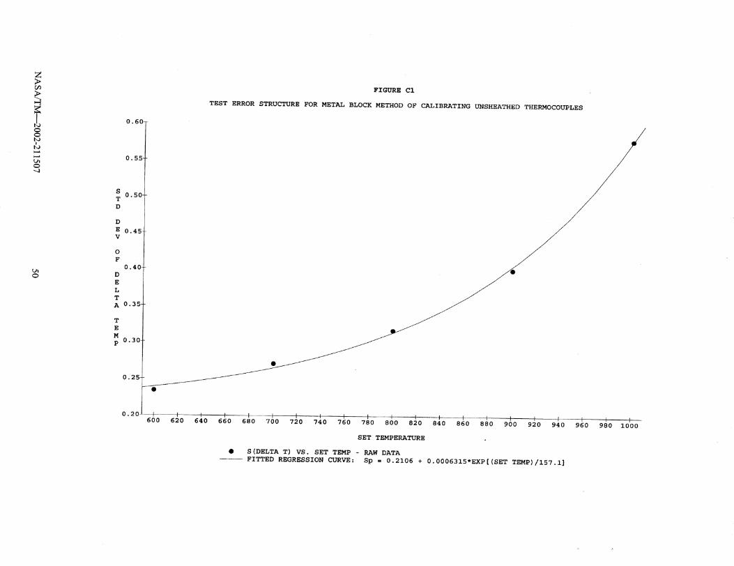
Z>U_

O

tm

tn

FIGURE C1

TEST ERROR STRUCTURE FOR METAL BLOCK METHOD OF CALIBRATING UNSHEATHED THERMOCOUPLES

0.55-

S 0T "

D

D

E 0.45-V

O

F

DE 0.4(

L /

A 0.3

T

E

p 0.30

0.2

0.20 _ i I I I I I i I I ....I I J I I I I I # J I600 620 640 660 680 700 720 740 760 780 800 820 840 860 880 900 920 940 960 980 I000

SET TEMPERATURE

• S(DELTA T) VS. SET TEMP - RAW DATA

FITTED REGRESSION CURVE: Sp = 0.2106 + 0.0006315*EXP[(SET TEMP)/157.1]

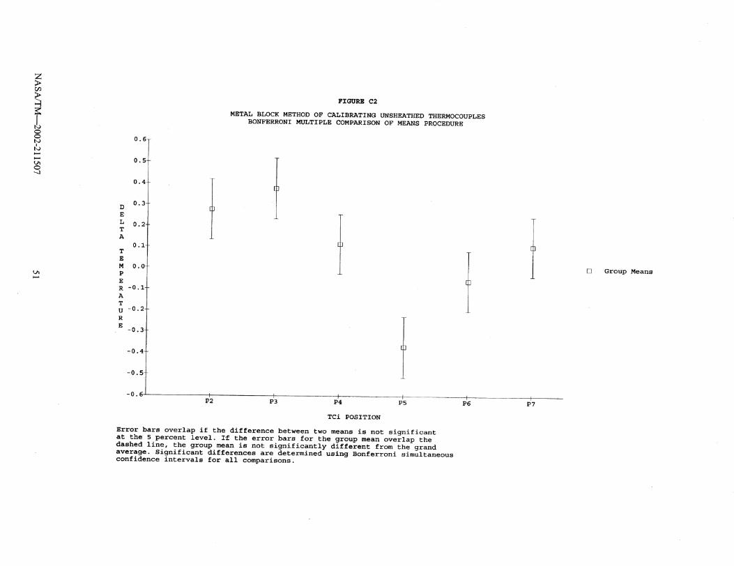
Z>_n

_J

tno-j

tm

FIGURE C2

METAL BLOCK METHOD OF CALIBRATING UNSHEATHED THERMOCOUPLES

BONFERRONI MULTIPLE COMPARISON OF MEANS PROCEDURE

0.6-

0.5-

0.4

0.3-

0.2-

0.I

0.0

-0.I-

-0.2--

-0.3-

-0.4_

-0.5

-0.6 I f i I I fP2 P3 P4 P5 P6 P7

TCi POSITION

Error bars overlap if the difference between two means is not significant

at the 5 percent level. If the error bars for the group mean overlap the

dashed line, the group mean is not significantly different from the grand

average. Significant differences are determined using Bonferroni simultaneous

confidence intervals for all comparisons.

Group Means

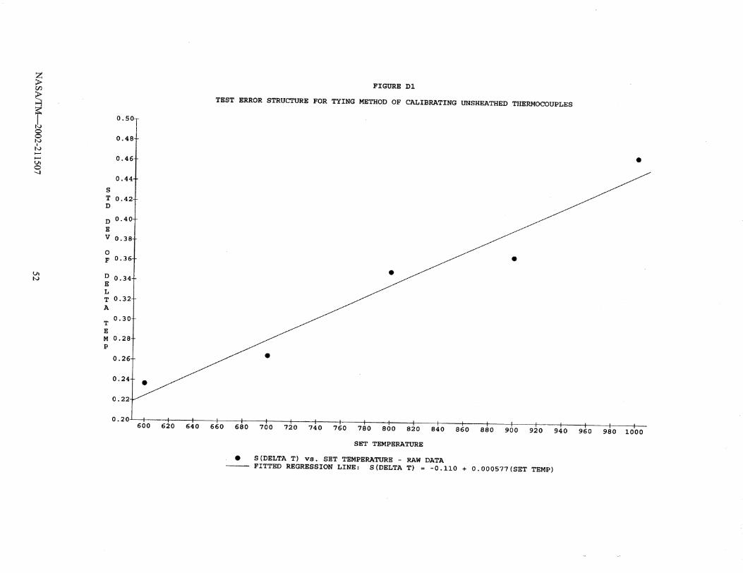
Z>u_

O

b_

L_

t_

0°

0.4

S

T 0.42-

D

D 0.4

E

V 0.3

O

F 0.36-

D 0.E

L

T 0.3

A

0.30T

E

M 0.2

P

0.2,

0.2_

FIGURE D1

TEST ERROR STRUCTURE FOR TYING METHOD OF CALIBRATING UNSHEATHED THERMOCOUPLES

600 620 640 660 680 700 720 740 760 780 800 820 840 860 880 900 920 940 960 980 1000

SET TEMPERATURE

• S(DELTA T) vs. SET TEMPERATURE - RAW DATA

FITTED REGRESSION LINE: S(DELTA T) = -0.110 + 0.000577(SET TEMP)

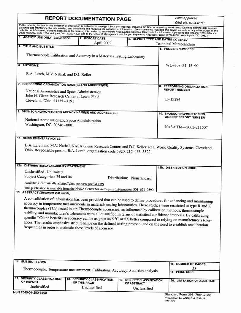
REPORT Form Approved

• OMB No. 0704-0188

Public reporting burden for this collection of information is estimated to average 1 hour per response, including the time for reviewing instructions, searching existing data sources,gathering and maintaining the data needed, and completing and reviewing the collection of information. Send comments regarding this burden estimate or any other aspect of thiscollection of information, including suggestions for reducing this burden, to Washington Headquarters Services, Directorate for Information Operations and Reports, 1215 JeffersonDavis Highway, Suite 1204, Arlington, VA 22202-4302, and to the Office of Management and Budget, Paperwork Reduction Project (0704-0188), Washington, DC 20503.

1. AGENCY USE ONLY (Leave blank) S COVERED

Technical Memorandum4. TITLE AND SUBTITLE

5. FUNDING NUMBERS

Thermocouple Calibration and Accuracy in a Materials Testing Laboratory

6. AUTHOR(S)

B.A. Lerch, M.V. Nathal, and D.J. Keller

7. PERFORMING ORGANIZATION NAME(S) AND ADDRESS(ES)

National Aeronautics and Space Administration

John H. Glenn Research Center at Lewis Field

Cleveland, Ohio 44135-3191

9. SPONSORING/MONITORING AGENCY NAME(S) AND ADDRESS(ES)

National Aeronautics and Space Administration

Washington, DC 20546-0001

11. SUPPLEMENTARY NOTES

WU-708-31-13-00

8. PERFORMING ORGANIZATION

REPORT NUMBER

E-13284

10. SPONSORING/MONITORING

AGENCY REPORT NUMBER

NASA TM--2002-211507

B.A. Lerch and M.V. Nathal, NASA Glenn Research Center; and D.J. Keller, Real World Quality Systems, Cleveland,Ohio. Responsible person, B.A. Lerch, organization code 5920, 216-433-5522.

12a. DISTRIBUTION/AVAILABILITY STATEMENT

Unclassified- Unlimited

Subject Categories: 35 and 04 Distribution: Nonstandard

Available electronically at http://gltrs.grc.nasa.gov/GLTRS

This publication is available from the NASA Center for AeroSpace Information, 301-621-0390.

13. ABSTRACT (Maximum 200 words)

12b. DISTRIBUTION CODE

A consolidation of information has been provided that can be used to define procedures for enhancing and maintaining

accuracy in temperature measurements in materials testing laboratories. These studies were restricted to type R and K

thermocouples (TCs) tested in air. Thermocouple accuracies, as influenced by calibration methods, thermocouple

stability, and manufacturer's tolerances were all quantified in terms of statistical confidence intervals. By calibrating

specific TCs the benefits in accuracy can be as great as 6 °C or 5X better compared to relying on manufacturer's toler-

ances. The results emphasize strict reliance on the defined testing protocol and on the need to establish recalibration

frequencies in order to maintain these levels of accuracy.

14. SUBJECT TERMS

Thermocouple; Temperature measurement; Calibrating; Accuracy; Statistics analysis

17. SECURITY CLASSIFICATIONOF REPORT

Unclassified

NSN 7540-01-280-5500

15. NUMBER OF PAGES

5816, PRICE CODE

Standard Form 298 (Rev. 2-89)Prescribedby ANSI Std. Z39-18298-102

20. LIMITATION OF ABSTRACT