Thermodynamic Analysis of a High Temperature Heat Pump

MASTER THESIS

ENERGY TECHNOLOGY FOR SUSTAINABLE DEVELOPENT

Thermodynamic Analysis of a High

Temperature Heat Pump coupled

with an Organic Rankine Cycle for

Energy Storage

AUTHOR: LINDEMAN, LUKAS

SUPERVISOR: HASSAN, ABDELRAHMAN HUSSEIN

UPV TUTOR: CORBERÁN SALVADOR, JOSÉ MIGUEL

Academic Year: 2017-18

“July 2018”

i

ACKNOWLEDGEMENTS

First, I would like to thank Prof. José Miguel Corberán Salvador for helping me during this year

and for giving me the opportunity to be part of this project.

Secondly, I would like to thank Dr. Abdelrahman Hussein Hassan for giving me tremendous

support and valuable guidance during this work. I am very thankful for the feedback he has given

me and the discussions we have had during this project.

Finally, I would like to thank my mother and father for the love and support they have always

given me. Without them this would not have been possible.

The current thesis has been implemented within the framework of the CHESTER project, which

has received funding from the European Union’s Horizon 2020 research and innovation program

under grant agreement No 764042

iii

RESUMEN

La transición energética hacia las energías renovables requiere de nuevas soluciones para el

almacenamiento de energía, ya que las tecnologías de almacenamiento existentes están

asociadas con desventajas como el tiempo de descarga, el coste, el uso del terreno etc. Este

trabajo está enmarcado dentro del proyecto Europeo CHESTER (Compressed Heat Energy

STorage for Energy from Renewable sources). Cuando hay exceso de energía eléctrica en la red,

el sistema de almacenamiento térmico utiliza una bomba de calor (HP) para aumentar la

temperatura del calor residual y almacenarlo. El sistema de almacenamiento es un sistema

latente (LHS) mediante materiales de cambio de fase (PCM) y un sistema de almacenamiento

sensible (SHS) mediante dos tanques de agua. Cuando la red demanda energía eléctrica, el

sistema de almacenamiento a alta temperatura se utiliza acoplado a un ciclo orgánico de

Rankine (ORC) para producir electricidad.

Para evaluar la eficiencia del sistema se ha desarrollado un modelo termodinámico, con el que

se han analizado: tres temperaturas de cambio de fase del PCM (133, 149 y 183 °C), la

configuración de la bomba de calor y del sistema ORC y varias características de los fluidos

refrigerantes, especialmente la pendiente de la curva de vapor saturado del refrigerante.

Los resultados indican que los fluidos isoentrópicos tienen el mejor comportamietno, siendo el

R1233zd(E) considerado como el mejor fluido de trabajo para bajas y medias temperaturas de

fusión. Para una temperatura de fusión de 133 °C y una temperatura de la fuente de calor de 75

°C, una eficiencia igual a 1 del ciclo completo puede ser alcanzada. Para alta temperatura el

fluido con mejor comportamiento es el R141b. Fluidos secos como el HFO1336mzz(Z) y el

ciclopentano presentan el peor comportamiento de los fluidos seleccionados. No se considera

beneficioso para el sistema un ciclo con dos etapas de compresión ni tampoco un ciclo ORC con

procesos de recuperación o regeneración.

Palabras calves: Almacenamiento térmico, bombas de calor de alta temperatura, ciclo orgánico

de Rankine, modelado numérico.

v

RESUM

La transició energètica cap a les energies renovables requerix de noves solucions per a

l'emmagatzemament d'energia, ja que les tecnologies d'emmagatzemament existents estan

associades amb desavantatges com el temps de descàrrega, el cost, l'ús del terreny etc. Este

treball està emmarcat dins del projecte Europeu CHESTER (Compressed Heat Energy STorage for

Energy from Renewable sources). Quan hi ha excés d'energia elèctrica en la xarxa, el sistema

d'emmagatzemament tèrmic utilitza una bomba de calor (HP) per a augmentar la temperatura

de la calor residual i emmagatzemar’l-ho. El sistema d'emmagatzemament és un sistema latent

(LHS) per mitjà de materials de canvi de fase (PCM) i un sistema d'emmagatzemament sensible

(SHS) per mitjà de dos tancs d'aigua. Quan la xarxa demanda energia elèctrica, el sistema

d'emmagatzemament a alta temperatura s'utilitza acoplat a un cicle orgànic de Rankine (ORC)

per a produir electricitat.

Per a avaluar l'eficiència del sistema s'ha desenvolupat un model termodinàmic, amb el que

s'han analitzat: tres temperatures de canvi de fase del PCM (133, 149 i 183 °C) , la configuració

de la bomba de calor i del sistema ORC i diverses característiques dels fluids refrigerants,

especialment el pendent de la corba de vapor saturat del refrigerant. Els resultats indiquen que

els fluids isoentròpics tenen el millor comportament, sent el R1233zd (E) considerat com el

millor fluid de treball per a baixes i mitges temperatures de fusió. Per a una temperatura de

fusió de 133 °C i una temperatura de la font de calor de 75 °C, una eficiència igual a 1 del cicle

complet pot ser aconseguida. Per a alta temperatura el fluid amb millor comportament és el

R141b. Fluids secs com el HFO1336mzz (Z) i el ciclopentano presenten el pitjor comportament

dels fluids seleccionats. No es considera beneficial per al sistema un cicle amb dos etapes de

compressió ni tampoc un cicle

Paraules Claus: Emmagatzemament tèrmic, bombas de calor d'alta temperature, cicle orgànic

de Rankine, modelatge numèric.

vii

ABSTRACT

The transition towards an increasing share of renewable energy in the electricity production

requires new solutions of energy storage. Existing energy storage technologies can provide good

solutions but are also associated with various constraints such as land use, discharge time, cost

etc. This thesis has been carried out under the frame of the European project CHESTER

(Compressed Heat Energy STorage for Energy from Renewable sources). During times of excess

electricity production, a heat energy storage system uses a heat pump (HP) to pump low-grade

thermal energy to a higher temperature reservoir where the heat is stored. The reservoir

consists of a latent heat storage (LHS) unit with a phase changing material (PCM) and a Sensible

heat storage (SHS) unit with two water tanks. At times of insufficient electricity production, the

stored energy is used to operate an organic Rankine cycle (ORC) to produce electricity.

A thermodynamic model has been developed to evaluate the system performance. Three

different melting temperatures of the PCM (133, 149 and 183 °C) are evaluated as well as some

characteristics of the working fluid, especially the slope of the saturated vapor curve (dry,

isentropic or wet fluid). The system configuration of the HP and the ORC are also analyzed.

The results indicated that isentropic fluids have the best overall system performance.

R1233zd(E) is considered to be the best working fluid for the low and medium melting

temperatures. For a melting temperature of 133 °C, a roundtrip efficiency of 1 can be reached if

the source temperature is 75 °C. For the high temperature storage, R141b is the best working

fluid. Dry fluids such as HFO1336mzz(Z) and Cyclopentane have the lowest performance of the

selected working fluids. A two-stage compression in the HP is not considered to be beneficial for

the system, neither is an ORC cycle with recuperation or regeneration processes.

Key words: Thermal storage system, High temperature heat pump, Organic Rankine cycle,

Numerical modeling.

viiii

TABEL OF CONTENTS

ACKNOWLEDGEMENTS ................................................................................................................ iii

RESUMEN ...................................................................................................................................... v

RESUM .......................................................................................................................................... vii

ABSTRACT ...................................................................................................................................... ix

TABEL OF CONTENTS ..................................................................................................................... xi

LIST OF FIGURES .......................................................................................................................... xiii

LIST OF TABLES ........................................................................................................................... xiiii

1. Introduction ........................................................................................................................ 16

1.1 Background.................................................................................................................. 16

1.2 Aims and Objectives .................................................................................................... 17

1.3 State of the art ............................................................................................................ 18

1.3.1 Heat Pump ........................................................................................................... 18

1.3.2 Organic Rankine Cycle ......................................................................................... 21

1.3.3 Selection of working fluid .................................................................................... 25

1.3.4 Storage System .................................................................................................... 27

1.3.5 Full System .......................................................................................................... 27

2. Methodology ....................................................................................................................... 31

2.1 Overall system (CHEST) ............................................................................................... 31

2.1.1 Performance indicators ....................................................................................... 31

2.2 Heat Pump Configuration ............................................................................................ 32

2.2.1 Governing equations ........................................................................................... 33

2.2.2 Evaporator ........................................................................................................... 34


2.3 Organic Rankine Cycle ................................................................................................. 35

2.3.1 Governing equations ........................................................................................... 35

2.3.2 Condenser ........................................................................................................... 36


2.4 Thermal Energy Storage Units ..................................................................................... 37

2.4.1 Latent storage system ......................................................................................... 38

2.4.2 Sensible heat storage .......................................................................................... 39

2.5 Refrigerant Selection ................................................................................................... 40

2.6 Case Study ................................................................................................................... 42

2.6.1 Low temperature storage, Case 1 ....................................................................... 42

2.6.2 Medium temperature storage, Case 2 ................................................................ 43

x

2.6.3 High temperature storage, Case 3 ...................................................................... 43

2.7 Simulating software .................................................................................................... 43

2.8 Safety Variables ........................................................................................................... 43

3. Results and Discussion ........................................................................................................ 45

3.1 Case study based on PCM melting temperature ........................................................ 45

3.1.1 Case 1 (Tmelt=133 °C) ............................................................................................ 45

3.1.2 Case 2 (Tmelt=149°C) ............................................................................................. 49

3.1.3 Case 3 (Tmelt=183 °C) ............................................................................................. 52

3.2 Effect of Regeneration and Recuperation Processes .................................................. 55

3.2.1 ORC with regeneration ........................................................................................ 55

3.2.2 ORC with Recuperation ....................................................................................... 56

3.3 Parametric study on Pinch Point temperature and Pressure drop in Heat exchangers

56

3.3.1 Pinch Point Analysis ............................................................................................. 56

3.3.2 Pressure Drop Analysis ........................................................................................ 57

4. Conclusions and Future Work ............................................................................................. 58

4.1 Conclusions ................................................................................................................. 58

4.2 Future work ................................................................................................................. 59

References ................................................................................................................................... 60

Appendix ..................................................................................................................................... 63

A. System Parameters ............................................................................................................. 63

A1. Parameters for the Charging Cycle ............................................................................... 63

A2. Parameters for the Discharging Cycle ........................................................................... 64

B. EES code and Diagram window. .......................................................................................... 65

B1. Diagram window ........................................................................................................... 65

B2. EES code ........................................................................................................................ 67

xi

LIST OF FIGURES

Figure 1. Energy storage technologies based on the discharge time and the system power

rating [1]. ..................................................................................................................................... 16

Figure 2. Basic schematic of CHEST [3]. ...................................................................................... 17

Figure 3. Cycle effects when increasing condensation temperature [6]. ................................... 19

Figure 4. Two stage HP with a flash tank [6]. .............................................................................. 19

Figure 5. Two stage HP with a flash tank for FGI and FGR [6]. ................................................... 20

Figure 6. Commercially available heat pumps with highest heat sink temperature [7]. ............ 20

Figure 7. Ongoing projects developing HTHP [7]. ....................................................................... 21

Figure 8. The basic ORC [12]. ...................................................................................................... 22

Figure 9. Losses between the heat carrier and the working fluid [12]. ...................................... 22

Figure 10. Transcritical ORC [12]. ................................................................................................ 23

Figure 11. Trilateral ORC [12]. ..................................................................................................... 23

Figure 12. ORC using a zeotropic fluid [12]. ................................................................................ 24

Figure 13. Recuperating ORC [12]. .............................................................................................. 24

Figure 14. Regenerative ORC [16]. .............................................................................................. 25

Figure 15. T-s diagram showing a charging and discharging cycle for three different types of

fluids (a-dry, b-wet and c-isentropic) [18]................................................................................... 26

Figure 16. Layout of the charging cycle [22]. .............................................................................. 28

Figure 17. Layout of the discharging cycle [22]. ......................................................................... 28

Figure 18. Schematic of the discharging system [22]. ................................................................ 29

Figure 19. Schematic of the complete charging/discharging cycle [18]. .................................... 30

Figure 20. Gross and net roundtrip efficiency of the system [18]. ............................................. 30

Figure 21. Layout of the overall system. ..................................................................................... 31

Figure 22. Configuration of the charging cycle. .......................................................................... 32

Figure 23. Energy Balance Flash Tank ......................................................................................... 33

Figure 24. Temperature profile of the source heat exchanger. .................................................. 34

Figure 25. ORC with recuperator and regenerator. .................................................................... 35

Figure 26. Temperature profile in the sink heat exchanger. ...................................................... 36

Figure 27. The thermal storage system. ..................................................................................... 37

Figure 28. Temperature profile of the heat exchanger in the LHS. ............................................ 38

Figure 29. Schematic of the SHS. ................................................................................................ 39

Figure 30. Temperature profile of the heat exchangers in the SHS............................................ 40

Figure 31. Working range of selected refrigerants. .................................................................... 42

Figure 32. Flow Chart for simulation of safety variables. ........................................................... 44

Figure 33. Cycle representation on T-s diagram for the working fluids used in Case 1, where

Tsource=70 oC. ................................................................................................................................ 46

Figure 34. Roundtrip efficiency for CHEST system for Case 1. .................................................... 47

Figure 35. HP volumetric heating capacity, Case 1. .................................................................... 47

Figure 36. HP final discharge temperature, Case 1. .................................................................... 47

Figure 37. HP coefficient of performance, Case 1. ..................................................................... 48

Figure 38. HP’s Evaporator superheat, Case 1. ........................................................................... 48

Figure 39. Thermal efficiency and volumetric expansion ratio for ORC, Case 1. ........................ 48


Tsource=70 oC. ................................................................................................................................ 49


xii

Figure 42. HP’s coefficient of performance, Case 2. ................................................................... 50

Figure 43. HP’s final discharge temperature, Case 2. ................................................................. 50

Figure 44. HP’s volumetric heating capacity, Case 2. ................................................................. 51




Tsource=70 oC . ............................................................................................................................ 52


Figure 49. HP’s volumetric cooling capacity, Case 3. .................................................................. 53

Figure 50. HP’s final discharge temperature, Case 3. ................................................................. 53

Figure 51. HP’s coefficient of performance, Case 3. ................................................................... 54



Figure 54. Effects of regeneration process on the CHEST system performance. ....................... 55

Figure 55. Effect of an increasing recuperator efficiency and the effect on roundtrip efficiency.

..................................................................................................................................................... 56

Figure 56. Roundtrip efficiency Vs. pinch points in heat exchangers. ........................................ 57

Figure 57. Roundtrip efficiency Vs. pressure drop in heat exchangers. ..................................... 57

Figure 58. First part of diagram window. .................................................................................... 65

Figure 59. Second part of diagram window ................................................................................ 66

xiii

LIST OF TABLES

Table 1. Melting temperature of three selected PCMs. ............................................................. 38

Table 2. Selected refrigerants categorized by type, normal boiling point (NBP), critical

temperature, pressure at 25 °C and critical pressure. ................................................................ 41

Table 3. Safety variables ............................................................................................................. 43

Table 4. Parameters for the Charging cycle. ............................................................................... 63

Table 5. Parameters for the Discharging cycle ........................................................................... 64

16

1. INTRODUCTION

1.1 BACKGROUND Carbon is the source of most of the electricity generation in the world today. CO2 is released to

the atmosphere whenever a carbon-based fuel is combusted and this contributes to the global

warming. To reduce the CO2 emissions, conventional carbon-based electricity generation needs

to be phased out to make room for electricity generation from renewable energy sources (RES).

One problem associated with this transition is the intermittency of RES. Since carbon-based fuels

such as natural gas or coal have a good storage potential, the electricity generation can be

scheduled with a high level of certainty. This is not the case for many RES and therefore it is

more difficult to generate electricity to match the demand curve. The future grid will need to

adapt to the availability of RES if the electricity generation is going to always meet the demand.

One way of reducing the uncertainty of electricity generation associated with RES is to integrate

energy storage solutions in the grid. Whenever the supply of electricity is higher than the

demand, the excess electricity can be used to charge various energy storage systems that later

can be used for electricity generation when the demand is higher than the supply.

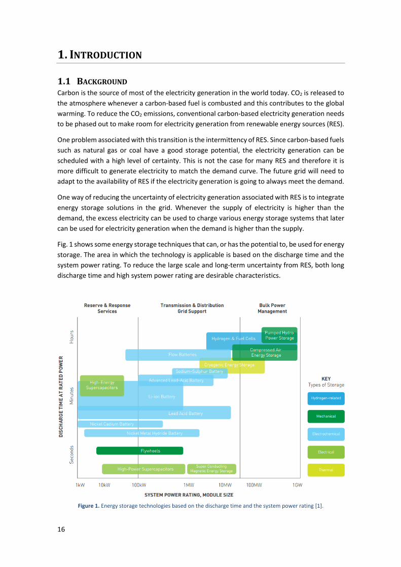
Fig. 1 shows some energy storage techniques that can, or has the potential to, be used for energy

storage. The area in which the technology is applicable is based on the discharge time and the

system power rating. To reduce the large scale and long-term uncertainty from RES, both long

discharge time and high system power rating are desirable characteristics.

Figure 1. Energy storage technologies based on the discharge time and the system power rating [1].

17

There are many techniques for energy storage with different levels of maturity explained in

literature. Among the techniques suggested in the Fig. 1, Pumped Hydro Storage (PHS) is by far

the most mature and widely used technique. When electricity is available at a low price, water

is pumped from a lower reservoir to a high reservoir to increase its potential energy. Later,

during times with a high price of electricity, the water is released through the turbines to

generate electricity. The efficiency of PHS is usually in the range of 65-85 %. PHS is however

limited by geological constraints and it needs an appropriate elevation and a good supply of

water. [2]

Among the less developed and used systems are Compressed Air Energy Storage (CAES) and

Hydrogen Storage. CAES uses excess electricity to compress air into underground caverns or

tanks. When electricity is needed, gas is combusted together with the stored high-pressure air

and expanded through a turbine to generate electricity. The efficiency of CAES systems are

around 70%. Hydrogen Storage uses excess electricity to electrolyze water to create hydrogen.

The overall efficiency is low, around 30% and is not yet a mature technology. [2]

1.2 AIMS AND OBJECTIVES

This thesis has been carried out under the frame of the European project CHESTER (Compressed

Heat Energy STorage for Energy from Renewable sources). The CHESTER project pursues the

development and evaluation of an innovative, efficient and smart energy storage and

management system to provide increased flexibility to the power grid. In addition, it will

incorporate advanced features that allow the integration of thermal RES such as solar, biomass,

waste heat, geothermal, etc. This system consists of a high-temperature heat pump (HT-HP), a

thermal energy storage system (TES), and a heat engine based on organic Rankine cycle (ORC).

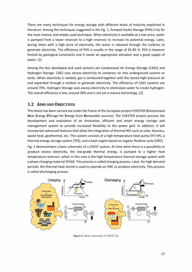
Fig. 2 demonstrates a basic schematic of a CHEST system. At time when there is a possibility to

produce excess electricity, the low-grade thermal energy, is pumped to a higher heat

temperature reservoir, which in this case is the high-temperature thermal storage system with

a phase changing material (PCM). This process is called charging process. Later, for high demand

periods, the thermal heat stored is used to operate an ORC to produce electricity. This process

is called discharging process.

Figure 2. Basic schematic of CHEST [3].

18

The Integration of RES allows a higher flexibility of the CHEST system, making it capable of

efficiently responding under different boundary conditions and needs. Based on the state of

boundary conditions the roundtrip efficiency of the system could, in theory, equal or even

exceed 100%.

To efficiently charge the high-temperature heat storage system, a HP that operates between

evaporation temperature of 30-100 °C and condensation temperature up to 200 °C should be

utilized. Later, the fluid of the ORC system evaporates at a temperature below the melting

temperature of the PCM. The sink temperature should be as low as possible in order to increase

the ORC efficiency hence the overall performance of CHEST system.

The main objective of the current work is to assess the thermodynamic performance of the

CHEST system. To achieve this main objective the following specific objectives should be fulfilled:

Refrigerants comparison and selection

HT-HP cycle, modelling, and analysis

ORC cycle, modelling, and analysis

Numerical model development of the CHEST.

Validation and parametric studies.

1.3 STATE OF THE ART A state of the art has been made in order to investigate has been previously done in the field.

Focus has been put on the complete charging/discharging system as well as possible

configurations of the HP and ORC that would yield a better overall efficiency.

1.3.1 Heat Pump

The basic HP consists of a condenser, an evaporator, a compressor and an expansion valve.

However, using a basic HP configuration for applications with a high temperature lift can be

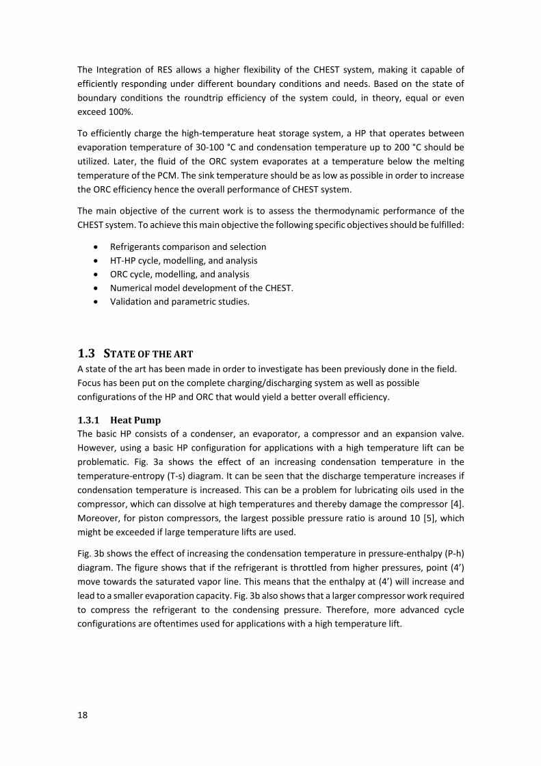
problematic. Fig. 3a shows the effect of an increasing condensation temperature in the

temperature-entropy (T-s) diagram. It can be seen that the discharge temperature increases if

condensation temperature is increased. This can be a problem for lubricating oils used in the

compressor, which can dissolve at high temperatures and thereby damage the compressor [4].

Moreover, for piston compressors, the largest possible pressure ratio is around 10 [5], which

might be exceeded if large temperature lifts are used.

Fig. 3b shows the effect of increasing the condensation temperature in pressure-enthalpy (P-h)

diagram. The figure shows that if the refrigerant is throttled from higher pressures, point (4’)

move towards the saturated vapor line. This means that the enthalpy at (4’) will increase and

lead to a smaller evaporation capacity. Fig. 3b also shows that a larger compressor work required

to compress the refrigerant to the condensing pressure. Therefore, more advanced cycle

configurations are oftentimes used for applications with a high temperature lift.

19

Figure 3. Cycle effects when increasing condensation temperature [6].

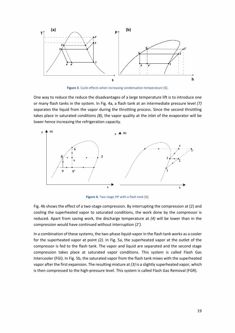
One way to reduce the reduce the disadvantages of a large temperature lift is to introduce one

or many flash tanks in the system. In Fig. 4a, a flash tank at an intermediate pressure level (7)

separates the liquid from the vapor during the throttling process. Since the second throttling

takes place in saturated conditions (8), the vapor quality at the inlet of the evaporator will be

lower hence increasing the refrigeration capacity.

Figure 4. Two stage HP with a flash tank [6].

Fig. 4b shows the effect of a two-stage compression. By interrupting the compression at (2) and

cooling the superheated vapor to saturated conditions, the work done by the compressor is

reduced. Apart from saving work, the discharge temperature at (4) will be lower than in the

compression would have continued without interruption (2’).

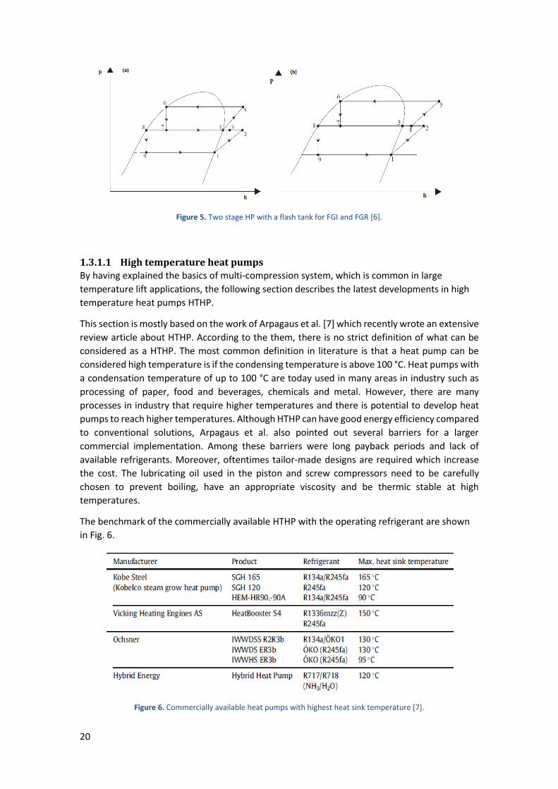
In a combination of these systems, the two-phase liquid-vapor in the flash tank works as a cooler

for the superheated vapor at point (2). In Fig. 5a, the superheated vapor at the outlet of the

compressor is fed to the flash tank. The vapor and liquid are separated and the second stage

compression takes place at saturated vapor conditions. This system is called Flash Gas

Intercooler (FGI). In Fig. 5b, the saturated vapor from the flash tank mixes with the superheated

vapor after the first expansion. The resulting mixture at (3) is a slightly superheated vapor, which

is then compressed to the high-pressure level. This system is called Flash Gas Removal (FGR).

P

h

T

s

1

2

2'

3

3'

4 4'

(a) (b)

1

2

2'

3

3'

4 4'

20

Figure 5. Two stage HP with a flash tank for FGI and FGR [6].

1.3.1.1 High temperature heat pumps

By having explained the basics of multi-compression system, which is common in large

temperature lift applications, the following section describes the latest developments in high

temperature heat pumps HTHP.

This section is mostly based on the work of Arpagaus et al. [7] which recently wrote an extensive

review article about HTHP. According to the them, there is no strict definition of what can be

considered as a HTHP. The most common definition in literature is that a heat pump can be

considered high temperature is if the condensing temperature is above 100 °C. Heat pumps with

a condensation temperature of up to 100 °C are today used in many areas in industry such as

processing of paper, food and beverages, chemicals and metal. However, there are many

processes in industry that require higher temperatures and there is potential to develop heat

pumps to reach higher temperatures. Although HTHP can have good energy efficiency compared

to conventional solutions, Arpagaus et al. also pointed out several barriers for a larger

commercial implementation. Among these barriers were long payback periods and lack of

available refrigerants. Moreover, oftentimes tailor-made designs are required which increase

the cost. The lubricating oil used in the piston and screw compressors need to be carefully

chosen to prevent boiling, have an appropriate viscosity and be thermic stable at high

temperatures.

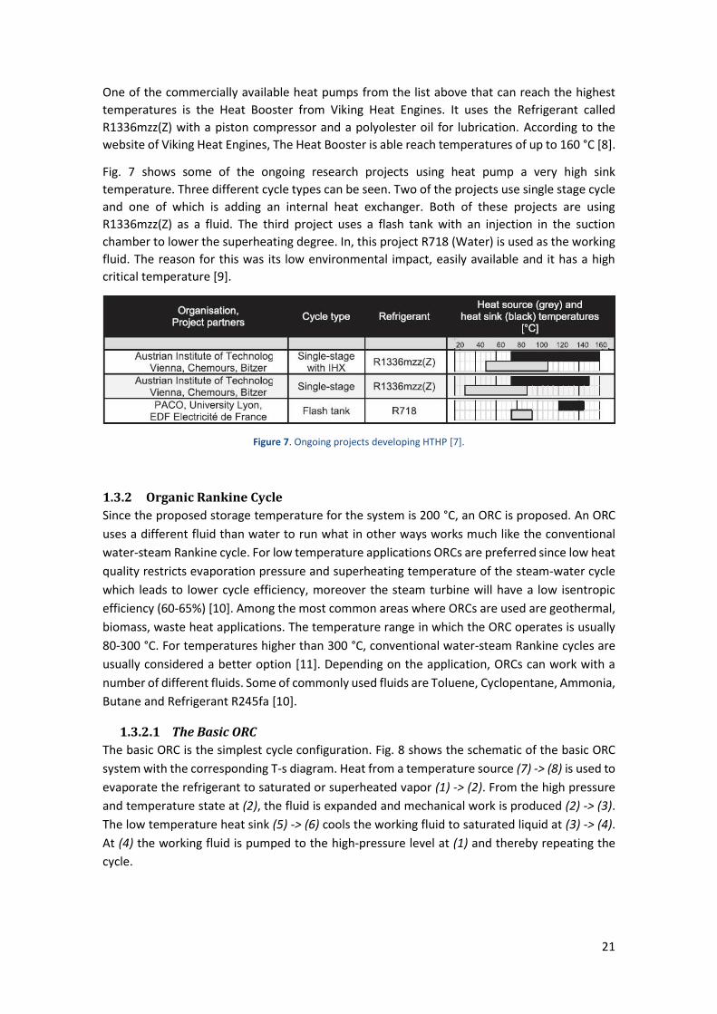
The benchmark of the commercially available HTHP with the operating refrigerant are shown

in Fig. 6.

Figure 6. Commercially available heat pumps with highest heat sink temperature [7].

21

One of the commercially available heat pumps from the list above that can reach the highest

temperatures is the Heat Booster from Viking Heat Engines. It uses the Refrigerant called

R1336mzz(Z) with a piston compressor and a polyolester oil for lubrication. According to the

website of Viking Heat Engines, The Heat Booster is able reach temperatures of up to 160 °C [8].

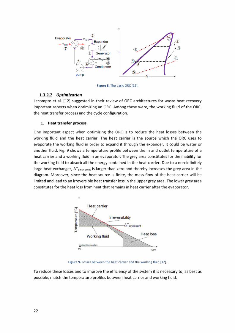
Fig. 7 shows some of the ongoing research projects using heat pump a very high sink

temperature. Three different cycle types can be seen. Two of the projects use single stage cycle

and one of which is adding an internal heat exchanger. Both of these projects are using

R1336mzz(Z) as a fluid. The third project uses a flash tank with an injection in the suction

chamber to lower the superheating degree. In, this project R718 (Water) is used as the working

fluid. The reason for this was its low environmental impact, easily available and it has a high

critical temperature [9].

Figure 7. Ongoing projects developing HTHP [7].

1.3.2 Organic Rankine Cycle

Since the proposed storage temperature for the system is 200 °C, an ORC is proposed. An ORC

uses a different fluid than water to run what in other ways works much like the conventional

water-steam Rankine cycle. For low temperature applications ORCs are preferred since low heat

quality restricts evaporation pressure and superheating temperature of the steam-water cycle

which leads to lower cycle efficiency, moreover the steam turbine will have a low isentropic

efficiency (60-65%) [10]. Among the most common areas where ORCs are used are geothermal,

biomass, waste heat applications. The temperature range in which the ORC operates is usually

80-300 °C. For temperatures higher than 300 °C, conventional water-steam Rankine cycles are

usually considered a better option [11]. Depending on the application, ORCs can work with a

number of different fluids. Some of commonly used fluids are Toluene, Cyclopentane, Ammonia,

Butane and Refrigerant R245fa [10].

1.3.2.1 The Basic ORC

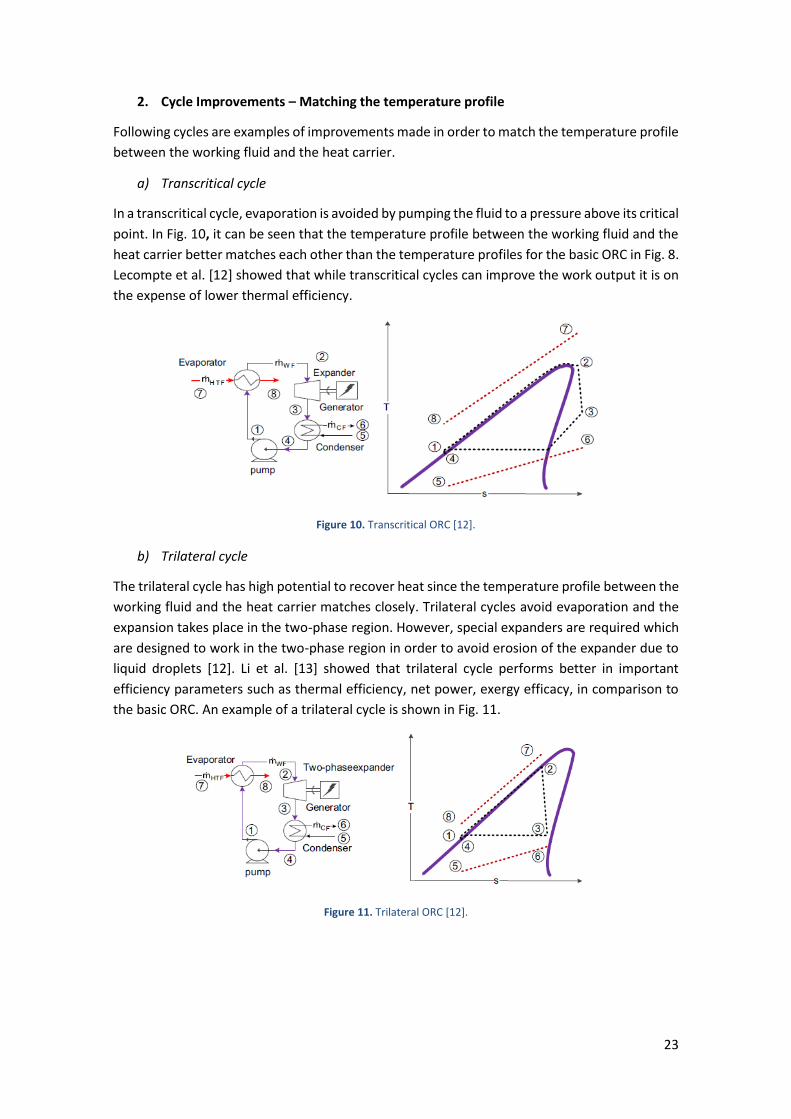
The basic ORC is the simplest cycle configuration. Fig. 8 shows the schematic of the basic ORC

system with the corresponding T-s diagram. Heat from a temperature source (7) -> (8) is used to

evaporate the refrigerant to saturated or superheated vapor (1) -> (2). From the high pressure

and temperature state at (2), the fluid is expanded and mechanical work is produced (2) -> (3).

The low temperature heat sink (5) -> (6) cools the working fluid to saturated liquid at (3) -> (4).

At (4) the working fluid is pumped to the high-pressure level at (1) and thereby repeating the

cycle.

22

Figure 8. The basic ORC [12].

1.3.2.2 Optimization

Lecompte et al. [12] suggested in their review of ORC architectures for waste heat recovery

important aspects when optimizing an ORC. Among these were, the working fluid of the ORC,

the heat transfer process and the cycle configuration.

1. Heat transfer process

One important aspect when optimizing the ORC is to reduce the heat losses between the

working fluid and the heat carrier. The heat carrier is the source which the ORC uses to

evaporate the working fluid in order to expand it through the expander. It could be water or

another fluid. Fig. 9 shows a temperature profile between the in and outlet temperature of a

heat carrier and a working fluid in an evaporator. The grey area constitutes for the inability for

the working fluid to absorb all the energy contained in the heat carrier. Due to a non-infinitely

large heat exchanger, ΔTpinch point is larger than zero and thereby increases the grey area in the

diagram. Moreover, since the heat source is finite, the mass flow of the heat carrier will be

limited and lead to an irreversible heat transfer loss in the upper grey area. The lower grey area

constitutes for the heat loss from heat that remains in heat carrier after the evaporator.

Figure 9. Losses between the heat carrier and the working fluid [12].

To reduce these losses and to improve the efficiency of the system it is necessary to, as best as

possible, match the temperature profiles between heat carrier and working fluid.

23

2. Cycle Improvements – Matching the temperature profile

Following cycles are examples of improvements made in order to match the temperature profile

between the working fluid and the heat carrier.

a) Transcritical cycle

In a transcritical cycle, evaporation is avoided by pumping the fluid to a pressure above its critical

point. In Fig. 10, it can be seen that the temperature profile between the working fluid and the

heat carrier better matches each other than the temperature profiles for the basic ORC in Fig. 8.

Lecompte et al. [12] showed that while transcritical cycles can improve the work output it is on

the expense of lower thermal efficiency.

Figure 10. Transcritical ORC [12].

b) Trilateral cycle

The trilateral cycle has high potential to recover heat since the temperature profile between the

working fluid and the heat carrier matches closely. Trilateral cycles avoid evaporation and the

expansion takes place in the two-phase region. However, special expanders are required which

are designed to work in the two-phase region in order to avoid erosion of the expander due to

liquid droplets [12]. Li et al. [13] showed that trilateral cycle performs better in important

efficiency parameters such as thermal efficiency, net power, exergy efficacy, in comparison to

the basic ORC. An example of a trilateral cycle is shown in Fig. 11.

Figure 11. Trilateral ORC [12].

24

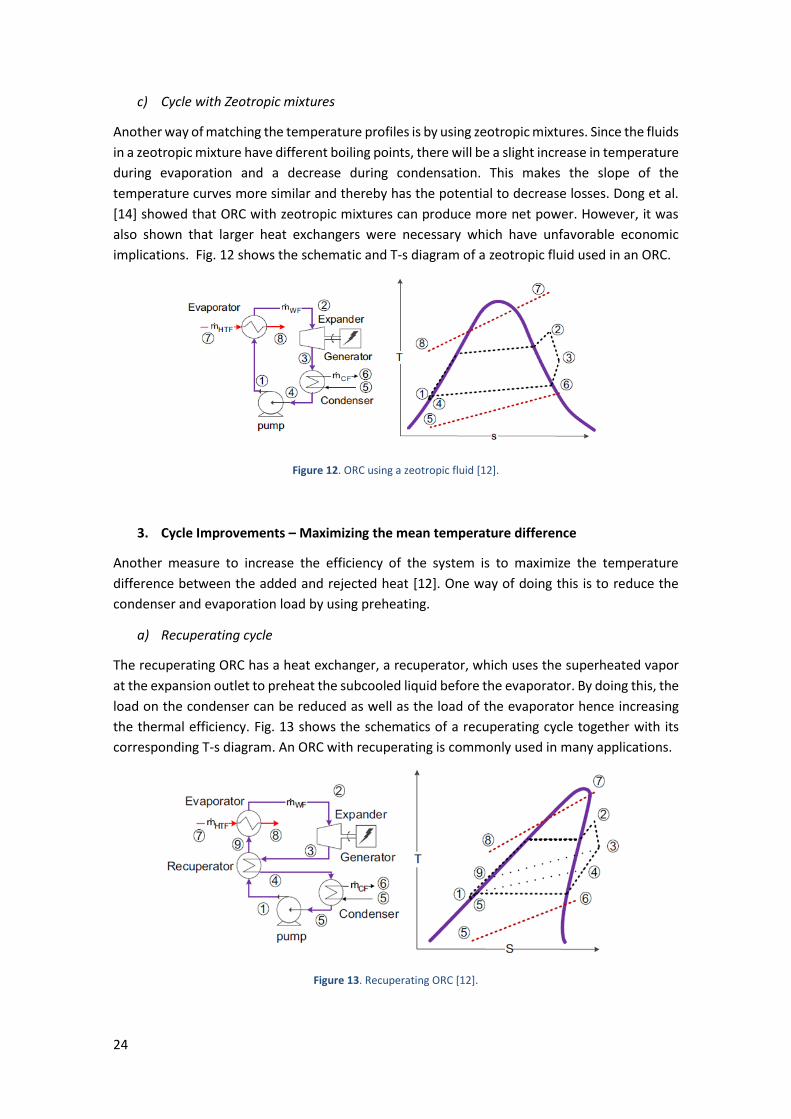
c) Cycle with Zeotropic mixtures

Another way of matching the temperature profiles is by using zeotropic mixtures. Since the fluids

in a zeotropic mixture have different boiling points, there will be a slight increase in temperature

during evaporation and a decrease during condensation. This makes the slope of the

temperature curves more similar and thereby has the potential to decrease losses. Dong et al.

[14] showed that ORC with zeotropic mixtures can produce more net power. However, it was

also shown that larger heat exchangers were necessary which have unfavorable economic

implications. Fig. 12 shows the schematic and T-s diagram of a zeotropic fluid used in an ORC.

Figure 12. ORC using a zeotropic fluid [12].

3. Cycle Improvements – Maximizing the mean temperature difference

Another measure to increase the efficiency of the system is to maximize the temperature

difference between the added and rejected heat [12]. One way of doing this is to reduce the

condenser and evaporation load by using preheating.

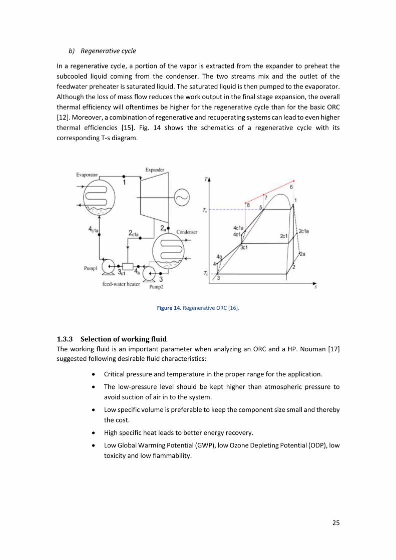
a) Recuperating cycle

The recuperating ORC has a heat exchanger, a recuperator, which uses the superheated vapor

at the expansion outlet to preheat the subcooled liquid before the evaporator. By doing this, the

load on the condenser can be reduced as well as the load of the evaporator hence increasing

the thermal efficiency. Fig. 13 shows the schematics of a recuperating cycle together with its

corresponding T-s diagram. An ORC with recuperating is commonly used in many applications.

Figure 13. Recuperating ORC [12].

25

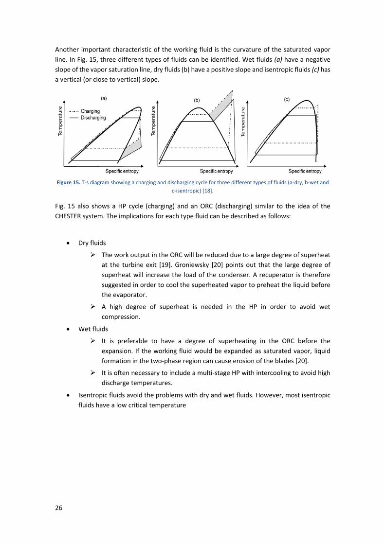
b) Regenerative cycle

In a regenerative cycle, a portion of the vapor is extracted from the expander to preheat the

subcooled liquid coming from the condenser. The two streams mix and the outlet of the

feedwater preheater is saturated liquid. The saturated liquid is then pumped to the evaporator.

Although the loss of mass flow reduces the work output in the final stage expansion, the overall

thermal efficiency will oftentimes be higher for the regenerative cycle than for the basic ORC

[12]. Moreover, a combination of regenerative and recuperating systems can lead to even higher

thermal efficiencies [15]. Fig. 14 shows the schematics of a regenerative cycle with its

corresponding T-s diagram.

Figure 14. Regenerative ORC [16].

1.3.3 Selection of working fluid

The working fluid is an important parameter when analyzing an ORC and a HP. Nouman [17]

suggested following desirable fluid characteristics:

Critical pressure and temperature in the proper range for the application.

The low-pressure level should be kept higher than atmospheric pressure to

avoid suction of air in to the system.

Low specific volume is preferable to keep the component size small and thereby

the cost.

High specific heat leads to better energy recovery.

Low Global Warming Potential (GWP), low Ozone Depleting Potential (ODP), low

toxicity and low flammability.

26

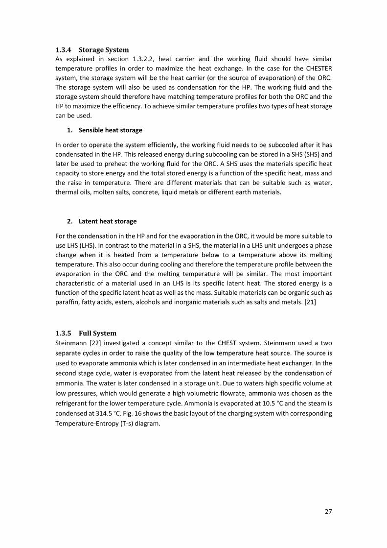
Another important characteristic of the working fluid is the curvature of the saturated vapor

line. In Fig. 15, three different types of fluids can be identified. Wet fluids (a) have a negative

slope of the vapor saturation line, dry fluids (b) have a positive slope and isentropic fluids (c) has

a vertical (or close to vertical) slope.

Figure 15. T-s diagram showing a charging and discharging cycle for three different types of fluids (a-dry, b-wet and

c-isentropic) [18].

Fig. 15 also shows a HP cycle (charging) and an ORC (discharging) similar to the idea of the

CHESTER system. The implications for each type fluid can be described as follows:

Dry fluids

The work output in the ORC will be reduced due to a large degree of superheat

at the turbine exit [19]. Groniewsky [20] points out that the large degree of

superheat will increase the load of the condenser. A recuperator is therefore

suggested in order to cool the superheated vapor to preheat the liquid before

the evaporator.

A high degree of superheat is needed in the HP in order to avoid wet

compression.

Wet fluids

It is preferable to have a degree of superheating in the ORC before the

expansion. If the working fluid would be expanded as saturated vapor, liquid

formation in the two-phase region can cause erosion of the blades [20].

It is often necessary to include a multi-stage HP with intercooling to avoid high

discharge temperatures.

Isentropic fluids avoid the problems with dry and wet fluids. However, most isentropic

fluids have a low critical temperature

27

1.3.4 Storage System

As explained in section 1.3.2.2, heat carrier and the working fluid should have similar

temperature profiles in order to maximize the heat exchange. In the case for the CHESTER

system, the storage system will be the heat carrier (or the source of evaporation) of the ORC.

The storage system will also be used as condensation for the HP. The working fluid and the

storage system should therefore have matching temperature profiles for both the ORC and the

HP to maximize the efficiency. To achieve similar temperature profiles two types of heat storage

can be used.

1. Sensible heat storage

In order to operate the system efficiently, the working fluid needs to be subcooled after it has

condensated in the HP. This released energy during subcooling can be stored in a SHS (SHS) and

later be used to preheat the working fluid for the ORC. A SHS uses the materials specific heat

capacity to store energy and the total stored energy is a function of the specific heat, mass and

the raise in temperature. There are different materials that can be suitable such as water,

thermal oils, molten salts, concrete, liquid metals or different earth materials.

2. Latent heat storage

For the condensation in the HP and for the evaporation in the ORC, it would be more suitable to

use LHS (LHS). In contrast to the material in a SHS, the material in a LHS unit undergoes a phase

change when it is heated from a temperature below to a temperature above its melting

temperature. This also occur during cooling and therefore the temperature profile between the

evaporation in the ORC and the melting temperature will be similar. The most important

characteristic of a material used in an LHS is its specific latent heat. The stored energy is a

function of the specific latent heat as well as the mass. Suitable materials can be organic such as

paraffin, fatty acids, esters, alcohols and inorganic materials such as salts and metals. [21]

1.3.5 Full System

Steinmann [22] investigated a concept similar to the CHEST system. Steinmann used a two

separate cycles in order to raise the quality of the low temperature heat source. The source is

used to evaporate ammonia which is later condensed in an intermediate heat exchanger. In the

second stage cycle, water is evaporated from the latent heat released by the condensation of

ammonia. The water is later condensed in a storage unit. Due to waters high specific volume at

low pressures, which would generate a high volumetric flowrate, ammonia was chosen as the

refrigerant for the lower temperature cycle. Ammonia is evaporated at 10.5 °C and the steam is

condensed at 314.5 °C. Fig. 16 shows the basic layout of the charging system with corresponding

Temperature-Entropy (T-s) diagram.

28

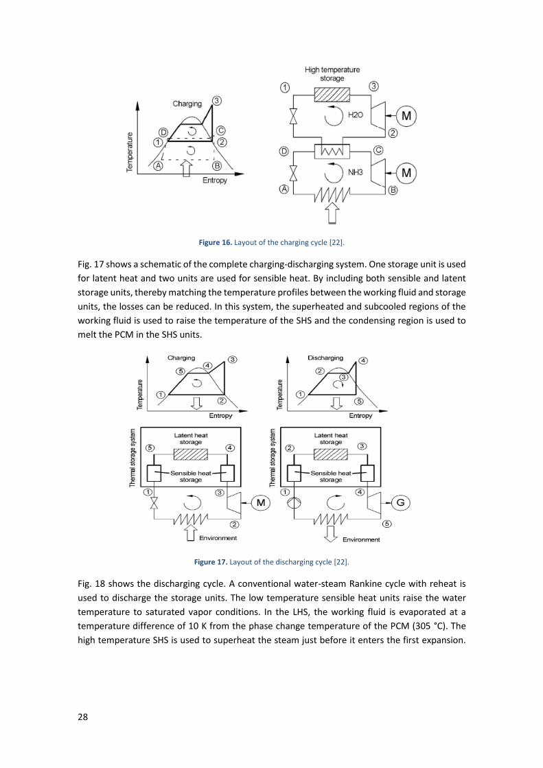
Figure 16. Layout of the charging cycle [22].

Fig. 17 shows a schematic of the complete charging-discharging system. One storage unit is used

for latent heat and two units are used for sensible heat. By including both sensible and latent

storage units, thereby matching the temperature profiles between the working fluid and storage

units, the losses can be reduced. In this system, the superheated and subcooled regions of the

working fluid is used to raise the temperature of the SHS and the condensing region is used to

melt the PCM in the SHS units.

Figure 17. Layout of the discharging cycle [22].

Fig. 18 shows the discharging cycle. A conventional water-steam Rankine cycle with reheat is

used to discharge the storage units. The low temperature sensible heat units raise the water

temperature to saturated vapor conditions. In the LHS, the working fluid is evaporated at a

temperature difference of 10 K from the phase change temperature of the PCM (305 °C). The

high temperature SHS is used to superheat the steam just before it enters the first expansion.

29

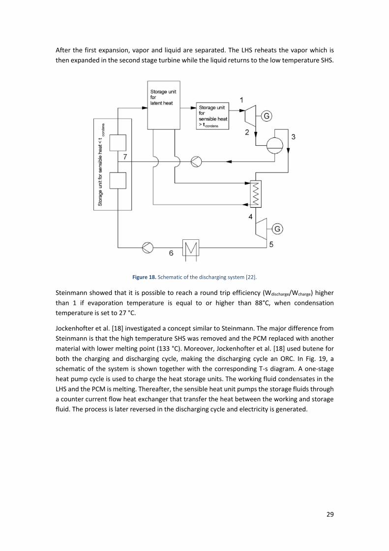
After the first expansion, vapor and liquid are separated. The LHS reheats the vapor which is

then expanded in the second stage turbine while the liquid returns to the low temperature SHS.

Figure 18. Schematic of the discharging system [22].

Steinmann showed that it is possible to reach a round trip efficiency (Wdischarge/Wcharge) higher

than 1 if evaporation temperature is equal to or higher than 88°C, when condensation

temperature is set to 27 °C.

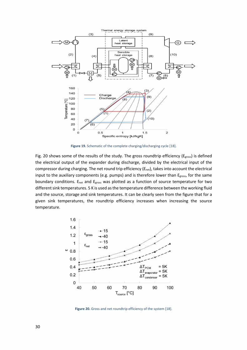
Jockenhofter et al. [18] investigated a concept similar to Steinmann. The major difference from

Steinmann is that the high temperature SHS was removed and the PCM replaced with another

material with lower melting point (133 °C). Moreover, Jockenhofter et al. [18] used butene for

both the charging and discharging cycle, making the discharging cycle an ORC. In Fig. 19, a

schematic of the system is shown together with the corresponding T-s diagram. A one-stage

heat pump cycle is used to charge the heat storage units. The working fluid condensates in the

LHS and the PCM is melting. Thereafter, the sensible heat unit pumps the storage fluids through

a counter current flow heat exchanger that transfer the heat between the working and storage

fluid. The process is later reversed in the discharging cycle and electricity is generated.

30

Figure 19. Schematic of the complete charging/discharging cycle [18].

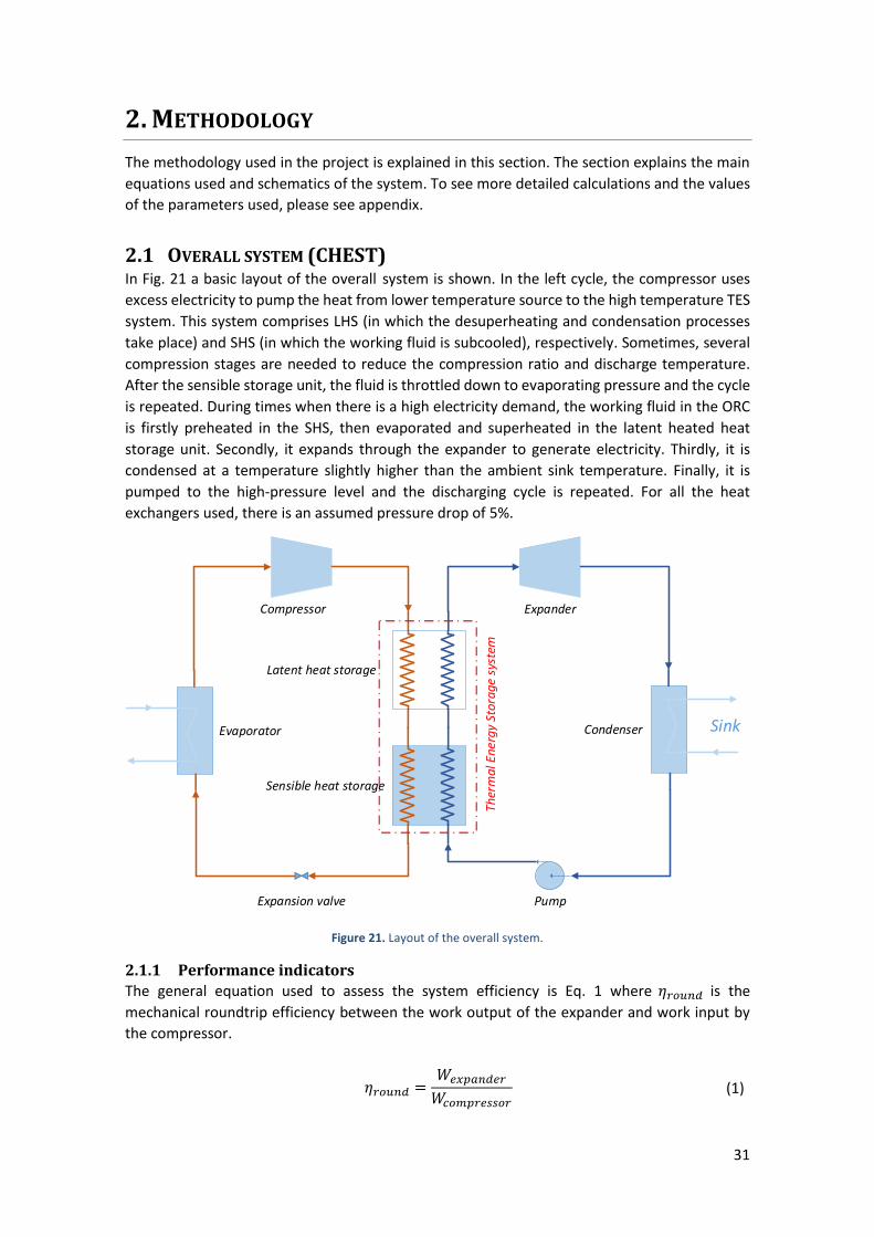
Fig. 20 shows some of the results of the study. The gross roundtrip efficiency (Ɛgross) is defined

the electrical output of the expander during discharge, divided by the electrical input of the

compressor during charging. The net round trip efficiency (Ɛnet), takes into account the electrical

input to the auxiliary components (e.g. pumps) and is therefore lower than Ɛgross, for the same

boundary conditions. Ɛnet and Ɛgross was plotted as a function of source temperature for two

different sink temperatures. 5 K is used as the temperature difference between the working fluid

and the source, storage and sink temperatures. It can be clearly seen from the figure that for a

given sink temperatures, the roundtrip efficiency increases when increasing the source

temperature.

Figure 20. Gross and net roundtrip efficiency of the system [18].

31

2. METHODOLOGY

The methodology used in the project is explained in this section. The section explains the main

equations used and schematics of the system. To see more detailed calculations and the values

of the parameters used, please see appendix.

2.1 OVERALL SYSTEM (CHEST) In Fig. 21 a basic layout of the overall system is shown. In the left cycle, the compressor uses

excess electricity to pump the heat from lower temperature source to the high temperature TES

system. This system comprises LHS (in which the desuperheating and condensation processes

take place) and SHS (in which the working fluid is subcooled), respectively. Sometimes, several

compression stages are needed to reduce the compression ratio and discharge temperature.

After the sensible storage unit, the fluid is throttled down to evaporating pressure and the cycle

is repeated. During times when there is a high electricity demand, the working fluid in the ORC

is firstly preheated in the SHS, then evaporated and superheated in the latent heated heat

storage unit. Secondly, it expands through the expander to generate electricity. Thirdly, it is

condensed at a temperature slightly higher than the ambient sink temperature. Finally, it is

pumped to the high-pressure level and the discharging cycle is repeated. For all the heat

exchangers used, there is an assumed pressure drop of 5%.

Figure 21. Layout of the overall system.

2.1.1 Performance indicators

The general equation used to assess the system efficiency is Eq. 1 where 𝜂𝑟𝑜𝑢𝑛𝑑 is the

mechanical roundtrip efficiency between the work output of the expander and work input by

the compressor.

𝜂𝑟𝑜𝑢𝑛𝑑 =

𝑊𝑒𝑥𝑝𝑎𝑛𝑑𝑒𝑟𝑊𝑐𝑜𝑚𝑝𝑟𝑒𝑠𝑠𝑜𝑟

(1)

Pump

Compressor Expander

CondenserEvaporator

Latent heat storage

Sensible heat storage

Expansion valve

Sink

Ther

mal

Ene

rgy

Stor

age

syst

em

32

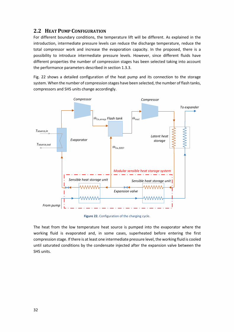
2.2 HEAT PUMP CONFIGURATION For different boundary conditions, the temperature lift will be different. As explained in the

introduction, intermediate pressure levels can reduce the discharge temperature, reduce the

total compressor work and increase the evaporation capacity. In the proposed, there is a

possibility to introduce intermediate pressure levels. However, since different fluids have

different properties the number of compression stages has been selected taking into account

the performance parameters described in section 1.3.3.

Fig. 22 shows a detailed configuration of the heat pump and its connection to the storage

system. When the number of compression stages have been selected, the number of flash tanks,

compressors and SHS units change accordingly.

Figure 22. Configuration of the charging cycle.

The heat from the low temperature heat source is pumped into the evaporator where the

working fluid is evaporated and, in some cases, superheated before entering the first

compression stage. If there is at least one intermediate pressure level, the working fluid is cooled

until saturated conditions by the condensate injected after the expansion valve between the

SHS units.

Evaporator

Tsource,in

Tsource,out

Flash tank

Compressor Compressor

Latent heat storage

Sensible heat storage unitSensible heat storage unit

Expansion valve

To expander

From pump

Modular sensible heat storage system

33

2.2.1 Governing equations

For times when there are several compression stages, Eq. 2 [6] is used to obtain the optimum

intermediate pressure (assuming similar pressure ratios between stages).

𝑃𝑗 = 𝑃𝑒𝑣𝑎𝑝 (𝑃𝑐𝑜𝑛𝑑𝑃𝑒𝑣𝑎𝑝

)

𝑖𝑁𝑆𝐶

(2)

where j is the index for current intermediate pressure level, P is the pressure and NSC is total

number of stages of compression.

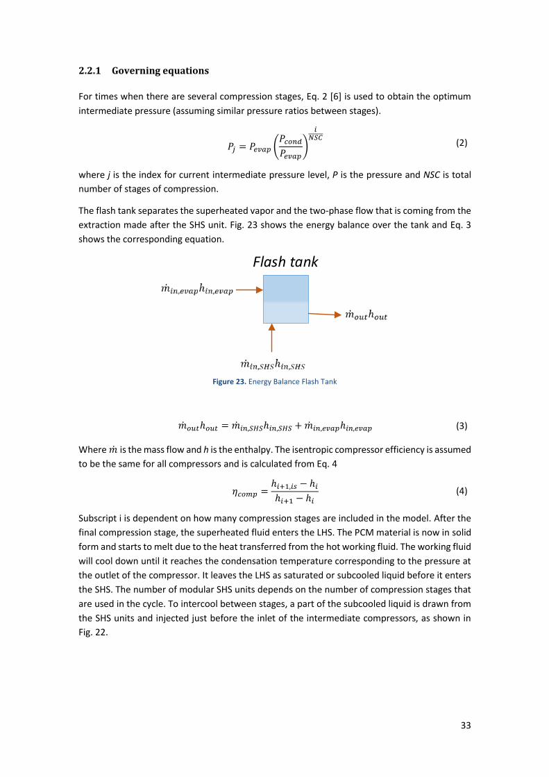
The flash tank separates the superheated vapor and the two-phase flow that is coming from the

extraction made after the SHS unit. Fig. 23 shows the energy balance over the tank and Eq. 3

shows the corresponding equation.

Figure 23. Energy Balance Flash Tank

�̇�𝑜𝑢𝑡ℎ𝑜𝑢𝑡 = �̇�𝑖𝑛,𝑆𝐻𝑆ℎ𝑖𝑛,𝑆𝐻𝑆 + �̇�𝑖𝑛,𝑒𝑣𝑎𝑝ℎ𝑖𝑛,𝑒𝑣𝑎𝑝 (3)

Where �̇� is the mass flow and h is the enthalpy. The isentropic compressor efficiency is assumed

to be the same for all compressors and is calculated from Eq. 4

𝜂𝑐𝑜𝑚𝑝 =

ℎ𝑖+1,𝑖𝑠 − ℎ𝑖ℎ𝑖+1 − ℎ𝑖

(4)

Subscript i is dependent on how many compression stages are included in the model. After the

final compression stage, the superheated fluid enters the LHS. The PCM material is now in solid

form and starts to melt due to the heat transferred from the hot working fluid. The working fluid

will cool down until it reaches the condensation temperature corresponding to the pressure at

the outlet of the compressor. It leaves the LHS as saturated or subcooled liquid before it enters

the SHS. The number of modular SHS units depends on the number of compression stages that

are used in the cycle. To intercool between stages, a part of the subcooled liquid is drawn from

the SHS units and injected just before the inlet of the intermediate compressors, as shown in

Fig. 22.

Flash tank

34

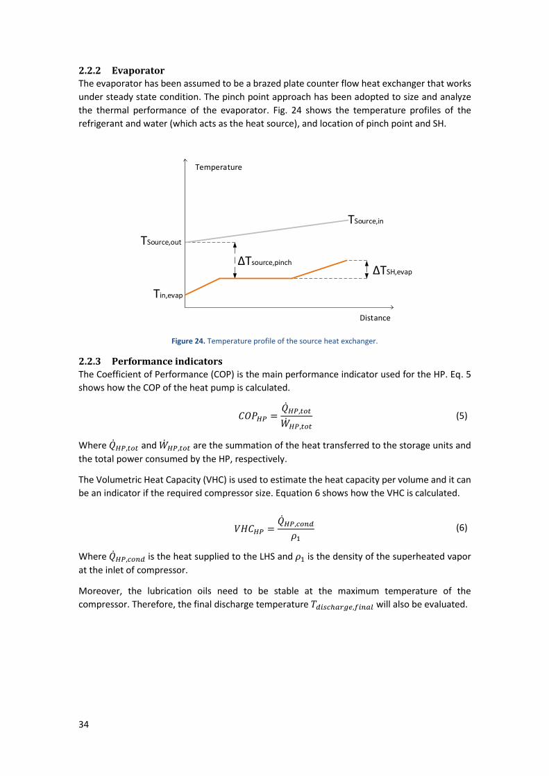
2.2.2 Evaporator

The evaporator has been assumed to be a brazed plate counter flow heat exchanger that works

under steady state condition. The pinch point approach has been adopted to size and analyze

the thermal performance of the evaporator. Fig. 24 shows the temperature profiles of the

refrigerant and water (which acts as the heat source), and location of pinch point and SH.

Figure 24. Temperature profile of the source heat exchanger.


The Coefficient of Performance (COP) is the main performance indicator used for the HP. Eq. 5

shows how the COP of the heat pump is calculated.

𝐶𝑂𝑃𝐻𝑃 =

�̇�𝐻𝑃,𝑡𝑜𝑡

�̇�𝐻𝑃,𝑡𝑜𝑡 (5)

Where �̇�𝐻𝑃,𝑡𝑜𝑡 and �̇�𝐻𝑃,𝑡𝑜𝑡 are the summation of the heat transferred to the storage units and

the total power consumed by the HP, respectively.

The Volumetric Heat Capacity (VHC) is used to estimate the heat capacity per volume and it can

be an indicator if the required compressor size. Equation 6 shows how the VHC is calculated.

𝑉𝐻𝐶𝐻𝑃 =

�̇�𝐻𝑃,𝑐𝑜𝑛𝑑𝜌1

(6)

Where �̇�𝐻𝑃,𝑐𝑜𝑛𝑑 is the heat supplied to the LHS and 𝜌1 is the density of the superheated vapor

at the inlet of compressor.

Moreover, the lubrication oils need to be stable at the maximum temperature of the

compressor. Therefore, the final discharge temperature 𝑇𝑑𝑖𝑠𝑐ℎ𝑎𝑟𝑔𝑒,𝑓𝑖𝑛𝑎𝑙 will also be evaluated.

Tin,evap

TSource,out

ΔTSH,evapΔTsource,pinch

Temperature

Distance

TSource,in

35

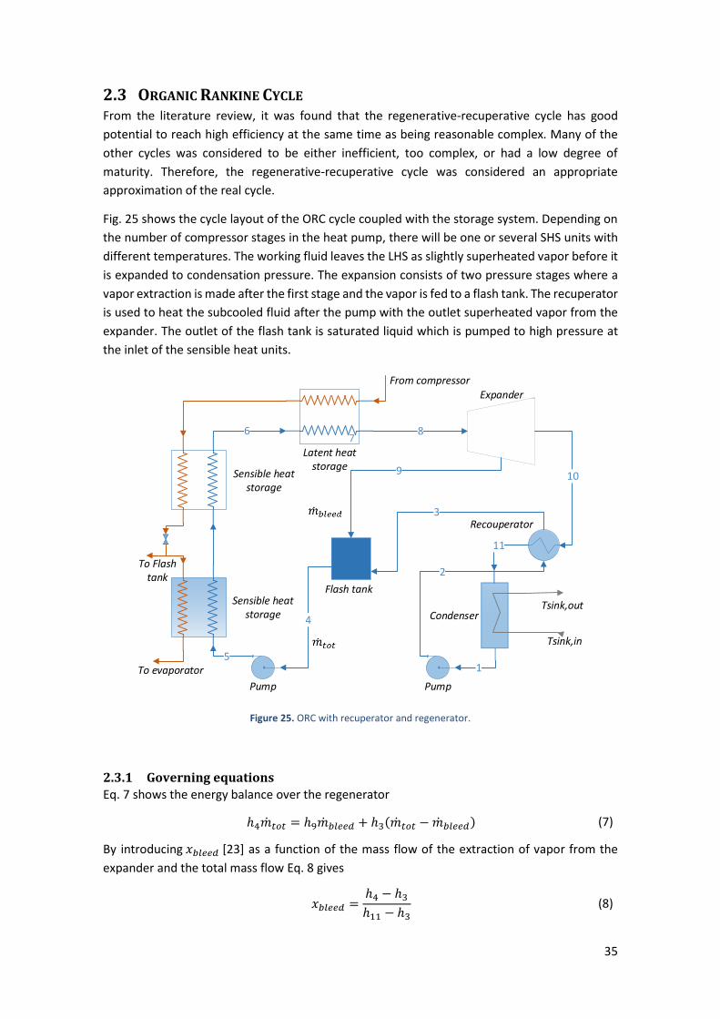
2.3 ORGANIC RANKINE CYCLE From the literature review, it was found that the regenerative-recuperative cycle has good

potential to reach high efficiency at the same time as being reasonable complex. Many of the

other cycles was considered to be either inefficient, too complex, or had a low degree of

maturity. Therefore, the regenerative-recuperative cycle was considered an appropriate

approximation of the real cycle.

Fig. 25 shows the cycle layout of the ORC cycle coupled with the storage system. Depending on

the number of compressor stages in the heat pump, there will be one or several SHS units with

different temperatures. The working fluid leaves the LHS as slightly superheated vapor before it

is expanded to condensation pressure. The expansion consists of two pressure stages where a

vapor extraction is made after the first stage and the vapor is fed to a flash tank. The recuperator

is used to heat the subcooled fluid after the pump with the outlet superheated vapor from the

expander. The outlet of the flash tank is saturated liquid which is pumped to high pressure at

the inlet of the sensible heat units.

Figure 25. ORC with recuperator and regenerator.

2.3.1 Governing equations

Eq. 7 shows the energy balance over the regenerator

ℎ4�̇�𝑡𝑜𝑡 = ℎ9�̇�𝑏𝑙𝑒𝑒𝑑 + ℎ3(�̇�𝑡𝑜𝑡 − �̇�𝑏𝑙𝑒𝑒𝑑) (7)

By introducing 𝑥𝑏𝑙𝑒𝑒𝑑 [23] as a function of the mass flow of the extraction of vapor from the

expander and the total mass flow Eq. 8 gives

𝑥𝑏𝑙𝑒𝑒𝑑 =

ℎ4 − ℎ3ℎ11 − ℎ3

(8)

9 10

11

1

2

3

5

6 8

4

PumpPump

Recouperator

Condenser

Expander

Flash tankSensible heat

storage

Latent heat storage

Tsink,in

To evaporator

To Flash tank

Sensible heat storage

Tsink,out

From compressor

7

36

Eq. 9 shows the energy balance over the recuperator

ℎ3 − ℎ2 = ℎ10 − ℎ11 (9)

Eq. 10 shows the recuperator effectiveness and is defined as

𝜀𝑟𝑒𝑐 =

ℎ3 − ℎ2ℎ10 − ℎ2,𝑝𝑟𝑖𝑚

(10)

Where ℎ2,𝑝𝑟𝑖𝑚 is the smallest enthalpy value that ℎ2 can have with the condition 𝑇10 = 𝑇2.

Eq. 11 shows the isentropic efficiency of the pumps, which is calculated as

𝜂𝑝𝑢𝑚𝑝 =

ℎ𝑖+1,𝑖𝑠 − ℎ𝑖ℎ𝑖+1 − ℎ𝑖

(11)

Where i is 0 and 3.

Eq. 12 shows how the bleed pressure is defined.

𝑃𝑏𝑙𝑒𝑒𝑑 = 𝑃𝑖(𝑃𝑒𝑣𝑎𝑝 − 𝑃𝑐𝑜𝑛𝑑) + 𝑃𝑐𝑜𝑛𝑑 (12)

Where 𝑃𝑖 is a value from 0 to 1. This equation makes 𝑃𝑏𝑙𝑒𝑒𝑑 vary between the condensation

pressure (when 𝑃𝑖 = 0) and the evaporation pressure (when 𝑃𝑖 = 1).

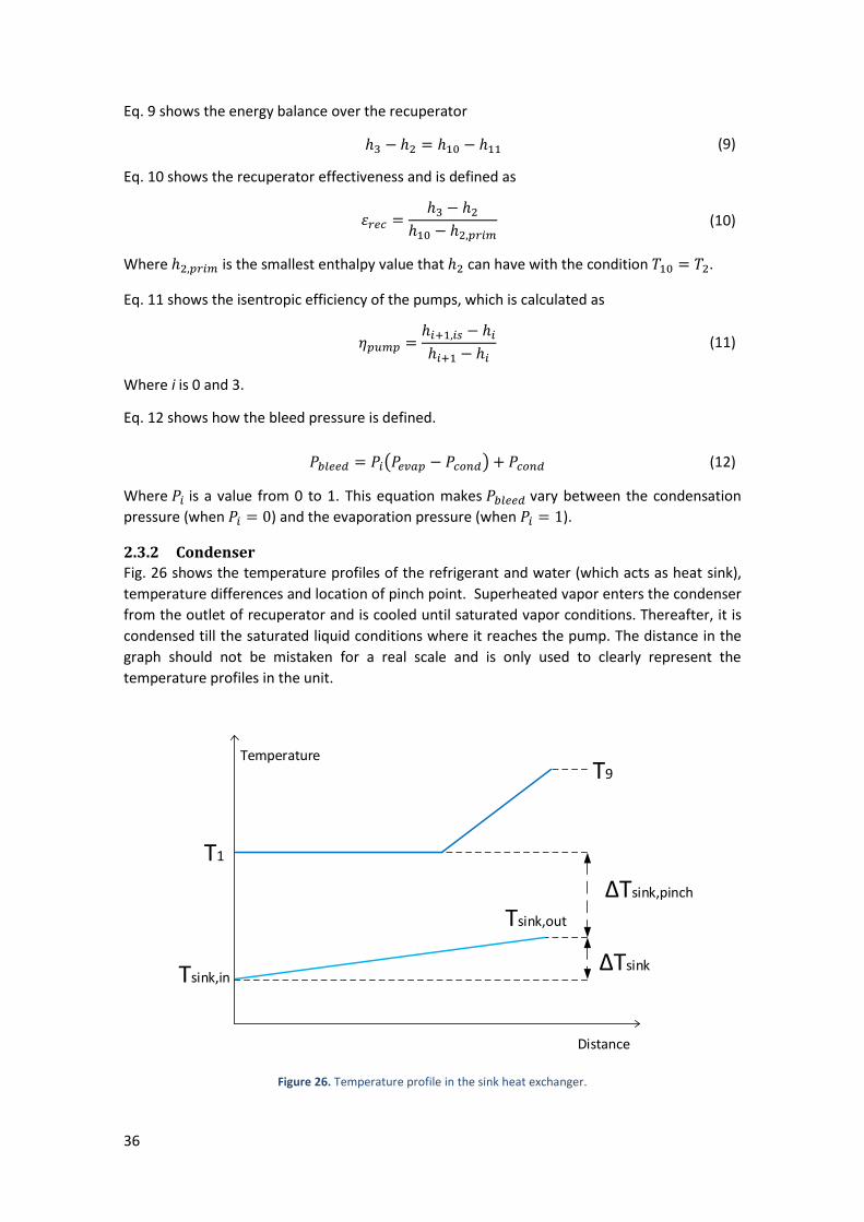
2.3.2 Condenser

Fig. 26 shows the temperature profiles of the refrigerant and water (which acts as heat sink),

temperature differences and location of pinch point. Superheated vapor enters the condenser

from the outlet of recuperator and is cooled until saturated vapor conditions. Thereafter, it is

condensed till the saturated liquid conditions where it reaches the pump. The distance in the

graph should not be mistaken for a real scale and is only used to clearly represent the

temperature profiles in the unit.

Figure 26. Temperature profile in the sink heat exchanger.

Tsink,in

Tsink,out

T9

T1

ΔTsink

ΔTsink,pinch

Temperature

Distance

37


Following parameters are used to evaluate the system performance for the ORC. The thermal

efficiency is defined in Eq. 13 as the work output of the expander divided by the total thermal

input from the storage unit.

𝜂𝑡ℎ𝑒𝑟𝑚𝑎𝑙 =

�̇�𝑛𝑒𝑡

�̇�𝑖𝑛 (13)

In order to avoid supersonic flow problems, large sized expanders and a large number of stages,

the specific volume ratio between the outlet and the inlet of the expander should be as low as

possible. Therefore Rayegan et al. [24] suggested adding a parameter, VER (Vapour Expansion

Ratio), to the evaluation, shown in Eq. 14

𝑉𝐸𝑅 =𝜈𝑜𝑢𝑡𝜈𝑖𝑛

(14)

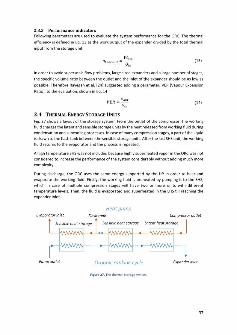
2.4 THERMAL ENERGY STORAGE UNITS Fig. 27 shows a layout of the storage system. From the outlet of the compressor, the working

fluid charges the latent and sensible storage units by the heat released from working fluid during

condensation and subcooling processes. In case of many compression stages, a part of the liquid

is drawn to the flash tank between the sensible storage units. After the last SHS unit, the working

fluid returns to the evaporator and the process is repeated.

A high temperature SHS was not included because highly superheated vapor in the ORC was not

considered to increase the performance of the system considerably without adding much more

complexity.

During discharge, the ORC uses the same energy supported by the HP in order to heat and

evaporate the working fluid. Firstly, the working fluid is preheated by pumping it to the SHS,

which in case of multiple compression stages will have two or more units with different

temperature levels. Then, the fluid is evaporated and superheated in the LHS till reaching the

expander inlet.

Figure 27. The thermal storage system.

Evaporator inlet

Expander inlet

Compressor outlet

Latent heat storageSensible heat storageSensible heat storage

Pump outlet Organic rankine cycle

Heat pump Flash tank

38

2.4.1 Latent storage system

Although this work has not focused on the storage units, a short review was made in order to

find possible materials for the LHS unit. The LHS unit contains a PCM that will undergo a phase

change when the system is charging and discharging. For an efficient storage, the PCM should

have high latent heat of fusion as well as specific heat and thermal conductivity [25]. To know

the condensation and evaporation temperature of the HP and the ORC it is necessary to find

materials that have a melting temperature in an appropriate range for the application. Table 1

shows the three selected materials that was used in the thermodynamic analysis of the CHEST

system.

Table 1. Melting temperature of three selected PCMs.

Material Tmelt (°C)

LiNO3–KNO3 [26] 133

KNO2-NaNO3 [26] 149

LiOH-LiNO3 [26] 183

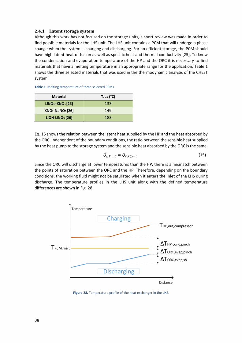
Eq. 15 shows the relation between the latent heat supplied by the HP and the heat absorbed by

the ORC. Independent of the boundary conditions, the ratio between the sensible heat supplied

by the heat pump to the storage system and the sensible heat absorbed by the ORC is the same.

�̇�𝐻𝑃,𝑙𝑎𝑡 = �̇�𝑂𝑅𝐶,𝑙𝑎𝑡 (15)

Since the ORC will discharge at lower temperatures than the HP, there is a mismatch between

the points of saturation between the ORC and the HP. Therefore, depending on the boundary

conditions, the working fluid might not be saturated when it enters the inlet of the LHS during

discharge. The temperature profiles in the LHS unit along with the defined temperature

differences are shown in Fig. 28.

Figure 28. Temperature profile of the heat exchanger in the LHS.

ΔTORC,evap,sh

ΔTHP,cond,pinch

ΔTORC,evap,pinch

THP,out,compressor

TPCM,melt

Charging

Discharging

Temperature

Distance

39

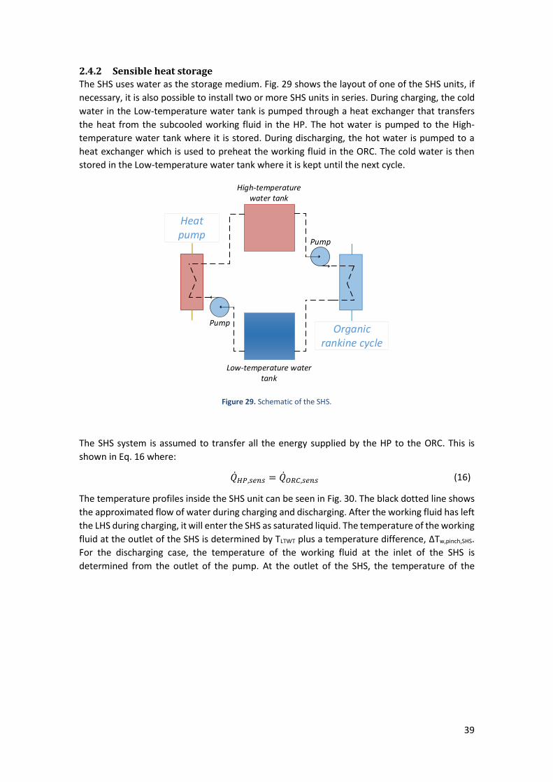
2.4.2 Sensible heat storage

The SHS uses water as the storage medium. Fig. 29 shows the layout of one of the SHS units, if

necessary, it is also possible to install two or more SHS units in series. During charging, the cold

water in the Low-temperature water tank is pumped through a heat exchanger that transfers

the heat from the subcooled working fluid in the HP. The hot water is pumped to the High-

temperature water tank where it is stored. During discharging, the hot water is pumped to a

heat exchanger which is used to preheat the working fluid in the ORC. The cold water is then

stored in the Low-temperature water tank where it is kept until the next cycle.

Figure 29. Schematic of the SHS.

The SHS system is assumed to transfer all the energy supplied by the HP to the ORC. This is

shown in Eq. 16 where:

�̇�𝐻𝑃,𝑠𝑒𝑛𝑠 = �̇�𝑂𝑅𝐶,𝑠𝑒𝑛𝑠 (16)

The temperature profiles inside the SHS unit can be seen in Fig. 30. The black dotted line shows

the approximated flow of water during charging and discharging. After the working fluid has left

the LHS during charging, it will enter the SHS as saturated liquid. The temperature of the working

fluid at the outlet of the SHS is determined by TLTWT plus a temperature difference, ΔTw,pinch,SHS.

For the discharging case, the temperature of the working fluid at the inlet of the SHS is

determined from the outlet of the pump. At the outlet of the SHS, the temperature of the

High-temperature water tank

Organic rankine cycle

Heat pump

Low-temperature water tank

Pump

Pump

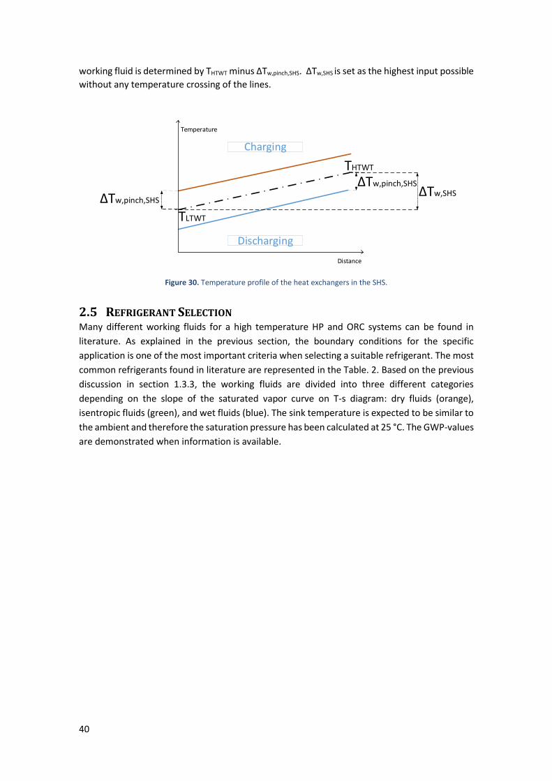
40

working fluid is determined by THTWT minus ΔTw,pinch,SHS. ΔTw,SHS is set as the highest input possible

without any temperature crossing of the lines.

Figure 30. Temperature profile of the heat exchangers in the SHS.

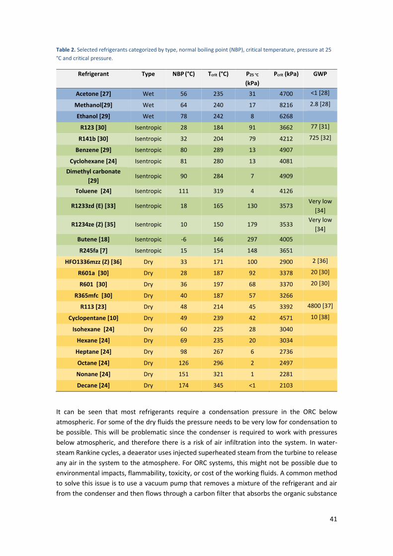
2.5 REFRIGERANT SELECTION Many different working fluids for a high temperature HP and ORC systems can be found in

literature. As explained in the previous section, the boundary conditions for the specific

application is one of the most important criteria when selecting a suitable refrigerant. The most

common refrigerants found in literature are represented in the Table. 2. Based on the previous

discussion in section 1.3.3, the working fluids are divided into three different categories

depending on the slope of the saturated vapor curve on T-s diagram: dry fluids (orange),

isentropic fluids (green), and wet fluids (blue). The sink temperature is expected to be similar to

the ambient and therefore the saturation pressure has been calculated at 25 °C. The GWP-values

are demonstrated when information is available.

ΔTw,SHSΔTw,pinch,SHS

THTWT

Charging

Discharging

Temperature

Distance

ΔTw,pinch,SHS

TLTWT

41

Table 2. Selected refrigerants categorized by type, normal boiling point (NBP), critical temperature, pressure at 25

°C and critical pressure.

Refrigerant Type NBP (°C) Tcrit (°C) P25 °C

(kPa)

Pcrit (kPa) GWP

Acetone [27] Wet 56 235 31 4700 <1 [28]

Methanol[29] Wet 64 240 17 8216 2.8 [28]

Ethanol [29] Wet 78 242 8 6268

R123 [30] Isentropic 28 184 91 3662 77 [31]

R141b [30] Isentropic 32 204 79 4212 725 [32]

Benzene [29] Isentropic 80 289 13 4907

Cyclohexane [24] Isentropic 81 280 13 4081

Dimethyl carbonate

[29] Isentropic 90 284 7 4909

Toluene [24] Isentropic 111 319 4 4126

R1233zd (E) [33] Isentropic 18 165 130 3573 Very low

[34]

R1234ze (Z) [35] Isentropic 10 150 179 3533 Very low

[34]

Butene [18] Isentropic -6 146 297 4005

R245fa [7] Isentropic 15 154 148 3651

HFO1336mzz (Z) [36] Dry 33 171 100 2900 2 [36]

R601a [30] Dry 28 187 92 3378 20 [30]

R601 [30] Dry 36 197 68 3370 20 [30]

R365mfc [30] Dry 40 187 57 3266

R113 [23] Dry 48 214 45 3392 4800 [37]

Cyclopentane [10] Dry 49 239 42 4571 10 [38]

Isohexane [24] Dry 60 225 28 3040

Hexane [24] Dry 69 235 20 3034

Heptane [24] Dry 98 267 6 2736

Octane [24] Dry 126 296 2 2497

Nonane [24] Dry 151 321 1 2281

Decane [24] Dry 174 345 <1 2103

It can be seen that most refrigerants require a condensation pressure in the ORC below

atmospheric. For some of the dry fluids the pressure needs to be very low for condensation to

be possible. This will be problematic since the condenser is required to work with pressures

below atmospheric, and therefore there is a risk of air infiltration into the system. In water-

steam Rankine cycles, a deaerator uses injected superheated steam from the turbine to release

any air in the system to the atmosphere. For ORC systems, this might not be possible due to

environmental impacts, flammability, toxicity, or cost of the working fluids. A common method

to solve this issue is to use a vacuum pump that removes a mixture of the refrigerant and air

from the condenser and then flows through a carbon filter that absorbs the organic substance

42

[39]. Consequently, for condensation temperatures of 25 °C or lower a vacuum pump will have

to be introduced to the system in order to remove possible air infiltration.

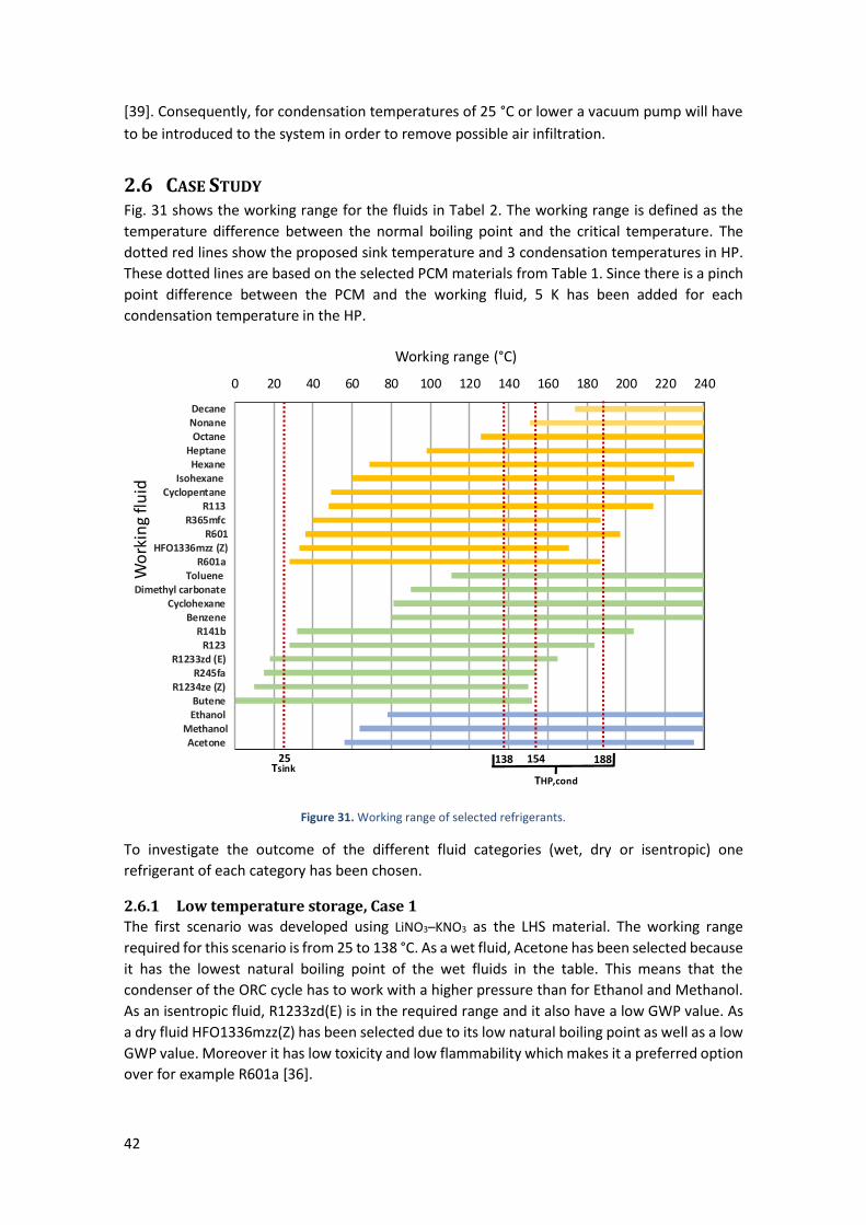
2.6 CASE STUDY Fig. 31 shows the working range for the fluids in Tabel 2. The working range is defined as the

temperature difference between the normal boiling point and the critical temperature. The

dotted red lines show the proposed sink temperature and 3 condensation temperatures in HP.

These dotted lines are based on the selected PCM materials from Table 1. Since there is a pinch

point difference between the PCM and the working fluid, 5 K has been added for each

condensation temperature in the HP.

Figure 31. Working range of selected refrigerants.

To investigate the outcome of the different fluid categories (wet, dry or isentropic) one

refrigerant of each category has been chosen.

2.6.1 Low temperature storage, Case 1

The first scenario was developed using LiNO3–KNO3 as the LHS material. The working range

required for this scenario is from 25 to 138 °C. As a wet fluid, Acetone has been selected because

it has the lowest natural boiling point of the wet fluids in the table. This means that the

condenser of the ORC cycle has to work with a higher pressure than for Ethanol and Methanol.

As an isentropic fluid, R1233zd(E) is in the required range and it also have a low GWP value. As

a dry fluid HFO1336mzz(Z) has been selected due to its low natural boiling point as well as a low

GWP value. Moreover it has low toxicity and low flammability which makes it a preferred option

over for example R601a [36].

0 20 40 60 80 100 120 140 160 180 200 220 240

AcetoneMethanol

EthanolButene

R1234ze (Z)R245fa

R1233zd (E)R123

R141bBenzene

CyclohexaneDimethyl carbonate

TolueneR601a

HFO1336mzz (Z)R601

R365mfcR113

CyclopentaneIsohexane

HexaneHeptane

OctaneNonaneDecane

Wo

rkin

g fl

uid

Working range (°C)

188138 15425

THP,condTsink

43

2.6.2 Medium temperature storage, Case 2

The working range required for this scenario is from 25 to 154 °C. The same refrigerants have

been chosen for this scenario as for the low temperature storage.

2.6.3 High temperature storage, Case 3 The working range required for this scenario is from 25 to 188 °C. For the high temperature

storage, Acetone has been selected as the wet fluid. R141b has a natural boiling point that is

close to the sink temperature and it has a critical temperature above 188 °C. It is in fact the only

isentropic refrigerant which has a natural boiling point close to the sink while it still has a

sufficiently high critical temperature. Unfortunately, it has a high GWP value and therefore the

system designer needs take measures in order to prevent leaking. With these considerations

taken into account, it was chosen as best the isentropic fluid for the high temperature storage.

As Cyclopentane is a common fluid to use in ORC system and has a neglectable GWP it was

chosen as the dry fluid. A flammable, low GWP fluid has a natural boiling point that is higher

than the sink temperature.

2.7 SIMULATING SOFTWARE Engineering Equation Solver (EES) has been used to develop the proposed model for the CHEST

system and to run the simulations and parametric studies. This program has been chosen

because it allows for simple programing, direct access to the thermal properties of a vast amount

of working fluids, and detailed output results and figures.

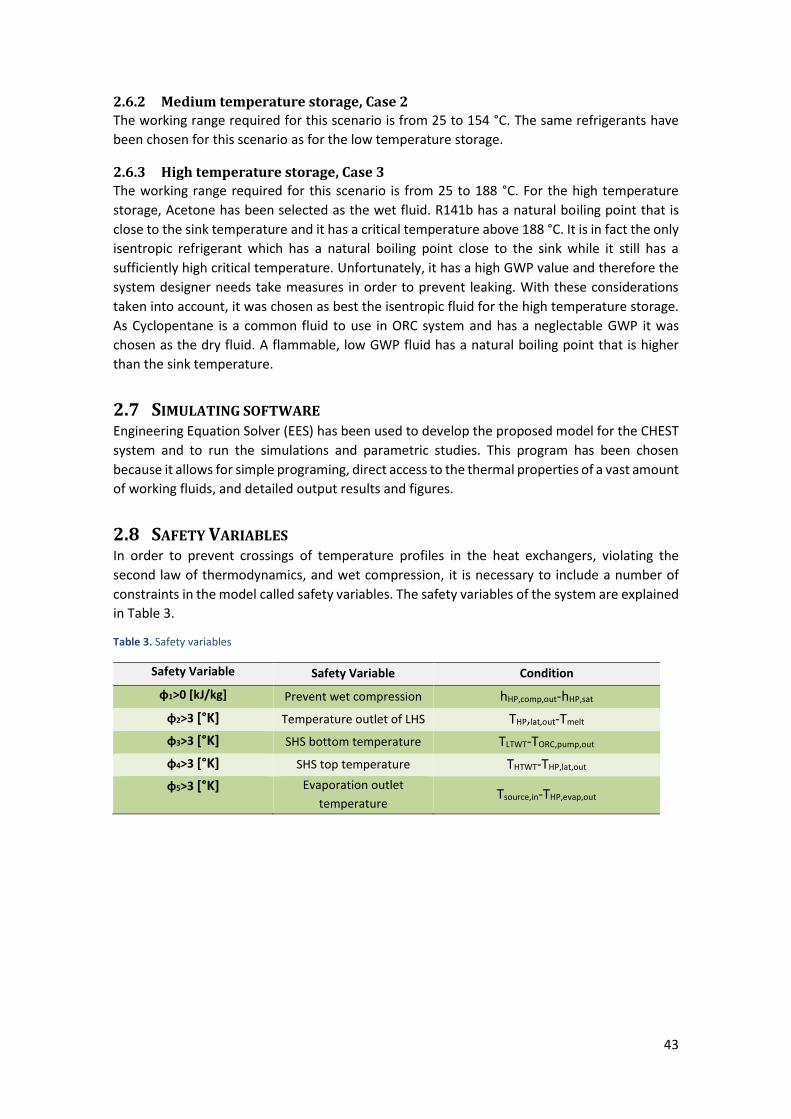
2.8 SAFETY VARIABLES In order to prevent crossings of temperature profiles in the heat exchangers, violating the

second law of thermodynamics, and wet compression, it is necessary to include a number of

constraints in the model called safety variables. The safety variables of the system are explained

in Table 3.

Table 3. Safety variables

Safety Variable Safety Variable Condition

ɸ1>0 [kJ/kg] Prevent wet compression hHP,comp,out-hHP,sat

ɸ2>3 [°K] Temperature outlet of LHS THP,lat,out-Tmelt

ɸ3>3 [°K] SHS bottom temperature TLTWT-TORC,pump,out

ɸ4>3 [°K] SHS top temperature THTWT-THP,lat,out

ɸ5>3 [°K] Evaporation outlet

temperature Tsource,in-THP,evap,out

44

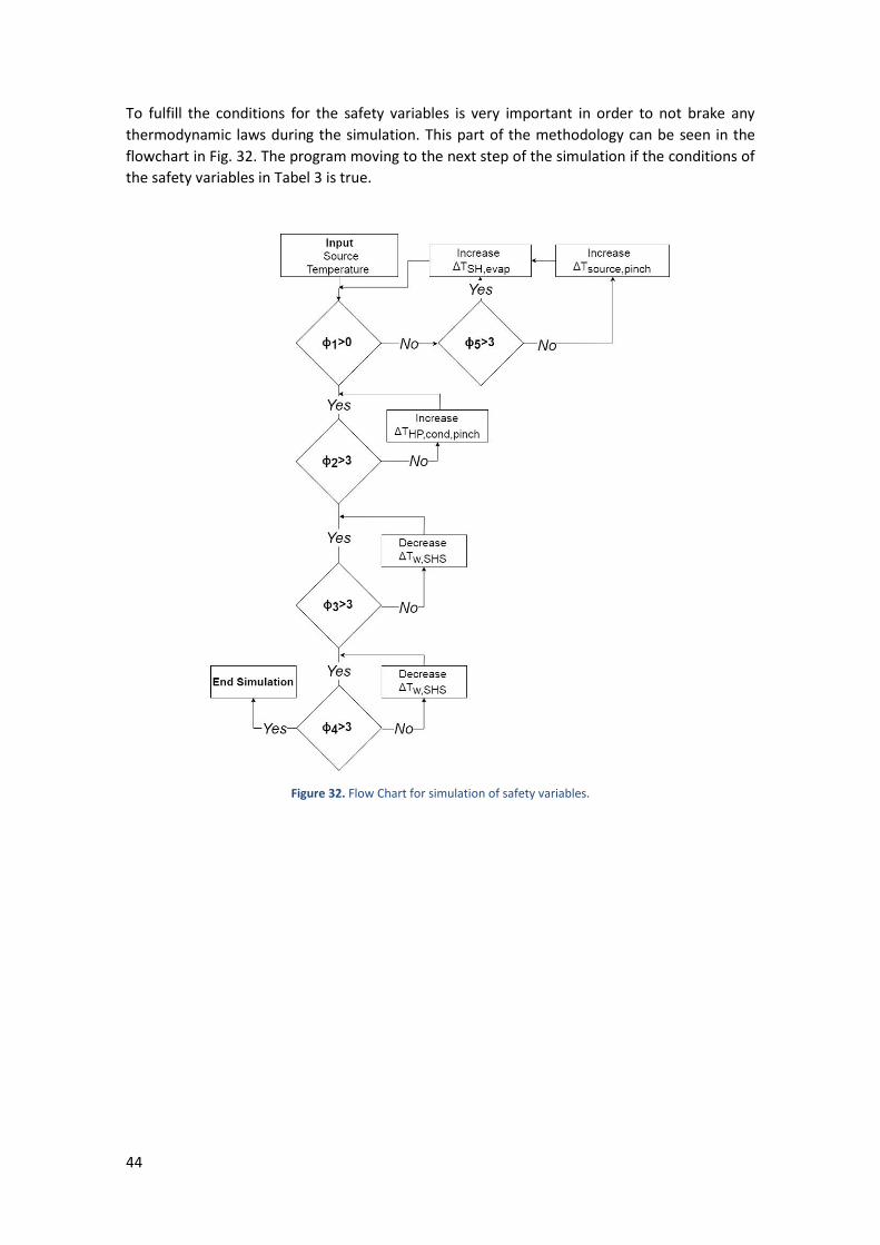
To fulfill the conditions for the safety variables is very important in order to not brake any

thermodynamic laws during the simulation. This part of the methodology can be seen in the

flowchart in Fig. 32. The program moving to the next step of the simulation if the conditions of

the safety variables in Tabel 3 is true.

Figure 32. Flow Chart for simulation of safety variables.

45

3. RESULTS AND DISCUSSION

3.1 CASE STUDY BASED ON PCM MELTING TEMPERATURE The first part of the results section will include the simulations of the CHEST system for three

cases regarding the PCM melting temperatures in Table 1 and suggested refrigerants for each

case. The HP has been selected to use one stage compression for all the refrigerants except for

Acetone where two-stage compression are included in the analysis. In the initial analysis, the

ORC has been set to be a simple cycle without recuperation or regeneration. The performance

indicators explained in the methodology have been calculated by varying the source

temperature from 40 to 100 °C. The sink temperature is kept constant as 25 °C. The pressure

drop is kept constant at 5% for all heat exchanger and the pinch point temperatures are kept at

3 K.

In the second part of the results a more detailed analysis is done using the R1233zd(E) as working

fluid in the system, in order to evaluate the impacts of pressure drop variation in the heat

exchangers, pinch points variation, recuperation and regeneration processes on the whole

CHEST system performance.

3.1.1 Case 1 (Tmelt=133 °C)

The selected refrigaerants that is used for comparison in this case is Acetone, R1233zd(E) and

HFO1336mzz(Z).

a) Cycle simulation on T-s diagram

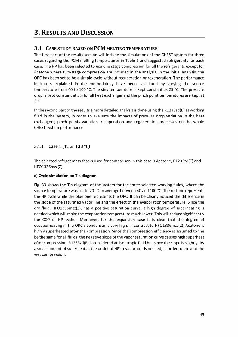
Fig. 33 shows the T-s diagram of the system for the three selected working fluids, where the

source temperature was set to 70 °C an average between 40 and 100 °C. The red line represents

the HP cycle while the blue one represents the ORC. It can be clearly noticed the difference in

the slope of the saturated vapor line and the effect of the evaporation temperature. Since the

dry fluid, HFO1336mzz(Z), has a positive saturation curve, a high degree of superheating is

needed which will make the evaporation temperature much lower. This will reduce significantly

the COP of HP cycle. Moreover, for the expansion case it is clear that the degree of

desuperheating in the ORC’s condenser is very high. In contrast to HFO1336mzz(Z), Acetone is

highly superheated after the compression. Since the compression efficiency is assumed to the

be the same for all fluids, the negative slope of the vapor saturation curve causes high superheat

after compression. R1233zd(E) is considered an isentropic fluid but since the slope is slightly dry

a small amount of superheat at the outlet of HP’s evaporator is needed, in order to prevent the

wet compression.

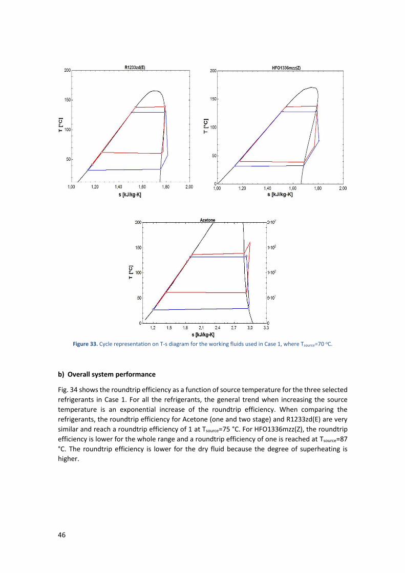
46

Figure 33. Cycle representation on T-s diagram for the working fluids used in Case 1, where Tsource=70 oC.

b) Overall system performance

Fig. 34 shows the roundtrip efficiency as a function of source temperature for the three selected

refrigerants in Case 1. For all the refrigerants, the general trend when increasing the source

temperature is an exponential increase of the roundtrip efficiency. When comparing the

refrigerants, the roundtrip efficiency for Acetone (one and two stage) and R1233zd(E) are very

similar and reach a roundtrip efficiency of 1 at Tsource=75 °C. For HFO1336mzz(Z), the roundtrip

efficiency is lower for the whole range and a roundtrip efficiency of one is reached at Tsource=87

°C. The roundtrip efficiency is lower for the dry fluid because the degree of superheating is

higher.

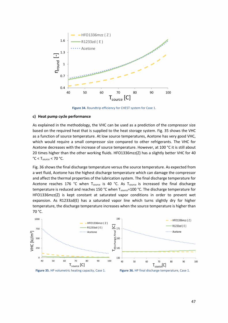
47

Figure 34. Roundtrip efficiency for CHEST system for Case 1.

c) Heat pump cycle performance

As explained in the methodology, the VHC can be used as a prediction of the compressor size

based on the required heat that is supplied to the heat storage system. Fig. 35 shows the VHC

as a function of source temperature. At low source temperatures, Acetone has very good VHC,

which would require a small compressor size compared to other refrigerants. The VHC for

Acetone decreases with the increase of source temperature. However, at 100 °C it is still about

20 times higher than the other working fluids. HFO1336mzz(Z) has a slightly better VHC for 40

°C < Tsource < 70 °C.

Fig. 36 shows the final discharge temperature versus the source temperature. As expected from

a wet fluid, Acetone has the highest discharge temperature which can damage the compressor

and affect the thermal properties of the lubrication system. The final discharge temperature for

Acetone reaches 176 °C when Tsource is 40 °C. As Tsource is increased the final discharge

temperature is reduced and reaches 150 °C when Tsource=100 °C. The discharge temperature for

HFO1336mzz(Z) is kept constant at saturated vapor conditions in order to prevent wet

expansion. As R1233zd(E) has a saturated vapor line which turns slightly dry for higher

temperature, the discharge temperature increases when the source temperature is higher than

70 °C.

Figure 35. HP volumetric heating capacity, Case 1.

Figure 36. HP final discharge temperature, Case 1.

0.4

0.7

1

1.3

1.6

40 50 60 70 80 90 100

ηro

un

d[-

]

Tsource [C]

HFO1336mzz ( Z )

R1233zd ( E )

Acetone

0

250

500

750

1000

40 50 60 70 80 90 100

VH

C [k

J/m

3 ]

HFO1336mzz ( Z )

R1233zd ( E )

Acetone

Tsource [C]

130

145

160

175

190

40 50 60 70 80 90 100

Td

isch

arg

e,f

ina

l[C

]

HFO1336mzz ( Z )

R1233zd ( E )

Acetone

Tsource[C]

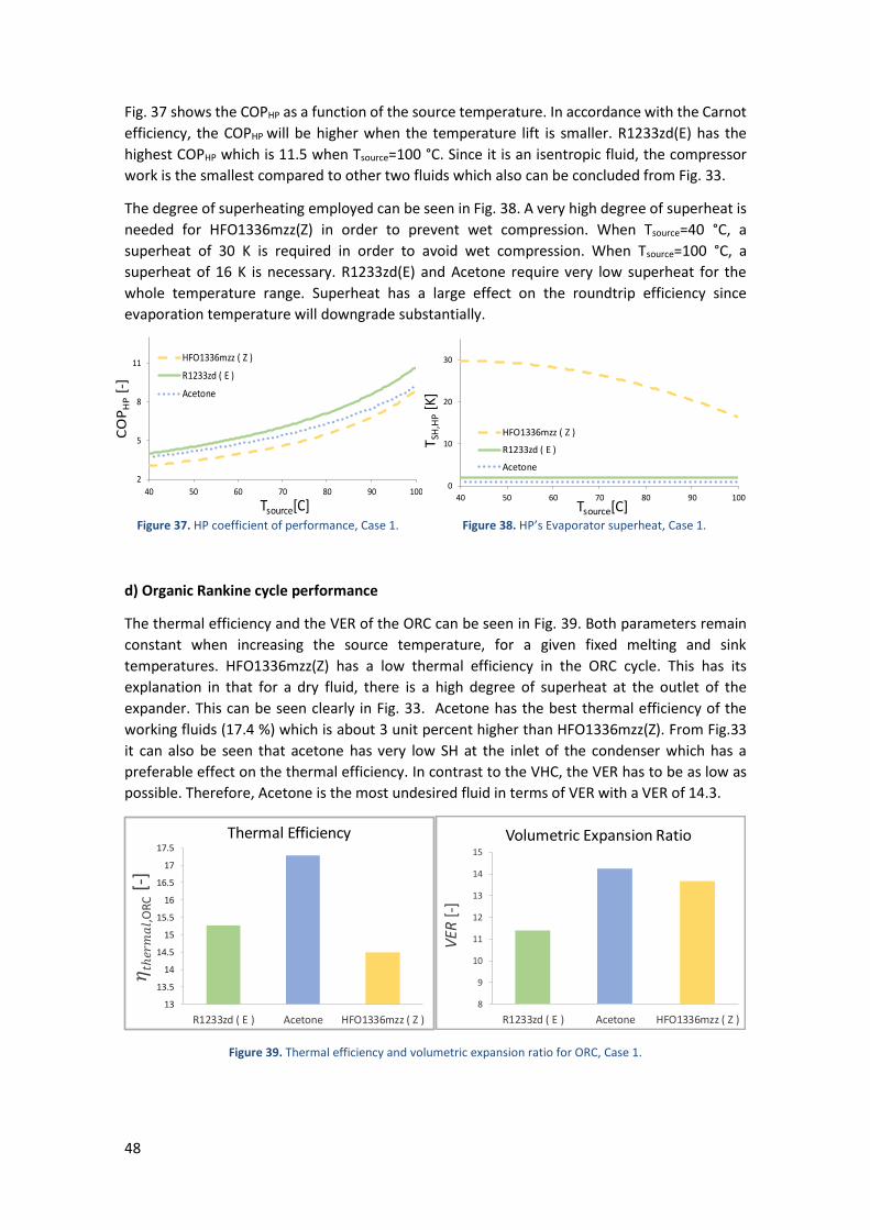
48

Fig. 37 shows the COPHP as a function of the source temperature. In accordance with the Carnot

efficiency, the COPHP will be higher when the temperature lift is smaller. R1233zd(E) has the

highest COPHP which is 11.5 when Tsource=100 °C. Since it is an isentropic fluid, the compressor

work is the smallest compared to other two fluids which also can be concluded from Fig. 33.

The degree of superheating employed can be seen in Fig. 38. A very high degree of superheat is

needed for HFO1336mzz(Z) in order to prevent wet compression. When Tsource=40 °C, a

superheat of 30 K is required in order to avoid wet compression. When Tsource=100 °C, a

superheat of 16 K is necessary. R1233zd(E) and Acetone require very low superheat for the

whole temperature range. Superheat has a large effect on the roundtrip efficiency since

evaporation temperature will downgrade substantially.

Figure 37. HP coefficient of performance, Case 1.

Figure 38. HP’s Evaporator superheat, Case 1.

d) Organic Rankine cycle performance

The thermal efficiency and the VER of the ORC can be seen in Fig. 39. Both parameters remain

constant when increasing the source temperature, for a given fixed melting and sink

temperatures. HFO1336mzz(Z) has a low thermal efficiency in the ORC cycle. This has its

explanation in that for a dry fluid, there is a high degree of superheat at the outlet of the

expander. This can be seen clearly in Fig. 33. Acetone has the best thermal efficiency of the

working fluids (17.4 %) which is about 3 unit percent higher than HFO1336mzz(Z). From Fig.33

it can also be seen that acetone has very low SH at the inlet of the condenser which has a

preferable effect on the thermal efficiency. In contrast to the VHC, the VER has to be as low as

possible. Therefore, Acetone is the most undesired fluid in terms of VER with a VER of 14.3.

Figure 39. Thermal efficiency and volumetric expansion ratio for ORC, Case 1.

2

5

8

11

40 50 60 70 80 90 100

CO

PH

P[-

]

Tsource[C]

HFO1336mzz ( Z )

R1233zd ( E )

Acetone

0

10

20

30

40 50 60 70 80 90 100

TSH

,HP

[K]

Tsource[C]

HFO1336mzz ( Z )

R1233zd ( E )

Acetone

13

13.5

14

14.5

15

15.5

16

16.5

17

17.5

R1233zd ( E ) Acetone HFO1336mzz ( Z )

ℎ ,

OR

C[-

]

Thermal Efficiency

8

9

10

11

12

13

14

15


VER

[-]

Volumetric Expansion Ratio

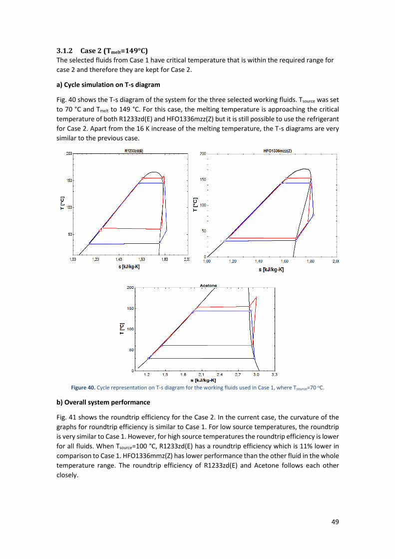
49

3.1.2 Case 2 (Tmelt=149°C)

The selected fluids from Case 1 have critical temperature that is within the required range for

case 2 and therefore they are kept for Case 2.


Fig. 40 shows the T-s diagram of the system for the three selected working fluids. Tsource was set

to 70 °C and Tmelt to 149 °C. For this case, the melting temperature is approaching the critical

temperature of both R1233zd(E) and HFO1336mzz(Z) but it is still possible to use the refrigerant

for Case 2. Apart from the 16 K increase of the melting temperature, the T-s diagrams are very

similar to the previous case.

Figure 40. Cycle representation on T-s diagram for the working fluids used in Case 1, where Tsource=70 oC.


Fig. 41 shows the roundtrip efficiency for the Case 2. In the current case, the curvature of the

graphs for roundtrip efficiency is similar to Case 1. For low source temperatures, the roundtrip

is very similar to Case 1. However, for high source temperatures the roundtrip efficiency is lower

for all fluids. When Tsource=100 °C, R1233zd(E) has a roundtrip efficiency which is 11% lower in

comparison to Case 1. HFO1336mmz(Z) has lower performance than the other fluid in the whole

temperature range. The roundtrip efficiency of R1233zd(E) and Acetone follows each other

closely.

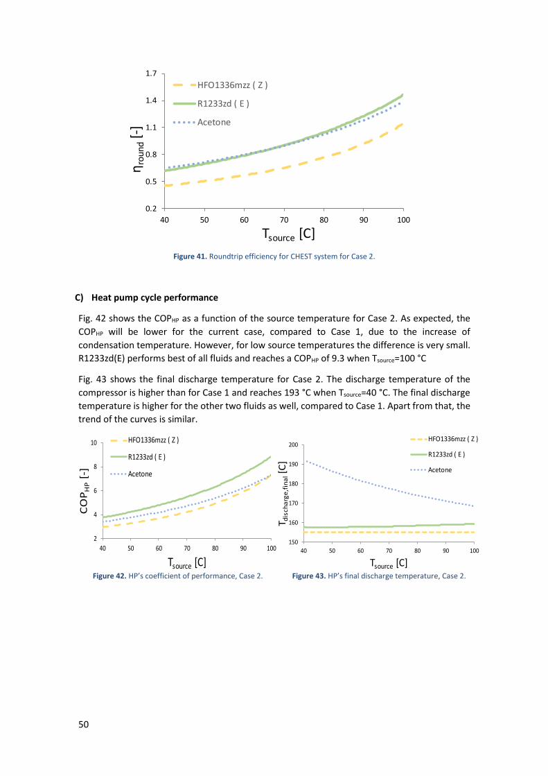
50


C) Heat pump cycle performance

Fig. 42 shows the COPHP as a function of the source temperature for Case 2. As expected, the

COPHP will be lower for the current case, compared to Case 1, due to the increase of

condensation temperature. However, for low source temperatures the difference is very small.

R1233zd(E) performs best of all fluids and reaches a COPHP of 9.3 when Tsource=100 °C

Fig. 43 shows the final discharge temperature for Case 2. The discharge temperature of the

compressor is higher than for Case 1 and reaches 193 °C when Tsource=40 °C. The final discharge

temperature is higher for the other two fluids as well, compared to Case 1. Apart from that, the

trend of the curves is similar.

Figure 42. HP’s coefficient of performance, Case 2.

Figure 43. HP’s final discharge temperature, Case 2.

0.2

0.5

0.8

1.1

1.4

1.7

40 50 60 70 80 90 100

ηro

un

d [-

]

Tsource [C]

HFO1336mzz ( Z )

R1233zd ( E )

Acetone

2

4

6

8

10

40 50 60 70 80 90 100

CO

PH

P[-

]

Tsource [C]

HFO1336mzz ( Z )

R1233zd ( E )

Acetone

150

160

170

180

190

200

40 50 60 70 80 90 100

T dis

cha

rge

,fin

al[C

]

Tsource [C]

HFO1336mzz ( Z )

R1233zd ( E )

Acetone

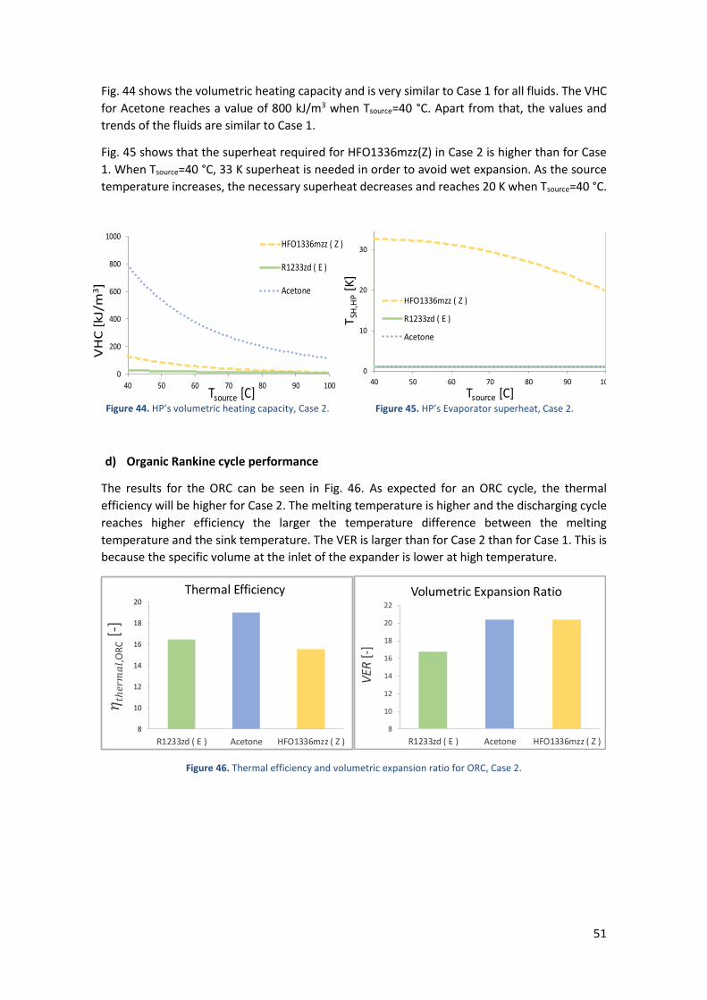
51

Fig. 44 shows the volumetric heating capacity and is very similar to Case 1 for all fluids. The VHC

for Acetone reaches a value of 800 kJ/m3 when Tsource=40 °C. Apart from that, the values and

trends of the fluids are similar to Case 1.

Fig. 45 shows that the superheat required for HFO1336mzz(Z) in Case 2 is higher than for Case

1. When Tsource=40 °C, 33 K superheat is needed in order to avoid wet expansion. As the source

temperature increases, the necessary superheat decreases and reaches 20 K when Tsource=40 °C.

Figure 44. HP’s volumetric heating capacity, Case 2.



The results for the ORC can be seen in Fig. 46. As expected for an ORC cycle, the thermal

efficiency will be higher for Case 2. The melting temperature is higher and the discharging cycle

reaches higher efficiency the larger the temperature difference between the melting

temperature and the sink temperature. The VER is larger than for Case 2 than for Case 1. This is

because the specific volume at the inlet of the expander is lower at high temperature.


0

200

400

600

800

1000

40 50 60 70 80 90 100

VH

C [

kJ/

m3]

Tsource [C]

HFO1336mzz ( Z )

R1233zd ( E )

Acetone

0

10

20

30

40 50 60 70 80 90 100

TSH

,HP

[K]

Tsource [C]

HFO1336mzz ( Z )

R1233zd ( E )

Acetone

8

10

12

14

16

18

20


ℎ ,

OR

C[-

]

Thermal Efficiency

8

10

12

14

16

18

20

22


VER

[-]


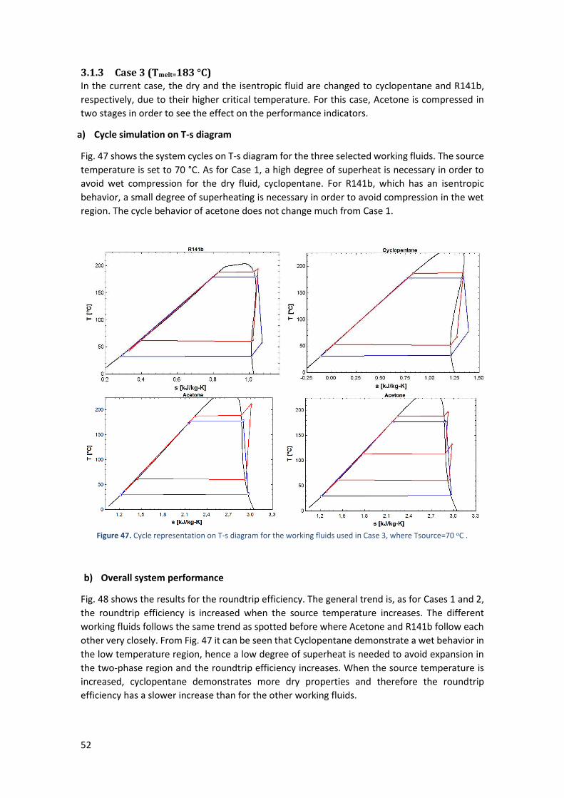
52

3.1.3 Case 3 (Tmelt=183 °C)

In the current case, the dry and the isentropic fluid are changed to cyclopentane and R141b,

respectively, due to their higher critical temperature. For this case, Acetone is compressed in

two stages in order to see the effect on the performance indicators.


Fig. 47 shows the system cycles on T-s diagram for the three selected working fluids. The source

temperature is set to 70 °C. As for Case 1, a high degree of superheat is necessary in order to

avoid wet compression for the dry fluid, cyclopentane. For R141b, which has an isentropic

behavior, a small degree of superheating is necessary in order to avoid compression in the wet

region. The cycle behavior of acetone does not change much from Case 1.

Figure 47. Cycle representation on T-s diagram for the working fluids used in Case 3, where Tsource=70 oC .


Fig. 48 shows the results for the roundtrip efficiency. The general trend is, as for Cases 1 and 2,

the roundtrip efficiency is increased when the source temperature increases. The different

working fluids follows the same trend as spotted before where Acetone and R141b follow each

other very closely. From Fig. 47 it can be seen that Cyclopentane demonstrate a wet behavior in

the low temperature region, hence a low degree of superheat is needed to avoid expansion in

the two-phase region and the roundtrip efficiency increases. When the source temperature is

increased, cyclopentane demonstrates more dry properties and therefore the roundtrip

efficiency has a slower increase than for the other working fluids.

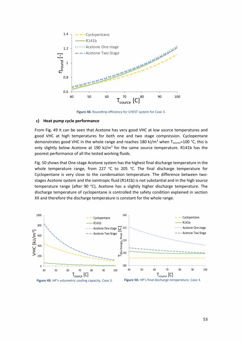
53


c) Heat pump cycle performance

From Fig. 49 it can be seen that Acetone has very good VHC at low source temperatures and

good VHC at high temperatures for both one and two stage compression. Cyclopentane

demonstrates good VHC in the whole range and reaches 180 kJ/m3 when Tsource=100 °C, this is

only slightly below Acetone at 190 kJ/m3 for the same source temperature. R141b has the

poorest performance of all the tested working fluids.

Fig. 50 shows that One-stage Acetone system has the highest final discharge temperature in the

whole temperature range, from 227 oC to 205 oC. The final discharge temperature for

Cyclopentane is very close to the condensation temperature. The difference between two-

stages Acetone system and the isentropic fluid (R141b) is not substantial and in the high source

temperature range (after 90 oC), Acetone has a slightly higher discharge temperature. The

discharge temperature of cyclopentane is controlled the safety condition explained in section

XX and therefore the discharge temperature is constant for the whole range.

Figure 49. HP’s volumetric cooling capacity, Case 3.

Figure 50. HP’s final discharge temperature, Case 3.

0.6

0.8

1

1.2

1.4

40 50 60 70 80 90 100

ηro

und

[-]

Tsource [C]

Cyclopentane

R141b

Acetone One stage

Acetone Two Stage

0

200

400

600

800

1000

40 50 60 70 80 90 100

VH

C [

kJ/

m3]

Tsource [C]

Cyclopentane

R141b

Acetone One stage

Acetone Two Stage

180

195

210

225

240

40 50 60 70 80 90 100

T dis

ch

arg

e, fi

na

l[C

]

Tsource [C]

Cyclopentane

R141b

Acetone One stage

Acetone Two Stage

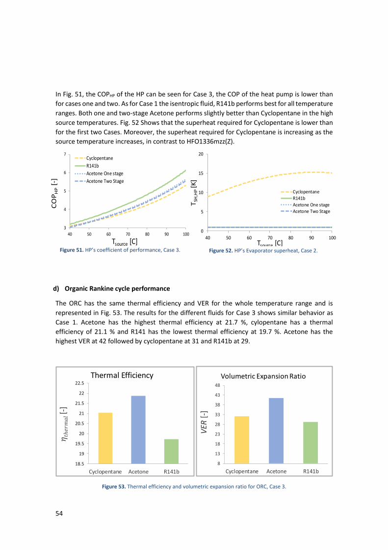
54

In Fig. 51, the COPHP of the HP can be seen for Case 3, the COP of the heat pump is lower than

for cases one and two. As for Case 1 the isentropic fluid, R141b performs best for all temperature

ranges. Both one and two-stage Acetone performs slightly better than Cyclopentane in the high

source temperatures. Fig. 52 Shows that the superheat required for Cyclopentane is lower than

for the first two Cases. Moreover, the superheat required for Cyclopentane is increasing as the

source temperature increases, in contrast to HFO1336mzz(Z).

Figure 51. HP’s coefficient of performance, Case 3.



The ORC has the same thermal efficiency and VER for the whole temperature range and is

represented in Fig. 53. The results for the different fluids for Case 3 shows similar behavior as

Case 1. Acetone has the highest thermal efficiency at 21.7 %, cylopentane has a thermal

efficiency of 21.1 % and R141 has the lowest thermal efficiency at 19.7 %. Acetone has the

highest VER at 42 followed by cyclopentane at 31 and R141b at 29.


3

4

5

6

7

40 50 60 70 80 90 100

CO

PH

P[-

]

Tsource [C]

Cyclopentane

R141b

Acetone One stage

Acetone Two Stage

0

5

10

15

20

40 50 60 70 80 90 100

TSH

,HP

[K]

Tsource [C]

Cyclopentane

R141b

Acetone One stage

Acetone Two Stage

18.5

19

19.5

20

20.5

21

21.5

22

22.5

Cyclopentane Acetone R141b

ℎ [-

]

Thermal Efficiency

8

13

18

23

28

33

38

43

48

Cyclopentane Acetone R141b

VER

[-]


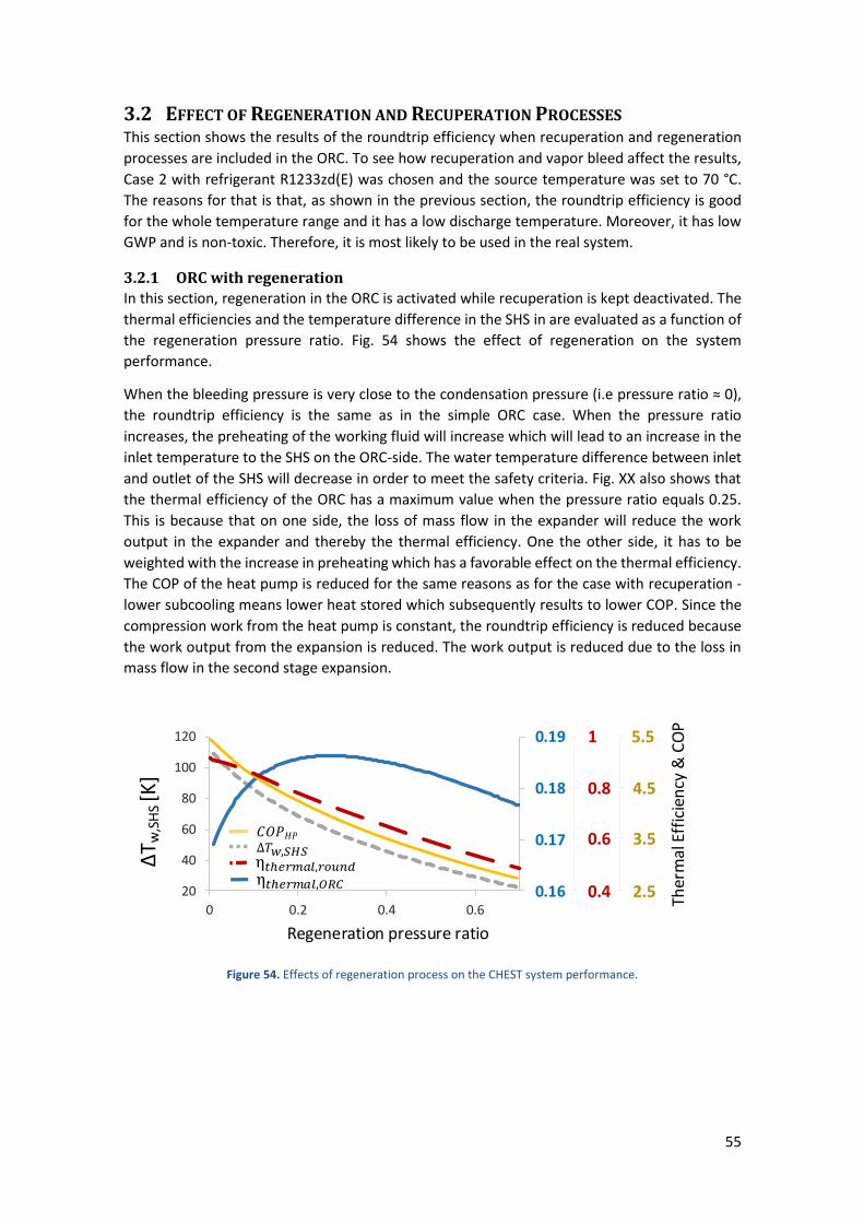
55

3.2 EFFECT OF REGENERATION AND RECUPERATION PROCESSES This section shows the results of the roundtrip efficiency when recuperation and regeneration

processes are included in the ORC. To see how recuperation and vapor bleed affect the results,

Case 2 with refrigerant R1233zd(E) was chosen and the source temperature was set to 70 °C.

The reasons for that is that, as shown in the previous section, the roundtrip efficiency is good

for the whole temperature range and it has a low discharge temperature. Moreover, it has low

GWP and is non-toxic. Therefore, it is most likely to be used in the real system.

3.2.1 ORC with regeneration

In this section, regeneration in the ORC is activated while recuperation is kept deactivated. The

thermal efficiencies and the temperature difference in the SHS in are evaluated as a function of

the regeneration pressure ratio. Fig. 54 shows the effect of regeneration on the system

performance.

When the bleeding pressure is very close to the condensation pressure (i.e pressure ratio ≈ 0),

the roundtrip efficiency is the same as in the simple ORC case. When the pressure ratio

increases, the preheating of the working fluid will increase which will lead to an increase in the

inlet temperature to the SHS on the ORC-side. The water temperature difference between inlet

and outlet of the SHS will decrease in order to meet the safety criteria. Fig. XX also shows that

the thermal efficiency of the ORC has a maximum value when the pressure ratio equals 0.25.

This is because that on one side, the loss of mass flow in the expander will reduce the work

output in the expander and thereby the thermal efficiency. One the other side, it has to be

weighted with the increase in preheating which has a favorable effect on the thermal efficiency.

The COP of the heat pump is reduced for the same reasons as for the case with recuperation -

lower subcooling means lower heat stored which subsequently results to lower COP. Since the

compression work from the heat pump is constant, the roundtrip efficiency is reduced because

the work output from the expansion is reduced. The work output is reduced due to the loss in

mass flow in the second stage expansion.

Figure 54. Effects of regeneration process on the CHEST system performance.

0.16

0.17

0.18

0.19

20

40

60

80

100

120

0 0.2 0.4 0.6

ΔTw

,SH

S

Pressure ratio

Effect of regeneration on cycle efficiency

𝑡ℎ𝑒𝑟𝑚𝑎𝑙,𝑟𝑜𝑢𝑛𝑑 𝑇 ,𝑆𝐻𝑆

𝑡ℎ𝑒𝑟𝑚𝑎𝑙,𝑂𝑅𝐶

𝐶𝑂𝑃𝐻𝑃

1

0.6

0.8

0.4

5.5

3.5

4.5

2.5

Ther

mal

Eff

icie

ncy

& C

OP

ΔT w

,SH

S [K

]

Regeneration pressure ratio




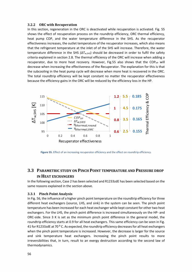
56

3.2.2 ORC with Recuperation

In this section, regeneration in the ORC is deactivated while recuperation is activated. Fig. 55

shows the effect of recuperation process on the roundtrip efficiency, ORC thermal efficiency,

heat pump COP, and the water temperature difference in the SHS. As the recuperator

effectiveness increases, the outlet temperature of the recuperator increases, which also means

that the refrigerant temperature at the inlet of of the SHS will increase. Therefore, the water

temperature difference in the SHS (∆Tw,SHS) should be decreased in order to fulfil the safety

criteria explained in section 2.8. The thermal efficiency of the ORC will increase when adding a

recuperator, due to more heat recovery. However, Fig.55 also shows that the COPHP will

decrease when increasing the effectiveness of the Recuperator. The explanation for this is that

the subcooling in the heat pump cycle will decrease when more heat is recovered in the ORC.

The total roundtrip efficiency will be kept constant no matter the recuperator effectiveness

because the efficiency gains in the ORC will be reduced by the efficiency loss in the HP.

Figure 55. Effect of an increasing recuperator efficiency and the effect on roundtrip efficiency.

3.3 PARAMETRIC STUDY ON PINCH POINT TEMPERATURE AND PRESSURE DROP

IN HEAT EXCHANGERS In the following section, Case 2 has been selected and R1233zdE has been selected based on the

same reasons explained in the section above.

3.3.1 Pinch Point Analysis

In Fig. 56, the influence of a higher pinch point temperature on the roundtrip efficiency for three

different heat exchangers (source, LHS, and sink) in the system can be seen. The pinch point

temperature has been increased for each heat exchanger while kept constant for other two heat

exchangers. For the LHS, the pinch point difference is increased simultaneously on the HP- and

ORC-side. Since 3 K is set as the minimum pinch point difference in the general model, the

roundtrip efficiency starts at 0.9 for all heat exchangers. This same efficiency can be seen in Fig.

41 for R1233zdE at 70 ⁰ C. As expected, the roundtrip efficiency decreases for all heat exchangers

when the pinch point temperature is increased. However, the decrease is larger for the source

and sink temperature heat exchangers. Increasing the pinch point results to more

irreversibilities that, in turn, result to an exergy destruction according to the second law of

thermodynamics.

0.6

0.8

1

1.2

95

100

105

110

115

0 0.2 0.4 0.6 0.8 1

Recuperator effectiveness

5.5

3.5

4.5

2.5

0.185

0.165

0.175

0.155

Ther

mal

Eff

icie

ncy

& C

OP

Recuperator effectiveness

Effect of recuperation on cycle efficiency

ΔT w

,SH

S [K

]




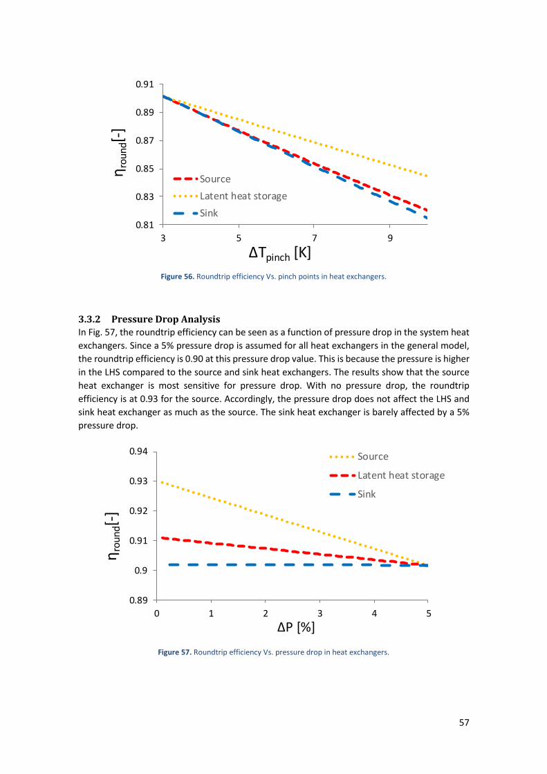
57

Figure 56. Roundtrip efficiency Vs. pinch points in heat exchangers.

3.3.2 Pressure Drop Analysis

In Fig. 57, the roundtrip efficiency can be seen as a function of pressure drop in the system heat

exchangers. Since a 5% pressure drop is assumed for all heat exchangers in the general model,

the roundtrip efficiency is 0.90 at this pressure drop value. This is because the pressure is higher

in the LHS compared to the source and sink heat exchangers. The results show that the source

heat exchanger is most sensitive for pressure drop. With no pressure drop, the roundtrip

efficiency is at 0.93 for the source. Accordingly, the pressure drop does not affect the LHS and

sink heat exchanger as much as the source. The sink heat exchanger is barely affected by a 5%

pressure drop.

Figure 57. Roundtrip efficiency Vs. pressure drop in heat exchangers.

0.81

0.83

0.85

0.87

0.89

0.91

3 5 7 9

ηro

un

d[-

]

∆Tpinch [K]

Source

Latent heat storage

Sink

0.89

0.9

0.91

0.92

0.93

0.94

0 1 2 3 4 5

ηro

un

d[-]

∆P [%]

Source

Latent heat storage

Sink

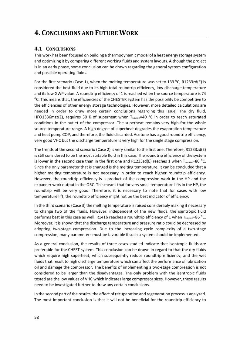
58

4. CONCLUSIONS AND FUTURE WORK

4.1 CONCLUSIONS This work has been focused on building a thermodynamic model of a heat energy storage system

and optimizing it by comparing different working fluids and system layouts. Although the project

is in an early phase, some conclusion can be drawn regarding the general system configuration

and possible operating fluids.

For the first scenario (Case 1), when the melting temperature was set to 133 ⁰C, R1233zd(E) is

considered the best fluid due to its high total roundtrip efficiency, low discharge temperature

and its low GWP value. A roundtrip efficiency of 1 is reached when the source temperature is 74

⁰C. This means that, the efficiencies of the CHESTER system has the possibility be competitive to

the efficiencies of other energy storage technologies. However, more detailed calculations are

needed in order to draw more certain conclusions regarding this issue. The dry fluid,

HFO1336mzz(Z), requires 30 K of superheat when Tsource=40 ⁰C in order to reach saturated

conditions in the outlet of the compressor. The superheat remains very high for the whole

source temperature range. A high degree of superheat degrades the evaporation temperature

and heat pump COP, and therefore, the fluid discarded. Acetone has a good roundtrip efficiency,

very good VHC but the discharge temperature is very high for the single stage compression.

The trends of the second scenario (Case 2) is very similar to the first one. Therefore, R1233zd(E)

is still considered to be the most suitable fluid in this case. The roundtrip efficiency of the system

is lower in the second case than in the first one and R1233zd(E) reaches 1 when Tsource=80 ⁰C.

Since the only parameter that is changed is the melting temperature, it can be concluded that a

higher melting temperature is not necessary in order to reach higher roundtrip efficiency.

However, the roundtrip efficiency is a product of the compression work in the HP and the

expander work output in the ORC. This means that for very small temperature lifts in the HP, the

roundtrip will be very good. Therefore, it is necessary to note that for cases with low

temperature lift, the roundtrip efficiency might not be the best indicator of efficiency.

In the third scenario (Case 3) the melting temperature is raised considerably making it necessary

to change two of the fluids. However, independent of the new fluids, the isentropic fluid

performs best in this case as well. R141b reaches a roundtrip efficiency of 1 when Tsource=86 ⁰C.

Moreover, it is shown that the discharge temperature and pressure ratio could be decreased by

adopting two-stage compression. Due to the increasing cycle complexity of a two-stage

compression, many parameters must be favorable if such a system should be implemented.

As a general conclusion, the results of three cases studied indicate that isentropic fluids are

preferable for the CHEST system. This conclusion can be drawn in regard to that the dry fluids

which require high superheat, which subsequently reduce roundtrip efficiency; and the wet

fluids that result to high discharge temperature which can affect the performance of lubrication

oil and damage the compressor. The benefits of implementing a two-stage compression is not

considered to be larger than the disadvantages. The only problem with the isentropic fluids

tested are the low values of VHC which indicates large compressor sizes. However, these results

need to be investigated further to draw any certain conclusions.

In the second part of the results, the effect of recuperation and regeneration process is analyzed.

The most important conclusion is that it will not be beneficial for the roundtrip efficiency to

59

include regeneration or recuperation process in the CHEST system. This conclusions is valid as

long as most of the subcooled liquid in the HP is used for the SHS and later, to preheat the ORC.

The third part of the results includes the effect of pressure drop and pinch point temperature

on the roundtrip efficiency. As expected, a higher pinch point temperature have a negative

effect on the roundtrip efficiency. The sink and the source heat exchangers has an 11% reduction

of roundtrip efficiency and are most effected by larger pinch point difference. Therefore, the

design and selection of heat exchangers, especially source and sink heat exchangers are crucial

and affect significantly on the overall system performance.

The source if affected most by a pressure drop. Therefore, it can be noticed that especial effort

should be put in the design of the heat exchanger in the source heat exchangers in order to

avoid high pressure drops could have a high impact on the roundtrip efficiency.

4.2 FUTURE WORK This work has focused on the preliminary thermodynamic model of the CHEST system. Much

work remains until the model is ready to be used as a base for a real prototype. A more detailed

of the HP is required in order to size the components. Future work should also include transient

operation. Time has not been included in the calculations so far and it is necessary in order to

evaluate the performance and operation of the thermal storage unit. From an operational point

of view, the best would be to store the heat as long as possible in order to wait for high demand

of electricity or low renewable electricity production.

The heat exchangers also need to be dimensioned and a more detailed mathematical model

should be developed for them, using for example LMTD or ε-NTU method. The compressor and

the expander also need to be sized to obtain performance correlations that can be used to

calculate more realistic values for efficiencies.

60

REFERENCES

[1] “Technology Options,” 2018. [Online]. Available: http://www.esru.strath.ac.uk/EandE/Web_sites/14-15/Industrial_autonomy/2_1_technology_options.html. [Accessed: 06-Mar-2018].

[2] M. Aneke and M. Wang, “Energy storage technologies and real life applications – A state of the art review,” Appl. Energy, vol. 179, pp. 350–377, 2016.

[3] “Compressed Heat Energy Storage for Energy from Renewable sources. Project ID: 764042,” 2018. [Online]. Available: https://cordis.europa.eu/project/rcn/214061_en.html. [Accessed: 05-Jul-2018].

[4] S. Feja, C. Hanzelmann, and S. Zuber, “PT and viscosity measurements of High-Temperature Ammonia Heat Pump Lubricants,” Int. J. Refrig., vol. 88, pp. 221–228, 2018.

[5] E. Granryd, I. Ekroth, P. Lundqvist, A. Melinder, B. Palm, and P. Rohlin, Refrigeration Engineering, 4th ed. Stockholm: Department of Energy Technology, Division of Applied Thermodynamics and Refrigeration, Royal Institute of Technology, KTH, 2003.

[6] Lesson 12 Multi-Stage Vapour Compression Refrigeration Systems, Version 1. IIT Kharagpur.

[7] C. Arpagaus, F. Bless, M. Uhlmann, J. Schiffmann, and S. S. Bertsch, “High temperature heat pumps: Market overview, state of the art, research status, refrigerants, and application potentials,” Energy, vol. 152, 2018.

[8] Group Viking Development, “Viking Heat Engines,” 2018. [Online]. Available: http://www.vikingheatengines.com/heatbooster. [Accessed: 07-May-2018].

[9] M. Chamoun, R. Rulliere, P. Haberschill, and J. L. Peureux, “Experimental and numerical investigations of a new high temperature heat pump for industrial heat recovery using water as refrigerant,” Int. J. Refrig., vol. 44, pp. 177–188, 2014.

[10] B. Vanslambrouck, “Energetical, Technical and Economical considerations by choosing between a Steam and an Organic Rankine Cycle for Small Scale Power Generation,” 2011.

[11] H. Ohman, “Organic Rankine Cycles, Low Temperature Power Cycles,” 2016.

[12] S. Lecompte, H. Huisseune, M. Van Den Broek, B. Vanslambrouck, and M. De Paepe, “Review of organic Rankine cycle (ORC) architectures for waste heat recovery,” Renew. Sustain. Energy Rev., vol. 47, pp. 448–461, 2015.

[13] Z. Li et al., “Comparison study of Trilateral Rankine Cycle, Organic Flash Cycle and basic Organic Rankine Cycle for low grade heat recovery,” Energy Procedia, vol. 142, pp. 1441–1447, 2017.

[14] B. Dong, G. Xu, T. Li, Y. Quan, and J. Wen, “Thermodynamic and economic analysis of zeotropic mixtures as working fluids in low temperature organic Rankine cycles,” Appl. Therm. Eng., vol. 132, pp. 545–553, 2018.

[15] K. Braimakis and S. Karellas, “Energetic optimization of regenerative Organic Rankine Cycle (ORC) configurations,” Energy Convers. Manag., vol. 159, no. September 2017, pp.

61

353–370, 2018.

[16] H. Xi, M. J. Li, C. Xu, and Y. L. He, “Parametric optimization of regenerative organic Rankine cycle (ORC) for low grade waste heat recovery using genetic algorithm,” Energy, vol. 58, pp. 473–482, 2013.

[17] J. Nouman, “Comparative studies and analyses of working fluids for Organic Rankine Cycles - ORC,” 2012.

[18] H. Jockenhöfer, W. D. Steinmann, and D. Bauer, “Detailed numerical investigation of a pumped thermal energy storage with low temperature heat integration,” Energy, vol. 145, pp. 665–676, 2018.

[19] K. H. Kim, “Effects of Superheating on Thermodynamic performance of regenerative organic Rankine cycles,” Eng. Technol., vol. 59, no. 6, pp. 1515–1519, 2011.

[20] A. Groniewsky, G. Györke, and A. R. Imre, “Description of wet-to-dry transition in model ORC working fluids,” Appl. Therm. Eng., vol. 125, pp. 963–971, 2017.

[21] G. Alva, Y. Lin, and G. Fang, “An overview of thermal energy storage systems,” Energy, vol. 144, pp. 341–378, 2018.

[22] W. D. Steinmann, “The CHEST (Compressed Heat Energy STorage) concept for facility scale thermo mechanical energy storage,” Energy, vol. 69, pp. 543–552, 2014.

[23] P. J. Mago, L. M. Chamra, K. Srinivasan, and C. Somayaji, “An examination of regenerative organic Rankine cycles using dry fluids,” Appl. Therm. Eng., vol. 28, no. 8–9, pp. 998–1007, 2008.

[24] R. Rayegan and Y. X. Tao, “A procedure to select working fluids for Solar Organic Rankine Cycles (ORCs),” Renew. Energy, vol. 36, no. 2, pp. 659–670, 2011.

[25] A. Dinker, M. Agarwal, and G. D. Agarwal, “Heat storage materials, geometry and applications: A review,” J. Energy Inst., vol. 90, no. 1, pp. 1–11, 2017.

[26] J. Pereira da Cunha and P. Eames, “Thermal energy storage for low and medium temperature applications using phase change materials - A review,” Appl. Energy, vol. 177, pp. 227–238, 2016.

[27] B. J. Woodland, A. Krishna, E. A. Groll, J. E. Braun, W. T. Horton, and S. V. Garimella, “Thermodynamic comparison of organic Rankine cycles employing liquid-flooded expansion or a solution circuit,” Appl. Therm. Eng., vol. 61, no. 2, pp. 859–865, 2013.

[28] ipcc, “IPCC Fourth Assessment Report: Climate Change 2007,” 2007. [Online]. Available: https://www.ipcc.ch/publications_and_data/ar4/wg1/en/ch2s2-10-3-2.html. [Accessed: 06-Jun-2018].

[29] J. Xu and C. Yu, “Critical temperature criterion for selection of working fluids for subcritical pressure Organic Rankine cycles,” Energy, vol. 74, no. C, pp. 719–733, 2014.

[30] D. Wang, X. Ling, H. Peng, L. Liu, and L. L. Tao, “Efficiency and optimal performance evaluation of organic Rankine cycle for low grade waste heat power generation,” Energy, vol. 50, no. 1, pp. 343–352, 2013.

[31] Linde Group, “R123.” [Online]. Available: http://www.linde-gas.com/en/products_and_supply/refrigerants/hcfc_refrigerants/r123/index.html.

62

[32] L. Daikin Industries, “HCFC-141b,” 2019. [Online]. Available: https://www.daikin.com/chm/products/pdfDown.php?url=pdf/tds/tds_hcfc141b_e.pdf. [Accessed: 05-Jul-2018].

[33] M. Welzl, F. Heberle, and D. Brüggemann, “Simultaneous experimental investigation of nucleate boiling heat transfer and power output in ORC using R245fa and R1233zd(E),” Energy Procedia, vol. 129, pp. 435–442, 2017.

[34] “A year in low GWP refrigerants development,” 2016. [Online]. Available: https://www.kth.se/en/itm/inst/energiteknik/forskning/ett/projekt/koldmedier-med-lag-gwp/low-gwp-news/utvecklingen-pa-koldmediefronten-under-aret-som-gatt-1.636006.

[35] R. Nagata, C. Kondou, and S. Koyama, “Comparative assessment of condensation and pool boiling heat transfer on horizontal plain single tubes for R1234ze(E), R1234ze(Z), and R1233zd(E),” Int. J. Refrig., vol. 63, pp. 157–170, 2016.

[36] “R1336mzz-Z - new generation nonflammable low GWP refrigerant,” 2014. [Online]. Available: https://www.kth.se/en/itm/inst/energiteknik/forskning/ett/projekt/koldmedier-med-lag-gwp/low-gwp-news/r1336mzz-z-ett-nytt-hogtemperaturkoldmedium-med-bra-egenskaper-1.501202. [Accessed: 06-Jun-2018].

[37] “Refrigerants - Environmental Properties.” [Online]. Available: https://www.engineeringtoolbox.com/Refrigerants-Environment-Properties-d_1220.html. [Accessed: 05-Jul-2018].

[38] “Reducing Greenhouse Gas Emissions at GE’s Refrigerator Manufacturing Facilities,” 2011. [Online]. Available: http://pressroom.geappliances.com/news/reducing-greenhouse-gas-emissions-190718. [Accessed: 05-Jul-2018].

[39] E. Macchi and M. Astolfi, Organic Rankine Cycle (ORC) Power Systems Technologies and Applications. Elsevier, 2017.

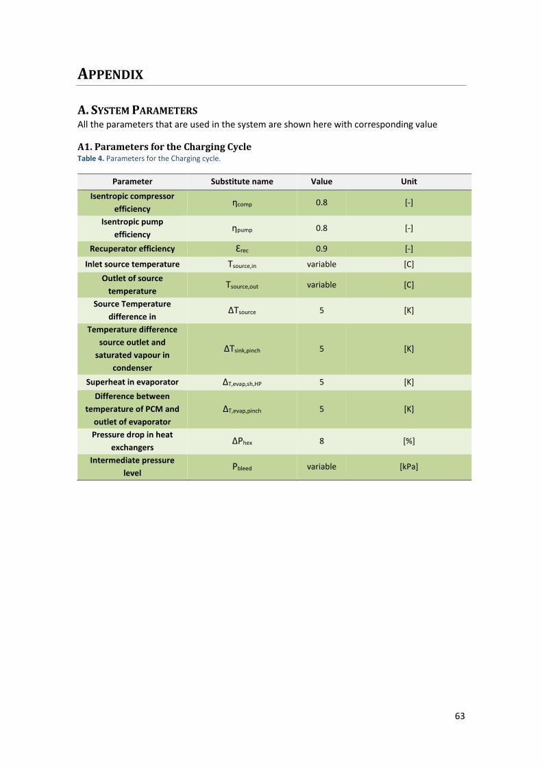
63

APPENDIX

A. SYSTEM PARAMETERS All the parameters that are used in the system are shown here with corresponding value

A1. Parameters for the Charging Cycle Table 4. Parameters for the Charging cycle.

Parameter Substitute name Value Unit

Isentropic compressor

efficiency ηcomp 0.8 [-]

Isentropic pump

efficiency ηpump 0.8 [-]

Recuperator efficiency Ɛrec 0.9 [-]

Inlet source temperature Tsource,in variable [C]

Outlet of source

temperature Tsource,out variable [C]

Source Temperature

difference in ΔTsource 5 [K]

Temperature difference

source outlet and

saturated vapour in

condenser

ΔTsink,pinch 5 [K]

Superheat in evaporator ΔT,evap,sh,HP 5 [K]

Difference between

temperature of PCM and

outlet of evaporator

ΔT,evap,pinch 5 [K]

Pressure drop in heat

exchangers ΔPhex 8 [%]

Intermediate pressure

level Pbleed variable [kPa]

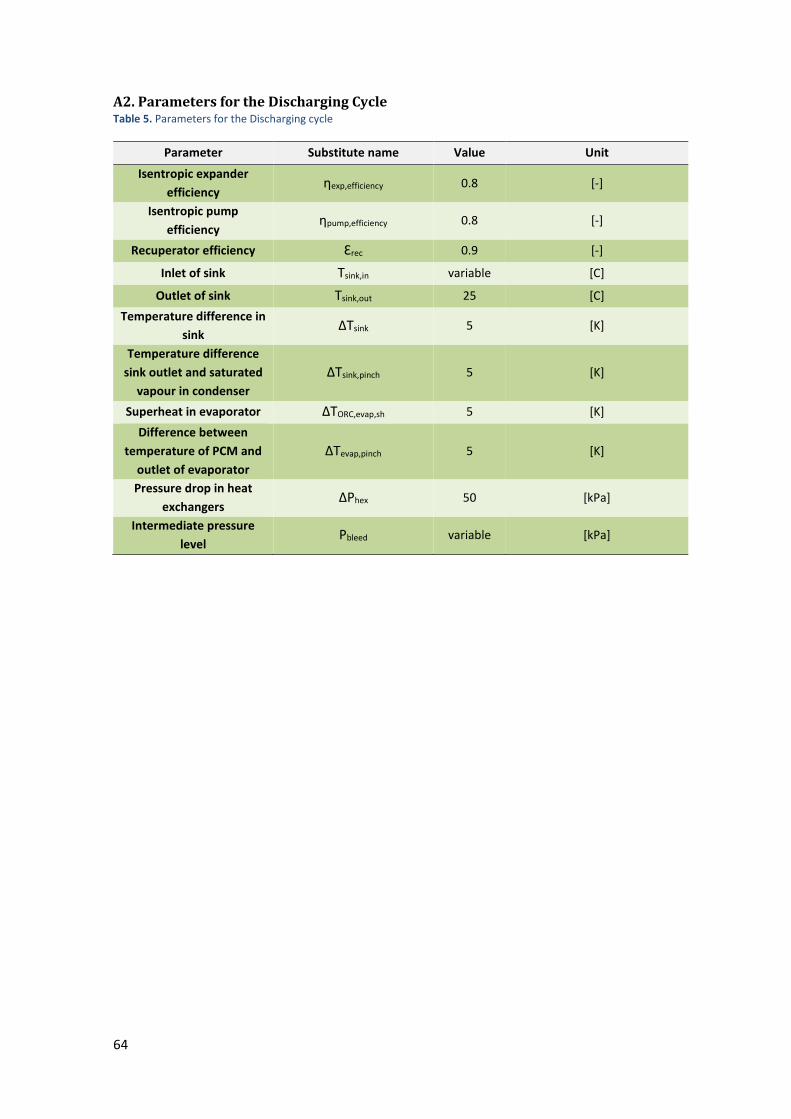
64

A2. Parameters for the Discharging Cycle Table 5. Parameters for the Discharging cycle

Parameter Substitute name Value Unit

Isentropic expander

efficiency ηexp,efficiency 0.8 [-]

Isentropic pump

efficiency ηpump,efficiency 0.8 [-]

Recuperator efficiency Ɛrec 0.9 [-]

Inlet of sink Tsink,in variable [C]

Outlet of sink Tsink,out 25 [C]

Temperature difference in

sink ΔTsink 5 [K]

Temperature difference

sink outlet and saturated

vapour in condenser

ΔTsink,pinch 5 [K]

Superheat in evaporator ΔTORC,evap,sh 5 [K]

Difference between

temperature of PCM and

outlet of evaporator

ΔTevap,pinch 5 [K]

Pressure drop in heat

exchangers ΔPhex 50 [kPa]

Intermediate pressure

level Pbleed variable [kPa]

65

B. EES CODE AND DIAGRAM WINDOW. The diagram window and the EES code used for R1233zd(E) and source temperature of 70 °C.

Are shown in this section. The program can easily be altered to work for all the scenarios

explained in the report.

B1. Diagram window First part of the Diagram Window.

Figure 58. First part of diagram window.

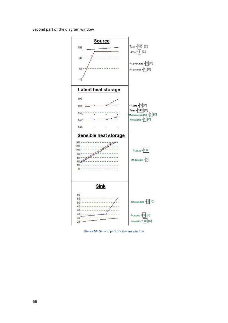
66

Second part of the diagram window

Figure 59. Second part of diagram window

67

B2. EES code { DELTA_T_pinch_evap} { m_comp_1} { eta_isen} {NCSC} { T_w_in} { DELTA_T_w} { DELTA_T_pinch_evap} { DELTA_T_SH_evap} { DELTA_T_cond} { T_melt} { eta_isen_ORC} { epsilon_HEX_ORC} { eta_isen_Pump1_ORC} {eta_isen_Pump1_ORC} { T_w_in} { DELTA_T_bw} { DELTA_T_w_pinch_ORC} {SH=Yes} { m_comp_1} Ref$='R1233zd(E)' "Refrigerant" DELTA_P_evap=P_evap*0,05 "Pressure drop in kPa" DELTA_P_cond=50 "Pressure drop" DELTA_P_evap_ORC=50 "Pressure drop" DELTA_P_cond_ORC=P_cond_ORC*0,05 "Pressure drop in kPa" T_w_out=T_w_in - DELTA_T_w "Temperature of source outlet" T_cond=T_melt+DELTA_T_cond+1 "Condensation temperature, +1 to compensate for pressure drop" P_evap=pressure(Ref$;T=T_evap;x=0) "Evaporating pressure" T_evap=T_w_out-DELTA_T_pinch_evap "Evaporation Temperature" P_cond=p_sat(Ref$;T=T_cond) "Condensation pressure" NSC=NSCS "Number of compression stages" NP=(4*NSC)+2 "Total number of cycle points" Duplicate j=1;NSC Eta_is[j]=Eta_isen "Compressor efficiency" End "Safety Variables for Criteria" Safety_T_bot=T_bot-T_ORC[5] Safety_T_top=T[NSC*2+2]-T_top Safety_Sink=T_ORC[1]-T_in_w_ORC Safety_Melt=T[NSC*2+2]-T_melt Safety_Source=T_w_in-T[1] Safety_two_phase=h[NSC*2]-h[NSC*2+1] Safety_SH_ORC_OUTLET=T_melt-T_ORC[8]

68

x[0]=0 "Imaginary distance in a Heat exchanger" x[1]=1 x[2]=2 x[3]=3 T_draw_w[0]=T_w_out "Temperature profile: Source" T_draw_w[1]=(T_draw_w[0]+T_draw_w[2])/2 T_draw_w[2]=(T_draw_w[1]+T_draw_w[3])/2 T_draw_w[3]=T_w_in T_draw_evap[0]=T[NSC*4+2] "Temperature profile: Evaporator" T_draw_evap[1]=T_evap T_draw_evap[2]=T_evap T_draw_evap[3]=T[1] T_draw_evap_sat[0]=T_evap "Temperature profile: Evaporation Temperaure" T_draw_evap_sat[1]=(T_draw_evap_sat[0]+T_draw_evap_sat[2])/2 T_draw_evap_sat[2]=(T_draw_evap_sat[1]+T_draw_evap_sat[3])/2 T_draw_evap_sat[3]=T_evap T_draw_melt[0]=T_melt "Temperature profile: Melting Temperaure" T_draw_melt[1]=T_melt T_draw_melt[2]=T_melt T_draw_melt[3]=T_melt T_draw_cond[3]=T[NSC*2] "Temperature profile: Condensation HP" T_draw_cond[2]=T_cond T_draw_cond[1]=T_cond T_draw_cond[0]=T[NSC*2+2] T_draw_evap_ORC[0]=T_ORC[6] "Temperature profile: Evaporation ORC" T_draw_evap_ORC[1]=T_ORC[7] T_draw_evap_ORC[2]=T_ORC[7] T_draw_evap_ORC[3]=T_ORC[8] "Draw just to make figure work, bugg" T_control[1]=T_ORC[6]-5 T_control[2]=T_ORC[6]-5 T_control[3]=T_ORC[6]-5 T_control[4]=T_ORC[6]-5 T_draw_w_ORC[0]=T_in_w_ORC "Temperature profile: Sink" T_draw_w_ORC[1]=(T_draw_w_ORC[2]+T_draw_w_ORC[0])/2 T_draw_w_ORC[2]=(T_draw_w_ORC[1]+T_draw_w_ORC[3])/2 T_draw_w_ORC[3]=T_out_w_ORC T_draw_cond_ORC[0]=T_ORC[1] "Temperature profile: Condensation ORC" T_draw_cond_ORC[1]=(T_draw_cond_ORC[0]+T_draw_cond_ORC[2])/2 T_draw_cond_ORC[2]=T_cond_ORC T_draw_cond_ORC[3]=T_ORC[15] T_draw_rec_HT_ORC[0]=T_ORC[15] "Temperature profile: Recuperator" T_draw_rec_HT_ORC[1]=T_ORC[14] T_draw_rec_LT_ORC[0]=T_ORC[2] "Temperature profile: Recuperator" T_draw_rec_LT_ORC[1]=T_ORC[3] ORC_drawT[1]=T_ORC[1] "Temperature profile:T-s Diagram. To draw the cycle so that fluid reaches saturated conditions and not cross the saturated liquid line" ORC_drawT[2]=T_ORC[2]

69

ORC_drawT[3]=T_ORC[3] ORC_drawT[4]=T_ORC[4] ORC_drawT[5]=T_ORC[5] ORC_drawT[6]=if(entropy(ref_ORC$;P=P_ORC[6];x=0);s_ORC[6];temperature(ref_ORC$;P=P_ORC[6];x=0);T_ORC[6];T_ORC[6]) ORC_drawT[7]=if(entropy(ref_ORC$;P=P_ORC[6];x=0);s_ORC[6];T_ORC[6];T_ORC[6];temperature(ref_ORC$;P=P_ORC[6];x=0)) ORC_drawT[8]=T_ORC[7] ORC_drawT[9]=T_ORC[8] ORC_drawT[10]=T_ORC[9] ORC_drawT[11]=T_ORC[10] ORC_drawT[12]=T_ORC[11] ORC_drawT[13]=T_ORC[12] ORC_drawT[14]=T_ORC[13] ORC_drawT[15]=T_ORC[14] ORC_drawT[16]=T_ORC[15] ORC_drawT[17]=T_ORC[16] ORC_drawT[18]=T_ORC[17] ORC_drawT[19]=T_ORC[18] ORC_draws[1]=s_ORC[1] ORC_draws[2]=s_ORC[2] ORC_draws[3]=s_ORC[3] ORC_draws[4]=s_ORC[4] ORC_draws[5]=s_ORC[5] ORC_draws[6]=if(entropy(ref_ORC$;P=P_ORC[6];x=0);s_ORC[6];entropy(ref_ORC$;P=P_ORC[6];x=0);s_ORC[6];s_ORC[6]) ORC_draws[7]=if(entropy(ref_ORC$;P=P_ORC[6];x=0);s_ORC[6];s_ORC[6];s_ORC[6];entropy(ref_ORC$;P=P_ORC[6];x=0)) ORC_draws[8]=s_ORC[7] ORC_draws[9]=s_ORC[8] ORC_draws[10]=s_ORC[9] ORC_draws[11]=s_ORC[10] ORC_draws[12]=s_ORC[11] ORC_draws[13]=s_ORC[12] ORC_draws[14]=s_ORC[13] ORC_draws[15]=s_ORC[14] ORC_draws[16]=s_ORC[15] ORC_draws[17]=s_ORC[16] ORC_draws[18]=s_ORC[17] ORC_draws[19]=s_ORC[18] "The SHS is drawn" Sensible_draw_ORC[0]=T_ORC[5] Sensible_draw_ORC[1]=T_ORC[6] Sensible_draw_[0]=T_bot Sensible_draw_[1]=T_top Sensible_draw_HP[0]=T[NSC*4+1] Sensible_draw_HP[1]=T[NSC*2+2] Duplicate j=1;NSC "Calculating pressures and intermedate pressures based on the defined temperatures" P[2*j-1]=(P_evap*(P_cond/P_evap)^((j-1)/NSC))-DELTA_P_evap End Duplicate j=1;NSC P[2*j]=P_evap*(P_cond/P_evap)^(j/NSC) "Assuming similar pressure ratios" End Duplicate j=1;NSC P[NP+1-2*j]= P[NP-2*j]-50 "Inlet Pressures from Expansion Valves, pressure drop"

70

End Duplicate j=1;NSC P[NP+2-2*j]= P[2*j-1]+DELTA_P_evap "Outlet Pressures from Expansion Valves, pressure drop" End Duplicate j=2;NSC m_inject[j-1]=m_comp[j-1]*((h[2*j-2]-h[2*j-2+1])/(h[2*j-2+1]-h[NP+2-2*j])) "Calculations of mass flow" m_comp[j]=m_comp[j-1]+m_inject[j-1] End "Saturated conditions in evaporator" h[0]=enthalpy(Ref$;P=P[0];x=1) T[0]=temperature(Ref$;P=P[0];x=1) v[0]=volume(Ref$;P=P[0];x=1) s[0]=entropy(Ref$;P=P[0];x=1) $IF SHE$='YES' "If superheat in included" P[1]=P[0] T[1]=T_evap+DELTA_T_SH_evap h[1]=enthalpy(Ref$;P=P[1];T=T[1]) v[1]=volume(Ref$;P=P[1];h=h[1]) s[1]=entropy(Ref$;P=P[1];h=h[1]) $ELSE h[1]=h[0] T[1]=T[0] v[1]=v[0] s[1]=s[0] $ENDIF Duplicate j=1;NSC "Inlet to compressor, Saturated vapour" h[2*j-1+2]=enthalpy(Ref$;P=P[2*j-1+2];x=1) T[2*j-1+2]=temperature(Ref$;P=P[2*j-1+2];x=1) v[2*j-1+2]= volume(Ref$;P=P[2*j-1+2];x=1) s[2*j-1+2]=entropy(Ref$;P=P[2*j-1+2];x=1) End Duplicate j=1;NSC "Outlet of compressor" s_is[2*j]=s[2*j-1] "Isentropic properties" h_is[2*j]=enthalpy(Ref$;P=P[2*j];s=s_is[2*j]) h[2*j]=h[2*j-1]+((h_is[2*j]-h[2*j-1])/(Eta_is[j])) "Actual properties with isentropic efficiency" T[2*j]=temperature(Ref$;P=P[2*j];h=h[2*j]) v[2*j]=volume(Ref$;P=P[2*j];h=h[2*j]) s[2*j]=entropy(Ref$;P=P[2*j];h=h[2*j]) End P[2*NSC+1]=P[2*NSC]+(P[2*NSC+2]-P[2*NSC])*(h[2*NSC+1]-h[2*NSC])/(h[2*NSC+2]-h[2*NSC]) "Inlet Properties to the LHS, after superheat" h[2*NSC+1]=enthalpy(Ref$;P=P[2*NSC+1];x=1) T[2*NSC+1]=temperature(Ref$;P=P[2*NSC+1];x=1) v[2*NSC+1]=volume(Ref$;P=P[2*NSC+1];x=1) s[2*NSC+1]=entropy(Ref$;P=P[2*NSC+1];x=1) P[2*NSC+2]=P[2*NSC]DELTA_P_cond "Outlet Properties to the LHS" h[2*NSC+2]=enthalpy(Ref$;P=P[2*NSC+2];x=0) T[2*NSC+2]=temperature(Ref$;P=P[2*NSC+2];x=0) v[2*NSC+2]=volume(Ref$;P=P[2*NSC+2];x=0)

71

s[2*NSC+2]=entropy(Ref$;P=P[2*NSC+2];x=0) $IF Nr_cycle$='1' "IF conditions depending on number of cycles" "Subcooling storage and inlet to evaporator" h[5]=enthalpy(Ref$;T=T[5];P=P[5]) v[5] =volume(Ref$;P=P[5];h=h[5]) s[5] =entropy(Ref$;P=P[5];h=h[5]) h[6]=h[5] T[6]=temperature(Ref$;P=P[6];h=h[6]) v[6]=volume(Ref$;P=P[6];h=h[6]) s[6]=entropy(Ref$;P=P[6];h=h[6]) $ENDIF $IF Nr_cycle$='2' h[7]=h[8] T[7]=temperature(Ref$;h=h[7];P=P[7]) "Subcooling storage and inlet to evaporator" v[7] =volume(Ref$;P=P[7];h=h[7]) s[7] =entropy(Ref$;P=P[7];h=h[7]) h[8]=enthalpy(Ref$;P=P[8];x=0) T[8]=temperature(Ref$;P=P[8];h=h[8]) v[8]=volume(Ref$;P=P[8];h=h[8]) s[8]=entropy(Ref$;P=P[8];h=h[8]) h[9]=enthalpy(Ref$;P=P[9];T=T[9]) v[9]=volume(Ref$;P=P[9];h=h[9]) s[9]=entropy(Ref$;P=P[9];h=h[9]) h[10]=h[9] T[10]=temperature(Ref$;P=P[10];h=h[10]) v[10]=volume(Ref$;P=P[10];h=h[10]) s[10]=entropy(Ref$;P=P[10];h=h[10]) $ENDIF $IF Nr_cycle$='3' "IF conditions depending on number of cycles" h[9]=h[10] T[9]=temperature(Ref$;P=P[9];h=h[9]) "Subcooling storage and inlet to evaporator" v[9] =volume(Ref$;P=P[9];h=h[9]) s[9] =entropy(Ref$;P=P[9];h=h[9]) h[10]=enthalpy(Ref$;P=P[10];x=0) T[10]=temperature(Ref$;P=P[10];h=h[10]) v[10]=volume(Ref$;P=P[10];h=h[10]) s[10]=entropy(Ref$;P=P[10];h=h[10]) h[11]=h[12] T[11]=temperature(Ref$;P=P[11];h=h[11]) "Subcooling storage and inlet to evaporator" v[11] =volume(Ref$;P=P[11];h=h[11]) s[11] =entropy(Ref$;P=P[11];h=h[11]) h[12]=enthalpy(Ref$;P=P[12];x=0) T[12]=temperature(Ref$;P=P[12];h=h[12]) v[12]=volume(Ref$;P=P[12];h=h[12]) s[12]=entropy(Ref$;P=P[12];h=h[12]) h[13]=enthalpy(Ref$;P=P[13];T=T[13]) v[13]=volume(Ref$;P=P[13];h=h[13]) s[13]=entropy(Ref$;P=P[13];h=h[13]) h[14]=h[13] T[14]=temperature(Ref$;P=P[14];h=h[14]) v[14]=volume(Ref$;P=P[14];h=h[14]) s[14]=entropy(Ref$;P=P[14];h=h[14]) $ENDIF

72

P[NP+1]=P[NP]+(P[NP+2]-P[NP])*(h[NP+1]-h[NP])/(h[NP+2]-h[NP]) "For DRAWING y1=y0+(y2-y0)*(x1-x0)/(x2-x0) - Linear interpolation" h[NP+1]=if(h[4*NSC+2];enthalpy(Ref$;P=P[NP+1];x=0);enthalpy(Ref$;P=P[NP+1];x=0);h[3*NSC+2];h[3*NSC+2]) s[NP+1]=entropy(Ref$;P=P[NP+1];h=h[NP+1]) T[NP+1]=temperature(Ref$;P=P[NP+1];h=h[NP+1]) P[NP+2]=P[0] "Virtual Point to Close the Cycle" h[NP+2]=h[0] T[NP+2]=T[0] v[NP+2]=v[0] s[NP+2]=s[0] Duplicate j=1;NSC SC[j]=T[NP-2*j]-T[NP+1-2*j] "Subcooling" End SC_tot=sum(SC[j]; j=1;NSC) "Total summation of subcooling" Duplicate j=1;NSC W_comp[j]=m_comp[j]*(h[2*j]-h[2*j-1]) "Work copressor" End W_comp_tot=sum(W_comp[j]; j=1;NSC) "Total compressor work" Q_evap=m_comp[1]*(h[1]-h[NP]) "Cooling Capacity" Q_SHS=m_comp[NSC]*(h[2*NSC]-h[2*NSC+1]) "Capacity of superheating heat storage at Pcond" Q_LHS=m_comp[NSC]*(h[2*NSC+1]-h[2*NSC+2]) "Capacity of LHS at Pcond" Duplicate j=1;NSC Q_SCS[j]=m_comp[NSC-j+1]*(h[2*NSC+j*2]-h[2*NSC+j*2+1]) "Summary of each subcooling storage unit" End Q_SCS_tot=sum(Q_SCS[j]; j=1;NSC) "Total capacity for subcooling storage modules" Q_HST_tot=Q_SHS+Q_LHS+Q_SCS_tot "Total heat storage capacity" COP_heat=Q_HST_tot/W_comp_tot "Heating COP" Q_SCHS_ORC=Q_SCS_tot "Total Subcooling heat from ORC is equal to total subcooling heat from HP" Q_Upper_Heat_ORC=Q_LHS+Q_SHS "Total upper heat (Latent storage unit) of ORC is equal to total Latent + The small amount of superheat from HP" Q_Upper_Heat_ORC=m_dot_ref_ORC*(h_ORC[8]-h_ORC[6]) "Mass flow of ORC is determined" Q_SCHS_ORC=m_dot_ref_ORC*(h_ORC[6]-h_ORC[5]) "Enthalpy of ORC at Inlet of latent heat / Outlet of Sensible heat is calculated" // For heat exchange in SHS T_ORC[6]=T_top-DELTA_T_Sensible "Equations for defining the SHS" T[NSC*4+1]=T_bot+DELTA_T_Sensible DELTA_T_W_TB=T_top-T_bot ref_ORC$=Ref$ "ORC refrigerant"

73

P_atm_ORC=1013,25 T_out_w_ORC=T_in_w_ORC+DELTA_T_w_ORC "Outlet temperature of the water" T_evap_ORC=T_melt-DELTA_T_pinch_evap_ORC-DELTA_T_SH_ORC "Evaporation temperature of ORC" P_evap_ORC=p_sat(ref_ORC$;T=T_evap_ORC) "Evaporation pressure of ORC" T_cond_ORC=T_out_w_ORC+DELTA_T_pinch_ORC "Evaporation pressure of ORC" P_cond_ORC=p_sat(ref_ORC$;T=T_cond_ORC) "Condensation tempaerature of ORC" P_bleed_ORC=(P_evap_ORC-P_cond_ORC)*P_bleed_ratio+P_cond_ORC "Define the bleeding pressure" "Before pump 1" P_ORC[1]=P_cond_ORC-2*DELTA_P_cond_ORC h_ORC[1]=enthalpy(ref_ORC$;P=P_ORC[1];x=0) s_ORC[1]=entropy(ref_ORC$;P=P_ORC[1];x=0) T_ORC[1]=t_sat(ref_ORC$;P=P_ORC[1]) $IF Bleed$='YES' "Conditions if bleed is activated" P_ORC[2]=P_bleed_ORC-DELTA_P $ELSE P_ORC[2]=P_evap_ORC+2*DELTA_P_evap_ORC $ENDIF h_2_is_ORC=enthalpy(ref_ORC$;P=P_ORC[2];s=s_ORC[1]) "Isentropic value" h_ORC[2]=(h_2_is_ORC-h_ORC[1])/eta_is_pump1_ORC+h_ORC[1] s_ORC[2]=entropy(ref_ORC$;P=P_ORC[2];h=h_ORC[2]) T_ORC[2]=temperature(ref_ORC$;P=P_ORC[2];s=s_ORC[2]) P_ORC[3]=P_ORC[2] "Recuperation value" s_ORC[3]=entropy(ref_ORC$;P= P_ORC[3];h=h_ORC[3]) T_ORC[3]=temperature(ref_ORC$;s=s_ORC[3];P=P_ORC[3]) h_3_prim_ORC=enthalpy(ref_ORC$;T=T_ORC[14];P=P_ORC[3]) "Enthalpy of SC liquid at the temperature after expansion, used to calculate maximum efficiency of the recouperator" $IF Bleed$='YES' "If bleed is activated" X_mass_ORC=(h_ORC[4]-h_ORC[3])/(h_ORC[9]-h_ORC[3]) "Energy balance over the regenerator where X_mass=m_flow_bleed/m_flow_tot" P_ORC[4]=P_bleed_ORC -DELTA_P h_ORC[4]=enthalpy(ref_ORC$;P= P_ORC[4];x=0) s_ORC[4]=entropy(ref_ORC$;P= P_ORC[4];x=0) T_ORC[4]=temperature(ref_ORC$;P=P_ORC[4];x=0) P_ORC[5]=P_evap_ORC "Inlet to LHS" h_5_is_ORC=enthalpy(ref_ORC$;P=P_ORC[5];s=s_ORC[4]) h_ORC[5]=(h_5_is_ORC-h_ORC[4])/eta_is_pump2_ORC+h_ORC[4] s_ORC[5]=entropy(ref_ORC$;P=P_ORC[5];h=h_ORC[5]) T_ORC[5]=temperature(ref_ORC$;P=P_ORC[5];s=s_ORC[5]) $ELSE P_ORC[4]=P_ORC[3] s_ORC[4]=s_ORC[3] T_ORC[4]=T_ORC[3] h_ORC[4]=h_ORC[3]

74

P_ORC[5]=P_ORC[3] s_ORC[5]=s_ORC[3] T_ORC[5]=T_ORC[3] h_ORC[5]=h_ORC[3] $ENDIF P_ORC[6]=P_evap_ORC+DELTA_P_evap_ORC s_ORC[6]=entropy(ref_ORC$;P= P_ORC[6];h=h_ORC[6]) T_ORC[6]=temperature(ref_ORC$;P=P_ORC[6];h=h_ORC[6]) P_ORC[7]=P_ORC[6]+(P_ORC[8]-P_ORC[6])*(h_ORC[7]-h_ORC[6])/(h_ORC[8]-h_ORC[6]) " For drawing: y1=y0+(y2-y0)*(x1-x0)/(x2-x0) - Linear interpolation" h_ORC[7]=enthalpy(ref_ORC$;P=P_ORC[7];x=1) "Saturated vapor" s_ORC[7]=entropy(ref_ORC$;P= P_ORC[7];x=1) T_ORC[7]=temperature(ref_ORC$;P=P_ORC[6];x=1) "Superheated vapor" P_ORC[8]=P_evap_ORC s_ORC[8]=entropy(ref_ORC$;P=P_ORC[8];h=h_ORC[8]) h_ORC[8]=enthalpy(ref_ORC$;P=P_ORC[8];T=T_ORC[8]) T_ORC[8]=T_ORC[7]+DELTA_T_SH_ORC v_8= volume(ref_ORC$;P=P_ORC[8];T=T_ORC[8]) $IF Bleed$='YES' "Conditions if bleed is included" P_ORC[9]=P_bleed_ORC h_9_is_ORC=enthalpy(ref_ORC$;P=P_ORC[9];s=s_ORC[8]) eta_is_expander_ORC=((h_ORC[8]-h_ORC[9])+(1-X_mass_ORC)*(h_ORC[9]-h_ORC[14]))/((h_ORC[8]-h_9_is_ORC)+(1-X_mass_ORC)*(h_9_is_ORC-h_14_is_ORC)) "To calculate the enthalpy at the bleed point with the efficiency of the expander" s_ORC[9]=entropy(ref_ORC$;P=P_ORC[9];h=h_ORC[9]) T_ORC[9]=temperature(ref_ORC$;h=h_ORC[9];s=s_ORC[9]) "Point for drawing line to regenerator" P_ORC[10]=P_ORC[9]+(P_ORC[11]-P_ORC[9])*(s_ORC[10]-s_ORC[9])/(s_ORC[11]-s_ORC[9]) h_ORC[10]=enthalpy(ref_ORC$;P= P_ORC[10];x=1) s_ORC[10]=entropy(ref_ORC$;P= P_ORC[10];x=1) T_ORC[10]=temperature(ref_ORC$;P=P_ORC[10];x=1) "Point for drawing line to regenerator" P_ORC[11]=P_ORC[4] h_ORC[11]=h_ORC[4] s_ORC[11]=s_ORC[4] T_ORC[11]=T_ORC[4] "Point for drawing line to regenerator" P_ORC[12]=P_ORC[10] h_ORC[12]=h_ORC[10] s_ORC[12]=s_ORC[10] T_ORC[12]=T_ORC[10] "Point for drawing line to regenerator" P_ORC[13]=P_ORC[9] h_ORC[13]=h_ORC[9] s_ORC[13]=s_ORC[9] T_ORC[13]=T_ORC[9] "Outlet of recouperator" $ELSE "If not bleed is activated" "Many point are excluded if bleed is not included" P_ORC[9]=P_ORC[8] s_ORC[9]=s_ORC[8] T_ORC[9]=T_ORC[8] h_ORC[9]=h_ORC[8]

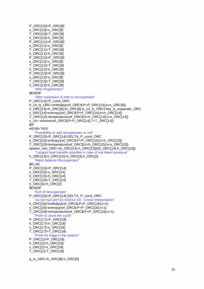
75

P_ORC[10]=P_ORC[8] s_ORC[10]=s_ORC[8] T_ORC[10]=T_ORC[8] h_ORC[10]=h_ORC[8] P_ORC[11]=P_ORC[8] s_ORC[11]=s_ORC[8] T_ORC[11]=T_ORC[8] h_ORC[11]=h_ORC[8] P_ORC[12]=P_ORC[8] s_ORC[12]=s_ORC[8] T_ORC[12]=T_ORC[8] h_ORC[12]=h_ORC[8] P_ORC[13]=P_ORC[8] s_ORC[13]=s_ORC[8] T_ORC[13]=T_ORC[8] h_ORC[13]=h_ORC[8] "After Regenerator" $ENDIF "After expansion & inlet to recouperator" P_ORC[14]=P_cond_ORC h_14_is_ORC=enthalpy(ref_ORC$;P=P_ORC[14];s=s_ORC[8]) h_ORC[14]=h_ORC[8]-(h_ORC[8]-h_14_is_ORC)*eta_is_expander_ORC s_ORC[14]=entropy(ref_ORC$;P=P_ORC[14];h=h_ORC[14]) T_ORC[14]=temperature(ref_ORC$;h=h_ORC[14];s=s_ORC[14]) v_14= volume(ref_ORC$;P=P_ORC[14];T=T_ORC[14]) $IF HEX$='YES' "Possiblility to add recouperator or not" P_ORC[15]=P_ORC[14]-DELTA_P_cond_ORC s_ORC[15]=entropy(ref_ORC$;P=P_ORC[15];h=h_ORC[15]) T_ORC[15]=temperature(ref_ORC$;h=h_ORC[15];s=s_ORC[15]) epsilon_hex_ORC=(h_ORC[14]-h_ORC[15])/(h_ORC[14]-h_ORC[16]) "Largest heat transfer possible in case of low bleed pressure" h_ORC[14]-h_ORC[15]=h_ORC[3]-h_ORC[2] "Mass balance Recouperator" $ELSE P_ORC[15]=P_ORC[14] s_ORC[15]=s_ORC[14] h_ORC[15]=h_ORC[14] T_ORC[15]=T_ORC[14] h_ORC[3]=h_ORC[2] $ENDIF "Exit of recouperator" P_ORC[16]=P_ORC[14]-DELTA_P_cond_ORC "y1=y0+(y2-y0)*(x1-x0)/(x2-x0) - Linear interpolation" h_ORC[16]=enthalpy(ref_ORC$;P=P_ORC[16];x=1) s_ORC[16]=entropy(ref_ORC$;P=P_ORC[16];x=1) T_ORC[16]=temperature(ref_ORC$;P=P_ORC[16];x=1) "Point to close the cycle" P_ORC[17]=P_ORC[18] h_ORC[17]=h_ORC[18] s_ORC[17]=s_ORC[18] T_ORC[17]=T_ORC[18] "Point for bugg in the system" P_ORC[1]=P_ORC[18] h_ORC[1]=h_ORC[18] s_ORC[1]=s_ORC[18] T_ORC[1]=T_ORC[18] q_in_ORC=h_ORC[8]-h_ORC[5]

76

$IF Bleed$='YES' "Taking into account if there is a loss of mass flow in turbine or not" work_net_ORC=(h_ORC[8]-h_ORC[9])+(1-X_mass_ORC)*(h_ORC[9]-h_ORC[14])-(1-X_mass_ORC)*(h_ORC[2]-h_ORC[1])-(h_ORC[5]-h_ORC[4]) $ELSE work_net_ORC=(h_ORC[8]-h_ORC[14])-(h_ORC[2]-h_ORC[1])-(h_ORC[5]-h_ORC[4]) $ENDIF eta_thermal_ORC=work_net_ORC/q_in_ORC eta_thermal_round=(work_net_ORC*m_dot_ref_ORC)/W_comp_tot T_discharge=T[NSC*2] VHC=Q_HST_tot*v[1] VER=v_14/v_8 VCC=(h[1]-h[NSC*4+2])/v[1]

Documents

Thermodynamic Analysis of a High Temperature Heat Pump