University of Nevada

Reno

Thermodynamic and Hydraulic Testing

of Cryogenic Turbines

A thesis submitted in partial fulfillment of the requirements for the degree of Master of Science

in Mechanical Engineering

by

Philip R. LeGoy

Dr. Yunus A. Cengel, Thesis Advisor

December 1998

ii

Thesis of Philip R. LeGoy is approved: Thesis Advisor Department Chair Dean, Graduate School

University of Nevada

Reno

December 1998

iii

1998 Philip Richard LeGoy All Rights Reserved

No part of this publication may be reproduced, stored in a retrieval system, or

transmitted, in any form or by any means, electronic, mechanical, photocopying, recording, or otherwise, without the prior written permission of

Philip Richard LeGoy.

Printed in the United States of America by Ebara International Corporation

Cryodynamics Division’s Research and Development Department.

ISBN 0-9670646-0-0

iv

ACKNOWLEDGEMENTS

The author would like to acknowledge and thank EBARA

International Corporation in Sparks Nevada for their support in this endeavor.

Thanks to G. Louis Weisser, General Manager of EBARA

International’s Sparks Facility, for allowing me to do this Thesis on the subject matter contained within.

A special thank you, to my Father L. Robert LeGoy, for proof reading

my work. Thanks to both my Mother Shirley M. LeGoy and my Father, for just

being my parents and supporting whatever I wanted to do. A special thanks, to Dr. Hans Kimmel, Vice President of Research

and Development at EBARA International for his personal support and advice.

I would also like to thank Dr. Yunus Cengel, for his guidance and

cooperation in working with EBARA International Corporation. Thanks for all of the help I received from the test crew and the test

department at EBARA International Corporation.

Last but not least a very special thank you to my wife Grááááinne and my daughter Ciara, for their patience with me while I pursued this Masters degree.

v

ABSTRACT

Thermodynamic and hydraulic testing of the newly developed Cryogenic

Hydraulic Radial Turbine-Generator assembly, an alternative to the conventional

Joule-Thompson valve which is used in Cryogenic Liquefaction plants, was

successfully performed. Included in this process was the complete design and

build of the first ever turbine of this kind from the conceptual idea to the prototype

turbine, the creation of a test bed and the development of the algorithms for the

analysis. Significant power recovery and refrigeration were demonstrated by the

testing. This is an advantage over the Joule-Thompson valve, which does not

recover power and does not refrigerate as efficiently. Up to 78% isentropic

efficiency for the Turbine-Generator assembly and up to 1.5 °F temperature drop

across the turbine are calculated from the test data.

vi

TABLE OF CONTENTS

INTRODUCTION ........................................................................................................................ 1 Chapter 1 BACKGROUND......................................................................................................... 2

1.1 General Background/History of the turbine generator .................................................... 2 Figure 1. Joule Thompson Valve - Process Design............................................................... 3 Figure 2. Turbine Generator - Process Design...................................................................... 3

1.2 Testing of the Turbine Generator................................................................................... 4 Chapter 2.0 TURBINE DESIGN ................................................................................................. 6

2.1 Mechanical Design........................................................................................................ 6 2.2 Electrical Design ........................................................................................................... 7

Chapter 3.0 TEST FACILITY DESIGN ....................................................................................... 9 3.1 Mechanical Design........................................................................................................ 9 3.2 Electrical Design ........................................................................................................... 9

Figure 3. Test Facility Design Schematic with Earliest Temperature Sensor Configuration.. 11 Figure 4. Test Facility Design Schematic with Silicon Diode Temperature Sensors Added .. 12 Figure 5. Test Facility Design Details with Sensor Locations for 12TG-24........................... 13 Figure 6. Test Facility Design Details with Sensor Locations for 4TG-122........................... 14

Chapter 4.0 TEST PROCEDURES........................................................................................... 15 Chapter 5.0 TEST DATA AND RESULTS................................................................................ 16

5.1 Hydraulic & Electrical - Data Reduction Algorithms...................................................... 16 Figure 7. USEM Power versus Efficiency curves ................................................................ 20

5.2 Hydraulic Example Problems....................................................................................... 21 5.3 Thermodynamic - Data Reduction Algorithms.............................................................. 23 5.4 Thermodynamic Example Problems ............................................................................ 25 5.5 Single-Stage Turbine................................................................................................... 26

5.5.1 Hydraulic & Electrical Data - Reduced Data & Curves........................................... 27 Figure 8. Curve Cryoturbine Test 574mm Dia. Runner 15 February, 1996; File: Runtr22A . 28 Figure 9. Curve Cryoturbine Test 574mm Dia. Runner 15 February, 1996; File: Runtr22B . 29 Figure 10. Curve Cryoturbine Test 574mm Dia. Runner Oct. 4, 1996; File: Runtr23A.......... 31 Figure 11. Curve Cryoturbine Test 574mm Dia. Runner Oct. 4, 1996; File: Runtr23B.......... 32 5.5.2 Thermodynamic Data - Reduced Data & Curves................................................... 33

Figure 12. Curve ∆T versus Isentropic Efficiency File: TurbAll............................................. 34

Figure 13. Curve ∆T versus Isentropic Efficiency File: TurbAll1........................................... 35

Figure 14. Curve ∆T versus Isentropic Efficiency File: TurbCeng ........................................ 37

Figure 15. Curve ∆T versus Isentropic Efficiency File: Turb40DA........................................ 38

Figure 16. Curve ∆T versus Isentropic Efficiency File: Turb40DB........................................ 39 5.6 Two-Stage Turbine...................................................................................................... 40

5.6.1 Hydraulic & Electrical Data - Reduced Data & Curves........................................... 40 Figure 17. Curve Cryoturbine Test 278mm Dia. Runner Dec. 11, 1996; File: Runtr49A....... 41 Figure 18. Curve Cryoturbine Test 278mm Dia. Runner Dec. 11, 1996; File: Runtr49B ...... 42 5.6.2 Thermodynamic Data - Reduced Data & Curves................................................... 43

Figure 19. Curve ∆T versus Isentropic Efficiency File: Turb49C .......................................... 44

Figure 20. Curve ∆T versus Isentropic Efficiency File: Turb49D .......................................... 45 Chapter 6.0 ERROR ANALYSIS .............................................................................................. 46 Chapter 7 DISCUSSION OF RESULTS.................................................................................... 47

7.1 The original goals........................................................................................................ 47 7.2 Technical Innovations, why things were done to Attain the Goals ................................ 47 7.3 Results........................................................................................................................ 50 7.4 Significance of Results................................................................................................ 53

CONCLUSION.......................................................................................................................... 54 RERENCES.............................................................................................................................. 56 APPENDIX ............................................................................................................................... 60

1

INTRODUCTION

Two prototype turbine generators were used for these tests. A 12TG-24 turbine with a 4-

pole generator, design speed is 1500-rpm and a 4TG-122 turbine with a 2-pole generator; design

speed is 3000-rpm. EBARA International Corporation manufactured these turbines as a research

and development project.

The turbine generator model number 12TG-24 was designed at the EBARA International

Corporation Cryodynamics Division Office, 350 Salomon Circle, Sparks, Nevada. This turbine is a

single-stage device tested in Liquefied Natural Gas (LNG) and it was designed with a 4-pole

generator. The second turbine tested was a model 4TG-122. This turbine is a two-stage turbine

that was tested in LPG (Liquefied Propane Gas) and designed with a 2-pole generator. Both

turbines are referenced in this thesis.

2

Chapter 1 BACKGROUND

1.1 General Background/History of the turbine generator

A. The project started with a design plan, which included two basic concepts:

1. A turbine is a pump running in reverse and EBARA is a leader in cryogenic

pump manufacture. Why not build a turbine by the same method? Before

designing the basic turbine several sources were referenced.9-38

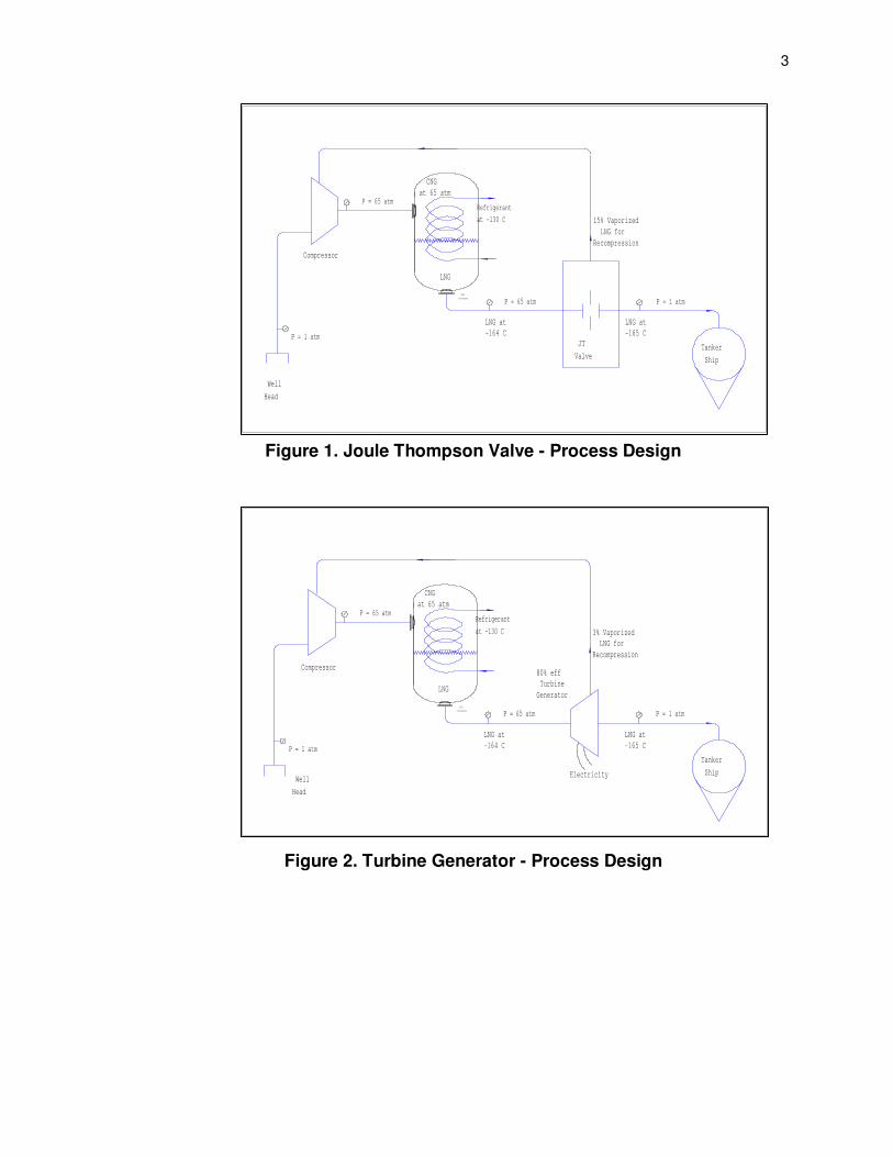
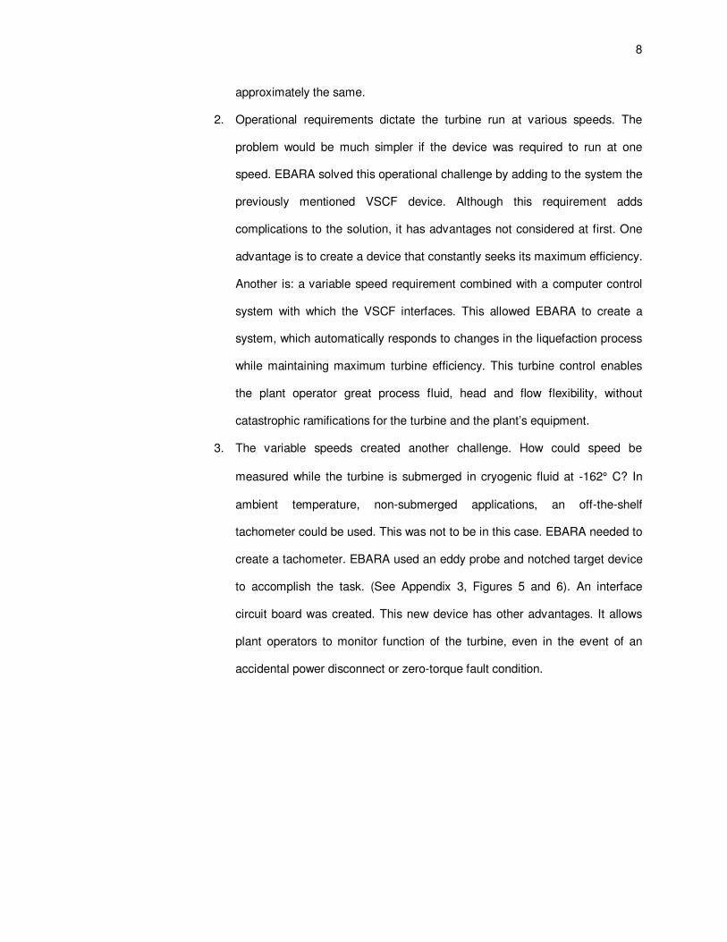
2. LNG liquefaction plants always try to improve efficiency. Joule-Thompson

(JT) valves are integral components in a liquefaction plant. A turbine running

in cryogenic liquids is able to replace a Joule-Thompson valve used in

liquefaction processes.1, 2, 9

The turbine is more efficient than the JT valve by

reducing the kinetic energy and therefore reduces liquid boil off caused by

the use of the JT valve. This method improves process efficiencies by as

much as 12%. The following two figures (See Figures 1 & 2) shown describe

the liquefaction process before and after a turbine has replaced the JT valve.

The reduction in vaporized LNG increases process efficiency.

3

Figure 1. Joule Thompson Valve - Process Design

Figure 2. Turbine Generator - Process Design

Well

Head

P = 1 atm

Refrigerant

at -130 C

LNG

HEAT

EXCHANGER

JT

Valve

Compressor

P = 65 atm

P = 65 atm P = 1 atm

CNG

at 65 atm

LNG at

-164 C

LNG at

-165 C

15% Vaporized

LNG for

Recompression

Tanker

Ship

80% eff

Turbine

Generator

Electricity

Tanker

Ship

3% Vaporized

LNG for

Recompression

LNG at

-165 C

LNG at

-164 C

CNG

at 65 atm

P = 1 atm P = 65 atm

P = 65 atm

Compressor

Well

Head

HEAT

EXCHANGER

LNG

Refrigerant

at -130 C

P = 1 atm

4

B. The next step in the project was to put together a cost benefit analysis:

1. This was to show EBARA (See Appendix 1) it could enjoy the savings in point

two (2) above. This was completed on February 7, 1995. It must be pointed

out every pump EBARA makes is a fully engineered product so the costs

incurred by tooling were virtually non-existent. The project became official

and was funded February 22, 1995. A great deal of work led to development

of this device and these tests.

C. The third step was to find information on reverse running pumps used as

turbines. The following information is the Prior Art: items leading to this

development.

1. See the enclosed literature search.9-38

Search items were read to extract

design features desired in a reverse running pump used as a turbine. Spring,

1995.

D. The fourth step was to find a device capable to control a generator running at

variable speeds under variable loads:

1. The device chosen was a Variable Speed Constant Frequency device

(VSCF) that was, at the time, built by Kenetech U.S. Windpower for windmill

applications. Spring, 1995.20

1.2 Testing of the Turbine Generator

The purposes of the Turbine Generator Testing were as follows.

1. Define turbine generator mechanical operation parameters and show data

points are repeatable.

2. Define vibration characteristics of turbine generator mechanical operation.

3. Determine the VSCF would control the turbine generator.

4. Rework and fine-tune a VSCF tachometer target system so it would permit

control.

5. Determine data points and speeds for zero-torque operation and show data

5

points are repeatable.

6. Determine function and vibration at zero-torque operation for machine.

7. Determine the measurement techniques and efficiency of the machine.

These tests were conducted in accordance with the Test Procedure TP-1400012A and its

addenda (See Appendix 11).

6

Chapter 2.0 TURBINE DESIGN

Analyzing the types of pumps EBARA built made the Turbine generator selection. The

selection was guided by several criteria.

1. Several pump to turbine designs were done by other entities. The literature search9-38

was performed in an attempt to identify those examples. One, very good reference

was the U.S. Department of Energy’s research on low head, high flow turbines done

at the Idaho National Engineering Laboratory in Idaho Falls, Idaho.10

2. Which pumps had the best quality, longevity, robust design and efficiency? Also of

concern was availability and “off the shelf” access to a large number of parts. One

type of pump stood out in all of these areas, the 12EC-24.

3. The 12EC-24 pump is EBARA’s primary shipboard service pump. A large number of

those were being built in the next two years. This allowed Research and

Development (R & D) to have testing options available. The fact so many pumps

were being built in the near future allowed R & D to make use of rejected parts and

also various booster pumps.

4. The turbine would need to have a booster pump to run it and test it since it was

needed to provide the flow and head necessary to emulate a liquefaction plant.

2.1 Mechanical Design

A turbine is not a pump, yet pumps and turbines are turbomachinery. It is important to

make distinctions. Pump designs were converted to turbine designs to make the

prototypes. One design is (See Appendix 2, Turbine Drawing 7000205) the 4-pole

single-stage turbine. The following Drawing is the same for the 2-pole two-stage

turbine. (See Appendix 3, Turbine Assembly Drawing 4900627)

1. A turbine flows reverse of the same pump design. Therefore streamlines of fluid

have to be considered reverse of the design of a pump. So the turbine had to be

machined in reverse of the original pump design. Therefore impeller designs

7

were converted to runner designs. (See Appendix 4 & 5, Turbine Runner

Drawings 4001345 & 4001990)

2. When a pump is designed it has to have a larger power source, “a motor”, than

the hydraulic power it must deliver. This is to compensate for the hydraulic losses

of pump impellers, to move the liquid it is designed to carry. When a turbine

generator is designed it needs a smaller electric power device, “a generator”,

than the size of the pump motor. This is to compensate for the hydraulic losses of

the turbine runners. This is if one is dealing with the same hydraulic power,

produced in a pump and extracted in a turbine. Essentially the turbine was built

with the same castings, the same basic components as the pump. The

differences are noted above. Since the turbine generator has the same features

as an EBARA pump, it is completely submersible. This gives the turbine

generator the advantage of no mechanical transitions from the liquefied

cryogenic explosive hydrocarbon environment to ambient air.

2.2 Electrical Design

An Induction Motor can be used as an Induction Generator. An induction device

is capable of running as a motor or a generator. This is as a pump is a turbine

and so a turbine is a pump. Yet, like a pump has to be modified to allow for the

performance differences, so does the induction motor/generator. An added

requirement of this particular project is the device must run at variable speeds

and compensate for various load differences. (See Appendix 6 & 7, Generator

Drawings 5900114 & 5900159)

1. Load requirements of the mechanical device apply to the electrical device as

well. Since the generator is producing power, it needs to produce power at a

better efficiency and quality, than it uses as a motor. Where a motor is rated

at 440 volts the generator needs to be rated at 480 volts. This is a grid

requirement to compensate for grid losses. Otherwise the two devices are

8

approximately the same.

2. Operational requirements dictate the turbine run at various speeds. The

problem would be much simpler if the device was required to run at one

speed. EBARA solved this operational challenge by adding to the system the

previously mentioned VSCF device. Although this requirement adds

complications to the solution, it has advantages not considered at first. One

advantage is to create a device that constantly seeks its maximum efficiency.

Another is: a variable speed requirement combined with a computer control

system with which the VSCF interfaces. This allowed EBARA to create a

system, which automatically responds to changes in the liquefaction process

while maintaining maximum turbine efficiency. This turbine control enables

the plant operator great process fluid, head and flow flexibility, without

catastrophic ramifications for the turbine and the plant’s equipment.

3. The variable speeds created another challenge. How could speed be

measured while the turbine is submerged in cryogenic fluid at -162° C? In

ambient temperature, non-submerged applications, an off-the-shelf

tachometer could be used. This was not to be in this case. EBARA needed to

create a tachometer. EBARA used an eddy probe and notched target device

to accomplish the task. (See Appendix 3, Figures 5 and 6). An interface

circuit board was created. This new device has other advantages. It allows

plant operators to monitor function of the turbine, even in the event of an

accidental power disconnect or zero-torque fault condition.

9

Chapter 3.0 TEST FACILITY DESIGN

The test facility at EBARA International Corporation’s location in Sparks Nevada was

designed for pumps. It has the unique distinction of being the largest cryogenic liquefied

explosive gas test facility in the world. Although unique, it was not designed to test

turbines. A redesign of the test facility had to be made. (See Appendix 8, the Turbine

Test Loop, Modification and Assembly Drawing 9000543; 9, Turbine Test Loop,

Modifications and Assembly Drawing 9000712; and 10, Turbine One Line Diagram and

Schedules Drawing 9000591)

3.1 Mechanical Design

The test pad design had to support both a turbine and a pump in the test loop.

(See the Schematics of Pump and Turbine Figure 1 and Figure 2). The 12TG-24,

4-pole turbine and the 4TG-122/4TG-12, 2-pole design were both modified from

pump design test configurations to accommodate these designs as turbines with

their respective booster pumps.

3.2 Electrical Design

Substantial rewiring was necessary to support the power generator and the

VSCF (See Appendix 10 for details).

1. The first challenge was deciding if the VSCF method of control could be done

on the turbine generator. The R & D department personnel discussed using a

load-bank scheme and a grid-excitation scheme for the turbine running at a

fixed speed. R & D had several versions of these concepts operating at once.

They could use a capacitor in conjunction with a load-bank. They could use a

load-bank in conjunction with the VSCF, etc. The VSCF was decided upon

but the supplier did not really know if they could convert this technology to

the application. The tachometer still had to be designed to make it work.

10

2. The second challenge was to decide where the power would go. Where it

would be connected to the grid. If it were connected to the grid on the power

utility side it would entail enormous certifications and paperwork. Kenetech

had assured R & D the power produced by the turbine generator would come

out of the controller meeting IEEE-519 requirements for harmonic distortion

and power quality. Kenetech guaranteed this. This assured R & D the power

produced was not going to cause any problems with EBARA’s electrical

systems nor with the local utility company. Therefore, the power was put into

the grid on the EBARA side of the utility connection just ahead of the test

facility’s own Motor Generator Set used to test pumps. This arrangement was

ideal because during every turbine generator test a booster pump was used

to produce head and flow. The power was being used during testing.

3. The third challenge was to wire the controller and install it into the test

generator room. Using a spare breaker space in the main switchboard in

EBARA’s generator room accomplished this. The main pump-testing

generator is a 1.2MW variable speed DC motor coupled to a 1MW AC

generator; thus it can produce variable frequency AC. This device is

supported by many sensitive components and relies on clean power from the

grid. Since the VSCF produced clean power it pumped it back into the

system before the generator and after the utility connection, as mentioned in

item 2 above. (See the one line diagram Appendix 10 for details.)

4. The fourth challenge was to monitor the systems. This challenge became a

constantly changing target. It depended upon the test done; the items R & D

personnel were trying to define and the turbine tested. Filtering and signal

shielding were a design problem, due to the variable frequency power

generated. The items monitored are the test data sensors and are shown in

Figure 3 & Figure 4.

Figure 3. Test Facility Design Schematic with Earliest Temperature Sensor Configuration

11 S.O.V.

10

S.O.

V.

TO LPG

TANK

2

3

6

78

9

4

5

1

S.O.

V.

S.O.V.

*

*

S.O.

V.

S.O.V.

P

TURBINE

S.O.V.

S.O.V.

S.O.

V.

S.O.

V.

S.O.V.

S.O.

V.

P

OUT 2

T

OUT 2

F.C.V.

P

IN 2

T

IN 2

VENT

FILL

LINE

VENT LINE

LN2

LNG

LLBOOSTER

PUMP

TURBINE

HEAT

EXCHANGER

A M - GV W

A VSCFCV W

CONTROL

ROOM MONITORS

TO TACHOMETERTO VMSTO PROXIMITY DETECTOR

LL : LIQUID LEVEL

S.O.V.: SHUT OFF VALVE

F.C.V.: FLOW CONTROL VALVE

* : CONNECT TO TRANSMITTER

SYMBOLS

*

**

*

*

*

P

OUT 3

T

OUT 3

11

Figure 4. Test Facility Design Schematic with Silicon Diode Temperature Sensors Added

T

IN 2

***

*

SYMBOLSLL : LIQUID LEVEL

S.O.V.: SHUT OFF VALVE

F.C.V.: FLOW CONTROL VALVE

* : CONNECT TO TRANSMITTER

TO PROXIMITY DETECTORTO VMSTO TACHOMETER

CONTROL

ROOM MONITORS

WV VSCFCA

WV M - GA

HEAT

EXCHANGER

TURBINE

BOOSTER

PUMPLL

LPG

LN2

VENT LINE

FILL

LINE

VENT

T

IN 1

P

IN

F.C.V.

T

OUT 1

P

OUT

S.O.

V.

S.O.V.

S.O.

V.

S.O.

V.

S.O.V.

S.O.V.

P

TURBINE

S.O.V.

S.O.

V.* *

*

S.O.V.

S.O.

V.

1

5

4

9

87

6

3

2

TO LPG

TANK

S.O.

V.

10

S.O.V.11

* T

OUT 2

12

13

Figure 5. Test Facility Design Details with Sensor Locations for 12TG-24

SCALE: NONE

VIEW A

Eddy Probe for

Lift measurement

S/N 51203D-3

Eddy Probe For

Tachometer

2 PLACES

22░ APARTS/N 60202-1

S/N 60217-2

or

S/N 60217-1

S/N 60217-4

Oct. 4

T out 3 Thermocouple

FLOW

CONTROL

VALVE

SHARP EDGE

ORIFACE PLATE

DELTA P FLOW

MEASUREMENT

PRESSURE TAP

PIPING THRU

HEAD PLATE

A

1685 GALLON

TEST TANK

12TG-24

TURBINE ASSY

P/N 7000205

OUTLET

DATUM

LOW LEVEL

LIQUID TAP

TURBINE ASSEMBLY

Oct. 4

P in 2 Pressure Tap

T in 2 Thermocouple

T in Silicon Diode

INLET

DATUM

Feb. 15

P out 3

T out 3

Thermocouple

Feb. 15

P in 2

T in 2

Thermocouple

Oct. 4

P out 2

T out 2 Thermocouple

T out Silicon Diode

Feb. 15

P out 2

T out 2 Thermocouple

Oct. 4

P out 3 Pressure Tap

Note: Items Reflect

Computer Data

Collection

Variables

Accels

used S/Ns

PCPs 630

PCPs 373

PCPs 202

12.00"

0.035"

0.035"

19.1"Zs=

151.0"Zd=

Figure 6. Test Facility Design Details with Sensor Locations for 4TG-122

P out 2

T out Silicon Diode

T out Thermocouple

P in 2

T in Silicon Diode

T in Thermocouple

FLOW

CONTROL

VALVE

SHARP EDGE

ORIFACE PLATE

DELTA P FLOW

MEASUREMENT

INLET

DATUM

SEE A OF

PREVIOUS FIGURE

OUTLET

DATUM

LOW LEVEL

LIQUID TAP

TURBINE ASSY 4TG-122

KIT PN 4900627-01 & -02

TURBINE ASSEMBLY

1200 GALLON

TEST TANK

77.30"Zd=

35.96"Zs=

13

15

Chapter 4.0 TEST PROCEDURES

The test procedures cited are the actual procedures used in the testing of both turbines.

Included is just one of the test procedures involved because of the level of complication

undertaken with the testing.

1. TP-1400011B: This EBARA test procedure was to determine how the 4-pole single-

stage turbine performed as a pump. The idea was R & D people could learn how the

two devices were actually related and they could verify the mechanical functionality of

the turbine. This test took place December 27, 1995.6

2. TP-1400012A: This EBARA test procedure was to find if the 4-pole single-stage

turbine design performed as a turbine and to get performance data from the turbine.

The first procedure was to get the turbine to work. R & D had to verify the VSCF

would indeed perform as planned. This test procedure includes three addenda to the

procedure because it was not known how to advance with testing until after

preliminary attempts. These tests took place from January 20, 1996 through October

4, 1996. (See Appendix 11: TP-1400012A)

3. TP-1400013A: This EBARA test procedure was arranged to compare turbine test

data. R & D personnel needed to evaluate the effect the booster pump would have

on the test data extracted from the test arrangement with the turbine and pump. It

was also tested as a secondary way to predict efficiency of the turbine. This test took

place on February 9, 1996.7

4. TP-1400008: This EBARA test procedure was put together to test the two-stage, 2-

pole turbine generator. This procedure took place from December 4, 1996 through

December 12, 1996.8

16

Chapter 5.0 TEST DATA AND RESULTS

Test results are vast. The goal was to find if it was possible to build and operate this kind

of turbine and how efficient the turbine might be. The turbine met and exceeded all

predictions. The thermodynamic implications of the turbine are it can reduce boil off of the

liquids. An interesting side effect is the reduction in pressure in the fluid creates a slight

temperature drop. The following results show this.

5.1 Hydraulic & Electrical - Data Reduction Algorithms

The Algorithms are as follows and they apply to the turbine reduced data spread

sheets as they appear with the reduced data. (See Appendix 12, 13 and 19)

The following items are those listed in the Input Data area of the spreadsheet.

This data comes from the basic geometry of the test stand. This includes placement of sensors

and sizes of the inlet and outlet of the test vessel, etc. The Specific Gravity measurement and the

temperature measurement are also entered in this area.

The following items are the items listed in the Calculations area of the spreadsheet.

Items from ASME’s 6th edition Fluid Meters Book pg. 65.

24

(See example calculations sheet for details Section 6.1.)

The Reynolds number Re = ρVD/µ.

Where ρ = density, V = Assumed Average Velocity of the fluid flow, D = The Diameter of the inlet

pipe and µ = the Liquid Viscosity.

d = The diameter of the outlet vessel.

Beta Ratio β = Ratio of Diameters d/D.

K1 (lambda) = 1000/√Re

K2 (b) = (0.0002 + (0.0011/D)) + (0.0038 + (0.0004/D))[β2 + (16.5 + 5D)β16

].

K0 = (0.6014 - 0.01352D-1/4

) + (0.3760 + 0.07257D-1/4

)((0.00025/(D2β2

+ 0.0025D)) + β4 + 1.5β16

)).

17

K = K0 + K2*K1.

The areas of the inlet and outlet are calculated here. The gauge height is also noted in this area.

The following items are those listed in the hydraulic data area.

RPM: Data is the average of the highest and lowest speeds read from the Kenetech

controller, or data read directly from the computer listing for the test.

T in Data from the thermocouple or silicon diode placed at inlet of turbine.

S.G. in Item calculated from T. in data. S.G. in = 11/11700 °f [T@S.G. - T in] + S.G.

T out Data from the thermocouple or silicon diode placed at outlet of turbine.

S.G. out Calculated as in S.G. in using T out data.

∆∆∆∆P Data from orifice pressure tap measurement.

P in Data from pressure tap at entrance to turbine.

P out Data from pressure tap at outlet of turbine.

Q gpm Flow calculated from ∆P. Using Kinematic Viscosity, Reynolds Number and the orifice

constant. Items from ASME’s 6th edition Fluid Meters Book pg. 65. (See initial

calculations sheet for details). This calculation is Q = 753.2 √∆P/ S.G. for the 12TG-24

or Q = 125.5 √∆P/ S.G. for the 4TG-12/4TG-122. Note: Q = AOriface K √2∆P/ρ Iterate

Re and Q 3 times for a less than 1% “negligible” improvement in accuracy but

sometimes this will catch large errors in flow calculations.

Q m3/Hr Converted gpm data to metric units.

Q m3/min Converted Q m

3/Hr data.

Q m3/sec Converted Q m

3/Hr data.

Hf (m) Friction Head calculated from sensors to turbine inlet.

TDH TDH = Pout - Pin + V2out - V

2in + (Zout - Zin) - Hf

ρρρρ 2g

1. Vin = Q/Ain (in Ft/s) Vout = Q/Aout (in Ft/s)

Ain = π/4(Din)2 Aout = π/4 (Dout)

2

Zin and Zout are the gauge height in feet.

18

ρ is just 62.4 #/Ft3 multiplied by the S.G..

T in C This is just the temperature recorded in °F converted to °C.

T out C This is the same as above.

∆∆∆∆P P in and P out This is just the same as the previous items with the same name converted to

kg/cm2

The following are those listed in the power and efficiency area of the spreadsheet.

RPM Copied RPM data from above.

kW lo Data unused here.

kW hi Data unused here.

kW out total Data measured on the grid side of the VSCF controller.

Hyd. kW This is the Hydraulic power calculated from the given data.

kW = *((S.G.in + S.G.out)/2)*Q*TDH*Gravity

Q is in (m3/ hr) TDH is in (m).

Eff Total This is the efficiency of the total power produced and released into the grid. This is

nothing more than. kW out total/Hyd kW.

Eff VSCF This is the efficiency of the VSCF calculated from the Generator power output and the

grid side power provided to the grid. This is calculated by kW out Gen/kW out total.

Eff TG This is the Isentropic efficiency of the turbine for the process. This is the efficiency that

will predict how much energy can be extracted from the process stream. This is the

efficiency of the turbine and the generator in combination. This efficiency is calculated

by kW out Gen/Hyd kW.

kW out Gen This is the power measured on the generator side of the VSCF.

Eff Gen This is the efficiency of the generator as informed to us by USEM (U.S. Electric Motors)

the efficiencies have been taken from the included curves. (See the Following Figure 7)

kW shaft This is power of the generator divided by the reported efficiency of the generator. This

calculation is kW out Gen/Eff Gen.

19

Eff Turb This is the shaft power divided by the hydraulic power. This calculation is kW

shaft/Hyd kW.

Figure 7. USEM Power versus Efficiency curves

20

21

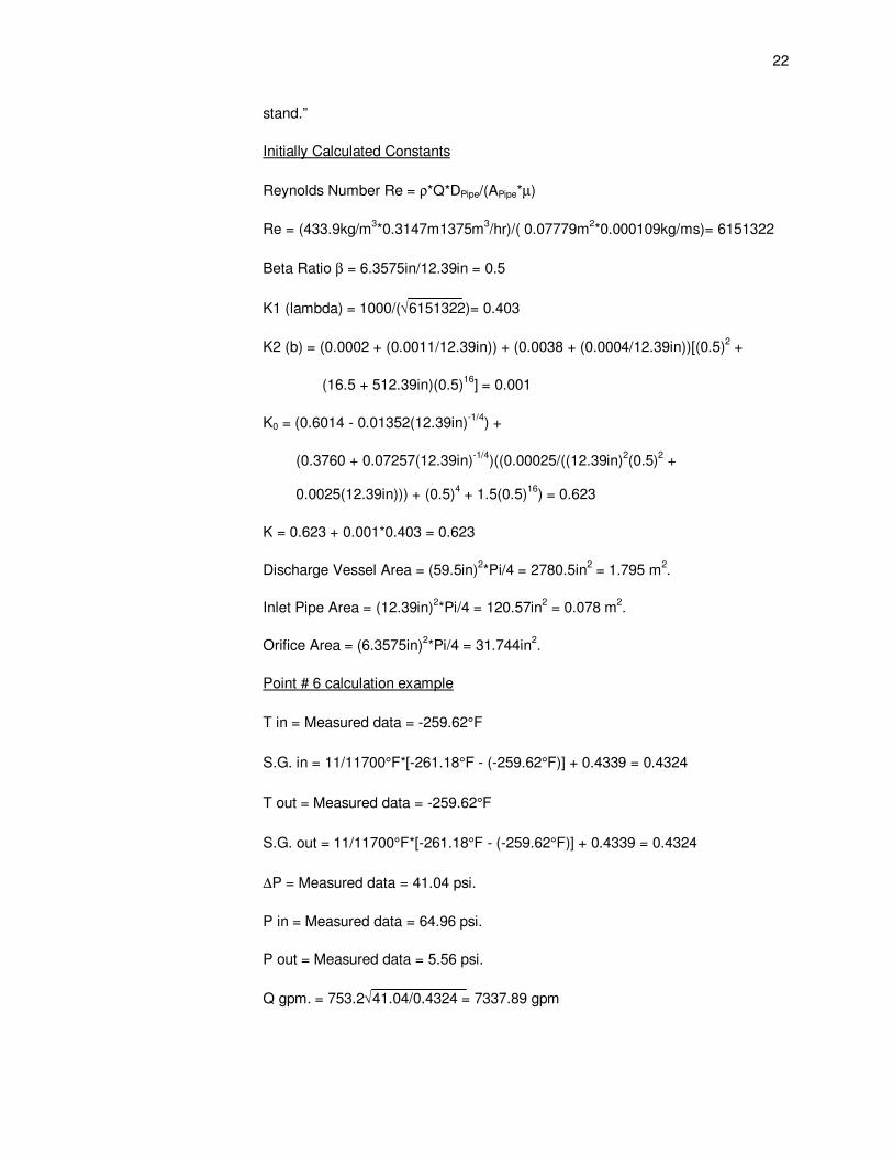
5.2 Hydraulic Example Problems

Example 1: A Hydraulic Institute approved method of calculating hydraulic

efficiency of a turbo machinery type device. This method includes a

Sharp edge orifice flow problem. Liquid head calculations and

Hydraulic power calculations. Efficiency is calculated using power

out divided by power in. The following calculation is for the data

point # 6 gathered during test number 96121C-T1 File: Turb17B

(See Appendix 12.)

Given Input Data:

Let Inlet Pipe Diameter = 12.390 inches = 0.3147m “the I.D. of a 12 inch

Schedule 10S Stainless Steel pipe at the point where the measurements of

temperature and pressure are taken.” APipe = (π/4)(0.3147)2 = 0.07779m

2

Let Orifice Diameter = 6.3575 inches “A sharp edge orifice designed for this

application.”

Test Liquid assumed density for this application = 26.5#/ft3 = ρ = 433.9 kg/m

3

Liquid Viscosity = 0.109 Centipoise = 0.000109 kg/ms “A property of the liquid,

looked up from tables.”

Test Liquid temperature = -261.18 °F “Measured from liquid before and after test

then averaged.”

Test Liquid Specific Gravity = 0.4339 “Measured from liquid before and after test

then averaged.”

Test Fluid assumed average design flow = 6054.1gpm = 1375 m3/hr

Discharge Vessel Diameter = 59.500 inches “The I.D. of the actual test vessel at

the point where the temperature and pressure measurements are taken.”

Gauge Height = 14.16 ft. = 4.32 M. “This item is measured directly from the test

22

stand.”

Initially Calculated Constants

Reynolds Number Re = ρ*Q*DPipe/(APipe*µ)

Re = (433.9kg/m3*0.3147m1375m

3/hr)/( 0.07779m

2*0.000109kg/ms)= 6151322

Beta Ratio β = 6.3575in/12.39in = 0.5

K1 (lambda) = 1000/(√6151322)= 0.403

K2 (b) = (0.0002 + (0.0011/12.39in)) + (0.0038 + (0.0004/12.39in))[(0.5)2 +

(16.5 + 512.39in)(0.5)16

] = 0.001

K0 = (0.6014 - 0.01352(12.39in)-1/4

) +

(0.3760 + 0.07257(12.39in)-1/4

)((0.00025/((12.39in)2(0.5)

2 +

0.0025(12.39in))) + (0.5)4 + 1.5(0.5)

16) = 0.623

K = 0.623 + 0.001*0.403 = 0.623

Discharge Vessel Area = (59.5in)2*Pi/4 = 2780.5in

2 = 1.795 m

2.

Inlet Pipe Area = (12.39in)2*Pi/4 = 120.57in

2 = 0.078 m

2.

Orifice Area = (6.3575in)2*Pi/4 = 31.744in

2.

Point # 6 calculation example

T in = Measured data = -259.62°F

S.G. in = 11/11700°F*[-261.18°F - (-259.62°F)] + 0.4339 = 0.4324

T out = Measured data = -259.62°F

S.G. out = 11/11700°F*[-261.18°F - (-259.62°F)] + 0.4339 = 0.4324

∆P = Measured data = 41.04 psi.

P in = Measured data = 64.96 psi.

P out = Measured data = 5.56 psi.

Q gpm. = 753.2√41.04/0.4324 = 7337.89 gpm

23

Q m3/Hr = 7337.89/4.4029 = 1666.60 m

3/Hr

Q m3/min = 1666.60/60 = 27.78 m

3/min

Q m3/sec = 27.78/60 = 0.4629 m

3/sec

TDH = [((4.57 kg/cm2*10)/0.4324) - ((0.39 kg/cm

2*10)/0.4324)] +

[{((0.463 m3/sec)/0.078 m

2)2 - ((0.463 m

3/sec)/1.795 m

2)2}/2(9.81m/s

2)] +

4.30m - 0.465m = 102.23 m

Hyd. kW = ((0.4324 + 0.4324)/2)*(kg/m3)*(0.4629 m

3/sec)*(102.23m)*(9.81m/s

2)

= 200.73

Eff TG = 156.20/200.73 = .778 or 77.8%

kW shaft = 156.20/.945 = 165.29

Eff Turb = 165.29/200.73 = .823 or 82.3%

5.3 Thermodynamic - Data Reduction Algorithms

The Algorithms are as follows and they apply to the turbine reduced data spread

sheets as they appear with the reduced data.

RPM is the speed of the turbine as it was recorded during testing.

T in 2 is the temperature as it was recorded during testing by the Silicon Diode or the

Thermocouple.

T out 2 is the temperature as it was recorded during testing by the Silicon Diode or the

Thermocouple.

∆∆∆∆T in F = (T out 2 - T in 2). This is the change in temperature caused by the turbine’s pressure

reduction.

Isentropic Eff: This is the Turbine Generator Isentropic Efficiency reported in the Hydraulic Data

Reduction Algorithms.

Isentropic (Eff)2 is the above efficiency data squared.

24

(∆∆∆∆T)*(Eff) is the isentropic efficiency multiplied by the change in temperature for the least squares

calculation.

The next column of items are the sums of the items ∆T in F, Isentropic Eff, Isentropic (Eff)2,

(∆T)*(Eff), at each speed and the item n is the number of items at each speed.

The last column of items is the actual least squares calculations based upon the following.

Least Squares Algorithm

For ∆∆∆∆T = a + b(Eff)

or y = a + bx

Let Error = q and then square the formula and sum it.

q = Σ(y - a - bx)2

Now do the partial derivative of q with respect to a and b.

1. Do the algebra to square the expression first.

q = Σ[(y - a - bx)(y - a - bx)]

= Σ(y2 - ay -bxy - ay + a

2 + abx - bxy + abx + b

2x

2)

= Σ(y2 - 2ay - 2bxy + 2abx + b

2x

2 + a

2)

2. δ q/δ a = Σ(-2y + 2bx + 2a)

= -2Σ(y - a - bx)

3. δ q/δ b = Σ(-2xy + 2ax + 2bx2)

= -2Σx(y - a - bx)

4. Now set both partials equal to zero and solve for a and b.

(1) 0 = Σ(y - a - bx)

(2) 0 = Σ(xy - xa - bx2)

(1) Can be rewritten as the following normal equation for a series of items 1 - n.

(1) Σy = an + bΣx

(2) Can be rewritten as the following normal equation for a series of items 1 - n.

(2) Σxy = aΣx + bΣx2

25

(1) Can be rewritten as.

(1) a = (1/n)(Σy - bΣx)

Now put (1) into (2).

Σxy = (1/n)(Σy - bΣx)Σx + bΣx2

Now solve for b.

b = [Σxy - (1/n)( Σx)( Σy)]/[Σx2 - (1/n)( Σx)

2]

Now solve for a put b into (1).

a = (1/n)(Σy - [{Σxy - (1/n)(Σx)(Σy)}/{Σx2 - (1/n)(Σx)

2}]Σx)

Next we let y = ∆T and we let x = (Eff) for Efficiency. Then we apply the final formula to a and

b and we get the following two equations used in the algorithm for the least squares linear

equation of the data.

b = [Σ[(Eff)*∆T] - (1/n)(Σ(Eff))(Σ∆T)]/[Σ(Eff)2 - (1/n)(Σ(Eff))

2]

a = (1/n)(Σ∆T - [{[Σ(Eff)*∆T] - (1/n)(Σ(Eff))(Σ∆T)}/{Σ(Eff)2 - (1/n)(Σ(Eff))

2}]Σ(Eff))

5.4 Thermodynamic Example Problems

Example 2: Least Squares Example for ∆T verses Efficiency. This problem is for

the reduced Thermodynamic Data from File: Turb49 at 2400 RPM.

Given Input Data

n = 12

Σ(Eff) = Σx = 725.734

Σ(Eff)2 = Σx

2 = 45907.102

Σ(∆T) = Σy = 5.534

Σ(∆T*Eff) = Σxy = 237.465

Calculations for the given data points in the File: Turb49

Let equation (1) be of the form: Σy = an + bΣx from the Least Squares algorithm.

(1) 5.534 = a(12) + b(725.734)

26

Let equation (2) be of the form: Σxy = aΣx + bΣx2 from the Least Squares

algorithm.

(2) 237.465 = a(725.734) + b(45907.102)

(1) becomes a(12) = 5.534 - b(725.734)

a = (5.534 - b(7.25.734))/12

a = 0.461 - b(60.478)

put (1) into (2) 237.465 = [0.461 - b(60.478)](725.734) + b(45907.102)

237.465 = 334.684 - b(43890.820) + b(45907.102)

-97.219 = b[45927.102 - 43890.820]

∴ b = -97.219/2016.282 = -0.0482

Now solve for a: a = 0.461 - b(60.478)

a = 0.461 - (-0.0482)(60.478)

a = 3.376

5.5 Single-Stage Turbine

The following cited items are actual test data in reduced form and the resulting

curves. For the single-stage turbine only. The best initial performance data

collected for the 12TG-24 turbine was in the testing done February 15, 1996. In

order to make this thesis easier to read only the pertinent resulting curves have

been included. All other listed curves are included in the Appendix. This testing

became the target of most of EBARA’s subsequent procedures. R & D personnel

used this as the test performance data, which was repeated most often. As a

result the test data shown here are the benchmark results for comparison all

other tests that follow the original procedure were weighed against. The first test

data covered is the February 15, 1996 benchmark data. Further testing was done

October 4, 1996 with a special emphasis on temperature sensors. R & D people

27

added Silicon Diode temperature sensors to the instrumentation package. They

are more accurate. The Silicon Diodes were a new item. They were monitored to

trust the results.

5.5.1 Hydraulic & Electrical Data - Reduced Data & Curves

Test No.: 96121-T1 February 15, 1996

Reduced Data Sheets: (See Appendix 12)

Reduced Hydraulic Data Sheets (Orifice Coefficients and Turbine Test Points)

Note: The P in data was calculated from a friction factor correction formula;

P in = (P in 2 “Raw Data”) + (∆P*0.268). This was necessary because the P in

pressure taps were too close to the Vena-contracta of the orifice plate.

1. Sheet: 96121-T1, File: Turb15B.

2. Sheet: 96121B-T1, File: Turb16B.

3. Sheet: 96121C-T1, File: Turb17B.

4. Sheet: 96121D-T1, File: Turb18B.

Curves: Flow, Head, Power and Efficiency

1. File: Runtr22A (See Figure 8)

2. File: Runtr22B (See Figure 9)

Figure 8. Curve Cryoturbine Test 574mm Dia. Runner 15 February, 1996; File: Runtr22A

28

0 100 200 300 400 500 600 700 800 900 1000 1100 1200 1300 1400 1500 1600 1700 1800

FLOW (m3/hr)

-10

0

10

20

30

40

50

60

70

80

90

100

110

120

TU

RB

INE

HE

AD

(m

)

20

30

40

50

60

70

80

90

100

110

120

130

140

150

TU

RB

INE

GE

N E

FF

(%

)

ZERO-TORQUE

700 RPM

900 RPM1100 RPM

1300 RPM

1500 RPM

1700 RPM

1800 RPM

CRYOTURBINE TEST574mm Dia. Runner 15 February, 1996

EFFs

1021.5

HEADs

EBARA International Corp

1222

836.5

1228.5

1418

RPMs

Model No. 12TG-24 Date: Aug 7, 1996 P. LeGoy

(Run 15 - 125, 126, 127, 128) File: Runtr22A

Liquid: LNG, S.G. .433, Temp -165C

Figure 9. Curve Cryoturbine Test 574mm Dia. Runner 15 February, 1996; File: Runtr22B

29

0 100 200 300 400 500 600 700 800 900 1000 1100 1200 1300 1400 1500 1600 1700 1800

FLOW (m3/hr)

-10

0

10

20

30

40

50

60

70

80

90

100

110

120

TU

RB

INE

HE

AD

(m

)

ZERO-TORQUE700 RPM

900 RPM

1100 RPM

1300 RPM

1500 RPM1700 RPM

1800 RPM

CRYOTURBINE TEST574mm Dia. Runner 15 February, 1996

1021.5

HEADs

EBARA International Corp

1222

836.5

1228.5

1418

RPMs

Model No. 12TG-24 Date: Aug 8, 1996 P. LeGoy

(Run 15 - 125, 126, 127, 128) File: Runtr22B

Liquid: LNG, S.G. .433, Temp -165C

-100

1020

304050

60

708090

100110

120130140

150160

170180190

200

210220230

240250

PO

WE

R (

kW

)

POWERs (kW)

30

Test No.: 96288-T1 & 96289-T1 October 4, 1996

Reduced Data Sheets (See Appendix 13):

Reduced Hydraulic Data Sheets

1. Sheet: 96288-T1, File: Turb41B.

2. Sheet: 96289-T1, File: Turb40D.

Curves: Flow, Head, Power and Efficiency

1. File: Runtr23A (See Figure 10)

2. File: Runtr23B (See Figure 11)

Figure 10. Curve Cryoturbine Test 574mm Dia. Runner Oct. 4, 1996; File: Runtr23A

31

0 100 200 300 400 500 600 700 800 900 1000 1100 1200 1300 1400 1500 1600 1700 1800

FLOW (m3/hr)

0

10

20

30

40

50

60

70

80

90

100

110

120

130

TU

RB

INE

HE

AD

ZERO-TORQUE900 RPM

1300 RPM

1500 RPM

1900 RPM

CRYOTURBINE TEST574mm Dia. Runner Oct. 4, 1996

POW

ERs (KW

)

HEADs

EBARA International Corp

1164.0

1356.5

1727.5

2074.5

RPMs

Model No. 12TG-24 Date: October 14, 1996 P. LeGoy

(Run 26) File: Runtr23A

Liquid: LNG, S.G. .4282, Temp -160.92C

-100

10

2030

4050

6070

8090

100

110120

130140150

160170

180190

200210

220230240

250

PO

WE

R (

kW

)

Figure 11. Curve Cryoturbine Test 574mm Dia. Runner Oct. 4, 1996; File: Runtr23B

32

0 100 200 300 400 500 600 700 800 900 1000 1100 1200 1300 1400 1500 1600 1700 1800

FLOW (m3/hr)

0

10

20

30

40

50

60

70

80

90

100

110

120

130

TU

RB

INE

HE

AD

20

30

40

50

60

70

80

90

100

110

120

130

140

150

ZERO-TORQUE

900 RPM

1300 RPM

1500 RPM

1900 RPM

CRYOTURBINE TEST574mm Dia. Runner Oct. 4, 1996

EFFs

HEADs

EBARA International Corp

1164.0

1356.5

1727.5

2074.5

RPMs

Model No. 12TG-24 Date: October 14, 1996 P. LeGoy

(Run 26) File: Runtr23B

Liquid: LNG, S.G. .4282, Temp -160.92C

TU

RB

INE

GE

N E

FF

(%

)

33

5.5.2 Thermodynamic Data - Reduced Data & Curves

Test No.: 96121-T1 February 15, 1996

Note: Temperature data taken during this test were taken with thermocouples. (See

Figures 3 & 5)

Reduced Data Sheets: (See Appendix 14)

1. File: Turb15B.

2. File: Turb16B.

3. File: Turb17B.

4. File: Turb18B.

Curves: ∆T verses Isentropic Efficiency

1. File: TurbAll. (All speed data linearly curve fit separately in order to show the

temperature trends.) (See Figure 12)

2. File: TurbAll1. (All speed data linearly curve fit separately but only curve fit to the data

that is over 50% efficiency) (See Figure 13)

3. File: TurbAll2. (All the data from all of the combined speeds then curve fit to a 3rd

order fit.) (See Appendix 15)

Figure 12. Curve ∆∆∆∆T versus Isentropic Efficiency File: TurbAll

34

Figure 13. Curve ∆∆∆∆T versus Isentropic Efficiency File: TurbAll1

35

36

Test No.: 96288-T1 & 96289-T1 October 4, 1996

Note: Temperature data taken during this test were taken with thermocouples and the

silicon diodes in various combinations. (See Figures 4 & 5)

Reduced Data Sheets: (See Appendix 16)

File: Turb40D for 1300 RPM

Curves: ∆T verses Isentropic Efficiency (For sensor configuration See Figure 5)

1. File: TurbCeng Figure 14. (1300 RPM with ∆T comparison of all of the sensors in and

all of the sensors out averaged.)

2. File: Turb40DA Figure 15 (1300 RPM Data with all data points from all sensors with

only one least squares line is plotted on them.)

3. File: Turb40DB Figure 16 1300 RPM data (Tin2 – Tout2 ∆T comparison of both

Silicon Diodes.) (Tin1 – Tout2 ∆T comparison of Thermocouple in and Silicon Diode out.)

(Tin1 – Tout3 ∆T comparison of Thermocouple in, and Thermocouple out mounted on

mouth of turbine.) (Tin2 – Tout1 ∆T comparison of Silicon Diode in, and Thermocouple

out mounted on mouth of turbine.) (Tin2 – Tout3 ∆T comparison of Thermocouple in, and

Thermocouple out mounted in the piezometer ring.) (Tin1 – Tout1 ∆T comparison of both

Thermocouples.) All on same graph for visual comparison.

4. File: Turb40DC (See Appendix 17) (1300 RPM Data with all data points from all

sensors as 3rd

order curve fit.)

5. File: Turb40DD (See Appendix 18) (1300 RPM Data with all data points from all

sensors as 3rd

order curve fit combined with 3rd

order curve fit of theoretical data.)

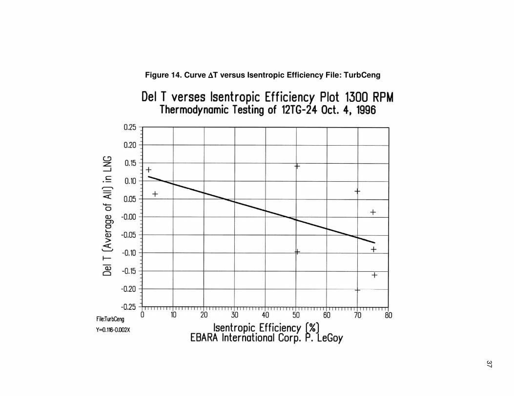
Figure 14. Curve ∆∆∆∆T versus Isentropic Efficiency File: TurbCeng

37

Figure 15. Curve ∆∆∆∆T versus Isentropic Efficiency File: Turb40DA

38

Figure 16. Curve ∆∆∆∆T versus Isentropic Efficiency File: Turb40DB

39

40

5.6 Two-Stage Turbine

The following items are actual test data in their reduced form and the resulting

curves. At this point the test crew was very familiar with the Silicon Diode

temperature sensors and the temperature results are more believable.

5.6.1 Hydraulic & Electrical Data - Reduced Data & Curves

Test No.: 96335-T1 December 11, 1996

Reduced Data Sheets: (See Appendix 19)

Reduced Hydraulic Data Sheets (Orifice Coefficients and Turbine Test Points)

1. Sheet: 96335-T1, File: Turb49.

Curves: Flow, Head, Power and Efficiency

1. File: Runtr49A (See Figure 17)

2. File: Runtr49B (See Figure 18)

Figure 17. Curve Cryoturbine Test 278mm Dia. Runner Dec. 11, 1996; File: Runtr49A

0 10 20 30 40 50 60 70 80 90 100 110 120 130 140 150 160 170 180 190 200 210 220 230 240

FLOW (m3/hr)

0

20

40

60

80

100

120

140

160

180

200

220

240

260

280

300

320

340

360

TU

RB

INE

HE

AD

(m

)

0

20

40

60

80

100

120

140

160

180

200

220

240

260

280

300

320

340

360

TU

RB

INE

GE

N.

EF

F (

%)

2400 RPM

2800 RPM

3000 RPM

CRYOTURBINE TEST AS TWO STAGE UNIT278mm Dia. Runner Dec. 11, 1996

EFFs

HEADs

EBARA International Corp

Model No. 4TG-12/2Date: February 19, 1997 P. LeGoy

(Run 33) File: Runtr49A

Liquid: LPG, S.G., .599 Temp -48C

41

Figure 18. Curve Cryoturbine Test 278mm Dia. Runner Dec. 11, 1996; File: Runtr49B

0 10 20 30 40 50 60 70 80 90 100 110 120 130 140 150 160 170 180 190 200 210 220 230 240

FLOW (m3/hr)

0

20

40

60

80

100

120

140

160

180

200

220

240

260

280

300

320

340

360

TU

RB

INE

HE

AD

(m

)

0

20

40

60

80

100

120

140

160

180

200

220

240

260

280

300

320

340

360

PO

WE

R (

kW

)

2400 RPM

2800 RPM

3000 RPM

CRYOTURBINE TEST AS TWO STAGE UNIT278mm Dia. Runner Dec. 11, 1996

POWER (kW)

HEADs

EBARA International Corp

Model No. 4TG-12/2Date: February 19, 1997 P. LeGoy

(Run 33) File: Runtr49B

Liquid: LPG, S.G., .599 Temp -48C

42

43

5.6.2 Thermodynamic Data - Reduced Data & Curves

Test No.: 96335-T1 December 11, 1996

Note: Silicon Diode sensors are very delicate, are easy to break and can easily be

incorrectly set up. Test and R & D persons had everything working properly for this test

where other tests not reported here were not as fortunate.

Reduced Data Sheets: (See Appendix 20)

1. File: Turb49 for 2400 RPM, 2800 RPM and 3000 RPM.

2. File: Turb49 Average of Sensors at 2400 RPM, 2800 RPM and 3000 RPM

Curves: ∆T verses Isentropic Efficiency all data evaluated with Silicon Diodes

1. File: Turb49C. (All Speeds data – Least Squares) (See Figure 19)

2. File: Turb49D. (3 speeds – Least Squares) (See Figure 20)

3. File: Turb49E. (2800-RPM Average of Sensors and 3rd

order polynomials both tested

and theoretical data.) (See Appendix 21)

Figure 19. Curve ∆∆∆∆T versus Isentropic Efficiency File: Turb49C

44

Figure 20. Curve ∆∆∆∆T versus Isentropic Efficiency File: Turb49D

45

46

Chapter 6.0 ERROR ANALYSIS

The Uncertainty Analysis was done by Mehmet Kanoglu, M.Sc. and Yunus A.

Cengel, Ph.D., P.E.39

The initial equipment error data came from the test

department and the R & D department. Included are the methods by which R & D

came up with the basic error numbers.

The Error in the temperature reading using the silicon diode at the turbine inlet is

found by simply taking the manufacturer’s reported error and multiplying it by 1/3.

Then add up all of the bias errors together. This gives the user a reasonable

value to use in an error analysis because the manufacturer reports worst case

error. The manufacturer reports ± .2°F error for the silicon diode style

temperature sensor. Multiplied by 1/3 is . ± 0.067°F. For the Current source the

manufacturer reports ± 0.009°F Multiplied by 1/3 is ± 0.003°F. For wire voltage

bias the manufacturer reports no measurable uncertainty due to the 4 wire

configuration used. The current source and the voltage wire bias are negligible

they drop out in Error = √Σ(T1-n)2.

∴∴∴∴ Total Error = ±±±± 0.067°°°°F.

The Error in the temperature reading using a thermocouple at the turbine outlet is

found the same way. The manufacturer reports ± 3.825°F error for the

thermocouple style temperature sensor. Multiplied by 1/3 is ± 1.274°F. The

manufacturer of the current transmitter reports ± 0.255°F error for the sensor.

Multiplied by 1/3 is ± 0.085°F. The manufacturer of the temperature sensor

interface board reports ± 0.283°F error for this temperature sensor. Multiplied by

1/3 is ± 0.509°F. In this temperature measurement scheme there is a signal

conditioner, the thermocouple wire and an analog to digital converter these have

all been assumed to have too small an affect on temperature to be considered.

Again using Error = √Σ(T1-n)2. ∴∴∴∴ Total Error = ±±±± 1.374°°°°F.

47

Chapter 7 DISCUSSION OF RESULTS

7.1 The original goals

The goals of the turbine project from the Thermodynamic and Hydraulic Testing of

Cryogenic Turbines standpoint were.

1. Produce, test and demonstrate a power recovery turbine generator, which will

replace the JT valve in the refrigeration cycle for liquefaction processes.

2. Show by testing, the power recovery turbine generator breaks down pressure,

produces electric power, and lowers the temperature of the process liquid.

3. Show a speed controlled power recovery turbine generator will operate at various

pressure and flow combinations “operating points” and produce performance maps

“curves”, of said points.

4. Demonstrate goals 2 and 3 above through repeating results of “benchmark” tests

thus providing evidence JT valves can be replaced with a power recovery turbine

generator and subsequently increase the total efficiency of Liquefaction processes.

7.2 Technical Innovations, why things were done to Attain the

Goals

• The Variable Speed Design was a natural requirement of the type of service for

which the turbine generator was built. It was also a customer requirement. This is due

to the nature of operation parameters of most Cryogenic Liquefaction plants. Plants

operate at various head and flow points. By varying the speed of the turbine runner,

the fluid impact angle is adjusted on the runner in such a way as to control the

efficiency of the turbine. When a plant is constructed many of the operating points are

predetermined. Even the best predictions have some margin of error. So through

time and normal plant operations the operational point locations with respect to head

and flow are adjusted to optimal locations. Also the production gas changes over time

depending upon supply and demand in the market. These variables are good

48

reasons to have a power recovery turbine that will change its operational

characteristics to match plant operations while continuously seeking out the

maximum efficiency, through speed changes.

• Turbine Testing Requirements were somewhat unknown when testing began. The

first task was testing the turbine as a pump.6

The first turbine testing was to experimentally put a load on the turbine and see what

happed. Caution was the main concern. Using a test procedure TP-140012A (See

Appendix 11) that was modeled around a pump test procedure the turbine testing

began. The first testing was done without energizing the generator excitation field.

Using a pump hydraulically more powerful than the turbine it was controlled by

variable speed as a booster pump. It was easy to run the turbine up and down the

speed curve in a free spinning zero-torque condition.

During this free spinning testing many procedural requirements were defined. First it

became apparent there were certain valve sequences to follow. The first testing was

fraught with obstacles such as pressure relief valves popping off and data gathering

signal interference. This beginning series of testing was dedicated to debugging.

The generator excitation field was energized. The tachometer signals had problems

caused by the variable frequency power and those had to be addressed. During this

period of testing many of the generator-electrical parameters were deciphered and

that part took the VSCF drive people almost a week.3, 20

Generation was achieved in

fits and starts. When performance data was initially calculated it was done on a point

by point basis. Each point was calculated and hand plotted. This allowed testing to

continue in a discovery mode. Using this technique, it was easy to identify when

instrumentation was acting incorrectly and when basic calculation assumptions were

incorrect. This took much time but techniques were perfected and the first good

results came about on February 15, 1996. See Figures 8 & 9 and Sections 5.1, 5.2

49

and 5.5.1.1 for calculations and data. This successful test became the benchmark

test.

Testing on October 4, 1996 is of interest in this thesis because it included new and

more accurate temperature measurement devices; Silicon Diodes. These sensors

are more accurate and they have an accuracy within the range necessary to show

the temperature drop created by the turbine.

• Data Reduction Algorithm Modifications were made to the spread sheet items listed

in figures 8 & 9 and the correction formula is listed on page 25 Pin = (P in 2 “Raw

Data”) + (∆P*0.268). This correction was added to the data reduction algorithms

because the inlet pressure tap to the turbine was incorrectly located. This tap is one

of the primary pressure measurement locations used to determine Total Dynamic

Head (TDH). The pressure tap was located in the vena contracta of the fluid stream

and that caused the pressure measurement to be low. This formula proportionally

increased the value of measured pressure entering the turbine and the results were

more in line with results that came from a correctly placed pressure tap. During later

testing the pressure taps were placed in a better location and this was no longer a

problem. See figure 5 for the locations of the various pressure taps. On February 15

the tap was on the orifice tap and on October 4 the tap was at the entrance to the

turbine itself.

• The 1300-rpm temperature data is the only data represented for figures 14-16

because the Silicon Diodes failed during and after this test. The Silicon Diode

temperature sensors are fragile and expensive. Therefore the only data

thermodynamically of interest is the 1300-rpm data where the sensors were partially

working. The turbine seems to have better efficiency at the 1300-rpm speed therefore

the turbine was run at this point first to get that data before equipment failed. It

seemed logical if the turbine ran at its maximum efficiency the temperature drop

would be more dramatic.

50

• Testing of the second turbine was the result of the question: What if? What if the one

turbine’s performance was design specific? What if the same results could not be

achieved with a multistage turbine or a turbine that was required to run at 2-pole

speeds? What if the power extraction process would not work in another liquid such

as LPG? The simplest quickest way to answer these questions was to build another

prototype and design it to answer these questions. Therefore the two-stage turbine

(See Appendix 3) was built and tested in LPG at 2-pole speeds.

7.3 Results

• Figures 8 & 9 are the benchmark test results from February 15, 1996. These data are

broken down into two graphs with multiple curves on each. Figure 8 is dedicated to

the efficiency data Figure 9 is dedicated to the power data. The HEAD’s curve on

each is the operational point curve. This curve depicts the user’s operating conditions

at various speeds. The EFF’s curve is the isentropic efficiency curve. The isentropic

efficiency represents the power extracted from the process stream. This is (kinetic

energy)/(electric energy) as the power is extracted the liquid will cool. The zero-

torque curve is the curve mapped out during the turbine free spinning. The power

curve on Figure 9 is merely the measured electrical power recovered. The tabulated

data can be found in both the reduced and raw format, (See Appendix 12). All of the

calculations done to produce these curves are represented as example problems and

algorithms in sections 5.1 and 5.2. These graphs represent the true performance

map of the turbine and represent the successful prediction of the turbine operational

characteristics.

• Figures 10 and 11 are presented in the same format as Figures 8 & 9. They are

represented to provide supporting documentation for the temperature drop

calculations and the resulting graphs depicting the temperature drops Figures 14-16.

They are also presented to provide completeness of the hydraulic testing portion of

51

this thesis. The tabulated data can be found in both the reduced and raw format,

(See Appendix 13).

• Figures 12 and 13 depict the temperature drop caused by the turbine during

benchmark testing of February 15. In Figure 12 all of the data collected were fit to a

line at each speed. (See Appendix 14 for the fit calculations.) Most but not all of the

linear fits showed a trend toward cooling of the liquid during power recovery. But

three of the speed lines showed a trend toward heating. Since it seems logical

energy extraction is better when efficiency is better; then at the better efficiencies,

(say better that 50%), the measurable temperature drop would be more dramatic. In

Figure 13, all data with efficiency less than 50% are thrown out and the graph

showed even stronger evidence of the cooling trend. At this point only two lines

showed a trend toward heating and the other five lines show a more dramatic trend

toward cooling. Although this data by itself is convincing it needs more evidence

because this data was collected with a thermocouple. Thermocouples have an error

almost as dramatic as the temperature drop itself. As a matter of practice several

forms of least squares fit were applied to the temperature data. A third order

representation of this is found as Appendix 15.

• Figures 14-16 more strong evidence of the trend toward cooling of the liquid during

power recovery. Figure 14 comes from an average of all of the temperature sensors

used in the testing of the turbine on October 4. (See Appendix 16) Using a

comparison of each sensor to one another: Silicon Diodes to Thermocouples, Silicon

Diodes to Silicon Diodes and Thermocouples to Thermocouples. Each type of

combination was evaluated to decipher the best results. (See Figure 16) Results

showed four of the six sensor combinations indicated a cooling trend. Silicon Diodes

showed a definite negative slope toward cooling. Technical difficulties in the sensor

wiring the Silicon Diode data could not be trusted. Therefore an average of all of the

sensor data was taken and the trend in the data was obvious. (See Figure 14)

52

Another linear least square curve was done using each data point from each sensor.

It also showed an obvious trend toward cooling. (See Figure 15) Therefore this was

considered strong evidence of the cooling trend caused by power recovery and

conversion of kinetic energy to electricity from the process liquid. Again, as a matter

of practice, several forms of least squares fit were applied to the temperature data. A

third order representation of this is found as Appendix 17 and 18. Appendix 18 is

compared to Double Interpolated data a representative of which is Appendix 22.

These data are from the testing and also data which came from methane properties

found on tables.25

• Figures 17 and 18 are composed of the same elements as Figures 8 & 9. They are

represented to provide supporting documentation for the temperature drop

calculations and the resulting graphs depicting the temperature drops in Figures 19 &

20. They are also presented to provide completeness of the hydraulic testing portion

of this thesis. The tabulated data can be found in both the reduced and raw format.

(See Appendix 19)

• Figures 19 & 20 represent the most believable evidence of the trend toward cooling

indicated by the Silicon Diodes. Figure 19 represents a linear least squares analysis

of the Silicon Diode data for all speeds combined on one graph. (See Appendix 20

for the fit calculations) Figure 20 is the Silicon Diode data represented alone for each

speed. (See Appendix 20 for the fit calculations) The results speak for themselves.

The error involved with the Silicon Diode temperature measurement is ± 0.067°F and

the error involved with the Thermocouple sensors is ± 1.374°F the Silicon Diode data

is more convincing than the Thermocouple data. (See section 6.1) As a matter of

practice several forms of least squares fit were applied to the temperature data a

third order representation of this is found as Appendix 21. Appendix 21 is compared

to Double Interpolated data a representative of which is Appendix 22.5 This data is

53

from the testing and also data that came from methane properties looked up on

tables.25

7.4 Significance of Results

• Variable Speed Power Recovery Turbines are valuable to the Liquefaction industry

by virtue of their operational characteristics.

• The higher the efficiency the greater the cooling effect.

• The mapping of performance curves enables turbine performance and efficiencies to

be maximized.

• New measurement and testing techniques have been defined and proven.

54

CONCLUSION

Primary goals of this thesis were to design, build and test, both hydraulically and

thermodynamically, the cryogenic turbine and the associated facilities needed to

complete the task. The author has tried to include most of the design features, the

collected data and the actual algorithms used. Taking note of the rather lengthy appendix

it becomes obvious this thesis is a body of work, which tries to cover the aforementioned

goals. Also this thesis lays down a record of the testing methods used for a Variable

Speed Constant Frequency (VSCF) hydraulic turbine concept which had not been done

before.3, 20

As a side note G. Louis Weisser, General Manager of EBARA International

Corporation in Sparks Nevada, patented this turbine.4

The best indication of the potential of this type of turbine is read off the graphs generated

during the testing of February 15, 1996. (See Figures 8 & 9) These graphs clearly show

the prototype was getting efficiencies close to 78% and with some Computational Fluid

Dynamic analysis the efficiency could easily be 80% as stated in the introduction. It is

interesting to note the 78% efficient device is better than the original cost benefit analysis

proposed device by 18% (See Appendix 1). EBARA International Corporation, for its own

power recovery efforts, will eventually use this turbine.

Also it has been shown, during the Hydraulic Power Extraction process, there is a

measurable amount of temperature drop (See Figure 20). The traditional method of

reducing the pressure in a process stream is by a Joule Thompson Valve. It has been

shown the cryogenic hydraulic turbine generator is an excellent replacement for the JT

valve. Therefore, the cryogenic turbine can be used to reduce very high Liquefaction

process pressures. This pressure introduced into the fluid during the Liquefaction process

has been successfully reduced without inducing much friction in the liquid by the turbine

generator. The idea of the turbine generator is to reduce the liquid pressure to ambient,

or near ambient pressure, in a safe efficient manner, which will dispose of the excess

kinetic energy in the process stream. A 100% efficient cryogenic turbine will reduce the

55

pressure without causing the liquid to heat up. Using a Joule Thompson Valve the liquid

will heat up due to friction. An example double interpolation problem is shown with a

comparison of the JT valve with actual turbine data and the 100% efficient turbine case.

(See Appendix 22) Dr. Cengel first represented this analysis in his paper.5

56

RERENCES

1. Kimmel, H. E., “Speed controlled turbine expanders”, Hydrocarbon Engineering

May/June 1997.

2. Cengel, Y. A., and Kimmel, H. E. “Power Recovery Through Thermodynamic Expansion

of Liquid Methane”, Proceedings of the 59th Annual American Power Conference, Illinois

Institute of Technology, Chicago, April 1997.

3. LeGoy P.R., AND KIMMEL, H. E. “Cryogenic Turbine Generators with Variable Speed

Constant Frequency Control”, Proceedings of the 60th Annual American Power

Conference, Illinois Institute of Technology, Chicago, April 1998.

4. Weisser, G. L. “Hydraulic Turbine Power Generator Incorporating Axial Thrust

Equalization Means” United States Patent 5,659,205 August 19, 1997.

5. Cengel Y. A., Department of Mechanical Engineering University of Nevada, Reno “The

Effect of Power Generation on the Temperature of Cryogenic Liquid Methane” Prepared

for EBARA International Corporation May 30, 1996.

6. LeGoy P. R., “Test Procedure TP-140011B” Prepared for EBARA International

Corporation October 25, 1995.

7. LeGoy P. R., ‘Test Procedure TP-140013A’ Prepared for EBARA International

Corporation January 18, 1996.

8. LeGoy P. R., “Test Procedure TP-140008” Prepared for EBARA International Corporation

December 4, 1996.

9. Sheldon, L. H., “An Analysis of the Applicability and Benefits of Variable Speed

Generation for Hydropower” Small Hydro Power Fluid Machinery 1984 Pg. 201 – 208.

The Winter Meeting of the American Society of Mechanical Engineers New Orleans,

Louisiana December 9-14, 1984.

10. “Small Hydro Plant Development Program: DOE/ID/01570—T21 (Volumes 1, 2 & 3)”

October 1980 U. S. Department of Energy Distributed by National Technical Information

57

Service U. S. Department of Commerce Springfield, VA

11. Pfau A. “Modern Hydraulic Prime Movers” Consulting Engineer Hydraulic Turbine

Division. Copyright 1943, by Allis-Chalmers Mfg. Co.

12. Wagner S. K., Webb D. R., Mayo H. A. Jr., Papadakis C. N.. “Small Hydro Power Fluid

Machinery 1984” Presented at The Winter annual meeting of the American Society of

Mechanical Engineers New Orleans, Louisiana December 9-14, 1984. The American

Society of Mechanical Engineers United Engineering Center 345 East 47th Street New

York, N. Y. 10017.

13. “Wind Turbines Technology Status” EPRI Technical Assessment Guide, Electrical Supply

1993 EPRI # TR-102275-V1R7 June, 1993 Pg. 8-138 Sec. 8.7.3

14. Lobanoff and Ross “Centrifugal Pumps: Design & Application” Second Edition Gulf

Publishing Company Book Division P. O. Box 2608, Houston, Texas 77252-2608

15. Hicks T. G. “Power Generation Calculations Reference” Guide Second Edition Pg. 193 -

194. Published by McGraw - Hill.

16. Wislicenus G. F. “Fluid Mechanics of Turbo Machinery” Second ed. New York, Dover

Publications 1995 Pg. 80 - 81

17. Chapman S. J. “Electrical Machinery Fundamentals” Second Edition. Pg. 565 - 567 & 616

- 621. Published by McGraw - Hill.

18. “Small and Mini Hydropower Plants” Published by McGraw - Hill

19. French M. J. “Energy Derived From Expansion of Liquefied Gas” U.S. Patent # 3203191,

New Maiden England assignor to Conch International Methane Limited, Nassau

Bahamas, a company of the Bahamas. Filed July 20, 1961.

20. Richardson R. D. and Eardman W. L. “Variable Speed Wind Turbine” U.S. Patent #

5083039, San Ramon CA., & Livermore CA. Filed February 1, 1991. Assignee: U.S.

Windpower, Inc. Livermore CA.

21. Meacher J. S. and Ruecitta D. E. “Hermetic Turbine Generator” U.S. Patent # 4362020,

58

Bailston Lake, New York and, Bailston Spa, New York. Filed December 7, 1982.

Assignee: Mechanical Technology Inc. Latham, New York.

22. Sato S., Yamamoto H., Okayama Y. “Pipeline Built-In Electric Power Generating Set”

U.S. Patent # 4740711, All of Kanagawa Japan. Filed April 26, 1988. Assigned: Fuji

Electric Co., Ltd., Kanagawa Japan.

23. Johnson L.L. and Renaudin G. “Liquid Turbines improve LNG operations”; The Oil and

Gas Journal, Nov. 18, 1996 v94 n47 p31(4).

24. Bean H. S. “Fluid Meters Their Theory and Application” 6th edition 1971 Pg. 65. Published

by American Society of Mechanical Engineers United Engineering Center 345 East 47th

Street New York, N. Y. 10017

25. Friend D. G., Ely J. F., and Ingham H. “Thermophysical Properties of Methane”,

Thermophysics Division, National Institute of Standards and Technology, Boulder

Colorado 80303 Copyright 1989 U. S. Secretary of Commerce on behalf of the United

States. Copyright is assigned to the American Institute of Physics and the American

Chemical Society.

26. Fox and McDonald “Introduction to Fluid Mechanics” Third Edition 1985, Published by

John Wiley & Sons.

27. Cengel Y. A. “Thermodynamics An Engineering Approach” Second Edition and Michael A

Boles McGraw Hill, Inc. Princeton Road, S-1 Highstown, NJ 08520

28. Kreyszig “Advanced Engineering Mathematics” Fifth Edition Pg. 819, Published by John

Wiley and Sons. 1983.

29. Karassik, Krutzsch, Fraser and Messina “Pump Handbook” Second Edition. Published by

McGraw - Hill 1986.

30. Rayleigh, Lord “The Turbo-Expander for Gas Liquefaction” (1898) Nature, 58, 199

31. Thrupp E. C. “A simple Liquefying System Using an Expansion Turbine” British Patent

No. 26767 of 1898 and U.S. Patent No. 642,505 of 1900.

59

32. Johnson J. E., Jr. “An Apparatus for Liquefying Gases” U.S. Patent No. 627,696 of 1899

33. Crommett C. F. and O. J. “A Refrigerative Expansion Turbine with a Tangential Inward

Flow Pattern” U.S. Patent No. 1,110,423 of 1914.

34. Davis H. N. “An Expansion Turbine of Unusual Thermodynamic Concept” U.S. Patent No.

1,420,626 of 1922.

35. Linde. R. “Commercial Application of an Expansion Turbine for Gas Liquefaction” (1934)

Z. ges. Kalteindustr., 41, 193-6.

36. Zerkowitz G. “An Inward Radial Flow Turbine” German Patent Nos. 608,963 (1935) and

627,369 (1936). British Patents Nos. 433,800 and 434,363 of 1935. U.S. Patent no.

2,165,994 of 1939.

37. Kapitza P. “Refrigerative Turbines” (1939) Russian J. Phys. (English edn.), 1, 7-28.

38. Swearingen J. S. “Elliott-Sharples Radial Flow Reaction Turbine”, (1947) Trans.

American Institute of Chemistry Engrs., 43, 83-90.

39. Kanoglu M., Cengel Y. A. “Uncertainty Analysis” Prepared for EBARA International

Corporation January 22, 1997.

60

APPENDIX