Embed Size (px)
Citation preview

Thermodynamic modelling of ultra-long-term durability of cementitious binders for waste immobilisation
By
Dale Prentice
Academic Supervisors:
John L. Provis and Susan A. Bernal
Industrial supervisors:
Mark Bankhead and Martin Hayes
A thesis submitted in fulfilment of the requirements for the degree of
Doctor of Philosophy
Department of Materials Science and Engineering
The University of Sheffield
September 2018


I
Abstract
Treatment of intermediate-level waste (ILW) generated as a by-product from nuclear power in the UK
requires a long-term strategy to safely dispose of the waste. Encapsulation of ILW in a cement matrix
is the current UK methodology, followed by storing the waste for potentially thousands of years in
geological disposal facilities (GDFs). Understanding of the cement phase assemblage is key to
predicting how these cements will behave in the long term. Thermodynamic modelling of cement
hydrate phases is a powerful tool which can be used to predict the effects of cement hydration. This
thesis investigates the quality of thermodynamic modelling to predict stable phase assemblages of
blast furnace slag-Portland cement (BFS-PC) cements, representing UK nuclear industry practice,
under conditions that are expected during the storage of encapsulated ILW.
Three BFS-PC ratios (1:1, 3:1 and 9:1) were tested at different curing ages to determine the degree of
hydration of the precursor materials to use as input parameters for thermodynamic modelling.
Characterisation of the phase assemblages were compared to the thermodynamic modelling results
to assess the robustness of the modelling approach. A solid solution model for C(-A)-S-H was used to
explicitly incorporate aluminium into the C-S-H phase to more accurately portray the chemical
structure in the BFS-PC system. Thermodynamic modelling was capable of accurately simulating the
change in phase assemblage as curing time increased. Variation of precursor materials was effectively
modelled.
Temperature fluctuations are expected to occur within the GDF once the waste is stored within it. BFS-
PC samples were cured for one year at 35 °C followed by periods of curing at 50 °C, 60 °C and 80 °C.
Major phase changes were not observed until the curing temperature reached 60 °C, whereby
hemicarbonate and ettringite destabilised. At a curing temperature of 80 °C, the sulphate and
carbonate AFm and AFt phases were not observed in cement phase assemblages, however siliceous
hydrogarnet was present. Two thermodynamic modelling approaches were used to simulate the
effects of temperature change. It was determined that the thermodynamic simulation should not
contain siliceous hydrogarnet when simulating BFS-PC hydration up to 60 °C but should contain
siliceous hydrogarnet for higher temperatures.

II
The Pitzer model used as a means to produce activity coefficients, was compared with the generalised
dominant electrolyte activity model, Truesdell-Jones, to assess whether modelling of cement phases
may be improved. A large ion-interaction parameter database was required to use the Pitzer model
for simulating cement hydration. Solubility studies of cement phases and cement pore solution data
were used as a means to compare the activity coefficient models. The more complex nature of the
Pitzer model caused the simulations to require runtimes up to 18 times more than the Truesdell-Jones
method. The pore solution of the BFS-PC systems was compared with the predictions from the activity
coefficient models, which determined that the Pitzer model provided minimal improvement over the
Truesdell-Jones method. However, the Pitzer model proved more effective for simulating higher
concentration systems, therefore, the Pitzer model may be required in future modelling projects when
simulating concentrated groundwater interactions with the cement wasteforms.

III
Acknowledgements
Before I began working on this thesis I knew relatively nothing of cement or its importance and
versatility in this world. There are some people whom I need to thank for opening my eyes to the
wonderful world of cementitious materials. First and foremost, I must express my gratitude to my
academic supervisors, Professor John L. Provis and Dr. Susan A. Bernal. Without their tutelage and
never-ending vigour for the subject matter, I would never have been able to complete this work. The
years spent on this work flew by due to their optimism and amazing support they shared with me. For
that I will always be grateful.
Thanks must be given to my industrial sponsor, The National Nuclear Laboroatory, for co-funding this
project and specific thanks to my industrial supervisors Dr. Mark Bankhead and Dr. Martin Hayes. With
help from Mark and Martin, I was always able to keep focused on the bigger picture of the project and
how my work may be used for practical means. A special thanks to Mark for providing a wonderful
work environment during my placement at NNL and helping me become a part of his team for a short
period of time.
I owe a great deal of gratitude to all of those who helped train me and provide a fantastic experience
over the years working in the Immobilisation Science Laboratory. Thanks to Dr. Oday Hussein for
training me on every piece of equipment and he’s unending patience with the ‘Pore press saga’. A
great deal of thanks to Dr. Samuel A. Walling, Dr. Laura J. Gardner and Dr. Brant Walkley for helping
me analyse so many different pieces of data and teaching me how to streamline my efforts. Also, a
grounding thanks to Dr. Daniel J. Bailey for always reminding me that cements are lame, and ceramics
are amazing.
Of course, I must thank all of the other students who I shared countless experiences with from the
office over the years and helped me see the fun side of academic work, along with the scientific. I
would inevitably forget to mention someone, so instead, I express my gratitude to everyone who
shared the office with me.
Finally, I would never have had the courage to pursue my goals without the support of my family and
to them I offer my greatest thanks.
To Ali, Alex-Craig, Charlie and Moose, on Wednesdays we wore pink. You made me who I am. Where would I be without
you? Probably in a skip on Crookesmoore road. You complete me. I wouldn’t be me without you. Thanks guys, you basically
wrote this. All of my love,
The Biggest D

IV
Contents
Abstract .................................................................................................................................................... I
Acknowledgements ................................................................................................................................ III
List of Figures ........................................................................................................................................ VII
List of Tables ......................................................................................................................................... XV
1 Synopsis........................................................................................................................................... 1
2 Introduction and Literature Review ................................................................................................ 3
2.1 Nuclear Waste Management .................................................................................................. 3
2.1.1 Geological disposal facility .............................................................................................. 5
2.1.2 Temperature profile of cemented wasteforms in the GDF ............................................ 8
2.2 Portland cement and blended cement ................................................................................... 9
2.2.1 Portland cement ............................................................................................................. 9
2.2.2 Cement and supplementary materials.......................................................................... 10
2.2.3 Blast Furnace Slag (BFS) ................................................................................................ 11
2.2.4 Phase assemblage of BFS-PC cements .......................................................................... 11
2.2.5 Pore solution ................................................................................................................. 19
2.3 Thermodynamic modelling for cementitious systems.......................................................... 21
2.3.1 Law of mass action (LMA) and Gibbs energy minimisation (GEM) methods................ 22
2.3.2 Activity coefficient models ............................................................................................ 26
2.4 Cement thermodynamic database ....................................................................................... 29
2.5 Conclusion ............................................................................................................................. 31
3 Materials and Methods ................................................................................................................. 33
3.1 Materials ............................................................................................................................... 33
3.2 Mix design ............................................................................................................................. 34
3.3 Analytical techniques ............................................................................................................ 34
3.3.1 Selective dissolution – EDTA dissolution....................................................................... 34
3.3.2 X-ray diffraction (XRD) .................................................................................................. 36
3.3.3 27Al and 29Si magic angle spinning (MAS) nuclear magnetic resonance (NMR) ............ 37
3.3.4 Scanning electron microscopy ...................................................................................... 42
3.3.5 Pore solution extraction and ICP-OES ........................................................................... 42
3.4 Thermodynamic modelling ................................................................................................... 42
4 Phase evolution of slag-rich cementitious grouts for immobilisation of nuclear wastes: an
experimental and modelling approach ................................................................................................. 45
4.1 Introduction .......................................................................................................................... 45

V
4.2 Experimental methodology................................................................................................... 47
4.2.1 Mix Design ..................................................................................................................... 47
4.2.2 Analytical techniques .................................................................................................... 47
4.2.3 27Al and 29Si MAS NMR .................................................................................................. 48
4.2.4 Thermodynamic modelling ........................................................................................... 48
4.3 Experimental results and discussion ..................................................................................... 49
4.3.1 X-ray diffraction. ........................................................................................................... 49
4.3.2 27Al MAS NMR ............................................................................................................... 51
4.3.3 29Si MAS NMR ................................................................................................................ 54
4.3.4 Determination of degree of hydration using 29Si MAS NMR and selective dissolution 58
4.4 Thermodynamic modelling ................................................................................................... 61
4.4.1 Calculating the hydrate phase assemblage................................................................... 61
4.4.2 Comparison of C-A-S-H gel structural characteristics between model and experiment
63
4.4.3 Modelling of aged BFS:PC cements............................................................................... 64
4.5 Conclusions ........................................................................................................................... 66
5 Thermodynamic modelling of BFS-PC cements under temperature conditions relevant to the
geological disposal of nuclear wastes ................................................................................................... 67
5.1 Introduction .......................................................................................................................... 67
5.2 Effect of temperature on the mineralogy of cements .......................................................... 68
5.3 Experimental methodology................................................................................................... 70
5.3.1 Mix Design ..................................................................................................................... 70
5.3.2 Analytical techniques .................................................................................................... 71
5.4 Experimental Results and Discussion .................................................................................... 73
5.4.1 Degree of hydration of BFS ........................................................................................... 73
5.4.2 X-ray diffraction and qualitative analysis ...................................................................... 74
5.4.3 Determination of chemical composition of the C(-A)-S-H phase by SEM ..................... 81
5.4.4 Chemical composition of hydrotalcite-like phase using SEM-EDS ................................ 87
5.5 Evaluation of the efficacy of thermodynamic modelling ...................................................... 90
5.5.1 Selection of potential phase assemblage constituents ................................................ 90
5.6 Phase assemblage as a function of temperature .................................................................. 91
5.6.1 Chemical composition of C-A-S-H phase using thermodynamic modelling as a function
of temperature .............................................................................................................................. 95
5.6.2 Chemical composition of the hydrotalcite-like phase (MA-OH-LDH – solid solution
model) using thermodynamic modelling as a function of temperature ...................................... 98
5.7 Conclusions ........................................................................................................................... 99
6 Using Pitzer parameters in GEMS for predicting blended cements. .......................................... 101

VI
6.1 Introduction ........................................................................................................................ 101
6.2 Modelling approach ............................................................................................................ 102
6.2.1 Activity coefficient models .......................................................................................... 102
6.2.2 Incorporating Pitzer equations into GEMS ................................................................. 106
6.2.3 Estimating Pitzer parameters ...................................................................................... 107
6.2.4 Testing applicability of the Pitzer model and simulation setup .................................. 108
6.2.5 Assessing the quality of the calculated data ............................................................... 109
6.3 Pore solution extraction from hydrated samples ............................................................... 110
6.4 Modelling results comparing the Pitzer model with the Truesdell-Jones equation ........... 111
6.4.1 Portlandite .................................................................................................................. 112
6.4.2 Ca-Al-OH ...................................................................................................................... 116
6.4.3 Ca-Al-SO4-OH ............................................................................................................... 120
6.4.4 Ca-Al-CO3-OH .............................................................................................................. 126
6.4.5 Mg-Al-OH .................................................................................................................... 127
6.4.6 Ca-Si-Al-OH .................................................................................................................. 133
6.5 Pore solution of blended cements ...................................................................................... 150
6.5.1 Experimental results ................................................................................................... 150
6.5.2 Thermodynamic modelling of pore solutions ............................................................. 154
6.5.3 Influence of the different modelling methods............................................................ 158
6.5.4 Computing time .......................................................................................................... 161
6.6 Conclusions ......................................................................................................................... 161
7 Conclusions and future work ...................................................................................................... 163
7.1 Conclusions ......................................................................................................................... 163
7.2 Future work ......................................................................................................................... 165
8 Appendix ..................................................................................................................................... 167
8.1 Analysis of siliceous hydrogarnet phase ............................................................................. 167
8.2 Summary of SEM-EDS results .............................................................................................. 169
8.3 Thermodynamic data for phases used in simulations ........................................................ 170
8.4 Pitzer parameter database ................................................................................................. 180
References .......................................................................................................................................... 186
Publications from thesis ...................................................................................................................... 210
Journal Publications ........................................................................................................................ 210
Conference Publications ................................................................................................................. 210
Other conference presentations ..................................................................................................... 210

VII
List of Figures
Figure 2.1: Volume proportion of total packaged waste comprising of HLW, ILW and LLW (VLLW
included in the LLW) as of 2016 [4]. ....................................................................................................... 4
Figure 2.2: Schematic of the multiple barrier approach for intermediate level waste and high level
waste [23]. .............................................................................................................................................. 6
Figure 2.3: Schematic of a generic GDF proposed for in the UK (SF: spent fuel; UILW: unshielded ILW;
SILW: shielded ILW)[28]. ......................................................................................................................... 7
Figure 2.4: Approximate temperature profile of an ILW waste package due to GDF emplacement and
backfilling [8,10,30,31]. ........................................................................................................................... 8
Figure 2.5: Ternary phase diagram showing the CaO, Al2O3 and SiO2 composition of Portland cement
and SCMs, based on phase diagram produced by Lothenbach et al. [37]. ........................................... 10
Figure 2.6: The C-S-H/C-A-S-H structure depicted using dreierketten units. The green triangles
represent paired silicate dimers, blue triangles are bridging silicon tetrahedra, the red triangles
represent silicon replacement with aluminium, the purple, orange and pink circles represent Ca2+, K+
and Na+ ions respectively. ..................................................................................................................... 14
Figure 2.7: The Ca/Si of C-S-H as a function of a) calcium concentration and b) silicon concentration.
The dotted and solid line indicates the Ca/Si when silica and portlandite forms, respectively. Optimal
solubility data collated by Walker et al. [65] from the following sources: [53,54,65,69–83]. ............. 15
Figure 2.8: Impact of molar ratios of SO3/Al2O3 versus CO2/Al2O3 on the possible phase assemblage of
AFm/AFt phases in the presence of excess portlandite [97]. ............................................................... 18
Figure 2.9: Potassium and sodium concentrations in the pore solution of BFS-PC cements of variable
water to binder ratios (w/b) at different levels of slag replacement. The central black lines indicate the
95% interval within CEM I data collated by Vollpracht et al. [104]. ..................................................... 20
Figure 2.10: The difference in Gibbs energy between portlandite and reactants until the point of
precipitation, thereafter portlandite precipitates out of solution as more Ca(OH)2 is added to the
system. .................................................................................................................................................. 25

VIII
Figure 2.11: Thermodynamic modelling of the activity coefficients for Ca2+ and OH- ions in the Ca(OH)2
system, with varying concentration of Ca(OH)2 added to solution. ..................................................... 25
Figure 2.12: Thermodynamic modelling of brucite and magnesium-oxychloride (MgOxyCl) in the Mg-
Cl-OH system using the Pitzer model (P) and Truesdell-Jones (T) equation. The Pitzer parameters and
solubility data used are from Harvie et al. [100]. ................................................................................. 28
Figure 2.13: No miscibility gaps in the calcium to silicon molar ratios (C/S or Ca/Si) are observed when
predicting the mole fractions of the end-members in the a) CSHQ and b) CNASH_ss models. Modified
from Kulik [64] and Myers et al. [146], respectively. ............................................................................ 31
Figure 3.1: X-ray diffractograms of anhydrous a) PC and b) BFS. ......................................................... 37
Figure 3.2. Fitting of the 29Si MAS NMR spectrum of anhydrous PC: a) experimental data, b) fitted
deconvolution, c) alite spectrum, and d) belite spectrum. ................................................................... 40
Figure 3.3. Fitting of the 29Si MAS NMR spectrum of anhydrous slag: a) experimental data and b) fitted
deconvolution. ...................................................................................................................................... 40
Figure 4.1: X-ray diffractograms of hydrated BFS:PC, a) 1:1, b) 3:1 and c) 9:1 ratios, up to a curing time
of 360 days. ........................................................................................................................................... 50
Figure 4.2: 27Al MAS NMR spectra for a) 1:1, b) 3:1 and c) 9:1 BFS:PC grouts. .................................... 53
Figure 4.3: Example deconvolutions of 29Si MAS NMR spectra for a) 1:1, c) 3:1 and e) 9:1 grouts after
360 days, and 29Si MAS NMR spectra for b) 1:1, d) 3:1 and f) 9:1 grouts from 28 days to 360 days of
curing. ................................................................................................................................................... 55
Figure 4.4: Degree of reaction of BFS within the different blend ratios, based on 29Si NMR MAS
deconvolutions (NMR) and on selective dissolution (EDTA). ............................................................... 60
Figure 4.5: Degree of reaction of calcium silicate clinker phases (alite and belite) within the different
blend ratios, based on 29Si MAS NMR spectral deconvolutions. .......................................................... 60
Figure 4.6: Hydrate phase assemblages predicted using thermodynamic modelling, for a) 1:1, b) 3:1
and c) 9:1 grouts reacting at 35°C, based on the experimentally determined (NMR) degree of hydration
data up to 360 days............................................................................................................................... 62

IX
Figure 4.7: Calculated phase assemblage of BFS:PC cements using the degree of hydration and
precursor materials reported by Taylor et al. [45]. .............................................................................. 64
Figure 5.1: Degree of hydration (DoH) of BFS determined from EDTA selective dissolution, within BFS-
PC blended cements of ratio 1:1, 3:1 and 9:1, for the temperature profiles 360A, 28B, 28C and 28D.
.............................................................................................................................................................. 74
Figure 5.2: XRD patterns of a) 1:1, b) 3:1 and c) 9:1 BFS-PC samples cured at 35 °C for 1 year (360A)
and then at either 60 °C (tC) or 80 °C (tD) for a further 28 days. Phases identified are: C – C-A-S-H, P –
portlandite, E – ettringite, M – monosulphate, H – hemicarbonate, Mc – monocarbonate, Ht –
hydrotalcite, B – belite, and Si – siliceous hydrogarnet. ....................................................................... 76
Figure 5.3: Highlighted low-angle regions of the XRD patterns of a) 1:1, b) 3:1 and c) 9:1 BFS-PC samples
cured at 35 °C for 1 year and then at either 60 °C (C) or 80 °C (D) for up to 28 days. Phases identified
are: E – ettringite, M – monosulphate, H – hemicarbonate, Mc – monocarbonate, and Ht – hydrotalcite
.............................................................................................................................................................. 79
Figure 5.4: XRD patterns for 1:1 BFS:PC cements after curing at 35 °C for one year and being transferred
to 80 °C for up to 360 days (temperature profile D). The C3AS0.41H5.18 and C3AS0.84H4.30 chemical
formulae depict the siliceous hydrogarnet phases available in the CEMDATA14 database. ............... 80
Figure 5.5: Unit cell size plot as a function of Si-hydrogarnet: PDF data used include card numbers 24–
0217 (a = 12.57 for C3AH6); 32–0151 (a = 12.29 for C3ASH4); 31–0250 (a = 12.00 for C3AS2H2)and 33–
0260 (a = 11.846 for C3AS3). References include: [149,210,211,217] and t.s. = this study. ................. 81
Figure 5.6: Histograms of the molar ratios of spot analyses of the 1:1 BFS-PC cement cured at 35 °C for
360 days, showing a) Si/Ca and b) Al/Ca molar ratios determined from calibrated SEM-EDS analysis.
.............................................................................................................................................................. 83
Figure 5.7: Al/Ca versus Si/Ca graph of the a) 1:1 b) 3:1 and c) 9:1 BFS-PC cement cured at 35 °C for
360 days. The dashed oval highlights the region where a C-A-S-H phase with Ca/Si ~ 1.0 – 1.6 and Al/Si
~ 0.1 – 0.2 would appear. The tie lines leading from the centre of the circle lead to the other prominent
cement hydrates which may intermix with C-A-S-H (AFt – ettringite, AFm – monosulphate, CH –
portlandite). The red square denotes the statistically determined Ca/Si and Al/Si ratio for the individual
formulations. ......................................................................................................................................... 84
Figure 5.8: Al/Ca versus Si/Ca graphs for the 3:1 BFS-PC cement cured at 35 °C for 360 days and then
exposed to (a) 35 C, (b) 50 C, (c) 60 C and (d) 80 C for a further 28 days. The dashed oval highlights
X
the region where a C-A-S-H phase with Ca/Si 1.0 – 1.6 and Al/Si 0.1 – 0.2 would appear. The tie lines
leading from the centre of the circle lead to the other prominent cement hydrates which may intermix
with C-A-S-H (AFt – ettringite, AFm – monosulphate and CH – portlandite). The red square denotes
the statistically determined Ca/Si and Al/Si ratio for the individual formulations. .............................. 85
Figure 5.9: BSE-SEM images of 3:1 BFS-PC cement cured at a) 35 °C for 360 days and then exposed to
b) 50 °C, c) 60 °C, and d) 80 °C for a further 28 days. ........................................................................... 86
Figure 5.10: Mg/Si versus Al/Si atom ratios from EDS analysis for the a) 1:1 b) 3:1 and c) 9:1 28B BFS:PC.
Data manipulation was conducted using Mg/Al minimum of 1.0, Mg/Al maximum of 2.5, and Al/Si
maximum of 0.5. The red line highlights the line of best fit through the data points and the Mg/Al value
is taken from the gradient. The green and blue tie-lines are example lines of gradient 2, which is
generally indicative of the lower Mg/Al examples of a hydrotalcite-group LDH. ................................ 88
Figure 5.11: Phase assemblages of a) 1:1, b) 3:1 and c) 9:1 BFS-PC cements determined using the
thermodynamic modelling software GEMS [132]. The prediction of phase formation was determined
as a function of temperature while the remnant precursor content was kept constant. Siliceous
hydrogarnet was only allowed to form above 60 °C, and each graphic shows a break at this point to
reflect the change in model assumptions. The phase notations correspond to: BFS – Blast furnace slag,
PC – Portland cement, C – C-A-S-H, P – portlandite, E – ettringite, M – monosulphate, H –
hemicarbonate, Mc – monocarbonate, Ht – hydrotalcite and Si – siliceous hydrogarnet. .................. 92
Figure 5.12: XRD patterns of a) 1:1, b) 3:1 and c) 9:1 BFS-PC cements exposed to different temperature
regimes. Phases identified are: C – C-A-S-H, P – portlandite, E – ettringite, M – monosulphate, H –
hemicarbonate, Mc – monocarbonate, Ht – hydrotalcite, B – belite and Si – siliceous hydrogarnet. . 94
Figure 5.13: Molar ratios of a) Ca/Si and b) Al/Si within C-A-S-H as a function of temperature using the
two different modelling approaches (SH above, and NS below, a cutoff temperature of 60 °C in each
case) as a function of the BFS:PC ratios. The symbols correspond to SEM-EDS results, while the lines
represent the modelling results. The solid line represents the NS method and the dotted line
represents the SH method. ................................................................................................................... 97
Figure 5.14: Molar ratio of Mg/Al within the magnesium hydrotalcite-like LDH phase of 1:1, 3:1 and
9:1 BFS-PC, using the MA-OH-LDH model developed by Myers et al [123]. ........................................ 98
Figure 6.1: Programme structure for Pitzer parameter database lookup. ......................................... 107
XI
Figure 6.2: Pore press used for acquisition of pore fluid from cured BFS-PC cement samples. The
dimensions of the press are represented: a) before the sample has been compressed, and b) at the
expected maximum level of compression of a cement sample. ........................................................ 111
Figure 6.3: The application of different parameterisations of the Pitzer aqueous solution model to the
prediction of portlandite solubility in NaCl solutions: a) highlighting the importance of selection and
parameterisation of the aqueous species; P(CaOH+) denotes the Pitzer model including CaOH+ in the
calculations, P denotes a fully parameterised Pitzer model without CaOH+, and S denotes the Pitzer
model using only the parameters generated from the Simoes estimation equations; b) showing the
detrimental effect that the Pitzer model with all parameters set to zero (PF – equation 6.17) has on
the predictions in comparison with the Truesdell-Jones (T) equation. Both plots show experimental
data from Duchesne and Reardon [66]............................................................................................... 114
Figure 6.4: Portlandite solubility in a) NaOH and b) KOH, with different aqueous modelling approaches,
Pitzer parameter sets, and aqueous species used for calculations. P denotes a fully parameterised
Pitzer model, T denotes the Truesdell-Jones equation, and S denotes the Pitzer model including
parameters generated only from the Simoes Pitzer estimation equations. Experimental data are from
Duchesne and Reardon [66] (D&R-Exp). ............................................................................................. 115
Figure 6.5: Modelling the aqueous solution within the Ca-Al-OH system based on the solubility data of
Lothenbach et al. [233]. The Pitzer aqueous solution model using parameters from the literature, P,
was compared with parameters obtained from estimating interaction paramaters using the equations
created by Simoes et al. [225], S; with the literature data being supplemented by estimated
parameters, SP; and with the Truesdell-Jones aqueous solution model, T. The variables affected were
a) OH- concentration, b) Ca concentration, c) Al concentration and d) pH. ....................................... 117
Figure 6.6: Invariant points using the Pitzer model for the a) Ca-Al-OH, b) Ca-Al-K-OH and c) Ca-Al -Na-
OH systems. The coloured lines represent the phases present in the modelling at given concentrations.
The square represents the invariant point of Al(OH)3 + C3AH6 [150] and the circle represents invariant
point of C3AH6 + CH (a) - [150], b) – [234] and c) - [235]. .................................................................. 118
Figure 6.7: Simulated portlandite and gypsum precipitation using the P and T methods. The coloured
lines denote when portlandite (CH) or gypsum (Gp) were predicted to precipitate from solution using
the different activity coefficient models. Data obtained from Duchesne and Reardon [66]. ............ 121
Figure 6.8: Phase diagram of the Mg-Al-OH system constructed through thermodynamic modelling.
The MA-OH-LDH phase consists of an solid-solution model fitted by Myers et al. [146]. ................. 129

XII
Figure 6.9: Aqueous solution properties in the Mg-Cl-Na-Al-OH system (MgOH2 = 0.125 mol/L, Al(OH)3
= 0.0625 mol/L, and 0 < NaCl < 2.5 mol/L), considering the effect of increasing concentration of NaCl
on: a) pH, b) magnesium solubility, c) aluminium solubility, d) 𝛾OH-, e) 𝛾AlO2- and f) 𝛾Mg2+, using different
aqueous solution methods. P denotes a fully parameterised Pitzer model, T denotes the Truesdell-
Jones equation, S denotes the Pitzer model including parameters generated only from the Simoes
Pitzer estimation equations and SP denotes the Pitzer parameters supplemented with Simoes
parameters. Solubility data were taken from Gao and Li [242]. ........................................................ 132
Figure 6.10: The C-S-H/C-A-S-H structure using a) dreierketten units and b) in high Na+ and K+
concentrations. The green triangles represent paired silicate dimers, blue triangles are bridging silicon
tetrahedra, the red triangles represent silicon replacement with aluminium, the purple, orange and
pink circles represent Ca2+, K+ and Na+ ions respectively. .................................................................. 133
Figure 6.11: Considering the aqueous speciation of a) calcium and b) silicon in the Ca-Si-OH system,
and c) how removing different aqueous species impacts the solubility of calcium and silicon using the
Truesdell-Jones equation. Experimental data collected from the literature: [53,54,65,69–83]. ....... 135
Figure 6.12: Comparison of a) pH, b) calcium vs. silicon concentration, c) calcium concentration vs.
Ca/Si of the C-S-H, and d) silicon concentration vs. Ca/Si of the C-S-H, in the Ca-Si-OH system. Literature
data are from [53,54,65,69–83], compared to predictions from different aqueous solution models,
with the CaOH+ and SiO2(aq) species removed from the Pitzer models. The Pitzer aqueous solution
model using parameters from the literature is denoted P; with parameters obtained from estimating
interaction parameters using method of Simoes et al. [225] is shown as S; the literature data
supplemented by estimated parameters is SP; and the Truesdell-Jones aqueous solution model, T.
............................................................................................................................................................ 138
Figure 6.13: Modelling the impact of K2O concentration on the a) calcium concentration and b) pH,
and the impact of Na2O concentration on the c) calcium concentration and d) pH. The concentrations
of K2O and Na2O modelled were 1, 50 and 300 mmol/L, for models P, S, SP, and T. Solubility data taken
from Hong and Glasser (filled circles) [59]. ......................................................................................... 139
Figure 6.14: Comparison of the measured values (from L’Hopital et al. [63]) for a) Ca/Si, b) Al/Si and c)
pH versus the values calculated using the C-A-S-H end-member model. The Pitzer model (P) was used
to compare the datasets in the above graphs. The different colours represent the Ca/Si ratios in the
bulk solution, ranging from 0.6 to 1.6, and the different shapes represent a range of Al/Si ratios from
0.03 to 0.33. The dotted lines indicate the estimated experimental error for the data acquisition,
represented as difference from the solid line y = x. ........................................................................... 143

XIII
Figure 6.15: Comparison of the calculated and measured concentration of aqueous species a)
aluminium, b) OH-, c) silicon and d) calcium, using the C-A-S-H end-member model to compare to
solubility data from L’Hopital et al. [63]. The different colours represent the Ca/Si ratios in the bulk
solution, ranging from 0.6 to 1.6, and the different shapes represent a range of Al/Si ratios from 0.03
to 0.33. The dotted lines indicate a ± 1 order of magnitude difference from the solid line y = x. The red
dotted line in a) denotes the experimental detection limit. .............................................................. 144
Figure 6.16: Comparison of the calculated and measured values for a) Ca/Si, b) Al/Si and c) pH, using
data collected by L’Hopital et al. [63]. The Pitzer model (P) was used in all model calculations shown.
The different colours represent a range of Ca/Si in the bulk solution from 0.6 to 1.6 and the different
shapes represent a range of KOH concentration from 0.01 to 0.5 mol/L. The dotted lines indicate the
maximum possibility of error for the data acquisition from the experimental study, as difference from
the solid line y = x. The black triangle represents Ca/Si = 1.0, Al/Si = 0.1 and a KOH concentration of
0.5 mol/L. ............................................................................................................................................ 146
Figure 6.17: Comparison of the calculated and measured concentration of aqueous species a)
aluminium, b) OH-, c) silicon and d) calcium, using solubility data from L’Hopital et al. [63]. The different
colours represent a range of Ca/Si ratios in the bulk solution from 0.6 to 1.6, and the different shapes
represent a range of KOH concentration from 0.01 to 0.5 mol/L. The dotted lines indicate a ± 1 order
of magnitude difference from the solid line y = x. The black triangle represents Ca/Si = 1.0, Al/Si = 0.1
and a potassium hydroxide concentration of 0.5 mol/L. The red dotted line in a) denotes the
experimental detection limit. ............................................................................................................. 148
Figure 6.18: Comparison of the Pitzer model (P) and Truesdell-Jones (T) equation for prediction of
gibbsite precipitation in the presence NaOH across a range of ionic strengths (IS). The experimental
data was taken from Wesolowski [111]. ............................................................................................ 149
Figure 6.19: Pore solution compositions of the a) 1:1, b) 3:1 and c) 9:1 BFS-PC cements at different
curing ages. ......................................................................................................................................... 152
Figure 6.20: Simulation of the pore solution of BFS-PC with varying ratios, a) and b) 1:1, c) and d) 3:1
and e) and f) 9:1. The different aqueous solution models used were Pitzer – a), c) and e), and Truesdell-
Jones equation – b), d) and f). Colours indicate the different aqueous elements, and the different
curing ages are shown as different shapes. ........................................................................................ 155
Figure A8.1: XRD patterns for cements with BFS:PC ratios a) 1:1, b) 3:1 and c) 9:1 after curing at 35 °C
for one year and being transferred to 80 °C for up to 360 days (temperature profile D). The C3AS0.41H5.18

XIV
and C3AS0.84H4.30 chemical formulae depict the siliceous hydrogarnet phases available in the
CEMDATA14 database. ....................................................................................................................... 168
Figure A8.2: XRD patterns of cements with BFS:PC ratios 1:1, 3:1 and 9:1 after curing at 35 °C for 360
days and being transferred to 80 °C for 360 days (temperature profile D). Silicon content of the
siliceous hydrogarnet determined from unit cell analysis, Figure 5.5 from section 5.4.3Figure 5.5 of
the main article. .................................................................................................................................. 169

XV
List of Tables
Table 3.1: Major constituents of raw materials, as determined by X-ray fluorescence (XRF) and
represented as oxides. .......................................................................................................................... 33
Table 3.2: Blaine fineness and particle size distribution (PSD) analysis of raw materials. ................... 34
Table 3.3. Clinker phases present in anhydrous PC, as quantified by 29Si MAS NMR and by the Taylor-
Bogue method....................................................................................................................................... 39
Table 3.4: Chemical shift ranges in which the different silicon Qx species are located using 29Si NMR.
.............................................................................................................................................................. 41
Table 3.5: Chemical shift ranges that the different silicon Qx species are located using 27Al NMR. .... 41
Table 3.6: Thermodynamic data for the end-members in the solid-solution model for C-A-S-H.
Standard thermodynamic properties at 25 °C and 1 bar. ..................................................................... 43
Table 4.1: Site allocations for silicon environments in 29Si MAS NMR spectra. .................................... 54
Table 4.2: Results of deconvolution of the 29Si MAS NMR spectra as a function of time and cement
composition. ......................................................................................................................................... 57
Table 4.3: Summary of structural characteristics of the C-A-S-H gel forming in BFS:PC cements based
on the 29Si MAS NMR results ................................................................................................................ 58
Table 4.4: Summary of structural characteristics of the C-A-S-H gel derived from thermodynamic
modelling. ............................................................................................................................................. 64
Table 4.5: Portlandite content, as weight percentage of the hydrates formed at varying degrees of slag
replacement. Results from 20 year sample are from Taylor et al. [45]. ............................................... 65
Table 4.6: Structural characteristics of the C-A-S-H gel of the 20 year old sample (20 y) analysed by
Taylor et al. [45] and thermodynamic modelling (GEMS) for these systems. ...................................... 66
Table 5.1: Approximate temperature profile of an ILW waste package due to GDF emplacement and
backfilling [8,10,30,31]. ......................................................................................................................... 68
Table 5.2: Sample reference IDs for the different curing profiles; t is time in days. ............................ 70

XVI
Table 5.3: Comparison of the molar ratios of the BFS, obtained from XRF and SEM-EDS data, and the
corrected values obtained by calibration of the EDS data using information from XRF. ..................... 72
Table 5.4: Elemental correction factors used to correct the SEM-EDS analysis. .................................. 72
Table 5.5: Molar ratios of common cement phases (precursors and hydrates) which may affect the
chemical composition measurements. ................................................................................................. 82
Table 5.6: SEM-EDS analysis of the Mg/Al ratio of the hydrotalcite-like phase for different BFS-PC ratios
and temperatures of curing. Samples were cured at 35 °C for 1 year (360A) and then at either 60 °C
(tC) or 80 °C (tD) for a further 28 days. Samples were cured at 35 °C for 1 year, followed by 80 °C for 1
year and finally cured for 28 days at 50 °C (tE). Samples cured at 35 °C for 2 years (720A). ............... 90
Table 5.7: Clinker degree of hydration values used in thermodynamic modelling. Taylor-Bogue analysis
determined the clinker phase ratios in the initial PC: C3S = 71.9 wt.%, C2S = 6.8 wt.%, C3A = 8.0 wt.%,
C4AF = 7.7 wt.% [122]. ........................................................................................................................... 91
Table 6.1: Concentration limits and step sizes for the concentration arrays used to model the Ca-Al-
SO4-OH and Ca-Al-CO3-OH systems. ................................................................................................... 109
Table 6.2: Invariant points determined using the P, T, S and SP methods in the Ca-Al-OH system. The
term nm denotes a value that was not measured. ............................................................................. 119
Table 6.3: Invariant points determined using the P, T, and S methods in the Ca-SO4-OH system. .... 122
Table 6.4: Invariant points determined using the P, T, S and SP methods in the Ca-Al-SO4-OH system.
............................................................................................................................................................ 123
Table 6.5: Invariant points determined using the P, T, S and SP methods in the Ca-Al-SO4-OH systems
with the inclusion of KOH or NaOH. ................................................................................................... 125
Table 6.6: Invariant points determined using the P, T, S and SP methods in the Ca-Al-CO3-OH systems.
............................................................................................................................................................ 127
Table 6.7: Invariant points within the Mg-Al-OH system determined from XRD analysis of the crystal
structure compared to the invariant points determined from the MA-OH-LDH solid solution model
[146]. ................................................................................................................................................... 128

XVII
Table 6.8: The sum of squared errors (SSE) for the pH, OH-, Mg and Al concentrations in solution,
comparing the thermodynamic modelling results in GEMS to the experimental data for the Mg-Al-Na-
Cl-OH system. The four aqueous solution model methods compared were the Pitzer model with
literature parameters (P), Pitzer model using estimated Simoes parameters (S), Pitzer parameters from
the literature supplemented by Simoes parameters (SP) and the Truesdell-Jones equation (T). ..... 130
Table 6.9: Concentration of calcium required in the Ca-Si-OH system for portlandite to precipitate.
............................................................................................................................................................ 137
Table 6.10: The logarithm of the sum of square errors (SSE) for calcium and pH concentration
calculated across the 1, 5, 15, 50, 100 and 300 mmol/L concentrations of Na2O or K2O, using the
different modelling methods. Solubility data taken from Hong and Glasser [59]. The Pitzer aqueous
solution model, P, was compared with parameters obtained from estimating interaction paramaters
using the equations created by Simoes et al. [225], S; with the literature data being supplemented by
estimated parameters, SP; and with the Truesdell-Jones aqueous solution model, T. ..................... 140
Table 6.11: Thermodynamic properties of C-S-H and C-A-S-H end-members in the model used for
simulation of C-A-S-H formation. Standard thermodynamic properties at 25 °C and 1 bar .............. 141
Table 6.12: Log SSE values, comparing the calculated results using the C-A-S-H end-member model
with measured solubilities in the Ca-Al-Si-OH system [63]. ............................................................... 142
Table 6.13: The log SSE values highlighting the difference of the modelled results compared to the
calculated results using the C-A-S-H end-member model, compared to the solubility study of the Ca-
Al-Si-OH system in NaOH or KOH [108]. ............................................................................................. 149
Table 6.14: Pore solution chemistry determined for the 1:1, 3:1 and 9:1 BFS-PC cements at curing ages
ranging from 14 to 360 days. nm denotes a value which was not measured. Curing ages for the samples
were different due to malfunctions of the pore press at different dates of pore solution acquisition.
............................................................................................................................................................ 151
Table 6.15: Log SSE values of the various aqueous species simulated in the pore solution of the 1:1,
3:1 and 9:1 BFS-PC using the different aqueous solution models, with HS- Pitzer parameters [247].
............................................................................................................................................................ 159
Table 6.16: Log SSE values of the various aqueous species simulated in the pore solution of the 1:1,
3:1 and 9:1 BFS-PC using the different aqueous solution models, without HS- Pitzer parameters. .. 160

XVIII
Table 6.17: Time taken to run the simulations for the 1:1, 3:1 and 9:1 BFS-PC systems to simulate one
year of hydration using the Pitzer model and the Truesdell-Jones equation. .................................... 161
Table A8.1: Silicon hydrogarnet phases silicon content linked to the lattice parameter a. ............... 167
Table A8.2: Results of calibrated SEM-EDS analysis of the Ca/Si and Al/Si ratios of the C-A-S-H phase,
for different BFS-PC ratios and temperature regimes. ....................................................................... 170
Table A8.3: Thermodynamic properties of the solid phases forming in each of the modelling
approaches. The 'x' marked in the 'Presence in simulation' column, denotes whether the phase was
allowed to form in the two different modelling options. Standard thermodynamic properties at 25 °C
and 1 bar. ............................................................................................................................................ 171
Table A8.4: Aqueous species used during the modelling. Standard thermodynamic properties at 25 °C
and 1 bar. ............................................................................................................................................ 175
Table A8.5: Gaseous species used for thermodynamic modelling. Standard thermodynamic properties
at 25 °C and 1 bar. ............................................................................................................................... 179
Table A8.6: Binary species Pitzer parameters. .................................................................................... 180
Table A8.7: Mixed electrolyte Pitzer parameters. .............................................................................. 182
1
1 Synopsis
Intermediate level waste (ILW) is defined as waste that has a higher than acceptable radioactivity for
waste to be categorised as low-level waste, but does not generate significant heat, generated during
the operational phase of the nuclear fuel cycle. This waste is currently encapsulated by blended
cement composed of blast furnace slag (BFS) and Portland cement (PC), in the UK. The current long-
term objective is to store this waste in a geological disposal facility (GDF). Thermodynamic modelling
may be an option to predict how the blended cements will react over an extended period of time.
The purpose of this thesis was to assess the effectiveness and potential improvement of
thermodynamic modelling for predicting the phase assemblage and pore solution of BFS-PC.
Experimental studies are conducted to validate the thermodynamic modelling and assessment of a
more complex aqueous solution modelling approach is tested to improve the modelling approach.
Chapter 2 outlines the current UK policy and waste management approach for ILW and how cements
have been used in the past to treat this wasteform. The expected conditions of these wasteforms are
detailed, to highlight how the changing conditions may impact the chemistry of the BFS-PC used to
encapsulate the waste. Specific consideration is given to the effect of changing temperatures on phase
evolution of cements. In addition, an overview is provided of how thermodynamic modelling has been
used to effectively model cement systems, specifically blended cements.
Chapter 3 summarises the materials and experimental procedures used to validate the
thermodynamic modelling. This includes an overview of how thermodynamic modelling simulates
phase precipitation from aqueous solution, and the difference between the aqueous solution models
available.
Chapter 4 assesses the effectiveness of thermodynamic modelling for simulating BFS-PC hydration
over 360 days of curing. Throughout the thesis, three formulations of BFS-PC are tested (1:1, 3:1 and
9:1) to assess the robustness of the modelling approach. The variation in BFS content was performed
2
to simulate how changing the chemistry of the cement effected the simulated phase assemblage.
Degree of hydration data are collected using EDTA selective dissolution and 29Si solid state magic angle
spinning nuclear magnetic resonance (MAS-NMR) to provide input data to simulate the BFS-PC
hydration. Characterisation techniques such as X-ray diffraction (XRD), 29Si and 27Al MAS-NMR are used
to determine the phases formed at various ages of curing, to compare to the simulated results.
Chapter 5 considers the impact of curing cement samples at 35 °C for 360 days and then exposing
them to temperatures of 50, 60 and 80 °C up to 360 days, to simulate the temperature changes that
may occur for the cements in the underground repository. Characterisation of the phases is performed
using XRD and analysis of the chemical structure of the calcium aluminosilicate hydrate phase (C-A-S-
H). The phase assemblage and chemical structure of C-A-S-H are compared to the thermodynamic
modelling results considering the effects of the change of temperature on the three different
formulations.
An extensive investigation of a more complex aqueous solution model known as the Pitzer ion-
interaction model is conducted in chapter 6, to simulate cement phase hydration. Cement phase
solubility data and pore solution of the 1:1, 3:1 and 9:1 BFS-PC cements are used as the basis to
compare the Truesdell-Jones aqueous solution model with the Pitzer model. Assessment of the
computing time and ease of use are conducted to form a final recommendation of which aqueous
model to use.
Chapter 7 summarises the work performed throughout this thesis and concludes with
recommendations of how best to continue improving thermodynamic modelling of blended cements.

3
2 Introduction and Literature Review
2.1 Nuclear Waste Management
The first nuclear reactors in the UK were built in 1947/48 at Harwell, Oxfordshire and in 1950/51 at
Windscale, Cumbria, for the procurement of plutonium to use in the UK military nuclear weapons
programme and to further the understanding of nuclear reactors [1]. The first power generating
reactors were commissioned in 1956 at Calder Hall where four Magnox reactors producing 60 MWe
each provided power while producing plutonium [2]. Over the next 60 years, further nuclear power
plants were constructed and added to the power generation of the UK electricity grid. As of 2017 the
UK produced 21% of the national energy supply from nuclear power [3].
A by-product of nuclear power is the production of radioactive waste. Approximately 188 000 m3 of
radioactive waste has been produced in the UK as of 2016 [4]. Management of radioactive material
involves the containment and isolation of material that contains or is contaminated with radionuclides
at concentrations which exceed standardised safety levels. Waste produced from the production of
nuclear power can be placed into three main categories [5]:
• High level waste (HLW) – exceeds clearance levels of radioactivity and produces high levels of
heat output. Higher heat output is considered when designing the treatment for this waste.
• Intermediate level waste (ILW) – material exceeding the radioactivity levels of LLW. Specialty
handling is required which includes; shielding in handling and storage but does not have to
include heat input when designing the treatment process. Storage of this waste may be at
ground level.
• Low level waste (LLW) – contains radioactive material below clearance levels. Material
containing activity below this level can be disposed with standard waste, otherwise it must be
sent to specialty disposal facilities. This does not require shielding in handling or storage.
The main criteria for treating these radioactive materials includes volume reduction, removal of
radionuclides and the change of physical state and chemical composition [5]. To satisfy these criteria,
management methods of these wastes vary in design.
4
HLW is derived from reprocessing of fuel and contains the vast majority of the radioactivity produced
from the nuclear fuel cycle, consisting of 95.4% of total radioactivity [6]. Currently in the UK, HLW is
treated using a vitrification process that incorporates the waste into a glass matrix and stored in
stainless steel canisters. This method immobilises the radionuclides and turns the waste form into a
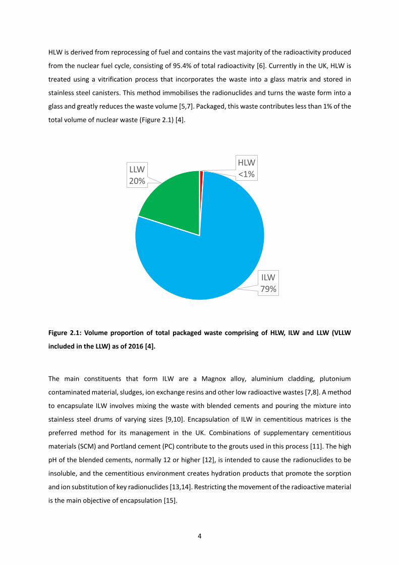
glass and greatly reduces the waste volume [5,7]. Packaged, this waste contributes less than 1% of the
total volume of nuclear waste (Figure 2.1) [4].
Figure 2.1: Volume proportion of total packaged waste comprising of HLW, ILW and LLW (VLLW
included in the LLW) as of 2016 [4].
The main constituents that form ILW are a Magnox alloy, aluminium cladding, plutonium
contaminated material, sludges, ion exchange resins and other low radioactive wastes [7,8]. A method
to encapsulate ILW involves mixing the waste with blended cements and pouring the mixture into
stainless steel drums of varying sizes [9,10]. Encapsulation of ILW in cementitious matrices is the
preferred method for its management in the UK. Combinations of supplementary cementitious
materials (SCM) and Portland cement (PC) contribute to the grouts used in this process [11]. The high
pH of the blended cements, normally 12 or higher [12], is intended to cause the radionuclides to be
insoluble, and the cementitious environment creates hydration products that promote the sorption
and ion substitution of key radionuclides [13,14]. Restricting the movement of the radioactive material
is the main objective of encapsulation [15].
HLW<1%
ILW79%
LLW20%

5
A highly durable cement wasteform provides a safer method to store and transport potentially
hazardous material [5]. Blast furnace slag (BFS) blended with PC is used extensively for this purpose,
at varying degrees of replacement (75 to 90% replacement). High replacement levels are used because
of the slower reactivity of BFS with water, which decreases the heat released by hydration of grout
constituents during the early stages of curing [16–18]. Blended cements are also widely available and
relatively inexpensive for the purpose of encapsulating a wide range of wastes.
Due to the large volumes of waste still awaiting treatment, as well as the need to monitor and maintain
the cemented products now in interim storage awaiting final disposal, further understanding of
potential interactions between the cementitious grouts and the encapsulated wastes is necessary.
Despite the large volumes of waste being produced, supply of the precursor materials has been a
constant issue over the years [19], therefore a method to be able to predict how the old and new
cementitious constituents react to form different phase assemblages is required.
LLW is treated in a similar way to ILW through mixing it with cement, however the waste packages
contain greater volumes of waste due to the lower levels of activity [20]. These waste packages are
currently being stored at different sites around the UK depending on the severity of their activity. For
instance, LLW is stored at a dedicated repository site at Drigg [21].
2.1.1 Geological disposal facility
As in many countries, the current policy to manage current and future nuclear waste in England and
Wales would involve storage within a geological disposal facility (GDF) [22]. This facility would be the
heart of a multi-barrier defence system to ensure that nuclear waste is stored safely and away from
the biosphere (Figure 2.2). The multi-barrier method consists of treating the waste into a durable
wasteform (e.g. cemented ILW), encasing the wasteform, designed barriers that act as buffers if the
waste package was to be damaged or release of radionuclides occurs and a stable geological
environment that the facility is hosted within [23].
6
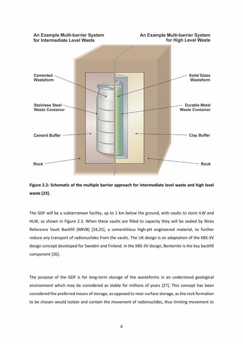
Figure 2.2: Schematic of the multiple barrier approach for intermediate level waste and high level
waste [23].
The GDF will be a subterranean facility, up to 1 km below the ground, with vaults to store ILW and
HLW, as shown in Figure 2.3. When these vaults are filled to capacity they will be sealed by Nirex
Reference Vault Backfill (NRVB) [24,25], a cementitious high-pH engineered material, to further
reduce any transport of radionuclides from the vaults. The UK design is an adaptation of the KBS-3V
design concept developed for Sweden and Finland. In the KBS-3V design, Bentonite is the key backfill
component [26].
The purpose of the GDF is for long-term storage of the wasteforms in an understood geological
environment which may be considered as stable for millions of years [27]. This concept has been
considered the preferred means of storage, as opposed to near-surface storage, as the rock formation
to be chosen would isolate and contain the movement of radionuclides, thus limiting movement to

7
the environment [23]. Further consideration must be given to the location and rock formations chosen
as to prevent future issues arising from seismic activity and glaciation in the distant future [27].
Figure 2.3: Schematic of a generic GDF proposed for in the UK (SF: spent fuel; UILW: unshielded ILW;
SILW: shielded ILW)[28].
The safety and security of the GDF is of the greatest concern, as it will not be built unless high safety,
security and environmental protection standards are met which are required by the UK Environment
Agency and Office for Nuclear Regulation. The latest update considering the framework for
implementing a GDF, highlights the importance of community involvement for choosing a site for the
GDF [29]. Community involvement is imperative as the basis of the framework states that the
community can withdraw from the process up to a specific point - the Test of Public Support (a
mechanism to determine whether the inhabitants of the host community agree to the siting of the
GDF). Therefore, within the framework, constant communication and cooperation with the potential
host community is key.

8
It is expected to take 15 to 20 years to identify and select a site that may be suitable for GDF and a
further 10 years to construct the repository. As of the 2018 ‘Implementing Geological Disposal’ report,
no communities or sites have been chosen [29].
2.1.2 Temperature profile of cemented wasteforms in the GDF
The required lifespan of a UK GDF remains to be defined, and a location has not yet been selected.
However, an approximate temperature profile has been created to enable scientific work to support
a safety case, considering the possible extremes in the conditions to which the cement wasteforms
may be exposed Figure 2.4 [8,10,30,31].
UK ILW waste packages are currently stored above ground at locations across the UK. An average
expected temperature of 20 °C has been assumed for this period based on the storage locations
[8,10,30,31]. Thermal modelling conducted by the Nuclear Decommissioning Authority (NDA) created
an extreme case scenario based on the possible heat output of ILW waste packages stored in
underground vaults) [10,31]. In this study, a heat output of 6 Wm-3 was used to model the most
extreme scenario (average heat output from low heat generating waste – 1.1 Wm-3 until 2040 and
declining to 0.5 Wm-3 by 2090; heat generation from non-radiogenic mechanisms – 3 Wm-3 due to
corrosion of waste; microbial degradation of materials – 2 Wm-3 [10]).
Figure 2.4: Approximate temperature profile of an ILW waste package due to GDF emplacement and
backfilling [8,10,30,31].

9
During the periods of transporting and storing the waste packages within excavated GDF vaults, taking
an expected 50 years, the general air temperature was predicted to be 35 °C (period I in Figure 2.4).
A further period of 50 years for care and maintenance is also expected to produce an average air
temperature of 35 °C (period II). After the GDF has been filled with waste packages, the vaults will be
backfilled with NRVB. The expected heat output from the hydration of the NRVB in an enclosed space,
coupled with reduced ventilation within the vault, is expected to raise the temperature of the GDF to
a maximum of 80 °C, for a period of 5 years (period III). After this point, the vaults are expected to
cool to 50 °C for 25 years (period IV), then eventually return to temperatures of 35 – 45 °C (period V).
A clear understanding of how the cement may react based on the changing temperatures is an
imperative for predicting the suitability of using blended cement for long-term storage.
2.2 Portland cement and blended cement
2.2.1 Portland cement
Portland cement is a hydraulic binder primarily created from thermal treatment of limestone and clay
[32]. When mixed with water, the hydraulic phases within the cement react exothermically to produce
a hardened paste [33]. The main operational feature of cement formation is the heating of the
limestone and clay in kilns to temperatures over 1400 °C [32], where they form nodules which are
called clinker. With the clinker, oxides are formed which differ from those that were present in the
minerals before heating. The cement once formed is ground into a fine powder and combined with
gypsum (CaSO4·2H2O) or other calcium sulphate compounds to control the rate of setting and strength
development [33].
The four main phases produced within the cement clinker are alite (C3S), belite (C2S), aluminate (C3A)
and ferrite (C4AF). It is common practice in cement chemistry to abbreviate the oxide containing
components as seen below:
C = CaO S = SiO2 A = Al2O3 N = Na2O S̅ = SO3
F = Fe2O3 M = MgO H = H2O K = K2O C̅ = CO2
Portland cement contains 50-70% C3S, 15-30% C2S, 5-0% C3A and 5-15% C4AF [33]. Of these phases C3S
and C3A are the most rapidly hydrating phases. These provide early strength formation, however C3A
reacts much more rapidly and must be controlled by the addition of the calcium sulphates to slow

10
down the rate of hydration to achieve longer, and more desirable setting times [32]. Slower hydrating
phases such as C2S and C4AF contribute to later strength development [34]. Each of the clinker phases
has a variety of polymorphs and can change in composition due to ionic substitutions, altering the
kinetics of hydration [33].
2.2.2 Cement and supplementary materials
Supplementary cementitious materials (SCMs) are widely used in concrete by either being added to
the cement during the grinding phase or separately in the concrete mixer [35]. Material considered as
SCMs such as blast furnace slag, fly ash from coal combustion and other pozzolanic materials are used
to replace fractions of cement [35]. Pozzolanic material are natural synthetic compounds that react
with calcium hydroxide and water to form a hardened substance [36]. The main advantage of using
these materials is that they are considered by-products from other processes and thus are considered
to contribute no CO2 to the use of cement or concrete [37]. They are generally different from cement
as can be seen in Figure 2.5. In terms of treatment with radioactive material, the reduced heat of
hydration exhibited by PC-SCM hydration, yet retaining a high pH (pH > 12), makes these materials
ideal for treating ILW.
Figure 2.5: Ternary phase diagram showing the CaO, Al2O3 and SiO2 composition of Portland cement
and SCMs, based on phase diagram produced by Lothenbach et al. [37].

11
2.2.3 Blast Furnace Slag (BFS)
Similarly to Portland cement production, BFS is the result of reactions at high temperatures. It is
formed as a liquid between 1350 and 1550 °C during the extraction of iron [38]. Silica and alumina
react with the limestone present in the ore during the extraction process [12]. If left to cool slowly,
the BFS forms a stable crystalline phase with no cementitious properties; however, when cooled
rapidly to temperatures below 800 °C, it forms a glass with hydraulic capabilities [39]. Of the solid
formed from this process 50 – 90% of this is a hydraulic glassy compound where the rate of cooling
influences the amount of glass formed. In general, the higher percentage of vitreous material formed,
the greater the reactivity of the slag [40].
The chemical composition of BFS from any single steel plant remains relatively stable in the short term,
however, even from the same plant over the last 30 years the composition may change [19,38]. This
is most likely down to the varying composition of the ore extracted from the ground. The general
composition of BFS contains MgO, 4-10%; Al2O3, 10-20%; SiO2, 30-40% and CaO, 35-45%, as well as a
small amount of sulphur [38].
Along with composition, the specific surface area affects reactivity. The glassy structure is ground up
into fine particles similar in surface area to Portland cement (PC), known as ground granulated blast
furnace slag (GGBFS). The average specific surface area of PC is approximately 330 m2/kg [32] while
GGBFS can range from 230 – 350 m2/kg [19]. In the nuclear waste industry a coarser BFS of average
specific surface area 340 m2/g is used to reduce the level of reactivity to reduce the level of heat
output during hydration [19]. The densities of granulated or pelletized blast furnace slags are typically
2880-2960 kg/m3 [33].
2.2.4 Phase assemblage of BFS-PC cements
Reactivity of BFS has been shown to be significantly slower than that of PC in the presence of water,
whereby in BFS-PC cements the degree of reaction of the BFS decreases as the level of replacement
increases [40–42]. Increasing the pH through the addition of greater levels of PC or alkali activators,
leads to an increased degree of reaction of the slag [33,40]. In the case of PC, it has been reported
that the clinker phases have a much higher solubility than that of the hydrate phases that are formed
[37,43]. The higher solubility of the precursor material leads to the dissolution of these phases quite

12
readily. In the presence of PC, the Ca(OH)2 produced from the hydration of the clinker phases has been
identified as activating the vitreous BFS structure. Studies have highlighted the reduced level of
Ca(OH)2 as the BFS replacement increases, indicating its consumption to aid in the formation of
hydrate phases [14,40,44]. After long-term hydration of a completely BFS containing system hydrated
by water, the degree of hydration reached 22% after 20 years and contained no Ca(OH)2, highlighting
the importance of an activating material [45].
The main hydrate phases observed in BFS-PC are calcium aluminosilicate hydrate (C-A-S-H),
portlandite (Ca(OH)2 or CH), ettringite (Ca3Al2O6·3CaSO4·32H2O), calcium monosulfoaluminate hydrate
(Ca3Al2O6·CaSO4·12H2O - monosulfate), calcium monocarboaluminate hydrate (Ca3Al2O6·CaCO3·11H2O
- monocarbonate), calcium hemicarboaluminate hydrate (Ca3Al2O6·CaCO3·12H2O - hemicarbonate)
and magnesium aluminium hydrotalcite-like hydrate (M-A-H – hydrotalcite-like) [37,46]. The variation
of oxide content in precursor material of the BFS-PC cement leads to alteration of the cement phases
formed.
2.2.4.1 Ca-Al-Si-OH
The main hydration phases of Portland cement are formed through the hydration reaction of the
silicon containing clinker phases:
C3S + (3 − 𝑥 + 𝑛)H → C𝑥 − S − H𝑛 + (3 − 𝑥)CH
C2S + (2 − 𝑥 + 𝑛)H → C𝑥 − S − H𝑛 + (2 − 𝑥)CH
2.1
2.2
Whereby tricalcium silicate (C3S) and dicalcium silicate (C2S) dissolve to form the precipitates C-S-H
and portlandite as shown in equation 2.1 and 2.2, respectively [47]. The main hydrate phase in PC,
calcium silicate hydrate (C-S-H), consists of a disordered layered silicate gel with variable calcium,
silicon and water content. Ordinarily in PC the molar ratio of Ca/Si of the C-S-H is greater than 1.5 and
may be described as a disordered jennite-like phase - (CaO)1.5-1.9SiO2·(H2O)x or C-S-H(II). Replacement
of the PC with BFS reduces the overall Ca/Si within the system thus altering the C-S-H structure to
form a lower Ca/Si phase similar to a tobermorite-like structure - (CaO)0.83SiO2·(H2O)1.5 or C-S-H(I). In
cement systems a combination of the two phases is generally observed [33,48,49].

13
Silicate tetrahedra bond together through oxygen bridges (Si-O-Si) to produce a chain structure (Figure
2.6). The different structural forms of silica are denoted as Q0, Q1, Q2, Q3 and Q4, whereby each
superscript corresponds to the number of silicon species which are linked with the silicon tetrahedra
[50–52]. Paired tetrahedra (which can form dimers, denoted as Q1) are joined to calcium oxide layers.
Two silicate tetrahedra may join onto a third which does not come in contact with the calcium oxide
layer. This combination of three silicate tetrahedra forms a dreierketten unit. The third silicon
tetrahedron acts as a bridge between other paired silicate sites to create the silicate chain (Figure 2.6).
The chains encompass a calcium oxide layer which may connect two parallel silicate chains. Low
calcium cement systems produce longer mean chain lengths (MCLs) through the incorporation of
additional silicon into the chain structure. In low pH (pH < 10.5) and low Ca/Si (Ca/Si < 0.85) conditions,
the bridging tetrahedra may form a cross-link (denoted as Q3) to link two silicate chains to form a
phase similar to naturally occurring tobermorite [49,53,54]. The ratio of calcium to silicon in solution
impacts the chain length and overall silicate structure of C-S-H, whereby this Ca/Si ratio becomes a
defining feature [55–58].
The linear chains have an interlayer space between them which allows the presence of water to
interact with the silicate chains. On bridging sites or at the end of silicate chains, cationic species act
as charge balancers (-Si-O-X+) which give rise to different chemical environments for the silicon species
[59–61]. At higher pH levels the chemical environment becomes saturated in OH- ions which reduces
the connectivity of the silicate chains (-Si-OH) and reduces the inclusion of charge balancing ions
[59,62,63].

14
Figure 2.6: The C-S-H/C-A-S-H structure depicted using dreierketten units. The green triangles
represent paired silicate dimers, blue triangles are bridging silicon tetrahedra, the red triangles
represent silicon replacement with aluminium, the purple, orange and pink circles represent Ca2+, K+
and Na+ ions respectively.
Synthesis of the C-S-H phase indicates the importance of the bulk chemistry of the environment on
the chemical composition formed. Reviews performed by Kulik [64] and Walker et al. [65] highlight
the shifting Ca/Si based on the concentrations of calcium and silicon in solution as shown in Figure
2.7. From the data summarised by Walker et al. [65], it is easy to observe the clear dependence of the
Ca/Si on the calcium and silicon concentrations, as calcium levels increase, the Ca/Si increases and the
opposite occurs when the silicon concentration increases. Formation of secondary phases cause a limit
of the concentration of calcium and silicon in solution. Portlandite formation occurs at [Ca] > 18
mmol/L which leads to a maximum calcium concentration in the C-S-H system (Figure 2.7a) [66].
Amorphous silica precipitates at [Si] of approximately 2-5 mmol/L [67,68].

15
Figure 2.7: The Ca/Si of C-S-H as a function of a) calcium concentration and b) silicon concentration.
The dotted and solid line indicates the Ca/Si when silica and portlandite forms, respectively. Optimal
solubility data collated by Walker et al. [65] from the following sources: [53,54,65,69–83].
Increasing replacement of PC with BFS causes a decrease in the Ca/Si within the C-S-H as the bulk Ca/Si
of the system decreases [37,45,84]. An increasing presence of aluminium within the system leads to
the replacement of silicon with aluminium. Bridging silicon tetrahedra may also be replaced by
aluminium, to form a C-A-S-H gel (Figure 2.6). Variation of the aluminium concentration in solution
causes corresponding aluminium substitution into the aluminosilicate chains, whereby the Al/Si and
Ca/Al values now define the phase [57,58,63,85]. The Al[IV] species may replace the Q2b or Q3 sites in
the silicate chain by maintaining the dreierketten unit [50,86]. Based on ab initio calculation, it is
understood that aluminium can predominantly only replace the bridging sites in the aluminosilicate
chain as aluminium inclusion in paired sites is very thermodynamically disfavoured [87]. Aluminium
cannot form a bridge with another aluminium ion (Al-O-Al) due to Loewenstein’s principle [88] which
limits the level of replacement in the aluminosilicate chain. Substitution of these sites may provide an
Al/Si of up to 0.33 within the dreierketten unit. In BFS-PC cements, due to the compositional changes
of the system, the Ca/Si often decreases as the Al/Si increases [37,45,84,89,90].
2.2.4.2 Ca-Al-SO4-CO3-OH
Calcium sulphoaluminate phases are the result of hydration of C3A and sulphur containing species
within the cement. The hydration phases are much more likely to form in standard cement systems
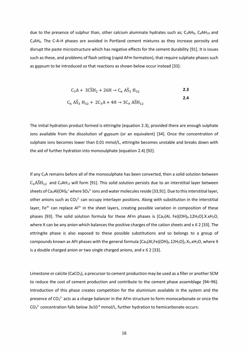
16
due to the presence of sulphur than, other calcium aluminate hydrates such as; C2AH8, C4AH19 and
C3AH6. The C-A-H phases are avoided in Portland cement mixtures as they increase porosity and
disrupt the paste microstructure which has negative effects for the cement durability [91]. It is issues
such as these, and problems of flash setting (rapid AFm formation), that require sulphate phases such
as gypsum to be introduced so that reactions as shown below occur instead [33]:
C3A + 3CS̅H2 + 26H → C6 AS̅3 H32
C6 AS̅3 H32 + 2C3A + 4H → 3C4 AS̅H12
2.3
2.4
The initial hydration product formed is ettringite (equation 2.3), provided there are enough sulphate
ions available from the dissolution of gypsum (or an equivalent) [34]. Once the concentration of
sulphate ions becomes lower than 0.01 mmol/L, ettringite becomes unstable and breaks down with
the aid of further hydration into monosulphate (equation 2.4) [92].
If any C3A remains before all of the monosulphate has been converted, then a solid solution between
C4AS̅H12 and C4AH13 will form [91]. This solid solution persists due to an interstitial layer between
sheets of Ca2Al(OH)6+ where SO4
2- ions and water molecules reside [33,91]. Due to this interstitial layer,
other anions such as CO32- can occupy interlayer positions. Along with substitution in the interstitial
layer, Fe3+ can replace Al3+ in the sheet layers, creating possible variation in composition of these
phases [93]. The solid solution formula for these AFm phases is [Ca2(Al, Fe)(OH)6.12H2O].X.xH2O,
where X can be any anion which balances the positive charges of the cation sheets and x ≤ 2 [33]. The
ettringite phase is also exposed to these possible substitutions and so belongs to a group of
compounds known as AFt phases with the general formula [Ca3(Al,Fe)(OH)6.12H2O]2.X3.xH2O, where X
is a double charged anion or two single charged anions, and x ≤ 2 [33].
Limestone or calcite (CaCO3), a precursor to cement production may be used as a filler or another SCM
to reduce the cost of cement production and contribute to the cement phase assemblage [94–96].
Introduction of this phase creates competition for the aluminium available in the system and the
presence of CO32- acts as a charge balancer in the AFm structure to form monocarbonate or once the
CO32- concentration falls below 3x10⁻⁴ mmol/L, further hydration to hemicarbonate occurs:
17
C3A + CC̅ + 11H → C4 AC̅H11
C3A + 0.5CC̅ + 0.5CH + 11.5H → C4 AC̅0.5H12
2.5
2.6
Higher levels of PC in the system which are higher in calcium and generally sulphate and carbonate
levels, causes the portlandite, ettringite and monocarbonate phases to form in greater quantities.
When BFS replacement increases, these phases decrease in concentration and lower calcium
containing phases become more abundant.
Despite the higher aluminium content available in the slag for formation of sulphate and carbonate
Aft or AFm phases, with increasing slag content less of these are expected to form, due to less gypsum
and calcite being available from the PC. Less oxidised sulphur will be available as there is only S2- found
in slag [39]. Ettringite and monosulphate formation relies on the availability of SO42- ions in solution,
therefore with only highly reduced sulphur available, the possibility of these phases forming is greatly
reduced [12]. However, the ettringite which does form, acts as a sink for Al3+ and Ca2+ ions from the
dissolution of the anhydrous slag which accelerates further dissolution of Al from BFS [12,33].
Reduction of CaCO3 in the system with the reduction of PC content will reduce the CO32- available,
which will impact the possible phase assemblage. Matschei et al. [97] was able to identify the impact
of the molar ratios of SO3, CO2 and Al2O3 (Figure 2.8), and how the combination of the elements,
impact the AFm or AFt phases formed. The lower solubility of CO2-containing phases, as shown
through various solubility studies [92,98–100], causes the carbonate-containing AFm phases to
precipitate out of solution more readily and require lower CO2/Al2O3 than SO3/Al2O3 to form.

18
Figure 2.8: Impact of molar ratios of SO3/Al2O3 versus CO2/Al2O3 on the possible phase assemblage
of AFm/AFt phases in the presence of excess portlandite [97].
2.2.4.3 Mg-Al-OH
Higher levels of MgO and Al2O3 have a large influence on the hydration phases. With larger amounts
of these compounds, hydrotalcite-like solid solution levels are expected to increase [60,101,102]. For
this phase, the magnesium to aluminium ratio (M/A) is key. A hydrotalcite-like solid solution (Mg1-
xAlx(OH)2+x∙mH2O) [103], which has a layered double hydroxide form, incorporates the MgO from the
BFS-PC aqueous solution [101].
This hydration phase has been proposed to have an inhibitory effect on C-A-S-H formation as the MgO
content increases, because the aluminium is less likely to be taken up by the C-A-S-H phase and is used
to form the hydrotalcite-like phase instead [102]. Bernal et al. [60] on the other hand, argue that
hydrotalcite formation benefits the formation of the C-S-H phase, because the hydrotalcite acts as an
aluminium sink. With less aluminium available to substitute with the silicon, longer chain lengths are
observed due to less bridging site substitution. It can be argued that the lower level of substitution

19
adds to the strength and stability of the gel-like phase [60]. Therefore, although the magnesium
inhibits the C-A-S-H formation, it promotes the development of C-S-H [60].
2.2.5 Pore solution
The pore solution of cement systems is key to forming cement hydrate phases. Once the solid
precursors dissolve, it is the void areas or the pores of the cement structure that become saturated
and leads to the precipitation of solid phases [47]. As the curing age increases, the concentration of
ions in solution alters based on the rate of reaction of the precursor materials. In general, the
concentrations of elements in solution are higher at early ages (0 – 10 days) and plateau after 28 days
[104].
High solubility of sodium and potassium released from sulphate phases (Na2SO4 or K2SO4) or
incorporated in the clinker phases, leads to a sharp increase of alkalinity in PC systems at young ages
(< 10 days) [33]. The weight percentages of Na2O and K2O in the initial precursor materials impact the
maximum concentration of sodium and potassium in solution. At higher BFS replacement, the weight
percentage of Na2O and K2O in the precursors are much lower than PC systems, resulting in a lower
concentration of Na+ and K+. The potassium and sodium concentrations individually may exceed 800
mmol/L depending on the precursor compositions, whereas BFS-PC may have concentrations as low
as 50 mmol/L [104,105], as shown in Figure 2.9.
The Na+ and K+ species act as charge balancing ions for many of the cement phases, specifically the C-
S-H or C-A-S-H phases and become withdrawn from solution. For PC systems, the high Ca/Si of the C-
S-H phase has a reduced alkali distribution ratio (Rd) which causes the Na+ and K+ concentrations to
increase as the clinker phases continue to hydrate [59,62]. In BFS-PC cements, the reduction of the
Ca/Si ratio causes the Rd to increase as the slag hydrates which reduces the Ca/Si ratio of the C-A-S-H
phase. The lengthening of the MCL requires greater levels of charge balancing in the aluminosilicate
chain, thus the uptake of Na+ and K+ ions increases as the MCL increases [61,85,104,106–108].
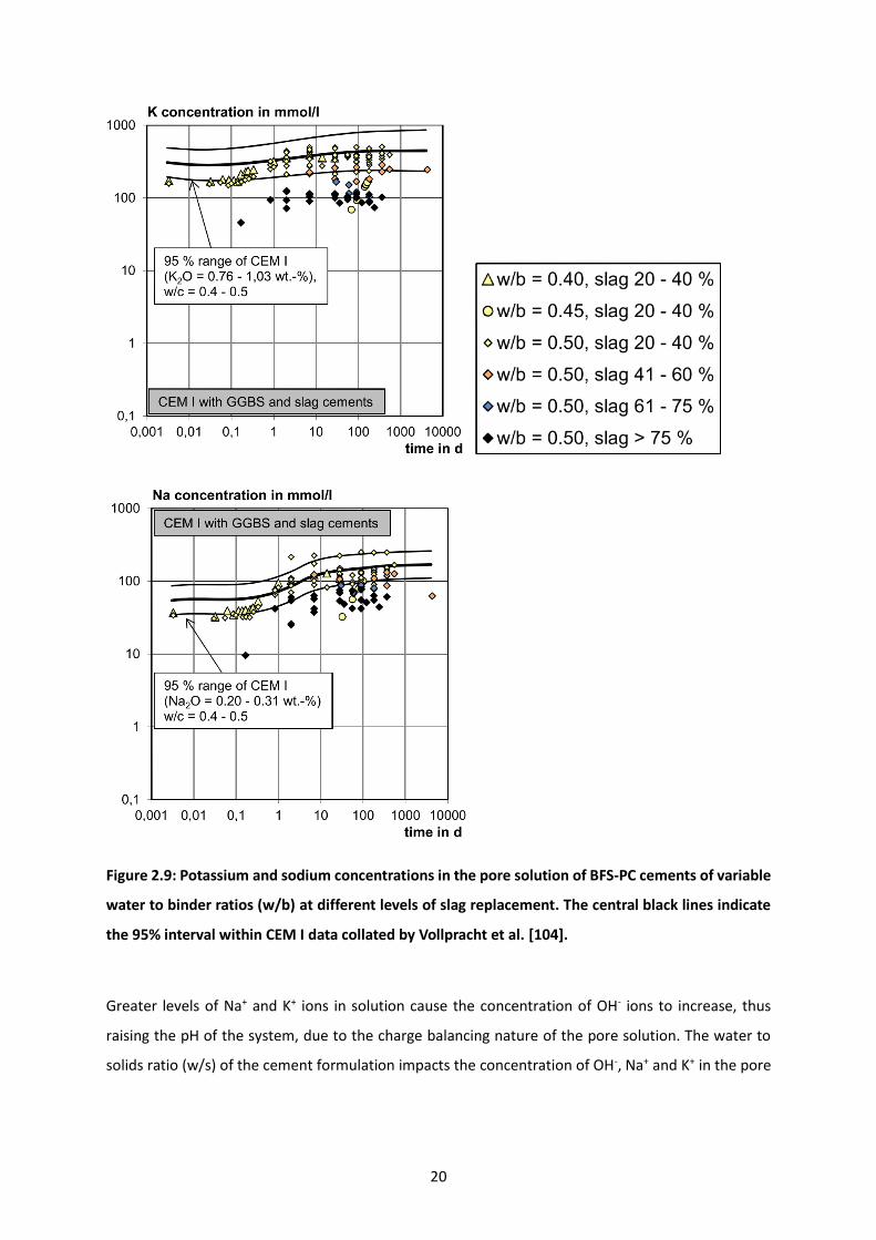
20
Figure 2.9: Potassium and sodium concentrations in the pore solution of BFS-PC cements of variable
water to binder ratios (w/b) at different levels of slag replacement. The central black lines indicate
the 95% interval within CEM I data collated by Vollpracht et al. [104].
Greater levels of Na+ and K+ ions in solution cause the concentration of OH- ions to increase, thus
raising the pH of the system, due to the charge balancing nature of the pore solution. The water to
solids ratio (w/s) of the cement formulation impacts the concentration of OH-, Na+ and K+ in the pore

21
solution, at lower w/s the concentrations of these ions increase [104]. The resulting pH of cements
are between 12 and 14 [37].
Calcium solubility is highly dependent on pH, and this precipitates out of solution more readily in the
presence of OH- ions to form portlandite [66]. Due to the high pH and readily available abundance of
OH- ions in PC and BFS-PC cements, there is minimal difference in the concentrations recorded in the
different systems, where calcium concentrations are commonly less than 10 mmol/L [37,104]. At pH
greater than 12 in the presence of calcium, silicon concentrations are less than 1 mmol/L, due to the
low solubility of the C-S-H and C-A-S-H phases [48,64,65].
Solubility of aluminium and magnesium phases are significantly low (often below instrumental
detectable limits) which results in very low concentrations in both PC and BFS-PC systems which
causes minimal difference of the recorded concentrations in the literature [109–111].
Sulphate concentrations are recorded between 1 and 80 mmol/L for BFS-PC cements at later age,
which is lower than that observed in the PC systems [104]. The increase of pH in the Ca-SO3-Al2O3-OH
system causes the solubility of ettringite and monosulphate to increase due to the solubility of
portlandite decreasing, which reduces the concentration of calcium available to form sulphur-
containing phases [112,113]. Therefore a higher concentration of sulphate is required in solution to
force the equilibrium to allow both phases to form [98,113]. However, the main sulphur species in BFS
is S2- which does not form hydrate phases readily. The review conducted by Vollpracht et al. [104],
investigated the total sulphur concentrations in BFS-PC cements. However, due to the increasing
sulphide concentration with increased BFS replacement, the total sulphur concentration may increase
with time as is the case with alkali activated slag (AAS) [114].
2.3 Thermodynamic modelling for cementitious systems
Development of different cementitious systems to constantly improve carbon efficiency, to take
advantage of new resources or for waste treatment purposes, requires further understanding of the
hydration phases forming. This can be performed using many geochemical modelling software
packages such as PHREEQC [115], Geochemist’s Workbench (GWB) [116] and GEM-Selektor (GEMS)
[117]. Using software packages such as GEMS it is possible to predict the phase assemblage of cement

22
systems by using degree of hydration (DoH) or degree of reaction (DoR) data as input parameters.
Utilising thermodynamic databases of cement phases, for instance CEMDATA14 within GEMS, it is
possible to assess what phases may form. This is important for assessing how altering the precursor
material will affect the final phase assemblage. Implementing this modelling approach has been used
for PC systems [118–121], SCM cements [37,122–126] and alternative cements such as calcium
sulphoaluminate cements [127]. There are two main approaches that are used in the modelling
packages, the law of mass action (LMA) algorithm or Gibbs energy minimisation (GEM) technique.
Both are described extensively in geochemical textbooks [116,117,128].
2.3.1 Law of mass action (LMA) and Gibbs energy minimisation (GEM) methods
Equilibrium constants are imperative to LMA methods for determining stable phase assemblages
within aqueous solutions [117]. The LMA technique utilises log K values for the aqueous complexes at
a given temperature and pressure [129]. In LMA coding these are used to produce saturation indexes
(SIs) along with other values to mass and charge balance, bulk composition. It is completed using
Newton-Raphson iterations. This method uses linear approximations to find the correct root of a
problem. It involves estimating the likely answer and iterates using the linear (tangent line)
approximation. If used correctly this iterative method can be very useful and produce results to a high
degree of accuracy [130]. However, this method is based on ‘local’ information, therefore if the initial
approximation is not close enough to the root, then an incorrect root is determined, or the iteration
does not converge. For thermodynamic modelling it is a logical process to use since the Newton-
Raphson iterations attempt to find the lowest possible value, which in thermodynamics indicates the
most stable phase [131].
The solubility product (𝐾𝑆𝑂) can be used to determine the saturation index (𝑆𝐼) of a compound in
aqueous solution. The purpose of determining the SIs of a compound ([𝐴𝐵]) is to calculate the
likelihood that they will precipitate or dissolve in aqueous solutions [129]. They take into account the
activities of the components at equilibrium (𝐾𝑆𝑂 = {𝐴}𝑒𝑞𝑎 {𝐵}𝑒𝑞
𝑏 ) and activities while interacting within
water (𝐼𝐴𝑃 = {𝐴}𝑎𝑐𝑡𝑢𝑎𝑙𝑎 {𝐵}𝑎𝑐𝑡𝑢𝑎𝑙
𝑏 ) in the system that is being modelled. When SI = 0, the solution is at
equilibrium between the mineral and solution, SI < 0 the product is at subsaturation and SI > 0 the
product is supersaturated [121]. This is one method of determining the likelihood of a solid phase
forming from an aqueous solution and is a main underlying step in the LMA procedure.

23
𝑆𝐼 = log (𝐼𝐴𝑃
𝐾𝑆𝑂)
2.7
Another approach to determine stable phase assemblages is the Gibbs Energy Minimisation (GEM)
technique. In this method, the stable phase assemblage is determined by finding the minimum Gibbs
free energy which indicates the system is at equilibrium whereby no more spontaneous reactions are
likely to occur [132]. Gibbs free energy of a system is defined as 𝐺 = ∑ 𝑛𝑖𝜇𝑖𝑖 , where 𝑛𝑖 is the moles
of the 𝑖 component and 𝜇𝑖 is the partial molal Gibbs free energy [133]. The GEM approach works on a
mass and charge balance basis of the entire system. Composition at equilibrium is defined from the
stoichiometrically possible phases based on the bulk composition [121]. The Gibbs free energy of
reaction can be linked to the solubility product [129] and provide the solid phase using Gibbs free
energy of formation data at standard conditions (2.8):
∆𝑟𝐺° = ∑ 𝑣𝑖𝑖
∆𝑓𝐺° = −𝑅𝑇 ln 𝐾𝑆𝑂 2.8
In the equation, 𝑣𝑖 corresponds to the stoichiometric coefficients of the reactants, R = 8.31451 J/mol/K
is the universal gas constant and T, is the temperature in Kelvin. From this approach, the solubility
product is determined from thermodynamic data in addition to mass and molar balance information
alone [120]. GEMS converts the standard chemical potential of species (𝜇𝑖0) into the actual chemical
potential (𝜇𝑖 ), by applying corrections based on the system:
𝜇𝑖 = 𝜇𝑖0 + 𝑅𝑇𝑙𝑛𝛾𝑖𝑐𝑖 2.9
Where 𝜇𝑖 is the calculated chemical potential, 𝑅 is the universal gas constant, 𝑇 is temperature (K),
activity coefficients of aqueous species (𝛾𝑖) and 𝑐𝑖 is the molal concentration of species 𝑖. The activity
coefficients of aqueous species consider the aqueous environment of each aqueous species in solution
and define how readily these species react. The combination 𝛾𝑖𝑐𝑖 may be referred to as the activity
(𝑎𝑖). An example of an activity coefficient model is the Truesdell-Jones equation, which is an extension
of the Debye-Hückel equation [134]:

24
𝑙𝑜𝑔10𝛾𝑖 =−𝐴𝛾z𝑖
2√𝐼
1 + �̇�𝐵𝛾√𝐼+ 𝑏𝛾𝐼 + 𝑙𝑜𝑔10
𝑋𝑗𝑤
𝑋𝑤
2.10
Here, 𝛾𝑖 and zi are the activity coefficient and charge of the 𝑖th aqueous species respectively, 𝐴𝛾 and
𝐵𝛾 are temperature and pressure dependent coefficients, 𝐼 is the molal ionic strength (𝐼 =
0.5 ∑ 𝑐𝑖𝑛𝑖=1 z𝑖
2), 𝑋𝑗𝑤 is the molar quantity of water, and 𝑋𝑤 is the total molar amount of the aqueous
phase. A common ion size parameter, �̇� and short-range interaction parameter, 𝑏𝛾, are used
[104,134]. The activity coefficient is applied to the standard chemical potential, 𝜇𝑖0, of each aqueous
species to provide a better representation of how it would realistically behave in solution.
Use of this modelling approach may be highlighted by considering the portlandite system. The
corrections applied to the standard chemical potentials that form portlandite (Ca2+ and OH-) are
displayed in equation 2.11 and 2.12. Incrementally increasing the Ca(OH)2 concentration from 0 to
18.8 mmol/L in solution, causes no portlandite to form as shown in Figure 2.10 as the difference
between the Gibbs energy of formation of the reactants and the hydrate phase was not less than zero
(2.13 and 2.14). Saturating the solution with the reactants combined with applying the activity
coefficient, causes portlandite to precipitate out of solution at Ca(OH)2 concentrations greater than
18.8 mmol/L.
𝜇Ca2+ = 𝜇Ca2+𝑜 + 𝑅𝑇𝑙𝑛𝛾Ca2+𝑐Ca2+ 2.11
𝜇OH− = 𝜇OH−𝑜 + 𝑅𝑇𝑙𝑛𝛾OH−𝑐OH− 2.12
∆𝐺 = 𝐺𝐶𝐻𝑜 − (𝜇𝐶𝑎2+ + 2𝜇𝑂𝐻−) 2.13
∆𝐺 = negative - Portlandite precipitates 2.14

25
Figure 2.10: The difference in Gibbs energy between portlandite and reactants until the point of
precipitation, thereafter portlandite precipitates out of solution as more Ca(OH)2 is added to the
system.
Figure 2.11: Thermodynamic modelling of the activity coefficients for Ca2+ and OH- ions in the
Ca(OH)2 system, with varying concentration of Ca(OH)2 added to solution.
Once the saturation point of 18.8 mmol/L of Ca(OH)2 is reached in solution, any further Ca(OH)2 added
to the system precipitates out of solution, hence the linear increase of portlandite formation after
18.8 mmol/L. The constant concentration of Ca(OH)2 remaining in solution results in a constant
activity coefficient of Ca2+ and OH- ions in solution as the concentration of the solution does not change
thereafter (Figure 2.11).
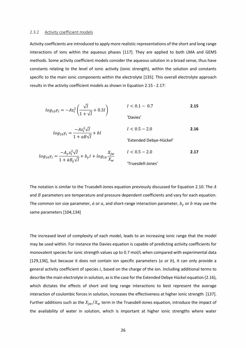
26
2.3.2 Activity coefficient models
Activity coefficients are introduced to apply more realistic representations of the short and long range
interactions of ions within the aqueous phases [117]. They are applied to both LMA and GEMS
methods. Some activity coefficient models consider the aqueous solution in a broad sense, thus have
constants relating to the level of ionic activity (ionic strength), within the solution and constants
specific to the main ionic components within the electrolyte [135]. This overall electrolyte approach
results in the activity coefficient models as shown in Equation 2.15 - 2.17:
𝑙𝑜𝑔10𝛾𝑖 = −𝐴z𝑖2 (
√𝐼
1 + √𝐼+ 0.3𝐼)
𝐼 < 0.1 − 0.7
‘Davies’
2.15
𝑙𝑜𝑔10𝛾𝑖 =−𝐴z𝑖
2√𝐼
1 + 𝑎𝐵√𝐼+ 𝑏𝐼
𝐼 < 0.5 − 2.0
‘Extended Debye-Hückel’
2.16
𝑙𝑜𝑔10𝛾𝑖 =−𝐴𝛾z𝑖
2√𝐼
1 + �̇�𝐵𝛾√𝐼+ 𝑏𝛾𝐼 + 𝑙𝑜𝑔10
𝑋𝑗𝑤
𝑋𝑤
𝐼 < 0.5 − 2.0
‘Truesdell-Jones’
2.17
The notation is similar to the Truesdell-Jones equation previously discussed for Equation 2.10. The 𝐴
and 𝐵 parameters are temperature and pressure dependent coefficients and vary for each equation.
The common ion size parameter, �̇� or 𝑎, and short-range interaction parameter, 𝑏𝛾 or 𝑏 may use the
same parameters [104,134]
The increased level of complexity of each model, leads to an increasing ionic range that the model
may be used within. For instance the Davies equation is capable of predicting activity coefficients for
monovalent species for ionic strength values up to 0.7 mol/L when compared with experimental data
[129,136], but because it does not contain ion specific parameters (𝑎 or 𝑏), it can only provide a
general activity coefficient of species 𝑖, based on the charge of the ion. Including additional terms to
describe the main electrolyte in solution, as is the case for the Extended Debye Hückel equation (2.16),
which dictates the effects of short and long range interactions to best represent the average
interaction of coulombic forces in solution, increases the effectiveness at higher ionic strength [137].
Further additions such as the 𝑋𝑗𝑤 𝑋𝑤⁄ term in the Truesdell-Jones equation, introduce the impact of
the availability of water in solution, which is important at higher ionic strengths where water

27
molecules are less available to form hydrating spheres [136]. Development of the equations 2.15 to
2.17 provide general descriptions of the aqueous solution and provide activity coefficients based on
the charge of the ions, however are not ion specific, which is not the case with the Pitzer model:
𝑙𝑛𝛾𝑀 = 𝑧𝑀2 𝐹 + ∑ 𝑚𝑎(2𝐵𝑀𝑎 + 𝑍𝐶𝑀𝑎)
𝑎
+ ∑ 𝑚𝑐(2Ф𝑀𝑐 + ∑ 𝑚𝑎ψ𝑀𝑐𝑎
𝑎
)
𝑐
+ ∑ ∑ 𝑚𝑎𝑚𝑎′ψ𝑎𝑎′𝑀
𝑎′
𝑎 <
+ |𝑧𝑀| ∑ ∑ 𝑚𝑐𝑚𝑎𝐶𝑐𝑎
𝑎𝑐
𝐼 < 0.5 − 6.0 [135]
‘Pitzer model’
2.18
The Pitzer model (Equation 2.18 – expanded in Chapter 6) determines the activity coefficients of
individual aqueous species through parameterising interactions of individual aqueous species in
solution, through virial expansion [135]. The model contains an initial Debye-Hückel term (𝐹) which
describes the solution as a whole, followed by second (𝐵𝑀𝑎, 𝐶𝑀𝑎) and third (Ф𝑀𝑐, ψ𝑀𝑐𝑎) virial
expansions. The second virial expansion considers the interactions of a binary aqueous solution
containing species of different charges. Inclusion of a third aqueous species may incorporate
electrolyte mixing terms if the parameter values exist. The mixing terms describe the interaction of
like-signed species (Ф𝑀𝑐), or like-signed species in contact with a third species of a different sign
(ψ𝑀𝑐𝑎). At higher ionic strengths (IS > 2 mol/L) the higher density of ions in solution forces the
interactions of like-signed ions and ternary species [136]. The use of ion specific interaction
parameters therefore improve this modelling approach by providing specific ion values. Through the
use of fitting tools, it is possible to determine the interaction parameters of multicomponent systems.
The Pitzer model was originally developed to improve existing aqueous solution modelling to improve
the accuracy at ionic strengths of greater than 0.1 [138–141]. The Pitzer model has been remarked to
have ‘unparalleled precision’ for determining thermodynamic properties of strong electrolyte
systems, however reduces in quality when parameters for aqueous species are missing in
multicomponent solutions [142]. A key disadvantage to the Pitzer model is the large dependence on

28
large amounts of solubility data required to maintain a thorough parameter database [100,110,143–
145]. A clear advantage of the Pitzer model over the Truesdell-Jones equation can be seen in Figure
2.12 when considering precipitation of magnesium oxychloride in the presence of brucite. The Pitzer
model, due to the high level of parameterisation, was capable of modelling the transition of brucite
to magnesium oxychloride in high concentrations of MgCl2. However, the Truesdell-Jones equation
became less effective at modelling the system at MgCl2 concentrations greater than 1 mol/L. This may
be important for predicting how magnesium-containing wastes interacts with nearby groundwater
[110].
Figure 2.12: Thermodynamic modelling of brucite and magnesium-oxychloride (MgOxyCl) in the Mg-
Cl-OH system using the Pitzer model (P) and Truesdell-Jones (T) equation. The Pitzer parameters and
solubility data used are from Harvie et al. [100].
The extended Debye-Hückel and Truesdell-Jones equations have been used extensively for modelling
cement systems [37,118–127] as the IS of cement is generally between 0.5 and 3.0 which is within
effective range of these models [104,146,147]. Use of the more complicated and parameter database
intensive Pitzer model is rarely used when considering cement phases and has not been used to
simulate cement hydration, but only specific cement phases [66,98,99,148]. The high quality of the
results and ease of use when using the simpler equations, reduces the requirement for using the Pitzer

29
parameters. However, as shown in Figure 2.12, the Pitzer model has a greater quality of modelling
more complex systems, which may arise when cement systems are in contact with waste.
2.4 Cement thermodynamic database
The thermodynamic database used throughout this work was the CEMDATA14 which has been
developed to include iron containing phases [119,149], AFm and AFt phases in the Ca-Al-SO4-CO3-OH
system [97,150], a magnesium hydrotalcite-like solid-solution model [123,146], a C-S-H solid solution
model [64] and other minor phases observed in cement phases [118,123,151,152].
The use of solid-solution models was incorporated into the database to accurately portray how
variable composition phases such as the magnesium hydrotalcite-like [123], ettringite, monosulphate
[150], C-S-H [64] and C-(A)-S-H [122] phases form. Solid solution models may determine the chemical
composition of the solid-solution based on the chemical environment and may react to any changes,
without any extra coding when setting up modelling projects. For instance the Ca/Si of the C-S-H model
may be altered based on the available [Ca] and [Si] which results in greater accuracy of the aqueous
solution [64,114,146].
The solid-solutions are comprised of end-members (𝑖) that have individual thermodynamic properties.
In the case of the C-S-H end-member model developed by Kulik [64], four end-members were chosen
based on known chemical structures of tobermorite-like and jennite-like structures. The total Gibbs
free energy of a solid solution (∆𝐺𝑠𝑠) may be determined through the following equations:
∆𝐺𝑠𝑠 = ∑ 𝑋𝑖 ∆𝑓 𝐺𝑖𝑜
𝑖
+ 𝐺𝑀 2.19
𝐺𝑀 = ∆𝐺𝑖𝑑 + ∆𝐺𝑀𝑒𝑥 2.20
∆𝐺𝑖𝑑 = RT ∑ 𝑋𝑖 𝑙𝑛 𝑋𝑖
𝑖
2.21
∆𝐺𝑀𝑒𝑥 = RT ∑ 𝑋𝑖 𝑙𝑛 𝛾𝑖
𝑖
2.22
Where, 𝑋𝑖 is the mole fraction of end-member 𝑖, ∆𝑓 𝐺𝑖𝑜 is the standard Gibbs energy of formation of
the end-member, 𝐺𝑀 is the Gibbs energy of a mechanical mixture end-members, ∆𝐺𝑖𝑑 is the Gibbs
30
energy of mixing of an ideal solid solution, ∆𝐺𝑀𝑒𝑥 is the excess Gibbs energy of mixing of a solid solution
and 𝛾𝑖 is the activity coefficient of end member, 𝑖. The initial equation (2.19) is in a similar form to
that of equation 2.9 whereby the chemical potential of the phase (𝜇𝑖0) is the sum of all of the end-
members that form the solid solution and the mole fraction of each end-member has an impact on
the total Gibbs energy of the solid solution. The 𝐺𝑀 term represents the correction of the standard
chemical potential (𝑎𝑖) by considering the aqueous environment in the system.
An ideal solid solution has an excess Gibbs energy of mixing (∆𝐺𝑀𝑒𝑥) equal to zero due to the solid
solution being capable of mixing in all proportions within the solid-solution model range. For instance,
the C-S-H and later the C(-N)-A-S-H model were developed as ideal models, as the Ca/Si range in C-S-
H that the models were designed for (0.67 – 1.63 and 0.67 – 1.3, respectively), were capable of
achieving any Ca/Si value within the specified range based on solubility data. At either end of the Ca/Si
ranges, secondary phases formed (amorphous silica formed at Ca/Si < 0.67 and portlandite formed at
Ca/Si >1.63 or 1.3) which was therefore outside the compositional range of the models as highlighted
in Figure 2.13. The limitations of the CNASH_ss models for use in high calcium content systems is the
maximum Ca/Si of 1.3 and the CSHQ model does not have aluminium inclusion. Neither model
accurately portrays the chemical composition of C(-A)-S-H in BFS-PC cements, as the Ca/Si ratio in BFS-
PC cement commonly exceeds 1.3 and includes silicon substitution with aluminium [44,45]. However,
a combination of the two models may provide a useful insight into the formation of C-A-S-H [122,125].
The solid solution models developed by Matschei et al. [92,150] required the inclusion of ∆𝐺𝑀𝑒𝑥 mixing
terms to correctly model the AFm and AFt phases due to the miscibility gaps in the solid solution
models. For instance the monosulphate solid solution, C4 AS̅𝑥H13−x, contains a miscibility gap
between 0.03 ≤ x ≤ 0.5.

31
Figure 2.13: No miscibility gaps in the calcium to silicon molar ratios (C/S or Ca/Si) are observed
when predicting the mole fractions of the end-members in the a) CSHQ and b) CNASH_ss models.
Modified from Kulik [64] and Myers et al. [146], respectively.
2.5 Conclusion
Blended cements are a viable waste management option for the encapsulation of ILW material for
large scale disposal due to the adsorption properties of the hydrate phases, low heat of hydration and
long-term durability. Based on the long-term goals for storing the waste using blended cements, it is
imperative that modelling approaches are assessed for the applicability of predicting how these
cements may develop over different curing ages and temperatures. Assessment of the modelling
approach requires degree of hydration data for the precursor materials as input parameters, recorded
chemical composition of variable composition phases (such as C(-A)-S-H and magnesium hydrotalcite-
like phase), characterised hydrate phase assemblages at various curing ages and pore solution data.
Curing BFS-PC samples with different BFS-PC ratios will provide a good basis for assessing the
robustness of the modelling approach for evaluating cement systems with variable precursor
compositions. Use of thermodynamic modelling therefore could provide the possibility of future
proofing changing cement supplies or alterations in the precursor composition.
Inclusion of a more ion specific activity coefficient modelling approach, the Pitzer model, may further
improve predictive capabilities for thermodynamic modelling. The greater capability of using a multi
parameter aqueous solution model may produce greater accuracy for predicting the precipitation of

32
solid phases out of solution, therefore improving the accuracy for predicting the pore solution
chemistry of blended cement systems. However, a large aqueous species interaction database is
required to utilise the Pitzer model.

33
3 Materials and Methods
3.1 Materials
The precursor materials used were Ribblesdale CEM I 52.5N PC and Port Talbot ground granulated BFS
(BS EN 15167-1 GGBS), supplied by the National Nuclear Laboratory. The oxide compositions of the
precursors used are displayed in Table 3.1 as determined by X-ray fluorescence (XRF). The powders
presented were used throughout the study as they are representative of the materials used currently
by the UK national nuclear industry for waste immobilisation [3]. The Blaine fineness, and a summary
of the particle size distribution (PSD) obtained using laser diffraction, of the PC and BFS are
reported in Table 3.2.
Table 3.1: Major constituents of raw materials, as determined by X-ray fluorescence (XRF) and
represented as oxides.
Oxide (wt.%) PC BFS
CaO 63.7 39.2
SiO2 20.8 35.1
Al2O2 5.1 13.4
Fe2O3 2.6 0.2
MgO 2.3 9.9
SO3 3.7 1.0
Na2O 0.6 0.2
K2O 0.8 0.6
TiO2 0.2 0.8
MnO2 0.1 0.2
P2O5 0.2 -

34
Table 3.2: Blaine fineness and particle size distribution (PSD) analysis of raw materials.
Particle parameter PC BFS
Blaine fineness (cm2/g) 4241 4870
PSD D10/μm 2.18 2.16
PSD D50/μm 14.3 15.3
PSD D90/μm 46.9 53.1
3.2 Mix design
Cementitious grouts composed of 1:1, 3:1 and 9:1 BFS:PC were produced with a water/solids (w/s)
mass ratio of 0.35, cured at 35 °C . These mix ratios and curing temperature conditions were chosen
to resemble the current interim storage conditions of ILW waste packages. A variation of the curing
regime is introduced in Chapter 5 to replicate the possible temperature changes that may occur in a
GDF site and are discussed further in that chapter [8,10,30,31].
3.3 Analytical techniques
A variety of analytical techniques were applied to assess the degree of hydration of the precursor
materials and to characterise the hydration phases formed. Selective dissolution using EDTA was
performed to determine the degree of hydration of the slag and these results were compared with
29Si magic angle spinning (MAS) nuclear magnetic resonance (NMR) experiments to confirm the quality
of the results. X-ray diffraction (XRD) alongside 27Al and 29Si MAS NMR were performed to identify the
solid phases forming at different curing ages. The use of 29Si MAS NMR and scanning electron
microscopy (SEM) were used to determine the chemical composition of the C-A-S-H phase.
3.3.1 Selective dissolution – EDTA dissolution
The crystal structures observed in PC hydration allow the use of crystallographic techniques to
determine the extent of reaction of the original clinker phases, however the amorphous nature of BFS
creates difficulty in assessing the degree of hydration when using techniques common to PC
calculations, such as Rietveld refinement [46,96,153]. Selective dissolution is a widely used technique
to assess the degree of hydration of BFS in blended cement systems [41,154].

35
Kocaba et al. [89,155] determined that the selective dissolution technique was ineffective at
calculating the degree of hydration of BFS, however Tan [105] argued that the selective dissolution
used in the Kocaba studies was not considered the most effective selective dissolution technique. A
round-robin study conducted by Durdzinski et al. [156] highlighted the issues with different degree of
hydration testing methods and resolved that each technique had flaws which required addressing.
The main benefits of selective dissolution are that it is a simpler, less analytically intensive and a well-
documented technique within the literature which provides reasonably reliable results
[40,41,154,157].
Selective dissolution [41,105,154] was performed to provide a quantitative determination of the
degree of hydration of the BFS by dissolving PC and hydration products while leaving slag grains intact.
Selective dissolution of the hydrated cement phases was performed and discussed in Chapters 4 and
5.
The selective dissolution method developed by Luke and Glasser was used in this study [154]. Initially,
93.0 g of disodium EDTA·2H2O was dissolved in a mixture of 250 mL of triethanolamine and 500 mL of
water. The solution was transferred to a volumetric flask. 173 mL of diethylamine was added into the
solution, then the mixture was made up to 1000 mL with water. For each extraction test, 50 mL of the
above solution was pipetted into a beaker and diluted to 800 mL with distilled water. After the diluted
solution was brought to a temperature of 20 ± 2 °C, 0.5 g of dried and ground sample (particles size
smaller than 63 µm) was weighed to the nearest 1 mg, then sprinkled over the surface of solution. The
solution was stirred using a magnetic mixer for 120±5 min maintaining a constant temperature, then
filtered under vacuum through a 90 mm diameter Whatman GF/C filter which had been previously
washed with 100 mL of distilled water, dried at 105 °C, and weighed. The residue was washed 5 times
with 10 mL of distilled water per washing, dried at 105 °C for 1 hour, and weighed to the nearest 1
mg.
Anhydrous PC and BFS were dissolved by EDTA solution using the same method as used for the
hydrated samples, to determine the proportion of PC and BFS dissolved, 2.0% and 86.9%, respectively.
Corrections were applied to the data for the hydrated samples, to account for the minor amounts of
PC remaining after selective dissolution, the few percent of anhydrous slag that was dissolved, and
the hydrotalcite-group minerals that are not dissolved, in the residue [154,158]. It was assumed that
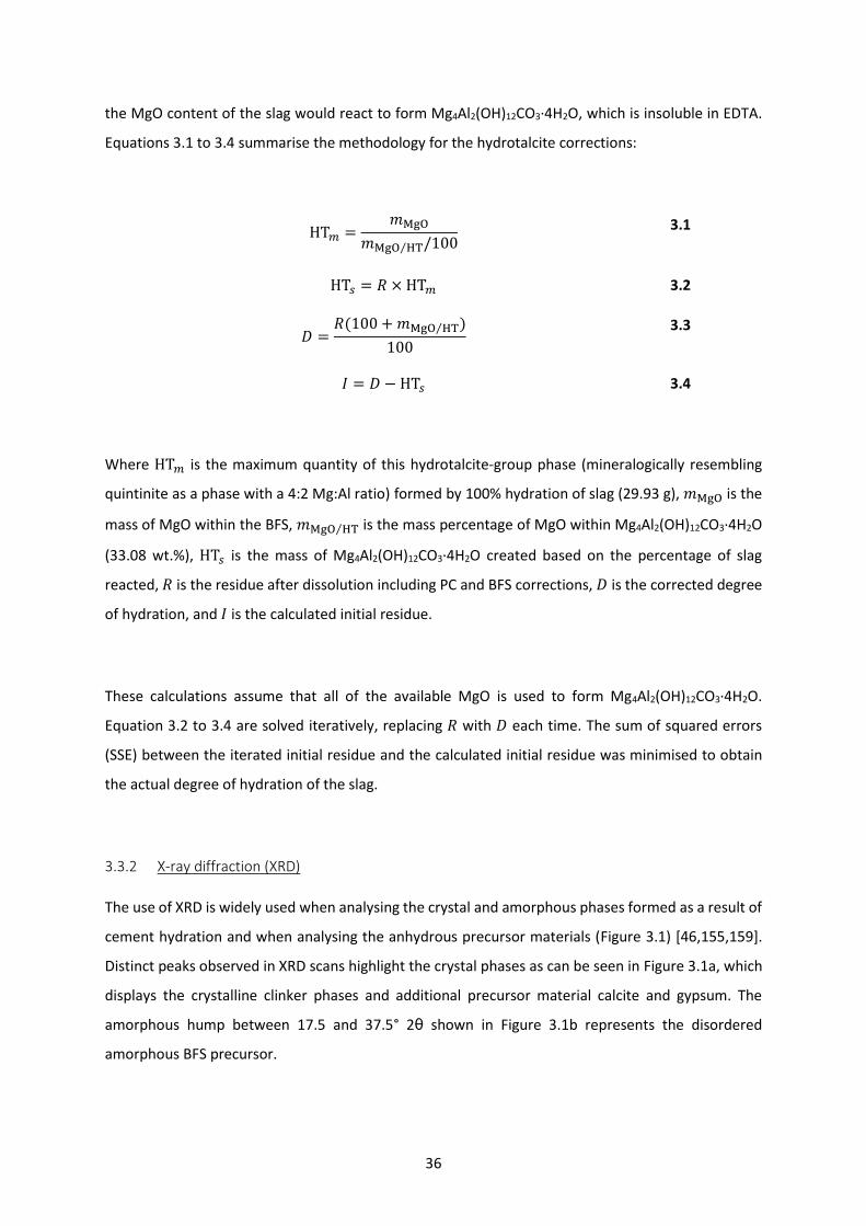
36
the MgO content of the slag would react to form Mg4Al2(OH)12CO3·4H2O, which is insoluble in EDTA.
Equations 3.1 to 3.4 summarise the methodology for the hydrotalcite corrections:
HT𝑚 =𝑚MgO
𝑚MgO HT⁄ /100 3.1
HT𝑠 = 𝑅 × HT𝑚 3.2
𝐷 =𝑅(100 + 𝑚MgO HT⁄ )
100
3.3
𝐼 = 𝐷 − HT𝑠 3.4
Where HT𝑚 is the maximum quantity of this hydrotalcite-group phase (mineralogically resembling
quintinite as a phase with a 4:2 Mg:Al ratio) formed by 100% hydration of slag (29.93 g), 𝑚MgO is the
mass of MgO within the BFS, 𝑚MgO HT⁄ is the mass percentage of MgO within Mg4Al2(OH)12CO3·4H2O
(33.08 wt.%), HT𝑠 is the mass of Mg4Al2(OH)12CO3·4H2O created based on the percentage of slag
reacted, 𝑅 is the residue after dissolution including PC and BFS corrections, 𝐷 is the corrected degree
of hydration, and 𝐼 is the calculated initial residue.
These calculations assume that all of the available MgO is used to form Mg4Al2(OH)12CO3·4H2O.
Equation 3.2 to 3.4 are solved iteratively, replacing 𝑅 with 𝐷 each time. The sum of squared errors
(SSE) between the iterated initial residue and the calculated initial residue was minimised to obtain
the actual degree of hydration of the slag.
3.3.2 X-ray diffraction (XRD)
The use of XRD is widely used when analysing the crystal and amorphous phases formed as a result of
cement hydration and when analysing the anhydrous precursor materials (Figure 3.1) [46,155,159].
Distinct peaks observed in XRD scans highlight the crystal phases as can be seen in Figure 3.1a, which
displays the crystalline clinker phases and additional precursor material calcite and gypsum. The
amorphous hump between 17.5 and 37.5° 2θ shown in Figure 3.1b represents the disordered
amorphous BFS precursor.
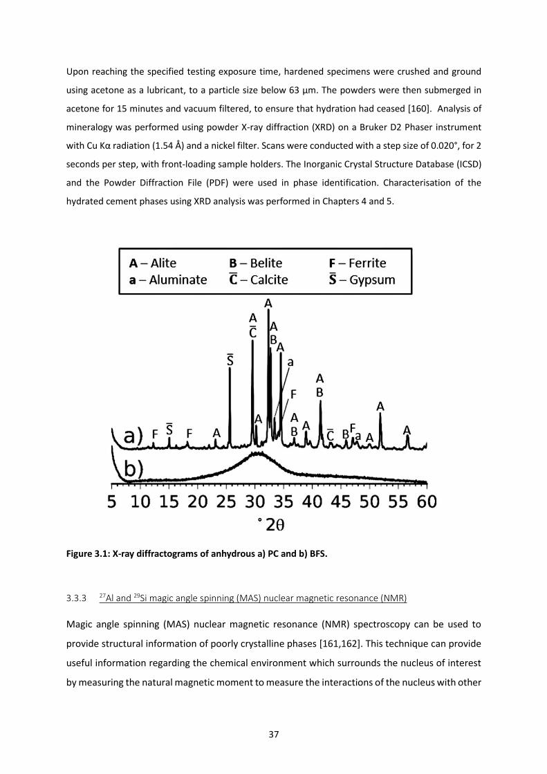
37
Upon reaching the specified testing exposure time, hardened specimens were crushed and ground
using acetone as a lubricant, to a particle size below 63 µm. The powders were then submerged in
acetone for 15 minutes and vacuum filtered, to ensure that hydration had ceased [160]. Analysis of
mineralogy was performed using powder X-ray diffraction (XRD) on a Bruker D2 Phaser instrument
with Cu Kα radiation (1.54 Å) and a nickel filter. Scans were conducted with a step size of 0.020°, for 2
seconds per step, with front-loading sample holders. The Inorganic Crystal Structure Database (ICSD)
and the Powder Diffraction File (PDF) were used in phase identification. Characterisation of the
hydrated cement phases using XRD analysis was performed in Chapters 4 and 5.
Figure 3.1: X-ray diffractograms of anhydrous a) PC and b) BFS.
3.3.3 27Al and 29Si magic angle spinning (MAS) nuclear magnetic resonance (NMR)
Magic angle spinning (MAS) nuclear magnetic resonance (NMR) spectroscopy can be used to
provide structural information of poorly crystalline phases [161,162]. This technique can provide
useful information regarding the chemical environment which surrounds the nucleus of interest
by measuring the natural magnetic moment to measure the interactions of the nucleus with other
38
surrounding nuclei [163]. Using information from this technique, it is possible to measure the
average chemical composition of amorphous material such as C(-A)-S-H [45,58,60,164,165]. In this
study 29Si MAS NMR was used to determine the degree of hydration of the silicon-containing clinker
phases and BFS, determine the chemical composition and mean chain length of C(-A)-S-H. 27Al MAS
NMR was used to confirm the presence of aluminium within the C-S-H structure.
Solid-state 27Al and 29Si magic angle spinning nuclear magnetic resonance (MAS NMR) spectra were
collected on a Varian VNMRS 400 (9.4 T) spectrometer with either a 4 mm zirconia (for 27Al) or 6 mm
zirconia (for 29Si) rotor. The 27Al MAS NMR single pulse experiments were collected at 104.198 MHz
using the following parameters: 14 kHz spinning speed, minimum of 5700 scans, pulse width of 1 μs
(25°) and a 0.2 s relaxation delay. The 29Si MAS NMR single-pulse experiments were recorded at 79.435
MHz using the following parameters: 6.8 kHz spinning speed, minimum of 7000 scans, pulse width of
4.7 μs (90°) and a relaxation delay of 5 s. Poulsen et al. [162] showed that a 5 s relaxation delay may
result in an under-quantification of belite as there may not be enough time for the nuclei to fully relax
prior to the next pulse, depending on the iron content of the cement tested, and its incorporation into
different clinker phases. Edwards et al. [166] also showed a difference between the intensity ratio of
alite to belite as a function of relaxation delay, however for delays between 3 and 70 s, the difference
was minimal. It is also not clear whether differences in relaxation behaviour between different Si
environments in the hydrate products will have a significant influence on quantification under the
experimental conditions used here. Therefore, no correction of the silicon intensities for this effect
was performed here, and the error in the quantification of resonances due to the differences in
relaxation behaviour between different silicon sites is estimated to be ± 5%. 29Si, and 27Al chemical
shifts are referenced to external samples of tetramethylsilane (TMS), and a 1.0 M aqueous solution of
Al(NO3)3, respectively.
Deconvolutions were performed using non-linear minimisation of the sum of squared errors using
Gaussian curves to obtain the best fit for comparing the deconvolution with the experimental data
[60,123,167,168]. Constraints were placed on the linewidths and peak positions dependent on the
peak being analysed, as detailed below.
Quantification and deconvolution of the anhydrous PC was performed using 9 overlapping peaks with
varying linewidths for alite (-64.5 to -76.5 ppm) and a single peak for belite (-71.3 ppm) with an

39
observed linewidth (FWHM) of 0.33 ppm [162] (Figure 3.2). A relative belite to alite intensity of 0.13
was determined. This relative intensity was used in conjunction with the CaO and SiO2 contents
determined by XRF (Table 3.1) to determine the quantity of alite and belite available in the PC [162].
This calculation is in good agreement with the quantity of alite and belite determined using the
modified Taylor-Bogue method [169] as seen in Table 3.3. These clinker compositions were used to
define the thermodynamic modelling precursor values. Fitting of the anhydrous BFS showed a large
broad resonance from -65 to -90 ppm (Figure 3.3). It was assumed that all hydration of the anhydrous
material was congruent.
Table 3.3. Clinker phases present in anhydrous PC, as quantified by 29Si MAS NMR and by the Taylor-
Bogue method.
29Si MAS NMR Taylor-Bogue
Alite 72.6 71.9
Belite 7.6 6.8
Aluminate - 8.0
Ferrite - 7.7
Potential ranges of chemical shifts indicating the chemical environments observed in the C(-A)-S-H
phase are summarised in Table 3.4. The chemical shifts determined from literature sources were used
as a guideline for determining the chemical shifts used in Chapter 4.
The 27Al spectra in addition to the 29Si spectra may provide confirmation of the aluminium substitution
in the C-S-H phase. The 27Al spectra is divided into three main regions to signify the different co-
ordination numbers of aluminium: Al[IV], Al[V] and Al[VI]. The aluminium species incorporated into
cement phases are summarised in Table 3.5.

40
Figure 3.2. Fitting of the 29Si MAS NMR spectrum of anhydrous PC: a) experimental data, b) fitted
deconvolution, c) alite spectrum, and d) belite spectrum.
Figure 3.3. Fitting of the 29Si MAS NMR spectrum of anhydrous slag: a) experimental data and b)
fitted deconvolution.

41
Table 3.4: Chemical shift ranges in which the different silicon Qx species are located using 29Si NMR.
Silicon environment Configuration Chemical shift (ppm) Ref.
Q0
-74.0 [60,168,170]
Q1
-77.8 to -79.85 [50,51,60,63,158,170–
172]
Q2(1Al)
-80 to -83 [50,51,60,63,158,170–
172]
Q2
-84.5 to -86.0 [50,51,60,63,158,170–
172]
Q3(1Al)
-89.0 to -92.5 [50,60]
Q3
-93.0 to -96.0 [50,60,63]
Table 3.5: Chemical shift ranges that the different silicon Qx species are located using 27Al NMR.
Aluminium co-
ordination
Phases present Chemical shift range (ppm) Ref.
Al[IV] C-A-S-H, C3A, BFS > 50 [50,51,173–
176]
Al[V] Interlayer charge
balancing aluminium (IT)
20-50 [50]
Al[VI] Ettringite, monosulphate,
magnesium hydrotalcite-
like, third aluminate
hydrate (TAH)
< 20 [33,51,173]

42
3.3.4 Scanning electron microscopy
Scanning electron microscopy (SEM) was performed using a Hitachi TM 3030 instrument with a 20 kV
accelerating voltage, a working distance of 8 mm and a backscatter detector. Samples were cut and
polished using non-aqueous lubricants immediately prior to analysis. An evenly distributed selection
of points across a representative 400 µm × 400 µm section of the sample was analysed using a Bruker
Quantax 70 X-ray energy dispersive spectroscopy (EDS) detector to determine chemical compositions.
Further explanation of the methods used to determine chemical composition of the C(-A)-S-H and
hydrotalcite-like phase are in Chapter 5.
3.3.5 Pore solution extraction and ICP-OES
Pore solution of the blended cements were obtained using the steel-die method [118,177–179] to
compare activity coefficient models in Chapter 6. Further explanation of the methodology may be
found in Chapter 6, section 6.3 (Pore solution extraction from hydrated samples).
3.4 Thermodynamic modelling
Thermodynamic modelling was performed using GEM-Selektor v3 [132,180] using the CEMDATA14
database which is an updated version of CEMDATA07 [151]. GEMS utilises a Gibbs energy minimisation
algorithm which determines the most stable phase assemblage. Included within this study is a solid-
solution model for C-A-S-H adapted from the work of Myers et al. [146] and Kulik [64], in Table 3.6.
This adaptation was used to provide a greater Ca/Si ratio within the modelled C-A-S-H gel to describe
BFS:PC cements, as opposed to the alkali-activated slags for which the CNASH_ss model was originally
developed [146]. A similar approach was also adopted by Elakneswaran et al. [125] using PHREEQC
[115,129]. A hydrotalcite-like solid solution model (MA-OH-LDH [146]) replaced the OH-Hydrotalcite
phase found within CEMDATA14 to better represent the magnesium aluminate hydrate (M-A-H)
phase. The solid, aqueous and gaseous phases utilized throughout this study are shown in Table A8.3
to A8.5 found in the Appendix.
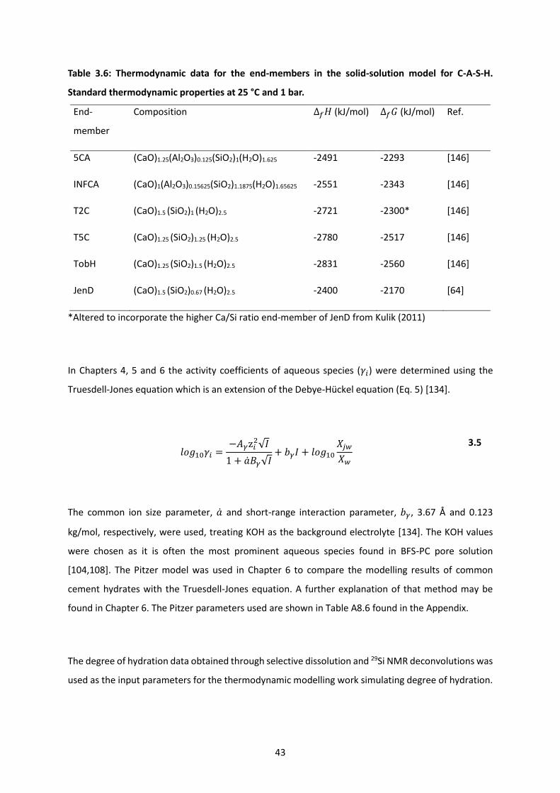
43
Table 3.6: Thermodynamic data for the end-members in the solid-solution model for C-A-S-H.
Standard thermodynamic properties at 25 °C and 1 bar.
End-
member
Composition ∆𝑓𝐻 (kJ/mol) ∆𝑓𝐺 (kJ/mol) Ref.
5CA (CaO)1.25(Al2O3)0.125(SiO2)1(H2O)1.625 -2491 -2293 [146]
INFCA (CaO)1(Al2O3)0.15625(SiO2)1.1875(H2O)1.65625 -2551 -2343 [146]
T2C (CaO)1.5 (SiO2)1 (H2O)2.5 -2721 -2300* [146]
T5C (CaO)1.25 (SiO2)1.25 (H2O)2.5 -2780 -2517 [146]
TobH (CaO)1.25 (SiO2)1.5 (H2O)2.5 -2831 -2560 [146]
JenD (CaO)1.5 (SiO2)0.67 (H2O)2.5 -2400 -2170 [64]
*Altered to incorporate the higher Ca/Si ratio end-member of JenD from Kulik (2011)
In Chapters 4, 5 and 6 the activity coefficients of aqueous species (𝛾𝑖) were determined using the
Truesdell-Jones equation which is an extension of the Debye-Hückel equation (Eq. 5) [134].
𝑙𝑜𝑔10𝛾𝑖 =−𝐴𝛾z𝑖
2√𝐼
1 + �̇�𝐵𝛾√𝐼+ 𝑏𝛾𝐼 + 𝑙𝑜𝑔10
𝑋𝑗𝑤
𝑋𝑤
3.5
The common ion size parameter, �̇� and short-range interaction parameter, 𝑏𝛾, 3.67 Å and 0.123
kg/mol, respectively, were used, treating KOH as the background electrolyte [134]. The KOH values
were chosen as it is often the most prominent aqueous species found in BFS-PC pore solution
[104,108]. The Pitzer model was used in Chapter 6 to compare the modelling results of common
cement hydrates with the Truesdell-Jones equation. A further explanation of that method may be
found in Chapter 6. The Pitzer parameters used are shown in Table A8.6 found in the Appendix.
The degree of hydration data obtained through selective dissolution and 29Si NMR deconvolutions was
used as the input parameters for the thermodynamic modelling work simulating degree of hydration.

44
Alkali distribution ratios (Rd) to simulate alkali uptake in the C-A-S-H phase were used for sodium and
potassium. The distribution ratios calculate the uptake of alkalis from solution based on the mass of
C-A-S-H formed and the concentration of alkalis in solution:
𝑅𝑑 =𝑐𝑠 𝑤
𝑐𝑑 𝑠
3.6
Where, 𝑐𝑠 is the concentration of the alkali in the solid phase (mol/mL), 𝑐𝑑 is the concentration of
the alkali in solution (mol/mL) and w/s is the water to solid ratio (mL/g). Alkali distribution ratios for
Na2O and K2O of 2 and 1.2, respectively, were used for the C-A-S-H phase, following the method of
Lothenbach et al. [151]. These values were chosen as they are similar to the values determined by
Hong and Glasser [59,85] for C-S-H and C-A-S-H phases with Ca/Si values between 1.2 and 1.6.

45
4 Phase evolution of slag-rich cementitious grouts for
immobilisation of nuclear wastes: an experimental and modelling
approach
Note: This chapter is based primarily on the paper “Phase evolution of slag-rich cementitious grouts
for immobilisation of nuclear wastes” by D. P. Prentice, S. A. Bernal, M. Bankhead, M. Hayes and J. L.
Provis. Published in Advances in Cement Research. 2017, 30(8), pp. 345-360.
4.1 Introduction
Encapsulation of intermediate level radioactive waste (ILW) in cementitious matrices is the preferred
method for its disposal in the UK. Combinations of supplementary cementitious materials (SCM) and
Portland cement (PC) contribute to the grouts used in this process [11]. The high pH of the blended
cements, normally 12 or higher [12], is intended to cause the radionuclides to be insoluble, and the
cementitious environment creates hydration products that promote the sorption and ion substitution
of key radionuclides [13,14]. Restricting the movement of the radioactive material is the main
objective of encapsulation [15].
A highly durable cement wasteform provides a safer method to store and transport potentially
hazardous material [5]. Blast furnace slag (BFS) blended with PC is used extensively for this purpose,
at varying degrees of replacement (75 to 90% replacement). High replacement levels are used because
of the slower reactivity of BFS with water, which decreases the heat released by hydration of grout
constituents during the early stages of curing [16–18]. Blended cements are also widely available and
relatively inexpensive for the purpose of encapsulating a wide range of wastes.
In the UK, 108,000 m3 of ILW had already been generated by April 2016, of which 41,400 m3 had been
converted into cemented wasteforms awaiting long term storage, leaving large quantities still awaiting
treatment [4]. Therefore, due to the large volumes of waste still awaiting treatment, as well as the
need to monitor and maintain the cemented products now in interim storage awaiting final disposal,
further understanding of potential interactions between the cementitious grouts and the
encapsulated wastes is necessary. Despite the large volumes of waste being produced, supply of the

46
precursor materials has been a constant issue over the years [19], therefore a method to be able to
predict how the old and new cementitious constituents react to form different phase assemblages is
required.
Investigations of cement for immobilisation of radioisotopes have primarily focused on the
incorporation of ions within the cement hydrate phases such as calcium silicate hydrates (C-S-H),
ettringite, and calcium monosulphoaluminate hydrate (“monosulphate”), due to the variety of
cationic and anionic substitutions that may take place within these stable phases. The silicate chain-
based, layered structure of C-S-H offers a variety of sites to host substituents, whether within the
silicate chain, such as the replacement of silicon by aluminium to form C-A-S-H type products
[86,165,167,181], or as charge balancing ions within the interlayer region [108,146,170]. The high
surface area of the C-A-S-H gel provides a surface for ionic sorption or substitution for interlayer sites
[182]. Ettringite (Ca3Al2O6·3CaSO4·32H2O) hosts numerous SO42- ions located within the channels of
columns of calcium and aluminium polyhedra which provides the possibility for anionic replacement.
At lower sulphate concentrations, monosulphate (Ca3Al2O6·CaSO4·12H2O) is more dominant
[45,89,183] and forms a lamellar hexagonal structure. Both ettringite and monosulphate require
charge balancing of a cationic structure by exchangeable anions, which can be replaced by anionic
radionuclides [182,184,185]. Another main phase associated with BFS-rich cements is a Mg-Al-
hydrotalcite-like phase, and although this is well known to act as a good receptor for Cl- and CO32-
binding [186,187], its role in uptake of important radionuclides still requires further investigation.
The nature and amount of hydration products forming in BFS-PC blended cements are highly
dependent on temperature, curing time, PC and slag content, and slag composition
[45,89,151,183,188–191]. Although BFS:PC grouts have been extensively studied over recent decades,
evaluation has mostly focused on assessment of young specimens and a small portfolio of samples
which have been analysed at regular intervals since the 1990s [44,45,86,90], and therefore there
remain open questions around the chemical, mineralogical and microstructural changes these
materials will undergo over the potentially millions of years for nuclear waste cementation [27].
Thermodynamic modelling is a very useful tool that can be used to predict how the changes in blend
ratios of a cement system will affect the aqueous and solid hydration products in the longer term
[118,120,121]. This can be performed using geochemical modelling software packages such as GEM-

47
Selektor (GEMS) [132,180], and utilises solid-solution models in conjunction with thermodynamic
databases for defined phases to predict the formation of cement hydrates. The key limitation of this
method at present is the difficulty in accurately parameterising an end-member model for the
complex multi-component hydrates present in cements, based on limited and often conflicting
experimental results [64,65,146]. Therefore, the purpose of this study is to assess the effectiveness of
a geochemical model for C(-A)-S-H in predicting phase assemblages of the slag cement systems used
in the UK nuclear industry. Using this technique, predictions based on the precursor materials used
for nuclear waste encapsulation may be performed to quickly and accurately assess whether new
supplies of BFS and PC are capable of providing the necessary performance characteristics in the long
term.
4.2 Experimental methodology
4.2.1 Mix Design
Cementitious grouts composed of 1:1, 3:1 and 9:1 BFS:PC (compositions in Table 3.1) were produced
with a water/solids (w/s) mass ratio of 0.35, cured at 35 °C. These mix ratios and curing temperature
conditions were chosen to resemble the current interim storage conditions of ILW waste packages. A
summary of the materials were provided in Chapter 3, Section 3.1.
4.2.2 Analytical techniques
Upon reaching the specified curing age, hardened specimens were crushed and ground using acetone
as a lubricant, to a particle size below 63 µm. They were then vacuum washed with acetone to ensure
hydration had ceased [160].
Analysis of the crystalline phases was performed using powder X-ray diffraction (XRD) on a Bruker D2
Phaser instrument with Cu Kα radiation and a nickel filter. Scans were conducted with a step size of
0.020°, for 2 seconds per step. Samples were front loaded by pouring the sample into a sample holder,
then smoothed over with a glass tile.

48
Selective dissolution of the hydrated samples was conducted to determine the degree of hydration of
the BFS in each sample. The EDTA method was used [41,105,154]. The technique used was explained
in Chapter 3, Section 3.3.1.
4.2.3 27Al and 29Si MAS NMR
Data collected from these scans were used to: (1) determine the degree of hydration for direct
comparison with the results obtained through selective dissolution, (2) obtain the degree of hydration
of clinker phases, and (3) identify poorly crystalline reaction products which are difficult to observe by
XRD.
Solid-state 27Al and 29Si magic angle spinning nuclear magnetic resonance (MAS NMR) spectra were
collected on a Varian VNMRS 400 (9.4 T) spectrometer with either a 4 mm zirconia (for 27Al) or 6 mm
zirconia (for 29Si) rotor. 29Si, and 27Al chemical shifts are referenced to external samples of
tetramethylsilane (TMS), and a 1.0 M aqueous solution of Al(NO3)3, respectively. Further explanation
can be found in Chapter 3, Section 3.3.3.
4.2.4 Thermodynamic modelling
Thermodynamic modelling was performed using GEM-Selektor v3 [132,180] using the CEMDATA14
database which is an updated version of CEMDATA07 [151]. A summary of the solid, aqueous and
gaseous phases used are summarized in Table A8.3 to A8.5, found in the Appendix.
The activity coefficients of aqueous species (𝛾𝑖) were determined using the Truesdell-Jones equation
which is an extension of the Debye-Hückel equation (Equation 4.1) [134].
𝑙𝑜𝑔10𝛾𝑖 =−𝐴𝛾z𝑖
2√𝐼
1 + �̇�𝐵𝛾√𝐼+ 𝑏𝛾𝐼 + 𝑙𝑜𝑔10
𝑋𝑗𝑤
𝑋𝑤
4.1
Here, 𝛾𝑖 and zi are the activity coefficient and charge of the ith aqueous species respectively, 𝐴𝛾 and
𝐵𝛾 are temperature and pressure dependent coefficients, I is the molal ionic strength, 𝑋𝑗𝑤 is the molar

49
quantity of water, and 𝑋𝑤 is the total molar amount of the aqueous phase. A common ion size
parameter, �̇� (3.67 Å) and short-range interaction parameter, 𝑏𝛾 (0.123 kg/mol), were used, treating
KOH as the background electrolyte [134].
Alkali distribution ratios for Na2O and K2O of 2 and 1.2 [59,85,118], respectively, were used for the C-
A-S-H phase, as explained in Chapter 3, Section 3.4.
4.3 Experimental results and discussion
4.3.1 X-ray diffraction.
X-ray diffractograms highlighting the impact of the varying levels of slag in the hydration products of
the blended cements assessed are depicted in Figure 4.1. Phases present for each curing time and
blend ratio are portlandite (ICSD #15471), calcium hemicarboaluminate-AFm (hemicarbonate, PDF
#00-036-0129), calcium monocarboaluminate-AFm (monocarbonate, PDF #00-036-0377), calcium
monosulphoaluminate-AFm (monosulphate, ICSD #100138), a hydrotalcite-like phase (PDF #00-014-
0525), ettringite (ICSD #16045), and C-A-S-H (PDF 34-0002).
In the 1:1 BFS:PC grout, evidence of the formation of ettringite (with a distinctive peak at 9.08° 2θ)
can be seen at each age tested, however between 28 days and 56 days the intensity of this peak drops
just as a slight increase in monosulphate (9.93° 2θ) emerges. The ettringite transforms into
monosulphate when the ratio of SO42- to Al3+ decreases [192], as it is the case as more slag reacts. The
3:1 BFS:PC system exhibits a very small ettringite peak intensity after 28 days and none at later curing
ages, while the 9:1 blend exhibits no ettringite and has a much more distinct monosulphate peak.
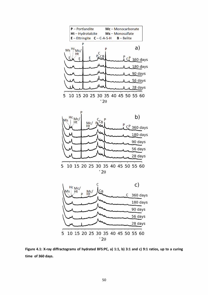
50
Figure 4.1: X-ray diffractograms of hydrated BFS:PC, a) 1:1, b) 3:1 and c) 9:1 ratios, up to a curing
time of 360 days.

51
Other AFm phases such as hemicarboaluminate and monocarboaluminate are detected (10.75° and
11.5° 2θ) as a result of reaction of the small amount of calcite in the cement (as identified by XRD,
Figure 4.4) during hydration, and potentially some superficial carbonation contamination of the
samples. The availability of calcite restricts the formation of monosulphate [193], leading to a weak
reflection assigned to this phase within the 1:1 grout. Within the 3:1 and 9:1 grouts the monosulphate
peak is more pronounced compared with grouts with lower BFS content, as the sulphate levels are
not high enough to form ettringite at the elevated curing temperature used here (35°C), except
perhaps in the very early stages of hydration, and instead AFm phases were formed.
The hydrotalcite-like phase is formed as a solid solution with a varying Mg:Al ratio which impacts its
crystal structure [194,195], therefore the position of its basal reflection peak may vary between 11.2°
and 11.6° 2θ [186,187,196]. All three grouts assessed have distinct peaks at 11.6° 2θ; within the 1:1
grout this can also be attributed to monocarbonate, however for the 3:1 and 9:1 grouts it is likely that
this peak is instead due to a hydrotalcite-like phase. The MgO content of the slag used in this study is
9.9 wt.%, Table 3.1, which is sufficient for hydrotalcite-group minerals to form in slag-dominated
binders [197]. There is also less calcite available to form carboaluminate phases when the PC content
is low, which further supports this line of reasoning. The peaks corresponding to the hydrotalcite-like
phase have a much greater intensity in the 3:1 grout than the others, which is attributed to the greater
degree of hydration of slag in this cement.
Portlandite and C-A-S-H gel were the hydration products with the highest peak intensities for the 1:1
and 3:1 grouts. The peak intensity of portlandite decreased with the increasing of BFS content, and in
the case of the 9:1 grout, at longer curing times. The consumption of portlandite with time in the 9:1
grout leads to the formation of more C-A-S-H, as more silicon becomes available from the dissolution
of slag, as the hydration progresses.
4.3.2 27Al MAS NMR
Figure 4.2 includes the 27Al MAS NMR spectra of the anhydrous PC and BFS, along with those of the
hydrated samples. The spectrum of the anhydrous BFS displays a very broad resonance between 50
and 80 ppm, centred around 67 ppm. This is consistent with a tetrahedral aluminium coordination
state. Anhydrous cement contains two aluminium-containing phases; tricalcium aluminate
(aluminate) and tetracalcium aluminoferrite (ferrite). From the broad peak around 81 ppm [51,173]

52
and the sharp peak at 9.4 ppm it is assumed that only aluminate can be identified here by NMR, due
to the suppression of the signal from the ferrite phase due to the close proximity of iron to the
aluminium nuclei in that phase [198].
Samples cured for 28 days or more, across all blend ratios, do not display any evidence of the C3A peak
at 81 ppm, indicating that essentially all of the aluminate in the PC has reacted. Within the Al(IV)
region, a shoulder emerges to the left of the slag peak at 71 ppm for all samples. A resonance at this
chemical shift is indicative of aluminium substitution within the C-S-H silicate chains [50,51,174–176].
There is clearly a greater influence in the Al(IV) region with increasing slag content in the grouts. In
the 1:1 grouts there is only a slight shoulder on the underlying broad feature, however in the 3:1 and
particularly the 9:1 grout the peak at 71 ppm becomes more defined. The increasing definition of the
71 ppm peak indicates more incorporation of aluminium within the C-S-H gel, which takes place mainly
at the Q2 bridging sites within the dreierketten silicate chain structure (Richardson 2014; L’Hôpital et
al. 2016).
The Al(V) species exhibited at 36 ppm was identified in all formulations as interlayer charge balancing
aluminium (denoted IT) [50].
Noticeable changes occur within the Al(VI) region of the spectra between 0 and 20 ppm as a function
of curing time and slag content. Within this region it is evident that ettringite is only observed, at
around 13 ppm [51,173], in the 1:1 grout from 28 to 360 days. The sharp ettringite peak appears to
become less defined at longer curing times. This peak is not evident at all in the 3:1 and 9:1 grouts,
consistent with the XRD data (Figure 4.2b, 4c). There are clearly not enough sulphate ions within the
solution to stabilise the ettringite in the lower PC containing grouts and for later age 1:1 grouts.

53
Figure 4.2: 27Al MAS NMR spectra for a) 1:1, b) 3:1 and c) 9:1 BFS:PC grouts.
Clear evidence of AFm phase formation can be seen at 9.8 ppm; this can be attributed to
monosulphate, hemicarbonate and/or monocarbonate due to the interchangeability of the charged
ion within AFm phases, [Ca2(Al(OH)6)·X·𝑥H2O] where X is one unit of a single charged ion or half a unit
of a doubly charged ion [33]. This peak may also indicate the presence of octahedral aluminium in
hydrotalcite (expected at 9.7 ppm, so strongly overlapping the AFm resonance). All of these phases
were identified in these grouts by XRD (Figure 4.2) and contribute to the peak intensity in this region.
A stronger resonance at this chemical shift was observed in the 1:1 grout as a result of the presence
of larger amounts of cement supplying calcite and gypsum. At 3.9 ppm, the third aluminate hydrate
(TAH) was identified in all grouts and curing times. The lack of sulphate ions and an increase in
aluminium present in the cements with the higher BFS contents leads to a more distinct resonance
assigned to the TAH phase [173].

54
4.3.3 29Si MAS NMR
Figure 4.3 shows the 29Si MAS NMR spectra of each sample analysed; Figure 4.3a, c and e show
examples of the deconvoluted 29Si MAS NMR of the 1:1, 3:1 and 9:1 grouts, respectively, after 360
days of curing, while Figure 4.3b, d and f show the full sets of spectra as a function of curing time. In
conducting the deconvolutions, peaks associated with the C-A-S-H gel were limited to a linewidth of
3.5 ppm (FWHM) and the peak positions were allowed to vary within ±0.1 ppm of the values provided
in Table 4.1, to account for the variation of the local environments of silicon within this disordered
phase.
Table 4.1: Site allocations for silicon environments in 29Si MAS NMR spectra.
Silicon site Chemical shift (ppm)
Q0 -74.0
Q1 (I) -77.8
Q1 (II) -79.8
Q2 (1Al) -81.6
Q2 -84.7
Q3 (1Al) -88.0
Q3 -93.0
The broad glassy slag peaks overlaps the signals from unreacted alite and belite, alongside the Q0,
Q1(I), Q1(II) and Q2(1Al) sites of C-A-S-H gel, where the two Q1 environments are distinguished by the
nature of the charge-balancing cations (monovalent and divalent), whose differing field strengths lead
to the observation of separate resonances [146,168]. The slag peak overlaps the monomeric and
dimeric silicate species (Q0, Q1(I) and Q1(II)) to a significant extent, which may impact the
quantification of the Ca/Si ratio within the C-A-S-H gel. The site located at -74.0 ppm, represents a
hydrated silicon monomer, Q0, however the precise structure in which this site is located is still
unknown. Previous studies have highlighted that this silicon environment is linked with greater slag
content within the BFS:PC system [60,86,168], and this was the case for the 3:1 grout as seen in Table
4.2, where raising the slag content and increasing the hydration of the slag results in a greater Q0
intensity than was observed for the 1:1 grout. This was not the case for the 9:1 ratio; it is possible that
the lower degree of slag hydration in the 9:1 system resulted in a lower intensity for this peak.

55
Figure 4.3: Example deconvolutions of 29Si MAS NMR spectra for a) 1:1, c) 3:1 and e) 9:1 grouts after
360 days, and 29Si MAS NMR spectra for b) 1:1, d) 3:1 and f) 9:1 grouts from 28 days to 360 days of
curing.
Increased PC content resulted in the presence of more Q1 sites due to the higher level of calcium
supplied by PC. Correspondingly, the Q1 prevalence decreased, and Q2(1Al) and Q2 increased, over
time as more slag hydrated, thus increasing the amount of silicon available to extend the silicon chains
within the C-A-S-H gel. The chemical shift values used in the deconvolutions for the silicon linked to
the aluminium substituted sites (Q2(1Al)) and the paired silicon sites (Q2) were more similar to those
used in the literature for white PC and BFS:PC [50,158,171,172] than those found in alkali activated
slag [168], as the chemical environments of these peaks are influenced by the alkali concentration.
Each specimen exhibited signs of aluminium substitution within a cross-linking site in the C-A-S-H gel
(Q3(1Al)) at -88 ppm, and small signs of cross-linking silicon (Q3) at -93 ppm. These peak intensities are
much smaller than the other peaks, and are observed at similar levels across each time and blend
ratio. Cross-linking is most dominant within the 1:1 and 9:1 systems, where aluminium substitution is
most prevalent.

56
Table 4.3 summarises the structural characteristics of the C-A-S-H gel in each sample, calculated from
the deconvoluted NMR spectra [58]. The mean chain length (MCL) (Equation 4.2) was seen to increase
with BFS content and curing duration, as a result of the increased aluminium and silicon levels within
the C-A-S-H; Ca/Si ratios calculated from Equation 16 of the paper of Richardson [58] decreased with
increased curing duration, while Al/Si (Equation 4.3) remained constant, consistent with the discussion
presented above. Despite evidence of less cross-linking within the 3:1 system than the others, it still
achieved a greater MCL because of the higher proportion of bridging sites when compared with the
1:1 system.
MCL = 2
(Q1
Q1 + Q2(0Al) +32 Q2(1Al) + Q3(0Al) + Q3(1Al)
)
4.2
Al
Si=
12
Q2(1Al)
Q1 + Q2(0Al) + Q2(1Al) + Q3(0Al) + Q3(1Al)
4.3
The Ca/Si ratio of each grout calculated from this method was significantly lower than what has been
observed in the literature for comparable cements [44]. Rarely has the Ca/Si ratio been published
when derived from 29Si MAS NMR data of hydrated cementitious materials, however the Al/Si and
MCL are often provided using this methodology [50,51,171,172]. Generally, TEM-EDX or SEM-EDX
data are considered to provide more accurate results when considering the Ca/Si values of C-A-S-H
gels in hydrated cementitious systems.
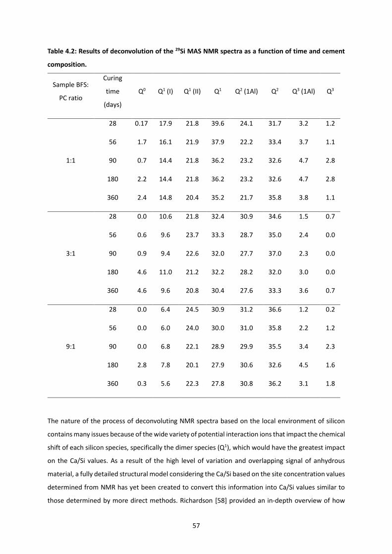
57
Table 4.2: Results of deconvolution of the 29Si MAS NMR spectra as a function of time and cement
composition.
Sample BFS:
PC ratio
Curing
time
(days)
Q0 Q1 (I) Q1 (II) Q1 Q2 (1Al) Q2 Q3 (1Al) Q3
1:1
28 0.17 17.9 21.8 39.6 24.1 31.7 3.2 1.2
56 1.7 16.1 21.9 37.9 22.2 33.4 3.7 1.1
90 0.7 14.4 21.8 36.2 23.2 32.6 4.7 2.8
180 2.2 14.4 21.8 36.2 23.2 32.6 4.7 2.8
360 2.4 14.8 20.4 35.2 21.7 35.8 3.8 1.1
3:1
28 0.0 10.6 21.8 32.4 30.9 34.6 1.5 0.7
56 0.6 9.6 23.7 33.3 28.7 35.0 2.4 0.0
90 0.9 9.4 22.6 32.0 27.7 37.0 2.3 0.0
180 4.6 11.0 21.2 32.2 28.2 32.0 3.0 0.0
360 4.6 9.6 20.8 30.4 27.6 33.3 3.6 0.7
9:1
28 0.0 6.4 24.5 30.9 31.2 36.6 1.2 0.2
56 0.0 6.0 24.0 30.0 31.0 35.8 2.2 1.2
90 0.0 6.8 22.1 28.9 29.9 35.5 3.4 2.3
180 2.8 7.8 20.1 27.9 30.6 32.6 4.5 1.6
360 0.3 5.6 22.3 27.8 30.8 36.2 3.1 1.8
The nature of the process of deconvoluting NMR spectra based on the local environment of silicon
contains many issues because of the wide variety of potential interaction ions that impact the chemical
shift of each silicon species, specifically the dimer species (Q1), which would have the greatest impact
on the Ca/Si values. As a result of the high level of variation and overlapping signal of anhydrous
material, a fully detailed structural model considering the Ca/Si based on the site concentration values
determined from NMR has yet been created to convert this information into Ca/Si values similar to
those determined by more direct methods. Richardson [58] provided an in-depth overview of how

58
using different structural models influenced the Ca/Si ratio determined using NMR data, and
highlighted the variation in the possible results based on which model was used. It was concluded that
the use of NMR data consistently yielded lower Ca/Si values when compared to SEM or TEM results.
Analysis using the CSTM method [164] provides good agreement for NMR data of alkali activated slag
(AAS) systems, but its application here also tended to produce low Ca/Si values. Despite these issues,
NMR data can still supply useful information about the trend in Ca/Si values based on the blend ratio
and time of curing of the cement systems of interest in this study; the actual values should be treated
as semi-quantitative rather than absolute.
Table 4.3: Summary of structural characteristics of the C-A-S-H gel forming in BFS:PC cements based
on the 29Si MAS NMR results
Time
(days)
Al/Si Ca/Si Mean Chain Length (MCL)
1:1 3:1 9:1 1:1 3:1 9:1 1:1 3:1 9:1
28 0.12 0.15 0.16 1.13 1.07 1.05 5.64 7.13 7.49
56 0.11 0.14 0.15 1.11 1.07 1.05 5.77 6.83 7.71
90 0.12 0.14 0.15 1.11 1.05 1.04 6.14 7.06 7.95
180 0.12 0.15 0.16 1.11 1.08 1.05 6.14 6.80 8.07
360 0.11 0.14 0.15 1.08 1.06 1.03 6.16 7.19 8.27
4.3.4 Determination of degree of hydration using 29Si MAS NMR and selective dissolution
As described in section 4.2.3, the fitted 29Si MAS NMR spectra of the anhydrous materials were scaled
and used as components in the deconvolution of the spectra of the reaction products, to determine
the degree of hydration of each constituent within the hydrated samples. Comparison of the degree
of hydration between the (independent) 29Si MAS NMR and selective dissolution techniques for BFS,
Figure 4.4, displays good agreement between the two techniques. The BFS in the 1:1 and 3:1 blends
was slower to react when compared to some reports of other BFS:PC blended cements of the same
proportions [41,96], but does align better with various other reports in the literature [40,46,156]. This
may be attributed to the rather lower w/s ratio used here, which is based on the UK nuclear industry’s
specification for acceptable mixes [17,19]. Determination of the extent of reaction by NMR spectral
deconvolution has an error margin of approximately 5% as previously discussed based on the

59
relaxation delay [52,162], whilst the selective dissolution technique used here has reported errors of
up to 10% [199], so these possible variations must also be considered when comparing the results
reported here to those available in the literature. Higher slag inclusion would be expected to result in
a lower degree of hydration of the slag, as there is less portlandite produced by PC hydration that
would activate the latent hydraulic character of the slag, and this trend was borne out in the current
results. After 360 days the 9:1 system had approximately half the degree of reaction of the 3:1,
whereas the difference between 3:1 and 1:1 was less marked; both of these systems contained
significant residual portlandite according to the XRD data in Figure 4.1, so this was evidently less of a
limitation at slag contents of up to 75%.
Across all blend ratios, the degree of alite hydration as determined by deconvolution of 29Si MAS NMR
spectra reached at least 79.0% after 28 days, but from this time up to 360 days there was only a small
further increase (Figure 4.5). Higher BFS content led to a higher degree of hydration of the alite,
possibly due to the higher water to alite ratio in the higher-BFS systems, where the slower reaction of
the slag means that more water and space are available for PC hydration in the early stages of the
reaction process, in a form of the filler effect commonly seen in blended cements, but taken to an
extreme case where the cement is only 10-25% PC. A moderate degree of reaction of belite can be
seen in all blends assessed, but not exceeding 65% even at 360 days in any of the cements evaluated;
the belite in the 9:1 grout showed very little reaction beyond 90 days. This may be because belite is
more prone to react at higher pH [42], and the pore solution pH of BFS:PC cements is reduced when
they contain very high fractions of BFS [104].

60
Figure 4.4: Degree of reaction of BFS within the different blend ratios, based on 29Si NMR MAS
deconvolutions (NMR) and on selective dissolution (EDTA).
Figure 4.5: Degree of reaction of calcium silicate clinker phases (alite and belite) within the different
blend ratios, based on 29Si MAS NMR spectral deconvolutions.

61
4.4 Thermodynamic modelling
4.4.1 Calculating the hydrate phase assemblage
Using the degree of hydration data presented above, prediction of the phase assemblages via
thermodynamic modelling (Figure 4.6) gave results which corresponded well with the phases
identified experimentally.
As expected, the C-A-S-H gel was dominant in all grouts, and was predicted to entirely consume
portlandite by 28 days in the 9:1 system. The fact that this was not observed experimentally (i.e. a
small quantity of portlandite persisted at all ages in Figure 4.1) may indicate spatial heterogeneity of
the blended cement leading to deviations from the assumed equilibrium behaviour, as has been
discussed recently by Skocek et al. [200] for other low-clinker cements. Portlandite formation was
much higher in the 1:1 cement (14 wt.% after 360 days) than the 3:1 cement (10 wt.% after 360 days),
which corresponds well with the XRD data.
Ettringite appears in the model phase assemblages at early age for all blends assessed, however in the
3:1 and 9:1 cements it was predicted to be replaced by monosulphate, after 60 days and 6 days,
respectively. From the experimental data presented above, only a small amount of ettringite was
observed in the 3:1 system at 28 days, and none from 56 days onwards, while no ettringite was
observed in the 9:1 system. Ettringite was still predicted in the 1:1 system after 360 days, along with
increasing monosulphate as curing time and the degree of hydration of the BFS increased. It is possible
that experimental factors not fully captured in the thermodynamic model – particularly the influence
of sulphide provided by the slag, which can be incorporated into AFm phases [201] and/or oxidised to
sulphate – will lead to under-prediction of the stability of ettringite in the model applied here.
However, the predicted increase in monosulphate content in higher-BFS cements did align well with
the experimental data. It should also be noted that the TAH phase identified by NMR was not included
within the thermodynamic database used in this work.

62
Figure 4.6: Hydrate phase assemblages predicted using thermodynamic modelling, for a) 1:1, b) 3:1
and c) 9:1 grouts reacting at 35°C, based on the experimentally determined (NMR) degree of
hydration data up to 360 days.
Hydrotalcite-group phase formation was predicted to increase with BFS content and degree of
hydration of the slag; after 360 days hydrotalcite comprised as much as 12.6 wt.% of the solid binder
constituents in the 9:1 system, respectively. Thus, we identify the peak at 11.6° 2θ in Figure 4.1 as
mainly attributed to hydrotalcite formation. Figure 4.6 displays the reducing amount of
monocarbonate forming when lower levels of PC are available in the system to provide calcite. In the
3:1 and 9:1 system, hemicarbonate becomes the dominant carbonate hydrate phase at later ages,
rather than monocarbonate, as can be seen in the XRD results. Matschei et al. [95,97] demonstrated

63
that the lower amount of CO32- ions present in the pore solution causes this phase transition from
monocarbonate to hemicarbonate.
4.4.2 Comparison of C-A-S-H gel structural characteristics between model and experiment
The use of the high-Ca/Si end-members in the model may be the cause of the under-prediction of
portlandite formation in the 9:1 system. The Ca/Si ratio of C-A-S-H in the modelled 9:1 system after
360 days was 1.373 (Table 4.4), which is higher than the 1.03 determined from the NMR spectra here
(Table 4.3), but more similar to the value published by Richardson & Groves for a 9:1 cement also
based on UK nuclear industry-specification materials, which was 1.29 [44]. There was a better
agreement for the 3:1 system as it was closer to the value expected from literature data, Ca/Si
between 1.34 – 1.40 [44]. In the 3:1 and 9:1 systems, the Ca/Si ratio decreases as Al/Si increases. As
expected, the Ca/Si ratio in the C-A-S-H is highest in the 1:1 formulation but using this model, it was
only marginally higher than the 3:1 after 360 days.
Only the 1:1 system shows no alteration of the calculated C-A-S-H molar ratios with time, consistent
with the NMR results (Table 4.3 which showed minimal variation. Under-prediction of the Ca/Si in the
1:1 system corresponds to the over-prediction of Al/Si within the C-A-S-H gel. Another limitation is
that once the Ca/Si ratio of the C-A-S-H gel reaches 1.4 to 1.5, portlandite formation is more favourable
than incorporating more calcium within the C-S-H gel, which limits the Ca/Si ratio to this range.
As a result of the minimum Ca/Si of C-A-S-H formation required before portlandite can be formed, no
portlandite was observed in the simulated 9:1 system, despite the fact that portlandite was observed
in the X-ray diffractograms up to 360 days. This issue was highlighted in the creation of the CSHQ
model whereby once the C-S-H reached a Ca/Si of 1.5, portlandite would begin to form alongside the
C-S-H [64].
However, a promising trend in the model results is that with higher levels of slag hydration, the Ca/Si
value decreases and the Al/Si value increases, as was seen in the NMR results. Overprediction of the
mean chain length (MCL) within the 1:1 grout occurs due to the poor agreement of the Ca/Si and Al/Si
values, however the 3:1 and 9:1 systems display better agreement despite the differences between
predicted and experimental Ca/Si ratios.

64
Table 4.4: Summary of structural characteristics of the C-A-S-H gel derived from thermodynamic
modelling.
Time
(days)
Al/Si Ca/Si MCL
1:1 3:1 9:1 1:1 3:1 9:1 1:1 3:1 9:1
28 0.137 0.135 0.156 1.424 1.427 1.408 7.234 7.204 7.494
56 0.137 0.136 0.161 1.424 1.430 1.404 7.234 7.206 7.496
90 0.137 0.140 0.161 1.424 1.424 1.403 7.232 7.260 7.576
180 0.137 0.144 0.162 1.424 1.420 1.384 7.232 7.320 7.754
360 0.137 0.144 0.163 1.424 1.419 1.373 7.232 7.320 7.860
4.4.3 Modelling of aged BFS:PC cements
Applicability of this method to samples cured for extended durations than those evaluated in this
study is of critical importance when applying this method to long-term storage or disposal of wastes.
Here it is the thermodynamic modelling approach described in Section 2.4 is applied for modelling 20
year old BFS:PC samples, whose detailed characterisation was carried out by Taylor et al. [45]. The
phase assemblage predictions show good agreement with the identified hydration products forming
in the aged cements (Figure 4.7). The dominant phases at later age are hydrotalcite and C-A-S-H gel,
and the good agreement regarding portlandite content is particularly notable (Table 4.5).
Figure 4.7: Calculated phase assemblage of BFS:PC cements using the degree of hydration and
precursor materials reported by Taylor et al. [45].

65
At advanced curing ages the end-member model used in this study for blended cements was struggling
with the same issues as the earlier age samples in section 4.4.2, whereby the C-A-S-H gel required a
certain Ca/Si ratio before portlandite could form. This has led to an over-prediction of the Ca/Si ratio
of the C-A-S-H gel (Table 4.6) and no predicted portlandite formation in the 9:1 system. There was a
greater variation of the Ca/Si ratio in the 9:1 system when compared to the 1:1 and 3:1 systems, due
to the much lower amount of calcium available for reaction.
Table 4.5: Portlandite content, as weight percentage of the hydrates formed at varying degrees of
slag replacement. Results from 20 year sample are from Taylor et al. [45].
BFS:PC blend ratios % portlandite in phase assemblage
20 year sample GEMS
1:1 10 14
3:1 3 2
9:1 1 0
Under-prediction of the Al/Si ratio was not as severe as the over-prediction of the Ca/Si ratio. There
was a small increase in Al/Si as BFS replacement increased. Based on the geochemical equilibrium
calculations that govern the software, the bulk Ca/Si and Al/Si ratios govern the performance of the
C-A-S-H end-member model. As similar levels of bulk Al/Si were observed in each system (approx. Al/Si
= 0.35), there was little variation in the Al/Si ratio of the C-A-S-H (which is limited in the model by the
allowable degree of incorporation of Al into Si sites in the tobermorite structure), however, the Ca/Si
ratio was much lower within the 9:1 system which caused the greater variation as a function of age.
Following the experimental results, the later age samples had a larger MCL than the earlier age
samples modelled. Values from the modelling work were significantly lower than those observed
experimentally, however the clear increase of MCL in all grouts when compared to the earlier age
samples does indicate reasonable applicability of the model to later age cements.

66
Table 4.6: Structural characteristics of the C-A-S-H gel of the 20 year old sample (20 y) analysed by
Taylor et al. [45] and thermodynamic modelling (GEMS) for these systems.
BFS:PC
blend ratios
Al/Si Ca/Si MCL
20 y GEMS 20 y GEMS 20 y GEMS
1:1 0.14 0.14 1.32 1.43 13.8 8.2
3:1 0.16 0.14 1.31 1.43 16.1 8.2
9:1 0.18 0.15 1.18 1.30 14.3 9.5
4.5 Conclusions
Prediction of cement hydrate phase assemblages using thermodynamic modelling is fundamentally
dependent on the availability of a complete and accurate database for all phases present, and this
work has demonstrated that this still poses some challenges in the description of BFS-PC blends at
high BFS content. Qualitatively, good agreement of the predicted phase assemblage can be observed
for the one year cured cement systems between the NMR and XRD results. All the main phases
observed experimentally were present in the simulated phase assemblages, and in comparable
proportions at each age of curing. This agreement highlights the potential use of using 29Si MAS NMR
with careful spectral deconvolution for determination of the degree of hydration for silicon-containing
cement constituents.
The calculation of structural characteristics of the C-A-S-H gel using a thermodynamic modelling
approach still has limitations, however it is promising that the trend of Ca/Si, Al/Si and MCL follows
what is observed from experimental results. The end-member compositions and energetics of the C-
A-S-H gel still require refinement, possibly including introduction of alkali containing end-members
and/or the incorporation of aluminium into interlayer sites. Improvement of the aqueous solution
modelling approach may also be a method of improving the structural accuracy of the solid solution
phases within blended cements. Methods such as the specific ion interaction theory (SIT) or Pitzer
models may lead to an improved ability to predict the phase assemblages of these complex systems.
Introducing these methods will also allow a greater level of accuracy when combining this method for
predicting interactions of cements with wastes.

67
5 Thermodynamic modelling of BFS-PC cements under
temperature conditions relevant to the geological disposal of
nuclear wastes
5.1 Introduction
Nuclear power has been used as an energy source across Europe for approximately 70 years, and in
the United Kingdom alone, approximately 146 520 m3 of radioactive waste has been produced as of
2016 [4]. Of this, 110 000 m3 will require processing and storing in a secure facility. As in many
countries, the current policy to manage current and future nuclear waste in England and Wales is to
store it within a geological disposal facility (GDF) [22]. This facility would be the heart of a multi-barrier
defence system to ensure that nuclear waste is stored safely and away from the biosphere. The GDF
will be a subterranean facility, up to 1 km below the ground, with vaults to store intermediate level
waste (ILW) and high level waste (HLW). When these vaults are filled to capacity they will be sealed
by Nirex Reference Vault Backfill (NRVB) [24,25], a cementitious high-pH engineered material, to
further reduce any transport of radionuclides from the vaults.
To date, UK ILW has been encapsulated in blended cements, primarily Portland Cement (PC) blended
with blast furnace slag (BFS). BFS-PC cements have desirable properties for treating nuclear fuel cycle
wastes [5,11–15,17]:
• The blended cement creates a highly durable, affordable wasteform to store and transport
the waste [5];
• High pH of the pore solution (≥12) reduces radionuclide solubility [13–15];
• Cementitious hydration products create high surface area and binding sites for the sorption
and/or ionic substitution of radionuclides [13,14];
• Blending PC with high volumes of BFS gives a lower heat of hydration at early age, to avoid
excessive temperature rises that may be detrimental to stability [17];
• Stability at varying temperature ranges ensures good durability in a changing temperature
environment [17].
The required lifespan of a UK GDF remains to be defined, and a location has not yet been selected.
However, an approximate temperature profile has been created to enable scientific work to support

68
a safety case, considering the possible extremes in the conditions to which the cement wasteforms
may be exposed (Table 5.1) [8,10,30,31].
Table 5.1: Approximate temperature profile of an ILW waste package due to GDF emplacement and
backfilling [8,10,30,31].
Phase of completion Timescale (years)
Temperature (maximum - °C)
I Emplacement 50 30 – 40
II Care and maintenance 50 30 – 40
III Short-term backfill 5 80
IV Long-term backfill 25 50
V Post-closure of GDF - 35 – 45
5.2 Effect of temperature on the mineralogy of cements
Changing the temperature of Portland cement alters the mineralogy of the hydrate phases formed
[151], including changing the solubility relationships that determine the concentrations of key ions in
the pore solution, which define the stability of cement hydrates [150,202,203].
The solubility relationships that drive formation of calcium silicate hydrate, C-S-H, the dominant
binding phase in hydrated PC, are not particularly sensitive to changes in temperature within the range
of interest here [151,202]. Martinez-Ramirez and Frías [204], and Bahafid et al. [205], showed that the
Ca/Si ratio of C-S-H in hydrated Portland cements decreased with increasing temperature, which
resulted in a longer mean chain length (MCL) of the C-S-H, and densification. Similar trends are also
observed in Al rich C-S-H (C-A-S-H), forming in Portland cements blended with supplementary
cementitious materials (SCMs), presenting an increased silicon content driven by an increased extent
of the pozzolanic reaction at higher temperatures [188,191,206]. At higher temperatures, increased
incorporation of aluminium from solution into bridging sites of the C-A-S-H phase also increases the
MCL [167,202], as well as the Al/Si ratio [189,207].
Portlandite formation in hydrated PC is only marginally affected by an increase in temperature
[151,202,208]. Escalante-Garcia [40,190] showed that during hydration of BFS-PC blends at elevated
temperatures, BFS exhibits a greater acceleration in its reaction kinetics than alite. This increasing slag

69
hydration reaction results in increased consumption of portlandite and leads to a further reduction in
portlandite content in the system [191,206].
It has been well documented that ettringite (Ca3Al2O6·3CaSO4·32H2O) becomes unstable above 48 °C
in hydrated PC and blended cement systems [120,150,151,203]; above 48 °C, AFm-structured calcium
monosulphoaluminate (‘monosulphate’ - Ca3Al2O6·CaSO4·12H2O) becomes the dominant
sulphoaluminate phase [192,209] up to ~80 °C. Carbonate AFm phases (‘monocarbonate’ -
Ca3Al2O7·CaCO3·11H2O and ‘hemicarbonate’ - Ca3Al2O6·0.5CaCO3·12H2O) are also stable up to 40-90 °C
[150].
Silica-free hydrogarnet (katoite - Ca3Al2(OH)12) is stable at temperatures above 8 °C, however SO42-
and CO32- tend to destabilise katoite in favour of sulphate or carbonate AFm phases up to 55 °C
[120,149,150,210]. Siliceous hydrogarnet (Ca3Al2(SiO4)y(OH)4(3-y) ; 0 < y < 3) has been synthesised at
temperatures up to 350 °C [211], and at higher temperatures, more [SiO4]4- ions replace the OH- ions.
At lower temperatures (25 – 55 °C), the higher pH in hydrated PC drives the solid solution towards a
higher OH- content, thus reducing the silicon uptake in this phase. When the temperature increases,
the pH drops and siliceous hydrogarnet is more stable than katoite or AFm phases [210].
Hydrotalcite-group layered double hydroxide (LDH) type phases (Mg(1-x)Alx(OH)(2+x).mH2O, 0.2 ≤ 𝑥 ≤
0.33) [103] are prominent in blended or alkali-activated cements due to the high levels of magnesium
and aluminium in the precursor materials [37,67,123]; these remain stable throughout the
temperature range of interest here (30 – 80 °C).
It is essential to understand how temperature changes in the context of a GDF will affect the hydrate
phases in blended cements that encapsulate ILW, to enable reliable prediction of how the waste
packages will evolve over the millennia that they will be stored. Therefore, this study considers the
influence of temperature changes on cured BFS-PC cements with varying BFS:PC ratios and
temperature profiles, to simulate anticipated GDF conditions. It should be noted that no interaction
with the backfill material or groundwater is described in this work; the scope of this study relates
solely to the performance of the wasteforms themselves. Thermodynamic modelling has been shown
to accurately and reliably predict the stability of cement hydrate phases under different conditions

70
[123,150,151]. Therefore, thermodynamic modelling can predict phase assemblage, and hence
enabling to infer how cementitious wasteforms may perform under GDF conditions.
5.3 Experimental methodology
5.3.1 Mix Design
Cementitious grouts with ratios of 1:1, 3:1 and 9:1 BFS:PC (compositions in Table 3.1) were produced
with a water to solids (w/s) mass ratio of 0.35, to span the formulation envelope for UK ILW grouts.
The precursor materials used were Ribblesdale CEM I 52.5N PC and Port Talbot ground granulated
BFS, (BS EN 15167-1 GGBS), supplied by the National Nuclear Laboratory. The oxide compositions of
the precursors used are displayed in Table 3.1. Samples were mixed in batches then poured into 50
mL tubes, sealed, and cured in an oven according to the specified temperature regime (see below)
until testing.
Table 5.2: Sample reference IDs for the different curing profiles; t is time in days.
Sample name Curing temperature profile
tA Samples cured at 35 °C for time, t.
tB Samples cured at 35 °C for 1 year, then cured at 50 °C for time, t.
tC Samples cured at 35 °C for 1 year, then cured at 60 °C for time, t.
tD Samples cured at 35 °C for 1 year, then cured at 80 °C for time, t.
tE Samples cured at 35 °C for 1 year, then cured at 80 °C for 1 year, and
finally cured for 28 days at 50 °C.
After 360 days of curing at 35 °C, the samples were transferred to ovens at either 50 °C, 60 °C or 80
°C. Samples were analysed 1, 3, 7 and 28 days after being transferred to the higher temperature ovens,
and also 360 days after being transferred to an oven at 80 °C. Additional samples that had been cured
at 35 °C for one year and exposed to 80 °C for another year were then transferred to an oven at 50 °C
for 28 days. Samples were also cured at 35 °C for up to 720 days as a reference point. The notation
used throughout the manuscript for each temperature profile is summarised in Table 5.2. While the
timeframes used in this study do differ from those shown in Table 5.1 for reasons of practicality, this

71
was deemed the most suitable approach to testing the applicability of thermodynamic modelling to
these systems. It was chosen that one year was an acceptable timeframe to represent 50 years
because the phases formed show little variation between 1 and 20 years as was shown by Richardson
and Groves [44] and Taylor et. al [45]. Therefore, it was assumed that minimal phase changes would
occur between 1 and 50 years.
5.3.2 Analytical techniques
Upon reaching the specified testing exposure time, hardened specimens were crushed and ground
using acetone as a lubricant, to a particle size below 63 µm. The powders were then submerged in
acetone for 15 minutes and vacuum filtered, to ensure that hydration had ceased [160].
Analysis of mineralogy was performed using powder X-ray diffraction (XRD) on a Bruker D2 Phaser
instrument with Cu Kα radiation (1.54 Å) and a nickel filter. Scans were conducted with a step size of
0.020°, for 2 seconds per step, with front-loading sample holders. The Inorganic Crystal Structure
Database (ICSD) and the Powder Diffraction File (PDF) were used in phase identification.
Scanning electron microscopy (SEM) was performed using a Hitachi TM 3030 instrument with a 20 kV
accelerating voltage, a working distance of 8 mm and a backscatter detector. Samples were cut and
polished using non-aqueous lubricants immediately prior to analysis. An evenly distributed selection
of points across a representative 400 µm × 400 µm section of the sample was analysed using a Bruker
Quantax 70 X-ray energy dispersive spectroscopy (EDS) detector to determine chemical compositions.
Comparison of the EDS data with the XRF results for the BFS was performed to provide an external
calibration for the EDS results on the basis of molar elemental ratios (Table 5.3). The EDS data analysis
was conducting using 20 points from each of 5 identifiable slag grains that were embedded in the grout
matrix of the 9:1 system that had been hydrated for 360 days at 35 °C; the points selected were for
areas which had clearly not undergone any hydration.
A slight difference between some of the molar ratios was observed when comparing the EDS and XRF
results, particularly the ratios containing calcium and magnesium. As the EDS was conducted on a
benchtop SEM instrument, its precision is expected to be challenged by the differences in interaction

72
volume in elemental analysis for lower vs. higher atomic number elements [212], and the difficulty in
mapping of oxygen [183,213]. Using a linear regression solver, correction factors for the measured
EDS intensities of silicon, aluminium, calcium and magnesium were created to best match the EDS
molar ratios to the XRF results, Table 5.4. These correction factors were applied to calibrate the point
analysis data obtained for the hydrated samples.
Table 5.3: Comparison of the molar ratios of the BFS, obtained from XRF and SEM-EDS data, and the
corrected values obtained by calibration of the EDS data using information from XRF.
Ca/Si Si/Ca Al/Si Al/Ca Ca/Al Mg/Si Mg/Al Mg/Ca
XRF 1.20 0.85 0.45 0.38 2.63 0.42 0.94 0.36
Original EDS (μ±σ) 1.32(0.13) 0.76(0.10) 0.45( 0.05) 0.34(0.06) 2.90(0.46) 0.40(0.04) 0.90(0.10) 0.31(0.05)
Post-corrections 1.20 0.84 0.44 0.38 2.66 0.41 0.93 0.35
Table 5.4: Elemental correction factors used to correct the SEM-EDS analysis.
Silicon Aluminium Calcium Magnesium Sulphur
0.97 0.96 0.88 1.00 1.00
Degree of hydration values for the Portland clinker and BFS in each blend after 360 days at 35 °C were
taken from Chapter 4. For samples that were cured for longer durations, the degree of hydration of
slag was determined using the same selective dissolution technique as described in [122].
Thermodynamic modelling was performed using GEM-Selektor v3 (GEMS) [132,180] using the
CEMDATA14 database which is an updated version of CEMDATA07 [151]. Activity coefficients for
aqueous species were determined using the Truesdell-Jones extension to the Debye-Hückel equation
[134]:
𝑙𝑜𝑔10𝛾𝑖 =−𝐴𝛾z𝑖
2√𝐼
1 + �̇�𝐵𝛾√𝐼+ 𝑏𝛾𝐼 + 𝑙𝑜𝑔10
𝑋𝑗𝑤
𝑋𝑤
5.1
Here, 𝛾𝑖 and zi are the activity coefficient and charge of the 𝑖th aqueous species respectively, 𝐴𝛾 and
𝐵𝛾 are temperature and pressure dependent coefficients, 𝐼 is the molal ionic strength, 𝑋𝑗𝑤 is the molar
quantity of water, and 𝑋𝑤 is the total molar amount of the aqueous phase. A common ion size
73
parameter, �̇� (3.67 Å) and short-range interaction parameter, 𝑏𝛾 (0.123 kg/mol), were used, treating
KOH as the background electrolyte [104,134].
Alkali distribution ratios for Na2O and K2O of 2 and 1.2 [59,85,118], respectively, were used for C-A-S-H
phase for both modelling approaches, as was performed in Chapter 4.
Mineral phases within CEMDATA14 are recorded at standard conditions (298 K and 1 atm), therefore
temperature corrections for the Gibbs energy of formation, ∆𝐺𝑇 , of these minerals are required to
extrapolate to the temperatures of interest, T. Integration of the heat capacity function (Eq. 5.2) is
used in GEMS [120,151,203]:
∆𝑎𝐺𝑇0
0 = ∆𝑓𝐺𝑇0
0 − 𝑆𝑇0
0 (𝑇 − 𝑇0) − ∫ ∫𝐶𝑝
0
𝑇
𝑇
𝑇0
𝑇
𝑇0
𝑑𝑇𝑑𝑇
= ∆𝑓𝐺𝑇0
0 − 𝑆𝑇0
0 (𝑇 − 𝑇0) − 𝑎0 (𝑇𝑙𝑛T
𝑇0− 𝑇 + 𝑇0) − 𝑎1(𝑇 − 𝑇0)2
− 𝑎2
(𝑇 − 𝑇0)
2𝑇 ∙ 𝑇02 − 𝑎3
(√𝑇 − √𝑇0)2
√𝑇0
5.2
Where ∆𝑓𝐺𝑇0
0 is the standard Gibbs energy of formation, 𝑆𝑇0
0 is the standard absolute entropy at
𝑇0 = 298 K, and 𝐶𝑝0 is the standard heat capacity. where 𝑎0, 𝑎1, 𝑎2, and 𝑎3 are the empirical
coefficients of the heat capacity equation 𝐶𝑝0 = 𝑎0 + 𝑎1𝑇 + 𝑎2𝑇−2 + 𝑎3𝑇−0.5. The apparent Gibbs
free energy of formation, ∆𝑎𝐺𝑇0
0 , refers to the free energies of the elements.
5.4 Experimental Results and Discussion
5.4.1 Degree of hydration of BFS
In all blends, BFS hydration increased slightly when transferring a sample that had been cured at 35
°C for a year to a higher curing temperature for an additional 28 days (Figure 5.1), consistent with
previously reported data showing that BFS hydration in BFS-PC cements increases at higher
temperature [40,214]. However, the maximum increase in hydration degree was 2.2%, as the majority
of the anhydrous material had already reacted during the first year of curing at 35°C, and variations
of the calculated values lie within the experimental errors. A lack of pore space due to the initially low

74
w/s used for producing the assessed cements (w/s 0.35) may also have restricted the further hydration
after one year of curing. For curing regimes 360D and 28E, each blend showed an increase of no more
than 2% in BFS hydration degree beyond the degree reached for a given condition (i.e. the 80 °C point
in Figure 5.1).
Figure 5.1: Degree of hydration (DoH) of BFS determined from EDTA selective dissolution, within
BFS-PC blended cements of ratio 1:1, 3:1 and 9:1, for the temperature profiles 360A, 28B, 28C and
28D.
5.4.2 X-ray diffraction and qualitative analysis
5.4.2.1 Effect of curing temperatures at 60 and 80 °C
The powder diffraction patterns for the cement pastes cured with temperature profiles 1 to 28C and
1 to 28D (i.e. pastes transferred to 60 or 80 °C after a year at 35 °C), with 360A as a reference point,
are presented in Figure 5.2. All pastes show some residual belite peaks; there are also minor
contributions from alite and ferrite clinker components (see section 4.1), although these are too small
to mark on Figure 5.2.

75

76
Figure 5.2: XRD patterns of a) 1:1, b) 3:1 and c) 9:1 BFS-PC samples cured at 35 °C for 1 year (360A)
and then at either 60 °C (tC) or 80 °C (tD) for a further 28 days. Phases identified are: C – C-A-S-H, P
– portlandite, E – ettringite, M – monosulphate, H – hemicarbonate, Mc – monocarbonate, Ht –
hydrotalcite, B – belite, and Si – siliceous hydrogarnet.
The three formulations showed minimal loss or alteration of portlandite (ICSD #15471), or C-A-S-H
formation, when exposed to higher temperatures for 28 days after initial curing at 35°C for one year.
In the 3:1 and 9:1 cements after 1 and 3 days at both 60 and 80 °C, the peak at 29.4° 2 attributed to
a C-A-S-H type phase resembling Al-substituted tobermorite (PDF #34-0002) becomes sharper as the
sudden elevation in temperature causes a spike in crystallinity of the C-A-S-H phase. After 28 days of
curing at high temperature the reflection broaden and the sharpness become less prominent, which
is attributed to lengthening of the aluminosilicate chains with silicate polymerization at elevated
temperature [215,216], inducing some structural disorder.
The impact of temperature on the sulphate and carbonate AFm and AFt type phases can be observed
in Figure 5.3. Ettringite (ICSD #16045) was only observed in the 1:1 cement after 360 days at 35 °C.
After 3 days at 60 °C, the majority of the ettringite reflection peak was depleted, indicating that

77
ettringite had been destabilised at higher temperature. This depletion was completed within 1 day at
80 °C. At both of these temperatures, the resulting release of sulphate into the pore solution led to
the formation of monosulphate (ICSD #100138).
The monosulphate peak intensity increased continuously with time in the samples transferred to 60
°C because of the decomposition of ettringite; this also occurs in the 80 °C samples up until 3 days.
However, after 7 days at 80 °C, monosulphate can no longer be observed in the 1:1, 3:1 or 9:1 cements,
although it persists at a curing temperature of 60 °C in the 1:1, 3:1 and 9:1 cements after 28 days.
Depletion of the hemicarbonate (PDF #00-036-0129) reflection intensity at 60 °C was observed in the
1:1 and 3:1 systems after 28 days at elevated temperature. This is attributed to depletion of OH- ions
corresponding to the known phenomenon of a pH drop at increased temperature [203]. There is some
overlap of the main reflection peaks assigned to monocarbonate (approx. 11.7° 2, PDF #00-036-0377)
and the broader peak attributed to hydrotalcite-like LDH phase (11.2 – 11.6° 2, PDF #00-014-0525),
making it difficult to differentiate between these two phases [187]. Similarly to the sulphate-
containing AFm phases, after 28 days at 80 °C, hemicarbonate peaks were no longer observable, and
the remaining peak at 11.6° 2 was most likely to represent hydrotalcite-like LDH. The significantly
lower solubility of magnesium and aluminium [109] from the hydrotalcite-like LDH caused this phase
to persist at higher temperatures. The peak at 11.6° 2 may be attributed to monocarbonate, however
due to the low content of carbonate in the system, this phase was unlikely to persist at this
temperature.
In general, hydrates containing higher contents of water became destabilised by the increase of
temperature more rapidly than those with lower water content. This is evident through the
persistence of the portlandite (2 moles of water per formula unit), C-A-S-H phase (2 – 4 moles of
water), and the formation of siliceous hydrogarnet (3 – 6 moles of water) at 80 °C. The exception to
this trend was hydrotalcite-like LDH (10 - 14 moles of water), as this phase is more stable against
dissolution as mentioned above, and there are not obvious less-hydrated magnesium aluminates to
which it could be converted in this temperature range.

78

79
Figure 5.3: Highlighted low-angle regions of the XRD patterns of a) 1:1, b) 3:1 and c) 9:1 BFS-PC
samples cured at 35 °C for 1 year and then at either 60 °C (C) or 80 °C (D) for up to 28 days. Phases
identified are: E – ettringite, M – monosulphate, H – hemicarbonate, Mc – monocarbonate, and Ht
– hydrotalcite
5.4.2.2 Siliceous hydrogarnet (Ca3Al2(SiO4 )3-y(OH)4y) formation at 80 °C
Within the CEMDATA14 database used in GEMS, there are two forms of siliceous hydrogarnet:
C3AS0.41H5.18 and C3AS0.84H4.30. Understanding which phase to use in this instance was based upon the
method of Dilnesa et al. [149], and Okoronkwo and Glasser [210]. The silicon content of the cubic
siliceous hydrogarnet structure was determined using the lattice parameter a, obtained from XRD
analysis and interpolating between grossular (C3AS3) and katoite (C3AH6) on a linear scale; Kyritsis et
al. [211] and Rivas et al. [217] have shown experimentally that this method is effective, and highlighted
the miscibility gap between C3AS0.41H5.18 and C3AS0.84H4.30. The lattice parameter values for C3AS0.41H5.18
and C3AS0.84H4.30 are 12.480 and 12.376 Ȧ, respectively, and these were used to determine which form
of siliceous hydrogarnet was most similar to the phase formed at 80 °C in the cements used in this
study.
From Figure 5.4 it is evident that the higher-Si siliceous hydrogarnet phase (C3AS0.84H4.30) was more
representative of the phase observed in the XRD data obtained for the BFS-PC cements assessed in

80
this study. The lattice parameter a of siliceous hydrogarnet determined using the samples cured at 35
°C for 360 days then at 80 °C for a further 360 days (360D) was 12.355 Ȧ for the 1:1 blend, and 12.324
Ȧ for the 3:1 and 9:1 blends as displayed in Figure 5.5. These values equated to a silicon content of
0.92 mol in the 1:1, and 1.05 mol in the 3:1 and 9:1 cements, Figure 5.5. The bulk Ca/Si ratio in the 1:1
cement was higher than in the 3:1 and 9:1 cements due to the lower slag replacement, which gave a
lower level of silicon replacement within the siliceous hydrogarnet structure. Therefore, when utilising
GEMS for the higher temperatures, the higher silicon content phase (C3AS0.84H4.30) was used to
represent siliceous hydrogarnet, as this was the phase within the database that gave the closest
correspondence to the experimental results. The additional silicon content observed in the BFS-PC
cements evaluated can be attributed to the high availability of silicon and the moderate pH of these
cements, which favours incorporation of silicate over hydroxide in the hydrogarnet structure.
Figure 5.4: XRD patterns for 1:1 BFS:PC cements after curing at 35 °C for one year and being
transferred to 80 °C for up to 360 days (temperature profile D). The C3AS0.41H5.18 and C3AS0.84H4.30
chemical formulae depict the siliceous hydrogarnet phases available in the CEMDATA14 database.

81
Figure 5.5: Unit cell size plot as a function of Si-hydrogarnet: PDF data used include card numbers
24–0217 (a = 12.57 for C3AH6); 32–0151 (a = 12.29 for C3ASH4); 31–0250 (a = 12.00 for C3AS2H2)and
33–0260 (a = 11.846 for C3AS3). References include: [149,210,211,217] and t.s. = this study.
5.4.3 Determination of chemical composition of the C(-A)-S-H phase by SEM
The composition of the C-A-S-H phase was determined by SEM-EDS point analysis, which was
conducted manually by choosing 200 points focusing on C-A-S-H regions by selecting points on the
darker rims around anhydrous grains and the light grey areas found in the cement matrix. Due to the
nature of cement hydration, these areas are intermixed with other hydrate phases. Elemental ratio
plots were used similarly to previous studies [183,188,213,218] to determine the least intermixed
regions containing C-A-S-H phases, and quantification of the elemental ratios was calibrated as
described in section 2.2 using the XRF and EDS data for anhydrous BFS grains. In a plot of Al/Ca vs.
Si/Ca, the high Si/Ca (0.6 – 1.0) cluster of points represents the composition of the C-A-S-H phase, is
summarised by the molar ratio comparisons in Table 5.5. Durdzinski et al. [183] and Rossen et al. [213]
used a statistical approach to determine the area of least intermixing. A point two standard deviations
above the mean (𝜇 + 2𝜎) of the distribution of Si/Ca values was deemed to best represent the point

82
of least intermixing; this is larger than 95% of values assuming a normal distribution and is therefore
considered one of the highest Si/Ca values which can best describe pure C-A-S-H phases. The mean
Al/Ca value is used to define the molar content of aluminium within C-A-S-H phases [183,213]. Dividing
the Al/Ca by the Si/Ca value, it was possible to obtain the Al/Si value of the C-A-S-H phases.
Table 5.5: Molar ratios of common cement phases (precursors and hydrates) which may affect the
chemical composition measurements.
Phase Chemical formula Al/Ca Si/Ca S/Ca Mg/Al Al/Si Ca/Si
Alite C3S - 0.33 - - - 3.00
Belite C2S - 0.50 - - - 2.00
BFS - 0.38 0.85 - 0.90 0.45 1.20
Siliceous-Hydrogarnet (Si molar ratio = 1.0)
C3ASH4 0.67 0.33 - - 2.00 3.00
Siliceous-Hydrogarnet (Si molar ratio = 0.84)
C3AS0.84H4.3 0.67 0.28 - - 2.38 3.57
Katoite C3AH6 0.67 0.00 - - - -
C-A-S-H (Ca/Si = 1.2, Al/Si = 0.1) C1.2A0.1SH 0.17 0.83 - - 0.20 1.20
C-A-S-H (Ca/Si = 1.4, Al/Si = 0.075) C1.4 A0.075SH 0.11 0.71 - - 0.15 1.40
C-A-S-H (Ca/Si = 1.6, Al/Si = 0.05) C1.6A0.05SH 0.06 0.63 - - 0.10 1.60
Ettringite (AFt) C6As3H32 0.33 - 0.50 - - -
Monosulphate (AFm) C4AsH12 0.50 - 0.25 - - -
An example of the analysis of the 1:1, 3:1 and 9:1 BFS:PC formulations after 360 days of curing at 35
°C can be seen in Figure 5.6 and Figure 5.7. The histogram plots shown in Figure 5.6 show the Si/Ca
and Al/Ca values obtained from the EDS measurement of the 1:1 BFS-PC blend, which appear to be
well described by a normal distribution. Most of the data points fall outside of the C-A-S-H phase
region, shown in Figure 5.7; this is expected for these blended cement systems because of the intimate
intermixing of hydrate species on a length scale finer than the EDS analysis spot size. However, there
is clear evidence that the monosulphate and ettringite phases are heavily intermixed and varied within
the sample, since not many of the points follow a distinct tie line to the other phases. Ettringite,
monosulphate, hemicarbonate and monocarbonate may all shift the spread of data points to higher
Al/Ca values, as summarised in Table 5.5.
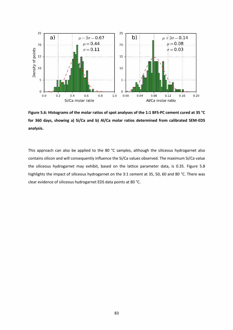
83
Figure 5.6: Histograms of the molar ratios of spot analyses of the 1:1 BFS-PC cement cured at 35 °C
for 360 days, showing a) Si/Ca and b) Al/Ca molar ratios determined from calibrated SEM-EDS
analysis.
This approach can also be applied to the 80 °C samples, although the siliceous hydrogarnet also
contains silicon and will consequently influence the Si/Ca values observed. The maximum Si/Ca value
the siliceous hydrogarnet may exhibit, based on the lattice parameter data, is 0.35. Figure 5.8
highlights the impact of siliceous hydrogarnet on the 3:1 cement at 35, 50, 60 and 80 °C. There was
clear evidence of siliceous hydrogarnet EDS data points at 80 °C.
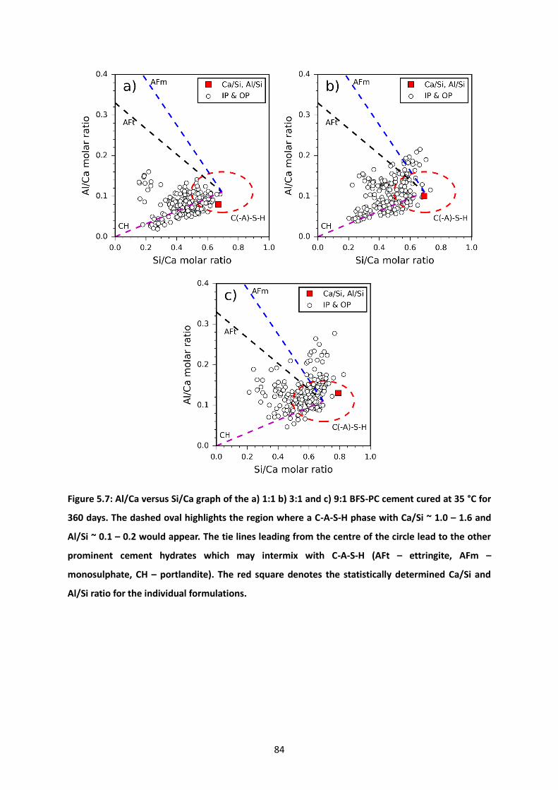
84
Figure 5.7: Al/Ca versus Si/Ca graph of the a) 1:1 b) 3:1 and c) 9:1 BFS-PC cement cured at 35 °C for
360 days. The dashed oval highlights the region where a C-A-S-H phase with Ca/Si ~ 1.0 – 1.6 and
Al/Si ~ 0.1 – 0.2 would appear. The tie lines leading from the centre of the circle lead to the other
prominent cement hydrates which may intermix with C-A-S-H (AFt – ettringite, AFm –
monosulphate, CH – portlandite). The red square denotes the statistically determined Ca/Si and
Al/Si ratio for the individual formulations.

85
Figure 5.8: Al/Ca versus Si/Ca graphs for the 3:1 BFS-PC cement cured at 35 °C for 360 days and then
exposed to (a) 35 C, (b) 50 C, (c) 60 C and (d) 80 C for a further 28 days. The dashed oval highlights
the region where a C-A-S-H phase with Ca/Si 1.0 – 1.6 and Al/Si 0.1 – 0.2 would appear. The tie lines
leading from the centre of the circle lead to the other prominent cement hydrates which may
intermix with C-A-S-H (AFt – ettringite, AFm – monosulphate and CH – portlandite). The red square
denotes the statistically determined Ca/Si and Al/Si ratio for the individual formulations.
The back scattered electron (BSE) images in Figure 5.9a-d highlight the variation of the morphology of
the 3:1 BFS-PC cement cured at different temperatures. Region 1 in Figure 5.9a represents a fully
hydrated BFS particle and the inner-product C-A-S-H phase (intermixed with hydrotalcite-group LDH)

86
in close proximity to the slag grain. Region 2 in Figure 5.9b highlights the more porous structure of the
outer-product C-A-S-H phase which forms within the initially fluid-filled space of the cement matrix.
These regions appeared denser at higher temperatures, specifically highlighted in the 80 °C sample in
region 3. Region 3 appears from its angular shape to have been a slag grain similar to region 1, but
which has almost fully dissolved. Other hydrated and partially hydrated slag grains are observed in
regions 4 and 5, respectively.
Figure 5.9: BSE-SEM images of 3:1 BFS-PC cement cured at a) 35 °C for 360 days and then exposed to
b) 50 °C, c) 60 °C, and d) 80 °C for a further 28 days.
A decrease in Ca/Si and increase of Al/Si ratio (Table A8.2 in the Appendix) at higher temperature was
observed across the three formulations. Condensation reactions of the monomeric and dimeric
silicates may lead to an expulsion of calcium ions and water from the C-A-S-H phase, leading to higher
polymerisation of the gel at increasing temperatures [216], consistent with this observation. The Ca/Si
decrease was greatest in the 1:1 BFS-PC blend, with the ratio decreasing by as much as 0.1 units from
35 °C to 80 °C. The Ca/Si decrease may be more prominent in the 1:1 formulation because there was
a) b)
c) d)
1 2
3
4
5
87
more available Ca to be redistributed upon a change in temperature. This may be the cause of the
greater variation in the Ca/Si observed in the work of Bahafid et al. [205] compared with the work of
Burciaga-Diaz et al. [219]: Bahafid et al. considered a high Ca/Si class G cement and observed a drop
in Ca/Si by 0.2 between 25 and 90 °C, whereas Burciaga-Diaz et al. studied alkali-activated slag cement
systems (with much less Ca than class G cement) at 20 and 60 °C in which there was no clear overall
change in the Ca/Si or Al/Si values.
An increasing abundance of silicate chain sites becoming available as a result of the condensation of
calcium silicate species provided an opportunity for aqueous aluminium species to bridge gaps in the
silicate chain. The additional opportunity for bridging in the aluminosilicate chains may be the cause
for the increase of the Al/Si in all three formulations. The 1:1 formulation displayed the greatest rise
in Al/Si ratio, increasing by 0.04 units. The 9:1 formulation exhibited the largest Al/Si values, at Al/Si
reaching 0.19.
5.4.4 Chemical composition of hydrotalcite-like phase using SEM-EDS
The hydrotalcite-like phase was a major hydration product that persisted at the elevated
temperatures. The hydrotalcite-like LDH formed, became intermixed with the other hydration
products, specifically C-A-S-H because of the dependence on phase formation through slag dissolution
[213,218]. Therefore, the points taken for the C-A-S-H analysis were also used in determining the
Mg/Al molar ratio within hydrotalcite-like LDH.
In blended cement systems the structure of hydrotalcite-like LDH has been shown to be heavily reliant
on the content of BFS and PC available. Richardson and others [44,45] observed higher Mg/Al values
in hydrotalcite formed in blended cements with less BFS. The direct cause for this is the possibility for
Al to react with other common AFm and AFt phases containing sulphate or carbonate. The Al which is
not incorporated into these sulphate- and carbonate-containing hydrous calcium aluminate phases
may then be split between the C-A-S-H and hydrotalcite-like LDH phases. There are no other phases
in BFS-PC cements that contain Mg, therefore all of the available Mg forms hydrotalcite-like LDH,
whereas Al may be distributed between other hydrates. A lower availability of sulphate and carbonate
in the higher BFS systems causes an abundance of free Al ions, which in turn decreases the Mg/Al
value in hydrotalcite-like LDH.

88
Figure 5.10: Mg/Si versus Al/Si atom ratios from EDS analysis for the a) 1:1 b) 3:1 and c) 9:1 28B
BFS:PC. Data manipulation was conducted using Mg/Al minimum of 1.0, Mg/Al maximum of 2.5,
and Al/Si maximum of 0.5. The red line highlights the line of best fit through the data points and the
Mg/Al value is taken from the gradient. The green and blue tie-lines are example lines of gradient 2,
which is generally indicative of the lower Mg/Al examples of a hydrotalcite-group LDH.
Taking the gradient of a line of best fit for the atom ratios Mg/Si versus Al/Si has been shown to provide
the most reliable results for determining the Mg/Al of hydrotalcite-like LDH [218], as observed in the
1:1, 3:1 and 9:1 28B samples in Figure 5.10.

89
Directly plotting the line of best fit resulted in poor results which did not provide a good representation
of the hydrotalcite-like LDH structure. A wide array of Mg/Si and Al/Si ratios has resulted in a poor
description of the hydrotalcite-like LDH structure. A large amount of intermixing has occurred as a
result of the finite EDS spot size, and the mineralogical complexity of these cements.
In previous studies, the Mg/Al line gradient was taken by assessing the ‘left-most’ data-points that
were collected [186,218]. Emulating this approach, three limiting factors were applied to the data
collected: 1) provide a maximum of the Al/Si of the dataset, 2) round the Al/Si to 3 decimal places and
obtain the ‘tail’ value or lowest Mg/Al value associated with that Al/Si value (this was to determine
‘left most value’ at a given Al/Si), and 3) within the data array, create a minimum and maximum Mg/Al
from the elemental atomic percentages. The settings that provided the Mg/Al line gradient most
consistent with expected results were: maximum Al/Si = 0.5, minimum Mg/Al = 1.0, and maximum
Mg/Al = 2.5. However, using this data manipulation method, no coherent or discernible pattern was
obtained (Table 5.6). This method still relies heavily on the assumption that the intermixing Al
containing species are restricted to C-A-S-H and hydrotalcite-like LDH. The sulphate and carbonate
phases containing Al will also affect this method of analysis, reducing the effective Mg/Al ratio as these
contribute Al but not Mg to the calculation. Therefore, an accurate representation of the effect of
temperature and BFS-PC formulation on the hydrotalcite-like LDH structure cannot be definitively
obtained from these data.

90
Table 5.6: SEM-EDS analysis of the Mg/Al ratio of the hydrotalcite-like phase for different BFS-PC
ratios and temperatures of curing. Samples were cured at 35 °C for 1 year (360A) and then at either
60 °C (tC) or 80 °C (tD) for a further 28 days. Samples were cured at 35 °C for 1 year, followed by 80
°C for 1 year and finally cured for 28 days at 50 °C (tE). Samples cured at 35 °C for 2 years (720A).
Temperature regime
Formulation Mg/Al
360A 1:1 1.378
360A 3:1 1.920
360A 9:1 1.917
720A 1:1 1.645
720A 3:1 1.660
720A 9:1 2.169
28B 1:1 2.462
28B 3:1 2.087
28B 9:1 1.619
28C 1:1 1.167
28C 3:1 2.336
28C 9:1 1.648
28D 1:1 2.077
28D 3:1 2.234
28D 9:1 1.687
360D 1:1 1.547
360D 3:1 1.404
360D 9:1 1.506
28E 1:1 2.283
28E 3:1 1.712
28E 9:1 1.742
5.5 Evaluation of the efficacy of thermodynamic modelling
5.5.1 Selection of potential phase assemblage constituents
Two modelling approaches were followed in this study, with calculations conducted with (“SH
approach”) and without (“NS approach”) the presence of a siliceous hydrogarnet; the phases available
for hydration are summarised in Table A8.3 found in the Appendix. A similar methodology was applied
by Deschner et al. [188] and by Dilnesa et al. [119] for low pH cements and 3 year old cements,
respectively. This approach was intended to ensure the correct phases form at the different
temperatures, incorporating restrictions which may be kinetic rather than thermodynamic in
foundation. Taylor and Richardson [45] showed that siliceous hydrogarnet does not form in blended
cements up to 20 years of curing at 20 °C, therefore highlighting that its inclusion in potential phase
assemblages at lower temperatures is unwarranted. Deschner et al. [188] used the SH approach for
91
temperatures above 50 °C, which causes the monosulphate, monocarbonate and hemicarbonate
phases to become destabilised as siliceous hydrogarnet is a more stable alternative. In the current
study, monosulphate, monocarbonate and hemicarbonate phases were observed up to 60 °C by XRD,
and therefore the upper limit of the NS method and the lower limit of the SH method were changed
to 60 °C.
A constant degree of reaction of the BFS and clinker phases was used for each system. The DoH of BFS
at 60 °C was used for the NS method and the DoH of BFS at 80 °C was used for the SH method (Figure
5.1). The reaction of slag was assumed to be congruent. The DoH values of clinker phases were taken
from Chapter 4, with an additional 5% reaction included to replicate the increase of temperature on
the clinker phases. The 5% additional clinker reaction was estimated due to the higher degree of
reaction of the clinker phases at the lower temperatures, therefore it was assumed this would occur
at higher temperatures. A summary of the DoH values can be seen in Table 5.7. Calcite and gypsum
were observed in the anhydrous PC XRD diffractograms and were quantified by Rietveld analysis (data
not shown) to be 4.5 and 3.5 wt.%, respectively of the PC fraction of the systems.
Table 5.7: Clinker degree of hydration values used in thermodynamic modelling. Taylor-Bogue
analysis determined the clinker phase ratios in the initial PC: C3S = 71.9 wt.%, C2S = 6.8 wt.%, C3A =
8.0 wt.%, C4AF = 7.7 wt.% [122].
Clinker phase
DoH (%)
1:1 3:1 9:1
C3S 87 93 95
C2S 68 55 47
C3A 100 100 100
C4AF 81 81 81
5.6 Phase assemblage as a function of temperature
The phases predicted by thermodynamic modelling to form in the 1:1 BFS:PC system exposed to
temperatures below 60 °C were C-A-S-H, portlandite, ettringite, monosulphate, monocarbonate and
hydrotalcite-like LDH (Figure 5.11a). The ettringite phase was no longer stable above 52 °C, consistent
with the XRD results of this study where ettringite was still observed up to 50 °C as seen in Figure
5.12a and Figure 5.3a, and only after 28 days at 60 °C does it appear to have mostly converted into
monosulphate.
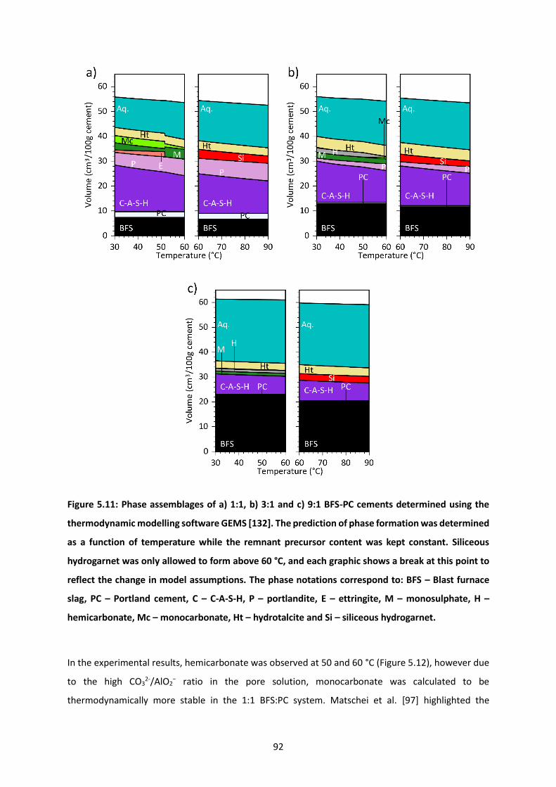
92
Figure 5.11: Phase assemblages of a) 1:1, b) 3:1 and c) 9:1 BFS-PC cements determined using the
thermodynamic modelling software GEMS [132]. The prediction of phase formation was determined
as a function of temperature while the remnant precursor content was kept constant. Siliceous
hydrogarnet was only allowed to form above 60 °C, and each graphic shows a break at this point to
reflect the change in model assumptions. The phase notations correspond to: BFS – Blast furnace
slag, PC – Portland cement, C – C-A-S-H, P – portlandite, E – ettringite, M – monosulphate, H –
hemicarbonate, Mc – monocarbonate, Ht – hydrotalcite and Si – siliceous hydrogarnet.
In the experimental results, hemicarbonate was observed at 50 and 60 °C (Figure 5.12), however due
to the high CO32-/AlO2
− ratio in the pore solution, monocarbonate was calculated to be
thermodynamically more stable in the 1:1 BFS:PC system. Matschei et al. [97] highlighted the

93
importance of the SO3/Al2O3 and CO2/Al2O3 ratios within Portland cement systems, which determined
which of the sulphate and carbonate AFm or Aft phases form in each specific instance, as there are
small energetic differences between various members of these families. In the 1:1 cement the
SO3/Al2O3 and CO2/Al2O3 ratios were 0.4 and 0.2, respectively. According to Matschei et al. [97], this
pair of ratios should form monosulphate and hemicarbonate. However, due to the presence of the
more thermodynamically stable C-A-S-H and hydrotalcite-like LDH phases, which withdraw the
aluminium from solution, the effective sulphate and carbonate contents become much higher with
respect to Al2O3. This causes the thermodynamic model to predict the formation of higher SO3 and
CO2 rich-phases. Within the 3:1 (Figure 5.11b) and 9:1 (Figure 5.11c) cements, monosulphate was
consistently observed in the modelling and experimental results up to 60 °C. Hemicarbonate became
destabilised at higher temperatures in the 3:1 cement, however as CO2/Al2O3 increases with increasing
temperature, formation of monocarbonate occurred. The CO2/Al2O3 ratio was consistently lower in
the 9:1 cement as this contained the lowest amount of calcite (supplied by the PC), therefore it was
possible for hemicarbonate to persist.
A trend of decreasing volume of C-A-S-H and increasing portlandite was observed in the 1:1 and 3:1
blends as the temperature increased. The densification of the C-A-S-H phase at higher Al/Si and lower
Ca/Si ratios (see the specific volumes of each end-member in the C-A-S-H model in Table A8.3 in the
Appendix) led to a decreasing volume of the C-A-S-H phase as temperature increased. More calcium
is available for formation of other phases as a result of the decreasing Ca/Si of the C-A-S-H, therefore
the volume of portlandite increases.
Thermodynamic modelling appropriately describes the phases forming at the various temperatures
investigated, however simulating the decrease of temperature from 80 °C to 50 °C using the NS and
SH methodology may not be as effective. Figure 5.12 shows that the phases observed experimentally
were the same as those predicted using the SH method, however the suggested protocol of
determining the phase assemblage up to 60 °C disagrees with the recorded phase assemblage for the
tE temperature profile, where the sample has been held at 80 °C for an extended period before
returning to lower temperature. Therefore, it is recommended that once the cement has reached a
temperature at which the siliceous-hydrogarnet phase may form, the SH method must be used to
accommodate this change. This gives further indication that the limitation on formation of siliceous
hydrogarnet at near-ambient temperature is kinetic rather than thermodynamic, as this phase persists
after cooling once it has formed at higher temperature. Conversely, it is possible that a longer period

94
at 50 °C may be necessary to determine whether the phase assemblage will re-equilibrate to a
hydrogarnet-free state in the very long term. The possibility that the waste packages may reach a
temperature of 80 °C is still considered the most extreme scenario for use in safety case development,
providing an upper limit on what may occur in practice [30].
Figure 5.12: XRD patterns of a) 1:1, b) 3:1 and c) 9:1 BFS-PC cements exposed to different
temperature regimes. Phases identified are: C – C-A-S-H, P – portlandite, E – ettringite, M –
monosulphate, H – hemicarbonate, Mc – monocarbonate, Ht – hydrotalcite, B – belite and Si –
siliceous hydrogarnet.

95
Volume expansion of the hydrates is not expected based on the results from Figure 5.11 which would
be a cause of concern for potential cracking in the waste packages. The reduced possibilty of cracking
can be seen as a positive to reinforce the notion that cement encapsulation is a viable option for long-
term storage of ILW. Small levels of shrinkage are expected as a result of the densification of the
C-A-S-H phase.
5.6.1 Chemical composition of C-A-S-H phase using thermodynamic modelling as a function of
temperature
The different phases allowed to form within a simulation of hydration of cements affect the predicted
composition of the C-A-S-H phase (Figure 5.13). The NS method predicted a decline in Ca/Si and an
increase in Al/Si for each cement up to 60 °C, coinciding with what was determined from SEM-EDS
analysis. A notable decrease in the Ca/Si ratio (Figure 5.13a), with an increase in Al/Si (Figure 5.13b),
was observed at 52 °C and 50 °C in the 1:1 and 3:1 cements, respectively, in the thermodynamic model
outputs. This is caused by the decomposition of ettringite in the 1:1 BFS:PC system and the conversion
of hemicarbonate to monocarbonate in the 3:1 cement. In each case, it is likely that an increase in
aluminium concentration in the pore solution caused the sharp rise of Al/Si within the C-A-S-H phase.
A result of the dominance of the hydrogarnet phase in the SH method, a more consistent pattern in
Ca/Si and Al/Si values was observed in those simulations. The highly stable siliceous hydrogarnet
competes with the C-A-S-H phase for the calcium, aluminium and silicon in the system. Dilnesa et al.
[149] highlighted the minimal effect of increasing temperature on the C3AS0.84H4.3 hydrogarnet phase.
Accordingly, the Ca/Si value of the 9:1 system described by the SH model did not vary a great deal
(Figure 5.13a) because of the strong competition for the available silicon and calcium between the
two phases: C-A-S-H and siliceous hydrogarnet. Without the formation of portlandite, which was
predicted in the 1:1 and 3:1 cements but not at 9:1 systems, the C-A-S-H phase composition was
influenced by the formation of the hydrogarnet phase. The hydrogarnet phase has a similar solubility
to that of C-A-S-H at pH > 11.5 [108,149], so both phases co-exist in the 9:1 cement. The amount of
siliceous hydrogarnet remains relatively constant throughout the SH method simulations for each BFS-
PC ratio as a function of temperature.
The Ca/Si values within C-A-S-H were generally under-predicted in the NS method due to the
competition with other calcium containing phases. However, the Al/Si was generally over-predicted

96
due to the lower Gibbs energy of the 5CA and INFCA end-members (end-member model used to
describe C-A-S-H phase, Table A8.3 in the Appendix). This was exhibited further by the sudden increase
of the Al/Si in the C-A-S-H phase once the decomposition of ettringite occurs. A combination of these
two factors led to an increase in availability of calcium for higher portlandite formation observed in
the 1:1 and 3:1 cements. Within the 9:1 systems, the Ca/Si was over-predicted consistently due to the
lower Ca/Si end-members withdrawing the calcium from solution in place of forming portlandite.
The Ca/Si in the SH method was generally over-predicted due to the C-A-S-H phase containing a higher
calcium content when compared to siliceous hydrogarnet which was competing for calcium. Similarly,
the Al/Si within C-A-S-H was reduced in the SH method compared to the NS method due to siliceous
hydrogarnet containing a higher Al/Si ratio than the end-members used for the creation of C-A-S-H
and was stable throughout the temperature range (60 – 90 °C), whereas phases such as ettringite were
not stable across the temperature range in the NS method (30 – 60 °C).
This impact on the level of change of the Ca/Si and Al/Si at each temperature point was not explicitly
observed via the SEM-EDS data, however the general trends of decreasing Ca/Si and increasing Al/Si
with the increase of temperature were observed in both modelling methods and in the SEM-EDS data
as exhibited in Figure 5.13.

97
Figure 5.13: Molar ratios of a) Ca/Si and b) Al/Si within C-A-S-H as a function of temperature using
the two different modelling approaches (SH above, and NS below, a cutoff temperature of 60 °C in
each case) as a function of the BFS:PC ratios. The symbols correspond to SEM-EDS results, while the
lines represent the modelling results. The solid line represents the NS method and the dotted line
represents the SH method.
For both methods, the polymerisation of the aluminosilicate chains was well represented due to the
resulting reduction of Ca/Si and increase in Al/Si in the C-A-S-H phase, with increased curing
temperature. For the 1:1 and 3:1 samples, the Ca/Si was under-predicted and the Al/Si was over-
predicted by up to 2.1 % and 13.8% respectively. Integrating aluminium-containing end-members into
C-A-S-H models has been a continual issue. Recreating aluminium end-members with lower (Al/Si =
0.1) or very high (Al/Si = 0.33) Al contents based on the additive method proposed by Kulik [64] and
Myers [146], did not provide useful additions to the C-A-S-H model for the cementitious systems
simulated in this study. The highly stable nature of the current end-members causes a redundancy in
other end-members because they do not form in any meaningful amounts to contribute to the phase
assemblage of blended cements or the chemical composition of C-A-S-H in varying environments. This
is further highlighted by the results of the 9:1 cement system, which rigidly maintains a Ca/Si ratio
between 1.3 and 1.37, accumulating the remaining calcium in the system that cannot reach the higher
Ca concentration required to form portlandite. As a result of the C-A-S-H phase restricting the
formation of portlandite, its Ca/Si ratio was over-predicted in the 9:1 system by up to 7.4%. The higher
Al/Si ratio expected in the 9:1 cement resulted in greater accuracy, whereby the Al/Si was over-
estimated by no more than 7.6%.

98
5.6.2 Chemical composition of the hydrotalcite-like phase (MA-OH-LDH – solid solution model) using
thermodynamic modelling as a function of temperature
The chemical composition of the hydrotalcite-like LDH phase (calculated using the MA-OH-LDH) was
reliant on the other phases formed, Figure 5.14. The NS method produced a lower Mg/Al due to the
lower temperatures and the greater diversity of Al containing phases. Increasing the temperature
reduced the availability of Al due to the increasing Al/Si within C-A-S-H, however for phase transition
areas such as the diminishing levels of the other sulphate and carbonate AFm and AFt phases, more
Al became available to form hydrotalcite-like LDH. The decrement of the Mg/Al value from 52 °C and
above was a result of the decomposition of ettringite in the 1:1 cement and the decomposition of
hemicarbonate in the 3:1 cement. The 9:1 cement maintained an increasing Mg/Al value due to the
minimal alteration of changes in the available phases. Corresponding with experimental data, the
Mg/Al ratio was larger in cements that had lower BFS content [44,45].
The SH method resulted in a greater and more consistent Mg/Al ratio due to the presence of siliceous
hydrogarnet dominating the availability of Al, resulting in less freely available Al.
Figure 5.14: Molar ratio of Mg/Al within the magnesium hydrotalcite-like LDH phase of 1:1, 3:1 and
9:1 BFS-PC, using the MA-OH-LDH model developed by Myers et al [123].

99
5.7 Conclusions
The alteration in phase assemblages in hydrated mature BFS-PC systems which are subjected to step-
changes in temperature occurs relatively rapidly and is of importance in the context of emplacement
of cemented nuclear waste in a geological disposal facility. Sulphate and carbonate containing AFm
and AFt type phases are not greatly affected by the increase of temperature from 35 to 50 °C after
360 days of curing at 35 °C; transferring these samples to an environment of 50 °C did not cause major
phase changes. However, the higher water content phases such as ettringite and hemicarbonate
become destabilised at around 60 °C. When a 360-day cured cement is transferred from 35 to 80 °C
environments, a rapid transition occurs: after 3 to 7 days, the sulphate and carbonate AFm and AFt
phases have been destabilised and replaced by siliceous hydrogarnet.
Thermodynamic modelling of these systems has been shown to accurately replicate the changes in
phase assemblage observed when cements are transferred to higher temperature after 360 days of
curing, when held at the elevated temperature for 28 days at a range of temperatures, and up to 360
days in the case of a transfer to an 80 °C environment.
The phase assemblage formed after a subsequent decrease of temperature from 80 °C to 50 °C (after
360 days at 35°C and another 360 days at 80 °C) could be accurately predicted by a model which
allowed siliceous hydrogarnet to form, although this phase needed to be suppressed in simulations of
the samples which had never been heated above 60°C. This provides further evidence that the
absence of siliceous hydrogarnet from cement phase assemblages at near-ambient or slightly elevated
temperature is due to kinetic, rather than pure thermodynamic, limitations.
Description of the chemical composition of the C-A-S-H phase followed the trends observed
experimentally in BFS-PC cements. The Ca/Si values were very slightly under-predicted for the 1:1 and
3:1 systems, and over-predicted in the 9:1 cement by up to 7.4%. The Al/Si ratio was over-predicted
in all cements, by up to 13.8% in the worst cases. Inclusion of additional end-members with low (Al/Si
= 0.1) or high Al/Si (Al/Si = 0.33) values based on the additive method did not contribute any
meaningful change on the chemical composition of the C-A-S-H phase.

100
Understanding of how the C-A-S-H phase forms and alters with composition, and the quantity of other
phase formation, is important in waste immobilisation applications as it enables prediction of how this
key phase interacts with dissolved species including radionuclides. Additional studies are required to
determine the effects of alkali, aluminium and groundwater leaching effects on the C-A-S-H phase,
but this study has provided essential insight into the temperature effects that may influence PC-BFS
blends in this safety-critical application.

101
6 Using Pitzer parameters in GEMS for predicting blended cements.
6.1 Introduction
Thermodynamic modelling of cement phases has been used extensively in the past to predict the
phase assemblages of many varieties of cements. Utilizing geochemical software such as GEMSelektor
(GEMS), PHREEQC, MTDATA or Geochemist’s workbench (GwB) can provide good results when
predicting how the initial chemistries of cements will influence the solids formed, whether considering
ordinary Portland cements [113,119–121,126,150,151] or cements containing supplementary
cementitious materials (SCMs) [101,102,122,124,125,183,220].
The methodologies for determining stable phase assemblages may be determined from two main
approaches: by Gibbs energy minimisation (GEM), or through the law of mass action (LMA). Both
techniques include a mass balance approach to ensure all material available in the system which may
react is accounted for. The GEM method uses Gibbs energy as the basis for determining whether a
solid phase is stable within the system by considering the phase Gibbs energy as a sum of the chemical
potentials (µ𝑖) of the aqueous species that form the solid phase and applying a correction for the
activity coefficient (𝛾𝑖). The activity coefficient provides description of the non-ideal scenario, which
is indicative of the electrolyte solution environment. Activity coefficients are also used in conjunction
with the LMA method, however in this case the molar concentrations that combine to form the
solubility product (KSP) are effectively modified. Both approaches apply the activity coefficient factor
as a means of more accurately portraying the aqueous solution and the effect the solution may have
on aqueous ions, therefore leading to impact on the formation of solid phases. How GEM and LMA
methods are utilised in cement chemistry are well documented [118,120,128,132,180,221].
Activity coefficient equations are generally derived from a basic Debye-Hückel-type equation as seen
in Equation 6.1 and expanded in section 6.2.1 (Activity coefficient models). The Debye-Hückel
functional form may be used for dilute electrolytes, however at higher ionic strengths, more detailed
methods are used.
log 𝛾𝑖 = −𝐴𝑧𝑖2√𝐼 6.1

102
Where 𝐴 is a temperature dependent variable (𝐴 = 1.824928 × 10⁶𝜌𝑜1/2
(𝜀𝑇)−3/2, with 𝜌𝑜 the
density of water, 𝜀 the dielectric constant of water, and 𝑇 in kelvin) [136], 𝑧𝑖 is the charge of aqueous
species 𝑖, 𝐼 is the ionic strength of the solution (𝐼 = 0.5 ∑ 𝑐𝑖𝑛𝑖=1 z𝑖
2, where 𝑐𝑖 is the molal concentration
of species 𝑖), and 𝛾𝑖 is the activity coefficient of species 𝑖.
Adaptation of Equation 6.1 by adding additional terms to better describe the electrolyte being
simulated, has led to the improvement of aqueous solution modelling and to the creation of other
models effective at varying ionic strengths. The Pitzer model utilises ion-specific interaction
parameters alongside the ionic strength to provide greater accuracy for the activity coefficients for
individual aqueous species. The Pitzer model has been highlighted for its benefits over other activity
coefficient models due to the higher level of accuracy in more concentrated solutions
[66,100,110,111,143,145]. Portland cements, blended cements and alkali activated material (AAM)
generally have ionic strength values of 0.1 to 2.0 mol/L in their pore solutions [104,120].
Improved accuracy for determining the hydration of cement phases may be important, and
additionally, cement is currently used as a waste immobilisation or encapsulation method for various
waste streams [11,15,147,184,222]. Waste streams may increase the IS of the system, including
through corrosion of the waste, and require the use of improved aqueous solution models such as the
Pitzer method. Groundwater interaction models that consider the eventuality of a waste package
interacting with nearby groundwater may also benefit from the inclusion of a more robust aqueous
solution model. Therefore, the applicability and the possible improvements for modelling cement
hydration and pore solution chemistry were tested in this chapter.
6.2 Modelling approach
6.2.1 Activity coefficient models
Thermodynamic modelling was performed using GEMS in conjunction with the CEMDATA14 database
for cement phases, and data from the literature when considering non-cement oriented systems
(phases used are the same as the NS method, summarized in Table A8.3). The GEMS software
determines the minimum Gibbs energy of the system by precipitating solids out of solution through

103
equilibrium solvers [132,180]. This method determines molar amounts of phases based on the
chemical potential of each phase that may be created:
𝐺 = ∑ 𝑥𝑗µ𝑗
𝑗
6.2
Where, 𝑥𝑗 and µ𝑗 are the mole fraction and chemical potential of solid phase, 𝑗, respectively. Solid
phases are calculated to have formed if the sum of the chemical potentials of the aqueous species
become more negative than the chemical potential of the solid and the ∆𝐺 becomes negative (∆𝐺 =
∆𝐺(𝑝𝑟𝑜𝑑𝑢𝑐𝑡𝑠) − ∑ ∆𝐺(𝑎𝑞𝑢𝑒𝑜𝑢𝑠 𝑟𝑒𝑎𝑐𝑡𝑎𝑛𝑡𝑠)𝑖𝑖 ). In an ideal system, the standard chemical potential,
𝜇𝑖0, for aqueous species 𝑖 would be used, however systems in reality are not ideal. Therefore, an
additional term must be applied to the chemical potential which includes an activity coefficient, 𝛾𝑖, to
define a more realistic chemical potential of each species based on the chemical environment of the
system:
𝜇𝑖 = 𝜇𝑖0 + 𝑅𝑇𝑙𝑛𝛾𝑖𝑐𝑖 6.3
Where 𝑅 is the ideal gas constant (8.314 Jmol-1 K-1), 𝑇 is temperature (K) and 𝑐𝑖 is the molal
concentration of species 𝑖. There are many methods for determining the activity coefficient. Most
common methods involve using the Davies (Equation 6.4 [129]), Truesdell-Jones (Equation 6.5 [134])
or Helgeson (Equation 6.6 [137]) equations which are variations of the Debye-Hückel equation
(Equation 6.1). Each of the methods utilize the ionic strength (𝐼 = 0.5 ∑ 𝑐𝑖𝑧𝑖𝑛𝑖=1 , where 𝑐𝑖 is the molal
concentration and 𝑧𝑖 is the charge of species 𝑖) of the system and provide activity coefficients based
on the charge of the species. They provide little variation based on the species and are applicable up
to varying ionic strengths. Within GEMS, these activity coefficient models are built into the software
and have been used to good effect for predicting a range of cement hydrate systems
[101,102,122,124,125,183,220].

104
𝑙𝑜𝑔10𝛾𝑖 = −𝐴z𝑖2 (
√𝐼
1 + √𝐼+ 0.3𝐼)
𝐼 < 0.1 − 0.7 6.4
𝑙𝑜𝑔10𝛾𝑖 =−𝐴z𝑖
2√𝐼
1 + 𝑎𝐵√𝐼+ 𝑏𝐼
𝐼 < 0.5 − 2 6.5
𝑙𝑜𝑔10𝛾𝑖 =−𝐴𝛾z𝑖
2√𝐼
1 + �̇�𝐵𝛾√𝐼+ 𝑏𝛾𝐼 + 𝑙𝑜𝑔10
𝑋𝑗𝑤
𝑋𝑤
𝐼 < 0.5 − 2 6.6
Another approach is to use ion specific activity coefficients determined using the Pitzer model
[100,135,144], which is a significantly more complex method and requires ion-specific parameters,
thus an expansive database, as shown in Equation 6.7 to 6.13. There have been different variations of
the Pitzer model, however the one used within GEMS is the Harvie, Moller and Weare (HMW)
[100,144] formulation. The equations are presented here to yield the activity coefficients, 𝛾𝑀, for
cationic species, 𝑀. In Equation 6.7 and 6.8, mc is the molality (mol/kg solvent) of cation c, with charge
zc. Subscripts M, c and 𝑐′ refer to cations. The subscripts can be exchanged for X, a and 𝑎′ to refer to
anions. The summation index, c, denotes the sum over all cations in the system. The double
summation index, c < 𝑐′, relates to the sum over all interactions with dissimilar cations. Equivalent
definitions apply to the summation indices for anions. Further explanation of the terms have been
well documented in previous publications [100,135,144,145].
𝑙𝑛𝛾𝑀 = 𝑧𝑀2 𝐹 + ∑ 𝑚𝑎(2𝐵𝑀𝑎 + 𝑍𝐶𝑀𝑎)
𝑎
+ ∑ 𝑚𝑐(2Ф𝑀𝑐 + ∑ 𝑚𝑎ψ𝑀𝑐𝑎
𝑎
)
𝑐
+ ∑ ∑ 𝑚𝑎𝑚𝑎′ψ𝑎𝑎′𝑀
𝑎′
𝑎 <
+ |𝑧𝑀| ∑ ∑ 𝑚𝑐𝑚𝑎𝐶𝑐𝑎
𝑎𝑐
𝐼 < 0.5 − 6.0 6.7
The Pitzer-HMW approach incorporates the use of a virial coefficient expansion in terms of molality.
An initial term which encompasses the system as a whole, in this case the Debye-Hückel type term (F)
(Equation 6.8), is followed by interaction coefficients that consider the interaction between pairs of
aqueous species (B’s, C’s and Ф’s) and a term that includes ternary species interactions (ψ).

105
𝐹 = −𝐴𝜙
[√𝐼
1 + 𝑏√𝐼+
2
𝑏1 + ln(1 + 𝑏√𝐼)] + ∑ ∑ 𝑚𝑐𝑚𝑎𝐵′𝑐𝑎
𝑎𝑐
+ ∑ ∑ 𝑚𝑐𝑚𝑐′Ф′𝑐𝑐′
𝑐′
𝑐 <
+ ∑ ∑ 𝑚𝑎𝑚𝑎′Ф′𝑎𝑎
𝑎′
𝑎 <
6.8
Where 𝐴𝜙
equals 0.392 for water and 𝑏 is a universal empirical parameter equal to 1.2, both at 25 °C
[138].
𝐵𝑀𝑋𝜙
= 𝐵𝑀𝑋(0)
+ 𝐵𝑀𝑋(1)
𝑒−𝛼𝑀𝑋√𝐼 + 𝐵𝑀𝑋(2)
𝑒−𝛼′𝑀𝑋√𝐼 6.9
𝐵𝑀𝑋 = 𝐵𝑀𝑋(0)
+ 𝐵𝑀𝑋(1)
𝑔(𝛼𝑀𝑋√𝐼) + 𝐵𝑀𝑋(2)
𝑔(𝛼′𝑀𝑋√𝐼) 6.10
𝐵𝑀𝑋′ =
𝜕𝐵𝑀𝑋
𝜕𝐼= 𝐵𝑀𝑋
(1) 𝑔′(𝛼𝑀𝑋√𝐼)
𝐼+ 𝐵𝑀𝑋
(2) 𝑔′(𝛼′𝑀𝑋√𝐼)
𝐼
6.11
Where the functions 𝑔(𝑥) and 𝑔′(𝑥) are defined (with 𝑥 = 𝛼𝑀𝑋√𝐼 ) as:
𝑔(𝑥) = 2(1 − (1 + 𝑥)𝑒𝑥)/𝑥2 6.12
𝑔′(𝑥) = −2(1 − (1 + 𝑥 +𝑥2
2) 𝑒−𝑥)/𝑥2
6.13
It is important to note that for electrolyte interactions where the charges are 1-1 or 1-2, only the terms
including 𝐵𝑀𝑋(0)
and 𝐵𝑀𝑋(1)
are necessary. In this instance 𝛼 = 2, however for 2-2 electrolyte interactions
the 𝐵𝑀𝑋(2)
term is included, with 𝛼 = 1.4 and 𝛼′ = 12.0. The alteration to the 𝐵𝑀𝑋 equations based on
the 2-2 electrolyte takes into account the increased likelihood of higher valence ions to interact within
the solution.
Inclusion of only the 𝐵𝑀𝑋 terms has been credited to be sufficient for many electrolytes up to an ionic
strength of 4 mol/L [138,139]. To increase the range of validity of this method, the third virial
coefficient for binary interactions, 𝐶𝑀𝑋 and the mixed electrolyte ψ and Ф coefficients may be used

106
[140,141]. The third virial coefficient 𝐶𝑀𝑋 of binary ion interactions is defined to be independent of
ionic strength. The Ф term describes the interactions between like-charged ions (Ф𝑐𝑐 = 𝜃𝑀𝑀 +
𝜃𝑀𝑀𝐸 ). The 𝜃𝑀𝑀 parameters account for unsymmetric mixing effects involving 1-2 or 1-3 ion
interactions, and 𝜃𝑀𝑀𝐸 can be derived to account for the excess energy of mixing. The ψ term
describes ternary ion interactions ѱ𝑖𝑗𝑘, of two ions with the same signed charge and one ion with a
differently signed charge.
6.2.2 Incorporating Pitzer equations into GEMS
Previous investigations using the Pitzer parameters with thermodynamic models for cement systems
have been conducted by Damidot et al. [98,99,148] and Duchesne and Reardon [66]. Within these
investigations, PHREEQE was utilised alongside the PHRQPITZ speciation code used at that time; these
models are now incorporated into the PHREEQC code [115]. Using the Pitzer parameters within
PHREEQC is quite simple as it contains a database within the software and can be easily applied.
However, within GEMS, the user has to manually input the Pitzer interaction values based on the ion
code assigned to each by the software. This can be a tedious and time consuming task for simple
systems, and for complex systems such as cements, it is a greater problem. Therefore, a programme
was created here, that can convert the aqueous species listings obtained using GEMS and provides an
output file containing the Pitzer parameters in a format that can be used within GEMS.
Utilisation of the Pitzer model requires extensive databases for complex systems such as cement
hydration. Other geochemical modelling packages such as PHREEQC and GwB have databases
containing Pitzer parameters incorporated into the software. The PHREEQC database has been
incorporated into the one used within this study, with additional parameters included where possible,
or values updated and replaced where better parameter values have been identified. A simple ion-
interaction and database lookup programme has been created using Python to use specifically with
the Pitzer model user interface applied in GEMS (Figure 6.1).

107
Figure 6.1: Programme structure for Pitzer parameter database lookup.
6.2.3 Estimating Pitzer parameters
Interaction parameters are generally determined through empirical means by using solubility data
over a wide range of ionic strengths of binary or ternary systems. Using this method in multi-species
systems has been proven to work effectively for systems including up to 11 aqueous species [223,224],
proving that these binary electrolyte values can be applied to more complex scenarios. Simulation of
a BFS-PC cement may include the use of greater than 70 aqueous species, creating a significantly more
complex system. As a result of the large number of aqueous species, there may not be interaction
parameters available within the literature to describe some important interactions. For example, to
form katoite (C3AH6), interaction parameters between Ca2+- OH- and Ca2+- AlO2- would be highly
desirable to be used, however, within the literature there are not parameters available for Ca2+- AlO2-
interactions. Therefore, missing interaction parameters have been estimated using Equation 6.14 and
6.15, from Simoes et al. [225]:
𝐵𝑀𝑋(0)
= 0.04850𝑧𝑀1.62𝑧𝑋
−1.35|𝑟𝑀 − 1.5𝑟𝑋|1.2 + 0.03898 6.14

108
𝐵𝑀𝑋(1)
= 0.00738𝑧𝑋−0.4(𝑧𝑀
2 𝑧𝑋0.6(1 + |𝑟𝑀 − 1.2𝑟𝑋|0.2))2
+ 0.16800𝑧𝑀2 𝑧𝑋
0.2(1 + |𝑟𝑀 − 1.2𝑟𝑋|0.2) − 0.09320𝑧𝑋−0.4
6.15
Where 𝑧𝑀 and 𝑧𝑋 are the charges of the cation and anion, respectively, and 𝑟𝑀 and 𝑟𝑋 are the ionic
radii of the cation and anion, respectively. This method was proven to be effective across a range of
ionic strengths, when only the 𝐵𝑀𝑋(0)
and 𝐵𝑀𝑋(1)
values were used in binary solutions [225]. This method
was verified using the osmotic coefficient data for binary ion interactions in solution, which is a
technique often used to derive Pitzer parameters. A strong correlation of ionic radius and charge with
the second virial coefficient parameters (𝐵𝑀𝑋(0)
and 𝐵𝑀𝑋(1)
) was determined to create Equation 6.14 and
6.15. Simoes et al. [225] highlighted that this technique was not ideal for producing parameters for
ion pairs/complexes for 1-1 electrolytes. The model does not account for the parameters independent
of ionic strength such as the 𝐶𝑀𝑋 values, therefore its results become less accurate above ionic
strengths of ~4 mol/L. When considering cement systems, this method may be viable due to cement
pore solutions generally registering an ionic strength range of 0.5 to 3 mol/L [104,120].
A database of ionic radii was created using the data collected by Marcus [226,227], similar to the
approach of Simoes et al. [225]. A similar database lookup tool was created to ensure that the correct
interaction parameters were used in the simulations in GEMS.
6.2.4 Testing applicability of the Pitzer model and simulation setup
The solubilities of common cement phases were simulated using the Pitzer model (P), and compared
to results obtained using the Truesdell-Jones equation (T). Solubility data from the literature,
describing the invariant points for phase transitions based on composition in the system, were used
as the main basis for comparison. Trials of the Pitzer model using only parameters created using the
Simoes estimation equations (S) and using Pitzer parameters taken from the literature which are
supplemented by Simoes-method estimated parameters (SP), were tested. A comparison and lookup
tool was created to compile the SP parameters. The tool determined which ionic interactions had
Pitzer parameters from the literature, and these were supplemented by filling the missing parameters
based on the ionic interactions created for the Simoes (S) method.
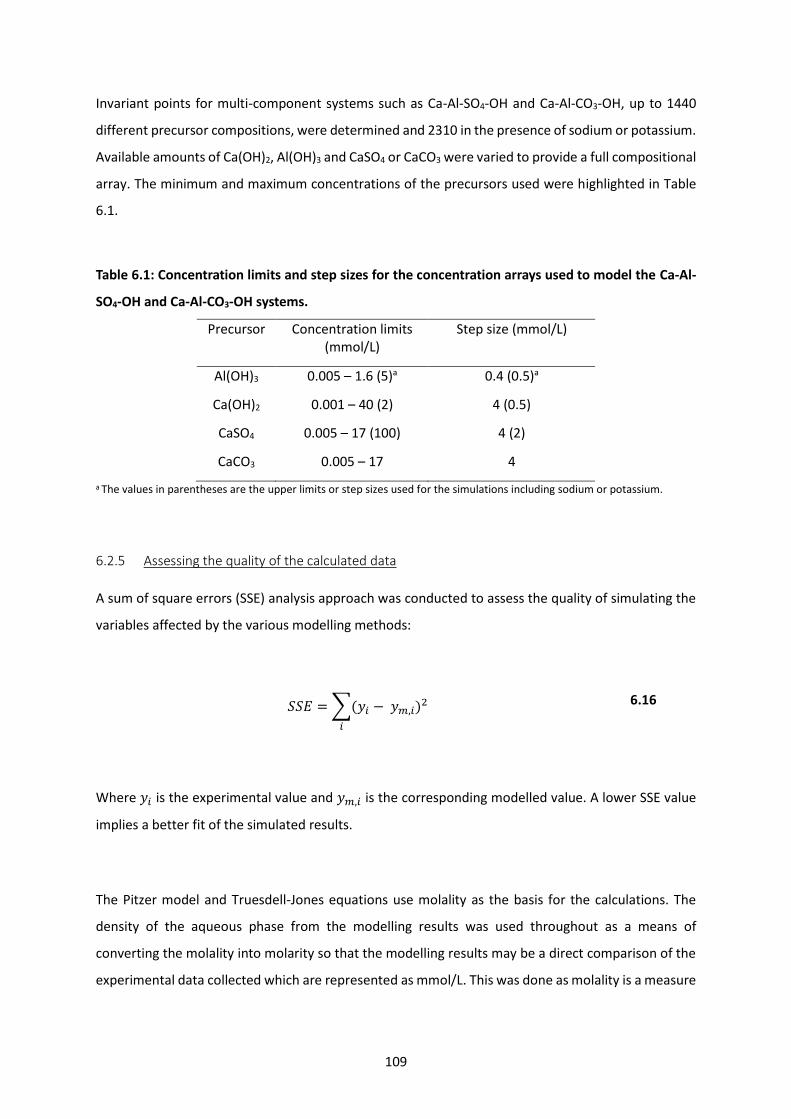
109
Invariant points for multi-component systems such as Ca-Al-SO4-OH and Ca-Al-CO3-OH, up to 1440
different precursor compositions, were determined and 2310 in the presence of sodium or potassium.
Available amounts of Ca(OH)2, Al(OH)3 and CaSO4 or CaCO3 were varied to provide a full compositional
array. The minimum and maximum concentrations of the precursors used were highlighted in Table
6.1.
Table 6.1: Concentration limits and step sizes for the concentration arrays used to model the Ca-Al-
SO4-OH and Ca-Al-CO3-OH systems.
Precursor Concentration limits (mmol/L)
Step size (mmol/L)
Al(OH)3 0.005 – 1.6 (5)a 0.4 (0.5)a
Ca(OH)2 0.001 – 40 (2) 4 (0.5)
CaSO4 0.005 – 17 (100) 4 (2)
CaCO3 0.005 – 17 4
a The values in parentheses are the upper limits or step sizes used for the simulations including sodium or potassium.
6.2.5 Assessing the quality of the calculated data
A sum of square errors (SSE) analysis approach was conducted to assess the quality of simulating the
variables affected by the various modelling methods:
𝑆𝑆𝐸 = ∑(𝑦𝑖 − 𝑦𝑚,𝑖)2
𝑖
6.16
Where 𝑦𝑖 is the experimental value and 𝑦𝑚,𝑖 is the corresponding modelled value. A lower SSE value
implies a better fit of the simulated results.
The Pitzer model and Truesdell-Jones equations use molality as the basis for the calculations. The
density of the aqueous phase from the modelling results was used throughout as a means of
converting the molality into molarity so that the modelling results may be a direct comparison of the
experimental data collected which are represented as mmol/L. This was done as molality is a measure

110
of millimoles per kilogram of water in the system, as opposed to millimoles per litre of aqueous
solution which requires a density correction.
6.3 Pore solution extraction from hydrated samples
Pore solutions of blended BFS-PC cement samples were tested to provide data for direct comparison
of the modelling approaches. The steel die method was used to extract the pore solution [118,177–
179]. Three formulations of BFS-PC: 1:1, 3:1 and 9:1, were tested at different curing ages. A constant
water to solids ratio (w/s) of 0.35 and curing temperature of 35 °C were used. Samples were poured
into 500 mL HDPE bottles and sealed with a screw cap with Parafilm wrapped around the top.
Samples had the top and bottom of the cylinders removed to ensure a flat surface when being placed
into a cement pore press. The total volume of the sample was thus reduced to 468 mL for all of the
samples. The pore press design displayed in Figure 6.2 highlights the dimensions of the press used. A
hole in the middle of the base of the press directed the pore fluid through a channel which had a
syringe attached at the end. Before squeezing the samples, a hole was drilled into the centre of the
sample to create a channel for the pore water to flow without creating a blockage in the hole in the
base of the pore press. Samples were placed inside the press and gradually exposed to pressures of
up to 550 MPa.
Samples were initially planned to be tested at 28, 56, 90, 180 and 360 days following the curing ages
used for characterisation performed throughout this thesis. Recurrent issues leading to the damage
of the pore press caused consistent delays and resulted in missing curing ages for some of the samples
of each formulation.
Extracted pore fluid was tested using ICP-OES (Spectro Ciros Vision ICP-ES) to obtain the
concentrations of major elements such as: Al, Ca, Fe, K, Mg, Na, Si and S. The samples were filtered
and diluted by a minimum of 5 times. In the case of the 360 day 9:1 sample, the pore fluid was diluted
by 10 times due to the high concentration of sulphur in solution.

111
Figure 6.2: Pore press used for acquisition of pore fluid from cured BFS-PC cement samples. The
dimensions of the press are represented: a) before the sample has been compressed, and b) at the
expected maximum level of compression of a cement sample.
6.4 Modelling results comparing the Pitzer model with the Truesdell-Jones equation
The majority of the thermodynamic data used in the CEMDATA14 database for the cement phases
were developed using the extended Debye-Hückel model (Equation 6.4) to provide the activity
coefficients to create the Gibbs energy of formation or solubility products [118,149,150]. The phases
therefore are optimised for this specific aqueous model. The characterisation of most cement phases
is generally in good agreement with solubility data. However, utilisation of the Pitzer model to provide
an ion specific activity coefficient may improve the results.
The Truesdell-Jones (T) and the Pitzer (P) model using parameters from the literature, were used to
model common cement hydrates in solution to determine whether the Pitzer model provided a
greater level of accuracy. The Pitzer model using only Simoes et al. [225] parameters (S) and
parameters that were supplemented by Simoes et al. The (SP) were also compared to assess whether

112
the inclusion of estimated parameters improved the fitting of data. Table A8.6 and Table A8.7
(Appendix.) contain the Pitzer parameters used throughout the study.
6.4.1 Portlandite
Portlandite (Ca(OH)2) is one of the most common hydrates found within a cement phase assemblage,
and Ca2+ and OH- ions form a large portion of the solute in cement pore solutions. Parameters for the
interaction of Ca2+ and OH- in various aqueous environments were rigorously tested in previous years,
therefore providing a worthwhile basis to compare modelling approaches and parameters [66,100].
6.4.1.1 Portlandite in the presence of NaCl
In multi-electrolyte systems the inclusion and exclusion of different aqueous ions was an important
factor to consider. In the studies focused on parameterisation of ions involved in portlandite solubility
studies, the CaOH+ complex ion was not included in the parameterisation. Instead, this species was
implicitly accounted for through the inclusion of the 𝐵𝑀𝑋(2)
and 𝐶𝑀𝑋 interaction parameters, which are
ordinarily utilised for 2-2 ionic charged species and imply ternary ion interactions, respectively
[66,139]. In general, ion pairs such as CaOH+ are not parameterised because of the unsymmetric
nature of the ions in solution. This unsymmetric behaviour has created issues in fitting parameters to
ion pairs because the nature of fitting the parameters has an underlying relationship to the difference
in ionic radii of the interacting ions [138,225]. This is highlighted further through the impact that not
accounting for this unsymmetrical behaviour leads to an under-prediction of calcium concentration in
solution when using the Simoes-method parameters. This issue was present in all calcium-containing
systems.
However, within aqueous solution modelling software, ion pairs are considered in the solution
chemistry by default. This is the case within the GEMS software. The inclusion of non-parameterised
aqueous species may have large implications or create errors when modelling an aqueous system.
Figure 6.3a highlights the impact that a non-specifically-parameterised ion (CaOH+) and an aqueous
species (NaOH(aq)) have on the solubility of portlandite calculated using the Pitzer model within a
NaCl electrolyte. The speciation of calcium into Ca2+ and CaOH+, when the CaOH+ was permitted to
form in solution, caused a significant error in the precipitation of portlandite. Coupled with the
consumption of Na+ ions to form NaOH(aq), which reduced apparent ionic strength, there was an error

113
in the calculated calcium concentration by up to 97.9% at a concentration of 3.75 mol/L of NaCl. This
level of error is highlighted by Figure 6.3b, where the Pitzer equation with no parameters in this system
was compared to the Truesdell-Jones (T) method.
Without the second and third virial coefficients (𝐵𝑀𝑋 and 𝐶𝑀𝑋, respectively) the Pitzer activity
equation is greatly simplified:
𝑙𝑛𝛾𝑀 = 𝑧𝑀2 𝐹 6.17
𝐹 = −𝐴𝜙
[√𝐼
1 + 𝑏√𝐼+
2
𝑏1 + ln(1 + 𝑏√𝐼)]
6.18
The version of the Pitzer model displayed in Equation 6.17 becomes inadequate for IS > 0.1 as the
equation represents long-range interactions of a very dilute electrolyte, whereas this is not the case
in the actual system. The example displayed in Figure 6.3b further highlights the need for complete
parameterisation of the aqueous species involved in a solution when using the Pitzer model. The Pitzer
model solely using the Debye-Hückel term (denoted in Figure 6.3b as PF) provides a significantly worse
fit. For further studies of prominent cement phases, the inclusion of neutral aqueous species or ion
pairs were removed in the instances that no Pitzer parameters were available.
The Simoes parameters were tested alongside the Pitzer parameters in Figure 6.3a and provide a good
agreement with the solubility data, reaching a maximum error of 34.2% at 3.75 mol/L of NaCl. The
Simoes parameters follow a similar trend to the solubility data, which makes this method a potentially
viable approach to fill vacancies in the Pitzer parameter database, although it is evidently less
desirable than the use of parameters specifically fitted to the system of interest.

114
Figure 6.3: The application of different parameterisations of the Pitzer aqueous solution model to
the prediction of portlandite solubility in NaCl solutions: a) highlighting the importance of selection
and parameterisation of the aqueous species; P(CaOH+) denotes the Pitzer model including CaOH+
in the calculations, P denotes a fully parameterised Pitzer model without CaOH+, and S denotes the
Pitzer model using only the parameters generated from the Simoes estimation equations; b)
showing the detrimental effect that the Pitzer model with all parameters set to zero (PF – equation
6.17) has on the predictions in comparison with the Truesdell-Jones (T) equation. Both plots show
experimental data from Duchesne and Reardon [66].
6.4.1.2 Portlandite in the presence of NaOH and KOH
Cement pore solutions are high in pH due to the dominance of alkaline constituents such as NaOH and
KOH [33,104,228]. Portlandite precipitation in water occurs between 18.2 and 22.6 mmol/L of Ca(OH)2
[66]. The inclusion of additional ions such as Na+, K+ and OH- ions in solution, as KOH or NaOH are
introduced, gradually reduces the activity coefficients of Ca2+ and OH- through affecting the IS in the
activity coefficient models, up to mid molal values (0.3 < IS < 1.0 mol/L), after which point the activity
coefficients begin to increase as a result of the ‘salting out’ effect [116]. Ordinarily for the T method,
the activity coefficient will begin to increase after 0.7 mol/L to compensate for the increasing
abundance of like-signed ions in solution, which increases the effect of the long-range coulombic

115
forces on the ions [136]. Addition of greater concentrations of OH- due to the increasing level of NaOH
or KOH compensates for the reduction of the activity coefficient.
This simple relationship of portlandite solubility decreasing with the addition of NaOH or KOH was
well represented by the T, P and S methods, Figure 6.4. There was marginal difference in the initial
solubility of portlandite in water at 20.3, 22.1 and 17.2 mmol/L for the T, P and S methods,
respectively. A constant under-prediction of the calcium solubility was observed using the Simoes
parameters within the NaOH system, however for the KOH system, the fit was near identical to the
Pitzer parameters. This may be affected by the impact of the difference of the ionic radii of the
aqueous pairing. The ionic radius of K+ (1.38 Ȧ) is more similar to the ionic radius of OH- (1.33 Ȧ) than
Na+ (1.02 Ȧ) is compared to OH-. This improved level of symmetry of the ions may be the cause of the
improved fit of the KOH system.
Figure 6.4: Portlandite solubility in a) NaOH and b) KOH, with different aqueous modelling
approaches, Pitzer parameter sets, and aqueous species used for calculations. P denotes a fully
parameterised Pitzer model, T denotes the Truesdell-Jones equation, and S denotes the Pitzer model
including parameters generated only from the Simoes Pitzer estimation equations. Experimental
data are from Duchesne and Reardon [66] (D&R-Exp).

116
6.4.2 Ca-Al-OH
Interactions between calcium and aluminium ions are a key aspect in cement hydration, particularly
when considering the aluminium-containing AFm and AFt phases that form due to the Ca2Al(OH)6+
ions encapsulating SO42- or CO32- ions, either as columns in the case of AFt phases or as layers for AFm
phases [97,229,230]. The generalised structures are [Ca3Al(OH)6∙12H2O]2∙X3∙xH2O and
[Ca2Al(OH)6∙12H2O]2∙X∙xH2O for AFt and AFm phases, respectively, where X denotes a double
negatively charged ion and x denotes the number of moles of water.
Lothenbach et al. produced solubility data over a range of CaO/Al2O3 molar ratios (0.5 – 1.2) [231].
These results are compared to the outcomes of the different modelling methods in Figure 6.5. Each of
the modelling methods provided a prediction of the same phases at each CaO/Al2O3 ratio, and there
were minimal differences in the predicted concentrations of aqueous species remaining in solution.
The main aluminium species observed was AlO2- (used as a master species in GEMS to represent
Al(OH)4-), providing over 99.99% of the aluminium in the modelled results. Above a pH of 4.5, AlO2
- is
known to be the dominant aluminium aqueous species [232]. Pitzer parameters exist for Ca2+-OH-
interactions, however, there are no parameters for Ca2+-AlO2- interactions, or any other aluminium
species interaction parameters within this system. Therefore, incorporation of a Ca2+-AlO2- parameter
into the Pitzer database using the Simoes parameters was expected to provide a more precise fit of
the solubility data (Appendix – Table A8.6).
The comparison of the models displayed that minimal difference was observed predicting the aqueous
solution. The Truesdell-Jones equation provides a better fit overall, particularly excelling at predicting
the calcium concentration. This is to be expected as the C3AH6 Gibbs energy value in the database was
fitted using the extended Debye-Hückel equation, in a form similar to the Truesdell-Jones equation
[92,150,233]. The introduction of the Ca2+-AlO2- interaction parameters provided minimal benefit in
terms of improving the quality of prediction of phase formation or solubility.
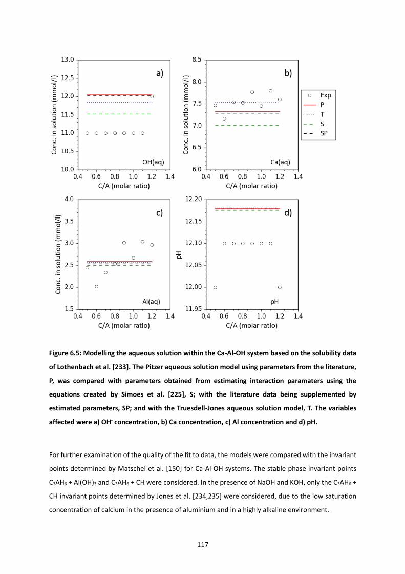
117
Figure 6.5: Modelling the aqueous solution within the Ca-Al-OH system based on the solubility data
of Lothenbach et al. [233]. The Pitzer aqueous solution model using parameters from the literature,
P, was compared with parameters obtained from estimating interaction paramaters using the
equations created by Simoes et al. [225], S; with the literature data being supplemented by
estimated parameters, SP; and with the Truesdell-Jones aqueous solution model, T. The variables
affected were a) OH- concentration, b) Ca concentration, c) Al concentration and d) pH.
For further examination of the quality of the fit to data, the models were compared with the invariant
points determined by Matschei et al. [150] for Ca-Al-OH systems. The stable phase invariant points
C3AH6 + Al(OH)3 and C3AH6 + CH were considered. In the presence of NaOH and KOH, only the C3AH6 +
CH invariant points determined by Jones et al. [234,235] were considered, due to the low saturation
concentration of calcium in the presence of aluminium and in a highly alkaline environment.

118
Figure 6.6: Invariant points using the Pitzer model for the a) Ca-Al-OH, b) Ca-Al-K-OH and c) Ca-Al -
Na-OH systems. The coloured lines represent the phases present in the modelling at given
concentrations. The square represents the invariant point of Al(OH)3 + C3AH6 [150] and the circle
represents invariant point of C3AH6 + CH (a) - [150], b) – [234] and c) - [235].
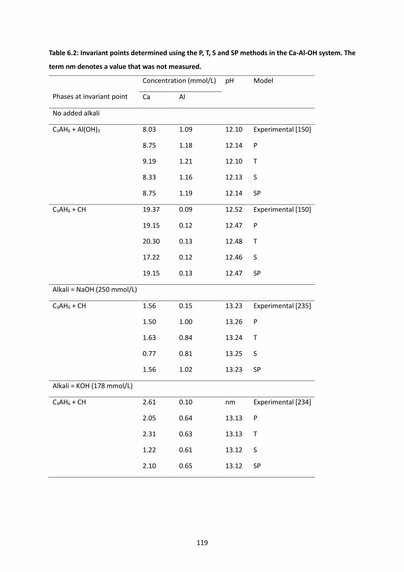
119
Table 6.2: Invariant points determined using the P, T, S and SP methods in the Ca-Al-OH system. The
term nm denotes a value that was not measured.
Phases at invariant point
Concentration (mmol/L) pH Model
Ca Al
No added alkali
C3AH6 + Al(OH)3 8.03 1.09 12.10 Experimental [150]
8.75 1.18 12.14 P
9.19 1.21 12.10 T
8.33 1.16 12.13 S
8.75 1.19 12.14 SP
C3AH6 + CH 19.37 0.09 12.52 Experimental [150]
19.15 0.12 12.47 P
20.30 0.13 12.48 T
17.22 0.12 12.46 S
19.15 0.13 12.47 SP
Alkali = NaOH (250 mmol/L)
C3AH6 + CH 1.56 0.15 13.23 Experimental [235]
1.50 1.00 13.26 P
1.63 0.84 13.24 T
0.77 0.81 13.25 S
1.56 1.02 13.23 SP
Alkali = KOH (178 mmol/L)
C3AH6 + CH 2.61 0.10 nm Experimental [234]
2.05 0.64 13.13 P
2.31 0.63 13.13 T
1.22 0.61 13.12 S
2.10 0.65 13.12 SP

120
Determination of the invariant points for each model provided good agreement with the experimental
data (Table 6.2). Without additional alkalis, the Pitzer parameters were marginally more effective at
predicting the solubility of the calcium and aluminium in solution. Inclusion of NaOH and KOH into the
system, led to a slight increase in accuracy for determining the C3AH6 + CH invariance point for the T
method as the saturation concentration of aluminium was larger in the other methods. The prediction
of calcium saturation was lower in the P, S and SP methods as was the case for the portlandite
solubility studies, however the difference between these methods and the T method was minimal.
The additional Ca2+-AlO2- interaction parameters made no improvement due to the low concentration
of aqueous species.
6.4.3 Ca-Al-SO4-OH
Gypsum (CaSO4) acts as a precursor for ettringite (Ca6Al2(SO4)3(OH)12∙26H2O) and calcium
monosulphoaluminate (monosulphate (Ms), (3CaO∙Al2O3∙CaSO4∙12H2O)) formation and is commonly
present in PC. The impact on the prediction of the precipitation of gypsum in a Ca-SO4-OH environment
using the various aqueous solution models may be observed in Figure 6.7 and Table 6.3. The invariant
point taken from Matschei et al. [150] was similar to the work summarised by Duchesne and Reardon
[66] whereby, once portlandite formed, up to 13 mmol/L of CaSO4 was required to form gypsum. There
was minimal difference between the different modelling approaches, and the Pitzer model provided a
slightly more accurate fit especially when considering the invariant point. The decreased solubility of
calcium and sulphate species resulted in precipitation at lower calcium and sulphur levels. The
exclusion of the CaOH+ ion and CaSO4(aq) species from the Pitzer simulations assisted in reducing the
content of calcium and sulphur in aqueous form, to create the portlandite-gypsum invariant point.
Removing additional aqueous species from the calculations in the Truesdell-Jones method (e.g. the
CaOH+ complex ion, and the CaSO4(aq) neutral complex) led to decreased solubility of portlandite and
gypsum, however when the thermodynamic data were created for the CEMDATA databases, these
aqueous species were available to form. Therefore, the aqueous species were included in the
formation of common cement hydrates [118,150,151].
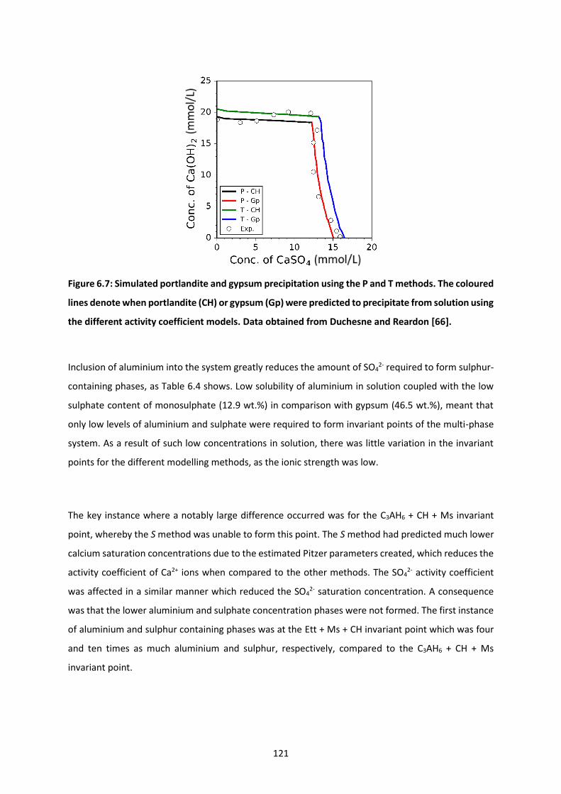
121
Figure 6.7: Simulated portlandite and gypsum precipitation using the P and T methods. The coloured
lines denote when portlandite (CH) or gypsum (Gp) were predicted to precipitate from solution using
the different activity coefficient models. Data obtained from Duchesne and Reardon [66].
Inclusion of aluminium into the system greatly reduces the amount of SO42- required to form sulphur-
containing phases, as Table 6.4 shows. Low solubility of aluminium in solution coupled with the low
sulphate content of monosulphate (12.9 wt.%) in comparison with gypsum (46.5 wt.%), meant that
only low levels of aluminium and sulphate were required to form invariant points of the multi-phase
system. As a result of such low concentrations in solution, there was little variation in the invariant
points for the different modelling methods, as the ionic strength was low.
The key instance where a notably large difference occurred was for the C3AH6 + CH + Ms invariant
point, whereby the S method was unable to form this point. The S method had predicted much lower
calcium saturation concentrations due to the estimated Pitzer parameters created, which reduces the
activity coefficient of Ca2+ ions when compared to the other methods. The SO42- activity coefficient
was affected in a similar manner which reduced the SO42- saturation concentration. A consequence
was that the lower aluminium and sulphate concentration phases were not formed. The first instance
of aluminium and sulphur containing phases was at the Ett + Ms + CH invariant point which was four
and ten times as much aluminium and sulphur, respectively, compared to the C3AH6 + CH + Ms
invariant point.

122
Table 6.3: Invariant points determined using the P, T, and S methods in the Ca-SO4-OH system.
Phases at invariant point Concentration (mmol/L) pH Model
Ca S
CH + Gypsum 30.69 12.47 12.43 Experimental [150]
30.95 12.25 12.43 P
32.90 13.30 12.43 T
28.60 8.80 12.43 S
Minimal solubility data exist for Ca-Al-SO4-OH-K or Ca-Al-SO4-OH-Na systems, and the data available
were recorded before phases such as monosulphate were widely considered in such measurements
[234–236]. In the sodium and potassium containing systems the Gyp + CH + Ett and Gyp + CH were
considered. The Ca-Al-SO4-OH system was exposed to 89 and 125 mmol/L of K2O and Na2O,
respectively.
All of the models accurately predicted the calcium, sulphate and pH concentrations. However,
aluminium prediction was 104 times lower in the simulated results when compared to the
experimental data. This may be because no ICP analysis was performed by Jones [234,235] and the
stable invariance point was determined through undersaturation studies using a fixed mass of
aluminium and variable calcium and sulphur masses. Therefore, the calcium and sulphur
concentrations at the point of precipitation were more rigorously tested than that for the aluminium
content. Comparing the Matschei et al. [150] solubility data in the Ca-Al-SO4-OH system with those
determined by Jones et al. [236], the aluminium concentration was much lower in the more modern
results determined by Maschei et al. The calcium and sulphur concentrations were different by up to
5 mmol/L, which provides some credence to the data collected by Jones et al. in the studies used in
Table 6.5. Therefore, definitively deciding which model performed better may not be possible based
on the presented data. However, an understanding of how the phases behave in the presence of
sodium and potassium, and increasing pH, may still be predicted using the data.
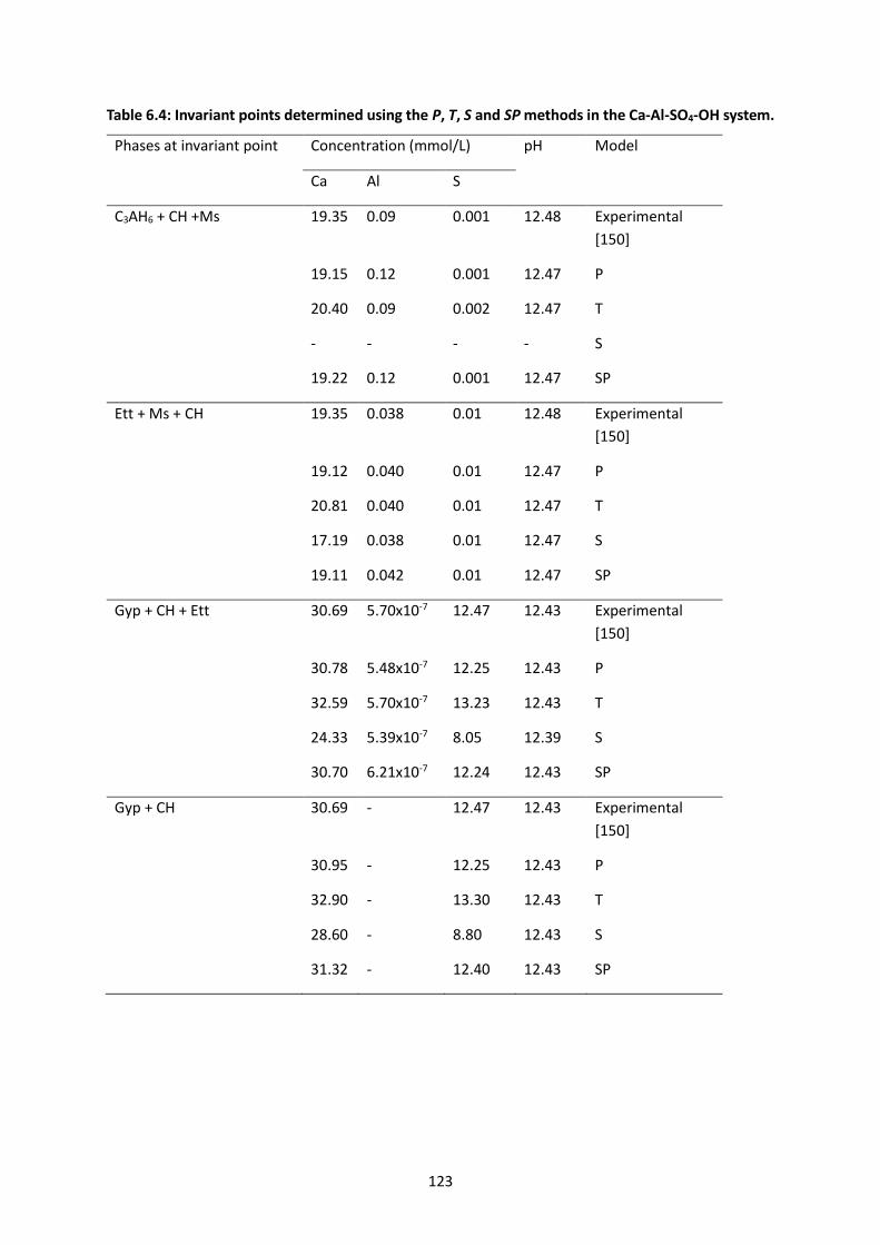
123
Table 6.4: Invariant points determined using the P, T, S and SP methods in the Ca-Al-SO4-OH system.
Phases at invariant point Concentration (mmol/L) pH Model
Ca Al S
C3AH6 + CH +Ms 19.35 0.09 0.001 12.48 Experimental
[150]
19.15 0.12 0.001 12.47 P
20.40 0.09 0.002 12.47 T
- - - - S
19.22 0.12 0.001 12.47 SP
Ett + Ms + CH 19.35 0.038 0.01 12.48 Experimental
[150]
19.12 0.040 0.01 12.47 P
20.81 0.040 0.01 12.47 T
17.19 0.038 0.01 12.47 S
19.11 0.042 0.01 12.47 SP
Gyp + CH + Ett 30.69 5.70x10⁻⁷ 12.47 12.43 Experimental
[150]
30.78 5.48x10⁻⁷ 12.25 12.43 P
32.59 5.70x10⁻⁷ 13.23 12.43 T
24.33 5.39x10⁻⁷ 8.05 12.39 S
30.70 6.21x10⁻⁷ 12.24 12.43 SP
Gyp + CH 30.69 - 12.47 12.43 Experimental
[150]
30.95 - 12.25 12.43 P
32.90 - 13.30 12.43 T
28.60 - 8.80 12.43 S
31.32 - 12.40 12.43 SP
124
In the presence of additional alkalis, the formation of sulphur-containing phases requires greater
levels of sulphate in solution at a higher pH (Table 6.5). Feng et al. [113] and Damidot and Glasser
[112,148] modelled the effect of alkalis on the phase formation in the Ca-Al-SO4-OH system in the
presence of NaOH and KOH. Each of the studies concluded that the greater reduction of the Ca2+
activity coefficient in the system led to greater levels of predicted precipitation of portlandite,
following the trend observed in Figure 6.4. The decreased predicted solubility of portlandite at higher
pH consumed calcium from the solution and thus required greater levels of sulphate in solution to
form the sulphur-containing phases, when compared to systems without added alkalis.
The IS of the potassium and sodium-containing systems reached a maximum of 0.25 and 0.35 molal,
respectively, in the simulations. Both simulations are within the effective IS range of the Truesdell-
Jones model, which resulted in minimal difference of the sets of results across the different models.
Only the additional inclusion of Ca2+-AlO2- parameters were used in the SP method due to the highly
parameterised species used, and this additional parameter had minimal impact on the effectiveness
of the Pitzer method.

125
Table 6.5: Invariant points determined using the P, T, S and SP methods in the Ca-Al-SO4-OH systems
with the inclusion of KOH or NaOH.
Phases at invariant point Concentration (mmol/L) pH Model
Ca Al S
KOH (178 mmol/L)
Gyp + CH + Ett 16.50 4.00x10⁻² 66.00 - Experimental [234]
17.16 1.29x10⁻⁶ 69.19 12.44 P
17.21 1.26x10⁻⁶ 68.13 12.44 T
11.09 1.19x10⁻⁶ 65.40 12.43 S
16.95 1.32x10⁻⁶ 69.04 12.44 SP
Gyp + CH 16.65 - 66.90
Experimental [234]
17.18 - 68.27 12.70 P
17.26 - 68.11 12.72 T
11.36 - 65.10 12.69 S
16.97 - 68.11 12.70 SP
NaOH (250 mmol/L)
Gyp + CH + Ett 15.39 2.50x10⁻² 93.90 12.77 Experimental [235]
16.24 1.61x10⁻⁶ 97.86 12.75 P
15.70 1.47x10⁻⁶ 95.44 12.44 T
10.29 1.38x10⁻⁶ 95.76 12.45 S
15.70 1.74x10⁻⁶ 97.47 12.47 SP
Gyp + CH 15.39 - 93.90 12.77 Experimental [235]
16.18 - 95.20 12.75 P
15.60 - 95.18 12.78 T
10.29 - 93.17 12.75 S
15.73 - 94.99 12.75 SP

126
6.4.4 Ca-Al-CO3-OH
Finely ground calcite or limestone (CaCO3) are used as supplementary cementitious materials in PC
and blended cements [95,96], which leads to the formation of calcium monocarboaluminate
(monocarbonate (Mc), (3CaO∙Al2O3∙(CaCO3)∙11H2O)) and calcium hemicarboaluminate
(hemicarbonate (Hc), (3CaO∙Al2O3∙(CaCO3)0.5∙11.5H2O)) phases in the presence of aluminium. The
aqueous species for the Ca-Al-CO3-OH system are generally well parameterised for the Pitzer model
although, similar to the Ca-Al-SO4-OH system, the Ca2+-AlO2- interaction parameters are not available
in the literature.
The low content of CO32- required to form hemicarbonate (3.9 wt.%) means that there is a lower
minimum carbonate concentration required to form a Ca-Al-CO3-OH phase compared to the case of
Ca-Al-SO4-OH system. The C3AH6 + CH + Hc invariant point requires similar calcium and aluminium
content, however 1000 times less CO32-, compared to the amount of SO4
2- required to form C3AH6 +
CH + Ms. Less CO32- was required for each of the stable invariant points, only up to 0.0065 mmol/L of
CO32- was required at the maximum concentration of this ion (forming calcite + CH predicted using the
T method).
The Truesdell-Jones equation provided more accurate fitting of the CO32- species, however the Pitzer
methods were no more than 0.0052 mmol/L different from the experimental results. The Pitzer model
provided a more accurate representation of calcium concentrations in solution and the calculated
aluminium concentration was similar for both methods.
Similar to the Ca-Al-SO4-OH system, the main impact on the quality of predictions was from the
different selection of aqueous species. The CaOH+ and CaCO3(aq) complexes were not used with the
Pitzer model, as the rest of the parameters had been fitted without them. The result of not having
these aqueous species available was a reduced calcium and carbonate content required in solution
before the phases precipitated. Additional Simoes-method parameters added to the Pitzer database
had minimal effect on the saturation concentrations of aqueous species.
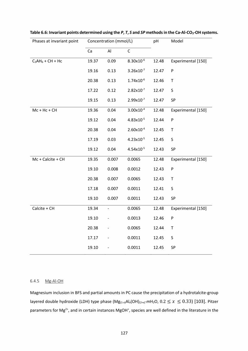
127
Table 6.6: Invariant points determined using the P, T, S and SP methods in the Ca-Al-CO3-OH systems.
Phases at invariant point Concentration (mmol/L) pH Model
Ca Al C
C3AH6 + CH + Hc 19.37 0.09 8.30x10⁻⁶ 12.48 Experimental [150]
19.16 0.13 3.26x10⁻⁷ 12.47 P
20.38 0.13 1.74x10⁻⁶ 12.46 T
17.22 0.12 2.82x10⁻⁷ 12.47 S
19.15 0.13 2.99x10⁻⁷ 12.47 SP
Mc + Hc + CH 19.36 0.04 3.00x10⁻⁴ 12.48 Experimental [150]
19.12 0.04 4.83x10⁻⁵ 12.44 P
20.38 0.04 2.60x10⁻⁴ 12.45 T
17.19 0.03 4.23x10⁻⁵ 12.45 S
19.12 0.04 4.54x10⁻⁵ 12.43 SP
Mc + Calcite + CH 19.35 0.007 0.0065 12.48 Experimental [150]
19.10 0.008 0.0012 12.43 P
20.38 0.007 0.0065 12.43 T
17.18 0.007 0.0011 12.41 S
19.10 0.007 0.0011 12.43 SP
Calcite + CH 19.34 - 0.0065 12.48 Experimental [150]
19.10 - 0.0013 12.46 P
20.38 - 0.0065 12.44 T
17.17 - 0.0011 12.45 S
19.10 - 0.0011 12.45 SP
6.4.5 Mg-Al-OH
Magnesium inclusion in BFS and partial amounts in PC cause the precipitation of a hydrotalcite-group
layered double hydroxide (LDH) type phase (Mg(1-x)Alx(OH)(2+x)∙mH2O, 0.2 ≤ 𝑥 ≤ 0.33) [103]. Pitzer
parameters for Mg2+, and in certain instances MgOH+, species are well defined in the literature in the

128
presence of anions other than OH- [135,143,237,238]. Neither species was parameterised with the
AlO2- species, which in pH environments common to cement acts as a precursor to the formation of
hydrotalcite-LDH. The Simoes method is available to provide interaction parameters for the Mg2+-AlO2-
interactions, however no ionic radius data were available for MgOH+, for similar reasons to why no
CaOH+ ionic radius data may be found. Only mixed electrolyte terms for H+-Mg2+ (𝜃𝑐𝑐) and OH--AlO2-
(𝜃𝑎𝑎) were obtained for the Pitzer model using terms from the literature [237,239].
A magnesium aluminium hydrotalcite-LDH solid solution model (MA-OH-LDH) was used to test the
various aqueous solution models. The MA-OH-LDH model represents a solid solution of hydrotalcite-
LDH with a varying Mg/Al of 2 to 4 [124,146]. An aqueous environment containing Mg-Al-OH would
expect to yield up to three solid phases, such as brucite, gibbsite and hydrotalcite-LDH. The invariant
points of these phases have been studied extensively and are summarised in Table 6.7
[194,195,240,241].
Table 6.7: Invariant points within the Mg-Al-OH system determined from XRD analysis of the crystal
structure compared to the invariant points determined from the MA-OH-LDH solid solution model
[146].
Invariant Points (Al/Al+Mg, molar ratios)
Brucite + HT HT HT + Gibbsite Reference
- 0.23 0.33 [241]
- 0.25 0.44 [195]1
0.004 0.17 0.33 [194]
0.002 0.25 0.33 This study
1The samples tested in this study contained hydroxycarbonates.
Simulation of the Mg-Al-OH system was conducted through applying a range of Al/Al+Mg molar ratios,
where the total Al+Mg content was set to 1 mol/L in 1 L of water. From Al/Al+Mg = 0.002 – 0.23, the
model predicts a region of hydrotalcite-LDH and brucite formation. A pure hydrotalcite-LDH phase
forms in the region Al/Al+Mg = 0.25 – 0.33 (Figure 6.8) which is within the range determined
experimentally (0.23 – 0.44 [195,241]). A mixed hydrotalcite-LDH and gibbsite region was observed at
Al/Al+Mg > 0.33. This phase assemblage was observed for all aqueous solution models.

129
The low level of solubility of the phases in this system resulted in no difference in the invariant points
between the different modelling approaches. The inclusion of the six 𝐵𝑀𝑋(0)
and six 𝐵𝑀𝑋(1)
parameters
obtained using the Simoes estimations had no effect in this system compared to the under-
parameterised Pitzer method and the Truesdell-Jones method.
Figure 6.8: Phase diagram of the Mg-Al-OH system constructed through thermodynamic modelling.
The MA-OH-LDH phase consists of an solid-solution model fitted by Myers et al. [146].
The Pitzer model for the Mg-Cl-Na-Al-OH system was well parameterised and provided a more
thorough basis to assess the precipitation of hydrotalcite-like LDH phases using the various aqueous
solution models. The data used were created by Gao and Li [242] to assess the solubility of
Mg4Al2(OH)14∙3H2O, which is an end-member in the MA-OH-LDH model. The MA-OH-LDH model was
used in this study as opposed to restricting the solid composition to the single phase
Mg4Al2(OH)14∙3H2O, due to the flexibility of the MA-OH-LDH model at predicting the chemical structure
of hydrotalcite, and because the MA-OH-LDH model has been used in previous BFS cement hydration
modelling studies [122,124].
The simulation consisted of Al(OH)3 and Mg(OH)2 at concentrations of 62.5 and 125 mmol/L,
respectively in 1 L of water. A varying concentration of NaCl from 0 – 2.5 mol/L was added to the
system. The comparison of the results of the different modelling methods in comparison to the
solubility data [242] can be seen in Figure 6.9.

130
Pitzer parameters for the Mg-Cl-Na-Al-OH system required minimal additions due to the work that has
been conducted in the past modelling magnesium oxychloride solubility [100,110].
Considering the sum of squared errors (SSE) across the eight NaCl concentrations, Table 6.8, the Pitzer
parameters and SP method performed better than the S and T methods when considering the pH,
magnesium concentration and aluminium concentration. The pH was most accurately portrayed by
the SP method, which had an incremental improvement on the Pitzer parameters (Figure 6.9a). The
Simoes parameters performed similarly to the Pitzer parameters up until 0.5 mol/L of NaCl, however
the S method became steadily less effective, as did the Truesdell-Jones equation.
Table 6.8: The sum of squared errors (SSE) for the pH, OH-, Mg and Al concentrations in solution,
comparing the thermodynamic modelling results in GEMS to the experimental data for the Mg-Al-
Na-Cl-OH system. The four aqueous solution model methods compared were the Pitzer model with
literature parameters (P), Pitzer model using estimated Simoes parameters (S), Pitzer parameters
from the literature supplemented by Simoes parameters (SP) and the Truesdell-Jones equation (T).
pH (SSE)
Concentration (SSE – x10-8 mmol/L) Model
OH- Mg Al
0.13 14.50 0.97 2.89 P
0.22 16.00 2.66 3.15 T
0.15 8.95 1.25 3.55 S
0.12 9.87 1.05 2.92 SP
Across the four modelling approaches the AlO2- and Mg2+ were the dominant species of their
respective elements in solution (both above 95%). Therefore, AlO2--Mg2+ interactions were added to
the SP parameters. Additionally, Mg2+-OH- parameters were also available. The effect of the Pitzer
parameters on the activity coefficients of the OH-, AlO2- and Mg2+ ions (Figure 6.9d, e and f,
respectively) can highlight the impact of the modelling method and the parameters used on the
system. All of the models were within a factor of 10 of each other when predicting the AlO2-
concentration, however the difference between the activity coefficients was as high as 72.3 % (S, 0.96
cf. P, 0.45). For the Mg2+ species, the difference was more significant as the highest difference was
131
105.9 % (SP, 0.39 cf. T, 0.12). The OH- activity coefficient was least affected as the greatest difference
was 30.2 % (S, 0.8 cf. P, 0.59). The maximum differences were observed at an NaCl concentration of
2.5 mol/L.
The much greater increase of 𝛾OH-, 𝛾AlO2- and 𝛾Mg2+ at high ionic strength using the parameters
determined by the S method led to decreasing levels of ions required to form MA-OH-LDH. Using the
P and SP parameters, the decrease in Mg2+ activity coefficients at 0 < NaCl < 0.75 mol/L, followed by
an increase at NaCl > 0.75 mol/L, caused the concentration of magnesium required to form MA-OH-
LDH to increase and then decrease as NaCl was added. Simultaneously, the levelling and lower 𝛾AlO2-
causes more aluminium to be required to form MA-OH-LDH as the NaCl concentration increased. The
activity of AlO2- was greatly influenced by the Na+-AlO2
- parameters in the SP method, taken from Park
and Englezos [239], as there was infinitesimal variation in the AlO2- activity coefficient between the P
and SP method. The Park and Englezos Na+-AlO2- parameters are up to two orders of magnitude
smaller than the Simoes parameters for the same species, which is the cause of the large difference
in the AlO2- activity coefficient between the P and S methods.
The inclusion of Mg2+-OH- parameters had an impact on 𝛾-Mg2+ in the SP method compared to the P
method, as 𝛾Mg2+ was 0.1 units higher at [NaCl] = 2.5 mol/L in the SP method. The Mg2+-OH- parameters
included with the SP method were of a similar magnitude to the Mg2+-Cl- parameters. The comparable
difference between the parameters allowed the Simoes parameters to affect 𝛾Mg2+. Further evidence
of this can be observed in the difference in 𝛾OH-, which varies between the P and SP methods due to
the inclusion of Mg2+-OH- parameters in the SP method. The lack of change in 𝛾AlO2- with the inclusion
of the Mg2+-AlO2- parameters indicates that it had minimal effect on the system and did not affect
𝛾Mg2+. Overall, the inclusion of the additional Simoes-method parameters to the Pitzer database had a
minimal effect on the solubility of MA-OH-LDH.

132
Figure 6.9: Aqueous solution properties in the Mg-Cl-Na-Al-OH system (MgOH2 = 0.125 mol/L,
Al(OH)3 = 0.0625 mol/L, and 0 < NaCl < 2.5 mol/L), considering the effect of increasing concentration
of NaCl on: a) pH, b) magnesium solubility, c) aluminium solubility, d) 𝜸OH-, e) 𝜸AlO2- and f) 𝜸Mg2+, using
different aqueous solution methods. P denotes a fully parameterised Pitzer model, T denotes the
Truesdell-Jones equation, S denotes the Pitzer model including parameters generated only from the
Simoes Pitzer estimation equations and SP denotes the Pitzer parameters supplemented with
Simoes parameters. Solubility data were taken from Gao and Li [242].

133
6.4.6 Ca-Si-Al-OH
The main hydrate phase in blended cement C-A-S-H is comprised of aluminosilicate chains which
encompass a calcium oxide layer (Figure 6.10a). The composition of this phase is highly dependent on
the chemical environment of the system which causes variation in the Ca/Si and Al/Si molar ratios
within the phase [57,58,63,85].
A water-filled interlayer space between two silicate or aluminosilicate chains allows for the sorption
of cations which act as charge balancers. In the presence of high concentrations of calcium and
additional alkalis (e.g. Na+ and K+), the increased OH- ions reduce the content of bridging sites in the
silicate chains and increase the Ca/Si ratio of the C-S-H/C-A-S-H phases (Figure 6.10b) [59].
Figure 6.10: The C-S-H/C-A-S-H structure using a) dreierketten units and b) in high Na+ and K+
concentrations. The green triangles represent paired silicate dimers, blue triangles are bridging
silicon tetrahedra, the red triangles represent silicon replacement with aluminium, the purple,
orange and pink circles represent Ca2+, K+ and Na+ ions respectively.
6.4.6.1 Ca-Si-OH
Walker et al. [65] conducted a thorough review of the solubility of C-S-H and the value of the studies
created in the literature. Based on rigorous selection criteria, Walker et al. were able to reduce an
identified 777 data entries from the literature to 207 reliable points, and included an additional 26 at

134
low Ca/Si (0.19 – 0.83) [53,54,65,69–83]. This data-set was used in this study to compare the different
aqueous modelling methods with the CSHQ model developed by Kulik [64].
Pitzer parameters with calcium and silicon interactions do not exist in the literature. The disordered
nature of C-S-H, low solubility and low ionic strength of the solutions used in determining the solubility
data are likely to be the main cause. Various aqueous models using different software packages exist
and the current model used as default in the CEMDATA14 database, the CSHQ model, consistently
over-predicts silicon concentrations in solution [64]. The model is limited to a minimum Ca/Si of 0.67
and maximum Ca/Si of 1.67 as a result of reaching the solubility points of amorphous silica and
portlandite, respectively. The CSHQ model developed by Kulik [64] was used to simulate the Ca-Si-OH
systems in sections 6.4.6.1 and 6.4.6.2 of this study.
Further consideration was given to the aqueous species available in the system because a number of
aqueous species interactions were not parameterised. Figure 6.11a and b depict the effect of the Ca/Si
ratio on the aqueous speciation for calcium and silicon, respectively. The modelled work shown in
Figure 6.11 was performed using the Truesdell-Jones equation. Silicon was split between the HSiO3-,
CaSiO3(aq) and SiO2(aq) species in solution. Increasing calcium content caused the SiO2(aq) species to
no longer appear at Ca/Si > 1.0, by which point the CaSiO3(aq) species became dominant in solution
as the Ca/Si ratio exceeded the Ca/Si molar ratio of the CaSiO3(aq) species (Ca/Si = 1.0). A declining
content of silicon in solution caused the silicon concentration in solution to be heavily dependent on
the CaSiO3(aq) species. However, as a mole fraction of all of the calcium in solution, the CaSiO3(aq)
declined as the calcium content increased, due to the increasing pH rising to 12.5. At a pH of 11.7 and
Ca/Si of 1.04, the concentration of CaOH+ becomes more prominent than the CaSiO3(aq). Miron et al.
[109] determined that there are no solubility studies that provide adequate thermodynamic data for
the CaSiO3(aq) species, however it has provided a useful addition to modelling databases to improve
calcium and silicon solubility studies up to temperatures of 500 °C.
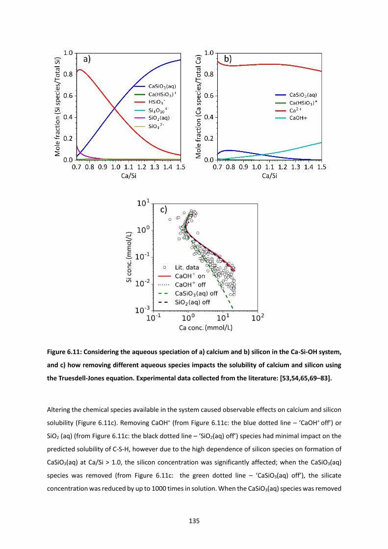
135
Figure 6.11: Considering the aqueous speciation of a) calcium and b) silicon in the Ca-Si-OH system,
and c) how removing different aqueous species impacts the solubility of calcium and silicon using
the Truesdell-Jones equation. Experimental data collected from the literature: [53,54,65,69–83].
Altering the chemical species available in the system caused observable effects on calcium and silicon
solubility (Figure 6.11c). Removing CaOH+ (from Figure 6.11c: the blue dotted line – ‘CaOH+ off’) or
SiO2 (aq) (from Figure 6.11c: the black dotted line – ‘SiO2(aq) off’) species had minimal impact on the
predicted solubility of C-S-H, however due to the high dependence of silicon species on formation of
CaSiO3(aq) at Ca/Si > 1.0, the silicon concentration was significantly affected; when the CaSiO3(aq)
species was removed (from Figure 6.11c: the green dotted line – ‘CaSiO3(aq) off’), the silicate
concentration was reduced by up to 1000 times in solution. When the CaSiO3(aq) species was removed

136
from the system, the CaOH+ concentration increased up until portlandite began to form. This effect
occurred for each of the modelling approaches (P, T, S and SP methods)
In the systems studied in the previous sections (Ca-Al-SO4-OH, Ca-Al-CO3-OH and Mg-Al-OH), the
aqueous neutral complexes were removed, however in the Ca-Si-OH system, due to the large
detrimental impact of the removal of CaSiO3(aq) (from Figure 6.11c: the green dotted line –
‘CaSiO3(aq) off’) on the silicon concentration, it was maintained for the Pitzer models.
The Pitzer methods had CaOH+ and SiO2(aq) species removed from among the possible aqueous
species. Removal of these species with the use of the different aqueous models proved to have little
effect on the pH, calcium and silicon in the aqueous solution, Figure 6.12a and b, respectively. Figure
6.11a and b shows that the CaOH+ and SiO2(aq) species were ever more than 20% of the Ca or Si
present, respectively, and that was at extreme compositions, hence these species had minimal impact
on the system. The different modelling methods did provide a variation on the Ca/Si at different
calcium and silicon concentrations, Figure 6.12c and d, respectively.
Using the known ionic radii of SiO32- and HSiO3
- from the literature [226,227], it was possible to
estimate interaction parameters with calcium for these species. The Ca2+-SiO32- interaction parameters
had no effect on the system due to the low concentration of SiO32- in solution as shown in Figure 6.11a.
Inclusion of Ca2+-HSiO3- parameters had minimal impact on the system overall but reduced the
saturation concentrations of silicon in the S and SP methods. The observable deviation of the solubility
of silicon of the S and SP methods from the P method occurs at 0.7 mmol/L of silicon in solution. The
HSiO3- species becomes less prevalent in solution as the calcium content increases, however due to
the low concentration of silicon overall, it decreases the saturation concentration of silicon within the
Ca/Si range of 0.72 to 1.5.
The Ca2+-HSiO3- parameters increased the saturation concentration of calcium in the SP method
compared to the P method, creating a maximum difference of 0.03 mmol/L (at Ca/Si = 1.63) between
the predictions obtained using the two sets of parameters. This alteration affected the aqueous phase
composition at which portlandite began to precipitate once the CSHQ model reached its maximum
Ca/Si ratio of 1.63. The calcium concentration required to form portlandite in each model is

137
summarised in Table 6.9. The concentrations are the same for portlandite solubility from section 6.4.1:
Portlandite. In the previous section, the SP method was not tested as the Simoes method provided no
additional parameters.
Table 6.9: Concentration of calcium required in the Ca-Si-OH system for portlandite to precipitate.
Calcium concentration
(mmol/L)
Model
19.10 P
20.40 T
17.20 S
19.13 SP
The Pitzer models predicted that less calcium was required to reach the portlandite phase boundary
than the Truesdell-Jones equation. This effect is mainly attributed to the removal of the CaOH+ species
from the Pitzer methods. A definitive point defining at what concentrations does portlandite
precipitate in the presence of C-S-H has not been determined experimentally, due to the gel-like
nature of the phase and the varying solubility data [54,65,243].

138
Figure 6.12: Comparison of a) pH, b) calcium vs. silicon concentration, c) calcium concentration vs.
Ca/Si of the C-S-H, and d) silicon concentration vs. Ca/Si of the C-S-H, in the Ca-Si-OH system.
Literature data are from [53,54,65,69–83], compared to predictions from different aqueous solution
models, with the CaOH+ and SiO2(aq) species removed from the Pitzer models. The Pitzer aqueous
solution model using parameters from the literature is denoted P; with parameters obtained from
estimating interaction parameters using method of Simoes et al. [225] is shown as S; the literature
data supplemented by estimated parameters is SP; and the Truesdell-Jones aqueous solution model,
T.

139
6.4.6.2 Impact of Na2O and K2O
The alkali sorption experiments conducted by Hong and Glasser [59] were used as a point of
comparison for the different modelling approaches in sodium and potassium environments. Varying
molar ratios of Ca(OH)2 and SiO2 were used, at a liquid/solid mass ratio of 15 (0.6 g solids in 9 g of
water). The Ca/Si molar ratios studied were 0.85, 1.2, 1.5 and 1.8, at alkali concentrations of 1, 5, 15,
50, 100 and 300 mmol/L. For ease of visualisation, only the data for 1, 50 and 300 mmol/L of Na2O and
K2O are presented in Figure 6.13. Calcium saturation concentration and pH were the available
comparative values from that study. The NaOH (aq) and KOH (aq) complex species were removed
from the Pitzer models as Pitzer parameters for these species are not parameterised, and all other
species that were used to model the Ca-Si-OH system remained the same as for section 6.4.6.
Figure 6.13: Modelling the impact of K2O concentration on the a) calcium concentration and b) pH,
and the impact of Na2O concentration on the c) calcium concentration and d) pH. The concentrations
of K2O and Na2O modelled were 1, 50 and 300 mmol/L, for models P, S, SP, and T. Solubility data
taken from Hong and Glasser (filled circles) [59].

140
Pitzer parameters were developed for the interactions of Na+-HSiO3- and K+-HSiO3
- by Provis et al. [244]
through modelling silicon speciation in highly alkaline environments and compared with 29Si NMR
results. The Q0 species with a charge of -1 was used from the Provis et al. [244] study as this was
representative of the aqueous HSiO3- species.
The different modelling methods had little impact on the calculated pH in relation to Ca/Si for the
different alkali concentrations, in the range Ca/Si > 1.0 (Figure 6.13b and d). As was the case in the Ca-
Si-OH system, the variation in calcium solubility was minimal between the different methods until the
point of portlandite precipitation, where the calcium concentration required to form portlandite
followed the order: T > P/SP > S. The CSHQ model was effective at modelling the inclusion of sodium
and potassium in solution, as the solubility of portlandite reduced at higher concentrations of alkalis,
as was observed experimentally [59].
Table 6.10: The logarithm of the sum of square errors (SSE) for calcium and pH concentration
calculated across the 1, 5, 15, 50, 100 and 300 mmol/L concentrations of Na2O or K2O, using the
different modelling methods. Solubility data taken from Hong and Glasser [59]. The Pitzer aqueous
solution model, P, was compared with parameters obtained from estimating interaction paramaters
using the equations created by Simoes et al. [225], S; with the literature data being supplemented
by estimated parameters, SP; and with the Truesdell-Jones aqueous solution model, T.
Alkali log SSE([Ca2+]/[mmol/L]) log SSE(pH) Model
K2O 2.25 -0.44 P
2.18 -0.46 T
2.40 -0.44 S
2.25 -0.44 SP
Na2O 1.98 -0.14 P
1.97 -0.15 T
2.10 -0.13 S
1.98 -0.14 SP
The logarithm of the sum of squared errors (SSE) was calculated across the 1, 5, 15, 50, 100 and 300
mmol/L concentrations of Na2O or K2O for each method, Table 6.10. The IS did not exceed 0.3 for

141
these systems, therefore the inclusion of the Pitzer models had little effect on the outcome, as was
shown in the minimal difference in the log SSE values.
6.4.6.3 Ca-Al-Si-OH
The C-A-S-H model used to describe the solid phase formation in the Ca-Al-Si-OH system was updated
from the C(-N)-A-S-H solid solution model developed by Myers et al. [146]. The sodium end-members
were removed and the JenD end-member from the CSHQ model [64] was included in the updated
model (Table 6.11). The solid-solution model used six end-members which had a chemical composition
range of 0.66 < Ca/Si < 2.24 and 0 < Al/Si < 0.26. Each of the six end-members contained calcium and
silicon, however, only two end-members contained aluminium. The applicability of this ideal solid
solution model and the effect of the different aqueous models were tested using the solubility data
collected by L’Hopital et al. [63] for the Ca-Al-Si-OH system. The modelling was conducted by
replicating the various molar ratios used in the study, with the mass of the precursor solids (CaO, SiO2
and CaO∙Al2O3) set to 2 g and the water/solids mass ratio held constant at 45.
Table 6.11: Thermodynamic properties of C-S-H and C-A-S-H end-members in the model used for
simulation of C-A-S-H formation. Standard thermodynamic properties at 25 °C and 1 bar
Phases ΔHf°
(kJ mol−1)
ΔGf°
(kJ mol−1)
Ca/Si
(molar ratio)
Al/Si
(molar ratio)
Reference
5CA, C1.25A0.125S1H1.625 −2491 −2293 1.25 0.25 [146]
INFCA, C1A0.15625S1.1875H1.65625 −2551 −2343 0.84 0.26 [146]
JenD, C1.5S0.67H2.5 −2401 −2169 2.24 - [64]
T2C, C1.5S1H2.5 −2721 −2298 1.50 - [122]
T5C, C1.25S1.25H2.5 −2780 −2517 1.00 - [146]
TobH, C1S1.5H2.5 −2831 −2560 0.66 - [146]
The results obtained using the C-A-S-H model for each modelling approach were similar for each
model, as shown by the log SSE values summarised in Table 6.12, therefore only the results obtained
for the Pitzer model are displayed in Figure 6.14 and Figure 6.15.

142
Table 6.12: Log SSE values, comparing the calculated results using the C-A-S-H end-member model
with measured solubilities in the Ca-Al-Si-OH system [63].
Log SSE(Molar ratios) Log SSE(Concentration/[mmol/L]) Log SSE(pH) Model
Ca/Si Al/Si Ca Si Al OH-
-0.88 -1.22 2.03 1.94 -0.93 2.49 -0.22 P
-0.89 -1.22 2.00 1.65 -0.92 2.40 -0.23 T
-0.86 -1.22 2.15 1.94 -0.94 2.36 -0.21 S
-0.88 -1.22 2.03 1.94 -0.93 2.49 -0.22 SP
A greater range of calcium containing end-members provides an improved description of the Ca/Si
ratio compared to the Al/Si ratio in the C-A-S-H phase (Figure 6.14a and Figure 6.14b, respectively).
The C-A-S-H model was most accurate for compositions of Ca/Si > 0.8 and Al/Si < 0.33. The Ca/Si was
inaccurate by more than 0.1 for three instances: Ca/Si = 0.6 and Al/Si = 0.33, Ca/Si = 0.8 and Al/Si =
0.33 and, Ca/Si = 1.4 and Al/Si = 0.1. The Ca/Si was over-predicted in the Ca/Si = 0.6 and 0.8 systems
due to the increased pH following the replacement of SiO2 by CaO∙Al2O3 (CA). The higher pH shown in
Figure 6.14c caused the higher Ca/Si end-members to become more stable, thus increasing the Ca/Si
ratio.
The model prediction of Al/Si ratio was less accurate due to the limited number of aluminium-
containing end-members within the model. Additional end-members were introduced with chemical
compositions Ca/Si = 1.4 and Al/Si 0.05; and Ca/Si 1.0 and Al/Si = 0.1; to provide greater diversity of
the Al/Si values. However, due to the stability of the current end-members, the additional end-
members did not have any impact on the system when included. There was generally good agreement
at low and mid-range Al/Si values, but Al/Si was generally over-predicted at Ca/Si > 1.0 and Al/Si > 0.1
as the bulk composition of the system approached the chemical composition of the 5CA and INFCA
end-members.

143
Figure 6.14: Comparison of the measured values (from L’Hopital et al. [63]) for a) Ca/Si, b) Al/Si and
c) pH versus the values calculated using the C-A-S-H end-member model. The Pitzer model (P) was
used to compare the datasets in the above graphs. The different colours represent the Ca/Si ratios
in the bulk solution, ranging from 0.6 to 1.6, and the different shapes represent a range of Al/Si
ratios from 0.03 to 0.33. The dotted lines indicate the estimated experimental error for the data
acquisition, represented as difference from the solid line y = x.
The predicted concentration of the hydroxyl ion, silicon and calcium aqueous species, were within an
order of magnitude of the measured values, Figure 6.15. Under-prediction of aluminium in solution
occurred for the low Al/Si systems (0.03 and 0.05) as the available aluminium was withdrawn into the
C-A-S-H model (Figure 6.15a). It must be noted that the aluminium concentration in the experimental

144
data used here was recorded as <0.0037 mmol/L for the Al/Si = 0.03 and 0.05 systems (denoted by
the red dotted line in Figure 6.15a), as the aluminium concentration was below the detectable limit
[63], therefore the much lower aluminium concentration determined using the end-member model
may be more accurate than the plotted results indicate. The lowest silicon concentration using the
end-member model was 0.03 mmol/L, which was similar to that determined in the C-S-H system due
to the inclusion of the TobH end-member for both systems.
Figure 6.15: Comparison of the calculated and measured concentration of aqueous species a)
aluminium, b) OH-, c) silicon and d) calcium, using the C-A-S-H end-member model to compare to
solubility data from L’Hopital et al. [63]. The different colours represent the Ca/Si ratios in the bulk
solution, ranging from 0.6 to 1.6, and the different shapes represent a range of Al/Si ratios from 0.03
to 0.33. The dotted lines indicate a ± 1 order of magnitude difference from the solid line y = x. The
red dotted line in a) denotes the experimental detection limit.
For the Pitzer models the CaOH+ and AlOOH (aq) species were restricted from forming. The different
aqueous solution models performed similarly as shown in Table 6.12. The low ionic strength of the
system, reaching a maximum of 0.047 mol/L, was low enough to not gain benefit from the inclusion

145
of Pitzer parameters. The log SSE values show that the Truesdell-Jones model was the most accurate
when considering the aqueous concentrations and molar ratios of the C-A-S-H phase.
Additional parameters were included in the SP model compared to the Pitzer database, these were
the Ca2+-HSiO3-, Ca2+-SiO3
2- and Ca2+-AlO2- interactions. However, no discernible difference was noted
with the inclusion of these parameters.
6.4.6.4 Impact of KOH and NaOH
The applicability of the solid solution model and the effect of the different aqueous models in the
presence of sodium and potassium were tested using the solubility data collected by L’Hopital et al.
[108]. The modelling was conducted by simulating the various molar ratios used in the study, ensuring
the mass of the precursor solids (CaO, SiO2 and CaO∙Al2O3) was 2 g and the water to solids mass ratio
was constant at 45. In the solubility study, the majority of the tests were performed with an Al/Si of
0.05 and a range of Ca/Si ratios from 0.6 to 1.6 [108]. The samples with various Ca/Si and Al/Si ratios
were mixed with potassium hydroxide and sodium hydroxide concentrations ranging from 0.01 mol/L
to 0.5 mol/L. Commonly, BFS-PC cements with a minimum BFS replacement level of 50% produce a C-
A-S-H composition with Al/Si > 0.1 [44,45,122]. Therefore, the synthetic Al/Si used in the study was
not ideal for testing the solid and aqueous solution models in increased alkaline conditions, but the
data appear to be the best available in the literature so were used as far as possible.
The ideal solid solution model and the different aqueous models performed similarly for the KOH and
NaOH systems. The KOH studies contained a larger range of concentrations and were therefore
selected to be presented in Figure 6.16 and Figure 6.17.
The ideal solid solution model performed well across the range of Ca/Si ratios examined (Figure 6.16a).
The modelling of the lower Ca/Si ratio of 0.6 was greatly influenced by the addition of KOH, as at low
concentrations (0.01 mol/L) the model prediction of Ca/Si in the solid phase was increased by up to
0.08 compared to the system without added alkalis. However, the experimental data did not exhibit
any increase in Ca/Si at such low KOH concentrations [108]. The INFCA and T5C end-members were
increasingly dominant as the KOH content increased, which caused Ca/Si and Al/Si to increase (Figure
6.16a and b). Above Ca/Si = 0.6, the model performed well, and the Al/Si ratio was similar to 0.05 for

146
all other Ca/Si ratios. The calculated pH for each chemical composition fell within the margin of error
from the experimental results, Figure 6.16c.
Figure 6.16: Comparison of the calculated and measured values for a) Ca/Si, b) Al/Si and c) pH, using
data collected by L’Hopital et al. [63]. The Pitzer model (P) was used in all model calculations shown.
The different colours represent a range of Ca/Si in the bulk solution from 0.6 to 1.6 and the different
shapes represent a range of KOH concentration from 0.01 to 0.5 mol/L. The dotted lines indicate the
maximum possibility of error for the data acquisition from the experimental study, as difference
from the solid line y = x. The black triangle represents Ca/Si = 1.0, Al/Si = 0.1 and a KOH concentration
of 0.5 mol/L.
147
The aqueous solution species were effectively modelled, as the hydroxyl ion, silicon and calcium
concentrations were predicted to within an order of magnitude of the experimental results. The
aluminium concentration was under-predicted again because of the low detection level of aluminium.
This was an issue in systems where the added alkali concentration was less than 0.1 mol/L. However,
the aluminium prediction was most accurate for the Ca/Si = 0.6 tests, contrary to the prediction of
Al/Si. The prominence of the aluminium end-members at higher Ca/Si, whereby the Ca/Si began to
equal that used in the end-members, caused the withdrawal of additional aluminium from solution.
The ratios Al/Si of 0.25 and 0.26 within the 5CA and INFCA end-members, respectively, caused this
reduction of aluminium in solution. However, the correct trend of increasing aluminium in solution as
greater levels of KOH and NaOH were introduced into solution was observed in the simulations
Silicon concentration increased and calcium decreased in solution with increasing KOH and NaOH
content in the simulations, as was expected based on the literature [59,108,245]. This was the result
of shifting the equilibrium of the system in favour of higher Ca/Si in the C-A-S-H phase. Increasing the
alkalinity significantly reduced the calcium concentration in solution, by an order of magnitude
comparing Figure 6.15d and Figure 6.17d. The minimum calcium concentration limit of the end-
members in the solid solution model was reached at approximately 0.1 mmol/L in the Ca/Si = 0.6, 0.8
and 1.0 systems, which caused the plateau in Figure 6.17d. In contrast, the silicon concentration
increased by up to two orders of magnitude when comparing the same Ca/Si values in the Ca-Al-Si-
OH system, highlighting the reduction of the silicon content in the C-A-S-H phase due to the impact of
additional alkalis.
The Pitzer models applied here had the CaOH+, AlO2H(aq), KOH(aq) and NaOH(aq) species restricted
from forming. The ionic strength of the alkaline systems reached a maximum of 0.5 mol/L which was
within the effective limit for the Truesdell-Jones equation; this meant that in the KOH and NaOH
systems, minimal difference between the modelling approaches were observed. The log SSE values
for the NaOH systems were lower than for the KOH systems due to the larger number of data points
analysed in the KOH systems (Table 6.13).

148
Figure 6.17: Comparison of the calculated and measured concentration of aqueous species a)
aluminium, b) OH-, c) silicon and d) calcium, using solubility data from L’Hopital et al. [63]. The
different colours represent a range of Ca/Si ratios in the bulk solution from 0.6 to 1.6, and the
different shapes represent a range of KOH concentration from 0.01 to 0.5 mol/L. The dotted lines
indicate a ± 1 order of magnitude difference from the solid line y = x. The black triangle represents
Ca/Si = 1.0, Al/Si = 0.1 and a potassium hydroxide concentration of 0.5 mol/L. The red dotted line in
a) denotes the experimental detection limit.
The largest difference between the modelling methods was observed in the concentration of
aluminium. The Truesdell-Jones model was more effective than the Pitzer models, despite the
inclusion of interaction parameters for Na+ and K+ ions with the AlO2- species. At higher ionic strengths
(IS > 2.5 mol/L) the Pitzer model has been observed to model the interactions of sodium and
aluminium with greater accuracy than the Truesdell-Jones equation, Figure 6.18, by comparing the
solubility of gibbsite in the presence of NaOH. Consistently, the Truesdell-Jones equation calculated
that less aluminium was required to form gibbsite, compared to the Pitzer model. Therefore, the fact
that these systems had IS < 0.5 mol/L resulted in minimal differences in the results, however the C-A-
S-H phase precipitated at lower aluminium concentrations using the Truesdell-Jones equation, which

149
was the cause of the greater level of accuracy. Including the NaOH (aq) or KOH (aq) dissolved
complexes led to an improved fit of the Pitzer models (not presented in Table 6.13) due to the
reduction of Na+ and K+ ions in solution; however, the Truesdell-Jones method was still more effective
at modelling the aluminium concentration.
Table 6.13: The log SSE values highlighting the difference of the modelled results compared to the
calculated results using the C-A-S-H end-member model, compared to the solubility study of the Ca-
Al-Si-OH system in NaOH or KOH [108].
Alkali Log SSE(Molar ratios) Log SSE(Concentration/[mmol/L])mol/L Log SSE(pH) Model
Ca/Si Al/Si Ca Si Al OH-
KOH 0.37 -1.86 1.64 4.20 0.22 4.60 0.30 P
0.36 -1.87 1.58 4.15 -0.04 4.34 0.30 T
0.37 -1.86 1.80 4.20 0.30 4.62 0.30 S
0.36 -1.86 1.63 4.19 0.24 4.32 0.31 SP
NaOH -1.12 -2.42 0.53 3.56 0.13 4.12 -0.49 P
-1.15 -2.43 0.58 3.51 -0.59 3.70 -0.41 T
-1.11 -2.42 0.96 3.56 0.25 4.12 -0.50 S
-1.12 -2.42 0.53 3.55 0.30 4.14 -0.49 SP
Figure 6.18: Comparison of the Pitzer model (P) and Truesdell-Jones (T) equation for prediction of
gibbsite precipitation in the presence NaOH across a range of ionic strengths (IS). The experimental
data was taken from Wesolowski [111].

150
6.5 Pore solution of blended cements
Improving the pore solution modelling of cements was the key objective of this study when
considering the application of the Pitzer model to the description of aqueous solutions. To this end,
thermodynamic models of the pore solution of 1:1, 3:1 and 9:1 BFS:PC cements cured at 35 °C with a
constant w/s of 0.35, for up to 360 days of curing, were compared against experimental results. The
precursor materials used were the same as those used in Chapter 4.
The pore solution modelling results were obtained simultaneously alongside the modelling performed
in Chapter 4. Experimentally, pore solution was acquired using the steel die method as explained in
section 0.
6.5.1 Experimental results
Pore solution was intended to be collected at 14, 28, 56, 90, 180 and 360 days for the three BFS-PC
formulations (1:1, 3:1 and 9:1 - Table 6.14). However, due to repeated damage to the hydraulic press
used to apply the load to the pore press, and recurring internal damage to the pore press itself, pore
solution was not able to be collected for each of the planned curing ages for each formulation.

151
Table 6.14: Pore solution chemistry determined for the 1:1, 3:1 and 9:1 BFS-PC cements at curing
ages ranging from 14 to 360 days. nm denotes a value which was not measured. Curing ages for the
samples were different due to malfunctions of the pore press at different dates of pore solution
acquisition.
BFS-PC Curing age
(days)
Concentration (mmol/L) pH
Al Ca K Mg Na S Si
1:1 14 0.32 0.64 345 0.001 165 32.1 1.65 nm
28 0.47 1.28 368 0.007 196 70.2 4.20 13.28
56 0.15 0.55 279 0.004 165 54.6 2.37 nm
90 1.65 1.24 252 0.815 150 38.1 6.20 13.30
3:1 56 0.35 0.97 161 0.000 124 81.1 1.66 13.18
90 0.20 0.79 142 0.013 108 6.741 0.74 13.23
180 0.35 1.80 127 0.197 104 14.01 1.64 13.17
360 0.54 1.60 123 0.168 97.9 43.71 3.20 13.15
9:1 28 0.52 0.54 79.8 0.022 66.1 49.91 1.83 13.06
56 0.72 2.74 103 0.416 83.1 287 1.55 13.10
90 0.57 1.11 96.7 0.002 77.4 359 0.40 13.11
180 0.31 1.15 88.2 0.042 78.3 471 0.51 13.05
360 0.59 2.25 77.8 0.264 70.9 477 0.97 13.06
1Sulphur concentration may have been under-recorded. Suspected to have been under-recorded by the
analytical instrumentation due to the precipitation of sulphide species during ICP analysis, which may have led
to reduced vaporisation in the ICP equipment, leading to a reduced measurement of sulphur.

152
Figure 6.19: Pore solution compositions of the a) 1:1, b) 3:1 and c) 9:1 BFS-PC cements at different
curing ages.
The concentration of sodium and potassium was larger in the pore solutions of the higher PC content
formulations, as PC was the major source of alkalis in these cements and proceeded to decrease with
time. There was up to 175 mmol/L more potassium in the 1:1 system than the 3:1 or 9:1 (Figure 6.19a,
b and c, respectively) systems at the curing ages of 56 and 90 days (up to 91.7% > 3:1 or 9:1), whereas
the difference in sodium concentration was up to 80 mmol/L (up to 66.1%) greater in the 1:1 cement.
The potassium concentration was higher than sodium in each formulation due to the higher alkali
distribution ratio (Rd) of sodium in the C-A-S-H phase [59,85,108]and that there was greater mass of

153
potassium in the starting materials (Table 3.1 in Chapter 3). The decreasing concentration of
potassium and sodium was due to the increasing content of C-A-S-H as the degree of hydration (DoH)
of slag increased [122].
Calcium concentration did not drop below 3 mmol/L in solution due to the high alkalinity of the
systems, with pH values greater than 13.0 at each curing age. Concentrations of sodium and potassium
greater than 70 mmol/L, as observed in each of the pore solution results, have been shown to reduce
the solubility of any of the calcium containing phases [59,66,108,234]. The reduction of the potassium
and sodium concentrations in the 9:1 system was linked to the marginally higher concentration of
calcium in solution compared to the 1:1 and 3:1 cements.
Silicon concentration in solution was lower with increasing BFS content in the system. The decreased
pH and calcium concentration allowed the extension of the aluminosilicate chains within the C-A-S-H
phase, withdrawing greater levels of silicon from solution [122]. Higher alkalinity also reduces the
mean chain length (MCL) of aluminosilicate chains. An example of this may be seen in the analysis of
20 year old BFS-PC cement [45] and 18 year old alkali activated slag (AAS) [218]. The 75 and 90% BFS
replacement of the PC produced MCLs of 16.1 and 14.3, respectively compared to the AAS MCL of 9.7.
The BFS-PC systems contained less aluminium and silicon than the AAS system, however the lower pH
of the BFS-PC cement promotes the polymerisation of silica tetrahedra as less silanol groups are
deprotonated [59,62]. This reduction of deprotonation due to the presence of less OH- ions in solution
causes greater levels of silicon to precipitate into the aluminosilicate chain.
Aluminium concentration was twice as high in the 1:1 cement compared to the 3:1 and 9:1 cements
after 90 days (0.21 and 0.10 mmol/L, respectively). Inclusion of greater levels of magnesium to form
hydrotalcite-like LDH, and elongated aluminosilicate chains in the C-A-S-H phase, cause the reduction
of dissolved aluminium in solution. The reduced pH contributes to the reduction of solubility of
aluminium phases, as was shown with gibbsite precipitation in the presence of NaOH [111], and
aluminium uptake in the C-A-S-H phase [108].
Total sulphur concentration in PC decreases with time as the sulphate species precipitates into
ettringite or monosulphate, whereby the concentration plateaus after 10 to 100 days [104,118]; this

154
was observed in the 1:1 formulation by 90 days. The main sulphur species present in BFS is sulphide
which does not form the sulphur-containing AFm or AFt phases as readily as sulphate can.
Consequently, the reduced sulphur species remains in solution and are expected to be the cause of
the higher sulphur concentration in the 9:1 system, which increased with time as the DoH of the slag
increased. The sulphur content was more similar to AAS systems than PC systems [114,246]. This may
also have occurred in the 1:1 system but no pore solution was able to be collected after 90 days.
The sulphur content in the 28 day 9:1 and 3:1 samples after 56 days, was suspected to have been
under-recorded by the analytical instrumentation due to the precipitation of sulphide species during
ICP analysis, which may have led to reduced vaporisation in the ICP equipment, leading to a reduced
measurement of sulphur. Therefore, the majority of the 3:1 sulphur analysis may be inaccurate.
However, a trend of increasing sulphur concentration was observed for the 3:1 and 9:1 systems after
56 days of hydration. This potential under-recording of sulphur was noted in Table 6.14 as these
samples were not diluted up to 10 times.
The concentrations of magnesium recorded using ICP-OES were generally less than 1 ppm due to the
low solubility of the hydrotalcite-like LDH phase [109]. The detection limit for the equipment was also
around 1 ppm, therefore the magnesium concentrations determined may be subject to some error.
6.5.2 Thermodynamic modelling of pore solutions
The Pitzer and Truesdell-Jones modelling results are visualised in Figure 6.20a – f. The different
modelling approaches highlight the applicability of each method to modelling the pore solution of BFS-
PC cements. Figure 6.20a, c and e represent the modelling performed using the Pitzer model for the
1:1, 3:1 and 9:1 formulations, respectively, and Figure 6.20b, d and f represent the modelling
performed using the Truesdell-Jones equation for the 1:1, 3:1 and 9:1 formulations, respectively.
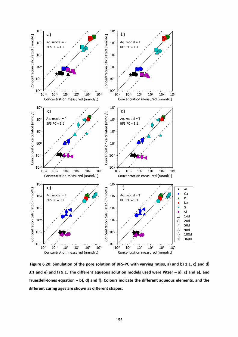
155
Figure 6.20: Simulation of the pore solution of BFS-PC with varying ratios, a) and b) 1:1, c) and d)
3:1 and e) and f) 9:1. The different aqueous solution models used were Pitzer – a), c) and e), and
Truesdell-Jones equation – b), d) and f). Colours indicate the different aqueous elements, and the
different curing ages are shown as different shapes.

156
Alkali distribution ratios (Rd) were used to simulate alkali uptake in the C-A-S-H phase for sodium and
potassium, as in chapters 4 and 5. Alkali distribution ratios for Na2O and K2O of 2 and 1.2, respectively,
were used for the C-A-S-H phase in each of the modelling approaches. These values were chosen as
they are similar to the values determined by Hong and Glasser [59,85] for C-S-H and C-A-S-H phases
with Ca/Si values between 1.2 and 1.6.
The alkali retention factors chosen were effective at simulating the effect of alkali binding with C-A-S-
H for sodium and potassium species in solution. The experimental data show a rise in sodium and
potassium concentrations after 28 days in the 1:1 formulation ( Figure 6.20a and b), however once the
C-A-S-H phase became dominant, the sodium and potassium concentrations declined in the pore
solution. The 3:1 and 9:1 systems displayed the highest sodium and potassium concentrations after
56 days, thereafter the concentrations decreased until 360 days following the experimental results,
Figure 6.20c and d and Figure 6.20e and f, respectively.
Modelling of the sulphur species was accurate for each formulation, as only a single data point was
incorrect by more than an order of magnitude (56 days – 3:1, Figure 6.20c and d), despite the
experimental error. The correct trends for each system were observed using the modelling approach,
whereby as the degree of hydration of the slag increased, more sulphur was observed in the pore
solution in the 3:1 and 9:1 systems. The main sulphur species in the simulation results was HS- in the
3:1 and 9:1 systems, particularly at later ages when the sulphate from the PC had been consumed.
The dominance of the HS- species based on the modelling work occurs when the clinker phases reduce
their rate of hydration and stop contributing high levels of calcium to the system. In the 3:1 system,
this occurs at 136 days in the simulation (HS- consists of 99.99% of aqueous sulphur species in
solution), whereby a sudden increase of HS- occurs as the level of monosulphate remains constant, as
no more sulphate or calcium ions are introduced into the system. Excessive oxidation of the sulphur
species in the initial hydration of BFS-PC in the 9:1 modelling results, and the subsequent inclusion as
sulphate into the monosulphate phase was the cause of the under-prediction of sulphur
concentrations in this system. Monosulphate reached 94.2% of the maximum phase volume after 3
days which was the point where HS- exceeded 90% of the sulphur species in solution as any available
SO42- was withdrawn into the monosulphate.
157
Calcium prediction was accurate across the formulations. Calcium concentrations in the 1:1 and 3:1
simulations were below 1.8 mmol/L, which corresponds to what was observed in the experimental
results. The higher concentrations of potassium and sodium decreased the saturation concentration
of the calcium in solution, causing calcium to precipitate at lower concentrations. However, comparing
the 3:1 and 9:1 formulations, the combined sodium and potassium concentration was 90 mmol/L
greater in the 3:1 system. The decreased solubility of calcium being affected by potassium
concentration was displayed in Figure 6.4b; this led to an increase in calcium concentration in the 9:1
pore solution, which was effectively simulated in Figure 6.20e and f.
Silicon concentration was under-predicted for each of the systems using the C-A-S-H model, however
the correct trend of greater levels of silicon remaining in solution with increasing PC content was
observed. Simulation of silicon concentration was least effective in the 1:1 system, simulating up to
17 times less Si being present in solution compared to the recorded value. However, that difference
was only 5.83 mmol/L on an absolute scale. Compared to the acceptable difference between
potassium concentrations in the modelled and experimental results (e.g. concentration of potassium
for 3:1 at 90 days of curing: experimental 141.7 mmol/L and simulated 163.50 mmol/L), the precision
of the silicon concentration was within 6 mmol/L, which was significantly lower than that of the
potassium example. The formation of CaSiO3 (aq) was the limiting factor for the silicon in solution, as
any excess silicon was withdrawn into this aqueous complex species, which was the cause of the lack
of variability in silicon concentration for all simulations. When simulations were run without the
CaSiO3 (aq) species in solution, greater levels of silicon were drawn into the C-A-S-H phase, which
caused worse agreement with the experimental results.
The same effect observed for aluminium concentration for C-A-S-H and gibbsite when using the
different modelling methods, was observed in the pore solution simulations. Aluminium solubility
increased using the Pitzer model as it was recorded up to 100 times as much aluminium in the pore
solution in the 3:1 and 9:1 systems when compared to the Truesdell-Jones. Over-prediction of
aluminium using the Pitzer model and under-prediction using the Truesdell-Jones model resulted in
both the modelling methods recording values in the accepted range.
The consistently good agreement of calcium and aluminium concentration in solution using both
modelling methods, indicates that the C-A-S-H model adequately interacts with the other hydration

158
phases within the CEMDATA14 database and accurately portrays the pore solution. The limited
accuracy of the silicon concentration is a point requiring improvement for the C-A-S-H model.
However, the limitation on the capability to model silicon concentrations is derived from the CSHQ
model where the formation of the CaSiO3 (aq) species acts a limiting factor. Perhaps redevelopment
or reparameterisation of the CaSiO3 (aq) species may improve silicon simulation as was suggested by
Miron et al.[109].
Simulation of the magnesium concentration was challenging across the formulations and curing ages.
The simulated values in the pore solution were 103 mmol/L lower than those determined from ICP.
However, the values determined from ICP were below the lowest detectable limit for aqueous species
(< 1 ppm). Therefore, magnesium was expressed with low solubility in the modelled results, and this
can be considered broadly indicative of what was observed in the experimental results.
6.5.3 Influence of the different modelling methods
The aqueous species which were restricted from forming while testing the Pitzer models in previous
systems, were also restricted while simulating the BFS-PC pore solution: CaOH+, AlO2H (aq), SiO2(aq),
CaCO3 (aq), CaSO4 (aq), KOH (aq) and NaOH (aq). Many more aqueous species which did not have
Pitzer parameters or which were aqueous complexes remained active (e.g. HS- and MgSO4 (aq)),
however, for many of the unparameterised species, the influence they imposed on the system was
presumed minimal. For instance, many iron species were not parameterised, however the dissolved
iron content in the BFS-PC systems was very low. The log SSE of each of the aluminium, calcium,
potassium, sodium, sulphur and silicon concentrations using the different aqueous models can be seen
in Table 6.15.
Using the ionic radius database to produce the S parameters, 300 interaction parameters were created
due to the inclusion of 69 aqueous species (Table A8.4 found in the Appendix). Inputting such a large
number of parameters into the GEMS software was not possible as the programme could not process
that amount. The software could not converge on an equilibrium point when inputting more than 280
interaction parameters. Therefore, the cation selection was restricted to Ca2+, K+, Mg2+ and Na+ as
these are the dominant cation species in BFS-PC cement. All anionic species that may form with these
ions using the ionic radius database were included in the Pitzer parameters for the S method. The
number of parameters was reduced to 128 which GEMS was capable of using. This same approach
was used to apply the additional species to the SP method. except for the Mg2+-OH- interactions as

159
these parameters created a worse fit for the MA-LDH-OH model (Figure 6.9). A total of 48 interaction
parameters were added to the Pitzer parameters from the literature. The majority of the additional
parameters were cationic interactions with S2O32-, HSO3
-, SO32- and S2-. However, these sulphur species
were significantly lower in concentration compared to the HS- species. Additional SO42- parameters
were not necessary as each of the cationic species chosen had corresponding Pitzer parameters with
SO42-. The calcium interactions with the AlO2
- and HSiO3- were also included.
Table 6.15: Log SSE values of the various aqueous species simulated in the pore solution of the 1:1,
3:1 and 9:1 BFS-PC using the different aqueous solution models, with HS- Pitzer parameters [247].
BFS:PC Al Ca K Na S Si Model
1:1 0.30 -0.29 3.70 4.32 3.30 1.72 P
0.32 -0.24 3.70 4.32 3.60 1.77 T
0.32 0.32 3.70 4.31 3.27 1.74 S
0.10 -0.19 3.68 4.31 3.57 1.74 SP
3:1 -0.54 -0.34 3.55 2.47 3.96 1.17 P
-0.50 0.06 3.55 2.47 3.97 1.18 T
-0.51 0.22 3.55 2.47 3.96 1.17 S
-0.21 -0.37 3.51 2.44 3.88 1.18 SP
9:1 0.03 1.70 3.69 2.68 5.50 0.81 P
0.04 1.88 3.69 2.68 5.50 0.81 T
0.04 1.40 3.69 2.68 5.50 0.81 S
0.04 1.45 3.69 2.68 5.50 0.81 SP
The Pitzer models, compared to the Truesdell-Jones equation, provided minimal improvement across
the different formulations, when comparing the simulated aqueous concentrations to the
experimental results. The P method generally performs as well as the T method, or slightly better as
can be seen for calcium simulation in the 3:1 system (P = -0.34 and T = 0.06, Table 6.15). The ionic
strengths of these systems range from 0.3 – 0.5 mol/L, which was not high enough to cause a
significant effect on the different models.
Part of the reason for the minimal improvement is also likely to be due to the method of creation of
the thermodynamic data of the hydration products, as they were all optimised for use with the

160
Truesdell-Jones or extended Helgeson equations [64,118,146,150]. The greatest impact on these
systems was whether the ion interactions were parameterised, as can be most effectively observed in
the difference between including, or not, the HS- parameters (Table 6.15 and Table 6.16) [247]. The
higher slag content in the 3:1 and 9:1 systems produced greater levels of HS- after 90 and 56 days,
respectively, according to the simulation results. This increased concentration in the pore solution
caused the Ca2+-HS- parameters to have a greater effect on the calculated saturation concentrations
of calcium.
The inclusion of the Simoes parameters combined with the Pitzer parameters from the literature
reduced the saturation concentrations of all species, which provided an improved fit for calcium which
was generally over-predicted using the Pitzer model.
Table 6.16: Log SSE values of the various aqueous species simulated in the pore solution of the 1:1,
3:1 and 9:1 BFS-PC using the different aqueous solution models, without HS- Pitzer parameters.
BFS:PC Al Ca K Na S Si Model
1:1 0.32 -0.19 3.70 4.32 3.60 1.78 P
0.32 -0.24 3.70 4.32 3.60 1.77 T
0.32 0.32 3.70 4.31 3.27 1.74 S
0.27 -0.24 3.70 4.32 3.34 1.74 SP
3:1 -0.44 0.69 3.48 2.37 3.88 1.18 P
-0.50 0.06 3.55 2.47 3.97 1.18 T
-0.51 0.22 3.55 2.47 3.96 1.17 S
-0.57 -0.40 3.55 2.47 3.96 1.17 SP
9:1 0.40 2.06 3.59 2.82 5.60 0.83 P
0.04 1.88 3.69 2.68 5.50 0.83 T
0.04 1.40 3.69 2.68 5.50 0.81 S
0.02 1.61 3.69 2.68 5.50 0.81 SP

161
6.5.4 Computing time
The main drawback of the Pitzer model was the significant increase in computing time. The simulation
setup for 360 days’ hydration of BFS-PC used 360 steps. Table 6.17 highlights the difference in
simulation run-time between the two techniques. The Pitzer method required significantly longer to
run the one year simulation compared to the Truesdell-Jones equation, with minimal improvement in
the predictions.
Table 6.17: Time taken to run the simulations for the 1:1, 3:1 and 9:1 BFS-PC systems to simulate one
year of hydration using the Pitzer model and the Truesdell-Jones equation.
Formulation (BFS:PC) Time to complete simulation (s)
Pitzer Truesdell-Jones Δt (P-T)
1:1 466 41 425
3:1 863 50 813
9:1 166 32 244
* Computer specifications – Intel(R) CoreTM i7-4500 CPU, installed RAM 16.00 GB, and 64-bit operating system.
Perhaps in simulations which consider the interaction of cement systems with highly concentrated
groundwaters or other aqueous systems, the Pitzer model may prove more effective and produce
different results to the Truesdell-Jones equation as was the case in the Mg-Al-Cl-OH and Na-Al-OH
systems (Figure 6.9 and Figure 6.18, respectively). However, simulating BFS-PC hydration was effective
using the Truesdell-Jones equation which requires less time to run.
6.6 Conclusions
Cement phases generally have very low solubility which causes them to form stable phase
assemblages. This low solubility leads to ionic strength values of less than 0.5 mol/L in their pore
solutions. Low ionic strength means that it is possible to describe pore solution chemistry using less
complicated aqueous solution models such as the extended Debye-Hückel or Truesdell-Jones
equations, as opposed to more complicated and parameter intensive models such as the Pitzer model
which are needed at higher ionic strengths. Thermodynamic modelling of cement systems using the
Pitzer model requires a vast database of aqueous species interactions, where the majority of the
species do not yet have full parameter sets available for the Pitzer model.

162
Considering aqueous systems that contain common cement phases such as: Ca-Al-SO4-OH, Ca-Al-CO3-
OH, Mg-Al-OH and Ca-Al-Si-OH, the use of the Pitzer model provided little to no improvement in
prediction of the solubility of the cementitious phases. When including extra species such as Na, K or
Cl into these systems to increase the ionic strength, minimal difference was still observed as most of
the experimental data from the literature did not exceed an IS of 0.5 mol/L. Although the solubility
data have been used effectively to produce thermodynamic data of common cement phases, these
datasets did not highlight the improvement that the Pitzer model may bring at very high ionic
strengths. In general the difference between the Pitzer model and the commonly used Truesdell-Jones
equation was minimal, ranging from 0.001 to 10 mmol/L in ionic concentrations.
Updating the Pitzer parameters obtained from the literature with parameters estimated using the
method of Simoes et al. did not significantly improve the quality of the fit for aqueous species. Overall,
the inclusion of the estimated Pitzer parameters led to minimal improvement for simulating the pore
solution of BFS-PC, but may still be a useful tool for completing a Pitzer parameter cement database.
It is critical to carefully consider which species (or complexes) are included in the aqueous phase
model, as the inclusion of extra complexes which were not used in parameterising the solid phase
chemistry can cause errors. The GEMS lookup tool was vital for improving the efficiency for compiling
Pitzer parameters into a useful format to be used with the GEMS software.
In conclusion, the Pitzer model provides little improvement compared to the Truesdell-Jones equation
when considering the aqueous chemistry in equilibrium with cement phases. The added computing
time and complications of using the model are not necessary for simulating BFS-PC hydration,
therefore will not be recommended for simple BFS-PC systems. Perhaps when other cements or
wastes are introduced, or when simulating interactions between cement and high ionic strength
solutions, then it may prove beneficial, but currently it is unnecessary for hydration of standard
blended cements.

163
7 Conclusions and future work
7.1 Conclusions
The work presented in this thesis has shown the efficacy of using thermodynamic modelling to
simulate cement hydration of BFS-PC systems of variable BFS-PC ratios. The use of GEMS was shown
to provide reliable results when simulating cement hydration in conditions which ILW encapsulated
waste packages are stored or expected to be stored. Degree of hydration data of the precursor
materials, characterisation of the cement phase assemblage, chemical analysis of the C(-A)-S-H phase
and pore solution data were obtained to create a complete dataset required to effectively assess the
quality of thermodynamic modelling. Assessment of the Truesdell-Jones and Pitzer activity coefficient
models was performed to improve the quality of results created through thermodynamic modelling.
The two techniques used to determine DoH of the slag phase in Chapter 4, EDTA selective dissolution
and 29Si MAS NMR were in good agreement. Deconvolution of the 29Si spectra were used to determine
the DoH of alite and belite. The input data obtained from the techniques provided useful input
parameters for simulating cement hydration up to 360 days in the 1:1, 3:1 and 9:1 BFS-PC
formulations. Portlandite, monosulphate, hemicarbonate, magnesium hydrotalcite-like and C(-A)-S-H
were present in each formulation from 28 to 360 days of curing. Ettringite formed in the 1:1
formulation due to the higher level of sulphate, provided by gypsum within the system. Qualitatively
the simulation results were in good agreement with the experimental work as they displayed the same
phases as determined through XRD, 29Si and 27Al NMR analysis. 29Si NMR provided useful data
concerning the chemical structure of C(-A)-S-H in BFS-PC. The Ca/Si determined from 29Si NMR was
much lower than expected compared to literature data, whereby the maximum Ca/Si in the 1:1
formulation was 1.13, in the case where values of Ca/Si > 1.4 were expected. However, the 29Si NMR
results were useful for identifying the trend of decreasing Ca/Si as BFS replacement increased. The
overlapping of the PC and BFS 29Si environments near the Q1 sites were the cause for the lower values.
The Al/Si values determined were largest in the 9:1 and lowest in the 1:1 formulations. The 1:1, 3:1
and 9:1 formulations had Al/Si values which averaged 0.12, 0.14 and 0.15 between 28 and 360 days
of curing at 35 °C. The Al/Si calculated through thermodynamic modelling was over-predicted in the
1:1 system and was more accurate when simulating the 3:1 and 9:1 formulations. At lower
temperatures using DoH data, thermodynamic modelling was effective at simulating BFS-PC
hydration.

164
Changing the curing temperatures in Chapter 5, simulated the possible conditions expected in a future
GDF site for storing ILW. Samples cured for 360 days at 35 °C, followed by curing at temperatures of
50 °C, 60 °C and 80 °C, showed minimal signs of additional hydration of the slag after 28 days under
these new conditions. The alteration in curing temperature resulted in the destabilisation of ettringite
and hemicarbonate at temperatures above 60 °C. After 28 days of curing at 80 °C the sulphur and
carbon containing AFm and AFt phases destabilised and siliceous hydrogarnet formed. The silicon
replacement of OH- in the siliceous hydrogarnet increased as the level of BFS replacement increased.
The silicon content in the siliceous hydrogarnet phase was 0.92 mol in the 1:1, and 1.05 mol in the 3:1
and 9:1 cements. The silicon content in these phases was most similar to the C3AS0.84H4.30 phase found
in the CEMDATA14 database, which was used in the higher temperature simulations. Two modelling
approaches were used to simulate the increasing temperature in the GDF: the NS method was used
for the temperature range 30 to 60 °C and did not contain C3AS0.84H4.30 as a possible hydrate phase
and the SH method was used for the temperature range 60 to 80 °C and contained C3AS0.84H4.30 as a
possible phase. Siliceous hydrogarnet was not formed in the formulations cured at temperatures of
60 °C and below, however siliceous hydrogarnet was a major hydrate phase at 80 °C. Between 60 and
80 °C, siliceous hydrogarnet began to form, therefore it is included within that temperature range.
The same phases were observed in the modelling results as were observed in the experimental work.
The Ca/Si and Al/Si in C(-A)-S-H were determined through SEM-EDS. The Ca/Si decreased in each
formulation as the temperature increased as the Al/Si increased. The condensation reaction of the
monomer and dimer silicates lead to the removal of calcium ions from the C(-A)-S-H phase. This
reaction causes an abundance of silicate chain sites which allows the possibility of further aluminium
incorporation in the aluminosilicate chain. The Ca/Si values were very slightly under-predicted for the
1:1 and 3:1 systems for the NS method but slightly over predictive in the SH method. In the 9:1
formulation both, methods over-predicted 7.4%. The Al/Si ratio was over-predicted in all cements and
for each method, by up to 13.8%. Thermodynamic modelling was capable of determining the phase
assemblage BFS-PC over a range of temperatures using two modelling approaches.
Improving the aqueous solution modelling in Chapter 6 indicated that the Pitzer model provided
minimal benefit when simulating the precipitation of cement hydrates. A GEMS Pitzer parameter
lookup tool was created to produce a set of Pitzer parameters in a format which may be used in GEMS.
This tool greatly reduced the length of time required to acquire all necessary Pitzer parameters. The
Pitzer model required a large database of interaction parameters for the cement systems which may

165
contain up to 69 species. It was shown that the absence of interaction parameters may cause errors.
Inclusion of estimated Pitzer parameters using the Simoes et al. methodology were used to fill any
vacancies in the database. The additional parameters produced minor improvements, or caused larger
deviations from solubility data, as was the case in the Mg-Al-Na-Cl-OH system. Pore solution data was
calculated using the P, T, S and SP methods. The log SSE values were similar for each modelling
method, however the calculation of calcium in the P method showed the greatest level of
improvement. The required time to run a simulation using the Pitzer parameters to calculate 360 days
of cement hydration required up to 10 minutes, however the Truesdell-Jones equation required less
than 1 minute to complete the same simulation. Simulating cement hydration does not require the
Pitzer model to acquire reliable results, however for future applications when modelling of cement
interactions with the corroded waste form or the cement comes into contact with groundwater, the
Pitzer model may provide more accurate results.
The work presented here demonstrates the reliability to simulate BFS-PC hydration under conditions
expected of the encapsulated ILW.
7.2 Future work
Although the work presented here identifies the applicability of thermodynamic modelling of cement
systems used by the nuclear industry, additional work can be done to improve the quality of the
modelling work or provide greater predictive abilities:
• Continue to create complete experimental datasets of hydrated cement systems which
include degree of hydration data, chemical compositions of solid-solutions, characterisation
of the phases assemblage, quantification of the phase assemblage and pore solution.
• Continue producing solubility data of cement phases. Solubility of C-A-S-H in the presence of
alkalis at various Ca/Si and Al/Si and additional alkalis to improve solid solution models of this
phase. Produce more solubility studies of the common hydrate phases in varying alkaline
concentrations.
• Include radionuclides in the precursor materials to test the applicability of thermodynamic
modelling for ILW encapsulation.
• Couple predictive hydration models of BFS-PC. The predictive model results may be used as
precursor input values.

166
• Extend the length of time the samples are exposed to elevated temperatures. Raise samples
to 80 °C and lower them for longer than 28 days to assess whether siliceous hydrogarnet alters
in structure or destabilises at lower temperatures in BFS-PC.
• Collect pore water data of BFS-PC hydration at different temperatures.
• Maintain and update the Pitzer parameter database.
• Potentially use the solubility studies for fitting Pitzer interaction parameters.
• Use thermodynamic modelling as a tool to simulate groundwater interactions with cement in
the case of exposure to the groundwater in the GDF.

167
8 Appendix
8.1 Analysis of siliceous hydrogarnet phase
The cubic structure of siliceous hydrogarnet indicates the silicon content within this phase as governed
by the lattice parameter a. The data collected to create Figure 5.5 from section 5.4.3 are reported in
Table A8.1.
Table A8.1: Silicon hydrogarnet phases silicon content linked to the lattice parameter a.
Lattice parameter a (Ȧ)
Si content (mol per formula unit)
Chemical Structure (Ca3Al2(SiO4)3-y(OH)4y)
Reference
11.850 3.00 Ca3Al2(SiO4)3.00 PDF 33–0260
12.000 2.00 Ca3Al2(SiO4)2.00(OH)4.00 PDF 31–0250
12.093 2.00 Ca3Al2(SiO4)2.00(OH)4.00 [211]
12.215 1.50 Ca3Al2(SiO4)1.50(OH)6.00 [211]
12.288 1.20 Ca3Al2(SiO4)1.20(OH)7.20 [210]
12.290 1.00 Ca3Al2(SiO4)1.00(OH)8.00 PDF 32–0151
12.312 1.10 Ca3Al2(SiO4)1.10(OH)7.60 [210]
12.324 1.05 Ca3Al2(SiO4)1.05(OH)7.79 (3:1/9:1 – this study)
12.337 1.00 Ca3Al2(SiO4)1.00 (OH)8.00 [211]
12.355 0.92 Ca3Al2(SiO4)0.92(OH)8.30 (1:1 – this study)
12.376 0.84 Ca3Al2(SiO4)0.84(OH)8.64 [149]
12.410 0.70 Ca3Al2(SiO4)0.7(OH)9.20 [210]
12.480 0.41 Ca3Al2(SiO4)0.41(OH)10.36 [149]
12.495 0.33 Ca3Al2(SiO4)0.33(OH)10.68 [217]
12.507 0.30 Ca3Al2(SiO4)0.30(OH)10.80 [210]
12.528 0.18 Ca3Al2(SiO4)0.18(OH)11.28 [217]
12.529 0.18 Ca3Al2(SiO4)0.18(OH)11.28 [217]
12.547 0.10 Ca3Al2(SiO4)0.1(OH)11.60 [217]
12.563 0.04 Ca3Al2(SiO4)0.04(OH)11.84 [217]
12.575 0.00 Ca3Al2(OH)12.00 [217]
12.580 0.00 Ca3Al2(OH)12.00 PDF 24-0217
The higher silicon content phase (C3AS0.84H4.30) best represents the siliceous hydrogarnet forming in
the tD curing conditions evaluated in this study, considering the XRD results reported in Figure A8.1
and Figure A8.2. Figure A8.1 a-c) highlights the formation of siliceous hydrogarnet in 1:1, 3:1 and 9:1
BFS-PC cements when cured up to curing condition 28D. The silicon content in the BFS-PC cements
did not varied after 360 days at 80 °C, indicating that at longer ages, the C3AS0.84H4.30 phase was stable.

168
Figure A8.1: XRD patterns for cements with BFS:PC ratios a) 1:1, b) 3:1 and c) 9:1 after curing at 35
°C for one year and being transferred to 80 °C for up to 360 days (temperature profile D). The
C3AS0.41H5.18 and C3AS0.84H4.30 chemical formulae depict the siliceous hydrogarnet phases available in
the CEMDATA14 database.

169
Figure A8.2: XRD patterns of cements with BFS:PC ratios 1:1, 3:1 and 9:1 after curing at 35 °C for 360
days and being transferred to 80 °C for 360 days (temperature profile D). Silicon content of the
siliceous hydrogarnet determined from unit cell analysis, Figure 5.5 from section 5.4.3 of the main
article.
8.2 Summary of SEM-EDS results
The SEM-EDS data collected to determine the chemical composition of the C-A-S-H phase, as a
function of various temperature regimes are reported in Table A8.2. These results are represented in
Figures 5.7 and 5.8 from the main manuscript.

170
Table A8.2: Results of calibrated SEM-EDS analysis of the Ca/Si and Al/Si ratios of the C-A-S-H phase,
for different BFS-PC ratios and temperature regimes.
Temperature regime
BFS:PC blend Ca/Si Al/Si Mean Si/Ca
Std. dev. Si/Ca
Mean Al/Ca
Std. dev. Al/Ca
360A 1:1 1.49 0.12 0.44 0.67 0.08 0.14
360A 3:1 1.45 0.15 0.46 0.69 0.10 0.18
360A 9:1 1.27 0.17 0.56 0.79 0.13 0.21
720A 1:1 1.49 0.12 0.43 0.67 0.08 0.15
720A 3:1 1.45 0.16 0.51 0.69 0.11 0.20
720A 9:1 1.27 0.17 0.57 0.79 0.13 0.26
28B 1:1 1.47 0.15 0.49 0.68 0.10 0.18
28B 3:1 1.43 0.17 0.51 0.70 0.12 0.20
28B 9:1 1.24 0.17 0.59 0.81 0.14 0.22
28C 1:1 1.45 0.16 0.40 0.69 0.11 0.35
28C 3:1 1.39 0.17 0.52 0.72 0.12 0.23
28C 9:1 1.22 0.17 0.61 0.82 0.14 0.23
28D 1:1 1.39 0.17 0.56 0.72 0.12 0.18
28D 3:1 1.37 0.18 0.55 0.73 0.13 0.24
28D 9:1 1.21 0.19 0.64 0.83 0.16 0.26
360D 1:1 1.37 0.16 0.50 0.73 0.12 0.23
360D 3:1 1.35 0.18 0.51 0.74 0.13 0.25
360D 9:1 1.19 0.19 0.61 0.84 0.16 0.28
28E 1:1 1.39 0.17 0.56 0.72 0.12 0.24
28E 3:1 1.37 0.18 0.54 0.73 0.13 0.23
28E 9:1 1.22 0.18 0.54 0.82 0.15 0.28
8.3 Thermodynamic data for phases used in simulations
This study uses an adapted solid-solution model for C-A-S-H adapted from the work of Myers et al.
[146] and Kulik [64], Table A8.3. This adaptation was used to provide a greater Ca/Si ratio within the
modelled C-A-S-H gel to describe BFS:PC cements, as opposed to the alkali-activated slags for which
the Myers model was originally developed. A similar approach was also adopted by Elakneswaran et
al. [125] using PHREEQC [115,129]. A hydrotalcite-like solid solution model (MA-OH-LDH [146])
replaced the OH-hydrotalcite phase found within CEMDATA14 to better represent the magnesium
aluminate hydrate (M-A-H) phase. A summary of the solid phases and in which modelling method they
were utilised are summarised in Table A8.3 . The NS method phases were used in Chapters 4, 5 and 6
whereas, the SH method was used in Chapter 5. Aqueous and gaseous phases included within this
study are summarised in Table A8.4 and Table A8.5, respectively. The same aqueous and gaseous
species were used throughout each modelling method.
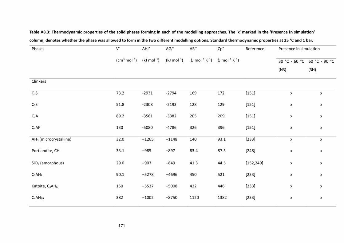
171
Table A8.3: Thermodynamic properties of the solid phases forming in each of the modelling approaches. The 'x' marked in the 'Presence in simulation'
column, denotes whether the phase was allowed to form in the two different modelling options. Standard thermodynamic properties at 25 °C and 1 bar.
Phases V°
(cm3 mol−1)
ΔHf°
(kJ mol−1)
ΔGf°
(kJ mol−1)
ΔSf°
(J mol−1 K−1)
Cp°
(J mol−1 K−1)
Reference Presence in simulation
30 °C - 60 °C
(NS)
60 °C - 90 °C
(SH)
Clinkers
C3S 73.2 -2931 -2794 169 172 [151] x x
C2S 51.8 -2308 -2193 128 129 [151] x x
C3A 89.2 -3561 -3382 205 209 [151] x x
C4AF 130 -5080 -4786 326 396 [151] x x
AH3 (microcrystalline) 32.0 −1265 −1148 140 93.1 [233] x x
Portlandite, CH 33.1 −985 −897 83.4 87.5 [248] x x
SiO2 (amorphous) 29.0 −903 −849 41.3 44.5 [152,249] x x
C2AH8 90.1 −5278 −4696 450 521 [233] x x
Katoite, C3AH6 150 −5537 −5008 422 446 [233] x x
C4AH19 382 −1002 −8750 1120 1382 [233] x x

172
Table A8.3 continued
CAH10 194 −5288 −4623 610 668 [233] x x
Strätlingite, C2ASH8 216 −6360 −5705 546 603 [150] x x
Lime, C 16.8 −635 −604 39.7 42.8 [249] x x
Brucite, MH 24.6 −923 −832 63.1 77.3 [249–251] x x
Sulphates
Ettringite, C6As3H32 707 −17535 −15206 1900 2174 [151] x x
Gypsum, CsH2 74.7 −2023 −1798 194 186 [250,251] x x
Anhydrite, Cs 45.9 −1435 −1322 107 99.6 [250,251] x x
Calcium monosulfoaluminate–hydroxoaluminate hydrate non-ideal solid solution [150]
Calcium monosulfoaluminate hydrate,
C4AsH12
309 −8750 −7779 821 942 [150] x x
C4AH13 274 −8300 −7324 700 930 [233] x x
C-A–S–H gel ideal solid solution end-members, ‘C-A-S-H_ss-hi’ [122]
5CA, C1.25A0.125S1H1.625 57.3 −2491 −2293 163 177 [146] x x
INFCA, C1A0.15625S1.1875H1.65625 59.3 −2551 −2343 154 181 [146] x x

173
Table A8.3 continued
JenD*, C1.5S0.67H2.5a 80.6 −2401 −2169 173 209 [146] x x
T2C*, C1.5S1H2.5b 80.6 −2721 −2298 167 237 [122] x x
T5C, C1.25S1.25H2.5 79.3 −2780 −2517 160 234 [146] x x
TobH, C1S1.5H2.5 85.0 −2831 −2560 153 231 [146] x x
Hydrogarnet solid solution model, C3(A,F)S0.84H4.32
C3AS0.84H4.32_0.5 71.2 -2924 -2682 187 206 [149] - x
C3FS0.84H4.32_0.5 74.3 -2411 -2240 420 216 [149] - x
MA-OH-LDH ideal solid solution end-members, ‘MA-OH-LDH_ss’ [123]
M4AH10 219 −7160 −6358 549 648 [103,252] x x
M6AH12 305 −9007 −8023 675 803 [123] x x
M8AH14 392 −10853 −9687 801 958 [123] x x
Carbonates
Aragonite, Cc 34.2 −1207 −1128 90.2 81.3 [250,251] x x
Calcite, Cc 36.9 −1207 −1129 92.7 81.9 [250,251] x x

174
Table A8.3 continued
Magnesite, Mc 28.0 −1113 −1029 65.7 75.8 [250,251] x x
MA-c-LDH, M4AcH9 220 −7374 −6580 551 647 [151] x x
Calcium monocarboaluminate hydrate,
C4AcH11
262 −8250 −7337 657 881 [150] x x
Calcium hemicarboaluminate hydrate,
C4Ac0.5H12
285 −8270 −7336 713 906 [150] x x
Calcium tricarboaluminate hydrate,
C6Ac3H32
650 −16792 −14566 1858 2121 [150] x x
aThe asterisk for the T2C* end-member depicts a slight change of the Gibbs free energy determined by Myers et al [146] to better incorporate the higher Ca/Si end-
member, JenD, from the CSHQ model developed by Kulik [64].
x - denotes when a phase was available to form within the two different modelling approaches.
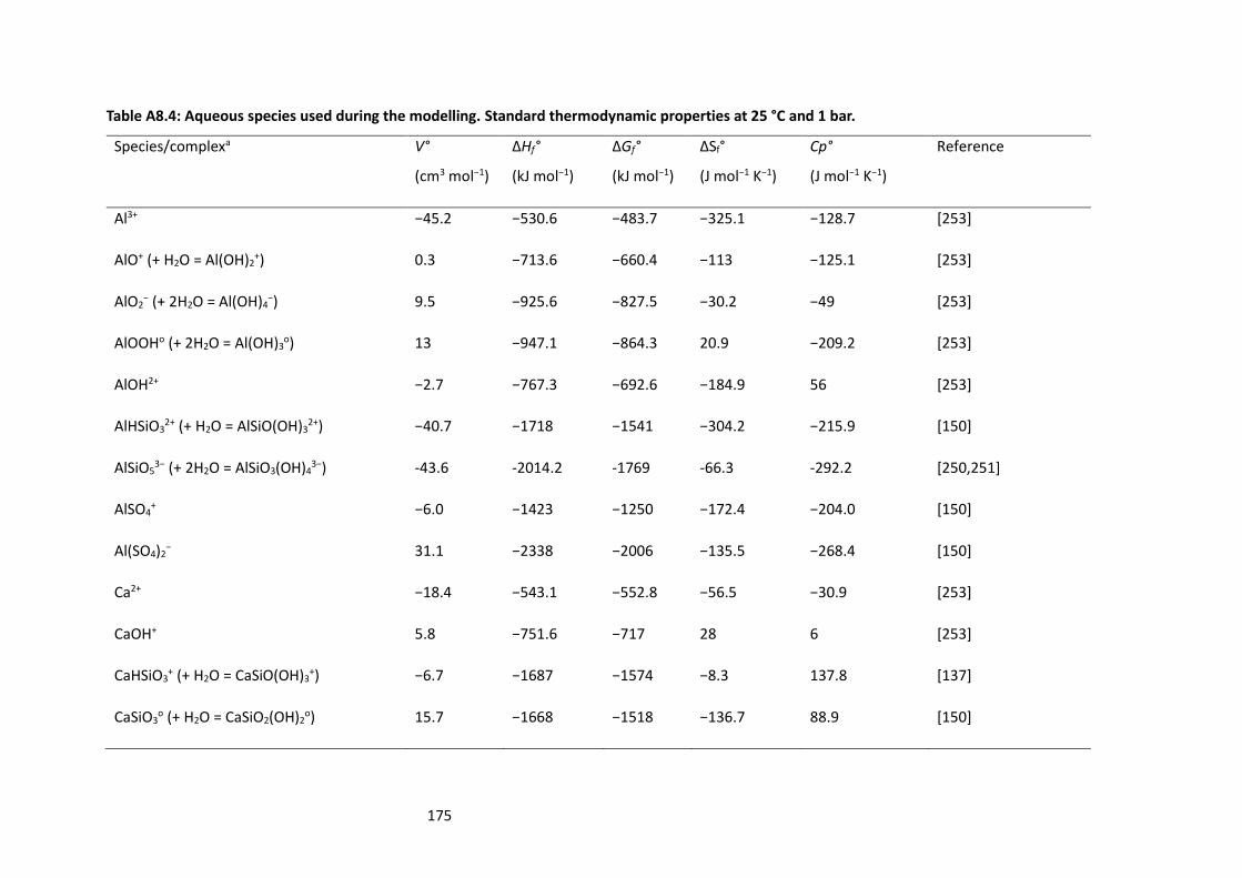
175
Table A8.4: Aqueous species used during the modelling. Standard thermodynamic properties at 25 °C and 1 bar.
Species/complexa V°
(cm3 mol−1)
ΔHf°
(kJ mol−1)
ΔGf°
(kJ mol−1)
ΔSf°
(J mol−1 K−1)
Cp°
(J mol−1 K−1)
Reference
Al3+ −45.2 −530.6 −483.7 −325.1 −128.7 [253]
AlO+ (+ H2O = Al(OH)2+) 0.3 −713.6 −660.4 −113 −125.1 [253]
AlO2− (+ 2H2O = Al(OH)4
−) 9.5 −925.6 −827.5 −30.2 −49 [253]
AlOOHo (+ 2H2O = Al(OH)3o) 13 −947.1 −864.3 20.9 −209.2 [253]
AlOH2+ −2.7 −767.3 −692.6 −184.9 56 [253]
AlHSiO32+ (+ H2O = AlSiO(OH)3
2+) −40.7 −1718 −1541 −304.2 −215.9 [150]
AlSiO53− (+ 2H2O = AlSiO3(OH)4
3−) -43.6 -2014.2 -1769 -66.3 -292.2 [250,251]
AlSO4+ −6.0 −1423 −1250 −172.4 −204.0 [150]
Al(SO4)2− 31.1 −2338 −2006 −135.5 −268.4 [150]
Ca2+ −18.4 −543.1 −552.8 −56.5 −30.9 [253]
CaOH+ 5.8 −751.6 −717 28 6 [253]
CaHSiO3+ (+ H2O = CaSiO(OH)3
+) −6.7 −1687 −1574 −8.3 137.8 [137]
CaSiO3o (+ H2O = CaSiO2(OH)2
o) 15.7 −1668 −1518 −136.7 88.9 [150]

176
Table A8.4 continued
CaSO4o 4.7 −1448 −1310 20.9 −104.6 [137]
CaCO3o −1.6 −1202 −1099 10.5 −123.9 [137]
CaHCO3+ 13.3 −1232 −1146 66.9 233.7 [250,251]
Na+ −1.2 −240.3 −261.9 58.4 38.1 [253]
NaOHo 3.5 −470.1 −418.1 44.8 −13.4 [253]
NaSO4− 18.6 −1147 −1010 101.8 −30.1 [150]
NaCO3− −0.4 −938.6 −797.1 −44.3 −51.3 [250,251]
NaHCO3o 32.3 −929.5 −847.4 154.7 200.3 [250,251]
HSiO3− (+ H2O = SiO(OH)3
−) 4.5 −1145 −1014 20.9 −87.2 [137]
SiO2o (+ 2H2O = Si(OH)4
o) 16.1 −887.9 −833.4 41.3 44.5 [152,254]
SiO32− (+ H2O = SiO2(OH)2
2−) 34.1 −1099 −938.5 −80.2 119.8 [150]
S2O32− 27.6 −649.9 −520.0 66.9 −238.5 [253]
HSO3− 33.0 −627.7 −529.1 139.7 −5.4 [253]
SO32− −4.1 −636.9 −487.9 −29.3 −281.0 [253]
HSO4− 34.8 −889.2 −755.8 125.5 22.7 [253]
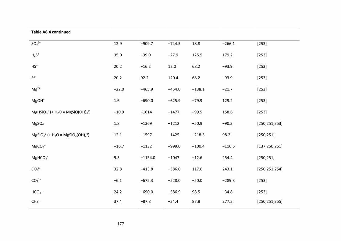
177
Table A8.4 continued
SO42− 12.9 −909.7 −744.5 18.8 −266.1 [253]
H2So 35.0 −39.0 −27.9 125.5 179.2 [253]
HS− 20.2 −16.2 12.0 68.2 −93.9 [253]
S2− 20.2 92.2 120.4 68.2 −93.9 [253]
Mg2+ −22.0 −465.9 −454.0 −138.1 −21.7 [253]
MgOH+ 1.6 −690.0 −625.9 −79.9 129.2 [253]
MgHSiO3+ (+ H2O = MgSiO(OH)3
+) −10.9 −1614 −1477 −99.5 158.6 [253]
MgSO4o 1.8 −1369 −1212 −50.9 −90.3 [250,251,253]
MgSiO3o (+ H2O = MgSiO2(OH)2
o) 12.1 −1597 −1425 −218.3 98.2 [250,251]
MgCO3o −16.7 −1132 −999.0 −100.4 −116.5 [137,250,251]
MgHCO3+ 9.3 −1154.0 −1047 −12.6 254.4 [250,251]
CO2o 32.8 −413.8 −386.0 117.6 243.1 [250,251,254]
CO32− −6.1 −675.3 −528.0 −50.0 −289.3 [253]
HCO3− 24.2 −690.0 −586.9 98.5 −34.8 [253]
CH4o 37.4 −87.8 −34.4 87.8 277.3 [250,251,255]

178
Table A8.4 continued
OH− −4.7 −230 −157.3 −10.7 −136.3 [253]
H+ 0 0 0 0 0 [253]
H2Oo 18.1 −285.9 −237.2 69.9 75.4 [256]
H2o 25.3 −4.0 17.7 57.7 166.9 [250,251,254]
N2o 33.4 −10.4 18.2 95.8 234.2 [254]
O2o 30.5 −12.2 16.4 109 234.1 [254]
o denotes neutral species within aqueous solution.
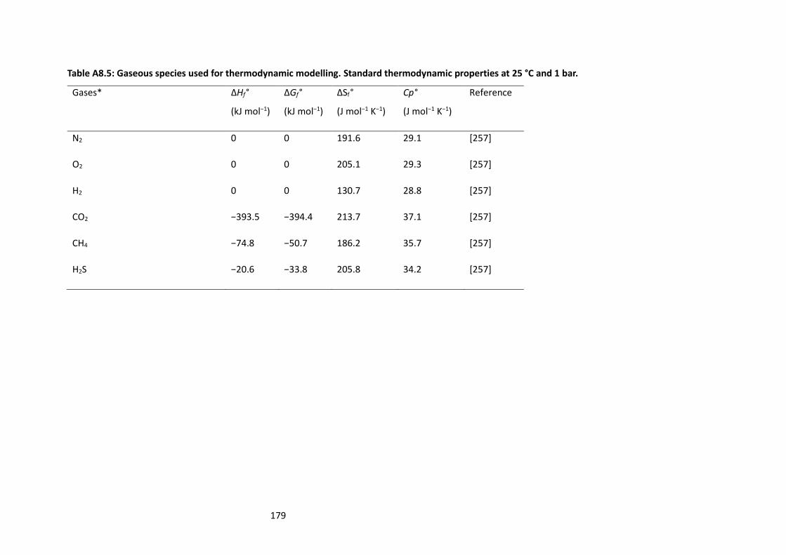
179
Table A8.5: Gaseous species used for thermodynamic modelling. Standard thermodynamic properties at 25 °C and 1 bar.
Gases* ΔHf°
(kJ mol−1)
ΔGf°
(kJ mol−1)
ΔSf°
(J mol−1 K−1)
Cp°
(J mol−1 K−1)
Reference
N2 0 0 191.6 29.1 [257]
O2 0 0 205.1 29.3 [257]
H2 0 0 130.7 28.8 [257]
CO2 −393.5 −394.4 213.7 37.1 [257]
CH4 −74.8 −50.7 186.2 35.7 [257]
H2S −20.6 −33.8 205.8 34.2 [257]

180
8.4 Pitzer parameter database
The Pitzer parameters used in Chapter 6 are summarised in Tables A8.6 and A8.7.
Table A8.6: Binary species Pitzer parameters.
Cation
(M)
Anion
(X)
Binary Pitzer Parameter Binary Pitzer Parameter Reference
B(0) B(1)
B(2) C(0)
B(0) B(1)
B(2) C(0)
Al3+ HSO4- 1.025 5.426
-0.0486 [135] [135]
[258]
Al3+ SO42- 0.822 21.22 -4813 -0.0799 [143] [143] [143] [143]
Ca2+ CO32- 0.16 2.1 -46
[259] [259]
Ca2+ HCO3- 0.39975 2.977
[135] [237]
Ca2+ HS- 0.069 2.264
[247] [247]
Ca2+ HSO4- 0.2145 2.5275
[135] [135]
Ca2+ NO3- 0.1683 1.65
-0.00687 [143] [143]
Ca2+ OH- -0.1421 -0.3727 -11.052 -0.0092 [66] [66] [66] [66]
Ca2+ SO42- 0.2 3.546 -54.24 0.114 [135] [237] [135] [237]
Ca2+ Cl- 0.31 1.7085 -1.13 0.00215 [143]
[66] [66]
Ca2+ ClO4- 0.438 1.76
[259] [259]
Fe2+ HSO4- 0.4273 3.48
[260] [135]
Fe2+ NO3- 0.367078 1.584761
[261] [261]
Fe2+ SO42- 0.2568 3.063 -42 0.0209 [260] [260] [260] [260]
H+ HSO4- 0.2709 0.0299
[262] [262]
H+ NO3- 0.111 0.3805
-0.00424 [143] [143]
[143]
H+ SO42- -0.0216 0.1194
0.0317 [262] [262]
[262]
H+ Cl- 0.1775 0.2945
[66]
[66]

181
Table A8.6 continued
H+ ClO4- 0.1813 0.276
0.0008 [143]
[143] [66]
K+ AlO2- 0.094 0.32
-0.0012 [111] [111]
[111]
K+ CO32- 0.1305 1.43
0.00024 [143] [260]
[143]
K+ HCO3- -0.01558 0.25
0.00469 [143] [237]
[143]
K+ HS- -0.337 0.884
[247] [247]
K+ HSiO3- 0.208 0.34
[244] [244]
K+ HSO4- -0.0003 0.1735
[260] [135]
K+ OH- 0.1298 0.32
0.0041 [66] [66]
[135]
K+ SCN- 0.04159 0.1048
-0.00254 [143] [143]
K+ SO32- 0.065 1
[135] [135]
K+ SO42- 0.0317 0.756
0.00818 [237] [237]
[237]
Mg2+ CO32- 0.18 1.804 -46
[259] [259]
Mg2+ HCO3- 0.033 0.84975
[135] [135]
Mg2+ HS- 0.466 2.264
[247] [247]
Mg2+ HSO4- 0.4746 1.729
[260] [260]
Mg2+ NO3- 0.3405 12.9 -46
[143] [263] [135]
Mg2+ SO42- 0.2135 3.367 -40.15 0.02875 [237] [237] [143] [237]
Mg2+ Cl- 0.3553 1.65
0.00651 [143] [237] [237]
Mg2+ ClO4- 0.4956 2.097
[143] [143]
MgOH+ Cl- -0.1 1.658
[260] [260]
Na+ AlO2- -0.0083 0.071
0.00977 [239] [239]
[239]
Na+ CO32- 0.04625 1.389
0.0044 [143] [260]
[260]
Na+ HCO3- -0.05876 0.5535 8.22
[143] [143] [237]

182
Table A8.6 continued
Na+ HS- -0.103 0.884
[247] [247]
Na+ HSiO3- 0.162 0.34
[244] [244]
Na+ HSO4- 0.0454 0.398
[260] [260]
Na+ OH- 0.0864 0.253
0.0044 [239] [239]
[239]
Na+ S2O32- 0.06306 1.254
0.004673 [143] [143]
[143]
Na+ SCN- 0.1048 0.3242
[143] [143]
Na+ SO32- 0.08015
[264,265]
Na+ SO42- 0.01959 1.049 0.005416 0.005416 [143] [143]
Na+ Cl- 0.07831 0.2769
0.006718 [143] [143] [237] [143]
Na+ ClO4- 0.05422 0.2861
0.00148 [143] [143] [143] [237]
NH4+ SO4
2- -0.05094 0.2068
-0.00285 [143] [143] [143]
Table A8.7: Mixed electrolyte Pitzer parameters.
Aq. Species Aq. Species Aq. Species Parameter Type Parameter value Reference
CO2 Ca2+ -
0.183 [260]
CO2 K+ -
0.051 [260]
CO2 Mg2+ -
0.183 [260]
CO2 Na+ -
0.085 [260]
SiO2 Ca2+ -
0.2925 [266]
SiO2 K+ -
0.03224 [266]
SiO2 Mg2+ -
0.2925 [266]
SiO2 Na+ -
0.0925 [266]
CO2 HSO4- -
-0.003 [260]

183
Table A8.7 continued
CO2 SO42- -
0.075 [237]
SiO2 NO3- -
-0.0094 [266]
SiO2 SO42- -
-0.13963 [266]
Ca2+ H+ -
0.092 [135]
Ca2+ K+ -
0.032 [135]
Ca2+ Na+ -
0.07 [135]
K+ H+ -
0.005 [135]
K+ Na+ -
-0.012 [135]
Mg2+ Ca2+ -
0.007 [135]
Mg2+ H+ -
0.1 [260]
Mg2+ Na+ -
0.07 [135]
Na+ H+ -
0.0368 [264,265]
NH4+ H+ -
-0.019 [135]
AlO2- OH- -
-0.2255 [239]
ClO4- Cl- -
0.0341 [267]
CO32- OH- -
0.1 [135]
CO32- SO4
2- -
0.02 [135]
HCO3- CO3
2- -
-0.04 [135]
HCO3- SO4
2- -
0.01 [135]
OH- Cl- -
-0.05 [135]
OH- SO42- -
-0.013 [135]
Ca2+ K+ SO42-
-0.0365 [237]
Cl- H+ Ca2+
-0.015 [135]

184
Table A8.7 continued
Cl- H+ Mg2+
-0.011 [135]
Cl- H+ Na+
-0.004 [135]
Cl- Mg2+ MgOH+
0.028 [260]
Cl- Na+ Ca2+
-0.007 [135]
Cl- Na+ Mg2+
-0.012 [135]
ClO4- H+ Na+
-0.016 [135]
CO32- Na+ K+
0.003 [135]
H+ K+ SO42-
0.197 [260]
HCO3- Na+ K+
-0.003 [135]
HSO4- H+ K+
-0.0265 [135]
HSO4- H+ Mg2+
-0.0178 [135]
HSO4- H+ Na+
-0.0129 [135]
NO3- H+ Na+
-0.0274 [268]
NO3- Na+ K+
-0.001 [135]
SO42- Ca2+ Mg2+
0.024 [135]
SO42- K+ Mg2+
-0.048 [135]
SO42- Na+ Ca2+
-0.055 [135]
SO42- Na+ K+
-0.01 [135]
SO42- Na+ Mg2+
-0.015 [135]
SO42- Na+ NH4
+
-0.0013 [135]
Ca2+ Cl- OH-
-0.025 [135]
K+ CO32- HCO3
-
0.012 [135]
K+ OH- AlO2-
-0.0388 [239]

185
Table A8.7 continued
K+ OH- CO32-
-0.01 [135]
K+ SO42- CO3
2-
-0.009 [135]
K+ SO42- HSO4
-
-0.0677 [135]
K+ SO42- OH-
-0.05 [135]
Mg2+ SO42- HCO3
-
-0.161 [135]
Mg2+ SO42- HSO4
-
-0.0425 [135]
Na+ Cl- ClO4-
-0.0057 [267]
Na+ Cl- OH-
-0.006 [135]
Na+ CO32- HCO3
-
0.002 [135]
Na+ OH- AlO2-
-0.0048 [111]
Na+ OH- CO32-
-0.017 [135]
Na+ SO42- CO3
2-
-0.005 [135]
Na+ SO42- HCO3
-
-0.005 [135]
Na+ SO42- HSO4
-
-0.0094 [135]
Na+ SO42- OH-
-0.009 [135]

186
References
[1] L. Arnold, Windscale 1957: Anatomy of a Nuclear Accident, 3rd ed., Palgrave Macmillan, New
York, 1995. doi:10.1007/978-1-349-24008-1.
[2] J. Mahaffey, Atomic Accidents: A History of Nuclear Meltdowns and Disasters: From the Ozark
Mountains to Fukushima, 1st ed., Pegasus Books, New York, 2014.
[3] BEIS, Digest of UK energy statistics 2017, (2017) 260 pp. doi:10.1016/0301-4215(88)90136-X.
[4] NDA, Radioactive Wastes in the UK: Summary of Data for International Reporting 2016, 2017.
[5] M.I. Ojovan, W.E. Lee, An introduction to nuclear waste immobilisation, Elsevier, Amsterdam,
2006. doi:10.1016/S1369-7021(06)71394-3.
[6] NDA, Radioactive Wastes in the UK: UK Radioactive Waste Inventory Report, 2017.
https://ukinventory.nda.gov.uk/wp-content/uploads/sites/18/2014/01/2016UKRWMI-UK-
Radioactive-waste-inventory-report.pdf.
[7] G.V. Hutson, Waste Treatment, in: Wilson, P.D. (Ed.), The Nuclear Fuel Cycle: from Ore to
Wastes, 1st ed., Oxford University Press, 1996.
[8] H. Godfrey, G. Cann, Effect of chloride on magnox corrosion with respect to carbon-14 release
post closure, NNL, Risley. (2015).
[9] NDA, Radioactive Wastes in the UK: A Summary of the 2013 Inventory, Cumbria, UK, 2013.
www.nda.gov.uk/ukinventory.
[10] NDA, Geological Disposal: Guidance on the application of the Waste Package Specifications for
unshielded waste packages, Oxford, UK, 2014. www.nda.gov.uk.
[11] M. Atkins, F.P. Glasser, Application of Portland cement-based materials to radioactive waste
immobilization, Waste Manag. 12 (1992) 105–131. doi:10.1016/0956-053X(92)90044-J.
[12] M. Moranville-Regourd, Cements made from blastfurnace slag, in: Hewlett, P.C. (Ed.), Lea’s
Chemistry of Cement and Concrete, 4th ed., 2003. doi:10.1016/B978-075066256-7/50023-0.
[13] F.P. Glasser, Progress in the immobilization of radioactive wastes in cement, Cem. Concr. Res.
22 (1992) 201–216. doi:10.1016/0008-8846(92)90058-4.
[14] J.H. Sharp, J. Hill, N.B. Milestone, E.W. Miller, Cementitious Systems for Encapsulation of
Intermediate Level Waste, in: Proc. ICEM 2003 9th Int. Conf. Radioact. Waste Manag. Environ.
Remediat., 2003: pp. 1–10. doi:10.1115/ICEM2003-4554.

187
[15] N.C. Collier, N.B. Milestone, The encapsulation of Mg(OH)2 sludge in composite cement, Cem.
Concr. Res. 40 (2010) 452–459. doi:10.1016/j.cemconres.2009.10.007.
[16] J. Hill, J.H. Sharp, The mineralogy and microstructure of three composite cements with high
replacement levels, Cem. Concr. Compos. 24 (2002) 191–199. doi:10.1016/S0958-
9465(01)00041-5.
[17] C.A. Utton, M. Hayes, J. Hill, N.B. Milestone, J.H. Sharp, Effect of temperatures up to 90 °C on
the early hydration of Portland-blastfurnace slag cements, J. Am. Ceram. Soc. 91 (2008) 948–
954. doi:10.1111/j.1551-2916.2007.02124.x.
[18] C.H. Bland, J.H. Sharp, A conduction calorimetric study of gasifier slag-portland cement blends,
Cem. Concr. Res. 21 (1991) 359–367. doi:10.1016/0008-8846(91)90017-C.
[19] M.J. Angus, I.H. Godfrey, M. Hayes, S. Foster, Managing change in the supply of cement
powders for radioactive waste encapsulation – Twenty years of operational experience, in:
WM2010 Conf. Phoenix, U.S.A, 2010.
[20] NDA, Geological Disposal: An introduction to the generic Disposal System Safety Case, 2010.
doi:978-1-84029-445-3.
[21] NDA, The 2013 UK Radioactive Waste Inventory, 2013.
[22] S.J. Benbow, M.O. Rivett, N. Chittenden, A.W. Herbert, S. Watson, S.J. Williams, S. Norris,
Potential migration of buoyant LNAPL from Intermediate Level Waste (ILW) emplaced in a
Geological Disposal Facility (GDF) for UK radioactive waste, J. Contam. Hydrol. 167 (2014) 1–
22. doi:10.1016/j.jconhyd.2014.07.011.
[23] DECC, Implementing Geological Disposal: A Framework for the long-term management of
higher activity radioactive waste, 2014.
[24] A.J. Francis, R. Cather, I.G. Crossland, Science Report Nirex Safety Assessment Research
Programme: Development of the Nirex Reference Vault Backfill; Report on Current Status in
1994, (1997).
[25] R.G.W. Vasconcelos, N. Beaudoin, A. Hamilton, N.C. Hyatt, J.L. Provis, C.L. Corkhill,
Characterisation of a high pH cement backfill for the geological disposal of nuclear waste: The
Nirex Reference Vault Backfill, Appl. Geochem. 89 (2017) 180–189.
doi:10.1016/j.apgeochem.2017.11.007.
[26] NDA, A Review of the Development of Bentonite Barriers in the KBS-3V Disposal Concept,

188
Harwell Oxford, UK, 2014. doi:10.1007/978-1-61779-821-4.
[27] F.M. McEvoy, D.I. Schofield, R.P. Shaw, S. Norris, Tectonic and climatic considerations for deep
geological disposal of radioactive waste: A UK perspective, Sci. Total Environ. 571 (2016) 507–
521. doi:10.1016/j.scitotenv.2016.07.018.
[28] NDA, Geological Disposal: Near-field evolution status report, 2010.
[29] BEIS, Implementing Geological Disposal – Working With Communities, 2018.
[30] F.M.I. Hunter, B.T. Swift, An assessment of the generation of GDF-derived gas using the 2007
Derived Inventory, AMEC. (2013).
[31] S.C. Boden, Nirex Vault Environment Feasibility Study: Summary Report, NNC Ltd. (2002).
[32] W. Kurdowski, Cement manufacture, in: Bensted, J. Barnes, P. (Eds.), Structure and
Performance of Cements, 2nd ed., Spon Press, 2002.
[33] H.F.W. Taylor, Cement Chemistry, 2nd ed., Thomas Telford Services Ltd, London, 1990.
doi:10.1016/S0958-9465(98)00023-7.
[34] J.W. Bullard, H.M. Jennings, R.A. Livingston, A. Nonat, G.W. Scherer, J.S. Schweitzer, K.L.
Scrivener, J.J. Thomas, Mechanisms of cement hydration, Cem. Concr. Res. 41 (2011) 1208–
1223. doi:10.1016/j.cemconres.2010.09.011.
[35] C.D. Lawrence, The Production of Low-Energy Cements, in: Hewlett, P.C. (Ed.), Lea’s Chemistry
of Cement and Concrete, 4th ed., 2003. doi:10.1016/B978-075066256-7/50021-7.
[36] F. Massazza, Pozzolana and Pozzolanic Cements, in: Hewlett, P.C. (Ed.), Lea’s Chemistry of
Cement and Concrete, 4th ed., 2004.
[37] B. Lothenbach, K.L. Scrivener, R.D. Hooton, Supplementary cementitious materials, Cem.
Concr. Res. 41 (2011) 1244–1256. doi:10.1016/j.cemconres.2010.12.001.
[38] P.W. Scott, The Chemistry and Mineralogy of Some Granulated and Pelletized Blastfurnace
Slags, Mineral. Mag. 50 (1986) 141–147. doi:10.1180/minmag.1986.050.355.19.
[39] E. Lang, Blastfurnace cements, in: Bensted, J., Barnes, P. (Eds.), Structure and Performance of
Cements, 2nd ed., Spon Press, 2002.
[40] J.I. Escalante, L.Y.Y. Gómez, K.K. Johal, G. Mendoza, H. Mancha, J. Méndez, Reactivity of blast-
furnace slag in Portland cement blends hydrated under different conditions, Cem. Concr. Res.
31 (2001) 1403–1409. doi:10.1016/S0008-8846(01)00587-7.

189
[41] J.S. Lumley, R.S. Gollop, G.K. Moir, H.F.W. Taylor, Degrees of reaction of the slag in some blends
with Portland cements, Cem. Concr. Res. 26 (1996) 139–151. doi:10.1016/0008-
8846(95)00190-5.
[42] Y. Kawabata, K. Yamada, Evaluation of Alkalinity of Pore Solution Based on the Phase
Composition of Cement Hydrates with Supplementary Cementitious Materials and its Relation
to Suppressing ASR Expansion, J. Adv. Concr. Technol. 13 (2015) 538–553.
doi:10.3151/jact.13.538.
[43] K.L. Scrivener, P. Juilland, P.J.M. Monteiro, Advances in understanding hydration of Portland
cement, Elsevier Ltd, 2015. doi:10.1016/j.cemconres.2015.05.025.
[44] I.G. Richardson, G.W. Groves, Microstructure and microanalysis of hardened cement pastes
involving ground granulated blast-furnace slag, J. Mater. Sci. 27 (1992) 6204–6212.
doi:10.1007/BF01133772.
[45] R. Taylor, I.G. Richardson, R.M.D. Brydson, Composition and microstructure of 20-year-old
ordinary Portland cement–ground granulated blast-furnace slag blends containing 0 to 100%
slag, Cem. Concr. Res. 40 (2010) 971–983. doi:10.1016/j.cemconres.2010.02.012.
[46] R. Snellings, A. Salze, K.L. Scrivener, Use of X-ray diffraction to quantify amorphous
supplementary cementitious materials in anhydrous and hydrated blended cements, Cem.
Concr. Res. 64 (2014) 89–98. doi:10.1016/j.cemconres.2014.06.011.
[47] I. Odler, Hydration, Setting and Hardening of Portland Cement, in: Hewlett, P.C. (Ed.), Lea’s
Chemistry of Cement and Concrete, 4th ed., 2003. doi:10.1016/B978-075066256-7/50018-7.
[48] B. Lothenbach, A. Nonat, Calcium silicate hydrates: Solid and liquid phase composition, Cem.
Concr. Res. 78 (2015) 57–70. doi:10.1016/j.cemconres.2015.03.019.
[49] I.G. Richardson, The calcium silicate hydrates, Cem. Concr. Res. 38 (2008) 137–158.
doi:10.1016/j.cemconres.2007.11.005.
[50] G.K. Sun, J.F. Young, R.J. Kirkpatrick, The role of Al in C-S-H: NMR, XRD, and compositional
results for precipitated samples, Cem. Concr. Res. 36 (2006) 18–29.
doi:10.1016/j.cemconres.2005.03.002.
[51] M.D. Andersen, H.J. Jakobsen, J. Skibsted, Incorporation of aluminum in the calcium silicate
hydrate (C-S-H) of hydrated Portland cements: A high-field 27Al and 29Si MAS NMR investigation,
Inorg. Chem. 42 (2003) 2280–2287. doi:10.1021/ic020607b.

190
[52] J. Skibsted, H.J. Jakobsen, C. Hall, Quantification of calcium silicate phases in Portland cements
by 29Si MAS NMR spectroscopy, J. Chem. Soc. Faraday Trans. 91 (1995) 4423–4430.
doi:10.1039/FT9959104423.
[53] A. Atkinson, J.A. Hearne, C.F. Knights, Aqueous Chemistry and Thermodynamic Modelling of
CaO–SiO2–H2O gels, J. Chem. Soc. 0 (1989) 2371–2379. doi:10.1039/DT9890002371.
[54] J.J. Chen, J.J. Thomas, H.F.W. Taylor, H.M. Jennings, Solubility and structure of calcium silicate
hydrate, Cem. Concr. Res. 34 (2004) 1499–1519. doi:10.1016/j.cemconres.2004.04.034.
[55] I.G. Richardson, J.G. Cabrera, The nature of C-S-H in model slag-cements, Cem. Concr. Compos.
22 (2000) 259–266. doi:10.1016/S0958-9465(00)00022-6.
[56] A. Nonat, The structure and stoichiometry of C-S-H, Cem. Concr. Res. 34 (2004) 1521–1528.
doi:10.1016/j.cemconres.2004.04.035.
[57] F. Puertas, M. Palacios, H. Manzano, J.S. Dolado, A. Rico, J. Rodríguez, A model for the C-A-S-H
gel formed in alkali-activated slag cements, J. Eur. Ceram. Soc. 31 (2011) 2043–2056.
doi:10.1016/j.jeurceramsoc.2011.04.036.
[58] I.G. Richardson, Model Structures for C-(A)-S-H(I), Acta Crystallogr. Sect. B Struct. Crystallogr.
Cryst. Chem. B70 (2014) 903–923. doi:10.1107/S2052520614021982.
[59] S.Y. Hong, F.P. Glasser, Alkali binding in cement pastes. Part I: the C-S-H phase, Cem. Concr.
Res. 29 (1999) 1893–1903. doi:10.1016/S0008-8846(99)00187-8.
[60] S.A. Bernal, R. San Nicolas, R.J. Myers, R. Mejía De Gutiérrez, F. Puertas, J.S.J. Van Deventer,
J.L. Provis, MgO content of slag controls phase evolution and structural changes induced by
accelerated carbonation in alkali-activated binders, Cem. Concr. Res. 57 (2014) 33–43.
doi:10.1016/j.cemconres.2013.12.003.
[61] T.T.H. Bach, E. Chabas, I. Pochard, C. Cau Dit Coumes, J. Haas, F. Frizon, A. Nonat, Retention of
alkali ions by hydrated low-pH cements: Mechanism and Na+/K+ selectivity, Cem. Concr. Res.
51 (2013) 14–21. doi:10.1016/j.cemconres.2013.04.010.
[62] H. Stade, On the reaction of C-S-H(di, poly) with alkali hydroxides, Cem. Concr. Res. 19 (1989)
802–810. doi:10.1016/0008-8846(89)90051-3.
[63] E. L’Hôpital, B. Lothenbach, D.A. Kulik, K. Scrivener, Influence of calcium to silica ratio on
aluminium uptake in calcium silicate hydrate, Cem. Concr. Res. 85 (2016) 111–121.
doi:10.1016/j.cemconres.2016.01.014.

191
[64] D.A. Kulik, Improving the structural consistency of C-S-H solid solution thermodynamic models,
Cem. Concr. Res. 41 (2011) 477–495. doi:10.1016/j.cemconres.2011.01.012.
[65] C.S. Walker, S. Sutou, C. Oda, M. Mihara, A. Honda, Calcium silicate hydrate (C-S-H) gel
solubility data and a discrete solid phase model at 25 °C based on two binary non-ideal solid
solutions, Cem. Concr. Res. 79 (2016) 1–30. doi:10.1016/j.cemconres.2015.07.006.
[66] J. Duchesne, E.J. Reardon, Measurement and prediction of portlandite solubility in alkali
solutions, Cem. Concr. Res. 25 (1995) 1043–1053. doi:10.1016/0008-8846(95)00099-X.
[67] K.L. Scrivener, A. Nonat, Hydration of cementitious materials, present and future, Cem. Concr.
Res. 41 (2011) 651–665. doi:10.1016/j.cemconres.2011.03.026.
[68] C.-T.A. Chen, W.L. Marshall, Amorphous silica solubilities IV. Behavior in pure water and
aqueous sodium chloride, sodium sulfate, magnesium chloride, and magnesium sulfate
solutions up to 350°C, Geochim. Cosmochim. Acta. 46 (1982) 279–287. doi:10.1016/0016-
7037(82)90255-1.
[69] M. Grutzeck, A. Benesi, B. Fanning, Silicon‐29 Magic Angle Spinning Nuclear Magnetic
Resonance Study of Calcium Silicate Hydrates, J. Am. Ceram. Soc. 72 (1989) 665–668.
doi:10.1111/j.1151-2916.1989.tb06192.x.
[70] J. Haas, Etude expérimentale et modélisation thermodynamique du système CaO-SiO2-(Al2O3)-
H2O, Université de Bourgogne, Français, 2012.
[71] A.W. Harris, M.C. Manning, W.M. Tearle, C.J. Tweed, Testing of models of the dissolution of
cements - Leaching of synthetic CSH gels, Cem. Concr. Res. 32 (2002) 731–746.
doi:10.1016/S0008-8846(01)00748-7.
[72] P. Henocq, Modélisation des interactions ioniques à la surface des Silicates de Calcium
Hydratés, L’Universite Laval, Quebec, Canada, 2005.
[73] I. Pointeau, Etude Mecanistique et modelisation de la retention de radionucleides par les
silicates de calcium hydrates (CSH) des ciments, Chimie, L’Universite de Reims Champage-
Ardenne, Reims, France, 2000.
[74] D. Sugiyama, Chemical alteration of calcium silicate hydrate (C-S-H) in sodium chloride solution,
Cem. Concr. Res. 38 (2008) 1270–1275. doi:10.1016/j.cemconres.2008.06.002.
[75] S.W. Swanton, H.J. Fairbrother, N.A. Turner, The effect of sodium chloride on the dissolution
of calcium silicate hydrate gels. II., 2006. doi:10.1016/j.wasman.2006.01.022.
192
[76] C.S. Walker, D. Savage, M. Tyrer, K.V. Ragnarsdottir, Non-ideal solid solution aqueous solution
modeling of synthetic calcium silicate hydrate, Cem. Concr. Res. 37 (2007) 502–511.
doi:10.1016/j.cemconres.2006.12.002.
[77] M. Atkins, F.P. Glasser, A. Kindness, Cement hydrate phase: Solubility at 25°C, Cem. Concr. Res.
22 (1992) 241–246. doi:10.1016/0008-8846(92)90062-Z.
[78] A. V. Chambers, T.G. Heath, F.M.I. Hunter, M.C. Manning, S.J. Williams, The effect of sodium
chloride on the dissolution of calcium silicate hydrate gels, 2005.
doi:10.1016/j.wasman.2006.01.022.
[79] A.-C. Courault, Simulation experimentale des C-S-H dans les betons modernes: Etude de la
composition et des proprietes a l’equilibre dans desmilieux complexes, Laboratoire de
Recherches sur la Réactivité des Solides, Universite de Bourgogne, 2000.
[80] E.P. Flint, L.S. Wells, Study of the system CaO-SiO2-H2O at 30 °C and of the reaction of water on
the anhydrous calcium silicates, Bur. Stand. J. Res. 12 (1934) 751–783.
doi:10.6028/jres.012.060.
[81] B.K. Fujii, W. Kondo, Heterogeneous Equilibrium of Calcium Silicate Hydrate in water at 30 °C,
J. Chem. Soc. Dalt. Trans. (1981) 645–651.
[82] F. Glasser, M. Tyrer, K. Quillin, The chemistry of blended cements and backfills intended for use
in radioactive waste disposal, Bristol (United Kingdom), 1999.
[83] S.A. Greenberg, T.N. Chang, Investigation of the Colloidal Hydrated Calcium Silicates. II.
Solubility Relationships in the Calcium Oxide-Silica-Water System at 25°, J. Phys. Chem. 69
(1965) 182–188. doi:10.1021/j100885a027.
[84] I.G. Richardson, G.W. Groves, Microstructure and microanalysis of hardened ordinary Portland
cement pastes, J. Mater. Sci. 28 (1993) 265–277. doi:10.1007/BF00349061.
[85] S.Y. Hong, F.P. Glasser, Alkali sorption by C-S-H and C-A-S-H gels: Part II. Role of alumina, Cem.
Concr. Res. 32 (2002) 1101–1111. doi:10.1016/S0008-8846(02)00753-6.
[86] I.G. Richardson, A.R. Brough, R. Brydson, G.W. Groves, C.M. Dobsont, Location of aluminum in
substituted calcium silicate hydrate (C-S-H) gels as determined by 29Si and 27Al NMR and EELS,
J. Am. Ceram. Soc. 76 (1993) 2285–2288. doi:10.1111/j.1151-2916.1993.tb07765.x.
[87] L. Pegado, C. Labbez, S. V. Churakov, Mechanism of aluminium incorporation into C–S–H from
ab initio calculations, J. Mater. Chem. A. 2 (2014) 3477. doi:10.1039/c3ta14597b.

193
[88] W. Loewenstein, The distribution of aluminum in the tetrahedra of silicates and aluminates.,
Am. Mineral. 39 (1954) 92–96.
[89] V. Kocaba, Development and evaluation of methods to follow microstructural development of
cementitious systems including slags, 2009. doi:10.5075/epfl-thesis-4523.
[90] K. Luke, E. Lachowski, Internal composition of 20-year-old fly ash and slag-blended ordinary
portland cement pastes, J. Am. Ceram. Soc. 91 (2008) 4084–4092. doi:10.1111/j.1551-
2916.2008.02783.x.
[91] E.M. Gartner, J.F. Young, D.A. Damidot, I. Jawed, Hydration of Portland Cement, in: Bensted, J.,
Barnes, P. (Eds.), Structure and Performance of Cements, 2nd ed., Spos Press, 2002.
[92] T. Matschei, Thermodynamics of Cement Hydration, University of Aberdeen, 2007.
[93] A. Quennoz, K.L. Scrivener, Interactions between alite and C3A-gypsum hydrations in model
cements, Cem. Concr. Res. 44 (2013) 46–54. doi:10.1016/j.cemconres.2012.10.018.
[94] B. Lothenbach, G. Le Saout, E. Gallucci, K. Scrivener, Influence of limestone and anhydrite on
the hydration of Portland cements, Cem. Concr. Res. 38 (2008) 848–860.
doi:10.1016/j.cemconcomp.2013.11.007.
[95] T. Matschei, B. Lothenbach, F.P. Glasser, The role of calcium carbonate in cement hydration,
Cem. Concr. Res. 37 (2007) 551–558. doi:10.1016/j.cemconres.2006.10.013.
[96] S. Adu-Amankwah, M. Zajac, C. Stabler, B. Lothenbach, L. Black, Influence of limestone on the
hydration of ternary slag cements, Cem. Concr. Compos. 100 (2017) 96–109.
doi:10.1016/j.cemconcomp.2013.11.007.
[97] T. Matschei, B. Lothenbach, F.P. Glasser, The AFm phase in Portland cement, Cem. Concr. Res.
37 (2007) 118–130. doi:10.1016/j.cemconres.2006.10.010.
[98] D. Damidot, F.P. Glasser, Thermodynamic investigation of the CaO-Al2O3-CaSO4-H2O system at
25°C and the influence of Na2O, Cem. Concr. Res. 23 (1993) 221–238. doi:10.1016/0008-
8846(93)90153-Z.
[99] D. Damidot, S. Stronach, A. Kindness, M. Atkins, F.P. Glasser, Thermodynamic investigation of
the CaO-Al2O3-CaCO3-H2O closed system at 25°C and the influence of Na2O, Cem. Concr. Res.
24 (1994) 563–572. doi:10.1016/0008-8846(94)90145-7.
[100] C.E. Harvie, N. Møller, J.H. Weare, The prediction of mineral solubilities in natural waters: The
Na-K-Mg-Ca-H-Cl-SO4-OH-HCO3-CO3-CO2-H2O system to high ionic strengths at 25 °C,

194
Geochim. Cosmochim. Acta. 48 (1984) 723–751. doi:10.1016/0016-7037(84)90098-X.
[101] M. Ben Haha, B. Lothenbach, G. Le Saout, F. Winnefeld, Influence of slag chemistry on the
hydration of alkali-activated blast-furnace slag — Part I: Effect of MgO, Cem. Concr. Res. 41
(2011) 955–963. doi:10.1016/j.cemconres.2011.05.002.
[102] M. Ben Haha, B. Lothenbach, G. Le Saout, F. Winnefeld, Influence of slag chemistry on the
hydration of alkali-activated blast-furnace slag — Part II: Effect of Al2O3, Cem. Concr. Res. 42
(2012) 74–83. doi:10.1016/j.cemconres.2011.08.005.
[103] I.G. Richardson, Clarification of possible ordered distributions of trivalent cations in layered
double hydroxides and an explanation for the observed variation in the lower solid-solution
limit, Acta Crystallogr. Sect. B Struct. Sci. Cryst. Eng. Mater. 69 (2013) 629–633.
doi:10.1107/S2052519213027905.
[104] A. Vollpracht, B. Lothenbach, R. Snellings, J. Haufe, The pore solution of blended cements: a
review, Mater. Struct. 49 (2015) 3341–3367. doi:10.1617/s11527-015-0724-1.
[105] Z. Tan, Experimental Study and Numerical Simulation of Tube Hydroforming, Ghent University,
2015.
[106] E. Schäfer, Einfluss der Reaktionen verschiedener Zementhauptbestandteile auf den
Alkalihaushalt der Porenlösung des Zementsteins, Technischen Universität Clausthal, 2004.
[107] Z. Tan, G. De Schutter, G. Ye, Y. Gao, L. Machiels, Influence of particle size on the early hydration
of slag particle activated by Ca(OH)2 solution, Constr. Build. Mater. 52 (2014) 488–493.
doi:10.1016/j.conbuildmat.2013.11.073.
[108] E. L’Hôpital, B. Lothenbach, K. Scrivener, D.A. Kulik, Alkali uptake in calcium alumina silicate
hydrate (C-A-S-H), Cem. Concr. Res. 85 (2016) 122–136. doi:10.1016/j.cemconres.2016.03.009.
[109] G.D. Miron, T. Wagner, D.A. Kulik, B. Lothenbach, An internally consistent thermodynamic
dataset for aqueous species in the system Ca-Mg-Na-K-Al-Si-O-H-C-Cl to 800 °C and 5 KBAR,
Am. J. Sci. 317 (2017) 755–806. doi:10.2475/07.2017.01.
[110] M. Altmaier, V. Metz, V. Neck, R. Müller, T. Fanghänel, Solid-liquid equilibria of Mg(OH)2(cr)
and Mg2(OH)3Cl·4H2O(cr) in the system Mg-Na-H-OH-Cl-H2O at 25°C, Geochim. Cosmochim.
Acta. 67 (2003) 3595–3601. doi:10.1016/S0016-7037(03)00165-0.
[111] D.J. Wesolowski, Aluminum Speciation and Equilibria in Aqueous-Solution: I. The Solubility of
Gibbsite in the system Na-K-Cl-OH-Al(OH)4 from 0 to 100 °C, Geochim. Cosmochim. Acta. 56

195
(1992) 1065–1091. doi:Doi 10.1016/0016-7037(92)90048-N.
[112] D. Damidot, F.P. Glasser, Thermodynamic investigation of the CaO-Al2O3-CaSO4-K2O-H2O
system at 25°C, Cem. Concr. Res. 23 (1993) 1195–1204. doi:10.1016/0008-8846(93)90180-H.
[113] P. Feng, C. Miao, J.W. Bullard, Factors Influencing the Stability of AFm and AFt in the Ca-Al-S-
O-H System at 25°C, J. Am. Ceram. Soc. 99 (2016) 1031–1041. doi:10.1111/jace.13971.
[114] A. Gruskovnjak, B. Lothenbach, L. Holzer, R. Figi, F. Winnefeld, Hydration of alkali-activated
slag: comparison with ordinary Portland cement, Adv. Cem. Res. 18 (2006) 119–128.
doi:10.1680/adcr.2006.18.3.119.
[115] D.L. Parkhurst, C.A.J. Appelo, Description of Input and Examples for PHREEQC Version 3 — A
Computer Program for Speciation , Batch-Reaction , One-Dimensional Transport , and Inverse
Geochemical Calculations., U.S. Geol. Surv. Tech. Methods, B. 6, Chapter A43. (2013) 6–43A.
doi:10.1016/0029-6554(94)90020-5.
[116] C.M. Bethke, Activity coefficients, in: Geochemical and Biogeochemical Reaction Modelling,
2nd ed., Cambridge University Press, 2007. doi:10.1017/CBO9780511619670.011.
[117] J. Bruno, D. Bosbach, D.A. Kulik, A. Navrotsky, Chemical thermodynamics of solid solutions of
interest in radioactive waste management: a state-of-the-art report, OECD, 2007. doi:978-92-
64-02655-1.
[118] B. Lothenbach, F. Winnefeld, Thermodynamic modelling of the hydration of Portland cement,
Cem. Concr. Res. 36 (2006) 209–226. doi:10.1016/j.cemconres.2005.03.001.
[119] B.Z. Dilnesa, E. Wieland, B. Lothenbach, R. Dähn, K.L. Scrivener, Fe-containing phases in
hydrated cements, Cem. Concr. Res. 58 (2014) 45–55. doi:10.1016/j.cemconres.2013.12.012.
[120] D. Damidot, B. Lothenbach, D. Herfort, F.P. Glasser, Thermodynamics and cement science,
Cem. Concr. Res. 41 (2011) 679–695. doi:10.1016/j.cemconres.2011.03.018.
[121] B. Lothenbach, Thermodynamic equilibrium calculations in cementitious systems, Mater.
Struct. 43 (2010) 1413–1433. doi:10.1617/s11527-010-9592-x.
[122] D.P. Prentice, S.A. Bernal, M. Bankhead, M. Hayes, J.L. Provis, Phase evolution of slag-rich
cementitious grouts for immobilisation of nuclear wastes, Adv. Cem. Res. 30 (2018) 345–360.
doi:10.1680/jadcr.17.00198.
[123] R.J. Myers, B. Lothenbach, S.A. Bernal, J.L. Provis, Thermodynamic modelling of alkali-activated
slag cements, Appl. Geochemistry. 61 (2015) 233–247. doi:10.1016/j.apgeochem.2015.06.006.

196
[124] R.J. Myers, S.A. Bernal, J.L. Provis, Phase diagrams for alkali-activated slag binders, Cem. Concr.
Res. 95 (2017) 30–38. doi:10.1016/j.cemconres.2017.02.006.
[125] Y. Elakneswaran, E. Owaki, S. Miyahara, M. Ogino, T. Maruya, T. Nawa, Hydration study of slag-
blended cement based on thermodynamic considerations, Constr. Build. Mater. 124 (2016)
615–625. doi:10.1016/j.conbuildmat.2016.07.138.
[126] R.H. Davies, J.A. Gisby, A. Dinsdale, M. Tyrer, C.S. Walker, F.P. Glasser, Thermodynamic
modelling of phase equilibria in cement systems: multiple sublattice model for solids in
equilibrium with non-ideal aqueous phase, Adv. Appl. Ceram. 113 (2014) 509–516.
doi:10.1179/1743676114Y.0000000205.
[127] F. Winnefeld, B. Lothenbach, Hydration of calcium sulfoaluminate cements — Experimental
findings and thermodynamic modelling, Cem. Concr. Res. 40 (2010) 1239–1247.
doi:10.1016/j.cemconres.2009.08.014.
[128] D.A. Kulik, Geochemical thermodynamic modelling of ion partitioning, EMU Notes Mineral. 10
(2010) 65–138. doi:10.1180/EMU-notes.10.3.
[129] C.A.J. Appelo, D. Postma, Geochemistry, Groundwater and Pollution, 2nd ed., 2005.
[130] K.A. Stroud, D.J. Booth, Advanced Engineering Mathematics, 5th ed., Palgrave Macmillan,
2011.
[131] G.M. Anderson, D.A. Crerar, Thermodynamics in Geochemistry: The Equilibrium Model, 1993.
[132] D.A. Kulik, T. Wagner, S. V. Dmytrieva, G. Kosakowski, F.F. Hingerl, K. V. Chudnenko, U.R.
Berner, GEM-Selektor geochemical modeling package: revised algorithm and GEMS3K
numerical kernel for coupled simulation codes, Comput. Geosci. 17 (2013) 1–24.
doi:10.1007/s10596-012-9310-6.
[133] G.M. Anderson, Thermodynamics of Natural Systems, Cambridge University Press, Cambridge,
2005. doi:10.1017/CBO9780511840258.
[134] H.C. Helgeson, D.H. Kirkham, G.C. Flowers, Theoretical prediction of the thermodynamic
behavior of aqueous electrolytes by high pressures and temperatures IV; calculation of activity
coefficients, osmotic coefficients and apparent molal & standard relative partial molal
properties to 600°C & 5 kB, Am. J. Sci. 281 (1981) 1249–1516. doi:10.2475/ajs.281.10.1249.
[135] K.S. Pitzer, Ion interaction approach: theory and data correlation, in: Pitzer, K. S. (Ed.), Activity
Coefficients in Electrolyte Solutions, 2nd ed., 1991.

197
[136] D. Langmuir, Activity Coefficients of Dissolved Species in: Aqueous Environmental
Geochemistry, 1997. doi:10.1029/97EO00355.
[137] D.A. Sverjensky, E.L. Shock, H.C. Helgeson, Prediction of the thermodynamic properties of
aqueous metal complexes to 1000°C and 5 kb, Geochim. Cosmochim. Acta. 61 (1997) 1359–
1412.
[138] K.S. Pitzer, Thermodynamics of electrolytes. I. Theoretical basis and general equations, J. Phys.
Chem. 77 (1973) 268–277. doi:10.1021/j100621a026.
[139] K.S. Pitzer, G. Mayorga, Thermodynamics of electrolytes. II. Activity and osmotic coefficients
for strong electrolytes with one or both ions univalent, J. Phys. Chem. 77 (1973) 2300–2308.
doi:10.1021/j100638a009.
[140] K.S. Pitzer, G. Mayorga, Thermodynamics of electrolytes. III. Activity and osmotic coefficients
for 2-2 electrolytes, J. Solution Chem. 3 (1974) 539–546. doi:10.1007/BF00648138.
[141] K.S. Pitzer, J.J. Kim, Thermodynamics of Electrolytes. IV. Activity and Osmotic Coefficients for
Mixed Electrolytes, J. Am. Chem. Soc. 96 (1974) 5701–5707. doi:10.1021/ja00825a004.
[142] P.M. May, D. Rowland, Thermodynamic Modeling of Aqueous Electrolyte Systems: Current
Status, J. Chem. Eng. Data. (2017) acs.jced.6b01055. doi:10.1021/acs.jced.6b01055.
[143] P.M. May, D. Rowland, G. Hefter, E. Königsberger, A generic and updatable pitzer
characterization of aqueous binary electrolyte solutions at 1 bar and 25 °C, J. Chem. Eng. Data.
56 (2011) 5066–5077. doi:10.1021/je2009329.
[144] C.E. Harvie, J.H. Weare, The prediction of mineral solubilities in natural waters: The Na-K-M-
Ca-Cl-SO2-H2O system from zero to high concentration at 25°C, Geochim. Cosmochim. Acta. 44
(1980) 981–997. doi:10.1016/0016-7037(80)90287-2.
[145] D. Rowland, E. Königsberger, G. Hefter, P.M. May, Aqueous electrolyte solution modelling:
Some limitations of the Pitzer equations, Appl. Geochemistry. 55 (2015) 170–183.
doi:10.1016/j.apgeochem.2014.09.021.
[146] R.J. Myers, S.A. Bernal, J.L. Provis, A thermodynamic model for C-(N-)A-S-H gel: CNASH_ss.
Derivation and validation, Cem. Concr. Res. 66 (2014) 27–47.
doi:10.1016/j.cemconres.2014.07.005.
[147] M.U. Okoronkwo, M. Balonis, L. Katz, M.C.G. Juenger, G. Sant, A thermodynamics-based
approach for examining the suitability of cementitious formulations for solidifying and

198
stabilizing coal-combustion wastes, J. Environ. Manage. 217 (2018) 278–287.
doi:10.1016/j.jenvman.2018.02.095.
[148] D. Damidot, F.P. Glasser, Investigation of the CaO-Al2O3-SiO2-H2O system at 25 °C by
thermodynamic calculations, Cem. Concr. Res. 25 (1995) 22–28. doi:10.1016/0008-
8846(94)00108-B.
[149] B.Z. Dilnesa, B. Lothenbach, G. Renaudin, A. Wichser, D.A. Kulik, Synthesis and characterization
of hydrogarnet Ca3(AlxFe1-x)2(SiO4)y(OH)4(3-y), Cem. Concr. Res. 59 (2014) 96–111.
doi:10.1016/j.cemconres.2014.02.001.
[150] T. Matschei, B. Lothenbach, F.P. Glasser, Thermodynamic properties of Portland cement
hydrates in the system CaO-Al2O3-SiO2-CaSO4-CaCO3-H2O, Cem. Concr. Res. 37 (2007) 1379–
1410. doi:10.1016/j.cemconres.2007.06.002.
[151] B. Lothenbach, T. Matschei, G. Möschner, F.P. Glasser, Thermodynamic modelling of the effect
of temperature on the hydration and porosity of Portland cement, Cem. Concr. Res. 38 (2008)
1–18. doi:10.1016/j.cemconres.2007.08.017.
[152] D.A. Kulik, M. Kersten, Aqueous solubility diagrams for cementitious waste stabilization
systems. 4. A carbonation model for Zn-Doped calcium silicate hydrate by Gibbs energy
minimization, Environ. Sci. Technol. 36 (2002) 2926–2931. doi:10.1021/es010250v.
[153] R. Snellings, X-ray powder diffraction applied to cement, in: Scrivener, K., Snellings, R.,
Lothenbach, B. (Eds.), A Practical Guide to Microstructural Analysis of Cementitious Materials,
1st ed., 2015. doi:doi:10.1201/b19074-5.
[154] K. Luke, F.P. Glasser, Selective dissolution of hydrated blast furnace slag cements, Cem. Concr.
Res. 17 (1987) 273–282. doi:10.1016/0008-8846(87)90110-4.
[155] V. Kocaba, E. Gallucci, K.L. Scrivener, Methods for determination of degree of reaction of slag
in blended cement pastes, Cem. Concr. Res. 42 (2012) 511–525.
doi:10.1016/j.cemconres.2011.11.010.
[156] P.T. Durdziński, M. Ben Haha, S.A. Bernal, N. De Belie, E. Gruyaert, B. Lothenbach, E. Menéndez
Méndez, J.L. Provis, A. Schöler, C. Stabler, Z. Tan, Y. Villagrán Zaccardi, A. Vollpracht, F.
Winnefeld, M. Zając, K.L. Scrivener, Outcomes of the RILEM round robin on degree of reaction
of slag and fly ash in blended cements, Mater. Struct. 50 (2017) 135. doi:10.1617/s11527-017-
1002-1.
[157] J.I. Escalante-García, A.F. Fuentes, A. Gorokhovsky, P.E. Fraire-Luna, G. Mendoza-Suarez,
199
Hydration Products and Reactivity of Blast-Furnace Slag Activated by Various Alkalis, J. Am.
Ceram. Soc. 86 (2003) 2148–2153. doi:10.1111/j.1151-2916.2003.tb03623.x.
[158] H.M. Dyson, I.G. Richardson, A.R. Brough, A combined 29Si MAS NMR and selective dissolution
technique for the quantitative evaluation of hydrated blast furnace slag cement blends, J. Am.
Ceram. Soc. 90 (2007) 598–602. doi:10.1111/j.1551-2916.2006.01431.x.
[159] K. Scrivener, R. Snellings, B. Lothenbach, A Practical Guide to Microstructural Analysis of
Cementitious Materials, (2016) 1–509.
[160] I. Ismail, S.A. Bernal, J.L. Provis, S. Hamdan, J.S.J. Van Deventer, Drying-induced changes in the
structure of alkali-activated pastes, J. Mater. Sci. 48 (2013) 3566–3577. doi:10.1007/s10853-
013-7152-9.
[161] I.G. Richardson, L. Black, J. Skibsted, R.J. Kirkpatrick, Characterisation of cement hydrate phases
by TEM, NMR and Raman spectroscopy, Adv. Cem. Res. 22 (2010) 233–248.
doi:10.1680/adcr.2010.22.4.233.
[162] S.L. Poulsen, V. Kocaba, G. Le Saoût, H.J. Jakobsen, K.L. Scrivener, J. Skibsted, Improved
quantification of alite and belite in anhydrous Portland cements by 29Si MAS NMR: effects of
paramagnetic ions., Solid State Nucl. Magn. Reson. 36 (2009) 32–44.
doi:10.1016/j.ssnmr.2009.05.001.
[163] J. Skibsted, Nuclear magnetic resonance spectroscopy of proteins, in: Scrivener, K., Snellings,
R., Lothenbach, B. (Eds.), A Practical Guide to Microstructural Analysis of Cementitious
Materials, 1st ed., 2016.
[164] R.J. Myers, S.A. Bernal, R. San Nicolas, J.L. Provis, Generalized structural description of calcium-
sodium aluminosilicate hydrate gels: the cross-linked substituted tobermorite model.,
Langmuir. 29 (2013) 5294–306. doi:10.1021/la4000473.
[165] E. L’Hôpital, B. Lothenbach, G. Le Saout, D.A. Kulik, K. Scrivener, Incorporation of aluminium in
calcium-silicate-hydrates, Cem. Concr. Res. 75 (2015) 91–103.
doi:10.1016/j.cemconres.2015.04.007.
[166] C.L. Edwards, L.B. Alemany, A.R. Barron, Solid-state 29Si NMR analysis of cements: Comparing
different methods of relaxation analysis for determining spin-lattice relaxation times to enable
determination of the C3S/C2S ratio, Ind. Eng. Chem. Res. 46 (2007) 5122–5130.
doi:10.1021/ie070220m.
[167] R.J. Myers, S.A. Bernal, J.D. Gehman, J.S.J. Van Deventer, J.L. Provis, The role of Al in cross-

200
linking of alkali-activated slag cements, J. Am. Ceram. Soc. 98 (2015) 996–1004.
doi:10.1111/jace.13360.
[168] S.A. Bernal, J.L. Provis, B. Walkley, R. San Nicolas, J.D. Gehman, D.G. Brice, A.R. Kilcullen, P.
Duxson, J.S.J. Van Deventer, Gel nanostructure in alkali-activated binders based on slag and fly
ash, and effects of accelerated carbonation, Cem. Concr. Res. 53 (2013) 127–144.
doi:10.1016/j.cemconres.2013.06.007.
[169] H.F.W. Taylor, Modification of the Bogue calculation, Adv. Cem. Res. 2 (1989) 73–77.
doi:10.1680/adcr.1989.2.6.73.
[170] I.G. Richardson, G.W. Groves, The incorporation of minor and trace elements into calcium
silicate hydrate (C-S-H) gel in hardened cement pastes, Cem. Concr. Res. 23 (1993) 131–138.
doi:10.1016/0008-8846(93)90143-W.
[171] J. Skibsted, M.D. Andersen, The effect of alkali ions on the incorporation of aluminum in the
calcium silicate hydrate (C-S-H) phase resulting from portland cement hydration studied by 29Si
MAS NMR, J. Am. Ceram. Soc. 96 (2013) 651–656. doi:10.1111/jace.12024.
[172] Z. Dai, T.T. Tran, J. Skibsted, Aluminum incorporation in the C-S-H phase of white portland
cement-metakaolin blends studied by 27Al and 29Si MAS NMR spectroscopy, J. Am. Ceram. Soc.
97 (2014) 2662–2671. doi:10.1111/jace.13006.
[173] M.D. Andersen, H.J. Jakobsen, J. Skibsted, A new aluminium-hydrate species in hydrated
Portland cements characterized by 27Al and 29Si MAS NMR spectroscopy, Cem. Concr. Res. 36
(2006) 3–17. doi:10.1016/j.cemconres.2005.04.010.
[174] P. Faucon, A. Delagrave, J.C. Petit, C. Richet, J.M. Marchand, H. Zanni, Aluminum incorporation
in calcium silicate hydrates (C-S-H) depending on their Ca/Si ratio, J. Phys. Chem. B. 103 (1999)
7796–7802. doi:10.1021/jp990609q.
[175] X. Pardal, F. Brunet, T. Charpentier, I. Pochard, A. Nonat, 27Al and 29Si solid-state NMR
characterization of calcium-aluminosilicate-hydrate, Inorg. Chem. 51 (2012) 1827–1836.
doi:10.1021/ic202124x.
[176] I.G. Richardson, A.R. Brough, G.W. Groves, C.M. Dobson, The characterization of hardened
alkali-activated blast-furnace slag pastes and the nature of the calcium silicate hydrate (C-S-H)
phase, Cem. Concr. Res. 24 (1994) 813–829. doi:10.1016/0008-8846(94)90002-7.
[177] R.S. Barneyback, S. Diamond, Expression and analysis of pore fluids from hardened cement
pastes and mortars, Cem. Concr. Res. 11 (1981) 279–285. doi:10.1016/0008-8846(81)90069-7.

201
[178] J. Duchesne, M.A. Bérubé, Evaluation of the validity of the pore solution expression method
from hardened cement pastes and mortars, Cem. Concr. Res. 24 (1994) 456–462.
doi:10.1017/CBO9781107415324.004.
[179] V. Räsänen, V. Penttala, The pH measurement of concrete and smoothing mortar using a
concrete powder suspension, Cem. Concr. Res. 34 (2004) 813–820.
doi:10.1016/j.cemconres.2003.09.017.
[180] T. Wagner, D.A. Kulik, F.F. Hingerl, S. V. Dmytrievava, Gem-selektor geochemical modeling
package: TSolMod library and data interface for multicomponent phase models, Can. Mineral.
50 (2012) 1173–1195. doi:10.3749/canmin.50.5.1173.
[181] I.G. Richardson, G.W. Groves, The structure of the calcium silicate hydrate phases present in
hardened pastes of white Portland cement/blast-furnace slag blends, J. Mater. Sci. 32 (1997)
4793–4802. doi:10.1023/A:1018639232570.
[182] M.L.D. Gougar, B.E. Scheetz, D.M. Roy, Ettringite and C-S-H portland cement phases for waste
ion immobilization: A review, Waste Manag. 16 (1996) 295–303. doi:10.1016/S0956-
053X(96)00072-4.
[183] P.T. Durdziński, M. Ben Haha, M. Zajac, K.L. Scrivener, Phase assemblage of composite
cements, Cem. Concr. Res. 99 (2017) 172–182. doi:10.1016/j.cemconres.2017.05.009.
[184] N. Mobasher, H. Kinoshita, S.A. Bernal, C.A. Sharrard, Ba(OH)2 - Blast furnace slag composite
binders for encapsulation of sulphate bearing nuclear waste, Adv. Appl. Ceram. 113 (2014)
460–465. doi:10.1179/1743676114Y.0000000148.
[185] C. Cau Dit Coumes, S. Courtois, S. Peysson, J. Ambroise, J. Pera, Calcium sulfoaluminate cement
blended with OPC: A potential binder to encapsulate low-level radioactive slurries of complex
chemistry, Cem. Concr. Res. 39 (2009) 740–747. doi:10.1016/j.cemconres.2009.05.016.
[186] X. Ke, S.A. Bernal, J.L. Provis, Controlling the reaction kinetics of sodium carbonate-activated
slag cements using calcined layered double hydroxides, Cem. Concr. Res. 81 (2016) 24–37.
doi:10.1016/j.cemconres.2015.11.012.
[187] X. Ke, S.A. Bernal, J.L. Provis, Uptake of chloride and carbonate by Mg-Al and Ca-Al layered
double hydroxides in simulated pore solutions of alkali-activated slag cement, Cem. Concr. Res.
100 (2017) 1–13. doi:10.1016/j.cemconres.2017.05.015.
[188] F. Deschner, B. Lothenbach, F. Winnefeld, J. Neubauer, Effect of temperature on the hydration
of Portland cement blended with siliceous fly ash, Cem. Concr. Res. 52 (2013) 169–181.

202
doi:10.1016/j.cemconres.2013.07.006.
[189] R.J. Myers, E. L’Hôpital, J.L. Provis, B. Lothenbach, Effect of temperature and aluminium on
calcium (alumino)silicate hydrate chemistry under equilibrium conditions, Cem. Concr. Res. 68
(2015) 83–93. doi:10.1016/j.cemconres.2014.10.015.
[190] J.I. Escalante-García, J.H. Sharp, Effect of temperature on the hydration of the main clinker
phases in Portland cements: part II, blended cements, Cem. Concr. Res. 28 (1998) 1245–1257.
doi:10.1016/S0008-8846(98)00115-X.
[191] J.I. Escalante-García, J.H. Sharp, The chemical composition and microstructure of hydration
products in blended cements, Cem. Concr. Compos. 26 (2004) 967–976.
doi:10.1016/j.cemconcomp.2004.02.036.
[192] B.A. Clark, P.W. Brown, The formation of calcium sulfoaluminate hydrate compounds: Part I,
Cem. Concr. Res. 29 (1999) 1943–1948. doi:10.1016/S0008-8846(99)00200-8.
[193] A. Schöler, B. Lothenbach, F. Winnefeld, M. Zajac, Hydration of quaternary Portland cement
blends containing blast-furnace slag, siliceous fly ash and limestone powder, Cem. Concr.
Compos. 55 (2015) 374–382. doi:10.1016/j.cemconcomp.2014.10.001.
[194] M.C. Gastuche, G. Brown, M.M. Mortland, Mixed Magnesium-Aluminium Hydroxides, Clay
Miner. 7 (1967) 193–201. doi:10.1180/claymin.1967.007.2.06.
[195] I. Pausch, H.H. Lohse, K. Schürmann, R. Allmann, Syntheses of disordered and Al-rich
hydrotalcite-like compounds, Clays Clay Miner. 34 (1986) 507–510.
doi:10.1346/CCMN.1986.0340502.
[196] I.G. Richardson, The importance of proper crystal-chemical and geometrical reasoning
demonstrated using layered single and double hydroxides, Acta Crystallogr. B. 69 (2013) 150–
162. doi:10.1107/S205251921300376X.
[197] J.L. Provis, S.A. Bernal, Geopolymers and Related Alkali-Activated Materials, Annu. Rev. Mater.
Res. 44 (2014) 299–327. doi:10.1146/annurev-matsci-070813-113515.
[198] F. Brunet, T. Charpentier, C.N. Chao, H. Peycelon, A. Nonat, Characterization by solid-state
NMR and selective dissolution techniques of anhydrous and hydrated CEM V cement pastes,
Cem. Concr. Res. 40 (2010) 208–219. doi:10.1016/j.cemconres.2009.10.005.
[199] H.F.W. Taylor, K. Mohan, G.K. Moir, Analytical study of pure and extended portland cement
pastes: I, Pure Portland cement pastes, J. Am. Ceram. Soc. 68 (1985) 685–690.

203
doi:10.1111/j.1151-2916.1985.tb10124.x.
[200] J. Skocek, M. Zajac, C. Stabler, M. Ben Haha, Predictive modelling of hydration and mechanical
performance of low Ca composite cements: Possibilities and limitations from industrial
perspective, Cem. Concr. Res. 100 (2017) 68–83. doi:10.1016/j.cemconres.2017.05.020.
[201] L. Nedyalkova, B. Lothenbach, J. Tits, E. Wieland, U. Mäder, Effect of redox conditions on sulfur
and selenium binding in AFm phases, Goldschmidt Abstr. (2017).
[202] J.J. Thomas, D. Rothstein, H.M. Jennings, B.J. Christensen, Effect of hydration temperature on
the solubility behavior of Ca-, S-, Al-, and Si-bearing solid phases in Portland cement pastes,
Cem. Concr. Res. 33 (2003) 2037–2047. doi:10.1016/S0008-8846(03)00224-2.
[203] T. Matschei, F.P. Glasser, Temperature dependence, 0 to 40 °C, of the mineralogy of Portland
cement paste in the presence of calcium carbonate, Cem. Concr. Res. 40 (2010) 763–777.
doi:10.1016/j.cemconres.2009.11.010.
[204] S. Martínez-Ramírez, M. Frías, The effect of curing temperature on white cement hydration,
Constr. Build. Mater. 23 (2009) 1344–1348. doi:10.1016/j.conbuildmat.2008.07.012.
[205] S. Bahafid, S. Ghabezloo, M. Duc, P. Faure, J. Sulem, Effect of the hydration temperature on the
microstructure of Class G cement: C-S-H composition and density, Cem. Concr. Res. 95 (2017)
270–281. doi:10.1016/j.cemconres.2017.02.008.
[206] C.C. Castellano, V.L. Bonavetti, H.A. Donza, E.F. Irassar, The effect of w/b and temperature on
the hydration and strength of blastfurnace slag cements, Constr. Build. Mater. 111 (2016) 679–
688. doi:10.1016/j.conbuildmat.2015.11.001.
[207] T.T.H. Bach, C. Cau Dit Coumes, I. Pochard, C. Mercier, B. Revel, A. Nonat, Influence of
temperature on the hydration products of low pH cements, Cem. Concr. Res. 42 (2012) 805–
817. doi:10.1016/j.cemconres.2012.03.009.
[208] J.I. Escalante-García, J.H. Sharp, Effect of temperature on the hydration of the main clinker
phases in Portland cements: Part I, neat cements, Cem. Concr. Res. 28 (1998) 1245–1257.
doi:10.1016/S0008-8846(98)00115-X.
[209] B.A. Clark, P.W. Brown, The formation of calcium sulfoaluminate hydrate compounds: Part II,
Cem. Concr. Res. 30 (2000) 233–240. doi:10.1016/S0008-8846(99)00234-3.
[210] M.U. Okoronkwo, F.P. Glasser, Compatibility of hydrogarnet, Ca3Al2(SiO4)x(OH)4(3 -X), with
sulfate and carbonate-bearing cement phases: 5-85 °C, Cem. Concr. Res. 83 (2016) 86–96.

204
doi:10.1016/j.cemconres.2016.01.013.
[211] K. Kyritsis, N. Meller, C. Hall, Chemistry and morphology of hydrogarnets formed in cement-
based CASH hydroceramics cured at 200° to 350°C, J. Am. Ceram. Soc. 92 (2009) 1105–1111.
doi:10.1111/j.1551-2916.2009.02958.x.
[212] K.L. Scrivener, A. Bazzoni, B. Mota, J.E. Rossen, Electron Microscopy, in: Scrivener, K. L.,
Snellings, R., Lothenbach, B. (Eds), A Practical Guide to Microstructural Analysis of
Cementitious Materials, 1st ed., CRC Press, 2016. doi:10.1007/978-1-62703-776-1.
[213] J.E. Rossen, K.L. Scrivener, Optimization of SEM-EDS to determine the C–A–S–H composition in
matured cement paste samples, Mater. Charact. 123 (2017) 294–306.
doi:10.1016/j.matchar.2016.11.041.
[214] M. Regourd, Structure and behaviour of slag Portland cement hydrates, Proc. 7th Int. Congr.
Chem. Cem. Paris, Fr. I (1980) III-2/10-26.
[215] J.J. Thomas, H.M. Jennings, A colloidal interpretation of chemical aging of the C-S-H gel and its
effects on the properties of cement paste, Cem. Concr. Res. 36 (2006) 30–38.
doi:10.1016/j.cemconres.2004.10.022.
[216] X. Cong, R.J. Kirkpatrick, Effects of the temperature and relative humidity on the structure of
CSH gel, Cem. Concr. Res. 25 (1995) 1237–1245. doi:10.1016/0008-8846(95)00116-T.
[217] J.M. Rivas Mercury, P. Pena, A.H. De Aza, X. Turrillas, I. Sobrados, J. Sanz, Solid-state 27Al and
29Si NMR investigations on Si-substituted hydrogarnets, Acta Mater. 55 (2007) 1183–1191.
doi:10.1016/j.actamat.2006.09.032.
[218] I.G. Richardson, S. Li, Composition and structure of an 18-year-old 5M KOH-activated ground
granulated blast-furnace slag paste, Constr. Build. Mater. 168 (2018) 404–411.
doi:10.1016/j.conbuildmat.2018.02.034.
[219] O. Burciaga-Díaz, L.Y. Gómez-Zamorano, J.I. Escalante-García, Influence of the long term curing
temperature on the hydration of alkaline binders of blast furnace slag-metakaolin, Constr.
Build. Mater. 113 (2016) 917–926. doi:10.1016/j.conbuildmat.2016.03.111.
[220] F. Deschner, F. Winnefeld, B. Lothenbach, S. Seufert, P. Schwesig, S. Dittrich, F. Goetz-
Neunhoeffer, J. Neubauer, Hydration of Portland cement with high replacement by siliceous
fly ash, Cem. Concr. Res. 42 (2012) 1389–1400. doi:10.1016/j.cemconres.2012.06.009.
[221] D.A. Kulik, Dual-thermodynamic estimation of stoichiometry and stability of solid solution end

205
members in aqueous-solid solution systems, Chem. Geol. 225 (2006) 189–212.
doi:10.1016/j.chemgeo.2005.08.014.
[222] S.A. Walling, H. Kinoshita, S.A. Bernal, N.C. Collier, J.L. Provis, Structure and properties of binder
gels formed in the system Mg(OH)2-SiO2-H2O for immobilisation of Magnox sludge, Dalt. Trans.
44 (2015) 8126–8137. doi:10.1039/C5DT00877H.
[223] E. Königsberger, G. Eriksson, P.M. May, G. Hefter, Comprehensive model of synthetic Bayer
liquors. Part 1. Overview, Ind. Eng. Chem. Res. 44 (2005) 5805–5814. doi:10.1021/ie050024k.
[224] E. Königsberger, S. Bochmann, P.M. May, G. Hefter, Thermodynamics of impurities in
hydrometallurgical processes, Pure Appl. Chem. 83 (2011) 1075–1084. doi:10.1351/PAC-CON-
11-02-07.
[225] M.C. Simoes, K.J. Hughes, D.B. Ingham, L. Ma, M. Pourkashanian, Estimation of the Pitzer
Parameters for 1–1, 2–1, 3–1, 4–1, and 2–2 Single Electrolytes at 25 °C, J. Chem. Eng. Data. 61
(2016) 2536–2554. doi:10.1021/acs.jced.6b00236.
[226] Y. Marcus, Thermodynamics of Solvation of Ions Part 5. Gibbs Free Energy of Hydration at
298.15 K, J. Chem. Soc., Faraday Trans. 87 (1991) 2995–2999.
doi:10.1017/CBO9781107415324.004.
[227] Y. Marcus, A simple empirical model describing the thermodynamics of hydration of ions of
widely varying charges, sizes, and shapes, Biophys. Chem. 51 (1994) 111–127.
doi:10.1016/0301-4622(94)00051-4.
[228] G. Plusquellec, M.R. Geiker, J. Lindgård, J. Duchesne, B. Fournier, K. De Weerdt, Determination
of the pH and the free alkali metal content in the pore solution of concrete: Review and
experimental comparison, Cem. Concr. Res. 96 (2017) 13–26.
doi:10.1016/j.cemconres.2017.03.002.
[229] E.E. Lachowski, S.J. Barnett, D.E. Macphee, Transmission electron optical study of ettringite and
thaumasite, Cem. Concr. Compos. 25 (2003) 819–822. doi:10.1016/S0958-9465(03)00107-0.
[230] I. Baur, P. Keller, D. Mavrocordatos, B. Wehrli, C.A. Johnson, Dissolution-precipitation
behaviour of ettringite, monosulfate, and calcium silicate hydrate, Cem. Concr. Res. 34 (2004)
341–348. doi:10.1016/j.cemconres.2003.08.016.
[231] B. Lothenbach, L. Pelletier-Chaignat, F. Winnefeld, Stability in the system CaO–Al2O3-H2O, Cem.
Concr. Res. 42 (2012) 1621–1634. doi:10.1016/j.cemconres.2012.09.002.

206
[232] G.D. Miron, T. Wagner, D.A. Kulik, C.A. Heinrich, Internally consistent thermodynamic data for
aqueous species in the system Na-K-Al-Si-O-H-Cl, Geochim. Cosmochim. Acta. 187 (2016) 41–
78. doi:10.1016/j.gca.2016.04.026.
[233] B. Lothenbach, L. Pelletier-Chaignat, F. Winnefeld, Stability in the system CaO-Al2O3-H2O, Cem.
Concr. Res. 42 (2012) 1621–1634. doi:10.1016/j.cemconres.2012.09.002.
[234] F.E. Jones, The Quinary System CaO–Al2O3–CaSO4–K2O–H2O (1 per cent KOH) at 25°C, J. Phys.
Chem. 48 (1944) 356–378. doi:10.1021/j150438a002.
[235] F.E. Jones, The quinary system CaO-Al2O3-CaSO4-Na2O-H2O (1 per cent NaOH) at 25°C, J. Phys.
Chem. 48 (1944) 379–394. doi:10.1021/j150438a003.
[236] F.E. Jones, The Quaternary System CaO–Al2O3–CaSO4–H2O at 25°C. Equilibria with Crystalline
Al2O3–3H2O, Alumina Gel, and Solid Solution, J. Phys. Chem. 48 (1944) 311–356.
doi:10.1021/j150438a001.
[237] C.A.J. Appelo, Principles, caveats and improvements in databases for calculating
hydrogeochemical reactions in saline waters from 0 to 200 °C and 1 to 1000 atm, Appl.
Geochemistry. 55 (2015) 62–71. doi:10.1016/j.apgeochem.2014.11.007.
[238] E. Konigsberger, P. Schmidt, H. Gamsj, Solid-Solute Phase Equilibria in Aqueous Solution. VI .
Solubilities , Complex Formation, and Ion-Interaction Parameters for the System Na+ - Mg2+ -
ClO4- - CO2 - H20 at 25 °C, 21 (1992) 1195–1216.
[239] H. Park, P. Englezos, Osmotic coefficient data for NaOH-NaCl-NaAl(OH)4-H2O system measured
by an isopiestic method and modeled using Pitzer’s model at 298.15 K, Fluid Phase Equilib. 155
(1999) 251–259. doi:10.1016/S0378-3812(98)00460-9.
[240] F. Cavani, F. Trifirò, A. Vaccari, Hydrotalcite-type anionic clays: Preparation, properties and
applications., Catal. Today. 11 (1991) 173–301. doi:10.1016/0920-5861(91)80068-K.
[241] G. Mascolo, O. Marino, A new synthesis and characterization of magnesium-aluminium
hydroxides, Miner. Mag. 43 (1980) 619.
[242] W. Gao, Z. Li, Solubility and KSP of Mg4Al2(OH)14·3H2O at the various ionic strengths,
Hydrometallurgy. 117–118 (2012) 36–46. doi:10.1016/j.hydromet.2012.02.003.
[243] A. Kumar, B.J. Walder, A. Kunhi Mohamed, A. Hofstetter, B. Srinivasan, A.J. Rossini, K. Scrivener,
L. Emsley, P. Bowen, The Atomic-Level Structure of Cementitious Calcium Silicate Hydrate, J.
Phys. Chem. C. (2017) acs.jpcc.7b02439. doi:10.1021/acs.jpcc.7b02439.

207
[244] J.L. Provis, P. Duxson, G.C. Lukey, F. Separovic, W.M. Kriven, J.S.J. Van Deventer, Modeling
speciation in highly concentrated alkaline silicate solutions, Ind. Eng. Chem. Res. 44 (2005)
8899–8908. doi:10.1021/ie050700i.
[245] D.E. Machphee, K. Luke, F.P. Glasser, E.E. Lachowski, Solubility and aging of calcium silicate
hydrates in alkaline solutions at 25 °C, J. Am. Ceram. Soc. 72 (1989) 646–654.
doi:10.1111/j.1151-2916.1989.tb06189.x.
[246] S. Song, H.M. Jennings, Pore solution chemistry of alkali-activated ground granulated blast-
furnace slag, Cem. Concr. Res. 29 (1999) 159–170. doi:10.1016/S0008-8846(98)00212-9.
[247] F.J. Millero, The thermodynamics and kinetics of the hydrogen sulfide system in natural waters,
Mar. Chem. 18 (1986) 121–147. doi:10.1016/0304-4203(86)90003-4.
[248] R.A. Robie, B.S. Hemingway, Thermodynamic properties of minerals and related substances at
298.15 K and 1 bar (105 Pascals) pressure and at higher temperatures, 1995.
[249] H.C. Helgeson, J.M. Delany, H.W. Nesbitt, Summary and critique of the thermodynamic
properties of rock-forming minerals, Am. J. Sci. 278 (1978) 1–229.
[250] W. Hummel, U. Berner, E. Curti, F.J. Pearson, T. Thoenen, Nagra/PSI Chemical Thermodynamic
Data Base 01/01, Parkland, Florida, 2002.
[251] T. Thoenen, W. Hummel, U. Berner, E. Curti, The PSI/Nagra Chemical Thermodynamic Database
12/07, Villigen PSI, Switzerland, 2014.
[252] R.K. Allada, A. Navrotsky, J. Boerio-Goates, Thermochemistry of hydrotalcite-like phases in the
MgO-Al2O3-CO2-H2O system: A determination of enthalpy, entropy, and free energy, Am.
Mineral. 90 (2005) 329–335. doi:10.2138/am.2005.1737.
[253] E.L. Shock, D.C. Sassani, M. Willis, D.A. Sverjensky, Inorganic species in geologic fluids:
Correlations among standard molal thermodynamic properties of aqueous ions and hydroxide
complexes, Geochim. Cosmochim. Acta. 61 (1997) 907–950. doi:10.1016/S0016-
7037(96)00339-0.
[254] E.L. Shock, H.C. Helgeson, D.A. Sverjensky, Calculation of the thermodynamic and transport
properties of aqueous species at high pressures and temperatures: Standard partial molal
properties of inorganic neutral species, Geochim. Cosmochim. Acta. 53 (1989) 2157–2183.
doi:10.1016/0016-7037(89)90341-4.
[255] E.L. Shock, H.C. Helgeson, Calculation of the thermodynamic and transport properties of

208
aqueous species at high pressures and temperatures: Standard partial molal properties of
organic species, Geochim. Cosmochim. Acta. 54 (1990) 915–945. doi:10.1016/0016-
7037(90)90429-O.
[256] J.W. Johnson, E.H. Oelkers, H.C. Helgeson, SUPCRT92: A software package for calculating the
standard molal thermodynamic properties of minerals, gases, aqueous species, and reactions
from 1 to 5000 bar and 0 to 1000 °C, 1992. doi:10.1016/0098-3004(92)90029-Q.
[257] D.D. Wagman, W.H. Evans, V.B. Parker, R.H. Schumm, I. Halow, The NBS tables of chemical
thermodynamic properties. Selected values for inorganic and C1 and C2 organic substances in
SI units, J. Phys. Chem. Ref. Data. 18 (1982) 1807–1812. doi:10.1063/1.555845.
[258] G.M. Marion, J.K. Crowley, B.J. Thomson, J.S. Kargel, N.T. Bridges, S.J. Hook, A. Baldridge, A.J.
Brown, B. Ribeiro da Luz, C.R. de Souza Filho, Modeling aluminum-silicon chemistries and
application to Australian acidic playa lakes as analogues for Mars, Geochim. Cosmochim. Acta.
73 (2009) 3493–3511. doi:10.1016/j.gca.2009.03.013.
[259] G.M. Rosenblatt, Estimation of activity coefficients in concentrated sulfite‐sulfate solutions,
AIChE J. 27 (1981) 619–626. doi:10.1002/aic.690270413.
[260] C.A.J. Appelo, D.L. Parkhurst, V.E.A. Post, Equations for calculating hydrogeochemical reactions
of minerals and gases such as CO2 at high pressures and temperatures, Geochim. Cosmochim.
Acta. 125 (2014) 49–67. doi:10.1016/j.gca.2013.10.003.
[261] G.M. Marion, D.C. Catling, J.S. Kargel, Modeling aqueous ferrous iron chemistry at low
temperatures with application to Mars, Geochim. Cosmochim. Acta. 67 (2003) 4251–4266.
doi:10.1016/S0016-7037(03)00372-7.
[262] S.L. Clegg, J.A. Rard, K.S. Pitzer, Thermodynamic Properties of 0-6 mol kg-1: Aqueous Sulfuric
Acid from 273.15 to 328.15 K, J. Chem. Soc. Faraday Trans. 90 (1994) 1875–1894.
doi:10.1039/FT9949001875.
[263] R.N. Roy, J. Zhang, M.A. Sibblies, F.J. Millero, The pK2* for the Dissociation of H2SO3 in NaCl
Solutions with Added Ni2+, Co2+, Mn2+, and Cd2+ at 25 °C, Ocean Sci. 20 (1991) 467–478.
doi:10.1007/BF00650803.
[264] H. Kim, W.J. Frederick, Evaluation of Pitzer Ion Interaction Parameters of Aqueous Electrolytes
at 25°C. 2. Ternary Mixing Parameters, J. Chem. Eng. Data. 33 (1988) 177–184.
doi:10.1021/je00052a035.
[265] H.-T. Kim, W.J. Frederick, Evaluation of Pitzer Ion Interaction Parameters of Aqueous

209
Electrolytes at 25°C. 1. Single Salt Parameters, J. Chem. Eng. Data. 33 (1988) 177–184.
doi:10.1021/je00052a035.
[266] M. Azaroual, C. Fouillac, J.M. Matray, Solubility of silica polymorphs in electrolyte solutions, I.
Activity coefficient of aqueous silica from 25° to 250°C, Pitzer’s parameterisation, Chem. Geol.
140 (1997) 155–165. doi:10.1016/S0009-2541(97)00046-6.
[267] C.Y. Chan, K.H. Khoo, Calculation of activities and solubilities of alkali metal perchlorates at high
ionic strengths in multicomponent aqueous systems, J. Solution Chem. 17 (1988) 547–567.
doi:10.1007/BF00651462.
[268] C.F. Weber, Calculation of Pitzer Parameters at High Ionic Strengths, Ind. Eng. Chem. Res. 39
(2000) 4422–4426. doi:10.1021/ie000411o.

210
Publications from thesis
Journal Publications
D. P. Prentice, S. A. Bernal, M. Bankhead, M. Hayes and J. L. Provis. “Phase evolution of slag-rich
cementitious grouts for immobilisation of nuclear wastes”, Advances in Cement Research. 2017, 30(8),
pp. 345-360.
D. P. Prentice, B. Walkley, S. A. Bernal, M. Bankhead, M. Hayes and J. L. Provis. “Thermodynamic
modelling of BFS-PC cements under temperature conditions relevant to the geological disposal of
nuclear wastes”, Manuscript submitted to Cement and Concrete Research. (Accepted 12/1/2019)
Conference Publications
D. P. Prentice, S. A. Bernal, M. Bankhead, M. Hayes and J. L. Provis. “Thermodynamic modelling of
Portland/slag nuclear wasteforms”, in: 35th Cement and Concrete Science Conference, Aberdeen,
2015.
D. P. Prentice, S. A. Bernal, M. Bankhead, M. Hayes and J. L. Provis. “Phase evolution of slag-rich
cementitious grouts for immobilisation of nuclear wastes: an experimental and modelling approach”,
in: 36th Cement and Concrete Science Conference, Cardiff, 2016.
Prentice, D., Bernal, S., Bankhead, M., Hayes, M. and Provis, J. “Using the Pitzer model to predict
aqueous solution compositions of Portland cements blended with supplementary materials”, 71st
RILEM week and ICACMS 2017, Chennai, 2017.
Other conference presentations
D. P. Prentice, S. A. Bernal, M. Bankhead, M. Hayes and J. L. Provis. “Using Pitzer parameters to predict
aqueous solutions of synthetic C-A-S-H gels”, in 1st International Conference on Construction Materials
for Sustainable Future, Zadar, 2017 (Poster presentation)

211
D. P. Prentice, S. A. Bernal, M. Bankhead, M. Hayes and J. L. Provis. “Phase assemblage within
Portland/slag blended cements: A thermodynamic modelling and experimental approach”, in: 4th
Mechanisms and Modelling of Waste/Cement Interactions, Murten, 2016 (Oral presentation).
D. P. Prentice, S. A. Bernal, M. Bankhead, M. Hayes and J. L. Provis. “Thermodynamic modelling of
cementitious materials”, in The NNL Waste Management, Decommissioning and Disposal (WMD&D)
Signature Research Programme (SRP) Seminar, Warrington, 2015 (Oral and poster presentation).