NASA CONTRACTOR

REPORT

i

THERMODYNAMICS AND HIGHER-ORDER FLUID THEORIES

d [I Prepared under Grant No. NsG-664 by

;i ii

PRINCETON UNIVERSITY

i Princeton, N.J.

% for i

NATIONAL AERONAUTICS AND SPACE ADMINISTRATION . WASHINGTON, D. C. . AUGUST 1965

https://ntrs.nasa.gov/search.jsp?R=19650021973 2018-07-12T19:36:04+00:00Z

TECH LIBRARY KAFB. NM

THERMODYNAMICS AND HIGHER-ORDER FLUID THEORIES

By D. C. Leigh

Distribution of this report is provided in the interest of information exchange; Responsibility for the contents resides in the author or organization that prepared it.

Prepared under Grant No. NsG-664 by PRINCETON UNIVERSITY

Princeton, N. J.

for

NATIONAL AERONAUTICS AND SPACE ADMINISTRATION

For sole by the Clearinghouse for Federal Scientific ond Technical Information Springfield, Virginia 22151 - Price $2.00

--

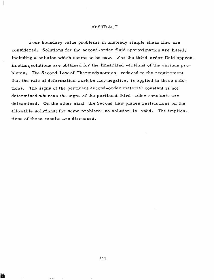
ABSTRACT

Four boundary value problems in unsteady simple shear flow are

considered. Solutions for the second-order fluid approximation are listed,

including a solution which seems to be new. For the third-order fluid approx-

imation,solutions are obtained for the linearized versions of the various pro-

blems. The Second Law of Thermodynamics, reduced to the requirement

that the rate of deformation work be non-negative, is applied to these solu-

tions. The signs of the pertinent second-order material constant is not

determined whereas the signs of the pertinent third-order constants are

determined. On the other hand, the Second Law places restrictions on the

allowable solutions; for some problems no solution is valid. The implica-

tions of these results are discussed.

iii

Contents

Page

1.

2.

3.

4.

Introduction

1.1 Simple-fluids and n- th order approximations

1.2 The Second Law of Thermodynamics

1.3 Unsteady simple shear flows: boundary value problems

Second-order approximation

2.1 Solutions

2.2 Application of the Second Law

Third-order approximation

3.1 Solutions to linearized problems

3.2 Application of the Second Law

Discussion and conclusions

Acknowledgements

1

3

5

10

14

21

27

29

32

V

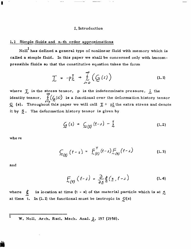
1. Introduction

1.1 Simple fluids and n-th order approximations

Nell’ has defined a general type of nonlinear fluid with memory which is

called a simple fluid. In this paper we shall be concerned only with imcom-

pressible fluids so that the constitutive equation takes the form

(l-1)

where .z is the stress tensor, p is the indeterminate pressure, I- the

identity tensor, 34 w> is a functional over the deformation history tensor

g (91. Througho’i: t&s paper we will call 5 + pi the extra stress and denote

itby 2. The deformation history tensor is given by

whe re

(1.2)

(1.3)

and

where 5 is location at time (t - s) of the material particle which is at X

at time t. In (1.1) the functional must be isotropic in z(s)

1 W. Nell, Arch. Ratl. Mech. Anal. 2, 197 (19581.

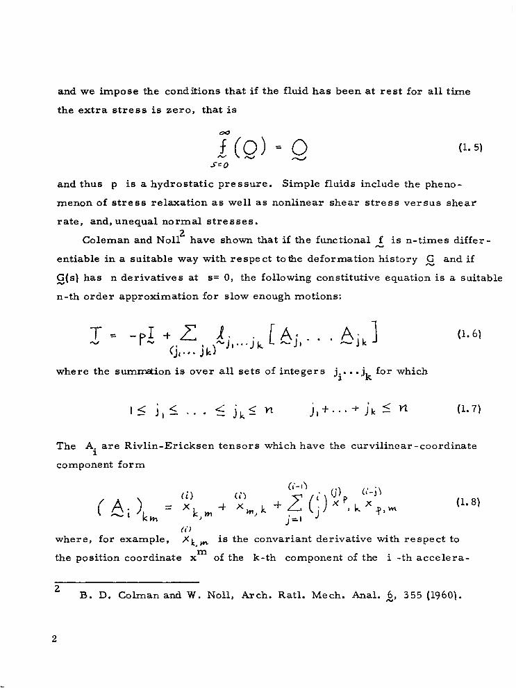
and we impose the conditions that if the fluid has been at rest for all time

the extra stress is zero, that is

00

f (0) = Q 5-z

and thus p is a hydrostatic pressure. Simple fluids include the pheno-

menon of stress relaxation as well as nonlinear shear stress versus shear

(1. 51

rate, and, unequal normal stresses. 7

Coleman and N011~ have shown that if the functional 2 is n-times differ -

entiable in a suitable way with respect tothe deformation history s and if

s(s) has n derivatives at s= 0, the following constitutive equation is a suitable

n-th order approximation for slow enough motions:

where the sum-ion is over all sets

The Ai are Rivlin-Ericksen tensors

component form

of integers ji.. . j, for which

M j,+...+ j, I M

(1.6)

(1.7)

which have the curvilinear -coordinate

i-l

/ , \ ti) +h‘()

; ij) (L-; \

( fii )k = 'k,m -I Xti,k j-i j xP"X?~m (1.8)

l9l (c')

where, for example, , )c k cn is the convariant derivative with respect to

the position coordinate x m

of the k-th component of the i -th accelera-

2 B. D. Colman and W. Noll, Arch. Ratl. Mech. Anal. f~, 355 (1960).

I

tion. The S,,..jl; are material coefficients and the relation (1.6) is linear and

isotropic in each A.. -1

The precise manner in which (1.6) is an approximation to (1.1) can be

found in Ref. 2. Suffice it to say here that if the time scale is slowed down

byafactor o(, O,Co(L I , the error made in approximating (1.1) by

(1.6) is higher than order n in OS . In particular (1.6) does not include

stress relaxationeffects; that is, if the first n time derivatives of the

motion vanish the stress reduces to the hydrostatic pressure.

A logical question to ask is whether the constitutive equation (1.6) can

be any more than an n-th order approximation to a simple fluid. That is, is

it reasonable to assert that (1.6) could represent a fluid for all histories no

matter what their magnitude; can we talk about n-th order fluids? This ques-

tion will be partially answered in the remainder of this paper.

1.2 The Second Law of Thermodynamics

The differential balance of energy can be written in the form

(1.9)

where E =;41 is the rate of deformation tensor, E is the internal energy

per unit mass, Cj is the heat flux vector and r is the heat supply per unit

mass and is the density. The differential entropy balance is given by

(1.10)

where is the entropy per unit mass, 8 is the absolute temperature

and x is the entropy production per unit mass. Following Coleman and No113

3 B. D. Coleman and W. Noll, Arch. Ratl. Mech. Anal., 2, 167 (1963).

3

we state the Second Law of Thermodynamics as the requirement that d

be non-negative for all admissible thermo-mechanical processes. By ad-

missible thermo-mechanical processes are meant processes which satisfy

the balance of linear momentum as well as the balance of energy and also

satisfy all assumed constitutive equations. The Second Law thus is seen to

place restrictions on the allowable constitutive equations and/ or, as we

shall see, on the allowable motions. From (1.9) and (1.10) we get for the

Second Law

For an incompressible material (1.11) reduces to

(1.11)

(1.12)

We can restrict our attention to purely mechanical variables by assum-

ing that the entropy and internal energy are constant, and, that the entropy

production due to heat conduction vanishes, so that (1.12) reduces to

Ye* = tr (@Z 0 (1.13)

which says that the entropy production is due entirely to the rate of deform-

ation work. We cannot say how much the above assumptions are restrictions

until we say something about the constitutive equations for the thermal

variables E , 3

and q . Materials and conditions for which the inequality

(1.13) holds are discussed zy Coleman4. We will comment further on this point

4 B. D. Coleman, Arch. Ratl. Mech. Anal., 2, 273 (1962). The starting point of the relevant discussion in that reference is justified by B. D. Coleman, Arch. Ratl. Mech. Anal. , 17, l(1964) which contains a general thermodynamic theory of materials with memory.

4

in Section 4. Such considerations are beyond the scope of this paper. However,

we can note the following. If there is no heat flow, which is the case for an

adiabatic material, then by (1.9) and (1.13) we have

(1.14)

that is, in order for the balance of energy to be maintained heat must be

withdrawn at each point at a rate exactly equal to that determined by the rate

of deformation work. On the other hand, if the entropy production due to

heat conduction vanishes because the fluid is such a good conductor that ye

is zero, then by (1.9), if r= o, we require that

(1.15)

that is, q is determined by the rate of deformation work. (Note that in the

latter caz q is indeterminate in the sense that it is not determined from a N

constitutive equation. The situation is quite analogous to the indeterminate

pressure in incompressible fluids).

1.3 Unsteady simple shear flows: boundary value problems

An unsteady simple shear flow is a flow whose velocity field x can be

represented in a Cartesian rectilinear coordinate system by the following

components

L4= NY,f) v= 0 N =o (1.16)

The differential equation form of the balance of linear momentum can be

5

expressed in vector notation by

where x is the derivative operator and b rV is the external body force

per unit mass. We will assume that fb ~ can be derived from a potential

x by means of p- = - b ,VX . We then introduce in the usual way the modi-

fied pressure @ by means of

d-p-c/X (1.18)

Then, in terms of the extra stress 2, the balance of linear momentum

becomes

(1.19)

Since the velocity is assumed to be independent of x and z it

follows that the Rivlin-Ericksen tensors are also independent of x and z

and also along with (1.16) it follows that

5 XZ = s,, = s,, = 0

It then follows that the components of (1.19) reduce to

a& = 0

(1.20)

(1.21)

(1.22)

(1.23)

6

We see that the modified pressure must be independent of L and from (1.21)

and (1.22) that

and hence (1.21) reduces to

3, SK, = p 3, 4.4 + Jj4 (t)

(1.24)

(1.25)

where (L (t) is the modified pressure gradient in the x-direction. The

analysis of this paragraph is a generalization of one contained in Markovitz

and Coleman. 5

We now list several boundary value problems in unsteady simple shear

flow:

Problem 1: We consider the boundary conditions

u(o,t) = ‘CT u (L, t) = 0 (1.26)

along with the assumption that the modified pressure 4 has no gradient

in the x - direction so that by (1.24)

(1.27)

For arbitrary initial conditions this problem is transient as well as unsteady,

5 H. Markovitz and B. D. Coleman, Phys. Fluids, 2, 833 (1964).

7

For this problem we make the following non-dimensionalization

(1.28)

and the boundary conditions (1.26) reduce to

The rest of the problems we consider are unsteady but oscillatory and

so do not require initial conditions.

Problem 2:

l.4 (o,t) = UC05 Rt d-J) = 0

This time we make the following non-dimensionalization

which reduces (1.30) to

(1.30)

(1.31)

u(o,9) = cost ci(l,f) = 0 (1.32)

Problem 3: Consider a variation of the preceding problem in which

L=au 9 that is we have the boundary conditions

ub,-o = Ucosnt u(oO,t) = 0 (1.33)

We introduce the non-dimensionalization

which gives the dimensionless boundary conditions

Problem 4: A final problem in unsteady simple shear flow has the

boundary conditions

(1.35)

L&J) = u(-L,t) = 0 .

with the pressure gradient in the x-direction given by

With the non-dimensionalization

(1.361, and (1.37) reduces to

and

(1.34)

(1.36)

(1.37)

(1.38)

(1.39)

(1.40)

9

2. Second-order approximation

2.1 Solutions

For n -2 equation (1.6) reduces to

where the fact has been used that for incompressible fluids h-/j), = 0

and also all isotropic tensors have been absorbed in the indeterminate

pressure term -pL . For n=l we would have only the linear term PA -,

which compri ses the classical linear theory of viscous fluids. Each of the

second-order terms is nonlinear: the first because ~4, is squared and the

second because /j, contains a product term as given by (1.8). The co-

efficient /t is the usual linear viscosity and /A, (4

and 4 /c”z are second-

order material coefficients.

For unsteady simple shear flow Coleman and No11 in Ref. 2 derived the

following non-zero components of the extra stress:

and from (1.25) the governing differential equation for the velocity profile:

(2.3)

where the subscripts on U indicate partial differentiation.

It was noted by Coleman and No11 that, rather surprisingly for a non-

linear theory, the velocity profile is governed by a linear equation. However

from (2.2) it is seen that the normal stresses are nonlinear as well as unequal.

10

I -

We now present the solutions, for the second-order approximation thee ry,

to the boundary value problems listed in Section 1.3.

Problem 1: Using (1.27) and (1.28) equation (2.3) reduces to

where is the dimensionless group

(2.4)

(2 l 5)

The steady- state solution of (2.4) is

6 and the unsteady solution which can be found by separation of variables ,

after nondimensionalizing in the above way, is

We see that a departure in the initial velocity distribution from the steady

state is represented by a Fourier series. On examination of (2.7) we note

that for positive AA’, that is for a positive value of the material constant Cal

P2 ’ (1) every term of the series is convergent, whereas for negative A

only terms for which

6 T. W. Ting, Arch. Ratl., Med. Anal. g, l(l9631

11

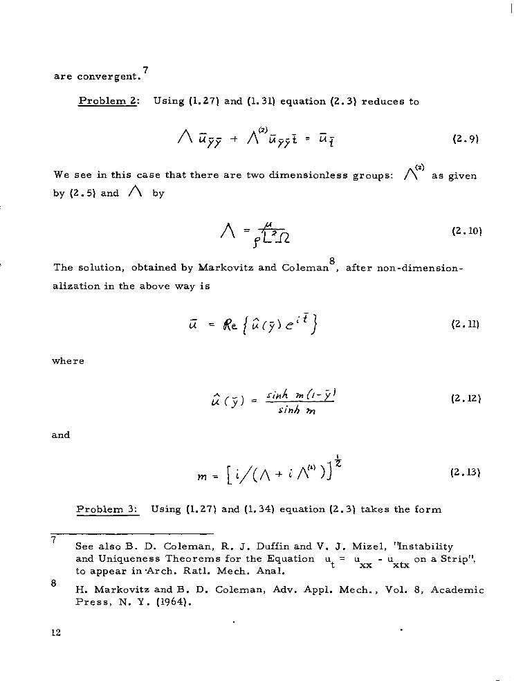
are convergent. 7

Problem 2: Using (1.27) and (1.31) equation (2.3) reduces to

(2.9)

We see in this case that there are two dimensionless groups: (4

n as given

by (2.5) and A by

(2.10)

The solution, obtained by Markovitz and Coleman8, after non-dimension-

alization in the above way is

where

and

Problem 3: Using (1.27) and (1.34) equation (2.3) takes the form

(2.11)

(2.12)

(2.13)

7 See also B. D. Coleman, R. J. Duffin and V. J. Mizel, “instability and Uniqueness Theorems for the Equation

Ut = “xx - Uxtx on a Strip”, to appear in-Arch. Ratl. Mech. Anal.

8 H. Markovitz and B. D. Coleman, Adv. Appl. Mech., Vol. 8, Academic Press, N. Y. (1964).

. 12 .

-

(2.14)

where now the dimensionless group AZ’ is given by

The solution to this problem was obtained by Markovitz and Coleman in

Ref. 5 and, after the above non-dimensionalization, is

where

(2.16)

(2.17)

The parameters A and B are always real and positive regardless of the (2)

sign or magnitude of A .

Problem 4: Using (1.38) equation (2.3) reduces to

(2.18)

(2) where A is given by (2.10) and A by (2.5). The non-transient solu-

tion to this problem can be found by assuming a solution of the form

(2.19)

13

One then finds that the solution is given by

(2.20)

(2.21)

where m is given by (2.13).

2.2 Application of the Second Law

Substituting the constitutive equation (2.1) of the second-order approxima-

tion into the Second Law inequality (1.13) we find that

(2.22)

A solution to Sec. 2.l which satisfies the thermal assumptions leading (1.13)

must also satisfy the inequality (2.22).

For unsteady simple shear (2.22) reduces to

(2.23)

We see from (2.23) that for steady motion

pro (2.24)

which is the well-known result that the viscosity of the classical linear

theory must be positive.

Consider a flow in which the velocity gradient tiY = o at some instant

of time t for some y . Then U> is a minimum at that instant and

14

a$/&= 0 and by (2.23) yey= 0 at such an instant. But also by (2.23) p0 Y

must be a minimum when fed=0 so that b(peX)/;lt = 0 , that is

(2.25)

There are two possibilities: (= 1 ,uZ = 0 , or , >‘(ti;)/3tL = 0

which is equivalent to au, hf = 0 . Now assuming that p: is

unequal to zero in order that we are dealing with the second-order approxi-

mational rather than the linear approximation, we have the conclusion that

a flow for which ccy=o andbuT/% # 0 violates the Second Law of

Thermodynamics in the form (1.13). In the light of this remark we now

examine the four solutions for unsteady simple shear flow contained in

Section 2.1.

Problem 1 : The velocity gradient calculated from (2.7) is

Let us suppose that there is a 7. at a certain instant of time L

that

where

(2.26)

such

(2.27)

B, = PITTA, exp

that is, the velocity profile has a maximum or minimum at a certain instant

15

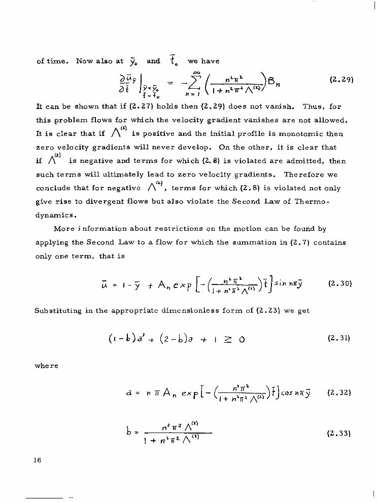
of time. Now also at y0 and To we have

(2.29)

It can be shown that if (2.27) holds then (2.29) does not vanish. Thus, for

this problem flows for which the velocity gradient vanishes are not allowed.

It is clear that if /\ (9

is positive and the initial profile is monotomic then

zero velocity gradients will never develop. On the other, it is clear that (21

if A is negative and terms for which (2.8) is violated are admitted, then

such terms will ultimately lead to zero velocity gradients. Therefore we

conclude that for negative f?’ , terms for which (2.8) is violated not only

give rise to divergent flows but also violate the Second Law of Thermo-

dynamics.

More information about restrictions on the motion can be found by

applying the Second Law to a flow for which the summation in (2.7) contains

only one term, that is

iTi = J - y + A, -p - Ii (2.30)

Substituting in the appropriate dimensionless form of (2.23) we get

(I -h’ -+ (z-b)a -+ I 1 o (2.31)

where

a= nrA,.,exp - r c

n27i2

I + rl=Tj1 /p )1 f co5nsiy (2.32)

16

(2.33)

Now the left-hand side of (2.31) is a quadratic form in a and it has the

discriminant b2 which is positive or zero. For b# 0 then the inequality

is violated for some values of a whereas for b = 0, that is A 13 = 0, the

inequality is satisfied. The question then is: for a given A(” , for what

values of n and A ,, is the inequality satisfied for all jY ? For AC’)

positive we have

o<b<l for /if),0 (2.34)

which means that the entropy production is negative when a lies in the

range

I --<a< -1 I- b

that is

From (2.32) and (2.36) we see that for

nrlA,IL- I

(2.35)

(2.36)

(2.37)

a does not enter the range of (2.36). Another way of stating (2.37) is that

-25 G-5 0 Y

17

(2.38)

Next let us consider negative (21

A . We then write b in the form

(2.39)

Now for n restricted by (2.8) b is negative and hence (l-b) is positive so

that again the entropy production is again negative over a finite range of a,

this time

I < d < -(I - nZ7rL I /\(L)I~ (2.40)

From (2.32) and (2.40) we see we must have the condition

OTT 1 An 1 5 I - H=+ 1 /tL’ 1 (2.41)

which is a..more severe restriction than (2.38). This can also be put in

the form

Problem 2: From (2.11) we have

u- = 7

where from (2.12)

(2.42)

(2.43)

;y = - m cosb H-l (I-j3 Sihh m

(2.44)

18

Recalling that III as given by (2.13) is complex we see that there are many

possibilities for 27 to be zero. It is clear from the boundary conditions

of the problem that for a given ji the velocity gradient is periodic with the

same frequency as the oscillating wall, Now from (2.43) we have

(2.45)

NOW let Gg=re 3 and therefore

When Cip = 0 we have (4 + 5 ,=7$2 modulo

(2.46)

(2.47)

which is not zero when (C$I -c ? > = X/Z modulo r . Therefore this problem

violates the Second Law for all values of the parameters of the problem.

Problem 3: From the solution (2.16) and (2.17) we get that the

velocity gradient vanishes for all ( yO ) to) which satisfy

tab (f. - By,) = 2 (2.48)

(2 l 49)

19

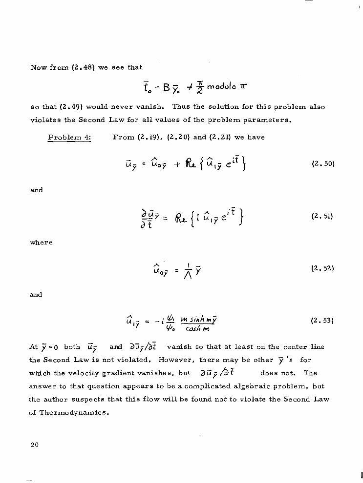
Now from (2.48) we see that

so that (2.49) would never vanish. Thus the solution for this problem also

violates the Second Law for all values of the problem parameters.

Problem 4: From (2.191, (2.20) and (2.21) we have

and

where

(2.50)

(2. 51)

(2. 52)

and

At J=O both cy and diiji/bT vanish so that at least on the center line

the Second Law is not violated. However, there may be other 7 ‘s for

which the velocity gradient vanishes, bu? aq /br does not. The

answer to that question appears to be a complicated algebraic problem, but

the author suspects that this flow will be found not to violate the Second Law

of Thermodynamics.

20

F‘

3. Third-order approximation

3.1 Solutions to linearized wroblems

(3.1)

where in addition to the linear and second-order terms of (2.1) we have five

new terms, each with a new material constant.

For unsteady simple shear flow the extra stress components are

1%) 61 sxy = p uy + pz

-(3) 3 uyt +p uy +p uyit

sxz= syz =o

Szz = 0

whe re

Substituting the first equation of (3.2) into (1.21) we get

(3.21

(3.3)

(3.4)

21

We note immediately that this governing differential equation is nonlinear

and also that we now have second-order time differentiation. We present

here solutions to linearized versions of the boundary value problems listed

in Section l3.

Problem 1: Using (1.27) and (1.28) equation (3.4) reduces to

(3.5)

where in addition to (4 A given by (2.5) we have two more dimensionless

numbers

(3.6)

Again we have the steady-state solution (1 - 7 ). Since (3.5) is non-

linear we are not surprised to find that an exact solution by analysis is not

readily obtained. For example, the method of separation of variables which

can be used to find the solutionto the linear equation (2.4) does not work in

this case. We therefore settle for a perturbation analysis of the steady state

solution; we assume a series solution of the form

where C is a parameter which tends to zero. Upon substitution into

(3.5) and equating coefficients of t we have

(3.7)

(3.8)

22

which is a linear differential equation for the first term v&f) in the

series of (3.7). The velocity perturbation ? must satisfy the boundary

conditions that it vanish on both boundaries.

By separation of variables we obtain the following solution of (3.5):

where

n=r

Because of the second-time derivative we must specify the acceleration as

well as the velocity at time t = 0 in order to determine- a solution.

For what combinations of values of Atz) r\‘:’ and fiy is the above

solut.ion convergent? Off hand it does not apiear that the condition (2.8)

for negative fi2’ automatically carries over to the stability analysis of

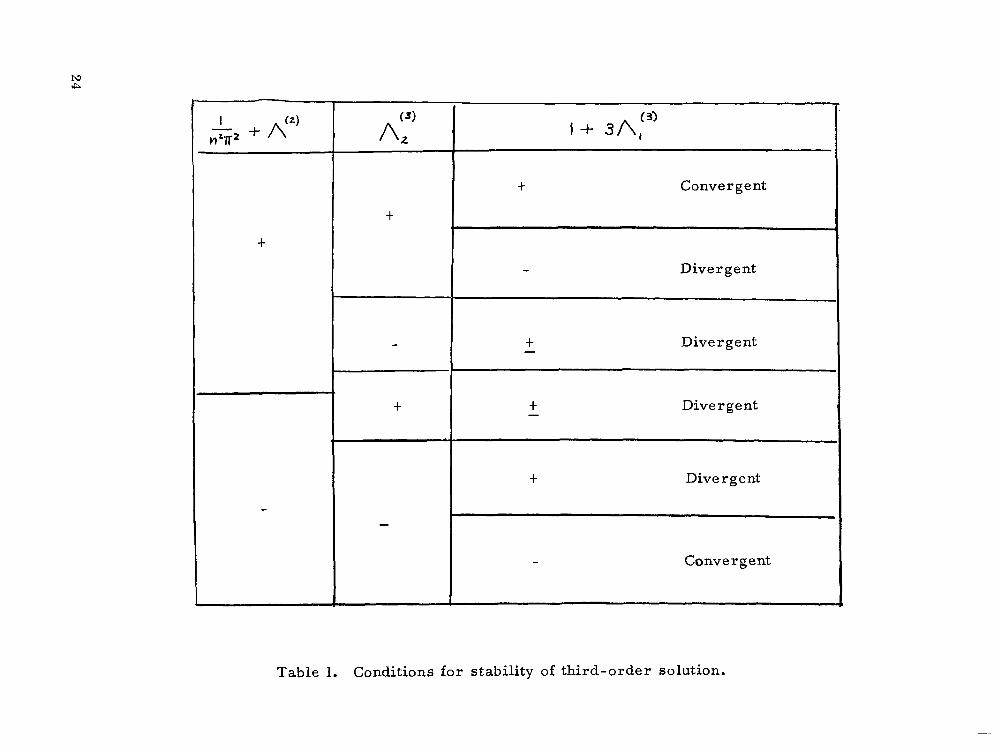
the third-order theory. The conditions for which the solution (3.9) and

(3.10) converges or diverges are summarized in Table 1. We note that for

-k /f’) ) r\:” and (I+3A:l)) must all have the same

sign. If -0) P

is negative then, by (3.6) (I + 3Ay’) could change sign

as U/ L is varied. However r\y’ and ( +j+ -t p?‘) cannot change sign

with U./L. Therefore in

23

t

(3)

&

t

I + 3A,L3’

t Convergent

Divergent

Divergent

Divergent

Divergent

Convergent

Table 1. Conditions for stability of third-order solution.

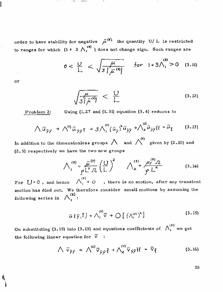
- (4 order to have stability for negative f the quantity U/ L is restricted

to ranges for which (1 t 3 A,(‘) ) does not change sign. Such ranges are

or

J -r-q 3lp 1 (3.12)

Problem 2: Using (1.27 and (1.31) equation (3.4) reduces to

In addition to the dimensionless groups A and

(2.5) respectively we have the two new groups

given by (2.10) and

For u=O,andhence A, =O , there is no motion, after any transient

motion has died out. We therefore consider small motions by assuming the (3)

following series in A, :

(3.15)

13) On substituting (3.15) into (3.13) and equations coefficients of r\, we get

the following linear equation for 7 :

(3.16)

25

The solution of (3.16) is just a slight modification of that for the corres-

ponding solution for the second-order approximation theory; ii is given

by the right-hand side of (2 .ll) and (2.12) but (2.13) is replaced by

Problem 3: Using (1.27) and (1.34) equation (3.4) reduces to

u-- yy + /q2)qyf -I- 3 /f’( q!!g + /q&fj = Gz

r\t” (3) (3)

where is given by (2.15) and A, and A 2 by

(3.17)

(3.18)

(3.19)

As in the previous problem we look for a solution for small motions by means

of (3.. 15). The resultant linear equation for T(y,f) is

(3.20)

The solution to this problem is given by the right-hand side of (2.16) with

(2.17) replaced by I

2- A, 13 = (3.21)

The parameters A and B are always real and positive regardless of the

signs or magnitudes of (4 // and

36

Problem 4: Using (1.38) equation (3.4) reduces to

A u (3.22)

where A is given by (2.10) and Af’ by (2. 5) and /\‘:I and /\1: are

given by

(3.23)

Again we look for a solution for small motions by means of (3.15). The

resultant linear equation for V(y,V) is

A v yF (3.24)

The solution to this problem is given by the right-hand side of (2.19)

by (2.20) and (2.21) but (2.13) is replaced by (3.17).

3.2 Application of the Second Law

Substituting the constitutive equation (3.1) of the third-order approxima-

tion into the Second Law inequality (1.13) we find that

27

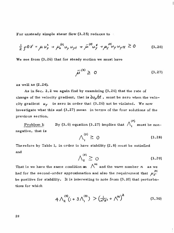
For unsteady simple shear flow (3.25) reduces to

We see from (3.26) that for steady motion we must have

(3.26)

(3.27)

as well as (2.24).

As in Sec. 2.2 we again find by examining (3.26) that the rate of

change of the velocity gradient, that is 3uybt , must be zero when the velo-

city gradient uy is zero in order that (3.26) not be violated. We now

investigate what this and (3.27) mean in terms of the four solutions of the

previous section.

13) Problem 1: By (3.6) equation (3.27) implies that A, must be non-

negative, that is

(3.28)

Therefore by Table 1, in order to have stability (2.8) must be satisfied

and

(3.29)

That is we have the same condition on /P and the wave number n as we had for the second-order approximation and also the requirement that r:

be positive for stability. It is interesting to note from (3.10) that perturba-

tions for which

4A3 + 3 Ar3’, > (AZ -I- &y2 (3.30)

28

decay sinusoidally rather than purely exponentially.

It likely can be shown that as in the case of the second-order approx-

imation for this problem the velocity profile for a perturbed steady flow

must be monotonic in order that the Second Law is not violated. It likely

can also be shown that violation of the stability conditions also violates the

Second Law.

Problems 2, 3, and 4: Since the solutions of the linearized versions

of these problems differ from the solutions of the corresponding second-order

problems by only unimportant changes in constants and since the Second Law

criterion regarding zero velocity gradients is unchanged, all of our results of

Sec. 2.2 for these problems carry over here. That is, the solutions for

Problems 2 and 3 are not allowed for the third-order approximation whereas, -

as far as we have investigated, the solution of Problem 4 is allowed. -

4. Discussion and conclusions

We have found that the Second Law of Thermodynamics in the form of

the requirement that the rate of deformation work be non-negative places

restrictions on allowable motions for the second and third-order approxima-

tion to fluids as well as placing restrictions on the material constants appear-

ing in these theories.

Let us first discuss the restrictions on material constants. In addition

to the classical result that the linear material coefficient /LA

is positive, - (31 we found from the Second Law that the third order material constants p

and f:’ must be positive. On the other hand, we see that the sign of

the second-order material constant /e which appeared in the analysis for

unsteady simple shear flow, is not determined. It may be possible to find

restrictions on the signs of the second-order coefficients by examining flows

29

other than unsteady shear. It is interesting to note that other evidence

indicates that A” is non-zero and negative. Coleman and Markovitz’

have shown that if one assumes on the ‘basis of thermodynamic intuition”

that the stress relaxation function of linear viscoelasticity is positive for

all times, then p /r) L

is negative. Furthermore, experimental determina- (r,

tion of /uL , in particular by Markovitz and Brown 10

, have yielded only

negative values thus far.

We turn now to the restrictions placed on allowable motions. It

turned out that for the oscillating wall problems, Problems 2 and 3, - -

the solutions for the second and third-order approximation theories>were

not valid for any values of the parameters of these problems. Problem 1 -2

the problem where one wall is moving with constant velocity, only has valid

solutions for restricted initial conditions: the velocity profile must be

monotonic and, if rl”

is negative, cannot contain harmonics above a

certain value which is dependent on l/A l On the other hand, the solu-

tion to Problem 2 when the flow is driven by a pulsating pressure gradient,

is valid as far as we have checked. It is interesting to note in Problem 1 -1

that the conditions for stability are consistent with satisfying the Second

Law. From both stability and thermodynamic considerations, we conclude

that the second and third-order theories are just approximation theories and

cannot be used indiscriminately as theories for any physically well-posed

problem. If such things as second-and third-order fluids existed in their

own right we would expect to get valid solutions for Problems 2 and 3, and, - -

Problem 1 for all initial conditions. On the other hand the linear theory can -

be used as a fluid theory in that solutions for any physically well-posed problem

do not violate the Second. Law. In 1951 Truesdell 11

suggested that the inequality

9 B. D. Coleman and H. Markovitz, J. App. Phys., 2, 1 (1964).

10 H. Markovitz and D. R. Brown, Trans, Sot. Rheol., 7, 137 (1963).

11 C. Truesdell, J. Math. Pure Appl., (91, 301 111 (1951).

30

(1.13) be a rerstriction not on constitutive equations but rather on allowable

motions. Coleman in Ref. 4 advanced the point of view that (1.13) must hold

for certain motions, namely those for which the reduction from (1.12) to (1.13)

is valjd; if (1.13) be violated in one of these motions, then the constitutive

equation should be rejected.. At least, the constitutive equation should be

rejected for those motions for which the Second Law is violated.

It may be that the Second .Law inequality (1.13) as a requirement on

unsteady problems considered in this paper for the second-and-third-order

fluid approximations is inconsistent with the simultaneous approximations

appropriate to the thermal variables. It’may be necessary to set to zero

certain second and third-order thermal material constants in order to

reduce to (1.13). It is intended to investigate this.. point in the near future.

A flow is said to be a helical flow if there exists a cylindrical coordinate

system tr, 8, Z) in which the physical components of the velocity have the

form

v,= 0 “I3 = N(r,t> v, = U(d) (4.1)

In Ref. 5 it is developed that, for the second-order approximation, the com-

ponents ti and u of the velocity field are determined by two separated,

line ar , third-order partial differential equations. Problems corresponding

to Problems 2 and 4 are then solved for in the case of Poiseuille flow (W = 0) -

and corresponding to Problem c in the case of Couette flow (u = o) . Explicit

solutions are obtained when appropriate “small gap” approximations are made.

The Second Law takes the following form for helical flow of the second-order

fluid approximation:

31

For Poiseuille flows (4.2) reduces to

and for Couette flows (4.2) reduces to

(4.3)

(4.4)

It would appear that the results we have obtained from applying the Second

Law to unsteady simple shear flows will carry over to the analogous pro-

blems in Poiseuille and Couette flowsof Ref. 5.

Acknowledgements

This work was supported in part by the National Aeronautics

and Space Administration under Research Contract NsG-664 with Princeton

University.

32

-

NASA-Langley, 1965 CR-292

“The aeronazrtical and space activities of ihe Uniled Stales shall be conducted so as to contribute . . . to the erpansio)z of bmnan kuowl- edge of pbenm~,zena in the atmosphere azd space. The Administration shall provide for the widest practicable and appropriate dissemination of informalion concerning its aclivihes and the tesnlts Ibereof .”

-NATIONAL AERONAUTICS AND SPACE ACT OF 1958

NASA SCIENTIFIC AND TECHNICAL PUBLICATIONS

TECHNICAL REPORTS: Scientific and technical information considered important, complete, and a lasting contribution to existing knowledge.

TECHNICAL NOTES: Information less broad in scope but nevertheless of importance as a contribution to existing knowledge.

TECHNICAL MEMORANDUMS: Information receiving limited distri- bution because of preliminary data, security classification, or other reasons.

CONTRACTOR REPORTS: Technical information generated in con- nection with a NASA contract or grant and released under NASA auspices.

TECHNICAL. TRANSLATIONS: Information published in a foreign language considered to merit NASA distribution in English.

TECHNICAL REPRINTS: Information derived from NASA activities and initially published in the form of journal articles.

SPECIAL PUBLICATIONS: Information derived from or of value to NASA activities but not necessarily reporting the results .of individual NASA-programmed scientific efforts. Publications include conference proceedings, monographs, data compilations, handbooks, sourcebooks, and special bibliographies.

Details on the availability of these publications may be obtained from:

SCIENTIFIC AND TECHNICAL INFORMATION DIVISION

NATIONAL,AERONAUTICS AND SPACE ADMINISTRATION

Washington, D.C. 20546