Thermodynamics and Ionic Conductivity of Block Copolymer Electrolytes

by

Nisita Sidra Wanakule

A dissertation submitted in partial satisfaction of the

requirements for the degree of

Doctor of Philosophy

in

Chemical Engineering

in the

Graduate Division

of the

University of California, Berkeley

Committee in charge:

Professor Nitash P. Balsara, Chair Professor John Newman

Professor Ting Xu

Fall 2010

1

Abstract

Thermodynamics and Ionic Conductivity of Block Copolymer Electrolytes

by

Nisita Sidra Wanakule

Doctor of Philosophy in Chemical Engineering

University of California, Berkeley

Professor Nitash P. Balsara, Chair

Solid electrolytes have been a long-standing goal of the battery industry since they have been considered safer than flammable liquid electrolytes and are capable of producing batteries with higher energy densities. The latter can be achieved by using a lithium metal anode, which is unstable against liquid electrolytes. Past attempts at polymer electrolytes for lithium-anode batteries have failed due to the formation of lithium dendrites after repeated cycling. To overcome this problem, we have proposed the use of microphase separated block copolymers. High ionic conductivity is obtained in soft polymers such as poly(ethylene oxide) (PEO) where rapid segmental motion, which is needed for ion transport, necessarily results in a decrease in the rigidity of the polymer. Block copolymers have the ability to decouple the requirements of high modulus, needed to prevent dendrite growth, and high ionic conductivity. Furthermore, the use of block copolymers may enable the creation of well-defined, optimized pathways for ion transport.

This dissertation presents studies of a poly(styrene-block-ethylene oxide) (SEO) copolymer blended with the lithium salt LiTFSI for use as a polymer electrolyte. In this case, the PEO is the ionically conducting block whereas the PS provides mechanical rigidity. The polymers used for this study were synthesized via anionic polymerization to obtain copolymers with low polydispersity. The introduction of a nonconducting microphase undoubtedly decreases the overall conductivity of the block copolymer relative to that of the ionically conducting homopolymer. Furthermore, the addition of salts into the block copolymer can be viewed as adding a selective solvent to the system. This invariably changes the energetic interactions in the systems. It is our goal to determine the correlation between the salt concentration and polymer phase behavior, and determine the effects of phase behavior on the ionic conductivity.

2

The polymer electrolyte system is designated as SEO (a-b)/LiTFSI where a = molecular weight of the PS block (kg/mol) and b = molecular weight of the PEO block (kg/mol). By varying the salt concentration, r = [Li]/[EO], and by varying a and b, several different morphologies such as alternating lamellae, hexagonally packed cylinders, and a cocontinuous network phase are obtained. Characterization of the electrolyte systems includes a combination of small-angle Xray scattering, optical birefringence measurements, and alternating current impedance spectroscopy.

The phase behavior and thermodynamics of the block copolymers as a function of LiTFSI concentration are also explored. It is assumed that the LiTFSI resides mainly in the PEO phase, the polymer with the higher dielectric constant, which is known for solvating lithium salts very effectively. Upon addition of LiTFSI salts to SEO systems, we obtain a disorder-to-order transition at a particular salt concentration. Further increases in the salt concentration have been shown to lead to other phase transitions such as lamellar to gyroid, or gyroid to cylinders. Changes in morphology cannot be attributed to increases in volume fraction of the PEO/LiTFSI phase alone. It is hypothesized that the presence of salts increases the effective Flory Huggins chi parameter, χeff. Using six different SEO/LiTFSI mixtures with accessible order-to-disorder transitions, we can develop a relationship to estimate the change in χeff with salt concentration. It was established that this relationship is a linear function, in good agreement with theoretical predictions. This relationship was also obtained for a mixture of SEO polymers with the ionic liquid imidizolium TFSI (ImTFSI). The χeff relationships were approximately the same, indicating that the large anion drives the thermodynamics of the polymer/salt systems. The slope of the χeff vs. r line, m, is compared to theoretical calculations. The theoretically determined values were consistently higher than experimentally determined ones.

In this study, ionic conductivity measurements through order-order and order-disorder phase transitions (OOTs and ODTs) in mixtures of SEO with LiTFSI were performed to determine the effect of morphology on conductivity. The molecular weight of the blocks and the salt concentration were adjusted to obtain OOTs and ODTs within the available experimental window. The normalized conductivity (normalized by the ionic conductivity of a 20 kg/mol homopolymer PEO sample at the salt concentration and temperature of interest), was also calculated to elucidate the effect of morphology. For samples with a major phase PEO block (e.g. volume fraction of PEO in SEO is greater than 0.5), no dramatic changes in conductivity were seen when transitioning through different morphologies. The well-known Vogel-Tamman-Fulcher (VTF) equation provides an excellent fit for the temperature dependence of the conductivities regardless of morphology. However, for samples with minor phase PEO block, the conductivity/structure relationship is more complex. Through in-situ conductivity/SAXS experiments, these samples show changes in conductivity with temperature, which are dependent upon the thermal history. The reason for these changes has not been established.

i

Table of Contents

List of Figures.......................................................................................................... iv  

List of Tables.......................................................................................................... vii  

Acknowledgements ............................................................................................... viii  

Chapter 1: Introduction..............................................................................................1  

1.1 Polymer Electrolytes for Lithium Batteries...................................................................... 1  

1.2 Block Copolymer Electrolytes.......................................................................................... 3  

1.3 Outline of Dissertation...................................................................................................... 6  

1.4 References......................................................................................................................... 7  

Chapter 2: Theoretical Treatment of Polymer Thermodynamics............................11  

2.1 Block Copolymer Thermodynamics............................................................................... 11  

2.2 Thermodynamics of Polymer/Salt Systems.................................................................... 15  

2.3 References....................................................................................................................... 18  

Chapter 3: Block Copolymer Characterization .......................................................20  

3.1 Polymer Synthesis and Characterization ........................................................................ 20  

3.2 Electrolyte Preparation ................................................................................................... 24  

3.3 Differential Scanning Calorimetry ................................................................................. 24  

3.4 Small-Angle XRay Scattering ........................................................................................ 25  

3.5 Birefringence Detection of the ODT .............................................................................. 28  

3.6 Impedance Spectroscopy ................................................................................................ 30  

3.6 References....................................................................................................................... 32  

Chapter 4: Effect of LiTFSI on the thermal properties and morphology of polystyrene-block-polyethylene oxide.....................................................................34  

ii

4.1 Thermal Properties of SEO/LiTFSI systems .................................................................. 34  

4.2 Effect of LiTFSI on Domain Size................................................................................... 36  

4.3 Characterization of Block Copolymer Electrolyte Morphology .................................... 41  

4.4 Phase Diagrams of SEO/LiTFSI Systems ...................................................................... 54  

4.5 Conclusions..................................................................................................................... 56  

4.6 References....................................................................................................................... 56  

Chapter 5: Comparison of Salts and Ionic Liquids on the Thermodynamics of PEO-containing Block Copolymers ........................................................................59  

5.1 Salts and Ionic Liquids in Polymer Electrolyte Membranes .......................................... 59  

5.2 Sample Preparation......................................................................................................... 61  

5.3 Thermal Properties and Phase Behavior......................................................................... 63  

5.4 Determination of the effective chi parameter ................................................................. 69  

5.5 Theoretical Predictions ................................................................................................... 75  

5.4 Conclusions..................................................................................................................... 78  

5.5 References....................................................................................................................... 78  

Chapter 6: Conductivity through order-order and order-disorder transitions of block copolymer electrolytes...................................................................................83  

6.1 Effect of Morphology on Conductivity .......................................................................... 83  

6.2 Decoupling Temperature Dependence on Conductivity................................................. 85  

6.3 Sample Preparation......................................................................................................... 87  

6.4 Conductivity through Transitions where PEO is the Major Phase ................................. 88  

6.5 Conductivity through Transitions where PEO is the Minor PHase................................ 91  

6.6 Conclusions..................................................................................................................... 98  

6.7 References....................................................................................................................... 99  

Chapter 7: Summary..............................................................................................100  

iii

7.1 Dissertation Summary .................................................................................................. 100  

7.2 References..................................................................................................................... 102  

Chapter 8: Appendix..............................................................................................104  

8.1 Procedure for SEO Synthesis........................................................................................ 104  

8.2 List of Synthesized Polymers ....................................................................................... 108  

8.3 Birefringence Experiment Procedure ........................................................................... 109  

iv

List of Figures

Figure 1.1: Theoretical block copolymer phase diagram................................................................4 Figure 1.2: Schematic of block copolymers electrolyte setup with electrodes...............................6

Figure 2.1: Theoretically predicted spinodal curve of block copolymers ....................................13 Figure 2.2: Phase diagrams for a block copolymer with N = 106 and N = 104 ...........................15

Figure 3.1: The SEC trace of the PS precursor and the block copolymer SEO(6.4 – 7.2). ...........21 Figure 3.2: MALDI-TOF spectrum for the PS precursor to SEO(4.6 – 3.7). ................................22

Figure 3.3: H NMR spectrum for SEO(6.4 - 7.2). .........................................................................23 Figure 3.4: DSC scan from a neat sample of SEO(6.4 – 7.2) .......................................................25

Figure 3.5: Schematic of a typical SAXS setup.............................................................................26 Figure 3.6: The 2-D scattering image acquired from a SAXS experiment on SEO(6.4 – 7.2) ....26

Figure 3.7: Azimuthally averaged scattering profiles for SEO(6.4 – 7.2) r = 0.085, SEO(2.3 – 4.6) r = 0.10, SEO(3.1 – 5.1) r = 0.05, and SEO(1.4 – 2.5) r = 0.05 .....................................28

Figure 3.8: Schematic of apparatus to measure birefringence......................................................29 Figure 3.9: Birefringence signal versus temperature of SEO(6.4 - 7.2) at r = 0............................30

Figure 3.10: Nyquist plot and Bode plot of SEO(4.6 – 3.7), r = 0.020 at 80 °C ..........................31 Figure 3.11: Equivalent circuit diagram for polymer electrolytes.................................................32 Figure 4.1: DSC thermograms from the second heating run on SEO(6.4 – 7.2) ..........................35

Figure 4.2: DSC scan of SEO(4.6 – 3.7), r = 0.02 at 10 °C/min. .................................................36 Figure 4.3: Plot of PEO/LiTFSI volume vs r.................................................................................37

Figure 4.4: SAXS profiles for SEO(6.4 – 7.2) at 107 °C .............................................................38 Figure 4.5: Changes in φEO for SEO(6.4 – 7.2)...........................................................................39

Figure 4.6: Domain size as a function of salt concentration for SEO(6.4 – 7.2) at 107 °C..........40 Figure 4.7: SAXS profiles at 69 ± 3 ˚C for SEO(2.3 - 4.6) at various r .......................................42

Figure 4.8: SAXS profiles of SEO(2.3-4.6) at r = 0.05 at selected temperatures..........................43 Figure 4.9: Birefringence signal vs temperature of SEO(2.3 - 4.6) at r = 0.05 .............................44

Figure 4.10: SAXS profiles for SEO(5.3 – 3.6) r = 0.019 and SEO(5.3 – 3.0) r = 0.027 ............45 Figure 4.11: SAXS profile for SEO(5.3 – 3.6) at r = 0.025 at selected temperatures. .................46

Figure 4.12: SAXS, FWHM, and birefringence plots of SEO(4.6 – 3.7) r = 0.20 .......................47 Figure 4.13: SAXS and FWHM plots of SEO(3.1-5.1) at r = 0.03 ...............................................48

v

Figure 4.14: Birefringence signal vs temperature of SEO(3.1-5.1) r = 0.03 .................................48 Figure 4.15: SAXS profiles of SEO(3.1-5.1) at r = 0.05 ...............................................................49

Figure 4.16: Birefringence signal vs temperature of SEO(3.1-5.1) r = 0.05 .................................51 Figure 4.17: Birefringence signal vs time for SEO(3.1-5.1) at r = 0.05 ........................................51

Figure 4.18: Background-subtracted SAXS intensity vs q of SEO(2.3-4.6) r = 0.05....................52 Figure 4.19: Schematic representations of two possible scenarios for the structure of weakly

ordered SEO/LiTFSI mixtures ...............................................................................................53 Figure 4.20: The fraction of the scattering invariant attributed to the sharp Gaussian peak, fG, of

SEO(2.3-4.6) at r = 0.05, plotted against TODT.T. ...............................................................54 Figure 4.21: Phase diagrams of various SEO/LiTFSI combinations.............................................55

Figure 5.1: Schematic of Li+ cation, TFSI- anion, and Im+ cation...............................................60 Figure 5.2: DSC scans of SEO with LiTFSI and ImTFSI ............................................................64

Figure 5.3: SAXS profiles at 100 °C for SEO(3.1 – 5.1) mixed with a) LiTFSI, b) 50:50 mixture of both, and c) ImTFSI at various salt concentrations ...........................................................65

Figure 5.4: Phase behavior of SEO(3.1-5.1) at various temperatures and concentrations of LiTFSI and ImTFSI ...............................................................................................................66

Figure 5.5: Birefringence detection of the ODT for SEO(3.1 – 5.1) r = 0.03 with LiTFSI and ImTFSI...................................................................................................................................67

Figure 5.6: Effect of LiTFSI and ImTFSI on domain size of SEO(3.1-5.1).................................68 Figure 5.7: Plot of χeff vs r for LiTFSI, ImTFSI, and 50:50 Mix in SEO from the mean-field

calculated χeff and fluctuation corrected χeff ........................................................................71 Figure 5.8: SAXS profiles of SEO(1.4-2.5) r = 0.12, SEO(1.4-2.5) r = 0.15, SEO(1.5-1.3) r =

0.12, and SEO(1.5-1.3) r = 0.15 at various temperatures ......................................................74 Figure 5.9: Plot of χeff vs r and the corresponding equations for SEO(6.4 - 7.2) ........................75

Figure 5.10: Comparison of theoretical and experimental m values for various anions ...............77 Figure 6.1: Plot of conductivity vs 1000/T for a PEO homopolymer at r = 0.03 and r = 0.5........87

Figure 6.2: Plot of conductivity versus 1000/T for SEO(6.4-7.2), SEO(1.4-2.5), SEO(2.3-4.6), and SEO(3.1-5.1) all at r = 0.05 and SEO(3.1-5.1) at r = 0.03. .............................................88

Figure 6.3: Plot of normalized conductivity versus temperature for SEO(6.4-7.2), SEO(1.4-2.5), SEO(2.3-4.6), and SEO(3.1-5.1) all at r = 0.05, and SEO(3.1-5.1) at r = 0.03. ....................90

Figure 6.4: Normalized conductivity vs temperature for a) SEO(5.3 – 3.0) at r = 0.027, b) SEO(5.3 – 3.6) at r = 0.019, and SEO(4.6 – 3.7) at r = 0.020. ..............................................92

Figure 6.5: Conductivity versus 1000/T for a) SEO(5.3 – 3.0), r = 0.027, b) SEO(5.3 – 3.6), r = 0.019, c) SEO(4.6 – 3.7), r = 0.020, and d) SEO(5.3 – 3.6), r = 0.025 from simultaneous SAXS/PEIS experiment. ........................................................................................................93

vi

Figure 6.6: Normalized conductivity and FWHM of the primary peak in SAXS profiles versus temperature plots for a) SEO(5.3 – 3.0), r = 0.027, b) SEO(5.3 – 3.6), r = 0.019, c) SEO(4.6 – 3.7), r = 0.020, and d) SEO(5.3 – 3.6), r = 0.025 from simultaneous SAXS/PEIS experiment..............................................................................................................................94

Figure 6.7: Normalized conductivity, FWHM of primary SAXS peak, and temperature versus time for SEO(5.3 – 3.6) at r = 0.019 during a simultaneous SAXS/PEIS experiment. .........96

Figure 6.8: Conductivity versus 1000/T for SEO(5.3 – 3.6) at r = 0.019 during an in-situ SAXS/PEIS experiment. ........................................................................................................97

Figure 6.9: FWHM for SEO(5.2 – 3.6), r = 0.019 and SEO(4.6 – 3.7), r = 0.020 samples with and without simultaneous PEIS experiments.........................................................................98

vii

List of Tables

Table 3.1: Characterization of copolymers used in this study .......................................................23 Table 3.2: Higher order reflections for different structure factors................................................27

Table 4.1: Salt concentration vs density of PEO/LiTFSI data.......................................................36 Table 4.2: Summary of SEO/LiTFSI systems with transitions......................................................52

Table 5.1: Properties of LiTFSI and ImTFSI.................................................................................60 Table 5.2: Characterization of polymers used in this study..........................................................62

Table 5.3: List of polymer systems and locations of order-disorder transition temperatures.......69 Table 5.4: List of parameters used to determine χeff from experimental results ..........................70

Table 5.5: Estimated values of r and corresponding φ used in the calculations for each polymer to obtain an ODT ...................................................................................................................72

Table 6.1: Summary of SEO/LiTFSI systems in this study..........................................................89 Table 6.2: Summary of SEO/LiTFSI systems in this study..........................................................93

viii

Acknowledgements

There are many people I would like to acknowledge during my PhD tenure. First, my advisor, Nitash Balsara, always had a positive view of research. He was excited when data was not what we (or others) expected, but was also excited when data went exactly as predicted (the so-called “boring” data). I must also thank Professor John Newman for his infinite wisdom and engaging discussions.

My work would not be quite as successful or enjoyable without the help of my labmates, former and present. It is my pleasure to acknowledge Dr. Alisyn Nedoma and Scott Mullin in our favorite means of communication:

To Ali and Scott, Who knew what I was after: Science and laughter.

I thank Shrayesh Patel, who was never too busy to help me work on a problem, even outside of his expertise. I always appreciated the help from David Wong and Nick Young, who would come in on the weekends just to help me set up equipment or open a jar. I also had the pleasure to work with both Dr. Justin Virgili and Alex Teran. I enjoyed research discussions with Justin, who was always able to restore my confidence in our project idea and data. Alex was always hardworking and willing to help out with my experiments. I also acknowledge Keith Beers and Greg Stone for their insightful discussions. I extend my warmest thanks to Dr. Hany Eitouni, Dr. Mohit Singh, Dr. Enrique Gomez, and Dr. Moon Park. They helped me get started in the lab, and were constantly there for me through the hardships of graduate school. It was also a pleasure to work with my undergraduate researcher, Ariel Tsui, who was excited about all aspects of research. I would like to thank the rest of the Balsara Lab and also the Newman Lab, who have all been an integral part of my PhD.

My time at Berkeley would not have been complete without my friends. It is my pleasure to thank Dr. Marie Fojas, Dr. Megan Fox, and Marisa Palucis. They were always there to support and encourage me in both my graduate school experience and culinary explorations. My classmates Greg Doerk, Penny Gunterman, Matt Traylor, Priya Shah, Mike Zboray, and Will Vining were always there to provide witty comments, outside perspective, and general support whether we were doing homework or thesiswork.

Finally, I thank my mother, my father, and my sister. Even though they were over 2000 miles away, they somehow manage to always be there for me during the most crucial moments.

1

Chapter 1

Introduction

1.1 POLYMER ELECTROLYTES FOR LITHIUM BATTERIES

There is a recent interest in lithium-anode batteries for applications such as electric vehicles due to its theoretically high energy and power densities.[1-3] Liquid electrolytes used in current rechargeable lithium-ion batteries are not suitable for lithium-anode batteries because of the instability of the lithium/electrolyte interface. A solid polymer electrolyte is a desirable alternative since it is solvent-free, stable against the lithium metal, and able to form thin, flexible membranes. A promising polymer electrolyte for rechargeable lithium metal batteries is polyethylene oxide (PEO), which readily dissolves lithium salts of the form LiX such as Li[N(SO2CF3)2] (LiTFSI), LiCF3SO3 (lithium triflate), or LiClO4

- (lithium perchlorate). In this case, the ether oxygen on the PEO chain complexes with the Li+ in LiX salts while the X- is freely floating nearby to maintain electroneutrality. The effect of salts on the conductivity and structure of PEO-based polymer electrolytes will be discussed in this dissertation.

1.1.1 Properties of PEO/salt electrolytes

The effect of salts on the properties of PEO homopolymers has been studied extensively.[4-9] An overview of this body of work can be found in ref. [9]. The nature of both the cations and anions affects the properties of PEO/salt mixtures. It has been reported that the solubility of alkali metal salts with TFSI- as the counterion in PEO (molecular weight of about 4 kg/mol) increases with decreasing ion radius. In this dissertation we often use the molar ratio of cations to monomers in the ion-solvating polymer chain or block, r, to quantify the salt concentration in our system. The values of r at the solubility limit for LiTFSI, NaTFSI, and KTFSI are 0.67, 0.25, and 0.20, respectively. The phase diagrams of PEO/NaTFSI and PEO/LiTFSI, reported in refs. [7] and [10], exhibit important differences. Crystalline intermediate compounds are obtained at EO:Na ratios of 7:1 and 3:1 in PEO/NaTFSI with melting points of 50 and 68 oC, respectively, and at EO:Li ratios of 6:1, 3:1 and 2:1 in PEO/LiTFSI with melting points of 46, 85, and 110 oC, respectively. In the case of PEO/LiTFSI, crystallization of PEO is not observed in compositions between r = 0.08 and 0.17, resulting in a window that has been referred to as the crystallinity gap. The crystallinity gap is not found in PEO/NaTFSI or PEO/KTFSI, i.e. there is no suppression of PEO crystallization in the presence of NaTFSI or KTFSI. The solubility limit of alkali metal salts is also affected by changes in the anion. For example, changing the anion from TFSI- to SCN- changes the solubility limit from r

2

= 0.67 to 0.33. In contrast, the values of r at the solubility limit for LiSCN and KTFSI are within experimental error (0.20). Changing the anion from TFSI- to CF3SO2N(CH2)3OCH3

- (MPSA-) results in a dramatic change in phase behavior. The phase behavior of PEO/LiMPSA is that of a simple binary eutectic with no intermediate crystalline compounds or crystallinity gaps. In contrast, the phase behavior of PEO/KMPSA contains a large crystallinity gap.

It is evident from the above discussion that the behavior of both crystalline and amorphous PEO/salt mixtures depends on the chemical structure of the anion and the cation. Effects such as ion dissociation, charge delocalization, and dispersive interactions between the ions and the polymer (particularly for large cations) play an important role in determining phase behavior. Some insight into the underpinnings of the observed phase behavior is obtained by measuring the ionic conductivity of PEO/salt mixtures. Studies of LiTFSI, NaTFSI, and KTFSI in PEO show that the conductivity values of these systems in the low-salt concentration limit have a weak dependence on the cation (LiTFSI and NaTFSI have conductivity values of 1.1x10-3 S/cm while KTFSI has a value of 0.9x10-3 S/cm at r = 0.03).[10] This is probably because most of the current is carried by the anion. The measured transference number of the cation in LiTFSI/PEO mixtures, the most widely studied system, ranges from 0.17 to 0.4 (depending on salt concentration).[11] The nature of the anion has a profound effect on conductivity. The conductivity values of PEO/LiTFSI mixtures at low temperatures are several-fold higher than that of PEO mixed with LiClO4 or LiCF3SO3 at the same r.[5, 7, 9, 12] This is principally due to the large TFSI- anion, which has high charge delocalization allowing for greater dissociation.[9] Spectroscopic studies indicate that the dissociation of alkali metal salts in PEO is complicated by the formation of ion pairs, triplets (Li+ associated with an ion pair), and other complex aggregates.[4]

Another class of salts is ionic liquids (IL). ILs are molten salts at moderate temperatures. These compounds are of great current interest in these materials due to their unique physiochemical properties (e.g. nonflammability, negligible vapor pressure, electrochemical stability, etc.) and their ability to promote ion conduction.[13-18] Their liquid structure and high ionic conductivity (at 30 °C, ILs have conductivity values on the order of 10-3 to 10-2 S/cm [17, 19, 20]) have been shown to enhance conductivity of PEO/LiTFSI systems. Thus, ionic liquids have been investigated as a supporting electrolyte for the PEO/LiTFSI system for lithium batteries.

The thermal properties of IL-containing PEO systems differ from PEO/LiTFSI systems. DSC thermograms of PEO/LiTFSI/IL systems have distinct crystallinity peaks corresponding to either PEO crystals or P(EO)6LiTFSI crystals at all ionic liquid concentrations.[14, 16, 21, 22] That is, PEO/LiTFSI/IL mixtures do not exhibit full suppression of the crystallinity peak as seen in the crystallinity gap of PEO/LiTFSI systems. There is some suppression of the crystalline phases. Zhu et al.[22] measured the decrease in ΔHm upon addition of 1-ethyl-3-methylimidazolium TFSI (EMITFSI) or N-methyl-N-propylpiperidinium TFSI (PP13TFSI) to a sample of P(EO)20LiTFSI. In the equimolar IL to LiTFSI case, ΔHm decreases from 73.94 J/g for PEO/LiTFSI (r = 0.05) to 41.66 J/g for PEO/LiTFSI/EMITFSI (r = 0.10) and 36.46 J/g for PEO/LiTFSI/PP13TFSI (r = 0.10). Similarly, Cheng et al[21] measured a decrease in ΔHm for P(EO)20LiTFSI systems with 1-butyl-4-methylpyridinium (BMPyTFSI). At r = 0.10, equimolar LiTFSI:BMPyTFSI, ΔHm = 20.89 J/g. Despite the presence of crystals in PEO/LiTFSI/IL

3

systems, room temperature conductivity of these samples is still high. At 20 °C, the conductivity values of PEO/LiTFSI systems with various PYR1ATFSI ILs range from 2.02x10-6 to 1.28x10-

4.[18] In the case of pure EMITFSI in PEO or SEO studied by Simone et al.,[20] complete suppression of crystallinity is seen at r = 0.20 and r = 0.25. Simone et al. also note a change in SEO phase behavior with increasing EMITFSI content. As EMITFSI concentration is increased, the samples transform from CYL (with minor phase PEO), to LAM, to CYL (with major phase PEO).

1.1.2 Failures of PEO as electrolytes

Problems with PEO as an electrolyte for rechargeable lithium-anode batteries arise when the electrolytes were subjected to charge-discharge cycles. It was determined that the Li+ ions did not plate uniformly on the anode, and, after several cycles, lithium dendrites formed on the anode.[23-25] These dendrites eventually short-circuited the battery. Theoretical calculations indicate that dendrite nucleation can be prevented if a polymer with a shear modulus on the order of 5 GPa is used as the electrolyte (the shear modulus of PEO-based electrolytes is in the 106 Pa range).[26] This presents a problem since the mechanism of ion conduction involves rapid segmental motion of the polymer chain.[27] Thus, high ionic conductivity is typically obtained in soft or rubbery polymers.[28, 29]

To address this challenge, PEO-based block copolymers can be used to decouple the mechanical strength and ionic conductivity. Past studies in our group using lamellar samples have observed conductivity values around 10-4

S/cm and shear moduli above 100 MPa.[30] PEO homopolymer, by comparison, has conductivity values around 2x10-3

S/cm and shear modulus around 1 kPa at the same temperature. It was determined that block copolymers successfully decoupled the ionic conductivity from the elastic modulus.

1.2 BLOCK COPOLYMER ELECTROLYTES

There is a growing interest in the use of microphase separated block copolymers as electrolytes in batteries and fuel cells.[1, 30-44] In these applications, block copolymers are either mixed with ionic species such as lithium salts blended with poly(ethylene oxide)-containing copolymers or ionic species are incorporated in the block copolymer chain as in the case in poly(styrene sulfonate)-containing block copolymers. Due to the fact that most organic polymers are not compatible with ions, ion transport is usually restricted to one of the microphases of the block copolymer. The use of block copolymers may enable the creation of well-defined, optimized pathways for ion transport. In addition, the chemical composition and morphology of the nonconducting microphase can be tuned to optimize other aspects of the electrolyte such as puncture strength or shear modulus. While the ion-conducting pathways can be aligned by the application of external fields, the present dissertation is concerned with samples with randomly oriented morphologies obtained in the absence of external fields.

4

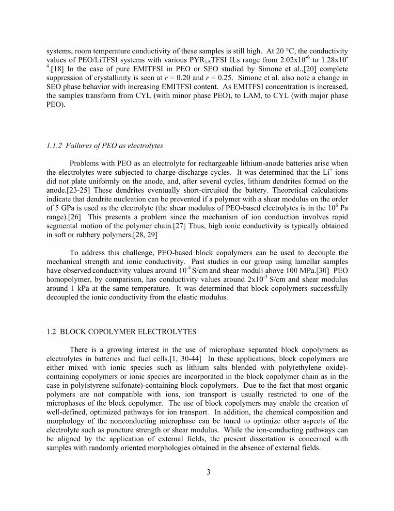
1.1.1 Block copolymer self assembly

Block copolymers are known to self assemble into a wide variety of morphologies such as lamellae (LAM), gyroid (GYR), and hexagonally packed cylinders (CYL).[32, 45-53] These ordered phases contain characteristic length scales on the order of 10 to 100 nm. The phase behavior of neat block copolymers is governed by the volume fraction of one of the blocks, φ (in this dissertation, the PEO block volume fraction is used), the degree of polymerization, N, and the Flory Huggins interaction parameter, χ, which is a measure of the dispersive interactions between the two monomers comprising the block copolymer.[45] The theoretical block copolymer phase diagram from ref [48] is plotted in Figure 1.1. The χ parameter is typically inversely related to temperature. Thus, different morphologies are accessible by changing the temperature.

Figure 1.1: Theoretical block copolymer phase diagram taken from ref [48]. Here, f is equivalent to φA, Scp is closed pack spheres, S is bcc spheres, C is hexagonally packed cylinders, G is gyroid, and L is lamellar.

Charge transport enabled by the presence of continuous domains such as LAM, CYL, and networks can be exploited to obtain structured polymer electrolyte membranes (PEM). Typically, when block copolymers are designed for use as a PEM, one block preferentially solvates the ionic species (e.g. salts), enabling ion conduction. Although an ionic species can be incorporated into the backbone of a polymer chain, we focus on polymer electrolytes where ionic species are added to the polymer. The second block, which is non-conductive, can be tuned to optimize other aspects of the PEM such as mechanical strength. In this dissertation, we present work on a poly(styrene-block-ethylene oxide) (SEO) copolymer. The PEO block dissolves the lithium salt, while the polystyrene (PS) block provides the mechanical strength.

5

1.1.2 Effect of salts on block copolymer electrolytes

Previous experimental [33, 54, 55] and theoretical studies [56] have demonstrated that adding salts to block copolymers results in an increase of the "effective" Flory-Huggins interaction parameter, χeff. This leads to increase in the size of the microphases.[54, 56, 57] There are, however, experiments that suggest that the interactions between salts and block copolymers are more complicated. Epps et al. observed that the addition of lithium perchlorate in poly(styrene-block-isoprene-block-ethylene oxide) copolymers stabilized the hexagonally packed cylinders over network phases. [34, 35] The disappearance of network phases is particularly relevant for electrolyte applications where the presence of ion-transporting channels is important. In contrast, we have shown that the addition of LiTFSI to certain SEO copolymers leads to the stabilization of a GYR phase over disordered phase or LAM phase. The effect of LiTFSI on the morphology and Flory Huggins interaction parameter of SEO is discussed in this dissertation.

1.1.3 Effect of block copolymer morphology on conductivity

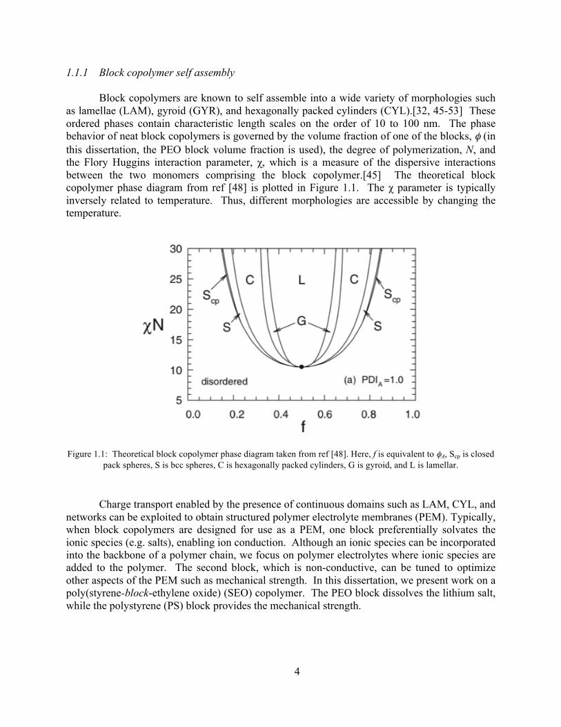
The addition of a nonconducting block to the electrolyte will result in a decrease in the attainable ionic conductivity value. It can be assumed that the conductivity, σ, is proportional to the volume fraction of the conducting block, φC. The conductivity should also depend on the tortuosity of the pathways for ion transport. This is accounted for by introducing the morphology factor, f:

(1.1)

where σC is the intrinsic conductivity of the conducting microphase. Depending on the morphology of the block copolymer system, f will vary between 0 and 1. For example, if lamellar samples were completely aligned parallel to the electrodes as shown schematically in Figure 1.2a, then f = 0. However, if the lamellae were aligned perpendicular to the electrodes as shown in Figure 1.2b, then f = 1. Note that there are two electrode orientations in which the lamellae would be perpendicular. For this dissertation, only randomly oriented grains, such as those in Figure 1.2c, are considered. In this case, Sax and Ottino[58] argue that an average of two-thirds of the grains will be oriented perpendicular, and thus f = 2/3. For a HEX or spheres morphology where the conducting block is the minor component, f = 1/3 and f = 0, respectively. For cocontinuous networks, such as GYR or HEX and spheres with the conducting block as the major component, f = 1.

6

Figure 1.2: Schematic of block copolymers electrolyte setup with electrodes for a) lamellae parallel with electrodes, b) lamellae perpendicular to electrodes, and c) randomly oriented grains of lamellae.

In practice, it has been shown that the morphology factor is lower than the values predicted by theory. It has also been shown that the conductivity of lamellar block copolymers increases with increasing molecular weight.[30] This is important for practical applications since the polymer also gets stiffer with increasing molecular weight. In studies with homopolymer PEO, it was determined that increasing the molecular weight of the electrolyte results in lower conductivity.[59] The effect of morphology on the conductivity of SEO/LiTFSI samples is discussed in this dissertation.

1.3 OUTLINE OF DISSERTATION

In Chapter 2, the previously developed theories behind polymer thermodynamics are discussed. This includes thermodynamics and phase behavior resulting from polymer-polymer interactions as well as polymer-salt interactions. Chapter 3 provides an overview of sample preparation and characterization techniques. The effect of adding LiTFSI to SEO on the thermal and phase behavior of the block copolymer is discussed in Chapter 4. Phase diagrams for the SEO/LiTFSI systems are presented at the end of the chapter. Chapter 5 quantifies the effect of salts on block copolymer thermodynamics by measuring the changes in the Flory Huggins interaction parameter. A study on the difference between adding the salt LiTFSI versus the ionic liquid imidizolium TFSI to SEO is also presented. The dependence of conductivity on the block copolymer morphology is discussed in Chapter 6. Block copolymer morphologies were varied with temperature, and the conductivity is measured through this transition. Finally, the dissertation is summarized in Chapter 7.

7

1.4 REFERENCES

1. Tarascon, J.M. and M. Armand, Issues and challenges facing rechargeable lithium batteries. Nature, 2001. 414(6861): p. 359-367.

2. Abruna, H.D., Y. Kiya, and J.C. Henderson, Batteries and electrochemical capacitors. Physics Today, 2008. 61(12): p. 43-47.

3. Scrosati, B. and J. Garche, Lithium batteries: Status, prospects and future. Journal of Power Sources, 2010. 195(9): p. 2419-2430.

4. Papke, B.L., M.A. Ratner, and D.F. Shriver, Vibrational spectroscopy and structure of polymer electrolytes, poly(ethylene oxide) complexes of alkali metal salts. Journal of Physics and Chemistry of Solids, 1981. 42(6): p. 493-500.

5. Vallée, A., S. Besner, and J. Prud'Homme, Comparative study of poly(ethylene oxide) electrolytes made with LiN(CF3SO2)2, LiCF3SO3 and LiClO4: Thermal properties and conductivity behaviour. Electrochimica Acta, 1992. 37(9): p. 1579-1583.

6. Robitaille, C.D. and D. Fauteux, Phase-Diagrams and Conductivity Characterization of Some Peo-Lix Electrolytes. Journal of the Electrochemical Society, 1986. 133(2): p. 315-325.

7. Lascaud, S., et al., Phase-Diagrams and Conductivity Behavior of Poly(Ethylene Oxide) Molten-Salt Rubbery Electrolytes. Macromolecules, 1994. 27(25): p. 7469-7477.

8. MacCallum, J.R. and C.A. Vincent, Polymer Electrolyte Reviews. 1987, New York City: Elsevier Applied Science Publishers.

9. Gray, F.M., Polymer Electrolytes. RSC Materials Monographs, ed. J.A. Connor. 1997, London: The Royal Society of Chemistry.

10. Perrier, M., et al., Mixed-Alkali Effect and Short-Range Interactions in Amorphous Poly(Ethylene Oxide) Electrolytes. Electrochimica Acta, 1995. 40(13-14): p. 2123-2129.

11. Edman, L., et al., Transport properties of the solid polymer electrolyte system P(EO)(n)LiTFSI. Journal of Physical Chemistry B, 2000. 104(15): p. 3476-3480.

12. Andreev, Y.G., P. Lightfoot, and P.G. Bruce, Structure of the polymer electrolyte poly(ethylene oxide)(3): LiN(SO2CF3)(2) determined by powder diffraction using a powerful Monte Carlo approach. Chemical Communications, 1996(18): p. 2169-2170.

13. Appetecchi, G.B., et al., Ternary polymer electrolytes containing pyrrolidinium-based polymeric ionic liquids for lithium batteries. Journal of Power Sources, 2010. 195(11): p. 3668-3675.

14. Shin, J.-H., W.A. Henderson, and S. Passerini, Ionic liquids to the rescue? Overcoming the ionic conductivity limitations of polymer electrolytes. Electrochemistry Communications, 2003. 5(12): p. 1016-1020.

15. Shin, J.H., W.A. Henderson, and S. Passerini, An elegant fix for polymer electrolytes. Electrochemical and Solid State Letters, 2005. 8(2): p. A125-A127.

8

16. Shin, J.H., W.A. Henderson, and S. Passerini, PEO-based polymer electrolytes with ionic liquids and their use in lithium metal-polymer electrolyte batteries. Journal of the Electrochemical Society, 2005. 152(5): p. A978-A983.

17. Shin, J.H., et al., Solid-state Li/LiFePO4 polymer electrolyte batteries incorporating an ionic liquid cycled at 40 degrees C. Journal of Power Sources, 2006. 156(2): p. 560-566.

18. Kim, G.T., et al., Solvent-free, PYR1A TFSI ionic liquid-based ternary polymer electrolyte systems I. Electrochemical characterization. Journal of Power Sources, 2007. 171: p. 861-869.

19. MacFarlane, D.R., et al., Pyrrolidinium Imides: A New Family of Molten Salts and Conductive Plastic Crystal Phases. The Journal of Physical Chemistry B, 1999. 103(20): p. 4164-4170.

20. Simone, P.M. and T.P. Lodge, Phase Behavior and Ionic Conductivity of Concentrated Solutions of Polystyrene-Poly(ethylene oxide) Diblock Copolymers in an Ionic Liquid. Acs Applied Materials & Interfaces, 2009. 1(12): p. 2812-2820.

21. Cheng, H., et al., Synthesis and electrochemical characterization of PEO-based polymer electrolytes with room temperature ionic liquids. Electrochimica Acta, 2007. 52(19): p. 5789-5794.

22. Zhu, C., H. Cheng, and Y. Yang, Electrochemical Characterization of Two Types of PEO-Based Polymer Electrolytes with Room-Temperature Ionic Liquids. Journal of The Electrochemical Society, 2008. 155(8): p. A569-A575.

23. Brissot, C., et al., In situ study of dendritic growth in lithium/PEO-salt/lithium cells. Electrochimica Acta, 1998. 43(10-11): p. 1569-1574.

24. Brissot, C., et al., Dendritic growth mechanisms in lithium/polymer cells. Journal of Power Sources, 1999. 82: p. 925-929.

25. Rosso, M., et al., Dendrite short-circuit and fuse effect on Li/polymer/Li cells. Electrochimica Acta, 2006. 51(25): p. 5334-5340.

26. Monroe, C. and J. Newman, The impact of elastic deformation on deposition kinetics at lithium/polymer interfaces. Journal of the Electrochemical Society, 2005. 152(2): p. A396-A404.

27. Boden, N., S.A. Leng, and I.M. Ward, Ionic-Conductivity and Diffusivity in Polyethylene Oxide Electrolyte-Solutions as Models for Polymer Electrolytes. Solid State Ionics, 1991. 45(3-4): p. 261-270.

28. Watanabe, M., et al., Ionic-Conductivity and Mobility in Network Polymers from Poly(Propylene Oxide) Containing Lithium Perchlorate. Journal of Applied Physics, 1985. 57(1): p. 123-128.

29. Kakihana, M., S. Schantz, and L.M. Torell, Raman-Spectroscopic Study of Ion-Ion Interaction and Its Temperature-Dependence in a Poly(Propylene-Oxide)-Based Nacf3so3-Polymer Electrolyte. Journal of Chemical Physics, 1990. 92(10): p. 6271-6277.

30. Singh, M., et al., Effect of molecular weight on the mechanical and electrical properties of block copolymer electrolytes. Macromolecules, 2007. 40(13): p. 4578-4585.

9

31. Cho, B.K., et al., Mesophase structure-mechanical and ionic transport correlations in extended amphiphilic dendrons. Science, 2004. 305(5690): p. 1598-1601.

32. Floudas, G., et al., Poly(ethylene oxide-b-isoprene) diblock copolymer phase diagram. Macromolecules, 2001. 34(9): p. 2947-2957.

33. Ruzette, A.V.G., et al., Melt-formable block copolymer electrolytes for lithium rechargeable batteries. Journal of the Electrochemical Society, 2001. 148(6): p. A537-A543.

34. Epps, T.H., et al., Phase behavior of lithium perchlorate-doped poly (styrene-b-isoprene-b-ethylene oxide) triblock copolymers. Chemistry of Materials, 2002. 14(4): p. 1706-1714.

35. Epps, T.H., et al., Phase behavior and block sequence effects in lithium perchlorate-doped poly(isoprene-b-styrene-b-ethylene oxide) and poly(styrene-b-isoprene-b-ethylene oxide) triblock copolymers. Macromolecules, 2003. 36(8): p. 2873-2881.

36. Soo, P.P., et al., Rubbery block copolymer electrolytes for solid-state rechargeable lithium batteries. Journal of the Electrochemical Society, 1999. 146(1): p. 32-37.

37. Trapa, P.E., et al., Block copolymer electrolytes synthesized by atom transfer radical polymerization for solid-state, thin-film lithium batteries. Electrochemical and Solid State Letters, 2002. 5(5): p. A85-A88.

38. Trapa, P.E., et al., Rubbery graft copolymer electrolytes for solid-state, thin-film lithium batteries. Journal of the Electrochemical Society, 2005. 152(1): p. A1-A5.

39. Park, M.J. and N.P. Balsara, Phase behavior of symmetric sulfonated block copolymers. Macromolecules, 2008. 41(10): p. 3678-3687.

40. Elabd, Y.A., et al., Transport properties of sulfonated poly (styrene-b-isobutylene-b-styrene) triblock copolymers at high ion exchange capacities. Macromolecules, 2006. 39(1): p. 399-407.

41. Elabd, Y.A., C.W. Walker, and F.L. Beyer, Triblock copolymer ionomer membranes Part II. Structure characterization and its effects on transport properties and direct methanol fuel cell performance. Journal of Membrane Science, 2004. 231(1-2): p. 181-188.

42. Niitani, T., et al., Synthesis of Li+ ion conductive PEO-PSt block copolymer electrolyte with microphase separation structure. Electrochemical and Solid State Letters, 2005. 8(8): p. A385-A388.

43. Niitani, T., et al., Characteristics of new-type solid polymer electrolyte controlling nano-structure. Journal of Power Sources, 2005. 146(1-2): p. 386-390.

44. Ioannou, E.F., et al., Lithium ion induced nanophase ordering and ion mobility in ionic block copolymers. Macromolecules, 2008. 41(16): p. 6183-6190.

45. Leibler, L., Theory of Microphase Separation in Block Co-Polymers. Macromolecules, 1980. 13(6): p. 1602-1617.

46. Fredrickson, G.H. and E. Helfand, Fluctuation Effects in the Theory of Microphase Separation in Block Copolymers. Journal of Chemical Physics, 1987. 87(1): p. 697-705.

10

47. Bates, F.S. and G.H. Fredrickson, Block copolymers - Designer soft materials. Physics Today, 1999. 52(2): p. 32-38.

48. Matsen, M.W., Polydispersity-induced macrophase separation in diblock copolymer melts. Physical Review Letters, 2007. 99(14): p. 4.

49. Matsen, M.W. and F.S. Bates, Unifying weak- and strong-segregation block copolymer theories. Macromolecules, 1996. 29(4): p. 1091-1098.

50. Matsen, M.W. and M. Schick, Stable and Unstable Phases of a Diblock Copolymer Melt. Physical Review Letters, 1994. 72(16): p. 2660-2663.

51. Khanna, V., et al., Effect of chain architecture and surface energies on the ordering behavior of lamellar and cylinder forming block copolymers. Macromolecules, 2006. 39(26): p. 9346-9356.

52. Hajduk, D.A., et al., The Gyroid: A New Equilibrium Morphology in Weakly Segregated Diblock Copolymers. Macromolecules, 1994. 27(15): p. 4063-4075.

53. Khandpur, A.K., et al., Polyisoprene-polystyrene diblock copolymer p hase diagram near the order-disorder transition. Macromolecules, 1995. 28(26): p. 8796-8806.

54. Young, W.S. and T.H. Epps, Salt Doping in PEO-Containing Block Copolymers: Counterion and Concentration Effects. Macromolecules, 2009. 42(7): p. 2672-2678.

55. Wang, J.Y., W. Chen, and T.P. Russell, Ion-complexation-induced changes in the interaction parameter and the chain conformation of PS-b-PMMA copolymers. Macromolecules, 2008. 41(13): p. 4904-4907.

56. Wang, Z.G., Effects of Ion Solvation on the Miscibility of Binary Polymer Blends. Journal of Physical Chemistry B, 2008. 112(50): p. 16205-16213.

57. Lee, D.H., et al., Swelling and shrinkage of lamellar domain of conformationally restricted block copolymers by metal chloride. Macromolecules, 2006. 39(6): p. 2027-2030.

58. Sax, J. and J.M. Ottino, Modeling of transport of small molecules in polymer blends - application of effective medium theory. Polymer Engineering and Science, 1983. 23(3): p. 165-176.

59. Shi, J. and C.A. Vincent, The effect of molecular weight on cation mobility in polymer electrolytes. Solid State Ionics, 1993. 60(1-3): p. 11-17.

11

Chapter 2

Theoretical Treatment of Polymer Thermodynamics

ABSTRACT

The previously developed theories of block copolymer thermodynamics and polymer/salt thermodynamics are summarized. Polymer phase behavior can be described by the theories developed by Flory and Huggins, Leibler, Matsen and Bates, and Fredrickson and Helfand. The last three are specific to block copolymers in the weak segregation limit. Wang has developed a theory to describe the effect of salts on polymer thermodynamics.

2.1 BLOCK COPOLYMER THERMODYNAMICS

2.1.1 Flory-Huggins theory

The thermodynamics of polymer-polymer interactions begin with the Flory-Huggins theory.[1, 2] The theory describes the changes in the free energy (ΔGm) of mixing polymer A with polymer B:

(2.1)

where k is the Boltzmann constant, T is the temperature, φi is the volume fraction of polymer i, Ni is the number of units of volume v in a chain of polymer i, where v is an arbitrary reference volume (we take v = 0.1 nm3), and χ is the Flory-Huggins interaction parameter between polymers A and B. The χ parameter incorporates the nonideal contributions to the free energy and can often be described as a linear function of 1/T:

(2.2)

where C1 is a constant generally associated with the enthalpic contributions and C2 is a constant associated with noncombinatorial entropic effects. Thus, the Flory-Huggins χ parameter is used as a measure of polymer thermodynamics. The combinatorial entropic

12

contributions are related to N-1, where N is the overall degree of polymerization of the block copolymer, such that the phase behavior of block copolymers can be described by the product χN.

At high values of χN, either large-molecular weight polymers or low temperatures, enthalpic interactions dominate, and ordered phases such as lamellae (LAM) or hexagonally packed cylinders (CYL) form as the system minimizes A-B contacts. The geometry of the ordered phases depend on both χN and φ, such that the block copolymer phase diagram can be mapped on a χN vs φ plot. The regime when χN > 100 is referred to as the strong segregation limit (SSL). As the value of χN decreases to 10.5 and lower, the polymer system undergoes an order-to-disorder transition (ODT) as entropic factors begin to dominate and a disordered phase (DIS) is obtained. The regime near the ODT is referred to as the weak segregation limit (WSL). Separate theoretical considerations are required for SSL and WSL regimes since they have different characteristics. For example, the domain size in the SSL is related to the product χ1/6N2/3 whereas in the WSL it is independent of χ and proportional to N1/2. In this dissertation, we focus on the WSL regime of amorphous polymers with upper critical solution temperature behavior (i.e., χ is positive). A more thorough review on block copolymer thermodynamics can be found in refs [3], [4], and [5].

2.1.2 Leibler’s theory of microphase separation

In the seminal paper by Leibler,[6] a mean-field theory is created to predict theoretically the phase behavior of block copolymers. For the calculations, Leibler looked at an ideal A-B block copolymer system where A and B have equal statistical segment lengths, all the polymers are of equal length (e.g. PDI = 1), and the polymers are incompressible. A reduced monomer density, ρA( ) and ρB( ), is defined as the ratio of local monomer density (at point ) to the overall monomer density of polymers A and B. Due to incompressibility, ρB( ) = 1- ρA( ). The variable ρA( ) is allowed to fluctuate while the overall monomer density must remain constant. Thus the order parameter is introduced:

(2.3)

where represents thermal averages and φA is the volume fraction of polymer A on the block copolymer chain. When the system is disordered, the compositional distribution of A and B segments is uniform at all points in space. That is, ρA( ) = φA, and ψ = 0. Using this definition, Leibler derived a free-energy expression from a fourth-order Landau expansion about this order parameter. This energy expression is used to determine the conditions where the ordered phase was stable over the disordered phase. The Landau expression is rigorously true for second-order phase transitions, and a good approximation for “weak first order” transitions. Accordingly, Leibler finds that order-to-disorder transitions are second order at φ = 0.5 and are weak first-order transitions in the vicinity of φ ~ 0.5. Although he postulates that the nature of

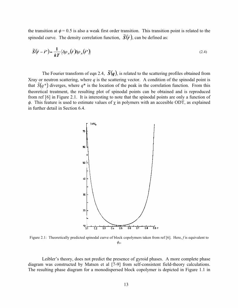
13

the transition at φ = 0.5 is also a weak first order transition. This transition point is related to the spinodal curve. The density correlation function, , can be defined as:

(2.4)

The Fourier transform of eqn 2.4, , is related to the scattering profiles obtained from Xray or neutron scattering, where q is the scattering vector. A condition of the spinodal point is that diverges, where q* is the location of the peak in the correlation function. From this theoretical treatment, the resulting plot of spinodal points can be obtained and is reproduced from ref [6] in Figure 2.1. It is interesting to note that the spinodal points are only a function of φ. This feature is used to estimate values of χ in polymers with an accesible ODT, as explained in further detail in Section 6.4.

Figure 2.1: Theoretically predicted spinodal curve of block copolymers taken from ref [6]. Here, f is equivalent to φA.

Leibler’s theory, does not predict the presence of gyroid phases. A more complete phase diagram was constructed by Matsen et al [7-9] from self-consistent field-theory calculations. The resulting phase diagram for a monodispersed block copolymer is depicted in Figure 1.1 in

Vol. 13, No. 6, November-December 1980

5%)

20

Figure 3. Plot of sl(Q) as a function of x = q2R2 for the sample with f = 0.4 and for three values of xN: (-) xN = 0.0; (---) xN = 2.0; (-) xN = 5.0. The curves for the different xN are parallel.

Figure 1 shows that the position of the maximum q* does not depend on the monomer interactions. In fact, expression IV-5 has a maximum for x* = q*2R2 for which the function F(x*) (independent of x ) has a minimum. This is due to the fact that the monomer interactions are local and would not be the case if they had a finite range. The shape of the peak and the position of its maximum depend on the chains' composition f. Figure 2 shows a plot of x* vs. f. The dependence is weak for 0.2 < f < 0.8 for which q* is of the order of 2/R. For f small (large) q* increases rapidly.

The fact that the correlation function s(G) is sensitive to the interactions provides a direct method of measuring the interaction parameter x . Actually by measuring the scattering intensity by a molten block copolymer with chains with different molecular mass (but _the same com- position f ) and by plotting the extracted SV(G) vs. q2R2, one should obtain a series of parallel curves (Figure 3). The relative distance between the curves even for small xN is rather large, so the method seems to be promising.

The value of spinodal point ( x N ) , a t which the insta- bility occurs depends on the composition f of the chain. This dependence is illustrated in Figure 4.

V. Stability of Ordered Phases In this section we predict the symmetry and the peri-

odicity of the microdomain structure appearing just after the microphase separation transition (section V.1). Then we study the stability of various microdomain patterns and determine conditions of their equilibria (section V.2) . These considerations lead to a phase diagram of the di- block copolymer melt which will be discussed in section VI.

1. Criterion of the Microphase Separation. A. Landau Theory of the MST. We shall use a Landau- type analysis47 to describe the MST. In this approach the

\

Theory of Microphase Separation in Block Copolymers 1609

I

i 10

0.1 0.2 0.3 0.4 0.5 0.6 0.7 0.8 0 .9 f

Figure 4. The spinodal point (xN), as a function of composition f. For xN = (xM,, &q*) divergea.

free-energy density functional obtained in section I11 should be minimized with respect to the order parameter $(it) for different values of the interaction parameter x (temperature 29. This rather formidable task is much simplified when one considers the copolymer liquid near its spinoddpint , i.e., when xlV is close to the value (xN), for which S(q*) diverges. Actually, in such a case the correlation function has a very pronounced maximum for lijl = q* (cf. section IV and Figure 1). The contribution to the quadratic term in the free-energy expansion (eq 111-13, -14, -22)

F2 = Y2v-1CS-'(G)$(W4-q') (V-1) B

from the Fourier components of $ with # q* is very large. The terms of higher order in # (F3, F4, ... ) have no singularity for xN = (xM, so that the contributions of $({I to F3, F4, ... with different are roughly equivalent. This implies that near the spinodal the important fluctuations should be those with wave vectors = q* and that #(fl may be approximated by

$(F) = C +@)ei* 07-91 El*4,1

i = 1, ..., n with $*(GI = +(--G). From eq IV-1 and from the definition of the spinodal point

IQiI = q*

(V-3) The pefficient of this term is independent of the specific set (Qi). Therefore, to study the stability of different or- dered phases the free energy density should be minimized a t fixed &El+gij#(lj)]2. Making use of the symmetry properties of the coefficients r3(Q:?, G2, i j3 ) and r4(q1, i j2 , G3, G4), one can argueJhat a t equilibrium the magnitude I$(Q)l for all i j E l*Qi) should be equal. However, the

14

Chapter 1. Using this method, Matsen et al. calculated phases such as gyroid and closed packed spheres which were originally not predicted by Leibler’s treatment. We also note that both the Matsen construction and Leibler construction predict a spheres-to-DIS transition at all points on the spinodal curve except at φ = 0.5 (the critical point), where a LAM-to-DIS transition is seen. Although, this is not typically the case in experiments where LAM-to-DIS and CYL-to-DIS transitions have been seen at φ ≠ 0.5.

2.1.3 Fredrickson and Helfand’s fluctuation theory of microphase separation

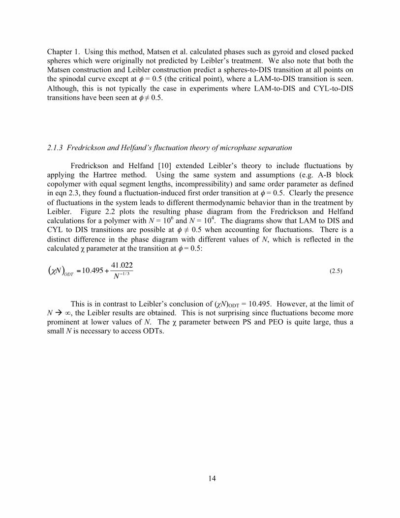
Fredrickson and Helfand [10] extended Leibler’s theory to include fluctuations by applying the Hartree method. Using the same system and assumptions (e.g. A-B block copolymer with equal segment lengths, incompressibility) and same order parameter as defined in eqn 2.3, they found a fluctuation-induced first order transition at φ = 0.5. Clearly the presence of fluctuations in the system leads to different thermodynamic behavior than in the treatment by Leibler. Figure 2.2 plots the resulting phase diagram from the Fredrickson and Helfand calculations for a polymer with N = 106 and N = 104. The diagrams show that LAM to DIS and CYL to DIS transitions are possible at φ ≠ 0.5 when accounting for fluctuations. There is a distinct difference in the phase diagram with different values of N, which is reflected in the calculated χ parameter at the transition at φ = 0.5:

(2.5)

This is in contrast to Leibler’s conclusion of (χN)ODT = 10.495. However, at the limit of N ∞, the Leibler results are obtained. This is not surprising since fluctuations become more prominent at lower values of N. The χ parameter between PS and PEO is quite large, thus a small N is necessary to access ODTs.

15

Figure 2.2: Phase diagrams for a block copolymer with N = 106 (left) and N = 104 (right) reproduced from ref [10]. Here, f is the same as φ, and HEX is the same CYL (hexagonally packed cylinders).

2.2 THERMODYNAMICS OF POLYMER/SALT SYSTEMS

2.2.1 Ion solvation

In order for a salt to be dissolved in a polymer, the total lattice energy of a salt must be compensated by ion-polymer interactions. The solvation of ions in a polymer matrix is governed by several entropic and enthalpic interactions, including (1) an increase in entropy and (2) an increase in enthalpy from breaking of salt crystal lattice and polymer lattice, (3) enthalpic gain/loss from short-range specific interactions between the ion and the polymer, and (4) decrease in entropy from rearrangement of polymer around the salts. The change in energy from factor (2), the enthalpy of the salt lattice (ΔHL), is known to be related to the size of the ions, and can be estimated using Bartlett’s relationship [11] (with respect to the gaseous ions):

(2.6)

where V is the volume of the salt determined from the sum of the cation and anion radius and assuming the salt is spherical and ΔHL is calculated in kJ/mol. Factor (4) leads to a decrease in entropy arising from the restricted movement of solvent molecules. The coordination of the Li+ with the PEO chain leads to strained conformations and restricted bond rotation. These increases in energy are balanced with factors (1) and (3). Although factor (3) can be either an increase or a decrease in enthalpy, presumably, the change in enthalpy is negative from the preferred contact between cation/polymer over cation/anion. Thus the enthalpic interactions between the Li+ and the PEO play a major role in solvation energies. Note that if (4) has a greater effect than (1), this

€

ΔHL =232.8V3

+110

16

could lead to an overall negative change in entropy and the occurrence of salt precipitation at sufficiently high temperatures.

The hard/soft acid/base theory (HSAB) can be used to estimate the solubility strength of a particular salt in a polymer. In HSAB, hard acids have the strongest interactions with hard bases since hard species are stabilized by electrostatic interactions. On the other hand, soft species are stabilized by covalent interactions; thus soft acids have strong interactions with soft bases. Li+, which is small and non-polarizable, is considered a hard acid. The ether oxygens in the backbone of a PEO chain are considered a relatively hard base. Thus, a lithium salt would easily dissolve in PEO if the counteranion is a soft base. Large anions with delocalized charge, such as TFSI-, are considered soft bases, implying that PEO/LiTFSI is a good electrolyte.

2.2.2 Wang’s theory on the effect of ion solvation on polymer miscibility

Wang [12] investigated the effect of adding salts on the miscibility of two polymers A and B. Although Wang’s theory was formulated for blends of two homopolymers, the Li+ ions are tightly bound to the oxygen groups of the EO blocks in both the disordered and ordered states of block copolymers. Thus their energetics are, to a first approximation, unaffected by microphase separation. Two cases were explored: (1) ions are distributed homogeneously in a disordered mixture of A and B, and (2) in the vicinity of the ion there is an enrichment of the polymer with the higher dielectric, e.g. there is a heterogeneous distribution. Wang derives the energy density of a system consisting of polymer A, polymer B, and a dilute amount of monovalent salt to be:

(2.7)

where fFH(φ) is the free energy from Flory-Huggins theory as defined by eqn 2.1, c+ and c- are the concentrations of cations and anions, respectively, f+ and f- are the solvation energies of the cations and anions into the polymer blend, respectively, and cR is a reference concentration. For a monovalent salt, c+ = c- = c. The first term of eqn 2.7 is the enthalpic and entropic contributions for mixing polymers A and B. The final term (in the square brackets) account for the entropy of the ions, related to factor (1) from the discussion in Section 2.2.1. The second terms (in the parentheses) are accounting for factor (3) from the discussion in Section 2.2.1, the enthalpy from ion solvation. For the homogenously mixed case, the Born solvation energy is used for f- and f+:

(2.8)

17

where e is the electron charge, ε is the relative dielectric constant of the medium, ε0 is the vacuum permittivity, and a is the ion radius. The Born solvation energy accounts for the energy from moving a charged species from vacuum into a medium with a uniform dielectric constant. The polymer system is assumed to have a volume fraction weighted average dielectric constant. Using eqns 2.7 and 2.8 as the basis of the energetics of the system, an analytical expression for changes in χ is obtained for the homogeneous case:

(2.9)

In this result, it is assumed that polymer A and B have equal degrees of polymerization of (NA = NB = N) and monomer volume (vA = vB = v) and that the cation and anion are of equal size (a). The Bjerrum length, l0, is the length at which the energy between two charged species is equal to kT and given by l0 = e2/(4kTπε0).

For the case of heterogeneous distribution, the energetics of the system is comprised of an electrostatic contribution (fe) and the inhomogeneous Flory-Huggins-de Gennes square-gradient free energy (fFHdG):

(2.10)

(2.11)

In eqns 2.10 and 2.11, ψ is the electrostatic potential, fFH is eqn 2.1, and κ = kTb2/[18vφ(1 - φ)] where b is the statistical segment length of the polymers (assumed to be equal for A and B). A perturbation analysis about the overall composition, and then following the same methodology to obtaining eqn 2.9, the analytical expression for the case (2) is derived to be:

(2 - 12)

where λp is the packing length of the polymer defined by λp = v/b2. It is clear that case (2), which is governed by eqn 2.12 and has a lower solvation energy, will result in a smaller change in χ than in case (1), which is governed by eqn 2.9. In both cases, introducing ions into a system with ε < 20 will lead to a decrease in miscibility. However, when ε > 20, the polymers will become more miscible.

18

In the case of SEO, both components have relatively low dielectric constants (ε < 20). Therefore we expect the segregation strength of SEO/LiTFSI systems to be greater than for just SEO (i.e. decrease in miscibility). In ref. [13], Wanakule et al. measured the conductivity of a variety of SEO/LiTFSI mixtures across the ODT. There was neither a discontinuity at the ODT nor a change in slope in the temperature dependence of the conductivity in the ordered and disordered state. In other words, the temperature dependence of SEO/LiTFSI mixtures obtained from fully ordered systems, fully disordered systems, and systems with accessible ODTs was identical. We take this observation as evidence that the ions in the system have the same PEO-rich local environment regardless of the state of order of the samples. We thus expect equation 2.12 to apply to our system.

2.3 REFERENCES

1. Flory, P.J., Thermodynamics of high polymer solutions. Journal of Chemical Physics,

1941. 9(8): p. 660-661. 2. Huggins, M.L., Solutions of long chain compounds. Journal of Chemical Physics, 1941.

9(5): p. 440-440. 3. Bates, F.S. and G.H. Fredrickson, Block copolymers - Designer soft materials. Physics

Today, 1999. 52(2): p. 32-38. 4. Bates, F.S. and G.H. Fredrickson, Block Copolymer Thermodynamics - Theory And

Experiment. Annual Review of Physical Chemistry, 1990. 41: p. 525-557. 5. Hamley, I.W., The Physics of Block Copolymers. 1998: Oxford University Press.

6. Leibler, L., Theory of Microphase Separation in Block Co-Polymers. Macromolecules, 1980. 13(6): p. 1602-1617.

7. Matsen, M.W. and F.S. Bates, Unifying weak- and strong-segregation block copolymer theories. Macromolecules, 1996. 29(4): p. 1091-1098.

8. Matsen, M.W. and M. Schick, Stable and Unstable Phases of a Diblock Copolymer Melt. Physical Review Letters, 1994. 72(16): p. 2660-2663.

9. Matsen, M.W., Polydispersity-induced macrophase separation in diblock copolymer melts. Physical Review Letters, 2007. 99(14): p. 4.

10. Fredrickson, G.H. and E. Helfand, Fluctuation Effects in the Theory of Microphase Separation in Block Copolymers. Journal of Chemical Physics, 1987. 87(1): p. 697-705.

11. Jenkins, H.D.B., et al., Relationships among ionic lattice energies, molecular (formula unit) volumes, and thermochemical radii. Inorganic Chemistry, 1999. 38(16): p. 3609-3620.

19

12. Wang, Z.G., Effects of Ion Solvation on the Miscibility of Binary Polymer Blends. Journal of Physical Chemistry B, 2008. 112(50): p. 16205-16213.

13. Wanakule, N.S., et al., Ionic Conductivity of Block Copolymer Electrolytes in the Vicinity of Order-Disorder and Order-Order Transitions. Macromolecules, 2009. 42(15): p. 5642-5651.

20

Chapter 3

Block Copolymer Characterization

ABSTRACT

The material chosen for this study is poly(styrene – block – ethylene oxide) (SEO) where the polyethylene oxide (PEO) block is ionically conducting and the polystyrene (PS) block provides the mechanical strength. The polymers were synthesized via anionic polymerization. Polymer characteristics were determined using size exclusion chromatography, matrix-assisted laser desorption/ionization-time-of-flight mass spectroscopy, and 1H nuclear magnetic resonance spectroscopy. To the block copolymer system, we add the salt LiTFSI or the ionic liquid imidazolium TFSI (ImTFSI) to form the electrolyte. These were characterized using differential scanning calorimetry, small-angle Xray scattering, birefringence experiments, and ac impedance spectroscopy.

3.1 POLYMER SYNTHESIS AND CHARACTERIZATION

The poly(styrene-block-ethylene oxide) copolymers (SEO) were synthesized by anionic polymerization using the methods described in refs [1-3]. All the steps in the synthesis are performed under vacuum and in an argon glovebox. The polystyrene block was synthesized first using sec-butyl lithium as the initiator and benzene as the solvent. After 4 to 12 hours of reaction, the ethylene oxide monomer is added using P4 tert-butylphosphazene base as the catalyst. The polymerization of the PEO block is performed at 45 °C for 2 to 5 days. Finally, the copolymer is terminated with isopropanol. The copolymers were purified by filtration of the SEO dissolved in benzene through a 0.2 µm filter followed by precipitation in a cold hexane solution. The details of the synthesis procedure are outlined in the Appendix.

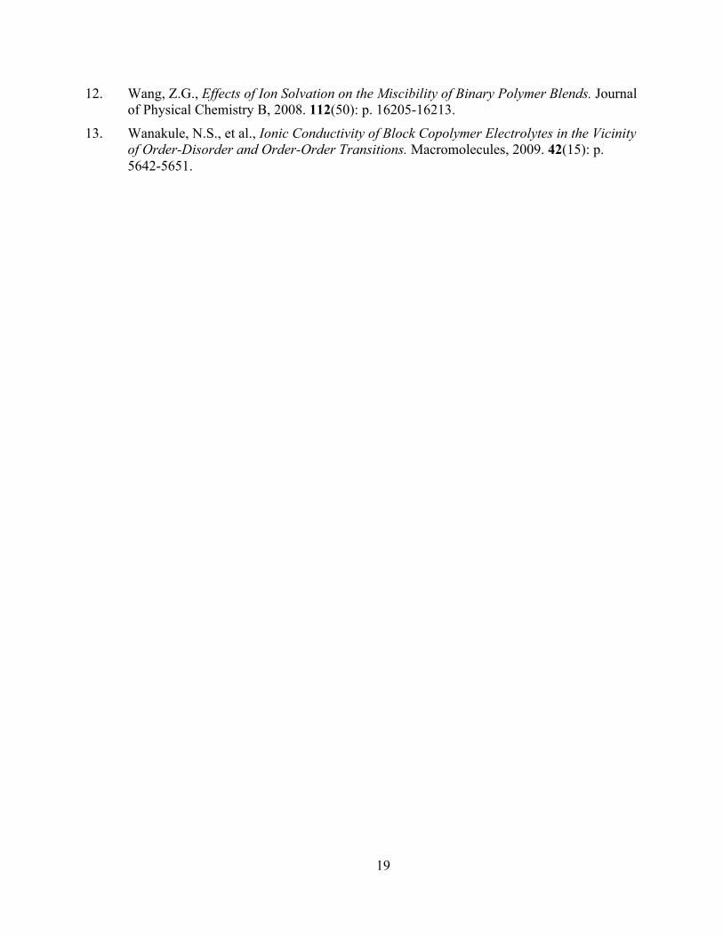
The molecular weight of the polystyrene block and the polydispersity indices (PDI) of the polystyrene block and overall polymer were obtained by size exclusion chromatography (SEC) using a Waters 717 plus autosampler instrument equipped with a Waters 486 tunable absorbance detector and Wyatt Tech DAWN EOS light-scattering detector calibrated with polystyrene standards. A typical SEC trace for SEO(6.4 – 7.2) and its PS precursor is shown in Figure 3.1. The SEC gives both the weight-averaged (Mw) and number-averaged (MN) molecular weight. We typically report the MN of the polymer to be the molecular weight. In Figure 3.1a, the elution time of 22 minutes corresponds to a MN of 6370 g/mol. The SEC trace in Figure 3.1b is used to determine the PDI of the SEO (here, the PDI is 1.02) and qualitatively show that the block copolymer was successfully formed.

21

Figure 3.1: The SEC trace of the a) polystyrene precursor and the b) block copolymer SEO(6.4 – 7.2).

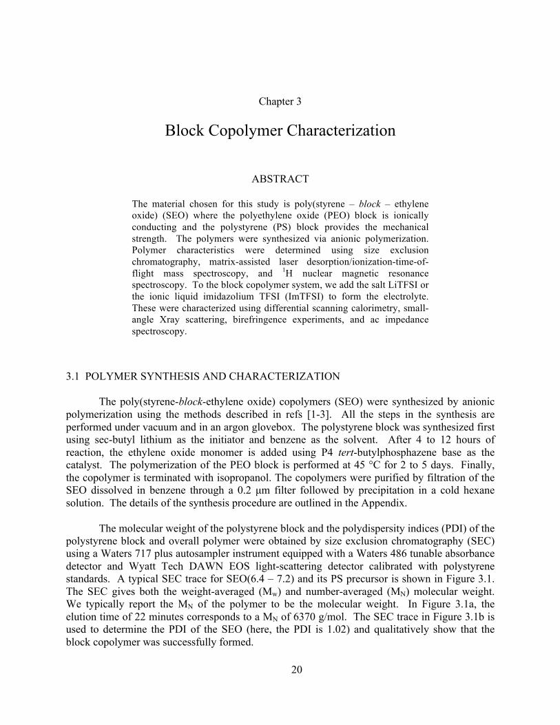
Small molecular weight polymers, i.e. smaller than 5 kg/mol, are on the tail end of the resolution for our SEC instruments. For this size, it is more accurate to use matrix-assisted laser desorption/ionization-time-of-flight mass spectrometry (MALDI-TOF MS) to measure the MN of the PS precursor. To prepare the sample, the PS is dissolved in tetrahydrofuran (THF) to form a 2 – 3 mg/mL solution. A 1 mg/mL solution of silver trifluoroacetate (AgTFA) in THF and a 10 mg/mL solution of anthracenetriol in THF are created as the indicator and matrix solutions, respectively. In a small vial, 20 µL of the polymer solution is added to 30 µL of the anthracenetriol/THF solution, followed by the addition of 2 µL of the AgTFA/THF solution. MALDI-TOF experiments were performed on a Voyager-DE™ system (PerSeptive Biosystems, USA). Figure 3.2 is a typical MALDI-TOF spectrum for SEO(4.6 – 3.7). Averaging over the spectrum values gives an MN of 4560 g/mol and a PDI of 1.02.

22

Figure 3.2: MALDI-TOF spectrum for the PS precursor to SEO(4.6 – 3.7).

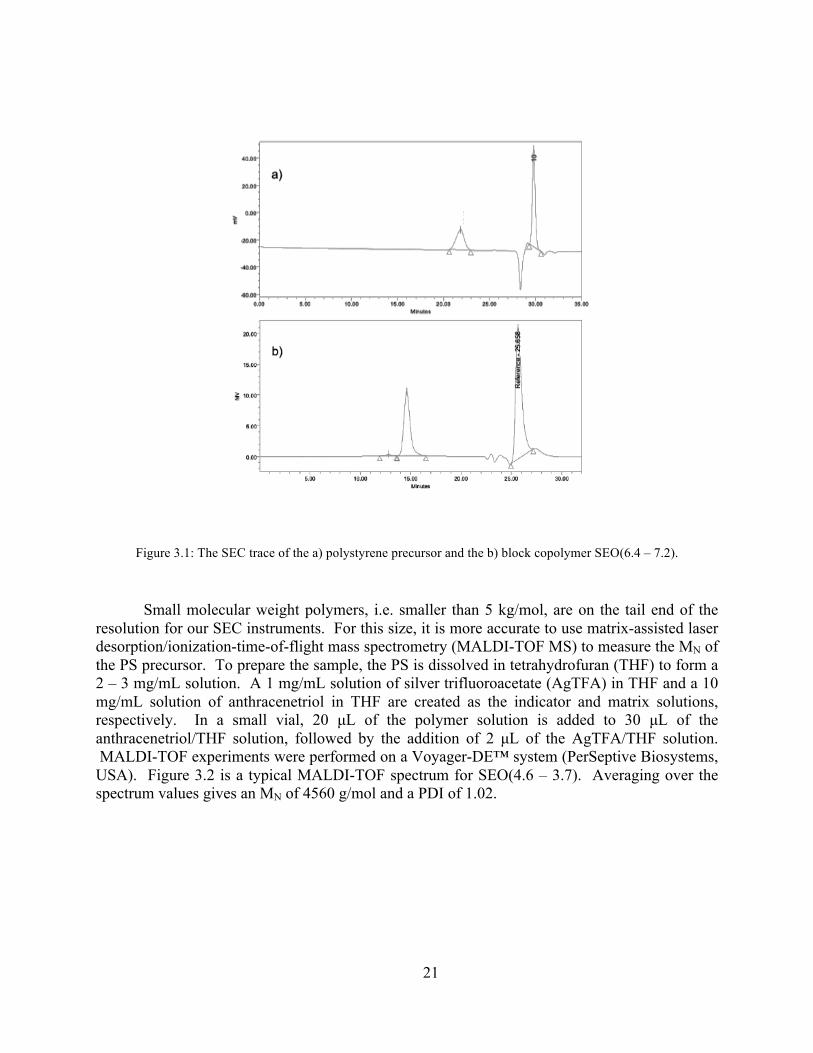
The molecular weight and volume fraction of the second block (PEO) was determined using 1H nuclear magnetic resonance (1H NMR) spectroscopy. Samples were prepared by dissolving the polymer in deuterated chloroform to form a 1 to 2 mg/mL solution. 1H NMR experiments were performed on an AMX-300 Spectrometer (Bruker Biospin Corporation). A typical 1H NMR spectrum for SEO(6.4 – 7.2) is shown in Figure 3.3. Trace amount of hydrogenated chloroform was used as the chemical-shift standard (7.3 ppm). The peaks around 7.0 and 6.6 correspond to the protons in the PS, and the peak at 3.6 corresponds to the protons in PEO (the peaks are outlined with a dashed box in the figure). From SEC, it is known that the PS MN is 6.4 kg/mol. Comparing integrated peak values in Figure 3.3 results in a PEO MN of 7.2 kg/mol and a volume fraction of 0.519.

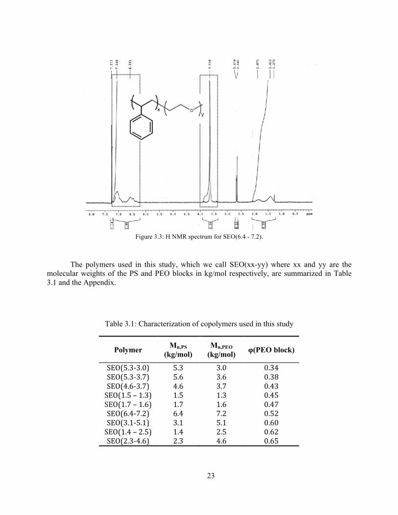
23

Figure 3.3: H NMR spectrum for SEO(6.4 - 7.2).

The polymers used in this study, which we call SEO(xx-yy) where xx and yy are the molecular weights of the PS and PEO blocks in kg/mol respectively, are summarized in Table 3.1 and the Appendix.

Table 3.1: Characterization of copolymers used in this study

Polymer Mn,PS (kg/mol)

Mn,PEO (kg/mol) φ(PEO block)  

SEO(5.3-­‐3.0)   5.3   3.0   0.34  SEO(5.3-­‐3.7)   5.6   3.6   0.38  SEO(4.6-­‐3.7)   4.6   3.7   0.43  SEO(1.5  –  1.3)   1.5   1.3   0.45  SEO(1.7  –  1.6)   1.7   1.6   0.47  SEO(6.4-­‐7.2)   6.4   7.2   0.52  SEO(3.1-­‐5.1)   3.1   5.1   0.60  SEO(1.4  –  2.5)   1.4   2.5   0.62  SEO(2.3-­‐4.6)   2.3   4.6   0.65  

24

3.2 ELECTROLYTE PREPARATION

It takes approximately 1.5 to 2 weeks to make the polymer electrolytes. The first step is to weigh out the amount of polymer into a glass vial using the analytically robust weigh-by-difference technique. This step can be done in a non-moisture-controlled environment. Due to the hygroscopic nature of the PEO and lithium salts, the rest of the sample preparation is carried out in an argon glovebox. The amount of polymer depends on final applications and how conservative we needed to be with the particular sample. A sample of 0.3 g is sufficient to prepare multiple scattering (~ 0.1 g) and conductivity (~ 10 mg) samples. Next, residual moisture in the polymers is evaporated as the polymers are heated at 90 to 100 °C under vacuum in the antechamber to the glovebox for 24 to 72 hours. The polymers are then taken into the glovebox and reweighed. The post-heat weight is used to determine the amount of salts needed to add to the system. Benzene is added to the polymers to make a dilute solution (in the range of 5 wt %), and stirred for approximately 3 hours.

The salt solution can be made concurrently with the polymer solution. The salts are heated to 150 to 200 °C under vacuum in the antechamber of the glovebox. A large amount can be done at one time and stored in the glovebox for further use. To make the solution, use 30% more salts than is needed for the batch to ensure that there will be enough. It is not a good idea to make a stock solution since the solvent will evaporate and the concentration of the solution would be inaccurate. In the glovebox, weigh the proper amount of salts into a vial or a volumetric flask. Add THF to the salts to make a 10 mg salt/mL THF solution. A salt solution that is too concentrated may precipitate when mixed with the polymer, but one that is too dilute will require too much THF, rendering the solution difficult to freeze dry. The solution is stirred for approximately 3 hours.

A calculated amount of salt/THF solution is added to the polymer/benzene solution using a pipette and stirred for 12 hours. If the resulting solution is cloudy, the samples are heated slightly while stirring to help the dissolution. The samples are then placed in a custom-built dessicator which attaches to the freeze dryer or a vacuum line outside of the glovebox. The samples are first frozen to -80 °C, and the temperature is slowly ramped up to room temperature while under active vacuum. The freeze drying process takes approximately 1 week. On the final day, the samples are heated to 40 °C under vacuum.

3.3 DIFFERENTIAL SCANNING CALORIMETRY

Melting and glass-transition temperatures (Tg) were measured by differential scanning calorimetry (DSC). DSC scans were performed on a TA Instruments DSC 2920 at 5 and 10 °C/min. Approximately 2 to 10 mg of sample were crimped in a glove box using hermetically sealed pans and placed inside a container with desiccant for transfer to the DSC. Indium and dodecane were used as calibration standards for the DSC. Samples underwent three heating and cooling cycles from -30 to 120 °C and were run against an empty aluminum reference pan. The melting point of PEO typically occurs around 60 °C,[4] but decreases with both molecular weight and salt concentration (as discussed in Chapter 5). Figure 3.4 is a typical DSC scan for

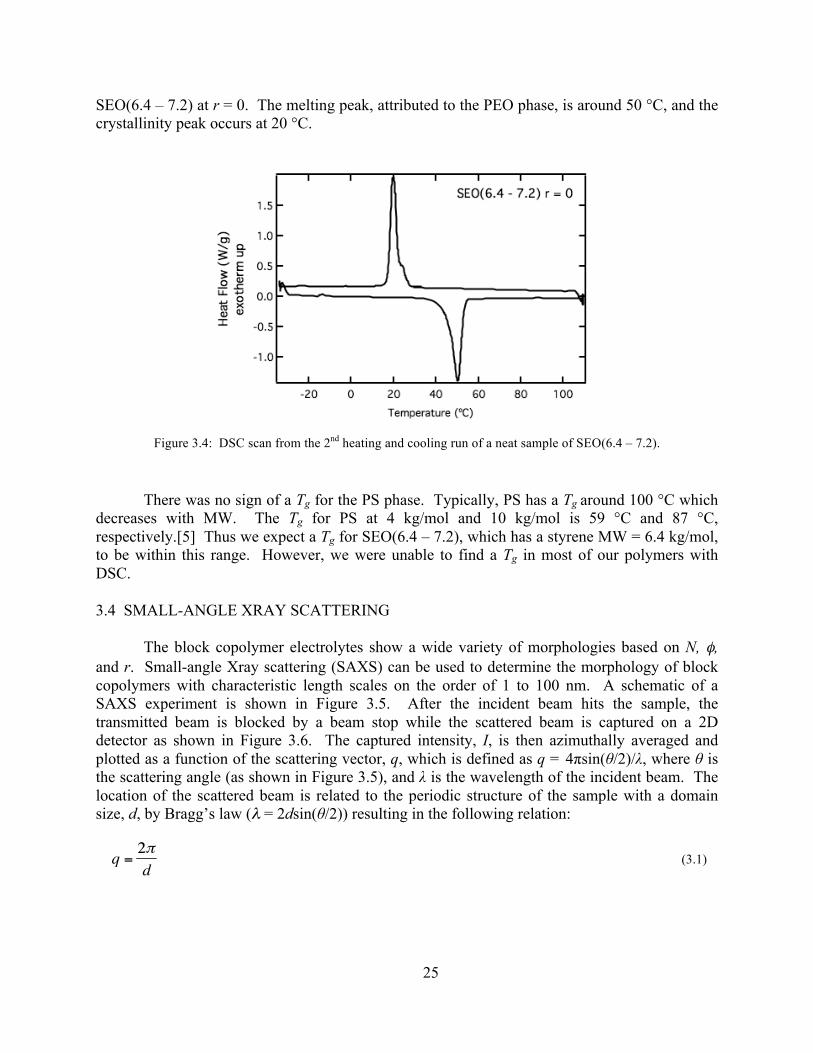
25

SEO(6.4 – 7.2) at r = 0. The melting peak, attributed to the PEO phase, is around 50 °C, and the crystallinity peak occurs at 20 °C.

Figure 3.4: DSC scan from the 2nd heating and cooling run of a neat sample of SEO(6.4 – 7.2).

There was no sign of a Tg for the PS phase. Typically, PS has a Tg around 100 °C which decreases with MW. The Tg for PS at 4 kg/mol and 10 kg/mol is 59 °C and 87 °C, respectively.[5] Thus we expect a Tg for SEO(6.4 – 7.2), which has a styrene MW = 6.4 kg/mol, to be within this range. However, we were unable to find a Tg in most of our polymers with DSC.

3.4 SMALL-ANGLE XRAY SCATTERING

The block copolymer electrolytes show a wide variety of morphologies based on N, φ, and r. Small-angle Xray scattering (SAXS) can be used to determine the morphology of block copolymers with characteristic length scales on the order of 1 to 100 nm. A schematic of a SAXS experiment is shown in Figure 3.5. After the incident beam hits the sample, the transmitted beam is blocked by a beam stop while the scattered beam is captured on a 2D detector as shown in Figure 3.6. The captured intensity, I, is then azimuthally averaged and plotted as a function of the scattering vector, q, which is defined as q = 4πsin(θ/2)/λ, where θ is the scattering angle (as shown in Figure 3.5), and λ is the wavelength of the incident beam. The location of the scattered beam is related to the periodic structure of the sample with a domain size, d, by Bragg’s law (λ = 2dsin(θ/2)) resulting in the following relation:

(3.1)

26

Figure 3.5: Schematic of a typical SAXS setup.

A sample with known domain size, such as silver behenate which has a Bragg peak at d = 58.380 Å and higher order reflections at 2d and 3d, is used to calibrate q for each experiment.

Figure 3.6: The 2-D scattering image acquired from a SAXS experiment on SEO(6.4 – 7.2)

SAXS samples are prepared by melting the polymer electrolyte into a 1 mm thick spacer and sealed in a custom-built airtight sample holder with Kapton windows. The samples are then annealed at 100 °C for 1 to 3 days. Figure 3.7 shows representative 1-D scattering profiles of block copolymers with (a) lamellar structure, (b) hexagonally packed cylinders structure, (c) gyroid structure, and (d) disordered phase seen in the SEO polymer electrolytes. The characteristic domain size of the structures is related to the primary scattering peak, labeled q* in Figure 3.7, according to eqn 3.1. The primary peak and higher-order reflections indicate the type of structure present. The allowable reflections for the different structures are listed in Table 3.2.

27

However the scattering profiles are actually a convolution of both the structure factor and the form factor. For example, if we take the case of lamellar samples, we can model the density profile as a periodic step function with dA and dB the thickness of the A and B lamellae respectively such that the domain size, d = dA + dB. For this system, the scattering intensity (I) is modeled as:[6]

(3.2)

where Δρ is the difference in electron density of polymer A and B (scattering contrast), and z is

the lattice factor defined as . From eqn 3.2, it follows that Bragg peaks must

occur at q values that satisfy q = 2πn/d, where n = 1, 2, 3… Furthermore, the nth order peak is proportional to sin2(πnφ)/n2, where φ is the volume fraction of polymer A and equivalent to dA/d. Thus, when φ = 0.5, the even order peaks disappear. However, when φ ≠ 0.5, the relative amounts of the phases can be determined by comparing relative peak intensities. Similarly, the CYL phases see a suppression of the 2q* peak due to the minimum in the form factor.[7]

Table 3.2: Higher-order reflections for different structure factors.[7, 8]

Structure Index

LAM   1,  2,  3,  4…  CYL   1,  √3,  √4,  √7,  √9…  GYR   √6,  √8,  √14,  √16,  √20…  DIS   n/a  

The disordered sample results in a broad peak (see Figure 3.7d) in the scattering profile from the “correlation hole,” which is the segment-segment correlation.[9] The location of this peak is related to the polymer coil size.

28

Figure 3.7: Azimuthally averaged scattering profiles for (a) SEO(6.4 – 7.2) r = 0.085 which forms a LAM structure, (b) SEO(2.3 – 4.6) r = 0.10 which forms a CYL structure, (c) SEO(3.1 – 5.1) r = 0.05 which forms a GYR structure, and (d) SEO(1.4 – 2.5) r = 0.05 which is DIS. The images in each plot are a schematic of each phase. The arrows

point to higher order reflections as indicated by the label.

SAXS experiments are performed at beamline 7.3.3 at the Advanced Light Source (ALS) at Lawrence Berkeley National Labs, beamline 1-4 at the Stanford Synchrotron Radiation Lightsource (SSRL) at the Stanford Linear Accelerator Center, and at beamline 15-ID-D at the Advanced Photon Source (APS) at Argonne National Lab. The ALS has an energy source of 10 keV, ΔE/E ~ 10-2, flux ~ 1012 photon/s, and a beam size of 1 mm x 0.7 mm. The SSRL beamline has an energy range of 7.1 – 9 keV, with ΔE/E ~ 4x10-3, flux ~ 1010 photon/s, and a beam size of 0.25 mm x 1 mm. The APS beamline has an energy range of 6 – 30 keV, with ΔE/E ~ 10-4, flux ~ 1012 - 1013 photon/s, and a beam size of 0.2 mm x 0.1 mm. The SAXS data from APS and ALS are reduced using the Nika Program for IgorPro developed by Jan Ilavsky at the APS. The SAXS data from SSRL are reduced using a program developed by John Pople.

3.5 BIREFRINGENCE DETECTION OF THE ODT

Order-to-disorder transition (ODT) temperatures can be measured using optical birefringence. Figure 3.8 shows a typical setup for birefringence measurements. A 633 nm

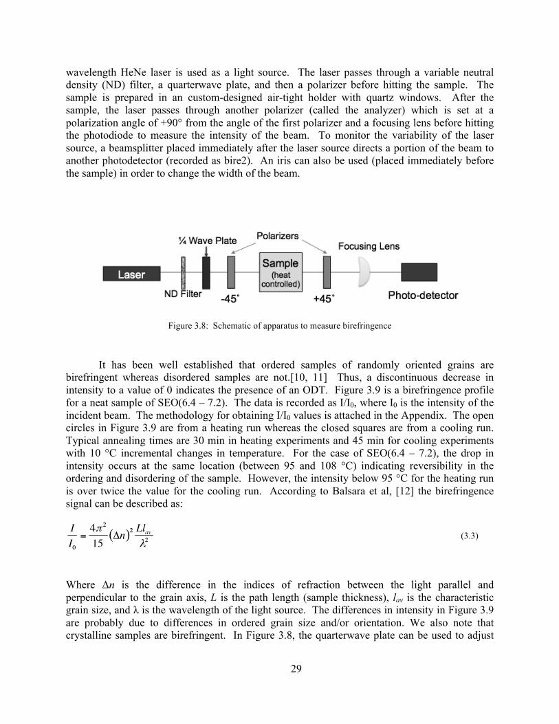
29

wavelength HeNe laser is used as a light source. The laser passes through a variable neutral density (ND) filter, a quarterwave plate, and then a polarizer before hitting the sample. The sample is prepared in an custom-designed air-tight holder with quartz windows. After the sample, the laser passes through another polarizer (called the analyzer) which is set at a polarization angle of +90° from the angle of the first polarizer and a focusing lens before hitting the photodiode to measure the intensity of the beam. To monitor the variability of the laser source, a beamsplitter placed immediately after the laser source directs a portion of the beam to another photodetector (recorded as bire2). An iris can also be used (placed immediately before the sample) in order to change the width of the beam.

Figure 3.8: Schematic of apparatus to measure birefringence

It has been well established that ordered samples of randomly oriented grains are birefringent whereas disordered samples are not.[10, 11] Thus, a discontinuous decrease in intensity to a value of 0 indicates the presence of an ODT. Figure 3.9 is a birefringence profile for a neat sample of SEO(6.4 – 7.2). The data is recorded as I/I0, where I0 is the intensity of the incident beam. The methodology for obtaining I/I0 values is attached in the Appendix. The open circles in Figure 3.9 are from a heating run whereas the closed squares are from a cooling run. Typical annealing times are 30 min in heating experiments and 45 min for cooling experiments with 10 °C incremental changes in temperature. For the case of SEO(6.4 – 7.2), the drop in intensity occurs at the same location (between 95 and 108 °C) indicating reversibility in the ordering and disordering of the sample. However, the intensity below 95 °C for the heating run is over twice the value for the cooling run. According to Balsara et al, [12] the birefringence signal can be described as:

(3.3)

Where Δn is the difference in the indices of refraction between the light parallel and perpendicular to the grain axis, L is the path length (sample thickness), lav is the characteristic grain size, and λ is the wavelength of the light source. The differences in intensity in Figure 3.9 are probably due to differences in ordered grain size and/or orientation. We also note that crystalline samples are birefringent. In Figure 3.8, the quarterwave plate can be used to adjust

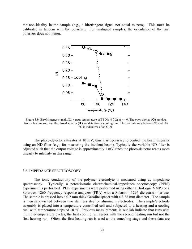
30

the non-ideality in the sample (e.g., a birefringent signal not equal to zero). This must be calibrated in tandem with the polarizer. For unaligned samples, the orientation of the first polarizer does not matter.

Figure 3.9: Birefringence signal, I/I0, versus temperature of SEO(6.4-7.2) at r = 0. The open circles () are data from a heating run, and the closed squares () are data from a cooling run. The discontinuity between 95 and 108

°C is indicative of an ODT.

The photo-detector saturates at 10 mV; thus it is necessary to control the beam intensity using an ND filter (e.g., for measuring the incident beam). Typically the variable ND filter is adjusted such that the output voltage is approximately 1 mV since the photo-detector reacts more linearly to intensity in this range.

3.6 IMPEDANCE SPECTROSCOPY

The ionic conductivity of the polymer electrolyte is measured using ac impedance spectroscopy. Typically, a potentiostatic electrochemical-impedance spectroscopy (PEIS) experiment is performed. PEIS experiments were performed using either a BioLogic VMP3 or a Solartron 1260 frequency-response analyzer (FRA) with a Solartron 1296 dielectric interface. The sample is pressed into a 0.2 mm thick Garolite spacer with a 3.88 mm diameter. The sample is then sandwiched between two stainless steel or aluminum electrodes. The sample/electrode assembly is placed into a temperature-controlled cell and subjected to a heating and a cooling run, with temperature steps of 10 °C. Previous measurements in our lab indicate that runs with multiple-temperature cycles, the first cooling run agrees with the second heating run but not the first heating run. Often, the first heating run is used as the annealing stage and these data are

31

discarded. The cooling-run data are presented unless otherwise specified. At each temperature step, the sample is annealed for 3 h before the impedance measurements. An alternating signal of 1, 10, or 100 mV with frequency scans of 1 MHz to 1 Hz was applied. At the end of the experiment, the sample thickness is measured.

The applied sinusoidal potential results in a sinusoidal current response. The frequency-dependent resistance, or impedance, Z, of the sample relates the potential and current signals. Accordingly, Z has both real and imaginary components. To analyze the impedance data, they are presented as either a Nyquist plot or Bode plot. Figure 3.10a and b are typical Nyquist and Bode plots, respectively, of SEO(4.6 – 3.7) at r = 0.020 and 80 °C with corresponding regimes labeled A, B, and C. The resistance of the sample (related to the conductivity) is determined from the B region.

Figure 3.10: a) Nyquist plot and b) Bode plot of SEO(4.6 – 3.7), r = 0.020 at 80 °C. Different regimes are labeled as A, the kinetic-controlled region, B, the sample resistance, and C, the diffusion-controlled region.

Often an equivalent-circuit diagram, such as the one shown in Figure 3.11, is used to explain the data in Figure 3.10. In the diagram, the resistance from charge transfer (RT) is in series with the Warburg impedance (W). The Warburg impedance is created by diffusion and is prevalent at low frequencies where reactants have to diffuse longer lengths. In contrast, the charge-transfer resistance is dictated by Butler-Volmer kinetics. The capacitance from the double layer (Cdl) is modeled in parallel to the RT and the W. This circuit is then in series with the solution resistance (Rs). The linear region and slope at low ω labeled as “C” in Figure 3.10a and b, respectively, arises from the Warburg impedance. The region labeled as “A” in Figure 3.10a and b is from the rest of the circuit diagram, i.e. Figure 3.11 without the W impedance, also known as the Randles cell.

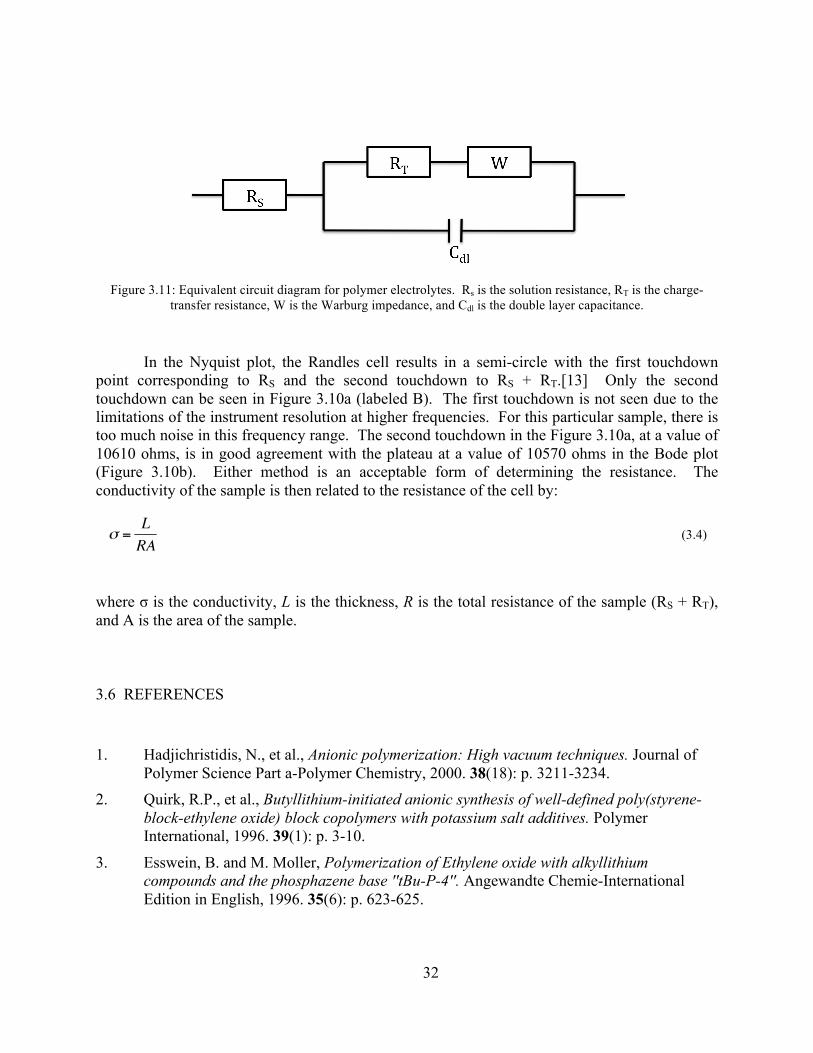
32

Figure 3.11: Equivalent circuit diagram for polymer electrolytes. Rs is the solution resistance, RT is the charge-transfer resistance, W is the Warburg impedance, and Cdl is the double layer capacitance.

In the Nyquist plot, the Randles cell results in a semi-circle with the first touchdown point corresponding to RS and the second touchdown to RS + RT.[13] Only the second touchdown can be seen in Figure 3.10a (labeled B). The first touchdown is not seen due to the limitations of the instrument resolution at higher frequencies. For this particular sample, there is too much noise in this frequency range. The second touchdown in the Figure 3.10a, at a value of 10610 ohms, is in good agreement with the plateau at a value of 10570 ohms in the Bode plot (Figure 3.10b). Either method is an acceptable form of determining the resistance. The conductivity of the sample is then related to the resistance of the cell by:

(3.4)

where σ is the conductivity, L is the thickness, R is the total resistance of the sample (RS + RT), and A is the area of the sample.

3.6 REFERENCES

1. Hadjichristidis, N., et al., Anionic polymerization: High vacuum techniques. Journal of

Polymer Science Part a-Polymer Chemistry, 2000. 38(18): p. 3211-3234. 2. Quirk, R.P., et al., Butyllithium-initiated anionic synthesis of well-defined poly(styrene-

block-ethylene oxide) block copolymers with potassium salt additives. Polymer International, 1996. 39(1): p. 3-10.

3. Esswein, B. and M. Moller, Polymerization of Ethylene oxide with alkyllithium compounds and the phosphazene base ''tBu-P-4''. Angewandte Chemie-International Edition in English, 1996. 35(6): p. 623-625.

33

4. Lascaud, S., et al., Phase-Diagrams and Conductivity Behavior of Poly(Ethylene Oxide) Molten-Salt Rubbery Electrolytes. Macromolecules, 1994. 27(25): p. 7469-7477.

5. Blanchard, L.-P., J. Hesse, and S.L. Malhotra, Effect of Molecular Weight on Glass Transition by Differential Scanning Calorimetry. Canadian Journal of Chemistry, 1974. 52: p. 3170-3175.

6. Roe, R.-J., Methods of X-ray and Neutron Scattering in Polymer Science. 2000, New York: Oxford University Press.

7. Hamley, I.W., The Physics of Block Copolymers. 1998: Oxford University Press.

8. Hajduk, D.A., et al., The Gyroid: A New Equilibrium Morphology in Weakly Segregated Diblock Copolymers. Macromolecules, 1994. 27(15): p. 4063-4075.

9. de Gennes, P.-G., Scaling Concepts in Polymer Physics. 1979, Ithaca, New York: Cornell University Press.

10. Amundson, K., et al., Optical Characterization of Ordering and Disordering of Block Copolymer Microstructure. Macromolecules, 1992. 25: p. 3896.

11. Garetz, B.A., et al., Birefringence and Diffraction of Light in Ordered Block-Copolymer Materials. Macromolecules, 1993. 26(12): p. 3151-3155.

12. Balsara, N.P., B.A. Garetz, and H.J. Dai, Relationship between Birefringence and the Structure of Ordered Block Copolymer Materials. Macromolecules, 1992. 25: p. 6072-6074.

13. Impedance spectroscopy: theory, experiment, and applications, ed. E. Barsoukov and J.R. Macdonald. 2005, Hoboken, NJ: John Wiley & Sons, Inc.

34

Chapter 4

Effect of LiTFSI on the thermal properties and morphology of polystyrene-block-polyethylene oxide

ABSTRACT

The thermal properties and phase behavior of different poly(styrene-block-ethylene oxide) systems mixed with varying concentrations of LiTFSI were measured using differential scanning calorimetry (DSC), small-angle Xray scattering (SAXS), and birefringence. The DSC measurements are in good agreement with literature. SAXS and birefringence measurements reveal that the addition of LiTFSI changes the morphology and leads to an increase in segregation strength and order-to-disorder transition temperatures.

4.1 THERMAL PROPERTIES OF SEO/LITFSI SYSTEMS

Samples of SEO(6.4 – 7.2) were mixed with LiTFSI to obtain mixtures with concentrations ranging from r = 0 to 0.125. Differential scanning calorimetry (DSC) was used to measure the thermal properties of these systems. Figure 4.1a plots the resulting DSC scans from the second heating run at 5 °C/min. The only thermal transitions seen are the crystalline PEO melting peaks at r = 0 to 0.05. It is clear that increasing the concentration of LiTFSI leads to a suppression of PEO crystallinity. The melting peak decreases from 50 to 40 oC as r is increased from 0 to 0.05, while ΔHm values decrease from 55 to 19 J/g. Greater than r = 0.05, there is complete suppression of the PEO crystals. The phase transitions in Figure 4.1a are used to construct the phase diagram in Figure 4.1b. This phase diagram is consistent with observations of Lascaud et al. [1] on PEO/LiTFSI homopolymer/salt mixtures. In that paper, they find that increasing the salt content from r = 0 to 0.083 in a (3.0 – 4.5) × 103 kg/mol PEO sample results in a decrease in melting temperatures from 60 to 40 °C. Within this region, amorphous PEO and crystalline PEO coexists. From r = 0.083 to 0.17, a “crystallinity gap” occurs. The onset of the crystallinity gap for the PEO-rich phase in SEO(6.4 – 7.2)/LiTFSI in Figure 4.1b is placed at 0.068 ± 0.017 (the average of the concentrations with and without complete suppression of PEO crystallinity). However, within error, the onset is in agreement to that of ref [1]. The fact that the phase behavior of SEO/LiTFSI data agrees with PEO/LiTFSI data indicates that the salts are preferentially segregating to the PEO-rich domains. This is due to the higher dielectric constant, ε, of the PEO domain (estimates of εPEO range from 4 to 8,[2-5] while that of εPS ranges from 2 to 4[6, 7]) and the specific interactions between the ether oxygen and Li+.[8, 9]

35

Figure 4.1: a) DSC thermograms from the second heating run on SEO(6.4 – 7.2) at various concentrations of LiTFSI. Plots are shifted for clarity. b) The phase behavior of the PEO block in SEO(6.4 – 7.2) as constructed

from DSC data. The solid line indicates the liquidus curve, dashed line indicates the border of the crystallinity gap, and the dotted line/open symbol is a possible alternate location of the liquidus line due to different crystal structure.

There are a few minor differences between the phase diagram in ref [1] and Figure 4.1b. At r = 0.02, the DSC scan in Figure 4.1a contains a large peak at 48 °C, and a small shoulder at 53 °C, indicating the presence of two melting events. It is possible that in addition to PEO crystals, a different crystal structure from PEO/Li+ complexes forms. For example, molecular dynamics simulations have suggested that the PEO forms a helical structure around the Li+ ions. [10] A second crystal structure is portrayed in Figure 4.1b with dotted lines and an open symbol since this structure has not been directly determined experimentally (e.g., spectroscopically). The location of the liquidus line in Figure 4.1b is also at a lower temperature than in ref [1]. It is unclear why the melting temperatures for the neat polymers is less for the SEO sample over the PEO samples since Lascaud et al. looked a smaller molecular weight PEO.

All other SEO polymers measured show similar PEO thermal behavior, with variations in the melting temperature due to molecular weight differences (i.e., lower molecular weight PEO samples have lower melting temperatures). Another feature of these DSC curves is the lack of Tg for styrene phase. For SEO(6.4 – 7.2), the PS phase should have a Tg of around 78 °C. [11] In fact, the only sample which contained a measurable glass transition temperature is SEO(4.6 – 3.7) at r = 0.02 as shown in Figure 4.2. Dotted lines in the figure are tangential to the curve, indicating the changes in slope (i.e., a second order transition) at 61 and 94 °C. This is in agreement with the literature value (for MWPS = 4.6 kg/mol, the interpolated Tg is 72 °C at 10 °C/min). [11] At this time, we are unable to explain why this particular sample contains a PS Tg while other samples do not.

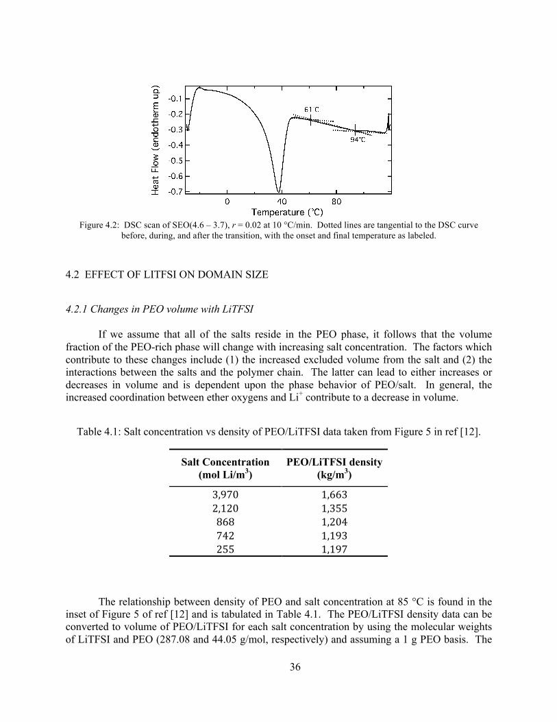
36

Figure 4.2: DSC scan of SEO(4.6 – 3.7), r = 0.02 at 10 °C/min. Dotted lines are tangential to the DSC curve before, during, and after the transition, with the onset and final temperature as labeled.

4.2 EFFECT OF LITFSI ON DOMAIN SIZE

4.2.1 Changes in PEO volume with LiTFSI

If we assume that all of the salts reside in the PEO phase, it follows that the volume fraction of the PEO-rich phase will change with increasing salt concentration. The factors which contribute to these changes include (1) the increased excluded volume from the salt and (2) the interactions between the salts and the polymer chain. The latter can lead to either increases or decreases in volume and is dependent upon the phase behavior of PEO/salt. In general, the increased coordination between ether oxygens and Li+ contribute to a decrease in volume.

Table 4.1: Salt concentration vs density of PEO/LiTFSI data taken from Figure 5 in ref [12].

Salt Concentration (mol Li/m3)

PEO/LiTFSI density (kg/m3)

3,970   1,663  2,120   1,355  868   1,204  742   1,193  255   1,197  

The relationship between density of PEO and salt concentration at 85 °C is found in the inset of Figure 5 of ref [12] and is tabulated in Table 4.1. The PEO/LiTFSI density data can be converted to volume of PEO/LiTFSI for each salt concentration by using the molecular weights of LiTFSI and PEO (287.08 and 44.05 g/mol, respectively) and assuming a 1 g PEO basis. The

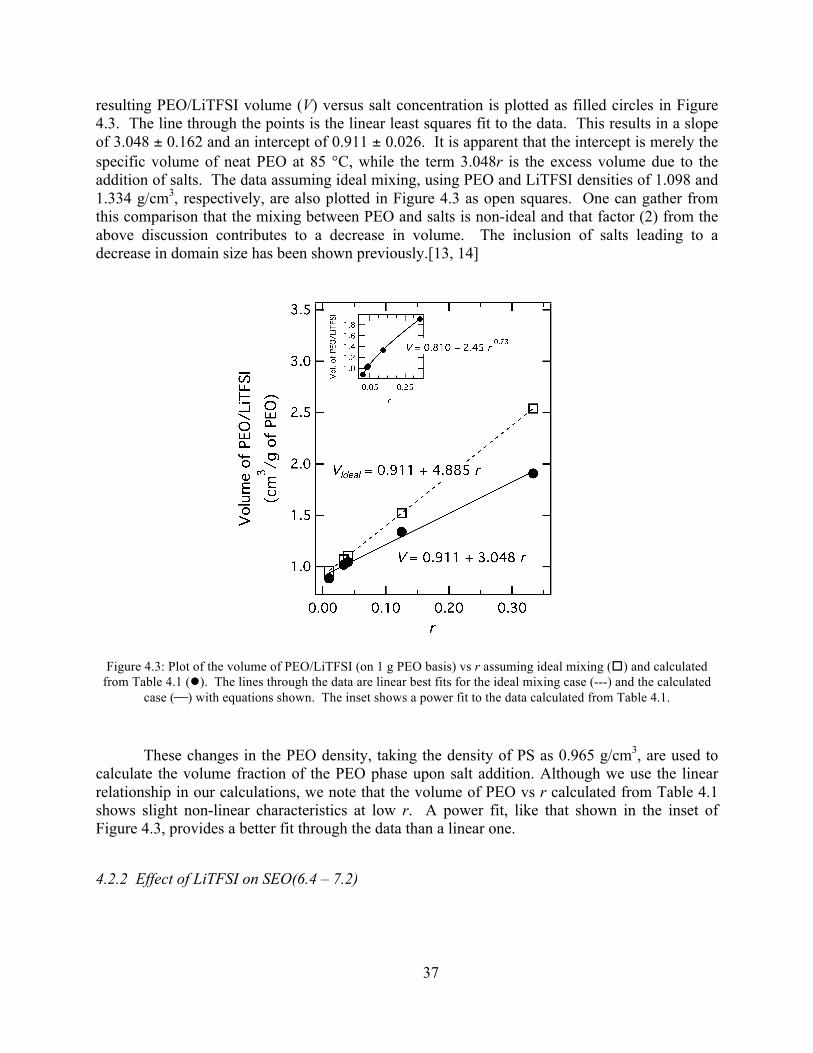
37

resulting PEO/LiTFSI volume (V) versus salt concentration is plotted as filled circles in Figure 4.3. The line through the points is the linear least squares fit to the data. This results in a slope of 3.048 ± 0.162 and an intercept of 0.911 ± 0.026. It is apparent that the intercept is merely the specific volume of neat PEO at 85 °C, while the term 3.048r is the excess volume due to the addition of salts. The data assuming ideal mixing, using PEO and LiTFSI densities of 1.098 and 1.334 g/cm3, respectively, are also plotted in Figure 4.3 as open squares. One can gather from this comparison that the mixing between PEO and salts is non-ideal and that factor (2) from the above discussion contributes to a decrease in volume. The inclusion of salts leading to a decrease in domain size has been shown previously.[13, 14]

Figure 4.3: Plot of the volume of PEO/LiTFSI (on 1 g PEO basis) vs r assuming ideal mixing () and calculated from Table 4.1 (). The lines through the data are linear best fits for the ideal mixing case (---) and the calculated

case (⎯) with equations shown. The inset shows a power fit to the data calculated from Table 4.1.

These changes in the PEO density, taking the density of PS as 0.965 g/cm3, are used to calculate the volume fraction of the PEO phase upon salt addition. Although we use the linear relationship in our calculations, we note that the volume of PEO vs r calculated from Table 4.1 shows slight non-linear characteristics at low r. A power fit, like that shown in the inset of Figure 4.3, provides a better fit through the data than a linear one.

4.2.2 Effect of LiTFSI on SEO(6.4 – 7.2)

38

SEO(6.4 – 7.2) is the largest molecular weight polymer of all the systems studied in this dissertation. Thus, it is the only polymer that has an ordered morphology in the neat state. Furthermore, the samples are LAM at all salt concentrations probed, allowing for direct comparisons of the domain size. Figure 4.4a shows the SAXS profiles for SEO(6.4 – 7.2) with increasing salt concentration at 107 °C. From these profiles, we can infer that increasing the salts leads to 1) an increase in the segregation strength of the block copolymer, 2) an increase in the asymmetry of the LAM structure, and 3) a general increase in domain size, but with a saturation limit. As r is increased from 0 to 0.02, a 3q* peak emerges, indicating that the addition of salts leads to stronger segregation of the block copolymers. This effect is due to an increase in the effective χ parameter (i.e., the χ parameter between the PEO/LiTFSI phase and the PS phase), which is discussed in further detail and quantified in Chapter 6.4. The increase in segregation strength is confirmed in Figure 4.4b where the full-width-half-maximum (FWHM) of the primary peak in the SEO(6.4 – 7.2) scattering profiles at various salt concentrations is plotted vs temperature. The jump in FWHM for r = 0 () at 107 °C designates the location of an order-to-disorder transition (ODT). This jump is not seen in any of the other salt concentrations probed. The lack of an ODT suggests that these samples have a higher effective χ than the neat sample.

Figure 4.4: a) SAXS profiles for SEO(6.4 – 7.2) at various salt concentrations at 107 °C. Profiles have been shifted for clarity. b) FWHM of primary peak in SAXS profiles for SEO(6.4 – 7.2) as a function of temperature for r = 0

(), r = 0.02 (), r = 0.05 (), r = 0.085 (), and r = 0.10 ().

39

As r is increased beyond 0.02, the 2q* and 4q* peak is visible. From the discussions in Chapter 3.4, the appearance of the even order reflections is evidence of asymmetry between the PEO domain and PS domain. Using eqn 3.2 for the ratio of the intensity of the q* and the 2q* peaks, the changes in φEO for SEO(6.4 – 7.2) is calculated and shown in Figure 4.5. In the same plot, the volume fraction calculated for SEO(6.4 – 7.2) using literature values of density changes in PEO with LiTFSI (described in section 4.2.1) is shown. There is a distinct difference in the results between the two methods. The φEO calculated from the SAXS profiles increases at almost half the rate as from the density calculations.

The method from density changes is chosen to determine the φEO for this study. This is because the intensity and background is not very well calibrated in these SAXS profiles and errors in calculated invariants may be substantial. Furthermore, the resolution is not ideal. The second peak cannot be seen at r = 0 or 0.02, indicating that φEO = 0.5. However, from NMR measurements, φEO = 0.519 at r = 0 (this was used as the reference point for φEO calculations from density changes).

Figure 4.5: Changes in φEO for SEO(6.4 – 7.2) as calculated from changes in PEO density changes with LiTFSI in ref [12] () and calculated from the SAXS profiles and eqn 4.2 ().

The changes in domain size, d, with r calculated from the SAXS profiles in Figure 4.4a (d = 2π/q*) is plotted in Figure 4.6. In addition to the factors that affect the changes in density or volume fraction of PEO with LiTFSI, the domain size may also be dependent on the χ parameter. As the concentration is increased from r = 0 to 0.085, the domain size increases by 25%. However, after r = 0.085, the rate at which d increases starts decreasing. This value of r coincides with both a maximum in conductivity and the crystallinity gap as discussed in section 4.1. We note that the SAXS profiles are for 107 °C, which is well above any thermal transitions. It has also been shown that increasing the domain size of the PEO block in SEO leads to an

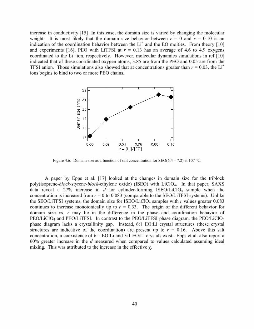
40

increase in conductivity.[15] In this case, the domain size is varied by changing the molecular weight. It is most likely that the domain size behavior between r = 0 and r = 0.10 is an indication of the coordination behavior between the Li+ and the EO moities. From theory [10] and experiments [16], PEO with LiTFSI at r = 0.13 has an average of 4.6 to 4.9 oxygens coordinated to the Li+ ion, respectively. However, molecular dynamics simulations in ref [10] indicated that of these coordinated oxygen atoms, 3.85 are from the PEO and 0.05 are from the TFSI anion. Those simulations also showed that at concentrations greater than r = 0.03, the Li+

ions begins to bind to two or more PEO chains.

Figure 4.6: Domain size as a function of salt concentration for SEO(6.4 – 7.2) at 107 °C.

A paper by Epps et al. [17] looked at the changes in domain size for the triblock poly(isoprene-block-styrene-block-ethylene oxide) (ISEO) with LiClO4. In that paper, SAXS data reveal a 27% increase in d for cylinder-forming ISEO/LiClO4 sample when the concentration is increased from r = 0 to 0.083 (comparable to the SEO/LiTFSI systems). Unlike the SEO/LiTFSI systems, the domain size for ISEO/LiClO4 samples with r values greater 0.083 continues to increase monotonically up to r = 0.33. The origin of the different behavior for domain size vs. r may lie in the difference in the phase and coordination behavior of PEO/LiClO4 and PEO/LiTFSI. In contrast to the PEO/LiTFSI phase diagram, the PEO/LiClO4 phase diagram lacks a crystallinity gap. Instead, 6:1 EO:Li crystal structures (these crystal structures are indicative of the coordination) are present up to r = 0.16. Above this salt concentration, a coexistence of 6:1 EO:Li and 3:1 EO:Li crystals exist. Epps et al. also report a 60% greater increase in the d measured when compared to values calculated assuming ideal mixing. This was attributed to the increase in the effective χ.

41

4.3 CHARACTERIZATION OF BLOCK COPOLYMER ELECTROLYTE MORPHOLOGY

The structure of the polymer electrolyte was determined by both small-angle Xray scattering (SAXS) and optical birefringence measurements. Samples for both experiments were prepared by pressing the polymer into sample holders with a 1 mm thick spacer and annealing at 90 to 110°C in a glovebox for 3 to 5 days. SAXS samples were sealed off in a custom-designed-airtight sample holder with kapton windows. Birefringence samples were sandwiched between two quartz discs and sealed with a silicone-based epoxy or sealed off in a custom-designed airtight sample holder. Due to the hygroscopic nature of the salts, glovebox integrity was maintained throughout all stages of experimentation.

Birefringence measurements were performed using the set up described in ref [18] with a plane-polarized beam of wavelength 633 nm as the source. The samples undergo two heating and cooling cycles with temperature steps of approximately 10 °C. For the heating runs, the sample is annealed at desired temperatures for at least 20 minutes whereas samples are held at temperatures for 45 min during cooling runs. The intensity of the beam after it passed through the sample and the two-crossed polarizer’s normalized by the incident intensity, I/I0, was recorded with a photodiode as a function of time and temperature.

At the end of SAXS experiments, Karl Fischer titrations were run on all the samples dissolved in benzene to ensure the samples were dry. The weight fraction of water was less than 0.0015 in all of the samples, and in most cases, comparable to the water content of the benzene used (ca. 5.4 ppm).

42

4.3.1 SAXS and birefringence measurements of transitions

Figure 4.7 shows the SAXS profiles at 69 ± 3 °C for SEO(2.3 – 4.6) at salt concentrations of r = 0, 0.02, 0.05, 0.085, and 0.10. The featureless scattering profile of the pure SEO(2.3 – 4.6) copolymer (r = 0) indicates that the sample is disordered (DIS). A well-defined but broad primary peak at q* = 0.57 nm-1 emerges when r is increased to 0.02 indicating the presence of periodic but disordered concentration fluctuations. Increasing r to 0.05 results in a sharpening of the primary peak [full width at half maximum (FWHM) changes from 0.16 to 0.02 nm-1 when r is changed from 0.02 to 0.05] indicating a disorder-to-order transition (DOT) induced by the increase in salt concentration.

Figure 4.7: SAXS profiles at 69 ± 3 ˚C for SEO(2.3-4.6) at r = 0, 0.02, 0.05, 0.085, and 0.10. The profiles have been multiplied by 1, 2, 10, 100, and 1000, respectively, to increase the clarity of the plots. Higher order peaks first appear at r = 0.05, which are marked with the inverted open triangles at √4 q* and √7 q*. Inverted closed triangles

mark the higher order peaks at √3 q*, √4 q* and √7 q*.

The higher order peaks at √4q* and √7q* at r = 0.05 are consistent with the formation of a CYL phase. As more salt is added to the system (r = 0.085 and 0.10), the √3q* peak becomes more prominent, indicating better ordering with increased salt concentration. The volume fraction of the PEO block in the neat copolymer is 0.65. At r = 0.085 and 0.10,   ϕEO for SEO(2.3-4.6) was estimated to be 0.70 and 0.71, respectively. At these volume fractions, neat

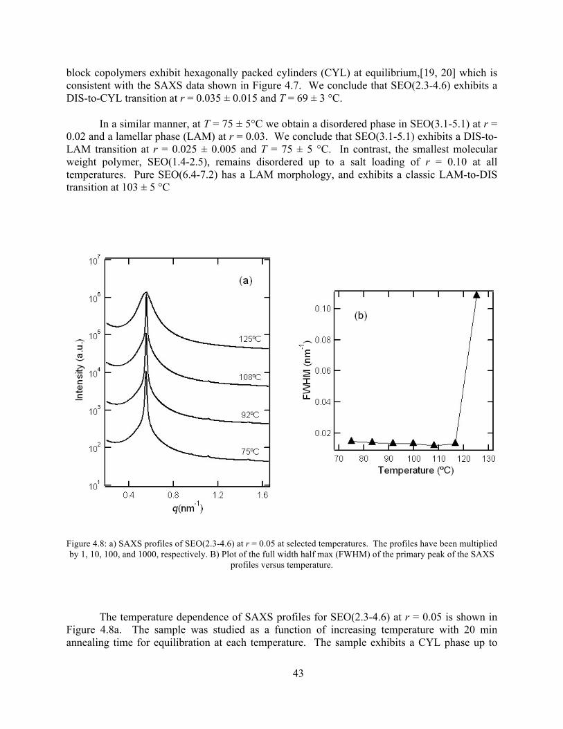
43

block copolymers exhibit hexagonally packed cylinders (CYL) at equilibrium,[19, 20] which is consistent with the SAXS data shown in Figure 4.7. We conclude that SEO(2.3-4.6) exhibits a DIS-to-CYL transition at r = 0.035 ± 0.015 and T = 69 ± 3 °C.

In a similar manner, at T = 75 ± 5°C we obtain a disordered phase in SEO(3.1-5.1) at r = 0.02 and a lamellar phase (LAM) at r = 0.03. We conclude that SEO(3.1-5.1) exhibits a DIS-to-LAM transition at r = 0.025 ± 0.005 and T = 75 ± 5 °C. In contrast, the smallest molecular weight polymer, SEO(1.4-2.5), remains disordered up to a salt loading of r = 0.10 at all temperatures. Pure SEO(6.4-7.2) has a LAM morphology, and exhibits a classic LAM-to-DIS transition at 103 ± 5 °C

Figure 4.8: a) SAXS profiles of SEO(2.3-4.6) at r = 0.05 at selected temperatures. The profiles have been multiplied by 1, 10, 100, and 1000, respectively. B) Plot of the full width half max (FWHM) of the primary peak of the SAXS

profiles versus temperature.

The temperature dependence of SAXS profiles for SEO(2.3-4.6) at r = 0.05 is shown in Figure 4.8a. The sample was studied as a function of increasing temperature with 20 min annealing time for equilibration at each temperature. The sample exhibits a CYL phase up to

44

117 °C. The increase of the FWHM from 0.013 to 0.11 nm-1 (Figure 4.8b) between 117 °C and 125 °C is indicative of a thermotropic ODT at 121 ± 4 °C. Birefringence experiments were also performed to confirm the presence of an ODT.[21, 22]

Figure 4.9 is a plot of the birefringence signal versus temperature from a heating (closed triangles with solid line) and a cooling run (open triangles with dashed line). The two runs are in good agreement with each other indicating reversibility of the ODT in this low molecular weight sample. A discontinuous decrease in the sample birefringence between 130 °C and 140 °C indicates an ODT at 135 ± 5 °C. The upper limit for the ODT obtained by SAXS is 5 °C lower than the lower limit of the ODT obtained by birefringence. We offer no explanation for this difference. We repeated the birefringence measurements on an independent sample and got the same ODT given above.

Figure 4.9: Birefringence signal, I/I0, versus temperature of SEO(2.3-4.5) at r = 0.05. The closed triangles (▲) are data from a heating run, and the open triangles (Δ) are data from a cooling run. The discontinuity between 130 and

140 °C is indicative of an ODT.

45

Similar measurements were done on SEO(5.3 – 3.6) at r = 0.019 and SEO(5.3 – 3.0) at r = 0.027. Figure 4.10 plots the SAXS profiles for the two polymers at various temperatures. At temperatures of 90 °C and lower, the SAXS peaks (e.g. those indicated by the arrows) index to q* and √3q* signifying a CYL phase. In this case, both SEO(5.3 – 3.6), r = 0.019 and SEO(5.3 – 3.0), r = 0.027 contain ϕEO/Salt < 0.50 such that the cylinders are comprised of PEO. In Figure 4.10a, the FWHM increases from 0.02 nm-1 to 0.09 nm-1 between 90 and 100 °C, indicating that SEO(5.3 – 3.6) at r = 0.019 has an ODT of 95 ± 5 °C. In Figure 4.10b, the FWHM increases from 0.02 to 0.1 nm-1 between 100 and 110 °C, indicating an ODT of 105 ± 5 °C for SEO(5.3 – 3.0) at r = 0.027. We note that the sharp peak around q = 1.0 nm-1 in the SAXS profile at 70 °C in Figure 4.10a is not a Bragg reflection but an error in the detector (zinger). Upon inspection of the 2D images, it is clear that there is a highly intense cluster of 2 or 3 pixels which are not from the sample.

Figure 4.10: SAXS profiles for a) SEO(5.3 – 3.6) at r = 0.019 and b) SEO(5.3 – 3.0) at r = 0.027. Arrows index to 1q* and √3q*, indicating a CYL morphology.

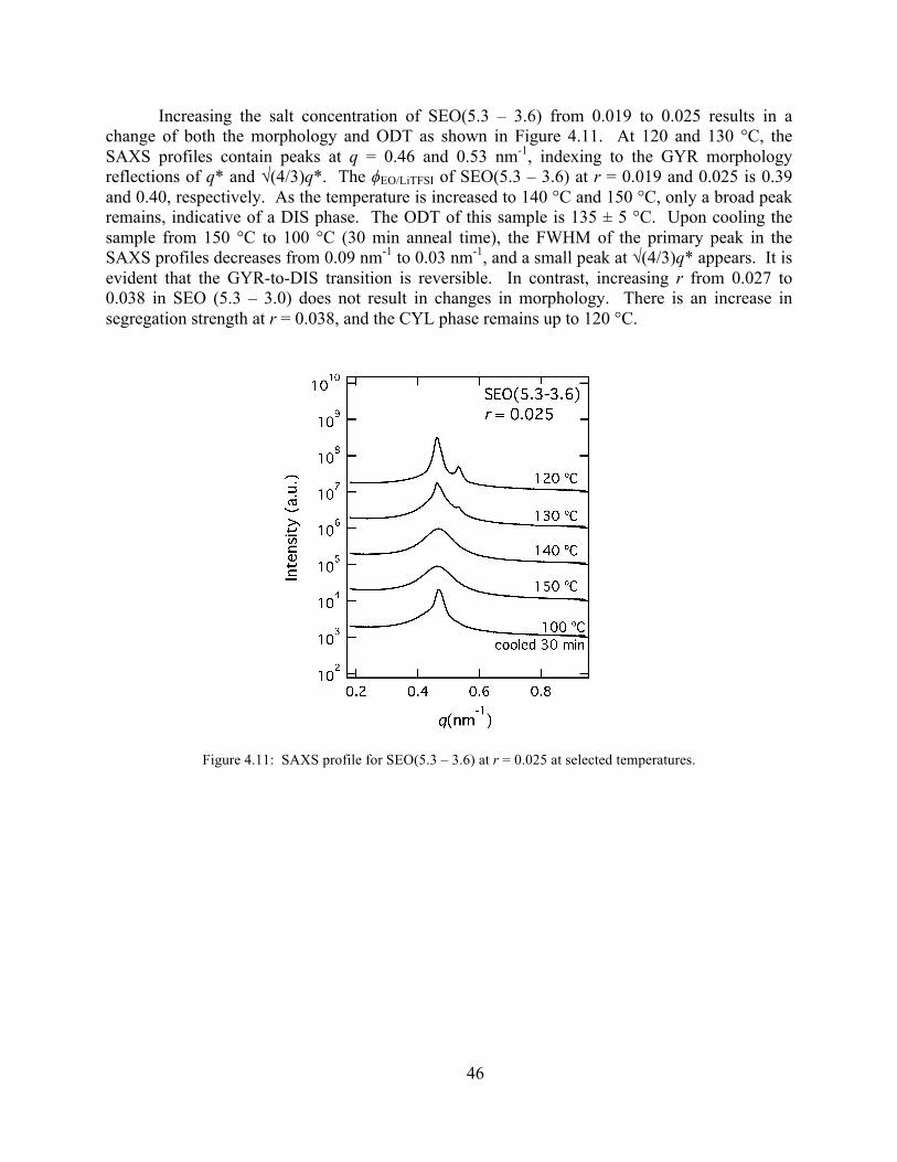
46

Increasing the salt concentration of SEO(5.3 – 3.6) from 0.019 to 0.025 results in a change of both the morphology and ODT as shown in Figure 4.11. At 120 and 130 °C, the SAXS profiles contain peaks at q = 0.46 and 0.53 nm-1, indexing to the GYR morphology reflections of q* and √(4/3)q*. The ϕEO/LiTFSI of SEO(5.3 – 3.6) at r = 0.019 and 0.025 is 0.39 and 0.40, respectively. As the temperature is increased to 140 °C and 150 °C, only a broad peak remains, indicative of a DIS phase. The ODT of this sample is 135 ± 5 °C. Upon cooling the sample from 150 °C to 100 °C (30 min anneal time), the FWHM of the primary peak in the SAXS profiles decreases from 0.09 nm-1 to 0.03 nm-1, and a small peak at √(4/3)q* appears. It is evident that the GYR-to-DIS transition is reversible. In contrast, increasing r from 0.027 to 0.038 in SEO (5.3 – 3.0) does not result in changes in morphology. There is an increase in segregation strength at r = 0.038, and the CYL phase remains up to 120 °C.

Figure 4.11: SAXS profile for SEO(5.3 – 3.6) at r = 0.025 at selected temperatures.

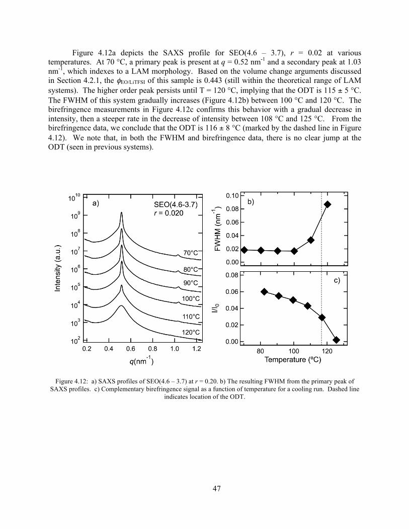
47

Figure 4.12a depicts the SAXS profile for SEO(4.6 – 3.7), r = 0.02 at various temperatures. At 70 °C, a primary peak is present at q = 0.52 nm-1 and a secondary peak at 1.03 nm-1, which indexes to a LAM morphology. Based on the volume change arguments discussed in Section 4.2.1, the φEO/LiTFSI of this sample is 0.443 (still within the theoretical range of LAM systems). The higher order peak persists until T = 120 °C, implying that the ODT is 115 ± 5 °C. The FWHM of this system gradually increases (Figure 4.12b) between 100 °C and 120 °C. The birefringence measurements in Figure 4.12c confirms this behavior with a gradual decrease in intensity, then a steeper rate in the decrease of intensity between 108 °C and 125 °C. From the birefringence data, we conclude that the ODT is 116 ± 8 °C (marked by the dashed line in Figure 4.12). We note that, in both the FWHM and birefringence data, there is no clear jump at the ODT (seen in previous systems).

Figure 4.12: a) SAXS profiles of SEO(4.6 – 3.7) at r = 0.20. b) The resulting FWHM from the primary peak of SAXS profiles. c) Complementary birefringence signal as a function of temperature for a cooling run. Dashed line

indicates location of the ODT.

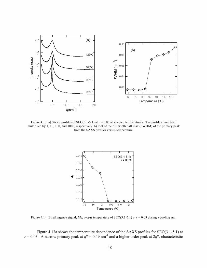
48

Figure 4.13: a) SAXS profiles of SEO(3.1-5.1) at r = 0.03 at selected temperatures. The profiles have been multiplied by 1, 10, 100, and 1000, respectively. b) Plot of the full width half max (FWHM) of the primary peak

from the SAXS profiles versus temperature.

Figure 4.14: Birefringence signal, I/I0, versus temperature of SEO(3.1-5.1) at r = 0.03 during a cooling run.

Figure 4.13a shows the temperature dependence of the SAXS profiles for SEO(3.1-5.1) at r = 0.03. A narrow primary peak at q* = 0.49 nm-1 and a higher order peak at 2q*, characteristic

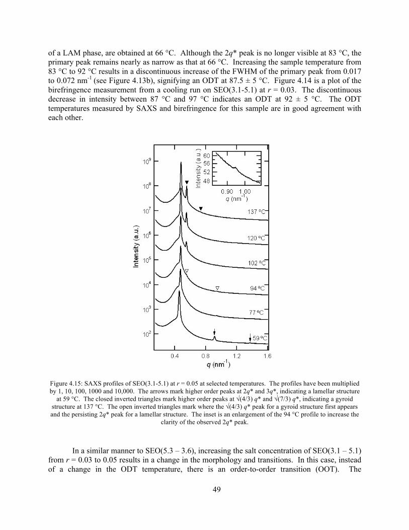
49

of a LAM phase, are obtained at 66 °C. Although the 2q* peak is no longer visible at 83 °C, the primary peak remains nearly as narrow as that at 66 °C. Increasing the sample temperature from 83 °C to 92 °C results in a discontinuous increase of the FWHM of the primary peak from 0.017 to 0.072 nm-1 (see Figure 4.13b), signifying an ODT at 87.5 ± 5 °C. Figure 4.14 is a plot of the birefringence measurement from a cooling run on SEO(3.1-5.1) at r = 0.03. The discontinuous decrease in intensity between 87 °C and 97 °C indicates an ODT at 92 ± 5 °C. The ODT temperatures measured by SAXS and birefringence for this sample are in good agreement with each other.

Figure 4.15: SAXS profiles of SEO(3.1-5.1) at r = 0.05 at selected temperatures. The profiles have been multiplied by 1, 10, 100, 1000 and 10,000. The arrows mark higher order peaks at 2q* and 3q*, indicating a lamellar structure

at 59 °C. The closed inverted triangles mark higher order peaks at √(4/3) q* and √(7/3) q*, indicating a gyroid structure at 137 °C. The open inverted triangles mark where the √(4/3) q* peak for a gyroid structure first appears and the persisting 2q* peak for a lamellar structure. The inset is an enlargement of the 94 °C profile to increase the

clarity of the observed 2q* peak.

In a similar manner to SEO(5.3 – 3.6), increasing the salt concentration of SEO(3.1 – 5.1) from r = 0.03 to 0.05 results in a change in the morphology and transitions. In this case, instead of a change in the ODT temperature, there is an order-to-order transition (OOT). The

50

temperature dependence of SAXS profiles for SEO(3.1-5.1) with r = 0.05 is shown in Figure 4.15. The higher order peaks at 2q* and 3q* seen at 59 °C (marked by arrows) indicate the presence of a LAM morphology. When the sample temperature is increased to 77 °C, the primary peak shifts from 0.456 to 0.475 nm-1. Further increase in sample temp to 94 °C results in the appearance of a new higher order peak at q = 0.548 nm-1. In addition, the higher order peak at 2q* persists (see inset of Figure 4.15). Further increase in sample temperature leads to an increase in the intensity of the higher order peak at q = 0.548 nm-1 and a reduction in the intensity of the peak at 2q*. The peaks at 137 °C are readily indexed as q*, √(4/3) q*, and √(7/3) q*, characteristic of scattering from a gyroid (GYR) phase. The SAXS data at temperatures between 77 and 137 °C show coexisting LAM and GYR phases. DSC data reveal that SEO(3.1-5.1) at r = 0.05 has a melting temperature of 42 °C and a crystallization temperature of 6 °C, well below the temperature range of the SAXS experiments. We thus do not believe that the LAM phase in our system is induced by crystallization as has been reported for different SEO copolymers in refs 54 and 55.

Birefringence can be used to study the LAM-GYR OOT because the LAM phase is birefringent while the GYR phase is not.[23-25] Equilibrated birefringence data obtained from SEO(3.1-5.1) with r = 0.05 after step increases in sample temperature are shown in Figure 4.16. The birefringence signal decreases continuously over a temperature range from 52 to 106 °C and is independent of temperature at temperatures above 106 °C. This is in contrast to previous birefringence studies of gyroid phases in diblock copolymer solutions where discontinuous changes in the signal were seen at the OOT.[23-25] The time-dependence of the birefringence signal obtained after step decreases in temperature are shown in Figure 4.17. Above 106 °C the birefringence signal is low and insensitive to changes in temperature except for a small overshoot at the beginning of temperature jumps. At temperatures below 106 °C, the birefringence increases after the temperature is lowered in the first 10 min or so after the quench and then reaches a time-independent plateau. We interpret the increase in signal to reflect conversion of some of the GYR grains into LAM. The coexistence of LAM and GYR at the phase boundary between the LAM and GYR phases is required by the Gibbs phase rule for binary mixtures. This coexistence may reflect the preferential partitioning of salt ions in either LAM or GYR phases. On the other hand, the coexistence of LAM and GYR may reflect the slow kinetics of OOTs involving the GYR phase, as has been noted in previous studies on pure diblock copolymers.[26, 27]

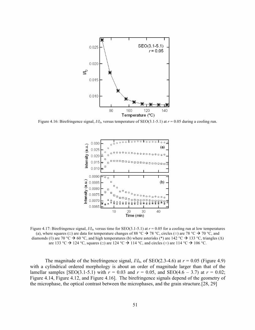
51

Figure 4.16: Birefringence signal, I/I0, versus temperature of SEO(3.1-5.1) at r = 0.05 during a cooling run.

Figure 4.17: Birefringence signal, I/I0, versus time for SEO(3.1-5.1) at r = 0.05 for a cooling run at low temperatures (a), where squares (□) are data for temperature changes of 88 °C 78 °C, circles (○) are 78 °C 70 °C, and

diamonds (◊) are 70 °C 60 °C, and high temperatures (b) where asterisks (*) are 142 °C 133 °C, triangles (Δ) are 133 °C 124 °C, squares (□) are 124 °C 114 °C, and circles (○) are 114 °C 106 °C.

The magnitude of the birefringence signal, I/I0, of SEO(2.3-4.6) at r = 0.05 (Figure 4.9) with a cylindrical ordered morphology is about an order of magnitude larger than that of the lamellar samples [SEO(3.1-5.1) with r = 0.03 and r = 0.05, and SEO(4.6 – 3.7) at r = 0.02; Figure 4.14, Figure 4.12, and Figure 4.16]. The birefringence signals depend of the geometry of the microphase, the optical contrast between the microphases, and the grain structure.[28, 29]

52

A summary of the phase transitions measured using SAXS and birefringence is given in Table 4.2. With the help of these data, we can create phase diagrams of the polymer/salt systems (Section 4.4) and calculate values of the effective χ parameter (Section 5.5).

Table 4.2: Summary of SEO/LiTFSI systems with transitions.

Polymer r Phase 1 Transition temperature Phase 2

SEO(6.4  –  7.2)   0   LAM   95  °C   DIS  SEO(5.3  –  3.6)   0.019   CYL   95  °C   DIS  SEO(4.6  –  3.7)   0.020   LAM   116  °C   DIS  SEO(5.3  –  3.6)   0.025   GYR   135  °C   DIS  SEO(5.3  –  3.0)   0.027   CYL   105  °C   DIS  SEO(3.1  –  5.1)   0.03   LAM   92  °C   DIS  SEO(2.3  –  4.6)   0.05   CYL   135  °C   DIS  SEO(3.1  –  5.1)   0.05   GYR   52  –  106  °C   LAM  

4.3.2 Coexistence of ordered and disordered phases

In some cases, it appears that the primary peak in a SAXS profiles is a supaposition of a broad peak and a narrow peak. An example of this is shown in Figure 4.18 where we show data obtained from SEO(2.3-4.6) at r = 0.05 at 117 oC. There are at least two possible explanations for this observation. (1) A coexistence of a disordered phase and an ordered phase, accompanied by a partitioning of the salt in the ordered domains as depicted in Figure 4.19a. (2) All of the sample is ordered but the lithium is not uniformly distributed in the PEO microphase as depicted in Figure 4.19b.

Figure 4.18: Background-subtracted SAXS intensity I-Ib versus scattering vector q of SEO(2.3-4.6) at r = 0.05 at T = 117 oC. The symbols represent the data and the curve is a least squares fit to equation (4.1).

53

In case (1), the disordered phase would contribute to the broad peak while the ordered phase would contribute to the narrow peak. Since the volume fraction of the ordered phase is expected to increase with quench depth below the ODT, we would expect the contribution due to the narrow peak to increase rapidly as TODT - T increases. If, instead, the lithium-rich domains were more ordered than the PEO domains as shown schematically in Figure 4.19b, then they would contribute to the sharp peak while the block copolymer microphases would contribute to the broad peak. There is evidence for the non-uniform distribution of lithium in PEO microphases of SEO/LiTFSI mixtures from energy-filtered transmission electron microscopy images.[9] For this scenario, the fraction of the SAXS signal attributable to the narrow peak would be independent of quench depth.

Figure 4.19: Schematic representations of two possible scenarios for the structure of weakly ordered SEO/LiTFSI mixtures. Light gray corresponds to the PEO phase, black corresponds to the PS phase, and medium gray circles represent LiTFSI. (a) Coexistence of an ordered and disordered phase. (b) Thin well-ordered lithium channels

within the PEO domain.

In an attempt to resolve which explanation is correct, a summation of a sharp Gaussian peak and a broad Lorentzian peak is fit to the primary peak after subtracting a decaying background:

(4.1)

The first expression on the right hand side is the Gaussian, G(q), contribution while the second term is the Lorentzian, L(q), contribution. The background term was determined by

fitting the equation to the data with the peak masked, using I0, A0, and c0 as

the fitting parameters. The resulting I(q)-Ib data were fit to equation 4-1 with A1, A2, x1, x2, c1, and c2 as fitting parameters. The relative contributions from the Gaussian and Lorentzian peaks

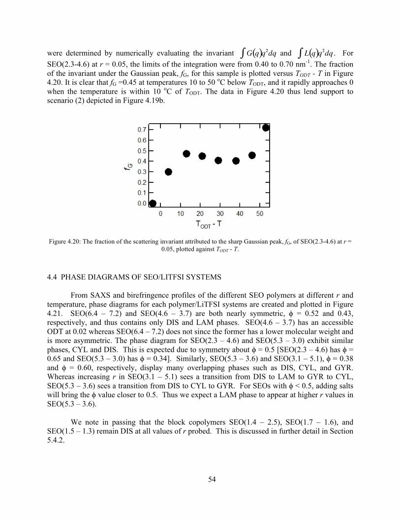
54

were determined by numerically evaluating the invariant and . For

SEO(2.3-4.6) at r = 0.05, the limits of the integration were from 0.40 to 0.70 nm-1. The fraction of the invariant under the Gaussian peak, fG, for this sample is plotted versus TODT - T in Figure 4.20. It is clear that fG =0.45 at temperatures 10 to 50 oC below TODT, and it rapidly approaches 0 when the temperature is within 10 oC of TODT. The data in Figure 4.20 thus lend support to scenario (2) depicted in Figure 4.19b.

Figure 4.20: The fraction of the scattering invariant attributed to the sharp Gaussian peak, fG, of SEO(2.3-4.6) at r = 0.05, plotted against TODT - T.

4.4 PHASE DIAGRAMS OF SEO/LITFSI SYSTEMS

From SAXS and birefringence profiles of the different SEO polymers at different r and temperature, phase diagrams for each polymer/LiTFSI systems are created and plotted in Figure 4.21. SEO(6.4 – 7.2) and SEO(4.6 – 3.7) are both nearly symmetric, ϕ = 0.52 and 0.43, respectively, and thus contains only DIS and LAM phases. SEO(4.6 – 3.7) has an accessible ODT at 0.02 whereas SEO(6.4 – 7.2) does not since the former has a lower molecular weight and is more asymmetric. The phase diagram for SEO(2.3 – 4.6) and SEO(5.3 – 3.0) exhibit similar phases, CYL and DIS. This is expected due to symmetry about ϕ = 0.5 [SEO(2.3 – 4.6) has ϕ = 0.65 and SEO(5.3 – 3.0) has ϕ = 0.34]. Similarly, SEO(5.3 – 3.6) and SEO(3.1 – 5.1), ϕ = 0.38 and ϕ = 0.60, respectively, display many overlapping phases such as DIS, CYL, and GYR. Whereas increasing r in SEO(3.1 – 5.1) sees a transition from DIS to LAM to GYR to CYL, SEO(5.3 – 3.6) sees a transition from DIS to CYL to GYR. For SEOs with ϕ < 0.5, adding salts will bring the ϕ value closer to 0.5. Thus we expect a LAM phase to appear at higher r values in SEO(5.3 – 3.6).

We note in passing that the block copolymers SEO(1.4 – 2.5), SEO(1.7 – 1.6), and SEO(1.5 – 1.3) remain DIS at all values of r probed. This is discussed in further detail in Section 5.4.2.

55

Figure 4.21: Phase diagrams of various SEO/LiTFSI combinations. The dotted lines are estimated locations of phase boundaries and the asterisks are locations of ODTs. The morphologies include LAM (), DIS (), CYL

(), GYR (), and LAM/GYR coexistence ().

56

4.5 CONCLUSIONS

The effect of the salt LiTFSI on the thermal properties and morphology of poly(styrene-block-ethylene oxide) copolymers was investigated. From DSC measurements, it was determined that the LiTFSI suppresses the crystallinity of the PEO block. This behavior is in agreement with literature for PEO/LiTFSI phase behavior indicating that the LiTFSI resides mainly in the PEO phase. There was a general increase in the domain size of a nearly symmetric SEO with a lamellar structure upon addition of salt as measured from small-angle Xray scattering (SAXS). This was attributed mostly to the free volume of the salt. However, from the salt concentration of r = 0.085 to 0.10, the domain size does not increase as rapidly as from r = 0 to 0.085. This was attributed to the increased coordination of Li+ ions to the oxygens in the PEO backbone. This behavior was not seen in previous studies of PEO-containing block copolymers with LiClO4. The appearance of the 2q* peak in SAXS profiles with increasing LiTFSI indicates that the increase in domain size is asymmetric, probably due to the LiTFSI partitioning into the PEO-rich domain.

SAXS and optical birefringence measurements were also used to map out phase diagrams, order-to-disorder transitions (ODTs), and order-to-order transitions (OOTs) of various SEO/LiTFSI systems. It is clear that adding LiTFSI to SEO increases the effective χ parameter between the polystyrene and polyethylene oxide-rich phases. Furthermore, a rich variety of phases is accessed with the addition of LiTFSI into an initially disordered SEO system.

4.6 REFERENCES

1. Lascaud, S., et al., Phase-Diagrams and Conductivity Behavior of Poly(Ethylene Oxide)

Molten-Salt Rubbery Electrolytes. Macromolecules, 1994. 27(25): p. 7469-7477. 2. Porter, C.H. and R.H. Boyd, Dielectric Study of Effects of Melting on Molecular

Relaxation in Poly(Ethylene Oxide) and Polyoxymethylene. Macromolecules, 1971. 4(5): p. 589-&.

3. Abraham, K.M., Z. Jiang, and B. Carroll, Highly conductive PEO-like polymer electrolytes. Chemistry of Materials, 1997. 9(9): p. 1978-1988.

4. Kumar, M. and S.S. Sekhon, Role of plasticizer's dielectric constant on conductivity modification of PEO-NH4F polymer electrolytes. European Polymer Journal, 2002. 38(7): p. 1297-1304.

5. Gray, F.M., C.A. Vincent, and M. Kent, A Study of the Dielectric-Properties of the Polymer Electrolyte Peo-Liclo4 over a Composition Range Using Time Domain Spectroscopy. Journal of Polymer Science Part B-Polymer Physics, 1989. 27(10): p. 2011-2022.

57

6. Yano, O. and Y. Wada, Dynamic Mechanical and Dielectric Relaxations of Polystyrene Below Glass Temperature. Journal of Polymer Science Part a-2-Polymer Physics, 1971. 9(4): p. 669-&.

7. Yu, S.Z. and P. Hing, Dynamic mechanical properties of polystyrene-aluminum nitride composite. Journal of Applied Polymer Science, 2000. 78(7): p. 1348-1353.

8. Simone, P.M. and T.P. Lodge, Phase Behavior and Ionic Conductivity of Concentrated Solutions of Polystyrene-Poly(ethylene oxide) Diblock Copolymers in an Ionic Liquid. Acs Applied Materials & Interfaces, 2009. 1(12): p. 2812-2820.

9. Gomez, E.D., et al., Effect of Ion Distribution on Conductivity of Block Copolymer Electrolytes. Nano Letters, 2009. 9(3): p. 1212-1216.

10. Borodin, O. and G.D. Smith, Mechanism of Ion Transport in Amorphous Poly(ethylene oxide)/LiTFSI from Molecular Dynamics Simulations. Macromolecules, 2006. 39(4): p. 1620-1629.

11. Blanchard, L.-P., J. Hesse, and S.L. Malhotra, Effect of Molecular Weight on Glass Transition by Differential Scanning Calorimetry. Canadian Journal of Chemistry, 1974. 52: p. 3170-3175.

12. Edman, L., et al., Transport properties of the solid polymer electrolyte system P(EO)(n)LiTFSI. Journal of Physical Chemistry B, 2000. 104(15): p. 3476-3480.

13. Lee, D.H., et al., Swelling and shrinkage of lamellar domain of conformationally restricted block copolymers by metal chloride. Macromolecules, 2006. 39(6): p. 2027-2030.

14. Kang, Y., et al., Broad-wavelength-range chemically tunable block-copolymer photonic gels. Nat Mater, 2007. 6(12): p. 957-960.

15. Singh, M., et al., Effect of molecular weight on the mechanical and electrical properties of block copolymer electrolytes. Macromolecules, 2007. 40(13): p. 4578-4585.

16. Mao, G.M., et al., Structure of liquid PEO-LiTFSI electrolyte. Physical Review Letters, 2000. 84(24): p. 5536-5539.

17. Epps, T.H., et al., Phase behavior and block sequence effects in lithium perchlorate-doped poly(isoprene-b-styrene-b-ethylene oxide) and poly(styrene-b-isoprene-b-ethylene oxide) triblock copolymers. Macromolecules, 2003. 36(8): p. 2873-2881.

18. Garetz, B.A., et al., Birefringence and Diffraction of Light in Ordered Block-Copolymer Materials. Macromolecules, 1993. 26(12): p. 3151-3155.

19. Floudas, G., et al., Poly(ethylene oxide-b-isoprene) diblock copolymer phase diagram. Macromolecules, 2001. 34(9): p. 2947-2957.

20. Khandpur, A.K., et al., Polyisoprene-polystyrene diblock copolymer phase diagram near the order-disorder transition. Macromolecules, 1995. 28(26): p. 8796-8806.

21. Balsara, N.P., B.A. Garetz, and H.J. Dai, Relationship between Birefringence and the Structure of Ordered Block Copolymer Materials. Macromolecules, 1992. 25(22): p. 6072-6074.

58

22. Balsara, N.P., et al., Birefringence Detection of the Order-to-Disorder Transition in Block Copolymer Liquids. Macromolecules, 1992. 25(15): p. 3896-3901.

23. Lodge, T.P., et al., Phase behavior of block copolymers in a neutral solvent. Macromolecules, 2003. 36(3): p. 816-822.

24. Hanley, K.J., T.P. Lodge, and C.I. Huang, Phase behavior of a block copolymer in solvents of varying selectivity. Macromolecules, 2000. 33(16): p. 5918-5931.

25. Lodge, T.P., B. Pudil, and K.J. Hanley, The full phase behavior for block copolymers in solvents of varying selectivity. Macromolecules, 2002. 35(12): p. 4707-4717.

26. Hajduk, D.A., et al., Stability of the perforated layer (PL) phase in diblock copolymer melts. Macromolecules, 1997. 30(13): p. 3788-3795.

27. Hajduk, D.A., et al., The Gyroid - a New Equilibrium Morphology in Weakly Segregated Diblock Copolymers. Macromolecules, 1994. 27(15): p. 4063-4075.

28. Kim, W.G., et al., Effect of quench depth on grain structure in quiescently ordered block copolymers. Journal of Chemical Physics, 2001. 114(22): p. 10196-10211.

29. Newstein, M.C., et al., Light-Scattering and Microscopy from Block-Copolymers with Cylindrical Morphology. Macromolecules, 1995. 28(13): p. 4587-4597.

59

Chapter 5

Comparison of Salts and Ionic Liquids on the Thermodynamics of PEO-containing Block Copolymers

ABSTRACT

We report on the thermal properties, phase behavior, and thermodynamics of a series of polystyrene-block-polyethylene oxide copolymers (SEO) mixed with the ionic species Li[N(SO2CF3)2] (LiTFSI), imidazolium TFSI (ImTFSI), and an equimolar mixture of LiTFSI and ImTFSI (Mix). Differential scanning calorimetric scans reveal similar thermal behavior of SEO/LiTFSI and SEO/ImTFSI at the same salt concentrations. Phase behavior and thermodynamics were determined using a combination of small-angle x-ray scattering and birefringence. The thermodynamics of our mixtures can be mapped on to the theory of neat block copolymer phase behavior provided the Flory-Huggins interaction parameter, χ, between the blocks is replaced by an effective χ (χeff) that increases linearly with salt concentration. The phase behavior and the value of m, the slope of the χeff versus salt concentration data, were similar for SEO/LiTFSI, SEO/ImTFSI, and SEO/Mix blends. The theory developed by Wang [J. Phys. Chem. B. 2008 41, 16205] provides a basis for understanding the fundamental underpinnings of the measured value of m. We compare our experimental results with the predictions of this theory with no adjustable parameters.

5.1 SALTS AND IONIC LIQUIDS IN POLYMER ELECTROLYTE MEMBRANES

The use of PEO and PEO-containing polymers as a viable solid electrolyte is still limited by the room temperature ionic conductivity. Sufficient conductivity values are only achieved at temperatures well above the melting temperature of PEO since high conductivity occurs in the amorphous state.[1] By using the salt, LiTFSI, conductivity values which are several-fold higher than that of PEO with LiClO4 or LiCF3SO3 can be achieved at room temperature. This is principally due to the large TFSI- anion, which have high charge delocalization allowing for greater dissociation.[2] Furthermore, the salt acts as a plasticizer of the PEO allowing for a large region of PEO/LiTFSI mixtures to be amorphous at room temperature.[3]

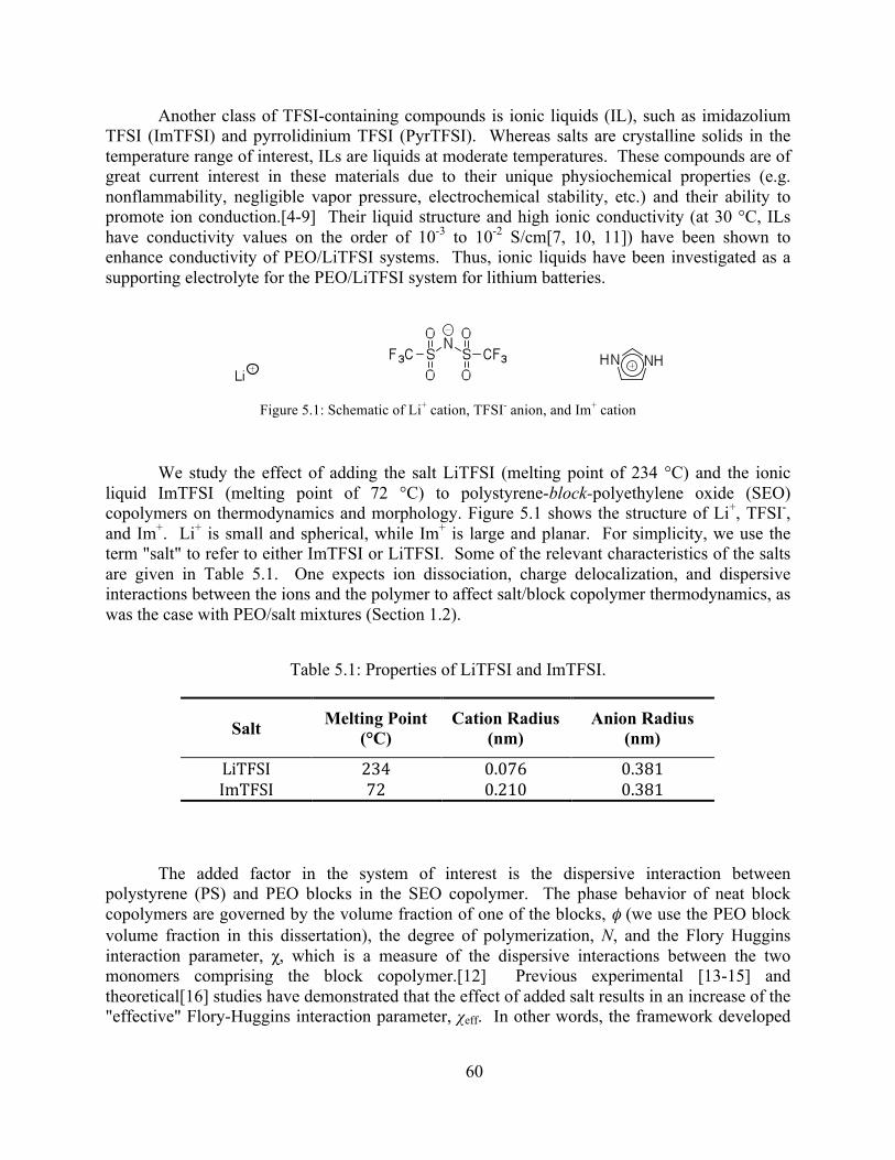
60

Another class of TFSI-containing compounds is ionic liquids (IL), such as imidazolium TFSI (ImTFSI) and pyrrolidinium TFSI (PyrTFSI). Whereas salts are crystalline solids in the temperature range of interest, ILs are liquids at moderate temperatures. These compounds are of great current interest in these materials due to their unique physiochemical properties (e.g. nonflammability, negligible vapor pressure, electrochemical stability, etc.) and their ability to promote ion conduction.[4-9] Their liquid structure and high ionic conductivity (at 30 °C, ILs have conductivity values on the order of 10-3 to 10-2 S/cm[7, 10, 11]) have been shown to enhance conductivity of PEO/LiTFSI systems. Thus, ionic liquids have been investigated as a supporting electrolyte for the PEO/LiTFSI system for lithium batteries.

Figure 5.1: Schematic of Li+ cation, TFSI- anion, and Im+ cation

We study the effect of adding the salt LiTFSI (melting point of 234 °C) and the ionic liquid ImTFSI (melting point of 72 °C) to polystyrene-block-polyethylene oxide (SEO) copolymers on thermodynamics and morphology. Figure 5.1 shows the structure of Li+, TFSI-, and Im+. Li+ is small and spherical, while Im+ is large and planar. For simplicity, we use the term "salt" to refer to either ImTFSI or LiTFSI. Some of the relevant characteristics of the salts are given in Table 5.1. One expects ion dissociation, charge delocalization, and dispersive interactions between the ions and the polymer to affect salt/block copolymer thermodynamics, as was the case with PEO/salt mixtures (Section 1.2).

Table 5.1: Properties of LiTFSI and ImTFSI.

Salt Melting Point (°C)

Cation Radius (nm)

Anion Radius (nm)

LiTFSI   234   0.076   0.381  ImTFSI   72   0.210   0.381  

The added factor in the system of interest is the dispersive interaction between polystyrene (PS) and PEO blocks in the SEO copolymer. The phase behavior of neat block copolymers are governed by the volume fraction of one of the blocks, φ (we use the PEO block volume fraction in this dissertation), the degree of polymerization, N, and the Flory Huggins interaction parameter, χ, which is a measure of the dispersive interactions between the two monomers comprising the block copolymer.[12] Previous experimental [13-15] and theoretical[16] studies have demonstrated that the effect of added salt results in an increase of the "effective" Flory-Huggins interaction parameter, χeff. In other words, the framework developed

61

for describing the thermodynamics of neat block copolymers can be used to describe the thermodynamics of block copolymer/salt mixtures provided χ is replaced by χeff. Similar concepts were used to describe the thermodynamic properties of block copolymer solvent mixtures.[17-20] Since the added salt resides primarily in one of the phases, the concomitant changes in φ must also be accounted for. In addition, a simple linear relationship between χeff and r has been proposed:

(5.1)

where χneat is the Flory-Huggins interaction parameter of the neat copolymer, and m is a system-dependent constant. The effect of salt addition on block copolymer thermodynamics is quantified by the magnitude of m. In the case of LiCl added to polystyrene-block-polymethylmethacrylate (SMMA) copolymers, χeff increases from 0.0360 to 0.0368, when r increases from 0 to 0.1, indicating that m is about 10-4.[13] Young et al. found that values of m in the cases of LiAsF6, LiClO4 and LiCF3SO3 in SEO copolymers are 5.70, 5.53 and 3.90, respectively.[14] Young et al. noted that the effective repulsion between the blocks gets weaker as the Lewis basicity of the anion decreases. In our previous publication, Wanakule et al. reported that m for SEO/LiTFSI is 1.56.[15] The data obtained in ref. [15] is consistent with the arguments of Young et al. There is considerable uncertainty in the determination of salt concentration in the SMMA/LiCl mixtures as it was obtained by spectroscopy owing to the immiscibility of the salt in the polymer.[13] No such difficulty arises in the case of mixtures of SEO and lithium salts and the salt concentration can readily be determined gravimetrically. The effect of this on the four order of magnitude difference in the measured values of m in SMMA and SEO is unclear.

Theoretical work by Wang [16] indicates that m can be calculated using independently determined parameters such as the dielectric constants of the two phases, the size of the ions, the extent of dissociation, the dielectric constant of the block copolymer microphases, and the statistical segment lengths of the copolymer chains. Here, we compare m from our experimental data and that reported in ref. [14] with the predictions of the theory developed in ref [16] without resorting to any adjustable parameters.

5.2 SAMPLE PREPARATION

The polystyrene-block-poly(ethylene oxide) copolymers used in this study were synthesized by sequential living polymerization using the methods described in refs [21-23]. LiTFSI salt, purchased from Sigma Aldrich, was heated at 100 °C under vacuum for 1-2 days to get rid of residual moisture and then stored in the glovebox. Imidazole (≥95%) and bis(trifluoromethane)sulfonimide (HTFSI, ≥95%) were purchased from Sigma Aldrich and

purified by sublimation under vacuum. Differential scanning calorimetry (DSC) and 1H NMR were used to assess the purity of the two starting materials. Purified imidazole and HTFSI

€

χeff = χneat +m⋅ r

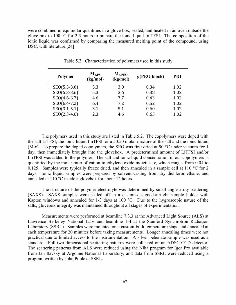
62

were combined in equimolar quantities in a glove box, sealed, and heated in an oven outside the glove box to 100 oC for 2-3 hours to prepare the ionic liquid ImTFSI. The composition of the ionic liquid was confirmed by comparing the measured melting point of the compound, using DSC, with literature.[24]

Table 5.2: Characterization of polymers used in this study

Polymer Mn,PS (kg/mol)

Mn,PEO (kg/mol) φ(PEO block)   PDI

SEO(5.3-­‐3.0)   5.3   3.0   0.34   1.02  SEO(5.3-­‐3.6)   5.3   3.6   0.38   1.02  SEO(4.6-­‐3.7)   4.6   3.7   0.43   1.02  SEO(6.4-­‐7.2)   6.4   7.2   0.52   1.02  SEO(3.1-­‐5.1)   3.1   5.1   0.60   1.02  SEO(2.3-­‐4.6)   2.3   4.6   0.65   1.02  

The polymers used in this study are listed in Table 5.2. The copolymers were doped with the salt LiTFSI, the ionic liquid ImTFSI, or a 50:50 molar mixture of the salt and the ionic liquid (Mix). To prepare the doped copolymers, the SEO was first dried at 90 °C under vacuum for 1 day, then immediately brought into the glovebox. A predetermined amount of LiTFSI and/or ImTFSI was added to the polymer. The salt and ionic liquid concentration in our copolymers is quantified by the molar ratio of cation to ethylene oxide moieties, r, which ranges from 0.01 to 0.125. Samples were typically freeze dried, and then annealed in a sample cell at 110 °C for 2 days. Ionic liquid samples were prepared by solvent casting from dry dichloromethane, and annealed at 110 °C inside a glovebox for about 12 hours.

The structure of the polymer electrolyte was determined by small angle x-ray scattering (SAXS). SAXS samples were sealed off in a custom-designed-airtight sample holder with Kapton windows and annealed for 1-3 days at 100 °C. Due to the hygroscopic nature of the salts, glovebox integrity was maintained throughout all stages of experimentation.

Measurements were performed at beamline 7.3.3 at the Advanced Light Source (ALS) at Lawrence Berkeley National Labs and beamline 1-4 at the Stanford Synchrotron Radiation Laboratory (SSRL). Samples were mounted on a custom-built temperature stage and annealed at each temperature for 20 minutes before taking measurements. Longer annealing times were not practical due to limited access to the instrumentation. A silver behenate sample was used as a standard. Full two-dimensional scattering patterns were collected on an ADSC CCD detector. The scattering patterns from ALS were reduced using the Nika program for Igor Pro available from Jan Ilavsky at Argonne National Laboratory, and data from SSRL were reduced using a program written by John Pople at SSRL.

63

Order-to-disorder transition (ODT) temperatures were confirmed using birefringence. Birefringence measurements were performed using the setup described in ref [25] with a plane-polarized laser beam with wavelength 633 nm as the source. The samples were subjected to two heating and cooling cycles with temperature steps of approximately 10 °C. Minimum annealing times for the heating and cooling runs at each temperature were 20 and 45 minutes, respectively. The intensity of the beam after it passed through the sample and the two crossed polarizers was recorded with a photodiode as a function of temperature, and then normalized by the incident intensity.

Differential scanning calorimetry (DSC) was performed on a TA Instruments DSC 2920. The samples were crimped in a glove box using hermetically sealed pans and placed inside a container with desiccant for transfer to the DSC. Indium and dodecane were used as calibration standards for the DSC. Samples underwent three heating and cooling cycles.

5.3 THERMAL PROPERTIES AND PHASE BEHAVIOR

We first focus on the thermal properties of SEO with LiTFSI and ImTFSI. Figure 5.2a and b show DSC scans of SEO(6.4-7.2) with varying concentrations of LiTFSI and SEO(3.1-5.1) with varying levels of ImTFSI, respectively, at 5 oC/min. The melting point of the PEO/salt microphase and the enthalpy of melting, ΔHm, decrease with increasing r in both SEO/LiTFSI and SEO/ImTFSI. The melting peak decreases from 50 to 40 oC as r is increased from 0 to 0.05, while ΔHm values decrease from 55 J/g to 19 J/g in SEO(6.4-7.2)/LiTFSI and 63 J/g to 32 J/g in SEO(3.1-5.1)/ImTFSI. At r values higher than 0.05, we observe complete suppression of crystallinity. This behavior is consistent with observations of Lascaud et al. on PEO/LiTFSI homopolymer/salt mixtures.[3] They measured a decrease in melting temperatures with increasing salt concentration up to r = 0.08. Between r = 0.08 to 0.17, a crystallinity gap appears in the PEO/LiTFSI phase diagram. The fact that the phase behavior of SEO/LiTFSI and SEO/ImTFSI data agrees with PEO/LiTFSI data indicates that the salts are preferentially segregating to the PEO-rich domains. This is due to the higher dielectric constant, ε, of the PEO domain (estimates of εPEO range from 4 to 8,[26-29] while that of εPS ranges from 2 to 4[30, 31]), and specific interactions between the ether oxygens and the cation.[11, 32]

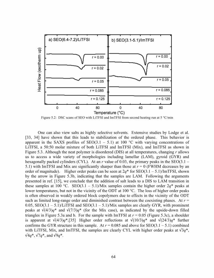
64

Figure 5.2: DSC scans of SEO with LiTFSI and ImTFSI from second heating run at 5 °C/min

One can also view salts as highly selective solvents. Extensive studies by Lodge et al. [33, 34] have shown that this leads to stabilization of the ordered phase. This behavior is apparent in the SAXS profiles of SEO(3.1 – 5.1) at 100 °C with varying concentrations of LiTFSI, a 50:50 molar mixture of both LiTFSI and ImTFSI (Mix), and ImTFSI as shown in Figure 5.3. Although the neat polymer is disordered (DIS) at all temperatures, changing r allows us to access a wide variety of morphologies including lamellar (LAM), gyroid (GYR) and hexagonally packed cylinders (CYL). At an r value of 0.03, the primary peaks in the SEO(3.1 – 5.1) with ImTFSI and Mix are significantly sharper than those at r = 0 (FWHM decreases by an order of magnitude). Higher order peaks can be seen at 2q* for SEO(3.1 – 5.1)/ImTFSI, shown by the arrow in Figure 5.3b, indicating that the samples are LAM. Following the arguments presented in ref. [15], we conclude that the addition of salt leads to a DIS to LAM transition in these samples at 100 °C. SEO(3.1 – 5.1)/Mix samples contain the higher order 2q* peaks at lower temperatures, but not in the vicinity of the ODT at 100 °C. The loss of higher order peaks is often observed in weakly ordered block copolymers due to effects in the vicinity of the ODT such as limited long-range order and diminished contrast between the coexisting phases. At r = 0.05, SEO(3.1 – 5.1)/LiTFSI and SEO(3.1 – 5.1)/Mix samples are clearly GYR, with prominent peaks at √(4/3)q* and √(7/3)q* (for the Mix case), as indicated by the upside-down filled triangles in Figure 5.3a and b. For the sample with ImTFSI at r = 0.05 (Figure 5.3c), a shoulder is apparent at √(4/3)q*.[35] Higher order reflections at √(10/3)q* and √(24/3)q* further confirms the GYR structure in this sample. At r = 0.085 and above for SEO(3.1 – 5.1) combined with LiTFSI, Mix, and ImTFSI, the samples are clearly CYL with higher order peaks at √3q*, √4q*, √7q*, and √9q*.

65

Figure 5.3: SAXS profiles at 100 °C for SEO(3.1 – 5.1) mixed with a) LiTFSI, b) 50:50 mixture of both, and c) ImTFSI at various salt concentrations. Arrows indicate higher order LAM reflections, closed upside-down triangles

indexes to GYR morphology, and open upside-down triangles indicate higher order CYL reflections.

Similar experiments were carried out over a range of temperatures between 70 and 150 °C, and a phase diagram (Figure 5.4) was constructed using SAXS profiles of SEO(3.1 – 5.1) with LiTFSI and ImTFSI at r = 0, 0.02, 0.03, 0.05, 0.085, and 0.125. Note that we generalize the definition of r to be the ratio of all cations to EO monomers in the mixtures. Also shown as the top axes of Figure 5.4a and b is the calculated volume fraction of the PEO-rich phase, φEO/Salt, in the presence (or absence) of salt. The changes in φEO/Salt due to changes in r were calculated using the relationship between the density of PEO/LiTFSI phase and salt concentration, as described in Section 4.2.1. Similar density data were not available for PEO/ImTFSI mixtures. We have assumed that the dependence of φEO/Salt on r for PEO/ImTFSI and PEO/LiTFSI are identical. The series of phase transitions shown in Figure 5.4 are the result of changes in both χeff and φEO/Salt with increasing r.

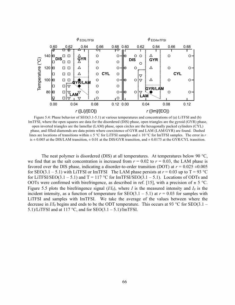
66

Figure 5.4: Phase behavior of SEO(3.1-5.1) at various temperatures and concentrations of (a) LiTFSI and (b) ImTFSI, where the open squares are data for the disordered (DIS) phase, open triangles are the gyroid (GYR) phase,

open inverted triangles are the lamellar (LAM) phase, open circles are the hexagonally packed cylinders (CYL) phase, and filled diamonds are data points where coexistence of GYR and LAM (LAM/GYR) are found. Dashed

lines are locations of transitions within ± 5 °C for LiTFSI samples and ± 10 °C for ImTFSI samples. The error in r is ± 0.005 at the DIS/LAM transition, ± 0.01 at the DIS/GYR transition, and ± 0.0175 at the GYR/CYL transition.

The neat polymer is disordered (DIS) at all temperatures. At temperatures below 90 °C, we find that as the salt concentration is increased from r = 0.02 to r = 0.03, the LAM phase is favored over the DIS phase, indicating a disorder-to-order transition (DOT) at r = 0.025 ±0.005 for SEO(3.1 – 5.1) with LiTFSI or ImTFSI The LAM phase persists at r = 0.03 up to T = 93 °C for LiTFSI/SEO(3.1 – 5.1) and T = 117 °C for ImTFSI/SEO(3.1 – 5.1). Locations of ODTs and OOTs were confirmed with birefringence, as described in ref. [15], with a precision of ± 5 °C. Figure 5.5 plots the birefringence signal (I/I0), where I is the measured intensity and I0 is the incident intensity, as a function of temperature for SEO(3.1 – 5.1) at r = 0.03 for samples with LiTFSI and samples with ImTFSI. We take the average of the values between where the decrease in I/I0 begins and ends to be the ODT temperature. This occurs at 93 °C for SEO(3.1 – 5.1)/LiTFSI and at 117 °C, and for SEO(3.1 – 5.1)/ImTFSI.

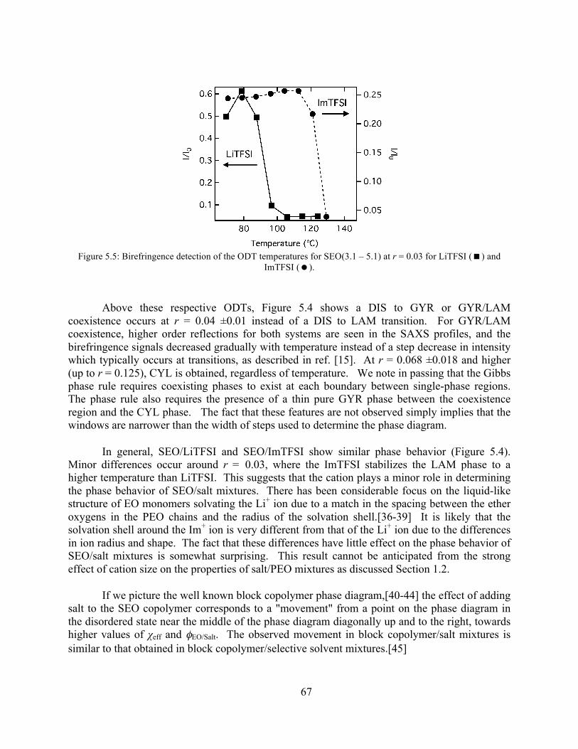
67

Figure 5.5: Birefringence detection of the ODT temperatures for SEO(3.1 – 5.1) at r = 0.03 for LiTFSI () and ImTFSI ().

Above these respective ODTs, Figure 5.4 shows a DIS to GYR or GYR/LAM coexistence occurs at r = 0.04 ±0.01 instead of a DIS to LAM transition. For GYR/LAM coexistence, higher order reflections for both systems are seen in the SAXS profiles, and the birefringence signals decreased gradually with temperature instead of a step decrease in intensity which typically occurs at transitions, as described in ref. [15]. At r = 0.068 ±0.018 and higher (up to r = 0.125), CYL is obtained, regardless of temperature. We note in passing that the Gibbs phase rule requires coexisting phases to exist at each boundary between single-phase regions. The phase rule also requires the presence of a thin pure GYR phase between the coexistence region and the CYL phase. The fact that these features are not observed simply implies that the windows are narrower than the width of steps used to determine the phase diagram.

In general, SEO/LiTFSI and SEO/ImTFSI show similar phase behavior (Figure 5.4). Minor differences occur around r = 0.03, where the ImTFSI stabilizes the LAM phase to a higher temperature than LiTFSI. This suggests that the cation plays a minor role in determining the phase behavior of SEO/salt mixtures. There has been considerable focus on the liquid-like structure of EO monomers solvating the Li+ ion due to a match in the spacing between the ether oxygens in the PEO chains and the radius of the solvation shell.[36-39] It is likely that the solvation shell around the Im+ ion is very different from that of the Li+ ion due to the differences in ion radius and shape. The fact that these differences have little effect on the phase behavior of SEO/salt mixtures is somewhat surprising. This result cannot be anticipated from the strong effect of cation size on the properties of salt/PEO mixtures as discussed Section 1.2.

If we picture the well known block copolymer phase diagram,[40-44] the effect of adding salt to the SEO copolymer corresponds to a "movement" from a point on the phase diagram in the disordered state near the middle of the phase diagram diagonally up and to the right, towards higher values of χeff and φEO/Salt. The observed movement in block copolymer/salt mixtures is similar to that obtained in block copolymer/selective solvent mixtures.[45]

68

Figure 5.6: Effect of LiTFSI () and ImTFSI () on domain size of SEO(3.1-5.1) at 90 °C. Dashed lines indicate location of disorder-order or order-order transitions.

Although the changes in morphology are similar, the changes in domain size (d) of SEO from LiTFSI and ImTFSI show different trends. Figure 5.6 is a plot of the of d versus the salt concentration for LiTFSI (open squares) and ImTFSI (closed circles) in the polymer SEO(3.1-5.1) at 90 °C. The domain sizes of these samples were determined from d = 2π/q*, where q* is the location of the primary peak in the SAXS profiles. The plot also shows the morphology associated with that particular r and domain size. At low values of r (between 0 and 0.03), the d increases for both salts at approximately the same rate (d increases from 12.2 nm to 13 nm with LiTFSI and 13.1 nm with ImTFSI). At values of r = 0.05 and above, domain size of the two different salts are no longer comparable. The d for SEO/ImTFSI samples continue to increase monotonically, although at a slower rate from 14 nm to 14.13 nm to 14.24 nm at r = 0.05, 0.085 and 0.125, respectively. The rate at which the d of SEO/LiTFSI samples increases also occurs at a slower rate. In fact, it appears that the domain size decreases from 13.6 nm to 13.4 nm when increasing r from 0.085 to 0.125. This can be explained by the increased coordination between Li+ cations and ether oxygens, which provides crosslinks within the PEO domain. Particularly for PEO/LiTFSI systems, a maximum in conductivity is obtained around r = 0.09, where the balance between increased charge carriers and increased coordination reaches and optimum. [3]

We can quantify the increase in χeff as a function of r by exploiting well-known relationships between χ and the ODT. By studying the phase behavior of several other SEO/salt mixtures in a similar manner to the analysis of SEO(3.1 – 5.1) above, ODTs at various salt concentrations were obtained. The results obtained in the vicinity of the order-disorder transitions in these systems are summarized in Table 5.3. Included in this list are binary mixtures of SEOs with LiTFSI, ImTFSI, and ternary mixtures of SEOs with 50:50 (mole basis) mixtures of LiTFSI:ImTFSI (labeled as Mix in Table 5.3). In the case of the LiTFSI:ImTFSI mixtures, r includes cations of both salts. The phase behavior reported in Table 5.3 was

69

obtained using a combination of SAXS and birefringence, as described in Chapter 4. In the case of SEO(4.6-3.7) doped with ImTFSI, we conclude that ODT occurs at r = 0.015 ± 0.005 since it is DIS at r = 0.01 and CYL at r = 0.02 across the accessible temperature window.

Table 5.3: List of polymer systems and locations of order-disorder transition temperatures. In cases where no ODT is observed between 50 to 150 °C, the structure is given instead.

Polymer Salt r ODT (°C)

SEO(6.4-­‐7.2)   N/A   0   107  SEO(5.3-­‐3.6)   LiTFSI   0.019   95  SEO(4.6-­‐3.7)   LiTFSI   0.02   115  SEO(5.3-­‐3.0)   LiTFSI   0.027   105  SEO(3.1-­‐5.1)   LiTFSI   0.03   93  SEO(2.3-­‐4.6)   LiTFSI   0.05   130  SEO(4.6-­‐3.7)   ImTFSI   0.01   DIS*  SEO(4.6-­‐3.7)   ImTFSI   0.02   CYL*  SEO(3.1-­‐5.1)   ImTFSI   0.03   117  SEO(3.1-­‐5.1)   Mix   0.03   80  SEO(2.3-­‐4.6)   Mix   0.05   130  

5.4 DETERMINATION OF THE EFFECTIVE CHI PARAMETER

Using the SEO polymers with accessible ODT’s at different r values, we can develop a relationship to estimate the change in the effective Flory-Huggins chi parameter, χeff, with salt concentration. We employed Leibler’s mean field theory on the thermodynamics of block copolymer melts (see Section 2.1) to determine χeff of the SEO/LiTFSI mixtures. According to Leibler:[12]

(5.2)

where N is defined by N = (vS/v0)NPS + (vEO/v0)NPEO, using v0 = 0.1 nm3, vEO is the volume of the PEO monomer (0.069 nm3), vS is the volume of the PS monomer (0.179 nm3), NPS is the number of styrene monomers in the PS block, NPEO is the number of EO monomers in the PEO block, and S1 is a variable that depends solely on the volume fraction of the EO-rich microphase (e.g. S1 = 10.5 for φEO=0.5). The values of φEO/Salt and N corresponding to each system are given in Table 5.4.

€

χeff N( )ODT

= S1 φEO / Salt( )

70

Table 5.4: List of parameters used in eqns 5.2 and 5.3 to determine χeff from experimental results

Polymer r N φEO/Salt S1 S2

SEO(6.4-­‐7.2)   0   219   0.52   10.6   17.5  SEO(5.3-­‐3.6)   0.019   145   0.395   11.3   19.7  SEO(4.6-­‐3.7)   0.01   135   0.436   10.7   18.9  SEO(4.6-­‐3.7)   0.02   135   0.443   10.7   18.8  SEO(5.3-­‐3.0)   0.027   136   0.357   12.4   21.8  SEO(3.1-­‐5.1)   0.03   131   0.62   11.8   20.8  SEO(2.3-­‐4.6)   0.05   110   0.68   13.9   25.3  

Using eqn 5.2 and Table 5.4, the χeff for each polymer/salt combination is calculated. Figure 5.7 plots χeff, MeanField vs r for SEO/LiTFSI mixtures (closed squares), SEO/Mix (closed triangles), and SEO/ImTFSI mixtures (closed circles). We note that SEO(2.3-4.6)/ImTFSI at r = 0.05 (the highest ImTFSI concentration probed) was macrophase separated (salt precipitation was visible to the naked eye). All of the other samples remain transparent over the temperature range of the experiments. This indicates that the solubility of ImTFSI in SEO(2.3-4.6) is less than that of LiTFSI. The line through the points in Figure 5.7 is the linear least squares fit through all the mean-field data with the corresponding fit equation, χeff, MeanField as a linear function of r indicated in the figure. This linear relationship corresponds with eqn 5.1 with the slope of the line, m, equal to 1.52 ± 0.2. The fact that the data for all salt/SEO mixtures lie on the same line indicates that despite the numerous differences between LiTFSI and ImTFSI including cation size and physical state, the thermodynamics of these SEO/salt systems is dominated by the interactions between the TFSI- anion and PEO. This is in sharp contrast to the phase behavior of PEO/salt mixtures which depends on the chemical structure of both the cation and the anion.

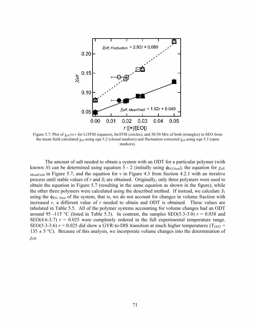
71

Figure 5.7: Plot of χeff vs r for LiTFSI (squares), ImTFSI (circles), and 50:50 Mix of both (triangles) in SEO from the mean-field calculated χeff using eqn 5.2 (closed markers) and fluctuation corrected χeff using eqn 5.3 (open

markers).

The amount of salt needed to obtain a system with an ODT for a particular polymer (with known N) can be determined using equation 5 - 2 (initially using φEO,Neat), the equation for χeff,

MeanField in Figure 5.7, and the equation for v in Figure 4.3 from Section 4.2.1 with an iterative process until stable values of r and S1 are obtained. Originally, only three polymers were used to obtain the equation in Figure 5.7 (resulting in the same equation as shown in the figure), while the other three polymers were calculated using the described method. If instead, we calculate S1 using the ϕEO, Neat of the system, that is, we do not account for changes in volume fraction with increased r, a different value of r needed to obtain and ODT is obtained. These values are tabulated in Table 5.5. All of the polymer systems accounting for volume changes had an ODT around 95 -115 °C (listed in Table 5.3). In contrast, the samples SEO(5.3-3.0) r = 0.038 and SEO(4.6-3.7) r = 0.025 were completely ordered in the full experimental temperature range. SEO(5.3-3.6) r = 0.025 did show a GYR-to-DIS transition at much higher temperatures (TODT = 135 ± 5 °C). Because of this analysis, we incorporate volume changes into the determination of χeff.

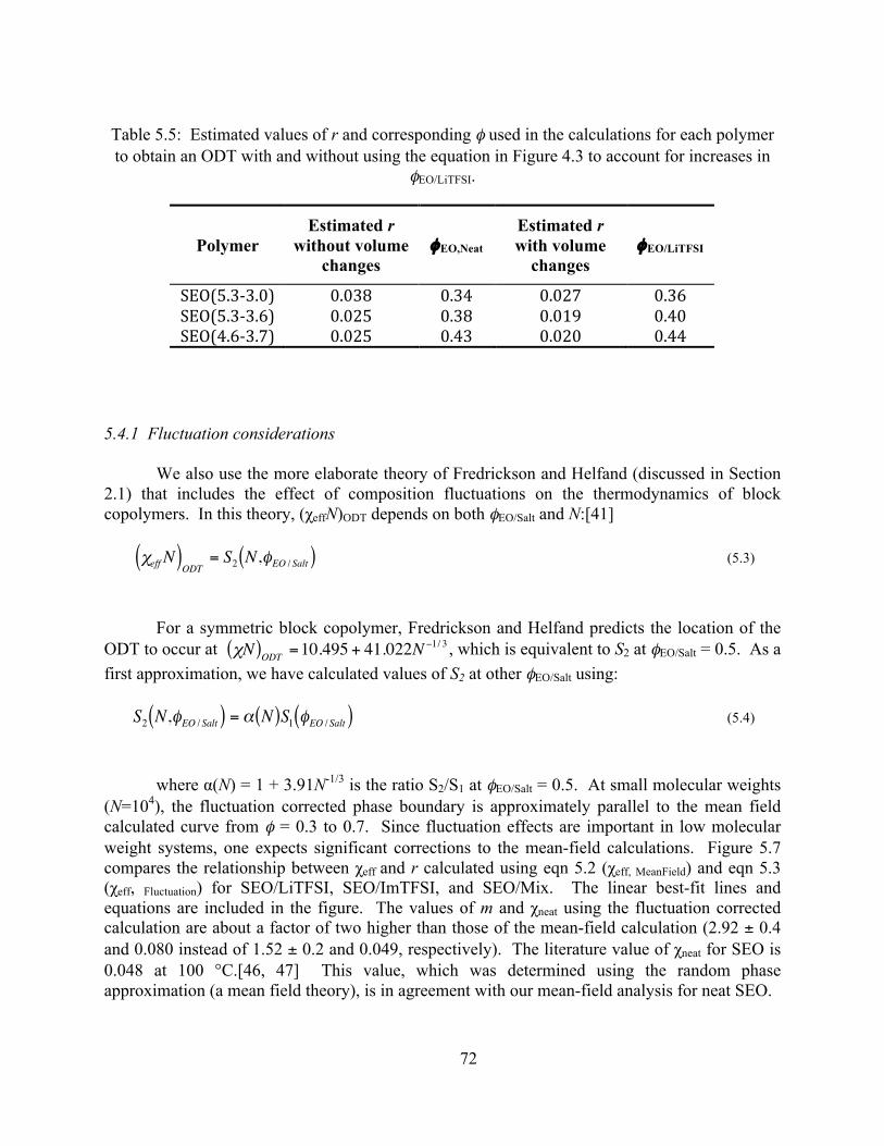
72

Table 5.5: Estimated values of r and corresponding φ used in the calculations for each polymer to obtain an ODT with and without using the equation in Figure 4.3 to account for increases in

φEO/LiTFSI.

Polymer Estimated r

without volume changes

φEO,Neat Estimated r with volume

changes φEO/LiTFSI

SEO(5.3-­‐3.0)   0.038   0.34   0.027   0.36  SEO(5.3-­‐3.6)   0.025   0.38   0.019   0.40  SEO(4.6-­‐3.7)   0.025   0.43   0.020   0.44  

5.4.1 Fluctuation considerations

We also use the more elaborate theory of Fredrickson and Helfand (discussed in Section 2.1) that includes the effect of composition fluctuations on the thermodynamics of block copolymers. In this theory, (χeffN)ODT depends on both φEO/Salt and N:[41]

(5.3)

For a symmetric block copolymer, Fredrickson and Helfand predicts the location of the ODT to occur at , which is equivalent to S2 at φEO/Salt = 0.5. As a first approximation, we have calculated values of S2 at other φEO/Salt using:

(5.4)

where α(N) = 1 + 3.91N-1/3 is the ratio S2/S1 at φEO/Salt = 0.5. At small molecular weights (N=104), the fluctuation corrected phase boundary is approximately parallel to the mean field calculated curve from φ = 0.3 to 0.7. Since fluctuation effects are important in low molecular weight systems, one expects significant corrections to the mean-field calculations. Figure 5.7 compares the relationship between χeff and r calculated using eqn 5.2 (χeff, MeanField) and eqn 5.3 (χeff, Fluctuation) for SEO/LiTFSI, SEO/ImTFSI, and SEO/Mix. The linear best-fit lines and equations are included in the figure. The values of m and χneat using the fluctuation corrected calculation are about a factor of two higher than those of the mean-field calculation (2.92 ± 0.4 and 0.080 instead of 1.52 ± 0.2 and 0.049, respectively). The literature value of χneat for SEO is 0.048 at 100 °C.[46, 47] This value, which was determined using the random phase approximation (a mean field theory), is in agreement with our mean-field analysis for neat SEO.

€

χeff N( )ODT

= S2 N,φEO / Salt( )

€

χN( )ODT =10.495 + 41.022N −1/ 3

€

S2 N,φEO / Salt( ) = α N( )S1 φEO / Salt( )

73

5.4.2 Molecular weight limitations

The estimated values of r needed for an ODT works well with moderately sized SEO (total MW of 6 – 13 kg/mol). However, this method fails with polymers of MW less than 4 kg/mol. Figure 5.8 plots the SAXS profiles of the polymers SEO(1.4 – 2.5) and SEO(1.5 – 1.3) at r = 0.12 and r = 0.15. SEO(1.4 – 2.5) has a total MW of 3.9 kg/mol with PEO as the major component (φEO = 0.62) and SEO(1.5 – 1.3) has total MW of 2.8 kg/mol with PEO as the minor phase (φEO = 0.45). Using the prescribed methodology above, an r value of 0.12 is needed to obtain an ODT in both of these systems. However, the SAXS profiles of SEO(1.4 – 2.5) and SEO(1.5 – 1.3) at r = 0.12 in Figure 5.8 a and c reveal samples which are DIS at all temperatures scanned. In this case, the samples were prepared by melting the polymer/salt mixtures into a spacer and sandwiching them inbetween lithium foil. We note in passing that SEO(1.4 – 2.5) were measured at lower temperatures. This should not affect the analysis since the samples do not exhibit crystallinity at this temperature.

As discussed in the previous section, a mere increase of 0.005 (from r = 0.02 to r = 0.025) was enough of a change to see a sample with an ODT and a sample which was fully ordered for the polymer SEO(4.6 – 3.7). We thus expect that increasing the salt concentration on a DIS sample would induce ordering. However, when we increase the salt concentration of both samples to r = 0.15 (a total increase of 0.03), the samples remain DIS (Figure 5.8 b and d). SEO (1.5 – 1.3) r = 0.15 at 60 °C seemed to show a very small narrow peak atop the broad peak in Figure 5.8d. Although, the sample shows no such peak at lower temperatures (e.g. 23 °C in the figure), where one expects it to be better ordered, or at higher temperatures. It also seems strange that SEO(1.4 – 2.5) r = 0.12 shows stronger scattering than its counterpart at r = 0.15. This could arise from many factors, such as differences in thicknesses of the sample or lithium foil.

It is unclear why these samples do not order. It is possible that the methodology to determine r is flawed, that there is a different interaction between PEO/LiTFSI at high r and low r with PS (different PEO/LiTFSI crystal structures) as evidenced by the non-linear relationship between PEO volume and domain size and r, the χeff approximations may not be valid, or that there is a solubility limit of the salts in PEO where ion pairs and aggregates no longer contribute to changes in χeff. From the PEO/LiTFSI phase diagram constructed by Lascaud et al.,[3] PEO/LiTFSI systems do not reach a different crystalline structure until r = 0.17 (where 6:1 complexes begin to form). It appears that SEO/LiTFSI at r = 0.15 and r = 0.12 should not behave any differently than with smaller values of r. It would be interesting to determine whether there is a solubility limit, where “free ions” and “paired ions” could be measured using a method such as Raman Spectroscopy,[48] however this is outside the scope of this project.

74

Figure 5.8: SAXS profiles of a) SEO(1.4-2.5) r = 0.12, b) SEO(1.4-2.5) r = 0.15, c) SEO(1.5-1.3) r = 0.12, and d) SEO(1.5-1.3) r = 0.15 at various temperatures. All samples appear to be disordered.

5.4.3 Using strong segregation theory

In ref. [14], Young et al experimentally measured m for mixtures of SEO with LiCF3SO3, LiClO4, and LiAsF6. In that paper, they used SEO copolymers with molecular weights that were significantly higher than those used in this paper (MW = 14.5 kg/mol). They observed an increase in the domain spacing with added salt, and used the strong segregation limit (SSL) theory of neat block copolymers to infer the effect of salt on χeff and m. According to SSL theory, the characteristic domain size is related to the χ parameter (d* ∝ χ1/6). Their values of χeff were determined relative to the value of χneat obtained from literature.[46]

A similar analysis can be performed on our largest molecular weight sample, SEO(6.4 – 7.2), which has a comparable molecular weight (13.6 kg/mol) to that of Young et al. The change in domain size with increasing r was discussed in Section 4.2.2 and plotted in Figure 5.9a. The resulting relationship of χeff vs r at various temperatures is shown in Figure 5.9b. The resulting equations from a linear regression are also shown in the figure. Since SEO/LiTFSI systems seem to contain two regimes on the dependence of salt on domain size (i.e. above and below r = 0.085), only values for r less than 0.085 are used in the regression analysis. The neat χ for each temperature was determined using relationships from literature. These relationships are quite comparable to the earlier mean field analysis (eqn 5.2) on the SEO/LiTFSI systems with ODTs.

75

If we look at the data in Figure 5.9 for T = 107 °C (average ODT values in the mean field analysis is 110 °C) we find that m is 1.58, which is in agreement with the mean field m of 1.52.

Figure 5.9: Plot of a) d vs r and b) χeff vs r with the corresponding linear fit equations for SEO(6.4 - 7.2) calculated from the characteristic domain sizes and SSL theory for 80 °C (), 107 °C (), 125 °C (), and 144 °C (). The

solid lines through the points are the fitted equations from linear regression analysis.

We note that the χN values for this polymer (ranges from 10 – 45, with salts) are in the intermediate regime as oppose to the strong segregation regime. Thus using SSL theory would overestimate the value of χ.

5.5 THEORETICAL PREDICTIONS

An expression for m in the mean-field limit by combining Flory Huggins theory with the Born energy for solvating an ion and translational entropy of the ions is derived in ref [16]. That theory is described in further detail in Section 2.2.2. In that theory, the change in χ arises from several competing effects: the tendency for free, mobile ions to be preferentially solvated by the phase rich in the component of the higher dielectric constant, the translational entropy of the ions, and the local enrichment of the higher dielectric component around an ion in the homogeneous mixture. The Li+ ions are tightly bound to the oxygen groups of the EO blocks in both the disordered and ordered states. Thus their energetics are, to a first approximation, unaffected by microphase separation. By the considerations in ref. [16], only the free anions contribute to changing the miscibility of the S and EO blocks. This is consistent with our experimental observation. Taking the TFSI- as the dominant contributor and accounting for differences in parameter definitions, we arrive at the following theoretical predictions for m:[35]

76

(5.5)

where vo is the reference volume and vEO is the volume of an EO monomer (same definition as in eqn 5.2), φEO is the volume fraction of PEO in the diblock, lo is the Bjerrum length in vacuum (43.6 nm at 110 °C), a is the radius of the anion, λp, the packing length (0.287 for a symmetric SEO system) which is defined by vo/bave

2 (where bave is the average statistical segment length defined by bPEObPS/(φEObPEO+ φSbPS) and bPEO and bPS are the statistical segment lengths of PEO and PS, respectively, based on a monomer of volume vo), ε is the average dielectric constant of the polymer defined as ε = (φEO)εPEO + (φS)εPS and Δε is the difference in dielectric constants defined as Δε = εPEO - εPS. For our calculations, we use φEO = 0.5, the PEO dielectric constant, εPEO = 7.5, and the PS dielectric constant, εPS = 2.6. Details of the derivation of eqn 5.5 are provided in ref [16], and are summarized in Section 2.2.2.

Equation 5 - 5 is derived assuming that (1) all of the salt ions are dissociated, (2) triplets and other charged aggregates are not present, and (3) the Li+ ions are bound to the PEO-blocks in both the ordered and disordered phases while the anions are free. However, charge neutrality and the higher dielectric constant of PEO will bias the anions to PEO-rich locations in both ordered and disordered states. In ref. [15], Wanakule et al. measured the conductivity of a variety of SEO/LiTFSI mixtures across the ODT. There was neither a discontinuity at the ODT nor a change in slope in the temperature dependence of the conductivity in the ordered and disordered state. In other words, the temperature dependence of SEO/LiTFSI mixtures obtained from fully ordered systems, fully disordered systems, and systems with accessible ODTs was identical. We take this observation as evidence that the ions in the system have the same PEO-rich local environment regardless of the state of order of the samples. This provides justification for assumption (3) in the analysis.

€

mtheory =Δχr

=voφEO8v

⎛

⎝ ⎜

⎞

⎠ ⎟ loaε⎛

⎝ ⎜

⎞

⎠ ⎟ loaε

− 4 −18λploπ 3εa2

⎛

⎝ ⎜

⎞

⎠ ⎟ Δεε

⎛

⎝ ⎜

⎞

⎠ ⎟ 2

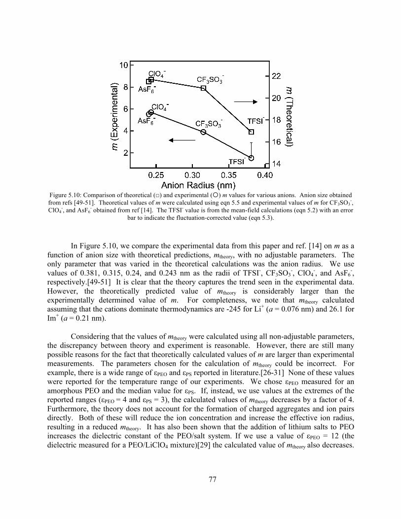
77

Figure 5.10: Comparison of theoretical (□) and experimental () m values for various anions. Anion size obtained from refs [49-51]. Theoretical values of m were calculated using eqn 5.5 and experimental values of m for CF3SO3

-, ClO4

-, and AsF6- obtained from ref [14]. The TFSI- value is from the mean-field calculations (eqn 5.2) with an error

bar to indicate the fluctuation-corrected value (eqn 5.3).

In Figure 5.10, we compare the experimental data from this paper and ref. [14] on m as a function of anion size with theoretical predictions, mtheory, with no adjustable parameters. The only parameter that was varied in the theoretical calculations was the anion radius. We use values of 0.381, 0.315, 0.24, and 0.243 nm as the radii of TFSI-, CF3SO3

-, ClO4-, and AsF6

-, respectively.[49-51] It is clear that the theory captures the trend seen in the experimental data. However, the theoretically predicted value of mtheory is considerably larger than the experimentally determined value of m. For completeness, we note that mtheory calculated assuming that the cations dominate thermodynamics are -245 for Li+ (a = 0.076 nm) and 26.1 for Im+ (a = 0.21 nm).

Considering that the values of mtheory were calculated using all non-adjustable parameters, the discrepancy between theory and experiment is reasonable. However, there are still many possible reasons for the fact that theoretically calculated values of m are larger than experimental measurements. The parameters chosen for the calculation of mtheory could be incorrect. For example, there is a wide range of εPEO and εPS reported in literature.[26-31] None of these values were reported for the temperature range of our experiments. We chose εPEO measured for an amorphous PEO and the median value for εPS. If, instead, we use values at the extremes of the reported ranges (εPEO = 4 and εPS = 3), the calculated values of mtheory decreases by a factor of 4. Furthermore, the theory does not account for the formation of charged aggregates and ion pairs directly. Both of these will reduce the ion concentration and increase the effective ion radius, resulting in a reduced mtheory. It has also been shown that the addition of lithium salts to PEO increases the dielectric constant of the PEO/salt system. If we use a value of εPEO = 12 (the dielectric measured for a PEO/LiClO4 mixture)[29] the calculated value of mtheory also decreases.

78

While many improvements can be proposed, ref. [16] provides a starting point for exploring the underpinnings of the phase behavior of block copolymer/salt mixtures.

5.4 CONCLUSIONS

The thermodynamics and phase behavior of mixtures of SEO copolymers with added salts (LiTFSI, ImTFSI, and mixtures thereof) was studied by SAXS and birefringence. This enables a study of the effect of the cation size on the properties of block copolymer electrolytes. All of our observations were consistent with the assumption that the salts reside exclusively in the PEO-rich microphase. The morphologies obtained as a function of added salt were in agreement with the calculated changes in volume of the PEO-rich microphase due to the presence of salt. In addition to changes in effective composition of the copolymer, the addition of salt increases the effective Flory-Huggins interaction parameter, χeff, between the PEO/salt system and PS. Surprisingly, the data obtained from mixtures containing LiTFSI and ImTFSI were similar, indicating that the thermodynamics are dominated by the nature of the anion. The parameter m that captures the increase in χeff with increasing salt concentration, r, obtained from experiments described here and those reported by Young et al.[14] were compared with theoretical predictions of Wang[16] with no adjustable parameters. The qualitative trends seen in the experiments are captured by theory but the predicted values of m are consistently higher than those measured experimentally. It is clear, however, that m decreases with increasing anion size and is independent of the cation size.

5.5 REFERENCES

1. Frech, R., et al., Crystalline and amorphous phases in the poly(ethylene oxide)-LiCF3SO3 system. Macromolecules, 1999. 32(3): p. 808-813.

2. Gray, F.M., Polymer Electrolytes. RSC Materials Monographs, ed. J.A. Connor. 1997, London: The Royal Society of Chemistry.

3. Lascaud, S., et al., Phase-Diagrams and Conductivity Behavior of Poly(Ethylene Oxide) Molten-Salt Rubbery Electrolytes. Macromolecules, 1994. 27(25): p. 7469-7477.

4. Appetecchi, G.B., et al., Ternary polymer electrolytes containing pyrrolidinium-based polymeric ionic liquids for lithium batteries. Journal of Power Sources, 2010. 195(11): p. 3668-3675.

5. Shin, J.H., W.A. Henderson, and S. Passerini, An elegant fix for polymer electrolytes. Electrochemical and Solid State Letters, 2005. 8(2): p. A125-A127.

79

6. Shin, J.H., et al., Solid-state Li/LiFePO4 polymer electrolyte batteries incorporating an ionic liquid cycled at 40 degrees C. Journal of Power Sources, 2006. 156(2): p. 560-566.

7. Shin, J.-H., W.A. Henderson, and S. Passerini, Ionic liquids to the rescue? Overcoming the ionic conductivity limitations of polymer electrolytes. Electrochemistry Communications, 2003. 5(12): p. 1016-1020.

8. Shin, J.H., W.A. Henderson, and S. Passerini, PEO-based polymer electrolytes with ionic liquids and their use in lithium metal-polymer electrolyte batteries. Journal of the Electrochemical Society, 2005. 152(5): p. A978-A983.

9. Kim, G.T., et al., Solvent-free, PYR1A TFSI ionic liquid-based ternary polymer electrolyte systems I. Electrochemical characterization. Journal of Power Sources, 2007. 171: p. 861-869.

10. MacFarlane, D.R., et al., Pyrrolidinium Imides: A New Family of Molten Salts and Conductive Plastic Crystal Phases. The Journal of Physical Chemistry B, 1999. 103(20): p. 4164-4170.

11. Simone, P.M. and T.P. Lodge, Phase Behavior and Ionic Conductivity of Concentrated Solutions of Polystyrene-Poly(ethylene oxide) Diblock Copolymers in an Ionic Liquid. Acs Applied Materials & Interfaces, 2009. 1(12): p. 2812-2820.

12. Leibler, L., Theory of Microphase Separation in Block Co-Polymers. Macromolecules, 1980. 13(6): p. 1602-1617.

13. Wang, J.Y., W. Chen, and T.P. Russell, Ion-complexation-induced changes in the interaction parameter and the chain conformation of PS-b-PMMA copolymers. Macromolecules, 2008. 41(13): p. 4904-4907.

14. Young, W.S. and T.H. Epps, Salt Doping in PEO-Containing Block Copolymers: Counterion and Concentration Effects. Macromolecules, 2009. 42(7): p. 2672-2678.

15. Wanakule, N.S., et al., Ionic Conductivity of Block Copolymer Electrolytes in the Vicinity of Order-Disorder and Order-Order Transitions. Macromolecules, 2009. 42(15): p. 5642-5651.

16. Wang, Z.G., Effects of Ion Solvation on the Miscibility of Binary Polymer Blends. Journal of Physical Chemistry B, 2008. 112(50): p. 16205-16213.

17. Lodge, T.P., et al., Phase behavior of block copolymers in a neutral solvent. Macromolecules, 2003. 36(3): p. 816-822.

18. Shibayama, M., et al., Ordered Structure in Block Polymer-Solutions .3. Concentration-Dependence of Microdomains in Non-Selective Solvents. Macromolecules, 1983. 16(9): p. 1427-1433.

80

19. Hashimoto, T., M. Shibayama, and H. Kawai, Ordered structure in block polymer solutions. 4. Scaling rules on size of fluctuations with block molecular weight, concentration, and temperature in segregation and homogeneous regimes. Macromolecules, 1983. 16(7): p. 1093-1101.

20. Fredrickson, G.H. and L. Leibler, Theory of Block Copolymer Solutions - Nonselective Good Solvents. Macromolecules, 1989. 22(3): p. 1238-1250.

21. Hadjichristidis, N., et al., Anionic polymerization: High vacuum techniques. Journal of Polymer Science Part a-Polymer Chemistry, 2000. 38(18): p. 3211-3234.

22. Quirk, R.P., et al., Butyllithium-initiated anionic synthesis of well-defined poly(styrene-block-ethylene oxide) block copolymers with potassium salt additives. Polymer International, 1996. 39(1): p. 3-10.

23. Esswein, B. and M. Moller, Polymerization of Ethylene oxide with alkyllithium compounds and the phosphazene base ''tBu-P-4''. Angewandte Chemie-International Edition in English, 1996. 35(6): p. 623-625.

24. Noda, A., et al., Bronsted Acid-Base Ionic Liquids as Proton-Conducting Nonaqueous Electrolytes. The Journal of Physical Chemistry B, 2003. 107(17): p. 4024-4033.

25. Garetz, B.A., et al., Birefringence and Diffraction of Light in Ordered Block-Copolymer Materials. Macromolecules, 1993. 26(12): p. 3151-3155.

26. Porter, C.H. and R.H. Boyd, Dielectric Study of Effects of Melting on Molecular Relaxation in Poly(Ethylene Oxide) and Polyoxymethylene. Macromolecules, 1971. 4(5): p. 589-&.

27. Abraham, K.M., Z. Jiang, and B. Carroll, Highly conductive PEO-like polymer electrolytes. Chemistry of Materials, 1997. 9(9): p. 1978-1988.

28. Kumar, M. and S.S. Sekhon, Role of plasticizer's dielectric constant on conductivity modification of PEO-NH4F polymer electrolytes. European Polymer Journal, 2002. 38(7): p. 1297-1304.

29. Gray, F.M., C.A. Vincent, and M. Kent, A Study of the Dielectric-Properties of the Polymer Electrolyte Peo-Liclo4 over a Composition Range Using Time Domain Spectroscopy. Journal of Polymer Science Part B-Polymer Physics, 1989. 27(10): p. 2011-2022.

30. Yano, O. and Y. Wada, Dynamic Mechanical and Dielectric Relaxations of Polystyrene Below Glass Temperature. Journal of Polymer Science Part a-2-Polymer Physics, 1971. 9(4): p. 669-&.

81

31. Yu, S.Z. and P. Hing, Dynamic mechanical properties of polystyrene-aluminum nitride composite. Journal of Applied Polymer Science, 2000. 78(7): p. 1348-1353.

32. Gomez, E.D., et al., Effect of Ion Distribution on Conductivity of Block Copolymer Electrolytes. Nano Letters, 2009. 9(3): p. 1212-1216.

33. Hanley, K.J., T.P. Lodge, and C.I. Huang, Phase behavior of a block copolymer in solvents of varying selectivity. Macromolecules, 2000. 33(16): p. 5918-5931.

34. Park, M.J., et al., Transient solidlike behavior near the cylinder/disorder transition in block copolymer solutions. Journal of Physical Chemistry B, 2006. 110(31): p. 15295-15301.

35. The appearance of a shoulder rather than a peak is probably due to the differences in instrument resolution at SSRL vs ALS. In general, the ALS has better resolution than SSRL. The samples with ImTFSI at r = 0.05 and higher were measured at SSRL. The rest of the samples were run at ALS. .

36. Lightfoot, P., M.A. Mehta, and P.G. Bruce, Crystal-Structure of the Polymer Electrolyte Poly(Ethylene Oxide)3licf3so3. Science, 1993. 262(5135): p. 883-885.

37. Londono, J.D., et al., Cation Environment in Molten Lithium Iodide Doped Poly(ethylene oxide). Macromolecules, 1997. 30(23): p. 7151-7157.

38. Mao, G.M., et al., Structure of liquid PEO-LiTFSI electrolyte. Physical Review Letters, 2000. 84(24): p. 5536-5539.

39. MacCallum, J.R. and C.A. Vincent, Polymer Electrolyte Reviews. 1987, New York City: Elsevier Applied Science Publishers.

40. Matsen, M.W. and F.S. Bates, Unifying weak- and strong-segregation block copolymer theories. Macromolecules, 1996. 29(4): p. 1091-1098.

41. Fredrickson, G.H. and E. Helfand, Fluctuation Effects in the Theory of Microphase Separation in Block Copolymers. Journal of Chemical Physics, 1987. 87(1): p. 697-705.

42. Bates, F.S. and G.H. Fredrickson, Block copolymers - Designer soft materials. Physics Today, 1999. 52(2): p. 32-38.

43. Matsen, M.W. and M. Schick, Stable and Unstable Phases of a Diblock Copolymer Melt. Physical Review Letters, 1994. 72(16): p. 2660-2663.

44. Cochran, E.W., C.J. Garcia-Cervera, and G.H. Fredrickson, Stability of the Gyroid Phase in Diblock Copolymers at Strong Segregation. Macromolecules, 2006. 39(7): p. 2449-2451.

82

45. Lodge, T.P., B. Pudil, and K.J. Hanley, The Full Phase Behavior for Block Copolymers in Solvents of Varying Selectivity. Macromolecules, 2002. 35(12): p. 4707-4717.

46. Cochran, E.W., D.C. Morse, and F.S. Bates, Design of ABC triblock copolymers near the ODT with the random phase approximation. Macromolecules, 2003. 36(3): p. 782-792.

47. Zhu, L., et al., Phase structures and morphologies determined by self-organization, vitrification, and crystallization: confined crystallization in an ordered lamellar phase of PEO-b-PS diblock copolymer. Polymer, 2001. 42(13): p. 5829-5839.

48. Edman, L., Ion association and ion solvation effects at the crystalline-amorphous phase transition in PEO-LiTFSI. Journal of Physical Chemistry B, 2000. 104(31): p. 7254-7258.

49. Jenkins, H.D.B., et al., Relationships among ionic lattice energies, molecular (formula unit) volumes, and thermochemical radii. Inorganic Chemistry, 1999. 38(16): p. 3609-3620.

50. Gu, B. and J.D. Coates, Perchlorate: environmental occurence, interactions and treatment. 2006, New York: Springer.

51. Krossing, I., et al., Why are ionic liquids liquid? A simple explanation based on lattice and solvation energies. Journal of the American Chemical Society, 2006. 128(41): p. 13427-13434.

83

Chapter 6

Conductivity through order-order and order-disorder transitions of block copolymer electrolytes

ABSTRACT

Ionic conductivity measurements through order-order and order-disorder phase transitions in mixtures of poly(styrene-block-ethylene oxide) (SEO) copolymers and lithium bis-trifluoromethylsulfonimide (LiTFSI), a common lithium salt used in polymer electrolytes, were studied using AC impedance spectroscopy. The SEO/LiTFSI mixtures exhibit disordered phases as well as lamellar, hexagonal packed cylinders, and gyroid microphases. The molecular weight of the blocks and the salt concentration was adjusted to obtain order-order and order-disorder transition temperatures within the available experimental window. The ionic conductivities of the mixtures and normalized conductivity (normalized by the ionic conductivity of a 20 kg/mol homopolymer PEO sample at the salt concentration and temperature of interest), were measured. For samples with major phase PEO block, the conductivity was independent of temperature, in spite of the presence of the above mentioned phase transitions. However, for samples with minor phase PEO block, the conductivity/structure relationship is more complex. In-situ conductivity/SAXS measurements reveal that this relationship is dependent on thermal history.

6.1 EFFECT OF MORPHOLOGY ON CONDUCTIVITY

It is reasonable to assume that the conductivity of block copolymers with one ionically conducting block, σ, is proportional to the volume fraction of the conducting block, φC. For unaligned samples, we also expect the conductivity to depend on the tortuosity of the pathways for ion transport, which we account for by introducing the morphology factor, f. We thus write,

(6.1)

where σC is the intrinsic conductivity of the conducting microphase. In the case of randomly oriented lamellar grains, Sax and Ottino[1] argue that, on average, one third of the grains will contain lamellae oriented perpendicular to the direction of charge transport, implying that f = 2/3. Similar arguments lead to an estimate of f = 1/3 for a HEX morphology with the conducting phase as the minor component. In the case of the GYR phase, the presence of a

84

three-dimensional network ensures transport in the desired direction is never blocked. We thus expect f = 1 in this case. Similarly, if the conducting phase is the major component in either BCC or HEX phases, then we also expect f = 1. Our use of eqn 6.1 to study the effect of morphology on conductivity of block copolymer electrolytes is based on two implicit assumptions: (1) the intrinsic conductivity of the conducting phase (σC) is not affected by morphology, and (2) barriers to transport occuring at grain boundaries are negligible.

Let us, for the moment, consider the most widely studied block copolymer phase transition, namely the ODT of symmetric copolymers that form LAM in the microphase separated state. To predict changes in conductivity at the ODT we need to know if eqn 6.1 is valid for disordered block copolymers. The validity of eqn 6.1 will depend on the detailed structure of the disordered phase. There are at least 3 different senarios. (1) If the disordered phase contains large amplitude concentration fluctuations, i.e. the sample contains disordered regions of essentially pure conducting and non-conducting phases, and if these regions are cocontinuous, then one might expect eqn 6.1 to be valid with f = 1, since there are no blocked transport directions in this system. If this were true, then there would be a discontinuous change in conductivity of (1/3)φCσC at the LAM-to-DIS transition. (2) If we imagine the large amplitude fluctuations to have a locally anisotropic "pancake" shape, then, on average, one third of the pancakes will be oriented orthogonal to the desired direction of transport, and one recovers f = 2/3. If this were true, then there would be no discontinuity in conductivity at the ODT of a LAM phase. (3) If there is extensive mixing of the conducting and non-conducting phases, i.e. the magnitude of the disordered concentration fluctuations is small, then clearly eqn 1 is not valid because the presence of the non-conducting component in the conducting phase will affect the intrinsic conductivity of the conducting phase. It is important to note that the magnitude of the concentration fluctuations in the vicinity of the ODT is a strong function of molecular weight[2] and thus one does not expect a universal dependence of conductivity across the ODT in block copolymer/salt mixtures.

6.1.1 Previous studies of conductivity through order transitions

Ruzette et al.[3] measured the conductivity through the LAM-to-DIS transition of an 80 kg/mol sample of poly(methyl methacrylate)-block-poly(oligo oxyethylene methacrylate) (PMMA-POEM) doped with lithium trifluoromethane sulfonate (LiCF3SO3). In that paper, they found that the conductivity in the disordered state deviated from the Vogel-Tamman-Fulcher (VTF, see Section 6.2.1) fits to the ordered state. That is, the conductivity behavior of the PMMA-POEM/LiCF3SO3 in the ordered state is different from the conductivity behavior in the disordered state. Similar to our observations with LiTFSI in SEO, Ruzette et al. were able to access an ODT by controlling the concentration of LiCF3SO3 in PMMA-POEM. For EO:Li concentrations of 23:1 and 25:1, the former is completely ordered in the temperature range of interest and the latter contains an ODT. According to the arguments outlined in the above section, the conductivity of the disordered state, with f = 1, should deviate above the VTF fits to the conductivity of the lamellar state (f = 2/3). Instead, Ruzette et al. observed a lower conductivity than expected after the ODT. We note in passing that both the PMMA and POEM blocks are ion-solvating.

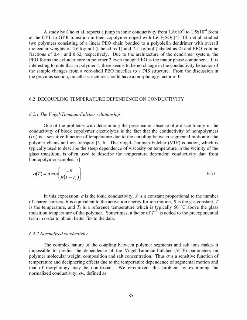
85

A study by Cho et al. reports a jump in ionic conductivity from 1.8x10-5 to 1.5x10-4 S/cm at the CYL-to-GYR transition in their copolymer doped with LiCF3SO3.[4] Cho et al. studied two polymers consisting of a linear PEO chain bonded to a polyolefin dendrimer with overall molecular weights of 4.6 kg/mol (labeled as 1) and 7.5 kg/mol (labeled as 2) and PEO volume fractions of 0.41 and 0.62, respectively. Due to the architecture of the dendrimer system, the PEO forms the cylinder core in polymer 2 even though PEO is the major phase component. It is interesting to note that in polymer 1, there seems to be no change in the conductivity behavior of the sample changes from a core-shell PEO micelles to a DIS structure. From the discussion in the previous section, micellar structures should have a morphology factor of 0.

6.2 DECOUPLING TEMPERATURE DEPENDENCE ON CONDUCTIVITY

6.2.1 The Vogel-Tamman-Fulcher relationship

One of the problems with determining the presence or absence of a discontinuity in the conductivity of block copolymer electrolytes is the fact that the conductivity of hompolymers (σC) is a sensitive function of temperature due to the coupling between segmental motion of the polymer chains and ion transport.[5, 6] The Vogel-Tamman-Fulcher (VTF) equation, which is typically used to describe the steep dependence of viscosity on temperature in the vicinity of the glass transition, is often used to describe the temperature dependent conductivity data from homopolymer samples:[7]

(6.2)

In this expression, σ is the ionic conductivity, A is a constant proportional to the number of charge carriers, B is equivalent to the activation energy for ion motion, R is the gas constant, T is the temperature, and T0 is a reference temperature which is typically 50 °C above the glass transition temperature of the polymer. Sometimes, a factor of T1/2 is added to the preexponential term in order to obtain better fits to the data.

6.2.2 Normalized conductivity

The complex nature of the coupling between polymer segments and salt ions makes it impossible to predict the dependence of the Vogel-Tamman-Fulcher (VTF) parameters on polymer molecular weight, composition and salt concentration. Thus σ is a sensitive function of temperature and deciphering effects due to the temperature dependence of segmental motion and that of morphology may be non-trivial. We circumvent this problem by examining the normalized conductivity, σN, defined as

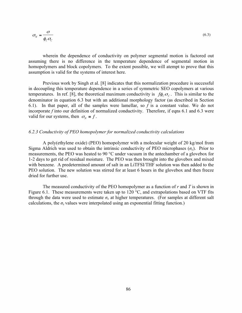
86

(6.3)

wherein the dependence of conductivity on polymer segmental motion is factored out assuming there is no difference in the temperature dependence of segmental motion in homopolymers and block copolymers. To the extent possible, we will atempt to prove that this assumption is valid for the systems of interest here.

Previous work by Singh et al. [8] indicates that this normalization procedure is successful in decoupling this temperature dependence in a series of symmetric SEO copolymers at various temperatures. In ref. [8], the theoretical maximum conductivity is . This is similar to the denominator in equation 6.3 but with an additional morphology factor (as described in Section 6.1). In that paper, all of the samples were lamellar, so f is a constant value. We do not incorporate f into our definition of normalized conductivity. Therefore, if eqns 6.1 and 6.3 were valid for our systems, then .

6.2.3 Conductivity of PEO homopolymer for normalized conductivity calculations

A poly(ethylene oxide) (PEO) homopolymer with a molecular weight of 20 kg/mol from Sigma Aldrich was used to obtain the intrinsic conductivity of PEO microphases (σc). Prior to measurements, the PEO was heated to 90 °C under vacuum in the antechamber of a glovebox for 1-2 days to get rid of residual moisture. The PEO was then brought into the glovebox and mixed with benzene. A predetermined amount of salt in an LiTFSI/THF solution was then added to the PEO solution. The new solution was stirred for at least 6 hours in the glovebox and then freeze dried for further use.

The measured conductivity of the PEO homopolymer as a function of r and T is shown in Figure 6.1. These measurements were taken up to 120 °C, and extrapolations based on VTF fits through the data were used to estimate σc at higher temperatures. (For samples at different salt calculations, the σc values were interpolated using an exponential fitting function.)

87

Figure 6.1: Plot of conductivity versus 1000/T for a 20 kg/mol PEO homopolymer at r = 0.03 (○) and r = 0.5 (□). Solid lines through the data points are VTF fits.

Lascaud et al.[9] measured the conductivity of mixtures of a 4 kg/mol PEO and LiTFSI as a function of salt concentrations and temperatures. The conductivity of this sample was somewhat higher than that of our 20 kg/mol PEO conductivity data due to well-established effects arising from differences in molecular weight, but the temperature dependence of the conductivities of the 2 sets of samples were similar. For consistency, we have used our measurements to compute σN.

6.3 SAMPLE PREPARATION

The copolymer/salt mixture was pressed into a Garolite(R) spacer with 125 µm thickness and a central hole 3.88 mm in diameter inside the glovebox. The sample was hot pressed at 90 – 110 °C for an hour between two mirror-polished stainless steel electrodes to ensure good contact between the electrodes and the electrolyte. The electrode-sample assembly was then placed in a home built thermostated conductivity cell connected to a Solartron 1260 Frequency Response Analyzer (FRA) with a Solartron 1296 Dielectric interface or VMP3. The complex impedance (Z' and Z" are the real and imaginary components of the impedance) of the samples were measured using the FRA at 10 ºC intervals during heating and cooling scans between 60 and 150 °C. An alternating current (AC) signal ranging from 5-100 mV in the frequency range (ω) of 10 Hz-1MHz was applied to generate the appropriate frequency response. The plateau value in the Bode plot of modulus of the complex impedance, |Z'+iZ"| versus ω, was taken as the sample resistance. This value was nearly identical to the semi-circle touchdown on Nyquist Z" versus Z' plots.

88

6.4 CONDUCTIVITY THROUGH TRANSITIONS WHERE PEO IS THE MAJOR PHASE

Plots of the temperature dependence on σ for selected SEO/salt mixtures are shown in Figure 6.2. We have included data from SEO(6.4-7.2) at r = 0.05 which is LAM at all temperatures, SEO(1.4-2.5) at r = 0.05 which is DIS at all temperatures, SEO(2.3-4.6) at r = 0.05 which exhibited a HEX-to-DIS transition at 135 °C, SEO(3.1-5.1) at r = 0.03 which exhibited a LAM-to-DIS transition at 92 °C, and SEO (3.1-5.1) at r = 0.05 which exhibited a gradual LAM-to-GYR transition between 52 °C and 106 °C. These systems and their structures are summarized in Table 6.1. The solid lines through the data in Figure 6.2 are VTF fits (eqn 6.2) with A, B, and T0 as fitting parameters. We leave T0 floating since the Tg of the polymer is a function of the salt concentration and molecular weight. It is of interest to note that the VTF equation fits the full data set showing no deviations at phase transitions.

Figure 6.2: Plot of conductivity versus 1000/T for SEO(6.4-7.2), SEO(1.4-2.5), SEO(2.3-4.5), and SEO(3.1-5.1) all at r = 0.05 and SEO(3.1-5.1) at r = 0.03. The lines through the data points are VTF fits. Dashed vertical lines mark

locations of the ODT’s.

89

Table 6.1: Summary of SEO/LiTFSI systems in this study.

Polymer r φPEO Phase(s) Transition Temperature

SEO(6.4  –  7.2)   0.05   0.56   LAM   N/A  SEO(3.1  –  5.1)   0.03   0.62   LAM    DIS   92  °C  SEO(2.3  –  4.6)   0.05   0.68   CYL    DIS   135  °C  SEO(3.1  –  5.1)   0.05   0.64   GYR    LAM   52  –  106  °C    SEO(1.4  –  2.5)   0.05   0.65   DIS   N/A  

Figure 6.3 plots the σN (see Section 6.2.2) of the systems listed in Table 6.1. The values of σN of SEO(1.4-2.5), r = 0.05, which is disordered in the temperature range of interest, and SEO(6.4-7.2), r = 0.05, which has a LAM morphology in the temperature range of interest, are 0.259 ± 0.017 and 0.013 ± 0.002, respectively, and have negligible dependence on temperature. The lack of dependence of σN on temperature for these widely different samples indicates that our normalization scheme accounts for the temperature-dependence of ion transport due to the temperature-dependence of segmental motion in SEO copolymers in the absence of phase transitions. The fact that the presence of polystyrene segments does not affect σN of SEO(1.4-2.5) with r = 0.05 indicates that the conducting pathways in the DIS phase are primarily PEO-rich domains that are qualitatively similar to those obtained in the ordered state. What is, perhaps, surprising is the dependence of σN on temperature is also weak for the 3 samples that exhibited phase transitions in the accessible temperature window (Figure 6.3). There seems to be a subtle increase in σN of SEO(3.1-5.1) at r = 0.03 between 60 and 90 oC, before leveling-off at about 0.35 at temperatures above 100 °C. The SEO(3.1-5.1), r = 0.03 sample exhibits an ODT at 92 °C (denoted by dashed line in Figure 6.3) which makes it tempting to conclude that the slight changes in the temperature dependence of σN seen in the vicinity of the ODT is due to this. However, SEO(2.3-4.6), r = 0.05, with an ODT at about 135 °C also exhibits similar behavior in the vicinity of 100 °C. The subtle changes seen in the temperature dependencies of σN in samples with accessible ODTs thus cannot be attributed to morphological transitions. In the ordered state, the polymer chains are part of a quasi-static solid morphology, while in the disordered state, the polymer chains diffuse freely with relatively few thermodynamic barriers.[10] The lack of sensitivity of σN on the location of the ODT indicates that ion transport is only affected by segmental motion, not chain motion in copolymers with molecular weights as low as 7 kg/mol.

90

Figure 6.3: Plot of normalized conductivity (as calculated from eqn 6.3) versus temperature for SEO(6.4-7.2), SEO(1.4-2.5), SEO(2.3-4.5), and SEO(3.1-5.1) all at r = 0.05, and SEO(3.1-5.1) at r = 0.03. The dashed vertical

lines mark the ODT.

The σN values of SEO(3.1-5.1), r = 0.05, the samples that exhibits a LAM-to-GYR transition at temperatures between 52 and 106 °C, are scattered between 0.32 and 0.38. It is evident that this OOT also has no effect on ionic conductivity. We note in passing that the estimated glass transition temperatures of the polystyrene homopolymers with molecular weights equal to those of the polystyrene blocks in our SEO copolymers with accessible phase transitions range from 45 °C to 52 °C.[11] All of our measurements were conducted at temperatures above 52 °C. We were unable to detect the glass transition in DSC scans of our SEO samples.

It is clear that our data do not support the arguments presented in the Section 6.1 where we defined the morphology factor, f. For example, if our arguments were correct then σN would increase by 50%, from 0.67 to 1.0, at the LAM-to-GYR transition (Figure 6.3). Instead we observe that σN is unaffected by this transition and is scattered around an average value of 0.35. Our experiments indicate that the there is no difference in the morphology factors of LAM and GYR phases.

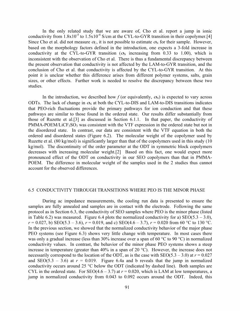
91

In the only related study that we are aware of, Cho et al. report a jump in ionic conductivity from 1.8x10-5 to 1.5x10-4 S/cm at the CYL-to-GYR transition in their copolymer.[4] Since Cho et al. did not measure σC, it is not possible to estimate σN for their sample. However, based on the morphology factors defined in the introduction, one expects a 3-fold increase in conductivity at the CYL-to-GYR transition (σN increasing from 0.33 to 1.00), which is inconsistent with the observation of Cho et al. There is thus a fundamental discrepancy between the present observation that conductivity is not affected by the LAM-to-GYR transition, and the conclusion of Cho et al. that conductivity is affected by the CYL-to-GYR transition. At this point it is unclear whether this difference arises from different polymer systems, salts, grain sizes, or other effects. Further work is needed to resolve the discrepancy between these two studies.

In the introduction, we described how f (or equivalently, σN) is expected to vary across ODTs. The lack of change in σN at both the CYL-to-DIS and LAM-to-DIS transitions indicates that PEO-rich fluctuations provide the primary pathways for ion conduction and that these pathways are similar to those found in the ordered state. Our results differ substantially from those of Ruzette et al.[3] as discussed in Section 6.1.1. In that paper, the conductivity of PMMA-POEM/LiCF3SO3 was consistent with the VTF expression in the ordered state but not in the disordered state. In contrast, our data are consistent with the VTF equation in both the ordered and disordered states (Figure 6.2). The molecular weight of the copolymer used by Ruzette et al. (80 kg/mol) is significantly larger than that of the copolymers used in this study (10 kg/mol). The discontinuity of the order parameter at the ODT in symmetric block copolymers decreases with increasing molecular weight.[2] Based on this fact, one would expect more pronounced effect of the ODT on conductivity in our SEO copolymers than that in PMMA-POEM. The difference in molecular weight of the samples used in the 2 studies thus cannot account for the observed differences.

6.5 CONDUCTIVITY THROUGH TRANSITIONS WHERE PEO IS THE MINOR PHASE

During ac impedance measurements, the cooling run data is presented to ensure the samples are fully annealed and samples are in contact with the electrode. Following the same protocol as in Section 6.3, the conductivity of SEO samples where PEO is the minor phase (listed in Table 6.2) was measured. Figure 6.4 plots the normalized conductivity for a) SEO(5.3 – 3.0), r = 0.027, b) SEO(5.3 – 3.6), r = 0.019, and c) SEO(4.6 – 3.7), r = 0.020 from 60 °C to 130 °C. In the previous section, we showed that the normalized conductivity behavior of the major phase PEO systems (see Figure 6.3) shows very little change with temperature. In most cases there was only a gradual increase (less than 30% increase over a span of 60 °C to 90 °C) in normalized conductivity values. In contrast, the behavior of the minor phase PEO systems shows a steep increase in temperature (greater than 40% in a span of 20 °C). However, the increase does not necessarily correspond to the location of the ODT, as is the case with SEO(5.3 – 3.0) at r = 0.027 and SEO(5.3 – 3.6) at r = 0.019. Figure 6.4a and b reveals that the jump in normalized conductivity occurs around 25 °C below the ODT (indicated by dashed line). Both samples are CYL in the ordered state. For SEO(4.6 – 3.7) at r = 0.020, which is LAM at low temperatures, a jump in normalized conductivity from 0.043 to 0.092 occurs around the ODT. Indeed, this

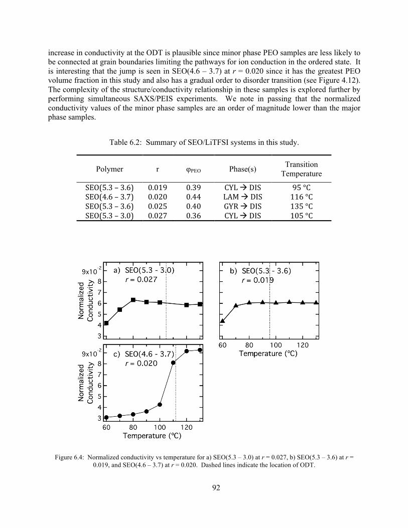
92

increase in conductivity at the ODT is plausible since minor phase PEO samples are less likely to be connected at grain boundaries limiting the pathways for ion conduction in the ordered state. It is interesting that the jump is seen in SEO(4.6 – 3.7) at r = 0.020 since it has the greatest PEO volume fraction in this study and also has a gradual order to disorder transition (see Figure 4.12). The complexity of the structure/conductivity relationship in these samples is explored further by performing simultaneous SAXS/PEIS experiments. We note in passing that the normalized conductivity values of the minor phase samples are an order of magnitude lower than the major phase samples.

Table 6.2: Summary of SEO/LiTFSI systems in this study.

Polymer r φPEO Phase(s) Transition Temperature

SEO(5.3  –  3.6)   0.019   0.39   CYL    DIS   95  °C  SEO(4.6  –  3.7)   0.020   0.44   LAM    DIS   116  °C  SEO(5.3  –  3.6)   0.025   0.40   GYR    DIS   135  °C  SEO(5.3  –  3.0)   0.027   0.36   CYL    DIS   105  °C  

Figure 6.4: Normalized conductivity vs temperature for a) SEO(5.3 – 3.0) at r = 0.027, b) SEO(5.3 – 3.6) at r = 0.019, and SEO(4.6 – 3.7) at r = 0.020. Dashed lines indicate the location of ODT.

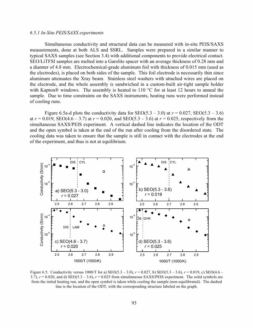
93

6.5.1 In-Situ PEIS/SAXS experiments

Simultaneous conductivity and structural data can be measured with in-situ PEIS/SAXS measurements, done at both ALS and SSRL. Samples were prepared in a similar manner to typical SAXS samples (see Section 3.4) with additional components to provide electrical contact. SEO/LiTFSI samples are melted into a Garolite spacer with an average thickness of 0.28 mm and a diamter of 4.8 mm. Electrochemical-grade aluminum foil with thickness of 0.015 mm (used as the electrodes), is placed on both sides of the sample. This foil electrode is necessarily thin since aluminum attenuates the Xray beam. Stainless steel washers with attached wires are placed on the electrode, and the whole assembly is sandwiched in a custom-built air-tight sample holder with Kapton® windows. The assembly is heated to 110 °C for at least 12 hours to anneal the sample. Due to time constraints on the SAXS instruments, heating runs were performed instead of cooling runs.

Figure 6.5a-d plots the conductivity data for SEO(5.3 – 3.0) at r = 0.027, SEO(5.3 – 3.6) at r = 0.019, SEO(4.6 – 3.7) at r = 0.020, and SEO(5.3 – 3.6) at r = 0.025, respectively from the simultaneous SAXS/PEIS experiment. A vertical dashed line indicates the location of the ODT and the open symbol is taken at the end of the run after cooling from the disordered state. The cooling data was taken to ensure that the sample is still in contact with the electrodes at the end of the experiment, and thus is not at equilibrium.

Figure 6.5: Conductivity versus 1000/T for a) SEO(5.3 – 3.0), r = 0.027, b) SEO(5.3 – 3.6), r = 0.019, c) SEO(4.6 – 3.7), r = 0.020, and d) SEO(5.3 – 3.6), r = 0.025 from simultaneous SAXS/PEIS experiment. The solid symbols are from the initial heating run, and the open symbol is taken while cooling the sample (non-equilibrated). The dashed

line is the location of the ODT, with the corresponding structure labeled on the graph.

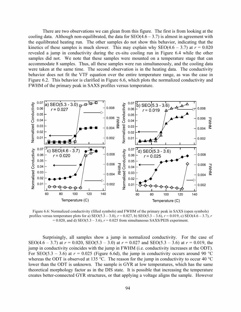
94

There are two observations we can glean from this figure. The first is from looking at the cooling data. Although non-equilibrated, the data for SEO(4.6 – 3.7) is almost in agreement with the equilibrated heating run. The other samples do not show this behavior, indicating that the kinetics of these samples is much slower. This may explain why SEO(4.6 – 3.7) at r = 0.020 revealed a jump in conductivity during the ex-situ cooling run in Figure 6.4 while the other samples did not. We note that these samples were mounted on a temperature stage that can accommodate 8 samples. Thus, all these samples were run simultaneously, and the cooling data were taken at the same time. The second observation is in the heating data. The conductivity behavior does not fit the VTF equation over the entire temperature range, as was the case in Figure 6.2. This behavior is clarified in Figure 6.6, which plots the normalized conductivity and FWHM of the primary peak in SAXS profiles versus temperature.

Figure 6.6: Normalized conductivity (filled symbols) and FWHM of the primary peak in SAXS (open symbols) profiles versus temperature plots for a) SEO(5.3 – 3.0), r = 0.027, b) SEO(5.3 – 3.6), r = 0.019, c) SEO(4.6 – 3.7), r

= 0.020, and d) SEO(5.3 – 3.6), r = 0.025 from simultaneous SAXS/PEIS experiment.

Surprisingly, all samples show a jump in normalized conductivity. For the case of SEO(4.6 – 3.7) at r = 0.020, SEO(5.3 – 3.0) at r = 0.027 and SEO(5.3 – 3.6) at r = 0.019, the jump in conductivity coincides with the jump in FWHM (i.e. conductivity increases at the ODT). For SEO(5.3 – 3.6) at r = 0.025 (Figure 6.6d), the jump in conductivity occurs around 90 °C whereas the ODT is observed at 135 °C. The reason for the jump in conductivity to occur 40 °C lower than the ODT is unknown. The sample is GYR at low temperatures, which has the same theoretical morphology factor as in the DIS state. It is possible that increasing the temperature creates better-connected GYR structures, or that applying a voltage aligns the sample. However

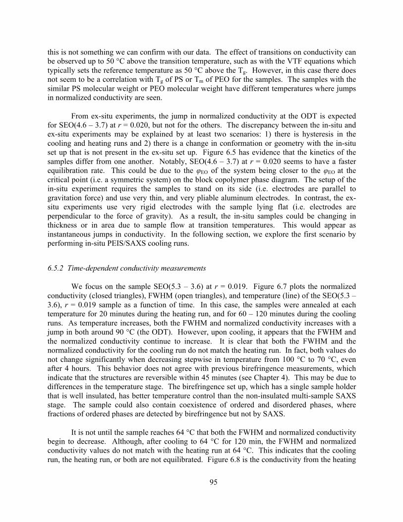
95

this is not something we can confirm with our data. The effect of transitions on conductivity can be observed up to 50 °C above the transition temperature, such as with the VTF equations which typically sets the reference temperature as 50 °C above the Tg. However, in this case there does not seem to be a correlation with Tg of PS or Tm of PEO for the samples. The samples with the similar PS molecular weight or PEO molecular weight have different temperatures where jumps in normalized conductivity are seen.

From ex-situ experiments, the jump in normalized conductivity at the ODT is expected for SEO(4.6 – 3.7) at r = 0.020, but not for the others. The discrepancy between the in-situ and ex-situ experiments may be explained by at least two scenarios: 1) there is hysteresis in the cooling and heating runs and 2) there is a change in conformation or geometry with the in-situ set up that is not present in the ex-situ set up. Figure 6.5 has evidence that the kinetics of the samples differ from one another. Notably, SEO(4.6 – 3.7) at r = 0.020 seems to have a faster equilibration rate. This could be due to the φEO of the system being closer to the φEO at the critical point (i.e. a symmetric system) on the block copolymer phase diagram. The setup of the in-situ experiment requires the samples to stand on its side (i.e. electrodes are parallel to gravitation force) and use very thin, and very pliable aluminum electrodes. In contrast, the ex-situ experiments use very rigid electrodes with the sample lying flat (i.e. electrodes are perpendicular to the force of gravity). As a result, the in-situ samples could be changing in thickness or in area due to sample flow at transition temperatures. This would appear as instantaneous jumps in conductivity. In the following section, we explore the first scenario by performing in-situ PEIS/SAXS cooling runs.

6.5.2 Time-dependent conductivity measurements

We focus on the sample SEO(5.3 – 3.6) at r = 0.019. Figure 6.7 plots the normalized conductivity (closed triangles), FWHM (open triangles), and temperature (line) of the SEO(5.3 – 3.6), r = 0.019 sample as a function of time. In this case, the samples were annealed at each temperature for 20 minutes during the heating run, and for 60 – 120 minutes during the cooling runs. As temperature increases, both the FWHM and normalized conductivity increases with a jump in both around 90 °C (the ODT). However, upon cooling, it appears that the FWHM and the normalized conductivity continue to increase. It is clear that both the FWHM and the normalized conductivity for the cooling run do not match the heating run. In fact, both values do not change significantly when decreasing stepwise in temperature from 100 °C to 70 °C, even after 4 hours. This behavior does not agree with previous birefringence measurements, which indicate that the structures are reversible within 45 minutes (see Chapter 4). This may be due to differences in the temperature stage. The birefringence set up, which has a single sample holder that is well insulated, has better temperature control than the non-insulated multi-sample SAXS stage. The sample could also contain coexistence of ordered and disordered phases, where fractions of ordered phases are detected by birefringence but not by SAXS.

It is not until the sample reaches 64 °C that both the FWHM and normalized conductivity begin to decrease. Although, after cooling to 64 °C for 120 min, the FWHM and normalized conductivity values do not match with the heating run at 64 °C. This indicates that the cooling run, the heating run, or both are not equilibrated. Figure 6.8 is the conductivity from the heating

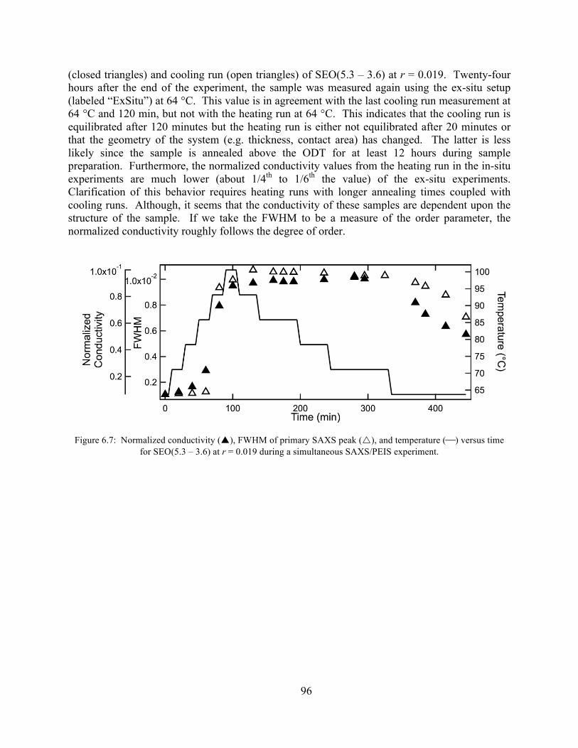
96

(closed triangles) and cooling run (open triangles) of SEO(5.3 – 3.6) at r = 0.019. Twenty-four hours after the end of the experiment, the sample was measured again using the ex-situ setup (labeled “ExSitu”) at 64 °C. This value is in agreement with the last cooling run measurement at 64 °C and 120 min, but not with the heating run at 64 °C. This indicates that the cooling run is equilibrated after 120 minutes but the heating run is either not equilibrated after 20 minutes or that the geometry of the system (e.g. thickness, contact area) has changed. The latter is less likely since the sample is annealed above the ODT for at least 12 hours during sample preparation. Furthermore, the normalized conductivity values from the heating run in the in-situ experiments are much lower (about 1/4th to 1/6th the value) of the ex-situ experiments. Clarification of this behavior requires heating runs with longer annealing times coupled with cooling runs. Although, it seems that the conductivity of these samples are dependent upon the structure of the sample. If we take the FWHM to be a measure of the order parameter, the normalized conductivity roughly follows the degree of order.

Figure 6.7: Normalized conductivity (), FWHM of primary SAXS peak (), and temperature (⎯) versus time for SEO(5.3 – 3.6) at r = 0.019 during a simultaneous SAXS/PEIS experiment.

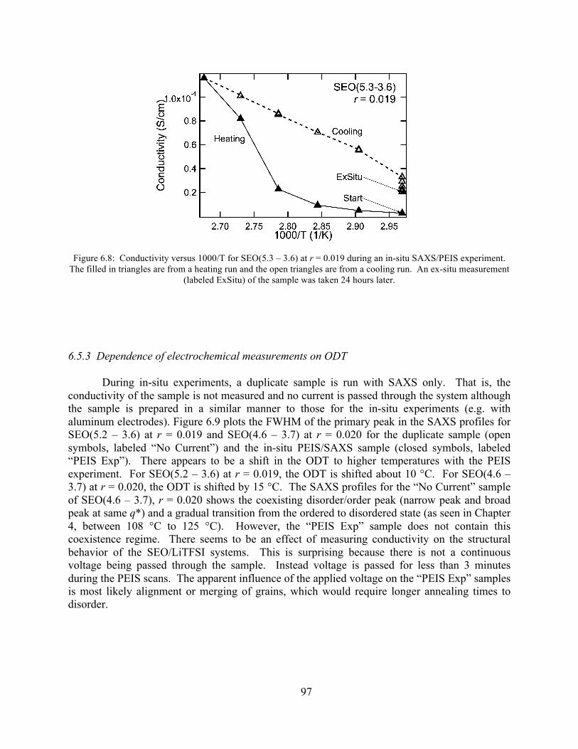
97

Figure 6.8: Conductivity versus 1000/T for SEO(5.3 – 3.6) at r = 0.019 during an in-situ SAXS/PEIS experiment. The filled in triangles are from a heating run and the open triangles are from a cooling run. An ex-situ measurement

(labeled ExSitu) of the sample was taken 24 hours later.

6.5.3 Dependence of electrochemical measurements on ODT

During in-situ experiments, a duplicate sample is run with SAXS only. That is, the conductivity of the sample is not measured and no current is passed through the system although the sample is prepared in a similar manner to those for the in-situ experiments (e.g. with aluminum electrodes). Figure 6.9 plots the FWHM of the primary peak in the SAXS profiles for SEO(5.2 – 3.6) at r = 0.019 and SEO(4.6 – 3.7) at r = 0.020 for the duplicate sample (open symbols, labeled “No Current”) and the in-situ PEIS/SAXS sample (closed symbols, labeled “PEIS Exp”). There appears to be a shift in the ODT to higher temperatures with the PEIS experiment. For SEO(5.2 – 3.6) at r = 0.019, the ODT is shifted about 10 °C. For SEO(4.6 – 3.7) at r = 0.020, the ODT is shifted by 15 °C. The SAXS profiles for the “No Current” sample of SEO(4.6 – 3.7), r = 0.020 shows the coexisting disorder/order peak (narrow peak and broad peak at same q*) and a gradual transition from the ordered to disordered state (as seen in Chapter 4, between 108 °C to 125 °C). However, the “PEIS Exp” sample does not contain this coexistence regime. There seems to be an effect of measuring conductivity on the structural behavior of the SEO/LiTFSI systems. This is surprising because there is not a continuous voltage being passed through the sample. Instead voltage is passed for less than 3 minutes during the PEIS scans. The apparent influence of the applied voltage on the “PEIS Exp” samples is most likely alignment or merging of grains, which would require longer annealing times to disorder.

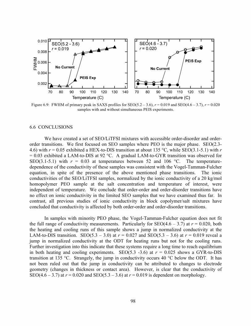
98

Figure 6.9: FWHM of primary peak in SAXS profiles for SEO(5.2 – 3.6), r = 0.019 and SEO(4.6 – 3.7), r = 0.020 samples with and without simultaneous PEIS experiments.

6.6 CONCLUSIONS

We have created a set of SEO/LiTFSI mixtures with accessible order-disorder and order-order transitions. We first focused on SEO samples where PEO is the major phase. SEO(2.3-4.6) with r = 0.05 exhibited a HEX-to-DIS transition at about 135 °C, while SEO(3.1-5.1) with r = 0.03 exhibited a LAM-to-DIS at 92 °C. A gradual LAM-to-GYR transition was observed for SEO(3.1-5.1) with r = 0.03 at temperatures between 52 and 106 °C. The temperature-dependence of the conductivity of these samples was consistent with the Vogel-Tamman-Fulcher equation, in spite of the presence of the above mentioned phase transitions. The ionic conductivities of the SEO/LiTFSI samples, normalized by the ionic conductivity of a 20 kg/mol homopolymer PEO sample at the salt concentration and temperature of interest, were independent of temperature. We conclude that order-order and order-disorder transitions have no effect on ionic conductivity in the limited SEO samples that we have examined thus far. In contrast, all previous studies of ionic conductivity in block copolymer/salt mixtures have concluded that conductivity is affected by both order-order and order-disorder transitions.

In samples with minority PEO phase, the Vogel-Tamman-Fulcher equation does not fit the full range of conductivity measurements. Particularly for SEO(4.6 – 3.7) at r = 0.020, both the heating and cooling runs of this sample shows a jump in normalized conductivity at the LAM-to-DIS transition. SEO(5.3 – 3.0) at r = 0.027 and SEO(5.3 – 3.6) at r = 0.019 reveal a jump in normalized conductivity at the ODT for heating runs but not for the cooling runs. Further investigation into this indicate that these systems require a long time to reach equilibrium in both heating and cooling experiments. SEO(5.3 -3.6) at r = 0.025 shows a GYR-to-DIS transition at 135 °C. Strangely, the jump in conductivity occurs 40 °C below the ODT. It has not been ruled out that the jump in conductivity can be attributed to changes to electrode geometry (changes in thickness or contact area). However, is clear that the conductivity of SEO(4.6 – 3.7) at r = 0.020 and SEO(5.3 – 3.6) at r = 0.019 is dependent on morphology.

99

6.7 REFERENCES

1. Sax, J. and J.M. Ottino, Modeling of Transport of Small Molecules in Polymer Blends - Application of Effective Medium Theory. Polymer Engineering and Science, 1983. 23(3): p. 165-176.

2. Fredrickson, G.H. and E. Helfand, Fluctuation Effects in the Theory of Microphase Separation in Block Copolymers. Journal of Chemical Physics, 1987. 87(1): p. 697-705.

3. Ruzette, A.V.G., et al., Melt-formable block copolymer electrolytes for lithium rechargeable batteries. Journal of the Electrochemical Society, 2001. 148(6): p. A537-A543.

4. Cho, B.K., et al., Mesophase structure-mechanical and ionic transport correlations in extended amphiphilic dendrons. Science, 2004. 305(5690): p. 1598-1601.

5. Kakihana, M., S. Schantz, and L.M. Torell, Raman-Spectroscopic Study of Ion-Ion Interaction and Its Temperature-Dependence in a Poly(Propylene-Oxide)-Based Nacf3so3-Polymer Electrolyte. Journal of Chemical Physics, 1990. 92(10): p. 6271-6277.

6. Watanabe, M., et al., Ionic-Conductivity and Mobility in Network Polymers from Poly(Propylene Oxide) Containing Lithium Perchlorate. Journal of Applied Physics, 1985. 57(1): p. 123-128.

7. Gray, F.M., Polymer Electrolytes. RSC Materials Monographs, ed. J.A. Conner. 1997, Cambridge: The Royal Society of Chemistry. 175.

8. Singh, M., et al., Effect of molecular weight on the mechanical and electrical properties of block copolymer electrolytes. Macromolecules, 2007. 40(13): p. 4578-4585.

9. Lascaud, S., et al., Phase-Diagrams and Conductivity Behavior of Poly(Ethylene Oxide) Molten-Salt Rubbery Electrolytes. Macromolecules, 1994. 27(25): p. 7469-7477.

10. Rosedale, J.H., et al., Order and Disorder in Symmetric Diblock Copolymer Melts. Macromolecules, 1995. 28(5): p. 1429-1443.

11. Blanchard, L.-P., J. Hesse, and S.L. Malhotra, Effect of Molecular Weight on Glass Transition by Differential Scanning Calorimetry. Canadian Journal of Chemistry, 1974. 52(18): p. 3170-3175.

100

Chapter 7

Summary

7.1 DISSERTATION SUMMARY

The objective of this study was to investigate the thermodynamic and electrochemical properties of block copolymers mixed with salts for use as a solid polymer electrolyte in lithium-anode batteries. The growing demand for green power sources has put rechargeable lithium-anode batteries, a system with high power and energy densities, in the forefront as a promising candidate for applications such as electric vehicles.[1-3] A block copolymer was used in this study in order to overcome the shortcomings of using a homopolymer. That is, using a block copolymer can increase the modulus of the electrolyte to prevent dendrite growth. Past studies indicate that each block in the block copolymers can be tuned independently to obtain a material with a much higher modulus and minimal decrease in ionic conductivity in comparison to its homopolymer counterpart.[4] The systems studied in this dissertation are the block copolymer poly(styrene-block-ethylene oxide) (SEO) mixed with the salt Li[N(SO2CF3)2] (LiTFSI) or the ionic liquid imidizolium TFSI (ImTFSI).

Block copolymers are able to microphase separate into ordered structures such as lamellae (LAM), hexagonally packed cylinders (HEX), and gyroid (GYR).[5-7] In Chapter 2, theories of block copolymer thermodynamics including the Flory Huggins theory, Leibler’s theory[5], and Fredrickson and Helfand’s theory[8] are discussed. Additionally, the theory developed by Wang[9] on the effect of salts on polymers is presented. These theories give a basis to understanding the effect of salts on block copolymers. An important parameter in each of these theories is the Flory Huggins interaction parameter, χ. This parameter, which is inversely related to temperature, is a dimensionless energy parameter that describes the thermodynamics of the block copolymer system.

All the polymers in this dissertation were synthesized via anionic polymerization. The polymer characteristics were determined with a combination of size exclusion chromatography (SEC), matrix-assisted laser desorption/ionization-time of flight mass spectroscopy, 1H nuclear magnetic resonance spectroscopy (NMR), and differential scanning calorimetry (DSC). The SEO is mixed with LiTFSI or ImTFSI at concentrations of r = 0 to 0.15, where r is the molar ratio of the cation to EO unit. The structure and thermodynamics of the block copolymer electrolytes were determined using a combination of birefringence detection of the order-to-disorder transition (ODT) and small-angle Xray scattering (SAXS). The conductivity of the samples was measured using ac impedance spectroscopy.

101

The phase behavior and thermal properties of SEO mixed with LiTFSI were discussed in Chapter 4. From DSC studies, it was determined that LiTFSI decreases the crystallinity of the PEO block, with complete suppression between r = 0.05 to r = 0.125. The phases of the PEO block in the SEO copolymer are in agreement with the phase diagram for hompolymer PEO/LiTFSI. From SAXS measurements of the sample SEO(6.4 – 7.2), it was determined that the addition of LiTFSI generally increases the domain size of the sample, most likely due to increase in free volume. From r = 0.085 to r = 0.10, the domain size does not increase as rapidly as from r = 0 to r = 0.085. This was attributed to the increased coordination of Li+ to ether oxygen. This behavior has not been seen in other PEO/salt systems.

Investigation of the SAXS profiles of SEO(6.4 – 7.2) revealed that increasing r increases both the lamellar asymmetry and the effective χ parameter (χeff) between the PS and PEO phases. Using both SAXS and birefringence, the phase behavior and ODT of several SEO samples were mapped out. A rich variety of phases are obtained, including HEX, LAM, and GYR even though the majority of the neat polymers are disordered. The ODT can be accessed by controlling the salt concentration. Phase diagrams of several SEOs as a function of r are presented at the end of Chapter 4.

The change in χeff as a function of r is quantified in Chapter 5. Using a combination of SAXS and birefringence, the ODT of several SEOs mixed with LiTFSI, ImTFSI, and a 50:50 mixture of both (Mix) were measured. Using the theories discussed in Chapter 2, the ODT was related to the χeff and plotted as a function of r. This relationship was determined to be linear with the slope of the line, m, a measurement of the change in the thermodynamic interactions with salts. Within error, the change in χeff for SEO/LiTFSI, SEO/ImTFSI, and SEO/Mix were the same, with m = 1.52. This indicates that the nature of the thermodynamics in this system is dominated by the large TFSI- anion. The theoretical predictions of Wang[9] were used to calculate the χeff of SEO with different salts. These were compared to the data in this dissertation and those reported by Young et al.[10]. Qualitatively, the trend with anion size is similar, but the absolute values of the theoretical χeff are consistently higher than the experimental values.

Finally, the effect of block copolymer morphology on conductivity is studied. The conductivity of the block copolymer should be less than that of the pure conducting homopolymer. The conductivity is assumed to scale by the volume fraction of the conducting block, φEO and the morphology factor, f. The morphology factor accounts for the alignment of randomly oriented grains in relation to the electrodes. For LAM samples, f = 2/3, while DIS, GYR, and HEX where the PEO is the major phase, f = 1. First, SEO samples where PEO is the major phase were examined. SEO(2.3-4.6) with r = 0.05 exhibited a HEX-to-DIS transition at about 135 °C, while SEO(3.1-5.1) with r = 0.03 exhibited a LAM-to-DIS at 92 °C. A gradual LAM-to-GYR transition was observed for SEO(3.1-5.1) with r = 0.03 at temperatures between 52 and 106 °C. The conductivity through the ODT and order-to-order transitions (OOT) were measured, and the Vogel-Tamman-Fulcher (VTF) equation was fit through the data. It was determined that the VTF equation fit reasonably well through the full set of data despite the presence of the transitions.

To hone in on the effect of morphology, the normalized conductivity values were calculated. The normalized conductivity was shown to successfully decouple the temperature

102

dependence from the conductivity measurements on samples that were fully disordered and fully ordered in the experimental temperature range. It was determined that the ODT and OOT have no effect on ionic conductivity of these samples.

In contrast, samples with PEO as the minority phase indicated a jump in conductivity. In this case, samples were run both ex-situ (similar to the major phase sample study) and in-situ, where SAXS and ac impedance spectroscopy were performed on the sample simultaneously. For SEO(4.6 – 3.7) at r = 0.020, jumps in conductivity and normalized conductivity were seen near the ODT in both in-situ and ex-situ experiments. Whereas SEO(5.3 – 3.0) at r = 0.027 and SEO(5.3 – 3.6) at r = 0.019 revealed a jump in conductivity at the ODT in in-situ experiments, but only a moderate rise in normalized conductivity 20 °C below the ODT in ex-situ experiments. Further investigation into SEO(5.3 – 3.6) at r = 0.019 suggests that this system takes a longer time to reach equilibrium than the other systems. Furthermore, sample SEO(5.3 – 3.6) at r = 0.025, which shows a GYR-to-DIS transition at 135 °C, revealed a jump in conductivity around 95 °C. These jumps in conductivity seen in the in-situ conductivity/SAXS measurements could be attributed to changes to electrode geometry (changes in thickness or contact area). However, is clear that the conductivity of SEO(4.6 – 3.7) at r = 0.020 and SEO(5.3 – 3.6) at r = 0.019 is dependent on morphology.

Continuing this study involves longer annealing times for these minor phase samples, in heating and cooling, ex-situ and in-situ. Unresolved issues such as the reason for the jump in conductivity during in-situ measurements need to be settled. Furthermore, it would be interesting to see the effect of current/voltage on these samples with in-situ experiments, especially if active electrodes (lithium) are used. An under-explored factor is the effect of grain sizes on the conductivity. By using one of these samples with an accessible ODT, e.g., SEO(2.3 – 4.6) at r = 0.05, changing quench depths below the ODT should lead to different grain size growths, which can be measured with birefringence.

Another area that could be improved upon is the measurement and predictions of the χeff parameter. In the theory developed by Wang, the calculated values of χeff were consistently higher than the experimental values. Since these calculations were based on nonadjustable parameters, it is necessary to obtain the best possible values for the equation. One property that is not well tabulated is the dielectric constant of PEO and PS in the temperature range of interest. Thus, measuring this property would be the next step for this study. Furthermore, more rigorous measurements of χ can be measured for SEO/LiTFSI samples by fitting the random phase approximation (RPA) to scattering data. To do RPA fits, a very precise measurement of absolute intensity is needed.

7.2 REFERENCES

1. Tarascon, J.M. and M. Armand, Issues and challenges facing rechargeable lithium batteries. Nature, 2001. 414(6861): p. 359-367.

2. Abruna, H.D., Y. Kiya, and J.C. Henderson, Batteries and electrochemical capacitors. Physics Today, 2008. 61(12): p. 43-47.

103

3. Scrosati, B. and J. Garche, Lithium batteries: Status, prospects and future. Journal of Power Sources, 2010. 195(9): p. 2419-2430.

4. Singh, M., et al., Effect of molecular weight on the mechanical and electrical properties of block copolymer electrolytes. Macromolecules, 2007. 40(13): p. 4578-4585.

5. Leibler, L., Theory of Microphase Separation in Block Co-Polymers. Macromolecules, 1980. 13(6): p. 1602-1617.

6. Matsen, M.W. and F.S. Bates, Unifying weak- and strong-segregation block copolymer theories. Macromolecules, 1996. 29(4): p. 1091-1098.

7. Bates, F.S. and G.H. Fredrickson, Block copolymers - Designer soft materials. Physics Today, 1999. 52(2): p. 32-38.

8. Fredrickson, G.H. and E. Helfand, Fluctuation Effects in the Theory of Microphase Separation in Block Copolymers. Journal of Chemical Physics, 1987. 87(1): p. 697-705.

9. Wang, Z.G., Effects of Ion Solvation on the Miscibility of Binary Polymer Blends. Journal of Physical Chemistry B, 2008. 112(50): p. 16205-16213.

10. Young, W.S. and T.H. Epps, Salt Doping in PEO-Containing Block Copolymers: Counterion and Concentration Effects. Macromolecules, 2009. 42(7): p. 2672-2678.

104

Chapter 8

Appendix

8.1 PROCEDURE FOR SEO SYNTHESIS

SEO block copolymers are synthesized using living anionic polymerization. This technique is sensitive to both oxygen and water; thus the solvents and monomers must be stringently purified and the synthesis performed on a high-vacuum line (10-3 torr) and an argon glove box. The full synthesis procedure takes approximately 7 days.

Solvent Purification

The first step is to purify benzene, the solvent used in the synthesis. There is one purification stage when the benzene is taken from the solvent columns.

1) Use a large reactor with a stir bar. 2) Place benzene from the columns into the reactor.

a. Need enough to make ~10 wt% solution. 3) Attach the reactor on the vacuum line and degas 3 times. 4) Distill the benzene from the reactor into a sec-butyllithium/diphenylethylene (sbl/dpe)

stage, and stir for 8 hours.

Styrene Purification

The next step is purification of the styrene monomer, and synthesis of polystyrene. This procedure has 1 or 2 stages:

1) Calcium Hydride (CaH2) stage. 2) Dibutyl Magnesium (DBM) stage.

Just doing one of the stages is sufficient to get a PDI below 1.1, with DBM giving slightly better PDI than just CaH2. Do both stages if only one stage is not sufficient.

Only 1 stage:

1) CaH2 stage preparation. a. Use long neck flask with stir bar. b. Ground CaH2 with mortar and pestle to get fine powder.

105

c. Add CaH2 to flask. i. Rule of thumb: 10 g for every 100 mL.

d. Add styrene to flask. e. Attach flask to vacuum and degas 3 times. f. Let stir for few hours.

OR

1) DBM stage preparation g. Bring reactor (with clean stir bar!) into glovebox and add DBM.

i. Rule of thumb: 10 mL of DBM (1.0 M in heptane) for 100 mL styrene. h. Attach reactor to vacuum line and degas. i. Distill off heptane into waste flask. j. Pull on reactor for a few hours (overnight is best) to get rid of residual heptanes. k. Bring reactor into glovebox and pipet in styrene. l. Reattach reactor to line and degas 3 times. m. Let stir for few hours (overnight is best).

2) Degas purification stage. 3) Flame torch line.

a. Make sure that it cools down before distillation of styrene because styrene can autoinitiate thermally.

4) Distill styrene from purification stage to reactor (or ampoule) using liquid nitrogen. a. Do NOT use warm bath (because of autoinitiation).

If doing both stages, do CaH2 stage first, and then distill from CaH2 stage to DBM stage.

Polymerization of styrene block

1) Attach reactor to the vacuum line. 2) Torch the reactor and vacuum line to get rid of impurities. 3) Distill trace amount of solvent into reactor. 4) Take reactor to glove box. 5) Pipette calculated amount of the initiator, sec-butyllithium. 6) Attach reactor back to vacuum line and degas. 7) Distill remaining solvent.

a. Always leave a small amount in sbl/dpe stage. 8) Distill monomer to ampoule.

a. Add more than needed to ampoule such that you can measure by difference. b. Remember that monomer will expand once it warms up. c. Do not leave in ampoule for too long (ie not longer than 1 day) since there are no

purifiers in the ampoule. 9) Distill monomer from ampoule to reactor. 10) Let react for at least 4 hours.

a. Solution should turn a pale yellow to a pale orange color (depending on concentration).

106

11) Take out a small amount of the solution and terminate with isopropyl alcohol (IPA) to characterize the first block.

Ethylene Oxide Purification

This completes the synthesis of the first block, ready for the addition of the ethylene oxide (EO) block. The purification of the EO monomer requires 3 steps:

1) Calcium Hydride (CaH2) stage. 2) N-butyl lithium (NbutLi) stage 1. 3) NbutLi stage 2.

Ethylene oxide monomer is a gas at room temperature (boiling point~ 11oC). All stages must be maintained at 0 °C (or lower) at all times.

1) Prepare CaH2 stage: a. Use long neck flask with stir bar. b. Ground CaH2 with mortar and pestle to get fine powder. c. Add CaH2 to flask.

i. Rule of thumb: 10 g for every 100 mL. d. Attach flask to vacuum line and pull.

2) Condense EO to CaH2 stage. a. Use regulator on EO cylinder, and attach with tubing to vacuum line.

i. Pull on tubing to allow for better condensation. b. Use dry ice/IPA mixture on CaH2.

i. If EO is not condensing very well, switch to LN2. 3) Degas CaH2 stage 2 times.

a. To degas, freeze stage with LN2. b. After closing off vacuum, take LN2 off stage and let stage warm up slightly

(about a minute), allowing a boundary layer to form around the flask. c. Place in dry ice (about a minute). d. Add IPA to dry ice.

i. This procedure slowly warms up the EO stage. 4) Stir EO on CaH2 overnight to remove residual moisture.

a. Maintain dry ice/IPA temperature on stage. 5) Preparation of nButLi stages:

a. Bring 2 reactors OR 2 long neck flasks (with clean stir bars!) into glovebox and add nButLi.

i. Rule of thumb: 10 mL of nButLi (1.0 M in cyclohexane). b. Attach reactor to vacuum line and degas. c. Distill off cyclohexane into waste flask. d. Pull on reactor for a few hours (overnight is best) to get rid of residual

cyclohexane. 6) Degas EO on CaH2. 7) Distill EO from CaH2 stage to nButLi stage 1.

a. Take away dry ice/IPA from CaH2 stage and let warm up slightly (~1 min).

107

b. Add ice to CaH2 stage (~1 min). c. Add water to CaH2 stage. d. Use LN2 on nButLi stage 1. e. Slowly open valve from CaH2 stage.

i. Listen for a hiss, which means you are distilling too fast. 8) Stir EO in nButLi stage 1 for 30 min on ice bath.

a. Take LN2 off nButLi stage 1 and let warm up slightly (~1 min). b. Add ice to CaH2 stage (~1-5 min). c. Add water to CaH2 stage.

9) Degas nButLi stage 1. 10) Repeat steps 7 through 9, for nButLi stage 1 to nButLi stage 2. 11) Distill EO from nButLi stage 2 to ampoule.

Polymerization of ethylene oxide block

1) Distill about 1 mL of monomer from ampoule to reactor. a. Distill any unreacted EO back to CaH2 stage.

2) Let react for at least 8 hours. a. Solution should turn clear.

3) Degas reactor and take reactor into glovebox. 4) Add the catalyst, tert-butyl phosphazene. 5) Repurify the ethylene oxide monomer (steps 6 -11 in the previous section). 6) Distill calculated amount of monomer from ampoule to reactor. 7) Set in a 45 °C bath and stir for 3 days.

Terminate reaction

1) Take reactor offline and bring into glove box. 2) Pipette in excess IPA and stir.

Clean polymer

1) Fill a large beaker with cold hexane. 2) Pour polymer from reactor into beaker. a. Polymer should precipitate right away. 3) Stir overnight. 4) Fish out polymer chunks and place into second 4L beaker with benzene. a. Take out as many polymer pieces as possible by “hand”, then throw away supernatant. 5) Stir for few hours. 6) Repeat hexane then benzene 2 more times (total of 3 precipitations). 7) Freeze dry.

108

8.2 LIST OF SYNTHESIZED POLYMERS

Name Lab Name Publication Name MPS

MEO

φEO

MTotal

SEON0 SEO11 SEO(6.4 – 7.2) 6368 7242 51.9 13,610

SEON1 SEO12 SEO(1.4 – 2.5) 1383 2471 61.9 3854

SEON2 SEO13 SEO(2.3 – 4.6) 2296 4607 64.6 6903

SEON3 SEO14 SEO(3.1 – 5.1) 3111 5134 60.0 8245

SEON4 SEO18 SEO(5.3 – 3.0) 5315 2968 33.7 8283

SEON5 SEO19 SEO(5.3 – 3.6) 5272 3580 38.0 8852

SEON6 SEO20 SEO(4.6 – 3.7) 4558 3733 42.7 8291

SEON7 SEO21 SEO(1.7 – 1.6) 1664 1646 47.0 3310

SEON8 SEO22 SEO(1.5 – 1.3) 1454 1323 45.0 2777

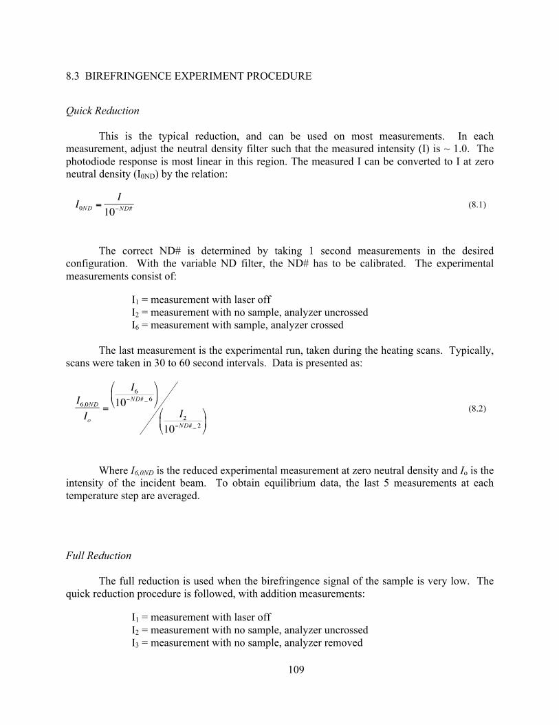
109

8.3 BIREFRINGENCE EXPERIMENT PROCEDURE

Quick Reduction

This is the typical reduction, and can be used on most measurements. In each measurement, adjust the neutral density filter such that the measured intensity (I) is ~ 1.0. The photodiode response is most linear in this region. The measured I can be converted to I at zero neutral density (I0ND) by the relation:

(8.1)

The correct ND# is determined by taking 1 second measurements in the desired configuration. With the variable ND filter, the ND# has to be calibrated. The experimental measurements consist of:

I1 = measurement with laser off I2 = measurement with no sample, analyzer uncrossed I6 = measurement with sample, analyzer crossed

The last measurement is the experimental run, taken during the heating scans. Typically, scans were taken in 30 to 60 second intervals. Data is presented as:

(8.2)

Where I6,0ND is the reduced experimental measurement at zero neutral density and Io is the intensity of the incident beam. To obtain equilibrium data, the last 5 measurements at each temperature step are averaged.

Full Reduction

The full reduction is used when the birefringence signal of the sample is very low. The quick reduction procedure is followed, with addition measurements:

I1 = measurement with laser off I2 = measurement with no sample, analyzer uncrossed I3 = measurement with no sample, analyzer removed

110

I5 = measurement with sample, analyzer removed I6 = measurement with sample, analyzer crossed The full reduction can be calculated by:

€

Tanalyzer =I2 − I1( )

I3 − I1( ) (8.3)

€

Tsample =I5 − I1( )

I3 − I1( ) (8.4)

€

Ibackground = I1 + Tsample ⋅ I4 − I1( )( ) (8.5)

€

Io = Tanalyzer ⋅ I5 − I1( ) (8.6)

€

IIo

=I6Io

(8.7)

Where each In has already been converted to zero neutral density.