Embed Size (px)
Citation preview
THERMODYNAMICS PERFORMANCE AND HEAT
TRANSFER ANALYSIS OF PARABOLIC TROUGH
COLLECTOR IN SOLAR POWER PLANT
OMID AFSHAR
FACULTY OF ENGINEERING
UNIVERSITY OF MALAYA
KUALA LUMPUR
2013
ii
THERMODYNAMICS PERFORMANCE AND HEAT
TRANSFER ANALYSIS OF PARABOLIC TROUGH
COLLECTOR IN SOLAR POWER PLANT
OMID AFSHAR
RESEARCH REPORT SUBMITTED IN PARTIAL
FULFILLMENT OF THE REQUIREMENT FOR THE
DEGREE OF MASTER OF ENGINEERING
FACULTY OF ENGINEERING
UNIVERSITY OF MALAYA
KUALA LUMPUR
2013
iii
UNIVERSITI MALAYA ORIGINAL LITERARY WORK DECLARATION
Name of Candidate: OMID AFSHAR (I.C/Passport No:)
Registration/Matric No: KGH100046
Name of Degree: Master of mechanical engineering Title of Project Paper/Research Report/Dissertation/Thesis (“this Work”):
THERMODYNAMIS PERFORMANCE AND HEAT TRANSFER ANALYSIS OF PARABOLIC TROUGH COLLECTOR IN SOLAR POWER PLANT
Field of Study: Renewable Energy, Heat transfer
I do solemnly and sincerely declare that:
(1) I am the sole author/writer of this Work; (2) This Work is original; (3) Any use of any work in which copyright exists was done by way of fair dealing and for
permitted purposes and any excerpt or extract from, or reference to or reproduction of any copyright work has been disclosed expressly and sufficiently and the title of the Work and its authorship have been acknowledged in this Work;
(4) I do not have any actual knowledge nor do I ought reasonably to know that the making of this work constitutes an infringement of any copyright work;
(5) I hereby assign all and every rights in the copyright to this Work to the University of Malaya (“UM”), who henceforth shall be owner of the copyright in this Work and that any reproduction or use in any form or by any means whatsoever is prohibited without the written consent of UM having been first had and obtained;
(6) I am fully aware that if in the course of making this Work I have infringed any copyright whether intentionally or otherwise, I may be subject to legal action or any other action as may be determined by UM.
Candidate’s Signature Date
Subscribed and solemnly declared before,
Witness’s Signature Date
Name:
Designation:
iv
Abstract
Today, solar energy can play a vital role in the world. Parabolic trough collector is one type
of solar devices that play an important role in the power system. The main components of
parabolic trough collector are curve mirror and receiver system. Iran is one of the potential
countries that use parabolic trough power plant system. In this research thermodynamics
performance like exergy and thermal efficiency will be considered on the first, tenth,
fifteenth, twentieth, twenty-fifth and thirtieth of September. Iran will be considered as a
case study in whole time. Then, heat transfer in different parts of receiver system will be
analyzed at 250˚C. Based on some experimental tools, temperature and mass flow rate and
solar parameter, can be estimated when it comes to thermodynamics and heat transfer
values. The result shows that the value of exergy and thermal efficiency on the first of
September is the highest. Second law efficiency on the first of September at 12 noon is
around 10% and the value of exergy at that time is approximately 15.5kJ/kg in collector
system. The value of convection heat transfer between the heat transfer fluid and the
receiver pipe was around 15.5kW in 250˚C.
v
Abstrak
Kini, tenaga solar boleh memainkan peranan penting di dunia. Pengumpul palung parabola
adalah satu jenis peranti solar yang memainkan peranan penting dalam sistem kuasa.
Komponen utama pengumpul palung parabola adalah cermin melengkung dan sistem
penerima. Iran adalah salah satu daripada negara berpotensi yang menggunakan lojikuasa
sistem palung parabola. Dalam kajian ini pada prestasi termodinamik seper ti exergy dan
kecekapan haba akan dipertimbangkan dalam satu, 5,10,15,20,25 dan 30 daripada
September dalam masa keseluruhan akan dipertimbangkan pada satu negara contoh Iran.
Iran akan dianggap sebagai kajian kes dalam keseluruhan masa. Kemudian, pemindahan
haba di bahagian-bahagian berlainan dari sistem penerima akan dianalisis pada 250˚C.
Berdasarkan beberapa alat eksperimen, suhu dan kadar aliran jisim dan solar parameter
boleh dianggarkan apabila datang kepada termodinamik dan nilai pemindahan haba. Hasil
menunjukkan bahawa nilai exergy dan kecekapan haba pada satu September merupakan
yang tertinggi. Kecekapan hukum kedua pada satu September pada pukul 12 petang adalah
sekitar 10% dan nilai exergy pada masa itu kira kira 15.5kJ/kg dalam sistem pengumpul.
Nilai pemindahan haba perolakan antara cecair pemindahan haba dan penerima paip adalah
sekitar 15.5kW dalam 250˚C.

vi
Acknowledgement
I take this opportunity to express my profound gratitude and deep regards to my guide (Dr.
Irfan Anjum Magami ) for exemplary guidance and constant encouragement throughout the
course of this thesis. Also, I thank my wife ( Najmeh Azizabadi) for her constant
encouragement without which this theses would not be possible.
OMID AFSHAR

vii
Contents Abstract ................................................................................................................................. iii
List of Figures ..................................................................................................................... viii
List of Tables ........................................................................................................................ ix
Nomenclature ........................................................................................................................ xi
1. Introduction .................................................................................................................... 1
1.1. Background ............................................................................................................. 1
1.2. Concentrated solar power plant ............................................................................... 2
1.3. History of parabolic trough solar power plant ........................................................ 8
1.4. Objectives .............................................................................................................. 11
2. Literature review ........................................................................................................... 13
2.1. Thermodynamics approach ................................................................................... 13
2.2. Heat Transfer approach ......................................................................................... 20
3. Methodology ................................................................................................................. 25
3.1. Solar measuring instruments ................................................................................. 25
3.2. Solar parameter ..................................................................................................... 30
3.3. Thermodynamic parameter.................................................................................... 32
3.4. Heat transfer parameter ......................................................................................... 34
3.5. Survey Data ........................................................................................................... 38
3.6. Solar parameter data .............................................................................................. 39

viii
3.7. Thermodynamics and heat transfer parameters ..................................................... 40
4 Result and Discussion ................................................................................................... 43
4.1 Solar parameter ..................................................................................................... 43
4.2 Thermodynamics results for collector system ....................................................... 48
4.3 Thermodynamics result for receiver system ......................................................... 51
4.4 Rankine system ..................................................................................................... 55
4.5 Heat transfer result ................................................................................................ 56
4.6 Ways to improve the performance ........................................................................ 60
5 Conclusion .................................................................................................................... 62
6 Recommendation .......................................................................................................... 64
7 Bibliography .................................................................. Error! Bookmark not defined.

ix
List of Figures Figure 1.1, Schematic of Fresnel reflector system . .............. Error! Bookmark not defined.
Figure 1.2, Schematic of solar dish system ........................... Error! Bookmark not defined.
Figure 1.3, Flowchart of solar dish system . ......................... Error! Bookmark not defined.
Figure 1.4, Sample of holder and support in PTC ................ Error! Bookmark not defined.
Figure 1.5, Fact of rotating of pylon in parabolic trough collector system Error! Bookmark
not defined.
Figure 1.6, The schematic of receiver tube ........................... Error! Bookmark not defined.
Figure 1.7, Schematic of parabolic trough collector system which has been combined by
rankine system. ..................................................................... Error! Bookmark not defined.
Figure 1.8. The schematic of oil parts and Rankine parts ..... Error! Bookmark not defined.
Figure 3.1, Sample of mass follow controller monitoring ......................................................... 26
Figure 3 2, Sample of short wavelength pyrometer gauge .................................................. 28
Figure 3.3, Solar temperature gauge .................................................................................... 29
Figure 3.4, Solar pressure gauge .......................................................................................... 30
Figure 3.5, Schematic of The oil cycle and the water cycle ................................................ 31
Figure 3.6, Heat transfer in a cross section at the solar collector and the thermal resistance
model used in the heat transfer analysis .............................................................................. 35
Figure 4.1, Solar beam radiation at 12 noon ........................................................................ 48
Figure 4.2, The value of first law efficiency for collector system at 12 noon ..................... 54
Figure 4.3, The percentage of receiver efficiency in the 20 segments ................................. 55
Figure 4.4, The percentage of collector efficiency in the different temperature ................. 59
Figure 4.5, Comparison of thermal losses in receiver part when sun is appear .......................... 59
Figure 4.6, Comparison of thermal losses value in receiver when sun is not appear .................. 60

x
xi
List of Tables
Table 1.1, Parabolic trough collector power planet ............................................................... 9
Table 2.1, Thermo physical properties of various paraffin types taken from ...................... 16
Table 2.2, The percentage of energy loss in different part of solar power plant ................. 23
Table 3.1, The value of number of days per months............................................................ 32
Table 3.2, Physical parameters of PTC in Shiraz ................................................................ 39
Table 3.3, The value of cloudy factor in Shiraz for different months .................................. 40
Table 3.4, Physical properties of VP1-oil ............................................................................ 41
Table 3.5, Physical properties of AISI 316L ....................................................................... 41
Table 3.6, Heat transfer parameters for receiver tube .......................................................... 42
Table 4.1, The solar parameters result for different days .................................................... 43
Table 4.2, The value of solar parameters result for first of Sep ........................................... 44
Table 4.3, The value of solar parameters result for 5th of Sep ............................................ 44
Table 4.4, The value of solar parameters result for 10th of Sep .......................................... 45
Table 4.5, The value of solar parameters result for15th of Sep ........................................... 45
Table 4.6, The value of solar parameters result for 20th of Sep .......................................... 46
Table 4.7, The value of solar parameters result for 25th of Sep .......................................... 46
Table 4.8, The value of solar parameters result for 30th of Sep .......................................... 47
Table 4.9, Inlet collector temperature and outlet parabolic collector temperature .................... 48
Table 4.10, The value of exergy and efficiency for collector system in first of Sep ........... 49
Table 4.11, The value of exergy and efficiency for collector system in 5th of Sep ............ 49
Table 4.12, The value of exergy and efficiency for collector system in 10th of Sep .......... 50
Table 4.13, The value of exergy and efficiency for collector system in 15th of Sep .......... 50
Table 4.14, The value of exergy and efficiency for collector system in 20th of Sep .......... 50
xii
Table 4.15, The value of exergy and efficiency for collector system in 25th of Sep .......... 51
Table 4.16, The value of exergy and efficiency for collector system in 30th of Sep .......... 51
Table 4.17, The value of exergy and efficiency for receiver system in first of Sep ...................... 52
Table 4.18, The value of exergy and efficiency for receiver system in 5th of Sep ............. 52
Table 4.19, The value of exergy and efficiency for receiver system in 10th of Sep ........... 52
Table 4.20, The value of exergy and efficiency for receiver system in 15th of Sep ........... 53
Table 4.21, The value of exergy and efficiency for receiver system in 20th of Sep ..................... 53
Table 4.22, The value of exergy and efficiency for receiver system in 25th of Sep ........... 53
Table 4.23, The value of exergy and efficiency for receiver system in 30th of Sep ........... 54
Table 4.24, Thermodynamics results for Rankine system ................................................... 56
Table 4.25, Heat transfer results for different part of receiver ............................................ 56

xiii
Nomenclature a: accommodation coefficient (-)
b: interaction coefficient (-)
cp: specific heat capacity (J/kgºK)
cfi: Cloudy factor (-)
Do: outside receiver pipe diameter (m)
Dpi: inside diameter of the receiver pipe (m)
Dgo: outside glass envelope diameter (m)
Dgi: inside glass envelope diameter (m)
fpi: friction factor for the inside surface of the receiver pipe, inside diameter of the receiver
pipe (-)
g: gravitational constant (m/s2)
h: convection heat transfer coefficient (W/m2ºC)
i: number of days (-)
I: solar radiation (W/m2)
Ib: solar beam radiation (W/m2)
Id: solar diffuse radiation (W/m2)
Io: average solar radiation (W/m2)
k: thermal conductivity (W/mºC)
kair: thermal conductivity of air (W/mºC)
kf: thermal conductivity of fluid (W/mºC)

xiv
kpipe: thermal conductivity of pipe (W/mºC)
kT: incident solar angle (-)
L: length (m)
Lc: critical length (m)
m: mass flow rate (kg/s)
n: day of year (-)
N: number of collector (-)
Nu: Nusselt number (-)
P: annulus gas pressure (Pa)
Pr: Prandtl number (-)
Qi: heat absorbed (W)
Qs: heat received (W)
Qu: heat absorbed to receiver (W)
Rb: optimum azimuth angle (-)
Ra: Rayleigh number (-)
Re: Reynolds number (-)
Ta: ambient temperature (K)
To : environment temperature (K)
Ts : solar temperature (K)
Tfi : inner temperature (K)
Tfo : outlet temperature (K)
V: velocity (m/s)
W0: aperture area (m)

xv
Xi : exergy absorbed (W)
Xc : exergy received (W)
Y: intercept factor (-)
Greek:
δ: Declination value (-)
θ: incidence angle (º)
: zenith angle (º)
Ф: latitude angle (º)
β: slope (º)
γ : surface azimuth angle (º)
ώ : hour angle (º)
η :efficiency (-)
τ : cover transmission (-)
a : receiver absorptivity (-)
λ: mean-free-path between collisions of a molecule (m)
ν: kinematic viscosity (m2/s)
ρ: density (kg/m3)
б: StefaneBoltzmann constant (W/m2K
4)

xvi
ɛpo: receiver pipe selective coating emissivity (-)
ɛgi: glass envelope emissivity (-)
1
1. Introduction
1.1.Background
Today, solar energy can play a vital role in the world. There was a huge revelation
in the human’s life after solar energy was introduced as the main source of energy. After a
few years, using solar energy became usual in the world. It would not be surprised when
solar energy is used by some of the electrical appliances like water heater, oven or even the
refrigerator and ice-maker. Just like many other forms of energy, solar energy can be used
in the industrial sector. It is very important because solar energy is introduced as the clean
energy when it comes to greenhouses gases. After several years, a useful key for reduction
pollution into environment was found although the thermal efficiency was not high.
However, these technologies were developed and engineers and scientists try to improve
the thermal energy considerably.
Solar energy exploitation and related new technologies are assuming as an increase
interest for industrialized countries where medium-to-long term production of low cost
energy with reduced emissions is carried out. Indeed, several solar energy power plants
have been designed and are currently under testing in many countries. An Italian law
assigned to Ente Nazionale per l'Energia Atomica (National Agency for Atomic Energy) -
ENEA- the mission to develop an R&D program of systems able to take advantage of solar
energy as a heat source at high temperature. One of the most relevant objectives of this
research program is study of Concentrating Solar Power (CSP) systems operating in the
medium temperatures, i.e. about 550°C, directed towards the development of a new and
low-cost technology to concentrate the direct radiation and efficiently convert solar energy
into high temperature heat (Giannuzzi et al., 2007). After the solar energy was globalized
and could find its special seat among industrial and scientific sector, the majority of firms

2
and companies had some idea about how to increase and improve that type of technology.
The most important factor is relating to collector and photovoltaic section. Using the
parabolic trough collector was one of the initial methods. It was used in power plant,
thermal and cooling systems. By using new technologies like nanofloid and phase change
material (PCM) are tried to improve efficiency of this kind of collector. As far as parabolic
trough collectors are concerned, the main applications are industrial process heat, domestic
hot water, air conditioning and refrigeration system, pumping irrigation water and
desalination (Fernández-García et al., 2010).
Trough collector is one of the collectors that are used in the solar energy systems. As long
as its background is considered, it had been used in the small power systems in Spain in
1981. Parabolic solar collectors able to generate temperatures greater than 500˚C, were
initially developed for industrial process heat applications (Bakos, 2006).
1.2. Concentrated solar power plant
In 1866, Auguste Mouchout used a parabolic trough to produce steam for the first
solar steam engine. The first patent for a solar collector was obtained by the Italian
Alessandro Battaglia in Genoa, Italy, in 1886. Over the following years, inventors such
as John Ericsson and Frank Shuman developed concentrating solar-powered devices for
irrigation, refrigeration, and locomotion. In 1913 Shuman finished a 55 HP parabolic solar
thermal energy station in Maadi, Egypt for irrigation. The first solar-power system using a
mirror dish was built by Dr. R.H. Goddard, who was already well known for his research
on liquid-fueled rockets and wrote an article in 1929 in which he asserted that all the
previous obstacles had been addressed (Corporation, 1929).
3
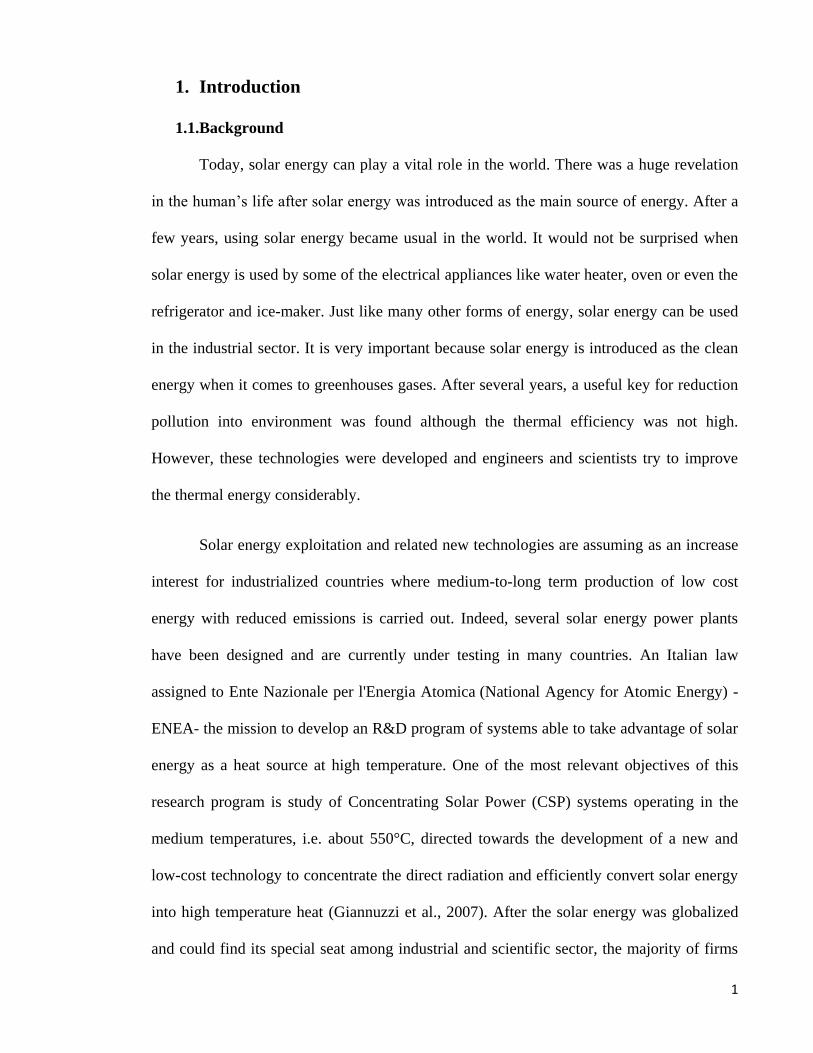
One of the types of concentrating solar power plant is called Fresnel reflector
system. Its components are flat plate collectors and one tower. A receiver has been
designed on top of this tower. After contacting sun’s rays to flat plate collector, sun’s rays
are reflected to receiver and caused to change the temperature (Feuermann and Gordon,
1991). Figure 1.1 shows the schematic of Fresnel reflector system (Nixon and Davies,
2012).
Figure 1.1, Schematic of Fresnel reflector system (Nixon & Davies, 2012)
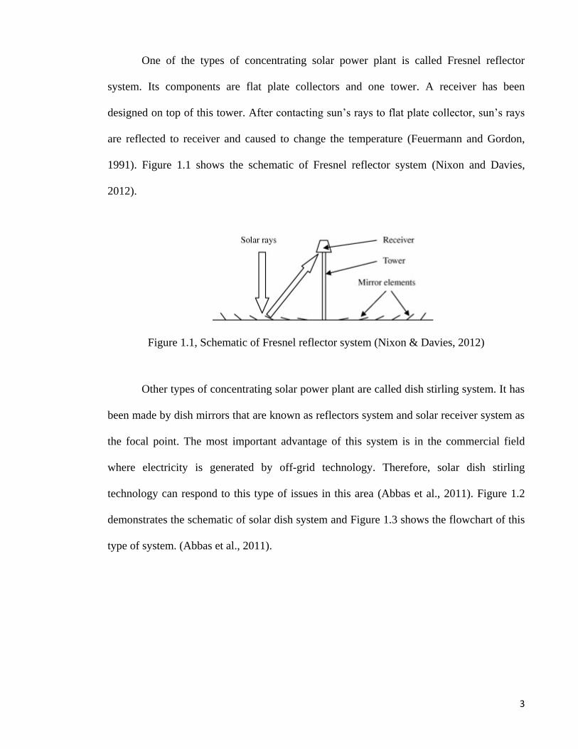
Other types of concentrating solar power plant are called dish stirling system. It has
been made by dish mirrors that are known as reflectors system and solar receiver system as
the focal point. The most important advantage of this system is in the commercial field
where electricity is generated by off-grid technology. Therefore, solar dish stirling
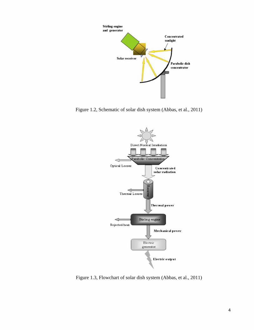
technology can respond to this type of issues in this area (Abbas et al., 2011). Figure 1.2
demonstrates the schematic of solar dish system and Figure 1.3 shows the flowchart of this
type of system. (Abbas et al., 2011).
4
Figure 1.2, Schematic of solar dish system (Abbas, et al., 2011)
Figure 1.3, Flowchart of solar dish system (Abbas, et al., 2011)
5
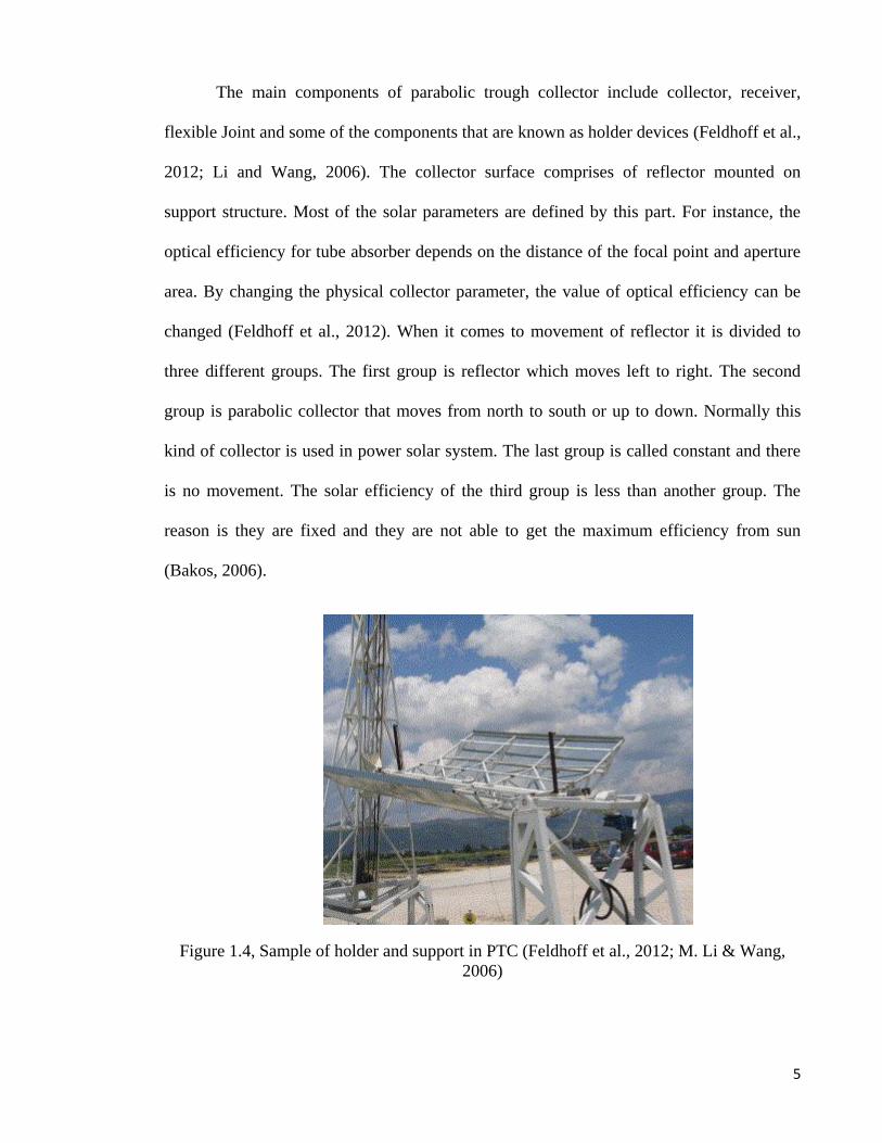
The main components of parabolic trough collector include collector, receiver,
flexible Joint and some of the components that are known as holder devices (Feldhoff et al.,
2012; Li and Wang, 2006). The collector surface comprises of reflector mounted on
support structure. Most of the solar parameters are defined by this part. For instance, the
optical efficiency for tube absorber depends on the distance of the focal point and aperture
area. By changing the physical collector parameter, the value of optical efficiency can be
changed (Feldhoff et al., 2012). When it comes to movement of reflector it is divided to
three different groups. The first group is reflector which moves left to right. The second
group is parabolic collector that moves from north to south or up to down. Normally this
kind of collector is used in power solar system. The last group is called constant and there
is no movement. The solar efficiency of the third group is less than another group. The
reason is they are fixed and they are not able to get the maximum efficiency from sun
(Bakos, 2006).
Figure 1.4, Sample of holder and support in PTC (Feldhoff et al., 2012; M. Li & Wang,
2006)
6
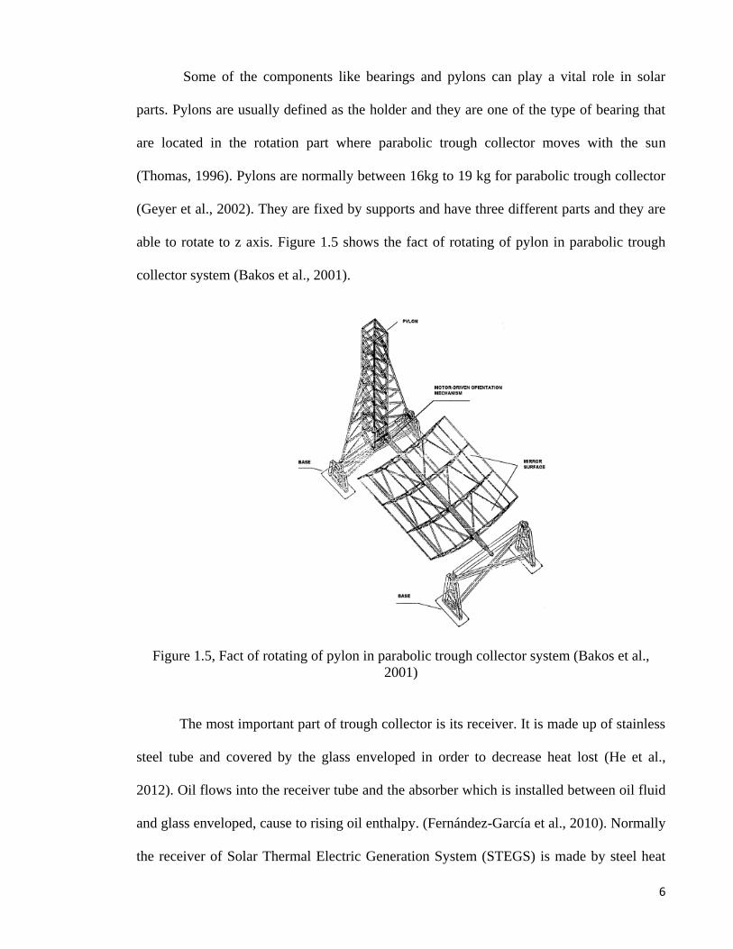
Some of the components like bearings and pylons can play a vital role in solar
parts. Pylons are usually defined as the holder and they are one of the type of bearing that
are located in the rotation part where parabolic trough collector moves with the sun
(Thomas, 1996). Pylons are normally between 16kg to 19 kg for parabolic trough collector
(Geyer et al., 2002). They are fixed by supports and have three different parts and they are
able to rotate to z axis. Figure 1.5 shows the fact of rotating of pylon in parabolic trough
collector system (Bakos et al., 2001).
Figure 1.5, Fact of rotating of pylon in parabolic trough collector system (Bakos et al.,
2001)
The most important part of trough collector is its receiver. It is made up of stainless
steel tube and covered by the glass enveloped in order to decrease heat lost (He et al.,
2012). Oil flows into the receiver tube and the absorber which is installed between oil fluid
and glass enveloped, cause to rising oil enthalpy. (Fernández-García et al., 2010). Normally
the receiver of Solar Thermal Electric Generation System (STEGS) is made by steel heat
7
absorption pipe and coated by black chrome material (Cohen, 1993; Odeh et al., 1998). in
solar power plant system, oil that is flowing in the inner tube, has low viscosity. In some
case water is used instead of synthetic oil. the most important advantages of water is its
price when it is compared by synthetic oil. but on the other hand synthetic oil insensitive to
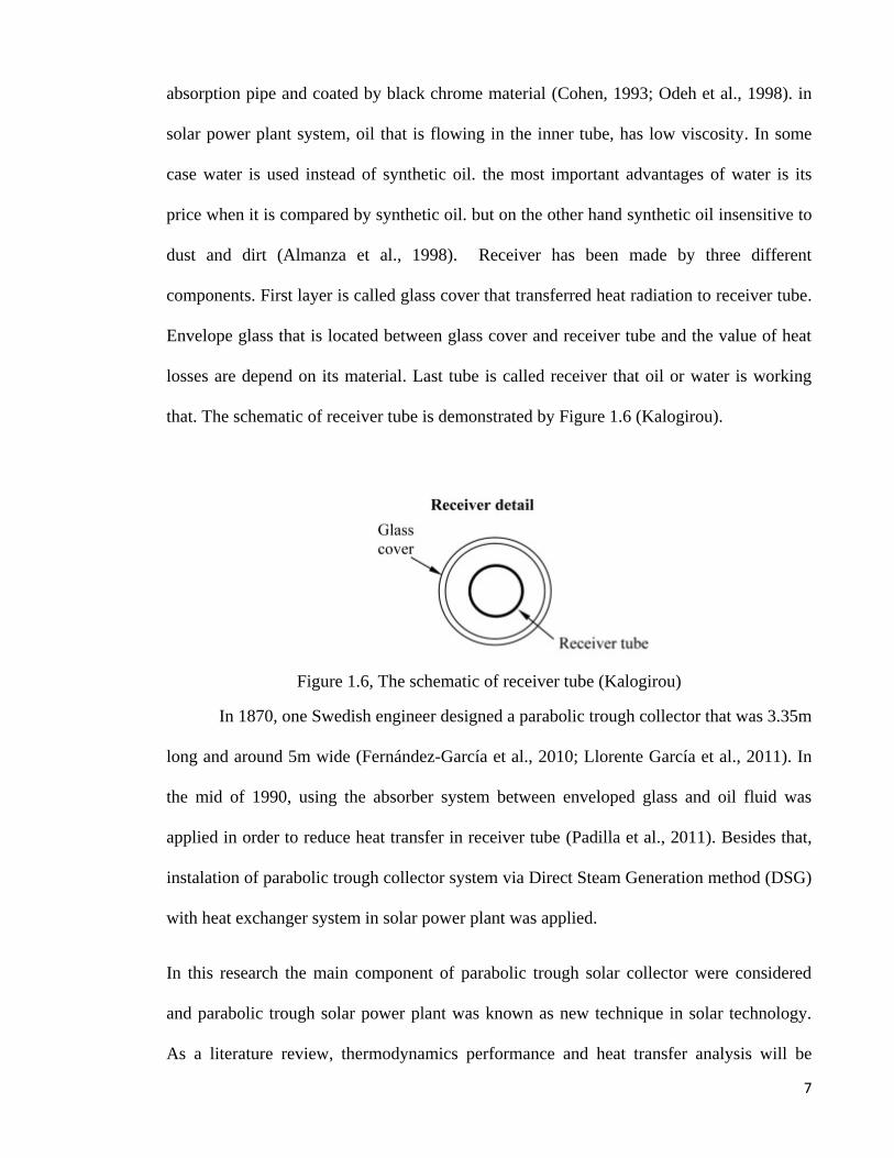
dust and dirt (Almanza et al., 1998). Receiver has been made by three different
components. First layer is called glass cover that transferred heat radiation to receiver tube.
Envelope glass that is located between glass cover and receiver tube and the value of heat
losses are depend on its material. Last tube is called receiver that oil or water is working
that. The schematic of receiver tube is demonstrated by Figure 1.6 (Kalogirou).
Figure 1.6, The schematic of receiver tube (Kalogirou)
In 1870, one Swedish engineer designed a parabolic trough collector that was 3.35m
long and around 5m wide (Fernández-García et al., 2010; Llorente García et al., 2011). In
the mid of 1990, using the absorber system between enveloped glass and oil fluid was
applied in order to reduce heat transfer in receiver tube (Padilla et al., 2011). Besides that,
instalation of parabolic trough collector system via Direct Steam Generation method (DSG)
with heat exchanger system in solar power plant was applied.
In this research the main component of parabolic trough solar collector were considered
and parabolic trough solar power plant was known as new technique in solar technology.
As a literature review, thermodynamics performance and heat transfer analysis will be

8
considered. Some of the new techniques that are caused to improve thermal efficiency in
power plant system in some of countries are reviewed. Also, new techniques and methods
that are caused to decrease of heat losses value in receiver system are considered.
Since, Iran is known as one of the countries that uses parabolic trough solar power plant,
thermodynamics performance like value of energy received, exergy, first and second law
efficiency are be estimated by some of proper associating data. Also, the value heat transfer
like conduction, convection and radiation in different part of receiver tube will be analyzed.
Last but not least, some of new techniques like using of phase change material (PCM) and
Nano fluid will be introduced.
1.3.History of parabolic trough solar power plant
Nowadays, solar power plant system is designed by different types of collector. Some of
them use the solar flat collector another one is designed by the concentrated solar collecotr.
According some of global reports, the maximum electricity generated has been reported at
Spain that had been designed in 2007 and it is able to generate approximately 20 MW
electricity including 50 hectares of area (energy, 2007). First time, in mid of 1991, the
newest type of concentrated solar collector, that was called parabolic trough collector, was
made. It has been concerned to two main components. Mirror surface and receiver tube are
two main components (Fisher and Lupfert, 2006).
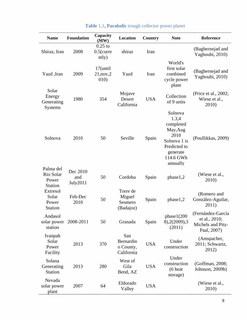
Table 1.1 shows the countries which are using parabolic solar power plant system
(energy, 2005).
9
Table 1.1, Parabolic trough collector power planet
Name Foundation Capacity
(MW) Location Country Note Reference
Shiraz, Iran 2008
0.25 to
0.5(curre
ntly)
shiraz Iran (Baghernejad and
Yaghoubi, 2010)
Yazd ,Iran 2009
17(until
21,nov,2
010)
Yazd Iran
World's
first solar
combined
cycle power
plant
(Baghernejad and
Yaghoubi, 2010)
Solar
Energy
Generating
Systems
1980 354
Mojave
Desert
California
USA Collection
of 9 units
(Price et al., 2002;
Wiese et al.,
2010)
Solnova 2010 50 Seville Spain
Solnova
1.3,4
completed
May,Aug
2010
Solnova 1 is
Predicted to
generate
114.6 GWh
annually
(Poullikkas, 2009)
Palma del
Rio Solar
Power
Station
Dec 2010
and
July2011
50 Cordoba Spain phase1,2 (Wiese et al.,
2010)
Extresol
Solar
Power
Station
Feb-Dec
2010 50
Torre de
Miguel
Sesmero
(Badajoz)
Spain phase1,2
(Romero and
González-Aguilar,
2011)
Andasol
solar power
station
2008-2011 50 Granada Spain
phase1(200
8),2(2009),3
(2011)
(Fernández-García
et al., 2010;
Michels and Pitz-
Paal, 2007)
Ivanpah
Solar
Power
Facility
2013 370
San
Bernardin
o County,
California
USA Under
construction
(Amspacher,
2011; Schwartz,
2012)
Solana
Generating
Station
2013 280
West of
Gila
Bend, AZ
USA
Under
construction
(6 heat
storage)
(Goffman, 2008;
Johnson, 2009b)
Nevada
solar power
plant
2007 64 Eldorado
Valley USA
(Wiese et al.,
2010)
10
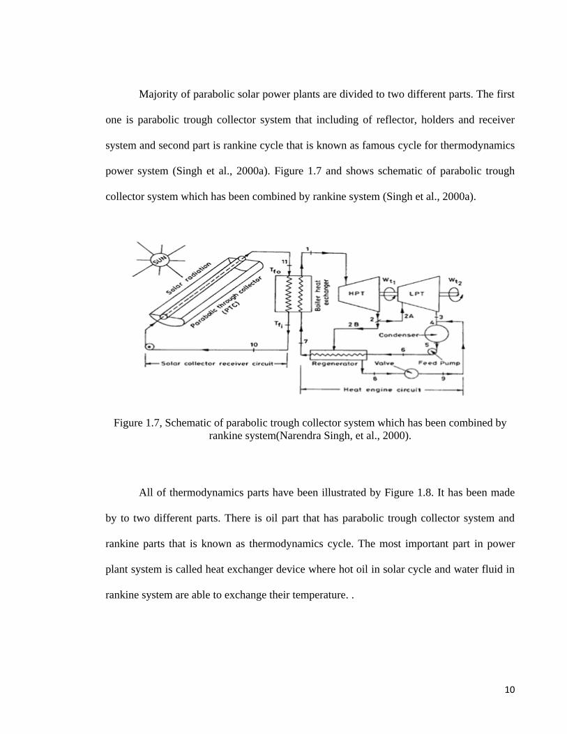
Majority of parabolic solar power plants are divided to two different parts. The first
one is parabolic trough collector system that including of reflector, holders and receiver
system and second part is rankine cycle that is known as famous cycle for thermodynamics
power system (Singh et al., 2000a). Figure 1.7 and shows schematic of parabolic trough
collector system which has been combined by rankine system (Singh et al., 2000a).
Figure 1.7, Schematic of parabolic trough collector system which has been combined by
rankine system(Narendra Singh, et al., 2000).
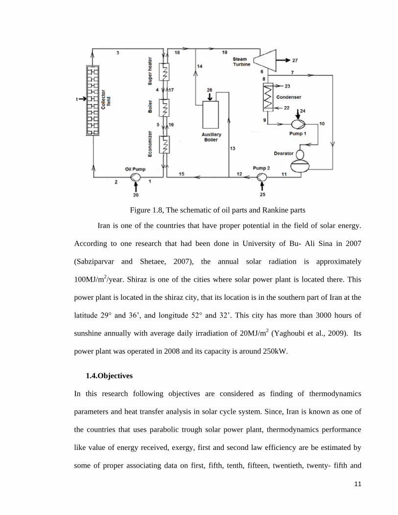
All of thermodynamics parts have been illustrated by Figure 1.8. It has been made
by to two different parts. There is oil part that has parabolic trough collector system and
rankine parts that is known as thermodynamics cycle. The most important part in power
plant system is called heat exchanger device where hot oil in solar cycle and water fluid in
rankine system are able to exchange their temperature. .
11
Figure 1.8, The schematic of oil parts and Rankine parts
Iran is one of the countries that have proper potential in the field of solar energy.
According to one research that had been done in University of Bu- Ali Sina in 2007
(Sabziparvar and Shetaee, 2007), the annual solar radiation is approximately
100MJ/m2/year. Shiraz is one of the cities where solar power plant is located there. This
power plant is located in the shiraz city, that its location is in the southern part of Iran at the
latitude 29° and 36’, and longitude 52° and 32’. This city has more than 3000 hours of
sunshine annually with average daily irradiation of 20MJ/m2 (Yaghoubi et al., 2009). Its
power plant was operated in 2008 and its capacity is around 250kW.
1.4.Objectives
In this research following objectives are considered as finding of thermodynamics
parameters and heat transfer analysis in solar cycle system. Since, Iran is known as one of
the countries that uses parabolic trough solar power plant, thermodynamics performance
like value of energy received, exergy, first and second law efficiency are be estimated by
some of proper associating data on first, fifth, tenth, fifteen, twentieth, twenty- fifth and

12
thirtieth of September are estimated. Also, the value heat transfer like conduction,
convection and radiation in different part of receiver tube will be analyzed. Last but not
least, some of new techniques like using of phase change material (PCM) and Nano fluid
will be introduced.
13
2. Literature review
2.1.Thermodynamics approach
One of the important solar power plant applications is generating of electricity.
Although, the value of thermal efficiency in fossil power plant is higher than solar power
plant, its value depends on thermodynamics parameter in rankine system. However, it can
be caused to generate of greenhouse gases into environment (Yang et al., 2011). On the
other hand, thermal efficiency is so low when it comes to solar power plant. There are
several ways to increase of thermal efficiency of power plant system. Since, thermal
efficiency of the system depends on solar efficiency of parabolic trough system, by
increasing solar efficiency can improve total efficiency. Since, solar power plant has been
designed by thermodynamics cycle, first law efficiency, second law efficiency and exergy
can play vital role in this type of structure. Normally, solar efficiency value is defined in
solar cycle where it has been designed by parabolic trough collector and receiver. That
value depends on several factors.
According to research that had been done Federal de Pernambuco University in
Brazil, the absorber in receiver can play an important role in increasing or decreasing
thermal efficiency. It can be found that when receiver tube is coated by evacuated tube
thermal efficiency is higher than when the case is non- evacuated (Rolim et al., 2009).
Using of CaO/CaCo3 as the absorber system prove that claim. Application of this kind of
absorber and using Brayton cycle instead of rankine cycle had been proposed by industrial
researcher in New Zealand in 2012. Although, this was only one model and was simulated,
the result was so significant. Thermal efficiency reached from 15% to approximately 40%
(Edwards and Materić, 2012). It had great effect on solar efficiency of the system. In some
of the case, like Spain where is used parabolic trough collector system in its power plant
14
system, using of two or more receiver systems, could have a proper effect on improving of
thermal efficiency (Imenes et al., 2006).
Besides that, other physical factors like changing aperture area size or length of
focal point can change the value of solar efficiency in parabolic trough collector system.
According to research in one of the university in Italy in 2011, these types of factors should
be introduced in collector part like mirror with, length and focal length (Sansoni et al.,
2011). Thermal efficiency is very important in design of solar power plant system. It has
effect on economic assessment of solar designing system. It can be said that increasing of
thermal efficiency has great effect on steam turbine capacity and that capacity is caused to
improve of economic assessment in power plant system (Hosseini et al., 2005).
According to one research that had been done in Indian Institute of Technology in
Delhi in 2012, optimize of solar efficiency is caused tothermal efficiency in rankine cycle
is improved and heat losses values in different parts of rankine cycle is reduced. According
to its research when solar efficiency is optimized in solar cycle, oil pressure working will
be also optimized and finally thermal efficiency is increased in rankine cycle. For instance,
in solar power plant that is located in India, when oil pressure increased from 90bar to
105bar, thermal efficiency of pump system will increase from 15% to 26% (Reddy et al.,
2012). Some of the case studies that had been studied in Technical University of Sofia in
2011, the best efficiency was obtained when the high pressure heaters were used in rankine
cycle in solar power plant system and thermal efficiency reached from 23% to 39% (Popov,
2011).
Shadowing and cloudy factor are known as important factors that are able to change
solar efficiency. Obviously, these types of factors are known as negative factors, if those
15
values are considerable. It can be found that, they can reduce thermal efficiency
considerably when those values are estimated more than 0.5. Shadowing and clouding
factor that are defined as the blocking factor are depending on radial and angular distance
of aperture area and also potential of solar energy area (Wei et al., 2010). Besides that,
other factors like airflow speed, rising temperature and pressure increase are caused to
improve solar efficiency (Cao et al., 2011). As far as temperature factor is considered, total
efficiency will be maximized when the saturated water temperature in the boiler is
maximized. According to experimental test in Dakin university in Australia, when the
saturated temperature reached to above 200˚C, thermal efficiency are estimated around
20% (You and Hu, 2002).
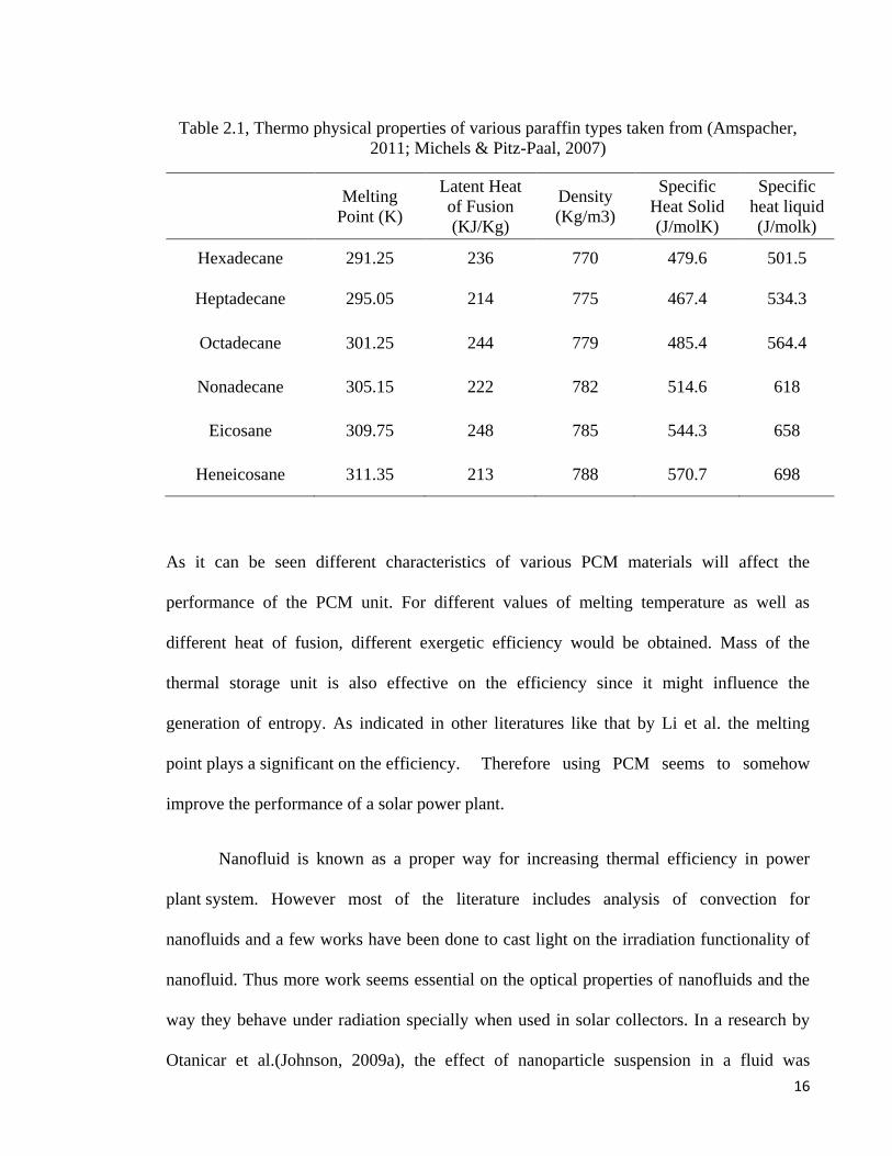
Phase Change Material technique (PCM) is known as a proper way for increasing thermal
efficiency in power plant system. It is used in some of the countries that have good solar
potential energy. Paraffin is chosen as the PCM used in solar power system. It is divided to
several groups. Among of them Heneicosane has the biggest melting point and density
value. Its density is 788 kg/m3. Table 2.1 includes the thermo physical properties of various
paraffin types taken from (Amspacher, 2011; Michels and Pitz-Paal, 2007).
16
Table 2.1, Thermo physical properties of various paraffin types taken from (Amspacher,
2011; Michels & Pitz-Paal, 2007)
Melting
Point (K)
Latent Heat
of Fusion
(KJ/Kg)
Density
(Kg/m3)
Specific
Heat Solid
(J/molK)
Specific
heat liquid
(J/molk)
Hexadecane 291.25 236 770 479.6 501.5
Heptadecane 295.05 214 775 467.4 534.3
Octadecane 301.25 244 779 485.4 564.4
Nonadecane 305.15 222 782 514.6 618
Eicosane 309.75 248 785 544.3 658
Heneicosane 311.35 213 788 570.7 698
As it can be seen different characteristics of various PCM materials will affect the
performance of the PCM unit. For different values of melting temperature as well as
different heat of fusion, different exergetic efficiency would be obtained. Mass of the
thermal storage unit is also effective on the efficiency since it might influence the
generation of entropy. As indicated in other literatures like that by Li et al. the melting
point plays a significant on the efficiency. Therefore using PCM seems to somehow
improve the performance of a solar power plant.
Nanofluid is known as a proper way for increasing thermal efficiency in power
plant system. However most of the literature includes analysis of convection for
nanofluids and a few works have been done to cast light on the irradiation functionality of
nanofluid. Thus more work seems essential on the optical properties of nanofluids and the
way they behave under radiation specially when used in solar collectors. In a research by
Otanicar et al.(Johnson, 2009a), the effect of nanoparticle suspension in a fluid was
17
investigated for direct absorption of solar radiation numerically as well as experimentally.
They concluded that the efficiency of would be augmented by 5% when a nanofluid is
used. The authors also outlined that the performance may be further enhanced by increasing
the volumetric concentration of particles. The effect of using Al2O3/water nanofluid on the
performance of a flat solar collector was also investigated by Yousefi et al.(Goffman, 2008)
The authors concluded that an increase of 28.3% in the overall efficiency was possible by
using a nanofluid with 0.2% volumetric concentration. The effect using surfactants was
also studied to see its influence on the fluid properties during direct absorption. An
augmentation of 15.63% was mentioned when surfactant were used in the suspension.
Another factor that is considered in thermodynamics approach is defined as the
exergy. Exergy plays a vital role in solar power plant system when it comes to second law
efficiency. Exergy analysis can be known as a proper factor in order to analyze of useful
energy based on second law of thermodynamics(Lior, 2002). Just like to solar efficiency
part, some of negative factors like cloudy factors, speed of windy and shadowing can be
reduced exergy value in solar power system (Kumar and Tiwari, 2011). As the result, when
exergy value is reduced, thermal efficiency will be decreased.
When it comes to solar power plant system, exergy can be calculated for each
different component. For instance, it can be found for collector system, boiler, pumps and
turbines system. According to research that was done in university of Ontario technology in
2010 (Regulagadda et al., 2010), exergy value was estimated for each different
thermodynamics instrument. Result illustrated, the value of exergy was related to
temperature and pressure of each components. Among of those components, exergy value
was the highest in the boiler system. Perhaps, the working value in boiler section was the
least when it was compared with turbine or pump system and heat absorbed value was
18
higher than the value of one in heat exchanger (Regulagadda et al., 2010). However, by
increasing of the numbers of extraction stages, exergy value will be reduced in boiler
device (Ying and Hu, 1999). For finding exergy value in turbine cycle, it is function of
pressure inlet in the rankine cycle. it can be said that, when the pressure is increased, the
value of exergy should be rose and when temperature inlet in pump system is increased,
exergy efficiency is also improved in rankine cycle (Al-Sulaiman et al., 2011). The exergy
value and second law of efficiency results can be shown into environment science. The
value of Carbone dioxide gases CO2 which is known as the one of the greenhouse gases, is
62000 tones less in solar power plant system when it was compared with the fossil power
plant(Suresh et al., 2010).
The most important factor in solar devices is to attend and estimated of maximum
and minimum of exergy losses value. According to research that was done by University of
Delhi in 2010 (Gupta and Kaushik, 2010), the maximum exergy losses occur in the solar
collector. It can be found that; solar collector is the first device for receiving solar energy
and the exergy value is depends on energy absorbed value by this device. Since, majority of
negative factors like windy and cloudy factors can have effect on collector directly, it can
be seen the maximum exergy losses value in this section. Unlike parabolic trough system,
the value of exergy losses in receiver system is so low. Since, receiver system is equipped
by envelop glass and absorber system, it can be absorbed the most value energy from
parabolic system. One of the proper strategies for increasing exergy value in collector
system is known as PCM technique. As it was mentioned before, Paraffin is chosen as the
PCM used in solar power system. Since, this type of material has great entropy generation (
because, it has high melting point) the exergy value can increased considerably
(Amspacher, 2011; Michels and Pitz-Paal, 2007).

19
Phase Change Material technology (PCM) is defined as a proper way to increase of
second law efficiency and improve of exergy. According to one research that was done by
(Li et al., 2012), by using of phase change material technique efficiency increased
dramatically. The useful efficiency in the first stage was approximately 19%. But by
increasing of phase change material stage, thermal efficiency is improved more than two
times. It reached to 58% when the phase change material changed to two stages (Li et al.,
2012). Secondly, by doubled of PCM stages the melting temperature reduced considerably.
It can be said that, PCM in the first stage will be able to reach melt temperature to 1000K in
the boiler section. But when it comes to second stage, the melt temperature is reduced by
750K(Li et al., 2012).
Unlike parabolic trough collector system, this scenario is completely different for
tower systems. According to research that was done by institute of electrical engineering in
Beijing in 2011(Xu et al., 2011), the maximum of exergy value occur in receiver system
and minimum value was reported in tower system. Since, flat plate collectors are used for
this system, the exergy value in this type of collector is well when it was compared with
parabolic trough collector system. Also, exergy efficiency has a big effect on heat transfer
irreversibility of the collector system and ambient air in collector system. When it comes to
parabolic trough collector system, exergy is function of two factors. It can be said that the
value of exrgy in receiver and collector system are function of unavoidable fluxes like
radiate and convective heat transfers (Calise et al.).
By comparison between flat plate collector and parabolic trough collector system in
case of exrgy efficiency, we realize that the maximum exergy efficiency is approximately
17% to 49% when it comes to flat plate collector system (Hosseini et al., 2013). It can be
increased by applying phase change material system to 58%(Hosseini et al., 2013). On the
20
other hand, when parabolic trough collector system is considered, exergy efficiency can
reach to 58% with excluding of PCM. It can be found that, parabolic trough collector
system can have higher efficiency in thermodynamics approach rather than solar flat
collector and photo voltaic system. In parabolic trough collector system exergy efficiency
plays an important role. By finding solar exergy in concentrating system, we would find
inefficient parts and factors that is led to it and optimum operating condition (Badescu,
2007).
2.2.Heat Transfer approach
George C. Bakos (Bakos, 2006) investigated and experimented to improve the two-
axis Sun tracking system for parabolic trough collector (PTC).The result shows thermal
efficiency of collector under the tracking better than fixed surface in the same whether
condition. The efficiency will be increased up to 46% by rotating collector.
M.J. Montes et al(Montes et al., 2009) investigated five parabolic trough collectors
with different size on a conventional synthetic oil parabolic trough plant without
hybridization and thermal storage to optimize economically. The result shows that the solar
multiple must be large enough to ensure a certain range where the solar thermal plant is
operating at nominal conditions, but it should not be very great. It also observed improving
the efficiency by means of more complex power cycles leads to significant investment
savings in the solar field size.
Adopting the Monte Carlo Ray-Trace Method (MCRT Method) calculated the solar
energy flux distribution on the outer wall of the inner absorber tube of a parabolic solar
collector receiver successfully. It shows that the non-uniformity of the solar energy flux
distribution is very large. Z.D. Cheng et al,(Cheng et al., 2010; Cheng et al., 2012)
21
calculated and analyzed Three-dimensional numerical simulation of coupled heat transfer
characteristics in the receiver tube by combination of the MCRT Method once with the
FLUENT software and another time with the Finite Volume Method (FVM). From the
experiment of Dudley et al respectively, this analysis is based on the heat transfer fluid and
physical model of Syltherm 800 liquid oil and LS2 parabolic solar collector. After taken
Temperature dependent properties of the oil and thermal radiation between the inner
absorber tube and the outer glass cover tube and by comparing with test results from three
typical testing conditions, the result showing average is within 2% difference. After
validating the model on three typical test conditions, the no-wall model, the no-radiation
model and the unabridged model are also simulated to give a further explanation of the
coupled heat transfer mechanism in the receiver tube. The results show that the radiation
loss in Model 3 is up to 153.70W m−2
. For improving the efficiency of collector the
radiation loss should be reduced as much as can. Then the temperature distributions of the
absorber tube outer surface and the effects of direct normal irradiance, Reynolds number
and emissivity of the inner tube wall on heat transfer characteristics can be investigated. η′
and η always agree well with each other which also prove that they used the reliable
models and methods for feasible and the numerical results.
Gabriel Morin et al (Morin et al., 2011) compared the electricity generation costs,
efficiency and heat loss between the Linear Fresnel Collector (LFC) and Parabolic Trough
Collector (PTC). The study shows that the costs for a linear Fresnel collector is around 78
and 216 €/m2 (or from 28% to 79% relative to PTC field cost) to reach cost-parity at
assumed reference solar field costs of 275 €/m2 for the PTC. Some of the different design
such as Primary mirror field, height of the receiver above the primary mirror field and Heat
transfer fluid and maximum operating temperature level. After modeling of two cases the
22
Parabolic Trough vacuum receiver shows much lower heat losses than the atmospheric
Fresnel receiver. And there is different in the power block due to the Fresnel daily steam
generation characteristics, there are more part load operation hours. In addition, the peak
heat production around solar noon leads to a higher dumping rate for the Linear Fresnel
during hours with high irradiation.
C. Kerkeni et al, (Kerkeni et al., 2002) calculated that main heat losses occur in
collector’s field by 71.8% which installed in 1984 in Tunisia. This plant has revealed the
limits of converting solar thermal energy into electricity at low temperatures.
Measurements taken for the different components of the plant have shown that the annual
electric energy production represents about 0.6% of the incident solar energy. Previous
calculations and studies show that when hot-water at 165C flows through a 6m by 2.3m
PTSC with 900 W/m2 solar insulation and 0 incident angle, the estimated collector
efficiency is about 55%. The thermal losses from the collector receiver are functions of
operating temperature. Depending on the receiver’s configuration and operational
conditions, the thermal losses through PTSC are changed in different ways.
M. Prakash et al(Prakash et al., 2009) experimented and did a numerical study of
the steady state convective losses occurring from a downward facing cylindrical cavity
receiver between 50 ⁰ C and 75 ⁰ C (for experimental) and 50⁰nC and 300 ⁰ C (for
numerical) temperature into the receiver with different angel. The experimental and
numerical result show the good agreement with maximum error of 14%.it can be said that
the result of heat lost when there is no wind is lower than included windy factor.
Narendra Singh et al, (Singh et al., 2000a) which study energy analysis of solar
thermal power and calculate losses of system and compared results. The result shows in
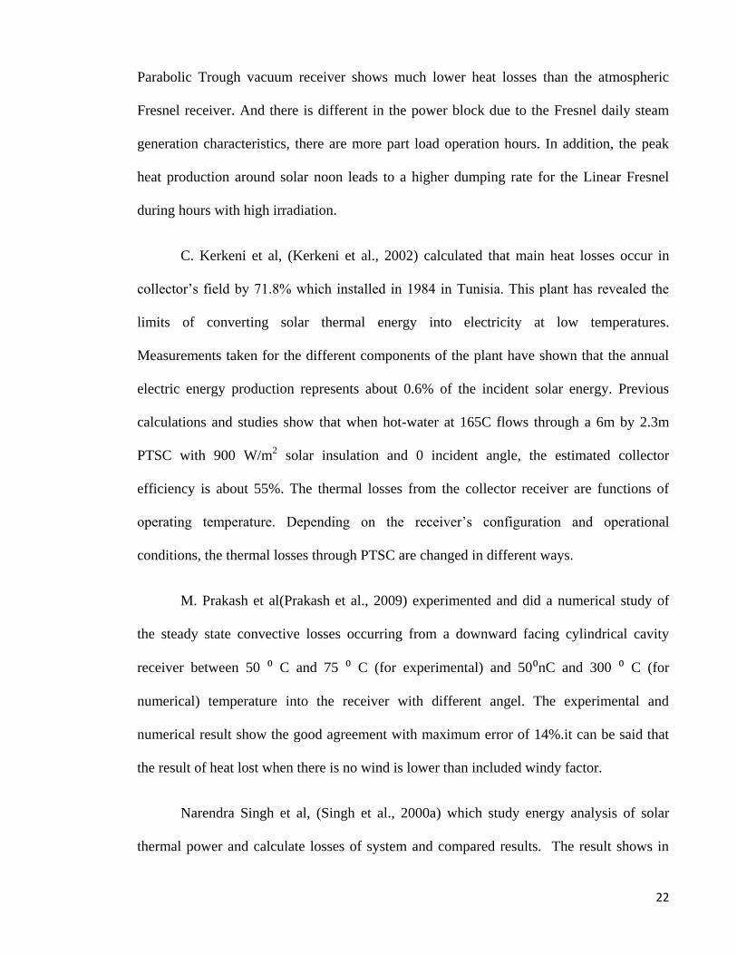
23
Table 2.2, which the percentage energy loss in heat engine circuit (72.37%) is more than
the collector (32.65%) and also more than collector-receiver assembly (56.30%). In fact, it
shows that the high quality energy is lost in collector-receiver assembly but energy lost in
heat engine is part of low quality energy.
Table 2.2, The percentage of energy loss in different part of solar power plant
Subsystem Energy loss (%) First law efficiency (%)
collector 32.65 67.36
receiver 35.12 64.88
collector-receiver 56.3 43.7
Boiler heat exchange 0 100
Heat engine 72.37 27.63
Overall system 87.93 12.07
Ming Qu (Ming Qu, 2006) has modeled calculated a PTSC system which included
50% water and 50% propylene glycol among three losses: conduction, convection and
radiation, the convection loss from absorb tube to supporting structures is the largest; the
next is the radiation loss from glass envelope to ambient air; the relative smaller is the
convection loss from glass envelope to ambient air.
S.D.Odeh (S. D. Odeh) simulated a model by TRANSYS to determine the annual
performance of a typical trough configuration under Australian conditions. This study
illustrates and analyzes parabolic though collector of which used in LUZ plant and water
are operating with synthetic oil. The study result for thermal losses shows that the high
thermal loss from the absorber tube outer wall to evacuated glass tube occurs by radiation
and second part of loss from the collector takes place between absorber tube and the
ambient via the vacuum bellows and supports. He proved that at wind speed of 3m/s the

24
measured and computed values are very close in the temperature range between 250- 400
°C which covers the operation range of a typical power plant.
25
3. Methodology
3.1.Solar measuring instruments
Since, Iran is located in north hemisphere and in September, it has the hottest
weather (September is in summer time for north hemisphere countries), therefore, this
month was chosen to collect solar data. Be sides that, among of summer months,
September has a minimum cloudy factor (According to Table 3.3). Randomly, 1st, 5
th, 10
th,
etc was chosen because the values of temperature and pressure between 1st to 5
th and 5
th to
10th
were mostly similar.
In this investigation, heat transfer and conversion model for high-temperature solar
cavity receiver can be explained by some of the experimental method like Monte- Carlo ray
tracing technique. In this investigation, experimental work is necessary. Therefore, some of
data that are exported by experimental work can play a vital role. In order to measure mass
flow rate, mass flow controllers monitoring might be a properly experimental set up.
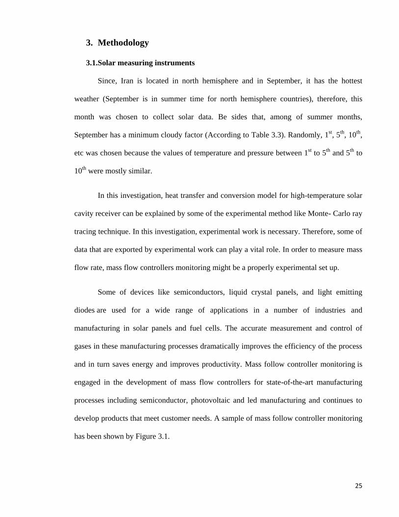
Some of devices like semiconductors, liquid crystal panels, and light emitting
diodes are used for a wide range of applications in a number of industries and
manufacturing in solar panels and fuel cells. The accurate measurement and control of
gases in these manufacturing processes dramatically improves the efficiency of the process
and in turn saves energy and improves productivity. Mass follow controller monitoring is
engaged in the development of mass flow controllers for state-of-the-art manufacturing
processes including semiconductor, photovoltaic and led manufacturing and continues to
develop products that meet customer needs. A sample of mass follow controller monitoring
has been shown by Figure 3.1.
26
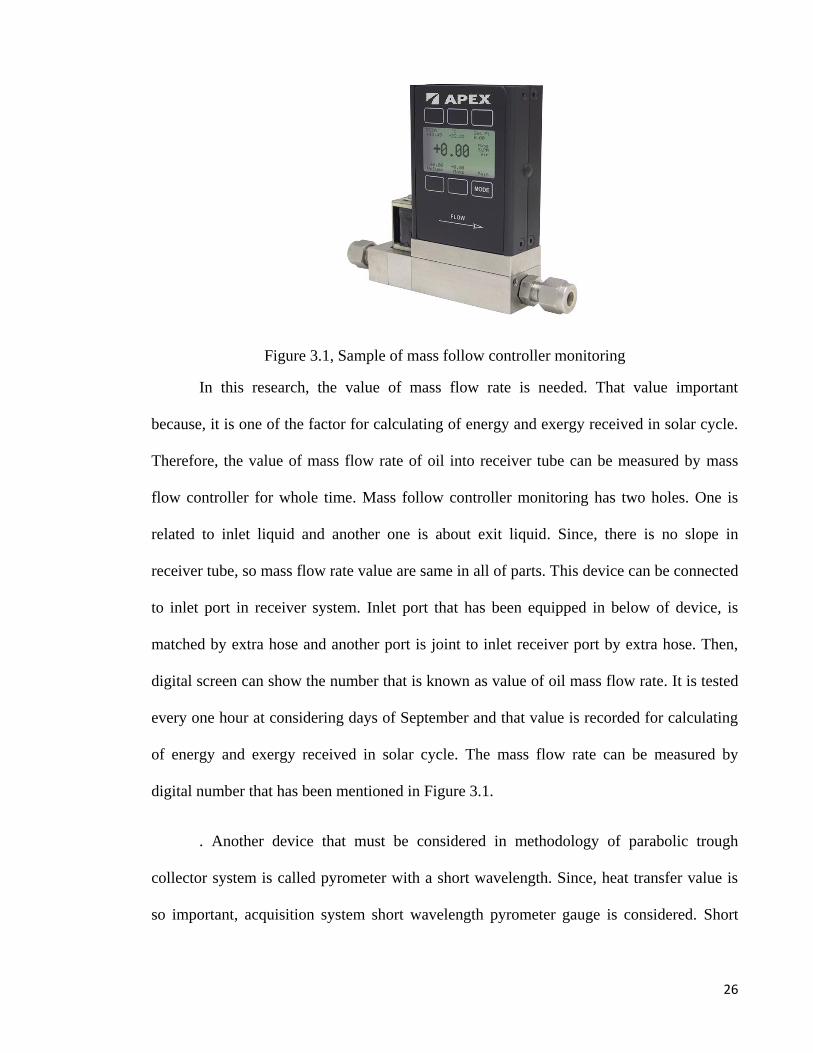
Figure 3.1, Sample of mass follow controller monitoring
In this research, the value of mass flow rate is needed. That value important
because, it is one of the factor for calculating of energy and exergy received in solar cycle.
Therefore, the value of mass flow rate of oil into receiver tube can be measured by mass
flow controller for whole time. Mass follow controller monitoring has two holes. One is
related to inlet liquid and another one is about exit liquid. Since, there is no slope in
receiver tube, so mass flow rate value are same in all of parts. This device can be connected
to inlet port in receiver system. Inlet port that has been equipped in below of device, is
matched by extra hose and another port is joint to inlet receiver port by extra hose. Then,
digital screen can show the number that is known as value of oil mass flow rate. It is tested
every one hour at considering days of September and that value is recorded for calculating
of energy and exergy received in solar cycle. The mass flow rate can be measured by
digital number that has been mentioned in Figure 3.1.
. Another device that must be considered in methodology of parabolic trough
collector system is called pyrometer with a short wavelength. Since, heat transfer value is
so important, acquisition system short wavelength pyrometer gauge is considered. Short
27
wavelength pyrometer gauge is special tools for measuring liquid temperature of metal
between 250˚C to 1800˚C.
The instrument has maximum value storage, minimum value storage, average and
difference function as well as an acoustic alarm. The high quality optics enables the
measurement of small objects from 4 mm, in combination with the close-up lens even from
1.25 mm. The short wavelength pyrometer gauge is a robust, digital and accurate pyrometer
with built-in data logger (750 values) for noncontact temperature measurement on metals,
ceramics, graphite etc. with a temperature range of 250 to 1800°C. The instrument is
equipped with a laser targeting light; the size of the laser spot has approximately the size of
the measuring spot.
In this research, for measuring of sky and environment temperature, this instrument was
used. Values of sky temperature were collected in each solar hour. Providing this kind of
data (sky and environment temperature) is necessary for calculating exergy received and
absorbed in collector and receiver system that are known as thermodynamics factor. This
instrument is equipped by a digital screen which is shown the exact value of sky
temperature by pushing a bottom which turn on a wavelength optical into the sky. The
optical system contains filters that restrict the wavelength-sensitivity of the devices to a
narrow wavelength band around 0.65 to 0.66 micons. The short wavelength pyrometer
gauge has some of advantages like; easy to handle, large illuminated LC display, laser
aiming, built-in data logger, long temperature range, high accuracy, fast temperature
detection, only 20 ms, measurement of smallest objects from 1.25 mm, integrated
additional functions, USB interface, analyzing software PortaWin (option). Besides that,
some of typically application like, preheating, tempering, hardening, normalizing, forging,
brazing, sintering, welding, rolling and founding has been important rather another similar

28
devices. Other filters reduce the intensity so that one instrument can have a relatively wide
temperature range capability. Then, digital screen can show the number that is known as
value of sky temperature. It is tested every one hour at considering days of September and
that value is recorded for calculating of energy and exergy received in solar cycle. A
sample of short wavelength pyrometer gauge has been illustrated by Figure 3.2;
Figure 3.2, Sample of short wavelength pyrometer gauge
Since, temperature and pressure are the main factors for determining of
thermodynamics parameters, some of digital devices for measuring temperature and
pressure are needed. According to heat convection theory that states value of Prandtel
number and Nusselt number are function of pressure value, so the accuracy value of hot oil
pressure in receiver system play a vital role in this research.
In this research, oil temperature in inlet and out let of receiver system is important.
For measuring of inlet and outlet oil temperature in receiver system, solar temperature
gauge is necessary. For this purpose, this device is installed into receiver tube. This
instrument is equipped by one digital screen and one hole. Also it is possible to measure of
solar temperature receive by parabolic system. It is installed on first ( where oil is entered)
and end (where hot oil goes into heat exchanger) of receiver system where hot oil flow into
the tube. Then, digital screen will show the number that is known as value of oil
29
temperature. It is tested every one hour at considering days of September and that value is
recorded for calculating of energy and exergy received in receiver and parabolic cycle.
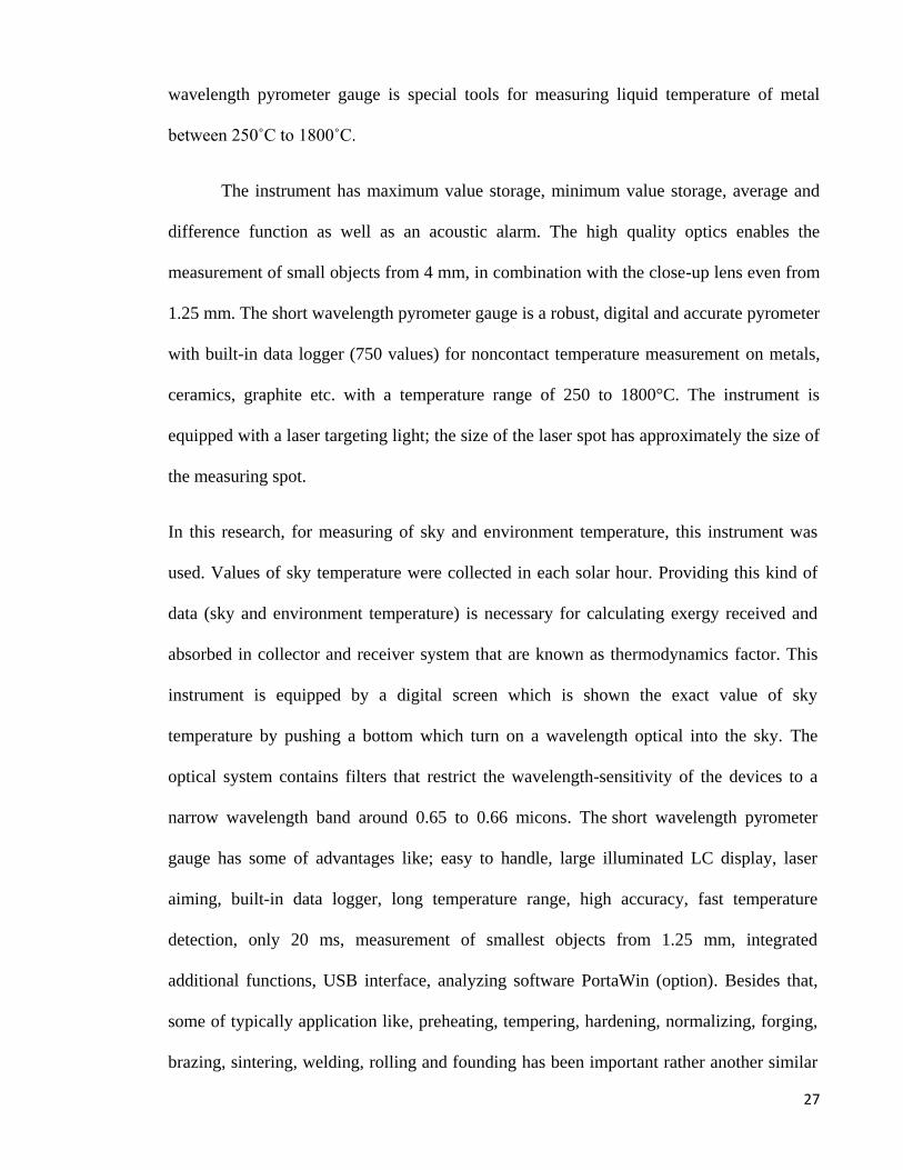
. In this research the values of inlet and outlet temperature were collected in each
solar hour. Providing this kind of data is necessary for calculating exergy received and
absorbed in receiver system. Sample of solar temperature and pressure gauge have been
demonstrated by Figure 3.3.
Figure 3.3, Solar temperature gauge
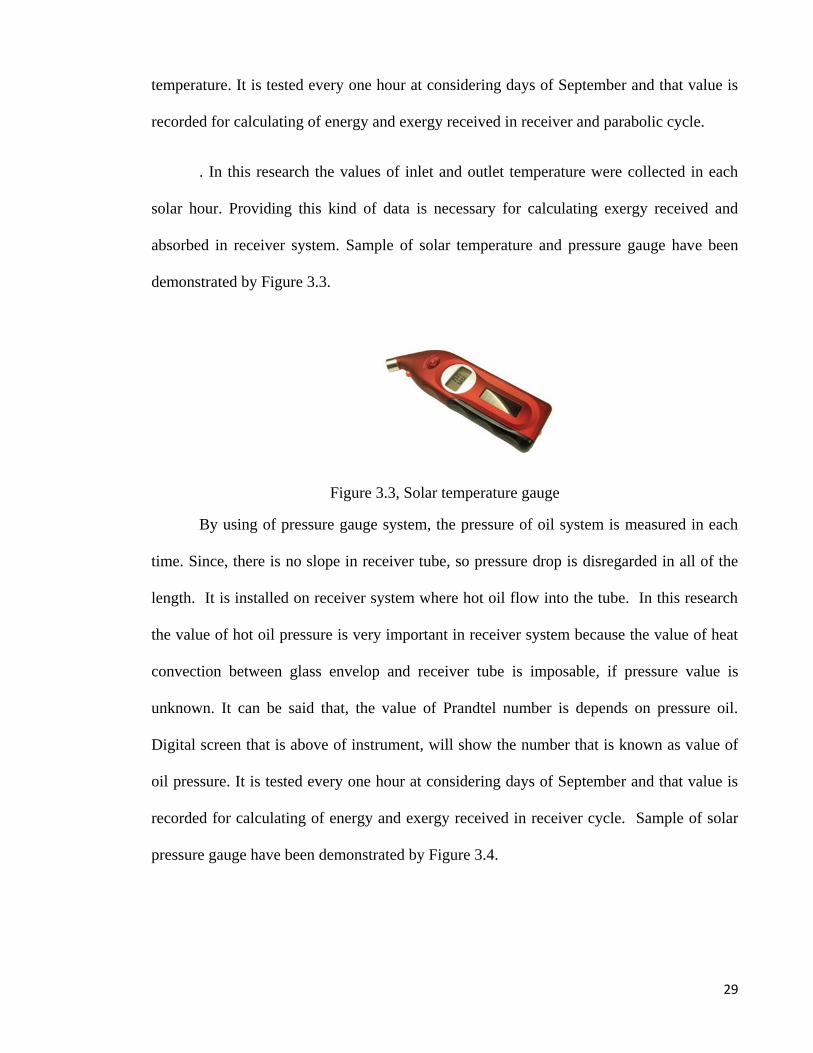
By using of pressure gauge system, the pressure of oil system is measured in each
time. Since, there is no slope in receiver tube, so pressure drop is disregarded in all of the
length. It is installed on receiver system where hot oil flow into the tube. In this research
the value of hot oil pressure is very important in receiver system because the value of heat
convection between glass envelop and receiver tube is imposable, if pressure value is
unknown. It can be said that, the value of Prandtel number is depends on pressure oil.
Digital screen that is above of instrument, will show the number that is known as value of
oil pressure. It is tested every one hour at considering days of September and that value is
recorded for calculating of energy and exergy received in receiver cycle. Sample of solar
pressure gauge have been demonstrated by Figure 3.4.
30
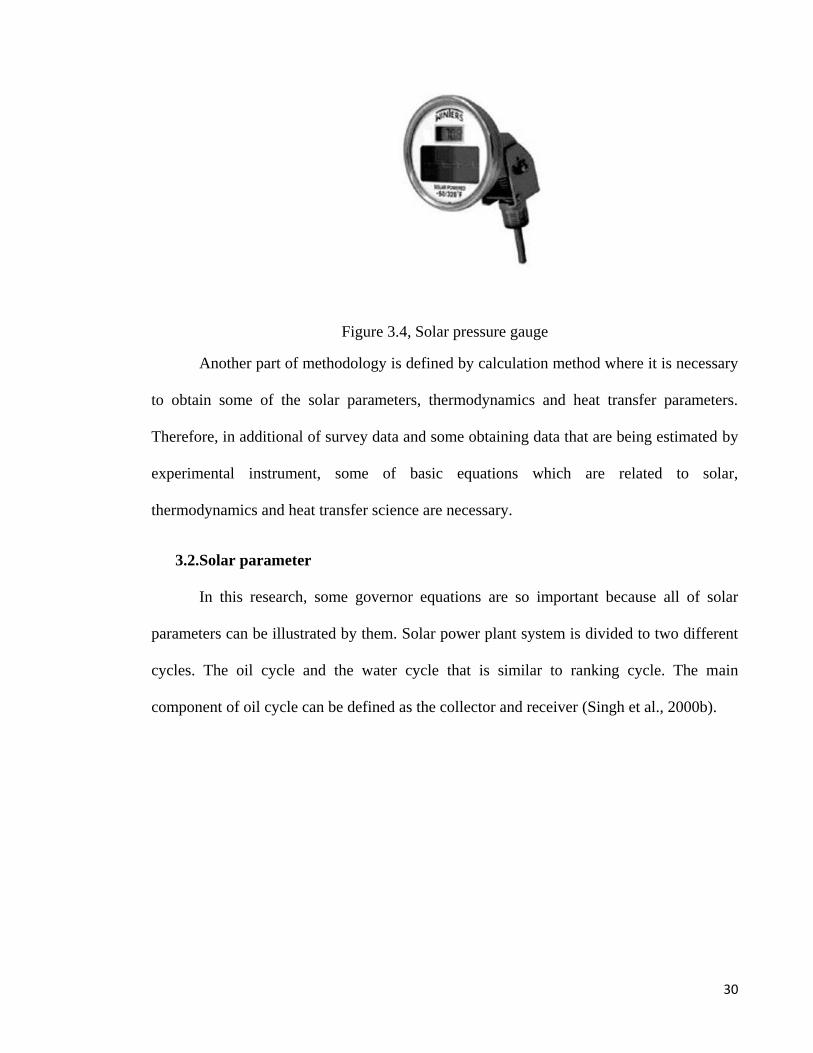
Figure 3.4, Solar pressure gauge
Another part of methodology is defined by calculation method where it is necessary
to obtain some of the solar parameters, thermodynamics and heat transfer parameters.
Therefore, in additional of survey data and some obtaining data that are being estimated by
experimental instrument, some of basic equations which are related to solar,
thermodynamics and heat transfer science are necessary.
3.2.Solar parameter
In this research, some governor equations are so important because all of solar
parameters can be illustrated by them. Solar power plant system is divided to two different
cycles. The oil cycle and the water cycle that is similar to ranking cycle. The main
component of oil cycle can be defined as the collector and receiver (Singh et al., 2000b).
31
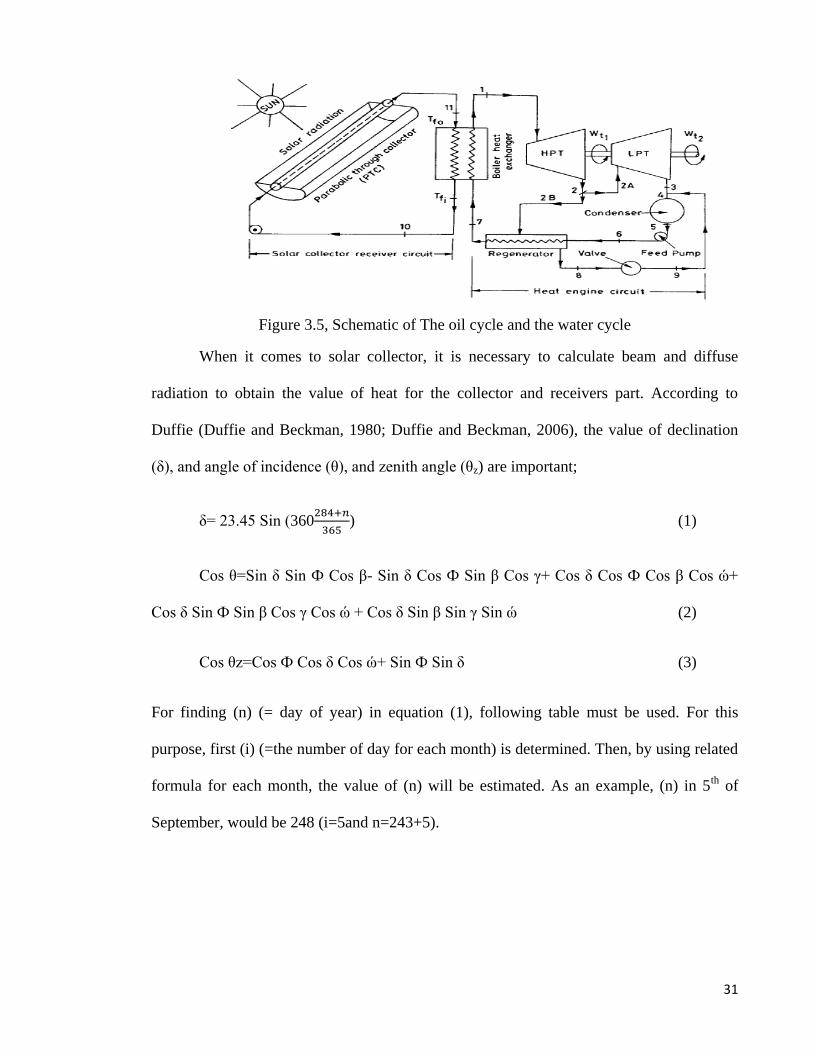
Figure 3.5, Schematic of The oil cycle and the water cycle
When it comes to solar collector, it is necessary to calculate beam and diffuse
radiation to obtain the value of heat for the collector and receivers part. According to
Duffie (Duffie and Beckman, 1980; Duffie and Beckman, 2006), the value of declination
(δ), and angle of incidence (θ), and zenith angle (θz) are important;
δ= 23.45 Sin (360
) (1)
Cos θ=Sin δ Sin Ф Cos β- Sin δ Cos Ф Sin β Cos γ+ Cos δ Cos Ф Cos β Cos ώ+
Cos δ Sin Ф Sin β Cos γ Cos ώ + Cos δ Sin β Sin γ Sin ώ (2)
Cos θz=Cos Ф Cos δ Cos ώ+ Sin Ф Sin δ (3)
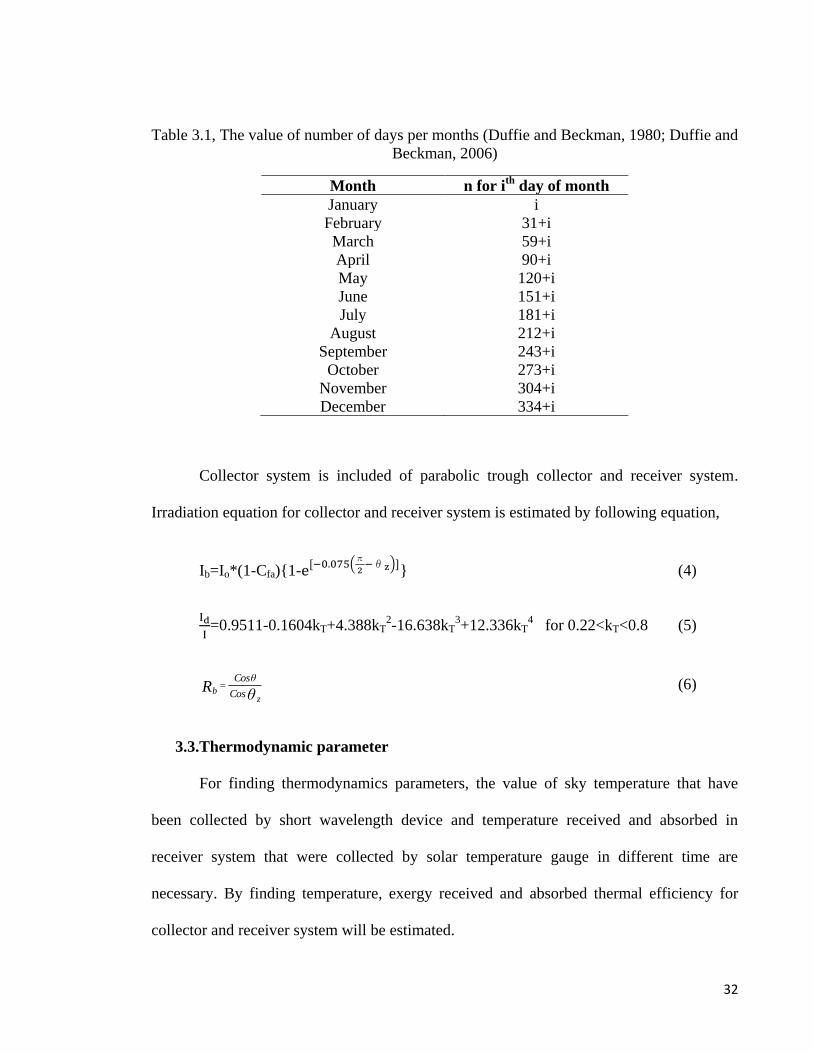
For finding (n) (= day of year) in equation (1), following table must be used. For this
purpose, first (i) (=the number of day for each month) is determined. Then, by using related
formula for each month, the value of (n) will be estimated. As an example, (n) in 5th
of
September, would be 248 (i=5and n=243+5).
32
Table 3.1, The value of number of days per months (Duffie and Beckman, 1980; Duffie and
Beckman, 2006)
Month n for ith
day of month
January i
February 31+i
March 59+i
April 90+i
May 120+i
June 151+i
July 181+i
August 212+i
September 243+i
October 273+i
November 304+i
December 334+i
Collector system is included of parabolic trough collector and receiver system.
Irradiation equation for collector and receiver system is estimated by following equation,
Ib=Io*(1-Cfa){1- (
) } (4)
=0.9511-0.1604kT+4.388kT
2-16.638kT
3+12.336kT
4 for 0.22<kT<0.8 (5)
θ
Rz
b Cos
θCos= (6)
3.3.Thermodynamic parameter
For finding thermodynamics parameters, the value of sky temperature that have
been collected by short wavelength device and temperature received and absorbed in
receiver system that were collected by solar temperature gauge in different time are
necessary. By finding temperature, exergy received and absorbed thermal efficiency for
collector and receiver system will be estimated.
33
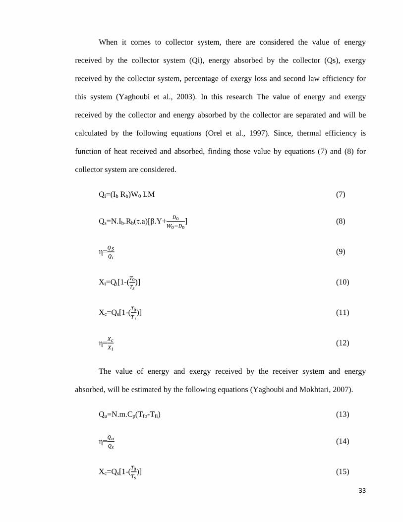
When it comes to collector system, there are considered the value of energy
received by the collector system (Qi), energy absorbed by the collector (Qs), exergy
received by the collector system, percentage of exergy loss and second law efficiency for
this system (Yaghoubi et al., 2003). In this research The value of energy and exergy
received by the collector and energy absorbed by the collector are separated and will be
calculated by the following equations (Orel et al., 1997). Since, thermal efficiency is
function of heat received and absorbed, finding those value by equations (7) and (8) for
collector system are considered.
Qi=(Ib Rb)W0 LM (7)
Qs=N.Ib.Rb(τ.a)[β.Y+
] (8)
η=
(9)
Xi=Qi[1-(
)] (10)
Xc=Qs[1-(
)] (11)
η=
(12)
The value of energy and exergy received by the receiver system and energy
absorbed, will be estimated by the following equations (Yaghoubi and Mokhtari, 2007).
Qu=N.m.Cp(Tfo-Tfi) (13)
η=
(14)
Xc=Qs[1-(
)] (15)
34
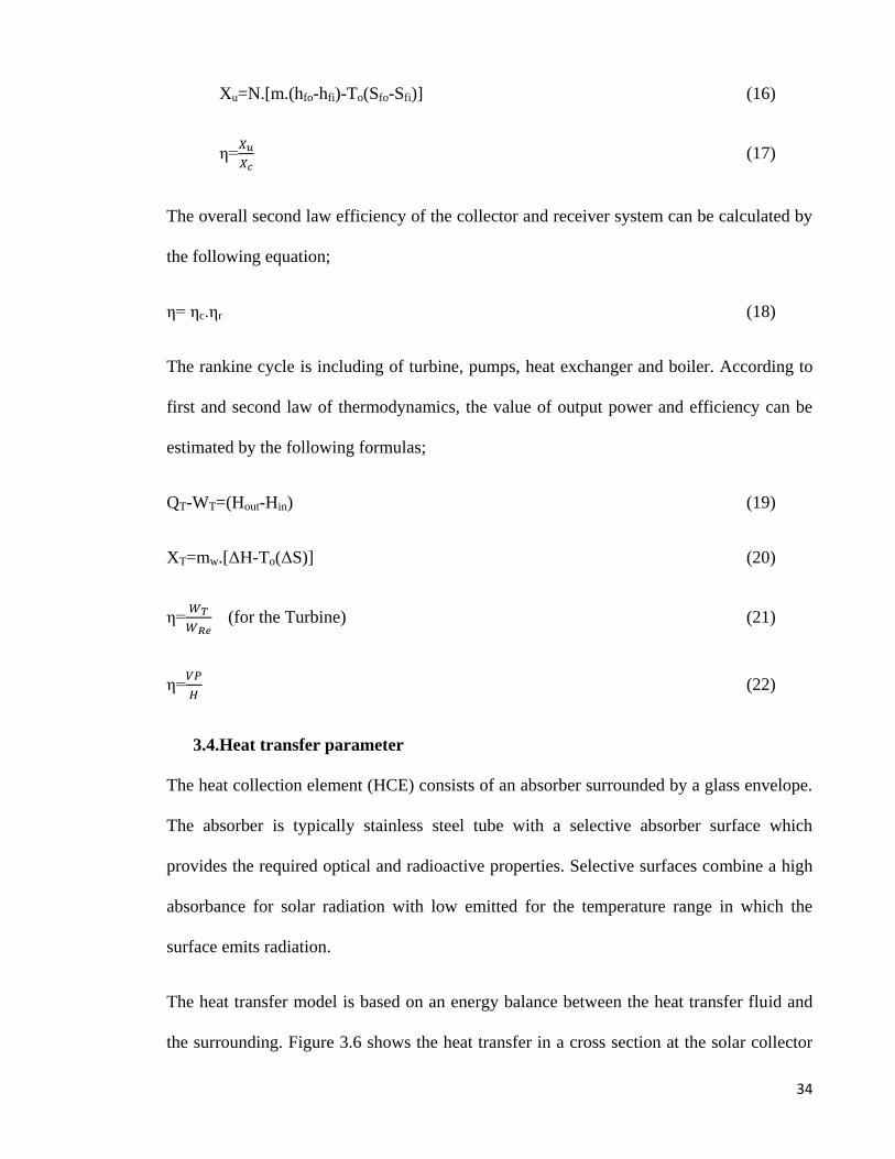
Xu=N.[m.(hfo-hfi)-To(Sfo-Sfi)] (16)
η=
(17)
The overall second law efficiency of the collector and receiver system can be calculated by
the following equation;
η= ηc.ηr (18)
The rankine cycle is including of turbine, pumps, heat exchanger and boiler. According to
first and second law of thermodynamics, the value of output power and efficiency can be
estimated by the following formulas;
QT-WT=(Hout-Hin) (19)
XT=mw.[ΔH-To(ΔS)] (20)
η=
(for the Turbine) (21)
η=
(22)
3.4.Heat transfer parameter
The heat collection element (HCE) consists of an absorber surrounded by a glass envelope.
The absorber is typically stainless steel tube with a selective absorber surface which
provides the required optical and radioactive properties. Selective surfaces combine a high
absorbance for solar radiation with low emitted for the temperature range in which the
surface emits radiation.
The heat transfer model is based on an energy balance between the heat transfer fluid and
the surrounding. Figure 3.6 shows the heat transfer in a cross section at the solar collector
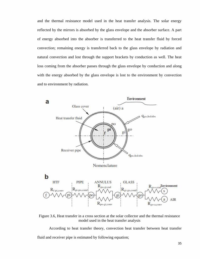
35
and the thermal resistance model used in the heat transfer analysis. The solar energy
reflected by the mirrors is absorbed by the glass envelope and the absorber surface. A part
of energy absorbed into the absorber is transferred to the heat transfer fluid by forced
convection; remaining energy is transferred back to the glass envelope by radiation and
natural convection and lost through the support brackets by conduction as well. The heat
loss coming from the absorber passes through the glass envelope by conduction and along
with the energy absorbed by the glass envelope is lost to the environment by convection
and to environment by radiation.
Figure 3.6, Heat transfer in a cross section at the solar collector and the thermal resistance
model used in the heat transfer analysis
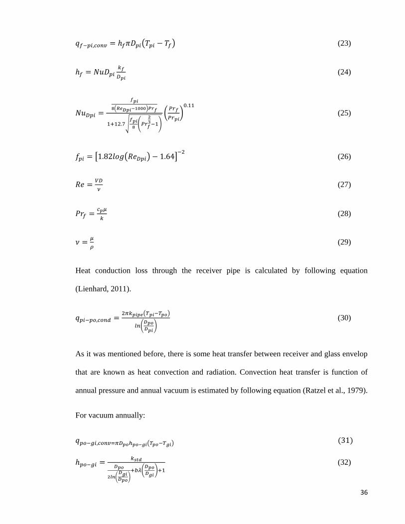
According to heat transfer theory, convection heat transfer between heat transfer
fluid and receiver pipe is estimated by following equation;
36
( ) (23)
(24)
( )
√
(
)
(
)
(25)
[ ( ) ]
(26)
(27)
(28)
(29)
Heat conduction loss through the receiver pipe is calculated by following equation
(Lienhard, 2011).
( )
(
)
(30)
As it was mentioned before, there is some heat transfer between receiver and glass envelop
that are known as heat convection and radiation. Convection heat transfer is function of
annual pressure and annual vacuum is estimated by following equation (Ratzel et al., 1979).
For vacuum annually:
( ) (31)
(
)
(
)
(32)
37
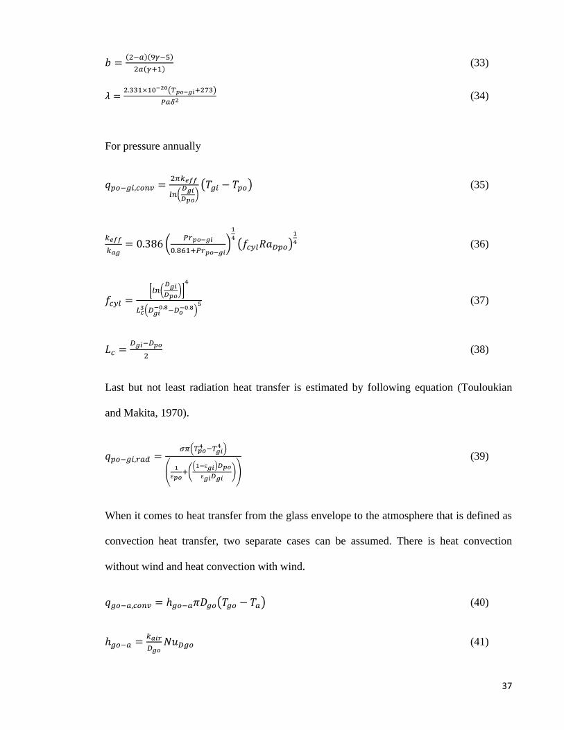
( )( )
( ) (33)
( )
(34)
For pressure annually
(
)( ) (35)
(
)
( )
(36)
[ (
)]
(
)
(37)
(38)
Last but not least radiation heat transfer is estimated by following equation (Touloukian
and Makita, 1970).
(
)
(
(
( )
))
(39)
When it comes to heat transfer from the glass envelope to the atmosphere that is defined as
convection heat transfer, two separate cases can be assumed. There is heat convection
without wind and heat convection with wind.
( ) (40)
(41)
38
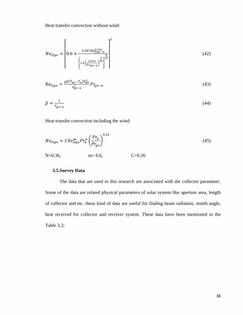
Heat transfer convection without wind:
[
{ (
)
}
]
(42)
( )
(43)
(44)
Heat transfer convection including the wind:
(
)
(45)
N=0.36, m= 0.6, C=0.26
3.5.Survey Data
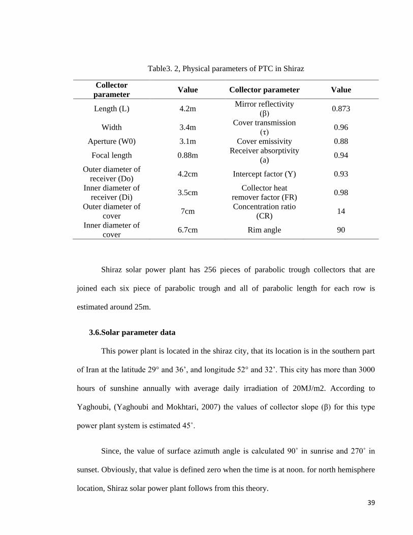
The data that are used in this research are associated with the collector parameter.
Some of the data are related physical parameters of solar system like aperture area, length
of collector and etc. these kind of data are useful for finding beam radiation, zenith angle,
heat received for collector and receiver system. These data have been mentioned in the
Table 3.2;
39
Table3. 2, Physical parameters of PTC in Shiraz
Collector
parameter Value Collector parameter Value
Length (L) 4.2m Mirror reflectivity
(β) 0.873
Width 3.4m Cover transmission
(τ) 0.96
Aperture (W0) 3.1m Cover emissivity 0.88
Focal length 0.88m Receiver absorptivity
(a) 0.94
Outer diameter of
receiver (Do) 4.2cm Intercept factor (Y) 0.93
Inner diameter of
receiver (Di) 3.5cm
Collector heat
remover factor (FR) 0.98
Outer diameter of
cover 7cm
Concentration ratio
(CR) 14
Inner diameter of
cover 6.7cm Rim angle 90
Shiraz solar power plant has 256 pieces of parabolic trough collectors that are
joined each six piece of parabolic trough and all of parabolic length for each row is
estimated around 25m.
3.6.Solar parameter data
This power plant is located in the shiraz city, that its location is in the southern part
of Iran at the latitude 29° and 36’, and longitude 52° and 32’. This city has more than 3000
hours of sunshine annually with average daily irradiation of 20MJ/m2. According to
Yaghoubi, (Yaghoubi and Mokhtari, 2007) the values of collector slope (β) for this type
power plant system is estimated 45˚.
Since, the value of surface azimuth angle is calculated 90˚ in sunrise and 270˚ in
sunset. Obviously, that value is defined zero when the time is at noon. for north hemisphere
location, Shiraz solar power plant follows from this theory.

40
According to Yaghoubi (Yaghoubi and Jafarpur, 1990), the value of cloudy factor
for different months in shiraz is estimated by following table. Also, the value of KT is
around 0.69.
Table 3.3, The value of cloudy factor in Shiraz for different months (Yaghoubi and
Jafarpur, 1990)
Month Cloudy factor
January 0.342
February 0.307
March 0.347
April 0.381
May 0.223
June 0.147
July 0.195
August 0.184
September 0.131
October 0.13
November 0.239
December 0.306
Since, the September month is considered for this research, the value of cloudy
factor is around 0.131.
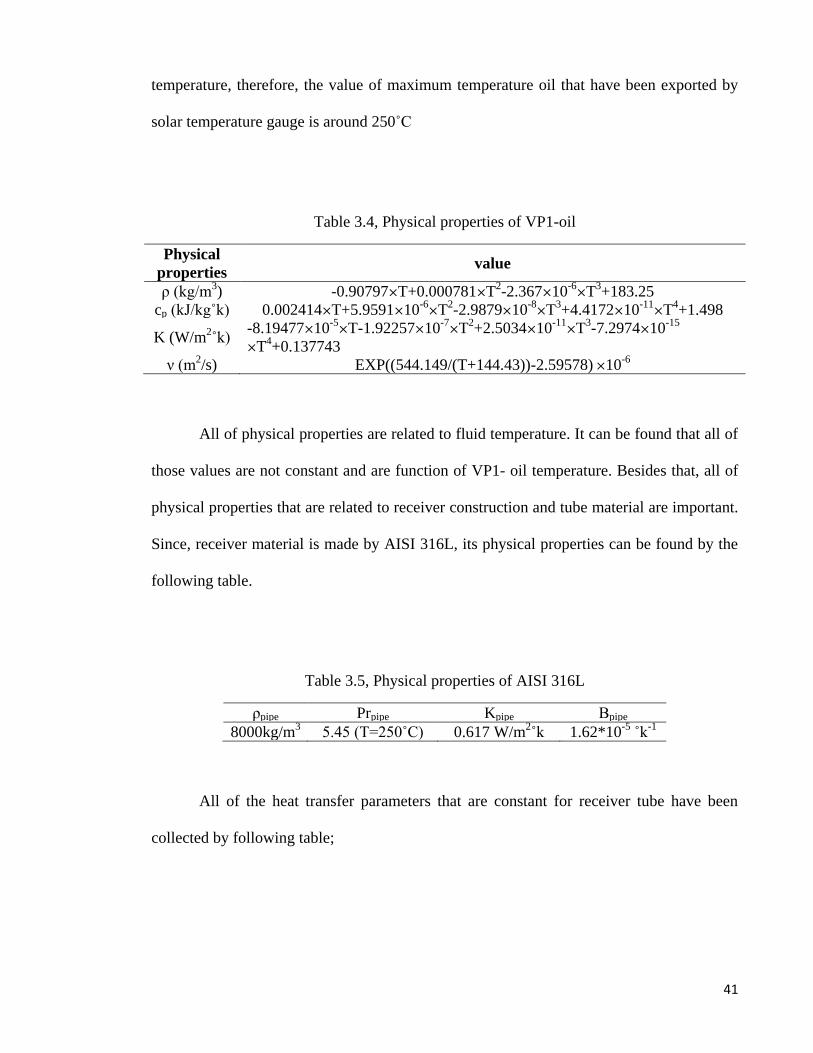
3.7.Thermodynamics and heat transfer parameters
The current fluid into the receiver tube is VP1-oil that all of physical properties can
be found by the following table. This oil is known as industrial oil and it is used special for
power system. Its liquid use range is between 12.5˚C to 400˚C and its vapor use range is
between 258˚C to 400˚C. It can be used as a liquid heat transfer fluid or as a boiling-
condensing heat transfer medium up to its maximum use temperature.
The temperature range is used for this research is between 200˚C to 250˚C that
occur at noon in the summer times. Since, physical properties of this oil are function of
41
temperature, therefore, the value of maximum temperature oil that have been exported by
solar temperature gauge is around 250˚C
Table 3.4, Physical properties of VP1-oil
Physical
properties value
ρ (kg/m3) -0.90797 T+0.000781 T
2-2.367 10
-6 T
3+183.25
cp (kJ/kg˚k) 0.002414 T+5.9591 10-6 T
2-2.9879 10
-8 T
3+4.4172 10
-11 T
4+1.498
K (W/m2˚k)
-8.19477 10-5 T-1.92257 10
-7 T
2+2.5034 10
-11 T
3-7.2974 10
-15
T4+0.137743
ν (m2/s) EXP((544.149/(T+144.43))-2.59578) 10
-6
All of physical properties are related to fluid temperature. It can be found that all of
those values are not constant and are function of VP1- oil temperature. Besides that, all of
physical properties that are related to receiver construction and tube material are important.
Since, receiver material is made by AISI 316L, its physical properties can be found by the
following table.
Table 3.5, Physical properties of AISI 316L
ρpipe Prpipe Kpipe Βpipe
8000kg/m3
5.45 (T=250˚C) 0.617 W/m2˚k 1.62*10
-5 ˚k
-1
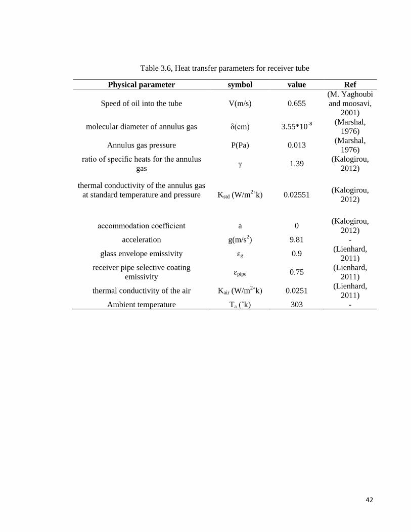
All of the heat transfer parameters that are constant for receiver tube have been
collected by following table;
42
Table 3.6, Heat transfer parameters for receiver tube
Physical parameter symbol value Ref
Speed of oil into the tube V(m/s) 0.655
(M. Yaghoubi
and moosavi,
2001)
molecular diameter of annulus gas δ(cm) 3.55*10-8
(Marshal,
1976)
Annulus gas pressure P(Pa) 0.013 (Marshal,
1976)
ratio of specific heats for the annulus
gas γ 1.39
(Kalogirou,
2012)
thermal conductivity of the annulus gas
at standard temperature and pressure
Kstd (W/m2˚k) 0.02551
(Kalogirou,
2012)
accommodation coefficient a 0 (Kalogirou,
2012)
acceleration g(m/s2) 9.81 -
glass envelope emissivity ɛg 0.9 (Lienhard,
2011)
receiver pipe selective coating
emissivity ɛpipe 0.75
(Lienhard,
2011)
thermal conductivity of the air Kair (W/m2˚k) 0.0251
(Lienhard,
2011)
Ambient temperature Ta (˚k) 303 -
43
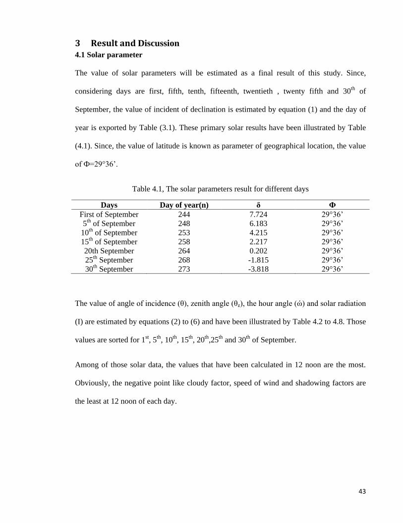
3 Result and Discussion 4.1 Solar parameter
The value of solar parameters will be estimated as a final result of this study. Since,
considering days are first, fifth, tenth, fifteenth, twentieth , twenty fifth and 30th
of
September, the value of incident of declination is estimated by equation (1) and the day of
year is exported by Table (3.1). These primary solar results have been illustrated by Table
(4.1). Since, the value of latitude is known as parameter of geographical location, the value
of Ф=29°36’.
Table 4.1, The solar parameters result for different days
Days Day of year(n) δ Ф
First of September 244 7.724 29°36’
5th
of September 248 6.183 29°36’
10th
of September 253 4.215 29°36’
15th
of September 258 2.217 29°36’
20th September 264 0.202 29°36’
25th
September 268 -1.815 29°36’
30th
September 273 -3.818 29°36’
The value of angle of incidence (θ), zenith angle (θz), the hour angle (ώ) and solar radiation
(I) are estimated by equations (2) to (6) and have been illustrated by Table 4.2 to 4.8. Those
values are sorted for 1st, 5
th, 10
th, 15
th, 20
th,25
th and 30
th of September.
Among of those solar data, the values that have been calculated in 12 noon are the most.
Obviously, the negative point like cloudy factor, speed of wind and shadowing factors are
the least at 12 noon of each day.
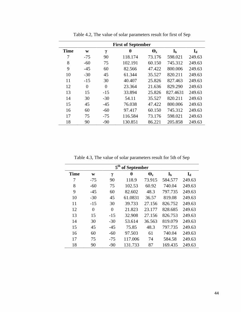
44
Table 4.2, The value of solar parameters result for first of Sep
First of September
Time w γ θ Θz Ib Id
7 -75 90 118.174 73.176 598.021 249.63
8 -60 75 102.191 60.150 745.312 249.63
9 -45 60 82.566 47.422 800.006 249.63
10 -30 45 61.344 35.527 820.211 249.63
11 -15 30 40.407 25.826 827.463 249.63
12 0 0 23.364 21.636 829.290 249.63
13 15 -15 33.894 25.826 827.4631 249.63
14 30 -30 54.11 35.527 820.211 249.63
15 45 -45 76.038 47.422 800.006 249.63
16 60 -60 97.417 60.150 745.312 249.63
17 75 -75 116.584 73.176 598.021 249.63
18 90 -90 130.851 86.221 205.858 249.63
Table 4.3, The value of solar parameters result for 5th of Sep
5th
of September
Time w γ θ Θz Ib Id
7 -75 90 118.9 73.915 584.577 249.63
8 -60 75 102.53 60.92 740.04 249.63
9 -45 60 82.602 48.3 797.735 249.63
10 -30 45 61.0831 36.57 819.08 249.63
11 -15 30 39.733 27.156 826.752 249.63
12 0 0 21.823 23.177 828.685 249.63
13 15 -15 32.908 27.156 826.753 249.63
14 30 -30 53.614 36.563 819.079 249.63
15 45 -45 75.85 48.3 797.735 249.63
16 60 -60 97.503 61 740.04 249.63
17 75 -75 117.006 74 584.58 249.63
18 90 -90 131.733 87 169.435 249.63
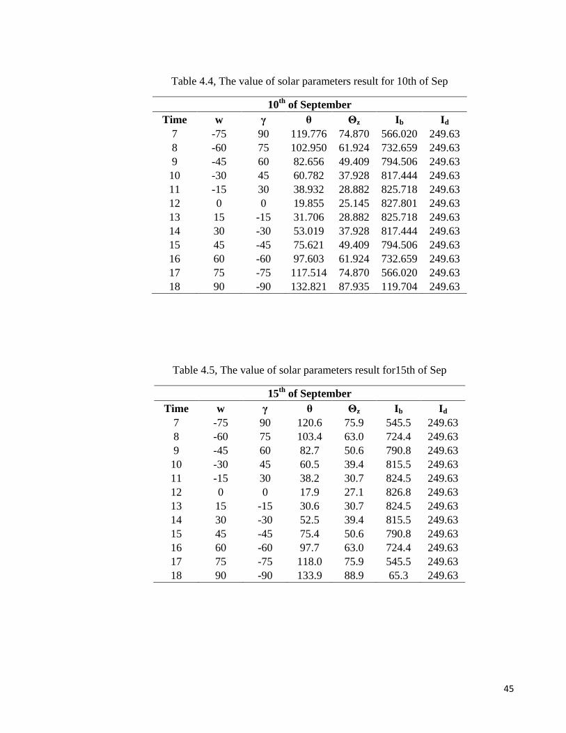
45
Table 4.4, The value of solar parameters result for 10th of Sep
10th
of September
Time w γ θ Θz Ib Id
7 -75 90 119.776 74.870 566.020 249.63
8 -60 75 102.950 61.924 732.659 249.63
9 -45 60 82.656 49.409 794.506 249.63
10 -30 45 60.782 37.928 817.444 249.63
11 -15 30 38.932 28.882 825.718 249.63
12 0 0 19.855 25.145 827.801 249.63
13 15 -15 31.706 28.882 825.718 249.63
14 30 -30 53.019 37.928 817.444 249.63
15 45 -45 75.621 49.409 794.506 249.63
16 60 -60 97.603 61.924 732.659 249.63
17 75 -75 117.514 74.870 566.020 249.63
18 90 -90 132.821 87.935 119.704 249.63
Table 4.5, The value of solar parameters result for15th of Sep
15th
of September
Time w γ θ Θz Ib Id
7 -75 90 120.6 75.9 545.5 249.63
8 -60 75 103.4 63.0 724.4 249.63
9 -45 60 82.7 50.6 790.8 249.63
10 -30 45 60.5 39.4 815.5 249.63
11 -15 30 38.2 30.7 824.5 249.63
12 0 0 17.9 27.1 826.8 249.63
13 15 -15 30.6 30.7 824.5 249.63
14 30 -30 52.5 39.4 815.5 249.63
15 45 -45 75.4 50.6 790.8 249.63
16 60 -60 97.7 63.0 724.4 249.63
17 75 -75 118.0 75.9 545.5 249.63
18 90 -90 133.9 88.9 65.3 249.63
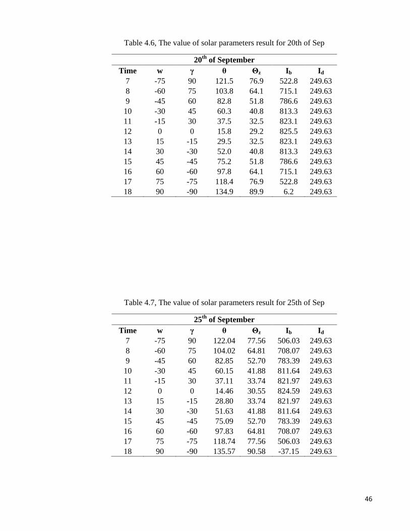
46
Table 4.6, The value of solar parameters result for 20th of Sep
20th
of September
Time w γ θ Θz Ib Id
7 -75 90 121.5 76.9 522.8 249.63
8 -60 75 103.8 64.1 715.1 249.63
9 -45 60 82.8 51.8 786.6 249.63
10 -30 45 60.3 40.8 813.3 249.63
11 -15 30 37.5 32.5 823.1 249.63
12 0 0 15.8 29.2 825.5 249.63
13 15 -15 29.5 32.5 823.1 249.63
14 30 -30 52.0 40.8 813.3 249.63
15 45 -45 75.2 51.8 786.6 249.63
16 60 -60 97.8 64.1 715.1 249.63
17 75 -75 118.4 76.9 522.8 249.63
18 90 -90 134.9 89.9 6.2 249.63
Table 4.7, The value of solar parameters result for 25th of Sep
25th
of September
Time w γ θ Θz Ib Id
7 -75 90 122.04 77.56 506.03 249.63
8 -60 75 104.02 64.81 708.07 249.63
9 -45 60 82.85 52.70 783.39 249.63
10 -30 45 60.15 41.88 811.64 249.63
11 -15 30 37.11 33.74 821.97 249.63
12 0 0 14.46 30.55 824.59 249.63
13 15 -15 28.80 33.74 821.97 249.63
14 30 -30 51.63 41.88 811.64 249.63
15 45 -45 75.09 52.70 783.39 249.63
16 60 -60 97.83 64.81 708.07 249.63
17 75 -75 118.74 77.56 506.03 249.63
18 90 -90 135.57 90.58 -37.15 249.63
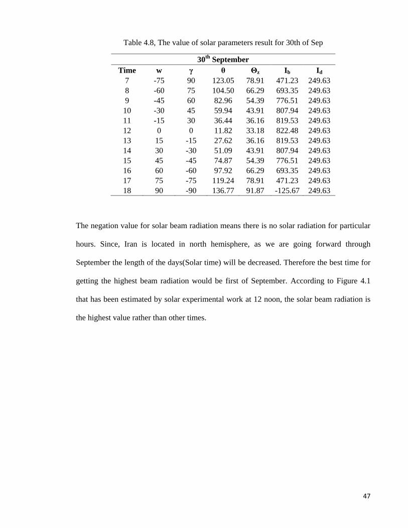
47
Table 4.8, The value of solar parameters result for 30th of Sep
30th
September
Time w γ θ Θz Ib Id
7 -75 90 123.05 78.91 471.23 249.63
8 -60 75 104.50 66.29 693.35 249.63
9 -45 60 82.96 54.39 776.51 249.63
10 -30 45 59.94 43.91 807.94 249.63
11 -15 30 36.44 36.16 819.53 249.63
12 0 0 11.82 33.18 822.48 249.63
13 15 -15 27.62 36.16 819.53 249.63
14 30 -30 51.09 43.91 807.94 249.63
15 45 -45 74.87 54.39 776.51 249.63
16 60 -60 97.92 66.29 693.35 249.63
17 75 -75 119.24 78.91 471.23 249.63
18 90 -90 136.77 91.87 -125.67 249.63
The negation value for solar beam radiation means there is no solar radiation for particular
hours. Since, Iran is located in north hemisphere, as we are going forward through
September the length of the days(Solar time) will be decreased. Therefore the best time for
getting the highest beam radiation would be first of September. According to Figure 4.1
that has been estimated by solar experimental work at 12 noon, the solar beam radiation is
the highest value rather than other times.
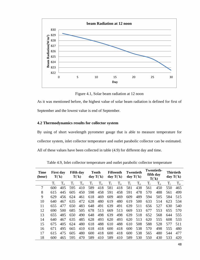
48
Figure 4.1, Solar beam radiation at 12 noon
As it was mentioned before, the highest value of solar beam radiation is defined for first of
September and the lowest value is end of September.
4.2 Thermodynamics results for collector system
By using of short wavelength pyrometer gauge that is able to measure temperature for
collector system, inlet collector temperature and outlet parabolic collector can be estimated.
All of these values have been collected in table (4.9) for different day and time.
Table 4.9, Inlet collector temperature and outlet parabolic collector temperature
Time
(hour)
First day
T(˚k)
Fifth day
T(˚k)
Tenth
day T(˚k)
Fifteenth
day T(˚k)
Twentieth
day T(˚k)
Twentieth-
fifth day
T(˚k)
Thirtieth
day T(˚k)
Ti To Ti To Ti To Ti To Ti To Ti To Ti To
7 600 405 595 410 589 418 581 418 581 438 561 450 550 465
8 615 445 605 450 598 458 591 458 591 478 570 488 561 499
9 629 456 624 461 618 469 609 469 609 489 594 505 584 515
10 640 467 635 472 628 480 619 480 619 500 633 514 623 534
11 655 477 650 483 648 491 639 491 639 511 656 527 630 540
12 690 500 685 505 678 513 669 513 669 533 677 553 655 570
13 655 485 650 490 648 498 639 498 639 518 652 568 644 555
14 640 467 635 485 628 493 620 493 620 513 620 555 608 533
15 675 405 624 480 618 488 610 488 610 508 588 528 577 511
16 671 495 665 410 618 418 600 418 600 538 570 498 555 480
17 615 475 605 480 600 418 600 418 600 538 565 480 544 477
18 600 465 595 470 589 410 589 410 589 530 550 430 533 420
822
823
824
825
826
827
828
829
830
0 5 10 15 20 25 30
Bea
m R
ad
iati
on
(W/m
2)
Day
beam Radiation at 12 noon
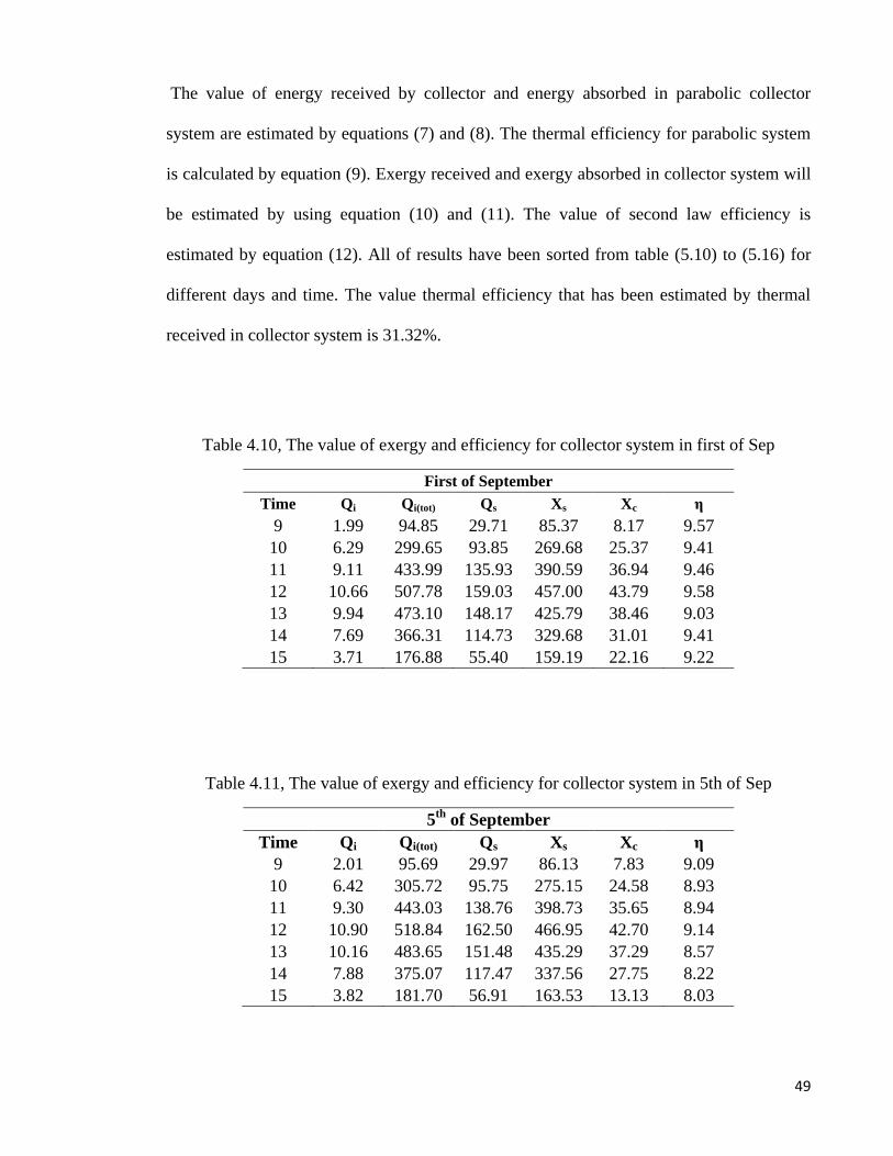
49
The value of energy received by collector and energy absorbed in parabolic collector
system are estimated by equations (7) and (8). The thermal efficiency for parabolic system
is calculated by equation (9). Exergy received and exergy absorbed in collector system will
be estimated by using equation (10) and (11). The value of second law efficiency is
estimated by equation (12). All of results have been sorted from table (5.10) to (5.16) for
different days and time. The value thermal efficiency that has been estimated by thermal
received in collector system is 31.32%.
Table 4.10, The value of exergy and efficiency for collector system in first of Sep
First of September
Time Qi Qi(tot) Qs Xs Xc η
9 1.99 94.85 29.71 85.37 8.17 9.57
10 6.29 299.65 93.85 269.68 25.37 9.41
11 9.11 433.99 135.93 390.59 36.94 9.46
12 10.66 507.78 159.03 457.00 43.79 9.58
13 9.94 473.10 148.17 425.79 38.46 9.03
14 7.69 366.31 114.73 329.68 31.01 9.41
15 3.71 176.88 55.40 159.19 22.16 9.22
Table 4.11, The value of exergy and efficiency for collector system in 5th of Sep
5th
of September
Time Qi Qi(tot) Qs Xs Xc η
9 2.01 95.69 29.97 86.13 7.83 9.09
10 6.42 305.72 95.75 275.15 24.58 8.93
11 9.30 443.03 138.76 398.73 35.65 8.94
12 10.90 518.84 162.50 466.95 42.70 9.14
13 10.16 483.65 151.48 435.29 37.29 8.57
14 7.88 375.07 117.47 337.56 27.75 8.22
15 3.82 181.70 56.91 163.53 13.13 8.03
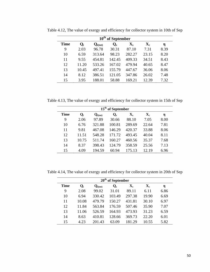
50
Table 4.12, The value of exergy and efficiency for collector system in 10th of Sep
10th
of September
Time Qi Qi(tot) Qs Xs Xc η
9 2.03 96.78 30.31 87.10 7.31 8.39
10 6.59 313.64 98.23 282.27 23.15 8.20
11 9.55 454.81 142.45 409.33 34.51 8.43
12 11.20 533.26 167.02 479.94 40.65 8.47
13 10.45 497.41 155.79 447.67 36.06 8.06
14 8.12 386.51 121.05 347.86 26.02 7.48
15 3.95 188.01 58.88 169.21 12.39 7.32
Table 4.13, The value of exergy and efficiency for collector system in 15th of Sep
15th
of September
Time Qi Qi(tot) Qs Xs Xc η
9 2.06 97.89 30.66 88.10 7.05 8.00
10 6.76 321.88 100.81 289.69 22.64 7.81
11 9.81 467.08 146.29 420.37 33.88 8.06
12 11.51 548.28 171.72 493.45 40.04 8.11
13 10.75 511.74 160.27 460.56 35.37 7.68
14 8.37 398.43 124.79 358.59 25.56 7.13
15 4.09 194.59 60.94 175.13 12.19 6.96
Table 4.14, The value of exergy and efficiency for collector system in 20th of Sep
20th
of September
Time Qi Qi(tot) Qs Xs Xc η
9 2.08 99.02 31.01 89.11 6.11 6.86
10 6.94 330.42 103.49 297.38 19.90 6.69
11 10.08 479.79 150.27 431.81 30.10 6.97
12 11.84 563.84 176.59 507.46 35.90 7.07
13 11.06 526.59 164.93 473.93 31.23 6.59
14 8.63 410.81 128.66 369.73 22.20 6.01
15 4.23 201.43 63.09 181.29 10.55 5.82
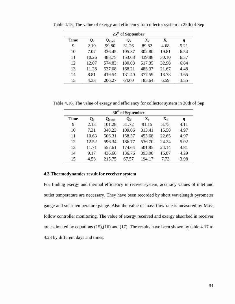
51
Table 4.15, The value of exergy and efficiency for collector system in 25th of Sep
25th
of September
Time Qi Qi(tot) Qs Xs Xc η
9 2.10 99.80 31.26 89.82 4.68 5.21
10 7.07 336.45 105.37 302.80 19.81 6.54
11 10.26 488.75 153.08 439.88 30.10 6.37
12 12.07 574.83 180.03 517.35 32.98 6.84
13 11.28 537.08 168.21 483.37 21.67 4.48
14 8.81 419.54 131.40 377.59 13.78 3.65
15 4.33 206.27 64.60 185.64 6.59 3.55
Table 4.16, The value of exergy and efficiency for collector system in 30th of Sep
30th
of September
Time Qi Qi(tot) Qs Xs Xc η
9 2.13 101.28 31.72 91.15 3.75 4.11
10 7.31 348.23 109.06 313.41 15.58 4.97
11 10.63 506.31 158.57 455.68 22.65 4.97
12 12.52 596.34 186.77 536.70 24.24 5.02
13 11.71 557.61 174.64 501.85 24.14 4.81
14 9.17 436.66 136.76 393.00 16.87 4.29
15 4.53 215.75 67.57 194.17 7.73 3.98
4.3 Thermodynamics result for receiver system
For finding exergy and thermal efficiency in reciver system, accuracy values of inlet and
outlet temperature are necessary. They have been recorded by short wavelength pyrometer
gauge and solar temperature gauge. Also the value of mass flow rate is measured by Mass
follow controller monitoring. The value of exergy received and exergy absorbed in receiver
are estimated by equations (15),(16) and (17). The results have been shown by table 4.17 to
4.23 by different days and times.
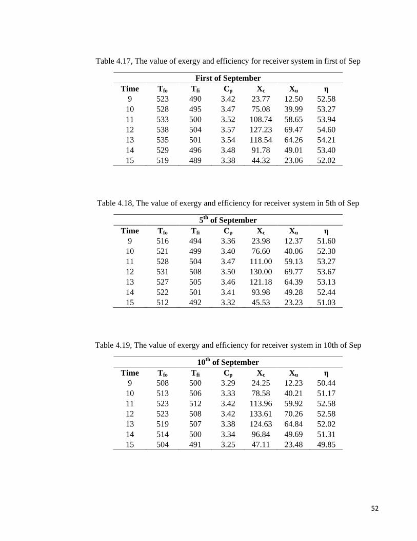
52
Table 4.17, The value of exergy and efficiency for receiver system in first of Sep
First of September
Time Tfo Tfi Cp Xc Xu η
9 523 490 3.42 23.77 12.50 52.58
10 528 495 3.47 75.08 39.99 53.27
11 533 500 3.52 108.74 58.65 53.94
12 538 504 3.57 127.23 69.47 54.60
13 535 501 3.54 118.54 64.26 54.21
14 529 496 3.48 91.78 49.01 53.40
15 519 489 3.38 44.32 23.06 52.02
Table 4.18, The value of exergy and efficiency for receiver system in 5th of Sep
5th
of September
Time Tfo Tfi Cp Xc Xu η
9 516 494 3.36 23.98 12.37 51.60
10 521 499 3.40 76.60 40.06 52.30
11 528 504 3.47 111.00 59.13 53.27
12 531 508 3.50 130.00 69.77 53.67
13 527 505 3.46 121.18 64.39 53.13
14 522 501 3.41 93.98 49.28 52.44
15 512 492 3.32 45.53 23.23 51.03
Table 4.19, The value of exergy and efficiency for receiver system in 10th of Sep
10th
of September
Time Tfo Tfi Cp Xc Xu η
9 508 500 3.29 24.25 12.23 50.44
10 513 506 3.33 78.58 40.21 51.17
11 523 512 3.42 113.96 59.92 52.58
12 523 508 3.42 133.61 70.26 52.58
13 519 507 3.38 124.63 64.84 52.02
14 514 500 3.34 96.84 49.69 51.31
15 504 491 3.25 47.11 23.48 49.85
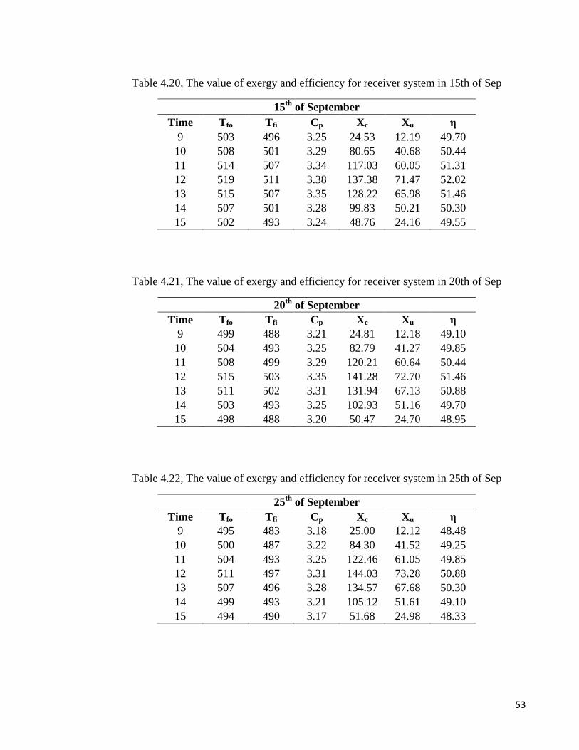
53
Table 4.20, The value of exergy and efficiency for receiver system in 15th of Sep
15th
of September
Time Tfo Tfi Cp Xc Xu η
9 503 496 3.25 24.53 12.19 49.70
10 508 501 3.29 80.65 40.68 50.44
11 514 507 3.34 117.03 60.05 51.31
12 519 511 3.38 137.38 71.47 52.02
13 515 507 3.35 128.22 65.98 51.46
14 507 501 3.28 99.83 50.21 50.30
15 502 493 3.24 48.76 24.16 49.55
Table 4.21, The value of exergy and efficiency for receiver system in 20th of Sep
20th
of September
Time Tfo Tfi Cp Xc Xu η
9 499 488 3.21 24.81 12.18 49.10
10 504 493 3.25 82.79 41.27 49.85
11 508 499 3.29 120.21 60.64 50.44
12 515 503 3.35 141.28 72.70 51.46
13 511 502 3.31 131.94 67.13 50.88
14 503 493 3.25 102.93 51.16 49.70
15 498 488 3.20 50.47 24.70 48.95
Table 4.22, The value of exergy and efficiency for receiver system in 25th of Sep
25th
of September
Time Tfo Tfi Cp Xc Xu η
9 495 483 3.18 25.00 12.12 48.48
10 500 487 3.22 84.30 41.52 49.25
11 504 493 3.25 122.46 61.05 49.85
12 511 497 3.31 144.03 73.28 50.88
13 507 496 3.28 134.57 67.68 50.30
14 499 493 3.21 105.12 51.61 49.10
15 494 490 3.17 51.68 24.98 48.33
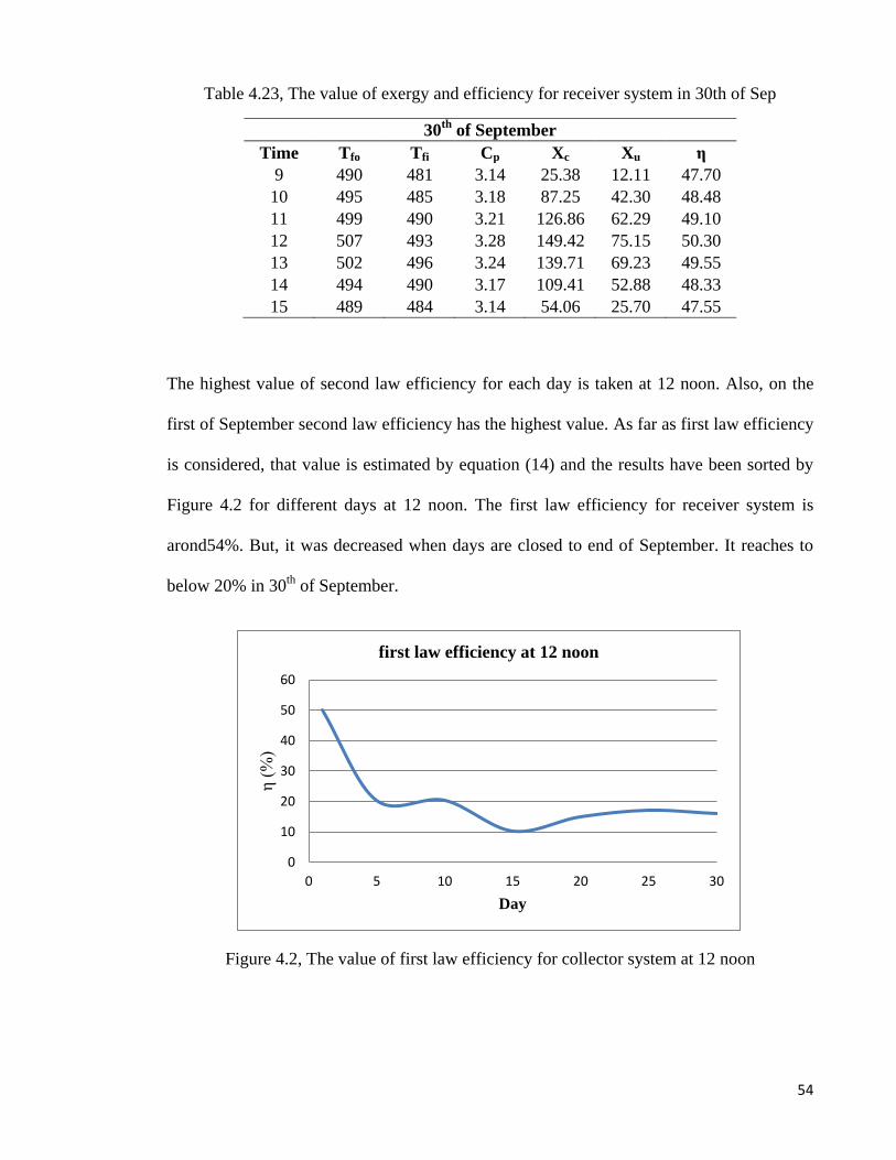
54
Table 4.23, The value of exergy and efficiency for receiver system in 30th of Sep
30th
of September
Time Tfo Tfi Cp Xc Xu η
9 490 481 3.14 25.38 12.11 47.70
10 495 485 3.18 87.25 42.30 48.48
11 499 490 3.21 126.86 62.29 49.10
12 507 493 3.28 149.42 75.15 50.30
13 502 496 3.24 139.71 69.23 49.55
14 494 490 3.17 109.41 52.88 48.33
15 489 484 3.14 54.06 25.70 47.55
The highest value of second law efficiency for each day is taken at 12 noon. Also, on the
first of September second law efficiency has the highest value. As far as first law efficiency
is considered, that value is estimated by equation (14) and the results have been sorted by
Figure 4.2 for different days at 12 noon. The first law efficiency for receiver system is
arond54%. But, it was decreased when days are closed to end of September. It reaches to
below 20% in 30th
of September.
Figure 4.2, The value of first law efficiency for collector system at 12 noon
0
10
20
30
40
50
60
0 5 10 15 20 25 30
η (
%)
Day
first law efficiency at 12 noon
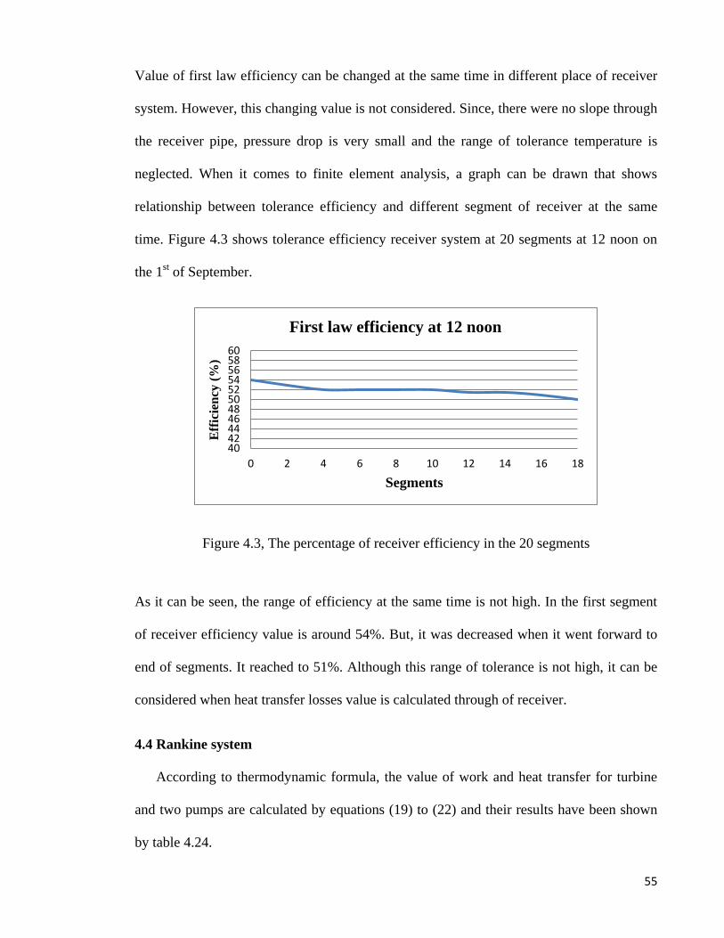
55
Value of first law efficiency can be changed at the same time in different place of receiver
system. However, this changing value is not considered. Since, there were no slope through
the receiver pipe, pressure drop is very small and the range of tolerance temperature is
neglected. When it comes to finite element analysis, a graph can be drawn that shows
relationship between tolerance efficiency and different segment of receiver at the same
time. Figure 4.3 shows tolerance efficiency receiver system at 20 segments at 12 noon on
the 1st of September.
Figure 4.3, The percentage of receiver efficiency in the 20 segments
As it can be seen, the range of efficiency at the same time is not high. In the first segment
of receiver efficiency value is around 54%. But, it was decreased when it went forward to
end of segments. It reached to 51%. Although this range of tolerance is not high, it can be
considered when heat transfer losses value is calculated through of receiver.
4.4 Rankine system
According to thermodynamic formula, the value of work and heat transfer for turbine
and two pumps are calculated by equations (19) to (22) and their results have been shown
by table 4.24.
4042444648505254565860
0 2 4 6 8 10 12 14 16 18
Eff
icie
ncy
(%
)
Segments
First law efficiency at 12 noon
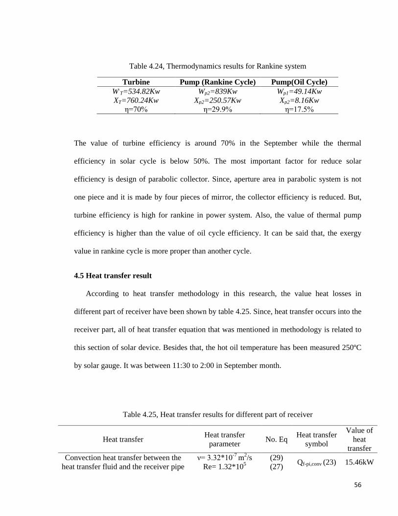
56
Table 4.24, Thermodynamics results for Rankine system
Turbine Pump (Rankine Cycle) Pump(Oil Cycle)
W.T=534.82Kw Wp2=839Kw Wp1=49.14Kw
XT=760.24Kw Xp2=250.57Kw Xp2=8.16Kw
η=70% η=29.9% η=17.5%
The value of turbine efficiency is around 70% in the September while the thermal
efficiency in solar cycle is below 50%. The most important factor for reduce solar
efficiency is design of parabolic collector. Since, aperture area in parabolic system is not
one piece and it is made by four pieces of mirror, the collector efficiency is reduced. But,
turbine efficiency is high for rankine in power system. Also, the value of thermal pump
efficiency is higher than the value of oil cycle efficiency. It can be said that, the exergy
value in rankine cycle is more proper than another cycle.
4.5 Heat transfer result
According to heat transfer methodology in this research, the value heat losses in
different part of receiver have been shown by table 4.25. Since, heat transfer occurs into the
receiver part, all of heat transfer equation that was mentioned in methodology is related to
this section of solar device. Besides that, the hot oil temperature has been measured 250ºC
by solar gauge. It was between 11:30 to 2:00 in September month.
Table 4.25, Heat transfer results for different part of receiver
Heat transfer Heat transfer
parameter No. Eq
Heat transfer
symbol
Value of
heat
transfer
Convection heat transfer between the
heat transfer fluid and the receiver pipe
ν= 3.32*10-7
m2/s
Re= 1.32*105
(29)
(27) Qf-pi,conv (23) 15.46kW
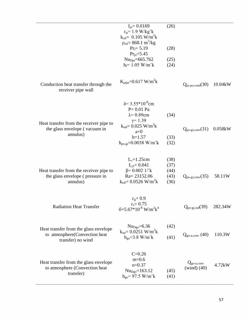
57
fpi= 0.0169
cp= 1.9 W/kg˚k
koil= 0.105 W/m2k
ρoil= 868.1 m3/kg
Prf= 5.19
Prpi=5.45
NuDpi=665.762
hf= 1.05 W/m˚k
(26)
(28)
(25)
(24)
Conduction heat transfer through the
receiver pipe wall
Kpipe=0.617 W/m2k
Qpi-po,cond(30)
10.04kW
Heat transfer from the receiver pipe to
the glass envelope ( vacuum in
annulus)
δ= 3.55*10-8
cm
P= 0.01 Pa
λ= 0.89cm
γ= 1.39
kstd= 0.025 W/m2k
a=0
b=1.57
hpo-gi=0.0038 W/m˚k
(34)
(33)
(32)
Qpo-gi,conv(31) 0.058kW
Heat transfer from the receiver pipe to
the glass envelope ( pressure in
annulus)
Lc=1.25cm
fcyl= 0.041
β= 0.002 1/˚k
Ra= 23152.06
keff= 0.0526 W/m2k
(38)
(37)
(44)
(43)
(36)
Qpo-gi,conv(35) 58.11W
Radiation Heat Transfer
ɛg= 0.9
ɛs= 0.75
б=5.67*10-8
W/m2k
4
Qpo-gi,rad(39)
282.34W
Heat transfer from the glass envelope
to atmosphere(Convection heat
transfer) no wind
NuDgo=6.36
kair= 0.0251 W/m2k
hgo=3.8 W/m˚k
(42)
(41)
Qgo-a,conv (40)
110.3W
Heat transfer from the glass envelope
to atmosphere (Convection heat
transfer)
C=0.26
m=0.6
n=0.37
NuDgo=163.12
hgo= 97.5 W/m˚k
(45)
(41)
Qgo-a,conv
(wind) (40)
4.72kW

58
Table 4.25 shows all of heat losses values that occur in different part of receiver. There are
seven different heat losses that among of them the Convection heat transfer between the
heat transfer fluid and the receiver pipe was the highest. Since, there is no vacuum between
glass envelop and receiver tube, the Nusselt number value was increased dramatically.
Therefore, coefficient convection is going up. In this research, heat convection equation has
been exported by equation (23) and its value in 250ºC for oil is around 15.46kW.
Heat transfer from the glass envelope to atmosphere is known as heat convection and it is
divided to windy and no windy status. Obviously, the Nusselt number in the case of windy
is more than another case. Therefore, the heat convection value in this section is around
4.72 kW for windy case that is frothy times as much as when there is no wind.
As long as Heat transfer from the receiver pipe to the glass envelope ( vacuum in annulus)
is considered, its value is the lowest. Since, the accommodation coefficient value is
assumed zero, the value of convection coefficient is decreased. Finally, heat losses value in
this section was below 1kW.
It can be said, the higher efficiencies are obtained when the annuals is under vacuum, but in
both cases at the high temperatures the collector efficiency drops gradually, which is more
notable for the black chrome coating. It can be found that, two different cases can be
considered. First case is air flow between glass envelop and receiver system. Another case
is defined when vacuum is installed between them. Obviously, thermal efficiency is higher
for different temperature when it comes to vacuum installation in receiver part. Figure 4.4
shows thermal efficiency values for vacuum and air installation in different temperature.
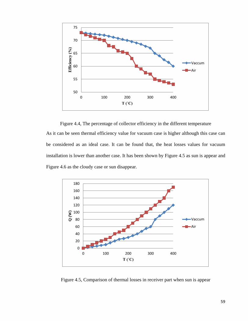
59
Figure 4.4, The percentage of collector efficiency in the different temperature
As it can be seen thermal efficiency value for vacuum case is higher although this case can
be considered as an ideal case. It can be found that, the heat losses values for vacuum
installation is lower than another case. It has been shown by Figure 4.5 as sun is appear and
Figure 4.6 as the cloudy case or sun disappear.
Figure 4.5, Comparison of thermal losses in receiver part when sun is appear
50
55
60
65
70
75
0 100 200 300 400
Eff
icie
ncy
(%
)
T (˚C)
Vaccum
Air
0
20
40
60
80
100
120
140
160
180
0 100 200 300 400
Q (
W)
T (˚C)
Vaccum
Air
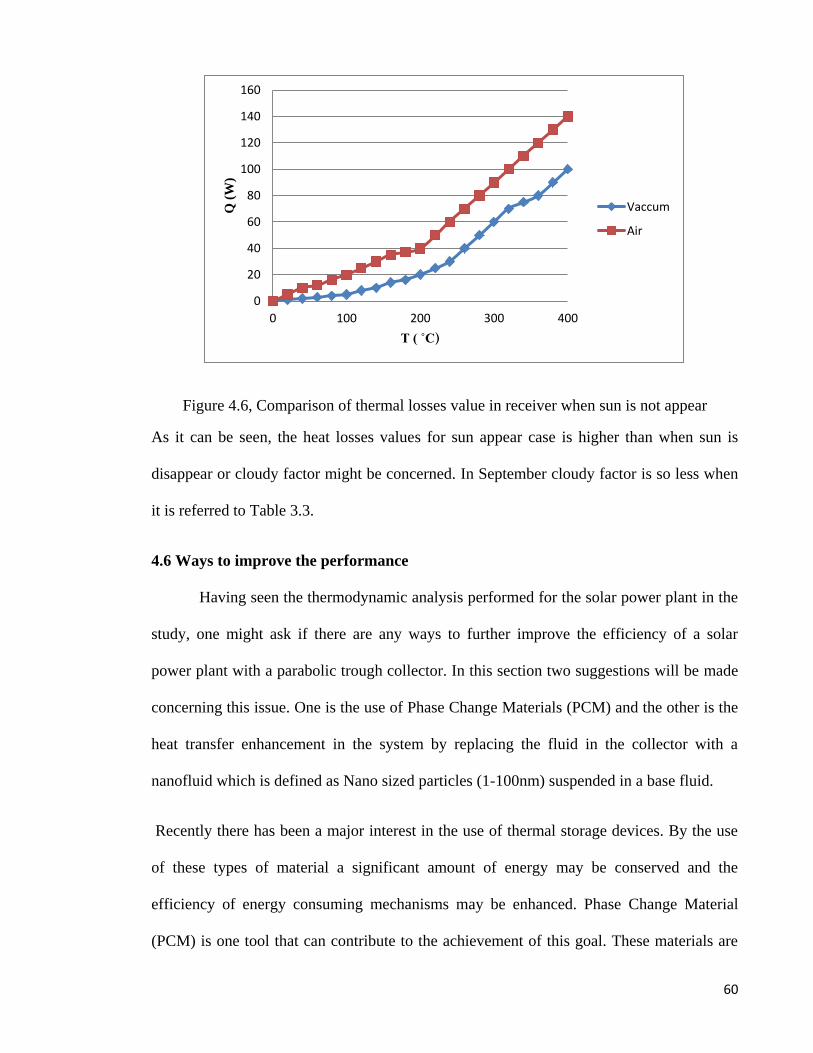
60
Figure 4.6, Comparison of thermal losses value in receiver when sun is not appear
As it can be seen, the heat losses values for sun appear case is higher than when sun is
disappear or cloudy factor might be concerned. In September cloudy factor is so less when
it is referred to Table 3.3.
4.6 Ways to improve the performance
Having seen the thermodynamic analysis performed for the solar power plant in the
study, one might ask if there are any ways to further improve the efficiency of a solar
power plant with a parabolic trough collector. In this section two suggestions will be made
concerning this issue. One is the use of Phase Change Materials (PCM) and the other is the
heat transfer enhancement in the system by replacing the fluid in the collector with a
nanofluid which is defined as Nano sized particles (1-100nm) suspended in a base fluid.
Recently there has been a major interest in the use of thermal storage devices. By the use
of these types of material a significant amount of energy may be conserved and the
efficiency of energy consuming mechanisms may be enhanced. Phase Change Material
(PCM) is one tool that can contribute to the achievement of this goal. These materials are
0
20
40
60
80
100
120
140
160
0 100 200 300 400
Q (
W)
T ( ˚C)
Vaccum
Air

61
capable of store the energy in a phase and then release it when needed by changing their
phase.
Nanofluid which is a colloidal mixture of a base fluid like water and solid nano particles
has showed some favorable behavior regarding this issue. During the recent years a
significant number of researches have been performed to disclose the unknown facts about
this new class of fluids.
Since, there are no mirror reflectors technology in Iran, all of aperture area has been
covered by three or four pieces of mirror. Therefore, there is no specific focal point for
each parabolic system. It can be found as the main factor to reduce thermal efficiency for
solar power plant system.
62
5 Conclusion
As conclusion, parabolic trough solar power plant system in Iran was considered. By
using some of the useful physical parameters and physical properties of receiver oil,
thermodynamics parameters were estimated and heat transfer could be analyzed. First, fifth,
tenth, fifteenth, twentieth, twentieth-fifth and thirtieth of September were calculation days,
the value of exergy and thermal efficiency were the highest value when it comes to first of
September.
Also, the value of exergy and thermal efficiency at 12 noon was the most. The exergy
received value was around 460kJ/kg at 12 noon of first September and the value of exergy
absorbed by collector was approximately 45kJ/kg. The energy efficiency of parabolic
trough collector system was calculated to be around 10%. It can be said that type of mirror
used is effective on the amount of efficiency. If one-piece mirror were used the efficiency
would be higher. On the other hand the second law efficiency for receiver system was
around 55% that by comparison of fossil power plant was low. Some technologies could be
utilized to improve the efficiency. Phase Change Material can be used to store thermal
energy. Nanofluid can also increase the performance since they can increase the heat
transfer to the receiver fluid.
As far as heat transfer is considered, the value of Convection heat transfer between the heat
transfer fluid and the receiver pipe was high in 250˚C. It was around 15.5kW. Also, the
value of heat transfer from the glass envelope to atmosphere with wind was higher than the
value of Heat transfer from the glass envelope to atmosphere without wind. It can be found
that coefficient of heat convection in case of wind is bigger than another one.

63
Various recirculation regions can be found on the leeward and forward sides of the
parabolic collector when the collector orientation changes with respect to wind direction.
The flow field and pressure field around the collector are affected by the small gap between
the two sections of collector’s sides and the distance between collector and the ground, and
less affected by the receiver tube.
Last but not least the value of thermal loss when it comes to on-sun case is more than when
the off-sun case. It is approximately two times more than ones. The resultant force on the
collector structure is maximum when wind blows normal to the opening and minimum
when the collector is oriented parallel with wind direction.

64
6 Recommendation
The following recommendations should be considered for further research in this area:
Since in a solar power plant the heat absorbed by the solar collector is to be transferred in a
suitable time and be used later in the power generating cycle such as a Rankine cycle, PCM
might be useful to store the energy resulting from radiation. To the best of authors’
knowledge very few studies have investigated the effect of latent heat storage by PCM
incorporated with a solar power plant. A model for energy and exergy analysis of latent
heat thermal storage usage is in a solar system. Their system included an air flow heated by
a solar collector entering a tank filled with PCM afterwards. Calculations done in this work
are used to perform a comprehensive second law analysis for the PCM used.
Enhancing the thermal performance of the solar collector is another way that could play a
remarkable role in the improvement of solar power plant efficiency. One of the ways is to
use a fluid with higher thermal performance so that more heat gain could be obtained from
the solar radiation. Nanofluid is known a new technique for reducing of heat losses value
and enhancement of thermal efficiency.
65
7 Bibliography
Abbas M., Boumeddane B., Said N., Chikouche A. (2011) Dish Stirling technology: A
100 MW solar power plant using hydrogen for Algeria. International Journal of
Hydrogen Energy 36:4305-4314. DOI: 10.1016/j.ijhydene.2010.12.114.
Al-Sulaiman F.A., Dincer I., Hamdullahpur F. (2011) Exergy modeling of a new solar
driven trigeneration system. Solar Energy 85:2228-2243. DOI:
10.1016/j.solener.2011.06.009.
Almanza R., Lentz A., Jiménez G. (1998) Receiver behavior in direct steam generation
with parabolic troughs. Solar Energy 61:275-278. DOI: 10.1016/s0038-
092x(97)88854-8.
Amspacher S. (2011) The Future of Large-Scale Solar Energy in California, University of
California.
Badescu V. (2007) Optimal control of flow in solar collectors for maximum exergy
extraction. International Journal of Heat and Mass Transfer 50:4311-4322. DOI:
10.1016/j.ijheatmasstransfer.2007.01.061.
Baghernejad A., Yaghoubi M. (2010) Exergy analysis of an integrated solar combined
cycle system. Renewable energy 35:2157-2164.
Bakos G.C. (2006) Design and construction of a two-axis Sun tracking system for parabolic
trough collector (PTC) efficiency improvement. Renewable Energy 31:2411-2421.
Bakos G.C., Ioannidis I., Tsagas N.F., Seftelis I. (2001) Design, optimisation and
conversion-efficiency determination of a line-focus parabolic-trough solar-collector
(PTC). Applied Energy 68:43-50. DOI: 10.1016/s0306-2619(00)00034-9.
66
Calise F., Palombo A., Vanoli L. A finite-volume model of a parabolic trough
photovoltaic/thermal collector: Energetic and exergetic analyses. Energy. DOI:
10.1016/j.energy.2012.08.021.
Cao F., Zhao L., Guo L. (2011) Simulation of a sloped solar chimney power plant in
Lanzhou. Energy Conversion and Management 52:2360-2366. DOI:
10.1016/j.enconman.2010.12.035.
Cheng Z., He Y., Xiao J., Tao Y., Xu R. (2010) Three-dimensional numerical study of heat
transfer characteristics in the receiver tube of parabolic trough solar collector.
International Communications in Heat and Mass Transfer 37:782-787.
Cheng Z., He Y., Cui F., Xu R., Tao Y. (2012) Numerical simulation of a parabolic trough
solar collector with nonuniform solar flux conditions by coupling FVM and MCRT
method. Solar Energy.
Cohen G.E. (1993) Operation and efficiency of large-scale solar thermal power plants.
Society of photo-optical instrumentation engineers, Bellingham, WA,(USA).
2017:332-337.
Corporation B. (1929) A new invention to harness the sun.
Duffie J.A., Beckman W.A. (1980) Solar engineering of thermal processes. NASA
STI/Recon Technical Report A 81:16591.
Duffie J.A., Beckman W.A. (2006) Solar engineering of thermal processes Wiley New
York.
Edwards S.E.B., Materić V. (2012) Calcium looping in solar power generation plants. Solar
Energy 86:2494-2503. DOI: 10.1016/j.solener.2012.05.019.
energy U.d.o. (2005) Concentrating solar parabolic reflector technologies.
energy U.d.o. (2007) Solar photovoltaics- flat plate.
67
Feldhoff J.F., Schmitz K., Eck M., Schnatbaum-Laumann L., Laing D., Ortiz-Vives F.,
Schulte-Fischedick J. (2012) Comparative system analysis of direct steam
generation and synthetic oil parabolic trough power plants with integrated thermal
storage. Solar Energy 86:520-530. DOI: 10.1016/j.solener.2011.10.026.
Fernández-García A., Zarza E., Valenzuela L., Pérez M. (2010) Parabolic-trough solar
collectors and their applications. Renewable and Sustainable Energy Reviews
14:1695-1721. DOI: 10.1016/j.rser.2010.03.012.
Feuermann D., Gordon J. (1991) Analysis of a two-stage linear Fresnel reflector solar
concentrator. Journal of Solar Energy Engineering;(United States) 113.
Fisher s., Lupfert e. (2006) Efficiency testing of parabolic trough collectors using the
dynamic tes. Solar energy.
Geyer M., Lüpfert E., Osuna R., Esteban A., Schiel W., Schweitzer A., Zarza E., Nava P.,
Langenkamp J., Mandelberg E. (2002) EUROTROUGH–Parabolic trough collector
developed for cost efficient solar power generation. pp. 04-06.
Giannuzzi G.M., Majorana C.E., Miliozzi A., Salomoni V.A., Nicolini D. (2007) Structural
Design Criteria for Steel Components of Parabolic-Trough Solar Concentrators.
Journal of Solar Energy Engineering 129:382. DOI: 10.1115/1.2769699.
Goffman E. (2008) Why Not the Sun? Advantages of and Problems with Solar Energy
journal.
Gupta M.K., Kaushik S.C. (2010) Exergy analysis and investigation for various feed water
heaters of direct steam generation solar–thermal power plant. Renewable Energy
35:1228-1235. DOI: 10.1016/j.renene.2009.09.007.
He Y.-L., Mei D.-H., Tao W.-Q., Yang W.-W., Liu H.-L. (2012) Simulation of the
parabolic trough solar energy generation system with Organic Rankine Cycle.
Applied Energy 97:630-641. DOI: 10.1016/j.apenergy.2012.02.047.
68
Hosseini M., Dincer I., Rosen M.A. (2013) Hybrid solar–fuel cell combined heat and
power systems for residential applications: Energy and exergy analyses. Journal of
Power Sources 221:372-380. DOI: 10.1016/j.jpowsour.2012.08.047.
Hosseini R., Soltani M., Valizadeh G. (2005) Technical and economic assessment of the
integrated solar combined cycle power plants in Iran. Renewable Energy 30:1541-
1555. DOI: 10.1016/j.renene.2004.11.005.
Imenes A.G., Buie D., Mills D.R., Schramek P., Bosi S.G. (2006) A new strategy for
improved spectral performance in solar power plants. Solar Energy 80:1263-1269.
DOI: 10.1016/j.solener.2005.04.021.
Johnson G. (2009a) Plugging into the Sun. National Geographic, September 2009: 28 53.
Johnson G. (2009b) Plugging into the Sun. National Geographic 216:28-53.
Kalogirou S.A. A detailed thermal model of a parabolic trough collector receiver. Energy.
DOI: 10.1016/j.energy.2012.06.023.
Kalogirou S.A. (2012) A detailed thermal model of a parabolic trough collector receiver.
Energy.
Kerkeni C., BenJemaa F., Kooli S., Farhat A., Maalej M. (2002) Performance evaluation of
a thermodynamic solar power plant: fifteen years of operation history. Renewable
Energy 25:473-487. DOI: 10.1016/s0960-1481(01)00077-5.
Kumar S., Tiwari G.N. (2011) Analytical expression for instantaneous exergy efficiency of
a shallow basin passive solar still. International Journal of Thermal Sciences
50:2543-2549. DOI: 10.1016/j.ijthermalsci.2011.06.015.
Li M., Wang L.L. (2006) Investigation of evacuated tube heated by solar trough
concentrating system. Energy Conversion and Management 47:3591-3601. DOI:
10.1016/j.enconman.2006.03.003.
69
Li Y.-Q., He Y.-L., Wang Z.-F., Xu C., Wang W. (2012) Exergy analysis of two phase
change materials storage system for solar thermal power with finite-time
thermodynamics. Renewable Energy 39:447-454. DOI:
10.1016/j.renene.2011.08.026.
Lienhard J.H. (2011) A heat transfer textbook Dover Publications.
Lior N. (2002) Thoughts about future power generation systems and the role of exergy
analysis in their development. Energy Conversion and Management 43:1187-1198.
Llorente García I., Álvarez J.L., Blanco D. (2011) Performance model for parabolic trough
solar thermal power plants with thermal storage: Comparison to operating plant
data. Solar Energy 85:2443-2460. DOI: 10.1016/j.solener.2011.07.002.
M. Yaghoubi, moosavi M.A. (2001) Three dimensional thermal expansion analysis of an
absorber tube in a parabolic trough collector. Iranian sceince & technology.
Marshal N. (1976) Gas Encyclopedia, New York: Elsevier.
Michels H., Pitz-Paal R. (2007) Cascaded latent heat storage for parabolic trough solar
power plants. Solar Energy 81:829-837.
Ming Qu D.H.A., Sophie V. Masson. (2006) A Linear Parabolic Trough Solar Collector
Performance Model VIII-3-3.
Montes M., Abánades A., Martínez-Val J., Valdés M. (2009) Solar multiple optimization
for a solar-only thermal power plant, using oil as heat transfer fluid in the parabolic
trough collectors. Solar Energy 83:2165-2176.
Morin G., Dersch J., Platzer W., Eck M., Häberle A. (2011) Comparison of Linear Fresnel
and Parabolic Trough Collector power plants. Solar Energy.
Nixon J.D., Davies P.A. (2012) Cost-exergy optimisation of linear Fresnel reflectors. Solar
Energy 86:147-156. DOI: 10.1016/j.solener.2011.09.024.
70
Odeh S.D., Morrison G.L., Behnia M. (1998) Modelling of parabolic trough direct steam
generation solar collectors. Solar Energy 62:395-406. DOI: 10.1016/s0038-
092x(98)00031-0.
Orel Z.C., Gunde M.K., Orel B. (1997) Application of the Kubelka-Munk theory for the
determination of the optical properties of solar absorbing paints. Progress in organic
coatings 30:59-66.
Padilla R.V., Demirkaya G., Goswami D.Y., Stefanakos E., Rahman M.M. (2011) Heat
transfer analysis of parabolic trough solar receiver. Applied Energy 88:5097-5110.
DOI: 10.1016/j.apenergy.2011.07.012.
Popov D. (2011) An option for solar thermal repowering of fossil fuel fired power plants.
Solar Energy 85:344-349. DOI: 10.1016/j.solener.2010.11.017.
Poullikkas A. (2009) Economic analysis of power generation from parabolic trough solar
thermal plants for the Mediterranean region—A case study for the island of Cyprus.
Renewable and Sustainable Energy Reviews 13:2474-2484.
Prakash M., Kedare S., Nayak J. (2009) Investigations on heat losses from a solar cavity
receiver. Solar Energy 83:157-170.
Price H., Lüpfert E., Kearney D., Zarza E., Cohen G., Gee R., Mahoney R. (2002)
Advances in parabolic trough solar power technology. Journal of Solar Energy
Engineering 124:109.
Ratzel A., Hickox C., Gartling D. (1979) Techniques for reducing thermal conduction and
natural convection heat losses in annular receiver geometries. J. Heat
Transfer;(United States) 101.
Reddy V.S., Kaushik S.C., Tyagi S.K. (2012) Exergetic analysis and performance
evaluation of parabolic trough concentrating solar thermal power plant (PTCSTPP).
Energy 39:258-273. DOI: 10.1016/j.energy.2012.01.023.
71
Regulagadda P., Dincer I., Naterer G.F. (2010) Exergy analysis of a thermal power plant
with measured boiler and turbine losses. Applied Thermal Engineering 30:970-976.
DOI: 10.1016/j.applthermaleng.2010.01.008.
Rolim M.M., Fraidenraich N., Tiba C. (2009) Analytic modeling of a solar power plant
with parabolic linear collectors. Solar Energy 83:126-133. DOI:
10.1016/j.solener.2008.07.018.
Romero M., González-Aguilar J. (2011) Solar thermal power plants: from endangerd
species to bulk power production in sun belt Regions. Chapter 3:10016-5990.
S. D. Odeh G.L.M.a.M.B. Thermal analysis of parabolic trough solar collectors for electric
power generation.
Sabziparvar A.A., Shetaee H. (2007) Estimation of global solar radiation in arid and semi-
arid climates of East and West Iran. Energy 32:649-655. DOI:
10.1016/j.energy.2006.05.005.
Sansoni P., Fontani D., Francini F., Giannuzzi A., Sani E., Mercatelli L., Jafrancesco D.
(2011) Optical collection efficiency and orientation of a solar trough medium-power
plant installed in Italy. Renewable Energy 36:2341-2347. DOI:
10.1016/j.renene.2011.02.004.
Schwartz C.L. (2012) 6. Concentrated thermal solar power and the value of water for
electricity. The Water-Energy Nexus in the American West:71.
Singh N., Kaushik S.C., Misra R.D. (2000a) Exergetic analysis of a solar thermal power
system. Renewable Energy 19:135-143. DOI: 10.1016/s0960-1481(99)00027-0.
Singh N., Kaushik S., Misra R. (2000b) Exergetic analysis of a solar thermal power system.
Renewable Energy 19:135-143.
72
Suresh M.V.J.J., Reddy K.S., Kolar A.K. (2010) 4-E (Energy, Exergy, Environment, and
Economic) analysis of solar thermal aided coal-fired power plants. Energy for
Sustainable Development 14:267-279. DOI: 10.1016/j.esd.2010.09.002.
Thomas A. (1996) Solar steam generating systems using parabolic trough concentrators.
Energy Conversion and Management 37:215-245. DOI: 10.1016/0196-
8904(95)00162-7.
Touloukian Y.S., Makita T. (1970) Thermophysical Properties of Matter-The TPRC Data
Series. Volume 6. Specific Heat-Nonmetallic Liquids and Gases, DTIC Document.
Wei X., Lu Z., Wang Z., Yu W., Zhang H., Yao Z. (2010) A new method for the design of
the heliostat field layout for solar tower power plant. Renewable Energy 35:1970-
1975. DOI: 10.1016/j.renene.2010.01.026.
Wiese A., Kleineidam P., Schallenberg K., Ulrich A.J., Kaltschmitt M. (2010) Renewable
power generation-a status report. Renewable Energy Focus 11:34-39, 42-45.
Xu C., Wang Z., Li X., Sun F. (2011) Energy and exergy analysis of solar power tower
plants. Applied Thermal Engineering 31:3904-3913. DOI:
10.1016/j.applthermaleng.2011.07.038.
Yaghoubi M., Mokhtari A. (2007) R. Hesami Thermo-economic analysis of Shiraz solar
thermal power plant, Proceedings of the Third International Conference on Thermal
Engineering: Theory and Applications Amman, Jordan.
Yaghoubi M., Azizian K., Kenary A. (2003) Simulation of Shiraz solar power plant for
optimal assessment. Renewable Energy 28:1985-1998.
Yaghoubi M., Armodly U., Kanan P. (2009) Shiraz Solar Thermal Power Plant
Construction and Steam Generation. Proceedings of SOLAR PACES.
Yaghoubi M.A., Jafarpur K. (1990) global solar radiation in fars province. Iranian journal
of science & technology 14.
73
Yang Y., Yan Q., Zhai R., Kouzani A., Hu E. (2011) An efficient way to use medium-or-
low temperature solar heat for power generation – integration into conventional
power plant. Applied Thermal Engineering 31:157-162. DOI:
10.1016/j.applthermaleng.2010.08.024.
Ying Y., Hu E.J. (1999) Thermodynamic advantages of using solar energy in the
regenerative Rankine power plant. Applied Thermal Engineering 19:1173-1180.
DOI: 10.1016/s1359-4311(98)00114-8.
You Y., Hu E.J. (2002) A medium-temperature solar thermal power system and its
efficiency optimisation. Applied Thermal Engineering 22:357-364. DOI:
10.1016/s1359-4311(01)00104-1.