ThermoElectric Power SystemSimulator (TEPSS)

Sponsored by NYSERDA’s Industrial Researchand Development Program

Robert J. StevensMechanical Engineering

Rochester Institute of Technology

2011 DOE Thermoelectrics Applications WorkshopJanuary 3 - 6, 2011

San Diego, CA

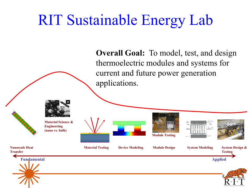
RIT Sustainable Energy Lab

Fundamental Applied

Nanoscale Heat Transfer

Material Science & Engineering(nano vs. bulk)

Material Testing Device Modeling Module Design

Module Testing

System Modeling System Design & Testing

Overall Goal: To model, test, and design thermoelectric modules and systems for current and future power generation applications.

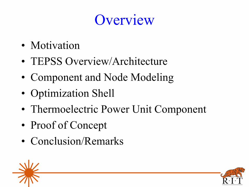
Overview• Motivation• TEPSS Overview/Architecture• Component and Node Modeling• Optimization Shell• Thermoelectric Power Unit Component• Proof of Concept• Conclusion/Remarks

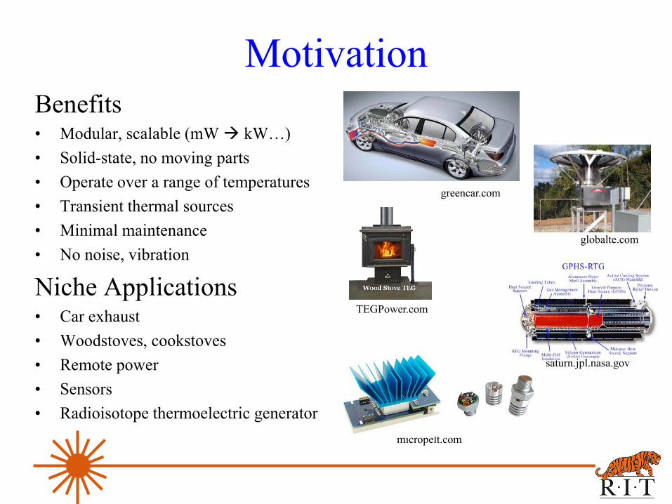
MotivationBenefits• Modular, scalable (mW kW…)• Solid-state, no moving parts• Operate over a range of temperatures• Transient thermal sources• Minimal maintenance• No noise, vibration

Niche Applications• Car exhaust• Woodstoves, cookstoves• Remote power• Sensors• Radioisotope thermoelectric generator

greencar.com

saturn.jpl.nasa.gov

TEGPower.com

globalte.com

micropelt.com

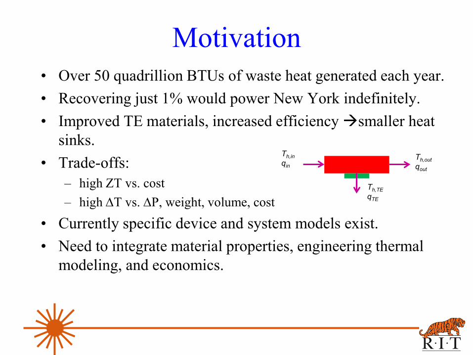
Motivation• Over 50 quadrillion BTUs of waste heat generated each year.• Recovering just 1% would power New York indefinitely.• Improved TE materials, increased efficiency smaller heat

sinks.• Trade-offs:

– high ZT vs. cost– high ∆T vs. ∆P, weight, volume, cost

• Currently specific device and system models exist.• Need to integrate material properties, engineering thermal

modeling, and economics.

Th,inqin

Th,outqout

Th,TEqTE

TEPSS Project GoalCreate a versatile tool to evaluate whether or not thermoelectrics are currently or will soon become technically and economically viable for a specific application and if so determine what the optimal system might look like.

• The tool should help quickly assess a range of potential applications for waste heat recovery using emerging thermoelectric materials.

• Most current thermoelectric modeling is geared towards very specific applications and may not consider system trade-offs.

• Historically module and system design have been loosely coupled.

7

TEPSS OverviewRequirements

• Solve system of equations for the system steady operating state• Unlimited system concepts defined by user• Objective function is defined by the user• Optimizes system configuration with respect to user defined design

variables• Open source and expandable• Easy to use, modify, and reuse

Challenges• Energy components are a combination of empirical, analytical or

FE/FD models• Often highly nonlinear system of component models• System of equations changes for each user defined concept

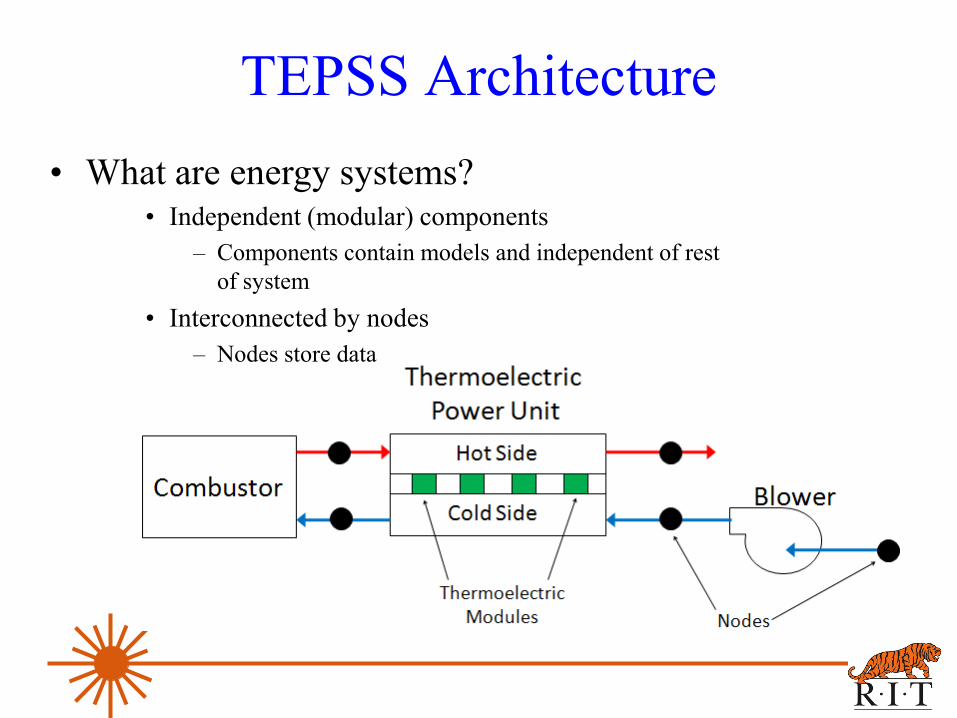
TEPSS Architecture• What are energy systems?

• Independent (modular) components– Components contain models and independent of rest

of system• Interconnected by nodes

– Nodes store data

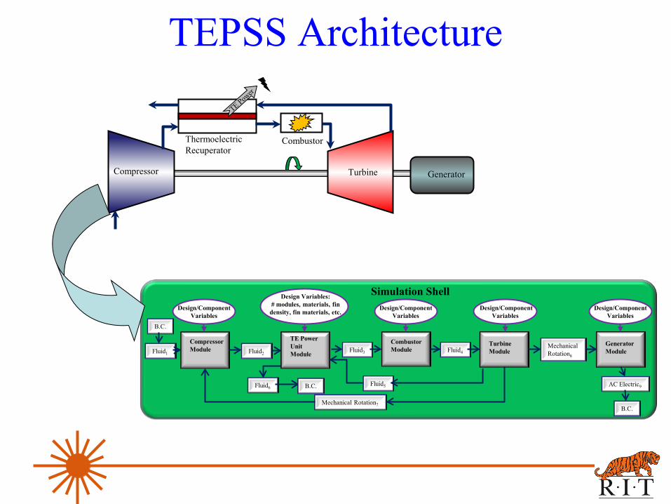
TEPSS Architecture

Compressor

Thermoelectric Recuperator

Combustor

Turbine Generator

Design Variables: # modules, materials, fin

density, fin materials, etc.

Fluid1

TE Power Unit Module

Compressor Module

Design/ComponentVariables

Combustor Module

Turbine Module

Design/ComponentVariables

Design/ComponentVariables

Simulation Shell

Fluid2 Fluid3 Fluid4

Mechanical Rotation7

Generator Module

Mechanical Rotation8

Fluid5Fluid6

Design/ComponentVariables

B.C. AC Electric9

B.C.

B.C.

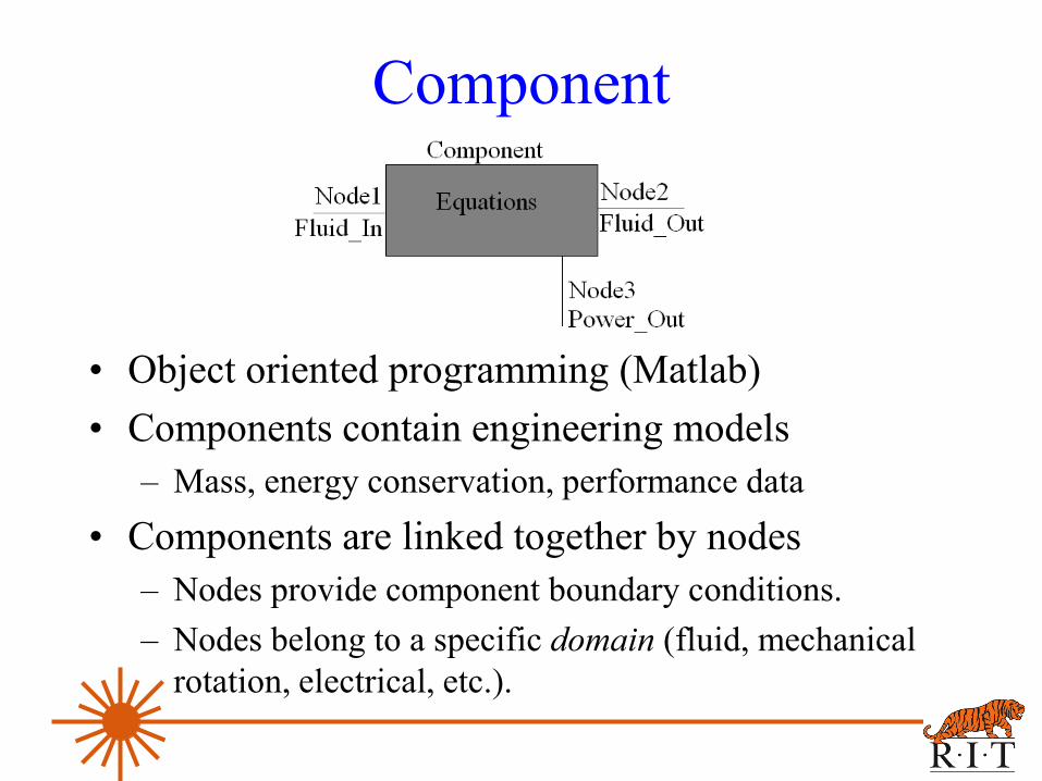
Component

• Object oriented programming (Matlab)• Components contain engineering models

– Mass, energy conservation, performance data• Components are linked together by nodes

– Nodes provide component boundary conditions.– Nodes belong to a specific domain (fluid, mechanical

rotation, electrical, etc.).

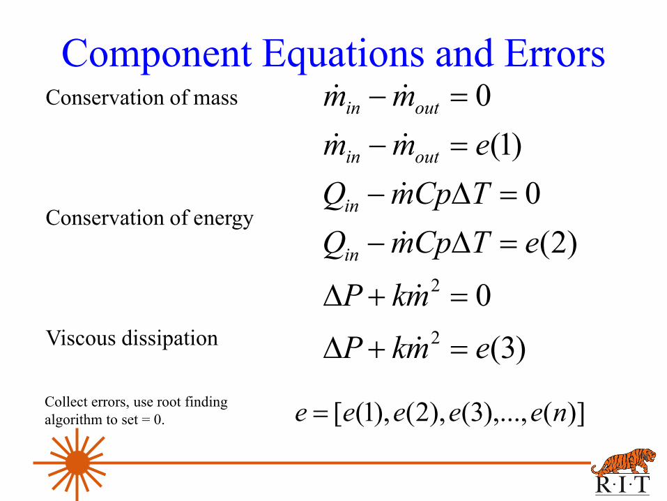
Component Equations and Errors

)3(0

)2(0

)1(0

2

2

emkPmkP

eTCpmQTCpmQemm

mm

in

in

outin

outin

=+∆

=+∆

=∆−=∆−

=−=−

Conservation of mass

Conservation of energy

Viscous dissipation

)](),...,3(),2(),1([ neeeee =Collect errors, use root finding algorithm to set = 0.

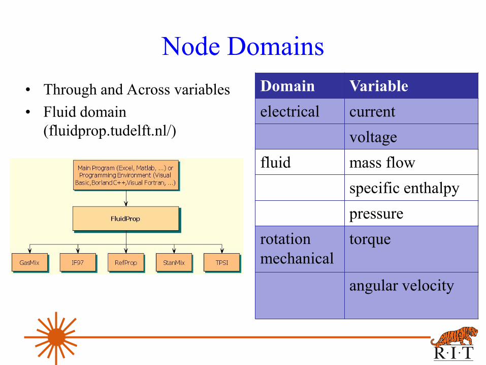
Node Domains• Through and Across variables• Fluid domain

(fluidprop.tudelft.nl/)

Domain Variableelectrical current

voltagefluid mass flow

specific enthalpypressure

rotation mechanical

torque

angular velocity

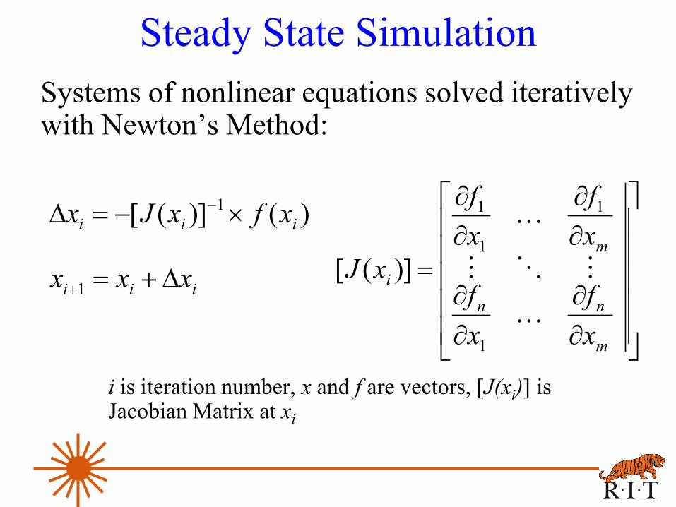
Steady State SimulationSystems of nonlinear equations solved iteratively with Newton’s Method:

i is iteration number, x and f are vectors, [J(xi)] is Jacobian Matrix at xi

)()]([ 1iii xfxJx ×−=∆ −

iii xxx ∆+=+1

∂∂

∂∂

∂∂

∂∂

=

m

nn

m

i

xf

xf

xf

xf

xJ

1

1

1

1

)]([

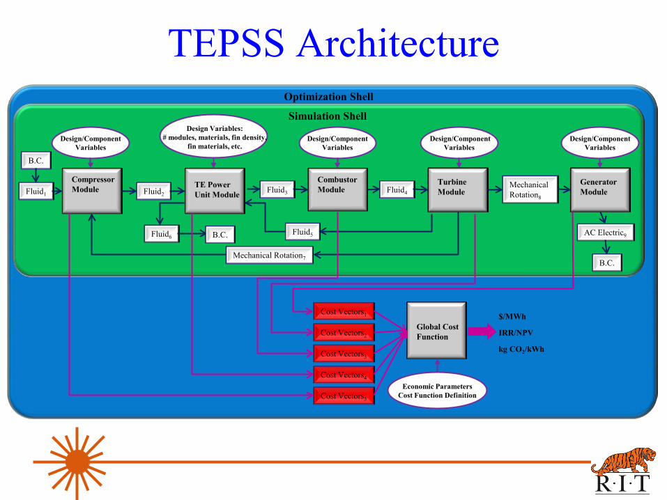
TEPSS Architecture

Design Variables: # modules, materials, fin density,

fin materials, etc.

Fluid1TE Power Unit Module

Compressor Module

Design/ComponentVariables

Combustor Module

Turbine Module

Global Cost Function

$/MWh

IRR/NPV

Design/ComponentVariables

Design/ComponentVariables

Simulation Shell

Fluid2 Fluid3 Fluid4

Mechanical Rotation7

Generator Module

Mechanical Rotation8

Fluid5Fluid6

Design/ComponentVariables

B.C. AC Electric9

B.C.

B.C.

Economic ParametersCost Function Definition

Optimization Shell

Cost Vectors1

Cost Vectors2

Cost Vectors3

Cost Vectors4

Cost Vectors5

kg CO2/kWh

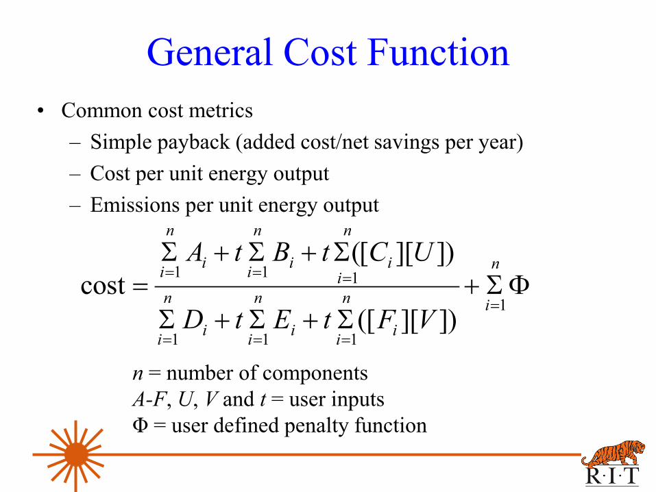
General Cost Function

ΦΣ+Σ+Σ+Σ

Σ+Σ+Σ=

=

===

=== n

iii

n

ii

n

ii

n

ii

n

ii

n

ii

n

VFtEtD

UCtBtA

1

111

111

])][([

])][[(cost

n = number of componentsA-F, U, V and t = user inputsΦ = user defined penalty function

• Common cost metrics– Simple payback (added cost/net savings per year)– Cost per unit energy output – Emissions per unit energy output

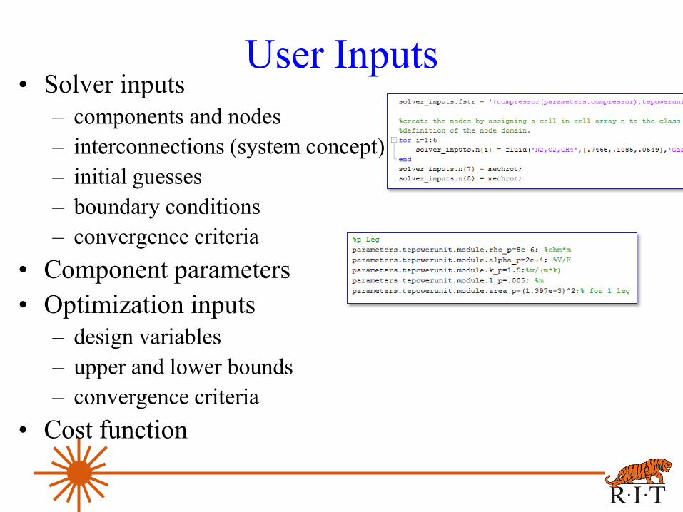
User Inputs• Solver inputs

– components and nodes– interconnections (system concept)– initial guesses– boundary conditions– convergence criteria

• Component parameters• Optimization inputs

– design variables– upper and lower bounds– convergence criteria

• Cost function

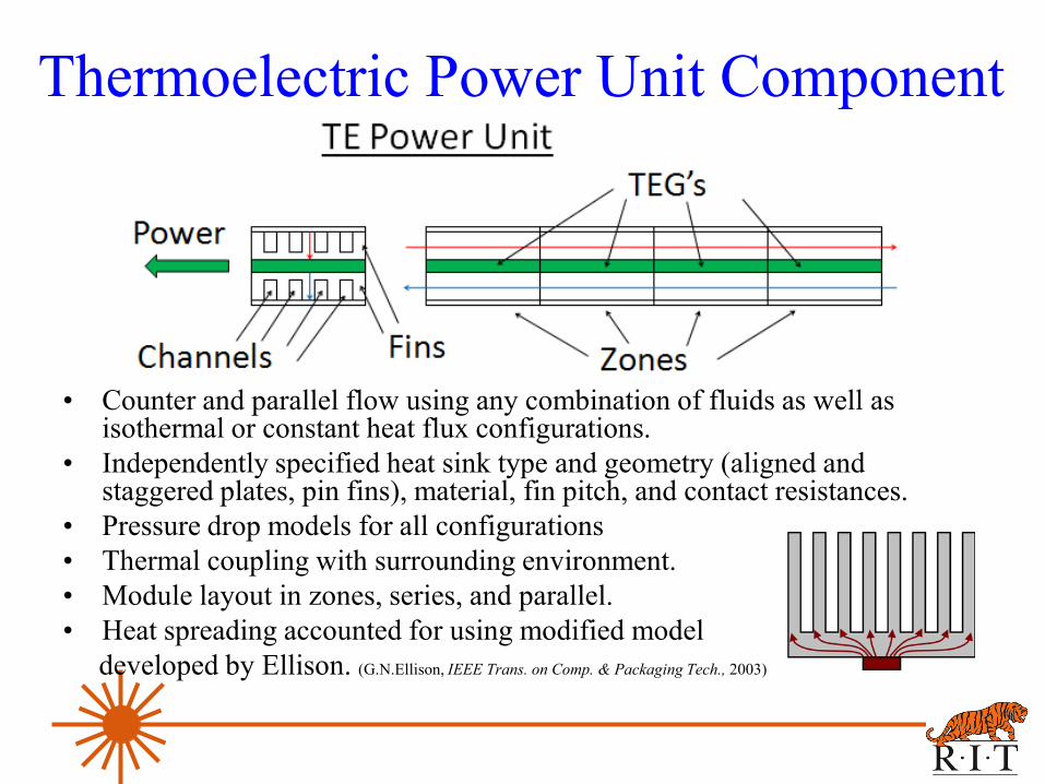
Thermoelectric Power Unit Component

• Counter and parallel flow using any combination of fluids as well as isothermal or constant heat flux configurations.

• Independently specified heat sink type and geometry (aligned and staggered plates, pin fins), material, fin pitch, and contact resistances.

• Pressure drop models for all configurations• Thermal coupling with surrounding environment.• Module layout in zones, series, and parallel.• Heat spreading accounted for using modified model

developed by Ellison. (G.N.Ellison, IEEE Trans. on Comp. & Packaging Tech., 2003)

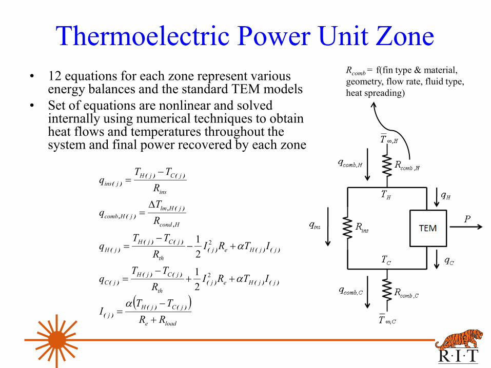
Thermoelectric Power Unit Zone• 12 equations for each zone represent various

energy balances and the standard TEM models• Set of equations are nonlinear and solved

internally using numerical techniques to obtain heat flows and temperatures throughout the system and final power recovered by each zone.

Rcomb = f(fin type & material, geometry, flow rate, fluid type, heat spreading)

( )loade

jCjHj

jjHejth

jCjHjC

jjHejth

jCjHjH

Hcond

jHlmjHcomb

ins

jCjHjins

RRTT

I

ITRIR

TTq

ITRIR

TTq

RT

q

RTT

q

+

−=

++−

=

+−−

=

∆=

−=

)()()(

)()()()()(

)(

)()()()()(

)(

,

)(,)(,

)()()(

α

α

α

2

2

21

21

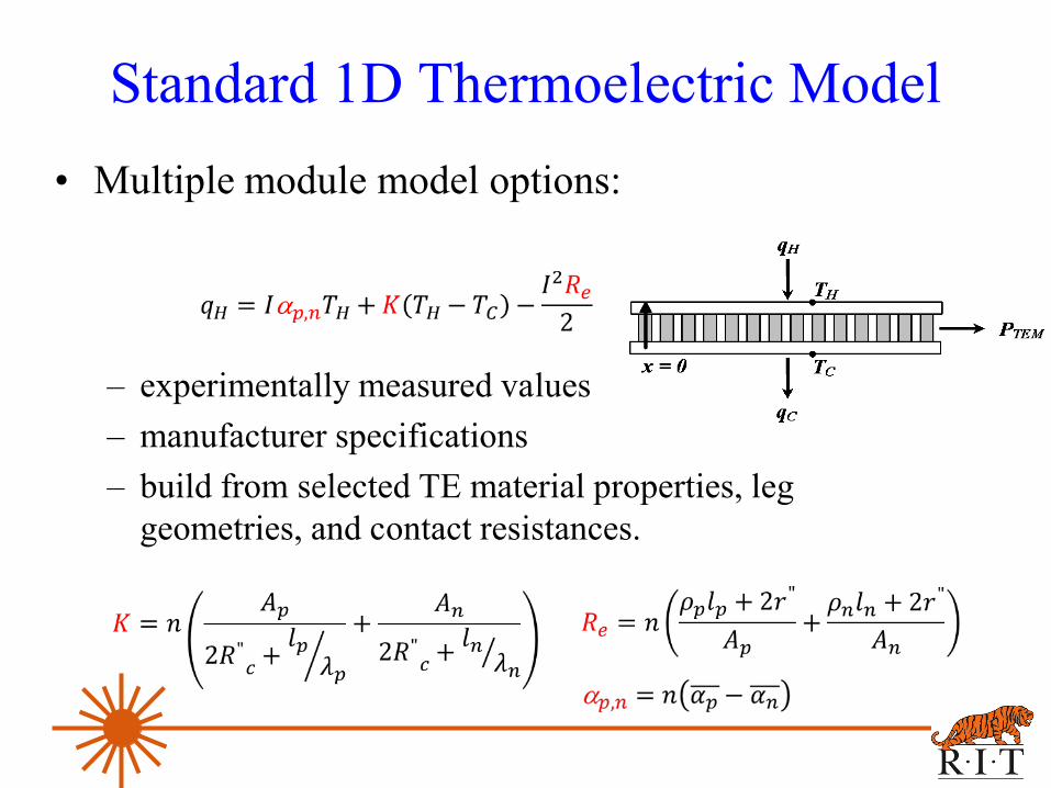
• Multiple module model options:

– experimentally measured values– manufacturer specifications– build from selected TE material properties, leg

geometries, and contact resistances.

Standard 1D Thermoelectric Model

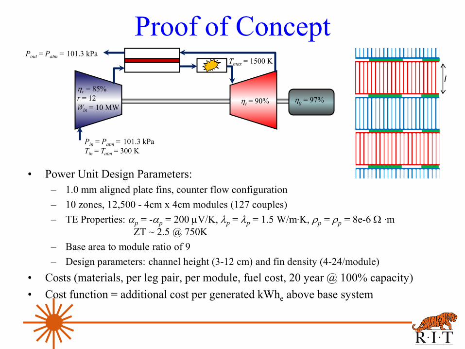
Proof of Concept

• Power Unit Design Parameters:– 1.0 mm aligned plate fins, counter flow configuration– 10 zones, 12,500 - 4cm x 4cm modules (127 couples)– TE Properties: αp = -αp = 200 µV/K, λp = λp = 1.5 W/m∙K, ρp = ρp = 8e-6 Ω ∙m

ZT ~ 2.5 @ 750K– Base area to module ratio of 9– Design parameters: channel height (3-12 cm) and fin density (4-24/module)

• Costs (materials, per leg pair, per module, fuel cost, 20 year @ 100% capacity)• Cost function = additional cost per generated kWhe above base system

Tmax = 1500 K

ηc = 85%r = 12Win = 10 MW

ηt = 90% ηg = 97%

Pin = Patm = 101.3 kPaTin = Tatm = 300 K

Pout = Patm = 101.3 kPa

l

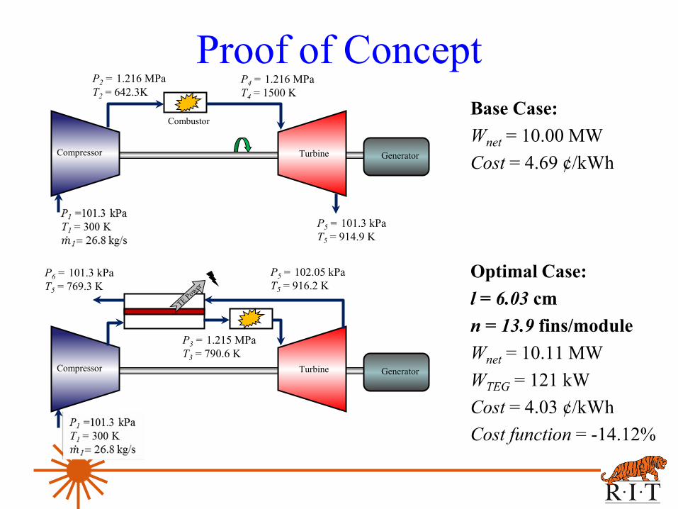
Proof of ConceptBase Case: Wnet = 10.00 MWCost = 4.69 ¢/kWh

Optimal Case:l = 6.03 cmn = 13.9 fins/moduleWnet = 10.11 MWWTEG = 121 kWCost = 4.03 ¢/kWhCost function = -14.12%

Compressor

Combustor

Turbine Generator

P2 = 1.216 MPaT2 = 642.3K

P4 = 1.216 MPaT4 = 1500 K

P5 = 101.3 kPaT5 = 914.9 K

Compressor Turbine Generator

P3 = 1.215 MPaT3 = 790.6 K

P5 = 102.05 kPaT5 = 916.2 K

P6 = 101.3 kPaT5 = 769.3 K

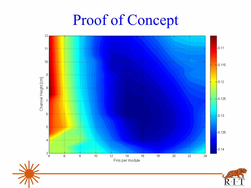
Proof of Concept

Closing Remarks• TEPSS environment has been developed for simulating and

optimizing thermoelectric power generation systems.• TEPSS is expandable with reusable and customizable

components.• New node domains and components can be added to increase

potential system concepts.• TEPSS will allow for the exploration of suitable applications for

emerging TE materials while coupling module level design with system level performance and economics.

• Working on more robust steady state solver and optimization options and developing more advanced component models.

• Interest in using/testing contact rjseme@rit.edu

Acknowledgements• John Kreuder• Andy Freedman• NYSERDA (Contract # 11135)

NYSERDA has not reviewed the information contained herein, and the opinions expressed in this presentation do not necessarily reflect those of NYSERDA or the State of New York.

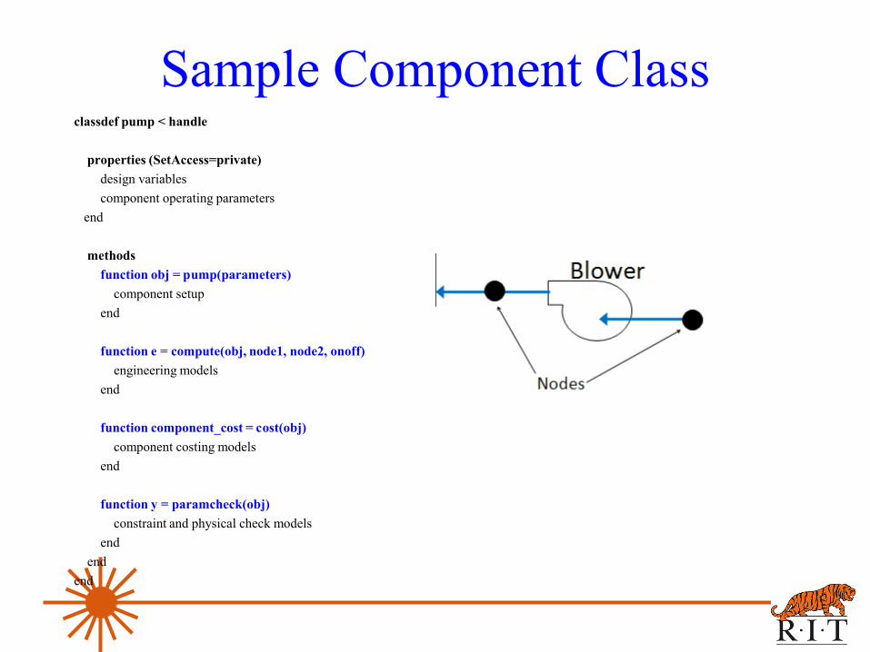
Sample Component Classclassdef pump < handle

properties (SetAccess=private)design variablescomponent operating parameters

end

methodsfunction obj = pump(parameters)

component setupend

function e = compute(obj, node1, node2, onoff)engineering models

end

function component_cost = cost(obj)component costing models

end

function y = paramcheck(obj)constraint and physical check models

end end

end

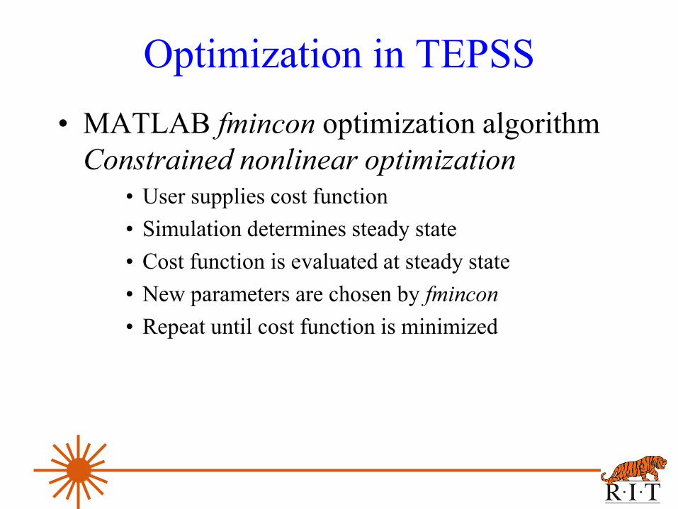
Optimization in TEPSS• MATLAB fmincon optimization algorithm

Constrained nonlinear optimization• User supplies cost function• Simulation determines steady state• Cost function is evaluated at steady state• New parameters are chosen by fmincon• Repeat until cost function is minimized