Embed Size (px)
Citation preview


Published by Department of Automatic ControlLund Institute of TechnologyBox 118SE-221 00 LUNDSweden
ISSN 0280–5316ISRN LUTFD2/TFRT–1053–SE
c� 1999 by Lars Malcolm PedersenAll rights reserved
Printed in Sweden by Lunds Offset ABLund 1999

Contents
Preface . . . . . . . . . . . . . . . . . . . . . . . . . . . . . . . . . . 9
1. Introduction . . . . . . . . . . . . . . . . . . . . . . . . . . . . 111.1 Problem Formulation . . . . . . . . . . . . . . . . . . . . 121.2 Outline of the Thesis . . . . . . . . . . . . . . . . . . . . 13
2. The Thickness Control Problem . . . . . . . . . . . . . . . . 162.1 Hot Rolling of Steel Plates . . . . . . . . . . . . . . . . . 162.2 Controlling the Plate Thickness . . . . . . . . . . . . . . 192.3 Conclusions . . . . . . . . . . . . . . . . . . . . . . . . . . 21
3. Thickness Control of Hot Rolling Mills . . . . . . . . . . . 223.1 What is Needed? . . . . . . . . . . . . . . . . . . . . . . . 223.2 What is Done Already? . . . . . . . . . . . . . . . . . . . 243.3 Analysis of the State-of-the-Art Solution . . . . . . . . . 263.4 What Can Be Improved?—An Example . . . . . . . . . . 283.5 Conclusions . . . . . . . . . . . . . . . . . . . . . . . . . . 31
4. Modeling of the Rolling Mill . . . . . . . . . . . . . . . . . . 324.1 Hydraulic System . . . . . . . . . . . . . . . . . . . . . . 334.2 Rolling Stand . . . . . . . . . . . . . . . . . . . . . . . . . 374.3 Total Model . . . . . . . . . . . . . . . . . . . . . . . . . . 504.4 Conclusions . . . . . . . . . . . . . . . . . . . . . . . . . . 53
5. Thickness Control—Data Collection . . . . . . . . . . . . . 545.1 Measurement Equipment . . . . . . . . . . . . . . . . . . 545.2 Measurements for Identification . . . . . . . . . . . . . . 575.3 Conclusions . . . . . . . . . . . . . . . . . . . . . . . . . . 58
6. Thickness Control—System Identification . . . . . . . . . 596.1 Hydraulic Systems . . . . . . . . . . . . . . . . . . . . . . 606.2 Rolling Stand . . . . . . . . . . . . . . . . . . . . . . . . . 666.3 Total Model . . . . . . . . . . . . . . . . . . . . . . . . . . 746.4 Conclusions . . . . . . . . . . . . . . . . . . . . . . . . . . 76
5

Contents
7. Thickness Control—Design . . . . . . . . . . . . . . . . . . . 787.1 Performance Specifications . . . . . . . . . . . . . . . . . 797.2 Analysis of Model . . . . . . . . . . . . . . . . . . . . . . 807.3 Choice of Control Methods . . . . . . . . . . . . . . . . . 837.4 Design of Controllers . . . . . . . . . . . . . . . . . . . . 837.5 Evaluation of Performance . . . . . . . . . . . . . . . . . 897.6 Conclusions . . . . . . . . . . . . . . . . . . . . . . . . . . 95
8. The Slab Temperature Control Problem . . . . . . . . . . 978.1 Reheat Furnaces . . . . . . . . . . . . . . . . . . . . . . . 978.2 Present Control Algorithms . . . . . . . . . . . . . . . . . 1008.3 The Slab Temperature Control Problem . . . . . . . . . . 1018.4 Analysis of the Slab Heating . . . . . . . . . . . . . . . . 1018.5 Conclusions . . . . . . . . . . . . . . . . . . . . . . . . . . 104
9. Temperature Control—Data Collection . . . . . . . . . . . 1069.1 The Data Collection Device—The Pig . . . . . . . . . . . 1069.2 A Measurement Series . . . . . . . . . . . . . . . . . . . . 1079.3 Conclusions . . . . . . . . . . . . . . . . . . . . . . . . . . 109
10. Temperature Control—System Identification . . . . . . . 11010.1 Model for Furnace Temperature . . . . . . . . . . . . . . 11110.2 Models for Slab Temperature . . . . . . . . . . . . . . . . 11610.3 Conclusions . . . . . . . . . . . . . . . . . . . . . . . . . . 127
11. Temperature Control—Design . . . . . . . . . . . . . . . . . 12811.1 The Control Problem . . . . . . . . . . . . . . . . . . . . . 12811.2 Design of FOCS Controller . . . . . . . . . . . . . . . . . 13011.3 Design of Nonlinear Controller . . . . . . . . . . . . . . . 14511.4 Conclusions . . . . . . . . . . . . . . . . . . . . . . . . . . 150
12. Temperature Control—Simulations . . . . . . . . . . . . . . 15312.1 Implementation of Simulation Model and Control Laws 15312.2 What to Investigate in Simulations? . . . . . . . . . . . . 15612.3 Robustness . . . . . . . . . . . . . . . . . . . . . . . . . . 15612.4 A Stop . . . . . . . . . . . . . . . . . . . . . . . . . . . . . 15712.5 Production . . . . . . . . . . . . . . . . . . . . . . . . . . . 159Conclusions . . . . . . . . . . . . . . . . . . . . . . . . . . . . . . 172
13. Temperature Control—Experimental Results . . . . . . . 17313.1 Comparison of New and Existing Parameters . . . . . . 17313.2 Results and Experiences . . . . . . . . . . . . . . . . . . 17613.3 What Is Left? . . . . . . . . . . . . . . . . . . . . . . . . . 18013.4 Conclusions . . . . . . . . . . . . . . . . . . . . . . . . . . 181
14. Conclusions . . . . . . . . . . . . . . . . . . . . . . . . . . . . . 18214.1 What Has Been Done? . . . . . . . . . . . . . . . . . . . . 18214.2 Results . . . . . . . . . . . . . . . . . . . . . . . . . . . . . 184
6

Contents
14.3 Future Work . . . . . . . . . . . . . . . . . . . . . . . . . 185
15. Bibliography . . . . . . . . . . . . . . . . . . . . . . . . . . . . 187
Notations . . . . . . . . . . . . . . . . . . . . . . . . . . . . . . . . . 193
7

Contents
8

Preface
This thesis is the result of four years work at The Danish Steel WorksLtd., Frederiksværk, Denmark and the Department of Automatic Control,Lund Institute of Technology, Sweden. The first three years from 1992 to1995 on full time and the last two years from 1997 to 1999 on half time.The first period has been supported financially by The Nordic Fund forTechnology and Industrial Development and The Danish Steel Works Ltd.The last period has been financed exclusively by The Danish Steel WorksLtd. The thesis is directed towards control engineers with interest in thehot rolling and reheating processes, but might also be of interest for othertechnicians working with the two processes.
Beside this thesis the work has been published in the technical reports[Pedersen, 1993], and [Pedersen, 1998], my licentiate thesis [Pedersen,1995b], and the conference papers and journal articles [Pedersen, 1994],[Pedersen, 1995a], [Pedersen and Wittenmark, 1996], [Pedersen, 1996],[Pedersen and Wittenmark, 1998a], [Pedersen and Wittenmark, 1998b],[Pedersen and Wittenmark, 1999], [Pedersen and Wittenmark, 1998d],and [Pedersen and Wittenmark, 1998c]. Furthermore 80 course creditsequivalent to two years of study time have been collected as a necessarypart of the Swedish PhD degree.
I would like to thank Kaj Groth and Niels Uhrbrand at The DanishSteel Works Ltd, Birgitte Rolf Jacobsen at the Danish Academy of Tech-nical Sciences, and professors Björn Wittenmark and Karl Johan Åströmat the Department of Automatic Control for making this project possibleand for the freedom I have had in planning and carrying out the projectwork. I would furthermore like to thank all my colleagues at The Dan-ish Steel Works and at The Department of Automatic Control for makingthese nice places to work. I would also like to direct a special thanks tothe employees in the Plate Mill at The Danish Steel Works Ltd. for theircooperation and feedback in the experiments with the implementation ofone of the control laws designed in this thesis.
9

At the Department of Automatic Control I would like to thank my advi-sor Björn Wittenmark for all his work in connection with this project andBo Bernhardsson for proof reading this thesis several times. At MEFOS,which is the Swedish research institute for the steel industry, I wouldlike to thank Bo Leden for his help in my work on the furnace modelingand control, and Hans Erik Wennerberg and Carsten Villadsen for alwaysbeing prepared to help and discuss problems related to the project.

1
Introduction
The reheat furnace and the rolling mill can be considered two of the mainprocesses in a plate mill. The reheat furnace is used for heating steelblocks, which is the raw material for the rolling mill and the rolling millis used for turning the steel block to a plate by making it wider, thinnerand longer.
The rolling mill and the furnace are quite different. The reheating isa thermal process, while the rolling mill is a mechanical process. Themain items of interest in the operation of the furnace is the productioncapacity, the energy consumption and the temperature distribution of thesteel blocks when they leave the furnace. The key variables of the rollingmill are production capacity, dimensional tolerances, plate flatness, andmetallurgical parameters.
Naturally, the two processes interact. The production capacity of therolling mill affects the operation of the reheat furnace and vice versaand to obtain proper flatness and thickness accuracy in the rolling mill aproper heating quality is important. Actually the two processes have evenmore in common:
• They are both large industrial processes where relatively small im-provements of the performance can lead to large economical benefits.
• It is not feasible to measure the main variables of interest: slabtemperature and plate thickness.
• The processes are multivariable, which implies that several vari-ables should be handled simultaneously.
• Proper operation of the processes is crucial to the product qualityand the capacity of the plate mill.
The above characteristics have made the reheat furnace and the platemill to two of the key processes for automatic control in the steel industryand this is the reason for considering them in this thesis which consist oftwo separate parts
11
Chapter 1. Introduction
• Modeling and control of the plate thickness in a hot rolling mill.
• Modeling and control of the temperature of the steel blocks heatedin the reheat furnace.
For more information on the two processes please refer to [Pedersen,1993], and [Pedersen, 1998]. Further details on the control of the twoprocesses will be given in Chapters 2, 3, and 8. Throughout the thesisdata and specifications from the rolling mill and reheat furnace no. 2 atThe Danish Steel Works Ltd. will be used in the work with the mod-els and control algorithms. The design for the furnace control system isfurthermore implemented at The Danish Steel Works Ltd.
1.1 Problem Formulation
The modeling in this thesis is made from a control engineer’s point ofview. Normally, control engineers work with relatively simple dynamicalmodels for the processes. The relatively simple models make it possible touse some more or less advanced mathematics for analysis and design. Thepoint of view in this work will therefore be different from the traditionalapproach, where either large and complex models are use for the furnacecontrol or static nonlinear models typically are used for the rolling mill.
To be able to design better controllers, better models are needed. There-fore, development of suitable models and methods to determine the pa-rameters of these models will be a key subject. To design an advancedcontrol strategy we need a dynamical multivariable model. To minimizethe number of parameters of the model and to ensure a good understand-ing, a physical model will be derived. Using the model it will be possible toevaluate the performance of the new control strategy using computer sim-ulations and to analyze the stability of the processes. The digital controlsystem on the reheat furnace makes it possible to perform experimentswith the design for this process and therefore to evaluate the result of thedesign in practice.
We thus arrive at the following problem formulation:
The purpose of this thesis is to improve the performanceof the slab temperature control for a reheat furnace and theplate thickness control for a hot rolling mill. The improvementwill done by:
• deriving dynamical multivariable models
• designing control strategies on the basis of the models
12

1.2 Outline of the Thesis
The performance of the improved control strategies will beevaluated by computer simulations and implementation of theslab temperature controller. The stability of the control loopswill also be investigated in connection with the controller de-sign.
It is usually hard to find a good mathematical model for a process at thefirst attempt. Process modeling therefore often is an iterative procedure.An initial modeling is necessary to decide which input and output signalsto collect for the system identification where the parameters of the modelare found. Using the results from the identification, the model is adjusted.Usually it is not necessary to collect new data. The controller will bedesigned when the model is ready. Sometimes the model is also changed inthe controller design when the characteristics of the model are evaluatedagain. Inspired by [Gustavsson, 1975] we can illustrate the modeling,design, and implementation procedure by Figure 1.1.
1.2 Outline of the Thesis
The task of this thesis is to develop models and control strategies forthe thickness control for a hot rolling mill and for the slab temperaturecontrol of a reheat furnace. The first part of the thesis is about thicknesscontrol and is more or less similar to my licentiate thesis. The last part ofthe thesis is about temperature control and has not been published before.This implies that the work of the thesis is presented in chronological order.
To give a background for this, three introductory chapters are includedas an introduction to the modeling and design. The contents of the thesisare as follows:
Chapter 2: The Thickness Control Problem. This chapter gives a ba-sic description of the hot rolling mill and the thickness controlproblem.
Chapter 3: Thickness Control of Hot Rolling Mills. Here it is de-scribed how the plate thickness is controlled today. The stateof the art solution is analyzed and an example of where thetraditional control fails is given.
Chapter 4: Modeling of the Rolling Mill. In this chapter the newmathematical models for the rolling mill are derived. Themodels are later used for the system identification, the con-troller design, and the computer simulations.
Chapter 5: Thickness Control—Data Collection. To find the param-eters of the models, measurements of the input and output
13

Chapter 1. Introduction
Modeling
Data collection
Identification
Controller design
Implementation
?
?
?
?
?
�
-
Figure 1.1 Flow diagram for the work in connection with the modeling and con-troller design. The figure illustrates the iterative nature of the modeling and designprocess.
variables are needed. The measurement procedure and theprocessing of the measurements are described here.
Chapter 6: Thickness Control—System Identification. The param-eters of the model are determined. When this is done themodels are ready for controller design, and computer simu-lations.
Chapter 7: Thickness Control—Design. The control law for the thick-ness control is designed and performance of the controller isevaluated using computer simulations. The stability and theeffect of the time varying material characteristics are also
14

1.2 Outline of the Thesis
investigated.
Chapter 8: The Slab Temperature Control Problem. Here a basic de-scription of the reheat furnace and the furnace control systemis given. Some basic process characteristics are also analyzed.
Chapter 9: Temperature Control—Data Collection. In this chapterthe data collection device is described and an example of thedata is given.
Chapter 10: Temperature Control—System Identification. Containsdescriptions of the models for the furnace and slab tempera-tures and results from the system identification of the modelparameters.
Chapter 11: Temperature Control—Design. Includes design of the lin-ear control law for the control system on the furnace at TheDanish Steel Works Ltd. and a new nonlinear control algo-rithm for the slab temperatures.
Chapter 12: Temperature Control—Simulations. Evaluation and com-parison of the performance of the linear and nonlinear con-trollers designed in the previous chapter.
Chapter 13 Temperature Control—Experimental Results. Containsa description and results from the experiments of the linearcontroller at the furnace no. 2 at The Danish Steel WorksLtd.
The conclusions on the work done in this thesis are given in Chapter 14.The important variables used throughout the thesis are listed in the lastchapter: Notations.
15

2
The Thickness ControlProblem
In this chapter a more detailed description of the hot rolling process isgiven. The description will serve as a basis for the work in the follow-ing chapters. The main purposes are to give the reader a feeling for theproblem and to introduce the necessary concepts. It should here be notedthat this is a description of the rolling process seen from a control engi-neer’s point of view and therefore a lot of details are left out. For moredetailed descriptions of the process the reader should read the referencesas a supplement.
In the following, hot rolling is first described in general and a shortintroduction to the planning of the rolling sequence is given. The function-ality of the rolling mill, relevant for the thickness control, is also described.After this the thickness control problem is described in more detail.
2.1 Hot Rolling of Steel Plates
The purpose of the hot rolling process is to turn preheated steel blocksinto plates, that is to make them longer and thinner. The steel blocksare called slabs. The thickness of the slabs is reduced by pulling themthrough two parallel rolls, see Figure 2.1.
Each time the plate is pulled through the rolls is called a pass andthe difference between the ingoing and outgoing thickness is called thethickness reduction. As indicated in Figure 2.1 it is possible to change theoutgoing thickness by moving the upper roll. Due to physical limitationsthe thickness reduction in one pass is limited. It is therefore necessarywith several passes before the plate has obtained the desired thickness. Inpractice this is done by reversing the rolls when the pass is finished and
16

2.1 Hot Rolling of Steel Plates
Rolling direction
Steel plate
Rolls Movement of upper roll
Figure 2.1 The principle of the hot rolling process. The thickness of the steel plateis reduced by pulling it through two parallel rolls.
then rolling the plate in the other direction. The series of passes from slabto finished plate is called a pass schedule. The above process is called hotrolling and the equipment performing the deformation of the steel plateis called a hot rolling mill.
The thickness of the slabs at The Danish Steel Works Ltd. are 100, 210,or 260 mm before the rolling is started. Before rolling the slab tempera-ture is around 1120 ○ C and after rolling the plate temperature is between1000 ○ C and 800 ○ C. Normally the width of a finished plate is between 2 mand 3 m, the length is between 10 m and 25 m, and the thickness is be-tween 6 mm and 100 mm. The weight of one plate varies between 1, 000kg and 13, 000 kg. The forces obtained during rolling are quite large, themaximal permitted vertical force, the rolling force, is 37.3 MN. This isequivalent to the weight of 1900 Volvo cars! To be able to handle theselarge forces the hot rolling mill is quite a solid construction, it is 13 mhigh, 5 m wide and the diameter of the rolls used for deforming the plateis 1 m. Even if the equipment is large it is possible to obtain quite accu-rate dimensions of the rolled plates, typical thickness tolerances for thinplates are in the range of ±0.2 mm.
A schematic diagram of the rolling mill is shown in Figure 2.2. Whencomparing to Figure 2.1 it is seen that a number of things are added. Thework rolls are the rolls used for deforming the steel plate, while the backuprolls are used for supporting the work rolls. This is to prevent excessivebending of the work rolls. The mill frame is used for holding the rolls andthe equipment used for positioning the upper roll pack, which consists ofthe upper backup and work rolls. There are two ways of adjusting theposition of the upper roll pack:
• using the screws;
• using the hydraulic positioning systems.
The screws are, as the name indicates, two large screws driven by two dc-motors while the hydraulic positioning systems are two grease cylinders
17

Chapter 2. The Thickness Control Problem
Upper backup roll
Upper work roll
Steel plate
Lower backup roll
Lower work roll
Screws
Hydraulic positioningsystems
North side South side
Rolling directionFront viewSide view
Mill frame
Roll gap
Roll position
Figure 2.2 Principal diagrams of the rolling mill seen from the side and the front.The main thing to note here is the functionality of the positioning systems for theupper rolls.
placed between the screws and the upper roll pack. The screws are usedfor large position changes between passes while the hydraulic systems areused for small position changes between and during the passes. There arescrews and hydraulic systems at both sides of the rolls. The two sides arein the thesis called the north and the south sides respectively, due tothe geographical layout at The Danish Steel Works Ltd. Note that it ispossible to adjust the position of the roll pack independently at the northand south sides and we therefore have a multivariable system.
The main limitation of the rolling mill is the magnitude of the supplypressure of the hydraulic systems. If the pressure due to the rolling forceexceeds this limit it is not possible for the hydraulic systems to operateand the rolling is terminated. This has to be taken into considerationwhen planning the thickness reductions of the pass schedule.
Using a minimum of time for rolling a plate has several advantages.One is that the rolling is finished while the plate still is hot and thereforesoft. Another advantage is that the rolling mill capacity is maximized.Careful planning of the pass schedule to ensure maximal utilization ofthe rolling mill capacity is therefore an important matter. Here maximalutilization implies that all passes should be rolled with a rolling force asclose to the limit as possible. Today the planning is handled by a computer
18

2.2 Controlling the Plate Thickness
control system which optimizes the thickness reduction in each pass toensure that the rolling is done as fast as possible, for a description ofa similar system see [Davies et al., 1983]. The computer control systemfinds the desired set-points for the roll position, rolling force, and platethickness. These set-points are transferred to the thickness control sys-tem, which operates in two modes:
• relative control, used the first 5 to 15 passes dependent on platelength, width and thickness
• absolute control, used in the last 4 passes.
The main difference between the absolute and relative control modes isthe way the thickness reference is generated. In relative control the taskof the thickness control system is to keep the thickness close to the valueobtained without thickness control in the beginning of the pass. The goalof the absolute control is to keep the thickness as close as possible tothe value specified by the planning system. The purpose of the relativecontrol is to prepare the plate for the absolute control. The absolute controlpart is the one relevant for the thickness accuracy.The thickness controlalgorithm is analyzed in Chapter 3.
2.2 Controlling the Plate Thickness
The reason why it is necessary to control the plate thickness during a passis that the vertical forces obtained in connection with the deformation ofthe steel plate are sufficiently large for elastic deformation of the rollingmill. At the maximal rolling force the deformation of the rolling mill is7 mm, which is of the same order of magnitude as the plate thicknessfor the thin plates in the final passes. Due to the elastic deformation ofthe rolling mill, two different concepts for the roll gap, see Figure 2.2, areused, the unloaded roll gap, which is the roll gap between the passes, andthe loaded roll gap, which is the roll gap during the pass.
The zero point of the unloaded roll gap varies with time. This is be-cause of the thermal expansion of the rolls due to heating by the steelplates and wear of the work rolls. It is therefore necessary to find thezero point for the unloaded roll gap regularly. This can be done is bypressing the rolls together with a large force. When the measured posi-tion is corrected for the mill deflection we have a reliable mean value forthe zero point of the unloaded roll gap. Another thing that affects the zeropoint of the unloaded roll gap is the roll eccentricity and ovalness. Thesephenomena vary considerably faster with time than the wear and thermalexpansion. Therefore more advanced methods are needed to compensatefor the roll ovalness and eccentricity.
19

Chapter 2. The Thickness Control Problem
Due to the bending of the rolls the plate is always thicker at the centerthan at the edges, this phenomenon is called plate crown. This resultsin an unnecessary use of material. To cancel this effect, to some extent,the work rolls are made thicker at the center than at the edges. This isreferred to as roll crown.
If the rolling force during the pass was constant it would be possibleto preset the position of the upper roll pack to ensure that the loaded rollgap was equal to the desired plate thickness. Unfortunately, the rollingforce is hard to predict and it varies during the pass. These variations aredue to different characteristics of the steel plate along the plate length:
• variation of the ingoing plate thickness;
• variation of the plate hardness.
The variations of the ingoing plate thickness are due to imperfect thick-ness control and the variations of the plate hardness are mainly inducedby variations of the plate temperature. The temperature variations aredue to inhomogeneous heating by the reheating furnaces and cooling bythe roller tables used for transporting the plate. As will be seen in the datacollection in Chapter 5 these disturbances have a significant influence onthe plate thickness. In general the dynamics of the hydraulic systems areconsiderably slower than the dynamics of the mill stand. This is one ofthe reasons why it is difficult to eliminate the high frequency variationsof the plate thickness. The steady state gain and the dynamics of therolling process vary with material properties, this will be investigated inChapter 7. Apart from the material properties the rolling force also varieswith the thickness reduction, see [Roberts, 1983].
The thickness of the steel plate is controlled by varying the positionof the hydraulic systems during the pass, that is, the hydraulic systemsare the actuators of the thickness control system. A main difficulty inconnection with the thickness control is that until now it has not beenpossible to measure the plate thickness during the rolling. The reasonis that it is difficult to build reliable equipment for measuring the platethickness because of the heat radiation from the steel plate and the steamfrom the water used for cleaning the plate surface during rolling. Since itis not possible to measure the thickness during the the pass it is necessaryto estimate it. This estimate can then be updated using a value of thethickness measured after the last pass, see [Ferguson et al., 1986].
The available measurements for the thickness control are:
• the positions of the screws;
• the positions of the hydraulic systems;
• the rolling forces at the north and south sides.
20

2.3 Conclusions
The rolling force is interesting because it is an internal variable which isclosely related to the plate hardness. Since it is possible to get a reliablemeasurement of the rolling force it is often used for the thickness control,see [Wood et al., 1977].
2.3 Conclusions
With the above basic description of the control problem in mind we con-clude that the thickness control mainly is a regulator problem where themain task of the thickness control is to eliminate the effects of processdisturbances. An additional difficulty, which makes the thickness controlproblem non-standard, is that it is not possible to measure the processoutput in connection with the control.
A natural question to be asked now is: How is the thickness controlproblem solved today? This question will be treated in the following chap-ter.
21
3
Thickness Control of HotRolling Mills
The purpose of this chapter is to describe the state of the art (1995) ofthickness control for hot rolling mills. This is done to prepare the readerfor the fundamental ideas used in the following chapters.
First a general statement of the thickness control problem is given anda general controller structure is derived. After this one of the state-of-the-art models is described and using this model the structure of a thicknesscontroller is found. The performance and stability of this control struc-ture is then analyzed. The thickness control laws rely on a fundamentalsymmetry assumption and in the last section an example is presented ofwhat happens if the symmetry assumption is not fulfilled. This is done toillustrate the potential advantages of a multivariable control strategy.
3.1 What is Needed?
Inspired by Chapter 2 we formulate the thickness control problem for hotrolling mills:
The purpose of the thickness control for a hot rolling mill is tomaintain the specified thickness despite:
• variations of the plate hardness;
• variations of the ingoing thickness.
Since the plate thickness can not be measured during rolling ithas to be estimated.
We conclude that we need a model for the controller design, a controllerable to cancel the above disturbances, and an observer for estimating the
22

3.1 What is Needed?
MillController - -
-
6
Observer�
�
6
-
xvr(t) f (t)
z(t)
ve(t)
r(t) -
v(t)
Figure 3.1 General structure of the thickness controller. Here f is the rolling forcemeasurement, z is the roll position measurement, v is the plate thickness, r is thethickness reference, ve is the estimate of the plate thickness, and xvr is the controlsignal for the positioning systems. The observer is necessary since it is not possibleto measure the plate thickness during rolling.
plate thickness during the rolling. Later on two models will be used. Onefor the controller design and one used in the observer for estimating theplate thickness. The reason for using two different models is that therolling force measurement is available when implementing the controller,but is not of much use when designing the controller since it is just aninternal variable of the rolling mill and not an independent input of theprocess. As will be seen later the rolling force is of good use when thethickness is to be estimated, and it is therefore used as an input for theobserver.
At our disposal we have the signals, see Figure 2.2,
• the upper roll positions at the north and the south sides, which arethe sums of the screw and the hydraulic positions, zT � [ zn zs ];
• the rolling force measurements at the north and south sides,f T � [ fn fs ].
The variables we want to control are
• the plate thickness at the north and south sides vT � [ vn vs ].The principal structure of the thickness controller is shown in Figure 3.1.Usually the same controller structure is used for absolute and relativecontrol. The controller parameters can be adjusted dependent on the modeof operation if necessary. The controller structure is used both for theexisting control strategy and the new control strategy developed in thisreport.
23

Chapter 3. Thickness Control of Hot Rolling Mills
3.2 What is Done Already?
Looking at the existing thickness control strategies described in variousarticles and papers we conclude that the models and observers used forcontrol purposes for the rolling stand are static and scalar, see for instance[Choi et al., 1994], [Edwards, 1978], [Asada et al., 1986], [Bryant et al.,1975], [Ferguson et al., 1986], [Ginzburg, 1984], [Atori et al., 1992], [Nak-agawa et al., 1990], [Saito et al., 1981], [Teoh et al., 1984], and [Yamashitaet al., 1976]. The scalar models are found by using the mean values of thevariables at the north and south sides.
Normally the rolling mill is modeled as a nonlinear spring K ( f , w)where w is the plate width f are the rolling forces. The plate is modeledas a time varying spring am(t). Since am and K are spring constants theyare real and positive.
Assuming that the plate thickness is equal to the loaded roll gap wefind that the mean value of the deflection of the rolling mill is the differ-ence between the mean value of the plate thickness after pass v and themean value of the roll positions z and ovalness o, see Figure 3.2,
v(t) − z(t) − o(t),where z � 1
2 (zn+ zs), , and v � 12(vn+ vs). vn is the plate thickness at the
north edge and vs is the plate thickness at the south edge.The deflection of the plate is equal to the thickness reduction, see
Figure 3.2
v−1(t) − v(t),where v−1 � 1
2 (v−1n+v−1s). Here v−1n is the ingoing thickness at the northedge and v−1s is the ingoing thickness at the south edge.
Since the rolling mill and the plate are modeled as springs we findthe mean value of the rolling force f by multiplying the deflection of therolling mill by the mill spring coefficient K and the deflection of the plateby the plate hardness am. As illustrated by Figure 3.2 these two forcesare equal and we therefore arrive at the equation
f (t) � am(t)(v−1(t) − v(t)) � K ( f , w)(v(t) − z(t) − o(t)), (3.1)where f � 1
2 ( fn+ fs). We are now able to derive the equations for the meanvalue of plate thickness v after pass, where we suppress the argumentsfor convenience
v � 1K
f + z+ o (3.2)
� KK + am
(z+ o) + am
K + amv−1. (3.3)
24

3.2 What is Done Already?
Rolling mill
Steel platea m
K
−1v (t)−v(t) v (t)−z(t)−o(t)
Figure 3.2 One of the state-of-the-art models used for thickness control today.The steel plate and the rolling mill are modeled as interconnected springs. am isthe spring coefficient of the material and K is the mill spring coefficient of themill. Note that the representation of the thickness reduction in the figure is a bitunphysical to obtain a simpler representation in the illustration.
We now see why the mean value of the force f is used for the thicknessestimation. Using the rolling force it is possible to estimate the plate thick-ness without knowing the plate hardness am and the ingoing thicknessv−1. The roll eccentricity and ovalness o still enters (3.2) as an unmeasur-able disturbance. Eq. (3.2) is often referred to as the gaugemeter equation.Note that the gain of the relation between mean value of the thickness vand the mean value of the position z in (3.3) is time varying due to thevariations of the plate hardness am and the mill spring coefficient K .
The two hydraulic systems are usually controlled using two innerloops, one for the south side and one for the north side, see for instance[Huzyak and Gerber, 1984], [Ginzburg, 1984], [Saito et al., 1981], and[Nakagawa et al., 1990]. We model the hydraulic systems as a secondorder system, with unit steady state gain
zh � Ghzr � ω2h
p2 + 2ζ hω hp+ω2h
zr (3.4)
where zr is the reference for the positioning system from the thicknesscontroller and zh is the mean position of the hydraulic systems found usingGh. For a perfect model fit we have z � zh. Here p � d
dt is the differentialoperator, and Gh is the transfer function for the hydraulic system.
25

Chapter 3. Thickness Control of Hot Rolling Mills
MillController - -
-
6
Observer ��
Controller -
6
-
zr(t) xvr(t) f (t)
z(t)
ve(t)
r(t) -
v(t)
Figure 3.3 The state-of-the-art thickness control. Here r is the reference for themean value of the plate thickness v, ve is the estimate of the mean value of the thick-ness, zr is the reference for the position controllers, and xvr are the control signalsfor the positing systems. The output signals are the roll positions z, the rolling forcesf , and the plate thicknesses v. In this solution the hydraulic positioning systemsare controlled by separate controllers.
Using (3.2) we obtain the observer for the thickness estimation
ve � 1K
f + z+ oe,
where K is an estimate of the mean value of the mill spring coefficientfor the north and south sides, oe is an estimate of the roll eccentricity andovalness o, and ve is an estimate of the mean value of the thickness v.Using this for estimating the plate thickness we have the control law
zr � Cv(p) (r − ve) � Cv(p)(
r − 1K
f − z− oe
), (3.5)
where Cv is the transfer function for the thickness controller and r is thereference for the mean thickness v.
The structure of the control system is shown in Figure 3.3. For moredetailed descriptions of the thickness control problem, see [Middleton andGoodwin, 1990] and [Grimble and Johnson, 1988].
3.3 Analysis of the State-of-the-Art Solution
Introducing zh for z in (3.5) and using (3.4) and (3.1) we find that
zh � GhCv
1+ GhCv
(r − am
K(v−1 − v) − oe
).
26

3.3 Analysis of the State-of-the-Art Solution
Inserting this for z in (3.3) and assuming that the material hardness am
varies slowly and that the estimate of the mill spring coefficient K is keptconstant during the pass we find that
(1− ϕ Gt)v � Kam + K
Gtr + Kam + K
(o− Gtoe)
+ am
am + K
(1− K
KGt
)v−1, (3.6)
where Gt � (GhCv)/(1+ GhCv) and ϕ � (K/K)am/(am + K ). Normallyan integrator is included in the thickness controller Cv and therefore thesteady state gain of Gt will be 1.
Performance
Several things can be concluded from (3.6). If K � K we will have fullcompensation for the mill deflection (v � r) at steady state, since 1−ϕ Gt
reduces to K/(am + K ) and the term on v−1 vanishes. However, if oe � 0then the roll eccentricity and ovalness o affects the mean value of theplate thickness v with a gain of 1 if K � K . It can be seen from (3.3) thatwithout the thickness control o is reduced by a factor K/(am + K ). Thethickness control therefore tends to amplify the effect of roll eccentricityand ovalness. For a more detailed analysis of the accuracy of the thicknesscontrol, see [Kokai et al., 1985].
It is not easy to see the dynamic effects of a change of the materialhardness am on the plate thickness v from (3.6). We only dare to concludethat 1−ϕ Gt and hereby the closed loop dynamics of the thickness controlsystem will be affected by such a disturbance.
The left side of (3.6) shows that the thickness control uses positivefeedback. This stems from the fact that if the plate thickness for somereason becomes too large it is necessary to close the roll gap which in-creases the rolling force and thereby the plate thickness by a factor ϕ Gt.Since ϕ < 1, for K � K the plate thickness v will, however, still be re-duced by closing the roll gap in this case. The positive feedback can alsobe seen from the fact that a too large rolling force makes it necessaryto close the roll gap which makes the force even larger—this also illus-trates the fact that the thickness control tends to amplify the rolling forcevariations.
The problem of eliminating the effects of the roll eccentricity and oval-ness o has been given much attention. There are two main groups ofmethods to reduce the impact of o
• Traditional methods, where it is exploited that o can be observedas small periodic variations in the rolling forces f . Here band-stop
27

Chapter 3. Thickness Control of Hot Rolling Mills
filters and dead-zones are used to prevent the thickness control toreact to these variations in the rolling force. These two methods onlycompensate partly for the roll eccentricity. Another possibility is toadd an inner force control loop to ensure that the small variations ofthe rolling are cancelled. This method is able to compensate fully forthe roll eccentricity and ovalness. For a comparison of these methodssee [Edwards, 1978].
• Advanced methods, where oe is estimated and used in the thicknesscontrol, as in (3.5).
Quite advanced methods have been used for the last alternative, see forinstance [Kitamura et al., 1987], [Yeh et al., 1991], and [Edwards et al.,1987].
Stability
To illustrate the stability problem we represent the characteristic polyno-mial on the form shown in Figure 3.4. Assuming that Gt is stable, andusing the small gain theorem, see [Desoer and Vidyasagar, 1975], we findthat the closed loop will be stable if
γ 1 ≥ sups�jω
tGt(s)t
γ 2 ≥ supttϕ (t)t
γ 1γ 2 < 1.
Even if it by the controller design is ensured that γ 1 ≤ 1, the mill springcoefficient K can vary approximately ±20%, which makes it necessaryto increase the value of the estimate of the mill spring coefficient K toensure that γ 2 < 1. Normally K is made 20% larger than K , this iscalled detuning and deteriorates the performance of the thickness controlsystem. Note that the problem with the instability is introduced by thefact that it is necessary to estimate the plate thickness using an observer.
3.4 What Can Be Improved?—An Example
A general comment to the way thickness control is done today could bethat the rolling mill is quite a complex structure which is modeled by aspring which is a simple mechanical structure. Several questions aboutthe dynamics and multivariable structure of the process can be asked. Weconcentrate on this and will therefore not look at the compensation for roll
28

3.4 What Can Be Improved?—An Example
� ��
� ��
Gt(p)-
ϕ (t)?
-
�
6
Figure 3.4 Standard representation of thickness control problem for using thesmall gain theorem to determine the stability.
eccentricity and ovalness, since this subject is considered well developedalready.
The models described above use the mean values of the variables of thenorth and south sides. The implicit assumption is that the rolling processis symmetric around the vertical symmetry line of the rolling mill. Thissymmetry can be disturbed if the plate is not centered in the mill or ifthe temperature of one side of the plate deviates from the temperature ofthe other side. The variations of the plate hardness is typically inducedby inhomogeneous heating by the reheating furnaces and inhomogeneouscooling by the roller tables.
The consequence of such asymmetric effects are shown in the simula-tions in Figure 3.5. Here the traditional thickness controller is combinedwith a more advanced model derived in the following chapters. In thesimulations the plate hardness across the plate width is asymmetric. Inthe simulations asymmetric conditions in the plate hardness of ±20 %between the plate edges are introduced at t � 0.5. For more details werefer to Chapter 7.
As seen from the figure the traditional control system does not reactproperly. The reason is that the mean value of the plate thickness is notchanged. Worse is the fact that the plate length of the two sides will bedifferent due to the different thickness reductions—this will give the platean undesired curved shape.
To compensate for the hardness asymmetry we need:
• a multivariable model;
• a multivariable observer;
• a controller that can handle the multivariable case.
Due to the nonzero mass of the roll pack and the damping of the rolling
29

Chapter 3. Thickness Control of Hot Rolling Mills
0 0.1 0.2 0.3 0.4 0.5 0.6 0.7 0.8 0.9 17.7
7.8
7.9
s
mm
z
0 0.1 0.2 0.3 0.4 0.5 0.6 0.7 0.8 0.9 14200
4400
4600
4800
s
kN
f
0 0.1 0.2 0.3 0.4 0.5 0.6 0.7 0.8 0.9 19.9
10
10.1
s
mm
v
Figure 3.5 The effect of asymmetric material hardness using the traditional thick-ness controller. Top plot, full: roll position north side zn and dashed: roll position atthe south side zs. These curves coincide. Middle plot, full: rolling force north sidefn and dashed: rolling force at the south side fs . Bottom plot, full: plate thicknessat north edge vn and dashed: plate thickness at south edge vs . It is seen that thethickness errors due to the asymmetric material conditions remains unaffected. Thesmall change in the roll position is due to a slight change of the sum of the rollingforces.
process the rolling mill is also a dynamical system. We will thus developdynamical multivariable models for the rolling mill in Chapter 4.
Since we are not able to measure the plate thickness we use the princi-ple illustrated by Figure 3.1—the main difference will be that we increasethe complexity of the observer, and the model used for the thickness con-trol. Since we can not measure the process output we are not able to usea standard observer. We will therefore use an open loop observer for esti-mating the plate thickness from the roll positions z and the rolling forcesf .
30

3.5 Conclusions
3.5 Conclusions
We have now described how the thickness control problem is solved today.The state of the art is a controller and an observer based on static scalarmodels. Investigating the thickness control system we find that specialstability and performance problems occur since it is necessary to estimatethe controlled output.
Since the thickness controllers today rely on a symmetry assumption,asymmetric rolling conditions cause errors in the control of the plate thick-ness. More complex models and controllers are necessary to handle thiscase. The derivation of these models and control strategies are the pur-poses of the work presented in the first part of this thesis.
31

4
Modeling of the Rolling Mill
The purpose of this chapter is to derive physical models for the rollingmill, which is divided into two subsystems:
• the hydraulic systems used for positioning the roll pack;
• the rolling stand used for deforming the steel plate.
The model for the hydraulic systems is more or less standard, see [Gou,1991], while the other is developed by the author and it will therefore bedescribed in more detail.
In the beginning of this chapter the model for the hydraulic systems isderived. This is done by explaining how the real systems work and whichvariables we can measure and from this determine a physical model thatdescribes the main characteristics of interest. The nonlinear differentialequations for the hydraulic systems are found from a physical model.
A model for the controller design and an observer for the thicknessestimation are derived. The difference is that the rolling forces, whichcontain important information about the material properties of the plate,are available for the observer. A physical model is used to find energyfunctions for the rolling stand. The partial differential equations for thestand are found from the energy functions and ordinary differential equa-tions are derived using modal truncation of the solution to the PDE.
The models for the hydraulic systems and the model for the rollingstand are combined to a total model for the entire system in the final partof the chapter.
Aspects connected with the system identification, such as parameteri-zation and identifiability, will be treated later, since they depend on whichrealization of the models that is appropriate for describing the real sys-tem.
32

4.1 Hydraulic System
p1 2
p
1AA
2
3A
Valve glider
Pressure measurement
Oil cylinder Grease cylinder
Servo valve
Grease piston
Common piston
xvn
z n
Positionmeasurements A4fn A4/
Figure 4.1 Schematic diagram of the main parts of the hydraulic system. Theservo valve controls the oil flow to the oil cylinder. The oil cylinder is connected tothe grease cylinder by the common piston. The grease piston moves the roll pack. Inthe figure zn is the position measurement, xvn is the valve glider position, A1, A2, A3,and A4 are areas of the hydraulic system, and fn is the rolling force measurement.
4.1 Hydraulic System
The modeling of the hydraulic systems has already been done by severalauthors. The suggested nonlinear models do not differ much. For applica-tion to rolling mills see, for instance, [Ginzburg, 1984], [Paul, 1975], and[Gou, 1991].
There are two hydraulic systems on the rolling mill, one for each side.The two systems are identical and therefore only the north system isconsidered in the following. The hydraulic system can be divided intothree main parts, see Figure 4.1:
• servo valve—controls the oil flow to the system;
• oil cylinder—positioning of common piston;
• grease cylinder—positioning of grease piston and roll pack.
Since the compressibility of grease is smaller than the compressibility ofoil it is possible to use a higher working pressure in the grease cylinder.This makes it possible to reduce the area of the grease piston, whichincreases the stability of the mechanical construction. The common piston,which connects the oil and grease cylinders, reduces the pressure from thegrease to the oil side and works as a mechanical amplifier.
The servo valve is used for controlling the velocity of the commonpiston. This is done by varying the flow “through" the oil cylinder. Thevelocity of the grease piston is controlled by adjusting the level in thegrease cylinder using the common piston. To ensure a low back pressure
33

Chapter 4. Modeling of the Rolling Mill
when adjusting the roll pack downwards the right side of the oil cylinderis drained for oil. Note that since the grease system is single acting theentire system is single acting. That the system is single acting impliesthat it is only possible to push the roll pack downwards with a largeforce.
The available measurements are, see Figure 4.1:
• position of valve glider of the servo valve xvn,
• position of the common piston zn,
• rolling force fn.
Note that even if it is the position of the grease piston we want tocontrol it is the position of the common piston that is measured. The twopositions can though easily be related by assuming that the grease isincompressible and using the ratio of the areas of the common piston.
The measurement of the grease pressure is used as a rolling forcemeasurement. The load on the hydraulic system is not directly includedin the model, it enters through the north rolling force fn. The most signif-icant part of the load is the friction between the work rolls and the millframe. This implies that the rolling force measurement also includes thefrictional forces from the movement of the upper roll pack, see [Zeltkalnset al., 1977]. Generally, backlash is not a problem when the plate is in themill since the mechanical system is pressed together with a large force.Furthermore, the positioning system is lubricated with grease. Backlashand friction will therefore not be considered here.
Physical Model
To be able to derive a mathematical model we first build a physical model,which includes the properties of the hydraulic systems we want to model,see Figure 4.2. Since it is not possible to measure the position of the greasepiston only the oil side is included in the physical model. The mass andfriction of the rest of the hydraulic system will therefore be included inthe load. Furthermore, the function of the servo valve is not consideredsince it is not essential for the functionality of the hydraulic system.
The positive direction of the flow Q1 of the left side of the oil cylinderis into the cylinder and the positive direction of the flow Q2 of the rightside of the oil cylinder is out of the cylinder. Note the leak flow betweenthe piston and the cylinder wall. Note furthermore that the pressures ofthe return paths of the servo valve are set to zero and the supply pressurePs is assumed constant.
To derive a model we need to know the pressure at both sides of theoil piston. To model the oil compressibility it is also necessary to knowthe time derivative of these pressures. Since the pressure is measured at
34

4.1 Hydraulic System
Q1
Q2
p=0p= sP
z
Oil cylinder
Servo valve
n
xvn
Q1
Q2
p=0 p= sP
z
Oil cylinder
Servo valve
n
xvn
+ +
2p = 0
η
Case 1 (x > 0) Case 2 (x < 0)vnvn
1 np ~ f 1 n sp ~ f + P
η2 s
p ~ P
Figure 4.2 The physical model for the hydraulic systems. The model illustratesthe situations when the piston is moved to the left and to the right. In the figure Q1and Q2 are the flows into the left and right side of the cylinder respectively, p1 andp2 are the pressures at the left and right sides of the piston respectively, Ps is thesupply pressure, and fn is the rolling force at the north side of the mill. When theservo valve glider position xvn is positive oil flows into the left side of the cylinderand the piston moves to the right, when the valve glider position is negative thepiston is moved to the left. Note that the right side of the cylinder is drained for oilto reduce the pressure at the right side of the piston when it is moved to the right.
the grease side only a linear combination of the pressures at the oil sidecan be measured, neglecting mass and friction of the common piston therelation is
A3
A4fn(t) � A1p1(t) − A2p2(t), (4.1)
where p1 and p2 are the pressures at the left and right sides of the oilcylinder, respectively, and fn is the rolling force. A1, A2, and A3 are theareas of the common piston corresponding to p1, p2, and fn/A4 and A4 isthe area of the grease piston.
Since the oil is drained from the right side of the oil cylinder, we havean additional leak flow. This makes it hard to find the values of the flowQ2 and the pressure p2. When the valve glider position xvn is positive andthe positioning system in Figure 4.2 is moving to the right there is noflow Q2 into the right side of the cylinder and we might assume that the
35

Chapter 4. Modeling of the Rolling Mill
this side is drained for oil in this case. This leads us to the assumption
A1p1(t) � A3
A4fn(t)
A2p2(t) � 0. (4.2)
When the valve glider position xvn is negative and the positioning systemtherefore moves upwards there is an oil flow into the right side of thecylinder and we can no longer assume that it is drained for oil. We heremake the simple assumption that the pressure A2p2 � η Ps. Intuitivelythe coefficient η tells us how much of the pressure at the servo valve thatis applied at the common piston. The assumptions leads to the equations
A1p1(t) � A2η Ps + A3
A4fn(t)
A2p2(t) � A2η Ps, (4.3)
which have been shown to work well in practice.
Derivation of Model
The model is derived by combining the flow through the servo valve andthe cylinder. Using [Trostmann, 1987] and [Gou, 1991] we find that theflows through the servo valve can be modeled as
Case 1: xvn(t) ≥ 0Q1(t) � k1xvn(t)√
p1(t) � k1xvn(t)√
Ps − fn(t)Q2(t) � k1xvn(t)
√p2(t) � 0
(4.4)
Case 2: xvn(t) < 0Q1(t) � k1xvn(t)
√p1(t) � k1xvn(t)
√η Ps + fn(t)
Q2(t) � k1xvn(t)√
p2(t) � k1xvn(t)√
η Ps,(4.5)
where k1 is a positive constant. The supply pressure Ps and k1 have beentransformed to equivalent constants assuming that A1 � A2. The zeropoint for the valve glider is at the middle position and the positive direc-tion of movement is from the right to the left. The two sets of equationscomes from the different flow paths depending on the position of the valveglider. The equations are derived using Bernoulli’s laws for flow throughan orifice—which in this case is the variable opening area of the servovalve.
36

4.2 Rolling Stand
Choosing the zero point for the common piston in the lowermost (to theright) position and the positive direction of movement to be upwards (fromthe right to the left), the flow through the oil cylinder can be modeled as
Q1(t) + Q2(t) � −(A1 + A2)zn(t) + A1k2(zt − zn(t)) fn(t) + k3 fn(t), (4.6)
where zt is the top position of the common piston, zn is the position ofthe common piston and k2 and k3 are positive constants. The first termon the right hand side is the flow due to the movement of the piston. Thesecond term is due to the compressibility of the hydraulic oil which isproportional to the volume. This explains the appearance of A1(zt − zn)which is the volume of the left side as a function of the position zn. Thethird term is the leak flow between the common piston and oil cylinderwall, which is assumed proportional to the pressure difference betweenthe two sides which by (4.2) and (4.3) is proportional to the rolling forcefn.
Combining (4.4), (4.5), and (4.6) we obtain the following differentialequations for the hydraulic system, where we introduce the variable zhn
as the output of the model
Model for hydraulic system
−zhn(t) � ahn1ξ n(t) − ahn2(zt − zhn(t)) fn(t) − ahn3 fn(t), (4.7)
where
ξ n(t) �
xvn(t)
√Ps − fn(t) xvn(t) ≥ 0
xvn(t)(√
η Ps +√
η Ps + fn(t)) xvn(t) < 0.
Inputs to the model are the valve glider position xvn and the rollingforce measurement fn and the output is the position of the common pistonzhn . For a perfect model match we have that zhn � zn.
4.2 Rolling Stand
We will now derive models for the rolling stand, which consist of the rollingmill frame, rolls and steel plate. Inputs to this model are the positions ofthe hydraulic systems and outputs are the plate thicknesses. As explainedin Chapter 3 both a model and an observer are needed for the thicknesscontrol system. The difference between the model and the observer is that
37

Chapter 4. Modeling of the Rolling Mill
the rolling force measurements are available to the observer but not tothe model.
In the following we will first derive the model with the thickness pro-file across the plate width as output. The output is then converted to anumber of normal coordinates, which are governed by a linear state spaceequation. We find that the rolling force can also be found from from thenormal coordinates. This is used for deriving the observer which has anestimate of the normal coordinates as output.
The author has found no reports in the literature that build a multi-variable dynamical model for the rolling stand. For descriptions of sim-pler models see, for instance, [Fujii and Saito, 1975], [Kokai et al., 1985],[Mizuno, 19], and [Stone, 1969].
Physical Model
The rolling stand with the plate consists of three main parts:
• roll pack—used for reducing the plate thickness;
• mill frame—holds the rolls;
• steel plate.
Since the border of the model for the hydraulic system is the commonpiston, the model for the rolling stand includes the grease cylinder. Thisimplies that the compressibility and damping of the grease will be implic-itly included in the rolling stand model. A schematic diagram is shown inFigure 4.3
The main characteristic of interest in the modeling of the rolling standis the elastic deflection of the roll pack and the mill frame and the plasticdeformation of the steel plate. The model should cover the behavior ofboth the rolling stand and the steel plate. We first assume that the millframe only deflects in vertical direction which is supported by the factthat vertical component of the rolling forces are dominating. The nextassumption is that the plate is always centered in the rolling mill, this isensured in practice by centering devices on each side of the rolling mill.Since the work and backup rolls are pressed together with a large forceduring rolling and the backup rolls work as the only support for the workrolls the work and backup rolls are joined to one roll. As a final part ofthe preparations for the modeling we set the width of the rolling stand isequal to the plate width, this includes some of the deflection of the rollsin the deflection of the mill frame in the model. This makes it possibleto use the mill spring coefficient K from the existing control system forthe physical model. Another advantage is that all the parameters will beindependent of the spatial variable in the width direction x, which results
38

4.2 Rolling Stand
Mill frame
Mill frame
Upper roll pack Backup roll
Work roll
Backup roll
Work roll
Steel plate
North positioningsystem
South positioningsystem
Figure 4.3 Diagram of the main parts of the rolling stand which are the roll pack,the mill frame, rolls, and steel plate. These are the elements we want to include inthe model.
Steel plate
Mill frame Mill frameRoll
Roll
North positioningsystem South positioning
system
Horizontalsymmetry line
Figure 4.4 Diagram of the main parts of the rolling stand, illustrating the as-sumptions made in the modeling: the work and backup rolls behave as one roll, theplate is always centered in the plate mill, and that the width of the rolls are equalto the plate width.
in a simpler structure of the mathematical model. The above assumptionsmake it possible to make the simplified model shown in Figure 4.4.
Considering plate halves above and below the horizontal symmetryline we now assume the forces applied for deforming the two parts areequal. A difference in the two forces will result in an adjustment of thevertical position of the plate and thus reestablish the equality of the forcesafter a while. Since these forces are small compared to the rolling forceswe believe that the effect of the vertical adjustments will be neglectable.
39

Chapter 4. Modeling of the Rolling Mill
0 w
Roll
Plate
Mill frame
x
d d
Mill frame
nf (t)
d
z (0,t) z (w,t)
sf (t)12_
2K 2K
Symmetry line
v (x,t)
p (x,t)
d
Figure 4.5 Physical model of the rolling stand. This figure is the basis for theenergy functions and thus the mathematical model for the rolling stand. In thefigure fn and fs are the rolling forces, zd is the roll position, pd is the pressuredistribution between plate and roll, vd is the plate thickness profile, and K is themill deflection coefficient.
Assuming that the hardness of the plate is the same for the top andbottom halves gives us the possibility to establish symmetry. This makesit only necessary to model one half of the rolling stand—we here chooseto consider the top half.
Using the above assumptions and experience from the system identi-fication the physical model shown on Figure 4.5 is developed. Here therolling stand is modeled as two springs and the roll pack is modeled as anelastic beam. The mill frame springs and the roll beam are deflected whenthe roll beam is subjected to the pressure distribution from the materialduring rolling. Using the positioning systems the thickness of the platecan be adjusted. Ideal plastic behavior is assumed, which implies that thethickness profile of the finished plate is the same as the roll profile. Inthe model the beam ends are built-in, this implies that the orientation ofthe beam ends are fixed. This gives two of the boundary conditions for themodel derived below.
To obtain a two dimensional model it is assumed that the area ofcontact between rolls and plate is a line. The thickness profile of the plateis 1
2 vd(x, t) and pd(x, t) is the pressure distribution applied to the workroll by the plate. Note that zd(0, t) and zd(w, t) in the figure are not thepositions of the hydraulic systems since the width of the rolling stand isset equal to the plate width—this will be taken into consideration whenderiving the model.
The available measurements are also shown in Figure 4.5:
• positions of hydraulic systems at the plate edges zd(0, t) and zd(w, t);• rolling forces f (t) � [ fn(t) fs(t) ]T ;
• thickness profile of the plate in the width direction 12 vd(x, t).
40

4.2 Rolling Stand
Since we only derive a model for the top half of the plate, we work with halfthe plate thickness and half the position zd. The two first measurementsare the same as for the hydraulic system while the thickness is measuredafter the rolling. The output of the model is the thickness profile 1
2vd(x, t).
The Model
Deriving the model is complicated and it is therefore divided into thefollowing steps:
• choice of material model;
• derivation of a partial differential equation (PDE) for the rollingstand;
• construction of an ordinary differential equation (ODE) from thePDE.
The theoretical aspects are described during the derivation.
Material model Since the rolling force is not available in the modelwe need a model for how the pressure distribution depends on the platethickness. This is a complex problem, but to preserve simplicity we hereassume plane strain, which implies that that the material is homogeneousand there consequently is no material flow in the sidewise direction. Theresult is that the pressure in one point only depends on the plate thicknessat that point. It is straight forward to remove the assumption that thematerial is homogeneous in the sidewise direction and this is done fortest purposes in Chapter 7. The important assumption is that there is nomaterial flow in the sidewise direction, since this excludes shear forceswhen deforming the material. A measure of the sidewise material flow ishow much wider the plate gets during rolling. In practice this amount issmall compared to the plate width, and this indicates that the sidewisematerial flow can be neglected in the model.
Generally, the material characteristics include a stiffness and a damp-ing term. The input variables are thickness reduction and roll velocity, see[Roberts, 1983] and [Guo, 1994]. Traditionally the models are nonlinearfunctions of the reduction
rd(x, t) �12 vd−1(x, t) − 1
2 vd(x, t)12 vd−1(x, t) ,
the strain rate (the time derivative of the reduction rd), and plate tem-perature. Here 1
2vd−1 is the thickness profile for the ingoing thickness.Note that the strain rate rd is a function of both vd, vd−1 and the workroll speed vr.
41

Chapter 4. Modeling of the Rolling Mill
To prevent waves in the length direction the computer planning systemtries to withhold a constant relative crown. This means that the shape ofthe thickness profile is keep constant in the last part of the pass schedule.This implies that we can assume that
12 vd(x, t) � ϖ (t) 1
2vd−1(x, t),
where ϖ always is smaller than 1.Using a nonlinear material model will result in a nonlinear PDE as
a model for the rolling stand. This will be hard to handle and assumingthat the thickness control works properly we choose to work with a linearmaterial model at a working point, which is valid for small variationsof vd, vd, and vr. Assuming that ϖ varies slowly we postulate that theexternal transverse force applied to the roll is
pd(x, t) � −am1(t)(1−ϖ (t)) 12vd(x, t)
− am2(t)(1−ϖ (t)) ddt
12vd(x, t) + am3(t)vr(t), (4.8)
where vr is the rotational speed of the work roll and am1, am2, and am3
are positive parameters. In the following we will include the variations ofϖ in am1 and am2. Note that the pressure profile will be a function of thethickness profile obtained in earlier passes, this gives the rolling processrepetitive structure, see for instance [Foda and Agathoklis, 1992].
The variation of the material parameters is mainly due to the vari-ations of the plate temperature which normally does not change muchduring one pass. As seen from (4.8) the material model for the steel plateis time varying. The system identification will be based on data from onepass and the controller design will also be done for one pass at the time.The main demand on the model is therefore that it should be valid for onepass at the time and not for the entire rolling. We therefore assume thatthe material parameters am1, am2, and am3 vary slowly compared to thedynamics of the rolling stand. This will make it possible to assume thatthe material parameters are constant when doing the modeling, systemidentification, and controller design and we will therefore be able to usemethods for time invariant systems for these tasks.
PDE for the rolling stand Assuming that the roll packs behave as socalled slender members we can model them as Euler-Bernoulli beams, see[Abildgaard, 1991] and [Crandall et al., 1978]. Slender members behave asthey were made of a large number of independent layers and this impliesthat no shear forces are present when the beam is deflected. The bending
42

4.2 Rolling Stand
moment of the roll pack is then given by
Mb � EI�2 1
2 vd(x, t)�x2 ,
where E is Young’s modulus of elasticity and I is the second moment ofarea of the work roll, see [Pedersen, 1995b]. The roll pack is, however, notexactly a slender member, but since the roll bending is small compared tothe roll geometry the shear strain will be small compared to the normalstrain when the roll is deformed. This justifies the assumptions.
To represent the effect of a position change on the thickness profile12 vd(x, t) for all x we introduce the function
zd(x, t) �[
1− x+ 12 (l−w)
lx+ 1
2 (l−w)l
][ 12 zn12 zs
]x ∈ [0, w],
where l is the width of the rolling stand. The variable zd(x, t) describesthe roll position across the plate width, see Figure 4.5.
The model for the rolling stand is found by forming the energy functionfor the mechanical structure shown in Figure 4.5 and then using theEuler-Lagrange equations on the energy functions, see [Meirovitch, 1980].The method used here is the same as that used in optimal control, herewe introduce the performance function∫ t2
t1
Ll(t)dt�∫ t2
t1
(Tl(t) − Vl(t))dt,
where Tl is the total kinetic energy and Vl is the total potential energy forthe system. In order to fulfill the physical laws, the system will always bein the state minimizing the performance function Ll , see [Hansen, 1993].
The energy functions for the physical model in Figure 4.5 are found to
Tl(t) � 12
∫ w
0ρ A( 1
2 vd(x, t))2dx
Vl(t) � 12
∫ w
0
(EI( 1
2v(2)d (x, t))2 + am1( 1
2 vd(x, t))2)
dx
+ 12
2K(( 1
2 vd(0, t) − zd(0, t))2+ ( 12vd(w, t) − zd(w, t))2) ,
where (i) denotes i times partial derivation with respect to x, ρ is the massdensity of steel, A is the cross sectional area of the roll pack and 2K isthe spring constant for half a leg of the mill frame, see [Pedersen, 1995b].
43

Chapter 4. Modeling of the Rolling Mill
The term in Tl is the kinetic energy due to the velocity of the roll pack,the first term in Vl are the potential energy due to the bending of the rollpack, the second term is the potential energy used for deforming the steelplate and the two last terms is the energy used for deforming the springsof the sides of the rolling stand.
The original Euler-Lagrange formulation only covers conservative sys-tems, i.e., systems without losses. To include the losses of the mate-rial model these are represented as non-conservative virtual work, see[Meirovitch, 1980]
δ W(t) �∫ w
0
(−am212 vd(x, t) + am3vr(t)
) 12δ vd(x, t)dx,
and can in this way be included in the Lagrangian formulation.Using Euler-Lagrange’s equations we obtain the PDE, see [Meirovitch,
1980]
EI 12v(4)d (x, t) + am1
12vd(x, t) +ρ A1
2 vd(x, t) �− am2
12 vd(x, t) + am3vr(t), x ∈ (0, w)
with the boundary conditions
12 v(1)d (0, t) � 0
12 v(1)d (w, t) � 0
(EI/2K ) 12 v(3)d (0, t) + 1
2 vd(0, t) � zd(0, t)−(EI/2K ) 1
2v(3)d (w, t) + 12 vd(w, t) � zd(w, t). (4.9)
Note that since we have a 4th order PDE we have four boundary condi-tions. The first two boundary conditions state that the orientation of thebeam ends are fixed while the two last imply that the forces at the beamends should be equal to the force applied to the springs.
A problem is now that we have non-homogeneous boundary conditions.This can be solved by a state transformation
u(x, t) � 12vd(x, t) − ε(x) 1
2 z(t), x ∈ [0, w]� 1
2vd(x, t) − ( 12 + w
2l cos( πw x)) 1
2 zn(t) −(
12 − w
2l cos( πw x)) 1
2 zs(t)(4.10)
where zT � [zn zs], u is the new state variable, and
ε(x) �[(1+ cos( π
w x)) (1− cos( πw x))
] 1− x+ 12 (l−w)
l 0
0x+ 1
2 (l−w)l
.
44

4.2 Rolling Stand
The state transformation moves the terms for the roll position zd(x, t)from the boundary conditions to the PDE and in this way we obtain anextra input.
Applying the state transformation we obtain the PDE
EIu(4) + am2u+ am1u+ρ Au � am3vr − am1ε 12 z− EIε (4) 1
2 z
− am2ε 12 z−ρ Aε 1
2 z, x ∈ (0, w), (4.11)
with the (now homogeneous) boundary conditions
u(1)(0, t) � 0
u(1)(w, t) � 0
(EI/2K )u(3)(0, t) + u(0, t) � 0
−(EI/2K )u(3)(w, t) + u(w, t) � 0.
We now have the PDE with boundary conditions on standard form andcan thus proceed with the solution of the problem.
Obtaining the ODE For the PDE we define the eigenvalue problem(EI
�4
�x4 + am1
)φ i(x) � λ iρ Aφ i(x). (4.12)
This equation is, in general, fulfilled for an infinite set of real eigenvaluesλ i and eigenfunctions φ i which furthermore have to fulfill the boundaryconditions. Note that the eigenfunctions must belong to the same functionspace as the solution to the PDE (they both have the same number ofcontinuous derivatives).
It can by partial integration and use of the boundary conditions beshown that the differential operator L is self adjoint (⟨La, b⟩ � ⟨a, Lb⟩where ⟨⋅⟩ is the inner product in L2[0, w]). This implies that the eigen-functions are orthogonal and they furthermore form a complete set. Sincethe solution to the PDE also belongs to this space it can be expanded as
u(x, t) �∞∑
i�1
φ i(x)qi(t),
where the qi’s are called normal coordinates and are continuous functionsof t.
Since it is hard to work with an infinite series it is necessary to use anapproximate method when obtaining the ODEs. The method that will be
45

Chapter 4. Modeling of the Rolling Mill
used here is Galerkin’s method. This has the advantage that it preservesthe symmetry of the system when the approximate solution is calculated.Furthermore, the method is simple to use and it is easy to understandthe main idea.
It is first of all assumed that the approximate solution u is given bythe finite series
u(x, t) � [φ 1(x) φ 2(x) ⋅ ⋅ ⋅ φ n(x)][q1(t) q2(t) ⋅ ⋅ ⋅ qn(t)]T . (4.13)
Introducing the approximate solution for u in the PDE, premultiplyingwith the eigenfunctions [φ 1 φ 2 ⋅ ⋅ ⋅ φ n]T and integrating with respect to xfrom 0 to w yields a set of differential equations for the normal coordinatesqi’s.
We now proceed with finding the eigenfunctions from (4.12) and theboundary conditions. In order to satisfy (4.12) it is necessary that
φ (4)i (x) � kφ i(x), i � 1, . . .
where k is a real constant. The solution for this differential equation is
φ i(x) � ci1 cos(β i x) + ci2 sin(β ix) + ci3 cosh(β ix) + ci4 sinh(β ix),
which also is suggested in [Meirovitch, 1980]. We thus find that λ i �(EIβ 4
i + am1)/ρ A.Inserting the solution in the boundary conditions results in the system
of equations0 β i 0 β i
−β i sin(β iw) β i cos(β iw) β i sinh(β iw) β i cosh(β iw)1 −β 3
i EI/2K 1 β 3i EI/2K
X1 X2 X3 X4
ci1
ci2
ci3
ci4
� 0,
where
X1 � β 3i (EI/2K ) sin(β iw) − cos(β iw)
X2 � −β 3i (EI/2K ) cos(β iw) − sin(β iw)
X3 � β 3i (EI/2K ) sinh(β iw) − cosh(β iw)
X4 � β 3i (EI/2K ) cosh(β iw) − sinh(β iw).
The coefficients (up to a scaling constant) lie in the null space of theabove matrix. For the null space to have a dimension larger than zero,
46

4.2 Rolling Stand
the determinant of the system should be zero—this can be utilized to findthe β i’s. Setting the determinant equal to zero yields the equation
(8β 3i K EI sinh(β iw) − 8K 2 cosh(β iw)) cos(β iw) +
8β 3i K EI cosh(β iw) − 4β 6
i EI2 sinh(β iw)) sin(β iw) + 8K 2 � 0,
which is transcendental and therefore has to be solved numerically. Toensure uniqueness of the eigenfunctions the coefficients are normalizedsuch that
∫ w
0ρ Aφ 2
i (x)dx � 1, i � 1, . . . .
Inserting the values for the physical constants found in in [Pedersen,1995b] we can find the eigenfunctions for one specific plate width w.
For us the two first eigenfunctions are the most interesting. The reasonfor this is that they describe the mean value and the wedge of the rollgap, see Figure 4.6. The eigenvalues β i are used in increasing magnitudewhen finding the eigenfunctions, this implies that the variations of theeigenfunctions as a function of x increases with i. The terms
∫ w0 εφ idx,∫ w
0 ε (4)φ idx, and∫ w
0 φ idx therefore decrease with increasing i. This is dueto the more and more high frequency nature of the eigenfunctions and thefact that the mean values of all other eigenfunctions than φ 1 are zero.
Looking at the differential equation found later in this chapter weconclude that the steady state gains of the differential equations for thenormal coordinates qi decrease with increasing i. Investing these steadystate gains from 1
2 z to q we find that they typically are of a order of mag-nitude 10−1 for the two first eigenfunctions φ 1 and φ 2, and then decreaseby a factor 10−3 for the following eigenfunctions. The system identificationhas been performed using the three first eigenfunctions, but as indicatedby the above, it was found that φ 3 had little or no importance. We there-fore only include the two first eigenfunctions in the model for the rollingstand.
Applying Galerkin’s method on (4.11) yields the polynomial matrixdescription (PMD), see [Kailath, 1980], relating the normal coordinates qto the roll positions z, and the work roll speed vr
(Ip2 + am2Γ1p+ EIΓ2 + am1Γ1
)q(t) �
am3Γ5vr(t) −(ρ AΓ3p2 + am2Γ3p+ am1Γ3 + EIΓ4
) 12 z(t),
47

Chapter 4. Modeling of the Rolling Mill
0 0.2 0.4 0.6 0.8 1 1.2 1.4 1.6 1.8 2−2.5
−2
−1.5
−1
−0.5
0
0.5
1
1.5
2
2.5
x
phi_1(x) and phi_2(x)
φ 1
φ 2
Figure 4.6 The first two eigenfunctions φ 1 and φ 2 for the rolling stand. Theydescribe the mean value and the wedge of the roll gap and are the ones that willbe considered in the following.
where
Γ1(i, j) �∫ w
0φ i(x)φ j(x)dx � 1
ρ Aδ ij
Γ2(i, j) �∫ w
0φ (4)i (x)φ j(x)dx � β 4
i
ρ Aδ ij
Γ3(i) �∫ w
0φ i(x)ε(x)dx
Γ4(i) �∫ w
0φ i(x)ε (4)(x)dx
Γ5(i) �∫ w
0φ i(x)dx
where (i, j) denotes the position of the i’th row and the j’th column. δ isthe Kronecker function
δ ij �{
1, when i � j
0, otherwise
Using the state transformation yc1 � qc+ρ AΓ312 z to remove the direct
term and the methods given in [Kailath, 1980] we obtain the state spaceequations
48

4.2 Rolling Stand
The model
yc1
yc2
qc
� [ Ac Bc
Cc Dc
] yc
12 z
vr
�
−am2Γ1 I 0 0
−EIΓ2 − am1Γ1 0 EI(ρ AΓ2 Γ3 − Γ4) am3Γ5
I 0 −ρ AΓ3 0
yc1
yc2
12 z
vr
(4.14)
The inputs are the roll positions z and the roll speed vr, and the outputsare the normal coordinates qc. yT
c � [ yc1 yc2 ] are the states of the model.Since several state transformations are involved when finding the abovemodel the state variables can not be given any direct physical interpreta-tion. For a perfect model match we have that qc � q.
The Observer
The purpose of the observer is to estimate the states of the model (4.14)in an appropriate way. The difference is that we here have the rollingforce measurements at our disposal.
Using the fact that the shear force is equal to the rolling force at thebeam ends we have that
−EIu(3)(x, t) � 2K u(0, t) � fn(t) (4.15)EIu(3)(x, t) � 2K u(w, t) � fs(t). (4.16)
Note that these are also the two last boundary conditions for (4.11). Itis in this way possible to use the rolling forces f for finding the normalcoordinates q. Using the approximative relationship
u(x, t) � φ 1(x)q1(t) + φ 2(x)q2(t)we can by (4.15) and (4.16) derive the matrix equation[
fn(t)fs(t)
]� 2K
[ φ 1(0) φ 2(0)φ 1(w) φ 2(w)
] [q1(t)q2(t)
]. (4.17)
Using the relationships found from (4.14) we get
qc(t) � yc1(t) −ρ AΓ312 z(t) (4.18)
yc1(t) � −am2Γ1 yc1(t) + yc2(t) (4.19)
49

Chapter 4. Modeling of the Rolling Mill
introducing the model output qc for q in (4.17), and using this equationtogether with (4.18) and (4.19) it is possible to find an estimate for yc.To simplify the structure of the observer we assume that yc2 is small andobtain
The observer
ye(t) �[
Γ6
am2Γ1Γ6
]f (t)+
[ ρ AΓ3
am2Γ3
]12 z(t) (4.20)
where
Γ6 � 12K
[ φ 1(0) φ 2(0)φ 1(w) φ 2(w)
]−1
Inputs are the roll positions z, the rolling forces f . The vector ye isthe estimate of the states of the model yc. The steady state gains of themodel and the observer are the same. For perfect model match we haveye equal to yc.
4.3 Total Model
As we have seen in (4.15) and (4.16) it is possible to find the rollingforce from the model for the rolling stand. The rolling force and its timederivative are used in the model for the hydraulic systems. This makes itpossible to make a total model for simulation by combining the models forthe hydraulic systems and the model for the rolling stand. Using (4.17)and inserting the output of the model qc for the normal coordinates q wehave that
fc(t) �[
fcn(t)fcs(t)
]� 2K F
[qc1(t)qc2(t)
], (4.21)
where
F �[ φ 1(0) φ 2(0)
φ 1(w) φ 2(w)]
By the above expression we can establish a connection between the mod-els for the hydraulic positioning systems and the model for the normal
50
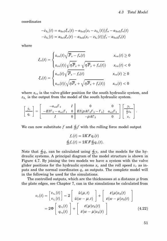
4.3 Total Model
coordinates
−zhn(t) � ahn1ξ n(t) − ahn2(zt − zhn(t)) fn− ahn3 fn(t)−zhs(t) � ahs1ξ s(t) − ahs2(zt− zhs(t)) fs− ahs3 fs(t)
where
ξ n(t) �
xvn(t)
√Ps − fn(t) xvn(t) ≥ 0
xvn(t)(√
η Ps +√
η Ps + fn(t)) xvn(t) < 0
ξ s(t) �
xvs(t)
√Ps − fs(t) xvs(t) ≥ 0
xvs(t)(√
η Ps +√
η Ps + fs(t)) xvs(t) < 0
where xvs is the valve glider position for the south hydraulic system, andzhs is the output from the model of the south hydraulic system.
[yc
qc
]�
−am2Γ1 I 0 0
−EIΓ2 − am1Γ1 0 EI(ρ AΓ2 Γ3 − Γ4) am3Γ5
I 0 −ρ AΓ3 0
yc
12 zh
vr
.
We can now substitute f and ddt f with the rolling force model output
fc(t) � 2K Fqc(t)ddt fc(t) � 2K F d
dtqc(t).
Note that ddt qc can be calculated using d
dt yc and the models for the hy-draulic systems. A principal diagram of the model structure is shown inFigure 4.7. By joining the two models we have a system with the valveglider positions for the hydraulic systems xv and the roll speed vr as in-puts and the normal coordinates qc as outputs. The complete model willin the following be used for the simulations.
The controlled outputs, which are the thicknesses at a distance µ fromthe plate edges, see Chapter 7, can in the simulations be calculated from
vc(t) �[
vcn(t)vcs(t)
]� 2
[u(µ, t)
u(w− µ, t)
]+[
ε(µ)zh(t)ε(w− µ)zh(t)
]
� 2Φ
[qc1(t)qc2(t)
]+[
ε(µ)zh(t)ε(w− µ)zh(t)
](4.22)
51

Chapter 4. Modeling of the Rolling Mill
South syst.
North syst.
Mill Force calc.
xvn(t)
xvs(t)
zhn(t)
zhs(t)
qc(t)
ddt yc(t)
ddtzhn(t)
-
-
66
??
?
6
-
-
ddt fcn(t)fcn(t)
ddtzhs(t)ddt fcs(t)
fcs(t)
-
-vr(t)
-
-
Figure 4.7 The total model for the rolling mill made by combining the models forthe hydraulic systems and the model for the rolling stand. The rolling forces andtheir derivatives are calculated using two of the boundary conditions for the PDE.
where
Φ �[ φ 1(µ) φ 2(µ)
φ 1(w− µ) φ 2(w− µ)]
.
In this way the plate thicknesses at the edges vc can be found using thenormal coordinates qc and the output from the model for the hydraulicsystems zh.
The observer
ye(t) �[
Γ6
am2Γ1Γ6
]fc(t) +
[ ρ AΓ3
am2Γ3
]12 zh(t)
will be used for estimating the states yc of the model for the rolling standwhen implementing the controller in the simulations. Here the additionalforce measurements are available for a better estimate of the plate thick-ness. The estimate for the normal coordinates qc can be calculated from
qe(t) � [ I 0 ] ye(t) −ρ AΓ312 zh(t).
Again the thickness at the north and south edge ven and ves can be calcu-lated using qe and (4.22).
52

4.4 Conclusions
4.4 Conclusions
We have now derived models for the hydraulic systems and the rollingstand. The model for the hydraulic systems is nonlinear with the rollingforce and servo valve glider position as inputs and the roll position asoutput. The model for the rolling stand is linear and multivariable withroll positions and rolling speed as inputs and normal coordinates for theeigenfunctions of the rolling stand as outputs. A static observer with rollpositions and the rolling forces as inputs and the states of the model forthe rolling stand as outputs is also found.
Using the boundary conditions for the rolling stand, the rolling forcescan be calculated. This makes it possible to combine the model for thehydraulic systems and the model for the rolling stand into a total modelfor the whole rolling mill. The total model will be used for computer sim-ulations.
The load of the hydraulic systems is included in the model for therolling stand. Since we in this model have a linear model for the dampingfriction between the roll pack and the mill frame is indirectly modeled asviscous friction. That this and the other assumptions in the modeling arereasonable will be investigated in the system identification.
To find the unknown parameters of the models for the hydraulic sys-tems and the rolling stand it is necessary to perform a system identifica-tion. The collection and preparation of the data for the system identifica-tion is described in Chapter 5.
53

5
Thickness Control—DataCollection
This chapter describes the data collection and the preprocessing of thedata necessary before the system identification can be performed. Thedata have been collected during normal production without any extraexcitation.
It will later be seen that the excitation is not ideal—this could beimproved by injecting an external input signal. Two things can be saidagainst this. First of all, the bandwidths of the hydraulic systems aresmall in comparison to the interesting modes of the rolling stand, andsecondly the rolling process is quite sensitive and there is a risk of de-stroying expensive equipment. Because of this it has been chosen to collectthe data during normal operation. This also has the advantage that theyare collected under realistic conditions.
Ten plates were measured. The data shown in this chapter will all befrom the same plate, which has a nominal thickness of 10 mm, a width of2.15 m and a length of 10.5 m. The data from this plate will also be usedfor all the examples in the rest of this report. The measurements are quiteunique since much effort has been made to get all the important signalsfor the rolling mill in one synchronized time series.
5.1 Measurement Equipment
From Chapter 4 we know that the relevant input and output signals forthe models are:
• The positions of the servo valve gliders xvn and xvs.
• The positions of the common pistons zn and zs.
• The rolling forces fn and fs.
54

5.1 Measurement Equipment
Name Variable
North valve glider position xvn
North hydraulic position zn
North rolling force fn
Roll speed vr
South valve glider position xvs
South hydraulic position zs
South rolling force fs
Table 5.1 The variables of the models which are possible to measure as electricalsignals. See also Figure 4.1.
• The rotational speed of the upper work roll vr.
• The plate thickness at the north edge, the center and the south edgevd(x1, t), vd(x2, t), and vd(x3, t).
The plate thickness is measured at the edges and the center since thesethree measurements give us the possibility to determine the plate crown.All variables in Table 5.1 exist as electrically measurable signals in therolling mill control systems, while the thickness has to be measured afterthe rolling when the plate is cold.
Electrically Measurable Signals
The signals measured electrically are shown in Table 5.1. The measure-ments are done during the last pass. The last pass is the one that theeffects the plate thickness. An example of the signals is shown in Fig-ure 5.1. Since the measurement of the valve glider positions is quite noisywe measure the reference signal for the valve glider position instead. Thethickness control is in absolute mode which yields the best excitation sincethis gives that largest variations in force and position. Note the low fre-quency excitation of zn and zs, furthermore, note that it is only possibleto collect data for approximately 4 s for the plate before the pass ends.
It is not possible to measure the thickness of the plate during rolling,see Chapter 2. Furthermore, the accuracy of the existing thickness mea-surement device, which is placed after the rolling mill, is not sufficient.It is therefore necessary to measure the plates after the rolling when theplate is cold. Using the data for material density for steel ρ presented inChapter 10 the thermal expansion from 20 ○ C to 1000 ○ C is computed to1.4% this is considered neglectable and is therefore not considered in thefollowing.
55

Chapter 5. Thickness Control—Data Collection
0 1 2 3 4−1
0
1
2
3
4x_vrn and x_vrs
s
V
0 1 2 3 44
4.2
4.4
4.6
4.8
5z_n and z_s
s
mm
0 1 2 3 4−2000
0
2000
4000
6000f_n and f_s
s
kN
0 1 2 3 42.5
3
3.5
4
4.5v_r
s
m/s
Figure 5.1 An example of the variables that are collected during one pass. Upperleft: the references for the north servo valve xvrn (full) and south servo valve xvrs(dashed). Upper right: north position zn (full) and south position zs (dashed). Lowerleft: north rolling force fn (full) and south rolling force fs (dashed). Lower right:peripheral speed of the upper work roll vr .
It was first tried to measure the plate thickness manually with a dis-tance of 10 cm using a micrometer screw gauge. These measurementsshowed large variations and it was believed that this was due to poorprecision of the screw gauge. A measurement device with an electronicscrew gauge with serial communication interface was then constructed,a pulse encoder for length measurement was also mounted. A constantorientation to the plate when performing the measurements in a morecontinuous way yielded a higher accuracy. The thickness measurementswere collected using a digital controller with the feature that the samplingfrequency could be controlled using the pulse encoder, see [Bengtsson,1994].
A fundamental problem when using the data is that the electricallymeasurable signals are obtained using time sampling and the thicknessmeasurements are obtained using spatial sampling. This problem is solvedby using the gaugemeter equation (3.2) for calculating a thickness esti-mate from the time sampled signals and then finding the times of the
56

5.2 Measurements for Identification
0 0.5 1 1.5 2 2.5 3 3.5−0.2
−0.15
−0.1
−0.05
0
0.05
0.1
0.15
0.2
0.25
0.3
s
mm
Figure 5.2 Measured thickness v (full) and estimated thickness ve (dashed) thick-ness, when they are not low-pass filtered. The spatial resolution of the thicknessmeasurements is 5 mm.
thickness measurements by minimizing the distance to the estimatedthickness, for more details please refer to [Pedersen, 1995b]. The result-ing thickness measurement and the thickness estimate are shown in Fig-ure 5.2. Notice the nice fit. This illustrates that the gaugemeter principlegives a good estimate of the mean value of the plate thickness at the twoedges.
5.2 Measurements for Identification
To obtain representative results for the identification it is chosen to mea-sure 10 plates with 5 different nominal thicknesses and 2 different widths,the dimensions are shown in Table 5.2.
The widths of 2 and 3 m are chosen since they are close to the min-imum and maximum of the plates rolled. The chosen thickness intervalis representative for the plate production since the thickness of 95 % ofthe produced plates are in this interval. The data were collected duringnormal production and additional information about plate temperature,roll position and calculated thickness was thus available from the reportsfrom the control system planning the rolling, see Chapter 2.
57

Chapter 5. Thickness Control—Data Collection
Thickness [mm] Small width [m] Large width [m]
6 2 3
10 2 3
20 2 3
30 2 3
40 2 3
Table 5.2 Nominal dimensions of the measured plates. The data from these tenplates will the basis for the system identification.
5.3 Conclusions
The inputs and outputs for the model for the rolling mill have now beencollected. The data consist of the key variables for the last pass for 10plates covering relevant thickness and width intervals.
Since the thickness measurements are found using spatial samplingand the other variables are found using time sampling it is necessary toalign the data in some way. This is done estimating the time scale of thethickness measurements using the gaugemeter equation.
We now have the model and the input and output data represented asa time series. We are thus ready for the system identification which willbe carried out Chapter 6.
58

6
Thickness Control—SystemIdentification
In this chapter the parameters of the models for the hydraulic systems,the model for the rolling stand, and the observer for the rolling standwill be identified. The purposes of the models are controller design andsimulation. Simplicity will be preferred to advanced structure. It will,in general, be possible to improve the results by adding more degreesof freedom, but this will imply lack of physical understanding and willtherefore be avoided.
Due to the lack of excitation, nonparametric methods will not be used.Instead we will use restrictive parameterizations. This implies that allconstants known in advance will be inserted in the models before thesystem identification is performed. The main advantage of this is thatone is quite sure that the model is correct if only a couple of parametersof a physically derived structure are identified.
Much effort and time has been put into finding appropriate parame-trizations and the problem of identifying the mill dynamics have beenreduced to finding two parameters. Furthermore, the parameter varia-tions are correlated with key variables. In this way we find parametricmodel variations which will be useful in the controller design.
The author has found no work on identification of rolling mills and thesystem identification is therefore described in detail. The model for thehydraulic systems is transformed to discrete time and a parameterizationof the model is chosen. After this, the identification method is chosen,and the results of the identification are presented. The procedure for theidentification of the rolling stand is similar, with the exception that wehere have to find the parameters of both the model and the observer.
59

Chapter 6. Thickness Control—System Identification
6.1 Hydraulic Systems
The model for the hydraulic systems was derived in Chapter 4. Here itwill be rewritten to a form appropriate for the system identification. Thisimplies a transformation to a suitable discrete time form. Since the modelis nonlinear we will be working with nonlinear system identification. Onlyresults for the model for the north hydraulic system will be shown here,since the model for the south system is similar.
Rewriting Equations
To be able to perform the system identification it is necessary to transformthe differential equation to discrete time form. Exploiting an idea given in[Johansson, 1993]we simply integrate the nonlinear differential equationsfor the north hydraulic system, see (4.7)
−zhn(t) � ahn1ξ n(t) − ahn2(zt − zhn(t)) fn− ahn3 fn(t), (6.1)
where
ξ n(t) �
xvn(t)
√Ps − fn(t) xvn(t) ≥ 0
xvn(t)(√
η Ps +√
η Ps + fn(t)) xvn(t) < 0.
If we furthermore divide by zt − zhn (which is always nonzero) beforeintegrating we save a numerical differentiation because the integrand(zt− zhn) d
dt fn then can be evaluated analytically. The result is
yn(t1, t2) � ahn1ξ n1(t1, t2) + ahn2ξ n2(t1, t2) + ahn3ξ n3(t1, t2), (6.2)
where
yn(t1, t2) � lnzt − zhn(t2)zt − zhn(t1)
ξ n1(t1, t2) �
∫ t2
t1
√Ps − fn(t)
zt − zhn(t)dt xvn(t) ≥ 0
∫ t2
t1
(√
η Ps + fn(t) +√
η Ps)zt − zhn(t)
dt xvn(t) < 0
ξ n2(t1, t2) � fn(t2) − fn(t1)
ξ n3(t1, t2) �∫ t2
t1
fn(t)zt − zhn(t)
dt.
60

6.1 Hydraulic Systems
Note that the parameters are unaffected by the discretization and thatthe system is still linear in the parameters. The integrals, which are notpossible to evaluate analytically, can be calculated numerically.
Parameterization
Different parameterizations of the hydraulic model have been investigatedand it is found that the parameterization of (6.2) works well. We thushave the three parameters ahn1, ahn2, and ahn3 to estimate. An analysisof the identifiability of the model for the hydraulic systems is found in[Pedersen, 1995b].
Identification
The performance index used in the identification is
Vn �N∑
k�1
θ 2n(k),
where θ n(k) is the prediction error of the model. The model for the northsystem is
yhn(k) � ahn1ξ1(k) + ahn2ξ2(k) + ahn3ξ3(k), (6.3)
where
ξ1(k) �
∫ k
k−h
√Ps − fn(t)
zt − zn(t) dt xvn(t) ≥ 0
∫ k
k−h
(√
η Ps + fn(t) +√
η Ps)zt − zn(t) dt xvn(t) < 0
ξ2(k) � fn(k) − fn(k− h)
ξ3(k) �∫ k
k−h
fn(t)zt − zn(t)dt.
The model for the south system is analogous and is therefore not shown.For the identification it has been found that a sampling interval of h �0.025 s is a good choice. Using this value of h some of the noise is averagedout while the dynamics of the system is still captured. η � 0.15 is foundto give the best results.
To prevent extensive nonlinear noise transformations and to weightthe data in an appropriate frequency interval the data is filtered usinga fourth order Butterworth filter with a cut-off frequency of 100 Hz. The
61

Chapter 6. Thickness Control—System Identification
relatively high cut off frequency is necessary due to the high frequencynature of ξ2. The filtering is done using the MATLAB-function idfilt. As-suming that the noise can be described as additive filtered white noiseimplies that the model used for the identification is
yhn(k) � ahn1ξ1(k) + ahn2ξ2(k) + ahn3ξ3(k) + C(q−1)e(k),
where
C(q−1) � 1+ c1q−1+ ⋅ ⋅ ⋅+ cnq−n
and e is a white noise sequence and q is the forward shift operator. Notethat the model has the same structure as an ARMAX-model with A(q−1) �1.
Since we have a non-standard problem we formulate the system identi-fication as an optimization problem. Recalling that the model has ARMAXstructure we simply compute the prediction error as
θ n(k) � 1C(q−1) (yn(k) − (ahn1ξ1(k)+ ahn2ξ2(k)+ ahn3ξ3(k))) ,
where
yn(k) � lnzt − zn(k)
zt − zn(k− 1) .
This implies that we use the Maximum Likelihood method, see [Åströmand Eykhoff, 1971]. It is found that a third order noise polynomial isappropriate in the system identification. The minimum of the performancefunction is found using the nonlinear least squares function leastsq inMATLAB. The integrals in the regressors are computed using the MATLAB-function trapz.
Results
The identification is performed on the discrete time model (6.3) using theten data sets described in Chapter 5. Since the signal for the position ofthe valve glider is very noisy the reference has been used instead. Usingspectral analysis it has been found that the dynamics of the servo valveis neglectable compared with the dynamics of the process. The change ofvariables is therefore not expected to affect the system identification.
A plot of a typical result is shown in Figure 6.1. The agreement isquite good considering the assumptions made when deriving the model.Furthermore, the prediction error is close to white noise which indicates
62

6.1 Hydraulic Systems
0 1 2 3 4−4
−2
0
2
4x 10
−3
s
y_h and y_{h_n}
0 1 2 3 4−4
−2
0
2
4x 10
−3
s
y_s and y_{h_s}
0 1 2 3 4
−5
0
5
x 10−4
s
epsilon_n
0 1 2 3 4
−5
0
5
x 10−4
s
epsilon_s
Figure 6.1 Results of the system identification of the hydraulic systems. Left sidetop: fit of the measured output yn (full) and the predicted output yhn (dashed) andbottom: the prediction error θ n. Right side top: fit of the measured output ys (full)and and predicted output yhs (dashed) and bottom: the prediction error θ s.
that we have an unbiased estimate of the parameters. Note that the be-ginning and end of the passes are included in the data—the peak in theprediction error for the north system arises when the plate enters themill.
An example of a simulation using the original differential equationand the measured system response is shown in Figure 6.2. The imple-mentation of the time derivatives when calculating d
dt f is done using thebackward difference approximation. The simulations are performed usingthe MATLAB-function ode45 with the reference for the valve glider posi-tions xvr and the rolling forces f as input signals. The parameters used inthe model are the ones identified from the data set shown. It is seen thatthere is good correspondence between the two responses. This shows thatthe assumption that the supply pressure Ps is constant and the assump-tions regarding the pressures at the right and left sides of the commonpiston at the oil side work well in practice.
63

Chapter 6. Thickness Control—System Identification
0 0.5 1 1.5 2 2.5 3 3.5 415
15.2
15.4
15.6
15.8
16
s
mm
z_n and z_{h_n}
0 0.5 1 1.5 2 2.5 3 3.5 415
15.2
15.4
15.6
15.8
16
s
mm
z_s and z_{h_s}
Figure 6.2 Simulation of the positions of the hydraulic systems using the parame-ters obtained from identification in simulation. Upper plot, full: measured responsefor north system zn and dashed: simulated response for north system zhn . Lowerplot, full: measured response for south system zs and dashed: simulated responsefor north system zhs .
North South
ahn1 8.9 ⋅ 10−1± 5 ⋅ 10−2 ahs1 8.1 ⋅ 10−1± 5 ⋅ 10−2
ahn2 −7.6 ⋅ 10−4± 2 ⋅ 10−4 ahs2 −9.2 ⋅ 10−4± 4 ⋅ 10−4
ahn3 −2.6 ⋅ 10−2± 2 ⋅ 10−2 ahs3 −2.7 ⋅ 10−2± 2 ⋅ 10−2
Table 6.1 Table for nominal values of parameters with deviations for the hydraulicsystems. The parameters are found using the 10 available data sets.
Values of ahn1
8.4e−01 9.4e−0112 34 567 8 910
Values of −ahn2
5.7e−04 9.6e−041 23 456 78 910
Values of −ahn3
8.5e−03 4.3e−0212 345 67 8 910
Figure 6.3 The distribution of the parameters for the north hydraulic system. Thenumbers refer to the ten data sets.
64

6.1 Hydraulic Systems
Values of ahs1
7.5e−01 8.6e−01123 45678 910
Values of −ahs2
5.2e−04 1.3e−031 234 56 7 8910
Values of −ahs3
1.0e−02 4.4e−0212 34 5 67 8 910
Figure 6.4 The distribution of the parameters for the south hydraulic system. Thenumbers refer to the ten data sets.
The parameters obtained from the identification of all the data setsare shown in Table 6.1. The distribution of the parameters for the twosystems are shown in Figures 6.3 and 6.4. For the design in Chapter 7we want to define a set of nominal parameters. The nominal parametersare chosen to be the center of the interval of the parameter estimates.
When identifying the above parameters the regressors were scaledto be of the same magnitude as the output—this was done to preventnumerical problems. Generally, all the regressors are of the same order ofmagnitude and we thus conclude that it is the parameters ahn1, and ahs1that have major influence. This implies that the model for the hydraulicsystems will be close to an integrator if it is linearized. It is seen thatthese parameters vary less than 10% while the other parameters all varywithin the same order of magnitude.
One could expect that the leak flows vary with the positions zn and zs
due to differences in the wear of the oil cylinders. The variations of theparameters ahn3 and ahs3 are therefore not surprising. The compressibilityof the oil covers many phenomena and it is therefore difficult to say muchabout the variations of the parameters ahn2 and ahs2. The zero point for theservo valve for the southern system varies quite much and it has thereforebeen necessary to compensate for this. Comparing with the north side theaccuracy of the parameter estimates seems to be unaffected by this.
Due to the small variations of the dominating parameters it is ex-pected that parameter variations are of little importance. To confirm thiswe simulate the differential equation using the nominal parameter val-ues. The result is shown in Figure 6.5. It is seen that the mean value ofthe simulated output drifts away, this is because the system is close to anintegrator. This implies that the model will be sensitive to offsets in theinput and since the zero point of the valve glider varies a bit this intro-duces the above effect. We solve the above problem by simply includingan integrator when designing the controller.
65
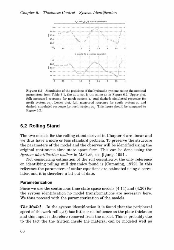
Chapter 6. Thickness Control—System Identification
0 0.5 1 1.5 2 2.5 3 3.5 415
15.2
15.4
15.6
15.8
16
sm
m
z_n and z_{h_n}, nominal parameters
0 0.5 1 1.5 2 2.5 3 3.5 415
15.2
15.4
15.6
15.8
16
s
mm
z_s and z_{h_s}, nominal parameters
Figure 6.5 Simulation of the positions of the hydraulic systems using the nominalparameters from Table 6.1, the data set is the same as in Figure 6.2. Upper plot,full: measured response for north system zn and dashed: simulated response fornorth system zhn . Lower plot, full: measured response for south system zs anddashed: simulated response for north system zhs . This figure should be compared toFigure 6.2.
6.2 Rolling Stand
The two models for the rolling stand derived in Chapter 4 are linear andwe thus have a more or less standard problem. To preserve the structurethe parameters of the model and the observer will be identified using theoriginal continuous time state space form. This can be done using theSystem identification toolbox in MATLAB, see [Ljung, 1991].
Not considering estimation of the roll eccentricity, the only referenceon identifying rolling mill dynamics found is [Cumming, 1972]. In thisreference the parameters of scalar equations are estimated using a corre-lator, and it is therefore a bit out of date.
Parameterization
Since we use the continuous time state space models (4.14) and (4.20) forthe system identification no model transformations are necessary here.We thus proceed with the parameterization of the models.
The Model In the system identification it is found that the peripheralspeed of the work roll vr(t) has little or no influence on the plate thicknessand this input is therefore removed from the model. This is probably dueto the fact the the friction inside the material can be modeled well as
66

6.2 Rolling Stand
static friction, which is independent of the magnitude of the deformationspeed. We thus have the model structure[
yc(t)qc(t)
]�[
Ac Bc
Cc Dc
] [yc(t)12 z(t)
]
�
−am2Γ1 I 0
−EIΓ2 − am1Γ1 0 EI(ρ AΓ2Γ3 − Γ4)I 0 −ρ AΓ3
[ yc(t)12 z(t)
],
(6.4)
where am1, am2 are unknown scalar parameters. The state space equationsare of fourth order. For an analysis of the identifiability of the model forthe rolling mill see [Pedersen, 1995b].
The Observer Since changes in roll position 12 z has a direct impact
on the plate thickness, it is only necessary to scale the coefficients of therolling force f and we thus introduce the matrix O f e. The model structurethen is
qe(t) � O f eΓ6 f (t), (6.5)
where
O f e �[
of e1 0
0 of e2
].
The two unknown parameters in the observer are of e1 , and of e2 .
Identification
Since we have a multivariable problem we use the performance function
V � det
(N∑
k�1
θ (k)θ (k)T)
,
where θ is the prediction error. This implies that we are using multivari-able maximum likelihood identification, see [Åström and Eykhoff, 1971].To keep the models simple we choose not to introduce noise models andwe therefore work with the state space structure
yc(t) � Ac yc(t) + Bc12 z(t) + e(t)
q(t) � Cc yc(t) + Dc12 z(t) + e(t),
67

Chapter 6. Thickness Control—System Identification
where e is white noise and q are the normal coordinates used in the se-ries expansion of the solution. The normal coordinates can be determinedusing the thickness measurements at the three different positions acrossthe plate width and the equation
12vd(x, t) � ε(x) 1
2 z(t) +2∑
i�1
φ i(x)qi(t), (6.6)
which is found by combining (4.10) and (4.13). Inserting the thicknessesof the three measurement tracks at the north edge, center, and south edgewith positions x1, x2, and x3 yields
12 vd(x1, t)12 vd(x2, t)12 vd(x3, t)
� ε(x1)
ε(x2)ε(x3)
12 z(t) +
φ 1(x1) φ 2(x1)φ 1(x2) φ 2(x2)φ 1(x3) φ 2(x3)
[ q1(t)q2(t)
]. (6.7)
The above equation system is over-determined and is therefore solved ina least squares sense in MATLAB.
To obtain a well conditioned problem, all the signals are scaled to haveamplitudes of the same order of magnitude. In the identification a fourthorder Butterworth filter with a cut-off frequency of 10 Hz is used forfiltering the position 1
2 z, the rolling force f , and the normal coordinatesq. To obtain agreement between the mean thickness calculated by themodel and the measurements, the mean value of the thickness at theplate edges is set to the value calculated using the gaugemeter equation,see Chapter 3. The procedure for the observer is similar to the above andis therefore not repeated here.
Results
The identification has been performed directly on the state space structureusing pem in MATLAB. Since the sampling interval is small we can assumethat the input signals are constant between the sampling instants whentransforming the model to discrete time. Using the values found in [Ped-ersen, 1995b] for the mill spring coefficient 2K , the stiffness of the rollpack EI, the mass of the roll pack ρ A, and the value for the plate width w,we calculate the eigenvalues β 1 and β 2, and the two first eigenfunctionsφ 1 and φ 2. The eigenfunctions are therefore computed in advance and arenot estimated in the system identification, where they enter through theΓ i-matrices.
Results for the Model The identification is based on the model withthe parameterization shown in (6.4), the position of the hydraulic system
68

6.2 Rolling Stand
0 1 2 3 4−1
−0.9
−0.8
−0.7
−0.6q_1 and q_{c_1}
s0 1 2 3 4
−0.01
−0.005
0
0.005
0.01q_2 and q_{c_2}
s
0 1 2 3 4−0.1
−0.05
0
0.05
0.1q_1−q_{c_1}
s0 1 2 3 4
−5
0
5
10x 10
−3 q_2−q_{c_2}
s
Figure 6.6 Identification results for the model. Left side, top: measured valueof the normal coordinate q1 (full) and estimated value of the normal coordinateqc1 (dashed), bottom: prediction error for qc1 . Right side, top: measured value ofthe normal coordinate q2 (full) and estimated value for the normal coordinate qc2(dashed), bottom: prediction error for qc2 . The results are not very good due to atime varying parameter am1.
12 z and the normal coordinates q found using (6.7). We obtain the resultsshown in Figure 6.6. The results are representative for all 10 data sets.
As seen from the figure, the agreement is not very good, this is be-cause the parameter am1 is time varying. The mean values of the normalcoordinates are, however, estimated quite well. The variations of am1 areinvestigated in more detail in [Pedersen, 1995b]. Note that the differencebetween the thickness at the two sides is predicted quite well consideringthe time varying parameter. This indicates that the plane strain assump-tion works well in our case.
Trial and error tests show that the precise value of the damping am2
is not critical for the result of the identification. This is probably becauseof the low frequency excitation of the roll positions z. We thus fix it at thevalue am2 � 200, which is the mean value found in the identification. Theparameter am1 is considered to be the most important parameter since it,
69

Chapter 6. Thickness Control—System Identification
am1 1.55 ⋅ 104 −1.62 ⋅ 105
am2 2.00 ⋅ 103
Table 6.2 Parameters for the model found using all 10 data sets.
together with β 1, determines both the undamped natural frequency andthe stationary gain of the system. When identifying the parameter for the10 data sets, we find that am1 varies one order of magnitude. Trying tocorrelate it with key parameters for the rolling process we find that am1
varies systematically with the plate hardness kp, for more details pleaserefer to [Pedersen, 1995b].
Performing the identification on all 10 data sets we find the parametersshown in Table 6.2. Due to variations of am1, which are well correlatedwith kp, we introduce no nominal data set for the model but use the valuesspecified by Table 6.2 instead.
A relevant question in connection with the variation of the parameteram1 is: How does this influence the dynamics of the rolling stand? To in-vestigate this we have seen that the dynamics of the model for the rollingstand can be divided into two SISO transfer functions. When transformingfrom normal coordinates qc to plate thickness vc the direct term almostdisappears. Neglecting this gives the relationships
vc(t) � Gvc (p)z(t)
� φ 1(µ)ρ Aγ 31 EIβ 41
ρ Ap2 + am2p+ EIβ 41 + am1
z(t)
vc(t) � Gvc (p)z(t)
� φ 2(µ)ρ Aγ 32 EIβ 42
ρ Ap2 + am2p+ EIβ 42 + am1
z(t)
where vc, vc is half the difference between the north and south platethickness vcn and vcs , z is the mean value of the north and south rollpositions zn and zs, and z is half the difference between zn and zs. Wesee that Gvc and Gvc have no zeros and it therefore only is necessary toinvestigate the locations of the poles of the transfer functions. Insertingthe values of am1 and am2 found in the system identification yields thepole locations shown in Figures 6.7 and 6.8.
We see that the poles tend to become faster and less damped whenthe plate hardness am1 increases. Unfortunately the steady state gainof Gvc and Gvc also decreases with increasing plate hardness am1 and itcan therefore not be concluded that is becomes easier to control the plate
70

6.2 Rolling Stand
−2000 −1500 −1000 −500 0 500 1000 1500 2000−2000
−1500
−1000
−500
0
500
1000
1500
2000
Real Axis
Imag
Axi
s
Figure 6.7 The pole locations for Gvc as a function of am1. The crosses correspondsto am1 � 0 and the poles with the largest imaginary part corresponds to the maximalvalue of am1. It is seen that the poles are real when am1 is small and becomes fasterand less damped when the value of am1 increases.
−2000 −1500 −1000 −500 0 500 1000 1500 2000−2000
−1500
−1000
−500
0
500
1000
1500
2000
Real Axis
Imag
Axi
s
Figure 6.8 The pole locations for Gvc as a function of am1. The crosses correspondsto am1 � 0 and the poles with the largest imaginary part corresponds to the maximalvalue of am1. It is seen that the poles becomes faster and less damped when thevalue of am1 increases.
thickness for the hard plates. For results of the system identification of atime varying model please refer to [Pedersen, 1995b].
Results for the Observer Using the observer given by (6.5), the rollingforce f , and q found from (6.7) we perform the system identification for
71

Chapter 6. Thickness Control—System Identification
0 1 2 3 4−1
−0.9
−0.8
−0.7
−0.6
s
q_1 and q_{e_1}
0 1 2 3 4−0.01
−0.005
0
0.005
0.01
s
q_2 and q_{e_2}
0 1 2 3 4−0.04
−0.02
0
0.02
0.04
s
q_1−q_{e_1}
0 1 2 3 4−0.01
−0.005
0
0.005
0.01
s
q_2−q_{e_2}
Figure 6.9 Identification results for the observer. Left side, top: measured valuefor the normal coordinate q1 (full) and estimated value for the normal coordinateqe1 (dashed), bottom: prediction error for qe1 . Right side, top: measured value forthe normal coordinate q2 (full) and estimated value for the normal coordinate qe2(dashed), bottom: prediction error for qe2 .
Values of o_fe1
0.9541 1.07412 34 567 89 10
Figure 6.10 Distribution of the parameter ofe1for the observer. The nominal value
of the parameter is 1.
the observer. A typical result is shown in Figure 6.9. Note that we noware able to predict the normal coordinates q quite well since we haveknowledge of the variations of the plate hardness am1 through the rollingforce measurement. The results shown are representative for all 10 datasets.
The values of the parameter of e1 are shown in Figure 6.10. It is seenhere that of e1 � 1, as expected. Ideally the parameters of e2 should alsohave the value 1, but from the system identification we find that of e2 � 0.2
72

6.2 Rolling Stand
for the plate width w � 2.15 and of e2 � 0.4 for w � 3.15. The reason thatwe only have data for two values of the plate width w is that the ten datasets are from plates with only two different widths. The reason for theplate widths being larger than specified in Chapter 5 is that the platesare rolled a bit wider than specified and then cut to the nominal measuresafter rolling.
Inspecting the force measurements we find that the boundary condi-tions
fn(t) � 2K u(0, t) � 2K (q1(t)φ 1(0) + q2(t)φ 2(0))fs(t) � 2K u(w, t) � 2K (q1(t)φ 1(w) + q2(t)φ 2(w))
:f (t) � 2Kφ 1(0)q1(t) (6.8)f (t) � 2Kφ 2(0)q2(t), (6.9)
where f is the mean value of the rolling forces and, f (t) is the differencebetween the forces, are not fulfilled. The plots of the left and right sidesof (6.8) and (6.9) are shown in Figure 6.11. Here we see that the left andright side of (6.8) agrees quite well but that there is a significant deviationbetween the left and right side of (6.9). The amplitude of the difference ofthe rolling forces f is too large—this explains why of e2 becomes smallerthan 1.
One explanation to the above could be that the connection betweenthe two legs of the rolling stand is not included in the physical model. Itis quite possible that the above difficulty could be avoided by inserting aspring between the two sides of the physical model. Another possibility isthat the force measurement is inaccurate. If this is found to be the case,an improvement of the force measurements is necessary to obtain a betteragreement between model and data.
Using the results from the identification we arrive at the values forthe nominal parameters shown in Table 6.3. Since the identification isbased on a fixed value of the parameter of e2 and the variation of of e1 issmall, no simulations of the nominal model is shown, since they will besimilar to the results of Figure 6.9.
Using (6.6) the thickness predicted by the observer at the measure-ment points can be calculated. The results are shown in Figure 6.12. Wenote that now the predicted and measured thicknesses agree quite welldue to the rolling force measurement. Also for the observer the calculatedplate crown is close to its measured value.
73
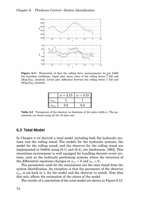
Chapter 6. Thickness Control—System Identification
0 0.5 1 1.5 2 2.5 3 3.53500
4000
4500
5000
5500
6000
skN
0 0.5 1 1.5 2 2.5 3 3.5−300
−200
−100
0
100
200
s
kN
Figure 6.11 Illustration of that the rolling force measurements do not fulfillthe boundary conditions. Upper plot: mean value of the rolling forces f full and2Kφ 1(0)q1 (dashed). Lower plot: difference between the rolling forces f full and2Kφ 2(0)q2 (dashed).
w � 2.15 w � 3.15
of e1 1 1
of e2 0.2 0.4
Table 6.3 Parameters of the observer as functions of the plate width w. The pa-rameters are found using all the 10 data sets
6.3 Total Model
In Chapter 4 we derived a total model including both the hydraulic sys-tems and the rolling stand. The models for the hydraulic systems, themodel for the rolling stand, and the observer for the rolling stand areimplemented in OMSIM using (6.1) and (6.4), see [Andersson, 1994]. Thissimulation environment is well equipped for handling discrete event sys-tems, such as the hydraulic positioning systems where the structure ofthe differential equations changes at xvn � 0 and xvs � 0.
The parameters used for the simulations are the ones found from thesystem identification. An exception is that the parameter of the observerof e2 is set back to 1, for the model and the observer to match. Note thatthis only affects the estimation of the states of the model.
The results of a simulation of the total model are shown in Figure 6.13.
74

6.3 Total Model
0 0.5 1 1.5 2 2.5 3 3.59.6
9.8
10
10.2
s
mm
v_n and v_{e_n}
0 0.5 1 1.5 2 2.5 3 3.59.6
9.8
10
10.2
s
mm
v_m and v_{e_m}
0 0.5 1 1.5 2 2.5 3 3.59.6
9.8
10
10.2
s
mm
v_s and v_{e_s}
Figure 6.12 The thickness at the plate edges and center calculated using theobserver. Upper plot: the measured value vd(x1) (full) and the calculated value ven
(dashed) of the thickness at the northern edge. Center plot: the measured valuevd(x2) (full) and the calculated value vem (dashed) of the thickness at the center.Lower plot: the measured value vd(x3) (full) and the calculated value ves (dashed)of the thickness at the southern edge vs.
The input signals are chosen as
xvrn(t) �{
10 0 ≤ t < 0.1
0 t > 0.1
xvrs(t) �{
10 0 ≤ t < 0.2
0 t > 0.2.
where xvrn is the reference signal for the north servo valve and xvrs isthe reference signal for the south servo valve. At t � 0 the outgoingthickness is equal to the ingoing thickness of the plate, which is 11.64mm and the rolling force is zero. Then the hydraulic positioning systemsmoves downwards, the rolling force increases and the outgoing thicknessdecreases. At t � 0.1 the north system stops, but it is seen that therolling force and the thickness at the north side continue to change due
75

Chapter 6. Thickness Control—System Identification
0 0.1 0.2 0.3−5
−4
−3
−2
−1
0
s
mm
z_h
0 0.1 0.20
2
4
6
8
10
s
V
x_vr
0 0.1 0.2 0.30
2000
4000
6000
s
kN
f_c
0 0.1 0.2 0.3
1
1.1
1.2
s
mm
v_c
Figure 6.13 Simulations of total model for rolling mill. Upper left: control signalfor valve glider positions for north xvrn (full) and south xvrs (dashed) hydraulic sys-tem. Upper right: Positions of north hydraulic system zhn (full) and south hydraulicsystem zhs (dashed). Lower left: north rolling force fcn (full) and south rolling forcefcs (dashed). Lower right, plate thickness north edge vcn (full) and plate thicknesssouth edge vcs (dashed).
to the movement of the position of the south system. This illustrates themultivariable structure of the system.
It is seen that the hydraulic systems act as integrators. They movewith a slightly different speed for the same input due to the differentvalues of the parameters ahn1 and ahs1. The states of the model yc andthe states of the observer ye are shown in Figure 6.14. The simulationhere is the same as the one shown in Figure 6.13. It is seen that thestates of the model and the states of the observer agrees well.
6.4 Conclusions
In this chapter we have found the parameters of the model for the rollingmill. For the hydraulic systems we have found a set of nominal parametersand for the model for the rolling stand we have found one constant and onetime varying parameter. For the observer we have found two parameters,one constant and one which varies with the plate width. The agreement
76

6.4 Conclusions
0 0.1 0.2 0.30
0.2
0.4
0.6
s
y_c(1) and y_e(1)
0 0.1 0.2 0.3−0.03
−0.02
−0.01
0
0.01
s
y_c(2) and y_e(2)
0 0.1 0.2 0.30
200
400
600
s
y_c(3) and y_e(3)
0 0.1 0.2 0.3−30
−20
−10
0
10
s
y_c(4) and y_e(4)
Figure 6.14 Comparison of the four states of the model yc (full) and the stateestimate found by the observer ye (dashed). It is seen that the agreement betweenthe real and estimated value is good.
between model and data are all satisfactory, it was, however, necessary tointroduce extra parameters in the observer since two of the four boundaryconditions used for calculating the plate thickness were not fulfilled.
The models have been implemented in a suitable simulation environ-ment and we are now ready for the controller design. This will be done inChapter 7.
77

7
Thickness Control—Design
The purpose of this chapter is to design a thickness controller for therolling mill, which consists of the hydraulic positioning systems and therolling stand. The purpose of the controller is to ensure that the desiredplate thickness is obtained with as small deviations as possible, despitethe process disturbances.
The performance specifications of the control systems are first given,this includes description of typical disturbances and the multivariablenature of the system. Then the controlled outputs are chosen, the multi-variable structure, the dynamics of the system, and the steady state gainsare analyzed.
The above forms the basis for the choice of methods for controllingthe rolling mill. The controllers are then designed using the models andparameters found in the previous chapters. In general, time invariantmethods will be used for the controller design and we therefore assumethat the material parameters are constant during the pass in the fol-lowing. The effects of the variations of the material parameters will beinvestigated in the simulations.
In the last section of this chapter the performance of the control systemis investigated using computer simulations. Here the effects of referencechanges and typical disturbances are found and commented.
No work on multivariable thickness control of hot rolling mills hasbeen found. Several descriptions of the single-input single-output caseare given in [Kokai et al., 1985], [Saito et al., 1981], [Teoh et al., 1984],[Ferguson et al., 1986] and many more. Furthermore, advanced controland estimation methods have been used in connection with the elimina-tion of the effects of roll eccentricity, see [Yeh et al., 1991], [Teoh et al.,1984], and [Asada et al., 1986]. For further details see Chapter 3.
78

7.1 Performance Specifications
7.1 Performance Specifications
As described in Chapters 2 and 3 the purpose of the thickness control isto obtain a specified constant thickness, despite disturbances such as
• variations of the plate hardness;
• variations of the ingoing thickness.
The thickness control problem is thus a regulator problem, see [Åströmand Wittenmark, 1997]. A central goal of the control is to minimize thethickness variations of the rolled plates. The quality level possible to ob-tain depends on saturation of the control signal and the amplitude of thevariations. It might therefore be necessary to minimize the variations byother means to obtain the desired value of the thickness variations.
The rolling process is a multivariable system, this has to be taken intoconsideration when controlling the process. A natural demand is to beable to control the thickness at the north and south edge independentlyof each other. This will make it possible to handle reference changes andcontrol errors at one edge with minimal effect on the thickness at theother edge. Furthermore, the controller has to be able to compensate forasymmetric material conditions. This is not possible with the existingcontrol, see Chapter 3.
A third important issue is the stability of the thickness control system.The stability is disturbed by two effects:
• variations of the material characteristics;
• the controlled variable (the thickness) has to be estimated.
This has lead to a detuning of the compensation for mill deflection intraditional thickness control systems, see Chapter 3. An analysis of thestability of the thickness control system is given in [Pedersen, 1995b].
In the system identification of the hydraulic systems in Chapter 6 wefound that the models of the hydraulic systems were sensitive to offsets inthe control variable. It was concluded that including an integrator in thecontroller would solve this problem when controlling the roll position. Wetherefore include an integrator in the controller design. It will bee seenlater that using an integrator is also a good idea in connection with thecontrol of the plate thickness.
The handling of the start and the end of the pass will not be discussedin the following. Since the plate ends usually are non rectangular, thephysical model for the rolling stand does not cover this case, since theplate will not have full width when entering the roll gap. The plate endsfurthermore tend to be colder than the rest of the plate. To ensure a properstart up and shut down of the control it is likely that a special controlstrategy is necessary to handle the beginning and end of the passes.
79

Chapter 7. Thickness Control—Design
7.2 Analysis of Model
The first natural question that arises is, at how many points in the widthdirection is it possible to control the thickness of the plate using the twohydraulic actuators. We study this to choose the number of outputs wewant to control. Looking at the state equations of the model we see thatin steady state we have that
yc(t) � 0 � Ac yc(t) + Bc12 z(t)
:yc(t) � −A−1
c Bc12 z(t),
where the system matrix Ac is invertible. The above implies that we areonly able to control the state vector in stationarity within a two dimen-sional plane. We can therefore not control more than two outputs in sta-tionarity with the thickness control. The thickness of a plate are normallymeasured at a distance µ from the plate edges. Our outputs are thus cho-sen as[
vn(t)vs(t)
]�[
vd(µ, t)vd(w− µ, t)
]� 2
[ φ 1(µ) φ 2(µ)φ 1(w− µ) φ 2(w− µ)
] [q1(t)q2(t)
]+[ ε(µ)
ε(w− µ)]
z(t).
Using our physical insight we choose the north position zn for controllingthe north thickness vn and the south position zs for controlling the souththickness vs.
Investigating the multivariable structure of the system we apply a stepof 1 mm at the north position zn. The open-loop step response is shownin Figure 7.1. We see that the thickness at both edges is affected by theposition change at one of the sides. Furthermore, it can be seen from thestep responses that two systems with different dynamics are involved.This is due to the fact that the dynamics for the normal coordinates qc1 andqc2 are different. Note the direct term, which is the result of inaccuraciesin connection with the state transforms used in the modeling. The directterm is small compared to the steady state gain of the system and it willbe neglected in the controller design. It will though be included in thesimulations.
The multivariable effect illustrated in Figure 7.1 causes trouble whencontrolling the thickness at the two sides independently. If the thicknessat the north side deviates from the specified value while the south thick-ness does not, it is not possible to obtain the correct thickness by just
80

7.2 Analysis of Model
0 0.002 0.004 0.006 0.008 0.01 0.0120
0.05
0.1
0.15
0.2
0.25
0.3
s
mm
v_c
Figure 7.1 Simulation using the total model in Section 6.3. Open-loop result ofa step change of 1 mm in the north position zn. The step is applied at t � 0. Full:thickness at north edge vcn and dashed: thickness at south edge vcs . It is seen thatthe position change at one side affects the thickness at both sides of the rollingstand
adjusting the hydraulic position at the north side. It is thus necessaryto consider the multivariable nature of the system when designing thecontroller. Ideally it should be possible to control the thickness at the twosides independently of each other.
Looking at the mean values for position z and thickness v, and neglect-ing the direct term, the relationship is given by the second order linearsystem
v(t) � Gvc(p)z(t) �φ 1(µ)ρ Aγ 31 EIβ 4
1
ρ Ap2 + am2p+ EIβ 41 + am1
z(t).
The dynamics of this transfer function varies due to the variations of am1.A similar transfer function Gvc can be derived for the wedge of the positionz and the wedge of the thickness v � 1
2 (vn−vs). Using the values obtainedfrom the system identification the undamped natural frequencies of thetwo transfer functions ω n and ω n are in the intervals
ω n ∈ [200, 432] rad/sω n ∈ [342, 658] rad/s.
81
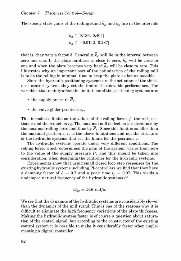
Chapter 7. Thickness Control—Design
The steady state gains of the rolling stand kg and kg are in the intervals
kg ∈ [0.136, 0.404]kg ∈ [−0.0142, 0.287],
that is, they vary a factor 3. Generally, kg will lie in the interval betweenzero and one. If the plate hardness is close to zero, kg will be close toone and when the plate becomes very hard kg will be close to zero. Thisillustrates why an important part of the optimization of the rolling millis to do the rolling in minimal time to keep the plate as hot as possible.
Since the hydraulic positioning systems are the actuators of the thick-ness control system, they set the limits of achievable performance. Thevariables that mainly affect the limitations of the positioning systems are:
• the supply pressure Ps;
• the valve glider positions xv.
This introduces limits on the values of the rolling forces f , the roll posi-tions z and the reduction rd. The maximal mill deflection is determined bythe maximal rolling force and thus by Ps. Since this limit is smaller thanthe maximal position zt it is the above limitations and not the structureof the hydraulic systems that set the limits for the positions z.
The hydraulic systems operate under very different conditions. Therolling force, which determines the gain of the system, varies from zeroto the value of the supply pressure Ps and this should be taken intoconsideration, when designing the controller for the hydraulic systems.
Experiments show that using small closed loop step responses for theexisting hydraulic systems including PI-controllers we find that they havea damping factor of ζ � 0.7 and a peak time tp � 0.07. This yields aundamped natural frequency of the hydraulic systems of
ω nh � 24.6 rad/s.
We see that the dynamics of the hydraulic systems are considerably slowerthan the dynamics of the mill stand. This is one of the reasons why it isdifficult to eliminate the high frequency variations of the plate thickness.Making the hydraulic system faster is of course a question about satura-tion of the control signal, but according to the constructor of the existingcontrol system it is possible to make it considerably faster when imple-menting a digital controller.
82

7.3 Choice of Control Methods
7.3 Choice of Control Methods
The controller design will be done in continuous time. This makes it pos-sible to utilize the structure of the physical models we have derived andidentified in the previous chapters. It will be necessary to implement thecontrol strategies using digital equipment and the control strategy there-fore has to be transformed to discrete time. This can be done using theapproximate methods described in [Åström and Wittenmark, 1997]. Theprice to be paid for this procedure is that it is necessary to implement thecontroller using a higher sampling frequency than if the design was donein discrete time.
To make the hydraulic systems work well at all operating points, it isnecessary to use a non-linear control strategy. Since we only have a firstorder system and all states and inputs can be measured or estimated, it ischosen to use feedback linearization for controlling the hydraulic systems,see [Slotine and Li, 1991].
The responses of the two sides of the rolling mill are separated usingeigenspace design described in [Harvey and Stein, 1978]. This makes itpossible to assign specified values to the eigenvectors of the closed loopsystem. The additional eigenvectors and eigenvalues for which we haveno specifications are furthermore placed in a “nice" way.
The variation of the material hardness am1 changes the steady stategain of the system and it is necessary to compensate for this in some way.The plate thickness can, despite the parameter variations, be estimatedusing the observer. Using an integrator it is possible to ensure that theclosed loop steady state gain is not affected by the parameter variations.The variations of the plate hardness am1 will still affect the dynamics andthe stability of the system.
The parameter variations raise the question if adaptive control isneeded. It will therefore in simulations be investigated if the performanceof the chosen design strategy is satisfactory or if a truly adaptive controlleris needed.
7.4 Design of Controllers
In the following sections the controllers for the hydraulic systems and therolling stand will be designed. The hydraulic systems will be controlledusing feedback linearization and the rolling stand will be controlled by astate feedback, found using eigenspace design.
83

Chapter 7. Thickness Control—Design
Hydraulic Systems
Since we have a first order system it is quite easy to derive a controllaw that linearizes the system. Even if some of the usual assumptionson the input function such as independence of the control variable xvn
and smoothness are not fulfilled it is still possible to do the feedbacklinearization. As usual we only show the results for the north system sincethe procedure of the south system is the same. To increase the numberof the degrees of freedom in the eigenspace design we give the hydraulicsystems a time constant κ when doing the feedback linearization. κ isthen used as a design parameter in the eigenspace design.
We choose the control signal as
xvrn(t) � 1−ahn1ξ n1(t)
(−ahn2ξ n2(t) − ahn3ξ n3(t) + rln (t) −κ zhn(t)) , (7.1)
where
ξ n1(t) �
√
Ps − fn(t) xvn(t) ≥ 0√η Ps +
√η Ps + fn(t) xvn(t) < 0
ξ n2(t) � (zt − zhn(t))ddt
fcn(t)ξ n3(t) � fn(t).
Here rln is the control signal from the thickness controller. The northposition zn, the position of the valve glider xvn, and the north rollingforce fn can be measured directly and d
dt fcn can be estimated using therelationship
ddt
fcn(t) � 2K Fddt
qc(t),
found in Section 4.3. To determine the derivative of the normal coordi-nates d
dt qc we can use the model for the rolling stand and the differentialequations for the hydraulic systems. This is not trivial since a good es-timate of the plate hardness am1 is necessary to do this. An alternativeis to use approximative numerical differentiation of the rolling force f tofind d
dt f .We note that the control strategy demands that fn < Ps. When the
pressure due to the rolling force fn gets close to the supply pressure Ps
the thickness control will in any case be switched off to prevent overloadof the hydraulic system. It is therefore not necessary to worry about thecase fn � Ps.
84

7.4 Design of Controllers
Using the above strategy the model for the hydraulic system reducesto
zhn(t) � −κ zhn(t) + rln(t)and can thus be inserted as an extra state in the state space equationsfor the rolling stand.
Thickness Controller for the Rolling Stand
We now proceed with the design of the controller for the rolling stand.The main idea is to design a well tuned controller which can handle asym-metric disturbances. The design will be performed on the model for therolling stand combined with the now linear hydraulic systems and twoadditional integrator states. The main idea in the eigenspace principle isthat, in addition to the desired closed loop poles, a set of desired closedloop eigenvectors is also specified—this is possible since we are workingwith a multivariable system, see [Kailath, 1980] and [Moore, 1976].
The response of the closed loop system due to the initial conditions qco
can be written as
vc(t) �n∑
j�1
Ccν j (ψ Tj qco)eλ j t, (7.2)
where the λ j ’s are the closed loop eigenvalues and ν j are the right closedloop eigenvectors defined by
(Iλ j − (Ac − Bc L))ν j � 0 (7.3)
and ψ j are the left closed loop eigenvectors fulfilling ψ Tj ν j � 1, see
[Kailath, 1980] for details.It is possible to affect the eigenvectors by the choice of the feedback
matrix L. It is here assumed that the closed loop eigenvalues are simple,this implies that the closed loop eigenvectors all are linearly independent.Assuming that the closed loop eigenvalues λ j 6� sp(Ac) we can rewrite(7.3) as
ν j � (Iλ j − Ac)−1 Bcµ j (7.4)µ j � −Lν j .
The idea of the eigenspace design is then to choose the feedback matrixL to obtain the desired eigenvectors, if possible.
The desired closed loop eigenvalues for the new thickness controllerare chosen to give the same magnitudes of the control signals as used bythe existing control system. There are two reasons for this:
85

Chapter 7. Thickness Control—Design
• It is hard to say when the hydraulic positioning systems saturatesince this depends on the nature of the disturbances and the char-acteristics of the supply equipment. It is therefore more natural toadjust the response speed of the controller when it is implemented.
• It will be possible to compare the performance of our control systemto the performance of the existing control system.
Using the control law found in the previous section the hydraulic sys-tems can be included as a part of the state space model. Since it is half ofthe position 1
2 z that is used in the model for the rolling stand it is mostconvenient to use half of the position as a state. As seen in the previoussection the steady state gain of the open loop system varies due to thevariations of the plate hardness am1. The simplest way of avoiding thisfor the closed loop system is to calculate the plate thickness
vc(t) � [Φ 0 ] yc(t)
and introduce two integral states i
ddt
i � 12 r(t) − vc(t)
where rT � [ rn rs ] are the references for the plate thickness. The statespace representation including the hydraulic positions and the integralstates is
yc(t)
12 zh(t)i(t)
vc(t)
�[
Ach Bch
Cch Dch
]
yc(t)12 zh(t)i(t)rl(t)12 r(t)
�
−am2Γ1 I 0 0 0 0
−EIΓ2 − am1Γ1 0 EI(ρ AΓ2 Γ3 − Γ4) 0 0 0
0 0 −κ I 0 I 0
−Φ 0 0 0 0 I
Φ 0 0 0 0 0
yc(t)
12 zh(t)i(t)rl (t)12 r(t)
(7.5)
Using the eigenspace design approach first described in [Harvey andStein, 1978] and later generalized in [Stein, 1979]we find that by choosingthe weighting matrices for a LQG controller in a special way it is possibleto obtain a set of specified closed loop eigenvalues and eigenvectors. Theeigenvalues and eigenvectors are obtained asymptotically as the control
86

7.4 Design of Controllers
weight σ tends to zero. The number of design parameters are thus reducedto one when the eigenvalues and eigenvectors are chosen. The result isthe algebraic Riccati equation with σ as design parameter
0 � PAch + ATchP + Q+ PBch1 R−1BT
ch1P/σ (7.6)
can be used for finding the feedback matrix
L � R−1BTch1
P/σ . (7.7)The derivation of the matrices Ach, Bch1 , Bch2 , Q, R is described in [Ped-ersen, 1995b].
Unfortunately, it is difficult to solve the Riccati equation algebraicallyand we therefore have to use numerical tools for finding L. An exampleof the results of the design with closed loop eigenvalues λ f � 125, a timeconstant for the linearized hydraulic systems κ � 50, and a control weightσ � 1⋅10−4 are shown in Figure 7.2. Note that the two sides are practicallydecoupled. Full decoupling requires large gains of the feedback matrix.This is not a good idea considering saturation and stability aspects.
When computing the steady state gain of the closed loop system wefind that
Cch(−Ach+ Bch1 L)−1Bch2 � I.
This indicates that the separation of the two sides has been successfulsince a reference change for one of the sides does not affect the other sidein stationarity.
As stated earlier it is not possible to measure the process output, andwe can therefore not use a traditional observer. Instead we use the staticrelationships found in Section 4.2 and extend it with the position mea-surement 1
2 z and the integral states i
ye(t)12 z(t)i(t)
� Deh
12 z(t)f (t)i(t)
�
ρ AΓ3 Γ6 0
am2Γ3 am2Γ1Γ6 0
I 0 0
0 0 I
12 z(t)f (t)i(t)
. (7.8)
The advantage of this approach is that we capture the variations of am1using the rolling force measurement.
The controller structure is shown in Figure 7.3. Note that the principalstructure is the same as the traditional one described in Chapter 3. Aninvestigation of the robustness shows that the system is stable for theparameter variations found in the system identification, for details pleaserefer to [Pedersen, 1995b].
87

Chapter 7. Thickness Control—Design
0 0.005 0.01 0.015 0.02 0.025 0.03 0.035 0.04 0.045 0.05−2
−1
0
1
2
3
Time (secs)
Am
plitu
de
z
0 0.005 0.01 0.015 0.02 0.025 0.03 0.035 0.04 0.045 0.05−0.5
0
0.5
1
1.5
Time (secs)
Am
plitu
de
v_c
Figure 7.2 Result of eigenspace design, response for step reference change of thethickness at the north edge. Upper plot, full: north position zhn and dashed: southposition zhs . Lower plot, full: thickness at north edge vcn and dashed: thickness atsouth edge vcs . Note that the south thickness is almost unaffected by the change ofthe thickness at the north edge.
Fb. Lin. Mill-
Observer−L
xvr(t) f (t)
z(t)
ye(t), 12 z(t)
Integrator
6
r(t)
-
�
6
i(t)
Thick. calc.�
?
-
-
�
ve(t)qe(t)
66
-
v(t)
? ?
Figure 7.3 The structure of the total controller, including feedback linearization,state feedback and integrator.
88

7.5 Evaluation of Performance
Final Form of Controller
The final form of the controller can be found from the feedback lineariza-tion (7.1) and the state feedback (7.7).
[xvrn(t)xvrs(t)
]� ∆1
∆2 − L
ye(t)12 z(t)i(t)
(7.9)
where
∆1 �[− 1
ahn1ξhn1 (t) 0
0 − 1ahs1ξhs1 (t)
]
∆2 �[−ahn2ξ n2(t) − ahn3ξ n3(t) −κ zn(t)−ahs2ξ s2(t) − ahs3ξ s3(t) −κ zs(t)
]where ξ s1 , . . . ,ξ s3 are defined as ξ n1 , . . . ,ξ n3 with the variables for thenorth side replaced with the variables for the south side. ye, and z are thedeviations from the working points for the two vectors found using theobserver.
The input vector for the controller can be found from (7.8). Note thatthis is a pretty simple second order nonlinear controller which will bestraight-forward to implement. We therefore conclude that despite thetedious design the controller structure is quite simple.
7.5 Evaluation of Performance
Several questions can be asked in connection with the performance of thethickness control. The two usual main concerns are
• response to reference changes;
• effects of typical disturbances.
Both subjects will be investigated in the following. The performance of thenew control system will be compared to the performance of the existingcontrol system, when possible. A central question is whether it is neces-sary to redesign the controller and how often this should be done. Thiswill also be investigated below. Again we simulate the whole system incontinuous time, that is we assume that the control law is implementedusing a high sampling frequency.
The linear transfer functions for the existing controllers for the hy-draulic systems and the thickness controller used in the computer sim-ulations have been provided by the constructor of the control system on
89

Chapter 7. Thickness Control—Design
the rolling mill at The Danish Steel Works Ltd. To be able to compare thenew and existing controllers the existing control is adjusted to compen-sate fully for the mill spring. This implies that the system is not detuned,see Section 3.3.
The feedback linearization is implemented using the mean values ofthe parameters for the north and south sides. To keep the implementationsimple d
dt f is found using ddt qc from the model used for simulating the
rolling stand.
Simulations
To investigate the response to reference changes and the effect of typicaldisturbances we will perform a number of simulations using the simu-lation model described in Chapter 6. The dynamics, static gain, and thedecoupling of the two sides can be investigated using a step change of thereference at one and both sides. Even if the integrator ensures that thestatic gain is unity despite the variations of the plate hardness am1, thedynamics of the system varies with this parameter. From the system iden-tification it is found that am1 ∈ [2 ⋅ 104, 2 ⋅ 105]. The controller is designedfor am1 � 5 ⋅104. It is therefore chosen to simulate the responses for meanvalues of the plate hardness am1 � {2 ⋅ 104, 5 ⋅ 104, 2 ⋅ 105} to investigatethe effects of the parameter variations on the dynamics of the closed loopsystem and the decoupling of the two sides. The above values of am1 canbe considered representative for the values where it is important that thethickness control operates well.
The simulations of changes of the thickness reference at both sidesand at one side subsequently are shown in Figures 7.4 and 7.5. Shownare the control signals for the servo valves xvrn and xvrs, and the platethickness at the edges vc. The reference at both sides r is changed from11.64 mm to 10.5 mm at t � 0 s and the reference at the north side rn ischanged from 10.5 to 10.25 at t � 0.5 s. Since it is not possible to controlthe two sides independently with the existing control system, rn is notchanged at t � 0.5 in the simulations of the existing controller shown inFigure 7.4.
From the simulations of the reference changes it is seen that the mag-nitudes of the control signals are similar. The existing control system isless damped and has a considerably longer settling time than the newone. Furthermore, the integrator of the existing control is considerablyslower, which is not desirable. It should be noted here that the existingcontrol system is tuned on line and it might turn out that the less dampeddynamics are desirable when eliminating the force disturbances.
From Figure 7.5 it is seen that the time constant of the new controlsystem also varies quite much with the plate hardness am1. But in allthree cases the separation of the two sides works well when the value for
90

7.5 Evaluation of Performance
0 0.5 1
−50
0
50
s
V
x_vr
0 0.5 1
10
10.5
11
11.5
s
mm
v_c
0 0.5 1
−50
0
50
s
V
x_vr
0 0.5 1
10
10.5
11
11.5
s
mm
v_c
0 0.5 1
−50
0
50
s
V
x_vr
0 0.5 110
11
12
s
mm
v_c
Figure 7.4 Simulation of the existing control system. A step change of the thick-ness references for both sides to 10.5 mm is done at t � 0. Left plots, full: controlsignal for north servo valve xvrn and dash-dotted: control signal for south servovalve xvrs. Right plots, full: the thickness at the north edge vcn and dash-dotted:the thickness at the south edge vcs . The top plots show a simulation for a soft plateand the lower plot a simulation for a hard plate. The plots in the middle are forthe parameter value used for the design of the eigenspace controller. Since we arenot able to change the thickness at only one side the two responses are similar andcan therefore not be distinguished. It is seen that the thickness does not reach thedesired value of 10.5 mm in the time interval shown in the figure. Since the rollingspeed is between two and four meters per second, the plots show the plate thicknessfor a plate length in this interval.
am1 is used for the design. In the other cases the thickness at the southside varies a couple of hundredths of a mm when the thickness at thenorth sides is changed. The damping of the control system is satisfactoryfor all three values of am1. Since the size of the control signal is thesame for all values of am1, not much will be gained from redesigning thecontroller.
From the above simulations we conclude that it is not necessary toredesign the controller because of the variations of am1 unless very harddemands on damping and separation of the two sides are present. Notethat, because of the variation of the model parameters with the plate
91

Chapter 7. Thickness Control—Design
0 0.5 1
−50
0
50
s
V
x_vr
0 0.5 1
10
10.5
11
11.5
s
mm
v_c
0 0.5 1
−50
0
50
s
V
x_vr
0 0.5 1
10
10.5
11
11.5
s
mm
v_c
0 0.5 1
−50
0
50
s
V
x_vr
0 0.5 110
11
12
s
mm
v_c
Figure 7.5 Simulation of the new control system. A step change of the thicknessreferences for both sides to 10.5 mm is done at t � 0, and a step change of thethickness reference for the north side is done at t � 0.5. Left plots, full: controlsignal for north servo valve xvrn and dash-dotted: control signal for south servovalve xvrs . Right plots, full: the thickness at the north edge vcn and dash-dotted:the thickness at the south edge vcs . The top plots show a simulation for a soft plateand the lower plot a simulation for a hard plate. The plots in the middle are for theparameter value used for the design of the eigenspace controller. Since the rollingspeed is between two and four meters per second, the plots show the plate thicknessfor a plate length in this interval.
width w, it will only be necessary to change the controller when w changes.Since the plate width does not change significantly during the rolling ofone plate, it will only be necessary to redesign the controller once for eachplate.
We now proceed with investigating the effects of the variations of am1during the pass. As mentioned before these variations mainly consist ofslow variations due to cold zones from the reheat furnaces and fast vari-ations from the cooling by the roller tables. It is here chosen to use stepchanges of the plate hardness to investigate the dynamics and the steadystate characteristics of the response to the variations of the plate hardnessam1. The variations of am1 are divided into
92

7.5 Evaluation of Performance
• changes in the mean value;
• changes in the value across the plate width.
In the first type of variations the symmetry of the rolling process is pre-served, this is not the case for the second type of variations.
In the modeling in Chapter 5 it is assumed that material characteris-tics are symmetric, but it is quite easy to introduce asymmetric materialconditions in the model for the rolling stand. This can be done assumingthat that the plate hardness across the plate width is
am1(x, t) � am1(t)(
1+ τ (t)2x−ww
), x ∈ [0, w].
The last term represents a linear variation of the plate hardness acrossthe plate width and τ is a unit step. Neglecting the influence on theeigenvalues β i and the eigenfunctions φ i we choose to implement thechanges in Γ1 which becomes
Γ1(t) �[ 1
ρ A τ (t) ∫w0 φ 2(x) 2x−w
w dx
τ (t) ∫ w0 φ 2(x) 2x−w
w dx 1ρ A
].
Inserting the above in the simulation program we are able to, approxi-mately, investigate the effects of asymmetric material conditions.
The simulations of the variations of the plate hardness am1 during thepass are shown in Figures 7.6 and 7.7. Again the simulations are donefor mean values am1 � {2 ⋅ 104, 5 ⋅ 104, 2 ⋅ 105} to investigate the responsesfor different plate hardnesses. The reference is changed from 11.64 mmto 10.5 mm at t � 0, am1 is changed to 0.8am1 at t � 0.5 and τ is changedfrom 0 to 0.2 at t � 1. The variations of mean value and the wedge of am1
are both set to 20%, this is inspired by the system identification wherewe found that am1 varies ±20% in the length direction.In the traditionalcontroller the start value of the plate thickness differs from 10.5, this isdue to the rather slow integrator.
From the simulations we see that the impact of the hardness variationsis most significant for large plate hardnesses am1. For am1 � 2 ⋅ 104 theeffect of the variations are hardly noticeable, for am1 � 5 ⋅ 104 they havesome effects on the plate thickness, and for am1 � 2 ⋅ 105 they have amajor impact on the plate thickness. The settling time and damping ofnew control is better than for the traditional control. Again similar valuesof the control signal are used for the new and the existing control.
Note that the new control is able to handle the asymmetric materialconditions while the traditional controller is not. Generally, it is for thethin, and therefore hard, plates that the most strict demands on the plate
93

Chapter 7. Thickness Control—Design
0.5 1 1.5−10
0
10
s
V
x_vr
0.5 1 1.510
10.5
11
s
mm
v_c
0.5 1 1.5−10
0
10
s
V
x_vr
0.5 1 1.510
10.5
11
s
mm
v_c
0.5 1 1.5
−50
0
50
s
V
x_vr
0.5 1 1.510
10.5
11
s
mm
v_c
Figure 7.6 Simulation of the existing control system with a desired thickness of10.5 mm. A step change of the mean value of the plate hardness am1 is done att � 0.5 and asymmetric hardness conditions are introduced by a step change of τ att � 1. Left plots, full: control signal for north servo valve xvrn and dashed: controlsignal for south servo valve xvrs . Right plots, full: the thickness at the north edgevcn and dashed: the thickness at the south edge vcs . The top plots show a simulationfor a soft plate and the lower plot a simulation for a hard plate. The plots in themiddle are for the plate hardness used for the design of the eigenspace controller.
thickness are present. The deviations shown for the traditional controllerwill result in a rejection of the plate. Additional problems with differentlength of the plate edges and the following problems with the plate topview shape can also be expected.
More simulations to investigate the effects of variations of the millspring coefficient 2K and the roll stiffness EI could be done. The varia-tions of these parameters do not affect the symmetry of the rolling pro-cess. Furthermore, the variations mostly affect the estimation of the platethickness and the responses of the new and existing control systems willtherefore be similar. It is therefore chosen not to show the simulations ofthese cases.
94

7.6 Conclusions
0.5 1 1.510
10.5
11
s
mm
v_c
0.5 1 1.5−10
0
10
s
V
x_vr
0.5 1 1.510
10.5
11
s
mm
v_c
0.5 1 1.510
10.5
11
s
mm
v_c
0.5 1 1.5
−50
0
50
s
V
x_vr
0.5 1 1.5−10
0
10
s
V
x_vr
Figure 7.7 Simulation of the new control system with a desired thickness of10.5 mm. A step change of the mean value of the plate hardness am1 is done att � 0.5 and asymmetric hardness conditions are introduced by a step change of τ att � 1. Left plots, full: control signal for north servo valve xvrn and dashed: controlsignal for south servo valve xvrs . Right plots, full: the thickness at the north edgevcn and dashed: the thickness at the south edge vcs . The top plots show a simulationfor a soft plate and the lower plot a simulation for a hard plate. The plots in themiddle are for the plate hardness used for the design of the eigenspace controller.
7.6 Conclusions
We have designed new controllers for the hydraulic positioning systemsand the rolling stand. The hydraulic systems are linearized using feedbacklinearization and included in the model for the rolling stand. A statefeedback for the now linear system is designed using eigenspace control.The main objective in connection with the eigenspace design is to separatethe response of the thickness at the two sides. The dynamics of the newcontrol system are chosen to obtain the same magnitude of the controlsignals as used by the existing controller. To ensure that the steady stategain of the system will be unity despite the variations of the materialparameters two integral states are introduced in the controller.
The stability of the linear control system is investigated in [Pedersen,
95

Chapter 7. Thickness Control—Design
1995b] and it is found that it will be stable for the expected parametervariations. The performance of the new and existing control systems arecompared using simulations. It is found that the dynamic performance ofthe new control system is better than the one of the traditional controlsystem. The new control system is, furthermore, able to handle asymmet-ric material conditions and differences in the thickness references for thetwo sides, this is not the case with the existing control system.
96

8
The Slab TemperatureControl Problem
The purpose of this chapter is to give an introduction to the slab tempera-ture control problem. This is done by first giving a brief description of thereheat furnace and then defining the slab temperature control problem.The chapter is finished by an analysis of the main characteristics of theheating problem.
8.1 Reheat Furnaces
The main purpose of a reheat furnace is to heat slabs (steel blocks whichare raw material for the plate mill) from a temperature around 20 ○ Cto a temperature of approximately 1120 ○ C before they are processed inthe rolling mill. The reheating furnaces are typically large box shapedstructures which are heated by a large number of oil or gas burners placedin the furnace floor, roof, or walls. The interior of the furnace is build usingspecial made ceramic bricks.
The fuel is mixed with a suitable amount of air in the burners beforeit is combusted in the furnace, and the exhaust gases leave the furnacethrough the stack. The stack is most commonly placed in the charge side ofthe furnace to ensure a maximal utilization of the hot air from the burners.Before the exhaust air is released it is passed through a recuperator whereit is used to heat the incoming air to the burners. To prevent cold air fromentering the furnace the furnace pressure is kept a small amount overthe atmospheric pressure. This is obtained by controlling the flow throughthe stack. Due to formation of scale, which is a result of an oxidation ofthe slab surface, it is sometimes attempted to control the oxygen contentof the furnace atmosphere. The scale formation usually consumes severalpercent of the steel volume heated by the furnace.
97

Chapter 8. The Slab Temperature Control Problem
The slabs enter the furnace at the charge end and leave the furnace atthe discharge end. In most furnaces the slabs are transported through thefurnace by water cooled walking beams, if it is a walking beam furnace, orpushed through the furnace on water cooled skids, if it is a pusher furnace.The transport systems cools the slabs locally and the result is skid marks,which are cold zones at the bottoms side of the slabs. Some furnacesdo not have a slab transport system, instead the slabs are charged anddischarged using a crane, these furnaces are called batch furnaces.
When operating the furnace temperature three things are given muchattention
• Slab temperature. This includes slab mean temperature, temper-ature gradient in the thickness direction, and skid marks.
• Furnace throughput. This covers the number of tons per hourheated by the furnace.
• Fuel consumption. As can be imagined the furnaces use largeamounts of energy for heating the slabs. Therefore, it is importantthat the slabs are heated using as little energy as possible.
The most important thing in furnace control is to heat the slabs to thespecified temperature profile with a minimal energy consumption. Thefurnace capacity is more or less given by the furnace design, but can ofcourse also be affected by the control system. An analysis and discussionof the furnace characteristics with respect to capacity, slab mean tem-perature, and energy consumption will be given in Section 8.4, while thecontrol systems for the slab heating are described in Section 8.2.
The example used throughout this thesis is the no. 2 reheat furnaceat The Danish Steel Works Ltd. This is a 46 m long walking hearth fur-nace, which implies that the slabs are transported using walking beamsprotected by ceramic bricks. The furnace is heated by 33 gas burnersplaced in the furnace wall and roof. Under normal operation the furnacecontains approximately 60 slabs. The slabs are moved approximately 600mm in each step which has a duration of 20 s. This implies that the slabsare moved approximately 10% of the time. The furnace has three paralleltracks, but in the following we will only consider one track. A schematicdiagram of the furnace is shown in Figure 8.1.
98

8.1 Reheat Furnaces
The furnace is divided into 5 con-trol zones as indicated in the fig-ure. Zone 0 is a uncontrolled zone,while Zone 1 is side fired. The burn-ers are indicated by the six circles.Zones 2, 3, and 4 are top fired andthe burners are shown by the ar-row heads in the roof. The open ar-rows show the main direction of theair flow through the furnace. Thefurnace temperature is measured innine points by thermocouples placedin the furnace roof with one ther-mocouple placed over each track.This implies that there are threethermocouples in the width directionat each measurement point. Nor-mally, the mean values of these threethermocouples are used as the fur-nace temperature measurement val-ues. The thermocouples are the rect-angles placed in the furnace roof.The four thermocouples marked witha "∗" are used for controlling the zonetemperature while the four thermo-couples in the furnace roof with lightframes are only used for measure-ment for the slab temperature con-trol system. For control purposes thefurnace temperature is assumed tobe uniform throughout each zone.The furnace temperatures are con-trolled by an ABB FICS system. Theslab temperatures are controlled byan ABB FOCSa system, which cal-culates the slab temperatures frommaterial data, temperature readingsfrom the thermocouples, and the airand gas flows to the burners.
aFuel Optimization Control System
Zone0
Zone1
Zone2
Zone
3
Zone
4
8.5
m
16.0
m
4.0
m
9.0
m
8.5
m
�
�
�
�
Figure 8.1 A schematic diagram of the reheat furnace no. 2 at The Danish Steel Works Ltd.
99

Chapter 8. The Slab Temperature Control Problem
8.2 Present Control Algorithms
The reheat furnace control systems are normally divided into a furnacetemperature control system and a slab temperature control system. Thesesystems are referred to as level I and level II systems, respectively. Themain task of the level I control system is to control the furnace tempera-ture. The furnace temperature control is handled by dividing the burnersinto a number of groups. The air and fuel flows to all burners in onegroup are then controlled using the temperature measurement from oneor more thermocouples placed in the zone. The control problem is mul-tivariable due to the flow between the zones, but the zone temperaturesare normally controlled independently of each other.
The main task of the level II systems is the control of the slab temper-ature to ensure proper heating quality and minimal energy consumption.The slab temperatures are controlled by varying the furnace tempera-tures. The minimal energy consumption is achieved by heating the slabsas late as possible to the specified temperature. The desired slab temper-ature reference is called the heating curve and is normally dependent onthe slab position in the furnace, slab dimensions, etc. The furnace tem-peratures are controlled to obtain the maximal heat input as far awayfrom the stack as possible. In this way the heat absorption of the slabs ismaximized, see [Fontana et al., 1983].
A general problem in slab temperature control is that it is not possi-ble to obtain a proper measurement of the slab temperature. The surfacetemperature of the slabs can, however, be measured using radiation py-rometers. A disadvantage of this measurement method is that if the slabhas a large temperature gradient the surface temperature will not be atrue measure of the mean slab temperature. It is also possible to measurethe surface temperature in the rolling mill where the steel temperatureusually is more homogeneous, in this case there will be a considerabletime delay between heating and temperature measurement, see [Schurkoet al., 1987]. Given an accurate model for the temperature drop duringrolling the pyrometer measurement can be used for adapting the param-eters of the slab temperature model.
For more details about the present furnace control algorithms, see[Pedersen, 1998]. In that literature review it is concluded that the impor-tance of the prediction of the slab temperature is seen from the fact thatthe models normally are used only for temperature prediction. Very fewexamples of controller designs based on the slab temperature models havebeen found in the literature. The most common solution for determiningthe furnace temperature set points are optimization algorithms using theprediction models or PI-controllers. It is also remarkable that only tworeferences on system identification have been found. No other reports on
100

8.3 The Slab Temperature Control Problem
parameter estimation of the rather complex PDE models are given thanthe one in this thesis.
8.3 The Slab Temperature Control Problem
Only a few model based controller designs have been found in the litera-ture. This indicates that the slab temperature control problem could be agood topic of research. The fact that only a few cases of system identifica-tion have been found confirms this choice. The remarks are relevant forboth the level I and the level II furnace control systems, but we chooseto work with the level II systems since they are the part of the controlsystems working closest with the main variable of interest in the furnacecontrol—the slab temperature.
The central variable in the design will be the mean temperature ofthe slabs, but also the temperature gradient and the furnace energy con-sumption will be considered. Given the level I control systems describedin Section 8.2, the furnace is subdivided into a number of furnace tem-perature control zones. In the control of the slab temperature each zonewill be considered separately, along the same lines as the arguments forderiving the principle of optimality it can be seen that a good control ofthe furnace can be accomplished by a good control of the temperature ofthe slabs in each furnace control zone.
The design problem is therefore a furnace zone containing nj slabs,see Figure 8.2. The slabs are moved through the furnace with velocityvs by the slab transport system, and the slab temperatures of zone j,T j
1 , . . . , T jnj are controlled by varying the furnace temperature T j
m of thej’th zone which influences the furnace temperature profile Tt.
8.4 Analysis of the Slab Heating
In the following we will have a look at the furnace throughput, slab tem-perature profile, and furnace energy consumption. We start with a modelfor the slab temperature profile in its most general form.
In the literature the slab temperature distribution is often describedby a one dimensional partial differential equation in the thickness di-rection of the slab, where it is assumed that the heating is mainly dueto radiation and convection from gas, furnace walls, and roof. Using theone dimensional model implies that it is assumed that the temperatureof the individual slab does not vary in the length or in the width direc-tion. If there is no heat transport through the slab sides this is a validassumption.
101

Chapter 8. The Slab Temperature Control ProblemT j
m(t)
Tt(x,t)
T j1(t) T j
2(t) T j3 (t) T j
nj (t)
y
x
vs(t)
Figure 8.2 Illustration of the slab temperature control problem. The temperaturesof the nj slabs passing through the j ’th zone with velocity vs are controlled byvarying the furnace temperature profile Tt in the zone. The coordinates x and y arealso shown in the figure.
The model can be described by the one dimensional heat equation, see[Siegel and Howell, 1992]
hρ (T)cp(T)�T�t(y, t) � �
�y
(λ (T)�T
�y(y, t)
)λ (T)�T
�y(0, t) � qb(t) � λ b(T(0, t)− Tb(t))
λ (T)�T�y(h, t) � qt(t) � σ ε t(T4
t (t) − T4(h, t)) + λ t(Tt(t) − T(h, t))T(y, 0) � To(y) (8.1)
where T is the temperature distribution of the slab dependent of heighty and time t. The slab thickness is denoted by h, ρ is the specific massof steel, cp is the specific heat capacity of steel, λ is the heat conductivityof steel, all depend on the slab temperature T . Furthermore, σ is Boltz-mann’s constant, and ε t is an emission factor of the slab top side. Thevariable To is the initial temperature distribution dependent of y, Tb isthe temperature below the slab and Tt is the temperature over the slab.Finally, λ t and λ b are the heat transfer coefficients for the slab top andbottom, respectively. A simpler version of (8.1) is often used for modelingslab temperature, see [Rixin and Baolin, 1992] and [Hollander and Zuur-bier, 1982]. Since the slab is mainly heated from the top in furnace no. 2the radiation term at the slab bottom is left out in the model. This is ingood agreement with the identification results presented in Chapter 10.
102

8.4 Analysis of the Slab Heating
In the following analysis of the slab heating process, the slab thicknessh is chosen to 260 mm which is the maximal value for the reheat furnaceno. 2. Slab with a nominal thickness of 260 mm have the longest heatingtimes and the largest temperature gradients and can therefore be seen asthe worst case with respect to these characteristics.
Unfortunately, (8.1) is a nonlinear partial differential equation (PDE)and it is difficult to solve analytically, therefore a simplified analysis hasto be performed. To do this we assume that the temperature of the slabis constant in the thickness direction, i.e. that it is independent of y andthat we only have heat conduction due to radiation which implies thatλ t and λ b are zero. This implies that we are only studying the meantemperature. In this case (8.1) reduces to
hρ cpdTdt(t) � σ ε t(T4
t − T4(t))
T(0) � To (8.2)
where T is the mean temperature of the slab in the thickness direction.Equation (8.2) is a nonlinear ordinary differential equation (ODE) andcan be solved if it is rewritten as a differential equation in the mean slabtemperature T
dt(T)dT
� hρ cp
σ ε t
1
(T4t (t) − T
4)t(To) � 0.
Assuming that the furnace temperature Tt is constant this equation hasthe solution
t(T) � hρ cp
2T3t σ ε t
(tan−1
(T)+ tanh−1
(T))
t(To) � 0 (8.3)
where T � T/Tt. Equation (8.3) is a transcendental equation and T cannot be isolated, but it still gives interesting qualitative information aboutthe heating process. Defining t0.99 as the time where the slab has reached99% of the furnace temperature Tt we have the equation
ht0.99
∝ 0.58σ ε t
ρ cpT3
t (8.4)
where ∝ means proportional to. Since the furnace throughput can be ap-proximated by h/t0.99 and we see from (8.4) that the furnace capacity is
103

Chapter 8. The Slab Temperature Control Problem
proportional to T3t if the shape of the furnace temperature as a function of
time t is kept constant. This implies that the furnace capacity increasesdramatically with increased furnace temperature. Note that an increase ofthe furnace temperature Tt will result in both shorter heating times t0.99
and higher slab temperatures. A 10% increase in temperature yields areduction in heating time by 33%. Note that beside the reduction in heat-ing time the slab is also heated to a 10% higher temperature. It shouldbe noted that we are only considering the mean temperatures of the slab.To have proper material quality it is necessary that the slab temperatureis reasonable uniform.
The energy used for heating slabs to the specified temperature is givenby the heat capacity of the steel block and can therefore not be affectedby the furnace control system. It is on the other hand possible to affectthe heat losses from the furnace. The energy losses may be divided intolosses from the furnace structure and losses through the exhaust gases.
The heat losses will increase with increasing gas temperature every-where in the furnace. Assuming steady state the conduction and convec-tion losses through the furnace structure qc are proportional to
qc ∝∫ l
0(Tt(x) − Ts) dx
where Ts is the temperature of the surroundings and l is the furnacelength. Since Tt ≫ Ts the argument of the integral will always be positive.To save energy we therefore want the furnace temperature to be as lowas possible.
The heat losses through the exhaust gases are proportional to
qs ∝ ms(0)Tt(0)
where the mass flow of the gas through the stack, ms, depends on posi-tion x. We see that higher temperatures and flows in the stack increasesthe energy losses of the furnace. Most reheat furnaces are counter flowfurnaces which means that the stack is placed at the charge end of thefurnace. The energy consumption can then be minimized by ensuring thatthe furnace temperature in the charge end is as low as possible.
8.5 Conclusions
In this chapter we have described the reheat furnaces used in the steelindustry for heating the raw material for the rolling mills. The furnacecontrol systems are normally divided into level I systems for controlling
104

8.5 Conclusions
the furnace temperature and level II systems for controlling the slab tem-peratures. After a short presentation of the state of the art of furnacecontrol systems it is chosen to go on with the work of designing a con-troller for the slab temperature.
After the definition of the control problem the slab heating is analyzed.The main characteristics of the control problem with respect to furnacecapacity, temperature gradients, and energy consumption are derived andit is concluded that furnace temperature and slab thickness are importantparameters of the heating process. To minimize energy consumption it isnecessary to heat the slabs as late as possible when operating the furnace.
105

9
Temperature Control—DataCollection
The purpose of this chapter is to describe the data collection of the slaband furnace temperatures. The measurements will be used in the sys-tem identification in Chapter 10, where the structure and parameters ofthe mathematical models for the furnace and slab temperature are deter-mined. We will start with a short description of the measurement deviceand then have a closer look at a measurement series.
9.1 The Data Collection Device—The Pig
The data collection device is a Thermophil STORTM which is a portabledata collection unit made especially for measuring slab temperatureswhen transported through the reheat furnace. When measuring the slabtemperature the Thermophil is put into a metal box filled with water.The box is mounted in a special made test slab, see Figure 9.1, and trans-ported through the furnace in the usual way. The only constraint is thatthe test slab maximally can stay in the furnace until the water is evapo-rated, which is about 7 hours. When the test slab is discharged from thefurnace, the data collection device is removed and the data are transferredto a PC using a serial link.
The slab temperatures are measured using steel coated thermocouplesmounted in holes that go 10%, 50%, and 90% into the slab in the thicknessdirection. A fourth thermocouple is used for measuring the temperatureof the furnace atmosphere on the top side of the slab.
106

9.2 A Measurement Series
Figure 9.1 The data collection device mounted on a test slab. The wires goinginto the slab are the steel coated thermocouples. The water box is covered heatprotective material to minimize the exposure to heat radiation.
9.2 A Measurement Series
The measurements of the slab top, center, and bottom temperatures andthe furnace atmosphere temperature are taken directly from the datarecord of the pig1 run is shown in Figure 9.3.
During the pig run the FOCS system calculates the slab position inthe furnace and measures the gas, and air flows and the temperaturesfrom the thermocouples mounted in the roof. An example of these data isshown in Figure 9.2. The data collection is carried out for all zones duringthe pig run. All in all 9 different data sets will be used in this thesis.
The furnace temperature from the FOCS system is used as input forthe slab temperature calculation and is generated by linear interpolationof the temperature reading from the thermocouples mounted in the roof,
1Originally the name is used for a self moving device for cleaning pipelines in both Danishand English. Of some reason this name is also used for the slab temperature measurementdevice at The Danish Steel Works Ltd. and the author has therefore taken the liberty totranslate this term to English.
107

Chapter 9. Temperature Control—Data Collection
0 1 2 3 4 5
200
400
600
800
1000
1200
1400
1600
1800
2000
2200
Time h
FOCS data for Zone 1
Ff1 (m3/h)
Tm1 (°C)
x (2*cm)
Figure 9.2 Example of FOCS data for zone 1 during a pig run. Among otherthings, the FOCS system records the fuel flow F1
f , zone temperature T1m , and slab
position x.
see Figure 8.1, using the slab and thermocouple positions. The roof tem-perature is used as input to the slab temperature models. It is seen fromFigure 9.3 that there is a reasonable agreement between the roof andatmosphere temperature measurements, it is, however, sometimes neces-sary to adjust the slab position to obtain proper agreement between thetwo temperature measurements, the reason for this probably being inac-curate data from the FOCS system. In a few of the measurements no goodagreement can be obtained between the atmosphere temperature Ta andthe roof temperature Tt. One reason for this can be flame radiation fromthe burners and cold air leaking into the furnace from the outside.
Two uncertainties of the furnace measurements are known to the au-thor. The first is that, even if the pig measures the slab temperatures witha fairly good accuracy within ±5 ○ C, the top slab temperature measure-ment T10% can be disturbed by heat conduction along the coating of thethermocouple. The top slab temperature should therefore be handled witha bit more caution than the other temperature measurements. The otheruncertainty is that the slab position x obtained from the FOCS systemare not always correct, the main reason is a to early or to late detectionof the time when the pig enters the furnace.
108

9.3 Conclusions
0 1 2 3 4 5 6 70
200
400
600
800
1000
1200
1400Data from pig and thermocouples in roof
Time h
Tem
pera
ture
o C
T10%
T50%
T90%
Ta
Tt
Figure 9.3 Measurement series from a pig run. The slab top temperature T10%,center temperature T50%, bottom temperature T90%, and the atmosphere tempera-tures Ta are taken directly from the data record from the pig. The roof temperaturesare generated by a linear interpolation of the roof thermocouple measurements Tt
using the slab position
9.3 Conclusions
This chapter contains a short description of the slab and furnace tem-perature measurements. The main message is that we measure the top,center, and bottom temperatures of the slab, the temperature of the fur-nace roof and the atmosphere temperature on the top side of the slab.All measurements are considered reliable, except possibly the slab toptemperature measurement and the slab position during the pig run.
109

10
Temperature Control—System Identification
The purpose of this chapter is to construct models for the furnace and slabtemperatures and identify the parameters of these models. The modelswill later be used for analysis, controller design, and computer simulationsof the reheat furnace operation. We will, in general, focus on makingadvanced and accurate models for the slab temperatures and try to makethe models for the furnace temperatures as simple as possible. For theslab temperature two models will be used, a simple model for design andanalysis and an advanced model for evaluation of the design.
We will first derive a model for the furnace temperatures, which consistof a differential equation for the zone temperature control thermocouplesand a static relation between these temperatures and the temperatures ofthe other thermocouples in the zone. We will then build two models for theslab temperatures, an ODE model for analysis and controller design, anda PDE model for simulation and verification of the control laws designedlater. The connection of the furnace model and the ODE model for theslab temperature is illustrated in Figure 10.1, the structure for the PDEmodel for the slab temperature is similar and therefore not shown here.Throughout this chapter j is used as zone number and i is used as theslab number in a zone.
110

10.1 Model for Furnace Temperature
Furnace Slab- - -
F jf Tt(xj
i ) T ji
Figure 10.1 Illustration of the models build in this chapter. The furnace model forzone j has fuel flow Fj
f as input and a furnace temperature profile Tt for the i’th slab
in zone j with position xji as output. The slab model has the furnace temperature
profile as input and the slab temperature T ji as output.
10.1 Model for Furnace Temperature
In the following we will derive models for the furnace temperatures. Wewill first derive a model for the temperatures measured by the thermo-couples used for the zone temperature control. When this is done a simplemodel relating the temperatures of all thermocouples in the zone to themeasurements for zone temperature control is constructed.
Zone Temperatures
The model for the zone temperatures will be used for simulation of thezone temperature control. Since the main purpose is the control of the slabtemperatures the model for the zone temperatures will be kept as simpleas possible, neglecting the fact that the furnace is a considerably morecomplex structure than the slabs. Our goal with the modeling is thereforeto gain insight in the zone temperature dynamics and the interactionbetween the furnace temperature control zones.
Inspired by [Kusters and van Ditzhuijzen, 1994] we use the physicalmodel shown in Figure 10.2 when constructing the model for the furnacetemperatures. As seen from the figure the slab movement also contributesto the transport of thermal energy and we therefore add this term to themodel described in [Kusters and van Ditzhuijzen, 1994].
When deriving the model we adopt the standard assumption that thezone temperature profile Tt is uniform throughout the zone in the lengthdirection, which implies that we are able to assume that it is equal to thetemperature measurement used for the zone temperature control T j
m. Fur-thermore, we assume that the air is incompressible and that the furnacecharacteristics do not vary with the zone temperature. The zone tempera-tures T j
m are the mean value of the thermocouple readings over the threetracks and vs is computed by differentiating the slab position recordings.
The energy balance for the zone implies that the total heat flow input
111

Chapter 10. Temperature Control—System Identification
qjf (t) qj
l (t) qj+1f (t)
qjb(t)
qjl (t)
qjs(t)
Figure 10.2 Simplified model for furnace zone j . In the figure qj+1f is the heat flow
received in the form of gas from the proceeding zone, qjf is the heat flow delivered
in the form of gas to the preceding zone, qjb is the heat flow input from the burners
in the zone, qjl represents the heat loss to the surroundings and slabs, and qj
s is theheat loss due to the movement of the slabs.
balance is
dEjz
dt� qj+1
f (t) − qjf (t) + qj
b(t) − qjl(t) − qj
s(t) (10.1)
where Ejz is the zone energy content of zone j, qj+1
f represents the heat
flow received from the next zone due to the air flow, qjf represents the
heat flow sent to the previous zone, qjb represents the heat flow input
from the burners and qjl represents the heat flow to the surroundings and
heat transferred to the slabs and qjs is the heat loss due to the movement
of the slabs.The terms in (10.1) can be represented by
qjf(t) ∝ T j
m(t)vjz(t)
qjb(t) ∝ F j
f (t)
qjl(t) ∝ (T j
m(t) − Ts(t)) +α (T jm(t) −
1nj
nj∑i�1
T ji (t)) � (1+α )T j
m(t) − β (t)
qjs(t) ∝ vs(t)(T j
1(t) − T jnj(t))
where T jm is the temperature for zone j, vj
z is the total air flow from zone j(and into zone j−1), F j
f is the fuel flow to the burners of zone j, and vs is
the velocity of the slabs. nj is the number of slabs in the zone, T ji is the
i’th the slab temperature of zone j, and Ts is the temperature outside the
112

10.1 Model for Furnace Temperature
furnace, Note that we have implicitly assumed that the slabs are heatedby convection in qj
l , this is necessary to obtain a linear model.A reasonable assumption is that the total air flow to and from the
zones originates from the burners in all the zones, this implies that
vjz(t) ∝
4∑i�j
F if (t). (10.2)
Since the air/fuel rate of the burners is constant this implies that theflow of hot air from a zone is proportional to the gas flow to the burners.The fuel flow is therefore chosen as inputs to the model.
The zone energy content is given by
dEjz
dt∝ d
dtT j
m(t)
and this together with the above results (10.1) can be represented as
T jm(t) � aj
1(vj+1z (t)T j+1
m (t) − vjz(t)T j
m(t)) + aj2 F j
f(t)+ aj
3T jm(t) + aj
4vs(t) − aj5 (10.3)
where aj1, aj
2, aj3, aj
4, and aj5 now are unknown parameters of the furnace
model. For the representation of qjl and qj
s to be correct it is necessary thatthe average slab temperature, and the initial and final slab temperaturesT j
1 and T jnj are constant over time. This is not always true, one example
is stops, where the slab temperatures tends to increase until the slabsstart moving again. This is especially true for zones 1 and 2, since thevariations in slab temperatures are largest here. Note that (10.3) is abilinear equation.
From (10.3) we construct the state space equationsT1
m
T2m
T3m
T4m
�
a13 − a1
1v1z a1
1v2z 0 0
0 a23 − a2
1v2z a2
1v3z 0
0 0 a33 − a3
1v3z a3
1v4z
0 0 0 a43 − a4
1v4z
T1m
T2m
T3m
T4m
+
a1
2 0 0 0
0 a22 0 0
0 0 a32 0
0 0 0 a42
F1f
F2f
F3f
F4f
+
a14
a24
a34
a44
vs −
a1
5
a25
a35
a45
(10.4)
113

Chapter 10. Temperature Control—System Identification
In this equation T jm, and vs are measurable and vj
z can be obtained from(10.2) where a factor proportional to qj
z can be computed from F jf . The
measurements for the system identification are taken from the FOCSsystem, see Section 9.2.
Before the identification the mean values of the variables are sub-tracted from the regressors, this implies that the identification is carriedout at a working point. Surprisingly the result is that the best model isobtained by only using the coefficients aj
2 and aj3. This corresponds to rep-
resenting each zone with a first order linear system. One reason for thisis probably that the quality of the data is not very good due to rare and ir-regular sampling which makes it hard to find a good estimate for the slabspeed for this purpose. Another reason is that we do not know the slabtemperatures which are necessary for determining the energy transportdue to the slab movement which is one of the major heat transports ofthe system since approximately 50% of the energy from the natural gas isabsorbed by the slabs. Most of the heat input takes place in zones 1 and2, were the temperature difference between furnace and slabs is large.The temperatures of the two zones are therefore affected significantly bythe temperatures of the slabs, which again are affected by the slab speed.
The lack of influence of the heat transport due to the hot gas can beexplained by the fact that zone 1 has far larger capacity compared to theother zones, while zone 2 has the second largest capacity. The capacitiesof zones 3 and 4 are small compared to the two first zones. This makesthe influence of the incoming flow to the zones small compared to the flowfrom the zone itself. A typical result of simulating (10.4) on a validationdata set is shown in Figure 10.3.
In general system identification using closed loop data can give prob-lems with the controller being identified instead of the system. Since weare doing closed loop identification here the result of the system identifi-cation leads to the question if the identification has given the right result.We investigate this by inspecting the data, by looking at the causality wefirst notice that it is pretty clear that it is the variations in the flowsF i
f that causes the variations in temperature T jm. The identified model
follows this pattern and we therefore conclude that we have identifiedthe transfer function of the furnace and not the transfer function of thecontroller.
The result of the identification is the state space equationsT1
m
T2m
T3m
T4m
�
a13 0 0 0
0 a23 0 0
0 0 a33 0
0 0 0 a43
T1m
T2m
T3m
T4m
+
a12 0 0 0
0 a22 0 0
0 0 a32 0
0 0 0 a42
F1f
F2f
F3f
F4f
(10.5)
114

10.1 Model for Furnace Temperature
0 2 4 6−150
−100
−50
0
50
100
Time h
Validation data from 970123, zone 1
0 2 4 6−150
−100
−50
0
50
100
Time h
Validation data from 970123, zone 2
0 2 4 6−150
−100
−50
0
50
100
Time h
Validation data from 970123, zone 3
0 2 4 6−150
−100
−50
0
50
100
Time h
Validation data from 970123, zone 4
Figure 10.3 Validation of the model for the furnace temperatures (10.4). Input tothe model are the fuel flows Fj
f (full) and output are the simulated zone tempera-
tures T jm (dashed), which should be compared to the measured zone temperatures
(dash-dot). Note the good agreement for zones 3 and 4 and the not so good agree-ment for zones 1 and 2. The deviation between measurement and output for zones 1and 2 are believed to be caused by the influence from the energy transport due tothe slab movements. Unfortunately we do not have sufficient information to includethe slab temperatures in the model.
with the coefficientsa1
2, a13
a22, a2
3
a32, a3
3
a42, a4
3
�
8.1 ⋅ 10−5, −1.4 ⋅ 10−3
2.7 ⋅ 10−4, −1.6 ⋅ 10−3
2.8 ⋅ 10−4, −1.4 ⋅ 10−3
1.3 ⋅ 10−3, −1.1 ⋅ 10−3
we see that the gains aj
2 and time constants aj3 are of the same magnitude
for the four zones. The gains of the zones are proportional to the burnercapacity and inversely proportional to the heat capacity. This can explainwhy zone 1 has a small gain despite its large capacity (contains many
115

Chapter 10. Temperature Control—System Identification
cold slabs) and zone 4 has a large gain despite its relatively small capacity(contains a few hot slabs). The time constants are proportional to the heatcapacity and inversely proportional to the heat losses and they seem tobalance each other since all time constants are of the same magnitude.
The working points for the linear model are
[ F1f F2
f F3f F4
f ]nom � [1690 419 277 50.4 ][T1
m T2m T3
m T4m ]nom � [1550 1570 1570 1500 ]
Note that the limitations in fuel flows F jf also yield an upper and lower
limit for the furnace temperatures T jm. The reason for the lower limit
is energy stored in slabs and furnace construction which prevents thetemperature from falling below a certain limit.
Temperature Profiles
With (10.4) we now have a reasonable representation of the temperaturemeasurement used for the zone temperature control. The next questionthen is how the temperatures of the rest of the thermocouples shown inFigure 8.1 depend on the values of the zone control temperatures.
In this model we assume that the temperature profile in entire furnaceis given by
Tt(xji , t) � p(xj
i )T jm(t) (10.6)
where xji is the position of the i’th slab in the j’th zone and p is a piecewise
linear temperature profile and T jm is the value measured by the thermo-
couple used for the zone temperature control. This representation is alsoused by [H. E. Pike and Citron, 1970]. If the zone is equipped with morethan one thermocouple these temperature measurements can be used forfinding p. Typical results of the application of (10.6) are shown in Fig-ure 10.4. The relatively good agreement in Figure 9.3 between the atmo-sphere temperature measurement and the temperature found by linearinterpolation of the thermocouple measurements shows that the linearinterpolation of (10.6) works well in practice.
10.2 Models for Slab Temperature
As mentioned in Section 8.4 the slabs are heated by radiation and con-vection from the gas and furnace walls. To construct a good model it isnecessary to look further into these phenomena which are illustrated byFigure 10.5.
The heat transport to and from the slab is due to
116

10.2 Models for Slab Temperature
0 2 4 6
800
1000
1200
1400Zone 1 from 970603
Time h
Tem
pera
ture
o C
0 2 4 6
800
1000
1200
1400Zone 3 from 970603
Time h
Tem
pera
ture
o C
0 2 4 6
800
1000
1200
1400Zone 4 from 970603
Time h
Tem
pera
ture
o C
Figure 10.4 Validation of equation (10.6) where the temperature of the four ther-mocouples used for temperature control is used for predicting the temperatures ofthe other four other thermocouples in the furnace. In the figures the thin lines arethe measurements and the thick lines are the predictions. The temperatures usedare the mean values of the three thermocouples over each furnace track. The tem-peratures for zone 2 is not shown in the plot since it only contains the thermocouplefor control.
Ta(x,t)
T jm(t)
Tt(x,t)
qt(t)
qb(t)
Figure 10.5 Illustration of the slab heating. The slab is heated by radiation andconvection from the gas from the burners and radiation from the furnace walls. Inthe figure Tt is the wall temperature profile, Ta is the atmosphere temperature, T j
mis the temperature measurement. The variable qt is the heat flux through the slabtop side and qb is the heat flux through the slab bottom.
• Radiation from furnace walls
• Radiation from gas
• Convection from gas
• Heat conduction to slab transport system
Throughout this work we assume that there is no heat transport betweenthe slabs. None of the results contradict this assumption.
117

Chapter 10. Temperature Control—System Identification
The heat transfer due to radiation is a complex equilibrium of reflec-tions between wall and slab and the absorption and emission of radiationof the gas, for more details see [Baehr and Stephan, 1996]. We will not gointo this discussion here, but pragmatically wait until the results of thesystem identification appears. One thing to bear in mind is that the radi-ation absorption and emission characteristics of the gas vary quite muchwith the fuel and we can therefore not expect the coefficients obtained inthe system identification to be valid for furnaces not heated by naturalgas. The heat transfer due to heat conduction and convection is also hardto predict due to the complex gas flow patterns in the furnace and we willagain await the results from the system identification.
The next natural question that arises is what the T jm we measure with
the thermocouple in the furnace roof represents—is it the roof tempera-ture Tt or is it the atmosphere temperature Ta? Again this can develop toquite a complicated discussion, but looking at Figure 9.3 wee see that thetemperatures measured with the thermocouples in the roof and the ther-mocouple on the pig are pretty much the same, this leads to the obviousassumption that Ta � Tt. The results shown later in this chapter showsthat this works well in practice.
The system identification of the models for the slab temperature will bea lot easier if we know the coefficients for the heat conduction λ , heat ca-pacity cp, and density ρ of (8.1). These material data are found in [Leden,1999], which again cites [Griffiths, 1953] and [Richter, 1973]. Plots of thecoefficients are shown in Figure 10.6. Knowing the material data for theslab reduces the identification problem to determining the coefficients ofthe boundary conditions.
The slab temperatures are controlled by the FOCS system and there-fore there is a risk of feedback in the data used for the system identifi-cation. Since the feedback is based on the furnace temperature measure-ment, which is the input to the slab temperature estimator, it is not likelythat this will cause problems in the identification. Since the identificationwill be validated by measurements from a number of pig runs there shouldbe little risk of wrong parameter estimates. The identification is carriedout for a limited slab thickness interval, the thinnest slab is 235 mm andthe thickest slab is 260 mm. We conclude that the model in any case willbe valid for 260 mm slabs, which will be the case treated in the controllerdesign in Chapter 11.
ODE for Slab Temperature
The purpose of the ODE model is analysis of and controller design for theslab heating process. We therefore choose to make this model as simpleas possible, given that it is able to predict the output with a reasonableaccuracy.
118

10.2 Models for Slab Temperature
200 400 600 800 10001200
30
35
40
45
50
55
Temperature °C
W/m
K
λ(T)
200 400 600 800 10001200
7500
7600
7700
7800
Temperature °C
kg/m
3
ρ(T)
200 400 600 800 10001200
600
800
1000
cp(T)
Temperature °C
J/kg
K
Figure 10.6 Material parameters for the steel type used at The DanishSteel Works Ltd. The peak in the heat capacity cp represents the energy re-lease/consumption in connection with a phase change of the steel.
In Section 8.3 we choose to control the slab center temperature andwe therefore use the slab center temperature measurement as outputfor our model. Inspired by [Pichler and Langer, 1989], [Hollander andZuurbier, 1982], and [Leden, 1986] we first identify the parameters ofa model where the slab temperature is considered homogeneous. This isobtained by considering a steel block with uniform temperature, unit area,and thickness h. The result is
dT ji
dt� 1
hρ (T ji )cp(T j
i )(
σ ε t
(T4
t (xji , t) − (T j
i (t))4)
+ λ t(Tt(xj
i , t) − T ji (t)
)+ λ b(T j
i (t) − Tb)) (10.7)
where h is the slab thickness, and ρ and cp are the material parametersdescribed in Section 10.2. σ is Boltzmann’s constant. The variables Tt
and Tb are the ambient temperatures of the slab top and bottom sides,respectively. The first two terms on the right hand side of (10.7) representthe energy flows to the slab by radiation and convection, respectively,while the third term represents the energy losses to the slab transportsystem. This term is new in the model compared to the models in thereferences above.
The parameters ε t, λ t, and λ b are found by simulating (10.7) usingode45 in MATLAB and minimizing the error between the slab center tem-perature measurementT50% and model output T j
i using the MATLAB opti-mization routines leastsq and fmins. During the identification it turnsout that we can use the interpolated temperatures from the roof thermo-couples from the FOCS system as Tt, see Section 9.2, and that Tb canbe considered constant. The result of the identification is shown in Fig-ure 10.7.
119

Chapter 10. Temperature Control—System Identification
0 1 2 3 4 5 6 70
200
400
600
800
1000
1200
1400Identification data from 970603
Time h
Tem
pera
ture
o C
Tij measured
Ta
Tij simulated.
Tt
Figure 10.7 Results of the system identification of the ODE for the slab centertemperature T j
i � T50% (10.7). The plot shows the furnace roof temperature Tt,the measured pig center temperature T j
i , and the simulated temperature T ji found
using (10.7).
Eight other data sets have been used for validating the results shownin Figure 10.7. The results of the validation are shown in Figures 10.8 and10.9. The conclusion of the validation is that (10.7) with the identified pa-rameters is a good model for the slab center temperature. Note that thereis a close connection between deviations between the atmosphere temper-ature measurement Ta and the thermocouple measurement Tt and thebad estimates of the model. This indicates that the model will give validpredictions given the correct inputs. The most likely reason for the largedeviations between the atmosphere and the thermocouple temperaturesis an inaccurate position calculation of the pig, a wrong position will leadto an error to the interpolation of the thermocouple temperatures andtherefore to a wrong input to the model.
The parameter values found in the system identification are
[ ε t, λ t, Tb, λ b ] � [0.52 52 305 −31 ] (10.8)
120

10.2 Models for Slab Temperature
0 2 4 60
200
400
600
800
1000
1200
1400Validation data from 960611
Time h
Tem
pera
ture
o C
0 2 4 60
200
400
600
800
1000
1200
1400Validation data from 961015
Time h
Tem
pera
ture
o C
0 2 4 60
200
400
600
800
1000
1200
1400Validation data from 970123
Time h
Tem
pera
ture
o C
0 2 4 60
200
400
600
800
1000
1200
1400Validation data from 970805
Time h
Tem
pera
ture
o C
Figure 10.8 Validation of the system identification of Figure 10.7. The line stylesused are the same as the ones in Figure 10.7. Note that the atmosphere temperatureTa is the thin full line. The deviations of "961015" seems to be due to errors in themeasurement of the input temperature Tt due to a wrong estimate of the slabposition xj
i . Note that we have a good agreement for "970123" despite its residencetime of 7 hours. Note that the atmosphere temperature Ta is missing for this pigrun.
Assuming that Tt � Ta the resulting emission coefficient between the walltemperature Tt and the slab can be reduced to
ε t �(
ε sw + 0.5ε s(ε g + Ags)
1− (1− ε s)(1− Ags))
see [Leden, 1985], where ε s is the emission factor for steel which normallyis around 0.8, ε sw � 0.4 is the exchange factor for radiation between slaband wall, ε g � 0.4 is the emission factor of the gas, and Ags � 0.5 is theabsorption coefficient of the gas. The result is ε t � 0.8 which is prettyfar from the value 0.52 found in the system identification. It should herebe mentioned that the model for the furnace no. 2 at The Danish SteelWorks Ltd. implemented in the steel temperature simulation programSTEELTEMP c� heat transfer due to convection is only included in zone 0
121

Chapter 10. Temperature Control—System Identification
0 2 4 60
200
400
600
800
1000
1200
1400Validation data from 980617
Time h
Tem
pera
ture
o C
0 2 4 60
200
400
600
800
1000
1200
1400Validation data from 980904
Time h
Tem
pera
ture
o C
0 2 4 60
200
400
600
800
1000
1200
1400Validation data from 981216
Time h
Tem
pera
ture
o C
0 2 4 60
200
400
600
800
1000
1200
1400Validation data from 990305
Time h
Tem
pera
ture
o C
Figure 10.9 Validation of the system identification of Figure 10.7. The line stylesused are the same as the ones in Figure 10.7. Note again that the deviations of"981216" and "990305" are due to a inaccurate furnace temperature Tt.
and therefore the heat input due to radiation has to be made larger inthis case compared to the model developed here.
The value of Tb is close to the temperature outside the furnace (inKelvin) and is therefore considered reasonable. It is hard to evaluate thecoefficients λ b and λ t, but the signs are right and they are both of thesame order of magnitude.
Computing the heat fluxes of the regressors of (10.7) shows that 80%of the heat input is due to radiation and 20% is due to convection. Thelosses to the transport is around 20% of the heat input. Note that thisshows that the analysis of the ODE in Section 8.4, where radiation wasconsidered the only heat source, relies on a realistic assumption.
PDE for Slab Temperature
The purpose of the PDE model is to evaluate the slab temperature controland we can therefore allow this model to be more complex than the ODEmodel described in the previous section. This time we take the model from
122

10.2 Models for Slab Temperature
Chapter 8
hρ (T)cp(T)�T�t(y, t) � �
�y
(λ (T)�T
�y(y, t)
)λ (T)�T
�y(0, t) � qb(t) � λ b(x)(T(0, t)− Tb(t))
λ (T)�T�y(h, t) � qt(t) � σ ε t(T4
t (t) − T4(h, t)) + λ t(Tt(t) − T(h, t))T(y, 0) � To(y) (10.9)
where
λ b(x) �{
0 for x ≤ 37 m
λ b for x > 37 m
and use it for the system identification without modifications. The iden-tification is carried out by implementing (10.9), including the nonlinearmaterial data, directly in FEMLAB, which is a FEM simulation tool forMATLAB, and use the optimization routines leastsq and fmins for deter-mining the parameters of (10.9).
It is no surprise that it is a more difficult task to identify the coeffi-cients of the PDE than the ODE. Several extensions such as introducingheat transfer coefficients λ t, and λ b dependent on the fuel flow and slabposition has been tried, but the identification results did not improve sig-nificantly. We basically end up with the same parameterization as in theidentification of the ODE, with the minor change that λ b now depends onthe slab position.
The 37 meters marks the limit between zones 3 and 4 where the slabenters a zone with considerably lower air flow, this leads to a lower furnacepressure and hereby to an increased leak flow of cold air.
In the identification the center temperature T50% and bottom temper-ature T90% are used since they turn out to be the most reliable measure-ments. The results of the identification are shown in Figure 10.10. Notethat the top temperature measurement T10% deviates from the simulation,a likely cause is heat conduction along the metal coat of the thermocoupleas discussed in Section 9.2. Note, furthermore, that the boundary condi-tion for heat conduction to the furnace construction seems to be simplified,since only the mean value of the variations of the slab bottom tempera-ture T90% are captured by the model. Despite this the overall accuracy ofthe system identification is good.
From the validation results in Figures 10.8 to 10.12 it is seen that theFEM simulations are more sensitive than the ODE simulations, but note
123
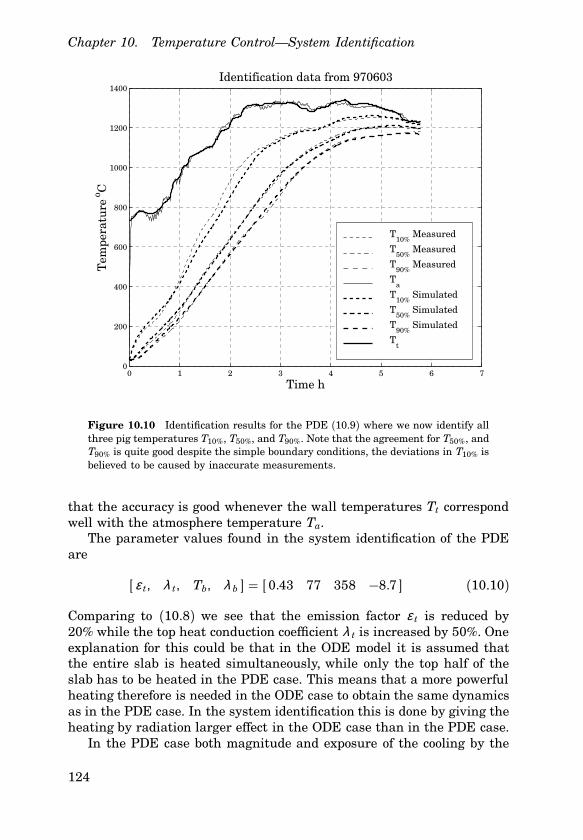
Chapter 10. Temperature Control—System Identification
0 1 2 3 4 5 6 70
200
400
600
800
1000
1200
1400Identification data from 970603
Time h
Tem
pera
ture
o C
T10%
Measured
T50%
Measured
T90%
Measured
Ta
T10%
Simulated
T50%
Simulated
T90%
Simulated
Tt
Figure 10.10 Identification results for the PDE (10.9) where we now identify allthree pig temperatures T10%, T50%, and T90%. Note that the agreement for T50%, andT90% is quite good despite the simple boundary conditions, the deviations in T10% isbelieved to be caused by inaccurate measurements.
that the accuracy is good whenever the wall temperatures Tt correspondwell with the atmosphere temperature Ta.
The parameter values found in the system identification of the PDEare
[ ε t, λ t, Tb, λ b ] � [ 0.43 77 358 −8.7 ] (10.10)
Comparing to (10.8) we see that the emission factor ε t is reduced by20% while the top heat conduction coefficient λ t is increased by 50%. Oneexplanation for this could be that in the ODE model it is assumed thatthe entire slab is heated simultaneously, while only the top half of theslab has to be heated in the PDE case. This means that a more powerfulheating therefore is needed in the ODE case to obtain the same dynamicsas in the PDE case. In the system identification this is done by giving theheating by radiation larger effect in the ODE case than in the PDE case.
In the PDE case both magnitude and exposure of the cooling by the
124

10.2 Models for Slab Temperature
0 2 4 60
500
1000
Validation data from 960611
Time h
Tem
pera
ture
o C
0 2 4 60
500
1000
Validation data from 961015
Time h
Tem
pera
ture
o C
0 2 4 60
500
1000
Validation data from 970123
Time h
Tem
pera
ture
o C
0 2 4 60
200
400
600
800
1000
1200
1400Validation data from 970805
Time h
Tem
pera
ture
o C
Figure 10.11 Validation results for the PDE (10.9). Note the good agreement for"960611" and "970805" where atmosphere temperature Ta , and wall temperature Tt
are in good agreement.
transport system represented by λ b and Tb is smaller than in the ODEcase. The explanation for this could be that in the FEM case the heattransport through the slab is modeled explicitly, while this has to be doneartificially in the ODE case. This will lead to a what seems like a heatloss to from the center in the ODE case.
125

Chapter 10. Temperature Control—System Identification
0 2 4 60
200
400
600
800
1000
1200
1400Validation data from 980617
Time h
Tem
pera
ture
o C
0 2 4 60
200
400
600
800
1000
1200
1400Validation data from 980904
Time h
Tem
pera
ture
o C
0 2 4 60
200
400
600
800
1000
1200
1400Validation data from 981216
Time h
Tem
pera
ture
o C
0 2 4 60
200
400
600
800
1000
1200
1400Validation data from 990305
Time h
Tem
pera
ture
o C
Figure 10.12 Validation results for the PDE (10.9). Note the good agreement for"980617" and "980904" where atmosphere temperature Ta , and wall temperature Tt
are in good agreement.
126

10.3 Conclusions
10.3 Conclusions
We are now finished building models for the slab temperature controlproblem. We have found that the temperature measurements used forzone temperature control can be represented by independent linear firstorder systems with a reasonable accuracy and that the other tempera-ture measurements in the zones can be represented as linear functions oftemperature control measurements.
Two models for the slab temperatures have been built and identified.The first model is a nonlinear ODE which is used for modeling the slabcenter temperature and the second model is a PDE which is used formodeling the slab top, center, and bottom temperatures. In both cases goodagreement is obtained during identification and validation which has beencarried out using 9 data sets collected over several years at The DanishSteel Works Ltd. One prerequisite for obtaining a good prediction of theslab temperature is that the calculated furnace temperature is correct,this is especially the case with the PDE model. The results indicate thatthe furnace can be regarded as a time invariant process which was notclear before the system identification.
The coefficients obtained from the ODE and PDE identification givea bit different pictures of the heating process. The results of the PDEidentification is believed to be the most reliable and it is concluded thatthe coefficients from the the ODE identification are biased due to theassumptions used when deriving the model.
127

11
Temperature Control—Design
The purpose of this chapter is to design algorithms for the control of theslab temperatures. First we will use the identification results from Chap-ter 10 to build a nonlinear state space model for all slabs in a furnacecontrol zone. Then we will design a linear control law similar to that ofthe FOCS system, the purpose of the design is optimization of the fur-nace control system at The Danish Steel Works Ltd. The final part of thechapter contains a design of a nonlinear control algorithm for the furnacecontrol problem—the performance of the linear and the two nonlinearalgorithms will be compared in Chapter 12 using computer simulations.
11.1 The Control Problem
We want to control the temperatures of the slabs in the reheat furnace no.2 at The Danish Steel Works Ltd. The furnace is divided into 4 furnacetemperature control zones, see Figure 8.1, and we control the i’th slabtemperature of the j’th zone T j
i by varying the furnace temperature setpoints T j
m and hereby the furnace temperature profile Tt of the controlzones, see Figure 8.2. The furnace temperatures are controlled by vary-ing the fuel flow to the burners. The main task of control system is tominimize the effects of the varying slab velocity vs, which can be seen asa measurable disturbance.
As mentioned in Section 8.3 we will consider the control of the slabtemperatures separately for each zone and the problem is reduced to con-trolling the temperatures of the nj slabs in each of the four furnace zones.
To simplify the notation in the following we assume that the materialproperties and thickness of all slabs in the zone are identical, it is straightforward to remove this assumption when necessary. Throughout this chap-
128

11.1 The Control Problem
ter i � 1, ⋅ ⋅ ⋅ , nj is used for slab index in the zone and j � 1, ⋅ ⋅ ⋅ , 4 is usedas zone number.
We build the model for all slabs in a control zone using the ODE modelin Section 10.2. Assuming that the zone contains nj slabs and definingthe state vector for zone j
T j(t)T � [T j1 (t) T j
2 (t) . . . T jnj (t)
]we obtain the following state space model from (10.7)
dT j
dt� G(T j)(F(T j) + U(Tt))
dxj
dt� 1vs(t) (11.1)
where
G(T j) �
g(T j
1 ) 0 . . . 0
0 g(T j2 )
. . ....
.... . .
. . . 0
0 . . . 0 g(T jnj )
F(T j)T � [ f (T j
1) f (T j2) ⋅ ⋅ ⋅ f (T j
nj)]
U(Tt)T � [u(xj1, T j
m) u(xj2, T j
m) ⋅ ⋅ ⋅ u(xjnj , T j
m)]
xj (t)T � [ xj1(t) xj
2(t) ⋅ ⋅ ⋅ xjnj (t)
]1T � [1 1 ⋅ ⋅ ⋅ 1 ] (11.2)
where we have used that
Tt(x, t) � p(xji )T j
m(t)
where p is the linear interpolation of the thermocouple measurementsdefined by (10.6), and T j
m is the furnace temperature measurement usedfor controlling the furnace temperature.
In (11.1) and (11.2) vs is the velocity of the slabs, xji is the position of
the i’th slab in the j’th zone, see Figure 8.2. The elements of (11.2) are
f (T ji ) � −ε tσ
(T j
i (t))4 − (λ t − λ b)T j
i (t) − Tbλ b, i � 1, . . . , nj
g(T ji ) �
1
hρ (T ji )cp(T j
i )u(xj
i , T jm) � ε tσ p4(xj
i)(T j
m(t))4 + λ tp(xj
i )T jm(t) (11.3)
129

Chapter 11. Temperature Control—Design
The material parameters ρ and cp are shown in Figure 10.6. Further-more, ε t, λ t, λ b, and Tb are the parameters found in the ODE systemidentification described in Section 10.2.
The mechanics of the model (11.1) are as follows: when a new slabenters zone j it is assigned states T j
1 and xj1, and the state numbers of
the other slabs in zone j are increased by one. When a slab leaves thezone, the states T j
nj and xjnj are removed from the system. Since the slabs
have different lengths these two events are independent.
11.2 Design of FOCS Controller
In the following we will go through the design of the slab temperaturecontroller of the FOCS system. The design has two purposes, it should beused
• for adjustment of the parameters of the existing FOCS system atThe Danish Steel Works Ltd.
• for comparison and introduction for the nonlinear deign presentedlater in this chapter
The controller structure is already given by the system at The DanishSteel Works Ltd., see Figure 11.1. The figure illustrates that the slab tem-perature controller C j
S for the j’th zone sets the reference to the furnacetemperature controller which again controls the fuel flow to the burnersof zone j.
The main purpose of the slab temperature control system is to mini-mize the heating error for zone j
ejL(t) �
nj∑i�1
rjL(i)(T j
i (t) − Tr(xji )) � rj
L T j − rjLTr(xj)
where Tr is the heating curve, and rjL is a vector of nonnegative weights
for the temperature deviation of zone j. The design variables of the systemare
• The heating curve Tr. The slab temperature reference Tr starts atroom temperature and ends at the desired final slab temperature.The heating curve is a function of slab position x.
• The feedforward tables. The tables specify the furnace tempera-ture set points as a function of the slab speed vs. This makes sensesince vs can be considered as a measurable disturbance of the slabtemperature control system.
130

11.2 Design of FOCS Controller
-
T jf f
-
6
Ff. table
1s
- - -
-
-
vs ?
- -f (⋅)xj
GjF Pj
S� �� rLT j
− � ��
C jS
T jmr T j
mrLTr
Figure 11.1 The controller structure for the FOCS system consists of PI con-trollers for the weighted slab temperature rj
LT j , and furnace temperature T jm. T j
f f
is the temperature reference from the feedforward tables, and T jmr is the furnace
tempeature reference from the slab tempeature controller. GjF is the closed loop
transfer function of the furnace temperature control system of zone j , C jS is the
transfer function of the slab temperature controller for zone j , and PjS is the trans-
fer function relating the furnace temperature and the weighted slab temperaturerj
L T j of zone j .
• The PI coefficients. Based on the slab temperature deviation fromthe heating curve the PI-controllers C j
S determines a correction ofthe furnace temperature reference from the feedforward tables.
In the following we will first determine the heating curve and feedforwardtables. We will then design the PI-controllers for the slab temperaturedeviation from the heating curve.
Heating Curve and Feedforward Tables
We start the controller design with a discussion of the heating curve andthe feedforward tables, which are parts of the classical approach to thesolution of the slab temperature control problem. The heating curve isa reference trajectory for the slab temperatures which sets the tempera-ture reference for the slabs as they are transported through the furnacewith speed vs. The feedforward tables contain the furnace temperatureset points necessary to follow the slab heating curve, for an example seeTable 11.1. The tables assumes constant slab speed.
The reference slab center temperature Tr is normally chosen as a func-tion of slab position xj
i instead of time t. In the case where the slabs aremoving with constant nominal speed vs0 there is no difference, but whena stop occurs the dependence on slab position ensures that rise in temper-ature reference is stopped and is first started when the slabs start movingagain. The dependence on x therefore prevents premature heating of theslabs.
A natural way of choosing the heating curve is to use the stationary
131

Chapter 11. Temperature Control—Design
solution of the differential equation for T ji when the slabs move through
the furnace with the nominal velocity vs0. The advantage of this approachis that in the nominal case the furnace temperatures T j
m can be keptconstant. It is also an advantage in the linear controller design, as wewill see later on. In the case where vs � 0 the differential equation forthe heating curves reduces to a static equation which can be used fordetermining the zone temperatures necessary to keep the slabs hot duringstops. In the following we only generate heating curve and feedforwardtables for the nontrivial case where vs0 > 0. As we will see later it is notcertain that the slab temperatures will stay on the heating curve duringthe stops.
To generate the constant velocity solution to the differential equationfor the slab temperature T j
i we define the differential equation for theheating curve Tr in zone j as
dTr
dt� dTr
dxdxdt� dTr
dxvs0 � g(Tr)( f (Tr) + u(x, T j
m0)):
dTr
dx� 1
vs0g(Tr)( f (Tr) + u(x, T j
m0))dxdt� vs0
Tr(0) � Tin (11.4)
where Tin is the initial slab temperature, and T jm0 is the constant furnace
temperature that ensures that the slab temperatures follow the heatingcurve. The nominal slab speed vs0 is chosen corresponding to a residencetime of 6.4 hours corresponding to vs0 � 0.002 m/s. The residence time isnormally 5 hours at The Danish Steel Works Ltd. The reason for the choiceof a larger residence time for calculating the heating curve Tr is that thefurnace is operated partially as a batch furnace, for further details pleaserefer to the discussion in Chapter 13.
We now have to find the furnace temperature setpoints T jm0 for the
four zones, j � 1, 2, 3, 4. To reduce the temperature gradient of the slabsand to ensure a buffer of hot slabs when the furnace is subjected to ele-vated speeds, we choose to keep the slab temperature T j
i at the desiredfinal temperatures in zones 3 and 4. The simulations of the PDE for theslab temperature in Chapter 12 and the experiences from the implemen-tation of the control strategy show that this is sufficient for ensuring asatisfactory mean temperature and temperature gradient. The remainingfreedom we use for minimizing the energy losses of the furnace, whichare discussed in Section 8.4.
132
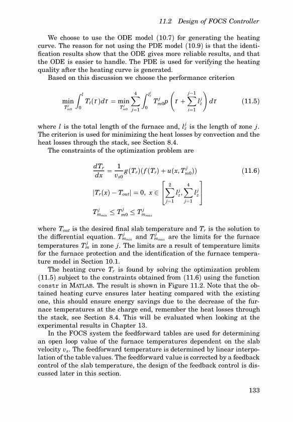
11.2 Design of FOCS Controller
We choose to use the ODE model (10.7) for generating the heatingcurve. The reason for not using the PDE model (10.9) is that the identi-fication results show that the ODE gives more reliable results, and thatthe ODE is easier to handle. The PDE is used for verifying the heatingquality after the heating curve is generated.
Based on this discussion we choose the performance criterion
minT j
m0
∫ l
0Tt(τ )dτ � min
T jm0
4∑j�1
∫ ljz
0T j
m0p
(τ +
j−1∑i�1
l jz
)dτ (11.5)
where l is the total length of the furnace and, l jz is the length of zone j.
The criterion is used for minimizing the heat losses by convection and theheat losses through the stack, see Section 8.4.
The constraints of the optimization problem are
dTr
dx� 1
vs0g(Tr)( f (Tr) + u(x, T j
m0)) (11.6)
tTr(x) − Toutt � 0, x ∈ 2∑
j�1
l jz,
4∑j�1
l jz
T j
mmin≤ T j
m0 ≤ T jmmax
where Tout is the desired final slab temperature and Tr is the solution tothe differential equation. T j
mmin and T jmmax are the limits for the furnace
temperatures T jm in zone j. The limits are a result of temperature limits
for the furnace protection and the identification of the furnace tempera-ture model in Section 10.1.
The heating curve Tr is found by solving the optimization problem(11.5) subject to the constraints obtained from (11.6) using the functionconstr in MATLAB. The result is shown in Figure 11.2. Note that the ob-tained heating curve ensures later heating compared with the existingone, this should ensure energy savings due to the decrease of the fur-nace temperatures at the charge end, remember the heat losses throughthe stack, see Section 8.4. This will be evaluated when looking at theexperimental results in Chapter 13.
In the FOCS system the feedforward tables are used for determiningan open loop value of the furnace temperatures dependent on the slabvelocity vs. The feedforward temperature is determined by linear interpo-lation of the table values. The feedforward value is corrected by a feedbackcontrol of the slab temperature, the design of the feedback control is dis-cussed later in this section.
133

Chapter 11. Temperature Control—Design
0 5 10 15 20 25 30 35 40 450
200
400
600
800
1000
1200
1400
x in m
Tem
pera
ture
o C
Heating curve for vs0
= 0.002 m/s
Zone 1 Zone 2 Zone 3 Zone 4
Tr New
Tt New
Tr Old
Figure 11.2 New and existing heating curves Tr for the control zones of the reheatfurnace with an initial temperature Tin of 20○ C and a final temperature Tout of1120○ C. Note that the new heating curve ensures significantly later heating thanthe existing one. The heating curve is used as a slab temperature reference as afunction of the slab positions x.
It is, in general, not possible to have the same heating curves for twodifferent slab speeds vs0 and vs0 since this implies that
dTr
dx� 1
vs0g(Tr)( f (Tr) + u(x, T j
m0)) �1
vs0g(Tr)( f (Tr) + u(x, T j
m0)):
u(x, T jm0) �
(vs0
vs0− 1)
f (Tr) + vs0
vs0u(x, T j
m0)
which is not possible to obtain with a constant T jm0. Given a nominal
speed different than vs0 we therefore choose the furnace temperaturesthat minimizes the distance to the heating curve, this is done by solvingthe optimization problem
minT j
mi
uTr − Tru∞
134

11.2 Design of FOCS Controller
0 1 2 3 4 5
200
400
600
800
1000
1200
Time h
Tem
pera
ture
o C
vs = 0.0025, ∆T = 96.6, T
avg = 1120
Zone 1 Zone 2 Zone 3 Zone 4
T10%
T50%
T90%Tij
Tm
Figure 11.3 Result of finding feedforward temperatures for the nominal residencetime of 5 hours corresponding to vs � 0.0025 in the feedforward table. In the figure∆T denotes the temperature gradient and Tavg denotes the average temperature ofthe FEM simulations at the time of discharge. The FEM simulation shows that thetemperature gradient is on the high side, around 97○ C but the experiments showthat no problems occur during rolling.
subject to the constraints
dTr
dx� 1
vsig(Tr)( f (Tr) + u(x, T j
mi))T j
mmin≤ T j
mi ≤ T jmmax
The problem is solved for five nominal speeds vsi between 0.0017 m/sand 0.005 m/s. Once more constr in MATLAB is used for determining theoptimal temperatures for the feedforward table. In the optimization thetemperatures of zones 3 and 4 are constrained to be larger than 1220 ○ Cand 1200 ○ C to ensure a minimal amount of flow and thereby pressurein the last part of the furnace. The maximal temperature of zone 4 isfurthermore set to 1240 ○ C to avoid too large temperature gradients of theslabs. The result of the optimization is presented in Figures 11.3, 11.4,and Table 11.1. Note here that speeds over 0.0025 m/s are not feasible,they are only included here since the appear in the tables of the FOCSsystem at The Danish Steel Works Ltd. The high speeds can only be usedfor 200 mm slabs.
135

Chapter 11. Temperature Control—Design
0 2 4 6
200
400
600
800
1000
1200
Time h
Tem
pera
ture
o C
vs = 0.0017, ∆T = 66.2, T
avg = 1134
0 1 2 3
200
400
600
800
1000
1200
Time h
Tem
pera
ture
o C
vs = 0.0033, ∆T = 119, T
avg = 1102
0 1 2 3
200
400
600
800
1000
1200
Time h
Tem
pera
ture
o C
vs = 0.0042, ∆T = 165, T
avg = 1037
0 0.5 1 1.5 2 2.5
200
400
600
800
1000
1200
Time hT
empe
ratu
re o C
vs = 0.005, ∆T = 215, T
avg = 975.6
Figure 11.4 Results of the determination of the zone temperatures for the nominalvelocities of the feedforward tables. In the figure ∆T denotes the temperature gradi-ent and Tavg denotes the average temperature of the FEM simulations at the timeof discharge. It is seen that the temperature gradients are not acceptable for slabvelocities over vs � 0.0025. The curve marking is the same as used in Figure 11.3.
m/s 0.0017 0.0025 0.0033 0.0042 0.0050
Zone 1 1227○ C 1320○ C 1320○ C 1320○ C 1320○ C
Zone 2 1308○ C 1330○ C 1330○ C 1330○ C 1330○ C
Zone 3 1240○ C 1220○ C 1330○ C 1330○ C 1330○ C
Zone 4 1200○ C 1227○ C 1240○ C 1240○ C 1240○ C
Table 11.1 New feedforward table with temperature setpoints for the four furnacecontrol zones. The setpoints are given for five different slab speeds. The feedforwardtable is used for generating an open loop temperature setpoint in the FOCS system.
At zero slab velocity the furnace temperatures are lowered to valuesspecified by a separate table containing multiplication factors for the fur-nace temperatures at the beginning of the stop. These tables will not beconsidered here.
Finding the Controller Coefficients
When controlling the temperature of the slabs it is normally desired thatthey follow the heating curve Tr which defines the control error for the i’th
136

11.2 Design of FOCS Controller
slab as T ji −Tr(xj
i ). It is natural to consider the temperature deviations ofthe slabs leaving the zone more important than the other slab temperaturedeviations, this is handled by introducing individual weight terms rj
L(i)for the slab temperature deviations. We now define the error function forzone j
ejL(t) �
nj∑i�1
rjL(i)(T j
i (t) − Tr(xji )) (11.7)
In the FOCS system four different choices of linear weight functions arepossible. We here choose the variant that gives equal weight to all theslabs in a zone, the reason for this is that the experiences from the exper-iments in Chapter 13 show that the heating of the cold slabs entering areas important as the temperature of the slabs leaving the zone. To keep thedesign simple we choose the same weight function rj
L for all four controlzones
rjL(i) �
1nj
, i � 1, . . . , n
Note that this choice of weight function yields∑
rjL(i) � 1. Since the zone
always is filled with slabs this choice of weight ensures a constant gainof the model of the slabs of a zone, as we will see later.
Looking at the control error Y ji � T j
i −Tr(xji) we obtain the differential
equation from (11.1)
dY ji
dt� dT j
i
dt− dTr
dt
� g(T ji )( f (T j
i ) + u(xji , T j
m)) −vs(t)vs0
g(Tr)( f (Tr) + u(xji , T j
m0)) (11.8)
Linearization of this equation around the heating curve Tr yields
dY ji
dt� a(xj
i)Y ji (t) + b(xj
i)(T jm(t) − T j
m0) + k(xji)(vs(t) − vs0)
137

Chapter 11. Temperature Control—Design
where
a(xji) �
�
�T ji
[g(T j
i )( f (T ji ) + u(xj
i , T jm0))
]∣∣∣∣T j
i �Tr(xji )
�g(Tr(xji))′( f (Tr(xj
i )) + u(xji , T j
m0))− g(Tr(xj
i ))(4ε tσ T3r (xj
i ) + (λ t − λ b))
b(xji) �
�
�T jm
[g(Tr(xj
i ))u(xji , T j
m)]∣∣∣∣
T jm�T j
m0
�g(Tr(xji))(4ε tσ p(xj
i )(T jm0)3 + λ tp(xj
i ))
k(xji) �
�
�vs
[−vs(t)
vs0g(Tr(xj
i))( f (Tr(xji )) + u(xj
i , T jm0))
]∣∣∣∣vs�vs0
�− 1vs0( f (Tr(xj
i )) + u(xji , T j
m0)
f , g, and u are defined in (11.3). Since g is based on tables it is differen-tiated numerically. We note that we have linearized around a trajectorythat is a stationary solution to the nonlinear differential equation for theslab temperature T j
i . This is a classical approach in nonlinear system the-ory. The fact that the heating curve is generated as a stationary solutionto the differential equation simplifies the linearization considerably.
Joining the linearized models for all slabs in zone j and introducingY j as the vector of slab temperature errors for zone j we end up with alinear state space model of order nj .
Y j (t) �Aj (xj )Y j(t) + B j (xj )(T jm(t) − T j
m0) + K j(xj )(vs(t) − vs0)ej
L(t) �C j Y j (t)
Aj has diagonal structure and B j , C j , and K j are vectors
Aj (xj) �
a(xj
1) 0 . . . 0
0 a(xj2)
. . ....
.... . .
. . . 0
0 . . . 0 a(xjnj )
B j (x)T � [ b(xj
1) b(xj2) ⋅ ⋅ ⋅ b(xj
nj )]
C j � [ rjL(1) rj
L(2) ⋅ ⋅ ⋅ rjL(nj)
]K j(x)T � [ k(xj
1) k(xj2) ⋅ ⋅ ⋅ k(xj
nj )]
138
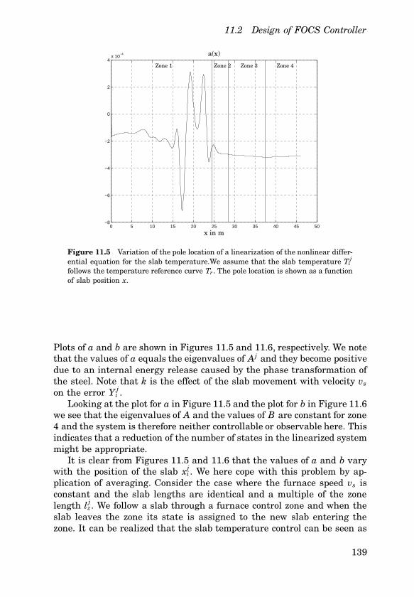
11.2 Design of FOCS Controller
0 5 10 15 20 25 30 35 40 45 50−8
−6
−4
−2
0
2
4x 10
−4
Zone 1 Zone 2 Zone 3 Zone 4
a(x)
x in m
Figure 11.5 Variation of the pole location of a linearization of the nonlinear differ-ential equation for the slab temperature.We assume that the slab temperature T j
ifollows the temperature reference curve Tr . The pole location is shown as a functionof slab position x.
Plots of a and b are shown in Figures 11.5 and 11.6, respectively. We notethat the values of a equals the eigenvalues of Aj and they become positivedue to an internal energy release caused by the phase transformation ofthe steel. Note that k is the effect of the slab movement with velocity vs
on the error Y ji .
Looking at the plot for a in Figure 11.5 and the plot for b in Figure 11.6we see that the eigenvalues of A and the values of B are constant for zone4 and the system is therefore neither controllable or observable here. Thisindicates that a reduction of the number of states in the linearized systemmight be appropriate.
It is clear from Figures 11.5 and 11.6 that the values of a and b varywith the position of the slab xj
i . We here cope with this problem by ap-plication of averaging. Consider the case where the furnace speed vs isconstant and the slab lengths are identical and a multiple of the zonelength l j
z. We follow a slab through a furnace control zone and when theslab leaves the zone its state is assigned to the new slab entering thezone. It can be realized that the slab temperature control can be seen as
139

Chapter 11. Temperature Control—Design
0 5 10 15 20 25 30 35 40 45 500.5
1
1.5
2
2.5
3
3.5
4
4.5x 10
−4
Zone 1 Zone 2 Zone 3 Zone 4
b(x)
x in m
Figure 11.6 Variation of the gain of a linearization of the nonlinear differentialequation for the slab temperature. We assume that the slab temperature T j
i followsthe temperature reference curve Tr . The variation is shown as a function of slabposition x.
a periodic problem since
a(t) � a(t+ tj)b(t) � b(t+ tj )k(t) � k(t+ tj )
where tj is the time it takes the slab to pass through zone j. The term kis not used here, but the influence of the slab speed vs is included by thefeedforward tables described earlier in this section.
Inspired by averaging theory [Åström and Wittenmark, 1995] we wantto approximate the system. Introduce the averaged slab temperature errorfor the i’th slab in zone j
Yji �
1tj
∫ tj
0Y(t) dt � vs0
l jz
∫ tj
0Y(t) dt
and Y j as the vector of averaged slab temperature errors for zone j. Set-ting T j
m − T jm0 � C j
S (p)C j Yj
where C jS (p) is the transfer function of the
140

11.2 Design of FOCS Controller
linear slab temperature controller for zone j we reformulate the differen-tial equation to
dYji
dt� vs0
l jz
∫ tj
0a(t) dt Y
ji(t) +
vs0
l jz
∫ tj
0b(t) dtC j
S(p) C j Yj (t)
� 1
l jz
∫ ljz
0a(x) dx Y
ji (t) +
1
l jz
∫ ljz
0b(x) dx C j
S(p)C j Yji (t)
� aj Yji(t) + b
jC j
S(p)C j Yj (t)
where l jz is the length of zone j and p is the differential operator. The ad-
vantages of the averaging are many, we are able to cope with the positivevalues of a, and as we will see in the following it is straight forward to de-sign the PI-controllers of the FOCS system for the averaged system. Notethat the averaged parameters are not dependent on the slab velocity vs,they are, however, only guaranteed to be relevant near the heating curveTr.
Representing each slab in the j’th zone by its averaged linear systemwe end up with a system matrix Aj with identical eigenvalues and thestate space representations for the zones can be reduced to the first ordersystem
PjS(s) �
C j Bj
s− aj �∑nj
1 rjL(i)b
j
s− aj � bj
s− aj (11.9)
where bj
and aj are found by averaging over the zone. We can also see thisas we control the slabs temperatures of the zone as the mean temperatureof one big piece of steel. Note that due to the special choice of weightfunction rj
L the slab lengths do not affect (11.9). The values found in theaveraging are
b
1
b2
b3
b4
�
2.3 ⋅ 10−4
4.0 ⋅ 10−4
3.5 ⋅ 10−4
3.7 ⋅ 10−4
a1
a2
a3
a4
�−1, 4 ⋅ 10−4
−2.7 ⋅ 10−4
−3.1 ⋅ 10−4
−3.1 ⋅ 10−4
141

Chapter 11. Temperature Control—Design
0 5 10 15 20 25 30 35 40 45−0.25
−0.2
−0.15
−0.1
−0.05
0
0.05
0.1
0.15
0.2
0.25
Position m
Am
plit
ude
Accuracy of averaging
Original equationAveraged equation0.2*Input
Figure 11.7 Check of validity of averaging. The original linearized system withthe time varying coefficients and the averaged equation (11.9) are simulated witha sawtooth wave as input. We note that there is a reasonable agreement betweenthe responses of the original and the averaged system.
Note that all the averaged systems are stable. To verify the dynamic prop-erties of the averaging of the system around the heating curve the orig-inal system with the time varying coefficients and the averaged systemare simulated with a sawtooth wave as input. The result is shown inFigure 11.7.
The controller structure of the FOCS system is shown in Figure 11.1,it has two PI-controllers, one for the furnace temperature T j
m and one forthe weighted slab temperature rj
L T j . The averaging analysis implies that
rjLT j � T
jand we have the linear first order transfer function (11.9) from
the furnace temperature T jm to the controlled variable. The disturbances
of the system—the variations of vs—enter the system through the refer-ence Tr, see Figure 11.1. This makes the linear controller design a servoproblem, see [Åström and Wittenmark, 1997]. Note that the temperaturefound using the feedforward tables T j
f f is related to a change of the ref-erence Tr. As we will see later this gives a pretty good reaction to thedisturbances introduced by the slab movement.
An investigation of the furnace temperature control shows that theperformance of these controllers are satisfactory and we therefore chooseto keep the existing controller structure for this algorithm.
142

11.2 Design of FOCS Controller
The transfer functions of the slab and furnace temperature controllersare given by
C jF (s) � K j
pF + K jiF
1s
C jS (s) � K j
pS + K jiS
1s
Neglecting dynamics of the fuel and air valves, which are considerablyfaster than the system dynamics, we end up with the second order closedloop transfer for the furnace and slab temperatures
T jm(s) � Gj
F (s)T jmr(s) �
aj2(K j
pFs+ K jiF)
s2 + (aj2K j
pF − aj3)s+ aj
2 K jiF
T jmr(s)
Tj (s) � Gj
S (s)rjLTr(s) �
bj (K j
pSs+ K jiS)
s2 + (bjK j
pS − aj )s+ bjK j
iS
rjLTr(s)
where it has been assumed that the dynamics of the transfer functionfor the furnace temperature Gj
F are fast compared to the dynamics of GjS
and therefore can be neglected in the second equation. Since the openloop time constants of the furnace zone temperature, see Section 10.1, isa factor 10 faster than the time constants for the slab temperature thisis considered a valid approximation.
Aiming at closed loop time constants half as long as the open loop timeconstants and a damping factor of 0.7 for the slab temperature yields thefollowing equations for the controller coefficients.
K jiS � −
4(aj)2b
j
K jpS � −
1.8aj
bj
A simulation of a standard slab velocity disturbance, see Section 12.3, isshown in Figure 11.8. The simulations have been carried out using thefull nonlinear model for the reheat furnace described in Chapter 12. Itis seen that the stop gives a rather large error in the slab temperaturesleaving the zone, but also that the PI-controller uses large control effortto counteract the disturbance.
The final question in the linear design is the variation of the slabdimensions. Since the material parameters of (11.3) are g � 1/(hρ cp) we
143

Chapter 11. Temperature Control—Design
0 2 4 6 8
1200
1220
1240
1260
1280
1300
Time h
Tem
pera
ture
° C
Tm1
0 2 4 6 80
500
1000
1500
2000
Time h
Flo
w m
3 /h
Ff1
0 2 4 6 8
0
50
100
150
Time h
Tem
pera
ture
° C
eL1
2 4 6 8−150
−100
−50
0
50
100
150
Time h
Tem
pera
ture
o C
Differences final temperature for zone 1
Figure 11.8 Response of the slab temperature control of zone 1 to a step distur-bance in the slab velocity vs when the slab temperatures are controlled using thePI-controller and feedforward table. The slab velocity is changed from its nominalvalue 0.002 m/s to zero at t � 1, to 0.0025 m/s at t � 2 and back to the nominalvalue at t � 3, see Figure 12.2. The plots show the reactions of the slab temperaturecontroller to the disturbance. We see that the slabs leaving the zone get approxi-mately 100 ○ C too hot, but this is taken care of later by zones 2 to 4. The responsesare kept within the permissible limits of the fuel flow F1
f and furnace temperatureT1
m . The control error is defined by e1L � r1
LY1 . The circles in the plot in the lowerright corner show the temperatures of the slabs leaving the zone. The bend on thecurve at t � 5.5 hours is the first slab which has entered the zone after the stop.The horizontal lines around Y j
i � 0 marks a heating error of ±10○ C.
see that approximatively
ai ∝ 1
h
bi ∝ 1
h
which make the gain and pole of (11.9) inversely proportional to the slabthickness h. The characteristic equation of the closed loop system becomes
144

11.3 Design of Nonlinear Controller
approximatively
s2 + hh(bj
KpS − aj)s+ hh
bjKiS � 0
which is stable for all positive values of h by Routh’s stability test. Thedifferent thicknesses are handled in the FOCS system by having a sepa-rate heating curve for each slab thickness. Note that a different heatingcurve for slabs of a different thickness might affect the result, since it willaffect the values of aj and b
j.
11.3 Design of Nonlinear Controller
When controlling the slab heating it is natural to start thinking about thepossibility of controlling the slab energy content. Unfortunately, the slabenergy content given by hρ cpT j
i is not a monotonic function of temperatureT j
i , due to the variations of ρ , and especially cp. Instead it turns out to befeasible to control the slab enthalpy hs which we define by
hs(T ji ) �
∫ T ji
0hρ (τ )cp(τ )dτ . (11.10)
Using this variable for the slab temperature control yields, beside thenice interpretation, a simplification of the nonlinear equations we wantto control. A plot of the enthalpy as generated on the basis of the heatingcurve of Figure 11.2 is shown in Figure 11.9.
In the following we will design a nonlinear controller for controlling(11.10), where the slabs are expected to follow the enthalpy curve inFigure 11.9 as they are transported through the furnace. This followsthe same lines as the linear controller in Section 11.2. This concept wecall enthalpy control. In the nonlinear design we will adopt the existingfurnace temperature controller and neglect the dynamics of the furnacetemperature, as in the linear design.
Choosing the enthalpy (11.10) as output of the nonlinear state spaceequation (11.1) we end up with the system
dT j
dt� G(T j )(F(T j) + U(Tt))
ejV (T) � 1
2
nj∑i�1
rjVi(Ej
i )2 (11.11)
145

Chapter 11. Temperature Control—Design
0 5 10 15 20 25 30 35 40 450
2
4
6
8
10
12
14
16x 10
8
x in m
hs(T
ij)
Zone 1 Zone 2 Zone 3 Zone 4
Figure 11.9 Enthalpy curve for the control zones of the reheat furnace with aninitial temperature of 20○ C and a final temperature of 1120○ C. The enthalpy curveis based on the heating curve in Figure 11.2 and (11.10).
where rjV is the error weight for the enthalpy controller, hs is defined by
(11.10) and
Eji (xj
i , T ji ) � hs(T j
i ) − hr(xji).
The weights of rjV now can be chosen freely. The enthalpy reference hr
which depends on slab position xji , is defined as
hr(xji ) �
∫ Tr(xji )
0hρ (τ )cp(τ ) dτ
Many other choices of error functions than the quadratic one used in(11.11) are possible, it is chosen here because it works well in practiceand we can use it for proving a stability result later on.
Using the nonlinear geometric methods for investigating the control-lability and observability, see [Nijmeijer and van der Schaft, 1991], of(11.11) is unfortunately not feasible due to the repeated differentiation ofg which is only given by numerical data. A sufficient condition for a sys-tem to be locally controllable is that the linearized system is controllable,
146

11.3 Design of Nonlinear Controller
see [Nijmeijer and van der Schaft, 1991]. As seen from the discussion inSection 11.2 this is not always the case. Using the linearized model we,furthermore, see that a sufficient condition for lack of (state) controlla-bility is that two slab temperatures T j
i and T jk are equal—this can, for
instance, happen during longer stops if the furnace temperature profile pis the same for xj
i and xjk. This indicates that it can be difficult to control
the furnace in these situations.Looking at the linearization in Section 11.2 we see that the linearized
system is not always observable in a neighborhood around the heatingcurve and we can therefore not derive sufficient conditions for observabil-ity either. Again we see that during stops where the slab temperaturesbecome equal we can get problems with the observability of the nonlinearsystem.
Investigating the methods suited for nonlinear controller design itturns out that feedback linearization is well suited for controlling theslab temperatures. Given a reference trajectory for the slab enthalpy hr
the main idea is to make the control error behave like the linear system
ddt
ejV � −cj
1ejV − cj
0
∫ t
0ej
V (τ ) dτ (11.12)
which we choose to have the same dynamics as the linearized system ofSection 11.2. Note that we have introduced an integral state in (11.12)which will ensure that the error ej
V converges to zero in the presence ofoffsets in (11.12). This is along the same ideas as the tracking problemdescribed in [Isidori, 1989], but there no integrator is used and further-more (11.11) is not affine in the input u due to the variation of p with theslab positions xj
i . We therefore have to solve the problem by other means.The first thing we note is that it is not possible to use the integrator in
(11.12), since ejV ≥ 0 the value of the integral will always be increasing,
instead we introduce the equation
ddt
ejV � −cj
1ejV − cj
0
nj∑i�1
rjVi
Eji
∫ t
0Ej
i (τ ) dτ (11.13)
and now the integrands can take positive as well as negative values, and
147

Chapter 11. Temperature Control—Design
(11.13) is usually still close to (11.12). Rewriting (11.13) yields
ddt
ejV �
nj∑i�1
rjVi
2E ji Ej
i � −cj1ej
V − cj0
nj∑i�1
rjVi
Eji
∫ t
0Ej
i (τ ) dτ (11.14)
: (11.15)nj∑
i�1
rjVi
Eji
(2E j
i + cj1Ej
i + cj0
∫ t
0Ej
i (τ ) dτ)� 0
which implies that the characteristic equations of the slab enthalpy errorsEj
i all have the characteristic equation
s2 + 12
cj1s+ 1
2cj
0 � 0
when the signs of Eji are the same, which typically is the case when the
system is subjected to large disturbances, when the controller action isimportant. To obtain the same dynamics in the large adjustments as thelinear controller in these cases we choose cj
0 � 8aj and cj1 � 0.707 ⋅ 8aj ,
where aj are the averaged poles of the linearized system in Section 11.2.The differential equation for the enthalpy error Ei
j is
ddt
Eji �
ddt
hs(T ji ) −
ddt
hr(Tr(xji))
� ( f (T ji ) + u(xj
i , T jm)) −
vs
vs0( f (Tr()xj
i) + u(xji , T j
m0)) (11.16)
Note that the material properties g are not present in (11.16), this is theadvantage of using the enthalpy hs as controlled output instead of thetemperature T j
i . Using the fact that u depends on T jm as in (11.3) gives a
fourth order polynomial for T jm when (11.16) and (11.13) are combined
α 1(T j
m(t))4 +α 2T j
m(t) � α 3 (11.17)
148

11.3 Design of Nonlinear Controller
where
α 1 �2ε tσnj∑
i�1
rjVi
p4(xji)Ej
i
α 2 �2λ t
nj∑i�1
rjVi
p(xji)Ej
i
α 3 �2nj∑
i�1
rjVi
Eji
[− f (T j
i ) +vs(t)vs0
( f (Tr(xji )) + u(xj
i , T jm0))
]
− cj1ej
V − cj0
nj∑i�1
rjVi
Eji
∫ t
0Ej
i (τ ) dτ
which can be done numerically by using for instance fzero in MATLAB.Note that f in α 3 represents the temperature losses, vs/vs0( f + u) canbe seen as a feedforward from the slab speed and cj
1ejV + cj
0
∑rj
ViEj
i∫
Eji
is the feedback part of the control law. We conclude that the nonlinearcontrol law has the features of the linear control law, but this time theyare automatically built-in.
The next question that arises it the stability of the control law. Usingthe Lyapunov function
V(Ej ,∫
Ej ) � ejV +
12
cj0
nj∑i�1
rjVi
(∫ t
0Ej
i (τ )dτ)2
with the time derivative
V (Ej ,∫
Ej) � ejV + cj
0
nj∑i�1
rjVi
Eji
∫ t
0Ej
i (τ )dτ (11.18)
� −cj1ej
V (11.19)
where Ej is a vector containg the enthalpy errors Eji for zone j. Since
V →∞ as (Eji ,∫
Eji ) → ∞ we have by the Global Invariant Set Theorem
in [Slotine and Li, 1991] that (Eji ,∫
Eji ) converges to the largest invariant
set where V � 0. This is given by
M � {x t (x1, . . . , xnj ) � 0, (xnj+1, . . . , x2nj ) ∈ Rnj}
and we therefore conclude that Eji → 0 as t → ∞. The control system is
therefore globally asymptotically stable. Note that we only have guarantee
149
Chapter 11. Temperature Control—Design
for stability when (11.17) is solvable. The solvability issue investigatedin the following.
In equation (11.17) we see that α 1 and α 2 are positive and since theleft hand side is a monotonically increasing function of T j
m we concludethat (11.17) will have a unique solution if and only if α 3 is positive. Thisis introduced by the physical limitation T j
m ≥ 0—it is not possible to coolthe slabs by reducing the temperature below 0 ○ K.
The conclusion is that the system is globally asymptotically stablewhen the slab temperatures T j
i are near the heating curve Tr. When toolarge deviations are present it is not sure that (11.17) is solvable. Thelarge deviations can, for instance, happen during stops or excessive fur-nace speeds. This is to some extent parallel to the controllability problemsof the linearized system.
The performance of the nonlinear control law (11.17) is investigatedby implementing the nonlinear state space model (11.1) and the controllaw (11.17) in MATLAB. The result of a step disturbance is shown in Fig-ure 11.10. The simulations have been carried out using the full nonlinearmodel for the reheat furnace described in Chapter 12. For the nonlinearequations we use the weight function
rjV �
1∑nj
i�1 rjVi
[ 1 ⋅ ⋅ ⋅ 1 2 5 10 20 50 100 ]
Note that the final slab temperatures converges faster towards the spec-ified value for the nonlinear controller, the price paid is somewhat largervariations of the fuel flow F1
f . Note that the nonlinear system is within±20 ○ C after about 4.5 hours, while the PI-controller reaches this level atapproximately 6.5 hours.
11.4 Conclusions
In this chapter we have designed both a linear and one nonlinear con-trol law for the slab temperature control problem. The linear design in-cludes a description of a new way of generating a heating curve, whichis the temperature reference, and the feedforward tables which are usedas feedforwards from the slab velocity. In the following section a new de-sign method for design of a PI control law for the slab temperatures isdescribed. This is done by linearizing the nonlinear model for the slabtemperature around the heating curve and reducing the model order. Thelinear design is based on the controller structure of the existing furnacecontrol system at The Danish Steel Works Ltd.
150

11.4 Conclusions
0 2 4 6 8
1200
1220
1240
1260
1280
1300
1320
Time h
Tem
pera
ture
° C
Tm1
0 2 4 6 80
500
1000
1500
2000
Time h
Flo
w m
3 /h
Ff1
0 2 4 6 80
1
2
3
4
5
x 1016
Time h
Tem
pera
ture
° C
eV1
2 4 6 8−150
−100
−50
0
50
100
150
Time h
Tem
pera
ture
o C
Differences final temperature for zone 1
Figure 11.10 Response of the slab temperature control of zone 1 to a step distur-bance in the slab velocity vs when the slab temperatures are controlled using theenthalpy controller. The slab velocity is changed from its nominal value 0.002 m/sto zero at t � 1, to 0.0025 m/s at t � 2 and back to the nominal value at t � 3, seeFigure 12.2. The plots show the reactions of the slab temperature controller. Theresponses are kept within the permissible limits of the fuel flow F1
f and furnacetemperature T1
m . e1V is the enthalpy error for zone 1. The circles in the plot in the
lower right corner show the temperatures of the slabs leaving the zone. The hori-zontal lines around Y j
i � 0 marks a heating error of ±10○ C. This figure should becompared to Figure 11.8.
The nonlinear control law, which is a new control algorithm for theslab temperature problem, is designed using feedback linearization. In thedesign the slab temperature is to follow a given enthalpy reference curvedependent on the slab position. The enthalpy reference is found usingthe heating curve from the linear design. Integral control action is usedin nonlinear control law and the closed loop dynamics of the nonlinearcontroller is chosen to be similar to the closed loop dynamics of the lineardesign. It is shown that the nonlinear controller is globally asymptoticallystable, given the equation for determining the furnace temperatures issolvable, and that the controller output is unique, if a solution exists.
It is interesting to note that the design of the nonlinear control law is
151

Chapter 11. Temperature Control—Design
straight forward while the linear controller design is requires more work.On the other hand the linear control law is straight forward to imple-ment while the nonlinear control law requires a solver for the nonlinearequation (11.17). The performances of the two control laws is investi-gated using computer simulations based on the full nonlinear model anda standard disturbance in the slab velocity. The simulations show that theresponse speed of the nonlinear controller is significantly faster than theresponse speed of the linear controller, the price paid is somewhat largervariations of the control signal.
A more complete comparison of the two controller concepts is given inthe next chapter, there more detailed simulations will be carried out andthe performance of the control systems will be investigated.
152

12
Temperature Control—Simulations
The purpose of this chapter is to evaluate and compare the performanceand robustness of the PI-controller and the enthalpy controller designed inChapter 11. The evaluation is done through computer simulations usingMATLAB.
We will first describe the simulation program and the cases be to sim-ulated. This is followed by an investigation of the robustness to parametervariations, the response to a standard disturbance, and finally a simula-tion of the real case when the furnace does production.
12.1 Implementation of Simulation Model and Control Laws
The purpose of the simulations is verifications of the control laws andit should therefore be possible to simulate the furnace operation withdifferent slab lengths (we neglect the thickness variations) and varyingslab speed. We should furthermore be able to simulate the slab heatingas the slabs are transported through the four furnace zones.
The simulations cover the center track of the three furnace tracks andthe inputs to the simulation programs are
• A vector of slab lengths. They can either be 2 m or a uniformlydistributed sequence with values in the interval [1.5, 2.5] m
• Slab speed, this is either the test function also used in the evaluationof the controller design in Chapter 11 or time series taken from thepig runs.
The outputs from the simulation program are the time series for
• The fuel flows F jf for each furnace zone.
153
Chapter 12. Temperature Control—Simulations
• The furnace temperature T jm for each furnace zone.
• The slab temperatures T ji computed using the ODE model for all
the slabs that passes through the furnace.
• The slab temperatures T10%, T50%, and T90%, computed for a chosencritical slab using the PDE model.
All are functions of time t. The same inputs and outputs are used for boththe PI-controller and the nonlinear controller.
The limitations of the temperature control system are the fuel flowsF j
f—they can not be smaller than zero or larger than a given limit for eachzone. Using the model derived in Section 10.1 the limitations in fuel flowlead to upper and lower limits of the furnace temperatures T j
m. There isfurthermore given limitations for the maximal permissible furnace tem-peratures to protect the furnace construction.
The simulation program should handle the following main tasks
• Material tracking, using the slab lengths and slab speed, the pro-gram should keep track of the slabs in the furnace zones.
• Simulation of furnace temperature, using the linear model for thefurnace temperatures derived in Section 10.1.
• Simulation of slab temperature, using the nonlinear ODE model forthe slab temperatures derived in Section 10.2
• Control of furnace temperature, using the PI-control algorithm forthe furnace temperatures.
• Control of slab temperatures, using the PI-controller or the nonlin-ear controller mentioned in Sections 11.2 and 11.3.
Given the slab lengths and the slab speed the simulation program firstdetermines at which times slabs enter and leave the four furnace zones.The simulation for each zone is stopped and started each time a slabenters or leaves the zone. When the simulation is stopped the importantvariables are stored and the initial values are determined with the newconstellation and the simulation is restarted with the new number of slabsin the zone. The simulation is handled by first simulating the entire runfor zone 1, and then simulating zone 2, with the final temperatures ofzone 1 as initial values etc. It is assumed that the slabs are 20 ○ C whenthey enter zone 1.
The models and the controllers are described by a set of differentialequations which is solved using the built-in function ode45. When thesimulations of all zones are finished the PDE model derived in Section 10.2is used for computing the temperatures for the slabs with the shortest
154

12.1 Implementation of Simulation Model and Control Laws
residence time in the furnace. This slab is expected to have the largesttemperature gradient since there has been a short time interval availablefor heat conduction through the slab. Note that the residence time isdetermined by the furnace operator and it can therefore not be affectedby the controllers.
The implementation of the furnace model and the slab temperaturemodels (11.1) is straight forward, the only modification is the extensionof zone 1 also to include zone 0 which is the dark zone without burnersbefore zone 1, see Figure 8.1. This is possible since the temperatures ofzone 0 are well correlated with the temperatures of zone 1.
To maintain simplicity it is chosen to implement the controllers ascontinuous time differential equations, it would, however, be straight for-ward to convert the control algorithms to discrete time. One possibilitywith the nonlinear controller would be to use a sampling time which isshort compared to the furnace time constants and to keep the furnacetemperature references constant between the sampling instants.
The implementation of the PI-controller is done by specifying the dif-ferential equation for the controller and by introduction of tracking toprevent integrator windup, see [Åström and Wittenmark, 1997]. The timeconstant for the tracking system is chosen to the same value as the inte-gral time. The feedforward from the slab speed is implemented as a table,and the feedforward value is found by linear interpolation of the tablevalues. During stops the feedforward value is set to the lower limit forthe furnace temperature. It should be noted that this is a simplificationof the function in the FOCS system where the furnace temperatures areramped down from the furnace temperatures T j
m when the stop occurs us-ing a table with multiplication factors depending on the stop time, whichin some cases might be unknown.
The equation for the nonlinear control algorithm (11.17) is solved byfirst computing the sign of the left side of the equation minus the rightside at the maximal and minimal furnace temperatures. If the two expres-sions have different signs the equation has a zero in the feasible furnacetemperature interval. In this case the solution is found using the functionfzero in MATLAB. The analysis in Chapter 11 shows us that this solutionis unique. If both expressions are negative it is not possible to obtain asufficiently high temperature to solve the equation and the furnace tem-perature reference is set to the maximal permissible value. Along thesame lines the furnace temperature reference is set to the lowest possiblevalue if both terms are positive. A condition for solving the equation isthat t∑i Ej
i t is larger than a specified limit, this is introduced to avoidproblems with solvability of the nonlinear equation when Ej is close tozero. In the nonlinear case the temperature reference newer gets outsidethe specified interval and we here choose to block the integrator when
155

Chapter 12. Temperature Control—Simulations
saturation occurs, instead of tracking the integral part.As mentioned in Section 11.2 the existing controller parameters are
used for controlling the furnace temperatures. The simulations indicatethat the furnace temperature controller settings do not have a major im-pact on the slab temperature control. This is sensible since the furnacetemperature dynamics are much faster than the slab temperature dynam-ics.
12.2 What to Investigate in Simulations?
Before carrying out the simulations it is important to realize that theoperation of the furnace is dictated by practical considerations and notby guidelines for optimal furnace operation. This implies that the fur-nace typically is operated at a high speed approximately 45 minutes andthen rests 15 minutes or more when slabs from furnace no. 1 are rolled.The large variations in slab speed makes the evaluation of the dynamicperformance and the temperature gradients especially important in ourcase.
The simulations presented in the following will be used for investigat-ing the robustness and the performance of the control algorithms. Threemain cases are considered
• The robustness, what happens when the parameters of the slab tem-perature model varies.
• The propagation of a standard disturbance, see Figure 12.2, throughthe furnace, the same case used for evaluation in the controller de-sign in Chapter 11, but now we look at all four zones.
• Doing production, here we use a recorded slab speed and differentslab lengths.
The simulation of the standard disturbance is used as an idealized in-troduction to the simulation with the real slab speed. The advantage ofthis approach is that the standard disturbance is more regular and theconsequences of the speed variation are more straight forward to analyze.
12.3 Robustness
Since it is hard to verify the robustness of the nonlinear system analyti-cally we choose to do a simple investigation of parameter variations usingthe simulation program. The parameters that can be expected to vary are
156

12.4 A Stop
� ��
−C j
S GjF Pj
S- - -- -
6
rLTr T jmr T j
m rLT j
Figure 12.1 Block diagram of controller configuration, where C jS is the slab tem-
perature controller for zone j , GjF is the closed loop transfer function from the
furnace temperature reference T jmr to the furnace temperature T j
m , and PjS is the
model for the slab temperatures. In the robustness test the parameters of PjS are
varied. The feedforward is not shown in the figure since it does not affect the sta-bility. Note that the block diagram covers the case for the PI-controller, the blockdiagram for the nonlinear controller is similar.
ε t, λ t, λ b, and Tb of the nonlinear ODE (11.1). In the simulations we varyeach parameters ±20% one at the time, see Figure 12.1.
The sensitivity to the parameter variations for the two controllers isevaluated by looking at the responses for the control error e for zone 1when subjected to the disturbance in slab velocity shown in Figure 12.2.No significant impact on the dynamics is seen and we therefore concludethat the slab temperature controllers are not sensitive to variations in thefour Specified parameters.
12.4 A Stop
The purpose of this simulation is to investigate the effect of a stop on theslab temperatures in the four furnace zones. This is done by simulatingthe complete furnace model with a constant slab length of 2 m and theslab velocity shown in Figure 12.2. During the first hour the velocitydisturbance represents that the furnace is operated at nominal speed,and then a stop occurs where the slab velocity is zero. After the stop theslabs of the furnace are hotter than specified by the heating curve and itis therefore possible to operate the furnace at a speed larger than nominalfor one hour. After this the furnace speed is reduced to its nominal level.
The fuel flows when the furnace is subjected to the the velocity distur-bances are shown in Figures 12.3 and 12.5, while the errors in the slabtemperatures as they leave the zone are shown in Figures 12.4 and 12.6.
The simulations show that the error is largest in zone 1—the prob-lem here is that the zone contains more than 10 slabs which all should
157
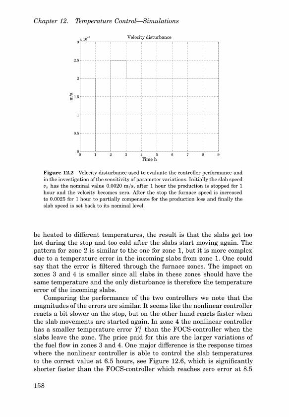
Chapter 12. Temperature Control—Simulations
0 1 2 3 4 5 6 7 8 90
0.5
1
1.5
2
2.5
3x 10
−3
Time h
m/s
Velocity disturbance
Figure 12.2 Velocity disturbance used to evaluate the controller performance andin the investigation of the sensitivity of parameter variations. Initially the slab speedvs has the nominal value 0.0020 m/s, after 1 hour the production is stopped for 1hour and the velocity becomes zero. After the stop the furnace speed is increasedto 0.0025 for 1 hour to partially compensate for the production loss and finally theslab speed is set back to its nominal level.
be heated to different temperatures, the result is that the slabs get toohot during the stop and too cold after the slabs start moving again. Thepattern for zone 2 is similar to the one for zone 1, but it is more complexdue to a temperature error in the incoming slabs from zone 1. One couldsay that the error is filtered through the furnace zones. The impact onzones 3 and 4 is smaller since all slabs in these zones should have thesame temperature and the only disturbance is therefore the temperatureerror of the incoming slabs.
Comparing the performance of the two controllers we note that themagnitudes of the errors are similar. It seems like the nonlinear controllerreacts a bit slower on the stop, but on the other hand reacts faster whenthe slab movements are started again. In zone 4 the nonlinear controllerhas a smaller temperature error Y j
i than the FOCS-controller when theslabs leave the zone. The price paid for this are the larger variations ofthe fuel flow in zones 3 and 4. One major difference is the response timeswhere the nonlinear controller is able to control the slab temperaturesto the correct value at 6.5 hours, see Figure 12.6, which is significantlyshorter faster than the FOCS-controller which reaches zero error at 8.5
158

12.5 Production
0 2 4 6 80
500
1000
1500
2000m
3 /h
Ff1
0 2 4 6 80
200
400
600
800
1000
m3 /h
Ff2
0 2 4 6 80
100
200
300
400
Time h
m3 /h
Ff3
0 2 4 6 80
50
100
150
Time h
m3 /h
Ff4
Figure 12.3 Effect of the velocity disturbance shown in Figure 12.2 on the fuelflows Fj
f of the four zones when the slab temperatures are controlled using thePI-controller. Note the oscillations, which are the result of cold slabs entering thezone and hot slabs leaving the zone.
hours, see Figure 12.4.
12.5 Production
We will now investigate the controller performance with varying slablengths and the recorded slab velocity from the pig runs. The first step isto take a look on the slab speed which is shown in Figure 12.7. We seethat the slab movements are close to pulses and it is difficult to use thissignal for the furnace temperature feedforward. It is therefore chosen tofilter the velocity by using a FIR-filter computing the mean velocity overthe last 30 minutes, see Figure 12.7.
Looking at the slab temperatures in Figures 12.8 and 12.12 and theresults in Table 12.1 we note that the slab temperatures becomes too largefor the FOCS-controller. The final temperatures are also more accurate
159
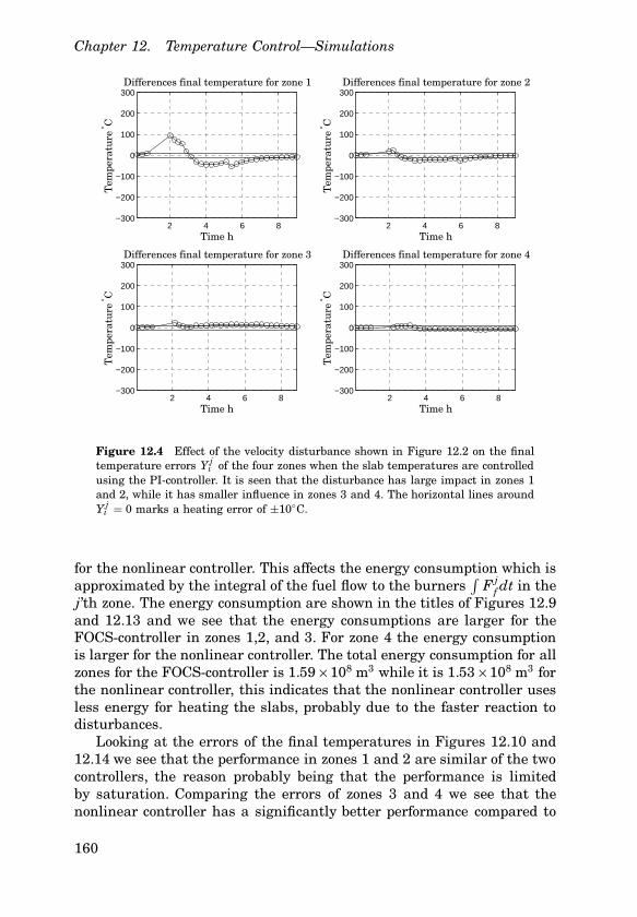
Chapter 12. Temperature Control—Simulations
2 4 6 8−300
−200
−100
0
100
200
300
Time h
Tem
pera
ture
° C
Differences final temperature for zone 1
2 4 6 8−300
−200
−100
0
100
200
300
Time h
Tem
pera
ture
° C
Differences final temperature for zone 2
2 4 6 8−300
−200
−100
0
100
200
300
Time h
Tem
pera
ture
° C
Differences final temperature for zone 3
2 4 6 8−300
−200
−100
0
100
200
300
Time h
Tem
pera
ture
° C
Differences final temperature for zone 4
Figure 12.4 Effect of the velocity disturbance shown in Figure 12.2 on the finaltemperature errors Y j
i of the four zones when the slab temperatures are controlledusing the PI-controller. It is seen that the disturbance has large impact in zones 1and 2, while it has smaller influence in zones 3 and 4. The horizontal lines aroundY j
i � 0 marks a heating error of ±10○ C.
for the nonlinear controller. This affects the energy consumption which isapproximated by the integral of the fuel flow to the burners
∫F j
f dt in thej’th zone. The energy consumption are shown in the titles of Figures 12.9and 12.13 and we see that the energy consumptions are larger for theFOCS-controller in zones 1,2, and 3. For zone 4 the energy consumptionis larger for the nonlinear controller. The total energy consumption for allzones for the FOCS-controller is 1.59�108 m3 while it is 1.53�108 m3 forthe nonlinear controller, this indicates that the nonlinear controller usesless energy for heating the slabs, probably due to the faster reaction todisturbances.
Looking at the errors of the final temperatures in Figures 12.10 and12.14 we see that the performance in zones 1 and 2 are similar of the twocontrollers, the reason probably being that the performance is limitedby saturation. Comparing the errors of zones 3 and 4 we see that thenonlinear controller has a significantly better performance compared to
160

12.5 Production
0 2 4 6 80
500
1000
1500
2000m
3 /h
Ff1
0 2 4 6 80
200
400
600
800
1000
m3 /h
Ff2
0 2 4 6 80
100
200
300
400
Time h
m3 /h
Ff3
0 2 4 6 80
50
100
150
Time h
m3 /h
Ff4
Figure 12.5 Effect of the velocity disturbance shown in Figure 12.2 on the fuelflows Fj of the four zones when the slab temperatures are controlled using theenthalpy controller. Note the oscillations, which are the result of cold slabs enteringthe zone and hot slabs leaving the zone. The reason for the flow of zone 3 being zeromost of the time is that the slabs already are heated to the specified temperaturein zone 2 and the working point for the linear model for the furnace temperature.This figure should be compared with Figure 12.3.
the FOCS-controller. The mean value of the heating error in zone 4 isµ 4 � −8.22 for the FOCS-controller and µ 4 � 1.52 for the nonlinearcontroller while the standard deviation for the nonlinear controller inzone 4 is less than 50% compared to the standard deviation for the FOCS-controller. The price paid is again larger variations of the fuel flows F j
f asseen from Figures 12.9 and 12.13.
The FEM simulations of the critical slab with the shortest residencetime in the furnace are shown in Figures 12.11 and 12.15 show that thecritical slab heated using the FOCS-controller has a heating error of −6 ○ Cand a temperature gradient ∆T of 77.7 ○ C, while the critical slab heatedusing the nonlinear controller has a temperature error of 7 ○ C and a tem-perature gradient ∆T of 74.9 ○ C. We conclude that the performance in thisdirection is equal for the FOCS-controller and the nonlinear controller.
161

Chapter 12. Temperature Control—Simulations
2 4 6 8−300
−200
−100
0
100
200
300
Time h
Tem
pera
ture
° C
Differences final temperature for zone 1
2 4 6 8−300
−200
−100
0
100
200
300
Time h
Tem
pera
ture
° C
Differences final temperature for zone 2
2 4 6 8−300
−200
−100
0
100
200
300
Time h
Tem
pera
ture
° C
Differences final temperature for zone 3
2 4 6 8−300
−200
−100
0
100
200
300
Time h
Tem
pera
ture
° C
Differences final temperature for zone 4
Figure 12.6 Effect of the velocity disturbance shown in Figure 12.2 on the finaltemperature errors Y j
i of the four zones when the slab temperatures are controlledusing the enthalpy controller. It is seen that the disturbance has large impact inzones 1 and 2, while it has smaller influence in zones 3 and 4. The horizontal linesaround Y j
i � 0 marks a heating error of ±10○ C. This figure should be comparedwith Figure 12.4.
The temperature gradient will be discussed further in Chapter 13.It hasnot been possible to detect any influence of the varying slab length, theconclusion here is that this is handled well by the normalization of theerror weights rj
L and rjV .
162
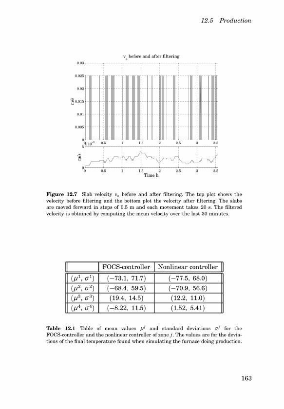
12.5 Production
0 0.5 1 1.5 2 2.5 3 3.50
0.005
0.01
0.015
0.02
0.025
0.03
vs before and after filtering
m/s
0 0.5 1 1.5 2 2.5 3 3.50
5x 10
−3
Time h
m/s
Figure 12.7 Slab velocity vs before and after filtering. The top plot shows thevelocity before filtering and the bottom plot the velocity after filtering. The slabsare moved forward in steps of 0.5 m and each movement takes 20 s. The filteredvelocity is obtained by computing the mean velocity over the last 30 minutes.
FOCS-controller Nonlinear controller
(µ 1, σ 1) (−73.1, 71.7) (−77.5, 68.0)(µ 2, σ 2) (−68.4, 59.5) (−70.9, 56.6)(µ 3, σ 3) (19.4, 14.5) (12.2, 11.0)(µ 4, σ 4) (−8.22, 11.5) (1.52, 5.41)
Table 12.1 Table of mean values µ j and standard deviations σ j for theFOCS-controller and the nonlinear controller of zone j . The values are for the devia-tions of the final temperature found when simulating the furnace doing production.
163

Chapter 12. Temperature Control—Simulations
0 2 4 6 8 10 12 14 16 180
200
400
600
800
1000
1200
Time h
Tem
pera
ture
° C
Simulation of slab temperature control, PI−controller
Figure 12.8 Slab temperatures T ji controlled by the FOCS-controller as they are
transported through the furnace. Note the reactions during and right after the stopbeginning around t � 4 h.
164

12.5 Production
0 5 10 15
1200
1220
1240
1260
1280
1300
1320
Tem
pera
ture
° C
Tm1
0 5 10 150
500
1000
1500
2000
Flo
w m
3 /h
Ff1, ∫ F
f1dt = 1.11e+08
0 5 10 15
1240
1260
1280
1300
1320
Tem
pera
ture
° C
Tm2
0 5 10 150
200
400
600
800
1000
Flo
w m
3 /h
Ff2, ∫ F
f2dt = 3.18e+07
0 5 10 15
1260
1280
1300
1320
Tem
pera
ture
° C
Tm3
0 5 10 150
100
200
300
400
Time h
Flo
w m
3 /h
Ff3, ∫ F
f3dt = 1.46e+07
0 5 10 15
1200
1250
1300
Tem
pera
ture
° C
Tm4
0 5 10 150
50
100
150
Time h
Flo
w m
3 /h
Ff4, ∫ F
f4dt = 1.49e+06
Figure 12.9 Fuel flows Fjf and furnace temperatures T j
m when the slab tempera-tures are controlled using the FOCS-controller.
165
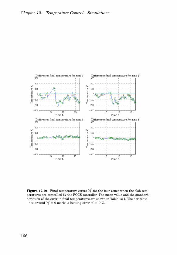
Chapter 12. Temperature Control—Simulations
5 10 15−300
−200
−100
0
100
200
300
Time h
Tem
pera
ture
° C
Differences final temperature for zone 1
5 10 15−300
−200
−100
0
100
200
300
Time h
Tem
pera
ture
° C
Differences final temperature for zone 2
5 10 15−300
−200
−100
0
100
200
300
Time h
Tem
pera
ture
° C
Differences final temperature for zone 3
5 10 15−300
−200
−100
0
100
200
300
Time h
Tem
pera
ture
° C
Differences final temperature for zone 4
Figure 12.10 Final temperature errors Y ji for the four zones when the slab tem-
peratures are controlled by the FOCS-controller. The mean value and the standarddeviation of the error in final temperatures are shown in Table 12.1. The horizontallines around Y j
i � 0 marks a heating error of ±10○ C.
166
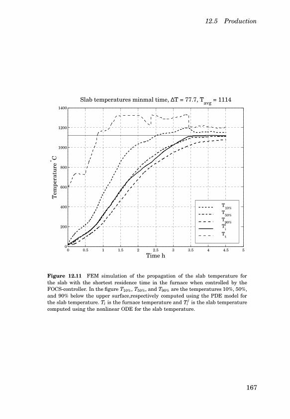
12.5 Production
0 0.5 1 1.5 2 2.5 3 3.5 4 4.5 50
200
400
600
800
1000
1200
1400
Slab temperatures minmal time, ∆T = 77.7, Tavg
= 1114
Time h
Tem
pera
ture
° C
T10%
T50%
T90%
Tij
Tt
Figure 12.11 FEM simulation of the propagation of the slab temperature forthe slab with the shortest residence time in the furnace when controlled by theFOCS-controller. In the figure T10%, T50%, and T90% are the temperatures 10%, 50%,and 90% below the upper surface,respectively computed using the PDE model forthe slab temperature. Tt is the furnace temperature and T j
i is the slab temperaturecomputed using the nonlinear ODE for the slab temperature.
167

Chapter 12. Temperature Control—Simulations
0 2 4 6 8 10 12 14 16 180
200
400
600
800
1000
1200
Time h
Tem
pera
ture
° C
Simulation of slab temperature control, Variable enthalp.
Figure 12.12 Slab temperatures T ji controlled by the nonlinear controller as they
are transported through the furnace. Note the reactions during the stop beginningat t � 4 h. This figure should be compared with Figure 12.8.
168

12.5 Production
0 5 10 15
1200
1250
1300
Tem
pera
ture
° C
Tm1
0 5 10 150
500
1000
1500
2000
Flo
w m
3 /h
Ff1, ∫ F
f1dt = 1.07e+08
0 5 10 15
1240
1260
1280
1300
1320
1340
Tem
pera
ture
° C
Tm2
0 5 10 150
200
400
600
800
1000
Flo
w m
3 /h
Ff2, ∫ F
f2dt = 3.13e+07
0 5 10 15
1260
1280
1300
1320
Tem
pera
ture
° C
Tm3
0 5 10 150
100
200
300
400
Time h
Flo
w m
3 /h
Ff3, ∫ F
f3dt = 1.24e+07
0 5 10 151200
1220
1240
1260
1280
1300
Tem
pera
ture
° C
Tm4
0 5 10 150
50
100
150
Time h
Flo
w m
3 /h
Ff4, ∫ F
f4dt = 2.4e+06
Figure 12.13 Fuel flows Fjf and furnace temperatures T j
m when the slab temper-atures are controlled using the nonlinear controller. This figure should be comparedwith Figure 12.9.
169

Chapter 12. Temperature Control—Simulations
5 10 15−300
−200
−100
0
100
200
300
Time h
Tem
pera
ture
° C
Differences final temperature for zone 1
5 10 15−300
−200
−100
0
100
200
300
Time h
Tem
pera
ture
° C
Differences final temperature for zone 2
5 10 15−300
−200
−100
0
100
200
300
Time h
Tem
pera
ture
° C
Differences final temperature for zone 3
5 10 15−300
−200
−100
0
100
200
300
Time h
Tem
pera
ture
° C
Differences final temperature for zone 4
Figure 12.14 Final temperature errors Y ji for the four zones when the slab tem-
peratures are controlled by the nonlinear controller. The mean value and the stan-dard deviation of the error in final temperatures are shown in Table 12.1. Thehorizontal lines around Y j
i � 0 marks a heating error of ±10○ C. This figure shouldbe compared with Figure 12.10.
170

12.5 Production
0 0.5 1 1.5 2 2.5 3 3.5 4 4.5 50
200
400
600
800
1000
1200
1400
Slab temperatures minmal time, ∆T = 74.9, Tavg
= 1127
Time h
Tem
pera
ture
° C
T10%
T50%
T90%
Tij
Tt
Figure 12.15 FEM simulation of the propagation of the slab temperature for theslab with the shortest residence time in the furnace when controlled by the nonlinearcontroller. In the figure T10%, T50%, and T90% are the temperatures 10%, 50%, and90% below the upper surface,respectively computed using the PDE model for theslab temperature. Tt is the furnace temperature and T j
i is the slab temperaturecomputed using the nonlinear ODE for the slab temperature. This figure should becompared with Figure 12.11.
171

Chapter 12. Temperature Control—Simulations
Conclusions
We have now investigated the performance and robustness of the FOCS-controller and the nonlinear controller for the slab temperatures. Therobustness is investigated by simulating the 16 cases found by varying thefour parameters of the model by ±20% for each controller. The parametervariations do not affect the dynamics of the response significantly and wetherefore conclude that the system is not especially sensitive to parametervariations.
The performances of the controllers are investigated by first subjectingthe four zones to the standard velocity disturbance and simulating thesystem with a slab speed obtained from the pig runs. The responses tothe standard disturbance show that the slab temperature error of zones 1and 2 are large, while the errors of zones 3 and 4 are small. The magnitudeof the errors are the same for the two controllers, but the response speedof the nonlinear controller is superior to the response speed of the linearcontroller. The price paid is larger variations of the control signal for thenonlinear controller.
The performances of the controllers when subjected to real slab speedsand varying slab lengths show that both controllers are able to control theslab temperatures with good accuracy. The performances of the two con-trollers are similar for zones 1 and 2, while the nonlinear controller issuperior for zones 3 and 4. The simulations also indicate that the en-ergy consumption for the nonlinear controller is smaller than the energyconsumption of the FOCS-controller. The FEM simulations show that thetemperature gradients for a critical slab heated using the two controlalgorithms are practically equal.
172
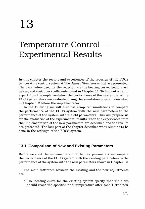
13
Temperature Control—Experimental Results
In this chapter the results and experiences of the redesign of the FOCStemperature control system at The Danish Steel Works Ltd. are presented.The parameters used for the redesign are the heating curve, feedforwardtables, and controller coefficients found in Chapter 11. To find out what toexpect from the implementation the performance of the new and existingFOCS parameters are evaluated using the simulation program describedin Chapter 12 before the implementation.
In the following we will first use computer simulations to comparethe performance of the FOCS system with the new parameters to theperformance of the system with the old parameters. This will prepare usfor the evaluation of the experimental results. Then the experiences fromthe implementation of the new parameters are described and the resultsare presented. The last part of the chapter describes what remains to bedone in the redesign of the FOCS system.
13.1 Comparison of New and Existing Parameters
Before we start the implementation of the new parameters we comparethe performance of the FOCS system with the existing parameters to theperformance of the system with the new parameters shown in Chapter 12.
The main difference between the existing and the new adjustmentsare
• The heating curve for the existing system specify that the slabsshould reach the specified final temperature after zone 1. The new
173

Chapter 13. Temperature Control—Experimental Results
0 5 10 15
1200
1250
1300
Tem
pera
ture
° C
Tm1
0 5 10 150
500
1000
1500
2000
Flo
w m
3 /h
Ff1, ∫ F
f1dt = 1.11e+08
0 5 10 15
1240
1260
1280
1300
1320
1340
Tem
pera
ture
° C
Tm2
0 5 10 150
200
400
600
800
1000
Flo
w m
3 /h
Ff2, ∫ F
f2dt = 3.17e+07
0 5 10 15
1250
1260
1270
1280
1290
Tem
pera
ture
° C
Tm3
0 5 10 150
100
200
300
400
Time h
Flo
w m
3 /h
Ff3, ∫ F
f3dt = 4.42e+05
0 5 10 15
1200
1250
1300T
empe
ratu
re ° C
Tm4
0 5 10 150
50
100
150
Time h
Flo
w m
3 /h
Ff4, ∫ F
f4dt = 5.78e+05
Figure 13.1 Fuel flows Fjf and furnace temperatures T j
m when the slab tempera-tures are controlled using the PI controller with the old parameters, heating curve,and feedforward tables. This figure should be compared with Figure 12.9.
heating curve specifies that this should happen after zone 2, seeSection 11.2.
• The existing feedforward tables specifies almost identical tempera-tures for the different speeds. The new feedforward tables containsignificantly different zone temperatures for the specified nominalspeeds.
• Comparing the new and existing controller coefficients we see that
174

13.1 Comparison of New and Existing Parameters
5 10 15−300
−200
−100
0
100
200
300
Time h
Tem
pera
ture
° C
Differences final temperature for zone 1
5 10 15−300
−200
−100
0
100
200
300
Time hT
empe
ratu
re ° C
Differences final temperature for zone 2
5 10 15−300
−200
−100
0
100
200
300
Time h
Tem
pera
ture
° C
Differences final temperature for zone 3
5 10 15−300
−200
−100
0
100
200
300
Time h
Tem
pera
ture
° C
Differences final temperature for zone 4
Figure 13.2 Final temperature errors Y ji for the four zones when the slab tem-
peratures are controlled by PI controller with the old parameters, heating curve andfeedforward tables. In the following we have µ j and σ j as the mean value and thestandard deviation of the error for zone j respectively. The results are µ1 � −67.2,σ 1 � 88.0, µ2 � −69.1, σ 2 � 73.0, µ3 � −19.9, σ 3 � 27.7, µ4 � −33.2, σ 4 � 17.7.The horizontal lines around Y j
i � 0 marks a heating error of ±10○ C. This figureshould be compared with Figure 12.10 and Table 12.1.
the new proportional gain is a factor 2 higher than the existing gainsand that the new integral gains are more than a factor 10 lower thanthe existing ones.
The results of the simulations are shown in Figures 13.1 and 13.2.
175

Chapter 13. Temperature Control—Experimental Results
Comparing Figures 13.1 and 13.2 for the existing controller parametersto Figures 12.9 and 12.10 for the new parameters we see that the errors forthe new parameters are significantly smaller than with the existing ones.This is a result of the new feedforward tables and controller coefficients—other simulations show that the existing coefficients results in a poorlydamped response. The later heating due to the new heating curve willresult in a larger temperature gradient, but the FEM simulations indi-cate that it will only yield an increase of approximately 2 ○ C which is notconsidered as a significant change. The total energy consumption of allfour zones is 1.44�108 m3 is significantly lower than the FOCS-controllerwith the new parameters, but note that slab temperatures of zones 3 and4 are significantly lower than specified for the FOCS-controller with theold settings.
13.2 Results and Experiences
Several new experiences were gained when the new parameters were im-plemented. First of all the heating curve is very critical. Three differentheating curves have been implemented. The two first heating curves end-ing after zone 3 and in the middle of zone 3 was implemented before theheating curve presented in Chapter 11 but none of them worked well. Thisindicates that the present heating curve is the limit of what is feasiblefor proper furnace operation.
During the experiments the author realized that the furnace was oper-ated partially as a batch furnace. The reason for this practice is that thefurnace no. 1, a pusher furnace with smaller capacity, can only be oper-ated 15 minutes consecutive minutes every hour, which leaves 45 minutesto operation of furnace no. 2.
The result of this practice is that furnace no. 2 is operated at an el-evated speed for approximately 45 minutes and then rests for approxi-mately 15 minutes. The furnace will only be able to deliver hot slabs atthe elevated speed if the slabs of zones 3 and 4 are at the specified tem-perature when the furnace operation starts after the break. The fact thatthe capacities of zones 3 and 4 are small compared to zones 1 and 2 am-plifies this effect. This is one of the explanations for why the old heatingcurve ends after zone 1 and why the author was forced to adjust the newheating curve to end after zone 2, in practice zones 1, 2, and 3 are usedas buffers of hot steel at high slab speeds. Zone 3 is then used as the lastresort if the slabs fail to follow the heating curve due to a too large slabspeed.
It is not possible for the furnace to heat the slabs at the average speedas specified by either the old or the new heating curve. Actually, the heat-
176

13.2 Results and Experiences
ing curve is computed using an average residence time of 6.4 hours, seeSection 11.2. This is done to ensure that a buffer of hot slabs is createdwhenever the furnace is stopped.
When implementing the feedforward tables the temperatures of zones 3and 4 were adjusted to obtain a higher furnace temperature. The adjust-ment was done to obtain a larger furnace pressure in the end of the fur-nace, which is an advantage according to the operators’ experience. Thisis in good agreement with the heat losses from the slab bottom surface inthe last part of the furnace described in Section 10.2.
Using the latest pig runs a systematic error of −20 ○ C was found in thefinal temperature of the FOCS system and the desired temperature wastherefore adjusted form 1120 ○ C to 1140 ○ C to counteract this offset. Thecontrol algorithm was furthermore modified to use the center temperaturefor temperature control instead of the mean temperature, since the pigruns showed that the latter value is not correct in the first part of theheating interval.
When implementing the controller parameters the author realized thatcoupling between slab temperature and furnace temperature is significantwhen cold slabs enter the zone. This was seen from the fact that if zone 1reacted too late, when cold slabs entered the zone, it was not possible toobtain a proper zone temperature even at full fuel flow. The result wasimproper heating of the slabs. Since the coupling between slab tempera-ture and zone temperature is not included in the model this problem wasnot revealed by the simulations. The operators were aware of this factand complained about the reaction with the old settings of the controlsystem, which after a stop first reacted when zone 1 were half filled withcold slabs.
The reason for the delayed response of zone 1 was that the slab temper-ature controller was allowed to reduce the furnace temperature specifiedby the feedforward tables by 100 ○ C when computing the set point for thefurnace temperature controller. Due to the batch oriented operation ofthe furnace the delay temperatures are kept high to ensure heating ofthe slabs during the stops. The result was that the slab temperature con-troller reduced the furnace temperature down to its lowest permissiblelimit and when cold slabs entered the zone the integral part kept downthe furnace temperature reference until the error went below zero—whichoccurred when the zone was half filled with cold slabs. This is probably thereason for the old heating curve being rather extreme, since this ensureshot slabs despite the slow reaction of the slab temperature controller ofzone 1. The reaction of the other furnace zones are of less importance sincethey are shorter and have smaller capacity, and therefore the reaction ofzone 1 is critical compared to the reaction of the other furnace zones.
When the new parameters were implemented the lower output limit of
177

Chapter 13. Temperature Control—Experimental Results
the slab temperature controller was adjusted form −100 ○ C to −60 ○ C andthis, together with the new controller parameters with a much smallerintegral gain and a double as large proportional gain yielded an instan-taneous reaction of zone 1 when cold slabs entered the zone. Note thatthe faster behavior of the controller was predicted by the simulations ofthe furnace operation. However, for zone 3 we decreased the maximal per-mitted adjustment from −50 ○ C to −20 ○ C and increased the integral timefrom approximately 500 s to 2500 s to obtain an immediate reaction whencold slabs entered the zone despite the other slabs in the zone being toohot. This is similar to the desired control action of zone 1.
The faster response of the slab temperature control system made itpossible to use the new heating curve, which results in a later heatingand therefore ought to lead to a smaller energy consumption. The slabtemperatures follow the heating curve better than before and the temper-atures after a stop are now closer to the heating curve than before. At thesame time the operators are now satisfied with the reaction of the furnacecontrol system and the furnace capacity is increased.
It is unfortunately hard to obtain dynamic plots from the FOCS sys-tem, but it is possible to obtain slab temperatures, slab weight, and dis-charge time from the production control systems. The result of the exper-iments are shown in Figures 13.3, 13.4, and 13.5.
The plot of the slab temperatures at time for discharge in Figure 13.3shows that the mean temperature has not been affected significantly bythe experiments, the reasons for the rather large value (approximately1160 ○ C) is a systematic error of 20 ○ C of the slab temperature calculationand the high furnace temperatures in zones 3 and 4 to ensure properfurnace pressure.
The temperature gradients shown in Figure 13.4 shows that the gra-dients has been large at two instants in February 1999. This correspondswith the two non optimal heating curves mentioned in the beginning ofthis section. Note that the temperature now are at the previous level,despite the later heating curve.
The plot of the discharged tons per day from furnace no. 2 shows a sig-nificant increase of discharged tons in the beginning of March 1999. Con-sidering the transient of the filter this corresponds well with the time forthe implementation new heating curve and controller coefficients, whichtook place between March 4th and March 11th. Before the adjustmentsthe production level is between 1350 tons/day and 1700 tons/day and af-ter the adjustments it is increased to lie between 1550 tons/day and 1900tons/day. Bearing in mind the short time interval for evaluation of theperformance this indicates an increase in productivity of approximately10%.
In 1998 the average natural gas consumption was 37.3 m3/ton, in
178
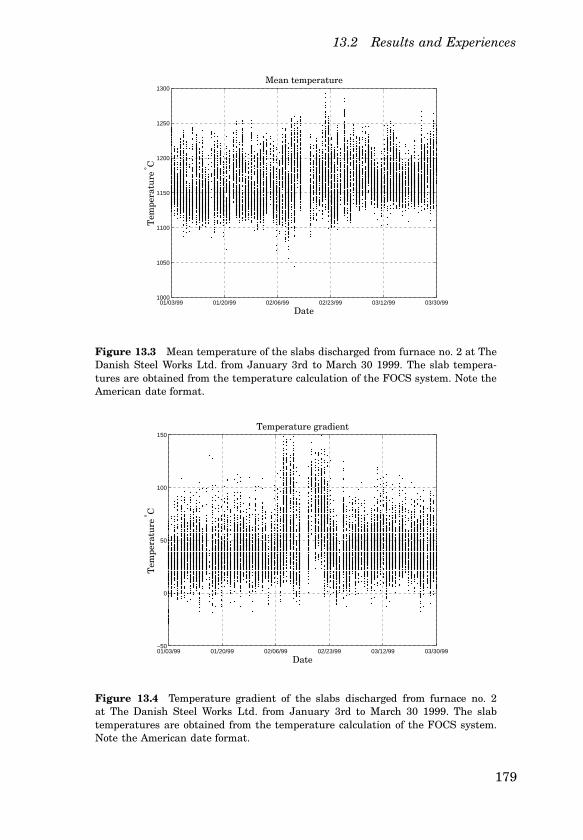
13.2 Results and Experiences
01/03/99 01/20/99 02/06/99 02/23/99 03/12/99 03/30/991000
1050
1100
1150
1200
1250
1300Mean temperature
Tem
pera
ture
° C
Date
Figure 13.3 Mean temperature of the slabs discharged from furnace no. 2 at TheDanish Steel Works Ltd. from January 3rd to March 30 1999. The slab tempera-tures are obtained from the temperature calculation of the FOCS system. Note theAmerican date format.
01/03/99 01/20/99 02/06/99 02/23/99 03/12/99 03/30/99−50
0
50
100
150Temperature gradient
Tem
pera
ture
° C
Date
Figure 13.4 Temperature gradient of the slabs discharged from furnace no. 2at The Danish Steel Works Ltd. from January 3rd to March 30 1999. The slabtemperatures are obtained from the temperature calculation of the FOCS system.Note the American date format.
179

Chapter 13. Temperature Control—Experimental Results
01/03/99 01/20/99 02/06/99 02/23/99 03/12/99 03/30/99
900
1000
1100
1200
1300
1400
1500
1600
1700
1800
1900
Tons per day
Ton
s
Date
Figure 13.5 Slab weight per day discharged from furnace no. 2 at The DanishSteel Works Ltd. from January 3rd to March 30 1999. The data are filtered using aFIR filter computing the mean value over 7 days. Note the American date format.
January 1999 it was 42.2 m3/ton, in February 1999 it was 38.1 m3/ton,and in March 1999 it was 36.3 m3/ton. The author has been warnedthat the energy consumption of the furnace varies considerably and wetherefore only dare to conclude that the new settings of the FOCS systemnot has caused the energy consumption to increase drastically.
13.3 What Is Left?
At the time being (April 1999) it still remains to adjust the heating strat-egy for 200 mm slabs, which has not been discussed, the reason beingthat the heating of the 260 mm slabs is the critical case with respect tofurnace capacity. The strategy with for the 200 mm slabs should be coordi-nated with the strategy for the 260 mm slabs, to obtain a unified heatingstrategy for the two slab thicknesses.
Another thing which remains to be tuned is the delay strategies. Herethe solution to the differential equation for the heating curve (11.4) forvs0 � 0 can be used for obtaining the temperatures necessary to keep theenergy content of the slabs in a zone at a constant level during a stop. Themodels for the furnace temperatures (10.5) can be used for determiningthe zone temperatures for different stop times.
180
13.4 Conclusions
13.4 Conclusions
This chapter contains a description of the implementation of the heatingcurve, feedforward table and controller parameters of the FOCS systemderived in Chapter 11.
Simulation results indicate that the new parameters yields a bettercontrol of the slab temperatures, and this is verified when implementingthe controller coefficients, feedforward tables, and heating curve. The im-plementation, however, also shows that saturation is a problem when coldslabs enter a zone, and this is not revealed by the simulations.
The main result of the implementation is that an increase in the re-sponse speed of zone 1 has resulted in a larger furnace capacity and that amore energy economical heating curve can be used. The furnace operatorsare very satisfied with the new setting and investigations show that themean value and temperature gradient of the slabs are unaffected by thenew settings, but that the furnace capacity seems to have been increasedby approximately 10%. It does not seem like the adjustments have causedthe energy consumption of the furnace to increase.
Remaining work on the adjustment of the FOCS system consists ofdesign of a heating strategy for 200 mm slabs and the tuning of the delaytables used during stops.
181

14
Conclusions
The title of this thesis is "Modeling and Control of Plate Mill Processes"and two such processes have been modeled and controlled, namely therolling mill and the reheat furnace. It is time to give the concluding re-marks on the work done, the obtained results, and the experience gainedduring the work. The chapter will be ended by suggestions for how thework can be continued.
14.1 What Has Been Done?
The two first chapters of the thesis contain a description and analysis ofthe thickness control problem. It is here concluded that the main distur-bances of the system is hardness variations of the plates and the task ofthe thickness control is to keep the plate thickness constant despite thesedisturbances. The classical solution is analyzed and it is concluded thatit can’t handle asymmetric hardness variations and that the estimationof the controlled output introduces stability problems.
In the modeling of the rolling mill a dynamical and multivariablemodel for the thickness control system is derived. The model consistsof a nonlinear model for the hydraulic thickness control actuators and alinear multivariable model for the rolling stand. Since the plate thicknessis not measured during rolling an observer is developed for estimationof the plate thickness. The data collection is carried out by measuringthe key variables of the rolling mill during normal production and thenmeasuring the plate thickness afterwards using a specially designed mea-surement device. Afterwards, the data sets are joined by formulating andsolving an optimization problem. This has given a unique set of data forthe system identification.
The parameters of the model for the rolling mill are found using thecollected data. A set of constant nominal parameters are found for thehydraulic positioning systems, where good agreement between model and
182

14.1 What Has Been Done?
data is obtained. Due to variations in the plate hardness during rollingthere is poor agreement between model and data when time invariantmethods are used for the system identification. The hardness variationsare included in the extra signal available for the observer, and thereforegood agreement between model and data is obtained in this case.
The model is used for designing a nonlinear multivariable thicknesscontrol algorithm. The algorithm is evaluated using computer simulationsand it is found that the new controller is able to handle the asymmetriccase and gives a more accurate thickness control compared to the existingcontrol system. The new control strategy is also found to be stable for therelevant parameter variations. The performance is also acceptable for thedifferent material characteristics of the steel plate found in the systemidentification.
The next part of the thesis concerning slab temperature control isstarted with a description of the reheat furnace where it is concludedthat the main disturbance in the furnace operation is variations of theslab speed. The task of the slab temperature control problem is to ensurea high furnace throughput, and a proper heating quality while keepingthe energy consumption at a minimum.
The data collection for the modeling of the slab temperature is carriedout by the pig, which is a transportable data collection device used formeasuring the slab temperature. While the pig is transported through thefurnace the key furnace variables are collected by the slab temperaturecontrol system. The data are used for identifying three models for thereheat furnace: a linear model for the furnace temperatures, a nonlinearODE model for the slab temperature, and a nonlinear PDE model for theslab temperature distribution. Fair agreement is obtained for the furnacemodel while good agreement is obtained for the two slab temperaturemodels.
A new way of obtaining parameters for the slab temperature controlsystem at The Danish Steel Works Ltd. is described in the thesis. Theslab temperature controller design is started by generating the heatingcurve, which is the slab temperature reference to be followed as the slabsare transported through the furnace. From the heating curve and modelfor the slab temperatures a feedforward table is generated. Furthermore,a first order model for the slab temperatures is generated using lineariza-tion and averaging. The linear model is used for finding parameters forthe PI-regulators controlling the slab temperatures. In the final part ofthe controller design a nonlinear controller is designed using the nonlin-ear ODE for the slab temperatures and it is shown that the nonlinearcontroller is globally asymptotically stable.
The robustness against parameter variations and the performance ofthe linear and nonlinear controller are investigated using computer simu-
183

Chapter 14. Conclusions
lations. The simulations show that none of the controllers are sensitive toparameter variations and that the performance of the nonlinear controlleris superior to the performance of the linear controller. The price paid isfaster variations of the control signal.
The heating curve, feedforward tables, and the controller parametersfound in the design have been implemented in the slab temperature con-trol system at The Danish Steel Works Ltd. The new controller parame-ters have introduced a faster reaction of the furnace when cold slabs arecharged into the furnace after a stop, this leads to increased furnace ca-pacity. The faster reaction also have made a later heating possible whichshould give a reduction in the furnace energy consumption. The furnaceoperators are very satisfied with the performance of the slab temperaturecontrol system and the experimental results indicate a 10% increase infurnace capacity, with unchanged mean temperatures and temperaturegradients. Data from the reheat furnace no. 2 indicate that the energyconsumption has not been increased by the adjustments.
14.2 Results
The results of the work in this thesis are models and controllers for therolling mill and reheat furnace derived using data from the processes atThe Danish Steel Works Ltd.
For the rolling mill the model for the hydraulic systems is nonlinearand is more or less standard, the contribution of the work presented hereis that the model is derived using real data from a rolling mill. The modelfor the mill frame and plate is new and it covers the multivariable natureof rolling process, this model is also derived using real data from the mill.
The thickness controller is a second order multivariable nonlinear con-trol law, able to handle the nonlinearity of the hydraulic systems andasymmetric material conditions of the plates. The controller can be sim-plified to PI controller for a first implementation, if necessary. To have amultivariable controller ready for implementation better data are neededfor a more complete investigation of the multivariable nature of the rollingprocess.
Three models have been derived for the reheat furnace. A simple modelfor furnace temperature and two advanced models for the slab tempera-ture. All models are derived using data from the reheat furnace at TheDanish Steel Works Ltd. The furnace model is used for the computersimulations, and the first model for the slab temperature can be usedfor evaluating the slab center temperature, while the other can be usedfor evaluating the slab temperature gradients, which are important forproper operation of the rolling mill
184

14.3 Future Work
For the slab temperature control problem we have two designs. Thefirst design is a PI-controller with the same structure as the slab tem-perature controller at The Danish Steel Works Ltd. This design has beenverified using experiments. The second design is a nonlinear controllerbased on the nonlinear model for the slab center temperature. If a modelis available this controller is easier to design and the simulations indicatea better performance, but a nonlinear solver is required to implement thecontrol law.
As mentioned in Chapter 1 the reheat furnace and the rolling millare two quite different processes. The author has, however, experiencedseveral factors common for the control of the two processes
• Given proper data and the necessary time it has been possible toderive models with few parameters that give reasonable predictionsof the process behavior. The models have been used for tuning thecontrol algorithms and experimental results from the furnace controlsystem show a performance improvement.
• Even if advanced controllers are used in this thesis it seems likethe existing PI controllers after the optimization does a job almostequally good. This especially seems to be the case with the furnacecontrol system.
• The knowledge gained in the work with the modeling and controlof a process is valuable in other contexts. One example is the dis-covery that the slabs are only cooled in the last part of the furnacewhen deriving the PDE model for the slab temperature and anotherexample is the measurement of the thickness variations introducedby the cold zones of the roller tables of the rolling mill.
As a final comment on the work done it should be mentioned that in thethickness control the main effort lies in the derivation and identificationof the multivariable model for the rolling mill since these models werenot available when the work on the thickness control was started. Theinitial situation for the temperature control problem was that both dataand models already were available for the slab temperature control. Sinceimplementation, and experiments, furthermore, were possible in this casethis is the reason for the controller design being the main subject in theslab temperature control part of the thesis.
14.3 Future Work
If the work presented in this thesis should be continued several openpoints are available for future work
185

Chapter 14. Conclusions
• Improvement of the rolling mill model. The crucial thing hereis to obtain data with better excitation. This could be done by spe-cial experiments and would make a better determination of, for in-stance, the multivariable structure and friction between roll packand rolling stand possible.
• Implementation of simplified thickness control law. Using themean value of the plate thickness the multivariable thickness algo-rithm can be turned into a nonlinear SISO PI-controller. The im-plementation of this controller has been going on for a while, thehardware is implemented an the program is being developed.
• Continuation of work with FOCS system. This work is actuallyalready going on in connection with a project done by MEFOS wherean adaption algorithm for the FOCS temperature estimator will beimplemented at The Danish Steel Works Ltd. . The measurement isobtained from radiation pyrometers near the rolling mill.
• Implementation of a nonlinear slab temperature controller.It seems that the nonlinear controller giver better results and iseasier to design. It would be interesting to implement it and see ifthe controller also works better in practice.
• Implementation of multivariable plate thickness controller.This is planned to be a part of an ECSC project starting medio 1999.The plan is to implement the thickness control law on the rollingmill at The Danish Steel Works Ltd. It is necessary to improve themultivariable models for the rolling mill before the control law isimplemented.
• Development of an advanced furnace model. As pointed outseveral places in the thesis the linear model of the furnace temper-ature could be improved considerably. An important part to includeis the interaction between the furnace temperature and the temper-ature of the slabs.
The author plans continue the work on one or more of the above itemsand hopes that it will be as much fun as doing the work presented in thisthesis.
186

15
Bibliography
ABILDGAARD, O. (1991): Issues in Unified Optimization of Systems andControllers. PhD thesis, Control Engineering Institute, TechnicalUniversity of Denmark.
ANDERSSON, M. (1994): Object-Oriented Modeling and Simulation ofHybrid Systems. PhD thesis, Department of Automatic Control, LundInstitute of Technology.
ASADA, Y. et al. (1986): “New feedforward gauge control method for coldtandem mills.” IFAC Proceedings of the 1986 Automation in MiningMineral and Metal Processing Conference.
ÅSTRÖM, K. J. and P. EYKHOFF (1971): “System identification – a survey.”Automatica, 7, pp. 123 – 162.
ÅSTRÖM, K. J. and B. WITTENMARK (1995): Adaptive control. Addison-Wesley Publishing Company.
ÅSTRÖM, K. J. and B. WITTENMARK (1997): Computer-Controlled Systems,third edition. Information and System Sciences Series. Prentice-Hall.
ATORI, H. et al. (1992): “Application of two-degree-of-freedom controlsystem to automatic gauge control.” American Control Conference.
BAEHR, H. D. and K. STEPHAN (1996): Wärme- und Stoffübertragung, 2edition. Springer Verlag.
BENGTSSON, G. (1994): Manual for µ -controller. First Control Systems AB,Västerås, Sweden.
BRYANT, G. F., P. D. SPOONER, and J.M.CALEY (1975): “Design of tandemmill dynamic control schemes.” Proceedings of the 5th IFAC WorldCongress.
187

Chapter 15. Bibliography
CHOI, S. G., M. A. JOHNSON, and M. J. GRIMBLE (1994): “PolynomialLQG control of back-up-roll eccentricity gauge variations in cold rollingmills.” Automatica, 30:6, pp. 975–992.
CRANDALL, S. H., N. C. DAHL, and T. J. LARDNER (1978): An Introductionto the Mechanics of Solids. McGraw Hill.
CUMMING, I. G. (1972): “On-line identification of a steel mill.” Automatica,8, pp. 531 – 541.
DAVIES, D. A. et al. (1983): “Control of gage, width, profile and shapeon rautatuukki’s 3.6-meter plate mill.” Iron and Steel Engineer,December.
DESOER, C. A. and M. VIDYASAGAR (1975): Feedback Systems: Input-Output Properties. Academic Press.
EDWARDS, W. J. (1978): “Design of entry strip thickness controls fortandem cold mills.” Automatica, 14, pp. 429–441.
EDWARDS, W. J. et al. (1987): “Roll eccentricity control for strip rollingmills.” Proceedings of the IFAC 10th Triennial World Congress.
FERGUSON, J. J. et al. (1986): “Modern hot-strip mill thickness con-trol.” IEEE Transactions on Industry Applications 1986, Septem-ber/October.
FODA, S. and P. AGATHOKLIS (1992): “Control of the metal rolling process. amultidimensional system approach.” Journal of the Franklin Institute,329:2, pp. 317–332.
FONTANA, P., A. BOGGIANO, A. FURINGHETTI, G. CABARAS, and C. A.SIMONCINI (1983): “An advanced computer control system for reheatfurnaces.” Iron and Steel Engineer, pp. 55 – 83.
FUJII, S. and M. SAITO (1975): “A new mathematical model for plate millcontrol.” Proceedings of the 5th IFAC World Congress.
GINZBURG, V. B. (1984): “Dynamic characteristics of automatic controlsystem with hydraulic actuators.” Iron and Steel Engineer.
GOU, R.-M. (1991): “Evaluation of dynamic characteristics of hagc system.”Iron and Steel Engineer, July.
GRIFFITHS, E. (1953): Physical constants of some commercial steels atelevated temperatures. Butterworths Scientific Publications, London,UK.
GRIMBLE, M. J. and M. A. JOHNSON (1988): Optimal Control and StocasticEstimation. Theory and Applications., vol. II, chapter 13.4 GaugeControl and the Back-up Roll Eccentricity Problem. John Wiley & Sons.
188

GUO, R.-M. (1994): “Material damping effect in cold rolling process.” Ironand Steel Engineer, December.
GUSTAVSSON, I. (1975): “Survey of applications of identification in chemicaland physical processes.” Automatica, 11, pp. 3–24.
H. E. PIKE, J. and S. J. CITRON (1970): “Optimization studies of a slabreheating furnace.” Automatica, 6, pp. 41 – 50.
HANSEN, E. B. (1993): Variationsregning (Eng: Calculus of Variations).Polyteknisk Forlag.
HARVEY, C. A. and G. STEIN (1978): “Quadratic weights for asymptoticregulator properties.” IEEE Transactions on Automatic Control, AC-23:3, pp. 378 – 387.
HOLLANDER, F. and S. P. A. ZUURBIER (1982): “Design, development andperformance of on-line computer control in a 3-zone reheating furnace.”Iron and Steel Engineer, January, pp. 44 – 52.
HUZYAK, P. and T. L. GERBER (1984): “Design and application of hydraulicgap control systems.” Iron and Steel Engineer, August.
ISIDORI, A. (1989): Nonlinear Control Systems, second edition. Springer-Verlag.
JOHANSSON, R. (1993): System Modeling and Identification. Prentice Hall.
KAILATH, T. (1980): Linear Systems. Prentice-Hall.
KITAMURA, A. et al. (1987): “Recursive identification technique for rolleccentricity control.” IFAC Proceedings of the 10th Triennial WorldCongress.
KOKAI et al. (1985): “Factors affecting the accuracy of plate tickness andtheir influences on plate flatness.” Transactions ISIJ, 25.
KUSTERS, A. and G. A. J. M. VAN DITZHUIJZEN (1994): “MIMO systemidentification of slab reheating furnace.” Proceedings of the IEEEConference on Control Applications, 3, pp. 1557 – 1563.
LEDEN, B. (1985): “Processtyrning af ämnesvärmningsugnar.” TechnicalReport. MEFOS.
LEDEN, B. (1986): “A control system for fuel optimization of reheatingfurnaces.” Scandinavican Journal of Metallurgy, 15, pp. 16 – 24.
LEDEN, B. (1999): User’s manual STEELTEMP-IE c� . MEFOS, Luleå.
LJUNG, L. (1991): System Identification Toolbox. The MathWorks, Inc.
189

Chapter 15. Bibliography
MEIROVITCH, L. (1980): Computational Methods in Structural Dynamics.Sijthoff & Noordhoff.
MIDDLETON, R. H. and G. G. GOODWIN (1990): Digital Control andEstimation. An Unified Approach., chapter 15 An Industial Case Study.Prentice Hall.
MIZUNO, K. (19??): “Multivariable nonlinear control system design formultistand rolling mill.” Hitachi Review.
MOORE, B. C. (1976): “On the flexibility offered by state feedback inmultivariable system beyond closed loop eigenvalue assignment.”IEEE Transactions on Automatic Control, October, pp. 689 – 692.
NAKAGAWA, S. et al. (1990): “Gauge control system for hot strip finishingmill.” In Proceedings of the IEEE Conference on Decision and Control,vol. 3.
NIJMEIJER, H. and A. VAN DER SCHAFT (1991): Nonlinear Dynamic ControlSystems. Springer-Verlag.
PAUL, F. W. (1975): “A mathematical model for evaluation of hydrauliccontrolled cold rolling mills.” Proceedings of the 5th IFAC WorldCongress.
PEDERSEN, L. M. (1993): “Plate thickness control of hot rolling mills.”Technical Report ISRN LUTFD2/TFRT--7513--SE. Department ofAutomatic Control, Lund Institute of Technology.
PEDERSEN, L. M. (1994): “Identification of hydraulic system on rollingmill.” In Preprints ot the 10th IFAC Symposium on System Identifica-tion, vol. 3, pp. 337 – 342.
PEDERSEN, L. M. (1995a): “Modeling and identification of hot rolling mill.”In Proceedings of 1995 American Control Conference, vol. 5, pp. 3674– 3678.
PEDERSEN, L. M. (1995b): “Multivariable thickness control of a hot rollingmill.” Licentiate Thesis ISRN LUTFD2/TFRT--LUFTD2/TFRT--3214--SE--SE. Department of Automatic Control, Lund Institute of Technol-ogy, Sweden.
PEDERSEN, L. M. (1996): “Multivariable model for a hot rolling mill.” TheControl of Profile and Flatness. The Institute of Materials. For a copyof this reference, please contact the author.
PEDERSEN, L. M. (1998): “Slab temperature control for reheating fur-naces.” Technical Report ISRN LUTFD2/TFRT--LUTFD2/TFRT--7581--SE--SE. Department of Automatic Control, Lund Institute ofTechnology, Sweden.
190

PEDERSEN, L. M. and B. WITTENMARK (1996): “Multivariable controllerdesign for hot rolling mill.” In Proceedings of the 13th Trennial IFACWorld Congress, vol. M, pp. 475 – 480. IFAC.
PEDERSEN, L. M. and B. WITTENMARK (1998a): “Multivariable controllerdesign for hot rolling mill.” IEEE Journal of Control Systems Technol-ogy.
PEDERSEN, L. M. and B. WITTENMARK (1998b): “On the reheat furnacecontrol problem.” In Proceedings of 1998 American Control Conference.
PEDERSEN, L. M. and B. WITTENMARK (1998c): “Optimization of thicknesscontrol system.” In Reglermöte ‘98. Lund.
PEDERSEN, L. M. and B. WITTENMARK (1998d): “Thickness control for aplate mill.” In Automation in Mining, Mineral, and Metal Processing.IFAC.
PEDERSEN, L. M. and B. WITTENMARK (1999): “Development of advancedfurnace control algorithm.” Steel Technology International, pp. 149 –152.
PICHLER, R. and R. LANGER (1989): “Automation concept for the control ofreheating furnaces in rolling mills.” Metallurgical Plant and Technol-ogy, pp. 68 – 75.
RICHTER, F. (1973): Die wichtigsten physikalischen Eigenshaften von52 Eisenwerkstoffen, vol. 8. Verlag Stahleisen M. B. H., Düsseldorf,Germany.
RIXIN, L. and N. BAOLIN (1992): “Mathematical model for dynamicoperation and optimum control of pusher type slab reheating furnace.”Industrial Heating, March, pp. 60 – 62.
ROBERTS, W. L. (1983): Hot Rolling of Steel, vol. 10 of ManufacturingEngineering and Materials Processing. Marcel Dekker.
SAITO, M. et al. (1981): “High-accuracy plate thickness control.” Proceed-ings of the IFAC 8th Triennial World Congress.
SCHURKO, R. J., C. WEINSTEIN, M. K. HANNE, and D. J. PELLECCHIA (1987):“Computer control of reheat furnaces: A comparison of strategies andapplications.” Iron and Steel Engineer, May, pp. 37 – 42.
SIEGEL, R. and J. R. HOWELL (1992): Thermal Radiation Heat Transfer,third edition. Taylor & Francis.
SLOTINE, J.-J. E. and W. LI (1991): Applied Nonlinear Control. PrenticeHall, Inc.
191

Chapter 15. Bibliography
STEIN, G. (1979): “Generalized quadratic weights for asymptotic regula-tor properties.” IEEE Transactions on Automatic Control, AC-24:4,pp. 559 – 565.
STONE, M. D. (1969): “Backup roll bending – for crown and gauge control.”Iron and Steel Engineer, December, pp. 69 – 87.
TEOH, E. K., G. C. GOODWIN, W. J. EDWARDS, and R. G. DAVIES (1984): “Animproved strip thickness controller for a rolling mill.” Proceedings ofthe IFAC 9th Triennial World Congress, vol. 4.
TROSTMANN, E. (1987): Hydraulisk Styring (Eng: Hydraulic Control).Instituttet for Styreteknik, DTH.
WOOD, G. E. et al. (1977): “Mill modulus variation and hysteresis – theireffect on hot strip mill agc.” Iron and Steel Engineer, January.
YAMASHITA, A., Y. MISAKA, N. HASE, and R. TAKAHASHI (1976): “Devel-opment of feedformward agc for 70" hot strip mill at Kashima SteelWorks.” The Sumitomo Search, no. 16, November, pp. 34–39.
YEH, T.-H. et al. (1991): “The development of new backup roll eccentricitycompensation system for the plate mill.” China Steel; Technical Report.
ZELTKALNS, A. et al. (1977): “Force sensing in rolling mills.” Iron and SteelEngineer, January.
192

Notations
A cross sectional area of roll pack, 43Aj system matrix for linearized slab temperature model, 138A1 area in hydraulic system corresponding to p1, 35A2 area in hydraulic system corresponding to p2, 35A3 area in hydraulic system corresponding to p3, 35A4 area of grease piston, 35Ac , Bc , Cc , Dc state space matrices for model for rolling stand, 49B j input matrix for linearized slab temperature model, 138C j output matrix for linearized slab temperature model, 138C j
F furnace temperature controller for zone j, 143C j
S slab temperature controller for zone j, 140Cv transfer function for traditional thickness controller, 26E Young’s modulus for steel, 43Ej vector of enthalpy errors for zone j, 149Ej
i control error for slab i in zone j for nonlinear controller, 146Ej
z thermal energy content of furnace zone j, 112F column vector of heat losses from slab, 129F matrix used for calculating fc, 50F j
f fuel flow of the burners of zone j, 108G diagonal matrix of material properties of slab, 129Gj
F closed loop transfer function for furnace temperature for zone j, 143Gj
S closed loop transfer function for furnace temperature for zone j, 143Gh transfer function for hydraulic systems controlled by Cz, 25Gt transfer function of thickness control system, 27I second moment of area for the work roll, 43K mill spring coefficient, 24K j input matrix for vs for linearized slab temperature model, 138KiF integral gain of furnace temperature controller, 143KiS integral gain of slab temperature controller, 143KpF proportional gain of furnace temperature controller, 143
193

Chapter 15. Notations
KpS proportional gain of slab temperature controller, 143L state feedback matrix for new thickness controller, 85Pj
S averaged system for slab temperatures of zone j, 141Ps supply oil pressure for hydraulic systems, 34Q weighting matrix for states in eigenspace design, 87Q1 flow into left side of oil cylinder, 34Q2 flow into right side of oil cylinder, 34R weighting matrix for control signal in eigenspace design, 87T temperature profile of slab in thickness direction, 102T j state vector of the slab temperatures of zone j, 129Ta furnace atmosphere temperature near slab top surface, 108Tb temperature below slab bottom surface, 102T j
i center temperature of the i’th slab in the j’th zone, 128T j
m furnace zone control temperature of the j’th zone, 101Tr heating curve, 131Ts temperature of furnace surroundings, 104Tt profile of furnace roof temperature, 101T10% slab temperature 10% of slab thickness from top surface, 109T50% slab temperature 50% of slab thickness from top surface, 109T90% slab temperature 90% of slab thickness from top surface, 109Tavg mean temperature of FEM simulations at discharge time, 135T j
f f setpoint from feedforward tables for zone j, 142Tin initial slab temperature, 132T j
m0 nominal furnace temperatures, 132T j
mmax upper furnace temperature limit for zone j, 133T j
mmin lower furnace temperature limit for zone j, 133T j
mr furnace temperature reference for zone j, 131Tout desired final slab temperature, 133U column vector of heat inputs to slab, 129Y j vector of temperature errors for zone j, 138Y j
i temperature error of the i’th slab in zone j, 137∆T temperature gradient of FEM simulations discharge time, 135Γ1, . . . , Γ6 matrices found in the modeling of the rolling stand, 48Φ matrix used for calculating vc and ve, 52β 1, β 2 solution of equation for finding the eigenfunctions φ 1 and φ 2, 46δ Kronecker function, 48ms air mass flow through stack, 104ε function used in state transformation to obtain u, 44ε t it the emissivity of slab top surface, 102η scaling factor for Ps to find p2, 37Gvc transfer function relating thickness difference to position difference,
70
194

ω n undamped natural frequency for Gvc , 82f difference between north and south rolling forces, 73kg steady state gain for Gvc , 82vc half the difference between north and south thickness from model, 70z half the difference between north and south roll positions, 70u approximate solution for u, 46κ time constant for feedback linearized hydraulic systems, 84λ heat conduction coefficient of steel, 102λ b heat conduction coefficient for bottom surface of slab, 102λ j j’th closed loop eigenvalue for rolling stand, 85λ t heat conduction coefficient for top surface of slab, 102µ j mean temperature error for zone j, 167µ distance from plate edge for thicknesses used as controlled outputs,
51ν1, ν2 finite right closed loop eigenvectors for rolling stand, 85ν3, . . . ,ν8 infinite right closed loop eigenvectors for rolling stand, 85ω nh undamped natural frequency for Gh, 82Gvc transfer function relating mean value of thickness to mean value of
positions, 70K estimate of mill deflection coefficient K , 26Ps oil supply pressure transformed to grease side, 36T slab mean temperature, 103T
joutput of averaged system for zone j, 142
Yji averaged temperature error for slab in zone j, 140
ω n undamped natural frequency for Gvc , 82aj pole for averaged linear slab model in zone j, 141b
jgain from furnace temperature for averaged linear slab model in zone
j, 141f mean value of rolling force, 24kg steady state gain for Gvc , 82r reference value for v in traditional control, 26v mean value of north and south plate thickness, 24vc mean value of north and south thickness from model, 70ve estimate of v, 26v−1 mean value of north and south plate thickness for previous pass, 24z mean value of roll positions, 24zh output of linear model for hydraulic system, 25zr reference for z in traditional thickness control, 25φ 1, φ 2 eigenfunctions obtained in the series expansion of u, 45ρ mass density of steel, 43σ j standard deviation of temperature error for zone j, 167σ Boltzmann’s constant, 102
195

Chapter 15. Notations
σ scalar control weight in eigenspace design, 87θ s prediction error for identification of south hydraulic system, 63θ n prediction error for identification of north hydraulic system, 61ϕ variable used in analysis of thickness control system, 27ϖ variation of the outgoing thickness vd relative to the outgoing thick-
ness vd−1, 42T variable used in analysis of slab heating, 103ξ1, . . . , ξ3 variables of model for hydraulic systems, 61ξ n1 , . . . , ξ n3 variables in the model for the north hydraulic system, 60i i times partial derivation with respect to x, 43a pole of linearized equation for T j
i , 138aj
1 parameter for heat transport due to hot air for zone j, 113aj
2 parameter for heat input for burners in zone j, 113aj
3 parameter for heat losses to surroundings for zone j, 113aj
4 parameter for heat loss due to slab transport for zone j, 113aj
5 offset for zone j in furnace temperature model, 113am plate hardness used in traditional modeling, 24ahn1 parameter for flow through servo valve in model for north hydraulic
system, 37ahn2 parameter for oil compressibility in model for north hydraulic sys-
tem, 37ahn3 parameter for leak flow in model for north hydraulic system, 37ahs1 parameter for flow through servo valve in model for south hydraulic
system, 37ahs2 parameter for oil compressibility in model for south hydraulic sys-
tem, 37ahs3 parameter for leak flow in model for south hydraulic system, 37am1 plate hardness, 42am2 plate damping, 42am3 parameter of vr in pd, 42b gain from T j
m of linearized equation for T ji , 138
cj0 integral gain of nonlinear controller for zone j, 147
cj1 proportional gain of nonlinear controller for zone j, 147
cp specific heat capacity of steel, 102e white noise sequence with unit variance, 62ej
L linear error function for zone j, 137ej
V error function for nonlinear controller, 145f heat losses of slab, 129f vector of rolling forces, 23fc vector of forces calculated using model for rolling stand, 50fn rolling force at north side, 23fs rolling force at south side, 23
196

fcn rolling force at north side found using model for the rolling stand, 50fcs rolling force at south side found using model for the rolling stand, 50g material properties for slab, 129h slab thickness, 102hr slab enthalpy reference, 146hs slab enthalpy, 145i integral states for rolling stand, 86k gain from vs of linearized equation for T j
i , 138kp plate hardness, 70l furnace length, 104l width of rolling stand, 43l jz length of zone j, 133
nj number of slabs in zone j, 101o roll eccentricity and ovalness, 24oe estimate of o, 26of e1 , of e2 parameters of observer, 67p differential operator, 25p function for interpolation of thermocouple measurements for obtaining
Tt, 116p1 pressure at left side of oil cylinder, 35p2 pressure at right side of oil cylinder, 35pd pressure distribution across plate width, 40q vector of normal coordinates, 47q vector of normal coordinates, 68q1, q2 the normal coordinates obtained in the series expansion of u, 45qb heat flux through slab bottom surface, 117qj
b heat input from burners in zone j, 112qc heat losses from furnace due to convection, 104qc vector of normal coordinates found using model for rolling stand, 49qj
f heat flow from zone j to zone j − 1, 112
qjl heat transport to slabs and surroundings in zone j, 112
qs heat losses due through stack, 104qj
s heat loss due to movement of slabs in zone j, 112qt heat flux through slab top surface, 117qc1, qc2 normal coordinates found using model for rolling stand, 49qe1, qe2 estimates of q1 and q2 found using observer, 52r vector of thickness references, 86rj
L vector of weight factors used in ejL, 137
rjV vector of weights used in ej
V , 146rd reduction across plate width, 41rl vector containing inputs for feedback linearization, 86rn reference for plate thickness at north edge, 86
197

Chapter 15. Notations
rs reference for plate thickness at south edge, 86rln input for feedback linearization of north hydraulic system, 84rls input for feedback linearization of south hydraulic system, 89t time, 24tj average time for the slab to pass through zone j, 140u heat inputs to slab, 129u new variable for obtaining homogeneous boundary conditions, 44v vector of plate thicknesses, 23vc vector of thicknesses calculated using rolling stand model, 51vd plate thickness across plate width, 40vn plate thickness at north edge, 23vr rotational speed of work roll, 41vs plate thickness at south edge, 23vs slab speed, 101vj
z total air flow out from zone j, 112v−1n ingoing plate thickness at north edge, 24v−1s ingoing plate thickness at south edge, 24vcn thickness at north side calculated using model for the rolling stand,
51vcs thickness at south side calculated using model for the rolling stand,
51vd−1 ingoing thickness across plate width, 41vem center thickness calculated using observer, 75ven plate thickness at the north edge found using observer, 52ves plate thickness at south edge found using observer, 52vs0 nominal slab speed used for generating heating curve, 131vsi nominal speeds of feedforward table, 135w plate width, 24x slab position, horizontal coordinate, 102x position in width direction for rolling mill, 38xj vector of slab positions in zone j, 129x1, . . . , x3 positions for measurement of plate thickness vd, 55xj
i position of the i’th slab in zone j, 111xv vector of servo valve positions, 51xvn position of servo valve glider of north hydraulic system, 34xvrn control signal for north servo valve, 56xvrs control signal for south servo valve, 56xvs position of servo valve glider of south hydraulic system, 51y position in slab thickness direction, vertical coordinate, 102yc states of the model for the rolling stand, 49ye estimate of yc found using observer, 50yn measured output for identification of south hydraulic system, 60ys measured output for identification of north hydraulic system, 63
198

yhn predicted output for identification of south hydraulic system, 61yhs predicted output for identification of north hydraulic system, 63z vector of grease piston positions, 23zd roll position across plate width, 40zn position of north grease piston, 23zs position of south grease piston, 23zt maximal value of position of grease piston, 37zhn north position found using model for hydraulic system, 37zhs south position found using model for hydraulic system, 51
199