THESIS

CLOUD-TO-GROUND LIGHTNING POLARITY AND ENVIRONMENTAL CONDITIONS OVER THE CENTRAL UNITED STATES

Submitted by Christina P. Kalb

Department of Atmospheric Sciences

In partial fulfillment of the requirements For the Degree of Master of Science

Colorado State University Fort Collins, Colorado

Summer 2007

ii

COLORADO STATE UNIVERSITY

DATE WE HEREBY RECOMMEND THAT THE THESIS PREPARED UNDER OUR

SUPERVISION BY CHRISTINA KALB ENTITLED CLOUD-TO-GROUND

LIGHTNING POLARITY AND ENVIRONMENTAL CONDITIONS OVER THE

CENTRAL UNITED STATES BE ACCEPTED AS FULFILLING IN PART

REQUIREMENTS FOR THE DEGREE OF MASTER OF SCIENCE.

Committee on Graduate Work

_________________________________________ William Cotton

_________________________________________ R. Steven Robinson

_________________________________________ Advisor: Steven A. Rutledge

__________________________________________ Richard H. Johnson, Head

iii

ABSTRACT

CLOUD-TO-GROUND LIGHTNING POLARITY AND ENVIRONMENTAL

CONDITIONS OVER THE CENTRAL UNITED STATES

The majority of cloud-to-ground (CG) lightning across the United States lowers

negative charge to the ground. However, recent studies have documented storms that

produce an abundance of positive CG lightning. These positive storms have been shown

to occur in different mesoscale regions on the same days, and in different thermodynamic

environments. This study uses radar data, and CG lightning data, to identify positive and

negative storms that occurred in the region between the Rocky Mountains and the

Mississippi River. The thermodynamic conditions in the environment of these storms are

derived from the Rapid Update Cycle model analysis, where the point nearest to the

storm, in the direction of storm motion was used.

Considerable scatter was present in the final results that limited the extent of the

trends seen. Out of all the variables used, cloud base height, dew point, 850-500 mb

lapse rate, and warm cloud depth showed the most difference between the positive and

negative storms. Positive storms tended to occur with lower cloud base heights, higher

dew points, smaller 850-500 mb lapse rates, and lower warm cloud depths. Little trend

was seen for CAPE, CIN, freezing level, lifted index, mean relative humidity, mid level

iv

relative humidity, precipitable water0-3 km wind shear, 0-6 km wind shear, storm

relative helicity, and θe.

The strength of the differences seen between the positive and negative storms

varies with the choice of percent positive used. Differences between the positive and

negative storms tended to decrease when 10% was chosen (as compared to 30%), but

they increased when 50% was chosen.

Christina P. Kalb Atmospheric Science Department

Colorado State University Fort Collins, CO 80523-1371

Summer, 2007

v

ACKNOWLEDGEMENTS

I thank Professor Steven Rutledge for his advice on this project, as well as the

other members of my committee, Professors William Cotton and R. Steven Robinson.

All members of the CSU radar meteorology group have been helpful and supportive

toward this project. I give special thanks to Rob Cifelli, and Tim Lang for their advice,

and to Paul Hein for his tireless technical support and programming advice.

I would also like to thank Sarah Tessendorf for her advice and comparable work,

and to Kyle Wiens for lightning advice and his help with IDL. Also, thanks to Ian Baker

and Mike Toy for their help using fortran. Dave Ahijevych deserves credit as he

maintains the radar composite data used in this project at the National Center for

Atmospheric Research, and has helped in the processing of the data. In addition, Stan

Benjamin was helpful with his insights to how the RUC data was processed and many

variables were calculated. Thanks to the Atmospheric Radiation Measurement (ARM)

program for maintaining the RUC model analysis used in this study. This research was

supported by the National Science Foundation under grant ATM-0309303, Dynamical,

Microphysical and Electrification Studies in Mid Latitude Convection.

vi

TABLE OF CONTENTS

LIST OF TABLES .......................................................................................................viii

LIST OF FIGURES ....................................................................................................... ix

1 INTRODUCTION............................................................................................... 1

2 BACKGROUND ................................................................................................. 3

a Cloud Electrification and Charge Structure.............................................. 3

b Hypothesis for Positive Cloud-to-Ground Lightning ............................... 4

c Relationships between Positive CG Lightning and the Local

Environment.............................................................................................. 5

d Climatological Relationships Between CG Lightning Polarity

and the Environment ................................................................................. 8

e The Role of Aerosols .............................................................................. 10

f Positive CG Lightning and Severe Storms ............................................. 11

3 DATA AND METHODOLOGY ..................................................................... 19

a Radar Data .............................................................................................. 19

b Cloud-to-Ground Lightning Data ........................................................... 20

c Thermodynamic Data.............................................................................. 21

d Analysis and Statistics ............................................................................ 27

4 RESULTS .......................................................................................................... 37

a All Cases ................................................................................................. 37

7

b. Monthly Results for All Cases................................................................ 39

c Polarity Reversal Cases........................................................................... 41

d Positive and Negative Cases with Hourly RUC Observations ............... 44

e Positive and Negative Cases with Mean and Median RUC

Observations ........................................................................................... 46

f Difference in Means Test........................................................................ 48

g Comparison of 10% as a Positive Polarity Indicator .............................. 49

h Comparison of 50% as a Positive Polarity Indicator .............................. 51

i Sensitivity Test on Errors in RUC Data Points....................................... 53

5 SUMMARY AND CONCLUSIONS ............................................................... 96

REFERENCES............................................................................................................ 101

viii

LIST OF TABLES

3.1 A list of the storms producing less than 30% positive CG lightning.................. 34

3.2 A list of the storms producing greater than 30% positive CG lightning............. 35

3.3 A list of the storms that switch polarity throughout their lifetime...................... 36

4.1 The average RUC values during the positive and negative phases of the

polarity reversal storms....................................................................................... 92

4.2 The average RUC values using all the data for the positive and negative

storms, and whether the difference between them was significant at the 95%

confidence level .................................................................................................. 93

4.3 The same as Table 4.2, except using average RUC values for each storm......... 94

4.4 The same as Table 4.2, except using median RUC values for each storm ......... 95

ix

LIST OF FIGURES

10

2.1 Electrification of Rime from Takahashi (1978).................................................. 13

2.2 The typical charge structure in clouds from Ahrens (2003) ............................... 14

2.3 Diagram of CG lightning polarity as a function of the location of the

surface equivalent potential temperature ridge (from Smith et al. 2000) ........... 15

2.4 The mean annual flash density for the United States (from Orville and

Huffines 2001) .................................................................................................... 16

2.5 The mean annual percentage positive across the United States (from

Orville and Huffines 2001) ................................................................................. 17

2.6 Climatology for wet bulb potential temperature, cloud base height, and a

summary of the locations of positive ground flash storms (from Williams

et al. 2005) .......................................................................................................... 18

3.1 The domain of this study..................................................................................... 28

3.2 Radar reflectivity and nearest RUC point used for 19 May 1998 and 8

June 1998 ............................................................................................................ 29

3.3 Correlations between the RUC model and environmental soundings for

a) surface pressure, b) surface temperature c) surface dew point and

d) surface relative humidity ................................................................................ 30

3.4 Average difference between environmental soundings and the RUC

Model for a) surface pressure, b) surface temperature, c) surface dew

point and d) surface relative humidity ................................................................ 31

11

3.5 Same as Figure 3.3, except for a) upper air temperatures and b) upper

air relative humidity............................................................................................ 32

3.6 Same as Figure 3.4, except for a) upper air temperatures and b) upper

air relative humidity............................................................................................ 33

4.1 Histogram of dew point temperature for all cases .............................................. 56

4.2 Same as Figure 4.1, except for precipitable water .............................................. 57

4.3 Same as Figure 4.1, except for mean relative humidity...................................... 58

4.4 Same as Figure 4.1, except for equivalent potential temperature ....................... 59

4.5 Same as Figure 4.1, except for cloud base height............................................... 60

4.6 Same as Figure 4.1, except for warm cloud depth.............................................. 61

4.7 Same as Figure 4.1, except for convective available potential energy ............... 62

4.8 Same as Figure 4.1, except for convective inhibition......................................... 63

4.9 Same as Figure 4.1, except for 850-500 mb lapse rates...................................... 64

4.10 Same as Figure 4.1, except for 700-500 mb lapse rates...................................... 65

4.11 Same as Figure 4.1, except for freezing level..................................................... 66

4.12 Same as Figure 4.1, except for 0-3 km wind shear............................................. 67

4.13 Same as Figure 4.1, except for 0-6 km wind shear............................................. 68

4.14 Same as Figure 4.1, except for storm relative helicity........................................ 69

4.15 Cloud base height and percent positive over time for a) 13 July 1998

and b) 5 July 2000............................................................................................... 70

4.16 Single variable plots using hourly RUC observations for the positive

12

and negative storms for a) dew point, b) precipitable water, c)

mean relative humidity and d) mid level relative humidity................................ 71

4.17 Same as Figure 4.18, except for a) cloud base height, b) warm

cloud depth, c) freezing level and d) equivalent potential temperature.............. 72

4.18 Same as Figure 4.18, except for a) 850-500 mb lapse rate, b)

700-500 mb lapse rate, c) convective available potential energy, and

d) convective inhibition ...................................................................................... 73

4.19 Same as Figure 4.18, except for a) 0-3 km wind shear, b) 0-6 km

wind shear, c) storm relative helicity and d) lifted index ................................... 74

4.20 Single variable plots using the mean RUC value across each of the

storms for a) dew point b) cloud base height, c) precipitable water,

and d) mid level relative humidity ...................................................................... 75

4.21 Same as Figure 4.22, except for a) cloud base height, b) warm

cloud depth, c) freezing level, and d) equivalent potential temperature............. 76

4.22 Same as Figure 4.22, except for a) 850-500 mb lapse rate, b)

700-500 mb lapse rate, c) convective available potential energy, and

d) convective inhibition ...................................................................................... 77

4.23 Same as Figure 4.22, except for a) 0-3 km wind shear, b) 0-6 km

wind shear, c) storm relative helicity, and d) lifted index .................................. 78

4.24 Single variable plots using hourly RUC data across each storm, and 10

percent as a positive polarity indicator for a) dew point, b) cloud base

13

height, c) warm cloud depth, and d) freezing level............................................. 79

4.23 Same as Figure 4.26, except for a) 850-500 mb lapse rate,

b) 700-500 mb lapse rate, c) storm relative helicity, and d) lifted index............ 80

4.26 Single variable plots using the mean RUC value for each storm and 10

percent as a positive polarity indicator for a) dew point, b) precipitable

water, c) cloud base height, and d) warm cloud depth........................................ 81

4.27 Same as Figure 4.28, except for a) 850-500 mb lapse rate, b)

700-500 mb lapse rate, c) convective available potential energy,

and d) storm relative helicity .............................................................................. 82

4.28 Single variable plots using the median RUC value for each storm and

10 percent as a positive polarity indicator for a) dew point and b) cloud

base height .......................................................................................................... 83

4.29 Single variable plots using hourly RUC data across each storm, and 50

percent as a positive polarity indicator for a) cloud base height, b) dew

point, c) equivalent potential temperature, and d) warm cloud depth ................ 84

4.30 Single variable plots using the mean RUC value for each storm, and 50

percent as a positive polarity indicator for a) cloud base height, b) dew

point, c) freezing level and d) warm cloud depth ............................................... 85

4.31 Same as Figure 4.32, except for a) 850-500 mb lapse rate, b) 700-500

mb lapse rate, c) mid level relative humidity and d) 0-3 km wind

shear .................................................................................................................... 86

14

4.32 Single variable plots using the median RUC value for each storm and

10 percent as a positive polarity indicator for a) 850-500 mb lapse rate,

and b) cloud base height ..................................................................................... 87

4.33 Single variable plot using only those storms with RUC data points

outside the precipitation area for a) dew point, b) precipitable water,

c) mean relative humidity, and d) mid level relative humidity........................... 88

4.34 Same as Figure 4.35, except for a) cloud base height, b) warm

cloud depth, c) freezing level, and d) equivalent potential temperature............. 89

4.35 Same as Figure 4.35, except for a) 850-500 mb lapse rate, b)

700-500 mb lapse rate, c) convective available potential energy, and

d) convective inhibition ...................................................................................... 90

4.36 Same as Figure 4.35, except for a) 0-3 km wind shear, b) 0-6 km

wind shear, c) storm relative helicity, and d) lifted index .................................. 91

15

Chapter 1

Introduction

The majority of cloud-to-ground (CG) lightning produced in thunderstorms across

the United States lowers negative charge to the ground (-CG). However, recent

observations have documented storms that produce an abundance of CG lightning

lowering positive charge to the ground (+CG), most often described as the percentage of

total CG lightning of positive polarity (PPCG). Some of these storms even generate +CG

flash rates and densities of 2 min-1 (Maier and Krider 1982; Peckham et al. 1984;

Williams et al. 1989; Carey and Rutledge 1996; Lang et al. 2000) or 0.1 to 0.5 km-2 h-2

(Stolzenburg 1990), comparable magnitudes to those typically observed for –CG storms

(MacGorman and Buress 1994; Stolzenburg 1994; Carey and Rutledge 1998; Lang and

Rutledge 2002; Carey et al. 2003).

In particular, storms with anomalously large PPCG have a geographic preference

to the central and north plains in the United States. Also, past studies have noted that

severe storms passing through regions that contain similar mesoscale properties on a

given day exhibit similar CG lightning behavior (Branick and Doswell 1992;

MacGorman and Burgess 1994; Smith et al. 2000). Both of these findings suggest that

the occurrence of anomalously high PPCG may be linked to specific mesoscale

environmental conditions. These specific mesoscale conditions likely play a role in

16

influencing the dynamics and microphysics of the storm, which thereby could influence

lightning behavior.

This study seeks to investigate the relationship between the local mesoscale

environment, and single to multi-cell thunderstorms. These include both positive and

negative strike dominated storms, and thunderstorms that switch lightning polarity

throughout their lifetime. Mesoscale convective systems (MCS) are purposely excluded

from this study. This is because MCS’s present a more complicated case, as interactions

between various components of an MCS make their lightning patterns more complicated.

For example, several studies have documented bipolar patterns in leading line trailing

stratiform MCS’s (Rutledge and MacGorman 1988; Rutledge et al. 1990; Engholm et al.

1990; Schuur et al. 1991; Hunter et al. 1992). In these studies, they find positive strikes

tend to occur in the stratiform region, and negative strikes in the leading convective line.

It is these interactions and complexities of MCS’s that we wish to avoid.

17

Chapter 2

Background

a. Cloud electrification and Charge Structure

Currently, there are a variety of hypothesized methods that could produce cloud

electrification, but the most accepted ones involve ice and supercooled liquid water. The

graupel-ice mechanism appears most capable of producing the magnitude of electric

fields found in thunderstorms (MacGorman and Rust 1998). In this mechanism, graupel

pellets grow by riming in a supercooled liquid water environment, and collide with ice

particles to produce charge transfer. Then, the differential fall speeds of the larger

graupel versus the smaller ice crystals produce charge separation where the graupel

would fall to the lower portion of the cloud and the ice particles remain suspended aloft.

The interested reader is referred to MacGorman and Rust (1998) for a complete listing of

hypothesized charge transfer mechanisms.

Several laboratory experiments have investigated the conditions by which

particles obtain charge during collisions using the non-inductive charge transfer

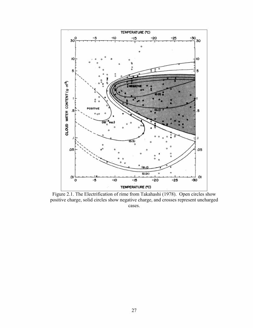
mechanism (Takahashi 1978; Saunders et al 1991; Saunders 1994). Although their results

differ, Takahashi (1978) is most commonly referenced in the literature. His results are

shown in Figure 2.1. The Takahashi lab experiments indicate that at temperatures

warmer than -10 oC, the rimed particle (usually graupel) will charge positively for a large

range of liquid water contents. However, below -10 oC, the sign of the charging depends

18

on liquid water content. At high liquid water contents, and very low liquid water

contents, the rimed particle will charge positively. Otherwise, it is expected to charge

negatively.

In most thunderstorms, the typical electrical structure (Figure 2.2) produced by

charging is either an ordinary dipole or tripole (Williams, 1989). This consists of a

dominant lower main negative charge region with a positive charge region above. In the

tripole, there is also a smaller, more localized, lower positive charge region below the

main negative region, perhaps due to reverse charging on the graupel at low

temperatures. However, more recent studies using balloon electric field measurements

report that outside of the updraft, the electrical structures are more complex, and may

contain up to six layers of charge (Stolzenburg et. al. 1998). There is also a negative

screening layer found at the top of many thunderclouds.

b. Hypothesis for Positive Cloud-to-Ground Lightning

Since most CG strikes are negative, and originate in the main negative charge

region of the thundercloud, how then are positive strikes produced? Williams (2001),

lists a variety of possible mechanisms for positive CG production. The first one is the

tilted dipole hypothesis (Brook et al 1982). In this mechanism, the upper positive charge

region is displaced horizontally by vertical wind shear, and therefore, leaves the upper

positive region exposed to initiate a positive CG. The tilted dipole mechanism is most

likely to occur in shallow convection, such as found in a post-frontal air mass. The

precipitation-unshielding hypothesis (Carey and Rutledge 1998) states that precipitation

carries the lower negative charge out of the storm, which leaves the upper positive charge

available to initiate a positive flash to the ground. Recent studies, however, favor an

19

inverted dipole/tripole hypothesis, with mid-level positive charge being situated between

an upper and lower negative charge layer. During the Severe Thunderstorm

Electrification and Precipitation Study, it was found that in the storms producing mostly

+CG’s, their electrical structure was an inverted dipole (Lang et al 2004; Rust and

MacGorman 2002; Krehbiel et al 2000; Wiens et al. 2005).

c. Relationships between Positive CG Lightning and the Local Environment

Several studies have been performed that examine the local thermodynamic

environment in contrast to the type of CG lightning produced. Smith et al. 2000 studied

surface equivalent potential temperature (θe) during three tornadic outbreaks. A

schematic of their results is shown in Figure 2.3. They found that storms whose CG

lightning polarity was negative tended to form in regions of weak θe gradients and

downstream of a θe maximum. However, storms whose CG lightning polarity was

positive tended to form in regions of strong θe gradients, upstream of a θe ridge. If the

storm moved adjacent to the θe ridge, then it remained positive, however, if it crossed the

ridge, then the storm tended to switch polarity and become negative. They theorized that

the switch in polarity was due to the weakening updrafts and precipitation fallout in the

region of lower θe.

Reap and MacGorman (1998) performed a similar study, but using model output

fields from the National Meteorological Center’s Limited-area Fine-mesh model (LFM)

and the Techniques Development Laboratory’s 10-Level Boundary Layer Model (BLM).

They determined that both positive and negative lightning occurrence showed a good

correlation with boundary layer fields such as relative vorticity, moisture convergence,

and vertical velocity. They also showed that the conditional probability of positive

20

lightning was chiefly determined by the dynamics of the low-level circulation and

moisture flux. However, they found that freezing level height and wind shear were less

significant than the boundary layer fields. In contrast to this study, Levin et al. (1996)

found that in Tel Aviv thunderstorms, the fraction of positive strikes was about 10% for

wind shear values less than 1.0 ms-1 km-1. However if the wind shear exceeded 4.5 ms-1

km-1, the fraction of positive strikes increased to ≥ 40%. Also, Rust et al. (1985), in a

study of positive thunderstorms in Oklahoma and Texas, found that storms with 850-300

mb wind shear greater than 2 x 10-3 s-1 produced mainly positive flashes. Curran and

Rust (1992) found in their study of low precipitation and supercell storms, both the

positive and negative storms contained shear magnitudes greater than the threshold given

by Rust et al. (1985). Therefore, they suggested that a threshold for the magnitude of the

vector-averaged shear may be a necessary, but not sufficient condition for the production

of positive ground flashes.

In their study of severe storms on 2 June 1995, Gilmore and Wicker (2002) found

that storms with the tallest 40 dBZ echoes and largest maximum mesocyclone strength

index (MSI) values remained or became positive strike dominated. Also, when a storm

was negative, it tended to have relatively smaller maximum MSIs and lower (in

elevation) 40 dBZ maximum echo location. From these analyses, they hypothesized that

increased updraft strength (as measured by the maximum 40 dBZ echo height) resulted in

a reduced negative CG rate. If this increase in updraft strength was coupled with a large

increase in liquid water content, then descending graupel could experience higher riming

accretion rates below the charge reversal level which could result in a larger positive

charge region and a predominance of positive CG lightning. However, when the updraft

21

weakens, and liquid water content decreases, a weaker lower positive charge region

results, which should favor negative CG lightning.

Finally, Carey and Buffalo (2006) performed a statistical analysis between many

different thermodynamic parameters and +CG lightning. They found that negative

storms occurred in environments with more moisture (defined by surface dew point,

mean mixing ratio in the lowest 100 mb, and precipitable water), higher mid level relative

humidity, and larger convective inhibition. Positive storms occurred in regions with

higher lifting condensation levels (a measure of cloud base height), lower freezing levels

and therefore, shallower warm cloud depths. They also found that mean lapse rates (850-

500 mb and 700-500 mb) were steeper in positive regions, surface temperatures were

greater, equilibrium level heights were higher (resulting in a larger free convective layer),

and 0-3 km shear was larger. There was no significant difference in convective available

potential energy, lifted index, 0-6 km wind shear, and θe. However, CAPE was larger for

positive storms within the mixed phase region (0-40oC).

Out of all these variables, Carey and Buffalo found the least overlap between

positive and negative storms for LCL and warm cloud depth. They suggest that positive

storms contain specific characteristics. First, higher LCL’s and lapse rates indicate

broader and stronger updrafts, which would allow for less mixing and entrainment

(Williams et al. 2005). Also, reduced warm cloud depths generate larger supercooled

water contents by suppression of coalescence, and larger CAPE between 0 and 40oC,

which would tend to suppress rainout. This would produce higher supercooled water

contents in the mixed phase region, and therefore positive charging of graupel by the

non-inductive charging mechanism. They also note that there is variability in many of

22

these parameters, and on certain days, it may be possible for one to compensate for

another. In addition, Lang and Rutledge (2002) hypothesize that a larger updraft volume

in combination with an elevated charge mechanism would produce more positive CG

lightning due to the greater reservoir of positive charge produced.

d. Climatological Relationships between CG Lightning Polarity and the Environment

A few studies have examined the relationship between CG lightning polarity and

the meteorological environment over the entire United States. Before discussing results

from these studies, the climatology of CG lightning over the United States is first

reviewed. The largest mean annual flash density across the United States (Figure 2.4)

peaks in Florida and along the Gulf Coast (Orville and Huffines 2001), in accordance

with the largest number of thunderstorms (Ahrens 2003). However, the percent of

positive strikes (Figure 2.5) shows a maximum from Southwest Colorado and Kansas,

extending up to Minnesota and the Dakotas and into Canada, and along the West Coast of

the United States (Orville and Huffines 2001). The west coast maximum is undoubtedly

associated with reduced -CG flash rates and an increase in +CG’s during winter storms

(Ely and Orville 2005). The lowest values occur over Florida and the Gulf Coast.

Orville and Huffines (2001) also noted that the mean monthly percentage of positive

flashes is the largest in the winter months, and lowest in the summer. Zajac and Rutledge

(2001) performed a similar study using data from 1995-1999 that confirmed these results.

The Zajac and Rutledge study emphasized the role of isolated multi-cell and supercell

thunderstorms in leading to the upper Great Plains maximum in positive CG lightning.

Williams et. al. (2005) examined the climatology of cloud base height and wet

bulb potential temperature (a proxy for instability) across the contiguous United States

23

(Figure 2.6). The studies of ground flash activity over the United States show that the

region of enhanced positive ground flashes corresponds to the wet bulb potential

temperature ridge. Williams et al. argue that storms in this region have the unusual

combination of enhanced instability and high cloud base height. Assuming that these

positive storms have inverted polarity structures, and that positive charging is produced

by superlative liquid water contents aloft in the mixed phased region, they give four ways

in which this could happen. A larger (wider) updraft would allow for less mixing,

thereby making it stronger. Also, a stronger updraft might suppress precipitation, which

would allow for higher liquid water contents aloft (Ludlam 1980). A thinning of the

coalescence zone would allow for less removal of water in this zone, resulting in higher

supercooled liquid water contents in the mixed phase region. In addition, larger aerosol

concentrations could suppress collision and coalescence, promoting higher liquid water

contents in the mixed phase region. The role of aerosol changes as a possible control of

lightning polarity is discussed later in this chapter.

Also, Carey et al. (2003) performed a study in which they used 10 years of

lightning data, and compared this to θe patterns. Their results show that the monthly

frequency maxima of severe storms were offset with respect to the θe ridge on severe

outbreak days. Positive storms tended to occur in a region of strong θe gradient to the

northwest of the θe ridge axis. However, negative storms occurred most often to the

southeast of the positive storm maximum, closer to the axis of the θe ridge, and in higher

average θe values. They also note that the relationship is noisy, and so it is likely that the

relationship is only indirect, or that θe is one of several possible environmental controls.

In addition, Knapp (1994) found that positive strike dominated storms occurred less

24

frequently in areas where the atmosphere tended to be closer to saturation in the vertical

(the southern plains and Midwest).

e. The Role of Aerosols

Recent studies have indicated that aerosols may have an affect on +CG lightning

and storm structure. Andreae et al. (2004), Williams et al. (2002), Rosenfeld and

Woodley (2003), Carey and Buffalo (2006), and Williams et al. (2005) state that an

increase in aerosols in the boundary layer will lead to a reduction in droplet size, and a

suppression of coalescence. This will then increase the liquid water content in the mixed

phase region. Lang and Rutledge (2006) investigated lightning behavior during the

Hayman fire of 2002. They found that –CG lightning was reduced during the fire, and

+CG were increased modestly; however the correlations between aerosol optical depth

and the location of +CG lightning were mixed. Also, Lyons et al. (1998), and Murray et

al. (2000) reported an increase in +CG lightning over the Southern Plains in a region

where smoke aerosol was advected northward from fires burning in Mexico and Central

America respectively. In contrast to these studies, Steiger and Orville (2003) saw a

decrease in the percentage positive strikes over a petrochemical refinery in Louisiana.

This same result was also observed over Houston, TX (Steiger et al. 2002) and Brazilian

urban areas (Naccarato et al. 2003).

Furthermore, Van Den Heever et al. (2006) found, in a modeling study, that the

addition of aerosols led to increased updraft and downdraft strength, and a greater

number of updrafts and downdrafts than in a cleaner atmosphere. In addition, increased

cloud condensation nuclei (CCN) increase the cloud water content in the early stages of a

thunderstorm. However, during the mature and dissipating stages, increases in giant

25

cloud condensation nuclei produce more cloud water, while cloud water tends to decrease

for the CCN case. Furthermore, Van Den Heever and Cotton (2007), show an initial

suppression of precipitation when CCN are enhanced, but precipitation is increased when

GCCN or IN are enhanced. All of these changes will affect the microphysics of the

storm and associated charging. At this current time, the role of aerosols in affecting +CG

lightning is uncertain, and complex.

f. Positive CG Lightning and Severe Storms

In general, while the thermodynamic conditions in which positive strike

dominated storms occur vary, it is widely agreed upon that many of these storms produce

severe weather. Carey et al (2003) examined the relationship between storm severity and

percentage of positive lightning. Carey et al. found a positive trend between percent

positive strikes and hail size up to 8 cm. Above 8 cm, the trend became flat to slightly

decreasing with hail size. However, across the United States, regional trends were

stronger than any trend between storm severity and percent positive lightning. Also,

Zajac and Rutledge (2001) suggested that predominantly positive CG storms in the

central and Northern plains were associated with isolated storms or convective lines that

had not yet fully developed into MCS’s. MacGorman and Burgess (1994) found that hail

tended to occur during the positive CG phase of thunderstorms. Hail is not likely once a

storm switched from positive to negative. Many other studies (Stolzenburg 1994; Curran

and Rust 1992; Reap and MacGorman 1989) have also linked positive CG production

with large hail. This makes sense, as hail size correlates with higher supercooled liquid

water contents.

26

However, the relationship between tornados and positive CG lightning is less

clear. Carey et al (2003) examined F scale and mean positive CG. The trend in positive

lightning percentage is flat from F0 to F2, increasing from F2 to F3, and then decreasing

to F4. There were relatively few F5 tornadoes, as expected, in their sample. In addition,

Seimon (1993), and MacGorman and Burgess (1994) showed a switch from positive to

negative CG flashes associated with tornados. Other studies that linked tornadoes to

+CG’s include Reap and MacGorman (1989), Gilmore and Wicker (2002), Perez et al.

(1997), and Smith et al. (2000).

While these above studies link positive storms with severe weather, negative

storms may also be severe. However, the reason why some severe storms produce

predominantly positive CG’s and others don’t is still unknown. This study seeks to

investigate the relationship between +CG lightning and various thermodynamic

parameters.

27

Figure 2.1. The Electrification of rime from Takahashi (1978). Open circles show

positive charge, solid circles show negative charge, and crosses represent uncharged cases.

28

Figure 2.2. Typical charge structure of a thunderstorm (from Ahrens 2003).

29

Figure 2.3. Schematic diagram of CG lightning polarity as a function of location to the surface equivalent potential temperature ridge. Idealized storm tracks are shown by the

bold arrows. (from Smith et. al. 2000)

30

Figure 2.4. The mean annual flash density for the United States (from Orville and

Huffines 2001).

31

Figure 2.5. The mean annual percent positive across the United States (from Orville and

Huffines 2001).

32

Figure 2.6. Climatology for wet bulb potential temperature (top) and cloud base height

(middle) for noontime in July. The bottom is a summary of locations of clustered positive ground flash storms for many different studies, and includes the zone of highest

Climatological percent positive and IC/CG ratio. (from Williams 2005).

33

Chapter 3

Data and Methodology

a. Radar Data

The radar data used in this study were composite horizontal reflectivity from the

NEXEAD network, obtained for the entire contiguous United States. Composite

reflectivity is the maximum base reflectivity value that occurs in a given vertical column.

This was used to eliminate the problems of storms tracking into and out of different radar

domains, and coordinates relative to the radar.

The domain focused on comprised the region between the Rocky Mountains and

the Mississippi River, and is shown in Figure 3.1. This region was chosen to incorporate

the many varying conditions that thunderstorms form in across the United States.

Twenty-five main storms were chosen over five years (1998 – 2002), occurring between

April and July. Then, storms occurring somewhere within the same time frame as the

main storm, and in neighboring states were identified and added to the data set. A list of

the storms included is given in Tables 3.1, 3.2, and 3.3. Ellipses were fit to both the 40

dBZ region, and the entire storm. To be included in the dataset, storms needed to satisfy

the following criteria. First, its 40 dBZ region must be larger than 10 km2, and the storm

must last for at least forty-five minutes. This is to eliminate clutter in the radar, and the

presence of air mass thunderstorms, which typically have lifetimes of less than one hour

(Ahrens, 2003). Second, the major to minor axis ratio must be less than five, as this ratio

34

defines a linear storm system (Rickenbach and Rutledge 1998). Also, a storm must have

a major axis length (fit to the entire storm) of less than 100 km, unless the presence of an

anvil was detected. A contiguous precipitation area of 100 km or more in one direction

defines a MCS (Houze 1993), which we previously stated would be excluded from our

study. Anvil clouds, when detected, usually have low reflectivities, since they are

composed of mainly ice, which has a lower dielectric constant than water. Therefore, if a

cloud signature believed to be an anvil contained reflectivities of less than 20 dBZ

(Heymsfield and Fulton 1998; Heymsfield et al., 1983), it was considered to be an anvil

and left in the dataset. If not, the storm was considered to meet MCS criteria, and was

excluded during that time frame, and the rest of its lifetime. Particular focus was given to

retaining a variety of storms in different locations, and dates across the five years, so as

not to bias the results to a particular region or month.

b. Cloud-to-Ground Lightning Data

Cloud-to-ground lightning data were obtained from the National Lightning

Detection Network (NLDN; Cummins et al. 1998). The NLDN measures the time,

location, peak current, and multiplicity of all detected CG strikes, using either a time of

arrival method, a magnetic direction finder method, (Krider et al. 1996), or combining

magnetic direction finder and time of arrival methods. Over most of the domain used, the

NLDN has a median location accuracy of 0.5 km; however, it increases slightly over the

northern high plains and south Texas. Also, the detection efficiency for first strokes is

above 80% for strikes greater than 5 kA over the majority of the domain used, with the

values dropping to about 70% in the Northern high plains (upper North Dakota and

Montana), and in Southern Texas. CG strikes with peak currents less than 10 kA were

35

not included in this study since they are likely misidentified intra-cloud flashes

(Cummins et. al. 1998).

Since the purpose of this study was to identify the dominant polarity of the cloud

to ground flashes of a particular storm, only those CG flashes that fell within the ellipse

fit to the 40 dBZ region of the storm were retained. This is because anvils of severe

storms often contain a predominance of positive ground flashes, while the region of deep

convection is usually negative (MacGorman and Burgess 1994). By eliminating these

strikes from the dataset, we are restricting ourselves to the dominant polarity of the storm,

and the region likely associated with the charge structure of the updraft. Then, the

lightning data were clustered to a specific storm, and totaled over every 15-minute period

throughout the life of the storm. From there, a storm was classified as either positive,

negative, or a polarity reversal storm. Positive storms are those that had a positive CG

percentage greater than 30% (after Knapp 1994), throughout the lifetime of the storm,

whereas negative storms had a positive CG percentage less than 30%. Storms that

changed polarity followed the same criteria, but the change in positive CG percentage

must occur over at least an hour’s time frame. This restriction was placed because the

temporal resolution of the thermodynamic data used is one hour. Therefore, changes in

the environment on shorter time scales than this cannot be accurately resolved.

c. Thermodynamic Data

Thermodynamic conditions were obtained from the Rapid Update Cycle (RUC) model

analysis. The motivation for using the RUC model was the high spatial and temporal

resolution, which will allow for detailed examination of the atmospheric conditions

several times during the lifetime of many storms. The model analysis has a 40 km grid

36

spacing for 1 April 1998 through 15 April 2002. It then switches to a 20 km grid spacing

from 15 May 2002 through 31 July 2002. Data were converted to isobaric coordinates

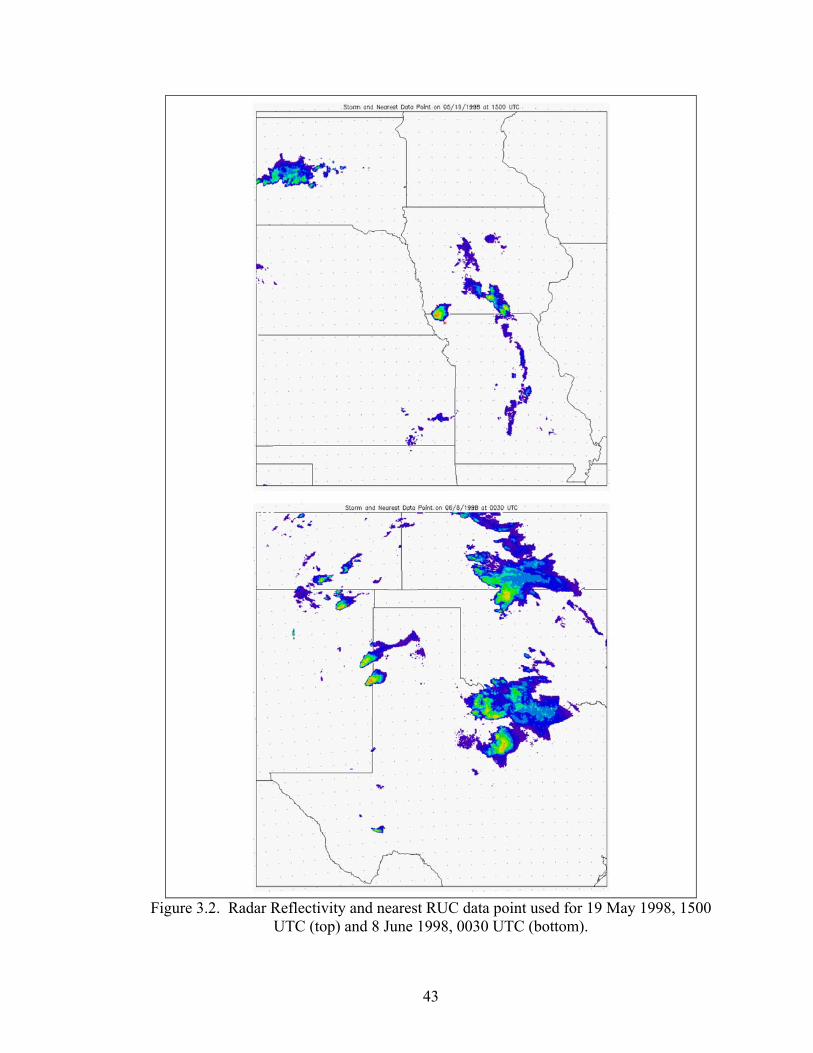
and are given every hour. The specific data point chosen for each storm was based on the

storm’s midpoint. Then, the nearest point in the direction of motion (as given by the

location of the midpoint in the next radar frame) of the storm was found. Note that this

may introduce errors, as some data points represent the inflow, but others are located

within the precipitation of the storm (Figure 3.2).

The model computes CAPE and CIN using an averaging of potential temperature

and water vapor mixing ratio in the lowest seven RUC native levels (approximately 45-

55 mb), and then taking the maximum buoyancy produced between the surface and

180mb (switched to 300mb on 6 May 1999). Freezing level is output both from the

bottom up and top down algorithms. The bottom up freezing level algorithm is used in

this project, defined as the first level in which the temperature drops below freezing.

Lifted index calculations use a surface parcel, and precipitable water is also calculated

using a surface based parcel and then summing the product of specific humidity at each

level multiplied by the mass of each layer (mid points between each level). Prior to

March 2000, storm relative helicity was computed using the Davies and Johns method in

which supercell motion is estimated to be thirty degrees to the right and eighty-five

percent of the mean wind vector for a 850-300 mb mean wind of less than 15 knots, and

seventy-five percent of the mean wind vector for a 850-500 mb mean wind of greater

than 15 knots. After March 2000, the Internal Dynamics method (Bunkers et al, 2002)

was used.

37

Other variables were calculated from model data. Cloud base height/lifting

condensation level (given in meters) are calculated using the formula from Williams et.

al., 2005:

)(67 dTTcbh −=

Warm cloud depth (also in meters) is defined as the difference between the freezing level

and the cloud base height. Mid level relative humidity is defined as the average relative

humidity between 700 and 500 mb layer, and mean relative humidity is the average

relative humidity through the depth of the RUC data. The shear values were calculated

using approximate heights since winds in the RUC model are given on a pressure grid.

The 0-3 km shear calculation uses the surface wind, and the wind given at the 700 mb

level. For 0-6 km shear, winds were used also at the surface, and the 450 mb level.

Wind shear (in m s-1) that was calculated is speed shear, and is given by the following

formula.

22 )__3()__3(_3 vsurfacevkmusurfaceukmshearkm −+−=

Also, the heights of the pressure levels and the freezing level had to be converted from

geopotential to geometric heights. The conversion is given as:

HGRHR

Ze

e

−=

where Re is the radius of the earth at latitude φ, G is the gravity ratio (ag

gG = ), and H is

geopotential height. Note that this does not factor in the change in gravity with height.

The effect of this was addressed by comparing the results of this calculation with a true

table factoring in the change in gravity with height. At a height of 200 km, the change

was only 6 km.

38

To assess the ability of the RUC model to accurately represent the thermodynamic

conditions present, model analysis was compared to thermodynamic soundings for April

through July of 1998 to 2002. Correlations for the 0000 UTC and 1200 UTC soundings

were done, as well as an average difference in means, and the standard deviation. These

were performed first to assess whether the variables varied similarly, and second to

measure whether the RUC and soundings are close in numeric values. Figure 3.3 shows

a four-panel plot of the correlations for surface pressure, temperature, dew point, and

relative humidity for 1998. While all the years are slightly different, they follow the

trend shown.

Surface pressure correlations are very high (above 0.95) for most of the United

States, with the exception of a few locations in the intermountain west. Note that these

regions are outside of our domain. Surface temperature correlations are also very high

across the central United States. Over the west, correlations drop off, but the minimum

of any year is only around 0.839. Surface dew point correlations remain above 0.9

throughout most of my domain, dropping off to around 0.6 to 0.7 over the intermountain

west. The relative humidity correlations follow almost the same pattern as the dew point

correlations. These indicate that at the surface, the RUC model varies closely in

alignment with the sounding variations over the domain of this project.

Figure 3.4 shows the average difference value between the reported sounding and

RUC model for the same surface variables during 1998. The average difference in

surface pressure is very small (approximately 1-2 hPa) across most of the United States.

However, over the high plains (including Denver, eastern Wyoming, western Nebraska

and South Dakota), the difference becomes as large as approximately 15 hPa. The 1998

39

plot also shows a minimum difference over Arizona, but this trend is not present in the

plot during other years. In addition, there is a local minimum centered over central

Arkansas (approximately -6 hPa). The mean temperature differences across the United

States are very small (typically less than 1 oC), with a maximum over the Salt Lake City

area in all plots except 2002. Also note that in the Southern Mountain regions (near

Albuquerque, NM), temperature differences increase to above 1 oC. The mean dew point

difference is very small across the central United States (less than 1 oC), with the

exception of the intermountain west, where are adjacent maxima and minima appear of

approximately -2 oC, and 4 oC. Surface relative humidity differences are more variable,

but all show an increase over the North Dakota, South Dakota, and Wyoming region.

This increase ranges from 5 to 9% over the five-year period selected for this study.

Differences across the rest of the central United States are small, with values between

|0%-2%|. These results indicate that the RUC model is very close in correlation and

specific number values when using the surface temperature data across the five years.

However, moisture and pressure may be a problem over the northern and high plains.

The upper air data shows a different pattern. Temperature and relative humidity

correlations for 1998 are shown in Figure 3.5. The temperature correlations are very

strong across the entire United States, despite looking like it has many different patterns.

The minimum over 1998 is 0.998, and the minimum over the four years is 0.977.

Relative humidity is more variable however. The plot shows decreasing correlations

toward the western and southern United States. Values across the central United States

are typically between 0.8 and 0.9. This indicates that the RUC is performing well with

40

upper air temperature values, but moisture is not exactly in correlation with the

soundings.

Examining the difference in upper air temperatures and relative humidity,

between the RUC model and the soundings (Figure 3.6) we notice that the temperature

difference is very small. Average difference values are less than 1 oC for all of the

United States. Upper level relative humidity, however, has slightly larger difference

amounts. Important to notice is the large maximum in differences (about 3%) over the

Albuquerque, NM region. Also, there is a smaller maximum over the Kansas area, closer

to 2%. Overall, relative humidity values are off by approximately 1-2% throughout the

domain of this study. This suggests that while the RUC model appears to do well with

upper air temperatures, moisture is more uncertain, especially as we move closer to the

Rocky Mountains (where the correlations dropped off).

The standard deviation of all these measurements (not shown) shows a different

pattern. Upper air temperatures, and surface pressure variations are small everywhere

(generally less than one). However, the standard deviations of surface dew point and

temperature tend to get larger as we move toward the southern Rocky Mountains.

Relative humidity measurements contain much variability throughout the region, but in

general, also show larger standard deviations as we move toward the Rocky Mountains.

Upper air relative humidity standard deviations are very large (maximum of 10-20%) and

also show much variability across the United States. This means that whether the RUC

model is accurate with moisture or not will vary from day to day. On average, it is a

good representation of the soundings; however, there may be cases in which the RUC

does not perform well.

41

d. Analysis and Statistics

Because of the large number of storms, a variety of plots and statistical methods

were used to determine if there are typical differences between storms dominated by

+CG’s, and those dominated by –CG’s. First, histograms of all the data where positive

and negative (polarity reversal storms were split by their positive and negative times, and

lumped with the positive and negative data) storm environmental conditions were

performed in an attempt to locate systematic differences. Then, the data were separated,

into positive and negative cases, and polarity reversal cases. Single variable plots of the

positive and negative storm data were performed. Also, due to non-normality in the data,

a Wilcox-Mann-Whitney rank sum test (Wilks 1995) was used to test whether the

positive and negative population distributions differed by location at the 95% confidence

level. For the polarity reversal cases, storm environmental conditions were plotted across

the length of the storm and then compared to the polarity reversal time and percent

positive strikes. Finally, sensitivity tests were performed to test the effect of data point

errors. Also, the percent positive was reduced to 10%, and increased to 50%, to test the

effects of using a 30% threshold in the study. This second threshold of 10% was chosen

after Orville and Huffines (2001). They show values typically larger than 10% in the

positive polarity corridor (Figure 2.5), but less than this value across the rest of the

domain used in this study. Also, Smith et al. (2000) in their study used 50% as the

positive polarity indicator.

42

Figure 3.1. A map showing the domain and states included in this study.

43

Figure 3.2. Radar Reflectivity and nearest RUC data point used for 19 May 1998, 1500

UTC (top) and 8 June 1998, 0030 UTC (bottom).

44

Figure 3.3. Correlations between the RUC model and environmental soundings for a) surface pressure, b) surface temperature, c) surface dew point, and d) surface relative

humidity.

45

Figure 3.4. The average difference between sounding and RUC model variables for a) surface pressure, b) surface temperature, c) surface dew point and d) surface relative

humidity for 1998.

46

Figure 3.5. Upper air correlations between the soundings and RUC model for a)

temperature and b) relative humidity.

47

Figure 3.6. The average difference between sounding and RUC model values for a)

upper level temperatures, and b) upper level relative humidity for 1998.

48

Table 3.1. A list of the storms producing mostly –CG’s, including the date, time and

location of the storm, and any severe weather associated with it.

49

Table 3.2. The same as Table 3.1, except for the +CG storms.

50

Table 3.3. A list of the polarity reversal storms including the date time, and location,

they occurred, severe weather that the storms produced and a classification of lightning behavior.

51

Chapter 4

Results

a. All Cases

Histograms of the environmental conditions for all storm cases are shown in

Figures 4.1-4.16. Environmental conditions for the positive (negative) storms and the

positive (negative) portion of the polarity reversal storms are binned together, and hourly

RUC observations are plotted for each storm. While many of these data show

considerable scatter (positive and negative storms occurring in similar environmental

conditions), a few trends are evident. Starting with the moisture variables, the histogram

of dew point temperature (Figure 4.1) shows low dew point temperatures associated with

mostly negative (–CG) storms. Positive storms do not begin to occur until dew point

temperatures are above 8oC. This trend can also be seen in precipitable water (Figure

4.2), as positive storms do not occur until 1.5 cm. However, there is an additional region

of large precipitable water values (above 4.5 cm) where we see only +CG storms

occurring. High moisture values for positive storms are seen in mean relative humidity

through the depth of the sounding (Figure 4.3), but the lower values (as seen in the

precipitable water plot) are not evident in mean relative humidity. Mid level relative

humidity (not shown) does not show a large amount separation between the positive and

negative storms. Equivalent potential temperature, θe (Figure 4.4), also does not show

much separation between the positive and negative storms, however, we do notice that

52

the histograms are shifted relative to each other. The positive storms show higher

frequencies at θe values above 355 K, whereas the negative storms are dominant below

this. These results are actually opposite those of Carey and Buffalo (2006), and Knapp

(1994), who found positive (negative) storms occurring in drier (moister) environments.

However, Carey and Buffalo (2006) focused their study in the Oklahoma, Texas

Panhandle, and Kansas regions, and Knapp (1994) makes a general statement based on

regional climatology (not on individual storm data).

Cloud base height (Figure 4.5) also does not show discernable separation between

the positive and negative storms, but warm cloud depth (Figure 4.6) shows a region of

only negative storms at relatively shallow warm cloud depths. Positive storms do not

begin to occur until warm cloud depths reach greater than 2000 m. These results are in

contrast to Carey and Buffalo (2006) who found higher cloud base heights and lower

warm cloud depths, and Williams et al. (2005) who hypothesized these same conditions

for positive CG producing storms. Both CAPE and CIN (Figures 4.7 and 4.8) show little

separation between the positive and negative storms. However, there are a few positive

storms that occur at very large CAPE and large negative CIN values. Lapse rates in the

850-500 layer (Figure 4.9) show negative storms at large lapse rages, but 700-500 mb

lapse rates (Figure 4.10) show little separation between the positive and negative storms.

Freezing level height (Figure 4.11) showed no apparent difference between the positive

and negative storms, similar to Gilmore and Wicker (2002), but in contrast to Carey and

Buffalo (2006). Lifted index (not shown) also showed little separation.

Wind shear in the 0-3 km layer (Figure 4.12) shows very little separation between

the positive and negative storms. This is in contrast to Gilmore and Wicker (2002),

53

Levin et al. (1996), and Carey and Buffalo (2006), but in agreement with Curran and Rust

(1992), who found wind shear to be a necessary but not sufficient condition for positive

storms. Deep layer (0-6 km) wind shear (Figure 4.13) also shows little separation

between the positive and negative storms. Carey and Buffalo (2006) also found no

significant difference in deep layer shear. Storm relative helicity (Figure 4.14) contains a

region of only negative storms at large helicity values.

b. Monthly Results for All Cases

In an attempt to isolate possible regional biases or seasonal trends, the data were

separated across the United States. It was broken up by months (April, May, June, July)

as Hagemeyer (1991) demonstrated changes in synoptic and mesoscale conditions in

association with different months. Histograms similar to Figures 4.1 to 4.14 were made

for each thermodynamic variable during each of the four months. Plots in this section are

omitted, but compared to the previous histograms.

Similar to the above results, the monthly positive and negative data contained

much overlap, with a few additional trends. We found the region of low negative dew

points in all plots, although precipitable water shows no trend except high positive values

in July above 5.0 cm), and low negative values in April and May. Mean relative

humidity values are high for positive storms in April, May and June, but not for July. In

addition, mean relative humidity values are typically larger in June and July (we see

values as high as 70-80%, whereas in May and April, maximum values are only 55%). θe

indicated no trend for April and May (values are low, ranging between 310 and 360 K),

but shows high values for positive storms (365 K and above) and lower values for

negative storms during June and July.

54

Cloud base height reveals little difference between the positive and negative

storms for May and June, but we see higher negative values for April and July. Also,

cloud base heights are much lower in May than in any other month (all values tend to be

below 1700 m, whereas cloud base heights may reach as high as 2700 m for the other

months). This is to be expected; the northward movement of the polar front jet would

lead to thunderstorms produced farther north in June and July. These storms have little

influence from the gulf moisture, so therefore have higher cloud bases. Warm cloud

depth shows almost no trend across the months, except low values (around 1000 m)

associated with negative storms in April. There are much lower freezing levels depths

(between 2900 m and 3600 m) associated with positive storms in April. However, in

June and July, freezing levels for positive storms start at around 4100 m, and continue to

larger values. All of these results may be evidence of variables compensating for one

another to produce the same result, as suggested by Carey and Buffalo (2006). The lower

freezing level in April and May could help sustain higher liquid water contents aloft by

making the coalescence zone shallower. However, in June and July, higher moisture

values could compensate for this effect by producing higher liquid water contents below

the freezing level and thereby could still produce positive charging.

Larger 700-500 mb lapse rates are seen with the negative storms in April and

June, but these lapse rates are smaller in May. However, for 850-500 mb lapse rates, the

negative storms are associated with larger lapse rates (near and above 8 oC km-1) in all

months except July. CAPE values are low for the negative cases in July, but the positive

storms show some values above 6000 J kg-1. In April, the negative CG cases have higher

CAPE values (near 4000-6000 J kg-1) than the positive CG storms. For CIN, we see

55

negative storms at larger negative CIN (-150 to -250 J kg-1) for April and May, but in

July, these same values (-150 to -200 J kg-1) are associated with positive storms. During

June, a few positive storms have large negative CIN, up near -250 to -450 J kg-1. Lifted

index shows higher values for negative storms in June, but less so in May.

Wind shear in the 0-3 km layer shows lower values (between 0 and 5 m s-1) for

negative storms in May, but little difference between the positive and negative storms is

seen across the other months. However, 0-6 km shear shows values between 20 and 30 m

s-1 for negative storms during April and between 25 and 40 m/s for May. Lower values

are seen in June (10-15 m s-1). Storm relative helicity shows much lower helicity values

in April for all cases (less than 300 m2 s-2), but these values sharply increase for the June

negative CG cases (between 600 and 1000 m2 s-2).

The histograms for April show the most separation between positive and negative

CG storms for all data. This may be due to the small April data set (only 5 cases), or to

the small region where these storms occurred (Oklahoma and Kansas only). Note that

this region is very similar to the one used by Carey and Buffalo (2006), however, the

results are not the same, in that we see higher moisture values for the positive storms.

However, similar to Carey and Buffalo, freezing levels are lower.

c. Polarity Reversal Cases

There are a total of ten cases in which the CG lightning switched polarity

throughout the storm’s lifetime (listed in Table 3.3). To determine if the switch

corresponded to any change in a particular thermodynamic parameter, each variable was

plotted across the lifetime of the storm, along with the percentage positive. Figure 4.15

shows a plot of cloud base height for the two polarity reversal storms that occurred in

56

July, 13 July 1998 and 5 July 2000 (note: the polarity reversal storms will be identified

by the first day in which the storm occurred, with the year omitted since no storms

overlap). These two storms show opposing trends in cloud base height, with a larger

cloud base height when the storm is negative for 13 July, but a lower cloud base height

when the storm was negative on 5 July. Table 4.1 lists the average RUC values for the 16

variables during each storm’s positive and negative phase (shown for simplicity). As can

be seen for cloud base height (Table 4.1), 7 storms (19 May, 13 July, 20 May, 26 June

storm 1, 26 June storm 3, 21 May storm 2, and 10 May) showed relatively lower cloud

base heights when the storm was positive (as opposed to when the storm was in its

negative phase). However, the other 3 (26 June storm 2, 21 may storm 1, and 5 July)

showed relatively higher cloud base heights when the storm was positive.

The moisture variables show contrasting trends across some of the storms. Dew

point is larger during the positive phase for 8 of the storms, but smaller for 2 of the

storms. Mean relative humidity and mid level relative humidity shows the exact opposite

trend, with higher mean relative humidity when the storm is positive for 2 storms, but

lower values for the other 8 storms. Precipitable water shows no apparent trend, with 5

storms containing higher precipitable water values when the storm is positive, and 5

being higher when the storm is negative. θe values are also larger when the storms are

positive (as compared to the negative phase of each storm) for 7 of the cases, but smaller

during the negative phase for 3 storms.

Freezing level depth is higher for 6 of the storms during their positive phase,

while warm cloud depth is larger for 8 of the storms during their positive phase. CAPE

follows θe, with 7 storms showing larger values during the positive phase, and 3 larger

57

during the negative phase. CIN shows no apparent difference, with 5 larger CIN values

and 5 smaller CIN values for the positive storms.

Lifted index is also split, with 5 storms showing a larger (more negative) lifted

index during the positive phase and 5 showing larger lifted indices during the negative

phase. The 850-500 mb lapse rates tend to be larger when the storm is negative (7

storms), and smaller when it is positive (3 storms). However, 700-500 mb lapse rates

show no obvious trend, with 5 storms containing steeper lapse rates during their positive

phase, and 5 storms showing shallower lapse rates during their positive phase.

As expected, 0-3 km and 0-6 km wind shear show similar trends. However, 8

storms show higher shear values when they are positive and only 2 lower values for 0-3

km shear, while only 6 show higher 0-6 km shear values, and 4 show lower values when

the storm is positive. Storm relative helicity also contains 8 storms that show higher

helicity values when the storm is positive, but only 2 lower.

There are only three storms out of this polarity reversal data set that occur on the

same day as positive and negative storms. The trend with the polarity reversal data in

comparison to the positive and negative storms is less variability. For example, if cloud

base height in the polarity reversal storm is lower in its positive phase than the positive

storms in the area, it tends to stay lower than the negative storms after the switch to the

negative phase. A few variables do not follow this trend. These include storm relative

helicity and θe. Otherwise, it is difficult to establish trends due to the low number of

cases that meet this criterion.

An additional difficulty with establishing trends for the polarity reversal cases is

partly due to the fact that all of the numbers are relative. For instance, while dew point

58

may be reduced as a storm is negative, this value may still be larger than another storm

during its positive phase. An example of this is the 19 May case. The average dew point

during the negative phase is 21oC. This is larger than the dew point value for all the other

storms during their positive phase except 19 May (22.35oC), and 26 June storm 1

(22.1oC). Also, the same storms do not show changes in the same variables. For

example, while CAPE and θe both show 7 storms with relatively larger values and 3

storms with relatively lower values during the positive phase; it is not the same 7 storms.

Furthermore, Table 4.1 shows that the numerical values for the positive versus the

negative phase are very close, and we don’t see a large shift in any one variable.

To further examine the cases, it is important to note the possibility that variables

may compensate for one another. This means that a change in different variables could

lead to the same result thermodynamically. For example, out of the three cases showing

higher cloud base heights, two of them (26 June storm 2, and 5 July) show reduced warm

cloud depths. The third, 21 May storm 1 does not. This could indicate the role of

decreasing the coalescence zone in producing higher liquid water contents aloft, whereas

the other storms (with low cloud base heights) may just be forming in regions containing

higher moisture contents.

d. Positive and Negative Cases with Hourly RUC Observations

The data were then separated to exclude the polarity reversal cases and examine

only the positive and negative CG cases. Figure 4.16 is a plot of four moisture variables

including all hourly RUC data points over the lifetime of each storm. These plots show

lots of scatter (similar to the histograms from part a), but some trends can be established.

Dew point values (Figure 4.16a) are similar for positive and negative storms, but there is

59

a relative lack of positive CG storms at very low dew points. This suggests a threshold of

approximately 5-10oC for positive CG storms to occur. In addition, precipitable water

also confirms negative storms at lower moisture values as the plot slopes downward

toward the negative storms, and there are a few stray negative values at low precipitable

water values (approximately 1.0 cm). A few positive CG storms also occur at very large

precipitable water values nearing 5.0 cm. Mean and mid level relative humidity (Figure

4.16 c and d) show almost no difference between the positive and negative storms.

Figure 4.17 shows plots for cloud base height, warm cloud depth, freezing level

and θe. Cloud base height (Figure 4.17a) illustrates a large range of values for the

negative storms, but the number of positive cases at very high cloud base heights is

reduced. Also, positive storms tend to occur at both high and low freezing level heights

(Figure 4.17c). Warm cloud depth and θe (Figure 4.17b) show very little separation

between the positive and negative storms.

Several instability parameters are shown in Figure 4.18. There is a slight

lowering of 850-500 mb lapse rate (Figure 4.18a) for the positive storms in respect to the

negative storms. However, this trend is less apparent in 700-500 mb lapse rates (Figure

4.18b), and little difference between the positive and negative storms can be discerned.

CAPE (Figure 4.18c) illustrates the lack of difference between positive and negative

storms, except the few stray very large values associated with positive storms, and CIN

(Figure 4.18d) similarly shows little differences.

Figure 4.19 includes the shear values and lifted index. Wind shear in the 0-3 and

0-6 km layers are very similar for the positive and negative storms. Both show little

difference between the positive and negative storms. Also, there is a relative lack of

60

positive storms at very high storm relative helicity values, and lifted index only shows

negative storms at values above 0 oC. Overall, results are very scattered, with only dew

point, and to a lesser extent precipitable water showing positive storms at high moisture,

and negative storms at low moisture. Also, positive storms show less instability, as

indicated by the lapse rate values.

e .Positive and Negative Cases with Mean and Median RUC Observations

In an attempt to reduce scatter in the data, and to be consistent with other studies

(Carey and Buffalo 2006; Smith et al. 2000), the mean and median RUC value across

each storm was calculated. Figure 4.20 shows the mean values for Dew point (a),

precipitable water (b), mean relative humidity (c), and mid level relative humidity (d).

The plot using median values with these same variables is not shown, because the results

are almost identical. Dew point values show positive and negative storms occurring in

similar environments. However, no positive storms occur at dew points lower than

approximately 12oC. Precipitable water also shows a similar trend with positive storms

occurring at large precipitable waters values (above 4.0 cm), and negative storms

occurring at smaller values, around 1.0 cm. Mean relative humidity values illustrates

almost no trend between positive and negative storms, but mid level relative humidity

shows negative storms at higher relative humidity (above 70%), and positive storms

below about 25%.

Cloud base height, warm cloud depth, freezing level, and θe are shown in Figure

4.21 a, b, c, and d respectively. Cloud base height now illustrates a trend, with lower

cloud base heights typically being associated with positive storms, and higher cloud base

heights being associated with negative storms. Warm cloud depth shows more positive

61

storms at larger warm cloud depths (above 3500 m), with relatively few negative storms

occurring with warm cloud depths greater than 3500 m. Freezing level heights are

clustered slightly higher for the positive storms than for the negative storms, but there are

also a few positive storms that occur at very low (around 3500 m) freezing levels. θe

shows little separation between the positive and negative storms. The only possible trend

in θe, (although not very significant), are positive storms in both very large (above 365 K)

and very small (below 325 K) θe values.

Figure 4.22 a, b, c, and d show 850-500 mb lapse rate, 700-500 mb lapse rate,

CAPE and CIN respectively. Lapse rates in the 850-500 mb layer still illustrate a

clustering of positive storms at smaller lapse rates, with larger lapse rates associated with

negative storms. The trend is similar for 700-500 mb lapse rates, but less apparent.

CAPE and CIN both show little differences between the positive and negative storms.

Shear, and lifted index are shown in Figure 4.23. Wind shear in the 0-3 km layer

(Figure 4.23a) is similar for the positive and negative storms, except for a lack of

negative storms above about 18 ms-1. Furthermore, 0-6 km shear (Figure 4.23b) shows

little separation between the positive and negative storms. In contrast, storm relative

helicity (Figure 4.23c) illustrates a slight clustering of positive storm values below the

clustering of negative storm values, but lifted index (Figure 4.23d) is similar for the

positive and negative storms.

These results were similar to some studies, yet different from others. The lower

cloud base heights seen with positive storms was opposite to Carey and Buffalo and

Williams et al. (2005), who found positive strike dominated storms occurring with higher

cloud base heights, and also positive storms at larger warm cloud depths. We also see

62

positive storms at higher dew points and precipitable water values, opposite to Carey and

Buffalo, and Knapp (2004). Freezing level and θe are similar to the Carey and Buffalo

results, with positive storms having lower freezing levels, and no trend in θe (in contrast

to Smith et al. 2000). However 850-500 mb and 700-500 mb lapse rates show the

opposite result, with steeper lapse rates for negative storms. Shear values (0-3 km and 0-

6 km) show no difference between the positive and negative storms, in contrast to Carey

and Buffalo, and Levin et al. (1996), but similarly to Reap and MacGorman (1998) and

Curran and Rust (1992).

f. Difference in Means Test

To further establish the significance of the previous plots, a Wilcox-Mann-

Whitney rank sum test (Wilks 1995) was used at the 95% confidence level to determine if

positive and negative CG storm means differed by location. Tables 4.2, 4.3, and 4.4

show the results for hourly RUC observations, mean RUC observations, and median

RUC observations respectively. When hourly data were used, dew point, cloud base

height, CAPE, CIN, warm cloud depth, 850-500 mb lapse rate, and mid level relative

humidity come out statistically different at the 95% confidence level. This is similar to

Carey and Buffalo (2006), who found warm cloud depth, cloud base height, dew point,

and 850-500 mb lapse rate significant at the 99.9% confidence level. The difference

between the present results and Carey and Buffalo is in the numerical values. These data

show lower cloud bases, higher warm cloud depths, higher dew points, lower 850-500 mb

lapse rates, and lower mid level relative humidity (as given by the number averages) for

positive CG storms. However, Carey and Buffalo show the exact opposite trend in all of

these variables. When the mean and median values for all the storms are used, the

63

significant variables change. All of the variables are significant when using mean values

except lifted index, storm relative helicity and 0-3 km wind shear. When using the

median values, storm relative helicity, mean relative humidity, and 0-6 km wind shear are

not significant at the 95% confidence level.

g. Comparison of 10% as a Positive Polarity Indicator

To test the choice of 30% as a positive polarity storm indicator, the single variable

plots were redone using 10% and 50%, with hourly RUC observations, mean RUC values

for each storm, and median RUC values for each storm. Switching to 10% alters some,

but not all, of the variables. Precipitable water still shows the high values for positive

storms, and low values associated with negative storms. Mean relative humidity, mid

level relative humidity, θe, 0-3 km shear and 0-6 km shear still show no apparent

difference between positive and negative storms. Also, the little separation between

positive and negative storms seen with CAPE and CIN values are still evident.

Figures 4.24 and 4.25 show the variables that change slightly when 10% positive

is used. Dew point (4.24a) no longer shows a threshold of 5-10oC for positive storms to

occur. Instead, both positive and negative storms occur at both low and high dew points.

Also, the reduced number of positive storms at high cloud base heights is no longer

present. Instead, there is little difference in cloud base height (4.24b) between the

positive and negative storms. Warm cloud depth (4.24c) still shows a few negative storm

values at very low warm cloud depths, but there are not as many as the original plot. In

contrast, the split trend in freezing level (4.24d) is stronger (positive storms at high and

low freezing levels, with negative values sandwiched in between) than the original plot.

64

The plots showing 850-500 mb lapse rate (4.25a) and 700-500 mb lapse rate

(4.25b) now show little difference between the positive and negative storms. When a

30% threshold was used, 850-500 mb lapse rates were slightly smaller for the positive

storms. Storm relative helicity (4.25c) now shows no difference between the positive and

negative storms. Lifted indices (4.25d) are also similar for the positive and negative

storms, in contrast to the original plot which only showed negative storm values above

0oC.

When using the mean value for each storm, we see similar changes as when using

hourly RUC observations. Mean relative humidity, mid level relative humidity, θe, CIN,

0-3 km shear, 0-6 km shear and lifted index all show no difference between the positive

and negative storms (as was seen when using 30% for the positive polarity indicator).

Freezing level still shows the original split level trend.

Dew point, precipitable water, cloud base height, and warm cloud depth are

shown in Figure 4.26, a, b, c, and d. Dew point again has positive and negative storms in

similar environments, in contrast to the previously seen threshold for positive storms.

Precipitable water contains the high precipitable water values for a few positive storms,

as seen previously, but there are no longer negative storms at low precipitable water

values. Cloud base height shows no difference between the positive and negative storms,

when it originally showed positive storms at low cloud base heights, and negative storms

at high cloud base heights. Warm cloud depth also shows no difference between the

positive and negative storms, instead of the higher warm cloud depth values for positive

storms, and lower values for negative storms.

65

Figure 4.27 is a plot of mean 850-500 mb lapse rates (a), 700-500 mb lapse rates

(b), CAPE (c), and storm relative helicity (d). The plot of 850-500 mb lapse rates now

confirms no trend instead of smaller lapse rates for positive storms. However, 700-500

mb lapse rates are larger for positive storms, instead of the original plot, which showed

similar lapse rates for both positive and negative storms. CAPE shows little separation

between the positive and negative storms. However, storm relative helicity values are

large for the positive storms, instead of the negative storms seen at high helicity values in

the original plot.

The majority of the median variables show similar trends to the mean plots listed

in the previous paragraph. The exceptions are cloud base height, and dew point, which

are shown in Figure 4.28, a and b respectively. Cloud base height follows the original

30% plot, with positive storms having lower cloud base heights, and negative storms

higher cloud base heights. This is in contrast to the little separation seen in the plots for

mean values. Dew point now shows no discernable difference between the positive and

negative storms.

h. Comparison of 50% as a Positive Polarity Indicator

Similarly, using 50% as a positive polarity indicator also only produces slight

changes in some of the variables. When examining all of the RUC data points for each

storm, we still see no apparent difference between the negative and positive points for

mean relative humidity, mid level relative humidity, 700-500 mb lapse rates, 0-3 km

shear, and 0-6 km shear. CAPE and CIN both show little difference between the positive

and negative storms, and lifted index still only shows a few negative data points above

0oC. Lapse rates in the 850-500 mb layer show slightly lower positive values, and

66

freezing level still shows the split trend, but it is a little less pronounced. Precipitable

water still confirms high values associated with positive storms, and low values with

negative storms, and storm relative helicity still only contains a few negative values at

high helicity values.

Figure 4.29 is a plot of the variables that do alter slightly. The low cloud base

heights with positive storms, and high cloud base heights with negative storms are more

pronounced than it was using the 30% positive polarity indicator. Positive storms all but

stop occurring with cloud base heights above 2000 m. Also, the originally seen threshold

of 5-10oC dew points for positive storms is more pronounced than originally seen. θe

shows less positive values at low θe, as the positive storms tend to cluster above 335 K.

A trend in warm cloud depth is apparent in this plot, with 2000 m as a threshold for

positive storms.

When using the mean value across each storm, different trends emerge. CAPE,

CIN, mean relative humidity, 0-6 km wind shear, storm relative helicity and θe show little

difference between the positive and negative storms. Lifted index still confirms values

near 0oC for negative CG storms, and precipitable water still contains a few positive

storms at high precipitable water, and a few negative storms at low precipitable water.

Figure 4.30 shows cloud base height (a), dew point (b), freezing level (c), and

warm cloud depth (d). Compared to the original plot using 30%, positive storms

occurring in lower cloud base heights, and negative storms in larger cloud base heights is

more pronounced. The same is true for dew point, where the lack of positive storms at

low dew points is more apparent. Also, the originally seen threshold for positive storms

is still evident, located close to 12oC. Freezing level no longer shows the split trend,

67

instead, positive storms tend to be associated with higher freezing levels than negative

storms. The trend for larger warm cloud depths with positive storms is also more

pronounced, with only a few positive storms occurring at warm cloud depths between

2000 and 3000 m.

Other variables that now show changes are plotted in Figure 4.31. Lapse rate in

the 850-500 mb layer (Figure 4.31a) shows smaller lapse rates associated with positive

storms. This trend is more pronounced than originally. However, 700-500 mb lapse

rates (Figure 4.31b) still show no apparent difference between the positive and negative

storms. Mid level relative humidity (Figure 4.31c) shows a lack of positive storms at

higher relative humidity values. Also, 0-3 km wind shear (Figure 4.31b) seems to

indicate a lack of positive storms at low wind shear values (below 10 m s-1).

The majority of the plots using median RUC values across each storm are very

similar to the mean plots discussed previously. The exceptions are 850-500 mb lapse

rate, and cloud base height, shown in Figure 4.32. Lapse rates in the 850-500 mb layer

shows a larger scatter associated with the negative CG cases, so the trend in the mean

plot (shallower lapse rates for positive storms) is less pronounced in the median plot. The

same is true for cloud base height. The negative storms show more scatter, so there is

less apparent difference between the positive and negative storms.

i. Sensitivity Test on Errors in RUC Data Points

To test the effect of possible errors in the RUC data point used (i.e. some points

are located in the storms radar echo, while others are not), only those storms that did not

contain any data points located in the precipitation were pulled out, and new single

variable plots made. Due to the low number of storms that met this criterion (13), only

68

hourly RUC observations across each storm are shown (instead of taking the mean and

median values). Figure 4.33 shows the plots for dew point, precipitable water, mean

relative humidity, and mid level relative humidity (a, b, c, and d respectively). Similar to

the original dew point plot, the new plot also shows a relative lack of positive storms at

low dew points. Precipitable water follows this trend, with a relative lack of positive

storms at low precipitable water values. However, in contrast to the original precipitable

water plot, there are no positive storms at very large precipitable water values. Mean

relative humidity in the original plots showed no trend, but following the other moisture

variables, there is now a clear region of low mean relative humidity with negative storms,

and high mean relative humidity with positive storms. Mid level relative humidity shows

mostly positive storms at high values, in contrast to the original plot, which showed no

trend.

Cloud base height (Figure 4.34a) still shows slightly larger cloud base heights

with negative storms and slightly lower cloud base heights with positive storms.

However, warm cloud depth (Figure 4.34b) shows little difference between the positive

and negative storms, in contrast to the slightly higher warm cloud depths for positive

storms shown originally. Freezing level (Figure 4.34c) shows lower values for the

positive storms, whereas the original plot showed a split trend (some positive storms at

low freezing levels, and the others at higher freezing levels). θe (Figure 4.34d) shows no

difference between the positive and negative storms, similar to the original plot.

The plot of 850-500 mb lapse rate (Figure 4.35a) shows a considerable amount of

scatter, but there is a clustering of negative storms at large lapse rates, and no clustering

of positive storms. This is similar to the original 850-500 mb lapse rate plot that shows

69

slightly lower lapse rates for the positive storms. Lapse rates in the 700-500 mb layer

(Figure 4.35b) show almost no difference between the positive and negative storm.

CAPE (Figure 4.35c) shows a few stray negative CG storms at high values, and CIN

(Figure 4.35d), shows little difference between the positive and negative storms.

Figure 4.36 shows 0-3 km Shear, 0-6 km shear, storm relative helicity, and lifted

index (a, b, c, and d respectively). We see a slight trend in 0-3 km shear, with only

negative storms occurring at low shear values, in contrast to the lack of trend seen in the

original plot. Shear over the 0-6 km layer, storm relative helicity, and lifted index show

no apparent difference between the positive and negative storms. This is similar to what

all three of the original plots showed for these variables.

70

Histogram of Dew Point

0

5

10

15

20

25

4 6 8 10 12 14 16 18 20 22 24 26

Dew Point (C)

Freq

uenc

yNegativePositive

Figure 4.1. Histogram of dew point temperature for all cases, using hourly RUC

observations, separated by the positive and negative storms.

71

Histogram of Precipitable Water

0

5

10

15

20

25

30

1 1.5 2 2.5 3 3.5 4 4.5 5 5.5

Precipitable Water (cm)

Freq

uenc

yNegativePositive

Figure 4.2. The same as Figure 4.1, except for precipitable water.

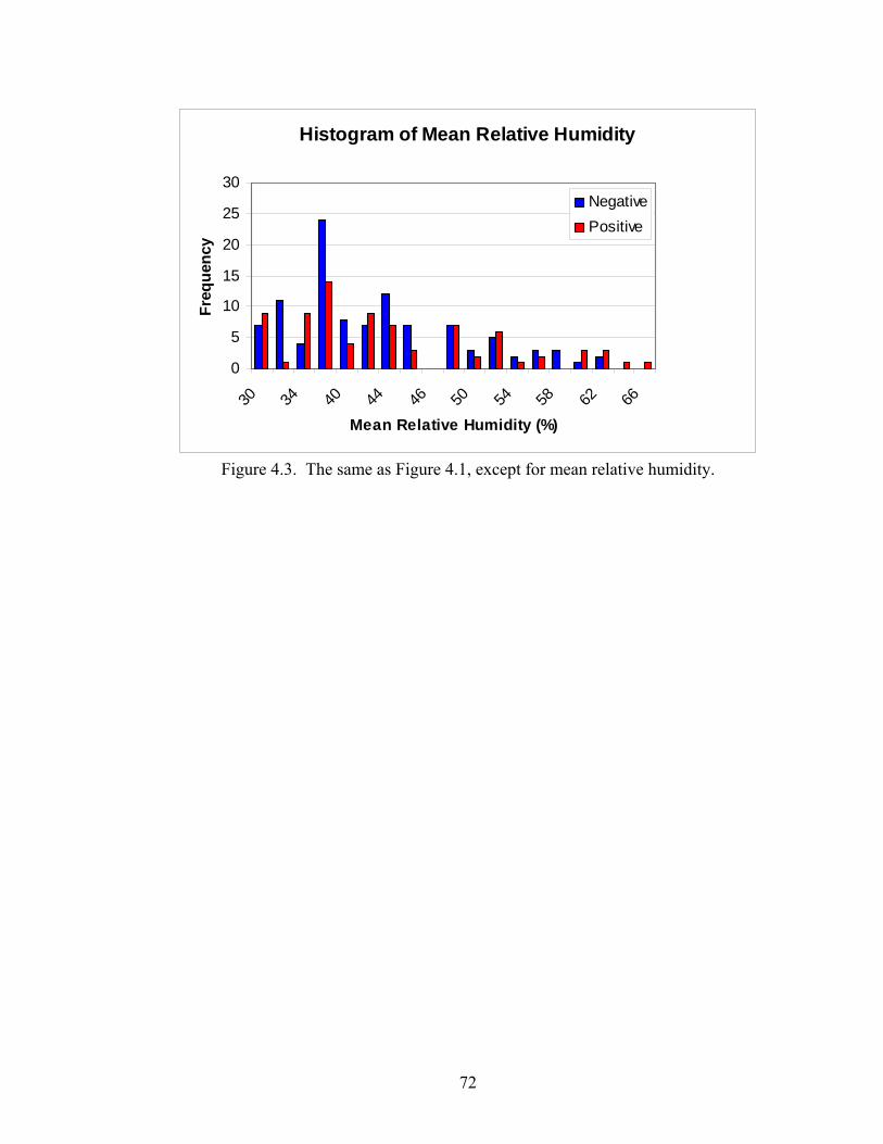
72

Histogram of Mean Relative Humidity

0

5

10

15

20

25

30

30 34 40 44 46 50 54 58 62 66

Mean Relative Humidity (%)

Freq

uenc

yNegativePositive

Figure 4.3. The same as Figure 4.1, except for mean relative humidity.

73

Histogram of Thetae

0

5

10

15

20

25

320 325 330 335 340 345 350 355 360 365 370 375

Thetae (K)

Freq

uenc

yNegativePositive

Figure 4.4. The same as Figure 4.1, except for equivalent potential temperature.

74

Histogram of Cloud Base Height

0

24

6

8

1012

14

16

040

080

012

0016

0020

0024

0028

00

Cloud Base Height (m)

Freq

uenc

yNegativePositive

Figure 4.5. The same as Figure 4.1, except for cloud base height.

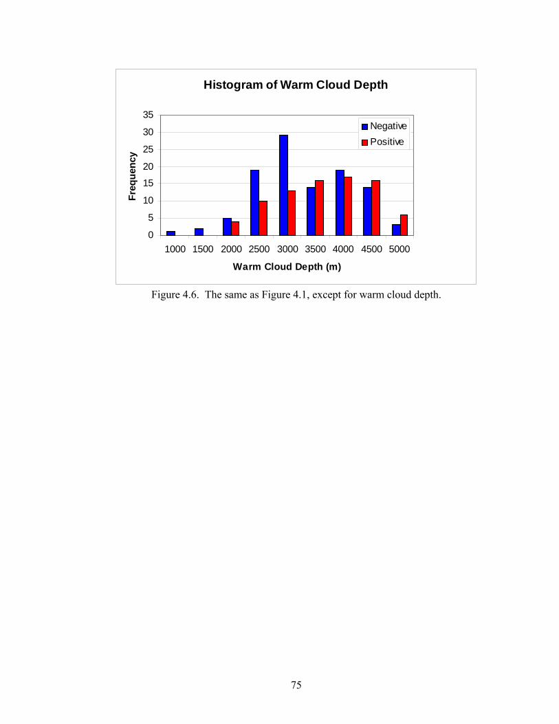
75

Histogram of Warm Cloud Depth

0

5

10

15

20

25

30

35

1000 1500 2000 2500 3000 3500 4000 4500 5000

Warm Cloud Depth (m)

Freq

uenc

yNegativePositive

Figure 4.6. The same as Figure 4.1, except for warm cloud depth.

76

Histogram of CAPE

0

2

4

6

8

10

12

060

012

0018

0024

0028

0036

0042

0048

0054

0060

0066

00

CAPE (J/kg)

Freq

uenc

yNegativePositive

Figure 4.7. The same as Figure 4.1, except for CAPE.

77

Histogram of CIN

05

10152025303540

-250

-230

-210

-190

-170

-150

-130

-110 -90

-70

-50

-30

-10

CIN (J/kg)

Freq

uenc

yNegativePositive

Figure 4.8. The same as Figure 4.1, except for CIN.

78

Histogram of 850 - 500 mb Lapse Rate

0

24

6

8

1012

14

5.8 6.2 6.6 7 7.4 7.8 8.2 8.6

850 - 500 mb Lapse Rate (C/km)

Freq

uenc

yNegativePositive

Figure 4.9. The same as Figure 4.1, except for 850-500 mb lapse rate.

79

Histogram of 700 - 500 mb Lapse Rate

02468

1012141618

5.8 6.2 6.6 7 7.4 7.8 8.2 8.6 9

700 - 500 mb Lapse Rate (C/km)

Freq

uenc

yNegativePositive

Figure 4.10. The same as Figure 4.1, except for 700-500 mb lapse rate.

80

Histogram of Freezing Level

05

1015202530354045

3100 3400 3700 4000 4300 4600 4900 5200

Freezing Level (m)

Freq

uenc

yNegativePositive

Figure 4.11. The same as Figure 4.1, except for freezing level.

81

Histogram of 0 - 3 km Wind Shear

0

5

10

15

20

2 4 6 8 10 12 14 16 18 20 22

Wind Shear (m/s)

Freq

uenc

yNegativePositive

Figure 4.12. The same as Figure 4.1, except for 0-3 km wind shear.

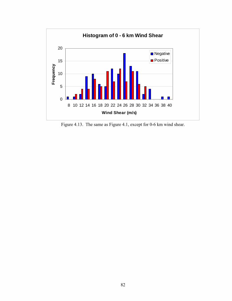
82

Histogram of 0 - 6 km Wind Shear

0

5

10

15

20

8 10 12 14 16 18 20 22 24 26 28 30 32 34 36 38 40

Wind Shear (m/s)

Freq

uenc

yNegativePositive

Figure 4.13. The same as Figure 4.1, except for 0-6 km wind shear.

83

Histogram of Storm Relative Helicity

02468

10121416

-50 50 150

250

350

450

550

650

750

850

950

Storm Relative Helicity (m^2/s 2)

Freq

uenc

yNegativePositive

Figure 4.14. The same as Figure 4.1, except for storm relative helicity.

84

Figure 4.15. A plot of cloud base over time (blue line) with percentage positive strikes (red) for a) 13 July 1998 and b) 5 July 2000. The black line indicates the time of the

polarity switch.

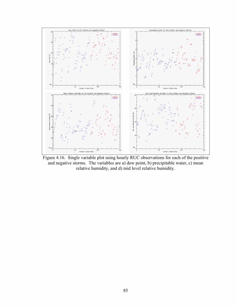
85

Figure 4.16. Single variable plot using hourly RUC observations for each of the positive

and negative storms. The variables are a) dew point, b) precipitable water, c) mean relative humidity, and d) mid level relative humidity.

86

Figure 4.17. The same as Figure 4.16, except for a) cloud base height, b) warm cloud

depth, c) freezing level, and d) θe.

87

Figure 4.18. The same as Figure 4.16, except for a) 850-500 mb lapse rate, b) 700-500

mb lapse rate, c) CAPE, and d) CIN.

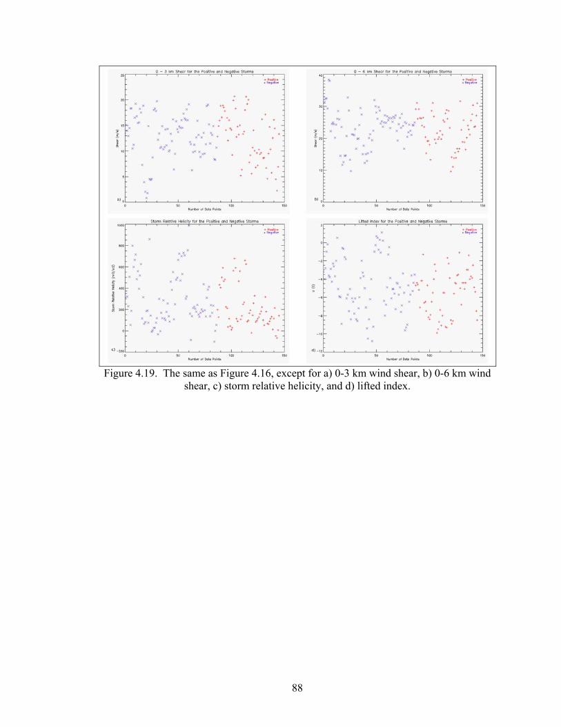
88

Figure 4.19. The same as Figure 4.16, except for a) 0-3 km wind shear, b) 0-6 km wind

shear, c) storm relative helicity, and d) lifted index.

89

Figure 4.20. Single variable plot using the mean RUC data for each storm, for a) dew

point, b) precipitable water, c) mean relative humidity, and d) mid level relative humidity.

90

Figure 4.21. The same as Figure 4.20, except for a) cloud base height, b) warm cloud

depth, c) freezing level, and d) θe.

91

Figure 4.22. The same as Figure 4.20, except for a) 850-500 mb lapse rate, b) 700-500

mb lapse rate, c) CAPE, and d) CIN.

92

Figure 4.23. The same as Figure 4.20, except for a) 0-3 km wind shear, b) 0-6 km wind

shear, c) storm relative helicity, and d) lifted index.

93

Figure 4.24. Single variable plot using all the RUC data across the length of each storm, but defining positive storms using 10% positive. The variables are a) dew point, b) cloud

base height, c) warm cloud depth, and d) freezing level.

94

Figure 4.25. Same as Figure 4.24, except for a) 850-500 mb lapse rate, b) 700-500 mb lapse rate, c) storm relative helicity, and d) lifted index.

95

Figure 4.26. Single variable plot using the mean RUC data for each storm, but defining

positive storms using 10% positive. The variables are a) dew point, b) precipitable water, c) cloud base height, and d) warm cloud depth.

96

Figure 4.27. The same as Figure 4.26, except for a) 850-500 mb lapse rate, b) 700-500

mb lapse rate, c) CAPE and d) storm relative helicity.

97

Figure 4.28. Single variable plot using the median value for each storm, and 10% as a

positive polarity indicator for a) dew point and b) cloud base height.

98

Figure 4.29. Single variable plots using all RUC data for each storm and 50% as a

positive polarity indicator. The variables are a) cloud base height, b) dew point, c) θe, and d) warm cloud depth.

99

Figure 4.30. Single variable plots using the mean RUC value for each storm, and 50% as

a positive polarity indicator. The variables are a) cloud base height, b) dew point, c) freezing level and d) warm cloud depth.

100

Figure 4.31. The same as Figure 4.30, except for a) 850-500 mb lapse rate, b) 700-500

mb lapse rate, c) mid level relative humidity and d) 0-3 km wind shear.

101

Figure 4.32. Single variable plots using the median RUC value for each storm, and 50% as a positive polarity indicator. The variables are a) 850-500 mb lapse rate and b) cloud

base height.

102

Figure 4.33. Single variable plot using only those storms with RUC data points outside the precipitation area for a) dew point, b) precipitable water, c) mean relative humidity,

and d) mid level relative humidity.

103

Figure 4.34. The same as figure 4.33, except for a) cloud base height, b) warm cloud

depth, c) freezing level, and d) θe.

104

Figure 4.35. The same as Figure 4.33, except for a) 850-500 mb lapse rate, b) 700-500

mb lapse rate, c) CAPE, and d) CIN.

105

Figure 4.36. The same as Figure 4.33, except for a) 0-3 km wind shear, b) 0-6 km wind

shear, c) storm relative helicity, and d) lifted index.

106

Table 4.1. The average RUC values during the positive and negative phases of the storm for the polarity reversal cases.

107

Table 4.2. The average of positive and negative hourly RUC values, and whether the

data points were significant at the 95% confidence level.

108

Table 4.3. The same as Table 4.2, except using the average value for each storm.

109

Table 4.4. The same as Table 4.2, except using median values for each storm.

110

Chapter 5

Summary and Discussion

While the data show an abundance of scatter between CG lightning occurrence

and environmental (thermodynamic) parameters, some trends can be established. The

most significant variables, in terms of differences between negative and positive CG

producing storms, are dew point, cloud base height, 850-500 mb lapse rate, and warm

cloud depth. These variables are among the ones that came out as significant in the

difference in means test, and also show some differences on the histograms and single

variable plots. The results illustrate that positive CG storms are typically associated with

lower cloud base heights, larger warm cloud depths, higher dew points, and smaller 850-

500 mb lapse rates. Also, there appears to be a threshold of approximately 2000 m warm

cloud depth and 10oC dew points before positive CG storms occur, at least based on our

data sample. This is in direct contrast to Carey and Buffalo (2006), who found that

positive storms are associated with higher cloud base heights, lower dew points,

shallower warm cloud depths, and larger 850-500 mb lapse rates. Also, Williams et al.

(2005) hypothesized higher cloud base heights and smaller warm cloud depths with

positive storms. Gilmore and Wicker (2002) also found that positive storms tended to

occur more often with stronger updrafts, in contrast to the smaller 850-500 mb lapse rates

observed here with positive storms. However, in agreement with Carey and Buffalo, but

111

in disagreement with Smith et al. (2000), there is little difference in θe between the

positive and negative storms.

Furthermore, this study also showed little difference between the positive and

negative storms for 0-3 km wind shear and 0-6 km wind shear. This is in agreement with

Reap and MacGorman (1998), and Curran and Rust (1992), who suggested that wind

shear may be a necessary, but not sufficient condition to identify positive storms.

However, this finding disagrees with Levin et al. (1996). Also, Carey and Buffalo found

little difference in 0-6 km wind shear, but the differences in 0-3 km wind shear were

significant at the 99% confidence level.

The choice of percent positive (10%, 30%, and 50% were used in this research)

did affect some of the results, especially those variables that came out as most significant.

Typically, with the variables such as cloud base height, 850-500 mb lapse rate, and warm

cloud depth, the differences between positive and negative storms were reduced when

using 10%, but increased when using 50%. For example, warm cloud depth, cloud base

height, and 850-500 mb lapse rate showed little differences between the positive and

negative storms when the 10% threshold was used. However, when using 50%, lower

cloud base heights, smaller lapse rates, and larger warm cloud depths were clearer than

when using 30% as a positive polarity indicator. This suggests that the trends that

emerge are sensitive to the choice in percent positive. Therefore, the choice in percent

positive may account for some of the scatter observed.

There are many other reasons that could explain why the data are very scattered.

The first is that the change in variables may be on a scale that is smaller than the RUC

model. This means that sub-mesoscale changes within a storm may cause changes in

112

storm microphysics and therefore in charge structure. These changes would not be

resolved by the RUC model. In addition, it is possible that the RUC model does not have

enough temporal resolution to resolve these changes. Some of the previous studies,

including Carey and Buffalo (2007) and Gilmore and Wicker (2002) use sounding data to

determine atmospheric parameters. Others, such as Reap and MacGorman (1989) use

model fields, and found similar predictors correlated with both positive and negative CG

lightning. In any case, different results appear in different studies, and the extent to

which the chosen model or sounding affects the results is unknown.

Furthermore, it is possible that in different thermodynamic regions across the

United States, there are variables more favorable to change. The majority of previous

studies investigated only a particular region across the United States. Carey and Buffalo

(2007) focused on the Oklahoma, Kansas region. The storms in Smith et al. (2000) also

occurred in this same region, and MacGorman and Burgess (1994) focused on storms in

Oklahoma and Kansas, and one storm in Illinois. The region used in this study is much

broader than any of the previous studies, so this in itself may contribute to increased

scatter. It is also possible that variables may compensate for one another. For example,

it was suggested that a decreased warm cloud depth would lead to higher liquid water

contents aloft by thinning the coalescence zone. Would this be any different than a storm

forming or moving into a region where the atmosphere already has higher liquid water

contents? Or, it is possible that there is more than one way to achieve positive charging

in a cloud. The various laboratory experiments do not agree solely on exactly what

temperature the rimer attains positive charge, but most of the studies do show two regions

at sub-freezing temperatures, one in a high moisture environment, and one in a very low

113

moisture environment. Furthermore, the role of aerosols has not been explored in this

project, although they likely affect storm and lightning behavior. The effects of changes

in aerosol contents were discussed in chapter 2.

Also, an additional issue we did not contend with in this project is the possible

contamination of narrow bipolar events in the lightning data. Narrow bipolar events

(NBE”s) are a distinct class of intracloud lightning discharges that produce electric-field

waveforms with a smooth initial rise to peak, and have VHF radio emissions stronger

than those emitted by the first return stroke of a CG flash (Eack 2004). Specifically, they

are characterized by an isolated short duration bipolar pulse (LeVine 1980; Smith et al.

2004), high signal to noise ratio, and with temporal isolation from other lightning-related

field changes (Wiens and Suszcynsky 2007). This suggests that a different type of

discharge process may be responsible for these narrow bipolar events (Smith et al. 1997).

In a recent study of the 22 June 2000 storm during the STEPS project, it was determined

that while this storm was classified by the NLDN as being predominantly positive, many

of these +CG’s were actually narrow bipolar events (Tessendorf et al. 2007). In fact, they

determined that all but two of the coincident events between the NLDN and the Los

Alamos Sferic Array (LASA) were NBE’s as opposed to +CG’s. Theses NBE’s had peak

currents above 60 kA, and so would not be filtered out using the typical 10 kA threshold

for intracloud flashes as suggested by Cummins et al. (1998).

However, Wiens and Suszcynsky (2007) examined NBE’s in relation to total

LASA events over the Great Plains. They determined that NBE’s made up only 0.43% of

the total lightning events recorded by LASA, with positive NBE’s being dominant.

Furthermore, they found that when NBE’s did occur, they tended to cluster in small

114

spatial regions. The majority of the NBE’s during this study were produced by only a

few storms. This suggests that not all storms will contain NBE activity, but some may

contain an anomalously large amount of NBE’s, which would bias the results. They also

found that NBE’s tend to occur more often in the strongest convection, although the

specific conditions that produce NBE’s instead of CG flashes are currently unknown.

The potential contamination of NBE’s in the NLDN data was not investigated in this

study.

115

References

Ahrens, D.C. 2003: Meteorology Today. Thompson Learning, Inc., California, 544pp.

Andreae, M.O., D. Rosenfeld, P. Artaxo, A.A. Costa, G.P. Frank, K.M. Longo, and

M.A.F. Silva-Dias, 2004: Smoking Rain Clouds Over the Amazon, Science, 303,

1337-1342.

Branick, M.L., and C.A. Doswell III, 1992: An Observation of the Relationship between

Supercell Structure and Lightning Ground-Strike Polarity. Wea. Forecasting, 7,

143-149.

Bunkers, M.J., et. al., 2000: Predicting Supercell Motion using a New

Hodograph Technique. Wea. Forecasting, 15, 61-79.

Brook, M., M. Nakano, P. Krehbiel, and T. Takeuti, 1982: The Electrical Structure of the

Hokuriku Winter Thunderstorms, J. Geophys. Res., 87, 1207-1215.

Carey, L.D., and K.M. Buffalo, 2006: Environmental Control of Cloud-to-Ground

Lightning Polarity in Severe Storms. Mon. Wea. Rev., in review.

Carye, L.D., W.A. Petersen and S.A. Rutledge, 2003: Evolution of Cloud-to-Ground

Lightning and Storm Structure in the Spencer, SD Supercell of 30 May 1998.

Mon. Wea. Rev., 131, 1811-1831,

Carey, L.D., and S.A. Rutledge, 1996: A Multiparameter Radar Case Study of the

Microphysical and Kinematic Evolution of a Lightning Producing Storm, Meteor.

Atmos. Phys., 59, 33-64.

Carey, L.D., and S.A. Rutledge, 1998: Electrical and Multiparameter Radar Observations

116

of a Severe Hailstorm. J. Geophys. Res., 103, 13,797-14,000.

Carey, L.D., S.A. Rutledge, and W.A. Petersen, 2003: The Relationship Between Severe

Storm Reports and Cloud-to-Ground Lightning Polarity in the Contiguous United

States from 1989 to 1998. Mon. Wea. Rev., 131, 1211-1228.

Cummins, K.L., M.J. Murphy, E.A. Bardo, W.L. Hiscox, R.B. Pyle, and A.E. Pifer, 1998:

A Combined TOA/MDF technology Upgrade of the U.S. National Lightning

Detection Network. J. Geophys. Res., 103, 9035-9044.

Curran, B.E. and W.D. Rust, 1992: Positive Ground Flashes Produced by Low-

Precipitation Thunderstorms in Oklahoma on 26 April 1984. Mon. Wea. Rev.,

120, 544-553.

Eack, K.B., 2004: Electrical Characteristics of Narrow Bipolar Events. Geophys. Res.

Lett., 31, l20102, doi:10.1029/2004GL021117.

Ely, B.L., and R.E. Orville, 2005: High Percentage of Positive Lightning Along the USA

West Coast. Geophys. Res. Lett., 32, L09815, doi: 10.1029/2005GL022782.

Engholm, C.D., E.R. Williams, and R.M. Dole, 1990: Meteorological and Electrical

Conditions Associated with Positive Cloud-to-Ground Lightning. Mon. Wea.

Rev., 118, 470-487.

Gilmore, M.S. and L.J. Wicker, 2002: Influences of the Local Environment on Supercell

Cloud-to-Ground Lightning, Radar Characteristics, and Severe Weather on 2 June

1995. Mon. Wea. Rev., 130, 2349-2372.

Hagemeyer, B.C., 1991: A Lower-Tropospheric Thermodynamic Climatology for March

through September: Some Implications for Thunderstorm Forecasting. Wea. and

Forecasting., 6, 254-270.

117

Heymsfield, G.M., R.H. Blackmer JR., and S. Schotz, 1983: Upper Level Structure of

Oklahoma Tornadic Storms on 2 May 1979. I: Radar and Satellite Observations.

J. Atmos. Sci., 40, 1740-1755.

Houze, R.A., Jr., 1993: Cloud Dynamics. Academic Press, New York, 573pp.

Hunter, S.M., T.J. Schuur, T.C. Marshall, and W.D. Rust, 1992: Electric and Kinematic

Structure of the Oklahoma Mesoscale Convective System of 7 June 1989. Mon.

Wea. Rev., 120, 2226-2239.

Johnson, J.T., P.L. MacKeen, A. Witt, E.D. Mitchell, G.J. Stumpf, M.D. Eilts, and K.W.

Thomas 1998: The Storm Cell Identification and Tracking Algorithm: An

Enhanced WSR-88D Algorithm. Wea. and Forecasting, 13, 263-276.

Knapp, D.I., 1994: Using Cloud-to-Ground Lightning Data to Identify Tornadic

Signatures and Nowcast Severe Weather. Natl. Wea. Dig., 19, 35-42.

Krehbiel, P.R., R.Thomas, W. Rison, T. Hamlin, J. Harlin, M. Stanley, J. Lombardo, and

D. Shown, 2000: Inverted Polarity Lightning in STEPS, abstract A62D-06, Fall.

Ann. Mtg. Amer. Geophys. Union, Eos Trans. AGU, 81, F90, San Francisco.

Krider, E.P., 1996: 75 Years of Research on the Physics of a Lightning Discharge, in

Historical Essays on Meteorology 1919-1995, edited by J.R. Fleming, pp. 31-350,

Am. Meteorol. Soc., Boston, MA.

Lang, T.J., L,J. Miller, M. Weisman, S.A. Rutledge, L.J. Barker III, V.N. Bringi, V.

Chandrasekar, A. Detwiler, N. Doesken, J. Helsdon, C. Knight, P. Krehbiel, W.A.

Lyons, D. MacGorman, E. Rasmussen, W. Rison, W.D. Rust, and R.J. Thomas,

2004: The Severe Thunderstorm Electrification and Precipitation Study (STEPS).

Bull. Am. Soc., 85, 1102-1125.

118

Lang, T.J., and S.A Rutledge, 2002: Relationships Between Convective Storm

Kinematics, Precipitation, and Lightning. Mon. Wea. Rev., 130, 2492-2506.

Lang, T.J., and S.A. Rutledge, 2006: Cloud-to-Ground Lightning Downwind of the 2002

Hayman Forest Fire in Colorado, Geophys. Res. Lett., 33, L03804,

doi:10.1029/2005GL024608.

Lang, T.J., S.A. Rutledge, J.E. Dye, M. Venticinque, P. Laroche, and E. Defer, 2000:

Anomalously Low Negative Cloud-to-Ground Lightning Flash Rates in Intense

Convective Storms Observed During STERAO-A. Mon. Wea. Rev., 128, 160-

173.

Levin, Z., Y. Yair, and B. Ziv: 1996. Positive Cloud-to-Ground Flashes and Wind Shear

in Tel-Aviv Thunderstorms. Geophys. Res. Lett., 23, No. 17, 0094-8534/1996GL-

00703.

LeVine, D.M., 1980: Source of the Strongest RF Radiation from Lightning. J. Geophys.

Res., 85, 4091-4095.

Ludlam, F.H., 1980: Clouds and Storms: The Behavior and Effect of Water in the

Atmosphere, The Pennsylvania State University Press, University Park.

Lyons, W.A., T.E. Nelson, E.R. Williams, J.A. Cramer, and T.R. Turner, 1998: Enhanced

Positive Cloud-to-Ground Lightning in Thunderstorms Ingesting Smoke from

Fires, Science, 282, 77-80.

MacGorman, D.R., and D.W. Burgess, 1994: Positive Cloud-to-ground Lightning in

Tornadic Storms and Hailstorms. Mon. Wea. Rev., 122, 1671-1697.

MacGorman, D.R., and W.D. Rust, 1998: The Electrical Nature of Storms. Oxford

University Press, 422 pp.

119

Maier, M.W., and P.E. Krider, 1982: A Comparative Study of the Cloud-to-Ground

Lightning Characteristics in Florida and Oklahoma Thunderstorms. Preprints,

12th Conf. on Severe Local Storms, San Antonio, TX, Amer. Meteor. Soc., 334-

337.

Murray, N.D., R.E. Orville, and G.R. Huffines, 2000: Effect of Pollution from Central

American Fires on Cloud-to-Ground Lightning in May 1998. Geophys. Res.

Lett., 27, 2249-2252.

Naccarato, K.P., O. Pinto Jr., and I.R.C.A. Pinto, 2003: Evidence of Thermal and Aerosol

Effects on the Cloud-to-Ground Lightning Density and Polarity over Large Urban

Aerosols. Geophys. Res. Lett., 30(13), doi: 10.1029/2003GL017496.

Orville, R.E. and G.R. Huffines, 2001: Cloud-to-Ground Lightning in the United States:

NLDN Results in the First Decade, 1989-98. Mon. Wea. Rev., 129, 1179-1193.

Peckham, D.W., M.A. Uman, and C.E. Wilcox Jr., 1984: Lightning Phenomenology in

the Tampa Bay Area. J. Geophys. Res., 89, 11789-11805.

Perez, A.H., L.J. Wicker, and R.E. Orville, 1997: Characteristics of Cloud-to-Ground

Lightning Associated With Violent Tornadoes. Wea. Forecasting, 12, 428-437.

Reap, R.M. and D.R. MacGorman: 1989. Cloud-to-Ground Lightning: Climatological

Characteristics and Relationships to Model Fields, Radar Observations, and

Severe Local Storms. Mon. Wea. Rev., 117, 518-535.

Rickenbach, T.M. and S.A. Rutledge, 1998: Convection in TOGA COARE: Horizontal

Scale, Morphology, and Rainfall Production. J. Atmos. Sci., 55, 2715-2729.

Rosenfeld, D. and W.L. Woodley: 2003. Closing the 5-Year Circle: From Cloud Seeding

to Space and Back to Climate Change through Precipitation Physics. In: Tao, W-

120

K, Adler, R. (Eds.), Chaper 6 of “Cloud Systems, Hurricanes, and the Tropical

Rainfall Measuring Mission”, Meteorol. Monogr. 51, pp. 59-80.

Rust, W.D. and D.R. MacGorman, 2002: Possibly Inverted-Polarity Electrical Structures

in Thunderstorms during STEPS. Geophys. Res. Lett., 29, No. 12,

10.1029/2001GL014303.

Rust, W.D., D.R. MacGorman, and S.J. Goodman, 1985: Unusual Positive Cloud-to-

Ground Lightning in Oklahoma Storms on 13 May 1983. Preprints, 14th Conf.

Severe Local Storms, Indianapolis, Amer. Meteor. Soc., 372-375

Rutledge, S.A. and D.R. MacGorman, 1988: Cloud-to-Ground Lightning Activity in the

10-11 June 1985 Mesoscale Convective System Observed During the Oklahoma-

Kansas PRE-STORM Project. Mon. Wea. Rev., 116, 1393-1408.

Rutledge, S.A., C. Lu, and D.R. MacGorman, 1990: Positive Cloud-to-Ground Lightning

in Mesoscale Convective Systems. J. Atmos. Sci., 47, 2085-2100.

Saunders, C.P.R., 1994: Thunderstorm Electrification Laboratory Experiments and

Charging Mechanisms. J. Geophys. Res., 99, 10,773-10,779.

Saunders, C.P.R., W.D. Keith, and R.P. Mitzeva, 1991: The effect of Liquid Water

Content on Thunderstorm Charging. J. Geophys. Res., 96, 11,007-11,017.

Schuur, T.J., B.F. Smull, W.D. Rust, and T.C. Marshall, 1991: Electrical and Kinematic

Structure of the Stratiform Precipitation Region Trailing and Oklahoma Squall

Line. J. Atmos. Sci., 48, 825-842.

Seimon, A., 1993: Anomalous Cloud-to-Ground Lightning in an F5-Tornado-Producing

Supercell Thunderstorm on 28 August 1990. Bull. Amer. Soc., 71, 1331-1338.

Smith, D.A., M.J. Heavner, A.R. Jacobson, X.M. Shao, R.S. Massey, R.J. Sheldon, and

121

K.C. Wiens, 2004: A Method for Determining Intracloud Lightning and

Ionospheric Heights from VLF/LF Electric Field Records. Radio, Sci., 39,

doi:10.1029/2002RS002790.

Smith, D.A., X.M. Shao, D.N. Holden, and C.T. Rhodes. 1997: Characterization of

Unique Thunderstorm Electrical Discharges. Eos. Trans. AGU, 78(46), Fall

Meet. Suppl., F77.

Smith, S.B., J.G. LaDue, and D.R. MacGorman, 2000: The Relationship between Cloud-

to-Ground Lightning Polarity and Surface Equivalent Potential Temperature

During Three tornadic Outbreaks. Mon. Wea. Rev., 128, 3320-3328.

Steiger, S.M., and R.E. Orville, 2003: Cloud-to-Ground Lightning Enhancement over

Southern Louisiana. Geophys. Res. Lett., 30(19), doi: 10.1029/2003GL017923.

Steiger, S.M., R.E. Orville, and G. Huffines, 2002: Cloud-to-Ground Lightning

Characteristics over Houston, Texas: 1989-2000. J. Geophys. Res., 107(D11),

doi: 10.1029/2001JD001142.

Stolzenburg, M., 1994: Observations of High Ground Flash Densities of Positive

Lightning in Summertime Thunderstorms. Mon. Wea. Rev., 116, 1740-1750.

Stolzenburg, M., 1990: Characteristics of the Bipolar Pattern of Lightning Locations

Observed in 1988 Thunderstorms. Bull. Amer. Meteor. Soc., 71, 1331-1338.

Takahashi, T., 1978: Riming Electrification as a Charge Generation Mechanism in

Thunderstorms. J. Atmos. Sci., 35, 1536-1548.

Takahashi, T., W.D. Rust, and T.C. Marshall, 1998: Electrical Structure in Thunderstorm

Convective Regions. 2. Isolated Storms. J. Geophys. Res., 103, 14,079-14,096.

Tessendorf, S.A., S.A. Rutledge, and K.C. Wiens, 2007: Radar and Lightning

122

Observations of Normal and Inverted Polarity Multicellular Storms from STEPS.

Mon. Wea. Rev., submitted.

Van Den Heever, S.C., G.G. Carrio, W.R. Cotton, P.J. DeMott, and A.J. Prenni, 2006:

Impacts of Nucleating Aerosol on Florida Storms. Part I: Mesoscale Simulations.

J. Atmos. Sci., 63, 1752-1775.

Van Den Heever, S.C. and W.R. Cotton, 2007: Urban Aerosol Impacts on Downwind

Convective Storms. J. Appl. Meteor., submitted.

Wiens, K.C., S.A. Rutledge, and S.A. Tessendorf, 2005: The 29 June Supercell Observed

during STEPS. Part II: Lightning and Charge Structure. J. Atmos. Sci., 62, 4151-

4177.

Wiens, K.C. and D.M. Suszcynsky, 2007: Relationships Among Narrow Bipolar Events,

“Total” Lightning, and Radar-inferred Convective Strength in Great Plains

Thunderstorms. J. Geophys. Res., in review.

Wilks, D.S., 1995: Statistical Methods in the Atmospheric Sciences. Academic Press,

467 pp.

Williams, E.R., 2001: The Electrification of Severe Storms. Severe Convective Storms,

Meteor., Monogr., No. 50, Amer. Meteor. Soc., 527-561.

Williams, E.R., Coauthors, 2002: Contrasting Convective Regimes over the Amazon:

Implications for Cloud Electrification. J. Geophys. Res., 107, (D20), 8082, LBA

Special Issue: doi:10.1029/2001JD000380.

Williams, E.R., V. Mushtak, D. Rosenfeld, S. Goodman, D. Boccippio, 2005:

Thermodynamic Conditions Favorable to Superlative Thunderstorm Updraft,

Mixed Phase Microphysics and Lightning Flash Rate. Atmos. Res., 76, 288-306.

123

Williams, E.R., M.E. Weber, and R.E. Orville, 1989: The Relationship Between

Lightning Type and Convective State of Thunderclouds. J. Geophys. Res., 94,

13213-13220.

Zajac, B.A. and S.A. Rutledge, 2001: Cloud-to-Ground Lightning Activity in the

Contiguous United States from 1995 to 1999. Mon. Wea. Rev., 129, 999-10