Embed Size (px)
Citation preview
THESIS
DESIGN AND CONSTRUCTION OF ELECTRIC MOTOR DYNAMOMETER AND GRID
ATTACHED STORAGE LABORATORY
Submitted by
Markus Lutz
Department of Mechanical Engineering
In partial fulfillment of the requirements
For the Degree of Master of Science
Colorado State University
Fort Collins, Colorado
Fall 2011
Master’s Committee: Advisor: Thomas Bradley Daniel Zimmerle Peter Young

Copyright by Markus Lutz 2011
All Rights Reserved

ii
ABSTRACT
DESIGN AND CONSTRUCTION OF ELECTRIC MOTOR DYNAMOMETER AND GRID
ATTACHED STORAGE LABORATORY
The purpose of this thesis is to describe the design and development of a
laboratory facility to both educate students on electric vehicle components as well as
allow researchers to gain experimental results of grid‐attached‐storage testing. With the
anticipated roll out of millions of electric vehicles, manufacturers of such vehicles need
educated hires with field experience. Through instruction with this lab, Colorado State
University plans to be a major resource in equipping the future electric vehicle work
force with necessary training and hands‐on experience using real world, full‐scale,
automotive grade electric vehicle components. The lab also supports research into grid‐
attached‐storage. This thesis explains the design objectives, challenges, selections,
construction and initial testing of the lab, and also provides context for the types of
education and research which can be performed utilizing the laboratory.

iii
ACKNOWLEDGEMENTS
This material is based on work supported by the Department of Energy under
Award Number DE‐EE0002627. This report was prepared as an account of work
sponsored by an agency of the United States Government. Neither the United States
Government nor any agency thereof, nor any of their employees, makes any warranty,
express or implied, or assumes any legal liability or responsibility for the accuracy,
completeness or usefulness of any information, apparatus, product, or process
disclosed, or represents that its use would not infringe on privately owned rights.
Reference herein to any specific commercial product, process, or service by trade name,
trademark, manufacturer, or otherwise does not necessarily constitute or imply its
endorsement, recommendation, or favoring by the United States Government or any
agency thereof. The views and opinions of authors expressed herein do not necessarily
state or reflect those of the United States Government or any agency thereof.

iv
THANKS
I would like to take this opportunity to thank everyone who made this research
possible. Dr. Thomas Bradley and Daniel Zimmerle provided countless hours of
guidance and support. They both have been critical in my graduate research and my
development as an engineer. I sincerely thank them for all of the time and support they
have given me.
This research would not have been possible without the contributions of the
American Recovery and Reinvestment Act, Clean Energy Super Cluster, Engineering
Student Technology Fee Committee, Colorado State University, and the Engines and
Energy Conversion Laboratory (EECL). Phil Bacon, Jacob Renquist, Andrew Geck, Brian
Huff and Justin Wagner, supplied a significant amount of technical expertise and
assistance in the construction of the lab and for them I am very thankful.
I would also like to thank God, my family and my friends who continually
provided for me and showed support and encouragement to overcome the many
obstacles I faced as well as for helping me pursue my dreams as an engineer.

v
TABLE OF CONTENTS
ABSTRACT ......................................................................................................................................... ii
ACKNOWLEDGEMENTS ................................................................................................................... iii
THANKS ........................................................................................................................................... iv
TABLE OF CONTENTS........................................................................................................................ v
LIST OF FIGURES ............................................................................................................................ viii
LIST OF TABLES ............................................................................................................................... xii
LIST OF ABBREVIATIONS ................................................................................................................ xiv
1. Introduction to the Electric Drivetrain Teaching Center ......................................................... 1
1.1 Motivation for Education ........................................................................................... 1
1.2 Motivation for Grid‐Attached‐Storage Research ....................................................... 3
1.3 Modes of Education for Dynamometer Laboratory ................................................... 5
1.4 Modes of Research for Grid‐Attached‐Storage .......................................................... 6
1.5 Objectives of the eDTC ............................................................................................... 7
2. Grid‐Attached‐Storage ........................................................................................................... 10
2.1 Grid‐Attached‐Storage Background ......................................................................... 10
2.1.1 Ancillary Services ...................................................................................................... 10
2.1.2 Energy Arbitrage ...................................................................................................... 12
2.1.3 Renewable Energy Firming ....................................................................................... 14
2.1.4 Second Use Batteries ............................................................................................... 15
2.1.5 Islanded Power Grids, Expeditionary Military, or Emergency Uses ......................... 16
2.2 System Overview ...................................................................................................... 17
2.3 Challenges to Overcome .......................................................................................... 19
2.3.1 Comply with Standards ............................................................................................ 19
2.3.2 Unusual Cooling Requirements for Industrial Labs .................................................. 22
2.3.3 Voltage Mismatch .................................................................................................... 23
vi
2.3.4 Time Delay Impact on Voltage/Frequency Measuring Device ................................. 24
2.4 Design ....................................................................................................................... 28
2.4.1 Inverter/Variable Frequency Drive .......................................................................... 28
2.4.2 Active Front End and Line Sync Card ........................................................................ 30
2.4.3 Battery Pack ............................................................................................................. 30
2.4.4 Transformer ............................................................................................................. 33
2.4.5 LC Filter ..................................................................................................................... 34
2.4.6 Cooling Circuit .......................................................................................................... 36
2.4.7 Voltage and Frequency Sensor ................................................................................. 37
2.4.8 Unique Safety Requirements ................................................................................... 39
2.4.8.1 Insulation Monitoring Device .......................................................................... 41
2.4.8.2 Insulated Connectors ....................................................................................... 42
2.5 Check Out and Verification ...................................................................................... 43
2.5.1 Finalized System Construction ................................................................................. 43
2.5.2 System Operation ..................................................................................................... 46
2.5.3 Testing Results ......................................................................................................... 48
3. Electric Vehicle Component Education through a Dynamometer ......................................... 51
3.1 Dynamometer Introduction ..................................................................................... 51
3.1.1 Various Methods of Motor Testing To Date ............................................................ 52
3.1.2 Uniqueness of this Set‐Up ........................................................................................ 53
3.2 High‐level System Overview of the Dynamometer Lab ........................................... 53
3.3 Design Challenges .................................................................................................... 55
3.3.1 Cogging and Other Vibration Effects ........................................................................ 55
3.3.2 Sizing of DC Power Supply ........................................................................................ 56
3.4 Design of this Equipment ......................................................................................... 59
3.4.1 Electric Motors ......................................................................................................... 60
3.4.2 Variable Frequency Drive ......................................................................................... 63
3.4.3 DC Power Supply ...................................................................................................... 63
3.4.4 Current Sensor ......................................................................................................... 65
3.4.5 Torque Sensor and Coupler Selection ...................................................................... 68
3.4.5.1 Objectives ........................................................................................................ 68
3.4.5.2 Method ............................................................................................................ 68

vii
3.4.5.3 Results ............................................................................................................. 72
3.4.5.4 Torque Sensor Selection .................................................................................. 73
3.4.6 Mounting Box for Torque Sensor and Two Electric Motors..................................... 75
3.4.7 Powertrain Control Module ..................................................................................... 81
3.4.8 Control Computer .................................................................................................... 81
3.4.9 Data Acquisition System ........................................................................................... 81
3.4.10 Emergency Stop Circuit ........................................................................................ 83
3.5 Check Out and Verification ...................................................................................... 84
3.5.1 Implementation and Construction ........................................................................... 85
3.5.2 Motor Spin‐Up and Coast Down Operation ............................................................. 88
3.6 Course Work Examples ............................................................................................ 89
3.6.1 Lab #1: Map Torque versus Speed Curve ................................................................. 90
3.6.2 Lab #2: Map Motor Efficiency Lab............................................................................ 94
3.6.3 Lab #3: Investigate Temperature Effects on Electric Motors ................................... 99
3.6.4 Lab #4: Intro to Grid‐Attached‐Storage Lab ........................................................... 101
4. Summary and Conclusions ................................................................................................... 105
4.1 Future of the eDTC ................................................................................................. 105
WORKS CITED ............................................................................................................................... 107
Appendix A – Wiring Schematics ................................................................................................. 113
Appendix B – Artisan Vehicle Systems Pin‐Out Listings ............................................................... 128
Appendix C – GD&T Print for Motor Mounting Box .................................................................... 133
Appendix D –Natural Frequency MatLab Procedure ................................................................... 134
Appendix E – Instructions for Changing the Absorber Inverter from Line Sync Control to Resolver
Control (GAS to Dyno Set‐Up) ...................................................................................................... 151

viii
LIST OF FIGURES
Figure 2‐1: Simplified Layout of Grid‐Attached‐Storage Equipment ................................ 18
Figure 2‐2: Liquid Cooling System Layout ......................................................................... 22
Figure 2‐3: Control Loop for GAS Systems ........................................................................ 25
Figure 2‐4: Impact of Measurement Delay on Microgrid Performance ........................... 26
Figure 2‐5: Detailed Highlights of Battery Pack Components .......................................... 32
Figure 2‐6: Cell Monitors for Each Cell of the Battery Pack.............................................. 33
Figure 2‐7: LC Filter Cabinet with Pre‐Charge Circuit Schematic ...................................... 36
Figure 2‐8: Cooling Pumps with Priming Valves, Flow Meters, and Foot Valves ............. 37
Figure 2‐9: Cooling Circuit Fans, Radiators, and Reservoir ............................................... 37
Figure 2‐10: Caddock Electronics Voltage Divider ............................................................ 39
Figure 2‐11: Bender IR155 Ground Fault Circuit Interrupter ............................................ 41
Figure 2‐12: Cam Connectors by Marinco. Clockwise: Female Cam Connector, Male Cam
Connector, and Demonstration of Installation, Panel Mounts ........................................ 42
Figure 2‐13: Overview of Components and Their Locations in 3D CAD Model ................ 44
Figure 2‐14: Actual Layout of GAS Components ............................................................... 45
Figure 2‐15: Actual Layout LC Filter Cabinet ..................................................................... 46
Figure 2‐16: Desk Control Box with Switch Callouts ......................................................... 47
Figure 2‐17: Display Parameters in DSE Lite with Arbitrary Values for Display Purposes
Only ................................................................................................................................... 48
Figure 2‐18: Screenshot of DSE Lite in Background with PCM GUI BMS Monitor in
Foreground ....................................................................................................................... 49

ix
Figure 2‐19: PCM GUI BMS Plot of Pack Current and Voltage vs. Time Plot (left) and Max
and Min Cell Voltage vs. Time Plot (right) ........................................................................ 49
Figure 2‐20: Voltage and VAR vs. Time Plot for DC Voltage Command and Real as well as
Reactive Power during the Discharge Event ..................................................................... 50
Figure 3‐1: Simplified Diagram of Dyno Set‐Up ................................................................ 54
Figure 3‐2: Schematic for Efficiency Calculations ............................................................. 57
Figure 3‐3: Schematic for eDTC Dynamometer Set‐Up .................................................... 59
Figure 3‐4: Output Torque of GP150WC Motor from Artisan Vehicle Systems ............... 61
Figure 3‐5: Output Power of GP150WC Motor from Artisan Vehicle Systems ................ 62
Figure 3‐6: Efficiency Curve of GP150WC Motor from Artisan Vehicle Systems ............. 62
Figure 3‐7: DC Disconnect Internals Showing Diode Installation ..................................... 64
Figure 3‐8: DC Bus Cabinet with Current Sensors Shown on Right .................................. 67
Figure 3‐9: Model Definitions Used to Determine System Natural Frequency with Mass
Numbers Labeled above Different Components .............................................................. 71
Figure 3‐10: Amplitude at each Different Mass Number for the Three Different Modes 72
Figure 3‐11: Visual Representation of Senor and Coupling Cost vs. Natural Frequency
Comparison with a Dashed Red Line Representing the Motor Natural Frequency ......... 73
Figure 3‐12: R+W America BK2 Bellows Coupling with Clamping Hub ............................. 74
Figure 3‐13: Sensor Technologies RWT320 Torque Sensor .............................................. 74
Figure 3‐14: Mounting Design Concept A. Motors Mounted on Reinforced Stands with
Cantilevered L‐Bracket Supports ...................................................................................... 76
Figure 3‐15: Mounting Design Concept B. Square Box Mounted within Square Plate with
Motor Mounting Holes ..................................................................................................... 77
Figure 3‐16: Mounting Design Concept C. Square Box Rotated 45 Degrees to Allow for
Most Interior Volume for Sensor and Couplers, Yet Still within Motor Mounting Holes 77
Figure 3‐17: Fundamental Finite Element Analysis of Design C with Concentrated Forces
at the Motor Mounting Bolt Holes ................................................................................... 78

x
Figure 3‐18: CAD Model Showing Dimensions between Motor Mounting Bolt Hole and
the Next Surface ............................................................................................................... 79
Figure 3‐19: 3D CAD Model of Design C with Mounting Feet Brackets and Bushings ..... 80
Figure 3‐20: Simplistic Schematic of E‐stop Logic ............................................................. 84
Figure 3‐21: 3D CAD Model Detailed Layout with Component Call‐Outs ........................ 85
Figure 3‐22: Inverter Rack with DC Bus Bar Cabinet ......................................................... 86
Figure 3‐24: Dyno Rig with Key Components Called Out ................................................. 87
Figure 3‐25: Control Cabinet Layout ................................................................................. 87
Figure 3‐26: Physical Layout of Constructed Components ............................................... 88
Figure 3‐27: Torque Curve at Continuous and Peak Torque ............................................ 91
Figure 3‐28: PV Simulator Screenshot of Manual_Voltage.vi ........................................... 93
Figure 3‐29: Screenshot and Explanations of Motor_Map.vi ........................................... 93
Figure 3‐30: Flow Schematic with Efficiencies at Each Component ................................. 95
Figure 3‐31: Example Motor Efficiency Map .................................................................... 96
Figure 5‐1: Control Cabinet Wiring ................................................................................. 114
Figure 5‐2: DAQ Wiring ................................................................................................... 115
Figure 5‐3: Linear Power Supply Wiring ......................................................................... 116
Figure 5‐4: Powertrain Control Module Wiring .............................................................. 117
Figure 5‐5: E‐Stop, Breakers, and Light Tower Wiring .................................................... 118
Figure 5‐6: GFCI and Battery Pack Wiring ....................................................................... 119
Figure 5‐7: Control Desk and Computer Wiring ............................................................. 120
Figure 5‐8: GAS Set‐Up Wiring ........................................................................................ 121
Figure 5‐9: Dyno Set‐Up Wiring ...................................................................................... 122
Figure 5‐10: Eagle 500W CPU Power Supply Wiring ....................................................... 123

xi
Figure 5‐11: Electric Fans Wiring .................................................................................... 124
Figure 5‐12: Terminal Block Layout in Control Cabinet .................................................. 125
Figure 5‐13: Terminal Block Layout in Control Cabinet (continued) .............................. 126
Figure 5‐14: Wiring Bundle Distribution in Control Cabinet ........................................... 127
Figure 5‐15: Natural Frequency Amplitude Response Plot ............................................ 135
Figure 5‐16: Spring‐mass diagram for the Sensor Tech and R+W couplings set‐up ....... 135
Figure 5‐17: Caveat #1 Mode Amplitudes for Each Mass in the Spring‐Mass System ... 141
Figure 5‐18: Caveat #2 Mode Amplitudes of Each Mass ................................................ 141
Figure 5‐19: Mass‐Spring Diagram of Interface Torque Sensor with Caveat #1 Shown
(Coupler and Torque Sensor Shaft Springs Paired Together) ......................................... 142
Figure 5‐20: Detailed View of Caveat #1 with Only the First Three Modes Shown ....... 145
Figure 5‐21: Mode Amplitude Plot of Caveat #2 for Interface Sensor ........................... 145
Figure 5‐22: Mode‐Amplitude Plot of Caveat #1 with the Interface Sensor and the
Supplied Interface Coupling ............................................................................................ 146
Figure 5‐23: Mode‐Amplitude Plot for Caveat #1 with Interface Sensor and BKM
Couplings ......................................................................................................................... 147
Figure 5‐24: Binsfeld Torque Sensors ............................................................................. 148
Figure 5‐25: Spring‐mass diagram of Binsfeld torque sensor set‐up ............................. 148
xii
LIST OF TABLES
Table 2‐1: Summary of Different Ancillary Services ......................................................... 11
Table 2‐2: Current Distortion Limits for General Distribution Systems (ISC and IL are
defined as system short circuit and load size respectively) ............................................. 21
Table 2‐3: Voltage Distortion Limits ................................................................................. 21
Table 2‐4: VFD Selection Comparison Chart ..................................................................... 29
Table 2‐5: GBS 40Ah Battery Cell Specifications ............................................................... 31
Table 2‐6: Jefferson Electric 150kVA Transformer Specifications .................................... 34
Table 2‐7: Voltage/Frequency Sensor Comparison .......................................................... 38
Table 3‐1: Required Make‐Up Power by the Power Supply Calculations ......................... 58
Table 3‐2: Compilation of Torque Sensors Considered for Selection ............................... 69
Table 3‐3: Coupling Selection Values ................................................................................ 70
Table 3‐4: Design Comparison for Different Mounting Box Designs ................................ 76
Table 5‐1: PCM 35 Pin Assignments ............................................................................... 129
Table 5‐2: PCM 25 Pin Assignments ............................................................................... 130
Table 5‐3: Absorber Inverter Feedback Cable Assignments for Dyno and GAS Set‐Ups 130
Table 5‐4: UUT Feedback Cable Pin Assignments ........................................................... 131
Table 5‐5: Deutsche Pin Battery Connector Assignments .............................................. 132
Table 5‐6: Colored Bundle Assignments and CAN Labeling ............................................ 132
Table 5‐7: Sensor Tech with R+W Couplers Caveat Comparison Results ....................... 140
Table 5‐8: Interface Sensor with R+W Couplers Caveat Comparison............................. 144

xiii
Table 5‐10: Interface coupling comparison results (all using caveat#1) ........................ 146
Table 5‐12: Binsfeld natural frequency results ............................................................... 149
Table 5‐14: Summary of Natural Frequency of Different Torque Sensors and Couplings
(lowest reported natural frequency shown for each case) ............................................ 150
xiv
LIST OF ABBREVIATIONS
AVS ‐ Artisan Vehicle Systems
AE ‐ Advanced Energy
AFE ‐ Active Front End
BMS ‐ Battery Management System
CAN ‐ Controller Area Network
cRIO ‐ Compact RIO Data Acquisition Chassis
CSU ‐ Colorado State University
DAQ ‐ Data Acquisition
Dyno ‐ Dynamometer
eDTC ‐ Electric Drivetrain Teaching Center
EMF ‐ Electromotive Force
EVs ‐ Electric Vehicles
FPGA ‐ Field‐Programmable Gate Array
GAS ‐ Grid‐Attached‐Storage
GFCI ‐ Ground Fault Circuit Interrupter
GUI ‐ Graphical User Interface
ICE ‐ Internal Combustion Engine
PCC ‐ Point of Common Coupling
PCM ‐ Powertrain Control Module
POI ‐ Point of Interference

xv
SAW ‐ Surface Acoustic Waves
SOC ‐ State of Charge
UUT ‐ Unit Under Test
V2G ‐ Vehicle to Grid
VFD ‐ Variable Frequency Drive

1
1. Introduction to the Electric Drivetrain Teaching Center
The purpose of this section of the paper is to describe the motivation behind the
Electric Drivetrain Teaching Center (eDTC) for both the educational and the research
components of the lab, the research possible in the lab, and finally the objectives for
both the drive‐train teaching configuration and grid‐attached‐storage (GAS)
configuration of the lab.
1.1 Motivation for Education
In the U.S. there are over 137 million passenger vehicles on the road using the
finite source of fossil fuel available on Earth. The United States of America has plans to
reduce this heavy dependence on fossil fuels, particularly on liquid fossil fuels (Bureau of
Transportation: Statistics, 2010). President Obama proposes to have 1 million hybrid vehicles on
the road by 2015 in order to reduce these emissions and the country’s dependence on
foreign oil (Mitlitski, 2011). Additionally, the American Recovery and Reinvestment Act
supported increased growth in the electric vehicle sector. Due to these initiatives, the
need for educated and trained students by automotive manufactures and clean
technology companies is increasing. Ford plans to hire 7,000 new employees to
manufacture hybrid and electric vehicles and BMW seeks to hire 2,600 new employees
for hybrid and electric system designs (Naughton, 2011) (Reiter, 2010). With these anticipated job
openings, the demand for students educated in hybrid vehicle technologies is increasing

2
substantially. However, educational research has shown that a key component to
successful engineering students is hands‐on experience (Warrington, Kirkpatrick, & Danielson, 2010).
Therefore, there is a need for a facility to provide real world training for students with
electric vehicle technology. Research has also shown that “…students have indicated
that using testing stations aids significantly in their understanding” (Slocombe, Wagner, Heber, &
Harner, 1990).
Currently, most vehicle drivetrain test systems are designed to test conventional,
that is internal combustion engines, drivetrains, and do not readily accommodate
electric drivetrain architectures. Electric drivetrain test systems must include special
considerations to account for the use of regenerative braking and electrical system
components not found in conventional drivetrains, including the harmonics generated
by the inverters and support for power electronics (Gavine, 2011). Development of drivetrain
test benches for conventional vehicles is a well‐understood science, based upon many
years of experience. However, since the electric drive train and battery components
differ greatly from conventional vehicle drivetrains, experience gained from these
applications is only partially transferable to electric vehicle, battery, and grid testing
(Uhlenbrock, 2010).
There are independent test stands for traction drives and batteries but none that
integrate the two with grid regeneration. For battery‐grid interaction, most test labs
emulate the battery using a suitable power supply, or utilize a scaled battery. Few test
stands utilize full‐scale automotive battery pack, including the associated protection and
thermal management systems.

3
1.2 Motivation for Grid‐Attached‐Storage Research
Grid‐attached‐storage (GAS) research studies the use of energy storage that is
connected to the grid and can be used to either discharge or store energy when desired.
GAS research exists at two scales, based upon the size of the battery system –
distributed, vehicle level, storage, such as Vehicle‐to‐Grid (V2G) ‐ and scale‐model
testing of utility‐scale storage.
As more electric vehicles (EVs) enter the garages of U.S. homes and businesses,
utilities are faced with an increasing problem of meeting increased electrical energy
demand. Utilities are also under pressure to reduce use of fossil fueled generation (Hadley
& Tsvetkova, 2008). Consumer preferences for when to charge their EVs could challenge
utilities and charging service providers by increasing grid congestion if charging occurs
simultaneously with peak electricity demand. Specifically, utilities are concerned that
cars that will return from the evening work commute and begin charging immediately,
at a time when the demand is typically at peak levels. Solutions have been proposed to
mitigate this problem include: controlled charging and using V2G to assist utilities in the
provision of ancillary services, such as peak shaving (e.g. demand response), frequency
regulation and renewables firming.
Several studies have estimated the impact of significant penetration of plug‐in
electric vehicles – whether hybrid or purely electric – on the national grid (Duvall, 2008), (Short
& Denholm, 2006), (Denholm & Short, 2006). Pacific Northwest National Laboratory stated: “… for the
United States as a whole, 84% of U.S. cars, pickup trucks and sport utility vehicles (SUVs)
could be supported by the existing infrastructure, although the local percentages vary

4
by region. This has a gasoline displacement potential of 6.5 million barrels of oil
equivalent per day, or 52% of the nation’s oil imports,” (Kintner‐Meyer, Schneider, & Pratt, 2006).
Mike Duvall of the Electric Powertrain Research Institute, adds, “a few decades from
now, there will be a 60 percent market share for plug‐in hybrids which would add 6 to 7
percent to electrical demand. The U.S. can handle most of this with existing capacity if
utilities and consumers have smart charging dialed in correctly,” (Brockman, 2008). These
reports highlight that significant penetrations of electric and plug‐in hybrid electric
vehicles can be accommodated with existing infrastructure if charging locations and
timing can be controlled.
Many researchers have studied the process of utilizing electric vehicles to
provide energy storage or ancillary services, known as vehicle to grid. Studies have
shown that the adoption of V2G has many variations and implications (Parks, Denholm, & Markel,
2007), (Vazquez & Lukic, 2010), (Kempton, Udo, & Huber, A Test of Vehicle‐To‐Grid (V2G) for Energy Storage and Frequency
Regulation in the PJM System, 2008), (Kempton, Tomić, Letendre, Brooks, & Lipman, 2001), (Kempton & Tomić, 2005), (Moura,
2006), (Turton & Moura, 2008), (Tomić & Kempton, 2007). More recent studies have identified challenges
with the V2G model including reliability and aggregation challenges (Quinn, Zimmerle, & Bradley,
2009).
In addition to the global and techno‐economic impacts listed above, integration
of vehicles into power systems may cause local power quality and control issues that
would benefit from laboratory testing of grid integration. Miller reports that, “voltage
depressions and power interruptions are rapidly becoming two of the hottest topics in
the field of power quality. Of particular interest is the need to supply a dependable,

5
efficient and controllable source of real and reactive power, which is available instantly
to support a large (greater than 0.5 MVA) load, even if the utility connection is lost”
(Miller, Zrebiec, Delmerico, & Hunt, 1996). Other studies have also indicated that distributed batteries
may be advantageous for ancillary services and energy buffering to minimize
distribution congestion (UC Davis, 2010). Distributed, vehicle‐scale battery storage provides
an attractive platform for providing such services.
Utilization of renewable resources such as wind, water, and solar has become a
key method to reduce fossil fuel consumption for electricity generation. However, most
renewable energy resources produce intermittent power, increasing the risk of voltage
and frequency instability, and requiring additional power generation assets to “fill in”
when renewable resources are not producing. In the case of instabilities, energy storage
systems, particularly short‐term buffering or “power smoothing” resources, will become
increasingly essential to grid operations.
Current research focuses on modeling and simulation to understand GAS but
little testing has been completed, particularly for islanded power systems or high‐speed
applications of grid‐connected systems. Real results can help automotive companies,
utilities, municipalities, and other intermediaries to make educated decisions on
component packaging, testing, safety, and charging related to GAS.
1.3 Modes of Education for Dynamometer Laboratory
As stated above in the motivation section, there exists a need for students to
obtain real world, hands‐on experience to supplement traditional coursework. For
vehicle studies, a lab should provide a safe environment to experience dynamometer

6
concepts, electric motors, inverters, controllers, data acquisition, high voltage safety,
and experimental methods. Students can learn about torque curves, efficiency maps,
and controller strategies in traditional classroom instruction, but only real world
interaction with a motor test stand can translate classroom instruction into a rounded
learning experience. The laboratory presented here is primarily targeted at
supplementing classroom instruction, with secondary objectives as a research platform.
1.4 Modes of Research for Grid‐Attached‐Storage
Several different modes of GAS research are currently being studied at national
labs, universities, and in industry, at a variety of size scales. One useful method to
classify GAS research is to classify based upon the operational timescale of the GAS
control algorithms: Slow – operating at a time scale of minutes to hours – or fast –
operating at time scales of milliseconds to minutes. “Slow” timescale applications focus
on energy‐related topics, such as arbitrage and peak shifting, which:
Require large amounts of energy storage relative to charge/discharge
rates, i.e. “low‐C” rated storage systems,
Use relatively slow control algorithms, typically in the range of 1‐4 second
control loops,
Are primarily driven by economic criteria such as variable electricity
pricing.
“Fast” timescale applications focus on power‐balance topics, such as frequency
regulation, which:

7
Require relatively small amounts of energy storage relative to
charge/discharge rates – i.e. “high‐C” rated storage systems,
Use fast closed‐loop control algorithms, typically in the range of
milliseconds,
Are primarily driven by technical criteria, such as frequency or voltage
stability.
The classification of GAS into “fast” and “slow” categories is not clear‐cut; some
applications (e.g. wind firming) could fall into either category, depending upon the
objectives being optimized.
Vehicle battery systems are better tuned for “fast” applications, and that is the
primary target for the GAS research capability of this laboratory. It is also important to
note that GAS mode of the laboratory was designed with research, not teaching, in
mind.
1.5 Objectives of the eDTC
The eDTC at Colorado State University will have two focuses: research and
education. Corresponding to these are grid‐attached‐storage and electric vehicle
dynamometer education respectively. These two focuses each have their own objectives
that contribute to the key areas of study mentioned above in the motivation sections.
The GAS lab is primarily focused on research, and its objectives are:
To provide a research facility that utilizes industry‐standard components,
at production scale.

8
To provide a flexible development platform for research into GAS
systems.
Typical questions that could be researched in the lab include:
Integration of GAS systems into grid systems
Dynamic response of automotive‐type components in GAS applications
Battery degradation and life‐time impacts of GAS operation modes
Development of control algorithms for GAS applications
The dynamometer component of the eDTC lab is primarily focused on education,
and its objectives are:
To educate students about electric vehicle components such as motors
and inverters.
To support development of laboratory hardware and coursework for
vehicle power plant testing and experiments.
To provide an environment for learning experimental methods.
Typically, educational topics include:
Dynamometer fundamentals
Motor torque curves
Motor‐Inverter efficiencies
Temperature effects
While each mode of operation has different objectives, the two operational
modes must utilize the same components (i.e. inverters, wiring, emergency stop circuits,
cooling circuits, etc.) whenever possible to reduce cost and space.

9
The next two chapters describe the GAS research mode Chapter 2 and the
dynamometer mode in Chapter 3. Each chapter contains a description of the challenges,
design, and results for each system. Finally, Chapter 4 presents summary results and
conclusions.

10
2. Grid‐Attached‐Storage
This chapter discusses the current GAS research (Section 2.1), the design
challenges (Section 2.3), design implementation (Section 2.4), and testing checkout
results (Section 2.5) of the GAS portion of the eDTC lab.
2.1 Grid‐Attached‐Storage Background
In order to understand the design of the GAS portion of the eDTC, this section
introduces the range of GAS research topics envisioned for the laboratory. These topics
include: an introduction of ancillary services (Section 2.1.1), energy arbitrage (Section
2.1.2), renewables firming (Section 2.1.3), battery second use (Section 2.1.4), and
islanded power grids (Section 2.1.5). While this is not a comprehensive coverage of GAS
research topics, it identifies the topics for which the lab was designed.
2.1.1 Ancillary Services
Utilities must balance load and generation on a second by second basis. To
maintain this balance, utilities engage in forward planning, ranging from hours to years
in advance of the current period. They also maintain reserve capacity at all times, to
compensate for unforeseen events such as loss of a generation unit, and to balance
between load forecasts and actual load. Reserves are typically provisioned using
“ancillary services” – i.e. generation services beyond simple energy production. Table

2
d
m
sh
&
ti
a
d
‐1 (Kirby, 2004) s
urations, an
As see
must use to m
hows there a
Corey, 2010). On
me scales. A
rbitrage – i.e
ischarging w
shows a typ
d cycle time
en above fro
maintain pro
are many po
ne way to ch
At a time sca
e. charging t
when energy
ically set of a
es.
Table 2‐1: S
om Table 2‐1
oper power s
otentials for
hoose betwe
ale of hours o
the battery w
y prices are h
11
ancillary ser
ummary of Dif
1, there are m
supply each
GAS based o
een the diffe
or longer, GA
when electri
higher. In sh
1
rvices and th
fferent Ancilla
many differe
with differe
on the opera
erent service
AS units can
icity is less e
horter time f
heir response
ary Services
ent services
ent characte
ational scen
es is based o
n be utilized
expensive an
frames, milli
e speeds,
that utilities
ristics. Eyer
arios desired
on comparing
for energy
nd then
seconds to
s
d (Eyer
g

12
minutes, GAS units can be used for voltage and frequency regulation. Voltage and
frequency control require the fastest response speeds of the types of ancillary services
shown in Table 2‐1. These applications are of high importance to many researchers
because they require rapid changes between charge and discharge operations that are
difficult to manage and create uncertain impacts on battery life. Additionally, current
research has found that the greatest near‐term economic return for grid storage is
quick‐response, high‐value electric services (Brooks, 2002).
In regulation and voltage control applications, batteries have several crucial
strengths relative to other generation systems. Batteries have a fast dynamic response,
allowing them to vary discharging (and charging) rates quickly, unlike large thermal
generation units. Batteries can also transition rapidly from an off‐line status full
operation, often within seconds. However, batteries are expensive, due to high up‐front
capital costs and short operational lives, relative to other generation assets.
The next sections discuss several applications of battery‐based GAS, both
ancillary services and other applications.
2.1.2 Energy Arbitrage
Infrequent but high electricity demands – commonly known as peak demands –
place significant strains on grid operations. One method of reducing peak demand is to
shift demand to non‐peak periods, a process commonly known as “peak shifting.” In
electrical markets with time‐of‐use or real‐time pricing, peak shifting applications can be
economically driven by energy arbitrage: Capturing electricity at times of low pricing,
and selling it back to the utility at times with higher pricing (Sioshansi, Denholm, Jenkin, & Weiss,

13
2009). For example, for Pacific Gas and Electric, high prices occur during peak pricing
periods, which are noon to 6:30pm and low prices occur during nighttime hours of
9:30pm to 8:30am(Pacific Gas and Electric, 2011). Energy arbitrage using existing price structures
provides a method to evaluate the economics of a particular GAS technology (Eyer & Corey,
2010).
As mentioned above, V2G is one method that has been proposed to implement
energy on a large scale. The practical impacts of V2G, however, have not been fully
tested. Test results could illuminate energy arbitrage performance, grid impacts, and
the impact of repeated deep cycling on vehicle batteries. Vehicle owners are worried
that if they participate in energy arbitrage, their car will not be charged and ready for
use when needed. Since most electric vehicles for sale on the market today have an
empty‐to‐full charge time of 8‐10 hours, the charging period could play a substantial
role on customer acceptance (EPRI, 2011). In addition, researchers are currently modeling
penetration rates, time of charge, and state of charge of battery to determine
usefulness of energy arbitrage (Quinn, 2011). However, little research has utilized physical
system testing to show validity of chosen control algorithms, to quantify the impact on
vehicle batteries, or to help utilities and consumers make educated decisions.
Utilities can also use GAS to create additional demand when system load is lower
than the lowest practical operation output of its conventional generators. “Since it can
take many hours to ramp up fossil fuel‐fired generation, the utility cannot simply curtail
the primary generation during periods of low demand. Consequently the utility curtails
renewable production instead (wind at night, solar during the day) and supplements

14
with fossil fueled backup”(Demand Energy, 2011). Alternatively, utilities could utilize GAS to
save power during these periods for use during periods of high demand.
2.1.3 Renewable Energy Firming
Many renewable electricity generation systems (e.g. solar or wind) typically
produce power intermittently, when the resource is available. The “challenge of load
balancing when the grid has a substantial portion of variable generation, and the costs
associated with providing dispatchable power to back up that variable generation, raises
the bar even higher [on grid control]”(Jost, 2011). One possible approach is to utilize GAS
systems to convert intermittent resources into “firm” generation sources – i.e.
generators that produce power output that can be predicted hours to days in advance.
This application is commonly known as “firming,” and is most often applied to wind
farms as “wind firming.”
In this case, GAS allows a renewable power producer to establish a firm power
production contract with a utility. To account for unpredictability in power production,
the power producer utilizes a GAS system to ensure a consistent power output over the
contract period (Walawalkar & Apt, 2008).
Where large amounts of renewables are connected to weak or small grid
systems, variable renewable power output can also create local frequency or voltage
instabilities. Several studies have been conducted to determine the technical and
economic feasibility of GAS as a method for smoothing unpredictable frequency spikes
(millisecond time scale) (Bredenberg, 2011), (Sandia National Laboratories, 2010), (Goggin, 2008), (Levitan, 2010),
(McGuinness & Fields, 2011).

15
2.1.4 Second Use Batteries
Utilizing batteries after their useful life in electric vehicles, an application
frequently termed “second life,” has also been a topic of recent research for GAS. The
defining point for end‐of‐life for electric vehicle batteries is defined as the point when a
battery has lost 20% of its original energy storage capacity or 25% of its peak power
capacity (Wolkin, 2011). While this definition is somewhat arbitrary and still in flux, it
recognizes that an electric vehicle depends upon its battery to provide sufficient energy
to meet range expectations and peak power to meet acceleration requirements. A
battery that no longer meets automotive requirements still has significant storage and
power capacity … but either or both has fallen below levels acceptable to the vehicle
owner.
Used automotive batteries can be utilized in several applications before they are
deemed unusable and need to be recycled. Applications include: back‐up power
supplies, utility stationary power supplies, emergency power supplies, and renewable
energy storage. In all these cases, both the initial and secondary customer can have cost
savings. However, numerous barriers have been identified (Cready, Lippert, & Phil, 2003).
According to Neubauer, second use of batteries is limited due to: “sensitivity to
uncertain degradation rates in second use, high cost of battery refurbishment and
integration, lack of market mechanisms and regulations, and the perception of used
batteries” (Neubauer & Pesaran, 2010).
Initial research has indicated that several alternatives exist for second use before
the battery is dismantled for recycling, including grid applications such as: frequency

16
regulation, energy buffering, and energy arbitrage. Battery re‐use for grid purposes is
also seen as an opportunity to reduce vehicle price through reduced recycling costs
(Neubauer & Pesaran, 2010). Other battery cost reduction options that may drive vehicle cost
down include leasing and increased standardization (Williams, 2010).
Research at EPRI (Electric Power Research Institute), University of California at
Davis, Sandia, and NREL (National Renewable Energy Laboratory) has made suggestions
for “second life” applications, but little of this research includes realistic physical testing.
Since there are many factors that determine the viability for second life batteries, more
specific case studies are required to prove economic, performance, and lifetime viability
of battery second use. Even tests on new batteries, such as testing performed by Xcel
Energy using batteries for frequency regulation, recommended that additional testing is
necessary to determine the rate of long‐term damage caused by rapid, frequent
charging and discharging of the battery (Himelic & Novachek, 2010). Southern California Edison
and DTE Energy also conducted real world testing of GAS applications. They used a large
system constructed using battery packs built by A123Systems to charge and discharge
energy at large wind power and solar power sites (Gupta, 2009).
These field tests used new batteries since large‐scale packs of used batteries are
currently unavailable. As a result, the performance characteristics of used automotive
packs are unknown.
2.1.5 Islanded Power Grids, Expeditionary Military, or Emergency Uses
The stabilization of electric microgrids utilized in emergency or expeditionary
military environments represents a technically distinct application of GAS systems.

17
These microgrids are small “island” power systems, unattached to any continental‐scale
grid. They are characterized by multiple, small, local generation sources servicing local
loads. Expeditionary military bases face some of the highest fuel costs for electricity
generation (Coomb, 2011), (Sheets, 2011). Therefore, these system operators have a strong
incentive to implement renewables to displace fuel consumption. However,
implementation of high‐penetration renewables on islanded grids may cause significant
voltage and frequency transients due to instantaneous power imbalance between load
and generation. In these applications, GAS could be implemented at a scale similar to
automotive battery applications – typically 5‐100KW – to dynamically eliminate power
imbalance, and thus the associated transients. This makes the use of automotive‐grade
equipment an attractive source of robust, inexpensive components for small GAS
systems. While this application has been modeled in simulation studies, physical testing
has been rare. In addition, physical testing is required to better understand component
requirements and integration into microgrid systems.
2.2 System Overview
The purpose of this section is to introduce the key components of the GAS
laboratory as a basis for subsequent discussion.
The key components necessary for grid‐attached‐storage are: a battery pack, an
inverter, an LC filter, and a transformer. Figure 2‐1 shows a simplified block diagram of
the major components of the GAS system and their configuration.

a
Begin
re:
1) Th
2) Th
dis
3) Th
ha
4) Th
48
5) Be
ou
inv
6) Th
ad
m
Figure
ning at the r
he electric ve
he inverter, w
scharging, a
he LC filter w
armonics cre
he transform
80VAC in this
etween the i
utput of whi
verter.
he voltage an
djusts set po
eet system p
e 2‐1: Simplifie
right hand si
ehicle batter
which invert
nd rectifies
with a pre‐ch
eated in the
mer steps up
laboratory.
inverter and
ch is used to
nd frequenc
ints for the
performance
18
ed Layout of G
de of Figure
ry pack, whic
ts the DC vol
AC grid pow
harge circuit,
inverter.
the inverter
the LC filter
o determine
y measurem
inverter and
e goals.
8
rid‐Attached‐S
e 2‐1 and wo
ch stores ele
ltage into gr
wer into DC p
, which filter
r voltage to
r is a voltage
voltage and
ments are fed
d battery ma
Storage Equipm
orking left, th
ectricity.
rid‐frequenc
power when
rs out the sw
the grid volt
e measurem
d frequency
d to a contro
anagement s
ment
he compone
cy AC when
charging.
witching
tage, which
ment device,
output of th
oller, which
system (BMS
ents
is
the
he
S) to

19
The key component to the system is the variable‐frequency drive (VFD), also
referred to as an inverter, which is equipped with a line synchronization card to allow
the drive to synchronize with the grid as a line‐synchronized inverter. The system also
contains protection elements, such as ground‐fault circuit interruption (GFCI) to monitor
battery isolation, a battery management system (BMS), and circuit disconnects. The
following section will discuss the challenges associated with these components.
2.3 Challenges to Overcome
This section of the grid‐attached‐storage lab describes the challenges with
designing and constructing a lab with automotive grade, full scale components. Key
design issues include the compliance with standards (Section 2.3.1), differences in
cooling requirements between industrial and automotive equipment (Section 2.3.2),
voltage mismatch between the automotive battery pack and the grid connection
(Section 2.3.3), and time delay impacts on designing a voltage/frequency measurement
device (Section 2.3.4).
2.3.1 Comply with Standards
While the utilization of automotive components provides unique research
capabilities, these components create special concerns with grid‐attached operation.
Inverter output must meet appropriate grid interconnection standards, including IEEE‐
519, thus requiring an LC filter and active front end (AFE) control. During normal
operation the variable frequency drive (VFD) produces significant current harmonics,
which can cause substantial impacts to other local loads or violate grid interconnection

20
standards. Current harmonics can distort the supply voltage, overload electrical
distribution equipment (such as transformers) and resonate with power factor
correction (Hoevenaars, 2003). The standard IEEE‐519 sets requirements for harmonic control
in electrical power systems. IEEE‐519 was first introduced in 1981 to provide direction
on dealing with harmonics introduced by static power converters and other nonlinear
loads. Section 10.1 of IEEE‐519 says: “The recommendation described in this document
attempts to reduce the harmonic effects at any point in the entire system by
establishing limits on certain harmonic indices (currents and voltages) at the point of
common coupling (PCC), a point of metering, or any point as long as both the utility and
the consumer can either access the point for direct measurement of the harmonic
indices meaningful to both or can estimate the harmonic indices at point of interference
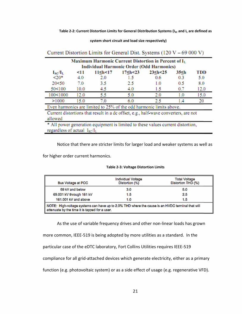
(POI) through mutually agreeable methods.” (Blooming & Carnovale, 2007). Table 2‐2 and Table
2‐3 highlight the limits recommended by IEEE‐519.
fo
m
p
co
fu
Table
Notice
or higher ord
As the
more commo
articular cas
ompliance fo
unction (e.g.
e 2‐2: Current D
s
e that there
der current h
e use of varia
on, IEEE‐519
se of the eDT
or all grid‐at
. photovolta
Distortion Lim
system short c
are stricter
harmonics.
Tabl
able frequen
is being ado
TC laborator
ttached devi
ic system) o
21
its for General
circuit and load
limits for lar
e 2‐3: Voltage
ncy drives an
opted by mo
ry, Fort Colli
ces which ge
or as a side e
1
l Distribution S
d size respecti
rger load an
e Distortion Lim
nd other non
ore utilities a
ns Utilities r
enerate elec
effect of usag
Systems (ISC an
vely)
d weaker sy
mits
n‐linear load
as a standard
requires IEEE
ctricity, eithe
ge (e.g. rege
nd IL are define
ystems as we
ds has grown
d. In the
E‐519
er as a prima
enerative VF
ed as
ell as
n
ary
D).
22
2.3.2 Unusual Cooling Requirements for Industrial Labs
Most industrial inverters or VFDs are air‐cooled while automotive units require
liquid cooling loops. Typically, industrial inverters have sufficient space and are
therefore mounted in large cabinets using forced‐air cooling. In contrast, automotive
inverters are designed to be mounted in confined spaces within vehicles where there is
insufficient space or access to outside air to utilize air‐cooling. Therefore, automotive
inverters and motors typically utilize liquid cooling circuits. This circuit presents design
issues with the construction of the lab. These additional requirements include layout,
temperature control, and proper pumping performance. Therefore, an automotive‐
grade water‐cooling circuit must be implemented, utilizing a radiator and electric fan
combination, similar to the set‐up in a vehicle.
Given the required cooling specifications from the inverter and motor suppliers,
a liquid cooling circuit was constructed. Figure 2‐2 illustrates the major system
components.
Figure 2‐2: Liquid Cooling System Layout

23
The cooling system is divided into two identical circuits, one for each inverter‐
motor pair, to ensure proper cooling when the units are asymmetrically loaded. Each
circuit utilizes a continuous 10gpm centrifugal pump running through a flow meter, an
automotive radiator with an electric fan, and an automotive closed loop thermocouple
relay switch to activate the fans.
The cooling circuit uses electric fans and radiators from a 1992‐1998 Honda Del
Sol. These were chosen based on small size, 12VDC operation, and low cost. A decision
was made to isolate thermal management from the control system to simplify control
modifications for research projects. This adds a degree of separation between the
control system of the lab and the cooling circuit, increasing overall system safety should
the computer for the controller crash. Automotive thermocouples and relays are used
to monitor the cooling circuit and activate cooling fans, without requiring any interface
from the control system.
2.3.3 Voltage Mismatch
The laboratory is connected to the grid at the standard industrial service voltage
of 480VAC 3‐Phase. In contrast, the battery voltage typical of automotive applications is
typically between 350 and 250VDC. As the state of charge (SOC) of the battery declines,
the voltage of the pack decreases. The automotive VFDs utilized for the laboratory do
not contain a “boost” section, typical of photovoltaic inverters. Therefore the maximum
AC output voltage is constrained by the DC voltage applied to the inverter by the
battery. The VFD utilized in the eDTC outputs 208VAC 3‐Phase at mid‐to‐high battery
voltages. At lower battery voltages the inverter output voltage drops as low as 184 VAC.
24
This lower voltage is not a common voltage for transformers, which are designed for
208‐480VAC. Ideally, a custom‐designed transformer would be procured with the
optimum turns ratio of 184:408. However, custom transformers were beyond the
budget available for this laboratory. Instead, the lab utilizes standard 208:480
transformer equipped with a ‐10% connection tap on the 208 V side. Use of the ‐10%
tap provides an effective turns ratio of 187:480, sufficiently close to the 184 V for
operation of most of the usable range of the battery.
In field applications, two methods exist to eliminate this voltage mismatch,
should companies wish to reduce the size, cost, and complexity of similar systems. The
first method is to specify a higher voltage battery, allowing the inverter to operate at
the grid voltage over the entire voltage range of the battery. This option would require a
600 to 750VDC battery pack for direct interconnection to 480VAC. The tradeoffs to this
design include costs related to the higher DC voltage and a significantly larger battery
system. Alternatively, the inverter could be equipped with a boost converter to match
the DC battery voltage to the desired AC voltage. Since the boost section is unneeded
during normal vehicle operation, a bypass circuit or bypass mode would be required.
2.3.4 Time Delay Impact on Voltage/Frequency Measuring Device
In all operation modes, accurate measurement of voltage and frequency is
required in order to properly control the output of the GAS system. In addition, for
stability applications, such as the small‐islanded systems described earlier, the latency
of voltage and frequency measurements is particularly critical. Measurements must be
completed quickly enough to support high‐speed control algorithms. The active control
25
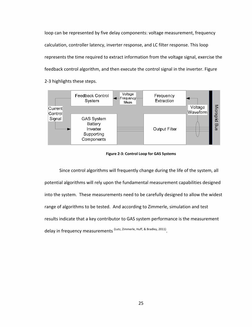
loop can be represented by five delay components: voltage measurement, frequency
calculation, controller latency, inverter response, and LC filter response. This loop
represents the time required to extract information from the voltage signal, exercise the
feedback control algorithm, and then execute the control signal in the inverter. Figure
2‐3 highlights these steps.
Figure 2‐3: Control Loop for GAS Systems
Since control algorithms will frequently change during the life of the system, all
potential algorithms will rely upon the fundamental measurement capabilities designed
into the system. These measurements need to be carefully designed to allow the widest
range of algorithms to be tested. And according to Zimmerle, simulation and test
results indicate that a key contributor to GAS system performance is the measurement
delay in frequency measurements (Lutz, Zimmerle, Huff, & Bradley, 2011).
co
sy
sy
p
h
P
p
m
q
p
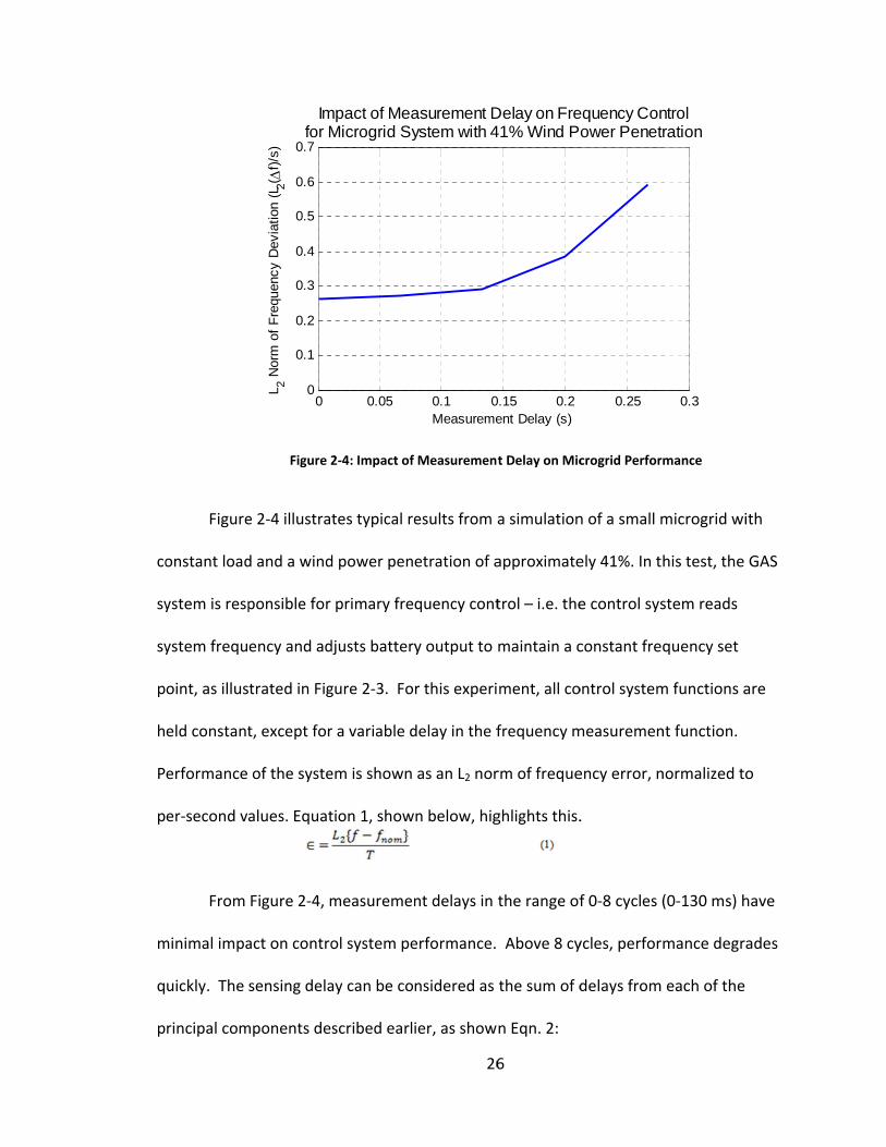
Figure
onstant load
ystem is resp
ystem frequ
oint, as illus
eld constant
erformance
er‐second va
From
minimal impa
uickly. The
rincipal com
Figure 2
e 2‐4 illustra
d and a wind
ponsible for
ency and ad
trated in Fig
t, except for
of the syste
alues. Equat
Figure 2‐4, m
act on contro
sensing dela
mponents de
00
0.1
0.2
0.3
0.4
0.5
0.6
0.7
L 2 Nor
m o
f F
requ
ency
Dev
iatio
n (L
2( f)
/s)
Imfor M
2‐4: Impact of
tes typical re
d power pen
primary fre
djusts battery
gure 2‐3. Fo
r a variable d
em is shown
tion 1, show
measuremen
ol system pe
ay can be co
scribed earl
0.05
mpact of MeaMicrogrid Sy
26
Measuremen
esults from a
etration of a
quency cont
y output to
r this experi
delay in the f
as an L2 nor
n below, hig
nt delays in
erformance.
nsidered as
ier, as show
0.1 0Measureme
asurement Dystem with 4
6
t Delay on Mic
a simulation
approximate
trol – i.e. the
maintain a c
ment, all co
frequency m
rm of freque
ghlights this.
the range of
Above 8 cy
the sum of d
n Eqn. 2:
0.15 0.2ent Delay (s)
Delay on Fre41% Wind P
crogrid Perform
n of a small m
ely 41%. In th
e control sys
constant freq
ontrol system
measuremen
ency error, n
.
f 0‐8 cycles (
ycles, perform
delays from
0.25
equency Conower Penetr
mance
microgrid wi
his test, the
stem reads
quency set
m functions a
nt function.
normalized to
(0‐130 ms) h
mance degra
each of the
0.3
ntrolration
ith
GAS
are
o
have
ades

ti
th
d
is
fr
h
p
o
T
m
re
m
d
d
d
Wher
me required
he controlle
is the f
ominated by
The ch
10
1.5
s believed th
requency tra
igher‐cost tr
ower meter
bjectives, a
his was achi
measuremen
esulting dela
≅ 17
must be filter
evelopment
elay of 20
esign will ex
e is the
d to convert
r cycle time,
first‐order ti
y the first‐or
hosen autom
. The outp
. Utilizin
hat the contr
ansducers ex
ransducers,
, are inappro
decision wa
eved using a
t every ½ cy
ay is approxi
for a 60 H
red. While th
t, initial estim
xhibit a total
e time requir
the voltage
, is the
me constant
rder time co
motive inver
put LC filter
g a high‐spe
rol latency sh
xhibit measu
often costin
opriate for s
s made to co
a zero‐crossi
ycle, from sa
mately data
z system. Du
he signal filt
mates indica
60 . S
control resp
27
red to collec
waveform t
e control res
t of the outp
nstant of th
ters exhibit
exhibits a fir
eed controlle
hould not ex
urement resp
g $800‐2000
small grid sys
ompute freq
ing algorithm
mples collec
a collection t
ue to measu
er may be m
ate filter cha
Summing est
ponse time o
7
ct the voltag
to a frequen
sponse time
put stages of
e LC filter.
fast control
rst‐order tim
er with antic
xceed 20 ms
ponse times
0 as an integ
stems. To m
quency direc
m capable of
cted during t
time plus co
urement nois
modified dur
racteristics w
timated resp
of60
ge waveform
ncy measure
of the VFD/
f the inverte
response tim
me constant
cipated cont
s. However,
s of 100‐200
grated comp
meet cost an
ctly from vol
f producing
the previous
mputationa
se, the comp
ring control a
will produce
ponse times
99 ,
m, is th
ment,
/inverter, an
er, which is
mes, with
where
trol algorithm
most low‐co
ms while
ponent of a
nd performan
tage wavefo
a frequency
s half cycle.
l time, or
puted freque
algorithm
e and effecti
, the system
, which is wi
he
is
nd
ms, it
ost
nce
orms.
y
The
ency
ve
m
thin

28
the control requirements of 0‐130ms as described above. Simulation results indicate
that this response time is adequate for controlling hybrid diesel‐wind grid systems
operating as small as 100 KW, although control of smaller grids may also be possible.
2.4 Design
Details on the choices for key components are described in this section. Specifics
of the inverter selection (Section 2.4.1) as well as its software (Section 2.4.2), the
battery pack (Section 2.4.3), transformer (Section 2.4.4), LC filter (Section 2.4.5), cooling
circuit (Section 2.4.6), and voltage/frequency measurement device (Section 2.4.7) are
included in the following subsections. Lastly, a discussion on the designed safety
(Section 2.4.8) is included. The core portion of the system was sourced from Artisan
Vehicle Systems (AVS) and was delivered as an integrated system.
2.4.1 Inverter/Variable Frequency Drive
Several suppliers were considered for the selection of the inverters or variable
frequency drives. Selections were narrowed based on automotive component use, dual‐
purpose (GAS and dynamometer) capabilities, cost, and design complexity. Table 2‐4
describes three different package options: an Artisan Vehicle Systems (previously called
Calmotors) assembly, a combination between an existing Advanced Energy (AE) power
supply and AVS, and third, an entire Eaton supplied package.

29
Table 2‐4: VFD Selection Comparison Chart
Package Three AVS VFDs plus LS Card
AE DC Power Supply plus two
AVS VFDs Three Eaton VFDs
Specifications
(3) 890CD Frame F, Line Sync Card, AFE,
Pre‐Charge, LC Filter, Connection
Kit
(1) AE Summit 57000007D, (2)
890CD Frame F, Line Sync Card, AFE, Pre‐Charge, LC Filter, Connection Kit
(1) RGX10014AAP1 Regenerative Drive, (2) SPI140A1‐4A3N1 Inverter Drive, AFE, Pre‐Charge, DC
Chopper, Sine wave Filter
Allows for Grid Connectivity for both dyno and
GAS?
Yes
Partially. Dyno: use a
simulated battery (power supply),
GAS: use a simulated load (P Q
demand)
No. Only GAS
Cost $31,200 $22,800 $35,000
Design Complexity Simplest
Requires heavy modifications when changing between dyno and GAS
modes
Missing parts (motors, PCM, and battery pack) would be from AVS so
there would need to be a lot of cooperation
between AVS and Eaton when
designing the lab
Based on the results from Table 2‐4, it was determined that selection number
two, the combination design between AVS and AE, would best fit all the requirements of
the lab except for regeneration to the grid during dyno mode. The requirement for
vehicle simulation favored this implementation of the AVS solution, as the Eaton
solution did not have automotive drives. The weakness to this solution is that an
additional component (AE DC Power Supply) is needed. Fortunately, the eDTC lab is

30
housed within the InteGrid laboratory of the Engines and Energy Conversion Laboratory,
which has volunteered an AE DC Power Supply for utilization when it’s not in use.
2.4.2 Active Front End and Line Sync Card
The active front end (AFE) and line sync card (LS) were sourced from AVS
because of the compatibility between the GAS and dynamometer (dyno) mode set‐up
using the same automotive grade inverter. The LS allows the AFE to monitor the three‐
phase supply voltage waveform and synchronize the inverter to the grid. Once
synchronized, the AFE acts as a four‐quadrant, sinusoidal, bi‐directional power supply.
Since the AFE and LS card are options for the inverter, one inverter can serve two
purposes. However changeovers between software, hardware, and cable connections
need to be made when switching between GAS and dyno set‐up with the inverter.
2.4.3 Battery Pack
The battery pack was sourced from AVS because it has the same scale and
performance as full‐size automotive electric vehicle packs. This pack came assembled
with a battery management system (BMS), as well as positive, negative, and pre‐charge
contactors, all packaged within an air‐cooled case. The manufacturer of the cells is GBS.
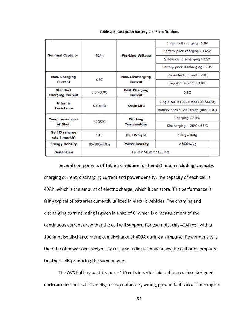
Specifications are listed below in Table 2‐5.
ch
4
fa
d
co
1
th
to
e
Sever
harging curr
0Ah, which
airly typical o
ischarging c
ontinuous cu
0C impulse d
he ratio of p
o other cells
The A
nclosure to
al compone
rent, dischar
is the amoun
of batteries
urrent rating
urrent draw
discharge ra
ower over w
producing t
VS battery p
house all the
Table 2‐5:
nts of Table
rging current
nt of electric
currently ut
g is given in
that the cel
ting can disc
weight, by ce
the same po
pack feature
e cells, fuses
31
GBS 40Ah Bat
2‐5 require
t and power
c charge, wh
ilized in elec
units of C, w
l will suppor
charge at 40
ell, and indic
ower.
s 110 cells in
s, contactors
1
ttery Cell Spec
further defi
r density. The
hich it can st
ctric vehicles
which is a me
rt. For exam
00A during a
cates how he
n series laid
s, wiring, gro
cifications
inition includ
e capacity o
tore. This pe
s. The charg
easurement
mple, this 40A
n impulse. P
eavy the cell
out in a cus
ound fault ci
ding: capacit
f each cell is
rformance i
ing and
of the
Ah cell with
Power densit
ls are compa
tom designe
ircuit interru
ty,
s
s
a
ty is
ared
ed
upter
(G
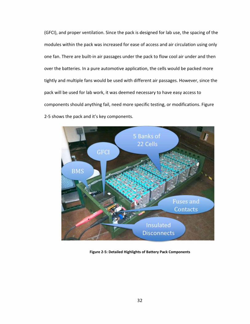
m
o
o
ti
p
co
2
GFCI), and p
modules with
ne fan. Ther
ver the batt
ghtly and m
ack will be u
omponents
‐5 shows the
roper ventila
hin the pack
re are built‐i
eries. In a pu
ultiple fans
used for lab w
should anyt
e pack and it
Fig
ation. Since
was increas
n air passag
ure automot
would be us
work, it was
hing fail, nee
t’s key comp
gure 2‐5: Detai
32
the pack is d
sed for ease
es under the
tive applicat
sed with diff
s deemed ne
ed more spe
ponents.
iled Highlights
2
designed for
of access an
e pack to flo
tion, the cell
ferent air pa
ecessary to h
ecific testing
s of Battery Pa
r lab use, the
nd air circula
ow cool air u
ls would be
ssages. How
have easy ac
g, or modific
ack Componen
e spacing of
ation using o
nder and th
packed mor
wever, since
ccess to
ations. Figur
ts
the
only
en
re
the
re

B
va
2
vo
d
2
Je
A clos
MS monitor
alue of the h
.4.4 Transf
The tr
oltage mism
ifferent sup
08V primary
efferson Elec
ser view of e
rs each cell v
highest cell t
Fi
former
ransformer w
match as disc
pliers to pro
y, and 480Y/
ctric. Specifi
ach cell, Fig
voltage, curr
to the user.
igure 2‐6: Cell
was sized ba
ussed in the
ovide a trans
/277V secon
cations are s
33
ure 2‐6, reve
rent, and tem
Monitors for E
ased on the o
e challenges
former that
dary. The low
shown in Ta
3
eals the BMS
mperature b
Each Cell of th
output from
section. Qu
t was designe
west cost bi
ble 2‐6.
S cell voltag
but only repo
he Battery Pack
m the VFD an
otes were se
ed for three
id was chose
e sensors. T
orts the max
k
d battery du
ent out to
e‐phase, 150
en from
he
x
ue to
kVA,
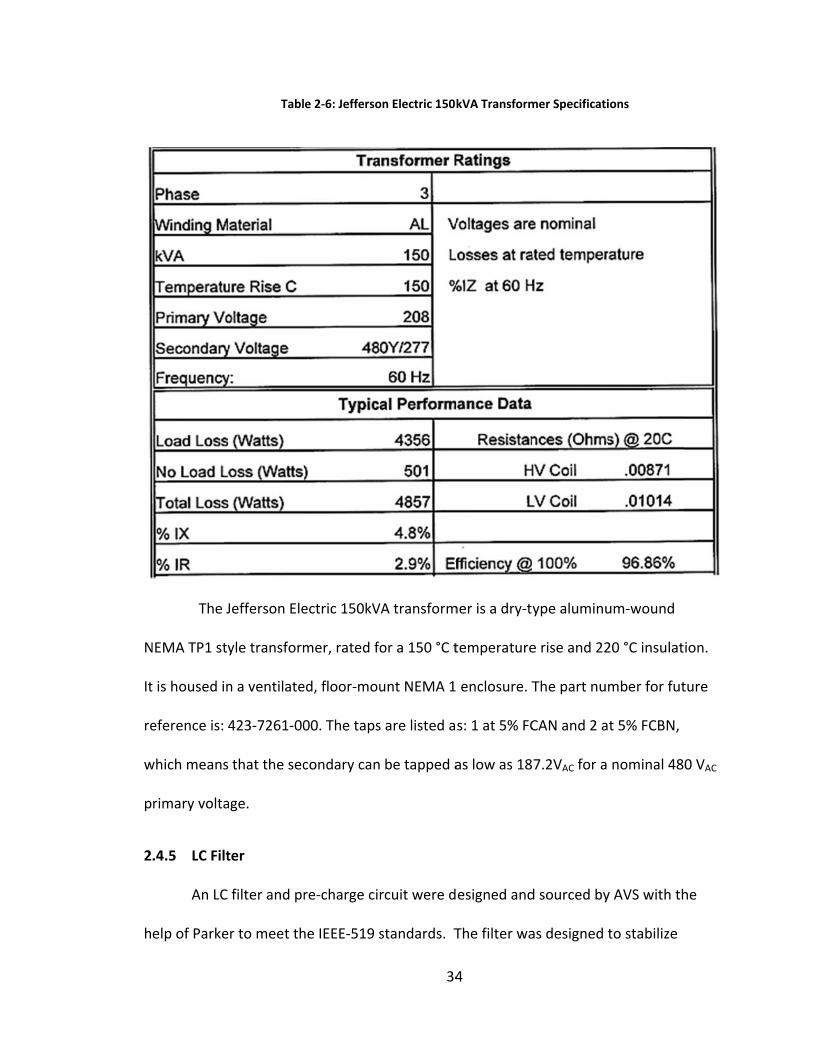
N
It
re
w
p
2
h
The J
NEMA TP1 sty
t is housed in
eference is:
which means
rimary volta
.4.5 LC Filt
An LC
elp of Parke
Tabl
Jefferson Ele
yle transform
n a ventilate
423‐7261‐00
that the sec
age.
ter
filter and pr
er to meet th
e 2‐6: Jefferso
ectric 150kV
mer, rated fo
ed, floor‐mou
00. The taps
condary can
re‐charge cir
he IEEE‐519 s
34
on Electric 150k
VA transform
or a 150 °C t
unt NEMA 1
s are listed a
be tapped a
rcuit were d
standards. T
4
kVA Transform
mer is a dry‐t
temperature
enclosure. T
s: 1 at 5% FC
as low as 18
esigned and
The filter wa
mer Specificati
ype aluminu
e rise and 22
The part num
CAN and 2 a
7.2VAC for a
d sourced by
as designed t
ions
um‐wound
20 °C insulat
mber for fut
t 5% FCBN,
nominal 48
y AVS with th
to stabilize
ion.
ture
0 VAC
he

35
within a few seconds at power up. The cutoff frequency was designed for less than half
the inverter switching frequency (2.5 kHz). The filter operates as an LCL filter, with the
transformer providing the secondary inductance. Parker was chosen to design the LC
filter to maintain capability with the inverter.
The final components were modeled in SimPower Systems to determine the
response time of a pre‐charge filter. However, since Jefferson did not provide
sufficiently detailed design information, it was only possible to create a basic model. The
model indicated that the pre‐charge resistors needed to be greater than 0.25 Ω in order
to limit the in‐rush current to less than three times the nominal current. Due to
concerns with the model, it was decided to utilize prior experience by AVS to size the
charging resistors. As a result, AVS sized the resistors at 45 Ω. Figure 2‐7 presents the
circuit schematic of the LC filter cabinet packaging, including the pre‐charge circuit.
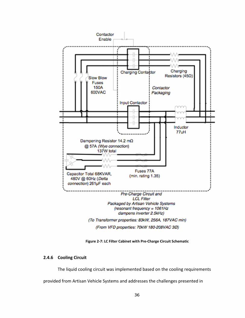
2
p
.4.6 Coolin
The liq
rovided from
Figu
ng Circuit
quid cooling
m Artisan Ve
ure 2‐7: LC Filte
g circuit was
ehicle System
36
er Cabinet wit
implemente
ms and addre
6
h Pre‐Charge C
ed based on
esses the ch
Circuit Schema
the cooling
hallenges pre
atic
requiremen
esented in
nts
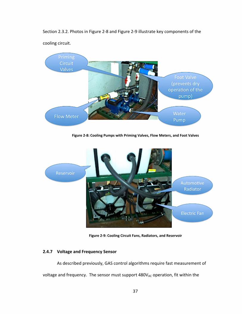
Se
co
2
vo
ection 2.3.2
ooling circui
.4.7 Voltag
As des
oltage and f
. Photos in F
t.
Figure 2‐8: C
F
ge and Freq
scribed prev
requency. T
Figure 2‐8 an
Cooling Pumps
Figure 2‐9: Coo
uency Senso
viously, GAS
The sensor m
37
nd Figure 2‐9
s with Priming
oling Circuit Fa
or
control algo
must support
7
9 illustrate k
g Valves, Flow
ns, Radiators,
orithms requ
t 480VAC ope
key compone
Meters, and F
and Reservoir
uire fast mea
eration, fit w
ents of the
Foot Valves
r
asurement o
within the
of

38
budget, and produce fast measurement time (less than 0.13s; see section 2.3.4). Table
2‐7 highlights the results of the various sensors considered for selection.
Table 2‐7: Voltage/Frequency Sensor Comparison
Sensor
AC
Voltage
Range
Response Time Price Output
Ohio Semitronics Inc. DMT‐
1024 100‐636V <100ms $1,405
±20mA,
RS‐485
Ohio Semitronics DSP‐008 600V <100ms $1,025 4‐20mA,
RS‐422
Elkor WattsOn‐1200‐MSCT1 480V 500ms $376 RS‐485
Power True Systems Corp.
2V‐33‐AD‐6‐A5‐D2 and 2F‐33‐
AD‐6‐A5‐D2
0‐500V
<400ms
A/D conversion
not included
Not
Available
0‐10V or
4‐20mA
Custom Built Voltage Divider
and National Instruments
cRio Data Acquisition
0‐750V
As fast as LabView
program is
designed
$480 ±4.8V
As seen above, the best sensors with the lowest response time (Ohio
Semitronics) are also the most expensive solutions. Therefore a custom‐built voltage
divider with NI DAQ solution was chosen. The sensor was built using a precision decade
resistor. The 1776‐C54 voltage divider by Caddock Electronics is shown in Figure 2‐10.
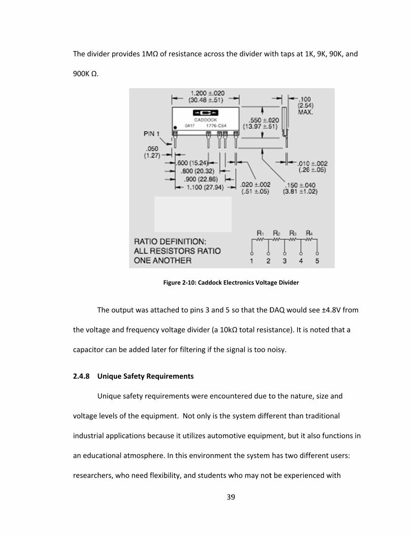
T
9
th
ca
2
vo
in
a
re
he divider p
00K Ω.
The o
he voltage a
apacitor can
.4.8 Uniqu
Uniqu
oltage levels
ndustrial app
n education
esearchers, w
rovides 1MΩ
utput was at
nd frequenc
n be added la
ue Safety Re
ue safety req
s of the equi
plications be
al atmosphe
who need fle
Ω of resistan
Figure 2‐10
ttached to p
cy voltage di
ater for filte
equirements
quirements w
ipment. Not
ecause it util
ere. In this e
exibility, and
39
nce across th
0: Caddock Ele
pins 3 and 5
vider (a 10k
ring if the sig
s
were encoun
t only is the
izes automo
nvironment
d students w
9
he divider wi
ctronics Volta
so that the D
kΩ total resis
gnal is too n
ntered due t
system diffe
otive equipm
the system
who may not
ith taps at 1
ge Divider
DAQ would s
stance). It is
noisy.
to the nature
erent than tr
ment, but it a
has two diff
t be experien
K, 9K, 90K, a
see ±4.8V fr
noted that a
e, size and
raditional
also function
ferent users
nced with
and
rom
a
ns in
:

40
electrically and mechanically dangerous equipment. Both of these users require
different safety measures. Relative to traditional safety standards, the system needs to
have ground fault detection, multiple E‐stop switch locations, and thermal
management. The insulation or ground fault detection device is discussed in the next
section. Emergency stop buttons are located throughout the test center in three
different areas to ensure that the user is always within ten feet of an E‐Stop. In typical
industrial environments E‐stop switches are included and installed in covers and doors
of the purchased system but since the components were sourced from an automotive
supplier, these switches were added during the lab design and construction. More
specifics of the E‐stop system are detailed in section 3.4.10. In addition to this safety,
light towers were installed to provide visual verification if a breaker is closed and the
system is live. This will visually notify users not to open breakers, control boxes, make
electrical connections or perform repairs when the system is energized.
The battery management system provided by Artisan monitors each cell
performance to determine battery safety and health. These values are communicated to
the Powertrain Control Module graphical user interface (PCM GUI). The PCM GUI
monitors the battery SOC and prevents operation if the battery SOC is not within the
defined operating range. For example, if the battery were fully charged when the GAS
controller commands a charging operation, which could over‐charge the battery, the
PCM would cancel the command in order to preserve battery health and proper use.
The PCM GUI software has limits defined for cell over/under voltage, over/under
temperature, and charge/discharge rate.

2
ag
w
o
d
G
p
u
a
co
a
3
la
.4.8.1 Insu
Batter
gainst short
with a ground
perational.
isconnects/o
GFCI system i
art of the sy
The B
nsafe outpu
ctive high vo
ompact size,
pplications.
2xx‐electric‐
ab.
lation Moni
ry subsystem
circuits betw
d fault circui
If for any re
opens the ba
is operation
ystem.
ender IR155
ut. The IR155
oltage lines o
, temperatu
Figure 2‐11
‐vehicles_DB
Fig
itoring Devic
ms present u
ween batter
it interrupte
eason the ba
attery conta
al only when
5 was chosen
5 monitors th
of battery an
re, and vibra
(image from
B_en_20101
gure 2‐11: Ben
41
ce
unique safety
ry supply line
r (GFCI), wh
ttery becom
acts and soun
n the battery
n because it
he insulation
nd the refere
ation makes
m: http://ww
1202.pdf) sho
nder IR155 Gro
1
y challenges
es and groun
hich engages
mes grounde
nds appropr
y is not conn
provides a c
n resistance
ence (chassi
s it ideally su
ww.iso‐f1.de
ows the Ben
ound Fault Circ
s, particularl
nd. The syst
s when the s
d, the GFCI
riate alarms.
nected to an
clear “ok” –
between th
is) ground. I
uited for hyb
/downloads
nder IR155 G
cuit Interrupte
y guarding
tem is equip
ystem is not
. Note that t
nd operating
safe or “not
he insulated
Its design fo
brid vehicle
s/iso‐F1‐IR15
GFCI used in
er
pped
t
the
g as
t ok”
and
r
55‐
the

2
sa
co
in
o
In
d
a
h
o
.4.8.2 Insu
Since
afe way to sw
onnections n
nterconnecti
pening the p
nstead, the c
isconnect ca
lso utilized f
igh current a
f a short circ
Fig
lated Conne
the lab is de
witch betwe
need to be u
ions would b
possibility th
connections
am‐lock conn
for event pow
and voltage
cuit.
gure 2‐12: Cam
Connec
ectors
esigned to op
een the two
unplugged fr
be difficult to
hat the syste
are perform
nectors from
wer and exp
demands an
m Connectors b
tor, and Demo
42
perate in tw
was require
rom the mot
o produce u
em could be
med using co
m Marinco E
peditionary m
nd allow safe
by Marinco. Clo
onstration of I
2
wo independ
ed. To conve
tor and attac
sing interloc
started in a
olored cablin
lectrical. The
military ope
e interconne
ockwise: Fema
nstallation, Pa
ent modes,
rt to GAS m
ched to the
cked breake
n invalid con
ng and shield
ese connect
rations, safe
ect while mi
ale Cam Conne
anel Mounts
GAS and dyn
ode, the inv
LC filter. The
rs and switc
nfiguration.
ded quick
ors, which a
ely handle th
nimizing the
ector, Male Ca
no, a
verter
ese
ches,
are
he
e risk
am

43
Figure 2‐12 (images from: http://www.beckelectric.com/store/pc/Marinco‐
Information‐c266.htm) illustrates the different cam connectors. They have a male or
female plug to prevent unintended connections. The system was designed such that the
user only matches the proper colors. The polarity and color of the plug were designed so
that only one arrangement is possible. Color‐coding was selected to minimize the
chance of inadvertently connecting incompatible power leads. DC leads are color coded
as black (V‐) and red (V+). The AC connections would normally use the industrial
standard of red‐white‐blue for 208 VAC. However, this would create the potential to
interconnect a red DC line with phase A of the 208 AC lines. Therefore, all AC lines are
color‐coded using the 480 VAC standard of brown‐orange‐yellow for the three phases.
With the use of these insulated connectors, users of the lab can quickly, safely, and with
confidence, change between the two lab set‐ups.
2.5 Check Out and Verification
This section describes overall lab construction (Section 2.5.1), a step‐by‐step
overview of the system operation (Section 2.5.2), and results of the system verification
tests (Section 2.5.3).
2.5.1 Finalized System Construction
A 3D CAD model was utilized to layout the lab. Figure 2‐13 illustrates this model
with call‐outs to the specific components of the lab.

D
ra
la
Figure
The C
During constr
atio as dictat
Figure
ab with call‐o
2‐13: Overview
CAD model il
ruction each
ted by the lo
e 2‐14 shows
outs labeling
w of Compone
llustrates ke
h conduit wa
ocal electrica
s the comple
g the major c
44
ents and Their
y componen
as sized acco
al code.
eted constru
components
4
Locations in 3
nts; conduits
ording to the
uction of the
s.
3D CAD Model
s and cabling
e required w
e GAS portio
g are not sho
wire size and
on of the eDT
own.
fill
TC
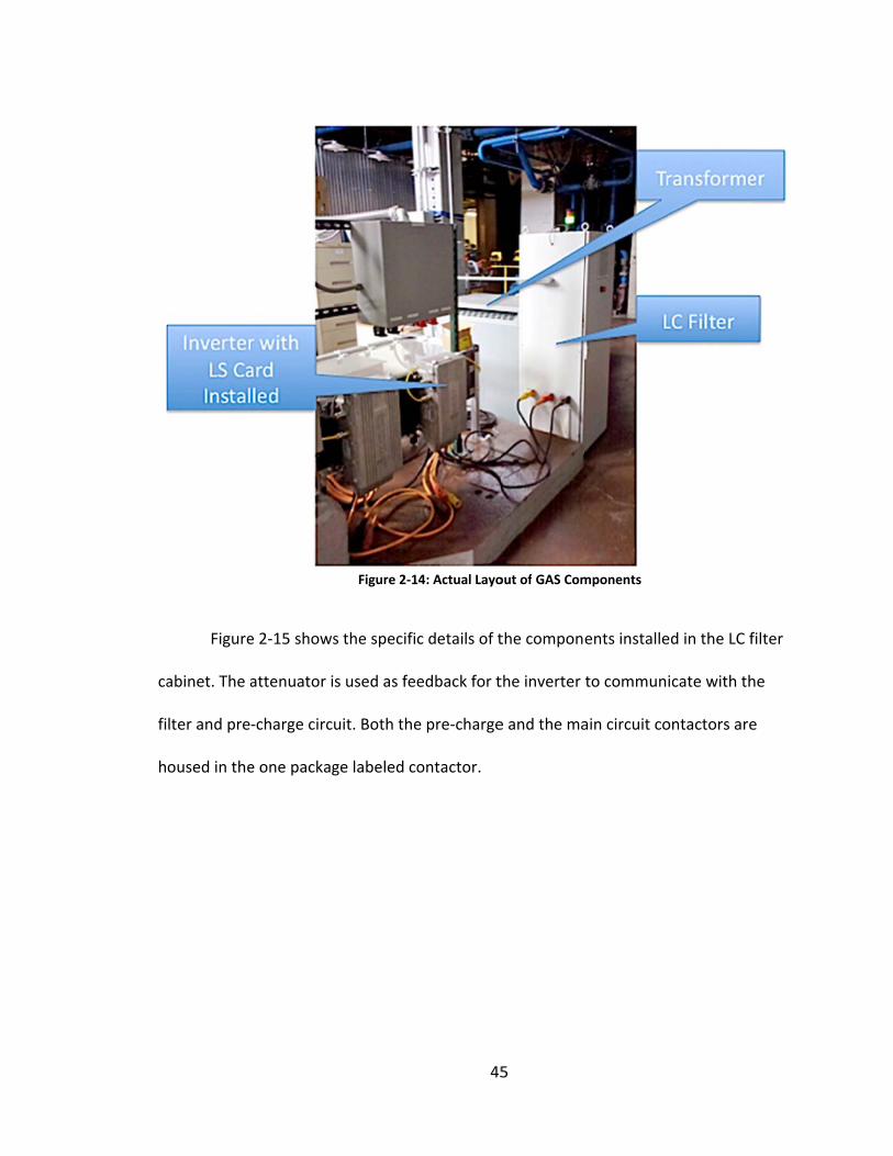
ca
fi
h
Figure
abinet. The a
lter and pre
oused in the
e 2‐15 shows
attenuator i
‐charge circ
e one packag
Figure 2‐1
s the specific
s used as fee
uit. Both the
ge labeled co
45
4: Actual Layo
c details of t
edback for t
e pre‐charge
ontactor.
5
out of GAS Com
the compon
the inverter
e and the ma
mponents
ents installe
to communi
ain circuit co
ed in the LC f
icate with th
ontactors are
filter
he
e
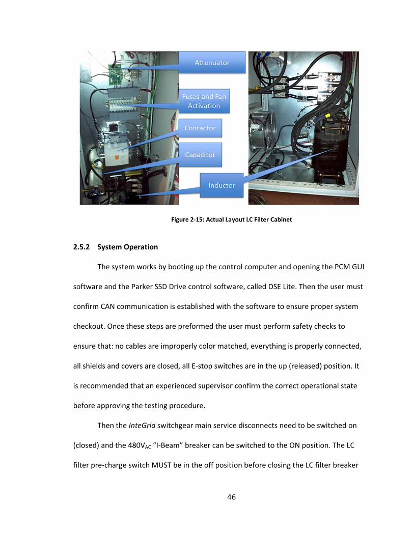
2
so
co
ch
e
a
is
b
(c
fi
.5.2 System
The sy
oftware and
onfirm CAN
heckout. On
nsure that: n
ll shields and
s recommen
efore appro
Then t
closed) and t
lter pre‐cha
m Operation
ystem works
the Parker S
communica
ce these ste
no cables ar
d covers are
ded that an
ving the test
the InteGrid
the 480VAC “
rge switch M
Figure 2
n
s by booting
SSD Drive co
tion is estab
eps are prefo
e improperly
e closed, all E
experienced
ting procedu
d switchgear
“I‐Beam” bre
MUST be in t
46
‐15: Actual Lay
up the cont
ontrol softw
blished with
ormed the u
y color matc
E‐stop switch
d supervisor
ure.
main servic
eaker can be
the off positi
6
yout LC Filter C
trol compute
are, called D
the softwar
ser must pe
ched, everyt
hes are in th
r confirm the
e disconnec
e switched to
ion before c
Cabinet
er and open
DSE Lite. The
re to ensure
erform safety
thing is prop
he up (releas
e correct ope
cts need to b
o the ON po
closing the LC
ing the PCM
en the user m
proper syste
y checks to
perly connec
sed) position
erational sta
be switched
osition. The L
C filter break
M GUI
must
em
ted,
n. It
ate
on
LC
ker

to
sh
A
m
vo
ca
w
sw
in
b
in
d
o prevent th
hould be act
At this point t
must ensure
oltage of 18
an be switch
will automati
witch may b
nvolves the u
ox (shown in
Using
nduction lea
emand valu
e LC filter ci
tivated at th
the breaker
that the GAS
7VAC. When
hed ON to be
cally close w
e turned to
user flipping
n Figure 2‐16
g the DSE Lit
kage, and cu
es the batte
rcuit from a
is time. The
to the LC filt
S inverter is
n the proper
egin the pre
with a loud “
begin the ba
g the “ENABL
6).
Figure 2‐16:
e software,
urrent dema
ery will charg
47
rcing. The fi
pump for th
ter can be sw
communica
voltage is o
‐charge. Aft
thud.” After
attery pre‐ch
LE” switch fo
Desk Control
the user can
and from the
ge or dischar
7
lter cabinet
he GAS circu
witched to t
ating properl
observed, the
er a few sec
r system che
harge and fu
or the GAS in
Box with Swit
n define curr
e battery. By
rge accordin
fans and the
uit must also
the ON posit
ly and seein
e LC pre‐cha
conds, the m
eckout, the b
ull connectio
nverter on th
tch Callouts
rent control
y defining th
ngly. The use
e radiator fa
be plugged
tion. The use
g an AC bus
arge contact
main contacto
battery key‐o
on. The final
he desk cont
mode, moto
e current
er can monit
ans
in.
er
ors
or
on
step
trol
or
tor
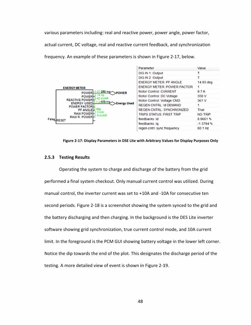
va
a
fr
2
p
m
se
th
so
li
N
te
arious param
ctual curren
requency. An
Figur
.5.3 Testin
Opera
erformed a
manual contr
econd period
he battery d
oftware show
mit. In the fo
Notice the di
esting. A mo
meters inclu
t, DC voltag
n example o
re 2‐17: Displa
ng Results
ating the sys
final system
rol, the inver
ds. Figure 2‐
ischarging a
wing grid sy
oreground is
p towards th
ore detailed v
ding: real an
e, real and r
of these para
ay Parameters
stem to char
m checkout. O
rter current
‐18 is a scree
nd then cha
nchronizatio
s the PCM G
he end of th
view of even
48
nd reactive p
reactive curr
ameters is sh
in DSE Lite wit
ge and disch
Only manual
was set to +
enshot show
arging. In the
on, true curr
UI showing
e plot. This d
nt is shown i
8
power, powe
rent feedbac
hown in Figu
th Arbitrary V
harge of the
l current con
+10A and ‐10
wing the syst
e backgroun
rent control
battery volt
designates t
in Figure 2‐1
er angle, pow
ck, and synch
ure 2‐17, bel
Values for Disp
battery from
ntrol was uti
0A for conse
tem synced t
d is the DES
mode, and
tage in the lo
the discharge
19.
wer factor,
hronization
ow.
lay Purposes O
m the grid
ilized. During
ecutive ten
to the grid a
Lite inverte
10A current
ower left cor
e period of t
Only
g
and
r
rner.
the

re
(s
Figure
Figur
During
eactive pow
shown in Fig
e 2‐18: Screen
re 2‐19: PCM G
g this testing
er of the sys
gure 2‐20).
shot of DSE Lit
GUI BMS Plot o
Min Cell V
g the scope
stem as well
49
te in Backgrou
of Pack Current
Voltage vs. Tim
function of D
as the volta
9
und with PCM
t and Voltage
me Plot (right)
DSE Lite was
age comman
GUI BMS Mon
vs. Time Plot (
s utilized to
nd along with
nitor in Foregro
(left) and Max
monitor the
h actual volt
ound
x and
e
tage
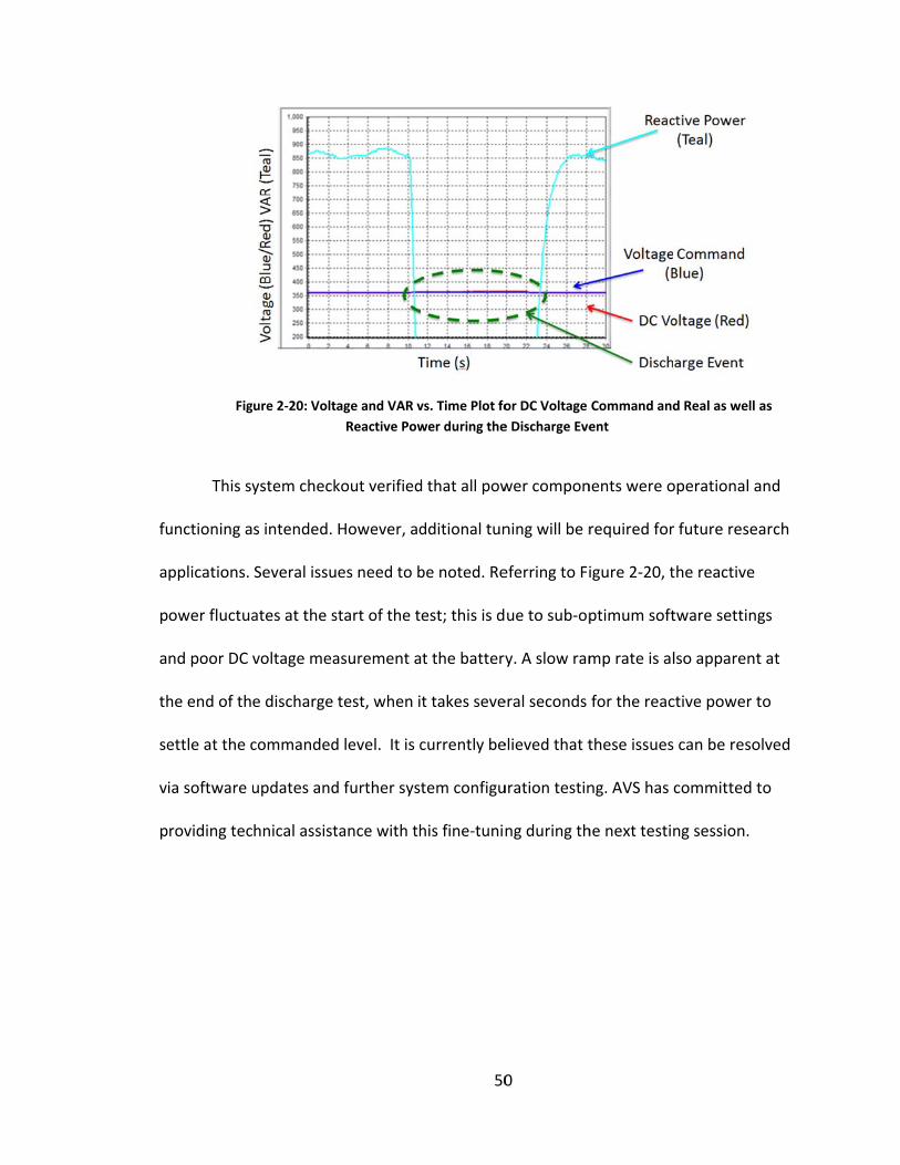
fu
a
p
a
th
se
vi
p
Fig
This sy
unctioning a
pplications.
ower fluctua
nd poor DC
he end of th
ettle at the c
ia software u
roviding tec
ure 2‐20: Volta
ystem check
s intended.
Several issu
ates at the s
voltage mea
e discharge
commanded
updates and
hnical assist
age and VAR v
Reactive Pow
kout verified
However, ad
es need to b
start of the t
asurement a
test, when i
d level. It is c
d further syst
tance with th
50
vs. Time Plot fo
wer during the
d that all pow
dditional tun
be noted. Re
est; this is d
t the battery
t takes seve
currently be
tem configu
his fine‐tunin
0
or DC Voltage
e Discharge Eve
wer compon
ning will be r
eferring to Fi
ue to sub‐op
y. A slow ram
eral seconds
elieved that t
uration testin
ng during th
Command and
ent
nents were o
required for
igure 2‐20, t
ptimum soft
mp rate is al
for the reac
these issues
ng. AVS has
he next testin
d Real as well
operational a
r future rese
the reactive
tware setting
lso apparent
ctive power t
can be reso
committed t
ng session.
as
and
arch
gs
t at
to
olved
to

51
3. Electric Vehicle Component Education through a Dynamometer
This chapter focuses on the dynamometer portion of the eDTC. Sections include
an introduction of to dynamometers (Section 3.1), an overview of the system (Section
3.2), the challenges that were presented with the system (Section 3.3), the design
selection of each of the key components (Section 3.4), a system check‐out (Section 3.5)
and course work example (Section 3.6).
3.1 Dynamometer Introduction
A dynamometer (hereafter referred to as dyno) is a device used as a brake to
test rotary machines. Dynamometers are utilized to test internal combustion engines,
motors, generators and related machines. A dyno consists of a shaft coupling and a
controllable loading mechanism, typically capable of independently controlling either
torque or speed of the unit under test (UUT). There are many different kinds of dyno
loading mechanisms, including: water brakes, eddy current brakes, electrical generators,
fan, hydraulic resistance loads, and controllable mechanical friction loads. Each type has
its own advantages and disadvantages, which needed to be considered based on the
requirements of the lab. Since the eDTC lab has very tight space requirements, this
limited many technologies. The electrical generator dyno type was pursued since it
would be the simplest to implement and most compact. Using an electrical motor as the
brake or absorber means that electrical power recovered from the dyno could be reused

52
by the system, thus requiring an external power to only provide power for the losses
within the system.
3.1.1 Various Methods of Motor Testing To Date
Many industrial and educational internal combustion engine (ICE) stands exist
around the world, but their design is very different compared to an automotive electric
motor test stand. The existing test benches have liquid cooling infrastructure, exhaust
venting, emissions measurement equipment, fuel storage, plumbing, and safety
precautions, as well as different sensors (O2, timing, thermocouples, pressure, mass air
flow rates, etc.). However, only a few of these components and testing knowledge can
be carried over to electric motor and GAS test stands. ICE test stands do not have
inverters, batteries, or traction DC power supplies. In addition to the differences, some
dynos (i.e. water brake dynos) do not have generators that can be used for regenerating
power back on to the local utility grid. In general, test operators would prefer to sell
power back to the grid. However, they are constrained by the utilities interconnection
regulations and additional expensive infrastructure. For this reason, most dyno test
stands today simply turn the used energy into heat and dissipate this energy during
testing. This gives operators more flexibility at the expense of continuous power input.
In the eDTC lab, it was desired to not use the dyno to produce waste heat but
rather minimize consumption by designing a regenerative solution. While the dyno set‐
up of this lab doesn’t have grid regeneration, it does feature a regenerative loop that
minimizes power consumption. This regenerative concept was selected to minimize
power input and to reduce cost of components.

53
3.1.2 Uniqueness of this Set‐Up
The CSU eDTC test lab is unique because the majority of current test labs support
only ICE testing. Few universities have full‐scale traction motor testing, making it
difficult for students to acquire hands‐on experience with electric vehicle components
and for researchers to perform physical testing. Many vehicle manufacturers,
component designers, and even national labs have electric motor testing facilities or
hybrid dynamometers, but few have an educational laboratory utilizing components of
this scale. The unique contribution of the eDTC laboratory is providing an educational
facility using full‐scale automotive components in a flexible system configuration.
3.2 High‐level System Overview of the Dynamometer Lab
This section describes the architecture of the dyno laboratory at a high level,
including the motor to test, the absorber motor, inverter drives for each motor, power
supply, and torque sensing.
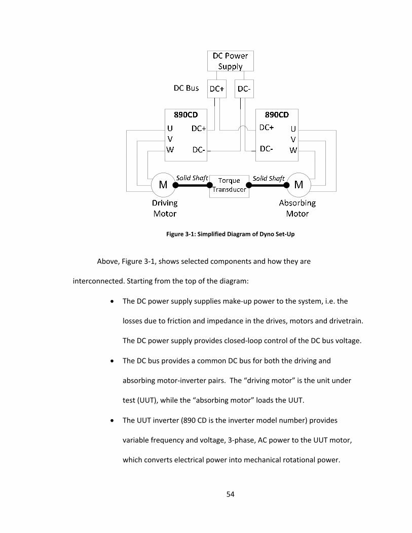
54
Figure 3‐1: Simplified Diagram of Dyno Set‐Up
Above, Figure 3‐1, shows selected components and how they are
interconnected. Starting from the top of the diagram:
The DC power supply supplies make‐up power to the system, i.e. the
losses due to friction and impedance in the drives, motors and drivetrain.
The DC power supply provides closed‐loop control of the DC bus voltage.
The DC bus provides a common DC bus for both the driving and
absorbing motor‐inverter pairs. The “driving motor” is the unit under
test (UUT), while the “absorbing motor” loads the UUT.
The UUT inverter (890 CD is the inverter model number) provides
variable frequency and voltage, 3‐phase, AC power to the UUT motor,
which converts electrical power into mechanical rotational power.

55
Control of the UUT inverter can be modified to support education or
research needs. Either speed or torque control are possible.
The torque sensor monitors both the torque and speed of the UUT.
The absorber motor loads the UUT, generating variable‐frequency, 3‐
phase, AC, power to its inverter.
The absorber inverter (also inverter model number 890 CD) absorbs
power from the absorber motor and drives that power back onto the DC
bus by adjusting its DC output voltage. Generally, the absorber will be
controlled using the opposite parameter of the UUT inverter – speed if
the UUT is controlling torque, and vice versa.
The only major component not shown in the figure is the power train control
module (PCM), which facilitates communication between the control computer and
inverters.
3.3 Design Challenges
This section elaborates on the challenges in the design and construction of the
dyno portion of the lab, and describes the selection of key components.
3.3.1 Cogging and Other Vibration Effects
Under certain high‐load conditions, traction motors may exhibit significant
cogging. In traction‐drive test mode this cogging can excite torsional vibration modes in
the drivetrain between the two motors. These vibrations may be amplified if the
compliance in the couplings and the torque transducer create natural vibration modes

56
near the excitation frequency. The top design speed of the system is 8,000 RPM. Given
that the motors have eight poles, the fundamental cogging frequency is 32,000 RPM or
533 Hz. To avoid resonance, an ideal solution would place the first vibration mode
above 1066 Hz. Given that the mass of the UUT and absorbing motors is largely set by
their size, the frequency requirement primarily impacts the selection of the torque
sensor and shaft couplings.
3.3.2 Sizing of DC Power Supply
The lab is not designed to utilize the battery as a motor power supply. Therefore a
DC power supply was utilized to power the inverters during testing. Each motor is rated
at 70kW. Therefore, if no regeneration is utilized, the lab must provide up to 70 kW to
the UUT motor (plus losses), and must dissipate up to 70 kW generated by the absorber
motor. However, the power supply demand can be greatly reduced if the power
generated by the absorber is reused within the dyno, and the need for a 70 kW load
bank can be entirely removed. In this architecture, only “make‐up” power will be
required to account for friction and impedance losses within the two motor/inverters.
This regenerative set‐up is achieved by placing both inverters on a shared DC bus.
Therefore, the size of the make‐up supply depends on the losses in the system.
To determine these losses, the worst efficiencies were used to calculate the
maximum make‐up power required for different power and speed situations. Figure 3‐2
shows how the system was modeled for calculating power consumption based on the
different efficiencies of the different components.
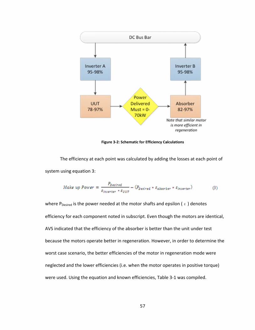
sy
w
ef
A
b
w
n
w
The ef
ystem using
where PDesired
fficiency for
AVS indicated
ecause the m
worst case sc
eglected and
were used. U
fficiency at e
equation 3:
d is the powe
each compo
d that the ef
motors oper
cenario, the
d the lower
sing the equ
Figure 3‐2:
each point w
er needed at
onent noted
fficiency of t
rate better in
better effici
efficiencies
uation and k
57
: Schematic fo
was calculate
t the motor
d in subscript
he absorber
n regenerati
encies of the
(i.e. when th
nown efficie
7
r Efficiency Ca
ed by adding
shafts and e
t. Even thou
r is better th
ion. Howeve
e motor in r
he motor op
encies, Table
alculations
g the losses a
epsilon (ε) d
ugh the moto
han the unit
er, in order t
egeneration
perates in po
e 3‐1 was co
at each poin
denotes
ors are ident
under test
to determine
n mode were
ositive torqu
ompiled.
nt of
tical,
e the
e
ue)
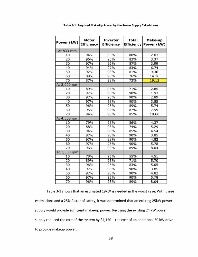
e
su
su
to
Table
stimations a
upply would
upply reduce
o provide ma
Table 3‐
3‐1 shows t
and a 25% fa
d provide suf
ed the cost o
akeup powe
‐1: Required M
hat an estim
actor of safet
fficient make
of the system
er.
58
Make‐Up Powe
mated 19kW
ty, it was de
e‐up power.
m by $4,150
8
er by the Powe
is needed in
etermined th
Re‐using th
0 – the cost o
er Supply Calcu
n the worst c
hat an existin
he existing 24
of an additio
ulations
case. With t
ng 25kW pow
4 kW power
onal 50 kW d
hese
wer
r
drive
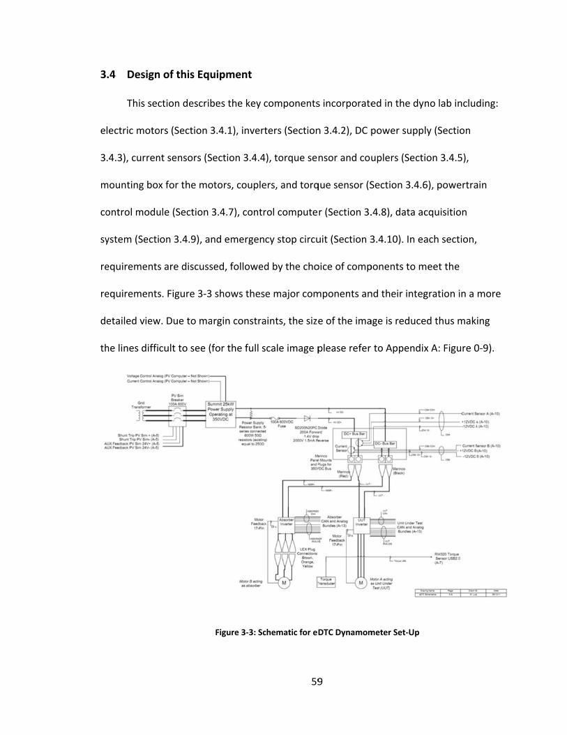
3
e
3
m
co
sy
re
re
d
th
.4 Design
This sec
lectric moto
.4.3), curren
mounting box
ontrol modu
ystem (Secti
equirements
equirements
etailed view
he lines diffi
n of this Equ
ction describ
ors (Section 3
nt sensors (S
x for the mo
ule (Section 3
on 3.4.9), an
s are discuss
s. Figure 3‐3
w. Due to ma
cult to see (f
uipment
bes the key c
3.4.1), invert
ection 3.4.4
otors, couple
3.4.7), contr
nd emergen
sed, followed
shows thes
rgin constra
for the full s
Figure 3‐3: Sc
59
components
ters (Section
4), torque sen
ers, and torq
rol compute
cy stop circu
d by the cho
e major com
aints, the size
scale image p
chematic for eD
9
s incorporate
n 3.4.2), DC p
nsor and cou
que sensor (S
r (Section 3.
uit (Section 3
oice of comp
mponents an
e of the ima
please refer
DTC Dynamom
ed in the dy
power supp
uplers (Secti
Section 3.4.6
.4.8), data ac
3.4.10). In ea
ponents to m
nd their integ
age is reduce
to Appendix
meter Set‐Up
no lab includ
ly (Section
ion 3.4.5),
6), powertra
cquisition
ach section,
meet the
gration in a
ed thus maki
x A: Figure 0
ding:
ain
more
ing
0‐9).

60
Starting from the left hand side of the figure:
The service disconnect provides power to the Summit™ DC Power Supply.
A diode prevents power flowing in reverse direction from the DC bus to
the DC power supply.
Both inverters are connected to the DC bus using Marinco insulated
power connectors.
Current sensors are shown within the DC bus bar area to monitor the
current flow to each inverter from the DC bus.
3.4.1 Electric Motors
For this lab, both a UUT motor and an absorber motor (acting primarily as a
generator) are needed. Since the lab will function as a test bed for any automotive‐
based electric motor, the choice of motors is not particularly crucial. Motors were
chosen for the dynamometer lab from Artisan Vehicle Systems because the automotive‐
style motors could be procured at below market cost and be pre‐package to work
together with AVS inverters and powertrain control module (PCM), as well as an open‐
source control system. The chosen motor pair is the Parker GP150WC motors packaged
and sold by AVS. They are surface mounted, three‐phase, permanent magnet
synchronous motors with 8‐poles, 70kW peak output, 8000rpm maximum speed, and
138Nm maximum torque. Figure 3‐4, Figure 3‐5, and Figure 3‐6, courtesy of AVS,
illustrate the torque, power, and efficiency curves of the selected motors. The high
performance to weight ratio and compact packaging of these motors is typical of
automotive motors.
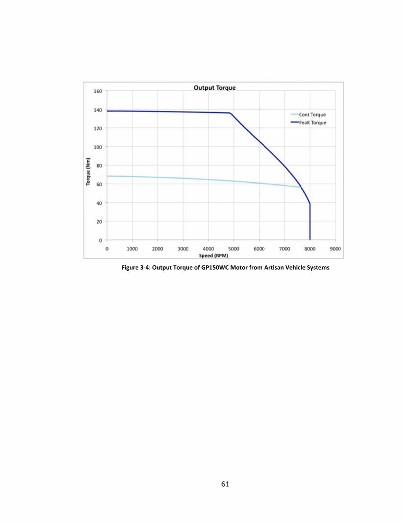
Figure 3‐4: Output Torqu
61
ue of GP150WC
1
C Motor from Artisan Vehiclle Systems
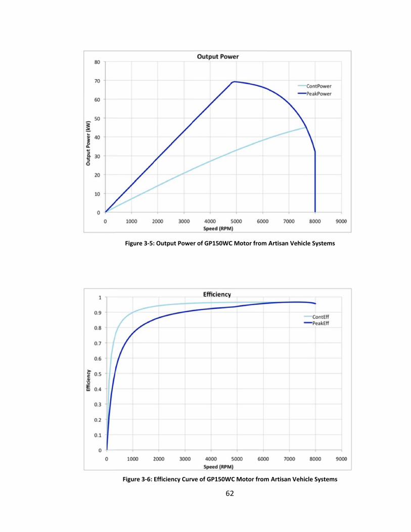
Figure 3‐5:
Figure 3‐6:
: Output Powe
Efficiency Curv
62
er of GP150WC
ve of GP150W
2
C Motor from A
WC Motor from
Artisan Vehicle
Artisan Vehic
e Systems
cle Systems

63
3.4.2 Variable Frequency Drive
Variable frequency drives (VFD) or inverters are needed in AC synchronous
motor applications to provide speed control. The VFDs match the 3‐phase power
required by the motors to the DC power available on the DC bus. Improper frequency
selection could potentially lead to significant motor slip causing stalling or damage to
the motor or VFD.
The choice of the VFDs was constrained by requirements for the GAS operation
mode, described in Section 2.4.1. While the UUT VFD is not utilized in GAS mode, the
absorber VFD is reused as the line inverter for GAS mode. To convert from GAS to dyno
mode, the user must disconnect the battery and LC filter from the DC bus, and connect
the UUT VFD to the DC bus. Additionally, the user must replace the “line
synchronization” (LS) with the resolver card necessary for dyno speed control, and the
data harness must be swapped appropriately. Detailed instructions of this procedure
can be found in Appendix E. Finally, the software on the inverter must be re‐
programmed to support dyno mode.
3.4.3 DC Power Supply
The eDTC utilizes an existing 25kW DC power supply from the InteGrid
Laboratory, a Summit™ 57000007D from Advanced Energy Incorporated. This supply
provides floating DC output, which means it is insensitive to the direction of DC current
flow when operational. However, in emergency shutdown events, the supply must be
protected from a potential current surge caused by discharge of output capacitance of
the VFDs. To provide this protection, a Vishay SD200N20PC diode was installed in the
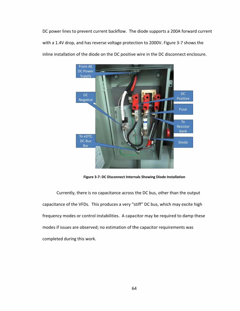
D
w
in
ca
fr
m
co
DC power line
with a 1.4V d
nline installa
Curre
apacitance o
requency mo
modes if issu
ompleted du
es to preven
rop, and has
tion of the d
Figu
ntly, there is
of the VFDs.
odes or cont
es are obser
uring this wo
nt current ba
s reverse vo
diode on the
ure 3‐7: DC Disc
s no capacita
This produc
trol instabilit
rved; no esti
ork.
64
ackflow. The
ltage protec
e DC positive
connect Intern
ance across
ces a very “s
ties. A capa
imation of th
4
e diode supp
ction to 2000
e wire in the
nals Showing D
the DC bus,
stiff” DC bus
citor may be
he capacitor
ports a 200A
0V. Figure 3‐
e DC disconn
Diode Installat
other than
s, which may
e required to
r requiremen
A forward cu
‐7 shows the
ect enclosur
tion
the output
y excite high
o damp thes
nts was
rrent
e
re.
se

65
3.4.4 Current Sensor
To measure the VFD power, it is necessary to measure both the DC bus voltage
and the current on each VFD connection. Voltage measurement was described in the
GAS description, above (Section 2.4.7). Current measurement is described below.
The three most common types of current sensor are: shunt, current transformer,
and Hall‐effect sensors. Current transformers are only suitable for AC current
measurements. Current shunts are often susceptible to noise, may have heating issues
at high current levels, and often require galvanic isolation to prevent floating DC‐mode
signals for damaging data acquisition equipment. Modern Hall‐effect sensors, however,
gain noise immunity by using built‐in amplification, and, because they are indirect
sensors, provide both galvanic isolation and virtually no heating at high current levels.
“Hall effect sensors are broadly deployed because of their dc current sensing capability,
galvanomagnetic isolation, and zero circuit insertion loss” (Zhou, 2003).
Within the Hall‐effect measurement type there are two different groups based
on their measurement control loop. These two groups are defined as open or closed
loop sensors. Open loop Hall‐effect current sensor designs internalize the current
carrying conductor, allowing the manufacturer to optimize the current sensor package’s
size and thermal characteristics. Measurement of open loop sensors usually has a more
limited range of linearity and cannot compensate for offset and residual field errors. The
closed loop Hall‐effect sensors, on the other hand, act as transformers that use a
reference voltage, which allows for higher accuracy than open loop control sensors. The
disadvantages to closed loop sensors include larger size and higher cost. The closed loop

66
sensor is typically more accurate because the output of the Hall‐effect element is
connected to a secondary coil, which generates a field to cancel the primary field’s
current. The amount of cancelling is proportional to the coil ratio between the two
(Dickinson & Milano, 2002).
Another consideration is the measurement signal. All Hall‐effect sensors need an
amplifier to increase the signal, but some closed loop sensors are designed to work with
a data acquisition system that measure the delta voltage and interprets this as current
flow. This allows for reduced component count, cost, and complexity.
Based on the above knowledge, the requirements for the current sensor
selection were: 425A peak measuring ability, sensor size must be smaller than the
allotted space in the junction box (6”x2”x6”), closed loop for accuracy, and lowest cost
relative to other closed loop options. The Honeywell CSNS300M current sensor was
chosen because it has +‐12VDC reference voltage requirement, 600A max
measurement, closed loop control, and ease of panel mounting. Figure 3‐8 shows the
final current sensor selection installed in the high voltage DC bus bar cabinet.
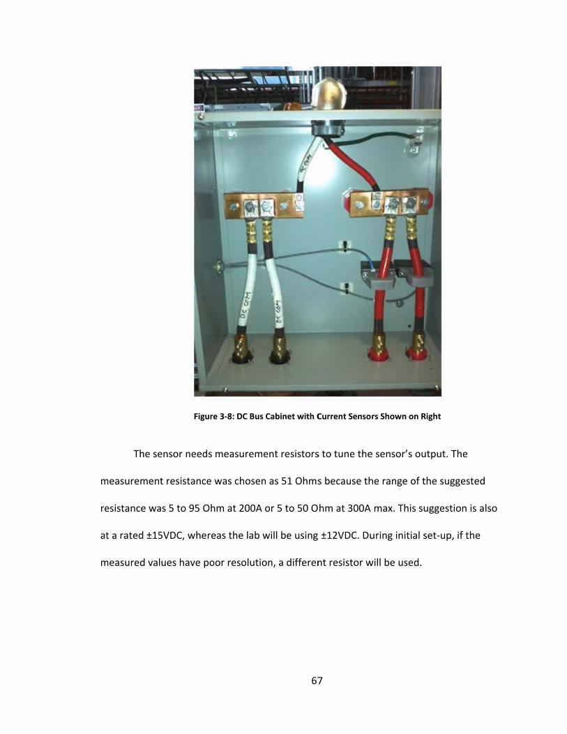
m
re
at
m
The se
measuremen
esistance wa
t a rated ±15
measured val
Figur
ensor needs
t resistance
as 5 to 95 Oh
5VDC, where
lues have po
re 3‐8: DC Bus
measureme
was chosen
hm at 200A o
eas the lab w
oor resolutio
67
Cabinet with C
ent resistors
n as 51 Ohms
or 5 to 50 O
will be using
on, a differen
7
Current Senso
s to tune the
s because th
hm at 300A
±12VDC. Du
nt resistor w
rs Shown on R
e sensor’s ou
he range of t
max. This su
uring initial s
will be used.
Right
utput. The
the suggeste
uggestion is
set‐up, if the
ed
also
e

68
3.4.5 Torque Sensor and Coupler Selection
3.4.5.1 Objectives
The eDTC needed to purchase a torque sensor that could be used in an electric
motor dynamometer to measure the torque in the system between the motor under
test and the absorber motor. The torque sensor requirements included: price, torsional
stiffness, sampling rate, non‐contact measurement, operational speed of 8000rpm, and
capable of withstanding 138Nm of torque. Due to the significant effect that cogging and
vibration can have on measurements, finding the best sensor depended on: max
measuring speed, max torque limit, cost, torsional stiffness, and moment of inertia. The
following sub‐section describes the method used to make the selection.
3.4.5.2 Method
Several torque sensors were investigated as valid sensors for the eDTC
dynamometer application. These were tabulated below (Table 3‐2) based upon the
selection parameters. In total, eleven sensors were considered for evaluation. In order
to narrow down the results, sensors over $5,500, rotational speeds below 10,000 rpm
and sampling rates slower than 1kHz were ignored.
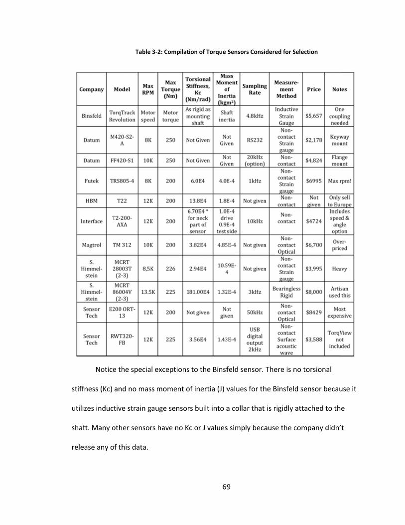
st
u
sh
re
Notice
tiffness (Kc)
tilizes induc
haft. Many o
elease any o
Table
e the specia
and no mas
tive strain g
other sensor
of this data.
3‐2: Compilati
l exceptions
s moment o
auge sensor
rs have no Kc
69
ion of Torque
to the Binsf
of inertia (J) v
rs built into a
c or J values
9
Sensors Consi
feld sensor.
values for th
a collar that
s simply beca
dered for Sele
There is no
he Binsfeld s
is rigidly att
ause the com
ection
torsional
sensor becau
tached to th
mpany didn’
use it
e
t

p
(s
ca
se
th
th
se
fr
d
N
In ord
arameters w
self‐centerin
apability, an
ensor resear
he torsional
he selected c
ensor‐couple
requency. Du
etermined.
Note that the
der to proper
were used in
ng and adequ
nd price. The
rch, it was re
stiffness of
couplings be
In order to
er combinat
uring this inv
Figure 3‐9 h
ere are two m
rly determin
the selectio
uate strengt
e selection ch
ecommende
the sensor. T
elow comply
Table
o further nar
tions was co
vestigation,
ighlights thi
methods of
70
ne the best c
on choices: t
h), speed ra
hoices are ta
ed that the c
This finding
y with this re
e 3‐3: Coupling
rrow down t
mpleted in o
different me
s model with
defining the
0
coupler for t
torsional spr
ange, balanc
abulated in T
oupling sho
helped narr
ecommenda
g Selection Va
the selection
order to det
ethods for d
h definitions
e model base
he system, t
ring rate, cla
ing quality, a
Table 3‐3. D
uld have at
row down th
tion.
lues
n, modeling
ermine the s
defining the
s of each of
ed on the pla
the following
mping quali
alignment
During torqu
least three t
he selection.
of different
system natu
model were
the compon
acement of t
g
ty
e
times
All
ural
e
nents.
the

to
u
sh
re
sy
fo
orsional stiff
nder investi
Fig
After
hown in Figu
epresentativ
ystem. More
ound in Appe
fness of the
gation.
gure 3‐9: Mod
N
modeling us
ure 3‐9 make
ve of the phy
e specific inf
endix D.
torque sens
el Definitions
Numbers Labe
sing both me
es most sens
ysical system
formation on
71
or shaft. The
Used to Deter
led above Diff
ethods it wa
se physically
m. Figure 3‐1
n the model
1
e red mass n
rmine System N
ferent Compon
s found that
y; therefore
10 illustrates
ing and deta
number 4 is
Natural Frequ
nents
t defining th
Caveat 2 is l
s the mode
ailed plot res
the definitio
ency with Mas
he system as
likely less
shapes of th
sults can be
on
ss
first
he
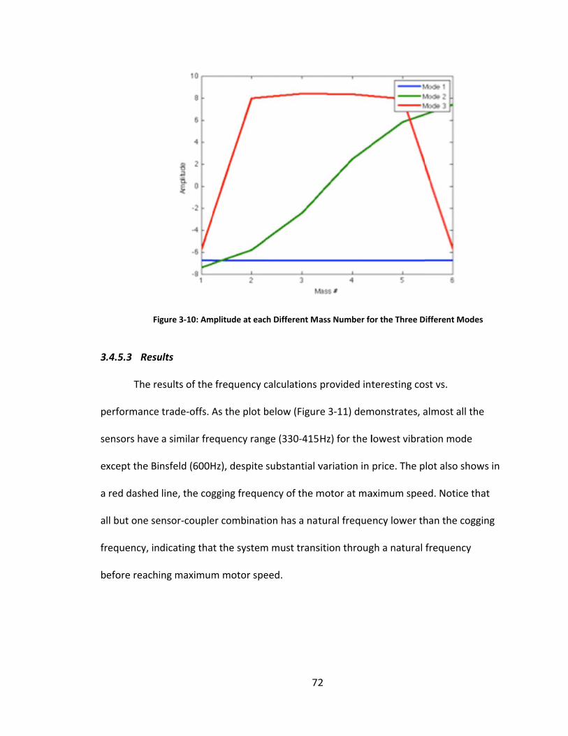
3
p
se
ex
a
a
fr
b
Fi
.4.5.3 Resu
The re
erformance
ensors have
xcept the Bi
red dashed
ll but one se
requency, in
efore reachi
gure 3‐10: Am
ults
esults of the
trade‐offs. A
a similar fre
nsfeld (600H
line, the cog
ensor‐couple
dicating tha
ing maximum
mplitude at eac
frequency c
As the plot b
equency rang
Hz), despite
gging freque
er combinati
t the system
m motor spe
72
ch Different Ma
calculations
below (Figur
ge (330‐415
substantial v
ency of the m
ion has a nat
m must trans
eed.
2
ass Number fo
provided int
re 3‐11) dem
Hz) for the l
variation in
motor at ma
tural freque
sition throug
or the Three D
teresting co
monstrates, a
lowest vibra
price. The p
aximum spee
ncy lower th
gh a natural
ifferent Mode
st vs.
almost all th
tion mode
lot also show
ed. Notice th
han the cogg
frequency
es
e
ws in
hat
ging
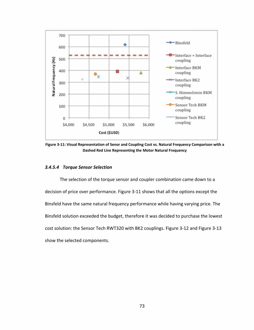
Fi
3
d
B
B
co
sh
igure 3‐11: Vis
.4.5.4 Torq
The se
ecision of pr
insfeld have
insfeld solut
ost solution:
how the sele
sual Represent
Dashed
que Sensor S
election of t
rice over per
e the same n
tion exceede
: the Sensor
ected compo
tation of Senor
d Red Line Rep
Selection
he torque se
rformance. F
natural frequ
ed the budge
Tech RWT3
onents.
73
r and Coupling
resenting the
ensor and co
Figure 3‐11 s
uency perfor
et, therefore
20 with BK2
3
g Cost vs. Natu
Motor Natura
oupler comb
shows that a
rmance whil
e it was deci
2 couplings. F
ural Frequency
al Frequency
bination cam
all the optio
e having var
ided to purc
Figure 3‐12 a
y Comparison w
me down to a
ns except th
rying price. T
hase the low
and Figure 3
with a
a
he
The
west
3‐13

b
d
T
w
th
a
tw
in
m
The Se
ased on mea
oes this in a
he applied t
which in turn
he resonant
fixed pick‐u
wo SAW dev
ndication of
magnetic field
Figure
F
ensor Techn
asuring the r
non‐contac
orque cause
causes a ch
frequency is
up. It is the a
vices, with el
the torque t
ds allowing t
3‐12: R+W Am
igure 3‐13: Sen
nologies torq
resonant fre
ct manner w
es a deforma
hange in its r
s coupled via
nalysis of th
lectronic pro
transmitted
their use in
74
merica BK2 Bel
nsor Technolo
que sensor u
equency cha
hen strain is
ation of the
resonant freq
a a non‐cont
he difference
ocessing and
by the shaft
motors, for
4
lows Coupling
ogies RWT320 T
utilizes a uniq
nge of Surfa
s applied to
quartz subst
quency. The
tact RF rotat
e in resonan
d calibration
t. SAW devic
example, wh
g with Clampin
Torque Sensor
que measuri
ace Acoustic
a shaft insid
trate of the
e frequency s
ting couple f
t frequencie
, that gives a
ces have a hi
here other a
ng Hub
r
ing techniqu
Waves (SAW
de the senso
SAW device
signal measu
from the sha
es between t
a precise
igh immunit
analog
ue
W). It
r.
,
uring
aft to
the
ty to

75
technologies are susceptible to electronic interference and are not suitable (Sensor
Technology, 2011).
Since no sufficiently stiff combination could be found within the project budget,
the system will be required to operate between the first and second harmonics during
certain tests. To minimize vibration, users will be asked not to operate near the
harmonic frequency for an extended period of time.
3.4.6 Mounting Box for Torque Sensor and Two Electric Motors
The design of an enclosure was investigated such that it will: protect users from
entanglement, allow for proper shaft alignments, and secure the mounting of motors.
Several different designs were considered and the selection was narrowed based on:
ease of machineability (and thus cost), minimal welding distortion, maximal alignment
between motor shafts, and sturdy mounting between motors and floor installation.
These are highlighted below in Table 3‐4.
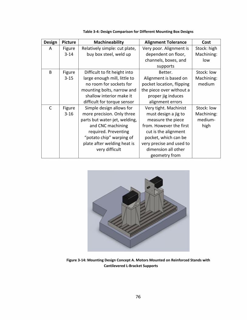
D
Design Pict
A Figu3‐1
B Figu3‐1
C Figu3‐1
Fi
Table
ure
ure 14
Relatibuy
ure 15
Diffilargeno r
mounshadiffic
ure 16
Simmoreparts b
anre
“potplate
gure 3‐14: Mo
3‐4: Design Co
Machineab
ively simple:y box steel, w
cult to fit hee enough miroom for socnting bolts, nllow interiorcult for torqu
ple design ae precision. Obut water‐jend CNC macquired. Prevtato chip” we after weldi
very diffic
ounting Design
Cantile
76
omparison for
bility
: cut plate, weld up
eight into ll, little to ckets for narrow and r make it ue sensor
llows for Only three et, welding, chining venting arping of ng heat is cult
n Concept A. M
vered L‐Bracke
6
r Different Mou
Alignmen
Very poordependechannels
sup
BeAlignmenpocket locthe piece o
proper alignm
Very tighmust demeasur
from. Howcut is thpocket, w
very precisdimensigeom
Motors Mounte
et Supports
unting Box De
nt Tolerance
r. Alignment ent on floor,s, boxes, andpports
etter. nt is based ocation, flippiover withoutjig induces
ment errors
ht. Machinistesign a jig to re the piece wever the fire alignmentwhich can bese and used ion all other etry from
ed on Reinforc
esigns
e Cos
is , d
Stock: Machin
low
n ng t a
Stock:Machinmedi
t
rst t e to
Stock:Machinmediuhig
ced Stands wit
st
high ning: w
low ning: um
low ning: um‐h
h

to
Figure
Figur
Inte
Design
olerances an
3‐15: Mountin
re 3‐16: Moun
erior Volume f
n C was the
nd allows for
ng Design Con
ting Design Co
for Sensor and
chosen desi
r easy access
77
cept B. Square
Mounting Ho
oncept C. Squa
d Couplers, Yet
gn because
s to mountin
7
e Box Mounted
oles
are Box Rotate
t Still within M
it features t
ng bolts. Onc
d within Squa
ed 45 Degrees
Motor Mountin
the tightest a
ce this desig
re Plate with M
to Allow for M
ng Holes
alignment
gn was chose
Motor
Most
en,

st
in
T
vo
to
w
m
fo
d
tress calcula
nternal finite
his estimate
on Mises str
o determine
worse loading
Figure
A cha
motor mount
or the socke
imensions, t
tions were p
e element an
ed model sho
ress of 3 ksi.
if the moto
g moments.
e 3‐17: Fundam
llenge in Des
ting bolts. Fi
t and driver
the proper a
performed u
nalysis solve
owed that lo
This simulat
r max torqu
mental Finite E
Moto
sign C was a
gure 3‐18 sh
between th
amount of sp
78
using SolidW
r. Figure 3‐1
oading the st
tion helped
e can damag
Element Analys
or Mounting B
llowing for s
hows the 3D
e box and th
pacing for a 9
8
Works 3D CAD
17 shows the
teel mountin
estimate the
ge the moun
sis of Design C
Bolt Holes
sufficient to
D CAD model
he bolt. Afte
9/16” nut an
D modeling s
e results of t
ng plates wo
e thickness o
nting box ev
C with Concent
ol space for
l of Design C
er redesignin
nd socket wa
software an
the simulatio
ould produce
of the steel
ven under th
trated Forces a
installing th
C and clearan
ng the box
as found.
d its
on.
e a
walls
e
at the
he
nce

to
H
co
h
p
cr
ax
m
a
Figure
The ot
o the box. Fr
However, we
ompany agr
eat. The res
Partic
roduce tight
ritical to ass
xisymmetric
milling the ali
mount of sp
3‐18: CAD Mo
ther crucial
rom a design
lding techni
eed to perfo
sulting defor
ular care wa
t alignment
ure the align
c. To minimiz
ignment poc
pare to accou
odel Showing D
design chall
n perspective
cians can’t g
orm the weld
rmation cou
as taken with
between the
nment pocke
ze machining
ckets was m
unt for the f
79
Dimensions be
Surface
enge was he
e, welding o
get tools in t
ds cautiously
ld then be re
h the machin
e motors mo
ets on either
g errors, the
inimized. Th
inishing of th
9
etween Motor
eat stress wh
on the interio
the tight cor
y, in a stagge
emoved dur
ning instruct
ounted on o
r end of the
e number of
he box was c
he plates), t
Mounting Bol
hen welding
or of the box
rners. The m
ered pattern
ring machini
tions. Since
pposite end
box are bot
machining s
cut to length
the access ho
lt Hole and the
g the plate e
x is ideal.
anufacturin
n to balance
ng.
the design m
ds of the box
th parallel an
steps prior t
h (with a sligh
ole was cut u
e Next
nds
g
the
must
x, it is
nd
o
ht
using

a
cr
e
b
a
co
to
m
vi
co
m
water jet, th
reate the ali
nsure prope
uilt by the m
ligned.
Many
onsidered as
o slide the te
most ICE dyn
ibrations, ru
oncrete anc
mounting box
he end plate
gnment poc
er alignment
manufacturin
different op
s well. Some
est rig on. Ho
o test stand
ubber isolatio
hors. Below,
x, angle brac
Figure 3‐19: 3
es were weld
ckets. All oth
. Machining
ng company,
ptions for at
e options inc
owever, sinc
s, direct con
on dampers
, Figure 3‐19
cket, and da
D CAD Model
80
ded on, and
her features
was comple
, to assure b
taching the
cluded buildi
ce the rig do
ncrete ancho
were added
9, is a picture
mpers.
of Design C wi
0
then both e
are based o
eted increme
both ends of
mounting b
ing a framew
oesn’t need t
ors could be
d between th
e of the fina
ith Mounting F
ends were m
off of these p
entally, utili
f the box we
ox to the flo
work of I‐bea
to be interch
used. In ord
he mounting
l design feat
Feet Brackets
machined to
pockets to
zing a uniqu
re properly
oor were
ams or box r
hangeable li
der to reduce
g box and th
turing the
and Bushings
ue jig,
rails
ke in
e
he

81
3.4.7 Powertrain Control Module
The powertrain control module (PCM) was supplied by Artisan Vehicle Systems
to provide communications between the inverters, batteries, and the user. The PCM is
designed to be a plug‐and‐play solution by AVS. However, since this set‐up is not a
traditional application where the PCM only receives throttle input from the user, several
communication modifications were made. Unlike vehicle control, the inverters in the lab
can be controlled in two different methods (speed and torque control). The user then
can select a multitude of different options to perform the desired test. These options
include holding a set rpm for an extended period of time while incrementally increasing
torque. This is very atypical for automotive use but standard for static laboratory
testing.
3.4.8 Control Computer
The following software was installed on the control computer: LabView,
TorqueSense, Parker SSD DSE Lite, and the AVS PCM GUI. It is also equipped with math
software to do analysis of results (Excel, MatLab, etc.) as well as modelers for control
loops (MatLab Simulink), and 3D CAD modeling for designing layouts and building parts
(SolidWorks). Fitted with this software, the computer functions as a way for the user to
monitor the system and command the devices to perform in certain desired manners.
3.4.9 Data Acquisition System
The data acquisition system (DAQ) chosen for the lab was based on cost,
functionality, and expandability. As a main chassis, the National Instruments (NI)

82
CompactRIO (cRIO) with real‐time controller and reconfigurable chassis (NI cRIO‐9074)
was chosen because it has: field‐programmable gate array (FPGA), 8 slots for cards, up
to 400 MHz real‐time processor, 128 MB DRAM memory, and 256 MB of nonvolatile
storage. In addition, the chassis was on sale because it will be replaced soon. One of the
disadvantages to this model however, is that it is over‐designed for its purpose in the
lab. Since the chassis is FPGA based, this requires additional complex programming,
which would have been avoided with a lower performance model. This adds more
upfront programming to commission the lab but allows for flexible upgrading of the
system in the future.
Proper cards were chosen for the cRio to handle the necessary I/O signals (digital
in/out and analog in/out), required single power, and sampling rate required for the
control system. For digital signals, the NI 9422 (8 channel, 24 to 60 V, 250 μs C series
sinking/sourcing digital input module) and NI 9472 (8 channel, 24 V Logic, 100 μs
sourcing C series digital output module) modules were chosen. Choice of the analog I/O
cards was subject to time delays requirements, which were discussed in detail in section
2.3.4 and 2.4.7. The two analog modules NI 9215 (4 channel, 100 kS/s, 16‐Bit, ±10 V
simultaneous sampling C series analog input module) and NI 9263 (4 channel, 100 kS/s,
16‐Bit, ±10 V, analog output module) were chosen because their sampling rate is greater
than 1kHz required for AC voltage measurements.
Lastly, an NI 9853 2‐Port, High‐Speed CAN Module specifically for NI CompactRIO
was selected in order for LabView to have CAN communications with all the key
components in the system. This will allow the user to transmit and receive CAN

83
messages between the PCM, BMS, and the inverters. This is necessary for increased
flexibility in communications between the devices and greater control of the system.
3.4.10 Emergency Stop Circuit
Typically, there are two ways to design an emergency stop (E‐stop) circuit in
industrial labs: series and parallel. In the series method, all switches have to be “ok” in
order for power to flow to the system. In a parallel design, all switches are independent,
but if the user closes one switch then the E‐stop bus is powered causing an emergency
stop of the system. The eDTC lab utilizes the parallel system. Once a single emergency
stop is signaled (push of an E‐stop switch or digitally pushing the DAQ E‐stop button),
24VDC flows to the trip bus, which immediately powers all shunt trips, enable signals,
and contactors to the de‐energized or open state. Figure 3‐20 shows a simplistic flow
diagram of the E‐stop circuit design.
It is important to note that the E‐stop system is completely independent of the
control system and does not require any input from the control computer to operate.
However, a signal from the control system can trip the E‐stop system, if necessary. The
system is reliable as 24VDC is supplied. Additional redundancy could be built into the
system to prevent the system from failing should the 24V become disconnected.
However, at this time it was deemed as unnecessary.
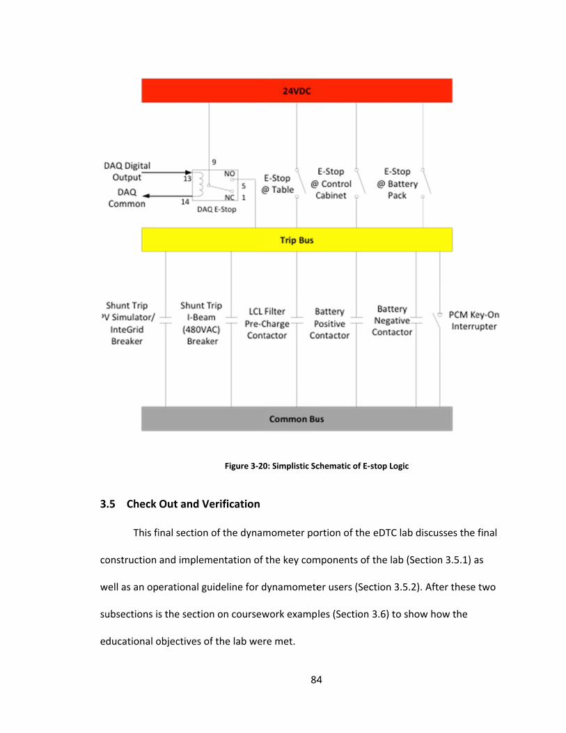
3
co
w
su
e
.5 Check
This fi
onstruction
well as an op
ubsections is
ducational o
Out and Ve
inal section o
and implem
erational gu
s the section
objectives of
Figure 3‐20
erification
of the dynam
mentation of
uideline for d
n on coursew
f the lab wer
84
0: Simplistic Sc
mometer po
the key com
dynamomete
work examp
re met.
4
chematic of E‐s
ortion of the
mponents of
er users (Sec
les (Section
stop Logic
eDTC lab di
the lab (Sec
ction 3.5.2).
3.6) to show
scusses the
ction 3.5.1) a
After these
w how the
final
as
two
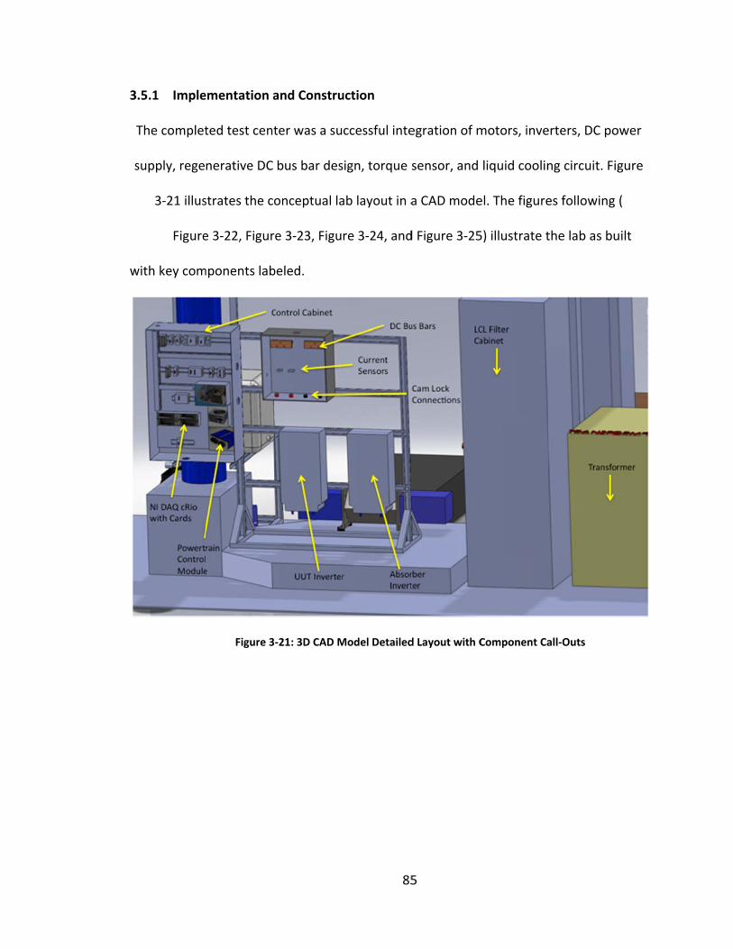
3
T
s
w
.5.1 Imple
The complet
supply, rege
3‐21 illus
Figure
with key com
ementation a
ted test cent
nerative DC
strates the co
e 3‐22, Figur
mponents lab
Figure 3
and Constru
ter was a su
bus bar des
onceptual la
re 3‐23, Figu
beled.
‐21: 3D CAD M
85
uction
ccessful inte
sign, torque
ab layout in a
re 3‐24, and
Model Detailed
5
egration of m
sensor, and
a CAD mode
d Figure 3‐25
d Layout with C
motors, inve
liquid coolin
el. The figure
5) illustrate t
Component Ca
erters, DC po
ng circuit. Fi
es following
the lab as bu
all‐Outs
ower
gure
(
uilt
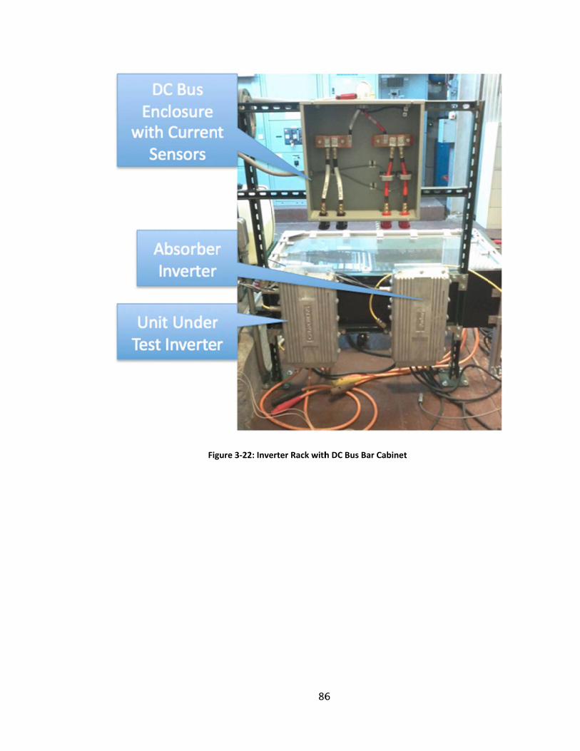
Figgure 3‐22: Inve
86
erter Rack with
6
h DC Bus Bar CCabinet
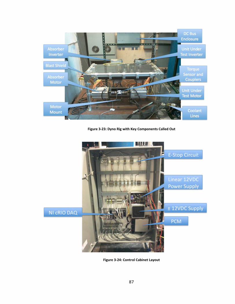
Figure 3‐23: Dy
Figu
87
yno Rig with K
re 3‐24: Contr
7
Key Componen
ol Cabinet Lay
nts Called Out
yout
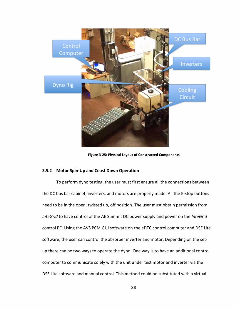
3
th
n
In
co
so
u
co
D
.5.2 Moto
To pe
he DC bus ba
eed to be in
nteGrid to ha
ontrol PC. U
oftware, the
p there can
omputer to
DSE Lite softw
F
r Spin‐Up an
rform dyno
ar cabinet, in
the open, t
ave control o
sing the AVS
e user can co
be two way
communicat
ware and ma
Figure 3‐25: Ph
nd Coast Do
testing, the
nverters, an
wisted up, o
of the AE Su
S PCM GUI s
ontrol the ab
s to operate
te solely wit
anual contro
88
hysical Layout o
own Operatio
user must fi
d motors are
off position.
mmit DC po
oftware on t
bsorber inve
e the dyno. O
th the unit u
ol. This meth
8
of Constructed
on
irst ensure a
e properly m
The user mu
ower supply
the eDTC co
rter and mo
One way is to
nder test m
hod could be
d Components
all the conne
made. All the
ust obtain pe
and power o
ontrol compu
otor. Depend
o have an ad
otor and inv
e substituted
s
ections betw
e E‐stop butt
ermission fr
on the InteG
uter and DSE
ding on the s
dditional con
verter via the
d with a virtu
ween
tons
om
Grid
E Lite
set‐
ntrol
e
ual

89
PC application that allows two DSE programs to run simultaneously on one PC. The
other method is to have the NI cRIO DAQ communicate via CAN to the PCM and
inverters, which can, in turn, communicate with both inverters. The first method is the
only implemented method at this time.
To start the system, the user must set the InteGrid DC power supply control
computer to command a bus voltage of 350 VDC. At the eDTC control computer, the user
may turn the enable key to begin testing the dyno. While monitoring the program on
the eDTC control computer (either LabView, AVS PCM GUI, or DSE Lite) the user can
define speed set points on the absorber and then “throttle” up or down the torque
request of the UUT motor. While performing different tests, the user can opt to record
data via the PCM GUI, which will save data as a .csv file for a later use.
When the user is finished performing the desired tests they must spin the
motors down to a stop by reducing the set points and switching the enable switch to the
OFF position for both inverters. After this, the InteGrid control PC must properly shut
down the DC power supply and open the service disconnects for all power equipment.
3.6 Course Work Examples
This section illustrates four different labs that professors will use to educate
students using the eDTC laboratory. These labs include mapping the torque of the
motors (Section 3.6.1), finding the efficiency of the lab (Section 3.6.2), understanding
thermal effects (Section 3.6.3), and an introduction to grid‐attached‐storage (Section
3.6.4).

90
3.6.1 Lab #1: Map Torque versus Speed Curve
Introduction: The objective of this lab is to learn more about motor
performance, in particular, the torque curve. Students will experience creating a torque
map similar to the torque curve in Figure 3‐26. To perform this test, the user defines a
set speed for the absorber motor and identifies the maximum torque achievable by UUT
at that speed. Since the motors are directly coupled, both will operate at the same
speed at all times, except for minor vibrational variations. The UUT is operated under
torque control – i.e. the user commands the UUT to output a defined torque. The
absorber is operated under speed control – i.e. it is commanded to always maintain a
set speed. When the user changes the UUT’s commanded torque, the UUT attempts to
produce that torque, while the absorber attempts to maintain a set speed. Since the
absorber is controlled so that it can always produce more torque than the UUT, the
speed may vary briefly before quickly returning to the commanded level.
During this test, the user will define 16 different speeds and record the max
torque that results for each. Students must plot these max points and compare them to
the torque curve below courtesy of www.artisanvs.com.
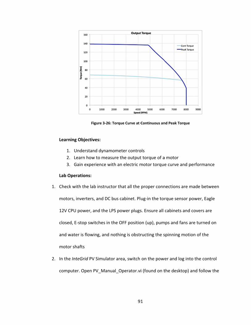
Learn
1.
2.
3.
Lab O
1. Check
motor
12V C
closed
and w
motor
2. In the
comp
Fi
ing Objectiv
Understan
Learn how
Gain expe
Operations:
k with the lab
rs, inverters,
PU power, a
d, E‐stop swi
water is flowi
r shafts
e InteGrid PV
uter. Open P
gure 3‐26: Tor
ves:
nd dynamom
w to measure
rience with
b instructor
, and DC bus
and the LPS
itches in the
ing, and not
V Simulator a
PV_Manual_
91
rque Curve at C
meter contro
e the output
an electric m
that all the
s cabinet. Plu
power plugs
e OFF positio
hing is obstr
area, switch
_Operator.vi
1
Continuous an
ols
t torque of a
motor torque
proper conn
ug‐in the tor
s. Ensure all
on (up), pum
ructing the s
on the pow
i (found on t
nd Peak Torqu
a motor
e curve and
nections are
rque sensor
cabinets and
mps and fans
spinning mot
er and log in
the desktop)
e
performanc
made betw
power, Eag
d covers are
are turned
tion of the
nto the cont
) and follow
ce
ween
le
e
on
rol
the

92
powering on instructions (screenshot shown in Figure 3‐27). Set the command
voltage to 350VDC
3. Return to the eDTC. Open the Motor_Map.vi (example screen shot is shown in
Figure 3‐28), SSD Drives: DSE Lite, and Calmotors GUI (also known as AVS PCM
GUI)
4. Set the absorber speed to 1,000rpm and switch on the enable switch on the desk
control box
5. Define the UUT inverter torque to 10% and switch on the enable switch
6. Quickly accelerate to 200% torque and let the motor stabilize for five seconds
and record the torque value
7. Ramp the torque back down to 0%
8. Change the absorber speed to 1,500rpm
9. Monitor the winding temperature at all times to assure that it is within 5oC of
the initial winding temperature. If the temperature increases, wait until it cools
sufficiently
10. Quickly accelerate the UUT to 200% torque and let it stabilize for 5 seconds.
Record the torque at this point
11. Ramp the torque back down to 0%
12. Repeat steps 6‐9 with 500rpm increments until you reach 8,000rpm
13. Plot your results on a Torque vs. Speed graph and submit to the instructor
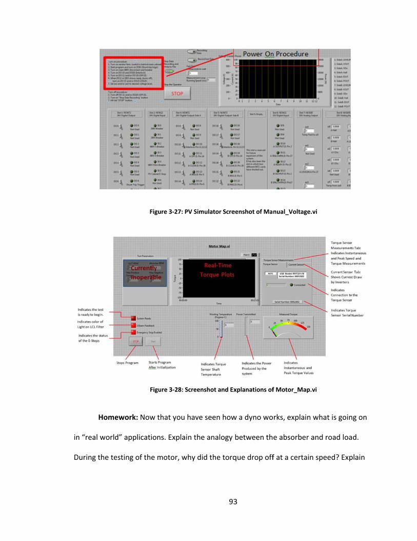
in
D
Home
n “real world
During the te
Fig
Fig
ework: Now
d” applicatio
esting of the
gure 3‐27: PV S
gure 3‐28: Scre
that you ha
ons. Explain t
motor, why
93
Simulator Scre
eenshot and Ex
ve seen how
the analogy
y did the torq
3
eenshot of Ma
xplanations of
w a dyno wo
between th
que drop off
nual_Voltage.
f Motor_Map.v
rks, explain
e absorber a
f at a certain
vi
vi
what is goin
and road loa
n speed? Exp
ng on
ad.
plain

94
why electric motors behave in this manner. Are there different ways to control electric
motors to change the impacts of the motor torque curve? Explain your reasoning.
Hand in your plot from in‐lab and your essay answers to the questions above to
your lab instructor before the beginning of the next lab.
3.6.2 Lab #2: Map Motor Efficiency Lab
Introduction: The purpose of this lab is to better understand the efficiencies of
an electric motor. As you learned in‐class, there are many parts of an electric motor,
which are subject to friction, heat, and electrical losses. This lab exercise investigates
these loses at a system level.
To investigate efficiency, you will compare the electrical power input into the
UUT inverter, the mechanical power transmitted to the absorber via the shaft coupling,
and the electrical power returned to the system by the absorber. Given measurements
at three points, it is possible to isolate the efficiency of subsets of the laboratory: The
efficiency of UUT inverter/motor, and the efficiency of the absorber inverter/motor.
Since one motor is operating exclusively in traction mode, and the other exclusively in
regenerative mode, it is possible to assess the efficiency of the same motor model in
both modes simultaneously. Figure 3‐29 shows the estimated efficiencies for each
component in the system.
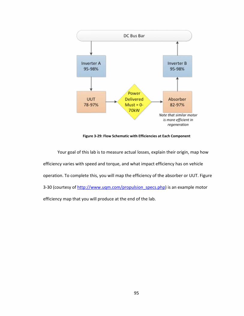
ef
o
3
ef
Your g
fficiency var
peration. To
‐30 (courtes
fficiency ma
Figure
goal of this l
ries with spe
o complete t
sy of http://w
ap that you w
e 3‐29: Flow S
ab is to mea
eed and torq
this, you will
www.uqm.c
will produce
95
chematic with
asure actual
que, and wha
map the eff
om/propuls
at the end o
5
h Efficiencies a
losses, expla
at impact eff
ficiency of th
ion_specs.p
of the lab.
t Each Compo
ain their orig
ficiency has
he absorber
php) is an exa
nent
gin, map how
on vehicle
r or UUT. Fig
ample moto
w
ure
or
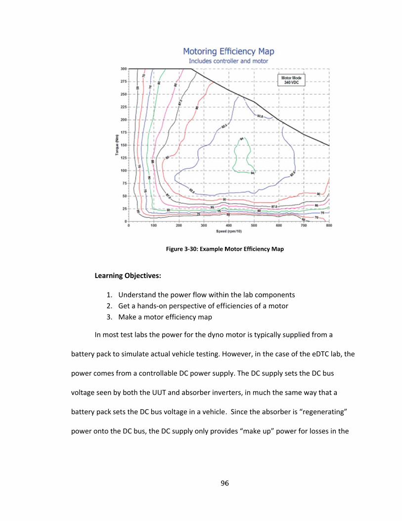
b
p
vo
b
p
Learn
1.
2.
3.
In mo
attery pack
ower comes
oltage seen
attery pack
ower onto t
ing Objectiv
Understan
Get a hand
Make a mo
st test labs t
to simulate
s from a con
by both the
sets the DC
he DC bus, t
Figure 3‐
ves:
nd the powe
ds‐on perspe
otor efficien
the power fo
actual vehic
trollable DC
UUT and ab
bus voltage
the DC supp
96
‐30: Example M
r flow within
ective of effi
ncy map
or the dyno
cle testing. H
power supp
bsorber inve
in a vehicle.
ly only provi
6
Motor Efficien
n the lab com
iciencies of a
motor is typ
However, in t
ply. The DC s
rters, in mu
. Since the a
ides “make u
ncy Map
mponents
a motor
pically suppli
the case of t
supply sets t
ch the same
absorber is “
up” power f
ied from a
the eDTC lab
the DC bus
e way that a
“regeneratin
for losses in t
b, the
ng”
the

97
UUT and absorber. By regenerating the absorbed power back onto the DC bus, the lab
minimizes the energy consumed and reduces the size of certain components.
Lab Procedure:
1. Check with the lab instructor that all the proper connections are made between
motors, inverters, and DC bus cabinet. Plug‐in the torque sensor power, Eagle
12V CPU power, and the LPS power plugs. Ensure all cabinets and covers are
closed, E‐stop switches in the OFF position (up), pumps are turned on and water
is flowing, and nothing is obstructing the spinning motion of the motor shafts
2. In the InteGrid PV Simulator area, switch on the power and log into the control
computer. Open PV_Manual_Operator.vi (found on the desktop) and follow the
powering on instructions. Set voltage to 350VDC – the emulated battery voltage
– and the safety current limit to 50A
3. Return to the eDTC control computer. Open the Motor_Map.vi, SSD Drives: DSE
Lite, and Calmotors GUI (also known as AVS PCM GUI)
4. Set absorber speed to 1,000rpm and then switch the enable to on for the
absorber inverter
5. Record winding temperature
6. Define the UUT inverter torque to 10% and switch the enable switch to the on
position
7. Enable data logging

98
8. Slowly ramp up the UUT torque to 200% using intervals of 20% and pausing for 5
seconds between steps (the more systematic you are with this, the easier it will
be to interpret your data)
9. Ramp torque down to 0%
10. Check the winding temperature. Is it within 5oC of the starting temp? If not, wait
until it cools (the cooling loop should quickly cool the motors) If yes, proceed to
the next step
11. Change the absorber speed to 1,500rpm
12. Repeat step 5
13. Ramp down torque to 0%
14. Repeat steps 5‐7 until absorber speed is 8,000rpm
15. Ramp down torque to 0% and absorber speed to 0rpm
16. Switch off enable switches for both inverters, safely power down the DC power
supply according to instructions, switch off all break disconnects
17. Open the data file showing absorber speed at each: torque, speed, voltage and
current (for both inverters) of the system
Homework: Do the calculations using equation one (show below) to determine the
system efficiency at each data point and create a plot of Torque vs. Speed with
“islands” of efficiency in different colors like the example in Figure 3‐30.

3
te
d
sc
p
.6.3 Lab #3
Introd
emperature
etermine ho
cenarios: ste
repared to a
Learn
1.
2.
Lab Pr
1. Check
motor
12V C
closed
is flow
2. In the
comp
powe
3. Open
AVS P
3: Investigat
duction: The
on the perfo
ow changes
eady state co
answer wher
ing Objectiv
Understan
Get a hand
rocedure:
k with the lab
rs, inverters,
PU power, a
d, E‐stop swi
wing, and no
e InteGrid PV
uter. Open P
ring on instr
the Motor_
CM GUI)
te Temperat
e purpose of
ormance of
in winding re
old, steady s
re the heat i
ves:
nd the impac
ds‐on perspe
b instructor
, and DC bus
and the LPS
itches in the
othing is obst
V Simulator a
PV_Manual_
ructions. Set
_Map.vi, SSD
99
ture Effects
this lab is to
a motor ope
esistance im
state hot, ac
is being tran
ct of temper
ective of mo
that all the
s cabinet. Plu
power plugs
e OFF positio
tructing the
area, turn on
_Operator.vi
t voltage to 3
D Drives: DSE
9
on Electric M
o investigate
erating in dif
mpact the mo
celeration, a
nsferred to a
rature on mo
otor operatio
proper conn
ug‐in the tor
s. Ensure all
on (up), pum
spinning mo
n the power
i (found on t
350VDC
E Lite, and Ca
Motors
e the impact
fferent state
otor output
and regener
and why.
otor perform
on in differe
nections are
rque sensor
cabinets and
mps are turne
otion of the
and log into
the desktop)
almotors GU
t of the wind
es. You will
in four
ration. Be
mance
nt condition
made betw
power, Eag
d covers are
ed on and w
motor shaft
o the contro
) and follow
UI (also know
ding
ns
ween
le
e
water
ts
l
the
wn as

100
4. Set the absorber speed to 1,000rpm, switch the enable absorber switch to on,
and record the initial winding temperature
5. Switch the UUT inverter enable switch to on after setting the torque to 5%
6. Slowly accelerate to 75% torque and wait until the system stabilizes
7. Note the temperature over 1 minute
8. Bring the torque down to 0%
9. Quickly accelerate to 75% torque and wait until the system stabilizes and record
the temperature in both the UUT and absorber motors
10. Bring the torque back down to 0%
11. Let the windings cool down to the initial temp before moving on to the next step
12. Change the absorber speed to 5,000rpm
13. Quickly accelerate to 200% torque
14. Record how the temperature of the winding responds to this input over time
15. After about 30 seconds, return to the torque to 0% and the absorber speed to
1,000rpm
16. Note the change you see in the temperature
17. Return both torque and speed to 0 and wait for the system to come to a stop.
Let the coolant flow until the winding temperature is at the initial temperature
when you started the lab
Homework: Discuss the effects of time and load in terms of temperature in the
UUT and absorber motors. Present the data you collected in a manner that you best
think describes the heat transfer.

101
Consider automakers performing these tests to determine how to best cool the
motor. When do you expect the motors to experience different heating characteristics?
Low torque up a hill, driving in reverse, highway cruising? Describe what will happen in
each one of these cases and a few of your own based on the results you have gathered
from this lab. Can you model the temperature characteristics of the motor at different
speeds and at different length durations? Organize these findings and hand them into
the lab director before the start of the next lab.
3.6.4 Lab #4: Intro to Grid‐Attached‐Storage Lab
Introduction: The purpose of this lab is to give students an initial contact with
grid‐attached‐storage to understand the relationship between grid demand and
allowable battery charge and discharge rates. Students will experience how a storage
device, such an automotive pack battery, interfaces with the grid.
“Grid‐attached‐storage” (GAS) involves connecting a storage device – in this case
a battery – to the utility grid and controlling the charge and discharge rate of the
storage to meet objectives such as grid stabilization, frequency regulation or peak
reduction. For example, a battery could be utilized for peak shaving – charging during
periods of low electricity consumption (typically when electricity cost is low) and
discharging during periods of peak electricity consumption (typically when electricity
cost is high).

102
This lab focuses on the basic requirements to control a battery GAS system
connected to the power grid. Students will monitor the behavior of the battery while
changing commanded charge and discharge levels.
Learning Objectives:
1. Understand grid‐attached‐storage components
2. Get a hands‐on perspective of GAS current control methods
3. Witness the effects of battery performance with short pulse demands
Lab Procedure:
1. Open the PCM GUI and DSE Lite programs at the eDTC control PC
2. Check with the lab supervisor that all the proper connections between the
inverter, battery, and transformer have been made. Ensure all safety checks are
in place: no cables are improperly color matched, everything is properly
connected, all shields and covers are closed, all E‐stop switches are in the off
position
3. Plug in the GAS water pump and close the priming valve to properly activate the
cooling loop. Plug in the Eagle 12V power supply plug and turn on the GAS
electric fan at the desk control box
4. Check that the battery is properly communicating with the PCM via CAN
5. Before moving to the next step, ensure that the LC filter pre‐charge e‐stop
switch in the LC filter cabinet is in the off or twisted up position. Strict adherence
to this will reduce the risk of arcing and damage to the LC filter
6. Follow InteGrid connection instructions to energize the 480VAC main tie breakers

103
7. Close the 480VAC I‐Beam breaker on, turn on the LC filter fans, and close the LC
filter knife switch on, letting the pre‐charge circuit come online
8. Turn on the inverter through the ENABLE rocker switch via the control box by the
eDTC control PC
9. Turn the battery key‐on at the control desk box to the on position. You should
hear the battery contactors switch the battery pre‐charge on and then close the
rest of the contactors
10. Once the system is synchronized with the grid, manual current control can begin
11. Using DSE Lite increase or decrease the current set‐points in 1% increments
following the control provided by your instructor
12. While manually controlling the current set points, monitor the battery SOC to
assure that the battery pack remains within its operational SOC limits
13. Take notes of how the controller responds, battery pack behaves, and the time
required for the system to respond to commanded changes in current output
14. Power down the system by commanding the PCM to open the battery contacts,
turning the key to the off position, disabling AFE (absorber inverter ENANBLE
rocker switch off), opening/switching off the LC filter breaker, and lastly the
480VAC breaker
15. To safely store the lab: unplug the battery connections, communication cable
(Deutsche 23‐pin connector). Unplug all the other power devices in the eDTC lab
(water pumps, Eagle 12VDC CPU power supply, linear power supply (LPS), etc.)

104
Homework: Hand in a discussion and a controller model to your lab supervisor
before the start of the next lab. In your discussion, consider the following questions:
How do the asymmetric charge and discharge limits impact the control
algorithm for the GAS system?
Given that a fully charged or discharged battery system can no longer
provide full control functionality to the grid, what control architecture
would you propose to maintain the SOC of the battery while still
responding to grid control requirements?
Given the step response characteristics of the system, what is the
maximum allowable control frequency for the system?
One application of GAS is to “firm” output from a renewable power plant, such
as a wind farm or photovoltaic system. The concept behind firming is to control
charging/discharging of the GAS system so that the combined output of the renewable
plant and GAS system maintains a constant, forecasted value. The second part of this
homework is to design a controller for renewable firming. As you witnessed, the lab
currently uses manual set‐point control for real and reactive power commands. Your
objective is to design a control algorithm to firm the output from a renewable power
plant. Your instructor will provide a time series output from a renewable power plant.
In the next lab, you will test your algorithm simulation and controller (pending instructor
approval) by uploading it to the inverter software controller to verify its robustness.

105
4. Summary and Conclusions
The eDTC lab at Colorado State University is a test bed that advances the
knowledge and training of engineers for a sustainable future. It allows for educating the
next work force in electrical mobility and provides researchers with the components to
test the implications of grid‐attached‐storage. The results from the lab will inform how
utilities and electrified vehicles interact as well as the repurposing EV batteries for GAS
systems.
This thesis described the need for understanding grid storage and its
implications, what challenges are accompanied with designing a test bed of this scale
with automotive‐grade components, why different components were chosen over
alternatives, and a brief demonstration of the system operation. The goals of the design
were accomplished and a successful lab was constructed.
4.1 Future of the eDTC
This is an exciting time for the eDTC lab because there are several new uses
designated for the GAS and dyno portions of the lab. First, new graduate students will
design new control algorithms for GAS for testing in both simulation and class
environments. Second, used batteries from Altairnano and A123 were donated to CSU
specifically for battery second use testing at the eDTC. Testing protocols and
performance of these batteries is of great importance to industry and national labs.

106
Third, EcoCar2 teams will begin drive cycle testing using the dyno portion of the eDTC.
This will provide real world results and validation to the modeling currently being
evaluated. Finally, beginning spring 2011, the new ENGR580a1 class will utilize the
course exercises designed in this thesis. With these and many more exciting projects,
the eDTC has begun to show its importance and usefulness to both researchers and
university students.
107
WORKS CITED
Blooming, T., & Carnovale, D. (2007). Application of IEEE Std 519‐992 Harmonic
Limits. IAS Atlanta Section. Appleton, WI: IEEE.
Bredenberg, A. (2011, April 25). Battery Storage: Smoothing Out the Wrinkles of
Renewable Energy. Retrieved May 22, 2011, from Thomas Net News:
http://news.thomasnet.com/green_clean/2011/04/25/battery‐storage‐smoothing‐out‐
the‐wrinkles‐of‐renewable‐energy/
Brockman, J. (2008, July 22). Plug In, Drive On: The Promise of Next‐Gen Hybrids.
Retrieved May 14, 2011, from NPR:
http://www.npr.org/templates/story/story.php?storyId=92792068
Brooks, A. (2002). Vehicle‐to‐Grid Demonstration Project: Grid Regulation
Ancillary Service with a Battery Electric Vehicle. AC Propulsion. CARB.
Bureau of Transportation: Statistics. (2010, May 03). Number of U.S. Aircraft,
Vehicles, Vessels, and Other Conveyances. Retrieved May 12, 2011, from Research and
Innovative Technology Administration (RITA), BTS:
http://www.bts.gov/publications/national_transportation_statistics/html/table_01_11.
html
Coomb, H. S. (2011). Renewable Sustainable Expeditionary Power. U.S. Navy,
Office of Naval Research. Arlington, VA: U.S. Navy.
Cready, E., Lippert, J., & Phil, J. (2003). Technical and Economic Feasibility of
Applying Used EV Batteries in Stationary Applications. Sandia National Laboratories.
Albuquerque, NM: Department of Energy.
Demand Energy. (2011). Demand Energy ‐ Renewables Firming. Retrieved
September 2011, from Demand Energy:
http://demandenergynetworks.com/applications/use‐case‐renewables‐firming.asp
Denholm, P., & Short, W. (2006). An Evaluation of Utility System Impacts and
Benefits of Optimally Dispatched Plug‐In Hybrid Electric Vehicles. National Renewable
Energy Laboratory. Golden, CO: Department of Energy.
108
Dickinson, R., & Milano, S. (2002, July 11). "Isolated Open Loop Current Sensing
Using Hall Effect Technology in an Optimized Magnetic Circuit. Concord, NH, USA.
Duvall, M. (2008). How many plug in hybrids can a smart grid handle? Plug‐In
2008. San Jose, CA: EPRI.
EPRI. (2011). Plugging In: A Consumer's Guide to the Electric Vehicle. Electric
Powertrain Research Institute. Palo Alto, CA: EPRI.
Eyer, J., & Corey, G. (2010). Energy Storage for the Electricity Grid: Benefits and
Market Potential Assessment Guide. Sandia National Laboratory. Albuquerque, NM:
Department of Energy.
Gavine, A. (2011, January). Ticket to Ride: User‐Friendly System. Electric and
Hybrid Vehicle Technology International , p. 50.
Goggin, M. (2008). Wind Power and Energy Storage Fact Sheet. American Wind
Energy Association. AWEA.
Gupta, P. (2009, August 26). Utility wants to deploy largest grid battery ever.
Retrieved May 30, 2011, from Reuters: http://www.reuters.com/article/2009/08/26/us‐
edison‐battery‐idUSTRE57P4PJ20090826?sp=true
Hadley, S., & Tsvetkova, A. (2008). Potential Impacts of Plug‐in Hybrid Electric
Vehicles on Regional Power Generation. Oak Ridge National Laboratory. Oak Ridge, TN:
Department of Energy.
Himelic, J., & Novachek, F. (2010). Sodium Sulfur Battery Energy Storage and Its
Potential To Enable Further Integration of Wind,. Xcel Energy Renewable Development
Fund. Denver, CO: Xcel Energy.
Hoevenaars, T. (2003). Interpreting IEEE Std 519 and Meeting its Harmonic Limits
in VFD Applications. IEEE.
Jost, B. (2011, September 1). Who Pays for Firming Up Variable Energy
Resources? Retrieved September 2011, from
http://www.powermag.com/renewables/wind/Who‐Pays‐for‐Firming‐Up‐Variable‐
Energy‐Resources_3977.html
Kempton, W., & Tomić, J. (2005). Vehicle‐to‐grid power fundamentals:
Calculating capacity and net revenue. Journal of Power Sources , 144 (1), 268‐279.

109
Kempton, W., Tomić, J., Letendre, S., Brooks, A., & Lipman, T. (2001). Vehicle to
grid power: Battery, hybrid and fuel cell vehicles as resources for distributed electric
power in California,. University of California, Davis, Davis Institute for Transportation
Studies. Davis, CA: University of California.
Kempton, W., Udo, V., & Huber, K. (2008). A Test of Vehicle‐To‐Grid (V2G) for
Energy Storage and Frequency Regulation in the PJM System. Mid‐Atlantic Grid
Interactive Cars Consortium.
Kintner‐Meyer, M., Schneider, K., & Pratt, R. (2006). Impacts assessment of plug‐
in hybrid vehicles on electric utilities and regional US power grids, Part 1: Technical
Analysis. Pacific Northwest National Laboratory. Richmond, WA: PNNL.
Kirby, B. (2004). Frequency Regulation Basics and Trends. Oak Ridge National
Laboratory. Oak Ridge, TN: Department of Energy.
Levitan, D. (2010, October 14). Rising Hopes that Electric Cars Can Play a Key
Role on the Grid. Retrieved May 22, 2011, from Yale Environment 360:
http://e360.yale.edu/feature/rising_hopes_that_electric_cars_can_play_a_key_role_on
_the_grid/2328/
Lutz, M., Zimmerle, D., Huff, B., & Bradley, T. (2011). Design and Construction of
Grid Attached Storage Simulator. ASME 2011 5th International Conference on Energy
Sustainability & 9th Fuel Cell Science, Engineering and Technology Conference (pp. 1‐9).
Washington, DC: ASME.
McGuinness, M., & Fields, C. (2011, May 18). Majority of Consumers Ready to
Consider Buying Plug‐in Electric Vehicles, But Challenge Utilities with their Car Charging
Demands. Retrieved May 21, 2011, from Accenture:
http://newsroom.accenture.com/article_display.cfm?article_id=5205
Miller, N., Zrebiec, R., Delmerico, R., & Hunt, G. (1996). Battery energy storage
systems for electric utility, industrial and commercial applications. Battery Conference
on Applications and Advances, 1996., Eleventh Annual (p. 235). Long Beach, CA: Dept. of
Power Syst. Eng., General Electric Co.
Mitlitski, J. (2011, February 18). Raising the Volt‐Age: Is Obama's Goal of 1
Million Electric Vehicles on U.S. Highways by 2015 Realistic? Retrieved May 12, 2011,
from Scientific American: http://www.scientificamerican.com/article.cfm?id=one‐
million‐electric‐vehicles‐by‐2015

110
Moura, F. (2006). Driving Energy System Transformation With “Vehicle‐to‐Grid”
Power. International Institute for Applied Systems Analysis.
Naughton, K. (2011, January 10). Ford to Hire 7,000 Workers to Help
Manufacture Electric, Hybrid Vehicles. Retrieved May 12, 2011, from Bloomberg:
http://www.bloomberg.com/news/2011‐01‐10/ford‐to‐hire‐7‐000‐workers‐to‐help‐
manufacture‐electric‐hybrid‐vehicles.html
Neubauer, J., & Pesaran, A. (2010). HEV/EV Li‐Ion Battery Second‐Use Project.
National Renewable Energy Laboratory. Golder, CO: Department of Energy.
Neubauer, J., & Pesaran, A. (2010). Secondary Use of PHEV and EV Batteries –
Opportunities & Challenges. 10th Advanced Automotive Battery Conference (pp. 1‐14).
Orlando, FL: Department of Energy.
Norton, R. (2000). Machine Design (2nd ed.). Prentice Hall.
Pacific Gas and Electric. (2011). Pacific Gas and Electric ‐ Tarrifs. Retrieved
September 2011, from http://www.pge.com/tariffs/tm2/pdf/ELEC_SCHEDS_A‐10.pdf
Parks, K., Denholm, P., & Markel, T. (2007). Costs and Emissions Associated with
Plug‐In Hybrid Electric Vehicle Charging in the Xcel Energy Colorado Service Territory.
National Renewable Energy Labortory Report. Golden, CO: Department of Energy.
Quinn, C. (2011). Evaluation of Distributed Energy Storage for Ancillary Service
Provision. MS Thesis, Colorado State University, Mechanical Engineering, Fort Collins,
CO.
Quinn, C., Zimmerle, D., & Bradley, T. (2009). The Effect of Communication
Architecture on the Availability, Reliability and Economics of Plug‐in Hybrid Electric
Vehicle‐to‐Grid Ancillary Services. Journal of Power Sources , 195, 1500–1509.
Reiter, C. (2010, 12 June). BMW Seeks 2,600 New Employees by End of 2011 on
Electric, Hybrid Systems. Retrieved May 12, 2011, from Bloomberg:
http://www.bloomberg.com/news/2010‐12‐06/bmw‐seeks‐2‐600‐new‐employees‐by‐
end‐of‐2011‐on‐electric‐hybrid‐systems.html
Sandia National Laboratories. (2010). Electric Power Industry Needs for Grid‐
Scale Storage Applications. Sandia National Laboratories. Department of Energy.
Sensor Technology. (2011). TorqSense ‐ How it Works. (Sensor Technology)
Retrieved June 11, 2010, from Sensor Technology: http://www.sensors.co.uk/about‐
us/technology/torqsense/
111
Sheets, A. (2011). The ReGenerator: Alternative Energy for Expeditionary
Missions. Retrieved May 23, 2011, from Raytheon: Technology Today:
http://www.raytheon.com/technology_today/2011_i1/regenerator.html
Short, W., & Denholm, P. (2006). A preliminary assessment of plug‐in hybrid
electric vehicles on wind energy markets. National Renewable Energy Laboratory.
Golden, CO: Department of Energy.
Sioshansi, R., Denholm, P., Jenkin, T., & Weiss, J. (2009). Estimating the value of
electricity storage in PJM: Arbitrage and some welfare effects. Elsevier , Energy
Economics, 269–277.
Slocombe, J., Wagner, L., Heber, A., & Harner, J. (1990). Test Equipment for
Determining Performance of Electric Motors. Applied Engineering in Agriculture , 100.
Tomić, J., & Kempton, W. (2007). Using fleets of electric‐drive vehicles for grid
support. Using fleets of electric‐drive vehicles for grid support , 168 (2), 459‐468.
Turton, H., & Moura, F. (2008). Vehicle‐to‐grid systems for sustainable
development: An integrated energy analysis. 75 (8), 1091‐1108.
UC Davis. (2010). Second Life Applications and Value of “Traction” Lithium
Batteries. University of California at Davis, Plug‐In Hybrid Electric Vehicle Research
Center. Davis, CA: UC Davis.
Uhlenbrock, R. e. (2010, May). Electric Drive Train Test – Quo Vadis? ATZ
Autotechnology , 10, pp. 56‐9.
Vazquez, S., & Lukic, S. e. (2010, December). Energy Storage Systems for
Transport and Grid Applications. IEEE Transactions on Industrial Electronics , 57 (12), pp.
3881‐3895.
Walawalkar, R., & Apt, J. (2008). Market Analysis of Emerging Electric Energy
Storage Systems. National Energy Technology Laboratory. Pittsburgh, PA: Department of
Energy.
Warrington, R., Kirkpatrick, A., & Danielson, S. (2010). Vision 2030 ‐ Creating the
Future of Mechanical Engineering Education Phase 1 Report. ASME Center for Education
Task Force.
Williams, B. (2010). A Strategy for Overcoming Plug‐in‐hybrid Battery Cost
Hurdles in California: Integrating Post‐Vehicle Battery‐to‐Grid (B2G) Use Values. TRB

112
Annual Meeting. 538, pp. 1‐28. Washington, DC: University of Califronia: Berkley:
Transportation Sustainability Research Center.
Wolkin, M. (2011, February 1). Before Recycling, Electric Car Batteries Enjoy a
Second Life. Retrieved February 11, 2011, from Conversations for Accelerating the
Transition to Sustainable Transportation: A Better Place Blog:
http://blog.betterplace.com/2011/02/before‐recycling‐electric‐car‐batteries‐enjoy‐a‐
second‐life/
Zhou, D. (2003, August 01). Testing Open and Closed Loop Current Sensors. Los
Gatos, CA, USA.

113
Appendix A– Wiring Schematics
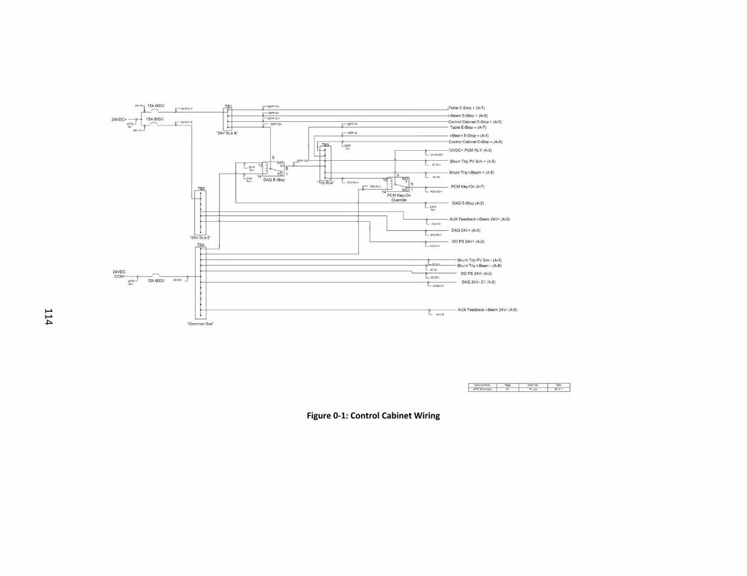
114
Figure 0‐1:
Control Cabinet WWiring
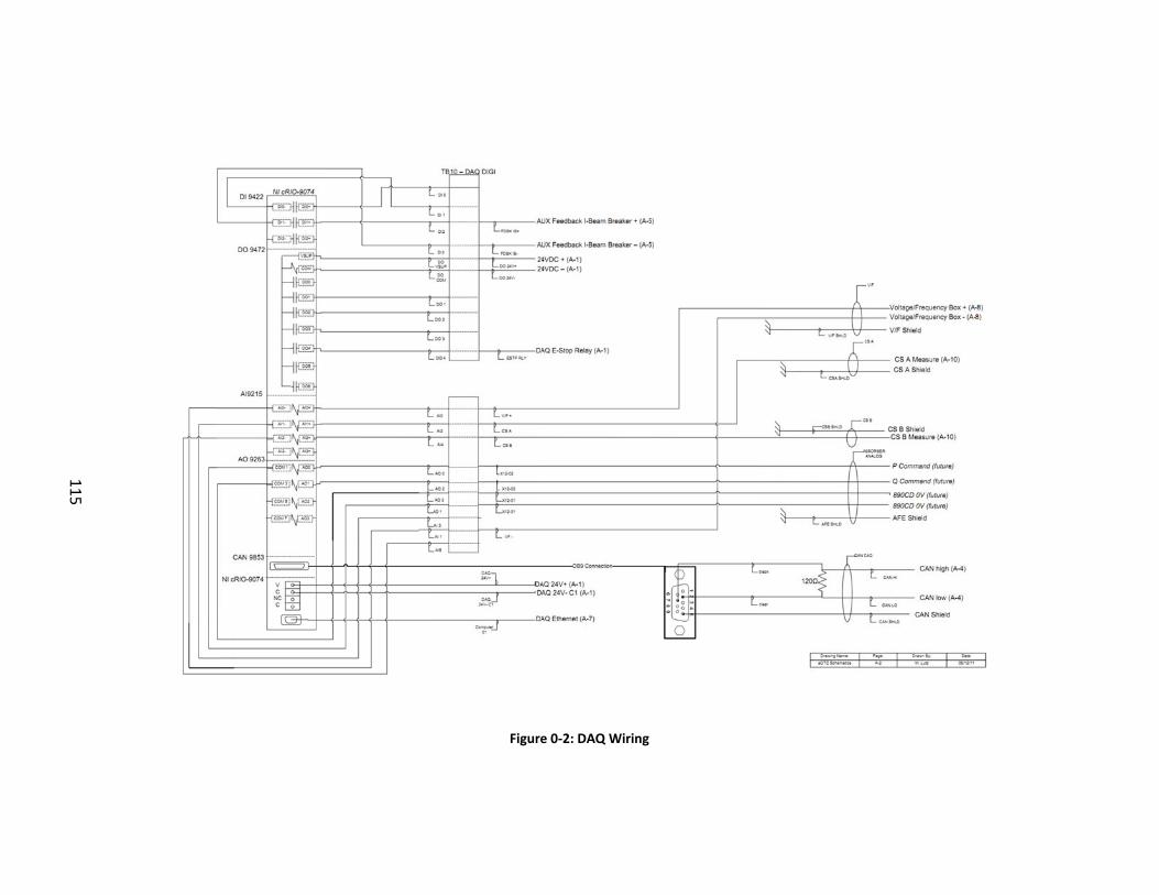
115
Figure
e 0‐2: DAQ Wiring
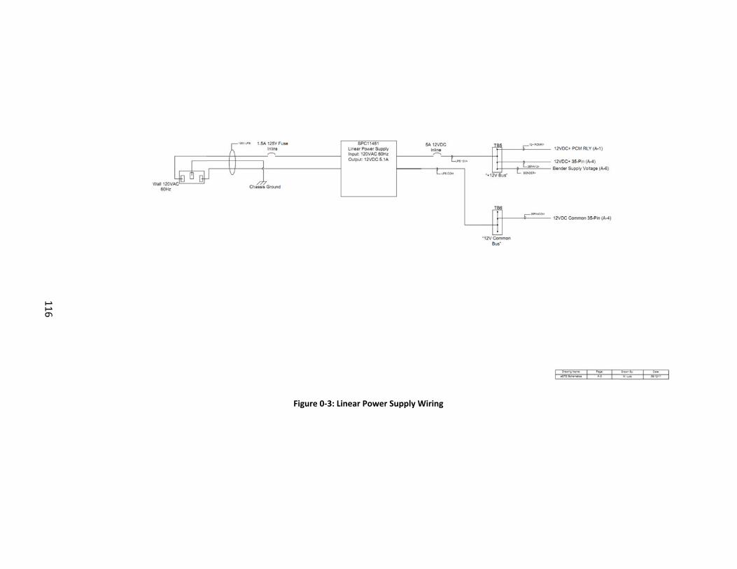
116
Figure 0‐3: Lin
near Power Supplyy Wiring
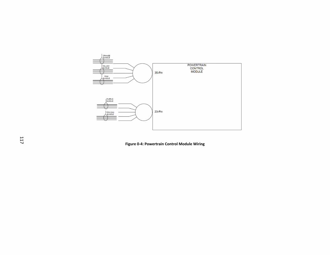
117
Figure 0‐4: Powe
rtrain Control Moddule Wiring
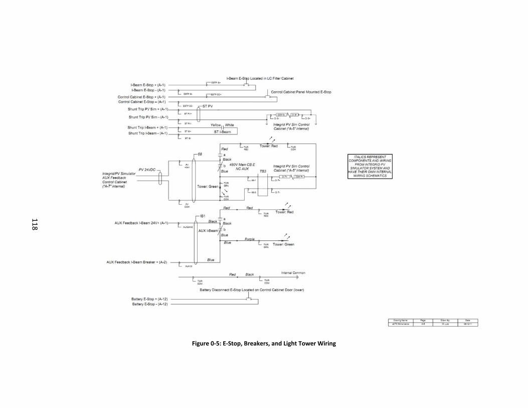
118
Figgure 0‐5: E‐Stop, B
Breakers, and Lightt Tower Wiring
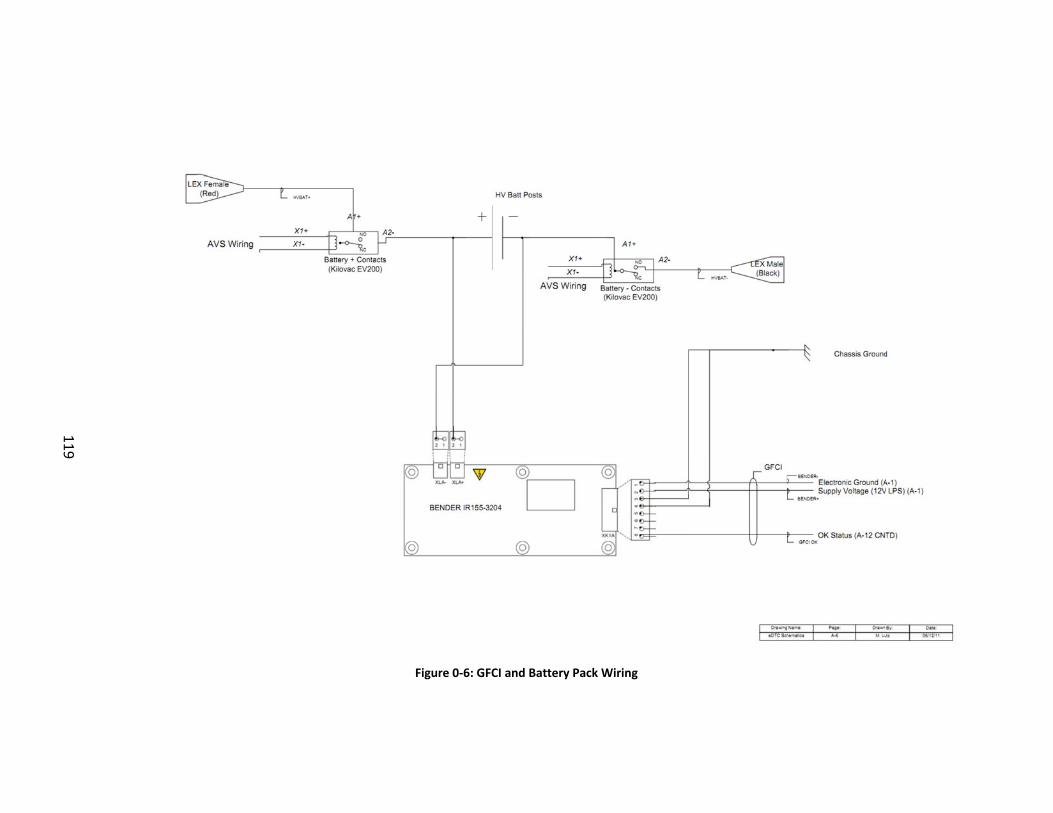
119
Figure 0‐6: GFC
CI and Battery Pacck Wiring
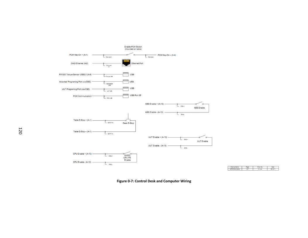
120
Figure 0‐7: Contro
ol Desk and Computer Wiring
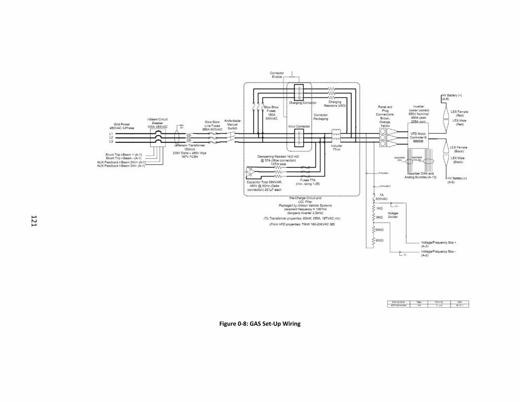
121
Figure 0‐
8: GAS Set‐Up Wirring
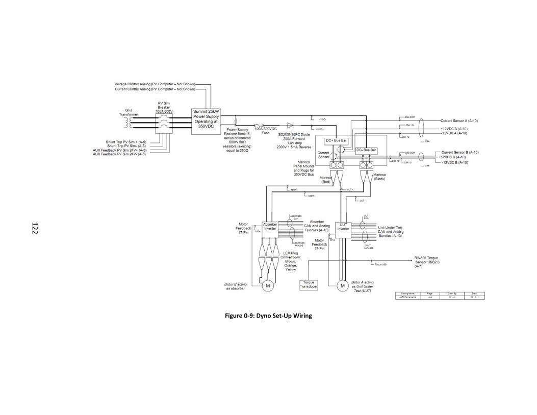
122
Figure 0‐9
9: Dyno Set‐Up Wiring
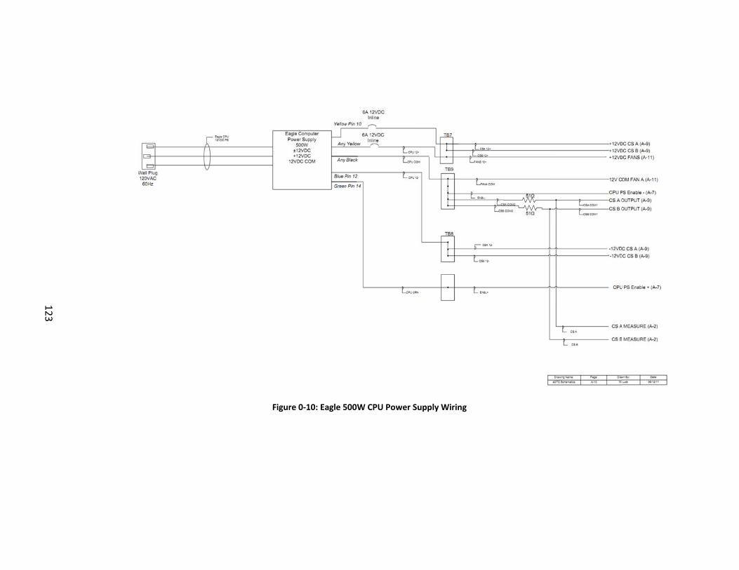
123
Figure 0‐10: Eagle 5
500W CPU Power SSupply Wiring
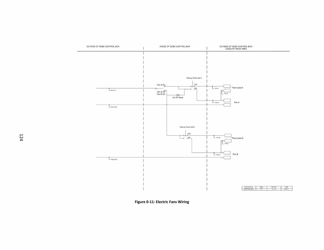
124
Figure 0‐1
11: Electric Fans W
iring
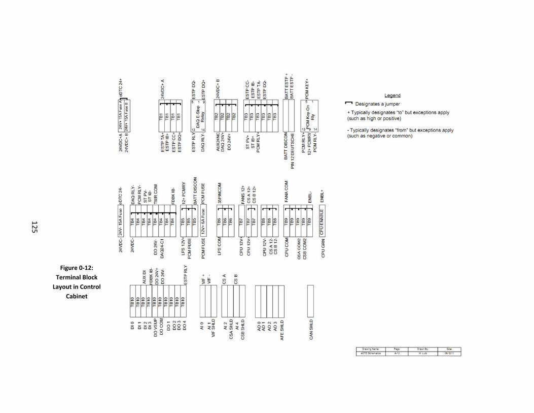
125
Figure 0‐12:
Terminal Block
Layout in Control
Cabinet
l
126
Figure 0‐‐13: Terminal Block
k Layout in Control Cabinet (continued)
127
Figurre 0‐14: Wiring Bun
ndle Distribution inn Control Cabinet

128
Appendix B– Artisan Vehicle Systems Pin‐Out Listings
Table 0‐1
129
1: PCM 35 Pin Assignments
Tablee 0‐3: Absorber
Table 0‐2
r Inverter Feed
130
2: PCM 25 Pin
dback Cable As
Assignments
ssignments forr Dyno and GAAS Set‐Ups
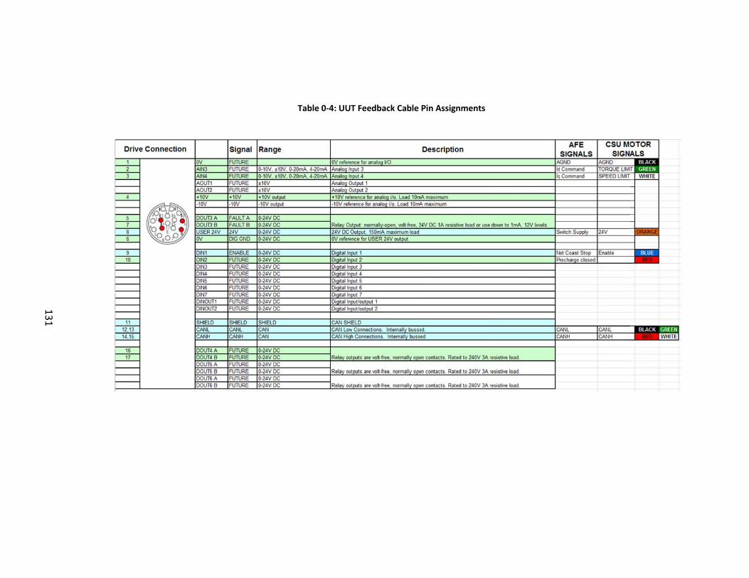
131
Table 0‐4: UU
UT Feedback Cable Pin Assignments
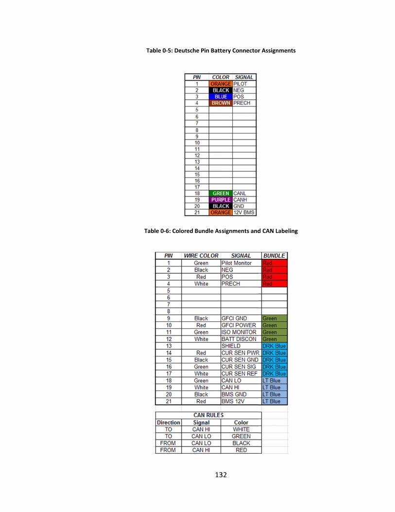
T
Ta
Table 0‐5: Deu
able 0‐6: Color
13
tsche Pin Batt
red Bundle Ass
32
tery Connector
signments and
r Assignments
d CAN Labeling
g

m
Show
mounting box
Appendi
n below is th
x.
ix C– GD&T
he geometri
13
T Print for
c dimension
33
Motor Mo
ns and tolera
ounting Bo
ances for the
ox
e motor

134
Appendix D–Natural Frequency MatLab Procedure
In order to further narrow down the results, an investigation of the natural
frequency of the sensor and couplings in the system must be analyzed. The motor
rotates at a maximum speed of 8,000rpm and thus the natural frequency needs to be
above this in order to not experience resonance. According to Norton, “usual design
strategy is to keep all forcing, self‐exciting, frequencies below the first critical frequency
by a factor of three or four” (Norton, 2000). Therefore it is crucial to determine the system
natural frequency of the torque sensor and couplings to be greater than 32,000 rpm for
safe operation. If the shaft system cannot be made higher than the required rotating
frequency, then the motors must be able to accelerate rapidly enough through the
resonance before the vibrations have a chance to build up amplitude. This allows the
system to operate at a speed higher than resonance. Figure 0‐15 (Source:
www.me.mtu.edu) illustrates the excitation at different dampening values for different
frequency ratios. The purpose of this plot is to show that as the natural frequency of the
system is approached (/n = 1), the displacement amplitude of the oscillations
increases significantly depending on the zeta (dampening) value.
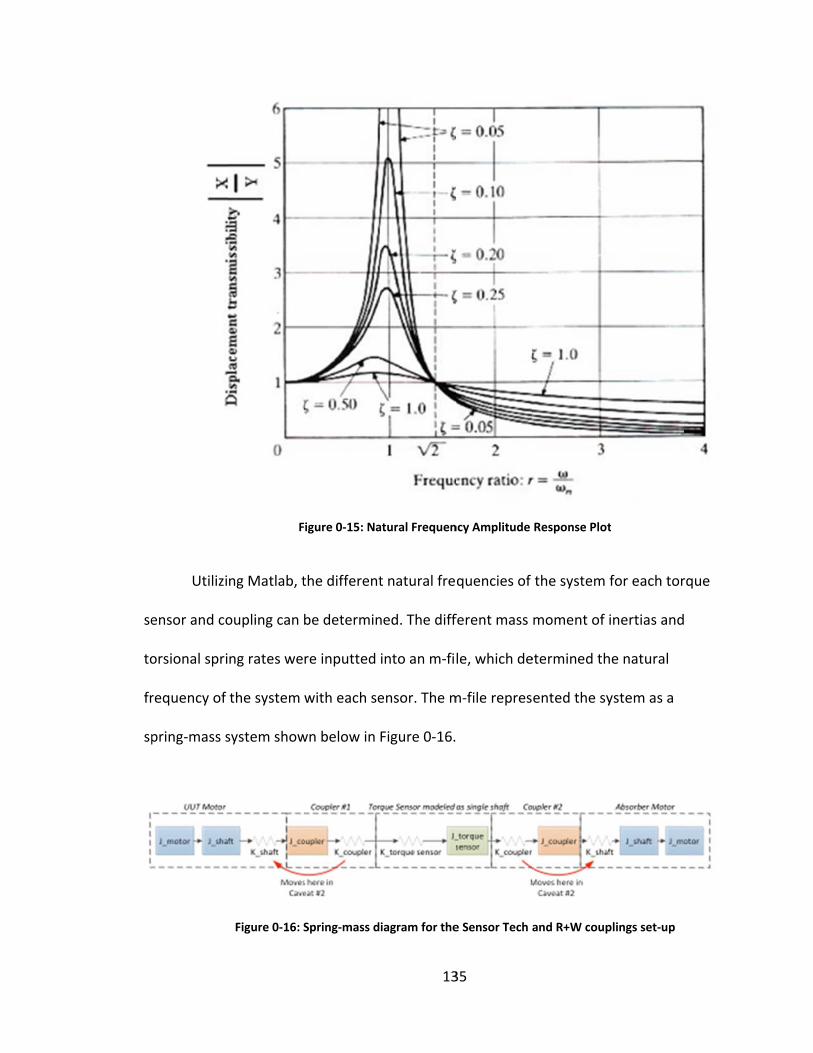
se
to
fr
sp
Utilizi
ensor and co
orsional spri
requency of
pring‐mass s
F
ng Matlab, t
oupling can b
ng rates we
the system
system show
Figure 0‐16: S
igure 0‐15: Na
the different
be determin
re inputted
with each se
wn below in
Spring‐mass d
13
atural Frequen
t natural fre
ned. The diff
into an m‐fil
ensor. The m
Figure 0‐16.
iagram for the
35
ncy Amplitude
quencies of
ferent mass
le, which de
m‐file repres
e Sensor Tech a
Response Plot
the system
moment of
etermined th
ented the sy
and R+W coup
t
for each tor
inertias and
he natural
ystem as a
plings set‐up
rque

136
Each mass moment of inertia (J) as well as torsional stiffness (K) is represented
for the motor and motor shaft, coupling, torque sensor, and identical coupling and
motor. The caveat to this analysis is how to model the spring representation of the
coupling torsional stiffness. It can be modeled on either the motor shaft side or torque
sensor shaft side of the coupler. Therefore an investigation will first be made between
these two different scenarios defined as caveat #1 and caveat #2. Figure 0‐16 uses
arrows to highlight how the coupling spring could be modeled on either side. These two
caveats are to be taking into account when analyzing the final natural frequency results.
However, it is crucial to understand that there needs to be a spring between two masses
so there must always be at least one coupler spring on one side of the torque sensor in
order for the analysis to run. With this in mind, only the left side coupler spring was
moved between caveat #1 and caveat #2 comparisons, leaving the right side coupler
spring connected to the torque sensor side.
Using the tabulated values from Table 3‐2 and Table 3‐3, the first investigation
(Sensor Tech RWT320 and R+W BK2 couplers) can be assigned to the above variables in
Figure 0‐16 for the scenario of the stiffest coupling and cheapest torque sensor (R+W
BK2 and RWT320 respectively). Below are the MatLab variable constant definitions to
the variables seen in Figure 0‐16.
%Mass Moments of Inertia:
Jm = 6.271E-3; %kg*m^2 (motor rotor) Artisan GP150WC
Js = 1.295E-4 %kg*m^2 (motor shaft) calculated using stainless steel and actual shaft mass
Jc = 4.5E-3; %kg*m^2 (coupler) assuming R+W America BK2 coupler

%
R
a
st
as
m
Jts
Torsiona
Ks =
Kc =
Kt =
The Ks
igidity) = 73
where
In ord
nd is volum
tainless stee
Using
s
Once
mass system
= 1.431eRWT320
al Stiffn
= 1.33E5; stainl
= 1.91E5;
= 3.56E4;
s (motor sha
X109 Pa for s
e
der to calcula
me. The den
el and the vo
these value
all the varia
shown in Fig
e-4; %kg*Torque s
ness (spr
%Nm/radless stee
%Nm/rad
%Nm/rad
aft torsional
stainless ste
ate the shaft
nsity of stain
olume was ca
es, the Ks for
bles are assi
gure 0‐16. N
13
*m^2 (torsensor
ring cons
d (motor el
d (BK2 co
d (torque
stiffness) w
el and the to
t mass, the e
less steel wa
alculated us
r stainless ste
igned, the m
Note that som
37
rque sens
stants):
shaft) c
oupler) g
e sensor)
was calculate
orsional stiff
equation:
as assumed
ing
eel of the m
m‐file relates
me mass me
sor) assu
calculate
given
given
d using G (M
fness equati
∗ , w
to be 7.90X
motor shaft c
s the variable
easurements
uming
ed assumi
Modulus of
on:
where is de
106 g/m3 for
an be calcul
es to the spr
s appear to b
ing
ensity
r 304
ated
ring
be in

138
kg, while others are in grams. These were converted to a common base in the
calculation section of the simulation.
% Relate the physical values to the generic spring mass system
J1 = Jm+Js
J2 = Jc;
J3 = Jts;
J4 = Jc;
J5 = Jm+Js;
% Caveat #1: Assuming the coupler "spring" is on the torque sensor shaft "spring"
K1 = Ks;
K2 = 1/(1/Kc + 1/Kt);
K3 = Kc;
K4 = Ks;
However if both the caveats mentioned above are considered, the program can
be re‐run with the coupler spring on the other side with the code shown below.
% Caveat #2: Assuming the coupler "spring" is on the motor shaft "spring"
K1 = 1/(1/Kc + 1/Ks);
K2 = Kt;
K3 = Kc;
K4 = Ks;

139
Continuing with the program code, the definition of the matrices for the Eigen
vector of phi and lambda appear as:
% Define the matrices of coefficients
J_mat = [J1 0 0 0 0;
0 J2 0 0 0;
0 0 J3 0 0;
0 0 0 J4 0;
0 0 0 0 J5]
K_mat = [ K1 -K1 0 0 0;
-K1 K1+K2 -K2 0 0;
0 -K2 K2+K3 -K3 0;
0 0 -K3 K3+K4 -K4;
0 0 0 -K4 K4]
[phi,lambda]= eig(K_mat,J_mat)
for i=1:5
nat_freq(i) = sqrt(lambda(i,i));
end
nat_freq_rpm = nat_freq*60/(2*pi)

C
w
to
C
m
w
p
w
0
th
w
ca
ax
a
The re
aveat #1 is w
when the cou
oque sensor
NaFrequency
Mo
Mo
Mo
Mo
These
aveat #1: wh
motor shaft a
worthy natur
oles X 8000
within the op
The re
‐17 and Figu
he analysis m
without dam
annot be co
xis shows ha
nd can be ig
esults from t
when the to
upler spring
).
Table 0‐
tural y At:
ode 2
ode 3
ode 4
ode 5
e results prov
hen the torq
and the coup
ral frequency
RPM / 2 pol
perating regi
esulting amp
ure 0‐18). Th
moves down
ping specifie
mpared. The
alf masses w
gnored for fu
these calcula
rque sensor
is paired wit
‐7: Sensor Tech
Caveatn (rpm)
19,5
67,5
72,4
379,
ve that the w
que sensor a
pling springs
y is mode tw
les per rotat
me.
plitude plot o
hese plots sh
n the length o
ed, the abso
ere are two
which is incor
uture mass p
14
ations are ta
and couplin
th the moto
h with R+W Co
t #1
500
570
450
,920
worse case,
and the coup
s being paire
wo since it is
tion = 32000
of the mass
how that mo
of the system
lute magnitu
notes on the
rrect. This on
plots. Second
40
abulated in T
ng springs ar
r shaft sprin
ouplers Caveat
Caveat n (rpm)
20,1
55,1
70,9
384,5
lowest natu
pling springs
ed. It also sho
closest to th
0 RPM. The l
at each mod
ode two has
m. It must b
ude of any m
e following p
nly appears
d, the y‐axis
Table 0‐7. Re
re together.
ng (on the lef
t Comparison
#2
160
130
950
510
ral frequenc
are paired i
ows that the
he forcing fr
lowest mode
de is shown
more vibrat
be noted how
mode is infin
plots. First th
due to the z
displays Am
emember th
Caveat #2 is
ft side of the
Results
Differe(#1‐#
‐660
12,44
1,50
‐4,59
cy, occurs in
instead of th
e only note
requency of
e, is, in fact,
below (Figu
ion amplitud
wever that
nite, and thu
he scale of t
zoom of the
mplitude with
at
s
e
ence #2)
0
40
00
90
he
8
well
re
de as
s
the x‐
axis
h a
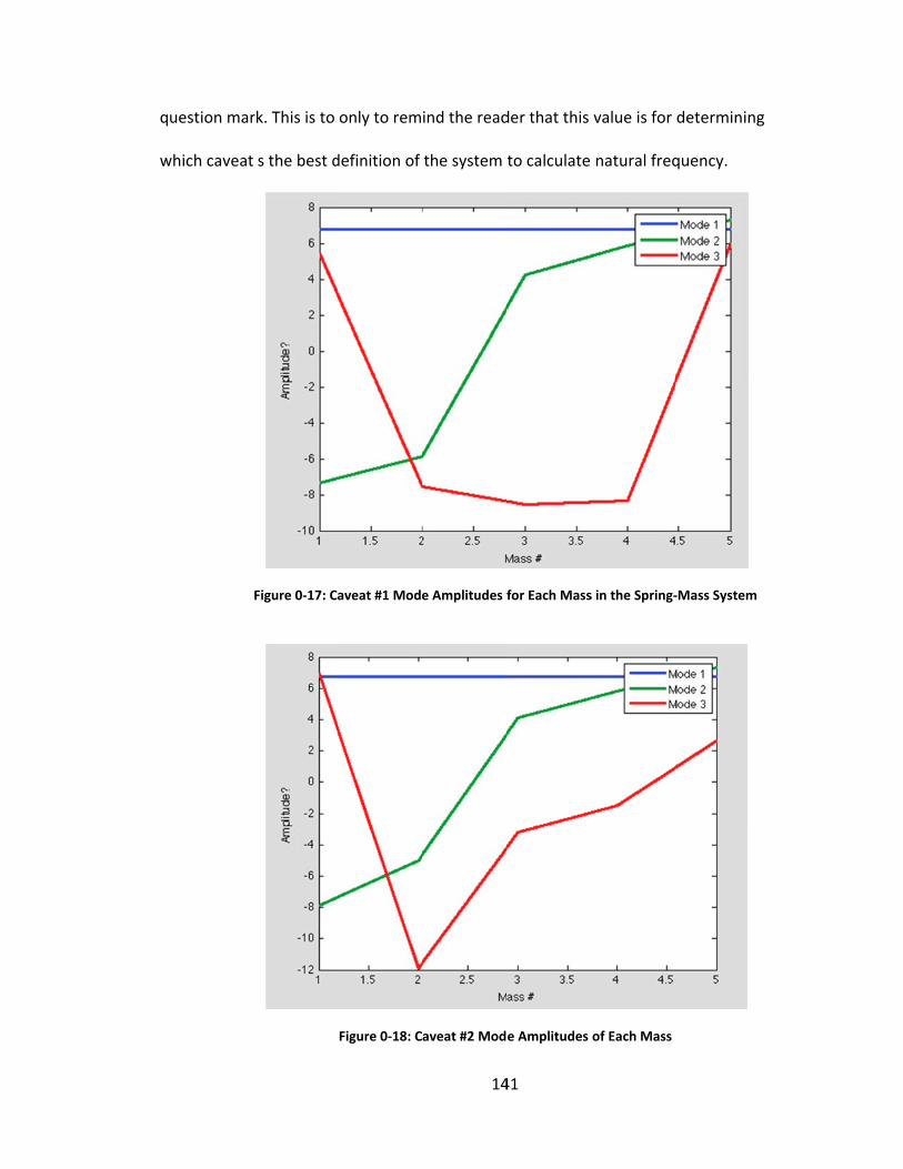
q
w
uestion mar
which caveat
rk. This is to
s the best d
Figure 0‐17: Ca
only to rem
definition of
aveat #1 Mode
Figure 0‐18: C
14
ind the read
the system
e Amplitudes f
aveat #2 Mod
41
der that this
to calculate
for Each Mass
e Amplitudes
value is for
natural freq
s in the Spring‐
of Each Mass
determining
quency.
‐Mass System
g

ca
th
n
sh
te
m
sh
o
d
w
at
c
The ke
ase changed
herefore Cav
To inv
eeded to be
hows the Int
echnology w
measures the
heet, the tor
f the shaft e
ifferent as w
whereas the t
ttached.
Figure
Below
%Mas
Jm =
Js =stee
Jc =coupler
ey take away
d the shape o
veat 2 is like
vestigate a d
e made to th
terface mass
where a throu
e torque bet
rsional stiffn
ends was calc
well because
test side of t
e 0‐19: Mass‐S
an
w is the set‐u
ss Moment
= 6.271E-
= 1.295E-el
= 4.5E-3;
y from these
of Mode 2 si
ly not repre
ifferent styl
e Matlab m‐
s moment of
ugh shaft ha
ween the dr
ness is only o
culated assu
e the drive si
the sensor s
Spring Diagram
nd Torque Sen
up for the Int
ts of Ine
3; %kg*m
4; %kg*m
%kg*m^2
14
e plots is tha
ignificantly.
sentative of
e sensor, the
‐file. The new
f inertias for
as a necked d
rive and test
of the neck c
uming stainle
de has no m
haft has diff
m of Interface T
sor Shaft Sprin
terface m‐fil
ertia:
m^2 (moto
m^2 (moto
2 (couple
42
at moving th
This does n
f the actual s
e Interface t
w mass‐spri
r the drive a
down portio
t side. Accor
component,
ess steel. Th
measuremen
ferent meas
Torque Sensor
ngs Paired Tog
le:
or) Artis
or shaft)
er) assum
he spring in t
not make sen
system.
torque senso
ng diagram,
nd test side.
on in the mid
rding to the
thus the tor
he moment o
t equipment
urement eq
r with Caveat #
gether)
san GP150
assumin
ming R+W
the “caveat #
nse physicall
or, modificat
, Figure 0‐19
. Interface u
ddle and this
Interface da
rsional stiffn
of inertias ar
t attached
uipment
#1 Shown (Cou
0WC
ng stainl
America
#2”
ly;
tions
9,
ses a
s
ta
ness
re
upler
less
BK2

143
Jd = 1E-4; %kg*m^2 (driven/Unit Under Test (UUT) side of torque sensor) assuming Interface T2 Torque sensor
Jt = 9E-5; %kg*m^2 (test/absorber side of torque sensor)
%Torsional Stiffness (spring constants):
Ks = 1.33E5; %Nm/rad (motor shaft) calculated assuming stainless steel
Kc = 1.91E5; %Nm/rad (coupler) given
Kt = 6.7E4; %Nm/rad (torque sensor) given
Kst = 1.977E5; %Nm/rad (torque sensor shaft) calculated using stainless steel
% Relate the physical values to the generic spring mass system
J1 = Jm+Js;
J2 = Jc;
J3 = Jd;
J4 = Jt;
J5 = Jc;
J6 = Jm+Js;
% Caveat #1: Assuming the coupler "spring" is on the torque sensor shaft "spring"
% K1 = Ks;
% K2 = 1/(1/Kc + 1/Kst);
% K3 = Kt;
% K4 = 1/(1/Kc + 1/Kst);
% K5 = Ks;

m
to
lo
0
sy
#
% Camotor sha
K1 =
K2 =
K3 =
K4 =
K5 =
After
o critique th
ocation in th
‐21. These f
ystem depen
1 is the wors
NaFrequency
Mo
Mo
Mo
Mo
Mo
aveat #2:aft "spri
= 1/(1/Kc
= Kst;
= Kt;
= Kst;
= 1/(1/Kc
running the
e difference
e mass‐sprin
igures are vi
nding on wh
st‐case scen
Table
tural y At:
ode 2
ode 3
ode 4
ode 5
ode 6
Assumining"
c + 1/Ks)
c + 1/Ks)
file for both
e in assumpt
ng diagram f
isual represe
hich caveat is
ario for earl
0‐8: Interface
Cave n (rpm
20,
67,3
72,8
308,
473,
14
ng the co
;
;
h caveat #1 a
ions. A plot
from Figure
entations of
s selected. It
iest natural
Sensor with R
at #1 m)
140
320
880
,360
,060
44
oupler "s
and caveat #
of the mode
0‐19 is show
the differen
t can again b
frequency.
R+W Couplers C
Cavea n (rpm
21,6
51,7
61,9
439,3
568,3
spring" i
#2, Table 0‐8
e amplitudes
wn in Figure
nces at each
be determin
Caveat Compa
at #2 m)
640
700
900
350
330
is on the
8 was produc
s at each
0‐20 and Fig
point in the
ed that cave
arison
Differe(#1‐#
‐1,50
15,62
10,98
‐130,9
‐95,2
e
ced
gure
e
eat
ence #2)
00
20
80
990
70
n
Lookin
atural frequ
Figure 0‐20:
Figure
ng at the dif
ency effects
Detailed View
0‐21: Mode A
ferent coup
s on the syst
14
w of Caveat #1 w
Amplitude Plot
lings availab
tem is anoth
45
with Only the
t of Caveat #2 f
ble for the In
er valuable
First Three Mo
for Interface S
nterface set‐
study. Show
odes Shown
Sensor
up and their
wn below (Ta
r
able
0
re
il
‐9) is a table
espective J a
lustrate thes
NaturaFrequency
Mo
Mo
Mo
Mo
Mo
Mo
Figu
e summarizin
and K terms
se findings f
Table 0
al y At:
R
ode 1
ode 2
ode 3
ode 4
ode 5
ode 6
re 0‐22: Mode
ng these find
were used f
or the first t
0‐9: Interface c
R+W BK2 coun (rpm
0
20,
67,3
72,8
308,
473,
e‐Amplitude Pl
14
dings. The th
or these calc
three modes
coupling comp
upling m)
In
0
140
320
880
,360
,060
lot of Caveat #
Interface Coup
46
hree differen
culations. Fi
s.
parison results
nterface coupn (rpm
0
23,4
105,0
125,1
346,9
495,3
#1 with the Int
pling
nt couplings
gure 0‐22 an
s (all using cave
pling )
R+
490
090
190
990
379
terface Sensor
with their
nd Figure 0‐
eat#1)
+W BKM coupn (rpm)
0
22,87
135,2
167,7
322,7
472,8
and the Supp
23
pling
70
210
780
740
890
lied
se
d
a
Figu
The n
ensor uses a
ata inductiv
ll with a non
ure 0‐23: Mode
ext sensor to
a strain gaug
ely. Figure 0
n‐contact co
e‐Amplitude P
o investigate
ge that is mo
0‐24 pictoria
llar.
14
lot for Caveat
e is the natu
ounted direct
lly illustrate
47
#1 with Interf
ural frequenc
tly on the m
s the differe
face Sensor an
cy of is the B
motor shaft a
ent sizes of B
nd BKM Coupli
Binsfeld. This
and transmit
Binsfeld sens
ngs
s
ts the
sors
th
h
T
n
Since
he sensor’s i
ow the mass
After
able 0‐10 we
atural frequ
the Binsfeld
nertia and s
s‐spring mod
Figure
running the
ere found. T
ency.
Figur
d attaches di
spring consta
del is change
e 0‐25: Spring‐
Matlab cod
The results sh
14
re 0‐24: Binsfe
rectly to the
ant can esse
ed for analys
mass diagram
e for this ne
how that the
48
eld Torque Sen
e shaft, only
entially be ig
sis.
of Binsfeld to
ew design, th
e second mo
nsors
one couple
nored. Figur
orque sensor se
he following
ode has the
r is needed a
re 0‐25 show
et‐up
g results seen
highest yet
and
ws
n in
seen

149
Table 0‐10: Binsfeld natural frequency results
Natural Frequency (rpm)
Mode 2 37,070
Mode 3 76,950
There are some assumptions to the Binsfeld model that need to be mentioned
however. The model assumes that the mass of the strain gauge collar on the shaft is
negligible because it is made of nylon and is mounted solidly on one shaft. The shaft
that has the sensor collar mounted to it would have a higher mass moment of inertia
but this was neglected for simplicity. A better approximation would be to add the
moment of inertia of the sensor collar to the coupler inertia. The assumptions used to
calculate these frequencies allow for the values to be higher than they would be in the
real‐life application.
Table 0‐11 summarizes the previous investigations into one table. Notice that
the R+W BK2 and BKM couplers were each tried with different sensors for a more
conclusive investigation.
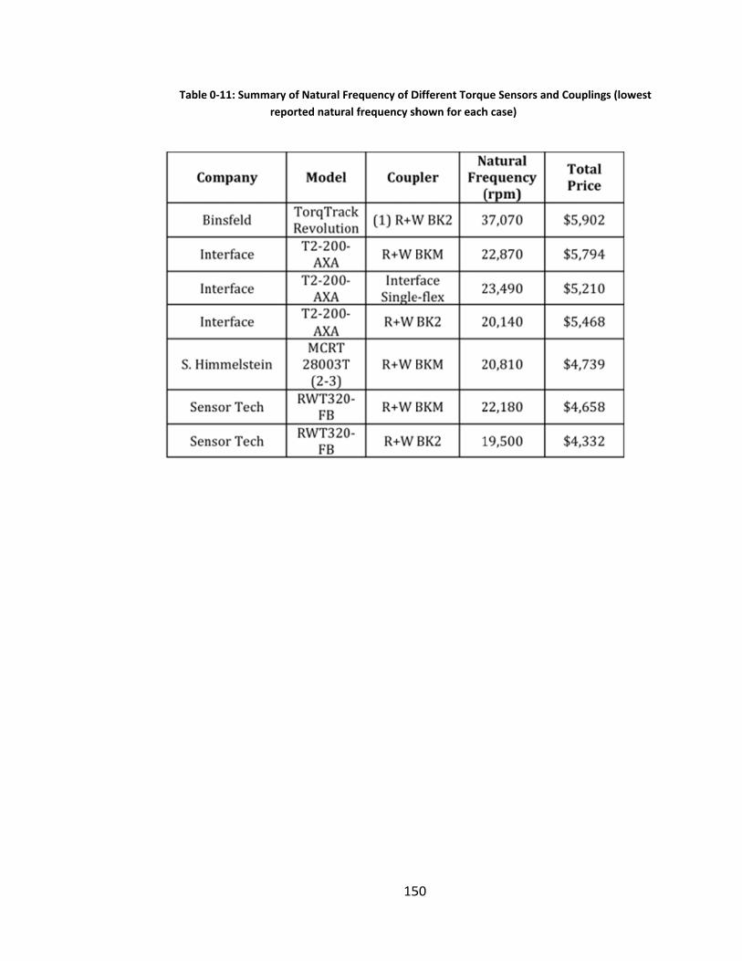
Table
0‐11: Summar
re
ry of Natural F
eported natura
15
Frequency of D
al frequency sh
50
Different Torqu
hown for each
ue Sensors and
h case)
d Couplings (loowest
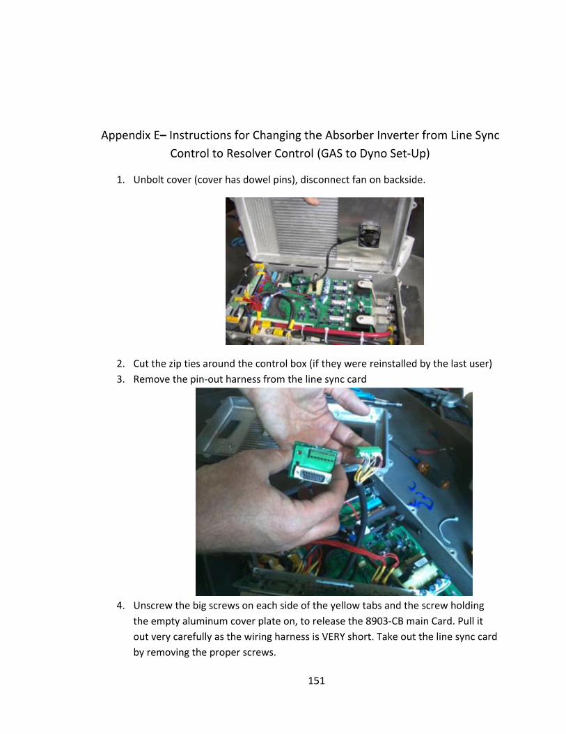
A
Appendix E
1. Unbol
2. Cut th
3. Remo
4. Unscr
the em
out ve
by rem
E– Instructi
Control
lt cover (cov
he zip ties ar
ove the pin‐o
rew the big s
mpty alumin
ery carefully
moving the p
ions for Ch
to Resolve
ver has dowe
ound the co
out harness f
screws on ea
num cover pl
as the wirin
proper screw
15
hanging the
er Control (
el pins), disc
ontrol box (if
from the line
ach side of th
late on, to re
ng harness is
ws.
51
e Absorber
(GAS to Dy
connect fan o
f they were r
e sync card
he yellow ta
elease the 8
s VERY short
r Inverter f
yno Set‐Up
on backside
reinstalled b
abs and the s
8903‐CB mai
t. Take out th
from Line S
p)
.
by the last us
screw holdin
n Card. Pull
he line sync
Sync
ser)
ng
it
card
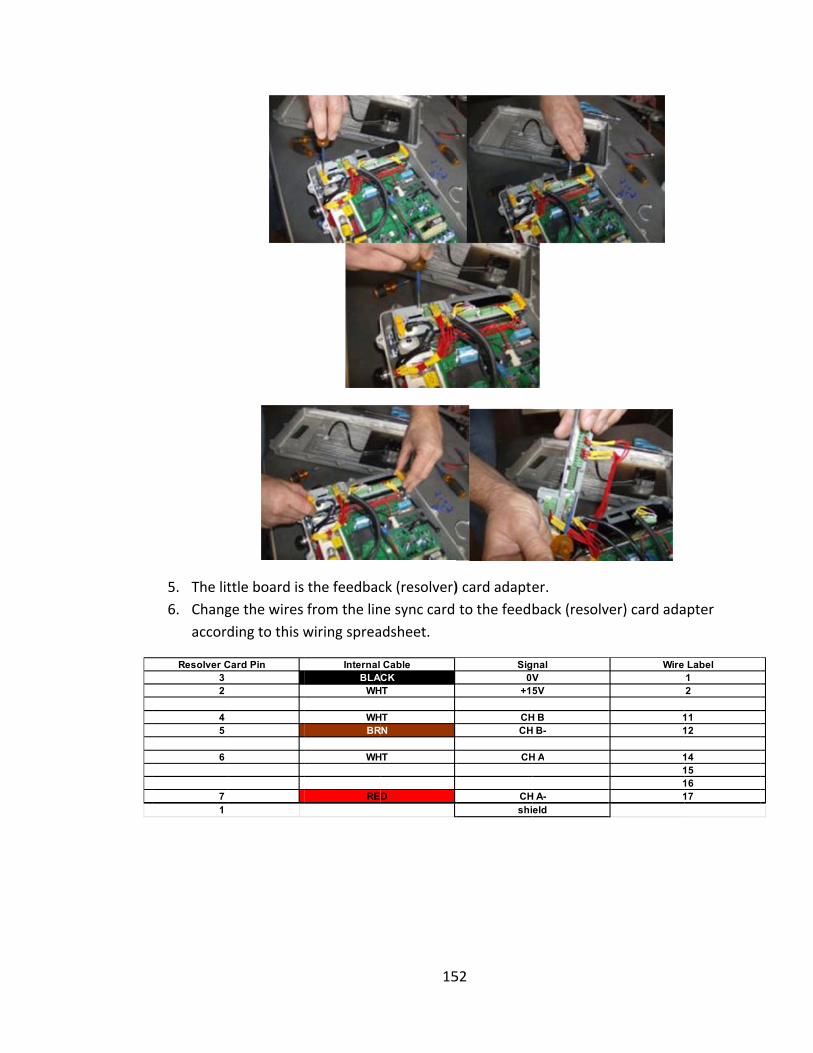
5. The lit
6. Chang
accord
Resolver C32
45
6
71
ttle board is
ge the wires
ding to this w
Card Pin
the feedbac
from the lin
wiring sprea
Internal BLA
WH
WHBR
WH
RE
15
ck (resolver)
ne sync card
adsheet.
CableACKHT
HTRN
HT
D
52
) card adapte
to the feedb
Sig0V
+1
CHCH
CH
CHshi
er.
back (resolv
nalV5V
H BH B-
H A
H A-eld
ver) card ada
Wire
11
1111
apter
Label12
1112
14151617
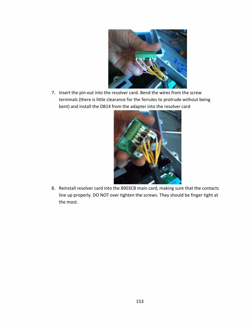
7. Insert
termin
bent)
8. Reinst
line u
the m
t the pin‐out
nals (there is
and install t
tall resolver
p properly. D
most.
t into the res
s little cleara
the DB14 fro
card into th
DO NOT ove
15
solver card.
ance for the
om the adap
e 8903CB m
er tighten the
53
Bend the wi
ferrules to
ter into the
main card, ma
e screws. Th
ires from the
protrude wi
resolver car
aking sure th
hey should b
e screw
thout being
rd
hat the cont
e finger tigh
tacts
ht at
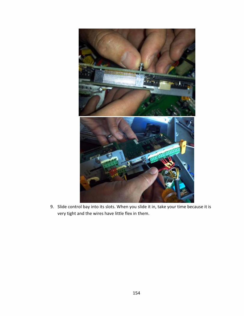
9. Slide c
very t
control bay i
ight and the
into its slots
e wires have
15
s. When you
little flex in
54
slide it in, ta
them.
ake your tim
me because it is
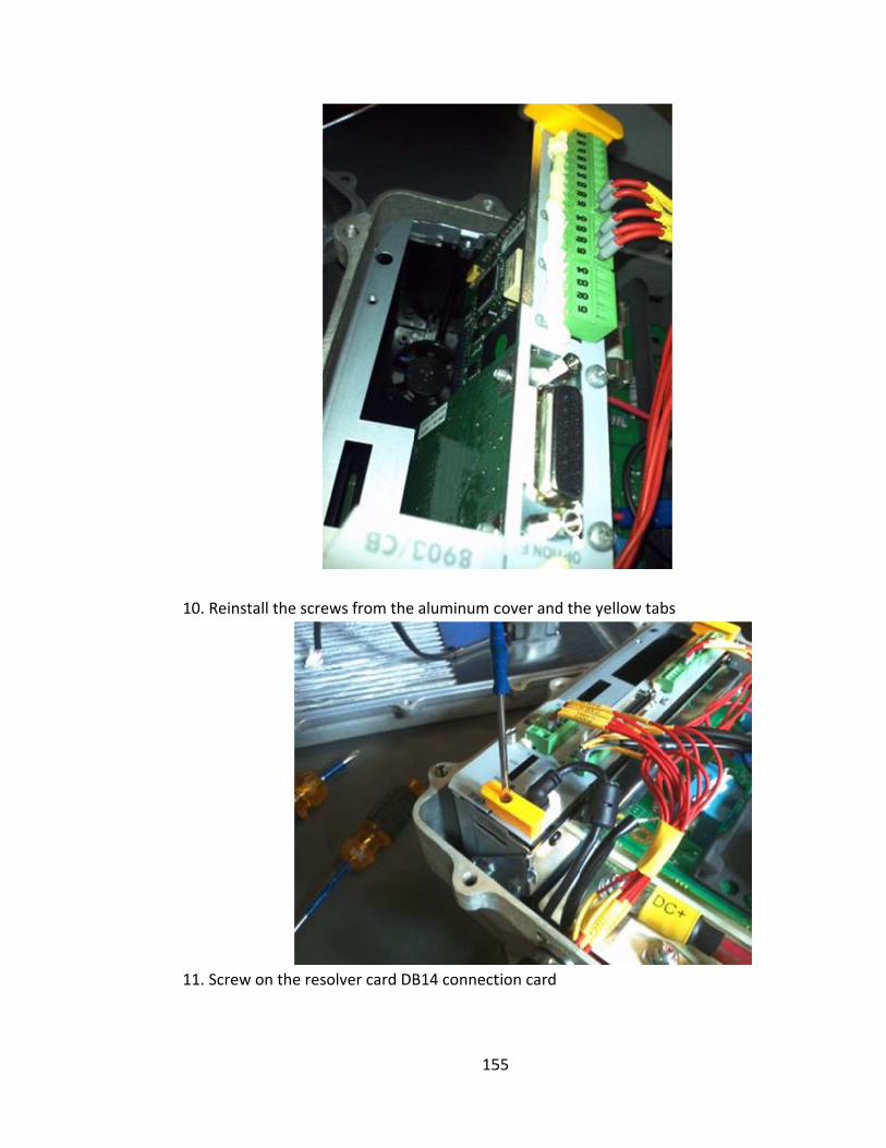
10. Reinst
11. Screw
tall the screw
w on the reso
ws from the
olver card DB
15
aluminum c
B14 connect
55
cover and th
tion card
he yellow tab
bs
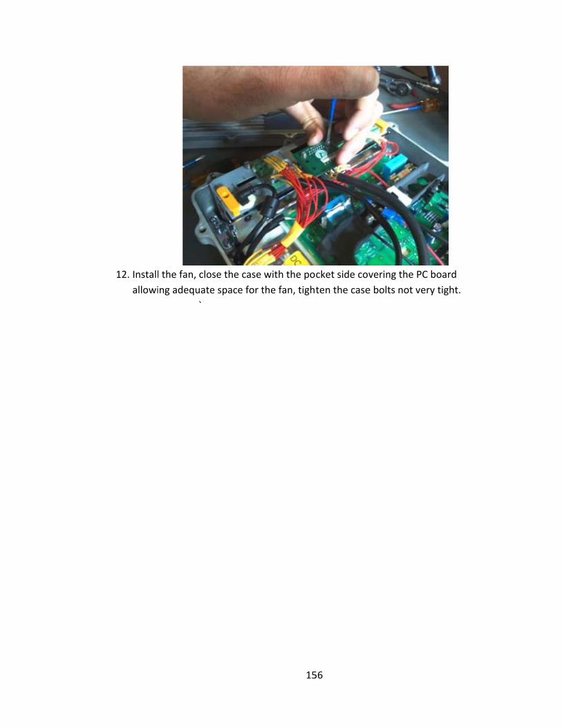
12. Install
allowi
l the fan, clo
ing adequate
`
ose the case
e space for t
15
with the po
the fan, tigh
56
cket side co
ten the case
vering the P
e bolts not v
PC board
ery tight.