Embed Size (px)
Citation preview
UNIVERSITY OF PITTSBURGH
SCHOOL OF INFORMATION SCIENCES M.S. IN TELECOMMUNICATIONS
“EXPLORING JAMMING ATTACKS USING OPNET 12.0”
THESIS
Submitted to the Graduate Faculty of The School of Information Sciences in partial fulfillment of the requirements for the degree
of
MASTER OF SCIENCE IN TELECOMMUNICATIONS
BY:
JESÚS MANUEL GONZALEZ DE JESÚS
ADVISOR:
PhD. Prashant Krishnamurthy
Pittsburgh, PA, USA NOVEMBER 2007
University of PittsburghSchool of Information Sciences
Department of Information Sciences and Telecommunications
This thesis was presented by:
Jesús Manuel González de Jesús
It was defended on:
November 16th, 2007
And approved by:
Dr. Richard A. Thompson, Assistant Professor
Dr. Martin Weiss, Assistant Professor
Thesis Advisor: Dr. Prashant Krishnamurthy, Assistant Professor
ii

School of Information Sciences Department of Information Sciences and Telecommunications
Master’s Thesis Defense
Student’s name: Jesús Manuel González de Jesús Thesis title: Exploring Jamming Attacks using OPNET® 12.0 Committee: Dr. Richard A. Thompson _________________ Information Sciences and Telecommunications Dr. Martin Weiss _________________ Information Sciences and Telecommunications Major Advisor: Dr. Prashant Krishnamurthy _______________ Information Sciences and Telecommunications Date: __________________ DIST Chair: ________________________ Date: __________
iii

Copyright © by Jesús Manuel González de Jesús
2007
iv

Exploring Jamming Attacks using Opnet® 12.0.
Jesús Manuel González de Jesús, MST
University Of Pittsburgh, 2007
Abstract:
Ad-hoc Networks are one of the most important achievements of current technology; they can
provide communication without needing a fixed infrastructure, which makes them suitable for
communication in disaster areas or when quick deployment is needed. However, since this kind
of network uses the wireless medium for communication, it is susceptible to malicious
exploitation at different layers. One of these attacks is a kind of denial of service attack (DoS)
that interferes with the radio transmission channel, this is also known as a jamming attack. In this
kind of attack, an attacker emits a radio signal that disturbs the energy of the packets causing
many errors in the packet currently being transmitted. Another version of this attack is to
constantly emit random semi-valid packets to keep the medium busy all the time, preventing the
honest nodes from switching from the listening mode to the transmitting mode. In rough
environments where there is constant traffic, a jamming attack causes serious problems;
therefore measures to prevent this attack are required. The purpose of this thesis is to explore the
underlying principles of jamming attacks (i.e., the effects of modulation techniques, interarrival
times of packets, transmitter’s and jammer’s power) using Opnet® as the simulation tool. This
work will be helpful so that in future research a useful, practical and effective solution can be
created to countermeasure the effects of jamming attacks. The objective here is to understand,
modify, and employ the models in OPNET 12.0® to simulate jamming attacks and understand
the limitations of the available models.
v
TABLE OF CONTENTS
TABLE OF CONTENTS ..........................................................................................vi
LIST OF FIGURES ..................................................................................................vii
ACKNOWLEDGEMENTS ......................................................................................x
1.0 INTRODUCTION ..............................................................................................1
1.1 MOTIVATION .......................................................................................1
1.2 THESIS OVERVIEW..............................................................................2
1.3 THESIS OUTLINE..................................................................................3
2.0 BACKGROUND ................................................................................................4
2.1 THE WIRELESS CHANNEL ................................................................4
2.1.1 Free space propagation .............................................................5
2.1.2 Large scale fading ....................................................................5
2.1.3 Small scale fading ....................................................................6
2.1.4 Coding and Modulation.............................................................7
2.2 MAC PROTOCOLS IN 802.11 ..............................................................8
2.2.1 802.11 overview .......................................................................8
2.2.2 MAC Protocols .........................................................................9
2.2.2.1 CSMA .......................................................................9
2.2.2.2 CSMA/CA .................................................................10
2.3 JAMMING ATTACKS .........................................................................11
2.3.1 Jammers classification ..............................................................12
2.3.1.1 Constant jammers ......................................................12
2.3.1.2 Deceptive jammers ....................................................12
2.3.1.3 Random jammers ......................................................12
2.3.1.4 Reactive jammers ......................................................13
2.3.2 Jamming detection ....................................................................13
2.3.2.1 Packet delivery ratio .................................................13
2.3.2.2 Signal strength ..........................................................14
2.3.2.3 Carrier sensing ..........................................................14
vi
2.3 OPNET® ...............................................................................................15
2.4.1 Radio transceiver pipeline.........................................................15
3.0 EXPERIMENT DESIGN ....................................................................................23
3.1 PROBLEM DEFINITION .....................................................................23
3.2 DATA ACQUISITION / MODEL SPECIFICATION............................23
3.2.1 Scenario 1 .................................................................................24
3.2.1.1 Jammer characteristics ...............................................25
3.2.1.2 Transmitter characteristics ........................................27
3.2.1.3 Receiver characteristics ............................................28
3.2.2 Scenario 2 .................................................................................29
3.2.2.1 Application definition and profile definition
characteristics..............................................................30
3.2.2.2 Nodes characteristics ................................................31
3.2.2.3 Jammer characteristics ..............................................35
3.2.3 Scenario 3 .................................................................................35
3.2.3.1 jammer characteristics ..............................................36
3.2.4 Scenario 4 .................................................................................37
3.2.4.1 Nodes characteristics ................................................37
3.2.5 Scenario 5 .................................................................................38
4.0 SIMULATIONS ANALYSIS .............................................................................39
4.1 SCENARIO 1 .........................................................................................39
4.2 SCENARIO 2 .........................................................................................45
4.3 SCENARIO 3 .........................................................................................50
4.4 SCENARIO 4 .........................................................................................51
4.5 SCENARIO 5 .........................................................................................53
5.0 CONCLUSIONS ................................................................................................56
APPENDIX A ...........................................................................................................58
APPENDIX B ...........................................................................................................61
BIBLIOGRAPHY......................................................................................................66
vii
LIST OF FIGURES
Figure 2.1 802.11 layers ................................................................................9
Figure 3.1 Scenario 1 layout ..........................................................................25
Figure 3.2 Jammer characteristics .................................................................25
Figure 3.3 Jammer inner modules..................................................................26
Figure 3.4 Characteristics of the jammer modules .......................................26
Figure 3.5 Transmitter’s characteristics.........................................................27
Figure 3.6 Transmitter’s modules characteristics ..........................................27
Figure 3.7 Receiver’s modules .....................................................................28
Figure 3.8 Receiver’s modules characteristics ..............................................29
Figure 3.9 Scenario 2 layout .........................................................................30
Figure 3.10 Profile and application definition characteristics ......................31
Figure 3.11 Nodes’ characteristics ................................................................32
Figure 3.12 Node’s modules .........................................................................32
Figure 3.13 Wireless_lan_mac module .........................................................33
Figure 3.14 Wlan_port_rx_0_0module .........................................................34
Figure 3.15 Wlan_port_tx_0_0module .........................................................34
Figure 3.16 Jammer’s modules .....................................................................35
Figure 3.17 Jammer’s modules characteristics .............................................35
Figure 3.18 Pulse jammer’s inner modules ...................................................36
Figure 3.19 Modules characteristics .............................................................36
Figure 3.20 Ad-hoc characteristics ...............................................................37
Figure 3.21 misbehaving node inner structure ..............................................38
Figure 4.1 Scenario 1 layout (75x 75 meters) ...............................................39
Figure 4.2 Traffic characteristics under normal circumstances ....................40
Figure 4.3 Traffic characteristics under a jamming attack ...........................41
Figure 4.4 Different modulation schemes under jamming attack .................43
Figure 4.5 Increasing the power at the jammer to 0.1 W ..............................44
Figure 4.6 Scenario 2 layout .........................................................................46
viii
Figure 4.7 Traffic without jamming attack ...................................................46
Figure 4.8 30-second close-up ......................................................................47
Figure 4.9 Traffic when a jammer is introduced ...........................................48
Figure 4.10 30-second close-up when the jammer is introduced ..................48
Figure 4.11 Before and after the jammer is introduced ................................49
Figure 4.12 30-second close-up ....................................................................50
Figure 4.13 Traffic before and after the random jamming attack .................51
Figure 4.14 Layout for scenario 3 .................................................................52
Figure 4.15 Traffic in 4 nodes before and after jamming .............................53
Figure 4.16 Scenario 5 layout .......................................................................54
Figure 4.17 before and after the misbehaving node is introduced ................54
Figure 4.18 before and after the misbehaving node is introduced in a more
populated network ...................................................................... 55
ix

ACKNOWLEDGEMENTS
This thesis would have not been possible without the support of the Autonomous University of
the State of Mexico and the University of Pittsburgh. I also thank my advisor Dr. Prashant
Krishnamurthy, whose insightful guidance helped me through all the process of writing this
thesis. I would also like to thank Dr. Richard Thompson and Dr. Martin Weiss for being part of
the committee to evaluate this work. My gratitude also goes to all my professors at the School of
Information Sciences, who with their classes transmitted to me the invaluable knowledge that
helped me in the development of this thesis. Finally, my foremost gratitude goes to God for
giving me the strength all this time.
x
1.0 INTRODUCTION
Wireless technologies have emerged to offer access to information or applications from any
place without being attached to a wall or floor by using wires; instead they use electromagnetic
waves to transmit information through the free-space medium. At the beginning, in Wireless
Local Area Networks (WLANs), the radio communication ranges were restricted to small areas
dictated by the transmission power of a central authority called the Access Point (AP). The AP
also had the responsibility of controlling all the activity in the network and often required a fixed
infrastructure. Ad-hoc networks emerged as a possible alternative for scenarios where a fixed
infrastructure does not exist and the environment is not suitable to build a fixed network. An ad-
hoc network is a kind of network that is easily deployed; the nodes only need to enter each
other’s radio range and the network configures itself; this is particularly important for
communication after natural disasters or in old buildings that cannot be wired.
1.1 MOTIVATION
Since nodes in an ad-hoc network use the radio wireless medium to communicate with other
nodes, it is pretty easy for an attacker to launch an attack against an honest node. There are many
attacks that can be launched against an ad hoc wireless network such as: radio interference
attacks, routing attacks, tunneling attacks, etc. In this thesis the focus is set to a special kind of
radio interference attack known as jamming attack. A jamming attack prevents legitimate users
from accessing the channel or by disrupting the communication between a sender and a receiver.
Jamming attacks are a problem that has represented a difficult challenge since World War II,
when they were launched against radars. Nowadays they still remain a serious problem even for
the most refined communication protocols implemented in the most sophisticated devices.
In a jamming attack the malicious node can act in one of two ways: 1) the attacker can send a
random radio signal to increase the background noise in the channel and thereby causing many
errors in the packet so that when that packet reaches the receiver it cannot correct the errors in
the packet, therefore discarding it; 2) in the second way, the attacker sends packets with a valid
packet format, that contains a valid frame header, but the data in it is useless. Such a packet may
1
prevent other packets from being sent to its intended receiver or it may collide with a legitimate
packet resulting in the loss of the packet in a similar way to the first way of attacking.
Nowadays, people need communication networks that can assure them that their information
remains private, that the information they are sending and receiving remains unchanged while it
is being transmitted, that the receiver is who it claims to be and finally that they can be
communicated whenever they need it. Jamming attacks affect the network in the sense that they
prevent all kinds of information exchange. As mentioned before, this problem remains an open
problem in the communications field; this is the reason why this thesis focuses on the exploration
of the underlying factors that can be exploited to prevent these kinds of attacks. Security
problems are something that cannot be eradicated completely. Every network should determine
an appropriate level of security depending on the user’s requirements, but what is sure is that no
network can claim it is safe or reliable if it cannot provide the required services whenever any
user requests them.
1.2 THESIS OVERVIEW
This thesis demonstrates the effect of jamming attacks over the performance of a wireless local
network; it uses as input variables the distance between the sender and the receiver, the power of
the jammer, the power of the transmitter and the packets’ interarrival times. The objective here is
to understand, modify, and employ the models in OPNET 12.0® to simulate jamming attacks
and understand the limitations of the available models.
Other factors that are taken into consideration are the network infrastructure; two kinds of
jamming attacks (random and deceptive) are simulated over client-server architectures. An ad-
hoc network is also simulated, but only under a deceptive jamming attack. A misbehaving node
is also simulated; it misbehaves in the sense that the node does not respect its MAC protocols
and greedily sends its packets without any restriction.
A network not running the standard 802.11 is also simulated to demonstrate how some
modulation schemes are more resistant to jamming attacks than others, which verifies that the
2
modulation scheme plays a significant role in a possible solution for the jamming attack
problem.
1.3 THESIS OUTLINE
This thesis is organized in five chapters: Chapter 2 provides the necessary background
knowledge so that the reader can have a better understanding of the topic presented. It briefly
describes how the communication takes place through the wireless channel, the MAC layer
protocols that are used by the standard 802.11, the research done by other people regarding
jamming attacks, and finally describes how the simulation tool OPNET® simulates wireless
communications. Chapter 3 sets the design of the experiment; it starts by defining the problem
and specifying the models used. Then the chapter is divided into 5 scenarios: the first scenario
describes a jammer constantly emitting a radio signal that disrupts valid packets. The second
scenario is a client-server network disrupted by a jammer constantly sending semi-valid packets.
The third scenario is the same scenario as in scenario two, but the disruption is caused by a
random jammer instead of a constant jammer. Scenario four presents an ad-hoc network
disrupted by the same jammer as in the second scenario, and finally scenario 5 shows the effects
of a misbehaving node that does not respect its MAC layer protocols, the node is located in an
ad-hoc network. Chapter 4 shows the simulations results and the analyses of each of the results;
this chapter is also divided into the scenarios specified in chapter 3. Finally, chapter 5 concludes
the results obtained in this thesis and suggests some topics for future research.
3
2.0 BACKGROUND
In this chapter the background material, required to understand and evaluate jamming attacks in
wireless networks is presented. The main topics discussed in this chapter are: the physical layer,
especially focusing on the characteristics of the wireless channel and the indoor path loss model;
the data link layer, in which some of the MAC protocols used in 802.11b/g are presented;
jamming attacks, which are categorized and explained; and finally the chapter focuses on
OPNET® the application package used to simulate all the previous characteristics, protocols and
attacks.
2.1 THE WIRELESS CHANNEL
In the communications field there are typically three ways of transporting information from a
sender to a receiver: 1) the wired medium, usually copper wires moving electrons; 2) the optical
medium, usually optical fiber transporting light quanta; and 3) the wireless medium that
transports information using electromagnetic radiation [1]. In this thesis when the term ‘wireless
channel’ is used, it denotes the transmission of information over a distance between a sender and
a receiver using the air as the communication medium.
As explained before the wireless channel, the wired channel and the optical channel are different
in nature therefore each channel has its own characteristics and is affected by different factors.
One of the most important differences is the way that each of them propagate the signals. In
wireless communication the information is contained in electromagnetic waves that are highly
affected by the environment itself. The environment can cause attenuation, reflection, diffraction
and/or scattering, these factors greatly impact the amount of energy contained in the signal that
reaches the receiver’s antenna.
Attenuation can be defined as the reduction in amplitude and intensity of a transmitted signal.
The attenuation of a signal in the wireless channel depends on the distance that it has to travel
and it is measured in decibels (dB) [2]. When there are obstacles between the sender and the
receiver the signal is rebounded many times until it reaches the receiver, this effect is known as
4

reflection. The reflection effect is usually accompanied by scattering, which takes place when a
signal hits a sharp edge and it is broken into two or more signals with different phase and level of
attenuation. As a consequence those signals will follow different paths and they will arrive at
different times at the receiver making it difficult for the receiver to correctly detect and interpret
the intended message. Another important factor that affects the propagation of the signal is the
movement of mobile nodes while there is an ongoing transmission.
2.1.1 Free space propagation
The model of free space assumes that the area between sender and receiver has no elements that
could absorb or reflect an electromagnetic wave. When the receiver’s antenna is isotropic the
free-space-loss factor Ls can be expressed as [3]:
( )24⎟⎠⎞
⎜⎝⎛=λπddLs (2-1)
Where:
d is the distance between sender and receiver,
λ is the wavelength of the propagation signal
Unfortunately since most communications take place near the earth’s surface, where there are
many elements that absorb or reflect the signals, the free space loss model is not very useful.
There are two types of fading effects that characterize mobile communication:
2.1.2 Large scale fading
Large scale can be defined as the reduction of power when a node is moving from one place to
another in large areas [3].
5
Part of the early work made on path-loss models was done by Okumara [4], the equations were
later transformed by Hata [5] into parametric formulas of the form:
( )n
p dddL ⎟⎟⎠
⎞⎜⎜⎝
⎛=
0
(2-2)
and
( )( ) ( )( ) ⎟⎟⎠
⎞⎜⎜⎝
⎛+=
00 log10
ddndBdLdBdL sp (2-3)
where d0 = 1km for large cells, 100m for microcells, and 1m for indoor channels.
Lp(d) is the average path loss as a function of the distance d in (dB). In reality, the loss varies
with location and it is usually characterized as a random variable having a log-normal
distribution.
Thus, the path loss Lp(d) can be expressed in terms of an average Lp(d) plus a random variable Xσ
as follows[7]:
( )( ) ( )( ) (dBXddndBdLdBdL sp σ+⎟⎟⎠
⎞⎜⎜⎝
⎛+=
0100 log10 ) (2-4)
Where:
Xσ = the zero-mean Gaussian random variable in dB, with standard deviation σ (in dB), Xσ is
site-and-distance-dependent.
2.1.3 Small scale fading
In large scale fading the change in the power of the signal is the result of moving over large
distances. In the small scale fading this is done over short distances. Small scale fading manifests
itself in two ways: 1) spreading of the signal over time and 2) as a time-variant behavior of the
6
channel. The channel is said to be time variant when the transmitter and the sender are moving,
which results in propagation path changes [4].
2.1.4 Coding and Modulation.
When two nodes are communicating they usually represent their data as a sequence of symbols
(i.e., 0s and 1s). Before modulating these symbols into an electromagnetic wave, they are passed
through an encoder to introduce, in a controlled way, some redundancy that can help the receiver
to overcome the effects of the noise and the interference encountered while the sequence is being
transmitted. After encoding the sender modulates the encoded sequence. Modulation serves as
the interface between the sender’s transmission circuits and the communications channel. The
main purpose of modulation is to map the encoded sequence into signal waveforms. Sometimes
the modulator maps each different bit into a different waveform, for instance if a binary sequence
is being used the modulator maps 0 into one waveform and 1 into another. Some other times the
modulator transmits n bit of information at a time (M-ary modulation) using 2n distinct
waveforms.
When the channel-corrupted signal reaches the receiver’s antenna; it is passed through a
demodulation process that reduces that waveform to a sequence of numbers that represent an
approximation of the data originally sent. The result is then passed through a decoder, which
attempts to reconstruct the original data using knowledge of the code used by the encoder and the
redundancy contained in the received data.
A measure of how well the communication is taking place is the frequency with which errors
occur in the decoded sequence. Generally speaking, the probability of error is a function of the
code characteristics, the types of waveforms used, the characteristics of the channel (the
background noise, etc.), and the method for demodulating and decoding.
7
2.2 MAC PROTOCOLS IN 802.11
After giving a brief explanation about how the wireless channel behaves, in this section the MAC
protocol used by the 802.11 standard is explored.
2.2.1 802.11 Overview
The IEEE 802.11 specifications are wireless standards that specify how the communication
"over-the-air" between a wireless client and a base station or access point or among wireless
clients must be done [8]. The standard 802.11 was first created in the 90’s and was developed by
the Institute of Electrical and Electronics Engineers (IEEE). It has been widely accepted by the
international community and has become one of the most used and continuously improved
technologies in wireless networks. 802.11 is a standard that is flexible, it allows the creation of
both infrastructure and infrastructure-free networks. In an infrastructure mode all the traffic in
the network passes through a central access point. In an infrastructure-free mode the network
nodes communicate directly among them without having to rely on a central authority.
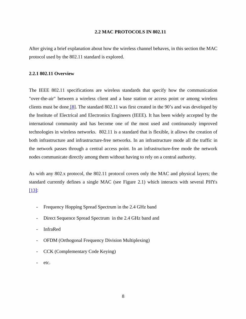
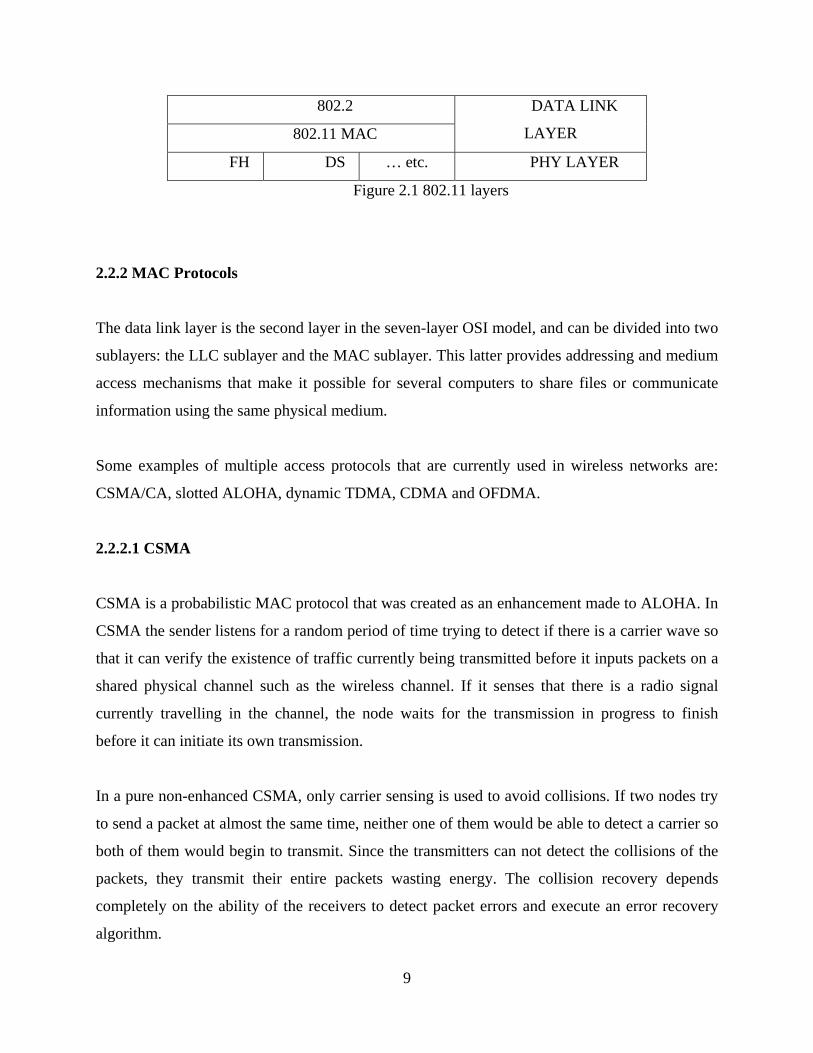
As with any 802.x protocol, the 802.11 protocol covers only the MAC and physical layers; the
standard currently defines a single MAC (see Figure 2.1) which interacts with several PHYs
[13]:
- Frequency Hopping Spread Spectrum in the 2.4 GHz band
- Direct Sequence Spread Spectrum in the 2.4 GHz band and
- InfraRed
- OFDM (Orthogonal Frequency Division Multiplexing)
- CCK (Complementary Code Keying)
- etc.
8
802.2
802.11 MAC
DATA LINK
LAYER
FH DS … etc. PHY LAYER
Figure 2.1 802.11 layers
2.2.2 MAC Protocols
The data link layer is the second layer in the seven-layer OSI model, and can be divided into two
sublayers: the LLC sublayer and the MAC sublayer. This latter provides addressing and medium
access mechanisms that make it possible for several computers to share files or communicate
information using the same physical medium.
Some examples of multiple access protocols that are currently used in wireless networks are:
CSMA/CA, slotted ALOHA, dynamic TDMA, CDMA and OFDMA.
2.2.2.1 CSMA
CSMA is a probabilistic MAC protocol that was created as an enhancement made to ALOHA. In
CSMA the sender listens for a random period of time trying to detect if there is a carrier wave so
that it can verify the existence of traffic currently being transmitted before it inputs packets on a
shared physical channel such as the wireless channel. If it senses that there is a radio signal
currently travelling in the channel, the node waits for the transmission in progress to finish
before it can initiate its own transmission.
In a pure non-enhanced CSMA, only carrier sensing is used to avoid collisions. If two nodes try
to send a packet at almost the same time, neither one of them would be able to detect a carrier so
both of them would begin to transmit. Since the transmitters can not detect the collisions of the
packets, they transmit their entire packets wasting energy. The collision recovery depends
completely on the ability of the receivers to detect packet errors and execute an error recovery
algorithm.
9

2.2.2.2 CSMA/CA
CSMA/CA is an improvement made to CSMA. This works as follows: once the transmitter
senses the channel as idle, it emits a signal letting all other nodes know that it is going to initiate
its transmission and that all other nodes have to wait, then it sends its frame. In 802.11, the
sender continues to wait for a random interval, and checks to see if the channel is still idle, if it is
still idle the node transmits and waits for an acknowledgment that indicates that the packet has
been received correctly. A back-off scheme is used to guarantee some grade of fairness among
all the nodes in the networks [10].
The use of CSMA/CA depends on the nature of the channel that is being used. CSMA/CA is
used where CSMA/CD cannot be implemented. CSMA/CD is used in copper-wired networks
and CSMA/CA is used in 802.11 based wireless LANs. The main problem of wireless LANs is
that it is not possible to listen while the transmitter is sending; therefore collision detection is not
possible. Another reason is the hidden terminal problem, where a node A, in range of the
receiver R, is not in range of the sender S, and therefore cannot know that S is transmitting to R.
A further enhancement made to CSMA/CA was made to reduce the probability of a collision,
because two transmitters cannot hear each other; the protocol defines a Virtual Carrier Sense
mechanism that works as follows:
When a node wants to transmit it first sends a Request To Send (RTS) packet. When the packet
reaches the receiver it senses the channel to make sure there is not an ongoing transmission. If it
senses the channel free it replies with a Clear To Send (CTS) packet, which includes the duration
of the transmission. Every node that listens to the RTC and CTS packets updates its local status
and backs off for the duration of the transmission [13].
10
2.3 JAMMING ATTACKS
Nowadays, wireless networks have become more affordable. As a consequence of this, they are
being deployed almost everywhere in different forms, ranging from cellular networks to sensor
and wireless local area networks. As these networks are gaining popularity, providing security
and trustworthiness is also becoming a key issue. Many architectures have been designed to
address the security problems in wireless networks [14]. So far, the proposed architectures that
solve some of the security problems in wireless networks address only the traditional services:
Authentication: by authentication it is understood that any node in the networks is who it claims
to be.
Confidentiality: a communication is confidential if and only if the information can be only seen
and understood by the sender and the intended receiver(s).
Integrity: this refers to the fact that the packet must not be modified during its travel from the
sender to the intended receiver by any intermediate malicious node.
However, wireless networks are susceptible to some other attacks that cannot be addressed by
the architectures mentioned before. One class of these attacks are the radio interference attacks,
which are also classified as a Denial of Service Attack (DoS).
Due to the wireless nature of the channel and that currently most of the network users can easily
get access to sophisticated technology the wireless medium poses no resistance against
eavesdropping or broadcasting attacks [15]. In a wireless domain it is really easy for an
adversary to sense when two legitimate wireless nodes are communicating. This implies that
launching a simple denial of service attack against a wireless networks by injecting fake
messages is really easy. A Denial of Service attack can be defined as an attack that renders the
network resources unavailable [16].
As explained in previous paragraphs, radio interference attacks cannot be defeated through
conventional security mechanisms. An adversary can simply override its medium access control
protocol (MAC) and continually send packets on the wireless channel. By doing so, it either
11

prevents users from being able to commence with legitimate MAC operations, or introduces
packet collisions causing forced and repeated backoffs [15].
2.3.1 Jammers classification
There are many different attack strategies that a jammer can perform in order to interfere with
other wireless nodes. The most accepted classification by the research community is: constant
jammers, deceptive jammers, random jammers and reactive jammers. This classification was
proposed in [13] [18].
2.3.1.1 Constant jammers: A constant jammer continuously emits a radio signal that represents
random bits; the signal generator does not follow any MAC protocol. If the signal transmitted is
strong enough to be sensed by a sender, it will always sense the medium as busy. It is
considered to be the most effective jammer because it usually drops the throughput to zero for a
long period of time until it runs out of energy. It is also considered non-energy efficient.
2.3.1.2 Deceptive jammers: Different from the continuous jammers, deceptive jammers do not
transmit random bits – instead they transmit semi-valid packets. This means that the packet
header is valid but the payload is useless. Therefore, when the legitimate nodes sense the channel
they sense that there is valid traffic currently being transmitted and they will backoff, since there
is no gap between two consecutive packets a valid node cannot transmit any packet, because it is
forced to remain in the ‘listening’ mode.
2.3.1.3 Random jammers: The two previous kinds of jammers are really efficient in terms of
denying service. They drop the throughput to zero, but they are not energy efficient. Random
jammers on the other hand are energy efficient but a little less efficient in denying service. They
alternate between two modes. In the first mode the jammer jams for a random period of time (it
can behave either like a constant jammer or a deceptive jammer), and in the second mode (the
sleeping mode) the jammer turns its transmitters off for another random period of time. The
energy efficiency is determined as the ratio of the length of the jamming period over the length
of the sleeping period.
12
2.3.1.4 Reactive jammers: Another aspect is that the three previous kinds of jammers do not
take the traffic patterns into consideration, meaning that sometimes they waste energy if they are
jamming when there is no traffic being exchanged in the network (active jamming). A reactive
jammer tries not to waste resources by only jamming when it senses that somebody is
transmitting. Its target is not the sender but the receiver, trying to input as much noise as possible
in the packet to modify as many bits as possible given that only a minimum amount of power is
required to modify enough bits so that when a checksum is performed over that packet at the
receiver it will be classified as not valid and therefore discarded [13].
2.3.2. Jamming detection
Currently there is not a dependable method to determine whether a network is being jammed or it
is only suffering from a weak connection, as [13] states: “Detecting radio interferences attacks
is challenging as it involves discriminating between legitimate and adversarial causes of poor
connectivity”.
The most accepted parameters to determine if a network is being jammed are: Packet Delivery
Ratio (PDR), signal strength and carrier sensing time.
2.3.2.1 Packet Delivery Ratio: Since the first thing that is affected by a jamming attack is the
throughput, it implies that the Packet Delivery Ratio at the receiver is low or null. Here, the
packet delivery ratio is defined as the number of packets that a node receives and classifies as
packets with a valid CRC divided by the number of all the packets received. If the PDR falls
drastically below the normal average (or a predefined threshold) then it can be said that the
network is under a jamming attack.
The most difficult part to apply this technique is the traffic characterization. In most cases the
transmission channel is not perfect; therefore the PDR is not perfect either, it is usually
13
something lower than 100%, it depends on many of the channel characteristics, such as the
distance, the transmitter’s transmission power, etc. Thus, the nature of the packet transmission
does not allow us to characterize accurately the traffic, taking into consideration that some times
there are unexpected situations, such as: network congestions, nodes failure, packet losses due to
the channel, etc. A simple threshold mechanism based on the PDR value can be used to
differentiate a jamming attack, regardless of the jamming model, from a congested network
condition [15]. Although the threshold mechanism is quite effective to differentiate jamming
from congestion it does not help to differentiate jamming from nodes failure or, in case of mobile
communications, the lost of communication with a moving node.
2.3.2.2 Signal strength: When a jammer is introduced into a network the signal strength
distribution is affected, two techniques have been proposed using the signal strength as the main
metric: 1) characterizing the average power in the signal and comparing it with a preset threshold
and 2) sampling the received signals and classifying their shape.
`
2.3.2.3 Carrier Sensing: As mentioned in section 2.3.1 constant jammers and deceptive
jammers keep the channel always busy, either with random or semi-valid traffic. This causes a
valid node, trying to send a valid packet, to repeatedly sense the channel as busy. Therefore if a
valid node determines that it has sensed the channel busy for a long period of time it can
conclude that a jamming attack is in progress. However this approach does not work for all kind
of jamming attacks, it might not be able to detect a random jammer or a reactive jammer.
As explained in this section, many metrics have been proposed to determine when a network is
being jammed, but none of them by itself can exactly detect a jamming attack, some combination
of these metrics have been proposed [15]. They increase the overall detection but they still
cannot determine if a network is being jammed with a 100% of exactitude.
14

2.4 OPNET
OPNET is a reliable application-oriented simulator that contains a set of libraries to efficiently
simulate wireless networks. Although OPNET simulation models are mostly created based on
built-in models, modifying the core of these models is not as difficult as it could sound. The
greatest requirement to be able to create simulations or modify the built-in models is to have
some intermediate programming skills in c/c++. These were two of the most important reasons to
use OPNET as the simulation tool for this thesis.
2.4.1 Radio Transceiver Pipeline
OPNET uses the Radio Transceiver Pipeline (RTP) to model wireless transmission of packets.
Whenever OPNET needs to simulate a wireless transmission it has to execute the fourteen-stage
radio transceiver pipeline. Most of these fourteen stages must be executed on a per-receiver
basis. However stage 0 is invoked only once for each pair of transmitting and receiving channels
in the network, this is done to establish a static binding between each transmitting channel and
the set of receiving channels that it is allowed to communicate with. Stage 1 is used to compute a
result that is common to all destinations, and therefore can be executed just once per
transmission. Finally each individual pipeline sequence might not be fully complete, depending
on the result of stage 2, because this stage is responsibly for determining if communication
between the transmitter and receiver is possible on a dynamic basis. Similarly, stage 3 might
classify a transmission as irrelevant with regard to its effect on a particular receiver channel,
thereby preventing the pipeline sequence from reaching the final stages [17].
The stages from 9 to 12 are invoked to evaluate the performance of the link according to changes
in the signal condition.
OPNET complements its software with a full description of each stage [17]:
15
STAGE 0: Receiver group
When the simulation process begins, the simulation kernel models the broadcast nature of the
radio by implementing multiple radio links between the transmitting channel and a set of receiver
channels. Each of the transmitters has to keep an updated list of all the possible candidates for
receiving a transmission from that transmitter. The simulation kernel checks every possible
transmitter-receiver channel pair, and creates a receiver group for each transmitter channel.
However, since the transceiver characteristics can continually change during the simulation
process, it is very difficult to keep the list in an updated state. What the kernel does to solve this
problem is to include all the nodes that can possibly become receivers at any point of time during
the simulation, future stages will help to discard some of the nodes, based on situations such as:
- Disjoint frequency bands: these are defined based on its base frequency and its
bandwidth. If the transmitter and receiver frequencies do not overlap then the receiver
transmission cannot affect the receiver’s channel.
- Physical separation: Physical separation is an important issue in wireless communication
and depends upon the path loss model as explained in section 2.1
- Antenna nulls: this applies when the model is using directional antennae.
This stage is really important because although including all the possible receivers for all
possible transmitters guarantees a more accurate simulation it also increases the time to finish the
simulation, causing slower simulations.
STAGE 1: Transmission delay
This stage must be executed on a dynamic basis, being re-started each time a new transmission
takes place. It is invoked immediately after the beginning transmission of a packet. The
calculations depend on the channel data rate and the length of the packet. The packet’s length is
divided by the data rate to obtain the transmission delay.
16
In this stage the amount of time required for the entire packet to complete transmission is
calculated. The value of this calculation is the result of the difference between the beginning of
transmission of the first bit and the end of transmission of the last bit of the packet. The obtained
result is used to schedule the end-of-transmission event at the kernel level. When this event
occurs the kernel can either start the transmission of the next packet in the system queue or start
an idle state if there is none. The transmission delay is used in conjunction with the result of the
transmission delay to calculate the time at which the packet will be received at its destination
(the time at which the last bit finishes arriving at the destination).
STAGE 2: Closure
This stage is invoked once for each receiver channel present in the transmitting channel’s
destination channel set. This stage was created to determine whether a particular receiver can be
affected by a transmission. Closure is defined as the ability of a transmission to reach the
receiver’s channel.
This stage is based on whether the signal can physically attain the candidate’s receiver channel
and affect it in any way. Therefore this stage is particularly important for jamming attacks. Other
factors affecting this stage are the obstruction of the signal (occlusion) by obstacles and/or the
surface of earth.
The computation of the closure is done based on a ray-tracing line of sight model. This algorithm
tests the line segment joining the transmitter and receiver for intersections with the earth’s
surface. If there an intersection exists, the receiver cannot be reached and the remaining of the
stages are not performed. This algorithm does not take into consideration the wave-bending
effect.
17
STAGE 3: Channel Match
This stage was created to classify the transmission with respect to the receiver channel. Three
possible classifications are defined:
- Valid: this classification is for the packets that are considered compatible with the
receiver channel and will possibly be accepted and processed by the receiving node.
- Noise: packets in this category are considered non-compatible with the receiver channel,
but have an impact on the receiver channel’s performance by generating interference.
- Ignored: if the packet is both non compatible with the receiver’s channel and does not
affect it in any way then it falls in this classification.
The characteristics analyzed by the module are: frequency, bandwidth, data rate, spreading code
and modulation.
STAGE 4: Transmitter Antenna Gain
The purposes of this stage us to calculate the gain provided by the transmitter’s antenna. This is
done based on the direction of the vector leading from the transmitter to the receiver.
The concept of antenna gain is understood as the phenomenon of magnification or reduction of
the transmitted signal energy, this phenomenon depends on the direction of the signal path. The
received energy depends also on the physical structure characteristics of the antenna and possible
phase manipulations of the signal. Isotropic antennas do not provide any gain because they have
a perfectly symmetric behavior with respect to all possible signal paths.
STAGE 5: Propagation Delay
The propagation delay is defined as the amount of time required for the packet’s signal to travel
from the radio transmitter to the radio receiver; this mainly depends on the distance between the
18

sender and receiver. Since the channel is pre-specified as the wireless medium the default speed
of the signal is the speed of light. Sometimes the distance of propagation can vary during the
packet transmission due to possible mobility of nodes; therefore some times the kernel has to
calculate two delays one at the beginning of the transmission of the packet and another at the end
of the transmission of the packet.
STAGE 6: Receiver Antenna Gain
The purposes of this stage us to calculate the gain provided by the receiver’s antenna. This is
done based on the direction of the vector leading from the transmitter to the receiver. The
concept of antenna gain is identical to that of the transmitter’s antenna gain.
STAGE 7: Receiver Power
This stage is aimed to calculate the received power of the arriving packet’s signal in watts. This
calculation depends on the distance separating receiver and transmitter, the power of the
transmitter, the transmission frequency, and transmitter and receiver antenna gains.
OPNET uses formula 2-1 to calculate the free space propagation loss.
As the final stage of the computation of the receiver carrier power, the transmitter and receiver
antenna gains are extracted from previous stages. Since the antennas gain are given in decibels
they must be converted to a non-logarithmic form and then they are multiplied with the other
variables of the link budget (transmission power, transmitter antenna gain, receiver antenna gain
and path loss).
STAGE 8: Interference Noise
This stage is only executed for a packet under one two possible circumstances:
19
- The packet is classified as valid by the stage 3 and arrives at the destination channel
while another packet is being received.
- The packet is classified as valid by stage 3 and starts being received by the destination
channel when another packet arrives.
The objective of this stage is to keep a record of the transmissions that arrive at the same time to
the same receiver channel. The kernel reserves a Transmission Data Attribute (DTA), whose
value is increased each time a valid packet arrives to the receiver interfering with another packet.
Once the packet completes reception the kernel subtracts its receiver power from the noise
accumulator of all valid packets that are still arriving at the channel.
STAGE 9: Background Noise
This stage calculates all other sources of noise that are not related to the interference noise. Other
sources are: thermal or galactic noise, emissions from neighboring electronics and radio
transmissions that are not modeled.
Background noise is characterized by an effective background temperature which is added to the
effective device temperature of a receiver. The noise figure of the receiver is obtained to
calculate the effective device temperature, assuming an operating temperature of 290K. The sum
of these temperatures, each representing a separate source of noise, is multiplied by the
bandwidth of the receiver channel and Boltzmann’s constant to obtain the added noise
contributed by the receiver to the processed signal.
The ambient noise power spectral density models sources of noise such as the urban noise in the
frequency band of interest. Both the ambient noise and the added noise are added to model the
overall effect o the modeled noise sources.
20
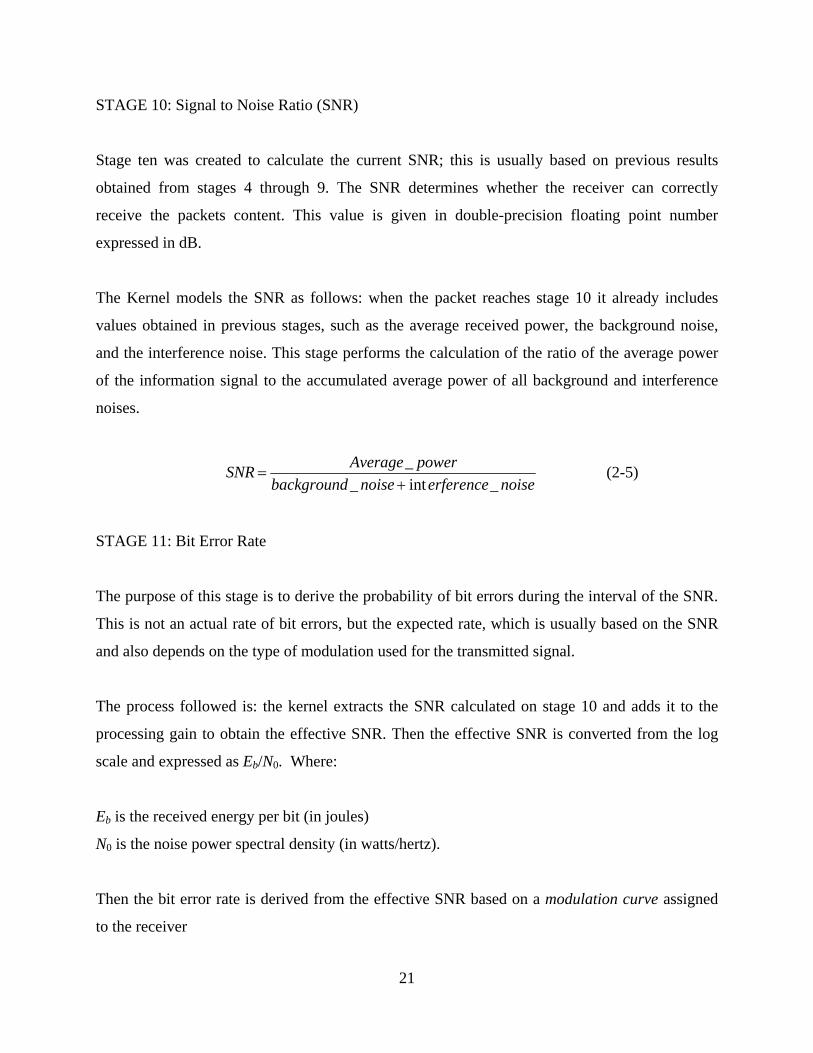
STAGE 10: Signal to Noise Ratio (SNR)
Stage ten was created to calculate the current SNR; this is usually based on previous results
obtained from stages 4 through 9. The SNR determines whether the receiver can correctly
receive the packets content. This value is given in double-precision floating point number
expressed in dB.
The Kernel models the SNR as follows: when the packet reaches stage 10 it already includes
values obtained in previous stages, such as the average received power, the background noise,
and the interference noise. This stage performs the calculation of the ratio of the average power
of the information signal to the accumulated average power of all background and interference
noises.
SNR =Average_ power
background _ noise+ interference_ noise (2-5)
STAGE 11: Bit Error Rate
The purpose of this stage is to derive the probability of bit errors during the interval of the SNR.
This is not an actual rate of bit errors, but the expected rate, which is usually based on the SNR
and also depends on the type of modulation used for the transmitted signal.
The process followed is: the kernel extracts the SNR calculated on stage 10 and adds it to the
processing gain to obtain the effective SNR. Then the effective SNR is converted from the log
scale and expressed as Eb/N0. Where:
Eb is the received energy per bit (in joules)
N0 is the noise power spectral density (in watts/hertz).
Then the bit error rate is derived from the effective SNR based on a modulation curve assigned
to the receiver
21

STAGE 12: Error Allocation
This part of the process estimates the number of bit errors in a packet segment where the bit error
rate probability has been calculated. This process also calculates the actual Bit Error Rate
obtained by dividing the number of errors in the segment by the size of the segment.
STAGE 13: Error correction
This is the final stage of the RTP, its purpose is to determine if a packet can be accepted and
processed correctly by the receiving node. This stage is based on the ability of the receiving node
to correct the errors detected on stage 12, if it is possible for it to correct all the errors it will
forward the packet to the corresponding output stream, if it is not able to correct the errors the
packet is destroyed.
22
3.0 EXPERIMENT DESIGN
In chapter 3 the way the experiment was designed is explained. It starts by stating the problem
addressed in this thesis, including the variables that are manipulated and the ones that are
collected to measure the effects of a jamming attack. Later in the chapter the layouts for each of
the scenarios is shown including a description of each of them.
3.1 PROBLEM DEFINITION
The purpose of this thesis is to study the effects of jamming attacks on the throughput, the
received power and the bit error rate probability in an 802.11 based wireless network by using as
input variables the jammer’s transmission power, the packet interarrival time at the jammer and
the distance between jammers and nodes, all of this using OPNET as the simulation tool.
3.2 DATA ACQUISITION / MODEL SPECIFICATION
For this study the input variables are: jammer’s transmission power, jammer’s packet interarrival
rate and the distance between the jammer and the nodes.
The jammer’s transmission power will be considered in 3 discrete values [0.032W, 0.066W,
0.1W]. 0.032 W is the most common transmission power used in current 802.11g access points;
and while 0.066 W is not widely used, it is the middle point between the most used transmission
power and the maximum transmission power allowed; and 0.1 W is the maximum power
accepted by the IEEE standards for a WLAN.
Packet interarrival times will also be considered in 3 discrete continuous values: [0.01sec, 0.05
sec, 0.1 sec]
23
In the first scenario the distance between the jammer and the receiver will constantly vary due to
the use of a mobile jammer inside the scenario. In the remainder of the scenarios the distance
will be fixed.
The outcomes for the first scenario will be plots of the energy received, the throughput and the
bit error rate probability versus time. For the second and third scenarios the outcomes will be
plots of the throughput, the time the access point’s transmitting circuits are busy and the time the
access point’s listening circuits are busy. For scenario four the outcomes are plots of the
throughput in nodes that are within and outside the jammer’s transmission range. Finally for
scenario five, the outcome is a graph that compares the cumulative throughput in the network
when no misbehaving node is present and when it is.
3.2.1 Scenario 1
Scenario 1 simulates the simplest of the jamming attacks. This attack consists of a single
transmitter (tx) sending valid traffic to a receiver (rx), both of them without any MAC protocol,
and a single jammer that is constantly emitting random non-valid packets, trying to cause
collision with valid packets to increase the probability of errors in them.
The simulation setup is as follows:
The scenario has a size of 75 × 75 meters, which is the average coverage provided by an AP
using the standard 802.11g [10]. The green line in Figure 3.1 shows the trajectory followed by
the mobile jammer.
24
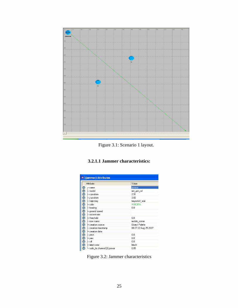
Figure 3.1: Scenario 1 layout.
3.2.1.1 Jammer characteristics:
Figure 3.2: Jammer characteristics
25

Figure 3.2 shows the jammer’s characteristics, it is created using the mrt_jam_ref model. This
mobile jammer will follow the trajectory specified by ‘trayecto1_real’ (green line in Figure 3.1),
and with a transmission power of 0.05 W.
Figure 3.3 shows that the inner structure of this jammer consists of three inner modules: the first
one is a traffic generator that is connected to a radio modulator that is connected to an antenna.
Figure 3.3 Jammer inner modules
In Figure 3.4 it is shown that the jammer sends jamming packets with a constant length of 1024
bits at a constant rate of 1 packet per second. When those packets arrive at the wireless
modulator they are converted into a suitable form to be transmitted by the antenna at a rate of
1024 bps with a power of 0.05 watts. The wireless modulator also specifies that the modulation
scheme is ‘jammod’ and all the processes that will apply to that packet. In this thesis the default
RTP stages will be used (RTP stages are described in section 2.4).
Traffic generator
characteristics
Radio modulator
characteristics
Antenna
characteristics
Figure 3.4 Characteristics of the jammer modules
26
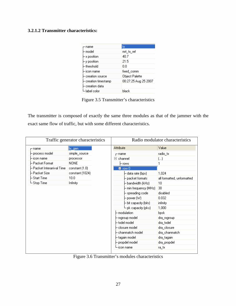
3.2.1.2 Transmitter characteristics:
Figure 3.5 Transmitter’s characteristics
The transmitter is composed of exactly the same three modules as that of the jammer with the
exact same flow of traffic, but with some different characteristics.
Traffic generator characteristics Radio modulator characteristics
Figure 3.6 Transmitter’s modules characteristics
27
The transmitter is created using the ‘simple_source’ module included in OPNET’s libraries. The
traffic source creates packets with an interarrival time of 1 packet per second and a constant
length of 1024 bits. The radio modulator uses the ‘bpsk’ modulation scheme to modulate the
signal (bpsk stands for Binary Phase Shift Keying). Only traffic with this kind of modulation will
be considered as valid traffic.
Within the jammer OPNET uses a special module called simple_jammer_source, which
generates packets with random bits and uses the simple_source module to generate valid traffic.
Also, at the jammer side, OPNET uses a special kind of modulation technique called ‘jammod’
that causes OPNET to interpret all traffic with this kind of modulation as interference.
The antenna has exactly the same characteristics as the one used in the jammer.
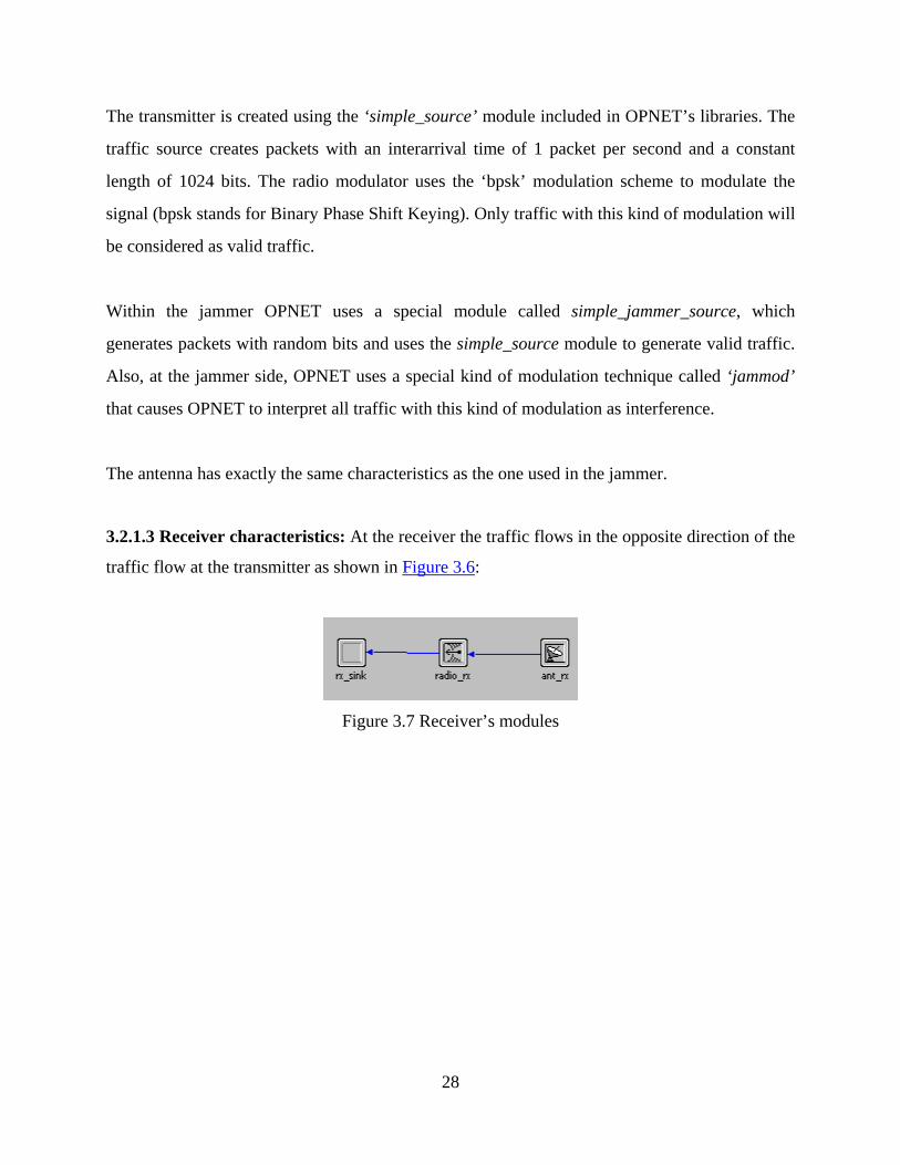
3.2.1.3 Receiver characteristics: At the receiver the traffic flows in the opposite direction of the
traffic flow at the transmitter as shown in Figure 3.6:
Figure 3.7 Receiver’s modules
28
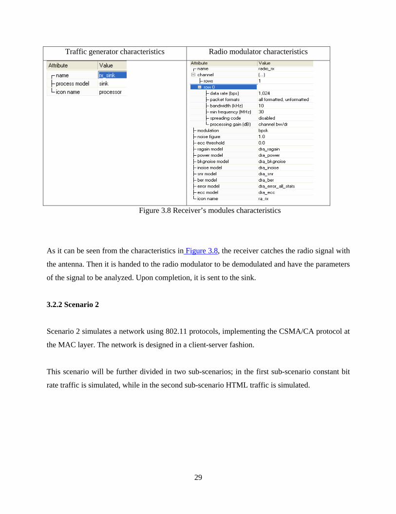
Traffic generator characteristics Radio modulator characteristics
Figure 3.8 Receiver’s modules characteristics
As it can be seen from the characteristics in Figure 3.8, the receiver catches the radio signal with
the antenna. Then it is handed to the radio modulator to be demodulated and have the parameters
of the signal to be analyzed. Upon completion, it is sent to the sink.
3.2.2 Scenario 2
Scenario 2 simulates a network using 802.11 protocols, implementing the CSMA/CA protocol at
the MAC layer. The network is designed in a client-server fashion.
This scenario will be further divided in two sub-scenarios; in the first sub-scenario constant bit
rate traffic is simulated, while in the second sub-scenario HTML traffic is simulated.
29
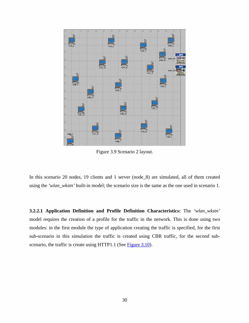
Figure 3.9 Scenario 2 layout.
In this scenario 20 nodes, 19 clients and 1 server (node_8) are simulated, all of them created
using the ‘wlan_wkstn’ built-in model; the scenario size is the same as the one used in scenario 1.
3.2.2.1 Application Definition and Profile Definition Characteristics: The ‘wlan_wkstn’
model requires the creation of a profile for the traffic in the network. This is done using two
modules: in the first module the type of application creating the traffic is specified, for the first
sub-scenario in this simulation the traffic is created using CBR traffic, for the second sub-
scenario, the traffic is create using HTTP1.1 (See Figure 3.10).
30
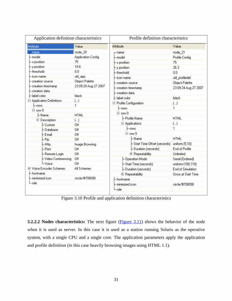
Application definition characteristics Profile definition characteristics
Figure 3.10 Profile and application definition characteristics
3.2.2.2 Nodes characteristics: The next figure (Figure 3.11) shows the behavior of the node
when it is used as server. In this case it is used as a station running Solaris as the operative
system, with a single CPU and a single core. The application parameters apply the application
and profile definition (in this case heavily browsing images using HTML 1.1).
31
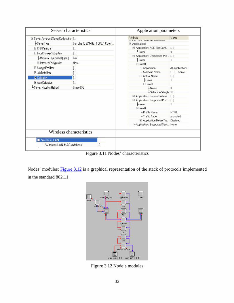
Server characteristics Application parameters
Wireless characteristics
Figure 3.11 Nodes’ characteristics
Nodes’ modules: Figure 3.12 is a graphical representation of the stack of protocols implemented
in the standard 802.11.
Figure 3.12 Node’s modules
32
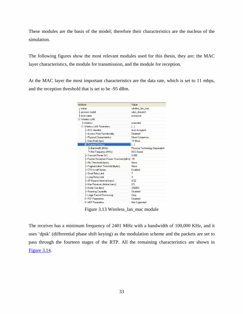
These modules are the basis of the model; therefore their characteristics are the nucleus of the
simulation.
The following figures show the most relevant modules used for this thesis, they are: the MAC
layer characteristics, the module for transmission, and the module for reception.
At the MAC layer the most important characteristics are the data rate, which is set to 11 mbps,
and the reception threshold that is set to be -95 dBm.
Figure 3.13 Wireless_lan_mac module
The receiver has a minimum frequency of 2401 MHz with a bandwidth of 100,000 KHz, and it
uses ‘dpsk’ (differential phase shift keying) as the modulation scheme and the packets are set to
pass through the fourteen stages of the RTP. All the remaining characteristics are shown in
Figure 3.14.
33
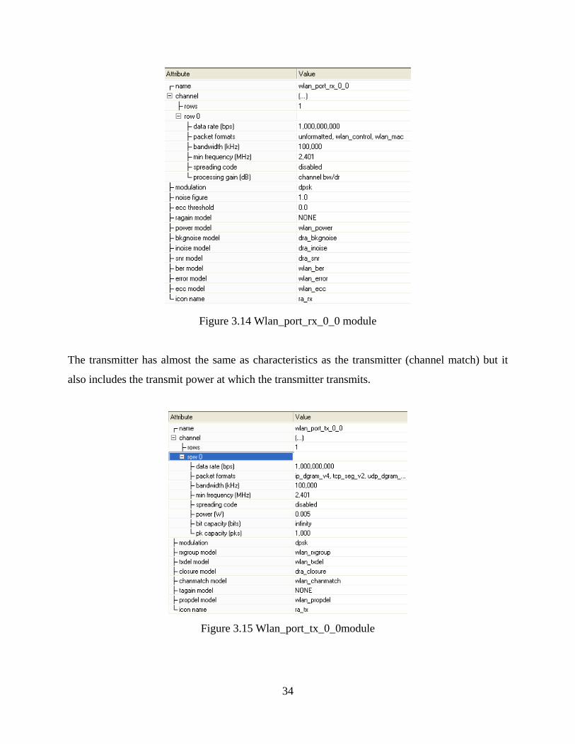
Figure 3.14 Wlan_port_rx_0_0 module
The transmitter has almost the same as characteristics as the transmitter (channel match) but it
also includes the transmit power at which the transmitter transmits.
Figure 3.15 Wlan_port_tx_0_0module
34
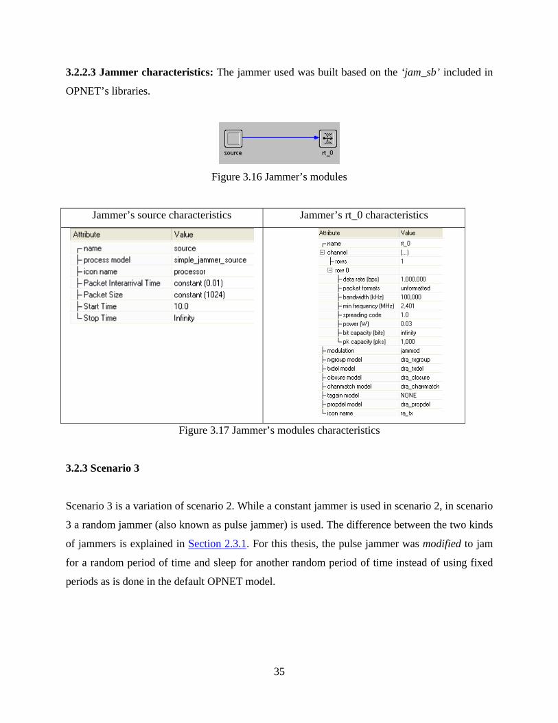
3.2.2.3 Jammer characteristics: The jammer used was built based on the ‘jam_sb’ included in
OPNET’s libraries.
Figure 3.16 Jammer’s modules
Jammer’s source characteristics Jammer’s rt_0 characteristics
Figure 3.17 Jammer’s modules characteristics
3.2.3 Scenario 3
Scenario 3 is a variation of scenario 2. While a constant jammer is used in scenario 2, in scenario
3 a random jammer (also known as pulse jammer) is used. The difference between the two kinds
of jammers is explained in Section 2.3.1. For this thesis, the pulse jammer was modified to jam
for a random period of time and sleep for another random period of time instead of using fixed
periods as is done in the default OPNET model.
35
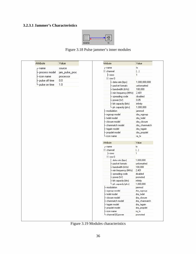
3.2.3.1 Jammer’s Characteristics
Figure 3.18 Pulse jammer’s inner modules
Figure 3.19 Modules characteristics
36
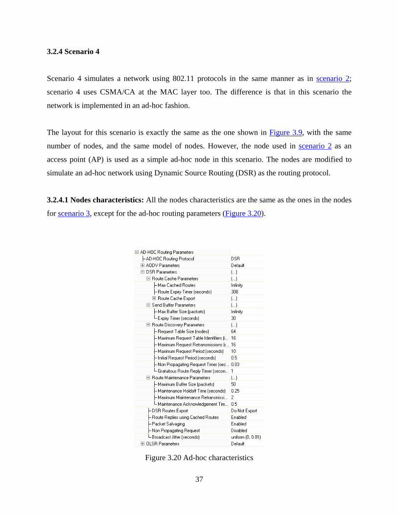
3.2.4 Scenario 4
Scenario 4 simulates a network using 802.11 protocols in the same manner as in scenario 2;
scenario 4 uses CSMA/CA at the MAC layer too. The difference is that in this scenario the
network is implemented in an ad-hoc fashion.
The layout for this scenario is exactly the same as the one shown in Figure 3.9, with the same
number of nodes, and the same model of nodes. However, the node used in scenario 2 as an
access point (AP) is used as a simple ad-hoc node in this scenario. The nodes are modified to
simulate an ad-hoc network using Dynamic Source Routing (DSR) as the routing protocol.
3.2.4.1 Nodes characteristics: All the nodes characteristics are the same as the ones in the nodes
for scenario 3, except for the ad-hoc routing parameters (Figure 3.20).
Figure 3.20 Ad-hoc characteristics
37
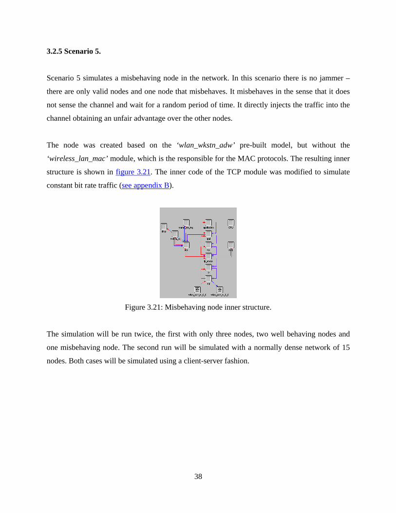
3.2.5 Scenario 5.
Scenario 5 simulates a misbehaving node in the network. In this scenario there is no jammer –
there are only valid nodes and one node that misbehaves. It misbehaves in the sense that it does
not sense the channel and wait for a random period of time. It directly injects the traffic into the
channel obtaining an unfair advantage over the other nodes.
The node was created based on the ‘wlan_wkstn_adw’ pre-built model, but without the
‘wireless_lan_mac’ module, which is the responsible for the MAC protocols. The resulting inner
structure is shown in figure 3.21. The inner code of the TCP module was modified to simulate
constant bit rate traffic (see appendix B).
Figure 3.21: Misbehaving node inner structure.
The simulation will be run twice, the first with only three nodes, two well behaving nodes and
one misbehaving node. The second run will be simulated with a normally dense network of 15
nodes. Both cases will be simulated using a client-server fashion.
38
4.0 SIMULATIONS ANALYSIS
Chapter four analyzes the results obtained from each of the scenarios described in the previous
chapter. The simulation results are shown in plots, each of them accompanied by a detailed
explanation.
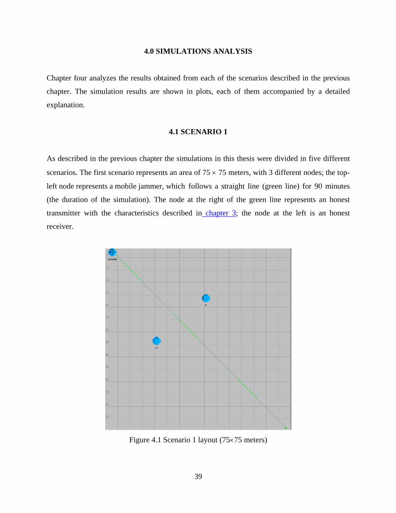
4.1 SCENARIO 1
As described in the previous chapter the simulations in this thesis were divided in five different
scenarios. The first scenario represents an area of 75 × 75 meters, with 3 different nodes; the top-
left node represents a mobile jammer, which follows a straight line (green line) for 90 minutes
(the duration of the simulation). The node at the right of the green line represents an honest
transmitter with the characteristics described in chapter 3; the node at the left is an honest
receiver.
Figure 4.1 Scenario 1 layout (75×75 meters)
39
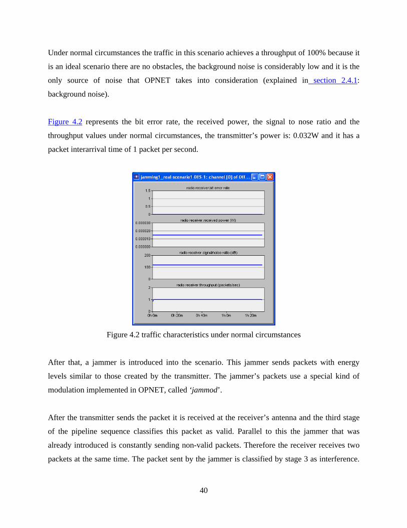
Under normal circumstances the traffic in this scenario achieves a throughput of 100% because it
is an ideal scenario there are no obstacles, the background noise is considerably low and it is the
only source of noise that OPNET takes into consideration (explained in section 2.4.1:
background noise).
Figure 4.2 represents the bit error rate, the received power, the signal to nose ratio and the
throughput values under normal circumstances, the transmitter’s power is: 0.032W and it has a
packet interarrival time of 1 packet per second.
Figure 4.2 traffic characteristics under normal circumstances
After that, a jammer is introduced into the scenario. This jammer sends packets with energy
levels similar to those created by the transmitter. The jammer’s packets use a special kind of
modulation implemented in OPNET, called ‘jammod’.
After the transmitter sends the packet it is received at the receiver’s antenna and the third stage
of the pipeline sequence classifies this packet as valid. Parallel to this the jammer that was
already introduced is constantly sending non-valid packets. Therefore the receiver receives two
packets at the same time. The packet sent by the jammer is classified by stage 3 as interference.
40

Then Stage eight keeps a record of the transmissions that arrived at the same time at the same
receiver channel.
When a packet A arrives to the receiver’s antenna at the same time than a packet B, stage 8
classifies packet A as noise for packet B and vice versa. In addition, the kernel reserves a
Transmission Data Attribute (DTA), whose value is increased each time a valid packet arrives to
the receiver interfering with another packet. Also the
Next figure (Figure 4.3) shows what happens when a jammer with a transmission power of
0.032W is inserted in the scenario. The transmitter keeps its transmission power of 0.032W and
uses ‘bpsk’ as the modulation scheme.
Figure 4.3 Traffic characteristics under a jamming attack.
As it can be observed from the graph (Figure 4.3), when the jammer is inserted in the scenario,
the bit error rate probability goes considerably up, reaching almost up to 4% of probability of
error per bit. Although this probability does not seem to be high enough to cause an error in each
bit the second plot titled ‘bit errors per packet’ demonstrates that in some cases more than 50 bits
41
are corrupted. It should also be recalled that sometimes only a couple of bits need to be modified
to cause the whole packet to be discarded. The bit error rate in OPNET is not simulated – it is
calculated from a table included in OPNET’s core (this table can be also found in [17].) The
third plot shows that the power at the receiver is also increased when the jammer is introduced,
but the SNR decreases considerably increasing the probability of errors in the packets; errors that
the receiver cannot correct which leads to a throughput of zero for around 30 minutes, until the
jammer is away from the sender and receiver and they can resume normal operations.
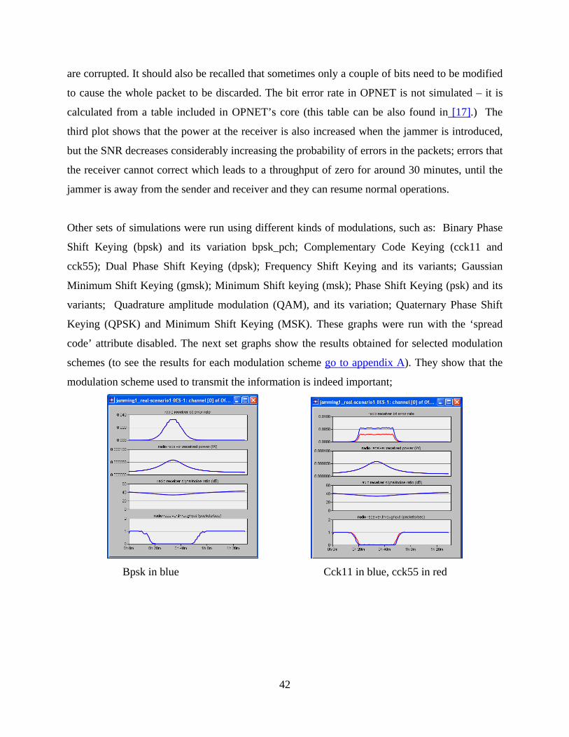
Other sets of simulations were run using different kinds of modulations, such as: Binary Phase
Shift Keying (bpsk) and its variation bpsk_pch; Complementary Code Keying (cck11 and
cck55); Dual Phase Shift Keying (dpsk); Frequency Shift Keying and its variants; Gaussian
Minimum Shift Keying (gmsk); Minimum Shift keying (msk); Phase Shift Keying (psk) and its
variants; Quadrature amplitude modulation (QAM), and its variation; Quaternary Phase Shift
Keying (QPSK) and Minimum Shift Keying (MSK). These graphs were run with the ‘spread
code’ attribute disabled. The next set graphs show the results obtained for selected modulation
schemes (to see the results for each modulation scheme go to appendix A). They show that the
modulation scheme used to transmit the information is indeed important;
Bpsk in blue Cck11 in blue, cck55 in red
42
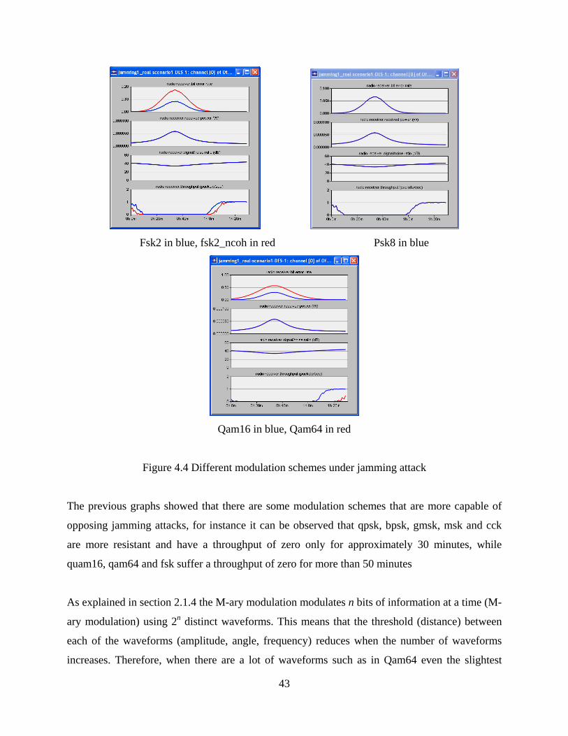
Fsk2 in blue, fsk2_ncoh in red Psk8 in blue
Qam16 in blue, Qam64 in red
Figure 4.4 Different modulation schemes under jamming attack
The previous graphs showed that there are some modulation schemes that are more capable of
opposing jamming attacks, for instance it can be observed that qpsk, bpsk, gmsk, msk and cck
are more resistant and have a throughput of zero only for approximately 30 minutes, while
quam16, qam64 and fsk suffer a throughput of zero for more than 50 minutes
As explained in section 2.1.4 the M-ary modulation modulates n bits of information at a time (M-
ary modulation) using 2n distinct waveforms. This means that the threshold (distance) between
each of the waveforms (amplitude, angle, frequency) reduces when the number of waveforms
increases. Therefore, when there are a lot of waveforms such as in Qam64 even the slightest
43

variation in the channel’s background noise causes a lot of bit errors, this is the main reason why
Qam 64 performs worse against a jamming attack. In the case of qpsk, bpsk, gmsk, msk and cck,
that use a very small number of waveforms to transmit data, the threshold (distance) between
each of those signals is bigger consequently they are more tolerant to the variation of the
background noise caused by the jammers.
If the spread code is enabled there is no difference in the results.
One of the most important input variables that must be taken into consideration is the power that
the jammer uses, for the next figure the power of the jammer was increased to 0.1 W
Figure 4.5 increasing the power at the jammer to 0.1 W.
Figure 4.5 shows that the probability of bit error rate increases to an unacceptable level of almost
10%, causing a little more than 100 bits per packet to be in error; the received power at the
receiver also was increased considerably; although the graphs now show much variation the
resulting throughput shows that that little variation has a great impact, the throughput is affected
for 1 hour and 10 minutes.
44

4.2 SCENARIO 2
In this scenario the focus is set on the communication between two nodes in a client-server
fashion. This scenario is divided in two parts, the first is simulated using a constant bit rate, and
the second one is simulated using the HTTP protocol under heavy web page browsing.
For both scenarios, the attacker first waits for 10 seconds to let the AP to reach a steady state,
and then it turns its radio jammer transmitter and starts sending out packets with valid but useless
packets. When a node has some traffic to send it senses the medium to avoid collisions but since
the jammer already started transmitting it will feel sensing the medium busy and it will be forced
to back off until the jammers ceases its jamming activity.
The most important input variables are: jammer’s interarrival rate, the jammer’s transmission
power and the distance between the jammer and the AP.
The output variables that must be observed are:
Throughput at the AP: since in this scenario there is only one AP in the network, all the traffic
must pass through it.
Transmitter’s busy time: it is the time a node spends transmitting its data.
Receiver’s listening time: this is the time a node spends listening to me medium waiting to access
it and transmit its data.
The first scenario consists of 19 hosts that are randomly distributed and 1 access point (AP)
located in the middle of the scenario; this scenario was designed so that each node is in the AP’s
transmission range.
45
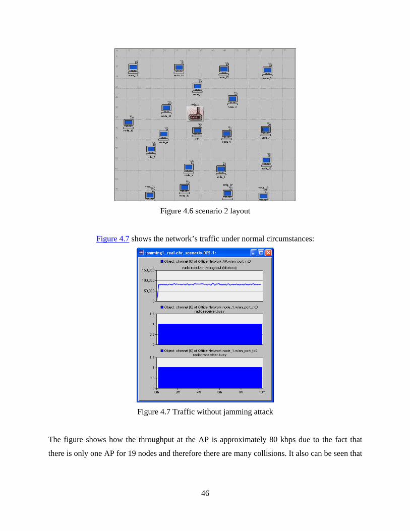
Figure 4.6 scenario 2 layout
Figure 4.7 shows the network’s traffic under normal circumstances:
Figure 4.7 Traffic without jamming attack
The figure shows how the throughput at the AP is approximately 80 kbps due to the fact that
there is only one AP for 19 nodes and therefore there are many collisions. It also can be seen that
46
the receiver is always busy, and the transmitter is always busy, which mean it is receiving and
sending traffic.
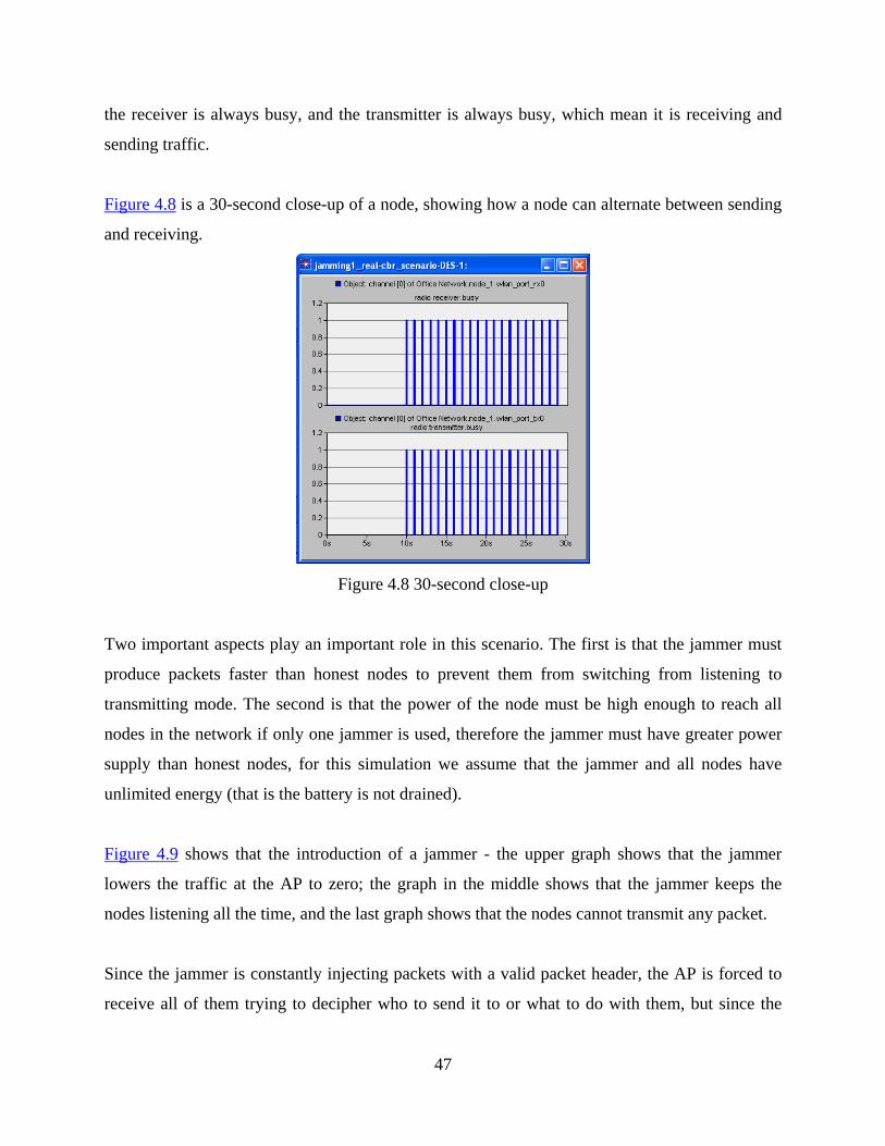
Figure 4.8 is a 30-second close-up of a node, showing how a node can alternate between sending
and receiving.
Figure 4.8 30-second close-up
Two important aspects play an important role in this scenario. The first is that the jammer must
produce packets faster than honest nodes to prevent them from switching from listening to
transmitting mode. The second is that the power of the node must be high enough to reach all
nodes in the network if only one jammer is used, therefore the jammer must have greater power
supply than honest nodes, for this simulation we assume that the jammer and all nodes have
unlimited energy (that is the battery is not drained).
Figure 4.9 shows that the introduction of a jammer - the upper graph shows that the jammer
lowers the traffic at the AP to zero; the graph in the middle shows that the jammer keeps the
nodes listening all the time, and the last graph shows that the nodes cannot transmit any packet.
Since the jammer is constantly injecting packets with a valid packet header, the AP is forced to
receive all of them trying to decipher who to send it to or what to do with them, but since the
47

packets are useless the AP drops them. This is why the AP is kept in the listening mode all the
time.
Figure 4.9 traffic when a jammer is introduced
A 30-second close-up was captured to show that the receiver is always active sensing the
channel, it is busy all the time, and therefore it cannot switch to a transmitting mode.
Figure 4.10 30-second close-up when the jammer is introduced
48

Another set of simulations was run, but instead of simulating traffic with a CBR the application
and profile definitions were changed to a heavy-web-browsing scenario, with an exponential
distribution instead of a constant distribution.
It was decided to use this sub-scenario because in real-world applications, the traffic is almost
never constant. Therefore HTTP traffic was thought to be a good example of a real world traffic
generator.
Figure 4.11 shows the traffic characterization before and after jamming. In the left graph it can
be seen that there is traffic with an exponential distribution and that both the transmitter and the
receiver are constantly busy; on the other hand, in the graph on the right, we can see that despite
the fact that the receiver is always busy, there is no throughput in the node.
Figure 4.11 before and after the jammer is introduced
Figure 4.11 shows the 30-second close-up, and it can be observed that the receiver has no time to
switch from the listening mode to the transmitter mode.
49

Figure 4.12 30-second close-up
4.3 SCENARIO 3
All the previous scenarios were focused on analyzing the effects of constant and deceptive
jammers in a client-server network. This scenario focuses on analyzing the effects of a random
jammer in the client-server network.
The layout is the same used for the network on scenario 1; all the nodes have the same
characteristics than those on scenario 2. The only difference is that in this scenario, the jammer,
instead of constantly injecting packets into the network, only sends packets for a random period
of time, and then goes to sleep for another random period of time. This kind of jamming is
considered an energy efficient jamming attack.
The goal of this kind of jammer is not drop the throughput to zero, but to reduce the throughput
considerably for a longer period of time.
50
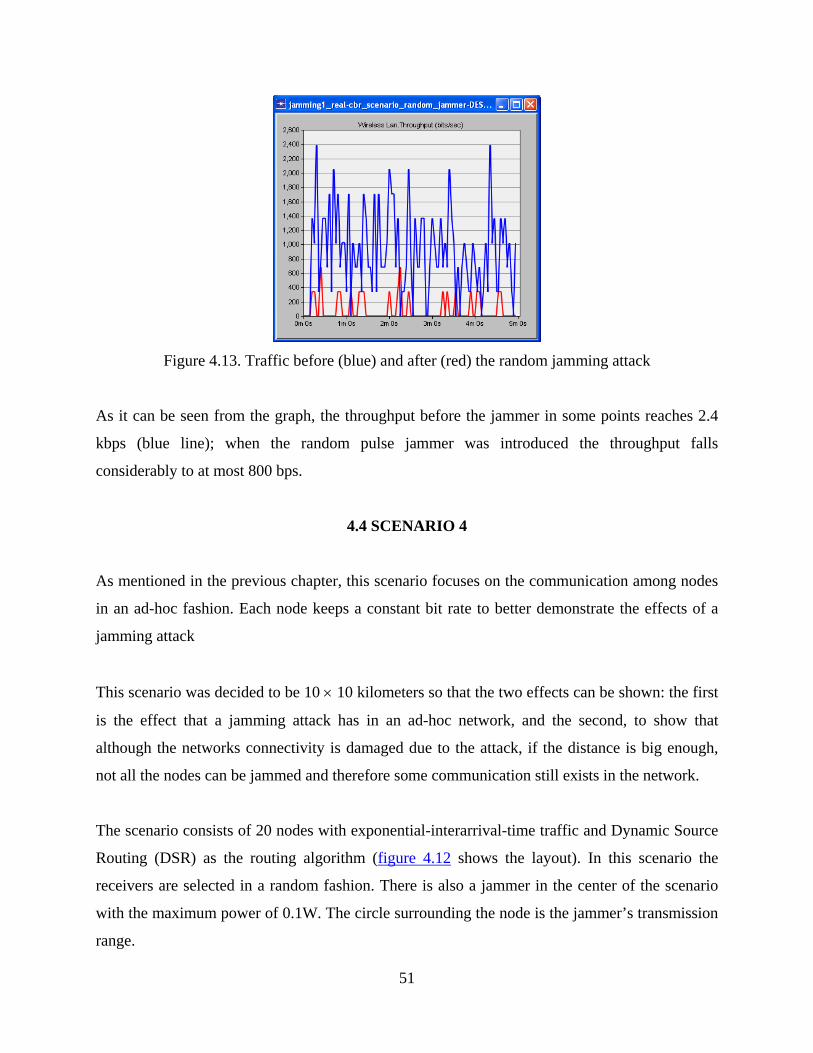
Figure 4.13. Traffic before (blue) and after (red) the random jamming attack
As it can be seen from the graph, the throughput before the jammer in some points reaches 2.4
kbps (blue line); when the random pulse jammer was introduced the throughput falls
considerably to at most 800 bps.
4.4 SCENARIO 4
As mentioned in the previous chapter, this scenario focuses on the communication among nodes
in an ad-hoc fashion. Each node keeps a constant bit rate to better demonstrate the effects of a
jamming attack
This scenario was decided to be 10 × 10 kilometers so that the two effects can be shown: the first
is the effect that a jamming attack has in an ad-hoc network, and the second, to show that
although the networks connectivity is damaged due to the attack, if the distance is big enough,
not all the nodes can be jammed and therefore some communication still exists in the network.
The scenario consists of 20 nodes with exponential-interarrival-time traffic and Dynamic Source
Routing (DSR) as the routing algorithm (figure 4.12 shows the layout). In this scenario the
receivers are selected in a random fashion. There is also a jammer in the center of the scenario
with the maximum power of 0.1W. The circle surrounding the node is the jammer’s transmission
range.
51
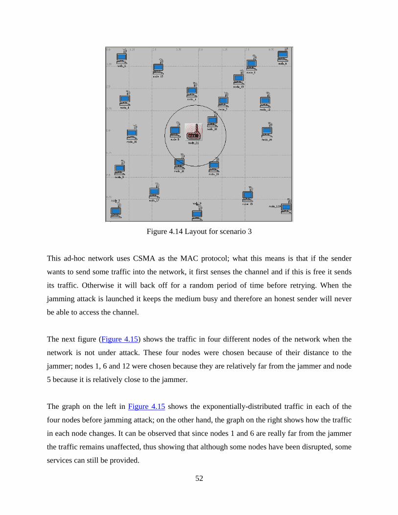
Figure 4.14 Layout for scenario 3
This ad-hoc network uses CSMA as the MAC protocol; what this means is that if the sender
wants to send some traffic into the network, it first senses the channel and if this is free it sends
its traffic. Otherwise it will back off for a random period of time before retrying. When the
jamming attack is launched it keeps the medium busy and therefore an honest sender will never
be able to access the channel.
The next figure (Figure 4.15) shows the traffic in four different nodes of the network when the
network is not under attack. These four nodes were chosen because of their distance to the
jammer; nodes 1, 6 and 12 were chosen because they are relatively far from the jammer and node
5 because it is relatively close to the jammer.
The graph on the left in Figure 4.15 shows the exponentially-distributed traffic in each of the
four nodes before jamming attack; on the other hand, the graph on the right shows how the traffic
in each node changes. It can be observed that since nodes 1 and 6 are really far from the jammer
the traffic remains unaffected, thus showing that although some nodes have been disrupted, some
services can still be provided.
52
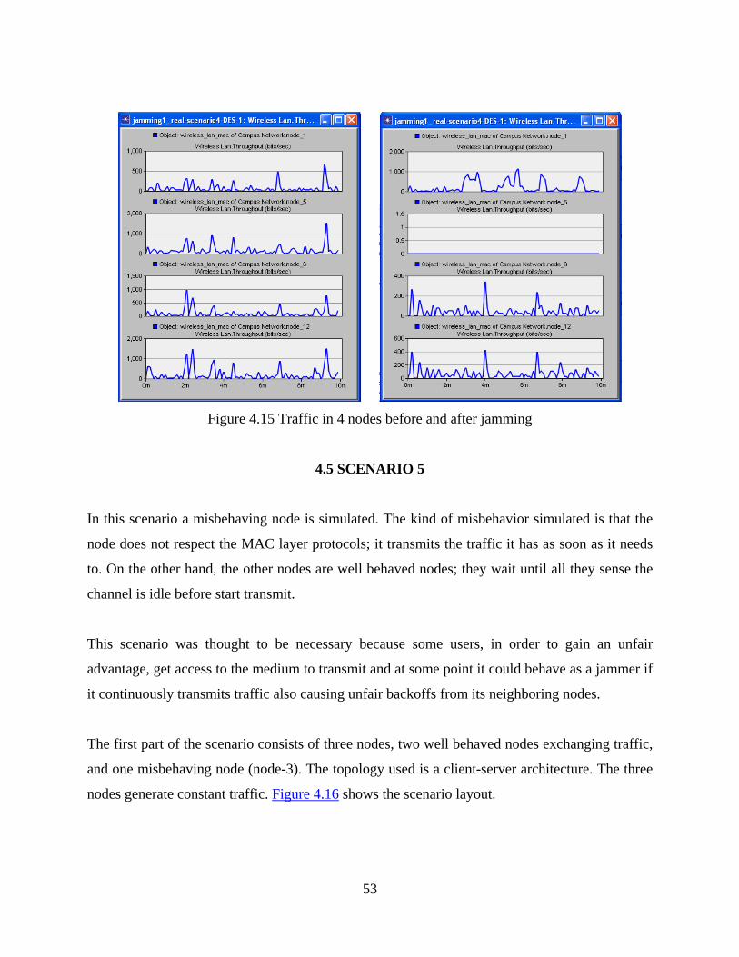
Figure 4.15 Traffic in 4 nodes before and after jamming
4.5 SCENARIO 5
In this scenario a misbehaving node is simulated. The kind of misbehavior simulated is that the
node does not respect the MAC layer protocols; it transmits the traffic it has as soon as it needs
to. On the other hand, the other nodes are well behaved nodes; they wait until all they sense the
channel is idle before start transmit.
This scenario was thought to be necessary because some users, in order to gain an unfair
advantage, get access to the medium to transmit and at some point it could behave as a jammer if
it continuously transmits traffic also causing unfair backoffs from its neighboring nodes.
The first part of the scenario consists of three nodes, two well behaved nodes exchanging traffic,
and one misbehaving node (node-3). The topology used is a client-server architecture. The three
nodes generate constant traffic. Figure 4.16 shows the scenario layout.
53
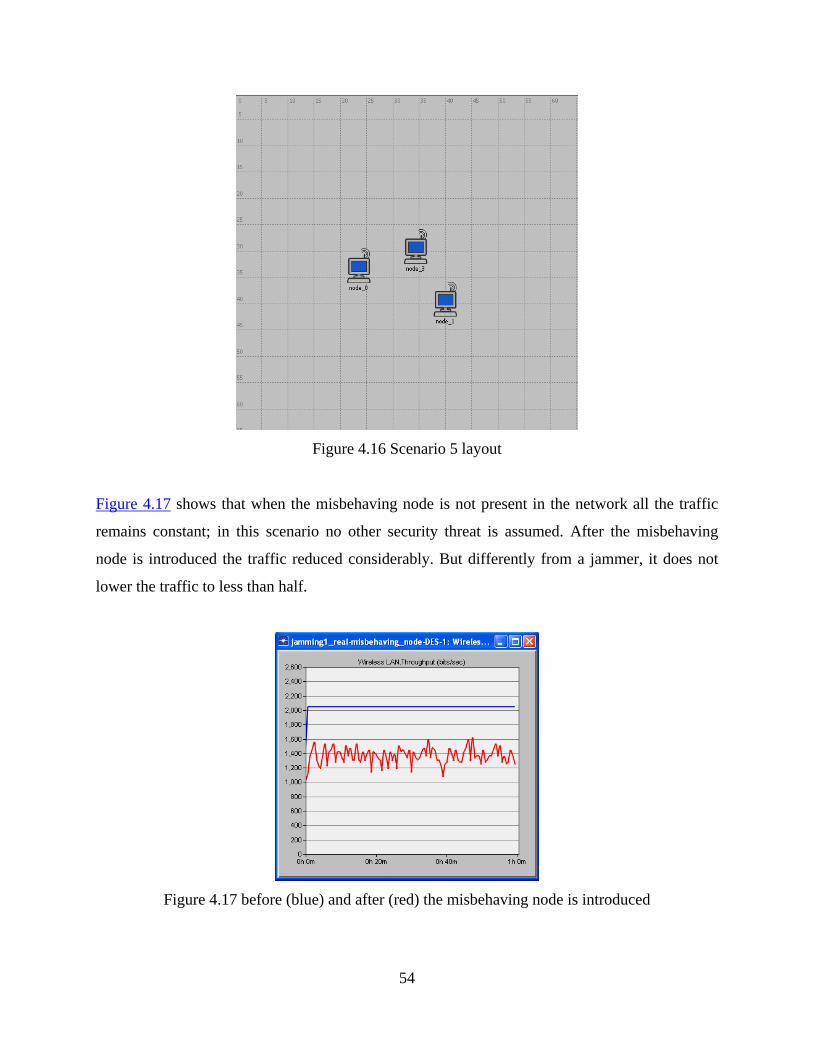
Figure 4.16 Scenario 5 layout
Figure 4.17 shows that when the misbehaving node is not present in the network all the traffic
remains constant; in this scenario no other security threat is assumed. After the misbehaving
node is introduced the traffic reduced considerably. But differently from a jammer, it does not
lower the traffic to less than half.
Figure 4.17 before (blue) and after (red) the misbehaving node is introduced
54
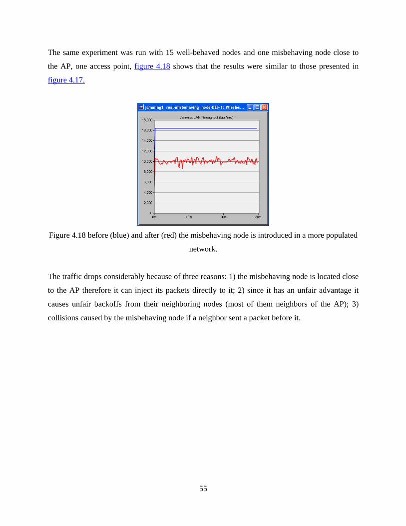
The same experiment was run with 15 well-behaved nodes and one misbehaving node close to
the AP, one access point, figure 4.18 shows that the results were similar to those presented in
figure 4.17.
Figure 4.18 before (blue) and after (red) the misbehaving node is introduced in a more populated
network.
The traffic drops considerably because of three reasons: 1) the misbehaving node is located close
to the AP therefore it can inject its packets directly to it; 2) since it has an unfair advantage it
causes unfair backoffs from their neighboring nodes (most of them neighbors of the AP); 3)
collisions caused by the misbehaving node if a neighbor sent a packet before it.
55
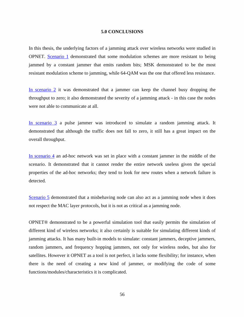
5.0 CONCLUSIONS
In this thesis, the underlying factors of a jamming attack over wireless networks were studied in
OPNET. Scenario 1 demonstrated that some modulation schemes are more resistant to being
jammed by a constant jammer that emits random bits; MSK demonstrated to be the most
resistant modulation scheme to jamming, while 64-QAM was the one that offered less resistance.
In scenario 2 it was demonstrated that a jammer can keep the channel busy dropping the
throughput to zero; it also demonstrated the severity of a jamming attack - in this case the nodes
were not able to communicate at all.
In scenario 3 a pulse jammer was introduced to simulate a random jamming attack. It
demonstrated that although the traffic does not fall to zero, it still has a great impact on the
overall throughput.
In scenario 4 an ad-hoc network was set in place with a constant jammer in the middle of the
scenario. It demonstrated that it cannot render the entire network useless given the special
properties of the ad-hoc networks; they tend to look for new routes when a network failure is
detected.
Scenario 5 demonstrated that a misbehaving node can also act as a jamming node when it does
not respect the MAC layer protocols, but it is not as critical as a jamming node.
OPNET® demonstrated to be a powerful simulation tool that easily permits the simulation of
different kind of wireless networks; it also certainly is suitable for simulating different kinds of
jamming attacks. It has many built-in models to simulate: constant jammers, deceptive jammers,
random jammers, and frequency hopping jammers, not only for wireless nodes, but also for
satellites. However it OPNET as a tool is not perfect, it lacks some flexibility; for instance, when
there is the need of creating a new kind of jammer, or modifying the code of some
functions/modules/characteristics it is complicated.
56
OPNET® offered the option of automatically collecting statistics and their corresponding
graphics. In this aspect its performance is pretty good, but an important drawback is that if the
user wants to measure an aspect of the network that is not included in the list of things OPNET
can measure, it is difficult to create a routine to do it. Finally, OPNET offers many details in its
models, but it also leads to slow-running simulations.
Some future work includes analyzing the effects of more than one jammer in each scenario, also
the use of one mobile jammer instead of fixed ones. Further future work consist of proposing an
algorithm to cope with jamming attacks and evaluating it through simulations.
57
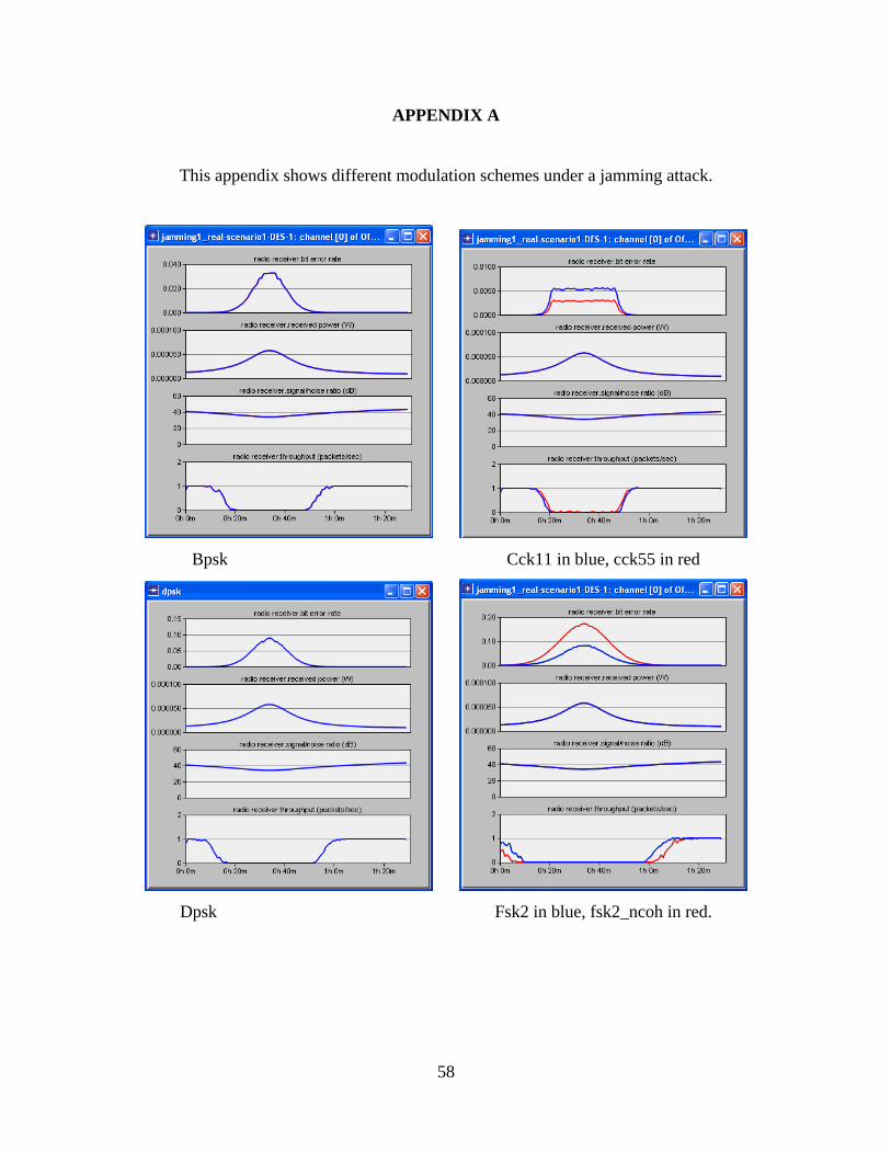
APPENDIX A
This appendix shows different modulation schemes under a jamming attack.
Bpsk Cck11 in blue, cck55 in red
Dpsk Fsk2 in blue, fsk2_ncoh in red.
58
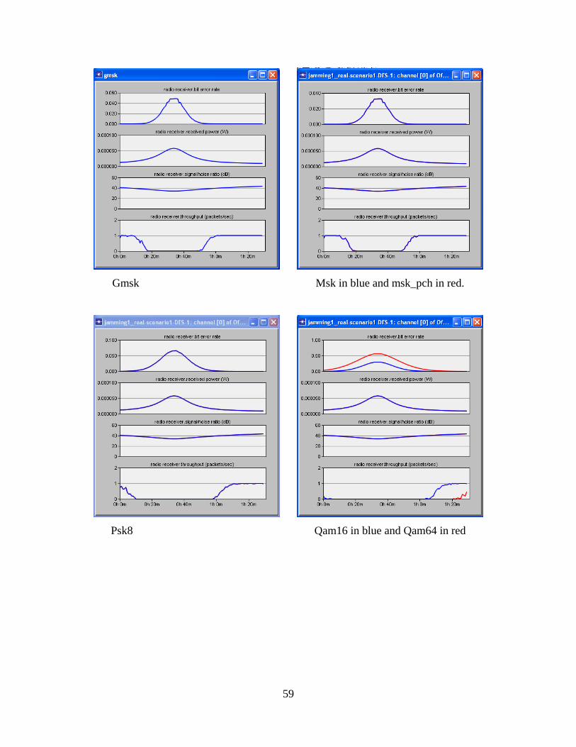
Gmsk Msk in blue and msk_pch in red.
Psk8 Qam16 in blue and Qam64 in red
59
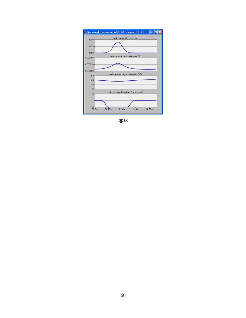
qpsk
60
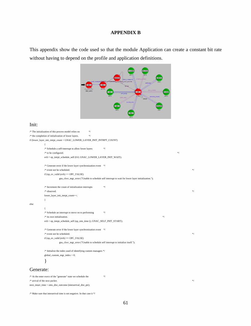
APPENDIX B
This appendix show the code used so that the module Application can create a constant bit rate
without having to depend on the profile and application definitions.
Init: /* The initialization of this process model relies on */
/* the completion of initialization of lower layers. */
if (lower_layer_init_intrpt_count < GNAC_LOWER_LAYER_INIT_INTRPT_COUNT)
{
/* Schedule a self-interrupt to allow lower layers */
/* to be configured. */
evh = op_intrpt_schedule_self (0.0, GNAC_LOWER_LAYER_INIT_WAIT);
/* Generate error if the lower layer synchronization event */
/* event not be scheduled. */
if (op_ev_valid (evh) == OPC_FALSE)
gna_clsvr_mgr_error ("Unable to schedule self interrupt to wait for lower layer initialization.");
/* Increment the count of initialization interrupts */
/* observed. */
lower_layer_init_intrpt_count++;
}
else
{
/* Schedule an interrupt to move on to performing */
/* its own initialization. */
evh = op_intrpt_schedule_self (op_sim_time (), GNAC_SELF_INIT_START);
/* Generate error if the lower layer synchronization event */
/* event not be scheduled. */
if (op_ev_valid (evh) == OPC_FALSE)
gna_clsvr_mgr_error ("Unable to schedule self interrupt to initialize itself.");
/* Initialize the index used of identifying custom managers */
global_custom_mgr_index = 0;
}
Generate: /* At the enter execs of the "generate" state we schedule the */
/* arrival of the next packet. */
next_intarr_time = oms_dist_outcome (interarrival_dist_ptr);
/* Make sure that interarrival time is not negative. In that case it */
61
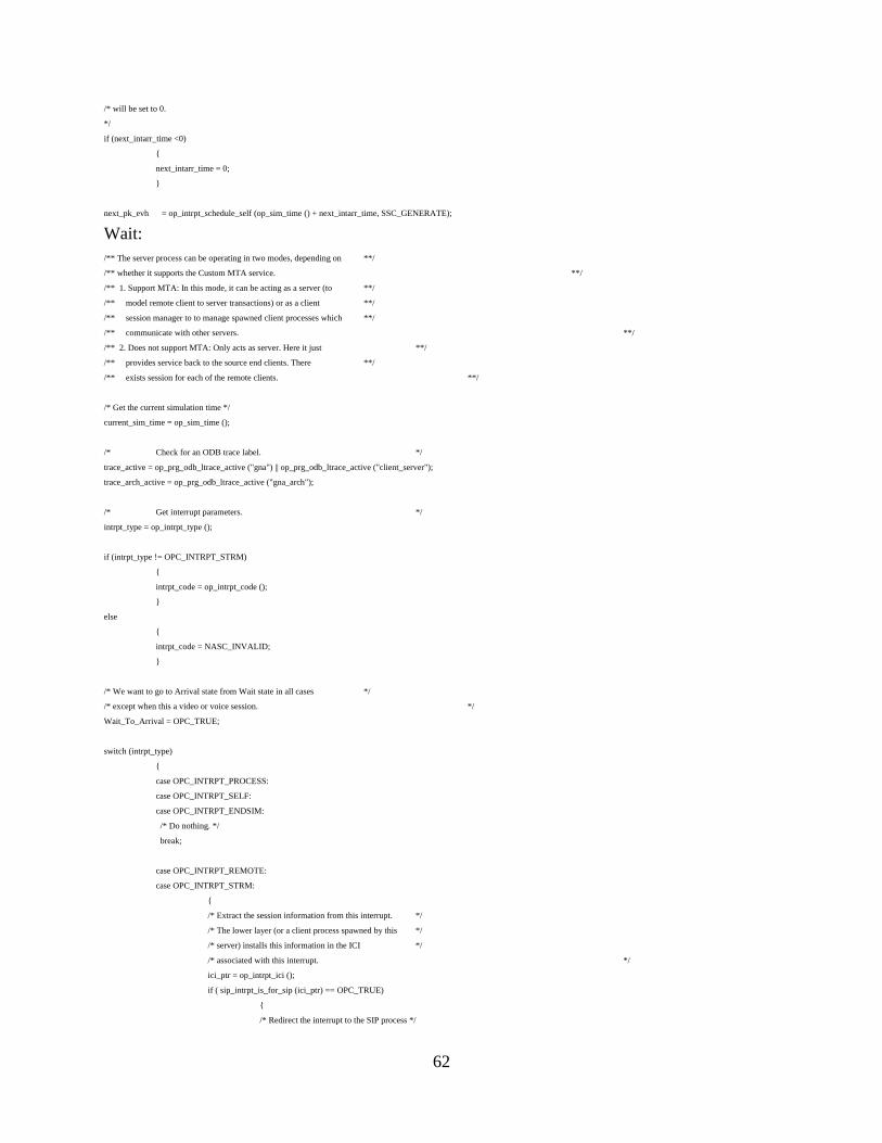
/* will be set to 0.
*/
if (next_intarr_time <0)
{
next_intarr_time = 0;
}
next_pk_evh = op_intrpt_schedule_self (op_sim_time () + next_intarr_time, SSC_GENERATE);
Wait: /** The server process can be operating in two modes, depending on **/
/** whether it supports the Custom MTA service. **/
/** 1. Support MTA: In this mode, it can be acting as a server (to **/
/** model remote client to server transactions) or as a client **/
/** session manager to to manage spawned client processes which **/
/** communicate with other servers. **/
/** 2. Does not support MTA: Only acts as server. Here it just **/
/** provides service back to the source end clients. There **/
/** exists session for each of the remote clients. **/
/* Get the current simulation time */
current_sim_time = op_sim_time ();
/* Check for an ODB trace label. */
trace_active = op_prg_odb_ltrace_active ("gna") || op_prg_odb_ltrace_active ("client_server");
trace_arch_active = op_prg_odb_ltrace_active ("gna_arch");
/* Get interrupt parameters. */
intrpt_type = op_intrpt_type ();
if (intrpt_type != OPC_INTRPT_STRM)
{
intrpt_code = op_intrpt_code ();
}
else
{
intrpt_code = NASC_INVALID;
}
/* We want to go to Arrival state from Wait state in all cases */
/* except when this a video or voice session. */
Wait_To_Arrival = OPC_TRUE;
switch (intrpt_type)
{
case OPC_INTRPT_PROCESS:
case OPC_INTRPT_SELF:
case OPC_INTRPT_ENDSIM:
/* Do nothing. */
break;
case OPC_INTRPT_REMOTE:
case OPC_INTRPT_STRM:
{
/* Extract the session information from this interrupt. */
/* The lower layer (or a client process spawned by this */
/* server) installs this information in the ICI */
/* associated with this interrupt. */
ici_ptr = op_intrpt_ici ();
if ( sip_intrpt_is_for_sip (ici_ptr) == OPC_TRUE)
{
/* Redirect the interrupt to the SIP process */
62
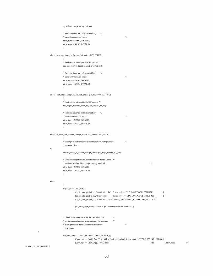
sip_redirect_intrpt_to_sip (ici_ptr);
/* Reset the interrupt codes to avoid any */
/* transition condition errors. */
intrpt_type = NASC_INVALID;
intrpt_code = NASC_INVALID;
}
else if ( gna_sup_intrpt_is_for_sup (ici_ptr) == OPC_TRUE)
{
/* Redirect the interrupt to the SIP process */
gna_sup_redirect_intrpt_to_dest_proc (ici_ptr);
/* Reset the interrupt codes to avoid any */
/* transition condition errors. */
intrpt_type = NASC_INVALID;
intrpt_code = NASC_INVALID;
}
else if ( traf_engine_intrpt_is_for_traf_engine (ici_ptr) == OPC_TRUE)
{
/* Redirect the interrupt to the SIP process */
traf_engine_redirect_intrpt_to_traf_engine (ici_ptr);
/* Reset the interrupt codes to avoid any */
/* transition condition errors. */
intrpt_type = NASC_INVALID;
intrpt_code = NASC_INVALID;
}
else if (is_intrpt_for_remote_storage_access (ici_ptr) == OPC_TRUE)
{
/* interrupt to be handled by either the remote storage access */
/* server or client.
*/
redirect_intrpt_to_remote_storage_access (rsa_mgr_prohndl, ici_ptr);
/* Reset the intrpt type and code to indicate that this intrpt */
/* has been handled. No more processing required. */
intrpt_type = NASC_INVALID;
intrpt_code = NASC_INVALID;
}
else
{
if ((ici_ptr == OPC_NIL) ||
(op_ici_attr_get (ici_ptr, "Application ID", &sess_ptr) == OPC_COMPCODE_FAILURE) ||
(op_ici_attr_get (ici_ptr, "Sess Type", &sess_type) == OPC_COMPCODE_FAILURE) ||
(op_ici_attr_get (ici_ptr, "Application Type", &app_type) == OPC_COMPCODE_FAILURE))
{
gna_clsvr_mgr_error ("Unable to get session information from ICI.");
}
/* Check if this interrupt is for the case when this */
/* server process is acting as the manager for spawned */
/* client processes (to talk to other client/server */
/* processes)
*/
if (((sess_type == GNAC_SESSION_TYPE_ACTIVE)) ||
((app_type == GnaC_App_Type_Video_Conferencing) && (intrpt_code != TPALC_EV_IND_OPEN)) ||
((app_type == GnaC_App_Type_Voice) && (intrpt_code !=
TPALC_EV_IND_OPEN)) ||
63
(app_type == GnaC_App_Type_Ace))
{
/* Even when the server is acting as the manager, */
/* it handles two cases where the interrupt is for */
/* itself (i.e., the server): */
/* 1. A session termination (this interrupt is */
/* scheduled by the managed client.) */
/* 2. Modeling request time delay (again this is */
/* scheduled by the managed client) -- this */
/* facilitates modeling of the server busy */
/* condition for modelign the request delays. */
if ((intrpt_code == GNAC_IND_SESS_OPEN_FAILED) || (intrpt_code == GNAC_IND_SESS_CLOSED)
|| (intrpt_code == GNAC_MODEL_REQUEST_TIME))
{
/* Do nothing. The transition conditions will */
/* figure out how to transition. */
cli_sess_ptr = (GnaT_Cli_Mgr_Session *) sess_ptr;
}
else
{
/* Invoke the session process using the process */
/* handle from the session record. */
cli_sess_ptr = (GnaT_Cli_Mgr_Session *) sess_ptr;
/* Check whether the client process is still alive. */
if (cli_sess_ptr != OPC_NIL)
{
if (op_pro_valid (cli_sess_ptr->prohndl) == OPC_TRUE)
{
if (op_pro_invoke (cli_sess_ptr->prohndl, OPC_NIL) ==
OPC_COMPCODE_FAILURE)
{
gna_clsvr_mgr_error ("Could not invoke session process to handle
received interrupt.");
}
}
}
else
{
/* Process model doesn't exist any more. */
if (intrpt_type == OPC_INTRPT_STRM)
{
/* If interrupt is stream interrupt, destroy packet. */
op_pk_destroy (op_pk_get (op_intrpt_strm ()));
}
}
/* Reset the interrupt codes to avoid any */
/* transition condition errors. */
intrpt_type = NASC_INVALID;
intrpt_code = NASC_INVALID;
}
}
/* If this is a video or voice session, do not go into arrival */
/* state.
*/
if ((app_type == GnaC_App_Type_Video_Conferencing) ||
(app_type == GnaC_App_Type_Voice))
{
Wait_To_Arrival = OPC_FALSE;
64

}
}
break;
}
default:
{
gna_clsvr_mgr_error ("Received unexpected interrupt in wait state.");
break;
}
}
65
BIBLIOGRAPHY
[1] Thompson, R. A. (2006). The physical layer of communication systems, MD: Artech
house.
[2] Zagzebski, J. A. (1996). Essentials of ultrasound physics, NY: Mosby Inc.
[3] Sklar B. et al. (1997). Rayleigh Fading Channels in Mobile Digital
communication Systems Part I: Characterization. IEEE communications
magazine, vol. 35.
[4] Okumara, Y. et al. (1968). Field Strength And Its Variability In VHF And UHF Land
Mobile Radio Service. Rev. Elec. Commun. Lab, vol 16.
[5] Hata, M. (1980). Empirical Formulae for Propagation Loss in Land Mobile Radio
Services. IEEE trans. Vehic. Tech. vol. VT-29, no. 3
[6] Cox, D.C. et al. (1984). 800 MHz Attenuation measured in and around suburban houses.
AT&T Bell Lab Tech. J., vol. 673, no. 6
[7] Rappaport, T.S.(1996). Wireless communications. NJ: Prentice Hall.
[8] IEEE. (2007). 802.11 working group for wireless local area networks. Retrieved August
15,2007, from http://standards.ieee.org/wireless/overview.html
66
[9] Halsall, F. (1996) Data communications, computer networks and open systems, UK:
Addison-Wesley
[10] Schiller, J. (2003). Mobile Communications, UK: Addison-Wesley.
[11] Brenner, P. (1996). A technical tutorial on the IEEE 802.11 protocol. Breezecom.
[12] Hu, Y. Perrig, A. and Johnson, D. (2003). Packet leashes: a defense against wormhole
attacks in wireless networks. Proceedings of IEEE Infocom 2003.
[13] Xu, W. Trappe, W. Zhang, Y. And Wood, T. (2005). The feasibility of launching and
detecting jamming attacks in wireless networks. International Symposium on Mobile Ad Hoc
Networking & Computing.
[14] Huang, Q. Kobayashi, H. and Liu, B. (2003). Modeling of distributed denial of service
attacks in wireless networks. IEEE Pacific Rim Conference on Communications, Computers and
Signal Processing.
[15] Xu, W. Trappe, W. and Zhang, Y. (2006). "Jamming Sensor Networks: Attack and
Defense Strategies," IEEE Networks Special Issue on Sensor Networks, Vol.20, No. 3
67
[16] Wood, A.D. Stankovic, J.A. and Zhou G. (2007). DEEJAM: Defeating Energy-Efficient
Jamming in IEEE 802.15.4-based Wireless Networks. The 4th Annual IEEE Communications
Society Conference on Sensor, Mesh and Ad Hoc Communications and Networks (SECON).
[17] OPNET. (2006). Wireless Module User Guide for IT Guru.
[18] Alnifie, G. and Simon, R. (2007). A multi-channel defense against jamming attacks in
wireless sensor networks. In Proceedings of the 3rd ACM Workshop on QoS and Security For
Wireless and Mobile Networks (Chania, Crete Island, Greece, October 22 - 22, 2007). Q2SWinet
'07.
68