Embed Size (px)
Citation preview
NAVAL POSTGRADUATE SCHOOL Monterey, California
THESIS
A NUMERICAL STUDY OF HEAT TRANSFER BEHAVIOR IN WELDING
by
Yasar Vehbi Isiklar
June, 1998
Thesis Advisor: Ashok Gopinath
ro
Approved for public release; distribution is unlimited.
[»SIC QUALITY INSPECTED 1
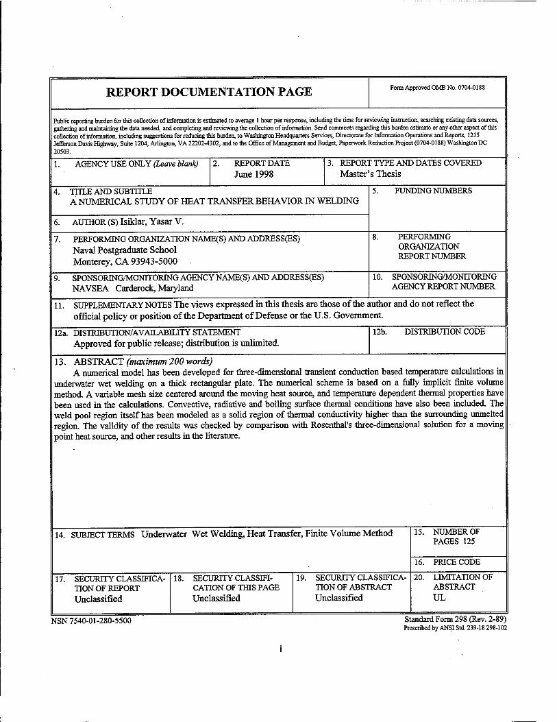
REPORT DOCUMENTATION PAGE Form Approved OMB No. 0704-0188
Public reporting burden for this collection of information is estimated to average 1 hour per response, including the time for reviewing instruction, searching existing data sources, gathering and maintaining the data needed, and completing and reviewing the collection of information. Send comments regarding this burden estimate or any other aspect of this collection of information, including suggestions for reducing this burden, to Washington Headquarters Services, Directorate for Information Operations and Reports, 1215 Jefferson Davis Highway, Suite 1204, Arlington, VA 22202-4302, and to the Office of Management and Budget, Paperwork Reduction Project (0704-0188) Washington DC 20503.
1. AGENCY USE ONLY (Leave blank) REPORT DATE June 1998
3. REPORT TYPE AND DATES COVERED Master's Thesis
TITLE AND SUBTITLE A NUMERICAL STUDY OF HEAT TRANSFER BEHAVIOR IN WELDING
6. AUTHOR (S) Isiklar, Yasar V.
5. FUNDING NUMBERS
7. PERFORMING ORGANIZATION NAME(S) AND ADDRESS(ES) Naval Postgraduate School Monterey, CA 93943-5000
PERFORMING ORGANIZATION REPORT NUMBER
9. SPONSORING/MONITOPJNG AGENCY NAME(S) AND ADDRESS(ES) NAVSEA Carderock, Maryland
10. SPONSORING/MONITORING AGENCY REPORT NUMBER
11. SUPPLEMENTARY NOTES The views expressed in this thesis are those of the author and do not reflect the official policy or position of the Department of Defense or the U.S. Government.
12a. DISTRmunON/AVATLABILITY STATEMENT Approved for public release; distribution is unlimited.
12b. DISTRIBUTION CODE
13. ABSTRACT (maximum 200 words) A numerical model has been developed for three-dimensional transient conduction based temperature calculations in
underwater wet welding on a thick rectangular plate. The numerical scheme is based on a fully implicit finite volume method. A variable mesh size centered around the moving heat source, and temperature dependent thermal properties have been used in the calculations. Convective, radiative and boiling surface thermal conditions have also been included. The weld pool region itself has been modeled as a solid region of thermal conductivity higher than the surrounding unmelted region. The validity of the results was checked by comparison with Rosenthal's three-dimensional solution for a moving point heat source, and other results in the literature.
14. SUBJECT TERMS Underwater Wet Welding, Heat Transfer, Finite Volume Method
17. SECURITY CLASSIFICA- TION OF REPORT Unclassified
18. SECURITY CLASSIFI- CATION OF THIS PAGE Unclassified
19. SECURITY CLASSIFICA- TION OF ABSTRACT Unclassified
15. NUMBER OF PAGES 125
16. PRICE CODE
20. LIMITATION OF ABSTRACT UL
NSN 7540-01-280-5500 Standard Form 298 (Rev. 2-89) Prescribed by ANSI Std. 239-18 298-102

11
Approved for public release; distribution is unlimited.
A NUMERICAL STUDY OF HEAT TRANSFER BEHAVIOR IN WELDING
Yasar V. Isiklar Lieutenant Junior Grade, Turkish Navy
B.S., Turkish Naval Academy, 1992
Submitted in partial fulfillment of the requirements for the degree of
MASTER OF SCIENCE IN MECHANICAL ENGINEERING
fromme
NAVAL POSTGRADUATE SCHOOL June 1998
Author:
Approved by:
in

IV
ABSTRACT
A numerical model has been developed for three-dimensional transient
conduction based temperature calculations in underwater wet welding on a thick
rectangular plate. The numerical scheme is based on a fully implicit finite volume
method. A variable mesh size centered around the moving heat source, and temperature
dependent thermal properties have been used in the calculations. Convective, radiative
and boiling surface thermal conditions have also been included. The weld pool region
itself has been modeled as a solid region of thermal conductivity higher than the
surrounding unmelted solid region. The validity of the results was checked by comparison
with Rosenthal's three-dimensional solution for a moving point heat source, and other
results in the literature.
v

VI
TABLE OF CONTENTS
I. INTRODUCTION 1
E. BACKGROUND 3
A. PREVIOUS STUDIES 3
B. FINITE VOLUME METHOD 7
m. MODEL DEVELOPMENT 13
A. DEFINING THE WORKPIECE .13
B. BOUNDARY CONDITIONS 14
1. Top Face 14
2. Other Faces 15
3. Simulating The Arc 16
4. Boiling Heat Transfer 16
a. Free Convection Regime 17
b. Nucleate Boiling Regime 18
c. Transition Boiling Regime 19
d. Film Boiling Regime 20
C. COEFFICIENTS USED IN THE EQUATIONS 22
D. DERIVATION OF THE EQUATIONS 23
IV. RESULTS AND DISCUSSION... 45
V. CONCLUSIONS AND RECOMMENDATIONS 61
APPENDLX A: PROGRAM STRUCTURE 63
vii
APPENDIX B: PROGRAM CODES 71
LIST OF REFERENCES 107
INITIAL DISTRIBUTION LIST Ill
vm
LIST OF SYMBOLS
SYMBOL DESCRIPTION UNITS
cp specific heat J/kg K Cs/ emprical constant d exponential factor g gravitational acceleration m/s2
h convective heat transfer coefficient; W/m2K h combined heat transfer coefficient W/m2 K
h c local heat transfer coeff. convection conductance W/m2 K
h r average heat transfer coeff. for radiation W/m2 K hfg latent heat of vaporization J/kg k thermal conductivity W/m K L characteristic length m q heat flux W/m2
q0 volumetric heat energy generation rate W/m3
Q heat input to the workpiece W r0 radius of the heat input distribution m R radial distance from the origin m t time s T temperature K or C U welding speed m/s V volume m3
a thermal diffusivity m2/s ß volumetric thermal expansion coefficient K"1
S distance between two neighboring grid points m A difference between values s surface emissivity 0 finite volume method coefficient // absolute viccosity Ns/m2
v kinematic viscosity m2/s p density kg/m3
<r Stefan-Boltzman constant W/m2 K4
ex surface tension N/m
IX

ACKNOWLEDGEMENTS
The author would like to gratefully acknowledge the support of NAVSEA for
this project.
The author would like especially to express his appreciation to Prof.Ashok
Gopinath for his expert assistance and creative influence throughout the course of this
research. The author also wishes to thank his colleague, Ltjg.Ibrahim Girgin for various
forms of assistance and computational support.
Finally, the author would like to express his sincere gratitude to his wife Gonul
and his family for their patience, understanding and encouragement during the
preparation of this thesis research.
XI

xn
I. INTRODUCTION
To improve the quality of the underwater welding and to accomplish a reliable,
permanent underwater wet welding capability has a great importance in today's industrial
and military facilities. With the development of underwater wet welding techniques, the
time and the money required for permanent and temporary repairs of ships and other
underwater structures can be minimized. Today, the use of hyperbaric welding process
obtains a limited quality of welding especially for the construction and repairs of
underwater pipelines. In this process a large pressure chamber is used to keep the water
away from the workpiece. But, operating this kind of chamber is very expensive and due
to the limited geometric size, only a few joint configurations can be enclosed in a
chamber [Ref.l]. The other welding techniques such as double shielding and flux
shielding also use the water removing theory from the arc area during welding. But, the
working area must be completely prevented from water for satisfactory welding results
[Ref. 2].
Currently, underwater wet welding is used for the temporary repair needs.
Because of their poor quality compared to surface (air) welds (they obtain 80% of the
tensile strength and 50% ductility of the surface welds [Ref. 3].), they must be replaced as
soon as possible. Therefore, the development of a more efficient wet welding technique is
the only solution to this problem.
The surrounding water environment during wet welding causes rapid cooling and
steep temperature gradients in the weld area behind the arc [Ref.4]. Because of the
1
extremely complex nature of the heat transfer phenomena between heated surface and the
water environment, a numerical model simulation is necessary.
In the present study, a numerical model has been developed for transient, three-
dimensional conduction heat transfer in underwater welding process on a thick
rectangular plate. The numerical scheme was based on fully implicit finite volume model,
including convection, radiation and boiling surface thermal boundary conditions. The
different regimes of boiling were accounted for on the surface. A variable mesh size
centered around an arc source moving at constant speed was used to determine
temperature variations inside and around the weld pool. The weld pool region itself has
been modeled as a solid region of thermal conductivity higher than the surrounding
unmelted solid region. The input data from the previous studies based on different
methods were used to check the accuracy and the validity of the numerical method.
II. BACKGROUND
A. PREVIOUS STUDIES
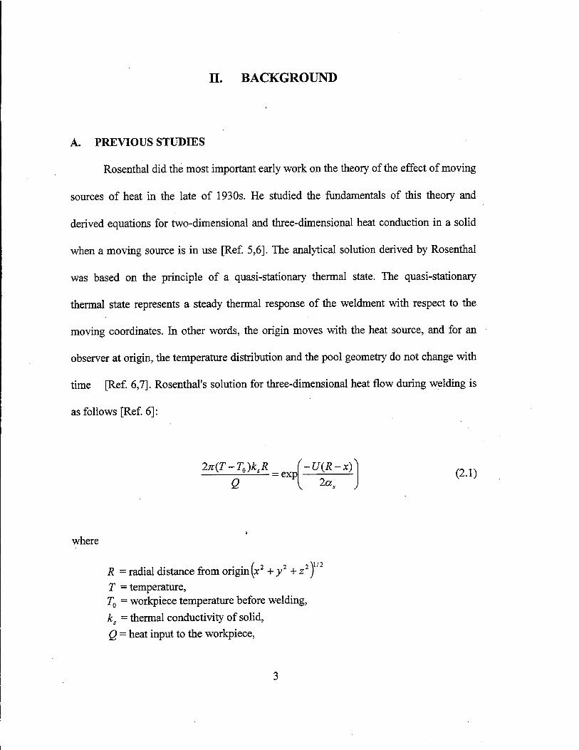
Rosenthal did the most important early work on the theory of the effect of moving
sources of heat in the late of 1930s. He studied the fundamentals of this theory and
derived equations for two-dimensional and three-dimensional heat conduction in a solid
when a moving source is in use [Ref. 5,6]. The analytical solution derived by Rosenthal
was based on the principle of a quasi-stationary thermal state. The quasi-stationary
thermal state represents a steady thermal response of the weldment with respect to the
moving coordinates. In other words, the origin moves with the heat source, and for an
observer at origin, the temperature distribution and the pool geometry do not change with
time [Ref. 6,7]. Rosenthal's solution for three-dimensional heat flow during welding is
as follows [Ref. 6]:
2x(T-T0)ksR —i =exp
Q
f U(R-x)^ 2a,
(2.1)
where
R = radial distance from origin [x2 + v2 + z2) T = temperature, TQ = workpiece temperature before welding, ks = thermal conductivity of solid, Q = heat input to the workpiece,
,1/2
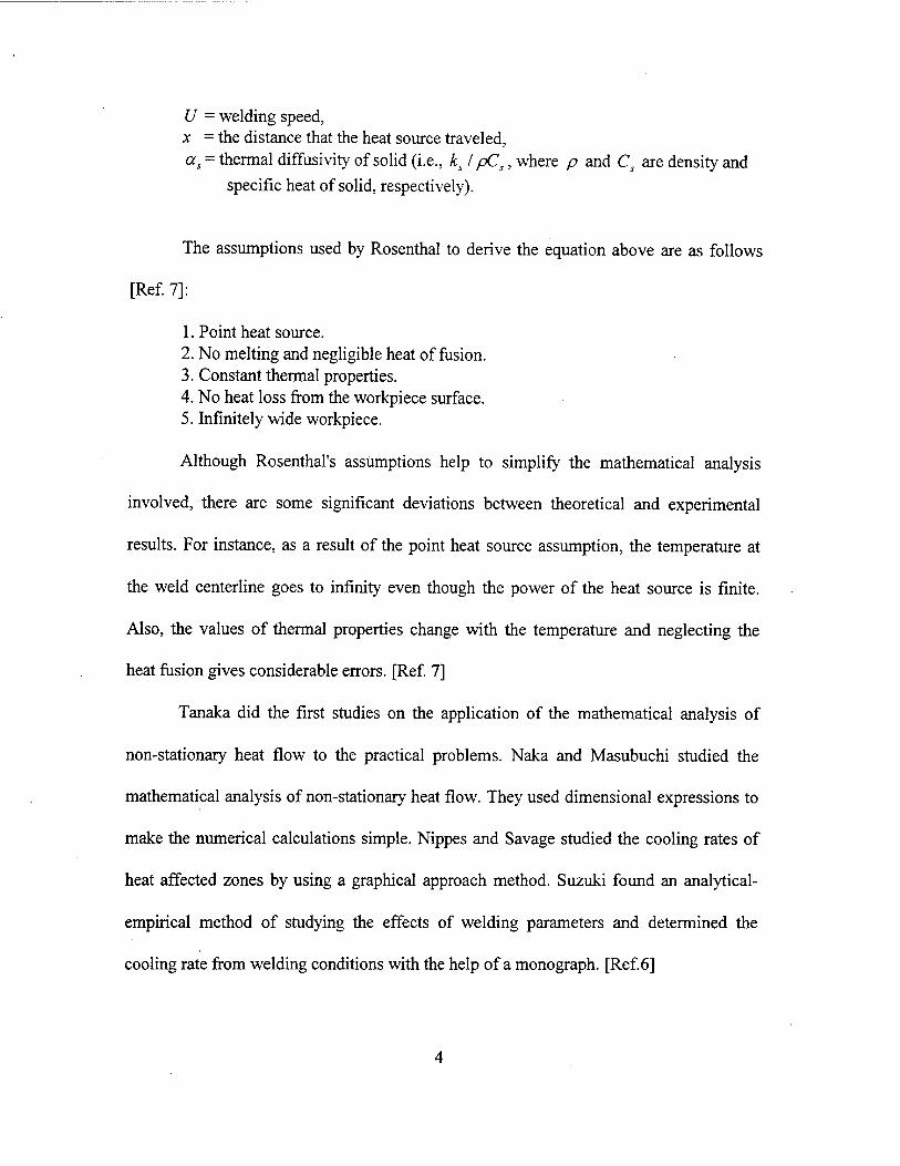
U = welding speed, x = the distance that the heat source traveled, as = thermal diffusivity of solid (i.e., ks I pC5, where p and Cs are density and
specific heat of solid, respectively).
The assumptions used by Rosenthal to derive the equation above are as follows
[Ref. 7]:
1. Point heat source. 2. No melting and negligible heat of fusion. 3. Constant thermal properties. 4. No heat loss from the workpiece surface. 5. Infinitely wide workpiece.
Although Rosenthal's assumptions help to simplify the mathematical analysis
involved, there are some significant deviations between theoretical and experimental
results. For instance, as a result of the point heat source assumption, the temperature at
the weld centerline goes to infinity even though the power of the heat source is finite.
Also, the values of thermal properties change with the temperature and neglecting the
heat fusion gives considerable errors. [Ref. 7]
Tanaka did the first studies on the application of the mathematical analysis of
non-stationary heat flow to the practical problems. Naka and Masubuchi studied the
mathematical analysis of non-stationary heat flow. They used dimensional expressions to
make the numerical calculations simple. Nippes and Savage studied the cooling rates of
heat affected zones by using a graphical approach method. Suzuki found an analytical-
empirical method of studying the effects of welding parameters and determined the
cooling rate from welding conditions with the help of a monograph. [Ref.6]
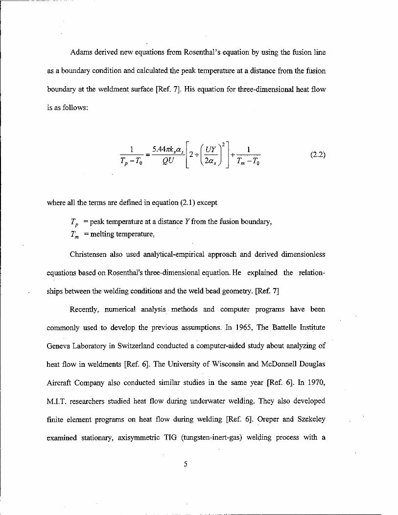
Adams derived new equations from Rosenthal's equation by using the fusion line
as a boundary condition and calculated the peak temperature at a distance from the fusion
boundary at the weldment surface [Ref. 7]. His equation for three-dimensional heat flow
is as follows:
1 5A4ftksas
Tp-T0 QU 2 +
2asJ + Tm-T0
(22)
where all the terms are defined in equation (2.1) except
T = peak temperature at a distance Y from the fusion boundary,
Tm = melting temperature,
Christensen also used analytical-empirical approach and derived dimensionless
equations based on Rosenthal's three-dimensional equation. He explained the relation-
ships between the welding conditions and the weld bead geometry. [Ref. 7]
Recently, numerical analysis methods and computer programs have been
commonly used to develop the previous assumptions. In 1965, The Battelle Institute
Geneva Laboratory in Switzerland conducted a computer-aided study about analyzing of
heat flow in weldments [Ref. 6]. The University of Wisconsin and McDonnell Douglas
Aircraft Company also conducted similar studies in the same year [Ref. 6]. In 1970,
M.I.T. researchers studied heat flow during underwater welding. They also developed
finite element programs on heat flow during welding [Ref. 6]. Oreper and Szekeley
examined stationary, axisymmetric TIG (tungsten-inert-gas) welding process with a
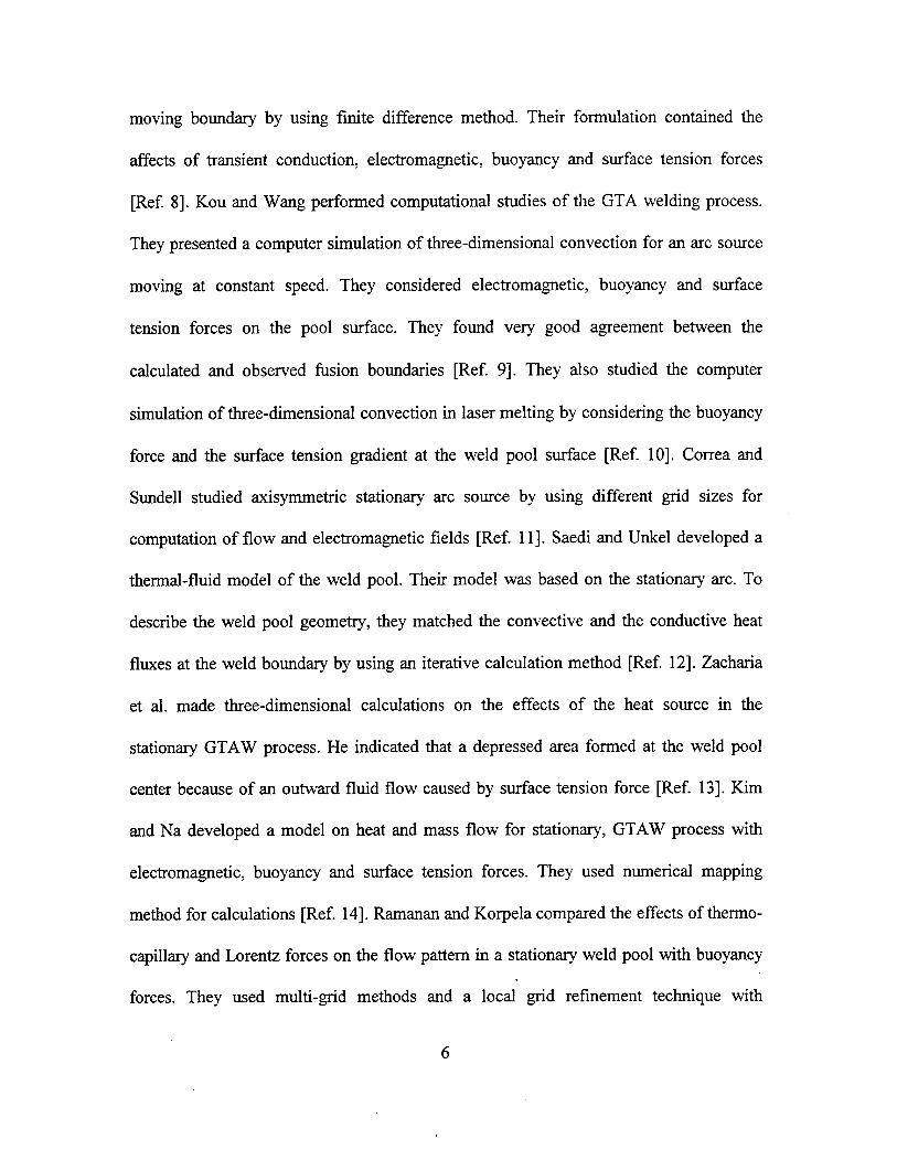
moving boundary by using finite difference method. Their formulation contained the
affects of transient conduction, electromagnetic, buoyancy and surface tension forces
[Ref. 8]. Kou and Wang performed computational studies of the GTA welding process.
They presented a computer simulation of three-dimensional convection for an arc source
moving at constant speed. They considered electromagnetic, buoyancy and surface
tension forces on the pool surface. They found very good agreement between the
calculated and observed fusion boundaries [Ref. 9]. They also studied the computer
simulation of three-dimensional convection in laser melting by considering the buoyancy
force and the surface tension gradient at the weld pool surface [Ref. 10]. Correa and
Sundell studied axisymmetric stationary arc source by using different grid sizes for
computation of flow and electromagnetic fields [Ref. 11]. Saedi and Unkel developed a
thermal-fluid model of the weld pool. Their model was based on the stationary arc. To
describe the weld pool geometry, they matched the convective and the conductive heat
fluxes at the weld boundary by using an iterative calculation method [Ref. 12]. Zacharia
et al. made three-dimensional calculations on the effects of the heat source in the
stationary GTAW process. He indicated that a depressed area formed at the weld pool
center because of an outward fluid flow caused by surface tension force [Ref. 13]. Kim
and Na developed a model on heat and mass flow for stationary, GTAW process with
electromagnetic, buoyancy and surface tension forces. They used numerical mapping
method for calculations [Ref. 14]. Ramanan and Korpela compared the effects of thermo-
capillary and Lorentz forces on the flow pattern in a stationary weld pool with buoyancy
forces. They used multi-grid methods and a local grid refinement technique with
axisymmetric stationary arc source [Ref. 14]. Ule, Joshi and Sedy determined three-
dimensional transient temperature variations in the GTAW process by using the explicit
finite difference method. They used different mesh sizes and temperature dependent
thermal properties. They also considered convective and radiative surface thermal
conditions during calculations [Ref. 16]. Kanouff and Greif studied the unsteady
development of an axisymmetric arc weld pool in GTAW process. They used moving
grids to follow the phase change boundary and considered the effects of Marangoni,
Lorentz and buoyancy forces in the calculations [Ref. 17]. Joshi, Dutta, Schupp and
Espinosa developed a three-dimensional numerical model to describe the flow circulation
phenomena in aluminum weld pools under non-axisymmetric Lorentz force field [Ref.
18,19].
B. FINITE VOLUME METHOD
The finite volume method is one of the simple and well-established
Computational Fluid Dynamics (CFD) techniques that were originally developed as a
special finite difference method [Ref. 19]. The stages of the numerical algorithm in this
method are as follows [Ref. 19]:
1. Formal integration of the governing equations of fluid flow over all the finite control volumes of the solution domain.
2. Discretisation involves the substitution of a variety of finite difference type approximations for the terms in the integrated equation representing flow process such as convection, diffusion and sources. This converts the integral equations into a system of algebraic equations.
3. Solution of the algebraic equations by an iterative method.
In the control volume integration, the calculation domain is divided into discrete
control volumes. There is only one control volume surrounding each grid point and the
boundaries of the control volumes are positioned side to side in the middle of the distance
between the grid points. Integrating the governing differential equation over each control
volume derives the resulting discretised equations. The discretised equations express the
conservation of quantities such as mass, momentum and energy for each control volume.
This characteristic exists for any number of grid points. The numerical solution insures
the validity of the conservation principle over the whole calculation domain for the
related quantities. Versteeg and Malalasekera [Ref. 20] wrote " This clear relationship
between the numerical algorithm and the underlying physical conservation principle
forms makes finite volume method much simpler to understand by engineers than finite
element and spectral methods". To understand the finite volume method better an
illustrative example can be given for one-dimensional steady state heat conduction
situation. [Ref. 20,21,22]
1. One dimensional steady state heat conduction
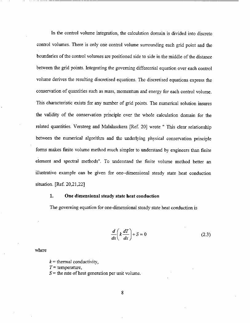
The governing equation for one-dimensional steady state heat conduction is
dx k—
V dx) + S = 0 (2.3)
where
k = thermal conductivity, T = temperature, iS = the rate of heat generation per unit volume.
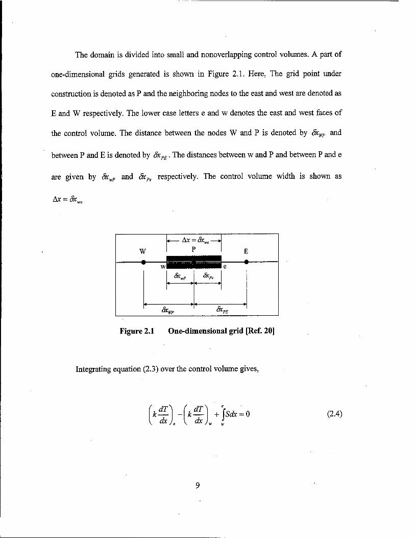
The domain is divided into small and nonoverlapping control volumes. A part of
one-dimensional grids generated is shown in Figure 2.1. Here, The grid point under
construction is denoted as P and the neighboring nodes to the east and west are denoted as
E and W respectively. The lower case letters e and w denotes the east and west faces of
the control volume. The distance between the nodes W and P is denoted by Sx^ and
between P and E is denoted by öxPE. The distances between w and P and between P and e
are given by äcwP and &cPe respectively. The control volume width is shown as
Ax = &c,„a
W
-*-
E
SxwP &cPe
& twp & CPE
Figure 2.1 One-dimensional grid [Ref. 20]
Integrating equation (2.3) over the control volume gives,
f JT\ f dT\ dT k
dx +
W VI
jSdx = 0 (2.4)
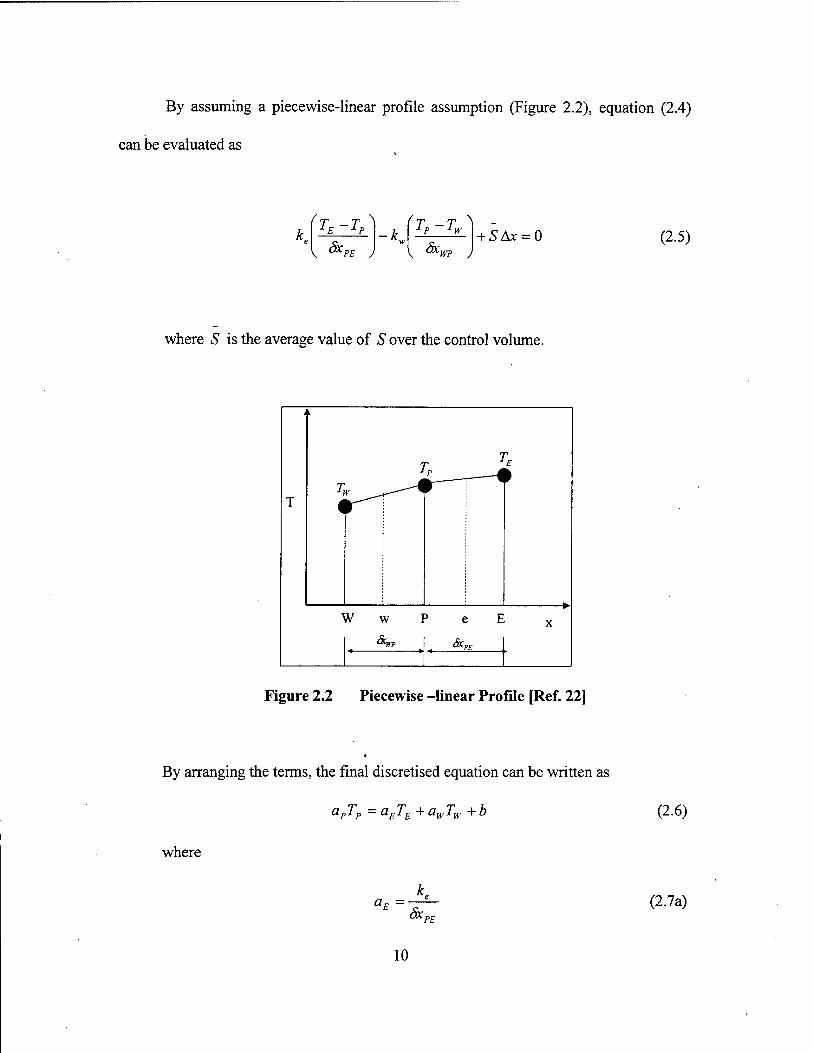
By assuming a piecewise-linear profile assumption (Figure 2.2), equation (2.4)
can be evaluated as
(T —T~\ lE 1P
Sx \ a*PE J -K
( T T ~\ 1P 1w
Sx + SAx = 0 (2.5)
where S is the average value of S over the control volume.
T
L
T v ^_^_
7 r 1 r
1 kV w I 5 e E X
Figure 2.2 Piecewise -linear Profile [Ref. 22]
By arranging the terms, the final discretised equation can be written as
aPTp =aETE +awTw +b (2.6)
where
aE = Sx PE
(2.7a)
10
aw = Sx, WP
ap =aE+ aw
b = SAx
(2.7b)
(2.7c)
(2.7d)
11

12
IE. MODEL DEVELOPMENT
A. DEFINING THE WORKPIECE
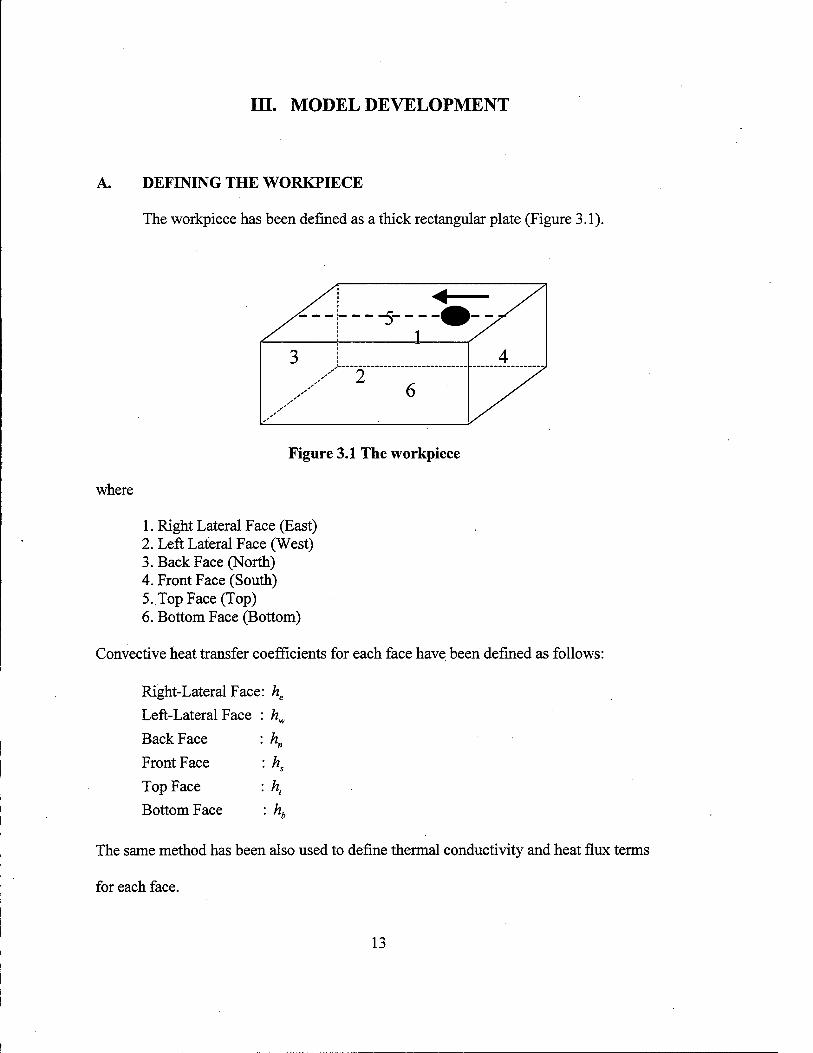
The workpiece has been defined as a thick rectangular plate (Figure 3.1).
5 9 1
H^/
3 4
S 2
6
Figure 3.1 The workpiece
where
1. Right Lateral Face (East) 2. Left Lateral Face (West) 3. Back Face (North) 4. Front Face (South) 5. Top Face (Top) 6. Bottom Face (Bottom)
Convective heat transfer coefficients for each face have been defined as follows:
Right-Lateral Face: he
Left-Lateral Face : hw
Back Face : hn
Front Face : hs
Top Face : ht
Bottom Face : hb
The same method has been also used to define thermal conductivity and heat flux terms
for each face.
13
B. BOUNDARY CONDITIONS
1. Top Face
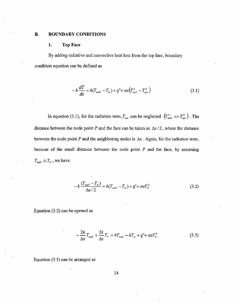
By adding radiative and convective heat loss from the top face, boundary
condition equation can be defined as
~k% = h{Twa" -rj + ^"+^fc -r-) f3'1)
In equation (3.1), for the radiation term, Tmr can be neglected. \T*aU » T*ur). The
distance between the node point P and the face can be taken as Ax/2, where the distance
between the node point P and the neighboring nodes is Ax . Again, for the radiation term,
because of the small distance between the node point P and the face, by assuming
Ty>all = TP » We haVe
_k(Twal, -T ) = _rj + q„+ a£T< {32)
Ax/2
Equation (3.2) can be opened as
Ik Ik ~—Twal, +—TP = hTwea-hTm+q"+<xT; (3.3)
Ax Ax
Equation (3.3) can be arranged as
14
/<->/, \ ■ wall
2k_
vAx j + h
lie = —TP+hTx-q"+asTP
4
Ax (3.4)
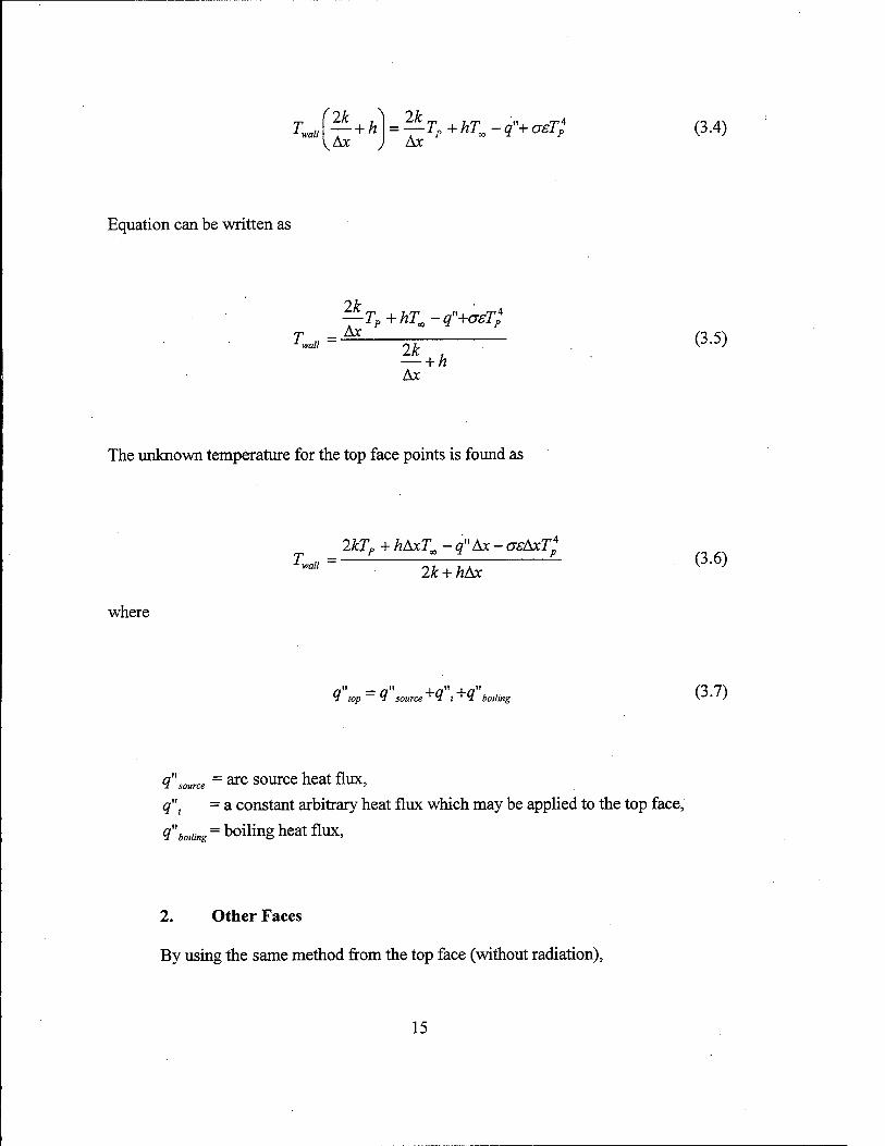
Equation can be written as
T = 1wall
2A
Ax TP+hTa>-q"+(7€TP"
2k_
Ax + h
(3.5)
The unknown temperature for the top face points is found as
■*wall ~
2kTP + hAxTa -q"Ax- crsAxT*
2k + hAx (3-6)
where
„n „it (z top tf source " l '9 boiling (3.7)
<l"sou™ = dxc source heat flux, q"t = a constant arbitrary heat flux which may be applied to the top face,
<fboiung = boiling heat flux,
2. Other Faces
By using the same method from the top face (without radiation),
15
_2kTP+hAxTcc-q"Ax Kall~ li^Mx (3-8)
3. Simulating the Arc
To simulate the heat input from the arc to the workpiece, it is assumed that the
heat input distribution of the arc have a Gaussian distribution on the top face of the
workpiece. The general equation is
Q = q0je '• 2mdr (3.9)
where
Q = the total heat input into the workpiece, q0 = the volumetric energy generation rate,
r0 - the radius of the heat input distribution,
d = the exponential factor,
By solving equation (3.9), the volumetric energy generation rate can be found as
q0=^ (3.10) m-0
4. Boiling Heat Transfer
Modes or regimes of boiling and the related equations can be classified as follows
(where ATe =TS-Tsal):
16
a. Free Convection Regime (ATe < 5 °C)
In this regime, natural convection effects determine the heat transfer
between the heating surface and surrounding liquid. Recommended correlations for upper
surface of heated plate are [Ref. 25]
NÜL = 0.5ARaxl" [itf <RaL<W) (3.11)
NUL = 0.15Jta}/3 (lO7 <RaL <10n) (3.12)
where the Rayleigh number,
Rai = gß(T,-T.)ü (313)
va
here
g = gravitational acceleration, m/s
and
ß = volumetric thermal expansion coefficient, K"1
v = kinematic viscosity, m /s a = thermal diffusivity, m /s L = characteristic length, L = Plate surface area (As)l Perimeter (P)
h = *^ (3.14)
and the value of heat flux is,
17
g"=h(Ts-TJ (3.15)
b. Nucleate Boiling Regime (5 °C < ATC < 30 °C)
The most useful nucleate pool boiling correlating equation was developed
by Rohsenow [Ref. 23, 24, 25,],
q"=Mihfs g(Pi-pv)
1/2 / cnATe pj e
(3.16) AAPr".
where the subscripts s, 1, and v express surface, saturated liquid state and vapor state. The
definition of each term in equation (3.16) are as follows:
/// = viscosity of the liquid, kg/ms
hfg = latent heat of vaporization, J/kg
g = gravitational acceleration, m/s2
P* = density of the saturated liquid, kg/m3
P* = density of the saturated vapor, kg/m3
a = surface tension of the liquid-to-vapor interface, N/m cpl = specific heat of saturated liquid, J/kgK
*Te = Ts-Tsa,
Pr, = Prandtl number of the saturated liquid
n = 1.0 for water, 1.7 for other fluids Csf = empirical constant that depends on the nature of the heating
surface fluid combination and whose numerical value varies from system to system
But, in underwater welding, the surrounding water temperature is below the
saturation temperature (between 0°C and 30 °C). This is called as the heat transfer to a
subcooled liquid. For the subcooled boiling, the heat flux can be estimated as [Ref. 23]
18
q"=qs"i i + ^l\^sat * liquid) 24 nhf.pv
Pv
og(p,-pv)
1/4
where
*/ a,
■■ thermal conductivity of the liquid, W/m.K : thermal diffusivity of the liquid (k I pcp), m
2/s and,
(3.17)
3 g(Pl-Pv)
1/2
PV
Og(Pl-Pv)
1/4
(3.18)
c. Transition Boiling Regime (30 °C < ATe < 120 °C)
For the transition-boiling regime, no sufficient theory has been derived.
This regime is between the maximum and minimum heat fluxes where [Ref. 23,25],
q"mxi = 0.U9hfgPv °g(Pl-Pv)
1/4
(3.19)
9"Bän = 0.09pvhJjs gv(Pi-pv)
(PI+PVY
1/4
(3.20)
By assuming a linear heat flux distribution in the transition boiling regime
(Figure 3.2), it can be written,
logfa"- ) ~ logto"^ ) __ logfa") - logta"^ ) Iog30-logl20 logAre-logl20
(3.21)
19
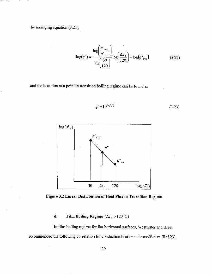
by arranging equation (3.21),
log ^ max
logfo") " min )
log
( AT ~]
30
V120y
(3.22)
and the heat flux at a point in transition boiling regime can be found as
»_ inlos(?") q"=\0 (3.23)
logo",)
4 " max
>
4
\ H min
30 A7; 120 log(A7;)
Figure 3.2 Linear Distribution of Heat Flux in Transition Regime
d. Film Boiling Regime (A7; > 120°C)
In film boiling regime for flat horizontal surfaces, Westwater and Breen
recommended the following correlation for conduction heat transfer coefficient [Ref.23],
20
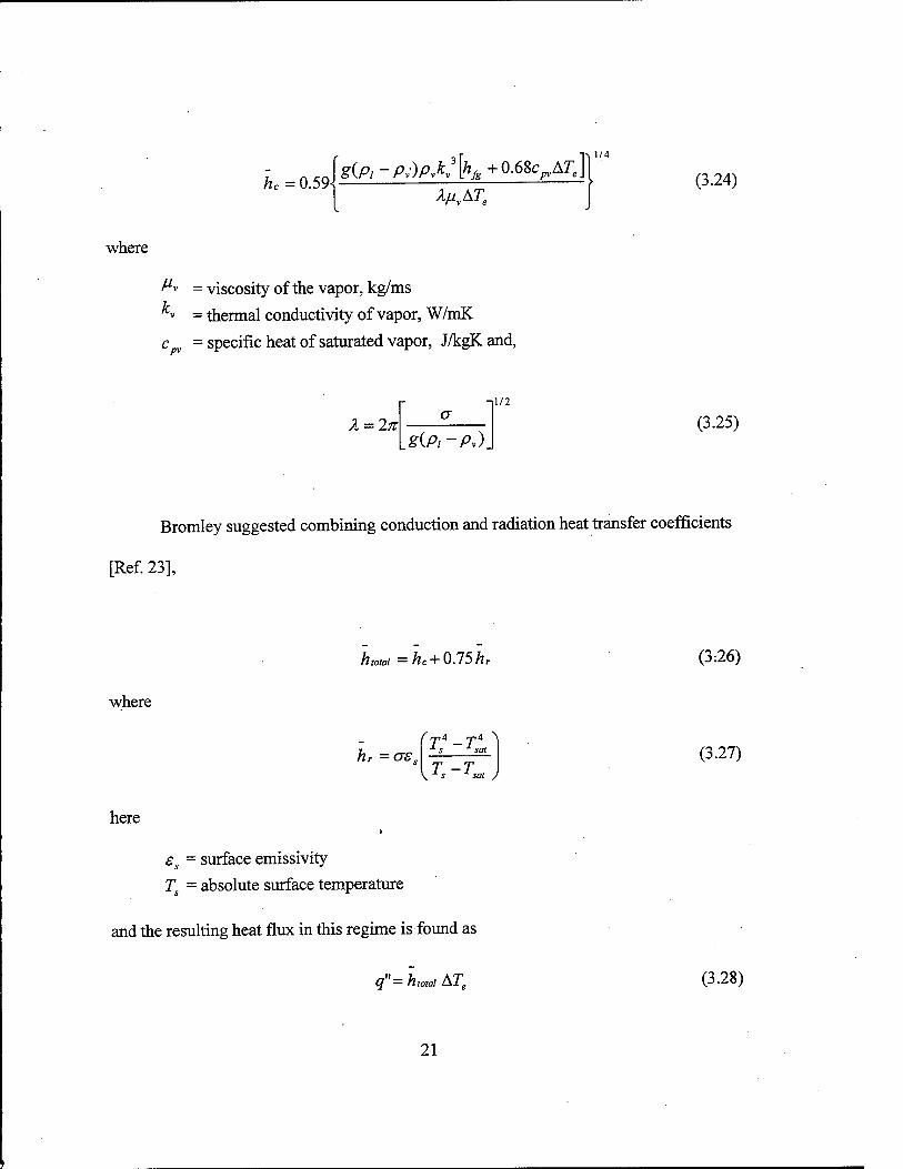
he = 0.59- 'g(p, -PJ)PX%S +0.68^ATJ
A//vA7e
1/4
(3.24)
where
^v = viscosity of the vapor, kg/ms v = thermal conductivity of vapor, W/mK
cv = specific heat of saturated vapor, J/kgKand,
X-2n g(Pl-Pv).
1/2
(3.25)
Bromley suggested combining conduction and radiation heat transfer coefficients
[Ref. 23],
htotal =hc+ 0.75 hr
where
hr =<JS,
' rjiA rp4 ^ * s * sat
T -T \xs x sat J
here
ss = surface emissivity
Ts = absolute surface temperature
and the resulting heat flux in this regime is found as
q"= htotai ATe
(3:26)
(3.27)
(3.28)
21
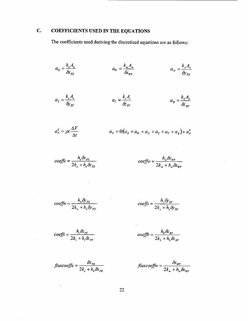
C. COEFFICIENTS USED IN THE EQUATIONS
The coefficients used deriving the discretised equations are as follows:
KA kA kA n — e e n — w w
E ~~ Ä, aw ~ "^ UN SxpE öxjyp öy PN
kA. „ -k<A> „ _M* as=tr °T=ir a*--^r- tysp ten ozBp
a0p = PC~Äf ÜP = 6^£ + °W + °N +aS+aT+ ÜB)+ "I
he&cPE KäXwp coeffe- — coeffw= M m
2ke + hedxPE 2kw + h^&Cwp
KfypN _«._ h,&sp coeffn = "-^ coeffs IK+KfypN 2ks+hsSy^ s ' "susSP
coeffi= h'&" coeßb- A'&" 1kt + htdzpj 2kb + hbdzBP
fluxcoeffe = — flvxcoeffw - ^ 2ke+heSxPE 2kw+hwäcwp
22
fliacoeffn = fypN
2kn+hnöyPN fluxcoeffs = fysp
2ks+hsSysp
fluxcoefft = dz PT
2k, + ht&PT fluxcoeffb ■■
dz BP
2kb+hbSzBP
radcoeff = PT
2kt +htSzPT
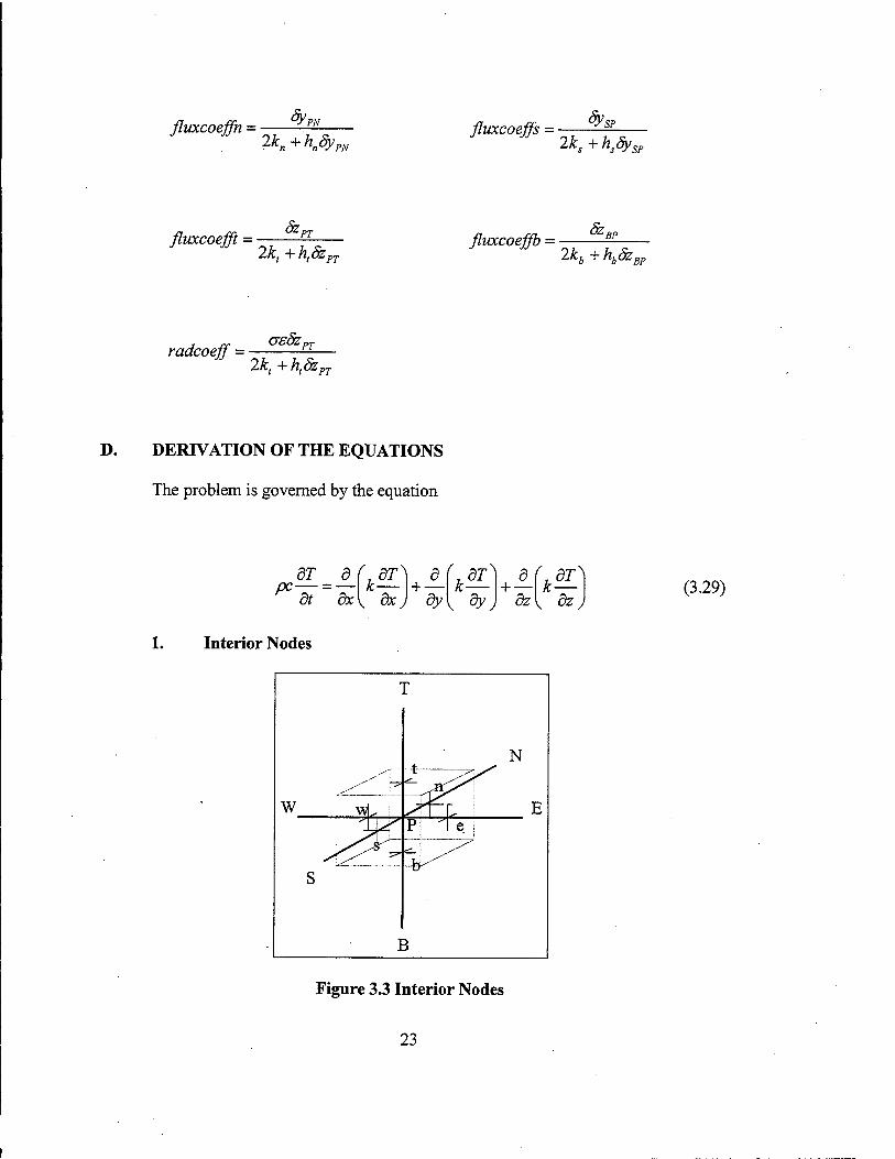
D. DERIVATION OF THE EQUATIONS
The problem is governed by the equation
8T d pc— = —
dt dx f, dT} d k— + —
r7 8T^ k—
v fyJ dz
r78T^ k—
V dz j (3.29)
1. Interior Nodes
r
N ...A ^
,s> s- j^\
w vyl ' L j E p He j
*r^ .^ i-_^ u ̂ ^
s
I
U
3
Figure 3.3 Interior Nodes
23
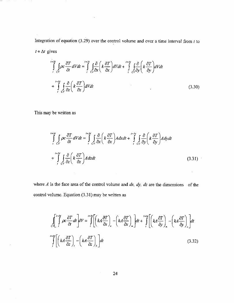
Integration of equation (3.29) over the control volume and over a time interval from t to
t + At gives
1+&1 dT „., ,+i rd(,&T}„„ '+? cdf,dT^ JJ^*=J£*£**+J£* l cv , cvdx\ dx) f c
Jvdy{ dy
dVdt
f c{dz{ dz) (3.30)
This may be written as
\pc—dVdt- —\k— Adxdt+ —\k— l CV t cv dx\ dx
Adydt
t+At
+ J }±U°" l CV dz\ dz
Adzdt (3.31)
where A is the face area of the control volume and dx, dy, dz are the dimensions of the
control volume. Equation (3.31) may be written as
t+At n en
t+At
dT , pc—dt ^ dt
t+At
dV: kA dT
dx Vr V dx
t+At
dt+ | kA df] dy
\
Jn
dt
M dz
'kA*? \ dz Jb
dt (3.32)
24
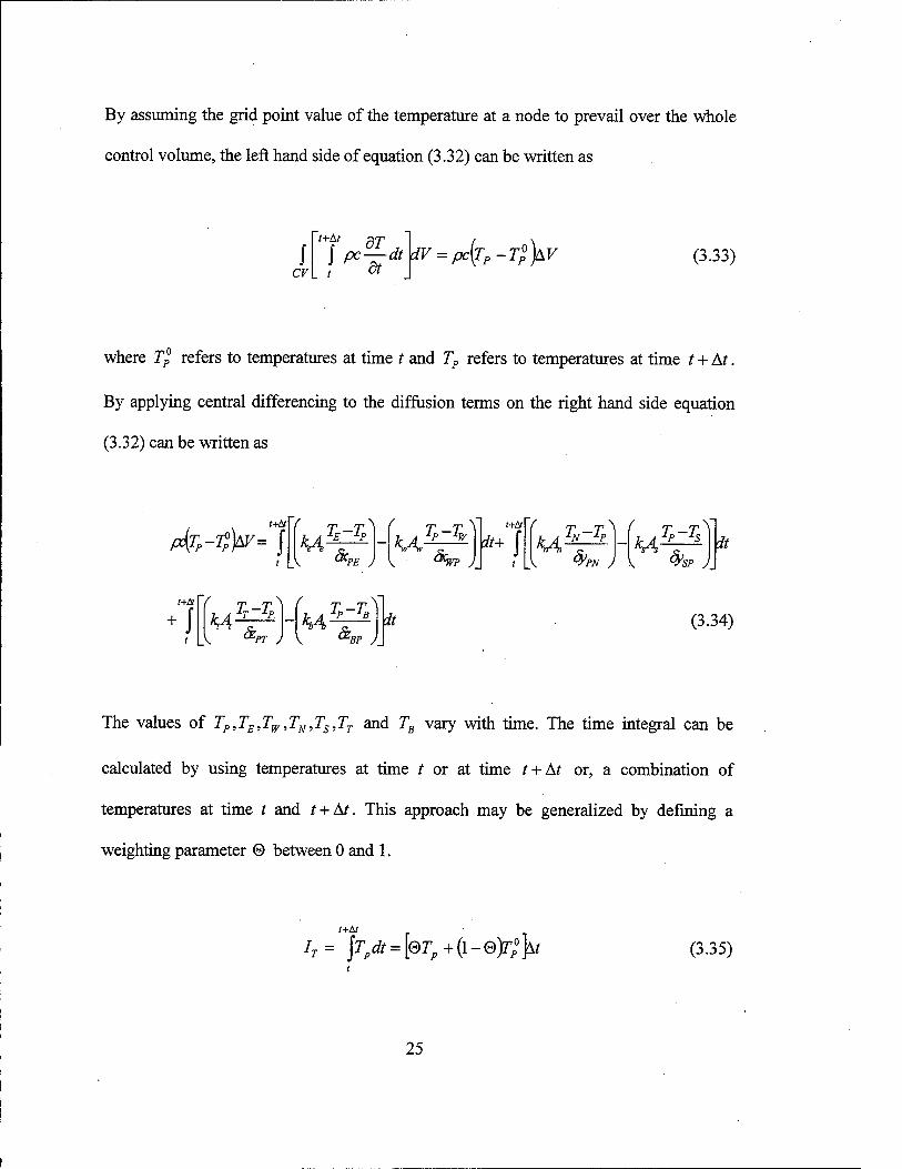
By assuming the grid point value of the temperature at a node to prevail over the whole
control volume, the left hand side of equation (3.32) can be written as
J cv
t+At
j pc^dt^lV = pc(TP-T°)AV (3.33)
where Tp° refers to temperatures at time t and Tp refers to temperatures at time t + At.
By applying central differencing to the diffusion terms on the right hand side equation
(3.32) can be written as
P(TP-I°)AV= J K4?B Tp 5c, "PE J
KAw T -T t+dt
Jt+j u% Tp fy} PN J
T -T
&i SP J
it
r+Ä
+ KA T p
&> ■PT J
T -T
&, •BP J
it (3.34)
The values of TP,TE,TW,TN,TS,TT and TB vary with time. The time integral can be
calculated by using temperatures at time t or at time t + At or, a combination of
temperatures at time t and t + At. This approach may be generalized by defining a
weighting parameter 0 between 0 and 1.
t+Al
iT= \Tpdt = [eTp+(i-®)r°l\t (3.35)
25
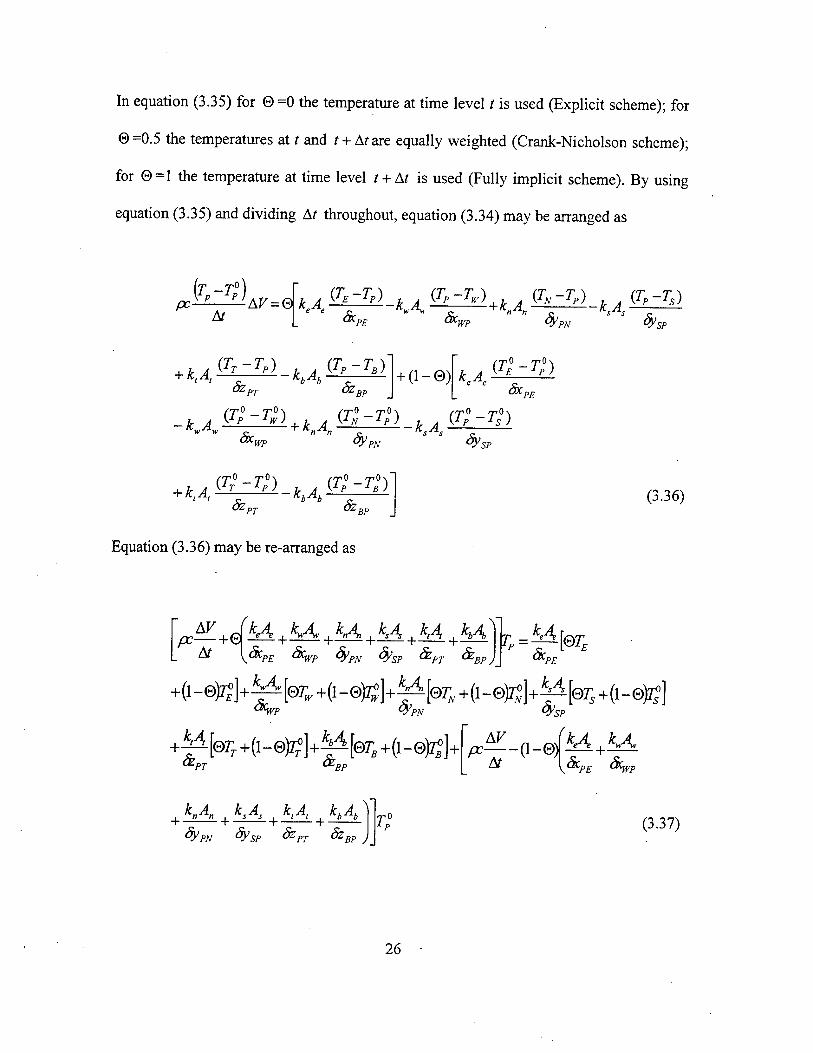
In equation (3.35) for 0 =0 the temperature at time level t is used (Explicit scheme); for
0=0.5 the temperatures at t and t + Ataxe equally weighted (Crank-Nicholson scheme);
for 0=1 the temperature at time level t + At is used (Fully implicit scheme). By using
equation (3.35) and dividing Ar throughout, equation (3.34) may be arranged as
pc- fc-tf) At
AV=S *A^-KA (I^M+KA,^fM-kA<^M
Sx PE Sx, WP &. PN Sy. SP
+ k,A. (TT-TP)
Sz -KA.V'-™ vb^b
PT
0 rrO
Sz BP
0 rrO
+ (1-0) kA {Tz~T*]
Sx PE
,k^2lfSi+kmAmVL3l-k,ZLni Sx WP %>PN &. SP
+ kA^Tr-Tp) ki (T?-T°) KtAi Ö KbAb 7.
PT Sz BP (3.36)
Equation (3.36) may be re-arranged as
&■
AV i efu . kA> ikA ikA i kA , M At äcPE ö^p fyPN fysp &pT &t BP J
7L M [QTE
+(i_0)^]+M:[err+(i-0K]+M cKfyp cyPN
PE
KA QTN+(^-®Kh^[®Ts+(l-®^}
+M[0rr+(1_0)7?]+M[07;+(1_0K & PT &
+ BP
§>SP
AV ( pc (1-0)
At A *A+KA CKpE OC^p
K^Ji.^ K./L. K. A. KL Ak ■ n n . 5 s . t t . o b
8yPN SySP Sz PT SZBp j T (3.37)
26
By putting the defined coefficients from the previous section, equation (3.37) may be
written as
[a°P + ®(aE+aw +aN+as +aT + aB )]rp = aE [®TE + (\-®)T°]
+ aw[®Tw+(l-®)T°]+aN{eTN+{l-e)r°]+as[®Ts+(\-®)rs0}
+ aT [®TT + (l - ®)r° ] + aB [®TB + (l - ®)T° ] + [a°P -(\-®)(aE +aw +aN+as+aT + aB)]TP (3.38)
Finally, by grouping the known and the unknown terms at each side, the discretised
equation is found as
apTp -®aETE -®awTw -®aNTN -®asTs -®aTTT -®aBTB = (1-0)
[aET»E +awT» +aNT° +rf +«Ä° +aBT°]+[al ~(1-©)(** +aw + aN+as + aT+aB)]TP (3.39)
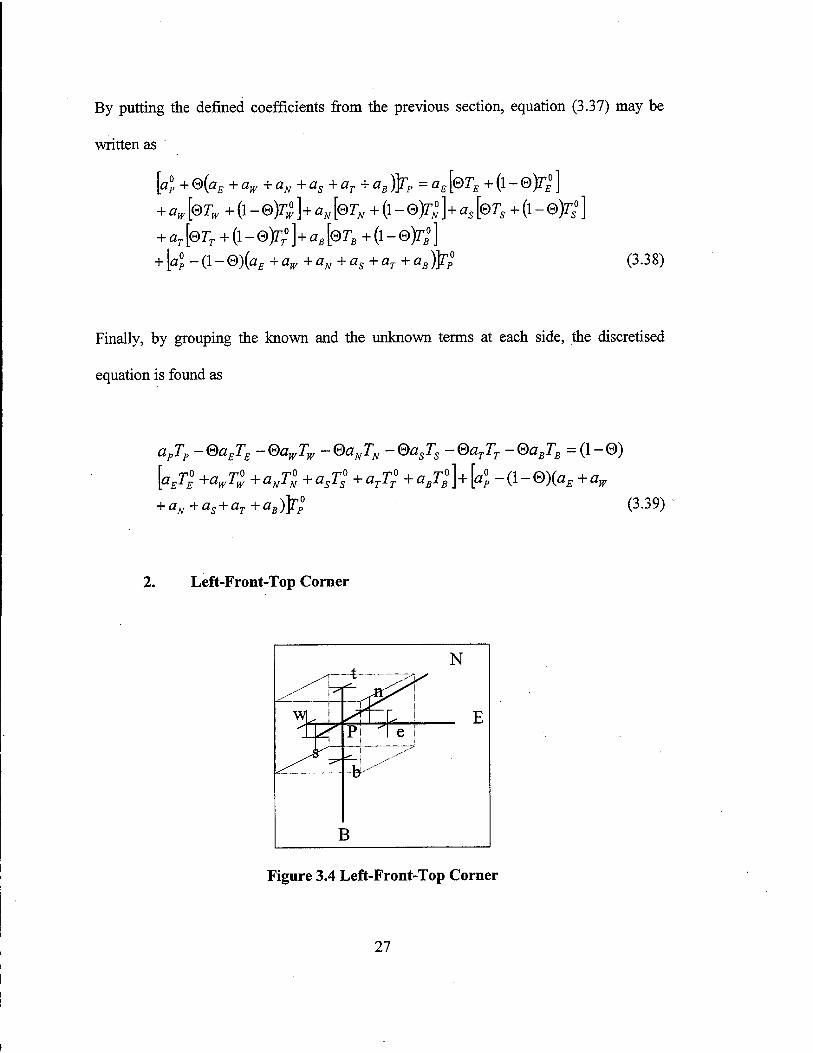
2. Left-Front-Top Corner
± _ _ N
—■ ^s-
F.
s ^i ra>^
W / S P e
A V ^ h ,-'
]
u
3
Figure 3.4 Left-Front-Top Corner
27
By using the same method from equations (3.30-3.33), equation (3.29) can be written as
/+A/ / rp rp jf. .TT-T. PE J & KA-
TP-TW
V Sc, WP )
t+N
it+j KA T -T lN XP
§>PK J
+ M,^-* &
f rp rp \
k„A h h
PT
vA^i & BP J
dt
WSP J
(3.40)
*
In equation (3.40), Tw and Ts take the value of equation (3.8) and Tr takes the value of
equation (3.6). By using these values and equation (3.35), we have
pc (T
P Tr\v = e
At o VE 1P) c.
CKpE OXjyp
2kjrp+hwäcWPTai -qnw&.l WP
2K+K&WP
+M.(7;_7>)_ fypN fySP
2ksAs(rr 2ksTP+hsöySPTx-g"söy, rp _ —'S^P ' "$ VTSP* 1P
s "SSP
2K+hsfy. SP
+ 2k,A,
Sz PT
2k,Tp +htdzPTT„ -g" &PT -as&PTT}
+ (1-0) k.A
Sx
2k, + h,&
?k A (rE-rP)-^^
-TD PT
KA b^b
ÖZ (TP-TB)
BP
E ~lP PE ÖX WP
T _ lP
2kJP+hwSxm,Tx-q"w&i
2K + K&wp
, k„An 0 _T0x_fMi + r. \2N 1P ) P
VPN WS?
,„ 2k5T«P+hsdySPT„-q"söy, SP
2ks+h5Sy, S^VSP
+ 2k,A,
8z PT
2ktTP +h,&PTTx -g"top&PT -GS&PTT}
2kt +htözPT
lP
J
ozBP
(3.41)
Equation (3.41) may be arranged as
28
AV pc—+0-^- +
+
At
2k,A,
keAe 2kwAw
& PT y 2k, + ht&PT i
2k I w
V 2kw +K®
CWPJ
| *„4 | 7kA L 2ks
fypN fysp I 2ks+hsfy, SPJ
KA ' & BP
L D —' 3c
[GTE +(l-®)T°E]+^[®TN +(l-0)7^] PE &
+ ̂ k+d-0)i:]- & BP
AV pc— -Q-&i-S-± + ^ At ' '
KA , 2*w4 QkpE CKfl/p
PN
Ik I w
v 2kw +K®CWPJ
+ KA fypN
+- 2k A
* SP
1 — 2k
2ks+hsSySP
\2*,V & PT
1 — 2k,
v 2k, +h,&PT j + KA
& BP
rpQ lP
+ 0 2kwAwfhwäcwpTx-q"wäcl
äc.
2ktA,
wp
2k +h äc„n, i + -
2kA
Sy.
& PT
h,&PTTa -g",op &PT -as&PTTf
2k, +h,dzPT
SP
4\
hsfyspT«-<l"söySP
2ks+hsSySP j
+ (1-0) 2«w^W
<Sc, WP 2kw + nvlax.wp j
2kA, (h.frJT„ -q\ dv,P\ 2*1,4 (K&rJ* ~4\op&PT-ae&PTT*
* SP V 2ks+hsfy isyysp j & PT V 2k, +h,& PT
(3-42)
Equation (3.42) may be re-arranged as
pc—+0 -J-L + At
+
KA , 2v4
2k,A, ( h,&i
@*P£ Ofcyff
"w"%7>
\2kv/+hJkWP j . "-«4 , 2*;4
#w ^:
^ 5P
'äV ^SP v^+^^s?y
+
rtAjic*pj>
^[eTB+(i-®)it]+
KA 'BP.
TP =M[0r£+(i-0)^]+|4L[©7;+(i-0)^] &, PE dyL PN
BP
AV pc-—(1-0) ^ At
KA ! 2ftw4 AA WP
2£„,+/u&» 'P£ '-"'WP \^n-w^'lw'MWPj
j ^»4 j 2fty4
4W #SP
^ ^s/»
V2^+//5^s/,y +
2*4 &, ,pr
h,&PT
2k, + h,&PT
KA BP.
7?+0 2kwA
WP
K&wpT«, <fw&i WP
2kw + K&wp 2K + K&WP ) fysp + 2*,4 4M Q"S%>sp \}KA
2ks+hsSySP 2ks+hsSy, SPJ & PT
29
h,özPTTx €top &PT OE&pjTp
v 2k, + h, &PT 2k, +ht&PT 2k, + h, dzPT j
q\ axt wp 2ksAs hsfySpT*
+ (1-0)
l"s %>SP
2M* &c WP 2kw+hw&lvP
2kw+hw&WP) oySP [2ks+hsSySP 2ks+hsSy
<l"top &PT
2k, + h,dz
+ 2*,4 SP ) & PT K2k, +hl&PT
PT
<JS5ZPTTP
2k, +h,SzPT j (3.43)
By putting the defined coefficients from the previous section, equation (3.43) may be
arranged as
[a°P + ®[aE + 2aw (coeffw) + aN + 2as (coeffs) + 2aT {coeffi) + aB ]]TP
= aE[®TE +(l-e)T°}+aN{QTN +(l-e)T°]+aB[®TB +(l-@)T°} + [a°P - (1 - ®)[aE + 2aw {coeffw) + aN + 2as (coeffs)
+ 2aT (coeffi) + aB Jr,0 + ®[2aw [(coeffw)Tx - (flwccoeffw)q\ ] + 2as [(coeffs)Ta - (fluxcoeffs)q"s ]
+ 2aT [(coeffi)Ta - (fluxcoefft)q",op -(radcoefft)^ ]
+ (1 - ®)[2aw [(coeffw)Ta - (fluxcoeffw)q" w ]
+ 2as [(coeffs)TK - (fluxcoeffs)q"s ]
+ 2aT {(coeffi)^ - (fluxcoefft)q",op -(radcoefft)TPA ] (3.44)
by putting heat flux terms from equation (3.7), equation (3.42) may be written as
[a°P + e[aE + 2aw (coeffw) + aN+ 2a s (coeffs) + 2aT (coeffi) + aB ]Jrp
= aE [®TE + (1 - ®)T°]+ aN [®TN + (1 - 0)7;° ]+ aB [®TB + (1 - 0)7B° ]
+ [a°P - (1 - G)[aE + 2aw (coeffw) + aN + 2as (coeffs)
+ 2aT (coeffi) + aB flr/ + [2aw (coeffw) +2as (coeffs) + 2aT (coefft)]Tx
- 2aw (fluxcoeffw)q"w-2as (fluxcoeffs)q" s -2aT (fluxcoefft)q",
30
• 2aT (fluxcoejft)q"source -2aT (fluxcoefft)q"boiling -2aT (radcoeff)Tp4 (3.45)
and, the discretised equation may be written as
[a°P + ®[aE + 2aw (coeffw) +aN + 2as (coeffs) + 2aT (coeffi)+ aB fl7/p
- ®aETE - eaNTN - ®aBTB = (1 - ®)[aET° + aNT°N + aBT<B ]
a°p - (1 - ®)[aE + 2aw (coeffw) + aN + 2as (coeffs) + 2aT (coeffi)+ aB ]r,
2aw (coeffw) + 2as (coeffs)+ 2aT (coeffi)]Tx - 2aw (fluxcoeffw)q" w
- 2as (fluxcoeffs)q"s -2aT (fluxcoeß)q", -2aT (flwccoeffi)q" source
- 2aT (flwccoefft)q\oiling -2aT (radcoeff)TP (3.46)
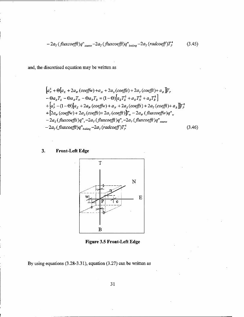
3. Front-Left Edge
r
.. t__ .._._._ N
.,-''"' ^.-'■^
F
^ fiCs^ w
**■
^ s p e A r _^..-'" ,-" u «,.-""'
I
u
1
Figure 3.5 Front-Left Edge
By using equations (3.28-3.31), equation (3.27) can be written as
31
r+Ä
pfrP-tW= J U5"5 <5c.
up w ■PE J ÖCfyp J.
it+\ u^ T -T
4i «v y
T -T kAP s
* 5f y
*
/+A/
M, T _r -'r if
f
PT J
T -T ^
v & £/> /
* (3.47)
In equation (3.47), 7^ and Ts take the value of equation (3.8). By using these values
and equation (3.35), we have
pP' 7>°)AF=e| Ar
kA
Sc (TE-TP)~ IKMT KJr+hAmT.-<f*&i
PE &, WP TP~
WP
2kw+K&wp
2k A +^-(TN-TPy
fypN WSP
2ksTp+hsfyspTx-<f'sSy; SP
' & (TP-TB)
BP
+ (1-0)
2ks +hsfySP
( 7
P
&PT
KA ,JQ „p. 2£»A jo 2kvTP +K^WP^CO ~V"w Sx-wp
+ki^(TN-rP)-^r
fypN WSP
CKpE CKfyp y
jo 2ksT?+hsfySPTx-q"sfySP
2ks +hsfySP
2kw +hw&m,
k.A, f"-t ST0 T'0\ ^b^b /"rO
& <rr
0-r;> KAu
PT ÖZ (rP-rB)
BP
(3.48)
Equation (3.48) may be arranged as
DC + 0 At
k»A„ ZK,„A„ e e , w v
OKpE ÜXyyp
2k.
2kw + KSxwp j + -
+ - 2k A. f
*. SP
1-- 2k,
^ 2ks + hsSySP J SzpT öz , k,A, kbAb
T 1" ■
BP
n n
fypN
_ keAe lp ~
STY PE ÖX
[0r£+(i-0)r£°]
32
+ ̂ - [®TN + (i - 8)7$ ]+£4- [©rr + (i - e)TT°]+M. [@rB + a _ ©^ ] dyPN dZpj. dzBP
pc^--(l-&) At
keAe 2kWA'W . f
- +
+ - 2k A
Sy SP
( - 1
V
(
2k
SxDr Sx
2k.
\ 2K + h„Sx, wuxWP J
fC„A„ n n
Zk,+K&sp
. K-A-t kbAb
(Ju p'p \JZi ryp
7>°+0
fypN
2kwAw ^aXjypT^ - q w Sx^,
Sx^ I 2kw + hdxv
2M. (KfyspT^-tf.fysp
+
fysp I 2ks+hs8ySP
2KAs(hsSySPTx-q"sSySP
Sy SP 2ks+hsSy ls^SP
+ (1-0) 2kwAw
wp V
Sx,
■w ' "v/^^WP
\ ■WP
wp V 2K + KSx VI 'wuxWP J
(3.49)
Equation (3.49) may be re-arranged as
DC + 0 At
k.A. 2k A. e e _i_ w w h^OXwp
Sx PE Sxjyp y2kw + h^SXwp j
.knAn 2ksAs
. kfAt kbAb
Szpj. SzBP
T = lp k.A.
fypN Sy
k*,-A.„
SP
KSy, syrsp
K2ks+hsSySPj
Sx [®TE +(1-®)TE
0]+^L[®TN +(1-0)7^]
PE Sy PN
fch-A-i, +^-[®TT +(i-0)rr°]+-^^[©r5 + (i-0)rs°]+
Sz PT Sz BP
AV pc—-(l-®) At
k.A. Sx PE
2.KWA„
Sx, wp
f7wäxm>
\2kw +hwSxwp j
K~A„ LK.A. , n n , s s
SP SyPN Syt
KSy, s^SP
s2ks+hsSySPj
+ -L-L + - U** DT* CK DD
T--0 LP
+ 0 f h..Sx^T w^^WP^x q\ Sx, w ^WP
V 2£w + "W"*W 2kw + h^SXwp j + -
2k A
Sy, SP
2ks+hsSySP) + (1-0)
Z/C„, A„
Sx, WP
hsSySPTx
\2ks+hsSySP
II c„ ^ */ w OXjyp
\2kw + nwSxwp 2kw + h^SXwp y
h Sx T
+ 2ksAs{ hsSySPTx
Sy, SP
q\ sy, \
s "SSP
2ks+hsSySP 2ks+hsSySP
33
(3.50)
By putting the coefficients from the previous section, equation (3.50) may be written as
[a°P + ®[aE + 2aw (coeffw) +aN + 2a s (coeffs) + aT + aB Jr?
®TE + (1-®)T° + aN[®TN + (\-®)T°]+aT[®TT + (1-0)^°]
®TB + (\-®)T°}+[ap -(l-®)[aE + 2aw(coeffw)+aN
+ 2as(coeffs) + aT + aB^ + ®[2aw[(coeffw)Tx - (fluxcoeftyq" w]
+ 2as[(coeffs)Tx -(fluxcoeffs)q"'J+(1 -®)[2aw[(coeffw)TK -(fluxcoeffw)q"w] + 2as [(coeffs)^ -(fluxcoeffs)q" s J (3.51)
= a
+ a
Equation (3.51) may be arranged as
[ap1 + ®[aE + 2aw {coeffw) +aN + 2a s (coeffs) + aT + aB ]Jrp
+ aN[®TN+(l-®)T°]+ar[®Tr+(l-®)TT°]
+ [a°p - (1 - ®)[aE + 2aw (coeffw) +aN
+ 2as (coeffs) + aT + aB JT/ + [2aw (coeffw) + 2a s (coeffs)]T„ - 2aw (fluxcoeffw)q\ -2a s (fluxcoeffs)q" s
= a
+ a
®TE+(1-®)T°
®TB + (1-®)T°
(3.52)
Finally, the discretised equation may be written as
[a°p + ®[aE + 2aw (coeffw) +aN + 2as (coeffs) + aT + aB ]frP - ®aETE - ®aNTN
-®aTTT -®aBTB = (\-®)[aET« +aNT°N +aTTT° +aX]+[ai -0-®)k
+ 2aw (coeffw) + aN + 2as (coeffs) + aT + aB JT/ + \2aw (coeffw) + 2as (coeffs)^ - 2aw (fluxcoeffw)q\ -2a s (fluxcoeffs)q" s (3.53)
34
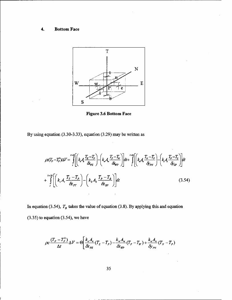
4. Bottom Face
w
T
_*■
N
E > ^
vA
s
s* P ^ e /^r -^
Figure 3.6 Bottom Face
By using equation (3.30-3.33), equation (3.29) may be written as
t+t*
fc(TF--®&y= J k^--5 3c, PE J
( T —T ~\
^ tyvp J
t+öt ' r„-2^ ">I4I c
#/>.
^ ^ ^A
V ^7w J
T -T xp xs
y Wsp j u it
t+&i
k.A TT-^ A r
& w y Ä (3.54)
In equation (3.54), TB takes the value of equation (3.8). By applying this and equation
(3.35) to equation (3.54), we have
At KAe (TE -TP)-^(TP -TW) + ^{TN -TP) Sx PE ÖX, wp Sy PN
35
öySP öz
+ (1-0)
2kU b-"-b
PT Öl BP
T - 2kbTp+hbözBPTm-q"bözBP
2kb+hbözBP j
\XE
1P) - \1p~Iw) + ~7 ^w_ipJ_T \Ip~Is)
tew» qyPN öys öx PE
0 rrO
"■WP 'SP
{ k,At Q r0 2kbAb ( Q 2^r,° + ^&^rM - q\ özBP \
°- 7 ° P 2kb+hh& öz PT ÖZ BP 'b^BP
(3.55)
Equation (3.55) may be arranged as
pc + © At
keAe ^ kwAw knAn ksAs ktAt 2kbAb
ox PE ÖX, wp
k.A.
öy
kA PN öysp özpT öz BP
1 — 2h
2kb+hböy, BP J
ÖX [®TE +(I-G)T°]+-£-?-[®TW +(i-0)r;]+^[©r, +(i-0)r„°]
PE ÖX, WP öy, PN
k.A, +^-[0r5+(i-0)rso]+^[0rr+(i-0)rr
o]+ öy, SP öz PT
pc—-(1-0) At
k.A. öx PE
kwAw | knAn ksAs ktAt 2kbA
öx
+ 0
• + • + + • WP fypN fysP fcpT
■+■ ÖZ BP
2k,
2kbAb
öz BP
K&BPT«>-q"b&
2kb+hbözBP
BP + (1-0) 2kbAb
2kb + hböyBP )
ÖZ BP 2kb+hbözBP jj (3.56)
Equation (3.56) may be re-arranged as
OC + 0 At
K.A. K„,A„, K„A„ K,A, K.A,
ÖX PE ÖX ■ + ■
WP fypN öy, +- 2kbAb
SP öz PT ÖZ BP
hbözBP
>2kb +hbözBP ,
36
k.A. [®TE +(I-®)T°]+^[®TW +(I-&)T:]+-^[®TN +(i-0)r;] <-PE VAWP
+^p-[®Ts +(i-0)rs°]+M-[0rr +(i-0)rr°]+
k^A
'FT
fypN
AV pc=—-(l-®)
-w—w ■-„—„ -s—s , *fA . ^b-"-b &„A„ ICrAr
8x, WP fypN $>SP & PT & BP
hbdzBP
2kb+hbözBPj
At
T;+®
k.A. 8x
2kbAb
dz BP
K&BPT„ q\ & BP
2kb + hbözBP 2kb + hbdzBP j + (1-0)
2kbAb
dz BP
K&BPT«
2kb+hbSzBP
q\ dz BP
2kb+hb8zBPj
PE
(3.57)
By using the defined coefficients, equation (3.57) may be written as
[a°P + e[aE + aw +aN +as+aT + 2aB {coeffb)^P = <*E [®TE + (1 - ®)T° ]
+ aw[®Tw + (l-®)T°}+aN[®TN + (l-®)T^]+as[®Ts + (1-0)7?]
+ aT [®TT + (1 - ®)T° ] + [a°p - (1 - ®)[aE + aw +aN +as+aT + 2aB (coeffbj^T*
+ ®[2aB [((coeffl?)TK ) - ((fluxcoeßb)q" b)]
+ (1 - ®)[2aB [{(coeffl>)Tj-((fluxcoeJ?b)q"b)] (3-58)
■^0 lp
And, the discretised equation may be written as
[a°p + ®[aE + aw +aN + as+aT + 2aB (coeffbj$Tp - ®aETE - ®awTw - ®aNTN
-®asTs -®aTTT = (1 -®)[aET° + awT« + aNT° + asTs° + aTTT°]+ [4
- (1 - ®)[aE +aw+aN+as+aT + 2a B (coeffb)^ + [2aB (coeffb)]Tx
-2aB{fluxcoefib)q\ (3-59)
The resulting discretised equations for the other parts of the workpiece are as follows
37
5. Left-Back-Top Corner
[a°p + ®[aE + 2a w (coeffw) + 2a N (coeffh) + as+ 2aT (coeffi) + aB^Tp- OaETE
-easTs -®aBTB = (1 -®)[aET° + asTs° + aBT°]+ [a°P -(1 -®)[aE + 2aw(coeffw)
+ 2a N (coeffh) + as+ 2aT (coeffi) + aB ]TP + [2aw (coeffw) +2aN (coejfn)
+ 2aT (coej?t))rx - 2aw (fluxcoeffw)q" w -2aN (flvxceeffn)q\ ~2aT (flwccoefft)q"',
- 2aT (fluxcoeffi)q"source -2aT (flvxcoefft)q\oiling
- 2aT (radcoeff)Tp (3.60)
6. Right-Back-Top Corner jsjgni-uacK-1 op corner
[ap + S[2aE (coeffe) + aw + 2aN (coeffh) + as+ 2aT (coeffi) + aB J7> - ®awTw
-easTs -®aBTB = (\-®)[awT° +asTs° + aBTQ
B]+[al - (I-®)[2aE (coeffe)
+ aw + 2a N (coejfn) + as + 2aT (coeffi) + aB ]TP + \2aE (coeffe) +2aN (coeffh)
+ 2aT (coeffi)]Ta - 2aE (fluxcoeffe)q"e -2aN (fluxcoeffh)q\ -2aT (fluxcoeffi)q",
- 2aT (fluxcoeffi)q"smrce -2aT (fluxcoeffi)q"'Mllllg
- 2aT (radcoeff)Tp (3.61)
Right-Front-Top Corner
[a°p + ®[2aE (coeffe) + aw+aN+ 2as (coeffs) + 2aT (coeffi) + aBjr, - ®awTw
-®aNTN -®aBTB=(l-®)[awT° +aNT°N + aBTB°]+[a°p - (I-®)[2aE (coeffe)
+ aw +aN + 2as (coeffs) + 2aT (coeffi) + aB ]TP + [2a E (coeffe) +2as (coeffs)
2aT (coeffi)^ - 2aE (fluxcoeffe)q"e -2as (fluxcoeffs)q"s -2aT (fluxcoefft)q",
- 2aT (fluxcoeffi)q"smrce-2aT (fluxcoeffi)q"'bt>aiHg
-2aT (radcoeff)Tp (3.62)
38
8. Left-Back-Bottom Corner
[a°p + ®[aE + 2aw {coeffw) + 2a N {coeffh) + as+aT+ 2aB{coeffb)^p - ®aETE
-®asTs -®aTTT = (1 - ®)[aET° + asTs° + aTTT°]+ [a°P - (1 - ®)[aE + 2aw{coeffw)
+ 2a N {coeffh) + as+aT+ 2aB (coeffbjfr?
+ \2aw {coeffw) +2aN {coeffh) + 2aB {coeffbj\Tx - 2aw {fluxcoeffw)q" w
- 2aN {fluxcoeffh )q\ -2aB {fluxcoeffb )q\ (3.63)
Right-Back-Bottom Corner
lw [a°p + ®[2aE {coeffe) + aw+ 2aN {coeffh) + as+aT+ 2aB {coeffb)fP - ®awTw
-®asTs -®aTTT = {l-®)[awT° +asTs + aTT°]+[a°p -{l-®)[2aE {coeffe)
+ aw+ 2a N {coeffh) + as+aT+ 2a B {coeffb)]rp
+ [2aE{coeffe) +2aN{coeffh)+ 2aB{coeffbj\Tco - 2aE{fluxcoeffe)q"e
- 2a N {fluxcoeffh)q"n -2a B {fluxcoeffb)q" b (3.64)
10. Left-Front-Bottom Corner
[ap + ®[aE + 2aw {coeffw) + aN+ 2as {coeffs) + aT+ 2aB {coeffb)\$TP - ®aETE
-®aNTN -®aTTT = {\-®)[aET° +aX +aTTT°]+[a°p - {I - ®)[a E+2aw {coeffw)
+ aN+ 2as {coeffs) + aT+ 2aB {coeffb)]rp
+ [2aw {coeffw) +2as {coeffs) + 2aB {coeffbj\Tx - 2aw {fluxcoeffw)q"w
- 2a s {fluxcoeffs)q"s -2a B {fluxcoeffb)q" b (3.65)
11. Right-Front-Bottom Corner
[a°p + ®[2aE{coeffe) + aw+aN+ 2as {coeffs) + aT+ 2aB{coeffb)\fP - ®awTw
- ®aNTN - ®aTTT = (1 -®)[awT° + aNT° + <*X]+ [4 - (1 - ®)[2aB{coeffe)
+ aw +aN+ 2a s {coeffs) + aT + 2a B {coeffb)]rp
+ [2aE {coeffe) +2as {coeffs) + 2aB {coeffb)^ - 2aE {flvxcoeffe)q\
-2as{fluxcoeffs)q"s+2aB{fluxcoeffb)q"b (3.66)
39
12. Top Face
[a°p +®[aE +aw+aN +as + 2aT(coefft) + aB^P -®aETE -®awTw
-GaNTN -®asTs -®aBTB =(\-<d)\aET°E +awT° +*X + rf + <vC]
+ [a°p - (1 - ©)[aE +aw+ aN +as+ 2aT (coefft) + aB ])TP0
+ [2aT (coefft)]Tx - 2aT (fluxcoefft)q", -2aT (fluxcoefft)q"source
- 2aT (ßuxcoeß)q"boiling -2aT (radcoeff)TP* (3.67)
13. Front Face
[a°p + e[aE +aw+aN+ 2as(coeffs) + aT + aB~§TP - ®aETE - ®awTw
- ®aJN - ®aTTT - ©aBTB = (1 -®)[aET° +awT°+ aNT° + aTTT° + aBT«B ]
+ [a°p - (1 - ©)[aE +aw+aN+ 2as (coeffs) + aT+aB JT/
+ [2as(coeffs)Yx -2as(fluxcoeffs)q"s (3.68)
14. Back Face
[a°p + ®[aE +aw+ 2aN(coeffh) + as + aT + aB~§TP -®aETE - ®awTw
-®asTs -®aTTT -®aBTB = (\-®)[aET° + awT°+asTs°+aTTT°+aBT°]
+ [a°p - (1 - ©)[aE +aw+ 2aN (coeffn) + as + aT + aB JT/
+ [2aN(coeffh)]rx -2aN(fluxcoeffh)q\ (3.69)
15. Left-Lateral-Face
[a°p + ®[aE + 2aw (coeffw) + aN + as + aT + aB \jfp - ®aETE - ®aNTN
- ®asTs - ®aTTT -®aBTB = (1 - ®)[aET° + aNT° + asr5° + aTT* + aBTB ]
+ [a°p - (1 - ®)[aE + 2aw (coeffw) + aN+as+ar+aB JT/
+ [2aw (coeffw)]Tx - 2aw (flwccoeffw)q\ (3.70)
40
16. Right-Lateral-Face
[a°p + ®[2aE (coeffe) + aw + aN + as + aT + aB^TP - ®awTw - ®aNTN
- ®asTs - ®aTTT - ®aBTB = (1 - ®)[awT° + aNT° + asTs° + aTTT° + aBT°B ]
+ [a°p - (1 - ®)[2aE (coeffe) + aw + aN + as + aT +aB ^°
+ [2aE(coeffej\rx -2aE(fluxcoeffe)q"e (3.71)
17. Front-Top Edge
[a°p + ®[aE + aw+aN + 2as (coeffs) + 2aT (coeffi) + aB \$TP - ®aETE
-®awTw -®aNTN -®aBTB=(l-®)[aET° + awT° +asT*+aBT*\
+ [a °p - (1 - ®)[aE +aw+aN+ 2as (coeffs) + 2aT (coeffi) + aB Jrp0
+ [2as (coeffs) + 2aT (coefft)]Tn - 2as (fluxcoeffs)q"s -2aT (fluxcoefft)q"t
- 2aT (fluxcoeffi)q"source -2aT (fluxcoefft)q" boiling
-2aT(radcoeff)TP4 (3.72)
18. Front-Bottom Edge
[ap + ®[aE +aw+aN+ 2as (coeffs) + aT+ 2aB (coeffbj§Tp - ®aETE
- ®awTw - ®aNTN - ®aTTT = (1 - ®)[aET° + awT° + aNT° + aTT° ]
+ [a°p - (1 - ®)[aE +aw+aN+ 2as (coeffs) + aT+ 2aB (coeffbj§T°p
+ [2as (coeffs) + 2aB (coeffb)]Tx
- 2a s (fluxcoeffs)q"s -2a B (fluxcoeffb)q" b (3.73)
19. Back-Top Edge
[a°p + ®[aE +aw+ 2aN (coeffn) + as+ 2aT (coeffi) + aB ]j7> - ®aETE
-®awTw -®asTs -®aBTB = (1-0)^^° +awT° +asTs° +aBT°]
+ [a°p.- (1 - ®)[aE + aw + 2aN (coeffn) + as+ 2aT (coeffi) + aB JT/
+ [2aN (coeffn) + 2aT (coefft)]Tx - 2aN (fluxcoeffh)q"n -2aT (fluxcoeffi)q"\
- 2aT (fluxcoeffi)q"source -2aT (flvxcoefft)q\oüing -2aT (radcoeff)^ (3.74)
20. Back-Bottom Edge
[a°p + ®[aE + aw + 2a N(coeffii) + as+ar+ 2a B(coeffib)^Tp - ®aETE
-®awTw -®asTs -®aTTT = (\-®)[aET° + awT° + asTs° +aTTT°]
+ [a°p - (1 - ®)[aE +aw+ 2aN (coeffii) + as+aT+ 2aB (coejfb)^
+ [2a N (coeffii) + 2a B (coeJfb)]Tx
- 2a N (fluxcoeJfh)q"n -2a B (fluxcoeffib)q" b
21. Front-Right Edge
(3.75)
[a°p + ®[2aE (coejfe) + aw+aN+ 2a s (coeffs) + aT+aB^Tp- ®aw Tw
-®aNTN -®aTTT -®aBTB = (l-®)[awT° +aNT°N +aTTT° +aBT«B]
+ [a°p - (1 - ®)[2aE (coejfe) + aw+aN+ 2as (coeffs) + aT+aB JT/
+ [2a E (coejfe) + 2a s (coejfi)]Tx
- 2aE (fluxcoejfe)q"e -2a s (fluxcoeffs)q"s (3.76)
22. Back-Left Edge
[a°p + ®[aE + 2aw (coeffw) + 2aN (coeffii) + as + aT + aB J7> - ®aETE
- ®asTs - ®aTTT - ®aBTB = (1 - ®)[aET° + asTs° + aTTT° + aBT° ]
+ [a°p - (1 - ®)[aE + 2aw (coejfw) + 2aN (coeffii) + as+aT+aB J7>°
+ [2aw (coejfw) + 2a N (coeffin)]Tx
- 2aw (fluxcoeffiw)q\ -2a N (jluxcoeffn)q\ (3.77)
23. Back-Right Edge
[a°p + ®\2aE (coejfe) + aw + 2aN (coeffii) + as + aT + aB §TP - ®awTw
-®asTs -®arTT -®aBTB =(\-®)[awT° +asTs°+aTTT° +aßrß°]
+ [aJ - (1 - ®)[2aE (coejfe) + aw+ 2aN (coeffn) + as+aT+aB ^
+ VaE (coeffe) + 2aN i.coejfh)]rx
- 2aE (fluxcoeffe)q\ -2aN (fluxcoeffii)q\ (3.78)
42
24. Left-Lateral-Top Edge
[a°P + ®[aE + 2aw (coeffw) + aN+as+ 2aT (coefft) + aB \^P - ®aETE
- ®aNTN - ®asTs - ®aBTB = (1 - ®)\aET°E + aNT° + <rf + aBT°B ]
+ [a°p - (1 - ®)[aE + 2aw (coeffw) + aN+as+ 2aT {coefft) + aB Jrp0
+ [2aw (coeffiv) + 2aT (coefft)]Tx - 2aw (fluxcoeffw)q" w -2aT (fluxcoeffi)q"t
- 2aT (fluxcoeffi)q"source-2aT (flwccoefft)q"boiling
-2aT(radcoeff)T* (3.79)
25. Left-Lateral-Bottom Edge
[a°p + ®[aE + 2aw (coeffw) + aN+as+aT + 2a B (coeffbj§TP - ®aETE
- ®aNTN - ®asTs - ®aTTT = (1 - ®)[aET° + aX + «rf + «rf ]
+ [a I - (1 - ®)[aE + 2aw (coeffw) + aN+as+aT+ 2a B (coeffb)^°
+ [2aw (coeffw) + 2aB (coeffbj\Tx
- 2aw (flvxcoeffw)q\ -2aB (fluxcoeffb)q" b (3.80)
26. Right-Lateral-Top Edge
[a°p + ®[2aE (coeffe) + aw+aN+as+ 2aT (coefft) + aB jrp - ®awTw
- ®aNTN - ®asTs - ®aBTB = (1 - ®)[awT» + aNT°N + asTs° + aBT°B ]
+ [a°p - (1 - ®)[2aE (coeffe) + aw+aN+as+ 2aT (coefft) + aB Jrp°
+ [2aE (coeffe) + 2aT (coefft)^ - 2aE (fluxcoeffe)q"e -2aT (fluxcoeffi)q"t
- 2aT (fluxcoefft)q"source-2aT (fluxcoeffi)q"boiling
-2aT(radcoeff)Tp4 (3.81)
43
27. Right-Lateral-Bottom Edge
[a°p + ®[2aE (coeffe) + aw +aN+as+aT+ 2a B (coeffbj^- ®awTw
- ®aNTN - ®asTs - ®aTTT = (1 - ®)[awT° + aNT° + asTs° + aTTT°]
+ [a°p - (1 - ®)[2aE (coeffe) + aw + aN +as+aT+ 2aB (coeffbjfr?
+ [2a E (coeffe) + 2a B (coeffb)]Tx
- 2a E (fluxcoeffe)q"e -2a B (fluxcoeffb)q\ (3.82)
44
IV. RESULTS AND DISCUSSION
Results are presented for the different cases discussed in greater detail below. As
noted earlier, a variable sized and moving numerical mesh was used in such a way that
the arc was always positioned at the center of the mesh where the spacing is the finest.
The goal is to be able to resolve the large temperature gradient features around the arc
and yet not incur a large overhead of computer resources, which would be required, if the
grid was uniformly fine all over. This strategy however did require that a separate mesh
generating routine be used which did demand some extra computational resources. The
weld pool region was also modeled as a solid region but with a thermal conductivity
higher than the surrounding unmelted region to simulate the effects of weld pool
convection. The discontinuity in the thermal conductivity boundaries was handled using
the standard technique of employing harmonic averaging at the boundary. Since the
coefficients of the system of equations depend on the temperature, an iterative solution
technique was used to achieve convergence in such a way that the maximum temperature
difference between two consecutive iterations at any grid point was no more than 0.1 °C.
The numerical solution method was used to examine different cases in freshwater
for a 40-mm-thick 70 x 90 mm workpiece with a moving heat source in the positive y-
direction.
Case la:
The validity of the numerical model was compared to Rosenthal's three-
dimensional solution for a moving heat source. At this point, convective, radiative and
boiling surface thermal conditions were not considered. A constant thermal conductivity
45
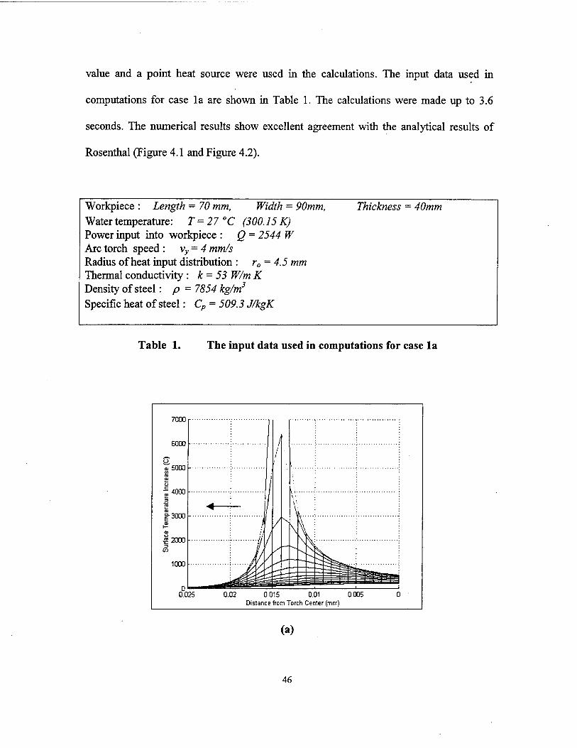
value and a point heat source were used in the calculations. The input data used in
computations for case la are shown in Table 1. The calculations were made up to 3.6
seconds. The numerical results show excellent agreement with the analytical results of
Rosenthal (Figure 4.1 and Figure 4.2).
Workpiece : Length = 70 mm, Width = 90mm, Water temperature: T=27°C (300.15 K) Power input into workpiece : Q = 2544 W Arc torch speed : vy = 4 mm/s Radius of heat input distribution : r0 = 4.5 mm Thermal conductivity : k = 53 W/m K Density of steel: p = 7854 kg/m3
Specific heat of steel: Cp = 509.3 J/kgK
Thickness = 40mm
Table 1. The input data used in computations for case la
(a)
46
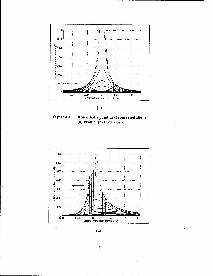
(b)
Figure 4.1 Rosenthal's point heat source solution: (a) Profile; (b) Front-view.
(a)
47
7000
0.01 0.005 0 -0.005 -0.01 Distance from Torch Center (mm)
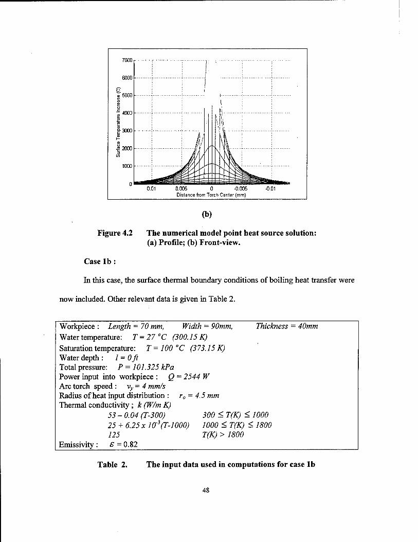
Figure 4.2
(b)
The numerical model point heat source solution: (a) Profile; (b) Front-view.
Case lb :
In this case, the surface thermal boundary conditions of boiling heat transfer were
now included. Other relevant data is given in Table 2.
Workpiece : Length = 70 mm, Width = 90mm, Thickness - 40mm Water temperature: T = 27°C (300.15 K) Saturation temperature: T= 100 °C (373.15 K) Water depth: l = 0ft Total pressure: P = 101.325 kPa Power input into workpiece : Q - 2544 W Arc torch speed : vy = 4 mm/s Radius of heat input distribution : r0 = 4.5 mm Thermal conductivity ; k (W/m K)
53 - 0.04 (T-300) 300 < T(K) < 1000 25 + 6.25 x ia3(T-1000) 1000 < T(K) < 1800 125 T(K) > 1800
Emissivity : £ = 0.82
Table 2. The input data used in computations for case lb
48
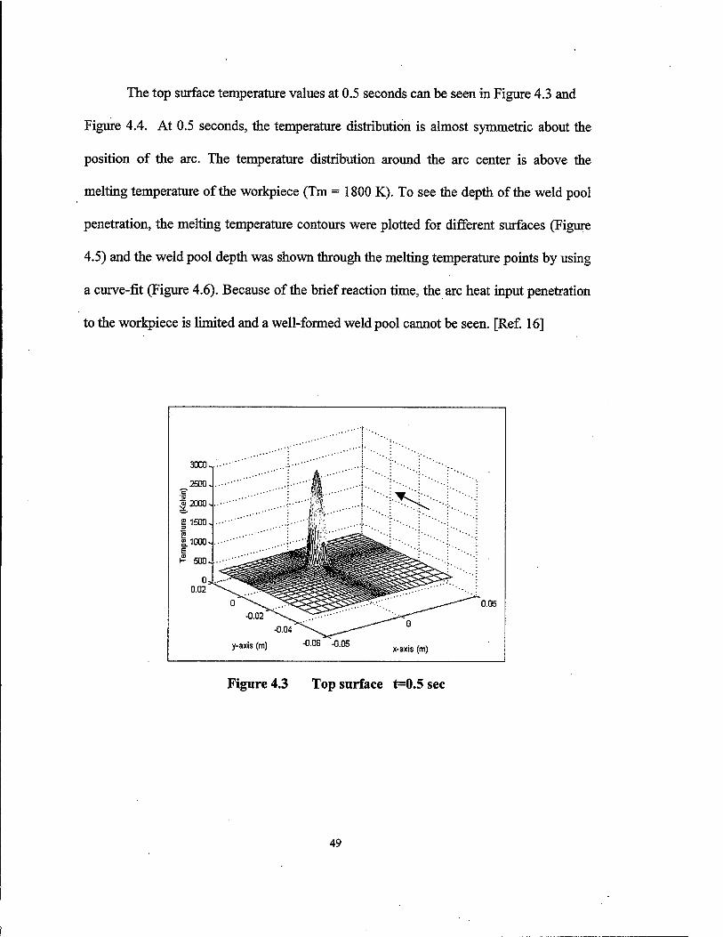
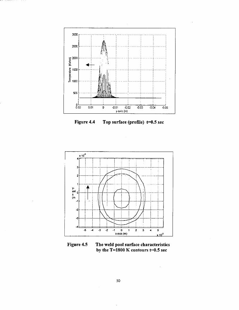
The top surface temperature values at 0.5 seconds can be seen in Figure 4.3 and
Figure 4.4. At 0.5 seconds, the temperature distribution is almost symmetric about the
position of the arc. The temperature distribution around the arc center is above the
melting temperature of the workpiece (Tm = 1800 K). To see the depth of the weld pool
penetration, the melting temperature contours were plotted for different surfaces (Figure
4.5) and the weld pool depth was shown through the melting temperature points by using
a curve-fit (Figure 4.6). Because of the brief reaction time, the arc heat input penetration
to the workpiece is limited and a well-formed weld pool cannot be seen. [Ref. 16]
0.05
y-axis (m) -°DB -005 x-axis (m)
Figure 4.3 Top surface t=0.5 sec
49
3000
2500
-E-2000 m
5 1500
1000
500
*r. i i : :
ml 1 : : i ' :
1 ML..;
i i i_ - .1 0.02 0.01 0 -0.01 -0.02 -0.03 -0.04 -0.05
y-axis (m)
Figure 4.4 Top surface (profile) t=0.5 sec
x10
y- axi s (m
-2
-5-4-3-2-1012345 x-axis (m) _xj£
Figure 4.5 The weld pool surface characteristics by the T=1800 K contours t=0.5 sec
50
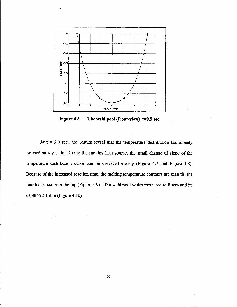
Figure 4.6 The weld pool (front-view) t=0.5 sec
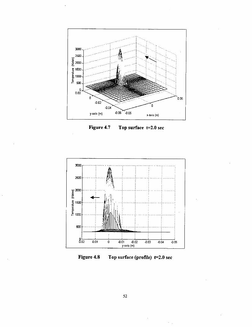
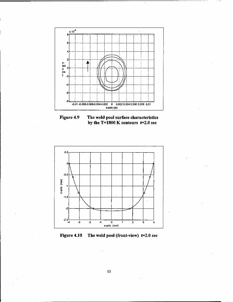
At t = 2.0 sec, the results reveal that the temperature distribution has already
reached steady state. Due to the moving heat source, the small change of slope of the
temperature distribution curve can be observed clearly (Figure 4.7 and Figure 4.8).
Because of the increased reaction time, the melting temperature contours are seen till the
fourth surface from the top (Figure 4.9). The weld pool width increased to 8 mm and its
depth to 2.1 mm (Figure 4.10).
51
y-axis (m) -0-06 -005 x-axis (m)
0.05
Figure 4.7 Top surface t=2.0 sec
3000 r
Figure 4.8 Top surface (profile) t=2.0 sec
52
x10
y- axi s 0 (m
) -2
4
-0.01 -0.008-0.006-0.004-0.002 0 0.002 0.004 0.006 0.008 0.01 x-axis (m)
Figure 4.9 The weld pool surface characteristics by the T=1800 K contours t=2.0sec
0.5
0
-0.5
? E
N
-1.5
-2
-2.5 1-3-2-10123' *
x-axis (mm)
Figure 4.10 The weld pool (front-view) t=2.0 sec
53
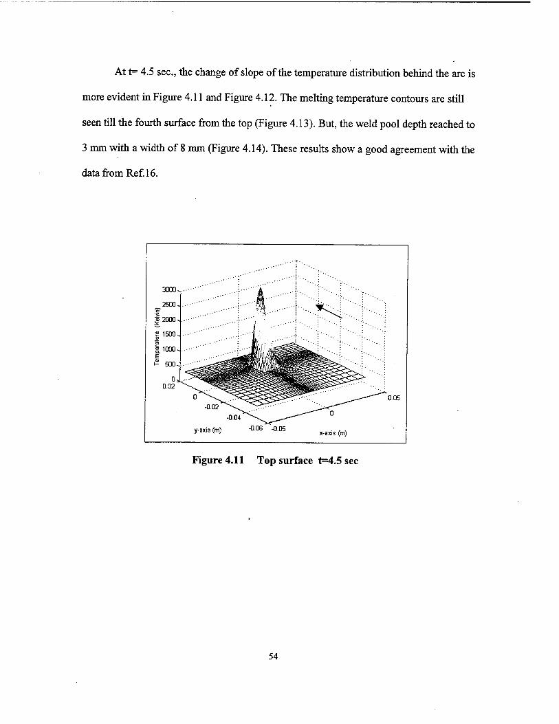
At t= 4.5 sec, the change of slope of the temperature distribution behind the arc is
more evident in Figure 4.11 and Figure 4.12. The melting temperature contours are still
seen till the fourth surface from the top (Figure 4.13). But, the weld pool depth reached to
3 mm with a width of 8 mm (Figure 4.14). These results show a good agreement with the
data from Ref. 16.
y-axis (m) -006 -0.05
0.05
x-axis (m)
Figure 4.11 Top surface t=4.5 sec
54
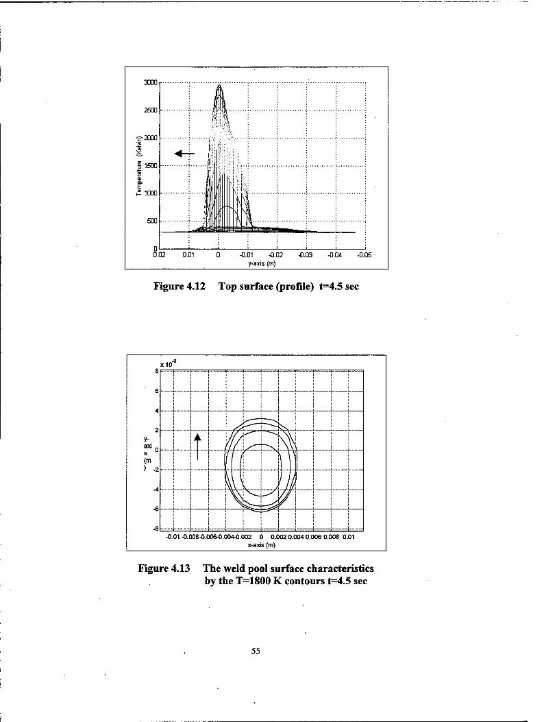
Figure 4.12 Top surface (profile) t=4.5 sec
X10
y-
-o (m ) -2
^=^
yjp^^ |_ |x^^n
t\ t / II \^^/
-0.01 -0.008-0.006-0.004-0.002 0 0.002 0.004 0.006 0.008 0.01 x-axis (m)
Figure 4.13 The weld pool surface characteristics by the T=1800 K contours t=4.5 sec
55
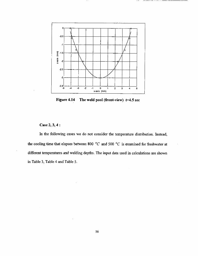
Figure 4.14 The weld pool (front-view) t=4.5sec
Case 2,3,4 :
In the following cases we do not consider the temperature distribution. Instead,
the cooling time that elapses between 800 °C and 500 °C is examined for freshwater at
different temperatures and welding depths. The input data used in calculations are shown
in Table 3, Table 4 and Table 5.
56
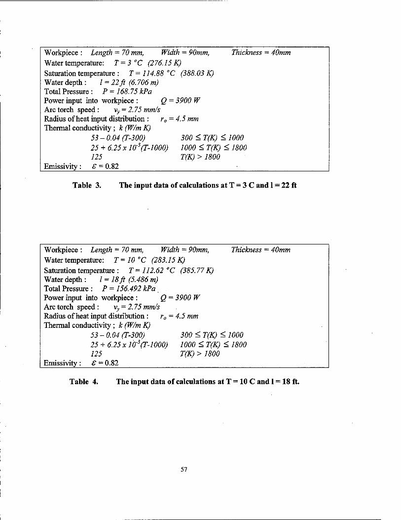
Workpiece : Length = 70 mm, Width = 90mm, Thickness = 40mm Water temperature: T = 3 °C (276.15 K) Saturation temperature : T= 114.88 °( Z (388.03 K) Water depth : / = 22 ft (6.706 m) Total Pressure : P = 168.75 kPa Power input into workpiece : Q - -- 3900 W Arc torch speed: vy = 2.75 mm/s Radius of heat input distribution : r0 - = 4.5 mm Thermal conductivity; Jc(W/mK)
53 - 0.04 (T-300) 300 < T(K) < 1000 25 + 6.25xl0-3(T-1000) 1000 < T(K) <1800 125 T(K) > 1800
Emissivity : S — 0.82
Table 3. The input data of calculations at T = 3 C and 1 = 22 ft
Workpiece : Length = 70 mm, Width = 90mm, Thickness = 40mm Water temperature: T=10°C (283. 15 K) Saturation temperature : T= 112.62 ° C (385.77 K) Water depth : 1 = 18 ft (5.486 m) Total Pressure : P = 156.492 kPa Power input into workpiece : Q = 3900 W Arc torch speed: vy = 2.75 mm/s Radius of heat input distribution : r0 = 4.5 mm Thermal conductivity; k (W/m K)
53 - 0.04 (T-300) 300 < T(K) < 1000 25 + 6.25xl0-3(T-1000) 1000 < T(K) < 1800 125 T(K) > 1800
Emissivity : S = 0.82
Table 4. The input data of calculations at T = 10 C and 1 = 18 ft.
57
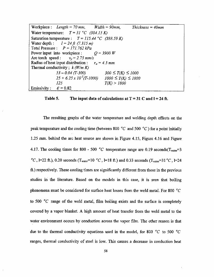
Workpiece : Length = 70 mm, Width = 90mm, Thickness = 40mm Water temperature: T= 31 °C (304.15 K) Saturation temperature : T= 115.44 "C (388.59 K) Water depth : / = 24 ft (7.315 m) Total Pressure : P = 171.762 kPa Power input into workpiece : Q = 3900 W Arc torch speed : vy = 2.75 mm/s Radius of heat input distribution : r0 = 4.5 mm Thermal conductivity ; k (W/m K)
53 - 0.04 (T-300) 300 < T(K) < 1000 25 + 6.25 x 10'3(T-1000) 1000 < T(K) < 11800 125 T(K) > 1800
Emissivity : £ = 0.82
Table 5. The input data of calculations at T = 31 C and 1 = 24 ft.
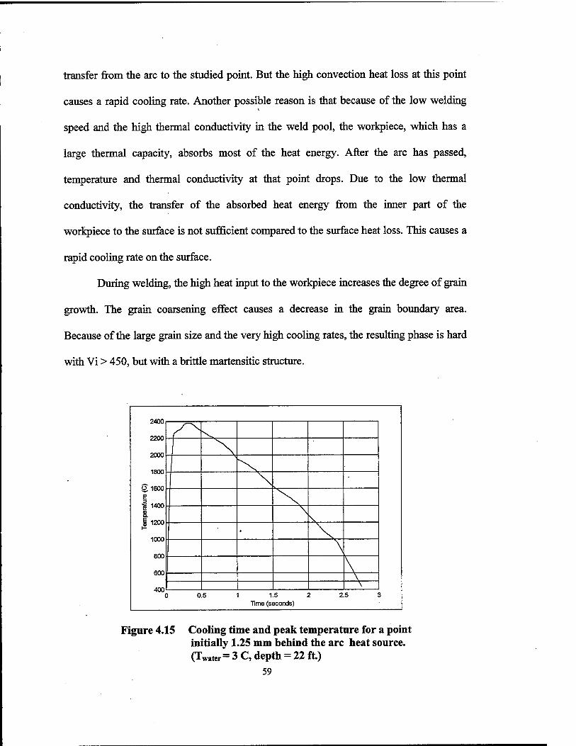
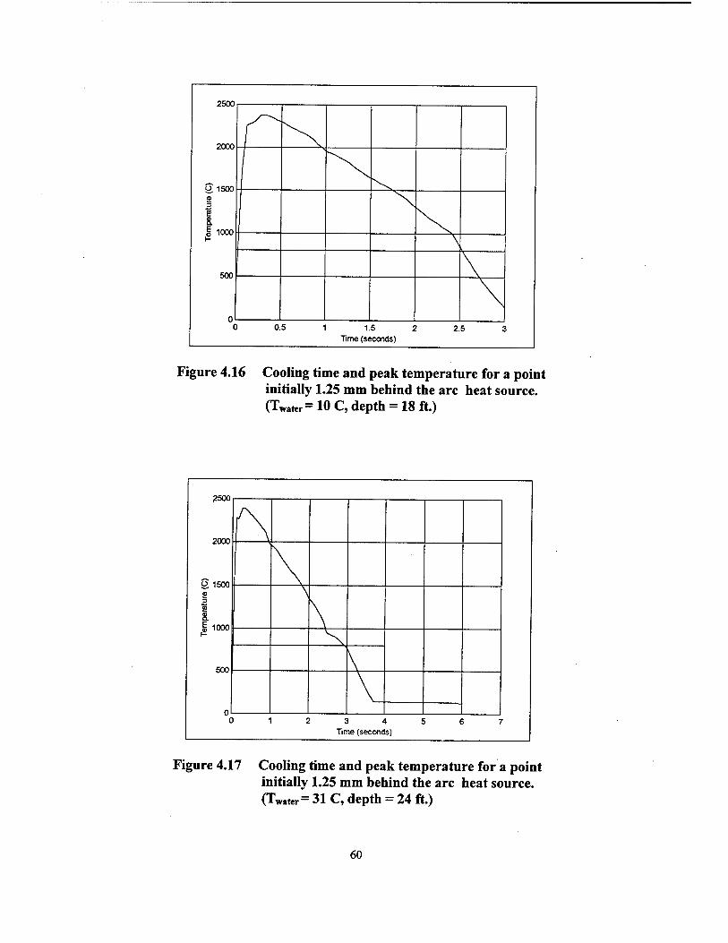
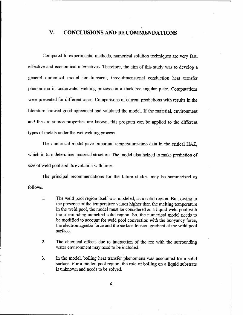
The resulting graphs of the water temperature and welding depth effects on the
peak temperature and the cooling time (between 800 °C and 500 °C) for a point initially
1.25 mm. behind the arc heat source are shown in Figure 4.15, Figure 4.16 and Figure
4.17. The cooling times for 800 - 500 °C temperature range are 0.19 seconds(Twater=3
°C, 1=22 ft.), 0.20 seconds (Twater=10 °C, 1=18 ft.) and 0.33 seconds (Twater=31 °C, 1=24
ft.) respectively. These cooling times are significantly different from those in the previous
studies in the literature. Based on the models in this case, it is seen that boiling
phenomena must be considered for surface heat losses from the weld metal. For 800 °C
to 500 °C range of the weld metal, film boiling exists and the surface is completely
covered by a vapor blanket. A high amount of heat transfer from the weld metal to the
water environment occurs by conduction across the vapor film. The other reason is that
due to the thermal conductivity equations used in the model, for 800 °C to 500 °C
ranges, thermal conductivity of steel is low. This causes a decrease in conduction heat
58
transfer from the arc to the studied point. But the high convection heat loss at this point
causes a rapid cooling rate. Another possible reason is that because of the low welding
speed and the high thermal conductivity in the weld pool, the workpiece, which has a
large thermal capacity, absorbs most of the heat energy. After the arc has passed,
temperature and thermal conductivity at that point drops. Due to the low thermal
conductivity, the transfer of the absorbed heat energy from the inner part of the
workpiece to the surface is not sufficient compared to the surface heat loss. This causes a
rapid cooling rate on the surface.
During welding, the high heat input to the workpiece increases the degree of grain
growth. The grain coarsening effect causes a decrease in the grain boundary area.
Because of the large grain size and the very high cooling rates, the resulting phase is hard
with Vi > 450, but with a brittle martensitic structure.
Tem
pera
ture
(C
)
8888888888?
\ N
\ >.
•
\ \ \
0.5 1 1.5 2 2.5 Time (seconds)
3
Figure 4.15 Cooling time and peak temperature for a point initially 1.25 mm behind the arc heat source. (TWater = 3 C, depth = 22 ft.)
59
5snn
Tem
pera
ture
(C
)
C 0.5 1 1.5 2 2.5 : Time (seconds)
Figure 4.16 Cooling time and peak temperature for a point initially 1.25 mm behind the arc heat source. (TWater= 10 C, depth = 18 ft.)
2500
2000
O 1500
I 1000
500
\
A,
3 4 Time (seconds)
Figure 4.17 Cooling time and peak temperature for a point initially 1.25 mm behind the arc heat source. (TWater= 31 C, depth = 24 ft.)
60
V. CONCLUSIONS AND RECOMMENDATIONS
Compared to experimental methods, numerical solution techniques are very fast,
effective and economical alternatives. Therefore, the aim of this study was to develop a
general numerical model for transient, three-dimensional conduction heat transfer
phenomena in underwater welding process on a thick rectangular plate. Computations
were presented for different cases. Comparisons of current predictions with results in the
literature showed good agreement and validated the model. If the material, environment
and the arc source properties are known, this program can be applied to the different
types of metals under the wet welding process.
The numerical model gave important temperature-time data in the critical HAZ,
which in turn determines material structure. The model also helped to make prediction of
size of weld pool and its evolution with time.
The principal recommendations for the future studies may be summarized as
follows.
1. The weld pool region itself was modeled, as a solid region. But, owing to the presence of the temperature values higher than the melting temperature in the weld pool, the model must be considered as a liquid weld pool with the surrounding unmelted solid region. So, the numerical model needs to be modified to account for weld pool convection with the buoyancy force, the electromagnetic force and the surface tension gradient at the weld pool surface.
2. The chemical effects due to interaction of the arc with the surrounding water environment may need to be included.
3. In the model, boiling heat transfer phenomena was accounted for a solid surface. For a molten pool region, the role of boiling on a liquid substrate is unknown and needs to be solved.
61
62
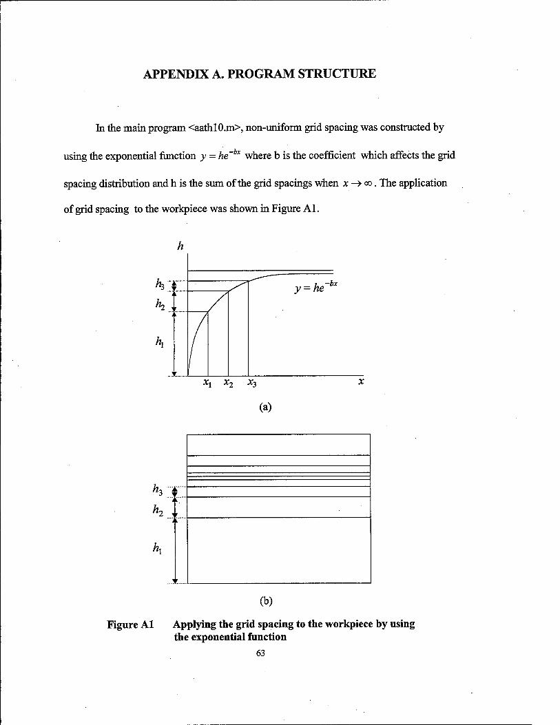
APPENDIX A. PROGRAM STRUCTURE
In the main program <aathl0.m>, non-umform grid spacing was constructed by
using the exponential function y - he~bx where b is the coefficient which affects the grid
spacing distribution and h is the sum of the grid spacings when x -»<x>. The application
of grid spacing to the workpiece was shown in Figure Al.
Xi Xn X3
(a)
n3 , r h2 ,
r
(b)
Figure Al Applying the grid spacing to the workpiece by using the exponential function
63
The distance in front of the moving heat source was called as "front" and the
distance behind the heat source was called as "back". The width and the thickness of the
plate were defined with the same terms. The variable "number" was used to define the
number of grid points in the "back" region. Variables "b" and "number" can be changed
to control the resolution of the grid spacing.
To simulate the heat input from the arc to the top surface, it was assumed that the
arc source heat flux distribution had a Gaussian distribution on the top surface. The
applied arc heat source was defined as a matrix, which its size was equal to the size of the
top surface. The value of heat flux at each grid point was calculated by using the x-
coordinate and the y-coordinate of that point. The resulting arc heat source matrix was
applied to the top surface.
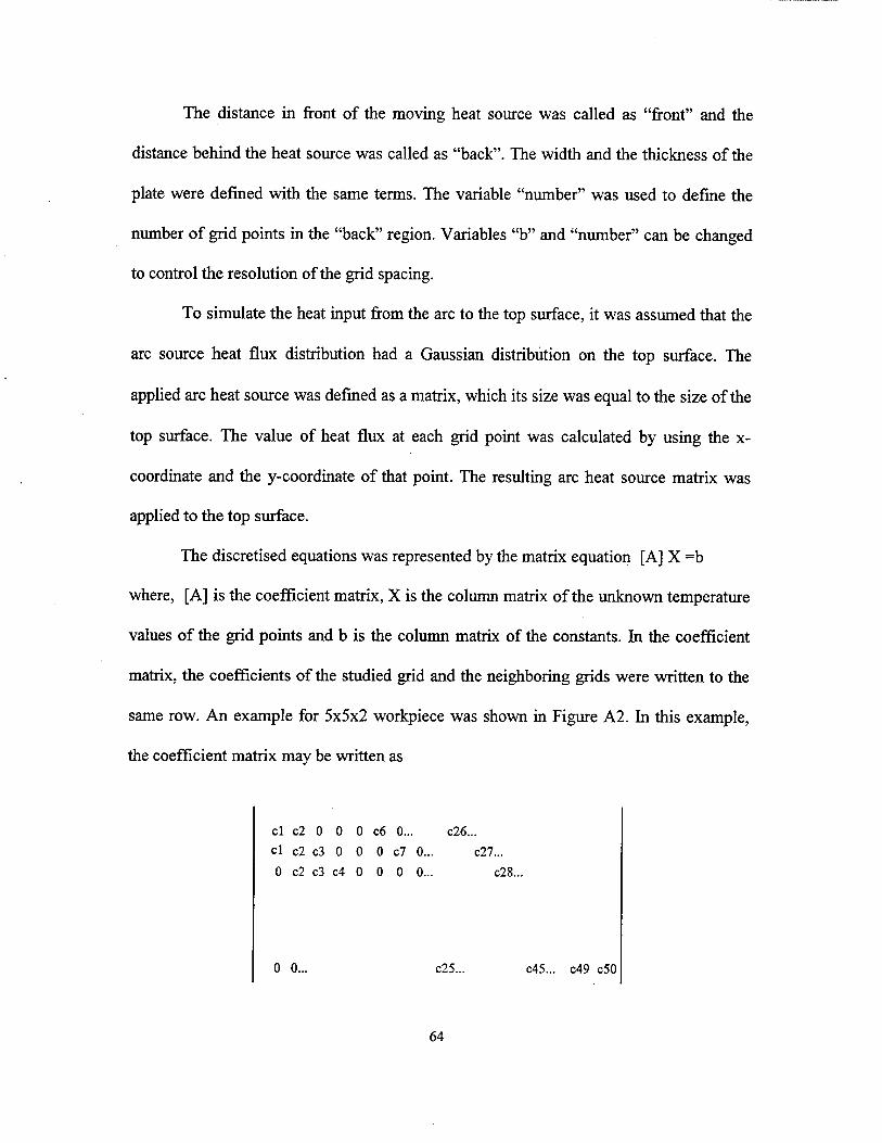
The discretised equations was represented by the matrix equation [A] X =b
where, [A] is the coefficient matrix, X is the column matrix of the unknown temperature
values of the grid points and b is the column matrix of the constants. In the coefficient
matrix, the coefficients of the studied grid and the neighboring grids were written to the
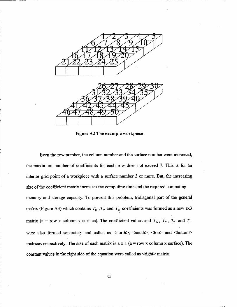
same row. An example for 5x5x2 workpiece was shown in Figure A2. In this example,
the coefficient matrix may be written as
cl c2 0 0 0 c6 0... c26...
cl c2 c3 0 0 0 c7 0... c27...
0 c2 c3 c4 0 0 0 0... c28...
0 0... c25. c45... c49 c50
64
\y\y\y\y\y\ V\
Figure A2 The example workpiece
Even the row number, the column number and the surface number were increased,
the maximum number of coefficients for each row does not exceed 7. This is for an
interior grid point of a workpiece with a surface number 3 or more. But, the increasing
size of the coefficient matrix increases the computing time and the required computing
memory and storage capacity. To prevent this problem, tridiagonal part of the general
matrix (Figure A3) which contains Tw, TP and TE coefficients was formed as a new ax3
matrix (a = row x column x surface). The coefficient values and TN, Ts, TT and TB
were also formed separately and called as <north>, <south>, <top> and <bottom>
matrices respectively. The size of each matrix is a x 1 (a = row x column x surface). The
constant values in the right side of the equation were called as <right> matrix.
65
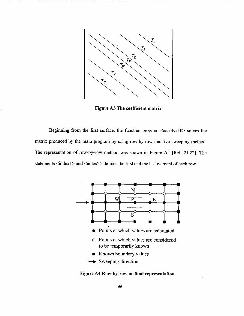
Figure A3 The coefficient matrix
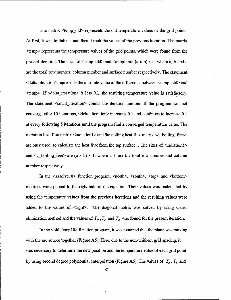
Beginning from the first surface, the function program <aasolvelO> solves the
matrix produced by the main program by using row-by-row iterative sweeping method.
The representation of row-by-row method was shown in Figure A4 [Ref. 21,22]. The
statements <indexl> and <index2> defines the first and the last element of each row.
-O- -6 W
-0
4 ■o -o
-0- -0- -0- 0-
• Points at which values are calculated
o Points at which values are considered to be temporarily known
■ Known boundary values
—► Sweeping direction
Figure A4 Row-by-row method representation
66
The matrix <temp_old> represents the old temperature values of the grid points.
At first, it was initialized and then it took the values of the previous iteration. The matrix
<temp> represents the temperature values of the grid points, which were found from the
present iteration. The sizes of <temp_old> and <temp> are (a x b) x c, where a, b and c
are the total row number, column number and surface number respectively. The statement
<delta_iteration> represents the absolute value of the difference between <temp_old> and
<temp>. If <delta_iteration> is less 0.1, the resulting temperature value is satisfactory.
The statement <count_iteration> counts the iteration number. If the program can not
converge after 10 iterations, <delta_iteration> increases 0.1 and continues to increase 0.1
at every following 5 iterations until the program find a converged temperature value. The
radiation heat flux matrix <radiationl> and the boiling heat flux matrix <q_boiling_free>
are only used to calculate the heat flux from the top surface.. The sizes of <radiationl>
and <q_boiling_free> are (a x b) x 1, where a, b are the total row number and column
number respectively.
In the <aasolvel0> function program, <north>, <south>, <top> and <bottom>
matrices were passed to the right side of the equation. Their values were calculated by
using the temperature values from the previous iterations and the resulting values were
added to the values of <right>. The diagonal matrix was solved by using Gauss
elimination method and the values of Tw, TP and TE was found for the present iteration.
In the <old_templ0> function program, it was assumed that the plane was moving
with the arc source together (Figure A5). Here, due to the non-uniform grid spacing, it
was necessary to determine the new position and the temperature value of each grid point
by using second degree polynomial enterpolation (Figure A6). The values of Ta, Tb and
67
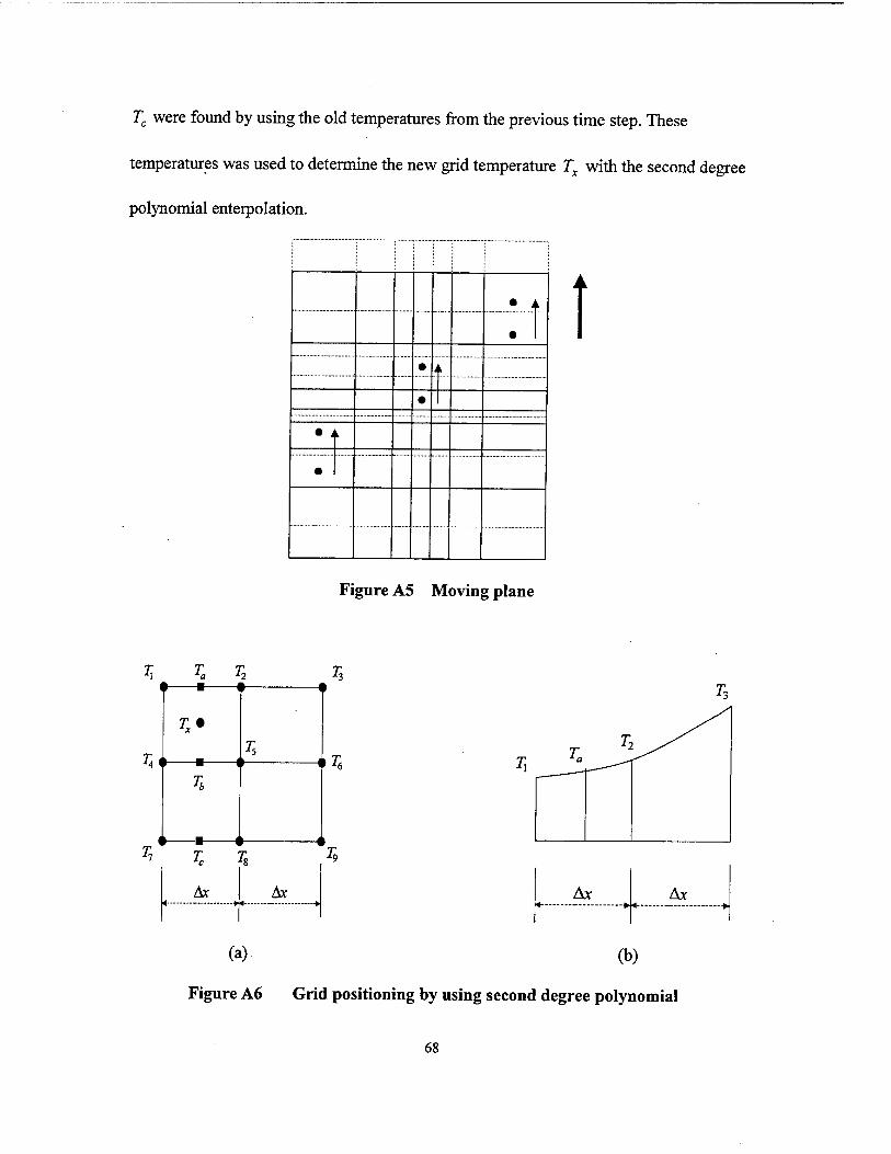
Tc were found by using the old temperatures from the previous time step. These
temperatures was used to determine the new grid temperature Tx with the second degree
polynomial enterpolation.
Tx Ta T2
Ax
• A
•
• A
• T~
• A
t
Figure A5 Moving plane
(1—■ «
T •
> II
T5
0 ■ i ► ii
T3
Tx T '■a ^-r
'' Tc Ts T9
Ax Ax Ax
(a) (b)
Figure A6 Grid positioning by using second degree polynomial
68

The function program <save_alllO> saves all 3-D temperature data at each time
step by overwriting onto. The other function program <save_thelO> saves top surface
temperatures at each time step into a different file name.
69

70
APPENDIX B. PROGRAM CODES
THE MAIN PROGRAM (aathlO.m)
% Need to define the function below to be able to use mcc % The symbol "al" itself has no significance - aathlO is the % name of the main program, function [al]=aathlO()
clear % clear all variables - not present in "aathlOgoon.m" close all % close all open figure windows
% save_me is a counter that is incremented after each time step % and is used to decide how often to save the calc temperature % data. save_me=0;
% save_counter is a counter that is also incremented with each % time step and is appended to the file name into which the temp % data is stored. save_counter=0; % not present in "aathlOgoon.m"
% Tinf is the ambient temp in deg C Tinf=27;
% TO is the initial temp in deg C T0=27;
% sil is the stefan-boltzmann const (SI units) sil=5.67E-8;
% epsilon is the emissivity of the surface epsilon=0;
% x-vel component of torch speed (m/s) vel_x=0;
% y-vel component of torch speed (m/s) vel_y=0.004;
% deltat_t is the time step (in sees) delta_t=0.001;
% Distance source moves in the x-direction in each time step(in m) deltax=vel x*delta t;
% Distance source moves in the y-direction in each time step (in m) deltay=vel_y*delta_t;
% q_up is the heat flux distribution on the upper surface (W/mÄ2)
71
% q_up is the heat flux distribution on the upper surface (W/mA2) % imposed by the torch/arc (implemented in matrix form) q_up=0;
%% q is a generic variable representing heat flux that may be %% present at any of the other surfaces and can be included %% in the nodal equations
% q_ is constant heat flux through the surfaces q_west=0; q_east=0; q_top=0; q_bottom=0; q_north=0; q_south=0;
% c is the cp [J/kg-K] c=509.3;
% ro is the density [kg/mA3] ro=7 854;
% Convection heat transfer coefficients from the faces [W/mA2-K] he=0; hw=0 hn=0 hs=0 ht=0 hb=0
% The distances between the grid point points
%% back is the portion of the moving grid behind the point %% of location of the source [in m] back=.05;
% b is the coefft in the exponential gridding function (eA(-b*x)) b=.13;
% number is the no. of grid points in the "back" region number=20;
%% Variables "b" and "number" above can be varied to control the %% features of the variable grid, such as change in grid spacing, %% etc. %% height is a vector that holds the coords of the grid points in the back-region. Note that the spacing between these grid %% points is the diff. between consecutive height entries and is %% stored in "int_back" height(1)=0;
72
% Note that int_back(l) > int_back(number), i.e. in reverse order for kk=l:number
height(kk+l)=back*(1-exp(-b*kk)); int_back(kk)=height(kk+1)-height(kk) ;
end
%% multiply is a scaling factor(close to 1) that scales height and %% int_back in such a way that it height(number) = back. multiply=back/(sum(int_back)-int_back(l)/2) int_back=multiply*int_back;
%% Similar to back, below are the variables front (front region of %% %% moving grid ahead of source), width (width of plate) and %% thickness. All distances in m. front=0.02; width=0.09; thickness=0.04;
%% int_front is the grid spacing in the front region. Initially %% set to 0. Then transfer from int-back one by one until sum of %% int-front entries exceeds front. int_front=0; counter=0;
while (sum(int_front)-int_front(length(int front))/2)<=front
% int_front below continually changes size as the spacings are % added. int_front=[int_front,int_back(length(int_back)-counter) ] ; counter=counter+l;
end
% Set first member which was initially 0 to null. % Meaningful spacing starts only from the 2nd member of int_front int front(!)=[];
%% The grid distance matrix in the y direction is y_intl starting %% from the top of front down through the source all the way to %% the bottom of back. % fliplr is to ge the desired ordering from front to back. y_intl=[fliplr(int_front),fliplr(int_back)];
% int_side holds grid spacing values over the width. % Same logic as for int_front int_side=0; counter=0;
while (sum(int_side)-int_side(length(int_side))/2)<=(width/2)
73
int_side=[int_side,int_back(length(int_back)-counter)]; counter=counter+l;
end
int side (!) = [];
'% The grid distance vector in the x dirextion is x_intl (y_intl % above. x_intl=[fliplr(int_side),int_side];
% The grid distance vector in the z dirextion is z_intl (y_intl % above) z_intl=0;
counter=0;
while (sum(z_intl)-z_intl(length(z_intl))12) <=thickness
z_intl=[z_intl,int_back(length(int_back)-counter)]; counter=counter+l;
end
z_intl(!)=[];
figure(1)
subplot(3,1,1) plot(x_intl) grid on
subplot(3,1,2) plot(y_intl) grid on
subplot(3,1,3) plot(z_intl) grid on
% row is the number of y nodes (along the length). row = length(y_intl)-1;
% col is the no. of x-nodes (across the plate width), col = length(x_intl)-1;
% surface is the no. of z-nodes (across the thickness), surface = length(z intl)-l;
74
% The value of teta determines the numerical scheme as follows:
% for Fully Implicit Method; teta=l % for Crank-Nicholson Method; teta=0.5 % for Explicit Method; teta=0
teta=l;
% For a a*b*c three dimensional matrix, % a:num rows, b:num cols, c:num surfaces. % Size of new > (a*b*c)*3 TP, TE, TW coefficients for the % whole grids. % Size of top > (a*b*c)*l TT coefficients for the whole
.% grids. % size of bottom —> (a*b*c)*l TB coefficients for the % whole grids. % size of north > (a*b*c)*1 TN coefficients for the whole % grids. % size of south > (a*b*c)*l TS coefficients for the whole % grids. % size of right > (a*b*c)*1 The values of the righthandside % of the matrix. % size of temp > (a*b)*c The temperatures of the grids.
% new is the coefft matrix for all the grid points in the 3-D % volume.
% 1st col holds the coeffts of the West (W) nodes. % 2nd col holds the coeffts of the (P) nodes. % 3rd col holds the coeffts of the East (E) nodes. new=zeros(row*col*surface, 3) ;
% right is the const (or b-vector) on the RHS right=zeros(row*col*surface, 1) ;
%% south, north, top, bottom hold the coeffts of the corresponding %% grid points. south=right; north=right; top=right; bottom=right ;
% Apply the initial condition to the plate. % "temp" is the temperature matrix.
% temp is a matrix that holds temperature values for each surface. % Note dimensions of temp carefully. % This initialization is not present "aathlOgoon.m". temp=TO*ones(row*surface, col);
75
% Below are parameters that specify the heat/arc source. % rO is the effective radius [m] of the gaussian heat source. r0=0.0045;
% ddd is a coefft that determines the gaussian spread. % The larger the ddd value, the more pointed the source. ddd=3;
% qrate_total is the total energy transfer rate from the source % [Watts] . qrate_total = 254 4;
% qO is the peak heat flux of the gaussian [W/m~2] qO=qrate_total*ddd/pi/rOA2;
% Calculate the q_up (heat flux distribution on the top face) %% xcenter and ycenter are the grid element numbers of the grid %% center at which the source/arc is located. xcenter=length(int_side); ycenter=length(int_front);
for nn=l:row for mm=l:col
% x(mm) is array with the x-coords of the mesh, if mm < xcenter
x (mm) =-sum(x_intl ( (mm+.l) : xcenter) ) ; elseif mm==xcenter
x(mm)=0; else
x(mm)=sum(x_intl((xcenter+1):mm)); end
% y(mm) is array with the y-coords of the mesh, if nn < ycenter
y(nn)=sum(y_intl((nn+1):ycenter)) ; elseif nn==ycenter
y(nn)=0; else
y(nn)=-sum(y_intl((ycenter+1):nn)) ; end
% initialize q_up using x() and y() coord info. q_up(nn,mm)=-qO*exp(-ddd*(x(mm)~2+y(nn)A2)/rOA2);
end end figure
% a mesh command to view the generated grid, mesh(x, y,q_up)
76
for time=delta_t:delta_t:200 % 200 is the final time in sees upto which the program should % go...
save_me=save_me+l;
disp('the interpolation time is ') tic % beginning of tic-toe loop
[temp]=old_templ0(row,col,surface,temp,x,y,deltax,deltay) ;
toe % end of tic-toe loop.
% figure % contour(x,y,temp(1:row,1:col))
disp('The matrix formation time is :')
tic % beginning of tic-toe loop.
%% Start to form the matrix by defining every point. % Beginning of creation of coefft matrix % loops step through each point on all the surfaces, cols and rows
for kk=l:surface for jj=l:row for ii=l:col
% The distances between the reference point and the adjoining % nodal points.
% Distance between P&E and P&W xpe=x_intl(ii+1) ; xwp=x_intl(ii);
% Distance between P&N and P&S ypn=y_intl(jj); ysp=y_intl(jj+l);
% Distance between P&T and P&B ' zpt=z_intl(kk); zbp=z_intl(kk+l) ;
%% The lateral surface areas of the faces of the control volume %% around the reference point.P.
% East-face area. Ae=(ypn/2+ysp/2)*(zpt/2+zbp/2); Aw=Ae;
77
% North-face area. An=(xpe/2+xwp/2)*(zpt/2 + zbp/2) ; As=An; % Top-face area. At=(xpe/2+xwp/2)*(ypn/2+ysp/2); Ab=At;
% The size of the control volume.
deltaV=(xpe/2+xwp/2)*(ypn/2+ysp/2)*(zpt/2+zbp/2);
% Routine to set thermal conductivities below:
% Initialize TEMP()s to 0 for logical ifs below: TEMP(1)=0;TEMP(2)=0;TEMP(3)=0;TEMP(4)=0;TEMP(5)=0; TEMP(6)=0;
% TP0 is the temperature of the current node. TP0=temp((kk-l)*row+jj,ii);
% T_west=TEMP(l) T_east=TEMP(2) T_north=TEMP(3) % T_south=TEMP(4) T_top=TEMP(5) T bottom=TEMP(6)
if ii==l % first col, no west neighbor, so... TEMP(1)=TP0; % set T_west to TP0
elseif ii==col % last col, no east neighbor, so. TEMP(2)=TP0; % set T_east to TP0
end
if jj—1 TEMP(3)=TP0;
elseif jj==row TEMP(4)=TP0;
end
if kk==l TEMP{5)=TP0;
elseif kk==surface TEMP(6)=TP0;
end
%% If current node P has a valid neighbor, then use temperature %% of that node....
if (TEMP(1)==0) TEMP(l)=temp((kk-1)*row+jj,ii-1);
end
78
if (TEMP(2)==0) TEMP(2)=temp((kk-1)*row+jj , ii+1) ;
end
if (TEMP(3)==0) TEMP(3)=temp((kk-1)*row+jj-1, ii) ;
end
if (TEMP(4)==0) TEMP(4)=temp((kk-1)*row+jj+1,ii);
end
if (TEMP(5)==0) TEMP(5)=temp((kk-2)*row+jj,ii);
end
if (TEMP(6)==0) TEMP(6)=temp(kk*row+jj,ii) ;
end
% Do loop to calculate k-values of all grid points, for kjl=l:6
% Now set the thermal conductivity values.
kelvin=TP0+273.15; kl=53; % nominal kl-value in W/m-K set here, but....
% Actual kl-values are calc below. if (kelvin>=300 & kelvin<1000)
kl=53-0.04*(kelvin-300); elseif (kelvin>=1000 & kelvin<1800)
kl=25+6.25E-3*(kelvin-1000); elseif kelvin>=1800
kl=125; end
% Find the thermal conductivity at the adjacent point. kelvin=TEMP(kj1)+273.15; k2=53; % nominal k2-value in W/m-K set here, but....
% Actual k2-values of neighbors calc here. if (ke'lvin>=300 & kelvin<1000)
k2=53-0.04*(kelvin-300); elseif (kelvin>=1000 & kelvin<1800)
k2=25+6.25E-3*(kelvin-1000); elseif kelvin>=1800
k2=125; end
79
% Harmonie mean thermal conductivity found next NEW_K(kjl) = 2*kl*k2/(kl+k2);
end
% Now redefine k's of the neighboring faces with values from NEW K kw=NEW_K(1) ke=NEW_K(2) kn=NEW_K(3) ks=NEW_K(4) kt=NEW_K(5) kb=NEW_K(6)
% Coefficients used in developing the discretised equations. ae=ke*Ae/xpe; aw=kw*Aw/xwp; an=kn*An/ypn; as=ks*As/ysp; at=kt*At/zpt; ab=kb*Ab/zbp; apO=ro*c*deltaV/delta_t; ap=teta*(ae+aw+an+as+at+ab)+apO;
% Coefficients used for the wall-medium interface part of the % discretised equations. coeffe=he*xpe/(2*ke+he*xpe); coeffw=hw*xwp/(2*kw+hw*xwp); coeffn=hn*ypn/(2*kn+hn*ypn); coeffs=hs*ysp/(2*ks+hs*ysp); coefft=ht*zpt/(2*kt+ht*zpt); coeffb=hb*zbp/(2*kb+hb*zbp);
% Coefficients used for the heat flux part of the discretised % equations.
fluxcoeffe=xpe/(2*ke+he*xpe); fluxcoeffw=xwp/(2*kw+hw*xwp); fluxcoeffn=ypn/(2*kn+hn*ypn); fluxcoeffs=ysp/(2*ks+hs*ysp); fluxcoefft=zpt/(2*kt+ht*zpt); fluxcoeffb=zbp/(2*kb+hb*zbp);
% Radiation coefft for surface b.c. - see thesis... radcoeff=sil*epsilon*zpt/(2*kt+ht*zpt);
% row_num is the index of the current point in the matrices being % used. row_num varies from 1:surface*col*row row_num=(kk-l)*row*col+(jj-1)*col+ii;
% For left-back-top corner
if ((kk==l) & (jj==l) & (ii==l))
80
% Temperature values for current time step for each relevant node. TP0=temp((kk-1)*row+jj,ii) ; TE0=temp((kk-1)*row+jj,ii+1) ; TS0=temp((kk-1)*row+jj+l,ii) ; TBO=temp(kk*row+jj,ii) ;
% Coeffts of grid points; note south and bottom later are moved to % the rhs. ■ % "new" is the A-matrix in the solution. % Note teta is the parameter which determines the numerical method % teta=l:fully implicit; teta=0:explicit; teta=0.5:Crank-Nicholson new(row_num,2)=apO+teta*(ae+2*aw*coeffw+2*an*coeffn+as+2*at*coefft+ab); new(row_num,3)=-teta*ae; south(row_num,1)=teta*as; bottom(row_num,1)=teta*ab;
% "right" is the constant b-matrix on the rhs... right(row_num,1)=(1-teta)*(ae*TE0+as*TS0+ab*TB0)+ ... (apO-(1-teta)*(ae+2*aw*coeffw+2*an*coeffn+as+2*at*coefft+ab))*TP0+ ... (2*aw*coeffw+2*an*coeffn+2*at*coefft)*Tinf -
2*at*fluxcoefft*q_up(jj,ii) ... -2*aw*fluxcoeffw*q_west-2*an*fluxcoeffn*q_north-2*at*fluxcoefft*q_top;
%% radiation & q_boiling_coeff belong to the rhs but are not included %% until later since they depend on the current temperature
% (a form of quasi-linearization of nonlinear temp terms) radiation(row_num,l)=-2*at*radcoeff; q_boiling_coeff(row_num,1)=-2*at*fluxcoefft;
% for right-back-top corner
elseif ((kk==l) & (jj==l) & (ii==col))
TP0=temp((kk-1)*row+jj,ii); TW0=temp((kk-1)*row+jj , ii-1) ; TS0=temp((kk-1)*row+jj+1, ii) ; TBO=temp(kk*row+jj, ii) ;
new(row_num,2)=ap0+teta*(2*ae*coeffe+aw+2*an*coeffn'+as+2*at*coefft+ab); new(row_num,1)=-teta*aw; south(row_num,l)=teta*as; bottom(row_num,l)=teta*ab;
right(row_num,l)=(l-teta)*(aw*TW0+as*TS0+ab*TB0)+ ... (apO-(1-teta)*(2*ae*coeffe+aw+2*an*coeffn+as+2*at*coefft+ab))*TP0+
(2*ae*coeffe+2*an*coeffn+2*at*coefft)*Tinf- 2*at*fluxcoefft*q_up(jj , ii)...
-2*ae*fluxcoeffe*q east-2*an*fluxcoeffn*q north-
2*at*fluxcoefft*q_top; radiation(row_num,1)=-2*at*radcoeff;
. 81
q_boiling_coeff(row_num,1)=-2*at*fluxcoefft;
% for left-front-top corner
elseif ((kk==l) & (jj==row) & (ii==l))
TP0=temp((kk-1)*row+jj,ii); TE0=temp((kk-1)*row+jj,ii+1); TN0=temp((kk-1)*row+jj-1,ii); TB0=temp(kk*row+j j,ii);
new(row_num,2)=ap0+teta*(ae+2*aw*coeffw+an+2*as*coeffs+2*at*coefft+ab); new(row_num, 3)=-teta*ae; north(row_num,1)=teta*an; bottom(row_num,l)=teta*ab;
right(row_num,1)=(1-teta)*(ae*TE0+an*TN0+ab*TB0)+ ... (apO-(1-teta)*(ae+2*aw*coeffw+an+2*as*coeffs+2*at*coefft+ab))*TP0+ ... (2*aw*coeffw+2*as*coeffs+2*at*coefft)*Tinf-2*at*fluxcoefft*q_up(jj,ii)
-2*aw*fluxcoeffw*q_west-2*as*fluxcoeffs*q_south-2*at*fluxcoefft*q_top; radiation(row_num,1)=-2*at*radcoeff; q_boiling_coeff(row_num,1)=-2*at*fluxcoefft;
% for right-front-top corner
elseif ((kk==l) & (jj==row) & (ii==col))
TP0=temp((kk-1)*row+jj, ii); TW0=temp((kk-1)*row+jj, ii-1) ; TN0=temp((kk-1)*row+jj-1, ii) ; TB0=temp(kk*row+j j,ii);
new(row_num,2)=ap0+teta*(2*ae*coeffe+aw+an+2*as*coeffs+2*at*coefft+ab); new(row_num,1)=-teta*aw; north(row_num,1)=teta*an; bottom(row_num,1)=teta*ab;
right(row_num,1)=(1-teta)*(aw+TW0+an+TN0+ab*TB0)+ ... (apO-(1-teta)*(2*ae*coeffe+aw+an+2*as*coeffs+2*at*coefft+ab))*TP0+
(2*ae*coeffe +2*as*coeffs +2*at*coefft)*Tinf- 2*at*fluxcoefft*q_up {j j, ii) ... .
-2*ae*fluxcoeffe*q_east-2*as*fluxcoeffs*q_south- 2*at*fluxcoefft*q_top; radiation(row_num,1)=-2*at*radcoeff; q_boiling_coeff(row_num,1)=-2*at*fluxcoefft;
82
% for left-back-bottom corner
elseif ((kk==surface) & (jj==l) & (ii==l))
TP0=temp((kk-1)*row+jj, ii); TE0=temp((kk-1)*row+jj, ii+1) ; TS0=temp((kk-1)*row+jj+1, ii) ; TT0=temp((kk-2)*row+jj,ii) ;
new(row_num,2)=ap0+teta*(ae+2*aw*coeffw+2*an*coeffn+as+at+2*ab*coeffb) ; new(row_num,3)=-teta*ae; south(row_num,l)=teta*as; top(row_num,1)=teta*at;
right(row_num,1)=(1-teta)*(ae*TE0+as*TS0+at*TT0)+ ... (apO-(1-teta)*(ae+2*aw*coeffw+2*an*coeffn+as+at+2*ab*coeffb))*TP0+ ... (2*aw*coeffw+2*an*coeffn+2*ab*coeffb)*Tinf ... -2*aw*fluxcoeffw*q_west-2*an*fluxcoeffn*q_north-
2*ab*fluxcoeffb*q_bottom;
% for right-back-bottom corner
elseif ((kk==surface) & (jj==l) & (ii==col))
TP0=temp((kk-1)*row+jj,ii); TW0=temp((kk-1)*row+jj,ii-1) ; TS0=temp((kk-1)*row+jj+1, ii) ; TT0=temp((kk-2)*row+jj , ii) ;
new(row_num,2)=apO+teta*(2*ae*coeffe+aw+2*an*coeffn+as+at+2*ab*coeffb) ; new(row_num,l)=-teta*aw; south(row_num,l)=teta*as; top(row_num,1)=teta*at;
right(row_num,1)=(1-teta)*(aw*TW0+as*TS0+at*TT0)+ ... (apO-(1-teta)*(2*ae*coeffe+aw+2*an*coeffn+as+at+2*ab*coeffb))*TP0+
(2*ae*coeffe+2*an*coeffn+2*ab*coeffb)*Tinf ... -2*ae*fluxcoeffe*q_east-2*an*fluxcoeffn*q_north-
2*ab*fluxcoeffb*q_bottom;
% for left-front-bottom corner
elseif ((kk==surface) & (jj==row) & (ii==l))
TP0=temp((kk-1)*row+jj,ii) ; TE0=temp((kk-1)*row+jj , ii+1) ,• TN0=temp((kk-1)*row+jj-l,ii) ; TT0=temp((kk-2)*row+jj,ii) ;
new(row_num,2)=ap0+teta*(ae+2*aw*coeffw+an+2*as*coeffs+at+2*ab*coeffb) ; new(row num,3)=-teta*ae;
83
north(row_num,1)=teta*an; top(row_num,1)=teta*at;
right(row_num,l) = (l-teta)*(ae*TE0+an+TN0+at*TT0)+ . . . (apO-(1-teta)*(ae+2*aw*coeffw+an+2*as*coeffs+at+2*ab*coeffb))*TP0+ (2*aw*coeffw+2*as*coeffs+2*ab*coeffb)*Tinf ... -2*aw*fluxcoeffw*q_west-2*as*fluxcoeffs*q_south-
2*ab*fluxcoeffb*q_bottorn;
% for right-front-bottom corner
elseif ((kk==surface) & (jj==row) & (ii==col))
TP0=temp((kk-1)*row+jj,ii); TW0=temp((kk-1)*row+jj,ii-1); TN0=temp((kk-1)*row+jj-1,ii); TT0=temp((kk-2)*row+j j,ii);
new(row_num,2)=ap0+teta*(2*ae*coeffe+aw+an+2*as*coeffs+at+2*ab*coeffb); new(row_num,1)=-teta*aw; north(row_num,1)=teta*an; top(row_num,1)=teta*at;
right(row_num,1) = (1-teta)*(aw*TW0+an*TN0+at*TT0)+ . . . (apO-(1-teta)*(2*ae*coeffe+aw+an+2*as*coeffs+at+2*ab*coeffb))*TP0+
(2*ae*coeffe +2*as*coeffs +2*ab*coeffb)*Tinf ... -2*ae*fluxcoeffe*q_east-2*as*fluxcoeffs*q_south-
2*ab*fluxcoeffb*q_bottom;
% for the top surface
elseif ((kk==l) & (jj>l) & (jj<row) & (ii>l) & (ii<col))
TP0=temp((kk-1)*row+jj,ii); TE0=temp((kk-1)+row+jj , ii + 1) ; TW0=temp((kk-1)*row+jj, ii-1); TN0=temp((kk-1)*row+jj-1,ii); TSQ=temp((kk-1)*row+jj+1, ii) ; TB0=temp(kk*row+jj, ii) ;
new(row_num,2)=apO+teta*(ae+aw+an+as + 2*at*coefft+ab) ; new(row_num,3)=-teta*ae; new(row_num,1)=-teta*aw; north(row_num,1)=teta*an; south(row_num,1)=teta*as; bottom(row_num,1)=teta*ab;
right(row_num,1)=(1-teta)*(ae*TE0+aw*TW0+an*TN0+as*TS0+ab*TB0)+ ... (apO-(1-teta)*(ae+aw+an+as+2*at*coefft+ab))*TP0 + 2*at*coefft*Tinf -
2*at*fluxcoefft*q_up(jj,ii)-2*at*fluxcoefft*q_top;
84
radiation(row_num,1)=-2*at*radcoeff; q_boiling_coeff(row_num,1)=-2*at*fluxcoefft;
for the bottom surface
elseif ((kk==surface) & (jj>l) & (jj<row) & (ii>l) & (ii<coi;
TP0=temp( (kk-l)'*row+jj,ii) ; TE0=temp((kk-1)*row+jj , ii+1) TW0=temp((kk-1)*row+jj,ii-l) TN0=temp((kk-1)*row+jj-1, ii) TS0=temp((kk-1)*row+jj+1, ii) TT0=temp((kk-2)*row+jj,ii) ;
new(row_num,2)=apO+teta*(ae+aw+an+as+at+2*ab*coeffb); new(row_num,3)=-teta*ae; new(row_num,l)=-teta*aw; north(row_num,1)=teta*an; south(row_num,1)=teta*as; top(row_num,1)=teta*at;
right(row_num,1)=(1-teta)*(ae*TE0+aw*TW0+an*TNO+as*TSO+at*TTO)+ ... (apO-(1-teta)*(ae+aw+an+as+at+2*ab*coeffb))*TP0 + 2*ab*coeffb*Tinf
2*ab*fluxcoeffb*q_bottom;
% for the front surface
elseif ((kk>l) & (kk<surface) & (jj==row) & (ii>l) & (ii<col))
TP0=temp((kk-1)*row+jj,ii); TE0=temp((kk-1)*row+jj,ii+1); TW0=temp((kk-1)*row+jj, ii-1) ; TN0=temp((kk-1)*row+jj-1, ii) ; TT0=temp((kk-2)*row+jj,ii) ; TBO=temp(kk*row+jj,ii) ;
new(row_num,2)=apO+teta*(ae+aw+an+2*as*coeffs+at+ab); new(row_num,3)=-teta*ae; new(row_num,l)=-teta*aw; north(row_num,l)=teta*an; top(row_num,1)=teta*at; bottom(row_num,1)=teta*ab;
right(row_num,l)=(1-teta)*(ae*TEO+aw*TW0+an*TNO+at*TTO+ab*TBO)+ ... (apO-(1-teta)*(ae+aw+an+2*as*coeffs+at+ab))*TP0 + 2*as*coeffs*Tinf
2*as*fluxcoef fs*q_so.uth;
% for the back surface
elseif ((kk>l) & (kk<surface) & (jj==l) & (ii>l) & (ii<col))
85
TPO=temp((kk-1)*row+jj,ii) ; TEO=temp((kk-1)*row+jj, ii + 1) ; TWO=temp((kk-1)*row+jj , ii-1); TSO=temp((kk-1)*row+jj + 1, ii) ; TTO=temp((kk-2)*row+jj,ii) ; TBO=temp(kk*row+j j,ii);
new(row_num,2)=ap0+teta*(ae+aw+2*an*coeffn+as+at+ab); new(row_num,3)=-teta*ae; new(row_num,1)=-teta*aw; south(row_num,1)=teta*as; top(row_num,1)=teta*at; bottom(row_num,l)=teta*ab;
right(row_num,l)=(l-teta)*(ae*TE0+aw*TW0+as*TS0+at*TT0+ab*TB0)+ ... (apO-(1-teta)*(ae+aw+2*an*coeffn+as+at+ab))*TP0 + 2*an*coeffn*Tinf
2*an*fluxcoeffn*q_north;
% for the left-lateral surface
elseif ((kk>l) & (kk<surface) & (jj>l) & (jj<row) & (ii==l))
TP0=temp((kk-1)*row+jj,ii); TE0=temp((kk-1)*row+jj,ii+1); TN0=temp((kk-1)*row+jj-1,ii); TS0=temp((kk-1)*row+jj+1,ii); TT0=temp((kk-2)*row+jj,ii); TB0=temp(kk*row+jj,ii);
new(row_num,2)=apO+teta*(ae+2*aw*coeffw+an+as+at+ab); new(row_num,3)=-teta*ae; north(row_num,1)=teta*an; south(row_num,1)=teta*as; top(row_num,1)=teta*at; bottom(row_num,1)=teta*ab;
right(row_num,1)=(1-teta)*(ae*TE0+an*TN0+as*TS0+at*TT0+ab*TB0)+ ... (apO-(1-teta)*(ae+2*aw*coeffw+an+as+at+ab))*TP0 + 2*aw*coeffw*Tinf
2*aw*fluxcoeffw*q_west;
% for the right-lateral surface
elseif ((kk>l) & (kk<surface) & (jj>l) & (jj<row) & (ii==col))
TP0=temp((kk-1)*row+jj, ii) ; TW0=temp((kk-1)*row+jj , ii-1); TN0=temp((kk-1)*row+jj-1,ii) ; TS0=temp((kk-1)*row+jj+1,ii); TT0=temp((kk-2)*row+jj,ii); TB0=temp(kk*row+jj,ii);
86
new(row_num,2)=apO+teta*(2*ae*coeffe+aw+an+as+at+ab); new(row_num,1)=-teta*aw; north(row_num,l)=teta*an; south(row_num,l)=teta*as; top(row_num,1)=teta*at; bottom(row_num,l)=teta*ab;
right(row_num,1)=(1-teta)*(aw*TW0+an*TN0+as*TS0+at*TT0+ab*TB0)+ ... (apO-(1-teta)*(2*ae*coeffe+aw+an+as+at+ab))*TP0 + 2*ae*coeffe*Tinf
2*ae*fluxcoeffe*q_east;
% for the front-top edge
elseif ((kk==l) & (jj==row) & (ii>l) & (ii<col))
TP0=temp((kk-1)*row+jj,ii); TE0=temp((kk-1)*row+jj,ii+1) ; TW0=temp((kk-1)*row+jj,ii-1); TN0=temp((kk-1)*row+jj-1,ii); TBO=temp(kk*row+jj,ii) ;
new(row_num,2)=apO+teta*(ae+aw+an+2*as*coeffs+2*at*coefft+ab); new(row_num,3)=-teta*ae; new(row_num,1)=-teta*aw; north(row_num,1)=teta*an; bottom(row_num, 1)=teta*ab;
right(row_num,1)=(1-teta)*(ae*TE0+aw*TW0+an*TN0+ab*TB0)+ ... (apO-(1-teta)*(ae+aw+an+2*as*coeffs+2*at*coefft+ab))*TP0 + ... (2*as*coeffs+2*at*coefft)*Tinf - 2*as*fluxcoeffs*q_south-
2*at*fluxcoefft*q_top ... -2*at*fluxcoefft*q_up{jj,ii);
radiation(row_num,1)=-2*at*radcoeff; q_boiling_coeff(row_num,1)=-2*at*fluxcoefft;
% for the front-bottom edge
elseif ((kk==surface) & (jj==row) & (ii>l) & (ii<col))
TP0=temp((kk-1)*row+jj,ii); TE0=temp((kk-1)*row+jj , ii+1); TW0=temp((kk-1)*row+jj , ii-1); TN0=temp((kk-1)*row+jj-1,ii); TT0=temp((kk-2)*row+jj , ii);
new(row_num,2)=ap0+teta*(ae+aw+an+2*as*coeffs+at+2*ab*coeffb) new(row_num,3)=-teta*ae; new(row_num,1)=-teta*aw;
north(row_num,l)=teta*an; top(row_num,l)=teta*at;
87
right(row_num,l) = (l-teta)*(ae*TEO+aw*TWO+an*TNO+at*TTO)+ . . . (apO-(l-teta)*(ae+aw+an+2*as*coeffs+at+2*ab*coeffb))*TPO + (2*as*coeffs+2*ab*coeffb)*Tinf - 2*as*fluxcoeffs*q_south-
2*ab*fluxcoeffb*q_bottom;
% for the back-top edge
elseif ((kk==l) & (jj==l) & (ii>l) & (ii<col))
TP0=temp((kk-1)*row+jj,ii); TE0=temp((kk-1)*row+jj,ii+1); TW0=temp((kk-1)*row+jj,ii-1); TS0=temp((kk-1)*row+jj + 1, ii); TBO=temp(kk*row+jj,ii);
new(row_num,2)=ap0+teta*(ae+aw+2*an*coeffn+as+2*at*coefft+ab) ; new(row_num,3)=-teta*ae; new(row_num,1)=-teta*aw; south(row_num, 1)=teta*as; bottom(row_num,1)=teta*ab;
right(row_num, l) = (l-teta)*(ae*TE0+aw*TW0+as*TS0+ab*TB0)+ ... (apO-(1-teta)*(ae+aw+2*an*coeffn+as+2*at*coefft+ab))*TP0 + .. (2*an*coeffn+2*at*coefft)*Tinf - 2*an*fluxcoeffn+q_north-
2*at*fluxcoefft*q_top... -2*at*fluxcoefft*q_up(jj,ii);
radiation(row_num,1)=-2*at*radcoeff ; q_boiling_coeff(row_num,1)=-2*at*fluxcoefft;
% for the back-bottom edge
elseif ((kk==surface) & (jj==l) & (ii>l) & (ii<col))
TP0=temp((kk-1)*row+jj,ii); TE0=temp((kk-1)*row+jj,ii+1); TW0=temp((kk-1)*row+jj,ii-1); TS0=temp((kk-1)*row+jj+1,ii); TT0=temp((kk-2)*row+jj,ii);
new(row_num,2)=apO+teta*(ae+aw+2*an*coeffn+as + at + 2*ab*coeffb) ; new(row_num,3)=-teta*ae; new(row_num,1)=-teta*aw; south(row_num,l)=teta*as; top(row_num,l)=teta*at;
right(row_num,1) = (1-teta)*(ae*TEO+aw*TW0+as*TS0 + at*TTO)+ . . . (apO-(1-teta)*(ae+aw+2*an*coeffn+as+at+2*ab*coeffb))*TP0 + .. (2*an*coeffn+2*ab*coeffb)*Tinf - 2*an*fluxcoeffn*q_north-
2*ab*fluxcoeffb*q bottom;
% for the front-left edge
elseif ((kk>l) & (kk<surface) & (jj==row) & (ii==l))
TP0=temp((kk-1)*row+jj,ii); TE0=temp((kk-1)*row+jj,ii+1); TN0=temp((kk-1)*row+jj-l,ii); TT0=temp((kk-2)*row+jj,ii); TB0=temp(kk*row+j j,ii);
new(row_num,2)=ap0+teta* (ae+2*aw.*coeffw+an+2*as*coeffs+at+ab) ; new(row_num,3)=-teta*ae; north(row_num, 1)=teta*an; top(row__num,1)=teta*at; bottom(row_num,1)=teta*ab;
right(row_num, l) = (l-teta)*(ae*TE0+an*TN0+at*TT0+ab*TB0)+ ... (apO-(1-teta)*(ae+2*aw*coeffw+an+2*as*coeffs+at+ab))*TP0 + .. (2*aw*coeffw+2*as*coeffs)*Tinf - 2*aw*fluxcoeffw*q_west-
2*as*fluxcoeffs*q south;
% for the front-right edge
elseif ((kk>l) & (kk<surface) & (jj==row) & (ii==col))
TP0=temp((kk-1)*row+j j,ii); TW0=temp((kk-1)*row+jj,ii-1); TN0=temp((kk-1)*row+jj-l,ii); TT0=temp((kk-2)*row+jj,ii); TBO=.temp(kk*row+j j,ii) ;
new(row_num,2)=ap0+teta*(2*ae*coeffe+aw+an+2*as*coeffs+at+ab); new(row_num, l)=-te'ta*aw; north(row_num,l)=teta*an; top(row_num,l)=teta*at; bottom(row_num,l)=teta*ab;
right(row_num,1)=(1-teta)*(aw*TW0+an*TN0+at*TT0+ab*TB0)+ ... (apO-(1-teta)*(2*ae*coeffe+aw+an+2*as*coeffs+at+ab))*TP0 + .. (2*ae*coeffe+2*as*coeffs)*Tinf - 2*ae*fluxcoeffe*q_east-
2*as*fluxcoeffs*q south;
% for the back-left edge
elseif ((kk>l) & (kk<surface) & (jj==l) & (ii==l))
TP0=temp((kk-1)*row+jj,ii); TE0=temp((kk-1)*row+jj , ii+1) ; TS0=temp((kk-1)*row+jj+l,ii); TT0=temp((kk-2)*row+jj , ii) ; TBO=temp(kk*row+jj,ii);
89
new(row_num,2)=ap0+teta*(ae+2*aw*coeffw+2*an*coeffn+as+at+ab); new(row_num,3)=-teta*ae; south(row_num,1)=teta*as; top(row_num,1)=teta*at; bottom(row_num,1)=teta*ab;
right(row_num,l) = (l-teta)*(ae*TEO+as*TSO + at*TTO+ab*TB0)+ . . . (apO-(1-teta)*(ae+2*aw*coeffw+2*an*coeffn+as+at+ab))*TP0 + .. (2*aw*coeffw+2*an*coeffn)*Tinf -2*aw*fluxcoeffw*q_west-
2*an*fluxcoeffn*q_north;
% for the back-right edge
elseif ((kk>l) & (kk<surface) & (jj==D & (ii==col))
TP0=temp((kk-1)*row+jj, ii); TW0=temp((kk-1)*row+jj, ii-1) ; TS0=temp((kk-1)*row+jj+1,ii); TT0=temp((kk-2)*row+jj,ii); TBO=temp(kk*row+jj, ii);
new(row_num,2)=apO+teta*(2*ae*coeffe+aw+2*an*coeffn+as+at+ab); new(row_num,1)=-teta*aw; south(row_num, 1)=teta*as; top'(row_num, 1) =teta*at; bottom(row_num,1)=teta*ab;
right(row_num,l) = (l-teta)*(aw*TW0 + as*TS0 + at*TT0 + ab*TB0)+ . . . (apO-(1-teta)*(2*ae*coeffe+aw+2*an*coeffn+as+at+ab))*TP0 + .. (2*ae*coeffe+2*an*coeffn)*Tinf - 2*ae*fluxcoeffe*q_east-
2*an*fluxcoeffn*q_north;
% for the left-lateral-top edge
elseif ((kk==l) & (jj>l) & (jj<row) & (ii==l))
TP0=temp((kk-1)*row+jj,ii); TE0=temp((kk-1)*row+jj,ii+1); TN0=temp((kk-1)*row+jj-1,ii); TS0=temp((kk-1)*row+jj+1,ii); TBO=temp(kk*row+jj,ii);
new(row_num,2)=apO+teta*(ae+2*aw*coeffw+an+as+2*at*coefft+ab); new(row_num,3)=-teta*ae; north(row_num,1)=teta*an; south(row_num,1)=teta*as; bottom(row_num,1)=teta*ab;
right(row_num,l)=(l-teta)*(ae*TE0+an*TN0+as*TS0+ab*TB0)+ ... (apO-(1-teta)*(ae+2*aw*coeffw+an+as+2*at*coefft+ab))*TP0 + ... (2*aw*coeffw+2*at*coefft)*Tinf - 2*aw*fluxcoeffw*q_west-
2*at*fluxcoefft*q_top... -2*at*fluxcoefft*q_up(jj,ii);
90
radiation(row_num,1)=-2*at*radcoeff ; q boiling_coeff(row_num,l)=-2*at*fluxcoefft;
% for the left-lateral-bottom edge
elseif ((kk==surface) & (jj>l) & (jj<row) & (ii==l))
TP0=temp((kk-1)*row+jj,ii); TE0=temp((kk-1)*row+jj,ii+1) ; TN0=temp((kk-1)*row+jj-1,ii) ; TS0=temp((kk-1)*row+jj+1,ii); TT0=temp((kk-2)*row+jj,ii);
new(row_num,2)=ap0+teta* (ae+2*aw*coeffw+an+as+at+2*ab*coeffb); new(row_num,3)=-teta*ae; north(row_num,l)=teta*an; south(row_num,1)=teta*as; top(row_num,1)=teta*at;
right(row_num,1)=(l-teta)*(ae*TE0+an*TN0+as*TS0+at*TT0)+ ... (apO-(l-teta)*(ae+2*aw*coeffw+an+as+at+2*ab*coeffb))*TP0 + .. (2*aw*coeffw+2*ab*coeffb)*Tinf - 2*aw*fluxcoeffw*q_west-
2*ab*fluxcoeffb*q_bottom;
% for the right-lateral-top edge
elseif ((kk==l) & (jj>l) & (jj<row) & (ii==col)
TP0=temp((kk-1)*row+jj,ii); TW0=temp((kk-1)*row+jj,ii-1); TN0=temp((kk-1)*row+jj-1,ii); TS0=temp((kk-1)*row+jj+1,ii); TB0=temp(kk*row+j j,ii);
new(row_num,2)=apO+teta*(2*ae*coeffe+aw+an+as+2*at*coefft+ab); new(row_num, l)=-teta*aw; north(row_num,l)=teta*an; south(row_num,1)=teta*as,• bottom(row_num,l)=teta*ab;
right(row_num,1) = (1-teta)*(aw*TW0+an*TN0+as*TS0+ab*TB0)+ . . . (apO-(l-teta)*(2*ae*coeffe+aw+an+as+2*at*coefft+ab))*TP0 + .. (2*ae*coeffe+2*at*coefft)*Tinf - 2*ae*fluxcoeffe*q_east-
2*at*fluxcoefft*q_top... -2*at*fluxcoefft*q_up(jj,ii);
radiation(row_num,1)=-2*at*radcoeff; q boiling coeff(row num,l)=-2*at*fluxcoefft;
% for the right-lateral-bottom edge
elseif ((kk==surface) & (jj>l) & (jj<row) & (ii==col)
91
TPO=temp((kk-1)*row+jj,ii); TWO=temp((kk-1)*row+jj, ii-1); TNO=temp((kk-1)*row+jj-1, ii) ; TSO=temp((kk-1)*row+jj + 1, ii) ; TTO=temp((kk-2)*row+jj,ii) ;
new(row_num,2)=apO+teta*(2*ae*coeffe+aw+an+as+at+2*ab*coeffb) new(row_num,1)=-teta*aw; north(row_num,1)=teta*an; south(row_num,1)=teta*as; top(row_num,1)=teta*at;
right(row_num, l) = (l-teta)*(aw*TW0+an*TN0+as*TS0+at*TT0)+ . . . (apO-(1-teta)*(2*ae*coeffe+aw+an+as+at+2*ab*coeffb))*TP0 + . (2*ae*coeffe+2*ab*coeffb)*Tinf - 2*ae*fluxcoeffe*q_east-
2*ab*fluxcoeffb*q_bottom;
% for the interior nodes %% as expected, note that the interior node has all of its neighbors %% contributing to the coefft matrices else
TP0=temp((kk-1)*row+jj,ii); TE0=temp((kk-1)*row+jj , ii + 1) ; TW0=temp((kk-1)*row+jj,ii-1); TN0=temp((kk-1)*row+jj-1, ii) ; TS0=temp((kk-1)*row+jj+1, ii); TT0=temp((kk-2)*row+jj,ii) ; TBO=temp(kk*row+jj,ii);
new(row_num,2)=ap; new(row_num,3)=-teta*ae; new(row_num,1)=-teta*aw; north(row_num,1)=teta*an; south(row_num,1)=teta*as; top(row_num,1)=teta*at; bottom(row_nurn,1)=teta*ab;
right(row_num,l)=(l-teta)*(ae*TE0+aw*TW0+an*TN0+as*TS0+at*TT0+ab*TB0)+
(apO-(1-teta)* (ae+aw+an+as+at+ab))*TP0;
end % the "end" of if loop to decide where node is located...
end % the "end" of loop for ii= ...(cols)
end % the "end" of loop for jj= .. . (rows)
end % the "end" of loop for kk= ...(surfaces)
toe % end of tic-toe loop
92
%% solve the matrix and find the new temperatures by using the "aasolvelO.m" %% function - row-by-row sweeping iterations from surface to surface
[temp]=aasolvelO(row,col,surface,new,right,north,south,top,bottom,
temp,radiation,q_boiling_coeff,Tinf,x_intl,y_intl,x,y);
% print the maximum temp in the entire 3-d grid max(max(temp))
%% save the row number, column_number, surface number, time and temperature %% in every iteration
save_me % print value of save_me counter
% time_step_interval is the freq at which to save temp data time_step_interval=l;
if (save_me/time_step_interval) == fix(save_me/time_step_interval)
%% save_counter is used in "save_thelO.m" function to apend to file- name %% in which temp data is being saved
save_counter=save_counter+l;
% save_thelO saves top-surface temp at each time-step into a diff file name
save_thelO(row,col,surface,time,temp(l:row,l:col),save_counter,b,x, y) ;
%% save_alllO saves all 3-d temp data at each time-step by overwriting onto %% the same file name - imp for restarting the iterations...
save_alllO(number,time,temp,b,delta_t,back,front,width,thickness,save_c ounter,save_me);
end
num_milli_secs=500; % freq at which to save all 3-d temp data for aa=l:20
if (round(save_me)==round(num_milli_secs*aa)) save_thelO(row,col,surface,time,temp,save_counter,b,x,y);
end
end
end
93
% THE FUNCTION PROGRAM (aasolve 10.m)
% this program solves the matrix produced by the main program % by using iterative sweeping method. %
function [temp] = aasolvelO(row,col,surface,new,right,north,south,top,
bottom,temp,radiation,q_boiling_coeff,Tinf,x_intl,y_intl,x,y);
% for a a*b*c three dimensional matrix, % % size of new > (a*b*c)*3 TP, TE, TW coefficients for the % whole grids % size of top > (a*b*c)*l TT coefficients for the whole grids % size of bottom —> (a*b*c)*l TB coefficients for the whole grids % size of north > (a*b*c)*l TN coefficients for the whole grids % size of south > (a*b*c)*l TS coefficients for the whole grids % size of right > (a*b*c)*l The values of the righthandside of % the matrix % size of temp. > (a*b)*c The temperatures of the grids % size of radiation —> (a*b)*l The radiation coefficients % size of q_boiling_coeff —> (a*b)*l The boiling and free % convection heat fluxes from the top surface
% initialize the temp_old, temp_old is the old temperatures of the % grid points. It is used to compare the temperatures before and after % the iterations. If the difference is less than 0.1, the iteration % is enough.
temp_old=temp+100*ones(size(temp));
it_num=0; temp_saturation=100;
delta_iteration=0.1; count_iteration=0;
while max(max(abs(temp_old-temp))) > delta_iteration
count_iteration = count_iteration+l;
if count_iteration>delta_iteration*50+5
delta_iteration=delta_iteration+0.1
end
max(max(abs(temp_old-temp)))
it_num=it_num+l % iteration number
94
disp(max(max(temp)) temp_old=temp;
The variables of the boiling regimes
g=9.81; csf=0.0132; ne=l; hfg=2257E3; ro_l=957.85; ro_v=0.6; surface_tension=58.9E-3; Prandtl=1.75; miw_l=2.775E-4; miw_v=12.02E-6; cpl=4211; cpv=2029; epsi_s=0.82; k_liq=0.682; k_vap=0.024 9; alpha_l=0.169E-6; T_sat=100; T_liquid=27; sigma s=5.67E-8;
pisi_pisi=zeros(row,col);
% start the iterations
for cz=l:surface % for the surfaces
for cy=l:row % for the rows
indexl=(cz-1)*row*col+(cy-1)*col+l; index2=(cz-1)*row*col+cy*col;
newl=new(indexl:index2,:); topl=top(indexl:index2,1); bottoml=bottom(indexl:index2,1); northl=north(indexl:index2,1) southl=south(indexl:index2,1) rightl=right(indexl:index2,1) radiationl=zeros(length(indexl:index2),1); q_boiling_free=zeros(length(indexl:index2) , 1);
for cx=l:col % for the columns
95
% multiply the coefficients by the temperatures
if cz==l
qqqq=0; % heat flux to the outside because of boiling or free convection
% The radiation heat flux from the top surface
radiationl(1:col,1)=radiation(((cy- 1)*col+l) : (cy*col),1).*(temp(cy,cx)A4) ; radiationl(ex,1)=radiation((cy-1)*col+cx,1)*(temp(cy,ex)A4) ;
% The boiling or free convection heat flux from the top surface
delta_temp = temp(cy,ex) - temp_saturation;
if (delta_temp<=5)
% Rayleigh number
T_film=(temp(cy,cx)+Tinf)/2+273.15; g=9.81; beta=-0.000000017 937*(T_filmA2)+0.0000188*T_film-0.0037515; alpha=-1.875E-12*(T_filmA2)+1.5525E-9*T_film-1.4995E-7; nu=l.125E-10*(T_filmA2)-8.285E-8*T_film+1.5584E-5; kconduc=-0.000008125*(T_filmA2)+0.00637 7 5*T_film-0.568 95;
% characteristic length L % The free convection coefficient will be found for a 1*1 m2 area
L=l/4;
Ra=abs(g*beta*(temp(cy,ex)-Tinf)*(LA3)/(nu*alpha));
if Ra<16
Nusselt=l;
else
if (Ra<=lE7) Nusselt=0.54*(realpow(Ra,0.25));
else Nusselt=0.15*(realpow(Ra,(1/3)));
end
end
h_boiling=Nusselt*kconduc/L;
96
q_boiling_free(cx,1)=q_boiling_coeff((cy-1)*col+cx, 1)*. . h_boiling*(temp(cy,ex)-Tinf);
qqqq=h_boiling*(temp(cy,ex)-Tinf);
end
if (delta_temp>5 & delta_temp<=30)
q_prime_s=miw_l*hfg*sqrt(g*(ro_l-ro_v)/surface_tension)* . . (cpl*delta_temp/csf/hfg/PrandtlAne)A3;
tau=pi/3*sqrt(2*pi)*sqrt(surface_tension/g/(ro_l-ro_v))*. . (realpow(abs(ro_vA2/surface_tension/g/(ro_l-
ro_v)),0.25));
q_boiling_free(ex, 1)=q_boiling_coeff((cy- 1)*col+cx,1)*q_prime_s*...
(l+(2*k_liq*(T_sat-T_liquid)/... sqrt(pi*alpha_l*tau))*24/(pi*hfg*ro_v)*. . . realpow(abs(ro_vA2/surface_tension/g/(ro_l-
ro_v)),.25));
qqqq=q_prime_s*... (l+(2*k_liq*(T_sat-T_liquid)/... sqrt(pi*alpha_l*tau))*24/(pi*hfg*ro_v)*... realpow(abs(ro_vA2/surface_tension/g/(ro_l-
ro v)),.25));
end
if (delta_temp>30 & delta_temp<=120)
q_max=0.14 9*hfg*ro_v*realpow(abs(surface_tension*g*(ro_l- ro_v)/ro_vA2),0.25);
q_min=0.09*ro_v*hfg*realpow(abs(surface_tension*g*(ro_l-ro_v)/. . . (ro_l+ro_v)A2),0.25);
1 log_q=logl0(q_max/q_min)/loglO(30/120)*loglO(delta_temp/120)+logl0(q_mi n); q_boiling_free(ex,1)=q_boiling_coeff((cy-1)*col+cx, 1)*10A(log_q) ; qqqq=10A(log_q); end
if (delta_temp>120) lambda=2*pi*realpow(abs(surface_tension/g/(rd 1-ro v)),0.5);
97
h_conduct=0.59*realpow(abs(g*(ro_lro_v)*ro_v*k vapA3*. . (hfg+0.68*cpv*delta_temp)/(lambda*miw_v*delta_temp)),.25);
h_radiate=sigma_s*epsi_s*(((temp(cy, ex))A4-(T_sat) "4)/. . . (temp(cy,ex)-T_sat));
h_boiling=h_conduct+0.75*h_radiate;
q_boiling_free(cx,1)=q_boiling_coeff((cy-1)*col+cx, 1)* . . h_boiling*(temp(cy, ex)-Tinf);
qqqq=h_boiling*(temp(cy,ex)-Tinf); end
pisi_pisi(cy,cx)=qqqq; end
if cz>l topi(ex,l)=topl(ex,1)*temp((cz-2)*row+cy,cx);
end
if cz<surface bottoml(ex,1)=bottoml(ex,1)*temp(cz*row+cy,ex);
end
if cy>l northl(ex,l)=northl(ex,1)*temp((cz-1)*row+cy-l,ex);
end
if cy<row southl(ex,l)=southl(ex,1)*temp((cz-1)*row+cy+l,ex);
end
end
% indexl...index2 shows the rows in the new matrix that the % calculations are done
if cz==l
right1(l:col,l)=rightl(l:col,1)+radiationl(l:col,1)+q_boiling_free(l:co 1,1);
end
right1(1:col,1)=rightl(1:col,1)+northl(1:col,1) ... +southl(l:col,l)+topl(l:col,l)+bottoml(l:col,l);
98
% solve the diagonal matrix by using Gauss elimination method
for i=l:col-l; newl(i,3)=newl(i,3)/newl(i,2); right1(i,1)=rightl(i,1)/newl(i,2); newl(i,2)=1;
newl(i+l,2)=newl(i+l,2)-newl(i+l,l)*newl(i,3); rightl(i+1,1)=rightl(i+1,1)-rightl(i,1)*newl(i+1,1); newl(i+1,1)=0;
end
rightl(col,1)=rightl(col,1)/newl(col,2); newl(col,2)=1;
for i=col:-l:2 rightl(i-1,l)=rightl(i-1,1)-rightl(i,1)*newl(i-l,3); newl(i-l,3)=0;
end
% The calculation is over, update the temperature matrix for the new values
temp((cz-1)*row+cy,:)=rightl(l:col, :) ' ;
end
end
end
% figure % mesh(x,y,pisi_pisi); % pisi_pisi
% title('heat')
99
% THE FUNCTION PROGRAM (oldjemp 10.m)
%% The function program (old_templO.m) finds out the new positions of %% the moving grid points at the new time step and the old temperature %% values of the new grid points by using second degree polynomial %% enterpolation.
function [temp]=old_templO(row,col,surface,temp,x,y,deltax,deltay);
%% This (for) loop finds out the x-coordinates of the new area where %% the grid points move after the time delta_t.
for forl=l:col
new pos x(l,forl)=x(1,forl)+deltax;
count = 1;
while ((x(l,count) < new_pos_x(1,forl)) & (count<col+10))
if count==col count=col+20; % There was "break" command here before,
end
count=count+l; end
if count>=col+20 count=col;
end
if (deltax>0)
if count>2 the right
count = count-2; else
if count > 1 count =count-l;
end end
end
% deltax>0 means if the source goes to
if (deltax<=0) the right
% deltax>0 means if the source goes to
if count==col count=count-2 ;
100
else if count>l count =count-l;
end end
end
pos x(forl) = count;
end
%% This (for) loop finds out the y-coordinates of the new area where %% the grid points move after the time delta t.
for1=0;
for forl=l:l:row
new_pos_y(forl)=y(1,forl)+deltay;
count = 1;
while ((y(l,count) > new_pos_y(1,forl)) & (count<row+10))
if count==row count=row+20;
end
count=count+l; end
if count>=row+20 count=row;
end
if (deltay>0)
if count==row count=count-2;
else if count>l
count = count-1; end
end end
if (deltay<=0)
% deltax>0 means if the source goes to % the right
% deltax>0 means if the source goes to the % right
101
if count>2 count=count-2;
else if count==2 count =count-l; end
end
end
po's_y(forl) = count;
end
%% Now, we know the coordinates of the area where the grid points %% move.We have to use second degree polynomial interpolation to find %% the temperature values of the new grid points. Here, we use the %% temperature values from the previous time step.
for forl=l:surface
for for2=l:row
for for3=l:col
% temperatures yO=temp((forl-1)*row+pos_y(for2) ,for3) ; yl=temp((forl-1)*row+pos_y(for2)+1,for3) ; y2=temp((forl-1)*row+pos_y(for2)+2, for3) ;
% positions xO=y(pos_y(for2)); xl=y(pos_y(for2)+1); x2=y(pos_y(for2)+2);
% our second degree polynomial is y=a*xA2+b*x+c % a, b, c are the coefficients. Now find these coefficients.
b=(yO* (x2A2-xlA2)+yl* (xO/s2-x2A2)+y2* (xlA2-xOA2) ) / . . . (x0*(x2A2-xlA2)+xl*(x0A2-x2A2)+x2*(xlA2-xOA2)) ;
if abs(xO)~=abs(x2) a=(y0-y2+b*(x2-x0))/(xOA2-x2A2);
else a=(yO-yl+b*(xl-xO))/(xOA2-xlA2);
end
c=yO-a*xOA2-b*xO;
temp_old((forl- D*row+for2,for3)=a*new_pos_y(for2)A2+b*new_pos_y(for2)+c;
102
% [pol_coeff]=polyfit(y(pos_y(for2):(pos_y(for2)+2)), % temp((((forl-1)*row+pos_y(for2)):((forl- l)*row+pos_y(for2)+2)),for3)',2); % temp_old((forl- 1)*row+for2,for3)=polyval(pol_coeff,new_pos_y(for2));
end end
end
for for1=1:surface
for for2=l:row
for for3=l:col
yO=temp_old((forl-1)*row+for2,pos_x(for3)) ; yl=temp_old((forl-1)*row+for2,pos_x(for3)+1) ; y2=temp_old((forl-1)*row+for2,pos_x(for3)+2) ;
xO=x(pos_x(for3)); xl=x(pos_x(for3)+1); x2=x(pos_x(for3)+2) ;
b=(y0*(x2A2-xlA2)+yl*(xCT2-x2A2)+y2*(xlA2-xCr2))/ ... (xO*(x2A2-xlA2)+xl*(xOA2-x2A2)+x2*(xlA2-xOA2)) ;
if abs(x0)~=abs(x2) a=(y0-y2+b*(x2-x0))/(xOA2-x2A2) ;
else a=(yO-yl+b*(xl-xO))/(xOA2-xlA2);
end
c=yO-a*xOA2-b*xO;
temp((forl- 1)*row+for2,for3)=a*new_pos_x(for3)A2+b*new_pos_x(for3)+c;
% [pol_coeff]=polyfit(x(pos_x(for3):(pos_x(for3)+2)), ... % temp_old((forl- 1)*row+for2,((pos_x(for3)):(pos_x(for3)+2))),2); % temp((forl-1)*row+for2,for3)=polyval(pol_coeff,new_pos_x(for3));
end end
end
103
% THE FUNCTION PROGRAM (save_alllO.m) % 1% the function program (save_alll0.m) saves all 3-d temp data at each %% time-step by overwriting onto
function []=save_alllO(number,time,temp, b, delta_t,back, front,width,thickness,sav e_counter,save_me);
save save alllO
104
% THE FUNCTION PROGRAM (save_thelO.m) Q. O
% the function program (save_thelO) saves top-surface temp at each % time-step into a diff file name %% (aathlO.m) and (aathlOgoon.m) can not be compiled without putting %% "%" symbol in front of save....,after compiling erase "%" symbol and %% save the program again.
function []=save_thelO(row,col,surface,time,temp, save_counter,b,x,y);
save (['temperaturelO_',num2str(save counter)]);
105

106
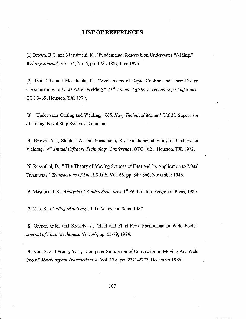
LIST OF REFERENCES
[1] Brown, R.T. and Masubuchi, K., "Fundamental Research on Underwater Welding,"
Welding Journal, Vol. 54, No. 6, pp. 178s-188s, June 1975.
[2] Tsai, C.L. and Masubuchi, K., "Mechanisms of Rapid Cooling and Their Design
Considerations in Underwater Welding," 11th Annual Offshore Technology Conference,
OTC 3469, Houston, TX, 1979.
[3] "Underwater Cutting and Welding," U.S. Navy Technical Manual, U.S.N. Supervisor
of Diving, Naval Ship Systems Command.
[4] Brown, A.J., Staub, J.A. and Masubuchi, K., "Fundamental Study of Underwater
Welding," 4th Annual Offshore Technology Conference, OTC 1621, Houston, TX, 1972.
[5] Rosenthal, D.," The Theory of Moving Sources of Heat and Its Application to Metal
Treatments," Transactions ofTheAS.M.E. Vol. 68, pp. 849-866, November 1946.
[6] Masubuchi, K., Analysis of Welded Structures, 1st Ed. London, Pergamon Press, 1980.
[7] Kou, S., Welding Metallurgy, John Wiley and Sons, 1987.
[8] Oreper, G.M. and Szekely, J., "Heat and Fluid-Flow Phenomena in Weld Pools,"
Journal of Fluid Mechanics, Vol.147, pp. 53-79,1984.
[9] Kou, S. and Wang, Y.H., "Computer Simulation of Convection in Moving Arc Weld
Pools," Metallurgical Transactions A, Vol. 17A, pp. 2271-2277, December 1986.
107
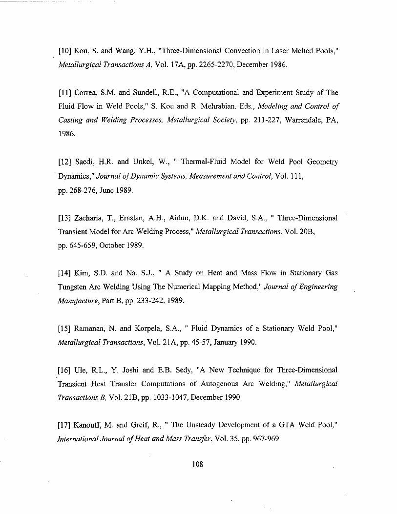
[10] Kou, S. and Wang, Y.H., "Three-Dimensional Convection in Laser Melted Pools,"
Metallurgical Transactions A, Vol. 17A, pp. 2265-2270, December 1986.
[11] Correa, S.M. and Sundeil, R.E., "A Computational and Experiment Study of The
Fluid Flow in Weld Pools," S. Kou and R. Mehrabian. Eds., Modeling and Control of
Casting and Welding Processes, Metallurgical Society, pp. 211-227, Warrendale, PA,
1986.
[12] Saedi, H.R. and Unkel, W., " Thermal-Fluid Model for Weld Pool Geometry
Dynamics," Journal of Dynamic Systems, Measurement and Control, Vol. Ill,
pp. 268-276, June 1989.
[13] Zacharia, T., Eraslan, A.H., Aidun, D.K. and David, S.A., " Three-Dimensional
Transient Model for Arc Welding Process," Metallurgical Transactions, Vol. 20B,
pp. 645-659, October 1989.
[14] Kim, S.D. and Na, S.J., " A Study on Heat and Mass Flow in Stationary Gas
Tungsten Arc Welding Using The Numerical Mapping Method," Journal of Engineering
Manufacture, Part B, pp. 233-242, 1989.
[15] Ramanan, N. and Korpela, S.A., " Fluid Dynamics of a Stationary Weld Pool,"
Metallurgical Transactions, Vol. 21A, pp. 45-57, January 1990.
[16] Ule, R.L., Y. Joshi and E.B. Sedy, "A New Technique for Three-Dimensional
Transient Heat Transfer Computations of Autogenous Arc Welding," Metallurgical
Transactions B, Vol. 21B, pp. 1033-1047, December 1990.
[17] Kanouff, M. and Greif, R., " The Unsteady Development of a GTA Weld Pool,"
International Journal of Heat and Mass Transfer, Vol. 35, pp. 967-969
108
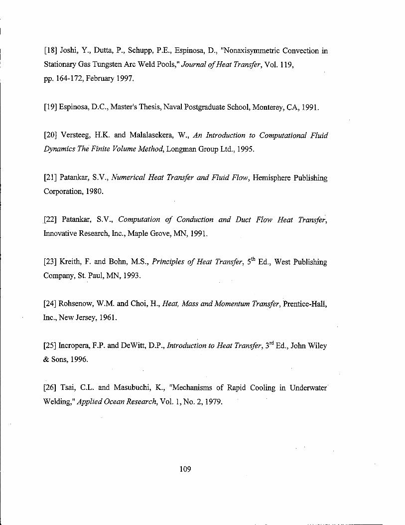
[18] Joshi, Y., Dutta, P., Schupp, P.E., Espinosa, D., "Nonaxisymmetric Convection in
Stationary Gas Tungsten Arc Weld Pools," Journal of Heat Transfer, Vol. 119,
pp. 164-172, February 1997.
[19] Espinosa, D.C., Master's Thesis, Naval Postgraduate School, Monterey, CA, 1991.
[20] Versteeg, H.K. and Malalasekera, W., An Introduction to Computational Fluid
Dynamics The Finite Volume Method, Longman Group Ltd., 1995.
[21] Patankar, S.V., Numerical Heat Transfer and Fluid Flow, Hemisphere Publishing
Corporation, 1980.
[22] Patankar, S.V., Computation of Conduction and Duct Flow Heat Transfer,
Innovative Research, Inc., Maple Grove, MN, 1991.
[23] Kreith, F. and Bohn, M.S., Principles of Heat Transfer, 5th Ed., West Publishing
Company, St. Paul, MN, 1993.
[24] Rohsenow, W.M. and Choi, H., Heat, Mass and Momentum Transfer, Prentice-Hall,
Inc., New Jersey, 1961.
[25] Incropera, F.P. and De Witt, D.P., Introduction to Heat Transfer, 3rd Ed., John Wiley
& Sons, 1996.
[26] Tsai, C.L. and Masubuchi, K., "Mechanisms of Rapid Cooling in Underwater
Welding," Applied Ocean Research, Vol. 1, No. 2,1979.
109

110
INITIAL DISTRIBUTION LIST
No. Copies
1. Defense Technical Information Center 2 8725 John J. Kingman Rd., STE 0944 Ft. Belvoir, VA 22060-6218
2. Dudley Knox Library 2 Naval Postgraduate School 411 Dyer Rd. Monterey, CA 93943-5101
3. Chairman, Code ME 1 Department of Mechanical Engineering Naval Postgraduate School Monterey, CA 93943-5000
4. Professor Ashok Gopinath, Code ME/GK 2 Department of Mechanical Engineering Naval Postgraduate School Monterey, CA 93943-5000
5. Naval/Mechanical Engineering Curricular Office, Code 34 1 Naval Postgraduate School Monterey, CA 93943-5000
6. Deniz Kuwetleri Komutanligi 2 Personel Daire Baskanligi Bakanliklar Ankara, TURKEY 06100
7. Deniz Harp Okulu Komutanligi 1 Kutuphane Tuzla, Istanbul, TURKEY 81704
8. Yasar Vehbi Isiklar 2 Feyzullah Mahallesi Esenyurt Sokak Tufekciler Apt. No. 16/6 Maltepe, Istanbul, TURKEY
111
9. Istanbul Teknik Universitesi Makina Muh.Bl. Ratip Berber Kutuphanesi Maslak, Istanbul, TURKEY
10. Ibrahim Girgin Deniz Harp Okulu Komutanligi Teknik Bilimler Bolum Baskanligi Makina Ogretim Uyesi Tuzla, Istanbul, TURKEY 81704
112