Embed Size (px)
Citation preview
Negative Sequence Impedance Measurement for DistributedGenerator Islanding Detection
by
Michael C. Wrinch
B.Sc., The University of British Columbia, 1995B.A.Sc., Memorial University of Newfoundland, 2000M.A.Sc., Memorial University of Newfoundland, 2002
A THESIS SUBMITTED IN PARTIAL FULFILMENT OFTHE REQUIREMENTS FOR THE DEGREE OF
Doctor of Philosophy
in
The Faculty of Graduate Studies
(Electrical and Computer Engineering)
The University Of British Columbia
(Vancouver)
December, 2008
c© Michael C. Wrinch 2008
Abstract
This thesis presents a method of detecting electrical islands in low voltage distributed generator net-
works by measuring negative sequence impedance differences between islanded and utility connections.
Extensive testing was conducted on a commercial building and 25 kV distributed generator fed network
by measuring naturally occurring and artificially injectednegative sequence components. Similarly, this
technique was tested using the IEEE 399-1990 bus test case using the EMTP software. The practical
measurements have been matched to simulations where further system performance characteristics of
detecting power system islands has been successfully demonstrated. Measured results indicate that un-
balanced load conditions are naturally occurring and readily measurable while deliberately unbalanced
loads can increase the accuracy of negative sequence impedance islanding detection. The typically low
negative sequence impedance of induction motors was found to have only a small effect in low voltage
busses, though large machines can effect the threshold settings. Careful placement of the island detector
is required in these situations. The negative sequence impedance measurement method is an improve-
ment on previous impedance measurement techniques for islanding detection due to its accuracy, and
distinctly large threshold window which have challenged previous impedance based islanding detection
techniques.
ii

Table of Contents
Abstract . . . . . . . . . . . . . . . . . . . . . . . . . . . . . . . . . . . . . . . . . . . . . . ii
Table of Contents . . . . . . . . . . . . . . . . . . . . . . . . . . . . . . . . . . . . . . . . . iii
List of Tables . . . . . . . . . . . . . . . . . . . . . . . . . . . . . . . . . . . . . . . . . . . . vii
List of Figures . . . . . . . . . . . . . . . . . . . . . . . . . . . . . . . . . . . . . . . . . . . viii
Acronyms . . . . . . . . . . . . . . . . . . . . . . . . . . . . . . . . . . . . . . . . . . . . . xi
Acknowledgements . . . . . . . . . . . . . . . . . . . . . . . . . . . . . . . . . . . . . . . . xiii
Dedication . . . . . . . . . . . . . . . . . . . . . . . . . . . . . . . . . . . . . . . . . . . . . xiv
1 Introduction . . . . . . . . . . . . . . . . . . . . . . . . . . . . . . . . . . . . . . . . . . 1
1.1 Motivation to Power System Protection for Distributed Generation . . . . . . . . . . . 1
1.1.1 Electrical Energy Supply and Demand . . . . . . . . . . . . . . .. . . . . . 2
1.1.2 Distributed Generation as a Viable Alternative . . . . .. . . . . . . . . . . . 2
1.1.3 Types of Distributed Generation . . . . . . . . . . . . . . . . . .. . . . . . . 3
1.2 Technical Challenges Facing Distributed Generation . .. . . . . . . . . . . . . . . . 3
1.2.1 Utility Perspective of Distributed Generator Network Islanding . . . . . . . . 5
1.2.2 The Problem: Detection of Unplanned Islands . . . . . . . .. . . . . . . . . 6
1.2.3 Research Motivation . . . . . . . . . . . . . . . . . . . . . . . . . . . .. . . 8
1.2.4 Impedance Measurement for islanding Detection . . . . .. . . . . . . . . . . 8
1.3 Proposed Solution: Negative Sequence Impedance Islanding Detection . . . . . . . . 10
1.4 Thesis Organization and Contributions . . . . . . . . . . . . . .. . . . . . . . . . . 11
1.4.1 Thesis Contributions . . . . . . . . . . . . . . . . . . . . . . . . . . .. . . . 11
1.4.2 List of Publications . . . . . . . . . . . . . . . . . . . . . . . . . . . .. . . 12
2 Review of Islanding Detection Methods . . . . . . . . . . . . . . . . . . . . . . . . . . . 13
2.1 Introduction . . . . . . . . . . . . . . . . . . . . . . . . . . . . . . . . . . . .. . . . 13
2.2 Distributed Generator Related Protection Issues . . . . .. . . . . . . . . . . . . . . . 13
2.2.1 Voltage Issues From Distributed Generator Installations . . . . . . . . . . . . 14
2.2.2 Short Circuit Current Issues . . . . . . . . . . . . . . . . . . . . .. . . . . . 17
iii
Table of Contents
2.2.3 Maintenance . . . . . . . . . . . . . . . . . . . . . . . . . . . . . . . . . . .19
2.2.4 Reclosure . . . . . . . . . . . . . . . . . . . . . . . . . . . . . . . . . . . . .20
2.2.5 Typical Interconnection Protection Schemes . . . . . . .. . . . . . . . . . . 20
2.3 Islanding Detection . . . . . . . . . . . . . . . . . . . . . . . . . . . . . .. . . . . . 21
2.3.1 Communication Based Islanding Detection Methods . . .. . . . . . . . . . . 23
2.3.2 Passive Islanding Detection Methods . . . . . . . . . . . . . .. . . . . . . . 25
2.3.3 Active Islanding Detection Methods . . . . . . . . . . . . . . .. . . . . . . . 28
2.4 Impedance Measurement . . . . . . . . . . . . . . . . . . . . . . . . . . . .. . . . . 35
2.4.1 Impulse Response . . . . . . . . . . . . . . . . . . . . . . . . . . . . . . .. 36
2.4.2 Islanding Detection using Continuous Injected Noise. . . . . . . . . . . . . . 39
2.5 Current and Voltage Measurability . . . . . . . . . . . . . . . . . .. . . . . . . . . . 43
2.5.1 Voltage Measurement . . . . . . . . . . . . . . . . . . . . . . . . . . . .. . 43
2.5.2 Current Measurement . . . . . . . . . . . . . . . . . . . . . . . . . . . .. . 47
2.6 Summary of Research Background . . . . . . . . . . . . . . . . . . . . .. . . . . . 50
3 Negative Sequence Impedance Islanding Detection. . . . . . . . . . . . . . . . . . . . . 52
3.1 Introduction . . . . . . . . . . . . . . . . . . . . . . . . . . . . . . . . . . . .. . . . 52
3.2 Derivation of System Negative Sequence Impedance Estimation . . . . . . . . . . . . 54
3.2.1 Two Circuit DC System . . . . . . . . . . . . . . . . . . . . . . . . . . . .. 54
3.2.2 Simple Three Phase System . . . . . . . . . . . . . . . . . . . . . . . .. . . 55
3.2.3 Balanced AC Systems . . . . . . . . . . . . . . . . . . . . . . . . . . . . .. 58
3.2.4 Unbalanced AC Systems . . . . . . . . . . . . . . . . . . . . . . . . . . .. . 60
3.2.5 Negative Sequence Current Flow in Unbalanced Loads . .. . . . . . . . . . . 62
3.2.6 Unbalanced Sources Injection . . . . . . . . . . . . . . . . . . . .. . . . . . 65
3.2.7 Negative Sequence Thevenin Impedance of the Network. . . . . . . . . . . . 66
3.3 Performance Characteristics of Negative Sequence Impedance Measurement . . . . . 67
3.3.1 Effect of Changing Per Cent of Unbalanced Load . . . . . . .. . . . . . . . 69
3.3.2 Effect of Strength of the System vs the Unbalanced LoadPower . . . . . . . . 69
3.3.3 Effect of Varying the Power of an Unbalanced Load . . . . .. . . . . . . . . 70
3.3.4 Effect of Changing Source Unbalance . . . . . . . . . . . . . . .. . . . . . . 71
3.3.5 Effect ofV2 andI2 Phase Angle on Different Unbalanced Configurations . . . 72
3.3.6 Multiple Unbalanced Loads in a System . . . . . . . . . . . . . .. . . . . . 74
3.4 Non Fundamental Frequency Negative Sequence Impedance. . . . . . . . . . . . . . 79
3.4.1 Sources of Harmonics from Non-Linear Components . . . .. . . . . . . . . 79
3.5 Sequence Components for Induction and Synchronous Machines . . . . . . . . . . . . 81
3.6 Implementation Strategy for Negative Sequence Islanding Detection . . . . . . . . . . 81
3.6.1 Naturally Occurring Negative Sequence Currents . . . .. . . . . . . . . . . . 82
3.6.2 Injected Negative Sequence Currents . . . . . . . . . . . . . .. . . . . . . . 83
3.7 Summary . . . . . . . . . . . . . . . . . . . . . . . . . . . . . . . . . . . . . . . . .84
iv
Table of Contents
4 Case Studies of Negative Sequence Impedance Islanding Detection . . . . . . . . . . . . 87
4.1 Introduction . . . . . . . . . . . . . . . . . . . . . . . . . . . . . . . . . . . .. . . . 87
4.2 Simulation of Standard IEEE 399-1997 Industrial Bus . . .. . . . . . . . . . . . . . 87
4.2.1 System Description . . . . . . . . . . . . . . . . . . . . . . . . . . . . .. . 87
4.2.2 Experimental Results . . . . . . . . . . . . . . . . . . . . . . . . . . .. . . 89
4.2.3 Discussion . . . . . . . . . . . . . . . . . . . . . . . . . . . . . . . . . . . .94
4.3 Practical Example 1: 25 kV Radially Feed Distributed Generator Network . . . . . . . 95
4.3.1 System Description . . . . . . . . . . . . . . . . . . . . . . . . . . . . .. . 95
4.3.2 Experimental Results . . . . . . . . . . . . . . . . . . . . . . . . . . .. . . 98
4.3.3 Discussion . . . . . . . . . . . . . . . . . . . . . . . . . . . . . . . . . . . .100
4.4 Practical Example 2: 600 V Fed Commercial Building . . . . .. . . . . . . . . . . . 100
4.4.1 System Description . . . . . . . . . . . . . . . . . . . . . . . . . . . . .. . 100
4.4.2 Experimental Results . . . . . . . . . . . . . . . . . . . . . . . . . . .. . . 103
4.4.3 Discussion . . . . . . . . . . . . . . . . . . . . . . . . . . . . . . . . . . . .110
4.5 Performance Comparison with other Impedance Based Islanding Detection Methods . 111
4.6 Summary . . . . . . . . . . . . . . . . . . . . . . . . . . . . . . . . . . . . . . . . .117
5 Conclusion . . . . . . . . . . . . . . . . . . . . . . . . . . . . . . . . . . . . . . . . . . . 119
5.1 Summary of Contributions . . . . . . . . . . . . . . . . . . . . . . . . . .. . . . . . 119
5.2 Future Work . . . . . . . . . . . . . . . . . . . . . . . . . . . . . . . . . . . . . .. 121
5.3 Final Remarks . . . . . . . . . . . . . . . . . . . . . . . . . . . . . . . . . . . .. . 124
Bibliography . . . . . . . . . . . . . . . . . . . . . . . . . . . . . . . . . . . . . . . . . . . . 125
Appendices
A Device Number Reference . . . . . . . . . . . . . . . . . . . . . . . . . . . . . . . . . . 135
B Symmetrical Components - The Basics . . . . . . . . . . . . . . . . . . . . . . . . . . . 138
C AEMC 3945 Three Phase Power Quality Meter . . . . . . . . . . . . . . . . . . . . . . 140
D Simulation Software Tools Used . . . . . . . . . . . . . . . . . . . . . . . . . . . . . . . 141
D.1 Aspen . . . . . . . . . . . . . . . . . . . . . . . . . . . . . . . . . . . . . . . . . . .141
D.2 Matlab . . . . . . . . . . . . . . . . . . . . . . . . . . . . . . . . . . . . . . . . . .141
D.3 Microtran Power Systems Simulator . . . . . . . . . . . . . . . . . .. . . . . . . . . 141
D.4 Power World . . . . . . . . . . . . . . . . . . . . . . . . . . . . . . . . . . . . . .. 141
D.5 Psim . . . . . . . . . . . . . . . . . . . . . . . . . . . . . . . . . . . . . . . . . . . 142
D.6 Simulink Power Systems Tool Box . . . . . . . . . . . . . . . . . . . . .. . . . . . 142
D.7 SKM Power Tools . . . . . . . . . . . . . . . . . . . . . . . . . . . . . . . . . . .. 142
v

Table of Contents
E Simulink Model: 600 V Fed Bus . . . . . . . . . . . . . . . . . . . . . . . . . . . . . . . 143
F Commonly Used Signal Processing Techniques. . . . . . . . . . . . . . . . . . . . . . . 144
vi

List of Tables
1.1 Types of DG and Typical Capacity . . . . . . . . . . . . . . . . . . . . .. . . . . . . 4
1.2 Technical Challenges for Distributed Generation . . . . .. . . . . . . . . . . . . . . . 5
1.3 Technical Challenges Associated with DG Islanding . . . .. . . . . . . . . . . . . . . 6
1.4 Factors Influencing Island Detectability . . . . . . . . . . . .. . . . . . . . . . . . . 9
2.1 Communication Islanding Detection Methods . . . . . . . . . .. . . . . . . . . . . . 22
2.2 Passive Islanding Detection Methods . . . . . . . . . . . . . . . .. . . . . . . . . . . 22
2.3 Active Islanding Detection Methods . . . . . . . . . . . . . . . . .. . . . . . . . . . 22
2.4 Data from Wang Experiment . . . . . . . . . . . . . . . . . . . . . . . . . .. . . . . 24
3.1 Base Performance Values for Practical System . . . . . . . . .. . . . . . . . . . . . . 69
3.2 Phase Angle For Different Unbalanced Load Types . . . . . . .. . . . . . . . . . . . 74
3.3 Base Case Values for Figure 3.19 . . . . . . . . . . . . . . . . . . . . .. . . . . . . . 75
3.4 Scenarios and Comments for Multiple Unbalanced Loads (All Values in pu) . . . . . . 77
3.5 Common Power System Non-linear Loads . . . . . . . . . . . . . . . .. . . . . . . . 80
3.6 Sequence Movement For Harmonics [120] . . . . . . . . . . . . . . .. . . . . . . . . 80
4.1 Experiments Modeled using IEEE 399 Standard Bus . . . . . . .. . . . . . . . . . . 89
4.2 Expected Impedances From Perspective of Test Loads (in pu) . . . . . . . . . . . . . 90
4.3 Experiment 1: IEEE 399 Bus System, Single Phase Unbalance of Load 3 and Load 5 . 91
4.4 Experiment 2a, Load 3 and Load 5 Unbalanced on Phase A . . . .. . . . . . . . . . . 91
4.5 Experiment 2b, Phase A Unbalance on Load 3 and Phase B Unbalance on Load 5 . . . 92
4.6 Using Averaging Equation 3.73 for Load 3 and Load 5 . . . . . .. . . . . . . . . . . 92
4.7 Induction Machine (1.6 MVA) Input Variables for EMTP . . .. . . . . . . . . . . . . 93
4.8 Expected Impedances From Induction Machine . . . . . . . . . .. . . . . . . . . . . 93
4.9 Case 3, IEEE 399 Bus System, Induction Machine on Feeder 2, Bus 2 . . . . . . . . . 93
4.10 Case 4, IEEE 399 Bus System, Induction Machine with Alternate Phase Unbalanced . 94
4.11 ExpectedZ2 Impedances From Positions ”A”, ”B” and ”C” (in pu) . . . . . . . . .. . 97
4.12 Measured Values for 25 kV System Positive and Negative Sequences . . . . . . . . . . 99
4.13 Experiments Simulated on 25 kV Practical System . . . . . .. . . . . . . . . . . . . 99
4.14 Simulated Values for 25 kV System Positive and NegativeSequences . . . . . . . . . 100
4.15 Induction Machine Parameters (15 kVA) Input Variablesfrom Simulink Power Library 109
4.16 Performance Characteristics to Compare Islanding Detection Techniques . . . . . . . . 112
vii

List of Figures
1.1 2006 United States Projected Summer Generation and Capacity [18] . . . . . . . . . . 3
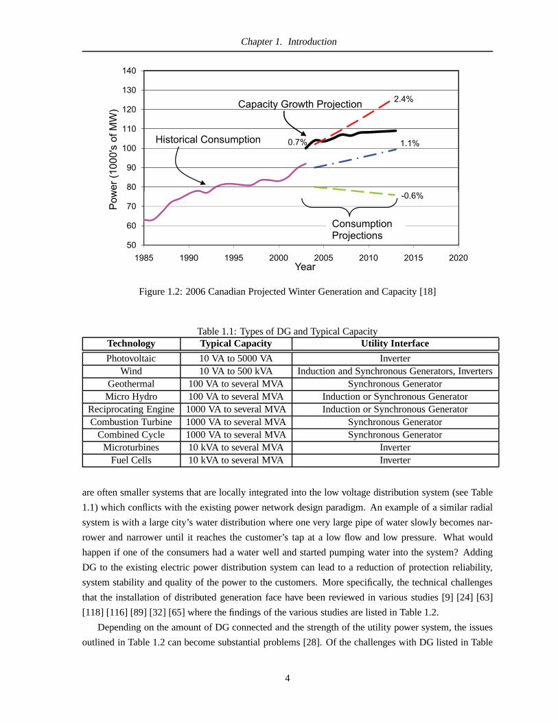
1.2 2006 Canadian Projected Winter Generation and Capacity[18] . . . . . . . . . . . . . 4
1.3 Power System Islanding Detection Schemes . . . . . . . . . . . .. . . . . . . . . . . 7
1.4 Non Detection Zone in Daily Load Profile Illustration . . .. . . . . . . . . . . . . . . 8
1.5 Radially Fed Distributed Generation System . . . . . . . . . .. . . . . . . . . . . . . 9
1.6 IEEE Standard 1547 Resonating Bus Islanding Detection Test Setup . . . . . . . . . . 10
2.1 Distributed Generation and Interconnection on a RadialSystem . . . . . . . . . . . . . 14
2.2 Ungrounded or Poorly Grounded DG Connections Causing Voltage Rise . . . . . . . . 15
2.3 Voltage Rise From Single Phase Fault on an Ungrounded System . . . . . . . . . . . . 16
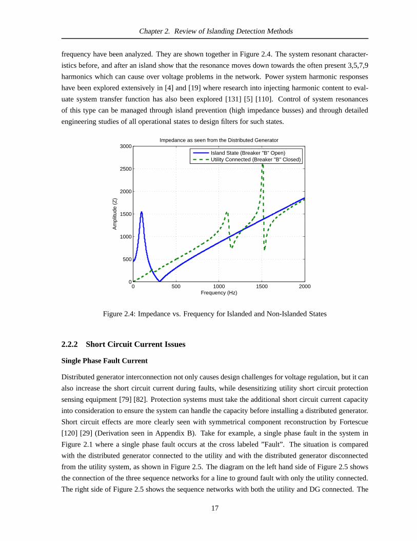
2.4 Impedance vs. Frequency for Islanded and Non-Islanded States . . . . . . . . . . . . . 17
2.5 Single Phase Fault Comparison Between Utility only and DG Connected System . . . 18
2.6 Example of Reduced Impedance Relay (21) Reach . . . . . . . . .. . . . . . . . . . 19
2.7 Distributed Generation (left) and DG Interconnection Protection (right) . . . . . . . . 21
2.8 Distributed Generation Multi Power Line Signaling Islanding Detection Issue . . . . . 23
2.9 Distributed Generation Power Line Signaling IslandingDetection . . . . . . . . . . . 25
2.10 Distributed Generation Transfer Trip Islanding Detection . . . . . . . . . . . . . . . . 26
2.11 Frequency Bias Islanding Detection . . . . . . . . . . . . . . . .. . . . . . . . . . . 31
2.12 Voltage Variation Islanding Detection . . . . . . . . . . . . .. . . . . . . . . . . . . 33
2.13 Basic Premise of Using Impedance Measurement for Islanding Detection . . . . . . . 35
2.14 Impedance Measurement Using High Voltage Capacitive Switching (Girgis [36]) . . . 36
2.15 Impedance Measurement Using TRIAC Controlled Capacitive Switching (Hopewell [44]) 38
2.16 US Patent 6,603,290 Drawing 1: Islanding Detection by Signal Injection . . . . . . . . 40
2.17 Negative Sequence Injection Concept and H-Bridge Injector Realization . . . . . . . . 42
2.18 Resistive Divider Voltage Measurement with Isolator .. . . . . . . . . . . . . . . . . 44
2.19 Voltage Transformer Equivalent Circuit . . . . . . . . . . . .. . . . . . . . . . . . . 45
2.20 Coupling Capacitor Voltage Transformer Equivalent Circuit . . . . . . . . . . . . . . . 45
2.21 Pockels Effect Voltage Measurement . . . . . . . . . . . . . . . .. . . . . . . . . . . 46
2.22 Resistive Shunt Current Measurement . . . . . . . . . . . . . . .. . . . . . . . . . . 47
2.23 Current Transformer Circuit with Burden . . . . . . . . . . . .. . . . . . . . . . . . 48
3.1 Negative and Positive Sequence Current Flow . . . . . . . . . .. . . . . . . . . . . . 53
3.2 Symmetrical Component Conversion . . . . . . . . . . . . . . . . . .. . . . . . . . . 54
viii

List of Figures
3.3 Two DC Circuits with Different Load Impedances . . . . . . . .. . . . . . . . . . . . 55
3.4 Three Phase Circuit (Single Line) Example with Different ‘Y’ Load Impedances . . . . 56
3.5 Three Phase Circuit Example Expanded with Different ‘Y’Load Impedances . . . . . 57
3.6 Three Phase Circuit Example Expanded and Logically Grouped . . . . . . . . . . . . 58
3.7 Three Phase Circuit with a Balanced Load . . . . . . . . . . . . . .. . . . . . . . . . 59
3.8 Balanced Symmetrical Component Circuits from BalancedLoad . . . . . . . . . . . . 60
3.9 Unbalanced Load and Balanced Source Circuit . . . . . . . . . .. . . . . . . . . . . 60
3.10 Symmetrical Component Concept in an Unbalanced System. . . . . . . . . . . . . . 62
3.11 Symmetrical Components Current Flow in an Unbalanced System Expanded Circuit . 64
3.12 System Performance Test Schematic with System Impedance and Load Impedance . . 68
3.13 Per Cent Unbalanced Load vs.V2 Magnitude and Phase (System Strength = 10 MVA) . 70
3.14 System Strength Vs.V2 with Varying Unbalanced Load from 0.5 MVA to 4.5 MVA . . 71
3.15 Unbalanced Load Size of 0 MVA to 3 MVA vs.V2, (Load unbalanced by 20%) . . . . 72
3.16 Utility Strength (SCC) vs.V2 (Varying Percent Source Unbalance of 5% to 30%) . . . 73
3.17 V2 Phase For Different Unbalanced Load Types Relative to 0, 240, 120 ABC Phases . . 75
3.18 I2 Phase For Different Unbalanced Load Types Relative to 0, 240, 120 V ABC Phases . 76
3.19 Single Line Diagram of Multiple Unbalanced Equal Load Scenario . . . . . . . . . . . 76
3.20 -10% to + 10% Load Unbalance on Both Phase A, Vs. CalculatedV2 (ZLoad = 2000pu ) 77
3.21 -10% to + 10% Load Unbalance on Alternating Phases Vs. CalculatedV2 . . . . . . . 78
3.22 -10% to + 10% Load Unbalance Vs. CalculatedV2 Averaged on A,B,C Alternating Phases 79
3.23 Induction and Synchronous Machine Negative Sequence Impedance . . . . . . . . . . 81
3.24 Natural Negative Sequence Impedance Islanding Detection Algorithm . . . . . . . . . 83
3.25 Negative Sequence Impedance Measurement Islanding Detection Concept . . . . . . . 84
3.26 Injected Components Negative Sequence Impedance Islanding Detection Algorithm . . 86
4.1 IEEE Standard 399-1997 (Brown Book) Reference Bus Case adapted From [65] . . . . 90
4.2 IEEE Standard 399-1997 Reference Bus Case with Induction Machine at Load 3 (Center) 94
4.3 Practical Example 1: 25 kV DG System Fed System Single Line Diagram . . . . . . . 96
4.4 Practical Example 1: 25 kV DG System Fed System Sequence Impedances . . . . . . 98
4.5 Practical Example 2: 600 V Commercial Office DG Fed SystemSingle Line Diagram . 102
4.6 Practical Example 2: 600 V Commercial Office 24 Hour PowerDemand . . . . . . . . 103
4.7 Practical Example 2: 600 VZ2 Measured Over 24 Hours . . . . . . . . . . . . . . . . 104
4.8 Practical Example 2: 600 V CombinedZLoad andZ2 Measured Over 24 Hours . . . . . 105
4.9 Practical Example 2: 600 VZ2 At Position 1 During Breaker A and B Opening . . . . 106
4.10 Practical Example 2: 208 V Negative Sequence InjectionExperimental Setup . . . . . 107
4.11 Practical Example 2: 208 V Negative Sequence ImpedancePhase to Phase Loads . . . 108
4.12 Practical Example 2: 600 V, PV Source Negative SequenceImpedance Transition . . . 109
4.13 Practical Example 2: 600 V Building PV DG Islanding Detection Results . . . . . . . 110
4.14 Practical Example 2: Building Solar DG Islanding Detection with Rotating Machine . 111
4.15 Building Solar DG Islanding Detection with Rotating Machine Voltage ABC . . . . . 112
ix

List of Figures
4.16 Practical Example 2: 208 V Bus Sequence Impedance Diagram from Lab . . . . . . . 113
4.17 IEEE 1547 1 2005 Test Bus . . . . . . . . . . . . . . . . . . . . . . . . . . .. . . . . 114
4.18 Impedance Between Islanded and Utility Connected Resonating Bus . . . . . . . . . . 115
B.1 Symmetrical Component Conversion . . . . . . . . . . . . . . . . . .. . . . . . . . . 138
B.2 Radially Fed System . . . . . . . . . . . . . . . . . . . . . . . . . . . . . . .. . . . 139
C.1 AEMC 3945 Power Quality Meter . . . . . . . . . . . . . . . . . . . . . . .. . . . . 140
E.1 Simulink Model From Practical Example 2: 600 V Fed Bus . . .. . . . . . . . . . . . 143
F.1 Convolution to Fourier Relationship . . . . . . . . . . . . . . . .. . . . . . . . . . . 144
x

Acronyms
CCVT Coupling Capacitor Voltage Transformers
CSA Canadian Standards Association
CT Current Transformer
DG Distributed Generator (Generation in the distribution layer)
FJ Frequency Jump
IEEE Institute of Electrical and Electronics Engineers
IGBT Insulated-gate Bipolar Transistor
IPP Independent Power Producer
LL Line to Line
LN Line to Neutral
MVA Mega Apparent Power (VA=√
W2 +VAR2 )
NDS Non Detection Zone
OF Over Frequency
OV Over Voltage
PCC Point of Common Coupling
PLL Phase Locked Loop
PT Potential Transformer
pu Per Unit
PV Photo Voltaic Cells (Solar Cells)
RL Resistor-Inductor
ROCOF Rate of Change of Frequency
SCADA Supervisory Control and Data Acquisition
SCC Short Circuit Capacity
SFS Sandia Frequency Shift
xi

Acronyms
SMS Slip Mode Frequency Shift
SVS Sandia Voltage Shift
THD Total Harmonic Distortion
UF Under Frequency
UL Underwriters’ Laboratories
UV Under Voltage
VA Apparent Power (VA=√
W2 +VAR2 )
VAR Reactive Power (Capacitors and Inductors)
W Watts
xii

Acknowledgements
There are many groups and individuals who helped to make thisthesis a success. In this section, the key
advisors, experts and supporters of the research will be mentioned.
First, I would like to thank the University of British Columbia’s Faculty of Applied Science who
provided the opportunity to conduct this work. In particular, my supervisor, Professor Jose Martı of
UBC, who’s extensive knowledge, vision and expertise played a key roll in the success of this work. I
would also like to thank my co-supervisor Dr. Mukesh Nagpal of BC Hydro who consistently offered
both technical and professional support throughout my research. I consider myself very fortunate to
have had the opportunity to work with these two world class experts.
Additional support came from within the Electric Power and Energy Systems lab at the University
of British Columbia. The international community of students in the lab offered a diverse background of
knowledge, problem solving and expertise that provided thedetails into various power system concepts
for the depth of knowledge that this research required. Someof the more helpful individuals I would
like to thank in no particular order are: Amir Rasuli, Liwei Wang, Marcelo Tomim, Michel AlSharidah,
Nathan Ozog and Tom De Rybel.
The literary style and grammar of this thesis was significantly improved from the expert advice and
support of David Greer.
The data acquired in this research could not have been attained without the support of several com-
panies and people who gave their time to further this work. The first is UBC Utilities where head
electrician, Stan Takenaka, provided the use of specialized three phase power signal monitoring equip-
ment and safe access to hard to reach high voltage areas throughout the campus. David Helliwell, CEO
of small energy group, offered additional information and support in this research. Finally I would like
to thank BC Hydro, where Dr. Wenpeng Luan and Mike Adams were key links to attaining the network
data and providing generalized system information from theBritish Columbian utility System.
xiii

Dedication
For my wife Amy and family.
xiv

Chapter 1
Introduction
1.1 Motivation to Power System Protection for Distributed Generation
This thesis presents a novel method of islanding detection for the protection of distributed generator
fed systems that has been tested on power distribution busses of 25 kV and less. Recent interest in
distributed generator installation into low voltage busses near electrical consumers, has created some
new challenges for protection engineers that are differentfrom traditional radially based protection
methodologies. Therefore, typical protection configurations need to be re-thought such as re-closures,
out-of-step monitoring, impedance relay protection zoneswith the detection of unplanned islanding of
distributed generator systems. The condition of islanding, defined as when a section of the non utility
generation system is isolated from the main utility system,is often considered undesirable because of
the potential damage to existing equipment, utility liability concerns, reduction of power reliability and
power quality.
Current islanding detection methods typically monitor over/under voltage and over/under frequency
conditions passively and actively; however, each method has an ideal sensitivity operating condition and
a non-sensitive operating condition with varying degrees of power quality corruption called the non-
detection zone (NDS). The islanding detection method developed in this thesis takes the theoretically
accurate concept of impedance measurement and extends it into the symmetrical component impedance
domain, using the existence of naturally and artificially produced unbalanced conditions. Specific appli-
cations, where this islanding detection method improves beyond existing islanding detection methods,
are explored where a generalized solution allows the protection engineer to determine when this method
can be used most effectively.
The practical concerns of voltage and current measurement accuracy using potential transformers
(PTs) and current transformers (CTs) are addressed in this thesis. Through field experimentation, CT
and PT bus monitors were evaluated to see if they contain the resolution for measuring negative sequence
voltage and current. The practical implementation for thisislanding detection scheme comes without
significant modifications and capital costs, as the implementation can be realized through choosing the
correct existing CT and PT positions and a software additionto digital relays or low voltage inverters.
To start, this thesis begins with a brief introduction to power systems in North America and the mo-
tivation for the use of distributed generation. Further chapters then detail the background and specifics
of this technique.
1

Chapter 1. Introduction
1.1.1 Electrical Energy Supply and Demand
Human progress has been linked to the increase of energy consumed per capita [92], [33]. In the last
20 years, electrical consumption has been steadily increasing in North America at a rate of 1.1% for
Canada, and 2.0% for the United states [18]; however, the investment into new bulk electric power
sources such as hydro dams and nuclear generation plants hasbecome politically, economically and
physically limited [75]. For example, transmission investment in the year 2000 was $2.5 billion dollars
less than the level of investment in 1975, where over this same period, electricity sales nearly doubled
[58]. At the current demand growth, the United States bulk electric power system is estimated to be
approximately 5 to 15 years away from the power demand exceeding the generation capacity as seen
in Figure 1.1. The United States has historically consumed amedian of 7.5 times the power of Canada
which can be seen in the Canadian winter demand growth in Figure 1.2.
Small localized power sources, commonly known as ”Distributed Generation” (DG), have become
a popular alternative to bulk electric power generation [88]. There are many reasons for the growing
popularity of DG; however, on top of DG tending to be more renewable, DG can serve as a cost effective
alternative to major system upgrades for peak shaving or enhancing load capacity margins. Additionally,
if the needed generation facilities could be constructed tomeet the growing demand, the entire distribu-
tion and transmission system would also require upgrading to handle the additional loading. Therefore,
constructing additional power sources and upgrading the transmission system will take significant cost
and time, both of which may not be achievable. These trends are not only limited to North America, but
worldwide, the demand for electricity is expected to doublein the next 20 years [114].
The costs of power outages to a country’s economy can be staggering. The cost associated with
power outages to all business sectors in the United States has been determined to be of the order $164
Billion US per year. More specifically, the average cost of a power outage to a medium sized company
is $1477 US for one second and $7000 US for one hour. Though thecost of one second of outage
is considerable, the cost of one hour, which is a 3600 times longer duration is only 4.7 times of cost
increase [70]; hence, initial quick outages are important to avoid significant cost implications to the
economy. Distributed Generators can assist in reducing these occurrences by strengthening networks
that are near to their stability limit.
1.1.2 Distributed Generation as a Viable Alternative
Traditionally, electrical power generation and distribution are purely a state owned utility. However, in
order to keep up with the growing demand, many states and provinces in North America are deregulating
the electrical energy system. This trend is not without its own challenges. For example, how is an
independent power producer (IPP) able to enter the market ?
Recent innovations in power electronics such as fast switching, high voltage Insulated Gate Bipolar
Transistors (IGBT) and developments in power generation technologies have made DG a considerable
alternative to either delaying infrastructure upgrades oras additional cogeneration support [3]. Though
the cost per kw-hr is still higher than basic power grid distribution costs, ($0.07/Kw-hr for gas turbines
2

Chapter 1. Introduction
400
500
600
700
800
900
1000
1100
1985 1990 1995 2000 2005 2010 2015 2020Year
Pow
er
(1000's
of
MW
)
Historical Consumption
Capacity Growth Projection
Consumption
Projections
0.5%
2.5%
1.5%
2.0%
Figure 1.1: 2006 United States Projected Summer Generationand Capacity [18]
and as high as $0.5/kw-hr for PV) [66] [59]. The trend to completely deregulate the North American
electric power grid along with the increasing trend in the cost of fossil fuels has resulted in the consid-
eration of DG as a viable opportunity. Currently, BC Hydro, Canada’s third largest utility has more than
50 Distributed Generator stations ranging from 0.07 MVA to 34 MVA [79].
1.1.3 Types of Distributed Generation
Distributed Generators can be broken into three basic classes: induction, synchronous and asynchronous.
Induction generators require external excitation (VARs) and start up much like a regular induction mo-
tor. They are less costly than synchronous machines and are typically less than 500 kVA. Induction
machines are most commonly used in wind power applications.Alternatively, synchronous generators
require a DC excitation field and need to synchronize with theutility before connection. Synchronous
machines are most commonly used with internal combustion machines, gas turbines, and small hydro
dams. Finally, asynchronous generators are transistor switched systems such as inverters. Asynchronous
generators are most commonly used with microturbines, photovoltaic, and fuel cells. A comparison of
each type of generation system can be seen in Table 1.1
1.2 Technical Challenges Facing Distributed Generation
Distributed Generation (DG) is not without problems. DG faces a series of integration challenges, but
one of the more significant overall problems is that the electrical distribution and transmission infras-
tructure has been designed in a configuration where few high power generation stations that are often
distant from their consumers, ”push” electrical power ontothe many smaller consumers. DG systems
3
Chapter 1. Introduction
120
130
140
) Capacity Growth Projection 2.4%
80
90
100
110we
r (10
00's
of M
W
Historical Consumption 0.7% 1.1%
50
60
70
1985 1990 1995 2000 2005 2010 2015 2020
Pow
Year
ConsumptionProjections
-0.6%
Year
Figure 1.2: 2006 Canadian Projected Winter Generation and Capacity [18]
Table 1.1: Types of DG and Typical CapacityTechnology Typical Capacity Utility Interface
Photovoltaic 10 VA to 5000 VA InverterWind 10 VA to 500 kVA Induction and Synchronous Generators, Inverters
Geothermal 100 VA to several MVA Synchronous GeneratorMicro Hydro 100 VA to several MVA Induction or Synchronous Generator
Reciprocating Engine 1000 VA to several MVA Induction or Synchronous GeneratorCombustion Turbine 1000 VA to several MVA Synchronous Generator
Combined Cycle 1000 VA to several MVA Synchronous GeneratorMicroturbines 10 kVA to several MVA Inverter
Fuel Cells 10 kVA to several MVA Inverter
are often smaller systems that are locally integrated into the low voltage distribution system (see Table
1.1) which conflicts with the existing power network design paradigm. An example of a similar radial
system is with a large city’s water distribution where one very large pipe of water slowly becomes nar-
rower and narrower until it reaches the customer’s tap at a low flow and low pressure. What would
happen if one of the consumers had a water well and started pumping water into the system? Adding
DG to the existing electric power distribution system can lead to a reduction of protection reliability,
system stability and quality of the power to the customers. More specifically, the technical challenges
that the installation of distributed generation face have been reviewed in various studies [9] [24] [63]
[118] [116] [89] [32] [65] where the findings of the various studies are listed in Table 1.2.
Depending on the amount of DG connected and the strength of the utility power system, the issues
outlined in Table 1.2 can become substantial problems [28].Of the challenges with DG listed in Table
4

Chapter 1. Introduction
Table 1.2: Technical Challenges for Distributed Generation
1. Voltage Regulation and Losses
2. Voltage Flicker
3. DG Shaft Over-Torque During Faults
4. Harmonic Control and Harmonic Injection
5. Increased Short Circuit Levels
6. Grounding and Transformer Interface
7. Transient Stability
8. Sensitivity of Existing Protection Schemes
9. Coordination of Multiple Generators
10. High Penetration Impacts are Unclear
11. Islanding Control
1.2, the problem of protection against unplanned islandingis a significant one. Islanding can be defined
as:
Islanding: The condition when a portion of the utility system is energized by one or more
DG sources and that portion of the system is separated electrically from the rest of the
utility system. DG islanding may be inadvertent or intentional [38].
1.2.1 Utility Perspective of Distributed Generator Network Islanding
Utilities have a more pragmatic point of view of distributedgeneration islanding [38]. Their goal is to
improve the distribution level (25 kV and below) customer service reliability especially in regions where
the reliability is below customer’s needs. It is believed that customer reliability could improve with the
addition of DG sources and that the DG may be able to sell electricity back to the utility. However,
without complex studies and frequent expensive system upgrades DG islanding is not allowed. Some
examples of these studies are: real and reactive power profile and control, planning for islanding, min-
imum/maximum feeder loading, islanding load profile, minimum/maximum voltage profile, protection
sensitivity and DG inertia. One more specific example is how substation auto-reclosers of circuit break-
ers and main line reclosers may be disabled and other protection devices may need to be removed to
allow proper coordination of utility sources and DG sources(covered in further chapters). Maintenance
times might also increase as utility workers will not only need to lockout the utility lines but they will
need to take additional time to lockout all the installed DG lines. Some of the required installation
studies an IPP must complete to be able to island are: 1. inadvertent islanding and planned islanding
study, 2. reliability study, 3. power quality study, 4. utility equipment upgrade assessment, 5. safety and
5

Chapter 1. Introduction
protection reviews, and 6. commercial benefit study. Clearly the costs of designing a DG to be capable
of islanding or to simply be installed into the main utility owned network requires extensive and costly
engineering and business reviews which may be outside the financial range of smaller DG suppliers.
An Example of Current Utility Islanding Policy: “Nearly all the BC Hydro distribution
feeders are radial, resulting in a power outage for all the load customers connected to the
feeder during a feeder outage. A DG without planned islanding capability does not pro-
vide increased customer service reliability hence the DG must be de-energized during the
outage.” [38]
1.2.2 The Problem: Detection of Unplanned Islands
As previously stated, Islanding is the condition when a portion of the electrical system is completely
disconnected from the rest of the electric utility and left generating electrical power on its own to its
local consumers. For unapproved DG systems, the current generalized industry standard is to discon-
nect all the DG sources from the island as soon as possible. The IEEE society has produced a standard
for Distributed Generation IEEE 1547, [54] [56], that highlights the IPP’s distributed generator require-
ments. One of the requirements for islanding detection states that if an island condition were to occur,
the distributed generator should detect and disconnect itself from the network within two seconds of the
island state occurring. However, other local utilities also have their own special requirements for IPPs
to comply to. One example of this is the Canadian utility, BC Hydro, which has a guideline on island-
ing detection requirements [38]. Apart from published standards and specialized industry requirements,
islanding conditions are technically undesirable. Dr Wilsun Xu’s report [128], highlights many of the
challenges and solutions of islanding distributed generation. The reasons for islanding detection are
evaluated by [65] [115] [25] [26] [38] and summarized in Table 1.3. As a result of the challenges listed
in Table 1.3, islanding detection is essential to the effective integration of distributed generation sources
into the existing power network.
Table 1.3: Technical Challenges Associated with DG Islanding
1. In general, a distributed generator is a ”weak” supply that does not have the stabilityand momentum of the typically strong utility system to effectively control transients.
2. A distributed generator’s behavior may be unpredictableif loads are mismatched to thesupply characteristics.
3. Upon reclosure from a fault, distributed generators willnot be synchronized with theutility system. The result would be potential damage to the distributed generator, theutility, or even the customer.
4. Uncontrolled islands may pose a threat for unaware utility workers.
5. The utility’s liability for the customer’s electricity quality can not be effectively man-aged with the current mismatch in utility vs. Independent Power Producer’s objectives.
6

Chapter 1. Introduction
There exists many islanding detection methods that can be fundamentally split into two basic cat-
egories: communication and local where local detection canthen be split into two more sub headings
of active and passive detection schemes [32] [128] [11] [43][34]. The families of islanding detection
schemes are illustrated in Figure 1.3.
Local DetectionCommunication Based
Transfer
Power Line
Signaling
Frequency
Voltage
Power
Harmonics
Impedance
Measurement
Freq/Phase or
Voltage Shift
Passive Active
Anti-Islanding Schemes
Trip
Figure 1.3: Power System Islanding Detection Schemes
The most reliable and also often the most difficult to implement islanding detection scheme shown in
Figure 1.3 is through direct communication between the distributed generators and the utility. Though
the trivial case for this method is extremely reliable, the practical implementation of transfer trip or
power line signalling can be inflexible, complex and expensive to implement (ie $80,000-$250,000 CAD
for a single DG installation) for higher penetration of distributed generators and in other more complex
systems. As a result, more cost effective methods of local islanding detection are preferred. Local
detection means that the Independent Power Producers are responsible for detecting and disconnecting
their generator(s) when an island condition occurs independently and without direct input from the local
utility.
Local islanding detection, listed in Figure 1.3, can be broken into passive and active techniques
[87]. Due to its negligible impact on power quality, a passive islanding detection method is desired.
Passive islanding detection monitors the distributed generator terminals for changes in the voltage, cur-
rent or frequency to estimate the system island state. Unfortunately, passive techniques have sensitivity
limitations; hence, active islanding detection methods are being proposed in combination with passive
methods [32] [128]. Active detection methods proposed in available literature, consist of a signal or
disturbance being injected into the network by the DG or nearto the DG and the resulting reaction is
then measured and compared to the pre-set threshold. The sensitivity of passive techniques is measured
by the Over/Under Voltage (OV) and Over/Under Frequency(OF) variance. Though theoretically OV
and OF are trivial to measure, customer loads can vary substantially, and typical +/- 6% variability [12]
[13] of OV and +/- 0.5 % OF are allocated in order to prevent unnecessary or “nuisance tripping” of the
generators [40]. One particularly difficult state to measure is during near equal generation vs. demand
7

Chapter 1. Introduction
by the DG in the islanded area (zero power flow at the point of common coupling). Though originally
this was considered to be a rare condition [117] [90], the installation of a large number of DG’s can
increase its probability. Figure 1.4 illustrates an example of the non-detection zone of a distributed
generation system during a twenty-four hour period.
Non Detection Zone (NDZ)
Time of Day
Load
DG Generation Level
Network Load
Islanding is undetectable in these zones
Figure 1.4: Non Detection Zone in Daily Load Profile Illustration
Though there are many islanding detection techniques available, there is no single method that has a
non detection zone of zero in all possible scenarios. As a result the power systems engineering commu-
nity is undecided on what type of islanding detection shouldbe used [87]. For example, IEEE standards
1547-2003 and 929-2000 specify performance characteristics of the islanding detection methods with
detailed test circuits that can be used to validate the method. Alternatively, the German standard for
islanding detection [102], requires that specific methods be used such as resistive and capacitive load
switching impulses to measure changes in the system’s Thevenin impedance.
1.2.3 Research Motivation
An ideal islanding detection system will operate under all system conditions with high security and
dependability. Unfortunately, attaining a system with a zero non-detection zone for all situations and
that has minimal power quality erosion is difficult. With each islanding detection method, there are
factors that can affect sensitivity and quality [128] [98].Some of these factors are summarized in Table
1.4. As previously mentioned, one of the most difficult states to determine is at zero power flow out of
the island to the utility. The objective of this thesis has been to develop an islanding detection technique
that can operate well under the zero power flow condition and other operating conditions with a low cost
of integration.
1.2.4 Impedance Measurement for islanding Detection
Of the many active islanding detection methods and their derivatives [32] [128] [43] [104] [95] [132]
[41] [124] [16] [31] [46] [126] [7] [5] , the impedance measurement difference between an island con-
dition and a non-island condition has theoretically a very low non-detection zone for radial systems
with strong network connections. Take for example, Figure 1.5 that consists of two 25kV loads,S1
8

Chapter 1. Introduction
Table 1.4: Factors Influencing Island Detectability
1. Penetration density of distributed generators
2. Complex derivatives of RLC loads and resonance decay
3. Harmonic noise
4. Varying and continuously changing loads
5. Predicting and measuring a base thresholds without live experimentation
andS2 that are being fed by the utility and DG. LoadsS1 andS2 consume a total resistive power of
1 MVA, the source DG has an output power of 5 MVA and the utilityhas a strength of 100 MVA. The
resulting impedances in pu withSBase= 100MVA andVBase= 25kV areZUtil = 1pu andZDG = 26pu.
The measured Thevenin impedance at the PCC when Breaker A isopen and closed would be nearly 26
times. Such a change in impedance in this system would allow for easy threshold settings for islanding
detection.
Figure 1.5: Radially Fed Distributed Generation System
There are several released patents that use the impedance measurement technique to detect islanding.
These methods are “Signal Injection”[43] [81] and “Variations in the Voltage and Frequency” [126].
Also as published by Asiminoaei in [5] [7], single non-harmonic frequency injection was found to be
an effective impedance measurement method. Though the non-harmonic frequency injection method
has demonstrated effective lab results, this technique suffers from a difficult and costly interfacing to
the power network. The technique used in this thesis is also based on impedance measurements, but as
introduced in Section 1.3, it uses signals already present in the power network.
Islanding Detection Comparison and Testing Issues
Test procedures to validate the performance characteristics of various islanding detection techniques are
complex due to the variety of possible types of islands and system characteristics that can exist. Test
procedures require trade-offs of practically realized labexperiments and tests that cover as many island
9

Chapter 1. Introduction
conditions as possible. This can be a costly and confusing process for standardization organizations
which are required to certify each DG for safe operation. Oneexample of a commonly used islanding
detection testing platform is the IEEE Resonating bus 1547 seen in Figure 1.6. The LRC system is set
to a quality factor of 1±0.05.
DGUtil
ZUtil ZDG
IslandingBreaker
R L C
Figure 1.6: IEEE Standard 1547 Resonating Bus Islanding Detection Test Setup
A number of methods previously proposed for islanding detection will be briefly discussed in the
next chapter with special attention paid to impedance measurement techniques.
1.3 Proposed Solution: Negative Sequence Impedance Islanding
Detection
In this thesis, the method described in [72] of using negative sequence components to determine power
system equivalents for voltage stability prediction is applied and extended to the problem of islanding
detection. This method constitutes a novel solution to realtime islanding detection for the protection of
distributed generators that uses symmetrical components negative sequence impedance measurements.
Symmetrical components were developed by Fortescue in 1918[120] and have long since been used by
protection engineers as a tool for power system fault analysis. Previous work using unbalanced voltage
for islanding detection appeared in [74] and [108]. However, these references found voltage unbalance
techniques to suffer from false tripping and had to be combined with several other techniques such as
total harmonic distortion monitoring and active frequencydrifting to enhance the accuracy. Other work
related to unbalanced distribution systems is presented in[101].
The method operates by unbalanced loads conducting currentinto the negative and zero sequence
symmetrical components networks that can be measured as an associated negative and zero sequence
voltage and current. The voltage or current can be calculated using the symmetrical component voltage
divider Equation 1.1 and then impedance calculated using Equation 1.2 which can be seen in Figure
1.5. Zsys is the Thevenin equivalent impedance towards the utility from the PCC (ZUtil +ZLine), Zload is
the positive sequence load impedance from the unbalanced loadS1 andE is the source voltage from the
10

Chapter 1. Introduction
utility. This Equation has been derived in Section 3.2 of this thesis.
[V012−PCC] = A−1 ·[
[Zload] · ([Zsys]+ [Zload])−1]
·A · [E012] (1.1)
In general, considering the system in Figure 1.5, the resultof measuring the negative sequence
voltage,V2−PCC, and negative sequence current,I2−PCC, where the loadS1 is unbalanced is the Thevenin
impedance of the network and utility as seen by the PCC bus andgiven in Equation 1.2. Then applying
this for use with DG Islanding detection,Z2−Sys will experience a step increase if the DG suddenly
islands from the utility connected system.
ZSys≈ ZUtil +ZLine ≈−1· V2−PCC
I2−PCC(1.2)
One anticipated challenge to applying this concept was the unbalanced voltage and current mea-
surability. However, field measurements using existing CTsand PTs of naturally occurring unbalanced
conditions in distribution systems were found to provide measurable sources of negative sequence cur-
rent and voltage. These measurements were made at several voltage distribution levels such as: 25 kV,
12 kV, 600 V and 208 V to demonstrate the validity of up stream negative sequence impedance mea-
surement for islanding detection.
1.4 Thesis Organization and Contributions
This thesis is divided into five logical Chapters. Chapter 1 serves as the introduction and Chapter 2
covers the background on the state-of-the art of islanding detection, protection of distributed generation
and current impedance measurement techniques. Chapter 3 contains a theoretical review and derivation
of negative sequence impedance islanding detection. Chapter 4 contains several cases of practical field
studies and studies of simulated models to demonstrate the validity of the technique and what typical
field values can be expected. Chapter 5 contains the conclusion and future research topics.
1.4.1 Thesis Contributions
This thesis introduces a novel solution to islanding detection for distributed generator protection using
symmetrical component negative sequence impedance measurements. The key contributions in this
thesis are as follows:
• Application of the concept of negative sequence impedance measurements to the problem of is-
landing detection for distributed generator protection.
• Theoretical analysis and performance of negative sequenceimpedance measurement for islanding
detection.
• Field data and network modeling supporting the measurability of naturally occurring of negative
sequence voltages and currents.
11

Chapter 1. Introduction
• Field data supporting the generation and measurability of injected negative sequence current.
• Development, modeling and practical experiments of the novel concept of averaging of three-
phase sequence injection impedance to enhance impedance measurement accuracy.
• A comprehensive review of all impedance measurement techniques for live systems in the past 20
years.
1.4.2 List of Publications
1. Publication 1: Michael C. Wrinch, Jose Martı, Mukesh Nagpal, “Negative Sequence Impedance
Island Detection on a Low Voltage Commercial Bus”, Electrical Power & Energy Conference
2008, IEEE Proceedings(accepted), 2008.
2. Publication 2: Woodroffe, Adrian, Wrinch, C. Michael, Pridie, Steven, “Power Delivery to Subsea
Cabled Observatories”, Oceans 2008, IEEE Proceedings(accepted), 2008.
3. Publication 3: Wrinch, C. Michael, Tomim, A. Marcelo, Martı,R. Jose, “An Analysis of Sub Sea
Electric Power Transmission Techniques from DC to AC 60 Hz and Beyond”, Oceans 2007, IEEE
Proceedings, 2007.
12
Chapter 2
Review of Islanding Detection Methods
2.1 Introduction
Distributed generator protection paradigms have some differences from traditional radial utility systems
that pose technical challenges to the protection engineer and safety concerns for the Independent Power
Producer and power customers. This chapter contains a review of protection concepts for: distributed
generators, how islanding detection fits into the protection mix, a description of typical measurement
systems, and a review of previous work on distributed generator islanding detection. The final part of
this chapter focuses more closely on localized impedance estimation used over the past 20 years and
how it is applied for use with islanding detection.
2.2 Distributed Generator Related Protection Issues
Distributed generator protection is an important topic, asit shows how distributed generator protection
islanding detection can be practically integrated and the scenarios which islanding detection can be best
applied. This section has been developed to cover the topic of distributed generator protection.
Distributed generators are low voltage small electrical sources (typically less than 30 MVA) located
in or near the customer loads, and like all other generators,they require electrical protection from short
circuits and abnormal system conditions. Some of these abnormal conditions are caused by the utility
system itself, such as, over voltages, unbalanced currents, abnormal frequency, and breaker reclosures
[77] [79] [8] [99] [34]. These conditions can happen very quickly causing generator failure and are of
great concern to the owner of the distributed generator. Similarly, the utility is concerned that instal-
lations of distributed generators will result in problems on the utility’s distribution equipment or to the
customer loads. utility distribution circuits are most commonly configured to supply radial loads where
the introduction of distributed generators results in a redistribution of power flow and can increase fault
currents as well as possible over voltages. Distributed generator (DG) interconnection protection must
address both the concerns of the utility and the distributedgenerator owner. An example of a typical
DG installation can be seen in Figure 2.1 which will be the center of the discussions in this chapter.
The system in Figure 2.1 contains the utility system on the left and the DG fed distribution system
at the lower right. In between these two electrical power sources are various customer loads. The dis-
tance from the utility substation to the distributed generator can be of varying distances resulting in the
strength of the utility connections from being very weak(long distance) to very strong(short distance).
The utility substation can isolate the DG fed bus or the DG canisolate itself from the system. A hy-
13

Chapter 2. Review of Islanding Detection Methods
Loads
Loads Loads
1 to 100 km
Loads
Loads
Loads
A
Utility Substation
DG System
Utility
Fault
Figure 2.1: Distributed Generation and Interconnection ona Radial System
pothetical fault marked with an ’X’ has been inserted for further discussion in this chapter. The first
subsections of this section detail the recommended protection standards for DG’s followed by some of
the key protection challenges associated with DG’s installed into an existing power network. The key
protection challenges associated with installations of distributed generators are: voltage variances, over
current, maintenance, utility liability and reclosures.
Recommendations, Standards and Guidelines
Though each utility will have their own specific guidelines according to the characteristics of each
particular region, there are several international standards available that can be used as guidelines. The
most important four are as follows [34]:
• IEEE C37.95-2003 IEEE Guide For Protective Relaying of Utility-Consumer Interconnections
[53]
• IEEE 929-2000 Recommended Practice for Utility Interface of Photovoltaic (PV) Systems [51]
• IEEE 242-2001 Recommended Practice for Protection and Coordination of Industrial and Com-
mercial Power Systems (IEEE Buff Book)[52]
• IEEE 1547 Series of Standards for Interconnection of Distributed Resources with Electric Power
Systems [54]
2.2.1 Voltage Issues From Distributed Generator Installations
There are three ways in which a distributed generator can affect the voltage profile of a distribution
system [9] [79]. The first is through the DG interconnecting transformer grounding, the second is
through a change in voltage sag fromI2Rprofile between the utility and the DG and the third is through
floating system resonant effects. Customers expect that theover and under voltages will remain within
14

Chapter 2. Review of Islanding Detection Methods
the utility’s specified tolerances which are typically nearthe ANSI voltage regulation allowance of +/-
6%, however some distributed generation configurations canpotentially push the regulation out of this
range. A few specific cases will be examined.
Interconnecting Transformer Grounding
The first cause of voltage rise in a distributed generation distribution system is through the feeder trans-
former grounding. An over voltage can occur with the near simultaneous occurrence of three conditions.
These conditions are: 1. A single line to ground fault occurson the line between the distributed gen-
erator and the utility substation, leaving the healthy lines untouched (80% of all fault types are single
phase [10] ); 2. The substation breaker opens to form an island; 3. A distributed generator has its
interconnection transformer connected as a low side WYE or DELTA and high side DELTA, or poorly
grounded WYE as seen in Figure 2.2. With these three occurrences, the non-grounded phase to neutral
voltages on the healthy utility side can rise to as high as 178% ( VLN ·√
3 ), hence potentially causing
damage to customer loads in only a few cycles. In a more practical system, the transformer would likely
saturate, providing a non-inductive path and also the faultimpedance of the shorted conductor would not
be zero. These factors limit the voltage somewhat to below 178% maximum. The voltage rise has been
illustrated in Figure 2.3 where phase B has been grounded andcan be seen to pull the ground/neutral to
Line ’B’ reference where the other two phases remain at theirrespective phase voltages.
UtilityConnection 1
DG
DGUtilityConnection 2
UtilityConnection 3
DG
DGUtilityConnection 4
Z
Z
Figure 2.2: Ungrounded or Poorly Grounded DG Connections Causing Voltage Rise
This over voltage condition can be mitigated in two ways, with a 4 wire WYE strongly grounded
system to eliminate the over voltages on the utility side, orwith coordinated anti islanding controls that
prevent the distributed generator from energizing ungrounded and islanded lines. Unfortunately, both
of these options carry additional risks with them. The first option of using a 4 wire WYE system carries
the risk of an increased short circuit condition (See Section 2.2.2 for more details) while the coordi-
nated anti-islanding can be complex and requires fast islanding detection times between the Distributed
15

Chapter 2. Review of Islanding Detection Methods
Va
Vb V c
Earth Reference
Before Single Phase Ground Fault
Va
Vb Vc
Earth Reference
During Phase B Ground Fault
Figure 2.3: Voltage Rise From Single Phase Fault on an Ungrounded System
Generator owner and the utility (see Section 2.3 for more specific details).
Voltage Sag, Voltage Rise
The second cause of over voltages is caused by voltage sag andrise due to changes in the operating
DG [34], the utility transformer tap settings and the load conditions. In normal conditions, the voltage
sags and rises are designed to be confined between the maximumand minimum allowable voltage
tolerances. However, if a DG system is operating in parallelwith a utility such as seen in Figure 2.1,
the greatest voltage sag occurs under heavy loading but a DG source (particularly a non dispatchable
source) poses additional complexity to voltage regulationdue to possible reverse power flow. Correction
for the voltage drop can be accomplished through capacitiveswitching, transformer tap changes, or with
regulation of the DG output. However, sudden changes in the distributed generation, such as those due
to maintenance or for non dispatchable types of DG, such as wind or solar, the regulation can become
more difficult. Transformer taps can reach their operational limits and additional intelligent control
mechanisms may be required [64].
Network Resonance
The third cause of over voltage is by resonant over voltages in an island condition. Resonating tran-
sients can occur during natural load switching, through capacitive corrective switching or during faults.
Network resonance occurs at the transfer function poles, orin the most simple RLC circuits, when
the capacitive and inductive reactance are equal, as seen byEquation 2.1. Herefo is the resonance
frequency,C is the capacitance in Farads, andL the inductance in Henrys. However, a distributed gen-
erator fed island is, by nature, a weak interconnection system and generally is much weaker and more
inductive than a utility connected network. Therefore, as seen in Equation 2.1, as the inductance goes
up, the resonant frequency goes down.
fo =1
2π√
C ·L(2.1)
To demonstrate the difference between an islanded state anda non island state in a system similar to
Figure 2.1, the island state (breaker ‘B’ open) and non-islanded state ( breaker ‘B’ closed) impedance vs
16
Chapter 2. Review of Islanding Detection Methods
frequency have been analyzed. They are shown together in Figure 2.4. The system resonant character-
istics before, and after an island show that the resonance moves down towards the often present 3,5,7,9
harmonics which can cause over voltage problems in the network. Power system harmonic responses
have been explored extensively in [4] and [19] where research into injecting harmonic content to eval-
uate system transfer function has also been explored [131] [5] [110]. Control of system resonances
of this type can be managed through island prevention (high impedance busses) and through detailed
engineering studies of all operational states to design filters for such states.
0 500 1000 1500 20000
500
1000
1500
2000
2500
3000Impedance as seen from the Distributed Generator
Frequency (Hz)
Am
plitu
de (
Z)
Island State (Breaker "B" Open)Utility Connected (Breaker "B" Closed)
Figure 2.4: Impedance vs. Frequency for Islanded and Non-Islanded States
2.2.2 Short Circuit Current Issues
Single Phase Fault Current
Distributed generator interconnection not only causes design challenges for voltage regulation, but it can
also increase the short circuit current during faults, while desensitizing utility short circuit protection
sensing equipment [79] [82]. Protection systems must take the additional short circuit current capacity
into consideration to ensure the system can handle the capacity before installing a distributed generator.
Short circuit effects are more clearly seen with symmetrical component reconstruction by Fortescue
[120] [29] (Derivation seen in Appendix B). Take for example, a single phase fault in the system in
Figure 2.1 where a single phase fault occurs at the cross labeled ”Fault”. The situation is compared
with the distributed generator connected to the utility andwith the distributed generator disconnected
from the utility system, as shown in Figure 2.5. The diagram on the left hand side of Figure 2.5 shows
the connection of the three sequence networks for a line to ground fault with only the utility connected.
The right side of Figure 2.5 shows the sequence networks withboth the utility and DG connected. The
17
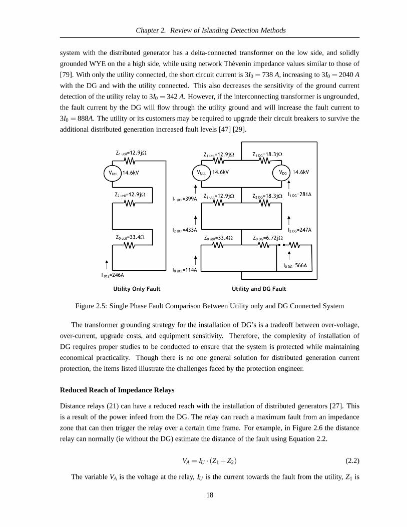
Chapter 2. Review of Islanding Detection Methods
system with the distributed generator has a delta-connected transformer on the low side, and solidly
grounded WYE on the a high side, while using network Thevenin impedance values similar to those of
[79]. With only the utility connected, the short circuit current is 3I0 = 738A, increasing to 3I0 = 2040A
with the DG and with the utility connected. This also decreases the sensitivity of the ground current
detection of the utility relay to 3I0 = 342A. However, if the interconnecting transformer is ungrounded,
the fault current by the DG will flow through the utility ground and will increase the fault current to
3I0 = 888A. The utility or its customers may be required to upgrade their circuit breakers to survive the
additional distributed generation increased fault levels[47] [29].
Figure 2.5: Single Phase Fault Comparison Between Utility only and DG Connected System
The transformer grounding strategy for the installation ofDG’s is a tradeoff between over-voltage,
over-current, upgrade costs, and equipment sensitivity. Therefore, the complexity of installation of
DG requires proper studies to be conducted to ensure that thesystem is protected while maintaining
economical practicality. Though there is no one general solution for distributed generation current
protection, the items listed illustrate the challenges faced by the protection engineer.
Reduced Reach of Impedance Relays
Distance relays (21) can have a reduced reach with the installation of distributed generators [27]. This
is a result of the power infeed from the DG. The relay can reacha maximum fault from an impedance
zone that can then trigger the relay over a certain time frame. For example, in Figure 2.6 the distance
relay can normally (ie without the DG) estimate the distanceof the fault using Equation 2.2.
VA = IU · (Z1+Z2) (2.2)
The variableVA is the voltage at the relay,IU is the current towards the fault from the utility,Z1 is
18

Chapter 2. Review of Islanding Detection Methods
the impedance to where the DG would be (not connected in this case) andZ2 is the impedance past the
DG. However, with the addition of the DG source into the system, the impedance estimate changes to
Equation 2.3.
VA = IU · (Z1+Z2)+ IDG ·Z2 (2.3)
The additionalIDG is the current from the currently connected DG source. Hence, solving for the
impedance seen from the relay with the DG in the system gives the result in Equation 2.4. Therefore,
the current ratio of the DG and the utility increases and the accuracy of the relay decreases making it
possible for the relay to be inoperable in fault zones.
ZRelay=VA
IU= Z1+Z2+
IDG
IUZ2 (2.4)
Fault
DG System
Utility
Z1 Z2
Normal Reach of Relay
Reduced Reach of Relay
A
VA
Figure 2.6: Example of Reduced Impedance Relay (21) Reach
2.2.3 Maintenance
Distribution power lines interconnected to distributed generators require periodic maintenance like all
other lines. Though this case is more of a practical situation, this detail is worth mentioning. The main-
tenance procedures are different in regular networks from those in networks with distributed generation.
In a radially fed line without distributed generation, onlythe upstream line is required to be “locked
out” for maintenance workers to service the line. However, with the addition of distributed generation,
the maintenance worker must know that there is a distributedgenerator downstream so that they will
lock out the lines on both sides of the area they are carrying out maintenance on. This safety concern for
each additional distributed generator will come at the costof documenting, communicating and training
for the utility service team. Islanding detection systems help to prevent potential hazards if the lock out
procedures are missed or overlooked.
19

Chapter 2. Review of Islanding Detection Methods
2.2.4 Reclosure
A large number of overhead line faults are transient in nature and can be cleared if the line is temporarily
de-energized. Utility statistics indicate that fewer than10% of all faults are permanent [29], and it has
been discovered that customer service continuity and system stability can be improved by automatically
reclosing the breaker. Multiple-shot reclosing breakers are used in areas with tree exposure, however,
when there are sources at both sides of the line, high speed reclosing can only safely occur if the
system, or if both generators have enough inertia to remain in phase during the dead time. In the case
of distributed generators, many of the sources are electronically generated through computer controlled
transistor switching, are low inertia generators, or are combinations of the two. These configurations
are unable to maintain synchronization after a line is opened from the main utility, forcing protection
engineers to re-adjust the reclosure sequence.
Due to the effectiveness of reclosures for power system fault clearing, distributed generators require
a mechanism to respond to temporary line opening. Islandingdetection allows a DG (particularly those
at a distance from the interconnection substation) to automatically disconnect themselves and allow the
utility system to automatically reclose and clear the fault. After the utility restoration, the distributed
generator can locally re-synchronize and re-connect. Thisprocess requires that the DG open its breakers
shortly after the loss of the utility connection.
2.2.5 Typical Interconnection Protection Schemes
As seen in the previous subsections, interconnection of DG requires a mixture of protection considera-
tions to ensure that customer loads and system equipment aresafe. The typical protective components
of the system illustrated in Figure 2.1, the protection requirements for distributed generators and one bus
of the substation can be seen in Figure 2.7 [10] [77] [79]. Both systems include: CT and PT measuring
transformers, an AC circuit breaker (52)1, protective relays for distance (21), over voltage (59) neu-
tral and line, under voltage (27), synchronization (25), directional power (32), phase sequence current
(46), phase sequence voltage (47), instantaneous over-current (50) neutral and line, over current (51),
directional over current (67), reclosing (79) and frequency (81) over, under and rate of change.
Suggested upgrades for distributed generators that may be required if the DG can supply reliable
power for an island are follows [79]:
• If the DG has a recloser breaker, replace the recloser breaker with a regular circuit breaker.
• Add a PT on the load side of feeder to allow dead line check logic
• Add three phase PTs on the high voltage side of the DG interconnection to allow for synchroniza-
tion upon reconnection.
• Use modern multifunction relays equipped with the items seen in Figure 2.7
1Appendix A contains ANSI/IEEE Device reference numbers
20

Chapter 2. Review of Islanding Detection Methods
G
52
46 32 51 51
27 59 8181U O
V N
25G
52
46 32 51 21
27 59 8181U O
U
47
2579 67
50N
PT
PT
CT
CT
PT
PT
Figure 2.7: Distributed Generation (left) and DG Interconnection Protection (right)
Protection of distributed generation installations can bea complex issue involving many optimiza-
tions, therefore, care must be taken for each system to maximize the system dependability and security
for the customers it serves [40]. Power system dependability is the degree of confidence of correct op-
eration after system trouble, where security is in the degree of confidence that a relay will not operate
incorrectly [29]. Islanding detection can be added on top ofthese basic relay sensors to improve control
actions.
2.3 Islanding Detection
Islanding detection is an effective tool for distributed generation protection. As introduced in Section
1.2.2 and seen in Figure 1.3, there are a number of islanding detection schemes currently developed.
Each class has a limitation and an advantage [11] [128] [34].It can be difficult to directly compare
all the islanding detection methods back to back, as each type will operate more effectively than the
other depending on the situation. For example, the change ofterminal voltage method may be ideal for
rotating machine generators due to their often large reactive component, where as the frequency shift
methods work well with inverter based generators that supply more real power. A good performing
islanding detection scheme has the ability to securely and dependably detect an island state. IEEE has
published standard 1547 [54] which details testing of single phase single source islanding detection
methods. Though the testing method is limited to only singleinverter systems, it is commonly used by
standards agencies such as the Canadian Standards Association (CSA) and Underwriters’ Laboratories
(UL), as benchmarks to approve grid tie power converter products for sale in North America. In this
section, the state-of-the-art of islanding detection methods will be discussed and reviewed for their
particular advantages and disadvantages. This discussionwill then lead to a more detailed analysis of
impedance measurement techniques in the next section.
Islanding detection is broken down into three main classifications: 1. Communication, 2. Passive
21

Chapter 2. Review of Islanding Detection Methods
Detection, and 3. Active Detection. For each of these classifications, there are a number of methods
which have been listed in Tables 2.1, 2.2 and 2.3 below. Thesemethods have been referenced to several
comprehensive reports [11] [128], and [34]. Methods not covered in these reports that have been more
recently developed will have references beside them. Each method will be described in relations to how
it works, its typical use, its advantages and its disadvantages. The final part of this section will contain
a detailed review of the state of the art of impedance measurement techniques and how they are being
applied to islanding detection.
Table 2.1: Communication Islanding Detection Methods
• Power Line Carrier Communications [129] [121]• Transfer Trip• Supervisory Control and Data Acquisition (SCADA)
Table 2.2: Passive Islanding Detection Methods
• Under/Over Voltage (Relay 59, 27)• Over/Under Frequency (Relay 81)• Voltage Phase Jump / Voltage Vector Shift / Frequency Phase Jump Relay• Detection of Voltage and/or Current Harmonics• Rate of Change of Frequency Relay (ROCOF)• Rate of Change of Voltage• Rate of Change of Real/Reactive Power and Power Factor• Signal Produced By Disconnect• Voltage Unbalance [108] [74]
Table 2.3: Active Islanding Detection Methods
• Slip-mode Frequency Shift• Frequency Bias• Sandia Frequency Shift• Sandia Voltage Shift• Frequency Jump• ENS or MSD (A device using multiple methods) [102]• Varying Terminal Voltage/Voltage Pulse• Reactive Error Export• Voltage Unbalance [74]• Impedance Monitoring (See section 2.4)
22
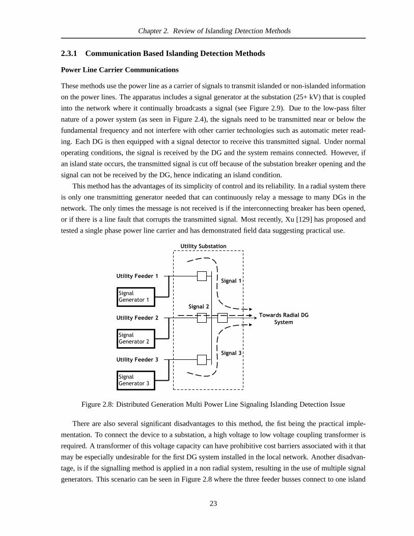
Chapter 2. Review of Islanding Detection Methods
2.3.1 Communication Based Islanding Detection Methods
Power Line Carrier Communications
These methods use the power line as a carrier of signals to transmit islanded or non-islanded information
on the power lines. The apparatus includes a signal generator at the substation (25+ kV) that is coupled
into the network where it continually broadcasts a signal (see Figure 2.9). Due to the low-pass filter
nature of a power system (as seen in Figure 2.4), the signals need to be transmitted near or below the
fundamental frequency and not interfere with other carriertechnologies such as automatic meter read-
ing. Each DG is then equipped with a signal detector to receive this transmitted signal. Under normal
operating conditions, the signal is received by the DG and the system remains connected. However, if
an island state occurs, the transmitted signal is cut off because of the substation breaker opening and the
signal can not be received by the DG, hence indicating an island condition.
This method has the advantages of its simplicity of control and its reliability. In a radial system there
is only one transmitting generator needed that can continuously relay a message to many DGs in the
network. The only times the message is not received is if the interconnecting breaker has been opened,
or if there is a line fault that corrupts the transmitted signal. Most recently, Xu [129] has proposed and
tested a single phase power line carrier and has demonstrated field data suggesting practical use.
Utility Substation
SignalGenerator 1
Utility Feeder 1
SignalGenerator 2
Utility Feeder 2
SignalGenerator 3
Utility Feeder 3
Towards Radial DG System
Signal 1
Signal 2
Signal 3
Figure 2.8: Distributed Generation Multi Power Line Signaling Islanding Detection Issue
There are also several significant disadvantages to this method, the fist being the practical imple-
mentation. To connect the device to a substation, a high voltage to low voltage coupling transformer is
required. A transformer of this voltage capacity can have prohibitive cost barriers associated with it that
may be especially undesirable for the first DG system installed in the local network. Another disadvan-
tage, is if the signalling method is applied in a non radial system, resulting in the use of multiple signal
generators. This scenario can be seen in Figure 2.8 where thethree feeder busses connect to one island
23

Chapter 2. Review of Islanding Detection Methods
bus. The implementation of this system, opposed to a simple radial system, will be up to three times the
cost. The following disadvantage is the required transmitting power - enough energy is required to be
transmitted into the system at a frequency close to the fundamental, and at a signal-to-noise ratio that
exceeds the normal signal to noise level in the system. The non-detection zone of this method occurs
when some loads on the system interfere with the transmittedsignal. In report [93], it was shown that
motor vibrations can cause wide band harmonic voltage fluctuations around the fundamental. These
fluctuations may cause potential nuisance trips of this detection method. Though lab experiments have
proven to be successful [41], including recent field tests [121], power consumption and system cost are
believed to still be challenges. For example, the tests by Wang [121] using intermittent transmission, had
an acceptable signal to noise level when the signal amplitude was above 2.5% (approximately 2 kW)
and it was not found to interfere with existing automatic meter reading power line carrier devices as
previously believed [11]. The lost revenue of a continuous 2kW signal to this technology would be
$1300 CAD to $2570 CAD per year in British Columbia, Canada asseen in the following calculations.
Data from Wang [121] and the cost per kW-hr can be seen in Table2.4. Current costs per kW-hr for
small industrial customers has been referenced from the BC Hydro general customer web site2.
Table 2.4: Data from Wang ExperimentVbase 480
Vin jected 2.5% to 5%Vbase
IRMS 168IPeak 1382
Cost/kWhr $0.0728
Cost calculations for the experiment per year use the following Equation 2.5.
Cost = $/kWhr·hoursyear·V · I/1000 (2.5)
= 0.00728·8760·480·0.025·168/1000= $1300
= 0.00728·8760·480·0.05·168/1000= $2570
Another problem for power line communication is the complexity of the network and the affected
networks. A perfectly radial network with one connecting breaker is a simple example of island signal-
ing; however, more complex systems with multiple utility feeders may find that differentiation between
upstream breakers difficult (seen in Figure 2.8).
Transfer Trip
Transfer trip detection schemes require all circuit breakers which island the DG to be monitored and
linked directly to the DG control, or through a central substation SCADA system. When a disconnection
is detected at the substation, the transfer trip system determines which areas are islanded and sends the
2http://www.bchydro.com/policies/rates/rates759.html
24

Chapter 2. Review of Islanding Detection Methods
Loads
Loads Loads
1 to 100 km
Loads
Loads
Loads
A
Utility Substation
DG System
SignalGenerator
SignalDetector
Utility
Figure 2.9: Distributed Generation Power Line Signaling Islanding Detection
appropriate signal to the DGs, to either remain in operation, or to discontinue operation. Transfer tip has
the distinct advantage similar to Power Line Carrier Signalthat it is a very simple concept. With a radial
topology that has few DG sources and a limited number of breakers, the system state can be sent to the
DG directly from each monitoring point. This is one of the most common schemes used for islanding
detection [11]. This system can be seen in Figure 2.10
The weaknesses of the transfer trip system are better related to larger system complexity cost and
control. As a system grows in complexity, the transfer trip scheme may also become obsolete, and need
relocation or updating. Reconfiguration of this device in the planning stages of DG network is necessary
in order to consider if the network is expected to grow or if many DG installations are planned. The
other weakness of this system is control. As the substation gains control of the DG, the DG may lose
control over power producing capability and special agreements may be necessary with the utility. If
the transfer trip method is implemented correctly in a simple network, there are no non-detection zones
of operation.
2.3.2 Passive Islanding Detection Methods
The following section contains an overview of the most commonly known islanding detection methods
using passive means. Passive islanding detection methods measure voltage, current and phase informa-
tion at the DG’s terminals or Point of Common Coupling (PCC),to determine if an island condition has
occurred. Many of these methods are very cost effective, as the relays are already in place for other pro-
tective requirements. The biggest challenge with passive detection techniques is setting an appropriate
sensor threshold that can identify the difference between islands and natural power system variations.
The general consensus is that the currently available passive islanding detection techniques need to be
combined with active methods to reduce the non-detection zone, to ensure a higher level of security and
dependability. In the following review, many of the methodshave been combined into one section as
they represent similar phenomena and performance characteristics. Passive islanding detection relia-
25

Chapter 2. Review of Islanding Detection Methods
Loads
LoadsLoads
1 to 100 km
Loads
Loads
Loads
A
Utility Substation
DG System
TransferTrip Monitor
Figure 2.10: Distributed Generation Transfer Trip Islanding Detection
bility is compounded further by the limited accuracy of current and voltage sensors. Accurate analysis
of islanding detection techniques must extend beyond computer simulations. Sensor accuracy and the
associated practical measurement challenges are discussed in Section 2.5 of this thesis. Despite all the
limitations of passive islanding detection, research on this topic continues, as the concept of zero system
disturbance for detection is the ideal.
Over/Under Frequency, Change of Frequency, Frequency Surge
Frequency based passive islanding detection schemes are often used with synchronous and induction
machines. If the generated power and the power consuming load are mismatched, the frequency of the
system will change. Hence, because the frequency of a power system is generally constant, when a
frequency mismatch occurs over a preset threshold, (such as> ±0.5Hz) the system is assumed to be in
an island state, and the DG relay will open the breaker. For example, as seen in the work by Geidl [34],
the power unbalance in an island between DG powerPDG and the load powerPLoad is given by Equation
2.6. By placing∆P into the Swing Equation 2.7, frequency decline can be seen when the generation
capacity is below the load demand [68] [79].
∆P = ∑PDG−∑PLoad (2.6)
The variable∆ f indicates the frequency change from the initial frequency,D indicates the load-
damping factor, or the ratio of percentage load change to percentage frequency change, andH indicates
the system’s inertia constant.
∆ f =∆PD
(1−e−Dt/2H) (2.7)
Another method for islanding detection using frequency is called Rate of Change of Frequency
26

Chapter 2. Review of Islanding Detection Methods
(ROCOF). This method does not use change of frequency,∆ f , but ∂ f∂t instead. Hence, a DG will trip if
the change in frequency exceeds a rate of a specified threshold. Typical threshold values for ROCOF in
60 Hz systems are between 0.1 Hz/s and 1.20 Hz/s [128]. This function needs to be considered during
the generator startup frequency change and fault settings to prevent nuisance tripping. It is important
to note that frequency, phase and magnitude of the voltage are related to power by Equations 2.8 2.9,
and 2.10 where P and Q are the real and reactive power,V1a andV1b are the voltages at two ends of
a line, andZ1 is the impedance of the line. Assuming the reactive part of the impedance is dominant,
changes in P mostly result in variations in phase and frequency, while changes in Q result in variations
in voltage.
P+ jQ =V1a ·V1b 6 θ
Z1(2.8)
Where P can be solved as:
P =V1a ·V1b
Z1·sin(θ) (2.9)
And Q can be solved as:
Q =V1a
Z1· (V1b ·cos(θ)−V1a) (2.10)
The final passive method using frequency is called the VectorSurge, which measures the change
of phase angle of the voltage waveform to a known reference waveform. When an island state occurs,
there can be an immediate phase shift by the DG to accommodatethe change in power requirements.
Once again, a threshold is set at the maximum phase jump allowed and if the DG system exceeds that
threshold, the relay is triggered. The performance of this method has been previously investigated [128]
and it has been found that a generator with a 33% or more power mismatch will result in a minimum
detection time of 300ms to operate.
The Vector Serge method is not useful for inverter-fed systems as inverters are either self com-
mutated or line commutated. Electronically driven systemsdo not change frequency when the load
changes, because computer control and Phase Locked Loops keep the frequency constant and near the
fundamental.
For all three passive frequency islanding detection schemes, generator power to consuming power
mismatches smaller than 20%, have exponentially increasing trip times, and are prone to nuisance trips
if set too sensitive. Of the three, ROCOF experiences the most significant trip time increase below a
20% power mismatch, followed by the Vector Jump and Change ofFrequency. The performance of
these three frequency based detection method are further complicated by the inertial constant of the
generator, multiple generators, voltage and frequency dependency of the feeder loads, and the excitation
control of the generator.
27

Chapter 2. Review of Islanding Detection Methods
Over/Under Voltage
Over and under voltage are also used for passive islanding detection, and often as a complementary
device coupled with frequency monitoring. Voltage variations occur as a result of a mismatch of reactive
power, Q, mismatch as seen in Equation 2.10. This relay operates on the principle that an excess
of reactive power mismatch will drive the voltage up and a deficit of reactive power will drive the
voltage down. Once the voltage falls out of the preset thresholds, the relay will open the breaker.
Hence, by determining the voltage change or its rate of change, it is possible to detect island states that
frequency effects alone cannot. Unfortunately, there is limited experience indicating that the reactive
power measurement relay will have higher performance than frequency variations. As real power draw
is often much greater than reactive power, a loss of mains is more likely to significantly change the
active power than the reactive power.
Rate of Change of Voltage
Rate of change of voltage has successfully been investigated in [97] where it was found that usual
voltage variations are slow in distribution systems, but ifone utility system becomes Islanded from the
main distribution system, the rate of change of voltage is larger than under regular operation. The non-
detection zone of this method is closely coupled with its sensitivity to network disturbances, except in
the case of island transitions.
Detection of Voltage and/or Current Harmonics
This method of islanding detection is generally applied in conjunction with inverter based technologies
when system harmonics are likely to be present. In this method, the island detector measures the total
harmonic distortion (THD), sets a threshold and then shuts down when the harmonic distortion exceeds
that level. If an assumption is made that a utility-connected system is more “stiff” than a DG-only
system, the THD will be less for a utility connected system than for a DG-only connected system. There
are several factors that can increase the level of harmonicsin a network. Examples include switching
power supplies, motor drives, and non linear components such as overloaded transformers. The level
of harmonics produced by inverters will change between fullload and no load conditions. A typical
requirement for Inverters is to meet the THD specification ofless than 5% under full load conditions.
These harmonics are often very small due to the low impedancesink provided by the utility system and
the measurability and the threshold setting will exhibit significant issues. This method has found setting
thresholds and the ability to accurately measure small harmonics to be very difficult to measure and
predict. Similar work has been completed in this field by the injection of harmonics, as discussed seen
in Section 2.3.3.
2.3.3 Active Islanding Detection Methods
The following section contains an overview of the most common known islanding detection methods
for distributed generators using local injection to enhance measurement accuracy. Active islanding de-
28

Chapter 2. Review of Islanding Detection Methods
tection techniques use a mix of advanced control, load switching, and voltage and current variances,
followed by measurement at specific times to augment the difference between islanded and non is-
landed scenarios. Many of the techniques reside inside inverters and switch controlled DGs, using the
signal processing capabilities already existing inside these products for power flow and synchroniza-
tion control. This makes the addition of software modifications for islanding detection very easy to
implement. Active islanding detection methods are bound bypractical actuation technologies, allow-
able active disturbance sizes, measurement sensitivity and multiple DG interference that may effect the
customer energy quality, reliability or safety of the system. For example, a current source inverter tracks
power by using Equation 2.11 to vary eitherIinverter, ω or φ to achieve the desired output power. Equation
2.11 can also be varied to make an islanding detection device, as discussed below.
i inverter = Iinvertersin(ωt + φ) (2.11)
Slip-mode Frequency Shift
Slip mode frequency shift (SMS) is an inverter based islanding detection scheme that uses a positive
feedback control to destabilize the source inverter when anisland condition occurs. As seen in Equation
2.11 a current source inverter uses positive feedback of thephase,φ, to slip the frequency out-of-phase
hence leading to short term frequency change. SMS is implemented by modifying the phase locked loop
(PLL) filter to be naturally out of phase at the fundamental. Under normal operating conditions without
SMS, the PLL tracks phase and frequency changes of the network. With SMS, the strength of the utility
source keeps the inverter in phase. However, if the frequency during an island is pushed upwards, due to
the out of phase filter, the PLL will see a negative phase errorand try to shift the frequency away from
the fundamental. Due to the positive feedback, the phase shift will be in the wrong direction to correct
the phase error. The frequency eventually will fall out of acceptable limits and the frequency relay will
open the breaker.
SMS also has the advantage of simple implementation as it only requires a modification to existing
components in the inverter filter. SMS has been tested to haveone of the smallest non-detection zones
for islanding detection and is effective in multiple inverter applications [95]. However, the SMS method
will fail if the frequency response of an islanded RLC load isgreater than the SMS system. Another non-
detection zone for SMS is with loads that have high-quality factor, Q, and have resonance frequencies
very close to the line frequency [96] [71]. The quality factor is related to the ratio of energy stored over
the power loss as seen in Equation 2.12 for a series RLC circuit where R is resistance, L is inductance
and C is capacitance.
Q =1R
√
LC
(2.12)
Due to the high gain of the positive feedback mechanism, highdensity installations with SMS may
cause power quality problems related to transient response. In smaller density installations, though, the
effect on power quality is low. This method has been found to have a non-detection zone in 60 Hz
29

Chapter 2. Review of Islanding Detection Methods
systems between 59.3 Hz and 60.5 Hz and for quality factors between 1.5 and higher, though this will
vary depending on the specific tuning of the control scheme [71].
Frequency Bias (Active Frequency Drift)
Frequency Bias, also known as Active Frequency Drift, is also an inverter and computer based islanding
detection technique that distorts the frequency output to create a continuous trend to “drift“ the fre-
quency away from the fundamental. The method works by altering the frequency, f, in Equation 2.11 by
slightly increasing the frequency of each 1/2 cycle followed by a “dead time“ where the system waits
for the fundamental to catch up to the biased frequency, as seen in Figure 2.11. The current in each
cycle can be described by Equation 2.13 wherei is the output current,I is the maximum current,fV is
the voltage frequency andδ f is the frequency change.
i =√
2Isin[2π( fV + δ f )] (2.13)
Similarly to Slip-Mode Frequency Shift, when the inverter is connected to the utility-fed network,
the strong utility keeps the system frequency stable. However, when the network becomes islanded, the
distorted frequency causes the system to seek the system load’s resonance frequency, resulting in the
inverter eventually drifting up or down causing the frequency relays to trip. Frequency bias can work
with multiple inverters as long as all inverters drift the frequency in the same direction, otherwise they
may not drift the frequency fast enough to meet the detectionrequirements. The Frequency Bias method
clearly requires a small amount of output power distortion where the distortion depends on how big the
bias is per 1/2 cycle. With Frequency Bias method, the non-detection zone is relatively large compared
to other methods and is found that the method is not particularly effective [95]. This method has been
found to have a non-detection zone in 60 Hz systems between 58.65 Hz and 60.5 Hz for quality factors
of 1.5 to 100 [71].
Sandia Frequency Shift
Sandia Frequency Shift (SFS) is an enhancement of the Frequency Bias Islanding detection method
which uses positive feedback. The positive feedback takes the error of the “dead zone,” as seen in Figure
2.11, as an error of the line frequency. When this system is connected to the utility, small frequency
changes push the inverter out of the range of the line frequency, but the strength of the utility keeps the
system stable. The feedback signal can be represented by Equation 2.14, wheref is the inverter terminal
voltage, f0 is the base frequency (such as 60 Hz),K is the positive feedback gain, andc f0 is the initial
chopping fraction [122].
θ f =π2(c f0 +K( f − f0)) (2.14)
When the utility is disconnected, the errors detected in frequency increase and the dead zone in-
creases. This method has been found to be a significant improvement over normal Frequency Bias,
except the transient performance degrades with higher density of sources using this system, and large Q
30
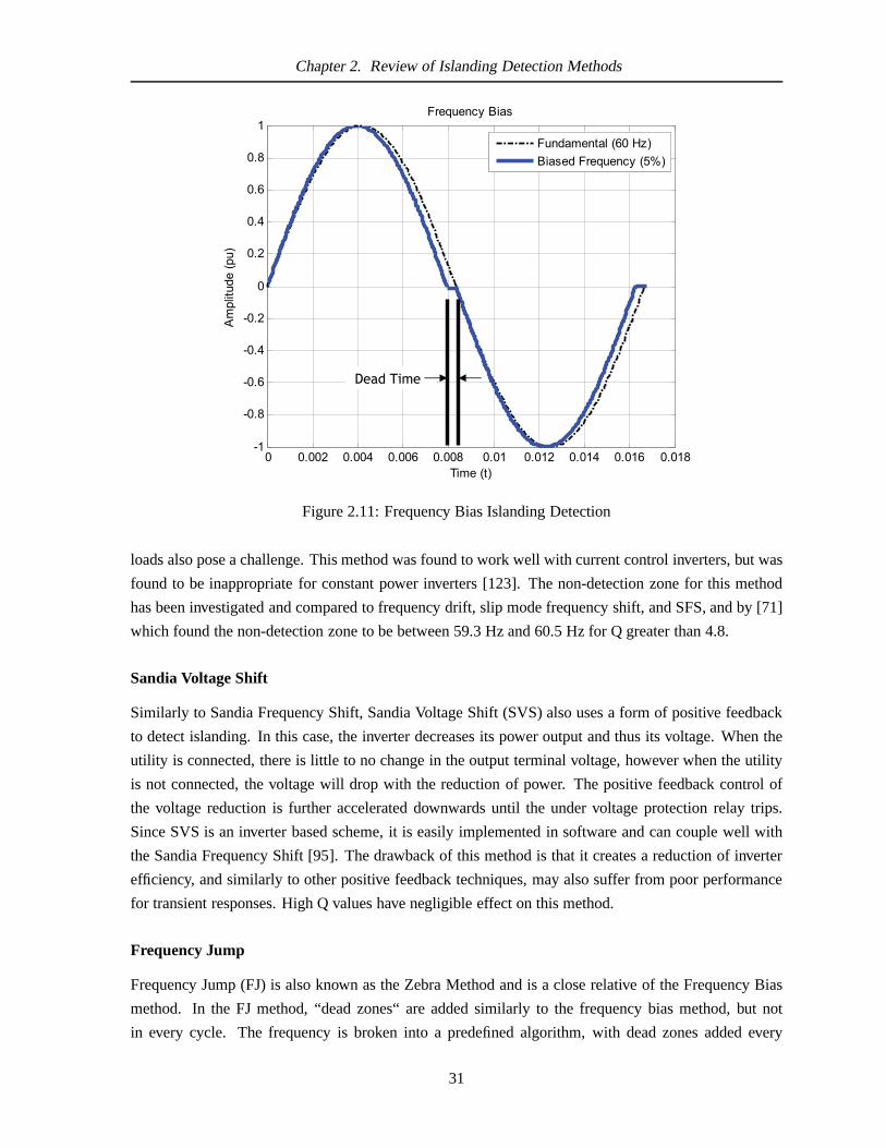
Chapter 2. Review of Islanding Detection Methods
0 0.002 0.004 0.006 0.008 0.01 0.012 0.014 0.016 0.018-1
-0.8
-0.6
-0.4
-0.2
0
0.2
0.4
0.6
0.8
1Frequency Bias
Time (t)
Ampl
itude
(pu)
Fundamental (60 Hz)Biased Frequency (5%)
Dead Time
Figure 2.11: Frequency Bias Islanding Detection
loads also pose a challenge. This method was found to work well with current control inverters, but was
found to be inappropriate for constant power inverters [123]. The non-detection zone for this method
has been investigated and compared to frequency drift, slipmode frequency shift, and SFS, and by [71]
which found the non-detection zone to be between 59.3 Hz and 60.5 Hz for Q greater than 4.8.
Sandia Voltage Shift
Similarly to Sandia Frequency Shift, Sandia Voltage Shift (SVS) also uses a form of positive feedback
to detect islanding. In this case, the inverter decreases its power output and thus its voltage. When the
utility is connected, there is little to no change in the output terminal voltage, however when the utility
is not connected, the voltage will drop with the reduction ofpower. The positive feedback control of
the voltage reduction is further accelerated downwards until the under voltage protection relay trips.
Since SVS is an inverter based scheme, it is easily implemented in software and can couple well with
the Sandia Frequency Shift [95]. The drawback of this methodis that it creates a reduction of inverter
efficiency, and similarly to other positive feedback techniques, may also suffer from poor performance
for transient responses. High Q values have negligible effect on this method.
Frequency Jump
Frequency Jump (FJ) is also known as the Zebra Method and is a close relative of the Frequency Bias
method. In the FJ method, “dead zones“ are added similarly tothe frequency bias method, but not
in every cycle. The frequency is broken into a predefined algorithm, with dead zones added every
31

Chapter 2. Review of Islanding Detection Methods
second or third cycle. When connected to the utility, the inverter only sees a modified current and an
unmodified utility linked voltage. When in island state, thevoltage and current change as per the inverter
programmed wave shape. Therefore, the inverter can detect an island by the modified frequency, or by
matching the voltage pattern to the inverter’s algorithm. This method is believed to lose effectiveness
when used in conjunction with many inverters that use the same algorithm [95].
ENS or MSD (A device using multiple methods)
The ENS method is more of a standard than an actual islanding detection technique, but for thorough-
ness, it is important to describe how it works for this process. ENS (DIN V VDE 0126-1-1 [102]) has
been required by law in Germany since 2006 for grid tied devices to use for islanding detection. The
standard is different from IEEE performance based standards [54], as it is prescriptive about specific
techniques, with particular performances that must be used. It includes a passive measurement com-
ponent and an active component. The passive component requires that the voltage does not exceed the
limits of 80% to 114%, and a frequency of 47.5 Hz to 50.2 Hz (50 Hz is the fundamental frequency
in Germany). The DG is to be disconnected within 200 ms (10 cycles) of these limits being exceeded.
Along with the instantaneous values, the average voltage measured over ten minutes must also not ex-
ceed the limit of 115%. Finally, a resonant LC load is to be switched in parallel with the system to
measure the impedance changes on all three phases. Changes outside of the original set range of 5%
results in a relay trip within 5 seconds of the occurrence.
The performance of this combined method has not been directly measured, but the load switching
method is described in the Impedance Measurement Section 2.4 if this chapter. The method has been
found to work well but at the cost of power quality degradation.
Varying Terminal Voltage/Voltage Pulse
Voltage Pulse Perturbation and Correlation are discussed in [34] and [113] where the frequency is kept
constant and the voltage output is varied at the inverter terminals. The first method modulates a square
pulse on top of the fundamental so that every few cycles the voltage increases for a short duration then
decreases. The change of voltage is then measured and the twoare compared. This can be seen in Figure
2.12.
Due to the usually strong utility connection, the voltage variation will be very small, however,
under island conditions the voltage change will be significantly larger. This method suffers from severe
limitations when more than one distributed generator is connected to the local network and the threshold
values are susceptible to corruption. The method has been further improved by using a random square
signal instead of a periodical signal to modulate and then further using a correlation function,φ, as seen
in Equation 2.15.
φ(τ) =1T
∫ T
0∆Er(t) ·∆Eg(t + τ)∂t (2.15)
HereEr is a random signal measured at the point of common coupling and Eg is the signal mea-
32
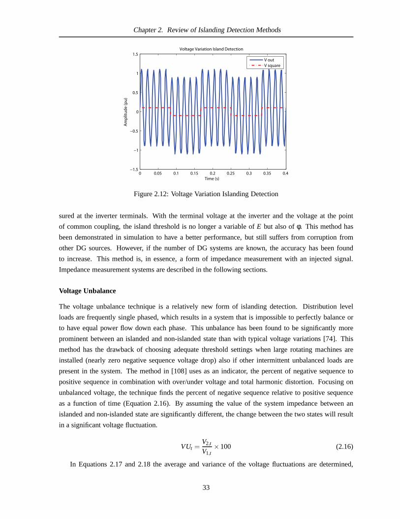
Chapter 2. Review of Islanding Detection Methods
Figure 2.12: Voltage Variation Islanding Detection
sured at the inverter terminals. With the terminal voltage at the inverter and the voltage at the point
of common coupling, the island threshold is no longer a variable of E but also ofφ. This method has
been demonstrated in simulation to have a better performance, but still suffers from corruption from
other DG sources. However, if the number of DG systems are known, the accuracy has been found
to increase. This method is, in essence, a form of impedance measurement with an injected signal.
Impedance measurement systems are described in the following sections.
Voltage Unbalance
The voltage unbalance technique is a relatively new form of islanding detection. Distribution level
loads are frequently single phased, which results in a system that is impossible to perfectly balance or
to have equal power flow down each phase. This unbalance has been found to be significantly more
prominent between an islanded and non-islanded state than with typical voltage variations [74]. This
method has the drawback of choosing adequate threshold settings when large rotating machines are
installed (nearly zero negative sequence voltage drop) also if other intermittent unbalanced loads are
present in the system. The method in [108] uses as an indicator, the percent of negative sequence to
positive sequence in combination with over/under voltage and total harmonic distortion. Focusing on
unbalanced voltage, the technique finds the percent of negative sequence relative to positive sequence
as a function of time (Equation 2.16). By assuming the value of the system impedance between an
islanded and non-islanded state are significantly different, the change between the two states will result
in a significant voltage fluctuation.
VUt =V2,t
V1,t×100 (2.16)
In Equations 2.17 and 2.18 the average and variance of the voltage fluctuations are determined,
33

Chapter 2. Review of Islanding Detection Methods
whereVUt (voltage unbalance) is the ratio of negative sequenceV2,t to positive sequenceV1,t , N is
the number of samples in one-cycle, t is the monitoring time,andVUavg,s is theVU reference value
initially set for the steady-state normal loading conditions. Then in Equation 2.18,VUavg,s is set for
initial conditions and if∆VUt remains within -100% and +50% for one cycle, theVUavg,s is updated by
theVUavg,t to allow for normal load variation.
VUavg,t =1N
N−1
∑i=0
VUt−i (2.17)
∆VUt =VUavg,s−VUavg,t
VUavg,s×100 (2.18)
The islanding detection decision is made by using the following rule seen in Equation 2.19.
RULE : (∆VUt > 50%)or(∆VUt < −100%) (2.19)
This technique was found to work very well in simulation, buthas not been tested in practical
systems. This technique will have a very small non-detection zone if the threshold is set correctly and
if the measurements are made accurately.
More recently, [74] a simulated voltage unbalance, in combination with active positive feedback
frequency drift for islanding detection, small disturbances caused the voltage unbalance technique to
falsely trip and the power quality was reduced using the frequency drift method. By combining the two,
the false tripping was reduced and the power quality was increased.
Current Unbalance
Karimi in [60] used negative sequence current injections for islanding detection in simulation. A voltage
source inverter controller made the injections. The negative-sequence current injection in the range of
2% to 3% allowed for fast islanding detection. The time of detection was less than 60 ms(3.5 cycles).
Active/Reactive Power Control
Though active and reactive power control scheme is mentioned here, active and reactive power variations
are a result of voltage and phase variations as seen in Equation 2.8. This section has covered variations of
voltage, phase and frequency which are implemented passively and actively; hence, employing similar
results and similar non-detection zones as if power variation was implemented.
One example is Reactive Error Export, discussed in [34]. Here, the generator maintains a specified
amount of reactive power. When the island state occurs, the inverter is unable to deliver the reactive
power and the phase changes. The error in the ability to export the reactive power is the trigger for an
island state.
34
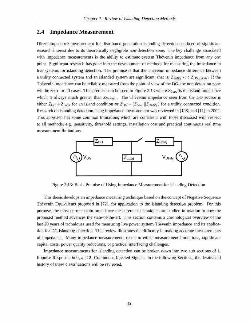
Chapter 2. Review of Islanding Detection Methods
2.4 Impedance Measurement
Direct impedance measurement for distributed generation islanding detection has been of significant
research interest due to its theoretically negligible non-detection zone. The key challenge associated
with impedance measurements is the ability to estimate system Thevenin impedance from any one
point. Significant research has gone into the development ofmethods for measuring the impedance in
live systems for islanding detection. The premise is that the Thevenin impedance difference between
a utility connected system and an islanded system are significant, that is,Zutility << ZDG Loads. If the
Thevenin impedance can be reliably measured from the pointof view of the DG, the non-detection zone
will be zero for all cases. This premise can be seen in Figure 2.13 whereZLoad is the island impedance
which is always much greater thanZUtility . The Thevenin impedance seen from the DG source is
eitherZDG + ZLoad for an island condition orZDG + (ZLoad||ZUtility ) for a utility connected condition.
Research on islanding detection using impedance measurement was reviewed in [128] and [11] in 2002.
This approach has some common limitations which are consistent with those discussed with respect
to all methods, e.g. sensitivity, threshold settings, installation cost and practical continuous real time
measurement limitations.
ZDG ZUtility
ZLoadVDG VUtility
Figure 2.13: Basic Premise of Using Impedance Measurement for Islanding Detection
This thesis develops an impedance measuring technique based on the concept of Negative Sequence
Thevenin Equivalents proposed in [72], for application tothe islanding detection problem. For this
purpose, the most current main impedance measurement techniques are studied in relation to how the
proposed method advances the state-of-the-art. This section contains a chronological overview of the
last 20 years of techniques used for measuring live power system Thevenin impedance and its applica-
tion for DG islanding detection. This review illustrates the difficulty in making accurate measurements
of impedance. Many impedance measurements result in eithermeasurement limitations, significant
capital costs, power quality reductions, or practical interfacing challenges.
Impedance measurements for islanding detection can be broken down into two sub sections of 1.
Impulse Response,h(t), and 2. Continuous Injected Signals. In the following Sections, the details and
history of these classifications will be reviewed.
35

Chapter 2. Review of Islanding Detection Methods
2.4.1 Impulse Response
Impedance Based Islanding Detection using an Impulse,δ(n)
One method for determining the island states of a distribution system is to monitor the transfer function
or H(ejω) for changes in the system impedance. Specifically, the transfer function of a system is its fre-
quency response over all frequencies. Some commonly used signal processing techniques used in this
section are described in Appendix F. Singular impulse disturbances have been used for impedance mea-
surement as they have the benefit of being short term disturbances with wide bandwidth characteristics.
The method requires a disturbance to be created into the power system to create a theoretical impulse of
infinite bandwidth,δ(n). As δ(n) contains energy in all bands,V(ω) andI(ω) can be measured to then
calculateZ(ω) by means of Ohm’s law as seen in Equation 2.20.
Z(ω) =V(ω)
I(ω)(2.20)
For example, in 1989 Girgis [36] investigated impedance transfer function analysis of a power grid
taking historical data using various impulses that were acquired at 12 kV bus with a switched 750 kVAR
capacitor (193 ohms or 13µF) to ground as the injected impulse. From the tests, a series of estimated
series RLC components were added to match the transfer function poles and zeros of the system as
seen in Figure 2.14. The signal processing techniques used to filter the signal were cross correlation
and fourier transform. The fourier transform sampling was very course (50 Hz/pt), but the technique
was able to demonstrate that the transfer function is not easily predictable like a simple RL circuit, and
may contain various resonances. Though the method could also potentially saturate various devices and
cause unforseen errors.
Figure 2.14: Impedance Measurement Using High Voltage Capacitive Switching (Girgis [36])
Two methods of measuring grid impedance suggested by DeOliveira [20] in 1991 are to 1. create a
disturbance by connecting and disconnecting an industrialload and 2. by connecting a non-linear load
and measuring the harmonic content. Laboratory experiments were conducted on both methods 1. by
36
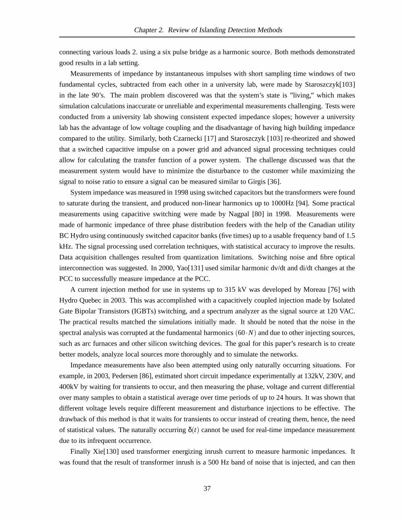
Chapter 2. Review of Islanding Detection Methods
connecting various loads 2. using a six pulse bridge as a harmonic source. Both methods demonstrated
good results in a lab setting.
Measurements of impedance by instantaneous impulses with short sampling time windows of two
fundamental cycles, subtracted from each other in a university lab, were made by Staroszczyk[103]
in the late 90’s. The main problem discovered was that the system’s state is ”living,” which makes
simulation calculations inaccurate or unreliable and experimental measurements challenging. Tests were
conducted from a university lab showing consistent expected impedance slopes; however a university
lab has the advantage of low voltage coupling and the disadvantage of having high building impedance
compared to the utility. Similarly, both Czarnecki [17] andStaroszczyk [103] re-theorized and showed
that a switched capacitive impulse on a power grid and advanced signal processing techniques could
allow for calculating the transfer function of a power system. The challenge discussed was that the
measurement system would have to minimize the disturbance to the customer while maximizing the
signal to noise ratio to ensure a signal can be measured similar to Girgis [36].
System impedance was measured in 1998 using switched capacitors but the transformers were found
to saturate during the transient, and produced non-linear harmonics up to 1000Hz [94]. Some practical
measurements using capacitive switching were made by Nagpal [80] in 1998. Measurements were
made of harmonic impedance of three phase distribution feeders with the help of the Canadian utility
BC Hydro using continuously switched capacitor banks (five times) up to a usable frequency band of 1.5
kHz. The signal processing used correlation techniques, with statistical accuracy to improve the results.
Data acquisition challenges resulted from quantization limitations. Switching noise and fibre optical
interconnection was suggested. In 2000, Yao[131] used similar harmonic dv/dt and di/dt changes at the
PCC to successfully measure impedance at the PCC.
A current injection method for use in systems up to 315 kV was developed by Moreau [76] with
Hydro Quebec in 2003. This was accomplished with a capacitively coupled injection made by Isolated
Gate Bipolar Transistors (IGBTs) switching, and a spectrumanalyzer as the signal source at 120 VAC.
The practical results matched the simulations initially made. It should be noted that the noise in the
spectral analysis was corrupted at the fundamental harmonics(60·N) and due to other injecting sources,
such as arc furnaces and other silicon switching devices. The goal for this paper’s research is to create
better models, analyze local sources more thoroughly and tosimulate the networks.
Impedance measurements have also been attempted using onlynaturally occurring situations. For
example, in 2003, Pedersen [86], estimated short circuit impedance experimentally at 132kV, 230V, and
400kV by waiting for transients to occur, and then measuringthe phase, voltage and current differential
over many samples to obtain a statistical average over time periods of up to 24 hours. It was shown that
different voltage levels require different measurement and disturbance injections to be effective. The
drawback of this method is that it waits for transients to occur instead of creating them, hence, the need
of statistical values. The naturally occurringδ(t) cannot be used for real-time impedance measurement
due to its infrequent occurrence.
Finally Xie[130] used transformer energizing inrush current to measure harmonic impedances. It
was found that the result of transformer inrush is a 500 Hz band of noise that is injected, and can then
37

Chapter 2. Review of Islanding Detection Methods
be used to solve for Equation 2.20. Similarity, disturbances have been accessed using STATCOM, or
similar power correction devices in 2002 by Diana[22] who monitored active capacitor banks to obtain
injected non-harmonic impedances.
In 2002, Xu [127] discussed how capacitor switching harmonic impedance estimation accuracy can
be enhanced and calculated in real-time by decomposing capacitive switched transients in theα−β−0
or Clark transform, instead of symmetrical component transform. Clark’s transform can be seen in
Equation 2.21. The subscript “s” is theα−β−0 and “h” is the harmonic number inZhs whereZ is the
impedance. The transform is then processed with the Fouriertransform and the harmonic impedances
are calculated as seen in Equation 2.22 whereXpre−hs is the voltage or current before the transient, and
Xpost−hs is the voltage or current during the transient.
Vα
Vβ
V0
=
1√6
2 −1 −1
0√
3√−3√
2√
2√
2
Va
Vb
Vc
= [T]
Va
Vb
Vc
(2.21)
Zhs =Vpre−hs−Vpost−hs
Ipre−hs− Ipost−hs(2.22)
In 1996, DG islanding detection using impulse response was initially published in IEEE by Hopewell
[44], who used half fundamental cycle capacitive (20µF) switching to create disturbances and com-
pared loss of mains (islanded state) to mains connection (utility connected) for distributed generation.
As shown in Figure 2.15, multiple inverter coordination andsignal corruption was seen as a limiting
issue with this technique. Multiple detection devices werediscussed, and it was theorized that by out of
phase switching between detectors, two DG devices could operate at the same time. Lab and Simulation
experiments were run.
ZDG ZUtility
ZLoadVDG VUtility
Cswitch
Figure 2.15: Impedance Measurement Using TRIAC ControlledCapacitive Switching (Hopewell [44])
Harmonic injector amplifiers were found to be useful for low voltage islanding detection (< 250
VAC), but difficulty arose when synthesizing the injected power requirements. Symmetrical injection
can be difficult, but in 2000, Palethorpe [84] used impulse response made from switching transistor
bridges using approximated experimental values. Then in Palethorpe’s [85], like his work in [84], with
a new approximated network, the power converter bridge was used to make the same measurements to
inject signals for impedance measurement with very accurate results with complex linear components
up to 2000 Hz. However, when non linear items such as diodes were introduced, the accuracy was at an
38

Chapter 2. Review of Islanding Detection Methods
unusable level.
Summary of Impulse Response Impedance Measurement
Impulse response for impedance measurement and islanding detection has primarily involved the switch-
ing of capacitors and power electronic devices to create large enough disturbances that can be measured
accurately by CTs and PTs while not consuming real power. Thedrawbacks of the impulse response
method are the practical costs of integration into higher voltage networks, infrequency of naturally
occurring changes and power quality reduction making them often impractical for low cost and high
penetrations of DG installations. However, it has been shown that if a constant source of noise can be
created at a low cost, the impedance measurement technique can be a practical solution for very accurate
islanding detection.
2.4.2 Islanding Detection using Continuous Injected Noise
Continuously injected signals for impedance based islanding detection addresses the intermittency prob-
lem of impulse type injections. They can also be made at a singular frequency and in real-time, hence, re-
ducing the energy requirement. Injection technique inserts a known source, while measuring impedance
from dividing voltage and current measurements at a pre-selected frequency. The advantage of using
such a technique is that other frequencies near to the dominant fundamental can be made, and if they
can be accurately measured, the impedance at the fundamental can be accurately estimated through in-
terpolation. This type of impedance measurement techniqueis advantageous over the impulse response
technique, as it is effective for evaluating the state of a power system continuously in real-time. Where
the impulse response is intermittent, it requires an intermittently large transient.
A network analyzer was used in 1994 and 1996 by Harris [39] andRhode [91] respectively, who
instrumented grid impedance measurement systems using an HP 3570A network analyzer with a power
amplifier injecting non fundamental frequency sweep. The coupling was achieved through a band stop
filter in combination with an isolation transformer. The injections were made in the lab (600 VAC
or less) through 20 Amp, 30 Amp and 400 Amp feeders. These experiments illustrated the effect of
local impedance variations and how this technique was predicably not useful for impedance measure-
ments of fundamental and its harmonics. However, nearby frequencies correlated with the fundamental
impedance accurately. In 1997 an injected voltage and a voltage divider to measure the impedance of the
power system was used by O’Kane[83], though the power systemlow pass characteristics and energy
requirements were not directly discussed, it can be estimated that to make a measurement around 0.01
pu it can require up to a full load energy related toV2.
Impedance measurements were then made from continuously injected signals by Di Piazza [21] and
Sumner [105] respectively in 2000 and 2001. They modeled andsimulated an injected square wave into
a power network to obtain impedance values dividing voltageby current to obtain an absolute value
of impedance. The technical challenge presented was the amount of energy required to be injected
into the system to be able to resolve meaningful measured values. Though simulation tests were made,
39

Chapter 2. Review of Islanding Detection Methods
experimental measurements on actual systems were still required. A switching inverter that could be
programmed for this algorithm was built by Sumner [106] in 2002, using a similarily controlled current
injection square-like wave as with Di Piazza [21] and Sumner[105] to measure the impedance of a
system using switching inverter devices as the injection source. The advantage of the system was that
the injected signal is computer controlled so it can be executed continuously on demand, and as a current
controller, it can be used to limit the size of the current disturbance. Tests were not verified on actual
power systems, although the method demonstrates effectivesignal to noise ratio. Then Sumner [107]
(same author as [106] and [105]) used the same system to estimate impedance to actively control shunt
loads in a laboratory setting.
In 2002, an injection device was used on 77kV and 230 kV HVDC converter sites in Japan by inject-
ing a 0.3% amplitude signal to measure impedance between 30 Hz and 400 Hz [112]. The conclusions
found that though the results looked promising, more testing is required to increase the accuracy. Signal
processing has been accomplished using:
1. A 60 Hz cancelation filter based on a phase locked loop
2. Clarke’s transformation and Park’s transformation
3. Transfer function computation that reduces the effect ofbackground noise
In 2003, a patent filed by Hochgraf [43] for islanding detection by measuring impedance through in-
jecting continuous signals from a three phase bridge inverter. The system is tripped when an impedance
changes to indicate an island condition has occurred from a known threshold. The concept of this patent
is shown in Figure 2.16, where a three phase bridge can be seento be computer controlled and monitored
for impedance at its interconnection terminals.
PowerGenerator
VaIa
SignalInjector
ImpedanceEstimation
ThresholdComparison
Rate of Change
Va* Vb* Vc*
System
VbIb
VcIc
+
+
+
+
+
+
Figure 2.16: US Patent 6,603,290 Drawing 1: Islanding Detection by Signal Injection
One year later, the injection technique was used with islanding detection standard ENS by Timbus
[109] (German abbreviation of: Main Monitoring units with allocated Switching Devices) to detect DG
40

Chapter 2. Review of Islanding Detection Methods
islands. A periodic injection of 75 Hz every 1 second is made by an inverter, removing the need for a
dedicated islanding detection unit. The injection frequency is ”tuned” or chosen to best fit the network
conditions. This technique was also discussed by Xu [128] in2004. Injection was found to be ideal for
islanding detection with 1 kW to 4 kW generators, but other smaller sized inverters may have practical
power limitations. Injection amplitudes of 0.02 pu to 0.07 pu were tested and it was determined that
0.05 pu offered the best results while keeping within IEEE power quality standards. Multiple inverters
were identified as a special case which would need to be addressed to prevent multi inverter signal
corruption. In 2004, the same method was used by Asiminoaei [5] and Timbus [109] where impedance
was measured by injecting a single frequency into the network. It was found that the amount of random
noise rejection of the transient method is a disadvantage and the data acquisition capabilities need to
be high and are often un-achievable. Impedance was measuredby injecting a 75Hz signal as a non
harmonic for 0.040 s at 1.5 Amps. Asiminoaei [5] considered the impedance at 75 Hz to behave similarly
to the fundamental of 50 Hz. It was shown the single frequencyinjection impedance measuring method
can be programmed directly into the inverter’s control algorithm for effective islanding detection. The
system consists of voltage injected into 220 VAC single phase utility voltages. In 2005, this topic is
further improved with Asiminoaei [7] and [6] as an extensionof his work [5] and discusses vector
method and FFT method at 75 Hz while discussing THD, power injected, and repetition rate vs. the
accuracy of the method. Practical measurements were made using a 10-bit AD converter at 1.3kH
sampling rate with high levels of accuracy. The experiment was validated with lab experiments, but
practical tests were not completed.
In 2006, multiple inverter coordination with single signalinjections for islanding detection were
addressed by Timbus [111] in the inverter used by the same team as Asiminoaei [5] and Sung-Il [108].
They used multiple inverter coordination to inject the 75 Hzsignals with another inverter, by offsetting
the injections by 0.05 s from each other. Fourier transformswere used to analyze the results and to
detect another inverter; a harmonic compensator was used.
In 2006, Timbus [110] discusses the amplitude, frequency and current controller gain technique
for impedance based islanding detection. The focus is on theENS requirement of a 0.5 ohm change
measured using an injection amplitude of 0.05 pu. Injectionrates made infrequently to lower the total
harmonic distortion (THD) is averaged where the overall goal of the work was to assess the value of not
having a specialized unit for islanding detection but instead placing it right into the inverter itself.
In 2005 and 2006, Katirae [65] and Hernandez-Gonzalez [42] respectively, both explore the idea of
micro-grid operation and islanding detection. However, [42] explores impedance measurement using
current injection to address island conditions. The injection is through the dq axis (Park’s Transform
[67]) using frequencies of 1 Hz to 40 Hz. Results are for a single source only, but claim to be effective
in simulations detecting in less than 33.3 ms and most effective at 1 Hz at 1% the fundamental. The
non-detection zone occurs in quality factors between 3 and 4in a resonating bus.
Finally, using an unbalanced source to create negative sequence injection, a ship’s impedance net-
work stability was monitored through measurement of the Th´evenin impedance. The impedance was
found to be accurately measurable through a multi-variablesolution of positive and negative sequence
41
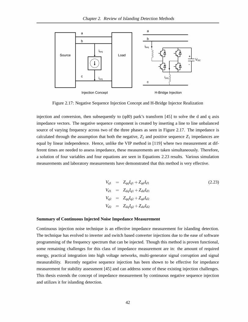
Chapter 2. Review of Islanding Detection Methods
Source
a
b
c
Loadibinj
icinj
a
b
c
ibinj
+
-
icinj
noitcejnI egdirB-H tpecnoC noitcejnI
VDC
Figure 2.17: Negative Sequence Injection Concept and H-Bridge Injector Realization
injection and conversion, then subsequently to (qd0) park’s transform [45] to solve the d and q axis
impedance vectors. The negative sequence component is created by inserting a line to line unbalanced
source of varying frequency across two of the three phases asseen in Figure 2.17. The impedance is
calculated through the assumption that both the negative,Z2 and positive sequenceZ1 impedances are
equal by linear independence. Hence, unlike the VIP method in [119] where two measurement at dif-
ferent times are needed to assess impedance, these measurements are taken simultaneously. Therefore,
a solution of four variables and four equations are seen in Equations 2.23 results. Various simulation
measurements and laboratory measurements have demonstrated that this method is very effective.
Vq1 = ZqqIq1 +ZqdId1 (2.23)
Vd1 = ZdqIq1 +ZddId1
Vq2 = ZqqIq2 +ZqdId2
Vd2 = ZdqIq2 +ZddId2
Summary of Continuous Injected Noise Impedance Measurement
Continuous injection noise technique is an effective impedance measurement for islanding detection.
The technique has evolved to inverter and switch based converter injections due to the ease of software
programming of the frequency spectrum that can be injected.Though this method is proven functional,
some remaining challenges for this class of impedance measurement are in: the amount of required
energy, practical integration into high voltage networks,multi-generator signal corruption and signal
measurability. Recently negative sequence injection has been shown to be effective for impedance
measurement for stability assessment [45] and can address some of these existing injection challenges.
This thesis extends the concept of impedance measurement bycontinuous negative sequence injection
and utilizes it for islanding detection.
42

Chapter 2. Review of Islanding Detection Methods
2.5 Current and Voltage Measurability
Of the challenges detailed for the various islanding detection techniques for impedance measurement,
voltage and current measurability has been consistently regarded as a significant limiting factor. There-
fore, this section contains a discussion of voltage and current sensor technology used today and will
cover the existing installed technology, sensor bandwidth, and accuracy at different voltage levels so
that simulation measurements can be addressed as either practical or not practical variations. With the
negative sequence impedance islanding detection technique developed in this thesis, some cases use
naturally occurring signals at distribution voltage levels where existing sensor current transformers and
where voltage transformer (CT and PT respectively) devicesare already installed. Sensor accuracy is a
key item that can limit the ability for some techniques to be effectively used. In this section, both cur-
rent and voltage measurement techniques will be addressed individually as they are tackled in slightly
different ways and require special consideration. Voltageand current transducers in the field today,
are a mix of older transducers and more modern computerized devices. However, the islanding detec-
tion technique described in this thesis requires complex signal processing from digitized measurements.
Therefore, the focus on current and voltage measurability will be on computerized data acquisition,
though it is important to keep in mind that the mechanical side of these sensors will not be discussed
here. There is significant literature on the specific topic ofhigh voltage measurement. Five key ref-
erences were chosen: [100] [78] [29] [73] [35] with IEEE standards for CTs and PTs used in power
systems as with [55]. More specific references are also mentioned throughout this section.
2.5.1 Voltage Measurement
Safe measurement of power system high voltages can not be directly accessed by computerized equip-
ment and must be reduced by often several orders of magnitudebefore being connected to a computer.
Utility distribution voltages range from residential 0.120 kV to line distribution of 50 kV depending
on the area and the application. However, for a typical computerized data acquisition analog to digital
converter, voltage levels of +/- 5 V or less are required. Therefore, from typical distribution voltage
of 25 kV, a voltage drop of nearly five orders of magnitude withminimal error must be achieved. The
techniques to achieve this can be broken down into several groups: 1. resistive divider, 2. step down
transformer, 3. capacitive voltage divider, 4. optical electrical field measurement and combinations of
all four. Each voltage and current method has better optimalperformance than the other techniques at
different voltage levels. As the technique described in this thesis has been tested at a span from 0.208 kV
to 25 kV, the following sub-sections shall review the four techniques listed here for methodology and
performance.
Resistive Voltage Divider
For low voltage applications (below 5000 V), resistive voltage divider electronics are the most common
form used to step down signals for accurate measurement. Therefore, resistive divider ratios from 1:100
to 1:1000 are needed. Precision, laser cut, mega Ohm resistor divider pairs can be purchased at a
43

Chapter 2. Review of Islanding Detection Methods
relatively low cost and have an accuracy ranging from 1.0 % to0.01 %. This type of resistor divider is
used with low voltage inverters and for precision measurements at higher voltages. Resistive dividers
have the advantage of being predicably linear over a wide range of frequencies from DC up to 100’s of
kHz. Purely resistive division requires an isolating circuit protector for unforseen transients and ground
loops. This concept can be seen in Figure 2.18 where there aretwo matched resistors,R1 andR2, which
have ratios of up toR1R2
= 1000. Following the two resistors, is an isolating amplifierthat taps off the
lower voltage resistorR2.
+
- Vmeasured
R1
R2
Isolation Barrier
0 to 5 kV
Figure 2.18: Resistive Divider Voltage Measurement with Isolator
Voltage Transformer and Coupling Capacitor Voltage Transformers
Voltage transformers (PTs) and coupling capacitor voltagetransformers (CCVTs) are the most common
measurement devices for converting higher system voltagesto more safe and usable lower voltage levels.
CCVTs are less expensive than standard PTs at higher voltagerated voltage levels, but can have inferior
transient response due to their ferroresonance effects. A PT consists of a step down transformer with
a burden impedance network for mechanical relay or computerbased relay inputs [29]. The equivalent
circuit of the PT can be seen in Figure 2.19 and has been modeled in EMTP by Fernandes [30]. The
circuit has a transformer equivalent circuit and an output burden impedance. The transformer equivalent
consists of a primary impedanceR1 and jωL1 that are reflected over to the secondary side by dividing
each by the square of the turns ratio,n2. Following the primary impedance, areR2 and jωL2 in series
connecting to the burden load where the voltage measurementis made. In between the primary and
secondary impedances are the magnetization resistance andinductance,RFe and jωLM. Under normal
operating conditions, the magnetization impedance is near99 pu [23]. Standardized maximum absolute
measurement errors for these devices range around 0.3 %, 0.6% and 1.2 % as specified in [55] and [57].
As the current draw for PTs are very low, transformer saturation is not an issue as it can be with current
measurement.
Conversely, the other common alternative developed for safe high voltage measurement are CCVTs
that consist of a combination of a capacitive coupled voltage dividers connected to the step down voltage
transformer. CCVTs are more cost effective to PTs at higher voltages (≥ 100kV) due to a reduction in
the isolation transformer size. As seen in the equivalent circuit in Figure 2.20, the voltage division
is accomplished through a series of capacitors that are thenparalleled by the transformer equivalent
44

Chapter 2. Review of Islanding Detection Methods
High Voltage
Connection
R1/n j L1/n R2 j L2
j LM RFe
RBurden
j LBurden
n:1
Scaled Output 2 2
Figure 2.19: Voltage Transformer Equivalent Circuit
circuit off of the low voltage portion of the capacitive divider chain. Though only two capacitors are
shown, these capacitors are often multiple capacitors stacked together, allowing the protection engineer
to select specific taps for the voltage level of interest. Theother components are the spark gap on the
left side of the circuit seen in Figure 2.20, and a resonance suppression circuit on the right. These two
additions are added to limit the over voltages during high frequency transients and to limit resonance
oscillations during transients. As compared to Figure 2.19, the CCVT’s complexity is higher than the
PT with the addition of capacitors. These third order components are most significantly noticed during
high speed transients, such as lightning strikes, where thecapacitive coupling can act like a short circuit.
The shorted high potential signal travels into the measurement system, where the spark gap limits the
over voltage into the sensitive circuitry, and the filter reduced the over voltage resonance between the
transformer and the voltage divider capacitors. However, under normal operating conditions at the
fundamental frequency, CCVTs are as accurate as PTs, but outside of the fundamental frequency, the
response is not linear and care must be taken to prevent falsereadings. Therefore, for steady state
voltage measurements used in this thesis, PTs and CCVTs willhave comparable accuracy.
High Voltage Line
R1/n jwL1/n R2 jwL2
jwLM RFe
n:1 Scaled Output-1/(jwc1)
-1/(jwc2)
Spark Gap
jwLTR
Ferro resonance suppression 2 2
Figure 2.20: Coupling Capacitor Voltage Transformer Equivalent Circuit
Optical Electric Field Measurement
The final method used for high voltage measurement is with electro-optical phenomena. This phenom-
ena is called the Pockels effect. Though this method is not commonly used due to its recent emergence
in the utility market, the optical interface has the distinct advantage of superior electrical isolation char-
45
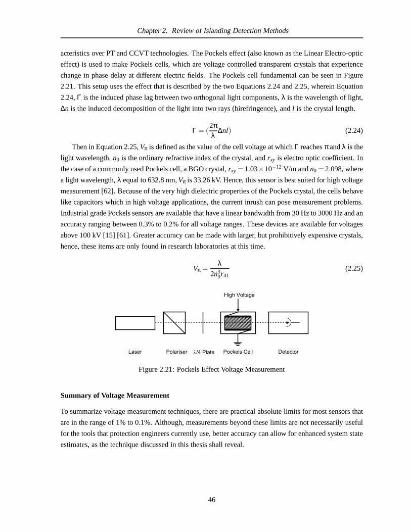
Chapter 2. Review of Islanding Detection Methods
acteristics over PT and CCVT technologies. The Pockels effect (also known as the Linear Electro-optic
effect) is used to make Pockels cells, which are voltage controlled transparent crystals that experience
change in phase delay at different electric fields. The Pockels cell fundamental can be seen in Figure
2.21. This setup uses the effect that is described by the two Equations 2.24 and 2.25, wherein Equation
2.24,Γ is the induced phase lag between two orthogonal light components,λ is the wavelength of light,
∆n is the induced decomposition of the light into two rays (birefringence), andl is the crystal length.
Γ = (2πλ
∆nl) (2.24)
Then in Equation 2.25,Vπ is defined as the value of the cell voltage at whichΓ reachesπ andλ is the
light wavelength,n0 is the ordinary refractive index of the crystal, andrxy is electro optic coefficient. In
the case of a commonly used Pockels cell, a BGO crystal,rxy = 1.03×10⁻¹² V/m andn0 = 2.098, where
a light wavelength,λ equal to 632.8 nm,Vπ is 33.26 kV. Hence, this sensor is best suited for high voltage
measurement [62]. Because of the very high dielectric properties of the Pockels crystal, the cells behave
like capacitors which in high voltage applications, the current inrush can pose measurement problems.
Industrial grade Pockels sensors are available that have a linear bandwidth from 30 Hz to 3000 Hz and an
accuracy ranging between 0.3% to 0.2% for all voltage ranges. These devices are available for voltages
above 100 kV [15] [61]. Greater accuracy can be made with larger, but prohibitively expensive crystals,
hence, these items are only found in research laboratories at this time.
Vπ =λ
2n30r41
(2.25)
Laser Polariser l/4 Plate
High Voltage
DetectorPockels Cell
Figure 2.21: Pockels Effect Voltage Measurement
Summary of Voltage Measurement
To summarize voltage measurement techniques, there are practical absolute limits for most sensors that
are in the range of 1% to 0.1%. Although, measurements beyondthese limits are not necessarily useful
for the tools that protection engineers currently use, better accuracy can allow for enhanced system state
estimates, as the technique discussed in this thesis shall reveal.
46

Chapter 2. Review of Islanding Detection Methods
2.5.2 Current Measurement
Similar to voltage measurement, there are a series of different methods for measuring current in power
systems. The current measurement techniques used in power systems are an optimization between cost,
practicality, target relay and accuracy. The most common methods for current measurement used today
are: 1. High and low side resistive shunts, 2. Current transducers, and 3. Opto-magnetic current
measurement. Each of these methods have a specific application and advantage over the other where the
general accuracy of all three commercial available items are similar.
High and Low Side Resistive Shunt
High and low side resistive shunts are used in low voltage (less than 1000 V) inverter applications due
to their simple installation and high bandwidth. This method consists of a very low value resistor, such
as 0.01Ω, in series with the output terminals; with a differential amplifier used to measure the voltage
drop across the resistor. Low side measurement places a series resistor along the ground return path,
while high side measurement places a series resistor inlinewith the high voltage output terminals. Low
side current measurement carries the disadvantage of inaccuracy if the system has ground loops and
can only be used with single phase inverters. For high side current measurement, as the source voltage
rises above several hundred volts, or if there is a significant common mode corruption, this method also
becomes significantly impractical and unsafe. High side measurement can be seen in Figure 2.22. The
accuracy of these sensors range from 1% to 0.1% of the full load current rating.
Phase A
Rshunt
0 to 300~VLN
+ -
IA_Measured
Phase BRshunt
To Load
Phase C
Rshunt
+ -
IB_Measured
+ -
IC_Measured
Isolation
Figure 2.22: Resistive Shunt Current Measurement
Current Transducers
Current transducers are the most common tool used for current measurement in power systems. They
have the advantage of protecting both personnel and other equipment from high voltage levels, and
47

Chapter 2. Review of Islanding Detection Methods
provide a reduction from high current carrying conductors to the measurement equipment. To measure
line currents, a current step down transformer concept is utilized with an iron core around the high
voltage current carrying conductor, which has an associated step down coil around the core, as seen in
Figure 2.23. The induced voltage in the secondary coil can bevery high, as described by Maxwell’s
Equation “Faraday’s Law” and seen in Equation 2.26 whereΦ(t) is the magnetic flux, andvturn is the
volts per turn. In high voltage systems, the magnetic flux is very large and requires the secondary burden
impedance be as low as possible so dangerously large voltages are not produced at the terminals. The
polarity of the transducer is dependant on the winding characteristics.
vturn(t) =∂Φ(t)
∂t(2.26)
The construction of low and high voltage transformers differ in only two ways. The first is the
voltage isolation and the second is the ferrite core size. The ferrite core must have the magnetic flux
carrying capacity that will not saturate under normal operation and during fault conditions. This requires
that the iron core be very large for high power systems. The equivalent circuit for a current transformer
is similar to Figure 2.19 with the difference being that the current transformer primary terminals are
connected in line (i.e. in series) with the power system, andthe voltage transformer is connected line
to line. When a current transformer’s core enters saturation, the transformer’s response becomes non
linear resulting in inaccurate measurements. Therefore, it is critical for the protection system’s proper
operation that measurements can be reliably and accuratelymade and that the CT does not saturate.
High Voltage Line IH
IH/N
RLine RLine
Burden: ZB
VB
Figure 2.23: Current Transformer Circuit with Burden
Low voltage and current transformers can be purchased at a relatively low cost with an accuracy
of 0.1% or less. However, with larger power system current transformers, accuracy must be carefully
48

Chapter 2. Review of Islanding Detection Methods
assessed at the system’s rated current and voltage. The magnetization current of the transformer is not
zero, so the assumption ofIPrimary = IBurden/N where N is the turns ratio is not accurate and the magne-
tization current must be taken into account. The accuracy ofthe measurement at the burden impedance
will depend on: the burden impedance, the connecting lead impedance, the current divider ratio, the
DC offset and the ferrite residual excitation characteristics. For example, the voltage at the secondary
current transformer terminals for a three phase faultVS, is as seen in Equation 2.27 whereIL/N is the
maximum secondary current,ZB is the connected burden impedance andZLead is the connection leads
and transformer connection impedance [2]. When the currentis below the normal transformer operat-
ing conditions, the magnetization impedance is very high, however, as the flux density approaches the
saturation point of the ferrite core, the excitation impedance drops and the measurement error signif-
icantly increases both in amplitude and in phase. The supplier of each current transducer will supply
the magnetization curve of the transducer so estimates on the transducer’s accuracy can be properly
estimated.
VS = IL/N(ZL +ZLead+ZB) (2.27)
High voltage CT accuracy would normally be difficult to assess due to the large number of CTs out in
the field; however, the IEEE standard C57.13-1993(R2003) [55] specifies the standardized characteristic
burdens and accuracy classes with the worst case allowable accuracy. For example, power revenue
metering CTs have an accuracy of less than 0.3% under full load. This value is critical for proper revenue
metering and for protective calculations. When taking fieldmeasurements of current transformers, it is
important to understand the measurement device so that proper protective decisions can be made for a
high level of system security and dependability.
Optical Magnetic Field Measurement
The final form of current measurement used in power systems isthrough magneto-optical effects. Unlike
the electrical field based Pockels effect, the Faraday effect (or Faraday rotation) is a magneto-optical
phenomenon where the interaction between light and a magnetic field change the polarization of the
transmitting light. The relationship occurs when the planeof polarization rotates proportionally to the
intensity of the magnetic field that is in the direction of thebeam of light. The Faraday effect was
discovered by Michael Faraday in 1845 which was some of the first experimental evidence of how light
and electromagnetism relate. The Faraday effect occurs in many optically transparent and dielectric
materials.
The relationship between the angle of the optical rotation of the wavelength polarization and the
magnetic field is seen in Equation 2.28 whereβ is the angle of rotation,B is the magnetic flux,d is the
length of the path of where the magnetic field interacts with the material, andν is the Verdet constant
for the material. The Verdet constant for most materials is found to be extremely small and wavelength
dependent. For example, typical glass-like materials haveconstants ranging between 0.02 and 0.089
min/Gauss-cm. Measurement errors for these sensors are linear throughout their operating region at
49
Chapter 2. Review of Islanding Detection Methods
0.2% or better [14] [1]. Similarly to Pockels effect, magneto-optical current measurement has superior
electrical isolation and no saturation effects over current transducers. However, they are a relatively new
commercial product in the utility industry and do not have high installation density.
β = νBd (2.28)
Summary of Current Measurement
Current measurement in power systems primarily consists ofcurrent transducers. These items have a
long product life, hence, when many of them were installed. Over the past 50 years, In North America,
there has been little need to replace them. The standardizedaccuracy depends on their use, but it will
range between 1% and 0.1% depending on where and when it was installed. Current measurement
in power systems plays a critical role for the protection of power systems. The islanding detection
technique described in this thesis has a higher level of performance, depending on the accuracy of the
sensors. Therefore, the highest accuracy sensors will offer some of the best results.
2.6 Summary of Research Background
This chapter has covered the background topics that are relevant to the current state-of-the art for this
thesis’ key contribution of negative sequence impedance measurement for islanding detection. These
topics are: distributed generator protection motivation,islanding detection techniques, impedance mea-
surement for islanding detection, and current and voltage measurement techniques and accuracy in
power system applications. The installation of distributed generation systems create significant new
challenges for the protection engineer. These challenges can be improved with a dependable and se-
cure locally running islanding detection system. Islanding detection can be used to provide additional
protection for service workers, assist in limiting voltagesurges, reduce short circuit currents, and al-
low for re-closure functions to operate as they were designed (before the installation of the distributed
generator).
There are many forms of islanding detection available with some associated standards to support
and test them. Of all the forms available, there are various performance characteristics, depending
on the application, load types, generator installation density and power system strength. Impedance
measurement techniques are the only methods that have a theoretically negligible non-detection zone.
Unfortunately, of all the impedance based techniques, theyall either have sensitivity, threshold settings,
installation cost or practical continuous real time measurement limitations.
Additionally, of the sensitivity limitations of impedancemeasurement techniques, existing power
system voltage and current measurement accuracy limits overall effectiveness. There are many tech-
niques commonly used for measuring voltage and current, ranging from parallel/series impedance
shunts, step up/down transformers and more recently, electo-optical and magneto-optical effects. How-
ever, with all the voltage and current measurement techniques available to the protection engineer, the
most common and frequently heavily installed methods at distribution levels are voltage and current
50

Chapter 2. Review of Islanding Detection Methods
transformers. Therefore, impedance measurement techniques used today for islanding detection must
fall into the physical measurement limitations of a maximumpractical accuracy of 0.1%, and a typical
accuracy to be expected to match the IEEE accuracy standard of 1% to 0.3 % of the rated load.
In the following chapter, a logical increment in the impedance measurement for islanding detection
is introduced. This method uses negative sequence impedance measurement, while taking practical
and simulations from various locations to demonstrate its effectiveness. The following Chapter 3, first
introduces the concept theoretically, followed by Chapter4 which analyzes some practical case studies.
51

Chapter 3
Negative Sequence Impedance Islanding
Detection
3.1 Introduction
This chapter contains the derivation and description of negative sequence impedance island detection for
distributed generation. Negative sequence impedance islanding detection is a novel form of impedance-
based islanding detection that can either use naturally occurring or injected negative sequence currents
and voltages. The negative sequence impedance islanding detection technique operates off the principle,
that an unbalanced load (or source) has a negative sequence current source at the point of the unbalanced
load’s interconnection. Unlike its positive sequence counterpart that are from generators, as seen in
Figure 3.1, the negative sequence currents are created at the unbalanced load (if the rest of the system is
balanced).
Current flows are different between DC systems and AC systems. In a DC system, the direction
of current is identified by the sign. In an AC system, the phaseangle and amplitude referenced to the
voltage dictates the direction of power flow.
In Figure 3.1, subscripts 1 and 2 indicate positive and negative sequence components respectively,
and subscript UL and BL stand for “Unbalanced Load” and “Balanced Load” respectively. In Figure
3.1, E1 is the positive sequence source,I1 is the positive sequence current,I2a−UL and I2b−UL are the
unbalanced load currents from the unbalanced load; UL,V1−UL andV2−UL are the positive and negative
sequence voltages at the unbalanced load,I1−BL is the positive sequence current into the balanced load,
andV1−BL andV2−BL are the positive and negative sequence voltages at the balanced load. From Figure
3.1, the impedance,Zsourcecan be expressed as in Equation 3.2 when the negative sequence current is
used. This method of impedance measurement allows for the negative sequence components to be used
as a real time anti-islanding sensor relay by measuring the impedance away from the unbalanced node
and comparing it to a known threshold before and after the island state occurs.
The negative sequence impedance islanding detector methodrequires two assumptions to function
correctly: 1. At the distribution level, a power system is rarely balanced, and 2. The utility source is
typically much stronger than the distributed generator in the islanded branch as seen in Equation 3.1.
The first assumption can be enhanced as discussed in previousimpedance measurement techniques
[45] by externally creating unbalanced conditions at the cost of the degradation of the system’s power
quality. Other factors to consider when using externally injected signal methods are the amount of re-
quired energy, practical integration into high voltage networks, multi generator signal corruption, and
52
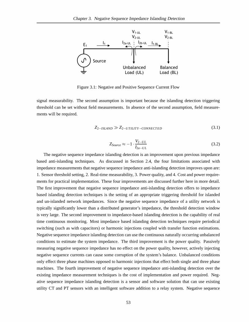
Chapter 3. Negative Sequence Impedance Islanding Detection
UnbalancedLoad (UL)
SourceBalancedLoad (BL)
I2a-UL I2b-ULI1
V1-ULV2-UL
E1
V1-BLV2-BL
I1-BL
Figure 3.1: Negative and Positive Sequence Current Flow
signal measurability. The second assumption is important because the islanding detection triggering
threshold can be set without field measurements. In absence of the second assumption, field measure-
ments will be required.
Z2−ISLAND≫ Z2−UTILITY−CONNECTED (3.1)
ZSource≈−1· V2−UL
I2a−UL(3.2)
The negative sequence impedance islanding detection is an improvement upon previous impedance
based anti-islanding techniques. As discussed in Section 2.4, the four limitations associated with
impedance measurements that negative sequence impedance anti-islanding detection improves upon are:
1. Sensor threshold setting, 2. Real-time measurability, 3. Power quality, and 4. Cost and power require-
ments for practical implementation. These four improvements are discussed further here in more detail.
The first improvement that negative sequence impedance anti-islanding detection offers to impedance
based islanding detection techniques is the setting of an appropriate triggering threshold for islanded
and un-islanded network impedances. Since the negative sequence impedance of a utility network is
typically significantly lower than a distributed generator’s impedance, the threshold detection window
is very large. The second improvement to impedance-based islanding detection is the capability of real
time continuous monitoring. Most impedance based islanding detection techniques require periodical
switching (such as with capacitors) or harmonic injectionscoupled with transfer function estimations.
Negative sequence impedance islanding detection can use the continuous naturally occurring unbalanced
conditions to estimate the system impedance. The third improvement is the power quality. Passively
measuring negative sequence impedance has no effect on the power quality, however, actively injecting
negative sequence currents can cause some corruption of thesystem’s balance. Unbalanced conditions
only effect three phase machines opposed to harmonic injections that effect both single and three phase
machines. The fourth improvement of negative sequence impedance anti-islanding detection over the
existing impedance measurement techniques is the cost of implementation and power required. Neg-
ative sequence impedance islanding detection is a sensor and software solution that can use existing
utility CT and PT sensors with an intelligent software addition to a relay system. Negative sequence
53

Chapter 3. Negative Sequence Impedance Islanding Detection
impedance islanding detection also does not use expensive large power coupling components such as
high VA transformers and capacitors that most other techniques based on injection require. The method
can be summarized using Equations 3.1 and Equation 3.2 whichare stated at the beginning of this
Section.
To fully understand the concept of negative sequence impedance islanding detection, this chapter
derives the method of negative sequence impedance measurement, demonstrates how the the unbalanced
load is a source of negative sequence current, analyzes the performance characteristics over a wide range
of scenarios and finally reiterates how the concept expressed in Equations 3.1 and 3.2 can be used as an
anti-islanding system for use with distributed generators.
3.2 Derivation of System Negative Sequence Impedance Estimation
The negative sequence impedance islanding detection method uses the symmetrical component trans-
form properties to measure the external system impedance. The symmetrical component vector trans-
formation was introduced by Fortescue in 1918 [120] to decouple three phase line interdependencies
into three linearly independent systems. The transform requires a matrix operator, A, and the vectorial
form of the ABC voltages or currents to convert the unbalanced system into three balanced independent
systems called Positive, Negative and Zero sequence, and they are indicated using subscripts 1, 2, 0, re-
spectively, as illustrated in Figure 3.2 and detailed in Appendix B. To introduce the derivation of system
negative sequence impedance, a simplified DC system and a three phase system will be presented for
comparison.
Figure 3.2: Symmetrical Component Conversion
3.2.1 Two Circuit DC System
Consider an example of two nearly identical DC circuits seenbelow in Figure 3.3 whereEo is the source
voltage,Zx is the transmission line impedance, andZy1 andZy2 are differing load impedances for each
circuit. The two circuits can be described by Equation 3.3 and Equation 3.4 seen below. The Load
resistancesZy1 andZy2 are not the same value in each circuit so the voltagesVA 6= VB and the currents
IA 6= IB. This means that each load is consuming a different power.
54

Chapter 3. Negative Sequence Impedance Islanding Detection
Eo
ZxVA
IA+
-Eo
Zx
VB
IB+
-
Zy1 Zy2
Figure 3.3: Two DC Circuits with Different Load Impedances
VA + IA ·Zx = Eo (3.3)
VB + IB ·Zx = Eo (3.4)
If Eo andZx are not known for either circuit,Zx can be found by measuringVA, IA, VB, IB. Equations
3.3 and 3.4 are combined together as seen in Equation 3.5 and thenZx is solved as seen in Equation
3.6. The solutions forZy1 andZx can be compared as seen in Equations 3.7 and 3.6. The solutionof
Equation 3.6 is only possible whenZy1 6= Zy2.
VA + IA ·Zx = VB + IB ·Zx (3.5)
VA−VB
IB− IA= Zx (3.6)
VA
IA= Zy1 (3.7)
3.2.2 Simple Three Phase System
Extending the same concept seen in the previous Section 3.2.1, Zx solution can also be applied to three
phase systems. Consider an example of the system seen in Figure 3.4. All variables are similar to the
previous example except the source voltages are sinusoidal: EA = Eo 6 0, EB = Eo 6 240,EC = Eo 6 120.
If there is no interphase coupling, the circuit in Figure 3.4has been expanded into its single phase
components as seen in Figure 3.5 and organized so that the three individual circuits can be clearly seen
in Figure 3.6.
The system of equations for the network can be seen in Equations 3.8, 3.9, 3.10.
VA + IA ·ZxA = EA (3.8)
VB + IB ·ZxB = EB (3.9)
VC + IC ·ZxC = EC (3.10)
55

Chapter 3. Negative Sequence Impedance Islanding Detection
[EABC]
[VABC]
[IABC][Zy]
[Zx]
Figure 3.4: Three Phase Circuit (Single Line) Example with Different ‘Y’ Load Impedances
If the three source voltages are of the same magnitude and 120degrees apart, the sum of the three
voltage vectors will be equal to zero as seen in Equation 3.11.
EA+EB +EC = 0 (3.11)
Then Equation 3.11 can be set to equal the sum of Equations 3.8, 3.9, 3.10 as seen in Equation 3.12.
0 = VA + IA ·ZxA+VB + IB ·ZxB+EB+VC + IC ·ZxC+EC (3.12)
If ZxA = ZxB = ZxC andZyA 6= ZyB 6= ZyC, Zx, Equation 3.12 can be solved for as seen in Equation
3.13. Normally, if theZy resistors were all the same, this solution would equate to a non-number, but
because of the differingZy resistances, the solution is non zero.
Zx = −1·VA +VB +VC
IA + IB + IC(3.13)
Consider the following more specific example. If the impedances are all considered to be purely
resistive then all the voltages and their associated currents are in phase (Figure 3.4). However, when
ZyA 6= ZyB 6= ZyC the difference of the unbalanced currents is 180 degrees outof phase of the voltage.
Take a case for Figure 3.4 whenEABC = 1 V, Zx ABC = 20 Ω, ZyA = ZyB = 1000Ω andZyC = ZyA+
Zunbalance= 1300Ω where all impedances are resistive. The resulting voltagesand currents are described
in Equation 3.14 to Equation 3.19.
VA = V 6 0 = 0.98046 0 (3.14)
VB = V 6 240= 0.98046 240 (3.15)
VC = (V +x)6 120= 0.98486 120 (3.16)
56

Chapter 3. Negative Sequence Impedance Islanding Detection
ZxA
ZxB
ZxC
ZyA
ZyCZyB
EA
EBEC
VA
VCVB
IA
IB
IC
Figure 3.5: Three Phase Circuit Example Expanded with Different ‘Y’ Load Impedances
IA = I 6 0 = 0.9804·10−3 6 0 (3.17)
IB = I 6 240= 0.9804·10−3 6 240 (3.18)
IC = (I −y)6 120= 0.7576·10−3 6 120 (3.19)
The difference between the voltages and currents are in Equation 3.20 and Equation 3.21. Notice
how the phase difference between the two is 180 degrees.
VA +VB +VC = 0.00456 120 (3.20)
IA + IB + IC = 2.2282·10−4 6 −60 (3.21)
Employing Equation 3.13 using the sum of V and I, the result isZx = 20 Ω as derived.
Zx = −1· VA +VB +VC
IA + IB+ IC= −1· 0.00456 120
2.2282·10−4 6 −60= 20 Ω (3.22)
These two examples illustrate how similar circuits can be used in combination to solve for resis-
tances in the reverse direction of the current flow. In a real power network, the network is much more
complex with mutually coupled components. In the followingsections, this concept is be extended to a
general solution by decomposing the phases into the negative sequence symmetrical component.
57
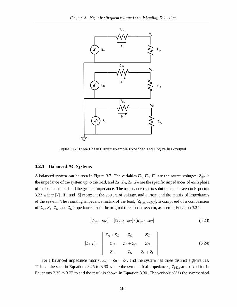
Chapter 3. Negative Sequence Impedance Islanding Detection
EA
ZxAVA
IA
EB
ZxBVB
IB
ZyA
ZyB
EC
ZxCVC
ICZyC
Figure 3.6: Three Phase Circuit Example Expanded and Logically Grouped
3.2.3 Balanced AC Systems
A balanced system can be seen in Figure 3.7. The variablesEA, EB, EC are the source voltages,Zsys is
the impedance of the system up to the load, andZA, ZB, ZC, ZG are the specific impedances of each phase
of the balanced load and the ground impedance. The impedancematrix solution can be seen in Equation
3.23 where[V], [I ], and[Z] represent the vectors of voltage, and current and the matrixof impedances
of the system. The resulting impedance matrix of the load,[ZLoad−ABC], is composed of a combination
of ZA , ZB, ZC, andZG impedances from the original three phase system, as seen in Equation 3.24.
[VLine−ABC] = [ZLoad−ABC] · [ILoad−ABC] (3.23)
[ZABC] =
ZA+ZG ZG ZG
ZG ZB +ZG ZG
ZG ZG ZC +ZG
(3.24)
For a balanced impedance matrix,ZA = ZB = ZC, and the system has three distinct eigenvalues.
This can be seen in Equations 3.25 to 3.30 where the symmetrical impedances,Z012, are solved for in
Equations 3.25 to 3.27 to and the result is shown in Equation 3.30. The variable ‘A’ is the symmetrical
58

Chapter 3. Negative Sequence Impedance Islanding Detection
V Line A V Line B V Line C
ZA= ZB= ZC(ZLoad)
ZG
ZA ZB ZC
[ZSys]
EA EB EC
Figure 3.7: Three Phase Circuit with a Balanced Load
component operator defined in B.2 in the following appendices. The solution in Equation 3.30 can
be illustrated in a conceptual schematic where the three symmetrical components are all independent
systems to each other, as seen in Figure 3.8. Since only the positive sequence system has a voltage
source, calculations of the voltage and current for this system can be reduced to only one simple circuit
where the current flows from the source to the load. Also, it isnotable that in many practical systems
Z1 is equal toZ2. ThoughZ1 is not exactly equal toZ2 such as with rotating machines, for this example,
this assumption is made because transmissionZ is commonly much greater than the machineZ. More
specific details on machine symmetrical impedances will be discussed in further sections.
A ·V012 = ZABC·A · I012 (3.25)
A−1 ·A ·V012 = A−1 ·ZABC·A· I012 (3.26)
Z012 = A−1 ·ZABC·A (3.27)
Z012 = A−1 ·ZABC·A (3.28)
= A−1 ·
ZA +ZG ZG ZG
ZG ZA +ZG ZG
ZG ZG ZA +ZG
·A (3.29)
=
ZA +3ZG 0 0
0 ZA 0
0 0 ZA
(3.30)
59

Chapter 3. Negative Sequence Impedance Islanding Detection
Z1 sys
Z1 Load
E1Z2 sys
Z2 Load
Z0 sys
Z0 Load
Positive Sequence Negative Sequence Zero Sequence
Figure 3.8: Balanced Symmetrical Component Circuits from Balanced Load
3.2.4 Unbalanced AC Systems
In a balanced system as seen in Section 3.2.3, the negative and zero sequence currents and voltages are
zero and linearly independent of each other (Figure 3.8); however, in an unbalanced system, this prop-
erty is no longer true. The result of an unbalanced load shallbe further explored with a similar circuit
containing the Thevenin impedance of a balanced grid and anunbalanced load as seen in Figure 3.9.
V Line A V Line B V Line C
ZA ZB ZC(ZLoad)
ZG
ZA ZB ZC
[ZSys]
EA EB EC
Figure 3.9: Unbalanced Load and Balanced Source Circuit
In Figure 3.9, solving forV012 at VLine betweenZSys andZLoad increases in complexity when the
ABC phase impedances of the load inZLoad are such thatZA 6= ZB 6= ZC. When solving for the sequence
components at the pointVLine, an impedance voltage divider of sequence components can beused. The
voltage divider for Figure 3.9 is seen in Equation 3.31 to 3.34 whereZLoad is given by equation 3.35,
ZSys is a balanced load given by Equation 3.37, andE012 is a balanced source given by Equation 3.38,
where there is only positive sequence voltage generated. Matrix [I3] in Equation 3.32 is the three by
three identity matrix.
60

Chapter 3. Negative Sequence Impedance Islanding Detection
[VABC] =[
[ZLoad] · ([ZSys]+ [ZLoad])−1]
·EABC (3.31)
A−1 · [VABC] = A−1 ·[
[ZLoad] · ([ZSys]+ [ZLoad])−1]
[I3] · [EABC] (3.32)
[V012] = A−1 ·[
[ZLoad] · ([ZSys]+ [ZLoad])−1]
A ·A−1 · [EABC] (3.33)
[V012] = A−1 ·[
[ZLoad] · ([ZSys]+ [ZLoad])−1]
·A · [E012] (3.34)
[ZLoad] =
ZA +ZG ZG ZG
ZG ZB +ZG ZG
ZG ZG ZC +ZG
(3.35)
[ZLoad(012)] = A−1 ·
ZA +ZG ZG ZG
ZG ZB+ZG ZG
ZG ZG ZC +ZG
·A (3.36)
[ZSys(012)] = A−1 ·
ZSys 0 0
0 ZSys 0
0 0 ZSys
·A (3.37)
E012 =
0
E1
0
(3.38)
Consider an example system whereE1 = 1 pu, ZSys= 41i pu, andZA = 500− 30% pu ,ZB =
500+ 30% pu,ZB = 500 pu andZG = 0 pu. Solving forV012 from Equation 3.34 results in Equation
3.39. With an unbalanced condition not only having a positive sequence voltage,V012 contains negative
and zero sequence components, and the “conceptual” result causing the negative sequence voltage can
be seen in Figure 3.10. Unfortunately, the true system is notquite as simple as the one shown in Figure
3.10 as will be discussed with the calculation of current flowfrom the sequence impedance matrix in
Section 3.2.5
V012 =
−0.0124−0.0047i
0.9200+0.0000i
−0.0124+0.0047i
pu (3.39)
61

Chapter 3. Negative Sequence Impedance Islanding Detection
Z1 sys
Z1 Load
E1 Z2 sys
Z2 Load
Z0 sys
Z0 Load
V2 V0
Positive Sequence Negative Sequence Zero Sequence
Figure 3.10: Symmetrical Component Concept in an Unbalanced System
3.2.5 Negative Sequence Current Flow in Unbalanced Loads
The circuit in Figure 3.10 has a current source produced at the load for negative and zero sequences. Is
the current flowing in to or out ofZ2 load andZ0 load ? From Figure 3.10, the current appears to flow
out of Z2 load andZ0 load and intoZSys. What is the real schematic where the current connects from the
positive sequence circuit to create the current in the negative and zero sequence networks? To evaluate
this, Equation 3.36 can be expanded to realize its symmetrical component impedance matrix. The result
of this expansion, now referred to asZ012, is a complex matrix listed in Equations 3.40 to 3.48. IfZA,
ZB, andZC are set unequal to each other, then there are no eigenvalues and the simplification seen in
Equation 3.30 will not occur. Therefore, the system needs tobe fully expanded into its individual matrix
components as in Equations 3.40 to 3.48.
Z012(1,1) =13· (ZA +ZB+ZC)+3ZG (3.40)
Z012(1,2) =13
(
ZA−12
ZB−√
32
ZBi − 12
ZC +
√3
2ZCi
)
(3.41)
Z012(1,3) = Z012(1,2)∗ (3.42)
Z012(2,1) = Z012(1,2)∗ (3.43)
Z012(2,2) =13· (ZA +Zb+ZC) (3.44)
Z012(2,3) = Z012(1,2) (3.45)
Z012(3,1) = Z012(1,2) (3.46)
Z012(3,2) = Z012(1,2)∗ (3.47)
Z012(3,3) = Z012(2,2) (3.48)
Further substitutions can then be made to simplify the result by inserting the newly defined variables
‘k‘ and ‘y‘ as seen in Equations 3.49 and 3.50. When ‘k‘ and ‘y‘are placed into Equations 3.40 to 3.48,
the result is the simplified form of the system shown in Equation 3.51.
62

Chapter 3. Negative Sequence Impedance Islanding Detection
k = −16(ZB +ZC) (3.49)
y =
√3
6(ZC−ZB) (3.50)
[Z012] =
13ZA−2k+ZG
13ZA +k+yi 1
3ZA +k−yi13ZA +k−yi 1
3ZA−2k 13ZA +k+yi
13ZA +k+yi 1
3ZA +k−yi 13ZA−2k
(3.51)
This new simplified matrix in Equation 3.51 can be seen to haveonly real components in the diagonal
and imaginary connecting components in the rest of the impedance matrix. Unlike the balanced solution
that originally had only diagonal components, the symmetric component transformation results in a
filled and complex impedance matrix. This matrix can be expanded and broken into mutual, independent
and imaginary matrix components as seen in Equation 3.52. The first two parts are symmetric with the
last ’y’ matrix being imaginary and unsymmetrical.
[Z012] =13(ZA +k) ·
1 1 1
1 1 1
1 1 1
︸ ︷︷ ︸
+
−3k+ZG 0 0
0 −3k 0
0 0 −3k
︸ ︷︷ ︸
mutual independent
+
0 y −y
−y 0 y
y −y 0
· i
︸ ︷︷ ︸
(3.52)
imaginary
This can be further realized into a physical representationif the assumption ofy<< 3k can be made
so that only the first two matrices are used and not the ’y’ imaginary matrix seen in Equation 3.52. The
advantage of such an approximation is that the system is symmetrical and can be realized as illustrated
in Figure 3.11.
When does this approximation ofy << 3k becomes inaccurate? Set a limiting boundary condition
of one order of magnitude for accuracy(10%). Therefore, if 3ky > 10 the approximation to remove
’y’ can be assumed valid. This ratio can be expanded as seen inEquation 3.53, and simplified in the
solution in Equation 3.54. Therefore, the unsymmetrical ’y’ matrix can be ignored whenZBZC
≤ 0.8908
(and all other perturbations ofZA,ZB,ZC). Therefore, in a typically unbalanced system, the amount of
unbalance may reach up to 100% with a typical value of 10%− 30% and if the impedances differ by
less than 10%, it can be seen that the approximation is valid.In other words, this approximation is valid
63

Chapter 3. Negative Sequence Impedance Islanding Detection
whenZsys<< ZLoad.
3ky
=16ZB + 1
6ZC√3
6 ZC−√
36 ZB
(3.53)
ZB
ZC> 10
√3−1
1+10√
3
> 0.8908 (3.54)
Using the approximation to the unsymmetrical matrix y,ZLoad(012) can be realized in a schematic
with the balancedZSys(012) impedance as seen in Figure 3.11. What can be noticed in this realization of
impedances is that the voltage sourceE1 remains as the only source; however, the source of the currents
are quite easily revealed to be a result ofI1 being divided up at nodeVM . Clearly from the schematic in
Figure 3.11, it can be seen that the current from theZ0 andZ2 sequences will indeed be sourced from
theE1, the system load; that is, flowing away from nodeVm and not into it.
Figure 3.11: Symmetrical Components Current Flow in an Unbalanced System Expanded Circuit
From the current and voltage derivation in symmetrical components with this configuration, the
current flows out of the unbalanced load and into the system allowing the use of ohms law for negative
sequence components to be as stated in Equation 3.2.
64
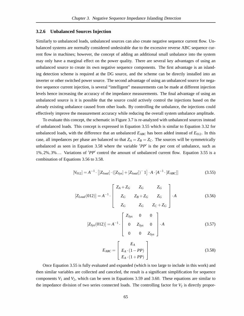
Chapter 3. Negative Sequence Impedance Islanding Detection
3.2.6 Unbalanced Sources Injection
Similarly to unbalanced loads, unbalanced sources can alsocreate negative sequence current flow. Un-
balanced systems are normally considered undesirable due to the excessive reverse ABC sequence cur-
rent flow in machines; however, the concept of adding an additional small unbalance into the system
may only have a marginal effect on the power quality. There are several key advantages of using an
unbalanced source to create its own negative sequence components. The first advantage is an island-
ing detection scheme is required at the DG source, and the scheme can be directly installed into an
inverter or other switched power source. The second advantage of using an unbalanced source for nega-
tive sequence current injection, is several “intelligent”measurements can be made at different injection
levels hence increasing the accuracy of the impedance measurements. The final advantage of using an
unbalanced source is it is possible that the source could actively control the injections based on the
already existing unbalance caused from other loads. By controlling the unbalance, the injections could
effectively improve the measurement accuracy while reducing the overall system unbalance amplitude.
To evaluate this concept, the schematic in Figure 3.7 is re-analyzed with unbalanced sources instead
of unbalanced loads. This concept is expressed in Equation 3.55 which is similar to Equation 3.32 for
unbalanced loads, with the difference that an unbalancedEABC has been added instead ofE012. In this
case, all impedances per phase are balanced so thatZA = ZB = ZC. The sources will be symmetrically
unbalanced as seen in Equation 3.58 where the variable′PP′ is the per cent of unbalance, such as
1%,2%,3%.... Variations of′PP′ control the amount of unbalanced current flow. Equation 3.55is a
combination of Equations 3.56 to 3.58.
[V012] = A−1 ·[[Zload] · ([ZSys]+ [Zload])
−1]·A · [A−1 · [EABC]] (3.55)
[ZLoad(012)] = A−1 ·
ZA +ZG ZG ZG
ZG ZB+ZG ZG
ZG ZG ZC +ZG
·A (3.56)
[ZSys(012)] = A−1 ·
ZSys 0 0
0 ZSys 0
0 0 ZSys
·A (3.57)
EABC =
EA
EA · (1−PP)
EA · (1+PP)
(3.58)
Once Equation 3.55 is fully evaluated and expanded (which istoo large to include in this work) and
then similar variables are collected and canceled, the result is a significant simplification for sequence
componentsV1 andV2, which can be seen in Equations 3.59 and 3.60. These equations are similar to
the impedance division of two series connected loads. The controlling factor forV2 is directly propor-
65

Chapter 3. Negative Sequence Impedance Islanding Detection
tional to the ‘PP‘ per cent value. This ideal case demonstrates the ability to create a more significant
negative sequence source through very small changes at the source, opposed to the much larger changes
required at a load. To compare the effect of unbalanced sources to an unbalanced load, the example in
Section 3.2.4 is used where an unbalanced load of±30% gave aV2 of approximately 0.013pu. While
an unbalanced source of±5% produces a negative sequence voltage of 0.028pu. Unbalanced sources
offer significant performance impact for negligible unbalance.
V1 = EA ·ZA
Zsys+ZA(3.59)
V2 = EA ·PP· 1√3· ZA
Zsys+ZA· i (3.60)
3.2.7 Negative Sequence Thevenin Impedance of the Network
As seen in the previous sections, unbalanced loads and sources create negative sequence voltage sources
(or at least the appearance) and an unbalanced current out ofthem. Therefore, by using Ohm’s law for
negative sequence components at the point of the unbalancedload or source; the results in Equation
3.61 became true. TheZ2 impedance measured at that point is the system Thevenin impedanceZ2(Sys)
out of that load. Conversely, measurements of positive sequence voltage and current at an unbalanced
load will result in the impedance ofZ1(Load). In general, assuming the system in Figure 3.9, the result
of measuring the negative sequence voltage and current at the load is the Thevenin impedance of the
system, as seen in Equation 3.61, with the advantage of no positive sequence sources interfering with
the result.
−1· V2(Load)I2(Load)
≈ ZSys (3.61)
Consider the following example the employs Equation 3.61. Take the system in Figure 3.9 where
the following values apply and the Load is±20% unbalanced:
[ZLoad] =
1000 0 0
0 1000∗1.2 0
0 0 1000∗0.8
(3.62)
[ZSys] =
10+100j 0 0
0 10+100j 0
0 0 10+100j
(3.63)
[EABC] =
16 0
16 240
16 120
(3.64)
66

Chapter 3. Negative Sequence Impedance Islanding Detection
At steady state,VLine−ABC is:
[VLine−ABC] =
0.98536 −5.65
0.98846 −124.72
0.98026 112.96
(3.65)
andILine−ABC is:
[ILine−ABC] =
0.00106 −5.65
0.00086 −124.72
0.00126 112.96
(3.66)
The symmetric component of V and I are:
[VLine−012] =
0.0126 −11.08
0.9846 −5.80
0.0126 156.00
(3.67)
[ILine−012] =
0.00016 84.63
0.00106 −5.96
0.00016 −108.29
(3.68)
The impedance from−1· V012I012
is:
[Z012] =
100.506 84
973.536 −179.8
100.506 84
=
10+100j
−973.5−2.4 j
10+100j
(3.69)
The impedance of the positive and negative sequence components areZ1 = 973.53+ 2.4 j pu and
Z2 = 10+100j pu respectively. The positive sequence impedance is near tothe 1000 pu base value while
the negative sequence impedance is an exact match to the 10+100j line impedance. The angles for the
positive sequence voltage and current are nearly identical. The phase angle difference of the negative
sequence voltage and the complex conjugate current is 84 degrees indicating reactive components.
3.3 Performance Characteristics of Negative Sequence Impedance
Measurement
As derived in the previous sections, negative sequence components existing in a power system can be
used to measure the impedance away from an unbalanced load orsource. The explanation only covered
the most basic of systems. How will this method operate over awide range of system conditions? This
section conducts a study of a series of scenarios based on a practical system1 producing qualitatively
1Practical System From a Distribution Network in British Columbia, Canada
67

Chapter 3. Negative Sequence Impedance Islanding Detection
viewable graphs over a specified range. The performance characteristics are broken down into six
components. These components are as follows:
1. Changing Per Cent of Unbalanced Load
2. Strength of System (impedance) vs. Unbalanced Load Power
3. Varying Power of Unbalanced Load
4. Power Factor of Loads
5. Phase Change From Different Unbalanced Load Configurations
6. Multiple Unbalanced Loads in an Island
[ZSys] [ZLoad]
E,I V,I E
Figure 3.12: System Performance Test Schematic with SystemImpedance and Load Impedance
The majority of these studies have been combined with multiple scenarios so trends can be viewed
clearly. For example, a varying power factor has been included in all the plots. The performance
evaluation comes from the one line diagram in Figure 3.12 where the base system variables are in
Table 3.1. In order for the scenarios to be easier to interpret, the impedancesZSys and ZLoad have
been converted to power, and referred to in the scenarios as “System Strength” for the transmission
short circuit powerZSys and “Load Strength” for the load demand. These values are calculated using
Equation 3.70 and the units are in MVA. The base impedances for ZSysandZLoad in Table 3.1 are similar
impedances to one of the case studies run in Chapter 4. The base impedanceZbase is calculated from
Equation 3.71.
Sload =V2
Z· 1106 (3.70)
Zbase=V2
Sbase=
(138·103)2
100·106 = 190.0Ω (3.71)
For example, in the first scenarioZsys is kept constant to the value in Table 3.1 which corresponds
to a transmission “System Strength” as seen in Equation 3.72.
S=V2
Zpu ·Zbase=
(138·103)2
(1.25+10j) · (19)≈ 10MVA (3.72)
68

Chapter 3. Negative Sequence Impedance Islanding Detection
Table 3.1: Base Performance Values for Practical SystemUnit Value UnitVBase 138 kVSBase 100 MVA
E(Sys) 1.0 V puXR(Sys) 8 -ZSys 1.25 +10.0j pu
ZLoad 100 puPFLoad 0.95 -
3.3.1 Effect of Changing Per Cent of Unbalanced Load
The first performance factor measures the effect an increasing unbalanced load has onV2. This effect
is important to verify that as the unbalance increases,V2 increases, and how the power fact can effect
that. The size of the unbalanced load is 1 MVA. The result can be seen in Figure 3.13. As the load
becomes increasingly unbalanced,V2 increases. Another way to look at the system is to refer to Figure
3.11 where as the load becomes more unbalanced, the couplingresistorZm(Load) increases to push
V2 higher. Figure 3.13 shows as the load becomes increasingly more unbalanced,V2 increases with a
yx type of slope. It also shows that lower power factors increase the effects of the unbalanced load
to increase the voltageV2, but in practical cases of< 30% unbalance,V2 will remain below 0.025 pu
and approach 0 as the per cent unbalanced load approaches to zero. A value of 0.025 pu is within
the practical measurability limits previously discussed.Before considering using negative sequence
impedance measurement islanding detection technique in a network, the system short circuit strength
and per cent unbalance will be an indicator of how measurablethe negative sequence components will
be.
Figure 3.13 also shows the phase change throughout the spectrum of unbalanced load conditions.
The most significant change in phase comes from the power factor and not from change in per cent
unbalance which remains relatively constant.
3.3.2 Effect of Strength of the System vs the Unbalanced LoadPower
This performance evaluation measures the effect of increasing the system strength relative to the load
size has on the amplitude ofV2 in the system. The unbalance of the load is 20% and ranges between
0.5 and 4.5 MVA. According to Figure 3.11, when the ratio of system impedance to the unbalanced
load impedance grows, the voltageV2 should decrease. In Figure 3.14, the change in system impedance
indicates that very estimate with a1x relationship. The initial rise between system strengths of0 to 10
MVA is a result of the power transfer relationship between impedances. When the transmission system
impedance approaches the impedance of the load, an undesirable drop inV2 occurs.Pmax occurs when
Zsys≈ Zload. Near equal system impedance to load impedance is not commonand if it occurs, under
voltage relays will likely trip. The phase also has a significant change between a weak system and a
strong system varying between 0 and 130 degrees. This is alsological when the system strength reduces
69

Chapter 3. Negative Sequence Impedance Islanding Detection
Figure 3.13: Per Cent Unbalanced Load vs.V2 Magnitude and Phase (System Strength = 10 MVA)
in value; the phase delay of the inductive load becomes more significant, causing phase delay. For a 2
MVA load, the maximum output ofV2 occurs when the system strength is between 10 and 30 MVA. The
outputV2 is from 0.035 pu to 0.02 pu. This evaluation identifies that large unbalanced loads produce the
most significantV2 output.
3.3.3 Effect of Varying the Power of an Unbalanced Load
This performance evaluation measures the effect of varyingthe unbalanced load size while keeping
a constant system strength of 10 MVA. This evaluation identifies how larger loads contain more pro-
nounced negative sequence voltage and that the voltage is not completely linear with power factors less
than 1 (Figure 3.15).
Varying the power of the unbalanced load has more of a linear effect. Once again, Figure 3.15
shows howV2 increases nearly linear with an increasing 20% unbalanced load. There is a significantly
less phase change per power increase of the load in contrast to Figure 3.14 where the phase makes a full
140 degree shift over the full span of system strength. Figure 3.15 indicates that higher load to system
strength ratios have a near linear effect on the availableV2 in the system. Some variability in the linearity
can be seen which is a result of the reactive component interactions. As the power factor approaches 1
the linearity can be seen to become more pronounced. In this case, the system needs a 20% unbalanced
load of near 0.75 MVA at any power factor to have aV2 of 1% and up compared toV1. This evaluation
70

Chapter 3. Negative Sequence Impedance Islanding Detection
Figure 3.14: System Strength Vs.V2 with Varying Unbalanced Load from 0.5 MVA to 4.5 MVA
has shown that as the load increases, the value of negative sequence voltage increases accordingly.
3.3.4 Effect of Changing Source Unbalance
This evaluation identifies how increasing the percent unbalanced input voltage effects the amount of
V2 in the system. In this evaluation, the terminal voltages at the source “E” are altered by a per cent
on one of the phases. The application of using the source as aninjection point for negative sequence
current is useful for a DG to directly use negative sequence impedance islanding detection directly from
its terminals without having to measure impedance from a nearby unbalanced load. Controlled terminal
voltage unbalance can be accomplished with inverter based DG systems through software programming
to alter the terminal voltage. This is not possible for rotating generators.
Changing unbalanced source has a more prominent effect on creating negative sequence voltages
then on unbalanced loads as shown in the contour plot of Figure 3.16. The change in voltage and its
measurability can rise proportionately with the per cent unbalance. Unlike the previous performance
examples, in which the negative sequence voltage came through the load direct; insertion of negative
sequence voltage from the source has the most significant impact and measurability regardless of the
system strength. For an unbalanced voltage of 10%, theV2 is approximately 5%. This has the advantage
of the injection point being able to control the amount of negative sequence voltage. The voltage can be
71

Chapter 3. Negative Sequence Impedance Islanding Detection
Figure 3.15: Unbalanced Load Size of 0 MVA to 3 MVA vs.V2, (Load unbalanced by 20%)
increased or decreased depending on the existing system conditions.
3.3.5 Effect ofV2 and I2 Phase Angle on Different Unbalanced Configurations
The change in negative sequence voltage and current phase angles with different load configurations is
evaluated in this section. Some examples of different load configurations are: loading on phase A to neu-
tral only, loading on phase B to neutral only, or loading fromphase A to phase B only. The impedance
calculated from−1 · V2I2
is the same regardless of the unbalanced load configuration,but the the phase
angle for both voltage and current change. Consider the circuit in Figure 3.12 where the impedances
Zsys= 10+ 100j pu andZload = 1000 pu. Zload is connected in WYE or∆ configuration depending
on the scenario. UnbalancingZload in different configurations changes the phase angle ofV2 and I2.
Some examples of different loading configurations are: to increase the impedance inZload−phase−A by
a per cent amount aboveZload−phase−B or Zload−phase−C, or by connectingZload from phase A to phase
B while not connecting any other loads to the BC or CA delta. The scenarios and results investigated
to demonstrate how the phase angle changes between different loading states are listed in Table 3.2 and
illustrated in Figures 3.17 and 3.18 for negative sequence voltage angle and negative sequence current
angle respectively.
In first scenario listed in Table 3.2, WYE connectedZload−A is increased by 20% whereZload−B
72

Chapter 3. Negative Sequence Impedance Islanding Detection
Figure 3.16: Utility Strength (SCC) vs.V2 (Varying Percent Source Unbalance of 5% to 30%)
andZload−C remain at the original 1000 pu. This is identified in Figures 3.17 and 3.18 as “V2 A+”. In
the second scenario listed in Table 3.2,Zload−A is decreased by 20% whereZload−B andZload−C remain
at the original impedance of 1000 pu. This is identified in Figures 3.17 and 3.17 as “V2 A-”. This
process repeats for all the individual remaining phase loading B± andC±. The final three scenarios
listed in Table 3.2 are∆ connected phase to phase unbalanced loads with the other twophases left
open. In the first phase to phase loaded case, a load of 1000 pu is placed between phases A and B
and no load is connected between phases B and C or phases C and A. This is identified in Table 3.2 as
∆,Zload−AB = 1000 and in Figures 3.17 and 3.18 as “V2 AB”. The negative sequence voltage and current
phases are calculated and placed in the table under “Phase Angle of V” for voltage phase and “Phase
Angle of I” for current phase.
Each of the scenarios show several interesting observations. TheV2 phase angle difference is 180o
when comparingZload−A+ andZload−A−. This is similar for the other two single phase scenarios of
Zload−B±20% andZload−C±20%. Another observation of interest is the 120o phase angle between the
three items in each “+”, “-” and “phase-to-phase” scenarios. For example,Zload−A+, Zload−B+, Zload−C+,
are all 120o out of phase. The 120o angle is clearly seen in Figure 3.17 and Figure 3.18 for voltages
and currents respectively. Each “+”, “-” and “phase-to-phase” scenario series presents different phase
angles from “0o”. The difference in the phase angle between the current and the voltage of all scenarios
is consistently 95o. The angleZsysis 85o. The sum of these two angles equates to 180o as 180−95= 85.
73

Chapter 3. Negative Sequence Impedance Islanding Detection
Table 3.2: Phase Angle For Different Unbalanced Load TypesUnbalanced Load Phase Angle of V Phase Angle of I
WYE, Zload−A +20% 73o 169o
WYE, Zload−A−20% −108o −12o
WYE, Zload−B +20% −166o −70o
WYE, Zload−B−20% 11o 107o
WYE, Zload−C +20% −46o 49o
WYE, Zload−C −20% 131o −132o
∆, Zload−AB = 1000,Zload−CA = Zload−BC = ∞
−41o 54o
∆, Zload−BC = 1000,Zload−CA = Zload−AB = ∞
78o 174o
∆, Zload−CA = 1000,Zload−BC = Zload−AB = ∞
−161o −65o
3.3.6 Multiple Unbalanced Loads in a System
In the previous sections, unbalanced impedance calculations were addressed using a single unbalanced
load or source in a perfectly balanced system. However in practical systems, other unbalanced loads
exist throughout the distribution layer that can corrupt impedance measurements. Not only are the
loads simply “unbalanced,” but they are unbalanced on phases A, B, C or in combinations of all three.
Therefore, multiple unbalanced components in a radial system pose as a source of corrupting impedance
information. Unbalanced loads can be complicated, but the interactions of multiple corrupting loads can
be understood using a simple two load radial example as illustrated in Figure 3.19, where the two load
impedance matrices,[ZLoad−1] and[ZLoad−2], are single phase, WYE connected, resistive loads. Of the
other components,[E] is a balanced voltage source with the system Thevenin impedance[ZSys] and
the distribution system impedance is[ZDist]. The solution for currents and voltages can be expressed
in an impedance matrix as[V] ≈ [E]− [I ] · ([Zsys] + [Zdist]) if Zload−x are very large where[V012] and
[I012] for nodeY are expressed, as previously, asA−1[VY] andA−1[IY] respectively. To better understand
the interaction, consider that all impedances are linearlyindependent connected in a grounded WYE
formation. By unbalancing single impedances in each phase,an accurate assessment of the interactions
can clearly be seen. The example in Figure 3.19 has the same impedances listed in Table 3.1. These
are fictitious values used to demonstrate the concept. In this example, the effect of negative sequence
impedance measurements made from the point of[ZLoad−2] when both[ZLoad−2] and[ZLoad−1] vary in
levels of unbalance is investigated. Table 3.3 contains thebase case information while the four scenarios
that will be investigated are listed in Table 3.4. Note that in this table, the result points to the specific
reference graph.[ZLoad−2] is impedance is found at position “Y” and calculated by usingthe equation:
−1 · VY−2IY−2
. The source voltageE remains balanced at 1 pu, and bothZSys and ZDist are set to 1 pu.
The LoadsZLoad−1 andZLoad−2 will have their impedances varied by a per cent on single phases. The
impedance of the two loads is 2000 pu. During this experiment, the expected impedance measured from
position ’Y’ is as follows: the positive sequence impedanceof V1I1≈ ZLoad−2 = 2000 pu and the negative
74

Chapter 3. Negative Sequence Impedance Islanding Detection
Figure 3.17:V2 Phase For Different Unbalanced Load Types Relative to 0, 240, 120 ABC Phases
sequence impedance ofV2I2
= (ZSys||ZLoad−1)+ZDist ≈ 2 pu.
The purpose of these scenarios is to illustrate how islanding detection threshold settings can be
effected when other unbalanced loads exist in the network. The effect that different load configura-
tions have on each other is investigated with a proposed averaging solution to reduce the impedance
measurement errors.
Table 3.3: Base Case Values for Figure 3.19Unit Value Unit
S(base) 1000 MVAV(base) 138 kVE(Sys) 1 pu
ZSys 1 puZDist 1 pu
ZLoad1 2000 puZLoad2 2000 puPFLoads 1 -
Scenario #1: Both Unbalanced Loads in Phase A Only
In this scenario, the load unbalance is made in only phase A ofeach WYE connected load which can
be seen in Figure 3.20. The load unbalance in both identical loads is varied between a range of 0%
to 5% on the contours forZLoad−1 and -10% to +10% forZLoad−2 values so that the unbalance trends
can be seen and how it effects the impedance measurements. Voltage and current values are taken from
75

Chapter 3. Negative Sequence Impedance Islanding Detection
Figure 3.18:I2 Phase For Different Unbalanced Load Types Relative to 0, 240, 120 V ABC Phases
[E]
[ZSys] [ZDist]
[ZLoad 2] [ZLoad 1]
[VX] [VY] Y X [IY]
Figure 3.19: Single Line Diagram of Multiple Unbalanced Equal Load Scenario
point “Y”. The A,B and C Voltages and currents are identified at point “Y” as vectors[VY] and [IY]
respectively. The trivial result whenZLoad−1 has 0% unbalance and the resulting measured negative
sequence source impedanceZLoad−2 at position “Y” is the exact expected value of 2 pu (ZLoad−1 =
2000 is 1000 times larger thanZsys and has little effect on the Thevenin impedance). However,each
consecutive line represents a per cent increase in the unbalance of the impedance of each load. What
is shown in this scenario (Figure 3.20) is the measuring impedanceZLoad−2 from position “Y” moves
from negative percentage to zero, the measurement accuracydecreases until the “knee” point where the
impedance quickly diverges towards 2000 pu. This “knee” point is approximately when the per cent
unbalance of each load equals each other. However, when the unbalance ofZLoad−2 grows from zero to
a positive per cent unbalance, the performance between 0.1%and 2% diverges to a very low value where
the unbalance is low and then quickly becomes more accurate as the unbalance increases. The level and
type of unbalance must be considered to avoid inaccurate impedance measurements in the region that
76

Chapter 3. Negative Sequence Impedance Islanding Detection
Table 3.4: Scenarios and Comments for Multiple Unbalanced Loads (All Values in pu)Case ZLoad−1 ZLoad−2 Result
1a 2000 + 5% ph A 2000 varying 0% to 10% ph A Figure 3.201b 2000 + 5% ph A 2000 varying -10% to 0% ph A Figure 3.202a 2000 + 5% ph B or C 2000 varying 0% to 10% ph A Figure 3.212b 2000 + 5% ph B or C 2000 varying -10% to 0% ph A Figure 3.213 special averaging caseZ2 swapping to ph A,B, and C averagedFigure 3.22
has poor performance.
Figure 3.20: -10% to + 10% Load Unbalance on Both Phase A, Vs. CalculatedV2 (ZLoad = 2000pu )
Scenario #2: Unbalanced Loads in Different Phases
In this scenario, the load unbalance consists of the two loads having unbalanced impedances on different
phases, which can be seen in Figure 3.21. In previous examples, phase angle changes with different
loading conditions and the error generated from multiple loads with different loading conditions can be
effected. For example, in this scenario,ZLoad−2 phase A is varied whileZLoad−1 phase B or C is altered.
The results differ from Scenario #1, in that the contours do not have the significantly low impedance
drop in the positive region. The rest of the curves are nearlya mirror image of Scenario #1 (Figure
3.20). However, similar to Scenario #1, near zero unbalancewhen the two unbalances nearly equal each
other, the impedance accuracy erodes up to the load impedance of 2000 pu. The knee point occurs when
77

Chapter 3. Negative Sequence Impedance Islanding Detection
the two unbalance values are equal in size.
Negative sequence impedance islanding detection method accuracy benefits when the the source
unbalanced load (Zload−2) is on a different phase to the unbalanced loads in the network.
Figure 3.21: -10% to + 10% Load Unbalance on Alternating Phases Vs. CalculatedV2
Scenario #3: Average Impedance With Unbalance in All Three Phases
This Scenario is a combination of of Scenario #1 and #2 by taking the impedance results of phase A, B,
C, unbalanced experiments onZLoad−1 and obtaining the average of the three as seen in Equation 3.73.
This Scenario was run by keepingZLoad−2 unbalance on phase A only, while running an unbalance
sweep throughZLoad−1 on phases A, B and C.
ZSys≈V2−A−unbal
I2−A−unbal+
V2−B−unbal
I2−B−unbal+
V2−C−unbal
I2−C−unbal(3.73)
The result of this Scenario can be seen in Figure 3.22. Where both of the previous Scenarios varied
differently on the +/- per cent of similar phase load change and on differing phase load change, the
averaging creates a symmetric result that converges to the ideal of 2 pu significantly faster than the
first two Scenarios. For unbalanced injection techniques, using an active phase unbalance swapping
and averaging produces the fastest converging and most accurate results. This multi-phase averaging
technique has been validated in a practical system which is described in the following Chapter 4.
78

Chapter 3. Negative Sequence Impedance Islanding Detection
Figure 3.22: -10% to + 10% Load Unbalance Vs. CalculatedV2 Averaged on A,B,C Alternating Phases
3.4 Non Fundamental Frequency Negative Sequence Impedance
Single frequency impedance measurements are effective forislanding detection, however, the measure-
ment accuracy can be increased with the use of unbalanced harmonics from naturally occurring unbal-
anced sources and loads to measure island conditions. Although power system impedance above the
fundamental are difficult to determine, there are some common trends that are present in distribution
systems that have lead to research in this topic. The first is from authors [4] and [19], who mapped
power system impedances in many grid configurations showinga predicable LR type impedance trend
in frequencies up to several kHz. This Section shall detail the sources of non-linear components and the
effect that it can have on negative sequence impedance islanding detection.
3.4.1 Sources of Harmonics from Non-Linear Components
Up to now, the systems analyzed have all been unbalanced passive components. Passive components
have the advantage of simple mathematical descriptions that can be expressed easily using Ohm’s law.
Non-linear loads corrupt the 60 Hz fundamental by injectinga spectrum of harmonics. This non-
fundamental energy can activate resonances and cause heating of rotating machines. Some types of
non-linear loads are discussed in the IEEE standard 519-1992 [50]. The following list is a summary of
the most significant non-linear loads in a power system that can be used for naturally occurring harmonic
injections.
The most common source of non-linear distortion in DC systems are AC-DC converters that use
79

Chapter 3. Negative Sequence Impedance Islanding Detection
Table 3.5: Common Power System Non-linear Loads
1. Saturated Transformers2. Diodes and Switching Silicone devices3. Arc Furnaces4. Static Var Compensators5. Inverters and DG sources6. Electronic Phase Control7. Switch mode power supplies8. PWM Drives9. Voltage dependant resistors
Table 3.6: Sequence Movement For Harmonics [120]
Harmonic SequencePositive Negative Zero
1 1 2 02 2 1 03 0 0 04 1 2 05 2 1 06 0 0 07 1 2 08 2 1 09 0 0 0
diode and SRC bridges to invert the AC waveforms to DC signalsand vice-versa. This conversion
creates odd harmonics from the fundamental equal ton= x·2+1 (ie 3,5,7,9...) where ‘n‘ is the harmonic
order and ‘x‘ is a counter from 0 to∞. The amplitude of each harmonic decreases by 1/n.
Sequence harmonics also appear in power systems, but for each harmonic the sequence number
changes due to the transform [120] as shown in Table 3.6. In theory, harmonic sequence impedances
are a promising option for increasing the accuracy of impedance estimation. However, the overriding
limitation of harmonic negative sequence impedance measurement is the measurability of the small
signals. For example, if a typical negative sequence voltage is in the range of 1%, the third and fifth
(most prominent) harmonics are typically in the range of 5% of the fundamental. Therefore, 1% of
5% equals 0.05% which exceeds a typical PT’s measurable limit. Although this topic poses significant
interest, it is outside of the basic theory and physical limits presented here, and practical experiments
were not conducted.
80

Chapter 3. Negative Sequence Impedance Islanding Detection
3.5 Sequence Components for Induction and Synchronous Machines
Negative and positive sequence impedances are equal to eachother in passive systems. This is not the
case for rotating synchronous and induction machines. Rotating machines have a significantly lower
negative sequence impedance under steady state conditions. When measuring[ZSys] from networks that
have large machines, the low negative sequence impedance can affect the value of the measured system
impedances; however, small rotating machines tend to have small overall significance in comparison
to the very low utility system impedance. TheV2 and I2 can become too small to measure. In a ma-
chine, the magnetic field from the negative sequence stator currents rotates at synchronous speed in
the opposite direction to the machine rotor. Viewing the currents from the rotor, the stator currents are
double frequency. Hence, currents of two times the rated frequency are then induced through to the ro-
tor circuits. Synchronous machines and induction machineshave similar but slightly differing negative
sequence impedance. The derivation of the impedances for each device is discussed in [68] and [120].
Figure 3.23 summarizes these impedances, where on the left hand side of Figure 3.23 is the impedance
of an induction machine and on the right side of Figure 3.23 isthe impedance of a synchronous ma-
chine. The induction machineXl is the stator leakage reactance,Ra is the stator resistance,XM is the
magnetizing reactance,Xr is the rotor leakage reactance.Rr is the rotor resistance ands is the slip. For
the synchronous machine,X”d andX”
q are the sub-synchronous d and q axis components from the parks
transformation. The variablesRa andRr are the stator resistance and rotor resistance respectively. For
the induction machine, the slip at full load is near 2, resulting in aR2, in Figure 3.23, approaching−12Rr .
These low impedances may have an effect on the threshold window for negative sequence impedance
islanding detection. They can create a falsely strong system. Several case studies are investigated in the
following chapter with rotating machines to show how various sizes can effect the proposed technique.
lXaR rXrR
MXrRs
sR = 12
""
""
2 2qd
qd
XXXXX+
=
22r
aRRR +=
Induction Machine Synchronous Machine
Figure 3.23: Induction and Synchronous Machine Negative Sequence Impedance
3.6 Implementation Strategy for Negative Sequence Islanding Detection
This section describes the implementation strategy of negative sequence islanding detection and how
it can be applied as a protective relay. In previous sections, negative sequence current is created from
81
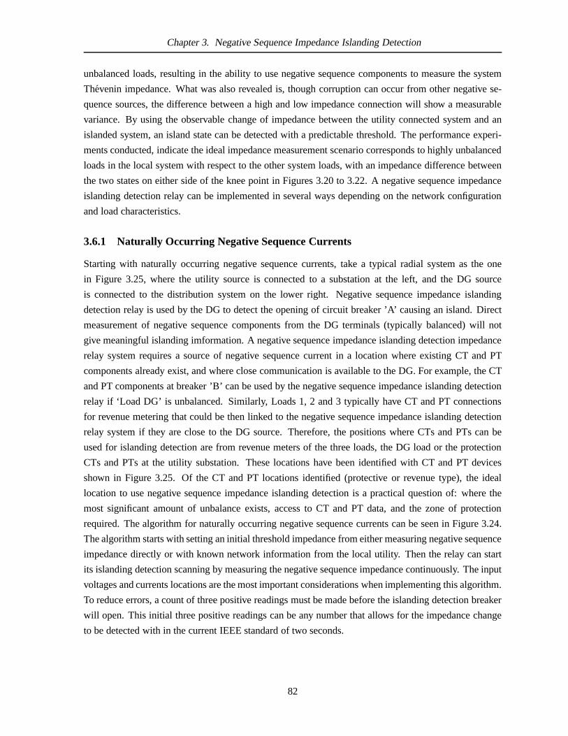
Chapter 3. Negative Sequence Impedance Islanding Detection
unbalanced loads, resulting in the ability to use negative sequence components to measure the system
Thevenin impedance. What was also revealed is, though corruption can occur from other negative se-
quence sources, the difference between a high and low impedance connection will show a measurable
variance. By using the observable change of impedance between the utility connected system and an
islanded system, an island state can be detected with a predictable threshold. The performance experi-
ments conducted, indicate the ideal impedance measurementscenario corresponds to highly unbalanced
loads in the local system with respect to the other system loads, with an impedance difference between
the two states on either side of the knee point in Figures 3.20to 3.22. A negative sequence impedance
islanding detection relay can be implemented in several ways depending on the network configuration
and load characteristics.
3.6.1 Naturally Occurring Negative Sequence Currents
Starting with naturally occurring negative sequence currents, take a typical radial system as the one
in Figure 3.25, where the utility source is connected to a substation at the left, and the DG source
is connected to the distribution system on the lower right. Negative sequence impedance islanding
detection relay is used by the DG to detect the opening of circuit breaker ’A’ causing an island. Direct
measurement of negative sequence components from the DG terminals (typically balanced) will not
give meaningful islanding imformation. A negative sequence impedance islanding detection impedance
relay system requires a source of negative sequence currentin a location where existing CT and PT
components already exist, and where close communication isavailable to the DG. For example, the CT
and PT components at breaker ’B’ can be used by the negative sequence impedance islanding detection
relay if ‘Load DG’ is unbalanced. Similarly, Loads 1, 2 and 3 typically have CT and PT connections
for revenue metering that could be then linked to the negative sequence impedance islanding detection
relay system if they are close to the DG source. Therefore, the positions where CTs and PTs can be
used for islanding detection are from revenue meters of the three loads, the DG load or the protection
CTs and PTs at the utility substation. These locations have been identified with CT and PT devices
shown in Figure 3.25. Of the CT and PT locations identified (protective or revenue type), the ideal
location to use negative sequence impedance islanding detection is a practical question of: where the
most significant amount of unbalance exists, access to CT andPT data, and the zone of protection
required. The algorithm for naturally occurring negative sequence currents can be seen in Figure 3.24.
The algorithm starts with setting an initial threshold impedance from either measuring negative sequence
impedance directly or with known network information from the local utility. Then the relay can start
its islanding detection scanning by measuring the negativesequence impedance continuously. The input
voltages and currents locations are the most important considerations when implementing this algorithm.
To reduce errors, a count of three positive readings must be made before the islanding detection breaker
will open. This initial three positive readings can be any number that allows for the impedance change
to be detected with in the current IEEE standard of two seconds.
82

Chapter 3. Negative Sequence Impedance Islanding Detection
Figure 3.24: Natural Negative Sequence Impedance Islanding Detection Algorithm
3.6.2 Injected Negative Sequence Currents
If connecting to an unbalanced load in the distribution system is not practical, or the unbalanced loads
are not large enough to produce a measurable result, negative sequence currents can also be injected.
This case is similar to the original mathematical evaluation of deliberately unbalancing loads to meet the
performance requirements as seen in Section 3.3.6. This canbe accomplished if the source is inverter-
based where it can be programmed internally to deliberatelyinject unbalanced current into feeder ’C’
in Figure 3.25 where the local CT and PT sensors are availableto measureZ2 for the negative sequence
impedance islanding detection relay. The specific algorithm can be seen in Figure 3.26. This algorithm
operates by deliberately unbalancing each phase individually then measuringZ2 for each of the three
unbalanced phases, and then using Equation 3.73 to average out the three calculated impedances to
83
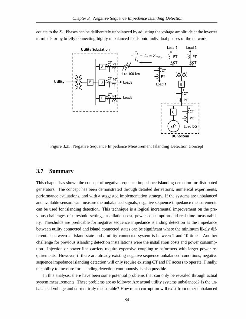
Chapter 3. Negative Sequence Impedance Islanding Detection
equate to theZ2. Phases can be deliberately unbalanced by adjusting the voltage amplitude at the inverter
terminals or by briefly connecting highly unbalanced loads onto individual phases of the network.
Figure 3.25: Negative Sequence Impedance Measurement Islanding Detection Concept
3.7 Summary
This chapter has shown the concept of negative sequence impedance islanding detection for distributed
generators. The concept has been demonstrated through detailed derivations, numerical experiments,
performance evaluations, and with a suggested implementation strategy. If the systems are unbalanced
and available sensors can measure the unbalanced signals, negative sequence impedance measurements
can be used for islanding detection. This technique is a logical incremental improvement on the pre-
vious challenges of threshold setting, installation cost,power consumption and real time measurabil-
ity. Thresholds are predicable for negative sequence impedance islanding detection as the impedance
between utility connected and island connected states can be significant where the minimum likely dif-
ferential between an island state and a utility connected system is between 2 and 10 times. Another
challenge for previous islanding detection installationswere the installation costs and power consump-
tion. Injection or power line carriers require expensive coupling transformers with larger power re-
quirements. However, if there are already existing negative sequence unbalanced conditions, negative
sequence impedance islanding detection will only require existing CT and PT access to operate. Finally,
the ability to measure for islanding detection continuously is also possible.
In this analysis, there have been some potential problems that can only be revealed through actual
system measurements. These problems are as follows: Are actual utility systems unbalanced? Is the un-
balanced voltage and current truly measurable? How much corruption will exist from other unbalanced
84

Chapter 3. Negative Sequence Impedance Islanding Detection
loads? These problems are examined in the following chapterwhere actual live systems are evaluated
for suitability and measurability. What has been revealed is that unbalanced loads that are more than
two to three times more unbalanced than the other, can cause accuracy errors that will make threshold
setting more difficult.
The theoretical analysis of negative sequence impedance islanding detection has been shown to
have promising theoretical characteristics. Further studies shall be conducted in the following chapter
on practical systems and practical scenarios to further demonstrate the concept’s suitability.
85

Chapter 3. Negative Sequence Impedance Islanding Detection
Figure 3.26: Injected Components Negative Sequence Impedance Islanding Detection Algorithm
86

Chapter 4
Case Studies of Negative Sequence
Impedance Islanding Detection
4.1 Introduction
In order to properly validate the method of negative sequence impedance islanding detection, three
practical case studies were considered. These experimentsprovided insight into the existence and mea-
surability of unbalanced voltages and currents (challenges identified in Chapter 2). These cases were
selected to cover a spectrum of systems where this techniquemay be useful. Experimentation with live
power systems is an essential component for validating any theoretical work (two of these cases contain
measurements from actual utility fed systems). Complete shutdowns, deliberate islanding and other
potential customer disruptions are outside the allowable scope of experiments on live systems; however,
the live islanded state measurements have been simulated inEMTP simulations that closely match the
existing network. The practical measurements have been carried out for utility-connected conditions
while simulations have been used to evaluate the islanded conditions.
The three cases evaluated in this chapter are: 1. IEEE 399-1997 standard industrial bus, 2. A 25 kV
distributed-generator fed radial system, and 3. A 600 V distributed-generator fed office building. The
first case has been run purely in simulation. Measurements for the second and third cases were taken
directly from actual operating utility fed systems.
4.2 Simulation of Standard IEEE 399-1997 Industrial Bus
4.2.1 System Description
The first system modeled in this chapter is a non-radial network consisting of multiple branches, two
distributed generator sources and a single utility connection. The system is a modification of IEEE 399-
1997 [48] from the micro grid modeling evaluation by Katiraei [65] (Figure 4.1). This is an industrial
bus network with multiple branches used to represent a small“microgrid” system. This case study was
conducted purely with simulation in EMTP software. The purpose of this case study was to demonstrate
that the change in measured negative sequence impedance between an islanded and utility condition is
significant. The size of the load unbalance vs. the measurability will also be evaluated. The unbalanced
measurements are taken at the bus feeding two unbalanced loads with several unbalanced loads mixed
into the network to provide a practical scenario of corrupting signals.
87

Chapter 4. Case Studies of Negative Sequence Impedance Islanding Detection
There are four main areas in this system (Figure 4.1). From the top, the utility source (1000 MVA)
and the connecting transformer and line contain the dominating impedances of this feeding system. The
interconnection Breaker “A” will be the point where the islanding will occur (located at near the top of
Figure 4.1). The second area is the 5 MVA ‘DG1’ source seen on the bottom right side of Figure 4.1
connected to ‘Bus 1’. This DG source is modeled as an ideal source with an associated impedance. The
third area is the 2.5 MVA ‘DG 2’ source on the bottom left side of Figure 4.1 connected to ‘Bus 3’. Both
DG1 and DG2 are modeled as ideal sources with impedances. Thefinal point of interest are Loads 1 to
5 which total to 7.7 MVA with an average power factor below 0.9. These loads are distributed along the
bottom of Figure 4.1 with 1.5 MVAR power factor correction capacitor bank near Feeder 1 off of the
PCC Bus that brings the confined power factor just above 0.9. All the simulated measurements in this
test case are in pu with a base voltage of 13.8 kV and a base power of 10 MVA.
The system is run at steady state with various scenarios listed in Table 4.1. Breaker “A” connecting
the utility bus to the network is opened and closed to demonstrate islanded and utility connected condi-
tions. The scenarios tested consisted of unbalanced load variations between Load 5 and Load 3 linear
loads and with a large induction machine. A summary of the particular cases is shown in Table 4.1.
Same phase unbalance in Case 2a indicates that the WYE connected loads on Load 3 and Load 5 are
both unbalanced on the same phase. For example, the impedance of same phase unbalance on Load 3
is:
Z3A = Dx ·Zx (4.1)
Z3B = Zx (4.2)
Z3C = Zx (4.3)
and on Load 5 is:
Z5A = Dy ·Zy (4.4)
Z5B = Zy (4.5)
Z5C = Zy (4.6)
The variablesDx andDy are per cent variations of the impedancesZx andZy. Conversely, the impedance
of different phase unbalance on Load 3 is:
Z3A = Dx ·Zx (4.7)
Z3B = Zx (4.8)
Z3C = Zx (4.9)
88

Chapter 4. Case Studies of Negative Sequence Impedance Islanding Detection
and on Load 5 is:
Z5A = Zy (4.10)
Z5B = Dy ·Zy (4.11)
Z5C = Zy (4.12)
Dy on Load 5 has moved toZ5B.
Table 4.1: Experiments Modeled using IEEE 399 Standard BusExperiment Description
1a. Load 5 Unbalanced, Measure Impedance from Load 5 at Bus 31b. Load 3 Unbalanced, Measure Impedance from Load 3 at Bus 22a. Load 3 and Load 5 Unbalanced, Measure Impedance from Load 3 (Bus 2) and
Load 5 (Bus 3) , Same Phase Unbalance2b. Load 3 and Load 5 Unbalanced, Measure Impedance from Load 3 (Bus 2) and
Load 5 (Bus 3) , Different Phase Unbalance3a. Load 3 with Induction Machine, Load 3 Unbalanced, Measure Impedance
from Load 3 (Bus 2)3b. Load 3 with Induction Machine, Load 5 Unbalanced, Measure Impedance
from Load 5 (Bus 3)4. Load 3 with Induction Machine, Unbalanced Loads 3 and 5 on Alternate
Phases, Impedance measured from both at Bus 3 and Bus 2
4.2.2 Experimental Results
The computed impedances from the several experiments run onthe network are shown in Figure 4.1,
listed in Table 4.1 and are detailed in this section. The expected impedances measured from the point
of each load are shown in Table 4.2 whereZLoad is the impedance towards the load andZ2 for the
Thevenin impedance towards the utility. The results of thestudies are taken from CTs and PTs at Bus 3
connection point for Load 5 and Bus 2 connection point for load 3. Load 3 and Load 5 are unbalanced
individually in the fist two experiments (Figure 4.1). The computational analysis values of voltages and
currents of each simulation are taken from steady state responses. To allow for a simplified comparison
of impedances, the absolute value of each load is shown. The impedance ratio of islanded to utility
connected state for Load 3 was 11.7 while the impedance ratiofor Load 5 was only 4.4. Under noisy
line conditions, threshold settings will be much more flexible with high impedance ratios such as with
Load 3.
Experiment 1a and 1b - Singular Unbalanced Loads
The first experiment in this case study is the trivial case where there is only one unbalanced load in
the simulation. The expected outcome should be near to the exact values of the mathematical estimate
(Table 4.2). The simulations were run first by setting the power flow towards the utility source to be
89

Chapter 4. Case Studies of Negative Sequence Impedance Islanding Detection
PCC BUS: 13.8kV
Sbase=10MVAVbase=13.8kV
Utility Source 1000 MVA X/R = 22.2
Line U1-U2 0.515+0.029j %69.0 kV
69/13.8 kV, 15 MVA 0.667+j5.33%
Line F1-B1 3.976+5.12j % 2.06 km
DG1 5 MVA
DG2 2.5 MVA
Load 5 0.9 MW
Load 4 0.9 MW 0.6 MVAR
Load 2 1.5 MW 1.0 MVAR
Load 1 0.8 MW 0.47 MVAR
Load 3 3.2 MW 1.9 MVAR
1.5 MVAR
redeeF 3 redeeF 1 redeeF 2
Bus 1 Bus 3
Bus 2 Line F3-B3 6.065+10.15j % 4.83 km
Line B1-L1 0.104+0.135j% 0.148km
Line B1-L2 0.732+0.095j% 0.104km
T1 13.8/0.48 1.0MVA8.21+57.5j%
T2 13.8/2.4 2.5MVA3.29+2.3j%
T3 13.8/2.4 3.75MVA2.44+14.8j%
Line F1-B2 3.564+2.66j% 0.976km
Line B3-L4 2.56+0.332j% 0.362km
Line B3-L5 0.732+0.095j% 0.189km
T4 13.8/0.48 1.25MVA5.6+48.0j%
T5 13.8/2.4 1.5MVA6.48+38.3j%
A
Figure 4.1: IEEE Standard 399-1997 (Brown Book) Reference Bus Case adapted From [65]
Table 4.2: Expected Impedances From Perspective of Test Loads (in pu)State |ZLoad| |Z2| Z2 Ratio
Load 3 Islanded 3.64 1.078Utility Connected 3.64 0.0916 11.7
Load 5 Islanded 11.1 0.843Utility Connected 11.1 0.193 4.4
near to zero (perfectly zero power flow is impossible with an unbalanced system). Breaker “A” is then
opened to simulate an island state. The two resulting impedances from the computational analysis are in
separate simulations from two separate unbalanced loads: Load 3 and Load 5. The positive and negative
sequence impedances (ZLoad andZ2) measured from experiment 1a and 1b are near to the mathematical
estimates (Table 4.2) and are listed in Table 4.3. In this experiment, Load 5 is unbalanced by 15% and
Load 3 is unbalanced by 10% in separate scenarios. Since Load5 is deeper in the network and has a
smaller value, the negative sequence current created is clearly much smaller than Load 3 which is nearly
four times the size of Load 5. The values of the currents and voltages are approaching the measurable
limits of 0.1% in some experiments and in others are below themeasurable limit. The negative sequence
impedances (Table 4.3) show the exact expected answers fromthe perspective of the test loads as if the
CTs and PTs could measure the low voltages and currents presented. This allows the computational
analysis of impedances to be compared with the theoretically expected values (Table 4.2).
90

Chapter 4. Case Studies of Negative Sequence Impedance Islanding Detection
Table 4.3: Experiment 1: IEEE 399 Bus System, Single Phase Unbalance of Load 3 and Load 5Load State V1 I1 |ZLoad| V2 I2 |Z2| Z2 Ratio
Load 3 Islanded 0.99 0.2720 3.64 0.0105 0.0098 1.078Utility Connected 0.99 0.2720 3.64 0.0012 0.0132 0.0916 11.7
Load 5 Islanded 0.99 0.0891 11.11 0.0024 0.0028 0.8464Utility Connected 0.99 0.0891 11.11 5.601e-4 0.0029 0.1960 4.3
Experiment 2a and 2b - Multiple Unbalanced Loads
The second experiment is similar to experiment 1, except instead of having only one unbalanced load in
the system, there are two unbalanced loads: Load 3 and Load 5.The expected outcome (Table 4.2) of
this test is a slightly corrupted impedance measurement. The test was completed twice (2a, 2b) with the
unbalanced loads both on Phase A for the first test (same phaseunbalance, Table 4.4) and the unbalanced
loads on alternate phases for test 2b. For test 2b, the unbalance for Load 5 was placed on Phase A and
the unbalance for Load 3 was placed on Phase B (alternating phase unbalance, Table 4.5). Load 5 is,
again, the smaller load of the two. What is revealed is that the unbalanced stronger Load 3 has less of an
effect on the utility-connected impedance computational analysis while the error for the weaker Load 5
is more severe. The impedance ratio change between the islanded state to the utility connected state on
Load 3 in experiments 1 to 2a and 2b increased from 11.7 to 14 and 10. While the ratio between the
islanded state to the utility connected state on Load 5 in experiments 1 to 2a and 2b increased from 4.3
to 10.95 and 8.01. Despite the error in the values of the calculated impedances, the ratios of islanded to
non-islanded conditions are still significant, thus allowing for reasonable threshold setting.
An important consideration is the estimate of the impedanceislanding trigger threshold. With Load
3, the utility-connected load is very similar to the first case (Experiment 2a, Table 4.3). However, for
Load 5 (lower into the network) the measured impedance valuechanges to a value 5.2 times smaller
between experiment 2a and 2b. Threshold settings and impedance ratios for islanding detection change
between locations and initial experimentation may be required on a practical system to asses the partic-
ular measured impedances.
Table 4.4: Experiment 2a, Load 3 and Load 5 Unbalanced on Phase ALoad State V1 I1 |ZLoad| V2 I2 |Z2| |Z2| Ratio
Load 3 Islanded 0.99 0.2720 3.64 0.0072 0.0052 1.393Utility Connected 0.99 0.2720 3.64 4.45e-4 0.0045 0.0989 14
Load 5 Islanded 0.99 0.0891 11.11 0.0079 0.0105 0.7549Utility Connected 0.99 0.0891 11.11 9.113e-4 0.0132 0.0690 10.95
When comparing theZ2 impedance values in between experiments 2a and 2b (Table 4.4and Table
4.5) the measured impedances change along with the impedance ratios between islanded and utility
connections. Using Equation 3.73 to apply the impedance averaging method developed in the previous
chapter, the impedances improved. Averaging the impedances resulted in an improvement of Load 3
91
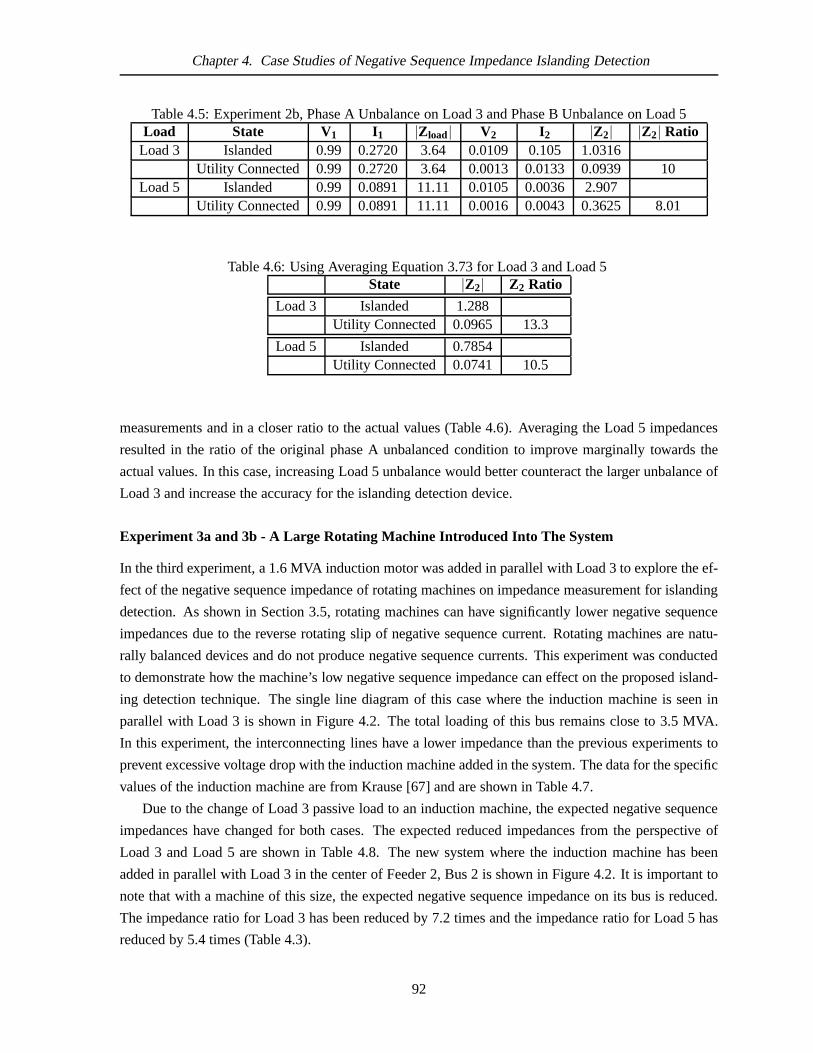
Chapter 4. Case Studies of Negative Sequence Impedance Islanding Detection
Table 4.5: Experiment 2b, Phase A Unbalance on Load 3 and Phase B Unbalance on Load 5Load State V1 I1 |Z load| V2 I2 |Z2| |Z2| Ratio
Load 3 Islanded 0.99 0.2720 3.64 0.0109 0.105 1.0316Utility Connected 0.99 0.2720 3.64 0.0013 0.0133 0.0939 10
Load 5 Islanded 0.99 0.0891 11.11 0.0105 0.0036 2.907Utility Connected 0.99 0.0891 11.11 0.0016 0.0043 0.3625 8.01
Table 4.6: Using Averaging Equation 3.73 for Load 3 and Load 5State |Z2| Z2 Ratio
Load 3 Islanded 1.288Utility Connected 0.0965 13.3
Load 5 Islanded 0.7854Utility Connected 0.0741 10.5
measurements and in a closer ratio to the actual values (Table 4.6). Averaging the Load 5 impedances
resulted in the ratio of the original phase A unbalanced condition to improve marginally towards the
actual values. In this case, increasing Load 5 unbalance would better counteract the larger unbalance of
Load 3 and increase the accuracy for the islanding detectiondevice.
Experiment 3a and 3b - A Large Rotating Machine Introduced Into The System
In the third experiment, a 1.6 MVA induction motor was added in parallel with Load 3 to explore the ef-
fect of the negative sequence impedance of rotating machines on impedance measurement for islanding
detection. As shown in Section 3.5, rotating machines can have significantly lower negative sequence
impedances due to the reverse rotating slip of negative sequence current. Rotating machines are natu-
rally balanced devices and do not produce negative sequencecurrents. This experiment was conducted
to demonstrate how the machine’s low negative sequence impedance can effect on the proposed island-
ing detection technique. The single line diagram of this case where the induction machine is seen in
parallel with Load 3 is shown in Figure 4.2. The total loadingof this bus remains close to 3.5 MVA.
In this experiment, the interconnecting lines have a lower impedance than the previous experiments to
prevent excessive voltage drop with the induction machine added in the system. The data for the specific
values of the induction machine are from Krause [67] and are shown in Table 4.7.
Due to the change of Load 3 passive load to an induction machine, the expected negative sequence
impedances have changed for both cases. The expected reduced impedances from the perspective of
Load 3 and Load 5 are shown in Table 4.8. The new system where the induction machine has been
added in parallel with Load 3 in the center of Feeder 2, Bus 2 isshown in Figure 4.2. It is important to
note that with a machine of this size, the expected negative sequence impedance on its bus is reduced.
The impedance ratio for Load 3 has been reduced by 7.2 times and the impedance ratio for Load 5 has
reduced by 5.4 times (Table 4.3).
92
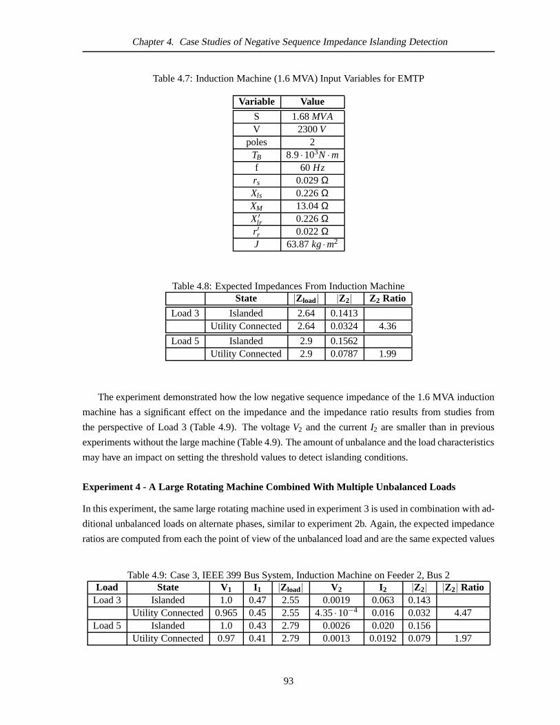
Chapter 4. Case Studies of Negative Sequence Impedance Islanding Detection
Table 4.7: Induction Machine (1.6 MVA) Input Variables for EMTP
Variable Value
S 1.68MVAV 2300V
poles 2TB 8.9·103N ·mf 60 Hzrs 0.029ΩXls 0.226ΩXM 13.04ΩX′
lr 0.226Ωr ′r 0.022ΩJ 63.87kg·m2
Table 4.8: Expected Impedances From Induction MachineState |Z load| |Z2| Z2 Ratio
Load 3 Islanded 2.64 0.1413Utility Connected 2.64 0.0324 4.36
Load 5 Islanded 2.9 0.1562Utility Connected 2.9 0.0787 1.99
The experiment demonstrated how the low negative sequence impedance of the 1.6 MVA induction
machine has a significant effect on the impedance and the impedance ratio results from studies from
the perspective of Load 3 (Table 4.9). The voltageV2 and the currentI2 are smaller than in previous
experiments without the large machine (Table 4.9). The amount of unbalance and the load characteristics
may have an impact on setting the threshold values to detect islanding conditions.
Experiment 4 - A Large Rotating Machine Combined With Multip le Unbalanced Loads
In this experiment, the same large rotating machine used in experiment 3 is used in combination with ad-
ditional unbalanced loads on alternate phases, similar to experiment 2b. Again, the expected impedance
ratios are computed from each the point of view of the unbalanced load and are the same expected values
Table 4.9: Case 3, IEEE 399 Bus System, Induction Machine on Feeder 2, Bus 2Load State V1 I1 |Z load| V2 I2 |Z2| |Z2| Ratio
Load 3 Islanded 1.0 0.47 2.55 0.0019 0.063 0.143Utility Connected 0.965 0.45 2.55 4.35·10−4 0.016 0.032 4.47
Load 5 Islanded 1.0 0.43 2.79 0.0026 0.020 0.156Utility Connected 0.97 0.41 2.79 0.0013 0.0192 0.079 1.97
93

Chapter 4. Case Studies of Negative Sequence Impedance Islanding Detection
PCC BUS: 13.8kV
Sbase=10MVAVbase=13.8kV
Utility Source 1000 MVA X/R = 22.2
Relay A
Line U1-U2 0.515+0.029j % 69.0 kV
69/13.8 kV, 15 MVA 0.667+j5.33%
Line F1-B1 3.976+5.12j % 2.06 km
DG1 5 MVA
DG2 2.5 MVA
Load 5 0.9 MW
Load 4 0.9 MW 0.6 MVAR
Load 2 1.5 MW 1.0 MVAR
Load 1 0.8 MW 0.47 MVAR
Load 3 2 MW
1.5 MVAR
redeeF 3 redeeF 1 redeeF 2
Bus 1 Bus 3
Bus 2 Line F3-B3 6.065+10.15j % 4.83 km
Line B1-L1 0.104+0.135j% 0.148km
Line B1-L2 0.732+0.095j% 0.104km
T1 13.8/0.48 1.0MVA 8.21+57.5j%
T2 13.8/2.4 2.5MVA 3.29+2.3j%
T3 13.8/2.4 3.75MVA 2.44+14.8j%
Line F1-B2 3.564+2.66j% 0.976km
Line B3-L4 2.56+0.332j% 0.362km
Line B3-L5 0.423+0.154j% 0.189km
T4 13.8/0.48 1.25MVA 5.6+48.0j%
T5 13.8/2.4 1.5MVA 6.48+38.3j%
A
Machine 1 1.6 MVA 75% Max Load
Figure 4.2: IEEE Standard 399-1997 Reference Bus Case with Induction Machine at Load 3 (Center)
as experiment 3 (Table 4.8). Unbalancing alternate phases resulted in very little additional voltage,V2,
and current,I2, corruption and the ratios are close to the expected values (Table 4.10). The impedance of
ZLoad remains as expected, closely matched to the impedances of the unbalanced loads shown in Table
4.10. There is a small improvement on the impedance ratios and the values ofZ2 for Load 3 but not for
Load 5.
Table 4.10: Case 4, IEEE 399 Bus System, Induction Machine with Alternate Phase Unbalanced
Load State |V1| |I1| |Z load| |V2| |I2| |Z2| |Z2| RatioLoad 3 Islanded 1.00 0.4657 2.55 0.0029 0.0167 0.2037
Utility Connected 0.96 0.4491 2.55 6.44·10−4 0.0160 0.0477 4.27Load 5 Islanded 1.00 0.4201 2.84 0.0030 0.0125 0.2865
Utility Connected 0.98 0.4073 2.84 0.0011 0.0127 0.1037 2.76
4.2.3 Discussion
The three experiments in the case study demonstrate the negative sequence impedance detection tech-
nique was effective for the experiments proposed. In the ideal balanced case, the computational analysis
were very accurate in both cases. However, when another unbalanced load is introduced into the system,
94

Chapter 4. Case Studies of Negative Sequence Impedance Islanding Detection
the results ofZ2 impedance accuracy decreases and the impedance ratio increases. The simulated accu-
racy ofZ2 had similar performance when the unbalanced loads were moved between phases resulting in
phase A on one load being unbalanced while phase B was unbalanced on the other. The most accurate
computational analysis ofZ2 came from Load 3, the largest unbalanced load. However, threshold set-
tings for islanding detection are easiest to set if the impedance ratio ofZ2 is very large. Load 5 has the
highestZ2 impedance ratio with an islanded to non islanded impedance ratio of over 11. In several of the
cases, the computational analysis of voltages and currentswere below practical measurable limits for
CTs and PTs and this method may require additional unbalanceadded to the system. When determining
where to locate the negative sequence impedance islanding detection relay, one must consider the level
of unbalance in the system, the utility and load impedances,the threshold setting and sensor accuracy.
In this case, the ideal location for islanding detection is either Load 3 or Load 5.
TheZ2 impedance decreased significantly when the large rotating machine was introduced into the
system. The impedance ratio of Load 5 dropped from 10.5 to 1.99 while the impedance ratio of Load 3
remained close to 4.3. In this scenario, the ideal location for the negative sequence islanding detection
relay is at Load 3. Care must be taken to choose the right location and to assess the unbalanced system
measurability for islanding detection in systems that contain large rotating machines.
4.3 Practical Example 1: 25 kV Radially Feed Distributed Generator
Network
4.3.1 System Description
The case study in this section corresponds to an actual operating system. The system, located in British
Columbia, Canada, is a 25 kV radial network fed by a 3.56 MVA run of the river distributed generator.
The purpose of this case study is to demonstrate how naturally occurring negative sequence components
can be used to measure the feeding system impedance in a 25 kV distribution network using commonly
installed CT and PT equipment. The impedance measurement capability can then be used as a centrally-
based islanding detector in the area. The 3.56 MVA distributed generator is capable of supporting
an island in the network but requires islanding detection toseparate the utility system. The system
schematic is in Figure 4.3. The 138 kV feeding utility is located at the top of the diagram, and the DG is
connected at the bottom. The points of voltage and current measurement are shown as three circles “A”,
“B” and “C” with corresponding CTs and PTs. Point “A” was usedto measure the negative sequence
current and voltage for the utility. Point “B” was used to used to measure the negative sequence current
and voltage for the DG. Point “C” was used to measure the negative sequence current and voltage for
the load, but this point was only simulated. The experimental data was taken while the system was
running at steady state under typical loading conditions over several days. The utility provided the
name plate data and impedances for all of the equipment (lines, transformers, generators, loads). The
particular names and locations of the network have been altered to protect the customer’s confidential
information. The expected values forZ2 (Thevenin impedances) measured from each of the three points
95

Chapter 4. Case Studies of Negative Sequence Impedance Islanding Detection
is the impedance towards the utility for “A”, towards the DG for “B” and parallel impedance between
the between the utility and the DG for “C”. The impedances canbe seen in Table 4.11.
Figure 4.3: Practical Example 1: 25 kV DG System Fed System Single Line Diagram
In previous sections, it was shown that the positive sequence current sources are created from the
generators and negative currents come from unbalanced loads. If the loads in the system in Figure 4.3
are unbalanced, the negative sequence impedance can be measured from A and “B”. Negative sequence
impedance measured at point A will correspond to the impedance toward the 138kV transmission system
and negative sequence impedance measured at point ’B’ will correspond to the impedance towards the
DG. The positive sequence impedance measured from either ofthese locations will not present any
meaningful information for islanding detection.
Selection of a CT and PT measurement point for the negative sequence impedance islanding detector
requires careful consideration. There are three potentiallocations “A”, “B” and “C” to be considered
that are shown in Figure 4.3. Position “A” CTs and PTs are measuring currents from the utility. If
96

Chapter 4. Case Studies of Negative Sequence Impedance Islanding Detection
Table 4.11: ExpectedZ2 Impedances From Positions ”A”, ”B” and ”C” (in pu)Position State |Z2|
”A” Islanded ∞Utility Connected 8.52
”B” Islanded 99.93Utility Connected 99.93
”C” Islanded 99.93Utility Connected 7.84
the negative sequence current is large enough fromLoad1 andLoad2, Position “A” negative sequence
impedance would equate to the utility impedance. Position “B” CTs and PTs are not ideal because
they would measure the negative sequence impedance towardsthe DG and not detect island conditions.
Position “C” atLoad1 may be a useful alternative to Position “A”. The CTs at Position “C” are different
from Potion “A” because they are likely to be significantly smaller and will have a higher sensitivity to
smaller currents. If the CTs at “A” are rated so large that small unbalanced currents are below the large
CT’s measurable limits, the CTs at Potion “C” may be used as alternatives.
A practical implementation problem may exist with this system for an Independent Power Producer
(IPP) who wants to install a negative sequence impedance islanding detector at Potion “A”. Installation
of negative sequence impedance islanding detection in manycases is ideally accessed at the utility sub
stations. The CTs and PTs at points “A” and “B” are owned by theutility at the substation and the IPP
may not have adequate access to them. However, the IPP (or theutility) can install negative sequence
impedance islanding detector by accessing privately ownedload CTs and PTs on the 25 kV bus at Load 1
or Load 2. This has been demonstrated at circle “C” with simulated experiments of the system.
The single line diagram in Figure 4.3 is expressed in a sequence component diagram of impedances
shown in Figure 4.4. The top circuit in Figure 4.4 is the positive sequence network, the second level
is the negative sequence network and the bottom circuit is the zero sequence network. The utility
provided the impedances (at 25 kV) for positive, negative and zero sequence symmetric components.
The impedances in Figure 4.4 can be converted from pu in Figure 4.3 by multiplyingZpu by Zbaseas
seen in Equation 4.13.
Zat 25 kV = Zpu ·Zbase
= Zpu ·(25·103)2
100·106 (4.13)
The unbalanced impedance block links the three sequence component circuits to an “unknown
schematic”. The connection between symmetrical components could be line-to-line, line-to-neutral,
or a combination of the two, but the true circuit is unknown and can only be presented as a “black box”.
Chapter 3 describes this problem in more detail. The power demand of the loads on the 25 kV bus vary
in time, but they can be assumed to range between 0.5 and 4 MVA (or a 1.25 kΩ to 150Ω). Refer to
97
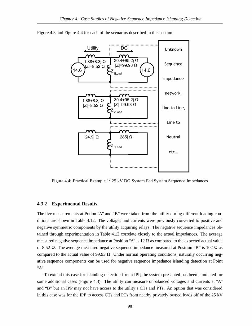
Chapter 4. Case Studies of Negative Sequence Impedance Islanding Detection
Figure 4.3 and Figure 4.4 for each of the scenarios describedin this section.
Figure 4.4: Practical Example 1: 25 kV DG System Fed System Sequence Impedances
4.3.2 Experimental Results
The live measurements at Potion “A” and “B” were taken from the utility during different loading con-
ditions are shown in Table 4.12. The voltages and currents were previously converted to positive and
negative symmetric components by the utility acquiring relays. The negative sequence impedances ob-
tained through experimentation in Table 4.12 correlate closely to the actual impedances. The average
measured negative sequence impedance at Position “A” is 12Ω as compared to the expected actual value
of 8.52 Ω. The average measured negative sequence impedance measured at Position “B” is 102Ω as
compared to the actual value of 99.93 Ω. Under normal operating conditions, naturally occurring neg-
ative sequence components can be used for negative sequenceimpedance islanding detection at Point
“A”.
To extend this case for islanding detection for an IPP, the system presented has been simulated for
some additional cases (Figure 4.3). The utility can measureunbalanced voltages and currents at “A”
and “B” but an IPP may not have access to the utility’s CTs and PTs. An option that was considered
in this case was for the IPP to access CTs and PTs from nearby privately owned loads off of the 25 kV
98

Chapter 4. Case Studies of Negative Sequence Impedance Islanding Detection
Table 4.12: Measured Values for 25 kV System Positive and Negative SequencesLocation Positive Sequence Negative Sequence
A |V1| |I1| |V1/I1| |V2| |I2| |Z2|(Ω)
Test 1 14900 106.70 140 35.70 2.65 13.47Test 2 14830 113.90 130 47.28 5.63 8.37Test 3 14810 63.10 235 44.98 2.95 15.24
Average 14847 95 168 43 4 12
B |V1| |I1| |V1/I1| |V2| |I2| |Z2|Test 1 15274 25.46 577 215.67 2.62 81.37Test 2 14567 7.78 1861 54.45 0.33 164Test 3 15475 149 103 36 0.82 44Test 4 14910 32 468 121 1.14 106Test 5 14920 35 423 92 0.81 115
Average: 15029 50 687 104 1 102
Table 4.13: Experiments Simulated on 25 kV Practical System1. Single unbalanced Load 1 with the utility connected2. Single unbalanced Load 1 and the system is islanded3. Both Load 1 and Load 2 are identically unbalanced load magnitudes on phase A with the
utility connected.4. Both Load 1 and Load 2 are identically unbalanced load magnitudes on phase A and the
system is islanded5. Same as case 3 with the unbalanced phase on Load 1 on phase A and Load 2 on phase B6. Same as case 4 with the unbalanced phase on Load 1 on phase A and Load 2 on phase B
Bus at circle “C” in Figure 4.3 (off the 25 kV bus, right hand, middle of the diagram). At this point,
the IPP can obtain unbalanced load data. The islanding detection scenarios investigated at point “C” are
listed in Table 4.13. The results of each scenario for islanded and non-islanded cases are listed in Table
4.14. The negative sequence impedances for Case #1 at Positions “A” and “B” have been computed
to cross-check the expected results from the following cases at Position “C”. The expected negative
sequence impedance computed from Position “C” for an islanded state is the impedance of Load 2 in
parallel with the impedance of the DG (99.93 Ω). Similarly, the expected negative sequence impedance
from Position “C” for a non-islanded state is the parallel impedance of Load 2, the DG, and the utility
(7.48 Ω).
The negative sequence impedances measured from Positions “A” and “B” confirm the Thevenin
impedance values of the utility and the DG respectively. Thenegative sequence impedance measured
value at “A” for Case #1 is 8.41Ω as compared to the actual value of 8.52Ω. The negative sequence
impedance measured at “B” for Case #1 is 97.93Ω as compared to the actual value of 99.93Ω.
The negative sequence impedances computed at “C” show the values drifting from the actual ex-
pected impedances (Table 4.14). The negative sequence impedance for experiments #2, #4 and #6 are
expected to indicate an islanded impedance ofZLoad2||ZDG = 96.41Ω. The computed impedances for
99

Chapter 4. Case Studies of Negative Sequence Impedance Islanding Detection
Table 4.14: Simulated Values for 25 kV System Positive and Negative SequencesExperiment Positive Sequence Negative Sequence
Experiment at “A” V1 I1 |V1/I1| V2 I2 |Z2|1 14414 13.3 1080 11.1 1.322 8.41
Experiment at “B” V1 I1 |V1/I1| V2 I2 |Z2|1 14414 43 334 11.1 0.113 97.93
Experiment at “C” V1 I1 |V1/I1| V2 I2 |Z2|1 14414 25.64 562 10.95 1.432 7.64
2 (island) 14554 25.64 562 117 1.22 95.643 14414 25.61 562 11.1 0.72 15.4
4 (island) 14554 25.88 562 116.83 0.586 199.265 14414 25.63 562 9.80 0.73 13.4
6 (island) 14553 25.89 562 100.3 0.69 145.33
these three experiments are 95.64 Ω, 199.26 Ω and 145.33 Ω respectively. The negative sequence
impedances for cases #1, #3 and #5 are expected to equalZLoad2||ZUtil ||ZDG = 7.84 Ω ; however, the
computed negative sequence impedances for the three cases are 7.64Ω, 15.4 Ω and 13.4 Ω respectively.
All the impedance results computed from the six experimentscorrelate to the estimated impedances.
However, impedance study results for cases 3 to 6 are distorted with unbalanced conditions from the
parallel connected unbalanced Loads 1 and 2.
4.3.3 Discussion
Field data of naturally occurring unbalanced voltages and currents can be used to measure the Thevenin
impedance towards both the DG and the utility sources. The measured Thevenin impedance can then
be used for islanding detection. Other unbalanced loads near to the impedance measurement system
reduces the accuracy of the impedance measurement but not the islanding detection capability. Similar
results can be achieved for islanding detection by accessing CTs and PTs from local loads. This case is
particularity useful if the utility bus’ CTs are too large toaccurately measure small unbalanced currents
or if an IPP requires an islanding detection system independent of the utility. This alternative case for the
IPP was presented through simulations of unbalanced loads in the network. The most accurate negative
sequence impedance measurements and computational analysis came directly from the utility CTs and
PTs which did not have the same corruption from parallel unbalanced loads.
4.4 Practical Example 2: 600 V Fed Commercial Building
4.4.1 System Description
The case study in this section describes an actual operational office building power system. The system
is a 600 V commercial building in British Columbia, Canada with a solar panel installation on the
roof. The purpose of this experiment was to demonstrate how negative sequence impedance can be
100

Chapter 4. Case Studies of Negative Sequence Impedance Islanding Detection
used for islanding detection on a low voltage bus. The electrical reach of negative sequence impedance
measurement is also investigated in this section. The four-story commercial building features office use
on the top three floors and some basic machining rooms and offices on the first floor. The solar panels
on the roof currently do not have the capacity to supply the entire building’s energy demand; however,
if a large array or other generating technology was installed, this building could potentially island in
the local network. The building is a newly constructed and energy efficient ’LEED’1 certified building.
The experiments conducted in this section use both naturally occurring and injected negative sequence
symmetric components to calculate the Thevenin impedanceout of the building.
These experiments were conducted at various locations in the building. A single line diagram with
an associated impedance diagram from the 69 kV utility distribution system to the 600 V office building
is shown in Figure 4.5. The single line diagram is on the left hand side of Figure 4.5 and the associated
impedances are shown on the right hand side of Figure 4.5. Details of the distribution system in the
single line diagram were supplied by the local, utility provider.
The building schematics did not specify the distribution cable and transformer impedances. The
impedance values of these components were found by measuring the voltage drop through the items
between two different loading conditions using Equation 4.14, Equation 4.15 and Equation 4.16. The
variable [E0] is a constant voltage source. The variable[Vlow load] is the three phase voltage vector
under low load conditions where,[Ilow load] is the corresponding three phase current vector out at this
low load state,[Vhigh load] is the three phase voltage vector under load and[Ihigh load] is the three phase
current vector out of the load. By combining Equations 4.14 and 4.15, the result is Equation 4.16. The
impedances shown in Figure 4.5 are in pu with a base power of 100 MVA. The base voltages are listed
on each bus.
[V0] = [Vhigh load]+ [Ihigh load] · [ZABC] (4.14)
[V0] = [Vlow load]+ [Ilow load] · [ZABC] (4.15)
ZABC =[Vlow load]− [Vhigh load]
[Ihigh load]− [Ilow load](4.16)
The experiments for negative sequence impedance islandingdetection were conducted at the three
bold numbers “1”, “2” and “3” in circles seen in Figure 4.5. Position “1” is the main building feeder
where natural unbalanced currents and voltages were measured for a 24-hour period. Position “2” is a
208 V feeder on the building’s 3rd floor where unbalanced injection experiments were run. Position 3
is at the solar panel DG inverter system where negative sequence current injection islanding detection
computational analysis simulations were run. Limited access to Position “3” prevented direct voltage
and current measurements, but detailed simulations were run to demonstrate the performance of the
negative sequence islanding detection technique at the DG inverter’s terminals. Realistic simulation
conditions were created by matching the loading and unbalanced conditions measured from Position
1Leadership in Energy & Environmental Design - Green Building Rating System by the U.S. Green Building Council
101

Chapter 4. Case Studies of Negative Sequence Impedance Islanding Detection
“1” and “2”. The data for all the experiments were acquired using the AEMC 3945 three phase power
analyzer and logger. The data was then converted to symmetric components using matlab scripts. The
AEMC 3945 is shown in Appendix C.
Figure 4.5: Practical Example 2: 600 V Commercial Office DG Fed System Single Line Diagram
The bold letters ’A’ and ’B’ in squares in Figure 4.5 represent the breakers where DG islanding could
occur. Position “A” is the main disconnect breaker for the 12.5kV to the 69 kV network. Position “B” is
the main building breaker at the 12kV to 600 V transformer. Testing island and non-island states poses
an experimental challenge as the main power switches in thiscase study could not be simply opened and
closed. Therefore, the non-islanded states have been directly measured on the live system and compared
to the actual impedance values where the islanded states were validated using the building model built in
Matlab Simulink Power Systems Library. The Simulink model was validated by comparing the voltage
quality and unbalance at various nodes with actual system measurements. The model is shown in Figure
E.1 in Appendix E.
The following experiments express impedances in pu. The pu base power for all the experiments is
102
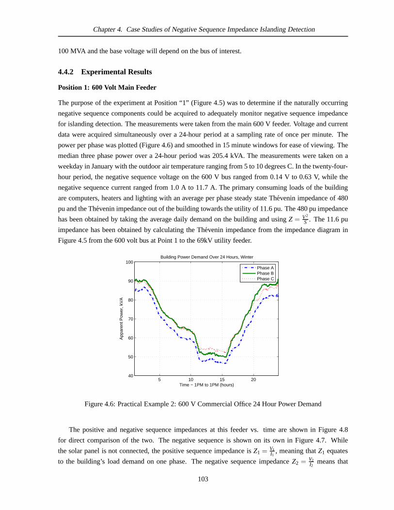
Chapter 4. Case Studies of Negative Sequence Impedance Islanding Detection
100 MVA and the base voltage will depend on the bus of interest.
4.4.2 Experimental Results
Position 1: 600 Volt Main Feeder
The purpose of the experiment at Position “1” (Figure 4.5) was to determine if the naturally occurring
negative sequence components could be acquired to adequately monitor negative sequence impedance
for islanding detection. The measurements were taken from the main 600 V feeder. Voltage and current
data were acquired simultaneously over a 24-hour period at asampling rate of once per minute. The
power per phase was plotted (Figure 4.6) and smoothed in 15 minute windows for ease of viewing. The
median three phase power over a 24-hour period was 205.4 kVA.The measurements were taken on a
weekday in January with the outdoor air temperature rangingfrom 5 to 10 degrees C. In the twenty-four-
hour period, the negative sequence voltage on the 600 V bus ranged from 0.14 V to 0.63 V, while the
negative sequence current ranged from 1.0 A to 11.7 A. The primary consuming loads of the building
are computers, heaters and lighting with an average per phase steady state Thevenin impedance of 480
pu and the Thevenin impedance out of the building towards the utility of 11.6 pu. The 480 pu impedance
has been obtained by taking the average daily demand on the building and usingZ = V2
S . The 11.6 pu
impedance has been obtained by calculating the Thevenin impedance from the impedance diagram in
Figure 4.5 from the 600 volt bus at Point 1 to the 69kV utility feeder.
5 10 15 2040
50
60
70
80
90
100Building Power Demand Over 24 Hours, Winter
Time − 1PM to 1PM (hours)
App
aren
t Pow
er, k
VA
Phase APhase BPhase C
Figure 4.6: Practical Example 2: 600 V Commercial Office 24 Hour Power Demand
The positive and negative sequence impedances at this feeder vs. time are shown in Figure 4.8
for direct comparison of the two. The negative sequence is shown on its own in Figure 4.7. While
the solar panel is not connected, the positive sequence impedance isZ1 = V1I1
, meaning thatZ1 equates
to the building’s load demand on one phase. The negative sequence impedanceZ2 = V2I2
means that
103

Chapter 4. Case Studies of Negative Sequence Impedance Islanding Detection
Z2 equates to the Thevenin impedance out of the building. The average negative sequence impedance
measured was 27.5 pu and the average positive sequence impedance measured was 480 pu. The actual
Thevenin impedance towards the utility was 11.6 pu and the average Thevenin impedance towards the
building was 480 pu. The experimentally measured negative sequence impedance correlates to the actual
Thevenin impedance away from the building averaging at 27.5 pu. The negative sequence impedance
varied randomly by±17.5 pu (Figure 4.7) and was not affected by the building load profile throughout
the day as the positive sequence impedance highlights (Figure 4.8).
Figure 4.7: Practical Example 2: 600 VZ2 Measured Over 24 Hours
The opening of Breakers “A” and “B” were simulated using the equivalent Simulink model as shown
in Figure 4.9. The model was created using the schematic given by the local utility and by modeling
live unbalanced conditions previously measured in the Simulink model. As Breaker “A” and “B” were
opened, the negative sequence impedance quickly increases. When Breaker “A” was opened, the nega-
tive sequence increased from 27 pu to 150 pu in less than 0.02 s. When Breaker “B” was opened, the
negative sequence increased from 150 pu to 86,000 pu in a similar amount of time. 86,000 pu is very
large meaningless number and it can be considered to be infinite. The building DG cannot support the
power requirements inside the network contained within Breaker “A” and so the voltage collapses when
Breaker “A” is opened. Some inaccuracy of the negative sequence impedance accuracy is expected due
to the other unbalanced loads in the system. However, when Breaker “B” was opened, the change in
negative sequence impedance was far more significant risingto near infinite levels.
104
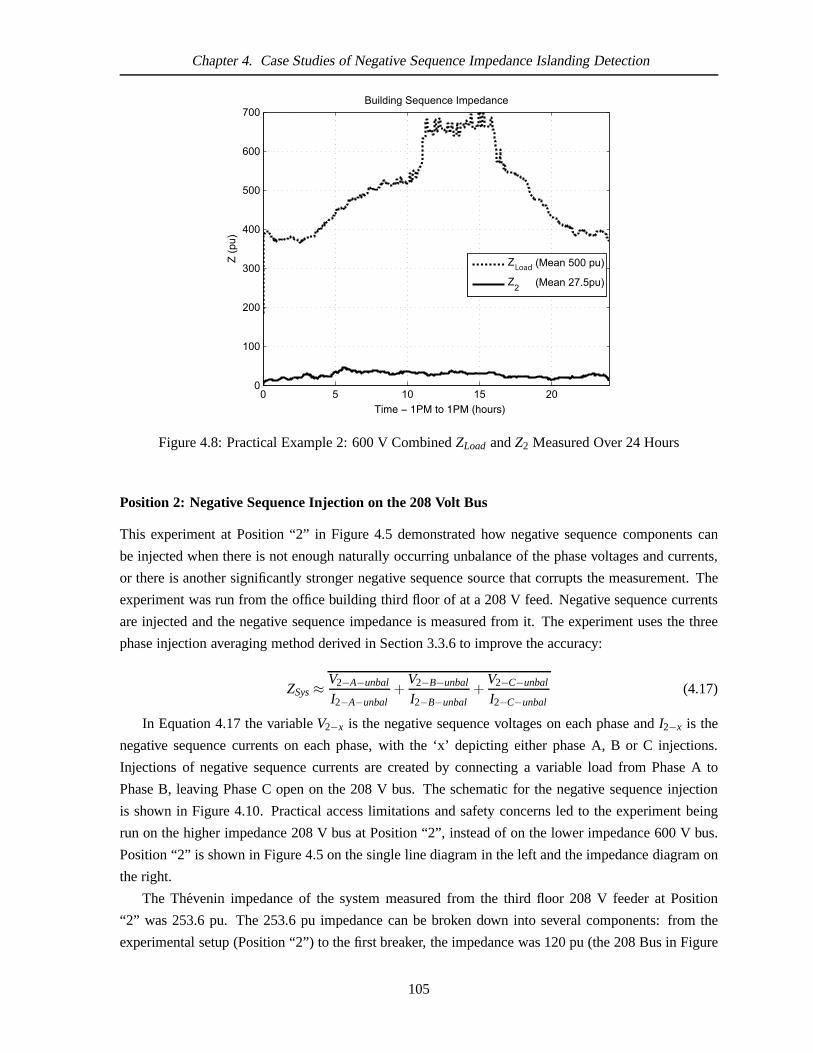
Chapter 4. Case Studies of Negative Sequence Impedance Islanding Detection
Figure 4.8: Practical Example 2: 600 V CombinedZLoad andZ2 Measured Over 24 Hours
Position 2: Negative Sequence Injection on the 208 Volt Bus
This experiment at Position “2” in Figure 4.5 demonstrated how negative sequence components can
be injected when there is not enough naturally occurring unbalance of the phase voltages and currents,
or there is another significantly stronger negative sequence source that corrupts the measurement. The
experiment was run from the office building third floor of at a 208 V feed. Negative sequence currents
are injected and the negative sequence impedance is measured from it. The experiment uses the three
phase injection averaging method derived in Section 3.3.6 to improve the accuracy:
ZSys≈V2−A−unbal
I2−A−unbal+
V2−B−unbal
I2−B−unbal+
V2−C−unbal
I2−C−unbal(4.17)
In Equation 4.17 the variableV2−x is the negative sequence voltages on each phase andI2−x is the
negative sequence currents on each phase, with the ‘x’ depicting either phase A, B or C injections.
Injections of negative sequence currents are created by connecting a variable load from Phase A to
Phase B, leaving Phase C open on the 208 V bus. The schematic for the negative sequence injection
is shown in Figure 4.10. Practical access limitations and safety concerns led to the experiment being
run on the higher impedance 208 V bus at Position “2”, insteadof on the lower impedance 600 V bus.
Position “2” is shown in Figure 4.5 on the single line diagramin the left and the impedance diagram on
the right.
The Thevenin impedance of the system measured from the third floor 208 V feeder at Position
“2” was 253.6 pu. The 253.6 pu impedance can be broken down into several components: from the
experimental setup (Position “2”) to the first breaker, the impedance was 120 pu (the 208 Bus in Figure
105

Chapter 4. Case Studies of Negative Sequence Impedance Islanding Detection
Figure 4.9: Practical Example 2: 600 VZ2 At Position 1 During Breaker A and B Opening
4.5), the impedance from the 208 V bus to the 208:600 volt transformer was 92 pu and the transformer’s
impedance is 35 pu (8%). The Thevenin impedance from the transformer towards the feeding system
was 11.6 pu (Position “1”) as shown in Figure 4.5.
Experiments of the non-islanded state were run on the live system while islanded states were con-
ducted in simulation. The impedance changes are measured and computed when Breaker “B” was
opened (Figure 4.5).
The measured impedance from injecting negative sequence components is shown in Figure 4.11,
impedance vs. power. The delta connected phase combinations listed in the legend of AB, BC and CA
represent the negative sequence impedance vs. injected power. For example, Phase AB represents a
load being placed on phases AB only while leaving phase BC andCA open. This is repeated for phases
BC and CA. The measured impedance measured from this experiment gave different negative sequence
impedances ranging from 500 pu to 100 pu on different phases.Additionally, the impedance mea-
surements do not stabilize until the injected power is over 1000 watts. The measurements achieved an
average of 277 pu by using the averaging technique of impedances (Figure 4.11 - “Smoothed Averaged
3 Phases”). When the averaging technique was employed with smoothing, more accurate impedance
readings were made with only 100 watts of injected power.
The system was islanded by opening Breaker “B” in simulation. The changes in impedance are
shown in Figure 4.12. After the initial stabilization of theislanding, there is a small change in impedance
between an islanded condition and a non-islanded condition. The change between an islanded and non
islanded state is only 20 pu is due to the high input impedancefrom the 208 V bus. The small change of
20 pu relative to the 200 pu steady state impedance is not adequate for accurate islanding detection. The
actual impedance of 253 pu is much higher than the small change of 11.6 pu that occurs from opening
106

Chapter 4. Case Studies of Negative Sequence Impedance Islanding Detection
Figure 4.10: Practical Example 2: 208 V Negative Sequence Injection Experimental Setup
Breaker “B”. This may make threshold settings for an islanding detection relay to detect Breaker “B”
opening very difficult at this Position because of the small 11.6 pu change relative to the 253 pu total
impedance.
Position 3: 600 Volt Solar Panel Coupling
The experiment at Position “3” as shown in Figure 4.5 is run atthe point of electrical coupling of the roof
top solar DG system. This system is currently integrated into the building directly through an inverter
that is then connected to a 208:600 transformer on the main bus of the building. The purpose of this case
is to show how negative sequence islanding detection can be used directly by the inverter. The inverter
injects negative sequence components into the network and computes the negative sequence impedance.
Islanded and non-islanded conditions have been tested by simulating the network and monitoring the
negative sequence components. The negative sequence injection technique is made by deliberately
lowering the voltage on one phase for several cycles and thenswitching to subsequent phases. As seen
in case study 2, individually unbalancing each phase and subsequently measuring the negative sequence
impedance allows the more accurate impedance averaging technique to be employed. Steady state
conditions for the experimental simulations are set so thatthere is near zero power flow from the utility
into the building. Zero power flow is the most difficult case for many islanding detection techniques.
The level of output unbalanced voltage at the inverter’s terminals was set to 2.5%.
The resulting two computed impedancesZLoad and Z2 of this experiment both quickly increase
when Breaker “B” was opened to island the system (Figure 4.13). The Thevenin impedance of the
system under non-islanded conditions from the solar DG is 37pu. The negative sequence impedance
107

Chapter 4. Case Studies of Negative Sequence Impedance Islanding Detection
Figure 4.11: Practical Example 2: 208 V Negative Sequence Impedance Phase to Phase Loads
computed was 39.2 pu. When Breaker “B” was opened, the negative sequence impedance increases
to 567.2 pu in under 0.015 s. The islanding detection relay threshold can be set in between these two
values. The building load impedance for this case is 525 pu. Normally, the impedanceZLoad would
not contain meaningful information. However, the power flowout of the building is set to nearly zero
so the positive sequence impedance computed from the inverter is approximately equal to the building
impedance,ZLoad (Figure 4.13).
Effect of Rotating Machines
In the same case study examined in Section 4.4.2, a large 15 kVA HVAC Fan (about 20 HP) was added
to the simulations. The machine was placed on the 3rd Floor 208 V Bus. The purpose of this experiment
was to compare the impedance change when a single large rotating machine was added into the system.
As shown in Section 3.5, rotating machines can have significantly lower negative sequence impedances
due to the reverse rotating field created by the negative sequence currents. When rotating machines are
known to be in the system, the islanding detection thresholdsettings may require more precision. A
typical office building contains many small ventilation fans ranging from 0.500kW to 2.5kW. The rotor
resistance of these machines dominates their negative sequence impedance component. A single large
machine has a lower overall impedance than many smaller machines making it a worst case scenario for
this case study.
Data acquisition for this case study starts when the machinereaches synchronous speed and the
network is stable. After the start of the case, the phase voltages and currents are monitored. Breaker
“B” is opened at 0.1 s and the machine is disconnected from thenetwork after 0.2 s. During this
108

Chapter 4. Case Studies of Negative Sequence Impedance Islanding Detection
Figure 4.12: Practical Example 2: 600 V, PV Source Negative Sequence Impedance Transition
time, the solar panel DG is unbalanced by 5 % on one phase and the negative and positive sequence
impedances are computed in pu similar to the previous section. The simulations are made using standard
linear components from the Simulink Power Library, and in particular, the machine power, voltage and
impedance parameters which are shown Table 4.15. All the machine values are in pu.
Table 4.15: Induction Machine Parameters (15 kVA) Input Variables from Simulink Power LibraryVariable Value
S 15 kVAV 208V
poles 2TB 0.1 puf 60 Hzrs 0.01965 puXls 14 puXM 510 puX′
lr 14 pur ′r 0.01965 pu
As shown in Figure 4.14, the impedance changed significantlybetween islanded and non-islanded,
and when the machine was disconnected from the network. Whenthe system was in a non-islanded
state, the negative sequence impedance computed was 42 pu. This impedance was slightly higher than
the expected system Thevenin impedance of 37 pu. Opening Breaker “B” increased the impedance to an
average of 316 pu in 25 ms. Disconnecting the 15 kW machine increased the impedance to an average
109

Chapter 4. Case Studies of Negative Sequence Impedance Islanding Detection
Figure 4.13: Practical Example 2: 600 V Building PV DG Islanding Detection Results
of 573 pu after 25 ms of instability. The ratio between islanded and non-islanded states with the rotating
machine is 7.5 opposed to the ratio of 14.3 for the same systemwithout the rotating machine. Clearly,
setting the threshold for islanding detection in this scenario would require additional care to take the
machine negative sequence impedance into account. The output of positive sequence impedanceZLoad
and the negative sequence impedanceZ2 is shown in Figure 4.14 and the raw voltage output sinusoidal
wave form for each phase is shown in Figure 4.15.
4.4.3 Discussion
Islanding detection using negative sequence impedance measurement on a 600 V bus has been demon-
strated. The method functions quickly (under a few cycles) and the impedance threshold window is
wide. The natural load unbalance of the building served as aneffective means for passively measuring
negative sequence impedance at the 600 V feeder. Injection methods at the 208 V busses are depen-
dant on the impedance of the connection to the 600 V bus, and the amount of corrupting unbalance in
the system. In all cases, the measurement accuracy of negative sequence impedance is dependant on
the amount of unbalance in the rest of the feeder. Additionalimprovements in measurement accuracy
the amount of required injected negative sequence current was the result of employing the three phase
impedance averaging method developed in this thesis. In allcases, the threshold windows were very
wide.
The 208 V bus experiment highlighted the errors caused from other unbalanced loads in the system.
This became more pronounced when different phase-to-phaseinjections were made and the impedances
were all different. This error is understood more clearly bylooking at a symmetric component sequence
110

Chapter 4. Case Studies of Negative Sequence Impedance Islanding Detection
Figure 4.14: Practical Example 2: Building Solar DG Islanding Detection with Rotating Machine
impedance diagram of the corrupting impedances illustrated in Figure 4.16. The single phase building
loads,Z208, inject single phase unbalanced symmetric currents through the “unknown” symmetric com-
ponent network box. The phase to phase lab experimentZLab injects the negative sequence current into
the system.The two unbalanced symmetrical component currents from “unknown” symmetric compo-
nent network andZUnbal1 combine to make a complex circuit representation. The complex combination
of unbalanced loads in the system results in Thevenin impedance measurement errors made atZLab.
In the third experiment, the 2.5% unbalanced voltage solar panel source accurately computed Thevenin
impedances of the system. The changes in islanding transitions were well pronounced. The solar in-
verter had no other equipment tied to the bus to corrupt the negative sequence impedance computations;
and the impedance of the 208:600 V transformer was 5%. A low Thevenin impedance of 37 pu made
a significant difference in islanding detection capabilityas compared to the previous experiment where
the Thevenin was in the hundreds of pu. The addition of a 15 kVA rotating machine to the network re-
duced the measured Thevenin impedance by close to 50%, but aclear threshold for islanding detection
is available.
4.5 Performance Comparison with other Impedance Based Islanding
Detection Methods
Negative sequence impedance islanding detection performswell under the presented cases. But, how
does this compare with other impedance based islanding detection methods? In this section, the neg-
ative sequence impedance islanding detection is compared with two other impedance based islanding
111

Chapter 4. Case Studies of Negative Sequence Impedance Islanding Detection
0 0.01 0.02 0.03 0.04 0.05 0.06 0.07 0.08 0.09 0.1
-800
-600
-400
-200
0
200
400
600
800
Time (s)
Volts
(V)
Solar Panel, Machine, and Unbalanced Voltage vs. Time
VAVBVC
Figure 4.15: Building Solar DG Islanding Detection with Rotating Machine Voltage ABC
detection methods. These methods are: 1. Non Harmonic Injection [7], and 2. Negative Sequence Volt-
age [74]. These methods will be compared to passive and active negative sequence impedance islanding
detection and to these two presented methods.
Quantitative performance characteristics are difficult todirectly compare, due to the multitude of
different configurations of networks. Nevertheless, thereare some key characteristics employed in this
section to provide insight into how each method performs. The characteristics these methods will be
compared to were chosen to address the weaknesses of impedance based islanding detection (Table
4.16).
Table 4.16: Performance Characteristics to Compare Islanding Detection Techniques
1. Non Detection Zone
2. Threshold Setting
3. Power Efficiency
4. Power Quality
Non-Detection Zone and Threshold Setting
The non-detection zone and threshold settings are the two most significant characteristics that determine
the value of an islanding detection system. The non-detection zone is the state in which the islanding
detection technique loses its sensitivity. The threshold setting is the point that triggers the detection
112

Chapter 4. Case Studies of Negative Sequence Impedance Islanding Detection
Figure 4.16: Practical Example 2: 208 V Bus Sequence Impedance Diagram from Lab
relay. Though the non-detection zone and the threshold setting of islanding detectors are different in
definition, they overlap when compared to islanding detection. Therefore, these two characteristics are
covered together in this section.
Positive sequence injection impedance measurement techniques are limited because the Thevenin
impedance is not measurable at the fundamental or at any of its harmonics. This is because the as-
sumption of Equation 4.18 does not apply when there are multiple sources at the same frequency in
the network. For example, injecting 60 Hz into a live 60 Hz system would not reveal any meaningful
impedance information about the network if Equation 4.18 isemployed.
ZThevenin=Vin ject
Iin ject(4.18)
Therefore, impedance measurements with injection techniques can only be made at frequencies near
to the fundamental. If it is assumed the system is similar to aresistor-inductor (RL) type circuit, the
impedance at the fundamental frequency is easily obtained through interpolation. However, resonance
characteristics (below 2kHz) in a practical system from power factor correcting capacitors and non-
linear devices make estimating the impedance much more difficult and in some cases, impossible.
If interpolation to the fundamental is not used, a non fundamental frequency impedance can then be
used. However, this carries additional threshold setting problems. Consider the IEEE standard 1547.1
113

Chapter 4. Case Studies of Negative Sequence Impedance Islanding Detection
resonance bus [56] for testing DG islanding detection as shown in Figure 4.17. In this scenario, there is
a single DG source, a load, an LC resonator and a Utility source. The Quality Factor, QF, is set to 1 and
the inductor, L, and the capacitor, C, are set to resonate at 59.5 Hz. The QF can be found using Equation
4.19.
To understand how the threshold settings are problematic, refer to Figure 4.18. Graphs ‘a’ and ‘b’
both contain plots of an islanded state and a non islanded state where graph ‘a’ is a high impedance
utility connection and graph ‘a’ is a low impedance utility connection. If 265 Hz is chosen for the in-
jected signal in the high impedance utility connection (Figure 4.18, graph a). The impedance difference
between and islanded state and a non-islanded states is zero(the intersection of the two curves). Setting
a threshold for islanding detection at this point is not possible. Similarly, with a low impedance utility
connection, the same condition occurs at 451 Hz. When the system impedance is already known, set-
ting the measuring frequency and threshold settings are relatively simple; however, in the system shown
here, the specifics of the system are not known and thresholdswill need to be calibrated each time the
network is changed. Therefore, the non-detection zone of the injection techniques are at frequencies in
which the threshold settings are near to zero.
QF = R·√
CL
(4.19)
Figure 4.17: IEEE 1547 1 2005 Test Bus
For the negative sequence voltage method [74], the non detection zone problem is due to different
factors from those affecting the harmonic injections method. The negative sequence voltage method
relies on a consistent and non changing negative sequence voltage source in order to prevent the island
detector from false tripping. This is because after the threshold voltage is initially set, re-setting the
threshold can be difficult and problematic. Unfortunately,the starting and stopping machines and un-
balanced loads can cause significant voltage fluctuations and the threshold would require a continual
updating algorithm for the voltage.
Consider the negative sequence voltage method for the case study in Section 4.2 of this chap-
114
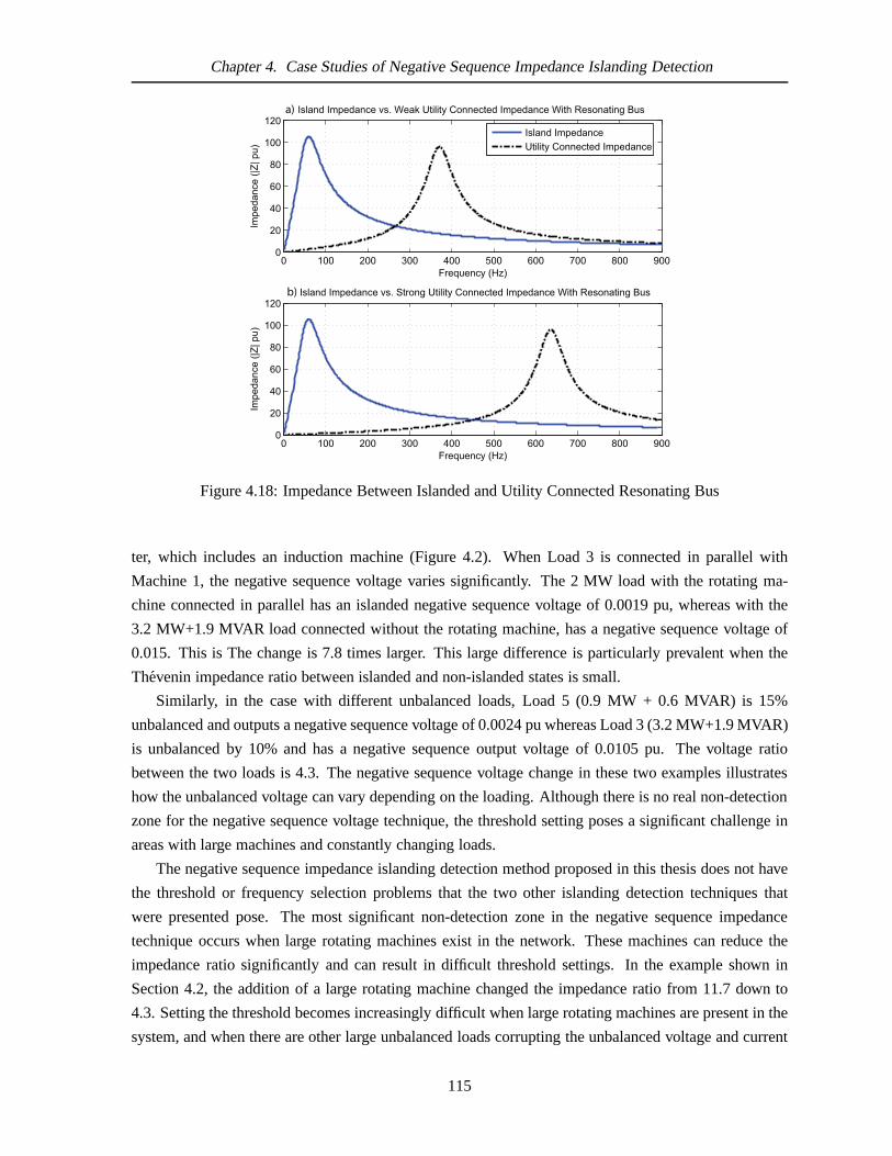
Chapter 4. Case Studies of Negative Sequence Impedance Islanding Detection
Figure 4.18: Impedance Between Islanded and Utility Connected Resonating Bus
ter, which includes an induction machine (Figure 4.2). WhenLoad 3 is connected in parallel with
Machine 1, the negative sequence voltage varies significantly. The 2 MW load with the rotating ma-
chine connected in parallel has an islanded negative sequence voltage of 0.0019 pu, whereas with the
3.2 MW+1.9 MVAR load connected without the rotating machine, has a negative sequence voltage of
0.015. This is The change is 7.8 times larger. This large difference is particularly prevalent when the
Thevenin impedance ratio between islanded and non-islanded states is small.
Similarly, in the case with different unbalanced loads, Load 5 (0.9 MW + 0.6 MVAR) is 15%
unbalanced and outputs a negative sequence voltage of 0.0024 pu whereas Load 3 (3.2 MW+1.9 MVAR)
is unbalanced by 10% and has a negative sequence output voltage of 0.0105 pu. The voltage ratio
between the two loads is 4.3. The negative sequence voltage change in these two examples illustrates
how the unbalanced voltage can vary depending on the loading. Although there is no real non-detection
zone for the negative sequence voltage technique, the threshold setting poses a significant challenge in
areas with large machines and constantly changing loads.
The negative sequence impedance islanding detection method proposed in this thesis does not have
the threshold or frequency selection problems that the two other islanding detection techniques that
were presented pose. The most significant non-detection zone in the negative sequence impedance
technique occurs when large rotating machines exist in the network. These machines can reduce the
impedance ratio significantly and can result in difficult threshold settings. In the example shown in
Section 4.2, the addition of a large rotating machine changed the impedance ratio from 11.7 down to
4.3. Setting the threshold becomes increasingly difficult when large rotating machines are present in the
system, and when there are other large unbalanced loads corrupting the unbalanced voltage and current
115

Chapter 4. Case Studies of Negative Sequence Impedance Islanding Detection
measurements.
Power Efficiency and Power Quality
Efficiency and power quality are both important design considerations when using any active islanding
detection technique. Power efficiency is a measurement of the amount of power the islanding detection
scheme consumes. Power quality is measured by how much the islanding detection scheme alters or
disrupts regular 60 Hz systems.
Harmonic injection islanding detection adds to the total harmonic distortion(THD) of the system.
For example, if a harmonic injection is made at an amplitude of 1% of the fundamental in the commercial
building example, an increase of 1% of THD may place the system outside of the allowable 5% limits.
Continuous injected harmonic power is extremely inefficient. Consider the previous example in the
office building discussed in Section 4.4. Injection method used near to the fundamental on the 600 bus
at the test building would have an impedance of approximately 11.6 pu. The base impedance is found
using Equation 4.20. The total power for a continuously injected signal of 1% of 600 V is given by
Equation 4.21. The continuous power required to run the islanding detection scheme can add up to 1%
of the total power produced by the DG.
Zbase=V2
base
Sbase=
6002
100·106 = 0.0036 (4.20)
V( f )2in j
Z( f )thev=
(600∗0.01)2
11.6∗Zbase= 862VA (4.21)
Consider using the injection technique on the 25 kV bus test case in Section 4.3 seen in Figure 4.3
using an injection amplitude of 1% of the fundamental. By placing the injection system on the 25 kV
bus, the Thevenin impedance near the fundamental is 13.8 pu. The resulting injected power at this
point is 7.2 kVA (Equation 4.22). The impedance used in theseexamples is at the fundamental, but the
power required will vary depending on the frequency in whichthe injection occurs. An alternative to
continuous harmonic injection to lower the power wasted is using periodical injection.
V( f )2in j
Z( f )thev=
(25·103 ∗0.01)2
13.8∗ (25·103)2
100·106
= 7.2 kVA (4.22)
Harmonic injection and unbalanced voltage (caused by negative sequence current injection) affect
the power quality in similar ways. Both will cause “non-torque” current to flow in rotating machines
wasted as heat. Voltage unbalance has little effect on single phase loads, but can cause excessive heating
on three phase rotating machines. This excessive heating reduces the machine’s lifetime and perfor-
mance over time. In the past Sections, voltage unbalance as low as 0.3% is measurable. For example, in
the lab setting in Practical Example 2: 600 V Commercial Building, the unbalanced load was injected
into the system between 0.3% and 1.2%. At 0.6% (approximately 1000 W), the impedance could be
resolved (seen in Figure 4.11).
116

Chapter 4. Case Studies of Negative Sequence Impedance Islanding Detection
4.6 Summary
In this chapter negative sequence impedance islanding detection has been applied to three test cases, and
then compared to two other islanding detection methods. Thethree test cases highlight how negative
sequence impedance islanding detection can function in different network configurations such as radial
networks, non radial networks, medium voltage buses and lowvoltage buses. Voltage and current mea-
surements from all the physical networks had naturally occurring unbalanced symmetric components.
The first case, based off of the IEEE standard industrial bus,was evaluated with multiple DG
sources, multiple unbalanced loads and a large rotating machine. The impedances measured were near
exact values of the anticipated outcome when there was only one single unbalanced load in the system.
However, multiple unbalanced loads were found to affect theimpedance measurement accuracy and
the ratio between the islanded and utility connected states. The size and amount of unbalanced loading
on the system produced errors in the measurements. The totalimpedance ratio increased when the two
loads were on the same phase, and the impedance did not changewhen the unbalanced conditions for the
two loads were on opposite phases. The introduction of a large rotating machine resulted in the biggest
reduction of the islanded to non-islanded impedance ratio and very small unbalanced voltages. The
machine used in this case was very large in size, but it showedhow significantly rotating machines can
affect the negative sequence impedance measurement capability. The unbalanced voltages and currents
were below the measurable limit of typical PT and CT sensors and implementing negative sequence
impedance islanding detection in this system using currentCT and PT technology may be difficult.
In the second case study, negative sequence islanding detection was tested on a 25 kV utility bus.
Unbalanced conditions were found to be measurable from the utility CT and PT sensors and the neg-
ative sequence impedance measured closely correlated to the system’s impedance. Further computer
simulations indicated similar results during island conditions. Sensor placement was investigated using
computer simulation. Nearby unbalanced loads were found tobe ideal sources of naturally occurring
negative sequence voltage and current, which the IPP could use as a method of independently conduct-
ing negative sequence impedance islanding detection.
The third case study evaluated negative sequence islandingdetection in a single office building with
a solar DG installation. The first experiment at the building’s main feeder measured naturally occurring
unbalanced conditions. The resulting negative sequence impedance closely correlated to the Thevenin
impedance away from the building. The second experiment wasconducted off a 208 V feeder from
the third floor of the building. Negative sequence current injection from the lab demonstrated how
current injections can be used to measure the Thevenin impedance away from the lab. Additionally,
averaging three phase negative sequence impedance measurements was found to improve the accuracy
while reducing the amount of needed injected current.
The last experiment of this case study used generated negative sequence components from the so-
lar DG for islanding detection. The inverter unbalance accurately measured the difference between
island and utility connected states up to the building main breaker. The addition of a rotating machine
decreased the impedance ratio between an islanded and non-islanded condition, although islanding de-
tection threshold could be set.
117

Chapter 4. Case Studies of Negative Sequence Impedance Islanding Detection
The last part of this chapter compared negative sequence impedance islanding detection with two
common impedance based islanding detection schemes. The effects of harmonic injection and volt-
age unbalance on power systems were addressed. Power quality, non-detection zone, efficiency, and
threshold settings were qualitatively compared with negative sequence impedance islanding. Negative
sequence impedance islanding detection is an improvement upon these two impedance based islanding
detection schemes in all the characteristics reviewed.
118
Chapter 5
Conclusion
Distributed generator installations into busses near electrical consumers have created new challenges for
protection engineers. The typical protection configurations such as unplanned islanding, reclosures, out
of step monitoring, impedance relay protection zones and ofdistributed generator systems need to be
reevaluated.
This chapter summarizes the main contributions presented in this work with suggested future re-
search on the method of negative sequence impedance islanding detection. This thesis has presented
a novel method of islanding detection for the protection of distributed generator fed systems. The
proposed islanding detection method measures the negativesequence impedance and compares it to a
known impedance threshold that signals an island conditionwhen the impedance increases past it.
Negative sequence impedance islanding detection is a unique addition to the existing islanding de-
tection techniques. Negative sequence impedance islanding detection addresses many of the existing
limitations of islanding detection.
5.1 Summary of Contributions
This thesis has made the following contributions to the fieldof islanding detection for distributed gen-
eration.
1. Development of a novel solution for islanding detection of distributed generators using
negative sequence impedance
This thesis presents a new concept of islanding detection based on the concept of negative se-
quence Thevenin impedance measurements [72]. The change in impedance between island and
utility connected systems is the threshold trigger. The proposed concept provides a more effective
impedance based islanding detection scheme that can be usedwith naturally occurring unbalanced
loads or with injected unbalanced currents.
The advantages of negative sequence impedance islanding detection are the wide impedance
threshold range setting, minimal integration costs, accuracy using naturally occurring unbalanced
loads and a fast response time of 25 ms compared to the 2 s IEEE 1547 standard. The minimal
integration costs are a result of only requiring existing system CT and PT sensors without having
to install expensive highly sensitive PTs and CTs to access voltage and current signals. In the
cases investigated, the existing naturally occurring unbalanced loads offer the necessary amount
of unbalanced conditions to support reliable impedance measurements for islanding detection.
119

Chapter 5. Conclusion
2. Theoretical analysis and performance of negative sequenceimpedance measurement for
islanding detection
The concept of negative sequence impedance islanding detection has been proven algebraically
and through simulations. The proof identified the correlation of the negative sequence impedance
to the Thevenin impedance away from the unbalanced load. This thesis models how each symmet-
rical component is created, and demonstrates the negative sequence performance characteristics
in terms of load sizes, power factor, connecting utility strength and the effects of multiple unbal-
anced loads.
The advantage of this analysis is that the performance characteristics are clearly expressed and can
be used to further determine the suitability of negative sequence impedance islanding detection in
a large number of scenarios.
3. Field data and network modeling supporting the measurability of naturally occurring neg-
ative sequence voltage and current
Field data was collected and the associated systems were modeled after to test the ability to acquire
real live data in the field for use with the negative sequence impedance islanding detection method.
The field data supports the measurability of naturally occurring negative sequence voltages and
currents on 25 kV, 600 V, and 208 V networks that lead to accurate impedance measurements
with clear threshold settings for islanding detection. Actual CT and PT sensors were used to
make measurements on live power systems proving that current technology can be used. Three
test cases were addressed to cover a range of scenarios. The test cases covered were 1. an IEEE
standard bus system modeled similarly seen in [65], 2. a 25 kVradial distributed generator fed
bus and 3. a 600 V office building. Live measurements and matching computer simulations were
made. Though the negative sequence voltages in scenario #1 were below typical CT and PT
measurement limits, the concept capability is still effectively demonstrated in simulation.
The advantage of these field experiments and simulations is two of the three practical scenarios
explicitly demonstrated that negative sequence impedanceislanding detection can be used in the
field; and the currently installed equipment has the sensitivity for accurate measurements.
4. Field data supporting the creation and measurability of injected negative sequence current
Simulations, numerical analysis and lab experiments were conducted to create negative sequence
injection for measuring negative sequence impedances. Themethod of injection can be applied
using a simple load or may be used in connection with equipment such as inverters, which can
deliberately inject negative sequence currents. Live experiments and simulations run on a 208 V
bus in an office building demonstrated that this method can bepractically used for measuring
impedances for distributed generator islanding detection.
The advantage of this work occurs in areas where there is no access to other unbalanced loads
or where the local unbalance from other loads is too great. This method can be used to offset
120
Chapter 5. Conclusion
the other unbalanced loads or simply as a negative sequence source in an area that does not have
naturally occurring unbalanced loads.
5. Design, modeling and practical experiments of a novel concept of three phase sequence in-
jection impedance measurement averaging to enhance impedance measurement accuracy
The concept of individual three phase sequence injection impedance measurement averaging with
injected negative sequence components was verified in an algebraic analysis, simulation and with
practical experiments on a 208 V bus in this thesis. Unbalanced systems were found to be consis-
tently unbalanced on one particular phase, however, by injecting negative sequence current into
the unbalanced system by deliberately loading phases AB, BC, then CA different impedance an-
swers were revealed. The average of the three impedances wasfound to equate to a more precise
Thevenin impedance.
This concept has the advantage of increasing the accuracy ofnegative sequence impedance mea-
surements while reducing the required power of the current injections for measuring Thevenin
impedance of the system.
6. A comprehensive review of all impedance measurement techniques for live systems in the
past 20 years
In this thesis, a comprehensive review of all impedance measurement techniques for live power
systems over the past 20 years was conducted. The review was organized by style of impedance
method and chronologically sorted. This comprehensive review is not available in any past works
and is necessary to fully understand the value of the conceptpresented in this thesis.
The advantage of this comprehensive review is that progression and limitations of current impedance
measurement techniques are revealed.
5.2 Future Work
Negative sequence impedance islanding detection technique has been demonstrated to operate in many
ideal network conditions; however, there are some future research topics that may further enhance the
concept. There are several significant areas to be explored in this work:
1. Techniques to improve or extend existing PT and CT performance
Through all the practical measurements and simulations, the unbalance voltage is often very small,
which limits the accuracy of the measurements. Many of the unbalanced voltages are in the range
of 1 % to 0.1 % which is near the absolute accuracy of some CTs and PTs. Though the accuracy
limitation of the CTs and PTs is around the typical measurements, the relative noise platform
may be much lower. This means the performance of these CTs andPTs may be extended beyond
the original expectations. Further investigation into PT and CT noise platforms and the typical
accuracy beyond the nameplate would assist in furthering this research.
121

Chapter 5. Conclusion
Measuring beyond the CT and PT noise platform has the potential to lead to nuisance tripping.
Higher accuracy system measurements can improve the reliability of measurements. Therefore,
further research into methods of improving existing installed CT and PT accuracy could be bene-
ficial. This would involve taking several typical CT and PT systems into a lab setting to evaluate
whether simple modifications could be made to further improve or estimate actual measurements.
Several enhancements to high voltage measurement techniques have been made in the past decade,
such as, using high accuracy laser cut resistor dividers, and optical current and voltage sensors.
Although they have not garnered wide spread industry acceptance. Investigations on more cost
effective replacements of existing old CTs and PTs would accelerate this; allowing for more wide
spread application of negative sequence islanding detection to be introduced.
This technique has not yet been applied to harmonic impedance measurements due to sensitivity
limitations. Network harmonics are often less than 5% of thefundamental, whereas unbalanced
harmonics would be only a fraction of that per cent limiting the measurability of these com-
ponents. Enhancements in voltage and current measurability will further enhance the ability to
address this concept beyond the theoretical analysis.
2. Sensor Reach Through Weak Connections and Heavy UnbalancedSystems
As seen in previous investigations, complex and multiple heavily unbalanced high system impedance
networks limit the ability to accurately measure island states, and limit the negative sequence
impedance sensor’s reach to the islanding breaker. Furtherresearch into these conditions may
extend the performance. The research could investigate alternatives with injection types with
the combination of phase and amplitude measurements. As this work has dealt with absolute
impedance measurements, phase errors and system amplitudetrend signatures may also present
potential for further research into the reach of negative sequence measurements.
3. Enhanced Understanding of Practical Unbalanced Conditions
This work consisted of a study of several sites with actual practical measurements on three scenar-
ios, one being simulation. However, a more comprehensive study of natural system unbalance is
needed. To date, there has been little research completed onunbalanced power systems whereas
most studies and approximations are made assuming perfectly balanced network states. This as-
sumption has lead to very little research and published dataon unbalanced networks and their
overall effect. Practical published cases are rare. The research community and the concept pre-
sented in this thesis would benefit from a detailed review of typical conditions for utilities around
the world.
Practical measurements are extremely difficult to attain due to national security requirements of
utilities. This leads to a reluctance of utilities to release any information indicating network per-
formance or locations of measurements. However, a specialized study with a partnership between
academia and industry with only Thevenin impedances of thespecific locations may allow for a
study such as this to be completed. Understanding of the unbalanced conditions that exist at vari-
122
Chapter 5. Conclusion
ous voltage levels from 500 kV to 4 kV will benefit further implementation and other applications
of using negative sequence impedance to measure the Thevenin impedance.
4. Transient and Disturbance Performance
Although negative sequence impedance estimation for islanding detection has been found to func-
tion well under steady-state conditions, transients and other disturbances create errors that may
lead to nuisance tripping. Performance details during transients require further study to improve
this limitation. For example, network transients can causedifficulty in sequence conversion with
very large errors. There are opportunities for modern filtering and other signal processing tech-
niques to enhance the ability to process the negative sequence impedance measurement beyond
the steady-state studies investigated in this work.
5. Integration challenges with grid tie inverters and relays
Stand alone devices and natural measurements have been studied in this work, however, integra-
tion strategies into inverter devices and power system relays requires further understanding. For
example, the active unbalanced sources using the averagingimpedance method is limited by the
effect on the system and power quality degradation. Active negative sequence current injection
requires study in minimizing the disturbance to the customer. A relay prototype or an inverter
for negative sequence impedance measurement and injectionalgorithms would be beneficial to
further understand the integration challenges.
6. Rotating Machine Negative Sequence Impedance
Rotating machines pose limitations to the measurement ability of negative sequence impedance
islanding detection. In smaller buildings where small motors and small HVAC systems exist,
the high impedance of these items is still much higher than low impedance utility connection.
Larger systems such as industrial facilities with rotatingmachines dominating the load can have
impedances that significantly lower the ability to detect anisland. The position of the islanding
detection sensor is critical to its sensitivity. Further study into how to reduce the effect of rotating
machines on this technique would greatly extend the value ofthis research.
This evaluation extends beyond motors to rotating induction and synchronous generators. The
injected unbalance in an inverter was investigated in this work, but rotating machine injections
were not. This limitation requires a detailed study which can benefit the community two-fold.
The first is to extend the use of negative sequence impedance islanding detection for machines as
well as investigating the life of machines with deliberate unbalanced output.
7. Negative Sequence Impedance Phase Response
This thesis covered absolute values for impedance measurements. This was because of the phase
errors encountered during signal processing and Fourier transform of the data. Very small errors or
sampling inaccuracies cause significant phase errors. Further investigation into the phase response
of negative sequence impedance may enhance the accuracy further.
123

Chapter 5. Conclusion
5.3 Final Remarks
The novel concept of negative sequence impedance islandingdetection has been introduced in this
thesis. The practical cases and mathematical evaluations highlight some practical applications where
this islanding detection scheme may be used. Negative sequence impedance islanding detection has
improved upon the threshold settings, non-detection zone,and installation cost limitations of other
impedance based methods. As has been shown, negative sequence impedance islanding detection is
a viable method for islanding detection applications.
124

Bibliography
[1] ABB. Abb focs fiber-optic current sensors datasheet.ABB, 1(1-2):2, 2005.
[2] ABB. Outdoor instrument transformers application guide. ABB, 1(2.1):1–124, 2005.
[3] Spencer Abraham. National transmission grid study. Technical report, US Department of Energy,
may 2002.
[4] J. Arrillaga. Power system harmonic analysis. Wiley, Chichester; New York, 1997. Jos Arrillaga.
[et al.].ill.; 25 cm.
[5] L. Asiminoaei, R. Teodorescu, F. Blaabjerg, and U. Borup. A new method of on-line grid
impedance estimation for pv inverter. InApplied Power Electronics Conference and Exposition,
volume 3, pages 1527–1533. APEC ’04. Nineteenth Annual IEEE, IEEE, 2004.
[6] L. Asiminoaei, R. Teodorescu, F. Blaabjerg, and U. Borup. A digital controlled pv-inverter
with grid impedance estimation for ens detection.Power Electronics, IEEE Transactions on,
20(6):1480 – 1490, 2005.
[7] L. Asiminoaei, R. Teodorescu, F. Blaabjerg, and U. Borup. Implementation and test of an online
embedded grid impedance estimation technique for pv inverters. Industrial Electronics, IEEE
Transactions on, 52(4):1136, 2005.
[8] P. Barker. Overvoltage considerations in applying distributed resources on power systems. In
Power Engineering Society Summer Meeting, 2002 IEEE, volume 1, page 109, 2002.
[9] P. P. Barker and R. W. De Mello. Determining the impact of distributed generation on power
systems. i. radial distribution systems. InPower Engineering Society Summer Meeting, 2000.,
volume 3, page 1645. IEEE, 2000.
[10] J. Lewis Blackburn.Protective relaying: principles and applications. Power engineering; 5. M.
Dekker, New York, 2nd edition, 1998. J. Lewis Blackburn.ill.; 24 cm.
[11] Ward Bower and Michael Ropp. Evaluation of islanding detection methods for photovoltaic
utility-interactive power systems. Report IEA PVPS Task 5 IEA PVPS T5-09: 2002, Sandia
National Laboratories Photovoltaic Systems Research and Development, March 2002.
[12] CSA Standard CAN3-C235-83.Preferred voltage levels for AC systems, 0 to 50 000 V. Canadian
Standards Association, 1983.
125

Bibliography
[13] C.Malone. Distribution system voltage and power quality, hydro ontario. Hydro Ontario, 2006.
[14] NXTPhase Corporation. Nxct optical current sensor datasheet.NXTPhase Corporation, 1(1-2):8,
2006.
[15] NXTPhase Corporation. Nxvt optical voltage sensor datasheet.NXTPhase Corporation, 1(1-2):2,
2006.
[16] Neil Cullen, Jim Thornycroft, and Alan Collinson. Riskanalysis of islanding of photovoltaic
power systems within low voltage distribution networks. Technical report, International Energy
Agency, 2002.
[17] L. S. Czarnecki and Z. Staroszczyk. On-line measurement of equivalent parameters of distribution
system and its load for harmonic frequencies.Power Delivery, IEEE Transactions on, 45(2):467
– 472, 1996.
[18] Kevin J. Dasso. The reliability of bulk electric systems in north america. Technical report, North
American Electric Reliability Council, September 2006.
[19] Francisco De la Rosa.Harmonics and power systems. Electric power engineering series. CRC
Taylor Francis, Boca Raton, FL, 2006. Francisco C. De La Rosa. ill.; 25 cm.
[20] A. de Oliveira, J. C. de Oliveira, J. W. Resende, and M. S.Miskulin. Practical approaches for ac
system harmonic impedance measurements.Power Delivery, IEEE Transactions on, 6(4):1721 –
1726, 1991.
[21] M. C. Di Piazza, P. Zanchetta, M. Sumner, and D. W. P. Thomas. Estimation of load impedance
in a power system. InHarmonics and Quality of Power, 2000. Proceedings. Ninth International
Conference on, volume 2, pages 520 – 525. IEEE, 2000.
[22] V. Diana, M. Sumner, P. Zanchetta, and M. Marinelli. Non-invasive power system impedance
monitoring for improved power quality. InPower Electronics, Machines and Drives, 2004.
(PEMD 2004). Second International Conference on, volume 1, page 265. IEEE, 2004.
[23] Hermann W. Dommel.EMTP Theory Book, volume 6. Microtran Power System Analysis Corp.,
Vancouver, 2 edition, 1996.
[24] M. K. Donnelly, J. E. Dagle, D. J. Trudnowski, and G. J. Rogers. Impacts of the distributed utility
on transmission system stability.Power Systems, IEEE Transactions on, 11(2):741–746, 1996.
[25] R. C. Dugan. Distributed resources and reliability of distribution systems. InPower Engineering
Society Summer Meeting, 2002 IEEE, volume 1, page 106. IEEE, 2002.
[26] R. C. Dugan and T. E. McDermott. Operating conflicts for distributed generation on distribution
systems. InRural Electric Power Conference, 2001. IEEE, 2001.
126

Bibliography
[27] R. C. Dugan and T. E. McDermott. Distributed generation. Industry Applications Magazine,
IEEE, 8(2):1–19, 2002.
[28] Ismail Mohamed Elmarkabi.Control and Protection of Distribution Networks with Distributed
Generators. dissertation, North Carolina State University, 2004.
[29] Walter A. Elmore.Protective relaying theory and applications. Marcel Dekker, New York, 2nd
edition, 2004.
[30] D. Fernandes, W. Neves, and J. Vasconcelos. A coupling capacitor voltage transformer repre-
sentation for electromagnetic transient studies. InInternational Conference on Power Systems
Transients, pages 1–6, New Orleans, 2003.
[31] Pai Fu-Sheng and Huang Shyh-Jier. A detection algorithm for islanding-prevention of dis-
persed consumer-owned storage and generating units.Energy Conversion, IEEE Transactions
on, 16(4):346–351, 2001.
[32] T. Funabashi, K. Koyanagi, and R. Yokoyama. A review of islanding detection methods for
distributed resources.Power Tech Conference Proceedings, 2003 IEEE Bologna, 2:1– 6, June
2003.
[33] Steve Gehl. Electricity technology roadmap: 2003 summary and synthesis. Technical report,
Electric Power Research Institute, November 2003.
[34] Martin Geidl. Protection of power systems with distributed generation: State of the art. Report,
Power Systems Laboratory of the Swiss Federal Institute of Technology, July 20 2005.
[35] F. Ghassemi, P. F. Gale, B. Clegg, T. Cumming, and C. Coutts. Method to measure cvt transfer
function. Power Delivery, IEEE Transactions on, 17(4):915 – 920, 2002.
[36] A. A. Girgis and R. B. McManis. Frequency domain techniques for modeling distribution or
transmission networks using capacitor switching induced transients.Power Delivery, IEEE Trans-
actions on, 4(3):1882 – 1890, 1989.
[37] John J. Grainger, William D. Stevenson, and William D. Stevenson. Power system analysis.
McGraw-Hill series in electrical and computer engineering. Power and energy. McGraw-Hill,
New York, 1994.
[38] BC Hydro Systems Group. Distribution power generator islanding guidelines. BC Hydro, 2006.
[39] M. B. Harris, A. W. Kelley, J. P. Rhode, and M. E. Baran. Instrumentation for measurement
of line impedance. InApplied Power Electronics Conference and Exposition, 1994. APEC ’94.,
page 887. IEEE, 1994.
[40] W. G. Hartmann. How to nuisance trip distributed generation. In Rural Electric Power Confer-
ence, 2003, pages C5–1. IEEE, 2003.
127

Bibliography
[41] Jatinder Singh Hayer.Signal Detection technique for Islanding Detection of Distributed Gener-
ators Using Power Line Signaling. PhD thesis, University of Alberta, 2004.
[42] R. Hernandez-Gonzalez, G. Iravani. Current injectionfor active islanding detection of
electronically-interfaced distributed resources.Power Delivery, IEEE Transactions on,
21(3):1698–1705, 2006.
[43] Clark Glenn Hochgraf. Anti-islanding detection scheme for distributed power generation. Visteon
Global Technologies, Inc., August 5 2003.
[44] P. D. Hopewell, N. Jenkins, and A. D. Cross. Loss-of-mains detection for small generators.
Electric Power Applications, IEE Proceedings-, 143(3):225 – 230, 1996.
[45] J. Huang and K. A. Corzine. Ac impedance measurement by line-to-line injected current. In
Industry Applications Conference, 2006. 41st IAS Annual Meeting, volume 1, page 300. IEEE,
2006.
[46] R. M. Hudson, T. Thorne, F. Mekanik, M. R. Behnke, S. Gonzalez, and J. Ginn. Implemen-
tation and testing of anti-islanding algorithms for ieee 929-2000 compliance of single phase
photovoltaic inverters. InPhotovoltaic Specialists Conference, 2002. Conference Record of the
Twenty-Ninth IEEE, page 1414. IEEE, 2002.
[47] BC Hydro. 35 kv and below interconnection requirementsfor power generators. Technical report,
BC Hydro, February 2007.
[48] IEEE-SA-Standards-Board. Ieee recommended practicefor industrial and commercial power
systems analysis.IEEE Std 399-1990, pages 1–495, 1990.
[49] IEEE-SA-Standards-Board. Ieee standard electrical power system device function numbers.
IEEE Std 519-1992, 1991.
[50] IEEE-SA-Standards-Board. Ieee recommended practices and requirements for harmonic control
in electrical power systems.IEEE Std 519-1992, pages 1–101, 1993.
[51] IEEE-SA-Standards-Board. Ieee recommended practicefor utility interface of photovoltaic (pv)
systems.IEEE Std 929-2000, pages 1–32, 2000.
[52] IEEE-SA-Standards-Board. Ieee recommended practicefor protection and coordination of in-
dustrial and commercial power systems.ANSI/IEEE Std 242-2001, pages 1–710, 2001.
[53] IEEE-SA-Standards-Board. Ieee guide for protective relaying of utility-consumer interconnec-
tions. IEEE Std C37.95-2002 (Revision of IEEE Std C37.95-1989), pages 1–49, 2003.
[54] IEEE-SA-Standards-Board. Ieee standard for interconnecting distributed resources with electric
power systems.IEEE Std 1547 2003, pages 1–27, 2003.
128

Bibliography
[55] IEEE-SA-Standards-Board. Ieee standard requirements for instrument transformers.IEEE Std
C57.13-1993(R2003) (Revision of IEEE Std C57.13-1978, pages 1–73, 2003.
[56] IEEE-SA-Standards-Board. Ieee standard conformancetest procedures for equipment intercon-
necting distributed resources with electric power systems. IEEE Std 1547.1-2005, pages 1–63,
2005.
[57] IEEE-SA-Standards-Board. Ieee standard for high-accuracy instrument transformers.IEEE Std
C57.13.6-2005, pages 1–6, 2005.
[58] Edison Electric Institute. Eei survey of transmissioninvestment. Report, May 2005.
[59] Electrical Power Research Institute. 1999 summary andsynthesis. Technical Report CI-112677-
V1, Electrical Power Research Institute, July 1999.
[60] H. Karimi ; A. Yazdani; R. Iravani. Negative-sequence current injection for fast islanding de-
tection of a distributed resource unit.Power Electronics, IEEE Transactions on, 23(1):298–307,
Jan. 2008.
[61] N. A. F. Jaeger and F. Rahmatian. Integrated optics pockels cell high-voltage sensor.Power
Delivery, IEEE Transactions on, 10(1):127–134, 1995.
[62] Santos JC, Taplamacioglu MC, and Hidaka K. Optical highvoltage measurement using pockels
microsingle crystal.Review of Scientific Instruments, 70(8):3271–3276, 1999.
[63] M. A. Kashem and Gerard Ledwich. Multiple distributed generators for distribution feeder volt-
age support.IEEE Transactions On Energy Conversion, 20:676–684, 2005.
[64] F. Katiraei, C. Abbey, and R. Bahry. Analysis of voltageregulation problem for a 25 kv distribu-
tion network with distributed generation. InPower Engineering Society General Meeting, 2006.
IEEE, page 8, 2006.
[65] F. Katiraei, M. R. Iravani, and P. W. Lehn. Micro-grid autonomous operation during and subse-
quent to islanding process.Power Delivery, IEEE Transactions on, 20(1):248 – 257, 2005.
[66] S. Knoke, J. Majeski, K. Smit, and K. Tarp. Installation, operation, and maintenance costs for dis-
tributed generation technologies. Technical Report 1007675, Electric Power Research Institute,
February 2003.
[67] Paul C. Krause, Oleg Wasynczuk, Scott D. Sudhoff, and Paul C. Krause.Analysis of electric ma-
chinery and drive systems. IEEE Press power engineering series. IEEE Press; Wiley-Interscience,
Piscataway, NJ New York, 2nd edition, 2002. Paul C. Krause, Oleg Wasynczuk, Scott D. Sud-
hoff.ill.; 25 cm. Rev. ed. of: Analysis of electric machinery. c1995.
[68] Prabha Kundur.Power System Stability and Control. Power System Planning and Operations
Program. McGraw-Hill, Inc., Palo Alto, 1 edition, 1994.
129

Bibliography
[69] B.P Lathi. Modern Digital and Analog Communication Systems, chapter 2.7, pages 40–45. Ox-
ford University Press, 189 Madison Avenue, New York, New York, 10016, 1998.
[70] David Lineweber and Shawn McNulty. The cost of power disturbances to industrial and digital
economy companies. Technical report, Primen, June 2001.
[71] L. A. C. Lopes and Sun Huili. Performance assessment of active frequency drifting islanding
detection methods.Energy Conversion, IEEE Transaction on, 21(1):171–180, 2006.
[72] Jose R. Martı. Provisional patent application: Method and apparatus for finding thevenin equiv-
alents in a power system and detecting voltage stability conditions. 61/006,056(056), 2007.
[73] Jose R. Martı, L. R. Linares, and H. W. Dommel. Currenttransformers and coupling-capacitor
voltage transformers in real-time simulations.Power Delivery, IEEE Transactions on, 12(1):164–
168, 1997.
[74] V. Menon and M. H. Nehrir. A hybrid islanding detection technique using voltage unbalance and
frequency set point.Power Systems, IEEE Transactions on, 22(1):442–448, 2007.
[75] John Micklethwait. Atomic renaissance.The Economist, 384(8545):102–104, September 2007.
[76] G. Moreau, H. H. Le, G. Croteau, G. Beaulieu, and E. Portales. Measurement system for har-
monic impedance of the network and validation steps. InQuality and Security of Electric Power
Delivery Systems, pages 69 – 73. CIGRE/PES 2003. CIGRE/IEEE PES International Symposium,
2003.
[77] Chuck Mozina. Distributed generation interconnection protection course. Beckwith Electric,
Course Handouts, 2007.
[78] M. Nagpal and C. Henville. Protection accessories course notes. Technical report, BC Hydro,
January 2007.
[79] M. Nagpal, F. Plumptre, R. Fulton, and T. G. Martinich. Dispersed generation interconnection-
utility perspective.Industry Applications, IEEE Transactions on, 42(3):864–872, 2006.
[80] M. Nagpal, W. Xu, and J. Sawada. Harmonic impedance measurement using three-phase tran-
sients.Power Delivery, IEEE Transactions on, 13(1):272 – 277, 1998.
[81] Zhihong Ye; Pengwei Du; John Keith Nelson; Wright Miller Nicholas. Anti-islanding protec-
tion systems for synchronous machine based distributed generators. General Electric Company,
September 18 2007.
[82] H. Nikkhajoei and R. H. Lasseter. Microgrid protection. In Power Engineering Society General
Meeting, 2007. IEEE, page 1, 2007.
130

Bibliography
[83] P. O’Kane and B. Fox. Loss of mains detection for embedded generation by system impedance
monitoring. InDevelopments in Power System Protection, Sixth International Conference on,
page 95. IEEE, 1997.
[84] B. Palethorpe, M. Sumner, and D. W. P. Thomas. Power system impedance measurement using
a power electronic converter. InHarmonics and Quality of Power, 2000. Proceedings. Ninth
International Conference on, volume 1, page 208. IEEE, 2000.
[85] B. Palethorpe, M. Sumner, and D. W. P. Thomas. System impedance measurement for use with
active filter control. InPower Electronics and Variable Speed Drives, 2000. Eighth International
Conference on, page 24. IEEE, 2000.
[86] K. O. H. Pedersen, A. H. Nielsen, and N. K. Poulsen. Short-circuit impedance measurement.
Generation, Transmission and Distribution, IEE Proceedings-, 150(2):169 – 174, 2003.
[87] Daniel Persson. Islanding detection in power electronic converter based distributed generation.
Master thesis, Industrial Electrical Engineering and Automation, February 2007.
[88] Manisa Pipattanasomporn, Michael Willingham, and Saifur Rahma. Implications of on-site dis-
tributed generation for commercial/industrial facilities. IEEE Transactions of Power Systems,
20(4):206–212, 2005.
[89] Arne Faaborg Povlsen. Impacts of power penetration from photovoltaic power systems in distri-
bution networks. Technical Report Report IEA PVPS T5-10: 2002, International Energy Agency,
February 2002.
[90] Satish J. Ranade, Deepak R. Sagi, Ravindra Mulpuri, Raghu Surabhi, and Joydeep Mitra. Like-
lihood of islanding in distribution feeders with photovoltaic generation. InPower Engineering
Society General Meeting, 2007. IEEE, page 1, 2007.
[91] J. P. Rhode, A. W. Kelley, and M. E. Baran. Complete characterization of utilization-voltage
power system impedance using wideband measurement.Industry Applications, IEEE Transac-
tions on, 33(6):1472 – 1479, 1997.
[92] Jeremy Rifkin. The Hydrogen Economy: The Creation of the Worldwide Energy Web and the
Redistribution of Power on Earth, volume 1. Penguin Putnam Inc., New York, NY, 1 edition,
2002.
[93] C. M. Riley, B. K. Lin, T. G. Habetler, and G. B. Kliman. Stator current harmonics and their
causal vibrations: a preliminary investigation of sensorless vibration monitoring applications.
Industry Applications, IEEE Transactions on, 35(1):94–99, 1999.
[94] A. Robert, T. Deflandre, E. Gunther, R. Bergeron, A. Emanuel, A. Ferrante, G. S. Finlay,
R. Gretsch, A. Guarini, J. L. Gutierrez Iglesias, D. Hartmann, M. Lahtinen, R. Marshall, K. Oon-
ishi, C. Pincella, S. Poulsen, P. Ribeiro, M. Samotyj, K. Sand, J. Smid, P. Wright, and Y. S.
131

Bibliography
Zhelesko. Guide for assessing the network harmonic impedance. InElectricity Distribution. Part
1: Contributions. CIRED. 14th International Conference and Exhibition on, volume 1. IEEE,
1997.
[95] M. E. Ropp, M. Begovic, and A. Rohatgi. Prevention of islanding in grid-connected photovoltaic
systems.Progress in Photovoltaics: Research and Applications, 7(1):39 – 59, 1999.
[96] Michael Eugene Ropp.Design issues for grid-connected photovoltaic systems. Dissertation,
Georgia Institute of Technology, 1998.
[97] S. K. Salman, D. J. King, and G. Weller. New loss of mains detection algorithm for embedded
generation using rate of change of voltage and changes in power factors. InDevelopments in
Power System Protection, 2001, Seventh International Conference on (IEE), page 82, 2001.
[98] O. Samuelsson and N. Strath. Islanding detection and connection requirements. InPower Engi-
neering Society General Meeting, 2007. IEEE, page 1, 2007.
[99] Tony Seegers. A report to the line protection subcommittee of the power system relay committee
of the ieee power engineering society. Technical report, IEEE, August 2004.
[100] Ken Sonnenberg. Current and voltage transformer basics. GE Multilin - Instrument Transformers,
Inc., March 2007.
[101] N. L. Soultanis, S. A. Papathanasiou, and N. D. Hatziargyriou. A stability algorithm for the
dynamic analysis of inverter dominated unbalanced lv microgrids. Power Systems, IEEE Trans-
actions on, 22(1):294–304, 2007.
[102] German Standard. Din vde 0126-1-1. Technical report,Selbstttige Schaltstelle zwischen
einer netzparallelen Eigenerzeugungsanlage und dem ffentlichen Niederspannungsnetz,, Febru-
ary 2006.
[103] Z. Staroszczyk. Problems in real-time wide band identification of power systems. InInstru-
mentation and Measurement Technology Conference, 1998. IMTC/98. Conference Proceedings.,
volume 2, page 779. IEEE, 1998.
[104] John Stevens, Russell Bonn, Jerry Ginn, and SigifredoGonzalez. Development and testing of
an approach to anti-islanding in utility-interconnected photovoltaic systems. Technical report,
Sandia National Laboratories, August 2000.
[105] M. Sumner, B. Palethorpe, D. Thomas, P. Zanchetta, andM. C. Di Piazza. Estimation of power
supply harmonic impedance using a controlled voltage disturbance. InPower Electronics Spe-
cialists Conference, 2001. PESC. 2001 IEEE 32nd Annual, volume 2, page 522. IEEE, 2001.
[106] M. Sumner, B. Palethorpe, D. W. P. Thomas, P. Zanchetta, and M. C. Di Piazza. A technique
for power supply harmonic impedance estimation using a controlled voltage disturbance.Power
Electronics, IEEE Transactions on, 17(2):207 – 215, 2002.
132

Bibliography
[107] M. Sumner, B. Palethorpe, P. Zanchetta, and D. W. P. Thomas. Experimental evaluation of active
filter control incorporating on-line impedance measurement. In Harmonics and Quality of Power,
2002. 10th International Conference on, volume 2, page 501. IEEE, 2002.
[108] Jang Sung-Il and Kim Kwang-Ho. An islanding detectionmethod for distributed generations
using voltage unbalance and total harmonic distortion of current. Power Delivery, IEEE Trans-
actions on, 19(2):745 – 752, 2004.
[109] A. V. Timbus, R. Teodorescu, F. Blaabjerg, and U. Borup. Online grid measurement and ens
detection for pv inverter running on highly inductive grid.Power Electronics Letters, IEEE,
2(3):77 – 82, 2004.
[110] A. V. Timbus, R. Teodorescu, F. Blaabjerg, and U. Borup. Ens detection algorithm and its im-
plementation for pv inverters.Electric Power Applications, IEE Proceedings-, 153(2):206 – 212,
2006.
[111] A. V. Timbus, R. Teodorescu, F. Blaabjerg, and U. Borup. Online grid impedance measurement
suitable for multiple pv inverters running in parallel. InApplied Power Electronics Conference
and Exposition, 2006. APEC apos;06. Twenty-First Annual, page 5. IEEE, 2006.
[112] K. Tomiyama, S. Ihara, R. J. Piwko, E. R. Pratico, and L.Crane. Impedance monitor performance
tests. InPower Engineering Society Winter Meeting, 2002., volume 1, page 538. IEEE, 2002.
[113] O. Tsukamoto, T. Okayasu, and K. Yamagishi. Study on islanding of dispersed photovoltaic
power systems connected to a utility power grid.Solar Energy, 70(6):505–511, 2001.
[114] Mossadiq Umedaly. A vision for growing a world-class power technology cluster in a smart,
sustainable british columbia. British Columbia Reports and Publications, 2005.
[115] G. J. Vachtsevanos and H. Kang. Simulation studies of islanded behavior of grid-connected
photovoltaic systems.Energy Conversion, IEEE Transactions on, 4(2):177–183, 1989.
[116] Bas Verhoeven. Utility aspects of grid connected photovoltaic power systems. Technical Report
IEA PVPS T5-01:1998, International Energy Agency, December 1998.
[117] Bas Verhoeven. Probability of islanding in utility networks due to grid connected photovoltaic
power systems. Technical report, International Energy Agency, september 2002.
[118] P. L. Villenueve. Concerns generated by islanding [electric power generation].Power and Energy
Magazine, IEEE, 2(3):49– 53, 2004.
[119] K. Vu, M. M. Begovic, D. Novosel, and M. M. Saha. Use of local measurements to estimate
voltage-stability margin.Power Systems, IEEE Transactions on, 14(3):1029–1035, 1999.
[120] C. F. Wagner and Robert David Evans.Symmetrical components as applied to the analysis of
unbalanced electrical circuits. McGraw-Hill, New York, London,, 1933.
133
Bibliography
[121] W. Wang, J. Kliber, G. Zhang, W. Xu, B. Howell, and T. Palladino. A power line signaling based
scheme for anti islanding protection of distributed generators part ii field test results.Power
Delivery, IEEE Transactions on, 22(3):1767–1772, 2007.
[122] Xiaoyu Wang, Walmir Freitas, Wilsun Xu, and Venkata Dinavahi. Impact of dg interface controls
on the sandia frequency shift antiislanding method.IEEE Transactions on Energy Conversion,
22(3):792–794, 2007.
[123] Xiaoyu Wang, Walmir Freitas, Wilsun Xu, and Venkata Dinavahi. Impact of interface controls on
the steady-state stability of inverter-based distributedgenerators. InPower Engineering Society
General Meeting, 2007. IEEE, page 1, 2007.
[124] Yuguang Wang.Utility Interactive Power Conditioning Systems IslandingProblem Solutions.
PhD thesis, Arizona State University, 1990.
[125] P. Welch. The use of fast fourier transform for the estimation of power spectra: A method
based on time averaging over short, modified periodograms.Audio and Electroacoustics, IEEE
Transactions on, 15(2):70 – 73, 1967.
[126] Robert Wills. Anti-islanding method and apparatus for distributed power generation. Plug Power
Inc., 2001.
[127] Xu Wilsun, E. E. Ahmed, Zhang Xiqin, and Liu Xian. Measurement of network harmonic
impedances: practical implementation issues and their solutions.Power Delivery, IEEE Transac-
tions on, 17(1):210–216, 2002.
[128] Xu Wilsun, K Mauch, and S. Martel. An assessment of distributed generation islanding detection
methods and issues for canada. Natural Resources Canada, 2004.
[129] J. Wilsun Xu; Guibin Zhang; Chun Li; Wencong Wang; Guangzhu Wang; Kliber. A power line
signaling based technique for anti islanding protection ofdistributed generators part i: Scheme
and analysis.Power Delivery, IEEE Transactions on, 22(3):1758–1772, 2007.
[130] C. Xie, S. B. Tennakoon, R. Langella, D. Gallo, A. Testa, and A. Wixon. Harmonic impedance
measurement of 25 kv single phase ac supply systems. InHarmonics and Quality of Power, 2000.
Proceedings. Ninth International Conference on, volume 1, page 214. IEEE, 2000.
[131] Xiao Yao, J. C. Maun, H. B. Mahmoud, T. Detroz, and Do Stephane. Harmonic impedance
measurement using voltage and current increments from disturbing loads. InHarmonics and
Quality of Power, 2000. Proceedings. Ninth International Conference on, volume 1, page 220.
IEEE, 2000.
[132] Jung Youngseok, Sol Junghun, Yu Gwonjong, and Choj Jaeho. Modelling and analysis of ac-
tive islanding detection methods for photovoltaic power conditioning systems. InElectrical and
Computer Engineering, 2004. Canadian Conference on, volume 2, page 979. IEEE, 2004.
134

Appendix A
Device Number Reference
This information comes from IEEE Standard Electrical PowerSystem Device Function Numbers [49].
1 - Master Element2 - Time Delay Starting or Closing Relay3 - Checking or Interlocking Relay4 - Master Contactor5 - Stopping Device6 - Starting Circuit Breaker7 - Anode Circuit Breaker8 - Control Power Disconnecting Device9 - Reversing Device10 - Unit Sequence Switch11 - Reserved for future application12 - Overspeed Device13 - Synchronous-speed Device14 - Underspeed Device15 - Speed - or Frequency-Matching Device16 - Reserved for future application17 - Shunting or Discharge Switch18 - Accelerating or Decelerating Device19 - Starting to Running Transition Contactor20 - Elect. operated valve (solenoid valve)21 - Distance Relay22 - Equalizer Circuit Breaker23 - Temperature Control Device24 - Over-Excitation Relay25 - Synchronizing or Synchronism-Check Device26 - Apparatus Thermal Device27 - Undervoltage Relay28 - Reserved for future application29 - Isolating Contactor30 - Annunciator Relay31 - Separate Excitation Device32 - Directional Power Relay33 - Position Switch34 - Motor-Operated Sequence Switch35 - Brush-Operating or Slip-Ring Short-Circuiting Device
135

Appendix A. Device Number Reference
36 - Polarity or Polarizing Voltage Devices37 - Undercurrent or Underpower Relay38 - Bearing Protective Device39 - Mechanical Conduction Monitor40 - Field Relay41 - Field Circuit Breaker42 - Running Circuit Breaker43 - Manual Transfer or Selector Device44 - Unit Sequence Starting Relay45 - Reserved for future application46 - Reverse-phase or Phase-Balance Current Relay47 - Phase-Sequence Voltage Relay48 - Incomplete-Sequence Relay49 - Machine or Transformer Thermal Relay50 - Instantaneous Overcurrent51 - AC Time Overcurrent Relay52 - AC Circuit Breaker53 - Exciter or DC Generator Relay54 - High-Speed DC Circuit Breaker55 - Power Factor Relay56 - Field Application Relay57 - Short-Circuiting or Grounding Device58 - Power Rectifier Misfire Relay59 - Overvoltage Relay60 - Voltage or Current Balance Relay61 - Machine Split Phase Current Balance62 - Time-Delay Stopping or Opening Relay63 - Pressure Switch64 - Ground Detector Relay65 - Governor66 - Starts per Hour67 - AC Directional Overcurrent Relay68 - Blocking Relay69 - Permissive Control Device70 - Electrically Operated Rheostat71 - Level Switch72 - DC Circuit Breaker73 - Load-Resistor Contactor74 - Alarm Relay75 - Position Changing Mechanism76 - DC Overcurrent Relay77 - Pulse Transmitter78 - Phase-Angle Measuring or Out-of-Step Protective Relay79 - AC-Reclosing Relay80 - Reserved for future application
136
Appendix A. Device Number Reference
81 - Frequency Relay82 - DC-Reclosing Relay83 - Automatic Selective Control or Transfer Relay84 - Operating Mechanism85 - Carrier or Pilot-Wire Receiver Relay86 - Lockout Relay87 - Differential Protective Relay88 - Auxiliary Motor or Motor Generator89 - Line Switch90 - Regulating Device91 - Voltage Directional Relay92 - Voltage and Power Directional Relay93 - Field Changing Contactor94 - Tripping or Trip-Free Relay95 - Reluctance Torque Synchrocheck96 - Autoloading Relay97 - For specific applications where other numbers are not suitable98 - For specific applications where other numbers are not suitable99 - For specific applications where other numbers are not suitable
Note: A suffix letter may be used with the device number; for example, suffix N is used if the deviceis connected to a Neutral wire (example: 59N in Siemens Relayis used for protection against NeutralDisplacement); and suffixes X,Y,Z are used for auxiliary devices. Similarly, the ”G” suffix denotes a”ground”, hence a ”51G” being an time over-current ground relay
137

Appendix B
Symmetrical Components - The Basics
Symmetrical component vector transformation was introduced by Fortescue in 1918, [120] [37] to de-
couple three phase line interdependencies into three linearly independent lines. The transform requires a
matrix operator and the vectorial form of the ABC voltages orcurrents to convert the unbalanced system
into three balanced independent systems called Positive, Negative and Zero sequence as illustrated in
Figure B.1.
Figure B.1: Symmetrical Component Conversion
Symmetrical components are calculated through the transformational operator ’A’ as seen in equa-
tions B.1 and B.2. The result is a sum of the vectors fromVABC andIABC in reference to the′A′ transfor-
mational matrix frame (Equation B.2). The transformation of phasorsVABC andIABC is accomplished by
multiplying the phasors by ’A’. The result are what is calledZero, Positive and Negative sequences, or
denoted as subscripts of: 0,1,2 for Zero, Positive and Negative sequences respectively. The sequence
conversion is as follows in Equation B.3.
a = 16 120o (B.1)
A =
1 1 1
1 a2 a
1 a a2
(B.2)
V012 = A−1 ·VABC (B.3)
For example, a balanced system seen in Figure B.2 has an impedance matrix solution for[V] as
seen in Equation B.4 where[V], [I ], and[Z] all represent matrix compositions of voltage, current and
138

Appendix B. Symmetrical Components - The Basics
impedance of the system. The resulting impedance matrix,[ZABC], is composed of a combination ofZA
, ZB, ZC, andZG (ground) impedances from the original three phase system asseen in Equation B.5.
[Z Sys ] [Z Load]
E,I V,I E
Figure B.2: Radially Fed System
[VLoad] = [ZLoad] · [ILoad] (B.4)
[ZABC] =
ZA+ZG ZG ZG
ZG ZB +ZG ZG
ZG ZG ZC +ZG
(B.5)
As the impedance is matrix is balanced,ZA = ZB = ZC, the system then has distinctive eigenvalues.
Or in Equations B.6 to B.9,Z012 is solved and the result is seen in Equation B.9. As only one ofthe
three systems has a voltage source, calculations of the voltage and current is reduced to only one simple
circuit where the current flows from the source to the load. Also, note thatZ1 is equal toZ2 (in most
practical systems, this assumption is acceptable but not always true)
A ·V012 = ZABC·A · I012 (B.6)
A−1 ·A ·V012 = A−1 ·ZABC·A· I012 (B.7)
[Z012] = A−1 ·ZABC·A (B.8)
Z0
Z1
Z2
=
ZA +3ZG 0 0
0 ZA 0
0 0 ZA
(B.9)
139

Appendix C
AEMC 3945 Three Phase Power Quality
Meter
Figure C.1: AEMC 3945 Power Quality Meter
140

Appendix D
Simulation Software Tools Used
Various analysis tools have been used thoughout out this thesis. This appendix contains a very brief
description of each of these tools so the reader may refer to use them to further their research.
D.1 Aspen
ASPEN OneLiner is a PC-based short circuit and relay coordination program for relay engineers. The
program OneLiner is a type of productivity tool. The engineer can change the relay settings and network
configuration and see the results of the change immediately such as: breaker curves, one-line diagrams,
and short circuits.
D.2 Matlab
Matlab is an interactive system and programming language for general scientific and technical compu-
tation and visualization. The basic Matlab data element is amatrix. Matlab commands are expressed
in a form very similar to that used in mathematics and engineering. There are two basic versions of
the software, the professional version and the student edition. The student edition is distributed by
Prentice-Hall, the professional version is distributed byThe MathWorks, Inc.
D.3 Microtran Power Systems Simulator
MicroTran is the UBC version of the EMTP, and is an advanced and reliable software tool for the
simulation of electromagnetic transients in power systems. Microtran was founded in 1987 by Hermann
W. Dommel, Jose R. Marti and Luis Marti. Professor Dommel is the father of the EMTP which he
originally developed in the late 1960s.
D.4 Power World
PowerWorld is a power systems analysis software, for real-time steady-state power system visualizations
and analysis. The interface is a single-line diagram. PowerWorld is most effective for complex power
flow solutions in detailed networks allowing matching of phase and power flows through the addition of
different loads and busses at different voltages.
141

Appendix D. Simulation Software Tools Used
D.5 Psim
Psim is a EMTP type simulation tool and design software for power electronics, power systems, motor
drives, and switching for dynamic systems. It has a fast simulation time and an easy-to-use graphic
interface. PSIM tool has an advantage of reducing common switching numeric oscillations.
D.6 Simulink Power Systems Tool Box
Simulink is an interactive system for the nonlinear simulation of dynamic systems in a state space
modeling atmosphere. It comes with basic signal processingand control blocks, but with the Power
Systems Tool Box, it becomes a module for the simulation of power systems. Its primary interface is a
graphic block diagramming tool and a customizable set of block libraries. It can handle linear, nonlinear,
continuous-time and discrete-time power systems. Simulink is closely integrated with Matlab and the
Simulink Power Systems Toolbox where it forms an effective electrical systems design and analysis
tool. Though this simulation tool is much slower and difficult to stabilize than EMTP type (non-state
space) simulators, the graphical interface and direct linkto Matlab’s superior analysis capability makes
it a worthwhile investment.
D.7 SKM Power Tools
SKM Power Tools is a set of modules and integrated tools that allow the user to simulate three-phase
power systems for design and analysis in steady-state. Sometools include load flow, voltage drop
calculations, motor starting, fault analysis with feeder,raceway and transformer sizing.
142
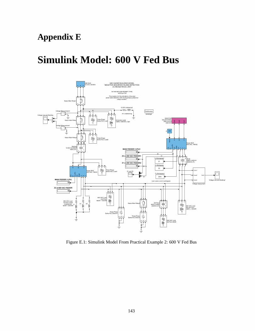
Appendix E
Simulink Model: 600 V Fed Bus
Figure E.1: Simulink Model From Practical Example 2: 600 V Fed Bus
143

Appendix F
Commonly Used Signal Processing
Techniques
Impulse response often takes significant signal processingto fully extract the wave forms and to cal-
culate the transfer function. A quick introduction on some of the most common signal processing
techniques used has been inserted here to facilitate the subsequent description of the techniques.
The most basic signal manipulation process can be seen in Figure F.1, which shows the paths for
calculating the transfer function of a system and breaking asignal into its individual frequencies. The
frequency domain transfer function,H(ejω) can be found from the input x[n] and the output y[n] through
convolution of the Fourier Transform. The most simple routeis to take the Fourier Transform of x[n]
and y[n] then divide the two as seen in equation F.2.
The discrete Fourier Transform is used to transform a time domain sampled signal to its frequency
domain representation. The transform is accomplished by calculating the sum of all the products of a
function at point “n” with the cosine wave and sine wave at point “n” with respect to a specific frequency.
All frequencies are set to the normalized interval between 0to 2π where 2π is equal to the sampling
frequency. The results for each frequency are real and imaginary values (Figure F.1). The squared sum
of the two values yields the magnitude of the specific frequencies.
X(ejω) =∞
∑n=−∞
x[n]ejωn (F.1)
x[n]convolution−−−−−−→
h(n)y[n]
F
xy
F
xy
X[e− jω]multiplication−−−−−−−→
H(e− jω)Y[e− jω]
Figure F.1: Convolution to Fourier Relationship
H(ejω) =Y(ejω)
X(ejω)=F (y[n])
F (x[n])(F.2)
y[n] =∞
∑k=−∞
x[k]h[n−k] = x[n]∗h[n] (F.3)
144
Appendix F. Commonly Used Signal Processing Techniques
Equation F.1 is for continuous infinite and requires an infinite time window. A sampled signal in
a finite window contains undesirable high frequency artifacts at the boundaries of the window. This
phenomenon is called the Gibbs Effect. To reduce the Gibbs Effect, a windowing function such as
Hamming and Hanning type windows can be multiplied onto the signal. These windows slowly taper
a signal’s amplitude at each end to zero, thereby diminishing the discontinuity and reducing the Gibbs
Effect. While all the windows listed effectively reduce theGibbs Effect, one of the most commonly
used is the Hamming window due to its consistently good results. Applying the window to a discretised
finite length sample results in Equation F.4,
X(ejω) =L
∑n=0
x[n]ejωn ·w[n] (F.4)
Power system frequency windowing is slightly different because the fundamental and its harmonics
are often significantly larger than all other non-harmonic signals being measured. The Gibbs effect can
be virually eliminated by carefully using a window the size of t = nf wheren is an integer value between
1 and inf, t is time and f is the frequency of the fundamental. This ensures that the sampling time
window exactlyfits an integer value of the fundamental. Therefore to maximize signal integrity using
Fourier Transform, windowing combined with specifically chosen time windows is critical. In some
cases a square window may be suitable.
Another common signal processing technique for improving signal-to-noise ratio and often used in
impedance measurement is cross-correlation [69]. The advantage of cross-correlation is that it matches
signal shapes regardless of the signal amplitude. For example, if two decaying sine waves of the same
frequency and different starting amplitudes are cross-correlated together, the strongest correlation occurs
when the start of the first wave matches the start of the secondwave. The formula for cross-correlation
is given in Equation F.5, where g and z are signals of the same length. The resultant output length is
2*M-1 where M is the length of the original two functions.
ψgz(τ) ≡∫ ∞
−∞g(t)z(t + τ)∂t (F.5)
Finally, an improved approach to using traditional Fast Fourier Transform (FFT) of voltage and
current is to use the MATLAB embedded function “transfer function estimation“ which uses Welch’s
averaged periodogram method [125]. Welch’s method auto-correlates and cross-correlates before using
an FFT to reduce the signal to noise ratio.
145