Tampereen teknillinen yliopisto. Julkaisu 1074 Tampere University of Technology. Publication 1074 Matti Isakov Strain Rate History Effects in a Metastable Austenitic Stainless Steel Thesis for the degree of Doctor of Science in Technology to be presented with due permission for public examination and criticism in Festia Building, Auditorium Pieni Sali 1, at Tampere University of Technology, on the 5th of October 2012, at 12 noon. Tampereen teknillinen yliopisto - Tampere University of Technology Tampere 2012

ISBN 978-952-15-2910-8 (printed) ISBN 978-952-15-2919-1 (PDF) ISSN 1459-2045

I

ABSTRACT

The mechanical behavior of metastable austenitic steels can be relatively complex in terms of temperature and strain rate sensitivity. This is connected to their low stacking fault energy and tendency towards martensitic transformations, which affect the dislocation slip characteristics and microstructural evolution in these materials during deformation. In this study, it is presented that the complex material behavior often reported in the literature can be rationalized in terms of the classical division of strain rate effects into instantaneous and evolutionary effects, which leads to the concept of strain rate history dependence. The behavior of metastable austenitic stainless steel EN 1.4318 was studied on the basis of this assumption. This thesis focuses on the mechanical testing at various strain rates and temperatures, but supplemental microstructural characterization results are presented in order to reveal the connection between the mechanical behavior and the microstructure. The mechanical tests involved measurements of the material behavior at strain rates ranging from 2·10-4 s-1 to 103 s-1 at temperatures -40 °C, +24 °C, and +80 °C. Low strain rate testing at strain rates below 100 s-1 was carried out with a servohydraulic materials testing machine, while high rate testing at 103 s-1 was done with a Tensile Hopkinson Split Bar (THSB) apparatus. Modifications that enabled rapid strain rate changes were introduced to the THSB setup. A momentum trap bar based modification was utilized in the measurement of the instantaneous strain rate sensitivity in the high rate region. Another modification involved the incorporation of a screw-driven low rate loading device to the THSB setup, which facilitated a change of over six decades in the specimen strain rate without the need of unloading the specimen and changing the test equipment. Microstructural characterization was based on the measurement of α’-martensite content in the deformed specimens using magnetic methods (Feritscope) and inspection of the deformation microstructures with a scanning electron microscope using the Electron Backscattered Diffraction analysis. The test results clearly demonstrate the soundness of the adopted approach. The apparent strain rate sensitivity deduced from the constant strain rate tests is negative due to the negative strain rate sensitivity of the strain hardening rate, which can be related to the reduced tendency of austenite to transform into α’-martensite at higher strain rates. In contrast, the instantaneous strain rate sensitivity is positive throughout the studied strain rate and temperature ranges, but shows a connection to the austenite stability. Moreover, the tests based on rapid strain rate changes reveal that the strain hardening and α’-martensite transformation rates decrease immediately after the strain rate increase. This feature cannot be explained solely by the macroscopic adiabatic heating, which in the literature is often used to explain the reduction of the transformation rate. An alternative explanation is sought from localized material heating taking place in the vicinity of newly formed α’-particles, which inhibits their further growth and coalescence. The existence of other inhibiting effects of strain rate on the α’-nucleation cannot, however, be excluded at this point.

II

III

PREFACE

This work was carried out at the Department of Materials Science of Tampere University of Technology during the years 2008-2012. Main funding was received from the Ministry of Education through the membership in the Graduate School Concurrent Engineering Tampere in 2008-2011. The author was also involved in industry related public research projects WHTank (2008-2009, funded by TEKES) and FABRICS (2010-2012, part of the FIMECC Demanding Applications Program). Notable funding was also received from the Technology Industries of Finland Centennial Foundation Fund for the Association of Finnish Steel and Metal Producers, Finnish Foundation for Technology Promotion, and TUT Foundation. The funding and resources provided by the above mentioned contributors are gratefully acknowledged. I wish to express my sincere gratitude to all the people who have helped me over the years. My supervisor, Professor Veli-Tapani Kuokkala guided me through the ups and downs of the world of research with his inspiring attitude, everlasting enthusiasm on exploring new things and personal commitment to my work. Members of the Graduate School CE Tampere and especially Professors Erno Keskinen and Michel Cotsaftis are gratefully thanked for the opportunity to see my work in a wider perspective. The contribution of the staff of the Outokumpu Tornio Works Tornio Research Centre and Raimo Ruoppa is acknowledged. I also wish to thank Professor Amos Gilat and his staff for hosting me during my stay at The Ohio State University and Mikko Hokka for the valuable help concerning the arrangements of the trip. The former and present personnel of the Department of Materials Science and especially the people working at the Laboratory of Materials Characterization are sincerely thanked for maintaining an atmosphere of kindness and collaboration. Kauko Östman contributed more to this work than I could have ever wished for by personally dedicating himself to helping me with the electron microscopy measurements. Like Kauko, Jari Kokkonen, Tuomo Saarinen, Turo Salomaa, Juuso Terva, and Ilari Jönkkäri all helped me in ways which extended from the laboratory through the coffee table far beyond the walls of the university. I can hardly imagine that I would have succeeded in my work without the creativity of Terho Kaasalainen and Ari Varttila during the construction of the test setups. Likewise, an idea of working with my thesis without the support from the Hopkinson group feels alien to me. Special thanks also to all the research assistants, who helped with the specimen preparation. I want to thank my long-time friends Ville, Eetu and Hanna for helping me to keep my feet on the ground along this path I have taken. Finally, I am deeply grateful to my parents for their love and support throughout my life. Tampere, September 2012 Matti Isakov

IV

AUTHOR’S CONTRIBUTION

The author carried out the literature research, planned the test program and carried out the mechanical tests of the test material. He also carried out the numerical simulations presented in this thesis. Magnetic measurements were carried out by the personnel at the Tornio Research Centre, Outokumpu Tornio Works according to the instructions of the author. Scanning electron microscopy (SEM) based measurements were carried out by Kauko Östman according to the instructions of the author. Final data processing and interpretation of the SEM results was carried out by the author. The author was involved, as part of a team (with Jari Kokkonen and Kauko Östman), in designing and constructing the temperature control systems and modifying the Tensile Hopkinson Split Bar for strain rate change experiments. The existing experimental setups and methods used in this study have been referenced in the text. The author analyzed the test results and wrote the original manuscripts of the related publications. The author’s findings and manuscripts were commented by his supervisor and by the co-authors. This thesis is the author’s original work and was commented by his supervisor.

V

CONTENTS

ABSTRACT ........................................................................................................................................ I PREFACE......................................................................................................................................... III AUTHOR’S CONTRIBUTION ...................................................................................................... IV LIST OF SYMBOLS AND ABBREVIATIONS............................................................................ VI 1 INTRODUCTION......................................................................................................................1 2 STRAIN RATE AND TEMPERATURE DEPENDENT PLASTICITY OF METALS.........3

2.1 Deformation of ductile metals...........................................................................................3 2.1.1 Deformation by dislocation motion .........................................................................3 2.1.2 Deformation-induced heating...................................................................................7 2.1.3 Concept of strain rate history ...................................................................................9

2.2 Plasticity of metastable austenitic stainless steels ......................................................... 10 2.2.1 Deformation microstructures in low SFE austenitic alloys.................................. 10 2.2.2 Mechanical behavior of low SFE austenitic stainless steels ................................ 15

3 METHODS FOR STRAIN RATE SENSITIVITY MEASUREMENTS ............................. 21 3.1 Testing methods for different strain rate regions........................................................... 21 3.2 Load relaxation tests....................................................................................................... 22 3.3 High strain rate tests with the Hopkinson Split Bar technique ..................................... 25

4 EXPERIMENTAL METHODS.............................................................................................. 31 4.1 Test material and general test methods.......................................................................... 31 4.2 Test setup for low strain rates ........................................................................................ 34

4.2.1 Constant strain rate and strain rate jump tests ...................................................... 34 4.2.2 Load relaxation tests.............................................................................................. 36

4.3 Test setup for high strain rates ....................................................................................... 38 4.3.1 Tensile Hopkinson Split Bar ................................................................................. 38 4.3.2 Momentum trapping based strain rate change tests with THSB .......................... 39 4.3.3 Incorporation of a low strain rate loading device to THSB.................................. 42

4.4 Simulations with the finite element method .................................................................. 45 4.5 Microstructural characterization .................................................................................... 46

5 RESULTS................................................................................................................................ 49 5.1 Low strain rate tests with different specimen geometries ............................................. 49 5.2 Constant strain rate tests at different strain rates and temperatures .............................. 53 5.3 Strain rate change tests ................................................................................................... 57 5.4 Yield point formation observed during mechanical testing .......................................... 65 5.5 Microstructural evolution............................................................................................... 67

5.5.1 Feritscope measurements....................................................................................... 67 5.5.2 EBSD measurements ............................................................................................. 69

6 DISCUSSION.......................................................................................................................... 77 6.1 Behavior of the material in terms of strain rate history dependence............................. 77 6.2 Microscopic aspects of material behavior ..................................................................... 80

6.2.1 Formation of strain-induced α’-martensite ........................................................... 80 6.2.2 Yield point formation ............................................................................................ 82 6.2.3 Instantaneous strain rate sensitivity ...................................................................... 83

7 CONCLUSIONS ..................................................................................................................... 89 7.1 Novel features................................................................................................................. 90 7.2 Suggestions for further studies....................................................................................... 90

REFERENCES................................................................................................................................. 92

VI

LIST OF SYMBOLS AND ABBREVIATIONS

αOC, nOC, βOC fitting parameters in the Olson-Cohen model β strain rate sensitivity parameter βT fraction of mechanical work of plastic deformation converted to heat γF fault energy per unit area γs surface energy per unit area Δd average distance moved by a dislocation between thermal activation events ΔGchem chemical free energy difference ΔG* Gibbs free energy of a thermal activation event ΔG0* Gibbs free energy of a thermal activation event in the absence of external

load ΔW* mechanical work done by external forces during a thermal activation event Δx distance moved by a dislocation segment during a thermal activation event ε strain εE engineering strain εp plastic strain

p plastic strain rate

0 reference constant in thermal activation theory θ strain hardening rate ν frequency of thermal activation events ν0 vibration frequency of a dislocation ρ density ρa molar density of atoms in a close-packed plane ρm density of mobile dislocations ρd density of dislocations σ stress σE engineering stress σA athermal component of flow stress σ* thermal component of flow stress τ* thermal part of shear stress acting on a slip system Ω atomic volume A cross-sectional area A* activation area b burgers vector of a dislocation bp burgers vector of a partial dislocation c specific heat capacity c0 propagation velocity of an elastic wave dx length of a material element E Young’s modulus Estr strain energy F force f phase volume fraction G shear modulus h internal heat release K stiffness k Boltzmann constant kT thermal conductivity

VII

L length of specimen gauge section under zero load L1 length of specimen gauge section under load Lg total length of specimen grip sections Ltr total length of the load train in a tensile test l length of a dislocation segment M geometrical factor relating dislocation slip to macroscopic plastic

deformation (Schmid factor) Ms starting temperature of thermal martensite Ms

σ starting temperature of stress-induced martensite Md starting temperature of strain-induced martensite m strain rate sensitivity parameter n thickness of an embryo q heat flow str general parameter describing microstructural dependence T temperature Tc critical temperature in thermally activated dislocation motion t time tw waiting time of a dislocation in front of a thermal obstacle tg gliding time of a dislocation between thermal obstacles u displacement V* activation volume v particle velocity wp mechanical work of plastic deformation done to a material element BCC body centered cubic DP dual phase EBSD electron backscatter diffraction FCC face centered cubic FEM finite element method HSB Hopkinson split bar K-S Kurdjumov-Sachs orientation relationship ND normal direction RD rolling direction RT room temperature SEM scanning electron microscope SFE stacking fault energy TEM transmission electron microscope TRIP transformation induced plasticity TWIP twinning induced plasticity TD transverse direction THSB tensile Hopkinson split bar

VIII

1

1 INTRODUCTION

The capability of metals to undergo extensive plastic deformation is one of the key contributors to the development of modern technology. Applications ranging from everyday utility articles to sophisticated impact energy absorbing components in automobiles all benefit from the microstructural phenomena, which lead to good strain hardening capability, ductility and high strength. However, in general this combination of mechanical properties is a compromise between individual properties, often exemplified by the inverse relationship between strength and ductility. Advances in the field of metallurgy have shown that the envelope of properties can be expanded by creating complex microstructures, which can consist of multiple phases or even undergo phase transformations during deformation. Modern examples of low alloyed steels utilizing a heterogeneous microstructure are, for example, Dual Phase (DP) steels and Transformation Induced Plasticity (TRIP) steels. In the former, the soft ferrite phase is strengthened with hard martensite islands, while in the latter an initially complex microstructure (ferrite, martensite, bainite and austenite) is further developed when the retained austenite transforms into α’-martensite during plastic deformation. In Twinning Induced Plasticity (TWIP) steels, on the other hand, microstructural refinement occurs not by phase transformation but by twinning in the austenitic microstructure. In TWIP steels, the stable austenitic microstructure at room temperature is obtained by heavy alloying with manganese. Other commonly used highly alloyed steels are austenitic stainless steels based on the classical 18Cr–8Ni wt.% composition. Although often chosen because of their excellent corrosion resistance, these steels are also used in applications requiring good mechanical properties, such as deep drawing, due to the inherently good ductility and strain hardening capability of the austenitic microstructure. The austenite phase in these steels, however, is generally metastable and can transform to martensite at sufficiently low temperatures especially when aided by external stress or plastic deformation. The composition of certain grades, such as EN 1.4318, is especially designed so that the strain-induced austenite to α’-martensite transformation takes place during room temperature plastic deformation, which leads to a notable increase in the strain hardening capability of the material. In somewhat more stable alloys the phase transformation works beneficially by postponing the onset of localized plastic flow and thus increasing the formability of the material. In addition to martensitic transformation, the generally low stacking fault energy of these steels facilitates also twinning during plastic deformation. Due to the high temperature sensitivity of both stacking fault energy and austenite stability, a particular alloy can show both stable and highly metastable behavior over a relatively narrow temperature region of only ~100 °C. In addition, since the initial microstructure is fully austenitic, the fraction of transformed material can reach nearly 100 %. Even though the compositions and microstructures of the above mentioned steels vary considerably, they have one thing in common; the more heterogeneous is the microstructure and the more complex are the deformation mechanisms, the more complex is the dependence of the material behavior on the deformation conditions, such as temperature and strain rate. That is, since the microstructure consists of several phases, the correctness of the analysis based on the “average grain” behavior is reduced. In addition, since the plastic deformation behavior is no longer necessarily governed solely by ordinary dislocation slip, but competing mechanisms, such as twinning, may also activate, the strain rate and temperature dependence can be different from those generally observed in metals. Another

2

factor that should be taken into account is that the microstructural evolution, which directly affects the material behavior, can be notably sensitive to the deformation conditions. This kind of sensitivity brings about the effect of deformation history on the material behavior, which means that not only the current deformation conditions affect the material behavior but also the preceding conditions of plastic deformation have to be accounted for [1-8]. In the above mentioned steels undergoing phase transformations during plastic deformation, one would expect these history effects to be likely. The fact that the mechanical behavior of advanced structural steels can be complex and that they are often used in demanding applications, such as in the automotive industry, undoubtedly underlines the need for their extensive mechanical testing. One of the main test parameters arising from the applications is the strain rate, but equally important is the control of temperature, not only due to application specific reasons but also due to the inherent linkage between strain rate and temperature in the mechanics of plastic deformation. Materials testing at wide ranges of strain rate with simultaneous temperature control is challenging, requiring special techniques and sophisticated test equipment. Further challenges are brought about by the possible deformation history dependence of the material behavior, which necessitates critical analysis of the results and often additional testing to clarify the overlapping effects of several test parameters. In this work the mechanical behavior of metastable austenitic stainless steel EN 1.4318 was studied from the perspective of deformation history dependence of the material behavior. An extensive mechanical testing program was carried out in uniaxial tension both at low and high strain rates at varying temperatures, supplemented by magnetic permeability and Electron Backscatter Diffraction (EBSD) measurements on selected specimens. The results are first used to show conclusively that the test material is notably strain rate history dependent. The discussion of the results is then continued by dividing the strain rate effects into instantaneous and evolutionary effects. The classical concept of thermally activated dislocation motion is used to analyze the former, while the latter is discussed in terms of the effects of α’-martensite transformation. For materials testing at high strain rates, the Hopkinson Split Bar technique [9] was used. The existing setup at Tampere University of Technology [10, 11] was modified for strain rate jump testing both within the high strain rate region and between the low and high strain rates. These modifications as well as their theoretical backgrounds are discussed in detail. In addition to the primary focus of the study, additional findings, including the effect of specimen geometry on the thermal boundary conditions as well as the possible occurrence of strain aging, are presented and discussed. This thesis is a monograph, but parts of the results have already been published elsewhere by the author [12-15].

3

2 STRAIN RATE AND TEMPERATURE DEPENDENT PLASTICITY OF METALS

2.1 Deformation of ductile metals

The plastic deformation of ductile metals is essentially governed by the motion and mutual interactions of dislocations. The influence of deformation conditions, such as temperature and strain rate, on the momentary material strength can be directly related to the ease at which the mobile dislocations can move. The traditional approach to explain strain rate and temperature dependency is discussed in Chapter 2.1.1, which presents the concept of thermally activated dislocation motion. One of the characteristic features of plastic deformation is that even though part of the mechanical work done to deform the material is stored in the microstructure (such as in the energy required to generate new dislocations), major part of the used energy is dissipated as heat. This means that in many practical applications as well as in laboratory scale testing the possible effects of material temperature increase have to be accounted for. This is discussed in Chapter 2.1.2. The general discussion of plastic deformation is concluded in Chapter 2.1.3 with the discussion of deformation history dependent material behavior. This concept arises naturally from the effects of deformation conditions on the microstructure development and can sometimes have a significant importance, when the strain rate and temperature dependence of the material behavior is analyzed.

2.1.1 Deformation by dislocation motion

During plastic deformation by dislocation slip, any obstacle hindering the motion of a dislocation can be defined as an entity, which either momentarily or permanently increases the free energy of the crystal when the dislocation surmounts it. The net effect of the obstacle on free energy can be a permanent increase (such as the increase of dislocation length by jog formation or the formation of new dislocations or dislocation pile-ups) or a temporary increase and then decrease (such as overcoming the periodic lattice friction or Peierls stress) of the energy. The strength of ductile metals is observed to increase with increasing strain rate and/or with decreasing temperature (note: this study is concentrated on the plastic deformation occurring at low homologous temperatures and at strain rates over 10-4, i.e., analysis of long-term phenomena, such as creep, is outside the scope of this work). The classical approach described in many text books [e.g., 16] to explain the observed behavior is the concept of thermally activated dislocation motion. According to this theory, the external stress required to cause plastic deformation by dislocation slip is divided into athermal (σA) and thermal (σ*) parts, as described in Equation 1 and illustrated in Figure 1: pA Tstrstr ,,* (1)

4

TcT

σA

σ

σ*pε

Figure 1. Schematic illustration of the temperature (T) and strain rate )( p dependence of the flow

stress components. Modified from [16]. In Equation 1 and in the following equations, str is used to indicate that the respective terms are dependent on the microstructure of the material. The athermal part of the flow stress represents obstacles, whose free energy increase is so high that the available thermal energy does not have a significant contribution to the slip process during any practical time span. Instead, the energy needed to surmount the obstacles is solely provided by the external work imparted to the dislocations. Examples of these obstacles are long range stress fields in the crystal and break-up of attractive dislocation junctions, which permanently increase the energy stored in the microstructure. In contrast, the thermal part of the flow stress represents obstacles, whose surmounting can be aided by thermal energy, i.e., part of the free energy increase is provided by thermal energy. Examples of these are overcoming the lattice friction and the formation of jogs in the intersecting dislocations (repulsive junctions). At a sufficiently high temperature thermal energy is constantly available so that all thermal obstacles are surmounted without the need of external work. Above this critical temperature Tc the material strength shows no dependence on temperature (except due to the effect of shear modulus change on obstacle strength) or strain rate. Between 0 K (where thermal energy is absent) and Tc the material strength shows negative temperature and positive strain rate dependence. Positive strain rate dependence is explained by the statistical nature of thermal energy, i.e., there exists a certain probability that enough thermal energy is available for the glide dislocation within a time frame relevant to the strain rate. A characteristic feature of thermally activated dislocation motion is that the glide time between successive obstacles (tg) is insignificant compared to the waiting time (tw) spent in front of an obstacle. This means that the strain rate during thermal activation is governed by the average time needed for a successful activation event, or to put it other way around, by the frequency of activation events (ν):

dbMt

db

M mw

mp

11

(2)

In Equation 2 M represents a geometrical factor relating dislocation slip to the macroscopic plastic deformation, ρm is the density of mobile dislocations, b is the burgers vector of a dislocation, and Δd is the average distance moved by the dislocation during and after a successful activation event before it is stopped by another obstacle. The activation frequency can be described using the Boltzmann distribution:

5

kT

G

e*

0

(3) In Equation 3 ν0 is the vibration frequency of a dislocation, k is the Boltzmann constant, and ΔG* is the Gibbs free energy required for the activation event. Insertion of Equation 3 into Equation 2 yields:

kT

G

kT

G

mp eedbM

*

0

*

01

(4)

Equation 4 describes how increasing temperature promotes thermally activated slip, but it also shows the importance of the obstacle size (in terms of free energy increase) in determining the activation frequency. The free energy increase does not have to come solely from thermal energy, but the mechanical work ΔW* done by the external load contributes to the process. To analyze this, an ideal thermal obstacle is considered. At a certain temperature in the absence of external stress, the free energy increase would be ΔG0*. Thus, under an external load the required thermal energy contribution is reduced by ΔW*: *** 0 WGG (5) In order to calculate the amount of mechanical work ΔW*, a segment of dislocation is considered. The length of the segment is denoted by l, the force exerted on the dislocation per unit length is τ*b (here only the thermal part of the flow stress is considered) and during the activation process the segment of the dislocation moves a distance denoted by Δx. Therefore, the amount of mechanical work is given by:

**

**

** VM

bAM

xblW (6)

The quantities A* and V* are called the activation area and activation volume, respectively. When Equation 4 is solved for ΔG* and Equations 1, 5 and 6 are inserted to the result, a relationship between strength, temperature and strain rate is obtained:

p

kTG

0ln* (7)

p

kTVM

G

00 ln*

** (8)

00

00 ln*

*ln*

**

p

p

kTGV

MkTG

V

M (9)

00 ln*

*

pA kTG

V

M (10)

6

Equation 10 is in accordance with experimental observations when 0 p , that is,

kTG * (when thermal obstacles have a significant contribution to strength). Equation 10 can also be used to derive the basic principles for an experimental method to study thermal activation. When strain rate is suddenly forced to change during deformation, a change in the material strength is observed. If the strain rate change is rapid enough compared to the average strain rate and the type of the deformation mechanism is not changed, Equation 10 can be assumed to be valid immediately before and after the jump:

0

10

0

20

12

ln**

ln**

pA

pA kTG

V

MkTG

V

M (11)

120

1

0

2lnln

*lnln

* pppp

kTV

MkT

V

M

(12)

kTV

M

p *ln

(13)

According to Equation 13, experimentally measured strain rate sensitivity can be directly related to the activation volume of the thermal activation process, if the other terms, such as

0 and ΔG0*, remain unaffected. Often it is experimentally more convenient to work with a 10-base logarithm than with the natural logarithm. In that case the strain rate sensitivity parameter β is defined as:

p

10log

(14)

Another often used strain rate sensitivity parameter m is defined as:

pp

m

10

10

log

log

ln

ln

(15)

It is often observed that at strain rates near 1000 s-1 or higher the strain rate sensitivity of the material strength starts to increase. This has been depicted as a change of rate controlling mechanism from thermal activation to so-called dislocation drag effects. In these conditions the flow stress becomes proportional to strain rate (instead of logarithmic dependence) and the material can be modeled as a Newtonian fluid. This is explained by noting that the stress acting on dislocations is higher than the resistance of glide obstacles, which sets the dislocations in an accelerating motion, which in turn causes additional resistance to their motion (such as the emission of phonons). [16] The discussion presented above applies to material behavior at constant microstructure, i.e., the dependence of strength on temperature and strain rate is evaluated in terms of instantaneous effects. However, the deformation conditions may also have evolutionary effects on the material behavior. Basically the development of the material microstructure

7

during deformation can be influenced by temperature and strain rate. An experimentally convenient method to evaluate the microstructure development during deformation is the measurement of the strain hardening rate (θ):

),,(*

),,( pp

pp

a

p

Tstrd

dTstr

d

d

d

d

(16)

Equation 16 depicts an important aspect noted by previous investigators [1, 2, 17, 18]: even though the instantaneous overcoming of athermal obstacles is independent of temperature and strain rate, the development of these obstacles can be influenced by the deformation conditions. An example of this are dislocation pile-ups, which cause long range stress fields and are thus athermal obstacles, but their formation and stability depends on dynamic recovery, which is a thermally activated process.

2.1.2 Deformation-induced heating

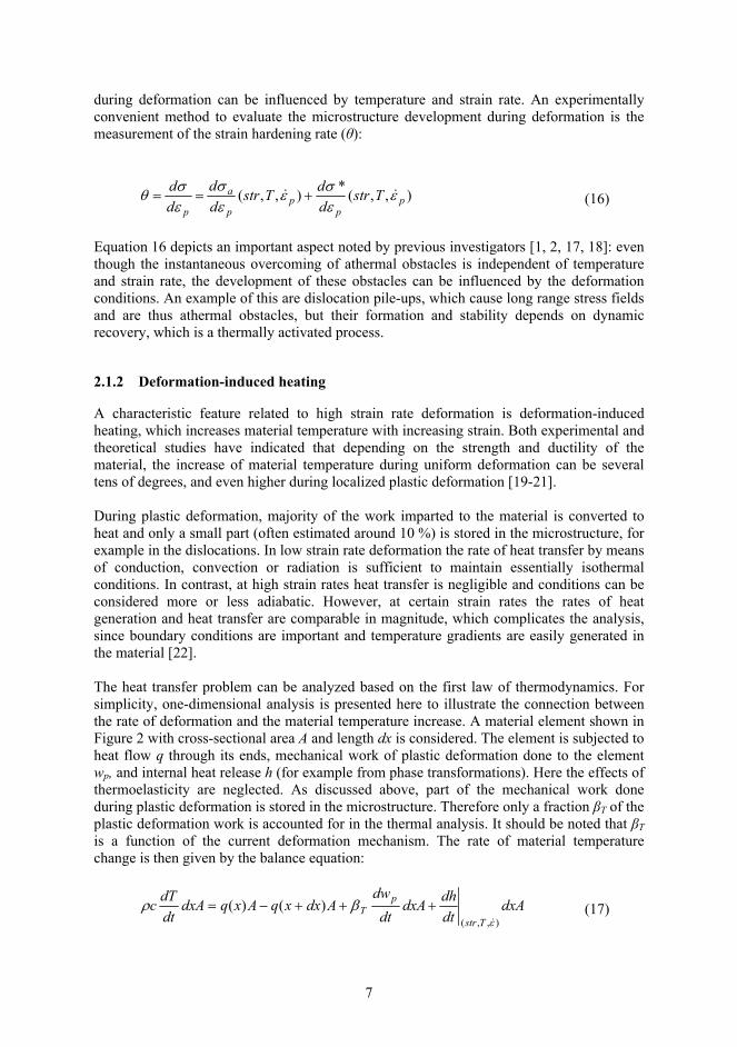
A characteristic feature related to high strain rate deformation is deformation-induced heating, which increases material temperature with increasing strain. Both experimental and theoretical studies have indicated that depending on the strength and ductility of the material, the increase of material temperature during uniform deformation can be several tens of degrees, and even higher during localized plastic deformation [19-21]. During plastic deformation, majority of the work imparted to the material is converted to heat and only a small part (often estimated around 10 %) is stored in the microstructure, for example in the dislocations. In low strain rate deformation the rate of heat transfer by means of conduction, convection or radiation is sufficient to maintain essentially isothermal conditions. In contrast, at high strain rates heat transfer is negligible and conditions can be considered more or less adiabatic. However, at certain strain rates the rates of heat generation and heat transfer are comparable in magnitude, which complicates the analysis, since boundary conditions are important and temperature gradients are easily generated in the material [22]. The heat transfer problem can be analyzed based on the first law of thermodynamics. For simplicity, one-dimensional analysis is presented here to illustrate the connection between the rate of deformation and the material temperature increase. A material element shown in Figure 2 with cross-sectional area A and length dx is considered. The element is subjected to heat flow q through its ends, mechanical work of plastic deformation done to the element wp, and internal heat release h (for example from phase transformations). Here the effects of thermoelasticity are neglected. As discussed above, part of the mechanical work done during plastic deformation is stored in the microstructure. Therefore only a fraction βT of the plastic deformation work is accounted for in the thermal analysis. It should be noted that βT is a function of the current deformation mechanism. The rate of material temperature change is then given by the balance equation:

dxAdt

dhdxA

dt

dwAdxxqAxqdxA

dt

dTc

Tstr

pT

),,(

)()(

(17)

8

In Equation 17 c and ρ are the specific heat capacity and density of the material, respectively. As indicated in Equation 17, heat release h within the material can be a complex function of the microstructural state and deformation conditions.

A

dx

q(x+dx)q(x)

wh

p

Figure 2. Material element subjected to heat flow, plastic deformation and internal heat generation. By assuming uniaxial loading and that the heat flow q is given simply by Fourier’s law with constant thermal conductivity kT, Equation 17 can be simplified as (heat transfer can also be formulated in terms of convection or radiation):

x

Tkxq T

)( (18)

dxx

qxqdxxq

)()( (19)

dt

dh

dt

d

x

Tk

dt

dTc p

TT

2

2

(20)

Due to its complexity, it is difficult to find a general analytical solution for Equation 20. Another aspect is that during plastic deformation the material volume is subjected also to a shape change and often three-dimensional heat flow, which were not accounted for in the above presented derivation. Therefore, numerical methods, such as finite element method, are commonly used in solving thermomechanically coupled problems. Equation 20 can, however, be used to evaluate the general features of deformation induced heating. One of the most important features of Equation 20 is that it shows how the thermal problem is dependent on the physical dimensions of the deforming volume and its surroundings, which is in contrast to the mechanical problem (stress and strain are essentially size independent in macroscopic scale, as long as the material is deforming uniformly). Temperature increase with respect to plastic strain increment can be obtained by dividing Equation 20 with plastic strain rate:

p

Tp

T

p d

dh

x

Tk

d

dTc

2

2

(21)

The first term on the right hand side of Equation 21 indicates a negative effect of strain rate on the net heat transfer during unit strain increment. However, the rate of heat transfer away from the material increases with increasing temperature difference between the deforming material and its surroundings. This is a further complicating factor, because basically it implies that a certain increase in the material temperature is always required for heat transfer to take place. At low strain rates this required temperature increase is, however,

9

very small and the conditions are essentially isothermal. On the other hand, at high strain rates the first term in Equation 21 is negligible despite the rapidly increasing temperature gradient. In this case the temperature increase in the material can be solved by simple integration (neglecting the internal heat release):

pT dc

Tp

0

1 (22)

Equation 22 is often used when high rate deformation is analyzed and, as noted above, it is based on the assumption of fully adiabatic conditions. As discussed above, analysis of the deformation-induced heating and its effects on the material behavior is complex at strain rates, where heat transfer takes place but is insufficient to maintain material temperature within a few degrees from the initial. In these cases the evolution of material temperature becomes dependent not only on the thermal properties of the test material but also on the physical dimensions of the deforming volume and thermal boundary conditions [22].

2.1.3 Concept of strain rate history

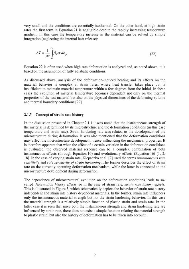
In the discussion presented in Chapter 2.1.1 it was noted that the instantaneous strength of the material is determined by its microstructure and the deformation conditions (in this case temperature and strain rate). Strain hardening rate was related to the development of the microstructure during deformation. It was also mentioned that the deformation conditions may affect the microstructure development, hence influencing the mechanical properties. It is therefore apparent that when the effect of a certain variation in the deformation conditions is evaluated, the observed material response can be a complex combination of both instantaneous effects (through Equation 10) and evolutionary effects (Equation 16) [1, 2, 18]. In the case of varying strain rate, Klepaczko et al. [2] used the terms instantaneous rate sensitivity and rate sensitivity of strain hardening. The former describes the effect of strain rate on the currently operating deformation mechanism, while the latter is connected to the microstructure development during deformation. The dependence of microstructural evolution on the deformation conditions leads to so-called deformation history effects, or in the case of strain rate, strain rate history effects. This is illustrated in Figure 3, which schematically depicts the behavior of strain rate history independent and strain rate history dependent materials. In the former, strain rate influences only the instantaneous material strength but not the strain hardening behavior. In this case the material strength is a relatively simple function of plastic strain and strain rate. In the latter case it is seen that since both the instantaneous strength and strain hardening rate are influenced by strain rate, there does not exist a simple function relating the material strength to plastic strain, but also the history of deformation has to be taken into account.

10

σ σ

εp εpε0 ε0ε1 ε1

a) b)

p2εp2ε

p2εp1ε p1ε

p1ε

p1p2 εε p1p2 εε

Figure 3. Schematic illustration of a) strain rate history independent and b) strain rate history dependent material behavior. Broken lines depict constant strain rate flow behavior at two different strain rates and solid lines flow behavior when strain rate is suddenly increased at ε0 and subsequently decreased at ε1. Modified from [16]. Several studies have been published on the strain rate history sensitivity of various materials [1-8, 23]. A general conclusion that can be drawn from these studies is that the appearance of history effects is strongly dependent on the operating deformation mechanism and in this way on the material at hand. Furthermore, a material can show both history independent and history dependent behavior depending on the deformation conditions and the amount of plastic strain [5, 8].

2.2 Plasticity of metastable austenitic stainless steels

In the previous Chapters, the general features of the strain rate and temperature dependent plasticity of ductile metals were discussed. In the following, the behavior of austenitic steels with low stacking fault energy (SFE) is described. Even though the basic principles still apply, the dissociation of the primary glide dislocations into two partial dislocations and the resulting stacking faults have a profound effect on the material behavior. The situation is further complicated by the fact that the austenitic phase with a face centered cubic (FCC) crystal structure is thermodynamically only in a metastable equilibrium near room temperature and can be triggered to transform into the more stable nearly body centered cubic (BCC) α’-martensite by mechanical stimulus. Therefore the discussion is first started by describing the various microstructural features of low SFE austenitic alloys in Chapter 2.2.1, after which the current knowledge on the strain rate and temperature sensitivity of these metals is reviewed in Chapter 2.2.2. Even though this thesis concentrates on the behavior of metastable austenitic stainless steels, studies on other austenitic alloys have also been referred to when found applicable.

2.2.1 Deformation microstructures in low SFE austenitic alloys

Many of the microstructural features of austenitic alloys have their origin in the elementary reaction of dislocation dissociation. In this reaction the original glide dislocation in the FCC lattice is dissociated into two Shockley partials, i.e.,

2116

1126

0112

aaa (23)

11

In terms of the elastic strain energy of dislocations, the dissociation is favored since the total strain energy stored in the dislocations (~Gb2) is reduced by the dissociation. The two partials are of the mixed type, i.e., they have both screw and edge components even if the original dislocation was purely an edge or a screw. The two screw components have opposite signs and thus attract each other, while the edge components have equal signs and repel each other. A simple geometrical consideration shows that the area bounded by the two partials has a faulted stacking sequence, i.e., the original FCC stacking of 111γ planes ...ABCABCABC... is shifted to ...ABCACABCA... by the leading partial and back to normal stacking by the trailing partial. This stacking fault represents a distortion of the lattice and thus consumes energy, commonly referred to as the stacking fault energy or SFE. In the elementary theory the width of the stacking fault is determined by the balance of the net repulsive force between the partials and the energy stored in the fault (dependent on the SFE of the material). However, for example Byun [24] noted that the partial dislocations have different Burgers vectors and thus the resolved shear stress acting on the partials due to external loading can be different. Therefore the width of the stacking fault is not only dependent on the SFE but also on the acting stress. Furthermore, on a microscopical level the equilibrium width can vary considerably due to the presence of local stress concentrators. Based on his analysis Byun [24] predicted a critical stress level at which the stacking fault width diverges and approaches infinity, or in practice, the grain size. At this point large stacking fault based features would appear in the microstructure. This prediction was supported by the microstructural observations of Talonen et al. [25, 26]. One of the main consequences of the dissociation of a perfect dislocation is the planarity of slip due to the inhibition of cross-slip. This is caused by the edge components of the partials, which effectively tie the partials to the original 111γ slip plane. Another consequence is the creation of various microstructural features based on stacking faults. As noted for example by Lee et al. [27], a single stacking fault is surrounded by two one-layer thick nanotwins on adjacent slip planes (...ABCACABCA... and ...ABCACABCA...). A single stacking fault is called intrinsic, because one atomic layer (in this case “B”) is missing from the normal sequence. However, if another stacking fault is formed on the plane on top of the faulted plane, the sequence becomes ...ABCACBCAB.... This fault is called extrinsic, because it can be interpreted to contain one extra “C” –plane. As can be seen, an extrinsic stacking fault is surrounded by two two-layer thick nanotwins (...ABCACBCAB.... and ...ABCACBCAB....). Successive overlapping of stacking faults on every plane leads to thickness growth of the two nanotwins [27]. In addition to the two nanotwins, an intrinsic stacking fault contains a one layer thick nucleus of hexagonal ε-martensite characterized by ...ACACAC... stacking [28]. If stacking faults continued to be overlapped on every second plane, the ε-martensite nucleus would grow in thickness [27, 29, 30]. Since the above described microstructural features have a common origin and they are difficult to distinguish from each other, especially in imperfect cases, often a collective term “shear band” is used to describe dense bundles of overlapping stacking faults and more or less perfect ε-martensite and twins [e.g., 26, 31, 32]. The term “shear band” used here should not be confused with the macroscopic shear bands observed in certain materials especially during high rate loading (i.e., “adiabatic shear bands”). Several studies have shown that the nucleation of strain-induced α’-martensite is strongly related to the partial dislocation motion on 111γ planes. The intersection volumes of two shear bands (consisting of ε’-martensite, twins, or more or less random arrays of stacking faults) on different slip planes [31, 33-42], single shear bands [38, 39, 41], shear band –

12

grain boundary / annealing twin boundary –intersections [34, 39, 40] as well as dislocation pile-ups [30, 43] and grain boundary triple points [39] have been identified as nucleation sites for strain-induced α’-martensite. The term “strain-induced” is used to distinguish the phenomenon from spontaneous martensitic nucleation during cooling, and from stress-assisted nucleation occurring below the yield strength of austenite. This is illustrated in Figure 4, which reproduces the classical representation of the temperature and stress dependence of α’-martensite nucleation first published by Olson and Cohen [44]. As indicated in Figure 4, strain-induced α’-martensite transformation occurs at temperatures between Ms

σ and Md at stress levels exceeding the initial yield strength of the parent phase, while between Ms and Ms

σ applied stress below the yield strength of austenite assists the chemical driving force. Below Ms, spontaneous transformation occurs without the need for external loading. The main difference between spontaneous, stress-assisted, and strain-induced α’-martensite formation is that in the latter case the nucleation sites are created during plastic deformation of the austenite phase. In addition, continued plastic deformation is required for the increase of the volume fraction of strain-induced α’.

Temperature

Str

ess

Ms Ms

σMd

Yield strength of austenite(initial yielding by slip)

Strain-inducednucleation

Str

ess-

assi

sted

nuc

leat

ion

(Ini

tial y

ield

ing

by

tran

sfor

mat

ion)

Figure 4. Schematic representation of the temperature and stress dependence of α’-martensite nucleation. After [44]. Various mechanisms have been proposed for the nucleation of strain-induced α’-martensite. Mangonon and Thomas [34] considered a transformation from ε- to α’-martensite under biaxial compressive stress. Olson and Cohen [44] analyzed a case of intersecting slip bands, one of which contained an array of partial dislocations on every third plane while on the other band partial dislocations were stacked on every second plane (hexagonal ε-martensite stacking). Olson and Cohen [44] postulated that in the slip band intersection the cores of the individual partial dislocations are spread on multiple planes so that correct BCC stacking is obtained according to the Bogers and Burgers model [45] for the FCC→BCC transformation. Furthermore, the formation of BCC α’-martensite in the intersection allows the partial dislocations to glide through the intersection. Allowing for the more or less random structure of real slip bands, Olson and Cohen [44] postulated that BCC nucleation will take place if the ideal arrangement can be obtained by atomic plane “shuffling” and dislocation core spreading during the process. Lagneborg [33] proposed that the core volumes of partial dislocations, in which the atomic stacking is close to BCC, would act as α’-martensite nucleation sites. Brooks et al. [28, 30] suggested in more general terms that α’-nucleation can take place in any dislocation configuration, such as a pile-up, where the atomic structure resembles the BCC structure. Lecroisey and Pineau [35] stated that α’-

13

nucleation will take place whenever it locally provides an easier mode of deformation, and gave an example of a partial dislocation intersecting a twin boundary, which resulted in α’-nucleation and propagation of slip on one of the twinned planes. The propagation of slip through an intersecting slip band via α’-martensite transformation was confirmed by the in situ transmission electron microscopy (TEM) experiments of Suzuki et al. [36]. In addition, Murr et al. [31, 37] observed that the shear band intersection volumes were not uniformly transformed to α’-martensite, which they related to the local deviations from the ideal transformation conditions. There does not seem to be a clear consensus in the literature whether ε-martensite is a necessary intermediate phase, which can be readily detected when γ transforms to α’ [34, 41, 46, 47], or if ε and α’ can also form independently from γ [35 , 36, 39, 43, 48-52]. The analysis is complicated by the fact that various characterization techniques (ranging from TEM and EBSD to x-ray diffraction ) have been used and, as noted above, the structure of the shear bands is often a fine-scaled complex mixture of perfect and faulted elementary structures, which have the same basic constituent (single stacking fault). Indeed, in many studies [35, 36, 39, 49, 50], where the existence of ε-martensite has not been concluded as a prerequisite for α’-nucleation, shear bands (twins, bundles of stacking faults) have still been identified as nucleation points for α’. It appears that even though the actual structure of shear bands varies according to the stability of their constituent elements (e.g., ε-martensite versus mechanical twins), the nucleation of α’ remains closely connected to the formation of shear bands during plastic deformation. In general it is agreed that the strain-induced α’-embryos are close to the Kurdjumov-Sachs (K-S) orientation relationship [e.g. 33-35, 41, 53], i.e., that the following relationships hold within a couple of degrees for one pair of planes and directions:

'

'

111||110

110||111

(24)

Previous transmission electron microscopy studies [35, 36, 42] indicate that the plane satisfying the K-S relation is parallel to one of the shear band planes while the K-S direction is usually parallel to the intersection line of the shear bands and thus parallel to the long axis of the α’-embryo. Based on the in situ experiments by Suzuki et al. [36] and further observations, Murr et al. [31, 37] postulated that the growth of α’-martensite occurs by repeated nucleation and coalescence of individual embryos. They also noted that even though the early appearance of α’-martensite is lath-like, due to the nature of the growth mechanism the resulting α’-particle may have an irregular polyhedral appearance especially when several different slip systems are activated. Hedström et al. [43] stated that at high α’-martensite volume fractions growth of the existing embryos becomes energetically more feasible than the nucleation of new embryos. They also proposed that the growth of α’ in one grain could also induce γ→α’ transformation in the surrounding grains. The models described above concentrate on the atomic motion needed for coherent α’-embryo nucleation without paying attention to the further accommodation of the α’-phase and possible relief of coherency strains. Experimental characterization of the internal structure of strain-induced α’-martensite is complicated by the small scale of the

14

nucleated embryos and by the fact that continued plastic deformation, which can affect the already existing α’-martensite, is needed for further growth of the phase. Nevertheless, experimental evidence indicates that the strain-induced α’-martensite is heavily faulted and contains a notably higher dislocation density than the parent γ-phase [25, 48, 54]. As a further evidence, using high resolution transmission electron microscopy, Inamura et al. [42] were able to detect interfacial dislocations inside a nanometer-sized α’-particle. Hedström et al. [43] proposed, based on γ-lattice strain measurements, that the initial coherency between austenite and martensite is gradually lost with increasing α’-particle size. Another aspect not yet discussed is the thermodynamic feasibility of the phenomena described above. As noted before, the elementary dislocation dissociation is controlled by the intrinsic SFE of the material, which has been found to decrease with decreasing temperature [11, 35, 55]. In addition, the chemical driving force for the γ→α’ phase transformation increases with decreasing temperature. However, the above discussed crystallographic strain-induced features (twins, ε- and α’-martensite) require additional considerations. The conditions for twin and ε-martensite formation were discussed by Lecroisey and Pineau [35]. They analyzed a case of active slip on a 111γ plane inducing a stacking fault on an intersecting 111γ plane, which already contained a stacking fault. Twin nucleus formation was taken to depend on the extrinsic stacking fault energy (energy required for the overlapping of two intrinsic stacking faults), while ε-martensite formation depended on the free energy difference between the γ- and ε-phases, which was also rationalized in terms of stacking fault energy. They also accounted for the strain energy related to the slight contraction normal to the basal plane during ε-phase nucleation and for the influence of local stress (either promoting or hindering the contraction). Based on their analysis, Lecroisey and Pineau [35] concluded that the deformation structures depend strongly on the stacking fault energy and that ε-martensite formation takes place at temperatures lower than twin formation, but an intermediate temperature range exists where the reaction depends on the local stress and hence both twins and ε-martensite are observed. These observations were later confirmed for a variety of alloys by Remy and Pineau [56, 57]. Another aspect of the nucleation phenomena was brought up by Fujita et al. [29], who observed during in situ TEM experiments that wide stacking faults induce the formation of other stacking faults on nearby slip planes. Furthermore, they observed that ε-phase was formed by a gradual change of irregular overlapping of stacking faults to a regular overlapping process on every second slip plane. This was related to the minimization of both the bulk free energy and the total energy stored in the stacking faults [29, 30]. Using the classical nucleation theory, Olson and Cohen [58, 59] formulated a simple approach to evaluate the stability of the above described microstructural features. The fault energy per unit area (γF) was formulated to consist of the molar chemical free energy difference between the parent and product phases (ΔGchem), molar strain energy (Estr), and surface energy per unit area (γs):

)(2)( nEGn sstrchem

AF (25) where ρA is the molar density of atoms in the 111γ plane and n is the thickness of the embryo. As noted in Equation 25, the molar chemical free energy difference and molar strain energy are assumed to be thickness independent, but the surface energy is allowed to

15

depend on the thickness of the embryo. The total energy associated with a particular embryo (such as ε- or α’-martensite) can decrease with increasing thickness, if the volume energy contribution (the sum of chemical free energy change and strain energy) is negative. Then, when the total energy reaches zero, the embryo will form spontaneously [58, 59]. This condition can also be used to calculate the minimum thickness of a stable strain induced α’-martensite embryo, if the other terms in Equation 25 are known. Using Equation 25, Staudhammer et al. [37] were able to calculate a critical thickness, which corresponded to their experimental findings (in the studied case 50-70 Å, or around 30 close-packed planes). In practice the thermodynamic data is limited, which hinders exact calculations. However, the main finding of the above presented treatment is that α’-martensite cannot nucleate on single stacking faults or thin shear bands, but a minimum shear band thickness is required before stable embryos form. Equation 25 also indicates a relationship between the stacking fault energy and the chemical driving force for ε-martensite nucleation, when a single stacking fault is considered as a one layer thick ε-martensite embryo [11, 58]. Another thermodynamic model for α’-martensite nucleation taking into account local stresses due to dislocation pile-ups was presented by Suzuki et al. [36]. They proposed that the nucleation is restrained by the coherent interfacial energy between the phases (which they neglected for small embryos) and by the elastic strain energy due to the misfit between the embryo and the parent lattice. The nucleation is promoted by the difference in Gibbs free energy between the phases and by the interaction energy between the nucleus and a dislocation pile-up in the austenite [36].

2.2.2 Mechanical behavior of low SFE austenitic stainless steels

As described in the previous Chapter, the dissociation of austenite glide dislocations can lead to various features in the deformation microstructures. A wide range of studies [35, 41, 46-49, 53, 60-71] indicate that the introduction of these features affects the mechanical behavior of the material. In low SFE austenitic stainless steels the most pronounced change in the behavior is observed in conjunction with the strain-induced α’-martensite transformation. Even though alloys which transform easily at room temperature are usually designated “metastable”, also “stable” austenitic alloys can undergo strain-induced martensitic transformations when deformed at sufficiently low temperatures. On the other hand, metastable alloys appear stable when deformation temperature is high enough. Indeed, the most striking feature related to metastable austenitic stainless steels is the abnormally high sensitivity of strain hardening behavior on the deformation temperature [25, 35, 41, 61, 62, 65-68, 71]. At sufficiently high temperatures, the strain hardening rate decreases continuously with increasing strain, but as temperature is decreased, the stress-strain curve becomes distinctly “s”-shaped. The strain hardening rate of the material then goes through a minimum, which can be lower than that measured at higher temperatures, then rises to a maximum, after which it decreases again with increasing strain. In many reported cases [35, 41, 65, 67, 68, 71], this distinct change in the behavior occurs in a temperature interval of only 50°C. Measurements on the evolution of α’-martensite volume fraction during deformation [46, 61, 62, 66, 68, 71] indicate that when the unusual strain hardening rate behavior takes place, the martensite volume fraction evolution also shows sigmoidal behavior, i.e., the rate of transformation is initially low, then goes through a maximum, and decreases again. With decreasing temperature the transformation starts to take place at lower strains and the maximum transformation rate increases [26, 61, 62, 68, 71]. It is also notable that the α’-martensite volume fraction can reach very high values, from 0.8 to almost 1 [26, 46, 49, 61, 62, 64, 66-68, 71, 72].

16

Olson and Cohen [32] formulated a simple model to account for the experimentally observed sigmoidal α’-martensite volume fraction evolution. They postulated that the nucleation of α’-martensite occurs at shear band intersections and the growth occurs by repeated nucleation (as described in the previous Chapter). At constant temperature the rate of shear band formation was formulated to depend on the SFE of the material and on the fraction of shear band free volume in austenite. The number of shear band intersections was taken to depend on the number of shear bands by a simple geometrical relation. Finally, the probability that α’-martensite nucleates at a given shear band intersection was formulated to depend on the chemical free energy difference between the phases (in practice on the temperature). Even though being simple, the model could be fitted to cover a wide range of deformation temperatures, and it has found later use [52, 71, 73-76]. It is generally accepted that in steels the martensite phase is notably stronger than the parent austenite. Thus qualitatively it seems reasonable that the high strain hardening rate observed in metastable austenitic alloys is linked to the formation of strain-induced α’-martensite. Development of the theories of the hardening effect of α’-martensite is, however, challenging, since a successful model should be able to explain the low strain hardening rate at the initial stages of α’-nucleation followed by the rapid increase of strain hardening, as well as the ductile behavior of the material even at high α’-martensite volume fractions. In addition, early researchers [33, 77] and more recently Gey et al. [38] reported inhomogeneity in the transformation behavior between individual austenite grains depending on their orientation with respect to external loading. This is also apparent in many studies [25, 35, 52, 64, 78-80], which show the evolution of the microstructure viewed under optical microscope, i.e., for a given amount of plastic strain and average α’-martensite volume fraction the microstructure consists of grains, which have transformed extensively, while some grains appear to be untransformed or the α’-phase is visible only under transmission electron microscope. The cause of the rapid reduction in the strain hardening rate during the early stages of α’-nucleation is still under debate. Some researchers [81, 82] have proposed that the reduction is caused by ε-martensite nucleation, while others have questioned this view, since the softening has been observed also without the presence of the ε-phase [36] and since the ε-particles work rather as obstacles to dislocation slip [25]. Interesting observations were brought up by the recent studies of Spencer et al. [40, 46], who predeformed a relatively stable alloy at room temperature and subsequently continued the deformation at a reduced temperature. The reduction of temperature led to a high density of Shockley partials and stacking faults due to the dissociation of unit dislocations in austenite. Plastic deformation was observed to concentrate to a Lüders band like transformation front, in which ε- and α’-martensite nucleated readily. Macroscopically this was seen as an extended period of low strain hardening rate in the tensile curve. Spencer et al. [40] explained the easy deformation in terms of transformation induced volume change, which was also suggested by Fang and Dahl [83]. Suzuki [36] suggested, based on in situ TEM studies, that easy deformation is caused by α’-martensite nucleation at the shear band intersections, which provides a mechanism for the shear bands to pass each other. Based on the experimental findings by Narutani [61], which indicate that the degree of softening is dependent on the α’-martensite transformation rate, Talonen [25] considered the chemical driving force for γ→α’-transformation as a reduction of the required external work for continued deformation.

17

One aspect related to the stage of easy deformation, which has received relatively little attention, are the results of the strain rate sensitivity measurements carried out by Huang et al. [84]. The results indicate that instantaneous strain rate sensitivity starts to increase after yielding, reaches a maximum value around the stage of easy deformation, and decreases again when the strain hardening rate starts to increase rapidly. Huang et al. [84] proposed that the instantaneous strain rate sensitivity is proportional to the α’-martensite transformation rate and that a sudden strain rate increase would increase the α’-volume fraction. The strength increase was explained in terms of increasing dislocation density in austenite and load transfer from austenite to martensite [84]. However, they did not report whether the strain hardening rate was affected by the strain rate change. De et al. [82] proposed another explanation for the results of Huang et al. [84]. Based on texture and ε-martensite volume fraction measurements on AISI 304 at similar deformation conditions, they argued that the increased strain rate sensitivity was related to the increased cross-slip tendency. Even though planar slip is favored by the low stacking fault energy, according to De et al. [82] after a certain amount of plastic deformation partial dislocations pile-up at obstacles and the cross-slip frequency increases leading to increased strain rate sensitivity. Based on texture analysis, De et al. [82] reported a maximum and then a decrease in the cross-slip frequency which, according to them, would explain the maximum point in the strain rate sensitivity. The later stages of plastic deformation have received more attention. At some point of deformation the softening effect prominent at the initial stages of α’-martensite nucleation is surpassed by strain hardening. The analysis and modeling of the strengthening mechanisms is complicated by the fact that the α’-martensite volume fraction is constantly increasing in the course of deformation. Experimental evidence indicates that the dislocation density in the austenite increases notably, while the dislocation density in the α’-martensite phase remains nearly constant on a higher level [25, 48, 54]. The high dislocation density of strain-induced α’-martensite explains also its high strength despite the low carbon content [46]. In situ diffraction measurements indicate that the α’-phase sustains higher stress than the parent γ-phase [25, 46, 62, 85, 86], which confirms that the martensite is acting as a reinforcing phase. The strengthening effect of α’-martensite has been explained in several ways in the literature. Mangonon and Thomas [87] compared dispersion and composite hardening models and decided on the latter, because the α’-particle spacing was high and the flow stress depended linearly on α’-volume fraction and was independent of α’-morphology [87]. Guimarães et al. [88, 89] modeled material behavior in terms of the plasticity of the austenite phase, in which hard α’-martensite dispersions decrease the effective grain size [88, 89] and enhance the dislocation generation in austenite [88]. The view that α’-martensite dispersions increase the dislocation density of the deforming austenite phase was supported by Narutani [48] and later by Talonen [25]. Byun [65] regarded the generation of new obstacles due to strain-induced nucleation of α’ (and other low SFE-dependent features, such as twins) as a less exhaustible strengthening mechanism than the ordinary dislocation network generation. Talonen [25] pointed out that the strengthening mechanism varies according to α’-fraction. At low α’-fractions the material behavior depends on the γ-deformation, but when the α’-martensite volume fraction exceeds the percolation threshold (~30 %), the plasticity of the material cannot anymore be accommodated by austenite deformation only and the deformation behavior of the α’-phase influences the macroscopic behavior.

18

In terms of numerical modeling of the material behavior and phase fraction evolution during strain-induced α’-transformation, there seems to be discrepancy between material modelers on how the macroscopic strain is divided between the phases. For example, Garion and Skoczen [90] based their model on the elastic behavior of the α’-phase but added a correction factor to the strengthening contribution of α’ in order to take into account its plasticity at higher strains. In contrast, some researchers [61, 91, 92] have assumed equal effective strain in both phases. Others [74, 75, 85, 93] have pointed out that the deformation between the phases is not equal due to the difference in their strength and used different methods to maintain internal consistency in their calculations. For example, Stringfellow et al. [74] as well as Tomita and Iwamoto [75] used a procedure, which divided the stress and strain between the phases based on their strength relative to the overall material strength. Instead of formulating the deformation distribution directly using strain, Hedström et al. [85] used a model, which equalizes the mechanical work imparted to the phases. Furthermore, in many studies [61, 74, 75, 90-92,] the transformation strain accompanying the phase transformation has been considered as another source of plastic deformation. Another topic which has received attention is that ductility seems to reach a maximum at temperatures slightly above the temperature range where the enhanced strain hardening behavior is observed [25, 36, 65, 67, 68, 73, 84, 94]. A general view [25, 52, 65, 68, 73, 76, 84, 85, 94] seems to be that the ductility enhancement is due to the prevention of localization of plastic deformation by α’-martensite nucleation at the incipient necks and stabilization of plastic deformation within the final neck. For this reaction to happen, the phase transformation needs to be slow enough at low strains, i.e., the deformation temperature needs to be higher to postpone the reaction. This view complies also with the fact that the overall level of strain-induced martensite is low but increases notably near the final fracture, when the ductility of the material is high [76, 84]. Furthermore, a simple geometrical study by Bhadeshia [95] shows that even in the best circumstances the transformation strain accompanying 100% phase transformation from austenite to α’-martensite is only around 0.15. Therefore, it appears that the ductility enhancement by α’-martensite transformation can be explained in terms of enhanced strain hardening discussed above. It should, however, be remembered that additional mechanisms may contribute to the behavior. For example, Tsakiris and Edmonds [70] related the ductility enhancement in a high-Ni alloy at 100 °C to deformation twinning. Several studies [52, 71, 76, 96-98] based on constant strain rate tests indicate that the strain hardening capability and total amount of transformed α’-martensite decrease with increasing strain rate. A general conclusion [52, 71, 73, 76, 96-98] seems to be that this is caused by deformation-induced heating, which suppresses the phase transformation. As described in Chapter 2.1.2, when strain rate is increased the time available for heat transfer to the surroundings becomes inadequate to maintain constant material temperature. In the case of metastable austenitic steels, the exothermic γ→α’ phase transformation itself works as an additional source of heating. Several studies [48, 80, 86, 97-99] indicate that notable deformation-induced heating starts to take place in austenitic stainless steels already around strain rate 10-2 s-1. In terms of dynamic material behavior, this strain rate is relatively low but, as discussed before, the heat conductivity of heavily alloyed austenitic stainless steels is low compared to other structural materials, which explains the observed heating already at low strain rates. In addition to deformation-induced heating, which can be considered a strain rate-history dependent phenomenon, also direct effects of strain rate have been reported, but to a lesser

19

extent. Murr et al. [31] observed higher amounts of shear bands and strain-induced α’-martensite at low strains at high strain rates (~103 s-1) for AISI 304 stainless steel, which was later verified by Talonen [25]. Similar results of positive strain rate dependency of α’-martensite formation at low strains were also reported by Raman and Padmanabhan [100] for AISI 304 LN at strain rates 10-4 ... 10-2 s-1. Huang et al. [84] reported positive strain rate dependency of α’-martensite formation in AISI 304 even at high strains in low rate tests (10-5 ... 10-3 s-1) carried out in a liquid bath (kerosene at 25 °C). In addition, Sachdev and Hunter [101] observed a positive strain rate effect on the α’-martensite volume fraction in a Fe-Ni austenitic steel deformed until fracture at strain rates 10-4 s-1 and 10-1 s-1. Published yield strength data [52, 76, 96] indicates positive strain sensitivity throughout the typical strain rate range covered in plasticity studies (10-4 ... 103 s-1), but to the author’s knowledge, only a few reports [84, 97, 102] have been published on the instantaneous strain rate sensitivity of austenitic stainless steels undergoing strain-induced γ→α’ phase transformation. This experimental evidence [84, 97, 102] suggests that the instantaneous strain rate sensitivity remains positive despite the large negative strain rate sensitivity of strain hardening rate. Furthermore, as noted above, the study by Huang et al. [84] indicates a relation between instantaneous strain rate sensitivity and the γ→α’-transformation. Even though the studies related to the strain rate sensitivity of metastable austenitic stainless steels have mainly concentrated on constant strain rate effects, examples showing the effects of varying temperature history exist [46, 61, 87]. As noted above, Spencer et al. [40, 46, 62] recently conducted experiments where the material was first deformed at room temperature and then at a reduced temperature, which resulted in rapid α’-nucleation at the shear bands generated by the combination of room temperature deformation and temperature reduction. An opposite temperature cycling was used to assess the strengthening effect of α’-martensite with little further nucleation [40, 46, 62]. A similar approach has been used also by other authors [61, 87]. In an earlier study, Nohara et al. [60] showed that the ductility of the material can be increased by deforming it in multiple stages so that reduced temperature is used in the final step to induce martensite nucleation at the incipient necks. A general conclusion, which can be made based on the above discussed literature is that metastable austenitic stainless steels are susceptible to deformation history effects because their microstructure evolves strongly during plastic deformation, but the evolution itself is a strong function of temperature and strain rate (at least through deformation-induced heating).

20

21

3 METHODS FOR STRAIN RATE SENSITIVITY MEASUREMENTS

Characterization of the plastic deformation behavior of materials comprises various different techniques ranging from quasi-static uniaxial loading to dynamic testing of complex specimen geometries. A common feature of all these tests is that the material response is characterized in terms of stress versus strain or stress versus strain rate. However, the test methods and setups vary according to the strain rate range. In general, the higher the strain rate, the more complex are the test methods and interpretation of the results.

3.1 Testing methods for different strain rate regions

In standardized uniaxial testing at a strain rate around 10-3 s-1, the test piece is subjected to a constant rate of deformation and its load versus elongation response is measured and numerically converted to the stress versus strain curve of the test material. In principle, the effects of strain rate can be studied by simply repeating the entire test or parts of it with a changed rate of deformation. However, in practice the upper strain rate limit of the test setup is relatively quickly reached (often strain rate 100 s-1 is considered a limiting value) due to two major reasons: 1) the inertia of the moving parts of the testing machine limits the maximum constant deformation rate that can be reached during the short time interval of the test and 2) stress wave propagation both in the specimen and in the testing machine starts to affect the measurement. While the former challenge can be somewhat addressed with a redesign of the actuator mechanism, the latter is essentially physical in nature and cannot be overcome. Stress wave propagation effects arise from the fact that when a solid material is loaded very quickly on its surface, it does not immediately reach a state of uniform load. Instead, the load is transferred in the material by means of stress waves, which can be studied using Newtonian physics. In a low strain rate test the stress wave propagation velocity is several orders of magnitudes higher than the loading rate of the specimen, and thus the wave effects can be ignored. However, as the strain rate is increased, test duration decreases towards the travel time of the stress waves in the setup. This means that the whole setup is no longer under force equilibrium, which complicates the measurement of the specimen stress. At even higher strain rates the stress wave propagation in the specimen itself becomes important in the test analysis. Due to the above presented reasons, a single test equipment cannot usually be used to cover a wide range of strain rates. With proper specimen geometry selection, modern servohydraulic materials testing machines can cover the low strain rate range of 10-4 ... 100 s-1. At high strain rates around 103 s-1 the Hopkinson Split Bar (HSB) technique is commonly used, since stress wave propagation in the setup is relatively simple and the technique provides a complete load versus elongation history of the specimen. At intermediate strain rates between 100 s-1 and 102 s-1 the situation is more complicated, since conventional testing techniques are hindered by the wave propagation effects but purely dynamical methods, such as the HSB method, cannot provide long enough test durations for large strain characterization. Various test setups have been used in the intermediate range, including high speed servohydraulic machines, drop towers, cam plastometers [16, 22], and servohydraulic setups equipped with a long HSB transmitted bar for load measurement

22

[103]. Tests at very high strain rates (above 104 s-1) usually involve the use of explosives or high velocity flying projectiles. Modern servohydraulic materials testing machines operate under closed-loop control, which allows rapid strain rate changes to be carried out easily during the tests. However, techniques used at higher strain rates are in general open-loop by nature, and therefore tests with strain rate jumps are more difficult to carry out. In addition, instrumentation in high strain rate tests is more challenging requiring the use of high frequency data collection equipment. In addition, certain measurement devices, which are readily available at low strain rates, such as mechanical extensometers, cannot be used at high strain rates. There is also a fundamental difference between low and high strain rates in terms of temperature control. At low strain rates the tests can be kept isothermal with the use of various heating or cooling methods, but in high strain rate testing only the initial material temperature can be controlled. As discussed in Chapter 2.1.2, deformation-induced heating increases material temperature with increasing plastic strain at high strain rates. Furthermore, between low and high strain rates there is a transition zone, where some heat flow takes place and the conditions are not purely isothermal nor adiabatic.

3.2 Load relaxation tests

In a load relaxation test the dependence of the material strength on strain rate is measured while the increase of plastic strain in the material is kept minimal. In this sense the load relaxation test is similar to the strain rate jump test, i.e., in both types of tests the aim is to measure the instantaneous strain rate sensitivity of the material while trying to minimize the effect of the strain rate sensitivity of strain hardening rate on the measured flow stress. In contrast to the strain rate jump test, where the measurement is essentially based on observations at two discrete strain rates (pre- and post-jump strain rates), in the load relaxation test the material is subjected to a continuously decreasing strain rate and the resulting change in flow stress is measured. Due to the nature of the test method, which is discussed in detail below, the strain rate decreases relatively quickly and wide ranges of strain rates can be covered in reasonable time spans. This fact is very useful in the traditional use of the method, i.e., in the characterization of material behavior at very low strain rates (near and below 10-3 s-1) [104-106]. However, Henderson et al. [107] showed that the method can be applied also at higher strain rates (up to 5 s-1). Similarly to the strain rate jump test, in the load relaxation test the main assumption is that the microstructure is practically unaltered during the strain rate change experiment, i.e., the densities of both athermal and thermal slip obstacles as well as mobile dislocations remain constant. In the context of thermally activated dislocation motion (Equation 1), the results of these tests are interpreted so that the change in the thermal component of flow stress (σ*) is assumed to dominate over the change in the athermal component (σa). For these two assumptions to be valid, the increase in plastic deformation during the measurement should be as small as possible. In practice the lower limit is set by the fact that some additional plastic deformation is always needed so that the relationship between strain rate and stress can be measured. A third assumption is that during the measurement the temperature is constant, i.e., the change in the thermal component of flow stress is caused only by the change in the strain rate. Equation 26 states the above mentioned treatment in a mathematical form:

23

0*,** 0 Tpa (26)

As presented in Equation 26, the increase in plastic strain is assumed to be so small that its effect on flow stress can either be neglected or described through the change in the athermal component of flow stress Δσa using the strain hardening rate θ0 measured immediately before the start of the strain rate sensitivity measurement. Another assumption in load relaxation tests started at strain rates near 1 s-1 is that even though deformation-induced heating occurs during the prestraining, the actual relaxation run is isothermal due to the negligible additional plastic work and rapidity of the test [107]. The load relaxation technique [104] is based on the fact that in any mechanical test setup the specimen and the load frame deform elastically under the applied load, thus acting as a spring-like storage of mechanical work. This is illustrated in Figure 5, which shows the components of the load train in a load relaxation test. Equation 27 describes the total load train length Ltr, which contains the original (zero load) length of the load train without the specimen (L0

tr), the elastic deformations of the specimen-load frame combination (represented by stiffness constants K1 and K2), and the instantaneous lengths (without elastic deformation) of the specimen gauge section (L) and the grip sections (Lg). The load train is loaded with axial force F.

gtrtr LL

K

F

K

FLL

210 (27)

Specimen grip section length Lg is included in the equation, since depending on the specimen geometry, additional deformation may take place outside the specimen gauge section. By differentiating Equation 27 with respect to time (indicated by dots over the variables), one obtains a relation between the rate of plastic deformation of the specimen and the rate of load change (Equation 28):

gtr LL

K

F

K

FL

21 (28)

F

Specimen gauge section (purely plastic)

Ltr

L

L1

LgSpecimen grip sections (purely plastic)

K , elastic deformation

of the specimen gauge section1

K , elastic deformation of the load frame

and specimen grip sections2

Figure 5. Schematic illustration of the sources of deformation in a uniaxial tensile test. In a conventional load relaxation test the actuator of the machine is stopped (Ltr is kept constant) after a certain initial straining period. Inspection of Equations 27 and 28 and Figure 5 shows that at this point the axial force F acting on the load train depends on the

24

elastic deformation of the whole setup, which in turn depends on the specimen length, since the total length of the load train is now fixed. The same axial load is carried by the specimen. Therefore the axial force is determined also by the product of the cross-sectional area of the specimen and the strain rate dependent material strength of the specimen. When the actuator is stopped, there is a natural tendency for the specimen strain rate to decrease. This decrease leads to a decrease in the material strength and hence in the axial load due to the positive instantaneous strain rate sensitivity. Simultaneously, the reduction of load causes a decrease in the elastic deformation of the load train, which promotes plastic deformation of the specimen. The result of this equilibrium between decreasing elastic deformation of the load train and increasing plastic deformation of the specimen is that the specimen is swept through a range of strain rates before finally coming to a rest. If the stiffness of the setup is high, only a small amount of additional specimen elongation is needed to cause a rapid reduction in the load, which effectively limits the amount of plastic strain accumulated in the specimen during the relaxation experiment. Henderson et al. [107] noted the difficulties related to accurate actuator control during experiments near 1 s-1 and proposed that one could ignore the requirement that actuator motion is exactly zero during the relaxation run as long as the increase in specimen deformation is still acceptable. They simplified the experimental and numerical treatment of the experiment by using an extensometer to directly measure the specimen gauge section elongation during the test. When an extensometer is used, machine rigidity and deformation outside the specimen gauge section can be neglected in the calculations and Equation 28 simplifies to Equation 29:

LLE

LK

FL p

s

1

1 (29)

As shown in Equation 29, the rate of specimen gauge section elongation is divided into a linear elastic part (determined by the elastic modulus Es of the test material) and a plastic part. Any anelastic or time-dependent plasticity (creep) effects are neglected in Equation 29. Specimen stress and plastic strain are related to the measured load and elongation using the instantaneous values of specimen cross-sectional area A and length L (under zero load). Finally, the instantaneous strain rate sensitivity is evaluated by plotting the stress, from which the strain hardening is extracted according to Equation 26, versus plastic strain rate, which can be calculated according to Equation 29 (in practice numerical calculations are simplified if elastic portion is subtracted from the measured total strain before the differentiation). Even though neglected in Equation 29, the total strain measured during the relaxation run may consist of anelastic strain in addition to linear elastic strain and plastic strain. Anelastic strain is time-dependent recoverable strain caused for example by the bowing/unbowing of immobile dislocations under the acting stress [108]. Neglecting the relaxation of anelastic strain during the load relaxation run may lead to an underestimation of the value of plastic strain and thus affect the stress versus plastic strain rate data. Another factor which may affect the results is the dynamic strain aging occurring during the relaxation run [106]. Dynamic strain aging locks the dislocations in place and thus hinders the measurement of strain rate sensitivity. The occurrence of dynamic strain aging can be studied by immediately reloading the specimen after the relaxation run and observing the appearance of a sharp yield point.

25

3.3 High strain rate tests with the Hopkinson Split Bar technique

The Hopkinson Split Bar (HSB) technique (also known as the Kolsky bar technique) [9] is a commonly used means for high strain rate testing around the strain rate of 103 s-1. In the HSB method a small specimen is attached between two long slender bars, called the incident bar and the transmitted bar. Elastic wave propagation in the bars is used for both specimen loading and stress-strain measurements. Tests can be done under various loading modes, such as compression, tension, and torsion. The details of the test setups vary but in general a HSB test is characterized by three distinct stress waves propagating in the bars; the incident, the reflected, and the transmitted wave. Figure 6 illustrates the basic principles of a tensile HSB test. The incident or the loading wave is created by either a projectile impact on the free end of the incident bar or by a rapid release of a preload in the incident bar. This elastic wave then propagates in the incident bar until it reaches the incident bar / specimen boundary. Typically the length of the wave notably exceeds the specimen length and the wave occupies a considerable part of the incident bar. As the incident wavefront reaches the specimen, a reflected wavefront with opposite sign moving in the incident bar in the opposite direction emerges. At the same time a transmitted wavefront with same sign and direction as the incident wave appears in the transmitted bar. The amplitudes of the emitted waves depend on the forces and velocities of the bar ends and they can thus be used to calculate the force versus elongation behavior of the specimen. Reflected and transmitted waves are being emitted for the duration of the incident wave or until the specimen fractures (in tensile or torsion loading). If the specimen fractures, the remaining incident wave is completely reflected back and the transmitted wave amplitude drops to zero. The reflected wave is caused by the deliberate impedance mismatch between the bars and the specimen. Impedance mismatch is created by a change in the cross-sectional area, density, or elastic modulus. In HSB testing the specimen cross-sectional area is usually made notably smaller than that of the bars. This means that the incident wave, which is elastic in the bar, is capable of causing plastic deformation in the specimen.

striker incident bar

incident wave

reflected wave

transmitted wave

strain gauges

specimen transmitted bar

I)

II)

III)

Figure 6. Schematic illustration of a tensile HSB test: I) main components of the setup, II) and III) wave motion in the bars. The fact that the waves in the bars remain elastic in all conditions, while the specimen is undergoing dynamic plastic deformation, is the primary reason for the simplicity and robustness of the HSB technique. As will be shown later, relatively simple relations for

26

specimen stress, strain rate, and strain can be formulated based on the measured waves in the bars. This simplicity, however, can lead to several sources of error in the measurements. The classical HSB analysis considers only the motion of the bar ends and the forces acting on them while paying no attention to the actual specimen behavior. Actually, stress wave propagation and reflection take place also in the specimen during the test. In the classical analysis it is assumed that due to the short length of the specimen compared to the loading duration, this wave motion takes place so quickly that the specimen can be considered to be deforming under force equilibrium. There seems to be general agreement in the literature [109-112] that during the loading of an elastic-plastic specimen in HSB, several elastic wavefront transits within the specimen are needed before force equilibrium is attained and the reflected and transmitted waves can be considered to represent the whole specimen volume. For metallic specimens the elastic wave speed is high enough so that force equilibrium is achieved already at low plastic strains. The rapid attainment of the equilibrium is further promoted by the finite rise time of the incident wave [109-111]. In addition to the above discussed longitudinal force non-equilibrium, also lateral inertia effects may affect the results especially at the very high strain rates [9, 113-116]. Since the HSB analysis does not directly measure the specimen gauge section behavior, possible boundary effects cannot be distinguished from the actual material behavior. In compression testing the main boundary effect is the friction between the specimen and the bar ends, which may lead to nonuniform stress and deformation in the specimen. In tensile testing the major boundary effect arises from the additional deformation occurring outside the gauge section, i.e., in the filleted transition zones and even in the grip sections of the dog-bone specimen. Since this additional deformation cannot be explicitly extracted from the measured relative bar end motion without additional measurement techniques, specimen strain is easily overestimated in the classical tensile HSB analysis. Previous investigations [117-120] have shown that the amount of additional deformation is strongly dependent on the specimen geometry and the strain hardening properties of the test material. As a rule of thumb, the higher the overall strain hardening rate of the material, the larger is the amount of additional deformation. The relative contribution of this deformation can be decreased by increasing the gauge length of the specimen. However, previous studies [119, 121, 122] indicate that maintaining stress and strain uniformity becomes more difficult with increasing gauge length due to the wave propagation effects. Thus the choice of proper tensile geometry is a compromise between conflicting demands (long gauge length suffers less from end-effects but is ill-suited for dynamic loading, reducing cross-sectional area increases the slenderness of the specimen but decreases the amplitude of the transmitted signal, etc.) Additional sources of uncertainty in tensile HSB testing arise from the need to rigidly attach the specimen to the bars. Different techniques ranging from purely mechanical [117, 122] to gluing [118, 119] have been reported in the literature. In all attachment methods the main goal is to minimize the distortion of the stress waves. As noted before, the three elastic stress waves in the bars are used as a basis of the analysis. Nowadays the most common method is the use of strain gauges attached to the bar surfaces. Since the incident and reflected waves overlap near the specimen end of the incident bar, the strain gauges cannot be attached in the immediate vicinity of the specimen. This means that the waves travel in the bars between the specimen and the strain gauges and may be subjected to distortion, which arises from the fact that the wave motion in real Hopkinson bars is not ideally uniaxial but includes additional effects, such as lateral inertia [123]. Wave dispersion occurs because each frequency component of the wave propagates in a characteristic velocity, the velocity being lower the higher the frequency. In practice wave

27

dispersion causes the waves measured by the strain gauges to be slightly different from those at the bar end / specimen boundaries. Wave dispersion can be accounted for for example by using numerical corrections based on mathematical models of the wave propagation [124]. When the measured waves are time-shifted and dispersion corrected to represent the waves at the specimen / bar boundaries, the uniaxial elastic stress wave theory is used as the basis for the classical HSB equations. The fundamental equations can be derived by considering a differential element of a uniform bar shown in Figure 7.

dxx

dx Figure 7. Differential element of a long slender bar. Momentum balance in the longitudinal direction yields:

2

2

t

uAdxAdx

xA

(30)

2

2

t

u

x

(31)

where σ and u are the stress and particle displacements in the bar, and A and ρ are the cross-sectional area and density of the bar, respectively. Since the waves are linear elastic, Hooke’s law between stress and bar strain ε applies:

x

uEE

(32)

By substitution of Equation 32 into Equation 31, the governing equation for the elastic wave propagation is obtained:

E

ct

u

cx

u

02

2

20

2

2

,1

(33)

In Equation 33 c0 represents the propagation velocity of the wave, which is dependent on the elastic modulus E and density of the bar material. It should be noted that in the derivation of Equation 33 the material was assumed to be in a uniaxial state of stress and the lateral expansion or contraction due to Poisson’s effect was not taken into account. Equation (33) is satisfied for example by the classical D’Alembert solution [123]: )()(),( 00 tcxgtcxftxu (34)

28

Equation 34 describes two stress pulses moving in opposite directions and represented by arbitrary functions f and g. These waves travel without dispersion at velocity c0. Particle velocity caused by the waves can be described by considering the first function f with connection to Hooke’s law:

)('),( 00 tcxfct

utxv

(35)

)('),( 0tcxEfx

uEtx

(36)

),(),(

),( 00 txcE

txctxv

(37)

As can be seen in Equation 37, particle velocity in the wave is dependent on the elastic strain caused by the wave, and in the tension wave (positive strain) the particle motion occurs in the direction opposite to the wave propagation direction. In the above treatment it was assumed that wave motion occurs without interference in a homogenous medium. However, if the wavefront encounters a boundary, where for example the cross-sectional area changes, wave reflection from and wave transmission through the boundary occurs [123]. In this case the amplitudes of the reflected and transmitted waves can be solved by considering force balance (Equation 38) and velocity continuity (Equation 39) across the boundary, when indices “a” and “b” are used to denote the different sides of the boundary:

0 i

BiBBi

AiAA AEAEF (38)

Bi

BiBi

AAiAboundary vcvcv 0000 (39)

Equation 39 also includes rigid body motion denoted by v0i, which allows the equation to be used also in the cases where sections of the bar are initially moving, such as in the impact of a striker against the free end of the incident bar. The above presented properties of the elastic waves can be used to calculate the force versus elongation behavior of the specimen in a HSB test. The average force in the specimen is given by the forces acting on the bar ends:

transrefincispec AEAEFFF 221121 2

1)(

2

1 (40)

where indices “1” and “2” refer to the incident and transmitted bars, respectively. When the specimen is deforming under force equilibrium, F1 and F2 are equal and either one can be used in the data analysis. However, in practice the signal quality of F1 is considerably

29

worse, since its calculation involves the numerical summation of two large numbers, which have values close to each other but opposite signs. The rate of elongation of the specimen can be calculated based on the velocities of the bar ends:

transrefinci

refincitrans

cc

ccvvdt

Ld

0201

010212

(41)

Specimen elongation is obtained from Equation 41 by integrating with respect to time. As can be seen in Equation 41, during a HSB test the specimen elongation rate and hence the specimen strain rate are not externally fixed by the incident wave amplitude alone, but depend also on the reflected and transmitted wave amplitudes and thus on the properties of the specimen. However, in general the specimen strain rate is dependent on the loading wave amplitude. This has been utilized by several authors [6, 125-135] to achieve rapid changes in the strain rate within the high strain rate region. The details of the setups vary depending whether the loading wave creation is based on a rapid release of the preload in the incident bar or on an impact of a striker against the free end of the incident bar. Lipkin et al. [6] modified a preload-based torsional HSB apparatus by clamping a steel tube around a titanium incident bar thus creating an abrupt change in the bar impedance. The result was that during the release of the pretorque in the incident bar the wave motion was disrupted so that the specimen was loaded with a variable amplitude wave. Gilat and Pao [125] used a similar method, where the incident bar consisted of a small tube and a large bar joined together in series. Nemat-Nasser et al. [126, 127] and Kapoor et al. [128] used momentum traps in striker based HSB systems to extract a part of the loading wave amplitude at a predetermined moment during the test. Other investigators modified the loading wave amplitude by using special strikers with an abrupt change in the impedance along the longitudinal axis together with conventional incident and transmitted bars. This was achieved by means of an abrupt cross-sectional area change [129-132] or the use of two different materials in series [133, 134]. Kobayashi et al. [135] used a tapered striker to create a continuous change in strain rate during the test. The above mentioned strain rate jump setups are limited to the high strain rate region. Several researchers [4, 5, 7, 23] have combined a quasi-static materials testing setup with a HSB system. In this way the strain rate can be instantaneously increased by several orders of magnitude without introducing any secondary effects, such as unloading or static strain aging of the material. In the setups described in references [4, 5, 7, 23] a torsional HSB apparatus was fitted with a low rate loading device and appropriate instrumentation for measuring the material behavior at quasi-static strain rates.

30

31

4 EXPERIMENTAL METHODS

The experimental part of this study is based on the characterization of one batch of austenitic stainless steel EN 1.4318. The test material was mechanically tested at various strain rates and temperatures paying particular attention to the strain rate history effects. Therefore tests with strain rate changes were done at low and high strain rates as well as between the low and high strain rate regions (both immediate and discontinuous strain rate changes). The effect of specimen geometry on deformation-induced heating was studied by in-situ temperature measurements during tensile tests of two different specimen geometries. The analysis was continued with thermomechanical finite element simulations. In addition to mechanical testing, the microstructure of selected specimens after deformation was characterized with magnetic permeability and Electron Backscatter Diffraction based measurements.

4.1 Test material and general test methods

The test material used in this study was austenitic stainless steel EN 1.4318 (AISI 301LN) produced by Outokumpu Stainless and supplied as a 2 mm thick sheet in the 2B-delivery condition (cold rolled, solution annealed, pickled and skin passed). Table 1 presents the chemical composition of the test material provided by the steel producer as well as the grain size determined using optical microscopy. Figure 8 shows an optical micrograph of the as-received test material. The cross-sectional sample was prepared by grinding down to P1200 silicon carbide paper and subsequently electrolytically polishing and etching in 39 % HNO3 + 61 % water solution. Table 1. Composition in weight percent and grain size of the test material.

C Si Mn Cr Ni Mo Cu N FeMean intercept

length (μm)ASTM GS

0.023 0.48 1.19 17.4 6.5 0.1 0.22 0.138 bal. 14 9

Figure 8. Optical micrograph of the as-received test material after electrolytic polishing and etching.

32

Figure 9 presents the specimen geometries used in this study. All tests were carried out using the L8R2 geometry, which was originally chosen for THSB testing based on the study of Curtze et al. [119]. The grip sections of the specimen varied according to the requirements of the test setup, i.e., in THSB testing short grip sections were used while the long grip sections with bolt holes were used in the low strain rate and low-to-high strain rate jump tests. Some low strain rate tests were repeated using the so-called “standard” geometry, which is similar to the geometry presented in the EN 10002-1 standard [136]. L8R2 specimens were prepared by cutting with CO2 laser, and standard specimens by conventional milling from the sheet so that the specimen loading axis was aligned parallel to the transverse direction of the rolled sheet.

4

8

25 mmR2

22

8

12

42

235 mm

118

155

40R37

20

30

RD

L8R2:

Standard:

TDND

Figure 9. Specimen geometries used in the study. Sheet thickness is 2 mm. The tensile test results were interpreted using the definitions and formulas presented below. The so-called engineering values for stress, strain, and strain rate were obtained using Equations 42, 43, and 44, respectively. Symbols A0 and L0 refer to the initial cross-sectional area and length of the gauge section between the extensometer knives. In low rate testing, force F was measured by a load cell and increase in gauge length ΔL by an extensometer with an original gauge length (L0) of 6 mm (50 mm for the standard specimen). In THSB testing the respective quantities were calculated based on the analysis of the measured waves using a nominal gauge length of 8 mm and transmitted bar signal for force F.

0A

FE (42)

0L

LE

(43)

0

1

Ldt

LdE

(44)

In order to take into account the decrease of the cross-sectional area and the increase of the gauge length during a tensile test, the so-called true values of stress and strain, Equations 45 and 46, were calculated assuming constancy of volume during plastic deformation. In the case of metastable austenitic steels this is slightly inaccurate, since the phase transformation from austenite to martensite involves a volume change in the order of a few percent. In the

33

present study, however, this effect was neglected for simplicity. Equations 45 and 46 are valid only during uniform deformation, i.e., until the onset of necking, which was in this study assumed to take place when the measured force F reached its maximum during the test. True strain rate and true strain hardening rate were obtained using Equations 47 and 48.

)1(00 EL

L

A

F

A

F EEE

(45)

)1ln(EL

dLd E

E

(46)

dt

d (47)

d

d (48)

The mechanical test program consisted of both constant strain rate tests and tests with rapid changes in the strain rate. The former tests where aimed to provide information about the general plastic deformation behavior of the test material while the latter tests were used in the strain rate sensitivity measurements and studies of the strain rate history dependence of the test material. In addition to room temperature, some of the tests were repeated at temperatures -40 °C and +80 °C. Table 2 summarizes the mechanical tests carried out in this study. Table 2. Summary of the mechanical tests.

Test type Test temperatures (°C)* Strain rate regions (s-1)

Constant strain rate tests -40, +24, +80 2·10-4 … 100, 103

Strain rate change tests (limited to the same strain rate region)

-40, +24, +80 2·10-4, 10-1, 103

Strain rate change test (from low to high strain rates)

+24 2·10-4 →103

Load relaxation tests +24 10-1 → 2·10-4

High strain rate tests on tensile prestrained specimens

+24 103

*) indicated temperatures refer to the beginning of the test

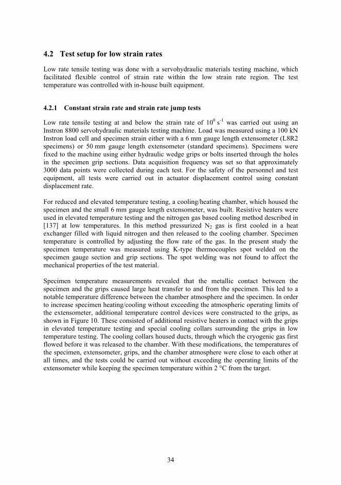
34

4.2 Test setup for low strain rates

Low rate tensile testing was done with a servohydraulic materials testing machine, which facilitated flexible control of strain rate within the low strain rate region. The test temperature was controlled with in-house built equipment.

4.2.1 Constant strain rate and strain rate jump tests

Low rate tensile testing at and below the strain rate of 100 s-1 was carried out using an Instron 8800 servohydraulic materials testing machine. Load was measured using a 100 kN Instron load cell and specimen strain either with a 6 mm gauge length extensometer (L8R2 specimens) or 50 mm gauge length extensometer (standard specimens). Specimens were fixed to the machine using either hydraulic wedge grips or bolts inserted through the holes in the specimen grip sections. Data acquisition frequency was set so that approximately 3000 data points were collected during each test. For the safety of the personnel and test equipment, all tests were carried out in actuator displacement control using constant displacement rate. For reduced and elevated temperature testing, a cooling/heating chamber, which housed the specimen and the small 6 mm gauge length extensometer, was built. Resistive heaters were used in elevated temperature testing and the nitrogen gas based cooling method described in [137] at low temperatures. In this method pressurized N2 gas is first cooled in a heat exchanger filled with liquid nitrogen and then released to the cooling chamber. Specimen temperature is controlled by adjusting the flow rate of the gas. In the present study the specimen temperature was measured using K-type thermocouples spot welded on the specimen gauge section and grip sections. The spot welding was not found to affect the mechanical properties of the test material. Specimen temperature measurements revealed that the metallic contact between the specimen and the grips caused large heat transfer to and from the specimen. This led to a notable temperature difference between the chamber atmosphere and the specimen. In order to increase specimen heating/cooling without exceeding the atmospheric operating limits of the extensometer, additional temperature control devices were constructed to the grips, as shown in Figure 10. These consisted of additional resistive heaters in contact with the grips in elevated temperature testing and special cooling collars surrounding the grips in low temperature testing. The cooling collars housed ducts, through which the cryogenic gas first flowed before it was released to the chamber. With these modifications, the temperatures of the specimen, extensometer, grips, and the chamber atmosphere were close to each other at all times, and the tests could be carried out without exceeding the operating limits of the extensometer while keeping the specimen temperature within 2 °C from the target.

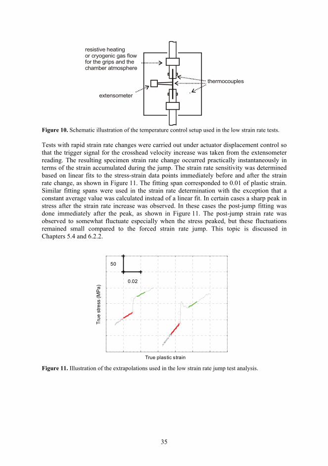
35

resistive heating or cryogenic gas flowfor the grips and thechamber atmosphere

extensometer

thermocouples

Figure 10. Schematic illustration of the temperature control setup used in the low strain rate tests. Tests with rapid strain rate changes were carried out under actuator displacement control so that the trigger signal for the crosshead velocity increase was taken from the extensometer reading. The resulting specimen strain rate change occurred practically instantaneously in terms of the strain accumulated during the jump. The strain rate sensitivity was determined based on linear fits to the stress-strain data points immediately before and after the strain rate change, as shown in Figure 11. The fitting span corresponded to 0.01 of plastic strain. Similar fitting spans were used in the strain rate determination with the exception that a constant average value was calculated instead of a linear fit. In certain cases a sharp peak in stress after the strain rate increase was observed. In these cases the post-jump fitting was done immediately after the peak, as shown in Figure 11. The post-jump strain rate was observed to somewhat fluctuate especially when the stress peaked, but these fluctuations remained small compared to the forced strain rate jump. This topic is discussed in Chapters 5.4 and 6.2.2.

True plastic strain

Tru

e s

tre

ss (

MP

a)

0.02

50

Figure 11. Illustration of the extrapolations used in the low strain rate jump test analysis.

36

4.2.2 Load relaxation tests

The load relaxation tests were carried out using the low rate testing setup described above. The test is started by deforming the L8R2 specimen at a constant cross-head velocity of 1 mm/s, corresponding to a strain rate of 10-1 s-1. The actual load relaxation run is started by stopping the actuator, which causes partial relaxation of the elastic deformation of the load train, while the specimen undergoes a small amount of additional plastic deformation with a rapidly decreasing strain rate, as explained in Chapter 3.2. The test data is recorded at a sampling frequency of 5 kHz during the relaxation run. Figures 12 and 13 present an example of a load relaxation run. As shown in Figure 12a, the actuator reaches a steady position relatively rapidly. In contrast, as shown in Figure 12b, the total strain measured directly from the specimen by the extensometer and the calculated plastic strain continue to increase at a decreasing rate. In the test shown in Figures 12 and 13, the measurement was stopped 2.1 seconds after the start of the relaxation run, at which point the plastic strain had increased less than 0.003 as compared to the start of the relaxation run.

1 2 3 41.34

1.36

1.38

1.4

1.42

Time (s)

Dis

pla

cem

en

t (m

m)

1 2 3 40.125

0.126

0.127

0.128

0.129

0.13

0.131

0.132

Time (s)

Tru

e s

tra

in

total

plastic

a) b) Figure 12. Example of a load relaxation test started at the strain rate of 10-1 s-1: a) actuator motion b) strain in the specimen gauge section. Figure 13a shows the calculated total and plastic strain rates in the specimen gauge section during the load relaxation run. For the calculation, the original data was first smoothed using a linear polynomial based local regression smoothing provided by the Matlab ® Curve Fitting Toolbox. The quality of the smoothed data was compared to the original data by eye and the smoothing span was adjusted so that in the beginning of the relaxation run less smoothing was used in order to correctly represent the rapid change in the strain rate. Figure 13b shows the change in stress during the load relaxation run. The measured flow stress was corrected for the effect of strain hardening based on Equation 26 using the strain hardening rate of 1400 MPa/(unit strain) measured just prior to the start of the load relaxation run. This procedure had quite a small influence on the results, since the maximum calculated change in the flow stress due to strain hardening was only about 4 MPa.

37

1 2 3 410

-5

10-4

10-3

10-2

10-1

Time (s)

Tru

e s

tra

in r

ate

(s

-1)

total

plastic

1 2 3 4500

550

600

650

700

Time (s)

Tru

e s

tre

ss (

MP

a)

a) b) Figure 13. Example of a load relaxation test started at the strain rate of 10-1 s-1: a) total and plastic strain rate in the gauge section and b) stress in the gauge section. As discussed in Chapter 3.2, several aspects have to be taken into account when the load relaxation test results are interpreted. In order to evaluate the possible contribution of anelasticity, both as-received and 20 % tensile strained specimens were loaded using an actuator velocity of 1 mm/s but stopping the actuator before the yield strength of the test material was reached. These tests did not show any detectable time dependent increase of elastic strain within 1.5 seconds from the start of the loading. In contrast, some downward deviation from the initial modulus of 200 GPa was observed at higher stress levels. This indicates small scale dislocation motion prior to macroscopic plastic deformation. However, this effect was neglected and the elastic modulus of 200 GPa was used throughout the calculations. Other aspects to be considered are the deformation-induced heating occurring during the monotonic deformation prior to the relaxation run and the possible heat transfer away from the gauge section during the actual relaxation measurement. It is reasonable to assume that due to the relatively low heat conductivity of the test material and small temperature difference between the specimen and its surroundings (below 100 K), the temperature change in the specimen gauge section is negligible within 0.5 seconds from the start of the load relaxation run. In contrast, at the same time there is a change in the specimen strain rate of almost three orders of magnitude, as seen in Figure 13a. Therefore, in order to measure the strain rate effects at a constant temperature, data measured after 0.5 seconds from the start of the load relaxation run was excluded from the results. It should, however, be noted that the data for different initial plastic strains do not correspond to the same initial temperature, but the relaxation run temperature increases with increasing initial plastic strain. In addition, the possible effect of dynamic strain aging occurring during the relaxation run cannot be excluded from the results. This effect is discussed in detail in Chapters 5.4 and 6.2.2.

38

4.3 Test setup for high strain rates

Compared to low rate testing, materials characterization at high strain rates is more complex. In this study, the high rate testing was based on an existing Tensile Hopkinson Split Bar apparatus, which was modified for strain rate jump tests. The experimental modifications were designed based on the analytical solutions of the wave motion in the current setups.

4.3.1 Tensile Hopkinson Split Bar

High strain rate testing near the strain rate of 1000 s-1 was carried out using the Tensile Hopkinson Split Bar apparatus at the Department of Materials Science of Tampere University of Technology. The constant strain rate test setup was essentially the same as described in references [10] and [11]. Figure 14 shows the components and dimensions of the setup. The setup consists of an incident bar made of tempered steel and a transmitted bar made of an aluminum alloy. The sheet specimen is glued with cyanoacrylate adhesive into slits machined to the ends of the bars. Compressed air is used to propel a steel striker tube against the flange at the free end of the incident bar. Striker length was varied between 1200 mm and 1600 mm according to the requirements of the test duration and striker velocity. Figure 14 depicts also the momentum trap bar used in the strain rate change experiments, which are discussed below. The elastic waves in the bars are measured with strain gauge pairs attached to the bars so that wave overlapping does not take place during the test. The strain gauge signals are amplified with Kyowa CDV-700A signal conditioners and recorded with a Yokogawa DL708E digital oscilloscope. Dispersion correction of the waves is carried out with a procedure described in [124].

400

1600

6200 mm 3000

20

Ø32

Transmitted bar(AA 2007) Ø22

Striker tube outer inner Ø22 (tempered steel)

Ø32,

Momentum trap bar (tempered steel)

Ø32 Incident bar (tempered steel)

Ø22

Figure 14. Schematic illustration of the THSB setup for constant strain rate testing. In addition, the momentum trap bar used in the strain rate change experiments is shown in front of the incident bar. The initial specimen temperature was controlled with temperature control blocks pressed against the specimen using pneumatic cylinders, as shown in Figure 15. This technique was first introduced by Hokka et al. [138] for elevated temperature testing using resistive heaters inside the copper blocks. In the present study the technique was modified for low temperature use by constructing aluminum blocks with ducts for cryogenic gas flow. The same liquid nitrogen based gas cooling setup was used as in the low strain rate testing. The block temperature was measured using thermocouples. In elevated temperature testing, molybdenum sulfide lubricant was used between the specimen and the blocks, while in reduced temperature testing pure ethanol was sprayed on the interfaces to prevent freezing and to provide lubrication. Immediately prior to the striker launch, the pressure was released

39

from the cylinders controlling the blocks. Measurements made on dummy specimens showed that until the start of the loading, the specimen temperature could be maintained within 5 °C from the target.

thermocouple

resistive heating or cryogenic gas flow cooling of the blocks

Figure 15. Schematic illustration of the temperature control setup used in the THSB tests.

4.3.2 Momentum trapping based strain rate change tests with THSB

For strain rate change tests within the high strain rate region, a momentum trap was added to the existing THSB setup. The setup, which follows the original idea of Nemat-Nasser [126, 127], is shown schematically in Figure 14. The trap is placed at a predetermined distance from the free end of the flange. The width of the gap between the momentum trap bar and the flange determines the moment when the strain rate change takes place during the test. In the current tests, a typical gap width was between 0.25 and 1.7 mm. The shape of the incident wave created with the THSB setup can be estimated by first considering the impact of the striker (velocity v0str) against the flange. As illustrated in Figure 16, three individual wavefronts are created: a compression wave in the striker (εstr), a tension wave in the incident bar propagating towards the specimen (εinci1), and a compression wave in the flange propagating away from the specimen (εinci2). By using Equations 38 and 39, the following solution is obtained for the loading wave amplitude (here the equations are simplified because the material properties are the same for all contacting parts and the flange cross-sectional area equals the sum of the incident bar and striker cross-sectional areas Ainci and Astr): 0)( 12 inciincistrstrincistrinci EAEAAAE (49) strstrinciinciboundary vcccv 001020 )( (50)

0

021 2 c

v

AA

A str

strinci

strinciinci

(51)

If the flange and the momentum trap are not in contact, the compression wave is reflected back from the free end of the flange as a wave of tension. In this case the calculation at the flange/striker/incident bar interface yields: 0))()(( 122 inciincistrstrinciincistrinci EAEAAAE (52) strstrinciinciinciboundary vccccv 00102020 )()( (53)

40

0

021 2

c

v

AA

A str

strinci

strinciinci

(54)

As can be seen, without a momentum trap the amplitude of the incident wave is increased by a factor of two when the reflection takes place at the free end of the flange. It should be noted that in Equations 52 to 54 it is assumed that the flange is under force equilibrium, i.e., the amplitudes of the compression wave originating from the striker-flange interface and the tension wave reflected from the free end of the flange are equal. In practice, this situation is reached rapidly due to the short length of the flange. As Figure 16 shows, when the momentum trap is in contact with the flange and the contacting areas are equal, the compression wave is transferred across the boundary and the loading wave amplitude remains at a value indicated by Equation 51, which is half of the value without the momentum trap. Therefore, when the gap between the momentum trap bar and the flange closes during the test due to the motion of the flange, a 50 % decrease is obtained in the loading wave amplitude. In principle, an amplitude increase could also be achieved by placing a short momentum trap in contact with the flange already in the beginning of the test. At a certain point during the test the tensile release wave reflected from the free end of the momentum trap would release the trap from the flange causing an increase in the loading wave amplitude. In practice, however, the contact between the flange and the trap is not perfect, which would cause some wave reflection at the interface and thus oscillations in the beginning of the loading wave.

C ( )εinci2

T (- )εinci2

C ( )strε

T ( )εinci1

v oundaryb

C

TC

flange

momentumtrap barstriker incident bar

Figure 16. Wave motion in the flange of the THSB apparatus without and with the momentum trap bar. Arrows denote the incipient waves, “C” for compression and “T” for tension wave. Figure 17 shows the waves measured during a THSB strain rate change test. In this test the specimen was loaded using a striker speed of 12.9 m/s. As can be seen, the ~50 % decrease in the incident wave amplitude at around 500 μs corresponds to a similar decrease in the reflected wave. Figure 17 shows also how the incident wave amplitude returns back to its original level after a certain (constant) period of time. This happens because the momentum trap is shorter than the striker and the tensile release wave propagating in the momentum trap reaches the flange/trap boundary while the striker is still loading the flange. Since the cross-sectional area of the specimen is considerably smaller than the cross-sectional areas of the bars, most of the incident wave is reflected back and the transmitted wave has a small amplitude compared to the other waves. This means that the specimen strain rate closely follows the incident wave amplitude, which is shown in Figure 18. It can be seen that the strain rate change occurs over several percent of specimen deformation due to the finite time needed for the incident wave amplitude change. In addition, oscillations appear after the jump. Therefore in the data analysis relatively large extrapolation fitting spans of 0.03...0.04 plastic strain were used, as illustrated in Figure 18. Another consequence of the large reflected wave and small transmitted wave is that in general the

41

incident bar end velocity is almost constant and transmitted bar end velocity is almost zero. This leads to an almost constant engineering strain rate, which in turn leads to a decreasing true strain rate with increasing plastic strain (actual gauge length of the specimen increases with increasing plastic strain). Therefore, in terms of elongation rate imposed to the specimen, the THSB tests were similar to the low rate tests carried out with the servohydraulic materials testing machine using constant displacement rate of the actuator (if the effects of the test machine elasticity are neglected).

0 500 1000 1500 2000-1.5

-1

-0.5

0

0.5

1

1.5

Time (s)

Ba

r st

rain

x 1

0-3

0 500 1000 1500 20000

0.05

0.1

0.15

0.2

0.25

0.3

Time (s)

Ba

r st

rain

x 1

0-3

a) b) Figure 17. Example of waves measured in a THSB strain rate change test: a) incident bar and b) transmitted bar. It should be noted that the figures have different scales.

0 0.1 0.2 0.3 0.4 0.5

200

400

600

800

1000

1200

1400

Tru

e p

last

ic s

tra

in r

ate

(s

-1)

True plastic strain0.1 0.2 0.3 0.4

700

800

900

1000

1100

1200

1300

Tru

e s

tre

ss (

MP

a)

True plastic strain

a) b) Figure 18. True plastic strain rate and true stress with respect to true plastic strain in the test shown in Figure 17.

42

4.3.3 Incorporation of a low strain rate loading device to THSB

In order to facilitate a large strain rate change directly from low strain rates to the high strain rate region, the THSB apparatus was fitted with a capability of prestraining the specimen in the strain rate range of 10-4 ... 10-3 s-1. The low strain rate loading setup consists of an electric motor, whose rotational movement is converted to linear motion using a spindle. As shown in Figure 19, this linear motion is transferred to the incident bar using a special fixture that allows the dynamic loading to be created by the impact of the striker on the flange. The loading fixture is attached to the incident bar with a M8 bolt so that the bolt transfers the quasi-static tensile loading but, when the striker hits the flange, the bolt can slide freely and no dynamic loading is transferred through the fixture. Furthermore, when the dynamic test is over but the incident bar is still in motion, the fixture collapses in a controlled way so that the incident bar is stopped by the shock absorber shown in Figure 19 and no load is transferred to the spindle. In contrast to the dynamic test, in the low rate test the transmitted bar has to be clamped to prevent any rigid-body movement in the setup. In the present setup the clamp is attached to the free end of the transmitted bar far enough from the strain gauges so that it does not interfere with the measurement of the transmitted wave and can thus be in place also during the dynamic test. Since the bars are loaded and clamped from their far ends, during low rate loading the test setup has relatively low stiffness compared to conventional test frames. For accurate specimen deformation measurement, an extensometer is used to directly measure the strain in the specimen gauge section. The extensometer is manually removed from the specimen a few seconds prior to the start of the dynamic loading. The amount of additional strain in the specimen between the removal of the extensometer and the start of the dynamic loading is monitored by a linear variable differential transducer (LVDT) attached to the incident bar. Throughout the test, the load acting on the specimen is measured using the strain gauges attached to the bars.

Incident bar

Free movement

Free movement (slide bearing)

Shock absorber

Spindle M8 bolt

Figure 19. Schematic illustration of the low strain rate loading fixture attached to the incident bar of the THSB setup. In the conventional testing with the current THSB setup the specimen is fixed to the bars with cyanoacrylate adhesive, which provides interference free joints and is also relatively convenient to apply and remove using mild heating and acetone. In contrast, during the use of the low strain rate prestraining device it was observed that the joints did not have necessary long-term strength during static loading. The problem was first addressed by fixing the specimen with 8 mm bolts through the holes shown in Figure 9. The bolts, however, introduced oscillations to the reflected and transmitted waves thus lowering the measurement accuracy of the device. The best combination of high enough joint strength and signal quality was found by using both the cyanoacrylate adhesive and mechanical fixing with the bolts. To minimize impedance differences, a steel bolt and an aluminum bolt

43

were used in the incident and transmitted bars, respectively. It should be noted, however, that even with this setup some signal quality and sensitivity was lost since the sharp yield peak observed for prestrained and room temperature aged specimens could not be detected when the bolts were used. This is illustrated in Figure 20.

0 0.05 0.1 0.15 0.2 0.25 0.30

200

400

600

800

1000

1200

Engineering strain1

En

gin

ee

rin

g s

tre

ss (

MP

a)

-0.025 0.025 0.075700

800

900

1000

1100

1200

1300

Engineering strain1

En

gin

ee

rin

g s

tre

ss (

MP

a)

Glue joint, 0.2 prestrain

Glue joint, 0.3 prestrain

Bolt and glue joint, 0.25 prestrain

a) b) Figure 20. Examples of transmitted signals obtained with different specimen attachment methods. When the prestraining is applied, some modifications have to be made to the classical THSB equations, because the strain gauge signals contain both the elastic waves and the static strain caused by the prestraining. In addition, when the striker hits the flange, it causes the incident bar to detach from the prestraining fixture. Therefore the incident wave is followed by an unloading wave, which affects the base level of the measured reflected wave. Figure 21 is a schematic depiction of the force distribution in the setup during different phases of the test. Based on Figure 21, in order to extract the incident and transmitted waves from the strain gauge signals, the strain corresponding to the preload should be subtracted from the gauge signals. In contrast, the reflected wave is propagating in an unloaded bar and therefore the strain gauge measures directly the reflected wave. The extracted waves can be used to calculate the specimen elongation rate according to Equation 41. However, when the forces acting on the bar ends are calculated, the pretension in the bars (denoted by εpre1 and εpre2 for the incident and the transmitted bar, respectively) has to be taken into account: 1111 prerefinciAEF (55)

)( 2222 pretransAEF (56)

44

Fx

I)

II)

III)

F0 xFx

F0 xFx

F0 x

Figure 21. Schematic depiction of the force distribution in the THSB setup with prestraining during different phases of the test: I) during prestraining, II) shortly after striker impact and III) shortly after the specimen has fractured. Figure 22 shows an example of the actual strain gauge signals measured during a THSB test with low strain rate prestraining. As discussed above, the base level of the signals has increased due to the preload. Between the incident and reflected waves the base level drops to zero due to the unloading wave following the incident wave. The transmitted wave is also followed by an unloading wave, which is created when the specimen fractures. This unloading wave has its origins in the elastic energy stored in the transmitted bar during the low strain rate prestraining. The macroscopic effect of the unloading wave is that when the specimen fractures, the transmitted bar starts to move in the direction opposite to the original bar motion (the clamp holding the transmitted bar in place during low rate loading is constructed so that it allows for motion in the direction away from the specimen).

0 500 1000 1500 2000-1.5

-1

-0.5

0

0.5

1

1.5

Time (s)

Ba

r st

rain

x 1

0-3

0 500 1000 1500 2000-0.05

0

0.05

0.1

0.15

0.2

0.25

0.3

Time (s)

Ba

r st

rain

x 1

0-3

a) b) Figure 22. Strain gauge signals recorded in a THSB test with low strain rate prestraining: a) incident bar and b) transmitted bar. It should be noted that the figures have different scales.

45

4.4 Simulations with the finite element method

In order to study the effect of specimen geometry on deformation-induced heating, finite element method (FEM) simulations of low rate tests were carried out with DS Simulia Abaqus 6.9 software. Calculations were done using the implicit solver and coupled thermal-mechanical analysis. The problem was simplified by assuming temperature and strain rate independent isotropic material model with linear elasticity and nonlinear hardening given by the effective stress-strain curve shown in Figure 23. The flow curve was based on experimental data, but it neglected the effect of the austenite to α’-martensite phase transformation on the mechanical properties. In addition, the effect of the phase transformation on the thermal analysis was neglected. It should be noted that the main purpose of the FEM analysis was to comparatively study how the specimen geometry influences the transition from nearly isothermal to fully adiabatic deformation conditions with increasing strain rate. Since the purpose was not to find the absolute temperature increase but to study the differences between the different specimen geometries, the simplifications in the analysis are believed to be justified.

0 0.05 0.1 0.15 0.2 0.25 0.30

100

200

300

400

500

600

700

800

900

Effective plastic strain

Effe

ctiv

e s

tre

ss (

MP

a)

Figure 23. Effective stress-strain curve used in the simulations. Due to the simplifications presented above, the only coupling between the thermal and mechanical analyses was the generation of heat due to plastic work. This meant that during each calculation step, the mechanical problem was solved independently of the thermal problem, after which the thermal problem was solved based on the updated data (geometry and heat generation) obtained from the mechanical solution. In the thermal analysis material density was 7900 kg/m3, specific heat capacity 500 J/(kg·K), and thermal conductivity 15 W/(m·K) [139]. The fraction of plastic work converted to heat was assumed to be 1. Both L8R2 and standard specimens were modeled with 3-dimensional 8-node linear brick elements using only 1/8 of the full specimen due to symmetry. Element side length was approximately 0.5 mm in the gauge section and 1 mm in the grip section. Tensile loading was simulated by setting a constant velocity to the grip section in the regions, where the tensile testing machine grips would hold the real specimen. Thermal boundary conditions were simulated by setting a convection boundary condition with a convection coefficient of 10 W/(m2·K) [19] on the free surfaces. This represented natural convection cooling by air. Heat transfer through the metallic grips was simulated by assuming a high convection coefficient of 1500 W/(m2·K) [137] on the respective surfaces. Heat transfer by radiation was neglected in the analysis.

46

4.5 Microstructural characterization

Characterization of the material microstructure after plastic deformation was carried out with magnetic induction and Electron Backscatter Diffraction (EBSD) measurements. Magnetic induction measurements were carried out at the Tornio Research Center of Outokumpu Tornio Works using Fischer Feritscope MP30, which is a handheld device designed for ferrite content measurement in austenitic and duplex stainless steels and their welds. The measuring probe of the device consists of a soft iron core, which is surrounded by two coils. The primary coil is used to create a low frequency alternating magnetic field, which induces current to the secondary coil. The magnetic permeability of the test material influences the magnetic field, which facilitates the measurement of the overall content of ferromagnetic phases (i.e., ferrite and α’-martensite). However, the measurement can be influenced by the geometry of the test piece (sheet thickness, possible curvature, and edge effects) as well as by the elastic [80, 140] and plastic deformation of the ferromagnetic phases [73]. Furthermore, the method does not take into account the possible differences in the permeability between the ferromagnetic phases. These factors require that the Feritscope readings are converted to actual phase fraction data using calibration specimens. In the case of metastable austenitic stainless steels, Feritscope data has been published in several studies [73, 78, 80, 96, 97, 140, 141]. The details of the calibration process vary between investigators. However, Talonen [78] and Beese [140] concluded independently that for EN 1.4318 the reading indicated by the Feritscope calibrated for ferrite measurements should be multiplied by ~1.7 in order to obtain the volume fraction of strain-induced α’-martensite. Similar results were obtained by the author of this thesis in a previous study [142] carried out for specimens with same dimensions as in this study. It should be noted that the specimens used in this study are susceptible to end effects due to their small size. For consistency, in this study all measurements were carried out on the longitudinal centerline of the specimen at the original (rolled) surface (Figure 24). Before the measurement the surface was cleaned with ethanol.

RD

RD

TD

TD

ND

ND

Feritscope measurements

EBSD measurements

A

A-A:

A

Figure 24. Areas on the specimens subjected to microstructural characterization. EBSD is based on the quantitative interpretation of the so-called Kikuchi patterns, which are formed in both transmission and scanning electron microscope. Kikuchi patterns originate from the diffraction of inelastically scattered primary electrons. The diffracted electrons fulfilling a certain Bragg condition compose a cone (so-called Kossel cone). When the various cones exiting the specimen surface are intersected with a plane such as a photographic plate or an image sensor of a digital camera, Kikuchi patterns are formed. These patterns are composed of pairs of parallel lines, so-called bands, which run in certain directions. Each band represents a distinct plane of the crystal. Two lines are formed

47

because diffraction occurs on both sides of a crystallographic plane. The trace of the diffraction plane is located at the center of the band, the width of which depends on the plane spacing (when the effects of projecting a cone on a flat surface are neglected). The intersections of bands represent zone axes. Hence the Kikuchi pattern contains also the symmetry of the crystal. [143, 144] If the crystal structure is known (or the number of different possibilities is reasonably limited), the orientation of the crystal can in principle be deduced by first indexing the pattern and subsequently calculating the angles between selected poles and some reference axis (such as the beam normal and one of the specimen edges). The indexing can be done by comparing the widths of the bands and their angles with each other, or by comparing them with standard patterns. [143] In practice, manual indexing of Kikuchi patterns and orientation determination is a laborious task especially in scanning electron microscopy work, in which the experimental setup is often less ideal. For example, the specimen is heavily tilted with respect to the primary beam to increase the intensity of back-scattered electrons and the surface (camera cell) capturing the pattern is not parallel to the specimen surface, pattern quality may not be good enough for a reliable determination of the width of the bands, etc. More importantly, modern scanning electron microscopes and digital cameras enable capturing of thousands of data points in reasonable time frames (detailed surface scans), which makes manual calculations practically impossible. This has led to the development of automated pattern indexing and orientation routines and software. The EBSD measurements in this study were carried out with Zeiss ULTRAplus field emission gun scanning electron microscope using a Nordlys F400 detector and Oxford Instruments HKL Channel 5 data acquisition and handling software package. The microscope was operated at 15 kV acceleration voltage. The working distance was set to 15 mm and the specimen was tilted 70° from horizontal. For pattern indexing, literature models for fcc iron (for austenite) and bcc iron (for α’-martensite) provided by the analysis software were used. In order to obtain unambiguous solutions, the detection and successful indexing of 9-11 bands in each pattern was set as a validity criterion. The detection of ε’-martensite was not attempted. All scans were performed on the (ND, RD) surface of the tensile specimens (Figure 9), i.e., the loading direction was normal to the scanned surface. The microscopical specimens were first cut from the tensile specimens with an abrasive cutter, then mounted in epoxy resin and ground with SiC grinding paper (down to P2500). Polishing of the surfaces was carried out electrolytically in Struers A2 solution at 25 V for 50 s. After polishing, the specimens were detached from the epoxy mounts and any organic residues were removed in plasmon asher before placing the specimens into the microscope chamber. Most of the scans were carried out on areas with an approximate size of 350 μm x 350 μm using a 0.5 μm step size (the distance between consecutive measurement points). The measurements were taken from areas located in the halfway between the centerline (parallel to RD) and the surface of the specimen (Figure 24). For more detailed analysis, some measurements were carried out on areas of 40 μm x 40 μm with a 0.06 μm step size.

48

49

5 RESULTS

In the following, the test results are presented starting with comparative studies of the effect of specimen geometry on the measured material behavior. Then the results of both constant strain rate and strain rate jump tests carried out at different temperatures and strain rate regions are presented. Following the mechanical test results, the findings of the microstructural studies on selected specimens are reported.

5.1 Low strain rate tests with different specimen geometries

Figure 25 presents stress-strain curves for the two studied specimen geometries at the strain rates of 2·10-4 s-1 and 2·10-3 s-1. For the L8R2 geometry, strain was measured using an extensometer with a gauge length of 6 mm, whereas with the standard specimen a 50 mm gauge length extensometer was used. As can be seen, below 0.15 engineering or 0.14 true strain identical results are obtained with the two geometries. However, the fracture strain is notably larger for the L8R2 geometry. This is expected, since in the L8R2 geometry, which has a low aspect-ratio, the neck covers virtually the whole gauge length, whereas in the standard geometry the necked region is local and has only a minor effect on the total elongation of the gauge length.

0 0.1 0.2 0.3 0.4 0.5 0.6 0.70

100

200

300

400

500

600

700

800

900

1000

Engineering strain (mm/mm)

En

gin

ee

rin

g s

tre

ss (

MP

a)

0 0.05 0.1 0.15 0.2 0.25 0.3 0.35 0.40

200

400

600

800

1000

1200

1400

True plastic strain

Tru

e s

tre

ss (

MP

a)

L8R2, 2x10-4 s-1

L8R2, 2x10-3 s-1

stand., 2x10-4 s-1

stand., 2x10-3 s-1

a) b) Figure 25. Examples of stress-strain curves obtained with different specimen geometries at different strain rates: a) engineering stress-strain curves and b) calculated true stress-strain curves. Figure 25 shows also the notably large differences in the strain hardening behavior of the two different types of specimens at true strains above 0.14, which leads to higher tensile strengths measured with the L8R2 specimen than with the standard specimen. Similar behavior was noted also by Larour [145]. Since the mechanical properties of the studied metastable steel are highly temperature sensitive due to the strain-induced austenite to α’-martensite phase transformation, the tensile tests were repeated with in-situ temperature measurements using spot welded K-type thermocouples. The results of these tests showed that in the standard specimen the temperature increase at lower strain rates is much higher than in the L8R2 specimen (Figure 26). This can be explained with the L8R2 specimen’s smaller gauge area/grip area ratio and smaller overall dimensions, which reduce the amount of thermal diffusion required to maintain the gauge area at a constant temperature during plastic deformation.

50

Figure 26 presents the theoretical temperature increase curves based on Equation 22 for both specimen geometries. The flow curves at the highest tested strain rates were used in the calculations, and the thermal properties were the same as in Chapter 4.4. The calculations neglect the heat release due to the martensitic transformation, and therefore the actual measured temperature increase can become higher than the calculated one. On the other hand, the fraction of mechanical work stored in the microstructure was assumed zero, which is not true for strain hardening materials. The temperature measurement itself requires heat transfer, so the real-time measurement of adiabatic heating is a somewhat abstract concept. Therefore the agreement between the measured and calculated temperature increase at the highest strain rate is probably somewhat coincidental, but the results presented in Figure 26 nevertheless indicate that a rather abrupt change from nearly isothermal conditions to almost adiabatic deformation occurs in a relatively narrow strain rate region. Furthermore, the point of this change seems to depend on the specimen geometry.

0 0.1 0.2 0.3 0.40

10

20

30

40

50

60

70

80

90

100

True plastic strain

Te

mp

era

ture

incr

ea

se (C

)

2x10-4 s-1

2x10-3 s-1

1x10-2 s-1

2x10-2 s-1

theoretical

0 0.1 0.2 0.3 0.40

10

20

30

40

50

60

70

80

90

100

True plastic strain

Te

mp

era

ture

incr

ea

se (C

)

2x10-4 s-1

1x10-3 s-1

2x10-3 s-1

theoretical

a) b) Figure 26. Measured surface temperature increases at the center of the specimen at different strain rates: a) L8R2 specimen and b) standard specimen. Theoretical temperature increase curves are based on the calculation of plastic work at the highest tested strain rates. The temperature increase in the standard specimen is further illustrated in Figure 27, which depicts the longitudinal temperature field on the surface of the specimen in a tensile test carried out at 2·10-3 s-1. For this measurement, nine thermocouples were spot welded on the centerline of the specimen. As seen in Figure 27, before necking the temperature field on the gauge section surface is uniform except for the somewhat higher temperature measured at the center of the specimen and steep temperature gradients develop on the filleted regions between the gauge section and the grip sections. This implies that despite the heat transfer by conduction, the heat generation rate in the gauge section is so high that the material temperature inevitably increases during the deformation. Figure 27 also shows that when the specimen starts to neck, the temperature at the center increases notably due to the localized deformation.

51

-80 -60 -40 -20 0 20 40 60 800

20

40

60

80

100

Longitudinal coordinate in undeformed specimen (mm)

Te

mp

era

ture

incr

ea

se (C

)

0.1 eng. strain

0.2 eng. strain

0.3 eng. strain

0.4 eng. strain

0.45 eng. strain

Figure 27. Measured temperature increase on the surface of a standard specimen during a tensile test at the strain rate of 2·10-3 s-1 at room temperature. The influence of specimen geometry on the deformation-induced heating was further studied by carrying out FEM-simulations. The calculation procedure is described in Chapter 4.4. Figure 28 summarizes the results of these simulations. As noted before, due to the simplifications in the analysis procedure concerning the material behavior, the absolute values of temperature are not expected to match the experimentally measured ones. The effect of specimen geometry was found to be the same as in the experimental tests, i.e., heating occurred at notably lower strain rates in the standard specimen. The simulation results are dependent on the boundary conditions, such as the selection of convection heat transfer coefficient. It is emphasized that in the simulations the thermal boundary conditions and material properties were kept constant and the only variables were the specimen geometry and the strain rate. The simulation results indicate that above strain rate 10-1 s-1 the conditions are nearly adiabatic for both geometries, which is in accordance with previous studies [52, 76, 97].

10-4

10-3

10-2

10-1

100

0

10

20

30

40

50

True plastic strain rate (s-1)

Te

mp

era

ture

incr

ea

se (C

)

Fully adiabatic

L8R2

stand.

L8R2, forced conv.

stand., forced conv.

Figure 28. Simulated temperature increases at the mid-length mid-width position of the specimen surface at 0.25 plastic strain as a function of strain rate. The effect of convection heat transfer was further studied by increasing the convection heat transfer coefficient from 10 W/(m2·K) to 550 W/(m2·K), which simulates the effect of forced convection by air blow [19]. Figure 28 presents the results of these simulations. As

52

can be seen, with forced convection the occurrence of notable deformation-induced heating is shifted to higher strain rates, but already at strain rate 2·10-1 s-1 the conditions are nearly adiabatic despite the more effective cooling. This indicates that above this strain rate the conduction heat transfer rate within the material becomes the limiting factor. Figure 29 presents examples of specimen temperature fields obtained from the simulations. In the case of the standard specimen, the simulations agree qualitatively with Figure 27, i.e., at higher strain rates the temperature increases uniformly throughout the gauge section and steep gradients develop in the filleted regions. In the L8R2 specimen the temperature gradient comprises also part of the gauge section causing a less uniform temperature field in the deforming material. The temperature gradient in the filleted regions is also dependent on the amount of deformation occurring in the fillets, which, in turn, depends on the strain hardening properties of the material. If the material strain hardens extensively in the gauge section, deformation spreads to the filleted areas causing heat generation also there. This then widens the area with nearly constant temperature towards the grip sections.

a) b) c)

d)

e)

ΔT (°C)

Figure 29. Simulated temperature fields on the specimen surfaces at 0.25 plastic strain: a) standard, 2·10-4 s-1 b) standard, 2·10-3 s-1 c) standard, 2·10-2 s-1 d) L8R2, 2·10-2 s-1 e) L8R2, 2·10-1 s-1. It should be noted that the standard and L8R2 specimens are not drawn to the same scale. The results of the experimental measurements and numerical simulations show the importance of maintaining consistency in the specimen geometry throughout the tests. Not only are some mechanical parameters, such as fracture strain, affected by the geometry but, as shown above, also the thermal boundary conditions of the gauge section are influenced by the geometry. This is especially critical at strain rates where the strain-induced heat generation and heat transfer to the surroundings are close to each other. At these strain rates the changes in the efficiency of heat transfer have the largest effect on the material temperature. At lower strain rates the heat generation is notably lower than the heat conduction, and the conditions remain almost isothermal despite the changes in the specimen geometry. At higher strain rates heat is generated at such a high rate and the whole test duration is so short that the gauge section deformation is practically adiabatic.

53

5.2 Constant strain rate tests at different strain rates and temperatures

Figure 30 presents examples of stress versus strain and strain hardening rate versus strain curves obtained at different temperatures at a constant strain rate of 2·10-4 s-1. The test material shows the typical behavior of a highly metastable austenitic stainless steel, i.e., the behavior of the material changes drastically over a relatively narrow temperature range between -40 °C and +80 °C. At the highest test temperature the material shows nearly parabolic behavior with continuously decreasing strain hardening rate except at very high strains. At lower temperatures a distinct “s”-shaped flow curve is observed. At -40 °C the strain hardening rate first decreases to a very low value, then rapidly increases to a very high value, and again decreases until necking of the specimen starts. Similar behavior is observed at +24 °C, but the changes in the strain hardening rate are less distinct and take place at higher plastic strains. As explained in Chapter 2.2.2, this kind of behavior is well documented in the literature [25, 35, 41, 61, 62, 65-68] and has been related to the strain-induced austenite to α’-martensite phase transformation. At +80 °C the material shows highest ductility accompanied with sudden bursts in the strain hardening rate at very high strains. The high ductility has been explained by the stabilizing effect of the austenite to α’-martensite phase transformation on plastic flow [25, 52, 65, 68, 73, 76, 84, 85, 94]. Because of the higher test temperature, the phase transformation does not take place until high amount of plastic deformation occurs at the incipient neck. The formation of strain-induced martensite increases the local strength of the material within the neck and stops the deformation at that point. In contrast, at lower temperatures the phase transformation takes readily place already during uniform deformation and the flow stabilization during necking does not occur. Careful inspection of the data obtained at +80 °C showed that at large strains the plastic deformation was no longer uniform in the gauge section despite the continued increase of the force. The extensometer signal became jerky, that is, the extension rate measured by the extensometer fluctuated despite the constant velocity of the actuator. This suggests that the plastic deformation was momentarily concentrated outside the extensometer knives, which caused a decrease in the extension rate measured by the extensometer, after which the plastic deformation returned back to the region measured by the extensometer. This artifact may have at least partly caused the bursts in the observed strain hardening rate seen in Figure 30b. However, similar jerkiness was also seen in the raw force data indicating that some kind of local necking had taken place causing a decrease in the force after which the neck had been removed and the force started to increase again.

54

0 0.1 0.2 0.3 0.4 0.50

400

800

1200

1600

True plastic strain1

Tru

e s

tre

ss (

MP

a)

2x10-4 s-1

0 0.1 0.2 0.3 0.4 0.50

2000

4000

6000

8000

10000

12000

True plastic strain1

Tru

e s

tra

in h

ard

en

ing

ra

te (

MP

a)

2x10-4 s-1

-40 C

+24 C+80 C

-40 C

+24 C+80 C

a) b) Figure 30. Effect of temperature on a) stress versus strain curve and b) strain hardening rate versus strain curve. Test strain rate is 2·10-4 s-1.

0 0.1 0.2 0.3 0.4 0.50

400

800

1200

1600

True plastic strain1

Tru

e s

tre

ss (

MP

a)

10-1 s-1

0 0.1 0.2 0.3 0.4 0.50

2000

4000

6000

8000

10000

12000

True plastic strain1

Tru

e s

tra

in h

ard

en

ing

ra

te (

MP

a)

10-1 s-1

-40 C

+24 C+80 C

-40 C

+24 C+80 C

a) b) Figure 31. Effect of temperature on a) stress versus strain curve and b) strain hardening rate versus strain curve. Test strain rate is 10-1 s-1.

0 0.1 0.2 0.3 0.4 0.50

400

800

1200

1600

True plastic strain1

Tru

e s

tre

ss (

MP

a)

103 s-1

0 0.1 0.2 0.3 0.4 0.50

2000

4000

6000

8000

10000

12000

True plastic strain1

Tru

e s

tra

in h

ard

en

ing

ra

te (

MP

a)

103 s-1

-40 C

+24 C+80 C

-40 C

+24 C+80 C

a) b) Figure 32. Effect of temperature on a) stress versus strain curve and b) strain hardening rate versus strain curve. Test strain rate is 103 s-1.

55

Figures 31 and 32 show the effect of strain rate on the overall flow behavior of the material at different temperatures. At +80 °C, the shape of the stress versus strain –curve is relatively independent of strain rate, while at lower temperatures notable changes take place, i.e., the maximum of strain hardening rate decreases and its occurrence is shifted to higher strains. A closer examination of the graphs shows that at strains below 0.1 the difference in the strain hardening rate between different strain rates is quite small and becomes evident only at higher strains. It should be noted that in the THSB tests the specimen strain was calculated based on the bar end motion, which easily causes an overestimation of the specimen strain. This overestimation depends on the amount of additional deformation occurring outside the gauge section, which in turn depends on the amount of strain hardening occurring within the gauge section. Therefore the THSB strain measurement method tends to decrease the possible differences between the tests done at different temperatures, i.e., the strain hardening occurring in the gauge section increases the overestimation of strain, which again decreases the measured strain hardening rate. However, the THSB results follow the trend observed already at 10-1 s-1, i.e., increasing strain rate decreases the strain hardening capability of the test material at low temperatures. Similar effects of strain rate on the behavior of metastable austenitic stainless steels have been reported previously [52, 71, 76, 96-98]. There exists a general agreement that the strain hardening capability of these materials is decreased due to the deformation-induced heating, which suppresses the austenite to α’-martensite phase transformation. As discussed in Chapter 5.1, notable heating occurs already in the low strain rate region below 100 s-1. Similar conclusions can be drawn based on the results of this study. The behavior of the test material at +80 °C agrees also with the room temperature studies [52, 76, 97] carried out on more stable grades. According to these investigations, the increase of uniform deformation due to the martensitic phase transformation quickly vanishes when the amount of deformation-induced heating increases with increasing strain rate. Figures 33 and 34 summarize the results of the constant strain rate tests carried out on the test material in terms of flow stress versus strain rate graphs. The strain rates used in Figures 33 and 34 were determined by calculating the instantaneous strain rate at each indicated strain value. As can be seen, the strain rate values fluctuate (the data points do not fit to exact vertical lines) especially at low strain rates at low temperatures. This happens because of the extensive strain hardening occurring in the gauge section, which tends to increase the deformation outside the gauge section. Since the tests were run under actuator displacement control, the gauge section strain rate was affected by this additional deformation. In addition, even in ideal conditions, if the engineering strain rate is kept constant, the true strain rate decreases due to the gauge length elongation. It should be noted that both the nominally constant strain rate as well as the strain rate jump tests were carried out under similar conditions. In addition, the fluctuations in the constant strain rate tests were small and smooth compared to the actual strain rate jump tests. Therefore the results are believed to be representative of the actual material behavior.

56

10-4

10-3

10-2

10-1

100

101

102

103

104

0

200

400

600

800

1000

1200

1400

1600

True plastic strain rate (s-1)

Flo

w s

tre

ss (

MP

a)

+24 C

=22 =34=87

0.02 0.1 0.2 0.3

Figure 33. Effect of strain rate on the flow stress at different true plastic strains. Initial test temperature is +24 °C. The indicated values of the strain rate sensitivity parameter β were calculated using Equation 14.

10-4

10-3

10-2

10-1

100

101

102

103

104

0

200

400

600

800

1000

1200

1400

1600

True plastic strain rate (s-1)

Flo

w s

tre

ss (

MP

a)

-40 C

=39

0.02 0.1 0.15 0.2

10-4

10-3

10-2

10-1

100

101

102

103

104

0

200

400

600

800

1000

1200

1400

1600

True plastic strain rate (s-1)

Flo

w s

tre

ss (

MP

a) +80 C

=19=29

0.02 0.1 0.2 0.3

a) b) Figure 34. Effect of strain rate on the flow stress at different true plastic strains. Initial test temperature is a) -40 °C and b) +80 °C. The indicated values of the strain rate sensitivity parameter β were calculated using Equation 14. According to constant strain rate tests, the apparent strain rate sensitivity of the test material becomes increasingly more complex when temperature is reduced. At +80 °C (Figure 34b), the material shows positive strain rate sensitivity of flow stress throughout the tested strain rate and strain ranges. At +24 °C (Figure 33), the strain rate sensitivity is positive at strains below 0.1 throughout the studied strain rate range but becomes highly negative at high strains at low strain rates. At -40 °C, the strain rate sensitivity is partly negative already at 0.1 plastic strain (Figure 34a). However, at all temperatures the yield strength of the material shows positive strain rate sensitivity in accordance with the thermal activation theory. The results of the constant strain rate tests confirm the observations of previous investigations [52, 76, 97] that the apparent strain rate sensitivity of the material is heavily dependent on the austenite stability, i.e., stacking fault energy of the material and the chemical driving force for the austenite to α’-martensite phase transformation. According to previous investigations [25, 71], the stability of the austenite phase in EN 1.4318 is very sensitive to temperature around room temperature. Therefore already a relative small temperature increase either by ambient temperature change or by deformation-induced heating has a large influence on the flow behavior of the material.

57

5.3 Strain rate change tests

Based on the results of the constant strain rate tests, it is evident that the positive strain rate sensitivity caused by thermal activation effects is masked by the strong negative strain rate sensitivity of the strain hardening rate of EN 1.4318. This view is further supported by the positive strain rate sensitivity of the yield strength observed at all test conditions and by the strain rate jump tests reported in the literature [84, 97, 102]. In addition, the study carried out by Huang et al. [84] indicates a relation between austenite stability and instantaneous strain rate sensitivity. In the present study, three different kinds of strain rate change tests were carried out: tests with sudden imposed changes in the strain rate (“jump tests”), load relaxation runs, and tests on prestrained material. Figure 35 shows examples of the two extremes of material behavior observed during the jump tests. At low temperatures a notable difference was observed between the apparent strain rate sensitivity deduced from the constant strain rate tests and the instantaneous strain rate sensitivity obtained from a jump test. As seen in Figure 35a, at -40 °C the apparent strain rate sensitivity is highly negative between 2·10-4 s-1 and 10-2 s-1 at high strains, while the strain rate jump from the lower to the higher strain rate clearly reveals positive instantaneous strain rate sensitivity. In contrast, at +80 °C similar tests show only minor differences between the constant strain rate and strain rate jump tests (Figure 35b), which implies that under these deformation conditions the apparent strain rate sensitivity of the material is mainly composed of the instantaneous strain rate sensitivity. This is further evidenced by the results of the constant strain rate tests, which indicate a relatively small effect of strain rate on the strain hardening rate at +80 °C compared to lower temperatures.

0 0.05 0.1 0.15 0.2 0.25 0.30

200

400

600

800

1000

1200

1400

1600

True plastic strain1

Tru

e s

tre

ss (

MP

a)

-40 C

2x10-4 s-1

10-2 s-1

0 0.1 0.2 0.3 0.4 0.5 0.60

200

400

600

800

1000

1200

True plastic strain1

Tru

e s

tre

ss (

MP

a)

+80 C

2x10-4 s-1

10-2 s-1

a) b) Figure 35. Examples of stress versus strain curves obtained from constant strain rate and strain rate jump tests: a) -40 °C and b) +80 °C. Black arrows denote the points of strain rate increase from the lower to the higher. Data from the jump tests was analyzed by calculating the strain rate sensitivity parameter β (Equation 14 on page 6) for each jump. Steady state values before and after the jump were used as described in Sections 4.2.1 and 4.3.2. The strain rate sensitivity parameter was then plotted against plastic strain, as shown in Figure 36a. The choice of the strain rate sensitivity parameter (β vs. m) somewhat affects the shape of the sensitivity versus strain

58

curves, as seen in Figure 36. The reason for this is that in the calculation of the β-parameter (Equation 14) the absolute magnitude of the flow stress change is compared to the logarithmic strain rate change, while in the m-parameter (Equation 15) calculation the logarithmic values of stress before and after the jump are used in the comparison. This means that in the latter parameter the height of the jump is scaled with respect to the current stress level. Therefore changes in the material flow stress due to strain hardening affect m even if β remains constant. In the present study β was used to quantify the material strain rate sensitivity because it can be directly related to the thermally activated dislocation motion, as described in Chapter 2.1.1. However, as illustrated in Figure 36, for both measures of strain rate sensitivity distinct differences in material behavior between test temperatures are observed.

0 0.1 0.2 0.3 0.4 0.50

10

20

30

40

50

60

70

80

True plastic strain 1

(M

Pa

)

2x10-4 10-2 s-1

-40 C

+24 C+80 C

0 0.1 0.2 0.3 0.4 0.50

0.02

0.04

0.06

0.08

True plastic strain 1

m 2x10-4 10-2 s-1

-40 C

+24 C+80 C

a) b) Figure 36. Effects of temperature and plastic strain on the strain rate sensitivity factors a) β and b) m. Strain rate jumps were carried out from 2·10-4 s-1 to 10-2 s-1. At +80 °C β remains almost constant in jumps from 2·10-4 s-1 to 10-2 s-1 until it starts to decrease at higher strains. At that time notable peaking of stress during the jump is observed. However, as noted before, the steady state value after the peak was used in the calculations. Peaking of stress was observed also at lower temperatures. This phenomenon is further discussed later in this thesis. As Figure 36 indicates, at lower temperatures β shows first an increase and then a decrease with increasing plastic strain, the effect being strongest at -40 °C. This kind of behavior is strikingly similar to the behavior of the strain hardening rate at the same conditions. As noted in Chapter 2.2.2, Huang et al. [84] carried out strain rate jump tests for AISI 304 austenitic stainless steel at different temperatures at low strain rates and noted a correlation between the strain rate sensitivity and martensite transformation rate. Later De et al. [82] reviewed the results of Huang et al. [84] and proposed that the increased strain rate sensitivity is caused by increased cross-slip activity.

59

0 0.1 0.2 0.3 0.4 0.50

10

20

30

40

50

60

70

80

True plastic strain 1

(M

Pa

)

10-1 100 s-1

-40 C

+24 C+80 C

0 0.1 0.2 0.3 0.4 0.50

20

40

60

80

100

120

140

True plastic strain 1

(M

Pa

)

103 5x102 s-1

-40 C

+24 C+80 C

a) b) Figure 37. Effects of temperature and plastic strain on the strain rate sensitivity factor β in a) jumps from 10-1 s-1 to 100 s-1 and b) jumps from 103 s-1 to 5·102 s-1. Dotted lines in b) indicate average levels at respective temperatures. Figure 37 shows the results of the strain rate jump tests carried out at higher strain rates. In jumps from 10-1 s-1 to 100 s-1 the behavior of the material resembles the behavior at lower strain rates, i.e., the increase and decrease in the strain rate sensitivity with increasing plastic strain are still visible, as seen in Figure 37a. However, at high strain rates near 103 s-1 the possible differences in the behavior between initial test temperatures are below the experimental scatter (Figure 37b). The measurement accuracy in the THSB jump testing was notably lower than in the low rate testing due to several reasons. Firstly, the magnitude of the strain rate change was relatively low, only around 50 % as opposed to around one decade in the low rate testing, which resulted in a relatively small change in the stress compared to the signal noise. Secondly, the duration of the strain rate change with respect to the overall test time was large and the strain rate change occurred over a longer strain interval. Thirdly, in the HSB technique the specimen strain rate and strength are inversely connected, i.e., the lower the specimen strength, the higher the strain rate for a given incident wave amplitude. This means that during a sudden incident wave reduction the specimen strain rate first starts to decrease, which leads to a specimen strength decrease due to thermal activation or dislocation drag effects, which in turn tends to lead to a specimen strain rate increase [6]. This, in connection with the requirement that force equilibrium is reached in the specimen, may further increase the time needed to obtain steady state deformation conditions after a strain rate change. Another difference between the low and high rate testing was that in the high rate testing the specimen strain rate was suddenly decreased instead of increasing it, which may have some effect on the observed behavior. However, in the low rate tests carried out by Venkadesan et al. [146], the jump direction was observed to influence only the transient behavior during the jump but not the actual steady state behavior. In addition, due to the small amplitude of the strain rate change in the THSB jump tests, the effect of the jump direction is probably small. As an attempt to increase the measurement accuracy of the THSB jump test, an alternative data analysis method was used. This approach was based on the experimental observation that the relatively small jump (from around 103 s-1 to around 5·102 s-1) did not seem to affect the general strain hardening behavior of the material. Furthermore, when the incident wave amplitude returned back to its original level due to the detachment of the momentum trap from the flange, the flow stress of the material returned back to the level observed in the constant strain rate tests. That is, the material behaved in a strain rate history independent

60

manner in these deformation conditions. An example of the behavior described above is seen in Figure 18. Based on these observations, data from each test was analyzed by using a polynomial fit to describe what the flow stress would have been if the strain rate reduction had not taken place in the test. That is, totally strain rate history independent behavior was assumed and the only effect of the strain rate change was taken to be the change in the flow stress determined by the strain rate sensitivity factor β. Another assumption was that β remains constant in the strain interval where strain rate is reduced. As described earlier, generally in the THSB tests the true strain rate decreases with increasing plastic strain because the engineering strain rate remains nearly constant. This was accounted for with a similar fitting procedure as in the case of the flow stress. Both fits were based on polynomial fits with respect to true plastic strain. A fifth order polynomial was used for the stress vs. strain curve and a linear fit for the strain rate vs. strain curve. Figure 38 illustrates this fitting procedure and parallel shift of the fitted curves to determine the stress reduction caused by the strain rate reduction. The strain rate sensitivity factor β was then determined using Equation 14 and the average values for the stress and strain rate change determined by the parallel shift of the fitting curves.

0 0.1 0.2 0.3 0.4 0.5

200

400

600

800

1000

1200

1400

Tru

e p

last

ic s

tra

in r

ate

(s

-1)

True plastic strain0.1 0.2 0.3 0.4

700

800

900

1000

1100

1200

1300

Tru

e s

tre

ss (

MP

a)

True plastic strain

a) b) Figure 38. Illustration of the alternative fitting procedure for THSB jump test analysis. Data from the same test as in Figures 17 and 18. Green curves: fits based on data outside the reduced strain rate region. Red curves: parallel shift of the fitted curves to match the reduced strain rate region data. Figure 39 presents the results of the THSB jump tests analyzed with the alternative method described above. To emphasize the averaging process used in the analysis, constant values of β are plotted over those ranges of plastic strain that were used in the calculation (as exemplified in Figure 38). As can be seen in Figure 39, the scatter in the data is somewhat reduced compared to Figure 37b, but the average values of β for different initial temperatures determined with the two analysis methods are in relatively close agreement. However, due to the assumptions made in the latter analysis method and taking into account the overall challenges in the THSB jump tests discussed above, it is doubtful whether these results are reliable in terms of the evolution of β with respect to plastic strain. Nevertheless, the effect of deformation conditions on the overall level of β is believed to be represented by these results. The trend seen in the lower strain rate tests is observed also in the THSB tests, i.e., with increasing strain rate the tests done at initial temperatures +24 °C and +80 °C start to show similar values of β, while at -40 °C the values remain considerably higher.

61

0 0.1 0.2 0.3 0.4 0.50

20

40

60

80

100

120

140

True plastic strain 1

(M

Pa

)

103 5x102 s-1

-40 C

+24 C+80 C

Figure 39. Effects of temperature and plastic strain on the strain rate sensitivity factor β in jumps from 103 s-1 to 5·102 s-1 analyzed with the method illustrated in Figure 38. The lines bounded by triangles illustrate the strain intervals from which the individual values of β were calculated. Dotted lines indicate average levels at respective temperatures. Comparison of Figures 36 to 39 shows that the overall level of strain rate sensitivity β increases with increasing strain rate. It should be remembered that β-values in these graphs reflect the sensitivity of the current microstructure. For example between Figures 36a and 37a, the initial strain rates and hence the microstructures before the jumps are different, even if the data is compared at the same plastic strain. Furthermore, in the tests at strain rates 10-1 s-1 and 103 s-1 notable deformation-induced heating increases the material temperature with increasing plastic strain. In order to further study the effect of strain rate on the instantaneous strain rate sensitivity, room temperature strain rate jump tests were carried out starting from 2·10-4 s-1 to different ending strain rates. These jumps can be considered nearly isothermal since the conditions before the jump are isothermal and the amount of plastic work done during the jump is negligible. Highest jumps of over six decades were obtained by incorporating the low strain rate prestraining device to the THSB apparatus, as explained in Chapter 4.3.3. Figure 40 presents the results of these tests with respect to plastic strain. When these results are compared to Figure 36a, it can be noted that the strain rate sensitivity behaves similarly with respect to plastic strain, but the overall magnitude of β increases with increasing strain rate. This can also be seen in the low strain data obtained from the constant strain rate tests (Figure 33), which indicates a change in the strain rate sensitivity at around 10-2 s-1 and then constant strain rate sensitivity until the sensitivity increases again at high strain rates near 103 s-1.

62

0 0.1 0.2 0.3 0.4 0.50

10

20

30

40

50

60

70

80

True plastic strain 1

(M

Pa

)

+24 C, 2x10-4 s-1

10-3 s-1

10-2 s-1

10-1 s-1

100 s-1

103 s-1

Figure 40. Effect of ending strain rate on the strain rate sensitivity factor β in the jumps starting from 2·10-4 s-1 at +24 °C. The changes in the instantaneous strain rate sensitivity with respect to strain rate were also observed in the load relaxation tests started at the strain rate of 10-1 s-1. Figure 41 illustrates how the strain rate sensitivity decreases with decreasing strain rate, especially at higher plastic strains. However, evidence suggesting also the possibility of dynamic strain aging occurring during the relaxation runs was found. This phenomenon may affect the observed strain rate sensitivity and is further discussed in Chapters 5.4 and 6.2.2. Figure 41 also shows β-values calculated for different strain rate regions. A fairly good correspondence with the jump tests was obtained, but a direct comparison between Figure 41 and for example Figure 37 is complicated due to the different nature of the jump and load relaxation tests. In the former tests the analysis was based on steady state values thus ignoring any transient behavior, while the latter method is inherently focused on the transient behavior due to the small amount of additional plastic deformation. Another point is that while the jump test data can be directly used to evaluate the strain rate sensitivity, the interpretation of the load relaxation data necessarily requires certain assumptions, as described in Chapter 3.2. However, both the jump and load relaxation tests indicate that the instantaneous strain rate sensitivity increases with increasing strain rate.

10-4

10-3

10-2

10-1

100

0

200

400

600

800

1000

1200

True plastic strain rate (s-1)

Tru

e s

tre

ss (

MP

a)

p = 0.06

p = 0.13

p = 0.22

p = 0.26

p = 0.30

=38 MPa

=20 MPa

=40 MPa

=22 MPa

Figure 41. Stress versus strain rate data obtained from load relaxation runs started at 10-1 s-1 at the initial test temperature of +24 °C.

63

The jump tests reveal also a notable effect of the sudden strain rate change on the strain hardening rate. This is illustrated in Figures 42 and 43, which show the effect of a strain rate jump on the stress versus strain and strain hardening rate versus strain curves in RT jump tests from 2·10-4 s-1 to 100 s-1 and from 2·10-4 s-1 to 103 s-1, respectively. As can be seen, the post-jump strain hardening rate seems to follow the strain hardening rate observed in the constant strain rate test at the higher rate rather than be affected by the low strain rate prior to the jump. This is especially evident at higher plastic strains, where the strain hardening rate decreases when the strain rate is suddenly increased.

0 0.1 0.2 0.3 0.4 0.50

200

400

600

800

1000

1200

1400

1600

True plastic strain1

Tru

e s

tre

ss (

MP

a)

+24 C

0 0.1 0.2 0.3 0.4 0.50

1000

2000

3000

4000

5000

6000

True plastic strain1

Tru

e s

tra

in h

ard

en

ing

ra

te (

MP

a)

+24 C

2x10-4 s-1

100 s-1

2x10-4 s-1

100 s-1

a) b) Figure 42. Effect of strain rate jump from 2·10-4 to 100 s-1 at 0.1 and 0.2 true plastic strain: a) stress versus strain curves and b) strain hardening rate versus strain curves. Initial test temperature is +24 °C. Black arrows denote the points of strain rate increase from the lower to the higher.

0 0.1 0.2 0.3 0.4 0.50

200

400

600

800

1000

1200

1400

1600

True plastic strain1

Tru

e s

tre

ss (

MP

a)

+24 C

0 0.1 0.2 0.3 0.4 0.50

1000

2000

3000

4000

5000

6000

True plastic strain1

Tru

e s

tra

in h

ard

en

ing

ra

te (

MP

a)

+24 C

2x10-4 s-1

103 s-1

2x10-4 s-1

103 s-1

a) b) Figure 43. Effect of strain rate jump from 2·10-4 to 103 s-1 at 0.09 and 0.18 true plastic strain: a) stress versus strain curves and b) strain hardening rate versus strain curves. Initial test temperature is +24 °C. Black arrows denote the points of strain rate increase from the lower to the higher. The effect of low rate prestraining on the dynamic material behavior was studied also using interrupted tests, i.e., the test material was first tensile loaded with a servohydraulic materials testing machine to a certain plastic strain, then unloaded and subsequently reloaded with the conventional THSB apparatus. Figure 44 presents the stress versus strain behavior observed in these tests. In general, the observed behavior was similar to the instantaneous strain rate jump tests carried out with the THSB apparatus with the prestraining device. The only exception was the appearance of a sharp yield peak at high

64

plastic strains in the interrupted tests. The precondition for this peaking may have been created during the unloading and storage time between the prestraining and dynamic loading. On the other hand, as noted in Chapter 4.3.3, the accuracy of the THSB jump setup was decreased by the bolts used in the specimen attachment. Therefore the possibility of dynamic strain aging occurring during the prestraining cannot be excluded from the results.

0 0.1 0.2 0.3 0.4 0.50

200

400

600

800

1000

1200

1400

1600

True plastic strain

Tru

e s

tre

ss (

MP

a)

+24 C

2x10-4 s-1

1000 s-1

2x10-4 s-1

+1000 s-1

Figure 44. True stress versus strain curves obtained from tests involving prestraining at 2·10-4 s-1 in a tensile testing machine, unloading, and reloading with the THSB apparatus at the strain rate of 103 s-1. All tests were carried out at room temperature. Time between prestraining and dynamic tests was 11 days. Figure 44 shows also how the apparent dynamic ductility of the material decreases with increasing prestrain. The true stress versus true plastic strain data was calculated only up to force maximum, i.e., to the start of necking in the tensile specimen. The decrease in the observed ductility can at least partly be explained by considering the start of necking using the Considére’s criterion. According to this criterion, necking starts when the true stress exceeds the true strain hardening rate (this criterion can be formulated from the load maximum criterion by using the definitions of true stress and strain). In the experiments presented in Figure 44, the flow stress increases because of the strain hardening occurring during prestraining and the thermal activation or drag effects after the strain rate jump, but the strain hardening rate at the higher strain rate seems to be independent of the prestraining. Therefore, it seems plausible that the rapid necking in the high strain rate tests after large prestraining occurs because the strain hardening capability of the material, which would have been adequate if the straining was continued at the low strain rate, is insufficient to prevent plastic instability at the notably higher stress level resulting from the increased strain rate.

65

5.4 Yield point formation observed during mechanical testing

The formation of sharp yield point was observed to a certain extent in all tests involving low strain rates around 2·10-4 s-1 except for the tests involving jumps from very low to very high strain rates with the modified THSB setup. As discussed above, in these tests the measurement accuracy was probably influenced by the specimen attachment method. Figures 45 to 47 present examples of the sharp yield points observed in different tests. A common factor was that the yield point became more pronounced with increasing plastic deformation. This is illustrated in Figure 45, which shows the gradual sharpening and increase of the height of the yield peak as the amount of deformation increases in the low rate jump tests. The yield point formation following the strain rate increase was observed also at reduced and elevated temperatures. Regardless of the temperature, first signs of yield point formation were observed at around 0.15 true plastic strain, and at around 0.2 true plastic strain the yield point was clearly visible. At +80 °C the yield peak became very pronounced, and at the highest tested plastic strain (Figure 45 VI)) the peak was sharp and the steady state flow stress values before and after the transient were close to each other despite the strain rate change.

True plastic strain

Tru

e s

tre

ss (

MP

a)

0.04

100

I)

II) III)

IV) V) VI)

Figure 45. Yield point formation in strain rate jumps between 2·10-4 s-1 and 10-2 s-1 at various plastic strains (εp) and temperatures: I) εp = 0.14, +24°C, II) εp = 0.2, +24°C, III) εp = 0.27, +24°C, IV) εp = 0.19, -40°C, V) εp = 0.27, +80 °C and VI) εp = 0.4, +80 °C. Figure 46 illustrates the yield point formation observed in the THSB tests on tensile prestrained specimens. The time between prestraining and the dynamic tests was not found to considerably affect the yield point formation in the studied time interval of 50 min ... 30 days. This, together with the findings of the low rate strain rate jump tests, implies that the phenomenon leading to the yield point formation is rapid even at room temperature. Due to the dynamic nature of the THSB test, the early yielding part of the curve is less reliable than the rest of the curve. However, the yield point formation was found to be consistent and in accordance with the results of the low rate jump tests.

66

0.12 0.14 0.16 0.18 0.2 0.22 0.24 0.26800

900

1000

1100

1200

1300

1400

True plastic strain

Tru

e s

tre

ss (

MP

a)

50 min between tests

5 days between tests

11 days between tests

30 days between tests

Figure 46. Yield point formation during loading with the THSB at 1000 s-1 after prestraining carried out at 2·10-4 s-1. Yield point formation was observed also in the load relaxation tests. Figure 47 shows the gradual appearance of the reloading transient with increasing plastic strain similarly to the strain rate change tests. However, the conditions in the strain rate jump and load relaxation tests are different, since in the former the strain rate is rapidly increased, leading to an inherent increase in the flow stress due to thermal activation effects, while in the latter the strain rate and flow stress both decrease. Furthermore, in the load relaxation tests the starting strain rate is high and deformation-induced heating takes place before the actual relaxation run. Therefore the results can be influenced by the cooling of the material occurring during the relaxation run.

True plastic strain

Tru

e s

tre

ss (

MP

a)

0.04

100

I)

II)III)

IV)

V)VI)

Figure 47. Yield point formation during reloading after a load relaxation run for various initial plastic strains (εp) for 0.5 s hold time: I) εp = 0.06, II) εp = 0.13, III) εp = 0.22, IV) εp = 0.3 and for 3.0 s hold time: V) εp = 0.13 and VI) εp = 0.22. Strain rate before and after the load relaxation run was 10-1 s-1.

67

5.5 Microstructural evolution

The evolution of the microstructure during plastic deformation was studied on selected specimens. Magnetic measurements were used to measure the bulk volume fraction of the strain-induced α’-martensite, while EBSD measurements were carried out to reveal the occurrence and morphology of α’ on a microscopic level. In particular, the aim of the microstructural studies was to answer the question as to what degree the observed bulk mechanical behavior can be explained in terms of the strain-induced martensitic transformation. Therefore especially the EBSD results were analyzed in terms of finding out the suitability of the so-called “average grain” approach (that is, whether bulk stress and strain can be converted to representative values in individual grains using simple geometrical factors and whether the bulk α’-volume fraction represents a typical volume fraction found in this “average grain”).

5.5.1 Feritscope measurements

The presence of the austenite to α’-martensite phase transformation was verified by Feritscope measurements carried out on specimens tested at +24 °C. Figure 48 shows the total volume fraction of transformed α’-martensite in the specimens deformed until fracture at different strain rates. The measurement points were located halfway between the fracture and the specimen grip sections. As can be seen, the phase transformation is reduced with increasing strain rate and the largest change takes place between strain rates 10-3 and 100 s-1. This observation is in agreement with the thermal analysis presented in Chapter 5.1 and the results reported in the literature [52, 71, 73, 76, 96-98], according to which the phase transformation is suppressed by deformation-induced heating.

10-4

10-3

10-2

10-1

100

101

102

103

104

0

0.1

0.2

0.3

0.4

0.5

0.6

0.7

0.8

0.9

1

True plastic strain rate (s-1)

f (

' )

Figure 48. Total volume fraction of transformed α’-martensite in specimens deformed at +24 °C until fracture at different strain rates. Measured using Feritscope with conversion factor 1.7. The evolution of α’-martensite volume fraction was monitored with a series of interrupted tensile tests carried out at strain rates 2·10-4 and 100 s-1 at room temperature. Figure 49 presents the results of these tests. Each data point represents a separate specimen (i.e., the specimens were not reloaded). The solid lines in Figure 49 present curve fits based on the Olson-Cohen model [32], in which αOC defines the rate of shear band formation with plastic

68

deformation, nOC relates the amount of shear band intersections to the amount of shear bands, and βOC is related to the probability of α’-martensite nucleation in a shear band intersection:

OCnpOCOCf exp1exp1'

(57)

The fitting parameters (αOC = 5.8, nOC = 4.5, βOC = 3.8) published by Talonen [25] were found suitable also for the present study at the strain rate of 2·10-4 s-1. However, at the strain rate of 100 s-1, parameters (αOC = 5.9, nOC = 4.5, βOC = 0.9) published by Talonen [25] for strain rate 2·102 s-1 resulted in a better fit than the parameters for 10-1 s-1. This can be explained by referring to Figure 48, which indicates a smaller difference in α’-transformation rate between 100 and 103 s-1 than between 10-1 and 100 s-1. In this kind of a fitting procedure the original assumption of the model, i.e., isothermal conditions, is violated in the case of high rate deformation. In fact, some researchers [52, 71] have published approaches where, instead of having a single set of model parameters, the model is used by integrating it over the entire test to take into account the increase of temperature and the resulting change of the parameters due to deformation-induced heating.

0 0.1 0.2 0.3 0.4 0.50

0.1

0.2

0.3

0.4

0.5

0.6

0.7

0.8

0.9

1

True plastic strain1

f (

' )

2x10-4 s-1

100 s-1

jump at p = 0.1

Figure 49. Evolution of α’-martensite volume fraction at strain rates 2·10-4 and 100 s-1 and after a strain rate change from the lower to the higher rate at 0.1 plastic strain. Initial test temperature is +24 °C. Measured using Feritscope with conversion factor 1.7.

Figure 49 presents also the results from tests where the strain rate was rapidly changed from 2·10-4 to 100 s-1 at 0.1 plastic strain. As can be seen, after the jump the transformation rate starts to deviate from the one observed at the lower strain rate and tends towards the rate observed at the higher strain rate in a constant strain rate test. This behavior is in accordance with the effect of a strain rate jump on the strain hardening rate (Figure 42), i.e., after the jump both the strain hardening rate and the α’-martensite transformation behavior are more dependent on the instantaneous strain rate than on the strain rate history. Similar behavior was seen also on prestrained and dynamically deformed specimens. Figure 50 presents the results of Feritscope measurements on these specimens after the high rate loading. The prestrained specimens show continued phase transformation during the high strain rate loading. However, as the prestrain level increases, the amount of strain-induced martensite,

69

which is formed during the high rate deformation, decreases in conjunction with the observed decrease of the uniform elongation (Figure 44).

0 0.1 0.2 0.3 0.4 0.50

0.1

0.2

0.3

0.4

0.5

0.6

0.7

0.8

0.9

1

True plastic strain at 2x10-4 s-1

f (

' )

2x10-4 s-1 to indicated strain

2x10-4 s-1 to indicated strain

+1000 s-1 to fracture

Figure 50. Total volume fraction of transformed α’-martensite in specimens deformed at +24 °C until fracture at 103 s-1 after prestraining at 2·10-4 s-1 at +24 °C. Time between prestraining and dynamic tests was 11 days. Measured using Feritscope with conversion factor 1.7. The solid line corresponds to a numerical fit based on Equation 57 and data shown in Figure 49.

5.5.2 EBSD measurements

Electron Backscatter Diffraction measurements carried out on the as-received and deformed specimens showed microstructural evolution characteristic to metastable austenitic stainless steels. The as-received microstructure consists of randomly oriented austenite grains, as seen in Figure 51. A particular feature of the microstructure is the large amount of thermal twin boundaries. In general, the amount of detected α’-martensite was low in the as-received material.

a) 50 µm b) 50 µm

111

001 101

Figure 51. Test material in the as-received condition: a) band contrast map with detected <111> -60° thermal twin boundaries indicated with red color and austenite grain boundaries with black color and b) inverse pole figure coloring showing the orientation of the austenite grains with respect to the loading direction. Scale bar length is 50 μm and step size 0.5 μm.

70

The EBSD measurements carried out on deformed specimens showed a qualitative correspondence with the Feritscope measurements in terms of the volume fraction of the α’-phase. The amount of non-indexed points, or so-called zero solutions, quickly increased with increasing deformation (from around 7 % in the as-received specimen to around 35 % in the specimen deformed to 0.2 plastic strain at 2·10-4 s-1) due to the distortion of the acquired Kikuchi patterns. Large amounts of zero solutions were concentrated near the grain boundaries and the transformed (and successfully) indexed α’-martensite, which can be expected based on the lattice distortion related to the transformation. However, mapping based on the average contrast of the Kikuchi patterns was found to be a straightforward means of presenting the deformed microstructures. Traces of slip on 111γ planes (shear bands) appeared as thin dark lines and transformed α’-martensite as darker and more faulted regions in the band contrast maps (examples are seen for example in Figures 55, 57, and 59). A notable feature in the studied microstructures is the inhomogeneous transformation behavior of individual grains, i.e., at low overall α’-martensite volume fractions some grains are extensively transformed, while in the others no transformation is detected. On the other hand, even at a high average martensite volume fraction some grains remain little transformed. In addition to this inhomogeneity, which can be observed on the scale of individual grains, another and more macroscopic inhomogeneity appears as band like regions parallel to the sheet surface, where the α’-transformation rate is generally higher than in the surrounding material. A particularly intense band with a thickness of around 200 μm was consistently found on the centerline of the specimens. Lichtenfeld et al. [52] observed similar behavior and related that to local variations in the chemical composition. In the present study, the lower magnification EBSD scans were performed so that this center band, if present, could be observed in the maps but the microstructural analysis concentrated more on the areas that appeared to have transformed more uniformly. Figures 52 to 54 depict representative microstructures of these areas after room temperature deformation to different plastic strains at different strain rates. The detection of very small α’-embryos, as well as narrow shear bands, was limited by the step sizes (0.5 μm or 0.06 μm) of the measurements and by the inherent measurement accuracy of the method [147, 148]. However, microstructural inhomogeneity is clearly evidenced in Figures 52 to 54, and a similar conclusion can also be drawn from the previous EBSD-based studies [38, 41, 51, 149]. It should be noted that also in the less transformed grains plastic deformation has taken place, which was evidenced for example by the diffuseness of the inverse pole figures viewed during the analysis.

71

a) 50 µm b) 50 µm Figure 52. Microstructure of a) specimen deformed at 2·10-4 s-1 to εp=0.1 at +24 °C and b) specimen deformed at 100 s-1 to εp=0.1 at +24 °C. Band contrast map of austenite with superimposed inverse pole figure coloring of α’-martensite (color coding according to Figure 51b). Austenite grain and thermal twin boundaries as well as boundaries between different α’-variants highlighted with black color. Scale bar length is 50 μm and step size 0.5 μm.

a) 50 µm b) 50 µm Figure 53. Microstructure of a) specimen deformed at 2·10-4 s-1 to εp=0.18 at +24 °C and b) specimen deformed at 100 s-1 to εp=0.19 at +24 °C. Scale bar length is 50 μm and step size 0.5 μm. Color coding according to Figure 52.

50 µm Figure 54. Microstructure of a specimen deformed at 2·10-4 s-1 to εp=0.1 at +24 °C and subsequently at 100 s-1 to εp=0.17 at +24 °C. Scale bar length is 50 μm and step size 0.5 μm. Color coding according to Figure 52.

72

Figures 55 and 57 present more detailed images of the microstructures after deformation to the macroscopic plastic strain of 0.1 at +24 °C at the strain rates of 2·10-4 s-1 and 100 s-1, respectively. Several distinct microstructural features can be seen in both figures. The inhomogeneity of the α’-transformation between different grains is clearly visible. In addition, Figure 57 shows large differences in the transformation behavior between areas joined by a thermal twin boundary. On the other hand, it can be seen in Figures 55 and 57 that α’-martensite has nucleated near the grain boundaries in otherwise untransformed grains, which is probably due to the increased dislocation activity and variations in the local stress state near the boundary. The blocky and irregular shape of the transformed α’-martensite is clearly visible in Figures 55 and 57. In addition, often more than one α’-variant has nucleated in a single austenite grain, as evidenced by the inverse pole figure based coloring. In general, a relationship close to the K-S-relation (Equation 24) was observed between the phases. These findings support the view that the growth of the α’-phase occurs by repeated nucleation and coalescence [31, 37]. Typically a few martensite variants dominate the transformation in an individual grain, indicating that variant selection [38, 150, 151] takes place during the transformation. Unfortunately the resolution of the present measurements did not allow for a detailed characterization of the individual shear bands. However, for example in the grain in the lower left corner of Figure 55 one can observe traces of two sets of shear bands (marked with arrows in Figure 55a) and the nucleation of α’ at the intersections of these bands. Analysis of the γ- and α’-pole figures for this grain (Figure 55d) shows that the α’-phase is composed of two variants following the K-S-relation. As Figure 56 shows schematically, the variants are twin-related with respect to a <111>α’ direction. This particular direction is the same as the <110>γ direction, which belongs to both of the 111γ planes, on which the shear bands appear to have formed. This is in agreement with the observations of previous transmission electron microscopy studies [35, 36, 42].

73

a) 10 µm b) 10 µm

c)

111

001 101

10 µm d)

γ

α’

110

ND

RD

111

110 111

Figure 55. Close-up of the specimen shown in Figure 52a: a) band contrast map, b) detected α’-martensite indicated with blue color, c) inverse pole figure colored map showing the orientation of the grains with respect to the loading direction, and d) pole figures generated from the large γ-grain in the lower left corner of the image. Specimen deformed at 2·10-4 s-1 to εp=0.1 at +24 °C. Scale bar length is 10 μm and step size 0.06 μm.

70°

traces of shear bands formed on respective planes

<111> (1. variant)α’

<111> (2. variant)α’

<110>γ<111>γ

+

54°

Figure 56. Schematic visualization of the orientation of the two martensite variants on the lower left corner of Figure 55a with respect to each other and to the parent austenite grain.

74

a) 10 µm b) 10 µm c) 10 µm Figure 57. Close-up of the specimen shown in Figure 52b: a) band contrast map b) detected α’-martensite indicated with blue color, and c) inverse pole figure colored map showing the orientation of the grains with respect to the loading direction (coloring similar to Figure 55c). Specimen deformed at 100 s-1 to εp=0.1 at +24 °C. Scale bar length is 10 μm and step size 0.06 μm. In the EBSD-based study by Gey et al. [38], the γ-grains mostly contained numerous wide shear bands and the nucleation of α’ took place within the shear bands and at their intersections. In the present study, however, at +24 °C wide shear bands were visible to a lesser extent and α’ seemed to have nucleated mainly in a more irregular manner, often concentrating near the grain and annealing twin boundaries, especially in the samples deformed to 0.1 plastic strain. This difference in the shear band formation and α’-morphology could be explained by the differences in the experimental setups (such as the step size of EBSD) but also by the low deformation temperature (-60 °C) used by Gey et al. [38], which substantially promoted shear band formation in the 304 stainless steel. Previously reported [33, 38, 77] suppression of the phase transformation in <100>-oriented austenite grains was not apparent in the present case in the specimens deformed at +24 °C. Unfortunately the amount of experimental data did not allow for a systematic analysis, which could have possibly shown statistical differences between different grain orientations. Furthermore, the analysis was further complicated in the specimens deformed to 0.2 plastic strain due to the large amount of zero-solutions, extensive deformation of the γ-grains, and the fact that at this plastic strain the α’-particles nucleated at the early stages of deformation had probably already undergone some deformation and lattice rotation. However, differences can be seen between the specimens deformed at 2·10-4 s-1 and 100 s-1. At the lower strain rate, in general, large individual or several smaller α’-particles appear to have grown within a single γ-grain, leading to a high degree of transformation in those grains (Figure 53a). In contrast, at the higher strain rate, where fewer γ-grains have undergone transformation, the transformation products appear mainly as single isolated α’-particles (Figure 53b). This is in accordance with the observation of Murr et al. [31] indicating that the coalescence of α’ is restricted at high strain rates. In the specimen where the strain rate was rapidly increased at 0.1 plastic strain, some clustering of α’ seems to have taken place (Figure 54). In order to further elucidate the effect of grain orientation on the α’-nucleation, the microstructures of some specimens deformed at -40 °C at the strain rate of 2·10-4 s-1 were analyzed. It was expected that the low temperature would considerably promote shear band formation in the test material, which should lead to increased α’-nucleation near the center of the austenite grains and thus to a stronger connection between austenite grain orientation and α’-transformation rate. Based on the results of the mechanical tests and previously

75

published studies [25, 71] on the microstructural evolution of EN 1.4318 at low temperatures, relatively little deformed specimens (below 0.08 plastic strain) were selected for the analysis. As expected, reduction of the deformation temperature to -40 °C led to a substantial increase in the α’-transformation rate. This is seen in Figure 58, which shows the microstructures after 0.03 and 0.08 plastic strain. In addition to the increase in the α’-content, a notable increase in the amount of traces of austenite shear bands was observed compared to the specimens deformed at room temperature (Figure 59). This implies that the reduction of stacking fault energy with decreasing temperature promotes stacking fault based fault structures (bundles of stacking faults, microtwins, ε-martensite) that are large enough to create contrast variations in the band contrast maps. In correspondence to the study of Gey et al. [38], more α’ nucleated at wide shear bands in the grain interiors. In addition, especially at the lowest studied plastic strain of 0.03, the transformation appeared to have mainly taken place in the austenite grains with an orientation other than <001> with respect to the external loading. Despite this, α’-transformation activity still appeared to have often taken place near the grain and annealing twin boundaries.

a) 50 µm b) 50 µm Figure 58. Microstructure of a) specimen deformed at 2·10-4 s-1 to εp=0.03 at -40 °C and b) specimen deformed at 2·10-4 s-1 to εp=0.08 at -40 °C. Scale bar length is 50 μm and step size 0.5 μm. Color coding according to Figure 52.

20 µm Figure 59. Close-up of the specimen shown in Figure 58a: a band contrast map showing a high density of visible shear bands in the austenite phase. Specimen deformed at 2·10-4 s-1 to εp=0.03 at -40 °C. Scale bar length is 20 μm and step size 0.06 μm.

76

77

6 DISCUSSION

The main objectives of this thesis were to study the effects of strain rate history in a metastable austenitic stainless steel, analyze the physical background of these effects and estimate their relevance with respect to the general behavior of metastable austenitic stainless steels, and to find rational methods to take these effects into account in practical design work. The results of the mechanical tests show conclusively the existence of strain rate history dependence of flow stress under certain deformation conditions. The microstructural studies, on the other hand, revealed large deformation-induced changes in the microstructure, which were expected based on the literature review and are a direct cause for the deformation history dependence. However, these studies revealed also the large degree of inhomogeneity in the microstructural evolution of the test material, which is a complicating factor in the analysis of its mechanical behavior. In the following, the occurrence of strain rate history effects are first discussed from a phenomenological point of view, after which a more detailed analysis of the deformation mechanisms is presented.

6.1 Behavior of the material in terms of strain rate history dependence

Based on the results presented in Chapter 5, it is evident that EN 1.4318 is strongly strain rate history dependent at temperatures near and below room temperature. When the results of the mechanical tests and microstructural studies are compared side by side, it becomes clear that the negative apparent strain rate sensitivity deduced from constant strain rate tests is a result of complex interactions between microstructural evolution, thermal activation kinetics, and deformation-induced heating. The fact that a notable amount of deformation-induced heating takes place already at intermediate strain rates and that the material is very sensitive to temperature expands the nature of the research problem from strain rate history dependent to a combined strain rate and temperature history dependent problem. Generally, the test data presented in Chapter 5 shows a relatively smooth continuation of the trend seen at lower strain rates (below 100 s-1) to the high strain rates (near 103 s-1) in terms of the positive strain rate sensitivity of yield strength (Figures 33 and 34) and instantaneous strain rate sensitivity (Figures 36, 37, 39, and 40). Similarly, the negative strain rate sensitivity of the strain hardening rate (Figures 30-32, 42 and 43) and the negative strain rate sensitivity of the total amount of transformed α’-martensite (Figure 48) are clearly reproduced in the THSB tests. This behavior is reasonable, since one would expect the mechanisms of thermal activation, which account for the instantaneous strain rate sensitivity and the strain rate sensitivity of yield strength, to remain essentially the same in the studied strain rate and temperature region. On the other hand, as the in situ temperature measurements and numerical simulations presented in Chapter 5.1 indicate, the transition from isothermal to adiabatic deformation conditions is essentially complete already around the strain rate 100 s-1. Thus one could expect that in terms of macroscopic adiabatic heating the strain rates 100 s-1 and 103 s-1 are relatively similar (while keeping in mind that due to the generally higher flow stress levels at the higher strain rate the amount of heating is also higher). This at least partly explains why the α’-martensite transformation and strain hardening behavior show most notable strain rate dependence at strain rates below 100 s-1. The premature necking and failure observed during the high strain rate tests on prestrained specimens (Figure 44) is a technologically important feature that underlines the importance

78

of the studies on strain rate history dependence. Even though this kind of material behavior can be predicted to some extent based on the observations made at lower strain rates (by using Considere’s criterion with predictions on the flow stress level and strain hardening rate), it is completely absent in the high rate tests made on the as-received material. This feature demonstrates that even though the high rate tests otherwise show trends similar to low rate tests, the strain rate history dependence can bring about behavior observed only at dynamic loading conditions. In the following, a simple phenomenological model is used to demonstrate how the strain rate history dependence can be numerically reproduced in the studied deformation conditions. The simplest way to approach the temperature and strain rate dependence of material behavior is through the instantaneous thermal activation effects on flow stress (second term in Equation 10) and by assuming that the evolution of the athermal component of flow stress (first term in Equation 10) is independent of the deformation conditions. However, interrupted jump tests [14] where the material was externally heated before the strain rate increase show that the differences between constant strain rate tests cannot be explained solely by temperature and strain rate effects on instantaneous flow stress. This is quite obvious, when one compares the microstructural evolution at different strain rates (for example in Figures 52 and 53). Evidently, strain rate history effects in this material are strongly related to the evolution of the athermal component of flow stress (first term in Equation 10). From a phenomenological point of view, the observation that the strain hardening rate seems to depend more on the current value of strain rate than on its history suggests that a rather simple model can be applied as a first approximation. The model presented here is based on the concept of athermal and thermal components of flow stress discussed for example by Klepazcko and Chiem [2]. Taking Equation 1 as the basis for this approach and using the strain rate sensitivity parameter β to account for the changes in the thermal part of the flow stress (with respect to a certain nonzero reference strain rate), the strain rate history can be accounted for by integrating the strain hardening rate with respect to plastic strain:

ref

pppp

ppp d

p

10

0

0 log),(),(

(58)

In Equation 58 σ0 corresponds to the initial yield strength at the reference strain rate ( ref ).

Depending on the deformation conditions, parameter β can be a function of plastic strain. It should be noted that even though this simple model does not explicitly include temperature as a variable, some temperature-effects are implicitly included in the strain rate dependence of the strain hardening rate. A fully non-isothermal model should include both instantaneous temperature sensitivity (such as described in Equation 10) as well as the effect of temperature on the strain hardening rate, when strain rate can also vary. Such a model would inherently contain cross-terms between the strain rate and temperature sensitivity of the strain hardening rate and is beyond the scope of this study. In the same manner, since the analysis of this work was mainly based on upward jumps from isothermal low strain rates to adiabatic high strain rates, it is unknown whether Equation 58 is suitable for the analysis of downward jumps from the high rate region to low rates. The analysis of this kind of a problem would require a series of experimental tests, which incorporate high rate prestraining followed by testing at low strain rates.

79

In order to evaluate the usability of the model, Equation 58 was fitted to the experimental data presented in Figure 43. Strain rate 2·10-4 s-1 was selected as the reference strain rate ( ref ), while strain rate 103 s-1 was taken as the ending strain rate of the jumps. For

simplicity, the instantaneous strain rate sensitivity parameter β was taken to be constant between these two strain rates, and a value of 43 MPa was chosen based on Figure 40. The strain hardening rates with respect to plastic strain were modeled with 9th and 5th degree polynomials for the lower and higher strain rates, respectively. These fits as well as the results of the integration of Equation 58 for different strain rate histories are presented in Figure 60.

0 0.1 0.2 0.3 0.4 0.50

200

400

600

800

1000

1200

1400

1600

True plastic strain1

Tru

e s

tre

ss (

MP

a)

+24 C, model

2x10-4 s-1

103 s-1

0 0.1 0.2 0.3 0.4 0.50

1000

2000

3000

4000

5000

6000

True plastic strain1

Tru

e s

tra

in h

ard

en

ing

ra

te (

MP

a)

+24 C, model

2x10-4 s-1

103 s-1

a) b) Figure 60. a) modeled stress versus strain curves for constant strain rates 2·10-4 and 103 s-1 and for strain rate jumps from the lower to the higher rate at 0.09 and 0.18 true plastic strain and b) strain hardening rate versus strain curves used in the model. Model corresponds to the data measured at the initial test temperature of +24 °C (Figure 43). As can be seen in Figure 60, this simple model can relatively well reproduce the observed general strain rate history dependence of flow stress. It is emphasized that this good fit is a direct consequence of the observed and implemented strain rate history independent behavior of the strain hardening rate. For this reason the strain hardening, which in this case is the only source of history dependence, can be modeled with the simple plastic strain based integral term presented in Equation 58. This approach, however, has obvious short-comings in terms of modeling the transient behavior following the strain rate change. In order to account for the transients, the strain hardening rate itself should be modeled as history dependent. In this example strain rate sensitivity was assumed constant, which, based on the experimental evidence, is an oversimplification. However, when compared to the large variations in the strain hardening rate with respect to plastic strain and strain rate, the assumption of constant instantaneous strain rate sensitivity can be justified in many cases.

80

6.2 Microscopic aspects of material behavior

The results presented in Chapter 5 bring about two major questions related to the microscopical behavior of the test material. Firstly, how the decrease in the strain hardening and α’-transformation rates immediately after a sudden strain rate jump can be explained and secondly, what is the reason for the observed variations in the instantaneous strain rate sensitivity with temperature and plastic strain. In the following these questions are addressed.

6.2.1 Formation of strain-induced α’-martensite

When the microstructural characteristics of the test material are considered, the strain-induced austenite to α’-martensite phase transformation is the likely cause for the strong strain rate history dependence. As already noted, the test material shows highly heterogeneous transformation behavior between individual grains. This complicates the analysis notably, since the mechanical test results in this study, and in the majority of published studies, represent the combined response of thousands of grains, i.e., the response of the so-called “average grain”. From this point of view, the effect of the phase transformation on material behavior can be notably higher on a local level than observed macroscopically. On the other hand, there is a risk that material behavior caused by other phenomena, such as twinning, are misinterpreted as being caused by the martensitic transformation. In order to explain the inhomogenous nature of the α’-phase transformation, some early [33, 77] and several more recent studies [38, 150-152] have concentrated on the effect of austenite grain orientation. Two main conclusions can be drawn from these studies. Firstly, the extent of shear band formation depends on the grain orientation with respect to the external stress [33, 38, 77]. Goodchild et al. [77] rationalized this in terms of the effect of applied stress on the partial dislocations bounding the stacking faults. For example, if the external stress is aligned close to <100>γ direction, higher stress acts on the trailing partial dislocations than on the leading partials, and the stacking fault width on 111γ planes decreases (i.e., the effect is similar to a sudden increase in SFE). The second effect of grain orientation is related to the observation that not necessarily all crystallographically possible α’-variants form with equal probability. Gey et al. [38] observed a strong variant selection especially in <100>γ grains. They related this to the decreased amount of nucleation sites in this orientation due to the low tendency for shear band formation, which would “single-out” preferential α’-variants. Kundu and Bhadeshia [150] addressed the variant selection by considering the work done by external stress (normal and shear components with respect to the martensite habit plane) in conjunction with the transformation strains of α’-nucleation. They found that the experimental observations of Gey et al. [38] could be reproduced when those variants where the external work added to the chemical driving force were selected. Later Humbert et al. [151] addressed the experimental data of Gey et al. [38] with a two step model, which considered ε-martensite formation aided by the work done by external stress as an intermediate step. The above presented approaches assume a homogenous local stress state determined by the external loading and grain orientation and thus neglect the effect of, for example, grain boundaries, dislocation pile-ups and geometrically necessary dislocations. In the present study α’-nucleation was found to readily take place near grain and annealing twin

81

boundaries especially in specimens deformed at 24 °C and a clear relationship between austenite grain orientation and α’-transformation rate was not apparent. This is reasonable, because near crystallographic boundaries the local stress state controlling the α’-nucleation differs from the one expected based on the external loading. Therefore, if notable portion of the overall transformation takes place near these boundaries, then a direct relation between γ-grain orientation and α’-transformation rate cannot be generally established. Reduction of the deformation temperature increases shear band formation and promotes α’-nucleation within grain interiors. In these conditions one would expect the analysis based on homogenous stress state to be more successful in explaining the variation of α’-transformation rate from grain to grain. However, in a polycrystal probable nucleation sites are easily generated near crystal boundaries due to the variations in the stress state and the higher dislocation activity compared to the grain interiors. Therefore it is expected that models based on the effect of external stress only are too limited to describe the variation of the α’-transformation rate in general. A general view in the literature [52, 71, 73, 76, 96-98] is that deformation-induced heating is the reason for the suppression of the deformation-induced martensitic phase transformation with increasing strain rate. This conclusion has been reached by noting that the macroscopic temperature increase during high rate deformation is consistent with the temperature sensitivity of the phase transformation measured in low strain rate tests carried out at different temperatures. As noted before, this view is supported also by the constant strain rate tests of this study. However, macroscopic heating cannot explain the reduction in both the strain hardening and α’-transformation rate observed after a sudden strain rate increase. That is, shortly after the strain rate jump the bulk material temperature should still be close to room temperature and the phase transformation should therefore readily take place and maintain the strain hardening rate at a high level. With continued straining one would then expect to see a gradual decrease in the strain hardening rate due to material temperature increase. The role of deformation induced heating can still be justified when material behavior is considered in a microscopic level. Within a single grain the deformation is concentrated in shear bands. This means that the heat generation due to plastic deformation is concentrated in a smaller than bulk material volume. Furthermore, the austenite to α’-martensite phase transformation, which occurs in a highly inhomogeneous manner between different grains, involves a free energy release, which causes an abrupt increase in the local material temperature if the time for heat conduction is insufficient. Therefore local material heating can be larger than the one predicted macroscopically. This theory of local heating was briefly discussed by Talonen [25], and it seems to be a plausible explanation for the observations of the jump tests: as the strain rate is suddenly increased, thermal conditions change abruptly from isothermal to adiabatic. Considering the general morphology of the transformed α’-martensite, it seems reasonable that when a suitable dislocation configuration is locally attained, the nucleation and growth of a single α’-particle will proceed rapidly. The free energy change of the phase transformation and increased local plasticity will then cause a rapid release of heat in the vicinity of this particle, which can effectively suppress further phase transformation, if the time available for heat transfer is insufficient. This theory complies also with the findings of Murr et al. [31], according to which the coalescence of α’-embryos is restricted at high strain rates.

82

On the other hand, the whole phenomenon of strain-induced α’-transformation is dependent on the preceding dislocation motion. Therefore, the direct effects of strain rate on α’-nucleation cannot be excluded from the analysis, especially since the results of instantaneous strain rate sensitivity measurements (Figure 36 and [84]) imply a certain connection between thermally activated dislocation motion and α’-transformation. According to some researchers [25, 31, 32, 71, 153], higher strain rate can promote the generation of shear bands (due to increased flow stress [25] or due to easier nucleation of Shockley partials [153]) before temperature effects start to dominate. De et al. [82] used the classical inverse relationship of temperature and strain rate to propose that the increase of strain rate is equivalent to a decrease in temperature, which leads to a decrease in SFE. Detailed reasoning for their conclusion was not, however, published. In contrast, Staudhammer et al. [37] speculated that high rate loading might lead to more irregular shear band configurations, which hinders the γ→α’ phase transformation. Apart from the above mentioned studies, in the present author’s opinion the direct connection between strain rate and strain-induced martensitic transformation has been relatively little addressed in the literature in comparison with the vast amount of studies concentrating on the effect of adiabatic heating.

6.2.2 Yield point formation

As described in Chapter 5.4, the formation of yield point was observed both in strain rate jump tests (Figures 45 and 46) and after load relaxation runs (Figure 47). There are several possible sources for this transient behavior. Firstly, the yield point can be related to the insufficiency of mobile dislocations to maintain the higher imposed strain rate [154]. This would explain the occurrence of the sharp yield point in strain rate jump tests. However, this theory may not properly explain the yield points found in the load relaxation runs, since the reloading strain rate was always the same as the initial strain rate and the accumulated strain during the relaxation run was small so that large changes in the microstructure are not expected to take place. Another explanation is that a strain aging mechanism is acting during the tests. For the strain rate jump and load relaxation tests the mechanism would have to be dynamic, while for the discontinuos tests (high strain rate tests of prestrained specimens) also a static mechanism could be possible. Previously dynamic strain aging has been related to yield transients observed at room temperature in austenitic stainless steels both in load relaxation runs [106, 155] and strain rate jump tests [146, 155]. Hannula et al. [106] assumed that pinning of dislocations by vacancy-interstitial atom pairs occurred when the mobile dislocations were temporarily stopped by thermal obstacles during the relaxation run. Ray et al. [155] related the aging to pipe diffusion of solute atoms to intersections of mobile dislocations and forest dislocations. Venkadesan et al. [146] interpreted the transient to be caused in strain rate jump tests by the adjustment of the local solute atom concentration around the dislocations to the new imposed strain rate. The tests in this study did not indicate the presence of serrated flow in general, which is often related to dynamic strain aging, except in the test carried out at 2·10-4 s-1 at +80°C (Figure 30). As discussed before, these serrations may have also been caused by the formation of strain-induced α’-martensite in incipient necks. Furthermore, as noted by previous investigators [156, 157], the appearance of serrated flow is not a necessary condition for dynamic strain aging, since serrated flow takes place only when the aging mechanism is strong enough to cause the steady state strain rate sensitivity to be negative.

83

The present study was focused on the general flow behavior of the test material, and therefore a systematic study on the cause of the stress transients was not carried out. Based on the above, the yield point formation observed in the current study may have been caused by changes in mobile dislocation density or strain aging of the material. However, different and in some cases multiple mechanisms may have been operating in different tests. For example, in the strain rate jump and load relaxation tests the material was constantly deformed during the test, whereas in the THSB tests of the prestrained material a static time period took place between the loadings. In addition, in the latter tests the material was unloaded between the tests, which may also contribute to the yield point formation, as discussed by Haasen and Kelly [158]. At the strain rate of 2x10-4 s-1 at +80 °C, instantaneous strain rate sensitivity β shows relatively steady decrease with increasing deformation. If dynamic strain aging was active during the test, it would explain the observed decrease since steady state values were used in calculating β. That is, when strain rate is suddenly increased, material responds according to its current microstructural state (including the possible strain aging mechanism) followed by a transient, during which the strain aging mechanism adjusts to the imposed strain rate leading to the steady state behavior [146]. Therefore, when β is determined based on steady state values, the condition of constant microstructure is somewhat violated. In fact, if the peak values of stress immediately after the strain rate jump are used in the calculation, β remains rather constant. The accurate measurement of these transients is, however, influenced for example by the data collection rate and test machine behavior [159]. Transient yield behavior similar to that at the test temperature of +80 °C was observed also at lower test temperatures. Therefore, the observed decrease in the instantaneous strain rate sensitivity after certain maximum might be partially caused by strain aging effects. However, the rapid increase of the strain rate sensitivity after yielding at +24 °C and the higher overall level at -40 °C are believed to be representative of the microstructural changes taking place at plastic strains below 0.15 apart from any above mentioned effects, since the stress transients were absent at these conditions.

6.2.3 Instantaneous strain rate sensitivity

In the following the results of the strain rate sensitivity measurements are analyzed in order to further clarify the rate controlling mechanism and to see whether a connection to the γ→α’ phase transformation exists. The measured strain rate sensitivity values can be transformed into respective thermal activation volumes and obstacle distances according to Equations 6 and 13:

MkTMkTMkTxblV pp

10lnlog10lnln

* 10

(59)

When the test results presented in Chapters 5.2 and 5.3 are considered in terms of analyzing the thermal activation mechanisms, two challenges appear: firstly, the evolution of the athermal component of flow stress is a strong function of strain rate and temperature, and secondly, except for the lowest tested strain rate, deformation is not isothermal. However, if the analysis is limited to very small plastic strains, then it can be assumed that the athermal component is nearly constant (i.e., in the as-received state) and the material is still at the initial temperature. In this case, according to Equation 10, the flow stress should show

84

tendency to increase with decreasing activation volume. Figure 61a presents measured flow stress versus calculated activation volume based on the data obtained from both constant strain rate and strain rate jump tests using the constants presented in Table 3. In order to limit the changes in the athermal flow stress to a minimum, material data obtained at plastic strains below 0.05 was used. For the strain rate change tests at low strain rates (Figures 36 and 37a), the flow stress immediately before the strain rate jump was used in Figure 61a. For the constant strain rate tests, the strain rate sensitivity was calculated based on the fits to the flow stress at 0.02 plastic strain versus strain rate (Figures 33 and 34). In contrast to the strain rate jump tests, the definition of flow stress is somewhat ambiguous, because the fits span over certain strain rate and stress regions, as seen in Figures 33 and 34. This is illustrated in 61a by the vertical lines, which are drawn across the stress region corresponding to the strain rate region used in the fitting. Data from the THSB jump tests was interpreted and plotted in terms of the average strain rate sensitivity (Figure 39) versus the average flow stress measured at 0.02 plastic strain at the strain rate of 103 s-1. Table 3. Numerical values for constants and material parameters used in the thermal activation analysis. Ω = atomic volume.

M 3.06 212

30a

Ω

(Å3) 8.57

k (J/K) 1.38·10-23 20a

b (Å) 2.54

G (GPa) [26] 77 60

pa

b (Å) 1.47

a0 (Å) [160] 3.59

0 500 1000 1500 2000 25000

100

200

300

400

500

600

700

800

900

1000

Flo

w s

tre

ss (

MP

a)

V* (Å3)

p < 0.05

-40 C+24 C+80 C

Const. sr.

Jump, low

Jump, THSB

0 0.05 0.1 0.15 0.2 0.25 0.30

500

1000

1500

2000

2500

True plastic strain

V*

(Å3 ) 2x10-4 10-2 s-1

-40 C

+24 C+80 C

a) b) Figure 61. Results of the thermal activation analysis: a) flow stress versus activation volume at small strains calculated based on both constant strain rate and strain rate change tests and b) activation volume versus plastic strain calculated based on strain rate jumps from 2·10-4 s-1 to 10-2 s-1. The general trend seen in Figure 61a is in accordance with Equation 10, i.e., the flow stress is inversely related to the activation volume. Figure 61a comprises tests carried out in a strain rate range of over six decades and a temperature range of 120 K. Relatively large scatter is seen especially at lower activation volumes. One particular case is the constant strain rate data obtained at -40 °C, which indicates nearly constant strain rate sensitivity throughout the tested strain rate region. However, considering the high sensitivity of both

85

strain hardening rate and instantaneous strain rate sensitivity on plastic strain at -40 °C, it is probable that notable microstructural changes take place in the material already at very low plastic strains. Another result, which does not fit to the general trend seen in Figure 61a is the positive effect of ending strain rate on the observed strain rate sensitivity (Figure 40). This is not unexpected, because in Equation 10 0 and ΔG0* can be functions of the acting stress and strain rate. On the other hand, the stacking fault energy of the test material is a strong function of temperature in this temperature region [26, 149]. Variations in SFE affect the equilibrium separation between partials and may thus also affect the thermal activation kinetics. The trend seen in Figure 61a is, however, in accordance with the observations reported by Byrnes et al. [161] for stable austenitic stainless steels. They determined the athermal and thermal components of flow stress using the data obtained from wide ranges of temperature and noted that the latter component decreases asymptotically towards zero with increasing activation volume. Based on this notion it can be stated that in Figure 61a the flow stress approaches the athermal flow stress component of the as-received material with increasing activation volume. As can be seen in Figure 61a, lower activation volumes are in general observed at low test temperatures. This is further illustrated in Figure 61b, which shows the evolution of the activation volume with respect to plastic strain and temperature at the strain rate of 2·10-4 s-1, at which the conditions can be considered isothermal. At all test temperatures the calculated activation volumes were several hundreds of cubic angstroms (corresponding to several tens of atomic volumes). Highest volumes, on the order of 2000 Å3, were found at +80 °C, as expected based on the lowest instantaneous strain rate sensitivity values. At high plastic strains the activation volume was calculated to be even higher, but as described above, the strain rate sensitivity measurement could be influenced by dynamic strain aging. In accordance with the increase of the strain rate sensitivity, the activation volume decreased with decreasing temperature, being around 60 atomic volumes at -40 °C. At -40 °C and +24 °C, a notable decrease of the activation volume with increasing plastic strain was also observed at plastic strains below 0.1. Further interpretation of the test results can be done by assuming that the average length of the activated dislocation segment (l) scales with the average distance between forest dislocations, which is inversely related to the square root of the dislocation density:

dd

xbVl

*1

~ (60)

For the numerical evaluation of Equation 60, data published in the literature was used. Talonen [25] reported for EN 1.4318 (AISI 301LN) an increase of ρd from 0.5·1014 m-2 to 2·1014 m-2 between zero and 0.1 plastic strain. Values on the same scale were also reported by Narutani [48] for AISI 301 and more recently by Shintani and Murata [54] for SUS 304. The simplest approach to obtain an estimation for the activation volume is to assume that the distance moved by the dislocation during a single activation event is on the same scale as the burgers vector (Δx ~ b). In the case of low SFE materials the choice of the burgers vector length for the calculations is somewhat ambiguous. Although the partial dislocations are normally notably separated from each other, the actual deformation mechanism may involve a constriction of a segment of the dislocation line. However, for simplicity, the burgers vector of a partial dislocation was used in the calculations. Table 4 presents calculated values for the forest dislocation separation, thermal activation area, and thermal

86

activation volume based on the literature values of ρd. As can be seen by comparing Figure 61 and Table 4, this relatively crude calculation seems to account for the correct scale of the experimentally measured activation volumes. This supports the assumption of forest dislocation cutting being the main rate controlling mechanism. Furthermore, the decrease of the activation volume with increasing plastic strain (in the absence of strain aging) is in correspondence with the increasing dislocation density. More accurate calculations, however, would require detailed knowledge on the actual segment length l and the type of the interaction mechanisms (i.e., whether the reaction involves local constriction of the stacking fault or reactions between individual partials). Table 4. Forest dislocation separation, thermal activation area and thermal activation volume with respect to dislocation density according to Equation 60.

ρd (·1014m-2) l = ρd -0.5 (Å) l·bp (Å2) l·bp

2 (Å3)

0.5 1400 2100 3000

1 1000 1500 2100

2 700 1000 1500 Equation 60 neglects two phenomena, which arise from the low stacking fault energy of the test material. Firstly, in general the slip is planar in these steels, which means that the local dislocation densities and hence the segment lengths can differ notably from the average approach used in Equation 60. Secondly, due to the low SFE, wide stacking faults, which are obstacles to intersecting dislocations, exist in the material further affecting l. The effect of SFE on the obstacle distance can also be the cause for the large decrease in the activation volume with decreasing temperature observed already at low strains (Figure 61b). That is, the reduction of temperature leads to easier dissociation of existing dislocations, which in turn decreases the average length of the activated dislocation segments. Based on the above treatment, it seems plausible that the dependence of instantaneous strain rate sensitivity on deformation conditions can be related to the effective forest dislocation density despite the α’-transformation. However, as already mentioned, the inhomogeneity of the phase transformation between grains complicates the analysis notably. That is, since only a fraction of the austenite grains is undergoing the transformation at a given time, their possible influence on the strain rate sensitivity is “averaged down” by the non-transforming grains. Another aspect is the direct influence of the inherent strain rate sensitivity of the BCC α’-phase on the behavior of the material. This effect is probably not large due to the low volume fraction of the α’-phase at this stage. It is also worthwhile to briefly review other explanations presented in the literature. Huang et al. [84] carried out strain rate cycling between 1.5x10-3 s-1 and 1.5x10-2 s-1 for AISI 304 stainless steel and observed a correlation between strain rate sensitivity parameter m and martensite transformation rate. This was explained in terms of the positive strain rate sensitivity of martensite transformation in the absence of adiabatic heating, which was, however, not further elucidated. As noted by Huang et al. [84], the higher amount of martensite at high strain rates could increase the flow stress by increasing the dislocation density of austenite or by changing the load distribution in the aggregate. The theory presented by Huang et al. [84] is rather complex, since according to it a rapid strain rate change involves two stages; first the martensite transformation rate is altered, which is most likely related to the changes in the dislocation motion in the austenite phase, and after that the new transformation rate leads to rapid changes in the microstructure, which determines

87

the flow stress. Based on this explanation, when strain rate is suddenly changed, one would expect to see large changes in the strain hardening rate, which is a measure of the microstructure development, rather than in the instantaneous flow stress, which is a measure of the current structure of the material. Huang et al. [84] did not report any changes in the strain hardening rate with strain rate changes and, in fact, the findings of the current study point to the opposite direction, i.e., to the reduction of the strain hardening and α’-transformation rates after the jump. Their explanation could still be valid, since although in practice the instantaneous strain rate change is considered microstructure preserving, in principle it could be possible that the microstructure changes already before the flow stress reaches a measurable steady state value at the new strain rate. De et al. [82] proposed another explanation for the results of Huang et al. [84]. Based on bulk texture and ε-martensite volume fraction measurements of AISI 304 at similar deformation conditions, they argued that the increased strain rate sensitivity was related to the increased cross-slip tendency. Even though planar slip is favored by the low stacking fault energy, according to De et al. [82] after a certain amount of plastic deformation partial dislocations pile-up at obstacles and the cross-slip frequency increases causing increased strain rate sensitivity. They based their conclusions on the comparison between measured intensities of copper- and brass-type texture components. De et al. [82] observed a maximum and then a decrease in the copper-type texture component and in the ε-martensite volume fraction, which, according to them, would be related to similar changes in the cross-slip tendency. In order to explain the apparent discrepancy between the increasing cross-slip tendency and the increase in the volume fraction of ε-martensite, De et al. [82] referred to the study by Fujita and Ueda [29], who observed cross-slip to take place via the generation of so-called stair-rod dislocations. It is, however, unclear whether thermal activation has a significant contribution to this kind of a process (originally Fujita related cross-slipping via this mechanism to stress concentrations caused by dislocation pile-ups). Another complicating factor in the analysis of De et al. [82] is the fact that the orientation dependence of the martensitic transformations might influence the macroscopically measured austenite texture, as argued by Nagy et al. [162]. Previously it has been noted [25, 61] that a reduction in the strain hardening rate is observed at the early stages of α’-nucleation (the so-called dynamic softening effect). Figure 62 presents the true strain hardening rate, calculated α’-transformation rate, and strain rate sensitivity with respect to strain at the strain rate of 2·10-4 s-1 at +24 °C. As can be seen, the strain rate sensitivity follows relatively closely the α’-transformation rate, as observed by Huang et al. [84]. It can be speculated that if the dynamic softening effect is related to the onset of α’-transformation [25, 61] and if the α’-transformation has a thermal activation dependent nucleation barrier, as discussed by Olson and Cohen [163, 164] and later by Kajiwara [165], then the contribution of α’-transformation to the overall plasticity could show strain rate sensitivity similar to the thermally activated dislocation slip. This view is further supported by the experiments carried out at -40 °C, which show similar but larger changes in the strain hardening rate and the strain rate sensitivity. On the other hand, at +80 °C, where the phase transformation is notably suppressed [25, 71], the above described phenomena are not observed. In the microstructural level, the role of thermal activation could be realized in terms of obtaining suitable dislocation arrangements in shear band intersections for the shear bands to pass each other by the nucleation of α’ with the mechanism observed by Suzuki et al. [36].

88

0 0.1 0.2 0.3 0.4 0.50

0.5

1

1.5

2

2.5

3

3.5

4

4.5

5

5.5

6

True plastic strain1

df (

' )

/ d p, (

d

/ d p

)/1

00

0

+24 C, 2x10-4 s-1

0 0.1 0.2 0.3 0.4 0.50

10

20

30

40

50

60

(M

Pa

)

df ( ' ) / dp

(d / dp)/1000

Figure 62. α’-transformation rate, true strain hardening rate, and instantaneous strain rate sensitivity β with respect to plastic strain at the strain rate of 2·10-4 s-1 at +24 °C. As can be deduced from the discussion presented above, the exact origins of the increasing instantaneous strain rate sensitivity and decreasing strain hardening rate at the early stages of α’-nucleation remain unclear. Based on the existing experimental evidence it cannot be concluded whether these two phenomena are directly related or a consequence of some third phenomenon. However, considering the behavior seen in Figure 62 with respect to the general knowledge of the nucleation mechanisms of strain-induced α’, it is likely that the phenomena share a common origin, i.e., partial dislocation glide and shear band formation on intersecting slip planes in the presence of notable chemical driving force for γ→α’.

89

7 CONCLUSIONS

Metastable austenitic stainless steel EN 1.4318 is a strongly strain rate history dependent material when deformed near and below room temperature. This can be related to the occurrence of the strain-induced austenite to α’-martensite phase transformation, which markedly alters the microstructure. Tests with sudden strain rate changes indicate positive strain rate sensitivity throughout the tested deformation conditions. An analysis based on the concept of thermally activated dislocation motion indicates that the instantaneous strain rate sensitivity can be explained by forest dislocation cutting even when the martensitic phase transformation takes place. However, microstructural studies show that the behavior of individual grains is notably heterogeneous with respect to the phase transformation, which reduces the representativeness of the analysis based on macroscopic measurements. In addition, the tests showed implications of dynamic strain aging, which may mask the basic strain rate sensitivity of the material at higher plastic strains. In contrast to the instantaneous strain rate sensitivity, the rate sensitivity of strain hardening rate is highly negative and the main reason for the strong strain rate history dependence of EN 1.4318. In correspondence with previous studies, notable macroscopic deformation induced heating and suppression of the martensitic phase transformation take place already at strain rates below 100 s-1. Strain rate jump tests, however, indicate that the strain hardening and α’-transformation rates decrease immediately after the strain rate increase, a feature which cannot be explained by the macroscopic heating. The explanation can be sought from the localized material heating due to the planar slip of the dislocations and the free energy release during the phase transformation. The direct effect of strain rate on the α’-nucleation and growth cannot, however, be excluded at this point and the topic needs to be further studied. As noted above, the microstructural characterization based on Electron Backscatter Diffraction measurements carried out on specimens deformed at different temperatures and strain rates indicates a large degree of inhomogeneity in the transformation behavior of individual austenite grains. Transformed martensite often appears in the vicinity of austenite grain and annealing twin boundaries, reflecting the dependency of the phase transformation on the local stress state and dislocation activity. Reduction of the deformation temperature increases the amount of wide shear bands and promotes the nucleation of α’-martensite also in the interiors of austenite grains. However, nucleation near the above mentioned boundaries is still commonly observed. The complex strain rate dependence of metastable austenitic stainless steels can be rationalized with the approach used in this study. The combination of constant strain rate and strain rate change tests allows to distinguish between evolutionary and instantaneous strain rate effects. The use of the Tensile Hopkinson Split Bar provides a robust means of studying material behavior at high strain rates. In addition, the modifications introduced to the existing test setup makes the THSB apparatus more suited to strain rate history studies.

90

7.1 Novel features

The following methods and findings are believed to be original:

1. The mechanical behavior of a metastable austenitic stainless steel was extensively studied from the viewpoint of strain rate history dependence. This approach was found successful in rationalizing the complex mechanical behavior of the test material. A simple phenomenological model was shown to be able to repeat the general behavior observed in the tests.

2. Strain rate jump tests showed that the strain hardening and α’-transformation rates

decrease immediately after a strain rate increase. This kind of behavior cannot be explained by the macroscopic adiabatic heating effects that are typically used to explain corresponding phenomena, such as negative apparent strain rate sensitivity of flow stress at large strains. Instead, based on the results obtained in this work it is proposed that this feature can be explained by the localized heating of the material [25] and by the reduced coalescence of α’-martensite embryos [31].

3. The results of the instantaneous strain rate sensitivity measurements were analyzed

in terms of forest dislocation cutting and a correlation to the austenite dislocation density was found also during α’-martensite formation.

7.2 Suggestions for further studies

Based on the state-of-the-art review of the current literature and the results presented in this thesis it is evident that there is need for further research on the strain rate history dependence of the mechanical behavior and microstructure evolution of metastable austenitic stainless steels. This study showed that the present knowledge of the effects of strain rate on materials undergoing strain-induced α’-phase transformation is still incomplete, for example concerning the dependence of the strain hardening rate on the strain rate. Also from the practical point of view further studies would be worthwhile, since improved understanding of the mechanisms of the interaction between strain rate and martensite transformation might eventually lead to new ways of maintaining and controlling the martensite transformation also at dynamic loading conditions, thus markedly increasing the performance and usability of these materials. It is believed that the methods and results presented in this work provide a solid framework for further experimental studies as well as for the development of more sophisticated material models. In addition, the existing theories and models could be improved by checking them against the findings of this work. Cases where low strain rate deformation takes place after high rate loading should be addressed. These studies would have both practical and scientific value since many industrial forming operations nowadays take place at high rates and, on the other hand, strain rate reduction after high rate loading could further elucidate the effects of strain rate on the α’-transformation. It can be speculated that the deformed regions with otherwise suitable dislocation structures are during the high strain rate deformation inhibited from transforming into α’ either because of adiabatic heating or because of a nucleation activation barrier, but might transform readily when the strain rate is reduced. Measurements of the strain hardening and α’-transformation rates could in this case reveal,

91

whether the density of the α’-nucleation sites generated at high strain rates is comparable to the low rate deformation and whether the transformation is inhibited by the above mentioned reasons. However, if little α’-transformation is observed immediately after the strain rate reduction (assuming that temperature is returned to initial), then the α’-transformation might be inhibited at high rates due to the lack of nucleation sites. The results of this study support the former view, since after a strain rate increase the material should contain preferential nucleation sites generated during the preceding low rate deformation. These sites should still transform readily unless inhibited by local heating or by a nucleation activation barrier, as concluded in this study. However, the question as to how rapidly the nucleation sites are consumed once they are formed still remains and complicates the above mentioned analysis, since rapid changes in the nucleation site density might take place already during the strain rate change before the steady state behavior on a macroscopic level is observed. Accurate in situ α’-volume fraction measurements during strain rate changes might also help to answer this question.

92

REFERENCES

[1] Klepaczko, J., Thermally Activated Flow and Strain Rate History Effects for some Polycrystalline f.c.c. Metals, Materials Science and Engineering 18 (1975), pp. 121-135.

[2] Klepaczko, J.R. and Chiem, C.Y., On rate sensitivity of f.c.c. metals, instantaneous

rate sensitivity and rate sensitivity of strain hardening, Journal of the Mechanics and Physics of Solids 34 (1986), pp. 29-54.

[3] Nicholas, T. Strain-rate and Strain-rate-history Effects in Several Metals in Torsion,

Experimental Mechanics 11 (1971), pp. 370-374. [4] Frantz, R.A. and Duffy, J., The Dynamic Stress-Strain Behavior in Torsion of 1100-0

Aluminum Subjected to a Sharp Increase in Strain Rate, Journal of Applied Mechanics 39 (1972), pp. 939-945.

[5] Senseny, P.E., Duffy, J., and Hawley, R.H., Experiments on Strain Rate History and

Temperature Effects During Plastic Deformation of Close-Packed Metals, Journal of Applied Mechanics 45 (1978), pp. 60-66.

[6] Lipkin, J.Campbell, J.D., and Swearengen, J.C., The effects of strain-rate variations on

the flow stress of OFHC copper, Journal of the Mechanics and Physics of Solids 26 (1978), pp. 251-268.

[7] Eleiche, A.S.M., Strain-rate History and Temperature Effects on the Torsional-shear

Behavior of a Mild Steel, Experimental Mechanics 21 (1981), pp. 285-294. [8] Eleiche, A.M., Albertini, C., and Montagnani, M., Response of AISI type 316

stainless steel to interrupted quasi-static to impact tension at elevated temperatures, Journal de Physique 46 (1985), pp. C5-495-C5-498.

[9] Kolsky, H., An Investigation of the Mechanical Properties of Materials at very High

Rates of Loading, Proceedings of the Physical Society B 62 (1949), pp. 676-700. [10] Hokka, M. Effects of Strain Rate and Temperature on the Mechanical Behavior of

Advanced High Strength Steels, Doctoral thesis, Tampere University of Technology, 2008.

[11] Curtze, S. Characterization of the Dynamic Behavior and Microstructure Evolution of

High Strength Sheet Steels, Doctoral thesis, Tampere University of Technology, 2009. [12] Isakov M., Kuokkala V.-T., and Ruoppa R., Effect of prior deformation on the

dynamic behavior of metastable austenitic stainless steel, Proceedings of the 2009 SEM Annual Conference and Exposition on Experimental and Applied Mechanics, Albuquerque, New Mexico, USA, June 1-4, 2009.

[13] Isakov M., Kuokkala V.-T., and Ruoppa R., Instantaneous strain rate sensitivity of

metastable austenitic stainless steel, Proceedings of the 9th International Conference

93

on the Mechanical and Physical Behaviour of Materials under Dynamic Loading (DYMAT), Brussels, Belgium, September 7-11, 2009, pp. 1449-1455.

[14] Isakov M., Kuokkala V.-T., and Ruoppa R., Microstructural and methodological

aspects of dynamic testing of stainless steels, Proceedings of the International Symposium on Plasticity and its Current Applications 2010, St. Kitts, January 3-8, 2010.

[15] Isakov, M., Kuokkala, V.-T., and Ruoppa, R., Load Relaxation Behavior of

Metastable Austenitic Stainless Steels at Quasi-Static Strain Rates, Steel Research International 82 (2011), pp. 237–241.

[16] Meyers, M. A., Dynamic Behavior of Materials, John Wiley & Sons, Inc., New York,

1994. [17] Kocks, U.F., Realistic constitutive relations for metal plasticity, Materials Science and

Engineering A 317 (2001), pp. 181-187. [18] Ghosh, A.K., On the measurement of strain-rate sensitivity for deformation

mechanism in conventional and ultra-fine grain alloys, Materials Science and Engineering A 463 (2007), pp. 36-40.

[19] Korhonen, A.S. and Kleemola, H.J., Effects of Strain Rate and Deformation Heating

in Tensile Testing, Metallurgical Transactions A 9A (1978), pp. 979-986. [20] Sachdev, A.K. and Hunter, J.E., Jr., Thermal Effects during Uniaxial Straining of

Steels, Metallurgical Transactions A 13A (1982), pp. 1063-1067. [21] Kapoor, R. and Nemat-Nasser, S., Determination of temperature rise during high

strain rate deformation, Mechanics of Materials 27 (1998), pp. 1-12. [22] ASM Handbook Volume 8, Mechanical Testing and Evaluation, High Strain Rate

Testing. ASM International, Materials Park, Ohio, 2000. [23] Campbell, J.D. and Dowling, A.R., The behaviour of materials subjected to dynamic

incremental shear loading, Journal of the Mechanics and Physics of Solids 18 (1970), pp. 43-63.

[24] Byun, T.S., On the stress dependence of partial dislocation separation and deformation

microstructure in austenitic stainless steels, Acta Materialia 51 (2003), pp. 3036-3071. [25] Talonen, J. Effect of strain-induced α’-martensite transformation on mechanical

properties of metastable austenitic stainless steels, Doctoral thesis, Helsinki University of Technology, 2007.

[26] Talonen, J. and Hänninen, H., Formation of shear bands and strain-induced martensite

during plastic deformation of metastable austenitic stainless steels, Acta Materialia 55 (2007), pp. 6108-6118.

94

[27] Lee, E.H., Yoo, M.H., Byun, T.S., Hunn, J.D., Farrel, K., and Mansur, L.K., On the origin of deformation microstructures in austenitic stainless steel: Part II – Mechanisms, Acta Materialia 49 (2001), pp. 3277-3287.

[28] Brooks, J.W., Loretto, M.H., and Smallman, R.E., Direct observations of martensite

nuclei in stainless steel, Acta Metallurgica 27 (1979), pp. 1839-1847. [29] Fujita, H. and Ueda, S., Stacking faults and f.c.c. (γ) → h.c.p (ε) transformation in

18/8-type stainless steel, Acta Metallurgica 20 (1972), pp. 759-767. [30] Brooks, J.W., Loretto, M.H., and Smallman, R.E., In situ observations of the

formation of martensite in stainless steel, Acta Metallurgica 27 (1979), pp. 1829-1838. [31] Murr, L.E., Staudhammer, K.P., and Hecker, S.S, Effects of Strain State and Strain

Rate on Deformation-Induced Transformation in 304 Stainless Steel: Part II. Microstructural Study, Metallurgical Transactions A 13A (1982), pp. 627-635.

[32] Olson, G.B. and Cohen, M., Kinetics of Strain-Induced Martensitic Nucleation,

Metallurgical Transactions A 6A (1975), pp. 791-795. [33] Lagneborg, R. The martensite transformation in 18% Cr-8% Ni steels, Acta

Metallurgica 12 (1964), pp. 823-843. [34] Mangonon, P.L., Jr. and Thomas, G., The Martensite Phases in 304 Stainless Steel,

Metallurgical Transactions 1 (1970), pp. 1577-1586. [35] Lecroisey, F. and Pineau, A., Martensitic Transformations Induced by Plastic

Deformation in the Fe-Ni-Cr-C System, Metallurgical Transactions 3 (1972), pp. 387-396.

[36] Suzuki, T., Kojima, H., Suzuki, K., Hashimoto, T., and Ichihara, M., An experimental

study of the martensite nucleation and growth in 18/8 stainless steel, Acta Metallurgica 25 (1977), pp. 1151-1162.

[37] Staudhammer, K.P., Murr, L.E., and Hecker, S.S, Nucleation and evolution of strain-

induced martensitic (b.c.c.) embryos and substructure in stainless steel: A transmission electron microscope study, Acta Metallurgica 31 (1983), pp. 267-274.

[38] Gey, N., Petit, B., and Humbert, M., Electron Backscattered Diffraction Study of ε/α’

Martensitic Variants Induced by Plastic Deformation in 304 Stainless Steel, Metallurgical and Materials Transactions A 36A (2005), pp. 3291-3299.

[39] Das, A., Sivaprasad, S., Ghosh, M., Chakraborti, P.C., Tarafder, S., Morphologies and

characteristics of deformation induced martensite during tensile deformation of 304 LN stainless steel, Materials Science and Engineering A 486 (2008), pp. 283-286.

[40] Spencer, K., Véron, M., Yu-Zhang, K., and Embury, J.D., The strain induced

martensite transformation in austenitic stainless steels Part 1 – Influence of temperature and strain history, Materials Science and Technology 25 (2009), pp. 7-17.

95

[41] Martin, S., Wolf, S., Martin, U., Krüger, L., and Jahn, A, Investigations on martensite formation in CrMnNi-TRIP steels, DOI: 10.1051/esomat/200905022 (2009).

[42] Inamura, T., Takashima, K., and Higo, Y., Crystallography of nanometre-sized α’-

martensite formed at intersections of mechanical γ-twins in an austenitic stainless steel, Philosophical Magazine 83 (2003), pp. 935-954.

[43] Hedström, P., Lienert, U., Almer, J., and Odén, M., Stepwise transformation behavior

of the strain-induced martensitic transformation in a metastable stainless steel, Scripta Materialia 56 (2007), pp. 213-216.

[44] Olson, G.B. and Cohen, M., A mechanism for the strain-induced nucleation of

martensitic transformations, Journal of the Less-Common Metals 28 (1972), pp. 107-118.

[45] Bogers, A.J. and Burgers, W.G., Partial dislocations on the 110 planes in the B.C.C.

lattice and the transition of the F.C.C. into the B.C.C. lattice, Acta Metallurgica 12 (1964), pp. 255-261.

[46] Spencer, K., Embury, J.D., Conlon, K.T., Véron, M., and Bréchet, Y., Strengthening

via the formation of strain-induced martensite in stainless steels, Materials Science and Engineering A 387-389 (2004) pp. 873-881.

[47] Lee, T.H., Oh, C.-S., Kim, S.-J., Effects of nitrogen on deformation-induced

martensitic transformation in metastable austenitic Fe-18Cr-10Mn-N steels, Scripta Materialia 58 (2008), pp. 110-113.

[48] Narutani, T., Effect of Deformation-Induced Martensitic Transformation on the Plastic

Behavior of Metastable Austenitic Stainless Steel, Materials Transactions, The Japan Institute of Metals 30 (1989), pp. 33-45.

[49] Choi, J.-Y. and Jim, W., Strain induced martensite formation and its effect on strain

hardening behavior in the cold drawn 304 austenitic stainless steels, Scripta Materialia 36 (1997), pp. 99-104.

[50] Hadji, M. and Badji, R., Microstructure and Mechanical Properties of Austenitic

Stainless Steels After Cold Rolling, Journal of Materials Engineering and Performance 11 (2002), pp. 145-151.

[51] de Abreu, H.F.G., de Carvalho, S.S., de Lima Neto, P., dos Santos, R.P., Freire, V.N.,

de Oliveira Silva, P.M., and Tavares, S.S.M., Deformation Induced Martensite in an AISI 301LN Stainless Steel: Characterization and Influence on Pitting Corrosion Resistance, Materials Research 10 (2007), pp. 359-366.

[52] Lichtenfeld, J.A., Mataya, M.C., and Van Tyne, C.J., Effect of Strain Rate on Stress-

Strain Behavior of Alloy 309 and 304L Austenitic Stainless Steel, Metallurgical and Materials Transactions A 37A (2006), pp. 147-161.

[53] Datta, K., Delhez, R., Bronsveld, P.M., Beyer, J., Geijselaers, H.J.M., and Post, J., A

low-temperature study to examine the role of ε-martensite during strain-induced

96

transformations in metastable austenitic stainless steels, Acta Materialia 57 (2009), pp. 3321-3326.

[54] Shintani, T. and Murata, Y., Evaluation of the dislocation density and dislocation

character in cold rolled Type 304 steel determined by profile analysis of X-ray diffraction, Acta Materialia 59 (2011), pp. 4314-4322.

[55] Rémy, L. and Pineau, A., Temperature Dependence of Stacking Fault Energy in

Close-Packed Metals and Alloys, Materials Science and Engineering 36 (1978), pp. 47-63.

[56] Rémy, L. and Pineau, A., Twinning and Strain-Induced F.C.C. → H.C.P.

Transformation on the Mechanical Properties of Co-Ni-Cr-Mo Alloys, Materials Science and Engineering 26 (1976), pp. 123-132.

[57] Rémy, L. and Pineau, A., Twinning and Strain-Induced F.C.C. → H.C.P.

Transformation in the Fe-Mn-Cr-C System, Materials Science and Engineering 28 (1977), pp. 99-107.

[58] Olson, G.B. and Cohen, M., A General Mechanism of Martensitic Nucleation: Part I.

General Concepts and the FCC → HCP Transformation, Metallurgical Transactions A 7A (1976), pp. 1897-1904.

[59] Olson, G.B. and Cohen, M., A General Mechanism of Martensitic Nucleation: Part II.

FCC → BCC and Other Martensitic Transformations, Metallurgical Transactions A 7A (1976), pp. 1905-1914.

[60] Nohara, K., Ono, Y., and Ohashi, N., Strain-Induced Martensitic Transformation in

Metastable Austenitic Stainless Steels in Multi-Stage Tensile Deformation at various Temperatures, Proceedings of the first Japan Institute of Metals International Symposium on New Aspects of Martensitic Transformation, Kobe, Japan, May 10-12, 1976, pp. 315-320.

[61] Narutani, T., Olson, G.B., and Cohen, M., Constitutive flow relations for austenitic

steels during strain-induced martensitic transformation, Journal de Physique 43 (1982), pp. C4-429-C4-434.

[62] Spencer, K., Conlon, K.T., Bréchet, Y., and Embury, J.D., The strain induced

martensite transformation in austenitic stainless steels Part 2 – Effect of internal stresses on mechanical response, Materials Science and Technology 25 (2009), pp. 18-28.

[63] Milititsky, M., De Wispelaere, N., Petrov, R., Ramos, J.E., Reguly, A., and Hänninen,

H., Characterization of the mechanical properties of low-nickel austenitic stainless steels, Materials Science and Engineering A 498 (2008), pp. 289-295.

[64] Andrade, M.S., Gomes, O.A., Vilela, J.M.C., Serrano, A.T.L., and de Moraes, J.M.D,

Formability Evaluation of Two Austenitic Stainless Steels, Journal of the Brazilian Society of Mechanical Sciences and Engineering 26 (2004), pp. 47-50.

97

[65] Byun, T.S., Hashimoto, N., and Farrel, K., Temperature dependence of strain hardening and plastic instability behaviors in austenitic stainless steels, Acta Materialia 52 (2004), pp. 3889-3899.

[66] Guntner, C.J. and Reed, R.P., The Effect of Experimental Variables Including the

Martensitic Transformation on the Low-Temperature Mechanical Properties of Austenitic Stainless Steels, Transactions of the American Society for Metals 55 (1962), pp. 399-419.

[67] Krüger, L., Wolf, S., Martin, U., Martin, S., Scheller, P.R., Jahn, A., and Weiss, A.,

The influence of martensitic transformation on mechanical properties of cast high alloyed CrMnNi-steel under various strain rates and temperatures, Journal of Physics: Conference Series 240 (2010), Article number 012098.

[68] Rosen, A., Jago, R., and Kjer, T., Tensile properties of metastable stainless steels,

Journal of Materials Science 7 (1972), pp. 870-876. [69] Ryoo, D.-Y., Kang, N., and Kang, C.-Y., Effect of Ni content on the tensile properties

and strain-induced martensite transformation for 304 stainless steel, Materials Science and Engineering A 528 (2011), pp. 2277-2281.

[70] Tsakiris, V. and Edmonds, D.V., Martensite and deformation twinning in austenitic

steels, Materials Science and Engineering A 273-275 (1999), pp. 430-436. [71] Nanga, S., Pineau, A., Tanguy, B., Nazé, L., and Santacreu, P.-O., Strain induced

martensitic transformation at high strain rate in two austenitic stainless steels, Proceedings of the 9th International Conference on the Mechanical and Physical Behaviour of Materials under Dynamic Loading (DYMAT), Brussels, Belgium, September 7-11, 2009, pp. 1023-1029.

[72] De, A.K., Murdock, D.C., Mataya, M.C., Speer, J.G., and Matlock, D.K., Quantitative

measurement of deformation-induced martensite in 304 stainless steel by X-ray diffraction, Scripta Materialia 50 (2004), pp. 1445-1449.

[73] Hecker, S.S., Stout, M.G., Staudhammer, K.P., and Smith, J.L., Effects of Strain State

and Strain Rate on Deformation-Induced Transformation in 304 Stainless Steel: Part I. Magnetic Measurements and Mechanical Behavior, Metallurgical Transactions A 13A (1982), pp. 619-626.

[74] Stringfellow, R.G., Parks, D.M., and Olson, G.B., A constitutive model for

transformation plasticity accompanying strain-induced martensitic transformations in metastable austenitic steels, Acta Metallurgica et Materialia 40 (1992), pp. 1703-1716.

[75] Tomita, Y. and Iwamoto, T., Constitutive modeling of TRIP steel and its application

to the improvement of mechanical properties, International Journal of Mechanical Sciences 37 (1995), pp. 1295-1305.

[76] Talonen, J., Nenonen, P., Pape, G., and Hänninen, H., Effect of Strain Rate on the

Strain-Induced γ→α´-Martensite Transformation and Mechanical Properties of

98

Austenitic Stainless Steels, Metallurgical and Materials Transactions A 36A (2005), pp. 421-432.

[77] Goodchild, D., Roberts, W.T., and Wilson, D.V., Plastic deformation and phase

transformation in textured austenitic stainless steel, Acta Metallurgica 18 (1970), pp. 1137-1145.

[78] Talonen, J., Aspegren, P., and Hänninen, H., Comparison of different methods for

measuring strain induced α´-martensite content in austenitic steels, Materials Science and Technology 20 (2004), pp. 1506-1512.

[79] Gonzales, B.M., Castro, C.S.B, Buono, V.T.L., Vilela, J.M.C., Andrade, M.S.,

Moraes, J.M.D., and Mantel, M.J., The influence of copper addition on the formability of AISI 304 stainless steel, Materials Science and Engineering A 343 (2003), pp. 51-56.

[80] Haušild, P., Davydow, V., Drahokoupil, J., Landa, M., and Pilvin, P., Characterization

of strain-induced martensitic transformation in a metastable austenitic stainless steel, Materials and Design 31 (2010), pp. 1821-1827.

[81] Reed, R.P. and Guntner, C.J., Stress-Induced Martensitic Transformation in 18Cr-8Ni

Steel, Transactions of the Metallurgical Society of AIME 230 (1964), pp. 1713-1720. [82] De, A.K., Speer, J.G., Matlock, D.K., Murdock, D.C., Mataya, M.C., and Comstock,

R.J., Jr., Deformation-Induced Phase Transformation and Strain Hardening in Type 304 Austenitic Stainless Steel, Metallurgical and Materials Transactions A 37A (2006), pp. 1875-1886.

[83] Fang, X.F. and Dahl, W., Strain hardening and transformation mechanism of

deformation-induced martensite transformation in metastable austenitic stainless steels, Materials Science and Engineering A141 (1991), pp. 189-198.

[84] Huang, G.L., Matlock, D.K., and Krauss, G., Martensite Formation, Strain Rate

Sensitivity, and Deformation Behavior of Type 304 Stainless Steel Sheet, Metallurgical Transactions A 20A (1989), pp. 1239-1246.

[85] Hedström, P., Lindgren, L.E., Almer, J., Lienert, U., Bernier, J., Terner, M., and Odén,

M., Load Partioning and Strain-Induced Martensite Formation during Tensile Loading of a Metastable Austenitic Stainless Steel, Metallurgical and Materials Transactions A 40A (2009), pp. 1039-1048.

[86] Rodríguez-Martínez, J.A., Pesci, R., and Rusinek, A., Experimental study of the

martensitic transformation in AISI 304 steel sheets subjected to tension under wide ranges of strain rate at room temperature, Materials Science and Engineering A 528 (2011), pp. 5974-5982.

[87] Mangonon, P.L., Jr. and Thomas, G., Structure and Properties of Thermal-

Mechanically Treated 304 Stainless Steel, Metallurgical Transactions 1 (1970), pp. 1587-1594.

99

[88] Guimarães, J.R.C. and De Angelis, R.J, Hardening by Deformation Induced Phase Transformation, Materials Science and Engineering 15 (1974), pp. 291-294.

[89] Eckstein, C.B. and Guimarães, J.R.C., Microstructure-property correlation in

martensite-austenite mixtures, Journal of Materials Science 19 (1984), pp. 3043-3048. [90] Garion, C. and Skoczen, B., Modeling of Plastic Strain-Induced Martensitic

Transformation for Cryogenic Applications, Journal of Applied Mechanics 69 (2002), pp. 755-762.

[91] Serri, J., Martiny, M., and Ferron, G., A numerical analysis of the formability of

unstable austenitic steels, Journal of Materials Processing Technology 164-165 (2005), pp. 1241-1247.

[92] Sierra, R. and Nemes, J.A., Investigation of the mechanical behaviour of multi-phase

TRIP steels using finite element methods, International Journal of Mechanical Sciences 50 (2008), pp. 649-665.

[93] Ramírez, J.A.C, Tsuta, T., Mitani, Y., and Osakada, K., Flow Stress and Phase

Transformation Analyses in the Austenitic Stainless Steel under Cold Working (Part 1, Phase Transformation Characteristics and Constitutive Formulation by Energetic Criterion), The Japan Society of Mechanical Engineers International Journal Series I 35 (1992), pp. 201-209.

[94] Shin, H.C., Ha, T.W., and Chang, Y.W., Kinetics of deformation induced martensitic

transformation in a 304 stainless steel, Scripta Materialia 45 (2001), pp. 823-829. [95] Bhadeshia, H.K.D.H., TRIP-assisted Steels?, ISIJ International 42 (2002), pp. 1059-

1060. [96] Larour, P., Verleysen, P., and Bleck, W., Influence of uniaxial, biaxial and plane strain

pre-straining on the dynamic tensile properties of high strength sheet steels, Journal de Physique IV 134 (2006), pp. 1085-1090.

[97] Talyan, V., Wagoner, R.H., and Lee, J.K., Formability of Stainless Steel,

Metallurgical and Materials Transactions A 29A (1998), pp. 2161-2172. [98] Andrade-Campos, A., Teixeira-Dias, F., Krupp, U., Barlat, F., Rauch, E.F., and

Grácio, J.J., Effect of Strain Rate, Adiabatic Heating and Phase Transformation Phenomena on the Mechanical Behaviour of Stainless Steel, Strain 46 (2010), pp. 283-297.

[99] Kumar, A. and Singhal, L.K., Effect of Strain Rate on Martensitic Transformation

during Uniaxial Testing of AISI-304 Stainless Steel, Metallurgical Transactions A 20A (1989), pp. 2857-2859.

[100] Raman, S.G. and Padmanabhan, K.A., Tensile deformation-induced martensitic

transformation in AISI304LN austenitic stainless steel, Journal of Materials Science Letters 13 (1994), pp. 389-392.

100

[101] Sachdev, A.K and Shea, M.M., Influence of Strain Rate and Temperature on the Deformation Behavior of a Metastable High Carbon Iron-Nickel Austenite, Metallurgical Transactions A 16A (1985), pp. 445-452.

[102] Kanni Raj, A., Satish Kumar, J., and Padmanabhan, K.A., Martensitic transformation

and plastic flow in metastable 2.5 wt.% nickel austenitic stainless steel sheets, Material Letters 38 (1999), pp. 386-390.

[103] Gilat, A. and Matrka, T.A., A New Compression Intermediate Strain Rate Testing

Apparatus, EPJ Web of Conferences 6 (2010), DOI: 10.1051/epjconf/20100639002. [104] Lee, D. and Hart, E.W., Stress Relaxation and Mechanical Behavior of Metals,

Metallurgical Transactions 2 (1971), pp. 1245-1248. [105] Meyers, M.A., Guimarães, J.R.C., and Avillez, R.R., On Stress-Relaxation

Experiments and Their Significance Under Strain-Aging Conditions, Metallurgical Transactions A 10A, (1979), pp. 33-40.

[106] Hannula, S.-P., Korhonen, M.A., and Li, C.-Y., Strain Aging and Load Relaxation

Behavior of Type 316 Stainless Steel at Room Temperature, Metallurgical Transactions A 17A (1986), pp. 1757-1767.

[107] Henderson, D.W., Kuo, R.C., and Li, C.-Y., J., Load-relaxation testing at elevated

strain rates, Journal of Materials Science 20 (1985), pp. 1257-1265. [108] Morris, D.G., Anelasticity and creep transients in an austenitic steel, Journal of

Materials Science 13 (1978), pp. 1849-1854. [109] Parry, D.J., Dixon, P.R., Hodson, S., and Al-Maliky, N., Stress equilibrium effects

within Hopkinson bar specimens, Journal de Physique IV 4 (1994), pp. C8-107-C8-112.

[110] Frew, D.J., Forrestal, M.J., and Chen, W., A Split Hopkinson Pressure Bar Technique

to Determine Compressive Stress-strain Data for Rock Materials. Experimental Mechanics 41 (2001), pp. 40-46.

[111] Yang, L.M. and Shim, V.P.W., An analysis of stress uniformity in split Hopkinson bar

test specimens, International Journal of Impact Engineering 31 (2005), pp. 129-150. [112] Rodríguez, J., Navarro, C., and Sánchez-Gálvez, V., Some corrections to the data

analysis of the dynamic tensile tests in the Hopkinson bar, Journal de Physique IV 4 (1994), pp. C8-83-C8-88.

[113] Davies, E.D.H. and Hunter, S.C., The dynamic compression testing of solids by the

method of the Split Hopkinson Pressure Bar, Journal of the Mechanics and Physics of Solids 11 (1963), pp. 155-179.

[114] Bertholf, L.D. and Karnes, C.H., Two-dimensional analysis of the Split Hopkinson

Pressure Bar system, Journal of the Mechanics and Physics of Solids 23 (1975), pp. 1-19.

101

[115] Gorham, D.A., An effect of specimen size in the high strain rate compression test,

Journal de Physique IV 1 (1991), pp. C3-411 –C3-418. [116] Warren, T.L and Forrestal, M.J, Comments on the Effect of Radial Inertia in the

Kolsky Bar Test for an Incompressible Material, Experimental Mechanics 50 (2010), pp. 1253-1255.

[117] LeBlanc, M.M and Lassila, D.H., Dynamic tensile testing of sheet material using the

split-Hopkinson Bar Technique, Experimental Techniques 17 (1993), pp. 37-42. [118] Verleysen, P. and Degrieck, J., Experimental investigation of the deformation of

Hopkinson bar specimens, International Journal of Impact Engineering 30 (2004), pp. 239-253.

[119] Curtze, S., Hokka, M., Kuokkala, V.-T., and Vuoristo, T., Experimental Analysis of

the Influence of Specimen Geometry on the Tensile Hopkinson Split Bar Test Results of Sheet Steels, Proceedings of the MS&T 2006 Conference, Cincinnati, OH, USA, October 15-19, 2006.

[120] Li, Y. and Ramesh, K.T., An optical technique for measurement of material properties

in the tension Kolsky bar, International Journal of Impact Engineering 34 (2007), pp. 784-798.

[121] Rusinek, A., Zaera, R., Klepaczko, J.R., and Cheriguene, R., Analysis of inertia and

scale effects on dynamic neck formation during tension of sheet steel, Acta Materialia 53 (2005), pp. 5387-5400.

[122] Huh, H., Kang W.J., and Han, S.S., A Tension Split Hopkinson Bar for Investigating

the Dynamic Behavior of Sheet Metals, Experimental Mechanics 42 (2002), pp. 8-17. [123] Graff, K.F., Wave motion in elastic solids, Dover Publications, Inc., New York, 1975. [124] Vuoristo, T. Effects of Strain Rate on the Deformation Behavior of Dual Phase Steels

and Particle Reinforced Polymer Composites, Doctoral thesis, Tampere University of Technology, 2004.

[125] Gilat, A. and Pao, Y.H., High-Rate Decremental-Strain-Rate Test, Experimental

Mechanics 28 (1988), pp. 322-325. [126] Nemat-Nasser, S., Li, Y.F., and Isaacs, J.B., Experimental/computational evaluation

of flow stress at high strain rates with application to adiabatic shear banding, Mechanics of Materials 17 (1994), pp. 111-134.

[127] Nemat-Nasser, S., Recovery Hopkinson Bar Techniques. In: ASM Handbook,

Volume 8, Mechanical Testing and Evaluation, 1st printing, ASM International, Materials Park, Ohio, 2000.

[128] Kapoor, R., Singh, J.B., and Chakravartty, J.K., High strain rate behavior of ultrafine-

grained Al-1.5 Mg., Materials Science and Engineering A 496 (2008), pp. 308-315.

102

[129] Nicolazo, C. and Leroy, M., Dynamic behaviour of α-iron under decremental step

pulses, Mechanics of Materials 34 (2002), pp. 231-241. [130] Takeyama, H., Sato, Y., Tobe, T., Kato, M., Takatsu, N., Some experiments of

determining flow stress curves of metals in some controlled courses of high strain-rate with a “soft” testing-machine, Journal de Physique 46 (1985), pp. C5-645-C5-650.

[131] Rittel, D., Ravichandran, G., and Venkert, A. The mechanical response of pure iron at

high strain rates under dominant shear, Materials Science and Engineering A 432 (2006), pp. 191-201.

[132] Van Slycken, J., Advanced Use of a Split Hopkinson Bar Setup Application to TRIP

Steels, Doctoral thesis, Ghent University, 2008. [133] Bragov, A.M. and Lomunov, A.K., Methodological aspects of studying dynamic

material properties using the Kolsky method, International Journal of Impact Engineering 16 (1995), pp. 321-330.

[134] Williamson, D.M., Drodge, D.R., and Proud, W.G., Two step loading of ABS polymer

in a SHPB, Society for Experimental Mechanics - 11th International Congress and Exhibition on Experimental and Applied Mechanics 1, (2008) pp. 224-232.

[135] Kobayashi, H., Daimaruya, M., Nojima, T., and Kajino, T., Effect of strain rate

change during uniaxial dynamic tensile tests on instability strain, Journal de Physique IV 10 (2000), pp. Pr9-433-Pr9-438.

[136] Suomen Standardoimisliitto SFS, SFS-EN 10002-1 Metallic materials. Tensile testing.

Part 1: Method of test at ambient temperature, Helsinki, 2002. [137] Apostol, M. Strain Rate and Temperature Dependence of the Compression Behavior

of FCC and BCC Metals, Development of Experimental Techniques and Their Application to Materials Modeling, Doctoral thesis, Tampere University of Technology, 2007.

[138] Hokka, M., Curtze, S., Kuokkala, V.-T., Tensile HSB testing of sheet steels at

different temperatures, Proceedings of the SEM Annual Conference and Exposition on Experimental and Applied Mechanics 2007, Springfield, MA, USA, June 3-6, 2007, Volume 2, p. 965.

[139] Suomen Standardoimisliitto SFS, SFS-EN 10088-1 Stainless steels. Part 1: List of

stainless steels, Helsinki, 2005. [140] Beese, A.M. and Mohr, D., Identification of the Direction-Dependency of the

Martensitic Transformation in Stainless Steel Using In Situ Magnetic Permeability Measurements, Experimental Mechanics 51 (2011), pp. 667-676.

[141] Fourlaris, G. and Gladman, T., Microscopical Characterisation of Martensite

Formation in a Metastable Austenitic Stainless Steel, Journal de Physique 7 (1997), pp. C5-423-C5-428.

103

[142] Isakov, M., Effects of strain rate and temperature on the tensile properties of austenitic

stainless sheet steels, Master of Science thesis, Tampere University of Technology, 2008.

[143] Johari, O. and Thomas, G., The Stereographic Projection and Its Applications,

Interscience Publishers, New York, 1969. [144] Engler, O. and Randle, V., Introduction to Texture Analysis: Macrotexture,

Microtexture, and Orientation Mapping, CRC Press, Boca Raton, 2010. [145] Larour, P., Strain rate sensitivity of automotive sheet steels: influence of plastic strain,

strain rate, temperature, microstructure, bake hardening and pre-strain, Doctoral thesis, Rheinisch -Westfälischen Technischen Hochschule Aachen, 2010.

[146] Venkadesan S., Rodriquez P., Padmanabhan K.A., Sivaprasad P.V., and Phaniraj C.,

Flow transients during strain rate jump tests in a titanium-modified austenitic stainless steel, Materials Science and Engineering A154 (1992), pp. 69-74.

[147] Isabell, T.C. and Dravid, V.P., Resolution and sensitivity of electron backscattered

diffraction in a cold field emission gun SEM, Ultramicroscopy 67 (1997), pp. 59-68. [148] Humbreys, F.J., Characterisation of fine-scale microstructures by electron backscatter

diffraction (EBSD), Scripta Materialia 51 (2004), pp. 771-776. [149] Curtze, S., Kuokkala, V.-T., Oikari, A., Talonen, J., and Hänninen, H.,

Thermodynamic modeling of the stacking fault energy of austenitic steels, Acta Materialia 59 (2011), pp. 1068-1076.

[150] Kundu, S. and Bhadeshia, H.K.D.H., Transformation texture in deformed stainless

steel, Scripta Materialia 55 (2007), pp. 779-781. [151] Humbert, M., Petit, B., Bolle, B., and Gey, N., Analysis of the γ-ε-α´ variant selection

induced by 10% plastic deformation in 304 stainless steel at -60°C, Materials Science and Engineering A 454-455 (2007), pp. 508-517.

[152] de Abreu, H.F.G., da Silva, M.J.G., Herculano, L.F.G., and Bhadeshia, H., Texture

Analysis of Deformation Induced Martensite in an AISI 301L Stainless Steel: Microtexture and Macrotexture Aspects, Materials Research 12 (2009), pp. 291-297.

[153] Ferreira, P.J., Vander Sande, J.B., Amaral Fortes, M., and Kyrolainen, A.,

Microstructure Development during High-Velocity Deformation, Metallurgical and Materials Transactions A 35A (2004), pp. 3091-3101.

[154] Porter, D., Personal communication, 30.5.2012. [155] Ray, S.K., Samuel, K.G., and Rodriguez, P., Dynamic strain ageing in Type 316

stainless steel at 300 K, Scripta Metallurgica et Materialia 27 (1992), pp. 271-276.

104

[156] Mulford, R.A. and Kocks, U.F., New observations on the mechanisms of dynamic strain aging and of jerky flow, Acta Metallurgica 27 (1979), pp. 1125-1134.

[157] Kubin, L.P. and Estrin, Y., Dynamic strain ageing and the mechanical response of

alloys, Journal de Physique III 1 (1991), pp. 929-943. [158]Haasen, P. and Kelly, A., A yield phenomenon in face-centered cubic single crystals,

Acta Metallurgica 5 (1957), pp. 192-199. [159] Brown, S.B. and Dave, V.R., Test Machine and Control System Interactions in the

Evaluation of Rate-Dependent Metal Flow, Journal of Engineering Materials and Technology 115 (1993), pp. 179-186.

[160] Edington, J.W., Practical Electron Microscopy in Materials Science, N.V. Philips’

Gloeilampenfabrieken, Eindhoven, 1974. [161]Byrnes, M.L.G., Grujicic, M., and Owen, W.S., Nitrogen strengthening of a stable

austenitic stainless steel, Acta Metallurgica 35 (1987), pp. 1853-1862. [162] Nagy, E., Mertinger, V., Tranta, F., and Sólyom, J., Deformation induced martensitic

transformation in stainless steels, Materials Science and Engineering A 378 (2004), pp. 308-313.

[163] Olson, G.B. and Cohen, M., A General Mechanism of Martensitic Nucleation: Part III.

Kinetics of Martensitic Nucleation, Metallurgical Transactions A 7A (1976), pp. 1915-1923.

[164] Olson, G.B. and Cohen, M., Stress-Assisted Isothermal Martensitic Transformation:

Application to TRIP Steels, Metallurgical Transactions A 13A (1982), pp. 1907-1914. [165] Kajiwara, S., Mechanism of Isothermal Martensitic Transformation, Materials

Transactions, The Japan Institute of Metals 33 (1992), pp. 1027-1034.