Embed Size (px)
Citation preview

THESIS
PATTERNS IN DYNAMICS
Submitted by
Francis C. Motta
Department of Mathematics
In partial fulfillment of the requirements
For the degree of Master of Science
Colorado State University
Fort Collins, Colorado
Spring 2012
Master’s Comittee:
Advisor: Patrick D. Shipman
R. Mark BradleyRenzo CavalieriGerhard Dangelmayr

Copyright by Francis Charles Motta 2012
All Rights Reserved

ABSTRACT
PATTERNS IN DYNAMICS
In this paper we introduce and explore the idea of persistent homology (PH) and discuss
several applications of this computational topology tool beyond its intended purpose. In
particular we apply persistence to data generated by dynamical systems. The application
of persistent homology to the circle map will lead us to rediscover the well-known result
about the distribution of points in the orbit of this ergodic system called the Three Distance
Theorem. We then apply PH to data extracted from several models of ion bombardment of
a solid surface. This will present us with an opportunity to discuss new ways of interpreting
PH data by introducing statistics on its output. Using these statistics we will begin to
develop a technique to answer questions of interest to physicists about the degree of ordering
present in the topography of a solid surface after ion bombardment. Finally we observe some
inherent limitations in PH and, through simple examples, develop techniques to improve the
technology. Specifically we will implement algorithms to iteratively spread points on a real
algebraic variety and demonstrate that the methodology works to improve the signals in the
output of PH.
ii

ACKNOWLEDGEMENTS
The author would like to thank his entire committee for taking the time to read this thesis.
He would also like to specifically thank his advisor Dr. Patrick Shipman for his infinite
patience and perpetual support of exploring new ideas, Dr. R. Mark Bradley for valuable
and grounding discussions, and Dr. Chris Peterson for his insights into persistent homology
and his ideas on how to apply it and improve it.
iii

TABLE OF CONTENTS
1 INTRODUCTION 1
2 PERSISTENT HOMOLOGY 22.1 Simplicial Homology . . . . . . . . . . . . . . . . . . . . . . . . . . . . . . . . . 22.2 The Rips Complex . . . . . . . . . . . . . . . . . . . . . . . . . . . . . . . . . . 82.3 Barcodes . . . . . . . . . . . . . . . . . . . . . . . . . . . . . . . . . . . . . . . . 11
3 THE CIRCLE MAP 133.1 Continued Fractions . . . . . . . . . . . . . . . . . . . . . . . . . . . . . . . . . 16
4 ION BOMBARDMENT 254.1 Linear Stability Analysis . . . . . . . . . . . . . . . . . . . . . . . . . . . . . . . 274.2 Non-Linear Analysis . . . . . . . . . . . . . . . . . . . . . . . . . . . . . . . . . 314.3 Persistent Homology Statistics . . . . . . . . . . . . . . . . . . . . . . . . . . . . 37
5 IMPROVING PH SAMPLES 43
6 OUTLOOK 51
iv

LIST OF FIGURES
2.1 Geometric simplicial complexes. . . . . . . . . . . . . . . . . . . . . . . . . . . . 32.2 2-dimensional simplicial complex. . . . . . . . . . . . . . . . . . . . . . . . . . . 72.3 Sequence of simplicial complexes using Rips method. . . . . . . . . . . . . . . . 102.4 Barcodes displaying the transition times where Betti numbers change. . . . . . . 11
3.1 100/800 iterations of the circle/modified circle map with angle a)
1+√
52
and b)
π. . . . . . . . . . . . . . . . . . . . . . . . . . . . . . . . . . . . . . . . . . . 143.2 Rips barcodes of 100 iterations of the modified circle map with angle a)
1+√
52
and b) π. . . . . . . . . . . . . . . . . . . . . . . . . . . . . . . . . . . . . . 15
3.3 Betti-0 barcodes for orbits under Tφ of various length . . . . . . . . . . . . . . . 153.4 Betti-0 barcode produced from the the first 17 points in the forward orbit of 0
under T 3√2. . . . . . . . . . . . . . . . . . . . . . . . . . . . . . . . . . . . . . 22
4.1 (i) The ac-plane partitioned into regions based on the types of bifurcations whichcan occur. For example above the line a = c, either bT,x or bT,y will be thecritical value of b (depending on which is larger). On the line a = c we havebT,y = a =: bII,y and below the a = c line bT,y is no longer valid; here either bT,xor bII,y will be the critical value of b (depending on which is larger). Similarreasoning shows a transition along the c = a
r1line, which can be above or
below the a = c line depending on the choice of r1. (ii) The prototypical
regions where Re(σ+(~k)) > 0 associated to the various critical values of b. . . 304.2 Plots of bT,x and bT,y as functions of r = r1 = r2 showing points and regions of
interest. . . . . . . . . . . . . . . . . . . . . . . . . . . . . . . . . . . . . . . 304.3 A defect in a hexagonal lattice which results in a hole (a topological circle) ap-
pearing at filtration time t = |u1|. . . . . . . . . . . . . . . . . . . . . . . . . 384.4 A time series of plots of u(x, y, t) evolving according to the coupled equations 4.1, 4.2
with parameters a = .4, c = .6, r1 = r2 = r3 = 1, λ = −.3 in a square re-gion (−120 ≤ x, y ≤ 120) at times (1a-e) t = 200, (2a-e) t = 1, 800, (3a-e)t = 9, 800, (4a-e) t = 30, 000. These show the evolution towards a hexago-nal array. (1-4a) shows the surface plots where lighter regions indicate largervalues of u(x, y, t). (1-4b) shows the same surface plots with the local max-ima [17] (peaks of the nanodots) highlighted by a blue dot. (1-4c) shows plotsof these peaks with the surface plot removed. (1-4d) are the Betti-0 barcodesgenerated by the blue points, considered as a sample of the plane. (1-4e) arethe Betti-1 barcodes generated by the blue points, considered as a sample ofthe plane. . . . . . . . . . . . . . . . . . . . . . . . . . . . . . . . . . . . . . 40
v

4.5 A time series of plots of u(x, y, t) evolving according to the isotropic KS equa-tion 4.3 with parameters r1 = r3 = 1, λ = −.3 in a square region (−120 ≤x, y ≤ 120) at times (1a-e) t = 200, (2a-e) t = 1, 800, (3a-e) t = 9, 800, (4a-e) t = 30, 000. (1-4a) shows the surface plots where lighter regions indicatelarger values of u(x, y, t). (1-4b) shows the same surface plots with the localmaxima [17] (peaks of the nanodots) highlighted by a blue dot. (1-4c) showsplots of these peaks with the surface plot removed. (1-4d) are the Betti-0barcodes generated by the blue points, considered as a sample of the plane.(1-4e) are the Betti-1 barcodes generated by the blue points, considered as asample of the plane. . . . . . . . . . . . . . . . . . . . . . . . . . . . . . . . . 41
4.6 Plot of the average Betti-1 barcode lengths as a function of time in timesteps of∆t = 200 for the range of times 200 ≤ t ≤ 30, 000 for the simulation presentedin Figure 4.4 . . . . . . . . . . . . . . . . . . . . . . . . . . . . . . . . . . . . 42
4.7 Plot of the average Betti-1 barcode lengths as a function of time in timestepsof ∆t = 200 for the range of times 200 ≤ t ≤ 30, 000 for the Kuramoto-Sivashinsky equation with parameters r1 = r3 = 1, λ = −.3 in the domain−120 ≤ x, y ≤ 120 . . . . . . . . . . . . . . . . . . . . . . . . . . . . . . . . 42
5.1 Two different samples of circle and their corresponding Betti-0 and Betti-1 bar-codes. (a) is an example of an evenly distributed sample while (b) is a poorlydistributed sample. . . . . . . . . . . . . . . . . . . . . . . . . . . . . . . . . 43
5.2 Snapshots at iteration numbers (a) 10, (b) 15, and (c) 20, showing the evolutionof the position of the sample points as they push against each other accordingto a 1
r2Coulomb’s law. . . . . . . . . . . . . . . . . . . . . . . . . . . . . . . 45
5.3 (a) Barcodes generated by a random sample of n = 40 orthogonal 2× 2 matricesand (b) barcodes after the sample is allowed to evolve under iterations of thealgorithm described above. . . . . . . . . . . . . . . . . . . . . . . . . . . . . 47
5.4 Samples of n = 150 points on the torus given by Equation 5.1, Betti-0, Betti-1,and Betti-3 barcodes for the associated sample taken at (i) 1, (ii) 30, (iii) 60,(iv) 90, (v) 120, and (vi) 150 iterations of the spreading procedure. . . . . . 49
vi

LIST OF TABLES
2.1 Persistent homology data . . . . . . . . . . . . . . . . . . . . . . . . . . . . . . 10
3.1 Betti-0 data for orbit of x = 0 of length n under Tφ. Highlighted transition timesindicate first occurrence of these new transition times. . . . . . . . . . . . . . 16
3.2 Betti-0 data for orbit of x = 0 of length n under T√2−1. Highlighted transitiontimes indicate first occurrence of these new transition times. . . . . . . . . . 18
vii

Chapter 1
INTRODUCTION
Mathematics has been classified with the trivializing generalization as the study of pat-
terns. It is true that just beyond this philosophical description is a myriad of mathematical
techniques, objects, and results which exhibit those most beautiful forms of symmetry and
pattern. Time and time again the exploitation and observation of patterns has lead to both
discovery and proof. While this is true in all areas of mathematics there is no greater source
of examples than dynamical systems. In this paper we will utilize a tool for visualization
to explore the structure of several dynamical systems. In Section 2 we introduce this tool,
known as persistent homology, exploring its origins and intended applications. Section 3
applies PH to a discrete dynamical system closely related to classical number theory. In
Section 4 we analyze a coupled system of PDEs which model the surface of a binary mate-
rial as it undergoes broad beam ion bombardment. We then define and apply some simple
statistics derived from PH to analyze the patterns which form in this model. Finally in
Section 5 we describe the inherent limitations of PH and demonstrate a method inspired
by dynamical systems theory for improving the tool itself. Thus this paper will not only
discuss some beautiful patterns present in a variety of dynamical systems, which we explore
by utilizing persistent homology, but it will also provide an opportunity to study the tool
itself by applying to it some carefully chosen dynamical systems.
1

Chapter 2
PERSISTENT HOMOLOGY
Understanding the topology of a set carved out by a collection of equations or prescribing
some topological characteristics to a set of noisy data motivated the development of persistent
homology. At its core this tool is a method of visualizing data which may lie elusively in
dimensions greater than three and in particular when that data is only a coarse or noisy
sampling of some underlying space. Here this tool is utilized for and beyond its original
purpose; said roughly, to describe coarse topological features of data. In our case this data
will be generated by dynamical systems.
By its design and intended application the output of persistent homology, that is the
strategy of visualization it renders (called a barcode), tends to require interpretation. How-
ever we shall see through example that this tool can reveal, for appropriately chosen data,
stunning regularity not provisional to the conclusions of a trained eye. In fact persistent
homology led us to a rediscovery and new characterization of a well-known and beautiful
observation of the distribution of points under irrational rotations of the circle.
While persistent homology may be defined in greater generality we restrict our attention
to more easily described building blocks: simplicial complexes.
2.1 Simplicial Homology
Definition 2.1.1. Consider a finite set A. A subset S ⊂ P(A) of the powerset of A is called
an abstract simplicial complex if s ∈ S =⇒ P(s) ∈ S. s is called a simplex and we say
the dimension of s is |s| − 1. The dimension of S is defined to be the maximum dimension
over all simplices it contains. (note: the emptyset being a simplex of a simplicial complex is
implied if not explicitly written).
2

For example take
A = a, b, c, d, e and
S = a, d, e , a, d , a, e , d, e , a, c , a , c , d , e.
S is a simplicial complex. For notational convenience, sets are sometimes written as square-
free monomials over the alphabet A (i.e. a, d, e = ade).
This abstract definition has a concrete geometric interpretation which will be invaluable
in understanding persistent homology. In essence we think of singleton sets as points (0
dimensional), 2-subsets as edges (1-dimensional), 3-subsets as faces (2 dimensional), etc.
Figure 2.1 shows the simplicial complex S in our example as a geometric figure as well as
a higher dimensional complex T containing (geometrically) a tetrahedron (i.e. a 4-subset).
We will prescribe an orientation to the faces by ordering the terms of the monomial. For
example the 1-simplex ab is an edge oriented by its vertices from a to b and the 2-simplex
abc is a face oriented by its edges a to b, b to c, then c to a.
Figure 2.1: Geometric simplicial complexes.
In this way any abstract simplicial complex of dimension d can be realized as a geometric
simplicial complex in R2d+1.
Remark 2.1.1. With the above examples in mind it is tempting to conclude that the required
dimension of the geometric representation in the previous statement is far too generous. But
consider the following simplicial complex on five letters: ab, ac, ad, ae, bc, bd, be, cd, ce, de, a, b, c, d, e.
3

This represents the complete graph on five vertices, a non-planar graph which cannot be em-
bedded in R2. In fact Van Kampen and Flores showed that for every dimension d there is a
d-dimensional simplicial complex which cannot be realized in R2d [1].
The definition of a simplicial complex is interpreted in the geometric context in the
following way: if an n-dimensional face (triangle, edge, etc) exists in the complex then so
does the (n− 1)-dimensional boundary of the face (which is itself a collection, generally, of
faces).
With simplicial complexes defined we are one step closer to constructing persistent
homology. What follows is a series of definitions and remarks to introduce and clarify the
additional tools needed.
Definition 2.1.2. A chain complex (of vector spaces) is a pair (V•, ∂•), where V• is a
sequence of vector spaces ...Vn, Vn−1, ..., V1, V0... connected by linear transformations ∂n :
Vn → Vn−1 (called boundary operators) with the property that ∂n ∂n+1 = 0 for all n.
A finite collection of vector spaces and boundary maps with the same property is called a
bounded chain complex.
Remark 2.1.2. A chain complex can be defined in greater generality as a sequence of abelian
groups. In this context the boundary maps are taken to be homomorphisms. The require-
ment that composition of successive boundary maps is the 0 map ensures that the image of
∂n+1 is a subspace of the kernel of ∂n for all n which is necessary to define homology. We
say a chain complex is exact if ker(∂n) = im(∂n+1) for all n.
Definition 2.1.3. Let (V•, ∂•) be a chain complex. Define the nth homology groupHn(V•, ∂•)
to be the quotient space of vector spaces 1
Hn(V•, ∂•) = ker(∂n)im(∂n+1)
1Had we chosen k-chains to be formal linear combinations of k-simplices with integer coefficients, theresulting chain complex would be composed of a sequence of free abelian groups with homology groups beingthe quotients of the subgroups defined by the kernel mod the image of the appropriate boundary maps.
4

Remark 2.1.3. Notice that every homology group of a chain complex will be trivial if and
only if the complex is exact. So homology is thought of as a measurement of the failure of
a complex to be exact.
The notions of simplicial complexes and chain complexes are momentarily connected
only by their common second word. This is no mere coincidence and the terminology is
suggestive of the strong relationship. In fact from a simplicial complex one can construct a
chain complex in a natural way.
Definition 2.1.4. Let S be a simplicial complex. For each 0 ≤ k ≤ dim(S) define a
simplicial k-chain to be a formal sum of k-dimensional simplices in S with real coefficients
and denote the vector space over the k-dimensional simplices (whose elements are these
formal sums) by Vk.
To illustrate a k-chain consider again the example where
S = ade, ad, ae, de, ac, a, c, d, e.
There is one 2-dimensional simplex, ade. We think of it as the basis vector for a
1-dimensional real vector space isomorphic to R. Likewise there are four 1-dimensional
simplices ac, ad, ae, and de. A simplicial 1-chain is a formal sum of the form r1(ac) +
r2(ad) + r3(ae) + r4(de), ri ∈ R. Together all simplicial 1-chains form a four dimensional
real vector space with basis ac, ad, ae, de. Finally S contains four 0-dimensional simplices
which define the vector space V0∼= R4. It remains to define boundary maps between the
vector spaces V•.
Definition 2.1.5. From the n-dimensional simplicial complex S construct the vector spaces
Vn, Vn−1, ..., V0. Define the chain complex of S, (V•, ∂•) by defining the boundary maps
∂k : Vk → vk−1 on the basis elements of Vk as follows:
Let σ = v0v1...vk. For each 1 ≤ k ≤ n 2
∂k(σ) =k∑i=0
(−1)iv0...vi...vk
5

where v0...vi...vk = v0...vi−1vi+1...vk (the (k − 1)-simplex derived from the k-simplex σ
by removing the ith vertex).
It is not difficult to see that ∂k ∂k+1 = 0 for all k and thus (V•, ∂•) is a bounded
chain complex. From this chain complex we define the simplicial homology of a simplicial
complex as in the general definition of homology:
Hk(S) = ker(∂k)im(∂k+1)
By construction our homology groups will be the quotients of real vector spaces RmRn∼=
Rm−n. It is worth noting that the dimension of the resulting vector space is the crucial
information contained in the homological data.
Definition 2.1.6. The kth Betti number of a simplicial complex S is βk = dim(Hk(S)).
In general the simplicial homology is very computable, however one would find the com-
putation by hand a painful and tedious process for all but the simplest simplicial complexes.
We end this section with such an concrete example. Consider the simplicial complex in
Figure 2.2,
S = abc, ab, ac, bc, ad, cd, a, b, c, d, e.
We define a chain complex of vector spaces including boundary maps ∂i, 0 ≤ i ≤ 2.
V0 = 〈a, b, c, d, e〉 = r1a+ r2b+ r3c+ r4d+ r5e|ri ∈ R ∼= R5
V1 = 〈ab, ac, bc, ad, cd〉 = s1ab+ s2ac+ s3bc+ s4ad+ s5cd|si ∈ R ∼= R5
V2 = 〈abc〉 = t1abc|t1 ∈ R ∼= R
0∂3→ V2
∂2→ V1∂1→ V0
∂0→ 0
2We define ∂0 to be the 0 map. This convention is used to define homology as opposed to reducedhomology in which the boundary map between the 0-dimensional simplices and what we will call the (-1)-dimensional simplices (the monomial 1) is defined by the standard definition given. This will have the effectof increasing the dimension of the 0th homology group by one. All other homology groups are unaffected bythe choice.
6

Figure 2.2: 2-dimensional simplicial complex.
Now consider how the boundary maps act on basis vectors. ∂0(v) = 0 for any 0-simplex
so by linearity ker(∂0) = V0. ∂1(ab) = b− a, ∂1(ac) = c− a, ∂1(bc) = b− c, ∂1(ad) = d− a,
∂1(cd) = c− d. Expressed as a matrix this linear transformation is:
∂1 =
a b c d e
ab −1 1 0 0 0
ac −1 0 1 0 0
ad −1 0 0 1 0
bc 0 −1 1 0 0
cd 0 0 −1 1 0
The rank of this matrix is 3 and so the dimension of the image of ∂1 is 3. Thus
H0(S) = R5
R3∼= R2 and the 0th Betti number is β0 = 2. Similarly we have ∂2(abc) = bc−ac+ab
∂2 =
( ab ac ad bc cd
abc 1 −1 0 1 0
)which has with rank 1. By the rank-nullity theorem dim(ker(∂1)) = 5−3 = 2. Therefore
H1(S) = R2
R∼= R and the 1st Betti number is β1 = 1. All higher order homologies are clearly
trivial (i.e. the 0 dimensional vector space consisting of the zero vector).
While this construction appears mysterious, the Betti numbers have very nice geometric
interpretations. Roughly speaking β0 is the number of connected components of the sim-
7

plicial complex, β1 is the number of topological 2-dimensional holes, β2 is the number of
3-dimensional holes (voids) [2]. In our example S had two connected components as well as
a single hole formed by the triangle with edges ac, ad, and cd. Beyond the significance of the
individual Betti numbers it is worth pointing out that homology is a topological invariant.
We say a topological space can be triangulated if there exists a homeomorphism between
the space and some simplicial complex. A deep theorem of algebraic topology says that the
homology the space is independent of choice of triangulation and, furthermore, is homotopy
invariant [3].
With simplicial homology established we are ready to introduce persistent homology.
2.2 The Rips Complex
The first objects with which we are concerned are finite collections of points of a metric
space (M,d). If we label such a set of points S = s1, ..., sn we can think of these points
as vertices in a 0-dimensional simplicial complex. Given the geometric realization of any
abstract simplicial complex in the previous section it is not hard to imagine constructing
other simplicial complexes from this vertex set. For example imagine connecting an edge
between s1 and s2 to define a new simplicial complex S ′ = s1s2∪S. Further imagine adding
edges s2s3, s3s1, and the face s1s2s3 to construct S ′′ = s1s2s3, s2s3, s3s1∪S ′. Observe that
we have created a sequence of simplicial complexes with the property S ⊂ S ′ ⊂ S ′′. This
is the defining characteristic of persistent homology: a collection of complexes (simplicial
or otherwise) Sii∈N equipped with inclusion maps from Si to Si+1. The fact that these
injections induce maps on the homology groups [3] is the property which persistent homology
exploits. This is because generators of the homology groups will disappear as our simplexes
grow. For example, if one were to do the computation, they would find that H0(S) ∼= Rn
8
(generated by the vertices) while H0(S ′) ∼= Rn−1 since the dimension of the image of ∂1
becomes a 1-dimensional subspace of V0 in the simplicial complex S ′. 3
Notice that such a process must necessarily terminate with the simplicial complex which
is the power set of S (the complex containing all possible simplicial complexes over S).
Definition 2.2.1. Consider a positive real parameter t ∈ R+. For each t define a simplicial
complex St on the vertex set S0 := S = s1, ..., sn such that if r < t then Sr ⊆ St (Sr
is a subcomplex of St). Then the collection of homology groups Hk(St) is a persistent
homology. t is called a filtration time.
The purpose for such a construction is to track those topological features which persist
for large filtration times and to identify the exact times when changes in the simplicial
complexes occur. Notice that since we are taking our collection of points to be finite there
will be a finite number of transition times; the values of the indexing parameter where a
change in the complex occurs.
There are several established and useful persistent homologies, or ways of constructing
a collection of complexes satisfying the required inclusion conditions. We restrict ourselves
to a very computable and easily described method.
Definition 2.2.2. Let S0 := S = s1, ..., sn. For each filtration time t ∈ R+ define the
complex St = Rips(S, t) to be the complex which includes edge sisj if d(si, sj) ≤ t and
include higher dimensional simplices in Rips(S, t) if all of its edges are included. This is
called the Rips filtration.
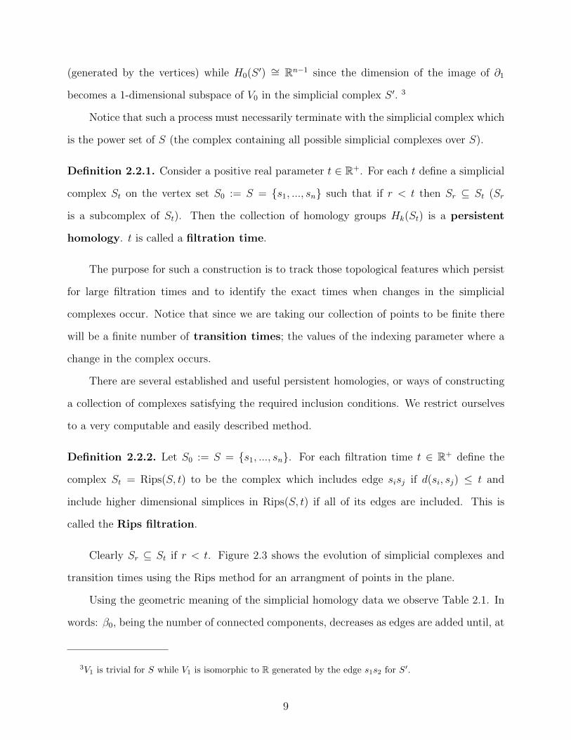
Clearly Sr ⊆ St if r < t. Figure 2.3 shows the evolution of simplicial complexes and
transition times using the Rips method for an arrangment of points in the plane.
Using the geometric meaning of the simplicial homology data we observe Table 2.1. In
words: β0, being the number of connected components, decreases as edges are added until, at
3V1 is trivial for S while V1 is isomorphic to R generated by the edge s1s2 for S′.
9
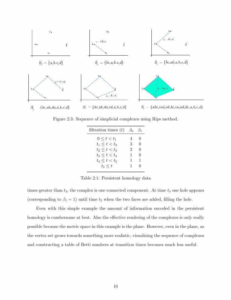
Figure 2.3: Sequence of simplicial complexes using Rips method.
filtration times (t) β0 β1
0 ≤ t < t1 4 0t1 ≤ t < t2 3 0t2 ≤ t < t3 2 0t3 ≤ t < t4 1 0t4 ≤ t < t5 1 1t5 ≤ t 1 0
Table 2.1: Persistent homology data
times greater than t3, the complex is one connected component. At time t4 one hole appears
(corresponding to β1 = 1) until time t5 when the two faces are added, filling the hole.
Even with this simple example the amount of information encoded in the persistent
homology is cumbersome at best. Also the effective rendering of the complexes is only really
possible because the metric space in this example is the plane. However, even in the plane, as
the vertex set grows towards something more realistic, visualizing the sequence of complexes
and constructing a table of Betti numbers at transition times becomes much less useful.
10

2.3 Barcodes
To solve the problem of storing and interpreting the persistent homology data a method
of visualization called a barcode is employed. For each i, 0 ≤ i ≤ n where n is the the
maximum index of the Betti numbers across all simplicial complexes we will construct a
Betti-i barcode. For fixed i we draw a copy of the indexing set (filtration times) along the
horizontal axis and at each time t plot βi(St) many points (along the vertical axis). The
result is a series of lines (or bars) which appear and disappear at transition times.
Sometimes (in particular in the Matlab program Plex - used to compute and display
barcodes) these are called the dimension-0 and dimension-1 Rips barcodes. However, in
that language the dimension-i barcode contains information related to the ith Betti number,
which is the dimension of the ith homology group. This overuse of the term ‘dimension’ can
be a source of confusion, so we will call the barcode associated with the ith Betti number
the Betti-i barcode.
Figure 2.4 shows the Betti-0 and Betti-1 Rips barcodes associated with the four points
in the plane in Figure 2.3.
Figure 2.4: Barcodes displaying the transition times where Betti numbers change.
Certainly as we increase the number of points n in our sample the Betti-0 Rips barcodes
can become very large. This reflects the fact that at filtration time t = 0 there are necessarily
n bars since the simplicial complex is merely the set of singletons (the points themselves) and
11

has n connected components. Nonetheless this method of visualization provides a reasonably
compact way of displaying a huge array of data.
As was stated in the introduction to this section persistent homology is used to try
and extract coarse topological information about an underlying set given a rough or noisy
sampling; what is sometimes called point-cloud data. Such conclusions regarding or de-
scriptions of the underlying set require interpretation of the barcodes and are subject to
concerns such as the uniformity and accuracy of the sampling. In our example one might
conclude that the four points were sampled from a set that is homeomorphic to a circle since
one Betti-1 barcode appears and persists for a relatively long interval before disappearing;
suggesting a single hole.
Remark 2.3.1. Perhaps more concerning is that the Rips complex can show higher dimen-
sional topological features than can exist in the space from which the points are sampled.4
One could instead use the Cech complex which does not present these problems. Con-
sider a set of points S0 with a metric, then the Cech complex Sε will contain an n-simplex
for those subsets of n+1 points which lie in a ball of radius ε/2. More geometrically consider
Uε =⋃s∈S0
Bε/2(s); the union of the balls of radius ε/2 centered on the vertex set S0. The
Nerve Lemma [4] states that Uε is homotopy equivalent to Sε which is not true for the Rips
filtration. However, the difficulty in computing the Cech complex compared with the highly
computable Rips complex and the scope of our first application justifies our use of the latter.
4As an example consider 17 points evenly distributed around a circle of radius 1. Approximately atfiltration time t = 1.79 a Betti-3 barcode appears and persists until t = 1.92 when a Betti-5 barcode appearsand persists until t = 1.99.
12
Chapter 3
THE CIRCLE MAP
The first dynamical system of interest is the well-studied circle map. For a fixed number
θ ∈ (0, 1) define Tθ : [0, 1)→ [0, 1) by
Tθ(x) = x+ θ mod 1
We think of this simple version of the circle map as rotation of a circle of circumference
1 by an angle θ. It is known that for θ ∈ R − Q this map is ergodic (for a proof using
Fourier series see [5]). In particular the forward orbit of a point x ∈ (0, 1) under iterations of
Tθ is dense in (0, 1) for irrational θ, while orbits are periodic for rational θ. This motivates
considering how the dynamics of the circle map are connected to classical number theory.
Another motivation originates from phyllotaxis, the arrangement of leaves on a plant
stem. In [6] a modified circle map is defined and its properties are explored. In particular this
modified circle map tracks the number of iterations as well as the displacement – becoming a
system acting on the plane. The y-axis can be thought of as the time variable while the x-axis
tracks the spatial position recorded by the standard circle map. This produces a cylindrical
lattice which is then mapped to the disk under an area preserving change of coordinates.
The family of lattices is defined in complete generality in [6].
Definition 3.0.1. L(λ,R, θ, g) =z1(λ, 2πRθ) + z2(0, 2πR
g)|(z1, z2) ∈ Z2
. Where λ ∈
R+, g ∈ N is the 2πRg
-periodic lattice in the plane (a cylindrical lattice on a cylinder of
radius R).
For simplicity we restrict our attention to λ = g = 1, R = 12π
. Explicitly T ′nθ (0) =
(nθ , n) ∈ R2 with Cartesian coordinates. Mapping the lattice (the orbit of 0 under T ′θ) to
the disk under an area preserving transformation defines the modified circle map:
13

(x, y) 7→ (√y cos(2πx),
√y sin(2πx)), for (x, y) ∈ L(1, 1
2π, θ, 1).
Orbits under the modified circle map are unbounded and so even for rational θ orbits are
no longer periodic. However points in the orbit of rational rotations lie on a finite number of
rays emanating from the origin. For irrational θ, spirals are observed and subtle features of
the distribution of points under different choices of rotation angle can be seen 1. In Figure 3.1
we have purposefully chosen to compare the golden number
1+√
52
(a quadratic algebraic
number) with π (a transcendental number) to illustrate this difference in distribution.
Figure 3.1: 100/800 iterations of the circle/modified circle map with angle a)
1+√
52
and
b) π.
Applying a Rips filtration to the orbit of initial condition x = 0 under the modified
circle map for different choices of rotation angle reiterates the contrast in the distribution of
points, as seen in Figure 3.2.
For now we return our focus to the standard circle map Tθ as it will prove sufficient to
address some of these observations.
Fix φ =
1 + 52
≈ .61803 and consider the Betti-0 barcodes of orbits of varying length
under iteration Tφ (starting at 0). In contrast to the highly irregular and unpredictable
barcodes illustrated in Figure 3.2 and in the literature (when this technique is applied to
5Notice the 7 clusters of points in the upper plot of Figure 3.1 b) and the 7 distinct spirals in the lowerimage.
14

Figure 3.2: Rips barcodes of 100 iterations of the modified circle map with angle a)
1+√
52
and b) π.
real-world data) stunning regularity is observed. In Figure 3.3 the Betti-0 barcodes for the
plots of n = 15, 21, 40, 50, and 100 points are given.
Figure 3.3: Betti-0 barcodes for orbits under Tφ of various length
We observe that there are at most 3 transition times where the number of Betti-0
barcodes decreases, with exactly 2 transition times in the plot of 21 points. The regularity
in these barcodes goes deeper; for orbits of fixed length in which three transition times are
present, the sum of the smaller two transition times is observed to be the third. And, for
example, the last transition time for n = 40 is the same as the middle transition time for
15

n = 21. More to the point a new transition time is introduced when a 22nd point is added.
Finally notice that for both n = 40 and n = 50 the simplicial complexes at filtration times
between the first and second transition times have 34 connected components. In fact this is
true for all n, 34 < n < 55. Consider Table 3.1 which records the barcode data for n points
and indicates when a new filtration time is introduced.
no. of points (n) β0 (transition time) β0 (transition time) β0 (transition time) new filt. time?
50 34 (.0131556) 5 (.021286) 1 (.0344416)
51 34 (.0131556) 4 (.021286) 1 (.0344416)
52 34 (.0131556) 3 (.021286) 1 (.0344416)
53 34 (.0131556) 2 (.021286) 1 (.0344416)
54 34 (.0131556) 1 (.021286)
55 34 (.0131556) 1 (.021286)
56 55 (.0081306) 33 (.0131556) 1 (.0212862) new time (smaller)
.
.
.
.
.
.
.
.
.
.
.
.
.
.
.
89 55 (.0081306) 1 (.0131556)
90 89 (.0050249) 53 (.0081306) 1 (.0131556) new time (smaller)
.
.
.
.
.
.
.
.
.
.
.
.
.
.
.
144 89 (.0050249) 1 (.0081306)
145 144 (.0031056) 88 (.0050249) 1 (.0081306) new time (smaller)
.
.
.
.
.
.
.
.
.
.
.
.
.
.
.
Table 3.1: Betti-0 data for orbit of x = 0 of length n under Tφ. Highlighted transition timesindicate first occurrence of these new transition times.
Counting the number of connected components which appear after the first transition
time (as we increase the orbit length under Tφ) yields a sequence of integers which are familiar
to most: the Fibonacci sequence. The barcodes lengths are significant as well. In particular
we observe that in the second column (the smallest filtration time where a transition occurs)
the transition time is exactly the distance from β0 · φ to the nearest integer. To understand
the significance of these integers and these transition times we briefly discuss a few results
from classical number theory.
3.1 Continued Fractions
There is another dynamical system on the unit interval closely related to the circle map
lurking in the background.
Definition 3.1.1. The Gauss Map G : [0, 1)→ [0, 1)
16

G(x) =
1x
, if x 6= 0
0, if x = 0
This map can be used to construct the continued fraction expansion of any real number.
For k ∈ N ak =⌊
1Gk(θ)
⌋. Then θ = [a0; a1, a2, ...] = a0 +
1
a1 +1
a2 +1
a3 + ...
is the continued
fraction expansion (CFE) of θ. The orbit of the Gauss map is finite if and only if theta is
rational, eventually terminating when Gm(q) = 0, q ∈ Q for some m. Thus the CFE of θ ∈ R
is finite if and only if θ ∈ Q. Given an irrational number with a non-finite CFE it is natural
to consider the sequence of rational numbers given by truncating the continued fraction.
Definition 3.1.2. The nth partial convergent of θ = [a0; a1, a2, ...] is the truncated con-
tinued fraction [a0; a1, a2, ..., an].
Proposition 3.1.1. Let pk = akpk−1+pk−2; p0 = a0, p1 = a1a0+1 and qk = akqk−1+qk−2; q0 =
1, q1 = a1. Then [a0; a1, a2, ..., an] = pnqn
.
A proof of this result and a complete treatment of other results referenced here are
available in [7] and many other classical number theory texts. For example many statements
about the convergence of the partial convergents and how well a number is approximated by
its convergents can be made. One rough observation is that larger partial quotients in the
CFE of a number will result in faster convergence of partial convergents.
For irrational numbers the algebraic degree tells us more about the dynamics of the
Gauss map and thus the rate of convergence of their partial convergents.
Theorem 3.1.1. The continued fraction expansion of θ ∈ R is periodic iff θ is a quadratic
surd.
This statement is as much is as known about the dynamics of the Gauss map on algebraic
numbers. For example it is not even known if the partial quotients of the continued fraction
17

expansion of any degree three algebraic number are bounded or unbounded. We mention
this now only because an equivalent characterization of the boundedness of partial quotients
will follow from the main result in this section.
Recall the observations at the end of Section 3; the appearance of the Fibonacci sequence
in the Betti-0 barcodes. In the language of CF theory these integers are the denominators
(and in fact the numerators) of the partial convergents to φ = [0; 1, 1, 1] =
1+√
52
. Recall
also that when plotting a Fibonacci number of points under rotation by φ only two transition
times appeared and the addition of a single point (extending the orbit length from 21 to 22
for example) resulted in a single barcode of a new (shorter) length to appear. It is tempting
to conclude that this is true for all irrationals but consider the analogous data to Table 3.1
for θ =√
2
= [0; 2, 2, 2], given in Table 3.2.
no. of points (n) β0 (transition time) β0 (transition time) β0 (transition time) new filt. time?
7 5 (.071067) 1 (.171572)
8 5 (.071067) 4 (.100505) 1 (.171572) new time (middle)
9 5 (.071067) 3 (.100505) 1 (.171572)
10 5 (.071067) 2 (.100505) 1 (.171572)
11 5 (.071067) 1 (.100505)
12 5 (.071067) 1 (.100505)
13 12 (.029437) 4 (.071067) 1 (.100505) new time (smaller)
.
.
.
.
.
.
.
.
.
.
.
.
.
.
.
17 12 (.029437) 1 (.071067)
18 12 (.029437) 11 (.04163) 1 (.071067) new time (middle)
.
.
.
.
.
.
.
.
.
.
.
.
.
.
.
29 12 (.029437) 1 (.04163)
30 29 (.012193) 11 (.029437) 1 (.04163) new time (smaller)
.
.
.
.
.
.
.
.
.
.
.
.
.
.
.
Table 3.2: Betti-0 data for orbit of x = 0 of length n under T√2−1. Highlighted transitiontimes indicate first occurrence of these new transition times.
For√
2
the denominators of the partial convergents are
2, 5, 12, 29, 70..., while new transition times are introduced immediately after
n ∈ 2, 3, 5, 7, 12, 17, 29, 41, 70, .... The observant will see that new smallest transition time
are introduced immediately after the denominators of the partial convergents, while new
transition times larger than the smallest existing time but smaller than the largest existing
time are introduced at these other special numbers. The subtlety is that partial convergents
only tell part of the story. Recall the partial convergents are defined by a recurrence relation
involving the partial quotients:
18

qk = akqk−1 + qk−2
This relation can be expressed by the vector-matrix equation
[ qkqk−1 ] =
[ak 11 0
]· [ qk−1
qk−2 ].
Thus one can compute the denominator of the kth partial convergent by multiplying [ q1q0 ] on
the left by the matrix product[ak 11 0
]. . . [ a1 1
1 0 ]
Example 3.1.1.√
2
= [0; 2, 2, 2]; (ai = 2,∀i).
[ 52 ] = [ 2 1
1 0 ]1 · [ 21 ] [ 12
5 ] = [ 2 11 0 ]2 · [ 2
1 ] [ 2912 ] = [ 2 1
1 0 ]3 · [ 21 ]
Again, the intermediate integers which are associated with the appearance of new tran-
sition times are not explicitly derived from the recurrence relation which defines the partial
convergents. However, matrices of the form [ n 11 0 ] can be factored into the product of 0, 1-
matrices. We fix these matrices for the remainder of the discussion with a definition
Definition 3.1.3. Let F = [ 1 11 0 ] be the Fibonacci matrix andG = [ 1 1
0 1 ] the inner matrix.
Proposition 3.1.2. [ n 11 0 ] = Gn−1F
The proof is a straightforward exercise in induction and matrix multiplication.
Now consider multiplication of the vectors [ q1q0 ], [ p1p0 ] by the factored forms of the matrices
derived from the CFE of some number θ = [a0; a1, a2, ...]. Recording the first entry in the
vectors after multiplication by every matrix (either F or G) gives rise to a sequence of
integers which contains as a subsequence those integers which are partial convergents to θ.
Definition 3.1.4. We define the full sequence of convergents and call all rational ap-
proximates obtained from the full sequence the total convergents. We call the sequence
of partial convergents the outer sequence and those members of the full sequence not in
the outer sequence the inner sequence.
19

Example 3.1.2.√
2
= [0; 2, 2, 2]; (ai = 2,∀i).
...G · F ·G · F ·G · F · [ 21 ]
Outer Sequence: [ 21 ] , [ 5
2 ] , [ 125 ] , [ 29
12 ] , [ 7029 ] ...
Inner Sequence: [ 32 ] , [ 7
5 ] , [ 1712 ] , [ 41
29 ] , ...
Full Sequence: [ 21 ] , [ 3
2 ] , [ 52 ] , [ 7
5 ] , [ 125 ] , [ 17
12 ] , [ 2912 ] , [ 41
29 ] , [ 7029 ] ...
With the full sequence of convergents defined we are ready to state the observations
in the Betti-0 barcodes as several conjectures. Let θ ∈ [0, 1) − Q and consider the orbit of
length n of a point under iterations of the map Tθ.
Conjecture 3.1.1. There are at most three transition times in the Betti-0 barcode 0 <
d1k < d2k < d3k with d1k + d2k = d3k taking the number of connected components from
n > n1 > n2 ≥ 1.
Conjecture 3.1.2. The number of connected components in the Rips simplicial complex
for filtration times between the first and second transition times is qk where qk is the largest
denominator in the partial convergents to θ not exceeding n.
Conjecture 3.1.3. If introducing the (n+ 1)th point results in a new transition time which
is smaller than than the existing two transition times (those in the Betti-0 barcodes for n
points) then n = qk for some k (n is in the outer sequence). Otherwise (if the new filtration
time is in the middle of the existing two) then n is an element of the inner sequence. Moreover
the number of connected components as in conjecture 3.1 remains the same.
The last sentence of conjecture 3.2 illustrates why a transition time being inserted be-
tween the existing two filtration times does not change the number of connected components
observed after the first transition time. On the other hand a new smallest filtration time (ap-
pearing in a plot of n+1 points) will correspond to a single barcode of that length appearing
at the top of the Betti-0 barcode. Thus after the first transition time (this new smallest one)
20
there will be exactly n connected components, which is the content of this conjecture. If
the above conjectures are true the following recursion formula can be given for the smallest
(and thus all 2) the transition times which will appear in the Betti-0 barcodes for a plot of
n points.
Corollary 3.1.1. Let the full sequence of θ be the set nkk∈N and for each k let n1k be the
largest element of the outer sequence less than or equal to nk. If d1k < d2k are the transition
times appearing in the Betti-0 barcodes of nk points. Then
d1k+1 =
1−d1knkn1k
, if d1k(nk + nk+1) > 1
d1k, if d1k(nk + nk+1) < 1
Proof. Fix n ∈ N, n > 3. From conjecture 3.1.1 we know (n−n1)d1+(n1−n2)d2+n3d3 = 1.
If we restrict our attention only to those numbers of points where addition of a single new
point under the map Tθ causes the creation of a new filtration time (namely the sequence nk)
then this equation becomes (nk − n1k)d1k + n1kd2k = 1 =⇒ nkd1k + n1k(d2k − d1k) = 1.
Of course if we have plotted nk points and there are only two transition times in the Betti-0
barcode then by the construction of the Rips complex there are only two different distances
between any two consecutive points. Implicit in conjecture 3.1.1 and 3.1.3 (and the reason
for the behavior of the rotation map) is that the introduction of the nk + 1 point will split
the largest of these two gaps into two smaller gaps. There are only two possibilities for the
resulting gap: Either the existing smaller gap remains the smallest gap (i.e. d1k+1 = d1k)
which happens when d1k(nk + n1k) < 1 or the new gap is smaller than any previously seen
(i.e. d1k+1 < d1k) which implies that d1k+1 = d2k − d1k by conjecture 3.1.1. This occurs
when d1k(nk + n1k) > 1.
2d2k = 1−(nk−n1k)d1kn1k
21

It remains then to prove conjectures 3.1.1-3.1.3. As it happens the content of the above
conjectures (which we observed through an application of the, perhaps overly sophisticated,
tool of persistent homology) is known by the name of the Steinhaus Conjecture which was
proved over 50 years ago and was given the name the Three Gap/Distance Theorem.
Theorem 3.1.2. (The Three Gap/Distance Theorem) Fix θ = [a0; a1, a2, ...]. Every integer
n ≥ 1 can be written uniquely as n = mqk + qk−1 + r where 1 ≤ m ≤ qk+1 and 0 ≤ r ≤ qk.
For n+ 1 points placed by rotations by θ, there are:
n+ 1− qk gaps between successive points of length d1k,
r + 1 gaps between successive points of length d2k, and
qk − r − 1 gaps between successive points of length d3k
To illustrate the connection between this theorem and the discussion above consider the
following example where the dataset is
T i3√2(0)|i = 0, 1, ..., n− 1 = 16.
Example 3.1.3. We consider the first 17 points in the forward orbit of the point 0 under
rotation by T 3√2, (3√
2 = [1; 3, 1, 5, 1, 1, 4, ...]). Figure 3.4 shows the Betti-0 barcode produced
by the Rips filtration applied to this collection of points in the plane. Using the notation in
Theorem 3.1.2 we have 16 = n = mqk + qk−1 + r. Here k = 2, (corresponding to a3 = 5)
and one can calculate from the above partial quotients q2 = 4. Then r = 1,m = 3 are the
only values satisfying the conditions of the theorem. Thus our expression for n becomes
16 = 3 · 4 + 3 + 1.
Figure 3.4: Betti-0 barcode produced from the the first 17 points in the forward orbit of 0under T 3√2.
22
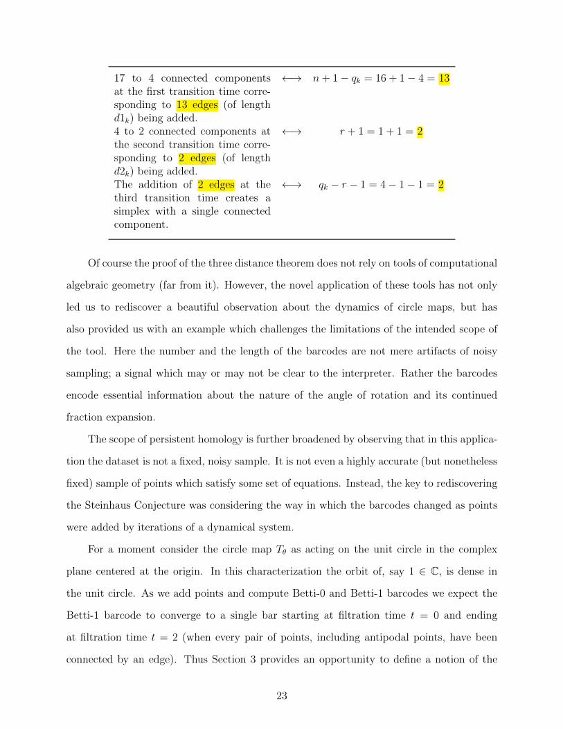
17 to 4 connected componentsat the first transition time corre-sponding to 13 edges (of lengthd1k) being added.
←→ n+ 1− qk = 16 + 1− 4 = 13
4 to 2 connected components atthe second transition time corre-sponding to 2 edges (of lengthd2k) being added.
←→ r + 1 = 1 + 1 = 2
The addition of 2 edges at thethird transition time creates asimplex with a single connectedcomponent.
←→ qk − r − 1 = 4− 1− 1 = 2
Of course the proof of the three distance theorem does not rely on tools of computational
algebraic geometry (far from it). However, the novel application of these tools has not only
led us to rediscover a beautiful observation about the dynamics of circle maps, but has
also provided us with an example which challenges the limitations of the intended scope of
the tool. Here the number and the length of the barcodes are not mere artifacts of noisy
sampling; a signal which may or may not be clear to the interpreter. Rather the barcodes
encode essential information about the nature of the angle of rotation and its continued
fraction expansion.
The scope of persistent homology is further broadened by observing that in this applica-
tion the dataset is not a fixed, noisy sample. It is not even a highly accurate (but nonetheless
fixed) sample of points which satisfy some set of equations. Instead, the key to rediscovering
the Steinhaus Conjecture was considering the way in which the barcodes changed as points
were added by iterations of a dynamical system.
For a moment consider the circle map Tθ as acting on the unit circle in the complex
plane centered at the origin. In this characterization the orbit of, say 1 ∈ C, is dense in
the unit circle. As we add points and compute Betti-0 and Betti-1 barcodes we expect the
Betti-1 barcode to converge to a single bar starting at filtration time t = 0 and ending
at filtration time t = 2 (when every pair of points, including antipodal points, have been
connected by an edge). Thus Section 3 provides an opportunity to define a notion of the
23

evolution, and ultimately the convergence, of barcodes. Such notions could have implications
in classifying topologically strange objects such as fractal Julia sets of complex polynomials
and in developing a definition of a measure of the degree of ergodicity of the circle map.
We consider another opportunity to analyze the evolution of barcodes in the next section.
24

Chapter 4
ION BOMBARDMENT
Experimental physicists have observed spontaneous pattern formation when a solid sur-
face is bombarded with a broad ion beam [9]-[12]. These patterns vary from parallel ripples
to highly ordered hexagonal arrays of nanodots. While academic interest in pattern and de-
fect formation has motivated research, much interest in these experimental observations lies
in their potential to improve fabrication of nanostructures or provide effective alternatives
to traditional fabrication methods. Ion bombardment has the potential to be a fast method
of producing regular nanostructures which are on the order of tens of nanometers; a scale
which matches that achieved by modern lithography techniques.
Several competing theories have emerged to model the hexagonal pattern formation
observed in experiments; two of which attempt to model the scenario of bombardment of
an elemental material [13]-[14] and one (the Bradley/Shipman theory studied in detail in
this paper) which emphasizes the necessity of a binary solid in the formation of hexagonal
patterns [15]. The first two theories study the Kuramoto-Sivashinsky equation1. The latter
argues that (generally) within a binary material one material is preferentially sputtered2
and that this results in a change in the relative concentrations of the two atomic species at
the surface. The theory suggests that this change in surface stoichiometry, when coupled
with the change in surface topography, is crucial in the formation of hexagonal arrays of
nanodots [15].
Naturally one of the primary goals of researchers in this area is to identify parameter
values which result in defect-free pattern formations. It is towards this end that we apply
1Modified with the addition of one or two nonlinear terms
2The effect of ejecting atoms from a solid by bombarding the surface with energetic particles.
25

persistent homology to ion bombardment data, both experimental and simulated. We do so
not only in the hope of supporting the models with a new method of comparison, but also
to demonstrate another application in which the evolution of barcodes can be studied.
Before we apply the computational homology tools we briefly explore the Bradley/Ship-
man theory and perform an analysis of the coupled system of equations. In [15] coupled
equations of motion describing the surface height and the relative concentrations of the com-
ponents of the binary material under normal incidence ion bombardment are derived and
analyzed. Here we perform a similar treatment of the equations modeling off-normal inci-
dence ion bombardment which introduces an anisotropy in the coupled system. In particular
we consider the following system:
ut = φ− (r1uxx + uyy)−∇2∇2u+ λ(r3u2x + u2
y) (4.1)
and
φt = −aφ+ b(r2uxx + uyy) + c∇2φ+ νφ2 + ηφ3, (4.2)
where u(x, y, t) is the surface height and φ(x, y, t) is the relative concentration of material
species. Thus choosing φ = 0 (and b = 0) this system reduces to the anisotropic Kuramoto-
Sivashinsky (AKS) equation [20].
ut = −(r1uxx + uyy)−∇2∇2u+ λ(r3u2x + u2
y). (4.3)
Choosing r1 = r2 = r3 = 1 reduces our system to the normal incidence equations in [15].
In [20] it is predicted that that remarkably defect-free ripples can be produced by
ion bombardment of a binary material because of the coupling between surface height and
composition; an interaction not present during bombardment of an elemental material. The
authors compare the AKS equation to the coupled system given in Eqns. 4.1, and 4.2, and
illustrate that the high degree of order is not present in the former. In the following sections
26

we provide a standard analysis of the coupled equations of motions before comparing the
models through the lens of PH.
4.1 Linear Stability Analysis
In this section we will perform linear stability analysis about the steady-state solution
u = φ = 0. First we fix the following notational conventions: l2 := r1k2x+k2
y and m2 := r2k2x+
k2y, where ~k = (kx, ky), bc(~k) is the maximum value of b for which σ(~k) = 0, bT = max
~kbc(~k),
c.c. denotes complex conjugate, and ∆i = ri∂2
∂x2+ ∂2
∂y2for i = 1, 2, 3.
The linear terms in Eqns. 4.1 and 4.2 can be expressed as a matrix equation;
∂
∂t
uφ
=
∆1 −∇2∇2 1
b(∆2) c∇2 − a
uφ
. (4.4)
Assuming seperable solutions of the form u = u0ei~k·~xeσt and φ = φ0e
i~k·~xeσt (where
~k = (kx, ky), and ~x = (x, y)), and substituting into Eqn. 4.4 gives
σu = ur1k2x + uk2
y − u(~k · ~k)2 + φ, (4.5)
and
σφ = −aφ− b(r2uk2x + uk2
y)− cφ~k · ~k. (4.6)
Then the dispersion relation σ can be seen as the solutions to the eigenvalue problem
σ
uφ
=
r1k2x + k2
y − k4 1
−b(r2k2x + k2
y) −a− ck2
uφ
. (4.7)
At b = bc(~k) (for ~k 6= ~0),
27

−k4 − l2 1
−bc(~k)m2 −ck2 − a
1
k4 − l2
=
0
0
. (4.8)
For ~k = ~0,
0 1
0 −a
u0
0
=
0
0
. (4.9)
Eqns. 4.8 and 4.9 lead to left eigenvectors, v1 = (ck2 + a, 1) and v2 = (a, 1) respectively.
These will be used in the nonlinear analysis in Section 4.1.
Eqn. 4.7 has solutions σ±(kx, ky) = T2±√
T 2
4−D, where
T = r1k2x + k2
y − k4 − a− ck2
D = (r1k2x + k2
y − k4)(−a− ck2) + b(r2k2x + k2
y).
(4.10)
Restricting our attention σ+, we look for unstable wave vectors ~k = (kx, ky) where the
dispersion relation is positive. By imposing the condition that σ = ∂σ∂x
= ∂σ∂y
= 0 and kx 6= 0
and ky 6= 0, we derive the following equations:
(a+ ck2) + c(r1k2x + k2
y)− 2k2(a+ ck2)− ck4 − b = 0
r1(a+ ck2) + c(r1k2x + k2
y)− 2k2(a+ ck2)− ck4 − br2 = 0
(a+ ck2)(r1k2x + k2
y)− (a+ ck2)k4 − b(r2k2x + k2
y) = 0.
(4.11)
These equations reduce to
28

br2 − 1
r1 − 1= a+ ck2
k2 = k2x + k2
y =r2 − r1
r2 − 1.
(4.12)
Assuming separately that ky = 0 and kx = 0 leads, respectively, to
br2 = r1(a+ ck2x)− (a+ ck2
x)k2x
k2x =
cr1 − a2c
(4.13)
b = a+ ck2y − (a− ck2
y)k2y
k2y =
c− a2c
.(4.14)
This derivation gives critical values of b : bT,x := (cr1+a)2
4cr2, bT,y := (c+a)2
4c, and bT :=
r2−1r1−1
(a+ c r2−r1
r2−1
)in terms of the other parameters.
For fixed choices of these parameters, one or more of the critical values of b is largest
among the three, and as b is decreased below this critical value, the dispersion relation
attains positive values. More precisely if we fix a, c, r1, and r2 Re(σ+(~k)) < 0 for all ~k
if b > bc (c ∈ x, y, T). When b = bc, Re(σ+(~k)) = 0 for certain wave vectors ~k (see
Eqns. 4.12, 4.13, and 4.14) and is negative elsewhere. As we decrease b below critical, small
regions of unstable wave vectors (i.e. ~k for which Re(σ+(~k)) > 0) form. Notice that each
bifurcation is valid only for certain choices of c and a. For example bT,y requires the critical
wavevector to be k2y = c−a
cwhich forces c > a. Figure 4.1 shows regions in the ac-plane
where the various critical values of b can be present and the prototypical regions of unstable
wavevectors associated to each bifurcation.
29

Figure 4.1: (i) The ac-plane partitioned into regions based on the types of bifurcations whichcan occur. For example above the line a = c, either bT,x or bT,y will be the critical value ofb (depending on which is larger). On the line a = c we have bT,y = a =: bII,y and belowthe a = c line bT,y is no longer valid; here either bT,x or bII,y will be the critical value ofb (depending on which is larger). Similar reasoning shows a transition along the c = a
r1line, which can be above or below the a = c line depending on the choice of r1. (ii) The
prototypical regions where Re(σ+(~k)) > 0 associated to the various critical values of b.
For certain choices of parameter values we can force the instability and, for example, a
roll pattern to orient itself along the kx or ky axis. In particular, either critical value bT,x or
bT,y can be made largest by an appropriate choice of parameters.
Example 4.1.1. Choosing r1 = r2 =: r we observe that for fixed a, c > 0, bT,x is a parabola
with minimum at r = ac.
Figure 4.2: Plots of bT,x and bT,y as functions of r = r1 = r2 showing points and regions ofinterest.
30

First, k2y = c−a
2cforces c > a. Also for bT,x to be a valid bifurcation we require r ≥ a
c,
thus we restrict our plot to the increasing portion of the curve bT,x(r). Equality occurs when
bT,y = bT,x at r = 1 (and r =(ac
)2< a
cso we ignore it).
As the system is allowed to evolve the solution moves progressively further from the
steady state around which our linear analysis was performed (u = φ = 0) and nonlinear
terms must be added. In the following section we derive amplitude equations for the time-
evolution of the unstable modes which appear for choices of b below critical.
4.2 Non-Linear Analysis
As we have stated, by choosing the parameter b slightly below critical bT the dispersion
relation σ(kx, ky) is greater than zero for choices of ~k in some regions of the kx, ky−plane. In
the case of normal incidence bombardment the dispersion relation exhibits total rotational
invariance and the region of active modes is an annulus. With the introduction of the
anisotropy our linear analysis shows that small regions of active modes can appear oriented
along the kx and/or ky axes for certain choices of parameters.
A priori, and in either case, for any choice of ε > 0 there are an infinite number of active
modes (for a, c chosen in Region I). Furthermore the passive modes are not bounded away
from 0; in other words there are passive modes which are arbitrarily close to 0. However,
since we are searching for solutions which give rise to lattice patterns (rolls, hexagons, etc.)
we will assume that all wavevectors contributing to the pattern lie on a lattice [22].
For a hexagonal lattice these wavevectors will be at angles of 2π3
to each other. This
leads to the resonance: ~k1 + ~k2 + ~k3 = ~0 [22] where we take ~k1 to be the most unstable
mode: corresponding to the maximum value of the dispersion relation. In both normal
incidence and off-normal-incidence active modes can resonate through the nonlinear terms
in the equations of motion.
We proceed by choosing b = bT (1− εb1) for some 0 < ε << 1 and b1 > 0 (i.e. b slightly
below critical) and expand our solutions in powers of ε.
31

~q =
uφ
=
0
0
+ ε~q1 + ε2~q2 + ..., qj =
ujφj
. (4.15)
We also expand the time-derivative in powers of ε: ∂t = ∂τ0 + ε∂τ1 + ε2∂τ2 + ..., since
the evolution of ~qj occurs at a time scale proportional to 1ε. Define η := εη, and assume η is
chosen so that η is of order 1.
The zeroth order of ε is trivially
0
0
=
0
0
.
The first order of ε yields
∂
τ0
−
−∆2 −∆1 1
b∆2 c∆− a
u1
φ1
=
0
0
. (4.16)
From our linear analysis we determined that Eqn. 4.16 has solutions of the form
~q1 =
u1
φ1
=∑~k 6=0
1
k4 − l2
(A~k(τ1)ei~k·~x + c.c.
)+
B0
, (4.17)
where here B ∈ R is called the soft-mode and corresponds to ~k = ~0.
The second order of ε leads to
−∆2 −∆1 1
b∆2 c∆− a
εu1 + ε2u2
εφ1 + ε2φ2
= −ε2 ∂
∂τ1
u1
φ1
+ ε2
λ∆3u1
νφ21 + ηφ3
1
. (4.18)
32

Letting L :=
−∆2 −∆1 1
b∆2 c∆− a
and equating powers of ε Eqn. 4.18 reduces to
L
u2
φ2
=1
εL
u1
φ1
− ∂
∂τ1
u1
φ1
+
λ∆3u1
νφ21 + ηφ3
1
. (4.19)
Letting Lc(~k) :=
−∆2 −∆1 1
bc(~k)∆2 c∆− a
, note that for each ~k
Lc(~k)
1
k4 − l2
ei~k·~x =
0
0
, (4.20)
which implies that
L
u1
φ1
= (L− Lc)
u1
φ1
=
0 0
(b− bc(~k))∆2 0
u1
φ1
.
(4.21)
Therefore we can rewrite Eqn. 4.19 as
~q2 = L
u2
φ2
=∑~k∈A
− ∂∂τ1
A~k(τ1)ei~k·~x + λ
(r3∂u1∂x
2+∂u1∂y
2)
1ε(b− bc(~k))
r2 ∂2A~kei~k·~x∂x2+∂2A~k
ei~k·~x
∂y2
− ∂∂τ1
(k4 − l2)A~k(τ1)ei~k·~x + νφ2
1 + ηφ31
.
(19)
At this point we take a moment to recall a result from functional analysis:
33

Theorem 4.2.1. (Fredholm Alternative) Let L : V → V be a linear map on a Banach space
V and for u ∈ V consider the equation L(u) = 0. Either
(i) L(u) = 0 has no nontrivial solutions, or
(ii) L∗(v) = 0 has a nontrivial solution v 6= 0 and L(u) = f has a solution iff 〈v|f〉 =
〈f |v〉 = 0 for all v such that L∗(v) = 0.3
We also note that
∫Ω
ei~k·~xdA = 0 for ~k 6= ~0 so that for v = 〈vx, vy〉ei
~k·~x and u =
〈ux, uy〉T ei~j·~x we have 〈v|u〉 = 0 unless ~k = ~j. Thus for Eqn. 19 to be solvable we require
that for every term of the form v~kei~k·~x, ~k 6= ~0, on the right hand side of Eqn. 19 the vector
v~k must be orthogonal to the left eigenvector derived in Section 4.1, (ck2 + a, 1).
We apply the solvability condition 〈~vi|~q2〉 = 0, (i = 1, 2) where v1 = (c~k2 + a, 1) and
v2 = (a, 1), the left eigenvectors corresponding to b = bc(~k) and ~k = (0, 0) respectively.4
First let us consider the soft mode. We search for all terms in ~q2 which involve ei~0·~x.
Consider first the terms in the quadratic nonlinearity λ(r3
∂u1∂x
2+ ∂u1
∂y
2)
.
∂u1
∂x=A1(ik1x)e
i~k1·~x − A∗1(ik1x)e−i~k1·~x
+ A2(ik2x)ei~k2·~x − A∗2(ik2x)e
−i~k2·~x
+ A3(ik3x)ei~k3·~x − A∗3(ik3x)e
−i~k3·~x
(4.22)
3L∗ is the adjoint of L and for our purposes 〈v|f〉 = 1Ω
∫Ω
v · fdA for Ω = [0, 2pi/|k|]× [0, 2pi/|k|].
4While we have derived these equations in complete generality we recall that the wavevectors of interestare ~k1, the most unstable mode, and ~k2 and ~k3 satisfying ~k1 + ~k2 + ~k3 = ~0.
34
∂u1
∂x
2
=(· · · − 2A1(ik1x)ei~k1·~xA∗1(ik1x)e
−i~k1·~x + · · ·
· · · − 2A2(ik2x)ei~k2·~xA∗2(ik2x)e
−i~k2·~x + · · ·
· · · − 2A3(ik3x)ei~k3·~xA∗3(ik3x)e
−i~k3·~x + · · · ).
(4.23)
A similar equation is derived for ∂u1∂y
2and the observation is that the only terms in the
quadratic nonlinearity λ(r3
∂u1∂x
2+ ∂u1
∂y
2)
which involve ei~0·~x are terms involving AjA
∗j . The
same is true in the quadratic nonlinearity νφ21:
νφ21 =(· · ·+ 2(k4
1 − l21)2A1A∗1 + · · ·
(· · ·+ 2(k42 − l22)2A2A
∗2 + · · ·
(· · ·+ 2(k43 − l23)2A3A
∗3 + · · · ).
(4.24)
The condition that ~k1 + ~k2 + ~k3 = ~0 forces those terms in the cubic nonlinearity which
involve A1A2A3 or A∗1A∗2A∗3 to resonate with the soft mode. Therefore
ηφ31 =η(· · ·+ 6(k4
1 − l21)A1(k42 − l22)A2(k4
3 − l23)A3 + · · ·
· · ·+ 6(k41 − l21)A∗1(k4
2 − l22)A∗2(k43 − l23)A∗3 + · · · ),
(4.25)
where l2i = r2(kix)2 + (kiy)
2(i = 1, 2, 3).
Putting the relevant terms together with the solvability condition implies that
0 =(a)
− ∂B∂τ1
+ 2λ3∑j=1
[r3(k2jx + (k2jy)AjA
∗j
]+ (1)
2ν
3∑j=1
[(k4j − l2j )2AjA
∗j
]+ 6η(k41 − l21)(k42 − l22)(k43 − l23)[A1A2A3 +A∗
1A∗2A
∗3]
(4.26)
=⇒
35
∂B
∂τ=
2
a
3∑j=1
(λ(r3(k2jx) + (kjy)2
)+ ν(k4j − l2j )
)AjA
∗j
+6η
a(k41 − l21)(k42 − l22)(k43 − l23)[A1A2A3 +A∗
1A∗2A
∗3].
(4.27)
We next apply the solvability condition to the triad of wavevectors ~k1, ~k2, and ~k3. Restricting
our attention to the amplitude A15 we first search for terms which involve ei
~k1·~x. The condi-
tion that ~k1 +~k2 +~k3 = ~0 =⇒ ~k1 = −~k2−~k3 (similarly ~k2 = −~k1−~k3 and ~k3 = −~k1−~k2). In
the quadratic nonlinearities λ(r3
∂u1∂x
2+ ∂u1
∂y
2)
and νφ21 these are the cross terms containing
A∗2A∗3. The cubic nonlinearity contains terms which resonate with ~k1, namely those which
contain A1AiA∗i , (i = 1, 2, 3). Then the solvability condition is given by the equation
0 =(ck21 + a)
(−∂A1
∂τ1+ 2λ (r3(k2xk3x) + (k2yk3y)A∗
2A∗3)
)−
1
ε(b− bc(~k1))(r2(k1x)2 + (k1y)2)A1 + (k41 − l21)
∂A1
∂τ1+ 2ν(k42 − l22)(k43 − l23)A∗
2A∗3
+ 3η((k41 − l21)3|A1|2 + 2(k41 − l21)(k42 − l22)2|A2|2 + 2(k41 − l21)(k43 − l23)2|A3|2
)A1
(4.28)
=⇒
∂A1
∂τ=σ1A1 + γ1A1
[(k41 − l21)|A1|]2
+
3∑j=2
2 ·[(k4j − l2j )|Aj |
]2+ α1A∗2A
∗3, (4.29)
where α1(~k1, ~k2, ~k3) =(ck21+a)(2λ)(r3(k2xk3x)+(k2yk3y))+2ν(k42−l22)(k43−l23)
ck21+a−k41+l21
and γ1(~k1, ~k2, ~k3) =3η(k41−l21)
ck21+a−k41+l21
and σ1 = σ(~k1).
Again, equations for ∂A2
∂τand ∂A3
∂τcan be derived from cyclic permutation of the indices.
We are interested in understanding the stable solutions to the above system (i.e. ∂Ai∂τ
= 0)
and at this point several reductions to particular cases can be made. The homogeneous state
A1 = A2 = A3 = 0 is the steady state solution u = φ = 0. Rolls will be achieved for stable
solutions to the amplitude equations where A2 = A3 = 0:
5The ODEs for A2 and A3 needed to complete the coupled system of amplitude equations can be derivedby cyclic permutation of the indices.
36

∂A1
∂τ=σA1 + γ(k4
1 − l21)A1|A1|2 = 0 (4.30)
which has solutions A1 = ±√
−σγ(k41−l41)
.
In the isotropic case the complexity of the system of amplitude equations is reduced by
applying equivariance under rotation [22]. This forces σ = σ1 = σ2 = σ3, γ = γ1 = γ2 = γ3
and α = α1 = α2 = α3 and enables us to solve explicitly the case where A1 = A2 = A3 6= 0
corresponding to hexagonal pattern formations [15]. This is more elusive in the anisotropic
because the coefficients on the quadratic terms of the amplitude equations are not all equal.
In particular the system is not gradient for all parameters and wavevectors. We would like
to at least check if, for certain choices of parameters and wavevectors, we can write the
amplitude equations as a gradient system. This investigation remains to be carried out.
4.3 Persistent Homology Statistics
In this section we will define several standard statistics on barcode data to explore the
evolution of a binary surface towards a stable hexagonal array of nanodots.
First consider the idealized scenario; the expected long-term stable solution for some
specified set of parameters which give rise to hexagonal ordering. This is a collection of
raised dots whose peaks lie precisely on a hexagonal lattice of points in the plane. Since
defects in the array come in the form of deviation of the peaks from this lattice, and because
of the limitations on the number of points which can feasibly be used as a sample within
current PH computational packages we will track only the local maximums of the surface
(i.e. the nanodot peaks) as it is altered by ion bombardment.
Definition 4.3.1. We can take a planar hexagonal lattice to be a set of points in the plane
generated by two vectors (of the same length) such that the angle between them is 2π3
radians.
That is
37

Hu1,u2 =m · u1 + n · u2|m,n ∈ Z and 2π
3= cos−1
(〈u1|u2〉|u1|2
).
We observe that within such a lattice, sets of three adjacent points form equilateral
triangles with side lengths |u1| = |u2|. Thus for such a set of points we know the structure
of the Betti-0 and Betti-1 Rips barcodes.
Consider a square region of the plane containing a planar hexagonal lattice. Assume
the subset of the lattice within this region contains n points. Then we expect for filtration
times 0 ≤ t < |u1| there will be n connected components in the Rips simplicial complexes.
At time t = |u1| edges of this length are added to the complex and, by the definition of the
Rips complex, two dimensional faces (the faces of the equilateral triangles) are also added.
In other words, for a true hexagonal lattice without defects, no Betti-1 homology class will
appear for any simplicial complex at any filtration time.
However, if we perturb the points of the lattice (i.e. introduce a defect) we can force
the appearance of a hole (a topological circle) and thus a bar in the Betti-1 barcode. We
illustrate this in Figure 4.3.
Figure 4.3: A defect in a hexagonal lattice which results in a hole (a topological circle)appearing at filtration time t = |u1|.
38

One observation then is that the more defects, and the greater their severity, the more
frequent and the larger the holes in the simplicial complexes may be and thus the longer
and more frequent the resulting Betti-1 barcodes. To illustrate this behavior we present
Figure 4.4 which shows time series snapshots of a simulated surface as it evolves towards a
hexagonal array.
We compare Figure 4.4 to Figure 4.5 which shows a simulated surface undergoing ion
bombardment according to the KS equation (with the same domain and parameters) and
the associated Betti-0 and Betti-1 barcodes. Notice that in the case of the coupled system of
equations the Betti-1 barcodes diminish in total and average length in time and the lengths
of the Betti-0 barcodes become more consistent. We formalize these observations by defining
some basic barcode statistics and applying them to this system.
Definition 4.3.2. Represent the Betti-j barcode data as a set of real intervals, βj =
[xji , yji ]|1 ≤ i ≤ k where each interval [xji , y
ji ] represents the bar in the Betti-j bar-
code which starts at xji and ends at yji . Define the total barcode length of βj to be
TotLen(βj
):=
k∑i=1
(yji − xji ). Further define the average barcode length of βj to be
AvgLen(βj
):=
TotLen(βj
)k
.
We can of course define other standard statistics such as the variance in the barcode
length and the standard deviation of the barcode lengths in a similar way. In Figure 4.6 we
plot the average Betti-1 barcode length from the same simulation as in Figure 4.4 and note
its decline towards 0 as the system evolves.
In Figure 4.7 we plot the average Betti-1 barcode length given by a simulation of the
Kuramoto-Sivashinsky equation 4.3 over the time interval 200 ≤ t ≤ 30, 000 for comparison
to the coupled system.
39

Figure 4.4: A time series of plots of u(x, y, t) evolving according to the coupled equa-tions 4.1, 4.2 with parameters a = .4, c = .6, r1 = r2 = r3 = 1, λ = −.3 in a squareregion (−120 ≤ x, y ≤ 120) at times (1a-e) t = 200, (2a-e) t = 1, 800, (3a-e) t = 9, 800,(4a-e) t = 30, 000. These show the evolution towards a hexagonal array. (1-4a) shows thesurface plots where lighter regions indicate larger values of u(x, y, t). (1-4b) shows the samesurface plots with the local maxima [17] (peaks of the nanodots) highlighted by a blue dot.(1-4c) shows plots of these peaks with the surface plot removed. (1-4d) are the Betti-0barcodes generated by the blue points, considered as a sample of the plane. (1-4e) are theBetti-1 barcodes generated by the blue points, considered as a sample of the plane.
40

Figure 4.5: A time series of plots of u(x, y, t) evolving according to the isotropic KS equa-tion 4.3 with parameters r1 = r3 = 1, λ = −.3 in a square region (−120 ≤ x, y ≤ 120) attimes (1a-e) t = 200, (2a-e) t = 1, 800, (3a-e) t = 9, 800, (4a-e) t = 30, 000. (1-4a) showsthe surface plots where lighter regions indicate larger values of u(x, y, t). (1-4b) shows thesame surface plots with the local maxima [17] (peaks of the nanodots) highlighted by a bluedot. (1-4c) shows plots of these peaks with the surface plot removed. (1-4d) are the Betti-0barcodes generated by the blue points, considered as a sample of the plane. (1-4e) are theBetti-1 barcodes generated by the blue points, considered as a sample of the plane.41
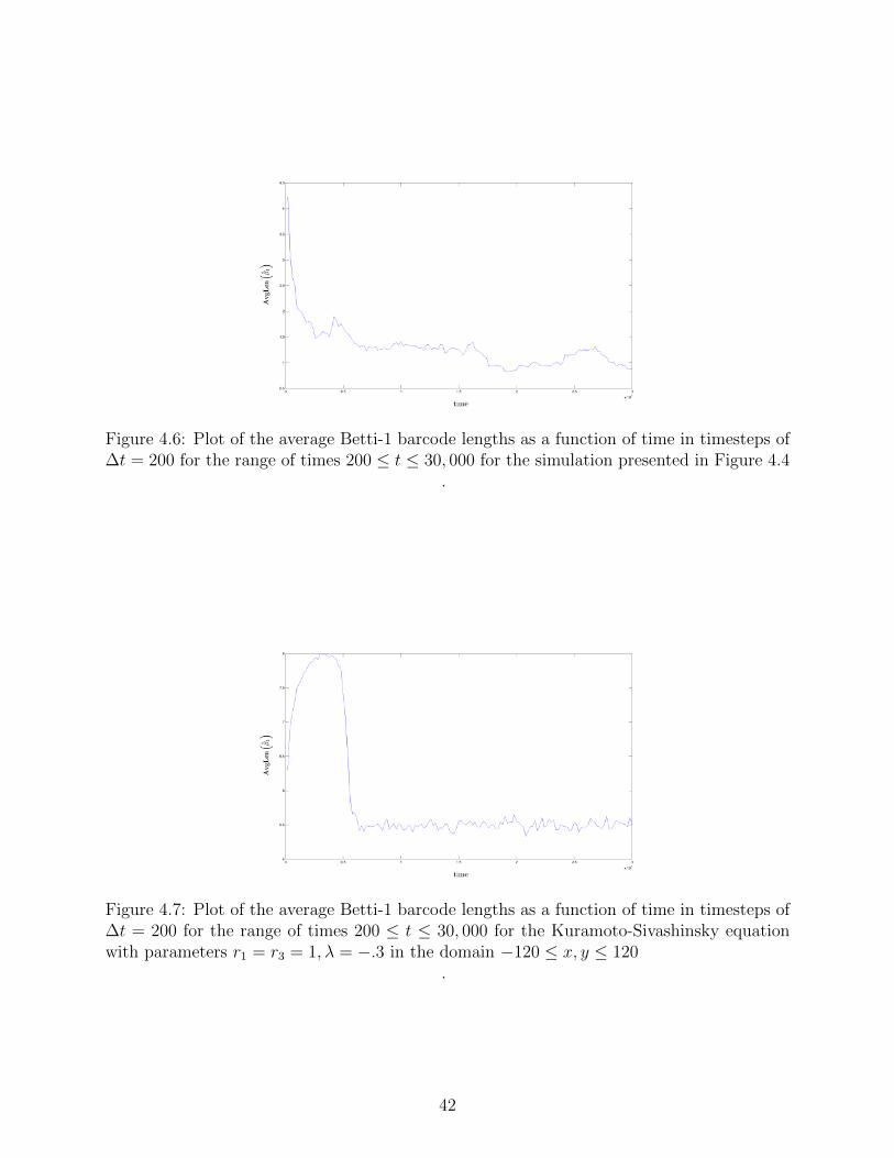
Figure 4.6: Plot of the average Betti-1 barcode lengths as a function of time in timesteps of∆t = 200 for the range of times 200 ≤ t ≤ 30, 000 for the simulation presented in Figure 4.4
.
Figure 4.7: Plot of the average Betti-1 barcode lengths as a function of time in timesteps of∆t = 200 for the range of times 200 ≤ t ≤ 30, 000 for the Kuramoto-Sivashinsky equationwith parameters r1 = r3 = 1, λ = −.3 in the domain −120 ≤ x, y ≤ 120
.
42
Chapter 5
IMPROVING PH SAMPLES
As we have stated, one of the principle goals and the original intention of computational
homology is to extract coarse topological features of some unknown space from a finite (often
noisy) sampling of points from that space. The first step in this process is collecting the
sample and so one inherent problem is ensuring that your sample is “good.” For now we will
take “good” to mean that the resulting persistence diagrams accurately reflect the topology
of the space from which the sample was gathered. For simple spaces, with well defined
notions of uniformity, we expect a good sample to be one which is evenly spread across
the underlying space so as to maximize the signals that indicate real homology classes and
minimize noise or false positives (i.e. persistent barcodes which are the result of unlucky
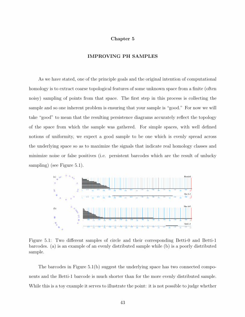
sampling) (see Figure 5.1).
Figure 5.1: Two different samples of circle and their corresponding Betti-0 and Betti-1barcodes. (a) is an example of an evenly distributed sample while (b) is a poorly distributedsample.
The barcodes in Figure 5.1(b) suggest the underlying space has two connected compo-
nents and the Betti-1 barcode is much shorter than for the more evenly distributed sample.
While this is a toy example it serves to illustrate the point: it is not possible to judge whether
43

a particular sample is good or bad using only the resulting persistence data (provided that
you do not already know the homology of the underlying space). One natural approach, and
a source of many interest unanswered questions about this technology, is to simply sample
more points. However, the computational complexity of existing algorithms greatly limits
the sample size to which PH can be applied. One could try and convince themselves of the
accuracy of a result by repeated sampling but this is both time consuming and provides no
guarantee of the correctness of the results. Alternatively one could try and improve a sample
by some method.
In this section we introduce an approach that aims to rearrange a sample across the
underlying space from which it was taken so as to improve the homological signal given by
PH. As a proof of concept we develop and implement an algorithm for the particular case
where the underlying manifold is the group of orthogonal, real 2× 2 matrices; a space whose
topological structure is known. Before that we construct an elucidating example to introduce
and explain the method.
Example 5.0.1. Consider the poor sampling of the circle given in Figure 5.1(b). If we
imagine these points as being positively charged particles, bound to the underlying space
S1, and we allow them to move on the circle then their natural tendency will be to spread
out into some minimum energy state. We can simulate this behavior by calculating the net
force acting on each point charge (according to, for example, Coulomb’s law), moving each
particle in the direction of this force some small distance, and then normalizing the resulting
position to bring the particle back to the unit circle. Figure 5.2 shows the evolution of the
poor sample of points under this iterative approach and the corresponding barcodes.
Since any sample of a space to which PH is applied will necessarily come equipped with
a distance matrix it is conceivable that sample points can always “push” on each other with
some “force” according to a sort of Coulomb’s law. The difficulty then, and what will change
from problem to problem, is in determining what it means to move points in the direction
of this force and in ensuring that points stay on the underlying space.
44

Figure 5.2: Snapshots at iteration numbers (a) 10, (b) 15, and (c) 20, showing the evolutionof the position of the sample points as they push against each other according to a 1
r2
Coulomb’s law.
We discuss answers to these questions with a space marginally more complicated than
S1, namely O2(R), and illustrate the impact the process can have on the persistence data.
Example 5.0.2. We begin by introducing a standard metric on the space of all matrices.
This induces a metric structure on the set O2(R) and so provides a method for populating
a distance matrix from a random sample of this space.
Definition 5.0.3. The Frobenius norm ||A||F =
√√√√ m∑i=1
n∑j=1
|ai,j|2 for A = [ai,j]1≤i≤m,1≤j≤n,
an m× n matrix. Define the Frobenius distance between two matrices to be distF (A,B) =
||A−B||F .
Let S = Si|1 ≤ i ≤ n ⊂ O2(R) be a collection of n orthogonal matrices. To apply
PH to this sample we first construct the distance matrix of all pairwise Frobenius distances
between points of S, that is the matrix D = [di,j]1≤i,i≤n, where di,j = distF (Si, Sj). We can
then apply a Rips filtration to construct a family of simplicial complexes whose homological
data is displayed as, the now familiar, barcodes.
45

It is known that O2(R) (with topology induced by the Frobenius norm for example) is
homeomorphic to two circles [16] (one for each allowable determinant: ±1). So we expect
a “good” sample S will lead to two persistent Betti-0 bars and two persistent Betti-1 bars.
The stronger this signal the better we will say the sample is. Motivated by the circle example
we imagine that each matrix has some charge associated to it to define a force field created
by the interaction of the n matrices in our sample.
Definition 5.0.4. For each pair (Si, Sj) define ForceF (Si, Sj) = 1distF (Si,Sj)
. For each matrix
Si ∈ S define totForceF (Si) =n∑j=1
forceF (Si, Sj). We note that the naming conventions are
chosen to maintain the clarity of the analogy to a physical system while in reality these
“forces” are merely positive numbers. Further define P (Si, Sj) =forceF (Si,Sj)
totForceF (Si); that is the
fraction of the of the total force on Si exerted by Sj.
We have in essence defined the magnitudes of the forces of interaction between the
matrices in our sample. We now need to define a direction in which these forces act. One
approach is to fix two sample points Si, Sj and define the matrix Si = αSi+P (Si, Sj)(1−α)Sj
to be the new “position” of Si after Sj has “pushed” on Si. Notice we have scaled the amount
of this displacement by the inverse of the Frobenius distance, maintaining the analogy to
Coulomb’s law.
Of course Si may no longer be an element of O2(R) and so we correct back to this space,
so as to simulate motion on the manifold itself, by finding the nearest orthogonal matrix
to Si and redefining Si to be this matrix. In particular define U : Md×d(R) → Md×d(R) as
U(X) = U · V ∗, where X = U · Σ · V ∗ is the singular value decomposition of X.1.
In both examples the effect of this spreading heuristic on the quality of the persistence
data is readily apparent. In the example involving orthogonal matrices the two Betti-1 bars
1U(X) is the nearest unitary matrix to X as measured by any unitarily invariant norm. [18]
46

Figure 5.3: (a) Barcodes generated by a random sample of n = 40 orthogonal 2× 2 matricesand (b) barcodes after the sample is allowed to evolve under iterations of the algorithmdescribed above.
are significantly lengthened and all but two Betti-0 bars are diminished giving a persistence
diagram that much better reflects the homology of O2(R).
While the particulars of this methodology will change from problem to problem we
highlight the fact that a very similar approach to the first example can be implemented for
an entire class of important topological objects: real algebraic varieties.
Given a system of polynomial equations we can consider its set of real solutions as living
in some high dimensional real vector space. In this setting the magnitude and direction of the
forces of interaction between elements of a sample of solutions are natural generalizations of
our simple example on the circle. As we have seen in the above examples this interaction will
likely displace our sample off the topological space we are interested in analyzing. However,
nonlinear numerical solvers using such approaches as trust-region and conjugate-gradient
methods [19] are fast and readily available2. Using the displaced point as an initial guess
2For example in Matlab’s optimization toolbox
47
(which by design would be near the variety) would, in theory, enable us to determine a
nearby point on the variety using these numerical optimization techniques, thus allowing us
to simulate motion on the object of interest. Through iteration of this process, our goal is to
evolve our sample to one which better reflects the topological signals produced by persistent
homology.
Example 5.0.3. As a second example we demonstrate an implementation of this general
technique on a compact surface; the torus given as the zero set of the following equation in
three variables,
F (x, y, z) =(
3−√x2 + y2
)2
+ z2 − 4 (5.1)
We begin with a very poor sampling of 150 points on this torus and then allow each
point to be influenced by its nearest neighbors. Again, we think of each point as being a
charged particle so that it experiences a repulsive force (governed by Coulomb’s law) from
the other sample points. New points are found by moving each point a small step in the
direction of the net force acting on them and then Matlab’s optimization toolbox is used
with these new point as initial conditions to calculate nearby points on the torus. In this way
motion on the manifold is simulated. Figure 5.4 shows time series snapshots of the sample
and the associated barcodes. Here we have plotted barcodes as points in the xy-plane; the
x-coordinate is the barcode start time and the y-coordinate is the barcode end time. Thus
long barcodes correspond to points far from the y = x line, while points near the diagonal
are weaker signals and can be considered noise.
Although these snapshots do not demonstrate fully the evolution of the barcodes, we
note the emergence of two Betti-1 barcodes which move, more or less horizontally, away
from the y = x line before stabilizing. These correspond to the two generators of the Betti-1
homology group which exist for a torus. Initially no simplicial complex in the filtration
contains a void but as the points spread noise appears in the Betti-2 barcode and, again, a
48

Figure 5.4: Samples of n = 150 points on the torus given by Equation 5.1, Betti-0, Betti-1,and Betti-3 barcodes for the associated sample taken at (i) 1, (ii) 30, (iii) 60, (iv) 90, (v)120, and (vi) 150 iterations of the spreading procedure.
49

single point moves horizontally away from the y = x line as the signal of a single Betti-2
generator (corresponding to the trapped volume in a torus) appears and strengthens.
If we consider a fixed sample size of a fixed metric space it is not known what finite subset
(sample) will produce the barcodes that best reflect the topology of the underlying space.
The ideal sample may very well differ between barcode dimensions. For a simple examples
such as the circle and the sphere we expect a distance matrix with minimal variance in the
distances between nearest neighbors (i.e. a uniformly distributed sample) will produce the
best barcodes. The author sees no reason why this need be the case for every manifold.
Moreover, even for a fixed dimension, the notion of a best barcode is not yet well defined.
Nonetheless one would like to be able to answer questions such as: which set of n points
sampled from a sphere gives rise to barcodes which most closely reflects the homology of the
sphere? For the torus? A real algebraic variety? And ultimately, can we produce an ideal
sample without knowing the underlying topology?
50

Chapter 6
OUTLOOK
In this paper we have introduced several applications of the computational geometry
tool, persistent homology, to data sets generated by dynamical systems. The application of
PH to the circle map led to the rediscovery of a beautiful and well-known result about the
distribution of points in the orbit of this ergodic system. Additionally we have extracted a
set of points in the plane from data generated by ion bombardment simulations. By applying
PH to this data we have not only suggested new ways of interpreting barcodes by defining
barcode statistics, we have also begun to develop a technique to answer questions of interest
to physicists about the degree of ordering present in a sample of a binary material after ion
bombardment. Finally we have observed some inherent limitations in PH and have started
to develop, through simple examples, techniques to improve the technology. Specifically we
have implemented algorithms to iteratively spread points on a real algebraic variety and
demonstrated that the methodology works to improve the signals in PH barcodes.
Still these ideas are only in their infancy and there are many directions we wish to
explore further. In the case of the modified circle map discussed in Section 3 we would like
to use PH to truly distinguish between rotation by the golden ratio and√
2, for example.
Ultimately we would like to use PH to order the real numbers by some measure of their
ergodicity and relate this distinction to the continued fraction expansion of the numbers.
One of the key ideas in constructing the modified circle map is that both temporal and
spatial information is tracked. We would like to do the same for other ergodic dynamical
systems such as the class of functions called linked twist maps [23]. It has been shown that
certain linked twist maps exhibit islands of non-ergodicity in their domain; topological circles
in the plane. We hope to explore further what PH can tell us about the behavior of these
51

systems both by considering them in standard form and by tracking temporal information
as well.
The analysis of the amplitude equations is, as of yet, incomplete and requires further
attention. We would like to at least be able to check if, for certain choices of parameters
and wavevectors we can write the amplitude equations as a gradient system; for a particular
choice of parameters does there exist wavevectors which make all the coefficients in the
quadratic nonlinearities equal to one another? Also, what is the value of the dispersion
relation at these wavevectors? By definition ~k1 will be an active mode but the same cannot
necessarily be said ~k2, and ~k3. If they are passive modes then what are the absolute values of
σ(~k2) and σ(~k3)? Answering this question might give us insight into how hexagonal ordering
can be achieved in the anisotropic case.
There are several questions of interest to the applied physics community which might
have answers in PH techniques. Dr. Mark Bradley has suggested applying this tool to identify
penta and hepta defects in disordered hexagonal lattices, to the problem of classifying viral
structures and large molecules, and to fingerprint data. In the same vein Dr. Patrick
Shipman has suggested applying PH to objective structures. Also, in this paper, we have
only compared models of ion bombardment. We would like to utilize PH to further compare
these models with the numerous examples of real-world experiments which demonstrate
spontaneous pattern formation for both normal and off-normal-incidence ion bombardment
of a solid surface. This has the potential to lead to a quantitative measurement of the degree
of ordering in nanostructures.
Towards the goal of improving a sample of point-cloud data from a topological manifold,
Dr. Shipman has speculated that one may be able to evolve the Swift-Hohenberg equation
or another appropriately chosen PDE to a stable solution which gives a good sampling. The
problems of minimal surfaces, packings, and (more generally) of the calculus of variations
may find a place to grow in computational topology.
52

The major commonality between these objectives is that they all attempt to build
connections between dynamical systems and computational topology. A natural, albeit very
broad, overarching question common to the ideas contained in this paper is how do barcodes
evolve as the input sample changes? This question is of particular interest and is one which
we hope to explore in the future.
53
Bibliography
[1] J. Matousek. Using the Borsuk-Ulam theorem: lectures on topological methods in com-
binatorics and geometry. Springer-Verlag Berlin Heidelberg. p 16.
[2] G. Carlsson, Topology and data. American Mathematical Society 46.2 (2009): 255-308.
[3] A. Hatcher. Algebraic Topology. Cambridge University Press, 2002.
[4] J. Leray. Sur la forme des espaces topologiques et sur les points fixes des reprsentations.
J. Math. Pures Appl. 24:95167, 1945.
[5] R. Bhatia. Fourier Series. The Mathematical Association of America, 2005.
[6] P. D. Shipman, Discrete and continuous invariance in phyllotactic tilings. Physical Review
E. 81, 031905 (2010).
[7] G.H. Hardy, E.M. Wright. An Introduction to the Theory of Numbers. Oxford University
Press, 2008.
[8] graphicalanalysis.m package, by Thomas LoFaro, [email protected]. Copyright 2001,
Thomas LoFaro.
[9] E. Chason, W. L. Chan, Spontaneous patterning of surfaces by low-energy ion beams,
Topics Appl. Physics 116 (2010) 53-71.
[10] B. Ziberi, M. Cornejo, F. Frost, B. Rauschenbach, Highly ordered nanopatterns on Ge
and Si surfaces by ion beam sputtering, J. Phys. Condens. Matter 21 (2009) 224003.
[11] S. Facsko, T. Dekorsy, C. Koerdt, C. Trappe, H. Kurz, A. Vogt, H. L. Hartnagel,
Formation of ordered nanoscale semiconductor dots by ion sputtering, Science 285 (1999)
1551-1553.
54
[12] F. Frost, A. Schindler, F. Bigl, Roughness evolution of ion sputtered rotating InP sur-
faces: Pattern formation and scaling laws, Phys. Rev. Lett. 85 (2000) 4116-4119.
[13] M. Castro et al., Phys. Rev. Lett. 94, 016102 (2005).
[14] S. Facsko et al., Phys. Rev. B 69, 153412 (2004).
[15] R. M. Bradley, P. D. Shipman, Spontaneous Pattern Formation Induced by Ion Bom-
bardment of Binary Compounds. Phys. Rev. Lett. 105, 145501 (2010).
[16] V.A. Zorich, Mathematical analysis, Volume 2. Springer-Verlag Berlin Heidelberg, 2004.
p. 324.
[17] extrema.m, extrem2.m packages, by Carlos Adrin Vargas Aguilera, nubeob-
[email protected]. Physical Oceanography MS candidate, Universidad de Guadalajara
Mexico, 2004.
[18] K. Fan and A. J. Hoffman, Some metric inequalities in the space of matrices. Proceedings
of the American Mathematical Society Vol. 6 No. 1, (Feb. 1955) pp. 111-116.
[19] T.F. Coleman, Y. Li, An Interior, Trust Region Approach for Nonlinear Minimization
Subject to Bounds. SIAM Journal on Optimization, Vol. 6, (1996) pp. 418-445.
[20] F.C. Motta, P.D. Shipman, R.M. Bradley, Highly Ordered Nanoscale Surface Ripples
Produced by Ion Bombardment of Binary Compounds. to be published, 2012: J. Phys.
D: Appl. Phys.
[21] Strogatz, Steven. Nonlinear Dynamics and Chaos. Westview Pr, (2000) pp. 343-353 160.
[22] Hoyle, Rebecca B. Pattern formation: an introduction to methods. Cambridge Univer-
sity Press, (2006) pp. 134-167.
[23] J.M. Ottino, R. Sturman, S. Wiggins. The Mathematical Foundations of Mixing: The
Linked Twist Map as a Paradigm in Applications: Micro to Macro, Fluids to Solids.
Cambridge University Press, 2006.
55


![Ranging and Grouping Patterns of a Western Lowland Gorilla ... · mountain gorillas [Jungers and Susman, 1984], the extremely folivorous and ter-restrial adaptation of mountain gorillas](https://img.pdfslide.net/doc/110x75/5e690aa9160ddf70c94ac5c5/ranging-and-grouping-patterns-of-a-western-lowland-gorilla-mountain-gorillas.jpg)