A COMBINATION SCHEME FOR INDUCTIVE LEARNING FROM

IMBALANCED DATA SETS

byAndrew Estabrooks

A Thesis Submitted to theFaculty of Computer Science

in Partial Fulfillment of the Requirementsfor the degree of

MASTER OF COMPUTER SCIENCE

Major Subject: Computer Science

APPROVED:

_________________________________________Nathalie Japkowicz, Supervisor

_________________________________________Qigang Gao

_________________________________________Louise Spiteri

DALHOUSIE UNIVERSITY - DALTECH

Halifax, Nova Scotia 2000

ii

DALTECH LIBRARY

"AUTHORITY TO DISTRIBUTE MANUSCRIPT THESIS"

TITLE:

A Combination Scheme for Learning From Imbalanced Data Sets

The above library may make available or authorize another library to make available individual photo/microfilm copies of this

thesis without restrictions.

Full Name of Author: Andrew EstabrooksSignature of Author: _________________________________Date: 7/21/2000

iii

TABLE OF CONTENTS

1. Introduction................................................................................11.1 Inductive Learning...................................................................11.2 Class Imbalance.......................................................................21.3 Motivation................................................................................41.4 Chapter Overview....................................................................4

2. Background................................................................................62.1 Learners...................................................................................6

2.1.1 Bayesian Learning...............................................................62.1.2 Neural Networks.................................................................72.1.3 Nearest Neighbor................................................................82.1.4 Decision Trees.....................................................................9

2.2 Decision Tree Learning Algorithms and C5.0..........................92.2.1 Decision Trees and the ID3 algorithm...............................102.2.2 Information Gain and the Entropy Measure......................112.2.3 Overfitting and Decision Trees..........................................132.2.4 C5.0 Options......................................................................15

2.3 Performance Measures..........................................................162.3.1 Confusion Matrix...............................................................172.3.2 g-Mean..............................................................................182.3.3 ROC curves........................................................................18

2.4 A Review of Current Literature..............................................192.4.1 Misclassification Costs......................................................192.4.2 Sampling Techniques........................................................22

2.4.2.1 Heterogeneous Uncertainty Sampling......................222.4.2.2 One sided Intelligent Selection.................................232.4.2.3 Naive Sampling Techniques......................................25

2.4.3 Classifiers Which Cover One Class....................................292.4.3.1 BRUTE......................................................................292.4.3.2 FOIL..........................................................................312.4.3.3 SHRINK....................................................................33

2.4.4 Recognition Based Learning..............................................34

3. Artificial Domain......................................................................393.1 Experimental Design..............................................................39

3.1.1 Artificial Domain...............................................................393.1.2 Example Creation..............................................................423.1.3 Description of Tests and Results.......................................43

3.1.3.1 Test # 1 Varying the Target Concepts Complexity. . .433.1.3.2 Test #2 Correcting Imbalanced Data Sets................49

iv

3.1.3.3 Test #3 A Rule Count for Balanced Data Sets..........563.1.4 Characteristics of the Domain and how they Affect the Results........................................................................................63

3.2 Combination Scheme.............................................................633.2.1 Motivation.........................................................................633.2.2 Architecture......................................................................65

3.2.2.1 Classifier Level..........................................................673.2.2.2 Expert Level..............................................................673.2.2.3 Weighting Scheme....................................................693.2.2.4 Output Level.............................................................69

3.3 Testing the Combination scheme on the Artificial Domain....70

4. Text Classification....................................................................744.1 Text Classification..................................................................74

4.1.1 Text Classification as an Inductive Process.......................754.2 Reuters-21578........................................................................77

4.2.1 Document Formatting.......................................................794.2.2 Categories.........................................................................794.2.3 Training and Test Sets......................................................80

4.3 Document Representation......................................................814.3.1 Document Processing........................................................824.3.2 Loss of information............................................................83

4.4 Performance Measures..........................................................844.4.1 Precision and Recall..........................................................854.4.2 F- measure........................................................................864.4.3 Breakeven Point................................................................864.4.4 Averaging Techniques.......................................................88

4.5 Statistics used in this study....................................................894.6 Initial Results.........................................................................904.7 Testing the Combination Scheme..........................................94

4.7.1 Experimental Design.........................................................944.7.2 Performance with Loss of Examples..................................954.7.3 Applying the Combination Scheme....................................97

5. Conclusion..............................................................................1045.1 Summary..............................................................................1045.2 Further Research.................................................................105

v

LIST OF TABLES

Table 2.4.1: An example lift table taken from [Ling and Li, 1998].......27Table 2.4.2: Accuracies achieved by C4.5 1-NN and SHRINK.............34Table 2.4.3: Results for the three data sets tested...............................37Table 3.1.1: Accuracies learned over balanced and imbalanced data

sets ............................................................................................48Table 3.1.2: A list of the average positive rule counts..........................58Table 3.1.3: A list of the average negative rule counts.........................58Table 3.3.1: This table gives the accuracies achieved with a single

classifier......................................................................................73Table 4.2.1: Top ten categories of the Reuters-21578 test collection...80Table 4.2.2: Some statistics on the ModApte Split...............................81Table 4.6.1: A comparison of breakeven points using a single classifier.

....................................................................................................91Table 4.6.2: Some of the rules extracted from a decision tree.............94Table 4.7.1: A comparison of breakeven points using a single classifier

....................................................................................................96Table 4.7.2: Classifiers excluded from voting.......................................99

vi

LIST OF FIGURES

NumberPage

Figure 1.1.1: Discrimination based learning on a two class problem.....2Figure: 2.1.1. A perceptron....................................................................8Figure 2.2.1: A decision tree that classifies whether it is a good day for

a drive or not..............................................................................10Figure 2.3.1: A confusion matrix..........................................................17Figure 2.3.2: A fictitious example of two ROC curves..........................18Figure 2.4.1: A cost matrix for a poisonous mushroom application.....20Figure 2.4.2: Standard classifiers can be dominated by negative

examples.....................................................................................30Figure 3.1.1: Four instances of classified data defined over the

expression (Exp. 1).....................................................................40Figure 3.1.2: A decision tree................................................................40Figure 3.1.3: A target concept becoming sparser relative to the number

of examples.................................................................................44Figure 3.1.4: Average error measured over all testing examples.........46Figure 3.1.5: Average error measured over positive testing examples.

....................................................................................................46Figure 3.1.6: Average error measured over negative testing examples

....................................................................................................47Figure 3.1.7: Error rates of learning an expression of 4x5 complexity.

....................................................................................................51Figure 3.1.8: Optimal level at which a data set should be balanced

varies..........................................................................................52Figure 3.1.9: Competing factors when balancing a data set................53Figure 3.1.10: Effectiveness of balancing data sets by downsizing and

over-sampling.............................................................................55Figure 3.1.11: C5.0 adds rules to create complex decision surfaces....61Figure 3.2.1 Hierarchical structure of the combination scheme..........66Figure 3.3.1: Testing the combination scheme on an imbalanced data

set (4x8)......................................................................................72Figure 3.3.2: Testing the combination scheme on an imbalanced data

set (4x10)....................................................................................72Figure 3.3.3: Testing the combination scheme on an imbalanced data

set (4x12)....................................................................................73Figure 4.1.1: Text classification viewed as a collection of binary

classifiers....................................................................................77Figure 4.2.1: A Reuters-21578 Article..................................................79Figure 4.3.1: A binary vector representation.......................................82

vii

Figure 4.4.1: An Interpolated breakeven point....................................87Figure 4.4.2: An Extrapolated breakeven point....................................87Figure 4.6.1: A decision tree created using C5.0.................................92Figure 4.7.1: A visual representation of the micro averaged results....96Figure 4.7.2: Micro averaged F1-measure of each expert and their

combination..............................................................................100Figure 4.7.3 Micro averaged F2-measure of each expert and their

combination..............................................................................100Figure 4.7.4 Micro averaged F0.5-measure of each expert and their

combination..............................................................................101Figure 4.7.5 Combining the experts for precision..............................102Figure 4.7.6 A comparison of the overall results................................103

viii

Dalhousie University

Abstract

A COMBINATION SCHEME FOR LEARNING FROM IMBALANCED

DATA SETS

by Andrew Estabrooks

Chairperson of the Supervisory Committee:Nathalie JapkowiczDepartment of Computer Science

This thesis explores inductive learning and its application to imbalanced data sets. Imbalanced data sets occur in two class domains when one class contains a large number of examples, while the other class contains only a few examples. Learners, presented with imbalanced data sets, typically produce biased classifiers which have a high predictive accuracy over the over represented class, but a low predictive accuracy over the under represented class. As a result, the under represented class can be largely ignored by an induced classifier. This bias can be attributed to learning algorithms being designed to maximize accuracy over a data set. The assumption is that an induced classifier will encounter unseen data with the same class distribution as the training data. This limits its ability to recognize positive examples.

This thesis investigates the nature of imbalanced data sets and looks at two external methods, which can increase a learner’s performance on under represented classes. Both techniques artificially balance the training data; one by randomly re-sampling examples of the under represented class and adding them to the training set, the other by randomly removing examples of the over represented class from the training set. Tested on an artificial domain of k-DNF expressions, both techniques are effective at increasing the predictive accuracy on the under represented class.

A combination scheme is then presented which combines multiple classifiers in an attempt to further increase the performance of standard classifiers on imbalanced data sets. The approach is one in which multiple classifiers are arranged in a hierarchical structure according to their sampling techniques. The architecture consists of

ix

two experts, one that boosts performance by combining classifiers that re-sample training data at different rates, the other by combining classifiers that remove data from the training data at different rates.

The combination scheme is tested on the real world application of text classification, which is typically associated with severely imbalanced data sets. Using the F-measure, which combines precision and recall as a performance statistic, the combination scheme is shown to be effective at learning from severely imbalanced data sets. In fact, when compared to a state of the art combination technique, Adaptive-Boosting, the proposed system is shown to be superior for learning on imbalanced data sets.

Acknowledgements

I thank Nathalie Japkowicz for sparking my interest in machine learning and being a great supervisor. I am also appreciative of my examiners for providing many useful comments, and my parents for their support when I needed it.

A special thanks goes to Marianne who made certain that I spent enough time working and always listening to everything I had to say.

x

xi

C h a p t e r O n e

1 INTRODUCTION

1.1 Inductive LearningInductive learning is the process of learning from examples, a set of rules, or more generally speaking, a concept that can be used to generalize to new examples. Inductive learning can be loosely defined for a two-class problem as the following. Let c be any Boolean target concept that is being searched for. Given a learner L and a set of instances X for which c is defined over, train L on X to estimate c. The instances X which L is trained on, are known as training examples and are made up of ordered pairs <x, c(x)>, where x is a vector of attributes (which have values), and c(x) is the associated classification of the vector x. L's approximation of c is its hypothesis h. In an ideal situation after training L on X, h equals c, but in reality a learner can only guarantee a hypothesis h, such that it fits the training data. Without any other information we assume that the hypothesis, which fits the target concept on the training data, will also fit the target concept on unseen examples. This assumption is typically based on an evaluation process, such as withholding classified examples from training to test the hypothesis.

The purpose of a learning algorithm is to be able to learn a target concept from training examples and be able to generalize to new instances. The only information a learner has about c is the value of c over the entire set of training examples. Inductive learners therefore assume that given enough training data the observed hypothesis over X

will generalize correctly to unseen examples. A visual representation of what is being described is given in Figure 1.1.1.

Figure 1.1.1: Discrimination based learning on a two class problem.

Figure 1.1.1 represents a discrimination task in which each vector <x, c(x)> over the training data X is represented by its class, as being either positive (+), or negative (-). The position of each vector in the box is determined by its attribute values. In this example the data has two attribute values; one plotted on the x-axis, the other on the y-axis. The target concept c is defined by the partitions separating the positive examples from the negative examples. Note that Figure 1.1.1 is a very simple illustration; normally data contains more than two attribute values and would be represented in a higher dimensional space.

1.2 Class ImbalanceTypically learners are expected to be able to generalize over unseen instances of any class with equal accuracy. That is, in a two class domain of positive and negative examples, the learner will perform on an unseen set of examples with equal accuracy on both the positive and negative classes. This of course is the ideal situation. In many applications learners are faced with imbalanced data sets, which can cause the learner to be biased towards one class. This bias is the result

2

of one class being heavily under represented in the training data compared to the other classes. It can be attributed to two factors that relate to the way in which learners are designed: Inductive learners are typically designed to minimize errors over the training examples. Classes containing few examples can be largely ignored by learning algorithms because the cost of performing well on the over-represented class outweighs the cost of doing poorly on the smaller class. Another factor contributing to the bias is over-fitting. Over-fitting occurs when a learning algorithm creates a hypothesis that performs well over the training data but does not generalize well over unseen data. This can occur on an under represented class because the learning algorithm creates a hypothesis that can easily fit a small number of examples, but it fits them too specifically.

Class imbalances are encountered in many real world applications. They include the detection of oil spills in radar images [Kubat et al., 1997], telephone fraud detection [Fawcett and Provost, 1997], and text classification [Lewis and Catlett, 1994]. In each case there can be heavy costs associated with a learner being biased towards the over-represented class. Take for example telephone fraud detection. By far, most telephone calls made are legitimate. There are however a significant number of calls made where a perpetrator fraudulently gains access to the telephone network and places calls billed to the account of a customer. Being able to detect fraudulent telephone calls, so as not to bill the customer, is vital to maintaining customer satisfaction and their confidence in the security of the network. A system designed to detect fraudulent telephone calls should, therefore,

3

not be biased towards the heavily over represented legitimate phone calls as too many fraudulent calls may go undetected.1

Imbalanced data sets have recently received attention in the machine learning community. Common solutions include:

Introducing weighting schemes that give examples of the under represented class a higher weight during training [Pazzani et al., 1994].

Duplicating training examples of the under represented class [Ling and Li, 1998]. This is in effect re-sampling the examples and will be referred to in this paper as over-sampling.

Removing training examples of the over represented class [Kubat and Matwin, 1997]. This is referred to as downsizing to reflect that the overall size of the data set is smaller after this balancing technique has taken place.

Constructing classifiers which create rules to cover only the under represented class [Kubat, Holte, and Matwin, 1998], [Riddle, Segal, and Etzioni, 1994].

Almost, or completely ignoring one of the two classes, by using a recognition based inductive scheme instead of a discrimination-based scheme [Japkowicz et al., 1995].

1.3 Motivation Currently the majority of research in the machine learning community has based the performance of learning algorithms on how well they function on data sets that are reasonably balanced. This has lead to the design of many algorithms that do not adapt well to imbalanced data sets. When faced with an imbalanced data set, researchers have

1 Note that this discussion ignores false positives where legitimate calls are thought to be fraudulent. This issue is discussed in [Fawcett and Provost, 1997].

4

generally devised methods to deal with the data imbalance that are specific to the application at hand. Recently however there has been a thrust towards generalizing techniques that deal with data imbalances.

The focus of this thesis is directed towards inductive learning on imbalanced data sets. The goal of the work presented is to introduce a combination scheme that uses two of the previously mentioned balancing techniques, downsizing and over-sampling, in an attempt to improve learning on imbalanced data sets. More specifically, I will present a system that combines classifiers in a hierarchical structure according to their sampling technique. This combination scheme will be designed using an artificial domain and tested on the real world application of text classification. It will be shown that the combination scheme is an effective method of increasing a standard classifier's performance on imbalanced data sets.

1.4 Chapter OverviewThe remainder of this thesis is broken down into four chapters. Chapter 2 gives background information and a review of the current literature pertaining to data set imbalance. Chapter 3 is divided into several sections. The first section describes an artificial domain and a set of experiments, which lead to the motivation behind a general scheme to handle imbalanced data sets. The second section describes the architecture behind a system designed to lend itself to domains that have imbalanced data. The third section tests the developed system on the artificial domain and presents the results. Chapter 4 presents the real world application of text classification and is divided into two parts. The first part gives needed background information and introduces the data set that the system will be tested on. The second

5

part presents the results of testing the system on the text classification task and discusses it effectiveness. The thesis concludes with Chapter 5, which contains a summary and suggested directions for further research.

6

C h a p t e r T w o

2 BACKGROUND

I will begin this chapter by giving a brief overview of some of the more common learning algorithms and explaining the underlying concepts behind the decision tree learning algorithm C5.0, which will be used for the purposes of this study. There will then be a discussion of various performance measures that are commonly used in machine learning. Following that, I will give an overview of the current literature pertaining to data imbalance.

2.1 LearnersThere are a large number of learning algorithms, which can be divided into a broad range of categories. This section gives a brief overview of the more common learning algorithms.

2.1.1 Bayesian LearningInductive learning centers on finding the best hypothesis h, in a hypothesis space H, given a set of training data D. What is meant by the best hypothesis is that it is the most probable hypothesis given a data set D and any initial knowledge about the prior probabilities of various hypothesis in H. Machine learning problems can therefore be viewed as attempting to determine the probabilities of various hypothesis and choosing the hypothesis which has the highest probability given D.

7

More formally, we define the posterior probability P(h|D), to be the probability of an hypothesis h after seeing a data set D. Bayes theorem (Eq. 1) provides a means to calculate posterior probabilities and is the basis of Bayesian learning.

A simple method of learning based on Bayes theorem is called the naive Bayes classifier. Naive Bayes classifiers operate on data sets where each example x consists of attribute values <a1, a2 ... ai> and the target function f(x) can take on any value from a pre-defined finite set V=(v1, v2 ... vj). Classifying unseen examples involves calculating the most probable target value vmax and is defined as:

Using Bayes theorem (Eq. 1) vmax can be rewritten as:

Under the assumption that attribute values are conditionally independent given the target value. The formula used by the naive Bayes classifier is:

8

where v is the target output of the classifier and P(ai|vj) and P(vi) can be calculated based on their frequency in the training data.

2.1.2 Neural NetworksNeural Networks are considered very robust learners that perform well on a wide range of applications such as, optical character recognition [Le Cun et al., 1989] and autonomous navigation [Pomerleau, 1993]. They are modeled after the human nervous system, which is a collection of neurons that communicate with each other via interconnections called axons. The basic unit of an artificial neural network is the perceptron, which takes as input a number of values and calculates the linear combination of these values. The combined value of the input is then transformed by a threshold unit such as the sigmoid function2. Each input to a perceptron is associated with a weight that determines the contribution of the input. Learning for a neural network essentially involves determining values for the weights. A pictorial representation of a perceptron is given in Figure 2.1.1.

Figure: 2.1.2. A perceptron.

2 The sigmoid function is defined as o(y) = 1 / (1 + e-y) and is referred to as a squashing function because it maps a very wide range of values onto the interval (0, 1).

9

2.1.3 Nearest NeighborNearest Neighbor learning algorithms are instance-based learning methods, which store examples and classify newly encountered examples by looking at the stored instances considered similar. In its simplest form all instances correspond to points in an n dimensional space. An unseen example is classified by choosing the majority class of the closest K examples. An advantage nearest neighbor algorithms have is that they can approximate very complex target functions, by making simple local approximations based on data, which is close to the example to be classified. An excellent example of an application, which uses a nearest neighbor algorithm, is that of text retrieval in which documents are represented as vectors and a cosine similarity metric is used to measure the distance of queries to documents.

2.1.4 Decision TreesDecision trees classify examples according to the values of their attributes. They are constructed by recursively partitioning training examples based each time on the remaining attribute that has the highest information gain. Attributes become nodes in the constructed tree and their possible values determine the paths of the tree. The process of partitioning the data continues until the data is divided into subsets that contain a single class, or until some stopping condition is met (this corresponds to a leaf in the tree). Typically, decision trees are pruned after construction by merging children of nodes and giving the parent node the majority class. Section 2.2 describes in detail how decision trees, in particular C5.0, operate and are constructed.

10

2.2 Decision Tree Learning Algorithms and C5.0C5.0 is a decision tree learning algorithm that is a later version of the widely used C4.5 algorithm [Quinlan, 1993]. Mitchell [1997] gives an excellent description of the ID3 [Quinlan, 1986] algorithm, which exemplifies its successors C4.5 and C5.0. The following section consists of two parts. The first part is a brief summary of Mitchell's description of the ID3 algorithm and the extensions leading to typical decision tree learners. A brief operational overview of C5.0 is then given as it relates to this work.

Before I begin the discussion of decision tree algorithms, it should be noted that a decision tree is not the only learning algorithm that could have been used in this study. As described in Chapter 1, there are many different learning algorithms. For the purposes of this study a decision tree algorithm was chosen for three reasons. The first is the understandability of the classifier created by the learner. By looking at the complexity of a decision tree in terms of the number and size of extracted rules, we can describe the behavior of the learner. Choosing a learner such as Naive Bayes, which classifies examples based on probabilities, would make an analysis of this type nearly impossible. The second reason a decision tree learner was chosen was because of its computational speed. Although, not as cheap to operate as Naive Bayes, decision tree learners have significantly shorter training times than do neural networks. Finally, a decision tree was chosen because it operates well on tasks that classify examples into a discrete number of classes. This lends itself well to the real world application of text classification. Text classification is the domain that the combination scheme designed in Chapter 3 will be tested on.

11

2.2.1 Decision Trees and the ID3 algorithm Decision trees classify examples by sorting them based on attribute values. Each node in a decision tree represents an attribute in an example to be classified, and each branch in a decision tree represents a value that the node can take. Examples are classified starting at the root node and sorting them based on their attribute values. Figure 2.2.1 is an example of a decision tree that could be used to classify whether it is a good day for a drive or not.

Figure 2.2.3: A decision tree that classifies whether it is a good day for a drive or not.

Using the decision tree depicted in Figure 2.2.1 as an example, the instance

<Road Conditions = Clear, Forecast = Rain, Temperature = Warm, Accumulation = Heavy>

12

would sort to the nodes: Road Conditions, Forecast, and finally Temperature, which would classify the instance as being positive (yes), that is, it is a good day to drive. Conversely an instance containing the attribute Road Conditions assigned Snow Covered would be classified as not a good day to drive no matter what the Forecast, Temperature, or Accumulation are.

Decision tress are constructed using a top down greedy search algorithm which recursively subdivides the training data based on the attribute that best classifies the training examples. The basic algorithm ID3 begins by dividing the data according to the value of the attribute that is most useful in classifying the data. The attribute that best divides the training data would be the root node of the tree. The algorithm is then repeated on each partition of the divided data, creating sub trees until the training data is divided into subsets of the same class. At each level in the partitioning process a statistical property known as information gain is used to determine which attribute best divides the training examples.

2.2.2 Information Gain and the Entropy MeasureInformation gain is used to determine how well an attribute separates the training data according to the target concept. It is based on a measure commonly used in information theory known as entropy. Defined over a collection of training data, S, with a Boolean target concept, the entropy of S is defined as:

where p(+) is the proportion of positive examples in S and p(-) the proportion of negative examples. The function of the entropy measure

13

is easily described with an example. Assume that there is a set of data S containing ten examples. Seven of the examples have a positive class and three of the examples have a negative class [7+, 3-]. The entropy measure for this data set S would be calculated as:

Note that if the number of positive and negative examples in the set were even (p(+) = p(-) = 0.5), then the entropy function would equal 1. If all the examples in the set were of the same class, then the entropy of the set would be 0. If the set being measured contains an unequal number of positive and negative examples then the entropy measure will be between 0 and 1.

Entropy can be interpreted as the minimum number of bits needed to encode the classification of an arbitrary member of S. Consider two people passing messages back and forth that are either positive or negative. If the receiver of the message knows that the message being sent is always going to be positive, then no message needs to be sent. Therefore, there needs to be no encoding and no bits are sent. If on the other hand, half the messages are negative, then one bit needs to be used to indicate that the message being sent is either positive or negative. For cases where there are more examples of one class than the other, on average, less than one bit needs to be sent by assigning shorter codes to more likely collections of examples and longer codes to less likely collections of examples. In a case where p(+) = 0.9 shorter codes could be assigned to collections of positive messages being sent, with longer codes being assigned to collections of negative messages being sent.

14

Information gain is the expected reduction in entropy when partitioning the examples of a set S, according to an attribute A. It is defined as:

where Values(A) is the set of all possible values for an attribute A and Sv is the subset of examples in S which have the value v for attribute A. On a Boolean data set having only positive and negative examples, Values(A) would be defined over [+,-]. The first term in the equation is the entropy of the original data set. The second term describes the entropy of the data set after it is partitioned using the attribute A. It is nothing more than a sum of the entropies of each subset Sv weighted by the number of examples that belong to the subset. The following is an example of how Gain(S, A) would be calculated on a fictitious data set. Given a data set S with ten examples (7 positive and 3 negative), each containing an attribute Temperature, Gain(S,A) where A=Temperature and Values(Temperature) ={Warm, Freezing} would be calculated as follows:

S = [7+, 3-]SWarm = [3+, 1-]SFreezing = [4+, 2-]

Information gain is the measure used by ID3 to select the best attribute at each step in the creation of a decision tree. Using this method, ID3

15

searches a hypothesis space for one that fits the training data. In its search, shorter decision trees are preferred over longer decision trees because the algorithm places nodes with a higher information gain near the top of the tree. In its purest form ID3 performs no backtracking. The fact that no backtracking is performed can result in a solution that is only locally optimal. A locally optimal solution is known as overfitting.

2.2.3 Overfitting and Decision TreesOverfitting is not a problem that is inherent to decision tree learners alone. It can occur with any learning algorithm that encounters noisy data or data in which one class, or both classes, are underrepresented. A decision tree, or any learned hypothesis h, is said to overfit training data if there exists another hypothesis h that has a larger error than h when tested on the training data, but a smaller error than h when tested on the entire data set. At this point the discussion of overfitting will focus on the extension of ID3 that is used by decision trees algorithms such as C4.5 and C5.0 in an attempt and avoid overfitting data.

There are two common approaches that decision tree induction algorithms can use to avoid overfitting training data. They are:

Stop the training algorithm before it reaches a point in which it perfectly fits the training data, and,

Prune the induced decision tree.

The most commonly used is the latter approach [Mitchell, 1997]. Decision tree learners normally employ post-pruning techniques that evaluate the performance of decision trees as they are pruned using a

16

validation set of examples that are not used during training. The goal of pruning is to improve a learner's accuracy on the validation set of data.

In its simplest form post-pruning operates by considering each node in the decision tree as a candidate for pruning. Any node can be removed and assigned the most common class of the training examples that are sorted to the node in question. A node is pruned if removing it does not make the decision tree perform any worse on the validation set than before the node was removed. By using a validation set of examples it is hoped that the regularities in the data used for training do not occur in the validation set. In this way pruning nodes created on regularities occurring in the training data will not hurt the performance of the decision tree over the validation set.

Pruning techniques do not always use additional data such as the following pruning technique used by C4.5.

C4.5 begins pruning by taking a decision tree to be and converting it into a set of rules; one for each path from the root node to a leaf. Each rule is then generalized by removing any of its conditions that will improve the estimated accuracy of the rule. The rules are then sorted by this estimated accuracy and are considered in the sorted sequence when classifying newly encountered examples. The estimated accuracy of each rule is calculated on the training data used to create the classifier (i.e., it is a measure of how well the rule classifies the training examples). The estimate is a pessimistic one and is calculated by taking the accuracy of the rule over the training examples it covers and then calculating the standard deviation assuming a binomial distribution. For a given confidence level, the lower-bound estimate is taken as a

17

measure of the rules performance. A more detailed discussion of C4.5's pruning technique can be found in [Quinlan, 1993].

2.2.4 C5.0 OptionsThis section contains a description of some of the capabilities of C5.0. C5.0 was extensively used in this study to create rule sets for classifying examples on two domains; an artificial domain of k-DNF (Disjunctive Normal Form) expressions, and a real world domain of text classification. The following has been adapted from [Quinlan, 2000].

Adaptive BoostingC5.0 offers adaptive boosting [Schapire and Freund, 1997]. The general idea behind adaptive boosting is to generate several classifiers on the training data. When an unseen example is encountered to be classified, the predicted class of the example is a weighted count of votes from individually trained classifiers. C5.0 creates a number of classifiers by first constructing a single classifier. A second classifier is then constructed by re-training on the examples used to create the first classifier, but paying more attention to the cases of the training set in which the first classifier, classified incorrectly. As a result the second classifier is generally different than the first. The basic algorithm behind Quinlan's implementation of adaptive boosting is described as follows.

Choose K examples from the training set of N examples each being assigned a probability of 1/N of being chosen to train a classifier.

Classify the chosen examples with the trained classifier. Replace the examples by multiplying the probability of the

misclassified examples by a weight B.

18

Repeat the previous three steps X times with the generated probabilities.

Combine the X classifiers giving a weight log(BX) to each trained classifier.

Adaptive boosting can be invoked by C5.0 and the number of classifiers generated specified.

Pruning OptionsC5.0 constructs decision trees in two phases. First it constructs a classifier that fits the training data, and then it prunes the classifier to avoid over-fitting the data. Two options can be used to affect the way in which the tree is pruned.

The first option specifies the degree in which the tree can initially fit the training data. It specifies the minimum number of training examples that must follow at least two of the branches at any node in the decision tree. This is a method of avoiding over-fitting data by stopping the training algorithm before it over-fits the data.

A second pruning option that C5.0 has affects the severity in which the algorithm will post-prune constructed decision trees and rule sets. Pruning is performed by removing parts of the constructed decision trees or rule sets that have a high predicted error rate on new examples.

Rule SetsC5.0 can also convert decision trees into rule sets. For the purposes of this study rule sets were generated using C5.0. This is due to the fact that rule sets are easier to understand than decision trees and can easily be described in terms of complexity. That is, rules sets can be

19

looked at in terms of the average size of the rules and the number of rules in the set.

The previous description of C5.0's operation is by no means complete. It is merely an attempt to provide the reader with enough information to understand the options that were primarily used in this study. C5.0 has many other options that can be used to affect its operation. They include options to invoke k-fold cross validation, enable differential misclassification costs, and speed up training times by randomly sampling from large data sets.

2.3 Performance MeasuresEvaluating a classifier’s performance is a very important aspect of machine learning. Without an evaluation method it is impossible to compare learners, or even know whether or not a hypothesis should be used. For example, learning to classify mushrooms as being poisonous or not, one would want to be able to very precisely measure the accuracy of a learned hypothesis in this domain. The following section introduces the confusion matrix that identifies the type of errors a classifier makes, as well as two more sophisticated evaluation methods. They are the g-mean, which combines the performance of a classifier over two classes, and ROC curves, which provide a visual representation of a classifier's performance.

2.3.1 Confusion MatrixA classifier's performance is commonly broken down into what is known as a confusion matrix. A confusion matrix basically shows the type of classification errors a classifier makes. Figure 2.3.1 represents a confusion matrix.

20

Hypothesis+ - Actual

Classa b +c d -

Figure 2.3.4: A confusion matrix.

The breakdown of a confusion matrix is as follows:

a is the number of positive examples correctly classified. b is the number of positive examples misclassified as negative c is the number of negative examples misclassified as positive d is the number of negative examples correctly classified.

Accuracy (denoted as acc) is most commonly defined over all the classification errors that are made and, therefore, is calculated as:

A classifier’s performance can also be separately calculated for its performance over the positive examples (denoted as a+) and over the negative examples (denoted as a-). Each are calculated as:

2.3.2 g-MeanKubat, Holte, and Matwin [1998] use the geometric mean of the accuracies measured separately on each class:

21

The basic idea behind this measure is to maximize the accuracy on both classes. In this study the geometric mean will be used as a check to see how balanced the combination scheme is. For example, if we consider an imbalanced data set that has 240 positive examples and 6000 negative examples and stubbornly classify each example as negative, we could see, as in many imbalanced domains, a very high accuracy (acc = 96%). Using the geometric mean, however, would quickly show that this line of thinking is flawed. It would be calculated as sqrt(0 * 1) = 0.

2.3.3 ROC curves ROC curves (Receiving Operator Characteristic) provide a visual representation of the trade off between true positives and false positives. They are plots of the percentage of correctly classified positive examples a+ with respect to the percentage of incorrectly classified negative examples a-.

Figure 2.3.5: A fictitious example of two ROC curves.

22

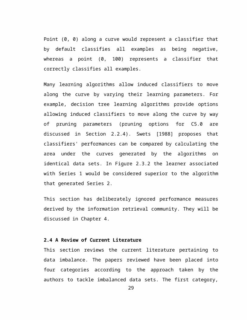
Point (0, 0) along a curve would represent a classifier that by default classifies all examples as being negative, whereas a point (0, 100) represents a classifier that correctly classifies all examples.

Many learning algorithms allow induced classifiers to move along the curve by varying their learning parameters. For example, decision tree learning algorithms provide options allowing induced classifiers to move along the curve by way of pruning parameters (pruning options for C5.0 are discussed in Section 2.2.4). Swets [1988] proposes that classifiers' performances can be compared by calculating the area under the curves generated by the algorithms on identical data sets. In Figure 2.3.2 the learner associated with Series 1 would be considered superior to the algorithm that generated Series 2.

This section has deliberately ignored performance measures derived by the information retrieval community. They will be discussed in Chapter 4.

2.4 A Review of Current LiteratureThis section reviews the current literature pertaining to data imbalance. The papers reviewed have been placed into four categories according to the approach taken by the authors to tackle imbalanced data sets. The first category, misclassification costs, reviews techniques that assign misclassification costs to training examples. The second category, sampling techniques, discusses data set balancing techniques that sample training examples, both in naive and intelligent fashions. The third category, classifiers that cover one class, describes learning algorithms that create rules to cover only one class. The last category, recognition based learning, discusses a learning method that ignores or makes little use of one class all together.

23

2.4.1 Misclassification CostsTypically a classifier's performance is evaluated using the proportion of examples that are incorrectly classified. Pazzani, Merz, Murphy, Ali, Hume, and Brunk [1994] look at errors made by a classifier in terms of their cost. For example, take an application such as the detection of poisonous mushrooms. The cost of misclassifying a poisonous mushroom as being safe to eat may have serious consequences and therefore should be assigned a high cost; conversely, misclassifying a mushroom that is safe to eat may have no serious consequences and should be assigned a low cost. Pazzani et al. [1994] use algorithms that attempt to solve the problem of imbalanced data sets by way of introducing a cost matrix. The algorithm that is of interest here is called Reduced Cost Ordering (RCO), which attempts to order a decision list (set of rules) so as to minimize the cost of making incorrect classifications.

RCO is a post-processing algorithm that can complement any rule learner such as C4.5. It essentially orders a set of rules to minimize misclassification costs. The algorithm works as follows:

The algorithm takes as input a set of rules (rule list), a cost matrix, and a set of examples (example list) and returns an ordered set of rules (decision list). An example of a cost matrix (for the mushroom example) is depicted in Figure 2.4.1.

HypothesisSafe Poisonous Actual

Class0 1 Safe10 0 PoisonousFigure 2.4.6: A cost matrix for a poisonous mushroom application.

24

Note that the costs in the matrix are the costs associated with the prediction in light of the actual class.

The algorithm begins by initializing a decision list to a default class which yields the least expected cost if all examples were tagged as being that class. It then attempts to iteratively replace the default class with a new rule / default class pair, by choosing a rule from the rule list that covers as many examples as possible and a default class which minimizes the cost of the examples not covered by the rule chosen. Note that when an example in the example list is covered by a chosen rule it is removed. The process continues until no new rule / default class pair can be found to replace the default class in the decision list (i.e., the default class minimizes cost over the remaining examples).

An algorithm such as the one described above can be used to tackle imbalanced data sets by way of assigning high misclassification costs to the underrepresented class. Decision lists can then be biased, or ordered to classify examples as the underrepresented class, as they would have the least expected cost if classified incorrectly.

Incorporating costs into decision tree algorithms can be done by replacing the information gain metric used with a new measure that bases partitions not on information gain, but on the cost of misclassification. This was studied by Pazzani et al. [1994] by modifying ID3 to use a metric that chooses partitions that minimize misclassification cost. The results of their experimentation indicate that their greedy test selection method, attempting to minimize cost, did not perform as well as using an information gain heuristic. They attribute this to the fact that their selection technique attempts to solely fit training data and not minimize the complexity of the learned concept.

25

A more viable alternative to incorporating misclassification costs into the creation of a decision trees, is to modify pruning techniques. Typically, decision trees are pruned by merging leaves of the tree to classify examples as the majority class. In effect, this is calculating the probability that an example belongs to a given class by looking at training examples that have filtered down to the leaves being merged. By assigning the majority class to the node of the merged leaves, decision trees are assigning the class with the lowest expected error. Given a cost matrix, pruning can be modified to assign the class that has the lowest expect cost instead of the lowest expected error. Pazzani et al. [1994] state that cost pruning techniques have an advantage over replacing the information gain heuristic with a minimal cost heuristic, in that a change in the cost matrix does not affect the learned concept description. This allows different cost matrices to be used for different examples.

2.4.2 Sampling Techniques2.4.2.1Heterogeneous Uncertainty SamplingLewis and Catlett [1994] describe a heterogeneous3 approach to selecting training examples from a large data set by using uncertainty sampling. The algorithm they use operates under an information filtering paradigm; uncertainty sampling is used to select training examples to be presented to an expert. It can be simply described as a process where a 'cheap' classifier chooses a subset of training examples for which it is unsure of the class from a large pool and presents them to an expert to be classified. The classified examples are then used to help the cheap classifier choose more examples for which

3 Their method is considered heterogeneous because a classifier of one type chooses examples to present to a classifier of another type.

26

it is uncertain. The examples that the classifier is unsure of are used to create a more expensive classifier.

The uncertainty sampling algorithm used is an iterative process by which an inexpensive probabilistic classifier is initially trained on three randomly chosen positive examples from the training data. The classifier is based on an estimate of the probability that an instance belongs to a class C:

where C indicates class membership and wi is the ith attribute of d attributes in example w; a and b are calculated using logistic regression. This model is described in detail in [Lewis and Hayes, 1994]. All we are concerned with here is that the classifier returns a number P between 0 and 1 indicating its confidence in whether or not an unseen example belongs to a class. The threshold chosen to indicate a positive instance is 0.5. If the classifier returns a P higher than 0.5 for an unknown example, it is considered to belong to the class C. The classifiers confidence in its prediction is proportional to the distance its prediction is away from the threshold. For example, the classifier is less confident in a P of 0.6 belonging to C than it is a P of 0.9 belong to C.

At each iteration of the sampling loop, the probabilistic classifier chooses four examples from the training set; the two which are closest and below the threshold and the two which are closest and above the

27

threshold. The examples that are closest to the threshold are those that it is least sure of the class. The classifier is then retrained at each iteration of the uncertainty sampling and reapplied to the training data to select four more instances that it is unsure of. Note that after the four examples are chosen at each loop, their class is known for retraining purposes (this is analogous to having an expert label examples).

The training set presented to the expert classifier can essentially be described as a pool of examples that the probabilistic classifier is unsure of. The pool of examples, chosen using a threshold, will be biased towards having too many positive examples if the training data set is imbalanced. This is because the examples are chosen from a window that is centered over the borderline where the positive and negative examples meet. To correct for this, the classifier chosen to train on the pool of examples, C4.5, was modified to include a loss ratio parameter, which allows pruning to be based on expected loss instead of expected error (this is analogous to cost pruning, Section 2.4.1). The default rule for the classifier was also modified to be chosen based on expected loss instead of expected error.

Lewis and Catlett [1994] show by testing their sampling technique on a text classification task that uncertainty sampling reduces the number of training examples required by an expensive learner such as C4.5 by a factor of 10. They did this by comparing results of induced decision trees on uncertainty samples from a large pool of training examples with pools of examples that were randomly selected, but ten times larger.

28

2.4.2.2One sided Intelligent SelectionKubat and Matwin [1997] propose an intelligent one sided sampling technique that reduces the number of negative examples in an imbalanced data set. The underlying concept in their algorithm is that positive examples are considered rare and must all be kept. This is in contrast to Lewis and Catlett's technique in that uncertainty sampling does not guarantee that a large number of positive examples will be kept. Kubat and Matwin [1997] balance data sets by removing negative examples. They categorize negative examples as belonging to one of four groups. They are:

Those that suffer from class label noise; Borderline examples (they are examples which are close to the

boundaries of positive examples); Redundant examples (their part can be taken over by other

examples); and Safe examples that are considered suitable for learning.

In their selection technique all negative examples, except those which are safe, are considered to be harmful to learning and thus have the potential of being removed from the training set. Redundant examples do not directly harm correct classification, but increase classification costs. Borderline negative examples can cause learning algorithms to overfit positive examples.

Kubat and Matwin’s [1997] selection technique begins by first removing redundant examples from the training set. To do this a subset C of the training examples, S, is created by taking every positive example from S and randomly choosing one negative example. The remaining examples in S are then classified using the 1-Nearest

29

Neighbor (1-NN) rule with C. Any misclassified example is added to C. Note that this technique does not make the smallest C possible, it just shrinks S. After redundant examples are removed, examples considered borderline or class noisy are removed.

Borderline, or class noisy examples are detected using the concept of Tomek Links [Tomek, 1976] that are defined by the distance between different class labeled examples. Take for instance, two examples x and y with different classes. The pair (x, y) is considered to be a Tomek link if there exists no example z, such that (x, z) < (x, y) or (y, z) < (y, x), where (a, b) is defined as the distance between example a and example b. Examples are considered borderline or class noisy if they participate in a Tomek link.

Kubat and Matwin's selection technique was shown to be successful in improving the performance using the g-mean on two of three benchmark domains: vehicles (veh1), glass (g7), and vowels (vwo). The domain in which no improvement was seen, g7, was examined and it was found that in that particular domain the original data set did not produce disproportionate values for g+ and g-.

2.4.2.3Naive Sampling TechniquesThe previously described selection algorithms balance data sets by significantly reducing the number of training examples. Both are intelligent methods that filter out examples using uncertainty sampling, or by removing examples that are considered harmful to learning. Ling and Li [1998] approach the problem of data imbalance using methods that naively downsize or over-sample data sets classifying examples with a confidence measurement. The domain of interest is data mining for direct marketing. Data sets in this field are typically two class

30

problems and are severely imbalanced, only containing a few examples of people who have bought the product and many examples of people who have not. The three data sets studied by Ling and Li [1998] are a bank data set from a loan product promotion (Bank), a RRSP campaign from a life insurance company (Life Insurance), and a bonus point program where customers accumulate points to redeem for merchandise (Bonus). As will be explained later, all three of the data sets are imbalanced.

Direct marketing is used by the consumer industry to target customers who are likely to buy products. Typically, if mass marketing is used to promote products (e.g., including flyers in a newspaper with a large distribution) the response rate (the percent of people who buy a product after being exposed to the promotion) is very low and the cost of mass marketing very high. For the three data sets studied by Ling and Li the response rates were 1.2% of 90,00 responding in the Bank data set, 7% of 80,000 responding in the Life Insurance data set, and 1.2% of 104,000 for the Bonus Program.

Data mining can be viewed as a two class domain. Given a set of customers and their characteristics, determine a set of rules that can accurately predict a customer as being a buyer or a non- buyer, advertising only to buyers. Ling and Li [1998] however, state that a binary classification is not very useful for direct marketing. For example, a company may have a database of customers to which it wants to advertise the sale of a new product to the 30% of customers who are most likely to buy it. Using a binary classifier to predict buyers may only classify 5% of the customers in the database as responders. Ling and Li [1998] avoid this limitation of binary classification by requiring that classifiers being used, give their classifications a

31

confidence level. The confidence level is required to be able to rank classified responders.

The two classifiers used for the data mining were Naïve Bayes, which produces a probability to rank the testing examples and a modified version of C4.5. The modification made to C4.5 allows the algorithm to give a certainty factor to a classification. The certainty factor is created during training and given to each leaf of the decision tree. It is simply the ratio of the number of examples of the majority class over the total number of examples sorted to the leaf. An example now classified by the decision tree not only receives the classification of the leaf it sorts to, but also the certainty factor of the leaf.

C4.5 and Naïve Bayes were not applied directly to the data sets. Instead, a modified version of Adaptive-Boosting (See Section 2.2.4) was used to create multiple classifiers. The modification made to the Adaptive-Boosting algorithm was one in which the sampling probability is not calculated from a binary classification, but from a difference in the probability of the prediction. Essentially, examples that are classified incorrectly with a higher certainty weight are given higher sampling probability in the training of the next classifier.

The evaluation method used by Ling and Li [1998] is known as the lift index. This index has been widely used in database marketing. The motivation behind using the lift index is that it reflects the re-distribution of testing examples after a learner has ranked them. For example, in this domain the learning algorithms rank examples in order of the most likely to respond to the least likely to respond. Ling and Li [1998] divide the ranked list into 10 deciles. When evaluating the ranked list, regularities should be found in the distribution of the

32

responders (i.e., there should be a high percentage of the responders in the first few deciles). Table 2.4.1 is a reproduction of the example that Ling and Li [1998] present to demonstrate this.

Lift Table

10%

10%

10%

10%

10%

10%

10%

10%

10%

10%

410 190 130 76 42 32 35 30 29 26Table 2.4.1: An example lift table taken from [Ling

and Li, 1998].

Typically, results are reported for the top 10% decile, and the sum of the first four deciles. In Ling and Li's [1998] example, reporting for the first four deciles would be 410 + 190 + 130 + 76 = 806 (or 806 / 1000 = 80.6%).

Instead of using the top 10% decile and the top four deciles to report results on, Ling and Li [1998] use the formulae:

where S1 through S10 are the deciles from the lift table.

Using ten deciles to calculate the lift index would result in a Slift index of 55% if the respondents were randomly distributed throughout the table. A situation where all respondents are in the first decile results in a SLift index of 100%.

Using their lift index as the sole measure of performance, Ling and Li [1998] report results for over-sampling and downsizing on the three data sets of interest (Bank, Life Insurance, and Bonus).

33

Ling and Li [1998] report results that show the best lift index is obtained when the ratio of positive and negative examples in the training data is equal. Using Boosted-Naïve Bayes with a downsized data set resulted in a lift index of 70.5% for Bank, 75.2% for Life Insurance, and 81.3% for Bonus. These results compared to SLift

indexes of 69.1% for Bank, 75.4% for Life Insurance, and 80.4% for the Bonus program when the data sets were imbalanced at a ratio of 1 positive example to every 8 negative examples. However, using Boosted-Bayes with over-sampling did not show any significant improvement over the imbalanced data set. Ling and Li [1998] state that one method to overcome this limitation may be to retain all the negative examples in the data set and re-sample the positive examples4.

When tested using their boosted version of C4.5, over-sampling saw a performance gain as the positive examples were re-sampled at higher rates. With a positive sampling rate of 20x, Bank saw an increase of 2.9% (from 65.6% to 68.5%), Life Insurance an increase of 2.9% (from 74.3% to 76.2%) and the Bonus Program and increase of 4.6% (from 74.3% to 78.9%).

The different effects of over-sampling and downsizing reported by Ling and Li [1998] were systematically studied in [Japkowicz, 2000], which broadly divides balancing techniques into three categories. The categories are: methods in which the small class is over-sampled to match the size of the larger class; methods by which the large class is downsized to match the smaller class; and methods that completely ignore one of the two classes. The two categories of interest in this section are downsizing and over-sampling.

4 This will be one of the sampling methods tested in Chapter 3.34

In order to study the nature of imbalanced data sets, Japkowicz proposes two questions. They are: what types of imbalances affect the performance of standard classifiers and which techniques are appropriate in dealing with class imbalances? To investigate these questions Japkowicz created a number of artificial domains which were made to vary in concept complexity, size of the training data and ratio of the under-represented class to the over-represented class.

The target concept to be learned in her study was a one dimensional set of continuous alternating equal sized intervals in the range [0, 1], each associated with a class value of 0 or 1. For example, a linear domain generated using her model would be the intervals [0, 0.5) and (0.5, 1]. If the first interval was given the class 1, the second interval would have class 0. Examples for the domain would be generated by randomly sampling points from each interval (e.g., a point x sampled in [0, 0.5] would be a (x, +) example, and likewise a point y sampled in (0.5, 1] would be an (y, -) example).

Japkowicz [2000] varied the complexity of the domains by varying the number of intervals in the target concept. Data set sizes and balances were easily varied by uniformly sampling different numbers of points from each interval.

The two balancing techniques that Japkowicz [2000] used in her study that are of interest here are over-sampling and downsizing. The over-sampling technique used was one in which the small class was randomly re-sampled and added to the training set until the number of examples of each class was equal. The downsizing technique used was one in which random examples were removed from the larger class until the size of the classes was equal. The domains and balancing

35

techniques described above were implemented using various discrimination based neural networks (DMLP).

Japkowicz found that both re-sampling and downsizing helped improve DMLP, especially as the target concept became very complex. Downsizing, however, outperformed over-sampling as the size of the training set increased.

2.4.3 Classifiers Which Cover One Class2.4.3.1BRUTERiddle, Segal, and Etzioni [1994] propose an induction technique called BRUTE. The goal of BRUTE is not classification, but the detection of rules that predict a class. The domain of interest which leads to the creation of BRUTE is the detection of manufactured airplane parts that are likely to fail. Any rule that detects anomalies, even if they are rare, is considered important. Rules which predict that a part will not fail, on the other hand are not considered valuable, no matter how large the coverage may be.

BRUTE operates on the premise that standard decision trees test functions such as ID3's information gain metric can overlook rules which accurately predict the smallest failed class in their domain. The test function in the ID3 algorithm averages the entropy at each branch weighted by the number of examples that satisfies the test at each branch. Riddle et al. [1994] give the following example demonstrating why a common information gain metric would fail to recognize a rule that can correctly classify a significant number of positive examples. Given the following two tests on a branch of a decision tree, information gain would be calculated as follows:

36

Figure 2.4.7: This example demonstrates how standard classifiers can be dominated by negative examples. It is taken from [Riddle, et al., 1994]. Note that the Gain function defined in Section 2.1.2 would prefer T2 to T1.

Using Gain(S, A) (3) as a test selection we get:

It can be seen that T2 will be chosen over T1 using ID3's information gain measure. This choice (T2) has the potential of missing a rule that would provide an accurate rule for predicting the positive class. Instead of treating positive and negative examples symmetrically, BRUTE uses the test selection function:

where n+ is the number of positive examples at the test branch and n -

the number of negative examples at the branch.

37

Instead of calculating the weighted average for each test, max_accuracy ignores the entropy of the negative examples and instead bases paths taken on the proportion of positive examples. In the previous example BRUTE would therefore choose T1 and follow the True path, because that path shows 100% accuracy on the positive examples.

BRUTE performs what Riddle et al. [1994] describe as a "massive brute-force search for accurate positive rules." It is an exhausted depth bounded search that was motivated by their observation that the predictive rules for their domain tended to be short. Redundant searches in their algorithm were avoided by considering all rules that are smaller than the depth bound in canonical order.

Experiments with BRUTE showed that it was able to produce rules that significantly outperformed those produced using CART [Breiman et al., 1984] and C4 [Quinlan, 1986]. BRUTE's average rule accuracy on their test domain was 38.4%, compared with 21.6% for CART and 29.9% for C45. One drawback is that the computational complexity of BRUTES depth bound search is much higher than that of typical decision tree algorithms. They do report, however, that it only took 35 CPU minutes of computation on a SPARC-10.

5 The accuracy being referred to here is not how well a rule set performs over the testing data. What is being referred to is the percentage of testing examples which are covered by a rule and correctly classified. The example Riddle et al.[1994] give is that if a rule matches 10 examples in the testing data, and 4 of them are positive, then the predictive accuracy of the rule is 40%. The figures given are averages over the entire rule set created by each algorithm. Riddle et al. [1994] use this measure of performance in their domain because their primary interest is in finding a few accurate rules that can be interpreted by factory workers in order to improve the production process. In fact, they state that they would be happy with a poor tree with one really good branch from which an accurate rule could be extracted.

38

2.4.3.2FOILFOIL [Quinlan, 1990] is an algorithm designed to learn a set of first order rules to predict a target predicate to be true. It differs from learners such as C5.0 in that it learns relations among attributes that are described with variables. For example, using a set of training examples where each example is a description of people and their relations:

< Name1 = Jack, Girlfriend1 = Jill, Name2 = Jill, Boyfriend2 = Jack, Couple12 = True >

C5.0 may learn the rule:

IF (Name1 = Jack) ^ (Boyfriend2 = Jack) THEN Couple12 = True.

This rule of course is correct, but will have a very limited use. FOIL on the other hand can learn the rule:

IF Boyfriend(x, y) THEN Couple(x, y) = True

where x and y are variables which can be bound to any person described in the data set. A positive binding is one in which a predicate binds to a positive assertion in the training data. A negative binding is one in which there is no assertion found in the training data. For example, the predicate Boyfriend(x, y) has four possible bindings in the example above. The only positive assertion found in the data is for the binding Boyfriend(Jill, Jack) (read the boyfriend of Jill is Jack). The other three possible bindings (e.g., Boyfriend(Jack, Jill)) are negative bindings, because there are no positive assertions in the training data.

The following is a brief description of the FOIL algorithm adapted from [Mitchell, 1997].

39

FOIL takes as input a target predicate (e.g., Couple(x, y)), a list of predicates that will be used to describe the target predicate and a set of examples. At a high level, the algorithm operates by learning a set of rules that covers the positive examples in the training set. The rules are learned using an iterative process that removes positive training examples from the training set when they are covered by a rule. The process of learning rules continues until there are enough rules to cover all the positive training examples. This way, FOIL can be viewed as a specific to general search through a hypothesis space, which begins with an empty set of rules that covers no positive examples and ends with a set of rules general enough to cover all the positive examples in the training data (the default rule in a learned set is negative).

Creating a rule to cover positive examples is a process by which a general to specific search is performed starting with an empty condition that covers all examples. The rule is then made specific enough to cover only positive examples by adding literals to the rule (a literal is defined as a predicate or its negative). For example, a rule predicting the predicate Female(x) may be made more specific by adding the literals long_hair(x) and ~beard(x).

The function used to evaluate which literal, L, to add to a rule, R, at each step is:

where p0 and n0 are the number of positive (p) and negative (n) bindings of the rule R, p1 and n1 are the number of positive and

40

negative binding of the rule which will be created by adding L to R and t is the number of positive bindings of the rule R which are still covered by R when L is added (i.e., t = p0 - p1).

The function Foil_Gain determines the utility of adding L to R. It prefers adding literals with more positive bindings than negative bindings. As can be seen in the equation, the measure is based on the proportion of positive bindings before and after the literal in question is added.

2.4.3.3SHRINKKubat, Holte, and Matwin [1998] discuss the design of the SHRINK algorithm that follows the same principles as BRUTE. SHRINK operates by finding rules that cover positive examples. In doing this, it learns from both positive and negative examples using the g-mean to take into account rule accuracy over negative examples. There are three principles behind the design of SHRINK. They are:

Do not subdivide the positive examples when learning; Create a classifier that is low in complexity; and Focus on regions in space where positive examples occur.

A SHRINK classifier is made up of a network of tests. Each test is of the form: xi[min ai ; max ai] where i indexes the attributes. Let hi

represent the output of the ith test. If the test suggests a positive test, the output is 1, else it is -1. Examples are classified as being positive if i hiwi > where wi is a weight assigned to the test hi.

SHRINK creates the tests and weights in the following way. It begins by taking the interval for each attribute that covers all the positive examples. The interval is then reduced in size by removing either the

41

left or right point based on whichever produces the best g-mean. This process is repeated iteratively and the interval found to have the best g-mean is considered the test for the attribute. Any test that has a g-mean less than 0.50 is discarded. The weight assigned to each test is wi

= log (gi/1-gi) where gi is the g-mean associated with the ith attribute test.

The results reported by Kubat et al. [1998] demonstrate that the SHRINK algorithm performs better than 1-Nearest Neighbor with one sided selection6. Pitting SHRINK against C4.5 with one sided selection the results became less clear. Using one sided selection resulted in a performance gain over the positive examples but a significant loss over the negative examples. This loss of performance over the negative examples results in the g-mean being lowered by about 10%.

Accuracies Achieved by C4.5, 1-NN and Shrink

Classifier

a+ a- g-mean

C4.5 81.1 86.6 81.71-NN 67.2 83.4 67.2SHRINK 82.5 60.9 70.9Table 2.4.2: This table is adapted from [Kubat et al., 1998]. It gives the accuracies achieved by C4.5 1-NN and SHRINK.

2.4.4 Recognition Based LearningDiscrimination based learning techniques, such as C5.0. create rules which describe both the positive (conceptual) class, as well as the negative (counter conceptual) class. Algorithms such as, BRUTE, and FOIL differ from algorithms such as C5.0, in that they create rules that only cover positive examples. However, they are still discrimination

6 One sided selection is discussed in Section 2.5.2.2. It is essentially a method by which negative examples considered harmful to learning are removed from the data set.

42

based techniques because they create positive rules using negative examples in their search through the hypothesis space. For example, FOIL creates rules to cover the positive class by adding literals until they do not cover any of the negative class examples. Other learning methods, such as back propagation applied to a feed forward neural network and K-nearest neighbor, do not explicitly create rules, but they are discrimination based techniques that learn from both positive and negative examples.

Japkowicz, Myers, and Gluck [1995] describe HIPPO, a system that learns to recognize a target concept in the absence of counter examples. More specifically, it is a neural network (called an autoencoder) that is trained to take positive examples as input, map them to a small hidden layer, and then attempt to reconstruct the examples at the output layer. Because the network has a narrow hidden layer it is forced to compress redundancies found in the input examples.

An advantage of recognition based learners is that they can operate in environments in which negative examples are very hard or expensive to obtain. An example Japkowicz et al. [1995] give is the application of machine fault diagnosis where a system is designed to detect the likely failure of hardware (e.g., helicopter gear boxes). In domains such as this, statistics on functioning hardware are plentiful, while statistics of failed hardware may be nearly impossible to acquire. Obtaining positive examples involves monitoring functioning hardware, while obtaining negative examples involves monitoring hardware that fails. Acquiring enough examples of failed hardware for training a discrimination based learner, can be very costly if the device has to be

43

broken a number of different ways to reflect all the conditions in which it may fail.

In learning a target concept, recognition based classifiers such as that described by Japkowicz et al. [1995] do not try to partition a hypothesis space with boundaries that separate positive and negative examples, but they attempt to make boundaries which surround the target concept. The following is an overview of how HIPPO, a one hidden layer autoencoder, is used for recognition based learning.

A one hidden layer autoencoder consists of three layers, the input layer, the hidden layer and the output layer. Training an autoencoder takes place in two stages. In the first stage the system is trained on positive instances using back-propagation7 to be able to compress the training examples at the hidden layer and reconstruct them at the output layer. The second stage of training involves determining a threshold that can be used to determine the reconstruction error between positive and negative examples.

The second stage of training is a semi-automated process that can be one of two cases. The first noiseless case is one in which a lower bound is calculated on the reconstruction error of either the negative or positive instances. The second noisy case is one that uses both positive and negative training examples to calculate the threshold ignoring the examples considered to be noisy or exceptional.

After training and threshold determination, unseen examples can be given to the autoencoder that can compress and then reconstruct them at the output layer, measuring the accuracy at which the example was 7 Note that back propagation is not the only training function that can be used. Evans and

Japkowicz [2000] report results using an auto-encoder trained with the One Step Secant function.

44

reconstructed. For a two class domain this is very powerful. Training an autoencoder to be able to sufficiently reconstruct the positive class, means that unseen examples that can be reconstructed at the output layer contain features that were in the examples used to train the system. Unseen examples that can be generalized with a low reconstruction error can therefore be deemed to be of the same conceptual class as the examples used for training. Any example which cannot be reconstructed with a low reconstruction error is deemed to be unrecognized by the system and can be classified as the counter conceptual class.

Japkowicz et al. [1995] compared HIPPO to two other standard classifiers that are designed to operate with both positive and negative examples. They are C4.5 and applying back propagation to a feed forward neural network (FF Classification). The data sets studied were:

The CH46 Helicopter Gearbox data set [Kolesar and NRaD, 1994]. This domain consists of discriminating between faulty and non-faulty helicopter gearboxes during operation. The faulty gearboxes are the positive class.

The Sonar Target Recognition data set. This data was obtained from the U.C. Irvine Repository of Machine Learning. This domain consists of taking sonar signals as input and determining which signals constitute rocks and which are mines (mine signals were considered the positive class in the study).

The Promoter data set. This data consists of input segments of DNA strings. The problem consists of recognizing which strings represent promoters that are the positive class.

45

Testing HIPPO showed that it performed much better than C4.5 and FF Classifier on the Helicopters and Sonar Targets domains. It performed equally with FF classifier on the promoters domain but much better than C4.5 on the same data.

Data Set ResultsData Set HIPPO C4.5 FF

ClassifierHelicopters

3.1250.9 15.6251.9

10.91.7

Promoters 200.7 351.4 201.4Sonar Targets

202.7 291.8 323.2

Table 2.4.3: Results for the three data sets tested. The figures represent the percent error along with their standard deviation as each algorithm was tested on the data.

46

47

C h a p t e r T h r e e

3 ARTIFICIAL DOMAIN

Chapter 3 is divided into three sections. Section 3.1 introduces an artificial domain of k-DNF expressions and describes three experiments that were performed using C5.0. The purpose of the experiments is to investigate the nature of imbalanced data sets and provide a motivation behind the design of a system intended to improve a standard classifiers performance on imbalanced data sets. Section 3.2 presents the design of the system that takes advantage of two sampling techniques; over-sampling and downsizing. The chapter concludes with Section 3.3, which tests the system on the artificial domain and presents the results.

3.1 Experimental DesignThis section begins by introducing the artificial domain of k-DNF expressions and explaining why this domain was chosen to conduct experiments on. Three experiments are then presented which investigate the nature of imbalanced data sets. The first experiment explores concept complexity as it effects imbalanced data sets. The second experiment investigates the two sampling techniques, downsizing and over-sampling. The last experiment looks at the rule sets created by C5.0 as data sets are balanced by over-sampling and downsizing .

48

3.1.1 Artificial DomainThe artificial domain chosen to experiment with is known as k-DNF (Disjunctive Normal Form) expressions. A k-DNF expression is of the form:

(x1^x2^…^xn) (xn+1^xn+2^…x2n)…(x(k-1)n+1^x(k-1)n+2^…^xkn)

where k is the number of disjuncts, n is the number of conjunctions in each disjunct, and xn is defined over the alphabet x1, x2,…, xj. ~x1, ~x2, …,~xj. An example of a k-DNF expression, K being 2, given as (Exp. 1).

x1^x3^~x5 ~x3^x4^x5 (Exp. 1)

Note that if xk is a member of a disjunct ~xk cannot be. Also note, (Exp. 1) would be referred to as an expression of 3x2 complexity because it has two disjuncts and three conjunctions in each disjunct.

Given (Exp. 1), defined over an alphabet of size 5, the following four examples would have classes indicated by +/-.

x1 x2 x3 x4 x5 Class

1) 1 0 1 1 0 +2) 0 1 0 1 1 +3) 0 0 1 1 1 -4) 1 1 0 0 1 -

Figure 3.1.8: Four instances of classified data defined over the expression (Exp. 1).

In the artificial domain of k-DNF expressions, the task the learning algorithm (C5.0) is to take as input a set of classified examples and learn the expression that was used to classify them. For example, given the four classified instances in Figure 3.1.1, C5.0 would take them as

49

input and attempt to learn (Exp. 1). Figure 3.1.2 gives and example of a decision tree that can correctly classify the instances in Figure 3.1.1.

Figure 3.1.9: A decision tree that correctly classifies instances (such as those in Figure 3.1.1) as satisfying (Exp. 1) or not. If an example to be classified is sorted to a positive (+) leaf in the tree it is given a positive class and satisfies expression (1).

K-DNF expressions were chosen to experiment with because of their similarity to the real world application of text classification which is the process of placing labels on documents to indicate their content. Ultimately, the purpose of the experiments presented in this chapter is to motivate the design of a system that can be applied to imbalanced data sets with practical applications. The real world domain chosen to test the system is the task of classifying text documents. The remainder of this section will describe the similarities and differences of the two domains: k-DNF expressions and text classification.

The greatest similarity between the practical application of text classification and the artificial domain of k-DNF expressions is the fact that the conceptual class (i.e., the class which contains the target concept) in the artificial domain is the under represented class. The

50

over represented class is the counter conceptual class and therefore represents everything else. This can also be said of the text classification domain because during the training process we label documents to be of the conceptual class (positive) and all other documents to be negative. The documents labeled as negative in a text domain represent the counter conceptual class and therefore represent everything else. This will be described in more detail in Chapter 4.

The other similarity between text classification and k-DNF expressions is the ability to affect the complexity of the target expression in a k-DNF expression. By varying the number of disjuncts in an expression we can vary the difficulty of the target concept to be learned.8 This ability to control concept complexity can map itself onto text classification tasks where not all classification tasks are equal in difficulty. This may not be obvious at first. Consider a text classification task where one needs to classify documents as being about a particular consumer product. The complexity of the rule set needed to distinguish documents of this type, may be as simple as a single rule indicating the name of the product and the name of the company that produces it. This task would probably map itself to a very simple k-DNF expression with perhaps only one disjunct. Now consider training another classifier intended to be used to classify documents as being computer software related or not. The number of rules needed to describe this category is probably much greater. For example, the terms "computer" and "software" in a document may be good indicators that a document is computer software related, but so might be the term "windows", if it appears in a document not containing the term "cleaner". In fact, the terms "operating" and "system" or "word" and "processor" appearing 8 As the number of disjuncts (k) in an expression increases, more partitions in the hypothesis

space are need to be realized by a learner to separate the positive examples from the negative examples.

51

together in a document are also good indicators that it is software related. The complexity of a rule set needed to be constructed by a learner to recognize computer software related documents is, therefore, greater and would probably map onto a k-DNF expression with more disjuncts than that of the first consumer product example.

The biggest difference between the two domains is that the artificial domain was created without introducing any noise. No negative examples were created and labeled as being positive. Likewise, there were no positive examples labeled as negative. For text domains in general there is often label noise in which documents are given labels that do not accurately indicate their content.

3.1.2 Example CreationFor the described tests, training examples were always created independently of the testing examples. The training and testing examples were created in the following manner:

A Random k-DNF expression is created on a given alphabet size (in this study the alphabet size is 50).

An arbitrary set of examples was generated as a random sequence of attributes equal to the size of the alphabet the k-DNF expression was created over. All the attributes were given an equal probability of being either 0 or 1.

Each example was then classified as being either a member of the expression or not and tagged appropriately. Figure 3.1.1 demonstrates how four generated examples would be classified over the expression (1).

The process was repeated until a sufficient number of positive and negative examples were attained. That is, enough examples

52

were created to provide an imbalanced data set for training and a balanced data set for testing.

For most of the tests, both the size of the alphabet used and the number of conjunctions in each disjunct were held constant. There were, however, a limited number of tests performed that varied the size of the alphabet and the number of conjunctions in each disjunct. For all the experiments, imbalanced data sets were used. For the first few tests, a data set that contained 5000 negative examples and 1200 positive examples was used. This represented a class imbalance of 5:1 in favor of the negative class. As the tests, however, lead to the creation of a combination scheme, the data sets tested were further imbalanced to a 25:1 (6000 negative : 240 positive) ratio in favor of the negative class. This greater imbalance more closely resembled the real world domain of text classification on which the system was ultimately tested. In each case the exact ratio of positive and negative examples in both the training and testing set will be indicated.

3.1.3 Description of Tests and ResultsThe description of each test will consist of several sections. The first section will state the motivation behind performing the test and give the particulars of its design. The results of the experiment will then be given followed by a discussion.

3.1.3.1Test # 1 Varying the Target Concepts ComplexityVarying the number of disjuncts in an expression varies the complexity of the target concept. As the number of disjuncts increases, the following two things occur in a data set where the positive examples are evenly distributed over the target expression and their number is held constant:

53

The target concept becomes more complex, and The number of positive examples becomes sparser relative to the

target concept.

A visual representation of the preceding statements is given in Figure 3.1.3.

Figure 3.1.10: A visual representation of a target concept becoming sparser relative to the number of examples.

Figures 3.1.3(a) and 3.1.3(b) give a feel for what is happening when the number of disjuncts increases. For larger expressions, there are more partitions that are needed to be realized by the learning algorithm and fewer examples indicating which partitions should take place.

The motivation behind this experiment comes from Schaffer [1993] who reports on experiments that show that data reflecting a simple target concept lends itself well to decision tree learners that use pruning techniques whereas complex target concepts lend themselves to best fit algorithms (i.e. decision trees which do not employ pruning techniques). Likewise, this first experiment investigates the effect of target concept complexity on imbalanced data sets. More specifically it

54

is an examination of how well C5.0 learns target concepts of increasing complexity on balanced and imbalanced data sets.

SetupIn order to investigate the performance of induced decision trees on balanced and imbalanced data sets, eight sets of training and testing data of increasing target concept complexities were created. The target concepts in the data sets were made to vary in concept complexity by increasing the number of disjuncts in the expression to be learned, while keeping the number of conjunctions in each disjunct constant. The following algorithm was used to produce the results given below.

Repeat x timeso Create a training set T(c, 6000+, 6000-)o Create a test set E(c, 1200+, 1200-)9

o Train C on To Test C on E and record its performance P1:1

o Randomly remove 4800 positive examples from To Train C on To Test C on E and record its performance P1:5

o Randomly remove 960 positive examples from To Train C on To Test C on E and record its performance P1:25

Average each P's over each x.

9 Note that throughout Chapter 3 the testing sets used to measure the performance of the induced classifiers are balanced. That is, there is an equal number of both positive and negative examples used for testing. The test sets are artificially balanced in order to increase the cost of misclassifying positive examples. Using a balanced testing set to measure a classifier's performance gives each class equal weight.

55

For this test expressions of complexity c = 4x2, 4x3, …, 4x8, and 4x1010

were tested over an alphabet of size 50. The results for each expression were averaged over x = 10 runs.

ResultsThe results of the experiment are shown in Figures 3.1.4, to 3.1.6. The bars indicate average error of the induced classifier on the entire test set. At first glance it may seem as though the error rate of the classifier is not very high for the imbalanced data set. Figure 3.1.4 shows that the error rate for expressions of complexity 4x7 and under, balanced at ratios of 1+:5- and 1+:25-, remains under 30%. An error rate lower than 30% may not seem extremely poor when one considers that the accuracy of the system is still over 70%, but, as Figure 3.1.5 demonstrates, accuracy as a performance measure over both the positive and negative class can be a bit misleading. When the error rate is measured just over the positive examples the same 4x7 expression has an average error of almost 56%.

Figure 3.1.6 graphs the error rate as measured over the negative examples in testing data. It can be easily seen that when the data set is balanced the classifier has an error rate over the negative examples that contributes to the overall accuracy of the classifier. In fact, when the training data is balanced, the highest error rate measured over the negative examples is 1.7% for an expression of complexity 4x10. However, the imbalanced data sets show almost no error over the negative examples. The highest error achieved over the negative data for the imbalanced data sets was less than one tenth of a percent at a balance ratio of 1+:5-, with an expression complexity of 4x10. When

10 Throughout this work when referring to expressions of complexity a x b (e.g., 4x2) a refers to the number of conjuncts and b refers to the number of disjuncts.

56

trained on a data set imbalanced at a ratio of 1+:25,- the classifier showed no error when measured over the negative examples.

Figure 3.1.11: Average error of induced decision trees measured over all testing examples.

Figure 3.1.12: Average error of induced decision trees measured over positive testing examples.

57

Figure 3.1.13: Average error of induced decision trees measured over negative testing examples. Note that the scale is much smaller than those in Figures 3.1.3 and 3.1.4.

DiscussionAs previously stated, the purpose of this experiment was to test the classifier's performance on both balanced and imbalanced data sets while varying the complexity of the target expression. It can be seen in Figure 3.1.4 that the performance of the classifier worsens as the complexity of the target concept increases. The degree to which the accuracy of the system degrades is dramatically different for that of balanced and imbalanced data sets11. To put this in perspective, the following table lists some of the accuracies of various expressions when learned over the balanced and imbalanced data sets. Note that the statistics in Table 3.1.1 are taken from Figure 3.1.4 and are not the errors associated with the induced classifiers, but are the accuracy in terms of the percent of examples correctly classified.

11 Throughout this first experiment it is important to remember that a learner's poor performance learning more complex expressions when trained on an imbalanced training set can be caused by the imbalance in the training data, or, the fact that there are not enough positive examples to learn the difficult expression. The question then arises as to whether the problem is the imbalance, or, the lack of positive training examples. This can be answered by referring to 3.1.10, which shows that by balancing the data sets by removing negative examples, the accuracy of induced classifier can be increased. The imbalance is therefore at least partially responsible for the poor performance of an induced classifier when attempting to learning difficult expressions.

58

Accuracy for Balanced and Imbalanced Data SetsComplexities

Balance 4x2 4x6 4x101+:1- 100% 99.9% 95.7%1+:5- 100% 78.2% 67.1%1+:25- 100% 76.3% 65.7%

Table 3.1.4: Accuracies of various expressions learned over balanced and imbalanced data sets. These figures are the percentage of correctly classified examples when tested over both positive and negative examples.

Table 3.1.1 clearly shows that a simple expression (4x2), is not affected by the balance of the data set. The same cannot be said for the expressions of complexity 4x6 and 4x10, which are clearly affected by the balance of the data set. As fewer positive examples are made available to the learner, its performance decreases.

Moving across Table 3.3.1 gives a feel for what happens as the expression becomes more complex for each degree of imbalance. In the first row, there is a performance drop of less than 5% between learning the simplest (4x2) expression and the most difficult (4x10) expression. Moving across the bottom two rows of the table, however, realizes a performance drop of over 30% on the imbalanced data sets when trying to learn the most complex expression (4x10).

The results of this initial experiment show how the artificial domain of interest is affected by an imbalance of data. One can clearly see that the accuracy of the system suffers over the positive testing examples

59

when the data set is imbalanced. It also shows that the complexity of the target concept hinders the performance of the imbalanced data sets to a greater extent than the balanced data sets. What this means is that even though one may be presented with an imbalanced data set in terms of the number of available positive examples, without knowing how complex the target concept is, you cannot know how the imbalance will affect the classifier.

3.1.3.2Test #2 Correcting Imbalanced Data Sets: Over-sampling vs. Downsizing

The two techniques investigated for improving the performance of imbalanced data sets that are of interest here are: uniformly over-sampling the smaller class, in this case it is the positive class which is under represented, and randomly under sampling the class which has many examples, in this case it is the negative class. These two balancing techniques were chosen because of their simplicity and their opposing natures, which will be useful in our combination scheme. The simplicity of the techniques is easily understood. The opposing nature of the techniques is explained as follows.

In terms of the overall size of the data set, downsizing significantly reduces the number of overall examples made available for training. By leaving negative examples out of the data set, information about the negative (or counter conceptual) class is being removed.

Over-sampling has the opposite effect in terms of the size of the data set. Adding examples by re-sampling the positive (or conceptual) class, however, does not add any additional information to the data set. It just balances the data set by increasing the number of positive examples in the data set.

60

SetupThis test was designed to determine if randomly removing examples of the over represented negative class, or uniformly over-sampling examples of the under represented class to balance the data set, would improve the performance of the induced classifier over the test data. To do this, data sets imbalanced at a ratio of 1+:25- were created, varying the complexity of target expression in terms of the number of disjuncts. The idea behind the testing procedure was to start with an imbalanced data set and measure the performance of an induced classifier as either negative examples are removed, or positive examples are re-sampled and added to the training data. The procedure given below was followed to produce the presented results.

Repeat x timeso Create a training set T(c, 240+, 6000-)o Create a test set E(c, 1200+, 1200-)o Train C on To Test C on E and record its performance Poriginal

o Repeat for n = 1 to 10 Create Td(240+, (6000 - n*576)-) by randomly

removing 576*n examples from T Train C on Td Test C on E and record its performance Pdownsize

o Repeat for n = 1 to 10 Create To((240 + n*576)+, 6000-) by uniformly over-

sampling the positive examples from T. Train C on Td Test C on E and record its performance Poversample

Average Pdownsize's and Poversample's over x.

This test was repeated for expressions of complexity c = 4x2, 4x3, …, 4x8 and 4x10 defined over an alphabet of size 50. The results were average over x = 50 runs.

61

ResultsThe majority of results for this experiment will be presented as a line graph indicating the error of the induced classifier as its performance is measured over the testing examples. Each graph is titled with the complexity of the expression that was tested, along with the class of the testing examples (positive, negative, or all) and compares the results for both downsizing and over-sampling, as each was carried out at different rates. Figure 3.1.7 is a typical example of the type of results that were obtained from this experiment and is presented with an explanation of how to interpret it.

Figure 3.1.14: Error rates of learning an expression of 4x5 complexity as either negative examples are being removed, or positive examples being re-sampled.

The y-axis of Figure 3.1.6 gives the error of the induced classifier over the testing set. The x-axis indicates the level at which the training data was either downsized, or over-sampled. The x-axis can be read the following way for each sampling method:

For downsizing the numbers represent the rate at which negative examples were removed from the training data. The point 0 represents

62

no negative examples being removed, while 100 represents all the negative examples being removed. The point 90 represents the training data being balanced (240+, 240-). Essentially, what is being said is that the negative examples were removed at 576 increments.

For over-sampling, the labels on the x-axis are simply the rate at which the positive examples were re-sampled, 100 being the point at which the training data set is balanced (6000+, 6000-). The positive examples were therefore re-sampled at 576 increments.

It can be seen from Figure 3.1.7 that the highest accuracy (lowest error rate) for downsizing is not reached when the data set is balanced in terms of numbers. This is even more apparent for over-sampling, where the lowest error rate was achieved at a rate of re-sampling 3465 (6576) or 4032 (7576) positive examples. That is, the lowest error rate achieved for over-sampling is around the 60 or 70 mark in Figure 3.1.7. In both cases the training data set is not balanced in terms of numbers.

Figure 3.1.8 is included to demonstrate that expressions of different complexities have different optimal balance rates. As can be seen from the plot of the 4x7 expression, the lowest error achieved using downsizing is achieved at the 70 mark. This is different than the results previously reported for the expression of 4x5 complexity (Figure 3.1.6). It is also apparent that the optimal balance level is reached at 50 the mark as opposed to the 60-70 mark in Figure 3.1.6.

63

Figure 3.1.15: This graph demonstrates that the optimal level at which a data set should be balanced does not always occur at the same point. To see this, compare this graph with Figure 3.1.6.

The results in Figures 3.1.7 and 3.1.8 may at first appear to contradict with those reported by Ling and Li [1998], who found that the optimal balance level for data sets occurs when the number of positive examples equals the number of negative examples. But this is not the case. The results reported in this experiment use accuracy as a measure of performance. Ling and Li [1998] use Slift as a performance measure. By using Slift. as a performance index, Ling and Li [1998] are measuring the distribution of correctly classified examples after they have been ranked. In fact, they report that the error rates in their domain drop dramatically from 40% with a balance ratio of 1+:1-, to 3% with a balance ratio of 1+:8-.

The next set of graphs in Figure 3.1.9 shows the results of trying to learn expressions of various complexities. For each expression the results are displayed in two graphs. The first graph gives the error rate of the classifier tested over negative examples. The second graph shows the error rate as tested over the positive examples. They will be used in the discussion that follows.

64

Figure 3.1.16: These graphs demonstrate the competing factors when balancing a data set. Points that indicate the highest error rate over the negative examples correspond to the lowest error over the positive examples.

Discussion

65

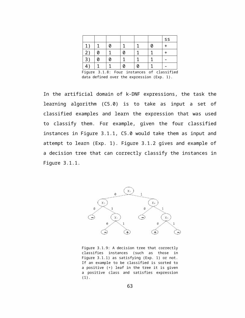
The results in Figure 3.1.9 demonstrate the competing factors when faced with balancing a data set. Balancing the data set can increase the accuracy over the positive examples, a+, but this comes at the expense of the accuracy over the negative examples, (a-). By comparing the two graphs for each expression in Figure 3.1.9, the link between a+ and a- can be seen. Downsizing results in a steady decline in the error over the positive examples, but this comes at the expense of an increase in the error over the negative examples. Looking at the curves for over-sampling one can easily see that sections with the lowest error over the positive examples correspond to the highest error over the negative examples.

A difference in the error curves for over-sampling and downsizing can also be seen. Over-sampling appears to initially perform better than downsizing over the positive examples until the data set is balanced when the two techniques become very close. Downsizing on the other hand, initially outperforms over-sampling on the negative testing examples until a point at which it completely goes off the charts.

In order to more clearly demonstrate that there is an increase in performance using the naïve sampling techniques that were investigated, Figure 3.1.10 is presented. It compares the accuracy of the imbalanced data sets using each of the sampling techniques studied. The balance level at which the techniques are compared is 1+:1-, that is, the data set is balanced at (240+, 240-) using downsizing and (6000+, 6000-) for over-sampling.

66

Figure 3.1.17: This graph demonstrates the effectiveness of balancing data sets by downsizing and over-sampling. Notice that over-sampling appears to be more effective than downsizing when the data sets are balanced in terms of numbers. The only case where downsizing outperforms over-sampling in this comparison is when attempting to learn an expression of 4x4 complexity.

The results from the comparison in Figure 3.1.10 indicate that over-sampling is a more effective technique when balancing the data sets in terms of numbers. This result is probably due to the fact that by downsizing we are in effect leaving out information about the counter conceptual class. Although over-sampling does not introduce any new information by re-sampling positive examples, by retaining all the negative examples, over-sampling has more information than downsizing about the counter-conceptual class. This effect can be seen referring back to Figure 3.1.9 in the differences in error over the negative examples of each balancing technique. That is, the error rate on the negative examples remains relatively constant for over-sampling compared to that of downsizing.

To summarize the results of this second experiment, three things can be stated. They are:

67

Both over-sampling and downsizing in a naïve fashion (i.e., by just randomly removing and re-sampling data points) are effective techniques for balancing the data set in question.

The optimal level at which an imbalanced data set should be over-sampled or downsized does not necessarily occur when the data is balanced in terms of numbers.

There are competing factors when each balancing technique is used. Achieving a higher a+ comes at the expense of a- (this is a common point in the literature for domains such as text classification).

3.1.3.3Test #3 A Rule Count for Balanced Data SetsUltimately, the goal of the experiments described in this section is to provide motivation behind the design of a system that combines multiple classifiers that use different sampling techniques. The advantage of combining classifiers that use different sampling techniques only comes if there is a variance in their predictions. Combining classifiers that always make the same predictions is of no value if one hopes that their combination will increase predictive accuracy. Ideally, one would like to combine classifiers that agree on correct predictions, but disagree on incorrect predictions.

Methods that combine classifiers such as Adaptive-Boosting attempt to vary learners' predictions by varying the training examples in which successive classifiers are presented to learn on. As we saw in Section 2.2.4, Adaptive-Boosting increases the sampling probability of examples that are incorrectly classified by already constructed classifiers. By placing this higher weight on incorrectly classified examples, the induction process at each iteration is biased towards creating a classifier that performs well on previously misclassified

68

examples. This is done in an attempt to create a number of classifiers that can be combined to increase predictive accuracy. In doing this, Adaptive-Boosting ideally diversifies the large rule sets of the classifiers.

SetupRules can be described in terms of their complexity. Larger rules sets are considered more complex than smaller rule sets. This experiment was designed to get a feel for the complexities of the rule sets produced by C5.0, when induced on imbalanced data sets that have been balanced by either over-sampling or downsizing. By looking at the complexity of the rule sets created, we can get a feel for the differences between the rule sets created using each sampling technique. The following algorithm was used to produce the results given below.

Repeat x timeso Create a training set T(c, 240+, 6000-)

o Create To(6000+,6000-) by uniformly re-sampling the positive examples from T and adding the negative examples from T.

o Train C on To

o Record rule counts Ro+ and Ro- for positive and negative rule sets

o Create Td(240+, 240-) by randomly removing 5670 negative examples from T.

o Train C on Td

o Record rule counts Rd+ and Rd- for positive and negative rule sets

Average rule counts over x.

For this test expressions of sizes c = 4x2, 4x3, …, 4x8, and 4x10 defined over and alphabet of size f = 50 were tested and averaged over x = 30 runs.

69

ResultsThe following two tables list the average characteristics of the rules associated with induced decision trees over imbalanced data sets that contain target concepts of increasing complexity. The averages are taken from rule sets created from data sets that were obtained from the procedure given above. The first table indicates the average number of positive rules associated with each expression complexity and their average size averaged over 30 trials. The second table indicates the average number of rules created to classify examples as being negative and their average size. Both tables will be used in the discussion that follows.

Positive Rule Counts

Down Sizing Over Sampling

Expression

Average rule size

Number of rules

Average rule size

Number of rules

4x2 4.0 2.0 4.0 2.04x3 4.0 4.1 4.0 3.04x4 3.8 5.6 4.0 4.04x5 4.6 11.1 4.0 5.04x6 4.7 13.5 4.0 6.0

70

4x7 4.8 15.3 4.3 7.24x8 4.9 15.4 8.3 36.24x10 5.0 18.6 8.5 43.7

Table 3.1.5: A list of the average positive rule counts for data sets that have been balanced using downsizing and over-sampling.

Negative Rule Counts

Down Sizing Over Sampling

Expression

Average rule size

Number of rules

Average rule size

Number of rules

4x2 2.0 9.4 2.0 13.44x3 3.3 17.3 3.4 33.44x4 4.0 17.5 4.6 44.14x5 4.6 21.7 5.2 50.44x6 4.8 19.0 5.6 78.34x7 4.7 17.7 5.75 75.14x8 5.0 17.4 5.9 94.64x10 4.9 18.1 6.0 89.5

Table 3.1.6: A list of the average negative rule counts for data sets that have been balanced using downsizing and over-sampling.

DiscussionBefore I begin the discussion of these results it should be noted that these numbers must only be used to indicate general trends towards rule set complexity. When being averaged for expressions of complexities 4x6 and greater the numbers varied considerably. The discussion will be in four parts. It will begin by attempting to explain the factors involved in creating rule sets over imbalanced data sets and then lead into an attempt to explain the characteristics of rules sets created by downsized data sets, followed by over-sampled rule sets. I will then conclude with a general discussion about some of the characteristics of the artificial domain and how they create the results that have been presented. Throughout this section one should

71

remember that the positive rule set contains the target concept, that is, the underrepresented class.

How does a lack of positive training examples hurt learning?Kubat et al. [1998] give an intuitive explanation of why a lack of positive examples hurts learning. Looking at the decision surface of a two dimensional plane, they explain the behavior of the 1-Nearest Neighbor (1-NN) rule. It is a simple explanation that is generalized as: "…as the number of negative examples in a noisy domain grows (the number of positives being constant), so does the likelihood that the nearest neighbor of any example will be negative." Therefore, as more negative examples are introduced to the data set, the more likely a positive example is to be classified as negative using the 1-NN rule. Of course, as the number of negative examples approaches infinity, the accuracy of a learner that classifies all examples as negative approaches 100% over negative data and 0% over the positive data. This is unacceptable if one expects to be able to recognize positive examples.

They then extend the argument to decision trees, drawing a connection to the common problem of overfitting. Each leaf of a decision tree represents a decision as being positive or negative. In a noisy training set that is unbalanced in terms of the number of negative examples, it is stated that an induced decision tree will be large enough to create regions arbitrarily small enough to partition the positive regions. That is, the decision tree will have rules complex enough to cover very small regions of the decision surface. This is a result of a classifier being induced to partition positive regions of the decision surface small enough to contain only positive examples. If there are many negative examples nearby, the partitions will be made very small to exclude

72

them from the positive regions. In this way, the tree overfits the data with a similar effect as the 1-NN rule.

Many approaches have been developed to avoid over fitting data, the most successful being post pruning. Kubat et al. [1998], however, state that this does not address the main problem. If a region in an imbalanced data set by definition contains many more negative examples than positive examples, post pruning is very likely to result in all of the pruned branches being classified as negative.

C5.0 and Rule SetsC5.0 attempts to partition data sets into regions that contain only positive examples and regions that contain only negative examples. It does this by attempting to find features in the data that are 'good' to partition the training data around (i.e., have a high information gain). One can look at the partitions it creates by analyzing the rules that are generated which create the boundaries. Each rule generated creates a partition in the data. Rules can appear to overlap, but when viewed as partitions in an entire set of rules, the partitions created in the data by the rule sets do not overlap. Viewed as an entire set of rules, the partitions in the data can be viewed has having highly irregular shapes. This is due to the fact that C5.0 assigns a confidence level to each rule. If a region of space is overlapped by multiple rules, the confidence level for each rule class that covers the space is summed. The class with the highest summed confidence level is determined to be the correct class. The confidence level given to each rule can be viewed as being the number of examples the rule covers correctly over the training data. Therefore, rule sets that contain higher numbers of rules are generally less confident in their estimated accuracy because each rule covers fewer examples. Figure 3.1.11 is presented in an attempt to

73

give a pictorial representation of what is being described here, given that the partition with the positive class has a higher confidence level than the partition indicating the negative class.

Figure 3.1.18: An example of how C5.0 adds rules to create complex decision surfaces. It is done by summing the confidence level of rules that cover overlapping regions. A region covered by more than one rule is assigned the class with the highest summed confidence level of all the rules that cover it. Here we assume Rule 1 has a higher confidence level than Rule 2.

DownsizingLooking at the complexity of the rule sets created by downsizing, we can see a number of things happening. For expressions of complexity 4x2, on average, the classifier creates a positive rule set that perfectly fits the target expression. At this point, the classifier is very confident in being able to recognize positive examples (i.e., rules indicating a positive partition have high confidence levels), but less confident in recognizing negative examples. However, as the target concept becomes more complex, the examples become sparser relative to the number of positive examples (refer to Figure 3.1.3). This has the effect

74

of creating rules that cover fewer positive examples, so as the target concept becomes more complex, the rules sets lose confidence in being able to recognize positive examples. For expressions of complexity 4x3-4x5, possibly even as high as 4x6, we can see that the rules sets generated to cover the positive class are still smaller than the rule sets generated to cover the negative class. For expressions of complexity 4x7-4x10, and presumably beyond, there is no distinction between rules generated to cover the positive class and those to cover the negative class.

Over-samplingOver-sampling has different effects than downsizing. One obvious difference is the complexity of the rule sets indicating negative partitions. Rule sets that classify negative examples when over-sampling is used are much larger than those created using downsizing. This is because there is still the large number of negative examples in the data set, resulting in a large number of rules created to classify them.

The rule sets created for the negative examples are given much less confidence than those created when downsizing is used. This effect occurs due to the fact that the learning algorithm attempts to partition the data using features contained in the negative examples. Because there is no target concept contained in the negative examples12 (i.e., no features to indicate an example to be negative), the learning algorithm is faced with the dubious task, in this domain, of attempting to find features that do not exist except by mere chance.

12 What is being referred to here is that the negative examples are the counter examples in the artificial domain and represent everything but the target concept.

75

Over sampling the positive class can be viewed as adding weight to the examples that are re-sampled. Using an information gain heuristic when searching through the hypothesis space, features which partition more examples correctly are favored over those that do not. The effect of multiplying the number of examples a feature will classify correctly when found gives the feature weight. Over sampling the positive examples in the training data therefore has the effect of giving weight to features contained in the target concept, but it also adds weight to random features which occur in the data that is being over-sampled. The effect of over-sampling therefore has two competing factors. The factors are:

One that adds weight to features containing the target concept. One that adds weight to features not containing the target

concept

The effect of features not relevant to the target concept being given a disproportionate weight can be seen for expressions of complexity 4x8 and 4x10. This can be seen in lower right hand corner of Table 3.1.2 where there are a large number of positive rules created to cover the positive examples. In these cases, the features indicating target concept are very sparse compared to the number of positive examples. When the positive data is over-sampled, irrelevant features are given enough weight relative to the features containing the target concept; as a result the learning algorithm severely overfits the training data by creating 'garbage' rules that partition the data on features not containing the target concept, but that appear in the positive examples.

76

3.1.4 Characteristics of the Domain and how they Affect the Results

The characteristics of the artificial domain greatly affect the way in which rule sets are created. The major determining factor in the creation of the rule sets is the fact that the target concept is hidden in the underrepresented class and that the negative examples in the domain have no relevant features. That is, the underrepresented class contains the target concept and the over represented class contains everything else. In fact, if over-sampling is used to balance the data sets, expressions of complexity 4x2 to 4x6 could still, on average, attain 100% accuracy on the testing set, if only the positive rule sets were used to classify examples with a default negative rule. In this respect, the artificial domain can be viewed as lending itself to being more of a recognition task than a discrimination task. One would expect classifiers such as BRUTE, which aggressively search hypothesis spaces for rules that cover only the positive examples, would work very well for this task.

3.2 Combination SchemeThis section describes the motivation and architecture behind a system that will be used to increase the performance of a standard classifier over an imbalanced data set. Essentially, the system can be described as a collection of classifiers that combines their predictive outputs to improve classification accuracy on the underrepresented class of an imbalanced data set. Combining classifiers is a technique in machine learning widely used to stabilize predictors and increase performance. One such technique, Adaptive-Boosting was described in Section 2.2.4 of this thesis.

77

3.2.1 MotivationAnalyzing the results of the artificial domain showed that the complexity of the target concept can be linked to how a imbalanced data set will affect a classifier. The more complex a target concept the more sensitive a learner is to an imbalanced data set. Experimentation with the artificial domain also showed that naively downsizing and over-sampling are effective methods of improving a classifier's performance on an underrepresented class. As well, it was found that with the balancing techniques and performance measures used, the optimal level at which a data set should be balanced does not always occur when there is an equal number of positive and negative examples. In fact, we saw in Section 3.1.3.2 that target concepts of various complexities have different optimal balance levels.

In an ideal situation, a learner would be presented with enough training data to be able to divide it into two pools; one pool for training classifiers at various balance levels, and a second for testing to see which balance level is optimal. Classifiers could then be trained using the optimal balance level. This, however, is not always possible in an imbalanced data set where a very limited number of positive examples is available for training. If one wants to achieve any degree of accuracy over the positive class, all positive examples must be used for the induction process.

Keeping in mind that an optimal balance level cannot be known before testing takes place, a scheme is proposed that combines multiple classifiers which sample data at different rates. Because each classifier in the combination scheme samples data at a different rate, not all classifiers will have an optimal performance, but there is the potential for one (and possibly more) of the classifiers in the system to be

78

optimal. A classifier is defined as optimal if it has a high predictive accuracy over the positive examples without losing its predictive accuracy over the negative examples at an unacceptable level. This loose definition is analogous to Kubat et al. [1998] using the g-mean as a measure of performance. In their study, Kubat et al. [1998] would not consider a classifier to be optimal if it achieved a high degree of accuracy over the underrepresented class by completely loosing confidence (i.e. a low predictive accuracy) on the over represented class. In combining multiple classifiers an attempt will be made to exploit classifiers that have the potential of having an optimal performance. This will be done by excluding classifiers from the system that have an estimated low predictive accuracy on the over represented class.

Another motivating factor in the design of the combination scheme can be found in the third test (Section 3.1.3.3). In this test, it was found that the rule sets created by downsizing and over-sampling have different characteristics. This difference in rule sets can be very useful in creating classifiers that can complement each other. The greater the difference in the rule sets of combined classifiers, the better chance there is for positive examples missed by one classifier, to be picked up by another. Because of the difference between the rule sets created by each sampling technique, the combination scheme designed uses both over-sampling and downsizing techniques to create classifiers.

3.2.2 ArchitectureThe motivation behind the architecture of the combination scheme can be found in [Shimshoni and Intrator, 1998] Shimshoni and Intrator's domain of interest is the classification of seismic signals. Their application involves classifying seismic signals as either being naturally

79

occurring events, or artificial in nature (e.g., man made explosions) In order to more accurately classify seismic signals, Shimshoni and Intrator create what they refer to as an Integrated Classification Machine (ICM). Their ICM is essentially a hierarchy of Artificial Neural Networks (ANNs) that are trained to classify seismic waveforms using different input representations. More specifically, they describe their architecture as having two levels. At the bottom level, ensembles, which are collections of classifiers, are created by combining ANNs that are trained on different Bootstrapped13 samples of data and are combined by averaging their output. At the second level in their hierarchy, the ensembles are combined using a Competing Rejection Algorithm (CRA)14 that sequentially polls the ensembles of which each can classify or reject the signal at hand. The motivation behind Shimshoni and Intrator's ICM is that by including many ensembles in the system, there will be some that are 'superior' and can perform globally well over the data set. There will, however, be some ensembles that are not 'superior', but perform locally well on some regions of the data. By including these locally optimal ensembles they can potentially perform well on regions of the data that the global ensembles are weak on.

Using Shimshoni and Intrator's architecture as a model, the combination scheme presented in this study combines two experts, which are collections of classifiers not based on different input

13 Their method of combining classifiers is known as Bagging [Breiman, 1996]. Bagging essentially creates multiple classifiers by randomly drawing k examples, with replacement, from a training set of data, to train each of x classifiers. The induced classifiers are then combined by averaging their prediction values.

14 The CRA algorithm operates by assigning a pre-defined threshold to each ensemble. If an ensemble's prediction confidence falls below this threshold, it is said to be rejected. The confidence score assigned to a prediction is based on the variance of the networks' prediction values (i.e., the amount of agreement among the networks in the ensemble). The threshold can be based on an ensemble's performance over the training data or subjective information.

80

representations, but based on different sampling techniques. As in Shimshoni and Intrator's domain, regions of data which one expert is weak on have the potential of being corrected by the other expert. For this study, the correction is an expert being able to correctly classify examples of the underrepresented class of which the other expert in the system fails to classify correctly.

The potential of regions of the data in which one sampling technique is weak on being corrected by the other is a result of the two sampling techniques being effective but different in nature. That is, by over-sampling and downsizing the training data, reasonably accurate classifiers can be induced that are different realizations over the training data. The difference was shown by looking at the differences in the rule sets created using each sampling technique. A detailed description of the combination scheme follows.

Figure 3.2.19 Hierarchical structure of the combination scheme. Two experts are combined.

81

The over-sampling expert is made up of classifiers which are trained on data samples containing re-sampled data of the under represented class. The downsizing expert is made up of classifiers trained on data samples where examples of the over represented class have been removed.

The combination scheme can be viewed as having three levels. Viewed from the highest level to the lowest level they are:

The output level, The expert level, and The classifier level.

3.2.2.1Classifier LevelThe classifier level of the system consists of independently trained classifiers, each associated with a confidence weight. The classifiers at this level are created as follows. First the training data for the system is divided into two pools. The first pool of data consists of all of the examples of the underrepresented class that are available and a number of the negative examples (in the study of the artificial domain we were able to create an unlimited number of negative examples) and will be referred to as the training examples. The second pool of training examples contains the remainder of the training data (all remaining examples of the over represented class) and will be referred to as weighting examples. The training for each classifier takes place in two stages. In the first stage of training, the classifiers are trained on the training examples. In the second stage of training, each classifier is tested on weighting examples. Each classifier is then assigned a weight proportional to the number of examples that it misclassifies at this stage. The purpose of this weight is to be able to estimate the

82

classifier's performance on the over represented class. The reasoning behind this is that although a classifier may be able to label the underrepresented class well, it could do this at the expense of misclassifying a very high proportion of the over represented class. This will be explained further in Section 3.2.2.3. The nature each classifier can be described at the expert level.

3.2.2.2Expert LevelThere are two experts in the system; each using different techniques in an attempt to improve the performance of the classifiers used on the underrepresented class. One expert attempts to boost the performance by over-sampling the positive examples in the training set, the other by downsizing the negative examples. Each expert is made up of a combination of multiple classifiers. One expert, the over-sampling expert, is made up of classifiers which learn on data sets containing re-sample examples of the under represented class. The other expert, referred to as the downsizing expert, is made up of classifiers that learn on data sets in which examples of the over represented class have been removed.

At this level each of the two experts independently classifies examples based on the classifications assigned at the classifier level. The classifiers associated with the experts can be arranged in a number of ways. For instance, an expert can tag an example as having a particular class if the majority of the classifiers associated with it tag the example as having that class. In this study a majority vote was not required. Instead, each classifier in the system is associated with a weight that can be either 1 or 0 depending on its performance when tested over the weighting examples. At the expert level an example is classified positive if the sum of its weighted classifiers predictions is at

83

least one. In effect, this is saying that an expert will classify an example as being positive if one of its associated classifiers tags the example as positive and has been assigned a weight of 1 (i.e., it is allowed to participate in voting).

Over Sampling ExpertEach classifier associated with this expert over samples the positive data in the training set at increasing rates. The interval increases for each classifier by a rate at which the final classifier in the system is trained on a data set that contains an equal number of positive and negative examples. Therefore, the rate at which the positive data is over sampled at classifier C is, in the case where N classifiers are combined, (C / N)*(n- - n+). In this study 10 classifiers were used to make up the over-sampling expert.

Downsizing ExpertThe downsizing expert attempts to increase the performance of the classifiers by randomly removing negative examples from the training data at increasing numbers. Each classifier associated with this expert downsizes the negative examples in the training set at increased interval, the last of which results in the number of negative examples equaling the number of positive. Combining N classifiers therefore results in the negative examples being downsized at a rate of (C / N)*(n- - n+) examples at classifier C. In this study 10 classifiers were used to make up the downsizing expert.

3.2.2.3Weighting SchemeAs previously stated, there is a weight associated with each classifier for each expert. For the purposes of this study the weight was used as a threshold to exclude classifiers from the system that incorrectly

84

classify too many examples of the over-represented class. More specifically, after training the classifiers, each was tested over the weighting examples. Any classifier that incorrectly classifies more than a defined threshold is assigned a weight of zero and is therefore excluded from the system. Any classifier that performs below the threshold is assigned a weight of one and participates in voting. The motivation behind this weighting scheme can be seen in Section 3.1.3.2 that shows a classifier's performance over the positive class is linked to its performance over the negative examples. That is, a+ comes at the expense of a-. The threshold used for the weighting scheme in the artificial domain was 240. The reasoning behind this choice will be explained in Section 3.3.

3.2.2.4Output LevelAt the output level a testing example is determined to have a class based on a vote of the two experts. In its simplest form, an example is considered to have a class if one or both of the experts consider the example as having the class. This was the voting scheme chosen for the artificial domain. Since the purpose of the system is to increase the performance of a standard classifier over the underrepresented class it was decided to allow an example to be classified as positive without agreement between the two experts. That is, only one expert is required to classify an example as positive for the example to be classified as positive at the output level. If the two experts are required to agree on their predictions, an example classified as positive by one expert, but negative by the other expert, would be classified as negative at the output level.

85

3.3 Testing the Combination scheme on the Artificial DomainSetupIn order to test the developed system on the artificial domain the following procedure was used. Thirty sets of data were generated, each containing disjoint training and test sets. Each training set consisted of 240 positive examples and 12,000 negative examples. This provided a data set which was severely imbalanced at a ratio of one positive example for every 25 negative examples. The negative examples were divided into two equal sets, half of which were pooled with the positive examples to train the system on and the other half to be used by the system to calculate weights on. The testing sets each contained 2400 examples, half of which were positive and half of which were negative. All results reported are averaged over 30 independent trials.

Threshold DeterminationDifferent thresholds were experimented with to determine which would be the optimal one to choose. The range of possible thresholds was -1 to 6000 being the number of weighting examples in the artificial domain. Choosing a threshold of -1 results in no classifier participating in voting and therefore all examples are classified as being negative. Choosing a threshold of 6000 results in all classifiers participating in voting.

Experimenting with various threshold values revealed that varying the thresholds only a small amount did not significantly alter the performance of the system when tested on what were considered fairly simple expressions (e.g. less than 4x5). This is because the system for simple expressions is very accurate on negative examples. In fact, if a threshold of 0 is chosen when testing expressions of complexity 4x5 and simpler, 100% accuracy is achieved on both the positive and

86

negative examples. This 100% accuracy came as a result of the downsizing expert containing classifiers that on average did not misclassify any negative examples.

Although individually, the classifiers contained in the downsizing expert were not as accurate over the positive examples as the over-sampling expert's classifiers, their combination could achieve an accuracy of 100% when a threshold of 0 was chosen. This 100% accuracy came as a result of the variance among the classifiers. In other words, although any given classifier in the downsizing expert missed a number of the positive examples, at least one of the other classifiers in the expert system picked them up and they did this without making any mistakes over the negative examples.

Choosing a threshold of 0 for the system is not effective for expressions of greater complexity in which the classifiers for both experts make mistakes over the negative examples. Because of this, choosing a threshold of 0 would not be effective if one does not know the complexity of the target expression.

Ultimately, the threshold chosen for the weighting scheme was 240. Any classifier that misclassified more than 240 of the weighting examples was assigned a weight of 0, else it was assigned a weight of 1. This weight was chosen under the rationale that there is an equal number of negative training examples and weighting examples. Because they are equal, any classifier that misclassifies more than 240 weighting examples has a confidence level of less than 50% over the positive class.

One should also note that because the threshold at each level above this was assigned 1 (i.e., only one vote was necessary at both the

87

expert and output levels) the system configuration can be viewed as essentially 20 classifiers requiring only one to classify an example positive.

ResultsThe results given below compare the accuracy of the experts in the system to the combination of the two experts. They are broken down into the accuracy over the positive examples (a+), the accuracy over the negative examples (a-) and the g-mean (g).

Figure 3.3.20: Testing the combination scheme on an imbalanced data set with a target concept complexity of 4x8.

88

Figure 3.3.21: Testing the combination scheme on an imbalanced data set with a target concept complexity of 4x10.

Figure 3.3.22: Testing the combination scheme on an imbalanced data set with a target concept complexity of 4x12.

Testing the system on the artificial domain revealed that the over-sampling expert, on average, performed much better than the downsizing expert on a+ for each of the expressions tested. The downsizing expert performed better on average than the over-sampling expert on a-. Combining the experts improved performance on a+ over

89

the best expert for this class, which was the over-sampling expert. As expected this came at the expense of a-.

Table 3.3.1 shows the overall improvement the combination scheme can achieve over using a single classifier.

Single Classifier (I) Results Compared to a Combination of Classifiers (CS)

a+ a- gExp I CS. I CS I CS4x8 0.33

80.958 1.0 0.925 0.581 0.942

4x10 0.367

0.895 1.0 0.880 0.554 0.888

4x12 0.248

0.812 1.0 0.869 0.497 0.839

Table 3.3.7: This table gives the accuracies achieved with a single classifier trained on the imbalanced data set (I) and the combination of classifiers on the imbalanced data set (CS).

90

C h a p t e r F o u r

4 TEXT CLASSIFICATION

Chapter 3 introduced a combination scheme designed to improve the performance of a single standard classifier over imbalanced data sets. The purpose of this chapter is to test the combination scheme on the real world application to text classification. This chapter is divided into seven sections. Section 4.1 introduces text classification and motivates its practical applications. Section 4.2 introduces the Reuters-21578 Text Categorization Test Collection. Sections 4.3 and 4.4 describe how the documents in the test collection will be represented for learning and the performance measures used to compare learners in text classification domains. Section 4.5 gives the statistics that will be used to evaluate the combination scheme and Section 4.6 some initial results. The chapter concludes with Section 4.7, which compares the performance of combination scheme designed in Chapter 3 to that of C5.0 invoked with Adaptive-Boosting.

4.1 Text ClassificationThe process by which a pre-defined label, or number of labels, are assigned to text documents is known as text classification. Typically, labels are assigned to documents based on the document's content and are used to indicate categories to which the document belongs. In this way, when a document is referred to as belonging to a category, what is being said is that the document has been assigned a label indicating its content. Documents can be grouped into categories based on the labels assigned to them. For example, a news article written about the

91

increasing price of crude oil may be assigned the labels COMMODITY, OPEC, and OIL indicating it belongs in those categories. Having accurate labels assigned to documents provides efficient means for information filtering and information retrieval (IR) tasks.

In an IR setting, pre-defined labels assigned to documents can be used for keyword searches in large databases. Many IR systems rely on documents having accurate labels indicating their content for efficient searches based on key words. Users of such systems input words indicating the topic of interest. The system can then match these words to the document labels in a database, retrieving those documents containing label matches to the words entered by the user.

Used as a means for information filtering, labels can be used to block documents from reaching users for which the document would be of no interest. An excellent example of this is E-mail filtering. Take a user who has subscribed to a newsgroup that is of a broad subject such as economic news stories. The subscriber may only be interested in a small number of the news stories that are sent to her via electronic mail, and may not want to spend a lot of time weeding through stories that are of no interest to find the few that are. If incoming stories have accurate subject labels, a user can direct a filtering system to only present those that have a pre-defined label. For example, someone who is interested in economic news stories about the price of crude oil may instruct a filtering system to only accept documents with the label OPEC. A person who is interested in the price of commodities in general, may instruct the system to present any document labeled COMMODITY. This second label used for filtering would probably result in many more documents being presented than the label OPEC,

92

because the topic label COMMODITY is much broader in an economic news setting than is OPEC.

Being able to automate the process of assigning categories to documents accurately can be very useful. It is a very time-consuming and potentially expensive task to read large numbers of documents and assign categories to them. These limitations, coupled with the proliferation of electronic material, have lead to automated text classification receiving considerable attention from both the information retrieval and machine learning communities.

4.1.1 Text Classification as an Inductive ProcessFrom a machine learning standpoint, categories are referred to as classes. For example, assigning the class CORN to a document means that the document belongs in a category of documents labeled CORN. The same document may also be assigned belong in the category CROP but not TREE. With this in mind, text classification can be viewed as a multi class domain. That is, given a set of documents there are a defined number of distinct categories, which typically can number in the hundreds, to which the documents can be assigned.

The inductive approach to text classification is as follows. Given a set of classified documents, induce an algorithm that can classify unseen documents. Because there are typically many classes that can be assigned to a document, viewed at a high level, text classification is a multi class domain. If one expects the system to be able to assign multiple classes to a document (e.g., a document can be assigned the classes COMMODITY OIL and OPEC) then the number of possible outcomes for a system can be virtually infinite.

93

Because text classification is typically associated with a large number of categories that can overlap, documents are viewed as either having a class or not having a class (positive or negative examples). For the multi class problem, text classification systems use individual classifiers to recognize individual categories. A classifier in the system is trained to recognize a document having a class, or not having the class. For an N class problem, a text classification system would consist of N classifiers trained to recognize N categories. A classifier trained to recognize a category, for example TREE, would, for training purposes, view documents categorized as TREE as positive examples and all other documents as negative examples. The same documents categorized as TREE would more than likely be viewed as negative examples by a classifier being trained to recognize documents belonging to the category CAR. Each classifier in the system is trained independently. Figure 4.1.1 gives a pictorial representation of text classification viewed as a collection of binary classifiers.

Figure 4.1.23: Text classification viewed as a collection of binary classifiers. A document to be classified by this system can be assigned any of N categories from N independently trained classifiers.

94

Note that using a collection of classifiers allows a document to be assigned more than one category (in this figure up to N categories).

Viewing text classification as a collection of two class problems results in having many times more negative examples than positive examples. Typically the number of positive examples for a given class is in the order of just a few hundred, while the number of negative examples is thousands or even tens of thousands. The Reuters-21578 data set consists of the average category having less than 250 examples, while the total number of negative examples exceeds 10000.

4.2 Reuters-21578The Reuters-21578 Text Categorization Test Collection was used to test the combination scheme designed in Chapter 3 on the real world domain of text categorization. Reuters Ltd. makes the Reuters-21578 Text Categorization Test Collection available for free distribution to be used for research purposes. The corpus is referred to in the literature as Reuters-21578 and can be obtained freely at http://www.research.att.com/~lewis. The Reuters-21578 collection consists of 21578 documents that appeared on the Reuters newswire in 1987. The documents were originally assembled and indexed with categories by Reuters Ltd, and later formatted in SGML by David D Lewis and Stephen Harding. In 1991 and 1992 the collection was formatted further and first made available to the public by Reuters Ltd as Reuters-22173. In 1996 it was decided that a new version of the collection should be produced with less ambiguous formatting and include documentation on how to use such a collection. The opportunity was also taken at this time to correct errors in the categorization and formatting of the documents. The importance of

95

correct unambiguous formatting by way of SGML markup is very important to make clear the boundaries of the document, such as the title and the topics. In 1996 Steve Finch and David D. Lewis cleaned up the collection and upon examination, removed 595 articles that were exact duplicates. The modified collection is referred to as Reuters-21578.

96

Figure 4.2.1 is an example of an article from the Reuters-21578 collection.

<REUTERS TOPICS="YES" LEWISSPLIT="TRAIN" CGISPLIT="TRAINING-SET" OLDID="5552" NEWID="9"><DATE>26-FEB-1987 15:17:11.20</DATE><TOPICS><D>earn</D></TOPICS><PLACES><D>usa</D></PLACES><PEOPLE></PEOPLE><ORGS></ORGS><EXCHANGES></EXCHANGES><COMPANIES></COMPANIES><UNKNOWN> &#5;&#5;&#5;F&#22;&#22;&#1;f0762&#31;reuter f BC-CHAMPION-PRODUCTS-&lt;CH 02-26 0067</UNKNOWN><TEXT>&#2;<TITLE>CHAMPION PRODUCTS &lt;CH> APPROVES STOCK SPLIT</TITLE><DATELINE> ROCHESTER, N.Y., Feb 26 - </DATELINE><BODY>Champion Products Inc said itsboard of directors approved a two-for-one stock split of itscommon shares for shareholders of record as of April 1, 1987. The company also said its board voted to recommend toshareholders at the annual meeting April 23 an increase in theauthorized capital stock from five mln to 25 mln shares. Reuter&#3;</BODY></TEXT></REUTERS>

Figure 4.2.24: A Reuters-21578 Article (Note that the topic for this example is Earn).

4.2.1 Document FormattingAs was previously stated, and can be seen in the example document, the collection is formatted with SGML. Each article in the collection is delimited by the opening tag <REUTERS TOPICS =?? LEWISSPLIT=?? CGISPLIT=?? OLDID=?? NEWID=??> and by the closing tag </REUTERS>. The only fields used in this study were the <TITLE> and <BODY> fields that were used to create the document vectors (this will be described in Section 4.3) and the <REUTERS TOPICS…> field to determine the category of each document.

97

4.2.2 CategoriesThe TOPICS field is very important for the purposes of this study. It contains the topic categories (or class labels) that an article was assigned to by the indexers. Not all of the documents were assigned topics and many were assigned more than one. Some of the topics have no documents assigned to them. Hayes and Weinstein [1990] discuss some of the policies that were used in assigning topics to the documents. The topics assigned to the documents are economic subject areas with the total number of categories for this test collection being 135. The top ten categories with the number of documents assigned to them are given in Table 4.2.1.

Top Ten Reuters-21578 Categories

Class Document Count

Earn 3987ACQ 2448MoneyFx 801Grain 628Crude 634Trade 551Interest 513Ship 305Wheat 306Corn 254

Table 4.2.8: A list of the top ten categories of the Reuters-21578 test collection and their document count.

4.2.3 Training and Test SetsIn order to be able compare experimental results on this particular data set, the Reuters-21578 corpus comes with recommended training and testing sets. Researchers who use the same documents for training and testing their systems can then compare results. For the purposes

98

of this study the ModApte split was used. The ModApte split essentially divides the documents into three sets. They are:

The training set, which consists of any document in the collection that has at least one category assigned and is dated earlier than April 7th, 1987;

The test set, which consists of any document in the collection that has at least on category assigned and is dated April 7th, 1987 or later; and

Documents that have no topics assigned to them and are therefore not used.

Table 4.2.2 lists the number of documents in each category.

ModApte Split Statistics

Set Document Count

Training 9603Test 3299Unused 8676

Table 4.2.9: Some statistics on the ModApte Split. Note that the documents labeled as unused receive this designation because they have no category assigned to them.

Training and testing a classifier to recognize a topic using this split can be best described using an example. Assume that the category of interest is Earn and we want to create a classifier that will be able to distinguish documents of this category from all other documents in this collection. The first step is to label all the documents in the training set and testing sets. This is a simple process by which all the documents are either labeled positive, because they are categorized as Earn, or

99

they are labeled negative, because they are not categorized as Earn. The category Earn has 3987 labeled documents in the collection, so this means that 3987 documents in the combined training and test sets would be labeled as positive and the remaining 8915 documents would be labeled as negative. The labeled training set would then be used to train a classifier which would be evaluated on the labeled testing set of examples.

4.3 Document RepresentationBefore documents can be presented to the classifier for training, some form of representation must be chosen. The most common form of document representation found in text classification literature is known as a "bag of words" representation. Most representations of this type treat each word, or a set of words, found in the corpus as a feature. Documents are represented as vectors, which are lists of words that are contained in the corpus. A binary vector representation can be used having each attribute in the document vector represent the presence or absence of a word in the document. Figure 4.3.1 shows how the sentence: "The sky is blue." would be represented using a binary vector representation defined over the set of words {blue, cloud, sky, wind}.

Figure 4.3.25: This is the binary vector representation of the sentence "The sky is blue." as defined over the set of words {blue, cloud, sky, wind}.

100

Simple variations of a binary representation include having attribute values assigned to the word frequency in the document (e.g., if the word sky appears in the document three times a value of three would be assigned in the document vector), or assigning weights to features according to the expected information gain. The latter variation involves prior domain information. For example, in an application in which documents about machine learning are being classified, one may assign a high weight to the terms pruning, tree, and decision, because these terms indicate that the paper is about decision trees. In this study a simple binary representation was used to assign words found in the corpus to features in the document vectors. The next section describes the steps used to process the documents.

4.3.1 Document ProcessingStandard techniques were used to create the binary document vectors. The text used for the representation of each document was contained in the <TITLE> and <BODY> fields of the documents. All other fields were ignored. The steps used in the creation of the document vectors are detailed below.

All punctuation and numbers were removed from the documents. The documents were then filtered through a stop word list15,

removing any words contained in the list. Stops words, such as conjunctions and prepositions, are considered to provide no information gain. It is a widely accepted technique to remove these words from a corpus to reduce feature set size.

The words in each document were then stemmed using Lovins stemmer16. Stemming maps words to their canonical form, for example, the words golfer, golfing, and golfed, would all be

15 The stop word list was obtained at http://www.dcs.gla.ac.uk/idom/ir_resources/linguistic_utils/stop-words.

101

mapped to the common stem golf. Stemming is another widely used practice IR to reduce feature set sizes.

Finally, the 500 most frequently occurring features were placed in the feature set to create the document vectors.

4.3.2 Loss of informationA feature set size of 500 was used due to space and computing time considerations. Using such a small feature set size, however, has the potential of losing too much information. Typically, feature set sizes used in document representation can be in the order of tens of thousands [Scott, 1999], [Joachims, 1998]. If not enough features are used there is the potential to miss features that have a high information gain. For example, if all documents with the category CORN have the term crop in them, this feature may be lost due to the fact there are few documents in the training data with the topic CORN. Removing the term crop from the feature set, by only using the 500 most frequently occurring terms, would be removing a feature which provides high information gain when trying to classify documents with the topic CORN.

Joachims [1998] discusses the fact that in high dimensional spaces, feature selection techniques (such as removing stop words in this study) are employed to remove features that are not considered relevant. This has the effect of reducing the size of the representation and can potentially allow a learner to generalize more accurately over the training data (i.e., avoid overfitting). Joachims [1998], however, demonstrates that there are very few irrelevant features in text classification. He does this through an experiment with the Reuters-21578 ACQ category, in which he first ranks features according to their binary information gain. Joachims [1998] then orders the features

102

according to their rank and uses the features with the lowest information gain for document representation. He then trains a naive Bayes classifier using the document representation that is considered to be the "worst", showing that the induced classifier has a performance that is much better than random. By doing this, Joachims [1998] demonstrates that even features which are ranked lowest according to their information gain, still contain considerable information.

Potentially throwing away too much information by using such a small feature set size did not appear to greatly hinder the performance of initial tests on the corpus in this study. As will be reported in Section 4.6, there were three categories in which initial benchmark tests performed better than those reported in the literature, four that performed worse and the other three about the same. For the purposes of this study it was felt that a feature set size of 500 was therefore adequate.

4.4 Performance MeasuresIn the machine learning community, the standard measure of a system's performance is accuracy. The accuracy of a system can be simply defined as the number of correctly classified examples divided by the total number of examples. However, this measure of performance is not appropriate for data sets of an imbalanced nature. Take for example, the category CORN in the Reuters-21578 testing set. With 56 positive examples and 3243 negative examples in the testing set, the accuracy attained by classifying each example as negative is 3243 / (3243 + 56) = 98%. Stubbornly classifying all documents as negative for each category, as was done with CORN, and averaging the

103

results for all the categories produces an accuracy of over 95%. While an accuracy of 95% looks impressive, classifying all documents as negative is not very useful. The IR community in particular has defined alternative measures to study a system's performance when faced with an imbalanced data set. In this section I will describe the commonly used F-measure, which combines precision and recall, and the breakeven point. Two averaging techniques known as micro averaging and macro averaging will also be discussed along with the benefits of each.

4.4.1 Precision and RecallIt was previously stated that accuracy is not a fair measure of a systems performance for an imbalanced data set. The IR community, instead, commonly basis the performance of a system on the two measures known as precision and recall.

PrecisionPrecision (P) is the proportion of positive examples labeled by a system that are truly positive. It is defined by:

where a is the number of correctly classified positive documents and c is the number of incorrectly classified negative documents. These terms are taken directly out of the confusion matrix (see Section 2.2.1).

104

In an IR setting, precision can be viewed as a measure of how many documents a system retrieves, relative to the number of positive documents it retrieves. In other words, it gives an indication of to what extent a system retrieves documents of a given class.

RecallRecall (R) is the proportion of truly positive examples verses the total number of examples that are labeled by a system as being positive. It is defined by:

where a is the number of correctly classified positive documents and b is the number of incorrectly classified positive documents (see Section 2.2.1).

In an IR setting it can be viewed as measuring the performance of a system in retrieving documents of a given class. Typically recall in an IR system comes at the expense of precision.

4.4.2 F- measureA method that is commonly used to measure the performance of a text classification system was proposed by Rijsbergen [1979] and is called the F-measure. This method of evaluation combines the trade-off between the precision and recall of a system by introducing a term B, which indicates the importance of recall relative to precision. The F-measure is defined as:

105

Substituting P and R with the parameters from the confusion matrix gives:

Using the F-measure requires results to be reported for some value of B. Typically the F-measure is reported for the values B = 1 (precision and recall are of equal importance), B = 2 (recall is twice as important as precision) and for B = 0.5 (recall is half as important as precision).

4.4.3 Breakeven PointThe breakeven point is another evaluation method that appears in the literature. This performance measure treats precision and recall as being equal tradeoffs. It relies on a system being able to vary a parameter in order to alter the ratio of precision and recall. For example, IR systems that use a cosine similarity test to determine documents' similarity, can vary the ratio of precision and recall by adjusting the similarity threshold. As the threshold is lowered, more relevant documents are retrieved, but so are typically non-relevant documents. C5.0 can vary the ratio by adjusting the pre and post pruning levels of induced rule sets and decision trees. The options that enable this are described in Section 2.2.4.

Being able to adjust the ratio of precision and recall performance of a system allows various values to be plotted. The breakeven point is calculated by interpolating or extrapolating the point at which precision equals recall. Figures 4.4.1 and 4.4.2 demonstrate how breakeven points are calculated.

106

Figure 4.4.26: The dotted line indicates the breakeven point. In this figure the point is interpolated.

Figure 4.4.27: The dotted line indicates the breakeven point. In this figure the point is extrapolated.

The breakeven point is a popular method of evaluating performance. Sam Scott [1999] used this method to measure the performance of the RIPPER [Cohen, 1995] system on various representations of the Reuters-21578 corpus and the DigiTrad [Greenhaus, 1996] corpus. Scott compares the evaluation method of the F-measure and the

107

breakeven point and reports a 99.8% correlation between the statistic gathered for the F1-measure and the breakeven point on the two corpuses he tested.

4.4.4 Averaging TechniquesThe discussion of performance measures, thus far, has been concerned with that of a single class. In real world domains, however, such as text classification, there are often many classes for which a system is tested on. Its performance should be evaluated as a whole on the entire set of classes. In order to accommodate a multiple class domain such as text classification, or more generally, systems in which each class is treated as a two class problem (refer to Section 4.1.1), two averaging techniques are commonly used in the literature [Scott 1999]. They are known as micro averaging and macro averaging. These different techniques are best described with an example.

Assume a three class domain (A, B, C) with the following confusion matrices and their associated precision, recall, and F1-measures:

Hypothesis

Hypothesis

Hypothesis

A + - B + - C + -Actual Class

+ 519

48 + 209

110

+ 15 31

- 10 423

- 114

567

- 3 951

Precision = 0.981 Precision = 0.647 Precision = 0.833

Recall = 0.915 Recall = 0.655 Recall = 0.326F1-measure = 0.947 F1-measure = 0.651 F1-measure =

0.469

Micro Averaging

108

Micro averaging considers each class to be of equal importance and is simply an average of all the individually calculated statistics. In this sense, one can look at the micro averaged results as being a normalized average of each class's performance. The micro averaged results for the given example are:

Precision = 0.820Recall = 0.632F1-measure = 0.689

Macro AveragingMacro averaging considers all classes to be a single group. In this sense, classes that have a lot of positive examples are given a higher weight. Macro averaged statistics are obtained by adding up all the confusion matrices of every class and calculating the desired statistic on the summed matrix. Given the previous example, the summed confusion matrix treating all classes as a single group is:

HypothesisMacro

+ -

Actual Class

+ 743 189- 127 1941

The macro averaged statistics for the example are therefore:

Precision = 0.854Recall = 0.797F1-measure = 0.824

Notice that the macro averaged statistics are higher that the micro averaged statistics. This is because class A performs very well and

109

contains many more examples than that of the other two classes. As this demonstrates, macro averaging gives more weight to easier classes that have more examples to train and test on.

4.5 Statistics used in this studyFor the purposes of this study, micro averaged breakeven point statistics are reported to compare initial results to those found in the literature. For the remainder of the chapter, results will be reported using the micro averaged F-measure for values of B = 0.5, 1.0, and 2.0. It is felt that the breakeven point could not be calculated with enough confidence to use it fairly. Reasons for this will be given as warranted.

The remainder of this chapter will be divided into three sections. The first section will give initial results of rule sets, created on the Reuters-21578 test collection using C5.0 and compare them to results reported in the literature. The second section will describe the experimental design and give results that are needed in order to test the combination scheme described in Chapter 3. The last section will report the effectiveness of the combination scheme and interpret the results.

4.6 Initial ResultsIn order to use C5.0 as a rule learner for the Reuters-21578 corpus the algorithm was initially tested on the data set to determine its effectiveness. It was felt that the algorithm used to test the combination scheme should perform at a comparable level to others used in the literature.

110

To make the comparison, binary document vectors were created as outlined in Section 4.3. The data set was then split into training and test sets using the ModApte split. By using the ModApte split, the initial results can be compared to those found in the literature that use the same split. The algorithm was then tested on the top ten categories in the corpus that would ultimately be used to test the effectiveness of the combination scheme. To compare the results to those of others, the breakeven point was chosen as a performance measure, as it is used as a performance measure in published results.

Calculating Breakeven PointsCalculating the breakeven point for each of the categories listed in Table 4.6.1 was done using the pruning options made available by C5.0. The process was one by which 10 precision/recall pairs were plotted at various pruning levels and the two highest points which could be used to linearly interpolate the breakeven point were chosen to make the calculation.

A Comparison of ResultsTable 4.6.1 is a list of published results for the top 10 categories of the Reuters-21578 corpus and the initial results obtained using C5.0. All rows are calculated breakeven points with the bottom row indicating the micro average of the listed categories. The results reported by Joachims [1998] were obtained using C4.5 with a feature set of 9962 distinct terms. In this case Joachims [1998] used a stemmed bag of words representation. The results reported by Scott [1999] were

111

obtained using RIPPER17 [Cohen, 1995] with a feature set size of 18590 distinct stemmed terms. In both cases Joachims [1998] and Scott [1999] used a binary representation as was used in this study. The results reported in Table 4.6.1 use only a single classifier.

Breakeven Point Statistics

CLASS C4.5 B.E. [Joachims, 1998]

RIPPER B.E. [Sam Scott, 1999]

C5.0 B.E.(Present study)

Earn 0.961 0.959 0.965ACQ 0.853 0.861 0.877MoneyFx 0.694 0.643 0.689Grain 0.891 0.906 0.880Crude 0.755 0.802 0.733Trade 0.592 0.644 0.615Interest 0.491 0.620 0.549Ship 0.809 0.777 0.725Wheat 0.855 0.848 0.881Corn 0.877 0.911 0.832Mico Average

0.778 0.797 0.774

Table 4.6.10: A comparison of breakeven points using a single classifier.

The micro averaged results in the Table 4.6.1 show that the use of C5.0 with a feature set size of 500 comes in third place in terms of performance on the categories tested. It does however perform very close to the results reported using C4.5 by Joachims [1998].

ACQ: An Example Decision Tree and Rule SetFigure 4.6.1 is an example of a decision tree created by C5.0 to obtain the preliminary results listed in Table 4.6.1. The category trained for was ACQ. For conciseness, the tree has been truncated to four levels. Two numbers represent the leaves in the tree. The first value gives the number of positive examples in the training data that sort to the leaf.

112

The second value is the number of negative examples that sort to the leaf. One interesting observation that can be made is that if the tree was pruned to this level by assigning the classification at each leaf to the majority class (e.g., rightmost leaf would be assigned the negative class in this tree), the resulting decision tree would only correctly classify 58% (970/1650) of the positive examples in the training data. On the other hand, 97% (7735/ 7945) of the negative examples in the training data would be classified correctly.

Figure 4.6.28: A decision tree created using C5.0. The category trained for was ACQ. The tree has been pruned to four levels for conciseness.

Table 4.6.2 is a list of some of the rules extracted from the decision tree in Figure XX by C5.0. The total number of rules extracted by C5.0 was 27. There were 7 rules covering positive examples and 20 rules

113

covering negative examples. Only the first three rules are listed for each class.

114

Extracted Rules

Positive Rules Negative RulesIF (acquir = 1 &Forecast = 0 &Gulf = 0 &Qtr = 0 &Vs = 0) Class = +.

IF (Acquir = 0 &Debt = 0 &Merger = 0 &Ris =0 &Stak = 0 &Takeover = 0)Class = -

IF (qtr =0 &Stak = 1)Class = +

IF (vs = 1) Class = -

IF (Takeover = 1) Class = +.

IF (qtr = 1)Class = -

Table 4.6.11: Some of the rules extracted from the decision tree in Figure 4.6.1.

4.7 Testing the Combination SchemeThe purpose of this experiment was to determine if the combination scheme designed in Chapter 3 would result in any significant performance gain over that of a classification scheme using Adaptive-Boosting. It was decided that the combination scheme should not be compared to a single classifier when tested on the real world application of text classification, because it would be unfair to test a scheme that uses multiple classifiers, to one that uses a single classifier. Adaptive-Boosting was chosen as the method used to combine the classifiers because it is state of the art and is provided by C5.0.

4.7.1 Experimental Design A process identical to that used to calculate the breakeven

points in Section 4.6 was followed, except that only a single data point was needed to calculate the F-measure. The single point was obtained using the default parameters for C5.0 with

115

Adaptive-Boosting invoked to combine 20 classifiers. The F-measure for values B = 1, 2, 0.5 were recorded for each of the tested categories.

For each category the number of positive examples was then reduced to 100 for training purposes. This was done by randomly selecting 100 documents containing the class being trained for and removing all other positive documents for training. Note, this meant that when training for each category there were different numbers of training examples. For example, training the system on the category ACQ meant that 1629 documents were removed from the training set because there were 1729 total positive examples of this class in the training data. Reducing the data set for INTEREST, however, only meant removing 382 documents.

F-measures were then recorded a second time for each modified category using Boosted C5.0.

The modified collection was then run through the system designed in Chapter 3 to determine if there was any significant performance gain on the reduced data set when compared to that of Boosted C5.0.

116

4.7.2 Performance with Loss of Examples

117

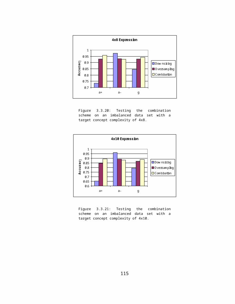
Table 4.7.118 compares the F-measures on the original data set before and after the number of positive examples is reduced to 100 for training. It should be noted that the statistic used to measure performance for the remainder of this chapter will be the F-measure. The breakeven point was not used because it was felt that it would not produce a fair measure of performance on the reduced data set. More explicitly, not enough data points, far enough apart to extrapolate or interpolate from, could be produced by varying C5.0's pruning options.

118

F-Measure Comparison

Original Performance - Adaptive Boosting

Performance with Example Loss - Adaptive Boosting

CLASS B = 1 B = 2 B = 0.5 B=1 B=2 B=0.5Earn 0.972 0.971 0.974 0.931 0.895 0.969ACQ 0.898 0.870 0.927 0.240 0.165 0.439MoneyFx 0.673 0.626 0.728 0.339 0.250 0.529Grain 0.854 0.824 0.886 0.800 0.726 0.890Crude 0.813 0.788 0.840 0.582 0.487 0.724Trade 0.518 0.460 0.594 0.257 0.183 0.431Interest 0.600 0.512 0.728 0.258 0.182 0.441Ship 0.751 0.833 0.684 0.233 0.162 0.414Wheat 0.905 0.928 0.884 0.873 0.873 0.873Corn 0.740 0.960 0.797 0.714 0.658 0.781Mirco Average 0.773 0.750 0.804 0.523 0.485 0.649

Table 4.7.12: This table compares F-measures of the original data set (original performance) to the reduced data set (performance with examples loss). Twenty classifiers were combined using Adaptive-Boosting to produce the results.

Figure 4.7.29: This graph gives a visual representation of the micro averaged results of Table 4.7.1. One can see a significant loss in performance when the number of positive examples is reduced for training.

As Figure 4.7.1 and Table 4.7.1 indicate, reducing the number of positive examples to 100 for training purposes severely hurt the

119

performance of C5.0. The greatest loss in performance is associated with B = 2, where recall is considered twice as important as precision. Note also that the smallest loss occurs when precision is considered twice as important as recall. This is not surprising when one considers that learners tend to overfit the under represented class when faced with an imbalanced data set. The next section gives the results of applying the combination scheme designed in Chapter 3 to the reduced data set.

4.7.3 Applying the Combination SchemeIn order to apply the combination scheme to a collection of data, the training data has to be divided into two pools of data: one containing examples to train the classifier on, and one to calculate the weighting scheme. The Reuters-21578 test collection provides an ideal set of examples to train the weights on. Using the ModApt split to divide the data leaves 8676 unlabeled documents that are not used for training purposes, these documents were used to train the weights for the system. The next section describes the weighting scheme that was used.

Calculating Thresholds for the Weighting SchemeInitial tests with the system indicated that a more sophisticated weighting scheme than that used for the artificial domain needed to be implemented for use on the text classification domain. When tested on the artificial domain of k-DNF expressions, a threshold of 240 (the number of positive training examples) was used. With this in mind, an initial threshold of 100 was chosen, as this was the number of positive training documents that remained in the imbalanced data set and the number of weighting examples was sufficient. Using 100 as a

120

threshold, however, did not allow enough classifiers to participate in voting to make the system useful.

Upon further investigation it was realized that the lack of classifiers participating in the voting was due to the nature of the weighting data. The documents used to calculate the weights were those defined as unused in the ModApte split. It was assumed at first that the documents were labeled as unused because they belonged to no category. This however is not the case. The documents defined by the ModApte as unused do not receive this designation because they have no category, they are designated as unused because they were simply not categorized by the indexers. This complicates the use of the unlabeled data to calculate weights.

In the artificial domain the weighing examples were known to be negative. In the text classification domain there may be positive examples contained in the weighting data. It is very difficult to know anything about the nature of the weighting data in the text application, because nothing is known about why the documents were not labeled by the indexers. A weighting scheme, based on the assumption that the unlabeled data is negative, is flawed. In fact, there may be many positive examples contained in the data labeled as unused.

121

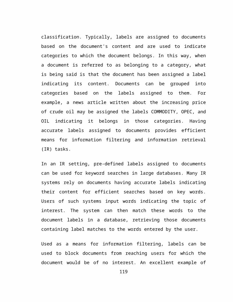
Instead of making assumptions about the weighting data, the first and

122

last19 classifiers in each expert are used to base the performance of the remaining classifiers in the expert. The weighting scheme is explained as follows:

Let Positive(C) be the number of documents which classifier C classifies as being positive over the weighting data. The threshold for each expert is defined as:

where C1 is the first classifier in the expert and Cn is the last classifier in the expert.

The weighting scheme for each expert is based on two (one for each expert) independently calculated thresholds. As in the artificial domain, any classifier that performs worse than the threshold calculated for it is assigned a weight of zero, otherwise it is assigned a weight of one.

Table 4.7.2 lists the performance associated with each expert as trained to recognize ACQ and tested over the weighting data. Using the weighting scheme previously defined results in a threshold of (105 + 648) / 2 = 377 for the downsizing expert and (515 + 562) / 2 = 539 for the over-sampling expert. The bold numbers indicate values that are over their calculated thresholds. The classifiers associated with these values would be excluded from voting in the system.

123

Excluded Classifiers20

Classifier

Downsizing Expert

Over-sampling Expert

1 105 5152 114 4693 191 4704 160 4655 312 4856 363 4877 275 5218 451 4849 549 47110 648 562Table 4.7.13: The bold numbers indicate classifiers that would be excluded from voting. Note that if a threshold of 100 were chosen, no classifiers would be allowed to vote in the system. The category trained for was ACQ.

ResultsFigures 4.7.2 to 4.7.4 give the Micro averaged results as applied to the reduced data set. The first two bars in each graph indicate the performance resulting from just using the downsizing and over-sampling experts respectively, with no weighting scheme applied. The third bar indicating the combination without weights, shows the results for the combination of the two experts without the classifier weights being applied. The final bar indicates the results of the full combination scheme applied with the weighting scheme.

124

Figure 4.7.30: Micro averaged F1-measure of each expert and their combination. Here we are considering precision and recall to be of equal importance.

Figure 4.7.31 Micro averaged F2-measure of each expert and their combination. Here we are considering recall to be twice as important as precision.

125

Figure 4.7.32 Micro averaged F0.5-measure of each expert and their combination. Here we are considering precision to be twice as important as recall.

DiscussionThe biggest gains in performance were seen individually by both the downsizing and over-sampling experts. In fact, when considering precision and recall to be of equal importance, both performed almost equally (downsizing achieved F1= 0.686 and over-sampling achieved F1

= 0.688 ). The strengths of each expert can be seen in the fact that if one considers recall to be of greater importance, over-sampling outperforms downsizing (over-sampling achieved F2 = 0.713 and downsizing achieved F2 = 0.680). If precision is considered to be of greater importance, downsizing outperforms over-sampling (downsizing achieved F0.5 = 0.670 and over-sampling achieved F0.5 = 0.663).

A considerable performance gain can also be seen in the combination of the two experts with the calculated weighting scheme. Compared to downsizing and over-sampling, there is a 3.4% increase in the F1

measure over the best expert. If one considers precision and recall to

126

be of equal importance these are encouraging results. If one considers recall to be twice as important as precision there is a significant performance gain in the combination of the experts but no real gain is achieved using the weighting scheme. There is a slight 0.4% improvement.

The only statistic that does not see an improvement in performance using the combination scheme as opposed to a single expert is the F0.5

measure (precision twice as important as recall). This can be attributed to the underlying bias in the design of the system that is to improve performance on the underrepresented class. The system uses downsizing and over-sampling techniques to increase accuracy on the underrepresented class, but this comes at the expense of the accuracy of the over represented class. The weighting scheme is used to prevent the system from performing exceptionally well on the underrepresented class, but losing confidence overall because it performs poorly (by way of false positives), on the class which dominates the data set.

It is not difficult to bias the system towards precision. A performance gain in the F0.5 measure can be seen if the experts in the system are made to agree on their prediction of being positive, in order for an example to be considered positive by the system. That is, at the output level of the system an example needs both experts to classify it as being positive in order to be classified as being positive. The following graph shows that adding this condition improves results for the F0.5

measure.

127

Figure 4.7.33 Combining the experts for precision. In this case the experts are required to agree on an example being positive in order for it to be classified as positive by the system. The results are reported for the F0.5 measure (precision considered twice as important as recall).

In order to put things in perspective, a final graph shows the overall results realized by the system. The bars labeled All Examples indicate the maximum performance that could be achieved using Boosted C5.0. The bars labeled 100 Positive Examples show the performance achieved on the reduced data set using Boosted C5.0 and the bars labeled Combination Scheme 100 Positive Examples show the performance achieved using the combination scheme and the weighting scheme designed in Chapter 2 on the reduced data set. It can clearly be seen from Figure 4.7.6 that the combination scheme greatly enhanced the performance of C5.0 on the reduced data set. In fact, if one considers recall to be twice as important as precision the combination scheme actually performs slightly better on the reduced data set. The micro averaged F2 measure for the balanced data set is 0.750, while a micro averaged measure of F2 = 0.759 is achieved on the reduced data set using the combination scheme.

128

Figure 4.7.34 A comparison of the overall results

129

C h a p t e r F i v e

5 CONCLUSION

This chapter concludes the thesis with a summary of its finding and suggests directions for further research.

5.1 SummaryThis thesis began with an examination of the nature of imbalanced data sets. Through experimenting with k-DNF expressions we saw that a typical discrimination based classifier (C5.0) can prove to be an inadequate learner on data sets that are imbalanced. The learner's shortfall manifested itself on the under represented class as excellent performance was achieved on the abundant class, but poor performance was achieved on the rare class. Further experimentation showed that this inadequacy can be linked to concept complexity. That is, learners are more sensitive to concept complexity when presented with an imbalanced data set.

Two balancing techniques were investigated in an attempt to improve C5.0's performance. They were re-sampling the under represented class and downsizing the over represented class. Each method proved to be effective on the domain at hand, as an improvement in performance over the under represented class was seen. This improvement however came at the expense of the over represented class.

130

The main contribution of this thesis lies in the creation of a combination scheme that combines multiple classifiers to improve a standard classifier's performance on imbalanced data sets. The design of the system was motivated through experimentation on the artificial domain of k-DNF expressions. On the artificial domain it was shown that by combining classifiers which sample data at different rates, an improvement in a classifier's performance on an imbalanced data set can be realized in terms of its accuracy over the under represented class.

Pitting the combination scheme against Adaptive-Boosted C5.0 on the domain of text classification showed that it could perform much better on imbalanced data sets than standard learning techniques that use all examples provided. The corpus used to test the system was the Reuters-21578 Text Categorization Test Collection. In fact, when using the micro averaged F-measure as a performance statistic, and testing the combination scheme against Boosted C5.0 on the severely imbalanced data set, the combination scheme achieved results that were superior. The combination scheme designed in Chapter 3 achieved between 10% to 20% higher accuracy rates (depending on which F-measure is used) than those achieved using Boosted C5.0.

Although the results presented in Figure 4.7.6 indicate the combination scheme provides better results than standard classifiers, it should be noted that these statistics could probably be improved by using a larger feature set size. In this study, only 500 terms were used to represent the documents. Ideally, thousands of features should be used for document representation.

131

It is important not to lose sight of the big picture. Imbalanced data sets occur frequently in domains where data of one class is scarce or difficult to obtain. Text classification is one such domain in which data sets are typically dominated by negative examples. Attempting to learn to recognize documents of a particular class using standard classification techniques on severely imbalanced data sets can result in a classifier that is very accurate at identifying negative documents, but not very good at identifying positive documents. By combining multiple classifiers which sample the available documents at different rates, a better predictive accuracy over the under represented class with very few labeled documents can be achieved. What this means is that if one is presented with very few labeled documents with which to train a classifier , overall results in identifying positive documents will improve by combining multiple classifiers which employ variable sampling techniques.

5.2 Further ResearchThere are three main extensions to this work. One extension is the choice in sampling techniques used to vary the classifiers in each expert. As the literature survey in Chapter 2 points towards, there are many intelligent approaches to sampling training examples to train classifiers on. In this thesis the two techniques of naively over-sampling and downsizing were chosen because of their opposing and simplistic natures. Both techniques proved to be sufficient for the task at hand as the main focus was in the combination of classifiers. This however leaves much room for investigating the effect of using more sophisticated sampling techniques in the future.

132

Another extension to this work is the choice of learning algorithm used. In this study a decision tree learner was chosen for its speed of computation and rule set understandability. Decision trees, however, are not the only available classifier that can be used. The combination scheme was designed independently of the classifiers that it combined. This leaves the choice of classifiers used open to the application that it will be applied to. Future work should probably consist of testing the combination scheme with a range of classifiers on different applications. An interesting set of practical applications to test the combination scheme on are various data mining tasks, such as direct marketing [Ling and Li, 1998], that are typically associated with imbalanced data sets.

Further research should be done to test the impact of automated text classification systems upon real-life scenarios. This thesis explored text classification as a practical application for a novel combination scheme. The combination scheme was shown to be effective using the F-measure. The F-measure as a performance gauge, however, does not demonstrate that the system can actually classify documents in such a way as to enable users to organize and then search for documents relevant to their needs. Ideally, a system should meet the needs of real-world applications. It should be tested to see if the combination scheme presented in this thesis can meet the needs of real-world applications, in particular text classification.

133

134

BIBLIOGRAPHY

Breiman, L., 'Bagging Predictors', Machine Learning, vol 24, pp. 123-140, 1996.

Breiman, L., Friedman, J., Olshen, R., and Stone, C., Classification and Regressions Trees, Wadsworth, 1984.

Cohen, W., 'Fast Effective Rule Induction', in Proc. ICML-95, pp. 115-123.

Schaffer, C., 'Overfitting Avoidance as Bias', Machine Learning, 10:153-178, 1993.

Eavis, T., and Japkowicz, N., 'A Recognition-Based Alternative to Discrimination-Based Multi-Layer Perceptrons' , in the Proceedings of the Thirteenth Canadian Conference on Artificial Intelligence. (AI'2000).

Fawcett, T. E. and Provost, F, 'Adaptive Fraud Detection', Data Mining and Knowledge Discovery, 1(3):291-316, 1997.

Freund, Y., and Schapire R., 'A decision-theoretic generalization of on-line learning and an application to boosting', Journal of Computer and System Sciences, 55(1):119-139, 1997.

Hayes, P., and Weinstein, S., ' A System for Content-Based Indexing of a Database of News Stories', in the Second Annual Conference on Innovative Applications of Artificial Intelligence, 1990.

Japkowicz, N., 'The Class Imbalance Problem: Significance and Strategies', in the Proceedings of the 2000 International Conference on Artificial Intelligence (IC-AI'2000): Special Track on Inductive Learning, 2000.

Japkowicz, N., Myers, C., and Gluck, M., 'A Novelty Detection Approach to Classification', in the Proceedings of the Fourteenth International Joint Conference on Artificial Intelligence (IJCAI-95). pp. 518-523, 1995.

135

Kubat, M. and Matwin, S., 'Addressing the Curse of Imbalanced Data Sets: One Sided Sampling', in the Proceedings of the Fourteenth International Conference on Machine Learning, pp. 179-186, 1997.

Kubat, M., Holte, R. and Matwin, S., 'Machine Learning for the Detection of Oil Spills in Radar Images', Machine Learning, 30:195-215, 1998.

LeCun, Y., Boser, B., Denker, J., Henderson, D., Howard, R., Hubbard, W., and Jackel, L., 'Backpropagation Applied to Handwritten Zip Code Recognition', Neural Computation 1(4), 1989.

Lewis, D., and Catlett, J., 'Heterogeneous Uncertainty Sampling for Supervised Learning', in the Proceedings of the Eleventh International Conference on Machine Learning, pp. 148-156, 1994.

Lewis, D., and Gale, W., 'Training Text Classifiers by Uncertainty Sampling', in the Seventeenth Annual International ACM SIGIR Conference on Research and Development in Information Retrieval, 1994.

Ling, C. and Li, C., 'Data Mining for Direct Marketing: Problems and Solutions', Proceedings of KDD-98.

Mitchell, T., Machine Leanring, McGraw-Hill, 1997.

Pazzanai, M., Marz, C., Murphy, P., Ali, K., Hume, T., and Brunk, C., 'Reducing Misclassification Costs', in the Proceedings of the Eleventh International Conference on Machine Learning, pp. 217-225, 1994.

Pomerleau, D., 'Knowledge-based Training of Artificial Neural Networks for Autonomous Robot Driving', In Connel, J., and Mahadevan, S., (Eds.), Robot Learning, 1993.

Quinlan, J., 'Induction of Decision Trees', Machine Learning, 1(1):81-106, 1986.

Quinlan, J., 'Learning Logical Definitions from Relations', Machine Learning, 5, 239-266, 1990.

Quinlan, J., C4,5: Programs for Machine Learning. San Mateo, CA: Morgan Kaufmann, 1993.

136

Quinlan, J., 'C5.0 An Informal Tutorial', http://www.rulequest.com/see5-win.html, 2000.

Riddle, P., Segal, R., and Etzioni, O., 'Representation Design and Brute-force Induction in a Boeing Manufacturing Domain', Applied Artificial Intelligence, 8:125-147, 1994.

Rijsbergen, C., Information Retrieval, second edition, London: Butterworths, 1997.

Scott, S., 'Feature Engineering for Text Classification', Machine Learning, in the Proceedings of the Sixteenth International Conference (ICML'99), pp. 379-388, 1999.

Shimshoni, Y., Intrator, N., 'Classification of Seismic Signals by Integrating Ensembles of Neural Networks', IEEE Transactions on Signal Processing, Special Issue on NN, 46(5), 1998.

Swets, J., 'Measuring the Accuracy of Diagnostic Systems', Science, 240, 1285-1293, 1988.

Thorsten J., 'Text Categorization with Support Vector Machines: Learning with Many Relevant Features', In Proc. ECML-98 pp. 137-142.

Tomik, I., 'Two Modifications of CNN', IEEE Transactions on Systems, Man and Communications, SMC-6, 769-772, 1976.

137

16 Lovins stemmer can be obtained freely at ftp://n106.is.tokushima-u.ac.ip/pub/IR/Iterated-Lovins-stemmer.

17 RIPPER is based on Furnkranz and Widmer's [1994] Incremental Reduced Error Pruning (IREP) algorithm. IREP creates rules, which, in a two class setting, cover the positive class. It does this using an iterative growing and pruning process. To do this, training examples are divided into two groups, one for leaning rules, and the other for pruning rules. During the growing phase of the process, rules are made more restrictive by adding clauses using Quinlan [1990]'s information gain heuristic. Rules are then pruned over the pruning data by removing clauses which cover too many negative examples. After a rule is grown and pruned, the examples it covers are removed from the growing and pruning sets. The process is repeated until all the examples in the growing set are covered by a rule or until a stopping

condition is met.18 The results are

reported using C5.0's Adaptive-Boosting option to combine 20 classifiers. The results using Boosted C5.0 only provided a slight improvement over using a single classifier. The micro averaged results of a single classifier created by invoking C5.0 with its default options were (F1=0.768, F2=0.745, F0.5=0.797) for the original data set, and (F1=0.503, F2=0.438, F0.5=0.619) for the reduced data set. Upon further investigation it was found that this can probably be attributed to the fact that Adaptive-Boosting adds classifiers to the system which, in this case, tended to overfit the training data. By counting the rule sets of subsequent decision trees added to the system, it was found that they steady grow in size. As decision trees grow in size, they tend to fit the training data more closely. These larger rule set sizes therefore point towards classifiers being added to the system that

overfit the data.19 The first classifier in an

expert is the classifier that trains on the imbalanced data set without over-sampling or downsizing the data. The last classifier in an expert is the classifier that learns on a balanced data set.

20 Note that the classifiers excluded from the system are the last ones (8, 9 and 10 in the downsizing expert and 10 in the over-sampling expert). These classifiers are trained on the data sets which are most balanced. It was shown in Figure 3.1.9 that as the data sets are balanced by adding positive examples or removing negative examples, the induced classifiers have the potential of loosing confidence over the negative examples. Since a classifier is included or excluded from the system based on its estimated performance over the negative examples, the classifiers most likely to be excluded from the system are those which are trained on the most balanced data sets.

4