Copyright

by

Vivek Kumar

2015

The Thesis Committee for Vivek Kumar Certifies that this is the approved version of the following thesis:

The Impacts of an Incentive-Based Intervention on Peak Period Traffic: Experience from the Netherlands

APPROVED BY SUPERVISING COMMITTEE:

Chandra R. Bhat

Stephen D. Boyles

Supervisor:

The Impacts of an Incentive-Based Intervention on Peak Period Traffic: Experience from the Netherlands

by

Vivek Kumar, B.Tech.

Thesis

Presented to the Faculty of the Graduate School of

The University of Texas at Austin

in Partial Fulfillment

of the Requirements

for the Degree of

Master of Science in Engineering

The University of Texas at Austin December, 2015

iv

Acknowledgements

First and foremost, I would like to acknowledge my ever supportive parents,

Jagdish and Radha Sahu, for their guidance and encouragement throughout my life. I owe

my success and achievement to them as they have been a continuous source of

inspiration. I would also like to thank my sister, Shikha, who always brought smile on my

face during my graduate endeavor.

I am taking this opportunity to express my heartfelt gratitude to Dr. Bhat, who

supported me throughout the course of my graduate studies. I am thankful for his

inspiring talks, valuable constructive criticism and friendly advice during the research.

Also, I am grateful to my reader Dr. Boyles, who has been very supportive and

encouraging in the discussions. I would also mention a big thank you to Dr. Pendyala

who provided valuable insights and guidance.

I express my thanks to my friends, Subodh, Alice, Patricia, Prateek, Venktesh,

Priyanka, Prateek, and Rahul for their support and advice at times when I was stressed

out as well as for their company in much needed recreation. I thank all my friends for

being the part of my graduate journey and making it enjoyable. Lastly, I would like to

thank the all the faculties who taught me in different courses and provided valuable

feedback and comments. I would like to give special thanks to Lisa Macias, for

supporting with administrative procedures at every step.

v

Abstract

The Impacts of an Incentive-Based Intervention on Peak Period Traffic: Experience from the Netherlands

Vivek Kumar, M.S.E.

The University of Texas at Austin, 2015

Supervisor: Chandra R. Bhat

Incentive-based travel demand management strategies are gaining increasing attention as

they are generally considered more acceptable by the traveling public and policymakers.

There is limited evidence on the impacts of such schemes, and the complex behavioral

traits that may affect how individuals respond to incentives aimed at shifting travel away

from peak period driving. This study presents a detailed analysis and modeling effort

aimed at understanding how incentives affect traveler choices using data collected from a

reward-based scheme conducted in 2006 in The Netherlands. The incentive scheme

analyzed in this study gave monetary reward or credits for smartphone thus nudging

commuters to avoid peak period driving by alternative time of travel or mode choice. The

mixed panel multinomial logit modeling approach adopted in this study is able to isolate

the impacts of incentives on behavioral choices while accounting for variations in such

impacts across socio-economic groups that may be due to unobserved individual

preferences and constraints. The model also sheds light on the effects of behavioral

inertia, where individuals are inclined to continue their past behavior even when it is no

longer optimal. Finally, the study offers insights on the extent to which behavioral

changes persist after the end of the incentive period. In general, it is found that incentives

vi

are effective in changing behavior and can overcome inertial effects; however,

individuals largely revert to their original behavior when the rewards are eliminated, thus

suggesting that incentives need to be provided for a sustained period to bring about

lasting change.

vii

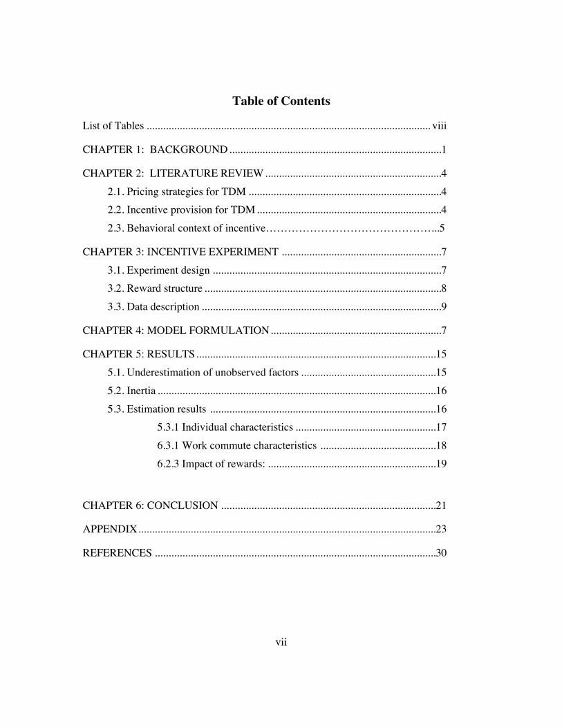
Table of Contents

List of Tables ....................................................................................................... viii

CHAPTER 1: BACKGROUND .............................................................................1

CHAPTER 2: LITERATURE REVIEW ................................................................42.1. Pricing strategies for TDM ......................................................................42.2. Incentive provision for TDM ...................................................................42.3. Behavioral context of incentive………………………………………...5

CHAPTER 3: INCENTIVE EXPERIMENT ..........................................................73.1. Experiment design ...................................................................................73.2. Reward structure ......................................................................................83.3. Data description .......................................................................................9

CHAPTER 4: MODEL FORMULATION ..............................................................7

CHAPTER 5: RESULTS .......................................................................................155.1. Underestimation of unobserved factors .................................................155.2. Inertia .....................................................................................................165.3. Estimation results ..................................................................................16

5.3.1 Individual characteristics ...................................................176.3.1 Work commute characteristics ..........................................186.2.3 Impact of rewards: .............................................................19

CHAPTER 6: CONCLUSION ..............................................................................21

APPENDIX ............................................................................................................23

REFERENCES ......................................................................................................30

viii

List of Tables

Table 1: Socio demographic composition .............................................................23

Table 2: Commute characteristics .........................................................................24

Table 3: Work place variables ...............................................................................25

Table 4: Level of rewards .....................................................................................26

Table 5: Alternative choice share ..........................................................................27

Table 6: Model estimation results .................................................................... 28-29

1

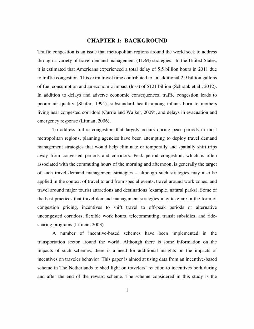
CHAPTER 1: BACKGROUND

Traffic congestion is an issue that metropolitan regions around the world seek to address

through a variety of travel demand management (TDM) strategies. In the United States,

it is estimated that Americans experienced a total delay of 5.5 billion hours in 2011 due

to traffic congestion. This extra travel time contributed to an additional 2.9 billion gallons

of fuel consumption and an economic impact (loss) of $121 billion (Schrank et al., 2012).

In addition to delays and adverse economic consequences, traffic congestion leads to

poorer air quality (Shafer, 1994), substandard health among infants born to mothers

living near congested corridors (Currie and Walker, 2009), and delays in evacuation and

emergency response (Litman, 2006).

To address traffic congestion that largely occurs during peak periods in most

metropolitan regions, planning agencies have been attempting to deploy travel demand

management strategies that would help eliminate or temporally and spatially shift trips

away from congested periods and corridors. Peak period congestion, which is often

associated with the commuting hours of the morning and afternoon, is generally the target

of such travel demand management strategies – although such strategies may also be

applied in the context of travel to and from special events, travel around work zones, and

travel around major tourist attractions and destinations (example, natural parks). Some of

the best practices that travel demand management strategies may take are in the form of

congestion pricing, incentives to shift travel to off-peak periods or alternative

uncongested corridors, flexible work hours, telecommuting, transit subsidies, and ride-

sharing programs (Litman, 2003)

A number of incentive-based schemes have been implemented in the

transportation sector around the world. Although there is some information on the

impacts of such schemes, there is a need for additional insights on the impacts of

incentives on traveler behavior. This paper is aimed at using data from an incentive-based

scheme in The Netherlands to shed light on travelers’ reaction to incentives both during

and after the end of the reward scheme. The scheme considered in this study is the

2

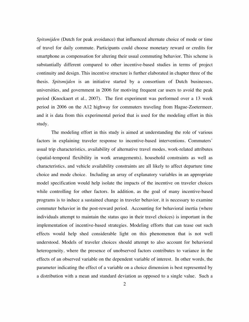
Spitsmijden (Dutch for peak avoidance) that influenced alternate choice of mode or time

of travel for daily commute. Participants could choose monetary reward or credits for

smartphone as compensation for altering their usual commuting behavior. This scheme is

substantially different compared to other incentive-based studies in terms of project

continuity and design. This incentive structure is further elaborated in chapter three of the

thesis. Spitsmijden is an initiative started by a consortium of Dutch businesses,

universities, and government in 2006 for motiving frequent car users to avoid the peak

period (Knockaert et al., 2007). The first experiment was performed over a 13 week

period in 2006 on the A12 highway for commuters traveling from Hague-Zoetermeer,

and it is data from this experimental period that is used for the modeling effort in this

study.

The modeling effort in this study is aimed at understanding the role of various

factors in explaining traveler response to incentive-based interventions. Commuters’

usual trip characteristics, availability of alternative travel modes, work-related attributes

(spatial-temporal flexibility in work arrangements), household constraints as well as

characteristics, and vehicle availability constraints are all likely to affect departure time

choice and mode choice. Including an array of explanatory variables in an appropriate

model specification would help isolate the impacts of the incentive on traveler choices

while controlling for other factors. In addition, as the goal of many incentive-based

programs is to induce a sustained change in traveler behavior, it is necessary to examine

commuter behavior in the post-reward period. Accounting for behavioral inertia (where

individuals attempt to maintain the status quo in their travel choices) is important in the

implementation of incentive-based strategies. Modeling efforts that can tease out such

effects would help shed considerable light on this phenomenon that is not well

understood. Models of traveler choices should attempt to also account for behavioral

heterogeneity, where the presence of unobserved factors contributes to variance in the

effects of an observed variable on the dependent variable of interest. In other words, the

parameter indicating the effect of a variable on a choice dimension is best represented by

a distribution with a mean and standard deviation as opposed to a single value. Such a

3

model specification can account for taste heterogeneity in the population arising from

unobserved attributes not included in the model. For this reason, the modeling effort in

this study – aimed at explaining how incentives affect departure time and mode choices –

utilizes the random parameter panel mixed multinomial logit approach which is capable

of accounting for repeated observations over time and population heterogeneity.

The remainder of this study is organized as follows. The next chapter provides an

overview of pricing and incentive-based strategies. The third chapter describes the

incentive-based scheme and also provides a brief overview of the data set used in the

study. The fourth chapter presents the modeling methodology while the fifth chapter

provides a discussion of model estimation results. Conclusions and implications of the

findings are in the sixth and final chapter of the thesis.

4

CHAPTER 2: LITERATURE REVIEW AND MOTIVATION

2.1. PRICING STRATEGIES FOR TDM Within the array of pricing-based policies, two broad possible approaches exist. In one

approach, a congestion charge is levied to deter individuals from traveling in the peak

period or along congested corridors. There are several real-world examples of such

pricing-based schemes around the world, including the Singapore Central Business

District congestion charge which reduced morning peak period traffic by 40 percent

(Phang and Toh, 1997) and the Central London congestion charge which contributed to

an automobile traffic decline of 20 percent ( Litman, 2006). While congestion pricing is

likely to be effective, there has been considerable resistance among the traveling public

and policymakers to such schemes particularly in the United States (Schaller, 2010).

New York City’s congestion pricing proposal despite getting widespread public support

was blocked by the State Legislature showing that opposition to pricing was motivated by

the negative individual-level impact on car owners. In general, Congestion pricing is

viewed as having a greater adverse impact on low income segments of the population,

and contributing to a fall in business activity, system inequities, and pricing inefficiency

(Gneezy and Rustichini, 2000).

2.2. INCENTIVES PROVISION FOR TDM

An alternative approach that has gained considerable attention is the incentive-based

paradigm where individuals are not priced, but rather travelers are given incentives to

travel in the off-peak periods or along uncongested corridors. There are a number of

success stories of incentives interventions in areas such as smoking cessation (Volpp et

al., 2009), adoption of safe driving (Dionne et al., 2011), and increased physical activity

and exercise (Charness and Gneezy, 2009). Along the same line, in transportation

domain, use of incentive for the travel behavior modification has been explored quite

recently. In 2003, a controlled study on 43 Kyoto University’s regular car preferring

students was performed where 23 students were given free bus ticket for a month. The

5

experiment produced evidence of increased frequency of bus usage among treated group

immediately and after a month after terminating free ticket provision (Fuzi and Kitamura,

2003). Another set of incentive based experiments in Melbourne (Australia), and Beijing

(China) that offered reduced or free transit fares for travel outside the peak hours were

found to be quite effective in reducing rush hour volumes (Currie, 2009 and Zhang et al.,

2014). In the City of Bangalore, an experiment named INSTANT offered rewards to

employees of a large IT firm traveling in non-congested time periods. It was observed

that the number of individuals traveling in less congested periods nearly doubled

(Merugu et al., 2009). The 2013 Smartrek initiative in Los Angeles (Hu et al., 2014)

offered differing levels of reward depending on the time of departure and route used for

travel in the region. It was found that, under the reward scheme, 60 percent of program

participants altered their time of departure, and by doing so they could reduce their travel

time by nearly 20 percent. Additionally, it was observed that by changing their departure

time, travelers could reduce their travel time by 19.4% on average. Singapore deployed

another project called Insinc in 2013 that managed peak demand in Singapore’s subway

system by rewarding commuters to travel in off-peak time. The overall shift of about

7.5% of peak trips was observed. This initiative showed that people who had information

about their friends participating in the program had a better chance of shifting departure

time (Pluntke and Prabhakar, 2013).

2.3. BEHAVIOR CONTEXT OF INCENTIVES

There is considerable literature that explains how and why incentive-based

strategies influence behavior. Incentive-based interventions work in the form of a nudge

or push and have been described by Thaler and Sunstein as an aspect of choice

architecture that alters people’s behavior in a predictable way without considerably

compromising their economic pursuit. Incentives are generally directed along three key

dimensions – economic benefits, social benefits, and moral uprightness (Levitt and

Dubner, 2010). In the context of travel behavior incentives, it is likely that individuals

respond to the economic benefits that they may realize and the social benefits that may

6

accrue to their community. These benefits may push people to direct their effort towards

modifying behavior, adapting to a new routine, and developing a strategy for embracing

change. One theory that has been proposed to explain the effects of incentives on

personal effort and adaptation is the goal setting theory. It identifies three possible ways

in which monetary incentives can take effect: 1) It can induce people to set goals when

they otherwise would not; 2) It may induce people to set more challenging goals (that

require higher effort) than they would otherwise; and 3) It may also contribute in greater

goal commitment than otherwise (Locke et al., 1981).

Although there is some experience with incentive-based schemes in the

transportation demand management arena, there is a need for in-depth analysis of the

impacts of such schemes. Prior research has been largely descriptive in nature

(comparing before-and-after statistics, or comparing an experimental group and a control

group) and has not exploited methodological tools and models capable of shedding

deeper insights into the effects of incentives on traveler behavior. More importantly,

previous research has rarely – if ever – analyzed the long-term (lasting) impacts of the

incentives once they are eliminated; there is little knowledge of the extent to which

individuals tend to switch back to their pre-incentive period behavior or continue to

exhibit the desired change in behavior following the end of the reward or incentive

period. In addition, it is important to consider pre-incentive period behavior as part of the

impact analysis; traveler choices in the pre-incentive period are dependent (endogenous)

variables and should not be treated as exogenous (independent explanatory) factors in an

impact analysis.

7

CHAPTER 3: INCENTIVE EXPERIMENT

The Spitsmijden is one of the largest reward based travel demand management (TDM)

strategies that offer an opportunity to assess the effectiveness of incentives in reducing

peak period vehicular traffic volumes. The program was initiated at the end of 2005 by a

group of Dutch companies, government agencies, and universities in The Netherlands

with the goal of developing an innovative mechanism to reduce traffic congestion on

roadways.

3.1 EXPERIMENT DESIGN

The pilot program, which is the focus of the current study, was launched in

October 2006 on Dutch A12 motorway corridor. Morning commuters driving from

Zoetermeer towards The Hague were eligible to participate in the program. A detailed

explanation of the program is available in Knockaert et al. Electronic vehicle

identification cameras were used to identify vehicles that traversed the roadway of

interest during the morning rush hours. Letters were sent to the households

corresponding to these vehicles, and a total of 340 individuals consented to participate in

the experiment. The participants completed an extensive questionnaire about their daily

commute, socio-economic and demographic characteristics, and work schedules and

arrangements. After the end of the program, the participants completed a post-

Spitsmijden experience survey. The project focused on the reduction of morning peak

period traffic volumes with the morning peak defined as 7:30-9:30 AM.

Participation in the pilot study required a 13-week commitment from participants’

side. The first two weeks were devoted to collect data about participants’ pre-reward

period travel choices. This was necessary because the reward made available to a person

was dependent on the level and frequency of peak period travel prior to the institution of

the reward. The reward period was ten weeks long; during this period, participants could

take advantage of rewards for avoiding peak period travel in the morning. The final week

8

was a non-reward period; however, the travel behavior of participants was recorded in

this final week to determine the extent to which participants reverted to their usual travel

behavior upon the termination of the reward and the extent to which the reward

mechanism may have brought about a longer-lasting change in traveler behavior.

Choices made by participants were registered using an On Board Unit (OBU) that

was installed in their vehicles. Information on routes and time of travel collected by the

OBU was transmitted automatically to a central database. Information on mode shifts

(i.e., participants who chose to work from home or use public transit or non-motorized

modes during the program period), was logged in a diary that had to be completed by

every program participant at the end of each day of the program period.

3.2 REWARD STRUCTURE

Upon registration, participants were allowed to choose between two reward

programs. The first was a monetary reward for avoiding the morning peak period. The

second type of reward was the accumulation of credits that could be exchanged for a

smartphone at the end of the program. Out of 340 participants, 232 participants went for

monetary reward scheme while the remainder chose the smartphone (a Yeti phone)

reward. Individuals could avail the rewards only if they recorded a net change in

behavior during the reward period. In other words, if an individual already avoided peak

period commuting to a large extent in the pre-reward period, then the individual had to

further cut his or her peak period commuting and record a net change in peak period

travel to be eligible for the reward.

Each participant who chose the monetary reward scheme experienced three

reward levels as follows: 1) €3 for avoiding the 7:30-9:30 AM period for three weeks; 2)

€7 reward for avoiding the 7:30-9:30 AM period for four weeks; and 3) A €3 reward for

choosing to avoid 8:00-9:00 AM period that increased to €7 if the complete peak period

of 7:30-9:30 AM was avoided, for three weeks. Participants of the Yeti phone reward

group received credits towards keeping the phone that was given to them at the beginning

of the experiment. These participants were asked to use the Yeti smartphone for trip

9

guidance and navigation as traffic information was relayed to them through the device. If

the person with the phone avoided the morning peak period more than a predetermined

number of days, then the participant was allowed to keep the phone; otherwise, the phone

had to be returned at the end of the experiment. The threshold of the number of days that

a participant had to avoid was customized to ensure a significant net change in behavior

between the pre-reward period and the reward period.

3.3 DATA DESCRIPTION

The data set included 13 weeks of observations of the program participants, yielding a

total of 22,165 participant-days of observations. However, after removing records with

missing data and no information about pre-reward period behavior, and in which the

participants did not work during the program period, the data set included 16,015

participant-days of observations. The final sample includes 324 unique participants of

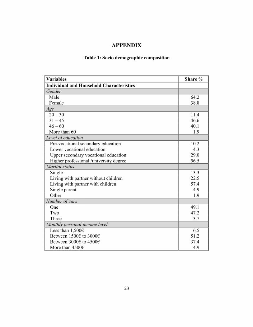
whom 208 were men and 116 were women. Table 1 provides a detailed description of

the sample and the data used in this study. More than 85 percent of the sample is

between the ages of 31 and 60 (the peak working years) and more than one-half of the

sample has a higher professional and university degree education. Nearly 60 percent of

the sample constitutes individuals living with a partner with children and just five percent

constitute single parents. Given the nature of the program, all participants own at least

one car; 47 percent own two cars, and just fewer than four percent own three cars.

Monthly personal income largely falls in the range of €1500 to €4500. Out of these 324

participants, 69 people did not wish to reveal their income in recruiting question survey.

To account for missing income data and avoid elimination of records due to missing

income information, their income was imputed using a multivariate imputation by

chained equation (MICE) methodology (Buuren and Oudshoorn, 2011). Participants’ age,

gender, education status, family composition and number of cars in the household were

used as independent variable for the estimating their corresponding income.

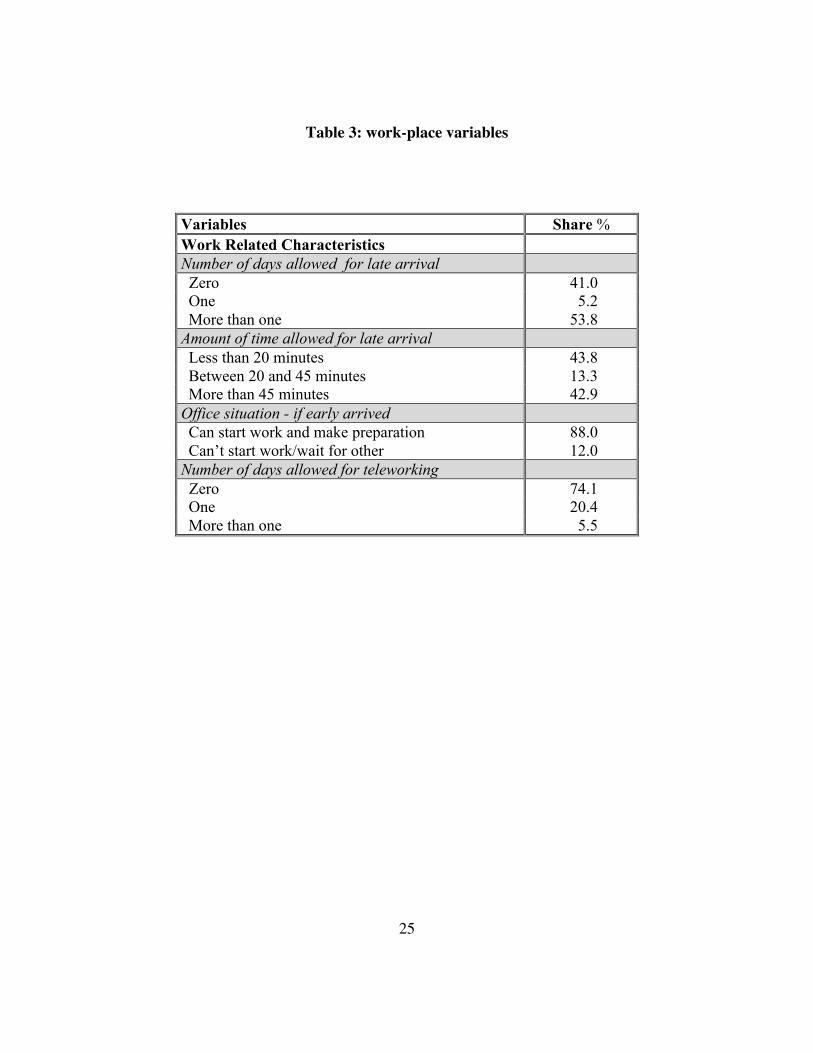
A large percent of the sample (41 percent) indicated that they had no flexibility

for late arrival at work. However, more than 50 percent of the sample indicated that they

10

could arrive late to work on more than one day per week, signifying a high level of

flexibility among the commuters in the sample. Only 12 percent indicated that they had

to wait for others before starting work in the event that they arrive early at work. Nearly

three-quarters of the sample could not telework, while 20 percent of the sample could

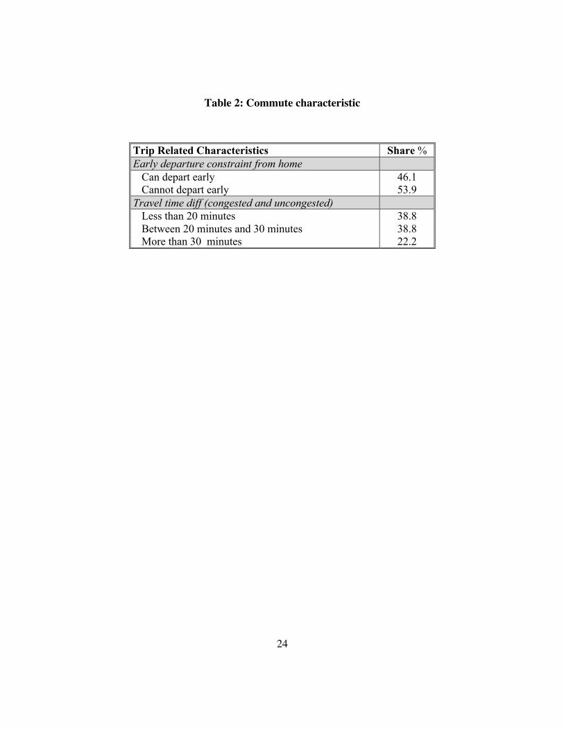
telework one day of the week. Among trip related characteristics, more than 50 percent

of the sample indicated that they were constrained and could not depart to work early.

The difference between congested and uncongested travel times was more than 30

minutes for 22.2 percent of the sample, indicating that a large percent of commuters

could save substantial travel time by shifting to an uncongested travel period.

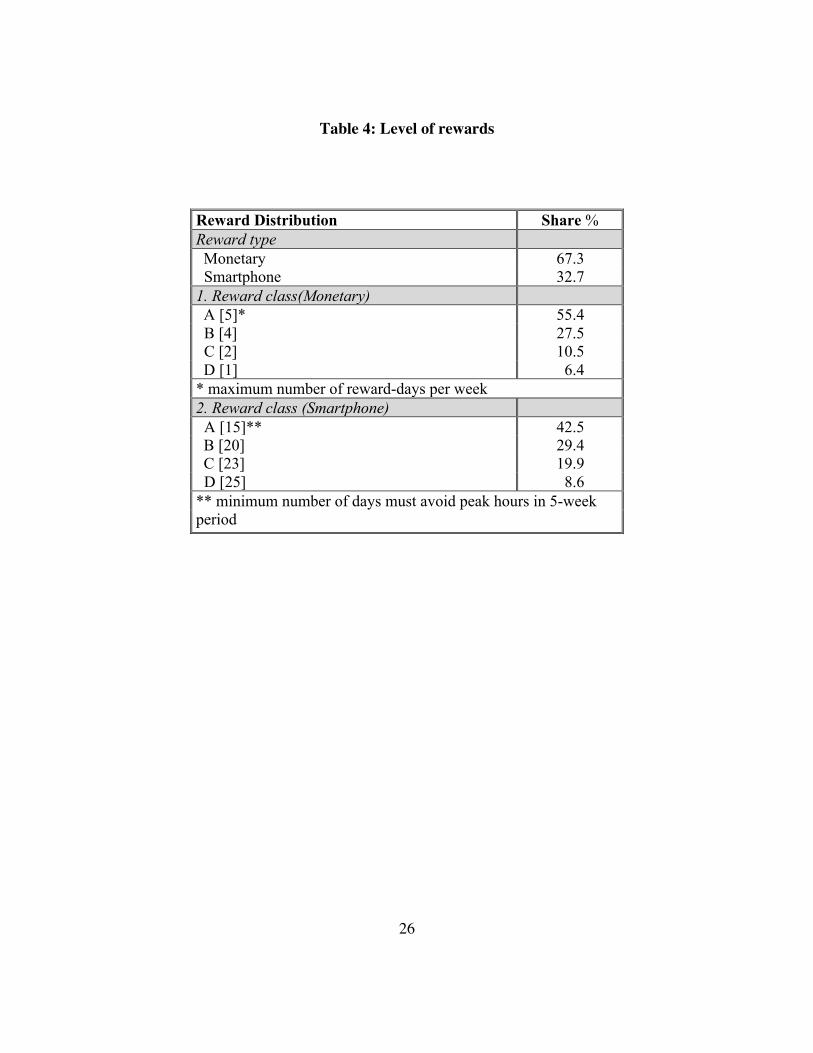
Two-thirds of the sample chose the monetary reward. In terms of reward class, 55

percent of the sample could collect a reward on all five days of the week (based on their

pre-reward period behavior). Only 6.4 percent of the sample was limited to collecting the

reward on one day of the week; these individuals presumably traveled four of the five

days each week during the off-peak period in the pre-reward period. Thus, they were

eligible for the reward on only one day of the week that would constitute a net change in

behavior. Among participants who chose the Yeti smartphone, nearly 43 percent had to

avoid morning rush hours on at least 15 days over a 5-week program period to keep the

phone. About 8.5 percent of the Yeti phone sample had to avoid the peak period on all

25 days of the five-week period to retain the smartphone. These thresholds were set

based on the usual behavior exhibited by the participants during the two-week pre-reward

period.

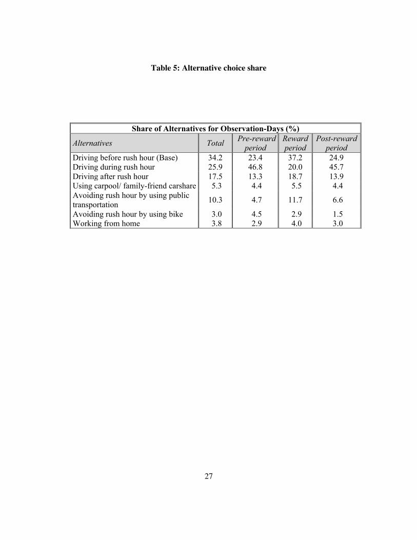
Finally, table 5 shows the shares of alternatives in the data set that comprises

16,015 observation-days. In the pre-reward period, 23.4 percent of the participants drove

before the rush hours, 46.8 percent traveled during rush hours, and 17.5 percent traveled

after the rush hours. The remaining individuals used alternative modes or worked from

home. The reward period shows considerable changes in travel behavior. During the

reward period, 37 percent traveled before the peak period, only 20 percent (down from

46.8) traveled during the rush hours, and 18.7 percent traveled after the peak period. The

percent of individuals using alternative modes or working from home increased from 16

11

percent in the pre-reward period to about 24 percent in the reward period. However, it

appears that individuals quickly revert to their pre-reward period behavior once the

incentives are eliminated. Behavior in the post-reward period largely mirrors the behavior

in the pre-reward period, with a very modest drop in peak period travel (from 46.8

percent to 45.7 percent). The share of bicycle travel dropped from 4.5 percent to 1.5

percent, while the share of public transportation use climbed from 4.7 percent to 6.6

percent. There is therefore some indication of a sustained, albeit modest, change in

behavior following the completion of the reward program.

12

CHAPTER 4: MODEL FORMULATION

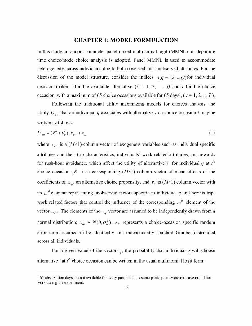
In this study, a random parameter panel mixed multinomial logit (MMNL) for departure

time choice/mode choice analysis is adopted. Panel MMNL is used to accommodate

heterogeneity across individuals due to both observed and unobserved attributes. For the

discussion of the model structure, consider the indices ),...,2,1( Qqq = for individual

decision maker, i for the available alternative (i = 1, 2, …, I) and t for the choice

occasion, with a maximum of 65 choice occasions available for 65 days1, ( t = 1, 2, .., T ).

Following the traditional utility maximizing models for choices analysis, the

utility qitU that an individual q associates with alternative i on choice occasion t may be

written as follows:

itqitqqit xvU εβ +ʹ+ʹ= )( (1)

where qitx is a (M×1)-column vector of exogenous variables such as individual specific

attributes and their trip characteristics, individuals’ work-related attributes, and rewards

for rush-hour avoidance, which affect the utility of alternative i for individual q at tth

choice occasion. β is a corresponding (M×1) column vector of mean effects of the

coefficients of qitx on alternative choice propensity, and qv is (M×1) column vector with

its thm element representing unobserved factors specific to individual q and her/his trip-

work related factors that control the influence of the corresponding thm element of the

vector qitx . The elements of the qv vector are assumed to be independently drawn from a

normal distribution; ),0(~ 2mqm Nv σ . itε represents a choice-occasion specific random

error term assumed to be identically and independently standard Gumbel distributed

across all individuals.

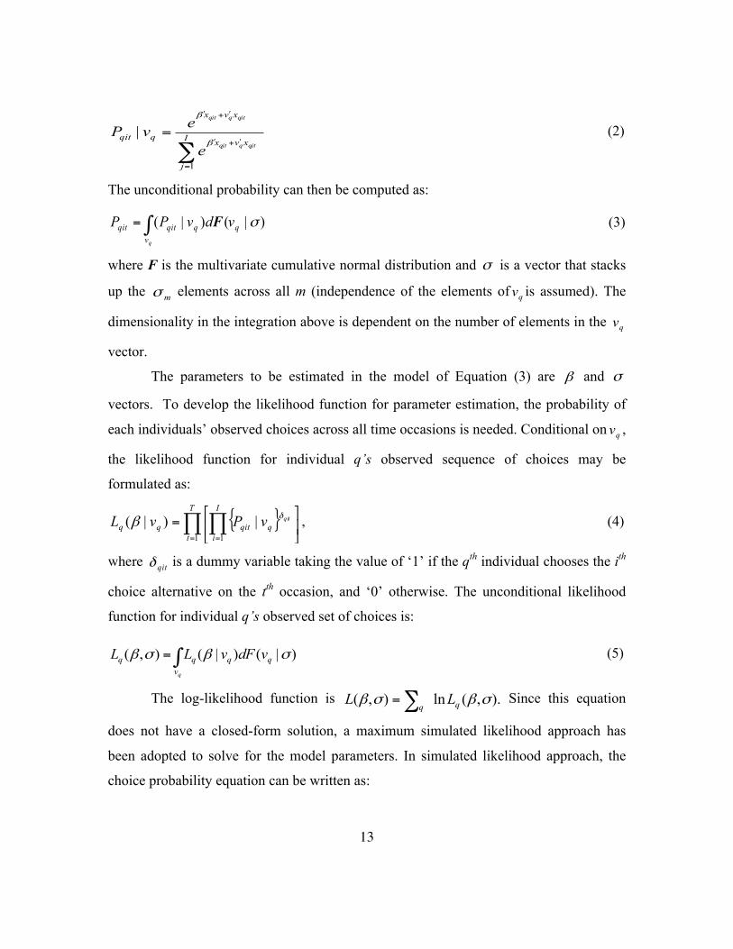
For a given value of the vector qv , the probability that individual q will choose

alternative i at tth choice occasion can be written in the usual multinomial logit form:

1 65 observation days are not available for every participant as some participants were on leave or did not work during the experiment.

13

∑=

ʹ+ʹ

ʹ+ʹ

= I

j

xvx

xvx

qqitqjtqqjt

qitqqit

e

evP

1

|β

β

(2)

The unconditional probability can then be computed as:

)|()|( σqv

qqitqit vdvPPq

∫= F (3)

where F is the multivariate cumulative normal distribution and σ is a vector that stacks

up the mσ elements across all m (independence of the elements of qv is assumed). The

dimensionality in the integration above is dependent on the number of elements in the qv

vector.

The parameters to be estimated in the model of Equation (3) are β and σ

vectors. To develop the likelihood function for parameter estimation, the probability of

each individuals’ observed choices across all time occasions is needed. Conditional on qv ,

the likelihood function for individual q’s observed sequence of choices may be

formulated as:

{ }∏ ∏= =

⎥⎦

⎤⎢⎣

⎡=

T

t

I

iqqitqq

qitvPvL1 1

|)|( δβ , (4)

where qitδ is a dummy variable taking the value of ‘1’ if the qth individual chooses the ith

choice alternative on the tth occasion, and ‘0’ otherwise. The unconditional likelihood

function for individual q’s observed set of choices is:

∫=qv

qqqq vdFvLL )|()|(),( σβσβ (5)

The log-likelihood function is ).,(ln),( σβσβ qqLL ∑= Since this equation

does not have a closed-form solution, a maximum simulated likelihood approach has

been adopted to solve for the model parameters. In simulated likelihood approach, the

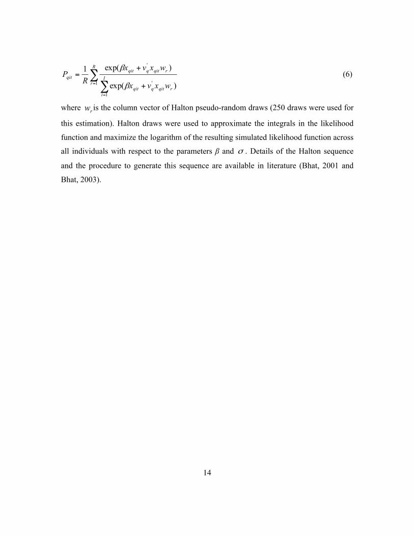
choice probability equation can be written as:

14

∑∑=

=

+

+=

R

rI

irqitqqit

rqitqqitqit

wxvx

wxvx

RP

1

1

'

'

)exp(

)exp(1

β

β (6)

where rw is the column vector of Halton pseudo-random draws (250 draws were used for

this estimation). Halton draws were used to approximate the integrals in the likelihood

function and maximize the logarithm of the resulting simulated likelihood function across

all individuals with respect to the parameters β and σ . Details of the Halton sequence

and the procedure to generate this sequence are available in literature (Bhat, 2001 and

Bhat, 2003).

15

CHAPTER 5: RESULTS

The variables selected for inclusion in the model specification are based on research

reported in the literature and the behavioral intuitiveness of model coefficients. For

understanding the impact of the reward, dummy variables representing reward categories

are included in the utility of all alternatives. The base alternative is taken to be travel

before peak period. For the reward, five different dummy variables are defined

representing €3, €7, €3-€7, credits for phone, and no credits-but with traffic information.

These dummy variables assume the value of zero in pre- and post-reward periods and

assume the value of one in the reward period. In this study, the data is modeled in a joint

fashion, stacking the observations of the pre-reward period, reward period, and post-

reward period respectively for each participant. Unobserved factors’ endogeneity that

affect pre-reward behavior also influence participants’ reward period and post-reward

behaviors, and the reward class (level) to which they belong.

5.1 UNDERESTIMATION OF UNOBSERVED FACTORS

Consider an individual who is very schedule oriented (independent of work time

flexibility) compared to observationally equivalent peers, and strictly follows a regimen

that is intrinsically aligned with usual workday timings. For this individual, this

unobserved attribute may contribute to his or her traveling in the pre-reward period

exclusively during the rush hours. As a result, this individual is eligible for the highest

reward class. If the pre-reward choices are considered exogenous in the modeling of

reward period choices, then individuals with a strong schedule orientation (which is

unobserved) will be probable to get a higher reward, while individuals with a relaxed

schedule orientation (and do not travel exclusively in the rush hours in the pre-reward

period) will be assigned to receive a lower reward. That is, individuals who are

intrinsically unlikely to change schedules are presented with a high reward while

individuals with a higher proclivity to change schedules are presented with a low reward.

16

The net result, if the pre-reward choices are considered entirely exogenous in reward

period choices, would be an underestimation of the effect of the reward on changing to

off-peak period travel. The way to address this is to consider the pre-reward period

choices as being endogenous to the reward period choices, and model the choices for

these different periods jointly to accommodate the unobserved rigid (or flexible) schedule

orientation of individuals. By controlling for this endogeneity, it is possible to get

econometrically consistent estimates of the effect of the reward on the likelihood to shift

to off-peak periods of travel. The same argument can be extended to other potential

unobserved factors (e.g., sensitivity to travel time, constraints at home or work) that

contribute to endogeneity of pre-reward choices.

5.2 INERTIA

To examine how the behavior of participants changed in response to the

temporary availability of a reward, a dummy variable is added to the specification. This

variable takes a value of zero for the pre-reward and reward periods, and a value of one in

the post-reward period. To explore differential impacts of rewards across gender,

income, and age, multiple interaction variables were included and tested for significance.

This inertia vector for each person was calculated by accounting total choice occasions

available to a person in the pre-reward period. So, for an observation-day, the inertia

effect was included in the utility equations for a person as RPRtiqiq dBRCRInertia ×= ,

where iqBRCR is the before reward-period choice ratio of individual q for alternative i.

The dummy variable RPRtd takes the value of one if the choice occasion is in reward or

before-reward periods and zero otherwise. A positive sign is expected on the inertia

variable for all alternatives.

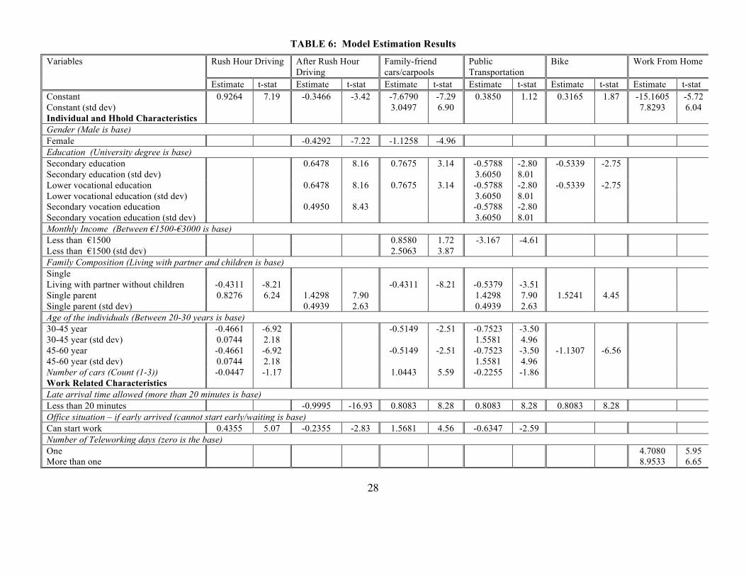
5.3 ESTIMATION RESULTS

Model estimation results are presented in Table 6. In light of the large number of

parameters in the model, a brief overview of key findings is provided in this chapter. The

17

constant term suggests that individuals are inclined to travel during the rush hour as

evidenced by the positive coefficient, and to a lesser degree by public transportation and

bicycle (where they can avail of the reward even when traveling during rush hours). The

significant standard deviations on the random parameters (constants) for shared-ride and

work from home suggest there are unobserved factors contributing to preference

heterogeneity for these alternatives. For example, gregarious individuals may be inclined

to carpool; and individuals who are employed in specific occupation types may be

inclined to work from home.

5.3.1 INDIVIDUAL CHARACTERISTICS

Among individual characteristics, females are less likely to travel after the rush

hour or via carpool with family and friends. In terms of education, those with lower

levels of education are more likely to travel after the rush hours, possibly due to lower

paying jobs that are part time or contractual in nature and afford schedule flexibility.

They are also more likely to share a ride, presumably due to vehicle ownership

constraints. On the other hand, they are less likely to use public transit; the significant

standard deviations on these random parameters suggest the presence of unobserved

factors affecting preference for transit. It is possible that these individuals live and work

in locations that are not well served by transit. Somewhat consistent with these results is

the finding that lower income individuals are more likely to share a ride and less likely to

ride transit. Those in the peak working age (30-60 years) are less likely to travel in rush

hours, less likely to share a ride, and less likely to use public transit. However, there is

significant preference heterogeneity when it comes to rush hour driving and use of public

transportation, possibly due to spatial effects and household and work constraints.

Individuals living in households without children appear to enjoy a less

constrained lifestyle as they eschew driving in rush hour, sharing a ride with others, and

using public transit. On the other hand, single parents – who may be very schedule

constrained – drive in rush hours and after rush hours (perhaps after dropping off a child

at school), and are more likely to use transit and bike modes. Single parents may also be

18

more responsive to the reward scheme due to financial constraints, and are hence more

likely to shift mode of transport in the reward and post-reward periods. However, there is

considerable preference heterogeneity exhibited by single parents. Additionally, higher

level of household car ownership is associated with reduced proclivity for rush hour

driving, propensity to share a ride and use of public transit; the flexibility that higher car

ownership levels afford explain these results.

5.3.2 WORK COMMUTE CHARACTERISTICS

Individuals with limited arrival time flexibility are more likely to travel before or

during rush hours that is consistent with expectations. They are also more likely to travel

by shared ride, public transit, and bicycle – signifying their desire to arrive on time at

work by any mode possible. Those who can start work even if they arrive early are more

likely to drive in the rush hours or share a ride (and thus arrive early or on time). As

expected, those who can telecommute are inclined to do so. Individuals who cannot

depart early (due to home constraints) are likely to avoid the peak period and travel after

the peak period.

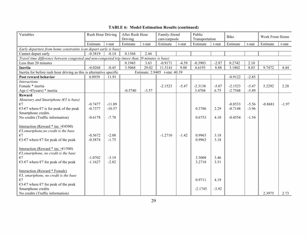
It is interesting to note that individuals, who have less than 20 minutes usual

travel time differential between congested and uncongested periods, are less likely to use

alternative modes such as shared ride and public transit; this is consistent with

expectations because driving is an acceptable proposition when congested conditions are

not terribly worse than uncongested conditions. Such individuals are more likely to

travel in the after-rush hour period and use bicycle, findings that are worthy of further

exploration.

Inertial effects are strong and significant. As expected, all coefficients are

positive – indicating the substantial presence of inertial effects that reinforce the

continuation of past behavior as long as it is not disturbed. The one negative coefficient

(albeit statistically insignificant) is associated with peak period driving; this coefficient is

negative because the inertial effect is shaken by virtue of the multi-week reward period.

In the reward period (that dominates the data set), many travelers were incentivized to

19

shift their time or mode of travel; in other words, inertia – although clearly present – was

overcome and had no impact during the reward period for this particular alternative as

large number of program participants changed their behavior (from traveling in peak

period by car).

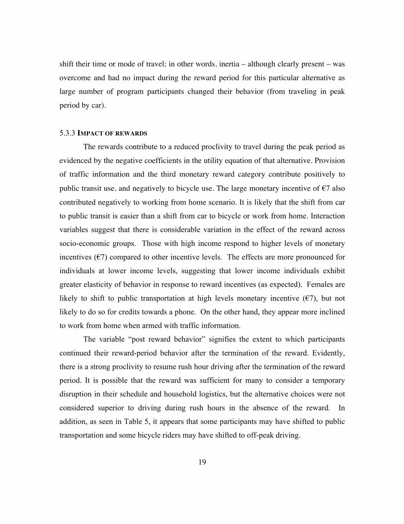
5.3.3 IMPACT OF REWARDS

The rewards contribute to a reduced proclivity to travel during the peak period as

evidenced by the negative coefficients in the utility equation of that alternative. Provision

of traffic information and the third monetary reward category contribute positively to

public transit use, and negatively to bicycle use. The large monetary incentive of €7 also

contributed negatively to working from home scenario. It is likely that the shift from car

to public transit is easier than a shift from car to bicycle or work from home. Interaction

variables suggest that there is considerable variation in the effect of the reward across

socio-economic groups. Those with high income respond to higher levels of monetary

incentives (€7) compared to other incentive levels. The effects are more pronounced for

individuals at lower income levels, suggesting that lower income individuals exhibit

greater elasticity of behavior in response to reward incentives (as expected). Females are

likely to shift to public transportation at high levels monetary incentive (€7), but not

likely to do so for credits towards a phone. On the other hand, they appear more inclined

to work from home when armed with traffic information.

The variable “post reward behavior” signifies the extent to which participants

continued their reward-period behavior after the termination of the reward. Evidently,

there is a strong proclivity to resume rush hour driving after the termination of the reward

period. It is possible that the reward was sufficient for many to consider a temporary

disruption in their schedule and household logistics, but the alternative choices were not

considered superior to driving during rush hours in the absence of the reward. In

addition, as seen in Table 5, it appears that some participants may have shifted to public

transportation and some bicycle riders may have shifted to off-peak driving.

20

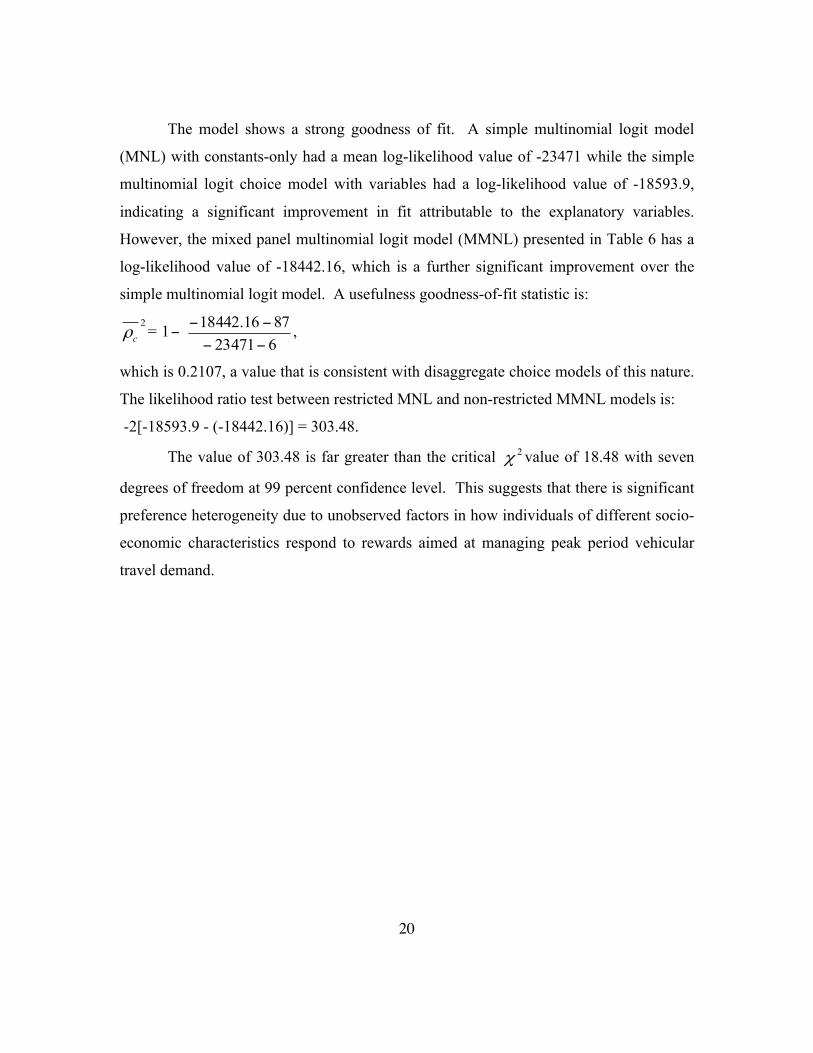
The model shows a strong goodness of fit. A simple multinomial logit model

(MNL) with constants-only had a mean log-likelihood value of -23471 while the simple

multinomial logit choice model with variables had a log-likelihood value of -18593.9,

indicating a significant improvement in fit attributable to the explanatory variables.

However, the mixed panel multinomial logit model (MMNL) presented in Table 6 has a

log-likelihood value of -18442.16, which is a further significant improvement over the

simple multinomial logit model. A usefulness goodness-of-fit statistic is:

2cρ = −1

6234718716.18442

−−

−− ,

which is 0.2107, a value that is consistent with disaggregate choice models of this nature.

The likelihood ratio test between restricted MNL and non-restricted MMNL models is:

-2[-18593.9 - (-18442.16)] = 303.48.

The value of 303.48 is far greater than the critical 2χ value of 18.48 with seven

degrees of freedom at 99 percent confidence level. This suggests that there is significant

preference heterogeneity due to unobserved factors in how individuals of different socio-

economic characteristics respond to rewards aimed at managing peak period vehicular

travel demand.

21

CHAPTER 6: CONCLUSION

Incentive-based schemes are being increasingly considered around the world to help

manage travel demand, particularly during peak periods, and bring about changes in

traveler choices towards more sustainable modes of transport, less congested times of

travel, and less congested corridors. Although there is some descriptive information on

the impacts of incentive-based travel demand management strategies, there is a need for

additional evidence on the impacts of such schemes on traveler behavior. It is necessary

to be able to isolate the effects of reward-based strategies on traveler behavior while

controlling for other explanatory factors, accounting for variations in effects across socio-

economic groups, and accommodating for the presence of individual taste heterogeneity

due to unobserved attributes. There is a paucity of modeling efforts that can provide deep

and rich insights into these aspects of the impacts of reward-based travel demand

management strategies.

This study aims to fill this need by offering a mixed panel multinomial logit

model of the effects of a reward based scheme on peak period vehicular travel. The study

is based on data collected in the Spitsmijden (Dutch for peak period avoidance) program

conducted in The Netherlands. Travel behavior data of 324 participants from the initial

experiment (conducted in 2006) is used in this study. Participants’ travel behavior was

measured during a pre-reward period of two weeks, during a reward period of 10 weeks,

and during a post-reward period of one week. About two-thirds of the participants opted

for monetary-based incentives while one-third chose a smartphone credit- or traffic-

information based incentive. The modeling methodology treats the pre-reward traveler

choices as endogenous to reward-period travel choices, thus recognizing that the level of

reward that an individual can attain is dependent on their usual (pre-reward) travel

behavior.

The mixed multinomial logit model offers deep insights into the effects of various

factors on traveler behavior in response to rewards. As expected, socio-economic factors,

22

work attributes, and trip characteristics (degree of flexibility) affect traveler response to

incentives. The level of incentive is also quite significant in explaining the choice of

alternative, with higher levels of incentive more likely to induce a desirable change in

behavior. It is found that inertia plays a significant role in human travel behavior; in

general, participants exhibited a high degree of inertia where they tended to continue

exercising the same travel choices unless the incentive made it worthwhile to get out of

their comfort zone. The incentive was able to overcome the inertia associated with

traveling in the peak period. Also, it is found that the incentive based scheme was not

sufficient to bring about lasting changes in behavior. Within just one week of the

termination of the reward program, travelers reverted largely to their pre-reward period

behavior – particularly with respect to driving in the rush hours. It is clear that many

individuals travel during the rush hours because that routine fits within the overall

schedule of their household and work life; while the incentive motivated individuals to

disturb that equilibrium and accept an alternate routine for a temporary period (when they

reaped the rewards), the inconvenience of changing behavior was substantial enough to

induce them to largely return to their usual pre-reward period behavior.

The moral of the story is that a temporary incentive may not be effective in

bringing about a sustained long term change in traveler behavior. Clearly the monetary

incentives are effective, because behavior changed significantly during the reward period.

The question is: how can this change be sustained over time after the reward systems are

removed? The answer to this question merits considerable additional research; focus

group sessions and post-experiment surveys that collect data on why individuals revert to

their original behavior would provide valuable insights to answer this question.

Incentives may have to be provided for a longer (to be determined) period of time so that

individuals get used to a new routine and home/work life arrangement; once they fall into

a new (presumably satisfactory) routine, then it is likely that the changes will stick

because of inertia effects and because the cost to change routine once again would be

greater than the value of the incentive that is being eliminated.

23

APPENDIX

Table 1: Socio demographic composition

Variables Share % Individual and Household Characteristics Gender Male 64.2

Female 38.8 Age 20 – 30 11.4

31 – 45 46.6 46 – 60 40.1 More than 60 1.9

Level of education Pre-vocational secondary education 10.2 Lower vocational education 4.3 Upper secondary vocational education 29.0 Higher professional /university degree 56.5

Marital status Single 13.3 Living with partner without children 22.5 Living with partner with children 57.4 Single parent 4.9 Other 1.9

Number of cars One 49.1 Two 47.2 Three 3.7

Monthly personal income level Less than 1,500€ 6.5 Between 1500€ to 3000€ 51.2 Between 3000€ to 4500€ 37.4 More than 4500€ 4.9

24

Table 2: Commute characteristic

Trip Related Characteristics Share % Early departure constraint from home

Can depart early 46.1 Cannot depart early 53.9

Travel time diff (congested and uncongested) Less than 20 minutes 38.8 Between 20 minutes and 30 minutes 38.8 More than 30 minutes 22.2

25

Table 3: work-place variables

Variables Share % Work Related Characteristics Number of days allowed for late arrival Zero 41.0 One 5.2 More than one 53.8

Amount of time allowed for late arrival Less than 20 minutes 43.8 Between 20 and 45 minutes 13.3 More than 45 minutes 42.9

Office situation - if early arrived Can start work and make preparation 88.0 Can’t start work/wait for other 12.0

Number of days allowed for teleworking Zero 74.1 One 20.4 More than one 5.5

26

Table 4: Level of rewards

Reward Distribution Share % Reward type Monetary 67.3 Smartphone 32.7

1. Reward class(Monetary) A [5]* 55.4 B [4] 27.5 C [2] 10.5 D [1] 6.4

* maximum number of reward-days per week 2. Reward class (Smartphone) A [15]** 42.5 B [20] 29.4 C [23] 19.9 D [25] 8.6

** minimum number of days must avoid peak hours in 5-week period

27

Table 5: Alternative choice share

Share of Alternatives for Observation-Days (%)

Alternatives Total Pre-reward period

Reward period

Post-reward period

Driving before rush hour (Base) 34.2 23.4 37.2 24.9 Driving during rush hour 25.9 46.8 20.0 45.7 Driving after rush hour 17.5 13.3 18.7 13.9 Using carpool/ family-friend carshare 5.3 4.4 5.5 4.4 Avoiding rush hour by using public transportation 10.3 4.7 11.7 6.6

Avoiding rush hour by using bike 3.0 4.5 2.9 1.5 Working from home 3.8 2.9 4.0 3.0

28

TABLE 6: Model Estimation Results

Variables Rush Hour Driving After Rush Hour Driving

Family-friend cars/carpools

Public Transportation

Bike Work From Home

Estimate t-stat Estimate t-stat Estimate t-stat Estimate t-stat Estimate t-stat Estimate t-stat Constant 0.9264 7.19 -0.3466 -3.42 -7.6790 -7.29 0.3850 1.12 0.3165 1.87 -15.1605 -5.72 Constant (std dev) 3.0497 6.90 7.8293 6.04 Individual and Hhold Characteristics Gender (Male is base) Female -0.4292 -7.22 -1.1258 -4.96 Education (University degree is base) Secondary education 0.6478 8.16 0.7675 3.14 -0.5788 -2.80 -0.5339 -2.75 Secondary education (std dev) 3.6050 8.01 Lower vocational education 0.6478 8.16 0.7675 3.14 -0.5788 -2.80 -0.5339 -2.75 Lower vocational education (std dev) 3.6050 8.01 Secondary vocation education 0.4950 8.43 -0.5788 -2.80 Secondary vocation education (std dev) 3.6050 8.01 Monthly Income (Between €1500-€3000 is base) Less than €1500 0.8580 1.72 -3.167 -4.61 Less than €1500 (std dev) 2.5063 3.87 Family Composition (Living with partner and children is base) Single Living with partner without children -0.4311 -8.21 -0.4311 -8.21 -0.5379 -3.51 Single parent 0.8276 6.24 1.4298 7.90 1.4298 7.90 1.5241 4.45 Single parent (std dev) 0.4939 2.63 0.4939 2.63 Age of the individuals (Between 20-30 years is base) 30-45 year -0.4661 -6.92 -0.5149 -2.51 -0.7523 -3.50 30-45 year (std dev) 0.0744 2.18 1.5581 4.96 45-60 year -0.4661 -6.92 -0.5149 -2.51 -0.7523 -3.50 -1.1307 -6.56 45-60 year (std dev) 0.0744 2.18 1.5581 4.96 Number of cars (Count (1-3)) -0.0447 -1.17 1.0443 5.59 -0.2255 -1.86 Work Related Characteristics Late arrival time allowed (more than 20 minutes is base) Less than 20 minutes -0.9995 -16.93 0.8083 8.28 0.8083 8.28 0.8083 8.28 Office situation – if early arrived (cannot start early/waiting is base) Can start work 0.4355 5.07 -0.2355 -2.83 1.5681 4.56 -0.6347 -2.59 Number of Teleworking days (zero is the base) One 4.7080 5.95 More than one 8.9533 6.65

29

TABLE 6: Model Estimation Results (continued)

Variables Rush Hour Driving After Rush Hour Driving

Family-friend cars/carpools

Public Transportation Bike Work From Home

Estimate t-stat Estimate t-stat Estimate t-stat Estimate t-stat Estimate t-stat Estimate t-stat Early departure from home constraints (can depart early is base) Cannot depart early -0.3819 -8.14 0.1368 2.44 Travel time difference between congested and non-congested trip (more than 20 minutes is base) Less than 20 minutes 0.1945 3.63 -0.9171 -4.59 -0.3903 -2.87 0.2742 2.10 Inertia -0.0268 -0.45 3.5068 29.02 11.5141 9.08 4.6193 8.88 3.1802 8.03 9.7472 4.44 Inertia for before rush hour driving as this is alternative specific Estimate: 2.9405 t-stat: 40.39 Post reward behavior 0.8939 11.91 -0.9122 -2.85 Interactions Female * inertia -2.1523 -5.47 -2.3138 -5.07 -2.1523 -5.47 5.2292 2.28 Age (>45years) * inertia -0.5740 -3.57 3.4704 6.75 -2.7548 -5.89 Reward Monetary and Smartphone (€3 is base) €7 -0.7477 -11.89 -0.8533 -5.56 -0.8681 -1.97 €3-€7 where €7 is for peak of the peak -0.7377 -10.57 0.3786 2.29 -0.7148 -3.96 Smartphone credits No credits (Traffic information) -0.6178 -7.78 0.6753 4.10 -0.4554 -1.54 Interaction (Reward * inc >€4500) €3,smartphone,no credit is the base €7 -0.5672 -2.08 -1.2710 -1.42 0.9963 3.18 €3-€7 where €7 for peak of the peak -0.5874 -1.75 0.9963 3.18 Interaction (Reward * inc >€1500) €3,smartphone, no credit is the base €7 -1.0702 -3.19 3.3008 3.46 €3-€7 where €7 for peak of the peak -1.1627 -2.82 3.2718 3.51 Interaction (Reward * Female) €3, smartphone, no credit is the base €7 0.9711 4.19 €3-€7 where €7 for peak of the peak Smartphone credits -2.1745 -3.92 No credits (Traffic information) 2.3975 2.73

30

REFERENCES

1. Bhat, C.R. (2001). Quasi-random maximum simulated likelihood estimation of the

mixed multinomial logit model. Transportation Research Part B, 35(7), 677-693.

2. Bhat, C.R. (2003). Simulation estimation of mixed discrete choice models using

randomized and scrambled Halton sequences. Transportation Research Part B, 37(9),

837-855.

3. Buuren, S., and Groothuis-Oudshoorn, K. (2011). MICE: Multivariate imputation by

chained equations in R. Journal of statistical software, 45(3), 1-67

4. Charness, G., and Gneezy, U. (2009). Incentives to exercise. Econometrica, 77(3),

909-931.

5. Currie, J., and Walker, W.R. (2009). Traffic congestion and infant health: Evidence

from E-ZPass. American Economic Journal: Applied Economics, 3(1), 65-90.

6. Currie, G. (2010). Quick and effective solution to rail overcrowding: free early bird

ticket experience in Melbourne, Australia. Transportation Research Record: Journal

of the Transportation Research Board, (2146), 35-42.

7. Dionne, G., Pinquet, J., Maurice, M., and Vanasse, C. (2011). Incentive mechanisms

for safe driving: a comparative analysis with dynamic data. The Review of Economics

and Statistics, 93(1), 218-227.

8. Fuji, S., and Kitamura, R. (2003). What does a one-month free bus ticket do to

habitual drivers. Transportation, 30, 81-95.

9. Gneezy, U., and Rustichini, A. (2000). Fine is a price, American Journal of Legal

Studies 29,

10. Hu, X., Chiu, Y.C., Delgado, S., Zhu, L., Luo, R., Hoffer, P., and Byeon, S. (2014).

Behavior insights for an incentive-based active demand management platform.

In Proceedings of the 93rd Annual Meeting of the Transportation Research Board,

Washington, DC.

31

11. Knockaert, J., Bliemer, M., Ettema, D., Joksimovic, D., Mulder, A., Rouwendal, J.,

and Van Amelsfort, D. (2007). Experimental design and modelling

Spitsmijden. Utrecht, Consortium Spitsmijden.

12. Levitt, S.D., and Dubner, S.J. (2010). Freakonomics, HarperCollins Publishers, New

York, NY.

13. Litman, T. (2003). The online TDM encyclopedia: Mobility management information

gateway. Transport Policy, 10(3), 245-249.

14. Litman, T. (2006). Lessons from Katrina and Rita: What major disasters can teach

transportation planners. Journal of Transportation Engineering, 132(1), 11-18.

15. Litman, T. (2006). London congestion pricing: Implications for other cities. Victoria

Transport Policy Institute, 10. http://core.ac.uk/download/pdf/6630967.pdf. Accessed

July. 29, 2015.

16. Locke, E.A., Shaw, K.N., Saari, L.M., and Latham, G.P. (1981). Goal setting and task

performance: 1969–1980. Psychological bulletin, 90(1), 125.

17. Merugu, D., Prabhakar, B.S., and Rama, N. (2009).An incentive mechanism for

decongesting the roads: A pilot program in Bangalore. In Proceedings of ACM

NetEcon Workshop.

http://storage.globalcitizen.net/data/topic/knowledge/uploads/20120217153716705.pd

f. Accessed July. 29, 2015.

18. Phang, S.Y., and Toh, R.S. (1997). From manual to electronic road congestion

pricing: The Singapore experience and experiment. Transportation Research Part

E, 33(2), 97-106.

19. Pluntke, C., & Prabhakar, B. (2013). INSINC: A Platform for Managing Peak

Demand in Public Transit. JOURNEYS, Land Transport Authority Academy of

Singapore.

20. Schaller, B. (2010). New York City’s congestion pricing experience and implications

for road pricing acceptance in the United States. Transport Policy, 17(4), 266-273.

21. Schrank, D., Eisele, B., and Lomax, T. (2012). TTI’s 2012 urban mobility report.

Texas A&M Transportation Institute, December 2012.

32

http://d2dtl5nnlpfr0r.cloudfront.net/tti.tamu.edu/documents/mobility-report-2012.pdf.

Accessed July. 29, 2015.

22. Shefer, D. (1994). Congestion, air pollution, and road fatalities in urban areas.

Accident Analysis & Prevention, 26(4), 501-509.

23. Thaler, R.H., and Sunstein, C.R. (2008). Nudge: Improving Decisions about Health,

Wealth, and Happiness. Yale University Press. \

24. Volpp, K.G., Troxel, A.B., Pauly, M.V., Glick, H.A., Puig, A., Asch, D.A., Galvin,

R., Zhu, J., Wan, F., DeGuzman, J., Corbett, E., Weiner, J., and Audrain-McGovern,

J. (2009). A randomized, controlled trial of financial incentives for smoking

cessation. New England Journal of Medicine, 360(7), 699-709.

25. Zhang, Z., Fujii, H., and Managi, S. (2014). How does commuting behavior change

due to incentives? An empirical study of the Beijing Subway System.Transportation

Research Part F, 24, 17-26.