Embed Size (px)
DESCRIPTION
Master thesis
Citation preview

Economic Scenario Generators
Mark Plomp
November 10, 2013
Msc thesis Stochastics and Financial Mathematics
Supervisors:Yulia Bondarouk (KPMG)
Jeroen Gielen(KPMG)Peter Spreij (UvA)

AcknowledgmentsThis thesis is the result of my master project carried out at the Fi-nancial Risk Management and Risk Actuarial Services department ofKPMG in Amstelveen. I would like to thank everyone who has en-couraged me and supported me in writing this thesis. At KPMG YuliaBondarouk was my main supervisor and Jeroen Gielen was my secondsupervisor. I want to thank the both of them for all the time they putin helping me with the thesis, all the great feedback and encouragingme to look at the subject from an actuarial and economical point ofview in stead of only looking at the mathematics. My supervisor atthe university was Peter Spreij. I also want to thank him for the greatguidance I got from him, especially with getting all the mathemati-cal details right. Further, I am very grateful to all the colleagues atKPMG; for all the help, the interesting discussions and the informaltalk from time to time.

AbstractIn 2009 the European Union agreed upon introducing a new regulatoryframework, called Solvency II, for insurance companies operating inthe EU. One of the requirements of the Solvency II directive states thatthe valuation of assets and liabilities needs to be market consistent.For most insurance companies the only practical method to achievea market consistent valuation is using a so called economic scenariogenerator (ESG). An ESG generates future scenarios for different riskfactors by Monte Carlo simulation of stochastic models correspondingto these risk factors.
In this thesis the construction and use of a market consistenteconomic scenario generator is investigated. The main question un-der investigation is what the sensitivities are in calibrating the ESGand simulating the future scenarios and what their impact is on theestimation of the market consistent value. Four risk factors are mod-elled for the ESG: interest rates, stocks, real estate and inflation rates.The Hull-White one factor model is used for the modelling of interestrates; stocks and real estate are modelled by the Black-Scholes-Hull-White model and the inflation rates are modelled with the Vasicekmodel. First on the basis of available literature the stochastic modelsare discussed and option pricing formulas corresponding to these mod-els are derived. Subsequently the calibration of the stochastic modelsto market data is discussed; matching the market prices of optionsto the option pricing formulas derived in the first part is one of themain parts of the calibration. Afterwards, for the analysis of the ESG,two types of insurance policies are modelled. The analysis includes:the impact of the characteristics of the policies on the value, the cal-ibration to different market data, estimation errors due to the MonteCarlo simulation and the impact of changes in the way the models arecalibrated.

Contents
I Background 6
1 General background 71.1 Solvency II . . . . . . . . . . . . . . . . . . . . . . . . . . . . . . . 71.2 Market Consistent Valuation . . . . . . . . . . . . . . . . . . . . . . 81.3 Economic Scenario Generator . . . . . . . . . . . . . . . . . . . . . 10
2 Technical background 12
II Theory 18
3 The interest rate model 193.1 The bond price . . . . . . . . . . . . . . . . . . . . . . . . . . . . . 20
3.1.1 Alternative representation of the short rate . . . . . . . . . . 243.2 Bond option . . . . . . . . . . . . . . . . . . . . . . . . . . . . . . . 24
3.2.1 Bond option under the Hull-White model . . . . . . . . . . . 29
4 The equity model 314.1 change of measure . . . . . . . . . . . . . . . . . . . . . . . . . . . . 33
5 The real estate model 385.1 Unsmoothing . . . . . . . . . . . . . . . . . . . . . . . . . . . . . . 39
6 The inflation model 41
7 Simulation 437.1 Euler Scheme . . . . . . . . . . . . . . . . . . . . . . . . . . . . . . 437.2 Discretisation and distributional error . . . . . . . . . . . . . . . . . 44
1
III Analysis and results 47
8 Calibration and simulation 488.1 Interest rate model . . . . . . . . . . . . . . . . . . . . . . . . . . . 488.2 Equity model . . . . . . . . . . . . . . . . . . . . . . . . . . . . . . 508.3 Real estate model . . . . . . . . . . . . . . . . . . . . . . . . . . . . 528.4 Inflation model . . . . . . . . . . . . . . . . . . . . . . . . . . . . . 548.5 simulation . . . . . . . . . . . . . . . . . . . . . . . . . . . . . . . . 55
9 Insurance Products 59
10 Analysis of the technical provisions 6310.1 Policy conditions . . . . . . . . . . . . . . . . . . . . . . . . . . . . 6310.2 Market conditions . . . . . . . . . . . . . . . . . . . . . . . . . . . . 6810.3 Estimation error . . . . . . . . . . . . . . . . . . . . . . . . . . . . 6910.4 Changes in the calibration . . . . . . . . . . . . . . . . . . . . . . . 73
11 Summary, Conclusions and Discussion 7711.1 Improvement of the ESG . . . . . . . . . . . . . . . . . . . . . . . . 78
A Derivation of Black’s formula 82
B Abstract Bayes’ Formula 84
C Geltner’s real estate unsmoothing method 86
2

Introduction
The goal of this thesis is to discuss the construction and use of a market consistenteconomic scenario generator (ESG) by insurance companies. A market consistentESG consists of various stochastic models and produces risk-neutral future sce-narios. It is a tool for insurers with which they can calculate the present value oftheir assets and liabilities, also called technical provisions. In this thesis we willbuild our own ESG, which will be programmed in Matlab.
The construction of an ESG requires one to make a choice of asset classes(or risk factors) to be modelled, which stochastic models we want to use to simulatethese classes and how these models are going to be calibrated. Subsequently,economic scenarios can be generated for the various asset classes and used tocalculate the technical provisions for various insurance products.
Typically many risk factors play a role in the asset management of aninsurer; for example, interest rates, inflation, credit spreads, equity movements,real estate prices and exchange rates. However, to control the complexity of themodel not all of these factors will be modelled. The most important assets inan insurance company’s portfolio are generally bonds, stocks and real estate [33].Also, inflation can be an important factor for the liabilities of an insurer, becauseoften guarantees embedded in insurance contracts are indexed yearly with theinflation rate. Therefore, we restrict ourselves to modelling these four risk factors,where bonds will be modelled by modelling interest rates.
During the last fifty years a large variety of stochastic models has beendeveloped for the three asset classes. Here the choice is made to use the Hull-Whiteone factor model for the stochastic interest rates, the Hull-White-Black-Scholesmodel for equity and real estate and the Vasicek model for inflation rates. Thischoice was made to get realistic results while controlling the complexity of theESG.
The Hull-White model is chosen because it can give an exact fit to thecurrent term structure, we can derive analytical formulas for interest rate deriva-tives, like swaptions, which makes it easier to calibrate the model accurately tomarket data and it is fairly easy to use the equity model under Hull-White interestrates. Moreover, for options the implied volatilities are higher for out-of-the-money
3

strikes, which is consistent with the volatility skew/smiles implied from marketprices of floors and swaptions [26]. This is a very desirable feature of the modelsince interest rate options embedded in an insurance product are usually writtenon out-of-the-money strikes.
For equity the Hull-White-Black-Scholes model is chosen because it is easyto use simultaneously with the Hull-White model and it is analytically tractable,which makes calibration to options easy.
The choice for the Vasicek model for inflation rates was made, because itis easy to handle and shows mean reverting behaviour, which is a desirable featurefor inflation.
Another analytically tractable interest rate model which can be fitted tothe term structure is the CIR++ model [5]. However, the equity model loses itsanalytical tractability under the CIR++ model. Therefore, the Hull-White modelis chosen over the CIR++ model.
As will be discussed in more depth in Chapter 1, it is preferred thatthe calibration of the model is done with liquidly traded financial instruments ifpossible. Therefore the interest model and the equity model will be calibrated toswaptions resp. (European) call options. For real estate and inflation, no liquidlytraded options or other derivatives are available, therefore we have to resort tohistorical data to calibrate the models. For real estate we will calibrate the modelbased on the historical values of a so called appraisal index and for inflation thecalibration will be done based on historical euro zone inflation rates.
Two types of insurance contracts will be modelled and valuated in thisthesis, both of which are life insurance contracts in which at least a guaranteedsum is paid at time of maturity, e.g. at retirement age.
The first contract we will model is called a surplus interest sharing policy.For this policy the return on a portfolio of government bonds is compared to areference yield. If the return on the portfolio during a period of one year is higherthan the reference yield, then part of the excess return is shared with the policyholder resulting in a higher sum of money at time of maturity.
The second contract is called an endowment policy. For this contract thepolicy holder can choose a fund to invest in, e.g. a mixed fund with bonds, stockand real estate. If at maturity the fund is worth more than the guaranteed sum,then part of the profits are shared with the policy holder.
As will also be discussed in more depth in Chapter 1, under Solvency IIthe insurance companies are obliged to calculate their technical provisions in amarket consistent way. Doing these calculations by using an Economic ScenarioGenerator had become very popular in the insurance industry [44]. Hence, it isvery important for insurance companies, regulators and other parties like KPMGinvolved with insurance companies, to understand how these models work and
4

what choices can be made when using a scenario generator. Therefore, the mainquestion about the ESG we develop in this thesis is
What are the sensitivities in calibrating the Economic Scenario Generator andsimulating future scenarios and what is the possible impact of these sensitivities
on the outcome of the technical provisions?
It goes without saying that changes in the calibration and simulation methods haveto fall within the market consistent framework. However, often markets aren’tcompletely liquid and some assumptions have to be made when calibrating themodels, because of this we can investigate what reasonable changes we can maketo these assumptions and what impact they have on the technical provisions.
Layout of the thesis
In Part I the background behind the ESG is discussed. Chapter 1 discusses newregulations for insurance companies, called Solvency II, are discussed, explains inmore depth what an ESG is and gives reasons for the use of ESG’s by insurers.Chapter 2 introduces some mathematical concepts which we will use throughoutthis thesis and will provide a mathematical basis upon which we will build ourstochastic models.
Part II covers the mathematical theory behind the models and the optionpricing formulas we use in the ESG. This will be done based on literature, whichwill be referred to during the chapters.
Part III is where the programmed ESG will be analysed and discussed.Chapter 8 will discuss the way in which the ESG is calibrated and provides exam-ples of the outcome of the calibration. In Chapter 10 we will have a look at thetechnical provisions corresponding to the modelled insurance products, which areexplained in Chapter 9, and in what way they are influenced by changing underly-ing conditions. Finally in Chapter 11 a summary of the thesis is given, the resultsare discussed and we look at possible improvements of the ESG.
5

Part I
Background
6
Chapter 1
General background
1.1 Solvency II
In the wake of the subprime mortgage crisis that started in 2007, in 2009 theEconomic and Financial Affairs Council, in which the Economic and Finance min-isters of the European Union are seated, approved the Solvency II Directive [44].Solvency II is a new regulatory framework for the European insurance industry.The main aims of which are to enhance policyholders protection, the stability ofthe financial system and to unify the insurance market in the EU as a whole, byestablishing harmonised solvency requirements across all member states.
In addition, the Solvency II Directive is developed to reflect new andimproved risk management standards to define capital requirements and to managerisks and it is partially a response to the previous market turmoil during thefinancial crisis of 2007-2008.
The European Insurance and Occupational Pensions Authority(EIOPA) has defined three pillars as a way of grouping the Solvency II require-ments. Pillar 2 contains the requirements for good governance and risk manage-ment of insurers and covers the supervisory activities and powers of regulators.The centerpiece of pillar 2 is the Own Risk And Solvency Assessment (ORSA),which is an internal process the insurer has to undertake to assess the adequacy ofits risk management and current and future solvency positions under normal andalso under severe stress scenarios. Pillar 3 focusses on disclosure and transparencyrequirements.
Pillar 1 covers all the quantative requirements that insurers must satisfyto demonstrate that they have sufficient capital resources. It requires that an in-surance firm must maintain technical provisions against liabilities and it definestwo capital requirements: the Minimal Capital Requirement (MCR) and the Sol-vency Capital Requirement (SCR). The MCR is set as a minimal level below which
7
financial resources should never fall. It is a trigger for regulatory intervention. TheSCR is the amount of capital an insurance company should hold under Solvency IIand it corresponds to the Value-at-Risk (VAR) of the own funds of an insurer setat a confidence level of 99, 5% over a one year period. This can be interpreted asthe requirement that only once in 200 years a company won’t have enough fundsto meet their obligations.
Initially the Solvency II directive was meant to become effective January1, 2013. However due to delays the implementation of Solvency II is postponed atleast until January 1, 2014. A reason for this is that the negotiations about theOmnibus-2 guideline have come to a halt and will resume in the second half of2013. Omnibus-2 discusses the transition measures that have to be taken for theimplementation of Solvency II and the role EIOPA will have as a supervisor. An-other reason is that EIOPA has issued an impact study, the Long Term GuaranteeAssessment (LTGA), at the beginning of 2013, which investigates the impact ofSolvency II on long term insurance products. It can be expected that followingthe conclusion of the LTGA further adjustments to the Solvency II framework willbe made, this could lead to further postponement of the implementation.
1.2 Market Consistent Valuation
One of the requirements of the Solvency II directive is that insurance companiesvalue their assets and liabilities in a market consistent way [44]. In this section wewill look at the meaning of a market consistent valuation; we will generally followthe explanation given in [14].
Before we look at a market consistent valuation, we first have to dis-cuss deep and liquid markets. The Bank of International Settlements defines adeep market as a market where large volume transactions are possible without(drastically) affecting the market price and a liquid market as a market whereparticipants can execute large volume transactions rapidly with a small impacton market prices. In such a market buyers and sellers constantly trade and theobserved market price emerges as a consensus opinion of the asset’s value.
It is important to note that the observed market price cannot be identifiedwith the objective values of the traded objects. Sometimes the market can over-or undervalue an object; an example of an overvaluation is the ’dot-com’ bubble atthe end of the twentieth century in which the stock value of internet companies andrelated companies rose rapidly, causing a large overvaluation of these companies[42].
However, market prices have some attractive properties that make themvery suitable for assessing the value of an asset. Firstly, they react quickly tochanges in relevant information. Secondly, the values are additive; the price of two
8

securities is the sum of the prices. Thirdly, the price does not depend on who orwhat is the buyer or the seller. And finally, at any given moment the market priceis unique.
When a market is no longer deep or liquid the uniqueness property is lost.Since the number of transactions and the total volume of transactions in such asituation is low, there is uncertainty about the market price at any given pointin time. In stock markets this is reflected in the form of a large bid-offer spread,which is the difference between the prices for which an asset can be sold and forwhich an asset can be bought.
As can be expected, not all markets are deep and liquid. In fact, thenumber of stocks and bonds that are liquidly traded is very small compared to thenumber of bonds and stocks that you can trade in. Moreover, most assets aren’teven traded in such a manner, e.g. insurance liabilities. So a priori there seems tobe no market consistent value for an insurance liability, since there is no deep andliquid market for these liabilities. We could ask ourselves the question what a fairvalue for these liabilities is at a given point in time.
The definition for a market consistent value we will adopt here is thefollowing from [31].
A market consistent value of an asset or liability is its market value, if it isreadily traded in a deep and liquid market at the point in time that the valuation
is struck. For any other asset or liability, a market consistent value is a bestestimate of what its market value would have been had it been traded in a deep
and liquid market.
For an insurance liability the goal of the market consistent valuation is to transferthe valuation problem into a setting where we have reliable and useful marketprices.
The present value of the liabilities of a insurance company are often alsoreferred to as the technical provisions. This is the amount of money an insurancecompany has to maintain to meet its expected obligations.
An insurance liability is defined by its resulting future cash flows. Thesecash flows can depend on claims, expenses, changes in the environment and otherrandom events. It can even be argued that some cash flows also depend on theparticular insurer holding the liability, e.g. the financial strength and profitabilityof a company can be part of the agreement.
Thus, to value an insurance liability the cash flows associated to it haveto be determined and subsequently the cash flows have to be replicated by usingcash flows of deeply traded financial instruments as good as possible. For cashflows that cannot be replicated or only partially, a risk margin has to be taken.For example a cash flow that depends on the value of the value of some underlying
9

portfolio of stocks and bonds can be replicated perfectly in general, while a cashflow in which mortality rates are a factor might not be entirely replicable andtherefore a risk margin has to be taken.
In this thesis we concern ourselves with the replicable parts of the futurecash flows.
1.3 Economic Scenario Generator
There are several methods insurers can use to calculate the technical provisions ina market consistent way. One of the most intuitive ways to replicate cash flows,using deeply traded financial instruments, might be to construct a replicatingportfolio. Another efficient way would be to use a closed-form solution to calculatethe market consistent value. However, in practice it turns out that both methodsare often hard to implement because of technical issues, the most important ofwhich is that most insurance contracts contain options that are path-dependentand have high dimensions [44]. Here path-dependent means that the cash flowsdepend on the way in which the underlying asset value moves during the lifetimeof the policy, not just on what asset value is achieved at the end of the contract.High dimensionality means that the various cash flows depend on many underlyingrisk factors. In these cases it is often hard to find a good replicating portfolio orto derive a closed-form solution and every different insurance contract would needa different replicating portfolio resp. closed-form solution. Therefore, it is moreconvenient to look for other methods that are easier to implement. Currently oneof the most used methods to value insurance liabilities is using a so called economicscenario generator (ESG). We will now discuss what an ESG is and why it can beused for market consistent valuations.
Using an ESG is a simulation based approach to valuation. By usingMonte Carlo simulation and various stochastic models, future scenarios are gen-erated. The aim is to model the underlying risk factors of the insurance contractsas good as possible. Subsequently, after the scenarios are generated, they can beused to backward calculate the present value of the insurance liabilities.
An essential feature of the stochastic models and subsequently the gen-erated scenario is that they have to be risk-neutral. This is because the firstfundamental theorem of asset pricing implies that if we want to price a claim in away that avoids arbitrage then this should be done by calculating the expectationin a risk-neutral setting. In the case of a Monte Carlo simulation this means wehave to take the average value of what the price of the claim would be under eachindividual scenario, when the scenarios are generated in a risk-neutral way.
Worthy of addressing here is the fact that even though we generate a setof scenarios in a risk-neutral way, each individual scenario can be considered to be
10

a real world scenario. The difference between risk-neutral scenarios and real worldscenario is not the paths themselves. If a path is possible in a real world settingit is also possible in a risk-neutral setting and vice-versa. The difference is in theprobability of these scenarios occurring or more correctly the distribution of thescenarios [22].
As we noted above we would like the ESG to simulate the underlyingrisk factors of the insurance liabilities. There is a large variety of risk factors towhich the cash flows can be sensitive. For example interest rates, inflation, creditspreads, equity movements, real estate prices and exchange rates. Therefore, foran ESG to be market consistent it needs to be able to reproduce the current pricesof deep and liquidly traded assets related to these risk factors, e.g. it needs to beable to reproduce the prices of options on equity as good as possible.
There a two ways in which the model can be calibrated in a market con-sistent way. The first way is to match the model prices as good as possible to themarket prices; this is usually done in a least squares sense. The second way isto calibrate the model to historical data, e.g. historical volatility of a certain riskfactor.
The former method is the preferred one where liquidly traded assets areavailable, since this method reproduces the current market prices best. However,sometimes prices of claims related to a specific risk factor aren’t available or themarket for these claims is not deep and liquid. In these cases the latter calibrationmethod has to be used.
Sometimes the two methods can be combined. Life insurance liabilitiesoften stretch far into the future and claims with such long maturities generallyaren’t available on the market. For example the implied volatility surface of optionson equity can be extrapolated based on long time historical volatilities beforecalibrating the model to market prices.
11
Chapter 2
Technical background
This chapter provides some of the basic concepts that we will use throughout thisthesis. For a more complete introduction into portfolio theory and option pricingsee [4].
First, let us denote the stochastic processes, which correspond to valueprocesses of the financial instruments we want to model, by Y = (Y1, ..., Ym); lateron in this thesis we will change the notation to reflect the type of asset we aremodelling, e.g. equity will be denoted by S.
Let us assume we have a probability space (Ω,F ,P) on which Y is de-fined and let the filtration F = Ft = σ(Y (s) : 0 ≤ s ≤ t)|t ≥ 0 satisfy the usualconditions.
As was mentioned in Section 1.3, we want to generate risk-neutral scenar-ios. Therefore we want the dynamics of our models to operate under a risk-neutralmeasure in stead of the real world measure P. Hence, we assume the existance ofan equivalent martingale measure (EMM), or risk-neutral measure, Q, with respectto the numeraire B(t), which is called the money account and will be defined inDefinition 2.8. The dynamics of the stochastic models in this thesis will be givenunder the risk-neutral measure Q.
Portfolios and contingent claims
As we mentioned in the introduction of the thesis, we want to calibrate our modelsto options. To derive analytic formulas for these options we need to introduce somedefinitions and assumptions about the market. Before we introduce this definitions,we remind ourselves that a stochastic process X = X(ω, t) is a progressivelymeasurable process if Ω × [0, t] 3 (ω, s) → X(ω, s) is Ft
⊗B[0, t]-measurable for
all t ≥ 0.
Definition 2.1. Suppose we have an n-dimensional F-adapted price process Z =(Z1, .., Zn). Then
12

• a portfolio is any n-dimensional progressively measurable process h = h(t) :t ≥ 0.
• the value process Πh corresponding to the portfolio h is given by
Πh(t) =n∑i=1
hi(t)Zi(t).
• a portfolio h is called self-financing if the value process Πh satisfies the con-dition
dΠh(t) =n∑i=1
hi(t)dZi(t).
One of the main assumptions throughout this thesis is that the market is arbitragefree. This is in fact implied by the existence of a risk-neutral measure Q, which weassumed at the beginning of this technical introduction. However, it is still usefulto recall the definition of an arbitrage opportunity.
Definition 2.2. An arbitrage opportunities in a market is a self-financing portfolioh such that
Πh(0) = 0,
P(Πh(T ) ≥ 0) = 1,
P(Πh(T ) > 0) > 0.
A (European) call option X is a contract that is defined on the price Zi of someunderlying asset at a specified maturity time T and with a strike price K. At timeT the value of the call option is given by
ΠX(T ) = max(Zi −K, 0).
More general, a contract which is completely defined in terms of one or more under-lying assets is called a contingent claim or derivative; the mathematical definitionis given below.
Definition 2.3. A random variable X is called a contingent claim with maturityT or T-claim if it is FT -measurable. The corresponding price process is denotedby ΠX(t) for 0 ≤ t ≤ T , where ΠX(T ) = X P-a.s..
We would like the contingent claims to have a unique price, therefore we need thenext definition of attainability and the following proposition.
13

Definition 2.4. We say that a T-claim X is attainable, if there exists a self-financing portfolio h such that
Πh(T ) = X, P-a.s..
In this case we call h a replicating portfolio for X.
Proposition 2.5. Suppose that the T-claim X is attainable and let h be a repli-cating portfolio for X. Then the only price process ΠX(t) which is consistent withthe no arbitrage assumption is given by ΠX(t) = Πh(t). Furthermore, if g is alsoa replicating portfolio for X, then Πh(t) = Πg(t).
Proof. Suppose at some time t we have ΠX(t) < Πh(t) then we can make anarbitrage by selling the portfolio h and buying the claim X; vice-versa for ΠX(t) >Πh(t). The same argument can also be used to show that Πh(t) = Πg(t) under theno arbitrage assumption.
Bonds, interest rates and swaptions
The interest rate model plays an important role in the ESG and we will see var-ious types of interest rates and assets based on interest rates during this thesis.Therefore, these are introduced here.
The most basic, to interest rates related, asset is a zero-coupon bond,which is defined as follows.
Definition 2.6. A maturity T zero coupon bond or T -bond is a contract ensuringthe holder one unit of currency, e.g. one euro, at time T . The price of the bond attime t is denoted by P (t, T ), for 0 ≤ t ≤ T .
Based on the definition of a zero-coupon bond we can define some different typesof interest rates.
Definition 2.7. • The simple forward rate for [T, S] at time t is given by
F (t, T, S) =1
S − T
(P (t, T )
P (t, S)− 1
).
• The simple spot rate for [t, T ] is
F (t, T ) =1
T − t
(1
P (t, T )− 1
).
• The continuously compounded forward rate for [T, S] at time t is given by
R(t, T, S) = − logP (t, S)− logP (t, T )
S − T.
14

• The instantaneous forward rate with maturity T at time t is defined as
f(t, T ) = limS↓T
R(t, T, S) = −∂ logP (t, T )
T − t
• The (instantaneous) short rate at time t is defined by
r(t) = f(t, t)
With this definition we can define the money account B(t).
Definition 2.8. The money account is defined by the dynamics
dB(t) = r(t)B(t)dt, B(0) = 1,
or equivalently
B(t) = exp
(∫ t
0
r(u)du
).
It can be interpreted as a bank account in which the profits are continuouslycompounded at the prevailing short rate of interest.
Since we want to calibrate our interest rate model to swaptions, we need to definewhat an interest rate swap is and what a swaption is, but before we do this wewill define a coupon bond.
Definition 2.9. A coupon bond is a contract specified by a number of futuredates T0 < T1 < T2 < ... < Tn, a sequence of coupons c1, .., cn and a nominal valueN , such that the owner receives ci at Ti for i = 1, ..., n and receives N at timeTn. The coupons can either be some fixed amount or floating, in which case thecoupons are determined at Ti−1 as ci = (Ti − Ti−1)F (Ti−1, Ti)N . Here F (Ti−1, Ti)is the simple spot rate defined in Definition 2.7.
It is not hard to determine the t ≤ T0 price of ci. In the fixed coupon case we canbuy ci P (t, Ti) bonds to get a payoff of ci at Ti. Therefore the t ≤ T0 price of ci isciP (t, Ti). For the floating case we first have to note that, from the definition ofF (Ti−1, Ti) we have at Ti
ci =1
P (Ti−1, Ti)− 1.
At time t the value of getting −1 at Ti is −P (t, Ti). The time t ≤ T0 value of1
P (Ti−1,Ti)is P (t, Ti−1), since if we buy at t a Ti−1-bond for P (t, Ti−1), we get 1 paid
15

out at Ti−1 and we can use this to buy 1P (Ti−1,Ti)
Ti-bonds. Therefore the time
t ≤ T0 value of ci is
P (t, Ti−1)− P (t, Ti). (2.1)
An interest rate swap is a contract in which floating rate interest payments areexchanged for fixed rate interest payments. We can see this as an agreementbetween two parties in which one party has a coupon bond which pays a fixedinterest rate and the other party has a coupon bond which pays a floating rate.The two parties then decide to exchange the coupons they receive for some periodof time, without exchanging the underlying bonds.
Definition 2.10. A payer interest rate swap settled in arrears is a contract whichis defined as follows. There are a number of future dates T1, T2, ..., Tn with usuallyTi−Ti−1 = δ, a fixed rate K and a nominal value N . At dates T1, ..., Tn the ownerof the contract pays KδN and receives floating F (Ti−1, Ti)δN .
At time Ti the net cash flow is equal to
Nδ(F (Ti−1, Ti)−K),
for which, by using the result we derived in (2.1), the t ≤ T0 value can be computedas
N(P (t, Ti−1)− P (t, Ti)−KδP (t, Ti)).
Now we can compute the t ≤ T0 value of the payer swap by summing over i =1, ..., n:
Πp(t) = N
(P (t, T0)− P (t, Tn)−Kδ
n∑i=1
P (t, Ti)
). (2.2)
A receiver interest rate swap is a swap in which the holder pays a floating rateand receives a fixed rate. Note that in this case the signs of the cash flows aboveare changed and as a consequence its t ≤ T0 value is Πr(t) = −Πp(t).
The remaining question now is how the swap rate K is determined. Bydefinition it is chosen such that at the time the contract is written, the value ofthe swap equals zero.
Definition 2.11. The forward swap rate at time t ≤ T0 is the fixed rate whichgives Πp(t) = −Πr(t) = 0 and is denoted by Rswap(t)
We thus get
Rswap(t) =P (t, T0)− P (t, Tn)
δ∑n
i=1 P (t, Ti).
16

We can use this equation to rewrite (2.2) to
Πp(t) = Nδ(Rswap(t)−K)n∑i=1
P (t, Ti). (2.3)
Now we can define a (payer) swaption, which is an option on a payer swap.
Definition 2.12. A payer swaption with strike rate K is a contract which givesthe owner the right at maturity date T (but not the obligation) to enter into apayer swap with fixed rate K. Usually the maturity date is set to coincide withthe first reset date of the onderlying swap, i.e. T = T0.
An equivalent definition can be given for a receiver swaption. If we use(2.3) for t = T0 we can see that the T0 payoff of the payer swaption is equal to
Nδ(Rswap(T0)−K)+n∑i=1
P (T0, Ti) (2.4)
The market prices of swaptions are given in terms of swaption volatilities thatare derived from Black’s formula for swaptions. Therefore we will need Black’sformula to calculate the market prices.
Theorem 2.13 (Black’s Formula for Swaptions). Black’s formula for the t ≤ T0price of a payer swaption is given by
Nδ(Rswap(t)Φ(d1(t))−KΦ(d2(t)))n∑i=1
P (t, Ti),
where
d1(t) =log(Rswap(t)
K) + 1
2σ(t)2(T0 − t)
σ(t)√T0 − t
,
d2(t) = d1 − σ(t)√T0 − t.
Here Φ denotes the standard normal distribution function. σ(t) is known as Black’sswaption volatility.
A justification for Black’s formula can be found in Appendix A.
17

Part II
Theory
18
Chapter 3
The interest rate model
In this chapter we will discuss the interest rate model we will use in our ESG. Wewant to calibrate our model to market prices of at-the-money swaptions. Therefore,we will derive an explicit formula for the price of a swaption under the chosen Hull-White model.
The Hull-White model is a short rate model, it defines the dynamics ofthe short rate. Short rate models were the earliest stochastic short rate models.The relation between the bond prices P (t, T ) and the short rate can be derivedfrom the time t value of P (T, T ) = 1. That is,
P (t, T ) = B(t)EQ[
1
B(T )
∣∣∣∣Ft]= EQ
[e−
∫ Tt r(s)ds
∣∣∣Ft] .The need for an arbitrage free model let Hull and White [24] to an extension of theVasicek model [45], which can be described by the stochastic differential equation:
dr(t) = λ(µ− r(t))dt+ σdW (t), r(0) = r0.
The Vasicek model on it’s own is a arbitrage free model, however when used in areal market situation an exact fit of the model to the market term structure is notpossible in general. Hence, bond options and other derivatives priced under theVasicek model would not be consistent with the market prices of bonds and wouldtherefore lead to arbitrage opportunities.
The extension of Hull and White allows for an arbitrage free calibrationsince it is possible get an exact fit to the currently observed term structure ofinterest rates. Under the risk-neutral measure Q, with the money market accountas numeraire, the dynamics of r(t) under the Hull-White extended Vasicek model
19

are described by
dr(t) = (θ(t)− a(t)r(t))dt+ σ(t)dW (t), r(0) = r0.
Not only can this model be fitted to the term structure with the θ(t) term, itcan also give an exact fit to the spot or forward volatilities with the σ(t) term.However, these high degrees of freedom make the model hard to handle analyticallyin general. Since we want to fit observed market prices of swaptions to modelprices in order to calibrate the ESG, it is convenient if we can derive an analyticalformula for the swaption prices under te model. Therefore we restrict ourselvesto the model known as the Hull-White one factor model [25], where a(t) = a andσ(t) = σ are constants in stead of functions of time. Thus, the dynamics of theHull-White one factor model are given by:
dr(t) = (θ(t)− ar(t))dt+ σdW (t), r(0) = r0. (3.1)
An exact fit to the volatility term structure is not possible anymore in this model,but we are still able to exactly fit the term structure and we now can derive ananalytic formula for the price of a swaption. Moreover, one of the great strengthsof this model is that we can also derive analytical formula’s for put and call optionson equity under Hull-White interest rates.
We will proceed as follows. First we will deduce an explicit formula forthe price of a bond P (t, T ) under the model and subsequently we will use it to geta formula for the price of a European option on a bond. This formula, togetherwith the so called Jamshidian’s trick [27], will get us the formula for the price ofa swaption under the Hull-White model.
3.1 The bond price
The first step to deriving a formula for the price of a bond is by analysing thesolution of the Hull-White SDE (3.1).
Proposition 3.1. The solution to the short rate dynamics in the Hull-White modelis given by
r(t) = e−a(t−s)(r(s) +
∫ t
s
θ(u)eaudu+ σ
∫ t
s
eaudW (u)
). (3.2)
Proof. The result can be verified by applying the Ito-formula to (3.2).
20

From this result it follows that r(t), conditional on Fs, is Gaussian withconditional expectation and conditional variance
E [r(t)|Fs] = e−a(t−s)(r(s) +
∫ t
s
θ(u)eaudu
),
Var [r(t)|Fs] = E[(σe−a(t−s)
∫ t
s
eaudW (u))2∣∣∣∣Fs]
= E[σ2e−2a(t−s)
∫ t
s
e2audu
∣∣∣∣Fs]=σ2e2as
2a
(1− e−2a(t−s)
).
Here we have used the Ito isometry to calculate the variance. Recall that (underour risk-neutral measure Q) we can represent bond prices as
P (t, T ) = EQ[e−∫ Tt r(s)ds|Ft
]Since r(t) is a Gaussian process, one can show that
∫ Ttr(s)ds is normally dis-
tributed, which means the bond price is an expectation of a lognormal distributionand of the form
P (t, T ) = exp
(E[−
∫ T
t
r(s)ds] +1
2Var[−
∫ T
t
r(s)ds]
). (3.3)
Now we remind ourselves that (3.1) is just a short hand notation for
r(t) = r0 +
∫ t
0
θ(s)ds− a∫ t
0
r(s)ds+
∫ t
0
σdW (s).
By rearranging terms and taking the expectation on both sides we get that
E[
∫ t
0
r(s)ds] =r0a
+1
a
∫ t
0
θ(s)ds− 1
aE[r(t)]
=r0a
+1
a
∫ t
0
θ(s)ds− e−at
a
(r0 +
∫ t
0
θ(s)easds
)=r0a
(1− e−at) +1
a
∫ t
0
θ(s)(1− ea(s−t))ds.
Moreover, from (3.2) we can derive
Cov[r(t), r(u)] = σ2e−a(t+u)E[
∫ t
0
easdW (s)
∫ u
0
easdW (s)]
= σ2e−a(t+u)∫ t∧u
0
e2asds
=σ2
2ae−a(t+u)(e2a(t∧u) − 1),
21

where we have made use of the Ito isometry and the independence of disjointBrownian increments. We can use this formula to calculate the variance
Var[
∫ t
0
r(s)ds] = E[(
∫ t
0
r(s)ds− E[
∫ t
0
r(s)ds])2]
=
∫ t
0
∫ t
0
E[(r(s)− E[r(s)])(r(u)− E[r(u)])]ds du
=
∫ t
0
∫ t
0
Cov[r(s), r(u)]ds du
=
∫ t
0
∫ t
0
σ2
2ae−a(t+u)(e2a(t∧u) − 1)ds du
=σ2
2a3(2at− 3 + 4e−at − e−2at).
For notational convenience, let us now define
B(t, T ) =1
a(1− e−a(T−t)) (3.4)
and insert the results in (3.3). Then
P (t, T ) = exp
(−r(t)
a(1− e−a(T−t))− 1
a
∫ T
t
θ(s)(1− ea(s−t))ds
+σ2
2a3(a(T − t)− 3
2+ 2e−a(T−t) − 1
2e−2a(T−t))
)= exp
(−r(t)B(t, T )−
∫ T
t
θ(s)B(T, s)ds
+σ2
2a2
∫ T
t
1− 2e−a(T−s) + e−2a(T−s)ds
)= exp
(−r(t)B(t, T )−
∫ T
t
θ(s)B(T, s)ds
+σ2
2
∫ T
t
B2(s, T )ds
). (3.5)
The function θ(t) gives us the opportunity to fit the theoretical bond prices tothe market prices. It follows from the definition of the instantaneous forward ratef(t, T ) = −∂log(P (t,T ))
∂Tthat
P (t, T ) = e−∫ Tt f(t,s)ds,
22

which implies there is a one-to-one correspondance between bond prices P (0, T ) | T >0 and the forward rate curve f(0, T ) | T > 0. Because of convenience we chooseto fit the forward rate curve to our model, which results in
f(0, T ) = − ∂
∂Tlog(P (0, T ))
=∂
∂TB(t, T )r0 +
σ2
2
∫ T
0
∂
∂TB2(s, T )ds−
∫ T
0
θ(s)∂
∂TB(s, T )ds
= e−aT r0 −σ2
2a
(1− e−aT
)2+
∫ T
0
θ(s)e−a(T−s)ds.
Here we implicitly used the fact that ∂∂TB(s, T ) = − ∂
∂sB(s, T ) to get the last
expression. We can solve the last equation for θ(t) by writing
f(0, T ) = y(T )− g(T ),
where
g(T ) =σ2
2a
(1− e−aT
)2and
y(T ) = e−aT r0 +
∫ T
0
θ(s)e−a(T−s)ds
= E [r(t)]
We can describe y(T ) = E [r(T )] by the ordinary differential equation
d
dty(t) = −ax(t) + θ(t), y(0) = r(0).
This leads us to the following expression for θ(t)
θ(t) =d
dty(t) + ay(t)
=d
dtf(0, t) +
d
dtg(t) + a (f(0, t) + g(t))
=d
dtf(0, t) + af(0, t) +
σ2
2a
(1− e−2at
). (3.6)
Now we can insert θ(t) into (3.5) and, skipping some tedious calculations, we arriveat the following result
23

Proposition 3.2. Under the Hull-White short rate model, with θ(t) chosen suchthat theoretical forward rate curve matches the observed forward rate curve, thetheoretical bond price is given by
P (t, T ) =P (0, T )
P (0, t)exp
(B(t, T )f(0, t)− σ2
4aB2(t, T )
(1− e−2at
)−B(t, T )r(t)
),
(3.7)where B(t, T ) is given by (3.4).
3.1.1 Alternative representation of the short rate
Equation (3.6) gives us the means to derive an alternative representation for theshort rate r(t). This representation will be used in the next chapter, in which theequity model is discussed, and it will also be used for the simulation of the shortrate.
Let us look at (3.2) again and insert (3.6) for θ(t). This results in
r(t) = f(0, t) +σ2
2a2(1− e−at)2 + σ
∫ t
0
e−a(t−s)dW (s).
Now we can write the short rate as r(t) = x(t) + φ(t) where
φ(t) = f(0, t) +σ2
2a2(1− e−at)2 and
x(t) = σ
∫ t
0
e−a(t−s)dW (s).
Here is φ(t) the deterministic part of the short rate and x(t) is a solution to
dx(t) = −ax(t)dt+ σdW (t), x(0) = 0. (3.8)
3.2 Bond option
In this section we will derive an analytic formula for the price of an option on azero coupon bond. First we take a look at a general option pricing formula whichwe will derive by using a change of measure technique. Here, for the most part,we will follow the arguments presented by German et al (1995) [21]. Afterwardsthe formula is applied to the Hull-White setting.
From the first fundamental theorem of asset pricing we know that a marketis arbitrage free if and only if there exists a (local) equivalent martingale measure
24

Q.1 Moreover, if the market is also complete or a contingent claim is attainable,we know it has a unique arbitrage free price, which we can calculate by takingthe expectation of the discounted claim under the risk-neutral measure. Whatwe should realize, however, is that this is a risk-neutral measure or EMM onlyrelative to a chosen numeraire. The classical choice for this numeraire is themoney account B(t) = e
∫ t0 r(s)ds. In fact, we have assumed that the dynamics of
our short-rate model are under the EMM with B as numeraire. However, we couldimagine that, under stochastic interest rates, the money account is not the mostconvenient choice for a numeraire. Suppose, for example, we have a T -claim X,then the price of X at t = 0 is given by
ΠX(0) = EQ[X(T )
B(T )
]= EQ
[e−∫ T0 r(t)dtX(T )
]. (3.9)
Since we’re dealing with stochastic interest rates, we would need to consider thejoint distribution of X and B and integrate with respect to that distribution. Thiscan turn out to be rather hard work. We might want to consider an alternative
numeraire. Because P (0, T ) = EQ[e−∫ T0 r(t)dt], which is observable in the market,
P (t, T ) might be a good choice of numeraire, therefore we introduce a new measurecorresponding to this numeraire.
Definition 3.3. T -forward measure For some fixed time T > 0 the T -forwardmeasure QT is the equivalent martingale measure for the numeraire P (t, T ).
As we will see in Corollary 3.5 the fair value of X at t = 0 can be calculated as
ΠX(0) = P (0, T )EQT [X(T )] ,
which looks more manageable than the expectation in (3.9).The first objective now is to find what the corresponding Girsanov-transformation
is when we change from Q to QT .To prove the following proposition, we need a result on conditional expec-
tations known as the Abstract Bayes’ Formula, which is given in Appendix B.
Proposition 3.4. If Q is the risk-neutral measure relative to the money accountB, then the likelihood process
LT (t) =dQT
dQ
∣∣∣Ft, 0 ≤ t ≤ T
1In fact this is not completely true in a continuous time setting, where we need a strongerconcept as ’no free lunch with vanishing risk’ to replace the arbitrage free condition. For more in-formation on this subject see Bjork [4] or the more technical paper of Delbaen and Schachermayer[12].
25
which makes QT a risk-neutral measure for numeraire P (t, T ) is given by
LT (t) =P (t, T )
P (0, T )B(t). (3.10)
Proof. For QT to be a martingale measure, we have to show that every (sufficientlyintegrable) price process X(t) normalized by P (t, T ) is a QT martingale. For sucha price process, we already know X(t)/B(t) is a Q-martingale and in particularso is LT (t). Applying the Abstract Bayes’ Formula, we can derive the requiredresult:
EQT[X(t)
P (t, T )
∣∣∣∣Fs] =EQ[LT (t) X(t)
P (t,T )
∣∣∣Fs]EQ [LT (t)|Fs]
=EQ[
P (t,T )P (0,T )B(t)
· X(t)P (t,T )
∣∣∣Fs]LT (s)
=
1P (0,T )
EQ[X(t)B(t)
∣∣∣Fs]LT (s)
=
1P (0,T )
· X(s)B(s)
LT (s)=
X(s)
P (s, T ).
Corollary 3.5. Let X be a T -claim s.t. EQ[|X|B(T )
]<∞, then
EQT [|X|] <∞
and the price of X under QT at time t is given by
ΠX(t) = P (t, T )EQT [X|Ft] .
Proof. Both follow from Proposition 3.4, since
EQT [|X|] = EQ [LT (T ) · |X|]
= EQ[
|X|P (0, T )B(T )
]<∞
and using Bayes’ Formula and the fact that B(t)P (t,T )
is a martingale under QT
ΠX(t) = B(t)EQ[
X
B(T )
∣∣∣∣Ft] = B(t)EQT
[1
LT (T )· XB(T )
∣∣∣Ft]EQT
[1
LT (T )
∣∣∣Ft]= P (t, T )EQT [X|Ft] .
26

Proposition 3.6. Suppose the Q-dynamics of a T -bond are of the form
dP (t, T ) = r(t)P (t, T )dt+ v(t, T )P (t, T )dW (t),
where W is a Q-Brownian Motion, then the dynamics of LT are given by
dLT (t) = v(t, T )LT (t)dW (t)
and as a consequence the dynamics of W under QT are given by
dW (t) = v(t, T )dt+ dW T (t)
where W T is a QT -Brownian Motion.
Proof. Remembering that dB(t) = r(t)B(t)dt, the first result follows from apply-ing the Ito formula to LT (t) (3.10) and the second result follows from applying theGirsanov Theorem, see for example [4].
We can use the change of measure to derive a general formula for pricing Europeancall option X with strike K maturing at time T on an S-bond with S > T . Thetime T value of X is thus
X = max (P (T, S)−K, 0) .
To ensure the existence of a unique arbitrage-free price, we assume that the optionis attainable in the sense of Definition 2.4.
Proposition 3.7. Let X be a European call option as above, then the t = 0 pricecan be written as
ΠX(0) = P (0, T )EQT[(
P (T, S)
P (T, T )−K
)+]
or
ΠX(0) = P (0, S)QS (P (T, S) > K)−KP (0, T )QT (P (T, S) > K). (3.11)
Here QS denotes the S-forward measure corresponding to numeraire P (t, S).
Proof. The first expression is a direct result from Corollary 3.5. The second resultfollows from using an indicator function and changing the measure as follows
EQ[
(P (T, S)−K)+
B(T )
]= EQ
[P (T, S)
B(T )1P (T,S)>K
]−KEQ
[1
B(T )1P (T,S)>K
]= P (0, S)EQS
[P (0, S)B(T )
P (T, S)· P (T, S)
B(T )1P (T,S)>K
]−KEQT
[P (0, T )B(T )
P (T, T )B(T )1P (T,S)>K
]= P (0, S)QS (P (T, S) > K)−KP (0, T )QT (P (T, S) > K) .
27

Now the task at hand is to find conditions under which we can evaluate the prob-abilities in (3.11). As it turns out, deterministic volatilities are sufficient for com-putability. So let us assume that the process
Z(t) =P (t, S)
P (t, T )for t ≤ S ∧ T
has a stochastic differential under Q of the form
dZ(t) = Z(t)µ(t)dt+ Z(t)σ(t)dW (t) for t ≤ s ∧ t, (3.12)
where σ(t) is deterministic (and µ(t) is sufficiently integrable). Note that Z isa QT -martingale and since the volatility process is unaffected by a Girsanov-transformation the dynamics of Z(t) are
dZ(t) = Z(t)σ(t)dW T (t)
under QT . Moreover, by applying the Ito-formula we can see that an explicitsolution is given by
Z(t) =P (0, S)
P (0, T )exp
(−1
2
∫ t
0
σ2(s)ds+
∫ t
0
σ(s)dW T (s)
).
The exponent has a normal distribution with variance
Σ2(T ) =
∫ T
0
σ2(t)dt
and we see that Z(T ) has a lognormal distribution. This leads us to the followingcalculation for the second probability in (3.11)
QT (P (T, S) > K) = QT
(P (T, S)
P (T, T )> K
)= QT (Z(T ) > K)
= Φ
log(
P (0,S)KP (0,T )
)− 1
2Σ2(T )√
Σ2(T )
=: Φ(d2),
where Φ is the cumulative distribution function of a standard normal randomvariable. Now the first probability in (3.11) is calculated in a similar fashion.First note that
QS (P (T, S) > K) = QS
(P (T, T )
P (T, S)<
1
K
)= QS
(Y (T ) <
1
K
).
28

So Y (t) = P (t,T )P (t,S)
= 1Z(t)
and it is a martingale under QS. Applying the Ito-formula
to 1Z(t)
results in
Y (t) =P (0, T )
P (0, S)exp
(−1
2
∫ t
0
σ2(s)ds−∫ t
0
σ(s)dW T (s)
),
andQS (P (T, S) > K) = Φ
(d2 +
√Σ2(T )
)=: Φ(d1)
3.2.1 Bond option under the Hull-White model
We want to apply the general bond option formula we derived in the previoussection to the Hull-White model. Therefore we need to check if the assumptionswe made in the derivation of the option formula are compatible with the Hull-White model. That is, we need to check if Z(t) = P (t,S)
P (t,T )has an SDE of the form
(3.12) where σ(t) is deterministic. From the explicit formula we derived for thebond price P (t, T ), equation (3.7), we can write Z(t) in the form
Z(t) = exp (A(t, S)− A(t, T )− (B(t, S)−B(t, T ))r(t)) ,
where
A(t, T ) = B(t, T )f(0, t)− σ2
4aB2(t, T )
(1− e−2at
).
Applying the Ito-formula gives us the dynamics of Z(t), which are of the form
dZ(t) = Z(t)(. . . )dt− Z(t)σ [B(t, S)−B(t, T )] dW (t),
where−σ [B(t, S)−B(t, T )] =
σ
aeat[e−aS − e−aT
]=: σ(t).
Thus σ(t) is deterministic and we can apply the previous results to get
Proposition 3.8. Hull-White bond option In our (restricted) Hull-Whitemodel, the price of a put option at time t ≤ T , with strike K and maturity Ton a zero-coupon bond maturing at S, is given by
ZBp(t, T, S,K) = KP (t, T )Φ(d1)− P (t, S)Φ(d2),
where
d1 =ln(KP (t,T )P (t,S)
)+ 1
2Σ2
√Σ2
d2 =√
Σ2 − d1
Σ2 =σ2
2a3(1− e2a(T−t)
) (1− e−a(S−T )
)2.
29

The swaption formula
We want to configure our model to swaption prices, so we still need to find anexplicit formula for swaptions. As it turns out, because of a clever trick developedby Jamshidian in 1989 [27], it possible for us to write a swaption as a portfolio ofput options on bonds.
Proposition 3.9. Let the definition of a swaps and a swaption be as in Defini-tion 2.10 and Definition 2.12. Then, under the Hull-white short rate model, theprice of a payer swaption strike K at time t ≤ T0 is given by
Swaptp(t, T0, T1, ..., Tn, N,K) = N
(ZBp(t, T0, Tn, Kn) +Kδ
n∑i=1
ZBp(t, T0, Ti, Ki)
),
whereKi = P (T0, Ti; r
∗)
and ZBp is given by Proposition 3.8.
Proof. Recall the formula for the price of a swap (2.2), which leads to the followingT0 value of a swaption
Π(T0) = N
(1− P (T0, Tn)−Kδ
n∑i=1
P (T0, Ti)
)+
. (3.13)
To express the dependence of the bond prices on the short rate of interest r we writeP (T0, Ti) = P (T0, Ti; r). The following two steps that finish the proof together areknown as Jamshidian’s trick. The most important observation of this trick is thatP (T0, Ti; · ) is monotone decreasing in r as we can see from (3.7). We can definer∗ as the rate for which
P (T0, Tn; r∗) +Kδ
n∑i=1
P (T0, Ti; r∗) = 1. (3.14)
Plugging this into (3.13) and using the monotonicity we get
N
((P (T0, Tn; r∗)− P (T0, Tn; r)) +Kδ
n∑i=1
(P (T0, Ti; r∗)− P (T0, Ti; r))
)+
= N(P (T0, Tn; r∗)− P (T0, Tn; r))+ +KδN
n∑i=1
(P (T0, Ti; r∗)− P (T0, Ti; r))
+.
30

Chapter 4
The equity model
In this chapter we will discuss the equity model we will use in our ESG. In agree-ment with what we did with the short rate model we want to calibrate our modelto market prices of (European) options on equity. Therefore, we will derive an ex-plicit formula for the price of an option in our model. In this chapter we basicallyfollow the derivation presented in [5].
We would like our equity model to be consistent with the stochastic shortrate we modelled in the previous chapter. Moreover, we would like our model tobe analytically tractable. We will see that both of these properties are met by theHull-White-Black-Scholes model; this is the classic Black-Scholes equity model,but with the stochastic Hull-White interest rates in stead of a constant rate. Thedynamics under Q for this equity model are thus given by
dS(t) = S(t)r(t)dt+ σSdWS(t), S(0) = S0,
where r(t) is the short rate under the Hull-White model, so
dr(t) = (θ(t)− ar(t))dt+ σrdWr(t), r(0) = r0.
Here the two Brownian motions are correlated with
d〈Wr,WS〉t = ρdt
for −1 ≤ ρ ≤ 1.
Proposition 4.1. A solution to the dynamics of the equity model is given by
S(t) = S(s) exp
(∫ t
s
r(u)du− 1
2σ2S(t− s) + σS(WS(t)−WS(s))
)(4.1)
Proof. The result can be verified by applying the Ito-formula to (4.1).
31

Because (Wr(t),Ws(t)) is a jointly Gaussian process, one can see from (4.1)that logS(t) has a normal distribution conditional on Fs and we can calculate itsconditional expectation and conditional variance. Recall that in Section 3.1.1 wesaw that we can write r(t) = x(t) + φ(t). From the SDE of x(t), equation (3.8),we can see that ∫ t
s
x(u)du =x(s)− x(t)
a+σra
∫ t
s
dWr(u)
and the explicit solution for x(t) is given by
x(t) = x(s)e−a(t−s) + σ
∫ t
s
e−a(t−u)dWr(u).
Combining the last two equations results in∫ t
s
x(u)du =1− e−a(t−s)
ax(s) +
σra
∫ t
s
(1− e−a(t−u)dWr(u).
Using the last equality, we have that
log
(S(t)
S(s)
)=
∫ t
s
r(u)du− 1
2σ2S(t− s) + σS(WS(t)−WS(s))
=1− e−a(t−s)
ax(s) + σ
∫ t
s
e−a(t−u)dWr(u) +
∫ t
s
φ(u)du
− 1
2σ2S(t− s) + σS(WS(t)−WS(s)), (4.2)
From this we can derive the conditional expectation by inserting r(s) − φ(s) forx(s) and integrating φ(t)
E[log
(S(t)
S(s)
)∣∣∣∣Fs] =1− e−a(t−s)
a
(r(s)− f(0, s)− σ2
2a2(1− e−as)2
)− 1
2σ2S(t− s) + log
(P (0, s)
P (0, t)
)+
σ2
2a2
[t− s+
2
a(e−at − e−as)− 1
2a(e−2at − e−2as)
].
We can also derive the conditional variance from equation (4.2):
Var
[log
(S(t)
S(s)
)∣∣∣∣Fs] = Var
[σ
∫ t
s
e−a(t−u)dWr(u) + σS
∫ t
s
dWS(u)
∣∣∣∣Fs]=σ2
a2
[t− s− 2
a(1− e−a(t−s)) +
1
2a(1− e−2a(t−s))
]+
1
2σ2S(t− s) + 2ρ
σrσSa
[t− s− 1
a(1− e−a(t−s))
].
32

4.1 change of measure
As in the case of the bond options, it is convenient to change the measure tothe T -forward measure if we want to derive an explicit formula for an equityoption. Since we’re dealing with two correlated Brownian motion, we have totake this correlation in to account when applying a Girsanov-transformation forthe Brownian motions. However, recall that any multivariate normal distributedrandom variable Z ∼ N(µ,Σ) can be written in the form Z = µ+L · Z where Z isa vector of independent standard normal random variables and Σ = L · L>. It istherefore easier for us to write our processes in terms of two independent Brownianmotions before we do a measure transform. Applying a Cholesky transformationleads us to
dWr(t) = dWr(t),
dWS(t) = ρdWr(t) +√
1− ρ2dWs(t)
where Wr and Ws are two independent Brownian motions and so
dr(t) = (θ(t)− ar(t))dt+ σrdWr(t),
dS(t) = S(t)r(t)dt+ S(t)σSρdWr(t) + S(t)σS√
1− ρ2dWs(t).
If we apply the Ito-formula to (3.7) we see that the dynamics of the bond priceare of the form
dP (t, T ) = P (t, T )(. . . )dt− P (t, T )σ
a
[1− e−a(T−t)
]dW (t)
and we can apply the Girsanov-transformation, which is similar to Proposition 3.6for multidimensional W . This results in two independent Brownian motions W T
r
and W Ts under the measure QT , defined by
dWr(t) = dW Tr (t)− σr
a
[1− e−a(T−t)
]dt
dWs(t) = dW Ts (t).
Hence, under the measure QT , the dynamics of r(t) and S(t) are described by
dr(t) =
(θ(t)− σ2
r
a
[1− e−a(T−t)
]− ar(t)
)dt+ σrdW
Tr (t), (4.3)
dS(t) = S(t)(r(t)− σrσSρ
a
[1− e−a(T−t)
])dt+ S(t)σSρdW
Tr (t) + S(t)σS
√1− ρ2dW T
s (t).
33
We can find solutions for these SDE’s which can be checked easily by using r(t) =x(t) + φ(t) and the Ito-formula. For all t ≤ T we have
r(t) = r(s)e−a(t−s) +
∫ t
s
θ(u)e−a(t−u)du
− σ2
a
∫ t
s
e−a(t−u)[1− e−a(T−u)
]du+ σ
∫ t
s
e−a(t−u)dW Tr (u)
= x(s)e−a(t−s) − σ2
a
∫ t
s
e−a(t−u)[1− e−a(T−u)
]du
+ σ
∫ t
s
e−a(t−u)dW Tr (u) + φ(t). (4.4)
and
S(T ) = S(t)exp
(∫ T
t
r(u)du− σrσSρ
a
∫ T
t
(1− e−a(T−u)
)du
−1
2σ2S(T − t) + σSρ
∫ T
t
dW Tr + σS
√1− ρ2
∫ T
t
dW Ts (u)
). (4.5)
From (4.3) we see that under QT we have
dx(t) = −(σ2r
a
[1− e−a(T−t)
]+ ax(t)
)dt+ σrdW
Tr (t),
which leads to∫ T
t
x(u)du =x(t)− x(T )
a− σ2
r
a2
∫ T
t
(1− e−a(T−u)
)du+ σrd
∫ T
t
W Tr (u)
and again since r(t) = x(t) + φ(t) from (4.4) we get∫ T
t
x(u)du =1− e−a(T−t)
ax(t)
− σ2r
a2
∫ T
t
(1− e−a(T−u)
)2du+
σra
∫ T
t
(1− e−a(T−u)
)dW T
r (u).
34

We can insert this into (4.5), which results in
S(T ) = S(t)exp
(1− e−a(T−t)
ax(t)− σ2
r
a2
∫ T
t
(1− e−a(T−u)
)2du
+σra
∫ T
t
(1− e−a(T−u)
)dW T
r (u) +
∫ T
t
f(0, u)du
+σ2r
2a2
∫ T
t
(1− e−au
)2du− σrσSρ
a
∫ T
t
(1− e−a(T−u)
)du
−1
2σ2S(T − t) + σSρ
∫ T
t
dW Tr (u) + σS
√1− ρ2
∫ T
t
dW Ts (u)
)Now the expectation of logS(t) conditional on Ft under QT can be calculated
EQT [log (S(T ))|Ft]
=1− e−a(T−t)
ax(t)− σ2
a2
(T − t+
2
ae−a(T−t) − 1
2ae−2a(T−t) − 3
2a
)+ log
(P (0, t)
P (0, T )
)+
σ2
2a2
(T − t+
2
a
(e−aT − e−at
)− 1
2a
(e−2aT − e−2at
))− σrσSρ
a
(T − t− 1
a
(1− e−a(T−t)
))− 1
2σ2S(T − t) + log(S(t))
=1− e−a(T−t)
ax(t)− V (t, T ) + log
(P (0, t)
P (0, T )
)+
1
2(V (0, T )− V (0, t))
− σrσSρ
a
(T − t− 1
a
(1− e−a(T−t)
))− 1
2σ2S(T − t) + log(S(t))
= B(t, T )(r(t)− φ(t))− V (t, T ) + log
(P (0, t)
P (0, T )
)+
1
2(V (0, T )− V (0, t))
− σrσSρ
a
(T − t− 1
a
(1− e−a(T−t)
))− 1
2σ2S(T − t) + log(S(t))
where
V (t, T ) :=σ2
a2
(T − t+
2
ae−a(T−t) − 1
2ae−2a(T−t) − 3
2a
).
By applying the bond price formula (3.7) to the last equation, we arrive at thefollowing result:
EQT [log (S(T ))|Ft] = log
(S(t)
P (t, T )
)− σrσSρ
a
(T − t− 1
a
(1− e−a(T−t)
))− 1
2σ2S(T − t)− 1
2V (t, T ) := m(t, T ). (4.6)
35

For the variance we get the following
VarQT
[log (S(T ))|Ft] = VarQT
[σra
∫ T
t
(1− e−a(T−u)
)dW T
r (u)
+σSρ
∫ T
t
dW Tr (u) + σS
√1− ρ2
∫ T
t
dW Ts (u)
∣∣∣∣Ft]= V (t, T ) + σ2
S(T − t)
+ 2σrσSρ
a
(T − t− 1
a
(1− e−a(T−t)
))=: v2(t, T ) (4.7)
Proposition 4.2. The price at time t for a European call option X with maturityT and strike K under the Black-Scholes-Hull-White model is given by
ΠX(t) = S(t)Φ
log(
S(t)KP (t,T )
)+ 1
2v2(t, T )√
v2(t, T )
−KP (t, T )Φ
log(
S(t)KP (t,T )
)− 1
2v2(t, T )√
v2(t, T )
Proof. From Corollary 3.5 we know that
ΠX(t) = P (t, T )EQT [(S(T )−K)+∣∣Ft] .
Since S(T ) has a lognormal distribution this expectation can be calculated asfollows:
EQT [(S(T )−K)+∣∣Ft] =
∫ ∞−∞
(ex −K)+√2πv2(t, T )
e− 1
2x−m(t,T )
v2(t,T ) dx
=
∫ ∞log(K)
(ex −K)√2πv2(t, T )
e− 1
2x−m(t,T )2
v2(t,T ) dx
=
∫ ∞log(K)−m(t,T )√
v2(t,T )
(em(t,T )+v2(t,T )y −K)√2π
e−12z2dz
= em(t,T )+ 12v2(t,T )
∫ ∞log(K)−m(t,T )√
v2(t,T )
1√2πe−
12(z−√v2(t,T ))2dz
−K∫ ∞
log(K)−m(t,T )√v2(t,T )
1√2πe−
12z2dz
36

= em(t,T )+ 12v2(t,T )Φ
(− log(K)−m(t, T ) + v2(t, T )√
v2(t, T )
)
−KΦ
(− log(K)−m(t, T )√
v2(t, T )
).
The result follows from the formula’s for m(t, T ), equation (4.6) and v2(t, T ),equation (4.7).
37

Chapter 5
The real estate model
In this chapter the real estate model is discussed. Unlike the equity and bondmarkets, there is no central regulated market for real estate transactions. Asis argued in [19] transactions in real estate are less frequent than on the bondand equity market and usually happen between two private parties. As a resultthe quality of information on real estate prices is considered to be poor. In thecase of real estate, the lack of information on transactions has led to the use ofappraisals as a basis for tracking price movements. Appraisals are often aggregatedto construct an appraisal index. Since real estate is a risky asset it assumed thatit has similar dynamics under Q as equity and because of that we choose to modelit by
dRE(t) = RE(t)r(t)dt+ σredWre(t), RE(0) = RE0. (5.1)
Since, except for the appraisal indices, there is almost no market data available,the model will be calibrated based on the historical volatility of real estate returns.For the remaining part of this chapter we will discuss appraisal indices and howto derive returns on real estate from these indices.
In an optimal setting, the appraisal index would give us an accurate re-flection of current market prices. However, there is substantial empirical evidenceimplying the existence of appraisal smoothing or ’appraisal lag’ [3][7][9] . It is sug-gested that market agents use information about previous appraisals of propertyas well as current market information, when appraising a property. On a individ-ual level this may be the optimal, if not the only, way to appraise a property, butwhen combined in an index this may not be optimal and its value may differ fromthe real market value. In addition to this, properties can be appraised at differentpoints in time, but are averaged out in the appraisal indices which are usuallyquoted quarterly or yearly. This implies an index value can be seen as a movingaverage of appraisal values.
Moreover, in [10] it is argued that the returns of appraisal indices havean abnormally low volatility compared to other risky assets, while the expected
38

returns are of the same order of magnitude. We can therefore argue that Economictheory suggests that the appraisal indices don’t reflect the real market prices. Thisis because market players show risk averse behaviour, this means that for a highervolatility of an asset they demand a higher average rate of return. But this alsomeans that if two traded assets have the same rate of return, they should also beequally volatile, because else no one would buy the most volatile asset.
5.1 Unsmoothing
To derive the real return series of estate and consequently the real historical volatil-ity of the returns, the appraisal index has to be unsmoothed. Over the years,various unsmoothing techniques have been suggested for appraisal indices and as-sets with similar characteristics as real estate. Two of the most well know andmost often used methods are developed by Geltner [18] and by Fisher, Geltnerand Webb [17]. In this thesis we choose to use the second unsmoothing method,because in comparison to the other method it allows for more information to beextracted from the data itself and because less assumptions are needed. We willnow discuss the model of Fisher et al. For the Geltner model, see Appendix C.
The method proposed by Fisher et al. is called the Full-Information Valueindex method. This name reflects that the unsmoothing of the appraisal index bythis method is done as if the real estate market is an efficient market i.e. theunderlying true returns are uncorrelated across time. The smoothing model isrepresented by
r∗t = w0rt + w(B)rt−1. (5.2)
Here w(B) is shorthand for
w(B) = w1 + w2B + w3B2 + . . . ,
where B is the lag operator i.e. Brt = rt−1, B2rt = rt−2, etc. Like before r∗t is the
smoothed index return and rt is the unsmoothed or real return. Substituting andexpressing r∗t in present and past values of r∗t−1, one can see that Equation (5.2)corresponds to an AR-model given by
r∗t = φ(B)r∗t−1 + et, (5.3)
where
φ(B) = φ1 + φ2B + . . .
and
et = w0rt.
39

Expression (5.3) can be inverted to obtain an explicit expression for rt as a functionof r∗t , r
∗t−1, . . . . This results in
rt =r∗t − φ(B)r∗t−1
w0
. (5.4)
We assumed unpredictable returns, which implies that et is white noise and givesus the opportunity to estimate the parameters φ trough standard univariate time-series estimation. However, to derive rt we need to make an additional assumptionto evaluate w0. In the paper of Fisher et al. an assumption on the volatility ofrt is made. It is widely perceived by institutional investors that the volatility oftrue commercial property returns is approximately half the real volatility of stockreturns σstock [18][17]. So
SD[rt] =σstock
2
and by taking the standard deviation on both sides in (5.4) this gives
w0 =2SD
[r∗t − φ(B)r∗t−1
]σstock
.
Where SD[r∗t − φ(B)r∗t−1
]is calculated as the empirical standard deviation based
on the historical smoothed return series r∗t and the estimated values of φ. Nowthe real returns rt can be derived.
One of the most important assumptions in this model is that the realestate market is informational efficient. However, as we argued before, the realestate market is not an efficient market. Thus, a way to interpret the resultingvalues are the values that would have prevailed if the market was efficient.
A simple extension of the model had been proposed by [8]. This is becauseit had been found that in the model by Fisher et al. the error term et not nec-essarily has a zero expectation and the derived series of return still show positiveautocorrelation. The solution that is proposed by Cho et al. is that a constantdrift term should be added to the model and two step differences ∆rt = rt − rt−2are used to get independent errors.
40

Chapter 6
The inflation model
The last risk factor that is modelled in the economic scenario generator is inflation.A lot of life insurance and pension products are ’indexed’ yearly on the basis ofinflation. This means that the payment at the maturity of the insurance contractis incremented each year with the inflation.
Unlike interest rates and stock indices, inflation rates are not constantlyobservable. The inflation rates in the eurozone are calculated monthly on the basisof changes in the consumer price index (CPI); for the inflation in the Netherlandsthis is done by the Dutch Central Bureau for Statistics (CBS) and for the infla-tion in the whole eurozone this is done by Eurostat, the statistics bureau of theEuropean Union. The CPI measures changes in the price level of a market basketof consumer goods and services purchased by households. The composition of themarket basket is standarised by EU guidelines. The most important categoriesin the CPI are housing, water, electricity and gas (24.5% of the total weight),transport (11.6%) and food and non-alcoholic beverages (11.3%).
There is strong evidence that suggests that inflation rates follow a meanreverting process [2][34]. Because the Vasicek model exhibits mean reverting be-haviour [45] and because it is not too hard to implement, given that we alreadydiscussed the extended Vasicek model of Hull-White for the modelling of interestrates, we choose to use it to model inflation in our ESG. The stochastic differentialequation is given by
dI(t) = λ(µ− I(t))dt+ σIdW (t), I(0) = I0.
Here µ is the long term mean, λ is the mean reverting speed and σI is the volatilityof the inflation.
Since there are no deep and liquid markets from which we can infer a termstructure of inflation or on which inflation derivatives are traded, the model willbe calibrated based on historical data. To do so we need the solution to the SDE.
41

Because the Vasicek model is a special case of the Hull-White model we can applyProposition 3.1 to get the solution to the short rate dynamics. So
I(t) = e−λt(I0 +
∫ t
0
λµeλsds+ σI
∫ t
0
eλsdW (s)
),
which gives us the following expectation and variance,
E[I(t)] = e−λtI0 + µ(1− e−λt
), (6.1)
Var[I(t)] = σ2I
(1− e−2λt
2λ
). (6.2)
In chapter (reference) we will discuss how these explicit formula’s can be used tocalibrate the inflation model to historical data.
42

Chapter 7
Simulation
When the parameters for each model and the correlation between the various riskfactors have been estimated, we want the economic scenario generator to generatefuture scenarios; this is done with Monte Carlo simulation. In this section thesimulation method is described and we will discuss two types of errors that canarise when doing such a simulation: discretisation errors and distributional errors.
7.1 Euler Scheme
If we want to simulate our stochastic models, we must discretise the stochasticprocesses, because we cannot generate continuous paths. While there are severaldiscretisation methods, we choose to use the Euler-Maruyama scheme [35], becauseit is the most straightforward to implement.
Let us assume we have a stochastic process of which the dynamics aredescribed by a stochastic differential equation of the form
dX(t) = µ(X(t), t)dt+ σ(X(t), t)dW (t), (7.1)
where W is a Brownian motion. We wish to simulate X over the interval [0, T ]and we have discretised the interval as 0 = t1 < t2 < ... < tm = T . Integrating theSDE from ti to ti+1 gives us
X(ti+1) = X(ti) +
∫ ti+1
ti
µ(X(s), s)ds+
∫ ti+1
ti
σ(X(s), s)dW (s). (7.2)
The starting point of any discretisation method should be to approximate thisexpression.
Now let us have a look at (7.2) in more depth. The first integral is aregular Riemann integral, but the second integral is a stochastic integral. Without
43

discussing the technical details, a convenient way to interpret a stochastic integralis ∫ t
0
σ(X(s), s)dW (s) = limh→0
∑σ(X(ti), ti)(W (ti+1)−W (ti)), (7.3)
where h = maxi |ti+1 − ti| is the width of the partition. Important to note is thatthe σ(X(ti), ti) are evaluated at the left-hand point of the time interval; this canbe interpreted as the inability to see into the future.
The Euler method is derived directly from the interpretation in (7.3). Itapproximates the integrals using the ’left point rule’. Hence (7.2) is approximatedby
X(ti+1) = X(ti) + µ(X(ti), ti)∆ti+1 + σ(X(ti), ti)∆Wi+1, (7.4)
where ∆ti+1 = (ti+1 − ti) and ∆Wi+1 = (W (ti+1) − W (ti)). Here the ∆Wi areincrements of a Brownian motion and thus the ∆Wi are independent randomvariables with a N(0,∆ti) distribution.
An alternative to the Euler method is given by the Milstein method [37].It is based on the expansion of the coefficients µ(X(t), t) and σ(X(t), t) by usingthe Ito formula. The Milstein discretisation method is given by
X(ti+1) = X(ti) + µ(X(ti), ti)∆ti+1 + σ(X(ti), ti)∆Wi
+1
2σ(X(ti), ti)
∂σ
∂x(X(ti), ti)
(∆Wi+1
2 −∆ti+1
). (7.5)
Generally the Milstein method has a higher order of convergence than the Eulermethod, but when the σ(X(t), t) term is a deterministic function of time equation(7.5) coincides with equation (7.4). For our ESG this is the case, since the volatilityterms of the stochastic models are all deterministic.
As was mentioned in the introduction of this chapter, all the stochasticmodels will be simulated using the Euler method. However, for the interest ratesmodel, we won’t directly simulate the Hull-White SDE in equation (3.1). We willuse the representation r(t) = x(t)+φ(t) derived in Section 3.1.1. The advantages ofsimulating r(t) by using the SDE for x(t) and adding φ(t) in stead of simulating theSDE of r(t) (3.1) directly is that we don’t need the derivative of the instantaneousforward rate f(0, t), which is part of θ(t).
7.2 Discretisation and distributional error
Recall that the purpose of the economic scenario generator is to calculate technicalprovisions of various insurance products. The technical provisions are defined as
44

the expected value (under the risk neutral measure) of the discounted future cashflows. Let X be a stochastic process, with a corresponding stochastic differentialequation as in (7.1), then calculating the technical provisions comes down to cal-culating expected values of the form EQ[f(X(T ))], for some given function f anddiscounting it with the current term structure.
Approximating the expectation by using the Monte Carlo simulation canresult in an error in the estimated value of the expectation. Generally this approx-imation error consists of two components: a statistical error and a discretisationerror.
The values realised by the Monte Carlo simulation are used to approximatethe expectation; that is
E[f(X(T ))] ≈N∑j=1
f(X(m)(T ;ωj))
N,
where X(m) is a discrete approximation of X, e.g. the result from the Euler method,corresponding to partition 0 = t1 < t2 < ... < tm = T . We can describe the errorof the Monte Carlo method as
E[f(X(T ))]−N∑j=1
f(X(m)(T ;ωj)
N(7.6)
= E[f(X(T ))− f(X(m)(T ))] +
(E[f(X(m)(T ))]−
N∑j=1
f(X(m)(T ;ωj))
N
). (7.7)
On the right hand side of (7.6) the first part of the error is what we call the timediscretisation error and the second part is the statistical error.
Let us first discuss the statistical error. The two theorems fundamentalto understanding the statistical error of Monte Carlo methods are the Law ofLarge Numbers and the Central Limit Theorem. According to the (strong) Law ofLarge Numbers, under the condition of i.i.d. distribution of the random variablesf(X(m)(T ;ωj), the statistical error converges almost surely to zero. However,this doesn’t give us any clue about the rate of convergence. This is done by theCentral Limit Theorem. Under the additional condition of finite variance ν2 of thef(X(m)(T ;ωj), the theorem states that
√N( N∑j=1
f(X(m)(T ;ωj)
N− E[f(X(m)(T ))]
) N(0, ν2), as N →∞.
Here the stands for weak convergence or convergence in distribution. Thetheorem implies roughly that the statistical error tends to zero as 1√
N. For a full
45

in depth treatment of the Law of Large numbers and the Central Limit Theoremsee for example [30].
While an intuitive explanation was given for the Euler-Maruyama schemein the last section, we actually didn’t discuss whether or not the scheme actuallygives us a feasible approximation, i.e. whether or not the discrete process X con-verges to the process X. Discussing the discretisation error only makes sense ifthe Euler-Maruyame scheme converges.
As it turns out the Euler scheme converges both in a strong sense, L1
convergence, as in a weak sense. We will only discuss the weak convergence, sincethe concept is the most appropriate one for our problem. For more on the strongconvergence see [32]. The following theorem not only gives us the weak convergenceof the discrete process it also gives us the rate of convergence.
Theorem 7.1. Assume that µ, σ and f are smooth functions and decay sufficientlyfast as |x| → ∞. Then there exists a C > 0 such that for m large enough thefollowing holds: ∣∣E[f(X(T ))− f(X(m)(T ))]
∣∣ ≤ C |max ∆ti| .
Proof. For a proof of the theorem see [32].
46

Part III
Analysis and results
47

Chapter 8
Calibration and simulation
In this chapter the calibration of the various models in the ESG is discussed. Welook at the market data used for calibrating the models, the model parametersthat are the result from fitting market prices to the model prices are given and thedifferences between market prices and the model prices are noted.
8.1 Interest rate model
As we noted before, the Hull-White model will be calibrated on the basis of at-the-money (ATM) swaptions. The model could also be calibrated to caplets orfloorlets, but there are only up to 20 ATM caplets resp. floorlets quoted at a giventime, while there can be up to 200 quotes for ATM swaption; this is becauseswaptions are quoted both for different option maturities as for different tenors ofthe underlying swap. Moreover, because more high maturity/high tenor swaptionsare quoted, we can calibrate the model better to higher maturities, which can bevery important for (life) insurance contracts with a high maturity.
The model is calibrated to the 6 months Libor ATM swaptions traded inEUR on the over the counter market (OTC) on 31-12-2012 quoted in terms ofBlack volatilities and taken from Bloomberg, see figure 8.1. The interest rate termstructure to which the model is fitted is the corresponding Libor swaprate curveon 31-12-2012 provided by Bloomberg, see figure 8.2.
48

Figure 8.1: ATM swaption implied volatility surface
Figure 8.2: term structure
Since swaptions are quoted in terms of implied volatilities, we have touse Black’s formula for swaptions, given in Theorem 2.13, to derive the marketprices. Because we have ATM swaption volatilities, the strike price K is equal tothe swaprate Rswap given by (2). Bloomberg also provides the swaprates togetherwith the volatilities, hence we can check whether or not we get the same swaprates when we derive the bond prices from the term structure and insert them inFormula (2). The calculated swap rates are not exactly the same as those providedby Bloomberg. The rooted mean square error can be found in Table 8.1. A possibleexplanation for these relatively small differences is that we just used 1
2for the time
steps of 6-months in the tenor structure, so we did not account for the underlying
49
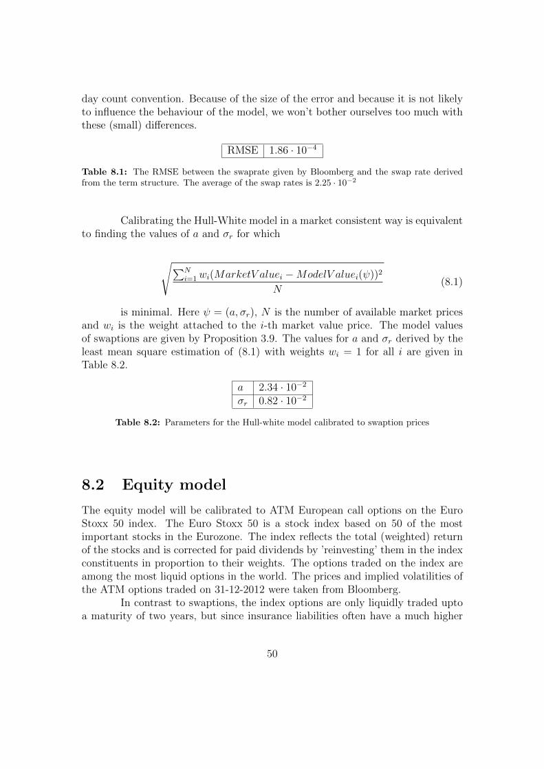
day count convention. Because of the size of the error and because it is not likelyto influence the behaviour of the model, we won’t bother ourselves too much withthese (small) differences.
RMSE 1.86 · 10−4
Table 8.1: The RMSE between the swaprate given by Bloomberg and the swap rate derivedfrom the term structure. The average of the swap rates is 2.25 · 10−2
Calibrating the Hull-White model in a market consistent way is equivalentto finding the values of a and σr for which
√∑Ni=1wi(MarketV aluei −ModelV aluei(ψ))2
N(8.1)
is minimal. Here ψ = (a, σr), N is the number of available market pricesand wi is the weight attached to the i-th market value price. The model valuesof swaptions are given by Proposition 3.9. The values for a and σr derived by theleast mean square estimation of (8.1) with weights wi = 1 for all i are given inTable 8.2.
a 2.34 · 10−2
σr 0.82 · 10−2
Table 8.2: Parameters for the Hull-white model calibrated to swaption prices
8.2 Equity model
The equity model will be calibrated to ATM European call options on the EuroStoxx 50 index. The Euro Stoxx 50 is a stock index based on 50 of the mostimportant stocks in the Eurozone. The index reflects the total (weighted) returnof the stocks and is corrected for paid dividends by ’reinvesting’ them in the indexconstituents in proportion to their weights. The options traded on the index areamong the most liquid options in the world. The prices and implied volatilities ofthe ATM options traded on 31-12-2012 were taken from Bloomberg.
In contrast to swaptions, the index options are only liquidly traded uptoa maturity of two years, but since insurance liabilities often have a much higher
50

maturity we would like to fit our model to maturities up to 50 years. If we wantto be able to do this, we must extrapolate the market data.
The extrapolation method we use here, is a (simplified) version of themethod proposed by the CRO Forum [11]. The CRO Forum is a group of profes-sional risk managers from the insurance industry that focuses on developing andpromoting industry best practices in risk management. The extrapolation methodis based on the market wide accepted assumption and observation that volatilityfollows a mean reverting process. In the model the forward implied volatility isdiscussed, which is related to the implied volatility in the same way as forwardrates are related to the zero-coupon interest rate structure. So we have
IV 2(T ) =1
T
∫ T
0
IV 2FWD(t)dt (8.2)
They propose that the forward volatility should converge to a long term forwardvolatility in the following way for t ≥ T :
IV 2FWD(t) = MarketIV 2
FWD(T )e−K(t−T ) + LongTermIV 2FWD(1− e−K(t−T )).
Here is T the time of the last liquid data point, MarketIV 2 the forward impliedvolatility derived form market quotes, LongTermIVFWD the long term impliedvolatility and K the mean reversion speed. The long term forward implied volatilitycan be derived using historical market data. In general, implied volatilities arehigher than historical volatilities which is supposed to be a consequence of the costof hedging/replicating an option. Furthermore there is a lot of uncertainty aboutwhat the long term implied volatility really is and this should also be accountedfor in the form of a surcharge on the historical long term implied volatility.
Because the determination of the long term implied volatility requires alot of data and expert knowledge, we will use the following simplification of themodel proposed above:
IV 2FWD(t) = IV 2
0 e−αt + IV 2
∞(1− e−αt).
Implementing this to (8.2) we get
IV 2model(t) = IV 2
∞ +1
αT(1− e−αT )(IV 2
0 − IV 2∞)
and we can obtain the values by, once again, minimising the rooted mean squareerror between the quoted market prices and the model prices.
RMSE =
√∑i(IVmodel(ti)− IVmarket(ti))2
N
51

Figure 8.3: The extrapolated option implied volatility curve and the implied volatilities quotedin the market as circles
N is the number of quoted market prices. See Figure 8.3 for a graphical comparisonbetween the extrapolated volatilities and the market volatilities.
The calibration can be done by minimizing the sum of squared errorsbetween market and model prices, see (8.1), where ψ = (σS, ρ). The marketprices are derived from the extrapolated implied volatility curve by using the termstructure we also used with the interest rate model together with the famousBlack-Scholes option pricing formula. The results can be seen in table (reference)
σS 0.24ρ −0.27
Table 8.3: Parameters for the Hull-white model calibrated to swaption prices
8.3 Real estate model
For the calibration of the real estate model the ROZ/IPD Property Index is used.The ROZ/IPD Property Index was established in 1997 and measures direct prop-erty returns in the Netherlands dating back to 1995. It is published annually.
As we discussed before, the index has to be unsmoothed before we canuse it for the calibration of our model. The unsmoothing method used, is that ofFisher et al. [17]. This model was chosen because of the complications with thedetermination of the factor α in the model of Geltner [18].
52

Quan and Quigley [39] [40] have shown that in the case of an annual indexan AR(1) model will adequately capture the individual appraisers behaviour. Inthe case of a quarterly index an AR(4) index would be te best choice, because someproperties are only appraised every half year or year in stead of every quarter.
Remember that we needed to assume that the volatility of the real returnswas half the volatility of stock returns. Because we chose to model our equity onthe Euro Stoxx 50 index, the volatility of stock returns has been derived fromhistorical data of the Euro Stoxx 50 index over the time period corresponding tothe time period over which we unsmooth the real estate index (1995-2012). Thevolatility over this period was 25, 99% annualized.
The result of the unsmoothing can bee seen in Figure 8.4 where we plottedboth the original data as the unsmoothed data.
Figure 8.4: Smoothed and unsmoothed real estate return (left) and real estate index (right).
As we can see the resulting volatility of the unsmoothed returns is signif-icantly higher than the unsmoothed returns and the resulting unsmoothed indexvalues are considerably lower at this point in time. A very desirable feature of theunsmoothed index is that is reflects the 2007-2008 financial crisis, the resultingcrash in stock markets and the following decline of real estate prices. Moreover,it also gives a good reflection of the current price level compared to the level be-fore the crisis. The Dutch Cental Bureau for Statistics (CBS) reports a decline of21, 3% in housing prices since te top of the housing bubble end 2007 [6]. This isfairly close to the 24% decline which can be derived from the unsmoothed index.
To calibrate our model we need the volatility of real estate σRE as wellas the correlations of real estate with interest rates ρr,RE and equity ρS,RE. Inequation (5.1) we defined the drift term for our real estate returns as the, at thattime, prevailing short rate. Therefore, to derive the volatility of real estate from
53

the unsmoothed index and to get correct correlations, we first have to correct theindex for the volatility of interest rates.
The correction is done as follows. First the index values are discountedby the historical interest rates; that is
ROZdisc(t) = ROZ(t)exp
(−∫ t
0
r(s)ds
),
for t = 0 at 31 december 1994 and t = 1, 2, .., 18. The historical interest ratesused for the discounting are those published by the Dutch Central Bank (DNB) attheir website. Secondly the (yearly) log-returns of the discounted index values aretaken. Finally, the volatility of real estate is taken to be the empirical volatility overthese log returns and the correlations are calculated by using the historical interestrates and the historical yearly log returns of the Eurostoxx50 index. The resultsare given in table (reference). (Eventueel plot Stoxx50 en smoothed/unsmoothedvergelijken nog)
σRE 0.13ρr,RE −0.09ρs,RE 0.38
Table 8.4: Parameters for the real estate model derived from historical data.
8.4 Inflation model
The calibration of the inflation model is based on the eurozone inflation rates from1991 to 2012 published by Eurostat.
As was already mentioned in the previous chapter, the mean and varianceof the Vasicek model are used to calibrate the model. If the sample time of datain the data set is δ then from (6.1) and (6.2) we can write the dynamics of theinflation as
Ii+1 = Iie−λδ + µ
(1− e−λδ
)+ σI
√1− e−2λδ
2λZ,
where Z ∼ N(0, 1). Thus the relation between consecutive observations Ii, Ii+1 islinear with an iid normal random term ε:
Ii+1 = aIi + b+ ε.
54
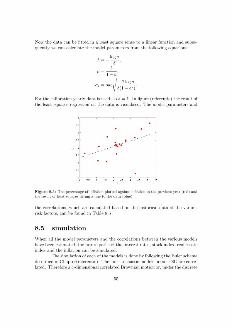
Now the data can be fitted in a least square sense to a linear function and subse-quently we can calculate the model parameters from the following equations:
λ = − log a
δ,
µ =b
1− a,
σI = sdε
√−2 log a
δ(1− a2).
For the calibration yearly data is used, so δ = 1. In figure (referentie) the result ofthe least squares regression on the data is visualised. The model parameters and
Figure 8.5: The percentage of inflation plotted against inflation in the previous year (red) andthe result of least squares fitting a line to the data (blue)
the correlations, which are calculated based on the historical data of the variousrisk factors, can be found in Table 8.5
8.5 simulation
When all the model parameters and the correlations between the various modelshave been estimated, the future paths of the interest rates, stock index, real estateindex and the inflation can be simulated.
The simulation of each of the models is done by following the Euler schemedescribed in Chapter(referentie). The four stochastic models in our ESG are corre-lated. Therefore a 4-dimensional correlated Brownian motion or, under the discrete
55

λ 0.9812µ 2.1342σI 1.08ρr,I 0.30ρs,I −0.76ρRE,I −0.34
Table 8.5: Parameters for the real estate model derived from historical data.
time Euler scheme, realisations of a 4-dimensional multivariate normal distributionhave to be generated.
Suppose now Σ is the correlation matrix that is the outcome of the cali-bration, then we want to generate values from a N(0,Σ) distribution. The way todo this has already been mentioned in Chapter 4, but will also be repeated here.First a 4-dimensional vector Z = (Z1, ..., Z4) of independent standard normal ran-dom variables is simulated. Secondly, we apply the Choleski decomposition to Σto get a lower triangle matrix L for which it holds that Σ = LL>. The last andfinal step is then to multiply L and Z, since then LZ ∼ N(0,Σ).
While the Choleski decomposition of a correlation matrix into a lowertriangle matrix is unique, there are multiple ways to decompose the correlationmatrix into Σ = LL>; any of these decompositions would also lead to LZ ∼N(0,Σ).
When the timestep ti+1−ti for the Euler method has been set, e.g. a month,a year etc., and the number of scenarios to be generated has been determined, wecan let the ESG produce scenarios. In Figure 8.6, 8.7, 8.8 and 8.9 an example ofgenerated scenarios together with their average is shown.
56

Figure 8.6: Generated interest rate scenarios (left) and the mean of the scenarios (right) basedon market data at 31-12-2012
Figure 8.7: Generated scenarios of the Eurostoxx50 index (left) and the mean of the scenarios(right) based on market data at 31-12-2012
Figure 8.8: Generated scenarios of the ROZ/IPD real estate index (left) and the mean of thescenarios (right) based on market data at 31-12-2012
57

Figure 8.9: Generated scenarios of the inflation rate in the eurozone (left) and the mean of thescenarios (right) based on market data at 31-12-2012
58

Chapter 9
Insurance Products
The whole purpose of the construction of an ESG, calibrating it to market dataand the generation of future scenarios is to calculate the technical provisions forinsurance contracts. Therefore, two types of life insurance products are modelledin this thesis and will be used to study some of the properties of our ESG. In thischapter we will discuss these two products and the way they are modelled.
The two life insurance products that will be modelled are a surplus inter-est sharing policy and an endowment policy. For both policies the maturity of thecontract is defined as the time to retirement of the policyholder, which for conve-nience is set at 67 for all policy holders. The distribution of the number of policiesas a function of the age at the inception of the contract is given in Figure 9.1. Thisis a (simplified version of a) distribution as it could be found in the real world foran insurance policy.
Figure 9.1: Number of policies as a function of the age of the policy holder at inception.
At inception, the policyholders of both products are guaranteed a minimalamount of money at maturity. We model the products as single-premium assurancepolicies; this means that no premiums are paid during the term of the policy. Also,
59

it is simpicitly assumed that all costs the policy holder has to pay to the insurerfor their services are deducted from the single-premium. Because someone whois older usually has more savings and therefore can invest more, the guaranteedamount of cash also depends on the age of the policy holder at the start of thecontract. The guaranteed amounts are plotted in Figure 9.2.
Figure 9.2: Guaranteed amount of money at inception as a function of age.
Mortality rates are also modelled, since these also have an impact on whencertain cash flows take place. Often with these products a life insurance policy issold. This ensures that in the event of the demise of the policy holder before thematurity date the guaranteed sum is paid to the heirs. In the model it is assumedthat every policy is sold with a life insurance policy. In practice, the chance ofpassing is modelled as a function of age, the year of birth, gender and other factorslike yearly income. For convenience, mortality is modelled only as a function ofage. The yearly mortality rates in the model can be seen in Figure 9.3; thesemortality rates are in line with empirical results [1].
Figure 9.3: Yearly mortality rates based on empirical results.
To calculate the technical provisions the future cash flows have to bediscounted. Echoing the opinion of the european commission and in anticipation
60

of the introduction of SolvencyII, the Dutch Central Bank (DNB) imposed the useof the so called Ultimate Forward Rate curve (UFR curve) from 30 June 2012 forthe discounting of cash flows of insurers [13]. For terms below 20 years, the UFRcurve is derived from the european swaprates and therefore for these terms equalto the curve we used when calibrating the interest rate model. For terms longerthan twenty years, the forward rate is extrapolated from the twenty years forwardrate to the Ultimate Forward Rate, which is set at 4.2%. The 4.2% is based onhistorical data for inflation (2%) and real interest rates (2.2%). The convergencetime is 40 years, so the 60 years forward rate is 4.2%.
There are two main reason for the introduction of the UFR. The first oneis that bond markets are not liquid for terms higher than 20 years and thereforemarket prices are not reliable. The second reason for introducing the UFR is tomake insurers with long term obligations, e.g. the obligations corresponding tothe insurance products that we use here, be less influenced by short term changesin interest rates. One of the arguments why this is a better method compared tousing the market rates is that beyond twenty years the liquidity of swaps drops andtherefore aren’t trustworthy. Of course the risk is that the current low interest ratesdon’t rise in the long run, which would mean that the current technical provisionsare too low with respect to the future liabilities [41]. The UFR curve is publishedevery month by DNB. The curve at 31-12-2012 is given in Figure 9.4.
Figure 9.4: The Ultimate Forward Rate curve published by DNB for 31-12-2012.
Surplus interest sharing policy
For the surplus interest sharing policy the amount of money paid at maturitydepends on the yearly return on a portfolio of government bonds with respect toa fixed discount rate.
61

In the Netherlands the portfolio of Dutch government bonds is standarisedby the Association of Insurers. The portfolio consists of bonds with a term between2 and 15 years. The return on the portfolio is called ’U-rendement’ and is reportedevery month by the Centre for Insurance Statistics (CVS).
In the model the yearly returns are calculated in the same way as is donein practice. However, it should be noted that we make the assumption here thatthe risk-free return in our model is the same as the return on Dutch governmentbonds.
The returns on the bond portfolio are compared every year with a fixeddiscount rate, which in our model is three percent. If the return is higher than thefixed rate the guaranteed sum will be increased with half of the surplus return.This means that if the return on the portfolio at the end of a year is 4% then theguaranteed sum will be increased with 0.5%. Only a part of the surplus return isgiven to the policy holder to protect the insurer against returns below the fixedrate in future years.
An important feature of this policy is that if the returns fall below thefixed discount rate, the guaranteed sum won’t be increased, but more importantlyit won’t be lowered either.
Also, because the return is based on a standarised portfolio which is mon-itored by the CVS, the return is not necessarily connected to the actual returnsthe insurance company is making.
Endowment policy
The endowment policy gives the policy holders a choice between different assetmixes to invest in. At the end of the term the insurer pays the policy holder thevalue of the investment at that time or the guaranteed sum if the value of theinvestments has fallen below the guarantee.
There are three types of portfolios the policy holder can invest in: a ’fixedincome’ portfolio, with only bonds with a remaining term between 2 and 15 years,a mixed portfolio, with 60% bonds, 25% stock and 15% invested in real estateand a ’risky’ portfolio, which for 70% consists of stocks and 30% of real estateinvestments. At the end of every year the different portfolios are rebalanced tomatch their initial weights. For example, the risky portfolio might consist of 80%stocks and 20% real estate at the end of a year due to price movements in the lastyear, then stocks have to be sold and real estate has to be bought in order to get70% stocks and 30% real estate in the portfolio at the start of next year.
Also, at the end of every year the guaranteed amount will be increasedwith the inflation percentage over that year. This way the purchasing power ofthe policy holder at maturity remains in tact.
62

Chapter 10
Analysis of the technicalprovisions
In this chapter we will have a look at the technical provisions (TP) corresponding tothe modelled insurance products and in what way they are influenced by changingunderlying conditions. First we will look at in what way the conditions of thepolicies influence the TP, then we will look at changes in the market conditions,thirdly estimation errors will be discussed and last but not least we will look atchanges that can be made to the calibration procedure.
10.1 Policy conditions
Now some insights will be given into what kind of impact some aspects of theinsurance policies have on the technical provisions. The calculations are done withscenarios generated based on the market data at 31-12-2012. The technical provi-sions for the situation described above, which will be referred to as the ’standardsituation’ from now on, can be found in Table 10.1
Standard situationSurplus interest 199.3Endowment: fixed 15.3Endowment: mixed 36.4Endowment: risky 90.5
Table 10.1: Technical provisions in millions of euros for the standard situation.
What might be notable is that the TP of the surplus interest sharingpolicy are much higher than that of the endowment policies. This is because for
63

the endowment policy the underlying portfolio is modelled and therefore the cashflows are only due to differences of the guaranteed with the guarantee, while nounderlying portfolio is modelled for the interest sharing policy.
distribution of the cash flows
When we look at the TP of the endowment policies there is also a big differencebetween the TP of the fixed income portfolio and the riskier portfolios. Thepolicy holder gets all the extra funds when the value of the portfolio is abovethe guarantee, but the insurance company has to make up the whole differenceif the value is below the guarantee. Because equity and real estate are morevolatile than bonds, the probability of a low value of the portfolio is bigger for the’mixed’ and ’risky’ portfolio than for the ’fixed income’ portfolio. Therefore, thetechnical provisions corresponding to the mixed and risky portfolio are higher. InFigure 10.1, this is illustrated with a histogram, for the risky and the fixed incomeportfolio, of the discounted value of the cash flows resulting from the differentscenarios.
Figure 10.1: Current value of the cash flows resulting from the different scenarios; for the fixedincome portfolio (blue) and the risky portfolio (red)
64

mortality rates
An aspect which gives us a good opportunity to look at some of the properties of themodel and the insurance policies is the mortality rate. The technical provisions arecalculated for two different situations. In the first situation the mortality rates areset to zero, so no one dies before the age of 67. This is not a realistic assumption,but it gives us some insight in what impact mortality has on the technical provisionsof a life insurance company. In the second situation the products are modelledwithout the life insurance policy. In the case of the surplus interest sharing policythe absence of a life insurance policy means that no money will be paid upon death,while in the case of the endowment policy it means that there is no guaranteedsum; the value of the investment at the time of death will be paid, no matterwhether it is below or above the current guaranteed sum. The technical provisionsare given in Table 10.2.
No mort. diff. No life ins. diff.Surplus interest 194.9 −2.19% 170.6 −14.37%Endowment: fixed 15.0 −2.09% 13.1 −14.29%Endowment: mixed 36.8 1.08% 31.9 −12.43%Endowment: risky 92.6 2.29% 79.9 −11.75%
Table 10.2: Technical provisions in millions and the percentage difference w.r.t. the standardsituation for when the mortality rates are set to zero and when policy holders have no extra lifeinsurance policy.
The difference between the standard situation and the situation withouta life insurance policy is the most easily explained. For the no life insurance case,when someone dies, the insurance company has to pay nothing to the heirs of asurplus interest rate policy and only has to pay the current value of the investmentsin the case of the endowment policy, which results in a net cash flow of zero. In thestandard case the insurer has to pay (at least) the guaranteed amount to the heirsand therefore it is obvious that the technical provisions in that case are higher.
The impact of zero mortality rates on the technical provisions is morecomplex and we need to discuss the policies separately. The lower technical provi-sions for the surplus interest rate policy are due to the discounting of cash flows. Ifa policy holder lives at least until the age of 67, the guaranteed sum has to be paidlater than when someone dies before this age. Because the cash flows have to bediscounted, the same cash flow at a later point in time gives a lower current valueof that cash flow. Of course, because of surplus interest sharing, the guaranteedamount could have gone up between the moment of death and when the policyholder would have reached the age of 67, but the surplus interest is most of the
65

time lower than the yearly discount rates and therefore doesn’t raise the currentvalue. A visual representation of the difference between the yearly discount ratesand the surplus interest can be found in Figure 10.2.
For the ’fixed income’ portfolio sort of the same thing holds as for thesurplus interest sharing policy. Remember that the guarantee is increased withthe inflation rate every year. Since on average the return made on the portfolioof bonds minus the inflation is lower than the yearly discount rate, the currentvalue of a cash flow resulting from someone passing away before the age of 67 ishigher than the current cash flow resulting from someone reaching the age of 67.Figure 10.2 also gives a visual representation of the difference between the yearlydiscount rates and the average return minus the inflation.
Figure 10.2: Yearly discount rates derived from the UFR curve (blue) compared with theaverage surplus interest (green) and the average return on a bond reduced with the inflation rate(red).
Now the question is why the technical provisions go up for the riskierportfolios, since one could argue that because of the risk neutral way in whichwe modelled equity and real estate the value of those asset classes, on average,grows at the rate of the modelled interest rates and therefore the same argumentas before should hold. However, the mean growth rate is not the prevailing factorin this case. The coverage ratio is the value of the portfolio divided by the totalvalue of the remaining guarantees. As we saw in Figure 10.1, the variance of thecoverage ratio is much larger for the risky portfolios than for the bond portfolio.In Figure 10.3 we can see that, while the mean of the coverage ratio goes up,the variance grows larger in time and the median drops. This implies that theprobability of a low coverage ratio is larger further into the future and in turn
66

this leads to a higher expectation of the value of a future cash flow. Therefore thetechnical provisions are higher when the mortality rates are set to zero.
Figure 10.3: Then mean of the coverage ratio for the risky portfolio (red), the median (blue)and the 16th and 84th percentile given by the error bars.
Coverage ratio
What might also be interesting is to investigate how sensitive the technical provi-sions are to changes in the coverage ratio of the endowment policies by changingthe coverage ratio at the start of the simulation. In the standard case we implicitlyassumed the that the coverage ratio was 100%.
It would be even more interesting if we knew the probabilities with whichthe coverage ratio could go up or down in the coming year, because then we wouldbe able to give a confidence interval for the TP. However, we need to remind our-selves that we are dealing with risk-neutral scenarios and not real world scenarios.Therefore, the construction of a confidence interval is not possible.
In Table 10.3 the TP are given for different coverage ratios at the startof the simulation and in Table 10.4 the percentage difference compared to thestandard situation are given.
As could be expected, the relative changes of technical provisions in Ta-ble 10.4 are the largest for the fixed income portfolio. This is because bonds areless volatile than stocks and real estate and hence the chances of the coverage ratiogetting back to 100% are smaller.
It is also worthwhile to look at the shape of the curve of the technicalprovisions plotted against the coverage ratio. For the fixed income portfolio thecurve is given in Figure 10.4. The shape of the curve is similar to that of the price
67
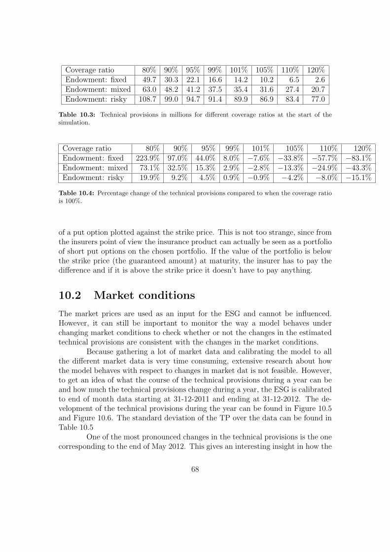
Coverage ratio 80% 90% 95% 99% 101% 105% 110% 120%Endowment: fixed 49.7 30.3 22.1 16.6 14.2 10.2 6.5 2.6Endowment: mixed 63.0 48.2 41.2 37.5 35.4 31.6 27.4 20.7Endowment: risky 108.7 99.0 94.7 91.4 89.9 86.9 83.4 77.0
Table 10.3: Technical provisions in millions for different coverage ratios at the start of thesimulation.
Coverage ratio 80% 90% 95% 99% 101% 105% 110% 120%Endowment: fixed 223.9% 97.0% 44.0% 8.0% −7.6% −33.8% −57.7% −83.1%Endowment: mixed 73.1% 32.5% 15.3% 2.9% −2.8% −13.3% −24.9% −43.3%Endowment: risky 19.9% 9.2% 4.5% 0.9% −0.9% −4.2% −8.0% −15.1%
Table 10.4: Percentage change of the technical provisions compared to when the coverage ratiois 100%.
of a put option plotted against the strike price. This is not too strange, since fromthe insurers point of view the insurance product can actually be seen as a portfolioof short put options on the chosen portfolio. If the value of the portfolio is belowthe strike price (the guaranteed amount) at maturity, the insurer has to pay thedifference and if it is above the strike price it doesn’t have to pay anything.
10.2 Market conditions
The market prices are used as an input for the ESG and cannot be influenced.However, it can still be important to monitor the way a model behaves underchanging market conditions to check whether or not the changes in the estimatedtechnical provisions are consistent with the changes in the market conditions.
Because gathering a lot of market data and calibrating the model to allthe different market data is very time consuming, extensive research about howthe model behaves with respect to changes in market dat is not feasible. However,to get an idea of what the course of the technical provisions during a year can beand how much the technical provisions change during a year, the ESG is calibratedto end of month data starting at 31-12-2011 and ending at 31-12-2012. The de-velopment of the technical provisions during the year can be found in Figure 10.5and Figure 10.6. The standard deviation of the TP over the data can be found inTable 10.5
One of the most pronounced changes in the technical provisions is the onecorresponding to the end of May 2012. This gives an interesting insight in how the
68

Figure 10.4: The technical provisions for the fixed income portfolio plotted against the coverageratio.
Standard deviation Absolute PercentageSurplus interest 2.12 1.05%Endowment: fixed 3.29 26.79%Endowment: mixed 3.75 11.57%Endowment: risky 4.74 5.34%
Table 10.5: Standard deviation (absolute value in millions and as a percentage of the mean) ofthe end of month data of the technical provisions ranging from 31-12-2011 to 31-12-2012.
TP can be influenced by turmoil in the financial market. In may 2012 elections ofthe parliament of Greece were held, but Greece failed to form a government andnew elections were scheduled for June. Because of the bad financial situation ofGreece, this caused turmoil on the financial markets during May.
From the standard deviations we can see that the technical provisions canbe quite volatile. Therefore it is important that an insurance company tries tohedge their risks and where this is not entirely possible holds an additional capitalto ensure it is able to meet it’s obligations.
10.3 Estimation error
As we discussed in Chapter 7 the Monte Carlo simulation of the stochastic modelsproduces a statistical or distributional error and a discretisation error. In this
69

Figure 10.5: The technical provisions of the endowment policies calculated based on end ofmonth data ranging from 31-12-2011 to 31-12-2012; fixed income (blue), mixed (green), risky(red).
section we will look at the influence of the number of scenarios that is generated,which corresponds to the statistical error, and the influence of size of the timesteps in the generated scenarios, which corresponds to the discretisation error.
Number of scenarios
To get good results it is important that the distributional error is minimized.Because of the central limit theorem we know that the more simulations are done,the smaller this error will become. However, doing more simulation comes at theprice of computation time. Therefore, we need to find a balance between thenumber of scenarios and the distributional error.
The number of scenarios that were generated for the calculation of theTP ranged from 10 to 15000. For each number of scenarios the ESG was run100 times, which means that 100 estimates of the TP were generated for each preset number of scenarios. In Table 10.6 the standard deviations of the estimatedtechnical provisions are given for each category and in Figure 10.7 the technicalprovisions for the mixed portfolio in the endowment policy are given as a functionof the generated scenarios for a set of 10000 scenarios.
A criterium was set for choosing an optimal number of generated scenarios,i.e. the number of scenarios for which the distributional error is small enough,while keeping the computation time as low as possible. The criterium used wasthat the standard deviation of the estimated technical provisions has to be less
70

Figure 10.6: The technical provisions of the surplus interest sharing policy calculated basedon end of month data ranging from 31-12-2011 to 31-12-2012.
than 1% of the mean of the estimated technical provisions. As it turns out thiscriterium is only met for all products when 10000 or 15000 scenarios are generatedand therefore to limit the computation time the standard number of scenarios togenerate was set at 10000. The percentages for 5000, 10000 and 15000 are givenin Table 10.7.
Let us take a brief look at what this really means to set this criterium at1%. In Table 10.1 the given estimate of the technical provisions for the endowmentpolicy with the risky portfolio was 90.5 million euro. This means that followingour criterium when doing simulations one standard deviation still corresponds toalmost one million euro. Therefore, it is very important for insurance companiesto limit the distributional error that is the result of Monte Carlo simulation, sinceerrors that are relatively small can lead to big absolute errors in terms of money.
Nr. of scenarios 10 100 500 1000 2000 5000 10000 15000Surplus interest 5.99 1.65 0.82 0.50 0.41 0.19 0.15 0.13Endowment: fixed 3.26 8.87 0.49 0.29 0.20 0.17 0.10 0.07Endowment: mixed 12.52 3.93 1.73 1.10 0.76 0.60 0.37 0.23Endowment: risky 23.27 7.02 3.26 2.19 1.48 1.06 0.66 0.49
Table 10.6: Standard deviation (in millions) of the technical provisions for different numbersof generated scenarios.
71

Figure 10.7: Technical provisions for the mixed portfolio of the endowment policy calculatedby each time adding one scenario
Nr. of scenarios 5000 10000 15000Surplus interest 0.09% 0.07% 0.07%Endowment: fixed 1.10% 0.68% 0.45%Endowment: mixed 1.64% 0.99% 0.65%Endowment: risky 1.17% 0.73% 0.54%
Table 10.7: Standard deviation of the estimated TP as a percentage of the mean of the estimatedTP.
The number of steps
As we saw in Chapter 7 in addition to the distributional error there is also adiscretisation error which is the result of approximating our continuous stochas-tic process with a discrete stochastic process by means of the Euler-Maruyamamethod. If we choose to do our simulation with smaller time steps, this comes atthe cost of computation time.
Simulations were done with time steps of 1 year, 6 months, 3 months, 2months and 1 month; the resulting technical provisions are given in Table 10.8.Afterwards the differences of the consecutive refinements were taken.
All the differences fall within two times the standard deviations given inTable 10.6 for 10000 scenarios, the majority within one standard deviation andno clear trend is visible in the refinement steps. Therefore, it is very hard todistinguish the discretisation error from the distributional error. The choice hasbeen made to simulate the scenarios with a time interval of 6 months.
72

Size of the steps 1 year 6 months 3 months 2 months 1 monthSurplus interest 199.4 199.4 199.5 199.3 199.1Endowment: fixed 15.2 15.3 15.4 15.4 15.4Endowment: mixed 35.5 35.6 36.3 36.0 36.4Endowment: risky 90.8 89.9 90.3 89.9 90.0
Table 10.8: Technical provisions corresponding to different time steps taken during the simu-lation
10.4 Changes in the calibration
Until now we discussed some properties of the calculation of the technical provi-sions that were either due to the Monte Carlo simulation method we use or dueto the characteristics of the insurance products. However, another very importantway to look at the model is by looking at it from a more actuarial point of view.This means that we look at the freedom someone has in using this model and inwhich ways the choices resulting from this freedom can influence the outcomes ofthe model, e.g. an insurance company could make choices that lower the technicalprovisions.
What cannot be influenced are the cash flows that are related to theinsurance products, because those are contractual. Nor can the market data bechanged. One could choose to calibrate your model to different instruments, e.g.calibrate the interest rates to caps, but regulating authorities like DNB requireinsurance companies to calibrate their models in a consistent way over time forthe calculation of the TP, so changing instruments whenever it is convenient isn’tpossible.
As a result, the only freedom in the use of the ESG can be found inthe calibration of the model. Therefore, we have to look for (sometimes implicit)assumptions we made when calibrating the models. We will have a closer look atchoices made in the calibration of the interest rate model and the equity model.
Equity model
The most obvious assumption in the calibration of the ESG was made in theequity model. Because options are only deep liquidly traded for relatively shortmaturities, we had to extrapolate the implied volatility curve. We chose to fit acurve to the market data and one of the output variables was the long term forwardimplied volatility. However, in the extrapolation method which is proposed by theCRO Forum[11] the long term forward implied volatility is an input variable, whichis mainly based on the historical volatility of the stock index. In the paper of the
73

CRO Forum the long term volatility of the Eurosoxx50 index, based on data upto 2008, is given as 23.06%. From our own data, which we got from Bloombergand which goes up to 2012, a volatility of 25.99% is derived. These two numbersare used as a reference in the investigation of the impact of calibrating the modelto different long term volatilities. It might be interesting to note that the longterm volatility that is a result of our ’standard’ calibration is 25.52%, which isnot a bad result if we look at the two other percentages. The model has beencalibrated for long term volatilities ranging from 20% to 28% with steps of 2%.The TP and the σS parameter of the equity model can be found in Table 10.9; thepercentage difference of the TP compared to the standard situation can be foundin Table 10.10. We only calculated the TP for the mixed and risky portfolios sinceequity has no influence on the other products.
Long term vol. 20% 22% 24% 26% 28%Endowment: mixed 31.6 33.2 35.1 36.7 38.1Endowment: risky 77.6 81.9 87.7 92.3 96.7σS 0228 0.237 0.246 0.255 0.264
Table 10.9: Technical provisions as a result of different long term implied volatilities and theσS parameter for equity.
Long term vol. 20% 22% 24% 26% 28%Endowment: mixed −13.20% −8.93% −3.60% 0.89% 4.73%Endowment: risky −14.33% −9.51% −3.12% 1.96% 6.75%
Table 10.10: Percentage change of the TP compared to the standard situation, where te longterm volatility is 25.52%.
As we can see the choice of a long term forward implied volatility canhave a significant impact on the outcome of the technical provisions. The changeof 25.52% to 26% already leads to a change of almost two percent in the technicalprovisions, which is more than 1.5 million in absolute value.
Interest rate model
In the calibration of the interest rate model to the swaption volatility surface, orequivalent, to the prices of swaption we made an assumption regarding the leastsquare fitting. In equation (8.1) we can choose weights wi for the each of themarket prices and we chose to set the weights equal to one and didn’t wonder ifthis was the right or best descision.
74

However, for the different maturities and different tenors we could arguethat setting all the weights to one is not the only feasible choice. There area lot quoted prices with a short maturity and tenor and only few prices withlonger maturities and tenors as can be seen in Figure 10.8. Therfore, the standardcalibration, which gives weight one to each quoted price, assigns more weight toshort terms (0-5 years) and in comparison less weight to medium terms (5-15 years)and to long terms (15+ years). The modelled insurance policies have the majorityof their obligations at medium and long terms, so assigning different weights seemsjustifiable.
Figure 10.8: Swaption volatility matrix for 31-12-2012 from Bloomberg.
A different method to deal with this problem would be to interpolate thevolatility surface and calculate the prices at equidistant points. However, to avoidfurther complications with choosing the right extrapolation method, we will adjustthe weights.
Before we propose how we can asess the weights for all the quoted prices,let us look at an example, where we compare two quotes: a 2 year tenor and 5year maturity swaption and a 25 year tenor and 20 year maturity swaption. Thedistance to the next tenor and the last tenor for the first price is 1 year, whenkeeping the maturity at 5 years and the same holds for the distance to the nextand last maturity when keeping the tenor at 2 years. For the second quoted pricethe distance to the next tenor and the last tenor is 5 year, when you keep thematurity at 20 years and the same holds for the distance to the next and lastmaturity when keeping the tenor at 25 years. To keep the weight wi proportionalto the distance to the neighbouring points we can set a weight of 1× 1 = 1 for thefirst point and 5× 5 = 25 for the second point
Let i1, ..., in be the different maturities and let j1, ..., jm be the different
75

tenors and let us change the notation of the weights to wik,jl . Then, in agreementwith the example, we can give a formula for the weights as follows for inner points:
wik,jl =ik+1 − ik−1
2× jl+1 − jl−1
2for 1 < k < n, 1 < l < m. (10.1)
For the different border and corner cases the formula is adjustment in similar ways,therefore we only give one case:
wik,jl =ik+1 − ik
2× jl+1 − jl−1
2for k = 1, 1 < l < m. (10.2)
To give some insight into the way the technical provisions change by chang-ing the weights according to (10.1) (10.2) it was decided to do the optimisationwith wki,j for k = 0, 0.25, 0.5, 0.75, 1. Note that k = 0 corresponds to the originalsituation. The results are given in Table 10.11
Size of the steps 0 0.25 0.5 0.75 1Surplus interest 199.3 200.5 200.4 200.4 200.5Endowment: fixed 15.3 15.7 15.7 15.8 15.5Endowment: mixed 36.4 36.0 36.1 36.5 35.5Endowment: risky 90.5 89.9 90.4 90.9 89.4Parameter: a 0.0420 0.0422 0.0424 0.0424 0.0425Parameter: σr 0.0103 0.0106 0.0107 0.0107 0.0107
Table 10.11: Technical provisions and the parameters a and σr corresponding to differentweights in the calibration of the interest rate model.
The most striking is that the parameters of the interest rate model donot change much under the change of the weights. This is also reflected in thetechnical provisions, since the changes in TP fall within the two times the standarddeviation of the distributional error we saw in Table 10.6. Moreover, there is noclear trend visible in the technical provisions.
76

Chapter 11
Summary, Conclusions andDiscussion
In this thesis we have constructed an Economic Scenario Generator (ESG) with thepurpose to calculate technical provisions (TP) of insurance contracts in a marketconsistent way. The reason for constucting an ESG was that other methods forthe calculation of TP, e.g. using a replicating portfolio or a closed form solution,were too complex to implement because of the path dependency of the contactsand the multiple underlying risk factors.
The choice was made to model interest rates, equity, real estate and in-flation rates. The interest rates were modelled with the Hull-White one factormodel, equity and real estate were modelled with the Hull-White-Black-Scholesmodel and the inflation rates were modelled by the Vasicek model.
To get a market consistent ESG the models had to be calibrated to marketprices, i.e. the market prices have to match the model prices as good as possible.Therefore, in (referentie chapters/secties interest rate and equity) we derived ex-plicit formulas for swaptions and European options for the interest rate resp. equitymodel. Because no options or other liquidly traded derivatives were available forreal estate and inflation rates in (referentie chapters/secties real estate en inflatie)we looked at methods to calibrate these models to historical data.
Subsequently in Chapter 8 we gave an example calibration of the modelsto market data at 31-12-2012. This was done by least square fitting the modelprices to the market prices of at-the-money euro swaptions and European optionson the Eurostoxx50 index. Here we first had to extrapolate the implied volatilitiesof the European options because only quotes of liquidly traded options with a shortmaturity were available. The real estate model was calibrated to the ROZ-IPDindex and the inflation to the historical eurozone inflation. Afterwards scenarioswere generated based on these calibrations.
Two types of insurance products were modelled: a surplus interest shar-
77

ing policy and an endowment policy for which one could choose between threedifferent portfolios to invest in. These products were described in Chapter 9 andin Chapter 10 they were used to study some properties of the ESG in relation tothe calculation of technical provisions for the policies. We looked at the impactof changes in the conditions of the policies, changes in market conditions, errorsin the estimation of the TP and ways in which the calibration procedure can bechanged and how that influences the technical provisions.
The most striking sensitivities in the model were the distributional errorthat is the result of Monte Carlo simulation and the choice of a long term impliedvolatility for the calibration of the equity model.
For the distributional error we saw that we needed at least 10000 scenariosin order to get the standard deviation of the estimated TP below 1% of the meanof the estimates. In practice this can still result in a large absolute error, since1% of the TP can already correspond to millions of euros. The ESG of Barrie &Hibbert, which is one of the best and most used scenario generators in the world[15], can only generate up to 5000 scenarios. Their ESG uses different modelsthan ours, e.g. the Displaced Diffusion Stochastic Volatility Libor Market Modeland the Stochastic Volatility Jump Diffusion model, so we can’t really derive theerror from the number of scenarios. Still, when using an ESG in practice, thedistributional error is a very important factor to keep track of.
In the case of the extrapolation of the equity implied volatility, we sawfrom the paper of the CRO Forum [11] that the determination of the long termforward implied volatility relies a lot on expert knowledge. As a consequence,the determination of the long term volatility heavily depends on what data andargumentation one uses to determine it. Moreover, we saw that a change of only0.5% of the long term volatilities can already lead to a 2% change in the technicalprovisions.
11.1 Improvement of the ESG
The ESG could be improved in several ways. It is possible to include models forother risk factors like credit spreads and exchange rates. Also, for each of thestochastic models we used, there are more advanced models that capture the mar-ket behaviour better than the models used here. We did not use these models,because the chosen models already capture market behaviour adequately and be-cause those models are too complex to discuss thoroughly in this thesis, hard toprogram correctly and/or would take too much time to calibrate and simulate dueto extra parameters and stochastic factors in these models.
One must always keep in mind what the purpose of the model is andthink about the level of complexity that is needed. If an insurance company
78

has various interest rate derivatives in its portfolio, but no equity derivatives,it might be necessary to improve the interest rate model, while improving theequity model won’t be very useful. Implementing a more complex model alsoincreases the computation time of both the calibration, because there are moreparameters, and the simulation, due to more risk factors in the model. Moreover,an important requirement of Solvency II is that the models and methods shouldbe well understood by senior management. Therefore, simplicity, transparencyand robustness of the ESG are desirable features and one must always ask oneselfif the benefit of implementing a more advanced model outweighs the increasedcomplexity resulting from those models.
Interest rate model
In our ESG we chose to use the Hull-White one factor model for the interestrates. The advantages for this model were that we could fit the model exactly tothe current term structure, we could derive analytical formulas for interest ratederivatives, like swaptions, which makes it easier to calibrate the model accuratelyto market data and it is fairly easy to use the equity model under Hull-Whiteinterest rates.
The model has some limitations. The model can produce negative interestrates. In practice however this doesn’t lead to any issues in the valuation, amongothers because the probability of this happening is small because of the meanreversion; see Pelsser [38] and Brigo and Mercurio [5]. Also, the model is a onefactor model and therefore, the interest rates are perfectly correlated, i.e. themodel can only produce parallel changes in the interest rates. The last importantlimitation is the constant volatility, because of which we cannot get an exact fit tothe complete volatility surface.
To deal with the perfect correlation of the interest rates, we could addextra stochastic factors, driven by an extra Brownian motion, to the model. Whileone factor explains 68% to 75% of the changes, two factors, which allows for shiftsin the level and slope of the yield curve, can already account for 85% to 90% ofthe changes according to Jamshidian and Zhu [29]. Therefore, an improvementwould be to extend the model to the Hull-White two factor model, which is alsoknown as the G2++ model. The advantages of this model are that it is stillanalytically tractable and it is still easy to use the equity model simultaneouslywith this model.
We could also add time-dependent or stochastic volatilities to the model.However, implementing stochastic volatilities can be very complex and the modelwould lose its easy tractability. Implementing time-dependent volatilities can giveadditional problems with getting an exact fit with the term structure of interestrates and also the use of the equity model [5].
79

The most advanced model for interest rates currently available is the Dis-placed Diffusion Stochastic Volatility Libor Market Model (DDSV-LMM). Themodel allows for an exact fit to the swaption implied volatility surface and is ca-pable of capturing the risk of changing implied volatilities, due to the stochasticvolatilities. One of the disadvantages is that it is not analytically tractable.
Equity
We used the Black-Scholes model with stochastic interest rates for our equity,which can also be referred to as the Hull-White-Black-Scholes model in our case.The advantages were that it is easy to use simultaneously with the Hull-Whitemodel and it is analytically tractable, which makes calibration to options easy.
There are some limitations with the model. The lognormal distributionof the stock doesn’t behave appropriate in extreme market conditions, since theheavy-tailed returns that can be seen in practice can’t be incorporated in thismodel. The model is also incapable to give an exact fit to the at-the-moneyimplied volatilities, because it has a constant volatility factor. Finally, we can’tcalibrate the model to different strikes because it is a one factor model.
The model could be improved by allowing for time dependent volatility.If the volatility parameter is defined as a piecewise constant function, then theadjusted model can be made to exactly fit the observed at-the-money impliedvolatilities. Again, as it turns out, it is not too hard to adapt the option pricingformulas to piecewise constant volatilities, thus retaining the analytical tractabil-ity. This can for example be seen in the model documentation of ING insurance[26], where they use the Hull-White two factor model and the equity model withpiecewise constant volatility in their ESG.
The most advanced model currently Stochastic Volatility Jump Diffusionmodel, which is basically a combination of Heston’s Stochastic Volatility model[23]and the Merton’s Jump Diffusion model [36]. Due to the stochastic volatility, themodel is capable of capturing the overall shape of the implied volatility surface.The merton model allows for rare events, jumps, in the equity value and is thereforeable to capture the skewness of stock returns better than other models.
Other models
We modelled real estate the same way as our equity model and because of that itsuffers from the same drawbacks as the equity model. Therefore, the model couldbe improved by a more complex model, in the same way as we suggested for theequity model. However, as we noted, not much accurate market data is availableand no options are liquidly traded for real estate, so calibrating a complexer modelto real estate data might not be feasible. In practice real estate can be modelled
80

with a simple model, like the one we used, that is linked to the more complexequity model and thus also demonstrates the desirable features of those models.This is for example done in the economic scenario generator of Barrie & Hibbert[28].
For the eurozone inflation we used the Vasicek model. Since the economiesin the eurozone are economically linked to each other, it can be assumed thatlong term inflation in each eurozone country is (almost) the same, but short terminflation may differ a lot. Therefore the model could be improved by addinga model for the spread between the eurozone inflation and the country specificinflation, where the spread has a mean reversion to zero.
81

Appendix A
Derivation of Black’s formula
In this appendix we give a justification for Black’s formula which was given inTheorem 2.13 and which we state below for completeness.
Theorem A.1 (Black’s Formula for Swaptions). Black’s formula for the t ≤ T0price of a payer swaption is given by
Nδ(Rswap(t)Φ(d1(t))−KΦ(d2(t)))n∑i=1
P (t, Ti),
where
d1(t) =log(Rswap(t)
K) + 1
2σ(t)2(T0 − t)
σ(t)√T0 − t
,
d2(t) = d1 − σ(t)√T0 − t.
Here Φ denotes the standard normal distribution function. σ(t) is known as Black’sswaption volatility.
Suppose the risk-neutral dynamics of Rswap(t) are given by
dRswap(t) = Rswap(t)σdW (t),
where σ > 0 is a constant and W a Brownian motion. Then we can derive thesolution for Rswap(t). That is,
Rswap(T ) = Rswap(t) exp
(−1
2σ2(T − t) + σ(W (T )−W (t))
).
82

Note that Rswap has a lognormal distribution. Now we can calculate the time tvalue of (Rswap(T )−K)+ for some strike K > 0.
E[(Rswap(T )−K)+
∣∣Ft] = E[(Rswap(T )−K)1Rswap(T )>K
∣∣Ft]=
∫ ∞log(
KRswap(t)
)(ez −K)f(z)dz
=
∫ ∞log(
KRswap(t)
) ezf(z)dz −K∫ ∞log(
KRswap(t)
) f(z)dz, (A.1)
where f is the density of a normal random variable Z with distributionN(−1
2σ2(T − t), σ2(T − t)) and we implicitly used the fact that W has independent
increments to deal with the conditional expectation. Let us first look at the secondterm in (A.1).
K
∫ ∞log(
KRswap(t)
) f(z)dz = K(1−∫ log
(K
Rswap(t)
)−∞
f(z)dz)
= K(1− Φ
(log( K
Rswap(t)) + 1
2σ(t)2(T0 − t)
σ(t)√T0 − t
))
= KΦ
(log(Rswap(t)
K)− 1
2σ(t)2(T0 − t)
σ(t)√T0 − t
)(A.2)
For the first term in (A.1) we have∫ ∞log(
KRswap(t)
) ezf(z)dz =
∫ ∞log(
KRswap(t)
) ez
σ√
(T − t)2πe− 1
2
(z+12σ
2(T−t))σ2(T−t) dz
=
∫ ∞log(
KRswap(t)
) 1
σ√
(T − t)2πe− 1
2
(z− 12σ
2(T−t))σ2(T−t) dz
= 1− Φ
(log( K
Rswap(t))− 1
2σ(t)2(T0 − t)
σ(t)√T0 − t
)
= Φ
(log(Rswap(t)
K) + 1
2σ(t)2(T0 − t)
σ(t)√T0 − t
). (A.3)
Inserting (A.2) and (A.3) into (A.1) and combining it with (2.4) gives us Black’sformula for swaptions.
83

Appendix B
Abstract Bayes’ Formula
In this appendix the Abstract Bayes’ Formula is given together with a proof. Theformula was used in the proof of Proposition 3.4.
Lemma B.1 (Abstract Bayes’ Formula). Let X be a random variable on (Ω,F ,P)and Q << P a probability measure on (Ω,F) with Radon-Nikodym derivative
L =dQdP
on F .
Furthermore, let X ∈ L1(Ω,F ,P) and G ⊂ F a sigma-algebra. Then
EQ [X|G] =EP [LX|G]
EP [L|G], Q-a.s..
Proof. Basically, the main trick in this proof is repeatedly applying the definitionof a conditional expectation. Take some G ∈ G, then∫
G
EQ [X|G]EP [L|G] dP =
∫G
EP [LEQ [X|G]∣∣G] dP
=
∫G
LEQ [X|G] dP
=
∫G
EQ [X|G] dQ
=
∫G
XdQ
=
∫G
LXdP
=
∫G
EP [LX|G] dP.
84

Which proves that
EQ [X|G]EP [L|G] = EP [L ·X|G] , P-a.s.
and hence Q-a.s. We only need to show that EP [L|G] 6= 0 Q-a.s. to finish theproof. This follows from
Q(EP [L|G] = 0
)=
∫EP[L|G]=0
dQ
=
∫EP[L|G]=0
LdP
=
∫EP[L|G]=0
EP [L|G] dP = 0.
85

Appendix C
Geltner’s real estate unsmoothingmethod
In this appendix we look at the unsmoothing method which was suggested byGeltner [18]. This model, which is sometimes referred to as the simplest reverse-engineering model [20], assumes the appraiser uses a simple ’Bayesian’ updatingrule to estimate the property value at each point in time. Formally, this must beunderstood as follows. Suppose we denote by V ∗t−1 the previous appraised valueand suppose the appraiser also has some (imperfect) empirical data V E
t about thecurrent real market value Vt. Thus
V Et = Vt + et, (C.1)
where et is some random error. Then, as we will see shortly, the optimal appraisalvalue of the property should be given by
V ∗t = αV Et + (1− α)V ∗t−1, (C.2)
where 0 ≤ α ≤ 1, which is given by
α =V ar[rt]
V ar[rt] + σ2t
. (C.3)
Here σ2t is the variance of the error term et, which is proportional to Vt, and rt is
the real market return rt = Vt−Vt−1
Vt−1. If we now combine (C.1) with (C.2) we get
V ∗t = αVt + αet + (1− α)V ∗t−1.
From this equation it can be made intuitively clear why this is the optimal appraisalmethod for a real estate agent. If we take α ≈ 1, a lot of weight will be attachedto the error term et, which can result in a large error in the appraised value of
86

the property. If α ≈ 0, (almost) no weight is assigned to the real market value Vtor the change in market value since t − 1. Since in an appraisal index appraisalsof different properties are aggregated, the error term et will diversify away. As aresult, the index will be updated in the following way
V ∗t = αVt + (1− α)V ∗t−1, (C.4)
which is obviously not optimal for α < 1. We can also see that we can derive theabsolute real returns rt = Vt − Vt−1 from the absolute index returns r∗t by
rt =r∗t − (1− α)r∗t−1
α.
One of the strengths of this model is that we don’t need to assume that the realestate market is efficient. In an efficient market we would have to assume thattrue market returns are uncorrelated, since all information is already included inthe current market price. In [20] it is implicated that the real estate market is notas informational efficient as the listed exchange market for, for example, stocks.This information inefficiency implies that the real estate market reacts slowly tonew information and as a consequence it has correlated returns.
Another reason why the model is widely used, is that after determining αthe model is really easy to use. However, one of the problems in this model liesin the determination of the smoothing factor α or equivalently in determining thevariance of rt and the variance of the error term et in (C.3). It is conventionalamong institutional investors that the variance of rt is half that of the stock mar-ket [18][17]. It is however much harder to determine σ2
t since it depends on thevariance of individual real estate transactions and only limited data on real estatetransactions is available.
87

Bibliography
[1] Arias E. (2007), United States Life Tables 2003, National Vital StatisticsReport, 54:14, 1-40.
[2] Baillie R.T., Chung C.F., Tieslau M.A. (1996), Analysing inflation by thefractionally integrated ARFIMA-GARCH model, Journal of Applied Econo-metrics, 11, 23-40.
[3] Barkham R. & Geltner D. (1994), Unsmoothing British valuation-based re-turns without assuming an efficient market, Journal of Property Research,11:2, 81-95.
[4] Bjork T. (2009), Arbitrage Theory In Continuous Time. Oxford UniversityPress.
[5] Brigo D. & Mercurio F. (2010), Interest Rate Models - Theory and Practice.With Smile, Inflation and Credit. Springer Finance, Springer-Verlag Berlin,Heidelberg, New York.
[6] Centraal Bureau voor de Statistiek (2012), Wonen in ongewone tijden - De re-sultaten van het Woononderzoek Nederland 2012, Ministerie van BinnelandseZaken en Koninkrijkrelaties, www.cbs.nl
[7] Chau K. W., MacGregor B. D.,Schwann G. M. (2001) Price discovery in HongKong real estate market,Journal of Property Research, 14:3, 189-210.
[8] Cho H., Kawaguchi Y., Shilling J.D. (2003), Unsmoothing Commercial Prop-erty Returns: A Revision to Fisher-Geltner-Webb’s Unsmoothing Methodol-ogy, Journal of Real Estate Finance and Economics, 27:3, 393-405.
[9] Clayton J., Geltner D., Hamilton S. (2001), Smoothing in commercial prop-erty appraisals: evidence from individual appraisals, Real Estate Economics,29:3, 337-360.
88

[10] Corgel J. B., Roos J. A. de (1999), Recovery of Real Estate Returns forPortfolio Allocation, Journal of Real Estate Finance and Economics, 18:3,279-296.
[11] CRO Forum (2010), Extrapolation of Market Data. CRO Forum Best prac-tices in risk management, www.thecroforum.org
[12] Delbaen F. & Schachermayer W. (1994), A general version of the fundamentaltheorem of asset pricing,Mathematische Annalen, 300, 463-520.
[13] DNB Bulletin (2012), DNB brengt bepaling rentecurve voor verzekeraars inlijn met Solvency II, De Nederlandsche Bank, www.dnb.nl
[14] Ernst & Young Global Solvency Taskforce (2008), The meaning of marketconsistency in Europe, Ernst & Young, www.ey.com.
[15] Faulkner M. (2012), Awards 2012: Best economic scenario generation soft-ware: Barrie & Hibbert, www.risk.net.
[16] Filipovic D. (2009), Term-Structure Models, Springer Finance.
[17] Fisher J. D., Geltner D. M., Webb R. B. (1994), Value Indices of CommercialReal Estate: A Comparison of Index Construction Methods, Journal of RealEstate Finance and Economics, 9, 137-164
[18] Geltner D. (1993) Estimating Market Values from Appraised Values withoutAssuming an Efficient Market. The Journal of Real Estate Research, 325-345.
[19] Geltner D., MacGregor B. D., Schwann G. M. (2003), Appraisal Smoothingand Price Discovery in Real Estate Markets, Urban Studies, 40:5, 1047-1064.
[20] Geltner D., Miller N.G., Clayton J., Eichholtz P. (2007), Commercial RealEstate Analysis & Investments, Thompson South-Western.
[21] German H., El Karoui N., Rochet J. (1995), Changes of Numeraire, Changesof Probability Measure and Option Pricing, Journal of Applied Probability,32:2, 443-458.
[22] Hatfield G. (2009), A Note Regarding Risk Neutral and Real World Scenar-iosDispelling a Common Misperception,Product Matters!, 73, 13-14, Societyof Actuaries.
[23] Heston S.L. (1993), A Closed-Form Solution for Options with StochasticVolatility with Applications to Bond ans Currency Options, The Review ofFinancial Studies, 6:2, 327-343.
89

[24] Hull J. & White A. (1990), Pricing Interest-Rate-Derivative Securities, TheReview of Financial Studies, 3:4, 573-592.
[25] Hull J. & White A. (1993), One-Factor Interest Rate Models and the Valua-tion of Interest Rate Derivative Securities, Journal of Financial and Quanta-tive Analysis, 28:2, 235-254.
[26] Tan J., Aboud A., Haastrecht A. van (2011), Risk-Neutral Calibration& Scenario Generation, Technical Model Documentation, ING insurance,www.ING.com.
[27] Jamshidian F. (1989), An Exact Bond Option Formula, The Journal ofFinance,44:1,205-209.
[28] Jessop N., Cheyne J. (2007), Incorporating Modified Betas and ImpliedVolatilities in Child Equity Calibrations, Barrie & Hibbert Knowledge Base,www.barrhibb.com.
[29] Jamshidian F. & Zhu Y. (1997), Scenario Simulation: Theory and methodol-ogy, Finance and Stochastics, 1, 43-67.
[30] Kallenberg O. (2002), Foundations of Modern Probability, Springer-VerlagBerlin Heidelberg New York.
[31] Kemp, M.H.D. (2009), Market Consistency: Model Calibration in ImperfectMarkets. John Wiley & Sons
[32] Kloeden P.E., Platen E. (1992), Numerical Solution of Stochastic DifferentialEquations, Springer-Verlag Berlin Heidelberg New York.
[33] Lee E. (2007), Understanding an Insurer’s Balance Sheet, the Motley Fool,www.fool.com
[34] Lee H.Y. & Wu J.L. (2001), Mean reversion of inflation rates: Evidence from13 OECD countries, Journal of Macroeconomics, 23:3, 477-487.
[35] Maruyama G. (1955), Continuous Markov processes and stochastic equations,Rendiconti del Circolo Matematico di Palermo, 4:1, 48-90.
[36] Merton R.C. (1976), Option pricing when underlying stock returns are dis-continuous, Journal of Financial Economics, 3, 135-144.
[37] Milshtejn, G. N. (1975), Approximate Integration of Stochastic DifferentialEquations, Theory of Probability & Its Applications, 19:3, 557-562.
90

[38] A.A.J. Pelsser (2000), Efficient Methods For Valuing Interest Rate Deriva-tives, Springer Finance.
[39] Quan D. & Quigly J. (1989), Inferring an Investment Return Series for RealEstate from Observations on Sales, Real Estate Economics, 17:2, 218-230.
[40] Quan D. & Quigly J. (1991), Price Formation and the Appraisal Function inReal Estate, Journal of Real Estate Finance and Economics, 4:2, 127-146.
[41] L. Rebel (2012), The Ultimate Forward Rate Methodology to Valuate Pen-sions Liabilities: A Review and an Alternative Methodology, A cooperationof Cardano Rotterdam and VU University Amsterdam, www.netspar.nl
[42] Valliere D. & Peterson R. (2004), Inflating the bubble: examining dot-com investor behaviour, Venture Capital: An International Journal of En-trepreneurial Finance, 6:1, 1-22.
[43] Valuation Actuary Symposium (2000), 2000 Valuation Actuary Sympo-sium Proceedings: Economic Scenario Generators, Society of Actuaries,www.soa.org
[44] Varnell E.M. (2009), Economic Scenario Generators and Solvency II, Pre-sented to the Institute of Actuaries, 23 November 2009.
[45] Vasicek O. (1977), An Equilibrium Characterization of the Term Structure,Journal of Financial Economics, 5, 177-188.
91