arX

iv:1

510.

0139

9v2

[qu

ant-

ph]

16

Feb

2016

The Wigner-Eckart Theorem for Reducible Symmetric Cartesian

Tensor Operators

Antonio O. Bouzas ∗

Departamento de Fısica Aplicada, CINVESTAV-IPN

Carretera Antigua a Progreso Km. 6, Apdo. Postal 73 “Cordemex”

Merida 97310, Yucatan, Mexico

February 17, 2016

Abstract

We explicitly establish a unitary correspondence between spherical irreducible tensor operators and

cartesian tensor operators of any rank. That unitary relation is implemented by means of a basis of

integer-spin wave functions that constitute simultaneously a basis of the spaces of cartesian and spherical

irreducible tensors. As a consequence, we extend the Wigner–Eckart theorem to cartesian irreducible

tensor operators of any rank, and to totally symmetric reducible ones. We also discuss the tensorial

structure of several standard spherical irreducible tensors such as ordinary, bipolar and tensor spherical

harmonics, spin-polarization operators and multipole operators. As an application, we obtain an explicit

expression for the derivatives of any order of spherical harmonics in terms of tensor spherical harmonics.

Keywords: spherical tensor, cartesian tensor, spherical harmonic, angular momentum, Wigner-Eckart

∗E-mail: abouzas@mda.cinvestav.mx

1

Contents

1 Introduction 3

2 The spin operator for cartesian tensors. 4

3 A basis for irreducible tensors and integer–spin wave–functions 53.1 Finite rotations . . . . . . . . . . . . . . . . . . . . . . . . . . . . . . . . . . . . . . . . . . . . 8

4 Cartesian and spherical irreducible tensor operators 8

5 The Wigner–Eckart theorem for irreducible cartesian tensor operators 11

6 Standard spherical irreducible tensor operators 116.1 Spherical harmonics . . . . . . . . . . . . . . . . . . . . . . . . . . . . . . . . . . . . . . . . . 11

6.1.1 An explicit expression for Yℓm . . . . . . . . . . . . . . . . . . . . . . . . . . . . . . . . 126.2 Bipolar spherical harmonics . . . . . . . . . . . . . . . . . . . . . . . . . . . . . . . . . . . . . 13

6.2.1 The binomial expansion for spherical harmonics . . . . . . . . . . . . . . . . . . . . . . 136.3 Tensor spherical harmonics . . . . . . . . . . . . . . . . . . . . . . . . . . . . . . . . . . . . . 146.4 Spin polarization operators . . . . . . . . . . . . . . . . . . . . . . . . . . . . . . . . . . . . . 156.5 Electric multipole moments . . . . . . . . . . . . . . . . . . . . . . . . . . . . . . . . . . . . . 15

7 The Wigner-Eckart theorem for reducible symmetric cartesian tensor operators 16

8 Derivatives of spherical harmonics to all orders 18

9 The Wigner-Eckart theorem for partially irreducible tensors 199.1 Magnetic multipole moments . . . . . . . . . . . . . . . . . . . . . . . . . . . . . . . . . . . . 20

10 Final remarks 22

A Angular momentum: notation and conventions 24

B Non–maximally–coupled bipolar spherical harmonics 26

C Proof of (81) 26

2

1 Introduction

The Wigner–Eckart theorem is one of the fundamental results in quantum angular-momentum theory. As iswell known, it states that the dependence on magnetic quantum numbers of the matrix elements of sphericalirreducible tensor operators (henceforth sitos) between angular–momentum eigenstates, is factorizable intoa Clebsch–Gordan (henceforth CG) coefficient. This leads to a drastic simplification of the calculation oftensor-operator matrix elements, such as those appearing in perturbative computations in molecular, atomicand nuclear systems (and more generally in rotationally invariant many-body problems), and a vast arrayof other quantum-mechanical systems such as, e.g., the theory of anisotropic liquids [1]. By now standardtextbook material, the Wigner–Eckart theorem was first formulated by Eckart [2] for rank-1 sitos andgeneralized by Wigner [3] to sitos of any rank. Wigner’s treatment is based on group–theoretic methodsinvolving finite rotation operators. The definition of sitos and the proof of the Wigner–Eckart theorembased on angular-momentum commutation relations (i.e., on infinitesimal rotation operators), as usuallyfound in textbooks [4, 5, 6, 7], is due to Racah [8].1

In this paper we consider the relationship between sitos and cartesian irreducible tensor operators(henceforth citos). We explicitly establish a unitary correspondence between them valid for any rank.The precise relation between spherical and cartesian tensors allows us to apply the technical machinery oftensor algebra to spherical tensors and, conversely, the techniques of quantum angular–momentum theory tocartesian tensors. That interplay is, in fact, the main subject of this paper. In this respect, our results are asignificant extension of the classic work of Zemach [10] and complementary to more recent results (e.g., [11]and references cited there).

Another important feature of our approach is that the coefficients of the unitary transformation relatingsitos and citos have a well-defined physical meaning: they are an orthonormal, complete set of standard spinwave–functions, satisfying the eigenvalue equations, phase conventions and complex–conjugation propertiesexpected of angular–momentum eigenstates and eigenfunctions which, furthermore, form a Clebsch–Gordanseries of angular–momentum states. They transform under rotations either as cartesian or as sphericaltensors, which explains their role in relating both types of tensors. By means of the relation betweenspherical and cartesian irreducible tensor operators we extend the Wigner–Eckart theorem to citos of anyrank. Remarkably, such an extension has not been considered before in the literature. We discuss alsothe cartesian tensorial form of several commonly occurring sitos (ordinary spherical harmonics, as well asbipolar and tensor ones, among others). Those cartesian expressions provide a viewpoint complementaryto the usual analytical one, by making the tensorial structure of sitos completely explicit, which makespossible to obtain relations that would otherwise be more difficult to find. Furthermore, writing sitos intensorial form is of interest in the context of relativistic theories, for example in connection with covariantpartial–wave expansions. The converse case is also true, since by mapping cartesian tensors into sphericalones their angular–momentum properties become apparent.

Reducible cartesian tensors occur frequently in physics, so the evaluation of the angular-momentummatrix elements of reducible tensor operators is clearly of interest. We obtain in this paper a furtherextension of the Wigner–Eckart theorem to a limited class of reducible tensor operators of any rank, namely,that of totally symmetric ones. This allows us to compute the matrix elements of tensor powers of the positionand of the momentum operators. As an application, we obtain an explicit expression for the gradients ofspherical harmonics to all orders in terms of tensor spherical harmonics. That result is a generalization ofthe well-known gradient formula [12, 7, 13] for first derivatives to derivatives of any order.

The paper is organized as follows. In the following section we introduce the spin operator for cartesiantensors and briefly discuss our notation and conventions for tensors. In section 3 we construct a standard basisof spin wave–functions for any integer spin and establish their main properties both as angular–momentumeigenfunctions and as a basis of the space of cartesian irreducible tensors. By means of that basis, in section 4we obtain the unitary relation between sitos and citos. In section 5 we establish the Wigner–Eckart theoremfor citos. In section 6 we analyze several sitos commonly used in the literature, including ordinary, bipolar,and tensor spherical harmonics, spin–polarization operators, and electric multipole operators, from the pointof view of their relation to citos. The Wigner–Eckart theorem for totally symmetric reducible tensors isdiscussed in section 7. Its application to the computation of derivatives of spherical harmonics to any order isworked out in section 8. In section 9 we discuss partially irreducible cartesian tensors, provide the extensionof the Wigner-Eckart theorem to them, and discuss the magnetic multipole expansion. Finally, in section 10

1A more detailed historical account is given in [9].

3

we give some concluding remarks. Our conventions for angular momentum theory are detailed in appendixA.

2 The spin operator for cartesian tensors.

Throughout this paper, unless otherwise indicated, we consider only proper rotations represented by properorthogonal matrices R with detR = 1, so we will not need to distinguish between tensors and pseudo-tensors. Given a fixed orthogonal coordinate frame, we denote coordinate versors either by x, y, z or by e i

(i = 1, 2, 3), with components e ij = δij so that e1,2,3 = x, y, z. An infinitesimal rotation is of the form

Rij(δ~θ ) = δij + δRij , with δRij = εikjδθk specified by the infinitesimal parameter δ~θ describing a rotation

by an infinitesimal angle |δ~θ| about the axis θ = δ~θ/|δ~θ|. By definition, a rank-n cartesian tensor transforms

under an infinitesimal rotation R(δ~θ) as

δAi1...in = δθj(εi1jkAki2...in + εi2jkAi1ki3...in + . . .+ εinjkAi1...in−1k). (1)

It is convenient to state the definition (1) in a more compact way by gathering the coefficients on its right-

hand side in a linear operator ~S(n)

δAi1...in = −iδθj(S(n)j)i1...in;k1...knAk1...kn

,(S(n)j

)i1...in;k1...kn

=

n∑

t=1

iεitjkt

n∏

p=1p6=t

δipkp. (2)

In particular (S(1)j)i;k = iεijk and R(~θ) = exp(−i~θ · ~S(1)) . From (2) it follows that the linear operators ~S(n)

are hermitian and, as expected, satisfy angular-momentum commutation relations

[S(n)k, S(n)h] = iεkhrS(n)r. (3)

We will therefore refer to ~S(n) as the “spin matrices” in the space of rank-n cartesian tensors. Anotherimportant consequence of the definition (2) is the recursion relation

(S(p+q)k)i1...ip+q ;j1...jp+q= (S(p)k)i1...ip;j1...jpδip+1jp+1 . . . δip+qjp+q

+ δi1j1 . . . δipjp(S(q)k)ip+1...ip+q;jp+1...jp+q, (4)

of which (2) itself is the solution. From (4) we obtain an equivalent relation for finite rotation operators,

(e−i~θ·~S(p+q)

)i1...ip+q ;j1...jp+q

=(e−i~θ·~S(p)

)i1...ip;j1...jp

(e−i~θ·~S(q)

)ip+1...ip+q ;jp+1...jp+q

. (5)

This equality is consistent with the fact that a rank n complex cartesian tensor transforms under rotationsas the tensor product of n vectors. Indeed, the r.h.s. of (5) is the rotation matrix in the space of rank-ntensors, and through iteration of the equality (5) we get

(e−i~θ·~S(n)

)i1...in;j1...jn

=(e−i~θ·~S(1)

)i1;j1

. . .(e−i~θ·~S(1)

)in;jn

= R(~θ )i1j1 . . .R(~θ )injn . (6)

A direct proof of (5) or (6) can be obtained by differentiating the equality with respect to θ = |~θ|, with θfixed, to find that both sides satisfy the same first–order differential equation. Alternatively, one can expandthe exponentials on both sides of (5) or (6) in powers of θ and use (4) to obtain a binomial expansion forthe powers in each term. Both procedures are straightforward, though somewhat tedious, so we omit thedetails for brevity. We include here for later reference the relation

(~S2(n))i1...in;h1...hn

= 2n

n∏

q=1

δiqhq+

n∑

p,t=1p6=t

(δiphtδithp

− δipitδhpht)

n∏

q=1p6=q 6=t

δiqhq, (7)

which gives the expression for the matrix of the squared spin operator.

4

The set of all rank-n complex irreducible (i.e., totally symmetric and traceless [14]) tensors is a 2n+ 1-

dimensional linear subspace of the space of complex rank-n tensors. That subspace is invariant under ~v · ~S(n)

for any vector ~v since, as can be seen from (2), vk(S(n)k)i1...in;j1...jnAj1...jn and vk(S(n)k)i1...in;j1...jnAi1...in

are totally symmetric and traceless in their free indices if the tensor Ah1...hnis irreducible. Similarly,

Ri1j1 . . .RinjnAj1...jn is irreducible if Ai1...in is. Given a tensor Ai1...in we define its associated totallysymmetrized tensor as

Ai1...in =∑

σ

Aiσ1 ...iσn, (8)

where the sum extends over all permutations iσ1 . . . iσnof i1 . . . in. The totally symmetric part of Ai1...in

is then 1/n!Ai1...in. Similarly, we denote by A(i1...in)0 the traceless part of Ai1...in (for example, r(irj)0 =rirj − 1/3|~r |2δij). The traceless part of the totally symmetrized tensor associated to Ai1...in is then denotedAi1...in0

. The irreducible component of Ai1...in is therefore 1/n!Ai1...in0. We provide a practical method

to compute the irreducible part of any tensor in the following section (see equation (24) below).

3 A basis for irreducible tensors and integer–spin wave–functions

In this section we construct an orthonormal basis for the (2s + 1)-dimensional space of irreducible rank-s

tensors, s ≥ 0 integer. The basis irreducible tensors are eigenfunctions of ~S 2 and z · ~S, and satisfy thephase conventions required of standard angularm–momentum eigenfunctions (see appendix A). They are,therefore, also a basis of spin-s wave–functions. Furthermore, as shown in the following section, those basistensors are the matrix elements of the unitary transformation mapping spherical irreducible tensor operatorsinto cartesian ones.

The basis of spin-1 wave functions consists of the simultaneous eigenvectors of (~S2(1))i;j = 2δij and

(z · ~S(1))i;j = iεi3j . We choose their global phase so as to obtain the usual polarization unit vectors

ε(1)(±1) = ∓ 1√2(x± iy), ε(1)(0) = z. (9a)

We can also write, more compactly,

ε(1)i(m) =

√4π

3Y1m(e i), m = 0,±1, (9b)

with Y1m a spherical harmonic, an equality that can easily be checked and whose origins are explainedbelow in section 6. The basis vectors (9) possess the following orthonormality, complex conjugation, andcompleteness properties

ε(1)(m′)∗ · ε(1)(m) = δm′m, ε(1)(m)∗ = (−1)mε(1)(−m),

1∑

m=−1

ε(1)i(m)ε(1)j(m)∗ = δij . (10)

From (9a) and (A.1b) we find that

〈1,m′|Sk|1,m〉 = ε(1)i(m′)∗(S(1)k)i;j ε(1)j(m), (11)

so the vectors (9) do satisfy the standard conventions for angular-momentum wave-functions, and in partic-ular the Condon–Shortley phase convention [15, 3, 16, 7] (see Appendix A).

Before discussing the general case of rank-s tensors it is convenient to briefly consider first the cases = 2. Thus, we look for a basis of spin-2 wave functions consisting of rank-2 tensors ε(2)ij(m), −2 ≤m ≤ 2. Because those basis wave-functions must be eigenfunctions of ~S2 with quantum number s = 2,without admixture of states with other s, the tensor ε(2)ij(m) must be irreducible. Otherwise, some non-vanishing linear combination of its components would exist that transforms as a lower-rank tensor, thereforerepresenting states of spin 1 or 0. Furthermore, the tensors ε(2)ij(m) must be orthonormal and satisfythe usual conventions (A.1a) for angular-momentum eigenstates. Given our spin-1 wave functions (9), thegeneral theory of angular momentum indicates that the sought–for rank-2 tensors are given by

ε(2)ij(m) =

1∑

m1,m2=−1

〈1,m1; 1,m2|2,m〉ε(1)i(m1)ε(1)j(m2). (12)

5

Explicit evaluation of the r.h.s. of this equation shows that ε(2)(m) are symmetric and traceless, therefore

irreducible. The spin operator ~S is represented in the space of rank-2 tensors by the spin matrix ~S(2) from(4), with

(~S2(2))i1i2;k1k2 = 4δi1k1δi2k2 − 2δi1i2δk1k2 + 2δi1k2δi2k1 . (13)

We see from (13) that irreducible tensors are eigenstates of ~S2(2) with eigenvalue s(s + 1) = 6, or s = 2,

antisymmetric tensors are eigenstates with s = 1 and tensors that are multiples of the identity correspondto s = 0. This decomposition of rank-2 tensor space corresponds, of course, to the usual decomposition intotraceless symmetric, antisymmetric, and trace parts.

We now turn to the general case s ≥ 2. The basis spin wave-functions must be 2s+ 1 rank-s irreducibletensors ε(s)i1...is(m), −s ≤ m ≤ s, constituting an orthonormal set satisfying the conventions (A.1b) forangular-momentum states. Furthermore, as functions of the spin s, they should be members of a Clebsch–Gordan series of angular-momentum states. Having already found the basis tensors for s = 1, 2, we proceedrecursively to define

ε(s)i1...is(m) =

s−1∑

m1=−s+1

1∑

m2=−1

〈s− 1,m1; 1,m2|s,m〉ε(s−1)i1...is−1(m1)ε(1)is(m2), −s ≤ m ≤ s. (14)

From this definition and the standard properties of CG coefficients [7, 13], we can easily derive the orthonor-mality and complex-conjugation relations

ε(n)i1...in(m′)∗ε(n)i1...in(m) = δm′m, ε(n)i1...in(m)∗ = (−1)mε(n)i1...in(−m). (15)

From the first equality we see that the tensors (14) do form an orthonormal set which is, therefore, a basisof a (2s+1)-dimensional subspace of the space of rank-s complex tensors. In order to identify that subspacewith the subspace of irreducible tensors, which has the same dimension, we have to prove that the basistensors are irreducible. For that purpose, we notice that (14) is a recursion relation with known coefficientsand initial condition (9). Exploiting the fact that the explicit expression for CG coefficients [7, 13] couplingangular momenta that differ by one unit, as in (14), is rather simple, we can solve the recursion by iterationto find

ε(n)i1...in(m) =

((n+m)!(n−m)!

(2n)!

) 12

1∑

s1,...,sn=−1s1+···+sn=m

(√2)n−

∑nh=1 |sh| ε(1)i1(s1) . . . ε(1)in(sn). (16)

This expression provides an explicit definition of εi1...in , equivalent to (14). It also shows that ε(n)i1...in istotally symmetric. Thus, in order to prove that it is also totally traceless it is enough to show that it istraceless with respect to the first pair of indices. That follows by induction, since ε(2)jj(m) = 0 as followsby explicit computation, and since ε(s−1)jji3...i(s−1)

(m) = 0 implies ε(s)jji3...is(m) = 0, by (14). Besides therecursive and explicit definitions (14) and (16), an implicit definition of ε(s) can also be given

ε(s)i1...is(m) =

√4π

s!(2s+ 1)!!∂i1 . . . ∂is (|~r|sYsm(r)) . (17)

This equality will be proved below, in section 6.1. The total symmetry of ε(ℓ)i1...iℓ(m) is apparent in (17),

and its tracelessness follows because |~r|ℓYℓm(r) is a solution to the Laplace equation.Since the set of (2s+1) spin-s wave functions (14) is an orthonormal basis of the subspace of irreducible

tensors, the orthogonal projector from the space of rank-s tensors onto that subspace must be given by

Xi1...is;j1...js =

s∑

m=−s

ε(s)i1...is(m)ε(s)j1...js(m)∗ =

s∑

m=−s

ε(s)i1...is(m)∗ε(s)j1...js(m). (18)

If the left-hand side of this equality is computed explicitly, (18) constitutes a completeness relation for thestandard tensors (14). In [17] an explicit expression is given for s = 2, 3, as well as an algebraic expressionvalid for any s. Those expressions are not particularly useful for the purposes of this paper, however, so weomit them for brevity. Rather, we shall regard (18) as an explicit expression for the projector Xi1...is;j1...js .Its usefulness is illustrated below in (24).

6

From (16) we find the two simple relations

ε(s)i1...is(±s) = ε(1)i1(±1) . . . ε(1)is(±1). (19)

These equalities are useful, together with standard recoupling identities, to compute reduced matrix elements.Furthermore, they imply ε(n1+n2)i1...in1+n2

(±(n1 + n2)) = ε(n1)i1...in1(±n1)ε(n2)in1+1...in1+n2

(±n2), so thebasis spin wave-functions (14) comply also with the Condon–Shortley phase convention for coupled angularmomentum states [15, 16], |j1, j2, j1 + j2, j1 + j2〉 = |j1, j1; j2, j2〉. Another important property of the basistensors (14) is the equality

ε(n1+n2)k1...kn1h1...hn2(m) =

n1∑

m1=−n1

n2∑

m2=−n2

〈n1,m1;n2,m2|n1 + n2,m〉ε(n1)k1...kn1(m1)ε(n2)h1...hn2

(m2),

(20)which shows that the maximal coupling of two standard tensors is again a standard tensor, and of which(14) is the particular case n1 = 1 or n2 = 1. It is possible to derive (20) directly by substituting (14) onits right-hand side and using recoupling identities [17]. Here we give a less direct proof. Both sides of the

equality (20) are by construction eigenstates of ~S2 and z · ~S with the same eigenvalues. Thus, form < n1+n2

both sides are obtained by repeated application of S− to their m = n1 + n2 values. Since for m = n1 + n2

both sides are seen to be equal by (19), the equality holds for m < n1 + n2 as well.

The spin operator ~S is represented in the space of rank-n tensors by the spin matrix (2). Notice that (4)

means that ~S(n) = ~S(n−1) ⊗ I1 + In−1 ⊗ ~S(1), which is consistent with the inductive definition (14). From(14) and (2) we can show the fundamental relation

〈n,m′|Sk|n,m〉 = ε(n)i1...in(m′)∗(S(n)k)i1...in;j1...jn ε(n)j1...jn(m), (21)

where the left-hand side is a standard angular-momentum matrix element as given by (A.1b). A detailedproof of (21) is given at the end of appendix A. Multiplying both sides of (21) by ε(n)(m

′) and summingover m′ we derive the equivalent relation

(S(n)k)i1...in;j1...jn ε(n)j1...jn(m) =n∑

m′=−n

ε(n)i1...in(m′)ε(n)h1...hn

(m′)∗(S(n)k)h1...hn;j1...jn ε(n)j1...jn(m)

=

n∑

m′=−n

ε(n)i1...in(m′)〈n,m′|Sk|n,m〉,

(22)

where in the first equality we used the fact that the tensor on the left-hand side is irreducible, thereforeinvariant under the projector (18). From (21) and (22) we can inductively prove a generalization of (21) toany number of spin-operator components

〈n,m′|Sk1 . . . Skp|n,m〉 = ε(n)i1...in(m

′)∗(S(n)k1. . . S(n)kp

)i1...in;j1...jn ε(n)j1...jn(m), p ≥ 1, (23)

and from this relation the corresponding generalization of (22) follows. The squared spin operator is rep-resented by (7). It is not difficult to verify from that equation that any rank-n irreducible tensor is an

eigenfunction of ~S2(n) with eigenvalue n(n+1). Lower eigenvalues correspond to tensors with less symmetry

or with non-vanishing traces.Lastly, we notice that, since the standard tensors (14) or their complex conjugates constitute an or-

thonormal basis of the linear space of rank-s irreducible tensors, given any rank-n complex tensor Ai1...in

its irreducible part can be written as

1

n!Ai1...in0

=

n∑

m=−n

ε(n)i1...in(m)∗ε(n)j1...jn(m)Aj1...jn . (24)

In fact, (24) provides a practical method to obtain the irreducible part of a reducible tensor. If the tensorAi1...in under consideration is irreducible, then the left-hand side of (24) is equal to Ai1...in .

7

3.1 Finite rotations

We turn next to the transformation properties of ε(s) under finite rotations. The theory of finite rota-tions in quantum mechanics is well known (see [3, 4, 5, 6, 7, 9, 13, 16]). The generator of infinitesimal

rotations is the total angular–momentum operator ~J . Thus, in terms of the normal parameters ~θ the uni-tary rotation operator is given by U(R(~θ )) = exp(−i~θ · ~J). Similarly, in terms of Euler angles we haveU(R(α, β, γ)) = exp(−iαJ3) exp(−iβJ2) exp(−iγJ3). The matrix representation of the rotation operatorU(R) in the eigenspace of total angular momentum j is defined as

U(R)|j,m〉 =∑

m′

|j,m′〉Djm′m(R), Dj

m′m(R) = 〈j,m′|U(R)|j,m〉. (25)

If the rotation matrix R is parameterized as a function of the Euler angles, the resulting rotation matricesDj

m′m(α, β, γ) are the Wigner D–matrices [3, 9, 13, 16]. Normal parameters may also be used, and the

resulting unitary rotation matrices Djm′m(~θ ) (sometimes denoted U j

m′m(~θ ) [13]) and their relation to Wigner

D–matrices have been extensively studied [9, 13]. The generic notation Djm′m(R) used here refers to any

such parameterization.From the definition (25), by using (21) and (6), for Dj

m′m(R) with integer j we get

Dℓm′m(R) = ε(ℓ)h1...hℓ

(m′)∗Rh1j1 . . .Rhℓjℓ ε(ℓ)j1...jℓ(m), 0 ≤ ℓ ∈ Z, (26)

which expressesDℓm′m(R) as the spherical components of the cartesian rotation matrix (R⊗· · ·⊗R)h1...hℓ;j1...jℓ .

Substituting (16) into (26) leads to an expression of Dn(R) with integer n in terms of D1(R)

Dnm′m(R) =

2n

(2n)!

√(n+m′)!(n−m′)!

√(n+m)!(n−m)!

×1∑

s′1,...,s′

n=−1

s′1+...+s′n=m′

1∑

s1,...,sn=−1

s1+...+sn=m

1

(√2)

∑nh=1(|s

′

h|+|sh|)

D1s′1s1

(R) . . . D1s′nsn

(R),(27)

which is formally analogous to (40) and which, like (26), holds for any parameterization used for R. Therelations (26) and (27) have not been given in the previous literature.

The transformation rules of the basis tensors ε(s) under finite rotations are summarized by the equalities

(e−i~θ·~S(n)

)i1...in;j1...jn

ε(n)j1...jn(m) = Ri1j1(~θ ) . . .Rinjn(

~θ )ε(n)j1...jn(m)

=∑

m′

ε(n)i1...in(m′)Dn

m′m(R),(28)

where the first equality is (6) and the second one is a direct consequence of (26). We see from (28) that underrotations the basis tensors ε(s) transform equally well as cartesian or as spherical tensors. This property isthe basis of the unitary relation between spherical and cartesian irreducible tensor operators discussed inthe following section.

4 Cartesian and spherical irreducible tensor operators

Let ~J be an angular-momentum operator, and |j,m〉 the simultaneous eigenstates of ~J 2 and z · ~J , satisfyingthe standard conventions (see appendix A). An operator Oi1...in is a rank-n cartesian tensor operator relative

to ~J if it satisfies the commutation relation

[Jk, Oi1...in ] = −(S(n)k)i1...in;j1...jnOj1...jn , (29)

with ~S(n) defined in (2). We say that Oi1...in is a cartesian irreducible tensor operator (henceforth cito)if it is totally symmetric and traceless. If Oi1...in is a generic tensor operator, its irreducible component is

8

1/n!Oi1...in0. An operator Onm, with integer n, m (n ≥ 0, −n ≤ m ≤ n) is a spherical irreducible tensor

operator (henceforth sito) relative to ~J if

[Ji, Onm] =

n∑

m′=−n

〈n,m′|Ji|n,m〉Onm′ . (30a)

From this equation and (A.3a) we get the equivalent statement that Onm is a sito if

[ε(1)(ǫ) · ~J,Onm] =√n(n+ 1)〈n,m; 1, ǫ|n,m+ ǫ〉On(m+ǫ), ǫ = 0,±1. (30b)

If Onm is a sito, then O†nm is not (unless n = 0) but (−1)mO†

n(−m) is. We call Onm hermitian if Onm =

(−1)mO†n(−m).

It is well known [4, 7, 13, 16] that if ai is a vector operator then A1m with A1(±1) = ∓(1/√2)(a1 ± ia3),

A10 = a3 is a rank-1 sito, and if bij is a rank-2 cartesian tensor operator then B2m with B2(±2) = (1/2)(b11−b22 ± 2ib12), B2(±1) = ∓(b13 ± ib21), B20 =

√3/2b33 is a rank-2 sito. It is clear that A1m = ε(1)i(m)ai and

B2m = ε(2)ij(m)bij . The following Lemma generalizes those relations to tensors of any rank.

Lemma 4.1. Let Oi1...in be a rank-n cartesian tensor operator, not necessarily irreducible, relative to the

angular-momentum operator ~J . Then Onm = ε(n)i1...in(m)Oi1...in is a rank-n sito relative to ~J .

Proof.

[Jk, Onm] = ε(n)i1...in(m)[Jk, Oi1...in ] =1

n!ε(n)i1...in(m)[Jk, Oi1...in0

]

= ε(n)i1...in(m)n∑

p=1

iεkipr1

n!Oi1...ip−1rip+1...in0

= ε(n)i1...in(m)

n∑

p=1

iεkipr

n∑

m′=−n

ε(n)i1...ip−1rip+1...in(m′)∗ε(n)q1...qn(m

′)Oq1...qn

=

n∑

m′=−n

〈n,m′|Sk|n,m〉ε(n)q1...qn(m′)Oq1...qn =

n∑

m′=−n

〈n,m′|Jk|n,m〉Onm′ ,

where the second equality holds because ε(n) is irreducible, the third one because Oi1...in0is a cartesian

tensor operator, the fourth one because of (24), and the fifth one by (21). In the last equality we used the

fact that ~S and ~J are both angular-momentum operators and, therefore, their matrix elements are bothgiven by (A.1b).

Reciprocally, by means of the spin wave–functions of section 3, citos can be obtained from sitos.

Lemma 4.2. Let Onm be a rank-n sito relative to the angular-momentum operator ~J . Then Oi1...in =∑nm=−n ε(n)i1...in(m)∗Onm is a rank-n cito relative to ~J .

Proof.

[Jk, Oi1...in ] =n∑

m=−n

ε(n)i1...in(m)∗[Jk, Onm] =n∑

m=−n

ε(n)i1...in(m)∗n∑

m′=−n

〈n,m′|Jk|n,m〉Onm′

=

n∑

m′=−n

Onm′

n∑

m=−n

〈n,m′|Sk|n,m〉ε(n)i1...in(m)∗

=

n∑

m′=−n

Onm′

n∑

m=−n

n∑

t=1

ε(n)q1...qt−1rqt+1...qn(m′)∗iεrkqt ε(n)q1...qn(m)ε(n)i1...in(m)∗

=n∑

t=1

iεrkqt

n∑

m=−n

ε(n)i1...in(m)∗ε(n)q1...qn(m)Oq1...qt−1rqt+1...qn

9

=

(n∑

m=−n

ε(n)i1...in(m)∗ε(n)q1...qn(m)

)(n∑

t=1

iεrkqtOq1...qt−1rqt+1...qn

)=

n∑

t=1

iεkitrOi1...it−1rit+1...in ,

where the second equality holds because Onm is a sito, the third one by (A.1b) and the fourth one by(21). Notice that, in the next-to-last equality, the sum in the last parentheses is totally symmetric inq1 . . . qn, because Oq1...qn is. It is traceless in, say, qt, q1 because εrkqt is antisymmetric in qt, r. Thus, bytotal symmetry it is totally traceless, therefore irreducible (with respect to q1 . . . qn). It is therefore leftunchanged by contraction with the first factor, which is a projector onto the subspace of irreducible tensors.The last equality then follows. We have, thus, proved that Oi1...in is a cartesian tensor operator relative to~J . Since its irreducibility is obvious by construction, it is a cito.

Furthermore, the sitos obtained from Lemma 4.1 and the citos from Lemma 4.2 are actually all possibleones. As we now show, there are no more sitos and citos than those described in the Lemmas.

Corollary 4.1. Onm is a rank-n sito relative to ~J if and only if there exists a rank-n cartesian tensoroperator Oi1...in relative to ~J , not necessarily irreducible, such that Onm = ε(n)i1...in(m)Oi1...in . If Oi1...in

is required to be irreducible, it is unique.

Proof. If Oi1...in is a cartesian tensor operator and Onm = ε(n)i1...in(m)Oi1...in , then Onm is a sito byLemma 4.1. On the other hand, if Onm is a sito then Oi1...in =

∑m′ ε(n)i1...in(m

′)∗Onm′ is a cito byLemma 4.2, and Onm = ε(n)i1...in(m)Oi1...in by the orthonormality of ε(n)i1...in(µ) with −n ≤ µ ≤ n. Theexistence statement is therefore proved.

Now let Onm and Oi1...in be as in the Corollary, Ai1...in 6= 0 such that Ai1...in0= 0, and O′

i1...in=

Oi1...in + Ai1...in . Clearly, O′i1...in

6= Oi1...in and ε(n)i1...in(m)Oi1...in = ε(n)i1...in(m)O′i1...in

, so Oi1...in is ingeneral not unique. If Oi1...in and O′

i1...in both satisfy the hipothesis and are irreducible, however, then theirdifference is also irreducible and ε(n)i1...in(m)(Oi1...in − O′

i1...in) = Onm − Onm = 0 for all −n ≤ m ≤ n, so

by completeness Oi1...in −O′i1...in

= 0 and therefore Oi1...in is unique.

Corollary 4.2. Oi1...in is a rank-n cito relative to ~J if and only if there exists a (unique) rank-n sito Onm

relative to ~J such that Oi1...in =∑n

m=−n ε(n)i1...in(m)∗Onm.

Proof. If Onm is a sito then Oi1...in =∑

m ε(n)i1...in(m)∗Onm is a rank-n cito relative to ~J , by Lemma4.2. Conversely, if Oi1...in is a cito then Onm = ε(n)i1...in(m)Oi1...in is a sito, by Lemma 4.1, and∑

m ε(n)j1...jn(m)∗ Onm =∑

m ε(n)j1...jn(m)∗ε(n)i1...in(m)Oi1...in = Oj1...jn , where the last equality followsby completeness. Thus, existence of Onm is necessary and sufficient, as stated.

If Onm and O′nm are sitos both satisfying the statement, then Onm = ε(n)i1...in(m)Oi1...in = O′

nm for all−n ≤ m ≤ n.

We call a cito Oi1...in and a sito Onm related to each other as described in the Lemmas “dual”

to each other. It is easily shown, using Corollaries 4.1 and 4.2, that Oi1...in = O†i1...in

if and only if

Onm = (−1)mO†n(−m).

As a simple illustration of the results presented in this section, consider a single spinless particle movingin a central potential. For that system any rank-n tensor operator must be a linear combination of theoperators

T(nr,np,nL)i1...in

= ri1 . . . rinrpinr+1 . . . pinr+np

Linr+np+1 . . . Lin , nr, np, nL ≥ 0, nr + np + nL = n. (31)

For each triple (nr, np, nL) we have a different cartesian tensor operator relative to ~L. None of them is

irreducible if n ≥ 2. Thus, every rank-n cito is a linear combination of T(nr,np,nL)

i1...in0, and every rank-n sito

Onm can be expressed as a linear combination of ε(n)i1...in(m)T(nr,np,nL)i1...in

. In section 6 below we brieflydescribe the tensor structure of the most common sitos.

10

5 The Wigner–Eckart theorem for irreducible cartesian tensor op-erators

If Onk is a rank-n sito relative to ~J the Wigner–Eckart theorem states that its matrix elements are givenby

〈j′,m′|Onk|j,m〉 = 〈j′||On||j〉〈j,m;n, k|j′,m′〉, (32)

where the reduced matrix element 〈j′||On||j〉 is independent of m, m′. From the Wigner–Eckart theoremfor sitos (32) and Corollary 4.2 we immediately obtain

Theorem (Wigner–Eckart theorem for citos). Let Oi1...in be a rank-n cito relative to ~J . Then, its matrixelements are given by

〈j′,m′|Oi1...in |j,m〉 = 〈j′||ε(n) ·O||j〉〈j,m;n,m′ −m|j′,m′〉ε(n)i1...in(m′ −m)∗,

where the reduced matrix element 〈j′||ε(n)k1...knOk1...kn

||j〉 depends on the operator O and on n, j′, j, butis independent of m′, m, and of i1 . . . in.

If the sito Onm and the cito Oi1...in are dual to each other in the sense of section 4, then it is clearthat 〈j′||On||j〉 = 〈j′||ε(n) ·O||j〉. The Wigner–Eckart theorem for citos applies to any scalar and cartesianvector operators, since for those the irreducibility requirement is moot. It can be extended to rank-n ≥ 2reducible tensor operators by expanding them in their irreducible components of rank n with 0 ≤ n ≤ n andapplying the theorem to each irreducible component separately. To the best of our knowledge, however, nosuch general decomposition theorem has been given in the literature. The simplest example is, of course,that of rank-2 cartesian tensors, whose decomposition is trivial to obtain,

〈j′,m′|Oh1h2 |j,m〉 = 〈j′||O(2)||j〉〈j,m; 2,m′ −m|j′,m′〉 ε(2)h1h2(m′ −m)∗

+ 〈j′||O(1)||j〉〈j,m; 1,m′ −m|j′,m′〉 εh1h2kε(1)k(m′ −m)∗ + 〈j||O(0)||j〉δj′jδm′mδh1h2 ,

O(2)i1i2 =1

2Oi1i20

, O(1)h =1

2εhk1k2Ok1k2 , O(0) =

1

3Okk.

(33)

Here, the operators O(q), 0 ≤ q ≤ 2, are rank-q citos relative to ~J . We wrote their reduced matrix elementswithout ε tensors for brevity, since no notational ambiguity may arise in this case. A generalization of theabove theorem to the case of totally–symmetric reducible tensor operators of any rank is given below insection 7, and to partially irreducible tensor operators in section 9.

6 Standard spherical irreducible tensor operators

In this section we consider some standard sitos from the point of view of the preceding sections, and discusstheir relation to citos. As a by-product, some relations among standard sitos are found that may be moredifficult to obtain by other methods, as shown in this section and in section 8.

6.1 Spherical harmonics

Spherical harmonics, as is easy to prove [17], can be written as

Yℓm(r) = Nℓε(ℓ)i1...iℓ(m)ri1 . . . riℓ , Nℓ =1√4π

√(2ℓ+ 1)!!

ℓ!. (34)

This equation shows that the cito dual to Yℓm in the sense of Lemma 4.1 is r(i1 . . . riℓ)0 , up to a multiplicativeconstant. The reduced matrix element of Yℓm is well-known from the literature [7, 13], so from (34) we find

〈ℓ′||ε(n)i1...in ri1 . . . rin ||ℓ〉 =1

Nn〈ℓ′||Yn||ℓ〉, 〈ℓ′||Yn||ℓ〉 =

√(2ℓ+ 1)(2n+ 1)

4π(2ℓ′ + 1)〈ℓ, 0;n, 0|ℓ′, 0〉, (35)

11

From (34) and the second equality in (15) we recover the familiar relation Yℓm(r)∗ = (−1)mYℓ(−m)(r).We notice that (17) follows immediately from (34). The relation inverse to (34) is given by (67) below.Substituting (34) in the addition theorem for spherical harmonics leads to

Pℓ(r · r ′) =(2ℓ− 1)!!

ℓ!r(i1 . . . r iℓ)0 r

′(i1. . . r ′

iℓ)0, (36)

which gives a multilinear representation for Legendre polynomials.The expressions (34) for Yℓm and (36) for Pℓ as multilinear forms on the unit sphere have useful applica-

tions, some of which we discuss below. Here, we briefly mention that (34) yields the numerical coefficientsin Stevens’ operator-equivalent method [18], as shown by the relation

〈j,m′|ε(n)i1...in(k)ri1 . . . rin |j,m〉 = 〈j||ε(n)j1...jnrj1 . . . rjn ||j〉〈j||ε(n)k1...kn

Jk1 . . . Jkn||j〉 〈j,m

′|ε(n)h1...hn(k)Jh1 . . . Jhn

|j,m〉, (37)

with the reduced matrix elements given by (35) and [17]

〈j||ε(n)k1...knJk1 . . . Jkn

||j〉 = 2−n

√n!

(2n− 1)!!

√(2j + n+ 1)!

(2j + 1)(2j − n)!. (38)

In the simplest case n = 2 (n = 1 being trivial) from (37) we get

2z2 − (x2 + y2) = 3z2 − r2 = r2C(j, 2)(2J2z − J2

x − J2y ) = C(j, 2)(3J2

z − j(j + 1)),

rirj = r2C(j, 2)1

2(Jijj + JjJi), i 6= j,

C(j, 2) = −4√j(j + 1)

√2j + 1

(2j − 1)(2j + 3)

√(2j − 2)!

(2j + 3)!.

(39)

Further discussion of the operator-equivalent method is outside the scope of this paper, however, so we referto [18, 19].

6.1.1 An explicit expression for Yℓm

Taking (34) as a definition of spherical harmonics leads to an explicit expression for them. From (34) weeasily obtain Y1m(r) in terms of the spherical coordinates θ, ϕ of r. On the other hand, from (34) and (16)we obtain

Yℓm(r) =

√2ℓ+ 1

4π

(√4π

3

)ℓ1

ℓ!

√(ℓ +m)!(ℓ−m)!

1∑

s1,...,sn=−1s1+...+sn=m

1

(√2)

∑nh=1 |sh|

Y1s1(r) . . . Y1sℓ(r). (40)

This expression for Yℓm in terms of Y1s can be put in a more explicit form by exploiting the total symmetry ofthe summand under permutations of the summation indices. We temporarily assumem > 0 for concreteness,and define N±1,0 as the number of 1s, -1s and 0s, respectively, in the summation multiindex (s1, . . . , sℓ) in(40). Thus, N1 +N−1 +N0 = ℓ, N1 −N−1 = m, and therefore N0 = ℓ+m− 2N1. It is also easy to see, byconsidering a few particular cases, that m ≤ N1 ≤ [(ℓ +m)/2], where [. . .] denotes integer part. There are(

ℓN1

)ways of distributing N1 1s among ℓ indices si, and there are

(ℓ−N1

N1−m

)ways to distribute N−1 = N1 −m

-1s among the remaining ℓ − N1 indices, and the remaining N0 indices must take the value 0. Thus, forgiven ℓ, m we can reduce the sum in (40) to a single sum over N1. By using the explicit form of Y1s, from(40) we obtain

Yℓm(r) =

√2ℓ+ 1

4π

√(ℓ−m)!

(ℓ+m)!eimϕPℓm(cos θ),

Pℓm(x) =(ℓ+m)!

ℓ!

[(ℓ+m)/2]∑

N1=m

(ℓ

N1

)(ℓ−N1

N1 −m

)(−1)N1

22N1−m(√1− x2)2N1−mxℓ−2N1+m,

(41)

valid for integer ℓ ≥ 0 and −ℓ ≤ m ≤ ℓ. We see that starting from (34) we not only recovered the standardexpression (A.4) but also obtained an explicit expression for the associated Legendre function Pℓm by purelytensorial considerations without reference to the Legendre differential equation. (For further expressions forPℓm and Yℓm see [13, 20]. See [21] for related recent results.)

12

6.2 Bipolar spherical harmonics

Consider a system formed by two spinless particles moving in a central potential, with orbital angularmomenta ~L1,2 coupled to total angular momentum ~J . Its angular wave function is given by a bipolar

spherical harmonic Y ℓ1ℓ2jm (r1, r2), defined as [13]

Y ℓ1ℓ2jm (r1, r2) ≡ 〈r1, r2|ℓ1, ℓ2, j,m〉 =

ℓ1∑

µ1=−ℓ1

ℓ2∑

µ2=−ℓ2

〈ℓ1, µ1; ℓ2, µ2|j,m〉Yℓ1µ1(r1)Yℓ2µ2(r2). (42)

Its complex conjugation properties follow from (42), Y ℓ1ℓ2ℓm (r1, r2)

∗ = (−1)ℓ1+ℓ2−ℓ(−1)mY ℓ1ℓ2ℓ(−m)(r1, r2) =

(−1)mY ℓ2ℓ1ℓ(−m)(r2, r1). From the Clebsch–Gordan coupling of two spherical harmonics [13] we have the equality

Y ℓ1ℓ2jm (r, r) =

√(2ℓ1 + 1)(2ℓ2 + 1)

4π(2j + 1)〈ℓ1, 0; ℓ2, 0|j, 0〉Yjm(r), (43)

that we will need below. Bipolar spherical harmonics define operators in the Hilbert state–space of the two–particle system, acting multiplicatively in the coordinate representation 〈r1, r2|Y ℓ1ℓ2

jm |ψ〉 = Y ℓ1ℓ2jm (r1, r2)ψ(r1, r2).

An analogous, but different, operator is obtained in the momentum representation by the multiplicative ac-tion of Y ℓ1ℓ2

jm (p1, p2). As operators, bipolar spherical harmonics are sitos of rank j relative to ~J = ~L1 + ~L2.

If the coupling in (42) is maximal, j = ℓ+ ℓ′, then Y ℓℓ′

jm has a tensorial representation analogous to (34)that follows from (20)

Y ℓℓ′

(ℓ′+ℓ)m(r, r ′) = NℓNℓ′ ε(j)i1...iℓj1...jℓ′ (m)ri1 . . . riℓ r′j1 . . . r

′jℓ′. (44)

Thus, a maximally-coupled bipolar spherical harmonic is dual to the cartesian irreducible tensor operatorNℓNℓ′ ri1 . . . riℓ r

′iℓ+1

. . . r ′iℓ+ℓ′0

. We have, in particular,

ε(2)ij(m) =4π

3Y 112m(ei, ej) (45)

which is the rank-2 analog of (9b).If the angular-momentum coupling in Y ℓℓ′

jm (r, r ′) is not maximal its tensorial expression is more compli-cated. It has been derived in the general case |ℓ′− ℓ| ≤ j ≤ ℓ′+ ℓ in [22] using the methods of [17], which arebeyond the scope of this paper. We quote the result without proof in (B.1) for completeness, and because weneed some of its consequences below. From that expression we can read off the cartesian irreducible tensordual to Y ℓℓ′

jm (r, r ′), which is the irreducible part of the tensor contracted with ε(j)i1...ij there.

6.2.1 The binomial expansion for spherical harmonics

Given two position vectors ~ra, a = 1, 2, it may be of interest to compute Yℓm(r), with ~r a linear combinationof ~r1,2, in terms of Yℓm(r1,2). For instance, ~r may be the center-of-mass of ~r1,2 or their associated relativeposition vector ~r1−~r2, or, in the momentum representation, the total or relative momentum of two particles.Setting r = (α~r1 + β~r2)/|α~r1 + β~r2| in (34), with α, β real numbers, applying the binomial expansion forthe multiple product of r there, and using (20), leads to the binomial expansion for spherical harmonics

Yℓm

(α~r1 + β~r2|α~r1 + β~r2|

)=

√4π

ℓ∑

n=0

1√2(ℓ− n) + 1

√(2ℓ+ 1

2n+ 1

)(α|~r1|)n(β|~r2|)ℓ−n

|α~r1 + β~r2|ℓY

n(ℓ−n)ℓm (r1, r2). (46)

Notice that the bipolar spherical harmonic in (46) is maximally coupled. The binomial expansion can be

extended to a multinomial expansion for Yℓm(~R/|~R|) with ~R =∑k

a=1 αa~ra, k ≥ 2. In that case, because allangular-momentum couplings are maximal as in (46), all coupling schemes lead to the same result.

13

6.3 Tensor spherical harmonics

Tensor spherical harmonics are simultaneous eigenfunctions of ~L2, ~S2, ~J2, and J3, as is appropriate tothe wave functions of a particle with spin ~S and orbital angular-momentum ~L coupled to total angular-momentum ~J . They are defined as [22]

(Y ℓnjm(r)

)i1...in

=

ℓ∑

µ=−ℓ

n∑

ν=−n

〈ℓ, µ;n, ν|j,m〉Yℓµ(r)ε(n)i1...in(ν). (47)

From the second equality in (15) and the conjugation of spherical harmonics we derive the conjugation rela-tion (Y ℓs

jm(r))∗i1...is = (−1)ℓ+s−j(−1)m(Y ℓsj(−m)(r))i1...is . The quantities Y ℓn

jm(r) are tensor functions definedon the unit sphere, known as spin-n spherical harmonics or rank-n tensor spherical harmonics. If n = 0we have that Y ℓ0

ℓm = Yℓm is an ordinary, scalar spherical harmonic. For n = 1, Y ℓ1jm(r) is a vector spherical

harmonic. In that case (47) agrees with the definition given in [7, 23], agrees with [24] up to a factor of i,and differs from those in [5, 13] in the choice of spin wave-function basis. Y ℓs

jm(r) transforms as a rank-s

cartesian tensor relative to ~J . Its total contraction with an orbital rank-s tensor operator transforms as arank-j sito relative to ~L, scalar relative to ~S.

Maximally coupled tensor spherical harmonics (j = ℓ + n) have a simple tensorial expression analogousto (34). By substituting (34) in (47) and using (20) we get

(Y ℓn(ℓ+n)m(r)

)i1...in

= Nℓε(ℓ+n)i1...iℓ+nrin+1 . . . rin+ℓ

. (48)

In particular we have the relations

(Y 0ssm(r))i1...is =

1√4πε(s)i1...is(m),

(Y ℓs(ℓ+s)m(r)

)i1...is

ris =

√ℓ+ 1

2ℓ+ 3

(Y

(ℓ+1)(s−1)(ℓ+s)m (r)

)i1...is−1

,

and(Y ℓn(ℓ+n)m(r)

)i1...in

ri1 . . . rin = (Nℓ/Nℓ+n)Y(ℓ+n)m(r) is an ordinary spherical harmonic. The tensorial

expression of non-maximally coupled tensor spherical harmonics is more involved than that of maximallycoupled ones. We can get some insight into it by relating tensor spherical harmonics to bipolar ones andusing (B.1). From (34), (42) and (47) we obtain the bipolar spherical harmonics as

Y ℓsjm(r, r ′) = Ns

(Y ℓsjm(r)

)i1...is

r ′i1 . . . r

′is . (49)

This relation can be inverted to write tensor spherical harmonics in terms of bipolar ones

(Y ℓsjm(r)

)i1...is

=√4π

√1

s!(2s+ 1)!(−1)ℓ+s−j∂′i1 . . . ∂

′is

(|~r ′|sY sℓ

jm(r ′, r)). (50)

From this equation and (B.1) the tensorial expressions of non-maximally coupled tensor spherical harmonicscan be obtained. More interestingly, by writing the cartesian tensors appearing in (B.1) as maximallycoupled tensor spherical harmonics, through (48), we can express non-maximally-coupled tensor sphericalharmonics in terms maximally coupled ones. Once those relations have been obtained, use of (48) yieldsthe sought-for tensorial expressions. We will restrict ourselves here to quoting the results for next– andnext–to–next–to–maximal coupling. For j = ℓ+ s− 1 we have

Y ℓs(ℓ+s−1)m(r) = −

√2ℓ+ 1

s(ℓ+ s)

(r · ~S(s)

)· Y (ℓ−1)s

(ℓ+s−1)m(r), (51)

Notice that in the momentum representation the matrix on the right-hand side would be the helicity operatorp · ~S. Similarly, for j = ℓ + s− 1 and s ≥ 2 we have

Y ℓs(ℓ+s−2)m(r) =

2ℓ− 1√s(2s− 1)

√2ℓ+ 1

ℓ− 1

1√2(ℓ+ s)− 1

√ℓ+ s− 1

×((

r · ~S(s)

)·(r · ~S(s)

)− s(ℓ + s− 1)

2ℓ− 1

)· Y (ℓ−2)s

(ℓ+s−2)m(r),

(52a)

14

and, if s = 1,

Y ℓ1(ℓ−1)m(r) =

√ℓ− 1

ℓY

(ℓ−2)1(ℓ−1)m(r)−

√2ℓ− 1

ℓY(ℓ−1)m(r) r. (52b)

Analogous relations can be obtained for j = ℓ + s − ν with ν ≥ 3. Additionally, such relations as (51) and(52) are of interest because they are independent of the spin wave-function basis used to define the tensorspherical harmonics. For brevity, however, we will not dwell longer on those issues here.

6.4 Spin polarization operators

In the (2s + 1)–dimensional space of spin states of a spin-s particle, the spin operator ~S may be viewed as

a (2s + 1) × (2s + 1) matrix and ~S2 = s(s + 1)I, with I the identity matrix. A complete set of (2s + 1)2

matrices in that space is given by the polarization operators defined in section 2.4 of [13] as

Tℓm(s) = κℓ(s)(~S · ~∇

)ℓ (|~r |ℓYℓm(r)

), κℓ(s) =

2ℓ

ℓ!

√4π(2s− ℓ)!

(2s+ ℓ+ 1)!, 0 ≤ ℓ ≤ 2s, −ℓ ≤ m ≤ ℓ. (53)

From this equation and (17) we immediately obtain the equivalent expression

Tℓm(s) = κ′ℓ(s)ε(ℓ)i1...iℓ(m)Si1 . . . Siℓ , κ′ℓ(s) = 2ℓ

√(2s− ℓ)!(2ℓ+ 1)!!

ℓ!(2s+ ℓ+ 1)!. (54)

Thus, Tℓm(s) is a rank-ℓ sito relative to ~S, dual to the cito 1/ℓ!Si1 . . . Siℓ0(i.e., the irreducible component

of the cartesian tensor operator Si1 . . . Siℓ) introduced in [10]. The reduced matrix element of Tℓm(s) is〈s||Tℓm(s)||s〉 =

√(2ℓ+ 1)/(2s+ 1). The operator Tℓm(s) is hermitian, Tℓm(s)† = (−1)mTℓ(−m)(s), and

satisfies the orthonormality relation

Tr(Tℓ′m′(s)†Tℓm(s)

)≡∑

µ

〈s, µ|Tℓ′m′(s)†Tℓm(s)|s, µ〉 = δℓ′ℓδm′m, (55)

which can be readily verified by inserting∑

µ′ |s, µ′〉〈s, µ′| between the two operators and applying theWigner–Eckart theorem to the resulting matrix elements. A more detailed description of the properties ofthe operators Tℓm(s) is given in the reference cited above.

6.5 Electric multipole moments

As an application of the results of section 6.1, we derive in this section a general expression for the cartesian2n-pole electric tensor and its relation to the spherical one. The magnetic multipoles are discussed below insection 9.1. The electric potential is given by [25]

φ(~r, t) =1

4πε0

∫

V

d3r′ρ(~r ′, t)

|~r − ~r ′| , (56)

where ρ(~r, t) is the charge density, assumed to vanish for all t outside a bounded volume V . The Coulombintegral (56) gives the potential φ(~r) in electrostatics, and in electrodynamics in the Coulomb gauge withρ(~r, t) the instantaneous charge density. More generally, (56) holds when retardation effects can be neglected.

Assuming |~r | > |~r ′| for all ~r ′ in V , we can substitute the well-known expansion of 1/|~r−~r ′| in sphericalharmonics [25] in (56) to obtain the spherical multipole expansion

φ(~r) =1

4πε0

∞∑

n=0

4π

2n+ 1

1

|~r |n+1

n∑

m=−n

q∗nmYnm(r), qnm =

∫

V

d3r′ρ(~r ′)|~r ′|nYnm(r ′). (57)

In this equation and in what follows we omit the temporal coordinate in φ(~r, t), ρ(~r, t) and qnm(t) for brevity.For n ≥ 0 fixed, the 2n + 1 quantities qnm are called “spherical 2n-pole moments” [25]. In the coordinaterepresentation in quantum mechanics qnm is a rank-n sito, as is apparent from the first equality in (57)

15

since Ynm is a rank-n sito and φ is a scalar. (Notice that our qnm is the complex conjugate of the one in[25].) A cartesian multipole expansion, on the other hand, is of the form

φ(~r) =1

4πε0

∞∑

n=0

1

n!

1

|~r |2n+1Qi1...inri1 . . . rin , (58)

where Qi1...in is the cartesian 2n-pole tensor. Clearly, Qi1...in must be a rank-n cartesian tensor, since φ in(58) is a scalar, and it must be completely symmetric since any antisymmetric part would not contributeto (58). It must also be traceless, because otherwise the traces of Qi1...in would make contributions ofO(1/rk+1) with k < n. Thus, Qi1...in is a rank-n cartesian irreducible tensor in the classical theory, and arank-n cito in the quantum theory. To obtain (58) and the expression for Qi1...in from (56), we start fromthe expansion of 1/|~r − ~r ′| in Legendre polynomials [25] written in the form

1

|~r − ~r ′| =∞∑

n=0

|~r ′|n|~r |n+1

Pn(r · r ′), (59)

which we substitute in (56). By using the expression (36) for the Legendre polynomial Pn we are led to (58)with

1

(2n− 1)!!Qi1...in =

∫

V

d3r′ρ(~r ′)r′(i1 . . . r′in)0

=

n∑

m=−n

ε(n)i1...in(m)∗ε(n)j1...jn(m)

∫

V

d3r′ρ(~r ′)r′j1 . . . r′jn .

(60)As is easy to check, for n = 0, 1, 2, Qi1...in is the total charge, dipole vector, and quadrupole tensor,respectively, of the charge distribution ρ. We can make contact with the notation of [26] by substituting

r(i1 . . . rin)0 = (−1)nrn+1

(2n− 1)!!∂i1 . . . ∂in

1

|~r | (61)

in (60). From (60) and (34) we get

qnm =1√4π

√2n+ 1

n!(2n− 1)!!Qi1...in ε(n)i1...in(m), Qi1...in =

√4π

√n!(2n− 1)!!

2n+ 1

n∑

m=−n

qnmε(n)i1...in(m)∗.

(62)We see that the rank-n spherical and cartesian multipole tensors are related to each other according tothe general results of section 4, up to a normalization constant. Equation (62) reproduces the expressionsfor qnm in terms of Qi1...in given in equations (4.4)—(4.6) of [25] (taking into account that our qnm is thecomplex conjugate of the one in that reference) for n = 0, 1, 2, and generalizes them to any natural n,making completely explicit the analogous relations obtained in [27].

7 The Wigner-Eckart theorem for reducible symmetric cartesian

tensor operators

The results of the previous sections, and in particular the Wigner–Eckart theorem, can in principle beextended to generic reducible tensors and tensor operators by decomposing them into their irreduciblecomponents. In this section we consider the extension to the case of totally symmetric reducible cartesiantensors.

We introduce a basis of totally symmetric rank-n tensors as the set of tensors εn,s(m) of rank n andspin s, with s = 0, 2, . . .n if n is even and s = 1, 3, . . .n if it is odd, and −s ≤ m ≤ s, defined as

εn,si1...in(m) = λ(n,s)1

n!ε(s)i1...is(m)δis+1is+2 . . . δin−1in. (63a)

It is clear from this definition that for s = n the basis tensor is irreducible and εn,ni1...in(m) = ε(n)i1...in(m).Furthermore, if n is even and s = 0 then ε(0)(0) = 1. The normalization constant in (63a) is given by

λ(n,s) =

(1

2nδnδ!

n!

s!

(2s+ 1)!!

(n+ s+ 1)!!

)1/2

, nδ =n− s

2. (63b)

16

From (63) the basis tensors are seen to satisfy the normalization and complex conjugation relations

εn,s′(m′)∗ · εn,s(m) = δs′sδm′m, εn,s(m)∗ = (−1)mεn,s(−m), (64)

where the dot stands for total index contraction. The definition (63) is far from arbitrary; from it and (17)we obtain the equality

εn,si1...in(m) = λ′(n,s)∂i1 . . . ∂in (|~r|nYsm(r)) , λ′(n,s) =

(4π

1

2nδnδ!

1

n!(n+ s+ 1)!!

)1/2

, (65)

valid for 0 ≤ n − s even, generalizing (17) to the case of totally symmetric reducible tensors, and whichcan be taken as a definition of εn,s equivalent to (63). It is clear from (63) that for n fixed there are(n+ 1)(n+ 2)/2 basis tensors, spanning the subspace of totally symmetric tensors. It is straightforward to

show from (2), (7) that the basis tensors εn,s(m) are eigenfunctions of ~S2(n) and z · ~S(n) with eigenvalues s

and m.Given any totally symmetric rank-n complex tensor Ai1...in we have the expansion

Ai1...in =

n∑

s=0(n−s)even

λ(n,s)

s∑

m=−s

(Tr(s)(A) · ε(s)(m)

)εn,si1...in(m)∗, Tr(s)(A)i1...is ≡ Ai1...isk1k1...knδ

knδ,

(66)with nδ as in (63b). As a particular case of (66) we have

ri1 . . . rin =

n∑

s=0(n−s)even

λ′(n,s)

s∑

m=−s

Ysm(r)εn,si1...in(m)∗, (67)

with λ′(n,s) as in (65), which is the relation inverse to (34). From the expansion (66) and the Wigner–Eckarttheorem for citos we obtain

Theorem (Wigner–Eckart theorem for totally symmetric tensor operators). Let Oi1...in be a totally sym-

metric cartesian tensor operator relative to ~J . Then, its matrix elements are given by

〈j′, µ′|Oi1...in |j, µ〉 =n∑

s=0(n−s) even

λ(n,s)〈j′||ε(s) · Tr(s)(O)||j〉s∑

m=−s

〈j, µ; s,m|j′, µ′〉εn,si1...in(m)∗. (68)

Among the most commonly–occurring totally symmetric tensor operators we have ri1 . . . rin and pi1 . . . pin .The former is the simplest possible example, since its traces are trivial to compute. We have

〈ℓ′, µ′|ri1 . . . rin |ℓ, µ〉 = |~r|nn∑

s=0(n−s) even

λ(n,s)〈ℓ′||ε(s)k1...ksrk1 . . . rks

||ℓ〉s∑

m=−s

〈ℓ, µ; s,m|ℓ′, µ′〉εn,si1...in(m)∗,

with the reduced matrix element given by (35). From this matrix element we obtain a related result involvingspherical harmonics

∑

µ′,µ

Yℓ′µ′(q ′)〈ℓ′, µ′|ri1 . . . rin |ℓ, µ〉Yℓµ(q)∗ =

n∑

s=0(n−s) even

(−1)ℓ′−s

√2ℓ′ + 1

2s+ 1λ(n,s)〈ℓ′||ε(s)k1...ks

rk1 . . . rks||ℓ〉

×s∑

m=−s

εn,si1...in(m)∗Y ℓℓ′

sm (q, q ′).

Notice that the left-hand side of this equality is just the matrix element 〈q ′|Pℓ′ ri1 . . . rinPℓ|q〉, with Pℓ theangular-momentum projector operator [17]. Setting q ′ = q in this last equality and using (43) on its right-hand side, we obtain the expansion in spherical harmonics of 〈q|Pℓ′ ri1 . . . rinPℓ|q〉. This simple exampleillustrates the power of our approach; the case of tensor powers of the momentum operator, pi1 . . . pin , isdiscussed in detail in the following section.

17

8 Derivatives of spherical harmonics to all orders

The gradient of Yℓm(r) can be expressed as a linear combination of vector spherical harmonics, a widelyknown result going back to [12] and now standard textbook material [7, 13, 16]. In this section we generalizethat result to the derivatives of Yℓm(r) of all orders, expressed in terms of tensor spherical harmonics, as anapplication of (68). For that purpose, we would like to write equalities of the form

∂i1 . . . ∂inYℓm(r) 6= 〈r|∂i1 . . . ∂in |ℓ,m〉 6=∑

ℓ′,m′

Yℓ′m′(r)〈ℓ′,m′|∂i1 . . . ∂in |ℓ,m〉.

The reason why we cannot use equal signs in these relations is that, whereas Yℓm(r) is independentof |~r |, ∂iYℓm(r) and higher derivatives are not. We remark, however, that |~r |n∂i1 . . . ∂inYℓm(r) and(|~r |∂i1) . . . (|~r |∂in)Yℓm(r) do not depend on |~r |. We are thus led to define the operator

Ω(n)i1...in = (−(n− 1)rin + |~r |∂in)(−(n− 2)rin−1 + |~r |∂in−1

). . . (−ri2 + |~r |∂i2 ) (|~r |∂i1) , (69)

satisfying the relation|~r |n∂i1 . . . ∂inf(~r ) = Ω(n)i1...inf(~r ), (70)

which is straightforward to prove by induction. If we set f(~r ) = Yℓm(r) in (70), then both sides areindependent of |~r |. We can therefore write

|~r|n∂i1 . . . ∂inYℓm(r) = 〈r|Ω(n)i1...in |ℓ,m〉 =∑

ℓ′,m′

Yℓ′m′(r)〈ℓ′,m′|Ω(n)i1...in |ℓ,m〉. (71)

Since Ω(n)i1...in is totally symmetric by (70), we can apply the theorem (68) to the right–hand side of (71).By using (68) and (47), from (71) we get

|~r|n∂i1 . . . ∂inYℓm(r) =

ℓ+n∑

ℓ′=ℓ−n

n∑

s=0(n−s) even

√2ℓ′ + 1

2ℓ+ 1(−1)ℓ

′−ℓλ2(n,s)

n!〈ℓ′||ε(s) · Tr(s)(Ω(n))||ℓ〉

×(Y ℓ′sℓm (r)

)i1...is

δis+1is+2 . . . δin−1in,

(72)

where we assume ℓ ≥ n, λ(n,s) is defined in (63b) and Tr(s)in (66). In order to make this expression moreexplicit we need to evaluate the traces. We do so by going back to (70), with f = Yℓm, and using the factthat Yℓm is an eigenfunction of the Laplace operator, to get2

|~r|n∂in . . . ∂i2k+1∂hk

∂hk. . . ∂h1∂h1Yℓm(r) = (−1)kℓ(ℓ+1)

(ℓ− 1)!!

(ℓ− 2k + 1)!!

(ℓ + 2k − 2)!!

ℓ!!Ω(n,2k+1)in...i2k+1

Yℓm(r),

(73a)where Ω(n,q)in...iq is the rank-(n− q + 1) tensor operator defined as

Ω(n,q)in...iq = (−(n− 1)rin + |~r |∂in)(−(n− 2)rin−1 + |~r |∂in−1

). . .(−(q − 1)riq + |~r |∂iq

). (73b)

The operator Ω(n,q) is a generalization of Ω(n) defined in (69), with Ω(n,1) = Ω(n). From (73) we obtain thesought–for traces of Ω(n) as

Tr(s)(Ω(n))i1...is = (−1)(n−s)/2ℓ(ℓ+ 1)(ℓ− 1)!!

(ℓ− n+ s+ 1)!!

(ℓ+ n− s− 2)!!

ℓ!!Ω(n,n−s+1)i1...is , (74)

with Tr(s) as defined in (66). The reduced matrix elements of Ω(n,q) appearing in (72) through the relation(74) can be evaluated with (19) by means of the usual recoupling techniques [16, 13]. We omit the algebrafor brevity and state here the result

〈ℓ′||εr · Ω(n,q)||ℓ〉 = (−1)(ℓ′−ℓ+r)/2

√r!

(2r − 1)!!

√2ℓ+ 1

2ℓ′ + 1

(ℓ − q + 2)!!

(ℓ′ − n+ 1)!!

(ℓ′ + n− 2)!!

(ℓ+ q − 3)!!〈ℓ, 0; r, 0|ℓ′, 0〉, (75)

2We define double factorials for odd integers n = 2k−1 as n!! =∏

k

h=1(2h−1) and for even integers n = 2k as n!! =

∏k

h=1(2h)

so that n! = n!!(n− 1)!!.

18

with r = n− q + 1 the rank of Ω(n,q). Notice that the CG coefficient on the right–hand side vanishes unlessℓ+ r − ℓ′ is even.

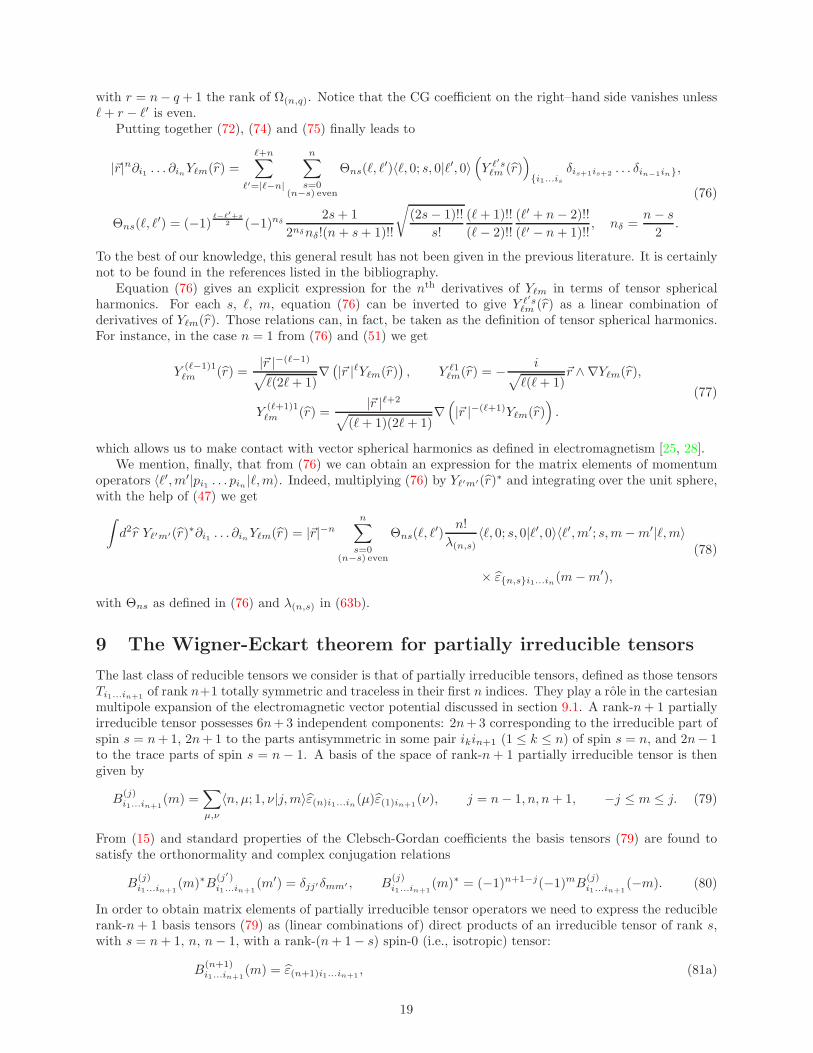
Putting together (72), (74) and (75) finally leads to

|~r|n∂i1 . . . ∂inYℓm(r) =

ℓ+n∑

ℓ′=|ℓ−n|

n∑

s=0(n−s) even

Θns(ℓ, ℓ′)〈ℓ, 0; s, 0|ℓ′, 0〉

(Y ℓ′sℓm (r)

)i1...is

δis+1is+2 . . . δin−1in,

Θns(ℓ, ℓ′) = (−1)

ℓ−ℓ′+s2 (−1)nδ

2s+ 1

2nδnδ!(n+ s+ 1)!!

√(2s− 1)!!

s!

(ℓ + 1)!!

(ℓ − 2)!!

(ℓ′ + n− 2)!!

(ℓ′ − n+ 1)!!, nδ =

n− s

2.

(76)

To the best of our knowledge, this general result has not been given in the previous literature. It is certainlynot to be found in the references listed in the bibliography.

Equation (76) gives an explicit expression for the nth derivatives of Yℓm in terms of tensor sphericalharmonics. For each s, ℓ, m, equation (76) can be inverted to give Y ℓ′s

ℓm (r) as a linear combination ofderivatives of Yℓm(r). Those relations can, in fact, be taken as the definition of tensor spherical harmonics.For instance, in the case n = 1 from (76) and (51) we get

Y(ℓ−1)1ℓm (r) =

|~r |−(ℓ−1)

√ℓ(2ℓ+ 1)

∇(|~r |ℓYℓm(r)

), Y ℓ1

ℓm(r) = − i√ℓ(ℓ+ 1)

~r ∧ ∇Yℓm(r),

Y(ℓ+1)1ℓm (r) =

|~r |ℓ+2

√(ℓ+ 1)(2ℓ+ 1)

∇(|~r |−(ℓ+1)Yℓm(r)

).

(77)

which allows us to make contact with vector spherical harmonics as defined in electromagnetism [25, 28].We mention, finally, that from (76) we can obtain an expression for the matrix elements of momentum

operators 〈ℓ′,m′|pi1 . . . pin |ℓ,m〉. Indeed, multiplying (76) by Yℓ′m′(r)∗ and integrating over the unit sphere,with the help of (47) we get

∫d2r Yℓ′m′(r)∗∂i1 . . . ∂inYℓm(r) = |~r|−n

n∑

s=0(n−s) even

Θns(ℓ, ℓ′)

n!

λ(n,s)〈ℓ, 0; s, 0|ℓ′, 0〉〈ℓ′,m′; s,m−m′|ℓ,m〉

× εn,si1...in(m−m′),

(78)

with Θns as defined in (76) and λ(n,s) in (63b).

9 The Wigner-Eckart theorem for partially irreducible tensors

The last class of reducible tensors we consider is that of partially irreducible tensors, defined as those tensorsTi1...in+1 of rank n+1 totally symmetric and traceless in their first n indices. They play a role in the cartesianmultipole expansion of the electromagnetic vector potential discussed in section 9.1. A rank-n+ 1 partiallyirreducible tensor possesses 6n+3 independent components: 2n+3 corresponding to the irreducible part ofspin s = n+1, 2n+1 to the parts antisymmetric in some pair ikin+1 (1 ≤ k ≤ n) of spin s = n, and 2n− 1to the trace parts of spin s = n − 1. A basis of the space of rank-n+ 1 partially irreducible tensor is thengiven by

B(j)i1...in+1

(m) =∑

µ,ν

〈n, µ; 1, ν|j,m〉ε(n)i1...in(µ)ε(1)in+1(ν), j = n− 1, n, n+ 1, −j ≤ m ≤ j. (79)

From (15) and standard properties of the Clebsch-Gordan coefficients the basis tensors (79) are found tosatisfy the orthonormality and complex conjugation relations

B(j)i1...in+1

(m)∗B(j′)i1...in+1

(m′) = δjj′δmm′ , B(j)i1...in+1

(m)∗ = (−1)n+1−j(−1)mB(j)i1...in+1

(−m). (80)

In order to obtain matrix elements of partially irreducible tensor operators we need to express the reduciblerank-n+ 1 basis tensors (79) as (linear combinations of) direct products of an irreducible tensor of rank s,with s = n+ 1, n, n− 1, with a rank-(n+ 1− s) spin-0 (i.e., isotropic) tensor:

B(n+1)i1...in+1

(m) = ε(n+1)i1...in+1, (81a)

19

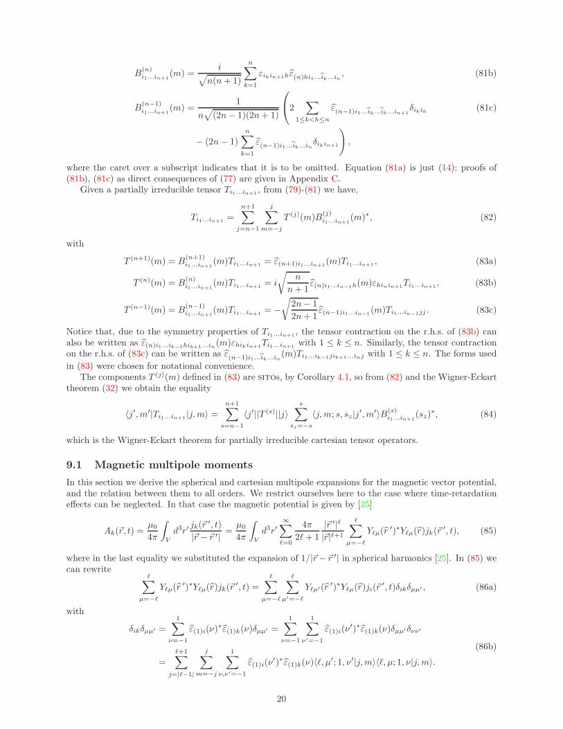
B(n)i1...in+1

(m) =i√

n(n+ 1)

n∑

k=1

εikin+1hε(n)hi1...ik...in , (81b)

B(n−1)i1...in+1

(m) =1

n√(2n− 1)(2n+ 1)

2

∑

1≤k<h≤n

ε(n−1)i1...ik...ih...in+1δikih (81c)

− (2n− 1)

n∑

k=1

ε(n−1)i1...ik...inδikin+1

),

where the caret over a subscript indicates that it is to be omitted. Equation (81a) is just (14); proofs of(81b), (81c) as direct consequences of (77) are given in Appendix C.

Given a partially irreducible tensor Ti1...in+1 , from (79)-(81) we have,

Ti1...in+1 =

n+1∑

j=n−1

j∑

m=−j

T (j)(m)B(j)i1...in+1

(m)∗, (82)

with

T (n+1)(m) = B(n+1)i1...in+1

(m)Ti1...in+1 = ε(n+1)i1...in+1(m)Ti1...in+1 , (83a)

T (n)(m) = B(n)i1...in+1

(m)Ti1...in+1 = i

√n

n+ 1ε(n)i1...in−1h(m)εhinin+1Ti1...in+1 , (83b)

T (n−1)(m) = B(n−1)i1...in+1

(m)Ti1...in+1 = −√

2n− 1

2n+ 1ε(n−1)i1...in−1

(m)Ti1...in−1jj . (83c)

Notice that, due to the symmetry properties of Ti1...in+1 , the tensor contraction on the r.h.s. of (83b) canalso be written as ε(n)i1...ik−1hik+1...in(m)εhikin+1Ti1...in+1 with 1 ≤ k ≤ n. Similarly, the tensor contractionon the r.h.s. of (83c) can be written as ε(n−1)i1...ik...in

(m)Ti1...ik−1jik+1...inj with 1 ≤ k ≤ n. The forms used

in (83) were chosen for notational convenience.The components T (j)(m) defined in (83) are sitos, by Corollary 4.1, so from (82) and the Wigner-Eckart

theorem (32) we obtain the equality

〈j′,m′|Ti1...in+1 |j,m〉 =n+1∑

s=n−1

〈j′||T (s)||j〉s∑

sz=−s

〈j,m; s, sz|j′,m′〉B(s)i1...in+1

(sz)∗, (84)

which is the Wigner-Eckart theorem for partially irreducible cartesian tensor operators.

9.1 Magnetic multipole moments

In this section we derive the spherical and cartesian multipole expansions for the magnetic vector potential,and the relation between them to all orders. We restrict ourselves here to the case where time-retardationeffects can be neglected. In that case the magnetic potential is given by [25]

Ak(~r, t) =µ0

4π

∫

V

d3r′jk(~r

′, t)

|~r − ~r ′| =µ0

4π

∫

V

d3r′∞∑

ℓ=0

4π

2ℓ+ 1

|~r ′|ℓ|~r|ℓ+1

ℓ∑

µ=−ℓ

Yℓµ(r′)∗Yℓµ(r)jk(~r

′, t), (85)

where in the last equality we substituted the expansion of 1/|~r− ~r ′| in spherical harmonics [25]. In (85) wecan rewrite

ℓ∑

µ=−ℓ

Yℓµ(r′)∗Yℓµ(r)jk(~r

′, t) =

ℓ∑

µ=−ℓ

ℓ∑

µ′=−ℓ

Yℓµ′(r ′)∗Yℓµ(r)ji(~r′, t)δikδµµ′ , (86a)

with

δikδµµ′ =

1∑

ν=−1

ε(1)i(ν)∗ε(1)k(ν)δµµ′ =

1∑

ν=−1

1∑

ν′=−1

ε(1)i(ν′)∗ε(1)k(ν)δµµ′δνν′

=

ℓ+1∑

j=|ℓ−1|

j∑

m=−j

1∑

ν,ν′=−1

ε(1)i(ν′)∗ε(1)k(ν)〈ℓ, µ′; 1, ν′|j,m〉〈ℓ, µ; 1, ν|j,m〉.

(86b)

20

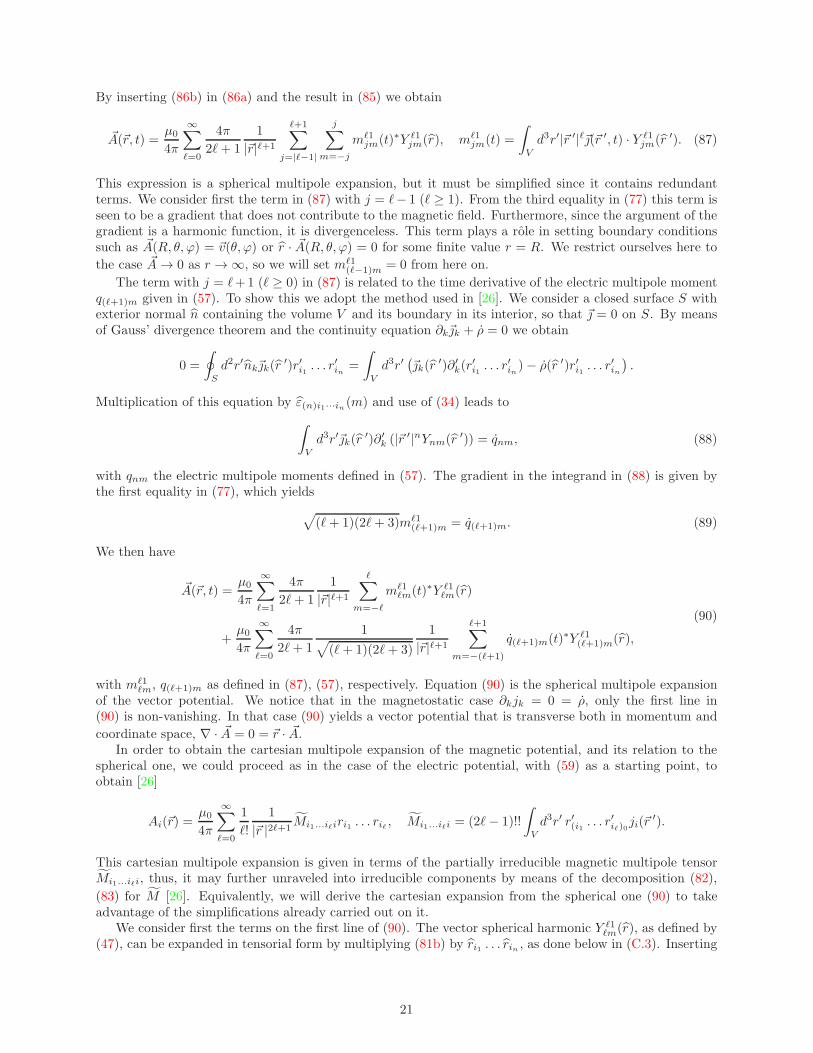
By inserting (86b) in (86a) and the result in (85) we obtain

~A(~r, t) =µ0

4π

∞∑

ℓ=0

4π

2ℓ+ 1

1

|~r|ℓ+1

ℓ+1∑

j=|ℓ−1|

j∑

m=−j

mℓ1jm(t)∗Y ℓ1

jm(r), mℓ1jm(t) =

∫

V

d3r′|~r ′|ℓ~(~r ′, t) · Y ℓ1jm(r ′). (87)

This expression is a spherical multipole expansion, but it must be simplified since it contains redundantterms. We consider first the term in (87) with j = ℓ− 1 (ℓ ≥ 1). From the third equality in (77) this term isseen to be a gradient that does not contribute to the magnetic field. Furthermore, since the argument of thegradient is a harmonic function, it is divergenceless. This term plays a role in setting boundary conditionssuch as ~A(R, θ, ϕ) = ~v(θ, ϕ) or r · ~A(R, θ, ϕ) = 0 for some finite value r = R. We restrict ourselves here to

the case ~A→ 0 as r → ∞, so we will set mℓ1(ℓ−1)m = 0 from here on.

The term with j = ℓ+1 (ℓ ≥ 0) in (87) is related to the time derivative of the electric multipole momentq(ℓ+1)m given in (57). To show this we adopt the method used in [26]. We consider a closed surface S withexterior normal n containing the volume V and its boundary in its interior, so that ~ = 0 on S. By meansof Gauss’ divergence theorem and the continuity equation ∂k~k + ρ = 0 we obtain

0 =

∮

S

d2r′nk~k(r′)r′i1 . . . r

′in =

∫

V

d3r′(~k(r

′)∂′k(r′i1 . . . r

′in)− ρ(r ′)r′i1 . . . r

′in

).

Multiplication of this equation by ε(n)i1···in(m) and use of (34) leads to

∫

V

d3r′~k(r′)∂′k (|~r ′|nYnm(r ′)) = qnm, (88)

with qnm the electric multipole moments defined in (57). The gradient in the integrand in (88) is given bythe first equality in (77), which yields

√(ℓ+ 1)(2ℓ+ 3)mℓ1

(ℓ+1)m = q(ℓ+1)m. (89)

We then have

~A(~r, t) =µ0

4π

∞∑

ℓ=1

4π

2ℓ+ 1

1

|~r|ℓ+1

ℓ∑

m=−ℓ

mℓ1ℓm(t)∗Y ℓ1

ℓm(r)

+µ0

4π

∞∑

ℓ=0

4π

2ℓ+ 1

1√(ℓ+ 1)(2ℓ+ 3)

1

|~r|ℓ+1

ℓ+1∑

m=−(ℓ+1)

q(ℓ+1)m(t)∗Y ℓ1(ℓ+1)m(r),

(90)

with mℓ1ℓm, q(ℓ+1)m as defined in (87), (57), respectively. Equation (90) is the spherical multipole expansion

of the vector potential. We notice that in the magnetostatic case ∂kjk = 0 = ρ, only the first line in(90) is non-vanishing. In that case (90) yields a vector potential that is transverse both in momentum and

coordinate space, ∇ · ~A = 0 = ~r · ~A.In order to obtain the cartesian multipole expansion of the magnetic potential, and its relation to the

spherical one, we could proceed as in the case of the electric potential, with (59) as a starting point, toobtain [26]

Ai(~r) =µ0

4π

∞∑

ℓ=0

1

ℓ!

1

|~r |2ℓ+1Mi1...iℓiri1 . . . riℓ , Mi1...iℓi = (2ℓ− 1)!!

∫

V

d3r′ r′(i1 . . . r′iℓ)0

ji(~r′).

This cartesian multipole expansion is given in terms of the partially irreducible magnetic multipole tensorMi1...iℓi, thus, it may further unraveled into irreducible components by means of the decomposition (82),

(83) for M [26]. Equivalently, we will derive the cartesian expansion from the spherical one (90) to takeadvantage of the simplifications already carried out on it.

We consider first the terms on the first line of (90). The vector spherical harmonic Y ℓ1ℓm(r), as defined by

(47), can be expanded in tensorial form by multiplying (81b) by ri1 . . . rin , as done below in (C.3). Inserting

21

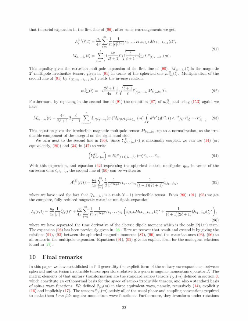
that tensorial expansion in the first line of (90), after some rearrangements we get,

A(1)j (~r, t) =

µ0

4π

∞∑

ℓ=1

1

ℓ!

1

|~r|2ℓ+1rk1 . . . rkℓ

εjkℓhMhk1...kℓ−1(t)∗,

Mk1...kℓ(t) =

ℓ∑

m=−ℓ

i4π

2ℓ+ 1ℓ!

√ℓ

ℓ+ 1mℓ1

ℓm(t)ε(ℓ)k1...kℓ(m).

(91)

This equality gives the cartesian multipole expansion of the first line of (90). Mk1...kℓ(t) is the magnetic

2ℓ-multipole irreducible tensor, given in (91) in terms of the spherical one mℓ1ℓm(t). Multiplication of the

second line of (91) by ε(ℓ)hk1···kℓ−1(m) yields the inverse relation:

mℓ1ℓm(t) = −i2ℓ+ 1

4π

1

ℓ!

√ℓ+ 1

ℓε(ℓ)k1···kℓ

Mk1...kℓ(t). (92)

Furthermore, by replacing in the second line of (91) the definition (87) of mℓ1ℓm and using (C.3) again, we

have

Mk1...kℓ(t) =

4π

2ℓ+ 1ℓ!

ℓ

ℓ+ 1

ℓ∑

m=−ℓ

ε(ℓ)k1···kℓ(m)∗ε(ℓ)h′k′

1···k′

ℓ−1(m)

∫

V

d3r′ (~(~r ′, t) ∧ ~r ′)h′ ~r′k′

1· · ·~r ′

k′

ℓ−1. (93)

This equation gives the irreducible magnetic multipole tensor Mk1...kℓ, up to a normalization, as the irre-

ducible component of the integral on the right-hand side.We turn next to the second line in (90). Since Y ℓ1

(ℓ+1)m(r) is maximally coupled, we can use (14) (or,

equivalently, (20)) and (34) in (47) to write

(Y ℓ1(ℓ+1)m

)= Nℓε(ℓ+1)j1...jℓj(m)rj1 . . . rjℓ . (94)

With this expression, and equation (62) expressing the spherical electric multipoles qℓm in terms of thecartesian ones Qi1...iℓ , the second line of (90) can be written as

A(2)j (~r, t) =

µ0

4π

∞∑

ℓ=1

1

ℓ!

1

|~r|2ℓ+1rk1 . . . rkℓ

1

(ℓ+ 1)(2ℓ+ 1)Qj1...jℓj , (95)

where we have used the fact that Qj1...jℓj is a rank-(ℓ+ 1) irreducible tensor. From (90), (91), (95) we getthe complete, fully reduced magnetic cartesian multipole expansion

Aj(~r, t) =µ0

4π

1

|~r | Qj(t)∗ +

µ0

4π

∞∑

ℓ=1

1

ℓ!

1

|~r |2ℓ+1rk1 . . . rkℓ

(εjkℓhMhk1...kℓ−1

(t)∗ +1

(ℓ+ 1)(2ℓ+ 1)Qk1...kℓj(t)

∗

),

(96)where we have separated the time derivative of the electric dipole moment which is the only O(1/r) term.The expansion (96) has been previously given in [26]. Here we recover that result and extend it by giving therelations (91), (92) between the spherical magnetic moments (87), (90) and the cartesian ones (93), (96) toall orders in the multipole expansion. Equations (91), (92) give an explicit form for the analogous relationsfound in [27].

10 Final remarks

In this paper we have established in full generality the explicit form of the unitary correspondence betweenspherical and cartesian irreducible tensor operators relative to a generic angular-momentum operator ~J . Thematrix elements of that unitary transformation are the standard rank-s tensors ε(s)(m) defined in section 3,which constitute an orthonormal basis for the space of rank-s irreducible tensors, and also a standard basisof spin-s wave functions. We defined ε(s)(m) in three equivalent ways, namely, recursively (14), explicitly(16) and implicitly (17). The tensors ε(s)(m) satisfy all of the usual phase and coupling conventions requiredto make them bona-fide angular-momentum wave functions. Furthermore, they transform under rotations

22

equivalently as cartesian or spherical tensors. We remark here that an analogous basis of cartesian irreduciblespinors can be constructed along the same lines [17, 10, 29]. Both the tensor and spinor bases are of the(non-relativistic) Rarita-Schwinger [29] type. With the spin wave functions ε(s)(m) as matrix elements of aunitary change of basis, we establish the relation between cartesian and spherical irreducible tensors of anyrank in section 4.

The unitary mapping described in 4 is important because it allows us to apply the methods and technicaltools of quantum angular–momentum theory to tensor algebra and vice versa. The interrelation of tensorand angular–momentum methods is used in section 5 to extend the Wigner–Eckart theorem to cartesianirreducible tensor operators of any rank, thus determining the form of their matrix elements. In principle,this result can be applied to any cartesian tensor operator, by linearly decomposing it into its irreduciblecomponents. In section 7 we take a step towards that goal by extending the Wigner–Eckart theorem tototally symmetric reducible tensors, which is the main result of this paper. Such an extension allows usto obtain matrix elements for arbitrary tensor powers of the position or momentum operators. This isexploited in section 8 to give an explicit expression for the gradients of any order of spherical harmonics.An additional extension of the Wigner-Eckart theorem to partially irreducible cartesian tensor operators isgiven in section 9. Partially irreducible tensors occur in some applications, such as the magnetic multipoleexpansion discussed in 9.1.

On the other hand, the results of section 3 and 4 also allow us to find the cartesian form of standardspherical tensors. Such cartesian tensorial forms provide a complementary approach to the usual analyticmethods often based on differential equations. In section 3.1 we show that Wigner D-matrices are thespherical components of three-dimensional rotation matrices, which leads to an expression of Dℓ as a linearcombination of products of D1 matrices. In section 6 we obtain the cartesian tensorial form of ordinary,bipolar and tensor spherical harmonics, and spin-polarization operators. We find some relations betweenthose standard functions that are of interest, like the decomposition of D-matrices mentioned above, thebinomial expansion for spherical harmonics, and the relation between tensor and bipolar spherical harmonics,based on the tensorial representations for them. We discuss also the relation between spherical and cartesianmultipoles of any rank, both for the scalar electric (section 6.5) and vector magnetic (9.1) potentials. Thebest illustration of the kind of relations referred to here, and of the power of our approach, is the explicitexpression for gradients of any order of spherical harmonics found in section 8.

Acknowledgements

The author has been partially supported by Sistema Nacional de Investigadores de Mexico.

References

[1] M. Kroger: Models for Polymeric and Anisotropic Liquids, Springer, New York 2005.

[2] C. Eckart: Reviews of Modern Physics 2, 305 (1930).

[3] E. Wigner: Group Theory and its Application to the Quantum Mechanics of Atomic Spectra, AcademicPress, New York 1959.

[4] L. D. Landau, E. M. Lifshitz: Quantum Mechanics, Butterworth–Heinemann, New York 2003.

[5] A. Messiah: Quantum Mechanics, Vol. 2, Elsevier, Amsterdam 1961.

[6] C. Cohen-Tannoudji, B. Diu, F. Laloe: Quantum Mechanics, Vol. 2, John Wiley, New York 1977.

[7] A. Galindo, P. Pascual: Quantum Mechanics I, Springer-Verlag, New York 1990.

[8] G. Racah: Physical Review 62, 438 (1942).

[9] L. C. Biedenharn, J. D. Louck: Angular Momentum in Quantum Physics, in Encyclopedia of Mathe-

matics and its Applications, G. C. Rota editor, Cambridge University Press, New York 2009.

[10] C. Zemach: Phys. Rev. 140, B97 (1965).

23

[11] J.-M. Normand, J. Raynal: J. Phys. A 15, 1437 (1982).

[12] H. A. Bethe: Handbuch der Physik 24, Springer, Berlin 1933.

[13] D. A. Varshalovich, A. N. Moskalev, V. K. Khersonskii: Quantum Theory of Angular Momentum, WorldScientific, New Jersey 1988.

[14] M. Hamermesh: Group Theory and Its Applications to Physical Problems, Dover, New York 1962.

[15] E. U. Condon, G. H. Shortley: The Theory of Atomic Spectra, 4th ed., Cambridge University Press,London 1957.

[16] A. R. Edmonds: Angular Momentum in Quantum Mechanics, Princeton University Press, Princeton,N.J. 1996.

[17] A. O. Bouzas: J. Phys. A 44, 165301 (2011).

[18] K. W. H. Stevens: Proc. Phys. Soc. A 65, 209 (1952) .

[19] P. Hoffman: J. Phys. A 24, 35 (1991) .

[20] A. Erdelyi et al.: Higher Trascendental Functions, Vol. 1, McGraw-Hill, New York 1953.

[21] G. F. Torres del Castillo: Rev. Mex. Fis. 59, 248 (2013) .

[22] A. O. Bouzas: J. Phys. A 44, 165302 (2011) .

[23] F. J. Yndurain: Relativistic Quantum Mechanics and Introduction to Field Theory, Springer, Berlin1996.

[24] R. G. Newton: Scattering Theory of Waves and Particles, Springer–Verlag, New York 1982.

[25] J. D. Jackson: ClassicalElectrodynamics, 3rd ed., Wiley, New York 1999.

[26] P. Kielanowski, M. Loewe: Rev. Mex. Fis. 44, 24 (1998).

[27] G. F. Torres del Castillo: Rev. Mex. Fis. 48, 348 (2002).

[28] E. L. Hill: Am. J. Phys. 22, 211 (1954).

[29] W. Rarita, J. Schwinger: Phys. Rev. 60, 61 (1941) .

A Angular momentum: notation and conventions

In this appendix we state our conventions for quantum angular–momentum theory [3, 4, 5, 6, 7, 9, 13, 15, 16].Throughout this paper we follow the convention of [4] that angular–momentum operators are dimensionless.

In particular, the orbital angular–momentum operator for a single particle is ~L = (1/~)~r ∧ ~p = −i~r ∧ ~∇. Inorder to switch to the alternate convention in which angular–momentum operators have units of ~ it sufficesto replace ~J (resp. ~L, ~S) in our equations by ~J/~ (resp. ~L/~, ~S/~).

Let ~J be a generic angular-momentum operator, [Jh, Ji] = iεhikJk. The simultaneous eigenstates of ~J 2

and J3 are denoted |j,m〉, with j ≥ 0 and −j ≤ m ≤ j integer or half-odd-integer. The state vectors |j,m〉are assumed to be normalized, therefore orthonormal, and their relative phases are chosen so that theysatisfy the usual convention

〈j,m′|J±|j,m〉 =√(j ∓m)(j ±m+ 1)δm′(m±1), 〈j,m′|J3|j,m〉 = mδm′(m±1). (A.1a)

In particular, they satisfy the Condon–Shortley phase convention 〈j,m′|J±|j,m〉 ≥ 0 [15, 16, 7]. For the

cartesian components of ~J we then have

〈j,m′|J12|j,m〉 = 1

2

√j(j + 1)−mm′(δm′(m+1) ± δm′(m−1)), (A.1b)

24

and the matrix element of J3 as in (A.1a). By using the relation

〈j,m; 1, ǫ|j,m′〉 = 1√j(j + 1)

×−ǫ√

2

√(j − ǫm)(j + ǫm+ 1) δm′(m+ǫ) if ǫ = ±1

mδmm′ if ǫ = 0, (A.2)

equation (A.1a) can be written more compactly as

〈j,m′|ε(1)(ǫ) · ~J |j,m〉 =√j(j + 1)〈j,m; 1, ǫ|j,m′〉, ǫ = 0,±1, (A.3a)

with ε(1)i(ǫ) defined in (9), from whence we obtain

〈j,m′|Jk|j,m〉 =√j(j + 1)〈j,m; 1,m′ −m|j,m′〉 εk(m′ −m)∗, (A.3b)

which is equivalent to (A.1b).For integer j the spatial wave–function associated with the orbital angular–momentum eigenstates is

given by the spherical harmonics, for which we follow the modern conventions [6, 7, 13, 25] (a different phaseconvention for Yℓm is used in older texts [4, 15, 16])

Yℓm(r) =

√2ℓ+ 1

4π

(ℓ−m)!

(ℓ+m)!Pℓm(cos θ)eimϕ, Pℓm(x) =

(−1)ℓ+m

ℓ!2ℓ(1 − x2)m/2 d

ℓ+m

dxℓ+m(1− x2)ℓ, (A.4)

where θ, ϕ are the polar coordinates of r, and where Pℓm(x) is an associated Legendre function of thefirst kind (as defined, e.g., in [7, 25]) that for m = 0 reduces to a Legendre polynomial Pℓ(x). An explicitexpression for Pℓm(x) is given in section 6.1.1.

We turn next to the coupling of angular momenta. Consider two subsystems with angular-momentumoperators ~Ja, a = 1, 2, each one acting on the Hilbert space of states Ha of its subsystem. Let H = H1⊗H2

be the state space of the total system, on which the total angular-momentum operator ~J = ~J1⊗ I2+ I1 ⊗ ~J2acts, where Ia is the identity operator on Ha. The definition of ~J is usually written in the abbreviated form~J = ~J1 + ~J2. If each subsystem a is in a state |ja, µa〉, simultaneous eigenstate of ( ~Ja)

2 and (Ja)3, the stateof the total system is the tensor product state |j1, µ1; j2, µ2〉 ≡ |j1, µ1〉 ⊗ |j2, µ2〉. On the other hand, the

states with definite total angular momentum |j1, j2, j,m〉 are chosen to be simultaneous eigenstates of ( ~J1)2,

( ~J2)2, ~J 2 and ~J3. The unitary transformation relating the two orthonormal bases of H is given by the CG

coefficients, which we denote as

|j1, j2, j,m〉 =∑

µ1,µ2

〈j1, µ1; j2, µ2|j,m〉|j1, µ1; j2, µ2〉. (A.5)

A global complex factor in the CG coefficients is determined by the normalization condition and the Condon–Shortley [15] phase convention 〈j1, j1; j2, j − j1|j, j〉 ≥ 0, which implies in particular that all CG coefficients

are real. Since |j1, j2, j,m〉 is by definition an eigenstate of ~J 2 and ~J3, the matrix elements of ~J betweenthose states do not depend on j1, j2,

〈j1, j2, j′,m′| ~J |j1, j2, j,m〉 = 〈j′,m′| ~J |j,m〉 = 〈j,m′| ~J |j,m〉δj′j , (A.6)

where the last matrix element is the standard one as given in (A.1b) or (A.3b).

Proof of (21) To prove (21) we proceed by induction on n. The case n = 1 is (11), which is seen to betrue by exhaustive evaluation of all possible cases m′,m = 0,±1. Assuming (21) to be true, we have toprove that

〈n+ 1,m′|Sk|n+ 1,m〉 = εi1...in+1(m′)∗(S(n+1)k)i1...in+1;j1...jn+1 εj1...jn+1(m), (A.7)

with −n− 1 ≤ m′,m ≤ n+ 1. From (4), the matrix ~S(n+1) can be written as

(S(n+1)k)i1...in+1;j1...jn+1 = (S(n)k)i1...in;j1...jnδin+1jn+1 + δi1j1 . . . δinjn(S(1)k)in+1;jn+1 .

Substituting this equality together with (14) into the right-hand side of (A.7) leads to

εi1...in+1(m′)∗(S(n+1)k)i1...in+1;j1...jn+1 εj1...jn+1(m) =

n∑

µ′,µ=−n

1∑

ν′,ν=−1

〈n, µ′; 1, ν′|n+ 1,m′〉〈n, µ; 1, ν|n+ 1,m〉

25

×(εi1...in(µ

′)∗(S(n)k)i1...in;j1...jn εj1...jn(µ)δν′ν + δµ′µεin+1(ν′)∗(S(1)k)in+1;jn+1 εjn+1(ν)

)

=

n∑

µ′,µ=−n

1∑

ν′,ν=−1

〈n, µ′; 1, ν′|n+ 1,m′〉〈n, µ; 1, ν|n+ 1,m〉(〈n, µ′|(SA)k|n, µ〉δν′ν + δµ′µ〈1, ν′|(SB)k|1, ν〉

),

where in the last equality we used the case n = 1 given by (11) and the inductive hypothesis (21) to expressthe matrix elements of S(n)k and S(1)k on the second line in terms of the matrix elements of a spin operator~SA for a spin-n system A and a spin operator ~SB for a spin-1 system B, respectively. ~SA,B being bothangular-momentum operators, their matrix elements are given by (A.1b). The total angular-momentum

operator for the total system A+B is ~S = ~SA ⊗ IB + IA ⊗ ~SB, and we have

=

n∑

µ′,µ=−n

1∑

ν′,ν=−1

〈n, µ′; 1, ν′|n+ 1,m′〉〈n, µ; 1, ν|n+ 1,m〉〈n, µ′; 1, ν′|Sk|n, µ, 1, ν〉

= 〈n, 1, n+ 1,m′|Sk|n, 1, n+ 1,m〉 = 〈n+ 1,m′|Sk|n+ 1,m〉,

where the last equality is (A.6).

B Non–maximally–coupled bipolar spherical harmonics

The bipolar spherical harmonics [13] defined in (42) have been given an explicit tensorial expression in [22].Here we quote that expression for Y ℓℓ′

jm (r, r ′) with a slightly different notation that is more appropriate tothe purposes of this paper. We assume ℓ′ ≥ ℓ for notational simplicity. The case ℓ′ < ℓ results from therelation Y ℓℓ′

jm (r, r ′) = (−1)ℓ′+ℓ−jY ℓ′ℓ

jm (r ′, r) that follows from the definition (42). Thus, for ℓ′ ≥ ℓ from [22]we find

Y ℓℓ′

jm (r, r ′) =iν

4π

√2jν!

√(2j

j + n

)√(2j + 1)(2ℓ+ 1)(2ℓ′ + 1)

(ℓ′ + ℓ+ j + 1)!

n∑

k1=k1min

k2max∑

k2=0k1+k2=n

(−1)k2

(n

k1

) qmax∑

q=qmin

× (2q − 1)!!

(t

2q

)εi1...ik2+qj1...jk1+qh1...ht−2q (m)ri1 . . . rik2+q

r ′j1 . . . r

′jk1+q

vh1 . . . vht−2qP(j−q)ℓ+k1

(r · r ′),

(B.1a)

where the following notations have been used

ν = ℓ′ + ℓ− j, n = ℓ′ − ℓ, t = j − n, ~v = r ∧ r ′, qmin = max0, ℓ+ k2 − ν,

k1min =

max0, n− ν

2max0, n− ν−1

2 , k2max =

min ν

2 , nmin ν−1

2 , n, qmax =

ℓ− ν

2 ν even

ℓ− ν−12 − 1 ν odd

,(B.1b)

and where P(k)n (x) is the kth derivative of the Legendre polynomial Pn(x). In (B.1a) it is understood that

the factor ri1 . . . rik2+qis to be replaced by 1 if k2 + q < 1, and analogously the other products of r ′ and

~v. It is not difficult to check that (B.1) reduces to (44) in the case of maximal coupling ν = 0. In the caseν > 0 of non-maximally coupled Y ℓℓ′

jm , (B.1) gives its dual cartesian irreducible tensor just as (44) does formaximally coupled ones.

C Proof of (81)

To derive (81b) we start from the second equality in (77) written in the form

(Y ℓ1ℓm(r))j = − i√

ℓ(ℓ+ 1)Nℓεjabra∂b

(ε(ℓ)k1...kℓ

(m)rk1 · · · rkℓ

), (C.1)

26

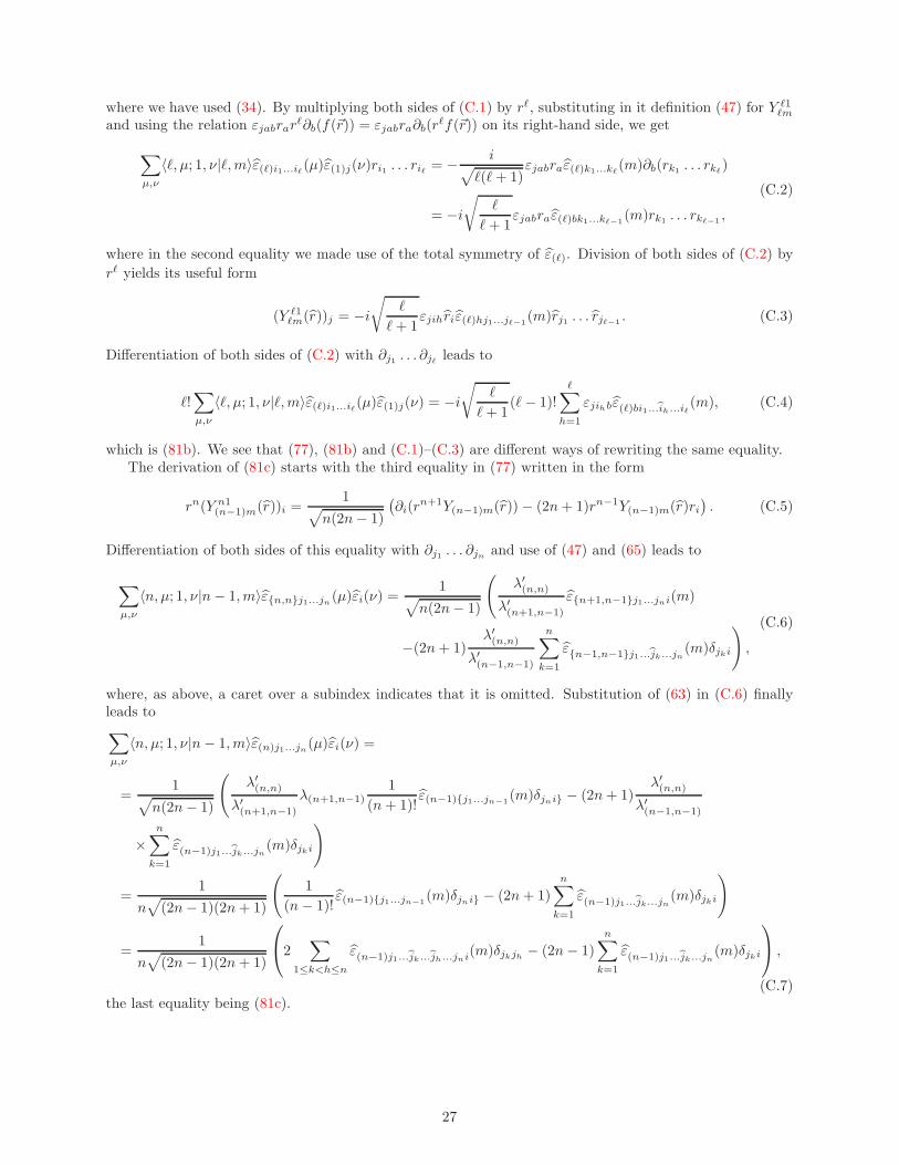
where we have used (34). By multiplying both sides of (C.1) by rℓ, substituting in it definition (47) for Y ℓ1ℓm

and using the relation εjabrarℓ∂b(f(~r)) = εjabra∂b(r

ℓf(~r)) on its right-hand side, we get

∑

µ,ν

〈ℓ, µ; 1, ν|ℓ,m〉ε(ℓ)i1...iℓ(µ)ε(1)j(ν)ri1 . . . riℓ = − i√ℓ(ℓ+ 1)

εjabraε(ℓ)k1...kℓ(m)∂b(rk1 . . . rkℓ

)

= −i√

ℓ

ℓ+ 1εjabraε(ℓ)bk1...kℓ−1

(m)rk1 . . . rkℓ−1,

(C.2)

where in the second equality we made use of the total symmetry of ε(ℓ). Division of both sides of (C.2) by

rℓ yields its useful form

(Y ℓ1ℓm(r))j = −i

√ℓ

ℓ+ 1εjihriε(ℓ)hj1...jℓ−1

(m)rj1 . . . rjℓ−1. (C.3)

Differentiation of both sides of (C.2) with ∂j1 . . . ∂jℓ leads to

ℓ!∑

µ,ν

〈ℓ, µ; 1, ν|ℓ,m〉ε(ℓ)i1...iℓ(µ)ε(1)j(ν) = −i√

ℓ

ℓ+ 1(ℓ− 1)!

ℓ∑

h=1

εjihbε(ℓ)bi1...ih...iℓ(m), (C.4)

which is (81b). We see that (77), (81b) and (C.1)–(C.3) are different ways of rewriting the same equality.The derivation of (81c) starts with the third equality in (77) written in the form

rn(Y n1(n−1)m(r))i =

1√n(2n− 1)

(∂i(r

n+1Y(n−1)m(r))− (2n+ 1)rn−1Y(n−1)m(r)ri). (C.5)

Differentiation of both sides of this equality with ∂j1 . . . ∂jn and use of (47) and (65) leads to

∑

µ,ν

〈n, µ; 1, ν|n− 1,m〉εn,nj1...jn(µ)εi(ν) =1√

n(2n− 1)

(λ′(n,n)

λ′(n+1,n−1)

εn+1,n−1j1...jni(m)

−(2n+ 1)λ′(n,n)

λ′(n−1,n−1)

n∑

k=1

εn−1,n−1j1...jk...jn(m)δjki

),

(C.6)

where, as above, a caret over a subindex indicates that it is omitted. Substitution of (63) in (C.6) finallyleads to∑

µ,ν

〈n, µ; 1, ν|n− 1,m〉ε(n)j1...jn(µ)εi(ν) =

=1√

n(2n− 1)

(λ′(n,n)

λ′(n+1,n−1)

λ(n+1,n−1)1

(n+ 1)!ε(n−1)j1...jn−1

(m)δjni − (2n+ 1)λ′(n,n)

λ′(n−1,n−1)

×n∑

k=1

ε(n−1)j1...jk...jn(m)δjki

)

=1

n√(2n− 1)(2n+ 1)

(1

(n− 1)!ε(n−1)j1...jn−1

(m)δjni − (2n+ 1)

n∑

k=1

ε(n−1)j1...jk...jn(m)δjki

)

=1

n√(2n− 1)(2n+ 1)

2

∑

1≤k<h≤n

ε(n−1)j1...jk...jh...jni(m)δjkjh − (2n− 1)

n∑

k=1

ε(n−1)j1...jk...jn(m)δjki

,

(C.7)the last equality being (81c).

27