Embed Size (px)
Citation preview

VOLUME III
THIRD NATIONAL COMMUNICATION OFBRAZIL TO THE UNITED NATIONSFRAMEWORK CONVENTION ON
CLIMATECHANGE


VOLUME III
THIRD NATIONAL COMMUNICATION OFBRAZIL TO THE UNITED NATIONSFRAMEWORK CONVENTION ON
CLIMATECHANGE
Ministry of Science, Technology and InnovationSecretariat of Policies and Programs of Research and Development
General Coordination of Global Climate ChangeBrasília2016
FEDERATIVE REPUBLIC OF BRAZIL
PRESIDENT OF THE FEDERATIVE REPUBLIC OF BRAZIL
DILMA VANA ROUSSEFF
MINISTER OF SCIENCE, TECHNOLOGY AND INNOVATION
CELSO PANSERA
EXECUTIVE SECRETARY
EMÍLIA MARIA SILVA RIBEIRO CURI
SECRETARY OF POLICIES AND PROGRAMS OF RESEARCH AND DEVELOPMENT
JAILSON BITTENCOURT DE ANDRADE
GENERAL COORDINATOR OF GLOBAL CLIMATE CHANGE
MÁRCIO ROJAS DA CRUZ

MCTI TECHNICAL TEAM
DIRECTOR OF THE THIRD NATIONAL COMMUNICATIONMÁRCIO ROJAS DA CRUZ
COORDINATOR OF THE THIRD NATIONAL COMMUNICATION MARCELA CRISTINA ROSAS ABOIM RAPOSO
TECHNICAL COORDINATOR OF THE THIRD BRAZILIAN INVENTORY OF ANTHROPOGENIC EMISSIONS BY SOURCES AND REMOVALS BY SINKS OF GREENHOUSE GASESEDUARDO DELGADO ASSAD
TECHNICAL COORDINATOR OF THE CLIMATE MODELS AND CLIMATE VULNERABILITIES AND ADAPTATION ON KEY-SECTOR STUDIESJOSE ANTONIO MARENGO ORSINI
SUPERVISORS OF THE THIRD NATIONAL COMMUNICATION BRENO SIMONINI TEIXEIRA
DANIELLY GODIVA SANTANA MOLLETA
MAURO MEIRELLES DE OLIVEIRA SANTOS
TECHNICAL ANALYSTS OF THE THIRD NATIONAL COMMUNICATIONCINTIA MARA MIRANDA DIAS
GISELLE PARNO GUIMARÃES
JULIANA SIMÕES SPERANZA
RENATA PATRICIA SOARES GRISOLI
TECHNICAL TEAM ANDRÉA NASCIMENTO DE ARAÚJO
ANNA BEATRIZ DE ARAÚJO ALMEIDA
GUSTAVO LUEDEMANN
JERÔNIMA DE SOUZA DAMASCENO
LIDIANE ROCHA DE OLIVEIRA MELO
MOEMA VIEIRA GOMES CORRÊA
RICARDO ROCHA PAVAN DA SILVA
RICARDO VIEIRA ARAUJO
SANDERSON ALBERTO MEDEIROS LEITÃO
SONIA REGINA MUDROVITSCH DE BITTENCOURT
SUSANNA ERICA BUSCH
VICTOR BERNARDES
ASSISTANT OF THE THIRD NATIONAL COMMUNICATIONMARIA DO SOCORRO DA SILVA LIMA
ADMINISTRATIVE TEAMANA CAROLINA PINHEIRO DA SILVA
ANDRÉA ROBERTA DOS SANTOS CAMPOS
RICARDO MORÃO ALVES DA COSTA
TRANSLATIONMARIANE ARANTES ROCHA DE OLIVEIRA

MINISTRY OF SCIENCE, TECHNOLOGY AND INNOVATION
ESPLANADA DOS MINISTÉRIOS, BLOCO E
PHONE: +55 (61) 2033-7923
WEB: http://www.mcti.gov.br
CEP: 70.067-900 – Brasília – DF
B823t Brazil. Ministry of Science, Technology and Innovation. Secretariat of Policies and Programs of Research and Development. General Coordination of Global Climate Change.
Third National Communication of Brazil to the United Nations Framework Convention on Climate Change – Volume III/ Ministry of Science, Technology and Innovation. Brasília: Ministério da Ciência, Tecnologia e Inovação, 2016.
333 p.: il.
ISBN: 978-85-88063-25-9
1. Climate Change. 2. UNFCCC. 3. National Communication. I. Title.
CDU 551.583
TECHNICAL COORDINATORS OF THE THIRD INVENTORYEmilio Lèbre La Rovere and Carolina Burle Schmidt Dubeux – Energy sector
João Wagner Silva Alves – Waste sector
Mauro Meirelles de Oliveira Santos – Industrial Processes sector
Mercedes Maria da Cunha Bustamante – Land Use, Land-Use Change and Forestry sector
Renato de Aragão Ribeiro Rodrigues – Agriculture sector
AUTHORS Adriana dos Santos Siqueira Scolastrici
Alberto Arruda Villela
Alexandre Berndt
Alexandre Rodrigues Filizola
Amanda Prudêncio Lemes
Amaro Olímpio Pereira Jr.
Ana Paula Contador Packer
Ana Paula Dutra de Aguiar
Anderson do Nascimento Dias
Bruna Cordeiro
Bruno Arantes Caldeira da Silva
Bruno José Rodrigues Alves
Carolina Monteiro de Carvalho
Cimelio Bayer
Claudia do Valle Costa
Cristiano Viana Serra Villa
Daniel Oberling
Elton César de Carvalho
Fernando Luiz Zancan
Flora da Silva Ramos Vieira Martins
Gustavo Abreu Malaguti
Iracema Alves Manoel Degaspari
Isabella da Fonseca Zicarelli
Jean Pierre Henry Balbaud Ometto
Julia Zanin Shimbo
Larissa Albino da Silva Santos
Laura Alexandra Romero
Leandro Fagundes
Leandro Sannomiya Sakamoto
Leonardo da Silva Ribeiro
Luan Santos
Luciane Garavaglia
Luiza Di Beo Oliveira
Magda Aparecida de Lima
Marcelo Buzzatti
Márcio Zanuz
Marcos Corrêa Neves
Maria Conceição Peres Young Pessoa
Mariana Pedrosa Gonzalez
Mariana Weiss de Abreu
Michele Karina Cotta Walter
Nilza Patrícia Ramos
Obdulio Diego Fanti
Patricia Turano de Carvalho
Paulo W. Pinto da Cunha
Pedro Valle de Carvalho e Oliveira
Raymundo Moniz de Aragão Neto
Roberta Zecchini Cantinho
Roberto de Aguiar Peixoto
Rodrigo Pacheco Ribas
Sonia Maria Manso Vieira
Talita Armborst
Thauan Santos
Thiago de Roure Bandeira de Mello
Tiago Zschornack
Viviane A. Alves Vilela
Walkyria Bueno Scivittaro
William Wills

COLLABORATORSAdemir Fontana
Ademir Rodrigo F. V. B. de Lima Amaro
Alessandra Fidelis
Aline Rocha Silva
Alison Leme dos Santos
Ana Catarine Franzini de Souza
Ana Paula Dalla Corte
Anderson Dias Silveira
Anderson Rodrigues Perez
Andrea Daleffi Scheide
Andreza Nogueira Leite
Antonio Florido
Arnildo Pott
Beata Emoki Madari
Beatriz Marimon
Ben Hur Marimon
Bruna Patrícia de Oliveira
Camila Isaac França
Carla Cabral Gonzalez
Carlos Alberto Flores
Carlos R. Sanquetta
Carmen Brandão Reis
Cauê Gustavo Lopes
Célia Regina Pandolphi Pereira
Ciniro Costa Junior
Claudia Pozzi Jantalia
Clotilde Pinheiro Ferri dos Santos
Daielle Silva do Amaral Faria
Daniel Costa Stockler Maia
Daniel Vieira
Daniella Flávia Villas Boas
Danilo Rocco Pettinati
Dayane de Carvalho Oliveira
Diane Pereira da Silva
Edson Sano
Eduardo Alves da Cunha

Eduardo Felipe Marcelino Bastos
Eduardo Shimabokuro
Elaine Cristina Cardoso Fidalgo
Eliana Kimoto Hosokawa
Eliza R. G. M. Albuquerque
Eloisa Aparecida Belleza Ferreira
Elza Maria da Silveira Ramos
Erika Caitano da Silva
Euler Melo Nogueira
Everardo Valadares de Sá B. Sampaio
Fabiana Aparecida Souza Silva
Fabiana Cristina de Oliveira Santos
Felippe Neri de Almeida
Fernanda Pereira de Oliveira Rocha
Fernando Moreira de Araujo
Fernando Zuchello
Flavia Cristina de Aragão Caloi
Francelo Mognon
Francois Fromard
Frans PareyinGabriela Aparecida de Oliveira Nakasone
Gabriela Lopez-Gonzalez
Giovana Maranhão Bettiol
Giselda Durigan
Giulia Nicoliello Biondi
Glauco Turci
Graziele Coraline Scofano da Rosa
Gustavo de Mattos Vasques
Heinrich Hasenack
Helber Freitas
Heloisa Sinátora Miranda
Henrique Yudi Oliveira Asakura
Igor de Souza Sermarini
Isabela Alvarenga de Mattos Landim
Isabele Kaori Une
Ivan Bergier
Jacqueline Oliveira de Souza
James Hutchison
Jaqueline Dalla Rosa
Jayson Campos de Souza
Jéssica Faria Mendes
Jéssica Goldoni Gandra
Jéssica Werber Godoy
Joao dos Santos Vila da Silva
Jorge Luis Silva Brito
Jorge Muniz
José Carlos Gomes de Souza
Josiane Guedes Rana Rosa
Josilene T. Vannuzini Ferrer
Juan Jacque Monteiro
Kennedy de Jesus
Laerte Ferreira Junior
Laila Akemi Pugaciov
Lais Queiroz de Araújo
Lenita Moreira Cendretti
Leonardo Oliveira Santos
Liana Anderson
Lucas Matheus dos Reis
Luciana Fatima de Souza Medeiros
Luciana Mamede dos Santos
Luisa Vega
Luiz Aragão
Luiz Clóvis Belarmino
Luiz Scherer
Manuela Antunes Jorge
Marcelo Henrique Moreira Santos
Marcelo Rodolfo Siqueira
Marco Aurélio Reis dos Santos
Marcos Vinicius Winckler Caldeira
Marcus Fernandes
Margarete Naomi Sato
Margareth Copertino
Mariana Florencio Marques
Mario Luiz Diamante Aglio
Mário Marcos do Espírito Santo
Marla de Oliveira Farias

Martha Mayumi Higarashi
Marcelo Miele
Maura Rejane de Araújo Mendes
Mayara Teodoro
Mirian Noemi Silva da Costa
Nicole Luana de Fátima P da Costa
Niro Higuchi
Osmira Fátima da Silva
Patricia Fatima de Mello Kutika
Paula de Melo Chiste
Paulo Armando Victoria de Oliveira
Petrea Miharu Hayashi Pereira
Priscila Cesar Rocha de Souza
Rafael Notarangeli Favaro
Rafaela Carlota Forastiero
Raíssa Caroline dos Santos Teixeira
Rangel Feijó de Almeida
Renides da Cruz Eller de Moraes
Ricardo Flores Haidar
Rita Marcia da Silva Pinto Vieira
Robert Michael Boddey
Rodolfo de Almeida Santos
Rodolfo Morais
Rodrigo da Silva Ferreira
Rodrigo da Silveira Nicoloso
Rodrigo Delgado Inacio
Romulo Menezes
Ronaldo de Souza Junior
Sabrina de Oliveira Pereira
Sabrina do Couto Miranda
Segundo Urquiaga
Sérgio Raposo Medeiros
Simone Vieira
Suzana Maria de Salis
Tainara Melo Siqueira
Talita Assis
Tatiana Almeida de Souza
Tatiana Amaral de Almeida Oliveira

Tayane Pereira Muts Guedes
Thiago Crestani Martins
Tiago Diniz Althoff
Valério de Patta Pillar
Vanildes Oliveira Ribeiro
Vitoria Inocencio Sobrinho
Wagner Júlio Noronha Lima
INSTITUTIONS INVOLVED – VOLUME IIINational Civil Aviation Agency (Agência Nacional de Aviação Civil – ANAC)
Beneficent Association of the state of Santa Catarina Coal Industry (Associação Beneficente da Indústria Carbonífera
de Santa Catarina – SATC)
Brazilian Association of Chemical Industry (Associação Brasileira da Indústria Química – ABIQUIM)
Brazilian Aluminum Association (Associação Brasileira de Alumínio – ABAL)
Brazilian Association of Lime Producers (Associação Brasileira de Produtores de Cal – ABPC)
Brazilian Coal Association (Associação Brasileira do Carvão Mineral – ABCM)
Clean Coal Technology Center (Centro Tecnológico de Carvão Limpo – CTCL)
Environmental Protection Agency of São Paulo State (Companhia Ambiental do Estado de São Paulo – CETESB)
National Steel Company (Companhia Siderúrgica Nacional – CSN)
National Department of Mineral Production of the districts of Rio Grande do Sul and Santa Catarina (Departamento
Nacional de Produção Mineral – DNPM dos distritos do Rio Grande do Sul e Santa Catarina)
Brazilian Agricultural Research Corporation (Empresa Brasileira de Pesquisa Agropecuária – Embrapa)
Mining companies of the states of Rio Grande do Sul, Santa Catarina and Paraná
Foundation for Space Science, Technology and Applications (Fundação de Ciência, Aplicações e Tecnologia
Espaciais – FUNCATE)
Brazil Steel Institute and associates (Instituto Aço Brasil – IABr e suas associadas)
The National Institute for Space Research (Instituto Nacional de Pesquisas Espaciais – INPE)
Rice Institute of the State of Rio Grande do Sul (Instituto Rio Grandense do Arroz)
Ministry of Science, Technology and Innovation (Ministério da Ciência, Tecnologia e Inovação – MCTI)
Ministry of Mines and Energy (Ministério de Minas e Energia – MME)
Ministry of the Environment (Ministério do Meio Ambiente – MMA)
P&D Business Consultants Ltd. (P&D Consultoria Empresarial Ltda.)
Petrobras
Brazilian Research Network on Global Climate Change (Rede Brasileira de Pesquisas sobre Mudanças Climáticas
Globais – Rede CLIMA)
Rima Industrial S.A.

Brazilian Coal Industry Extraction Union (Sindicato da Indústria de Extração de Carvão do Estado de Santa Catarina
– SIECESC)
National Cement Industry Union (Sindicato Nacional da Indústria do Cimento – SNIC)
University of Brasília (Universidade de Brasília – UnB)
Júlio de Mesquita Filho São Paulo State University - Faculty of Engineering, Guaratinguetá Campus (Universidade
Estadual Paulista “Júlio de Mesquita Filho” – UNESP (Faculdade de Engenharia de Guaratinguetá)
Federal University of Rio de Janeiro (Universidade Federal do Rio de Janeiro – UFRJ)
Federal University of Rio Grande do Sul (Universidade Federal do Rio Grande do Sul – UFRGS)
White Martins
SYMBOLS, ACRONYMS AND ABBREVIATIONS% – percentage
°C – Celsius degrees
A – Rivers and lakes
Aa – Alluvial Open Humid Forest
Ab – Lowland Open Humid Forest
ABETRE – Brazilian Association of Solid Waste Treatment Companies (Associação Brasileira de Empresas de
Tratamento de Resíduos)
ABIA – Brazilian Food Industry Association (Associação Brasileira das Indústrias da Alimentação)
ABIC – Brazilian Coffee Industry Association (Associação Brasileira da Indústria de Café)
ABIP – Brazilian Bakery and Confectionery Industry Association (Associação Brasileira da Indústria de Panificação
e Confeitaria)
ABIQUIM – Brazilian Association of Chemical Industry (Associação Brasileira da Indústria Química)
ABNT – Brazilian Association of Technical Standards (Associação Brasileira de Normas Técnicas)
ABPC – Brazilian Association of Lime Producers (Associação Brasileira de Produtores de Cal)
ABRACAL – Brazilian Association of Agricultural Limestone Producers (Associação Brasileira dos Produtores de
Calcário Agrícola)
ABRELPE – Brazilian Association of Public Cleaning and Special Wastes Companies (Associação Brasileira de
Empresas de Limpeza Pública e Resíduos Especiais)
ABS – acrylonitrile butadiene styrene
ABS/PA – acrylonitrile butadiene styrene/polyamide
Ac – Agricultural area
AC – State of Acre
Am – Open Montane Humid Forest
AM – State of Amazonas

ANAC – National Civil Aviation Agency (Agência Nacional de Aviação Civil)
ANP –Brazilian National Agency of Petroleum, Natural Gas and Biofuels (Agência Nacional do Petróleo, Gás e
Biocombustíveis)
Ap – Planted pasture
AP – state of Amapá
AR4 – IPCC Fourth Assessment Report
AR5 – IPCC Fifth Assessment Report
As – Open Submontane Humid Forest
BA – state of Bahia
BEN – National Energy Balance (Balanço Energético Nacional)
BEU – Useful Energy Balance (Balanço de Energia Útil)
BNF – Biological Nitrogen Fixation
BOD - Biochemical Oxygen Demand
bpd – barrels per day
BT – total biomass
C – carbon
C2F6 – hexafluorethane
Ca –Alluvial Deciduous Seasonal Forest
Ca(OH)2 – calcium hydroxide
CaC2 – calcium carbide
CaCO3– limestone
CaO – calcium oxide
Cb – Lowland Deciduous Seasonal Forest
CBH – circumference at breast height
CDM – Clean Development Mechanism
CE – state of Ceará
CETESB – Environmental Protection Agency of São Paulo State (Companhia Ambiental do Estado de São Paulo)
CF4 – tetrafluoromethane
CFCs – chlorofluorocarbons
CH4 – methane
CKD – Cement Kiln Dust
cm – centimeter
Cm – Montane Deciduous Seasonal Forest
CO – carbon monoxide
CO2 – carbon dioxide
CO2e – carbon dioxide equivalent
COD – Chemical Oxygen Demand
Cogen – Brazilian Cogeneration Association (Associação da Indústria de Cogeração de Energia)
CONAB – National Supply Company (Companhia Nacional de Abastecimento)
COP – Conference of the Parties
CORINAIR – Core Inventory Air Emissions
Cs – Submontane Deciduous Seasonal Forest
CS – Forests with selective logging
CSI – Cement Sustainability Initiative
Da –Alluvial Dense Humid Forest
Db – Lowland Dense Humid Forest
DBH – diameter at breast height
DEGRAD – Forest Degradation Mapping System in the Brazilian Amazon (Mapeamento da Degradação Florestal
na Amazônia Brasileira)
DETEX – Detection of Selective Logging (Projeto de Mapeamento de Ocorrências de Exploração Seletiva de Madeira)
DF – Federal District
Dl – High-Montane Dense Humid Forest
Dm – Montane Dense Humid Forest
DNPM – National Department of Mineral Production (Departamento Nacional de Produção Mineral)
DPA – Brazil’s Political-Administrative Division (Divisão Político-Administrativa do Brasil)
Ds – Submontane Dense Humid Forest
E&P – Exploitation and Production
Ea – Wooded Steppe
EF – emission factor
Eg – Woody-Grass Steppe
Embrapa – Brazilian Agricultural Research Corporation (Empresa Brasileira de Pesquisa Agropecuária)
Ep – Park Steppe
EPE – Energy Research Company (Empresa de Pesquisa Energética)
Fa – Alluvial Semi Deciduous Seasonal Forest
FAO – Food and Agriculture Organization of the United Nations
Fb – Lowland Semi Deciduous Seasonal Forest
FM – Managed Forest
Fm – Montane Semi Deciduous Seasonal Forest
FNM – Unmanaged Forest
FRA – Global Forest Resources Assessment
Fs – Submontane Semi Deciduous Seasonal Forest
FSec – Secondary Forest
FUNAI – National Indian Foundation (Fundação Nacional do Índio)
g – gram
Gg – gigagram
GHG – greenhouse gases
GM – Managed Grasslands
GNM – Unmanaged Grasslands
GO – state of Goiás
GSec – Secondary Grasslands
GTP – Global Temperature Potential
GWP – Global Warming Potential
ha – hectares
HDPE – high-density polyethylene
HCFCs – hydrochlorofluorocarbons
HFCs – hydrofluorocarbons
HGU – Hydrogen Generation Unit
HNO3 – nitric acid
IBGE – Brazilian Institute of Geography and Statistics (Instituto Brasileiro de Geografia e Estatística)
IDW – Inverse Distance Weighting
IL – Indigenous Lands
inhab – inhabitant
INPE – The National Institute for Space Research (Instituto Nacional de Pesquisas Espaciais)
IPCC – Intergovernmental Panel on Climate Change
kcal – kilocalorie
kg – kilogram
km2 – square kilometer
L – liter
La – Wooded Campinarana Arborized
Lb – Shrubby Campinarana
Ld – Forested Campinarana
LDPE – low-density polyethylene
Lg – Woody-Grass Campinarana
LLDPE – linear low-density polyethylene
LNG – liquefied natural gas
LULUCF – Land Use, Land-Use Change and Forestry
m2 – square meter
m3 – cubic meter
MA – state of Maranhão
Ma –Alluvial Mixed Humid Forest
MCTI – Ministry of Science, Technology and Innovation (Ministério da Ciência, Tecnologia e Inovação)
MDIs – Metered Dose Inhalers
MG – state of Minas Gerais
MgCO3 – dolomite

Ml – Montane Mixed High Humid Forest
MLME – Linear Spectral Mixing Model
mm – millimeter
Mm – Montane Mixed Humid Forest
MMA – Ministry of the Environment (Ministério do Meio Ambiente)
MME – Ministry of Mines and Energy (Ministério de Minas e Energia)
MS – state of Mato Grosso do Sul
Ms – Submontane Mixed High Humid Forest
Mt – megatonne
MT – state of Mato Grosso
MVC - monomeric vinyl chloride
N – nitrogen
N2O – nitrous oxide
NA – not applicable
Na2CO3 – neutral sodium carbonate
NASA – National Aeronautics and Space Administration
NBR – acrylonitrile-butadiene rubber
NE – Not Estimated area
Nex – nitrogen excreted
NH3 – ammonia
NMVOC – Non-methane volatile organic compounds
NO – Nitric oxide
NO2 – nitrogen dioxide
NOx – nitrogen oxides
O3 – ozone
ODS – ozone-depleting substances
OX – oxidation factor
Pa – Fluvial and/or lacustre Influenced Vegetation
PA – Protected Areas (Unidades de Conservação)
PA – state of Pará
PB – state of Paraíba
PE – state of Pernambuco
Pf – Pioneer formation Fluviomarine Influenced (mangrove)
PFCs – perfluorocarbons
PI – state of Piauí
Pm – Pioneer formation Marine Influenced (sand banks)
PMDBBS – Satellite Monitoring of Deforestation in Brazilian Biomes Project (Projeto de Monitoramento do
Desmatamento dos Biomas Brasileiros)
PNSB – National Survey of Basic Sanitation Study (Pesquisas Nacionais de Saneamento Básico)
pot – potential emissions
PPBio – Research Program for Biodiversity (Programa de Pesquisa em Biodiversidade)
PPCDAm – Action Plan for the Prevention and Control of Deforestation in the Legal Amazon (Plano de Ação para
a Prevenção e Controle do Desmatamento na Amazôonia Legal)
PROBIO – Conservation and Sustainable Use of Biological Diversity Project (Projeto de Conservação e Utilização
Sustentável da Diversidade Biológica)
PRODES – Project for Estimating Gross Deforestation of the Brazilian Amazon (Projeto de Monitoramento de
Desflorestamento na Amazôniaon Legal)
PVC – polyvinyl chloride
RAINFOR – Amazon Network of Forestry Inventories (Rede Amazônica de Inventários Florestais)
RAL – Mining Annual Report (Relatório Anual de Lavra)
RCU – Retarded Coking Unit
Ref – Reforestation
Res – Reservoirs
RF – radiative forcing
Rl – High Montane Vegetational Refuge
Rm – Montane Refuge
RO – state of Rondônia
ROM – run-of-mine
RPPN – Private Reserve of Natural Heritage (Reservas Particulares de Preservação Natural)
RR – state of Roraima
Rs – Submontane Refuge
S – Urban area
Sa – Wooded Savanna
SAR – IPCC Second Assessment Report
SBR – styrene-butadiene rubber
Sd – Forested Savanna
SD – standard deviation
SE – state of Sergipe
SF6 – sulfur hexafluoride
Sg – Woody-grass savanna
SIG – Geographic Information System (Sistema de Informação Geográfica)
SINDIPAN – Bakery and Confectionery Industry Union (Sindicato da Indústria de Panificação e Confeitaria)
SNC – Second National Communication
SNIC – National Cement Industry Union (Sindicato Nacional da Indústria do Cimento)
SNIS – National Sanitation Information System (Sistema Nacional de Informações sobre Saneamento)
SNUC – National System of Protected Areas (Sistema Nacional de Unidades de Conservação)
Sp – Park Savanna
SP – state of São Paulo
t – tonne
Ta – Wooded Steppe Savanna
TAR – IPCC Third Assessment Report
Td – Forested Steppe Savanna
TEAM – Tropical Ecology Assessment and Monitoring
Tg – Woody Grass Steppe Savanna
Tier – approach
TJ – terajoule
TM – thematic mapping
TNC – Third National Communication
TO – state of Tocantins
toe – tonne of oil equivalent
Tp – Park Steppe Savanna
UFCC – Fluid Catalytic Cracking Unit
UFPE – Federal University of Pernambuco
UFRPE – Federal Rural University of Pernambuco
UNESCO – United Nations Educational, Scientific and Cultural Organization
UNFCCC – United Nations Framework Convention on Climate Change
UNICA – Brazilian Association of Sugarcane Industry (União da Indústria de Cana-de-açúcar)
UVIBRA – Brazilian Vitiviniculture Union (União Brasileira de Vitivinicultura)
VS – volatile solids
WBCSD – World Business Council for Sustainable Development
ZAPE – agro-ecological zoning of the State of Pernambuco


TABLE OF CONTENTS
24
TABLE OF CONTENTS
1 INTRODUCTION ........................................................................................................................................................31
1.1. Greenhouse Gases ........................................................................................................................................32
1.2. Sectors covered .............................................................................................................................................33
1.2.1. Energy Sector ............................................................................................................................................. 33
1.2.1.1. Fuel Combustion .......................................................................................................................................33
1.2.1.2. Fugitive emissions ...................................................................................................................................34
1.2.2. Industrial Processes Sector ................................................................................................................... 34
1.2.2.1. Mineral products .....................................................................................................................................34
1.2.2.2. Chemical industry .....................................................................................................................................35
1.2.2.3. Metallurgical industry .............................................................................................................................35
1.2.2.4. Production and use of HFCs and SF6 .................................................................................................36
1.2.3. Agriculture Sector ..................................................................................................................................... 36
1.2.3.1. Enteric fermentation ..............................................................................................................................36
1.2.3.2. Manure Management .............................................................................................................................36
1.2.3.3. Rice cultivation ........................................................................................................................................37
1.2.3.4. Crop residue burning...............................................................................................................................37
1.2.3.5. N2O emissions from agricultural soils ..............................................................................................37
1.2.4. Land Use, Land-Use Change and Forestry Sector ...........................................................................37
1.2.5. Waste Sector ............................................................................................................................................... 38
1.2.5.1. Solid Waste Disposal ...............................................................................................................................38
1.2.5.2. Wastewater Treatment ............................................................................................................................38

2 SUMMARY OF ANTHROPOGENIC EMISSIONS BY SOURCES AND REMOVALS BY SINKS OF GREENHOUSE GASES ..................................................................................41
2.1. Carbon Dioxide Emissions .........................................................................................................................42
2.2. Methane Emissions ......................................................................................................................................46
2.3. Nitrous Oxide Emissions ............................................................................................................................49
2.4. Hydrofluorocarbons, Perfluorocarbons and Sulfur Hexafluoride Emissions ...........................52
2.5. Indirect Greenhouse Gases ........................................................................................................................53
3 ANTHROPOGENIC EMISSIONS BY SOURCES AND REMOVALS BY SINKS OF GREENHOUSE GASES BY SECTOR ............................................................................................63
3.1. Energy ...............................................................................................................................................................64
3.1.1. Characteristics of the Brazilian Energy Mix .................................................................................... 64
3.1.2. Fuel Combustion Emissions .................................................................................................................. 69
3.1.2.1. CO2 emissions from fuel combustion ...............................................................................................70
3.1.2.2. Emissions of other greenhouse gases from fuel combustion ...................................................77
3.1.3. Fugitive Emissions ................................................................................................................................... 92
3.1.3.1. Fugitive emissions from coal mining ...............................................................................................92
3.1.3.2. Fugitive emissions from oil and natural gas activities ...............................................................96
3.2. Industrial Processes .....................................................................................................................................98
3.2.1. Mineral Products ....................................................................................................................................... 99
3.2.1.1. Cement Production .................................................................................................................................99
3.2.1.2. Lime production ..................................................................................................................................... 100
3.2.1.3. Production and consumption of soda ash .................................................................................... 102
3.2.2. Chemical Industry ...................................................................................................................................102
3.2.2.1. Ammonia production .......................................................................................................................... 103
3.2.2.2. Nitric acid production ......................................................................................................................... 103
3.2.2.3. Adipic acid production ........................................................................................................................ 104
3.2.2.4. Caprolactam production ..................................................................................................................... 105
3.2.2.5. Calcium carbide production and use .............................................................................................. 105
3.2.2.6. Petrochemical and carbon black production .............................................................................. 106
3.2.2.7. Phosphoric Acid ...................................................................................................................................... 109
3.2.2.8. Production of other chemicals .......................................................................................................... 111
3.2.3. Metal Production ....................................................................................................................................113
3.2.3.1. Iron and Steel Production................................................................................................................... 113
3.2.3.2. Ferroalloy production .......................................................................................................................... 114
3.2.3.3. Aluminum production ......................................................................................................................... 115
3.2.3.4. Magnesium production ...................................................................................................................... 117
3.2.3.5. Summary of the estimates of the direct and indirect Greenhouse Gas emissions
from the production of metals ........................................................................................................ 117
3.2.4. Other Industries ......................................................................................................................................119
3.2.4.1. Pulp and Paper Industry ..................................................................................................................... 119
3.2.4.2. Food and Beverage .............................................................................................................................. 120
3.2.5. Emissions related to hydrofluorocarbon production .................................................................121
3.2.6. Emissions related to hydrofluorocarbon consumption .............................................................122
3.2.7. Emissions related to the consumption of sulfur hexafluoride ................................................125
3.3. Solvent and Other Product Use Sector .............................................................................................. 126
3.4. Agriculture .....................................................................................................................................................127
3.4.1. Livestock .................................................................................................................................................... 127
3.4.1.1. Enteric fermentation ............................................................................................................................ 129
3.4.1.2. Manure management .......................................................................................................................... 130
3.4.2. Rice Cultivation .......................................................................................................................................132
3.4.3. Crop Residue Burning ............................................................................................................................134
3.4.3.1. Sugarcane ................................................................................................................................................. 134
3.4.3.2. Herbaceous cotton ................................................................................................................................ 136
3.4.4. N2O emissions from agricultural soils ........................................................................................... 137
3.4.4.1. N2O emissions due to grazing animals .......................................................................................... 138
3.4.4.2. N2O emissions by other direct sources .......................................................................................... 139
3.4.4.3. N2O emissions from indirect sources ............................................................................................ 144
3.5. Land Use, Land-Use Change and Forestry ....................................................................................... 144

3.5.1. Methodology ............................................................................................................................................146
3.5.1.1. Land Use, Land-Use Change and Forestry .................................................................................... 146
3.5.1.2. Liming of agricultural soils ............................................................................................................... 146
3.5.2. Results ........................................................................................................................................................146
3.5.2.1. Amazon Biome ...................................................................................................................................... 147
3.5.2.2. Cerrado Biome ........................................................................................................................................ 148
3.5.2.3. Caatinga Biome ...................................................................................................................................... 149
3.5.2.4. Atlantic Forest Biome ........................................................................................................................... 150
3.5.2.5. Pampa Biome .......................................................................................................................................... 151
3.5.2.6. Pantanal Biome ...................................................................................................................................... 152
3.5.2.7. Consolidated results ............................................................................................................................. 152
3.5.2.8. Annual net anthropogenic CO2 emissions for the period 1990 to 2010............................ 184
3.6. Waste ..............................................................................................................................................................187
3.6.1. Solid waste disposal ..............................................................................................................................188
3.6.2. Waste incineration ..................................................................................................................................190
3.6.3. Wastewater treatment .........................................................................................................................190
3.6.3.1. Domestic and commercial wastewater .......................................................................................... 191
3.6.3.2. Industrial wastewater .......................................................................................................................... 192
4 UNCERTAINTY OF THE ESTIMATES ...................................................................................................................195
4.1. Uncertainty of CO2 Emission and Removal Estimates ..................................................................197
4.2. Uncertainty of CH4 Emission Estimates ............................................................................................ 198
4.3. Uncertainty of N2O Emission Estimates ........................................................................................... 200
REFERENCES ................................................................................................................................................................203
APPENDIX I METHODOLOGICAL DESCRIPTION FOR THE INVENTORY OF LAND USE, LAND-USE CHANGE AND FORESTRY ....................................................................................................................219
1 Detailed methodology for the Land Use, Land-use Change and Forestry sector ................... 220
1.1. Land representation ................................................................................................................................. 220
1.1.1. Construction of transition matrices between categories and sub-categories
for land use .............................................................................................................................................233

1.1.2. Estimates of emissions by sources and removals for assessed transitions .......................234
1.1.3. Emissions and removals associated with soil carbon stock changes ..................................235
1.1.4. Data .............................................................................................................................................................236
1.1.5. Definition of the emission factors and other parameters needed to estimate
emissions and removals of CO2 .........................................................................................................292
APPENDIX II FIRES NOT ASSOCIATED WITH DEFORESTATION ....................................................................299
APPENDIX III GREENHOUSE GAS EMISSIONS ESTIMATES BY GAS AND SECTOR, FROM 1990 TO 2010 ...........................................................................................................................................313


CHAPTER I INTRODUCTION

CHAPTER I INTRODUCTION

32
CHAPTER I INTRODUCTION
One of Brazil’s main requirements as a signatory of the United Nations Framework Convention on Climate
Change – hereinafter referred to as Convention – is the preparation and regular updating of the National Inventory
of Anthropogenic Emissions by Sources and Removals by Sinks of Greenhouse Gases Not Controlled by the Montreal
Protocol – hereinafter referred to as Inventory.
The preparation of this Inventory is in accordance with the Guidelines for the Elaboration of the National
Communications of the Parties Not Included in the Annex I to the Convention, established in Decision 17/CP.8 of
the Eighth Conference of the Parties to the Convention, held in Delhi, India, in October/November 2002.
This Inventory covers the period between 1990 to 2010. In relation to the period 1990 - 2005, this Inventory
updates the information presented in the previous Inventory (BRASIL, 2010).
The following documents, prepared by the Intergovernmental Panel on Climate Change (IPCC), were used
as basic technical guidance: “Revised 1996 IPCC Guidelines for National Greenhouse Inventories” – Guidelines
1996; “Good Practice Guidance and Uncertainty Management in National Greenhouse Gas Inventories” – Good
Practice Guidance 2000; and “Good Practice Guidance for Land Use, Land-Use Change and Forestry” – Good
Practice Guidance 2003. Some of the estimates have already taken into account the information published in
“2006 IPCC Guidelines for National Greenhouse Gas Inventories” (Guidelines 2006).
1.1. GREENHOUSE GASESClimate on Earth is governed by the constant stream of solar energy that passes through the atmosphere in the form
of visible light. The Earth returns part of this energy in the form of infrared radiation. Greenhouse gases (GHG) are those
present in the Earth’s atmosphere that can block part of the infrared radiation. Many of them, such as water vapor, carbon
dioxide (CO2), methane (CH4), nitrous oxide (N2O) and ozone (O3), exist naturally in the atmosphere and are essential for
the maintenance of life on Earth. Without them the planet’s temperature would be 30°C colder.
As a result of the anthropogenic activities in the biosphere, concentration levels of some gases, such as CO2,
CH4, and N2O, have been increasing in the atmosphere. In addition, the emission of other greenhouse gases,
chemical compounds produced by men only, such as chlorofluorocarbons (CFCs), hydrofluorocarbons (HFCs),
hydrochlorofluorocarbons (HCFCs), perfluorocarbons (PFCs), and sulfur hexafluoride (SF6), started to occur.

33
As determined by the Convention, the Inventory should include only the anthropogenic emissions by sources
and removals by sinks of greenhouse gases not controlled by the Montreal Protocol. Therefore, CFC and HCFC gases,
which destroy the ozone layer and are already controlled by the Montreal Protocol, are not considered, although
being greenhouse gases.
The greenhouse gases whose anthropogenic emissions and removals have been estimated in this Inventory
are CO2, CH4, N2O, HFCs, PFCs and SF6. Some other gases, such as carbon monoxide (CO), nitrogen oxides (NOx) and
other non-methane volatile organic compounds (NMVOCs), which are not direct greenhouse gases, influence the
chemical reactions that occur in the atmosphere. Information about the anthropogenic emissions of these gases is
also included in this Inventory when available.
1.2. SECTORS COVEREDDifferent activity sectors produce anthropogenic emissions of greenhouse gases. The present Inventory is
organized according to the structure suggested by the IPCC, covering the following sectors: Energy; Industrial
Processes; Solvent and Other Product Use; Agriculture; Land Use, Land-Use Change and Forestry and Waste
Treatment.
Removals of greenhouse gases occur in the Land Use, Land-Use Change and Forestry Sector as a result of
management of protected areas, reforestation, abandonment of managed land and increase in soil carbon stocks.
1.2.1. Energy SectorIn this sector, all anthropogenic emissions from energy production, transformation and consumption are
estimated. They include emissions resulting from fuel combustion as well as fugitive emissions in the chain of
production, transformation, distribution and consumption.
1.2.1.1. Fuel CombustionThe energy sector includes emissions of CO2 from the oxidation of carbon contained in fossil fuels when
they are burnt, either for the generation of other forms of energy, such as electricity, or for end use consumption.
Emissions of other greenhouse gases during the combustion process (CH4, N2O, CO, NOx, and NMVOC) are also
taken into account.
CO2 emissions in the case of biomass fuels (firewood, charcoal, litter, bleach, alcohol and bagasse) have been
informed, but not accounted for in the total emissions of the energy sector. Renewable source fuels do not generate
net CO2 emissions and the emissions associated with the non-renewable ones are included in the Land Use, Land-
Use Change and Forestry sector.

34
VOLUME IIITHIRD NATIONAL COMMUNICATION OF BRAZIL
As in the case of biomass fuels, CO2 emissions from fuel combustion supplied in the country for international
air and sea transportation (bunker fuels) are informed in accordance with decision 17/CP.8, but are not accounted
for in the total emissions of the Energy sector.
Due to the basic information available, emissions are presented according to the structure defined in the
National Energy Balance (BEN), which is similar, but not identical, to the structure suggested by the IPCC.
1.2.1.2. Fugitive emissionsThe Energy sector also includes greenhouse gas emissions from coal mining and processing, and also from the
extraction, transportation, and processing of oil and natural gas.
Emissions associated with coal mining include CH4 emissions from open-pit and underground mines, as well as
CO2 emissions by spontaneous combustion in waste piles of charcoal.
Emissions associated with oil and natural gas include fugitive emissions of CH4 during their extraction (venting),
during transport and distribution in ducts and vessels, and during its processing in refineries. CO2, CH4, and N2O
emissions by non-useful combustion (flaring) on extraction platforms of petroleum and natural gas and refineries
are also considered. The use of oil and natural gas, or their byproducts, to provide power for internal use in energy
production and transport is considered as combustion and is, therefore, treated in the fuel burning section.
CO2 emissions during flaring operations are included as fugitive emissions, even though they formally result
from combustion, as they are associated with a loss and not with the useful consumption of fuel.
1.2.2. Industrial Processes SectorThis sector entails estimates of anthropogenic emissions resulting from production processes in industries,
including the non-energy consumption of fuels as raw material, but excluding fuel burning for power generation,
which is reported in the Energy Sector.
The subsectors of mineral products, metallurgical industry, chemical industry and other non-energy uses of
fuels were considered, besides the production and use of HFCs, PFCs and SF6.
1.2.2.1. Mineral products This subsector includes emissions resulting from the production of cement, lime, other uses of limestone and
dolomite with calcination, and the use of sodium carbonate (soda ash).
Cement production generates CO2 emissions by the calcination of limestone (CaCO3) during the production of clinker.
In the lime production process, limestone and dolomite (CaCO3•MgCO3) are calcined, which also produces CO2. In the
glass industry, in the steel industry and in the production of magnesium CO2 emissions also occur by the calcination of

35
CHAPTER IINTRODUCTION
limestone and dolomite. The production of neutral sodium carbonate (soda ash) in Brazil is not a source of CO2 emissions
due to the production process used here, and only the use of this substance generates CO2 emissions.
1.2.2.2. Chemical industryAmong the inventoried emissions in this subsector, emissions of CO2 resulting from the production of ammonia,
the emissions of N2O and NOx emissions from production of nitric acid, and emissions of N2O, CO, and and NOx
resulting from the production of adipic acid are worth mentioning.
During production of other chemicals, there can also be greenhouse gas emissions, especially NMVOC emissions
from the petrochemical industry.
For this edition, the Solvent and Other Products Use Sector was included here, with approach only through
the non-energy use of lighting kerosene, hydrous alcohol, solvents and other non-energy petroleum products by
different sectors of the chemical industry.
1.2.2.3. Metallurgical industryThis subsector covers the steel and ferroalloy industries, where there are emissions in the process of ore
reduction, and also the production of non-ferrous metals, including aluminum and magnesium. Relevant emissions
of CO2, CH4, N2O, CO, NOx, NMVOC, PFCs and SF6 to each sector were estimated.
In the steel and ferroalloy industries, GHG is emitted when carbon contained in the reducing agent combines
with the oxygen in the metal oxides. These reducing agents, such as coal coke, are also used as fuel for energy
generation. Emissions associated with both processes are reported in this sector. Other emissions from the steel
industry are reported in the Energy Sector (coal coke production and power production) and in the Mineral
Production Sector (lime production, use of limestone and dolomite). The same principle adopted for fuel separation
used as a reducer for the steel industry was used for the ferroalloy and non-ferrous subsectors, except for aluminum
and magnesium, which used different estimate methodologies.
In the aluminum industry, CO2 emissions occur during the electrolysis process, when the oxygen of the aluminum
oxide reacts with the carbon of the anode. During the same process, if the level of aluminum oxide in the production
tank becomes too low, there can be a rapid increase in voltage (anodic effect). In this case, the fluoride contained in
the electrolytic solution reacts with the carbon of the anode, producing perfluorocarbons (CF4 and C2F6), which are
greenhouse gases of long residence time in the atmosphere. In the production of magnesium, there are emissions of
SF6 used as cover gas to prevent its oxidation.
Other industries
The Pulp and Paper subsector generates emissions during the chemical treatment to which wood pulp is
submitted in the production process. Such emissions depend on the type of raw material used and the quality of
the product that is to be obtained.

36
VOLUME IIITHIRD NATIONAL COMMUNICATION OF BRAZIL
In Brazil, eucalyptus is the major source of cellulose, with the predominance of the sulphate process, during
which CO, NOx, and NMVOC emissions occur. Such emissions have been estimated in this Inventory.
In the Food and Beverage subsector, NMVOC emissions occur during many transformation processes of primary
products, such as the production of sugar, animal feed, and beer. Emissions were estimated based on national
production data, with the use of default emission factors.
1.2.2.4. Production and use of HFCs and SF6
HFCs gases were developed in the 1980s and 1990s as alternatives to CFCs and HCFCs. The use of these gases
is being phased out because they deplete the ozone layer. HFCs are greenhouse gases that do not contain chlorine
and, therefore, do not affect the ozone layer.
During the production and use of HFCs there may be fugitive emissions. During the production process of HCFC-
22 there may be the secondary production of HFC-23 and their consequent emission.
SF6, another greenhouse gas produced only anthropogenically, has excellent characteristics for use in electrical
equipment of high capacity and performance. Brazil is not a producer of this gas. Thus, the reported emissions of
SF6 are due only to leakages during the use of equipment installed in the country.
1.2.3. Agriculture SectorAgriculture and livestock are economic activities of great importance in Brazil. Because of the vast extent of
agricultural and grazing lands, the country also occupies a prominent place in this sector’s world production.
Many are the processes that result in greenhouse gas emissions, which are described below.
1.2.3.1. Enteric fermentation Enteric fermentation, which is part of the digestive process of ruminant herbivores, is one of the major sources
of CH4 emissions in the country. The intensity of this process depends on several factors, such as the category of
animal, animal feed, the intensity of their physical activity, and different management practices. Among the various
categories of animals, cattle are the most important in terms of emissions, and the world’s second largest category.
1.2.3.2. Manure Management Manure management systems may generate CH4 and N2O emissions. Anaerobic decomposition produces CH4,
especially when animal wastes are stored in liquid form.

37
CHAPTER IINTRODUCTION
1.2.3.3. Rice cultivation When grown in flooded fields or floodplains, rice is an important source of CH4 emissions. This occurs due to the
anaerobic decomposition of the organic matter present in the water. In Brazil, however, most of the rice is produced
in non-flooded areas, thus reducing the importance of the subsector in the total emissions of CH4.
1.2.3.4. Crop residue burningThe imperfect practice of burning crop residues, carried out directly in the field, produces CH4, N2O, NOx, CO, and
NMVOC emissions. The CO2 emitted is not considered as net emissions as the same amount is necessarily absorbed,
through photosynthesis, during plant growth.
In Brazil, crop residue burning occurs mainly in the sugar cane crops.
1.2.3.5. N2O emissions from agricultural soilsN2O emissions from agricultural soils result from the use of nitrogen fertilizers, both synthetic and of animal
origin, and from manure deposition in pasture. The latter is not considered an important fertilizer application
because it is not intentional. However, it is the most important process in Brazil because of the predominance of
extensive livestock production. Crop residues left in the field are also sources of N2O emissions.
Also in this sector is the cultivation of organic soils, which increases the mineralization of organic matter and
releases N2O.
1.2.4. Land Use, Land-Use Change and Forestry SectorThis sector comprises estimates of emissions and removals of greenhouse gases associated with the increase
or decrease of carbon in aboveground and belowground biomass by replacing a particular type of land use by
another, as, for example, conversion of forest land to agricultural land or livestock production, or the replacement
of cropland with reforestation.
By extension, as recommended by the Good Practice Guidance LULUCF 2003, emissions and removals by land-
use are estimated for the use of land not subject to change, growth or loss under the same type of use (for example,
growth of secondary vegetation or even of primary vegetation in managed areas).
Estimates should consider all carbon compartments: aboveground living biomass; belowground living
biomass (roots); litter (branches and dead leaves); dead wood (either standing or lying on the ground); and
soil carbon. In addition, in this sector, emissions from the application of limestone in agricultural soils have
also been accounted for.
38
VOLUME IIITHIRD NATIONAL COMMUNICATION OF BRAZIL
CO2 is the predominant gas in this sector, but there are also emissions of other greenhouse gases such as CH4
and N2O due to imperfect field burning of wood and conversion of forest land to other uses.
CH4 emissions from reservoirs (dams, hydroelectric power plants, weirs, etc.) also occur, but they have not
been estimated in this inventory because there is no agreed methodology by the IPCC in its calculation due to the
difficulty in identifying the human-induced parcel of such emissions.
1.2.5. Waste Sector
1.2.5.1. Solid Waste DisposalDisposal of solid waste creates anaerobic conditions that generate CH4. The emission potential for CH4 increases
depending on the control conditions in landfills and the depth of the dumps. Waste incineration, an activity greatly
reduced in Brazil, generates emissions of several greenhouse gases (like all forms of combustion), mainly of CO2.
1.2.5.2. Wastewater TreatmentWastewater with a high degree of organic content has a great potential for CH4 emissions, especially domestic
and commercial sewage, effluents from the food and beverage industry, and from the pulp and paper industry. The
other industries also contribute to these emissions, but to a smaller degree.
In the case of the domestic sewage, because of the nitrogen content in food, N2O emissions also occur.


CHAPTER II SUMMARY OF ANTHROPOGENIC
EMISSIONS BY SOURCES AND REMOVALS BY SINKS OF
GREENHOUSE GASES
CHAPTER II SUMMARY OF ANTHROPOGENIC
EMISSIONS BY SOURCES AND REMOVALS BY SINKS OF
GREENHOUSE GASES

42
CHAPTER II SUMMARY OF ANTHROPOGENIC EMISSIONS BY SOURCES AND REMOVALS BY SINKS OF GREENHOUSE GASES
In 2010, net anthropogenic greenhouse gas emissions were estimated at 739,671 Gg CO2; 16,688.2 Gg CH4;
560.49 Gg N2O; 0.0767 Gg CF4, 0.0059 Gg C2F6, 0.0087 Gg SF6, 2.7196 Gg HFC-134a, 0.1059 Gg HFC-32, 0.5012 Gg
HFC-125 and 0.4671 Gg HFC-143a. Between 2005 and 2010, total CO2, CH4, and N2O emissions decreased by 66%,
9% and 8%, respectively. Greenhouse gas emissions with indirect effect were also assessed. In 2010, such emissions
were estimated at 3,429.4 Gg NOx; 35,050.4 Gg CO; and 6,387.2 Gg NMVOC.
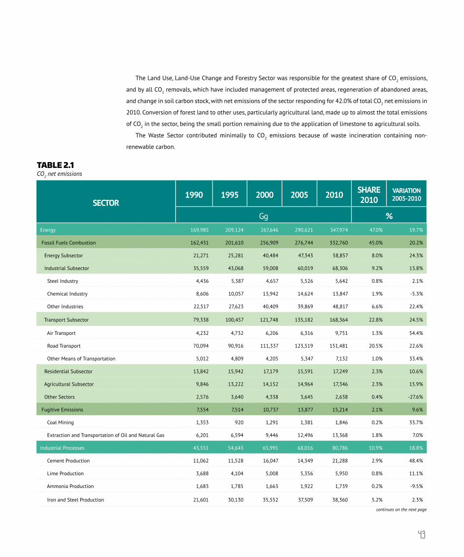
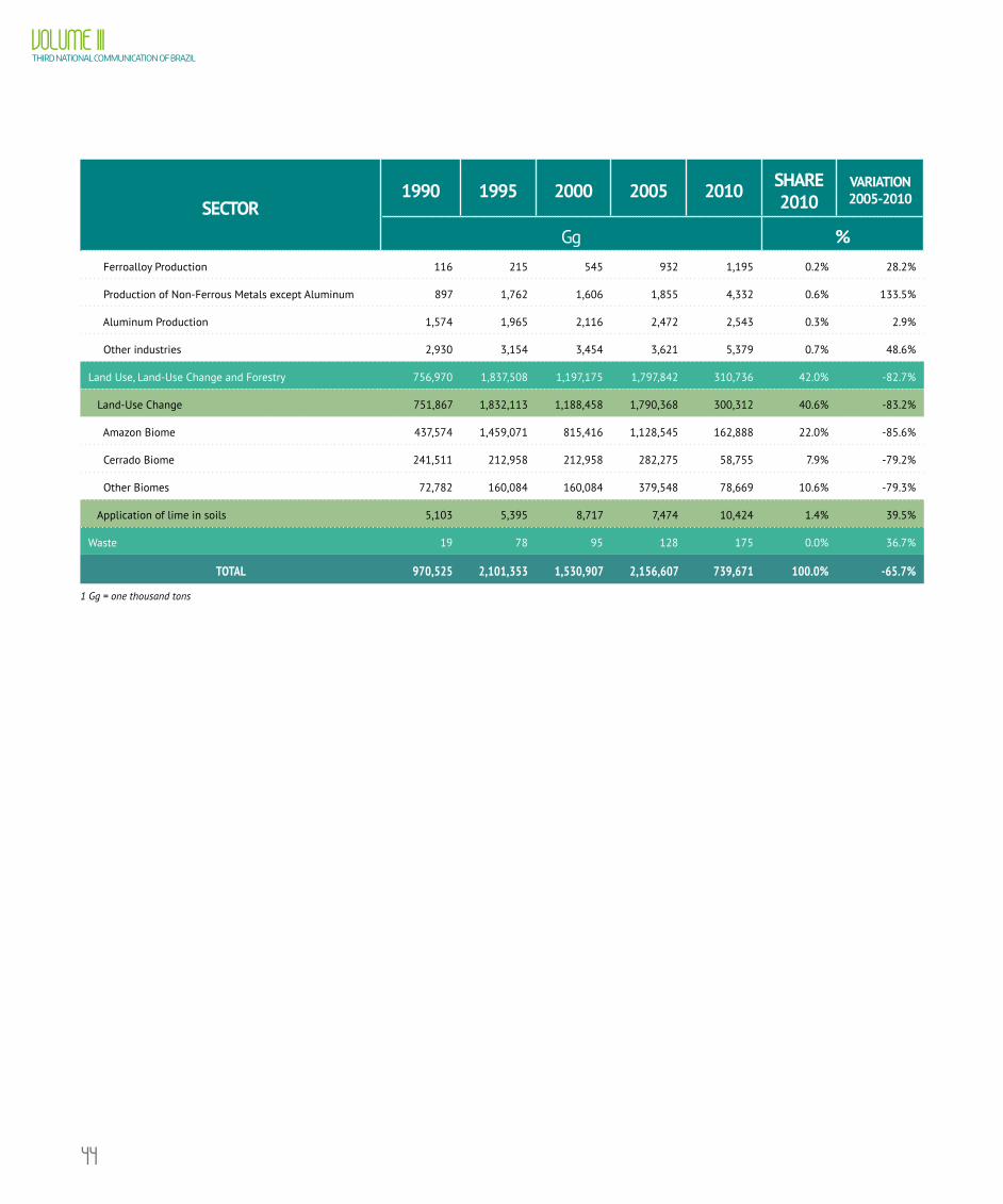
2.1. CARBON DIOXIDE EMISSIONSCO2 emissions result from various activities. Generally, the main source of emissions is the use of fossil fuels
for energy generation. Other important emission sources are the industrial processes of cement, lime, soda ash,
ammonia, and aluminum production, as well as waste incineration.
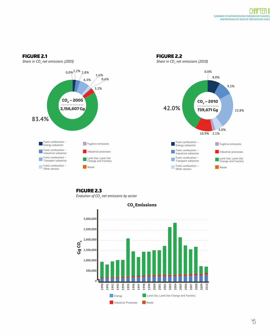
Historically, in Brazil, the largest share of estimated CO2 net emissions comes from land-use change,
particularly the conversion of forest land to agricultural land and livestock production. However, a significant
reduction in the emissions from this sector has been observed in recent years, which has contributed to the
increased participation of the Energy Sector in total CO2 emissions in 2010. It is also worth mentioning the
large share of renewable energy in the Brazilian energy mix, due to of hydroelectric power generation, use of
ethanol in transportation and sugar cane bagasse and charcoal in industry. Table 2.1 and Figures 2.2 and 2.3
summarize CO2 net emissions, per sector.
The Energy sector comprises emissions from fossil fuel combustion and fugitive emissions. Fugitive emissions
include flaring of gas in platforms and refineries, and the spontaneous combustion of coal in deposits and waste
piles. In 2010, CO2 emissions from the energy sector accounted for 47.0% of total CO2 emissions, having increased
by 19.7% in relation to 2005 emissions. The transport subsector alone represented 48.9% of CO2 emissions in the
Energy sector, and 22.8% of total CO2 emissions in 2010.
Emissions from industrial processes accounted for 10.9% of total emissions in 2010, with the production of iron
and steel accounting for the largest share (47.5%). From 2005 to 2010, emissions from industrial processes ranged
by 18.8%.
43
The Land Use, Land-Use Change and Forestry Sector was responsible for the greatest share of CO2 emissions,
and by all CO2 removals, which have included management of protected areas, regeneration of abandoned areas,
and change in soil carbon stock, with net emissions of the sector responding for 42.0% of total CO2 net emissions in
2010. Conversion of forest land to other uses, particularly agricultural land, made up to almost the total emissions
of CO2 in the sector, being the small portion remaining due to the application of limestone to agricultural soils.
The Waste Sector contributed minimally to CO2 emissions because of waste incineration containing non-
renewable carbon.
TABLE 2.1 CO2 net emissions
SECTOR 1990 1995 2000 2005 2010 SHARE
2010VARIATION 2005-2010
Gg %Energy 169,985 209,124 267,646 290,621 347,974 47.0% 19.7%
Fossil Fuels Combustion 162,431 201,610 256,909 276,744 332,760 45.0% 20.2%
Energy Subsector 21,271 25,281 40,484 47,343 58,857 8.0% 24.3%
Industrial Subsector 35,559 43,068 59,008 60,019 68,306 9.2% 13.8%
Steel Industry 4,436 5,387 4,657 5,526 5,642 0.8% 2.1%
Chemical Industry 8,606 10,057 13,942 14,624 13,847 1.9% -5.3%
Other Industries 22,517 27,623 40,409 39,869 48,817 6.6% 22.4%
Transport Subsector 79,338 100,457 121,748 135,182 168,364 22.8% 24.5%
Air Transport 4,232 4,732 6,206 6,316 9,751 1.3% 54.4%
Road Transport 70,094 90,916 111,337 123,519 151,481 20.5% 22.6%
Other Means of Transportation 5,012 4,809 4,205 5,347 7,132 1.0% 33.4%
Residential Subsector 13,842 15,942 17,179 15,591 17,249 2.3% 10.6%
Agricultural Subsector 9,846 13,222 14,152 14,964 17,346 2.3% 15.9%
Other Sectors 2,576 3,640 4,338 3,645 2,638 0.4% -27.6%
Fugitive Emissions 7,554 7,514 10,737 13,877 15,214 2.1% 9.6%
Coal Mining 1,353 920 1,291 1,381 1,846 0.2% 33.7%
Extraction and Transportation of Oil and Natural Gas 6,201 6,594 9,446 12,496 13,368 1.8% 7.0%
Industrial Processes 43,551 54,643 65,991 68,016 80,786 10.9% 18.8%
Cement Production 11,062 11,528 16,047 14,349 21,288 2.9% 48.4%
Lime Production 3,688 4,104 5,008 5,356 5,950 0.8% 11.1%
Ammonia Production 1,683 1,785 1,663 1,922 1,739 0.2% -9.5%
Iron and Steel Production 21,601 30,130 35,552 37,509 38,360 5.2% 2.3%
continues on the next page
44
VOLUME IIITHIRD NATIONAL COMMUNICATION OF BRAZIL
SECTOR 1990 1995 2000 2005 2010 SHARE
2010VARIATION 2005-2010
Gg % Ferroalloy Production 116 215 545 932 1,195 0.2% 28.2%
Production of Non-Ferrous Metals except Aluminum 897 1,762 1,606 1,855 4,332 0.6% 133.5%
Aluminum Production 1,574 1,965 2,116 2,472 2,543 0.3% 2.9%
Other industries 2,930 3,154 3,454 3,621 5,379 0.7% 48.6%
Land Use, Land-Use Change and Forestry 756,970 1,837,508 1,197,175 1,797,842 310,736 42.0% -82.7%
Land-Use Change 751,867 1,832,113 1,188,458 1,790,368 300,312 40.6% -83.2%
Amazon Biome 437,574 1,459,071 815,416 1,128,545 162,888 22.0% -85.6%
Cerrado Biome 241,511 212,958 212,958 282,275 58,755 7.9% -79.2%
Other Biomes 72,782 160,084 160,084 379,548 78,669 10.6% -79.3%
Application of lime in soils 5,103 5,395 8,717 7,474 10,424 1.4% 39.5%
Waste 19 78 95 128 175 0.0% 36.7%
TOTAL 970,525 2,101,353 1,530,907 2,156,607 739,671 100.0% -65.7%
1 Gg = one thousand tons
45
CHAPTER IISUMMARY OF ANTHROPOGENIC EMISSIONS BY SOURCES
AND REMOVALS BY SINKS OF GREENHOUSE GASES
FIGURE 2.1 Share in CO2 net emissions (2005)
FIGURE 2.2 Share in CO2 net emissions (2010)
CO2 – 2005
2,156,607 Gg
Fuels combustion – Industrial subsector
Fuels combustion – Transport subsector
Fuels combustion – Other sectors
Fugitive emissions
Industrial processes
Land Use, Land-Use Change and Forestry
Waste
2.2% 2.8%
6.3%1.6%
0.6%
3.2%
83.4%
0.0%
Fuels combustion – Energy subsector
CO2 – 2010
739,671 Gg
Fuels combustion – Industrial subsector
Fuels combustion – Transport subsector
Fuels combustion – Other sectors
Fugitive emissions
Industrial processes
Land Use, Land-Use Change and Forestry
Waste
Fuels combustion – Energy subsector
8.0%
9.2%
22.8%
5.0%2.1%10.9%
42.0%
0.0%
FIGURE 2.3 Evolution of CO2 net emissions by sector
Energy
Industrial Processes
Land Use, Land-Use Change and Forestry
Waste
CO2 Emissions
Gg
CO
2
0
500,000
1,000,000
1,500,000
2,000,000
2,500,000
3,000,000
1990
1991
1992
1993
1994
1995
1996
1997
1998
1999
2000
2001
2002
2003
2004
2005
2006
2007
2008
2009
2010

46
VOLUME IIITHIRD NATIONAL COMMUNICATION OF BRAZIL
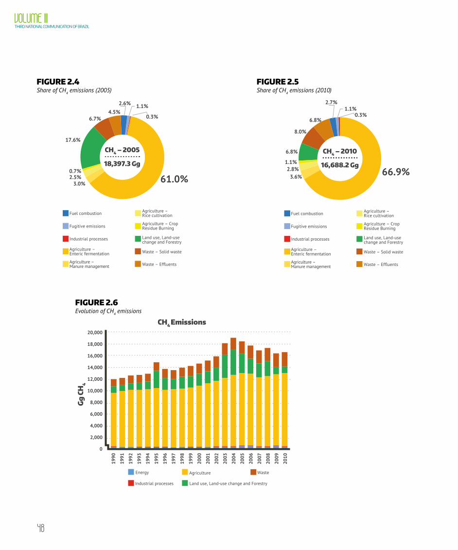
2.2. METHANE EMISSIONSCH4 emissions result from many activities, including landfills, wastewater treatment, oil and natural gas
processing systems, agricultural activities, coal mining, fossil fuel and biomass combustion, conversion of forest
land to other uses and some industrial processes.
In Brazil, the Agriculture Sector is the most significant contributor to CH4 emissions (74.4% in 2010), where the
main emission source is enteric fermentation (eructation) of ruminants, almost all of which from the cattle herd,
the world’s second largest cattle herd. In 2010, CH4 emissions associated with enteric fermentation were estimated
at 11,158 Gg, 89.9% of total CH4 emissions in the Agriculture sector. Manure management, irrigated rice cultivation,
and field burning of agricultural crops corresponded to remaining emissions.
In the Energy sector, CH4 emissions occur as a result of imperfect combustion of fuels and also because of CH4
leakage during the processes of natural gas production and transportation, and coal mining. CH4 emissions from
the energy sector represented, in 2010, 3,8% of total CH4 emissions, having increased by 8.1% in relation to 2005
emissions.
In the Industrial Processes sector, CH4 emissions occur during petrochemical production, but have little
participation in Brazilian emissions.
Emissions in the Waste Sector represented 14.8% of total CH4 emissions in 2010, while solid waste disposal was
responsible for 53,9% of this sector. In the 2005-2010 period, CH4 emissions from the Waste Sector increased by 19,4%.
In the Land Use, Land-Use Change and Forestry sector, CH4 emissions are caused by biomass burning in
deforestation areas. Such emissions represented 6.8% of total CH4 emissions in 2010.
TABLE 2.2 CH4 Emissions
SECTOR 1990 1995 2000 2005 2010 SHARE
2010VARIATION 2005-2010
Gg %Energy 545.8 473.6 511.8 684.8 629.1 3.8% -8.1%
Fuel combustion 455.3 388.1 392.8 478.6 448.2 2.7% -6.4%
Energy subsector 25.5 23.1 20.7 29.2 34.5 0.2% 18.2%
Industry subsector 15.7 18.1 19.9 28.4 34.4 0.2% 21.1%
Iron and Steel industry 0.2 0.2 0.2 0.2 0.3 0.0% 50.0%
Other industries 15.5 17.9 19.7 28.2 34.1 0.2% 20.9%
Transport subsector 72.6 85.8 75.6 74.4 66.9 0.4% -10.1%
Residential subsector 318.4 243.7 261.5 327.6 290.1 1.7% -11.4%
Other sectors 23.1 17.4 15.1 19.0 22.3 0.1% 17.4%
continues on the next page

47
CHAPTER IISUMMARY OF ANTHROPOGENIC EMISSIONS BY SOURCES
AND REMOVALS BY SINKS OF GREENHOUSE GASES
SECTOR 1990 1995 2000 2005 2010 SHARE
2010VARIATION 2005-2010
Gg % Fugitive emissions 90.5 85.5 119.0 206.2 180.9 1.1% -12.3%
Coal mining 49.7 41.1 43.3 49.1 39.2 0.2% -20.2%
Oil and Natural Gas Production and Transport 40.8 44.4 75.7 157.1 141.7 0.8% -9.8%
Industrial processes 47.1 41.2 43.7 54.9 45.3 0.3% -17.5%
Chemical industry 5.2 6.6 9.0 9.4 11.8 0.1% 25.5%
Production of metals 41.9 34.6 34.7 45.5 33.5 0.2% -26.4%
Agriculture 9,185.6 10,058.2 10,382.3 12,357.7 12,415.6 74.4% 0.5%
Enteric fermentation 8,223.9 8,957.1 9,349.5 11,213.8 11,158.0 66.9% -0.5%
Cattle 7,808.9 8,534.3 9,005.8 10,855.7 10,798.4 64.7% -0.5%
Dairy cattle 1,197.7 1,297.1 1,177.9 1,371.4 1,424.0 8.5% 3.8%
Beef cattle 6,611.2 7,237.2 7,827.9 9,484.3 9,374.4 56.2% -1.2%
Other animals 415.0 422.8 343.7 358.1 359.6 2.2% 0.4%
Manure Management 421.6 471.6 479.7 543.9 608.1 3.6% 11.8%
Cattle 191.2 208.7 215.9 254.0 258.7 1.6% 1.9%
Dairy cattle 35.9 38.5 34.1 39.7 44.0 0.3% 10.8%
Beef cattle 155.3 170.2 181.8 214.3 214.7 1.3% 0.2%
Pigs 159.5 173.7 166.5 178.7 214.9 1.3% 20.3%
Poultry 48.4 66.3 78.1 91.5 115.3 0.7% 26.0%
Other animals 22.5 22.9 19.2 19.7 19.2 0.1% -2.5%
Rice cultivation 433.6 510.8 448.1 463.7 464.2 2.8% 0.1%
Crop residues burning 106.5 118.7 105.0 136.3 185.3 1.1% 36.0%
Land Use, Land-Use Change and Forestry 1,041.5 2,895.7 2,048.8 3,237.9 1,135.5 6.8% -64.9%
Waste 1,173.7 1,418.7 1,754.2 2,062.0 2,462.7 14.8% 19.4%
Solid waste 824.4 965.3 1,149.4 1,237.1 1,327.0 8.0% 7.3%
Effluents 349.3 453.4 604.8 824.9 1,135.7 6.8% 37.7%
Industrial 82.6 149.1 233.1 388.3 622.9 3.7% 60.4%
Domestic 266.7 304.3 371.7 436.6 512.8 3.1% 17.5%
TOTAL 11,993.7 14,887.4 14,740.8 18,397.3 16,688.2 100.0% -9.3%
48
VOLUME IIITHIRD NATIONAL COMMUNICATION OF BRAZIL
FIGURE 2.4 Share of CH4 emissions (2005)
FIGURE 2.5 Share of CH4 emissions (2010)
Fuel combustion
Fugitive emissions
Industrial processes
Agriculture – Enteric fermentation
Agriculture – Manure management
Agriculture –Rice cultivation
Agriculture – CropResidue Burning
Land use, Land-use change and Forestry
Waste – Solid waste
Waste – Effluents
2.6% 1.1%
0.3%
61.0%3.0%2.5%0.7%
17.6%
6.7%4.5%
CH4 – 2005
18,397.3 Gg
Fuel combustion
Fugitive emissions
Industrial processes
Agriculture – Enteric fermentation
Agriculture – Manure management
Agriculture –Rice cultivation
Agriculture – CropResidue Burning
Land use, Land-use change and Forestry
Waste – Solid waste
Waste – Effluents
2.7%1.1%
0.3%
66.9%
6.8%
8.0%
6.8%
1.1%2.8%
3.6%
CH4 – 2010
16,688.2 Gg
FIGURE 2.6 Evolution of CH4 emissions
Energy
Industrial processes
Agriculture
Land use, Land-use change and Forestry
Waste
1990
1991
1992
1993
1994
1995
1996
1997
1998
1999
2000
2001
2002
2003
2004
2005
2006
2007
2008
2009
2010
0
2,000
4,000
6,000
8,000
10,000
12,000
14,000
16,000
18,000
20,000
Gg
CH
4
CH4 Emissions

49
CHAPTER IISUMMARY OF ANTHROPOGENIC EMISSIONS BY SOURCES
AND REMOVALS BY SINKS OF GREENHOUSE GASES
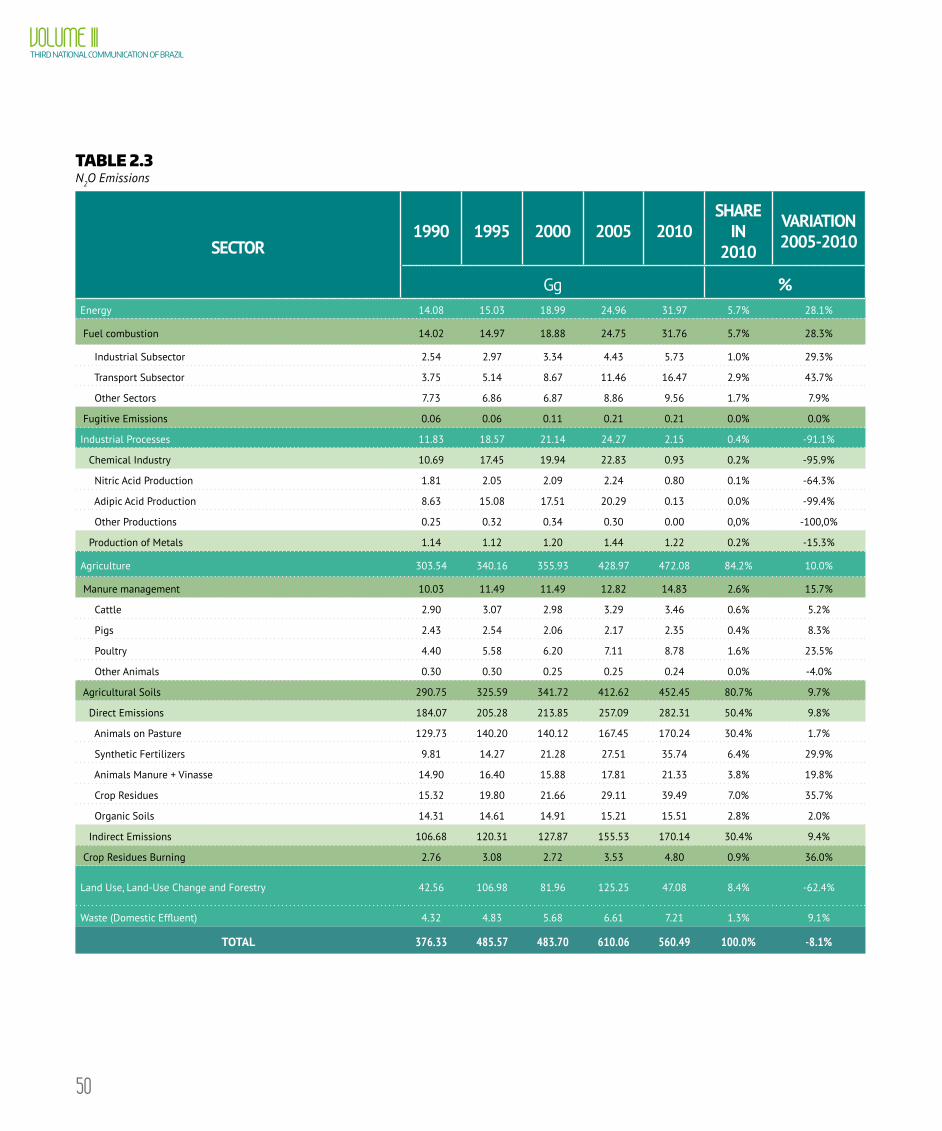
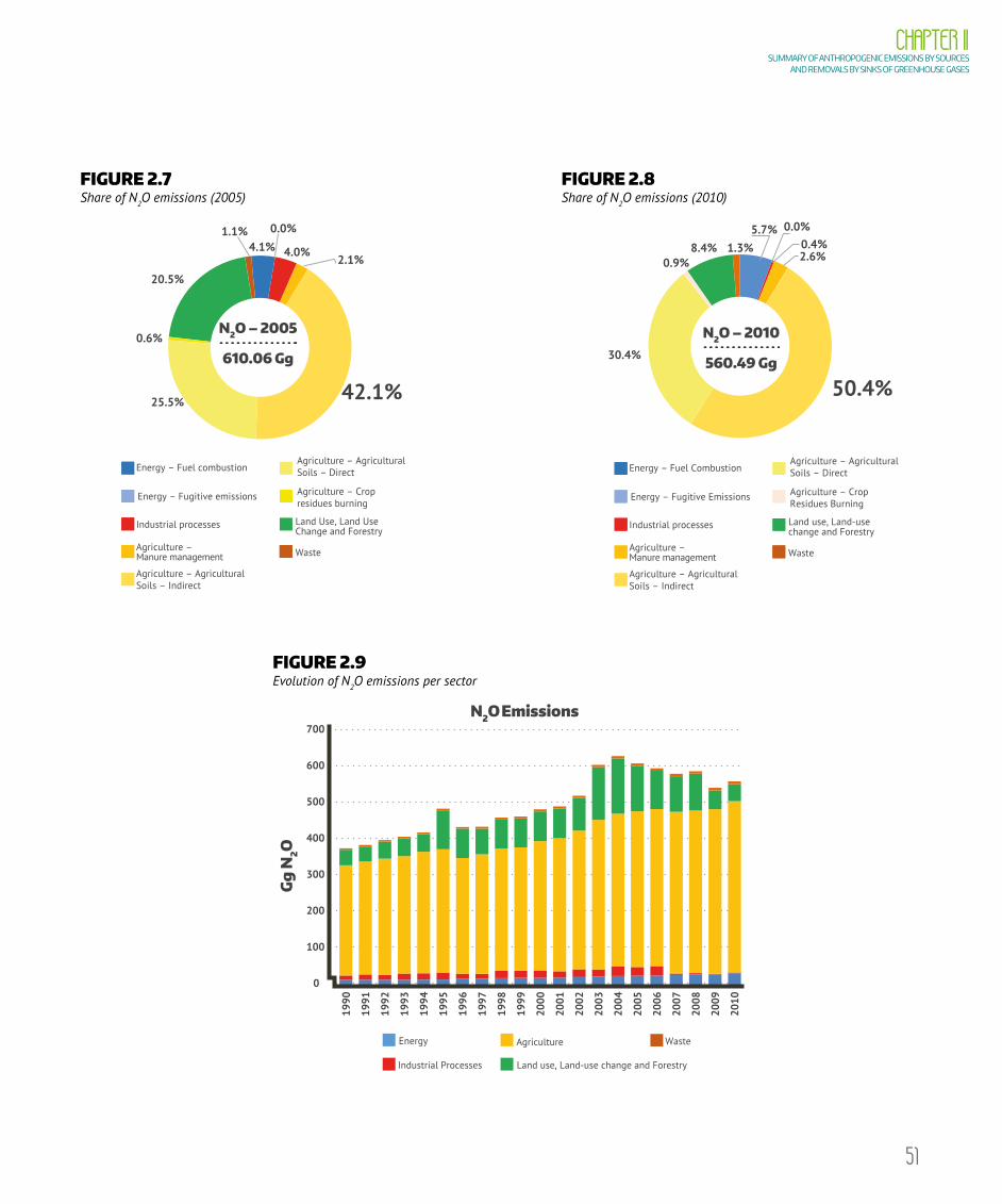
2.3. NITROUS OXIDE EMISSIONSN2O emissions result from various activities, including agricultural practices, industrial processes, biomass and
fossil fuel combustion and conversion of forest land to other uses.
In Brazil, N2O emissions occur predominantly in the Agriculture Sector (84.2% in 2010), mainly from manure
deposition in pasture. N2O emissions in the Sector grew by 10.0% between 2005 and 2010. Direct emissions of
agricultural soils account for 59.8% (36.1%, if taken into consideration only emissions of animals on pastures) in
the Agriculture Sector, in 2010; indirect emissions respond for 36.0%, followed by emissions from animal manure
(3.1%) and crop residues burning (0.9%).
N2O emissions in the Energy Sector represented only 5.7% of total N2O emissions in 2010, basically due to
imperfect fuel burning.
In the Industrial Processes sector, N2O emissions occur during the production of nitric and adipic acid – which is
very much reduced in both cases due to CDM projects aimed at reducing emissions, implemented as at 2007 – and
also in metal production; however, they represent, jointly, only 0.4% of total N2O emissions in 2010.
In the Land-use Change and Forestry Sector, N2O emissions occur mainly by biomass burning in deforestation
areas. These emissions accounted for 8.4% of total N2O emissions in 2010.
In the Waste sector, N2O emissions basically occur due to the presence of nitrogen in the protein for human
consumption, which ends up being released into the ground or into water bodies. Their contribution to total N2O
emissions was 1.3% in 2010. A much smaller share comes from waste incineration.
50
VOLUME IIITHIRD NATIONAL COMMUNICATION OF BRAZIL
TABLE 2.3 N2O Emissions
SECTOR1990 1995 2000 2005 2010
SHARE IN
2010
VARIATION 2005-2010
Gg %Energy 14.08 15.03 18.99 24.96 31.97 5.7% 28.1%
Fuel combustion 14.02 14.97 18.88 24.75 31.76 5.7% 28.3%
Industrial Subsector 2.54 2.97 3.34 4.43 5.73 1.0% 29.3%
Transport Subsector 3.75 5.14 8.67 11.46 16.47 2.9% 43.7%
Other Sectors 7.73 6.86 6.87 8.86 9.56 1.7% 7.9%
Fugitive Emissions 0.06 0.06 0.11 0.21 0.21 0.0% 0.0%
Industrial Processes 11.83 18.57 21.14 24.27 2.15 0.4% -91.1%
Chemical Industry 10.69 17.45 19.94 22.83 0.93 0.2% -95.9%
Nitric Acid Production 1.81 2.05 2.09 2.24 0.80 0.1% -64.3%
Adipic Acid Production 8.63 15.08 17.51 20.29 0.13 0.0% -99.4%
Other Productions 0.25 0.32 0.34 0.30 0.00 0,0% -100,0%
Production of Metals 1.14 1.12 1.20 1.44 1.22 0.2% -15.3%
Agriculture 303.54 340.16 355.93 428.97 472.08 84.2% 10.0%
Manure management 10.03 11.49 11.49 12.82 14.83 2.6% 15.7%
Cattle 2.90 3.07 2.98 3.29 3.46 0.6% 5.2%
Pigs 2.43 2.54 2.06 2.17 2.35 0.4% 8.3%
Poultry 4.40 5.58 6.20 7.11 8.78 1.6% 23.5%
Other Animals 0.30 0.30 0.25 0.25 0.24 0.0% -4.0%
Agricultural Soils 290.75 325.59 341.72 412.62 452.45 80.7% 9.7%
Direct Emissions 184.07 205.28 213.85 257.09 282.31 50.4% 9.8%
Animals on Pasture 129.73 140.20 140.12 167.45 170.24 30.4% 1.7%
Synthetic Fertilizers 9.81 14.27 21.28 27.51 35.74 6.4% 29.9%
Animals Manure + Vinasse 14.90 16.40 15.88 17.81 21.33 3.8% 19.8%
Crop Residues 15.32 19.80 21.66 29.11 39.49 7.0% 35.7%
Organic Soils 14.31 14.61 14.91 15.21 15.51 2.8% 2.0%
Indirect Emissions 106.68 120.31 127.87 155.53 170.14 30.4% 9.4%
Crop Residues Burning 2.76 3.08 2.72 3.53 4.80 0.9% 36.0%
Land Use, Land-Use Change and Forestry 42.56 106.98 81.96 125.25 47.08 8.4% -62.4%
Waste (Domestic Effluent) 4.32 4.83 5.68 6.61 7.21 1.3% 9.1%
TOTAL 376.33 485.57 483.70 610.06 560.49 100.0% -8.1%
51
CHAPTER IISUMMARY OF ANTHROPOGENIC EMISSIONS BY SOURCES
AND REMOVALS BY SINKS OF GREENHOUSE GASES
FIGURE 2.7 Share of N2O emissions (2005)
FIGURE 2.8 Share of N2O emissions (2010)
Energy – Fuel combustion
Energy – Fugitive emissions
Agriculture – Agricultural Soils – Indirect
Agriculture – Agricultural Soils – Direct
Agriculture – Crop residues burning
4.1% 4.0%
0.0%
2.1%
42.1%25.5%
0.6%
20.5%
1.1%
N2O – 2005
610.06 Gg
Industrial processes
Agriculture – Manure management
Land Use, Land Use Change and Forestry
Waste
Energy – Fuel Combustion
Energy – Fugitive Emissions
Agriculture – Agricultural Soils – Indirect
Agriculture – Agricultural Soils – Direct
Agriculture – Crop Residues Burning
N2O – 2010
560.49 Gg
Industrial processes
Agriculture – Manure management
Land use, Land-use change and Forestry
Waste
50.4%
30.4%
0.9%8.4% 1.3%
0.0%0.4%2.6%
5.7%
FIGURE 2.9 Evolution of N2O emissions per sector
Gg
N2O
Energy
Industrial Processes
Agriculture
Land use, Land-use change and Forestry
Waste
0
100
200
300
400
500
600
700
1990
1991
1992
1993
1994
1995
1996
1997
1998
1999
2000
2001
2002
2003
2004
2005
2006
2007
2008
2009
2010
N2O Emissions

52
VOLUME IIITHIRD NATIONAL COMMUNICATION OF BRAZIL
2.4. HYDROFLUOROCARBONS, PERFLUOROCARBONS AND SULFUR HEXAFLUORIDE EMISSIONS
HFCs, PFCs and SF6 gases do not originally exist in nature, being synthesized only by human activities.
Brazil does not produce HFCs. Imports of a little over 7 thousand tons of HFC-134a have been recorded since 2010
for use mainly in the air-conditioning and refrigeration subsector, with total fugitive emissions estimated at 2,719.6 t
HFC-134a that year. Imports of other gases within the same group totaled a little over one thousand tons in 2010.
PFCs (CF4 and C2F6) emissions occur during the manufacturing process of aluminum and result from the anodic
effect that takes place when the amount of aluminum oxide decreases in the electrolytic process pots. PFCs
emissions were estimated at 76.7 t CF4 and 5.9 t C2F6 in 2010, indicating a reduction of 38.1% and 43.3% in relation
to 2005, respectively.
SF6 is used as an insulator in large-sized electrical equipment. Emissions of this gas result from leakages from
equipment, especially during maintenance or when equipment is discarded. Historically, this gas had also been
used in the production process of magnesium to prevent metal oxidation in its liquid phase, but this stopped in
2010 due to a CDM project aimed at replacing this gas with SO2. SF6 emissions were estimated at 8.7 tons in 2010.
Table 2.4 summarizes HFCs, PFCs and SF6 emissions.
TABLE 2.4 HFCs, PFCs and SF6 Emissions
GAS ACTIVITY1990 1995 2000 2005 2010 VARIATION
2005-2010
Gg %HFC-23 HCFC-22 production 0.1202 0.1530 0.0000 0.0000 0.0000 NA
HFC-32 Potential emissions 0.0000 0.0000 0.0000 0.0000 0.1059 NA
HFC-125 Potential emissions 0.0000 0.0000 0.0071 0.1249 0.5012 301.2%
HFC-134a Actual emissions by use 0.0004 0.0028 0.4988 1.2279 2.7196 121.5%
HFC-143a Potential emissions 0.0000 0.0000 0.0075 0.0929 0.4671 403.0%
HFC-152a Potential emissions 0.0000 0.0000 0.0001 0.1748 0.0000 -100.0%
CF4 Aluminum production 0.3022 0.3060 0.1465 0.1239 0.0767 -38.1%
C2F6 Aluminum production 0.0263 0.0264 0.0117 0.0104 0.0059 -43.3%
SF6
Magnesium production 0.0058 0.0101 0.0103 0.0191 0.0000 -100.0%
Electrical equipment 0.0042 0.0041 0.0050 0.0061 0.0087 42.6%
Total SF6 0.0100 0.0142 0.0153 0.0252 0.0087 -65.5%

53
CHAPTER IISUMMARY OF ANTHROPOGENIC EMISSIONS BY SOURCES
AND REMOVALS BY SINKS OF GREENHOUSE GASES
2.5. INDIRECT GREENHOUSE GASESVarious gases influence the chemical reactions that occur in the troposphere and thus play an indirect role in
increasing the radiative effect. Such gases include CO, NOX and NMVOC. Emissions of these gases result mostly
from human activities.
The majority of CO and NOx emissions result from imperfect combustion either of fuels in the Energy Sector
or waste in the Agriculture Sector or biomass in deforestation areas in the Land-Use Change and Forestry Sector.
A small portion of CO emissions results from production processes, basically of aluminum; in relation to NOx, the
remaining emissions also occur in the Industrial Processes sector as a result of the production of nitric acid and
aluminum. CO emissions decreased by 49,7% between 2005 and 2010 and NOx emissions dropped by 15.7% in the
same period, mainly because of the decrease in the deforestation rate in Brazil.
Most NMVOC emissions result from the production and use of solvent (74.4% in 2010), but also from imperfect
fuel combustion (14.1% in 2010) or industrial processes (11.5% in 2010).
Tables 2.5, 2.6 and 2.7 present CO, NOx and NMVOC emissions, respectively.

54
VOLUME IIITHIRD NATIONAL COMMUNICATION OF BRAZIL
TABLE 2.5 CO Emissions
SECTOR 1990 1995 2000 2005 2010 SHARE
2010VARIATION 2005-2010
Gg %Energy 9,592.6 9,636.3 8,181.0 8,194.7 7,695.9 22.0% -6.1%
Fossil Fuel Combustion 9,592.6 9,636.3 8,181.0 8,194.7 7,695.9 22.0% -6.1%
Energy Subsector 1,398.0 1,208.5 1,104.3 1,528.1 1,617.9 4.6% 5.9%
Industrial Subsector 758.1 815.1 1,036.8 1,283.5 1,710.3 4.9% 33.3%
Steel Industry 2.5 3.2 8.2 11.4 11.4 0.0% 0.0%
Food and Beverage 182.3 175.8 187.5 204.8 260.9 0.7% 27.4%
Other Industries 573.3 636.1 841.1 1,067.3 1,438.0 4.1% 34.7%
Transport Subsector 5,902.9 6,419.3 4,776.2 3,807.3 2,933.7 8.4% -22.9%
Road Transportation 5,856.4 6,373.4 4,724.6 3,761.8 2,875.0 8.2% -23.6%
Other Transports 46.5 45.9 51.6 45.5 58.7 0.2% 29.0%
Residential Subsector 1,443.2 1,098.7 1,172.3 1,468.4 1,306.7 3.7% -11.0%
Other Sectors 90.4 94.7 91.4 107.4 127.3 0.4% 18.5%
Industrial Processes 900.8 778.0 790.5 1,022.4 809.6 2.3% -20.8%
Iron and Steel Production 775.0 656.2 676.1 867.3 633.2 1.8% -27.0%
Ferroalloys Production 60.8 64.2 72.5 96.7 96.7 0.3% 0.0%
Non-Ferrous Metals Production 44.4 27.6 3.7 4.6 4.9 0.0% 6.5%
Other Productions 20.6 30.0 38.2 53.8 74.8 0.2% 39.0%
Agriculture 3,627.6 4,045.8 3,576.4 4,644.4 6,313.5 18.0% 35.9%
Cotton crop waste burning 128.4 0.0 0.0 0.0 0.0 0.0% NA
Sugarcane burning 3,499.2 4,045.8 3,576.4 4,644.4 6,313.5 18.0% 35.9%
Land Use, Land-Use Change and Forestry 18,429.4 48,855.6 35,879.9 55,810.0 20,231.4 57.7% -63.7%
TOTAL 32,550.4 63,315.7 48,427.8 69,671.5 35,050.4 100.0% -49.7%

55
CHAPTER IISUMMARY OF ANTHROPOGENIC EMISSIONS BY SOURCES
AND REMOVALS BY SINKS OF GREENHOUSE GASES
TABLE 2.6 NOx Emissions
SECTOR 1990 1995 2000 2005 2010 SHARE
2010VARIATION 2005-2010
Gg %Energy 1,639.8 1,977.5 2,273.3 2,346.4 2,567.1 74.9% 9.4%
Fossil Fuel Combustion 1,639.8 1,977.5 2,273.3 2,346.4 2,567.1 74.9% 9.4%
Energy Subsector 214.9 266.6 395.0 479.8 577.5 16.8% 20.4%
Industrial Subsector 134.8 169.9 222.7 242.9 286.6 8.4% 18.0%
Steel Industry 10.4 12.3 11.1 12.1 12.0 0.3% -0.8%
Other Industries 124.4 157.6 211.6 230.8 274.6 8.0% 19.0%
Transport Subsector 1,138.8 1,352.6 1,457.4 1,414.0 1,459.7 42.6% 3.2%
Road Transportation 1021.6 1,237.5 1,355.3 1,287.4 1,290.6 37.6% 0.2%
Other Transports 117.2 115.1 102.1 126.6 169.1 4.9% 33.6%
Residential Subsector 29.2 26.3 28.5 31.3 30.6 0.9% -2.2%
Other Sectors 122.1 162.1 169.7 178.4 212.7 6.2% 19.2%
Industrial Processes 42.1 53.2 94.9 125.2 100.8 2.9% -19.5%
Production of metals 36.0 44.5 84.0 110.1 80.1 2.3% -27.2%
Other productions 6.1 8.7 10.9 15.1 20.7 0.6% 37.1%
Agriculture 98.6 109.9 97.2 126.2 171.6 5.0% 36.0%
Cotton crop waste burning 3.5 0.0 0.0 0.0 0.0 0.0% NA
Sugarcane burning 95.1 109.9 97.2 126.2 171.6 5.0% 36.0%
Land Use, Land-Use Change and Forestry 526.7 1,196.0 993.8 1,470.3 589.9 17.2% -59.9%
TOTAL 2,307.2 3,336.6 3,459.2 4,068.1 3,429.4 100.0% -15.7%
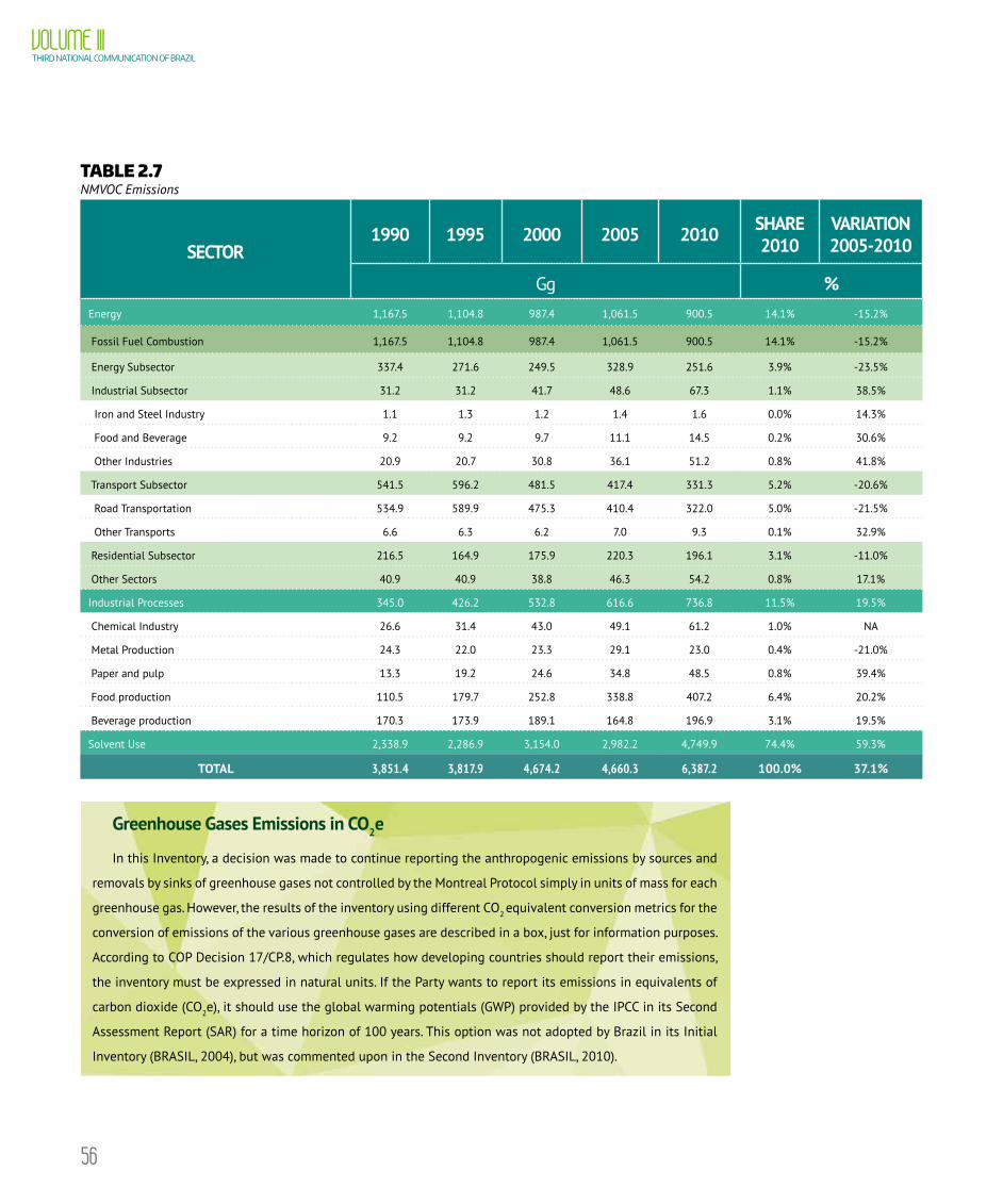
56
VOLUME IIITHIRD NATIONAL COMMUNICATION OF BRAZIL
TABLE 2.7 NMVOC Emissions
SECTOR 1990 1995 2000 2005 2010 SHARE
2010VARIATION 2005-2010
Gg %Energy 1,167.5 1,104.8 987.4 1,061.5 900.5 14.1% -15.2%
Fossil Fuel Combustion 1,167.5 1,104.8 987.4 1,061.5 900.5 14.1% -15.2%
Energy Subsector 337.4 271.6 249.5 328.9 251.6 3.9% -23.5%
Industrial Subsector 31.2 31.2 41.7 48.6 67.3 1.1% 38.5%
Iron and Steel Industry 1.1 1.3 1.2 1.4 1.6 0.0% 14.3%
Food and Beverage 9.2 9.2 9.7 11.1 14.5 0.2% 30.6%
Other Industries 20.9 20.7 30.8 36.1 51.2 0.8% 41.8%
Transport Subsector 541.5 596.2 481.5 417.4 331.3 5.2% -20.6%
Road Transportation 534.9 589.9 475.3 410.4 322.0 5.0% -21.5%
Other Transports 6.6 6.3 6.2 7.0 9.3 0.1% 32.9%
Residential Subsector 216.5 164.9 175.9 220.3 196.1 3.1% -11.0%
Other Sectors 40.9 40.9 38.8 46.3 54.2 0.8% 17.1%
Industrial Processes 345.0 426.2 532.8 616.6 736.8 11.5% 19.5%
Chemical Industry 26.6 31.4 43.0 49.1 61.2 1.0% NA
Metal Production 24.3 22.0 23.3 29.1 23.0 0.4% -21.0%
Paper and pulp 13.3 19.2 24.6 34.8 48.5 0.8% 39.4%
Food production 110.5 179.7 252.8 338.8 407.2 6.4% 20.2%
Beverage production 170.3 173.9 189.1 164.8 196.9 3.1% 19.5%
Solvent Use 2,338.9 2,286.9 3,154.0 2,982.2 4,749.9 74.4% 59.3%
TOTAL 3,851.4 3,817.9 4,674.2 4,660.3 6,387.2 100.0% 37.1%
Greenhouse Gases Emissions in CO2e
In this Inventory, a decision was made to continue reporting the anthropogenic emissions by sources and
removals by sinks of greenhouse gases not controlled by the Montreal Protocol simply in units of mass for each
greenhouse gas. However, the results of the inventory using different CO2 equivalent conversion metrics for the
conversion of emissions of the various greenhouse gases are described in a box, just for information purposes.
According to COP Decision 17/CP.8, which regulates how developing countries should report their emissions,
the inventory must be expressed in natural units. If the Party wants to report its emissions in equivalents of
carbon dioxide (CO2e), it should use the global warming potentials (GWP) provided by the IPCC in its Second
Assessment Report (SAR) for a time horizon of 100 years. This option was not adopted by Brazil in its Initial
Inventory (BRASIL, 2004), but was commented upon in the Second Inventory (BRASIL, 2010).
57
CHAPTER IISUMMARY OF ANTHROPOGENIC EMISSIONS BY SOURCES
AND REMOVALS BY SINKS OF GREENHOUSE GASES
GWP is based on the relative importance of greenhouse gases in relation to carbon dioxide in the production
of a quantity of energy (per unit area) several years after an emission impulse. This metric is characterized by
the integration of the radiative forcing (RF) of an emission pulse of a certain substance in a given time horizon.
Since the IPCC Third Assessment Report (TAR) (IPCC, 2001), it has been concluded that RF is a useful tool
to give a first-order estimate on the global relation between climate impacts and different mechanisms
of climate change (RAMASWAMY, et al. , 2001), and the value of the radiative forcing can be used to
estimate the overall balance on the change in average surface temperature because of different agents
involved in the system.
Although the use of GWP-SAR is suggested for inventories of non Annex I Parties, regular evaluation reports
of the IPCC present new values for GWP of gases. As of the IPCC Fifth Assessment Report (AR5) (IPCC, 2014),
the most recent publication on the subject, we can see for the first time the values for the Global Temperature
Potential (GTP), which Brazil also considers important. According to the IPCC, GTP is characterized as being an
endpoint metric based on temperature change, i.e., it is correlated to change in the average temperature of
global surface in a given future time horizon in response to an emission impulse.
According to the IPCC (2014) “the most appropriate metric and time horizon will depend on which aspects
of climate change are considered to be more important to a particular use. No metric is able to accurately
compare all the consequences of different emissions, and all of them have constrainsts and uncertainties”1.
IPCC also argues that the Global Temperature Potential (GTP) metric is more suitable for political decisions
based on targets, while the GWP is not directly related to a temperature limit such as the 2°C target2. In light
of this, the GTP metric is more consistent as a contribution to contain a global temperature increase below 2°C
against pre-industrial levels.
The Third Inventory presents the results using three sets of weighting values: the GWP-SAR, determined
by Decision 17/CP.8, the GWP-AR5, with cutting-edge science, and GTP-AR5, an old claiming of Brazil.
Table I presents previous GWP values according to SAR (IPCC, 1995) and GTP and actual GWP values
according to AR5 (IPCC, 2014).
12
1 IPCC, 2013: Summary for Policymakers. In: Climate Change 2013: The Physical Science Basis. Contribution of Working Group I to the Fifth Assessment Report of the Intergovernmental Panel on Climate Change [Stocker, T.F., D. Qin, G.-K. Plattner, M. Tignor, S.K. Allen, J. Boschung, A. Nauels, Y. Xia, V. Bex and P.M. Midgley (eds.)]. Cambridge University Press, Cambridge, United Kingdom and New York, NY, USA. SPM D.2 p.15.
2 See: Myhre, G., D. Shindell, F.-M. Bréon, W. Collins, J. Fuglestvedt, J. Huang, D. Koch, J.-F. Lamarque, D. Lee, B. Mendoza, T. Nakajima, A. Robock, G. Stephens, T. Takemura and H. Zhang, 2013: Anthropogenic and Natural Radiative Forcing. In: Climate Change 2013: The Physical Science Basis. Contribution of Working Group I to the Fifth Assessment Report of the Intergovernmental Panel on Climate Change [Stocker, T.F., D. Qin, G.-K. Plattner, M. Tignor, S.K. Allen, J. Boschung, A. Nauels, Y. Xia, V. Bex and P.M. Midgley (eds.)]. Cambridge University Press, Cambridge, United Kingdom and New York, NY, USA. pp. 710-720. See also: Stocker, T.F., D. Qin, G.-K. Plattner, L.V. Alexander, S.K. Allen, N.L. Bindoff, F.-M. Bréon, J.A. Church, U. Cubasch, S. Emori, P. Forster, P. Friedlingstein, N. Gillett, J.M. Gregory, D.L. Hartmann, E. Jansen, B. Kirtman, R. Knutti, K. Krishna Kumar, P. Lemke, J. Marotzke, V. Masson-Delmotte, G.A. Meehl, I.I. Mokhov, S. Piao, V. Ramaswamy, D. Randall, M. Rhein, M. Rojas, C. Sabine, D. Shindell, L.D. Talley, D.G. Vaughan and S.-P. Xie, 2013: Technical Summary. In: Climate Change 2013: The Physical Science Basis. Contribution of Working Group I to the Fifth Assessment Report of the Intergovernmental Panel on Climate Change [Stocker, T.F., D. Qin, G.-K. Plattner, M. Tignor, S.K. Allen, J. Boschung, A. Nauels, Y. Xia, V. Bex and P.M. Midgley (eds.)]. Cambridge University Press, Cambridge, United Kingdom and New York, NY, USA. pp. 58-59.

58
VOLUME IIITHIRD NATIONAL COMMUNICATION OF BRAZIL
TABLE I GWP (100 years) and GTP (100 years) factors
GASGWP
100 YEARS SAR-1995
GWP 100 YEARS AR5-2014
GTP 100 YEARS AR5-2014
CO2 1 1 1
CH4 21 28 4
CH4 fóssil 21 30 6
N2O 310 265 234
HFC-23 11,700 12,400 12,700
HFC-32 650 677 94
HFC-125 2,800 3,170 967
HFC-134a 1,300 1,300 201
HFC-143a 3,800 4,800 2,500
HFC-152 140 16 2
CF4 6,500 6,630 8,040
C2F6 9,200 11,100 13,500
SF6 23,900 23,500 28,200
FIGURE I Evolution of CO2e emissions by different metrics, 1990 to 2010
0
500,000
1,000,000
1,500,000
2,000,000
2,500,000
3,000,000
3,500,000
4,000,000
1990
1991
1992
1993
1994
1995
1996
1997
1998
1999
2000
2001
2002
2003
2004
2005
2006
2007
2008
2009
2010
GWP-SAR GWP-AR5 GTP-AR5
Brazilian Total Emissions
Gg
CO
2e

59
CHAPTER IISUMMARY OF ANTHROPOGENIC EMISSIONS BY SOURCES
AND REMOVALS BY SINKS OF GREENHOUSE GASES
TABLE II Anthropogenic emissions by sources and removals by sinks of greenhouse gases in CO2e using GTP and GWP metrics, by sectors
GWP - SARCO2e (Gg)
1990 1995 2000 2005 2010ENERGY 185,808 223,727 284,273 312,747 371,086
INDUSTRIAL PROCESSES 52,059 65,625 75,581 80,517 89,947
AGRICULTURE 286,998 316,671 328,367 392,491 407,067
LAND USE, LAND-USE
CHANGE AND FORESTRY792,038 1,931,478 1,265,606 1,904,666 349,173
WASTE 26,006 31,370 38,693 45,476 54,127
TOTAL 1,342,909 2,568,872 1,992,520 2,735,898 1,271,399
GWP - AR5CO2e (Gg)
1990 1995 2000 2005 2010ENERGY 189,319 226,707 287,395 316,985 374,554
INDUSTRIAL PROCESSES 52,038 65,283 75,000 79,972 90,866
AGRICULTURE 337,636 371,773 385,027 459,692 472,734
LAND USE, LAND-USE
CHANGE AND FORESTRY797,413 1,946,934 1,276,260 1,921,694 355,002
WASTE 34,027 41,084 50,717 59,613 71,041
TOTAL 1,410,434 2,651,780 2,074,399 2,837,956 1,364,197
GTP - AR5CO2e (Gg)
1990 1995 2000 2005 2010ENERGY 175,786 214,877 274,522 299,773 358,464
INDUSTRIAL PROCESSES 51,110 64,324 73,021 76,380 84,644
AGRICULTURE 107,774 119,828 124,817 149,809 160,125
LAND USE, LAND-USE
CHANGE AND FORESTRY771,096 1,874,123 1,224,546 1,840,104 326,293
WASTE 5,725 6,883 8,440 9,921 11,713
TOTAL 1,111,490 2,280,035 1,705,347 2,375,987 941,239

60
VOLUME IIITHIRD NATIONAL COMMUNICATION OF BRAZIL
FIGURE II CO2e emissions by sector in 2010, using different metrics. (A) GWP SAR, (B) GWP AR5 and (C) GTP AR5
Waste
Agriculture
2010CO2e (GWP - SAR)
29%
7%
32%
28%
4%
Energy
Industrial Processes
Land Use, Land-Use Change and Forestry
A
2010CO2e (GWP - AR5)
27%
7%
35%
26%
5%
Waste
Agriculture
Energy
Industrial Processes
Land Use, Land-Use Change and Forestry
B
Waste
Agriculture
Energy
Industrial Processes
Land Use, Land-Use Change and Forestry
2010CO2e (GTP - AR5)
38%
9%17%
35%1%
C
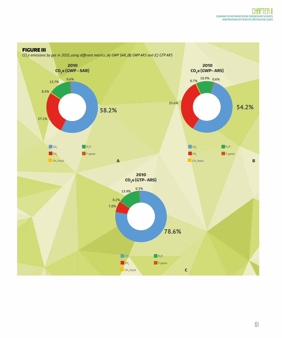
61
CHAPTER IISUMMARY OF ANTHROPOGENIC EMISSIONS BY SOURCES
AND REMOVALS BY SINKS OF GREENHOUSE GASES
FIGURE III CO2e emissions by gas in 2010, using different metrics. (A) GWP SAR, (B) GWP AR5 and (C) GTP AR5
2010CO2e (GWP - SAR)
13.7%
27.1%
0.5%
58.2%
0.6%
F-gases
CO2
CH4
CH4 fossil
N2O
A
2010CO2e (GWP- AR5)
F-gases
CO2
CH4
CH4 fossil
N2O
10.9%
33.6%
0.7%
54.2%
0.6%
B
2010CO2e (GTP- AR5)
F-gases
CO2
CH4
CH4 fossil
N2O
13.9%
7.0%
0.2%
78.6%
0.3%
C

CHAPTER III ANTHROPOGENIC
EMISSIONS BY SOURCES AND REMOVALS BY SINKS OF
GREENHOUSE GASES BY SECTOR
CHAPTER III ANTHROPOGENIC
EMISSIONS BY SOURCES AND REMOVALS BY SINKS OF
GREENHOUSE GASES BY SECTOR
64
CHAPTER III ANTHROPOGENIC EMISSIONS BY SOURCES AND REMOVALS BY SINKS OF GREENHOUSE GASES BY SECTOR
3.1. ENERGY
3.1.1. Characteristics of the Brazilian Energy MixThe Brazilian energy mix is characterized by the high share of renewable energy sources, partly due to the
country’s current state of development and the shortage of fossil energy resources until the 1970s. Strong
dependence on imported crude oil made the country vulnerable to oil shocks. This vulnerability, coupled with land
availability, resulted in some commercial uses of biomass, mainly ethanol in road transport and charcoal in the
steel sector, placing Brazil as one of the most relevant countries in terms of the use of fossil fuel source alternatives.
In order to understand Brazilian policy regarding fossil fuels, the behavior of fuel demand and greenhouse gas
emissions, it is necessary to consider oil price variation in real terms over the years. The first two oil crisis occurred
in 1973 and 1979, the latter having serious impacts for Brazil’s economy, which at the time was heavily dependent
on commodities exports in general, and on oil imports. In 1986, there was what was called a “countershock”, when
the average price of oil per barrel dropped significantly. A third crisis (or a structural change in price) began in 2005
and has been contributing to the leverage of the domestic oil industry.
With respect to gross domestic supply, Figure 3.1 shows the effect of price shocks in 1979 and in the beginning
of 2000s, reducing the oil demand in the immediate following years and increasing the demand for biomass. There
is also the increase in oil demand after the “countershock” in 1986. The decrease in oil demand after 2000 is closely
linked to the entry of Bolivia’s natural gas in the market. However, we clearly notice a return of the demand for
biomass. With respect to the structural change in the oil price as of 2005, even with the increase in price levels, there
was a strong growth in the demand for energy, especially supplied by the growth in natural gas and biomass supply.

65
FIGURE 3.1 Gross Domestic Supply, by source (thousand toe)
0
20000
40000
60000
80000
100000
120000
1970 1975 1980 1985 1990 1995 2000 2005 2010
(10
3 to
e)
Biomass and other renewable sources HydropowerPetroleum and
Liquefied Natural Gas
Natural Gas Coal Nuclear
Source: BRASIL (2013).
In 2010, primary fossil sources accounted for some 54% of domestic gross supply of energy. Out of those, oil and
oil by-products were responsible for the most significant contribution, followed by natural gas. From 1990 to 2010
there was an increase in fossil fuel consumption of almost 100%, from 72,207 to 143,831 thousand toe3. There is
a significant increase in the consumption of natural gas in the indicated period.
The evolution of final energy consumption can be observed in Table 3.1, which presents values for each period
of five-year consumption in thousand toe per energy source as of 1990. An increase in energy consumption can be
observed in the period from 1990 to 2010, covered by the Inventory, from some 123 to 228 thousand toe. In 2010,
as in 1990, diesel oil stood out and contributed with 18.2% of total energy consumption in the country. It is worth
highlighting that that only figures for energy consumption as fuel together with bunker values have emissions
estimated in this report. Other values (consumption as a reducer, raw materials and products for non-energy use)
are represented in the chapter on Industrial Processes and Product Use.
3 Tonne of oil equivalent.

66
VOLUME IIITHIRD NATIONAL COMMUNICATION OF BRAZIL
TABLE 3.1 Final energy consumption by source
SOURCE 1990 1995 2000 2005 2010 SHARE IN 2010
VARIATION 2005/ 2010
(103 toe) (%)Diesel Oil 20,851 25,468 30,903 34,277 41,481 18.2% 21.0%
Natural Gas (dry) 1,536 3,028 5,992 14,670 19,048 8.3% 29.8%
Motor Gasoline 7,279 10,823 13,205 13,595 17,525 7.7% 28.9%
LPG 5,476 6,426 7,836 7,121 7,701 3.4% 8.1%
Fuel Oil 10,128 11,823 11,573 7,270 6,068 2.7% -16.5%
Petroleum Coke 41 155 2,564 2,761 4,514 2.0% 63.5%
Refinary Gas 1,572 1,979 2,841 3,749 3,979 1.7% 6.1%
Natural Gas (humid) 740 249 1,292 2,016 3,382 1.5% 67.8%
Jet fuel 1,366 1,534 2,016 2,069 3,205 1.4% 54.9%
Other Energy Oil Products 957 1,440 2,179 2,133 2,219 1.0% 4.0%
Sub-bituminous Coal 1,166 1,058 1,706 1,323 1,852 0.8% 39.9%
Coke Oven Gas 1,324 1,489 1,415 1,467 1,738 0.8% 18.4%
Lignite 696 831 884 792 455 0.2% -42.6%
Coking Coal 92 394 720 803 439 0.2% -45.4%
Other renewable primary sources 25 22 65 141 119 0.1% -15.8%
Coal Tar 143 210 100 50 106 0.0% 113.0%
Coal coke 99 0 1 122 104 0.0% -15.1%
Aviation Gasoline 48 48 58 42 53 0.0% 26.5%
Other Bituminous Coal 0 0 0 0 12 0.0% -
Lighting Kerosene 188 101 56 25 7 0.0% -71.9%
Steam Coal 0 0 0 0 0 0.0% -
Naphtha 0 30 4 0 0 0.0% -
Gasworks Gas (Rio de Janeiro) 148 103 86 0 0 0.0% -
Gasworks Gas (São Paulo)) 132 17 0 0 0 0.0% -
Subtotal Fossil 54,008 67,228 85,495 94,428 114,006 49.9% 20.7%
Bagasse 11,666 14,875 14,122 22,675 34,146 14.9% 50.6%
Firewood 28,548 23,271 23,067 28,420 25,997 11.4% -8.5%
continues on the next page

67
CHAPTER IIIANTHROPOGENIC EMISSIONS BY SOURCES AND
REMOVALS BY SINKS OF GREENHOUSE GASES BY SECTOR
SOURCE 1990 1995 2000 2005 2010 SHARE IN 2010
VARIATION 2005/ 2010
(103 toe) (%)Hydrated Alcohol 5,208 5,072 2,776 2,885 8,251 3.6% 186.0%
Black Liquor 1,315 2,112 2,895 4,252 6,052 2.6% 42.3%
Anhydrous Alcohol 650 1,801 3,046 4,079 3,790 1.7% -7.1%
Biodiesel 0 0 0 0 2,033 0.9% -
Other primary (biomass) 382 470 570 849 1,165 0.5% 37.3%
Charcoal 1,156 826 718 866 723 0.3% -16.6%
Other primary (biogas) 0 0 0 0 5 0.0% -
Subtotal biomass 48,926 48,427 47,195 64,025 82,162 36.0% 28.3%
Final consumption as reducing agent (emissions in Industrial Processes sector)
Coal Coke 5,036 6,811 6,508 6,298 7,413 3.2% 17.7%
Charcoal 4,983 4,091 4,098 5,382 3,950 1.7% -26.6%
Coking Coal 0 297 1,843 2,490 2,385 1.0% -4.2%
Petroleum Coke 350 491 755 1,059 819 0.4% -22.7%
Other Bituminous Coal 0 0 0 0 0 0.0% -
Final consumption as raw material (emissions in Industrial Processes sector)
Naphtha 4,969 5,957 8,094 7,277 7,601 3.3% 4.4%
Natural Gas (Humid and Dry) 896 841 731 747 1,453 0.6% 94.4%
Hydrated Alcohol 459 548 515 284 438 0.2% 54.1%
Anhydrous Alcohol 32 64 122 74 149 0.1% 102.4%
Coal Tar 109 67 142 160 143 0.1% -10.9%
Refinary Gas 246 291 172 156 98 0.0% -36.9%
Kerosene 81 34 51 19 11 0.0% -41.3%
Final consumption of non-energy products
Other Non-Energy Oil Products 1,080 856 1,480 1,179 3,435 1.5% 191.4%
Bitumen (Asphalt) 1,283 1,244 1,742 1,461 2,793 1.2% 91.2%
Lubricants 698 674 821 856 1,106 0.5% 29.3%
Solvent 219 276 424 1,005 462 0.2% -54.0%
continues on the next page

68
VOLUME IIITHIRD NATIONAL COMMUNICATION OF BRAZIL
SOURCE 1990 1995 2000 2005 2010 SHARE IN 2010
VARIATION 2005/ 2010
(103 toe) (%)
Total
Subtotal (Fuel) 102,934 115,655 132,689 158,452 196,168 85.9% 23.8%
Subtotal (Reducing agent) 10,369 11,690 13,203 15,229 14,567 6.4% -4.3%
Subtotal (Raw material) 6,793 7,802 9,828 8,718 9,893 4.3% 13.5%
Subtotal (Non-energy products) 3,279 3,051 4,467 4,500 7,797 3.4% 73.3%
Total final consumption 123,375 138,199 160,188 186,899 228,424 100% 22.2%
Final Consumption as bunker
Fuel Oil 396 1,106 2,182 2,537 3,228 54.7% 27.3%
Jet Fuel + Bunker Gasoline 1,458 1,510 1,545 1,573 1,932 32.7% 22.9%
Bunker Diesel Oil 141 181 626 593 743 12.6% 25.3%
Total bunker 1,995 2,798 4,353 4,702 5,903 100.0% 25.6%
Source: BRASIL (2013).
A sectoral breakdown shows higher energy consumption in the industrial and transport subsectors. The industrial
subsector increased its share in total energy consumption between 1990 and 2010, jumping from 22.7% to 27.2%,
below the transport subsector, which went from 31% to 35.4%, with an increase of 34% in energy consumption
from 2005 to 2010, against 23.8% for fuels in industry, as shown in Table 3.2.
The evolution of final energy consumption by subsector is shown in Figure 3.2 for the period from 1990 to 2010.
TABLE 3.2 Final energy consumption, by subsector
SUBSECTOR AND USE1990 1995 2000 2005 2010 SHARE IN
2010
VARIATION 2005/ 2010
(103 toe) (%)Energy 27,379 26,855 30,092 40,322 49,370 25.2% 22.4%
Consumption of Energy Sector 11,421 12,096 11,948 16,479 21,956 11.2% 33.2%
Thermoelectric Plants 3,173 4,663 8,857 11,670 18,777 9.6% 60.9%
Charcoal Plants 12,785 10,096 9,288 12,173 8,637 4.4% -29.0%
Industrial 23,406 28,757 35,251 43,090 53,344 27.2% 23.8%
Transport 31,924 39,991 46,033 51,872 69,521 35.4% 34.0%continues on the next page

69
CHAPTER IIIANTHROPOGENIC EMISSIONS BY SOURCES AND
REMOVALS BY SINKS OF GREENHOUSE GASES BY SECTOR
SUBSECTOR AND USE1990 1995 2000 2005 2010 SHARE IN
2010
VARIATION 2005/ 2010
(103 toe) (%)Residential 13,821 12,575 13,497 14,672 14,342 7.3% -2.3%
Commercial and Public 1,050 1,327 1,615 1,488 1,191 0.6% -20.0%
Agriculture 5,354 6,150 6,202 7,009 8,400 4.3% 19.8%
Final energy consumption 102,934 115,655 132,689 158,452 196,168 100.0% 23.8%
FIGURE 3.2 Final energy consumption, by subsector
(10
3 to
e)
0
25000
50000
75000
100000
125000
150000
175000
200000
225000
1990 1995 2000 2005 2010
Industrial Transport Residential
Commercial and Public Agriculture Energy
Final energy consumption
The next section presents greenhouse gas emissions estimates due to production, transformation, transport
and consumption and is divided into two subsections: fuel combustion and fugitive emissions.
3.1.2. Fuel Combustion EmissionsThe combustion process essentially generates CO2 from oxidation of the carbon contained in fuels, thus
releasing energy. However, this process is imperfect, and as a consequence, it also produces CH4, CO and NMVOC.
N2O and NOx are also generated as a secondary effect.

70
VOLUME IIITHIRD NATIONAL COMMUNICATION OF BRAZIL
3.1.2.1. CO2 emissions from fuel combustion Brazil’s CO2 emissions from fuel combustion were estimated using two IPCC methodologies (IPCC, 1997): the
reference or top-down approach, in which CO2 emissions are calculated from fuel supply; and the sectoral or
bottom-up approach, in which CO2 emissions are calculated from each sector’s final energy consumption. Only
CO2 emissions from fossil fuels are considered in this chapter, and accounted for in the national total. Emissions
resulting from biomass fuel combustion are considered null by the IPCC as they derive from photosynthesis. They
are presented here for information purposes only, as shown in Table 3.3.
Emissions from non-renewable biomass consumption are covered in another specific methodological module
– Land-Use Change and Forestry (IPCC, 2006).
Emission estimates are based on production and consumption data by energy source obtained from the Brazilian
Energy Balance (BEN) (BRASIL, 2013), previously published by the Ministry of Mines and Energy (MME) and in recent
years published by the Energy Research Company (EPE), under the MME.
The three editions of the Useful Energy Balance (BEU) (BRASIL, 2006) available in Brazil (1983, 1993 and
2003) were used specifically for the sector-wide approach, aimed at breaking down fuel consumption into final
destinations. BEU provides the framework for the allocation of each energy sector in terms of final energy by type
of use for the several sectors, as well as respective efficiencies. Among the available destinations, the following are
relevant for emissions: Driving Force, Heat, Direct Heating, Cooling, Lighting, Electrochemistry and Others.
The main source of data for of emission factors used were the 2006 IPCC Guidelines for National Greenhouse
Gas Inventories (IPCC, 2006) and EMEP/EEA 2013 Air Pollutant Emission Inventory Guidebook 2013 (EMEP/EEA,
2013). In some cases specific emission factors have been developed and adopted in order to assess emissions of
different gases.
Top-down
The top-down approach is a simple procedure, where emissions from fuel combustion are calculated from
aggregate data on the fuel supply in a given economy. For such purpose, it uses the concept of apparent consumption,
which is added up to primary fuel production, primary and secondary fuel imports, then subtracted from primary
and secondary fuel exports, bunkers and stock variation (which may be positive or negative).
Non-energy fuel emissions are accounted for by the new Guidelines (IPCC, 2006) in Industrial Processes and
Product Use. They refer to raw materials of the chemical industry (part of the supply of naphtha, refinery gas, natural
gas, lighting kerosene, anhydrous and hydrous ethanol and tar), iron and steel fittings industry (part of coke supply
from coal, and oil and bituminous, coking and charcoal), and non-energy use products (full supply of lubricants,
asphalt, and other non-energy oil and solvent products) among others.
In the top-down approach, energy sources are separated by physical state of the primary product, fundamentally
corresponding to oil, oil by-products, and natural gas liquids (liquids), coal and coal by-products (solids) and dry
natural gas (gaseous). Table 3.3 presents the results of CO2 emissions estimated by the top-down approach for
1990, 1995, 2000, 2005 and 2010, and Figure 3.3 presents the share of biomass and fossil fuels.
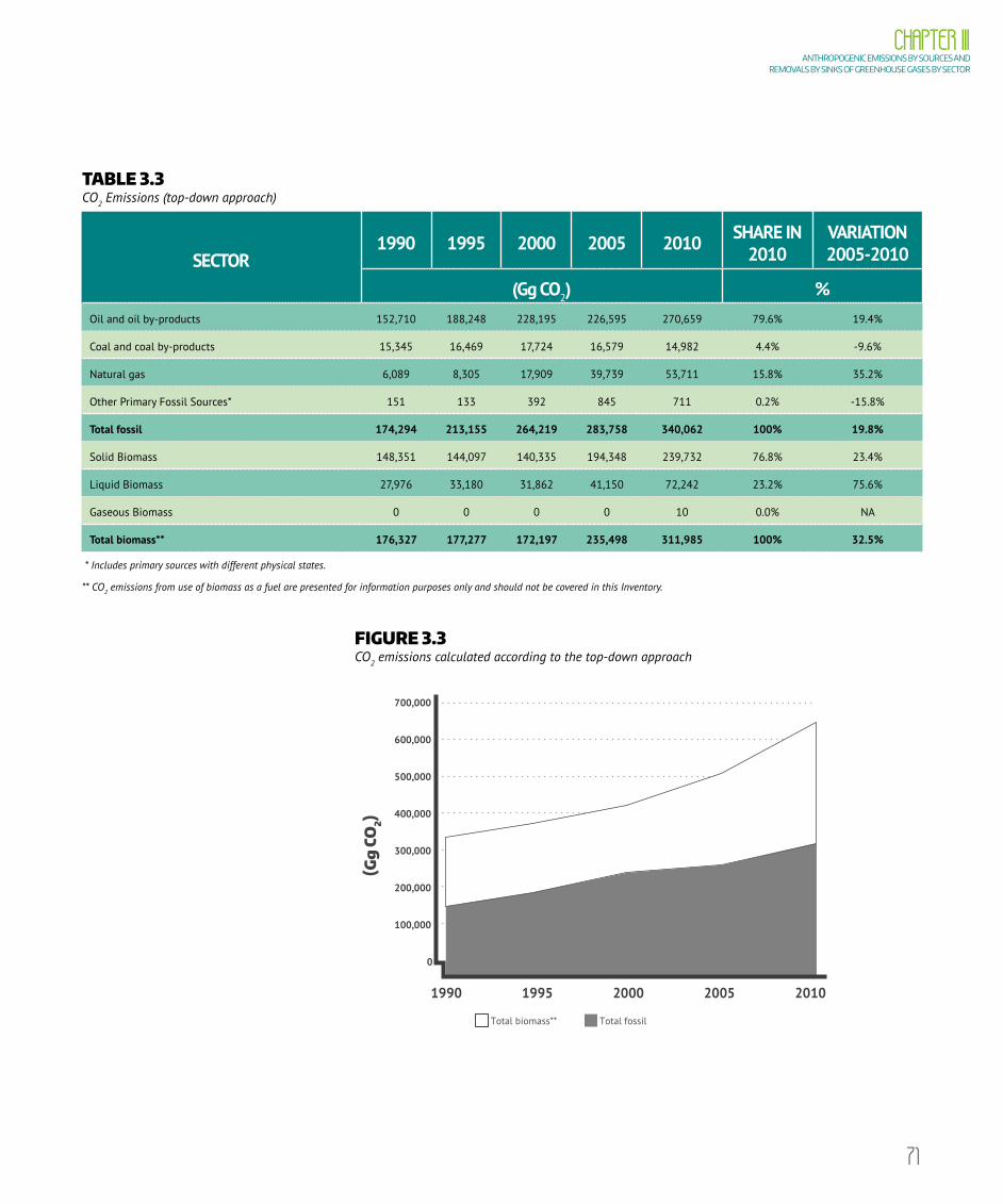
71
CHAPTER IIIANTHROPOGENIC EMISSIONS BY SOURCES AND
REMOVALS BY SINKS OF GREENHOUSE GASES BY SECTOR
TABLE 3.3 CO2 Emissions (top-down approach)
SECTOR 1990 1995 2000 2005 2010 SHARE IN
2010VARIATION 2005-2010
(Gg CO2) %Oil and oil by-products 152,710 188,248 228,195 226,595 270,659 79.6% 19.4%
Coal and coal by-products 15,345 16,469 17,724 16,579 14,982 4.4% -9.6%
Natural gas 6,089 8,305 17,909 39,739 53,711 15.8% 35.2%
Other Primary Fossil Sources* 151 133 392 845 711 0.2% -15.8%
Total fossil 174,294 213,155 264,219 283,758 340,062 100% 19.8%
Solid Biomass 148,351 144,097 140,335 194,348 239,732 76.8% 23.4%
Liquid Biomass 27,976 33,180 31,862 41,150 72,242 23.2% 75.6%
Gaseous Biomass 0 0 0 0 10 0.0% NA
Total biomass** 176,327 177,277 172,197 235,498 311,985 100% 32.5%
* Includes primary sources with different physical states.
** CO2 emissions from use of biomass as a fuel are presented for information purposes only and should not be covered in this Inventory.
FIGURE 3.3 CO2 emissions calculated according to the top-down approach
0
100,000
200,000
300,000
400,000
500,000
600,000
700,000
1990 1995 2000 2005 2010
Total biomass** Total fossil
(Gg
CO
2)

72
VOLUME IIITHIRD NATIONAL COMMUNICATION OF BRAZIL
Total CO2 emissions from fossil fuel combustion grew from 174,294 Gg CO2, in 1990, to 340,062 Gg CO2, in
2010, representing a 95% growth in the period. However, fossil fuel production recorded an increase from 38,744
to 125,188 thousand toe, a 223, 1% growth; imports, in turn, grew by 54.6%.
A significant increase in emissions from natural gas consumption (gaseous fossil) is noticed, which increases
its total emissions shares by almost five times. Liquid fossil fuels had their share reduced from 87.6% to 79.6%
between 1990 and 2010.
As already explained above, the approach used for inventories provides that CO2 emissions from fuel combustion
resulting from biomass should be informed, but not considered in the total emissions from the energy sector in
the country.
Bottom-up
The sectoral, or bottom-up, approach allows the identification of where and how emissions occur, favoring
the establishment of mitigation measures. This approach also addresses emissions of other greenhouse gases
emissions whose behavior is important.
The estimation of emissions based on the bottom-up approach considers the various destinations of fuel use.
Besides CO2, emissions of non-CO2 gases are estimated, namely: CO, CH4, N2O, NOx, and NMVOC.
CO2 emissions depend on fuel carbon content, and can be estimated at a high level of aggregation with
reasonable accuracy such as that proposed in the top-down approach. However, for non-CO2 gases it is necessary
to work with additional information on end-use, equipment technology, operating conditions, etc., and therefore
it is necessary to use a more disaggregated approach. Nevertheless, under the IPCC methodology (IPCC, 1997) it
is recommended that CO2 emissions are also estimated using a more disaggregated level of information, which
allows for a comparison between the two approaches, as will be addressed further ahead. In this sense, CO2
emissions from fuel combustion were estimated for the various sectors of the economy.
The determination of final consumption of fuels by sector demanded an adjustment of the available database.
The said adjustment was needed regarding the fuels as well as the activity sectors. In relation to emissions, each
country’s peculiarities are reflected in the difference of carbon content of the fuels used and/or the characteristics
of use and transformation equipment. Taking into account that in fuel combustion emission factors for non-CO2
gases depend on the technology used, an attempt was made to develop appropriate emission factors for Brazil by
identifying the equipment used by the various sectors.
Table 3.4 shows fossil fuel emissions for the 1990 to 2010 period. CO2 emissions in 2010 were estimated at
332,760 Gg, growing by 20.2% from 2005 to 2010. In 2010, diesel oil was the fossil fuel energy responsible for
higher shares of CO2 emissions, accounting for 38.7% of emissions for the year. Motor gasoline and dry natural gas
are also relevant for emissions and had similar shares in 2010 (15.3% and 13.4%, respectively). It is noteworthy that
diesel oil and motor gasoline maintained stable shares over the period, but dry natural gas increased considerably
(in 1990 it was only 2.2%).

73
CHAPTER IIIANTHROPOGENIC EMISSIONS BY SOURCES AND
REMOVALS BY SINKS OF GREENHOUSE GASES BY SECTOR
TABLE 3.4 CO2 emissions by fuel
SOURCE1990 1995 2000 2005 2010 SHARE IN
2010VARIATION 2005-2010
(Gg CO2) (%)Motor Gasoline 21,119 31,403 38,313 39,446 50,848 15.3% 28.9%
Aviation Gasoline 142 141 170 123 155 0.0% 26.0%
Lighting Kerosene 567 304 168 74 21 0.0% -71.6%
Jet Fuel 4,090 4,591 6,036 6,193 9,596 2.9% 54.9%
Diesel Oil 64,691 79,013 95,874 106,342 128,693 38.7% 21.0%
Fuel Oil 32,821 38,312 37,504 23,560 19,663 5.9% -16.5%
LPG 14,466 16,978 20,702 18,814 20,345 6.1% 8.1%
Petroleum Coke 167 634 10,467 11,271 18,426 5.5% 63.5%
Lignite 2,945 3,516 3,737 3,350 1,924 0.6% -42.6%
Sub-bituminous Coal 4,693 4,257 6,865 5,324 7,450 2.2% 39.9%
Other Bituminous Coal - - - - 48 0.0% -
Coking Coal 363 1,560 2,851 3,181 1,738 0.5% -45.4%
Coal Tar 482 711 338 168 359 0.1% 113.7%
Coal Coke 442 - 3 547 464 0.1% -15.2%
Natural Gas (Humid) 1,738 585 3,034 4,735 7,944 2.4% 67.8%
Natural Gas (Dry) 3,607 7,112 14,074 34,456 44,740 13.4% 29.8%
Refinery Gas 3,791 4,772 6,852 9,042 9,596 2.9% 6.1%
Other Energy Oil Products 2,938 4,420 6,686 6,546 6,809 2.0% 4.0%
Gasworks Gas – Rio de Janeiro 400 266 201 - - 0.0% -
Gasworks Gas – São Paulo 356 43 - - - 0.0% -
Coke Oven Gas 2,462 2,767 2,630 2,728 3,230 1.0% 18.4%
Naphtha - 92 12 - - 0.0% -
Other Primary Fossil Sources* 151 133 392 845 711 0.2% -15.9%
Total domestic emissions 162,431 201,610 256,909 276,744 332,760 100% 20.2%
*Includes primary sources in different physical states.
CO2 emissions from biomass as fuel are shown in Table 3.5 only for information purposes and should not be
considered in this Inventory. Only non-CO2 emissions from the combustion of these fuels will be considered. CO2
emissions from biomass consumption are addressed in another specific methodological module – Land Use, Land-
Use Change and Forestry (IPCC, 2003), where the balance between carbon emitted by removed biomass and carbon
absorbed during the growth of new plants is determined.

74
VOLUME IIITHIRD NATIONAL COMMUNICATION OF BRAZIL
TABLE 3.5 CO2 emissions from biomass use
SOURCE1990 1995 2000 2005 2010 SHARE IN
2010VARIATION 2005-2010
(Gg CO2) (%)Firewood 87,580 72,062 72,910 88,327 85,939 28.3% -2.7%
Charcoal 5,157 3,682 3,204 3,862 3,223 1.1% -16.5%
Bagasse 48,842 62,280 59,126 94,936 142,964 47.2% 50.6%
Other Primary (biogas) - - - - 19 0.0% -
Other Primary (biomass) 1,599 1,967 2,385 3,555 4,880 1.6% 37.3%
Black Liquor 5,249 8,426 11,552 16,965 24,148 8.0% 42.3%
Anhydrous Alcohol 1,928 5,338 9,031 12,090 11,234 3.7% -7.1%
Hydrated Alcohol 15,438 15,036 8,229 8,551 24,458 8.1% 186.0%
Biodiesel - - - - 6,306 2.1% -
Total 165,793 168,791 166,437 228,286 303,171 100.0% 32.8%
Figure 3.4 shows emissions calculated in accordance with the bottom-up approach for fossil fuels and biomass.
FIGURE 3.4 CO2 emissions (bottom-up approach)
Total biomass** Total fossil
(Gg
CO
2)
0
100,000
200,000
300,000
400,000
500,000
600,000
700,000
1990 1995 2000 2005 2010
Table 3.6 shows CO2 emissions by subsector for fossil fuels. The transport subsector was the largest source of
emissions in 2010, accounting for 50.6% of CO2 emissions. Road transport corresponds to 45.5% of total emissions

75
CHAPTER IIIANTHROPOGENIC EMISSIONS BY SOURCES AND
REMOVALS BY SINKS OF GREENHOUSE GASES BY SECTOR
that year and to 90% of all transport emissions. An increase by 24.5% in the CO2 emissions share is observed in this
subsector between 2005 and 2010.
TABLE 3.6 CO2 emissions of fuel by subsector
EMISSIONS BY SUBSECTOR1990 1995 2000 2005 2010 SHARE
IN 2010VARIATION 2005-2010
(Gg CO2) (%)Energy subsector 21,271 25,282 40,483 47,344 58,857 17.7% 24.3%
Public Service Power Plants 6,194 9,016 19,075 20,911 26,592 8.0% 27.2%
Self-Producers Power Plants 2,275 3,159 5,141 5,474 9,445 2.8% 72.5%
Charcoal Plants* 0 0 0 0 0 0.0% -
Energy consumption 12,802 13,106 16,268 20,958 22,820 6.9% 8.9%
Residential 13,842 15,942 17,179 15,591 17,249 5.2% 10.6%
Commercial 2,073 1,565 2,216 1,903 1,446 0.4% -24.0%
Public 503 2,075 2,122 1,742 1,192 0.4% -31.6%
Agriculture 9,846 13,222 14,152 14,964 17,346 5.2% 15.9%
Transport 79,337 100,457 121,748 135,182 168,364 50.6% 24.5%
Road Transportation 70,094 90,916 111,337 123,519 151,481 45.5% 22.6%
Railways 1,592 1,332 1,247 1,748 2,717 0.8% 55.4%
Civil Aviation 4,232 4,732 6,206 6,316 9,751 2.9% 54.4%
Navigation 3,420 3,477 2,958 3,599 4,415 1.3% 22.7%
Industrial 35,559 43,068 59,008 60,019 68,305 20.5% 13.8%
Cement 5,790 6,073 10,512 8,951 14,259 4.3% 59.3%
Iron and Steel 4,373 5,387 4,620 5,297 5,540 1.7% 4.6%
Ferroalloys 63 1 37 229 102 0.0% -55.5%
Mining and Pelleting 2,412 3,263 5,666 7,230 7,289 2.2% 0.8%
Non-Ferrous Metals 1,357 1,868 3,709 4,916 5,476 1.6% 11.4%
Chemical 8,606 10,057 13,942 14,624 13,847 4.2% -5.3%
Food and Beverages 3,239 4,074 4,476 3,755 3,965 1.2% 5.6%
Textiles 1,600 1,328 1,268 1,159 1,015 0.3% -12.4%
Pulp and Paper 2,464 3,384 4,320 3,840 3,632 1.1% -5.4%
Ceramic 1,692 2,691 3,382 3,805 4,888 1.5% 28.5%
Other industries 3,962 4,942 7,076 6,213 8,293 2.5% 33.5%
Total 162,431 201,610 256,909 276,744 332,760 100% 20.2%
* CO2 emissions from Charcoal Plants are from biomass.

76
VOLUME IIITHIRD NATIONAL COMMUNICATION OF BRAZIL
The industrial subsector was the source of 20.5% emissions from the Energy sector, with cement and chemicals
standing out, each of those responsible for approximately 4%. Noteworthy is the increase in emissions of the
cement sector, with a variation of 59.3% and the reduction of emissions of the ferroalloy sector, with a variation of
-55.5% from 2005 to 2010.
In the industrial subsector, in relation to Mining and Pelletizing, Iron and Steel, Ferroalloys and Non-Ferrous
Minerals, it is worth mentioning that part of their emissions are accounted for in Industrial Processes and Product
Use and refer to the use of energy as reducers, according to the IPCC Guidelines (IPCC, 1997 and 2006).
Among the subsectors with a minor share of total emissions, public and commercial were the ones with the
lowest contribution from 2005 to 2010.
Table 3.7 presents a comparison between CO2 emission estimates obtained from the two methods. Some
variation is expected between the two results, since they use different levels of aggregation and hypotheses that
may sometimes only apply to one of the approaches. The fact that bottom-up approach uses a broader scope of
variables also contributes to this difference.
In accordance with IPCC (1997), this difference can be considered reasonable if it is within a 2% range (negative
or positive). If the result extrapolates this limit, justifications must be submitted.
As shown in Table 3.7, the results from the top-down approach are consistently higher than those obtained
through the bottom-up approach. Estimates through the top-down approach do not account for energy losses
in processing and distribution, which leads to different estimates for the bottom-up approach. Besides, statistic
adjustments in the BEN contribute to the difference in results between the two approaches.
TABLE 3.7 CO2 emissions from fossil fuel combustion estimated by top-down and bottom-up approaches
SECTOR 1990 1995 2000 2005 2010
(Gg CO2)Top-Down (A) 174,294 213,155 264,219 283,758 340,062
Bottom-Up (B) 162,431 201,610 256,909 276,744 332,760
Difference (%)
((A-B)/B)7.3% 5.7% 2.8% 2.5% 2.2%
The BEN used to include information on bunker fuels for aviation (fuel supplied to air transport companies for
international transportation) in the export account (fuel exported as good), but it began to present the information in
a separate format since 1998. In this case, the National Civil Aviation Agency (ANAC) provided the information used, as
it separates bunker fuels data from exports since 1990. Furthermore, greater details in the distinction made between
national and international transportation grants more soundness to data submitted and ensures the adequacy of the
methodology to IPCC guidelines. In the case of civil aviation, therefore, more precise export and bunker fuels data,
obtained, respectively, from the National Agency of Petroleum, Natural Gas and Biofuels (ANP) and ANAC were used.
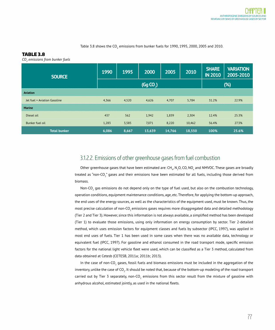
77
CHAPTER IIIANTHROPOGENIC EMISSIONS BY SOURCES AND
REMOVALS BY SINKS OF GREENHOUSE GASES BY SECTOR
Table 3.8 shows the CO2 emissions from bunker fuels for 1990, 1995, 2000, 2005 and 2010.
TABLE 3.8 CO2 emissions from bunker fuels
SOURCE1990 1995 2000 2005 2010 SHARE
IN 2010VARIATION 2005-2010
(Gg CO2) (%)Aviation
Jet fuel + Aviation Gasoline 4,366 4,520 4,626 4,707 5,784 31.2% 22.9%
Marine
Diesel oil 437 562 1,942 1,839 2,304 12.4% 25.3%
Bunker fuel oil 1,283 3,585 7,071 8,220 10,462 56.4% 27.3%
Total bunker 6,086 8,667 13,639 14,766 18,550 100% 25.6%
3.1.2.2. Emissions of other greenhouse gases from fuel combustionOther greenhouse gases that have been estimated are: CH4, N2O, CO, NOx and NMVOC. These gases are broadly
treated as “non-CO2” gases and their emissions have been estimated for all fuels, including those derived from
biomass.
Non-CO2 gas emissions do not depend only on the type of fuel used, but also on the combustion technology,
operation conditions, equipment maintenance conditions, age, etc. Therefore, for applying the bottom-up approach,
the end uses of the energy sources, as well as the characteristics of the equipment used, must be known. Thus, the
most precise calculation of non-CO2 emissions gases requires more disaggregated data and detailed methodology
(Tier 2 and Tier 3). However, since this information is not always available, a simplified method has been developed
(Tier 1) to evaluate those emissions, using only information on energy consumption by sector. Tier 2-detailed
method, which uses emission factors for equipment classes and fuels by subsector (IPCC, 1997), was applied in
most end uses of fuels. Tier 1 has been used in some cases when there was no available data, technology or
equivalent fuel (IPCC, 1997). For gasoline and ethanol consumed in the road transport mode, specific emission
factors for the national light vehicle fleet were used, which can be classified as a Tier 3 method, calculated from
data obtained at Cetesb (CETESB, 2011a; 2011b; 2013).
In the case of non-CO2 gases, fossil fuels and biomass emissions must be included in the aggregation of the
inventory, unlike the case of CO2. It should be noted that, because of the bottom-up modeling of the road transport
carried out by Tier 3 separately, non-CO2 emissions from this sector result from the mixture of gasoline with
anhydrous alcohol, estimated jointly, as used in the national fleets.

78
VOLUME IIITHIRD NATIONAL COMMUNICATION OF BRAZIL
Table 3.9 shows emissions of other greenhouse gases by fuels combustion for 1990, 1995, 2000, 2005 and 2010.
TABLE 3.9 Emissions from other greenhouse gases from fuel combustion
GAS1990 1995 2000 2005 2010 VARIATION
2005-2010
(Gg) (%)
CH4 455.3 388.1 392.8 478.6 448.2 -6.4%
N2O 14.02 14.97 18.88 24.75 31.76 28.3%
CO 9,592.6 9,636.3 8,181.0 8,194.7 7,695.9 -6.1%
NOx 1,639.8 1,977.5 2,273.3 2,346.4 2,567.1 9.4%
NMVOC 1,167.5 1,104.8 987.4 1,061.5 900.5 -15.2%
BUNKER FUELS EMISSIONS
CH4 0.0 0.0 0.1 0.1 0.2 25.3%
N2O 0.13 0.16 0.20 0.21 0.27 24.4%
CO 0.9 0.9 0.9 1.2 1.1 -6.0%
NOx 1.6 2.1 3.2 3.4 4.3 27.0%
NMVOC 2.9 7.3 14.9 16.9 21.4 26.8%
A more detailed analysis of the above results is found in the following items. Tables with emissions by fuel and
sector for the 1990 to 2010 period are presented for each gas. Each table also shows the percentage distribution
in 2010 and the corresponding growth rate for the 2005 to 2010 period.
Methane
In 2010 448.2 Gg CH4 were emitted from fuel combustion. Emissions showed a reduction of 6.4% in the 2005
to 2010 period.
Table 3.10 shows biomass fuel is the main source of CH4 (84.2% in 2010). Firewood was the main fuel in terms
of CH4 emissions (71.8%), followed by motor gasoline (11.2%) and by bagasse (9.6%). Among these fuels, firewood
and motor gasoline showed reduction of CH4 emissions by 10.4% and 18.1%, respectively, from 2005 to 2010.
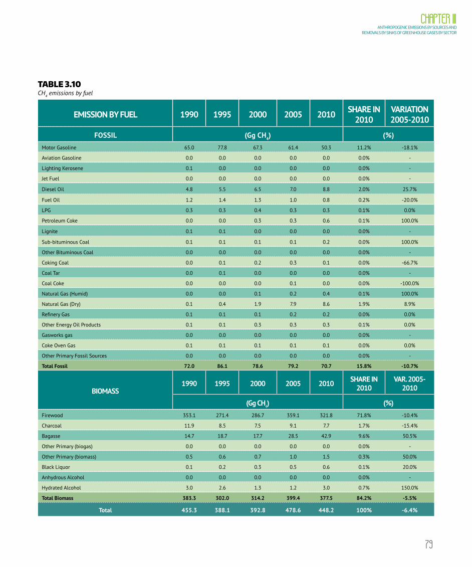
79
CHAPTER IIIANTHROPOGENIC EMISSIONS BY SOURCES AND
REMOVALS BY SINKS OF GREENHOUSE GASES BY SECTOR
TABLE 3.10 CH4 emissions by fuel
EMISSION BY FUEL 1990 1995 2000 2005 2010 SHARE IN 2010
VARIATION 2005-2010
FOSSIL (Gg CH4) (%)Motor Gasoline 65.0 77.8 67.3 61.4 50.3 11.2% -18.1%
Aviation Gasoline 0.0 0.0 0.0 0.0 0.0 0.0% -
Lighting Kerosene 0.1 0.0 0.0 0.0 0.0 0.0% -
Jet Fuel 0.0 0.0 0.0 0.0 0.0 0.0% -
Diesel Oil 4.8 5.5 6.5 7.0 8.8 2.0% 25.7%
Fuel Oil 1.2 1.4 1.3 1.0 0.8 0.2% -20.0%
LPG 0.3 0.3 0.4 0.3 0.3 0.1% 0.0%
Petroleum Coke 0.0 0.0 0.3 0.3 0.6 0.1% 100.0%
Lignite 0.1 0.1 0.0 0.0 0.0 0.0% -
Sub-bituminous Coal 0.1 0.1 0.1 0.1 0.2 0.0% 100.0%
Other Bituminous Coal 0.0 0.0 0.0 0.0 0.0 0.0% -
Coking Coal 0.0 0.1 0.2 0.3 0.1 0.0% -66.7%
Coal Tar 0.0 0.1 0.0 0.0 0.0 0.0% -
Coal Coke 0.0 0.0 0.0 0.1 0.0 0.0% -100.0%
Natural Gas (Humid) 0.0 0.0 0.1 0.2 0.4 0.1% 100.0%
Natural Gas (Dry) 0.1 0.4 1.9 7.9 8.6 1.9% 8.9%
Refinery Gas 0.1 0.1 0.1 0.2 0.2 0.0% 0.0%
Other Energy Oil Products 0.1 0.1 0.3 0.3 0.3 0.1% 0.0%
Gasworks gas 0.0 0.0 0.0 0.0 0.0 0.0% -
Coke Oven Gas 0.1 0.1 0.1 0.1 0.1 0.0% 0.0%
Other Primary Fossil Sources 0.0 0.0 0.0 0.0 0.0 0.0% -
Total Fossil 72.0 86.1 78.6 79.2 70.7 15.8% -10.7%
BIOMASS1990 1995 2000 2005 2010 SHARE IN
2010VAR. 2005-
2010
(Gg CH4) (%)Firewood 353.1 271.4 286.7 359.1 321.8 71.8% -10.4%
Charcoal 11.9 8.5 7.5 9.1 7.7 1.7% -15.4%
Bagasse 14.7 18.7 17.7 28.5 42.9 9.6% 50.5%
Other Primary (biogas) 0.0 0.0 0.0 0.0 0.0 0.0% -
Other Primary (biomass) 0.5 0.6 0.7 1.0 1.5 0.3% 50.0%
Black Liquor 0.1 0.2 0.3 0.5 0.6 0.1% 20.0%
Anhydrous Alcohol 0.0 0.0 0.0 0.0 0.0 0.0% -
Hydrated Alcohol 3.0 2.6 1.3 1.2 3.0 0.7% 150.0%
Total Biomass 383.3 302.0 314.2 399.4 377.5 84.2% -5.5%
Total 455.3 388.1 392.8 478.6 448.2 100% -6.4%

80
VOLUME IIITHIRD NATIONAL COMMUNICATION OF BRAZIL
In terms of sectoral emissions in 2010 (Table 3.11), the residential subsector was the main source of CH4
emissions (64.7%) especially because of firewood combustion. Then there is the transport subsector, highlighted by
road transport (14.8%). During the period from 2005 to 2010 there was significant growth in some subsectors such
as: public service power plants, self-producers and energy sector (50%, 136% and 56.6% respectively).
TABLE 3.11 CH4 emissions by subsector
EMISSIONS BY SUBSECTOR1990 1995 2000 2005 2010 SHARE IN
2010VARIATION 2005-2010
(Gg CH4) (%)
Broad Energy subsector
Public Service Power Plants 0.1 0.2 0.4 0.8 1.2 0.3% 50.0%
Self-Producers Power Plants 0.6 0.9 1.3 2.5 5.9 1.3% 136.0%
Charcoal Plants 16.1 12.7 11.7 15.3 10.8 2.4% -29.4%
Energy Sector 8.7 9.3 7.3 10.6 16.6 3.7% 56.6%
Industry
Cement 3.1 2.6 2.3 2.4 1.2 0.3% -50.0%
Iron and Steel 0.2 0.2 0.1 0.1 0.2 0.0% 100.0%
Ferroalloys 0.0 0.0 0.1 0.1 0.1 0.0% 0.0%
Mining and Pelleting 0.4 0.2 0.3 0.4 0.3 0.1% -25.0%
Non-Ferrous Metals 0.1 0.1 0.1 0.2 0.2 0.0% 0.0%
Chemical 0.8 0.8 1.3 2.4 2.5 0.6% 4.2%
Food and Beverages 6.8 10.1 11.1 17.7 23.2 5.2% 31.1%
Textiles 0.2 0.1 0.1 0.1 0.1 0.0% 0.0%
Pulp and Paper 1.0 1.2 1.5 1.8 2.5 0.6% 38.9%
Ceramics 2.2 2.0 2.2 2.3 3.0 0.7% 30.4%
Others 0.9 0.8 0.8 0.9 1.1 0.2% 22.2%
Subtotal 15.7 18.1 19.9 28.4 34.4 7.7% 21.1%
Transport
Road Transportation 72.2 85.4 75.2 74.0 66.3 14.8% -10.4%
Railways 0.1 0.1 0.1 0.1 0.2 0.0% 100.0%
Civil Aviation 0.0 0.0 0.0 0.0 0.0 0.0% -
Navigation 0.3 0.3 0.3 0.3 0.4 0.1% 33.3%
Subtotal 72.6 85.8 75.6 74.4 66.9 14.9% -10.1%
Other subsectors
Residential 318.4 243.7 261.5 327.6 290.1 64.7% -11.4%
Commercial 3.7 3.5 3.1 3.1 3.8 0.8% 22.6%
Public 0.1 0.1 0.0 0.0 0.0 0.0% -
Agriculture 19.3 13.8 12.0 15.9 18.5 4.1% 16.4%
Total 455.3 388.1 392.8 478.6 448.2 100% -6.4%
When comparing tables of emission results by fuel (Table 3.10) and by subsector (Table 3.11), the evaluation of
emissions by technology shows direct heating was responsible for 73.5% of CH4 emissions in 2010.
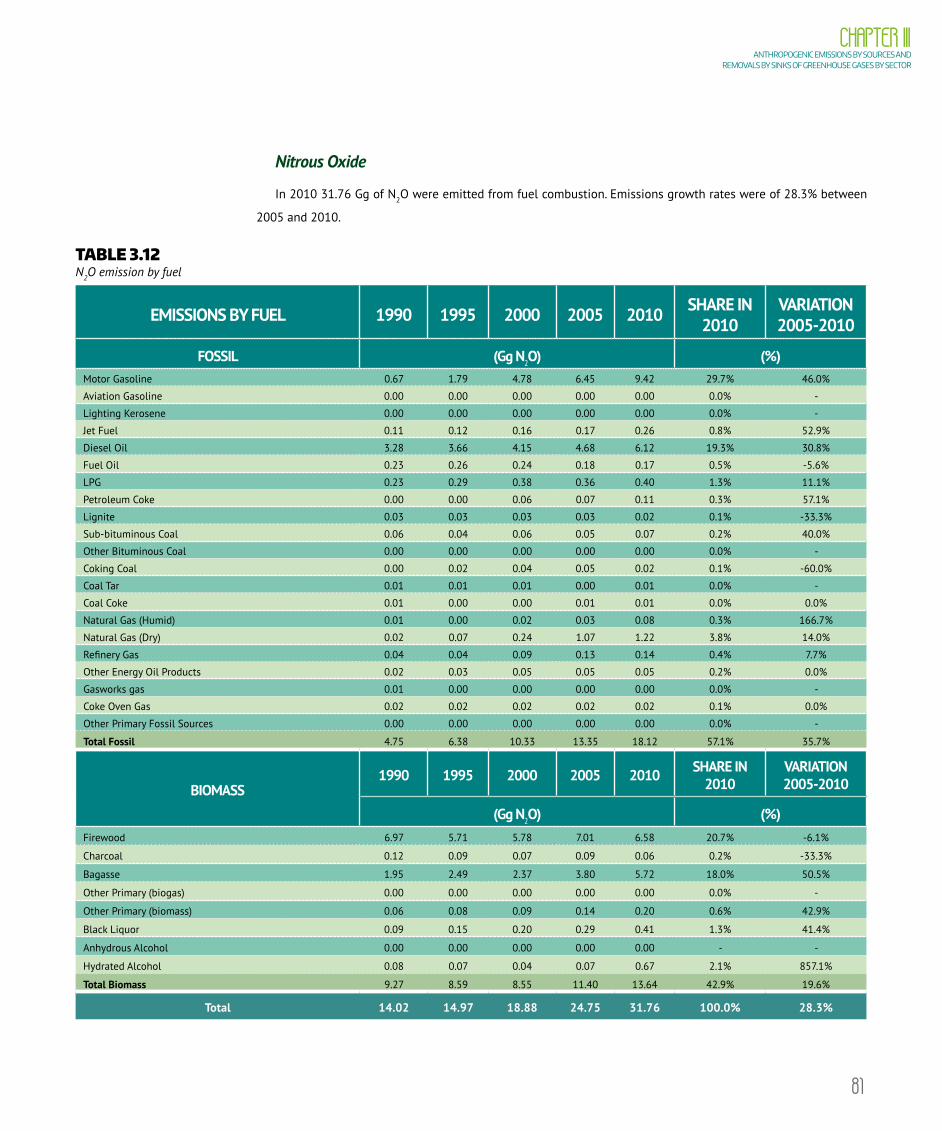
81
CHAPTER IIIANTHROPOGENIC EMISSIONS BY SOURCES AND
REMOVALS BY SINKS OF GREENHOUSE GASES BY SECTOR
Nitrous Oxide
In 2010 31.76 Gg of N2O were emitted from fuel combustion. Emissions growth rates were of 28.3% between
2005 and 2010.
TABLE 3.12 N2O emission by fuel
EMISSIONS BY FUEL 1990 1995 2000 2005 2010 SHARE IN 2010
VARIATION 2005-2010
FOSSIL (Gg N2O) (%)Motor Gasoline 0.67 1.79 4.78 6.45 9.42 29.7% 46.0%
Aviation Gasoline 0.00 0.00 0.00 0.00 0.00 0.0% -
Lighting Kerosene 0.00 0.00 0.00 0.00 0.00 0.0% -
Jet Fuel 0.11 0.12 0.16 0.17 0.26 0.8% 52.9%
Diesel Oil 3.28 3.66 4.15 4.68 6.12 19.3% 30.8%
Fuel Oil 0.23 0.26 0.24 0.18 0.17 0.5% -5.6%
LPG 0.23 0.29 0.38 0.36 0.40 1.3% 11.1%
Petroleum Coke 0.00 0.00 0.06 0.07 0.11 0.3% 57.1%
Lignite 0.03 0.03 0.03 0.03 0.02 0.1% -33.3%
Sub-bituminous Coal 0.06 0.04 0.06 0.05 0.07 0.2% 40.0%
Other Bituminous Coal 0.00 0.00 0.00 0.00 0.00 0.0% -
Coking Coal 0.00 0.02 0.04 0.05 0.02 0.1% -60.0%
Coal Tar 0.01 0.01 0.01 0.00 0.01 0.0% -
Coal Coke 0.01 0.00 0.00 0.01 0.01 0.0% 0.0%
Natural Gas (Humid) 0.01 0.00 0.02 0.03 0.08 0.3% 166.7%
Natural Gas (Dry) 0.02 0.07 0.24 1.07 1.22 3.8% 14.0%
Refinery Gas 0.04 0.04 0.09 0.13 0.14 0.4% 7.7%
Other Energy Oil Products 0.02 0.03 0.05 0.05 0.05 0.2% 0.0%
Gasworks gas 0.01 0.00 0.00 0.00 0.00 0.0% -
Coke Oven Gas 0.02 0.02 0.02 0.02 0.02 0.1% 0.0%
Other Primary Fossil Sources 0.00 0.00 0.00 0.00 0.00 0.0% -
Total Fossil 4.75 6.38 10.33 13.35 18.12 57.1% 35.7%
BIOMASS1990 1995 2000 2005 2010 SHARE IN
2010VARIATION 2005-2010
(Gg N2O) (%)Firewood 6.97 5.71 5.78 7.01 6.58 20.7% -6.1%
Charcoal 0.12 0.09 0.07 0.09 0.06 0.2% -33.3%
Bagasse 1.95 2.49 2.37 3.80 5.72 18.0% 50.5%
Other Primary (biogas) 0.00 0.00 0.00 0.00 0.00 0.0% -
Other Primary (biomass) 0.06 0.08 0.09 0.14 0.20 0.6% 42.9%
Black Liquor 0.09 0.15 0.20 0.29 0.41 1.3% 41.4%
Anhydrous Alcohol 0.00 0.00 0.00 0.00 0.00 - -
Hydrated Alcohol 0.08 0.07 0.04 0.07 0.67 2.1% 857.1%
Total Biomass 9.27 8.59 8.55 11.40 13.64 42.9% 19.6%
Total 14.02 14.97 18.88 24.75 31.76 100.0% 28.3%

82
VOLUME IIITHIRD NATIONAL COMMUNICATION OF BRAZIL
Table 3.12 shows that fossil fuels are the main sources of N2O (57.1% in 2010), having presented growth by
35.7% in emissions in the 2005 to 2010 period. N2O emissions demonstrate the role of gasoline in fossil fuel
emissions. N2O emissions from gasoline consumption accounted for 29.7% of total emissions in 2010, having
grown by 46% between 2005 and 2010.
As for emissions from biomass, firewood and bagasse are the main sources of N2O emissions (20.7% and 18%,
respectively). Despite the low turnout, it is necessary to stress the growth of hydrous ethanol from 2005 to 2010 (857.1%).
TABLE 3.13 N2O emissions by subsector
EMISSIONS BY SUBSECTOR1990 1995 2000 2005 2010 SHARE IN
2010VARIATION 2005-2010
(Gg N2O) (%)
Broad Energy
subsector
Public Service Power Plants 0.05 0.07 0.14 0.23 0.32 1.0% 39.1%
Self-Producers Power Plants 0.12 0.16 0.24 0.41 0.93 2.9% 126.8%
Charcoal Plants 2.14 1.69 1.56 2.04 1.45 4.6% -28.9%
Energy Sector 1.22 1.30 1.06 1.52 2.32 7.3% 52.6%
Industry
Cement 0.12 0.11 0.12 0.11 0.13 0.4% 18.2%
Iron and Steel 0.02 0.03 0.02 0.02 0.02 0.1% 0.0%
Ferroalloys 0.00 0.00 0.01 0.02 0.02 0.1% 0.0%
Mining and Pelleting 0.03 0.03 0.06 0.07 0.07 0.2% 0.0%
Non-Ferrous Metals 0.02 0.02 0.02 0.02 0.03 0.1% 50.0%
Chemical 0.12 0.11 0.13 0.18 0.18 0.6% 0.0%
Food and Beverages 1.31 1.70 1.84 2.69 3.52 11.1% 30.9%
Textiles 0.05 0.04 0.04 0.04 0.04 0.1% 0.0%
Pulp and Paper 0.39 0.49 0.60 0.75 1.03 3.2% 37.3%
Ceramics 0.29 0.27 0.31 0.31 0.41 1.3% 32.3%
Others 0.19 0.17 0.19 0.22 0.28 0.9% 27.3%
Subtotal 2.54 2.97 3.34 4.43 5.73 18.0% 29.3%
continues on the next page
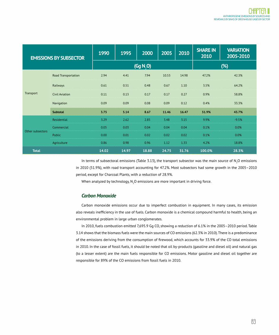
83
CHAPTER IIIANTHROPOGENIC EMISSIONS BY SOURCES AND
REMOVALS BY SINKS OF GREENHOUSE GASES BY SECTOR
EMISSIONS BY SUBSECTOR1990 1995 2000 2005 2010 SHARE IN
2010VARIATION 2005-2010
(Gg N2O) (%)
Transport
Road Transportation 2.94 4.41 7.94 10.53 14.98 47.2% 42.3%
Railways 0.61 0.51 0.48 0.67 1.10 3.5% 64.2%
Civil Aviation 0.11 0.13 0.17 0.17 0.27 0.9% 58.8%
Navigation 0.09 0.09 0.08 0.09 0.12 0.4% 33.3%
Subtotal 3.75 5.14 8.67 11.46 16.47 51.9% 43.7%
Other subsectors
Residential 3.29 2.62 2.85 3.48 3.15 9.9% -9.5%
Commercial 0.05 0.03 0.04 0.04 0.04 0.1% 0.0%
Public 0.00 0.01 0.02 0.02 0.02 0.1% 0.0%
Agriculture 0.86 0.98 0.96 1.12 1.33 4.2% 18.8%
Total 14.02 14.97 18.88 24.75 31.76 100.0% 28.3%
In terms of subsectoral emissions (Table 3.13), the transport subsector was the main source of N2O emissions
in 2010 (51.9%), with road transport accounting for 47.2%. Most subsectors had some growth in the 2005–2010
period, except for Charcoal Plants, with a reduction of 28.9%.
When analyzed by technology, N2O emissions are more important in driving force.
Carbon Monoxide
Carbon monoxide emissions occur due to imperfect combustion in equipment. In many cases, its emission
also reveals inefficiency in the use of fuels. Carbon monoxide is a chemical compound harmful to health, being an
environmental problem in large urban conglomerates.
In 2010, fuels combustion emitted 7,695.9 Gg CO, showing a reduction of 6.1% in the 2005–2010 period. Table
3.14 shows that the biomass fuels were the main sources of CO emissions (62.3% in 2010). There is a predominance
of the emissions deriving from the consumption of firewood, which accounts for 33.9% of the CO total emissions
in 2010. In the case of fossil fuels, it should be noted that oil by-products (gasoline and diesel oil) and natural gas
(to a lesser extent) are the main fuels responsible for CO emissions. Motor gasoline and diesel oil together are
responsible for 89% of the CO emissions from fossil fuels in 2010.

84
VOLUME IIITHIRD NATIONAL COMMUNICATION OF BRAZIL
TABLE 3.14 CO emissions by fuel
EMISSIONS BY FUEL 1990 1995 2000 2005 2010 SHARE IN 2010
VARIATION 2005-2010
FOSSIL (Gg CO) (%)
Motor Gasoline 4,527.9 5,174.8 3,967.7 3,116.1 2,278.6 29.6% -26.9%
Aviation Gasoline 30.4 30.2 36.4 26.3 33.3 0.4% 26.6%
Lighting Kerosene 0.5 0.3 0.1 0.1 0.0 0.0% -100.0%
Jet Fuel 2.6 2.9 3.9 4.4 5.2 0.1% 18.2%
Diesel Oil 178.1 216.6 257.2 275.8 310.3 4.0% 12.5%
Fuel Oil 13.8 17.5 18.9 20.0 16.1 0.2% -19.5%
LPG 2.8 3.7 5.7 4.6 5.0 0.1% 8.7%
Petroleum Coke 0.9 5.5 99.2 107.6 175.9 2.3% 63.5%
Lignite 1.2 1.1 0.7 0.5 0.4 0.0% -20.0%
Sub-bituminous Coal 4.1 2.5 1.6 1.4 2.6 0.0% 85.7%
Other Bituminous Coal 0.0 0.0 0.0 0.0 0.1 0.0% -
Coking Coal 0.0 0.1 0.2 0.3 0.1 0.0% -66.7%
Coal Tar 0.3 0.5 0.2 0.1 0.3 0.0% 200.0%
Coal Coke 3.8 0.0 0.0 4.8 4.0 0.1% -16.7%
Natural Gas (Humid) 1.8 0.7 3.0 6.1 8.6 0.1% 41.0%
Natural Gas (Dry) 2.9 6.1 14.2 37.9 46.2 0.6% 21.9%
Refinery Gas 3.0 4.2 4.6 4.9 5.3 0.1% 8.2%
Other Energy Oil Products 1.8 2.7 5.7 5.6 5.9 0.1% 5.4%
Gasworks gas 0.3 0.1 0.1 0.0 0.0 0.0% -
Coke Oven Gas 1.9 2.2 1.9 1.9 2.3 0.0% 21.1%
Other Primary Fossil Sources 0.1 0.1 0.1 0.0 0.0 0.0% -
Total Fossil 4,778.2 5,471.8 4,421.4 3,618.4 2,900.2 37.7% -19.8%
BIOMASS1990 1995 2000 2005 2010 SHARE
IN 2010VARIATION 2005-2010
(Gg CO) (%)
Firewood 2,910.5 2,332.0 2,367.6 2,924.3 2,605.2 33.9% -10.9%
Charcoal 183.9 128.9 110.6 134.5 103.5 1.3% -23.0%
Bagasse 328.2 366.0 314.0 496.7 892.4 11.6% 79.7%
Other Primary (biogas) 0.0 0.0 0.0 0.0 0.0 0.0% -
Other Primary (biomass) 9.1 12.8 17.0 28.3 29.9 0.4% 5.7%
Black Liquor 182.4 281.8 384.6 560.2 789.7 10.3% 41.0%
Anhydrous Alcohol 0.0 0.0 0.0 0.0 0.0 0.0% -
Hydrated Alcohol 1,200.3 1,043.0 565.8 432.3 375.0 4.9% -13.3%
Total Biomass 4,814.4 4,164.5 3,759.6 4,576.3 4,795.7 62.3% 4.8%
Total 9,592.6 9,636.3 8,181.0 8,194.7 7,695.9 100.0% -6.1%

85
CHAPTER IIIANTHROPOGENIC EMISSIONS BY SOURCES AND
REMOVALS BY SINKS OF GREENHOUSE GASES BY SECTOR
In terms of subsectoral emissions (Table 3.15), emissions from the transport subsector predominate, being the
main source of CO emissions in 2010 (38.1%), of which the road subsector stands out, with 37.4%. Nevertheless, it
must be emphasized that transport subsector showed a reduction of 22.9% in the emissions from 2005 to 2010,
while the industrial subsector, responsible for 22.2% of the CO total emissions, showed an increase by 33.3%.
TABLE 3.15 CO emissions by subsector
EMISSIONS BY SUBSECTOR1990 1995 2000 2005 2010 SHARE IN
2010VARIATION 2005-2010
(Gg CO) (%)
Broad Energy subsector
Public Service Power Plants 3.1 5.4 9.1 15.2 19.7 0.3% 29.6%
Self-Producers Power
Plants30.0 42.2 63.0 126.8 303.0 3.9% 139.0%
Charcoal Plants 1,070.6 845.4 777.7 1,019.3 723.2 9.4% -29.0%
Energy Sector 294.3 315.5 254.5 366.8 572.0 7.4% 55.9%
Industry
Cement 63.8 51.4 114.2 118.6 140.3 1.8% 18.3%
Iron and Steel 2.5 3.2 3.2 3.7 3.7 0.0% 0.0%
Ferroalloys 0.0 0.0 5.0 7.7 7.7 0.1% 0.0%
Mining and Pelleting 10.4 1.3 7.1 17.0 25.5 0.3% 50.0%
Non-Ferrous Metals 3.5 4.0 1.1 1.6 2.1 0.0% 31.3%
Chemical 29.5 25.1 20.4 21.5 22.5 0.3% 4.7%
Food and Beverages 182.3 175.8 187.5 204.8 260.9 3.4% 27.4%
Textiles 13.9 9.1 7.3 8.5 8.3 0.1% -2.4%
Pulp and Paper 254.4 369.1 483.5 673.1 938.9 12.2% 39.5%
Ceramics 134.9 121.3 140.8 149.0 202.1 2.6% 35.6%
Others 62.9 54.8 66.7 78.0 98.3 1.3% 26.0%
Subtotal 758.1 815.1 1,036.8 1,283.5 1,710.3 22.2% 33.3%
Transport
Road Transportation 5,856.4 6,373.4 4,724.6 3,761.8 2,875.0 37.4% -23.6%
Railways 5.4 4.5 4.3 6.0 9.7 0.1% 61.7%
Civil Aviation 33.0 33.1 40.3 31.0 38.5 0.5% 24.2%
Navigation 8.1 8.3 7.0 8.5 10.5 0.1% 23.5%
Subtotal 5,902.9 6,419.3 4,776.2 3,807.3 2,933.7 38.1% -22.9%
Other subsectors
Residential 1,443.2 1,098.7 1,172.3 1,468.4 1,306.7 17.0% -11.0%
Commercial 4.5 3.9 3.9 3.9 4.6 0.1% 17.9%
Public 0.4 0.9 0.6 0.5 0.2 0.0% -60.0%
Agriculture 85.5 89.9 86.9 103.0 122.5 1.6% 18.9%
Total 9,592.6 9,636.3 8,181.0 8,194.7 7,695.9 100% -6.1%

86
VOLUME IIITHIRD NATIONAL COMMUNICATION OF BRAZIL
When analyzing the emissions per technology, a concentration of the driving force emissions, consistent with
the large share of the transport subsector in the emissions of this gas, is observed.
Nitrogen Oxides
NOx emissions, which are indirect related greenhouse gases, are also an important pollution factor and may
cause a series of negative impacts on health, also contributing to acid rain.
Unlike what has been previously analyzed in terms of emission behavior for other non-CO2 gases reported
so far, NOx emissions are more directly related to fossil fuels as they involve high burning temperatures (90.3%
share of total emissions in 2010). Oil by-products (the emissions of diesel oil contribute with 59.4% to the total
emissions) and natural gas (9.4% participation) cause most emissions.
In 2010 2,567.1 Gg NOx were emitted from fuel combustion. The emissions growth rate was 9.4% during the
2005-2010 period.
TABLE 3.16 NOx emissions, by fuel
EMISSIONS BY FUEL 1990 1995 2000 2005 2010 SHARE IN 2010
VARIATION 2005-2010
FOSSIL (Gg NOX) (%)
Motor Gasoline 186.4 264.4 234.8 194.3 161.1 6.3% -17.1%
Aviation Gasoline 0.6 0.6 0.7 0.5 0.7 0.0% 40.0%
Lighting Kerosene 1.6 0.8 0.5 0.2 0.1 0.0% -50.0%
Jet Fuel 3.5 4.0 5.4 5.5 8.6 0.3% 56.4%
Diesel Oil 930.6 1,126.3 1,351.4 1,365.7 1,523.6 59.4% 11.6%
Fuel Oil 133.4 153.0 146.0 140.4 130.1 5.1% -7.3%
LPG 14.6 19.9 32.2 26.2 28.1 1.1% 7.3%
Petroleum Coke 0.6 1.4 18.9 20.0 32.7 1.3% 63.5%
Lignite 21.9 27.2 31.1 28.2 15.7 0.6% -44.3%
Sub-bituminous Coal 22.6 26.1 53.7 40.9 52.5 2.0% 28.4%
Other Bituminous Coal 0.0 0.0 0.0 0.0 0.2 0.0% -
Coking Coal 0.6 3.3 6.0 6.6 2.3 0.1% -65.2%
Coal Tar 2.6 4.1 1.8 0.9 2.1 0.1% 133.3%
Coal Coke 0.7 0.0 0.0 0.9 0.8 0.0% -11.1%
Natural Gas (Humid) 20.4 10.0 26.3 72.1 84.5 3.3% 17.2%
Natural Gas (Dry) 14.8 32.5 80.2 122.3 155.7 6.1% 27.3%
Refinery Gas 37.8 53.8 59.1 63.4 64.4 2.5% 1.6%
continues on the next page

87
CHAPTER IIIANTHROPOGENIC EMISSIONS BY SOURCES AND
REMOVALS BY SINKS OF GREENHOUSE GASES BY SECTOR
EMISSIONS BY FUEL 1990 1995 2000 2005 2010 SHARE IN 2010
VARIATION 2005-2010
FOSSIL (Gg NOX) (%)
Other Energy Oil Products 13.8 21.4 44.4 43.7 45.6 1.8% 4.3%
Gasworks gas 0.7 0.3 0.3 0.0 0.0 - -
Coke Oven Gas 11.8 14.1 10.4 9.2 8.3 0.3% -9.8%
Other Primary Fossil Sources 0.6 0.4 0.6 0.9 1.0 0.0% 11.1%
Total Fossil 1,419.6 1,763.6 2,103.8 2,141.9 2,318.1 90.3% 8.2%
BIOMASS1990 1995 2000 2005 2010 SHARE IN
2010VARIATION 2005-2010
(Gg NOX) (%)
Firewood 51.0 43.6 45.1 52.4 58.0 2.3% 10.7%
Charcoal 4.3 3.1 2.6 3.2 2.5 0.1% -21.9%
Bagasse 44.7 55.9 51.9 82.5 123.8 4.8% 50.1%
Other Primary (biogas) 0.0 0.0 0.0 0.0 0.0 0.000% -
Other Primary (biomass) 1.5 1.7 2.0 3.0 4.4 0.2% 46.7%
Black Liquor 5.9 9.6 13.2 19.4 27.7 1.1% 42.8%
Anhydrous Alcohol 0.0 0.0 0.0 0.0 0.0 - -
Hydrated Alcohol 112.8 100.0 54.7 44.0 32.6 1.3% -25.9%
Total Biomass 220.2 213.9 169.5 204.5 249.0 9.7% 21.8%
Total 1,639.8 1,977.5 2,273.3 2,346.4 2,567.1 100.0% 9.4%
Table 3.16 confirms that the main sources of NOx emissions are fossil fuels, with growth rate during the 2005-
2010 period (8.2%). In terms of subsectoral emissions in 2010 (Table 3.17), the transport subsector was the major
source of NOx emissions (56.9%), out of which 50.3% refer to road transport, followed by energy (14.5%) and
industrial (11.2%) subsectors. The subsectors that contributed the most to emissions showed increasing growth
rates during the 2005-2010 period: transport (3.2%), industry (18%) and energy (22%).
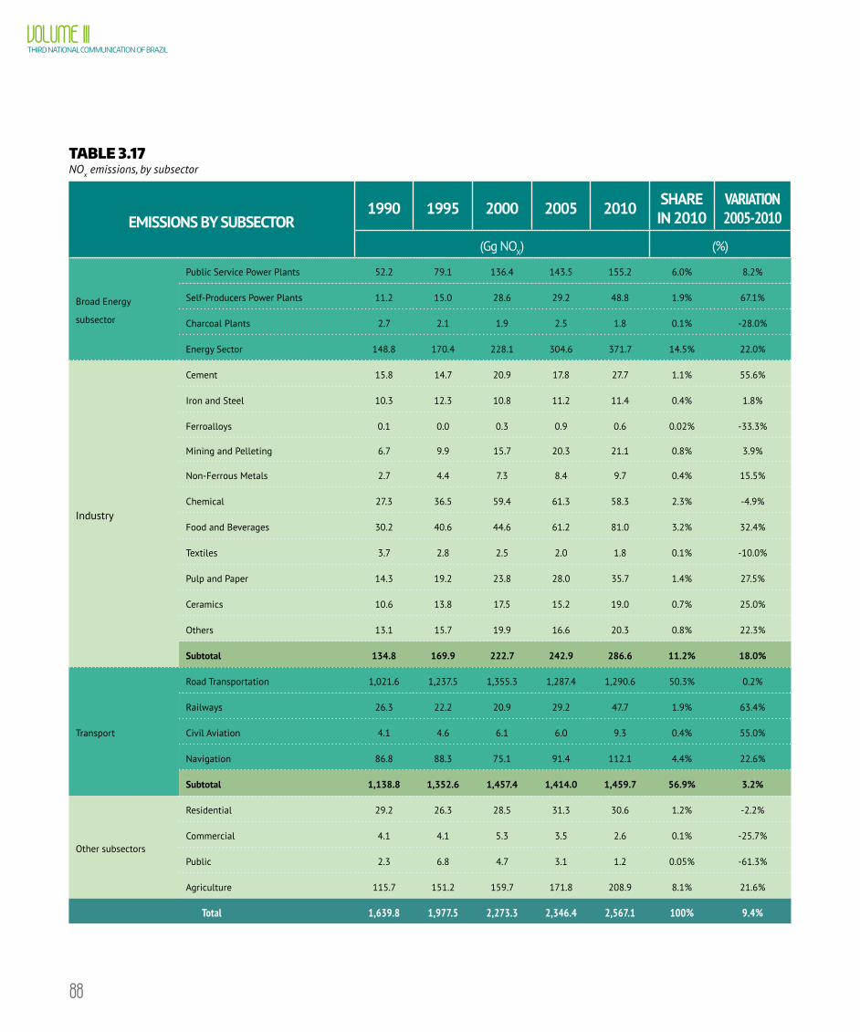
88
VOLUME IIITHIRD NATIONAL COMMUNICATION OF BRAZIL
TABLE 3.17 NOx emissions, by subsector
EMISSIONS BY SUBSECTOR1990 1995 2000 2005 2010 SHARE
IN 2010VARIATION 2005-2010
(Gg NOX) (%)
Broad Energy
subsector
Public Service Power Plants 52.2 79.1 136.4 143.5 155.2 6.0% 8.2%
Self-Producers Power Plants 11.2 15.0 28.6 29.2 48.8 1.9% 67.1%
Charcoal Plants 2.7 2.1 1.9 2.5 1.8 0.1% -28.0%
Energy Sector 148.8 170.4 228.1 304.6 371.7 14.5% 22.0%
Industry
Cement 15.8 14.7 20.9 17.8 27.7 1.1% 55.6%
Iron and Steel 10.3 12.3 10.8 11.2 11.4 0.4% 1.8%
Ferroalloys 0.1 0.0 0.3 0.9 0.6 0.02% -33.3%
Mining and Pelleting 6.7 9.9 15.7 20.3 21.1 0.8% 3.9%
Non-Ferrous Metals 2.7 4.4 7.3 8.4 9.7 0.4% 15.5%
Chemical 27.3 36.5 59.4 61.3 58.3 2.3% -4.9%
Food and Beverages 30.2 40.6 44.6 61.2 81.0 3.2% 32.4%
Textiles 3.7 2.8 2.5 2.0 1.8 0.1% -10.0%
Pulp and Paper 14.3 19.2 23.8 28.0 35.7 1.4% 27.5%
Ceramics 10.6 13.8 17.5 15.2 19.0 0.7% 25.0%
Others 13.1 15.7 19.9 16.6 20.3 0.8% 22.3%
Subtotal 134.8 169.9 222.7 242.9 286.6 11.2% 18.0%
Transport
Road Transportation 1,021.6 1,237.5 1,355.3 1,287.4 1,290.6 50.3% 0.2%
Railways 26.3 22.2 20.9 29.2 47.7 1.9% 63.4%
Civil Aviation 4.1 4.6 6.1 6.0 9.3 0.4% 55.0%
Navigation 86.8 88.3 75.1 91.4 112.1 4.4% 22.6%
Subtotal 1,138.8 1,352.6 1,457.4 1,414.0 1,459.7 56.9% 3.2%
Other subsectors
Residential 29.2 26.3 28.5 31.3 30.6 1.2% -2.2%
Commercial 4.1 4.1 5.3 3.5 2.6 0.1% -25.7%
Public 2.3 6.8 4.7 3.1 1.2 0.05% -61.3%
Agriculture 115.7 151.2 159.7 171.8 208.9 8.1% 21.6%
Total 1,639.8 1,977.5 2,273.3 2,346.4 2,567.1 100% 9.4%

89
CHAPTER IIIANTHROPOGENIC EMISSIONS BY SOURCES AND
REMOVALS BY SINKS OF GREENHOUSE GASES BY SECTOR
In relation to the technologies adopted, there is a predominance of driving force emissions, which account for
71.6% of emissions in 2010, also compatible with the role of the transport subsector regarding NOx emissions.
Non-Methane Volatile Organic Compounds
Non-methane volatile organic compounds (NMVOC) emissions are quantified in Table 3.18, which indicates a
reduction by 15.2% in total emissions during the 2005-2010 period. In 2010, 900.5 Gg NMVOC were emitted from
fuel combustion.
TABLE 3.18 NMVOC emissions by fuel
EMISSIONS BY FUEL 1990 1995 2000 2005 2010 SHARE IN 2010
VARIATION 2005-2010
FOSSIL (Gg NMVOC) (%)Motor Gasoline 373.8 431.7 351.2 300.7 230.2 25.6% -23.4%
Aviation Gasoline 0.6 0.6 0.7 0.5 0.7 0.1% 40.0%
Lighting Kerosene 0.1 0.0 0.0 0.0 0.0 0.0% -
Jet Fuel 0.6 0.7 1.0 0.8 0.5 0.1% -37.5%
Diesel Oil 60.9 74.5 88.7 88.5 91.1 10.1% 2.9%
Fuel Oil 3.6 4.1 3.7 3.2 3.4 0.4% 6.2%
LPG 0.8 0.7 1.2 1.3 1.2 0.1% -7.7%
Petroleum Coke 0.1 0.5 9.5 10.3 16.8 1.9% 63.1%
Lignite 0.1 0.1 0.1 0.0 0.0 0.0% -
Sub-bituminous Coal 0.5 0.3 0.2 0.1 0.3 0.0% 200.0%
Other Bituminous Coal 0.0 0.0 0.0 0.0 0.0 0.0% -
Coking Coal 0.0 0.0 0.0 0.0 0.0 0.0% -
Coal Tar 0.1 0.2 0.1 0.0 0.1 0.0% -
Coal Coke 0.4 0.0 0.0 0.5 0.4 0.0% -20.0%
Natural Gas (Humid) 0.1 0.1 0.2 0.4 0.5 0.1% 25.0%
Natural Gas (Dry) 0.2 0.4 1.0 2.4 3.0 0.3% 25.0%
Refinery Gas 0.3 0.4 0.6 0.8 0.8 0.1% 0.0%
Other Energy Oil Products 0.7 1.0 2.1 2.1 2.2 0.2% 4.8%
Gasworks gas 0.1 0.0 0.0 0.0 0.0 0.0% -
Coke Oven Gas 0.9 1.1 1.0 1.1 1.3 0.1% 18.2%
Other Primary Fossil Sources 0.0 0.0 0.0 0.0 0.0 0.0% -
Total Fossil 443.9 516.4 461.3 412.7 352.5 39.1% -14.6%
continues on the next page
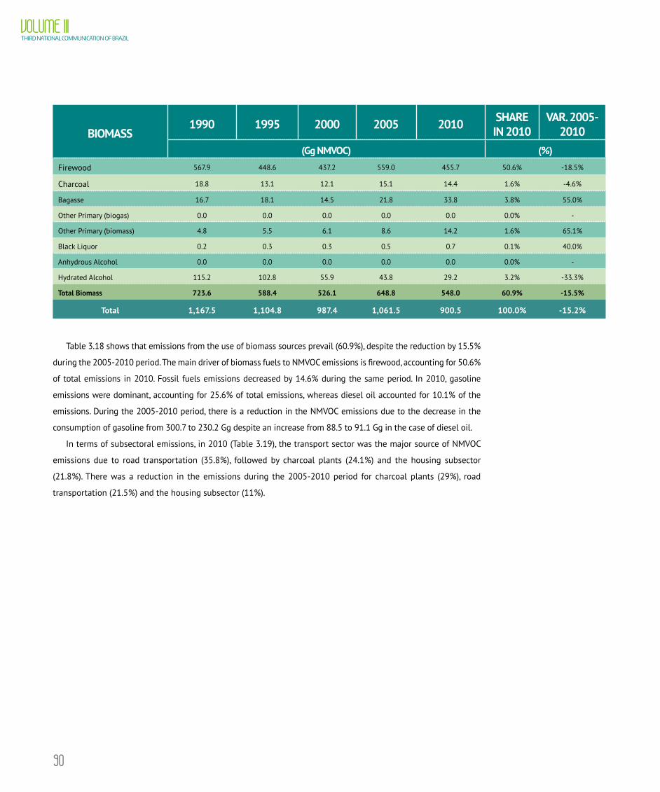
90
VOLUME IIITHIRD NATIONAL COMMUNICATION OF BRAZIL
BIOMASS1990 1995 2000 2005 2010 SHARE
IN 2010VAR. 2005-
2010(Gg NMVOC) (%)
Firewood 567.9 448.6 437.2 559.0 455.7 50.6% -18.5%
Charcoal 18.8 13.1 12.1 15.1 14.4 1.6% -4.6%
Bagasse 16.7 18.1 14.5 21.8 33.8 3.8% 55.0%
Other Primary (biogas) 0.0 0.0 0.0 0.0 0.0 0.0% -
Other Primary (biomass) 4.8 5.5 6.1 8.6 14.2 1.6% 65.1%
Black Liquor 0.2 0.3 0.3 0.5 0.7 0.1% 40.0%
Anhydrous Alcohol 0.0 0.0 0.0 0.0 0.0 0.0% -
Hydrated Alcohol 115.2 102.8 55.9 43.8 29.2 3.2% -33.3%
Total Biomass 723.6 588.4 526.1 648.8 548.0 60.9% -15.5%
Total 1,167.5 1,104.8 987.4 1,061.5 900.5 100.0% -15.2%
Table 3.18 shows that emissions from the use of biomass sources prevail (60.9%), despite the reduction by 15.5%
during the 2005-2010 period. The main driver of biomass fuels to NMVOC emissions is firewood, accounting for 50.6%
of total emissions in 2010. Fossil fuels emissions decreased by 14.6% during the same period. In 2010, gasoline
emissions were dominant, accounting for 25.6% of total emissions, whereas diesel oil accounted for 10.1% of the
emissions. During the 2005-2010 period, there is a reduction in the NMVOC emissions due to the decrease in the
consumption of gasoline from 300.7 to 230.2 Gg despite an increase from 88.5 to 91.1 Gg in the case of diesel oil.
In terms of subsectoral emissions, in 2010 (Table 3.19), the transport sector was the major source of NMVOC
emissions due to road transportation (35.8%), followed by charcoal plants (24.1%) and the housing subsector
(21.8%). There was a reduction in the emissions during the 2005-2010 period for charcoal plants (29%), road
transportation (21.5%) and the housing subsector (11%).

91
CHAPTER IIIANTHROPOGENIC EMISSIONS BY SOURCES AND
REMOVALS BY SINKS OF GREENHOUSE GASES BY SECTOR
TABLE 3.19 NMVOC emissions by subsector
EMISSIONS BY SUBSECTOR
1990 1995 2000 2005 2010 SHARE IN 2010
VARIATION 2005-2010
(Gg NMVOC) (%)
Broad Energy
subsector
Public Service
Power Plants0.8 1.4 2.1 3.0 3.5 0.4% 16.7%
Self-Producers
Power Plants0.4 0.6 1.2 1.5 2.4 0.3% 60.0%
Charcoal
plants321.2 253.6 233.3 305.8 217.0 24.1% -29.0%
Energy Sector 15.0 16.0 12.9 18.6 28.7 3.2% 54.3%
Industry
Cement 2.3 1.8 8.3 9.2 14.6 1.6% 58.7%
Iron and Steel 1.1 1.3 1.1 1.2 1.4 0.2% 16.7%
Ferroalloys 0.0 0.0 0.1 0.2 0.2 0.0% 0.0%
Mining and
Pelleting0.7 0.3 0.8 1.8 2.7 0.3% 50.0%
Non-Ferrous
Metals0.2 0.2 0.1 0.2 0.2 0.0% 0.0%
Chemical 2.5 2.9 3.3 3.4 3.4 0.4% 0.0%
Food and
Beverages9.2 9.2 9.7 11.1 14.5 1.6% 30.6%
Textiles 0.7 0.4 0.4 0.4 0.4 0.0% 0.0%
Pulp and
Paper7.9 9.0 10.2 12.7 18.5 2.1% 45.7%
Ceramics 4.1 3.7 4.2 4.5 6.4 0.7% 42.2%
Others 2.5 2.4 3.5 3.9 5.0 0.6% 28.2%
Subtotal 31.2 31.2 41.7 48.6 67.3 7.5% 38.5%
Transport
Road
Transportation534.9 589.9 475.3 410.4 322.0 35.8% -21.5%
Railways 2.3 2.0 1.9 2.6 4.2 0.5% 61.5%
Civil Aviation 1.3 1.3 1.7 1.3 1.2 0.1% -7.7%
Navigation 3.0 3.0 2.6 3.1 3.9 0.4% 25.8%
Subtotal 541.5 596.2 481.5 417.4 331.3 36.8% -20.6%continues on the next page

92
VOLUME IIITHIRD NATIONAL COMMUNICATION OF BRAZIL
EMISSIONS BY SUBSECTOR
1990 1995 2000 2005 2010 SHARE IN 2010
VARIATION 2005-2010
(Gg NMVOC) (%)
Other subsectors
Residential 216.5 164.9 175.9 220.3 196.1 21.8% -11.0%
Commercial 2.8 2.4 2.5 2.4 2.7 0.3% 12.5%
Public 0.3 0.8 0.8 0.6 0.4 0.0% -33.3%
Agriculture 37.8 37.7 35.5 43.3 51.1 5.7% 18.0%
Total 1,167.5 1,104.8 987.4 1,061.5 900.5 100% -15.2%
NMVOC emissions per subsector convey the predominance of the transport subsector, due to road traffic, which
accounts for 35.8%, followed by charcoal plants, which contribute with 24.1%, and the housing subsector, which
was the source for 21.8% of the total emissions in 2010.
The use in direct heating stands out with 51.3% of the emissions in 2010, followed by driving force with a
30.2% share in the total emissions of NMVOCs in 2010.
3.1.3. Fugitive Emissions
3.1.3.1. Fugitive emissions from coal mining This section presents estimates for greenhouse gas emissions from the coal mining industry, in mining and
processing operations, for the 1990-2010 period. The estimates include the fugitive emissions of CH4 of open pit
and underground mines and the post-mining activities. In addition to these, CO2 emissions from the spontaneous
combustion of waste piles are also estimated. Brazil did not report any cases in the period between 1990 and 2010
involving the recovery of gases and thermal conversion in coal mining companies. Therefore this category was
disregarded for the application of the IPCC methodology (1996).
Coal is formed from the burial and decomposition of vegetable matter. As they undergo burial and compaction
processes in deposition basins, these materials gradually increase their carbon content. External factors, such
as pressure, temperature and exposure time determine the characteristics of the coal, including the degree of
carbonification of these fuels.
Coal production in Brazil takes place in the three southern states in the country: Rio Grande do Sul, Santa
Catarina and Paraná, where the main coal reserves are located. Rio Grande do Sul is the state with the largest
geological reserves, followed by Santa Catarina and Paraná. Brazilian coal quality varies from south to north,
reducing ash content and increase calorific value and sulfur content, demanding environmental control due to SOx
emissions (sulfur oxides – SO2 and SO3).

93
CHAPTER IIIANTHROPOGENIC EMISSIONS BY SOURCES AND
REMOVALS BY SINKS OF GREENHOUSE GASES BY SECTOR
CH4 production is inherent to the coal formation process, being released to the atmosphere in the mining
process. The amount of CH4 released during the mining process is a primary function of the coal classification, of
the depth it is located, of its gas content and of the mining method. CO2 emissions may also occur as a result of
coal burning in waste deposits and piles.
Brazil produces two types of coal: energetic coal, also called steam coal, for industrial application in steam
and energy production; and metallurgical coal, for industrial application in steel mills. A significant increase can
be observed in steam coal production from 1990 to 2010. Metallurgical coal, on the other hand, has been entirely
imported since 2010.
Brazil’s dependence on imported coking coal rose from 79% in 2005 to 82% in 2010, mainly on account of the
metallurgical coal, and in the 1980s the steel industry started replacing the national metallurgical coal by the
imported coal.
The total production of run-of-mine (ROM) coal in Brazil is shown in Table 3.20. There was a small reduction in
terms of production compared to 2005. In 2010, 53.6% of coal production was from underground mines and 46.4%
from surface mines. Data used for developing this survey and applying the IPCC methodology were obtained from
official sources from national government entities, specifically the National Department of Mineral Production
(DNPM), under the Ministry of Mines and Energy (MME). These publications ceased in 2000, motivating a review of
the database and the consultation of the Annual Mining Report (RAL) informed by the sector to the DNPM.
ROM coal production data were obtained from Annual Carbon Industry Information/DNPM, detailed per mine.
However, there is no detailed data by mine for 1997 for the states of Rio Grande do Sul and Paraná and for 2000 there
is no data for any state. DNPM’s Brazilian Mineral Yearbook provides ROM coal production by state for 1996 to 2000 and
for the processed products from 1996 to 2010. As of 2005, along with DNPM (extracted directly from RAL) in the states
of Rio Grande do Sul, Santa Catarina and Paraná, considering the years from 2006 to 2012 as base years.
The share of coal and its by-products in the primary energy supply in Brazil dropped from 6.8% in 1990 to 6.4%
in 2005, and then to 5.4% in 2010. Coal’s share in the supply of primary energy exceeds national production due to
imports by several sectors.
TABLE 3.20 Run-of-mine coal production (ROM)
RUN-OF-MINE COAL(ROM)
1990 1995 2000 2005 2010 SHARE IN 2010
VARIATION 2005-2010
PRODUCTION (t) (%)
Open-pit mines
Rio Grande do Sul 3,577,545 3,587,888 5,950,038 4,250,367 4,523,071 46.4% 6.4%
Santa Catarina 21,970 453,236 383,873 131,720 0 0,0% -100.0%
Paraná 0 0 0 0 0 0,0% -
Total open-pit mines 3,599,515 4,041,124 6,333,911 4,382,087 4,523,071 46.4% 3.2%
continues on the next page

94
VOLUME IIITHIRD NATIONAL COMMUNICATION OF BRAZIL
RUN-OF-MINE COAL(ROM)
1990 1995 2000 2005 2010 SHARE IN 2010
VARIATION 2005-2010
PRODUCTION (t) (%)
Underground mines
Rio Grande do Sul 213,527 86,931 53,058 0 0 0.0% -
Santa Catarina 6,231,261 5,163,126 5,571,109 6,300,417 4,933,730 50.6% -21.7%
Paraná 239,313 254,172 108,225 287,573 293,328 3.0% 2.0%
Total underground mines 6,684,101 5,504,229 5,732,392 6,587,990 5,227,058 53.6% -20.7%
Total Brazil 10,283,616 9,545,353 12,066,303 10,970,077 9,750,129 100% -11.1%
Methane Emissions
Methane content in coal is related to factors like rank (degree of carbonification of the original vegetable
matter), depth of the layer and physical-chemical properties, among others. However, there are relevant geological
factors that affect the dynamic balance of methane found in the coal layer.
In the same way as presented in the Second Inventory, despite the initial effort of studies for the search of
emission factors that could better reflect the reality of Brazil’s coal mining and handling, for this publication
the approach adopted was the 1996 Tier 1 Guidelines minimum emission factors, not only for post-mining, but,
coherently, for the mining as well. The adopted approach aimed at safeguarding the reliability of calculated values,
considering that the experimental part pointed to divergences between the behavior conceptually foreseen for
methane emissions and the results achieved in the sampled mines. For open-pit mines, the minimum null value
for post-mining was discarded and an arbitrated value was used so measured emissions would not be disregarded.
The factors adopted in this Inventory are shown in Table 3.21.
TABLE 3.21 Emission factors for CH4 of fugitive emissions of coal production
EMISSION FACTORS FOR CH4 FUGITIVE EMISSION FROM COAL
LOW EMISSION LEVEL
MINING POST-MINING
(M3 CH4/t COAL)Underground mines 10 0.9
Open-pit mines 0.3 0.05
Total CH4 emissions are shown in Table 3.22. Underground mines accounted for 89.26% of total CH4 emissions,
open-air mines accounted for 2.3% and emissions from post-mining activities represented 8.4% of the total.
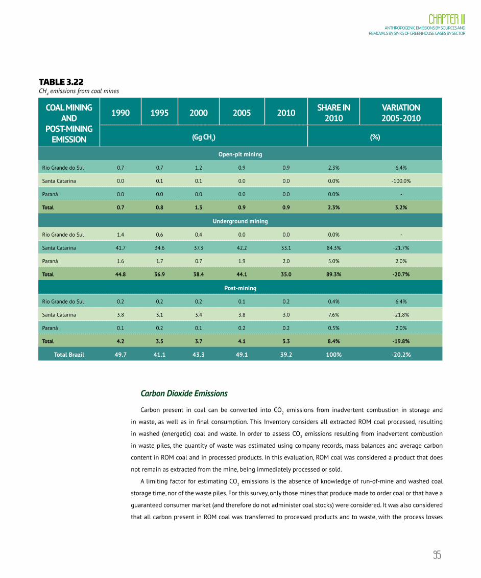
95
CHAPTER IIIANTHROPOGENIC EMISSIONS BY SOURCES AND
REMOVALS BY SINKS OF GREENHOUSE GASES BY SECTOR
TABLE 3.22 CH4 emissions from coal mines
COAL MINING AND
POST-MINING EMISSION
1990 1995 2000 2005 2010 SHARE IN 2010
VARIATION 2005-2010
(Gg CH4) (%)
Open-pit mining
Rio Grande do Sul 0.7 0.7 1.2 0.9 0.9 2.3% 6.4%
Santa Catarina 0.0 0.1 0.1 0.0 0.0 0.0% -100.0%
Paraná 0.0 0.0 0.0 0.0 0.0 0.0% -
Total 0.7 0.8 1.3 0.9 0.9 2.3% 3.2%
Underground mining
Rio Grande do Sul 1.4 0.6 0.4 0.0 0.0 0.0% -
Santa Catarina 41.7 34.6 37.3 42.2 33.1 84.3% -21.7%
Paraná 1.6 1.7 0.7 1.9 2.0 5.0% 2.0%
Total 44.8 36.9 38.4 44.1 35.0 89.3% -20.7%
Post-mining
Rio Grande do Sul 0.2 0.2 0.2 0.1 0.2 0.4% 6.4%
Santa Catarina 3.8 3.1 3.4 3.8 3.0 7.6% -21.8%
Paraná 0.1 0.2 0.1 0.2 0.2 0.5% 2.0%
Total 4.2 3.5 3.7 4.1 3.3 8.4% -19.8%
Total Brazil 49.7 41.1 43.3 49.1 39.2 100% -20.2%
Carbon Dioxide Emissions
Carbon present in coal can be converted into CO2 emissions from inadvertent combustion in storage and
in waste, as well as in final consumption. This Inventory considers all extracted ROM coal processed, resulting
in washed (energetic) coal and waste. In order to assess CO2 emissions resulting from inadvertent combustion
in waste piles, the quantity of waste was estimated using company records, mass balances and average carbon
content in ROM coal and in processed products. In this evaluation, ROM coal was considered a product that does
not remain as extracted from the mine, being immediately processed or sold.
A limiting factor for estimating CO2 emissions is the absence of knowledge of run-of-mine and washed coal
storage time, nor of the waste piles. For this survey, only those mines that produce made to order coal or that have a
guaranteed consumer market (and therefore do not administer coal stocks) were considered. It was also considered
that all carbon present in ROM coal was transferred to processed products and to waste, with the process losses

96
VOLUME IIITHIRD NATIONAL COMMUNICATION OF BRAZIL
being accounted for in the waste. Since in Santa Catarina, waste was reprocessed, carbon percentages were
estimated and the carbon thus calculated was added to the carbon in the run-of-mine coal for mass balance. For
calculating CO2 emissions, a 50% oxidation factor was used for waste.
Estimates of CO2 emissions from coal deposits and waste piles can be observed in Table 3.23 separately, and
by producer states.
TABLE 3.23 CO2 emissions from coal mines and waste piles
CALCULATING CO2 EMISSIONS FROM WASTE PILES 1990 1995 2000 2005 2010 VARIATION
2005-2010Carbon in Run-of-Mine coal (t)
Rio Grande do Sul 890,966 892,079 1,437,521 903,529 1,008,459 11.6%
Santa Catarina 1,438,429 1,331,633 1,390,053 1,628,249 1,377,788 -15.4%
Paraná 58,870 57,791 24,892 66,142 64,532 -2.4%
Brasil 2,388,265 2,281,503 2,852,467 2,597,920 2,450,779 -5.7%
Carbon in products (t)
Rio Grande do Sul 785,152 849,515 1,110,514 935,733 545,806 -41.7%
Santa Catarina 812,407 872,812 1,013,524 910,669 859,948 -5.6%
Paraná 52,684 57,181 24,167 30,429 38,043 25.0%
Brasil 1,650,244 1,779,508 2,148,205 1,876,831 1,443,796 -23.1%
Carbon in waste piles (t)
Rio Grande do Sul 105,814 42,564 327,008 0 462,653 -
Santa Catarina 626,022 458,821 376,529 717,580 517,841 -27.8%
Paraná 6,186 610 725 35,712 26,490 -25.8%
Brasil 738,022 501,995 704,262 753,292 1,006,983 33.7%
Emissions (Gg CO2) 1,353 920 1,291 1,381 1,846 33.7%
3.1.3.2. Fugitive emissions from oil and natural gas activitiesThis category includes emissions from production, processing, transportation and use of oil and natural gas
and from combustion not related to production. Therefore, anthropogenic emissions of CO2, CH4 and N2O are
estimated due to oil and natural gas activities. Fugitive emission sources are considered for: Exploration and
Production (E&P), Refining and Transportation. In addition to the emissions concerning Petrobras, the estimates of
emissions from other companies that carry out activities in the oil and gas industry in Brazil are also presented, for
the first time, between 2003 and 2010, calculated based on an extrapolation of data from the production and the
processing as well as the application of Petrobras’ implicit annual emission factors.
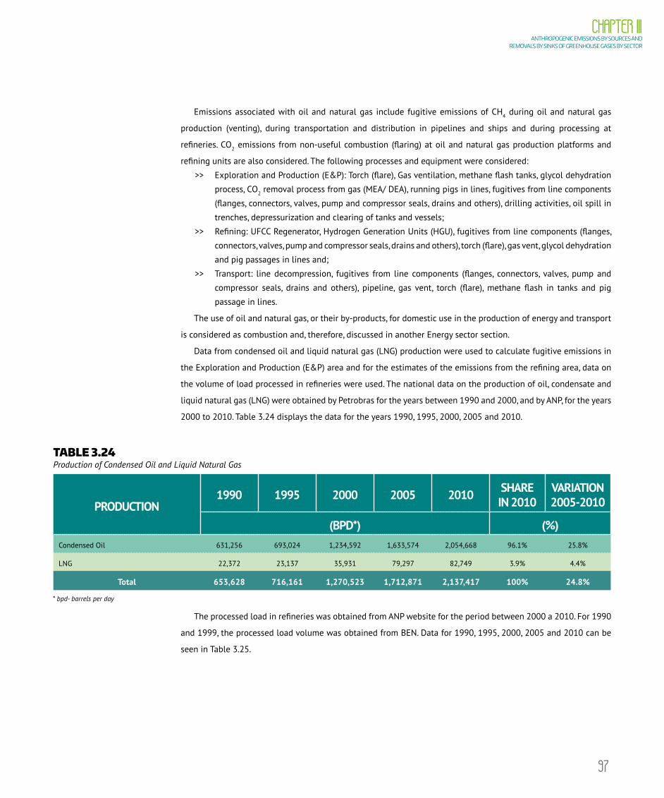
97
CHAPTER IIIANTHROPOGENIC EMISSIONS BY SOURCES AND
REMOVALS BY SINKS OF GREENHOUSE GASES BY SECTOR
Emissions associated with oil and natural gas include fugitive emissions of CH4 during oil and natural gas
production (venting), during transportation and distribution in pipelines and ships and during processing at
refineries. CO2 emissions from non-useful combustion (flaring) at oil and natural gas production platforms and
refining units are also considered. The following processes and equipment were considered:
>> Exploration and Production (E&P): Torch (flare), Gas ventilation, methane flash tanks, glycol dehydration
process, CO2 removal process from gas (MEA/ DEA), running pigs in lines, fugitives from line components
(flanges, connectors, valves, pump and compressor seals, drains and others), drilling activities, oil spill in
trenches, depressurization and clearing of tanks and vessels;
>> Refining: UFCC Regenerator, Hydrogen Generation Units (HGU), fugitives from line components (flanges,
connectors, valves, pump and compressor seals, drains and others), torch (flare), gas vent, glycol dehydration
and pig passages in lines and;
>> Transport: line decompression, fugitives from line components (flanges, connectors, valves, pump and
compressor seals, drains and others), pipeline, gas vent, torch (flare), methane flash in tanks and pig
passage in lines.
The use of oil and natural gas, or their by-products, for domestic use in the production of energy and transport
is considered as combustion and, therefore, discussed in another Energy sector section.
Data from condensed oil and liquid natural gas (LNG) production were used to calculate fugitive emissions in
the Exploration and Production (E&P) area and for the estimates of the emissions from the refining area, data on
the volume of load processed in refineries were used. The national data on the production of oil, condensate and
liquid natural gas (LNG) were obtained by Petrobras for the years between 1990 and 2000, and by ANP, for the years
2000 to 2010. Table 3.24 displays the data for the years 1990, 1995, 2000, 2005 and 2010.
TABLE 3.24 Production of Condensed Oil and Liquid Natural Gas
PRODUCTION1990 1995 2000 2005 2010 SHARE
IN 2010VARIATION 2005-2010
(BPD*) (%)Condensed Oil 631,256 693,024 1,234,592 1,633,574 2,054,668 96.1% 25.8%
LNG 22,372 23,137 35,931 79,297 82,749 3.9% 4.4%
Total 653,628 716,161 1,270,523 1,712,871 2,137,417 100% 24.8%
* bpd- barrels per day
The processed load in refineries was obtained from ANP website for the period between 2000 a 2010. For 1990
and 1999, the processed load volume was obtained from BEN. Data for 1990, 1995, 2000, 2005 and 2010 can be
seen in Table 3.25.
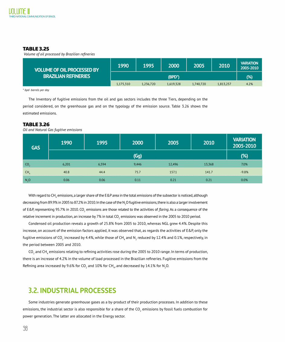
98
VOLUME IIITHIRD NATIONAL COMMUNICATION OF BRAZIL
TABLE 3.25 Volume of oil processed by Brazilian refineries
VOLUME OF OIL PROCESSED BY BRAZILIAN REFINERIES
1990 1995 2000 2005 2010 VARIATION 2005-2010
(BPD*) (%)1,175,310 1,236,720 1,619,328 1,740,720 1,813,257 4.2%
* bpd- barrels per day
The Inventory of fugitive emissions from the oil and gas sectors includes the three Tiers, depending on the
period considered, on the greenhouse gas and on the typology of the emission source. Table 3.26 shows the
estimated emissions.
TABLE 3.26 Oil and Natural Gas fugitive emissions
GAS1990 1995 2000 2005 2010 VARIATION
2005-2010
(Gg) (%)CO2 6,201 6,594 9,446 12,496 13,368 7.0%
CH4 40.8 44.4 75.7 157.1 141.7 -9.8%
N2O 0.06 0.06 0.11 0.21 0.21 0.0%
With regard to CH4 emissions, a larger share of the E&P area in the total emissions of the subsector is noticed, although
decreasing from 89.9% in 2005 to 87.2% in 2010. In the case of the N2O fugitive emissions, there is also a larger involvement
of E&P, representing 95.7% in 2010. CO2 emissions are those related to the activities of flaring. As a consequence of the
relative increment in production, an increase by 7% in total CO2 emissions was observed in the 2005 to 2010 period.
Condensed oil production reveals a growth of 25.8% from 2005 to 2010, whereas NGL grew 4.4%. Despite this
increase, on account of the emission factors applied, it was observed that, as regards the activities of E&P, only the
fugitive emissions of CO2 increased by 4.4%, while those of CH4 and N2 reduced by 12.4% and 0.1%, respectively, in
the period between 2005 and 2010.
CO2 and CH4 emissions relating to refining activities rose during the 2005 to 2010 range. In terms of production,
there is an increase of 4.2% in the volume of load processed in the Brazilian refineries. Fugitive emissions from the
Refining area increased by 9.6% for CO2 and 10% for CH4, and decreased by 14.1% for N2O.
3.2. INDUSTRIAL PROCESSESSome industries generate greenhouse gases as a by-product of their production processes. In addition to these
emissions, the industrial sector is also responsible for a share of the CO2 emissions by fossil fuels combustion for
power generation. The latter are allocated in the Energy sector.

99
CHAPTER IIIANTHROPOGENIC EMISSIONS BY SOURCES AND
REMOVALS BY SINKS OF GREENHOUSE GASES BY SECTOR
The main industrial processes that generate CO2 emissions in Brazil are iron and steel production, cement
production, lime production, aluminum production and ammonia production. Iron and steel production is the
largest source of CH4 emissions due to the use of charcoal by the pig iron industries. N2O emissions occur mainly
in the production processes of adipic and nitric acid, and also in the production of iron and steel. During the
production of iron and steel, iron-alloys and aluminum, there are emissions of CO and PFCs (CF4 and C2F6). Pulp
and paper production is the main NOx generator. The food and beverage subsector is responsible for most NMVOC
emissions by industrial processes. HFC emissions occur during their use in the refrigeration sector and during
production of HCFC-22.
3.2.1. Mineral Products
3.2.1.1. Cement Production In 2011, Brazil ranked 6th in cement production in the world, according to information of the 2012 Annual
Report of the National Cement Industry Union (SNIC, 2012) and production took place in several states. In 2012 the
cement industrial park was composed of 83 plants, 53 of which were integrated plants (out of which 46 associated
with the SNIC and 7 not) with oven for the production of cement clinker, and the other 30 were only mills (22 were
associated with the SNIC and 8 were not), which use the ready-made clinker.
Globally, approximately 90% of CO2 emissions from cement manufacturing occur during clinker production,
both for the calcination/decarbonation of raw material, or for the fuel combustion in furnaces. The remaining
emissions derive from the transportation of raw materials and for the electricity consumption at the factory. The
emissions reported in the Industrial Processes sector are only for calcination/ decarbonation of raw materials.
Clinker is obtained from the calcination of limestone (CaCO3), a process that generates CO2 emissions. Table 3.27
presents a summary of the data for the 1990 to 2010 period.
TABLE 3.27 Cement and clinker production
PRODUCT1990 1995 2000 2005 2010 VAR. 2005/ 2010
(103 t) (%)Cement 25,848 28,256 39,901 38,706 59,117 52.7%
Clinker 20,161 21,071 29,227 26,307 39,119 48.7%
Source: National Cement Industries Union – SNIC (2012).
The national cement industry has a tradition of using cement with additions, making use of by-products from
other activities (such as slag and thermoelectric ash) and alternative raw materials. These additions have been

100
VOLUME IIITHIRD NATIONAL COMMUNICATION OF BRAZIL
ongoing for over 50 years in the country, a practice that only recently has been adopted worldwide and which, in
addition to diversifying the applications and specific characteristics of the cement, leads to less CO2 emissions,
both by decreasing the production of clinker and by reducing the use of fossil fuels. The growing use, for a long
time, of additions to cement in Brazil has represented one of the most effective measures for the control and the
reduction of CO2 emissions from the industry.
For this reason the Brazilian cement industry is committed to obtaining every detailed information necessary
for the application of the sectoral methodology of the Cement Sustainability Initiative (CSI), an initiative of the
largest world cement groups linked to the World Business Council for Sustainable Development (WBCSD), aiming at
developing a series of environmental actions, among which are the control and the monitoring of GHG emissions.
This information is consistent with the Tier 3 approach of the 2006 IPCC Guidelines for National Inventories of
Greenhouse Gases (IPCC, 2006), which considers the composition of raw materials (carbonates) used, corrects the
emissions by the MgO content and includes other specific parameters such as the correction of cement kiln dust
(CKD), which is regarded as a system loss, and the carbon of the organic matter contained in raw materials. The
CO2 emissions were calculated using the default recommended by the CSI methodology and, whenever there were
no available data, the EF of 0.536 t CO2 /t clinker was used, considering the organic carbon contained in the raw
material. The results are summarized in Table 3.28.
TABLE 3.28 CO2 emissions from limestone decarbonation in cement production
EMISSIONS SOURCE1990 1995 2000 2005 2010 VAR. 2005/ 2010
(Gg CO2) (%)Cement production 11,062 11,528 16,047 14,349 21,288 48.4%
3.2.1.2. Lime productionIn 2010, Brazil was responsible for 2.5% of the global lime production, and was the fourth largest producer, after
China, United States and India, in this order.
The term lime is used in Brazilian literature and in Brazilian Association of Technical Standards (ABNT) to
designate the product made of calcium oxide (CaO) and calcium and magnesium oxide (CaO.MgO), resulting from
the calcination of limestone, magnesium and dolomite limestone. Lime is classified in accordance with the total
percentage of calcium oxide. Thus, when referring to a type of lime, reference is actually made to a range of products
with different amounts of CaO and CaO.MgO.
Lime is formed by heating limestone for decomposition of carbonates, a process called calcination or decarbonation.
It is carried out at high temperatures in a rotary oven, followed by CO2 emissions. Hydrated lime is obtained from
quicklime by adding water. Dolomite (CaCO3.MgCO3) can also be processed at high temperatures to obtain dolomite
lime (and CO2 emissions). Lime is a product with several applications, among which metallurgy, civil construction, pulp
and paper industry, water and effluent treatment, pH control and soil stabilization stand out.
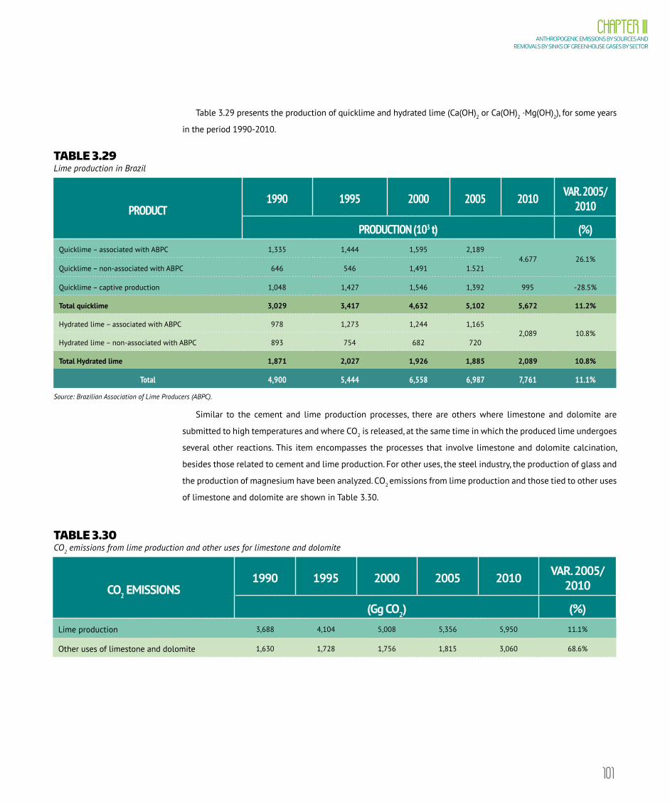
101
CHAPTER IIIANTHROPOGENIC EMISSIONS BY SOURCES AND
REMOVALS BY SINKS OF GREENHOUSE GASES BY SECTOR
Table 3.29 presents the production of quicklime and hydrated lime (Ca(OH)2 or Ca(OH)2 ·Mg(OH)2), for some years
in the period 1990-2010.
TABLE 3.29 Lime production in Brazil
PRODUCT1990 1995 2000 2005 2010 VAR. 2005/
2010
PRODUCTION (103 t) (%)Quicklime – associated with ABPC 1,335 1,444 1,595 2,189
4.677 26.1%Quicklime – non-associated with ABPC 646 546 1,491 1.521
Quicklime – captive production 1,048 1,427 1,546 1,392 995 -28.5%
Total quicklime 3,029 3,417 4,632 5,102 5,672 11.2%
Hydrated lime – associated with ABPC 978 1,273 1,244 1,1652,089 10.8%
Hydrated lime – non-associated with ABPC 893 754 682 720
Total Hydrated lime 1,871 2,027 1,926 1,885 2,089 10.8%
Total 4,900 5,444 6,558 6,987 7,761 11.1%
Source: Brazilian Association of Lime Producers (ABPC).
Similar to the cement and lime production processes, there are others where limestone and dolomite are
submitted to high temperatures and where CO2 is released, at the same time in which the produced lime undergoes
several other reactions. This item encompasses the processes that involve limestone and dolomite calcination,
besides those related to cement and lime production. For other uses, the steel industry, the production of glass and
the production of magnesium have been analyzed. CO2 emissions from lime production and those tied to other uses
of limestone and dolomite are shown in Table 3.30.
TABLE 3.30 CO2 emissions from lime production and other uses for limestone and dolomite
CO2 EMISSIONS1990 1995 2000 2005 2010 VAR. 2005/
2010
(Gg CO2) (%)Lime production 3,688 4,104 5,008 5,356 5,950 11.1%
Other uses of limestone and dolomite 1,630 1,728 1,756 1,815 3,060 68.6%

102
VOLUME IIITHIRD NATIONAL COMMUNICATION OF BRAZIL
3.2.1.3. Production and consumption of soda ashSoda ash (neutral sodium carbonate– Na2CO3) is used as feedstock in many industries, including glass, soap and
detergent manufacturing, pulp and paper production and water treatment.
Four different processes can be commercially used to produce soda ash. Three are referred to as natural
processes and use trona as a basic input. The fourth, the Solvay process, is classified as a synthetic process. The
natural processes are the only ones that produce CO2 emissions. Brazilian production, discontinued in 2002, used
the synthetic process, and thus no net emissions were produced.
CO2 emissions occur when soda ash is consumed in industry. Consumption is calculated based on data on
production, imports and exports of soda ash in Brazil, shown in Table 3.31.
TABLE 3.31 Production, imports, exports and consumption of soda ash
PRODUCT1990 1995 2000 2005 2010 VAR. 2005/
2010
(t) (%)
Production 195,893 203,950 190,616 - - NA
Imports 242,788 392,071 393,845 597,888 954,675 59.7%
Exports - 2 4 2 47 2230.0%
Consumption 438,681 596,019 584,457 597,886 954,629 59.7%
Source: Brazilian Association of Chemical Industry (ABIQUIM).
For the estimates of CO2 emissions, it is assumed that one carbon mol is released for each mol of soda ash consumed.
Hence the 0.415 t CO2 / t Na2CO3 emission factor was used. Estimated CO2 emissions are shown in Table 3.32.
TABLE 3.32 CO2 emission from soda ash consumption
USE OF SODA ASH1990 1995 2000 2005 2010 VAR. 2005/
2010
(Gg CO2) (%)
CO2 emissions 182 247 243 248 396 59.7%
3.2.2. Chemical IndustrySeveral production processes in the national chemical industry cause greenhouse gas emissions – CO2, CH4
and N2O – as well as indirect greenhouse gas emissions – CO, NOx and NMVOC. These emissions deriving from
the chemical sector in Brazil are associated with the production of ammonia, nitric acid, adipic acid, caprolactam,
calcium carbide calcium, petrochemicals (methanol, ethylene, dichloroethane and vinyl chloride, ethylene oxide and

103
CHAPTER IIIANTHROPOGENIC EMISSIONS BY SOURCES AND
REMOVALS BY SINKS OF GREENHOUSE GASES BY SECTOR
acrylonitrile), carbon black and petroleum coke. In addition, other chemicals such as ABS resins, phthalic anhydride,
styrene butadiene rubber (SBR), styrene, ethylbenzene, formaldehyde, polyvinyl chloride (PVC), polystyrene,
polyethylene (HDPE), polyethylene (LDPE), polyethylene (LLDPE), polypropylene and propylene produce indirect
emissions of volatile organic compounds such as SO2, NOx, NMVOC and CO. The production of titanium oxide was
not assessed, because the technological route used in Brazil does not emit GHG.
With the advance in biofuel production technologies, the national chemistry industry has begun to replace
fossil fuels, used as raw materials in its production processes, with renewable fuels. This action aims at reducing
greenhouse gas emissions in the process. Additionally, new N2O control technologies have been adopted, mainly for
adipic acid production, which were responsible for most of this sort of greenhouse gas emissions.
Direct greenhouse gases were estimated based on 2006 Guidelines (IPCC, 2006) and indirect greenhouse gases
based on 1996 Guidelines (IPCC, 1997).
3.2.2.1. Ammonia production Ammonia is one of the basic chemical products, produced in large quantities, used as a source of nitrogen. It is a
raw material for manufacturing urea, the main nitrogenized fertilizer, and for producing nitric acid, an intermediate
element in the production of ammonium nitrate fertilizer or explosive.
Ammonia production requires a source of hydrogen and another of nitrogen. The atmosphere is the nitrogen
source. Hydrogen can be obtained from different raw materials, such as: asphalt residue, residual refining gas,
natural gas, petrochemical naphtha and ethanol.
CO2 is generated as a by-product of ammonia production, and is released into the atmosphere. When there is
integration with an urea or methanol plant, part of this CO2 is used as a raw material to produce those products.
Alternatively, CO2 can also be recovered for use as a refrigerant fluid, in liquid carbonation and as an inert gas. In
all such cases, however, CO2 is short-lived and thus not deducted from ammonia production emissions.
Until 2005, the emissions from the production of ammonia were estimated on the basis of the measurement of
fuels used as raw materials in the process, as per the 2006 Guidelines, without the due discount of the share of CO2
intended for the production of urea in integrated plants as oriented in the 2006 Guidelines. After this, considering
the raw materials used in Brazil and their respective FEs, an average value was obtained for the national emission
factor of 1.46 t CO2 /t of ammonia, which was applied to all years of the 1990 to 2010 period.
Ammonia production is presented in Table 3.33, and the corresponding CO2 emissions are displayed in Table 3.34.
3.2.2.2. Nitric acid production Nitric acid (HNO3) is an inorganic compound mainly used for manufacturing synthetic fertilizers. It is the most important
compound not only as a feedstock in adipic acid production, but also as an intermediate element in concentrated nitric
acid production, as a nitration agent in organic compounds or as an input for the production of explosives.
104
VOLUME IIITHIRD NATIONAL COMMUNICATION OF BRAZIL
The traditional and commercially available production process for nitric acid involves the catalytic oxidation of
ammonia with air and the subsequent reactions of oxidation with water, through the Ostwald process, generating
N2O as a by-product. Furthermore, NOx emissions other than those from combustion may occur.
In production units in Brazil, which comprise low pressure and medium pressure and vacuum plants, there
are abatement technologies for NO and NO2 emissions (nitric oxide, nitrogen dioxide, generically called NOx), in
accordance with the standards established by environmental control entities.
From late 2006, CDM project activities began to be developed in Brazil, involving the installation of secondary
catalyzers for N2O destruction. After July 2007, with the implementation of a CDM project in medium-pressure
plant, this plant’s measured emission factor was reduced from 6.01 kg N2O/t HNO3 to 0.52 kg N2O/t HNO3.
N2O emissions were estimated using different methods, depending on the plant. For those plants that conducted
CDM project activities, it was possible to apply the most accurate method (Tier 3), with direct measurements of
emissions, which result in specific emission factors for each plant. For the others, the simplified method was used,
applying default emission factors from 2006 Guidelines.
For NOX emissions, the country’s specific emission factor was applied, 1.75 kg NOX /t nitric acid, in accordance
with ABIQUIM, as a result of the emission controls for these gases in the country.
Nitric acid production is shown in Table 3.33 and the corresponding N2O and NOX emissions in Table 3.34.
3.2.2.3. Adipic acid production Adipic acid is a white crystalline solid used as an intermediate in the manufacturing of synthetic fibers, plastics,
polyurethanes, elastomers and synthetic lubricants. Commercially, it is the most important aliphatic dicarboxylic
acid used in the manufacturing of polyester and nylon 6.6.
The only adipic acid plant in Brazil uses the two-stage production technology. The first involves cyclohexane
oxidation for the cyclohexanone/cyclohexanol mixture. The second stage involves the cyclohexanol oxidation
process using nitric acid. In this latter stage, N2O is released. Adipic acid production also emits CO and NOx.
An N2O abatement project at this factory was registered at the CDM Executive Board in the end of 2005, with
effective destruction of N2O from 2007. A dedicated installation was constructed for high temperature conversion
of nitrous oxide into nitrogen, as part of the N2O thermal decomposition process.
The measured N2O emission factor was of 0.270 t N2O/t adipic acid, applied from 1990 to 2006. After
implementation of the CDM project in 2007, there was a significant emission reduction, and the implicit emission
factor, also obtained by measurements, ranged from 0.00640 t N2O/t adipic acid to 0.00155 t N2O/t adipic acid.
Indirect greenhouse gases were estimated with national emission factors as a result of the control of emissions
of these gases in the country. CO emissions were estimated with a factor of 16 kg CO/t adipic acid. below the 1996
Guidelines default, 34.4 kg CO/t adipic acid. For NOx emissions, the emission factor of 5 kg NOx /t adipic acid, below
the default of 8.1 kg NOx /t adipic acid from the 1996 Guidelines, was applied.
Adipic acid production is shown in Table 3.33 and the corresponding N2O, CO and NOx emissions in Table 3.34.

105
CHAPTER IIIANTHROPOGENIC EMISSIONS BY SOURCES AND
REMOVALS BY SINKS OF GREENHOUSE GASES BY SECTOR
3.2.2.4. Caprolactam productionThe primary industrial use of caprolactam is as a monomer in the production of nylon-6. This chemical is also
used for manufacturing plastics, bristles, films, covers, carpets, synthetic leather, plasticizers, and automotive paints. It is
biodegradable and allows for a removal rate up to 94% for the chemical demand for oxygen in activated sludge systems.
Brazilian production of caprolactam stems from the hydrogenation of benzene to cyclohexane, oxidation of
cyclohexanol and cyclohexanone with nitric acid, a step in which N2O is generated, followed by the dehydrogenation
of the cyclohexanol produced and subsequent reaction with sulfate.
N2O emissions were based on plant measurements adopting the resulting average value of 6 kg N2O/t
caprolactam was adopted.
Caprolactam production is shown in Table 3.33 and the corresponding N2O emissions in Table 3.34.
3.2.2.5. Calcium carbide production and useCalcium carbide (CaC2) is produced from the calcination of limestone and the subsequent reduction of lime
with petroleum coke or charcoal. These two types of reducing agents are used in Brazil. Emissions related to lime
production are reported in the specific lime item. From the reaction of calcium carbide production, only those
emissions related to the use of petroleum coke, a fossil fuel, are considered.
Around 67% of the carbon contained in petroleum coke is retained in the final product (CaC2). Later use of
calcium carbide in the steel industry and in the production of acetylene leads to more CO2 emissions.
CO2 emissions associated with the production of calcium carbide (CaC2) were based on petroleum coke
consumption data, using the default emission factor of 1.7 t CO2 / t consumed coke. The emission factor 1.10 t CO2/
t CaC2 consumed was used for consumption, disregarding the emissions that occur after product exportation, which
accounts for about 15% of national production.
The calcium carbide production data are confidential. However, the corresponding emissions are shown in Table 3.34.
TABLE 3.33 Ammonia, nitric acid, adipic acid, and caprolactam production
CHEMICAL PRODUCT1990 1995 2000 2005 2010 VAR. 2005/ 2010
(t) (%)Ammonia 1,152,563 1,222,348 1,139,109 1,316,154 1,191,042 -9.5%
Nitric Acid 295,824 332,842 336,025 363,422 360,083 -0.9%
Adipic Acid 31,951 55,864 64,862 75,147 86,286 14.8%
Caprolactam 42,059 52,608 56,005 49,655 - -100.0%
Source: ABIQUIM.

106
VOLUME IIITHIRD NATIONAL COMMUNICATION OF BRAZIL
TABLE 3.34 Greenhouse gas emissions from ammonia, calcium carbide, nitric acid, adipic acid, and caprolactam production
GAS CHEMICAL PRODUCT1990 1995 2000 2005 2010 VAR. 2005/ 2010
(Gg) (%)
CO2
Ammonia 1,683 1,785 1,663 1,922 1,739 -9.5%
Calcium Carbide 0 4 51 35 42 20.0%
N2O
Nitric Acid 1.81 2.05 2.09 2.24 0.80 -64.3%
Adipic Acid 8.63 15.08 17.51 20.29 0.13 -99.4%
Caprolactam 0.25 0.32 0.34 0.30 0.00 -100.0%
CO Adipic Acid 0.5 0.9 1.0 1.2 1.4 16.7%
NOx
Nitric Acid 0.5 0.6 0.6 0.6 0.6 0.0%
Adipic Acid 0.2 0.3 0.3 0.4 0.4 0.0%
3.2.2.6. Petrochemical and carbon black production The petrochemical industry uses fossil fuels such as natural gas or refinery products such as naphtha as raw materials.
The same occurs in the carbon black production process, although it is not considered a petrochemical product.
Methanol
The main use of methanol is in the production of formaldehyde applied in the production of resins for the
furniture and plywood industry. It is also used to produce biodiesel, although in this application, methanol is
recyclable.
Methanol production technologies need hydrogen, CO and CO2. In Brazil, the process consists of low and high-
pressure synthesis and the raw materials are CH4 and CO2.
Natural gas fed in the synthesis reactor uses primary reformation as the process for hydrogen and CO generation.
CO2 as a raw material is obtained by partially recycling the gas produced in the CO conversion phase. Alternatively,
CO2 can be obtained as a by-product from another production process, as in ammonia production, for example.
The main greenhouse gases emitted are: CO2 and CH4, with estimated emissions with default factors of 0.267 t
CO2 / t methanol, and 2.3 kg CH4 / t methanol.
Ethylene
Ethylene is the most produced primary hydrocarbon in the country and one of the most important products in
the petrochemical industry value chain. It is used in the plastic production process including high and low density
polyethylenes and polyvinyl chloride, and is also used as a raw material in the manufacturing of vinyl chloride,
ethylene oxide, ethylbenzene and dichloroethylene.
107
CHAPTER IIIANTHROPOGENIC EMISSIONS BY SOURCES AND
REMOVALS BY SINKS OF GREENHOUSE GASES BY SECTOR
Ethylene is universally produced through the cracking of petrochemical raw materials. Ethylene production
also generates propylene, butadiene and aromatic compounds as secondary substances. The traditional naphtha
cracking process is the technological route used in Brazil. However, in 2004, natural gas was introduced for the first
time as a raw material in the pyrolysis process.
The main gases emitted are CO2 and CH4, in addition to NMVOC. By 2005, the emissions of CO2 were estimated
with the default emission factor of 1.73 kg CO2/t ethylene, corrected by a factor of 1.1 to account for the mix
of production line of the steam cracker process, which includes, in addition to ethylene, propylene, butadiene,
aromatic hydrocarbons and other chemicals. For CH4, default factors of 3 kg CH4/t ethylene were also used. As
of 2006, with the start-up of the plant that uses natural gas, the factors had to be calculated from the specific
measurements of the plants’ consumption of fossil raw materials. For carbon dioxide, the EFs from 2006 onwards
began to be 1.74 kg CO2/t ethylene, while for methane it was 3.54 kg CH4 /t of ethylene between 2006 and 2009
and 3.25 kg of CH4 /t of ethylene from 2010.
For indirect greenhouse gases, the default emission factor of the 1996 Guidelines, of 1.4 kg NMVOC/t
ethylene, was used.
Dichloroethane and vinyl chloride (MVC)
Dichloroethane (1.2 dichloroethane) was one of the first chlorinated hydrocarbons, synthesized in 1795, as a
light-colored oily, with a sweet chloroform scent. It is used as an intermediate in the production of vinyl chloride –
MVC, solvents, polychlorinated hydrocarbons, ethylene glycol and others. It is also used as a solvent for greases, oils
and fats, industrial cleaning, additive for fuels and in solvent formulations. It is also much used in the extraction of
natural products like steroids, vitamin A, caffeine and nicotine. MVC is applied as an intermediate in the production
of polyvinyl chloride, broadly used in electrical materials and wires manufacturing, civil construction materials,
tubes, connections and packaging.
Production of MVC and dichloroethane in Brazil uses direct chlorination and ethylene oxichlorination
technological route, using hydrogen chloride generated in dichloroethane cracking. MVC and dichloroethane
production plant can operate as a “balanced process” between the two products. Since the process does not reach
100% conversion of ethylene, a small percentage of raw material is not converted. Thus, exhaust gases are treated
to eliminate the chlorinated compounds formed in secondary reactions. Non-reacted ethylene is converted into
CO2 and the chlorinated compounds undergo a catalytic reduction process. Hence, clean gases are sent into the
atmosphere in compliance with environmental control entity demands.
The main greenhouse gases are CO2 and CH4, as well as NMVOC, with estimated emissions with default factors
of 0.294 t CO2 / t vinyl chloride, 0.0226 kg CH4 / t vinyl chloride and 8.5 kg NMVOC / t vinyl chloride and 2.2 kg
NMVOC / t dichloroethane, as per the 1996 Guidelines. The calculations are valid for the integrated production of
two chemicals.

108
VOLUME IIITHIRD NATIONAL COMMUNICATION OF BRAZIL
Ethylene oxide
The main use of ethylene oxide, or ethylene, in the world is in the production of ethylene glycol, commonly
known for its use as automotive refrigerant and anti-freeze. This chemical product is also used in the production
of polyester polymers, as an intermediate in the production of ethers, higher alcohols and amines. In Brazil, it is
mainly used to produce glycols. Additionally, ethylene oxide is broadly used in the sterilization of medical supplies
such as bandages, sutures and surgical instruments.
It can be produced through two technological routes. The first begins with the reaction of chlorine on
ethylene in the presence of water, followed by the dehydrochlorination of the ethylene chlorihydrin that forms.
The second one uses the direct oxidation of ethylene from the air. The latter is the process adopted in ethylene
oxide production in Brazil.
The main gases emitted are CO2 and CH4. CO2 emissions were estimated by the total carbon mass balance of
raw materials used, resulting in the factor of 0.52 t CO2 / t ethylene oxide; for CH4, the default factor used was 1.79
kg CH4 / t ethylene oxide.
Acrylonitrile
Acrylonitrile is used to manufacture acrylic fibers, organic syntheses, fumigants, surfactants and dyes. The most
known compounds that use it are NBR rubber, ABS resin and the ABS/PA mixture. The main gases emitted in its
production in Brazil are CO2 and CH4, as well as NMVOC. CO2 emissions were estimated from the total carbon mass
balance from raw materials used, resulting in the factor of 0.2325 t CO2 / t acrylonitrile; for the others, the default
factors used were 0.18 kg CH4 / t acrylonitrile and 1 kg NMVOC / t acrylonitrile.
Calcined Petroleum Coke
After petroleum coke, so-called “green petroleum coke”, has been produced in the refinery, this product can go
through another process, in a chemical industry, for purification meant to increase its carbon content, originating
the so-called calcined petroleum coke.
The green petroleum coke is a solid product, obtained from the cracking of heavy residual oils in waste
conversion units called Delayed Coking Units. In these places occurs the destruction of petroleum distillation
waste, especially vacuum waste, aiming at obtaining clear by-products. Calcined petroleum coke is produced in a
thermal process, which enables the drastic reduction of volatile matter content present in the green petroleum
coke. Calcined petroleum coke is used in mixtures with pitch in the production of anodes for the aluminum industry,
graphite electrodes and in the titanium oxide industry.
The emissions related to the use and/or the consumption of both the green and the calcined coke, either
domestically produced or imported, are estimated in other sectors of the inventory (production of metals, Fossil
Fuels Combustion). In the industrial chemical sector the emissions of methane (CH4), the main gas emitted from
coke calcining, are taking into account by calculating the default factor of 0.5 kg CH4/t coke produced.

109
CHAPTER IIIANTHROPOGENIC EMISSIONS BY SOURCES AND
REMOVALS BY SINKS OF GREENHOUSE GASES BY SECTOR
Carbon black
The main use of carbon black is as an additive in rubber for tires manufacturing. Another important use is as
a pigment in paints manufacturing. In Brazil, carbon black’s principal raw material is aromatic residue associated
with heavy fuel oil (naphthenic), and natural gas or fuel oil as a secondary raw material.
CO2 and CH4 are the major gases emitted. The total carbon mass balance of raw materials used estimated CO2
emissions. The emission factor calculated up to 2003 is of 1.989 t CO2 / t carbon black. As of 2004, due to the start-up of
a plant with lower emissions, the emission factor was recalculated to 1.618 t CO2 / t carbon black. In the emissions of CH4,
the Tier 1 method was used, with the default emission factor of 0.06 kg CH4 / t carbon black. For the indirect greenhouse
gases, the estimates of the Initial Inventory were kept, when only emissions of NOx were considered, with the emission
factor of 0.14 kg NOx / t carbon black, determined in the Second Inventory by the authors and by ABIQUIM.
Production data for petrochemicals and carbon black are shown in Table 3.35 and the corresponding emissions
are provided in Table 3.37.
TABLE 3.35 Petrochemical and carbon black production
CHEMICAL PRODUCT1990 1995 2000 2005 2010 VAR. 2005/2010
(t) (%)Methanol 168,557 205,134 211,584 240,360 205,999 -14.3%
Ethylene 1,499,714 1,881,078 2,633,818 2,699,831 3,276,627 21.4%
Vinyl Chloride 480,415 388,905 424,732 609,207 724,927 19.0%
Ethylene oxide 127,221 161,326 256,035 297,183 280,953 -5.5%
Acrylonitrile 78,000 79,825 87,361 76,780 94,501 23.1%
Calcined Petroleum Coque 226,204 318,073 265,707 300,829 485,058 61.2%
Carbon black 178,395 200,554 229,860 280,140 400,060 42.8%
3.2.2.7. Phosphoric AcidPhosphoric acid is mainly used to produce phosphate fertilizers, the most representative being monoammonium
phosphate, diammonium phosphate, simple superphosphate and triple superphosphate.
The raw materials used in the production of phosphoric acid include sulfuric acid and phosphate rock. The
latter contains inorganic carbon to a lesser or greater degree in the form of calcium carbonate (CaCO3), which is
an integral part of the mineral. The carbonate contained in the rock reacts with the sulfuric acid and produces
agricultural gypsum and CO2 as by-products.
CO2 emissions were based on the quantity of carbon in the phosphate concentrate, estimated at 0.6%. The use
of phosphate concentrate is shown in Table 3.36 and the corresponding CO2 emissions in Table 3.37.

110
VOLUME IIITHIRD NATIONAL COMMUNICATION OF BRAZIL
TABLE 3.36 Quantity of phosphate rock consumed in primary phosphoric acid production
CHEMICAL PRODUCT1990 1995 2000 2005 2010 VARIATION 2005/ 2010
(t) (%)Phosphate concentrate 2,817,000 3,888,000 4,725,106 5,631,000 5,071,682 -9.9%
TABLE 3.37 Greenhouse gas emissions from petrochemical, carbon black and phosphoric acid production
GAS CHEMICAL PRODUCT1990 1995 2000 2005 2010 VARIATION 2005/
2010
(Gg) (%)
CO2
Methanol 45 55 56 64 56 -12.5%
Ethylene 3 4 5 5 6 20.0%
Vinyl chloride 141 114 125 179 213 19.0%
Ethylene oxide 66 84 133 155 146 -5.8%
Acrylonitrile 18 19 20 18 22 22.2%
Carbon black 355 399 457 453 647 42.8%
Phosphoric acid 62 86 104 124 112 -9.7%
CH4
Methanol 0.4 0.5 0.5 0.6 0.5 -16.7%
Ethylene 4.5 5.6 7.9 8.1 10.6 30.9%
Vinyl chloride 0.0 0.0 0.0 0.0 0.0 NA
Ethylene oxide 0.2 0.3 0.5 0.5 0.5 0.0%
Acrylonitrile 0.0 0.0 0.0 0.0 0.0 NA
Calcined Petroleum Coque 0.1 0.2 0.1 0.2 0.2 0.0%
Carbon black 0.0 0.0 0.0 0.0 0.0 NA
NOx Carbon black 0.0 0.0 0.0 0.0 0.1 NA
NMVOC
Ethylene 2.1 2.6 3.7 3.8 4.6 21.1%
Vinyl chloride 4.1 3.3 3.6 3.9 6.2 59.0%
Acrylonitrile 0.1 0.1 0.1 0.1 0.1 0.0%

111
CHAPTER IIIANTHROPOGENIC EMISSIONS BY SOURCES AND
REMOVALS BY SINKS OF GREENHOUSE GASES BY SECTOR
3.2.2.8. Production of other chemicalsFor the chemical products in this section, with production presented in Table 3.38, indirect greenhouse gas
emissions were calculated using the default emission factors shown in Table 3.39. In general, they are default
factors from the 1996 Guidelines, but some were derived from technologies suggested by the Core Inventory Air
Emissions (CORINAIR) (phthalic anhydride, polyvinyl chloride – PVC and polystyrene) or determined by the authors
and by ABIQUIM (styrene butadiene rubber – SBR).
TABLE 3.38 Activity data for other chemical products
CHEMICAL PRODUCT1990 1995 2000 2005 2010 VARIATION
2005/ 2010
(t) (%)ABS 27,000 33,000 33,000 33,000 33,000 0.0%
Phthalic Anhydride 65,645 74,778 87,595 84,579 94,368 11.6%
Styrene butadiene rubber (SBR) 184,692 221,191 236,627 212,205 231,435 9.1%
Dichloroethane 538,183 494,361 541,335 581,366 578,200 -0.5%
Styrene 306,217 272,858 406,225 405,205 440,016 8.6%
Ethylbenzene 441,007 407,453 436,577 395,024 430,384 9.0%
Formaldehyde 177,391 276,426 357,262 508,680 490,614 -3.6%
PVC – Polyvinyl Chloride 504,330 581,332 648,199 640,319 724,927 13.2%
Polystyrene 134,332 168,615 175,575 317,434 390,234 22.9%
HDPE Polyethylene 322,219 494,547 891,050 812,160 1,092,409 34.5%
LDPE Polyethylene 626,028 594,985 646,832 681,686 916,913 34.5%
LLDPE Polyethylene* 0 149,753 333,756 442,274 594,888 34.5%
Polypropylene 303,841 558,252 847,639 1,212,200 1,586,213 30.9%
Propylene 793,544 1,076,832 1,409,375 1,731,428 2,191,597 26.6%
* The production of LLDPE polyethylene began in Brazil in 1993.
TABLE 3.39 NMVOC emission factors for other chemical products
CHEMICAL PRODUCTEMISSION FACTOR
(kg NMVOC / t PROD)
ABS 27.2
Phthalic Anhydride 1.3
Styrene butadiene rubber (SBR) 5.8
continues on the next page
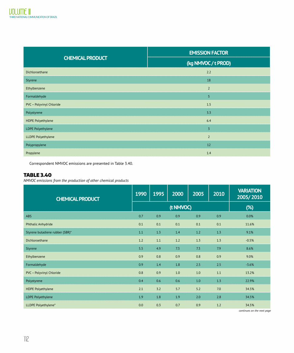
112
VOLUME IIITHIRD NATIONAL COMMUNICATION OF BRAZIL
CHEMICAL PRODUCTEMISSION FACTOR
(kg NMVOC / t PROD)Dichloroethane 2.2
Styrene 18
Ethylbenzene 2
Formaldehyde 5
PVC – Polyvinyl Chloride 1.5
Polystyrene 3.3
HDPE Polyethylene 6.4
LDPE Polyethylene 3
LLDPE Polyethylene 2
Polypropylene 12
Propylene 1.4
Correspondent NMVOC emissions are presented in Table 3.40.
TABLE 3.40 NMVOC emissions from the production of other chemical products
CHEMICAL PRODUCT1990 1995 2000 2005 2010 VARIATION
2005/ 2010
(t NMVOC) (%)ABS 0.7 0.9 0.9 0.9 0.9 0.0%
Phthalic Anhydride 0.1 0.1 0.1 0.1 0.1 11.6%
Styrene butadiene rubber (SBR)* 1.1 1.3 1.4 1.2 1.3 9.1%
Dichloroethane 1.2 1.1 1.2 1.3 1.3 -0.5%
Styrene 5.5 4.9 7.3 7.3 7.9 8.6%
Ethylbenzene 0.9 0.8 0.9 0.8 0.9 9.0%
Formaldehyde 0.9 1.4 1.8 2.5 2.5 -3.6%
PVC – Polyvinyl Chloride 0.8 0.9 1.0 1.0 1.1 13.2%
Polystyrene 0.4 0.6 0.6 1.0 1.3 22.9%
HDPE Polyethylene 2.1 3.2 5.7 5.2 7.0 34.5%
LDPE Polyethylene 1.9 1.8 1.9 2.0 2.8 34.5%
LLDPE Polyethylene* 0.0 0.3 0.7 0.9 1.2 34.5%
continues on the next page

113
CHAPTER IIIANTHROPOGENIC EMISSIONS BY SOURCES AND
REMOVALS BY SINKS OF GREENHOUSE GASES BY SECTOR
CHEMICAL PRODUCT1990 1995 2000 2005 2010 VARIATION
2005/ 2010
(t NMVOC) (%)Polypropylene 3.6 6.7 10.2 14.5 19.0 30.9%
Propylene 1.1 1.5 2.0 2.4 3.1 26.6%
Total 20.3 25.4 35.6 41.3 50.3 21.8%
*The production of this polyethylene began in Brazil in 1993.
3.2.3. Metal Production
3.2.3.1. Iron and Steel ProductionIn 2010, the Brazilian production of pig iron was of 30.8 Mt, a 23% growth when compared to the previous year.
The production of integrated plants was 25.8 Mt, while independent producers (pig iron market) produced 5.06 Mt.
Hence, independent producers accounted for only 16.4% of the total production. The steel produced in the same
year reached 32.9 million tons, the highest production in Latin America and 2.2% of the world production, which
totaled 1,498.9 million tons (BRASIL, 2011).
Up to 75% of CO2 emissions from steel manufacturing occur during the production of pig iron in the blast
furnace, i.e., in the reduction step of the iron ore. The remaining percentage results from the transportation of
raw materials, the generation of electric power and heat. The emissions in this sector include only the production
process, excluding power generation and transportation.
In Brazil, the production of pig iron and steel by integrated/semi-integrated plants uses petroleum coke, steam
coal of calorific value greater than or equal to 5,900 kcal/kg, metallurgical coal and coal coke as the main reducing
fuels. The production of pig iron by independent plants uses charcoal. The production of the plants is summarized
in Table 3.41.
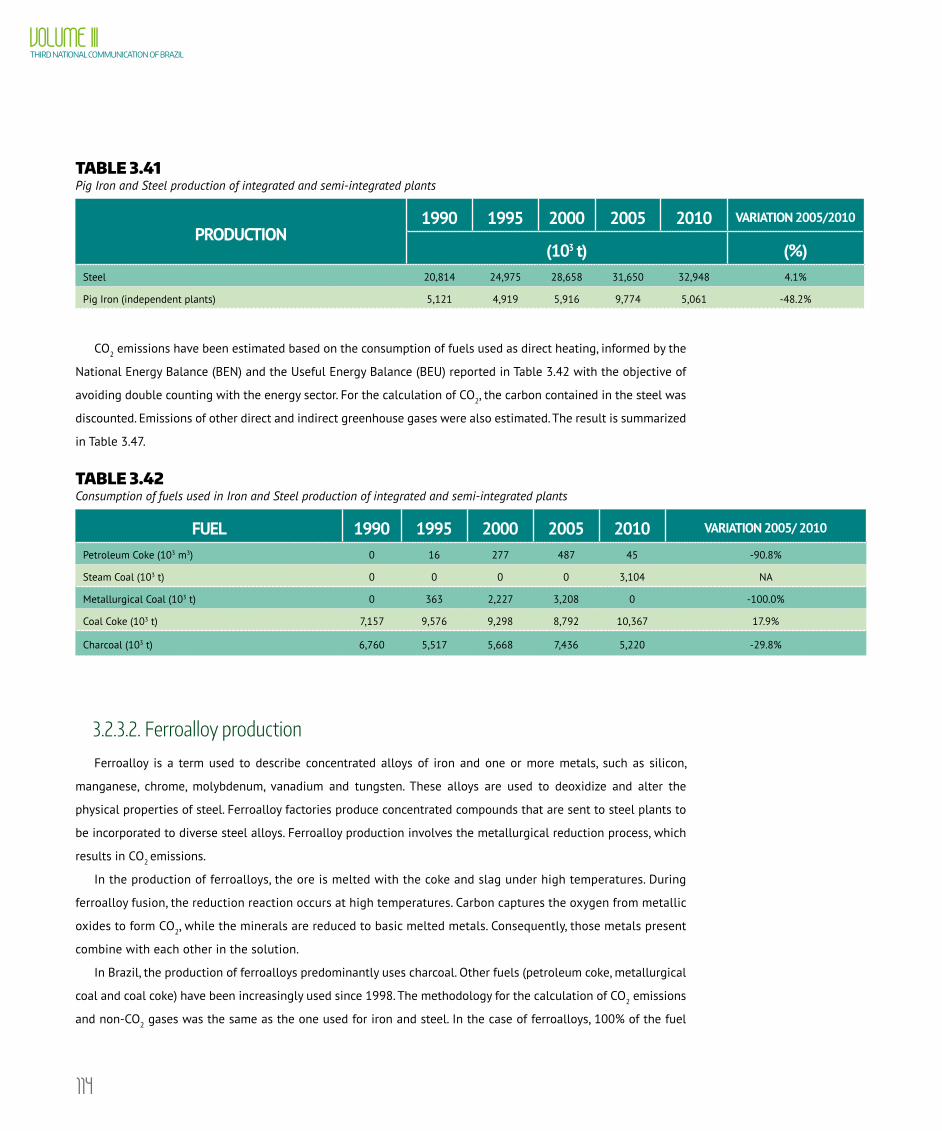
114
VOLUME IIITHIRD NATIONAL COMMUNICATION OF BRAZIL
TABLE 3.41 Pig Iron and Steel production of integrated and semi-integrated plants
PRODUCTION1990 1995 2000 2005 2010 VARIATION 2005/2010
(103 t) (%)Steel 20,814 24,975 28,658 31,650 32,948 4.1%
Pig Iron (independent plants) 5,121 4,919 5,916 9,774 5,061 -48.2%
CO2 emissions have been estimated based on the consumption of fuels used as direct heating, informed by the
National Energy Balance (BEN) and the Useful Energy Balance (BEU) reported in Table 3.42 with the objective of
avoiding double counting with the energy sector. For the calculation of CO2, the carbon contained in the steel was
discounted. Emissions of other direct and indirect greenhouse gases were also estimated. The result is summarized
in Table 3.47.
TABLE 3.42 Consumption of fuels used in Iron and Steel production of integrated and semi-integrated plants
FUEL 1990 1995 2000 2005 2010 VARIATION 2005/ 2010
Petroleum Coke (103 m3) 0 16 277 487 45 -90.8%
Steam Coal (103 t) 0 0 0 0 3,104 NA
Metallurgical Coal (103 t) 0 363 2,227 3,208 0 -100.0%
Coal Coke (103 t) 7,157 9,576 9,298 8,792 10,367 17.9%
Charcoal (103 t) 6,760 5,517 5,668 7,436 5,220 -29.8%
3.2.3.2. Ferroalloy productionFerroalloy is a term used to describe concentrated alloys of iron and one or more metals, such as silicon,
manganese, chrome, molybdenum, vanadium and tungsten. These alloys are used to deoxidize and alter the
physical properties of steel. Ferroalloy factories produce concentrated compounds that are sent to steel plants to
be incorporated to diverse steel alloys. Ferroalloy production involves the metallurgical reduction process, which
results in CO2 emissions.
In the production of ferroalloys, the ore is melted with the coke and slag under high temperatures. During
ferroalloy fusion, the reduction reaction occurs at high temperatures. Carbon captures the oxygen from metallic
oxides to form CO2, while the minerals are reduced to basic melted metals. Consequently, those metals present
combine with each other in the solution.
In Brazil, the production of ferroalloys predominantly uses charcoal. Other fuels (petroleum coke, metallurgical
coal and coal coke) have been increasingly used since 1998. The methodology for the calculation of CO2 emissions
and non-CO2 gases was the same as the one used for iron and steel. In the case of ferroalloys, 100% of the fuel

115
CHAPTER IIIANTHROPOGENIC EMISSIONS BY SOURCES AND
REMOVALS BY SINKS OF GREENHOUSE GASES BY SECTOR
consumption presented in BEN is considered as application in direct heating by BEU. Furthermore, in the absence
of further information and as recommended in the 2000 Good Practice Guidance (IPCC, 2000), the carbon contained
in iron-alloys was not considered.
National production data are shown in Table 3.43 and fuel consumption in Table 3.44. Emissions are summed
up in Table 3.47.
TABLE 3.43 Brazilian ferroalloy production
1990 1995 2000 2005 2010 VARIATION 2005/ 2010
(t) (%)Ferroalloy 807,663 756,625 736,672 1,171,583 924,749 -21.1%
Source: Statistical Yearbook Brazilian Metallurgical Industry– MME.
TABLE 3.44 Consumption of fuel used in ferroalloy production
FUEL 1990 1995 2000 2005 2010 VARIATION 2005/ 2010 (%)
Petroleum Coke (103 m3) 0 0 102 140 192 37.7%
Metallurgical Coal (103 t) 0 19 49 0 0 NA
Coal Coke (103 t) 37 51 8 134 156 16.6%
Charcoal (103 t) 560 590 666 883 880 -0.3%
3.2.3.3. Aluminum production Primary aluminum is obtained through bauxite mining, mineral found on the Earth’s crust. In 2012, the world’s
bauxite reserves totaled 28 billion tons, and Brazil holds 9.3% of this total, approximately 95% of the metallurgical
bauxite and 5% of the refractory one. The most expressive Brazilian reserves (95%) are located in the Northern region
(state of Pará), which has as main dealers the companies Alcoa Aluminio S.A., Norsk Hydro Brasil Ltda., Mineração Rio
do Norte S.A. and Votorantim Metais – Companhia Brasileira de Aluminio. Primary aluminum is produced through an
electrolytic reduction process. The reduction occurs in a carbon container that acts like a cathode and which contains
the electrolytic solution. The carbon anode is partially submerged in the solution and consumed during the process.
The electrolysis of aluminum oxide produces melted aluminum, which deposits on the cathode, and oxygen,
which deposits on the anode and reacts with the carbon, producing CO2 emissions. Some quantity of CO2 is also
produced when the anode reacts with other sources of oxygen (like air). Other gases emitted in the production of
primary aluminum are perfluorocarbons or PFCs, greenhouse gases that have a very long atmospheric life. The PFCs
emitted by the aluminum industry occasionally occur during the process of electrolytic reduction in events called

116
VOLUME IIITHIRD NATIONAL COMMUNICATION OF BRAZIL
anodic effects. These effects are unwanted due to also implying a loss of efficiency of the process and increased
energy consumption. Traditionally, the industry measures their occurrence in terms of frequency and duration. The
quantity of PFCs emitted by an aluminum reduction plant is a direct proportion of the frequency and the duration
of the anode effects.
The primary aluminum production process can use two main types of technology, Soderberg and Prebaked
Anode. The distinction between these technologies is related to the type of anode used. Brazilian aluminum
production by type of technology is shown in Table 3.45.
TABLE 3.45 Aluminum production by type of technology
TECHNOLOGY1990 1995 2000 2005 2010 VARIATION 2005/ 2010
(t ALUMINUM) (%)Soderberg 369,803 390,171 438,744 573,261 649,383 13.3%
Prebaked Anode 551,070 798,289 830,840 924,494 884,320 -4.3%
Total 920,873 1,188,460 1,269,584 1,497,755 1,533,703 2.4%
Source: Producing companies.
During the drafting of the Second National Inventory, the companies made a great effort to report their emissions
as accurately as possible, with developments in relation to the Initial Inventory. Each plant employed the best approach
(Tier) possible for the calculation of the emissions from their processes, in accordance with Table 3.46. Due to the lack
of specific information of each plant, as of 2008, the 2007 implicit emission factors have been used.
TABLE 3.46 Approaches applied for CO2 and PFCs emissions estimates per plant for the period 1990-2007
TECHNOLOGICAL ROUTEPLANT CO2 PFCS
TYPE SUBDIVISION
Soderberg
VSS and HSS Novelis (BA) Tier 2 Tier 2
HSS Novelis (MG) Tier 2 Tier 2
VSS Alcoa (MG) Tier 2 Tier 3
VSS CBA (SP) Tier 3 Tier 3
Prebaked Anode
CWPB Albras (PA) Tier 1
Tier 1 (1990-
1996)
Tier 3 (1997-
2007)
CWPB Alumar (MA) Tier 3 Tier 2
CWPB Valesul (RJ) Tier 2 Tier 1
GHG emissions related to the use of fuels in the production of aluminum are listed in Table 3.47 and CF4 and
C2F6 emissions are shown in Table 3.48.

117
CHAPTER IIIANTHROPOGENIC EMISSIONS BY SOURCES AND
REMOVALS BY SINKS OF GREENHOUSE GASES BY SECTOR
3.2.3.4. Magnesium production SF6 is used as a coverage gas to avoid oxidation of melted magnesium during production and casting of
metal magnesium products, and it normally leaks into the atmosphere. SF6 is considered a non-reactive gas and
ideally adapts to this type of protection, as “coverage” for molten magnesium (thus the term “coverage gas”). So, gas
consumption is used to estimate emissions. Table 3.48 presents SF6 emissions in this subsector.
3.2.3.5. Summary of the estimates of the direct and indirect Greenhouse Gas emissions from the production of metals
TABLE 3.47 GHG direct and indirect emissions from metal production
GAS FUEL TYPE PRODUCTION1990 1995 2000 2005 2010 VARIATION
2005/2010
Gg %
CO2
Fossil fuels
Pig-iron and steel 21,601 30,130 35,552 37,509 38,360 2.3
Ferroalloys 116 215 545 932 1,195 28.2
Aluminum 1,574 1,965 2,116 2,472 2,543 2.9
Other non-ferrous
metals897 1,762 1,606 1,855 4,332 133.6
Total fossil 24,188 34,073 39,818 42,768 46,430 8.6
Biomass*
Pig-iron and steel 18,758 15,200 15,490 20,026 14,321 -28.5
Ferroalloys 1,616 1,703 1,922 2,547 2,539 -0.3
Aluminum - - - - - NA
Other non-ferrous metals 1,137 652 26 35 42 17.7
Total biomass* 21,511 17,555 17,437 22,609 16,902 -25,2continues on the next page

118
VOLUME IIITHIRD NATIONAL COMMUNICATION OF BRAZIL
GAS FUEL TYPE PRODUCTION1990 1995 2000 2005 2010 VARIATION
2005/2010
Gg %
CH4
All
Pig-iron and steel 36.8 30.1 31.0 40.6 28.6 -29.5
Ferroalloys 3.0 3.2 3.6 4.8 4.8 -0.3
Other non-ferrous
metals2.1 1.3 0.1 0.1 0.1 11.8
Total 42.0 34.6 34.7 45.5 33.5 -26.4
N2O
Pig-iron and steel 1.02 1.00 1.09 1.31 1.08 -17.8
Ferroalloys 0.06 0.07 0.08 0.10 0.11 1.7
Non-ferrous metals 0.06 0.05 0.03 0.03 0.03 -11.3
Total 1.14 1.11 1.19 1.44 1.21 -16.2
CO
Pig-iron and steel 775.0 656.2 676.1 867.3 633.2 -27.0
Ferroalloys 60.8 64.2 72.5 96.7 96.7 0.0
Non-ferrous metals 44.4 27.6 3.7 4.6 4.9 6.4
Total 880.2 747.9 752.3 968.7 734.8 -24.1
NOx
Pig-iron and steel 25.5 30.8 66.4 90.8 60.1 -33.7
Ferroalloys 1.6 2.0 4.6 5.2 6.2 19.7
Non-ferrous metals 8.9 11.7 13.0 14.1 13.8 -2.5
Total 36.0 44.5 84.0 110.1 80.1 -27.2
NMVOC
Pig-iron and steel 21.6 19.6 21.1 26.3 20.2 -22.9
Ferroalloys 1.5 1.6 1.9 2.5 2.5 0.5
Non-ferrous metals 1.2 0.8 0.3 0.3 0.3 -18.6
Total 24.3 22.0 23.2 29.1 23.0 -20.9
*For information purposes only. These emissions are included in the Reference Report ‘Land Use, Land Use Change and Forestry’.
TABLE 3.48 Emissions from the metal production process not related to the use of fuel
PRODUCTION GAS1990 1995 2000 2005 2010 VARIATION 2005/ 2010
(Gg) (%)
AluminumCF4 0.3022 0.3060 0.1465 0.1239 0.0767 -38.1%
C2F6 0.0263 0.0264 0.0117 0.0104 0.0059 -43.3%
Magnesium SF6 0.0058 0.0101 0.0103 0.0191 - -100.0%

119
CHAPTER IIIANTHROPOGENIC EMISSIONS BY SOURCES AND
REMOVALS BY SINKS OF GREENHOUSE GASES BY SECTOR
3.2.4. Other Industries
3.2.4.1. Pulp and Paper Industry The Pulp and Paper sector is comprised of 62 companies and state agencies of products originating in the
cultivation of planted trees. This industry has 2.4 million hectares of own forestations, especially the Eucalyptus and
Pinus species, for the production of pulp and paper.
Preparation of pulp paste for papers and other purposes consists of separating the fibers from the other wood
components, especially lignin, which gives firmness to the wood. Some types of wood, such as pine and araucaria,
have long fibers (3 to 5 mm), whereas eucalyptus has shorter and thinner fibers (0.8 to 1.2 mm). Those from the first
group are called conifers or softwood, whereas those from the second group are called leafy or hardwood.
There are many and varied preparation processes for pulp paste, from the purely mechanical to the chemical,
in which wood is treated with chemical products, pressure and heat (temperatures greater than 150oC) to dissolve
the lignin. The use of chemical products in the process generates greenhouse gas emissions.
Pulp and paper paste production have three main phases: pulping, bleaching and paper production. The type
of pulping and the quantity of bleaching used depend on the nature of the raw material and the desired quality of
the final product. Kraft pulping is the most widely used process.
In Brazil, the most used process is a variation of Kraft, called Sulfate. It uses the same chemical products,
although employing higher doses of sodium sulfate and caustic soda, and it is cooked longer and at higher
temperatures. It is considered the most appropriate for obtaining chemical pastes from eucalyptus. There are CO,
NOx and NMVOC emissions during the process.
Table 3.49 presents a summary of Brazilian production of pulp paste, highlighting the sulfate process, which
generates indirect greenhouse gases.
TABLE 3.49 Brazilian pulp paste production
TYPE OF PULP /CHEMICAL PROCESS
1990 1994 2000 2005 2010 VAR. 2005/ 2010
(t) (%)
Chemical and Semi-Chemical Pulp 3,914,688 5,376,271 6,961,470 9,852,462 13,733,000 39.4%
Sulfate* 3,593,547 5,127,981 6,639,971 9,397,450 13,098,775 39.4%
Other Processes 321,141 248,290 321,499 455,012 634,225 39.4%
High Performance Pastes 436,455 452,599 501,796 499,651 431,000 -13.7%
Total 4,351,143 5,828,870 7,463,266 10,352,113 14,164,000 36.8%
Source: Ibá – Brazilian Tree Industry.
*For the sulfate process, the same share as in 1994 was considered for the subsequent years.
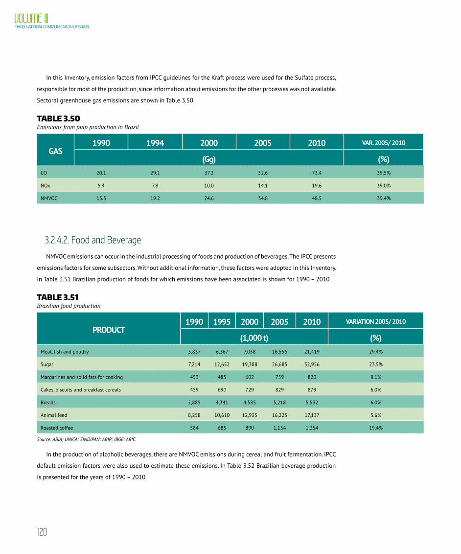
120
VOLUME IIITHIRD NATIONAL COMMUNICATION OF BRAZIL
In this Inventory, emission factors from IPCC guidelines for the Kraft process were used for the Sulfate process,
responsible for most of the production, since information about emissions for the other processes was not available.
Sectoral greenhouse gas emissions are shown in Table 3.50.
TABLE 3.50 Emissions from pulp production in Brazil
GAS1990 1994 2000 2005 2010 VAR. 2005/ 2010
(Gg) (%)CO 20.1 29.1 37.2 52.6 73.4 39.5%
NOx 5.4 7.8 10.0 14.1 19.6 39.0%
NMVOC 13.3 19.2 24.6 34.8 48.5 39.4%
3.2.4.2. Food and Beverage NMVOC emissions can occur in the industrial processing of foods and production of beverages. The IPCC presents
emissions factors for some subsectors. Without additional information, these factors were adopted in this Inventory.
In Table 3.51 Brazilian production of foods for which emissions have been associated is shown for 1990 – 2010.
TABLE 3.51 Brazilian food production
PRODUCT1990 1995 2000 2005 2010 VARIATION 2005/ 2010
(1,000 t) (%)Meat, fish and poultry 5,837 6,367 7,038 16,556 21,419 29.4%
Sugar 7,214 12,652 19,388 26,685 32,956 23.5%
Margarines and solid fats for cooking 453 485 602 759 820 8.1%
Cakes, biscuits and breakfast cereals 459 690 729 829 879 6.0%
Breads 2,885 4,341 4,585 5,218 5,532 6.0%
Animal feed 8,258 10,610 12,935 16,225 17,137 5.6%
Roasted coffee 584 685 890 1,134 1,354 19.4%
Source: ABIA; UNICA; SINDIPAN; ABIP; IBGE; ABIC.
In the production of alcoholic beverages, there are NMVOC emissions during cereal and fruit fermentation. IPCC
default emission factors were also used to estimate these emissions. In Table 3.52 Brazilian beverage production
is presented for the years of 1990 – 2010.
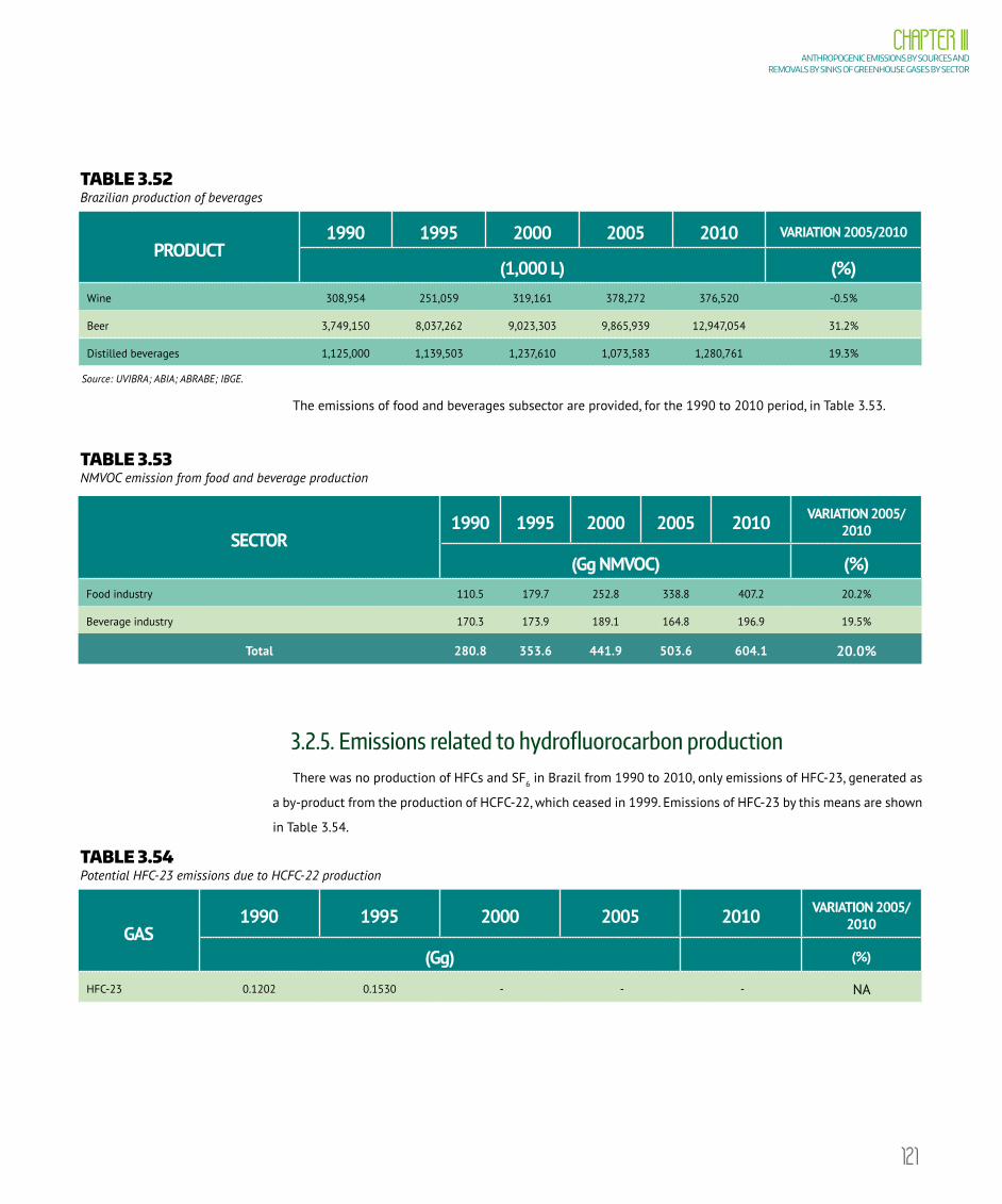
121
CHAPTER IIIANTHROPOGENIC EMISSIONS BY SOURCES AND
REMOVALS BY SINKS OF GREENHOUSE GASES BY SECTOR
TABLE 3.52 Brazilian production of beverages
PRODUCT1990 1995 2000 2005 2010 VARIATION 2005/2010
(1,000 L) (%)Wine 308,954 251,059 319,161 378,272 376,520 -0.5%
Beer 3,749,150 8,037,262 9,023,303 9,865,939 12,947,054 31.2%
Distilled beverages 1,125,000 1,139,503 1,237,610 1,073,583 1,280,761 19.3%
Source: UVIBRA; ABIA; ABRABE; IBGE.
The emissions of food and beverages subsector are provided, for the 1990 to 2010 period, in Table 3.53.
TABLE 3.53 NMVOC emission from food and beverage production
SECTOR1990 1995 2000 2005 2010 VARIATION 2005/
2010
(Gg NMVOC) (%)Food industry 110.5 179.7 252.8 338.8 407.2 20.2%
Beverage industry 170.3 173.9 189.1 164.8 196.9 19.5%
Total 280.8 353.6 441.9 503.6 604.1 20.0%
3.2.5. Emissions related to hydrofluorocarbon productionThere was no production of HFCs and SF6 in Brazil from 1990 to 2010, only emissions of HFC-23, generated as
a by-product from the production of HCFC-22, which ceased in 1999. Emissions of HFC-23 by this means are shown
in Table 3.54.
TABLE 3.54 Potential HFC-23 emissions due to HCFC-22 production
GAS1990 1995 2000 2005 2010 VARIATION 2005/
2010
(Gg) (%)
HFC-23 0.1202 0.1530 - - - NA
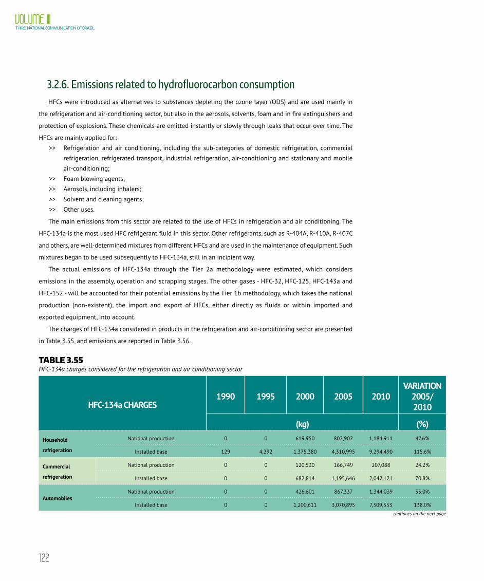
122
VOLUME IIITHIRD NATIONAL COMMUNICATION OF BRAZIL
3.2.6. Emissions related to hydrofluorocarbon consumptionHFCs were introduced as alternatives to substances depleting the ozone layer (ODS) and are used mainly in
the refrigeration and air-conditioning sector, but also in the aerosols, solvents, foam and in fire extinguishers and
protection of explosions. These chemicals are emitted instantly or slowly through leaks that occur over time. The
HFCs are mainly applied for:
>> Refrigeration and air conditioning, including the sub-categories of domestic refrigeration, commercial
refrigeration, refrigerated transport, industrial refrigeration, air-conditioning and stationary and mobile
air-conditioning;
>> Foam blowing agents;
>> Aerosols, including inhalers;
>> Solvent and cleaning agents;
>> Other uses.
The main emissions from this sector are related to the use of HFCs in refrigeration and air conditioning. The
HFC-134a is the most used HFC refrigerant fluid in this sector. Other refrigerants, such as R-404A, R-410A, R-407C
and others, are well-determined mixtures from different HFCs and are used in the maintenance of equipment. Such
mixtures began to be used subsequently to HFC-134a, still in an incipient way.
The actual emissions of HFC-134a through the Tier 2a methodology were estimated, which considers
emissions in the assembly, operation and scrapping stages. The other gases - HFC-32, HFC-125, HFC-143a and
HFC-152 - will be accounted for their potential emissions by the Tier 1b methodology, which takes the national
production (non-existent), the import and export of HFCs, either directly as fluids or within imported and
exported equipment, into account.
The charges of HFC-134a considered in products in the refrigeration and air-conditioning sector are presented
in Table 3.55, and emissions are reported in Table 3.56.
TABLE 3.55 HFC-134a charges considered for the refrigeration and air conditioning sector
HFC-134a CHARGES1990 1995 2000 2005 2010
VARIATION 2005/ 2010
(kg) (%)
Household
refrigeration
National production 0 0 619,950 802,902 1,184,911 47.6%
Installed base 129 4,292 1,375,380 4,310,995 9,294,490 115.6%
Commercial
refrigeration
National production 0 0 120,530 166,749 207,088 24.2%
Installed base 0 0 682,814 1,195,646 2,042,121 70.8%
AutomobilesNational production 0 0 426,601 867,337 1,344,039 55.0%
Installed base 0 0 1,200,611 3,070,895 7,309,553 138.0%
continues on the next page
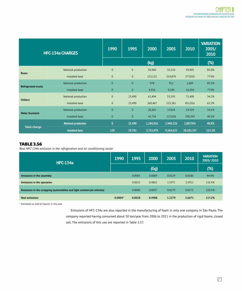
123
CHAPTER IIIANTHROPOGENIC EMISSIONS BY SOURCES AND
REMOVALS BY SINKS OF GREENHOUSE GASES BY SECTOR
HFC-134a CHARGES1990 1995 2000 2005 2010
VARIATION 2005/ 2010
(kg) (%)
BusesNational production 0 0 34,360 32,110 59,405 85.0%
Installed base 0 0 153,115 324,870 577,810 77.9%
Refrigerated trucksNational production 0 0 978 912 1,689 85.2%
Installed base 0 0 4,356 9,240 16,434 77.9%
ChillersNational production 0 25,490 61,404 53,193 71,400 34.2%
Installed base 0 25,490 260,467 525,361 852,016 62.2%
Water fountainsNational production 0 0 20,202 17,024 19,424 14.1%
Installed base 0 0 45,734 127,618 190,343 49.2%
Total chargeNational production 0 25,490 1,284,026 1,940,226 2,887,956 48.8%
Installed base 129 29,782 3,722,478 9,564,625 20,282,767 112.1%
TABLE 3.56 Real HFC-134a emission in the refrigeration and air conditioning sector
HFC-134a 1990 1995 2000 2005 2010 VARIATION
2005/ 2010
(Gg) (%)Emissions in the assembly 0.0003 0.0089 0.0129 0.0186 44.4%
Emissions in the operation 0.0025 0.4862 1.1971 2.5912 116.5%
Emissions in the scrapping (automobiles and light commercial vehicles) 0.0000 0.0037 0.0179 0.0573 220.5%
Real emissions 0.0004* 0.0028 0.4988 1.2279 2.6671 117.2%
* Estimated as half of imports in this year.
Emissions of HFC-134a are also reported in the manufacturing of foam in only one company in São Paulo. The
company reported having consumed about 50 ton/year from 2006 to 2011 in the production of rigid foams, closed
cell. The emissions of this use are reported in Table 3.57.

124
VOLUME IIITHIRD NATIONAL COMMUNICATION OF BRAZIL
TABLE 3.57 HFC-134a emission estimates in foams production
YEARUSE IN THE ASSEMBLY
LEAK IN THE ASSEMBLY ANNUAL LEAK TOTAL LEAK
10% 4.50% HFC-134a(Gg)
2006 0.050 0.005 0.0011 0.0061
2007 0.050 0.005 0.0034 0.0084
2008 0.050 0.005 0.0056 0.0106
2009 0.050 0.005 0.0079 0.0129
2010 0.050 0.005 0.0101 0.0151
Another source of emissions of the HFC-134a refrigerant fluid is in the use of medicinal Metered Dose Inhalers
aerosols (MDIs). This use only began in 2006 and the emissions are reported in Table 3.58.
TABLE 3.58 HFC-134a emission estimates in aerosol use
YEARHFC-134a EMISSIONS
(Gg)2006 0.0123
2007 0.0193
2008 0.0128
2009 0.0169
2010 0.0205
Table 3.59 shows HFC-134a emissions in the refrigeration and air-conditioning, foam and aerosols sectors.
TABLE 3.59 Real HFC-134a emissions
HFC-134a EMISSIONS1990 1995 2000 2005 2010 VARIATION 2005/
2010
(Gg) (%)
Refrigeration and air-conditioning 0.0004 0.0028 0.4988 1.2279 2.6671 117.2%
Foams - - - - 0.0151 NA
Aerosols - - - - 0.0374 NA
Total emissions 0.0004 0.0028 0.4988 1.2279 2.7196 121.5%
For the other refrigerants (HFC-32, HFC-125, HFC-143a and HFC-152a), the imports and exports were identified
whenever relevant. Table 3.60 shows the potential emissions of HFCs.

125
CHAPTER IIIANTHROPOGENIC EMISSIONS BY SOURCES AND
REMOVALS BY SINKS OF GREENHOUSE GASES BY SECTOR
TABLE 3.60 HFCs potential emissions
GAS1990 1995 2000 2005 2010 VARIATION 2005/ 2010
(Gg) (%)HFC-32 - - - - 0.1059 NA
HFC-125 - - 0.0071 0.1249 0.5012 301.3%
HFC-143a - - 0.0075 0.0929 0.4671 402.8%
HFC-152a - - 0.0001 0.1748 - -100.0%
3.2.7. Emissions related to the consumption of sulfur hexafluorideDue to its excellent properties as an inert, non-toxic, high dielectric rigidity insulation and non-flammable,
thermally stable and self-regenerating refrigerant, SF6 permitted the development of high capacity and performance
electrical equipment, which are also compact, light and safe. Among the electrical equipment developed as a result
of SF6, circuit breakers and shielded substations stand out using 10% of the physical space of the equivalent
conventional substations.
In Brazil, there is no production of SF6, but emissions occur due to gas leaks at SF6 insulated and shielded
substations.
The actual emissions of SF6 were informed by the studies carried out by MCTI for the Second Inventory, involving
the use of electrical power equipment and in the production of magnesium. At that time, the installed park of
equipment using SF6 was evaluated up to 2008. The extrapolation of this capacity up to 2010 took into account
the average growth during the ten previous years, considering an annual emission factor of 2% of the installed
capacity. For the production of magnesium, the use of SF6 was reported in the metal manufacture sector.
Table 3.61 below shows the first results in terms of installed capacity of SF6 in equipment, and an estimate of
annual leakage based on default factor, according to the 2000 Good Practice Guidance, at the amount of 2% per year.
TABLE 3.61 Installed capacity in terms of SF6 in equipment and estimates of annual leaks
DESCRIPTION 1990 1995 2000 2005 2010 VARIATION 2005/ 2010 (%)
Installed capacity (t SF6) 208.85 205.47 248.31 306.32 436.32 42.4%
SF6 emissions (Gg) 0.0042 0.0041 0.0050 0.0061 0.0087 42.6%

126
VOLUME IIITHIRD NATIONAL COMMUNICATION OF BRAZIL
3.3. SOLVENT AND OTHER PRODUCT USE SECTORThis sector has been completely modified in relation to the earlier inventories. Like in the Iron and Steel sub-
sector, compatibility with the National Energy Balance (BEN), was sought. Data on the use of solvents and other
products were taken from the same source and no longer from uncertain emission factors and activity data based
on other countries. Emissions of NMVOCs concerning the non-energy use informed at BEN, apart from the Chemical
Industry use, were counted in this sector. Thus, Lighting Kerosene, Hydrated Alcohol, Solvents, Other Non-Energy of
Petroleum were recorded. In addition, NMVOC emissions were recorded on account of the use of asphalt for paving,
on the basis of the 1997 IPCC emission factor.
The 1996 Guidelines indicate that, for a certain percentage of each fuel, the carbon will be stored in products
in a more or less permanent form, being necessary to estimate CO2 emissions for the others. Based on this
methodology, emissions relating to the use of lubricants were considered as if 80% would be stored, according
to the 2006 Guidelines (to consider 20% emitted in two strokes engines, in which the lubricant is burned with
the fuel). Lighting kerosene, hydrated alcohol, solvents and other non-energy of petroleum, in turn, will be 100%
emitted as NMVOC.
For the calculation of CO2 emissions from the use of lubricants, factors of 0.891 m3 / toe, 41.868 103 toe / TJ and,
finally, the emission factor of 20 t C/TJ were used. For NMVOC, default factors of 790 kg/m3 of lighting kerosene,
809 kg/m3 of hydrated alcohol, 740 kg/m3 of solvents and 873 kg/m3 of other petroleum energy were used.
It should be noted that these emissions fully include those calculated for the Second Inventory in the Solvent
and Other Products sector. The consumption of non-energy lubricants (CO2 emissions) and lighting kerosene,
hydrated alcohol, solvent and other non-energy petroleum products (emissions of NMVOC) informed by BEN are
presented in Table 3.61. CO2 emissions related to the consumption of lubricants and NMVOC from the use of
lighting kerosene, hydrated alcohol, solvent and other non-energy petroleum products are shown in Table 3.63.
TABLE 3.62 Date on activity and non-energy consumption informed by The Brazilian Energy Balance (BEN)
CONSUMPTION1990 1995 2000 2005 2010 VAR.2005/
2010
103 m3 (%)Lubricants 783 757 921 960 1,242 29.3%
Lighting Kerosene 0 0 0 29 9 -68.6%
Hydrated Alcohol 855 1,021 960 530 0 -100.0%
Solvents 281 354 543 1,287 592 -54.0%
Other Non-Energy Oil Products 1,213 962 1,663 1,324 3,948 198.1%
Pavement asphalt 1,143 1,079 1,575 1,269 2,578 103.2%

127
CHAPTER IIIANTHROPOGENIC EMISSIONS BY SOURCES AND
REMOVALS BY SINKS OF GREENHOUSE GASES BY SECTOR
TABLE 3.63 CO2 and NMVOC emissions by lubricants, solvents and other products use
GASES FUEL1990 1995 2000 2005 2010 VAR.2005/
2010
(Gg) (%)CO2 Lubricants 428 414 504 525 679 29.3%
NMVOC
Lighting Kerosene 0 0 0 23 7 -68.6%
Hydrated Alcohol 692 826 776 429 0 -100.0%
Solvents 208 262 402 953 438 -54.0%
Other Non-Energy Oil Products 1,059 840 1,452 1,156 3,447 198.1%
Pavement asphalt 380 359 524 422 858 103.2%
Total 2,339 2,287 3,154 2,982 4,750 59.3%
3.4. AGRICULTUREAgriculture, which includes livestock, is an economic activity of great importance in Brazil. Due to its large
extension of agricultural and grazing lands, the country is one of the largest producers of this sector in the world.
Agriculture and livestock activities generate greenhouse gas emissions that occur through several processes.
Enteric fermentation in ruminants is one of the most important sources of CH4 emissions in the country (64.4% in
2010). Manure management systems cause CH4 and N2O emissions from livestocks.
Flooded rice crops, which are one of the main sources of CH4 in the world, are not a very expressive emissions
source in Brazil, because a major portion of the rice is produced in non-flooded areas. Imperfect crop residue
burning produces CH4 and N2O emissions, besides NOx, CO and NMVOC. In Brazil, waste burning is applied in the
sugarcane and cotton crops.
N2O emissions in agricultural soils occur mainly from the animal manure in pastureland and also from soil
fertilization practices, which include the use of synthetic nitrogen fertilizers and animal waste management. The
use of organic soils for farming also generates N2O emissions.
3.4.1. LivestockThere are several processes in the cattle activity that cause greenhouse gas emissions. The production of CH4
is part of the normal digestive process in ruminant herbivores (enteric fermentation); animal waste management
produces CH4 and N2O emissions; the use of animal manure as a fertilizer and deposition of grazing animal wastes
also produce N2O in the soil.
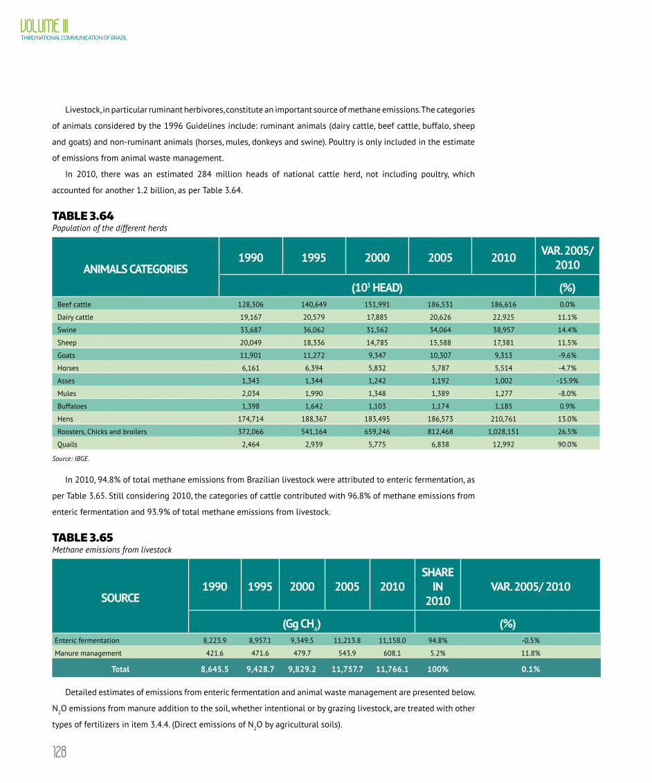
128
VOLUME IIITHIRD NATIONAL COMMUNICATION OF BRAZIL
Livestock, in particular ruminant herbivores, constitute an important source of methane emissions. The categories
of animals considered by the 1996 Guidelines include: ruminant animals (dairy cattle, beef cattle, buffalo, sheep
and goats) and non-ruminant animals (horses, mules, donkeys and swine). Poultry is only included in the estimate
of emissions from animal waste management.
In 2010, there was an estimated 284 million heads of national cattle herd, not including poultry, which
accounted for another 1.2 billion, as per Table 3.64.
TABLE 3.64 Population of the different herds
ANIMALS CATEGORIES1990 1995 2000 2005 2010 VAR. 2005/
2010
(103 HEAD) (%)Beef cattle 128,306 140,649 151,991 186,531 186,616 0.0%
Dairy cattle 19,167 20,579 17,885 20,626 22,925 11.1%
Swine 33,687 36,062 31,562 34,064 38,957 14.4%
Sheep 20,049 18,336 14,785 15,588 17,381 11.5%
Goats 11,901 11,272 9,347 10,307 9,313 -9.6%
Horses 6,161 6,394 5,832 5,787 5,514 -4.7%
Asses 1,343 1,344 1,242 1,192 1,002 -15.9%
Mules 2,034 1,990 1,348 1,389 1,277 -8.0%
Buffaloes 1,398 1,642 1,103 1,174 1,185 0.9%
Hens 174,714 188,367 183,495 186,573 210,761 13.0%
Roosters, Chicks and broilers 372,066 541,164 659,246 812,468 1,028,151 26.5%
Quails 2,464 2,939 5,775 6,838 12,992 90.0%
Source: IBGE.
In 2010, 94.8% of total methane emissions from Brazilian livestock were attributed to enteric fermentation, as
per Table 3.65. Still considering 2010, the categories of cattle contributed with 96.8% of methane emissions from
enteric fermentation and 93.9% of total methane emissions from livestock.
TABLE 3.65 Methane emissions from livestock
SOURCE1990 1995 2000 2005 2010
SHARE IN
2010VAR. 2005/ 2010
(Gg CH4) (%)Enteric fermentation 8,223.9 8,957.1 9,349.5 11,213.8 11,158.0 94.8% -0.5%
Manure management 421.6 471.6 479.7 543.9 608.1 5.2% 11.8%
Total 8,645.5 9,428.7 9,829.2 11,757.7 11,766.1 100% 0.1%
Detailed estimates of emissions from enteric fermentation and animal waste management are presented below.
N2O emissions from manure addition to the soil, whether intentional or by grazing livestock, are treated with other
types of fertilizers in item 3.4.4. (Direct emissions of N2O by agricultural soils).

129
CHAPTER IIIANTHROPOGENIC EMISSIONS BY SOURCES AND
REMOVALS BY SINKS OF GREENHOUSE GASES BY SECTOR
3.4.1.1. Enteric fermentationThe production of CH4 is part of the normal digestive process of ruminant animals. It occurs in much smaller
quantities in other herbivores. The contribution of non-ruminant animals to global methane emissions is considered
insignificant, representing only about 5.2% of total methane emissions from domestic and wild animals.
Emission intensity depends on the type of animal, the type and amount of food, the degree of digestibility and
the intensity of the animal’s physical activity, as a result of the diverse raising practices.
The estimate of emission factors is based on recognition of these parameters, which will allow for the evaluation
of emissions. In Brazil, due to its large territorial extension and wide dispersion of activity, with a diversity of
practices and food types provided to the animals, these parameters vary greatly.
Unfortunately, studies in this area are insufficient in the country. However, with the contribution of Brazilian
specialists, emission factors that could be straightforwardly applied to raising characteristics and regional
differences were obtained for cattle. The values obtained proved to be consistently higher than the IPCC Guidelines
default values (1997).
In accordance with diet characteristics, methane gas emissions were estimated to vary between 4% and 12%
of gross ingested food energy, with the average considered to be 8%. As the production of methane varies with
the quantity and quality of food ingested, different types and conditions for livestock production systems result in
different percentages of methane emissions. Food consumption is related to animal size, environmental conditions,
growth rate and production (milk, meat, wool and gestation). Generally, the greater this consumption, the greater
the CH4 emission and the better quality of the diet, the lower this emission will be per unit of ingested food.
Furthermore, it is necessary to consider that ruminants experience seasonal differences in food supply,
considering climatic conditions that alter pasture quality, which also differs in accordance with soil type. Thus, it
is possible to observe a seasonal pattern of weight gain in the wet season (hot) and weight loss in the dry season
(cold), which occurs in individuals over 3.5 years of age.
For dairy farming, production systems are observed with different degrees of specialization, from subsistence
properties – without techniques and daily production of less than 10 liters, to highly specialized producers - with
daily production above 50 thousand liters. It is estimated that only 2.3% of dairy properties are specialized and
that these are responsible for approximately 44% of total milk production in the country. On the other hand, 90%
of the producers considered small are responsible for only 20% of total production. There is also an intermediate
group in terms of property specialization that corresponds to 7.7% of producers and that are responsible for 36%
of production.
Zootechnical features were set for 1990-1995, 1996-2001 and 2002-2006, according to the peculiarities of the
country’s herds. Among these periods, there was a variation in digestibility and pregnancy data for the Southeast,
South and Central-West regions. Based on these parameters, methane emission factors were estimated for enteric
fermentation in livestock. For females in beef cattle and for dairy cattle, estimations also take into account the
production of milk, which is assumed to be the same in both cases and is available by state and year, resulting in
different emission factors for all years in each state.
For other animals, IPCC default emission factors were used due to the absence of consistent national data,
increasing the degree of uncertainty of the estimates.

130
VOLUME IIITHIRD NATIONAL COMMUNICATION OF BRAZIL
In Table 3.66 estimates are provided for methane emissions, resulting from enteric fermentation, in accordance
with animal category. Among the types of animals, non-dairy cattle was the major contributor for these emissions.
TABLE 3.66 CH4 emissions from enteric fermentation
TYPE OF ANIMAL1990 1995 2000 2005 2010
SHARE IN
2010
VAR. 2005/ 2010
(Gg CH4) (%)Bovines 7,809.9 8,534.3 9,005.8 10,855.7 10,798.4 96.8% -0.5%
Dairy cattle 1,197.7 1,297.1 1,777.9 1,371.4 1,424.0 12.8% 3.8%
Beef cattle 6,611.2 7,237.2 7,827.9 9,484.3 9,374.4 84.0% -1.2%
Other animals 415.0 422.8 343.7 358.1 359.6 3.2% 0.4%
Total 8,223.9 8,957.1 9,349.5 11,213.8 11,158.0 100% -0.5%
3.4.1.2. Manure management The main source of methane emissions is related to animal wastes treated under anaerobic conditions. This
occurs due to methanogenic bacteria activity in anaerobic conditions producing important quantities of CH4. This
process is favored when dejects are stored in liquid form.
Due to the characteristics of extensive cattle raising in Brazil, anaerobic treatment lagoons constitute a small
fraction of the management systems. Even for confined cattle, a restricted number of manure treatment facilities
can be observed. Animal wastes deposited in pasture dries and decomposes in the field, so that minimum quantities
of CH4 emissions are expected from this source. The use of manure as fertilizer is not expressive in the country. It
is estimated as no more than 20% in the cases of beef and dairy cattle and swine, and approximately 80% in the
case of poultry.
CH4 emissions were estimated using the methodologies recommended by the IPCC. Detailed methodology
that takes into account national feeding parameters, digestibility and management systems, obtained with the
collaboration of Brazilian specialists, was used for cattle and swine.
The manure composition is determined by the animal’s diet so that the greater the energy content and
digestibility of the food, the greater the capacity for CH4 production. Cattle fed a high quality diet produces a highly
biodegradable manure with greater potential for methane generation, whereas cattle fed a more fibrous diet will
produce a less biodegradable deject, containing more complex organic material, such as cellulose, hemicellulose
and lignin. The latter would be more closely associated with cattle raised on pastures in tropical conditions. The
higher emissions of methane from animal waste are associated with animals raised under intensive management.
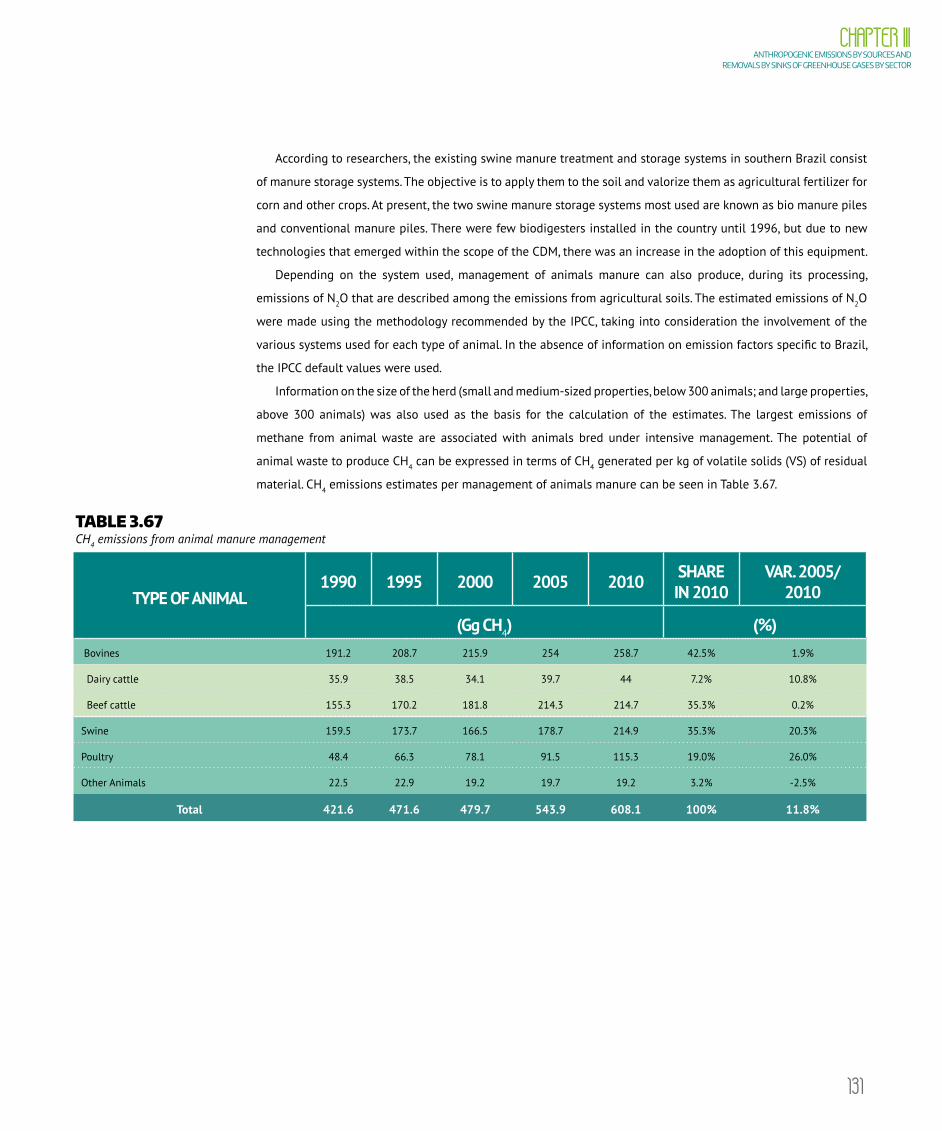
131
CHAPTER IIIANTHROPOGENIC EMISSIONS BY SOURCES AND
REMOVALS BY SINKS OF GREENHOUSE GASES BY SECTOR
According to researchers, the existing swine manure treatment and storage systems in southern Brazil consist
of manure storage systems. The objective is to apply them to the soil and valorize them as agricultural fertilizer for
corn and other crops. At present, the two swine manure storage systems most used are known as bio manure piles
and conventional manure piles. There were few biodigesters installed in the country until 1996, but due to new
technologies that emerged within the scope of the CDM, there was an increase in the adoption of this equipment.
Depending on the system used, management of animals manure can also produce, during its processing,
emissions of N2O that are described among the emissions from agricultural soils. The estimated emissions of N2O
were made using the methodology recommended by the IPCC, taking into consideration the involvement of the
various systems used for each type of animal. In the absence of information on emission factors specific to Brazil,
the IPCC default values were used.
Information on the size of the herd (small and medium-sized properties, below 300 animals; and large properties,
above 300 animals) was also used as the basis for the calculation of the estimates. The largest emissions of
methane from animal waste are associated with animals bred under intensive management. The potential of
animal waste to produce CH4 can be expressed in terms of CH4 generated per kg of volatile solids (VS) of residual
material. CH4 emissions estimates per management of animals manure can be seen in Table 3.67.
TABLE 3.67 CH4 emissions from animal manure management
TYPE OF ANIMAL1990 1995 2000 2005 2010 SHARE
IN 2010VAR. 2005/
2010
(Gg CH4) (%) Bovines 191.2 208.7 215.9 254 258.7 42.5% 1.9%
Dairy cattle 35.9 38.5 34.1 39.7 44 7.2% 10.8%
Beef cattle 155.3 170.2 181.8 214.3 214.7 35.3% 0.2%
Swine 159.5 173.7 166.5 178.7 214.9 35.3% 20.3%
Poultry 48.4 66.3 78.1 91.5 115.3 19.0% 26.0%
Other Animals 22.5 22.9 19.2 19.7 19.2 3.2% -2.5%
Total 421.6 471.6 479.7 543.9 608.1 100% 11.8%
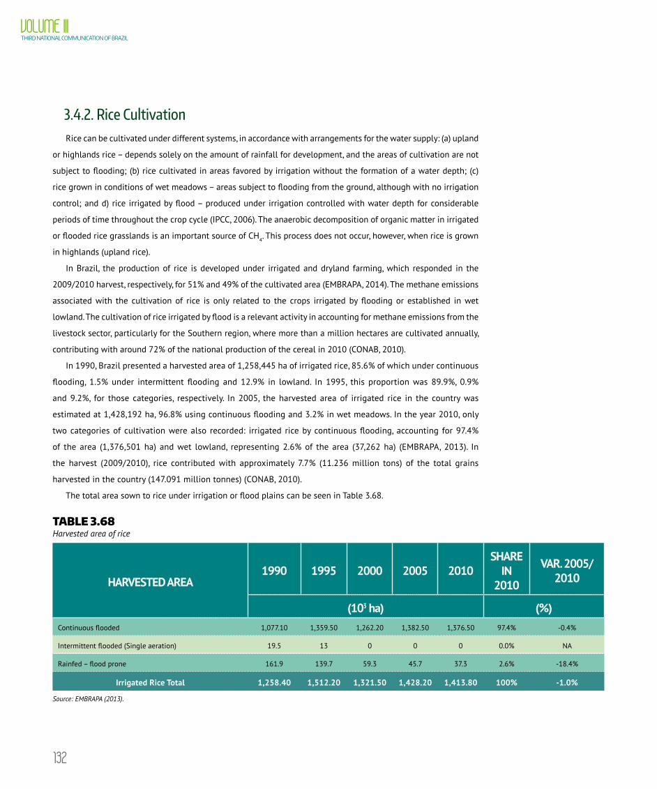
132
VOLUME IIITHIRD NATIONAL COMMUNICATION OF BRAZIL
3.4.2. Rice CultivationRice can be cultivated under different systems, in accordance with arrangements for the water supply: (a) upland
or highlands rice – depends solely on the amount of rainfall for development, and the areas of cultivation are not
subject to flooding; (b) rice cultivated in areas favored by irrigation without the formation of a water depth; (c)
rice grown in conditions of wet meadows – areas subject to flooding from the ground, although with no irrigation
control; and d) rice irrigated by flood – produced under irrigation controlled with water depth for considerable
periods of time throughout the crop cycle (IPCC, 2006). The anaerobic decomposition of organic matter in irrigated
or flooded rice grasslands is an important source of CH4. This process does not occur, however, when rice is grown
in highlands (upland rice).
In Brazil, the production of rice is developed under irrigated and dryland farming, which responded in the
2009/2010 harvest, respectively, for 51% and 49% of the cultivated area (EMBRAPA, 2014). The methane emissions
associated with the cultivation of rice is only related to the crops irrigated by flooding or established in wet
lowland. The cultivation of rice irrigated by flood is a relevant activity in accounting for methane emissions from the
livestock sector, particularly for the Southern region, where more than a million hectares are cultivated annually,
contributing with around 72% of the national production of the cereal in 2010 (CONAB, 2010).
In 1990, Brazil presented a harvested area of 1,258,445 ha of irrigated rice, 85.6% of which under continuous
flooding, 1.5% under intermittent flooding and 12.9% in lowland. In 1995, this proportion was 89.9%, 0.9%
and 9.2%, for those categories, respectively. In 2005, the harvested area of irrigated rice in the country was
estimated at 1,428,192 ha, 96.8% using continuous flooding and 3.2% in wet meadows. In the year 2010, only
two categories of cultivation were also recorded: irrigated rice by continuous flooding, accounting for 97.4%
of the area (1,376,501 ha) and wet lowland, representing 2.6% of the area (37,262 ha) (EMBRAPA, 2013). In
the harvest (2009/2010), rice contributed with approximately 7.7% (11.236 million tons) of the total grains
harvested in the country (147.091 million tonnes) (CONAB, 2010).
The total area sown to rice under irrigation or flood plains can be seen in Table 3.68.
TABLE 3.68 Harvested area of rice
HARVESTED AREA1990 1995 2000 2005 2010
SHARE IN
2010
VAR. 2005/ 2010
(103 ha) (%)Continuous flooded 1,077.10 1,359.50 1,262.20 1,382.50 1,376.50 97.4% -0.4%
Intermittent flooded (Single aeration) 19.5 13 0 0 0 0.0% NA
Rainfed – flood prone 161.9 139.7 59.3 45.7 37.3 2.6% -18.4%
Irrigated Rice Total 1,258.40 1,512.20 1,321.50 1,428.20 1,413.80 100% -1.0%
Source: EMBRAPA (2013).

133
CHAPTER IIIANTHROPOGENIC EMISSIONS BY SOURCES AND
REMOVALS BY SINKS OF GREENHOUSE GASES BY SECTOR
Studies conducted in different countries have shown the influence of several factors on CH4 emissions in
flooded rice fields. These factors include temperature, solar radiation, types of fertilizer, types of cultivars, and types
of soil. Brazil still does not have experimental data that allow defining specific emission factors under different
regional and climatic conditions. For this reason, IPCC default factors have been used.
Estimates for CH4 emissions from rice crop can be seen in Table 3.69. Emission reductions observed between
1995 and 2010 were due to a reduction in harvested area during the period. In 2010, emissions from rice cultivation
in continuous flooded fields represented 98.1%, and in lowlands, they accounted for 1.9% of total emissions. Table
3.70 shows the contribution of each region of the country to methane emissions from rice cultivation.
TABLE 3.69 CH4 emissions per rice cultivation regime
PLANTING REGIME1990 1995 2000 2005 2010 SHARE IN
2010VAR. 2005/
2010
(Gg CH4) (%)Continuous regime 393.6 476.4 433.9 452.7 455.3 98.1% 0.6%
Intermittent regime 1.2 0.8 0 0 0 0 NA
Rainfed – flood prone 38.9 33.5 14.2 11.0 8.9 1.9% -18.5%
Total 433.6 510.8 448.1 463.7 464.2 100% 0.1%
TABLE 3.70 CH4 emissions per rice cultivation region
REGION1990 1995 2000 2005 2010
SHARE IN
2010VAR. 2005/ 2010
(Gg CH4) (%)North 8.8 22.2 16.8 23.3 23.6 5.1% 1.1%
Northeart 16.3 18.9 15.4 16.2 14 3.0% -13.7%
Southeast 67.2 53.8 26.6 20 11.8 2.5% -41.1%
South 320.2 402.2 376.9 387.8 404.3 87.1% 4.3%
Central-West 21 13.7 12.4 16.3 10.5 2.3% -35.6%
Total 433.6 510.8 448.1 463.7 464.2 100% 0.1%
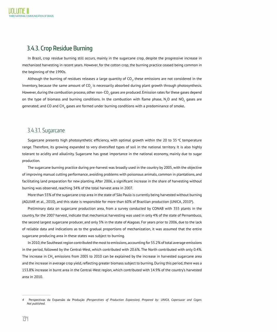
134
VOLUME IIITHIRD NATIONAL COMMUNICATION OF BRAZIL
3.4.3. Crop Residue BurningIn Brazil, crop residue burning still occurs, mainly in the sugarcane crop, despite the progressive increase in
mechanized harvesting in recent years. However, for the cotton crop, the burning practice ceased being common in
the beginning of the 1990s.Although the burning of residues releases a large quantity of CO2, these emissions are not considered in the
Inventory, because the same amount of CO2 is necessarily absorbed during plant growth through photosynthesis.
However, during the combustion process, other non- CO2 gases are produced. Emission rates for these gases depend
on the type of biomass and burning conditions. In the combustion with flame phase, N2O and NOX gases are
generated; and CO and CH4 gases are formed under burning conditions with a predominance of smoke.
3.4.3.1. SugarcaneSugarcane presents high photosynthetic efficiency, with optimal growth within the 20 to 35 oC temperature
range. Therefore, its growing expanded to very diversified types of soil in the national territory. It is also highly
tolerant to acidity and alkalinity. Sugarcane has great importance in the national economy, mainly due to sugar
production.
The sugarcane burning practice during pre-harvest was broadly used in the country by 2005, with the objective
of improving manual cutting performance, avoiding problems with poisonous animals, common in plantations, and
facilitating land preparation for new planting. After 2006, a significant increase in the share of harvesting without
burning was observed, reaching 34% of the total harvest area in 2007.
More than 55% of the sugarcane crop area in the state of São Paulo is currently being harvested without burning
(AGUIAR et al., 2010), and this state is responsible for more than 60% of Brazilian production (UNICA, 20104).
Preliminary data on sugarcane production area, from a survey conducted by CONAB with 355 plants in the
country, for the 2007 harvest, indicate that mechanical harvesting was used in only 4% of the state of Pernambuco,
the second largest sugarcane producer, and only 3% in the state of Alagoas. For years prior to 2006, due to the lack
of reliable data and indications as to the gradual proportions of mechanization, it was assumed that the entire
sugarcane producing area in these states was subject to burning.
In 2010, the Southeast region contributed the most to emissions, accounting for 55.2% of total average emissions
in the period, followed by the Central-West, which contributed with 20.6%. The North contributed with only 0.4%.
The increase in CH4 emissions from 2005 to 2010 can be explained by the increase in harvested sugarcane area
and the increase in average crop yield, reflecting greater biomass subject to burning. During this period, there was a
153.8% increase in burnt area in the Central-West region, which contributed with 14.9% of the country’s harvested
area in 2010.
4 Perspectivas da Expansão da Produção (Persperctives of Production Expansion). Prepared by: UNICA, Copersucar and Cogen. Not published.
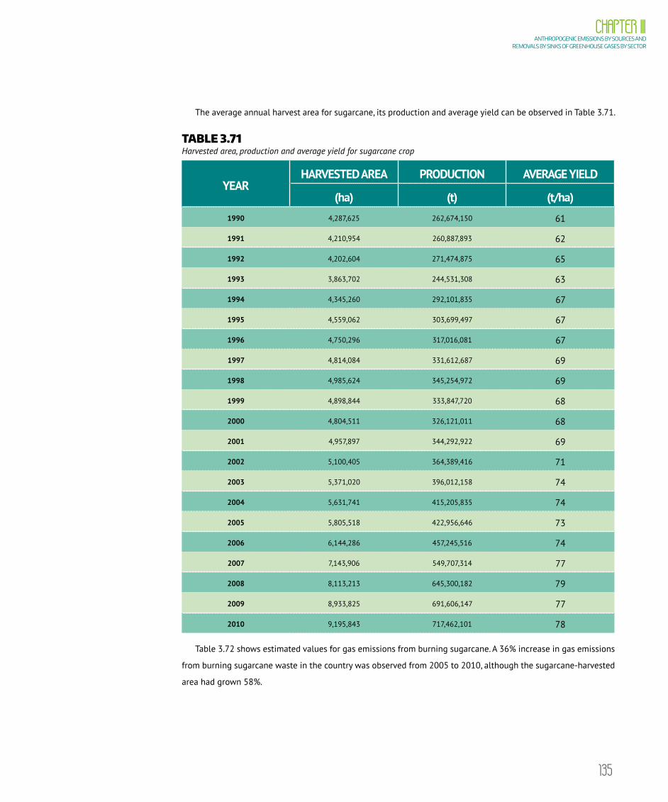
135
CHAPTER IIIANTHROPOGENIC EMISSIONS BY SOURCES AND
REMOVALS BY SINKS OF GREENHOUSE GASES BY SECTOR
The average annual harvest area for sugarcane, its production and average yield can be observed in Table 3.71.
TABLE 3.71 Harvested area, production and average yield for sugarcane crop
YEARHARVESTED AREA PRODUCTION AVERAGE YIELD
(ha) (t) (t/ha)1990 4,287,625 262,674,150 61
1991 4,210,954 260,887,893 62
1992 4,202,604 271,474,875 65
1993 3,863,702 244,531,308 63
1994 4,345,260 292,101,835 67
1995 4,559,062 303,699,497 67
1996 4,750,296 317,016,081 67
1997 4,814,084 331,612,687 69
1998 4,985,624 345,254,972 69
1999 4,898,844 333,847,720 68
2000 4,804,511 326,121,011 68
2001 4,957,897 344,292,922 69
2002 5,100,405 364,389,416 71
2003 5,371,020 396,012,158 74
2004 5,631,741 415,205,835 74
2005 5,805,518 422,956,646 73
2006 6,144,286 457,245,516 74
2007 7,143,906 549,707,314 77
2008 8,113,213 645,300,182 79
2009 8,933,825 691,606,147 77
2010 9,195,843 717,462,101 78
Table 3.72 shows estimated values for gas emissions from burning sugarcane. A 36% increase in gas emissions
from burning sugarcane waste in the country was observed from 2005 to 2010, although the sugarcane-harvested
area had grown 58%.

136
VOLUME IIITHIRD NATIONAL COMMUNICATION OF BRAZIL
TABLE 3.72 Emissions for sugarcane burning
GAS1990 1995 2000 2005 2010 VAR. 2005/ 2010
(Gg) (%)CH4 102.7 118.7 105.0 136.3 185.3 36.0%
N2O 2.66 3.08 2.72 3.53 4.80 36.0%
CO 3,499.2 4,045.8 3,576.4 4,644.4 6,313.5 35.9%
NOx 95.1 109.9 97.2 126.2 171.6 36.0%
3.4.3.2. Herbaceous cottonCotton crops are broken down into two categories, which are the herbaceous cotton and the arboreal cotton, the
latter characterized by being a perennial crop where waste is not burned. For this Inventory, based on information
obtained after consulting cotton production chain agents and current legislation, the practice of burning was
re-evaluated as a method for eradicating and eliminating crop residues for the period after 1990. According to
specialists, the common practice has been to grub and harrow crop residues, incorporating the waste to the soil,
in consonance with the non-obligatory burning in current legislation. Chemical treatment is most used in cases
of sprouting. It was thus assumed that there was a transition period between the obligatory and non-obligatory
burning of cotton crop wastes in the beginning of the 1990s, as well as the eradication mechanisms of crop
residues in the field. A gradual drop from 50% to 0% was considered from 1990 to 1995, as a fraction of the areas
still practicing burning. After this period, it was assumed that cotton waste burning no longer existed in the country.
TABLE 3.73 Emissions from cotton crop waste burning
GAS1990 1995 2000 2005 2010 VAR. 2005/ 2010
(Gg) (%)CH4 3.8 - - - - -
N2O 0.10 - - - - -
CO 128.4 - - - - -
NOX 3.5 - - - - -

137
CHAPTER IIIANTHROPOGENIC EMISSIONS BY SOURCES AND
REMOVALS BY SINKS OF GREENHOUSE GASES BY SECTOR
3.4.4. N2O emissions from agricultural soils Use of nitrogen fertilizers is pointed out as the main reason for the global increase in N2O emissions by
agricultural soils. However, in Brazil, the main source of emissions is manure from grazing animals. N2O emissions
also occur from applying animal manure as fertilizer, from the nitrogen found in agricultural waste and from the
atmospheric deposition of NOx and NH3.
N2O emissions from agricultural lands were subdivided into three categories, as per 1996 Guidelines:
>> N2O emissions from grazing animal manure;
>> other direct sources of N2O emissions, including the use of synthetic fertilizers, nitrogen from manure
used as fertilizer, the biological nitrogen fixation and crop residues; and
>> indirect sources of N2O emissions from the nitrogen used in agriculture, which include the volatilization
and subsequent atmospheric deposition of NOx and NH3 from fertilizer applications, and leaching and
runoff of nitrogen from fertilizers.
Estimates of N2O emissions from agricultural soils in Brazil are shown in Table 3.74. In 2010, total emissions
were estimated at 452.45 Gg N 2O, the highest share coming from direct emissions, in which grazing animal waste
is the main cause.
From 2005 to 2010, the different source of N2O emissions maintained the same order of importance as to their
contribution towards total N2O emissions from agricultural soils. The deposition of animal excrement in pastures
remained as the most important source. Indirect emissions represented 37.6% of the total in 2010.
It is important to underscore that recent results from studies on N2O emissions from national agriculture do
not confirm that biological nitrogen fixation is a relevant process for N2O emissions, an understanding in line with
the 2006 Guidelines, in which this source of emissions is absent. Therefore, biological fixation of nitrogen was not
considered as a source of emissions in this Inventory.
TABLE 3.74 N2O emissions per agricultural soil
SOURCE1990 1995 2000 2005 2010
SHARE IN
2010VAR. 2005/ 2010
(Gg N2O) (%)Direct emissions 184.07 205.28 213.85 257.09 282.31 62.4% 9.8%
Grazing animals 129.73 140.2 140.12 167.45 170.24 37.6% 1.7%
Bovine 107.99 118.49 122.04 148.83 152 33.6% 2.1%
Others 21.74 21.71 18.08 18.62 18.24 4.0% -2.0%
Synthetic fertilizers 9.81 14.27 21.28 27.51 35.74 7.9% 29.9%
Application of fertilizer 14.9 16.4 15.88 17.81 21.33 4.7% 19.8%
Bovine 4.74 5.03 4.87 5.46 5.77 1.3% 5.7%
Others + Vinasse 10.16 11.37 11.01 12.35 15.56 3.4% 26.0%
continues on the next page

138
VOLUME IIITHIRD NATIONAL COMMUNICATION OF BRAZIL
SOURCE1990 1995 2000 2005 2010
SHARE IN
2010VAR. 2005/ 2010
(Gg N2O) (%) Crop residues 15.32 19.8 21.66 29.11 39.49 8.7% 35.7%
Soy bean 4.85 6.26 8 12.47 16.75 3.7% 34.3%
Sugarcane 1.03 1.2 1.82 2.35 5.47 1.2% 132.8%
Beans 0.77 1.02 1.06 1.05 1.09 0.2% 3.8%
Rice 0.85 1.29 1.28 1.52 1.29 0.3% -15.1%
Corn 3.48 5.91 5.27 5.72 9.02 2.0% 57.7%
Manioc 2.66 2.78 2.52 2.83 2.73 0.6% -3.5%
Others 1.68 1.34 1.71 3.17 3.14 0.7% -0.9%
Organic Soils 14.31 14.61 14.91 15.21 15.51 3.4% 2.0%
Indirect emissions 106.68 120.31 127.87 155.53 170.14 37.6% 9.4%
Atmospheric deposition 22.31 25.18 26.53 32.69 35.65 7.9% 9.1%
Synthetic fertilizers 2.44 3.56 4.94 7.08 9.13 2.0% 29.0%
Animal fertilizer 19.87 21.62 21.59 25.61 26.52 5.9% 3.6%
Bovine 15.58 17.06 17.49 21.21 21.71 4.8% 2.4%
Others 4.29 4.56 4.1 4.4 4.81 1.1% 9.3%
Leaching 84.37 95.13 101.34 122.84 134.49 29.7% 9.5%
Synthetic Fertilizers 9.18 13.37 19.66 25.95 33.65 7.4% 29.7%
Animal Fertilizer 75.19 81.76 81.68 96.89 100.84 22.3% 4.1%
Bovine 58.44 63.96 65.59 79.53 81.41 18.0% 2.4%
Others 16.75 17.8 16.09 17.36 19.43 4.3% 11.9%
Total 290.75 325.59 341.72 412.62 452.45 100% 9.7%
3.4.4.1. N2O emissions due to grazing animalsWaste deposited on soils by animals during grazing is the most important source of N2O emissions by agricultural
soils in Brazil due to the large herd and the fact that extensive raising is the predominant cattle practice in the
country. The production systems are also characterized by large territorial extension, with pasture management
conducted continuously.

139
CHAPTER IIIANTHROPOGENIC EMISSIONS BY SOURCES AND
REMOVALS BY SINKS OF GREENHOUSE GASES BY SECTOR
In Brazil, between 2005 and 2010, total nitrogen directly excreted in pastures increased by 1.8%, and it is
possible to observe this evolution from data in Table 3.75. N2O emissions from grazing animals represented 37.6%
of emissions of this gas from agricultural soils, in 2010, with cattle as the main contributor of these emissions.
N2O emissions were estimated using IPCC default emission factors for the nitrogen content in animal wastes
and for the N2O emission factor for the quantity of nitrogen deposited. Among the Brazilian regions, in 2010,
the Central-West had the largest number of heads of beef cattle, corresponding to 34.6% of the Brazilian herd.
Table 3.75 shows that the Central-West region offers the highest contribution in quantity of nitrogen from animal
manure directly applied to pasture.
Beef cattle production in the beginning of the 2000s was characterized by a migration from the Southeast to
the Central-West and North regions. This explains the increase in the quantity of nitrogen applied directly to the
soil in the latter.
TABLE 3.75 Nitrogen amount in animal manure applied directly to pasture
SYSTEM1990 1995 2000 2005 2010 SHARE
IN 2010VAR. 2005/
2010
(t NEx*) (%)
Grazing animals
North 514,405 697,323 826,639 1,358,545 1,366,162 19.4% 0.6%
Northeast 1,157,440 1,050,992 1,004,210 1,162,718 1,233,083 17.5% 6.1%
Southeast 1,262,937 1,303,752 1,227,253 1,281,403 1,279,669 18.2% -0.1%
South 872,450 908,321 843,641 877,841 895,889 12.7% 2.1%
Central-West 1,465,912 1,757,240 1,851,101 2,226,094 2,253,743 32.1% 1.2%
Total 5,273,143 5,717,627 5,752,843 6,906,602 7,028,545 100% 1.8%
* Excreted nitrogen
3.4.4.2. N2O emissions by other direct sources
Use of synthetic fertilizer
The most important nitrogen fertilizers used in Brazil are urea, ammonia, anhydrous ammonium nitrate and
ammonium sulfate. Total consumption of synthetic nitrogen fertilizers in Brazil in 2010 was 2.854 million tonnes of
nitrogen content, 29.7% more than consumption in 2005 according to Table 3.76. Part of this nitrogen is incorporated
to plants and soil, part is volatized as NOx and NH3 and part is released as N2O. Due to the absence of specific studies
on emission factors for Brazil’s management and climate conditions, IPCC default emission factors have been used.
The share of the Southeast region in the total consumption of nitrogen fertilizers in the country increased
by 10.7% between 2005 and 2010, and accounted for the largest share of consumption in the country in 2010,

140
VOLUME IIITHIRD NATIONAL COMMUNICATION OF BRAZIL
with 37.9% of the total. The direct emissions of N2O by the use of synthetic fertilizers accounted for 7.9% of the
emissions of N2O from agricultural land in 2010, as shown in Table 3.74.
TABLE 3.76 Amount of fertilizer in the form of nitrogen delivered to the end consumer in Brazil from 1990 to 2010
REGION1990 1995 2000 2005 2010
SHARE IN
2010
VAR. 2005/ 2010
(t N) (%)North 1,273 4,941 13,731 22,692 33,113 1.2% 45.9%
Northeast 80,013 119,902 147,286 197,012 280,905 9.8% 42.6%
Southeast 402,060 563,642 721,382 977,190 1,081,888 37.9% 10.7%
South 231,403 327,147 499,749 631,653 882,822 30.9% 39.8%
Central-West 64,566 119,013 286,047 372,857 576,091 20.2% 54.5%
Brazil 779,315 1,134,645 1,668,195 2,201,404 2,854,819 100% 29.7%
Use of manure as fertilizer
The emissions of nitrous oxide (N2O) estimated in this section are related to the N2O produced during the
storage and treatment of animal waste, before being applied to the soil as a fertilizer. The term manure or waste
is used here collectively for both liquid and solid wastes produced by livestock. The emission of N2O from waste
during storage and treatment depends on the nitrogen and carbon contained therein, the duration of storage and
the type of treatment. The term “management system” is used for all types of storage and handling of manure.
The amount of nitrogen excreted by animals that does not occur directly in the pasture is assumed as being
applied to the soil as fertilizer.
According to the practices used in each region, it is considered that the managed manure, using the systems of
anaerobic lagoon, solid storage, dry lot, pasture, manure and biodigester, are applied in the grassland as fertilizer.
As for the N2O emission factors, the IPCC default values were adopted. The direct emissions of N2O by the use of
animal manure as fertilizer accounted for 4.7% of the emissions of N2O from agricultural land in 2010, as shown
in Table 3.74.
Except for the category of swine and poultry, a large part of manure is deposited directly in the pastures. In the
case of animals whose manure is “not managed”, that is, animals from pasture and paddock, manure are not stored
or processed, but deposited directly in the grassland.

141
CHAPTER IIIANTHROPOGENIC EMISSIONS BY SOURCES AND
REMOVALS BY SINKS OF GREENHOUSE GASES BY SECTOR
TABLE 3.77 Nitrogen amount in animal manure applied on soils (except grazing)
REGION1990 1995 2000 2005 2010
SHARE IN
2010
VAR. 2005/ 2010
(t NEx) (%)North 71,207 87,270 61,546 64,687 59,001 4.2% -8.8%
Northeast 207,200 197,977 171,135 181,051 177,911 12.6% -1.7%
Southeast 299,922 319,268 313,788 336,297 376,677 26.8% 12.0%
South 349,212 415,349 432,639 485,119 586,326 41.7% 20.9%
Central-West 123,310 140,701 138,503 176,124 207,686 14.8% 17.9%
Brazil 1,050,851 1,160,565 1,117,611 1,243,278 1,407,600 100% 13.2%
The quantities of nitrogen in manure used for fertilizers that directly generate emissions of N2O are estimated
at 80% of the total, with the remaining 20% corresponding to losses by volatilization of NH3 and NOx, which will
generate indirect emissions of N2O.
Table 3.78 shows emissions from manure management systems in Brazil, not including those deposited directly
in pastures, indicating that emissions of N2O from the management systems of animal waste are predominant in
the South region of the country.
TABLE 3.78 Summary of N2O emissions by animal manure management in Brazil
REGIÃO1990 1995 2000 2005 2010 SHARE IN
2010 VAR. 2005/ 2010
(Gg N2O) (%) North 0,73 0,91 0,66 0,67 0,62 4,2% -6,6%
Northeast 2,36 2,36 2,13 2,27 2,34 15,7% 3,1%
Southeast 2,95 3,3 3,47 3,79 4,37 29,5% 15,4%
South 2,98 3,73 3,94 4,45 5,52 37,2% 24,2%
Central-West 1,01 1,2 1,29 1,65 1,98 13,4% 20,5%
Total 10,03 11,49 11,49 12,82 14,84 100% 15,8%
Biological nitrogen fixation
The reduction process of atmospheric N2O to combined forms of ammonium-N using living organisms is called
biological nitrogen fixation. In Brazil, the practice of inoculation with specific bacteria for N2 fixation is routinely
used only in the soybean crop, and there is no other available information about its application in other crops.

142
VOLUME IIITHIRD NATIONAL COMMUNICATION OF BRAZIL
In relation to N2O emissions resulting from the biological nitrogen fixation (BNF) process using legumes, as
shown in 1996 Guidelines, Rochette and Janzen (2005) demonstrated that there are no data in literature to confirm
the existence of any relation between the two processes, thus BNF is no longer considered a source of N2O in 2006
Guidelines. The confirmation that the soy bean crop does not imply N2O emissions due to BNF associated with the
culture was achieved by Cardoso et al. (2008) by failing to find any difference between N2O emissions measured
in soil planted with a nodulating variety and another non-nodulating variety (unable to benefit from BNF). In the
South of Brazil, Jantalia et al. (2008) did not record N2O emissions either during soybean crop growth that could
suggest BNF as a relevant source of this gas.
Thus, for this Inventory, BNF was removed as a source of N2O, as described in the 2006 Guidelines methodology,
corroborated by national studies.
Crop residues
Nitrogen contained in crop residues and incorporated into the soil is also a source of N2O emissions. In order
to estimate these emissions, annual productions and the amount of dry matter per crop were used. The main crops
considered were sugarcane, corn, soybean, rice, beans, and cassava.
Considering the quantity of nitrogen contained in the waste of each main crop, as well as other annual crops,
there has been a 35.7% increase in the amount of nitrogen between 2005 and 2010 that returns to the agricultural
soil (Table 3.79), with soy bean standing out as the main contributor.
TABLE 3.79 Nitrogen amount in residue left on agricultural soils by crop
CROP1990 1995 2000 2005 2010 SHARE IN
2010VARIATION 2005/ 2010
(t N) (%)Soy bean 308,484 398,168 508,834 793,496 1,065,957 42.4% 34.3%
Sugarcane 65,863 76,150 115,631 149,598 347,858 13.8% 132.5%
Beans 49,241 64,925 67,352 66,588 69,613 2.8% 4.5%
Rice 54,232 82,040 81,372 96,413 82,113 3.3% -14.8%
Corn 221,385 376,103 335,182 364,139 574,150 22.8% 57.7%
Manioc 169,233 176,893 160,341 180,017 173,721 6.9% -3.5%
Others 107,201 85,489 108,978 201,545 199,954 8.0% -0.8%
Total 975,639 1,259,767 1,377,690 1,851,798 2,513,365 100% 35.7%
Due to lack of reliable data related to residues from permanent crops (coffee, coconut, oranges, among others),
the quantity of nitrogen that returns as waste from these crops was not calculated. The parameters used for
temporary crops (fraction of dry matter from the harvested product) would not serve as reference for perennial crop
waste, since residues from these cultures do not return to agricultural soils.
143
CHAPTER IIIANTHROPOGENIC EMISSIONS BY SOURCES AND
REMOVALS BY SINKS OF GREENHOUSE GASES BY SECTOR
For annual crops, a bibliographical study was conducted to estimate dry matter fraction of the product and
the nitrogen fraction of the aerial part of the plant. Due to the lack of better information, IPCC default emission
factors were used for nitrogen content in residues and for the portion of waste that remains in the field. Direct N2O
emissions from the use of harvest waste represented 8.7% of N2O emissions from agricultural soil in 2010, as per
Table 3.74, and the six main crops accounted for 92% of emissions for all crops.
High organic content soils
It is necessary to estimate the managed area for emissions of N2O through the management of organic soils,
which is multiplied by the emission factor (EF). For this Inventory, the area of organic soil was raised in accordance
with the IPCC definition (2006), which complies with the WRB system (FAO/UNESCO), taking into account the
following criteria:
1 thickness of 10 cm or more. Horizon with <20cm must be 12% or more of organic carbon when mixed up
to 20cm of depth;
2 the saturation of the soil with water must occur for a few days only, and the soil must have more than 20%
carbon (weight) or more than 35% organic matter;
3 If the soil is subject to episodes of saturation with water and has (1) at least 12% carbon in the case of not
having clay; (2) at least 18% carbon if it has 60% or more of clay; or (3) intermediate proportion of carbon
for intermediate proportion of clay.
The soil survey was based on the map of Brazilian soils developed by Embrapa (scale 1:5,000,000). Map units
were designed for each state, with the location of Histosols and Melanin Gleysols, whose descriptions meet the
specification for organic soils.
The components 1, 2 and 3 were considered (COMP1, COMP2 and COMP3), which represent the level of
importance of the soil class in the occurrence of associations of soils observed in the map unit. For each component,
the share of each soil class was established in the mapping units (MU), in which a 3 component MU stands for
component 1 (50%), component 2 (30%), component 3 (20%) and/or, in the case of 2 components, component 1
(60%), component 2 (40%), according to the criteria established for the composition of MU in soil surveys. The areas
of organic soils total 1,598,267.46 ha (15,982.6746 km2).
For the estimation of management, maps of land use in 1994 and 2002 were applied, which are set out in the report
of Land Use, Land-Use Change and Forestry in the Second National Communication. They were considered areas of
soils subjected to agricultural use, identified as ‘Agricultural Area’ (Ac), ‘Planted Pasture’ (Ap), ‘Managed Grassland’ (GM)
and ‘Reforestation’ (Ref), to which the identification used in the report of Land Use, Land-Use Change and Forestry was
foundational. In 1994, the areas of managed organic soils corresponded to 771,644.79 ha, and in 2002, 797,004,49
ha, which represented an increase of only 3.3% in 8 years, indicating some stability in the area managed. A simplified
assumption that the variation was linear between the two years evaluated and that the same model would apply to
estimates back to 1990 and projections up to 2010 was taken into account. Thus, the area managed in 1990 accounted
for 47.5% of the total area of organic soils in Brazil, and that increased linearly until 2010, reaching 51.5%.
According to the 1996 Guidelines, the cultivation of organic soils in subtropical and tropical regions implies
emissions from 8 to 16 kg N-N2O ha -1 year -1. Since the occurrence reports of organic soils are more geared toward
the Central-South region, an average value for the emission factor of N2O (EF) of 12kg N-N2O ha-1 year-1 was adopted.
144
VOLUME IIITHIRD NATIONAL COMMUNICATION OF BRAZIL
3.4.4.3. N2O emissions from indirect sources
Atmospheric deposition of NOx and NH3
Part of the nitrogen contained in synthetic fertilizers and in animal manure, used as fertilizers, volatilizes as
NOx and NH3. This part is discounted from the estimates of emissions from direct sources. However, part of these
gases is deposited again on the Earth’s surface, and if this deposition occurs on agricultural soils, it can result in
additional N2O emissions. It is impossible to determine where this deposition will occur, and it may even occur in
the oceans. Likewise, NOx and NH3 stemming from other sources, such as combustion, may deposit on agricultural
soils. Therefore, the uncertainty related to this portion of emissions is very large. It was decided to consider total
deposition corresponding to the volatilized gases from agricultural soils. IPCC default emission factors were used.
N2O emissions from atmospheric deposition of NOX and NH3, in 2010, represented 7.9% of N2O emissions from
agricultural soils, growing 9.1% compared to the value estimated in 2005, as per Table 3.74.
Nitrogen leaching and surface runoff
Part of the nitrogen applied to agricultural soils as synthetic fertilizers or animal manure is subject to leaching
and runoff, flowing through rivers into the ocean. These environments also have N2O emissions, classified as indirect
emissions from fertilizer applications. Uncertainty regarding N2O emission factors by runoff of this nitrogen is very
large, and there is no assessment concerning the most appropriate values for Brazil’s wide-ranging conditions. IPCC
default emission factors were used. In 2010, N2O emissions due to leaching and runoff nitrogen applied as fertilizer
accounted for 29.7% of N2O emissions from agricultural soils, a growth of 9.5% compared to the estimated value
for 1990, as per Table 3.73.
3.5. LAND USE, LAND-USE CHANGE AND FORESTRY The methodologies adopted for this part of the Inventory are consistent with those in the 2003 Good Practice
Guidance (IPCC, 2003), with updates of the 2006 IPCC Guidelines for National Greenhouse Gas Inventories (IPCC,
2006), when relevant. Even if these guides are not mandatory for developing countries, it was decided to use them
given the importance of emissions associated with Land use, Land-Use Change and Forestry (LULUCF) mentioned
in previous inventories (BRASIL 2004; 2010). In this context, a more detailed approach described in the guides was
again applied, which includes the spatially explicit observation of categories of land use and their conversions in
the evaluated period.
Emissions and removal estimates based on this methodology require a correct representation of areas and
their association with use categories proposed by the IPCC from a proper, consistent, complete, and transparent
approach. Thus, in order to reach an in-depth result of this work, the implementation of the inventory involved the
search of information in scientific literature and expert support from various regions of the country, both for the
145
CHAPTER IIIANTHROPOGENIC EMISSIONS BY SOURCES AND
REMOVALS BY SINKS OF GREENHOUSE GASES BY SECTOR
mapping of different uses of land and data compilation used for emissions and removals estimates. In addition, to
keep the whole process transparent and replicable, all steps are described in detail and their meta-data are made
available, when possible.
One of the difficulties associated with this sector is the identification of anthropogenic and non-anthropogenic
emissions and removals of greenhouse gases. Similarly to the Second National Inventory, this report applies the
concept of managed land proposed by the IPCC (IPCC, 2003; 2006), meaning that all emissions and removals
occurred on these lands are considered anthropogenic. On the other hand, emissions and removals occurred
on unmanaged lands are considered non-anthropogenic, except for the unmanaged area converted into other
categories of land use, as established in the Good Practice Guidance LULUCF (IPCC, 2003) and the 2006 IPCC
Guidelines (IPCC, 2006).
In the case of Brazil, Managed Land comprises the entire area contained in Indigenous Lands – according to
information provided by the National Indian Foundation (FUNAI), whose processes of demarcation are minimally in
the “Delimited” phase – in state and federal protected areas – according to the Ministry of the Environment (MMA)
and the National System of Protected Areas (SNUC), Law 9985/2000, except for the Private Reserves of Natural
Preservation (RPPN) due to the lack of consistent information about them.
The net anthropogenic emissions (emissions by sources minus removals by sinks) between two points in time
are estimated for all carbon stocks as follows: (i) living biomass (above and belowground biomass), (ii) dead organic
matter (litter and dead wood), (iii) organic carbon in the soil, as proposed by the IPCC (IPCC, 2003; 2006).
This Inventory presents average annual net emissions for the period between the years 2002 and 2010 for all
Brazilian biomes. Exceptionally for the Amazon, estimates are presented for the periods of 2002-2005 and 2005-
2010, in order to capture the impact of the implementation of the Action Plan for the Prevention and Control of
Deforestation of the Legal Amazon5 area (PPCDAm), established on 2004.
The activity data for this inventory was foremost based on image analysis of satellites with appropriate spatial
resolution (TM-Landsat-5, 30 meters; LISS-III/Resourcesat-1, 23,5 meters). The mapping of land-use categories/
subcategories was prepared on a 1:250.000 scale with a minimum mapping unity of 6 hectares. Whenever possible,
emission factors were based on national data, and when these data were not available, on default data of the IPCC
(IPCC, 2003; 2006). Those data associated with the methodological proposal of the IPCC enabled emission and
sink estimates for the studied period, taking into consideration the specificities of Brazilian biomes. It should be
noted that more detailed information on methods, data and results presented are found on the Reference Report
“Greenhouse Emissions for the Land Use, Land-Use Change and Forestry Sector”.
Based on these results, the average net annual emissions for the period 1994 to 2010 were estimated, as
described in section 3.5.2.8.
Additionally, CO2 emissions of resulting from liming – application of limestone on the soil to reduce its
acidification – are included in this sector.
5 Legal Amazon: Area encompassing whole nine states: Acre, Amazonas, Amapá, Maranhão (totally included since May 2008), Mato Grosso, Rondônia, Pará, Roraima and Tocantins, with a total of 5.02 million km2. It incorporates the whole Amazon biome (4.21 km2) and parts of the Cerrado and the Pantanal biomes.

146
VOLUME IIITHIRD NATIONAL COMMUNICATION OF BRAZIL
3.5.1. Methodology
3.5.1.1. Land Use, Land-Use Change and ForestryThe identification of areas under different categories of land-use/land-cover using approach 3 (Tier 3) of the
Good Practice Guidance LULUCF (IPCC, 2003) was continued in order to assure consistence of estimates of this
Third Inventory. All categories and changes occurred between the inventories are spatially identified for all the
national territory. This approach requires spatially explicit observations of transitions and, in the Brazilian case,
included managed and unmanaged areas. The methodology used to calculate emissions for land-use, land-use
change and forestry is detailed in Appendix I.
3.5.1.2. Liming of agricultural soils Emissions from lime application to soils are calculated based on the amount of lime commercialized in
Brazil annually, by state, between 1990-2010, based on the information provided by the Brazilian Association of
Agricultural Lime Producers (ABRACAL). Due to the lack of detailed information on the composition of lime sold
in the country it is assumed that the lime is composed basically of calcic limestone. The emission factor used to
calculate the emissions is 0.44 t CO2/t CaCO3.
3.5.2. ResultsThis Third Inventory presents updates of data activity and emission factors for the following reasons: (1) new
methodological approach (for example, new carbon content based on plant phytophysiognomy of the Amazon); (2)
updated data (for example, on planted forestry); (3) refined classification of land use/coverage. Hence, estimates for
the period of 1994-2002 were recalculated in order to assure consistence among periods. It is worth mentioning
that the mapping for the year 2002 used in the Second Inventory was based on a mapping commissioned by
the Ministry of the Environment (PROBIO I) and was prepared by six distinct institutions, resulting in some
inconsistencies when compared to the mapping of 2010. Therefore, the mappings for land use and land cover for
2002 were re-elaborated by the same team, which mapped 2010, assuring greater consistency and accuracy for the
classification of land use/cover.
Net anthropogenic CO2 emissions are presented for each of the six Brazilian biomes.
The following Tables show the areas of each transition between land use and land use cover that have been
considered between 1994 and 2002 and between 2002 and 2010 and then net emissions for each transition.
Exceptionally for the Amazon, the year of 2005 is also presented because there is a reduced level of deforestation
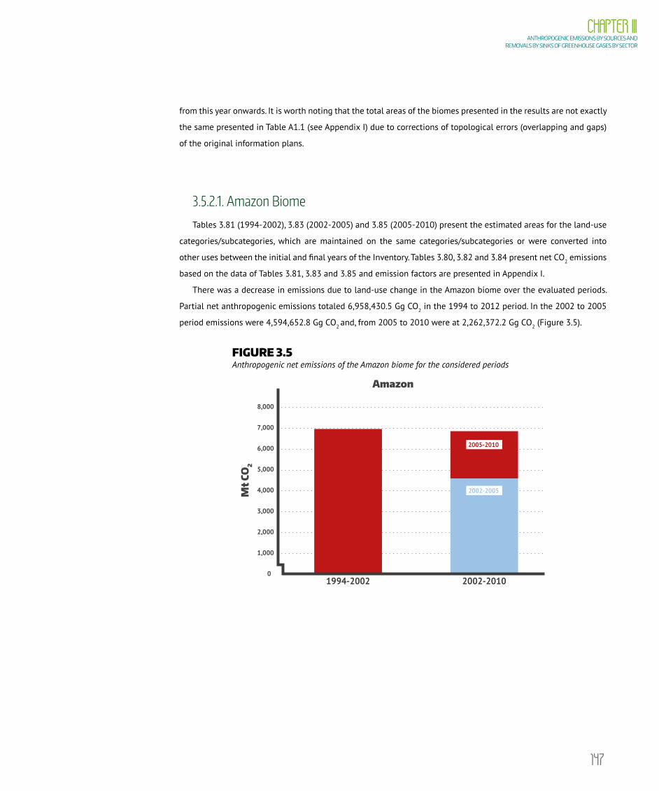
147
CHAPTER IIIANTHROPOGENIC EMISSIONS BY SOURCES AND
REMOVALS BY SINKS OF GREENHOUSE GASES BY SECTOR
from this year onwards. It is worth noting that the total areas of the biomes presented in the results are not exactly
the same presented in Table A1.1 (see Appendix I) due to corrections of topological errors (overlapping and gaps)
of the original information plans.
3.5.2.1. Amazon Biome Tables 3.81 (1994-2002), 3.83 (2002-2005) and 3.85 (2005-2010) present the estimated areas for the land-use
categories/subcategories, which are maintained on the same categories/subcategories or were converted into
other uses between the initial and final years of the Inventory. Tables 3.80, 3.82 and 3.84 present net CO2 emissions
based on the data of Tables 3.81, 3.83 and 3.85 and emission factors are presented in Appendix I.
There was a decrease in emissions due to land-use change in the Amazon biome over the evaluated periods.
Partial net anthropogenic emissions totaled 6,958,430.5 Gg CO2 in the 1994 to 2012 period. In the 2002 to 2005
period emissions were 4,594,652.8 Gg CO2 and, from 2005 to 2010 were at 2,262,372.2 Gg CO2 (Figure 3.5).
FIGURE 3.5 Anthropogenic net emissions of the Amazon biome for the considered periods
0
1,000
2,000
3,000
4,000
5,000
6,000
7,000
8,000
1994-2002 2002-2010
Mt
CO2
Amazon
2005-2010
2002-2005

148
VOLUME IIITHIRD NATIONAL COMMUNICATION OF BRAZIL
3.5.2.2. Cerrado BiomeTables 3.87 and 3.89 present estimated areas of each land-use change and land cover transition observed
between 1994 and 2002, and between 2002 and 2010 for the Cerrado biome. Tables 3.88 and 3.90 present net
anthropogenic CO2 emission related.
Net anthropogenic CO2 emissions related to land-use change and land cover in the Cerrado biome totaled
1,703,660.0 Gg CO2 in the period from 1994 to 2002, increasing to 1,845,024.7 Gg CO2 between the years 2002 to
2010 (Figure 3.6).
FIGURE 3.6 Anthropogenic net emissions of the Cerrado biome for the considered periods
Mt
CO2
0
200
400
600
800
1,000
1,200
1,400
1,600
1,800
2,000
1994-2002 2002-2010
Cerrado

149
CHAPTER IIIANTHROPOGENIC EMISSIONS BY SOURCES AND
REMOVALS BY SINKS OF GREENHOUSE GASES BY SECTOR
3.5.2.3. Caatinga BiomeTables 3.91 and 3.93 present the estimated areas of each transition observed between 1994 and 2002, and
between 2002 and 2010 for the Caatinga biome. Tables 3.92 and 3.94 show net anthropogenic CO2 emission
related.
Net anthropogenic CO2 emissions of the Caatinga biome totaled 190,190.9 Gg CO2 for the period of 1994-2002,
reducing to 77,708.0 Gg CO2 for the period of 2002 to 2010 (Figure 3.7).
FIGURE 3.7 Anthropogenic net emissions of the Caatinga biome for the considered periods
0
20
40
60
80
100
120
140
160
180
200
Mt
CO2
1994-2002 2002-2010
Caatinga

150
VOLUME IIITHIRD NATIONAL COMMUNICATION OF BRAZIL
3.5.2.4. Atlantic Forest BiomeTables 3.95 and 3.97 present the estimated areas of each transition observed between 1994 and 2002, and
between 2002 and 2010 for the Atlantic Forest biome. Tables 3.96 and 3.98 show net anthropogenic CO2 emission
related.
Land-use change emissions of the Atlantic Forest biome totaled 888,574.3 Gg CO2 for the period of 1994-2002,
increasing to 2,090,380.7 Gg CO2 for the period of 2002 to 2010 (Figure 3.8).
FIGURE 3.8 Net anthropogenic emissions of the Atlantic Forest biome for the considered periods
Mt
CO2
0
500
1,000
1,500
2,000
2,500
1994-2002 2002-2010
Atlantic Forest
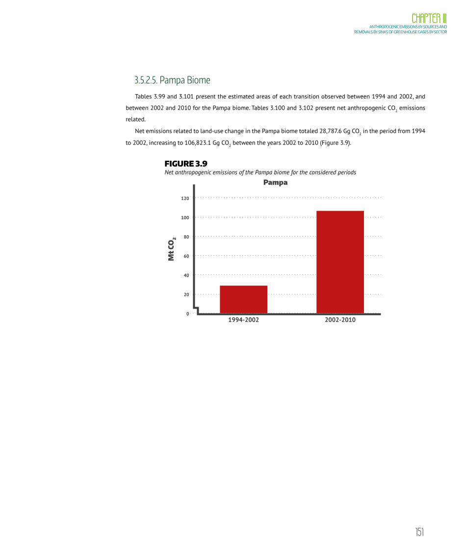
151
CHAPTER IIIANTHROPOGENIC EMISSIONS BY SOURCES AND
REMOVALS BY SINKS OF GREENHOUSE GASES BY SECTOR
3.5.2.5. Pampa BiomeTables 3.99 and 3.101 present the estimated areas of each transition observed between 1994 and 2002, and
between 2002 and 2010 for the Pampa biome. Tables 3.100 and 3.102 present net anthropogenic CO2 emissions
related.
Net emissions related to land-use change in the Pampa biome totaled 28,787.6 Gg CO2 in the period from 1994
to 2002, increasing to 106,823.1 Gg CO2 between the years 2002 to 2010 (Figure 3.9).
FIGURE 3.9 Net anthropogenic emissions of the Pampa biome for the considered periods
Mt
CO2
0
40
20
60
80
100
120
1994-2002 2002-2010
Pampa

152
VOLUME IIITHIRD NATIONAL COMMUNICATION OF BRAZIL
3.5.2.6. Pantanal BiomeTables 3.103 and 3.105 present the estimated areas of each of the transitions observed between 1994 and
2002, and between 2002 and 2010 for the Pantanal biome. Tables 3.104 and 3.106 show net anthropogenic CO2
emission related.
CO2 net emissions related to land-use change in the Pantanal biome totaled 173,116.3 Gg CO2 in the period
from 1994 to 2002, reducing to 133,913.3 Gg CO2 between the years 2002 to 2010 (Figure 3.10).
FIGURE 3.10 Net anthropogenic emissions of the Pantanal biome for the considered periods
0
20
40
60
80
100
120
140
160
180
200
Mt
CO2
1994-2002 2002-2010
Pantanal
3.5.2.7. Consolidated resultsTable 3.107 presents the estimated area of each transition observed between 1994 and 2002 in the country,
in relation to the matrix presented in the Second Inventory, but with some amendments. Table 3.108 presents net
anthropogenic emissions for the period from 1994 to 2002. Table 3.109 presents the areas of each transition of land
use and land cover for all biomes, but for the Amazon biome only one transition was considered, from 2002 to 2010.
Net anthropogenic CO2 emissions for the period from 2002 to 2010 are detailed on Table 3.110, which is not totally
compatible with Table 3.109, give that this Table the part in relation to transitions in the Amazon biome involves an
analysis of the intermediary situation in 2005.
Figure 3.11 presents partial net anthropogenic CO2 emissions for the periods from 1994 to 2002, and from 2002 to
2010 for the whole country. Net anthropogenic CO2 emissions related to land-use change in Brazil totaled 9,942,759.6
Gg CO2 from 1994 to 2002, and for the period from 2002 to 2010 totaled 11,110,874.8 Gg CO2. Table 3.80 presents net
emissions by biome for such periods.
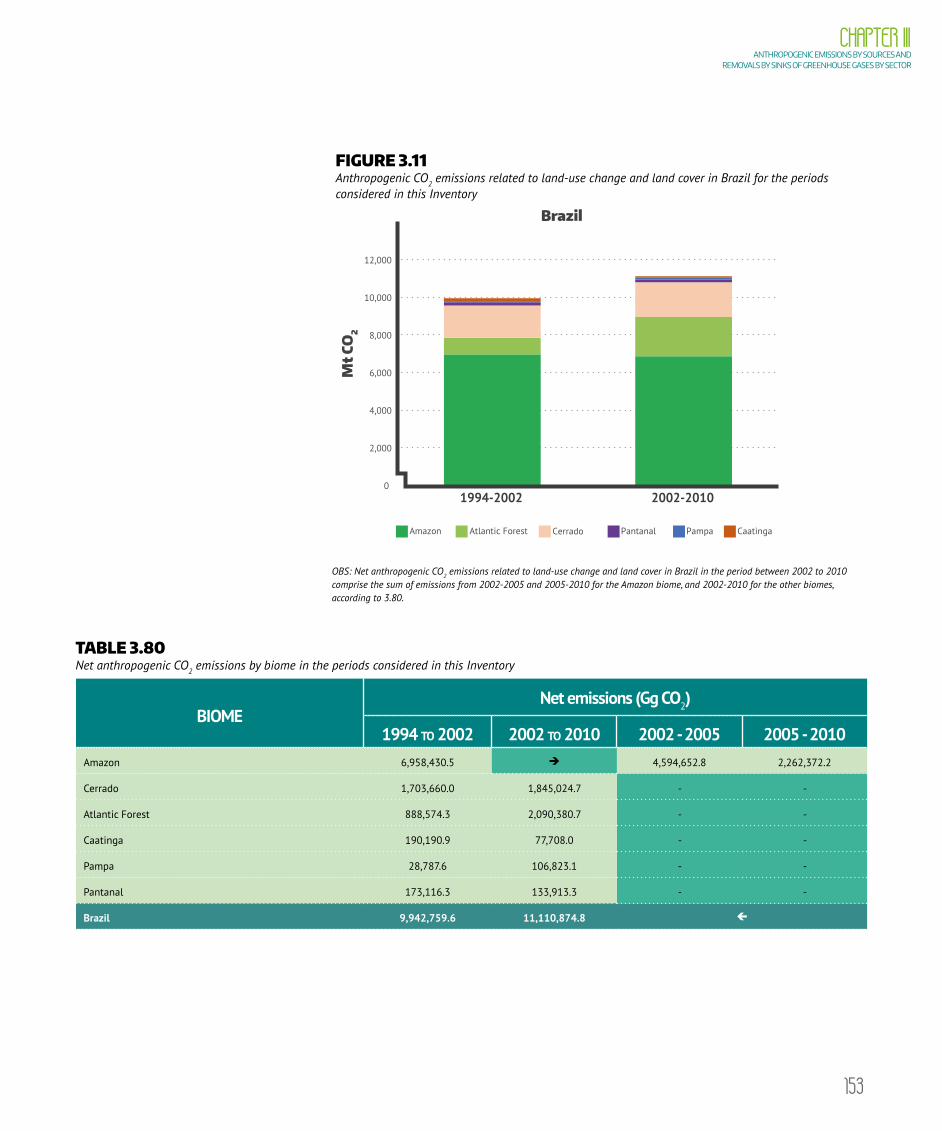
153
CHAPTER IIIANTHROPOGENIC EMISSIONS BY SOURCES AND
REMOVALS BY SINKS OF GREENHOUSE GASES BY SECTOR
FIGURE 3.11 Anthropogenic CO2 emissions related to land-use change and land cover in Brazil for the periods considered in this Inventory
Mt
CO2
0
2,000
4,000
6,000
8,000
10,000
12,000
1994-2002 2002-2010
Brazil
Amazon Atlantic Forest Cerrado Pantanal Pampa Caatinga
OBS: Net anthropogenic CO2 emissions related to land-use change and land cover in Brazil in the period between 2002 to 2010 comprise the sum of emissions from 2002-2005 and 2005-2010 for the Amazon biome, and 2002-2010 for the other biomes, according to 3.80.
TABLE 3.80 Net anthropogenic CO2 emissions by biome in the periods considered in this Inventory
BIOMENet emissions (Gg CO2)
1994 to 2002 2002 to 2010 2002 - 2005 2005 - 2010Amazon 6,958,430.5 4,594,652.8 2,262,372.2
Cerrado 1,703,660.0 1,845,024.7 - -
Atlantic Forest 888,574.3 2,090,380.7 - -
Caatinga 190,190.9 77,708.0 - -
Pampa 28,787.6 106,823.1 - -
Pantanal 173,116.3 133,913.3 - -
Brazil 9,942,759.6 11,110,874.8

154
VOLUME IIITHIRD NATIONAL COMMUNICATION OF BRAZIL
TABLE 3.81 Transition areas for land-use and land-cover identified in the Amazon biome for the period from 1994 to 2002 (hectare)
LAND-USE TRANSITION MATRIX IN THE AMAZON BIOME - 1994-2002 (ha)
LAND USE IN 1994
LAND USE IN 2002TOTAL 1994 % OF
BIOMEFNM FM FSEC REF CS GNM GM GSEC AP AC S A RES O NO
1994
FNM 216,613,348.8 39,369,988.0 798,320.7 28,645.9 235,584.8 13,901,301.2 399,023.2 17,445.9 117.6 9,307.8 8,196.0 408.9 271,381,689.0 64.5
FM 92,803,469.4 34,268.6 0.1 23,704.6 605,955.5 4,065.2 2,040.3 245.2 5,150.1 531.6 93,479,430.7 22.2 FSec 751,094.9 634.8 612,188.8 4,138.2 1,117.1 8.8 0.6 715.4 1,369,898.6 0.3 Ref 57.7 295,454.3 943.7 8.2 0.8 0.0 296,464.8 0.1 CS - - GNM 8,770.9 6,457,476.4 1,480,387.9 17,176.0 236,513.5 9,908.6 5,623.7 24.3 5.7 8,215,886.9 2.0 GM 2,695,998.4 218.2 6,832.6 142.1 51.5 6.0 2,703,248.7 0.6 GSec 104.4 8,383.2 8,690.9 0.0 47.9 17,226.4 0.0 Ap 1,639,036.8 22,442.2 7,938.9 26,517,358.5 101,130.1 62,596.7 296.0 404.8 1,226.0 1,531.2 28,353,961.2 6.7 Ac 13,560.9 0.1 64.5 58,815.5 556,189.5 339.3 1.6 628,971.5 0.1 S 189,812.3 189,812.3 0.0 A 92.4 57.5 145.8 11.4 12,723,074.4 22,671.0 12,746,052.5 3.0 Res 857.8 14.4 596,680.5 597,552.7 0.1 O 795.3 10,351.7 5.1 417.1 0.0 45,016.4 56,585.6 0.0 NO 27,608.7 54,620.5 24,757.0 290.1 321.1 37.9 354.7 3.3 711,347.7 266.0 3,605.7 96.6 1,802.7 16,005.3 841,117.3 0.2
Total 2002 216,641,049.9 132,228,135.4 3,262,749.7 356,342.8 259,610.6 6,457,514.3 4,176,741.0 33,784.0 42,670,445.4 1,074,882.7 282,686.3 12,723,954.3 629,406.6 62,112.4 18,483.0 420,877,898.3
% of biome 51.5 31.4 0.8 0.1 0.1 1.5 1.0 0.0 10.1 0.3 0.1 3.0 0.1 0.0 0.0
TABLE 3.82 Net CO2 emissions in the Amazon biome in the period from 1994 to 2002 (Gg)
NET EMISSIONS MATRIX IN THE AMAZON BIOME - 1994-2002 (Gg CO2)
LAND USE IN 1994
LAND USE IN 2002FROM THE SITUATION OF 1994
FNM FM FSEC REF CS GNM GM GSEC AP AC S A RES O NO
1994
FNM -248,293.4 437,773.1 15,433.3 27,194.6 7,381,720.2 160,142.2 12,270.3 6,431.0 5,028.9 7,797,700.1FM -1,170,561.1 19,882.3 0.1 2,468.4 349,506.9 2,115.5 1,353.8 170.5 3,246.9 -791,816.7FSec -109,279.3 80.2 131,285.6 818.3 385.4 0.1 188.1 23,478.5Ref 2.7 90.1 0.9 0.1 0.0 93.7CS
GNM -1,068.1 -11,290.4 822.1 5,742.6 380.1 405.3 0.5 -5,007.9GM -41,123.0 9.4 127.8 6.1 3.5 -40,976.2GSec -15.7 -127.9 -25.9 0.0 1.9 -167.6Ap -24,715.4 -3,491.7 153.5 1,791.8 3,684.0 24.0 75.6 -22,478.1Ac -815.5 0.0 0.4 -944.5 16.9 -1,742.7S
A
Res
O -32.2 -620.4 -652.6NO
From the situation of 2002
-1,418,854.5 322,815.7 10,938.1 29,663.0 -52,413.4 857.6 7,866,882.2 165,254.9 18,121.4 6,625.5 8,539.9 6,958,430.5
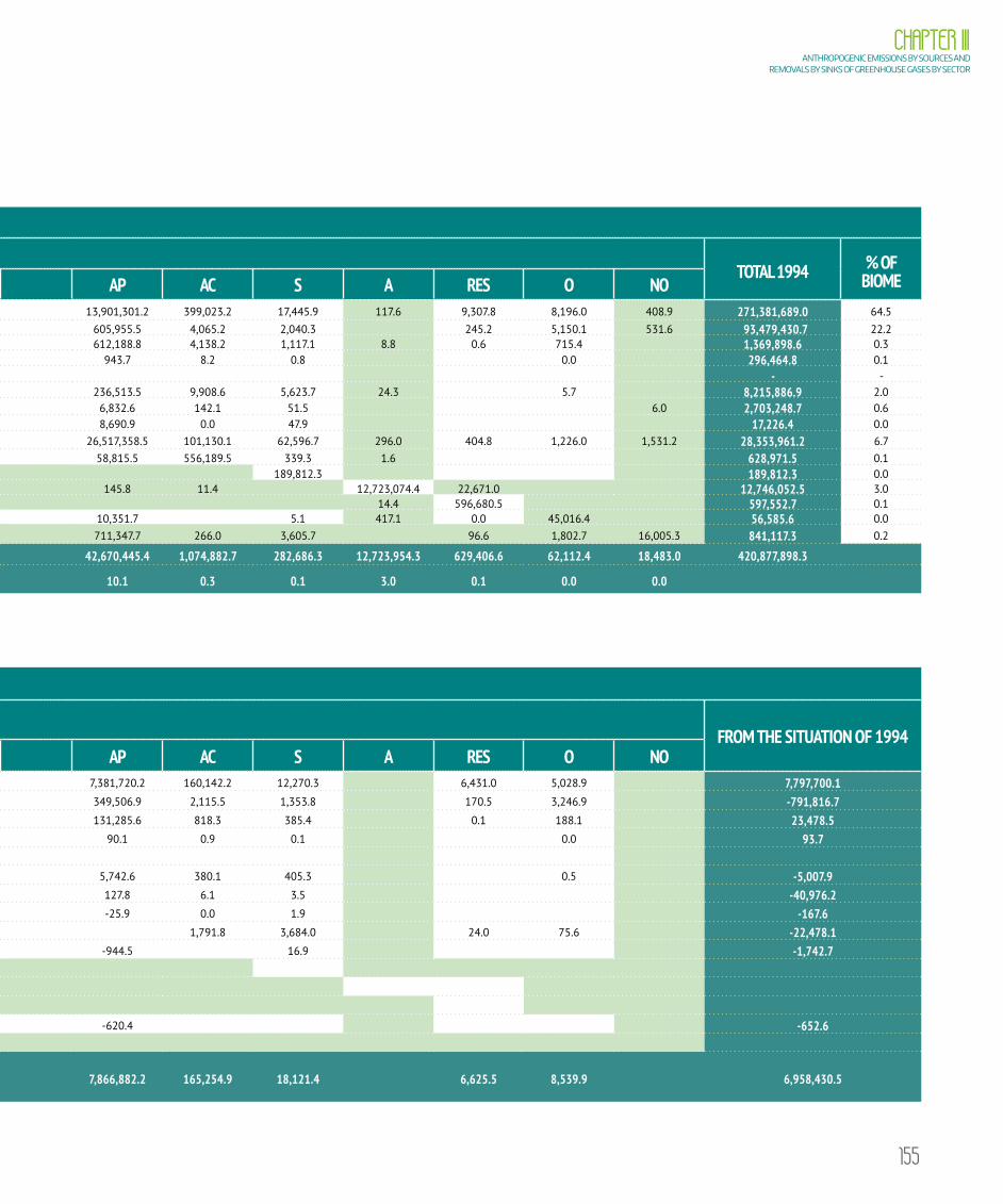
155
CHAPTER IIIANTHROPOGENIC EMISSIONS BY SOURCES AND
REMOVALS BY SINKS OF GREENHOUSE GASES BY SECTOR
TABLE 3.81 Transition areas for land-use and land-cover identified in the Amazon biome for the period from 1994 to 2002 (hectare)
LAND-USE TRANSITION MATRIX IN THE AMAZON BIOME - 1994-2002 (ha)
LAND USE IN 1994
LAND USE IN 2002TOTAL 1994 % OF
BIOMEFNM FM FSEC REF CS GNM GM GSEC AP AC S A RES O NO
1994
FNM 216,613,348.8 39,369,988.0 798,320.7 28,645.9 235,584.8 13,901,301.2 399,023.2 17,445.9 117.6 9,307.8 8,196.0 408.9 271,381,689.0 64.5
FM 92,803,469.4 34,268.6 0.1 23,704.6 605,955.5 4,065.2 2,040.3 245.2 5,150.1 531.6 93,479,430.7 22.2 FSec 751,094.9 634.8 612,188.8 4,138.2 1,117.1 8.8 0.6 715.4 1,369,898.6 0.3 Ref 57.7 295,454.3 943.7 8.2 0.8 0.0 296,464.8 0.1 CS - - GNM 8,770.9 6,457,476.4 1,480,387.9 17,176.0 236,513.5 9,908.6 5,623.7 24.3 5.7 8,215,886.9 2.0 GM 2,695,998.4 218.2 6,832.6 142.1 51.5 6.0 2,703,248.7 0.6 GSec 104.4 8,383.2 8,690.9 0.0 47.9 17,226.4 0.0 Ap 1,639,036.8 22,442.2 7,938.9 26,517,358.5 101,130.1 62,596.7 296.0 404.8 1,226.0 1,531.2 28,353,961.2 6.7 Ac 13,560.9 0.1 64.5 58,815.5 556,189.5 339.3 1.6 628,971.5 0.1 S 189,812.3 189,812.3 0.0 A 92.4 57.5 145.8 11.4 12,723,074.4 22,671.0 12,746,052.5 3.0 Res 857.8 14.4 596,680.5 597,552.7 0.1 O 795.3 10,351.7 5.1 417.1 0.0 45,016.4 56,585.6 0.0 NO 27,608.7 54,620.5 24,757.0 290.1 321.1 37.9 354.7 3.3 711,347.7 266.0 3,605.7 96.6 1,802.7 16,005.3 841,117.3 0.2
Total 2002 216,641,049.9 132,228,135.4 3,262,749.7 356,342.8 259,610.6 6,457,514.3 4,176,741.0 33,784.0 42,670,445.4 1,074,882.7 282,686.3 12,723,954.3 629,406.6 62,112.4 18,483.0 420,877,898.3
% of biome 51.5 31.4 0.8 0.1 0.1 1.5 1.0 0.0 10.1 0.3 0.1 3.0 0.1 0.0 0.0
TABLE 3.82 Net CO2 emissions in the Amazon biome in the period from 1994 to 2002 (Gg)
NET EMISSIONS MATRIX IN THE AMAZON BIOME - 1994-2002 (Gg CO2)
LAND USE IN 1994
LAND USE IN 2002FROM THE SITUATION OF 1994
FNM FM FSEC REF CS GNM GM GSEC AP AC S A RES O NO
1994
FNM -248,293.4 437,773.1 15,433.3 27,194.6 7,381,720.2 160,142.2 12,270.3 6,431.0 5,028.9 7,797,700.1FM -1,170,561.1 19,882.3 0.1 2,468.4 349,506.9 2,115.5 1,353.8 170.5 3,246.9 -791,816.7FSec -109,279.3 80.2 131,285.6 818.3 385.4 0.1 188.1 23,478.5Ref 2.7 90.1 0.9 0.1 0.0 93.7CS
GNM -1,068.1 -11,290.4 822.1 5,742.6 380.1 405.3 0.5 -5,007.9GM -41,123.0 9.4 127.8 6.1 3.5 -40,976.2GSec -15.7 -127.9 -25.9 0.0 1.9 -167.6Ap -24,715.4 -3,491.7 153.5 1,791.8 3,684.0 24.0 75.6 -22,478.1Ac -815.5 0.0 0.4 -944.5 16.9 -1,742.7S
A
Res
O -32.2 -620.4 -652.6NO
From the situation of 2002
-1,418,854.5 322,815.7 10,938.1 29,663.0 -52,413.4 857.6 7,866,882.2 165,254.9 18,121.4 6,625.5 8,539.9 6,958,430.5
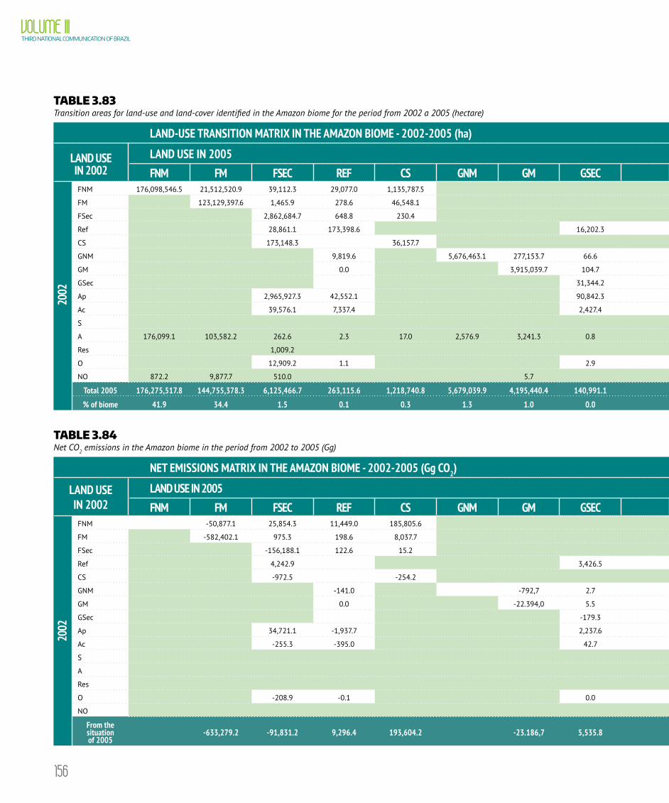
156
VOLUME IIITHIRD NATIONAL COMMUNICATION OF BRAZIL
TABLE 3.83 Transition areas for land-use and land-cover identified in the Amazon biome for the period from 2002 a 2005 (hectare)
LAND-USE TRANSITION MATRIX IN THE AMAZON BIOME - 2002-2005 (ha)
LAND USE IN 2002
LAND USE IN 2005TOTAL 2002 % OF
BIOMEFNM FM FSEC REF CS GNM GM GSEC AP AC S A RES O NO
2002
FNM 176,098,546.5 21,512,520.9 39,112.3 29,077.0 1,135,787.5 8,049,257.0 708,242.3 4,707.7 191,226.1 3,125.7 15,018.6 8,854,428.4 216,641,049.9 51.5
FM 123,129,397.6 1,465.9 278.6 46,548.1 544,559.1 7,273.5 1,661.9 205,304.3 8,908.7 2,175.9 8,280,561.9 132,228,135.4 31.4
FSec 2,862,684.7 648.8 230.4 358,979.7 11,621.0 1,191.7 3,024.4 615.2 202.4 23,551.4 3,262,749.7 0.8
Ref 28,861.1 173,398.6 16,202.3 8,183.5 32,414.0 208.0 10.6 7.9 97,056.8 356,342.8 0.1
CS 173,148.3 36,157.7 25,037.1 23,926.1 0.1 1,341.3 259,610.6 0.1
GNM 9,819.6 5,676,463.1 277,153.7 66.6 183,916.8 19,718.8 556.3 6,134.8 214.6 237.8 283,232.2 6,457,514.3 1.5
GM 0.0 3,915,039.7 104.7 21,084.3 4,024.8 79.1 2,122.4 1.5 234,284.4 4,176,741.0 1.0
GSec 31,344.2 1,687.2 99,4 3.5 649.8 33,784.0 0.0
Ap 2,965,927.3 42,552.1 90,842.3 36,853,444.7 1,366,461.6 64,197.9 32,359.9 8,948.3 17,228.0 1,228,483.3 42,670,445.4 10.1
Ac 39,576.1 7,337.4 2,427.4 123,956.6 895,834.8 1,325.0 683.1 74.2 3,668.0 1,074,882.7 0.3
S 281,887.1 799.2 282,686.3 0.1
A 176,099.1 103,582.2 262.6 2.3 17.0 2,576.9 3,241.3 0.8 54,588.9 483.9 2,065.8 12,124,397.4 20,385.5 3,730.2 232,520.4 12,723,954.3 3.0
Res 1,009.2 1,136.1 2.8 45.1 5,536.8 621,427.0 34.7 214.9 629,406.6 0.1
O 12,909.2 1.1 2.9 8,376.7 10.2 2.2 176.4 92.8 39,180.8 1,360.2 62,112.4 0.0
NO 872.2 9,877.7 510.0 5.7 456.2 11.0 390.8 8.3 6.6 6,344.5 18,483.0 0.0
Total 2005 176,275,517.8 144,755,378.3 6,125,466.7 263,115.6 1,218,740.8 5,679,039.9 4,195,440.4 140,991.1 46,234,663.7 3,070,124.2 358,318.7 12,570,987.8 663,792.0 77,824.6 19,248,496.6 420,877,898.3
% of biome 41.9 34.4 1.5 0.1 0.3 1.3 1.0 0.0 11.0 0.7 0.1 3.0 0.2 0.0 4.6
TABLE 3.84 Net CO2 emissions in the Amazon biome in the period from 2002 to 2005 (Gg)
NET EMISSIONS MATRIX IN THE AMAZON BIOME - 2002-2005 (Gg CO2)
LAND USE IN 2002
LAND USE IN 2005FROM THE SITUATION OF 2002
FNM FM FSEC REF CS GNM GM GSEC AP AC S A RES O NO
2002
FNM -50,877.1 25,854.3 11,449.0 185,805.6 4,378,696.0 288,786.6 2,938.6 1,582.4 9,411.9 4,853,647.3FM -582,402.1 975.3 198.6 8,037.7 314,309.2 2,993.6 1,001.5 6,932.3 1,320.0 -246,633.8FSec -156,188.1 122.6 15.2 80,167.1 1,956.5 321.3 113.8 53.7 -73,437.8Ref 4,242.9 3,426.5 1,344.7 5,023.9 38.7 1.5 14,078.2CS -972.5 -254.2 6,364.4 7,121.4 0.0 12,259.1GNM -141.0 -792,7 2.7 3,788.1 674,7 26.6 10.8 14.6 3,583.9GM 0.0 -22.394,0 5.5 520.3 35,6 5.2 0.1 -21,827.3GSec -179.3 -7.1 0,8 -185.6Ap 34,721.1 -1,937.7 2,237.6 16,825.0 2,563.9 344.2 690.0 55,444.1Ac -255.3 -395.0 42.7 -1,160.9 39.6 1.9 -1,727.0S
A
Res
O -208.9 -0.1 0.0 -338.9 -0.3 -548.2NO
From the situation of 2005
-633,279.2 -91,831.2 9,296.4 193,604.2 -23.186,7 5,535.8 4,783,682.7 323,417.9 6,935.6 8,985.3 11,491.8 4,594,652.8
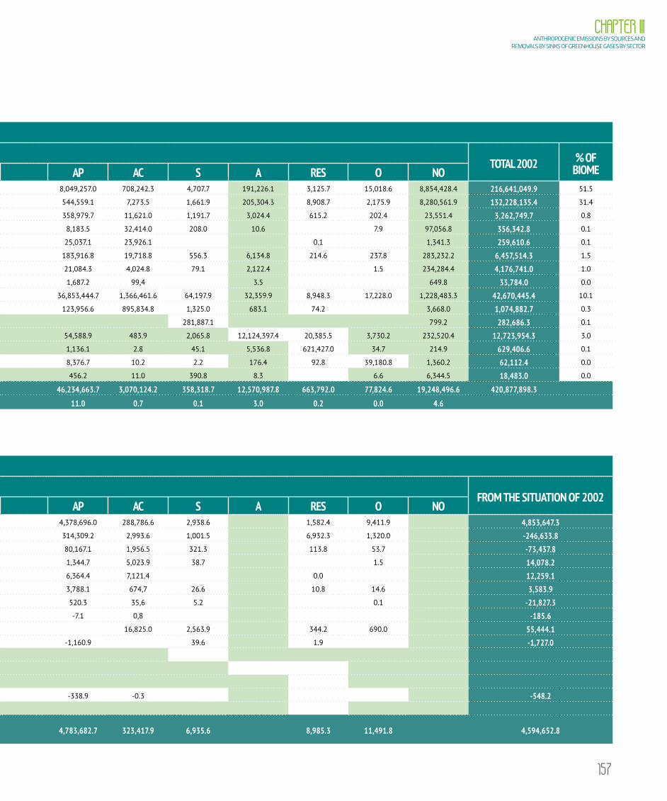
157
CHAPTER IIIANTHROPOGENIC EMISSIONS BY SOURCES AND
REMOVALS BY SINKS OF GREENHOUSE GASES BY SECTOR
TABLE 3.83 Transition areas for land-use and land-cover identified in the Amazon biome for the period from 2002 a 2005 (hectare)
LAND-USE TRANSITION MATRIX IN THE AMAZON BIOME - 2002-2005 (ha)
LAND USE IN 2002
LAND USE IN 2005TOTAL 2002 % OF
BIOMEFNM FM FSEC REF CS GNM GM GSEC AP AC S A RES O NO
2002
FNM 176,098,546.5 21,512,520.9 39,112.3 29,077.0 1,135,787.5 8,049,257.0 708,242.3 4,707.7 191,226.1 3,125.7 15,018.6 8,854,428.4 216,641,049.9 51.5
FM 123,129,397.6 1,465.9 278.6 46,548.1 544,559.1 7,273.5 1,661.9 205,304.3 8,908.7 2,175.9 8,280,561.9 132,228,135.4 31.4
FSec 2,862,684.7 648.8 230.4 358,979.7 11,621.0 1,191.7 3,024.4 615.2 202.4 23,551.4 3,262,749.7 0.8
Ref 28,861.1 173,398.6 16,202.3 8,183.5 32,414.0 208.0 10.6 7.9 97,056.8 356,342.8 0.1
CS 173,148.3 36,157.7 25,037.1 23,926.1 0.1 1,341.3 259,610.6 0.1
GNM 9,819.6 5,676,463.1 277,153.7 66.6 183,916.8 19,718.8 556.3 6,134.8 214.6 237.8 283,232.2 6,457,514.3 1.5
GM 0.0 3,915,039.7 104.7 21,084.3 4,024.8 79.1 2,122.4 1.5 234,284.4 4,176,741.0 1.0
GSec 31,344.2 1,687.2 99,4 3.5 649.8 33,784.0 0.0
Ap 2,965,927.3 42,552.1 90,842.3 36,853,444.7 1,366,461.6 64,197.9 32,359.9 8,948.3 17,228.0 1,228,483.3 42,670,445.4 10.1
Ac 39,576.1 7,337.4 2,427.4 123,956.6 895,834.8 1,325.0 683.1 74.2 3,668.0 1,074,882.7 0.3
S 281,887.1 799.2 282,686.3 0.1
A 176,099.1 103,582.2 262.6 2.3 17.0 2,576.9 3,241.3 0.8 54,588.9 483.9 2,065.8 12,124,397.4 20,385.5 3,730.2 232,520.4 12,723,954.3 3.0
Res 1,009.2 1,136.1 2.8 45.1 5,536.8 621,427.0 34.7 214.9 629,406.6 0.1
O 12,909.2 1.1 2.9 8,376.7 10.2 2.2 176.4 92.8 39,180.8 1,360.2 62,112.4 0.0
NO 872.2 9,877.7 510.0 5.7 456.2 11.0 390.8 8.3 6.6 6,344.5 18,483.0 0.0
Total 2005 176,275,517.8 144,755,378.3 6,125,466.7 263,115.6 1,218,740.8 5,679,039.9 4,195,440.4 140,991.1 46,234,663.7 3,070,124.2 358,318.7 12,570,987.8 663,792.0 77,824.6 19,248,496.6 420,877,898.3
% of biome 41.9 34.4 1.5 0.1 0.3 1.3 1.0 0.0 11.0 0.7 0.1 3.0 0.2 0.0 4.6
TABLE 3.84 Net CO2 emissions in the Amazon biome in the period from 2002 to 2005 (Gg)
NET EMISSIONS MATRIX IN THE AMAZON BIOME - 2002-2005 (Gg CO2)
LAND USE IN 2002
LAND USE IN 2005FROM THE SITUATION OF 2002
FNM FM FSEC REF CS GNM GM GSEC AP AC S A RES O NO
2002
FNM -50,877.1 25,854.3 11,449.0 185,805.6 4,378,696.0 288,786.6 2,938.6 1,582.4 9,411.9 4,853,647.3FM -582,402.1 975.3 198.6 8,037.7 314,309.2 2,993.6 1,001.5 6,932.3 1,320.0 -246,633.8FSec -156,188.1 122.6 15.2 80,167.1 1,956.5 321.3 113.8 53.7 -73,437.8Ref 4,242.9 3,426.5 1,344.7 5,023.9 38.7 1.5 14,078.2CS -972.5 -254.2 6,364.4 7,121.4 0.0 12,259.1GNM -141.0 -792,7 2.7 3,788.1 674,7 26.6 10.8 14.6 3,583.9GM 0.0 -22.394,0 5.5 520.3 35,6 5.2 0.1 -21,827.3GSec -179.3 -7.1 0,8 -185.6Ap 34,721.1 -1,937.7 2,237.6 16,825.0 2,563.9 344.2 690.0 55,444.1Ac -255.3 -395.0 42.7 -1,160.9 39.6 1.9 -1,727.0S
A
Res
O -208.9 -0.1 0.0 -338.9 -0.3 -548.2NO
From the situation of 2005
-633,279.2 -91,831.2 9,296.4 193,604.2 -23.186,7 5,535.8 4,783,682.7 323,417.9 6,935.6 8,985.3 11,491.8 4,594,652.8

158
VOLUME IIITHIRD NATIONAL COMMUNICATION OF BRAZIL
TABLE 3.85 Transition areas for land-use and land-cover identified in the Amazon biome for the period from 2005 to 2010 (hectare)
LAND-USE TRANSITION MATRIX IN THE AMAZON BIOME - 2005-2010 (ha)
LAND USE IN 2005
LAND USE IN 2010TOTAL 2005
% OF BIOMEFNM FM FSEC REF CS GNM GM GSEC AP AC S A RES O NO
2005
FNM 126,777,743.1 33,703,629.2 2,493.8 15,446.6 911,685.4 150,834.2 5,137,169.9 4,182.2 152,886.3 5,222.9 8,216.4 9,406,007.9 176,275,517.8 41.9FM 136,015,684.2 1,377.7 88.3 74,489.2 1,935.8 474,344.3 1,175.0 114,849.0 337.3 4,755.0 8,066,342.5 144,755,378.3 34.4
FSec 4,136,114.4 10,967.2 13,727.6 68,676.2 1,651,515.4 2,056.4 7,460.9 599.2 2,590.1 231,759.4 6,125,466.7 1.5
Ref 8,702.7 191,479.3 2,318.1 4,589.7 4,527.3 6.4 0.9 30.3 51,460.8 263,115.6 0.1
CS 956,142.7 150.9 167,526.2 6,158.0 61,226.7 58.4 439.5 27,038.2 1,218,740.8 0.3
GNM 5,280.5 4,223,184.1 659,739.3 2,952.6 123,101.0 299.5 73,442.4 19.0 291.3 590,730.3 5,679,039.9 1.3
GM 4.4 3,923,889.4 66.5 200.3 9,867.0 63.6 37,641.3 0.8 223,707.0 4,195,440.4 1.0
GSec 1,050.9 92,661.3 617.3 34,862.0 3.8 70.7 0.3 4.7 11,720.2 140,991.1 0.0
Ap 2,501,645.7 51,749.6 68,543.1 614,976.3 41,356,677.9 20,376.8 22,497.6 1,412.2 4,805.3 1,591,979.3 46,234,663.7 11.0
Ac 94,590.1 23,804.2 8,416.5 2,531,507.1 378,473.8 1,125.4 160.0 43.2 97.5 31,906.2 3,070,124.2 0.7
S 358,017.9 300.7 358,318.7 0.1
A 73,791.4 62,808.2 1,203.3 0.3 1.7 1,215.0 639.9 13.2 2,302.8 17,068.6 804.4 11,569,987.1 1,502.4 113.6 839,535.9 12,570,987.8 3.0
Res 3,534.4 2.8 838.9 8.2 28,162.8 629,386.4 152.5 1,706.1 663,792.0 0.2
O 5,469.8 2.1 1.1 3,329.7 345.5 39.7 169.3 66,140.4 2,327.1 77,824.6 0.0
NO 3,608,079.5 9,724,891.1 450,335.3 49,626.3 11,239.5 171,624.5 219,735.9 18,527.0 40,025.8 688,422.6 4,074.3 174,936.1 555.1 2,564.1 4,083,859.6 19,248,496.6 4.6
Total 2010 130,459,613.9 179,507,012.8 8,161,610.1 349,650.5 1,178,669.6 4,396,023.6 4,804,004.5 190,546.9 3,424,779.0 49,941,425.1 392,539.3 12,182,193.2 639,247.1 90,201.5 25,160,381.4 420,877,898.3
% of biome 31.0 42.7 1.9 0.1 0.3 1.0 1.1 0.0 0.8 11.9 0.1 2.9 0.2 0.0 6.0
TABLE 3.86 Net CO2 emissions in the Amazon biome in the period from 2005 to 2010 (Gg)
NET EMISSIONS MATRIX IN THE AMAZON BIOME - 2005-2010 (Gg CO2)
LAND USE IN 2005
LAND USE IN 2010FROM THE SITUATION OF 2005
FNM FM FSEC REF CS GNM GM GSEC AP AC S A RES O NO
2005
FNM -132,848.5 1,376.4 7,589.5 140,264.4 2,931,806.9 66,600.9 2,764.7 2,709.2 5,765.6 3,026,028.9FM -1.072.257,0 739.6 58.7 12,293.4 280,167.0 915.1 666.8 228.7 2,950.5 -774,237.0FSec -376,110.7 1,950.2 804.7 387,201.2 12,004.9 629.4 134.2 727.6 27,341.4Ref 1,139.3 504.6 672.0 731.9 1.2 6.2 3,055.2CS -8,132.6 55.8 -1,179.0 27,135.9 2,251.0 236.5 20,367.6GNM -318.9 -3,144.8 2,999.7 93.3 18.4 1.2 18.9 -332.1GM -0.2 -37,407.7 3.0 280.7 7.4 2.3 0.1 -37,114.6GSec -106.8 -883.4 -115.2 2.6 0.1 0.0 0.2 -1,102.5Ap 2,493.0 -4,899.5 1,544.3 8,465.7 976.3 66.0 234.3 8,880.2Ac -2,892.1 -2,584.7 114.5 -4,891.2 36.2 1.4 4.3 -10,211.7S
A
Res
O -142.7 -0.3 0.0 -160.2 -303.2NO
From the situatiton of 2010
-1,205,105.4 -381,529.8 1,743.7 152,183.5 -40,552.5 1,283.0 3,625,096.7 91,072.7 5,095.5 3,140.6 9,944.2 2,262,372.2

159
CHAPTER IIIANTHROPOGENIC EMISSIONS BY SOURCES AND
REMOVALS BY SINKS OF GREENHOUSE GASES BY SECTOR
TABLE 3.85 Transition areas for land-use and land-cover identified in the Amazon biome for the period from 2005 to 2010 (hectare)
LAND-USE TRANSITION MATRIX IN THE AMAZON BIOME - 2005-2010 (ha)
LAND USE IN 2005
LAND USE IN 2010TOTAL 2005
% OF BIOMEFNM FM FSEC REF CS GNM GM GSEC AP AC S A RES O NO
2005
FNM 126,777,743.1 33,703,629.2 2,493.8 15,446.6 911,685.4 150,834.2 5,137,169.9 4,182.2 152,886.3 5,222.9 8,216.4 9,406,007.9 176,275,517.8 41.9FM 136,015,684.2 1,377.7 88.3 74,489.2 1,935.8 474,344.3 1,175.0 114,849.0 337.3 4,755.0 8,066,342.5 144,755,378.3 34.4
FSec 4,136,114.4 10,967.2 13,727.6 68,676.2 1,651,515.4 2,056.4 7,460.9 599.2 2,590.1 231,759.4 6,125,466.7 1.5
Ref 8,702.7 191,479.3 2,318.1 4,589.7 4,527.3 6.4 0.9 30.3 51,460.8 263,115.6 0.1
CS 956,142.7 150.9 167,526.2 6,158.0 61,226.7 58.4 439.5 27,038.2 1,218,740.8 0.3
GNM 5,280.5 4,223,184.1 659,739.3 2,952.6 123,101.0 299.5 73,442.4 19.0 291.3 590,730.3 5,679,039.9 1.3
GM 4.4 3,923,889.4 66.5 200.3 9,867.0 63.6 37,641.3 0.8 223,707.0 4,195,440.4 1.0
GSec 1,050.9 92,661.3 617.3 34,862.0 3.8 70.7 0.3 4.7 11,720.2 140,991.1 0.0
Ap 2,501,645.7 51,749.6 68,543.1 614,976.3 41,356,677.9 20,376.8 22,497.6 1,412.2 4,805.3 1,591,979.3 46,234,663.7 11.0
Ac 94,590.1 23,804.2 8,416.5 2,531,507.1 378,473.8 1,125.4 160.0 43.2 97.5 31,906.2 3,070,124.2 0.7
S 358,017.9 300.7 358,318.7 0.1
A 73,791.4 62,808.2 1,203.3 0.3 1.7 1,215.0 639.9 13.2 2,302.8 17,068.6 804.4 11,569,987.1 1,502.4 113.6 839,535.9 12,570,987.8 3.0
Res 3,534.4 2.8 838.9 8.2 28,162.8 629,386.4 152.5 1,706.1 663,792.0 0.2
O 5,469.8 2.1 1.1 3,329.7 345.5 39.7 169.3 66,140.4 2,327.1 77,824.6 0.0
NO 3,608,079.5 9,724,891.1 450,335.3 49,626.3 11,239.5 171,624.5 219,735.9 18,527.0 40,025.8 688,422.6 4,074.3 174,936.1 555.1 2,564.1 4,083,859.6 19,248,496.6 4.6
Total 2010 130,459,613.9 179,507,012.8 8,161,610.1 349,650.5 1,178,669.6 4,396,023.6 4,804,004.5 190,546.9 3,424,779.0 49,941,425.1 392,539.3 12,182,193.2 639,247.1 90,201.5 25,160,381.4 420,877,898.3
% of biome 31.0 42.7 1.9 0.1 0.3 1.0 1.1 0.0 0.8 11.9 0.1 2.9 0.2 0.0 6.0
TABLE 3.86 Net CO2 emissions in the Amazon biome in the period from 2005 to 2010 (Gg)
NET EMISSIONS MATRIX IN THE AMAZON BIOME - 2005-2010 (Gg CO2)
LAND USE IN 2005
LAND USE IN 2010FROM THE SITUATION OF 2005
FNM FM FSEC REF CS GNM GM GSEC AP AC S A RES O NO
2005
FNM -132,848.5 1,376.4 7,589.5 140,264.4 2,931,806.9 66,600.9 2,764.7 2,709.2 5,765.6 3,026,028.9FM -1.072.257,0 739.6 58.7 12,293.4 280,167.0 915.1 666.8 228.7 2,950.5 -774,237.0FSec -376,110.7 1,950.2 804.7 387,201.2 12,004.9 629.4 134.2 727.6 27,341.4Ref 1,139.3 504.6 672.0 731.9 1.2 6.2 3,055.2CS -8,132.6 55.8 -1,179.0 27,135.9 2,251.0 236.5 20,367.6GNM -318.9 -3,144.8 2,999.7 93.3 18.4 1.2 18.9 -332.1GM -0.2 -37,407.7 3.0 280.7 7.4 2.3 0.1 -37,114.6GSec -106.8 -883.4 -115.2 2.6 0.1 0.0 0.2 -1,102.5Ap 2,493.0 -4,899.5 1,544.3 8,465.7 976.3 66.0 234.3 8,880.2Ac -2,892.1 -2,584.7 114.5 -4,891.2 36.2 1.4 4.3 -10,211.7S
A
Res
O -142.7 -0.3 0.0 -160.2 -303.2NO
From the situatiton of 2010
-1,205,105.4 -381,529.8 1,743.7 152,183.5 -40,552.5 1,283.0 3,625,096.7 91,072.7 5,095.5 3,140.6 9,944.2 2,262,372.2

160
VOLUME IIITHIRD NATIONAL COMMUNICATION OF BRAZIL
TABLE 3.87 Transition areas for land-use and land-cover identified in the Cerrado biome for the period from 1994 to 2002 (hectares)
LAND-USE TRANSITION MATRIX IN THE CERRADO BIOME - 1994-2002 (ha)
LAND USE IN 1994
LAND USE IN 2002TOTAL 1994 % OF
BIOMEFNM FM FSEC REF GNM GM GSEC AP AC S A RES O NO
1994
FNM 70,642,384.5 4,551,742.0 38,516.9 6,524,547.5 1,551,325.4 71,350.7 1,842.2 2,023.1 2,782.5 24,473.2 83,410,988.0 40.9
FM 6,848,585.1 688.3 55,062.9 6,493.9 4,828.1 20.7 6,915,679.1 3.4
FSec 0.0 0.0
Ref 16,709.9 1,987,032.6 7,614.9 109,682.7 57,551.1 115.7 16.1 369.9 2,179,092.9 1.1
GNM 14,791.8 32,198,920.5 4,653,399.3 2,630,265.6 1,057,043.3 28,812.1 935.3 220.6 955.1 41,118.3 40,626,462.0 19.9
GM 18.6 2,330,903.1 9,931.2 38,454.1 161.1 24.5 242.3 2,379,734.8 1.2
GSec 0.0 0.0
Ap 857,263.0 79,748.1 407,169.9 41,221,789.3 1,171,306.1 103,222.0 1,441.5 1,696.4 734.3 106,325.4 43,950,696.0 21.6
Ac 55,084.3 17,617.3 36,496.1 1,427,951.3 21,112,273.3 50,255.3 1,482.9 471.4 117.5 9,202.5 22,710,951.7 11.1
S 509,101.7 509,101.7 0.2
A 436.0 8.4 6.5 402.7 19.2 2,079.6 677.2 658,313.6 557.5 20.8 662,521.4 0.3
Res 826.7 0.5 186.7 427.3 255.9 4.7 451.6 336,271.3 338,424.8 0.2
O 140.2 70.1 41.2 198.1 519.8 3.3 107,402.7 108,375.3 0.1
NO 4,572.3 1,962.6 3,938.7 14,665.7 125,657.9 1,296.0 84.5 152,177.8 0.1
Total 2002 70,647,392.8 11,400,335.5 930,024.1 2,140,383.2 32,203,261.9 6,984,321.6 451,537.8 51,996,444.2 25,121,236.4 769,667.2 664,470.4 341,240.2 112,032.5 181,857.5 203,944,205.4
% of biome 34.6 5.6 0.5 1.0 15.8 3.4 0.2 25.5 12.3 0.4 0.3 0.2 0.1 0.1
TABLE 3.88 Net CO2 emissions in the Cerrado biome in the period from 1994 to 2002 (Gg)
NET EMISSIONS MATRIX IN THE CERRADO BIOME - 1994-2002 (Gg CO2)
LAND USE IN 1994
LAND USE IN 2002FROM THE SITUATION OF 1994
FNM FM FSEC REF GNM GM GSEC AP AC S A RES O NO
1994
FNM -13,351.8 2,677.0 1,250,177.1 300,107.4 18,175.7 643.3 1,027.5 1,559,456.3FM -40,178.4 -12.9 13,819.6 1,115.8 1,834.1 -23,421.8FSec
Ref 1,647.8 883.5 10,458.1 6,329.9 17.4 2.5 19,339.1GNM -1,446.1 -35,489.9 156,990.8 71,435.2 3,324.7 24.9 107.9 194,947.6GM -1.7 -35,554.0 592.6 2,550.1 18.2 2.3 -32,392.5GSec
Ap -12,777.7 -12,541.5 7,906.2 19,963.2 5,751.3 74.1 42.5 8,418.0Ac -2,991.6 -2,885.5 233.5 -19,306.4 2,255.8 19.4 5.6 -22,669.4S
A
Res
O -4.8 -2.3 -1.8 -8.5 -17.3NO
From the situation of 2002
-53,530.1 -14,126.2 -14,210.9 -71,044.0 9,020.9 1,412,730.1 401,493.2 31,377.1 761.7 1,188.2 1,703,660.0

161
CHAPTER IIIANTHROPOGENIC EMISSIONS BY SOURCES AND
REMOVALS BY SINKS OF GREENHOUSE GASES BY SECTOR
TABLE 3.87 Transition areas for land-use and land-cover identified in the Cerrado biome for the period from 1994 to 2002 (hectares)
LAND-USE TRANSITION MATRIX IN THE CERRADO BIOME - 1994-2002 (ha)
LAND USE IN 1994
LAND USE IN 2002TOTAL 1994 % OF
BIOMEFNM FM FSEC REF GNM GM GSEC AP AC S A RES O NO
1994
FNM 70,642,384.5 4,551,742.0 38,516.9 6,524,547.5 1,551,325.4 71,350.7 1,842.2 2,023.1 2,782.5 24,473.2 83,410,988.0 40.9
FM 6,848,585.1 688.3 55,062.9 6,493.9 4,828.1 20.7 6,915,679.1 3.4
FSec 0.0 0.0
Ref 16,709.9 1,987,032.6 7,614.9 109,682.7 57,551.1 115.7 16.1 369.9 2,179,092.9 1.1
GNM 14,791.8 32,198,920.5 4,653,399.3 2,630,265.6 1,057,043.3 28,812.1 935.3 220.6 955.1 41,118.3 40,626,462.0 19.9
GM 18.6 2,330,903.1 9,931.2 38,454.1 161.1 24.5 242.3 2,379,734.8 1.2
GSec 0.0 0.0
Ap 857,263.0 79,748.1 407,169.9 41,221,789.3 1,171,306.1 103,222.0 1,441.5 1,696.4 734.3 106,325.4 43,950,696.0 21.6
Ac 55,084.3 17,617.3 36,496.1 1,427,951.3 21,112,273.3 50,255.3 1,482.9 471.4 117.5 9,202.5 22,710,951.7 11.1
S 509,101.7 509,101.7 0.2
A 436.0 8.4 6.5 402.7 19.2 2,079.6 677.2 658,313.6 557.5 20.8 662,521.4 0.3
Res 826.7 0.5 186.7 427.3 255.9 4.7 451.6 336,271.3 338,424.8 0.2
O 140.2 70.1 41.2 198.1 519.8 3.3 107,402.7 108,375.3 0.1
NO 4,572.3 1,962.6 3,938.7 14,665.7 125,657.9 1,296.0 84.5 152,177.8 0.1
Total 2002 70,647,392.8 11,400,335.5 930,024.1 2,140,383.2 32,203,261.9 6,984,321.6 451,537.8 51,996,444.2 25,121,236.4 769,667.2 664,470.4 341,240.2 112,032.5 181,857.5 203,944,205.4
% of biome 34.6 5.6 0.5 1.0 15.8 3.4 0.2 25.5 12.3 0.4 0.3 0.2 0.1 0.1
TABLE 3.88 Net CO2 emissions in the Cerrado biome in the period from 1994 to 2002 (Gg)
NET EMISSIONS MATRIX IN THE CERRADO BIOME - 1994-2002 (Gg CO2)
LAND USE IN 1994
LAND USE IN 2002FROM THE SITUATION OF 1994
FNM FM FSEC REF GNM GM GSEC AP AC S A RES O NO
1994
FNM -13,351.8 2,677.0 1,250,177.1 300,107.4 18,175.7 643.3 1,027.5 1,559,456.3FM -40,178.4 -12.9 13,819.6 1,115.8 1,834.1 -23,421.8FSec
Ref 1,647.8 883.5 10,458.1 6,329.9 17.4 2.5 19,339.1GNM -1,446.1 -35,489.9 156,990.8 71,435.2 3,324.7 24.9 107.9 194,947.6GM -1.7 -35,554.0 592.6 2,550.1 18.2 2.3 -32,392.5GSec
Ap -12,777.7 -12,541.5 7,906.2 19,963.2 5,751.3 74.1 42.5 8,418.0Ac -2,991.6 -2,885.5 233.5 -19,306.4 2,255.8 19.4 5.6 -22,669.4S
A
Res
O -4.8 -2.3 -1.8 -8.5 -17.3NO
From the situation of 2002
-53,530.1 -14,126.2 -14,210.9 -71,044.0 9,020.9 1,412,730.1 401,493.2 31,377.1 761.7 1,188.2 1,703,660.0
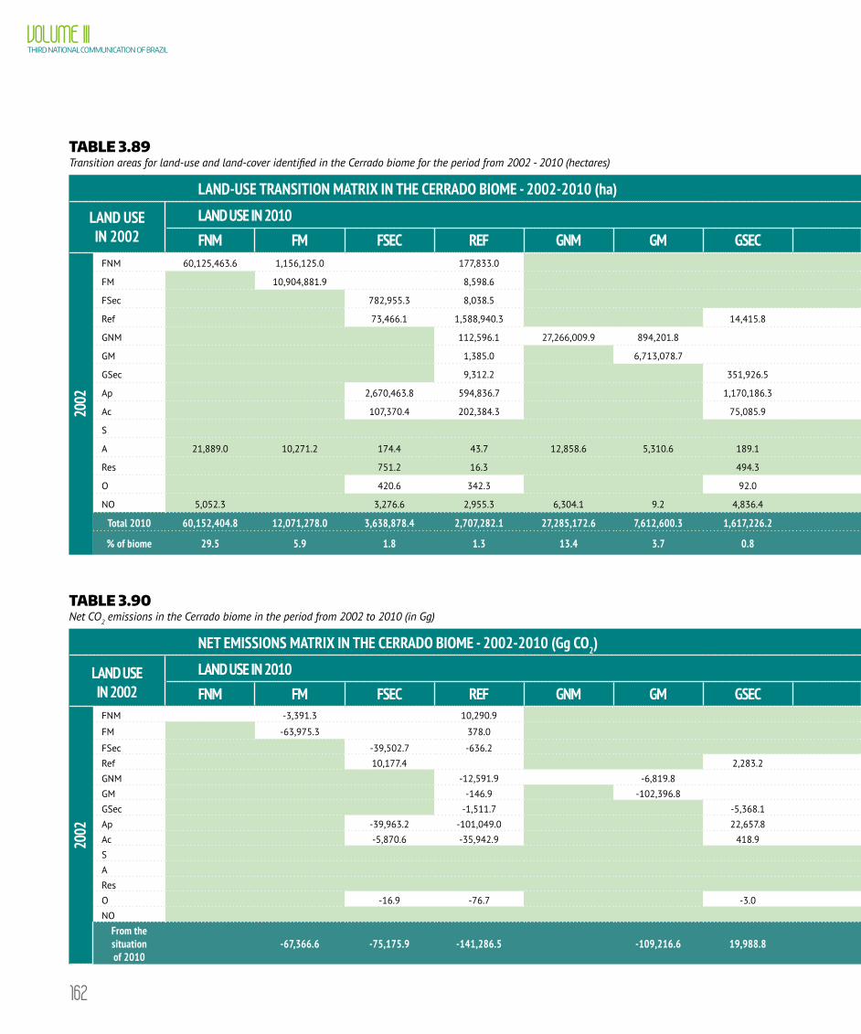
162
VOLUME IIITHIRD NATIONAL COMMUNICATION OF BRAZIL
TABLE 3.89 Transition areas for land-use and land-cover identified in the Cerrado biome for the period from 2002 - 2010 (hectares)
LAND-USE TRANSITION MATRIX IN THE CERRADO BIOME - 2002-2010 (ha)
LAND USE IN 2002
LAND USE IN 2010TOTAL 2002 % OF
BIOMEFNM FM FSEC REF GNM GM GSEC AP AC S A RES O NO
2002
FNM 60,125,463.6 1,156,125.0 177,833.0 6,798,388.7 2,078,315.1 23,798.2 86,093.3 154,258.1 5,807.7 41.310,3 70,647,392.8 34.6
FM 10,904,881.9 8,598.6 329,391.6 45,522.4 2,268.5 7,732.9 24,946.5 373.5 76,619.6 11,400,335.5 5.6
FSec 782,955.3 8,038.5 96,092.0 41,105.4 298.3 425.5 883.2 41.4 184.5 930,024.1 0.5
Ref 73,466.1 1,588,940.3 14,415.8 228,004.3 227,044.7 861.7 333.2 278.6 286.3 6,752.1 2,140,383.2 1.0
GNM 112,596.1 27,266,009.9 894,201.8 2,973,353.7 759,028.1 10,291.5 36,933.4 118,753.3 3,881.1 28,212.9 32,203,261.9 15.8
GM 1,385.0 6,713,078.7 205,470.1 29,668.0 3,162.9 1,552.3 13,979.4 163.7 15,861.5 6,984,321.6 3.4
GSec 9,312.2 351,926.5 63,184.9 26,371.0 143.0 233.2 309.2 53.5 4.3 451,537.8 0.2
Ap 2,670,463.8 594,836.7 1,170,186.3 44,618,907.5 2,774,888.5 72,263.9 13,314.5 57,951.2 8,662.2 14,969.7 51,996,444.2 25.5
Ac 107,370.4 202,384.3 75,085.9 2,859,339.7 21,809,340.0 54,969.9 5,443.2 5,704.2 1,009.5 589.3 25,121,236.4 12.3
S 769,667.2 769,667.2 0.4
A 21,889.0 10,271.2 174.4 43.7 12,858.6 5,310.6 189.1 9,046.7 1,321.2 227.2 536,807.5 65,644.0 196.2 491.1 664,470.4 0.3
Res 751.2 16.3 494.3 6,721.2 356.2 34.4 6,646.3 326,220.1 0.1 341,240.2 0.2
O 420.6 342.3 92.0 2,162.3 3.3 271.9 25.2 93.1 108,621.9 112,032.5 0.1
NO 5,052.3 3,276.6 2,955.3 6,304.1 9.2 4,836.4 145,940.4 12,195.6 1,180.1 83.9 23.5 181,857.5 0.1
Total 2010 60,152,404.8 12,071,278.0 3,638,878.4 2,707,282.1 27,285,172.6 7,612,600.3 1,617,226.2 58,336,003.2 27,805,159.6 939,438.8 695,624.4 769,020.9 129,097.0 185,018.9 203,944,205.4
% of biome 29.5 5.9 1.8 1.3 13.4 3.7 0.8 28.6 13.6 0.5 0.3 0.4 0.1 0.1
TABLE 3.90 Net CO2 emissions in the Cerrado biome in the period from 2002 to 2010 (in Gg)
NET EMISSIONS MATRIX IN THE CERRADO BIOME - 2002-2010 (Gg CO2)
LAND USE IN 2002
LAND USE IN 2010FROM THE SITUATION OF 2002
FNM FM FSEC REF GNM GM GSEC AP AC S A RES O NO
2002
FNM -3,391.3 10,290.9 1,322,750.9 424,891.8 5,854.0 36,096.5 1,338.0 1,797,830.7FM -63,975.3 378.0 59,941.7 7,909.7 478.7 4,482.3 73.6 9,288.7FSec -39,502.7 -636.2 6,975.5 3,788.6 39.5 111.8 8.1 -29,215.4Ref 10,177.4 2,283.2 31,615.3 34,928.1 170.0 54.8 54.5 79,283.3GNM -12,591.9 -6,819.8 175,453.8 53,483.2 1,180.7 12,253.9 405.0 223,364.8GM -146.9 -102,396.8 12,171.4 2,275.0 380.9 1,802.8 19.8 -85,893.9GSec -1,511.7 -5,368.1 638.3 617.3 8.7 21.4 3.0 -5,591.0Ap -39,963.2 -101,049.0 22,657.8 47,358.3 4,034.6 2,996.3 491.0 -63,474.3Ac -5,870.6 -35,942.9 418.9 -41,673.7 2,442.2 228.8 48.1 -80,349.2S
A
Res
O -16.9 -76.7 -3.0 -122.4 -0.1 -219.1NO
From the situation of 2010
-67,366.6 -75,175.9 -141,286.5 -109,216.6 19,988.8 1,567,750.8 575,251.7 14,589.2 58,048.6 2,441.3 1,845,024.7
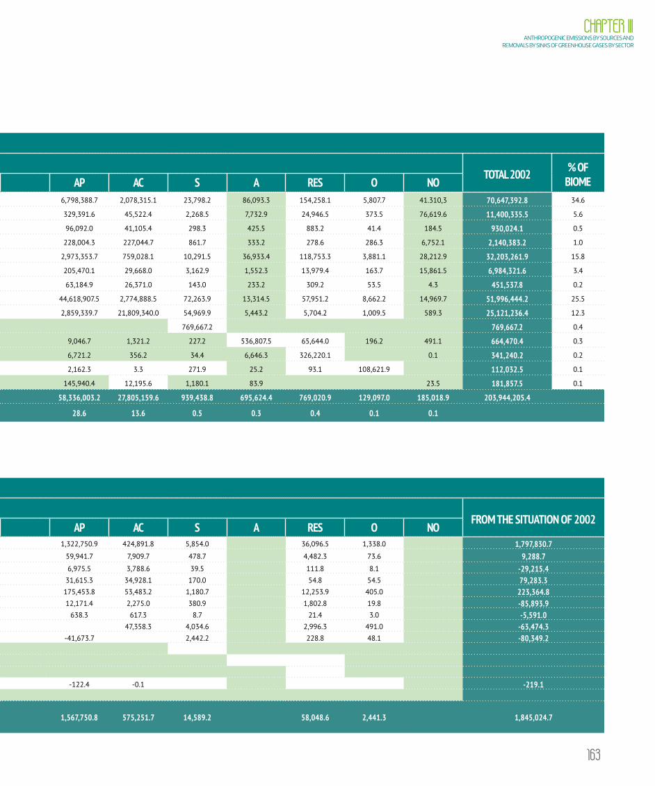
163
CHAPTER IIIANTHROPOGENIC EMISSIONS BY SOURCES AND
REMOVALS BY SINKS OF GREENHOUSE GASES BY SECTOR
TABLE 3.89 Transition areas for land-use and land-cover identified in the Cerrado biome for the period from 2002 - 2010 (hectares)
LAND-USE TRANSITION MATRIX IN THE CERRADO BIOME - 2002-2010 (ha)
LAND USE IN 2002
LAND USE IN 2010TOTAL 2002 % OF
BIOMEFNM FM FSEC REF GNM GM GSEC AP AC S A RES O NO
2002
FNM 60,125,463.6 1,156,125.0 177,833.0 6,798,388.7 2,078,315.1 23,798.2 86,093.3 154,258.1 5,807.7 41.310,3 70,647,392.8 34.6
FM 10,904,881.9 8,598.6 329,391.6 45,522.4 2,268.5 7,732.9 24,946.5 373.5 76,619.6 11,400,335.5 5.6
FSec 782,955.3 8,038.5 96,092.0 41,105.4 298.3 425.5 883.2 41.4 184.5 930,024.1 0.5
Ref 73,466.1 1,588,940.3 14,415.8 228,004.3 227,044.7 861.7 333.2 278.6 286.3 6,752.1 2,140,383.2 1.0
GNM 112,596.1 27,266,009.9 894,201.8 2,973,353.7 759,028.1 10,291.5 36,933.4 118,753.3 3,881.1 28,212.9 32,203,261.9 15.8
GM 1,385.0 6,713,078.7 205,470.1 29,668.0 3,162.9 1,552.3 13,979.4 163.7 15,861.5 6,984,321.6 3.4
GSec 9,312.2 351,926.5 63,184.9 26,371.0 143.0 233.2 309.2 53.5 4.3 451,537.8 0.2
Ap 2,670,463.8 594,836.7 1,170,186.3 44,618,907.5 2,774,888.5 72,263.9 13,314.5 57,951.2 8,662.2 14,969.7 51,996,444.2 25.5
Ac 107,370.4 202,384.3 75,085.9 2,859,339.7 21,809,340.0 54,969.9 5,443.2 5,704.2 1,009.5 589.3 25,121,236.4 12.3
S 769,667.2 769,667.2 0.4
A 21,889.0 10,271.2 174.4 43.7 12,858.6 5,310.6 189.1 9,046.7 1,321.2 227.2 536,807.5 65,644.0 196.2 491.1 664,470.4 0.3
Res 751.2 16.3 494.3 6,721.2 356.2 34.4 6,646.3 326,220.1 0.1 341,240.2 0.2
O 420.6 342.3 92.0 2,162.3 3.3 271.9 25.2 93.1 108,621.9 112,032.5 0.1
NO 5,052.3 3,276.6 2,955.3 6,304.1 9.2 4,836.4 145,940.4 12,195.6 1,180.1 83.9 23.5 181,857.5 0.1
Total 2010 60,152,404.8 12,071,278.0 3,638,878.4 2,707,282.1 27,285,172.6 7,612,600.3 1,617,226.2 58,336,003.2 27,805,159.6 939,438.8 695,624.4 769,020.9 129,097.0 185,018.9 203,944,205.4
% of biome 29.5 5.9 1.8 1.3 13.4 3.7 0.8 28.6 13.6 0.5 0.3 0.4 0.1 0.1
TABLE 3.90 Net CO2 emissions in the Cerrado biome in the period from 2002 to 2010 (in Gg)
NET EMISSIONS MATRIX IN THE CERRADO BIOME - 2002-2010 (Gg CO2)
LAND USE IN 2002
LAND USE IN 2010FROM THE SITUATION OF 2002
FNM FM FSEC REF GNM GM GSEC AP AC S A RES O NO
2002
FNM -3,391.3 10,290.9 1,322,750.9 424,891.8 5,854.0 36,096.5 1,338.0 1,797,830.7FM -63,975.3 378.0 59,941.7 7,909.7 478.7 4,482.3 73.6 9,288.7FSec -39,502.7 -636.2 6,975.5 3,788.6 39.5 111.8 8.1 -29,215.4Ref 10,177.4 2,283.2 31,615.3 34,928.1 170.0 54.8 54.5 79,283.3GNM -12,591.9 -6,819.8 175,453.8 53,483.2 1,180.7 12,253.9 405.0 223,364.8GM -146.9 -102,396.8 12,171.4 2,275.0 380.9 1,802.8 19.8 -85,893.9GSec -1,511.7 -5,368.1 638.3 617.3 8.7 21.4 3.0 -5,591.0Ap -39,963.2 -101,049.0 22,657.8 47,358.3 4,034.6 2,996.3 491.0 -63,474.3Ac -5,870.6 -35,942.9 418.9 -41,673.7 2,442.2 228.8 48.1 -80,349.2S
A
Res
O -16.9 -76.7 -3.0 -122.4 -0.1 -219.1NO
From the situation of 2010
-67,366.6 -75,175.9 -141,286.5 -109,216.6 19,988.8 1,567,750.8 575,251.7 14,589.2 58,048.6 2,441.3 1,845,024.7
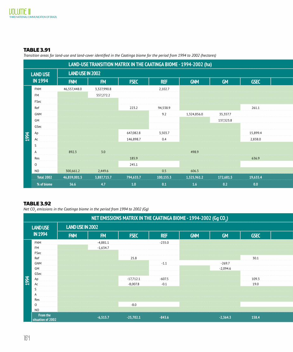
164
VOLUME IIITHIRD NATIONAL COMMUNICATION OF BRAZIL
TABLE 3.91 Transition areas for land-use and land-cover identified in the Caatinga biome for the period from 1994 to 2002 (hectares)
LAND-USE TRANSITION MATRIX IN THE CAATINGA BIOME - 1994-2002 (ha)
LAND USE IN 1994
LAND USE IN 2002TOTAL 1994 % OF
BIOMEFNM FM FSEC REF GNM GM GSEC AP AC S A RES O NO
1994
FNM 46,557,448.0 3,327,990.8 2,102.7 3,101,858.1 299,205.8 5,173.5 1,625.5 7,266.5 3,854.4 143,817.3 53,450,342.6 64.6
FM 557,272.2 18,795.0 187.5 0.0 2,912.1 579,166.9 0.7
FSec 0.0 0.0
Ref 223.2 94,538.9 261.1 1,508.0 96,531.2 0.1
GNM 9.2 1,324,856.0 35,357.7 76,262.1 12,683.5 100.9 1.5 767.6 35.5 1,157.0 1,451,231.1 1.8
GM 137,323.8 6,243.6 570.2 144,137.6 0.2
GSec 0,0 0.0
Ap 647,082.8 3,503.7 15,899.4 19,853,803.1 41,119.8 9,040.1 1,002.1 800.7 1,586.9 108,741.9 20,682,580.4 25.0
Ac 146,898.7 0.4 2,838.0 32,909.6 4,280,154.4 1,374.0 4.3 115.8 861.3 84,210.5 4,549,366.8 5.5
S 232,353.4 34.7 232,388.2 0.3
A 892.3 3.0 498.9 28.3 56.3 161,286.3 5.9 43.6 96.7 162,911.2 0.2
Res 185.9 636.9 36.0 48.5 493,730.0 96.5 494,733.9 0.6
O 245.1 844.3 1,019.4 0.4 112,438.3 114,547.5 0.1
NO 300,661.2 2,449.6 0.5 606.3 376,517.4 99,711.9 168.1 223.7 888.4 130.9 57,309.3 838,667.2 1.0
Total 2002 46,859,001.5 3,887,715.7 794,635.7 100,155.3 1,325,961.2 172,681.5 19,635.4 23,468,805.3 4,734,138.7 248,210.0 164,192.1 503,574.9 118,950.9 398,946.3 82,796,604.5
% of biome 56.6 4.7 1.0 0.1 1.6 0.2 0.0 28.3 5.7 0.3 0.2 0.6 0.1 0.5
TABLE 3.92 Net CO2 emissions in the Caatinga biome in the period from 1994 to 2002 (Gg)
NET EMISSIONS MATRIX IN THE CAATINGA BIOME - 1994-2002 (Gg CO2)
LAND USE IN 1994
LAND USE IN 2002FROM THE SITUATION OF 1994
FNM FM FSEC REF GNM GM GSEC AP AC S A RES O NO
1994
FNM -4,881.1 -235.0 198,375.4 19,546.4 557.3 1.097,8 616.9 215,077.7FM -1,634.7 1,438.2 25.7 0.0 -170.7FSec
Ref 25.8 30.1 167.0 222.8GNM -1.1 -269.7 2,292.3 599.1 5.6 41.7 2.0 2,669.9GM -2,094.6 285.6 -1,809.0GSec
Ap -17,712.1 -607.5 109.3 7.0 306.5 17.7 67.5 -17,811.7Ac -8,007.8 -0.1 19.0 -8.4 43.5 2.8 27.0 -7,924.0S
A
Res
O -8.0 -27.3 -28.9 -64.2NO
From the situation of 2002 -6,515.7 -25,702.1 -843.6 -2,364.3 158.4 202,522.8 20,149.2 912.9 1,159.9 713.3 190,190.9

165
CHAPTER IIIANTHROPOGENIC EMISSIONS BY SOURCES AND
REMOVALS BY SINKS OF GREENHOUSE GASES BY SECTOR
TABLE 3.91 Transition areas for land-use and land-cover identified in the Caatinga biome for the period from 1994 to 2002 (hectares)
LAND-USE TRANSITION MATRIX IN THE CAATINGA BIOME - 1994-2002 (ha)
LAND USE IN 1994
LAND USE IN 2002TOTAL 1994 % OF
BIOMEFNM FM FSEC REF GNM GM GSEC AP AC S A RES O NO
1994
FNM 46,557,448.0 3,327,990.8 2,102.7 3,101,858.1 299,205.8 5,173.5 1,625.5 7,266.5 3,854.4 143,817.3 53,450,342.6 64.6
FM 557,272.2 18,795.0 187.5 0.0 2,912.1 579,166.9 0.7
FSec 0.0 0.0
Ref 223.2 94,538.9 261.1 1,508.0 96,531.2 0.1
GNM 9.2 1,324,856.0 35,357.7 76,262.1 12,683.5 100.9 1.5 767.6 35.5 1,157.0 1,451,231.1 1.8
GM 137,323.8 6,243.6 570.2 144,137.6 0.2
GSec 0,0 0.0
Ap 647,082.8 3,503.7 15,899.4 19,853,803.1 41,119.8 9,040.1 1,002.1 800.7 1,586.9 108,741.9 20,682,580.4 25.0
Ac 146,898.7 0.4 2,838.0 32,909.6 4,280,154.4 1,374.0 4.3 115.8 861.3 84,210.5 4,549,366.8 5.5
S 232,353.4 34.7 232,388.2 0.3
A 892.3 3.0 498.9 28.3 56.3 161,286.3 5.9 43.6 96.7 162,911.2 0.2
Res 185.9 636.9 36.0 48.5 493,730.0 96.5 494,733.9 0.6
O 245.1 844.3 1,019.4 0.4 112,438.3 114,547.5 0.1
NO 300,661.2 2,449.6 0.5 606.3 376,517.4 99,711.9 168.1 223.7 888.4 130.9 57,309.3 838,667.2 1.0
Total 2002 46,859,001.5 3,887,715.7 794,635.7 100,155.3 1,325,961.2 172,681.5 19,635.4 23,468,805.3 4,734,138.7 248,210.0 164,192.1 503,574.9 118,950.9 398,946.3 82,796,604.5
% of biome 56.6 4.7 1.0 0.1 1.6 0.2 0.0 28.3 5.7 0.3 0.2 0.6 0.1 0.5
TABLE 3.92 Net CO2 emissions in the Caatinga biome in the period from 1994 to 2002 (Gg)
NET EMISSIONS MATRIX IN THE CAATINGA BIOME - 1994-2002 (Gg CO2)
LAND USE IN 1994
LAND USE IN 2002FROM THE SITUATION OF 1994
FNM FM FSEC REF GNM GM GSEC AP AC S A RES O NO
1994
FNM -4,881.1 -235.0 198,375.4 19,546.4 557.3 1.097,8 616.9 215,077.7FM -1,634.7 1,438.2 25.7 0.0 -170.7FSec
Ref 25.8 30.1 167.0 222.8GNM -1.1 -269.7 2,292.3 599.1 5.6 41.7 2.0 2,669.9GM -2,094.6 285.6 -1,809.0GSec
Ap -17,712.1 -607.5 109.3 7.0 306.5 17.7 67.5 -17,811.7Ac -8,007.8 -0.1 19.0 -8.4 43.5 2.8 27.0 -7,924.0S
A
Res
O -8.0 -27.3 -28.9 -64.2NO
From the situation of 2002 -6,515.7 -25,702.1 -843.6 -2,364.3 158.4 202,522.8 20,149.2 912.9 1,159.9 713.3 190,190.9
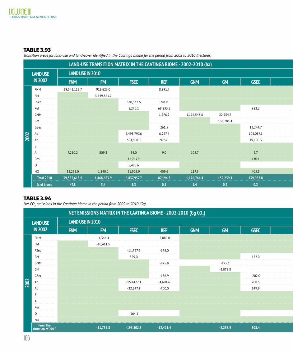
166
VOLUME IIITHIRD NATIONAL COMMUNICATION OF BRAZIL
TABLE 3.93 Transition areas for land-use and land-cover identified in the Caatinga biome for the period from 2002 to 2010 (hectares)
LAND-USE TRANSITION MATRIX IN THE CAATINGA BIOME - 2002-2010 (ha)
LAND USE IN 2002
LAND USE IN 2010TOTAL 2002 % OF
BIOMEFNM FM FSEC REF GNM GM GSEC AP AC S A RES O NO
2002
FNM 39,541,113.7 916,623.0 8,891.7 2,822,718.1 623,748.4 12,925.9 44,000.5 145,799.9 42,255.7 2,700,924.8 46,859,001.5 56.6
FM 3,549,361.7 94,891.1 44,335.7 896.1 2,959.6 1,801.1 1,818.3 191,652.1 3,887,715.7 4.7
FSec 670,333.6 241.8 71,653.2 22,972.9 702.9 1,216.8 1,051.9 123.4 26,339.2 794,635.7 1.0
Ref 5,270.1 68,833.5 982.2 4,653.7 3,178.1 0.5 23.4 17,213.8 100,155.3 0.1
GNM 1,276.2 1,176,543.8 22,954.7 32,537.6 29,980.1 552.0 2,969.7 19,353.9 1,432.1 38,361.2 1,325,961.2 1.6
GM 136,284.4 572.9 2.6 5.7 35,815.9 172,681.5 0.2
GSec 261.5 13,244.7 4,395.4 973.8 649.5 110.4 19,635.4 0.0
Ap 5,498,797.6 6,297.4 105,087.1 13,852,972.8 500,692.5 42,463.9 27,285.3 76,740.5 5,230.9 3,353,237.3 23,468,805.3 28.3
Ac 591,407.9 973.6 19,190.3 89,006.1 3,678,061.8 15,832.6 4,739.3 14,371.0 4,954.8 315,601.3 4,734,138.7 5.7
S 246,085.4 2,124.6 248,210.0 0.3
A 7,210.2 809.2 34.0 9.0 102.7 2.7 4,681.0 1,695.9 148.2 123,789.5 5,950.2 3,857.5 15,901.9 164,192.1 0.2
Res 14,717.9 140.1 2,684.5 1,570.5 12.0 3,776.8 472,912.9 1,605.4 6,154.7 503,574.9 0.6
O 5,490.6 1,647.6 1,783.6 141.3 202.3 1,746.9 106,183.2 1,755.3 118,950.9 0.1
NO 35,295.0 1,840.0 51,905.9 409.6 117.9 405.5 116,722.7 38,393.3 866.8 1,083.4 592.5 151,313.6 398,946.3 0.5
Total 2010 39,583,618.9 4,468,633.9 6,837,957.7 87,194.3 1,176,764.4 159,239.1 139,052.8 17,099,136.9 4,947,389.1 320,627.6 212,052.2 740,970.4 167,461.3 6,856,505.8 82,796,604.5
% of biome 47.8 5.4 8.3 0.1 1.4 0.2 0.2 20.7 6.0 0.4 0.3 0.9 0.2 8.3
TABLE 3.94 Net CO2 emissions in the Caatinga biome in the period from 2002 to 2010 (Gg)
NET EMISSIONS MATRIX IN THE CAATINGA BIOME - 2002-2010 (Gg CO2)
LAND USE IN 2002
LAND USE IN 2010FROM THE SITUATION OF 2002
FNM FM FSEC REF GNM GM GSEC AP AC S A RES O NO
2002
FNM -1,344.4 -5,880.0 193,654.0 39,510.7 1,989.0 15,863.2 18,965.6 262,758.1
FM -10,411.5 10,616.2 3,212.0 125.2 134.8 771.2 4,448.0
FSec -11,797.9 -174.0 1,934.6 452.0 53.2 44.3 14.4 -9,473.4
Ref 829.0 152.0 698.4 482.2 0.1 2,161.6
GNM -875.8 -175.1 925.6 1,357.2 30.9 1,028.4 77.4 2,368.6
GM -2,078.8 27.1 0.1 -2,051.6
GSec -186.9 -202.0 9.8 3.2 20,4 -355.5
Ap -150,422.1 -4,604.6 708.5 78.7 1,400.8 2,388.7 236.2 -150,213.8
Ac -32,247.2 -700.0 149.9 -42.2 538.3 442,1 181.2 -31,678.0
S
A
Res
O -164.1 -36.4 -55.5 -256.1
NO
From the situation of 2010 -11,755.8 -193,802.3 -12,421.4 -2,253.9 808.4 207,787.0 45,040.7 4,137.4 19,921.9 20,246.0 77,708.0
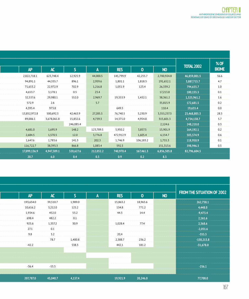
167
CHAPTER IIIANTHROPOGENIC EMISSIONS BY SOURCES AND
REMOVALS BY SINKS OF GREENHOUSE GASES BY SECTOR
TABLE 3.93 Transition areas for land-use and land-cover identified in the Caatinga biome for the period from 2002 to 2010 (hectares)
LAND-USE TRANSITION MATRIX IN THE CAATINGA BIOME - 2002-2010 (ha)
LAND USE IN 2002
LAND USE IN 2010TOTAL 2002 % OF
BIOMEFNM FM FSEC REF GNM GM GSEC AP AC S A RES O NO
2002
FNM 39,541,113.7 916,623.0 8,891.7 2,822,718.1 623,748.4 12,925.9 44,000.5 145,799.9 42,255.7 2,700,924.8 46,859,001.5 56.6
FM 3,549,361.7 94,891.1 44,335.7 896.1 2,959.6 1,801.1 1,818.3 191,652.1 3,887,715.7 4.7
FSec 670,333.6 241.8 71,653.2 22,972.9 702.9 1,216.8 1,051.9 123.4 26,339.2 794,635.7 1.0
Ref 5,270.1 68,833.5 982.2 4,653.7 3,178.1 0.5 23.4 17,213.8 100,155.3 0.1
GNM 1,276.2 1,176,543.8 22,954.7 32,537.6 29,980.1 552.0 2,969.7 19,353.9 1,432.1 38,361.2 1,325,961.2 1.6
GM 136,284.4 572.9 2.6 5.7 35,815.9 172,681.5 0.2
GSec 261.5 13,244.7 4,395.4 973.8 649.5 110.4 19,635.4 0.0
Ap 5,498,797.6 6,297.4 105,087.1 13,852,972.8 500,692.5 42,463.9 27,285.3 76,740.5 5,230.9 3,353,237.3 23,468,805.3 28.3
Ac 591,407.9 973.6 19,190.3 89,006.1 3,678,061.8 15,832.6 4,739.3 14,371.0 4,954.8 315,601.3 4,734,138.7 5.7
S 246,085.4 2,124.6 248,210.0 0.3
A 7,210.2 809.2 34.0 9.0 102.7 2.7 4,681.0 1,695.9 148.2 123,789.5 5,950.2 3,857.5 15,901.9 164,192.1 0.2
Res 14,717.9 140.1 2,684.5 1,570.5 12.0 3,776.8 472,912.9 1,605.4 6,154.7 503,574.9 0.6
O 5,490.6 1,647.6 1,783.6 141.3 202.3 1,746.9 106,183.2 1,755.3 118,950.9 0.1
NO 35,295.0 1,840.0 51,905.9 409.6 117.9 405.5 116,722.7 38,393.3 866.8 1,083.4 592.5 151,313.6 398,946.3 0.5
Total 2010 39,583,618.9 4,468,633.9 6,837,957.7 87,194.3 1,176,764.4 159,239.1 139,052.8 17,099,136.9 4,947,389.1 320,627.6 212,052.2 740,970.4 167,461.3 6,856,505.8 82,796,604.5
% of biome 47.8 5.4 8.3 0.1 1.4 0.2 0.2 20.7 6.0 0.4 0.3 0.9 0.2 8.3
TABLE 3.94 Net CO2 emissions in the Caatinga biome in the period from 2002 to 2010 (Gg)
NET EMISSIONS MATRIX IN THE CAATINGA BIOME - 2002-2010 (Gg CO2)
LAND USE IN 2002
LAND USE IN 2010FROM THE SITUATION OF 2002
FNM FM FSEC REF GNM GM GSEC AP AC S A RES O NO
2002
FNM -1,344.4 -5,880.0 193,654.0 39,510.7 1,989.0 15,863.2 18,965.6 262,758.1
FM -10,411.5 10,616.2 3,212.0 125.2 134.8 771.2 4,448.0
FSec -11,797.9 -174.0 1,934.6 452.0 53.2 44.3 14.4 -9,473.4
Ref 829.0 152.0 698.4 482.2 0.1 2,161.6
GNM -875.8 -175.1 925.6 1,357.2 30.9 1,028.4 77.4 2,368.6
GM -2,078.8 27.1 0.1 -2,051.6
GSec -186.9 -202.0 9.8 3.2 20,4 -355.5
Ap -150,422.1 -4,604.6 708.5 78.7 1,400.8 2,388.7 236.2 -150,213.8
Ac -32,247.2 -700.0 149.9 -42.2 538.3 442,1 181.2 -31,678.0
S
A
Res
O -164.1 -36.4 -55.5 -256.1
NO
From the situation of 2010 -11,755.8 -193,802.3 -12,421.4 -2,253.9 808.4 207,787.0 45,040.7 4,137.4 19,921.9 20,246.0 77,708.0

168
VOLUME IIITHIRD NATIONAL COMMUNICATION OF BRAZIL
TABLE 3.95 Transition areas for land-use and land-cover identified in the Atlantic Forest biome for the period from 1994 to 2002 (hectares)
LAND-USE TRANSITION MATRIX IN THE ATLANTIC FOREST BIOME - 1994-2002 (ha)
LAND USE IN 1994
LAND USE IN 2002TOTAL 1994 % OF
BIOMEFNM FM FSEC REF GNM GM GSEC AP AC S A RES O NO
1994
FNM 24,089,624.5 1,564,269.9 69,578.1 1,739,931.7 214,318.0 102,746.4 355.9 132,318.7 1,260.4 322,924.1 28,237,327.7 25.3
FM 3,827,963.1 2,970.8 76,734.8 2,261.7 12,526.0 19.1 267.0 55.6 4,002.8 3,926,801.0 3.5
FSec 0,0 0.0
Ref 67,412.4 2,652,245.6 3,041.2 29,886.5 2,181.3 880.9 36.2 3.9 12,952.8 2,768,640.8 2.5
GNM 14,479.6 3,091,758.8 82,370.1 355,017.4 54,302.2 3,291.0 16.2 6,461.9 307.9 10,249.7 3,618,254.7 3.2
GM 289.7 147,781.5 633.7 70.1 398.9 149,173.9 0.1
GSec 0,0 0.0
Ap 421,838.1 69,690.3 28,781.8 46,459,350.4 1,529,971.9 174,398.4 902.9 2,302,7 638,4 377,131.1 49,065,005.9 44.0
Ac 283,548.5 23,859.0 14,246.0 1,081,354.0 19,038,989.1 61,739.8 1,357.0 754.4 43.8 217,755.6 20,723,647.2 18.6
S 1,314,540.7 1,314,540,7 1.2
A 456.5 91.6 13.4 7.6 290.7 1,873.2 33.1 515,797.9 193.7 20.3 30.7 518,808.8 0.5
Res 8,770.9 79.6 377.6 398.9 419,071.5 539.8 429,238.3 0.4
O 72.7 9.1 478.3 82.9 842.0 59.9 13,715.9 15,260.8 0.0
NO 152,342.6 3,627.6 7,626.7 6,071.1 5.2 244,089.8 280,870.6 31,835.5 23.3 12,717.5 105.6 49,871.7 789,187.2 0.7
Total 2002 24,242,423.6 5,395,952.2 781,642.6 2,840,762.3 3,097,837.5 230,156.8 46,148.6 49,988,145.0 21,125,319.9 1,703,232.7 518,532.3 574,123.6 16,151.8 995,458.1 111,555,887.1
% of biome 21.7 4.8 0.7 2.5 2.8 0.2 0.0 44.8 18.9 1.5 0.5 0.5 0.0 0.9
TABLE 3.96 Net CO2 emissions in the Atlantic Forest biome in the period from 1994 to 2002 (Gg)
NET EMISSIONS MATRIX IN THE ATLANTIC FOREST BIOME - 1994-2002 (Gg CO2)
LAND USE IN 1994
LAND USE IN 2002FROM THE SITUATION OF 1994
FNM FM FSEC REF GNM GM GSEC AP AC S A RES O NO
1994
FNM -7,341.6 24,686.0 677,754.6 83,209.8 51,957.1 53,111.4 305.1 883,682.3
FM -35,931.8 980.2 30,877.4 1,062.9 5,597.5 110.3 38.2 2,734.6
FSec
Ref 2,779.1 349.6 2,865.9 243.7 136.3 5.5 0.6 6,380.7
GNM -1,638.3 -628.2 14,201.2 3,187.4 318.1 610.0 29.9 16,080.0
GM -26.3 -2,254.2 25.9 4.3 37.5 -2,212.9
GSec
Ap -6,381.3 -10,743.0 555.1 27,995.4 10,434.0 109.9 40.5 22,010.5
Ac -18,839.6 -3,645.9 35.2 -20,544.2 2,903.4 23.7 2.0 -40,065.3
S
A
Res
O -2.8 -2.0 -27.4 -3.5 -35.7
NO
From the situation of 2002 -43,273.5 -22,444.7 9,610.6 -2,882.4 940.0 705,153.4 115,699.9 71,384.0 53,970.7 416.2 888,574.3
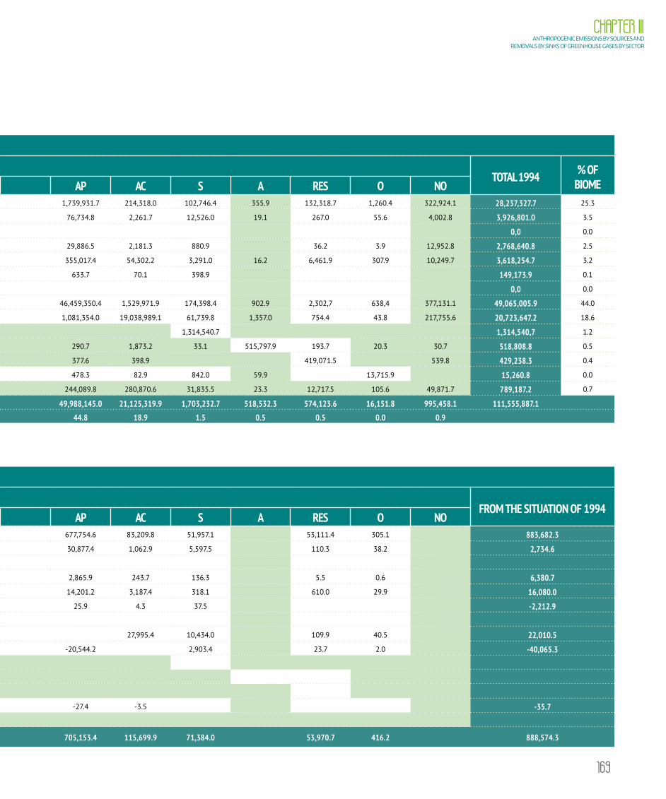
169
CHAPTER IIIANTHROPOGENIC EMISSIONS BY SOURCES AND
REMOVALS BY SINKS OF GREENHOUSE GASES BY SECTOR
TABLE 3.95 Transition areas for land-use and land-cover identified in the Atlantic Forest biome for the period from 1994 to 2002 (hectares)
LAND-USE TRANSITION MATRIX IN THE ATLANTIC FOREST BIOME - 1994-2002 (ha)
LAND USE IN 1994
LAND USE IN 2002TOTAL 1994 % OF
BIOMEFNM FM FSEC REF GNM GM GSEC AP AC S A RES O NO
1994
FNM 24,089,624.5 1,564,269.9 69,578.1 1,739,931.7 214,318.0 102,746.4 355.9 132,318.7 1,260.4 322,924.1 28,237,327.7 25.3
FM 3,827,963.1 2,970.8 76,734.8 2,261.7 12,526.0 19.1 267.0 55.6 4,002.8 3,926,801.0 3.5
FSec 0,0 0.0
Ref 67,412.4 2,652,245.6 3,041.2 29,886.5 2,181.3 880.9 36.2 3.9 12,952.8 2,768,640.8 2.5
GNM 14,479.6 3,091,758.8 82,370.1 355,017.4 54,302.2 3,291.0 16.2 6,461.9 307.9 10,249.7 3,618,254.7 3.2
GM 289.7 147,781.5 633.7 70.1 398.9 149,173.9 0.1
GSec 0,0 0.0
Ap 421,838.1 69,690.3 28,781.8 46,459,350.4 1,529,971.9 174,398.4 902.9 2,302,7 638,4 377,131.1 49,065,005.9 44.0
Ac 283,548.5 23,859.0 14,246.0 1,081,354.0 19,038,989.1 61,739.8 1,357.0 754.4 43.8 217,755.6 20,723,647.2 18.6
S 1,314,540.7 1,314,540,7 1.2
A 456.5 91.6 13.4 7.6 290.7 1,873.2 33.1 515,797.9 193.7 20.3 30.7 518,808.8 0.5
Res 8,770.9 79.6 377.6 398.9 419,071.5 539.8 429,238.3 0.4
O 72.7 9.1 478.3 82.9 842.0 59.9 13,715.9 15,260.8 0.0
NO 152,342.6 3,627.6 7,626.7 6,071.1 5.2 244,089.8 280,870.6 31,835.5 23.3 12,717.5 105.6 49,871.7 789,187.2 0.7
Total 2002 24,242,423.6 5,395,952.2 781,642.6 2,840,762.3 3,097,837.5 230,156.8 46,148.6 49,988,145.0 21,125,319.9 1,703,232.7 518,532.3 574,123.6 16,151.8 995,458.1 111,555,887.1
% of biome 21.7 4.8 0.7 2.5 2.8 0.2 0.0 44.8 18.9 1.5 0.5 0.5 0.0 0.9
TABLE 3.96 Net CO2 emissions in the Atlantic Forest biome in the period from 1994 to 2002 (Gg)
NET EMISSIONS MATRIX IN THE ATLANTIC FOREST BIOME - 1994-2002 (Gg CO2)
LAND USE IN 1994
LAND USE IN 2002FROM THE SITUATION OF 1994
FNM FM FSEC REF GNM GM GSEC AP AC S A RES O NO
1994
FNM -7,341.6 24,686.0 677,754.6 83,209.8 51,957.1 53,111.4 305.1 883,682.3
FM -35,931.8 980.2 30,877.4 1,062.9 5,597.5 110.3 38.2 2,734.6
FSec
Ref 2,779.1 349.6 2,865.9 243.7 136.3 5.5 0.6 6,380.7
GNM -1,638.3 -628.2 14,201.2 3,187.4 318.1 610.0 29.9 16,080.0
GM -26.3 -2,254.2 25.9 4.3 37.5 -2,212.9
GSec
Ap -6,381.3 -10,743.0 555.1 27,995.4 10,434.0 109.9 40.5 22,010.5
Ac -18,839.6 -3,645.9 35.2 -20,544.2 2,903.4 23.7 2.0 -40,065.3
S
A
Res
O -2.8 -2.0 -27.4 -3.5 -35.7
NO
From the situation of 2002 -43,273.5 -22,444.7 9,610.6 -2,882.4 940.0 705,153.4 115,699.9 71,384.0 53,970.7 416.2 888,574.3

170
VOLUME IIITHIRD NATIONAL COMMUNICATION OF BRAZIL
TABLE 3.97 Transition areas for land-use and land-cover identified in the Atlantic Forest biome for the period from 2002 to 2010 (hectares)
LAND-USE TRANSITION MATRIX IN THE ATLANTIC FOREST BIOME - 2002-2010 (ha)
LAND USE IN 2002
LAND USE IN 2010TOTAL 2002 % OF
BIOMEFNM FM FSEC REF GNM GM GSEC AP AC S A RES O NO
2002
FNM 17,637,695.9 442,297.5 657,903.9 2,469,071.5 1,104,576.4 51,192.2 135,978.4 510,265.7 8,079.1 1,225,362.9 24,242,423.6 21.7
FM 4,536,928.6 85,766.1 327,834.6 55,853.9 13,835.5 28,361.5 43,739.9 9,614.0 294,018.2 5,395,952.2 4.8
FSec 663,029.6 31,385.5 55,907.3 14,196.0 1,227.7 2,334.4 9,380.0 164.2 4,017.9 781,642.6 0.7
Ref 318,124.5 1,987,178.8 15,262.9 283,913.3 141,643.7 3,908.2 2,526.0 446.1 991.0 86,767.7 2,840,762.3 2.5
GNM 142,662.0 2,247,624.4 48,822.8 357,809.8 257,956.2 3,078.5 4,392.5 7,937.6 5,961.1 21,592.5 3,097,837.5 2.8
GM 13,031.1 188,536.6 10,340.1 12,812.5 1,063.9 454.0 156.8 3,468.5 293.2 230,156.8 0.2
GSec 4,427.2 35,353.2 4,439.7 1,266.8 40.6 527.1 45.4 48.6 46,148.6 0.0
Ap 3,678,084.9 1,203,947.7 235,653.9 34,439,259.4 7,633,441.8 244,160.8 44,593.1 33,965.7 19,147.5 2,455,890.0 49,988,145.0 44.8
Ac 649,397.4 207,300.6 63,169.2 1,859,769.1 18,034,845.6 86,876.9 30,369.0 10,700.0 3,355.4 179,536.6 21,125,319.9 18.9
S 1,699,864.8 3,368.0 1,703,232.7 1.5
A 19,819.6 10,725.1 238.8 523.3 839.7 4.3 8,948.5 7,724.5 1,807.0 441,546.4 13,468.9 396.6 12,489.5 518,532.3 0.5
Res 2,347.2 88.0 67.8 5,931.0 4,337.8 171.0 13,434.4 544,600.1 103.3 3,043.1 574,123.6 0.5
O 165.1 2.1 10.9 363.1 23.1 993.6 754.8 13.4 13,465.4 360.2 16,151.8 0.0
NO 210,784.6 4,647.1 233,107.8 27,577.3 10,366.9 10,240.3 145,516.3 187,540.6 3,755.9 655.9 725.1 308.0 160,232.4 995,458.1 0.9
Total 2010 17,868,300.0 4,994,598.3 5,544,495.3 4,361,793.8 2,258,831.0 237,359.4 359,762.6 39,969,103.7 27,456,219.0 2,111,976.5 705,927.7 1,175,444.8 65,054.2 4,447,020.7 111,555,887.1% of biome 16.0 4.5 5.0 3.9 2.0 0.2 0.3 35.8 24.6 1.9 0.6 1.1 0.1 4.0
TABLE 3.98 Net CO2 emissions in the Atlantic Forest biome in the period from 2002 to 2010 (Gg)
NET EMISSIONS MATRIX IN THE ATLANTIC FOREST BIOME - 2002-2010 (Gg CO2)
LAND USE IN 2002
LAND USE IN 2010FROM THE SITUATION OF 2002
FNM FM FSEC REF GNM GM GSEC AP AC S A RES O NO
2002
FNM -2,075.8 226,401.9 1,014,534.0 507,731.2 27,307.0 226,004.0 3,939.6 2,003,841.9
FM -42,586.6 32,040.8 163,634.9 25,961.2 7,739.0 27,657.9 4,422.3 218,869.5
FSec -104,051.4 1,962.7 9,278.5 2,773.5 343.4 2,029.7 43.3 -87,620.5
Ref 38,372.0 2,758.8 46,488.6 29,291.6 842.3 100.0 199.2 118,052.5
GNM -15,919.8 -372.4 13,308.6 14,626.5 283.9 662.2 586.0 13,175.0
GM -1,484.9 -2,875.8 400.1 752.2 100.9 14.9 328.3 -2,764.3
GSec -713.0 -539.3 11.0 26.9 2.4 1.6 -1,210.4
Ap -55,551.8 -187,058.6 4,563.4 146,274.6 15,937.0 1,769.5 1,262.2 -72,803.7
Ac -40,162.3 -33,785.0 64.1 -29,930.3 4,061.6 460.3 159.8 -99,131.8
S
A
Res
O -5.7 -0.5 -0.4 -20.4 -0.4 -27.4
NO
From the situation of 2010 -44,662.5 -161,399.2 21,443.5 -3,248.2 6,846.6 1,217,705.0 727,437.1 56,617.4 258,700.2 10,940.7 2,090,380.7

171
CHAPTER IIIANTHROPOGENIC EMISSIONS BY SOURCES AND
REMOVALS BY SINKS OF GREENHOUSE GASES BY SECTOR
TABLE 3.97 Transition areas for land-use and land-cover identified in the Atlantic Forest biome for the period from 2002 to 2010 (hectares)
LAND-USE TRANSITION MATRIX IN THE ATLANTIC FOREST BIOME - 2002-2010 (ha)
LAND USE IN 2002
LAND USE IN 2010TOTAL 2002 % OF
BIOMEFNM FM FSEC REF GNM GM GSEC AP AC S A RES O NO
2002
FNM 17,637,695.9 442,297.5 657,903.9 2,469,071.5 1,104,576.4 51,192.2 135,978.4 510,265.7 8,079.1 1,225,362.9 24,242,423.6 21.7
FM 4,536,928.6 85,766.1 327,834.6 55,853.9 13,835.5 28,361.5 43,739.9 9,614.0 294,018.2 5,395,952.2 4.8
FSec 663,029.6 31,385.5 55,907.3 14,196.0 1,227.7 2,334.4 9,380.0 164.2 4,017.9 781,642.6 0.7
Ref 318,124.5 1,987,178.8 15,262.9 283,913.3 141,643.7 3,908.2 2,526.0 446.1 991.0 86,767.7 2,840,762.3 2.5
GNM 142,662.0 2,247,624.4 48,822.8 357,809.8 257,956.2 3,078.5 4,392.5 7,937.6 5,961.1 21,592.5 3,097,837.5 2.8
GM 13,031.1 188,536.6 10,340.1 12,812.5 1,063.9 454.0 156.8 3,468.5 293.2 230,156.8 0.2
GSec 4,427.2 35,353.2 4,439.7 1,266.8 40.6 527.1 45.4 48.6 46,148.6 0.0
Ap 3,678,084.9 1,203,947.7 235,653.9 34,439,259.4 7,633,441.8 244,160.8 44,593.1 33,965.7 19,147.5 2,455,890.0 49,988,145.0 44.8
Ac 649,397.4 207,300.6 63,169.2 1,859,769.1 18,034,845.6 86,876.9 30,369.0 10,700.0 3,355.4 179,536.6 21,125,319.9 18.9
S 1,699,864.8 3,368.0 1,703,232.7 1.5
A 19,819.6 10,725.1 238.8 523.3 839.7 4.3 8,948.5 7,724.5 1,807.0 441,546.4 13,468.9 396.6 12,489.5 518,532.3 0.5
Res 2,347.2 88.0 67.8 5,931.0 4,337.8 171.0 13,434.4 544,600.1 103.3 3,043.1 574,123.6 0.5
O 165.1 2.1 10.9 363.1 23.1 993.6 754.8 13.4 13,465.4 360.2 16,151.8 0.0
NO 210,784.6 4,647.1 233,107.8 27,577.3 10,366.9 10,240.3 145,516.3 187,540.6 3,755.9 655.9 725.1 308.0 160,232.4 995,458.1 0.9
Total 2010 17,868,300.0 4,994,598.3 5,544,495.3 4,361,793.8 2,258,831.0 237,359.4 359,762.6 39,969,103.7 27,456,219.0 2,111,976.5 705,927.7 1,175,444.8 65,054.2 4,447,020.7 111,555,887.1% of biome 16.0 4.5 5.0 3.9 2.0 0.2 0.3 35.8 24.6 1.9 0.6 1.1 0.1 4.0
TABLE 3.98 Net CO2 emissions in the Atlantic Forest biome in the period from 2002 to 2010 (Gg)
NET EMISSIONS MATRIX IN THE ATLANTIC FOREST BIOME - 2002-2010 (Gg CO2)
LAND USE IN 2002
LAND USE IN 2010FROM THE SITUATION OF 2002
FNM FM FSEC REF GNM GM GSEC AP AC S A RES O NO
2002
FNM -2,075.8 226,401.9 1,014,534.0 507,731.2 27,307.0 226,004.0 3,939.6 2,003,841.9
FM -42,586.6 32,040.8 163,634.9 25,961.2 7,739.0 27,657.9 4,422.3 218,869.5
FSec -104,051.4 1,962.7 9,278.5 2,773.5 343.4 2,029.7 43.3 -87,620.5
Ref 38,372.0 2,758.8 46,488.6 29,291.6 842.3 100.0 199.2 118,052.5
GNM -15,919.8 -372.4 13,308.6 14,626.5 283.9 662.2 586.0 13,175.0
GM -1,484.9 -2,875.8 400.1 752.2 100.9 14.9 328.3 -2,764.3
GSec -713.0 -539.3 11.0 26.9 2.4 1.6 -1,210.4
Ap -55,551.8 -187,058.6 4,563.4 146,274.6 15,937.0 1,769.5 1,262.2 -72,803.7
Ac -40,162.3 -33,785.0 64.1 -29,930.3 4,061.6 460.3 159.8 -99,131.8
S
A
Res
O -5.7 -0.5 -0.4 -20.4 -0.4 -27.4
NO
From the situation of 2010 -44,662.5 -161,399.2 21,443.5 -3,248.2 6,846.6 1,217,705.0 727,437.1 56,617.4 258,700.2 10,940.7 2,090,380.7
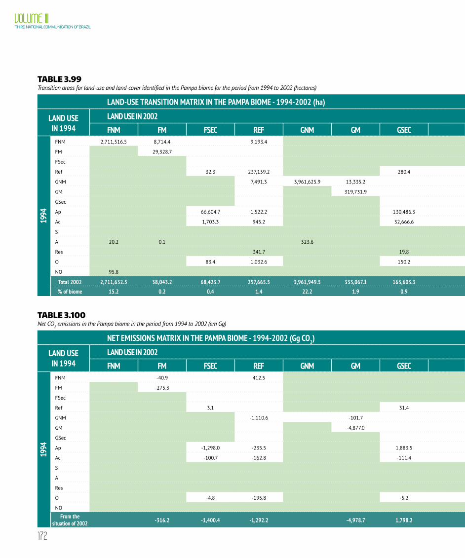
172
VOLUME IIITHIRD NATIONAL COMMUNICATION OF BRAZIL
TABLE 3.99 Transition areas for land-use and land-cover identified in the Pampa biome for the period from 1994 to 2002 (hectares)
LAND-USE TRANSITION MATRIX IN THE PAMPA BIOME - 1994-2002 (ha)
LAND USE IN 1994
LAND USE IN 2002TOTAL 1994 % OF
BIOMEFNM FM FSEC REF GNM GM GSEC AP AC S A RES O NO
1994
FNM 2,711,516.5 8,714.4 9,193.4 41,351.2 34,031.9 313.0 5,644.9 663.4 3.5 10,572.9 2,822,005.2 15.8
FM 29,328.7 59.8 28.1 130.2 29,546.9 0.2
FSec 0.0 0.0
Ref 32.3 237,139.2 280.4 658.4 103.5 12.6 198.1 238,424.5 1.3
GNM 7,491.3 3,961,625.9 13,335.2 87,175.8 306,034.4 3,963.3 21,277.3 3,090.2 9.0 1,740.4 4,405,742.8 24.6
GM 319,731.9 994.5 707.0 38.3 321,471.7 1.8
GSec 0.0 0.0
Ap 66,604.7 1,522.2 130,486.3 4,292,012.8 149,519.8 5,649.2 6,365.0 395.5 45.6 13,846.1 4,666,447.2 26.1
Ac 1,703.3 945.2 32,666.6 77,486.8 3,056,245.4 585.7 57,670.1 35.0 6.8 5,356.4 3,232,701.2 18.1
S 116,448.5 116,448.5 0.7
A 20.2 0.1 323.6 169.3 4,173.1 88.7 1,855,055.6 90.6 1,859,921.2 10.4
Res 341.7 19.8 89.3 10.6 362.3 54,125.5 54,949.1 0.3
O 83.4 1,032.6 150.2 246.5 54.4 5.2 133,272.8 134,845.1 0.8
NO 95.8 15.5 43.4 154.7 0.0
Total 2002 2,711,632.5 38,043.2 68,423.7 257,665.5 3,961,949.5 333,067.1 163,603.3 4,500,259.9 3,550,951.6 127,066.2 1,946,543.7 58,400.2 133,337.7 31,713.9 17,882,658.0
% of biome 15.2 0.2 0.4 1.4 22.2 1.9 0.9 25.2 19.9 0.7 10.9 0.3 0.7 0.2
TABLE 3.100 Net CO2 emissions in the Pampa biome in the period from 1994 to 2002 (em Gg)
NET EMISSIONS MATRIX IN THE PAMPA BIOME - 1994-2002 (Gg CO2)
LAND USE IN 1994
LAND USE IN 2002 FROM THE SITUATION OF 1994FNM FM FSEC REF GNM GM GSEC AP AC S A RES O NO
1994
FNM -40.9 412.5 9,205.8 8,706.5 136.8 141.3 1.4 18,563.4
FM -275.3 22.1 8.8 -244.3
FSec
Ref 3.1 31.4 65.4 11.9 2.0 113.8
GNM -1,110.6 -101.7 1,961.6 12,455.9 292.3 270.7 0.7 13,769.0
GM -4,877.0 24.2 27.2 -4,825.5
GSec
Ap -1,298.0 -235.5 1,883.5 2,528.9 315.2 24.0 2.4 3,220.4
Ac -100.7 -162.8 -111.4 -1,238.0 25.0 1.5 0.1 -1,586.2
S
A
Res
O -4.8 -195.8 -5.2 -16.1 -1.0 -222.9
NO
From the situation of 2002 -316.2 -1,400.4 -1,292.2 -4,978.7 1,798.2 10,025.1 23,738.3 771.4 437.5 4.6 28,787.6
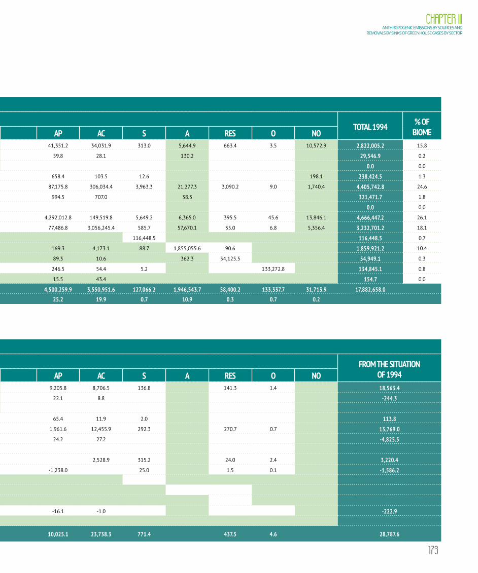
173
CHAPTER IIIANTHROPOGENIC EMISSIONS BY SOURCES AND
REMOVALS BY SINKS OF GREENHOUSE GASES BY SECTOR
TABLE 3.99 Transition areas for land-use and land-cover identified in the Pampa biome for the period from 1994 to 2002 (hectares)
LAND-USE TRANSITION MATRIX IN THE PAMPA BIOME - 1994-2002 (ha)
LAND USE IN 1994
LAND USE IN 2002TOTAL 1994 % OF
BIOMEFNM FM FSEC REF GNM GM GSEC AP AC S A RES O NO
1994
FNM 2,711,516.5 8,714.4 9,193.4 41,351.2 34,031.9 313.0 5,644.9 663.4 3.5 10,572.9 2,822,005.2 15.8
FM 29,328.7 59.8 28.1 130.2 29,546.9 0.2
FSec 0.0 0.0
Ref 32.3 237,139.2 280.4 658.4 103.5 12.6 198.1 238,424.5 1.3
GNM 7,491.3 3,961,625.9 13,335.2 87,175.8 306,034.4 3,963.3 21,277.3 3,090.2 9.0 1,740.4 4,405,742.8 24.6
GM 319,731.9 994.5 707.0 38.3 321,471.7 1.8
GSec 0.0 0.0
Ap 66,604.7 1,522.2 130,486.3 4,292,012.8 149,519.8 5,649.2 6,365.0 395.5 45.6 13,846.1 4,666,447.2 26.1
Ac 1,703.3 945.2 32,666.6 77,486.8 3,056,245.4 585.7 57,670.1 35.0 6.8 5,356.4 3,232,701.2 18.1
S 116,448.5 116,448.5 0.7
A 20.2 0.1 323.6 169.3 4,173.1 88.7 1,855,055.6 90.6 1,859,921.2 10.4
Res 341.7 19.8 89.3 10.6 362.3 54,125.5 54,949.1 0.3
O 83.4 1,032.6 150.2 246.5 54.4 5.2 133,272.8 134,845.1 0.8
NO 95.8 15.5 43.4 154.7 0.0
Total 2002 2,711,632.5 38,043.2 68,423.7 257,665.5 3,961,949.5 333,067.1 163,603.3 4,500,259.9 3,550,951.6 127,066.2 1,946,543.7 58,400.2 133,337.7 31,713.9 17,882,658.0
% of biome 15.2 0.2 0.4 1.4 22.2 1.9 0.9 25.2 19.9 0.7 10.9 0.3 0.7 0.2
TABLE 3.100 Net CO2 emissions in the Pampa biome in the period from 1994 to 2002 (em Gg)
NET EMISSIONS MATRIX IN THE PAMPA BIOME - 1994-2002 (Gg CO2)
LAND USE IN 1994
LAND USE IN 2002 FROM THE SITUATION OF 1994FNM FM FSEC REF GNM GM GSEC AP AC S A RES O NO
1994
FNM -40.9 412.5 9,205.8 8,706.5 136.8 141.3 1.4 18,563.4
FM -275.3 22.1 8.8 -244.3
FSec
Ref 3.1 31.4 65.4 11.9 2.0 113.8
GNM -1,110.6 -101.7 1,961.6 12,455.9 292.3 270.7 0.7 13,769.0
GM -4,877.0 24.2 27.2 -4,825.5
GSec
Ap -1,298.0 -235.5 1,883.5 2,528.9 315.2 24.0 2.4 3,220.4
Ac -100.7 -162.8 -111.4 -1,238.0 25.0 1.5 0.1 -1,586.2
S
A
Res
O -4.8 -195.8 -5.2 -16.1 -1.0 -222.9
NO
From the situation of 2002 -316.2 -1,400.4 -1,292.2 -4,978.7 1,798.2 10,025.1 23,738.3 771.4 437.5 4.6 28,787.6

174
VOLUME IIITHIRD NATIONAL COMMUNICATION OF BRAZIL
TABLE 3.101 Transition areas for land-use and land-cover identified in the Pampa biome for the period from 2002 to 2010 (in hectares)
LAND-USE TRANSITION MATRIX IN THE PAMPA BIOME - PAMPA - 2002-2010 (ha)
LAND USE IN 2002
LAND USE IN 2010TOTAL 2002 % OF
BIOMEFNM FM FSEC REF GNM GM GSEC AP AC S A RES O NO
2002
FNM 2,101,531.8 135,007.2 386,182.9 76,105.0 1,336.7 8,229.0 638.0 822.2 1,779.7 2,711,632.5 15.2
FM 36,024.6 67.4 1,287.1 431.4 9.7 85.4 137.6 38,043.2 0.2
FSec 32,258.9 2,214.1 20,706.0 12,708.5 99.9 67.7 114.2 254.4 68,423.7 0.4
Ref 365.4 236,843.1 589.4 15,489.3 2,139.7 227.6 119.7 192.5 209.2 1,489.5 257,665.5 1.4
GNM 60,257.4 2,734,365.3 276.9 514,059.6 593,453.2 5,119.0 48,829.9 3,762.7 176.0 1,649.5 3,961,949.5 22.2
GM 2,381.0 290,362.6 33,874.4 4,924.2 4.1 1,143.3 5.0 372.5 333,067.1 1.9
GSec 1,574.1 110,876.9 31,673.7 18,042.0 69.4 1,110.5 198.3 58.5 163,603.3 0.9
Ap 26,150.1 251,754.5 49,669.5 3,287,775.7 856,897.1 7,754.8 13,059.6 2,575.0 1,493.8 3,129.8 4,500,259.9 25.2
Ac 5,148.5 11,571.6 26,191.0 291,011.3 3,200,340.5 643.3 14,337.3 1,266.9 441.0 3,550,951.6 19.9
S 127,066.2 127,066.2 0.7
A 29,833.0 2,331.7 1,088.3 721.3 121,922.4 25,894.8 7,494.2 33,205.8 105,054.2 425.7 1,607,626.2 2,995.0 6,918.8 1,032.3 1,946,543.7 10.9
Res 31.2 7.3 521.5 247.4 361.4 4,263.9 52,967.5 58,400.2 0.3
O 3.5 5,622.1 1.3 504.0 840.4 819.2 43.7 153.7 125,349.9 133,337.7 0.7
NO 10,236.1 6,860.0 768.3 942.6 395.9 7,086.7 5,063.1 94.5 266.6 31,713.9 0.2
Total 2010 2,141,600.8 38,356.3 71,906.0 708,789.6 2,857,230.3 316,534.3 195,739.7 4,623,104.0 4,876,360.7 143,670.2 1,699,182.8 64,868.8 134,969.8 10,344.8 17,882,658.0
% of biome 12.0 0.2 0.4 4.0 16.0 1.8 1.1 25.9 27.3 0.8 9.5 0.4 0.8 0.1
TABLE 3.102 Net CO2 emissions in the Pampa biome in the period from 2002 to 2010 (in Gg)
NET EMISSIONS MATRIX IN THE PAMPA BIOME - 2002-2010 (Gg CO2)
LAND USE IN 2002
LAND USE IN 2010FROM THE SITUATION OF 2002
FNM FM FSEC REF GNM GM GSEC AP AC S A RES O NO
2002
FNM 7,640.4 83,363.8 22,238.8 570.4 193.7 210.8 114,218.0
FM -338.2 12.3 500.2 145.8 4.6 324.7
FSec -1,665.4 -143.1 2,132.5 1,777.5 19.8 22.1 2,143.4
Ref 56.2 100.7 2,441.9 376.0 47.5 42.1 46.7 3,111.2
GNM -8,910.8 -2.1 9,128.9 24,000.3 369.4 295.5 12.7 24,894.0
GM -323.5 -4,429.0 814.2 212.8 0.3 0.4 -3,724.8
GSec -259.6 -1,691.2 -83.5 255.1 3.9 10.2 -1,765.1
Ap -511.0 -39,998.8 720.5 15,335.2 432.1 142.1 53.0 -23,826.9
Ac -317.3 -2,039.0 -64.2 -5,071.5 23.6 51.8 -7,416.6
S
A
Res
O -0.2 -1,099.7 0.0 -19.2 -15.9 -1,135.0
NO
From the situation of 2010 -338.2 -2,437.6 -45,121.8 -4,431.1 -934.2 93,207.4 64,325.6 1,471.7 757.9 323.3 106,823.1

175
CHAPTER IIIANTHROPOGENIC EMISSIONS BY SOURCES AND
REMOVALS BY SINKS OF GREENHOUSE GASES BY SECTOR
TABLE 3.101 Transition areas for land-use and land-cover identified in the Pampa biome for the period from 2002 to 2010 (in hectares)
LAND-USE TRANSITION MATRIX IN THE PAMPA BIOME - PAMPA - 2002-2010 (ha)
LAND USE IN 2002
LAND USE IN 2010TOTAL 2002 % OF
BIOMEFNM FM FSEC REF GNM GM GSEC AP AC S A RES O NO
2002
FNM 2,101,531.8 135,007.2 386,182.9 76,105.0 1,336.7 8,229.0 638.0 822.2 1,779.7 2,711,632.5 15.2
FM 36,024.6 67.4 1,287.1 431.4 9.7 85.4 137.6 38,043.2 0.2
FSec 32,258.9 2,214.1 20,706.0 12,708.5 99.9 67.7 114.2 254.4 68,423.7 0.4
Ref 365.4 236,843.1 589.4 15,489.3 2,139.7 227.6 119.7 192.5 209.2 1,489.5 257,665.5 1.4
GNM 60,257.4 2,734,365.3 276.9 514,059.6 593,453.2 5,119.0 48,829.9 3,762.7 176.0 1,649.5 3,961,949.5 22.2
GM 2,381.0 290,362.6 33,874.4 4,924.2 4.1 1,143.3 5.0 372.5 333,067.1 1.9
GSec 1,574.1 110,876.9 31,673.7 18,042.0 69.4 1,110.5 198.3 58.5 163,603.3 0.9
Ap 26,150.1 251,754.5 49,669.5 3,287,775.7 856,897.1 7,754.8 13,059.6 2,575.0 1,493.8 3,129.8 4,500,259.9 25.2
Ac 5,148.5 11,571.6 26,191.0 291,011.3 3,200,340.5 643.3 14,337.3 1,266.9 441.0 3,550,951.6 19.9
S 127,066.2 127,066.2 0.7
A 29,833.0 2,331.7 1,088.3 721.3 121,922.4 25,894.8 7,494.2 33,205.8 105,054.2 425.7 1,607,626.2 2,995.0 6,918.8 1,032.3 1,946,543.7 10.9
Res 31.2 7.3 521.5 247.4 361.4 4,263.9 52,967.5 58,400.2 0.3
O 3.5 5,622.1 1.3 504.0 840.4 819.2 43.7 153.7 125,349.9 133,337.7 0.7
NO 10,236.1 6,860.0 768.3 942.6 395.9 7,086.7 5,063.1 94.5 266.6 31,713.9 0.2
Total 2010 2,141,600.8 38,356.3 71,906.0 708,789.6 2,857,230.3 316,534.3 195,739.7 4,623,104.0 4,876,360.7 143,670.2 1,699,182.8 64,868.8 134,969.8 10,344.8 17,882,658.0
% of biome 12.0 0.2 0.4 4.0 16.0 1.8 1.1 25.9 27.3 0.8 9.5 0.4 0.8 0.1
TABLE 3.102 Net CO2 emissions in the Pampa biome in the period from 2002 to 2010 (in Gg)
NET EMISSIONS MATRIX IN THE PAMPA BIOME - 2002-2010 (Gg CO2)
LAND USE IN 2002
LAND USE IN 2010FROM THE SITUATION OF 2002
FNM FM FSEC REF GNM GM GSEC AP AC S A RES O NO
2002
FNM 7,640.4 83,363.8 22,238.8 570.4 193.7 210.8 114,218.0
FM -338.2 12.3 500.2 145.8 4.6 324.7
FSec -1,665.4 -143.1 2,132.5 1,777.5 19.8 22.1 2,143.4
Ref 56.2 100.7 2,441.9 376.0 47.5 42.1 46.7 3,111.2
GNM -8,910.8 -2.1 9,128.9 24,000.3 369.4 295.5 12.7 24,894.0
GM -323.5 -4,429.0 814.2 212.8 0.3 0.4 -3,724.8
GSec -259.6 -1,691.2 -83.5 255.1 3.9 10.2 -1,765.1
Ap -511.0 -39,998.8 720.5 15,335.2 432.1 142.1 53.0 -23,826.9
Ac -317.3 -2,039.0 -64.2 -5,071.5 23.6 51.8 -7,416.6
S
A
Res
O -0.2 -1,099.7 0.0 -19.2 -15.9 -1,135.0
NO
From the situation of 2010 -338.2 -2,437.6 -45,121.8 -4,431.1 -934.2 93,207.4 64,325.6 1,471.7 757.9 323.3 106,823.1
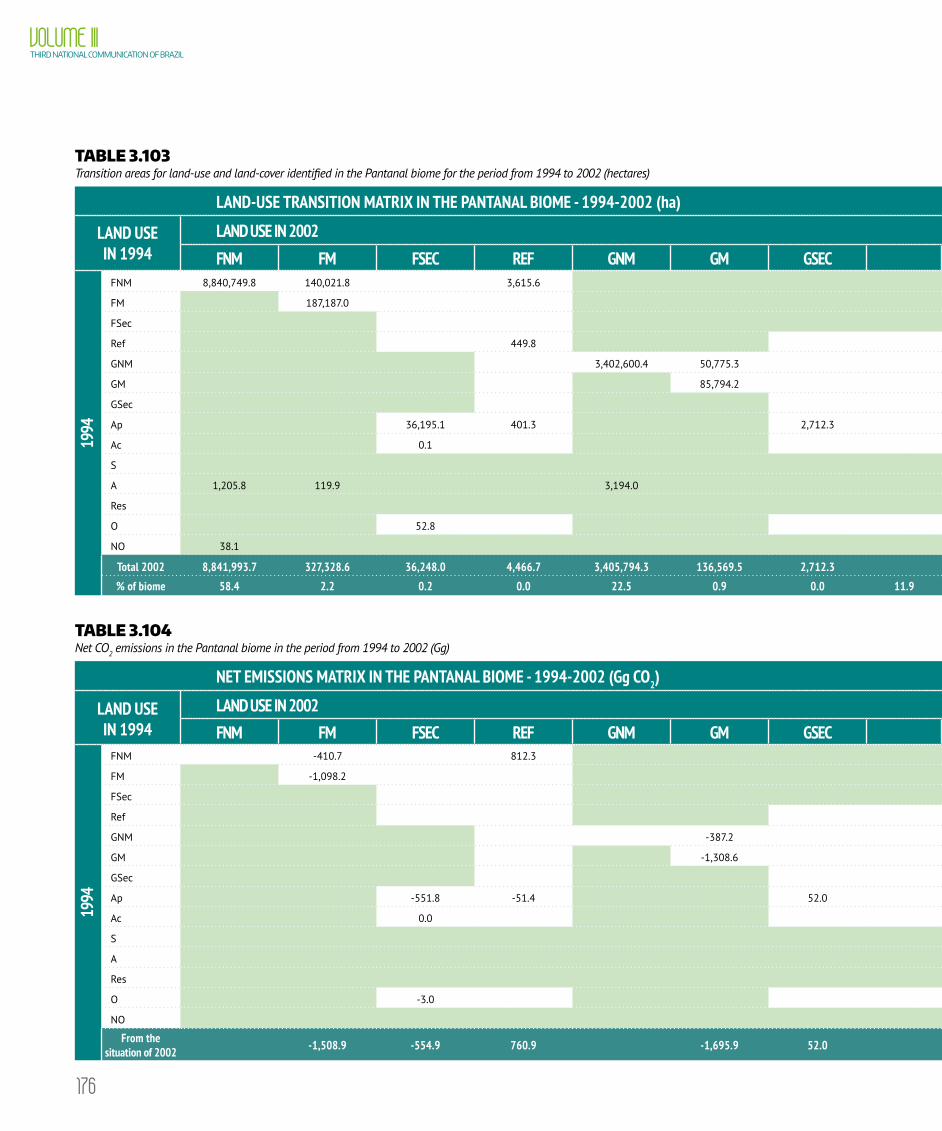
176
VOLUME IIITHIRD NATIONAL COMMUNICATION OF BRAZIL
TABLE 3.103 Transition areas for land-use and land-cover identified in the Pantanal biome for the period from 1994 to 2002 (hectares)
LAND-USE TRANSITION MATRIX IN THE PANTANAL BIOME - 1994-2002 (ha)
LAND USE IN 1994
LAND USE IN 2002TOTAL 1994 % OF
BIOMEFNM FM FSEC REF GNM GM GSEC AP AC S A RES O NO
1994
FNM 8,840,749.8 140,021.8 3,615.6 675,522.3 4,570.2 2,638.6 6,904.3 31.6 595.4 9,674,649.6 63.9
FM 187,187.0 5,155.8 773.7 193,116.4 1.3
FSec 0.0 0.0
Ref 449.8 449.8 0.0
GNM 3,402,600.4 50,775.3 161,305.4 17.9 10.0 748.9 3,615,457.8 23.9
GM 85,794.2 3,778.7 89,572.9 0.6
GSec 0.0 0.0
Ap 36,195.1 401.3 2,712.3 945,770.3 4,280.7 733.5 5.8 40.7 990,139.7 6.5
Ac 0.1 1,386.6 16,360.0 17,746.7 0.1
S 7,240.1 7,240.1 0.0
A 1,205.8 119.9 3,194.0 245.1 535,625.6 37.3 3.5 540,431.1 3.6
Res 6.8 6.8 0.0
O 52.8 192.1 10.2 1,094.0 1,349.1 0.0
NO 38.1 93.7 131.8 0.0
Total 2002 8,841,993.7 327,328.6 36,248.0 4,466.7 3,405,794.3 136,569.5 2,712.3 1,793,449.9 25,239.1 10,622.2 544,058.3 75.7 1,733.6 0.0 15,130,291.8
% of biome 58.4 2.2 0.2 0.0 22.5 0.9 0.0 11.9 11.9 0.2 0.1 3.6 0.0 0.0 0.0
TABLE 3.104 Net CO2 emissions in the Pantanal biome in the period from 1994 to 2002 (Gg)
NET EMISSIONS MATRIX IN THE PANTANAL BIOME - 1994-2002 (Gg CO2)
LAND USE IN 1994
LAND USE IN 2002FROM THE SITUATION OF 1994
FNM FM FSEC REF GNM GM GSEC AP AC S A RES O NO
1994
FNM -410.7 812.3 164,820.0 1,693.9 1,094.6 11.2 192.0 168,213.3
FM -1,098.2 1,084.8 -13.4
FSec
Ref
GNM -387.2 7,058.7 1.5 0.8 6,673.8
GM -1,308.6 -6.7 -1,315.3
GSec
Ap -551.8 -51.4 52.0 110.8 47.3 2.4 -390.8
Ac 0.0 -33.4 -33.4
S
A
Res
O -3.0 -14.4 -0.5 -17.9
NO
From the situation of 2002 -1,508.9 -554.9 760.9 -1,695.9 52.0 172,909.0 1,805.8 1,142.7 11.2 194.3 173,116.3

177
CHAPTER IIIANTHROPOGENIC EMISSIONS BY SOURCES AND
REMOVALS BY SINKS OF GREENHOUSE GASES BY SECTOR
TABLE 3.103 Transition areas for land-use and land-cover identified in the Pantanal biome for the period from 1994 to 2002 (hectares)
LAND-USE TRANSITION MATRIX IN THE PANTANAL BIOME - 1994-2002 (ha)
LAND USE IN 1994
LAND USE IN 2002TOTAL 1994 % OF
BIOMEFNM FM FSEC REF GNM GM GSEC AP AC S A RES O NO
1994
FNM 8,840,749.8 140,021.8 3,615.6 675,522.3 4,570.2 2,638.6 6,904.3 31.6 595.4 9,674,649.6 63.9
FM 187,187.0 5,155.8 773.7 193,116.4 1.3
FSec 0.0 0.0
Ref 449.8 449.8 0.0
GNM 3,402,600.4 50,775.3 161,305.4 17.9 10.0 748.9 3,615,457.8 23.9
GM 85,794.2 3,778.7 89,572.9 0.6
GSec 0.0 0.0
Ap 36,195.1 401.3 2,712.3 945,770.3 4,280.7 733.5 5.8 40.7 990,139.7 6.5
Ac 0.1 1,386.6 16,360.0 17,746.7 0.1
S 7,240.1 7,240.1 0.0
A 1,205.8 119.9 3,194.0 245.1 535,625.6 37.3 3.5 540,431.1 3.6
Res 6.8 6.8 0.0
O 52.8 192.1 10.2 1,094.0 1,349.1 0.0
NO 38.1 93.7 131.8 0.0
Total 2002 8,841,993.7 327,328.6 36,248.0 4,466.7 3,405,794.3 136,569.5 2,712.3 1,793,449.9 25,239.1 10,622.2 544,058.3 75.7 1,733.6 0.0 15,130,291.8
% of biome 58.4 2.2 0.2 0.0 22.5 0.9 0.0 11.9 11.9 0.2 0.1 3.6 0.0 0.0 0.0
TABLE 3.104 Net CO2 emissions in the Pantanal biome in the period from 1994 to 2002 (Gg)
NET EMISSIONS MATRIX IN THE PANTANAL BIOME - 1994-2002 (Gg CO2)
LAND USE IN 1994
LAND USE IN 2002FROM THE SITUATION OF 1994
FNM FM FSEC REF GNM GM GSEC AP AC S A RES O NO
1994
FNM -410.7 812.3 164,820.0 1,693.9 1,094.6 11.2 192.0 168,213.3
FM -1,098.2 1,084.8 -13.4
FSec
Ref
GNM -387.2 7,058.7 1.5 0.8 6,673.8
GM -1,308.6 -6.7 -1,315.3
GSec
Ap -551.8 -51.4 52.0 110.8 47.3 2.4 -390.8
Ac 0.0 -33.4 -33.4
S
A
Res
O -3.0 -14.4 -0.5 -17.9
NO
From the situation of 2002 -1,508.9 -554.9 760.9 -1,695.9 52.0 172,909.0 1,805.8 1,142.7 11.2 194.3 173,116.3
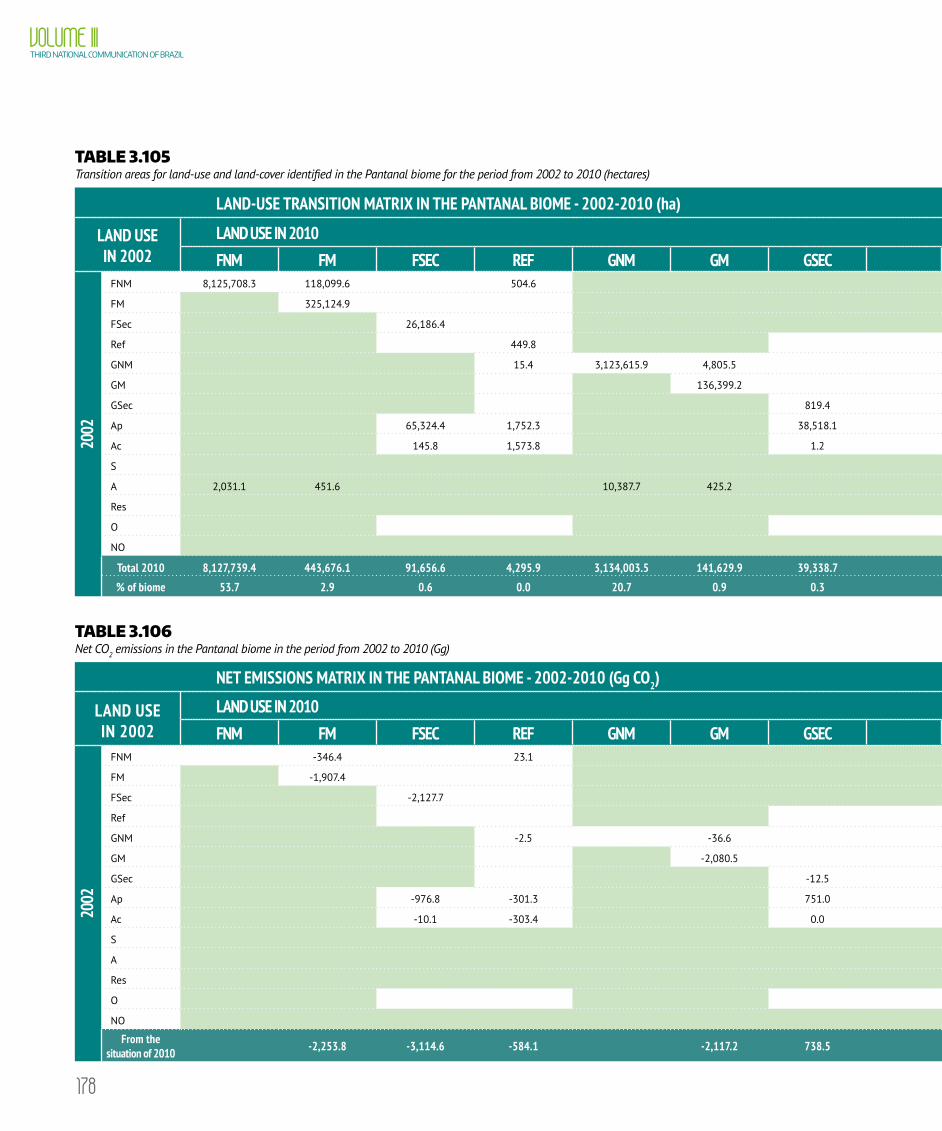
178
VOLUME IIITHIRD NATIONAL COMMUNICATION OF BRAZIL
TABLE 3.105 Transition areas for land-use and land-cover identified in the Pantanal biome for the period from 2002 to 2010 (hectares)
LAND-USE TRANSITION MATRIX IN THE PANTANAL BIOME - 2002-2010 (ha)
LAND USE IN 2002
LAND USE IN 2010TOTAL 2002 % OF
BIOMEFNM FM FSEC REF GNM GM GSEC AP AC S A RES O NO
2002
FNM 8,125,708.3 118,099.6 504.6 549,930.9 812.1 607.0 45,736.8 69.5 525.0 8,841,993.7 58.4
FM 325,124.9 1,343.1 860.6 327,328.6 2.2
FSec 26,186.4 9,945.0 116.5 36,248.0 0.2
Ref 449.8 4,016.8 4,466.7 0.0
GNM 15.4 3,123,615.9 4,805.5 254,274.7 8.2 36.4 23,037.3 1.0 0.1 3,405,794.3 22.5
GM 136,399.2 170.3 136,569.5 0.9
GSec 819.4 1,892.9 2,712.3 0.0
Ap 65,324.4 1,752.3 38,518.1 1,673,447.7 10,247.7 1,398.3 1,216.2 2.8 1,542.3 1,793,449.9 11.9
Ac 145.8 1,573.8 1.2 18,552.6 4,963.0 2.6 0.1 25,239.1 0.2
S 10,622.2 10,622.2 0.1
A 2,031.1 451.6 10,387.7 425.2 629.6 530,104.9 17.7 10.5 544,058.3 3.6
Res 75.7 75.7 0.0
O 511.1 1,222.5 1,733.6 0.0
NO 0.0 0.0
Total 2010 8,127,739.4 443,676.1 91,656.6 4,295.9 3,134,003.5 141,629.9 39,338.7 2,510,697.9 20,164.3 12,663.9 600,958.4 166.7 3,300.5 0.0 15,130,291.8
% of biome 53.7 2.9 0.6 0.0 20.7 0.9 0.3 16.6 0.1 0.1 4.0 0.0 0.0 0.0
TABLE 3.106 Net CO2 emissions in the Pantanal biome in the period from 2002 to 2010 (Gg)
NET EMISSIONS MATRIX IN THE PANTANAL BIOME - 2002-2010 (Gg CO2)
LAND USE IN 2002
LAND USE IN 2010FROM THE SITUATION OF 2002
FNM FM FSEC REF GNM GM GSEC AP AC S A RES O NO
2002
FNM -346.4 23.1 133,376.1 271.2 184.3 29.5 245.3 133,783.1
FM -1,907.4 324.0 -1,583.4
FSec -2,127.7 862.2 12.8 -1,252.7
Ref 616.5 616.5
GNM -2.5 -36.6 5,379.0 0.5 2.1 0.1 0.0 5,342.6
GM -2,080.5 6.8 -2,073.7
GSec -12.5 3.1 -9.4
Ap -976.8 -301.3 751.0 208.7 77.8 0.2 91.1 -149.4
Ac -10.1 -303.4 0.0 -408.6 0.0 -722.0
S
A
Res
O -38.2 -38.2
NO
From the situation of 2010 -2,253.8 -3,114.6 -584.1 -2,117.2 738.5 139,504.4 1,109.7 264.2 29.8 336.4 133,913.3
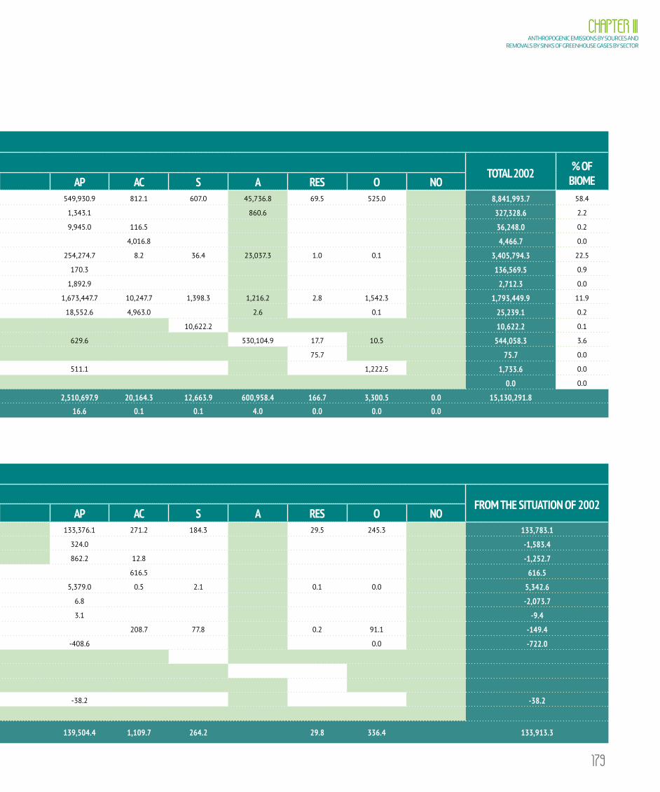
179
CHAPTER IIIANTHROPOGENIC EMISSIONS BY SOURCES AND
REMOVALS BY SINKS OF GREENHOUSE GASES BY SECTOR
TABLE 3.105 Transition areas for land-use and land-cover identified in the Pantanal biome for the period from 2002 to 2010 (hectares)
LAND-USE TRANSITION MATRIX IN THE PANTANAL BIOME - 2002-2010 (ha)
LAND USE IN 2002
LAND USE IN 2010TOTAL 2002 % OF
BIOMEFNM FM FSEC REF GNM GM GSEC AP AC S A RES O NO
2002
FNM 8,125,708.3 118,099.6 504.6 549,930.9 812.1 607.0 45,736.8 69.5 525.0 8,841,993.7 58.4
FM 325,124.9 1,343.1 860.6 327,328.6 2.2
FSec 26,186.4 9,945.0 116.5 36,248.0 0.2
Ref 449.8 4,016.8 4,466.7 0.0
GNM 15.4 3,123,615.9 4,805.5 254,274.7 8.2 36.4 23,037.3 1.0 0.1 3,405,794.3 22.5
GM 136,399.2 170.3 136,569.5 0.9
GSec 819.4 1,892.9 2,712.3 0.0
Ap 65,324.4 1,752.3 38,518.1 1,673,447.7 10,247.7 1,398.3 1,216.2 2.8 1,542.3 1,793,449.9 11.9
Ac 145.8 1,573.8 1.2 18,552.6 4,963.0 2.6 0.1 25,239.1 0.2
S 10,622.2 10,622.2 0.1
A 2,031.1 451.6 10,387.7 425.2 629.6 530,104.9 17.7 10.5 544,058.3 3.6
Res 75.7 75.7 0.0
O 511.1 1,222.5 1,733.6 0.0
NO 0.0 0.0
Total 2010 8,127,739.4 443,676.1 91,656.6 4,295.9 3,134,003.5 141,629.9 39,338.7 2,510,697.9 20,164.3 12,663.9 600,958.4 166.7 3,300.5 0.0 15,130,291.8
% of biome 53.7 2.9 0.6 0.0 20.7 0.9 0.3 16.6 0.1 0.1 4.0 0.0 0.0 0.0
TABLE 3.106 Net CO2 emissions in the Pantanal biome in the period from 2002 to 2010 (Gg)
NET EMISSIONS MATRIX IN THE PANTANAL BIOME - 2002-2010 (Gg CO2)
LAND USE IN 2002
LAND USE IN 2010FROM THE SITUATION OF 2002
FNM FM FSEC REF GNM GM GSEC AP AC S A RES O NO
2002
FNM -346.4 23.1 133,376.1 271.2 184.3 29.5 245.3 133,783.1
FM -1,907.4 324.0 -1,583.4
FSec -2,127.7 862.2 12.8 -1,252.7
Ref 616.5 616.5
GNM -2.5 -36.6 5,379.0 0.5 2.1 0.1 0.0 5,342.6
GM -2,080.5 6.8 -2,073.7
GSec -12.5 3.1 -9.4
Ap -976.8 -301.3 751.0 208.7 77.8 0.2 91.1 -149.4
Ac -10.1 -303.4 0.0 -408.6 0.0 -722.0
S
A
Res
O -38.2 -38.2
NO
From the situation of 2010 -2,253.8 -3,114.6 -584.1 -2,117.2 738.5 139,504.4 1,109.7 264.2 29.8 336.4 133,913.3

180
VOLUME IIITHIRD NATIONAL COMMUNICATION OF BRAZIL
TABLE 3.107 Transition areas for land-use and land-cover identified Brazil for the period from 1994 to 2002 (hectares)6
LAND-USE TRANSITION MATRIX IN BRAZIL - 1994-2002 (ha)
LAND USE IN 1994
LAND USE IN 2002TOTAL 1994 % OF
BIOMEFNM FM FSEC REF CS GNM GM GSEC AP AC S A RES O NO
1994
FNM 369,455,072.2 48,962,726.9 798,320.7 151,652.6 235,584.8 25,984,512.0 2,502,474.6 199,668.1 16,490.4 151,611.1 16,692.2 502,196.3 448,977,002.0 52.7
FM 104,253,805.6 34,268.6 3,659.2 23,704.6 761,763.8 13,036.4 19,394.4 923.1 512.2 5,205.7 7,467.2 105,123,741.0 12.3
FSec 751,094.9 634.8 612,188.8 4,138.2 1,117.1 8.8 0.6 715.4 1,369,898.6 0.2
Ref 84,435.6 5,266,860.5 11,197.6 142,679.3 59,844.2 1,009.9 36.2 20.0 13,520.7 5,579,604.1 0.7
CS
GNM 45,542.7 50,437,237.9 6,315,625.5 17,176.0 3,546,539.8 1,439,989.9 41,801.0 23,003.5 10,540.2 1,313.2 54,265.5 61,933,035.3 7.3
GM 308.3 5,717,532.9 218.2 28,414.2 39,373.3 611.5 38.3 24.5 818.5 5,787,339.7 0.7
GSec 104.4 8,383.2 8,690.9 0.0 47.9 17,226.4 0.0
Ap 3,668,020.5 177,307.7 592,988.6 139,290,084.3 2,997,328.5 355,639.9 10,013.2 5,600.2 4,271.8 607,575.7 147,708,830.3 17.3
Ac 500,795.8 42,421.9 86,311.2 2,679,903.7 48,060,211.6 114,294.0 60,515.8 1,376.6 1,029.4 316,524.9 51,863,384.9 6.1
S 2,369,496.7 34.7 2,369,531.5 0.3
A 3,103.1 280.5 19.9 4,426.7 19.2 2,958.8 6,791.2 121.8 16,449,153.5 23,556.0 67.3 148.2 16,490,646.2 1.9
Res 10,641.4 342.2 923.0 930.2 665.4 4.7 876.8 1,899,885.6 636.2 1,914,905.6 0.2
O 1,389.4 1,041.7 220.3 12,154.0 1,365.1 1,372.1 480.7 0.0 412,940.1 430,963.4 0.1
NO 485,318.7 60,697.7 24,757.0 9,879.9 321.1 10,654.0 359.9 3.3 1,346,729.8 506,549.8 36,905.4 247,0 13,702.4 2,039.2 123,270.8 2,621,436.1 0.3
Total de 2002 369,943,494.0 153,277,510.6 5,873,723.9 5,699,775.9 259,610.6 50,452,318.7 12,033,537.5 717,421.5 174,417,549.7 55,631,768.3 3,141,484.7 16,561,751.0 2,106,821.2 444,318.9 1,626,458.7 852,187,545.2 % of biome 43.4 18.0 0.7 0.7 0.0 5.9 1.4 0.1 20.5 6.5 0.4 1.9 0.2 0.1 0.2
TABLE 3.108 Net anthropogenic CO2 emissions in Brazil from 1994 to 20027
NET EMISSIONS MATRIX IN BRAZIL - 1994-2002 (Gg CO2)
LAND USE IN 1994
LAND USE IN 2002FROM THE SITUATION OF 1994
FNM FM FSEC REF CS GNM GM GSEC AP AC S A RES O NO
1994
FNM -274,319.5 437,773.1 43,786.2 27,194,6 9,682,053.0 573,406.2 84,191.9 61,436.0 7,171.7 10,642,693.2
FM -1,249,679.4 19,882.3 967.3 2,468,4 396,749.0 4,328.7 8,785.3 280.7 3,285.1 -812,932.4
FSec -109,279.3 80.2 131,285.6 818.3 385.4 0.1 188.1 23,478.5
Ref 4,458.4 1,294.6 13,646.4 6,586.4 155.8 5.5 3.1 26,150.3
CS
GNM -5,264.2 -48,167.2 822.1 188,247.4 88,059.2 4,346.9 947.3 140.9 229,132.4
GM -28.1 -87,211.4 9.4 1,049.5 2,587.6 59.3 2.3 -83,531.4
GSec -15.7 -127.9 -25.9 0.0 1.9 -167.6
Ap -63,436.3 -27,670.6 10,659.5 52,397.2 20,538.2 249.6 230.8 -7,031.7
Ac -30,755.3 -6,694.3 176.8 -42,074.9 5,244.7 47.3 34.7 -74,021.0
S
A
Res
O -55.5 -197.8 -7.5 -707.4 -42.4 -1,010.6
NO
From the situation of 2002 -1,523,998.9 258,587.5 4,963.0 29,663.0 -135,378.6 12,827.1 10,370,222.6 728,141.3 123,709.4 62,966.6 11,056.5 9,942,759.6
6 Secondary vegetations (FSec and GSec) in this period were mapped only in the Amazon biome. Class CS (selective logging) was not mapped during this period.7 Secondary vegetations (FSec and GSec) in this period were mapped only in the Amazon biome. Class CS (selective logging) was not mapped during this period.

181
CHAPTER IIIANTHROPOGENIC EMISSIONS BY SOURCES AND
REMOVALS BY SINKS OF GREENHOUSE GASES BY SECTOR
TABLE 3.107 Transition areas for land-use and land-cover identified Brazil for the period from 1994 to 2002 (hectares)6
LAND-USE TRANSITION MATRIX IN BRAZIL - 1994-2002 (ha)
LAND USE IN 1994
LAND USE IN 2002TOTAL 1994 % OF
BIOMEFNM FM FSEC REF CS GNM GM GSEC AP AC S A RES O NO
1994
FNM 369,455,072.2 48,962,726.9 798,320.7 151,652.6 235,584.8 25,984,512.0 2,502,474.6 199,668.1 16,490.4 151,611.1 16,692.2 502,196.3 448,977,002.0 52.7
FM 104,253,805.6 34,268.6 3,659.2 23,704.6 761,763.8 13,036.4 19,394.4 923.1 512.2 5,205.7 7,467.2 105,123,741.0 12.3
FSec 751,094.9 634.8 612,188.8 4,138.2 1,117.1 8.8 0.6 715.4 1,369,898.6 0.2
Ref 84,435.6 5,266,860.5 11,197.6 142,679.3 59,844.2 1,009.9 36.2 20.0 13,520.7 5,579,604.1 0.7
CS
GNM 45,542.7 50,437,237.9 6,315,625.5 17,176.0 3,546,539.8 1,439,989.9 41,801.0 23,003.5 10,540.2 1,313.2 54,265.5 61,933,035.3 7.3
GM 308.3 5,717,532.9 218.2 28,414.2 39,373.3 611.5 38.3 24.5 818.5 5,787,339.7 0.7
GSec 104.4 8,383.2 8,690.9 0.0 47.9 17,226.4 0.0
Ap 3,668,020.5 177,307.7 592,988.6 139,290,084.3 2,997,328.5 355,639.9 10,013.2 5,600.2 4,271.8 607,575.7 147,708,830.3 17.3
Ac 500,795.8 42,421.9 86,311.2 2,679,903.7 48,060,211.6 114,294.0 60,515.8 1,376.6 1,029.4 316,524.9 51,863,384.9 6.1
S 2,369,496.7 34.7 2,369,531.5 0.3
A 3,103.1 280.5 19.9 4,426.7 19.2 2,958.8 6,791.2 121.8 16,449,153.5 23,556.0 67.3 148.2 16,490,646.2 1.9
Res 10,641.4 342.2 923.0 930.2 665.4 4.7 876.8 1,899,885.6 636.2 1,914,905.6 0.2
O 1,389.4 1,041.7 220.3 12,154.0 1,365.1 1,372.1 480.7 0.0 412,940.1 430,963.4 0.1
NO 485,318.7 60,697.7 24,757.0 9,879.9 321.1 10,654.0 359.9 3.3 1,346,729.8 506,549.8 36,905.4 247,0 13,702.4 2,039.2 123,270.8 2,621,436.1 0.3
Total de 2002 369,943,494.0 153,277,510.6 5,873,723.9 5,699,775.9 259,610.6 50,452,318.7 12,033,537.5 717,421.5 174,417,549.7 55,631,768.3 3,141,484.7 16,561,751.0 2,106,821.2 444,318.9 1,626,458.7 852,187,545.2 % of biome 43.4 18.0 0.7 0.7 0.0 5.9 1.4 0.1 20.5 6.5 0.4 1.9 0.2 0.1 0.2
TABLE 3.108 Net anthropogenic CO2 emissions in Brazil from 1994 to 20027
NET EMISSIONS MATRIX IN BRAZIL - 1994-2002 (Gg CO2)
LAND USE IN 1994
LAND USE IN 2002FROM THE SITUATION OF 1994
FNM FM FSEC REF CS GNM GM GSEC AP AC S A RES O NO
1994
FNM -274,319.5 437,773.1 43,786.2 27,194,6 9,682,053.0 573,406.2 84,191.9 61,436.0 7,171.7 10,642,693.2
FM -1,249,679.4 19,882.3 967.3 2,468,4 396,749.0 4,328.7 8,785.3 280.7 3,285.1 -812,932.4
FSec -109,279.3 80.2 131,285.6 818.3 385.4 0.1 188.1 23,478.5
Ref 4,458.4 1,294.6 13,646.4 6,586.4 155.8 5.5 3.1 26,150.3
CS
GNM -5,264.2 -48,167.2 822.1 188,247.4 88,059.2 4,346.9 947.3 140.9 229,132.4
GM -28.1 -87,211.4 9.4 1,049.5 2,587.6 59.3 2.3 -83,531.4
GSec -15.7 -127.9 -25.9 0.0 1.9 -167.6
Ap -63,436.3 -27,670.6 10,659.5 52,397.2 20,538.2 249.6 230.8 -7,031.7
Ac -30,755.3 -6,694.3 176.8 -42,074.9 5,244.7 47.3 34.7 -74,021.0
S
A
Res
O -55.5 -197.8 -7.5 -707.4 -42.4 -1,010.6
NO
From the situation of 2002 -1,523,998.9 258,587.5 4,963.0 29,663.0 -135,378.6 12,827.1 10,370,222.6 728,141.3 123,709.4 62,966.6 11,056.5 9,942,759.6
6 Secondary vegetations (FSec and GSec) in this period were mapped only in the Amazon biome. Class CS (selective logging) was not mapped during this period.7 Secondary vegetations (FSec and GSec) in this period were mapped only in the Amazon biome. Class CS (selective logging) was not mapped during this period.
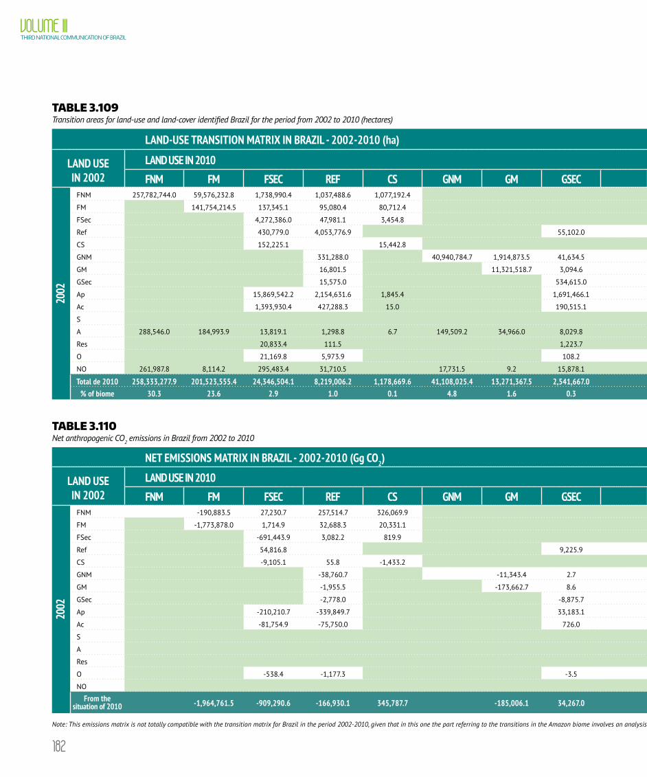
182
VOLUME IIITHIRD NATIONAL COMMUNICATION OF BRAZIL
TABLE 3.109 Transition areas for land-use and land-cover identified Brazil for the period from 2002 to 2010 (hectares)
LAND-USE TRANSITION MATRIX IN BRAZIL - 2002-2010 (ha)
LAND USE IN 2002
LAND USE IN 2010TOTAL 2002 % OF
BIOMEFNM FM FSEC REF CS GNM GM GSEC AP AC S A RES O NO
2002
FNM 257,782,744.0 59,576,232.8 1,738,990.4 1,037,488.6 1,077,192.4 25,351,075.4 4,763,886.4 100,283.7 652,243.8 819,479.4 79,907.7 16,963,969.3 369,943,494.0 43.4
FM 141,754,214.5 137,345.1 95,080.4 80,712.4 1,621,696.0 157,204.9 20,124.8 334,808.0 79,243.6 18,764.7 8,978,316.1 153,277,510.6 18.0
FSec 4,272,386.0 47,981.1 3,454.8 1,294,837.6 129,182.1 4,452.3 8,704.6 12,235.8 822.5 99,667.1 5,873,723.9 0.7
Ref 430,779.0 4,053,776.9 55,102.0 536,817.5 385,005.1 5,217.9 3,010.0 917.3 1,577.7 227,572.5 5,699,775.9 0.7
CS 152,225.1 15,442.8 63,614.5 27,210.0 0.6 1,117.6 259,610.6 0.0
GNM 331,288.0 40,940,784.7 1,914,873.5 41,634.5 4,388,778.7 1,659,017.4 20,174.2 194,881.1 149,949.0 12,007.2 798,930.4 50,452,318.7 5.9
GM 16,801.5 11,321,518.7 3,094.6 268,303.3 50,082.2 4,415.0 42,947.8 14,141.2 3,635.2 308,598.0 12,033,537.5 1.4
GSec 15,575.0 534,615.0 115,482.3 46,990.4 252.9 1,887.9 1,202.5 53.5 1,361.9 717,421.5 0.1
Ap 15,869,542.2 2,154,631.6 1,845.4 1,691,466.1 133,035,733.9 13,323,667.4 455,405.2 148,393.1 181,420.9 53,720.1 7,501,723.6 174,417,549.7 20.5
Ac 1,393,930.4 427,288.3 15.0 190,515.1 5,241,169.5 47,617,890.4 160,335.2 55,420.1 32,193.3 9,378.2 503,632.9 55,631,768.3 6.5
S 3,135,527.7 5,956.9 3,141,484.7 0.4
A 288,546.0 184,993.9 13,819.1 1,298.8 6.7 149,509.2 34,966.0 8,029.8 115,993.7 117,403.5 5,821.2 14,593,311.6 103,499.1 14,858.2 929,694.3 16,561,751.0 1.9
Res 20,833.4 111.5 1,223.7 16,878.7 6,659.9 270.1 56,989.5 1,991,958.3 1,788.0 10,108.2 2,106,821.2 0.2
O 21,169.8 5,973.9 108.2 12,925.9 2,660.5 2,344.6 1,236.3 2,160.6 393,263.5 2,475.6 444,318.9 0.1
NO 261,987.8 8,114.2 295,483.4 31,710.5 17,731.5 9.2 15,878.1 416,163.7 243,211.6 6,291.0 2,104.9 1,317.6 308.0 326,147.2 1,626,458.7 0.2
Total de 2010 258,333,277.9 201,523,555.4 24,346,504.1 8,219,006.2 1,178,669.6 41,108,025.4 13,271,367.5 2,541,667.0 172,479,470.8 68,530,071.7 3,920,916.3 16,095,938.7 3,389,718.7 590,084.5 36,659,271.6 852,187,545.2% of biome 30.3 23.6 2.9 1.0 0.1 4.8 1.6 0.3 20.2 8.0 0.5 1.9 0.4 0.1 4.3
TABLE 3.110 Net anthropogenic CO2 emissions in Brazil from 2002 to 2010
NET EMISSIONS MATRIX IN BRAZIL - 2002-2010 (Gg CO2)
LAND USE IN 2002
LAND USE IN 2010FROM THE SITUATION OF 2002
FNM FM FSEC REF CS GNM GM GSEC AP AC S A RES O NO
2002
FNM -190,883.5 27,230.7 257,514.7 326,069.9 10,058,181.8 1,350,031.2 41,608.0 282,478.5 39,876.8 12,192,108.1
FM -1,773,878.0 1,714.9 32,688.3 20,331.1 829,493.2 41,137.4 10,015.9 39,436.1 9,537.7 -789,523.4
FSec -691,443.9 3,082.2 819.9 488,551.5 22,765.8 1,406.6 2,455.9 847.1 -171,515.0
Ref 54,816.8 9,225.9 83,260.9 71,450.1 1,099.9 196.9 308.2 220,358.6
CS -9,105.1 55.8 -1,433.2 33,500.3 9,372.4 0.0 236.5 32,626.7
GNM -38,760.7 -11,343.4 2.7 210,983.6 94,235.7 1,912.0 14,252.1 1,114.7 272,396.7
GM -1,955.5 -173,662.7 8.6 14,220.5 3,283.1 489.6 1,818.1 348.3 -155,450.1
GSec -2,778.0 -8,875.7 456.4 905.9 15.1 53.5 3.2 -10,219.6
Ap -210,210.7 -339,849.7 33,183.1 234,546.2 25,422.4 7,707.0 3,057.9 -246,143.7
Ac -81,754.9 -75,750.0 726.0 -83,178.4 7,141.4 1,186.2 393.3 -231,236.3
S
A
Res
O -538.4 -1,177.3 -3.5 -735.7 -72.3 -2,527.2
NO
From the situation of 2010 -1,964,761.5 -909,290.6 -166,930.1 345,787.7 -185,006.1 34,267.0 11,634,734.0 1,827,655.5 89,110.9 349,584.3 55,723.6 11,110,874.8
Note: This emissions matrix is not totally compatible with the transition matrix for Brazil in the period 2002-2010, given that in this one the part referring to the transitions in the Amazon biome involves an analysis of the intermediate 2005 situation.
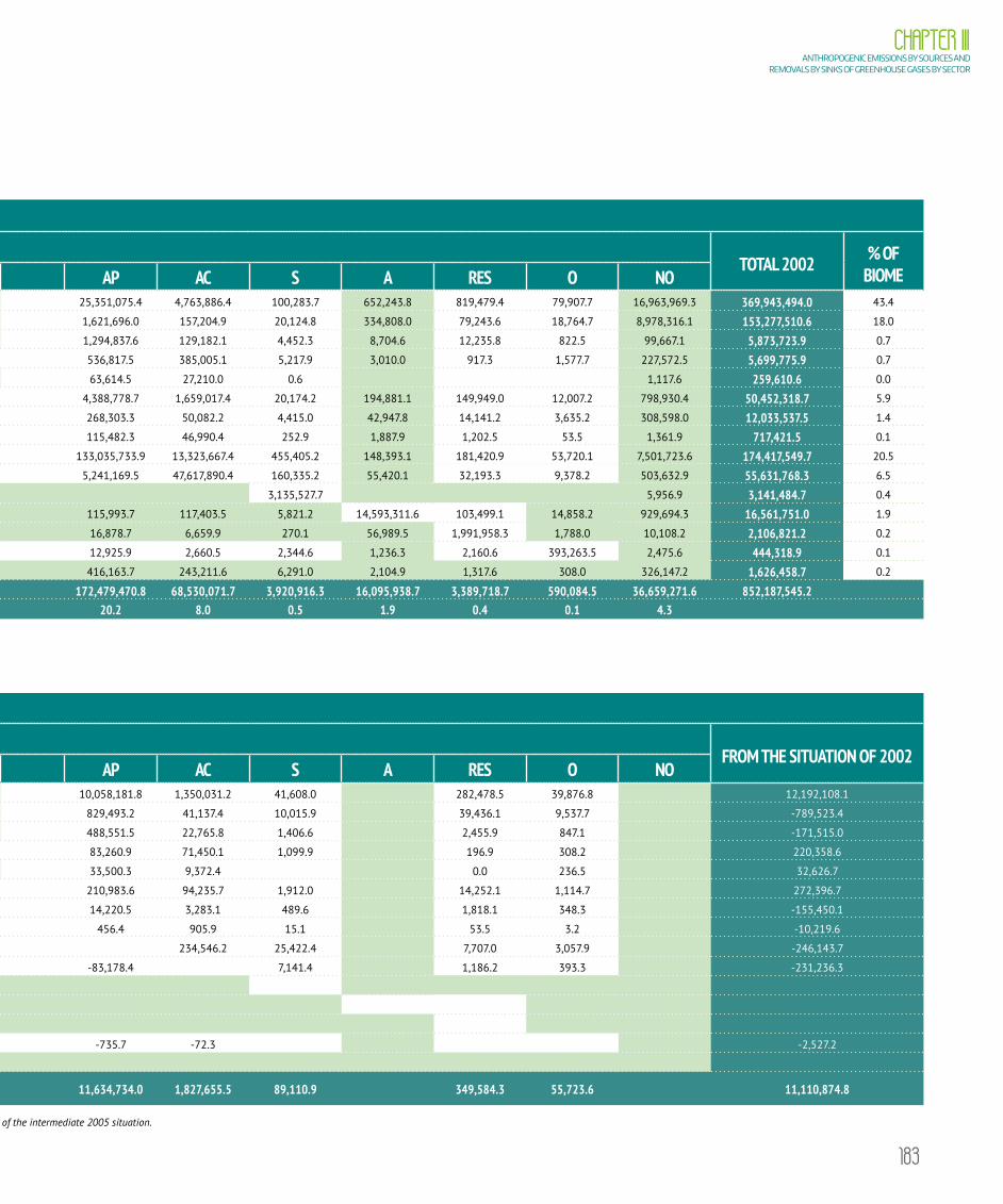
183
CHAPTER IIIANTHROPOGENIC EMISSIONS BY SOURCES AND
REMOVALS BY SINKS OF GREENHOUSE GASES BY SECTOR
TABLE 3.109 Transition areas for land-use and land-cover identified Brazil for the period from 2002 to 2010 (hectares)
LAND-USE TRANSITION MATRIX IN BRAZIL - 2002-2010 (ha)
LAND USE IN 2002
LAND USE IN 2010TOTAL 2002 % OF
BIOMEFNM FM FSEC REF CS GNM GM GSEC AP AC S A RES O NO
2002
FNM 257,782,744.0 59,576,232.8 1,738,990.4 1,037,488.6 1,077,192.4 25,351,075.4 4,763,886.4 100,283.7 652,243.8 819,479.4 79,907.7 16,963,969.3 369,943,494.0 43.4
FM 141,754,214.5 137,345.1 95,080.4 80,712.4 1,621,696.0 157,204.9 20,124.8 334,808.0 79,243.6 18,764.7 8,978,316.1 153,277,510.6 18.0
FSec 4,272,386.0 47,981.1 3,454.8 1,294,837.6 129,182.1 4,452.3 8,704.6 12,235.8 822.5 99,667.1 5,873,723.9 0.7
Ref 430,779.0 4,053,776.9 55,102.0 536,817.5 385,005.1 5,217.9 3,010.0 917.3 1,577.7 227,572.5 5,699,775.9 0.7
CS 152,225.1 15,442.8 63,614.5 27,210.0 0.6 1,117.6 259,610.6 0.0
GNM 331,288.0 40,940,784.7 1,914,873.5 41,634.5 4,388,778.7 1,659,017.4 20,174.2 194,881.1 149,949.0 12,007.2 798,930.4 50,452,318.7 5.9
GM 16,801.5 11,321,518.7 3,094.6 268,303.3 50,082.2 4,415.0 42,947.8 14,141.2 3,635.2 308,598.0 12,033,537.5 1.4
GSec 15,575.0 534,615.0 115,482.3 46,990.4 252.9 1,887.9 1,202.5 53.5 1,361.9 717,421.5 0.1
Ap 15,869,542.2 2,154,631.6 1,845.4 1,691,466.1 133,035,733.9 13,323,667.4 455,405.2 148,393.1 181,420.9 53,720.1 7,501,723.6 174,417,549.7 20.5
Ac 1,393,930.4 427,288.3 15.0 190,515.1 5,241,169.5 47,617,890.4 160,335.2 55,420.1 32,193.3 9,378.2 503,632.9 55,631,768.3 6.5
S 3,135,527.7 5,956.9 3,141,484.7 0.4
A 288,546.0 184,993.9 13,819.1 1,298.8 6.7 149,509.2 34,966.0 8,029.8 115,993.7 117,403.5 5,821.2 14,593,311.6 103,499.1 14,858.2 929,694.3 16,561,751.0 1.9
Res 20,833.4 111.5 1,223.7 16,878.7 6,659.9 270.1 56,989.5 1,991,958.3 1,788.0 10,108.2 2,106,821.2 0.2
O 21,169.8 5,973.9 108.2 12,925.9 2,660.5 2,344.6 1,236.3 2,160.6 393,263.5 2,475.6 444,318.9 0.1
NO 261,987.8 8,114.2 295,483.4 31,710.5 17,731.5 9.2 15,878.1 416,163.7 243,211.6 6,291.0 2,104.9 1,317.6 308.0 326,147.2 1,626,458.7 0.2
Total de 2010 258,333,277.9 201,523,555.4 24,346,504.1 8,219,006.2 1,178,669.6 41,108,025.4 13,271,367.5 2,541,667.0 172,479,470.8 68,530,071.7 3,920,916.3 16,095,938.7 3,389,718.7 590,084.5 36,659,271.6 852,187,545.2% of biome 30.3 23.6 2.9 1.0 0.1 4.8 1.6 0.3 20.2 8.0 0.5 1.9 0.4 0.1 4.3
TABLE 3.110 Net anthropogenic CO2 emissions in Brazil from 2002 to 2010
NET EMISSIONS MATRIX IN BRAZIL - 2002-2010 (Gg CO2)
LAND USE IN 2002
LAND USE IN 2010FROM THE SITUATION OF 2002
FNM FM FSEC REF CS GNM GM GSEC AP AC S A RES O NO
2002
FNM -190,883.5 27,230.7 257,514.7 326,069.9 10,058,181.8 1,350,031.2 41,608.0 282,478.5 39,876.8 12,192,108.1
FM -1,773,878.0 1,714.9 32,688.3 20,331.1 829,493.2 41,137.4 10,015.9 39,436.1 9,537.7 -789,523.4
FSec -691,443.9 3,082.2 819.9 488,551.5 22,765.8 1,406.6 2,455.9 847.1 -171,515.0
Ref 54,816.8 9,225.9 83,260.9 71,450.1 1,099.9 196.9 308.2 220,358.6
CS -9,105.1 55.8 -1,433.2 33,500.3 9,372.4 0.0 236.5 32,626.7
GNM -38,760.7 -11,343.4 2.7 210,983.6 94,235.7 1,912.0 14,252.1 1,114.7 272,396.7
GM -1,955.5 -173,662.7 8.6 14,220.5 3,283.1 489.6 1,818.1 348.3 -155,450.1
GSec -2,778.0 -8,875.7 456.4 905.9 15.1 53.5 3.2 -10,219.6
Ap -210,210.7 -339,849.7 33,183.1 234,546.2 25,422.4 7,707.0 3,057.9 -246,143.7
Ac -81,754.9 -75,750.0 726.0 -83,178.4 7,141.4 1,186.2 393.3 -231,236.3
S
A
Res
O -538.4 -1,177.3 -3.5 -735.7 -72.3 -2,527.2
NO
From the situation of 2010 -1,964,761.5 -909,290.6 -166,930.1 345,787.7 -185,006.1 34,267.0 11,634,734.0 1,827,655.5 89,110.9 349,584.3 55,723.6 11,110,874.8
Note: This emissions matrix is not totally compatible with the transition matrix for Brazil in the period 2002-2010, given that in this one the part referring to the transitions in the Amazon biome involves an analysis of the intermediate 2005 situation.
184
VOLUME IIITHIRD NATIONAL COMMUNICATION OF BRAZIL
3.5.2.8. Annual net anthropogenic CO2 emissions for the period 1990 to 2010The consolidated results presented in section 3.5.2.7 represent the estimates of the average net anthropogenic
emissions for the period 1994 to 2002 for all biomes, and 2002 to 2010 for all biomes except for the Amazon, which
was evaluated in two periods from 2002 to 2005, and from 2005 to 2010.
Based on these results, the net annual anthropogenic CO2 emissions for the period 1990-1994 were recalculated.
Net annual anthropogenic CO2 emissions for the period 1990-1994
This Third Inventory maintains the Second Inventory’s approach, when gross emission values were updated in
order to reflect carbon estimates of new stocks included (belowground living biomass, dead wood and litter), which
were not included in the Initial Inventory. The average CO2 emission values obtained were considered constant
for the years from 1990 to 1994 for all the biomes, except for the Amazon, which had gross total emission values
for the period from 1990 to 1994 distributed proportionally by year following gross deforestation variation values
observed by the PRODES8.
An amendment was made in relation to the Second Inventory related to CO2 removal by sinks of the managed
areas from 1990 to 1994, in which the same annual carbon removal of 0.62 t C/ha was considered throughout the
years in the managed areas of forest physiognomy identified in 1994 and considered as the same since 1990 for
all biomes. In this Inventory, each biome has its average removal rate: 0.43 t C/ha for the Amazon; 0.32 t C/ha for
Atlantic Forest and Pampa (whose removals of managed areas had not been not included); 0.20 t C/ha for Cerrado
and Pantanal; and 0.10 t C/ha for the Caatinga. Moreover, the forest physiognomy areas regarded as managed areas
were amended for the year of 1994.
Net annual anthropogenic CO2 emissions for the period 1994 to 2002
The average annual emission obtained for CO2 emissions for the 1994-2002 period was calculated for all
biomes, except for the Amazon biome, as a ratio of total net emissions for the period and the number of years of the
period (8 years). Consequently, this results in a linear distribution of emissions throughout the period. The Amazon
biome’s gross annual emissions (basically associated with primary forests converted to other uses) were estimated
by using an annual time series of gross deforestation generated by INPE (PRODES), resulting in an inconstant total
emission for each year of the period considered.
Annual net anthropogenic emissions for the period 2002 to 2010
Net average annual emission for the period from 2002 to 2010 was calculated for the Amazon for two
distinct periods: 2002-2005 and 2005-2010, adopting the same approach used for the period 1994-2002. The
information available on deforestation for the periods 2002-2008, and 2008-2009 for other biomes, provided by
the “Monitoring Project for the Brazilian Biomes Deforestation”9, allowed the application of the same approach
8 Project for Estimating Gross Deforestation of the Brazilian Amazon (PRODES), which accounts for clear cutting in the region. Information available at: http://www.obt.inpe.br/prodes/index.php
9 A partnership of IBAMA Remote Sensing Center, Secretary of Biodiversity and Forests of the Ministry of Environment and UNDP. Available in: http://siscom.ibama.gov.br/monitorabiomas/index.htm

185
CHAPTER IIIANTHROPOGENIC EMISSIONS BY SOURCES AND
REMOVALS BY SINKS OF GREENHOUSE GASES BY SECTOR
used in the Amazon for other biomes. Exceptionally for the Cerrado, deforestation estimates for the period 2009-
2010 was also originated from the abovementioned project. As a consequence, gross annual emissions for all
biomes were calculated using existing gross deforestation data for each biome. For 2010, the same annual gross
emission calculated for the year of 2009 for all biomes was presumed, except for the Amazon and the Cerrado.
Annual CO2 removals were estimated based on even distribution for the considered period. The results are
summarized in Table 3.111, which also lays out CO2 caused by liming of soils.
TABLE 3.111 Summary of annual net anthropogenic CO2 emissions for the period 1990-2010 per biome
SOURCE1990 1995 2000 2005 2010
SHARE IN
2010*
VARIATION 2005-2010
Gg %Land-Use Change 751,867 1,832,113 1,188,458 1,790,368 300,312 96.6 -83.2
Amazon Biome 437,574 1,459,071 815,416 1,128,545 162,888 52.4 -85.6
Cerrado Biome 241,511 212,958 212,958 282,275 58,755 18.9 -79.2
Atlantic Forest Biome 26,115 111,072 111,072 329,662 69,104 22.2 -79.0
Caatinga Biome 28,643 23,774 23,774 14,382 -4,291 -1.4 -129.8
Pantanal Biome 18,161 21,640 21,640 21,450 2,606 0.8 -87.9
Pampa Biome -137 3,598 3,598 14,054 11,250 3.6 -20.0
Liming 5,103 5,395 8,717 7,474 10,424 3.4 39.5
Total 756,970 1,837,508 1,197,175 1,797,842 310,736 100.0 -82.7
Other greenhouse gas emissions from burning
When the forest is converted to agricultural or livestock use, part of the original biomass is removed as
commercial timber or as firewood for charcoal or other fuel uses. The remaining wood debris left on the field are
usually burned in a non-efficient manner. As result, greenhouse gases such as CH4, N2O, CO and NOx are emitted
under this imperfect combustion. Here, only emissions associated with deforestation are calculated. Appendix II
shows assessments and considerations on burnings that are not related to deforestation.
In order to evaluate what is being burned on the field it is necessary to estimate the fraction removed before
combustion to be used somewhere else. In the Second Inventory, IBGE statistics on timber, charcoal and firewood
annual consumption, which are derived from extractive activities in native forests, were used as proxy. The
quantities of firewood, timber and charcoal derived from planted forests were not considered. The sum of timber
and charcoal from vegetable extraction and silviculture provided by the IBGE is far below the data provided by the
National Energy Balance (BEN), which is the main source of information for the Energy sector.

186
VOLUME IIITHIRD NATIONAL COMMUNICATION OF BRAZIL
Hence, the Third Inventory considered, in the case of firewood and charcoal, only the firewood data informed by
BEN, which includes firewood used for charcoal production and charcoal. As for timber harvesting, this Inventory
considered the part derived from vegetable extraction and silviculture (for the production of paper and pulp and
other uses), as informed by IBGE.
Quantities of firewood and wood extracted in round timbers had 25% humidity, according to the Reference
Report of the Energy sector (Bottom-Up approach – Methodological Annex), in order to keep information coherent.
Conversion to dry matter is necessary for the comparison with timber removed from forests to other uses and for
the correct application of emission factors for non-CO2 gases related to dry biomass.
Gross emissions resulting from forest conversion to other uses, except selective logging, and the ones resulting
from the conversion of native grassland to other uses were converted to dry matter, first for CO2 to C conversion, then
by considering carbon as being 47% of this dry matter. From this dry matter, the quantities extracted proportionally
to the gross emissions considered were deducted.
For the period 2005 a 2010 the fraction of carbon removed as commercial timber jumped from 3% to 7% of total
dry matter available from deforestation. On the other hand, the fraction removed as charcoal and firewood jumped
from 2% to 5% of total dry matter available from deforestation in the same period. This means that the biomass
effectively burned decreased from 95% to 88% of the total biomass available over that period of deforestation.
As for the combustion factor, an average value was estimated for each biome, differentiating the vegetation
structure between forest and native field, according to Table 3.112. Given that these factors were used for the
estimate of burning associated with deforestation, priority has been given to works carried out in slash and burn
areas. In the absence of such works, the values used are derived from burned areas, mainly for grassy field and
savannah vegetation.
TABLE 3.112 Combustion factors by biome, according to the vegetation structure, for the estimate of emissions from deforestation-related combustion, and sources used
BIOME STRUCTURE COMBUSTION FACTOR SOURCES
Amazon
Field 69.3 ² BARBOSA & FEARNSIDE, 2005
Forest 35.6 ¹
WARD et al., 1992; KAUFFMAN et al., 1995; ARAUJO et al., 1999;
FEARNSIDE et al., 1993; 1999; 2001; CARVALHO et al., 1995; 1998;
2001; DE ALENCASTRO GRAÇA et al., 1999
CerradoField 88.0 ² CASTRO & KAUFFMAN, 1998
Forest 43.5 ² CASTRO & KAUFFMAN, 1998
CaatingaField 88.0 ² Same as Cerrado
Forest 43.5 ² Same as Cerrado
Atlantic ForestField 88.0 ² Same as Cerrado
Forest 35.6 ¹ Same as Amazon
continues on the next page
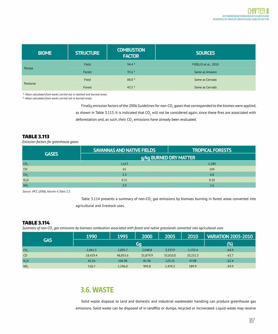
187
CHAPTER IIIANTHROPOGENIC EMISSIONS BY SOURCES AND
REMOVALS BY SINKS OF GREENHOUSE GASES BY SECTOR
BIOME STRUCTURE COMBUSTION FACTOR SOURCES
PampaField 94.4 ² FIDELIS et al., 2010
Forest 35.6 ¹ Same as Amazon
PantanalField 88.0 ² Same as Cerrado
Forest 43.5 ² Same as Cerrado
¹- Value calculated from works carried out in slashed and burned areas. ²- Value calculated from works carried out in burned areas.
Finally, emission factors of the 2006 Guidelines for non-CO2 gases that corresponded to the biomes were applied,
as shown in Table 3.113. It is indicated that CO2 will not be considered again, since these fires are associated with
deforestation and, as such, their CO2 emissions have already been evaluated.
TABLE 3.113 Emission factors for greenhouse gases
GASESSAVANNAS AND NATIVE FIELDS TROPICAL FORESTS
g/kg BURNED DRY MATTERCO2 1,613 1,580
CO 65 104
CH4 2.3 6.8
N2O 0.21 0.20
NOx 3.9 1.6
Source: IPCC (2006), Volume 4, Table 2.5.
Table 3.114 presents a summary of non-CO2 gas emissions by biomass burning in forest areas converted into
agricultural and livestock uses.
TABLE 3.114 Summary of non-CO2 gas emissions by biomass combustion associated with forest and native grasslands converted into agricultural uses
GAS1990 1995 2000 2005 2010 VARIATION 2005-2010
Gg (%)CH4 1,041.5 2,895.7 2,048.8 3,237.9 1,135.4 -64.9
CO 18,429.4 48,855.6 35,879.9 55,810.0 20,231.3 -63.7
N2O 42.56 106.98 81.96 125.25 47.08 -62.4
NOx 526.7 1,196.0 993.8 1,470.3 589.9 -59.9
3.6. WASTE Solid waste disposal to land and domestic and industrial wastewater handling can produce greenhouse gas
emissions. Solid waste can be disposed of in landfills or dumps, recycled or incinerated. Liquid waste may receive

188
VOLUME IIITHIRD NATIONAL COMMUNICATION OF BRAZIL
various forms of physical and chemical or biological treatments, whereas biological treatment can occur via
aerobic or anaerobic decomposition. In turn, waste incineration, like every combustion, generates GHG emissions,
depending on waste composition; however, this activity is not widespread in Brazil.
CH4 is the most important gas produced in the Waste sector, and may occur as a result from both solid waste
disposal to land and anaerobic wastewater handling. Significant quantities of emissions of CH4 produced are
released as a by-product of the waste anaerobic decomposition. The two major sources are waste disposal in
landfills and anaerobic wastewater treatments.
N2O emissions can also occur in domestic wastewater treatment, and are calculated on the basis of nitrogen
content in food.
This inventory estimates CH4 emissions from solid waste disposal to land and from domestic and industrial
wastewater handling. CO2 and N2O emissions from incineration and N2O emissions from human sewage treatment
are also considered.
In order to estimate greenhouse gas emissions from the Waste sector, the following data were necessary: urban
population, urban solid waste generation rates at municipal level and organic matter generation rates for wastewater
treatment, besides incinerated quantities. These data were gathered during the entire period of the elaboration of estimates.
However, part of the data needed for the estimations are not available for the entire country. In addition, some
data, such as waste disposal conditions, volume of generated waste, landfill or dump installations, as well as
wastewater treatment systems, organic matter content and type of incinerated waste, present large uncertainty.
3.6.1. Solid waste disposalWaste disposal in landfills and dumps generates CH4 under certain conditions, including: the amount of waste,
the deposit’s age, the presence of an anaerobic environment, acidity and handling conditions and facilities. The
better the landfill control conditions and the deeper the dump, which improve sanitary conditions, the greater CH4
emission potential.
The methodology for estimating CH4 emissions from solid waste disposal to land was the first order decay
method (Tier 2), as described in the Good Practice Guidance 2000. According to this method, CH4 emissions
persist over a long period of time, after waste disposal. The following data were necessary for the Tier 2 method
application: urban population, climate data (annual temperature and rainfall averages), quantity of waste disposed,
waste composition, quality of landfill operation and quantities of recovered and oxidized CH4, since 1970.
Data related to urban population of all municipalities in Brazil used in these estimates correspond to those
available in IBGE censuses for 1970, 1980, 1991 and 2000, and the 2010 Population Count. Waste generation types
and rates vary due to the country’s large territorial extension and to regional, economic and social differences.
The product of waste generation rate per capita and urban population estimated the amount of waste disposed
in landfills. Solid waste generation per capita rate was estimated based on data from CETESB and from the Brazilian
Association of Public Cleaning and Special Waste Companies (ABRELPE in the Portuguese acronym). In the past, according
to studies conducted by CETESB, the rate of waste generation per capita ranged between 0.4 and 0.7 kg/capita/day, with

189
CHAPTER IIIANTHROPOGENIC EMISSIONS BY SOURCES AND
REMOVALS BY SINKS OF GREENHOUSE GASES BY SECTOR
an estimated average daily rate of 0.5 kg/hab. This value was adopted in this Inventory as primary data of 1970. As of
2008 this rate became data published by ABRELPE (ABRELPE, 2008; 2009; 2010), calculated for each region of the country.
Thus, the rate of the years between 1970 and 2008 is estimated by the linear interpolation of the rates of 1970 and 2008.
Data on waste composition were classified as recommended in the Good Practice Guidance 2000 in the following
types of waste: paper and textiles; garden and other nonfood putrescible; food waste and wood and straw. Linear
regressions were used in estimates for each region of the country based on the waste composition data available
for some states and municipalities.
The following recommended classification was used for the methane correction factor: managed landfills (1.0),
unmanaged sites with a depth equal to or greater than five meters (0.8), and unmanaged sites with a depth less
than five meters (0.4). Furthermore, default values were adopted for the fraction of degradable organic carbon that
truly degrades (0.5) and for the fraction of methane in landfill gas (0.5).
To estimate CH4 emissions, the amount of methane recovered/oxidated should be discounted. For the 1990-2002
period, these amounts were deemed to be zero. From 2003 onwards, CH4 emissions reductions were considered
according to the monitoring reports for landfill CDM activity projects, for which there was monitoring reports
checked by Designated Operational Entities, as the regulation of CDM Executive Board.
It should be noted that small quantities of CH4 are deducted of the states emissions where are the CDM project
activities. As a landfill can receive waste from several municipalities, the amount of recovered methane can be
higher than the corresponding emission of a municipality, estimated on the basis of its urban population and other
parameters described throughout the document.
For cities with over 1,000,000 inhabitants, the existence of managed landfills was assumed. For these cases, the
oxidation factor (OX) – which reflects CH4 combustion that may happen in the landfill surface – of 0.1 was adopted,
according to the Good Practice Guidance 2000. For cities with fewer inhabitants, this factor was assumed to be null.
Based on these assumptions, CH4 emissions from solid waste disposal to land were estimated and are shown
in Table 3.115.
TABLE 3.115 CH4 emissions from solid waste disposal
SOURCE1990 1995 2000 2005 2010 VAR.
2005/2010
(Gg CH4) (%)Solid waste disposal 824.4 965.3 1,149.4 1,237.1 1,327.0 7.3
An increase in CH4 emissions was identified for the period due to demographic growth, changes in habits, life quality
improvement and industrial development, which caused an increase in the amount of waste generated. However, the
activities of CDM projects contributed to reduce part of this increase, due to the recovery and oxidation of CH4. The national
emissions would be higher without the reductions achieved by the CDM projects, which were 208.4 Gg CH4 in 2010.

190
VOLUME IIITHIRD NATIONAL COMMUNICATION OF BRAZIL
3.6.2. Waste incinerationGiven the difficulty in disposing of solid waste in Brazil’s metropolitan regions, alternative ways have been
considered and waste incineration stands out among the possible alternatives identified.
Incineration of urban waste has been more often considered as an alternative in large cities due to the increasing
cost of waste transportation to landfills, since these are getting farther away from metropolitan regions. This practice
is applied to a small fraction of total treated waste, and is most used for hazardous waste from industry and clinical
waste, which, in general, cannot be disposed of in common landfills and require special treatment. The incineration of
solid waste and municipal wastewater sludge was disregarded since they were not relevant in the period.
For the estimation of emissions of CO2 and N2O from the incineration of waste, the 2000 Good Practice Guidance
methodology was used. According to this methodology, the type of waste being incinerated determines the estimate
of CO2 emissions, the carbon contained in the type of waste, its fraction of fossil carbon and the burning efficiency
of the incinerators. Similarly, the estimate of N2O emissions is determined by the type and quantity of waste
incinerated and the emission factor for each type of waste.
For the carbon fossil part of the waste, the following Good Practice Guidance 2000 default values were used: 60 g C / g
clinical waste and 50 g C / g hazardous waste of industrial origin. The same value was adopted for fossil carbon percentage
in the other types of waste, and for this calculation the default values of the Good Practice Guidance 2000 were used.
Regarding the incinerators burning efficiency, no national data were identified. Thus, Good Practice Guidance
2000 default values were adopted. 2006 Guidelines default values were applied for the N2O emission factor, since
this information was not available in the IPCC previous guidelines.
Data for hazardous waste incineration were obtained from the Brazilian Association of Waste Treatment
Companies (ABETRE, 2006), National Sanitation Information System (SNIS) and incinerator operators and
manufacturers that responded to the data request made by CETESB. Emissions are shown in Table 3.116.
TABLE 3.116 CO2 and N2O emissions from solid waste incineration
GAS1990 1995 2000 2005 2010
VAR. 2005/2010
(Gg) (%)
CO2 19 78 95 128 175 36.7%
N2O 0.00 0.00 0.01 0.01 0.01 0.0%
3.6.3. Wastewater treatment Wastewater with high organic matter content has great CH4 emission potential, such as domestic and commercial
wastewater, effluents from food and beverage industries and those from the pulp and paper industry. In the case
of domestic wastewater, N2O emissions can occur due to the nitrogen content in human food. N2O emissions were
estimated by the amount of nitrogen present in human waste.

191
CHAPTER IIIANTHROPOGENIC EMISSIONS BY SOURCES AND
REMOVALS BY SINKS OF GREENHOUSE GASES BY SECTOR
3.6.3.1. Domestic and commercial wastewaterCH4 emissions were estimated based on the amount of organic material present in wastewater, expressed in
terms of Biochemical Oxygen Demand (BOD), which represents the amount of oxygen consumed by microorganisms
in the biochemical oxidation of organic matter.
Several systems are used for treating effluents in Brazil. Nevertheless, a large amount of sewage is discharged
directly into rivers and ocean, without treatment. According to the National Survey on Basic Sanitation (PNSB)
(IBGE, 1989; 2000; 2008), the untreated domestic wastewater thrown into water bodies has reduced, but the
advances were not very significant once compared to the population increase during the same period. Among the
various collective options for the biological treatment, the most commonly used in Brazil are the stabilization
lagoons and the various modifications of the activated sludge process, particularly those that employ the concept
of extended aeration and biological filters.
The emission of CH4 is estimated from the organic matter present in wastewater, expressed in terms of
Biochemical Oxygen Demand (BOD). The volume of wastewater generated per person depends on the quantity of
water consumed and usually corresponds to 80% of this consumption. The organic unit load varies from country to
country, between 0.02 and 0.08g BOD per inhabitant per day. The average BOD per capita of 0.054 kg BOD/ (hab.
day) in Brazil was used. For the maximum production capacity of methane, the default value of the 2000 Good
Practice Guidance, equal to 0.60 kg CH4/kg BOD, was used.
The population considered in this study is the one generating wastewater, given that domestic effluents are generated
the by the use of water for the transportation of domestic waste. The population that generates wastewater can be
estimated by the product between the total population of Brazil and the fraction of households with sinkhole. This
fraction is obtained by the ratio of the total households and households without a sinkhole (IBGE 1991; 2000; 2010).
The organic matter of domestic wastewater can be increased by launching industrial effluents into the urban sewage
systems or reduced by rainfall infiltrations in the sewage system. However, these data were considered to be null, since
there is no information on it. Anaerobic treatments in wastewater plants were considered, and they include anaerobic
digester for sludge, anaerobic processes in reactors and ponds, latrines and septic systems. Organic matter discharges
into the sea, rivers and lakes, in which CH4 emissions occur through anaerobic reactions, were also considered.
Methane recovered in anaerobic reactors and in anaerobic digesters of activated sludge systems was considered
to be completely destroyed in a burner, since that is the common practice in Brazil. Therefore, it was considered that
100% of the recovered methane is burned. Burner’s efficiency was considered to be of approximately 50%. Methane
oxidation was considered null for emissions at septic systems and anaerobic lagoon systems and for discharges of
untreated wastewater into water bodies.
Besides CH4, N2O emissions from human waste were also estimated based on population and on average
annual consumption per capita of protein, by state or region and the country’s population.
Data for protein consumption per capita were taken from FAO’s publication (FAO, 2009). The study identified
average values of 76.8g/day/person for the period 1994-1996, 79.4g/day/person for the period 1999-2001 and
84.5g/day/person for the period 2003-2005. Population data were the same as those used for CH4 estimates.
CH4 and N2O emissions due to the treatment of domestic and commercial wastewater are presented in Table 3.117
for the years 1990, 1995, 2000, 2005 and 2010.

192
VOLUME IIITHIRD NATIONAL COMMUNICATION OF BRAZIL
TABLE 3.117 Emissions from domestic and commercial wastewater treatment
GAS1990 1995 2000 2005 2010 VAR.
2005/2010
(Gg) (%)CH4 266.7 304.3 371.7 436.6 512.8 17.5%
N2O 4.32 4.83 5.67 6.60 7.20 9.1%
3.6.3.2. Industrial wastewaterIndustrial wastewater has been traditionally treated through the use of pond or activated sludge processes and
biological filters, besides the use of anaerobic reactors.
For this Inventory, industrial activities were kept with the greatest potential for methane emissions selected for the
Second Inventory, excluding emissions due to the consumption of cotton because of the uncertainties about the destination.
The improvement of the data survey for the estimation of emissions from industrial effluents included a survey to update
and review the emission data of organic load, in addition to the update of the effluent treatment of each industrial sector.
For the estimation of the emissions of CH4, data of the industrial production and the emission factor for each of the
sectors considered were used. The data relating to the industrial production of these sectors are presented in Table 3.118.
TABLE 3.118 Industrial production in main sectors that contribute to industrial wastewater emission
PRODUCT [UNIT] 1990 1995 2000 2005 2010VAR.
2005/2010
(%)Sugar [t] (a) 7,214,050 12,651,628 19,387,603 26,685,095 32,956,359 23.5%
Raw milk [1000 L] (b1) 14,484,000 18,110,938 22,014,202 24,660,202 30,163,539 22.3%
Alcohol [m3] (a) 11,920,335 12,751,811 12,983,108 15,388,567 25,690,918 66.9%
Cellulose [t] (c) 4,351,143 5,936,000 7,463,000 10,352,000 14,164,000 36.8%
Beer [1000 L] (b2) 3,749,150 8,037,262 9,023,303 9,865,939 12,947,054 31.2%
Slaughtering of poultry [t] (e) 1,604,696 2,317,657 3,316,897 6,411,962 8,609,058 34.3%
Slaughtering of cattle [t] (e) 2,835,762 2,533,950 2,163,855 6,144,629 7,445,632 21.2%
Slaughtering of swine [t] (e) 729,545 824,572 672,962 2,886,889 4,075,714 41.2%
Pasteurized milk [1000 L] (d) 4,054,000 3,150,000 1,630,000 1,550,000 1,690,000 9.0%
Source: (a) Unica, 2014; (b1) Abia, 2010; (b2) Abia, 2014; (c) IBA ( 2014); (d) ABVL, 2014; (e) IBGE - PIA - Product, 1998 to 2004 and IBGE - Statistical yearbook, 1990 to 1993 and 2011.

193
CHAPTER IIIANTHROPOGENIC EMISSIONS BY SOURCES AND
REMOVALS BY SINKS OF GREENHOUSE GASES BY SECTOR
Despite the great potential of methane emissions due to the high organic wastewater load, sugar and ethanol
industry effluents do not represent a source of CH4 emissions, since their effluents are discharged directly into
the soil as fertilizer without anaerobic treatment. Emissions from this sector were considered null, as in the
previous inventories.
Table 3.119 presents the data on the emission of organic load used in the estimate, which, once multiplied by
the maximum production capacity of CH4 0.60 kgCH4.kgBOD-1, provides the emission factor for each industrial sector.
TABLE 3.119 Organic load emission for each industrial sector
INDUSTRIAL SECTORORGANIC LOAD EMISSION
(kg BOD / t)Sugar 200
Raw milk 16.8
Alcohol 220
Cellulose 64.8
Beer 9.45
Poultry 5.85
Cattle 32.5
Swine 32.5
Pasteurized milk 16.8
Emissions estimates from industrial wastewater treatment are presented in Table 3.120.
TABLE 3.120 CH4 emissions from industrial wastewater treatment
GAS1990 1995 2000 2005 2010 VAR.
2005/2010
(Gg CH4) (%)CH4 82.6 149.1 233.1 388.3 622.9 60.4%


CHAPTER IV UNCERTAINTY OF
THE ESTIMATES
196
CHAPTER IV UNCERTAINTY OF THE ESTIMATES
The estimates of the anthropogenic emissions and removals of greenhouse gases presented in this Inventory
are subject to uncertainties due to various causes, from the lack of precision of the basic data to incomplete
knowledge of the processes that result in emissions or removals of greenhouse gases.
The 2000 Good Practice Guidance recognizes that the uncertainty of the estimates cannot be totally eliminated
and that the main objective should be to produce accurate estimates, i.e., which are neither underestimated nor
overestimated, while at the same time and whenever possible, seeking to improve estimate precision.
According to these recommendations, in the generation of the estimates presented in this Inventory, attempt
was made to ensure that they were not biased. For some activities this objective may not be fully achieved, whether
due to either the impossibility of estimating values for some subsectors, or the inappropriate default parameters
used in the absence of appropriate values for national conditions. These cases were highlighted in the previous
sections.
Estimate precision varied depending on the characteristics of each sector, the data available and the resources
that could be invested for determining more fitting emission factors for Brazilian circumstances. In that sense,
emphasis was given to the most relevant sectors in terms of greenhouse gas emissions.
The uncertainty of the inventory is due to uncertainty associated with each activity data, emission factors and
other parameters used in the estimates. Quantifying uncertainty for individual data items is as or more difficult to
assess as the actual information sought.
For many sectors, it was not possible to make a detailed uncertainty analysis of the estimates, since that would
require a considerable effort in analyzing the accuracy and precision of basic information used. Still, a general
assessment of the accuracy of the Inventory has been conducted on the basis of the reasoning/knowledge of
experts in specific areas and the use of default values described by the IPCC. The objective was just to identify the
sectors of the Inventory where most resources should be used in the future.
The precision associated with the activity data and the emission factors, as well as the emission or removal
estimates, is expressed in the ±x% form, meaning the 95% confidence interval limits for a value shown.
Considering that the joint participation of the three most important gases (CO2, CH4 and N2O) is more than 99%
in 2010, only these three gases will have their uncertainties analyzed.
The analysis of the uncertainties in each sector was made through the simplified approach of the 2000 Good
Practice Guidance, except for the Waste Treatment sector, which used the Monte Carlo method. The uncertainties
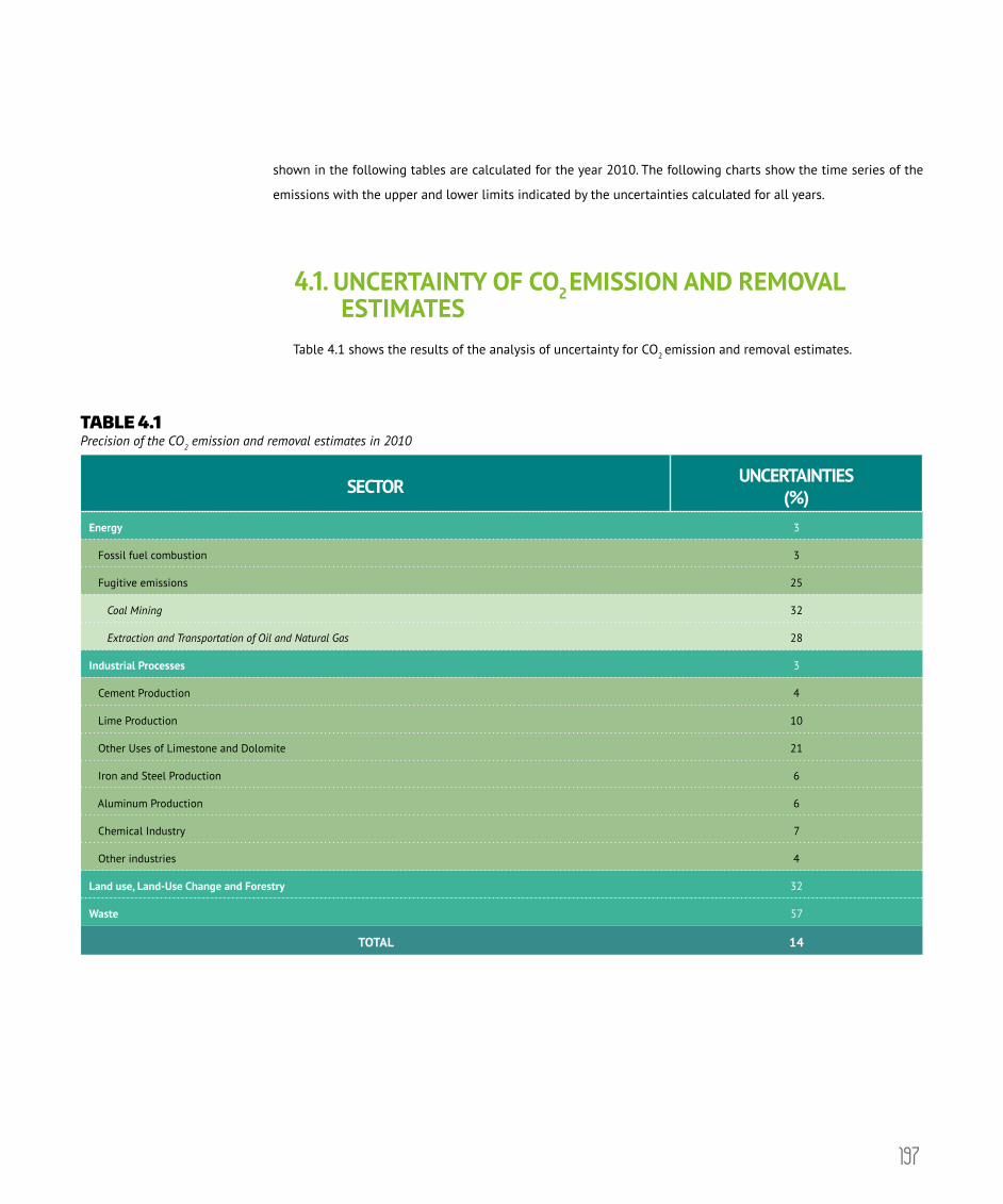
197
shown in the following tables are calculated for the year 2010. The following charts show the time series of the
emissions with the upper and lower limits indicated by the uncertainties calculated for all years.
4.1. UNCERTAINTY OF CO2 EMISSION AND REMOVAL ESTIMATES
Table 4.1 shows the results of the analysis of uncertainty for CO2 emission and removal estimates.
TABLE 4.1 Precision of the CO2 emission and removal estimates in 2010
SECTOR UNCERTAINTIES (%)
Energy 3
Fossil fuel combustion 3
Fugitive emissions 25
Coal Mining 32
Extraction and Transportation of Oil and Natural Gas 28
Industrial Processes 3
Cement Production 4
Lime Production 10
Other Uses of Limestone and Dolomite 21
Iron and Steel Production 6
Aluminum Production 6
Chemical Industry 7
Other industries 4
Land use, Land-Use Change and Forestry 32
Waste 57
TOTAL 14

198
VOLUME IIITHIRD NATIONAL COMMUNICATION OF BRAZIL
FIGURE 4.1 Evolution of the Brazilian CO2 emissions with uncertainty limits
0
500,000
1,000,000
1,500,000
2,000,000
2,500,000
3,000,000
3,500,000
4,000,000
1990
1991
1992
1993
1994
1995
1996
1997
1998
1999
2000
2001
2002
2003
2004
2005
2006
2007
2008
2009
2010
Gg
Total CO2 emissionswith an indication of the uncertainties
4.2. UNCERTAINTY OF CH4 EMISSION ESTIMATES Table 4.2 shows the results of the analysis of uncertainty for CH4 emission estimates.
TABLE 4.2 Precision of CH4 emission estimates in 2010
SECTOR UNCERTAINTY (%)
Energy 54
Fuel Combustion 73
Fugitive Emissions 45
Coal Mining 73
Extraction and Transportation of Oil and Natural Gas 54
Industrial Processes 11
Iron and Steel Production 15
Others from Metallurgy 15
Chemical Industry 17
continues on the next page

199
CHAPTER IV UNCERTAINTY OF THE ESTIMATES
SECTOR UNCERTAINTY (%)
Agriculture 31
Enteric Fermentation 34
Manure Management 38
Rice Cultivation 45
Crop Residue Burning 32
Land use, Land-Use Change and Forestry 72
Waste 16
Solid wastes 23
Wastewater 23
Industrial 30
Domestic 35
TOTAL 24
FIGURE 4.2 Evolution of the Brazilian CH4 emissions with uncertainty limits
1990
1991
1992
1993
1994
1995
1996
1997
1998
1999
2000
2001
2002
2003
2004
2005
2006
2007
2008
2009
2010
Gg
0
7,350
14,700
22,050
29,400
Total CH4 emissionswith an indication of the uncertainties

200
VOLUME IIITHIRD NATIONAL COMMUNICATION OF BRAZIL
4.3. UNCERTAINTY OF N2O EMISSION ESTIMATES Table 4.3, shows the results of the analysis of uncertainty for N2O emission estimates.
TABLE 4.3 Precision of N2O emission estimates in 2010
SECTOR UNCERTAINTY(%)Energy 101
Industrial processes 9
Chemical industry 5
Metallurgical Industry 16
Agriculture 49
Manure management 43
Agricultural soils 51
Grazing animals 81
Other direct sources 54
Indirect emissions 102
Crop Residue Burning 51
Land use, Land-Use Change and Forestry 101
Waste 15
TOTAL 42
FIGURE 4.3 Evolution of the Brazilian N2O emissions with uncertainty limits
0
100
200
300
400
500
600
700
800
900
1,000
1990
1991
1992
1993
1994
1995
1996
1997
1998
1999
2000
2001
2002
2003
2004
2005
2006
2007
2008
2009
2010
Gg
Total N2O emissionswith an indication of the uncertainties
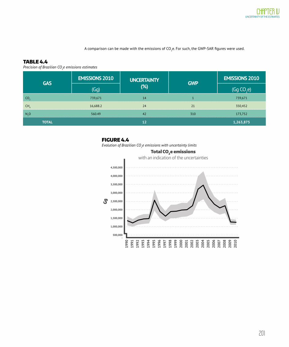
201
CHAPTER IV UNCERTAINTY OF THE ESTIMATES
A comparison can be made with the emissions of CO2e. For such, the GWP-SAR figures were used.
TABLE 4.4 Precision of Brazilian CO2e emissions estimates
GASEMISSIONS 2010 UNCERTAINTY
(%) GWPEMISSIONS 2010
(Gg) (Gg CO2e)CO2 739,671 14 1 739,671
CH4 16,688.2 24 21 350,452
N2O 560.49 42 310 173,752
TOTAL 12 1,263,875
FIGURE 4.4 Evolution of Brazilian CO2e emissions with uncertainty limits
Gg
Total CO2e emissionswith an indication of the uncertainties
- 500,000
1,000,000
1,500,000
2,000,000
2,500,000
3,000,000
3,500,000
4,000,000
4,500,000
1990
1991
1992
1993
1994
1995
1996
1997
1998
1999
2000
2001
2002
2003
2004
2005
2006
2007
2008
2009
2010

REFERENCES

REFERENCES

204
REFERENCES
ABDALA, G.C. et al. (1998). Above and belowground organic matter and root: shoot ratio in a cerrado in Central
Brazil. Brazilian Journal of Ecology, São Paulo, v.2, n.1, p.11–23.
ABETRE – Associação Brasileira de Empresas de Tratamento de Resíduos. (2006). Panorama atual da
incineração de resíduos industriais. Brasília.
ABIA – Associação Brasileira da Indústria da Alimentação. (2014). Produção de cerveja no Brasil entre 1990 a
2010. [correspondência pessoal]. E-mail enviado pelo senhor Cleber Sabonaro do Departamento de Economia
e Estatística - DECON da ABIA.
ABIC – Associação Brasileira da Indústria do Café. Indicadores da Indústria de Café no Brasil – 2014. Available
at: http://www.abic.com.br/publique/cgi/cgilua.exe/sys/start.htm?sid=61#1910
ABIQUIM – Associação Brasileira da Indústria Química e de Produtos Derivados. (1995). Anuário da Indústria
Química Brasileira.
______. (1997). Anuário da Indústria Química Brasileira.
______. (2000). Anuário da Indústria Química Brasileira.
______. (2005). Anuário da Indústria Química Brasileira.
______. (2008). Anuário da Indústria Química Brasileira.
______. (2012). Anuário da Indústria Química Brasileira.
ABLV – Associação Brasileira da Indústria de Leite Longa Vida. (2014). Access in: July 2014. Available at: http://
www.ablv.org.br
ABPC – Associação Brasileira dos Produtos de Cal. (2014). In: BRASIL, 2014 - Ministério da Ciência, Tecnologia
e Inovação. Coordenação-Geral de Mudanças Globais de Clima, 2014. Relatório de Referência Emissões de
Gases de Efeito Estufa nos Processos Industriais – Produtos Minerais (Parte II): Cal / Usos do Calcário e
Dolomita/Barrilha. Brasília: MCTI.
ABRABE – Associação Brasileira de Bebidas. (2014). Available at: http://www.abrabe.org.br/mercado.php.

205
ABRELPE – Associação Brasileira de Empresas de Limpeza Pública e Resíduos Especiais. (2008). Panorama
dos Resíduos Sólidos no Brasil 2008. São Paulo: ABRELPE.
______. (2009). Panorama dos Resíduos Sólidos no Brasil 2009. São Paulo: ABRELPE.
______. (2010). Panorama dos Resíduos Sólidos no Brasil 2010. São Paulo: ABRELPE.
ACCIOLY, L.J.O. et al. (2008). Biomassa nas Florestas de Caatinga nas Microrregiões do Seridó Oriental (RN) e Seridó
Ocidental (PB). In: XVII Reunião de Manejo e Conservação do Solo e da Água, 2008, Rio de Janeiro. Anais da XVII
Reunião de Manejo e Conservação do Solo e da Água.
ALBUQUERQUE, E. R. G. M. (2015). Biomassa de raízes em áreas com diferentes usos da terra e tipos de solos. Tese
de Doutorado (Botânica), Universidade Federal Rural de Pernambuco, Recife.
ALENCAR, A.A. et al. (2004). Modeling forest understory fires in an eastern Amazonian landscape. Ecological
Applications, v.14, n.4, p.139-149.
ALENCASTRO GRACA, P.M.L. et al. (1999). Burning of Amazonian forest in Ariquemes, Rondônia, Brazil: biomass,
charcoal formation and burning efficiency. Forest ecology and Management, v.120, n.1-3, p.179-191.
ALMEIDA, C.A. et al. (2009). Metodologia para mapeamento da vegetação secundária na Amazônia Legal. São José
dos Campos: INPE. 32p. Available at: http://mtc-m19.sid.inpe.br/col/sid.inpe.br/mtc-m19@80/2009/11.23.17.06/
doc/publicacao.pdf?languagebutton=pt-BR.
ALVES, A. R. (2011). Quantificação de biomassa e ciclagem de nutrientes em áreas de vegetação de Caatinga no município
de Floresta, Pernambuco. Tese de Doutorado (Manejo Florestal), Universidade Federal Rural de Pernambuco, Recife, 2011.
ALVES, D. et al. (1997). Biomass of primary and secondary vegetation in Rondônia, Western Brazilian
Amazon. Global Change Biology, v.3, n.5, p.451-461.
ALVES, L.F. et al. (2010). Forest structure and live aboveground biomass variation along an elevational gradient
of tropical Atlantic moist forest (Brazil). Forest Ecology and Management, v. 260, n. 5, p. 679–691, 2010.
AMARO, M.A. et al. (2013). Estoque volumétrico, de biomassa e de carbono em uma floresta estacional
semidecidual em viçosa, minas gerais. Revista Árvore, Viçosa, n.37, v.(5), p. 849-857, 2013.
AMORIM, I. L.; SAMPAIO, E. V. S. B.; ARAÚJO, E. L. (2005). Flora e estrutura da vegetação arbustivo arbórea de
uma área de caatinga do Seridó, RN. Acta Botanica Brasilica, v.19, p.615-623.
ARAÚJO,T.M. et al. (1999). Comparison of formulae for biomass content determination in a tropical rain forest
site in the state of Pará, Brazil. Forest Ecology Management, v. 117(1-3), p. 43-52.
ASNER, G. P. et al. (2005). Selective logging in the Amazon. Science, v. 310, p. 480–482.
ASSIS, M.A. et al. (2011). Florestas de restinga e de terras baixas na planície costeira do sudeste do Brasil:
vegetação e heterogeneidade ambiental; Restinga and Lowland forests in coastal plain of southeastern
Brazil: vegetation and environmental heterogeneity. Biota neotropical, v.11, n.2, p.103–121.
206
VOLUME IIITHIRD NATIONAL COMMUNICATION OF BRAZIL
BAHIA, T.O. et al. (2009). Florística e fitossociologia de veredas em diferentes estágios de conservação na APA
do Rio Pandeiros, norte de Minas Gerais. MG. Biota, Belo Horizonte, v.2, n.3, p. 14-21.
BAKER, T.R. et al. (2004). Increasing biomass in Amazonian forest plots. Philosophical Transactions of the
Royal Society of London. Series B: Biological Sciences, London, v.359, n.1443, p. 353-365.
BALCH, J.K. et al. (2008). Negative fire feedback in a transitional forest of southeastern Amazonia. Global
Change Biology, v.14, n.10, p.2276-2287.
BARBOSA, R. I.; FEARNSIDE, P. M. (1999). Incêndios na Amazônia brasileira: Estimativa da emissão de gases do
efeito estufa pela queima de diferentes ecossistemas de Roraima na passagem do evento El Niño (1997/1998).
Acta Amazonica, v. 29, p. 513-534.
BARBOSA, R.I.; FEARNSIDE, P.M. (2005). Above-ground biomass and the fate of carbon after burning in the
savannas of Roraima, Brazilian Amazonia. Forest Ecology and Management, v.216, n.1, p.295-316.
BARBOSA, R.I.; FERREIRA, C.A.C. (2004). Biomassa acima do solo de um ecossistema de “campina” em Roraima,
norte da Amazon Brasileira. Acta Amazonica, Manaus, v.34, n.4, p.577-586.
BARBOSA, R.I. et al. (2010). Ecossistemas terrestres de Roraima: Área e modelagem espacial da biomassa. IN:
BARBOSA, R.I.; MELO, V.F. (Ed.). Roraima: Homem, Ambiente e Ecologia. 1.ed. Boa Vista: FEMACT, p.347-368.
BERNOUX, M. et al. (2002). Brazil’s soil carbon stocks. Soil Science Society of America Journal, v. 66, p. 888-896, 2002.
BOINA, A. (2008). Quantificação de estoques de biomassa e de carbono em Floresta Estacional Semidecidual, Vale
do Rio Doce, Minas Gerais. Dissertação de Mestrado (Ciência Florestal) - Universidade Federal de Viçosa, Viçosa, MG.
BONGERS, F. et al. (1985). Phytomass structure of natural plant communities on spodosols in southern Venezuela:
the Bana woodland. Vegetation, v.63, n.1, p.13-34.
BORGO, M. (2010). A Floresta Atlântica do litoral norte do Paraná, Brasil: aspectos florísticos, estruturais e estoque
de biomassa ao longo do processo sucessional. Tese de Doutorado, Universidade Federal do Paraná, Curitiba.
BONINO, E.E. (2006). Changes in carbon pools associated with a land-use gradient in the Dry Chaco, Argentina.
Forest Ecology and Management, v. 223, p. 183-189.
BRACELPA – Associação Brasileira de Celulose e Pa pel. Relatório Estatístico 2009-2010. Available at: <http://
bracelpa.org.br/bra2/?q=node/461>.
BRACK, P. et al. (2009). Levantamento preliminar da flora e da vegetação do vale do rio Pelotas, no município
de Bom Jesus, RS, e a importância de sua conservação. INGA Estudos Ambientais, Porto Alegre.
BRASIL. (2004). Ministério da Ciência e Tecnologia. Coordenação-Geral de Mudanças Globais de Clima. Comunicação
Nacional Inicial do Brasil à Convenção-Quadro das Nações Unidas sobre Mudança do Clima. Brasília: MCT, 274p.
______. (2010). Ministério da Ciência, Tecnologia e Inovação. Coordenação-Geral de Mudanças Globais de Clima.
Segunda Comunicação Nacional do Brasil à Convenção-Quadro das Nações Unidas sobre Mudança do Clima.
Brasília: MCTI.

207
REFERENCES
______. (2011). Ministério das Minas e Energia. Anuário Estatístico do Setor Metalúrgico, 2011. Secretaria de Geologia,
Mineração e Transformação Mineral – MME.
______. (2013). Ministério de Minas e Energia. Balanço energético nacional, 2013. Available at: http://www.mme.gov.
br/mme/menu/todas_publicacoes.html.
______. (2006). Ministério de Minas e Energia. Empresa de Pesquisa Energética. Balanço energético nacional 2006:
ano base 2005. Rio de Janeiro: EPE.
______. (2004). Ministério da Ciência e Tecnologia. Coordenação-Geral de Mudanças Globais de Clima. Relatório
de Referência Emissões de Gases do Efeito Estufa no Setor Uso da Terra, Mudança do Uso da Terra e Florestas –
Emissões de CO2 pelo Uso da Terra, Mudança do Uso da Terra e Florestas. Brasília: MCT. 105 p. Access in: July 2014.
Available at: <http://www.mct.gov.br/upd_blob/0213/213346.pdf>.
______. (2004). Ministério da Ciência e Tecnologia. Coordenação-Geral de Mudanças Globais de Clima. Relatório
de Referência Emissões de Gases do Efeito Estufa no Setor Uso da Terra, Mudança do Uso da Terra e Florestas –
Emissões de CO2 pelo Uso da Terra, Mudança do Uso da Terra e Florestas. Brasília: MCT. 105 p. Access in: December
2015. Available at: <http://www.mct.gov.br/upd_blob/0213/213346.pdf>.
BRITEZ, R. M. de. et al. (2006). Estoque e incremento de carbono em florestas e povoamentos de espécies arbóreas
com ênfase na floresta atlântica do sul do Brasil. Colombo: EMBRAPA Florestas. 165 p.
______. Estoque e incremento de carbono em florestas e povoamentos de espécies arbóreas com ênfase na Floresta
Atlântica do Sul do Brasil. Dados eletrônicos. Colombo - PR: EMBRAPA Florestas (CD ROM).
BROWN, S. (1997). Estimating biomass and biomass change of tropical forests: a primer (Vol. 134). Food & Agriculture Org.
BRUN, E.J. (2004). Biomassa e Nutrientes na Floresta Estacional Decidual no município de Santa Tereza – RS. 2004.
Dissertação de Mestrado (Mestrado em Engenharia Florestal) - Universidade de Santa Maria, UFSM, Santa Maria.
CABIANCHI, G.M. (2010). Ciclagem de nutrientes via serapilheira em um fragmento ciliar do rio Urupá, Rondônia.
103 f. Dissertação de Mestrado (Mestrado em Ciências) – Universidade de São Paulo, USP, Piracicaba.
CABRAL, G. A. L. et al. (2013). Estrutura Espacial e Biomassa da Parte Aérea em Diferentes Estádios Sucessionais de
Caatinga, em Santa Terezinha, Paraíba. Revista Brasileira de Geografia Física, vol. 6, n.03.
CAÑA, B.B. et al. (2012). Relação entre biomassa aérea vegetal e NDVI no bioma Pampa. In: SIMPÓSIO BRASILEIRO
DE SENSORIAMENTO REMOTO - SBSR, XVI, 2012, Foz do Iguaçu. Anais. Foz do Iguaçu, p.2802.
CARDOSO, A.S. et al. (2008). Uma evidência de que a FBN não é um fonte direta de N2O na cultura da soja. In:
FERTBIO, Londrina – PR.
CARDOSO, E. L. et al. (2000). Composição e dinâmica da biomassa aérea após a queima em savana gramíneo-
lenhosa no Pantanal. Pesquisa Agropecuária Brasileira, Brasília, v. 35, n. 11, p. 2309-2316.
CARDOSO, E.L. et al. (2003). Efeitos da queima na dinâmica da biomassa aérea de um campo nativo no
Pantanal. Pesquisa Agropecuária Brasileira, Brasília, v. 38, n. 6, p. 747-752.

208
VOLUME IIITHIRD NATIONAL COMMUNICATION OF BRAZIL
CARVALHO, Jr A. et al. (1995). A tropical rainforest clearing experiment by biomass burning in the Manaus region.
Atmospheric Environment, v.29, n.17, p.2301-2309.
CARVALHO, Jr. A. et al. (1998). Combustion completeness in a rainforest clearing experiment in Manaus, Brazil.
Journal of Geophysical Research-Atmospheres, v. 103(D11), p.13195-13199, 1998.
CARVALHO, Jr A. et al. (2001). Biomass fire consumption and carbon release rates of rainforest-clearing
experiments conducted in Northern Mato Grosso, Brazil. Journal of Geophysical Research: Atmospheres, v.106,
n.D16, p.17877-17887.
CASTRO, E.A.; KAUFFMAN, J.B. (1998). Ecosystem structure in the Brazilian Cerrado: a vegetation gradient of
aboveground biomass, root mass and consumption by fire. Journal of tropical ecology, Sussex, v.14, n.03, p.263-283.
CATTANIO, J. H. et al. (2004). Phenology, litterfall, growth, and root biomass in a tidal floodplain forest in the
Amazon estuary. Revista Brasileira de Botânica, v.27, n.4, p.703-712.
CETESB – Companhia Ambiental do Estado de São Paulo. (2011a). Relatório da Qualidade do Ar no Estado de
São Paulo. São Paulo.
_________. (2011b). 1º Relatório de Referência do Estado de São Paulo de Emissões e Remoções Antrópicas de Gases
de Efeito Estufa, Período de 1990 a 2008. São Paulo.
_________. (2013). Emissões Veiculares no Estado de São Paulo 2012. São Paulo.
CHAO, K.J. et al. (2008). Wood density and stocks of coarse woody debris in a northwestern Amazonian landscape.
Canadian Journal of Forest Research, v. 38, p. 795–805.
CHAVE, J. et al. (2005). Tree allometry and improved estimation of carbon stocks and balance in tropical forests.
Oecologia, v. 145, p. 87-99.
CIANCIARUSO, M.V. et al. (2010). Aboveground biomass of functional groups in the ground layer of savannas under
different fire frequencies. Australian Journal of Botany, Collingwood, v.58, n.3, p.169-174.
COELHO, M.S. et al. (2012). Floristic composition and structure of a tropical dry forest at different successional
stages in the Espinhaço Mountains, southeastern Brazil. Interciência, v.37, n.3, p.190-196.
COGLIATTI-CARVALHO, L.; MATTOS-FONSECA, S. (2004). Quantificação da biomassa e do carbono em Rhizophora
mangle, Avicennia shaueriana e Laguncularia racemosa no manguezal da laguna de Itaipu, Niterói-RJ. In: SIMPÓSIO
DE ECOSSISTEMAS BRASILEIROS, 6., 2004, São José dos Campos. Programa e Resumos. São José dos Campos:
Academia de Ciências do Estado de São Paulo, INPA.
CONAB – Companhia Nacional de Abastecimento. (2010). Acompanhamento de safra brasileira: grãos, décimo
primeiro levantamento, agosto 2010. Brasília, DF: CONAB, v. 1, n.11. Available at: http://www.conab.gov.br/
OlalaCMS/uploads/arquivos/8218897d1eb5849906fc53856bddc894..pdf
CORINAIR – Core Inventory Air Emissions.(1996). Atmospheric Emission Inventory Guidebook – Solvent and
Other Product Use. Primeira Edição, EMEP - Co-operative Programme for Monitoring and Evaluation of the
Long Range Transmission of Air Polluents in Europe.

209
REFERENCES
COSTA, T. L. (2013). Biomassas radiculares e áreas em comunidades de Caatinga. Dissertação de mestrado (Botânica),
Universidade Federal Rural de Pernambuco, Recife.
COSTA, T.L. et al. (2014). Root and shoot biomasses in the tropical dry forest of semi-arid Northeast Brazil. Plant
and soil, v.378, n.1-2, 113-123.
CUMMINGS, D.L. et al. (2002). Aboveground biomass and structure of rainforests in the southwestern Brazilian
Amazon. Forest Ecology and Management, v. 163, p. 293-307.
CUNHA, G.M. et al. (2009). Biomassa e estoque de carbono e nutrientes em florestas montanas da Atlantic Forest na
região norte do estado do Rio de Janeiro. Revista Brasileira de Ciência do Solo, Viçosa, v.33, p.1175-1185.
CUNHA, S.R. et al. (2005). Production dynamics of Spartina alterniflora salt marshes in the estuary of Patos Lagoon
(RS, Brazil): a simulation model approach. Brazilian Journal of Aquatic Science and Technology, Itajaí, v.9, n.2, p.75-85.
DELITTI, W.B.C. et al. (2006). Biomass and mineralmass estimates in a” Cerrado” ecosystem. Brazilian Journal of
Botany, São Paulo, v.29, n.4, p.531-540.
DUARTE, M.M.; BENCKE, G.A. (2006). Plano de Manejo do Parque Estadual de Itapeva, RS.
DURIGAN, G. (2004). Estimativas de estoque de carbono na vegetação natural do estado de São Paulo. In G.
DURIGAN (Ed.) Oportunidades de negócios em segmentos produtivos nacionais. pp. 1-6. São Paulo: Secretaria do
Meio Ambiente do Estado de São Paulo. 2004.
EMBRAPA. (2003). Centro Nacional de Pesquisa de Solos. Sistema Brasileiro de Classificação de Solos. Brasília:
EMBRAPA Produção de Informação; Rio de Janeiro: EMBRAPA Solos.
EMBRAPA (2013). Embrapa Arroz e Feijão. Home Page. Access in: March 2014. Available at:http://www.cnpaf.
embrapa.br/transferencia/informacoestecnicas/index.php
EMBRAPA (2014). Embrapa Arroz e Feijão. Home Page, 2014. Access in: July 2014. Available at: http://www.cnpaf.
embrapa.br/socioeconomia/index.htm.
ESTRADA, G. C. D. et al. (2014). The economic evaluation of carbon storage and sequestration as ecosystem services
of mangroves: a case study from southeastern Brazil. International Journal of Biodiversity Science, Ecosystem
Services & Management, 2014.
FAO. (2010). Global forest resources assessment. FRA 2010. Rome: FAO. 340 p.
FEARNSIDE, P. M. (1992). Forest biomass in Brazilian Amazonia: comments on the estimate by Brown and Lugo.
Interciencia, v. 17, p. 19–27.
FEARNSIDE, P.M. et al. (1993). Rainforest burning and the global carbon budget: Biomass, combustion efficiency,
and charcoal formation in the Brazilian Amazon. Journal of Geophysical Research: Atmospheres, v.98, n.D9,
p.16733-16743.
FEARNSIDE, P.M.; GUIMARÃES, W.M. (1996). Carbon uptake by secondary forests in Brazilian Amazonia. Forest
Ecology and Management, v.80, n.1, p.35-46.
210
VOLUME IIITHIRD NATIONAL COMMUNICATION OF BRAZIL
FEARNSIDE, P.M. et al. (1999). Tropical forest burning in Brazilian Amazonia: measurement of biomass loading,
burning efficiency and charcoal formation at Altamira, Pará. Forest Ecology and Management, v.123, n.1, p.65-79.
FEARNSIDE, P.M. et al. (2001). Burning of Amazonian rainforests: burning efficiency and charcoal formation in forest
cleared for cattle pasture near Manaus, Brazil. Forest Ecology and Management, v.146, n.1, p.115-128.
FEARNSIDE, P.M. et al. (2009). Biomass and greenchouse-gas emissions from land-use change in Brazil’s Amazonian
“arc of deforestation”: The states of Mato Grosso and Rondônia. Forest Ecology Management, v. 258, p. 1968-1978.
FELDPAUSCH, T.R. et al. (2007). Secondary forest growth deviation from chronosequence predictions in central
Amazonia. Global Change Biology, v.13, n.5, p.967-979.
FELFILI, M.C. (2008). Proposição de critérios florísticos, estruturais e de produção para o manejo do cerrado sensu strico
do Brasil central. Tese de Doutorado (Doutorado em Ciências Florestais) – Universidade de Brasília, UnB, Brasília.
FERNANDES, A.H.B.M. et al. (2008). Estoques de Carbono do Estrato Arbóreo de Cerrados no Pantanal da Nhecolândia.
Circular Técnica - 68. Corumbá: EMBRAPA Pantanal. 5 p.
FERNANDES, M.E. (1997). The ecology and productivity of mangroves in the Amazon region, Brazil. Tese de
Doutorado – York University.
FERRAZ, E.M.N.; RODAL, M.J.N. (2006). Caracterização fisionômica-estrutural de um remanescente de floresta
ombrófila montana de Pernambuco, Brasil. Acta Botanica Brasilica, Belo Horizonte, v.20, n.4, p.911-926.
FIDELIS A. et al. (2006). Efeito do fogo na biomassa aérea e subterrânea dos Campos Sulinos. In: XXI REUNIÃO DO
GRUPO TÉCNICO EM FORRAGEIRAS DO CONE SUL – Grupo Campos: Desafios e oportunidades do Bioma Campos
frente à expansão e intensificação agrícola, 4-01, Pelotas: EMBRAPA – Clima Temperado.
FIDELIS, A. et al. (2010). Fire intensity and severity in Brazilian campos grasslands. Interciencia, v.35, n.10, p.739-745.
FIDELIS, A. et al. (2013). Above-and below-ground biomass and carbon dynamics in Brazilian Cerrado wet
grasslands. Journal of Vegetation Science, v.24, n.2, p.356-364.
FRANÇOSO, R.D. et al. (2013). Análise biogeográfica de espécies arbóreas do Cerrado como subsídio à criação de
unidades de conservação. Relatório Técnico não publicado. Brasília: Laboratório de Planejamento para Conservação
da Biodiversidade, Universidade de Brasília. 6p.
FROMARD, F. et al. (1998). Structure, above-ground biomass and dynamics of mangrove ecosystems: new data from
French Guiana. Oecologia, v.115, n.(1-2), p.39-53.
GAMA, J.R.V. et al. (2007). Fitossociologia de duas fitocenoses de floresta ombrófila aberta no município de Codó,
Estado do Maranhão. Revista Árvore, Viçosa, v.31, n.3, p.465-477.
GARIGLIO, M.A. et al. (2010). Uso sustentável e conservação dos recursos florestais da caatinga. Brasília: Serviço
Florestal Brasileiro, 367p.
GASPARRI, N.I. et al. (2008). Carbon pools and emissions from deforestation in extra-tropical forests of northern
Argentina between 1900 and 2005. Ecosystems, v.11, n.8, p.1247-1261.
211
REFERENCES
GIBSON, D.J. (2009). Grasses and grassland ecology. New York: Oxford University Press, 305p.
HAIDAR, R.F. (2008). Fitossociologia, Diversidade e sua relação com variáveis ambientais em florestas estacionais
do bioma Cerrado no Planalto Central e Nordeste do Brasil. Dissertação (Mestrado em Engenharia Florestal).
Departamento de Engenharia Florestal, Universidade de Brasília. Brasília.
HAIDAR, R.F. et al. (2013). Mapeamento das Regiões Fitoecológicas e Inventário Florestal do estado do Tocantins.
Palmas: SEPLAN, 136p.
HIGUCHI, N. et al. (1998). Biomassa da parte aérea da vegetação da floresta tropical úmida de terra-firme da Amazon
brasileira. Acta Amazonica, v.28, n.2, p.153-165.
HOLDSWORTH, A.R.; UHL, C. (1997). Fire in eastern Amazonian logged rain forest and the potential for fire reduction.
Ecological Application, V. 7, p. 713–725.
HUANG, M.; ASNER, G.P. (2010). Long-term carbon loss and recovery following selective logging in Amazon
forests. Global Biogeochemical Cycles, v.24, n.3.
HUTCHISON, J. et al. (2013). Predicting global patterns in mangrove forest biomass. Conservation Letters, v.7,
n.3, p.233-240.
IMAÑA-ENCINAS, J. et al. (1995). Fitossociologia dos indivíduos jovens da mata ciliar do córrego Capãozinho.
Revista Árvore, Viçosa, v. 19, n. 2, p.157-170.
IBGE – INSTITUTO BRASILEIRO DE GEOGRAFIA E ESTATÍSTICA. (2004). Mapa de Biomas do Brasil, primeira
aproximação. Rio de Janeiro, IBGE. Available at: http://mapas.ibge.gov.br/biomas2/viewer.htm
_________. (2012). Manual técnico da vegetação brasileira. Rio de Janeiro, Séries Manuais Técnicos em
Geociências, n. 1.
IPCC/OECD/IEA – Intergovernmental Panel On Climate Change, Organisation For Economic Co-Operation and
Development & International Energy Agency. (1997) Revised 1996 IPCC Guidelines for National Greenhouse
Gas Inventories. Bracknell.
IPCC – Intergovernmental Panel On Climate Change. (2003). Good Practice Guidance for Land Use, Land–Use
Change and Forestry. Kanagawa: Institute for Global Environmental Strategies.
_________. (2006). IPCC Guidelines for National Greenhouse Gas Inventories. Prepared by the National
Greenhouse Gas Inventories Programme. Kanagawa: Institute for Global Environmental Strategies.
ISAIA, E.M.B.I. et al. (1992). Avaliação do estoque lenheiro do Estado do Rio Grande do Norte. 1ª etapa:
Estratificação da vegetação nativa lenhosa através de composições coloridas do sensor TM landsat. Projeto
PNUD/FAO/BRA/IBAMA/87/007, n.4, Natal.
JACOBI, U.S. et al. (2013). Florística dos ecossistemas do Campus Carreiros, Rio Grande, Rio Grande do Sul,
Brasil. IHERINGIA Série Botânica, Porto Alegre, v.68, n.1, p.73-89.

212
VOLUME IIITHIRD NATIONAL COMMUNICATION OF BRAZIL
KAUFFMAN, J.B. et al. (1994). Relationships of fire, biomass and nutrient dynamics along a vegetation gradient
in the Brazilian cerrado. Journal of Ecology, v.82, n.3, p.519-531.
KAUFFMAN, J.B. et al. (1995). Fire in the Brazilian Amazon: 1. Biomass, nutrient pools, and losses in slashed
primary forests. Oecologia, n.104, v.4, p.397-408.
KLAUBERG, C. et al. (2010). Florística e estrutura de um fragmento de Floresta Ombrófila Mista no Planalto
Catarinense. Biotemas, v.23, n.1, p.35-47.
KNAK, R.B. (1999). Plano de Manejo do Parque Nacional da Lagoa do Peixe, Rio Grande: FNMA-FURG-IBAMA-
NEMA-UFPel.
KRISTENSEN, E. et al. (2008). Organic carbon dynamics in mangrove ecosystems: a review. Aquatic Botany, v.89,
n.2, p.201-219.
LIMA, J.R. et al. (2009). Composição florística da floresta estacional decídua montana de Serra das Almas, CE,
Brasil. Acta Botanica Brasilica, Belo Horizonte, v.23, n.3, p.756-763.
LINDNER, A.; SATTLER, D. (2011). Biomass estimations in forests of different disturbance history in the Atlantic
Forest of Rio de Janeiro, Brazil. New Forests, v.43, n.3, p.287-301.
MALHI, Y. et al. (2006). The regional variation of aboveground live biomass in old-growth Amazonian
forests. Global Change Biology, v.12, n.7, p.1107-1138.
MANRIQUE, S. et al. (2009). Estimacion de densidad de biomasa aerea em ecosistemas naturales de la provincia
de salta. Avances em Energías Renovables y Medio Ambiente, v.13, n.6, p. 37-45.
MATRICARDI, E. et al. (2010). Assessment of tropical forest degradation by selective logging and fire using
Landsat imagery. Remote Sensing of Environment, v. 114, p. 1117–1129.
MEDEIROS, T.C.C.; SAMPAIO E.V.S.B. (2008). Allometry of aboveground biomasses in mangrove species in
Itamaracá, Pernambuco, Brazil. Wetlands Ecology Management, v.16, p.323-330
MELO, A.C.G.; DURIGAN, G. (2006). Fixação de carbono em reflorestamentos de matas ciliares no Vale do
Paranapanema, SP, Brasil. Scientia forestalis, São Paulo, v.71, p.149-154.
MENDONÇA, A.V.R. et al. (2013). Estimação de biomassa aérea de espécies da caatinga no norte da Bahia.
Pesquisa Florestal Brasileira, v. 33, n. 76.
MENEZES, R.S.C. et al. (2012). Biogeochemical cycling in terrestrial ecosystems of the Caatinga Biome. Brazilian
Journal of Biology v.72 (3).
METZKER, T. et al. (2011). Forest dynamics and carbon stocks in Rio Doce State Park – an Atlantic rainforest
hotspotr. Current Science, v.100, n.12, p.1855-1862.
MIRANDA, S.C. (2012). Variação espacial e temporal da biomassa vegetal em áreas de Cerrado. Tese de
Doutorado (Doutorado em Ecologia). Brasília: Universidade de Brasília.
213
REFERENCES
MIRANDA, S.C. et al. (2014). Regional Variations in Biomass Distribution in Brazilian Savanna
Woodland. Biotropica, v.46, n.2, p.125-138.
MITCHARD, E.T.A. et al. (2014). Markedly divergent estimates of Amazon forest carbon density from ground
plots and satellites. Global Ecology and Biogeography, V.23, n. 8, p.935-946
MOKANY, K. et al. (2006). Critical analysis of root: shoot ratios in terrestrial biomes. Global Change Biology, v.12,
n.1, p.84-96.
MORAIS, V.A. et al. (2013). Carbon and biomass stocks in a fragment of cerradão in Minas Gerais state,
Brazil. Cerne, Lavras, v.19, n.2, p.237-245.
MOREIRA-BURGER, D.; DELITTI, W.B. (1999). Fitomassa epigéa da mata ciliar do Rio Mogi-Guaçu, Itapira-
SP. Brazilian Journal of Botany, São Paulo, v.22, n.3, p.429-435
NASCIMENTO, M.T. et al. (2007). Above-ground biomass changes over an 11-year period in an Amazon
monodominant forest and two other lowland forests. Plant Ecology, v.192, n.2, p.181-191.
NEPSTAD, D.C. et al. (1999). Large-scale impoverishment of Amazonian forests by logging and fire. Nature, v.398,
n.6727, p.505-508.
NOGUEIRA, E.M. et al. (2008). Estimates of forest biomass in the Brazilian Amazon: New allometric equations and
adjustments to biomass from wood-volume inventories. Forest Ecology and Management, v.256, n.11, p.1853-1867.
OLIVEIRA, M.S. et al. (2009). Avaliação da biomassa aérea e subterrânea dos campos sulinos. In: CONGRESSO DE
ECOLOGIA DO BRASIL, IX, 2009, São Lourenço. Anais. São Lourenço, p.1.
OTTMAR, R.D. et al. (2001). Stereo photo series for quantifying cerrado fuels in Central Brazil. Volume I, Portland,
Forest Service, U.S. Department of Agriculture, 87p.
PADILHA, D.R.C. (2011). Fitossociologia e estimativas da biomassa aérea e de carbono em chaco florestado no
Brasil. Dissertação de metrado (Mestrado em Biologia Vegetal). Campo Grande: Universidade Federal de Mato
Grosso do Sul (UFMS).
PAREYN, F. (2014). Departamento de Energia Nuclear, Universidade Federal de Pernambuco, UFPE, Campus Recife.
Personal communication.
PARUELO, J.M. et al. (2010). Carbon stocks and fluxes in rangelands of the Río de la Plata Basin. Rangeland Ecology
& Management, v.63, n.1, p.94-108.
PAULA, J.E. et al. (1990). Estudo dendrométrico e ecológico de mata ripária da região Centro-Oeste. Pesquisa
Agropecuária Brasileira, v.25, n.1, p.43-55.
PAULA, J.E. et al. (1993). Inventário de um hectare de mata ripária. Pesquisa Agropecuária Brasileira, v.28, n.2, p.143-152.
PAULA, J. E. et al. (1998). Levantamento quantitativo em três hectares de vegetação de cerrado. Pesquisa Agropecuária
Brasileira, v.33, n.5, p.613-620.
214
VOLUME IIITHIRD NATIONAL COMMUNICATION OF BRAZIL
PEREIRA, D.G.S. (2013). Conexões estruturais e florísticas de ecounidades da vegetação arbórea de uma planície
inundável no médio São Francisco. Dissertação (Mestrado em Engenharia Florestal). Lavras: Universidade Federal
de Lavras.
PEREIRA, S.B.A. et al. (2011). Florestas estacionais no cerrado: uma visão geral. Pesquisa Agropecuária Tropical, v.41, n.3.
PINHEIRO, E.D.S. (2008). Análises ecológicas e sensoriamento remoto aplicados à estimativa de fitomassa de
Cerrado na estação ecológica de Assis, SP. Tese de Doutorado (Doutorado em Ciências da Engenharia Ambiental).
São Carlos: Universidade de São Paulo (USP).
PIRES, L.A. et al. (2006). Produção, acúmulo e decomposição da serapilheira em uma restinga da Ilha do Mel,
Paranaguá, PR, Brasil. Acta Botanica Brasilica, Belo Horizonte, v.20, n.1, p.173-184.
RAMASWAMY, V. et al. (2001). Radiative forcing of climate change. In: Climate Change 2001: The Scientific Basis.
Contribution of Working Group I to the Third Assessment Report of the Intergovernmntal Panel on Climate Change
[J. T. Houghton, Y. Ding, D. J. Griggs, M. Noquer, P. J. van der Linden, X. Dai, K. Maskell and C. A. Johnson (eds.)]. Cambride
University Press, Cambridge, United Kingdom and New York, NY, USA, 349-416.
RAMOS E SILVA, C.A. et al. (2007). Dynamics of phosphorus and nitrogen through litter fall and decomposition in a
tropical mangrove forest. Marine environmental research, v.64, n.4, p.524-534.
REZENDE, A.V. et al. (2006). Comparação de modelos matemáticos para estimativa do volume, biomassa e
estoque de carbono da vegetação lenhosa de um cerrado sensu stricto em Brasília, DF. Scientia Florestalis,
Piracicaba, v.7, p.65-76.
RIBEIRO, S. C. et al. (2009). Quantificação de biomassa e estimativa de estoque de carbono em uma floresta madura
no município de Viçosa, Minas Gerais. Revista Árvore, Viçosa, v.33, n.5, p.917-926.
RIBEIRO, S.C. et al. (2011). Above-and Belowground biomass in a Brazilian Cerrado. Forest Ecology and
Management, v.262, n.3, p.491-499.
ROCHA, H.R.D. et al. (2002). Measurements of CO2 exchange over a woodland savanna (Cerrado sensu stricto) in
southeast Brasil. Biota Neotropica, São Paulo, v.2, n.1, p.1-11.
ROLIM S. G. et al. (2005). Biomass change in an Atlantic tropical moist forest: the ENSO effect in permanent sample
plots over a 22-year period, Oecologia, v. 142, n. 2, p. 238 – 246.
SALIS, S.M. et al. (2004). Equações para estimar biomassa e volume de madeira em cerradões do Pantanal da
Nhecolândia, MS. Circular Técnica. EMBRAPA Pantanal.
SALOMÃO, R.D.P. et al. (2007). Dinâmica da regeneração natural de árvores em áreas mineradas na Amazon. Boletim
do Museu Paraense Emílio Goeldi, Belém, v.2, n.2, p.85-139
SAMPAIO, V. S. B.; COSTA, T. L. (2011). Estoques e Fluxos de Carbono no Semi-Árido Nordestino: Estimativas
Preliminares. Revista Brasileira de Geografia Física, v. 6, p. 1275-129
215
REFERENCES
SANTOS, N.M. (2013). Os manguezais do complexo estuarino de Paranaguá: Variações interdecadais, distribuição
da biomassa aérea e formas de uso da madeira. Dissertação de Mestrado (Mestrado em Sistemas Costeiros e
Oceânicos) – Universidade Federal do Paraná, UFPR, Paraná.
SCARANELLO, M.A.D.S. (2010). Dinâmica da comunidade arbórea de floresta ombrófila densa de terras baixas e
de restinga no Parque Estadual da Serra do Mar, SP. Dissertação de Mestrado (Mestrado em Ciências). Piracicaba:
Universidade de São Paulo (USP).
SCARIOT, A.; SEVILHA, A.C. (2005). Biodiversidade, estrutura e conservação de florestas estacionais deciduais no
Cerrado. In: SCARIOT, A.; SOUSA-SILVA, J.C.; FELFILI, J.M. Cerrado: ecologia, biodiversidade e conservação. Brasília:
MMA, p.123-139.
SCHÖNGART, J. et al. (2011). Age-related and stand-wise estimates of carbon stocks and sequestration in the
aboveground coarse wood biomass of wetland forests in the Northern Pantanal, Brazil. Biogeosciences, v.8, n.11,
p.3407-3421
SCOLFORO, J.R. et al. (2008a). Volumetria, peso de matéria seca e carbono. In: SCOLFORO, J.R.; MELLO, J.M.; OLIVEIRA,
A.D. (Ed.). Inventário Florestal de Minas Gerais: Cerrado - Florística, Estrutura, Diversidade, Similaridade, Distribuição
Diamétrica e de Altura, Volumetria, Tendências de Crescimento e Áreas Aptas para Manejo Florestal. Lavras: UFLA,
p.361-438.
SCOLFORO, J.R. et al. (2008b). Volumetria, peso de matéria seca e carbono para o domínio da caatinga. In: MELLO,
J.M.; SCOLFORO, J.R.; CARVALHO, L.M.T. (Ed.). Inventário Florestal de Minas Gerais: Floresta Estacional Decidual –
Florística, Estrutura, Similaridade, Distribuição Diamétrica e de Altura, Volumetria, Tendências de Crescimento e
Manejo Florestal. Lavras: UFLA, p.157-208.
SCOLFORO, J.R. et al. (2008c). Volumetria, peso de matéria seca e carbono para o domínio atlântico em Minas Gerais.
In: SCOLFORO, J. R.; MELLO, J. M.; SILVA, C. P. de C. (Ed.). Inventário Florestal de Minas Gerais: Floresta Estacional
Semidecidual e Ombrófila - Florística, Estrutura, Similaridade, Distribuição Diamétrica e de Altura, Volumetria,
Tendências de Crescimento e Manejo Florestal. Lavras: UFLA, p.461-630.
SILVA, C.A.R. et al. (1998). Distribution and fluxes as macrodetritus of phosphorus in red mangroves, Sepetiba Bay,
Brazil. Mangroves and Salt Marshes, v.2, p.37–42.
SILVA, F.B.R. et al. (2001). Zoneamento Agroecológico do Estado de Pernambuco. Rio de Janeiro: EMBRAPA Solos.
SILVA, R.M.D. et al. (2010). The coastal restinga vegetation of Pará, Brazilian Amazon: a synthesis. Brazilian Journal
of Botany, v.33, n.4, p.563-573
SILVA, J.S.V.; CAPUTO, A.C.B. (2010). Localização e distribuição da vegetação Savana Estépica (Chaco) no Pantanal
brasileiro. In: SIMPÓSIO DE GEOTECNOLOGIAS NO PANTANAL, 3, Cáceres, Anais. p. 314-323.
SILVEIRA, V.X. (2009). Estrutura da biomassa vegetal e serapilheira em fragmentos de floresta ombrófila aberta
impactados pelo uso da terra, Rondônia. Dissertação de mestrado (Mestrado em Desenvolvimento Regional e Meio
Ambiente). Porto Velho: Universidade Federal de Rondônia (UNIR)
216
VOLUME IIITHIRD NATIONAL COMMUNICATION OF BRAZIL
SOCHER, L.G. et al. (2008). Biomassa aérea de uma floresta ombrófila mista aluvial no município de Araucária
(PR). Floresta, Curitiba, v.38, n.2, p.245-252.
SOUSA NETO, E. et al. (2011). Soil-atmosphere exchange of nitrous oxide, methane and carbon dioxide in a gradient
of elevation in the coastal Brazilian Atlantic forest. Biogeosciences, v.8, p.733-742.
SOUZA, L.Q. et al. (2012). How much nitrogen is fixed by tropical dry forest? 1. Trees and shrubs. Nutrient Cycling in
Agroecosystems, v.94, p.171-179.
STAPE, J.L. et al. (2011). Estimativas das taxas de sequestro de carbono na Reserva Particular do Patrimônio Natural
SESC Pantanal. 1. ed. Rio de Janeiro: SESC, Serviço Social do Comércio, v.1. 143p.
TIEPOLO, G. et al. (2002). Measuring and monitoring carbon stocks at the Guaraqueçaba climate action project,
Paraná, Brazil. In: INTERNATIONAL SYMPOSIUM ON FOREST CARBON SEQUESTRATION AND MONITORING, 2002.
Taiwan. Anais. Taiwan: Taiwan Forestry Research Institute, 2002. p.98-115.
TIESSEN, H. et al. (1998). Carbon sequestration and turnover in semiarid savannas and dry forest. Climatic change,
v.40, n.1, p.105-117.
TORRES, C.M.M.E. et al. (2013). Quantificação de bomassa e estocagem de carbono em uma floresta estacional
semidecidual, no Parque Tecnológico de Viçosa, MG. Revista Árvore, Viçosa, v.37, n.4, p.647-655.
VASCONCELOS, S. S. et al. (2005). Evolução de focos de calor nos anos de 2003 e 2004 na região de Madre de
Dios/Peru - Acre/Brasil - Pando/Bolívia (MAP): uma aplicação regional do banco de dados INPE/IBAMA. Anais XII
Simpósio Brasileiro de Sensoriamento Remoto, Goiânia, Brasil, 16-21 abril 2005, INPE, pp. 3411-3417.
VEIGA, L.G. (2010). Estoque de madeira morta ao longo de um gradiente altitudinal de Atlantic Forest no nordeste
do estado de São Paulo. Dissertação de Mestrado (Mestrado em Biologia Vegetal). Campinas: Universidade Estadual
de Campinas (Unicamp).
VERÍSSIMO, A. et al. (1995). Extraction of a high-value natural resource in Amazon: the case of mahogany. Forest
Ecology and Management, v. 72(1), p. 39-60.
VIEIRA, S.A. et al. (2011). Stocks of carbon and nitrogen and partitioning between above-and belowground pools in
the Brazilian coastal Atlantic Forest elevation range. Ecology and evolution, v.1, n.3, p.421-434.
VOGEL, H. L. M. et al. (2006). Quantificação da biomassa em uma floresta estacional decidual em Itaara, RS, Brasil.
Ciência Florestal, v.16, n.4, p.419-425.
WARD, D.E. et al. (1992). Smoke and fire characteristics for cerrado and deforestation burns in Brazil: BASE-B
experiment. Journal of Geophysical Research: Atmospheres, v.97, n.D13, p.14601-14619.
WATZLAWICK, L.F. et al. (2012). Stock of biomass and carbon in the montane mixes shade forest, Paraná. Scientia
Forestalis, Piracicaba, v.40, n.95, p.353-362.
WITTMANN, F. et al. (2008). Tree species composition, structure, and aboveground wood biomass of a riparian forest
of the Lower Miranda River, southern Pantanal, Brazil. Folia Geobotânica, v.43, n.4, p.397-411.
217
REFERENCES
XAVIER, G.P.S. (2009). Mudanças no estoque de carbono da biomassa lenhosa de florestas de várzea baixa da
Amazon Central ao longo de um gradiente sucessional. Dissertação de Mestrado (Mestrado em Ciências Biológicas).
Manaus: Instituto Nacional de Pesquisas da Amazon (Inpa).

APPENDIX I METHODOLOGICAL
DESCRIPTION FOR THE INVENTORY OF LAND USE, LAND-
USE CHANGE AND FORESTRY

APPENDIX I METHODOLOGICAL
DESCRIPTION FOR THE INVENTORY OF LAND USE, LAND-
USE CHANGE AND FORESTRY
220
APPENDIX I METHODOLOGICAL DESCRIPTION FOR THE INVENTORY OF LAND USE, LAND-USE CHANGE AND FORESTRY
1. DETAILED METHODOLOGY FOR THE LAND USE, LAND-USE CHANGE AND FORESTRY SECTOR
1.1. LAND REPRESENTATIONThe national territory was subdivided into spatial units (cells) in the form of polygons, which resulted from the
integration of the following data sources (information plans/layers):
>> Brazilian biomes;
>> Municipal limits;
>> Previous vegetation (phytophysiognomy);
>> Soil types;
>> Managed areas (Protected areas and indigenous land);
>> Land use and cover for the Cerrado, Atlantic Forest, Caatinga, Pampa and Pantanal biomes in 1994, 2002
and 2010; and,
>> Land use and cover for the Amazon biome in 1994, 2002, 2005 and 2010.
The crossing of information plans generated polygons that covered the entire national territory, for each year
analyzed. Each polygon pertains to a biome, municipality, soil type, and previous vegetation and land use/cover
in the years of interest. The analysis of the geo-referenced polygons allows identifying whether there have been
land use/cover changes through the years studied or not (for example, areas of primary forest converted into other
uses, or agricultural areas which remained as agricultural areas). Out of the crossing the information together
with the carbon stock data previously mentioned, it was possible to estimate the CO2 emissions for all the periods
considered. Each layer will be further detailed below.
Brazilian biomes
The division of the territory into six large biomes was based on the limits defined by the Brazilian Institute of
Geography and Statistics (IBGE, 2004) in cooperation with the Ministry of the Environment (MMA). This division is
associated with a number of environmental factors, such as the type of predominant vegetation, topography and/or
climatic conditions of the region. The distribution and area of the biomes are shown in Figure A1.1 and Table A1.1.

221
FIGURE A1.1 Distribution of the Brazilian biomes in the national territory (IBGE, 2004)
TABLE A1.1 Area of the Brazilian biomes
CONTINENTAL BRAZILIAN BIOMES APPROXIMATE AREA (km2) SHARE (%)Amazon 4,196,943 49.29
Cerrado 2,036,448 23.92
Atlantic Forest 1,110,182 13.04
Caatinga 844,453 9.92
Pampa 176,496 2.07
Pantanal 150,355 1.76
Brazil 8,514,877 100.00
Source: IBGE, 200410.
10
10 The difference between the country’s total area according to the data herein (852,151,763.5) and the data on the IBGE website (851,576,704.9) is 575,058.6 ha (0.06%), which might be due calculation parameters themselves, as a result of the projection used, besides the correction of overlapings in files in shapefile format.

222
VOLUME ITHIRD NATIONAL COMMUNICATION OF BRAZIL
Municipal borders
The inclusion of an information plan with political boundaries (country, states and municipalities) aimed
at facilitating specific consultations for each national region and identifying areas that are more affected with
deforestation and/or are converted to other uses. Moreover, these data lead to auxiliary information on crops and
silviculture from census data of the IBGE, agricultural data and others.
The IBGE’s 2010 Digital Municipal Grid was used in this study. This version portrays the current situation of
Brazil’s Political-Administrative Division, which adds the creation of one municipality to the data used in 2005,
going from 5,564 municipalities to 5,565.
Previous vegetation (phytophysiognomy)
According to the IBGE’s (2004) Vegetation Map of Brazil, forest formations cover more than 60% of the national
territory. These formations include humid forests (typical of regions that rainfalls are abundant all year long) and
seasonal forests (typical of dryer regions), which, despite being present in all biomes, are more usual in the Amazon
and Atlantic Forest, respectively.
Savannah formations are predominant in the Cerrado but also occur in other regions of the country, including the
Amazon. The steppe savanna occurs mainly in the northeastern Caatinga, but also in some areas of Roraima, Mato
Grosso’s Pantanal and a small part of the extreme west of Rio Grande do Sul. The steppe formation corresponds to
the grasslands, plateau and prairies in the far southern area of Brazil, in the Pampa biome. Campinaranas can be
found in Amazon, in the Rio Negro Basin.
Areas of pioneering formations, which are home to sandbank vegetation, mangroves and marshes, and the so-called
vegetation refuges, are also identified, besides vegetation refuges, usually comprised of relic mounds (IBGE, 2012).
The original map of 2004, made available by the IBGE at a scale 1:5,000,000 (http://www.ibge.gov.br) also
includes regions of ecological tensions, where contacts between the two phytophysiognomies occur.
The available map of the Project of Conservation and Sustainable Use of the Biodiversity – PROBIO I (http://
www.mma.gov.br/biodiversidade/projetos-sobre-a-biodiveridade/), of the Ministry of Environment (MMA), at scale
(1:250,000), was used in the Second Inventory as a basis for the definition of phytophysiognomies. As the maps
generated by the PROBIO I also had information related to the anthropized areas for all the biomes, these areas
were re-categorized based on the Vegetation Map of the IBGE and on a visual interpretation of the images of
TM/Landsat-5 for the year of 1994 (the same used in the Second Inventory). The resulting map presented re-
categorized areas of ecotones and of transitions, according to the dominant phytophysiognomy.
Consequently, the vegetation map produced by the Second National Inventory and used herein, called the “map
of previous vegetation”, is a result of the combination of the PROBIO I (MMA) and IBGE (2004) maps together, with
visual interpretation of images of 1994 for the anthropized areas.
The phytophysiognomies observed in the map of previous vegetation were grouped as forest or grassland
according to its formation/structure (Table A1.2). This classification was also based on the Technical Manual of the
Brazilian Vegetation (IBGE, 2012); FAO’s classification system for the land cover and the FAO’s Forest Resources
Assessment (FRA) (FAO, 2010).

223
APPENDIX I METHODOLOGICAL DESCRIPTION FOR THE INVENTORY
OF LAND USE, LAND-USE CHANGE AND FORESTRY
FIGURE A1.2 Map of previous vegetation (phytophysiognomies) of the Brazilian biomes
Source: Second National Inventory, modified from PROBIO I (MMA), IBGE (2004) and TM/Landsat-5 images.
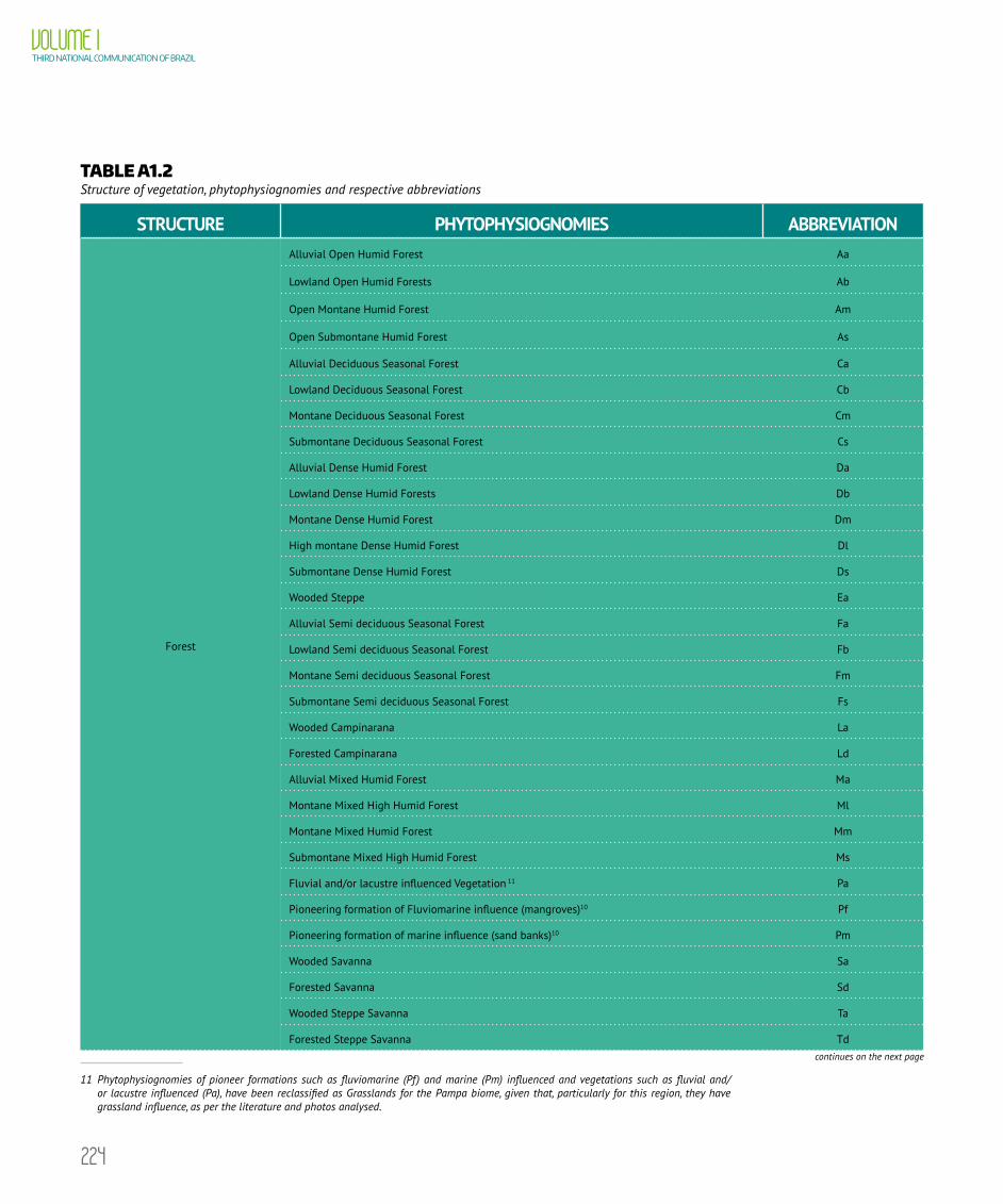
224
VOLUME ITHIRD NATIONAL COMMUNICATION OF BRAZIL
TABLE A1.2 Structure of vegetation, phytophysiognomies and respective abbreviations11
STRUCTURE PHYTOPHYSIOGNOMIES ABBREVIATION
Forest
Alluvial Open Humid Forest Aa
Lowland Open Humid Forests Ab
Open Montane Humid Forest Am
Open Submontane Humid Forest As
Alluvial Deciduous Seasonal Forest Ca
Lowland Deciduous Seasonal Forest Cb
Montane Deciduous Seasonal Forest Cm
Submontane Deciduous Seasonal Forest Cs
Alluvial Dense Humid Forest Da
Lowland Dense Humid Forests Db
Montane Dense Humid Forest Dm
High montane Dense Humid Forest Dl
Submontane Dense Humid Forest Ds
Wooded Steppe Ea
Alluvial Semi deciduous Seasonal Forest Fa
Lowland Semi deciduous Seasonal Forest Fb
Montane Semi deciduous Seasonal Forest Fm
Submontane Semi deciduous Seasonal Forest Fs
Wooded Campinarana La
Forested Campinarana Ld
Alluvial Mixed Humid Forest Ma
Montane Mixed High Humid Forest Ml
Montane Mixed Humid Forest Mm
Submontane Mixed High Humid Forest Ms
Fluvial and/or lacustre influenced Vegetation 11 Pa
Pioneering formation of Fluviomarine influence (mangroves)10 Pf
Pioneering formation of marine influence (sand banks)10 Pm
Wooded Savanna Sa
Forested Savanna Sd
Wooded Steppe Savanna Ta
Forested Steppe Savanna Td
11 Phytophysiognomies of pioneer formations such as fluviomarine (Pf ) and marine (Pm) influenced and vegetations such as fluvial and/or lacustre influenced (Pa), have been reclassified as Grasslands for the Pampa biome, given that, particularly for this region, they have grassland influence, as per the literature and photos analysed.
continues on the next page

225
APPENDIX I METHODOLOGICAL DESCRIPTION FOR THE INVENTORY
OF LAND USE, LAND-USE CHANGE AND FORESTRY
STRUCTURE PHYTOPHYSIOGNOMIES ABBREVIATION
Grassland
Woody Grass Steppe Eg
Park Steppe Ep
Shrubby Campinarana Lb
Woody-grass Campinarana Lg
High Montane Vegetational Refuge Rl
Montane Refuge Rm
Submontane Refuge Rs
Woody-grass Savanna Sg
Park Savanna Sp
Woody Grass Steppe Savanna Tg
Park Steppe Savanna Tp
Soil carbon stocks
The changes in soil carbon stock were estimated following the methodology used in the Second National Inventory.
The estimates followed the methodology proposed by Bernoux et al. (2002), consisting of the following steps:
1 adaptation of the EMBRAPA (2003), at scale 1:5,000,000;
2 adaptation of the IBGE vegetation map (IBGE, 2004), at scale 1:5,000,000 (see above);
3 making/creation of the soil and vegetation association map.
Firstly, the 69 classes categorized into the 18 soil orders of the Brazilian system of soil classification were
reclassified as per the IPCC (1996; 2003), which takes into consideration soil texture, base saturation and moisture.
The details of this class association are presented in Bernoux et al. (2002). Thus, classes were reclassified into six
large soil groups: Soils with high clay activity (S1); Oxisols with low clay activity (S2); Non-Oxisols with low clay
activity (S3); Sandy soils (S4); Organic soils (S5) and Other soils (S6). This results are shown in Figure A1.3.
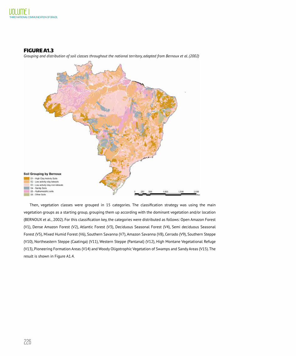
226
VOLUME ITHIRD NATIONAL COMMUNICATION OF BRAZIL
FIGURE A1.3 Grouping and distribution of soil classes throughout the national territory, adapted from Bernoux et al. (2002)
Then, vegetation classes were grouped in 15 categories. The classification strategy was using the main
vegetation groups as a starting group, grouping them up according with the dominant vegetation and/or location
(BERNOUX et al., 2002). For this classification key, the categories were distributed as follows: Open Amazon Forest
(V1), Dense Amazon Forest (V2), Atlantic Forest (V3), Deciduous Seasonal Forest (V4), Semi deciduous Seasonal
Forest (V5), Mixed Humid Forest (V6), Southern Savanna (V7), Amazon Savanna (V8), Cerrado (V9), Southern Steppe
(V10), Northeastern Steppe (Caatinga) (V11), Western Steppe (Pantanal) (V12), High Montane Vegetational Refuge
(V13), Pioneering Formation Areas (V14) and Woody Oligotrophic Vegetation of Swamps and Sandy Areas (V15). The
result is shown in Figure A1.4.
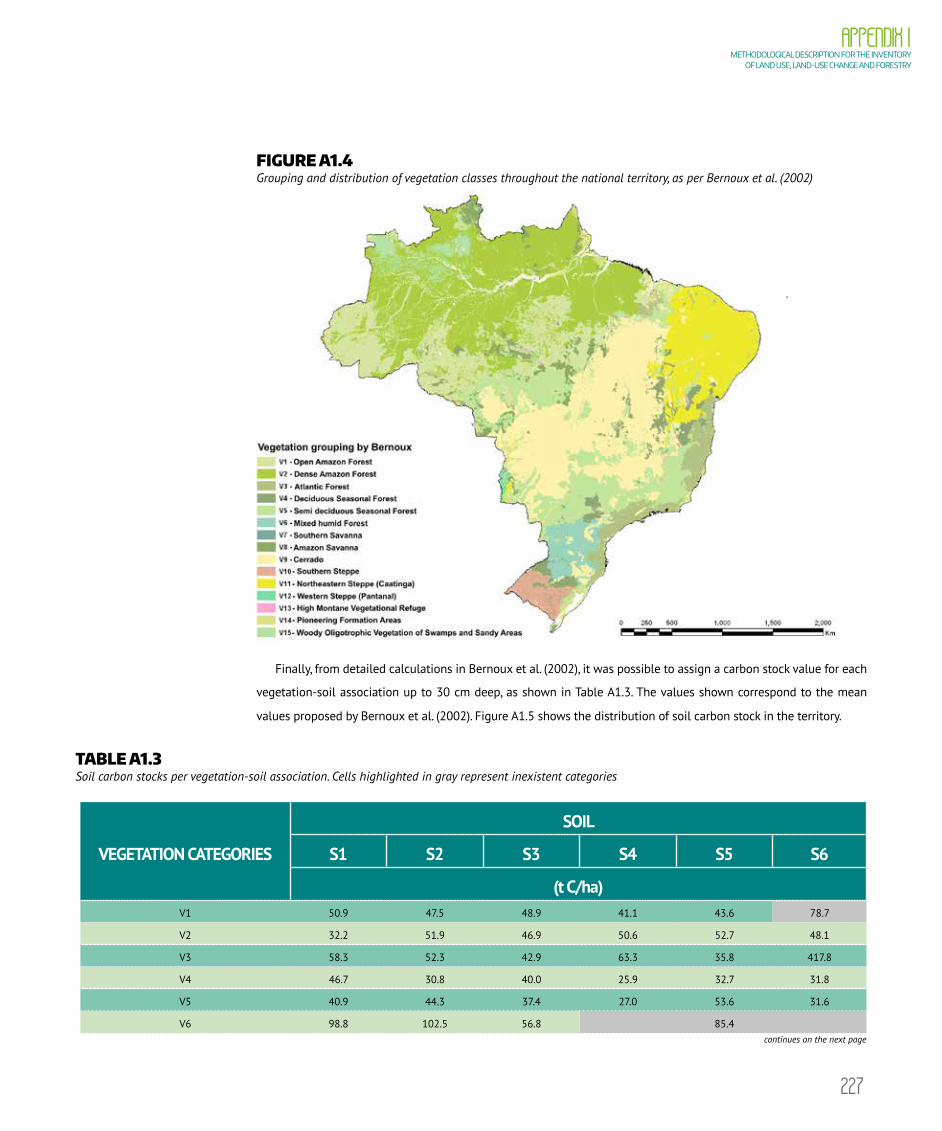
227
APPENDIX I METHODOLOGICAL DESCRIPTION FOR THE INVENTORY
OF LAND USE, LAND-USE CHANGE AND FORESTRY
FIGURE A1.4 Grouping and distribution of vegetation classes throughout the national territory, as per Bernoux et al. (2002)
Finally, from detailed calculations in Bernoux et al. (2002), it was possible to assign a carbon stock value for each
vegetation-soil association up to 30 cm deep, as shown in Table A1.3. The values shown correspond to the mean
values proposed by Bernoux et al. (2002). Figure A1.5 shows the distribution of soil carbon stock in the territory.
TABLE A1.3 Soil carbon stocks per vegetation-soil association. Cells highlighted in gray represent inexistent categories
VEGETATION CATEGORIES
SOIL
S1 S2 S3 S4 S5 S6
(t C/ha)V1 50.9 47.5 48.9 41.1 43.6 78.7
V2 32.2 51.9 46.9 50.6 52.7 48.1
V3 58.3 52.3 42.9 63.3 35.8 417.8
V4 46.7 30.8 40.0 25.9 32.7 31.8
V5 40.9 44.3 37.4 27.0 53.6 31.6
V6 98.8 102.5 56.8 85.4continues on the next page
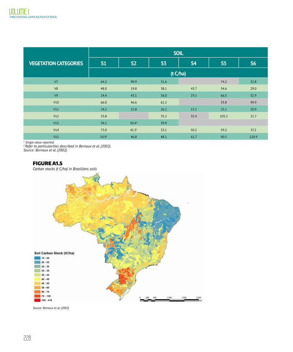
228
VOLUME ITHIRD NATIONAL COMMUNICATION OF BRAZIL
VEGETATION CATEGORIES
SOIL
S1 S2 S3 S4 S5 S6
(t C/ha)V7 64.2 90.9 51.6 74.2 32.8
V8 48.0 19.8 38.1 43.7 34.6 29.0
V9 24.4 43.1 36.0 19.2 66.5 32.9
V10 66.0 46.6 61.2 33.8 49.9
V11 24.2 25.8 26.2 15.1 25.1 20.9
V12 33.8 35.2 35.4 105.2 21.7
V13 34.1 50.41 39.9
V14 73.0 41.31 33.1 50.2 59.2 37.2
V15 50.92 46.8 48.1 61.7 90.5 120.91 Single value reported.2 Refer to particularities described in Bernoux et al. (2002).Source: Bernoux et al. (2002).
FIGURE A1.5 Carbon stocks (t C/ha) in Brazilians soils
Source: Bernoux et al. (2002)

229
APPENDIX I METHODOLOGICAL DESCRIPTION FOR THE INVENTORY
OF LAND USE, LAND-USE CHANGE AND FORESTRY
Land Use
The IPCC (2003, 2006) defines six broad land-use categories: Forest land, Grassland (including sub-category
Grazing), Cropland, Wetlands, Settlements and Other Land. The categories defined in this report were as follows:
Forest Land
Forest Lands are characterized by densification of trees, reducing the amount of light that reaches the soil, which
limits the development of bushes and grasses (IBGE, 2012). This category was defined by the phytophysiognomy
of previous vegetation. So, as per the Table A1.2, which characterizes the phytophysiognomy as a function of its
structure (forest or grassland), it was possible to adapt this classification to the one proposed by the IPCC (2006).
The following sub-categories of Forest Land were created:
I. Primary Forest in a Managed Area (FM)
The Primary Forest in a Managed Area refers to forests in which human action did not cause significant
alterations in its original structure and composition. Also found in managed areas, considered as Protected Areas
(PAs) or Indigenous Lands (IL).
It should be pointed out that Protected Areas were created between 1994 and 2010, as provided by Law No.
9,985/2000, and new IL were delimited by FUNAI. Table A1.4 summarizes quantitatively the representation of these
areas by biome, in 1994, 2002 and 2010. Figure A1.6 shows a visual distribution of them in the observed years.
TABLE A1.4 Protected Areas (PA) and Indigenous Lands (IL) considered in 1994, 2002 and 201012
BIOMEMANAGED AREAS (PA and IL) (ha)
1994 % BIOME 1994 2002 % BIOME
2002 2010 % BIOME 2010
Amazon 99,823,994.50 23.72 141,983,295.01 33.73 205,629,087.80 48.86
Cerrado 848,696.06 0.42 5,118,482.32 2.51 6,586,236.57 3.23
Caatinga 11,244,862.91 13.58 22,941,789.13 27.71 25,279,428.81 30.54
Atlantic Forest 5,710,351.70 5.12 9,897,023.15 8.87 10,681,769.67 9.58
Pantanal 502,985.19 3.32 614,120.31 4.06 614,591.48 4.06
Pampa 365,325.87 2.04 561,503.85 3.14 714,500.74 4.00
TOTAL 118,496,216.24 13.91 181,116,213.76 21.25 249,505,615.06 29.28
12 The increase in managed areas during the period 1994-2002 in comparison with the Second Inventory is due to more information available for indigenous lands. For the Third Inventory, an official letter was sent to FUNAI requesting information as to creation dates (delimitation, declaration, homologation). That information in systematized form allowed for the inclusion of areas that existed in the period 1994-2002, but were not considered in the Second Inventory, for example the Indigenous Land located in the higher part of the Rio Negro River. Ultimately, it is a review point and addition of information.
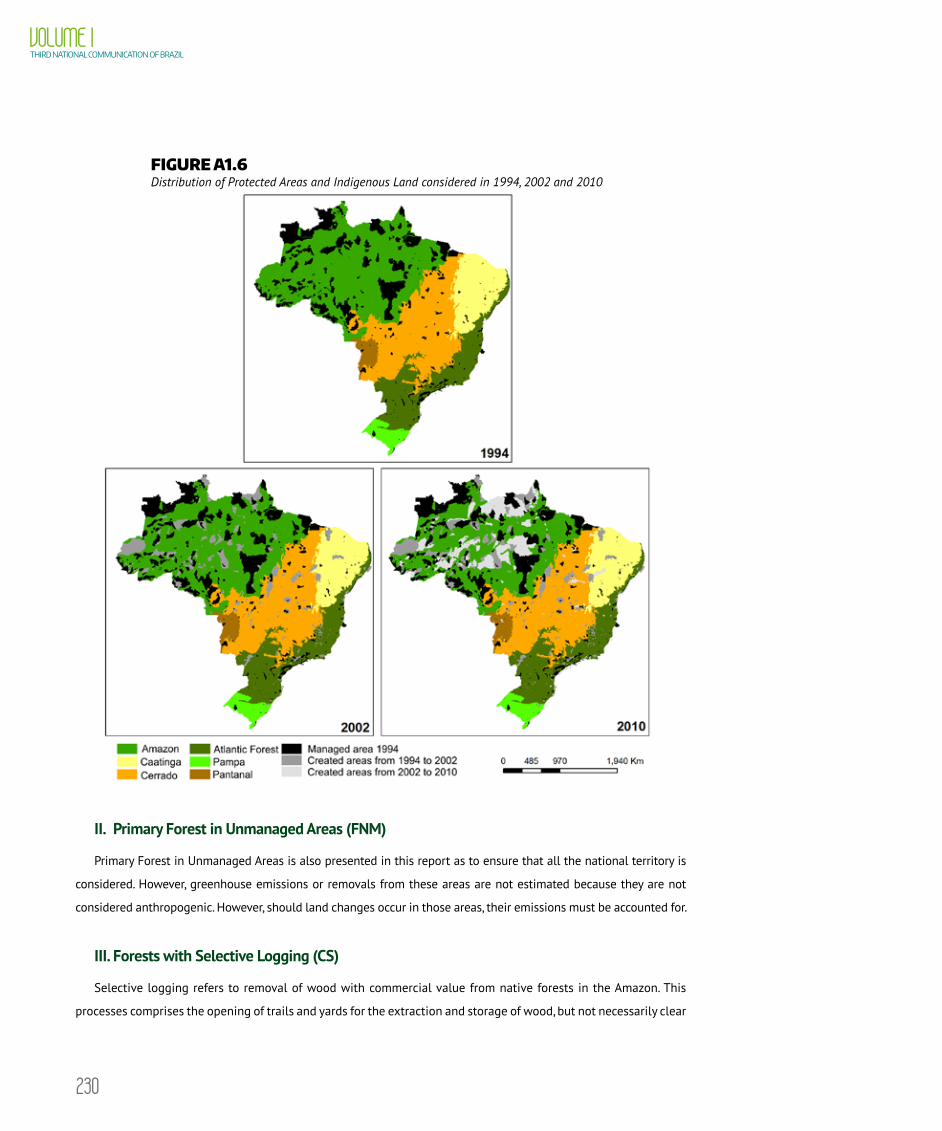
230
VOLUME ITHIRD NATIONAL COMMUNICATION OF BRAZIL
FIGURE A1.6 Distribution of Protected Areas and Indigenous Land considered in 1994, 2002 and 2010
II. Primary Forest in Unmanaged Areas (FNM)
Primary Forest in Unmanaged Areas is also presented in this report as to ensure that all the national territory is
considered. However, greenhouse emissions or removals from these areas are not estimated because they are not
considered anthropogenic. However, should land changes occur in those areas, their emissions must be accounted for.
III. Forests with Selective Logging (CS)
Selective logging refers to removal of wood with commercial value from native forests in the Amazon. This
processes comprises the opening of trails and yards for the extraction and storage of wood, but not necessarily clear

231
APPENDIX I METHODOLOGICAL DESCRIPTION FOR THE INVENTORY
OF LAND USE, LAND-USE CHANGE AND FORESTRY
cut (VERISSIMO et al., 1992; ASNER et al., 2005). These areas can be further explored, converted to agricultural use,
or abandoned (HOLDSWORTH & UHL, 1997; NEPSTAD et al., 1999).
The accounting of such areas in the estimates of emissions and/or removals of carbon is important, given that
without a plan for appropriate management, they represent one of the major causes of forest degradation, leaving
behind forest clearing, roads, damaged forests as well as erosion and soil compaction, changes in the nutrients
cycle and on the flora and structural vegetation composition (VERISSIMO et al., 1995; MATRICARDI et al., 2010).
IV. Secondary Forest (FSec)
Secondary forests have been identified as regeneration areas of primary forests (whether managed or not), which
have been changed in at least one of the periods considered herein (1994, 2002 and, in the Amazon, 2005). Areas of
secondary vegetation were only directly identified from primary forests in the Amazon biome, without intermediate
conversion into anthropogenic use, with space medium resolution satellite images. Forest degradation areas in the
Amazon are monitored by the DEGRAD Project13.
V. Reforestation (Ref)
Comprise single-cropping areas formed by tree species, mostly exotic ones, such as Eucalyptus spp. and Pinus spp.
Grasslands
Grasslands are identified by the predominance of herbaceous vegetation. Like Forests, the definition of this category
was based on the phytophysiognomy map. The portions of the territory that were not categorized as anthropized or as
water bodies (rivers and lagoons and reservoirs) were classified according to the map of previous vegetation.
a. Grasslands with Managed Native Vegetation (GM)
Refer to areas located in Protected Areas (PA) and Indigenous Lands (TI).
b. Grassland with Unmanaged Native Vegetation (GNM)
Like Unmanaged Primary Forests (FNM), Grasslands with Unmanaged Native Vegetation (GNM) are also
presented in this report to ensure that all the national territory is considered. Greenhouse gas emissions
and carbon removals from these areas are not estimated unless land changes occur, in which case emissions
must be accounted for.
c. Secondary Grassland Vegetation (GSec)
Includes native grassland vegetation that had been converted and is in regeneration process. The reasoning
for the identification of grassland vegetation in regeneration was the same adopted for Secondary Forests, as
described above.
13 The forest degradation mapping system in the Brazilian Amazon (DEGRAD) maps degraded forest areas with a tendency of being converted into clear cut on an yearly basis. More information at http://www.obt.inpe.br/degrad/).
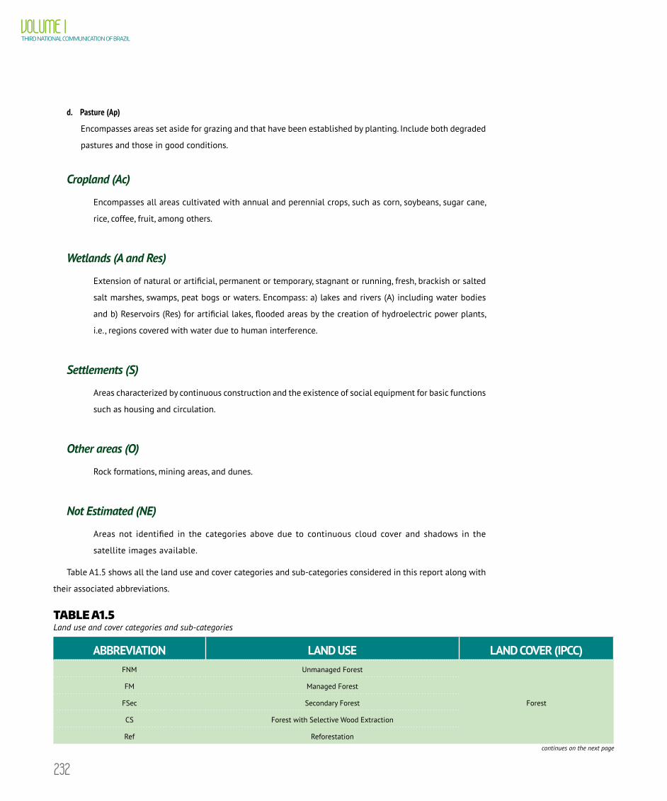
232
VOLUME ITHIRD NATIONAL COMMUNICATION OF BRAZIL
d. Pasture (Ap)
Encompasses areas set aside for grazing and that have been established by planting. Include both degraded
pastures and those in good conditions.
Cropland (Ac)
Encompasses all areas cultivated with annual and perennial crops, such as corn, soybeans, sugar cane,
rice, coffee, fruit, among others.
Wetlands (A and Res)
Extension of natural or artificial, permanent or temporary, stagnant or running, fresh, brackish or salted
salt marshes, swamps, peat bogs or waters. Encompass: a) lakes and rivers (A) including water bodies
and b) Reservoirs (Res) for artificial lakes, flooded areas by the creation of hydroelectric power plants,
i.e., regions covered with water due to human interference.
Settlements (S)
Areas characterized by continuous construction and the existence of social equipment for basic functions
such as housing and circulation.
Other areas (O)
Rock formations, mining areas, and dunes.
Not Estimated (NE)
Areas not identified in the categories above due to continuous cloud cover and shadows in the
satellite images available.
Table A1.5 shows all the land use and cover categories and sub-categories considered in this report along with
their associated abbreviations.
TABLE A1.5 Land use and cover categories and sub-categories
ABBREVIATION LAND USE LAND COVER (IPCC)FNM Unmanaged Forest
Forest
FM Managed Forest
FSec Secondary Forest
CS Forest with Selective Wood Extraction
Ref Reforestationcontinues on the next page
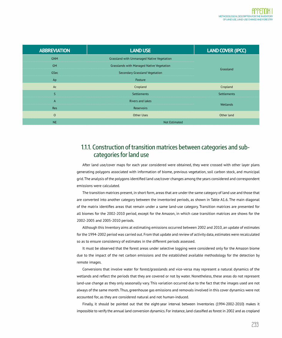
233
APPENDIX I METHODOLOGICAL DESCRIPTION FOR THE INVENTORY
OF LAND USE, LAND-USE CHANGE AND FORESTRY
ABBREVIATION LAND USE LAND COVER (IPCC)GNM Grassland with Unmanaged Native Vegetation
GrasslandGM Grasslands with Managed Native Vegetation
GSec Secondary Grassland Vegetation
Ap Pasture
Ac Cropland Cropland
S Settlements Settlements
A Rivers and lakesWetlands
Res Reservoirs
O Other Uses Other land
NE Not Estimated
1.1.1. Construction of transition matrices between categories and sub-categories for land use
After land use/cover maps for each year considered were obtained, they were crossed with other layer plans
generating polygons associated with information of biome, previous vegetation, soil carbon stock, and municipal
grid. The analysis of the polygons identified land use/cover changes among the years considered and correspondent
emissions were calculated.
The transition matrices present, in short form, areas that are under the same category of land use and those that
are converted into another category between the inventoried periods, as shown in Table A1.6. The main diagonal
of the matrix identifies areas that remain under a same land-use category. Transition matrices are presented for
all biomes for the 2002-2010 period, except for the Amazon, in which case transition matrices are shows for the
2002-2005 and 2005-2010 periods.
Although this Inventory aims at estimating emissions occurred between 2002 and 2010, an update of estimates
for the 1994-2002 period was carried out. From that update and review of activity data, estimates were recalculated
so as to ensure consistency of estimates in the different periods assessed.
It must be observed that the forest areas under selective logging were considered only for the Amazon biome
due to the impact of the net carbon emissions and the established available methodology for the detection by
remote images.
Conversions that involve water for forest/grasslands and vice-versa may represent a natural dynamics of the
wetlands and reflect the periods that they are covered or not by water. Nonetheless, these areas do not represent
land-use change as they only seasonally vary. This variation occurred due to the fact that the images used are not
always of the same month. Thus, greenhouse gas emissions and removals involved in this cover dynamics were not
accounted for, as they are considered natural and not human-induced.
Finally, it should be pointed out that the eight-year interval between Inventories (1994-2002-2010) makes it
impossible to verify the annual land conversion dynamics. For instance, land classified as forest in 2002 and as cropland
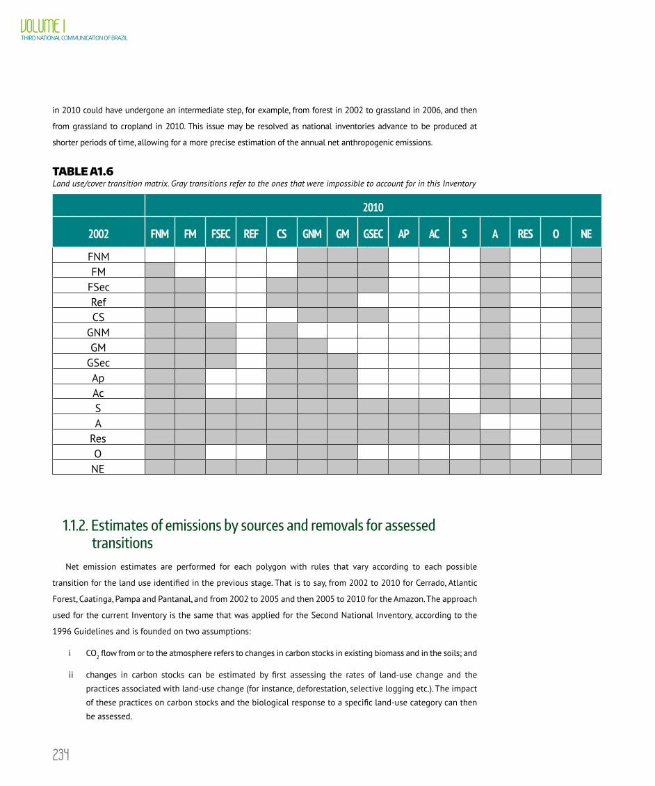
234
VOLUME ITHIRD NATIONAL COMMUNICATION OF BRAZIL
in 2010 could have undergone an intermediate step, for example, from forest in 2002 to grassland in 2006, and then
from grassland to cropland in 2010. This issue may be resolved as national inventories advance to be produced at
shorter periods of time, allowing for a more precise estimation of the annual net anthropogenic emissions.
TABLE A1.6 Land use/cover transition matrix. Gray transitions refer to the ones that were impossible to account for in this Inventory
2010
2002 FNM FM FSEC REF CS GNM GM GSEC AP AC S A RES O NE
FNM FM
FSec Ref CS
GNM GM
GSec Ap Ac S A
Res O
NE
1.1.2. Estimates of emissions by sources and removals for assessed transitions
Net emission estimates are performed for each polygon with rules that vary according to each possible
transition for the land use identified in the previous stage. That is to say, from 2002 to 2010 for Cerrado, Atlantic
Forest, Caatinga, Pampa and Pantanal, and from 2002 to 2005 and then 2005 to 2010 for the Amazon. The approach
used for the current Inventory is the same that was applied for the Second National Inventory, according to the
1996 Guidelines and is founded on two assumptions:
i CO2 flow from or to the atmosphere refers to changes in carbon stocks in existing biomass and in the soils; and
ii changes in carbon stocks can be estimated by first assessing the rates of land-use change and the
practices associated with land-use change (for instance, deforestation, selective logging etc.). The impact
of these practices on carbon stocks and the biological response to a specific land-use category can then
be assessed.
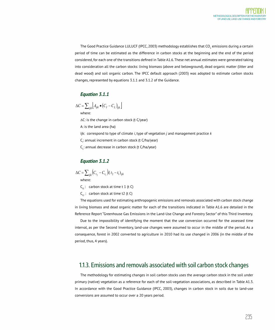
235
APPENDIX I METHODOLOGICAL DESCRIPTION FOR THE INVENTORY
OF LAND USE, LAND-USE CHANGE AND FORESTRY
The Good Practice Guidance LULUCF (IPCC, 2003) methodology establishes that CO2 emissions during a certain
period of time can be estimated as the difference in carbon stocks at the beginning and the end of the period
considered, for each one of the transitions defined in Table A1.6. These net annual estimates were generated taking
into consideration all the carbon stocks: living biomass (above and belowground), dead organic matter (litter and
dead wood) and soil organic carbon. The IPCC default approach (2003) was adopted to estimate carbon stocks
changes, represented by equations 3.1.1 and 3.1.2 of the Guidance.
Equation 3.1.1
( )[ ]∑ −•=∆ ijk ijkLIijk CCACwhere:
∆C: is the change in carbon stock (t C/year)
A: is the land area (ha)
ijk: correspond to type of climate i, type of vegetation j and management practice k
CI: annual increment in carbon stock (t C/ha/year)
CL: annual decrease in carbon stock (t C/ha/year)
Equation 3.1.2
( ) ijkijk tt ttCCC )/( 1212−−=∆ ∑
where:
Ct1 : carbon stock at time t 1 (t C)
Ct2 : carbon stock at time t2 (t C)
The equations used for estimating anthropogenic emissions and removals associated with carbon stock change
in living biomass and dead organic matter for each of the transitions indicated in Table A1.6 are detailed in the
Reference Report “Greenhouse Gas Emissions in the Land-Use Change and Forestry Sector” of this Third Inventory.
Due to the impossibility of identifying the moment that the use conversion occurred for the assessed time
interval, as per the Second Inventory, land-use changes were assumed to occur in the middle of the period. As a
consequence, forest in 2002 converted to agriculture in 2010 had its use changed in 2006 (in the middle of the
period, thus, 4 years).
1.1.3. Emissions and removals associated with soil carbon stock changesThe methodology for estimating changes in soil carbon stocks uses the average carbon stock in the soil under
primary (native) vegetation as a reference for each of the soil-vegetation associations, as described in Table A1.3.
In accordance with the Good Practice Guidance (IPCC, 2003), changes in carbon stock in soils due to land-use
conversions are assumed to occur over a 20 years period.
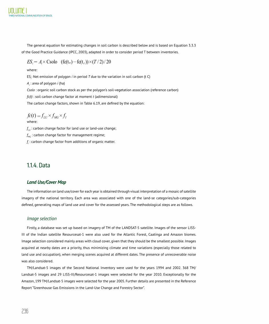
236
VOLUME ITHIRD NATIONAL COMMUNICATION OF BRAZIL
The general equation for estimating changes in soil carbon is described below and is based on Equation 3.3.3
of the Good Practice Guidance (IPCC, 2003), adapted in order to consider period T between inventories.
where:
ESi: Net emission of polygon i in period T due to the variation in soil carbon (t C)
Ai : area of polygon i (ha)
Csolo : organic soil carbon stock as per the polygon’s soil-vegetation association (reference carbon)
fc(t) : soil carbon change factor at moment t (adimensional)
The carbon change factors, shown in Table 6.19, are defined by the equation:
where:
fLU : carbon change factor for land use or land-use change;
fMG : carbon change factor for management regime;
fI : carbon change factor from additions of organic matter.
1.1.4. Data
Land Use/Cover Map
The information on land use/cover for each year is obtained through visual interpretation of a mosaic of satellite
imagery of the national territory. Each area was associated with one of the land-se categories/sub-categories
defined, generating maps of land use and cover for the assessed years. The methodological steps are as follows.
Image selection
Firstly, a database was set up based on imagery of TM of the LANDSAT-5 satellite. Images of the sensor LISS-
III of the Indian satellite Resourcesat-1 were also used for the Atlantic Forest, Caatinga and Amazon biomes.
Image selection considered mainly areas with cloud cover, given that they should be the smallest possible. Images
acquired at nearby dates are a priority, thus minimizing climate and time variations (especially those related to
land use and occupation), when merging scenes acquired at different dates. The presence of unrecoverable noise
was also considered.
TM/Landsat-5 images of the Second National Inventory were used for the years 1994 and 2002. 368 TM/
Landsat-5 images and 29 LISS-III/Resourcesat-1 images were selected for the year 2010. Exceptionally for the
Amazon, 199 TM/Landsat-5 images were selected for the year 2005. Further details are presented in the Reference
Report “Greenhouse Gas Emissions in the Land-Use Change and Forestry Sector”.

237
APPENDIX I METHODOLOGICAL DESCRIPTION FOR THE INVENTORY
OF LAND USE, LAND-USE CHANGE AND FORESTRY
Image processing
This stage involved basically the recording of the images and management of histograms (contrast application).
The selected TM/Landsat-5 images of 2010 were geo-referenced based on points of control on the images of 2002,
as a crossroad. This procedure assured that the mapped changes refer to changes occurred on the land and not
between two scenes. Scenes of the year 2005 in relation to the images of 2002 were also registered for the Amazon
biome. The geo-referenced images of the LISS-III/Resourcesat-1 followed the same procedure.
Themed mapping
After correcting the satellite images for contrast and brightness in order to facilitate the identification of areas
by the interpreters, all the areas with any type of human intervention, water bodies and reservoirs were mapped.
In order to identify areas of selective logging in the Amazon, digital processing techniques were used, according to
the DETEX14 approach, to highlight the changes in the spectral response of the forests with intervention.
Remaining areas (not mapped) were considered as primary vegetation areas. They were classified as either
forests or grasslands, managed or unmanaged, according to information of the previous vegetation map
(phytophysiognomies) and managed areas map (Protected Areas and Indigenous Land), respectively.
The categorization of Forests and Secondary Grasslands (FSec and GSec) was made through observation of
areas in previous years. For example, areas classified as vegetation (grasslands or forests) in 2010, which had
previously been classified as another type of cover (in 1994, 2002 or 2005), were considered as Grasslands or
Secondary Forests.
The themed mapping process was carried out considering 6 ha as minimum mapping area, with final output
scale at 1:250,000.
Land use and cover maps
Land use and cover maps for the entire national territory for the years 1994, 2002 and 2010 are shown in A1.7.
The maps for 1994 and 2002 provide the activity data to estimate the net greenhouse gas emissions were updated
to assure a higher consistency on the classification. For the Amazon, maps for 1994 and 2002 of the Second
Inventory were corrected and used, generating maps for 2005 and 2010 (Figure A1.8). Maps for the other biomes
are shown in Figures A1.9 to A1.13.
14 Project DETEX (Selective Logging Detection) is a system developed by INPE to monitor timber exploitation in the Amazon.
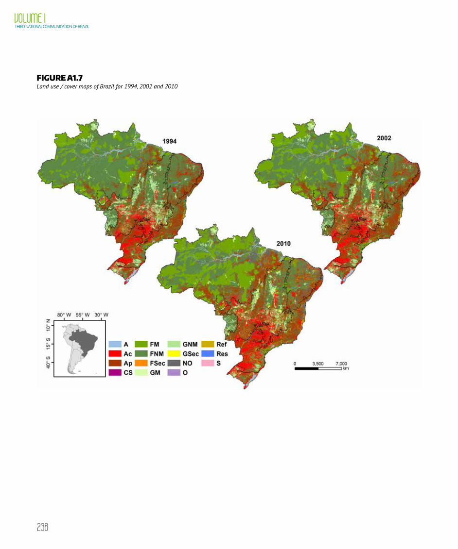
238
VOLUME ITHIRD NATIONAL COMMUNICATION OF BRAZIL
FIGURE A1.7 Land use / cover maps of Brazil for 1994, 2002 and 2010

239
APPENDIX I METHODOLOGICAL DESCRIPTION FOR THE INVENTORY
OF LAND USE, LAND-USE CHANGE AND FORESTRY
FIGURE A1.8 Land use / cover maps of the Amazon biome for 1994, 2002, 2005 and 2010
FIGURE A1. 9 Land use / cover maps of the Cerrado biome for 1994, 2002, and 2010

240
VOLUME ITHIRD NATIONAL COMMUNICATION OF BRAZIL
FIGURE A1.10 Land use / cover maps of the Atlantic Forest biome for 1994, 2002, and 2010
FIGURE A1.11 Land use / cover maps of the Caatinga biome for 1994, 2002, and 2010

241
APPENDIX I METHODOLOGICAL DESCRIPTION FOR THE INVENTORY
OF LAND USE, LAND-USE CHANGE AND FORESTRY
FIGURE A1.12 Land use / cover maps of the Pampa biome for 1994, 2002, and 2010
FIGURE A1.13 Land use / cover maps of the Pantanal biome for 1994, 2002, and 2010
242
VOLUME ITHIRD NATIONAL COMMUNICATION OF BRAZIL
Carbon stock changes in living biomass and dead organic matter
The values of carbon stock of phytophysiognomies of each Brazilian biome were estimated from values of
living biomass, both above and belowground, and dead organic matter (dead wood and litter). The approaches used
for these estimates were the following:
a. Calculation of stocks from structural data of the vegetation
The use of structural data of the vegetation (DBH and height) collected in the field was prioritized, obtained from
plots of forest inventories. The structural data relate to those of RADAMBRASIL project to the Amazon; the PROBIO
project provided by Embrapa Informatics for the Pantanal; the Forest Inventory of Tocantins to the Cerrado and
measurements carried out by researchers from the Federal University of Pernambuco for the Caatinga. Allometric
equations surveys were conducted so the most appropriate ones were applied to the data for each region (BROWN,
1997; MELO et al., 2007 in PINHEIRO, 2008; DELITTI et al., 2006). In addition to Brown’s equation (BROWN, 1997)
based on rainfall levels and seasonal trends used to the Amazon, other Brown’s equation was also used (BROWN,
1997; equation 3.2.1) for some of the phytophysiognomies in the Cerrado, Caatinga and Atlantic Forest biomes, in
an attempt to adjust the equation to the climate of the phytophysiognomies. Equations of Melo et al (2007 apud
PINHEIRO, 2008) for ‘the phytophysiognomy Sa and Sd, and Delitti et al. (2006) for the plant physiognomies Sp
were used for the Pantanal biome.
b. Biomass data out of literature review
Biomass values from other phytophysiognomies not covered in the databases above were obtained from a
review of the scientific literature. Papers already published referring to the dry matter of the vegetation were
chosen when they had a studied area corresponding to the phytophysiognomy of the biome.
When such assessment was not possible, papers carried on the same phytophysiognomy, but in other biome, were
chosen; taking into consideration factors as altitude, latitude, and geographic distance, temperature and rainfall.
This assessment was carried on with the aid of the Geographic System of Information (GSI).
Flora and structural resemblance together with other phytophysiognomy were assessed when a representative
value was not found for the specific phytophysiognomy, so that the value of the biomass could be used. In some
cases, in the absence of a published biomass value, allometric equations were applied to the research plant
sociological results, with average individual density per hectare, diameter at breast height (DBH) and basal area.
Under theses cases, the selected allometric equations are pan-tropical, using as a dependent variable the DBH and
the research developed by Brown (1997). The choice among the allometric equations presented by Brown (1997)
was made in accordance with phytophysiognomy, diameter of the trees and environmental characteristics, such as
precipitation and distribution of rainfall throughout the year (seasonality).
Whenever possible, preference has been given to the papers exhibiting values of biomass for a greater number of

243
APPENDIX I METHODOLOGICAL DESCRIPTION FOR THE INVENTORY
OF LAND USE, LAND-USE CHANGE AND FORESTRY
reservoirs (such as aboveground biomass for tree strata, shrub and herbaceous, that cover the trunk, bark, branches
and leaves; belowground biomass; dead organic matter, which includes dead wood and litter). The sampling effort
and the phytophysiognomy distribution were also considered as selection criteria.
c. Use of expansion factors and ratio
In the absence of values of belowground biomass or the dead organic matter biomass, factors based on a
literature review were used, particularly to the ratio of belowground and aboveground biomass (root-to-shoot)
to estimate the belowground biomass as well as the ratio of the dead and living biomass (dead wood stocks/live
biomass) and of the litter of the living biomass to estimate dead organic matter. In this case expansion factors
were prioritized calculated with biomass values obtained in the same vegetation type, preferably in the biome of
interest. When such values were not found, expansion factors, ratio and values associated with vegetation with
similar in structure, deciduousness and flora were used.
d. Use of IPCC default values
When values to represent the estimates to the ratio of belowground and aboveground biomass (root-to-shoot)
and dead organic matter were not found in the literature, default values established by the IPCC (2003, 2006) were
used; in accordance with the specific biome climatic zone and the ecological zone and biomass vegetation, when
applicable.
e. Consultations to multiple sources of evidence
The decisions about the values of living biomass and dead organic matter were endorsed, whenever possible,
via consultation to studies of phytosociology, management plans, technical reports, in addition to contact with
research experts in vegetation type and biomes. Photos of vegetation covers, found in publications and on Google
Earth, were also used to endorse the distribution and classification of vegetation.
Other biomass researches were used as multiple evidence sources aiming at comparing the values adopted and
minimizing the chances of choosing a non-representative study; with higher or lower biomass values for the
relevant phytophysiognomy.
f. Carbon in the Forest and Grassland biomass
The biomass of different carbon stocks in Forest and Grassland areas was converted into carbon using the IPCC
default values (2006) presented in Table A1.7.

244
VOLUME ITHIRD NATIONAL COMMUNICATION OF BRAZIL
TABLE A1.7 Carbon percentage in stocks of aboveground biomass, belowground biomass, dead wood, and litter in Forest and Grasslands (IPCC, 2006)
STOCKS FORESTS GRASSLANDSAboveground biomass 47% 47%
Belowground biomass 47% 47%
Dead wood (either lying on the ground or standing) 47% 50%
Litter 47% 40%
Methods and data used to estimate biomass and carbon stock of each phytophysiognomy in each biome are
described below. Further details of methods and values used are presented in the “Greenhouse Gas Emissions in
the Land-Use Change and Forestry Sector” Reference Report.
Amazon Biome
Data collected from the RADAMBRASIL Project
Like in the Second Inventory, estimates for the Amazon biome’s vegetation biomass were mostly based on the
forest inventory and phytophysiognomy maps from the RADAMBRASIL Project. Out of the 29 phytophysiognomies,
nine cover approximately 90% of the biome as follows: Alluvial Open Humid Forest (Aa), Lowland Open Humid
Forests (Ab), Open Submontane Humid Forest (As), Alluvial Dense Humid Forest (Da), Montane Dense Humid
Forest (Dm), Submontane Dense Humid Forest (Ds), Submontane Semi deciduous Seasonal Forest (Fs), Forested
Campinarana (Ld).
For the Third Inventory, only the samples of the RADAMBRASIL that presented locations with geographic
coordinates were used; samples that had only volume information of the RADAMBRASIL were disregarded. Samples
that did not present a representative number per phytophysiognomy (less than 10 samples per phytophysiognomy).
On the first part of this task, values of diameter at breast height (DBH15) of 100,222 trees measured in 1,668
samples of RADAMBRASIL.
Subsequently, a regionalization of the biomass values was proposed as a function of the basal area distribution
of the arboreal individuals for all the Amazon biome. For this stage, less representative samples were included
to aggregate more information of the inventoried regions. As a result, data of 102,837 trees measured in 1,682
samples of RADAMBRASIL were used for this regionalization (Figure A1.14).
15 CBH values measured by RADAMBRASIL were converted into DBH, as this is the input standard for allometric equations. For the converstion, the following equation was used: DBH=
CBH π

245
APPENDIX I METHODOLOGICAL DESCRIPTION FOR THE INVENTORY
OF LAND USE, LAND-USE CHANGE AND FORESTRY
FIGURE A1.14 Distribution of samples provided by the RADAMBRASIL Project
Selection of the allometric equations
The Third Inventory tested different allometric equations, in an attempt to define one that could better represent
the phytophysiognomy variation of all the biome (BROWN, 1997; CARVALHO JR. et al., 1998; ARAÚJO et al., 1999;
BAKER et al., 2004; CHAVE et al., 2005). The choice of these equations was made based on the regional broadness
of the collection of the field data, sample density and spatial distribution of the samples – as to represent the large
variability of the forest. The following equations were tested:
AGBinitial= 42.69 – 12.8 X DBH + 1.242 X DBH2, by Brown (1997) (Equation 1)
AGBinitial= EXP -2.134+(2.53xIn(DBH)), by Brown (1997) (Equation 2)
AGBinitial= 0.6 X (4.06 X DBH 1.76), by Araújo et al. (1999) (Equation 3)
AGBinitial= 1000 x 0.6 x EXP 3.323+2.546xln( DBH100
)
by Carvalho Jr. et al. (1998) (Equation 4)
AGBinitial= EXP 2.42xln(DBH)–2, by Baker et al. (2004) (Equation 5)
AGBinitial= EXP 0.33xln(DBH)+0.933xln(DBH)2 –0.122xln(DBH)3–0.37,
by Baker et al. (2004) (Equation 6)
AGBinitial= 0.642 X EXP –1.499+2.148xln(DBH)+0.207xln(DBH)2 –0.0281xln(DBH)3,
by Chave et al. (2005) (Equation 7)where AGBinitial corresponds to the tree’s dry matter in kg and the tree’s DBH is given in cm.
All the trees had their biomass calculated by each of different equations above. Subsequently, the following
steps were followed: (1) all the biomass of the trees within the sample of the RADAMBRASIL (AGBinicial) was

246
VOLUME ITHIRD NATIONAL COMMUNICATION OF BRAZIL
summed; (2) these samples were separated by phytophysiognomy and (3) the average of the AGBinitial (t/ha) of
the samples for each phytophysiognomy were calculated, as each sample of the RADAMBRASIL has one hectare.
Expansion factors and ratio
As the trees sampled by the RADAMBRASIL have a DBH higher or equal to 31.83 cm, two expansion factors
were applied in order to include trees with a DBH from 10 to 31.83 cm based on the phytophysiognomy (dense and
open forest)16, as proposed by Nogueira et al. (2008) and presented in Table A1.8. These authors also used data of
RADAMBRASIL and collected data on field of different regions of the Amazon in order to estimate this proportion.
Result is:
AVERAGE(AGBcorrection x ha–1)
= AVERAGE(AGBinitial x ha–1) x Correction factor10<DBH<31.83
TABLE A1.8 Expansion factors for the inclusion of biomass of tress with DBH between 10 and 31.83cm of the RADAMBRASIL Project’s phytophysiognomies
PHYTOPHYSIOGNOMY FOREST TYPE EXPANSION FACTOR10<DBH<31.83 CM
Aa Open 1.506
Ab Open 1.506
As Open 1.506
Da Dense 1.537
Db Dense 1.537
Dm Dense 1.537
Ds Dense 1.537
Fs Open 1.506
Ld Open 1.506
Source: Nogueira et al. (2008).
Other ratios were also applied according to Nogueira et al. (2008) in different regions of Amazon to open and
dense forests in order to include palm trees, lianas, underbrush, herb layer, dead wood, litter and belowground
biomass. Table A1.9 presents these expansion factors and ratios per stock. Based on the values, the following
equation applies:
AVERAGE(AGBtotal x ha–1)
= AVERAGE(AGBcorrection x ha–1) + (AVERAGE(AGBcorrection x ha–1)
x Total Correction factor)
16 Trees with DBH between 10 and 31.83cm correspond to a relative contribution of 33.6% for open forests and 34.9% for dense forests in the Amazon (NOGUEIRA et al., 2008).
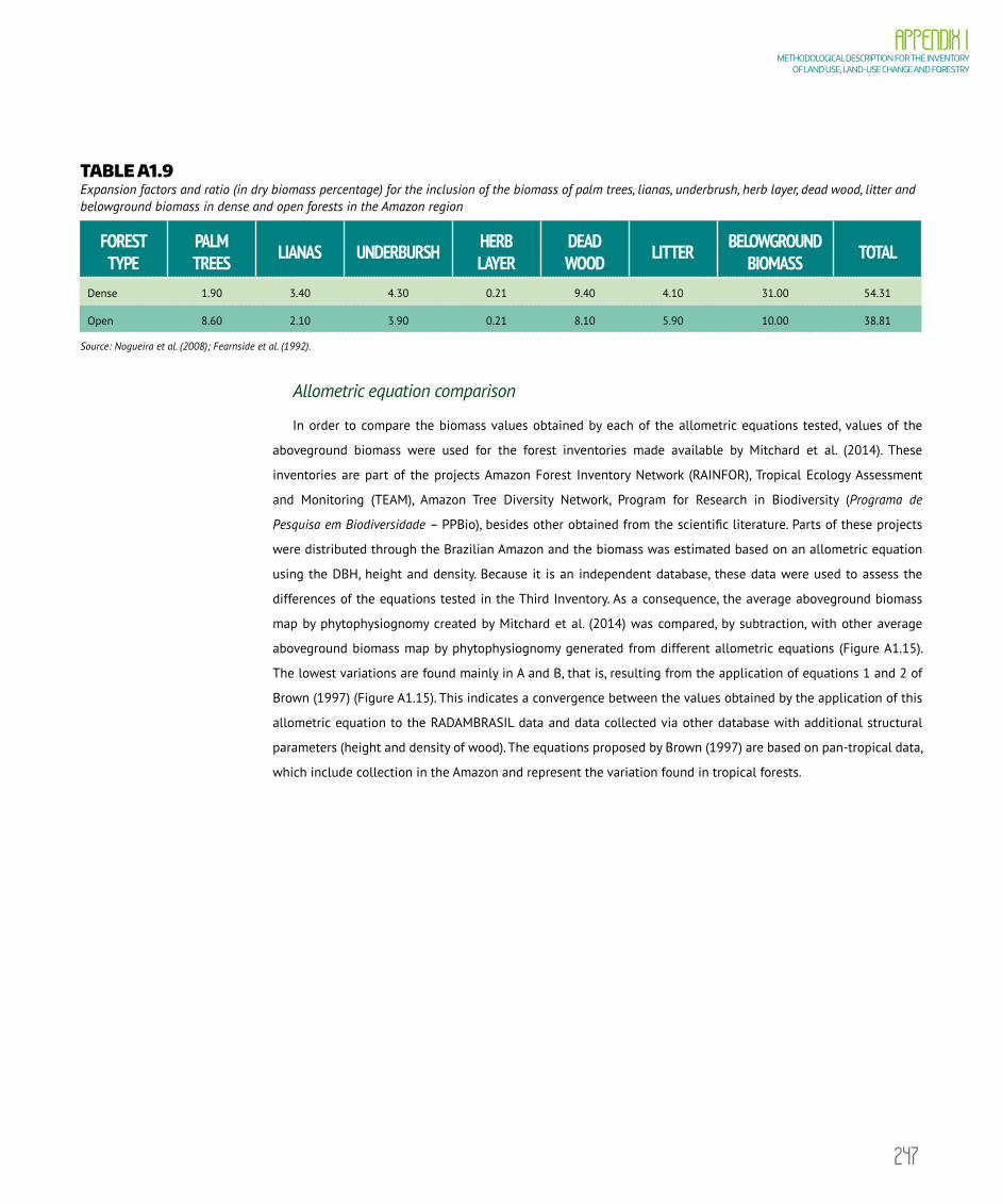
247
APPENDIX I METHODOLOGICAL DESCRIPTION FOR THE INVENTORY
OF LAND USE, LAND-USE CHANGE AND FORESTRY
TABLE A1.9 Expansion factors and ratio (in dry biomass percentage) for the inclusion of the biomass of palm trees, lianas, underbrush, herb layer, dead wood, litter and belowground biomass in dense and open forests in the Amazon region
FOREST TYPE
PALM TREES LIANAS UNDERBURSH HERB
LAYERDEAD WOOD LITTER BELOWGROUND
BIOMASS TOTAL
Dense 1.90 3.40 4.30 0.21 9.40 4.10 31.00 54.31
Open 8.60 2.10 3.90 0.21 8.10 5.90 10.00 38.81
Source: Nogueira et al. (2008); Fearnside et al. (1992).
Allometric equation comparison
In order to compare the biomass values obtained by each of the allometric equations tested, values of the
aboveground biomass were used for the forest inventories made available by Mitchard et al. (2014). These
inventories are part of the projects Amazon Forest Inventory Network (RAINFOR), Tropical Ecology Assessment
and Monitoring (TEAM), Amazon Tree Diversity Network, Program for Research in Biodiversity (Programa de
Pesquisa em Biodiversidade – PPBio), besides other obtained from the scientific literature. Parts of these projects
were distributed through the Brazilian Amazon and the biomass was estimated based on an allometric equation
using the DBH, height and density. Because it is an independent database, these data were used to assess the
differences of the equations tested in the Third Inventory. As a consequence, the average aboveground biomass
map by phytophysiognomy created by Mitchard et al. (2014) was compared, by subtraction, with other average
aboveground biomass map by phytophysiognomy generated from different allometric equations (Figure A1.15).
The lowest variations are found mainly in A and B, that is, resulting from the application of equations 1 and 2 of
Brown (1997) (Figure A1.15). This indicates a convergence between the values obtained by the application of this
allometric equation to the RADAMBRASIL data and data collected via other database with additional structural
parameters (height and density of wood). The equations proposed by Brown (1997) are based on pan-tropical data,
which include collection in the Amazon and represent the variation found in tropical forests.

248
VOLUME ITHIRD NATIONAL COMMUNICATION OF BRAZIL
FIGURE A1.15 Difference between aboveground biomass estimated by Mithchard et al. (2014) and results of equations 1 (A), 2 (B), 3 (C), 4 (D), 5 (E), 6 (F) and 7 (G)
ValidationDifference in biomass (t/ha)
A comparison of biomass estimates by different allometric equations due to the increase of DBH was
performed (Figure A1.16). Under this assessment the Higuchi et al. (1998) equation was also included, as used
in the Second Inventory. Both the Higuchi et al. (1998) and the quadratic equation 1 of Brown (1997) tend to
underestimate bigger individuals (Figure A1.16). However, Brown (1997) suggests the use of the equation (2)
(exponential) for trees with DBH lower than 160cm and quadratic equation (1) for trees with DBH greater or
equal 160 cm. According to the histogram of Figure A1.17, which represents the frequency of the trees inventoried
by the RADAMBRASIL by classes of DBH, there is a higher incidence of trees with DBH ranging from 31.83 to
130cm. Consequently, the exponential equation of Brown (1997) is more indicated as the major part of the
biomass is concentrated in samples with DBH lower than 160cm. Thus, the underestimation of individuals with
a DBH higher than 160cm, due to the application of the quadratic equation (1), would be compensated by the
overestimation of trees with DBH next to the 160cm threshold.
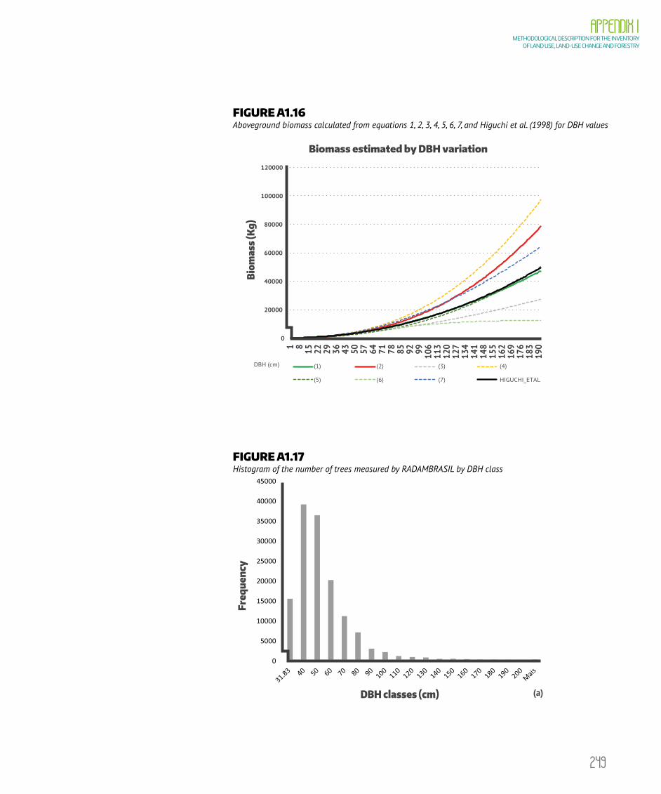
249
APPENDIX I METHODOLOGICAL DESCRIPTION FOR THE INVENTORY
OF LAND USE, LAND-USE CHANGE AND FORESTRY
FIGURE A1.16 Aboveground biomass calculated from equations 1, 2, 3, 4, 5, 6, 7, and Higuchi et al. (1998) for DBH values
(1)
(5) (6) (7) HIGUCHI_ETAL
(2) (3) (4)DBH (cm)
Bio
mas
s (K
g)
Biomass estimated by DBH variation
0
20000
40000
60000
80000
100000
120000
1 8 15 22 29 36 43 50 57 64 71 78 85 92 99 106
113
120
127
134
141
148
155
162
169
176
183
190
FIGURE A1.17 Histogram of the number of trees measured by RADAMBRASIL by DBH class
0
5000
10000
15000
20000
25000
30000
35000
40000
45000
Freq
uenc
y
DBH classes (cm) (a)
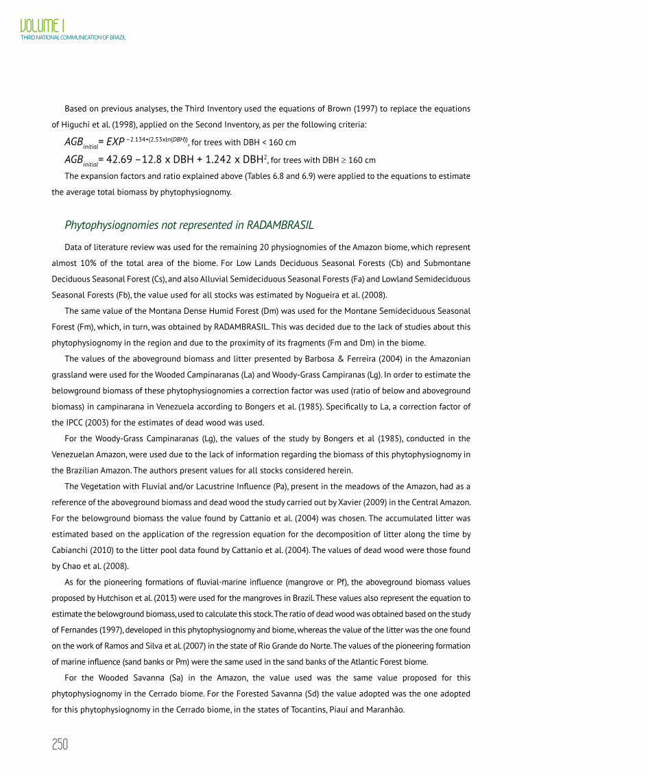
250
VOLUME ITHIRD NATIONAL COMMUNICATION OF BRAZIL
Based on previous analyses, the Third Inventory used the equations of Brown (1997) to replace the equations
of Higuchi et al. (1998), applied on the Second Inventory, as per the following criteria:
AGBinitial= EXP –2.134+(2.53xln(DBH)), for trees with DBH < 160 cm
AGBinitial= 42.69 –12.8 x DBH + 1.242 x DBH2, for trees with DBH ≥ 160 cm
The expansion factors and ratio explained above (Tables 6.8 and 6.9) were applied to the equations to estimate
the average total biomass by phytophysiognomy.
Phytophysiognomies not represented in RADAMBRASIL
Data of literature review was used for the remaining 20 physiognomies of the Amazon biome, which represent
almost 10% of the total area of the biome. For Low Lands Deciduous Seasonal Forests (Cb) and Submontane
Deciduous Seasonal Forest (Cs), and also Alluvial Semideciduous Seasonal Forests (Fa) and Lowland Semideciduous
Seasonal Forests (Fb), the value used for all stocks was estimated by Nogueira et al. (2008).
The same value of the Montana Dense Humid Forest (Dm) was used for the Montane Semideciduous Seasonal
Forest (Fm), which, in turn, was obtained by RADAMBRASIL. This was decided due to the lack of studies about this
phytophysiognomy in the region and due to the proximity of its fragments (Fm and Dm) in the biome.
The values of the aboveground biomass and litter presented by Barbosa & Ferreira (2004) in the Amazonian
grassland were used for the Wooded Campinaranas (La) and Woody-Grass Campiranas (Lg). In order to estimate the
belowground biomass of these phytophysiognomies a correction factor was used (ratio of below and aboveground
biomass) in campinarana in Venezuela according to Bongers et al. (1985). Specifically to La, a correction factor of
the IPCC (2003) for the estimates of dead wood was used.
For the Woody-Grass Campinaranas (Lg), the values of the study by Bongers et al (1985), conducted in the
Venezuelan Amazon, were used due to the lack of information regarding the biomass of this phytophysiognomy in
the Brazilian Amazon. The authors present values for all stocks considered herein.
The Vegetation with Fluvial and/or Lacustrine Influence (Pa), present in the meadows of the Amazon, had as a
reference of the aboveground biomass and dead wood the study carried out by Xavier (2009) in the Central Amazon.
For the belowground biomass the value found by Cattanio et al. (2004) was chosen. The accumulated litter was
estimated based on the application of the regression equation for the decomposition of litter along the time by
Cabianchi (2010) to the litter pool data found by Cattanio et al. (2004). The values of dead wood were those found
by Chao et al. (2008).
As for the pioneering formations of fluvial-marine influence (mangrove or Pf), the aboveground biomass values
proposed by Hutchison et al. (2013) were used for the mangroves in Brazil. These values also represent the equation to
estimate the belowground biomass, used to calculate this stock. The ratio of dead wood was obtained based on the study
of Fernandes (1997), developed in this phytophysiognomy and biome, whereas the value of the litter was the one found
on the work of Ramos and Silva et al. (2007) in the state of Rio Grande do Norte. The values of the pioneering formation
of marine influence (sand banks or Pm) were the same used in the sand banks of the Atlantic Forest biome.
For the Wooded Savanna (Sa) in the Amazon, the value used was the same value proposed for this
phytophysiognomy in the Cerrado biome. For the Forested Savanna (Sd) the value adopted was the one adopted
for this phytophysiognomy in the Cerrado biome, in the states of Tocantins, Piauí and Maranhão.

251
APPENDIX I METHODOLOGICAL DESCRIPTION FOR THE INVENTORY
OF LAND USE, LAND-USE CHANGE AND FORESTRY
For the Grassy-Woody savannas (Sg) and Park (Sp), as well as for the Wooded Steppe Savannas (Ta), Grassy-
Woody (Tg) and Park (Tp), values of aboveground biomass, dead wood and litter submitted by Barbosa & Fearnside
(2005) in the Amazon were used. For the estimation of the belowground biomass ratios proposed by Miranda et al.
(2014) were used.
The values by Barbosa & Fearnside (1999) were chosen for the Forested Steppe Savanna (Td) and Montane
Refuge (Rm) in the Amazon biome; for the estimation of belowground biomass, the ratios by Miranda et al. (2014)
were applied.
Map of the average total biomass per phytophysiognomy of the Amazon
In order to elaborate the map for the total average biomass of the phytophysiognomy of the Amazon (Figure
A1.20), the values of total average biomass by phytophysiognomy (Table A1.10) and the file in shapefile format of
the previous vegetation were united.
TABLE A1.10 Total average biomass (TB) by area unit (t/ha) for the different phytophysiognomies in the Amazon biome
ABBREVIATION PHYTOPHYSIOGNOMY TB (t/ha)
Aa Alluvial Open Humid Forest 390.00
Ab Lowland Open Humid Forest 349.11
As Open Submontane Humid Forest 312.65
Cb Lowland Deciduous Seasonal Forest 309.30
Cs Submontane Deciduous Seasonal Forest 290.10
Da Alluvial Dense Humid Forest 478.92
Db Lowland Dense Humid Forest 421.87
Dm Montane Dense Humid Forest 330.36
Ds Submontane Dense Humid Forest 420.66
Fa Floresta Estacional Semidecidual aluvial 283.40
Fb Lowland Semi Deciduous Seasonal Forest 309.30
Fm Montane Semi Deciduous Seasonal Forest 330.36
Fs Submontane Semi Deciduous Seasonal Forest 259.70
La Wooded Campinarana 117.10
Lb Shrubby Campinarana 40.76
Ld Forested Campinarana 296.34
Lg Woody-grass Campinarana 51.58
Pa Fluvial and/or lacustre influenced Vegetation 300.81
Pf Pioneering formation of fluviomarine influence 302.44
continues on the next page

252
VOLUME ITHIRD NATIONAL COMMUNICATION OF BRAZIL
ABBREVIATION PHYTOPHYSIOGNOMY TB (t/ha)
Pm Pioneering formation of marine influence 278.09
Rm Montane Refuge 12.12
Sa Wooded Savanna 84.94
Sd Forested Savanna 105.88
Sg Woody-Grass Savanna 25.24
Sp Park Savanna 32.42
Ta Wooded Steppe Savanna 25.45
Td Forested Steppe Savanna 72.33
Tg Woody-Grass Steppe Savanna 11.24
Tp Park Steppe Savanna 24.44
FIGURE A1.18 Total biomass map for the Amazon with average values per phytophysiognomy
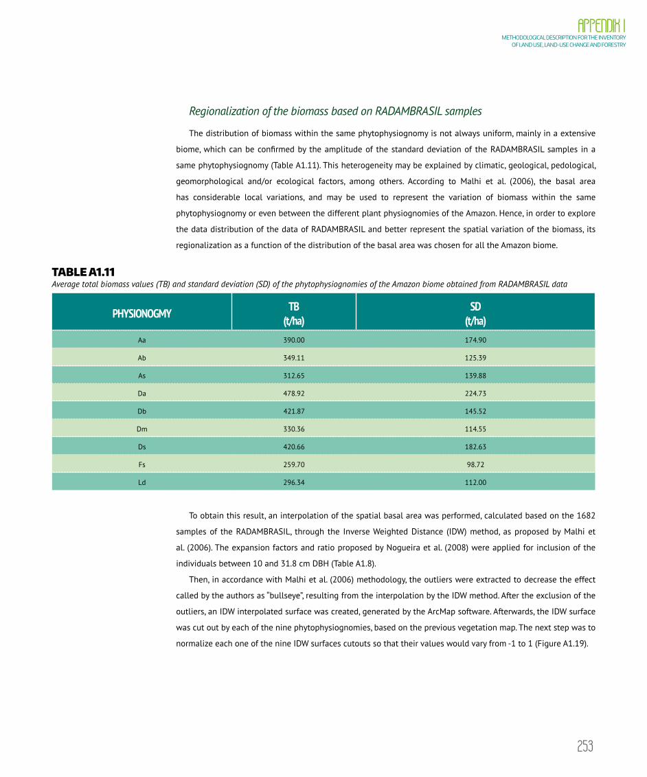
253
APPENDIX I METHODOLOGICAL DESCRIPTION FOR THE INVENTORY
OF LAND USE, LAND-USE CHANGE AND FORESTRY
Regionalization of the biomass based on RADAMBRASIL samples
The distribution of biomass within the same phytophysiognomy is not always uniform, mainly in a extensive
biome, which can be confirmed by the amplitude of the standard deviation of the RADAMBRASIL samples in a
same phytophysiognomy (Table A1.11). This heterogeneity may be explained by climatic, geological, pedological,
geomorphological and/or ecological factors, among others. According to Malhi et al. (2006), the basal area
has considerable local variations, and may be used to represent the variation of biomass within the same
phytophysiognomy or even between the different plant physiognomies of the Amazon. Hence, in order to explore
the data distribution of the data of RADAMBRASIL and better represent the spatial variation of the biomass, its
regionalization as a function of the distribution of the basal area was chosen for all the Amazon biome.
TABLE A1.11 Average total biomass values (TB) and standard deviation (SD) of the phytophysiognomies of the Amazon biome obtained from RADAMBRASIL data
PHYSIONOGMY TB(t/ha)
SD(t/ha)
Aa 390.00 174.90
Ab 349.11 125.39
As 312.65 139.88
Da 478.92 224.73
Db 421.87 145.52
Dm 330.36 114.55
Ds 420.66 182.63
Fs 259.70 98.72
Ld 296.34 112.00
To obtain this result, an interpolation of the spatial basal area was performed, calculated based on the 1682
samples of the RADAMBRASIL, through the Inverse Weighted Distance (IDW) method, as proposed by Malhi et
al. (2006). The expansion factors and ratio proposed by Nogueira et al. (2008) were applied for inclusion of the
individuals between 10 and 31.8 cm DBH (Table A1.8).
Then, in accordance with Malhi et al. (2006) methodology, the outliers were extracted to decrease the effect
called by the authors as “bullseye”, resulting from the interpolation by the IDW method. After the exclusion of the
outliers, an IDW interpolated surface was created, generated by the ArcMap software. Afterwards, the IDW surface
was cut out by each of the nine phytophysiognomies, based on the previous vegetation map. The next step was to
normalize each one of the nine IDW surfaces cutouts so that their values would vary from -1 to 1 (Figure A1.19).
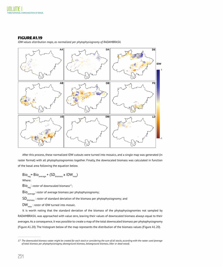
254
VOLUME ITHIRD NATIONAL COMMUNICATION OF BRAZIL
FIGURE A1.19 IDW values distribution maps, as normalized per phytophysiognomy of RADAMBRASIL
After this process, these normalized IDW cutouts were turned into mosaics, and a single map was generated (in
raster format) with all phytophysiognomies together. Finally, the downscaled biomass was calculated in function
of the basal area following the equation below.
Bioreg= Bioaverage + (SDbiomass x IDWmos)Where:
Bioreg: raster of downscaled biomass17;
Bioaverage: raster of average biomass per phytophysiognomy;
SDbiomass : raster of standard deviation of the biomass per phytophysiognomy; and
DWmos : raster of IDW turned into mosaic.
It is worth noting that the standard deviation of the biomass of the phytophysiognomies not sampled by
RADAMBRASIL was approached with value zero, leaving their values of downscaled biomass always equal to their
averages. As a consequence, it was possible to create a map of the total downscaled biomass per phytophysiognomy
(Figure A1.20). The histogram below of the map represents the distribution of the biomass values (Figure A1.20).
17 The downscaled biomass raster might be created for each stock or considering the sum of all stocks, according with the raster used (average of total biomass per phytophysionogmy, aboveground biomass, belowground biomass, litter or dead wood).

255
APPENDIX I METHODOLOGICAL DESCRIPTION FOR THE INVENTORY
OF LAND USE, LAND-USE CHANGE AND FORESTRY
FIGURE A1.20 Total biomass map, including living and dead biomass, downscaled by phytophysiognomy in the Amazon (a) and histogram of total biomass values (b)
(a)
Freq
uenc
y
Biomass (t/ha)
95,00090,00085,00080,00075,00070,00065,00060,00055,00050,00045,00040,00035,00030,00025,00020,00015,00010,000
5,0000
(b)

256
VOLUME ITHIRD NATIONAL COMMUNICATION OF BRAZIL
Regionalization of carbon stocks
The downscaled biomass map was converted into carbon stock as per the Table A1.7. Afterwards, the maps for
each of the stocks were created (aboveground biomass, belowground biomass, dead wood and litter) (Figure A1.21).
FIGURE A1.21 Carbon stock maps (t C/ha) of the Amazon based on the downscaled biomass maps from different stocks (Aboveground – A; Belowground – B; Litter – C and Dead Wood – D)
It was necessary to establish a process of zoning statistics in order to transfer the carbon values from pixels
to polygons, which compose the maps of the carbon stock account. This map is a vector representation of the
previous vegetation in a cellular space18 with resolution of 0.25 decimal degrees (Figure A1.22), in a shapefile
format. Average values for the carbon stocks of pixels to shapefile were attributed. The pixels that were on the edge
between two or more shapes (pixel’s edge) were considered centroid19, that it to say, to the shape they were within.
18 Cellular space is a homogeneous spacial assessment unit composed of a regular cell grid where each cell representes a set of attributes.19 Centroid is the point that corresponds to the geometric center of a certain shape.

257
APPENDIX I METHODOLOGICAL DESCRIPTION FOR THE INVENTORY
OF LAND USE, LAND-USE CHANGE AND FORESTRY
FIGURE A1.22 Vector representation of previous vegetation in a cellular space with resolution of 0.25 decimal degrees
Figures A1.23 and A1.26 show maps for each stock as a result of a combination of downscaled carbon stock as a
function of the basal area and in the phytophysiognomy map subdivided by cellular spaces. Finally, Figure A1.27 shows
the total carbon stock map of the Amazon biome. Table A1.12 presents the values of the average total carbon stock used
for each one of the 29 phytophysiognomies of the Amazon biome, references of where the values, expansion factors and
ratios were taken from, criteria for choice and other works whose values were taken into consideration.
FIGURE A1.23 Downscaled map of aboveground biomass carbon stock (t C/ha) in the Amazon

258
VOLUME ITHIRD NATIONAL COMMUNICATION OF BRAZIL
FIGURE A1.24 Downscaled map of dead wood carbon stock (t C/ha) in the Amazon
FIGURE A1.25 Downscaled map of litter carbon stock (t C/ha) in the Amazon

259
APPENDIX I METHODOLOGICAL DESCRIPTION FOR THE INVENTORY
OF LAND USE, LAND-USE CHANGE AND FORESTRY
FIGURE A1.26 Downscaled map of belowground biomass carbon stock (t C/ha) in the Amazon
FIGURE A1.27 Downscaled map of total carbon stock, including live and dead biomass, in the Amazon

260
VOLUME ITHIRD NATIONAL COMMUNICATION OF BRAZIL
TABLE A1.12 Total carbon stock by area unit (t C/ha) of the phytophysiognomies in the Amazon, origin biome of the estimates for aboveground biomass; sources used to generate total carbon stock; criteria used in choosing sources; other sources used
ABBRE-VIATION
TOTAL STOCK (t C/ha)
BIOME SOURCES CHOICE CRITERION OTHER SOURCES
Aa 183.3 Amazon
RADAMBRASIL (trees); Brown (1997) (allometric
equation); Nogueira et al. (2008) (underbrush,
palm trees, lianas, belowground biomass, dead
wood, litter); Fearnside (1992) (herbaceous plants)
Biome phytophysiognomy;
geographic coverage;
sample effort
Carvalho Jr. et al. (1998); Araújo et al.
(1999); Cummings et al. (2002); Baker
et al. (2004); Chave et al. (2005)
Ab 164.08 Amazon
RADAMBRASIL (trees); Brown (1997) (allometric
equation); Nogueira et al. (2008) (underbrush,
palm trees, lianas, belowground biomass, dead
wood, litter); Fearnside (1992) (herbaceous plants)
Biome phytophysiognomy;
geographic coverage;
sample effort
Carvalho Jr et al. (1998); Araújo et al.
(1999); Cummings et al. (2002); Baker
et al. (2004); Chave et al. (2005)
As 146.94 Amazon
RADAMBRASIL (trees); Brown (1997) (allometric
equation); Nogueira et al. (2008) (underbrush,
palm trees, lianas, belowground biomass, dead
wood, litter); Fearnside (1992) (herbaceous plants)
Biome phytophysiognomy;
geographic coverage;
sample effort
Carvalho Jr. et al. (1998); Araújo et al.
(1999); Cummings et al. (2002); Baker
et al. (2004); Chave et al. (2005)
Cb 145.37 Amazon Nogueira et al. (2008) (all stocks)
Biome phytophysiognomy;
number of stocks;
RADAMBRASIL samples
NA
Cs 136.35 Amazon Nogueira et al. (2008) (all stocks)
Biome phytophysiognomy;
number of stocks;
RADAMBRASIL samples
NA
Da 225.09 Amazon
RADAMBRASIL (trees); Brown (1997) (allometric
equation); Nogueira et al. (2008) (underbrush,
palm trees, lianas, belowground biomass, dead
wood, litter); Fearnside (1992) (herbaceous plants)
Biome phytophysiognomy;
geographic coverage;
sample effort
Carvalho Jr. et al. (1998); Araújo et al.
(1999); Cummings et al. (2002); Baker
et al. (2004); Chave et al. (2005)
Db 198.28 Amazon
RADAMBRASIL (trees); Brown (1997) (allometric
equation); Nogueira et al. (2008) (underbrush,
palm trees, lianas, belowground biomass, dead
wood, litter); Fearnside (1992) (herbaceous plants)
Biome phytophysiognomy;
geographic coverage;
sample effort
Alves et al. (1997); Carvalho Jr. et al.
(1998); Araújo et al. (1999); Cummings
et al. (2002); Baker et al. (2004); Chave
et al. (2005); Nascimento et al. (2007)
Dm 155.27 Amazon
RADAMBRASIL (trees); Brown (1997) (allometric
equation); Nogueira et al. (2008) (underbrush,
palm trees, lianas, belowground biomass, dead
wood, litter); Fearnside (1992) (herbaceous plants)
Biome phytophysiognomy;
geographic coverage;
sample effort
Alves et al. (1997); Carvalho Jr et al.
(1998); Araújo et al. (1999); Cummings
et al. (2002); Baker et al. (2004); Chave
et al. (2005)
Ds 197.71 Amazon
RADAMBRASIL (trees); Brown (1997) (allometric
equation); Nogueira et al. (2008) (underbrush,
palm trees, lianas, belowground biomass, dead
wood, litter); Fearnside (1992) (herbaceous plants)
Biome phytophysiognomy;
geographic coverage;
sample effort
Alves et al. (1997); Carvalho Jr. et al.
(1998); Araújo et al. (1999); Cummings
et al. (2002); Baker et al. (2004); Chave
et al. (2005)
continues on the next page

261
APPENDIX I METHODOLOGICAL DESCRIPTION FOR THE INVENTORY
OF LAND USE, LAND-USE CHANGE AND FORESTRY
ABBRE-VIATION
TOTAL STOCK (t C/ha)
BIOME SOURCES CHOICE CRITERION OTHER SOURCES
Fa 133.2 Amazon Nogueira et al. (2008) (all stocks)
Biome phytophysiognomy;
number of stocks;
RADAMBRASIL samples
NA
Fb 145.37 Amazon Nogueira et al. (2008) (all stocks)
Biome phytophysiognomy;
number of stocks;
RADAMBRASIL samples
Nascimento et al. (2007)
Fm 155.27 Amazon Same as Dm in Amazon Fragments close to Dm NA
Fs 122.06 Amazon
RADAMBRASIL (trees); Brown (1997) (allometric
equation); Nogueira et al. (2008) (underbrush,
palm trees, lianas, belowground biomass, dead
wood, litter); Fearnside (1992) (herbaceous plants)
Biome phytophysiognomy;
geographic coverage;
sample effort
Carvalho Jr. et al. (1998); Araújo et al.
(1999); Baker et al. (2004); Chave et
al. (2005)
La 20.52 Amazon
Barbosa and Ferreira (2004) (aboveground
biomass and litter); Bongers et al. (1985)
(aboveground biomass); IPCC (2006) (dead wood)
Belowground biomass and
litter in meadow in the
Amazon
Barbosa and Fearnside (1999); Barbosa
et al. (2010)
Lb 19.68 Amazon
Barbosa and Ferreira (2004) (aboveground
biomass and litter); Bongers et al. (1985)
(aboveground biomass); IPCC (2006) (dead wood)
Belowground biomass and
litter in meadow in the
Amazon
NA
Ld 139.28 Amazon
RADAMBRASIL (trees); Brown (1997) (allometric
equation); Nogueira et al. (2008) (underbrush,
palm trees, lianas, belowground biomass, dead
wood, litter); Fearnside (1992) (herbaceous plants)
Biome phytophysiognomy;
geographic coverage;
sample effort
Carvalho Jr. et al. (1998); Araújo et al.
(1999); Barbosa and Fearnside (1999);
Baker et al. (2004); Barbosa and
Ferreira (2004); Chave et al. (2005)
Lg 23.21 Amazon Bongers et al. (1985) (all stocks)Biome phytophysiognomy;
number of stocks
Barbosa and Fearnside (1999); Barbosa
and Ferreira (2004); Barbosa et al.
(2010)
Pa 141.38 Amazon
Xavier (2009) (aboveground biomass and dead
wood); Cattanio et al. (2004) (belowground
biomass and deposited litter); Cabianchi (2010)
(decomposition rate); Chao et al. (2008) (dead wood)
Alongside river plains NA
Pf 117.2 Brazil
Hutchison et al. (2013) (above and belowground
biomass); Fernandes (1997) (dead wood); Ramos
and Silva et al. (2007) (litter)
Review and modelling
about mangroves, value
for Brazil
Fromard et al. (1998); Silva et al.
(1998); Cogliatti-Carvalho and
Mattos-Fonseca (2004); Medeiros and
Sampaio (2008); Santos (2013)
Pm 130.7Atlantic
ForestSame as Atlantic Forest Phytophysiognomy Silva et al. (2010)
Rm 5.67 Amazon
Barbosa and Fearnside (1999) (aboveground
biomass, dead wood and litter); Miranda et al.
(2014) (belowground biomass)
Biome phytophysiognomy Ottmar et al. (2001)
continues on the next page
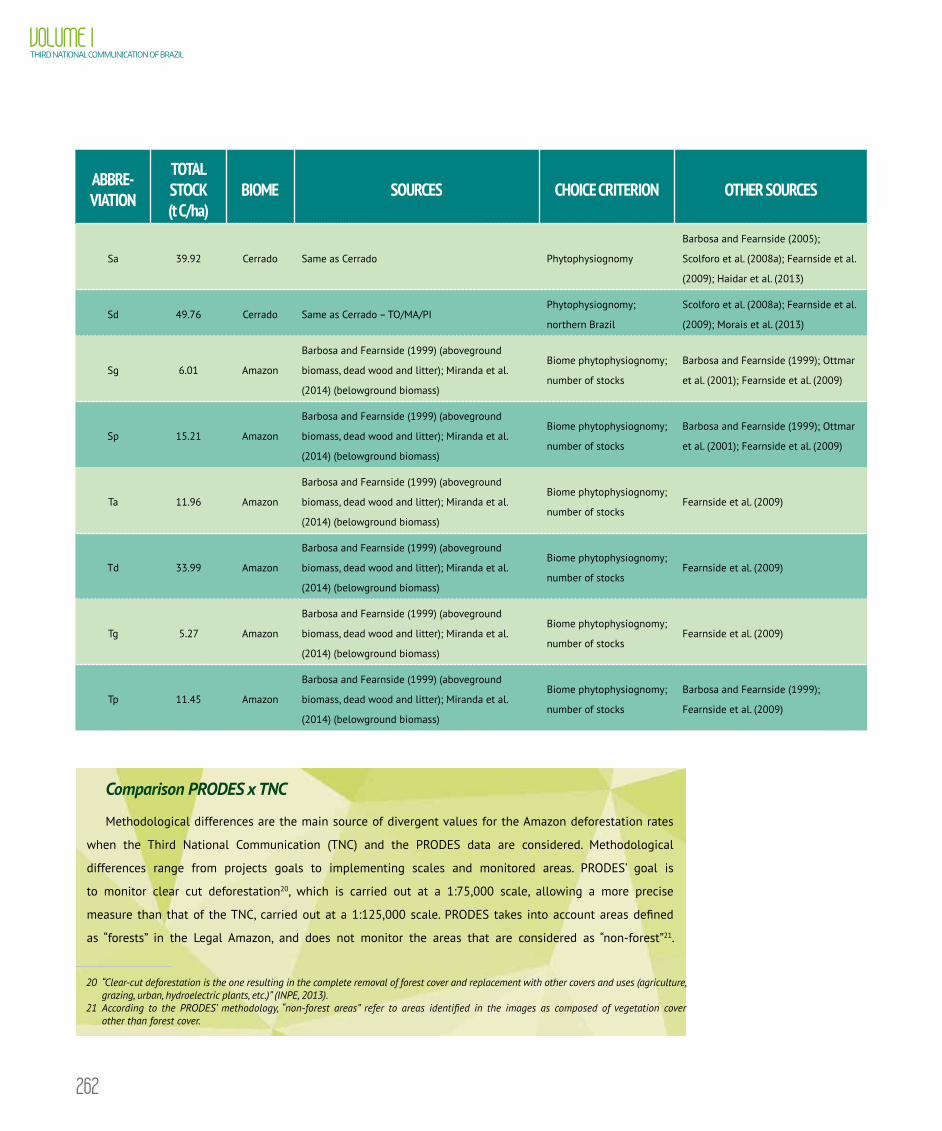
262
VOLUME ITHIRD NATIONAL COMMUNICATION OF BRAZIL
ABBRE-VIATION
TOTAL STOCK (t C/ha)
BIOME SOURCES CHOICE CRITERION OTHER SOURCES
Sa 39.92 Cerrado Same as Cerrado Phytophysiognomy
Barbosa and Fearnside (2005);
Scolforo et al. (2008a); Fearnside et al.
(2009); Haidar et al. (2013)
Sd 49.76 Cerrado Same as Cerrado – TO/MA/PIPhytophysiognomy;
northern Brazil
Scolforo et al. (2008a); Fearnside et al.
(2009); Morais et al. (2013)
Sg 6.01 Amazon
Barbosa and Fearnside (1999) (aboveground
biomass, dead wood and litter); Miranda et al.
(2014) (belowground biomass)
Biome phytophysiognomy;
number of stocks
Barbosa and Fearnside (1999); Ottmar
et al. (2001); Fearnside et al. (2009)
Sp 15.21 Amazon
Barbosa and Fearnside (1999) (aboveground
biomass, dead wood and litter); Miranda et al.
(2014) (belowground biomass)
Biome phytophysiognomy;
number of stocks
Barbosa and Fearnside (1999); Ottmar
et al. (2001); Fearnside et al. (2009)
Ta 11.96 Amazon
Barbosa and Fearnside (1999) (aboveground
biomass, dead wood and litter); Miranda et al.
(2014) (belowground biomass)
Biome phytophysiognomy;
number of stocks Fearnside et al. (2009)
Td 33.99 Amazon
Barbosa and Fearnside (1999) (aboveground
biomass, dead wood and litter); Miranda et al.
(2014) (belowground biomass)
Biome phytophysiognomy;
number of stocks Fearnside et al. (2009)
Tg 5.27 Amazon
Barbosa and Fearnside (1999) (aboveground
biomass, dead wood and litter); Miranda et al.
(2014) (belowground biomass)
Biome phytophysiognomy;
number of stocks Fearnside et al. (2009)
Tp 11.45 Amazon
Barbosa and Fearnside (1999) (aboveground
biomass, dead wood and litter); Miranda et al.
(2014) (belowground biomass)
Biome phytophysiognomy;
number of stocks
Barbosa and Fearnside (1999);
Fearnside et al. (2009)
Comparison PRODES x TNC
Methodological differences are the main source of divergent values for the Amazon deforestation rates
when the Third National Communication (TNC) and the PRODES data are considered. Methodological
differences range from projects goals to implementing scales and monitored areas. PRODES’ goal is
to monitor clear cut deforestation20, which is carried out at a 1:75,000 scale, allowing a more precise
measure than that of the TNC, carried out at a 1:125,000 scale. PRODES takes into account areas defined
as “forests” in the Legal Amazon, and does not monitor the areas that are considered as “non-forest”21.
20 “Clear-cut deforestation is the one resulting in the complete removal of forest cover and replacement with other covers and uses (agriculture, grazing, urban, hydroelectric plants, etc.)” (INPE, 2013).
21 According to the PRODES’ methodology, “non-forest areas” refer to areas identified in the images as composed of vegetation cover other than forest cover.

263
APPENDIX I METHODOLOGICAL DESCRIPTION FOR THE INVENTORY
OF LAND USE, LAND-USE CHANGE AND FORESTRY
The TNC, on the other hand, considers the entire national territory with its six biomes, and monitors all forest
and non-forest (grasslands) areas, following the definition of previous vegetation, produced by the Second
National Communication (SNC). Formation areas considered as forests in SNC and TNC exceed the areas
considered by PRODES as forests for the Amazon biome (Table I). In order to minimize these methodological
differences, the same scenes used in PRODES were used in the mapping of the Third Inventory, although
observed at two different scales according to each project. However, some images with large cloud cover were
replaced (91 scenes for 2005 and 54 scenes for 2010, in a total of 198). For the sake of comparing results,
a subtraction of the accumulated deforested areas of both projects for the years of interest was performed.
For the purposes of this Inventory, deforestation was considered as the sum of the areas of Ac, Ap, FSec, GSec,
Res, Ref, O and S, against the sum of PRODES’ deforested area and residues22 (Figure I). It is indicated that the
differences between the deforested areas of the two projects have, for the most part, values near zero km²
(86%, 91%, 91% and 90% of occurrences are shown between -50 and 50 km² in the comparisons for 1994,
2002, 2005 and 2010, respectively, as shown in the histograms and average values in Figure I). Furthermore,
some regions where with higher deforestation rates in this inventory (red cells) correspond to PRODES’ non-
forest regions (Figure I, Tables I to IV). The total correspondence among the deforested areas shown in this
document and PRODES’ non-forest areas was 0.2% in 1994; 0.1% in 2002; 4.4% in 2005 and 4.5% in 2010. In
relation to the increase of areas that were not monitored due to larger cloud cover at the time of mapping, it
can be seen that it also occurred in PRODES (Figure III). It should be noted that the comparison with the map
of 1994 was only possible when considering data of PRODES 1997, as the first period of digital PRODES is
1997-2000. Therefore, the main methodological differences that hinder the direct comparison of numbers and
results of these projects are underscored herein.
TABLE I Comparison of forest and non-forest areas in TNC and PRODES
COVERTNC PRODES REDUCED TO THE LIMIT OF
THE AMAZON BIOME USED IN TNC2 PRODES (LEGAL AMAZON)3
AREA (km²)1
Forest 3,964,940 3,800,956 3,894,571
Grasslands/Non- Forest 112,747 290,924 957,606
Hydrography 131,092 116,899 163,957
Total 4,208,779 4,208,779 5,016,134
1. Values may vary in relation to other official figures due to the geographic standards used for calculations.2. The forest area was estimated by the difference between the total area of the Amazon Biome and the non-forest area and hydrography of PRODES within that limit. 3. The forest area was estimated by the difference between the total area of the Legal Amazon and the non-forest area and hydrography of PRODES.
22 “Deforested areas that were detected by PRODES in a year that is not the year of occurrence” (Almeida et al., 2009).
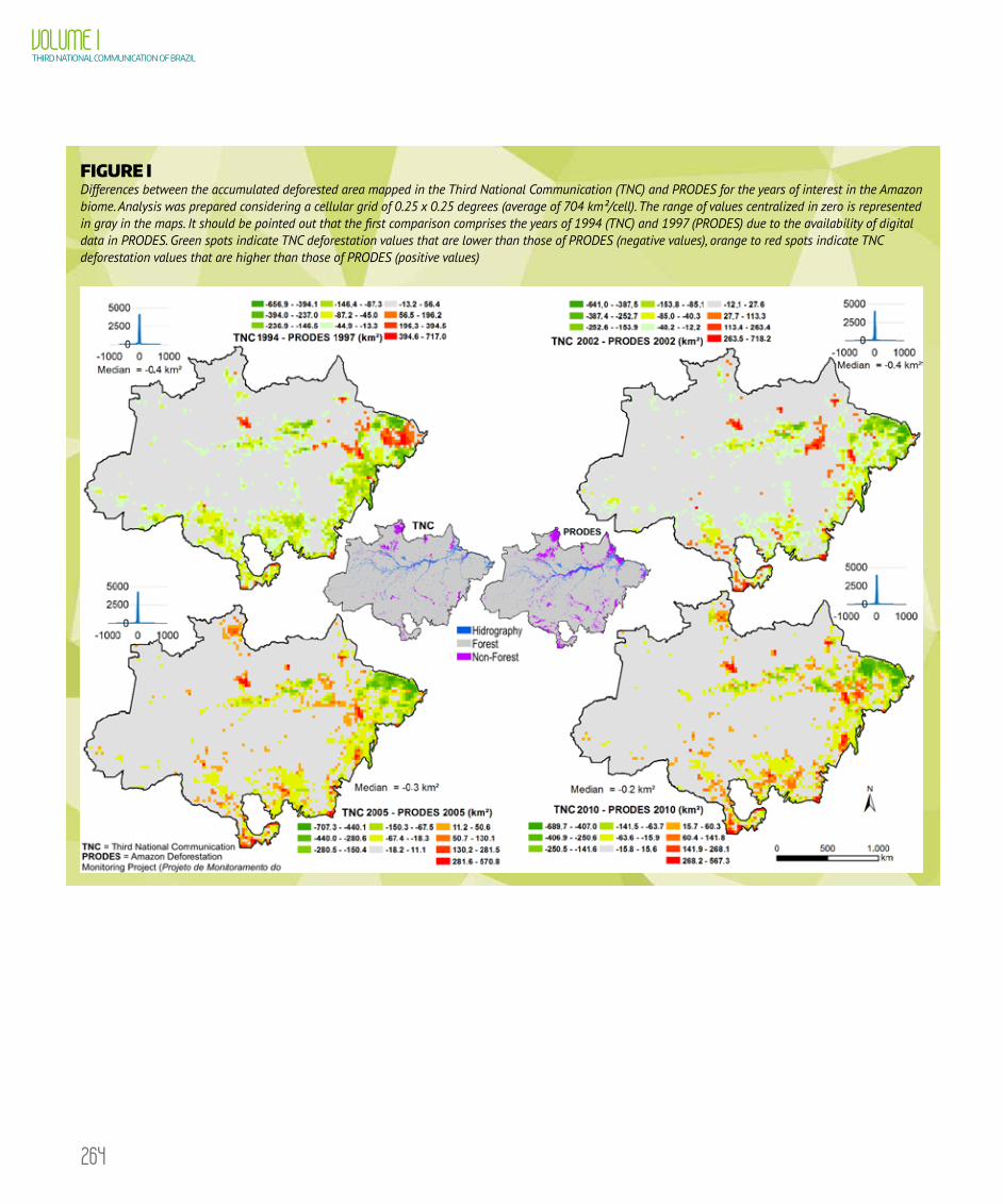
264
VOLUME ITHIRD NATIONAL COMMUNICATION OF BRAZIL
FIGURE I Differences between the accumulated deforested area mapped in the Third National Communication (TNC) and PRODES for the years of interest in the Amazon biome. Analysis was prepared considering a cellular grid of 0.25 x 0.25 degrees (average of 704 km²/cell). The range of values centralized in zero is represented in gray in the maps. It should be pointed out that the first comparison comprises the years of 1994 (TNC) and 1997 (PRODES) due to the availability of digital data in PRODES. Green spots indicate TNC deforestation values that are lower than those of PRODES (negative values), orange to red spots indicate TNC deforestation values that are higher than those of PRODES (positive values)

265
APPENDIX I METHODOLOGICAL DESCRIPTION FOR THE INVENTORY
OF LAND USE, LAND-USE CHANGE AND FORESTRY
TABLE II Correspondence area between the TNC map (1994) and PRODES (1997) for the Amazon Biome
TNC (1994) PRODES 1997 CORRESPONDENCE TOTAL TNC CORRESPONDENCE IN PRODES
CLASS AREA (ha) DEFORESTATION (ha) % HYDROGRAPHY
(ha) % NON-FOREST (ha) % %
FNM 271,381,689.0 11,895,283.3 4 28,785.8 0 777,644.8 0 5
FM 93,479,430.7 563,229,1 1 2,933.7 0 53,896.0 0 1
FSec 1,369,898.6 1,095,476.5 80 1.5 0 0.0 0 80
Ref 296,464.8 118,420.3 40 0,0 0 1,453.1 0 40
CS 0.0 - - - - - - -
GNM 8,215,886.9 147,141.4 2 0.0 0 177.6 0 2
GM 2,703,248.7 5,462.4 0 0.0 0 18,769.2 1 1
GSec 17,226.4 11,083.7 64 0.0 0 0.0 0 64
Ap 28,353,961.2 23,181,811.9 82 617.4 0 48,839.3 0 82
Ac 628,971.5 436,744.8 69 0.0 0 0.0 0 69
S 189,812.3 137,389.2 72 12.9 0 981.7 1 73
A 12,746,052.5 202,469.6 2 324,727.6 3 16,159.9 0 4
Res 597,552.7 3,472.0 1 104.2 0 149.5 0 1
O 56,585.6 42,319.9 75 66.0 0 48.6 0 75
NE 841,117.3 368,892.1 44 58.8 0 974.5 0 44
TABLE III Correspondence area between the TNC map (2002) and PRODES (2002) for the Amazon Biome
TNC (2002) CORRESPONDENCE IN THE ACCUMULATED PRODES 1997-2002 TOTAL TNC CORRESPONDENCE WITHIN PRODES
CLASS AREA (ha) DEFORESTATION (ha) % HYDROGRAPHY
(ha) % NON-FOREST (ha) % %
FNM 216,641,049.9 9,069,072.0 4 28,227.1 0 757,009.9 0 5
FM 132,228,135.4 1,713,066.2 1 2,751.6 0 55,812.7 0 1
FSec 3,262,749.7 2,464,150.2 76 113.0 0 2,174.5 0 76
Ref 356,342.8 162,507.9 46 0.0 0 1,453.0 0 46
CS 259,610.6 32,663.4 13 0.0 0 0.0 0 13
continues on the next page

266
VOLUME ITHIRD NATIONAL COMMUNICATION OF BRAZIL
TNC (2002) CORRESPONDENCE IN THE ACCUMULATED PRODES 1997-2002 TOTAL TNC CORRESPONDENCE WITHIN PRODES
CLASS AREA (ha) DEFORESTATION (ha) % HYDROGRAPHY
(ha) % NON-FOREST (ha) % %
GNM 6,457,514.3 111,130.5 2 0.0 0 177.6 0 2
GM 4,176,741.0 11.806,9 0 0.0 0 18,672.5 0 1
GSec 33,784.0 10,154.5 30 0.0 0 0.0 0 30
Ap 42,670,445.4 38,074,897.5 89 1,199.3 0 65,967.4 0 89
Ac 1,074,882.7 832,669.3 77 0.0 0 0.0 0 77
S 282,686.3 241,842.4 86 33.6 0 1,464.9 1 86
A 12,723,954.3 269,336.4 2 324,780.4 3 16,159.9 0 5
Res 629,406.6 7,793.2 1 104.2 0 152.3 0 1
O 62,112.4 48,449.3 78 98.9 0 49.4 0 78
NE 18,483.0 1,850.1 10 0.0 0 0.0 0 10
TABLE IV Correspondence area between the TNC map (2005) and PRODES (2005) for the Amazon Biome
TNC (2005) CORRESPONDENCE IN THE ACCUMULATED PRODES 1997-2005 TOTAL TNC CORRESPONDENCE WITHIN PRODES
CLASS AREA (ha) DEFORESTATION (ha) % HYDROGRAPHY
(ha) % NON-FOREST (ha) % %
FNM 176,275,517.8 7,723,642.1 4 697,138.0 0 8,259,718.1 5 9
FM 144,755,378.3 1,603,573.5 1 321,845.8 0 6,813,495.8 5 6
FSec 6,125,466.7 4,479,980.4 73 34,790.0 1 302,420.3 5 79
Ref 263,115.6 136,120.4 52 26.4 0 119,059.9 45 97
CS 1,218,740.8 58,086.8 5 27.8 0 797.5 0 5
GNM 5,679,039.9 94,980.3 2 15,796.9 0 4,712,704.7 83 85
GM 4,195,440.4 14,790.9 0 8,248.2 0 3,662,592.6 87 88
GSec 140,991.1 26,979.8 19 3,236.4 2 102,148.4 72 94
Ap 46,234,663.7 41,694,475.8 90 58,605.2 0 1,561,102.0 3 94
Ac 3,070,124.2 2,585,880.6 84 209.2 0 383,073.8 12 97
continues on the next page

267
APPENDIX I METHODOLOGICAL DESCRIPTION FOR THE INVENTORY
OF LAND USE, LAND-USE CHANGE AND FORESTRY
TNC (2005) CORRESPONDENCE IN THE ACCUMULATED PRODES 1997-2005 TOTAL TNC CORRESPONDENCE WITHIN PRODES
CLASS AREA (ha) DEFORESTATION (ha) % HYDROGRAPHY
(ha) % NON-FOREST (ha) % %
S 358,318.7 310,703.8 87 2,055.3 1 33,231.4 9 97
A 12,570,987.8 250,312.3 2 9,404,230.6 75 1,176,001.1 9 86
Res 663,792.0 17,093.2 3 610,285.8 92 2,140.8 0 95
O 77,824.6 59,447.6 76 2,879.3 4 4,666.4 6 86
NE 19,248,496.6 1,537,551.3 8 206,754.4 1 1,619,444.4 8 17
TABLE V Correspondence area between the TNC map (2010) and PRODES (2010) for the Amazon Biome
TNC (2010) CORRESPONDENCE IN THE ACCUMULATED PRODES 1997-2010 TOTAL TNC CORRESPONDENCE WITHIN PRODES
CLASS AREA (ha) DEFORESTATION (ha) % HYDROGRAPHY
(ha) % NON-FOREST (ha) % %
FNM 130,459,613.9 5,999,160.3 5 599.910,2 0 6,928,118.1 5 10
FM 179,507,012.8 1,444,800.3 1 364.327,6 0 7,645,892.0 4 5
FSec 8,161,610.1 5,322,220.6 65 42.805,4 1 410,931.3 5 71
Ref 349,650.5 222,269.8 64 12,7 0 117,639.7 34 97
CS 1,178,669.6 20,028.0 2 7,5 0 1,255.4 0 2
GNM 4,396,023.6 79,292.3 2 14,245.1 0 3,632,787.7 83 85
GM 4,804,004.5 15,829.0 0 7,776.9 0 4,149,008.7 86 87
GSec 190,546.9 30,303.7 16 3,306.2 2 147,417.9 77 95
Ap 49,941,425.1 45,254,571.2 91 57,353.2 0 1,727,276.8 3 94
Ac 3,424,779.0 2,959,181.6 86 90.4 0 371,009.0 11 97
S 392,539.3 343,550.8 88 2,805.1 1 34,558.8 9 97
A 12,182,193.2 247,132.3 2 9,258,761.8 76 1,342,433.7 11 89
Res 639,247.1 22,236.6 3 582,398.4 91 1,193.2 0 95
O 90,201.5 68,656.4 76 2,896.0 3 6,365.3 7 86
NE 25,160,381.4 3,116,038.1 12 768,567.5 3 2,590,409.5 10 26

268
VOLUME ITHIRD NATIONAL COMMUNICATION OF BRAZIL
FIGURE II Cloud-covered area at the moment of mapping (Amazon Biome) and PRODES (Legal Amazon), in the years of interest (TM/LANDSAT-5 images). The area that was not estimated by PRODES was obtained by the sum of cloud-covered areas and areas not-observed, and is available at http://www.dpi.inpe.br/prodesdigital/prodesmunicipal.php

269
APPENDIX I METHODOLOGICAL DESCRIPTION FOR THE INVENTORY
OF LAND USE, LAND-USE CHANGE AND FORESTRY
FIGURE III Not Estimated areas in TNC and PRODES due to cloud cover
2002 2005 2010
0
100,000
200,000
300,000
400,000
500,000
Are
a (k
m2 )
Not Estimated Area
Amazon Biome (TNC) Legal Amazon (PRODES)
Year
Cerrado Biome
The Cerrado is Brazil’s second largest biome and comprises a wide latitudinal range, which extends from the coastline
of the state of Maranhão to Southern Brazil. Thus, the choice was to regionalize the values of carbon stock of one given
phytophysiognomy per Brazilian state whenever possible or when the values varied greatly between different regions of
the biome. Environmental factors such as rainfall and seasonality were also considered for the assignment of values to
phytophysiognomies, since these abiotic characteristics influence the characteristics of the vegetation.
The six phytophysiognomies that had their values downscaled per states were: Forested Savanna (Sd), Montane
Deciduous Seasonal Forests (Cm) and Submontane Deciduous Seasonal Forests (Cs), Alluvial Semideciduous Seasonal
Forests (Fa), Lowland Semideciduous Seasonal Forests (fb) and Submontane Semideciduous Seasonal Forests (Fs).
For the Woodland Savanna (Cerradão or Sd), the values were divided into the following groups of states:
1 São Paulo, according to Pinheiro (2008), in Cerradão in Assis (SP);
2 Minas Gerais, Goiás, Distrito Federal and Bahia, according to the Forest Inventory of Minas Gerais
(SCOLFORO et al., 2008a);
3 Mato Grosso and Mato Grosso do Sul, with the same value as the Sd in the Pantanal;
4 Tocantins, Maranhão and Piauí, according to the Forest Inventory of the State of Tocantins (HAIDAR et al.,
2013), using Brown’s allometric equation (BROWN, 1997).
The belowground biomass of each group of Sd was estimated based on ratios for forests in the Cerrado
(MIRANDA et al., 2014); the dead wood was estimated according to the IPCC default value (2003) and the litter was
based on the correction factor calculated for Cerradão (MORAIS et al., 2013).

270
VOLUME ITHIRD NATIONAL COMMUNICATION OF BRAZIL
The Forested Savanna (Sa) encompasses the Open Wooded Savanna (Cerrado stricto sensu), Dense and Sparse
Cerrado. For this phytophysiognomy, a study with broad geographic coverage in Cerrado and number of pools was
chosen: aboveground biomass, dead wood and litter (OTTMAR et al., 2001). For the estimation of the belowground
biomass, the ratio for trees and shrubs of Cerrado was applied (MIRANDA et al., 2014).
For the Park Savanna (Sp), which encompasses the phytophysiognomies Campo Sujo (shrubby field) and Campo
de Murundu (mound field), an average of two total carbon stock values was calculated to represent the variation
of biomass in this phytophysiognomy as a whole. Ottmar et al. (2001) was chosen to represent shrubby fields with
prominent herb layer, due to greater geographic coverage and the number of aboveground biomass and dead
organic matter stocks considered. For this value, with lower biomass, the ratio for grassland vegetation in Cerrado
(MIRANDA et al., 2014) was used to estimate the belowground biomass. The other reference used represented the
areas of greater biomass in Sp, and the same value adopted for Sp was used in the Pantanal biome.
For the Woody Grass Savannah (Sg), the study carried out in clean grassland in the Cerrado biome was chosen,
with broader geographic coverage and more stocks (aboveground biomass and dead organic matter) (OTTMAR et
al., 2001). The belowground biomass of Sg was estimated based on the ratio for grassland vegetation in Cerrado
(MIRANDA et al., 2014). For the Montane Refuge (Rm), the same Sg values were adopted, due to the lack of studies
evaluating the aboveground biomass in this phytophysiognomy itself.
Due to the absence of values for Wooded Steppe (Ea) in the Cerrado biome, values of aboveground biomass in the
sensu stricto Cerrado and Cerrado Grassland were used (SCOLFORO et al., 2008a) in the state of Minas Gerais, where this
phytophysiognomy is noticed. For the estimation of belowground biomass, the ratio in the savanna vegetation in Cerrado
was used (MIRANDA et al., 2014), while for dead wood and litter, the ratio of Ottmar et al. (2001) was used.
As the Cerrado borders other four Brazilian biomes (Amazon, Atlantic Forest, Caatinga and Pantanal), in the absence
of values for the forest phytophysiognomies in Cerrado, values of the phytophysiognomies in nearby biomes were
used. For the Lowland Deciduous Seasonal Forest (Cb) the same value as the Pantanal biome was used.
For the Alluvial Open Humid Forests (Aa) and the Lowland (Ab), as well as for the Alluvial Dense Humid Forest
(Da), the same values applied to these phytophysiognomies in the Amazon biome were used.
For the Montane Dense Humid Forests (Dm) and Montane Semideciduous Seasonal Forests (Fm), as well as for
the pioneering formations of marine influence (Pm or Sandbank), the same values of these phytophysiognomies for
the Atlantic Forest biome were used. The Mixed Humid Forests are restricted to the Southeast (state of São Paulo)
and South (state of Paraná) in Brazil. In this case, the same values for the High-Montane Mixed Humid Forests (Ml)
and Montane (Mm) in the Atlantic Forest were used.
The Montane Deciduous Seasonal Forest (Cm) was downscaled in: 1) the states of Minas Gerais, Bahia and Goiás
with the same value chosen for this phytophysiognomy within the Caatinga biome; and 2) in the state of São Paulo,
same value adopted for Cm in the Pantanal biome.
The Submontane Deciduous Seasonal Forest (Cs) was downscaled in: 1) the states of Minas Gerais, Bahia, Goiás,
Federal District, Tocantins, Piauí and Maranhão with the same value for Cs in the Caatinga; and 2) the state of Mato
Grosso, Mato Grosso do Sul and São Paulo, with Cs value for the Pantanal biome.
The Lowland Semideciduous Seasonal Forest (Fb) was downscaled as follows: 1) state of Mato Grosso, the same
value of Fb in the Amazon; and 2) states of Goiás and Minas Gerais, the same value of this phytophysiognomy in
the Atlantic Forest biome.

271
APPENDIX I METHODOLOGICAL DESCRIPTION FOR THE INVENTORY
OF LAND USE, LAND-USE CHANGE AND FORESTRY
For the Open Submontane Humid Forests (As) and Submontane Dense Humid Forests (Ds), the values of
aboveground biomass obtained from the data of the Forest Inventory of the State of Tocantins (HAIDAR et al., 2013)
with application of the allometric equation described by Brown (1997) were chosen. The biomass of underbrush,
lianas, palm trees, underground biomass, litter, and dead wood were estimated using Nogueira et al. (2008) ratios,
from non-dense As Forests to Ds dense forests.
The Alluvial Semideciduous Seasonal Forest (Fa) was downscaled as follows:
1 states of Tocantins and Pará: average value of aboveground biomass of riparian and gallery forest of the
Inventory of the State of Tocantins (HAIDAR et al., 2013), as of the application of the Brown equation (1997);
2 states of Minas Gerais, Goiás, Distrito Federal and Bahia: the same value of Fa for the Atlantic Forest biome.
3 states of São Paulo and Paraná: the aboveground biomass value in riparian semideciduous mesophilic
forest in the state of São Paulo (MOREIRA-BURGER & DELITTI, 1999);
4 states of Mato Grosso and Mato Grosso do Sul: same value used of the Fa for the Pantanal biome.
For the estimation of the belowground biomass and dead wood of Fa, the IPCC default ratios were used (2003,
2006). For litter, a ratio calculated on the basis of the study of Moreira-Burger & Delitti (1999) was used for the
states grouped into 1, 2 and 4. For São Paulo and Paraná (group 3), these authors assessed the litter (MOREIRA-
BURGUER & DELITTI, 1999), and the use of ratios was not necessary.
The Submontane Semideciduous Seasonal Forest (Fs) was downscaled by the states:
1 Piauí, Maranhão and Bahia: value obtained from the DBH of trees (DAP > 10 cm), using a Brown’s allometric
equation (1997), in the states of Piauí and Maranhão (HAIDAR et al., 2013; FRANÇOSO et al., 2013).
2 Minas Gerais, Tocantins, Goiás, Distrito Federal, Mato Grosso, Mato Grosso do Sul, São Paulo and Rondônia:
value obtained in the Forest Inventory of the state of Minas Gerais (SCOLFORO et al., 2008c).
The belowground biomass of Fs was calculated on the basis of the IPCC default ratio (2006). For dead wood, the
correction factor used was in accordance with the IPCC (2003) and, as for litter, the correction factor was calculated
based a work done in Fm (AMARO et al., 2013)
The Vegetation with Fluvial and/or Lacustrine Influence (Pa) had the value of aboveground biomass based on
two studies carried out in paths of Cerrado. In one of them, the authors calculated the aboveground biomass for
the herbaceous vegetation in a path in Tocantins (FIDELIS et al., 2013). In another study, the authors presented
parameters such as average density of individuals per hectare and basal area for the vegetation of shrubs and
trees of a path in the state of Minas Gerais (BAHIA et al., 2009) and, based on these parameters, the aboveground
biomass was calculated by using an allometric equation (BROWN, 1997). The authors of the study made in TO
reported the belowground biomass of the herbaceous component. For the belowground biomass of the shrub-
tree component, the ratio according to Miranda et al. (2014) was used for forest phytophysiognomies in Cerrado.
For the dead wood, the default correction factor of the IPCC (2003) was used in relation to the shrubs-tree aerial
biomass. For the litter of the herbaceous component, a correction factor calculated for Clean Grassland was used
from Ottmar et al. (2001) and for the shrub-tree component, a correction factor was calculated in accordance
with Moreira-Burger & Delitti (1999).
For the pioneering formations of fluviomarine influence (Pf or Mangrove), located in Cerrado biome on the
coastline of Maranhão, the same value of Pf in the Amazon biome was used. This value was based on a literature
review and modeling about mangroves in the world, with a value for Brazil (HUTCHISON et al., 2013).
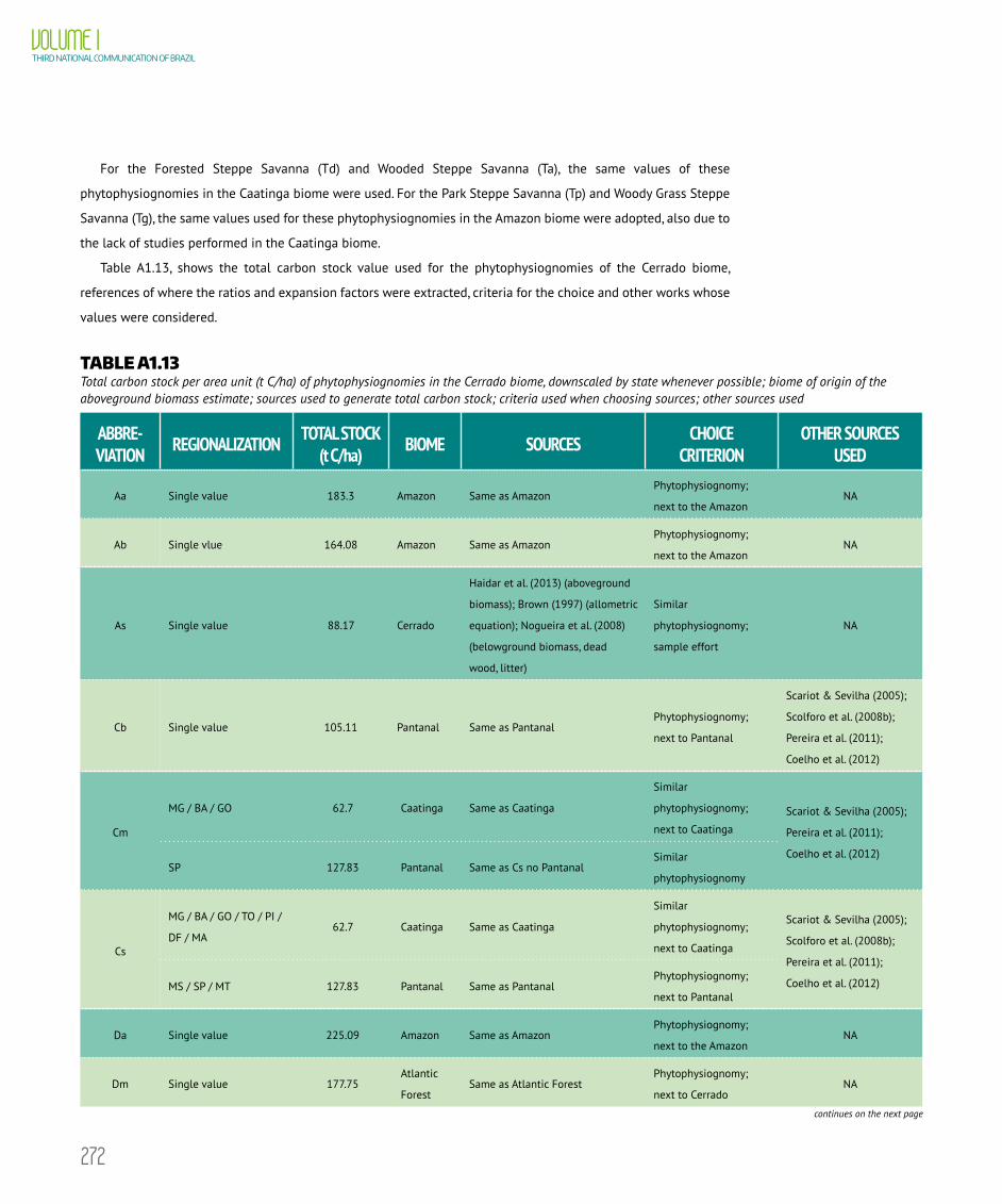
272
VOLUME ITHIRD NATIONAL COMMUNICATION OF BRAZIL
For the Forested Steppe Savanna (Td) and Wooded Steppe Savanna (Ta), the same values of these
phytophysiognomies in the Caatinga biome were used. For the Park Steppe Savanna (Tp) and Woody Grass Steppe
Savanna (Tg), the same values used for these phytophysiognomies in the Amazon biome were adopted, also due to
the lack of studies performed in the Caatinga biome.
Table A1.13, shows the total carbon stock value used for the phytophysiognomies of the Cerrado biome,
references of where the ratios and expansion factors were extracted, criteria for the choice and other works whose
values were considered.
TABLE A1.13 Total carbon stock per area unit (t C/ha) of phytophysiognomies in the Cerrado biome, downscaled by state whenever possible; biome of origin of the aboveground biomass estimate; sources used to generate total carbon stock; criteria used when choosing sources; other sources used
ABBRE-VIATION REGIONALIZATION TOTAL STOCK
(t C/ha) BIOME SOURCES CHOICE CRITERION
OTHER SOURCES USED
Aa Single value 183.3 Amazon Same as AmazonPhytophysiognomy;
next to the AmazonNA
Ab Single vlue 164.08 Amazon Same as AmazonPhytophysiognomy;
next to the AmazonNA
As Single value 88.17 Cerrado
Haidar et al. (2013) (aboveground
biomass); Brown (1997) (allometric
equation); Nogueira et al. (2008)
(belowground biomass, dead
wood, litter)
Similar
phytophysiognomy;
sample effort
NA
Cb Single value 105.11 Pantanal Same as PantanalPhytophysiognomy;
next to Pantanal
Scariot & Sevilha (2005);
Scolforo et al. (2008b);
Pereira et al. (2011);
Coelho et al. (2012)
Cm
MG / BA / GO 62.7 Caatinga Same as Caatinga
Similar
phytophysiognomy;
next to Caatinga
Scariot & Sevilha (2005);
Pereira et al. (2011);
Coelho et al. (2012)SP 127.83 Pantanal Same as Cs no Pantanal
Similar
phytophysiognomy
Cs
MG / BA / GO / TO / PI /
DF / MA62.7 Caatinga Same as Caatinga
Similar
phytophysiognomy;
next to Caatinga
Scariot & Sevilha (2005);
Scolforo et al. (2008b);
Pereira et al. (2011);
Coelho et al. (2012)MS / SP / MT 127.83 Pantanal Same as PantanalPhytophysiognomy;
next to Pantanal
Da Single value 225.09 Amazon Same as AmazonPhytophysiognomy;
next to the AmazonNA
Dm Single value 177.75Atlantic
ForestSame as Atlantic Forest
Phytophysiognomy;
next to CerradoNA
continues on the next page
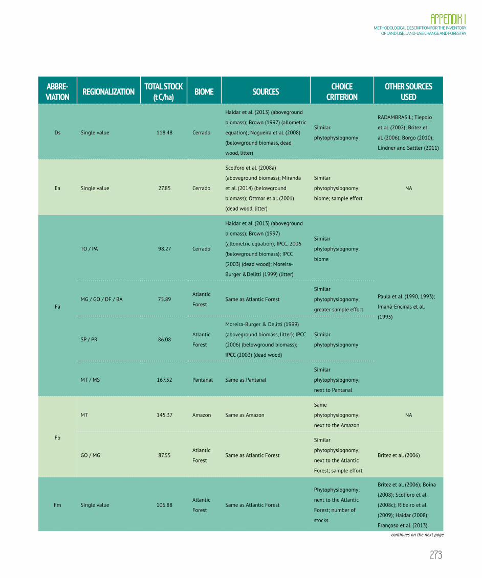
273
APPENDIX I METHODOLOGICAL DESCRIPTION FOR THE INVENTORY
OF LAND USE, LAND-USE CHANGE AND FORESTRY
ABBRE-VIATION REGIONALIZATION TOTAL STOCK
(t C/ha) BIOME SOURCES CHOICE CRITERION
OTHER SOURCES USED
Ds Single value 118.48 Cerrado
Haidar et al. (2013) (aboveground
biomass); Brown (1997) (allometric
equation); Nogueira et al. (2008)
(belowground biomass, dead
wood, litter)
Similar
phytophysiognomy
RADAMBRASIL; Tiepolo
et al. (2002); Britez et
al. (2006); Borgo (2010);
Lindner and Sattler (2011)
Ea Single value 27.85 Cerrado
Scolforo et al. (2008a)
(aboveground biomass); Miranda
et al. (2014) (belowground
biomass); Ottmar et al. (2001)
(dead wood, litter)
Similar
phytophysiognomy;
biome; sample effort
NA
Fa
TO / PA 98.27 Cerrado
Haidar et al. (2013) (aboveground
biomass); Brown (1997)
(allometric equation); IPCC, 2006
(belowground biomass); IPCC
(2003) (dead wood); Moreira-
Burger &Delitti (1999) (litter)
Similar
phytophysiognomy;
biome
Paula et al. (1990, 1993);
Imanã-Encinas et al.
(1995)
MG / GO / DF / BA 75.89Atlantic
ForestSame as Atlantic Forest
Similar
phytophysiognomy;
greater sample effort
SP / PR 86.08Atlantic
Forest
Moreira-Burger & Delitti (1999)
(aboveground biomass, litter); IPCC
(2006) (belowground biomass);
IPCC (2003) (dead wood)
Similar
phytophysiognomy
MT / MS 167.52 Pantanal Same as Pantanal
Similar
phytophysiognomy;
next to Pantanal
Fb
MT 145.37 Amazon Same as Amazon
Same
phytophysiognomy;
next to the Amazon
NA
GO / MG 87.55Atlantic
ForestSame as Atlantic Forest
Similar
phytophysiognomy;
next to the Atlantic
Forest; sample effort
Britez et al. (2006)
Fm Single value 106.88Atlantic
ForestSame as Atlantic Forest
Phytophysiognomy;
next to the Atlantic
Forest; number of
stocks
Britez et al. (2006); Boina
(2008); Scolforo et al.
(2008c); Ribeiro et al.
(2009); Haidar (2008);
Françoso et al. (2013)
continues on the next page
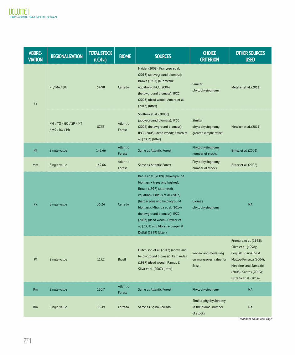
274
VOLUME ITHIRD NATIONAL COMMUNICATION OF BRAZIL
ABBRE-VIATION REGIONALIZATION TOTAL STOCK
(t C/ha) BIOME SOURCES CHOICE CRITERION
OTHER SOURCES USED
Fs
PI / MA / BA 54.98 Cerrado
Haidar (2008); Françoso et al.
(2013) (aboveground biomass);
Brown (1997) (allometric
equation); IPCC (2006)
(belowground biomass); IPCC
(2003) (dead wood); Amaro et al.
(2013) (litter)
Similar
phytophysiognomyMetzker et al. (2011)
MG / TO / GO / SP / MT
/ MS / RO / PR87.55
Atlantic
Forest
Scolforo et al. (2008c)
(aboveground biomass); IPCC
(2006) (belowground biomass);
IPCC (2003) (dead wood); Amaro et
al. (2003) (litter)
Similar
phytophysiognomy;
greater sample effort
Metzker et al. (2011)
Ml Single value 142.66Atlantic
ForestSame as Atlantic Forest
Phytophysiognomy;
number of stocksBritez et al. (2006)
Mm Single value 142.66Atlantic
ForestSame as Atlantic Forest
Phytophysiognomy;
number of stocksBritez et al. (2006)
Pa Single value 36.24 Cerrado
Bahia et al. (2009) (aboveground
biomass – trees and bushes);
Brown (1997) (allometric
equation); Fidelis et al. (2013)
(herbaceous and belowground
biomass); Miranda et al. (2014)
(belowground biomass); IPCC
(2003) (dead wood); Ottmar et
al. (2001) and Moreira-Burger &
Delitti (1999) (litter)
Biome’s
phytophysiognomyNA
Pf Single value 117.2 Brasil
Hutchison et al. (2013) (above and
belowground biomass); Fernandes
(1997) (dead wood); Ramos &
Silva et al. (2007) (litter)
Review and modelling
on mangroves, value for
Brazil
Fromard et al. (1998);
Silva et al. (1998);
Cogliatti-Carvalho &
Mattos-Fonseca (2004);
Medeiros and Sampaio
(2008); Santos (2013);
Estrada et al. (2014)
Pm Single value 130.7Atlantic
ForestSame as Atlantic Forest Phytophysiognomy NA
Rm Single value 18.49 Cerrado Same as Sg no Cerrado
Similar phyphysionomy
in the biome; number
of stocks
NA
continues on the next page

275
APPENDIX I METHODOLOGICAL DESCRIPTION FOR THE INVENTORY
OF LAND USE, LAND-USE CHANGE AND FORESTRY
ABBRE-VIATION REGIONALIZATION TOTAL STOCK
(t C/ha) BIOME SOURCES CHOICE CRITERION
OTHER SOURCES USED
Sa Single value 39.92 Cerrado
Ottmar et al. (2001) (aboveground
biomass, dead wood, litter);
Miranda et al. (2014)
(belowground biomass)
Biome’s
phytophysiognomy;
geographic coverage;
number of stocks
Kauffman et al. (1994);
Castro & Kauffman
(1998); Abdala et al.
(1998); Durigan (2004);
Barbosa & Fearnside
(2005); Rezende et al.
(2006); Felfili (2008);
Pinheiro (2008); Scolforo
et al. (2008a); Ribeiro et
al. (2011); Haidar et al.
(2013); Miranda (2012)
Sd
SP 68.99 Cerrado
Pinheiro (2008) (aboveground
biomass); Miranda et al. (2014)
(belowground biomass); IPCC
(2003) (dead wood); Morais et al.
(2013) (litter)
Phytophysiognomy in
the state of SP; in the
biome
Durigan (2004); Fernandes
et al. (2008)
MG / GO / DF / BA 52.42 Cerrado
Scolforo et al. (2008a)
(aboveground biomass); Miranda
et al. (2014) (belowground
biomass); IPCC (2003) (dead
wood); Morais et al. (2013) (litter)
Phytophysiognomy in
the state of MG; in the
biome
MT / MS / RO 103.45 Pantanal Same as PantanalPhytophysiognomy in the
state of MS; in the biome
TO / MA / PI 49.76 Cerrado
Haidar et al. (2013) (aboveground
biomass); Brown (1997) (allometric
equation); Miranda et al. (2014)
(belowground biomass); IPCC
(2003) (dead wood); Morais et al.
(2013) (litter)
Phytophysiognomy in
the state of TO; in the
biome
Sg Single value 18.49 Cerrado
Ottmar et al. (2001) (aboveground
biomass, litter); Miranda et al.
(2014) (belowground biomass)
Same
phytophysiognomy;
same biome; geographic
coverage; number of
stocks sampled
Kauffman et al. (1994);
Castro & Kauffman
(1998); Barbosa &
Fearnside (2005)
Sp Single value 24.65 Cerrado
Ottmar et al. (2001) (aboveground
biomass, dead wood, litter);
Miranda et al. (2014)
(belowground biomass); Same as
Pantanal
Biome’s
phytophysiognomy;
geographic coverage;
number of stocks;
biomass variation in Sp
Kauffman et al. (1994);
Castro & Kauffman
(1998); Barbosa &
Fearnside (2005)
continues on the next page

276
VOLUME ITHIRD NATIONAL COMMUNICATION OF BRAZIL
ABBRE-VIATION REGIONALIZATION TOTAL STOCK
(t C/ha) BIOME SOURCES CHOICE CRITERION
OTHER SOURCES USED
Ta Single value 15.23 Caatinga Same as CaatingaPhytophysiognomy;
sample effortNA
Td Single value 30.54 Caatinga Same as CaatingaPhytophysiognomy;
sample effortNA
Tg Single value 5.27 Amazon Same as Amazon Phytophysiognomy NA
Tp Single value 11.45 Amazon Same as Amazon Phytophysiognomy NA
Caatinga biome
The Caatinga occupies the Northeast region of Brazil and the Northern part of the state of Minas Gerais. It
is a region subject to a semiarid climate, high luminous intensity, high annual temperatures, irregularity in the
rainfall period and relatively low altitudes (which do not exceed 2,000 m). The action of these factors results in
a vegetation with adaptations to water shortage, usually small sized and possessing discontinuous canopy, small
leaves and branched individuals, with thorns or spines.
The greater part of the Caatinga biome (around 86%) is covered by phytophysiognomies that are typical of
Northeastern hinterlands region. For the Wooded Steppe (Ta) and Forested (Td) Savannas, data provided by PhD
Eliza Albuquerque, of the Federal Rural University of Pernambuco (UFRPE), were used. In this study, based on 79
plots distributed along Zona da Mata, Harsh and Hinterlands of the state of Pernambuco, researchers estimated the
aboveground biomass (tree, shrub and herbaceous), belowground (thin and thick roots) and dead organic matter
(dead wood and litter) (ALBUQUERQUE, 2015). The preference for the use of these data to estimate the biomass of
the two most representative phytophysiognomies of the biome was due to the large number of sample units, the
broader inclusion of stocks and their distribution, which was based on the Agro-ecological Zoning of Pernambuco
(ZAPE) (SILVA et al., 2001).
For the Park Steppe Savannas (Tp) and Woody Grass (Tg), the values of aboveground biomass and dead
organic matter were chosen from the work developed in these phytophysiognomies in the Amazon biome
(BARBOSA & FEARNSIDE, 2005). For the estimation of the belowground biomass, the IPCC ratio for semiarid
grassland (IPCC, 2006) was used.
The same value used for this phytophysiognomy in the states of Tocantins, Maranhão and Piauí in the Cerrado
biome was used for the Forested Savanna (Sd). For the Wooded Savanna (Sa), the same value of Sa in the Cerrado
biome was used, since its occurrence is mainly in the transition zone between the two biomes in the states of
Piauí, Bahia and Minas Gerais.
For the Park Savanna (Sp), due to its occurrence in the central region of Bahia and the northern Minas Gerais,
the values of aboveground biomass and dead organic matter in shrubby fields in the Cerrado biome were chosen
(OTTMAR et al., 2001), in addition to the application of the ratio for the estimation of belowground biomass for
grassland vegetation in Cerrado (MIRANDA et al., 2014).
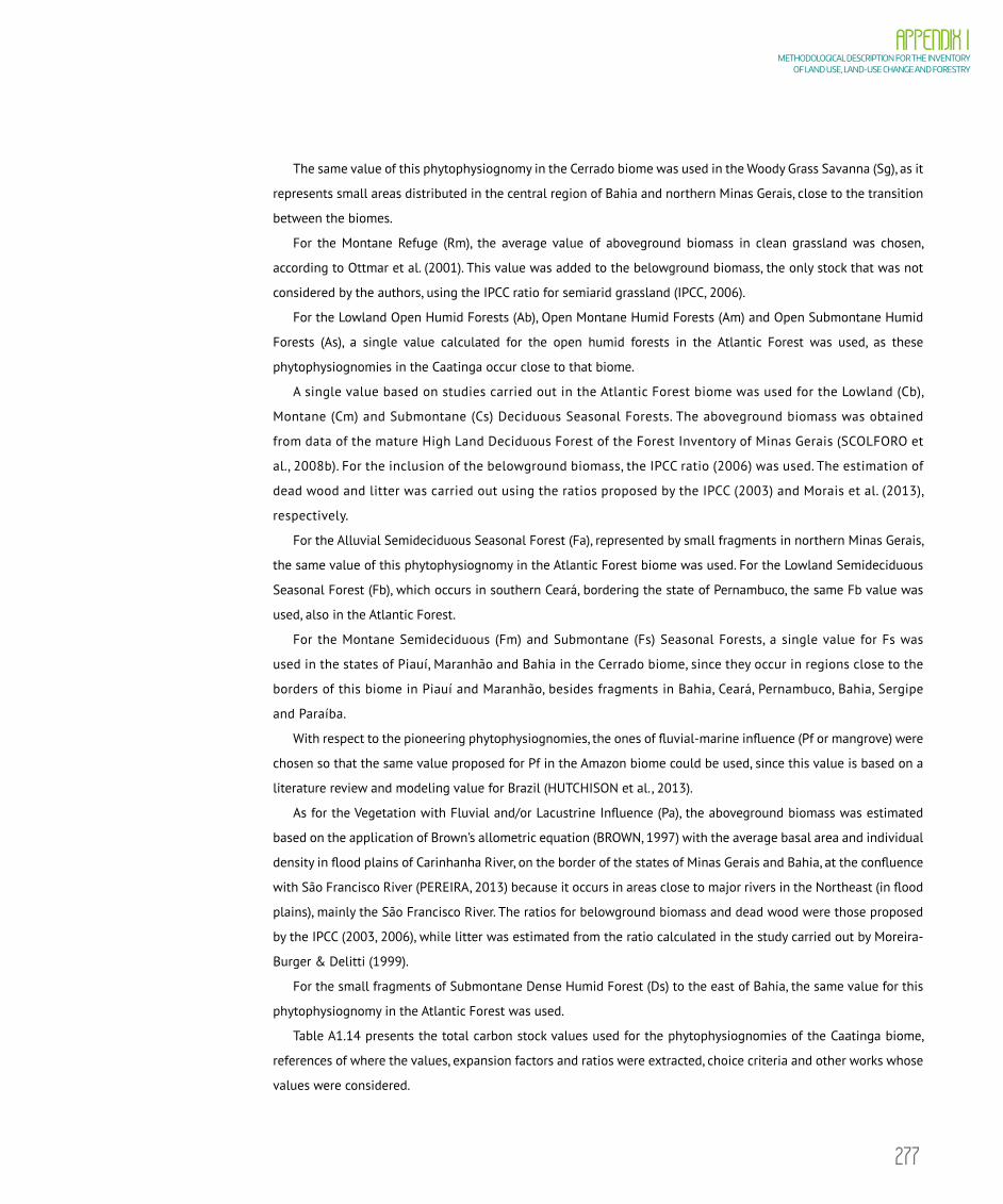
277
APPENDIX I METHODOLOGICAL DESCRIPTION FOR THE INVENTORY
OF LAND USE, LAND-USE CHANGE AND FORESTRY
The same value of this phytophysiognomy in the Cerrado biome was used in the Woody Grass Savanna (Sg), as it
represents small areas distributed in the central region of Bahia and northern Minas Gerais, close to the transition
between the biomes.
For the Montane Refuge (Rm), the average value of aboveground biomass in clean grassland was chosen,
according to Ottmar et al. (2001). This value was added to the belowground biomass, the only stock that was not
considered by the authors, using the IPCC ratio for semiarid grassland (IPCC, 2006).
For the Lowland Open Humid Forests (Ab), Open Montane Humid Forests (Am) and Open Submontane Humid
Forests (As), a single value calculated for the open humid forests in the Atlantic Forest was used, as these
phytophysiognomies in the Caatinga occur close to that biome.
A single value based on studies carried out in the Atlantic Forest biome was used for the Lowland (Cb),
Montane (Cm) and Submontane (Cs) Deciduous Seasonal Forests. The aboveground biomass was obtained
from data of the mature High Land Deciduous Forest of the Forest Inventory of Minas Gerais (SCOLFORO et
al., 2008b). For the inclusion of the belowground biomass, the IPCC ratio (2006) was used. The estimation of
dead wood and litter was carried out using the ratios proposed by the IPCC (2003) and Morais et al. (2013),
respectively.
For the Alluvial Semideciduous Seasonal Forest (Fa), represented by small fragments in northern Minas Gerais,
the same value of this phytophysiognomy in the Atlantic Forest biome was used. For the Lowland Semideciduous
Seasonal Forest (Fb), which occurs in southern Ceará, bordering the state of Pernambuco, the same Fb value was
used, also in the Atlantic Forest.
For the Montane Semideciduous (Fm) and Submontane (Fs) Seasonal Forests, a single value for Fs was
used in the states of Piauí, Maranhão and Bahia in the Cerrado biome, since they occur in regions close to the
borders of this biome in Piauí and Maranhão, besides fragments in Bahia, Ceará, Pernambuco, Bahia, Sergipe
and Paraíba.
With respect to the pioneering phytophysiognomies, the ones of fluvial-marine influence (Pf or mangrove) were
chosen so that the same value proposed for Pf in the Amazon biome could be used, since this value is based on a
literature review and modeling value for Brazil (HUTCHISON et al., 2013).
As for the Vegetation with Fluvial and/or Lacustrine Influence (Pa), the aboveground biomass was estimated
based on the application of Brown’s allometric equation (BROWN, 1997) with the average basal area and individual
density in flood plains of Carinhanha River, on the border of the states of Minas Gerais and Bahia, at the confluence
with São Francisco River (PEREIRA, 2013) because it occurs in areas close to major rivers in the Northeast (in flood
plains), mainly the São Francisco River. The ratios for belowground biomass and dead wood were those proposed
by the IPCC (2003, 2006), while litter was estimated from the ratio calculated in the study carried out by Moreira-
Burger & Delitti (1999).
For the small fragments of Submontane Dense Humid Forest (Ds) to the east of Bahia, the same value for this
phytophysiognomy in the Atlantic Forest was used.
Table A1.14 presents the total carbon stock values used for the phytophysiognomies of the Caatinga biome,
references of where the values, expansion factors and ratios were extracted, choice criteria and other works whose
values were considered.
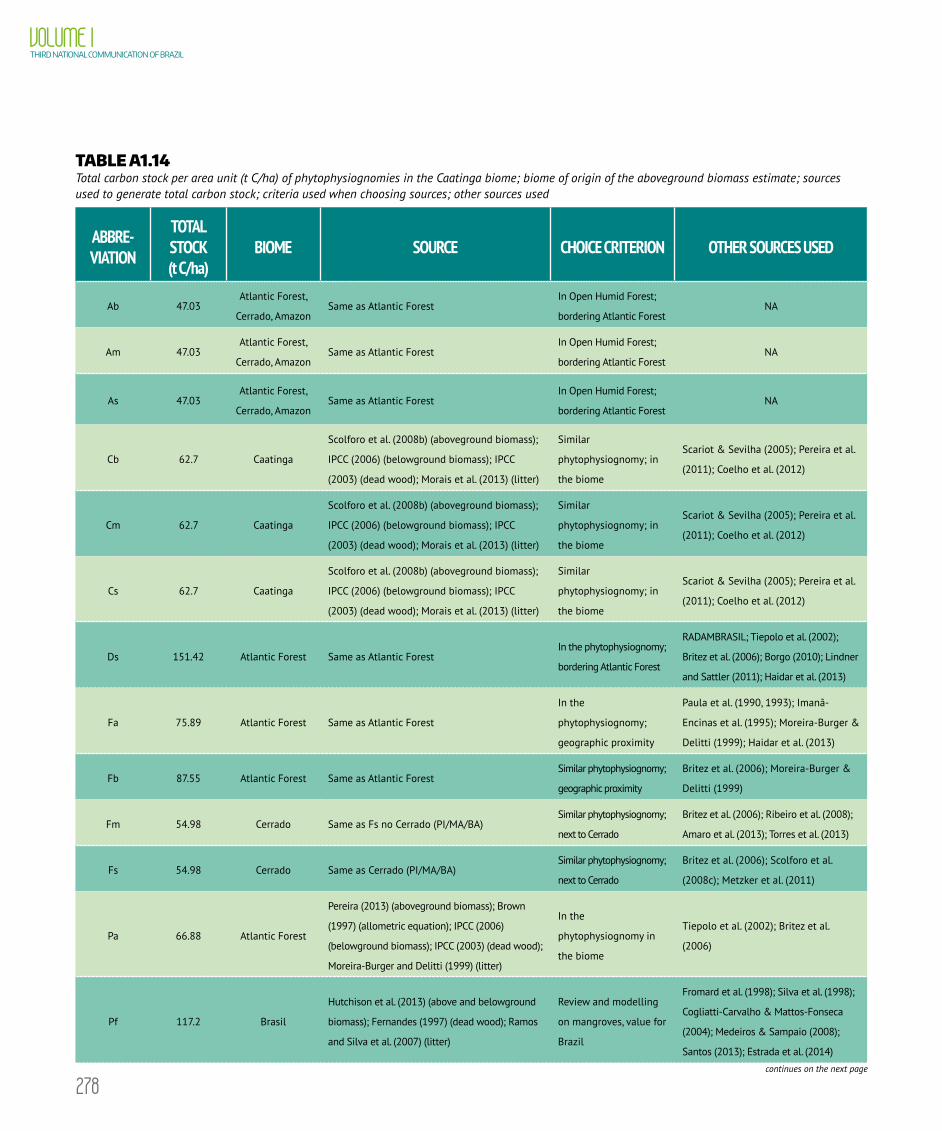
278
VOLUME ITHIRD NATIONAL COMMUNICATION OF BRAZIL
TABLE A1.14 Total carbon stock per area unit (t C/ha) of phytophysiognomies in the Caatinga biome; biome of origin of the aboveground biomass estimate; sources used to generate total carbon stock; criteria used when choosing sources; other sources used
ABBRE-VIATION
TOTAL STOCK (t C/ha)
BIOME SOURCE CHOICE CRITERION OTHER SOURCES USED
Ab 47.03Atlantic Forest,
Cerrado, AmazonSame as Atlantic Forest
In Open Humid Forest;
bordering Atlantic ForestNA
Am 47.03Atlantic Forest,
Cerrado, AmazonSame as Atlantic Forest
In Open Humid Forest;
bordering Atlantic ForestNA
As 47.03Atlantic Forest,
Cerrado, AmazonSame as Atlantic Forest
In Open Humid Forest;
bordering Atlantic ForestNA
Cb 62.7 Caatinga
Scolforo et al. (2008b) (aboveground biomass);
IPCC (2006) (belowground biomass); IPCC
(2003) (dead wood); Morais et al. (2013) (litter)
Similar
phytophysiognomy; in
the biome
Scariot & Sevilha (2005); Pereira et al.
(2011); Coelho et al. (2012)
Cm 62.7 Caatinga
Scolforo et al. (2008b) (aboveground biomass);
IPCC (2006) (belowground biomass); IPCC
(2003) (dead wood); Morais et al. (2013) (litter)
Similar
phytophysiognomy; in
the biome
Scariot & Sevilha (2005); Pereira et al.
(2011); Coelho et al. (2012)
Cs 62.7 Caatinga
Scolforo et al. (2008b) (aboveground biomass);
IPCC (2006) (belowground biomass); IPCC
(2003) (dead wood); Morais et al. (2013) (litter)
Similar
phytophysiognomy; in
the biome
Scariot & Sevilha (2005); Pereira et al.
(2011); Coelho et al. (2012)
Ds 151.42 Atlantic Forest Same as Atlantic ForestIn the phytophysiognomy;
bordering Atlantic Forest
RADAMBRASIL; Tiepolo et al. (2002);
Britez et al. (2006); Borgo (2010); Lindner
and Sattler (2011); Haidar et al. (2013)
Fa 75.89 Atlantic Forest Same as Atlantic Forest
In the
phytophysiognomy;
geographic proximity
Paula et al. (1990, 1993); Imanã-
Encinas et al. (1995); Moreira-Burger &
Delitti (1999); Haidar et al. (2013)
Fb 87.55 Atlantic Forest Same as Atlantic ForestSimilar phytophysiognomy;
geographic proximity
Britez et al. (2006); Moreira-Burger &
Delitti (1999)
Fm 54.98 Cerrado Same as Fs no Cerrado (PI/MA/BA)Similar phytophysiognomy;
next to Cerrado
Britez et al. (2006); Ribeiro et al. (2008);
Amaro et al. (2013); Torres et al. (2013)
Fs 54.98 Cerrado Same as Cerrado (PI/MA/BA)Similar phytophysiognomy;
next to Cerrado
Britez et al. (2006); Scolforo et al.
(2008c); Metzker et al. (2011)
Pa 66.88 Atlantic Forest
Pereira (2013) (aboveground biomass); Brown
(1997) (allometric equation); IPCC (2006)
(belowground biomass); IPCC (2003) (dead wood);
Moreira-Burger and Delitti (1999) (litter)
In the
phytophysiognomy in
the biome
Tiepolo et al. (2002); Britez et al.
(2006)
Pf 117.2 Brasil
Hutchison et al. (2013) (above and belowground
biomass); Fernandes (1997) (dead wood); Ramos
and Silva et al. (2007) (litter)
Review and modelling
on mangroves, value for
Brazil
Fromard et al. (1998); Silva et al. (1998);
Cogliatti-Carvalho & Mattos-Fonseca
(2004); Medeiros & Sampaio (2008);
Santos (2013); Estrada et al. (2014)
continues on the next page

279
APPENDIX I METHODOLOGICAL DESCRIPTION FOR THE INVENTORY
OF LAND USE, LAND-USE CHANGE AND FORESTRY
ABBRE-VIATION
TOTAL STOCK (t C/ha)
BIOME SOURCE CHOICE CRITERION OTHER SOURCES USED
Pm 123.67 Atlantic Forest
Assis et al. (2011) (aboveground biomass and litter
deposited); IPCC (2006) (belowground biomass);
Veiga (2010) (dead wood and litter); Pires et al.
(2006) (decomposition constant); Kristensen et al.
(2008) (decomposition regression equation)
Phytophysiognomy Britez et al. (2006)
Rm 16.24 CerradoOttmar et al. (2001) (aboveground biomass and
litter); IPCC (2006) (belowground biomass)
Similar
phytophysiognomy;
number of stocks
Barbosa & Fearnside (1999)
Sa 39.92 Cerrado Same as Cerrado
Similar
phytophysiognomy;
geographic proximity;
number of stocks
Paula et al. (1998); Scolforo et al.
(2008a); Haidar et al. (2013)
Sd 49.76 Cerrado Same as Cerrado (TO/MA/PI)
Similar
phytophysiognomy;
geographic proximity
Scolforo et al. (2008a); Morais et al.
(2013)
Sg 18.49 Cerrado Same as Cerrado
Similar
phytophysiognomy;
geographic proximity;
number of stocks
Barbosa & Fearnside (2005);
Sp 17.61 Cerrado
Ottmar et al. (2001) (aboveground biomass,
litter); Miranda et al. (2014) (belowground
biomass)
Similar
phytophysiognomy;
number of stocks;
occurrence in the
phytophysiognomy
Barbosa & Fearnside (2005)
Ta 15.23 Caatinga ALBUQUERQUE (2015) (all stocks)
In the
phytophysiognomy
in the biome; sample
effort; number of stocks
Tiessen et al. (1998); Amorim et al.
(2005); Accioly et al. (2008); Alves
(2011); Sampaio & Costa (2011);
Menezes et al. (2012); Souza et al.
(2012); Cabral et al. (2013); Costa
(2013); Mendonça et al. (2013)
Td 30.54 Caatinga ALBUQUERQUE (2015) (all stocks)
In the phytophysiognomy
in the biome; sample
effort; number of stocks
Menezes et al. (2012); Souza et al.
(2012); Cabral et al. (2013); Costa
(2013)
Tg 4.63 Amazon
Barbosa & Fearnside (2005) (aboveground
biomass, dead wood, litter); IPCC (2006)
(belowground biomass)
In the
phytophysiognomy,
number of stocks
NA
Tp 10.06 Amazon
Barbosa & Fearnside (2005) (aboveground
biomass, dead wood, litter); IPCC (2006)
(belowground biomass)
In the
phytophysiognomies,
number of stocks
NA

280
VOLUME ITHIRD NATIONAL COMMUNICATION OF BRAZIL
Atlantic Forest Biome
The Atlantic Forest covers the Eastern Brazilian shelf. Due to its wide latitudinal extension, it covers a wide range
of climate zones and has heterogeneous vegetation. The biome is composed of a mosaic of dense, open and mixed
humid forests; deciduous and semideciduous seasonal forests; altitudes grasslands, mangroves and sandbanks.
The Submontane Semideciduous Seasonal Forest (Fs), the most representative of the biome, had its aboveground
biomass estimated based on the work by Metzker et al. (2011), carried out in this phytophysiognomy in the state of
Minas Gerais. On the other hand, the belowground biomass and the dead wood were estimated based on the IPCC
default ratios (2003; 2006), while the ratio calculated from the data by Amaro et al. (2013) was used for litter, in
Montane Semideciduous Seasonal Forest (Fm). The work by Amaro et al. (2013) was also used to estimate the total
biomass of Fm, because the authors presented values for all stocks in this phytophysiognomy in the Atlantic Forest.
The average of the aboveground biomass values in Mature Riparian Semideciduous Forest of the Inventory
of Minas Gerais (SCOLFORO et al., 2008c) was used for the Alluvial Semideciduous Seasonal Forest (Fa). The
belowground biomass and dead wood were estimated according to default ratios of the IPCC (2003, 2006), while
litter was estimated based on the ratio in a riparian mesophilic forest (MOREIRA-BURGER & DELITTI, 1999).
Values of Mature Semideciduous Seasonal Forest presented by Scolforo et al. (2008c) in the Inventory of the
state of Minas Gerais were used for the Lowland Semideciduous Seasonal Forest (Fb), in the Atlantic Forest biome.
The stocks of belowground biomass and dead wood were estimated based on the default values of the IPCC (2003,
2006), while litter was estimated by the ratio obtained from Amaro et al. (2003).
The Mixed Humid Forest or Araucaria Forest occurs mainly in the southern region of the country (states of Santa
Catarina, Paraná and Rio Grande do Sul), in addition to São Paulo and Minas Gerais. For the Submontane Mixed
High Humid Forests (Ms), Montana (Mm) and High Humid Forest (Ml), values of aboveground and belowground
biomass as well as those regarding litter obtained by Watzwalick et al. (2012), in Paraná, were used. In order to
estimate the dead wood, the ratio proposed by the IPCC (2003) was used.
For the fragments of Alluvial Mixed Humid Forest (Ma) in the states of Santa Catarina and Paraná, aboveground
biomass and litter values were obtained from the study of Socher et al. (2008), also in the state of Paraná. In order
to estimate the belowground biomass and the dead wood, IPCC ratios (2003, 2006) were used.
The Dense Humid Forest is a perennial forest, that is, evergreen, which occurs in virtually the entire length of
the Atlantic Forest biome. For the Alluvial Dense Humid Forest (Da), the aboveground biomass values calculated
by Britez et al. (2006) in Santa Catarina and Rio Grande do Sul were used. For the belowground biomass estimate,
the ratio by Monkany et al. (2006) was used; for the dead wood, the IPCC ratio (2003) was applied; and for litter, the
ratio obtained from the work by Socher et al. (2008) was used.
For the Lowland (Db), Submontane (Ds) and Montana (Dm) Dense Humid Forests, the studies by Alves et al.
(2010) for the aboveground biomass were used; that of and Vieira et al. (2011) was applied for belowground
biomass, dead wood and litter, carried out in the state of São Paulo. It is worth noting that values for each of
these Dense Humid Forests (Db, Ds and Dm) are presented. For the High-Montane Dense Humid Forest (Dl),
the value of aboveground biomass calculated by Britez et al. (2006) was used based on the work carried out
in Paraná. In order to estimate the remaining stocks of Dl, the same proportions mentioned before for the Da
phytophysiognomy were used.
281
APPENDIX I METHODOLOGICAL DESCRIPTION FOR THE INVENTORY
OF LAND USE, LAND-USE CHANGE AND FORESTRY
For the Alluvial (Aa), the Lowland (Ab), the Montane (Am) and the Submontane (As) Open Humid Forests,
whose fragments occur in the states of Minas Gerais, Espirito Santo, Pernambuco and Alagoas, a single value was
chosen. The estimate of aboveground biomass was obtained from the average of seven values calculated using
the individual density and average diameter in the equation developed by Brown (1997). The studies used were
distributed in Rondônia, Pernambuco and Maranhão (SILVEIRA, 2009; FERRAZ & RODAL, 2006; GAMA et al. 2007).
The other stocks were estimated according to the ratios by Mokany et al. (2006) for the belowground biomass; the
IPCC ratio (2003) was used for dead wood; and those of Socher et al. (2008) were applied for litter.
For the Deciduous Seasonal Forest or Alluvial Broadleaved (Ca), found mainly in Rio Grande do Sul, the average
of the aboveground biomass values of Mature Riparian Deciduous Forest presented in the Forest Inventory of Minas
Gerais (SCOLFORO et al., 2008b) was used. The ratio proposed by the IPCC (2003, 2006) was used to incorporate the
belowground biomass and dead wood; the ratio in Riparian Semideciduous Mesophilic Forest (MOREIRA-BURGER
& DELITTI, 1999) was used for litter.
For the fragments of Low Land Deciduous Seasonal Forest (Cb), located in the state of Rio Grande do Norte, the
same value of this phytophysiognomy within the Caatinga biome was adopted.
The values obtained from the work by Brun (2004), conducted in the state of Rio Grande do Sul, were used
for the Montane (Cm) and Submontane (Cs) Deciduous Seasonal Forests, which mainly occur in Bahia and in the
South and Southeast regions of the country. The author evaluates all stocks, except that of dead wood, which was
estimated according to the IPCC ratio (2003).
The value for Wooded Steppe (Ea) was the same as that used for this phytophysiognomy in the Cerrado in
the Forest Inventory of Minas Gerais (SCOLFORO et al., 2008a), a state where Ea occurs in the Atlantic Forest. For
Woody Grass Steppe (Eg) the same value of this phytophysiognomy in the Pampa biome was chosen, since this
phytophysiognomy occurs in the transition with the Atlantic Forest in Rio Grande do Sul.
The Vegetation with Fluvial and/or Lacustrine Influence (Pa), in the Atlantic Forest, present mainly forest
structure and occur in the lowland areas of the rivers. Its aboveground biomass was estimated from the average of
the values calculated by Britez et al. (2006), in Paraná. The other stocks were obtained from ratios for belowground
biomass by Mokany et al. (2006); for dead wood, those by the IPCC (2003) were used; and for litter, those by Moreira-
Burger & Delitti (1999) were applied.
For the pioneering formations of fluvial-marine influence (mangroves or Pf), the same value of carbon stock of
the Amazon biome was used, which resulted from aboveground biomass according to Hutchison et al. (2013) for
mangroves in Brazil.
The aboveground biomass value for pioneering formations of marine influence (Pm) was extracted from Alves
et al. (2010), also published in Assis et al. (2011), for the sandbank vegetation of the state of São Paulo. For the
belowground biomass, the IPCC ratio (2006) was used. For the value of dead wood, the value by Veiga (2010)
was used, in the same study area of Alves et al. (2010) and Assis et al. (2011). Litter was estimated based on the
decomposition equation (KRISTENSEN et al., 2008), the decomposition rate constant (PIRES et al., 2006) and the
litter deposition value (ASSIS et al., 2011).
For the Montane (Rm) and Submontane (Rs) Refuges, the same value proposed for this phytophysiognomy in
the Cerrado biome was used (OTTMAR et al., 2001), due to lack of information regarding the biomass for these
phytophysiognomies and the biome itself. As for the High-Montana Refuge (Rl), values of aboveground biomass
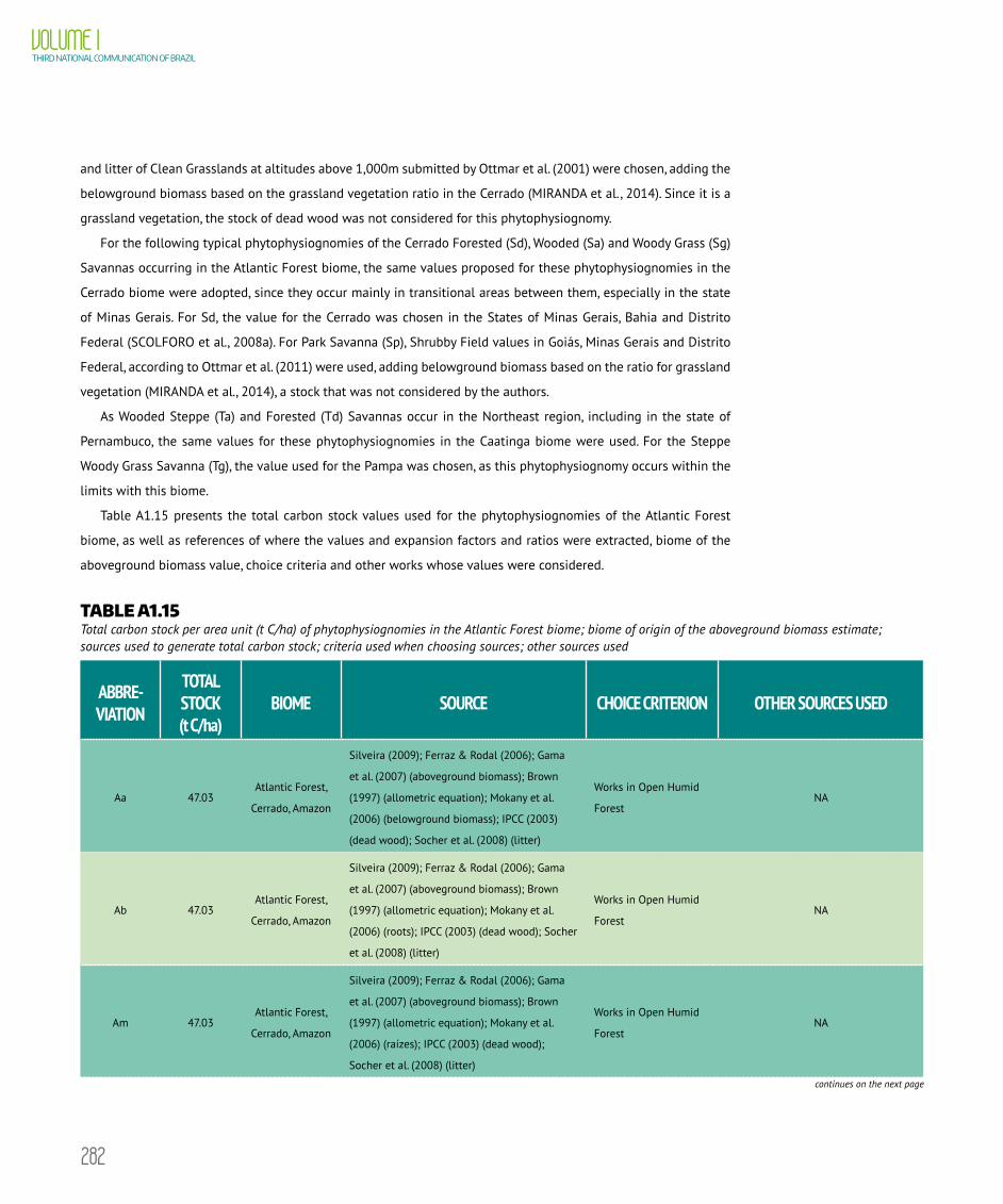
282
VOLUME ITHIRD NATIONAL COMMUNICATION OF BRAZIL
and litter of Clean Grasslands at altitudes above 1,000m submitted by Ottmar et al. (2001) were chosen, adding the
belowground biomass based on the grassland vegetation ratio in the Cerrado (MIRANDA et al., 2014). Since it is a
grassland vegetation, the stock of dead wood was not considered for this phytophysiognomy.
For the following typical phytophysiognomies of the Cerrado Forested (Sd), Wooded (Sa) and Woody Grass (Sg)
Savannas occurring in the Atlantic Forest biome, the same values proposed for these phytophysiognomies in the
Cerrado biome were adopted, since they occur mainly in transitional areas between them, especially in the state
of Minas Gerais. For Sd, the value for the Cerrado was chosen in the States of Minas Gerais, Bahia and Distrito
Federal (SCOLFORO et al., 2008a). For Park Savanna (Sp), Shrubby Field values in Goiás, Minas Gerais and Distrito
Federal, according to Ottmar et al. (2011) were used, adding belowground biomass based on the ratio for grassland
vegetation (MIRANDA et al., 2014), a stock that was not considered by the authors.
As Wooded Steppe (Ta) and Forested (Td) Savannas occur in the Northeast region, including in the state of
Pernambuco, the same values for these phytophysiognomies in the Caatinga biome were used. For the Steppe
Woody Grass Savanna (Tg), the value used for the Pampa was chosen, as this phytophysiognomy occurs within the
limits with this biome.
Table A1.15 presents the total carbon stock values used for the phytophysiognomies of the Atlantic Forest
biome, as well as references of where the values and expansion factors and ratios were extracted, biome of the
aboveground biomass value, choice criteria and other works whose values were considered.
TABLE A1.15 Total carbon stock per area unit (t C/ha) of phytophysiognomies in the Atlantic Forest biome; biome of origin of the aboveground biomass estimate; sources used to generate total carbon stock; criteria used when choosing sources; other sources used
ABBRE- VIATION
TOTAL STOCK (t C/ha)
BIOME SOURCE CHOICE CRITERION OTHER SOURCES USED
Aa 47.03Atlantic Forest,
Cerrado, Amazon
Silveira (2009); Ferraz & Rodal (2006); Gama
et al. (2007) (aboveground biomass); Brown
(1997) (allometric equation); Mokany et al.
(2006) (belowground biomass); IPCC (2003)
(dead wood); Socher et al. (2008) (litter)
Works in Open Humid
ForestNA
Ab 47.03Atlantic Forest,
Cerrado, Amazon
Silveira (2009); Ferraz & Rodal (2006); Gama
et al. (2007) (aboveground biomass); Brown
(1997) (allometric equation); Mokany et al.
(2006) (roots); IPCC (2003) (dead wood); Socher
et al. (2008) (litter)
Works in Open Humid
ForestNA
Am 47.03Atlantic Forest,
Cerrado, Amazon
Silveira (2009); Ferraz & Rodal (2006); Gama
et al. (2007) (aboveground biomass); Brown
(1997) (allometric equation); Mokany et al.
(2006) (raízes); IPCC (2003) (dead wood);
Socher et al. (2008) (litter)
Works in Open Humid
ForestNA
continues on the next page

283
APPENDIX I METHODOLOGICAL DESCRIPTION FOR THE INVENTORY
OF LAND USE, LAND-USE CHANGE AND FORESTRY
ABBRE- VIATION
TOTAL STOCK (t C/ha)
BIOME SOURCE CHOICE CRITERION OTHER SOURCES USED
As 47.03Atlantic Forest,
Cerrado, Amazon
Silveira (2009); Ferraz & Rodal (2006); Gama
et al. (2007) (aboveground biomass); Brown
(1997) (allometric equation); Mokany et al.
(2006) (belowground biomass); IPCC (2003)
(dead wood); Socher et al. (2008) (litter)
Works in Open Humid
ForestNA
Ca 121.76 Caatinga
Scolforo et al. (2008b) (aboveground biomass);
IPCC (2006) (belowground biomass); IPCC
(2003) (dead wood); Moreira-Burger and Delitti
(1999) (litter)
Similar
phytophysiognomy;
sample effort
Scariot & Sevilha (2005); Pereira et al.
(2011); Coelho et al. (2012)
Cb 62.7 Caatinga Same as Caatinga
Similar
phytophysiognomy;
sample effort; next to
Caatinga
Scariot & Sevilha (2005); Pereira et al.
(2011); Coelho et al. (2012)
Cm 106.41 Atlantic Forest
Brun (2004) (aboveground biomass,
belowground biomass, litter); IPCC (2003)
(dead wood)
Similar
phytophysiognomy in
the biome; number of
stocks
Scariot & Sevilha (2005); Scolforo
et al. (2008b); Pereira et al. (2011);
Coelho et al. (2012)
Cs 106.41 Atlantic Forest
Brun (2004) (aboveground biomass,
belowground biomass, litter); IPCC (2003)
(dead wood)
Similar
phytophysiognomy in
the biome; number of
stocks
Scariot & Sevilha (2005); Scolforo
et al. (2008b); Pereira et al. (2011);
Coelho et al. (2012)
Da 173.83 Atlantic Forest
Britez et al. (2006) (aboveground biomass); Mokany
et al. (2006) (belowground biomass); IPCC (2003)
(dead wood); Socher et al. (2008) (litter)
In the
phytophysiognomy in
the biome
RADAMBRASIL; Tiepolo et al. (2002)
Db 128.42 Atlantic Forest
Alves et al. (2010) (aboveground biomass);
Vieira et al. (2011) (belowground biomass, dead
wood, litter)
In the phytophysiognomy
in the biome; number of
stocks
RADAMBRASIL; Tiepolo et al. (2002); Rolim
et al. (2005); Britez et al. (2006); Assis et
al. (2011); Sousa Neto et al. (2011)
Dl 105.53 Atlantic Forest
Britez et al. (2006) (aboveground biomass); Mokany
et al. (2006) (belowground biomass); IPCC (2003)
(dead wood); Socher et al. (2008) (litter)
In the
phytophysiognomy in
the biome
RADAMBRASIL
Dm 177.75 Atlantic Forest
Alves et al. (2010) (aboveground biomass);
Vieira et al. (2011) (belowground biomass, dead
wood, litter)
In the
phytophysiognomy in
the biome; number of
stocks
RADAMBRASIL; Tiepolo et al. (2002);
Britez et al. (2006); Cunha et al. (2009);
Lindner and Sattler (2011); Sousa Neto
et al. (2011)
Ds 151.42 Atlantic Forest
Alves et al. (2010) (aboveground biomass);
Vieira et al. (2011) (belowground biomass, dead
wood, litter)
In the
phytophysiognomy in
the biome; number of
stocks
RADAMBRASIL; Tiepolo et al. (2002);
Britez et al. (2006); Borgo (2010);
Lindner and Sattler (2011); Sousa Neto
et al. (2011)
continues on the next page

284
VOLUME ITHIRD NATIONAL COMMUNICATION OF BRAZIL
ABBRE- VIATION
TOTAL STOCK (t C/ha)
BIOME SOURCE CHOICE CRITERION OTHER SOURCES USED
Ea 27.85 Cerrado Same as Cerrado
In similar
phytophysiognomy;
próxima ao Cerrado
NA
Eg 2.12 Pampa Same as Pampa
In the
phytophysiognomy;
next to Pampa
Oliveira et al. (2009)
Fa 75.89 Atlantic Forest
Scolforo et al. (2008c) (aboveground biomass);
IPCC (2006) (belowground biomass); IPCC
(2003) (dead wood); Moreira-Burger & Delitti
(1999) (litter)
Similar
phytophysiognomy;
sample effort
Britez et al. (2006); Wittman et al.
(2008); Haidar et al. (2013)
Fb 87.55 Atlantic Forest
Scolforo et al. (2008c) (aboveground biomass);
IPCC (2006) (belowground biomass); IPCC
(2003) (dead wood); Amaro et al. (2003) (litter)
Similar
phytophysiognomy
in the biome; sample
effort
Britez et al. (2006); Nogueira et al.
(2008)
Fm 106.88 Atlantic Forest Amaro et al. (2003) (todos os reservatórios)
In the
phytophysiognomy in
the biome; number of
stocks
Britez et al. (2006); Boina (2008);
Scolforo et al. (2008c); Ribeiro et al.
(2009); Haidar (2008); Françoso et al.
(2013); Torres et al. (2013)
Fs 123.05 Atlantic Forest
Metzker et al. (2011) (aboveground biomass);
IPCC (2006) (belowground biomass); IPCC
(2003) (dead wood); Amaro et al. (2003) (litter)
In the
phytophysiognomy in
the biome
RADAMBRASIL; Britez et al. (2006);
Scolforo et al. (2008c); Haidar (2008);
Françoso et al. (2013);
Ma 123.21 Atlantic Forest
Socher et al. (2008) (aboveground biomass and
litter); IPCC (2006) (belowground biomass);
IPCC (2003) (dead wood)
In the
phytophysiognomy in
the biome
Britez et al. (2006)
Ml 142.66 Atlantic Forest
Watzlawick et al. (2012) (aboveground biomass,
belowground biomass, litter); IPCC (2003)
(dead wood)
Similar
phytophysiognomy in
the biome; number of
stocks
Britez et al. (2006); Klauberg et al.
(2010)
Mm 142.66 Atlantic Forest
Watzlawick et al. (2012) (aboveground biomass,
belowground biomass, litter); IPCC (2003)
(dead wood)
In the
phytophysiognomy in
the biome; number of
stocks
Britez et al. (2006)
Ms 142.66 Atlantic ForestWatzlawick et al. (2012) (aboveground biomass,
litter); IPCC (2003) (dead wood)
Similar
phytophysiognomy in
the biome; number of
stocks
Britez et al. (2006); Klauberg et al.
(2010)
continues on the next page
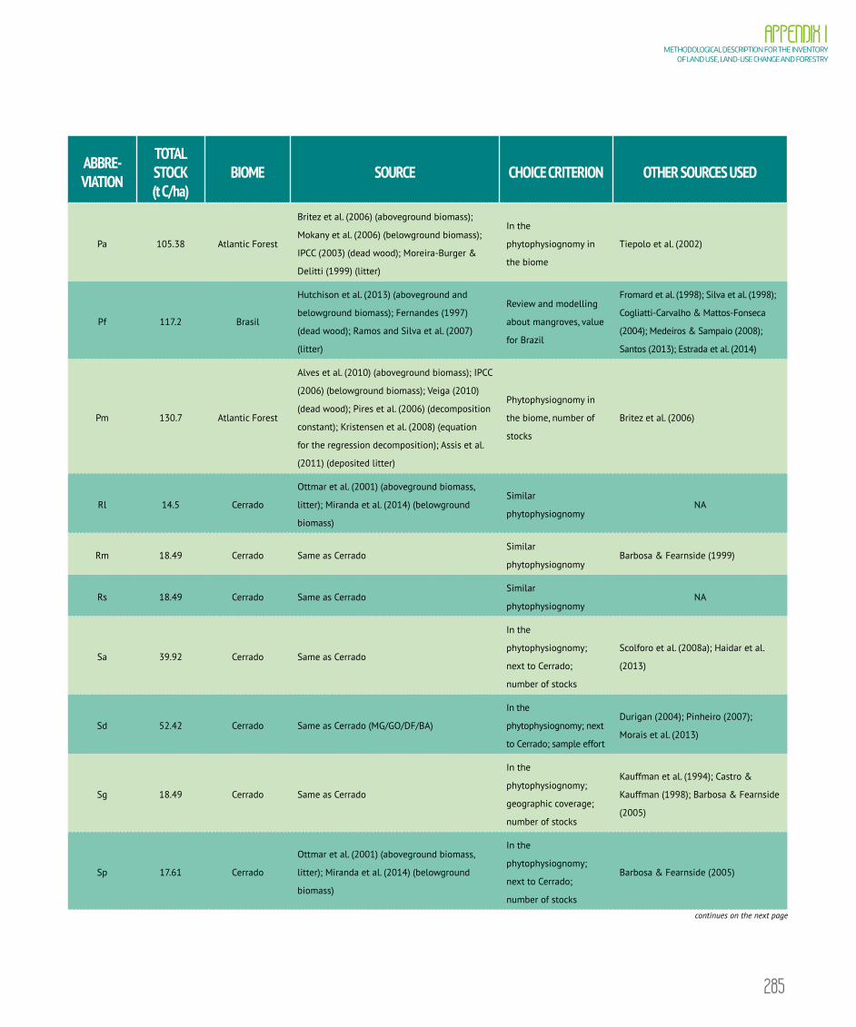
285
APPENDIX I METHODOLOGICAL DESCRIPTION FOR THE INVENTORY
OF LAND USE, LAND-USE CHANGE AND FORESTRY
ABBRE- VIATION
TOTAL STOCK (t C/ha)
BIOME SOURCE CHOICE CRITERION OTHER SOURCES USED
Pa 105.38 Atlantic Forest
Britez et al. (2006) (aboveground biomass);
Mokany et al. (2006) (belowground biomass);
IPCC (2003) (dead wood); Moreira-Burger &
Delitti (1999) (litter)
In the
phytophysiognomy in
the biome
Tiepolo et al. (2002)
Pf 117.2 Brasil
Hutchison et al. (2013) (aboveground and
belowground biomass); Fernandes (1997)
(dead wood); Ramos and Silva et al. (2007)
(litter)
Review and modelling
about mangroves, value
for Brazil
Fromard et al. (1998); Silva et al. (1998);
Cogliatti-Carvalho & Mattos-Fonseca
(2004); Medeiros & Sampaio (2008);
Santos (2013); Estrada et al. (2014)
Pm 130.7 Atlantic Forest
Alves et al. (2010) (aboveground biomass); IPCC
(2006) (belowground biomass); Veiga (2010)
(dead wood); Pires et al. (2006) (decomposition
constant); Kristensen et al. (2008) (equation
for the regression decomposition); Assis et al.
(2011) (deposited litter)
Phytophysiognomy in
the biome, number of
stocks
Britez et al. (2006)
Rl 14.5 Cerrado
Ottmar et al. (2001) (aboveground biomass,
litter); Miranda et al. (2014) (belowground
biomass)
Similar
phytophysiognomyNA
Rm 18.49 Cerrado Same as CerradoSimilar
phytophysiognomyBarbosa & Fearnside (1999)
Rs 18.49 Cerrado Same as CerradoSimilar
phytophysiognomyNA
Sa 39.92 Cerrado Same as Cerrado
In the
phytophysiognomy;
next to Cerrado;
number of stocks
Scolforo et al. (2008a); Haidar et al.
(2013)
Sd 52.42 Cerrado Same as Cerrado (MG/GO/DF/BA)
In the
phytophysiognomy; next
to Cerrado; sample effort
Durigan (2004); Pinheiro (2007);
Morais et al. (2013)
Sg 18.49 Cerrado Same as Cerrado
In the
phytophysiognomy;
geographic coverage;
number of stocks
Kauffman et al. (1994); Castro &
Kauffman (1998); Barbosa & Fearnside
(2005)
Sp 17.61 Cerrado
Ottmar et al. (2001) (aboveground biomass,
litter); Miranda et al. (2014) (belowground
biomass)
In the
phytophysiognomy;
next to Cerrado;
number of stocks
Barbosa & Fearnside (2005)
continues on the next page

286
VOLUME ITHIRD NATIONAL COMMUNICATION OF BRAZIL
ABBRE- VIATION
TOTAL STOCK (t C/ha)
BIOME SOURCE CHOICE CRITERION OTHER SOURCES USED
Ta 15.23 Caatinga Same as Caatinga
In the
phytophysiognomy;
number of stocks; next
to Caatinga
NA
Td 30.54 Caatinga Same as Caatinga
In the
phytophysiognomy;
number of stocks; next
to Caatinga
NA
Tg 12.6 Pampa Same as Pampa
Similar
phytophysiognomy;
next to Pampa
NA
Pampa Biome
The Pampa biome occurs only in the state of Rio Grande do Sul in Brazil, besides the neighboring countries of
Argentina and Uruguay. Temperate fields predominate in this biome, characterized by herbaceous vegetation, but
there are also forest and shrub formations from mountains to plains.
Studies carried out on the Pampa biome and in the state of Rio Grande do Sul were given priority. In the
absence of such studies, phytophysiognomies values in other biomes were used, preferably from the Atlantic
Forest, adjacent to the Pampa. In this last case, values of similar phytophysiognomies were used, always as close
as possible to the Brazilian Pampa.
For the Wooded Steppe (Ea), the values found for the Argentine Chaco (GASPARRI et al., 2008) were chosen.
This work was chosen because an aboveground biomass value was not found for this phytophysiognomy
in the Pampa biome itself and due to the geographic proximity and the structural resemblance to this
phytophysiognomy. The ratios used by the authors to estimate the belowground biomass (IPCC, 2006), dead
wood (IPCC, 2003) and litter (regional value) were kept because they were considered adequate. For the
Wooded Steppe Savanna (Ta), the same values of Ea in the Pampa biome were chosen, also due to the lack of
studies found in this phytophysiognomy.
For Woody Grass Steppe (Eg), aboveground and belowground biomass values in the Pampa biome in Rio
Grande do Sul were used (FIDELIS et al., 2006). A value for dead wood was not estimated because this is a strictly
herbaceous phytophysiognomy. For litter, a fixed value of a literature review presented in the book Grasses and
Grasslands Ecology (COUPLAND, 1993 apud GIBSON, 2009, table 7.2) was used.
For the Alluvial (Ca), the Montane (Cm) and the Submontane (Cs) Deciduous Seasonal Forests; the Montane
(Dm) and Submontane (Ds) Dense Humid Forests, as well as for the Submontane (Fs) and Montane (Fm)
Semideciduous Seasonal Forests, the same values and correction factors of these phytophysiognomies for the
Atlantic Forest were used.

287
APPENDIX I METHODOLOGICAL DESCRIPTION FOR THE INVENTORY
OF LAND USE, LAND-USE CHANGE AND FORESTRY
For Lowland Semideciduous Seasonal Forest (Fb), we used the aboveground biomass and litter values
accumulated in riparian semideciduous mesophilic forest (MOREIRA-BURGER & DELITTI, 1999), obtained in the
Atlantic Forest biome. For the belowground biomass and dead wood, IPCC default ratios (2003, 2006) were used.
For the Forested Savanna (Sd), values of aboveground, belowground biomass, and litter for Savannah-like vegetation
(Cerradão) in the Cerrado biome (MORAIS et al., 2013) were used. The IPCC ratio was used to estimate dead wood.
For the vegetation of fluvial and/or lacustrine influence (Pa), a review of pioneering formations of fluvial-marine
influence (Pf) and pioneering formations of marine influence (Pm), works and management plans of protected areas
on the coast and in the region of Lagoa dos Patos was carried out (KNAK, 1999; BRACK, 2006; DUARTE & BENCKE,
2006; JACOBI et al., 2013) along with a review of the scientific literature as well as of pictures of these vegetation in
the Pampa biome. Those analyzes concluded that the structure of those vegetation covers is predominantly formed
by grassland and swamps. As a result, values of the work carried out in Spartina densiflora Brongn swamp in Lagoa
dos Patos, in Rio Grande do Sul, were adopted (CUNHA et al., 2005).
The Woody Grass Steppe Savanna (Tg) occurs to the West of the biome and in the borders of Argentina and
Uruguay. For this grassland phytophysiognomy, the values of aboveground and belowground biomass, and litter in
the Uruguayan grasslands, characterized by herbaceous vegetation in the Basin of Rio de La Plata, (PARUELO et al.,
2010) were adopted. For the Woody-Grass Savanna (Sg), the same value used for Tg was adopted, due to the fact
that the two phytophysiognomies are close to each other and are structurally similar (that is, strictly grassland).
Table A1.16 presents the total carbon stock values used for the phytophysiognomies of the Pampa biome, references
to estimate total carbon stocks, biome of the aboveground biomass value, choice criteria and other sources used.
TABLE A1.16 Total carbon stock per area unit (t C/ha) of phytophysiognomies in the Pampa biome; biome of origin of the aboveground biomass estimate; sources used to generate total carbon stock; criteria used when choosing sources; and other sources used
ABBRE- VIATION
TOTAL STOCK (t C/ha)
BIOME SOURCE CHOICE CRITERION OTHER SOURCES USED
Ca 121.76 Caatinga
Scolforo et, al. 2008b (aboveground biomass);
IPCC, 2006 (belowground biomass); IPCC, 2003
(dead wood); Moreira-Burger & Delitti, 1999
(litter). Same as Atlantic Forest
Similar
phytophysiognomy;
sample effort
Scariot & Sevilha (2005); Pereira et al.
(2011); Coelho et al. (2012)
Cm 106.41 Atlantic Forest
Brun, 2004 (aboveground and belowground
biomass, litter); IPCC, 2003 (dead wood). Same
as Atlantic Forest
Similar
phytophysiognomy; next
to Pampa in the state of
RS; number of stocks
Scariot & Sevilha (2005); Vogel et al.
(2006); Scolforo et al. (2008b); Pereira
et al. (2011); Coelho et al. (2012)
Cs 106.41 Atlantic Forest
Brun, 2004 (aboveground and belowground
biomass); IPCC, 2003 (dead wood). Same as
Atlantic Forest
Similar
phytophysiognomy; next
to Pampa in the state of
RS; number of stocks
Scariot & Sevilha (2005); Vogel et al.
(2006); Scolforo et al. (2008b); Pereira
et al. (2011); Coelho et al. (2012)
continues on the next page
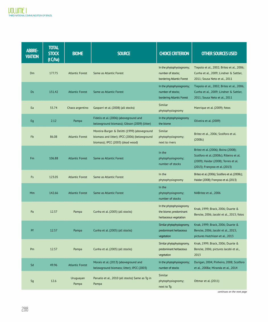
288
VOLUME ITHIRD NATIONAL COMMUNICATION OF BRAZIL
ABBRE- VIATION
TOTAL STOCK (t C/ha)
BIOME SOURCE CHOICE CRITERION OTHER SOURCES USED
Dm 177.75 Atlantic Forest Same as Atlantic Forest
In the phytophysiognomy;
number of stocks;
bordering Atlantic Forest
Tiepolo et al., 2002; Britez et al., 2006;
Cunha et al., 2009; Lindner & Sattler,
2011; Sousa Neto et al., 2011
Ds 151.42 Atlantic Forest Same as Atlantic Forest
In the phytophysiognomy;
number of stocks;
bordering Atlantic Forest
Tiepolo et al., 2002; Britez et al., 2006;
Cunha et al., 2009; Lindner & Sattler,
2011; Sousa Neto et al., 2011
Ea 55.74 Chaco argentino Gasparri et al. (2008) (all stocks)Similar
phytophysiognomyManrique et al. (2009); fotos
Eg 2.12 PampaFidelis et al. (2006) (aboveground and
belowground biomass); Gibson (2009) (litter)
In the phytophysiognomy
the biomeOliveira et al. (2009)
Fb 86.08 Atlantic Forest
Moreira-Burger & Delitti (1999) (aboveground
biomass and litter); IPCC (2006) (belowground
biomass); IPCC (2003) (dead wood)
Similar
phytophysiognomy;
next to rivers
Britez et al., 2006; Scolforo et al.
(2008c)
Fm 106.88 Atlantic Forest Same as Atlantic Forest
In the
phytophysiognomy;
number of stocks
Britez et al. (2006); Boina (2008);
Scolforo et al. (2008c); Ribeiro et al.
(2009); Haidar (2008); Torres et al.
(2013); Françoso et al. (2013)
Fs 123.05 Atlantic Forest Same as Atlantic ForestIn the
phytophysiognomy
Britez et al. (2006); Scolforo et al. (2008c);
Haidar (2008); Françoso et al. (2013)
Mm 142.66 Atlantic Forest Same as Atlantic Forest
In the
phytophysiognomy;
number of stocks
NABritez et al., 2006
Pa 12.57 Pampa Cunha et al. (2005) (all stocks)
In the phytophysiognomy
the biome; predominant
herbaceous vegetation
Knak, 1999; Brack, 2006; Duarte &
Bencke, 2006; Jacobi et al., 2013; fotos
Pf 12.57 Pampa Cunha et al. (2005) (all stocks)
Similar phytophysiognomy,
predominant herbaceous
vegetation
Knak, 1999; Brack, 2006; Duarte &
Bencke, 2006; Jacobi et al., 2013;
pictures Hutchison et al., 2013
Pm 12.57 Pampa Cunha et al. (2005) (all stocks)
Similar phytophysiognomy,
predominant herbaceous
vegetation
Knak, 1999; Brack, 2006; Duarte &
Bencke, 2006; pictures Jacobi et al.,
2013
Sd 49.96 Atlantic ForestMorais et al. (2013) (aboveground and
belowground biomass; litter); IPCC (2003)
In the phytophysiognomy;
number of stocks
Durigan, 2004; Pinheiro, 2008; Scolforo
et al., 2008a; Miranda et al., 2014
Sg 12.6Uruguayan
Pampa
Paruelo et al., 2010 (all stocks) Same as Tg in
Pampa
Similar
phytophysiognomy;
next to Tg
Ottmar et al. (2011)
continues on the next page

289
APPENDIX I METHODOLOGICAL DESCRIPTION FOR THE INVENTORY
OF LAND USE, LAND-USE CHANGE AND FORESTRY
ABBRE- VIATION
TOTAL STOCK (t C/ha)
BIOME SOURCE CHOICE CRITERION OTHER SOURCES USED
Ta 55.74Argentinean
Chaco
Gasparri et al., 2008 (all stocks) Same as Ea in
Pampa
Similar
phytophysiognomy;
climate zone
Manrique et al. (2009); fotos
Tg 12.6 Pampa uruguaio Paruelo et al. (2010) (all stocks)
Similar
phytophysiognomy;
geographic proximity;
review article
Caña et al. (2013)
Pantanal Biome
In addition to the aquatic-influenced vegetation (river-flood) a large vegetation mosaic with forest, savannah
and grassland formations represents the Pantanal biome. These vegetal formations are also bordered by the Chaco
to the south, the Amazon to the north, the Atlantic Forest and the Cerrado to the south and east of the biome.
Thus, the biomass values of the Pantanal vegetation were obtained from data collected in the field and literature
references preferably in the biome itself and, when this was not possible, references of the neighboring biomes
were used, such as the Amazon, Cerrado and Atlantic Forest.
The data collected in the field in these phytophysiognomies in the Pantanal were used for the Wooded (Sa)
and Forested (Sd) Savannas, from projects carried out in a partnership between EMBRAPA and PROBIO, developed
from 1997 to 2005 (SILVA, J. V. S.23). After a survey of allometric equations to estimate the aboveground biomass in
the Cerrado (ex.: DELITTI et al., 2006; REZENDE et al., 2006; SALIS et al., 2004; PINHEIRO, 2007), the ones used
by Pinheiro (2007) were chosen, according to Melo et al. (2007) for stricto sensu Cerrado and Cerradão. In these
equations the quadratic diameter and the height of trees with diameter at breast height (DBH) greater or equal
to 10cm were considered. For the Wooded (Sa) and Forested Savana (Sd), 18 and 24 5x20cm plots distributed in
the biome were used, respectively. For the belowground biomass, ratios of savannas and forests in the Cerrado
by Miranda et al. (2014) for Sa and Sd, respectively, were used. For Sa the ratio for dead wood and litter in Dense,
Typical and Shallow Cerrado, according to the data by Ottmar et al. (2001), were used. For Sd IPCC default ratios
(2003) for dead wood were used; and for litter, data according to Cerradão by Morais et al. (2013).
The Park Savanna (Sp) in the Pantanal includes the paratudal, canjiqueiral, lixeiral, campo sujo, cerrado de pantanal,
and campo de murundus vegetation (IBGE, 2012). The aboveground woody biomass was calculated from the equation
of Delitti et al. (2006) with the data collected by Haidar et al. (2013) in Park Savannah in Tocantins (in 10 wetland
areas of Bananal Island region) of trees with 30cm diameter and higher than 5cm from the ground. Added to this
value, the aboveground herbaceous biomass average in Shallow Cerrado, according to Ottmar et al. 2001. For the
belowground biomass the ratio of savanna vegetation was adopted, according to Miranda et al. (2014). For dead
wood and litter the ratios in Shallow Cerrado were chosen, according to Ottmar et al. (2001).
23 SILVA, J. V. S. (National Center for Technological Research on Agricultural Information, Brazilian Agricultural Research Corporation, EMBRAPA, Campinas). Personal communication, 2014.
290
VOLUME ITHIRD NATIONAL COMMUNICATION OF BRAZIL
Given that the Woody Grass Savanna (Sg) is a strictly grassland vegetation, the same total carbon stock value of
this phytophysiognomy in the Cerrado biome was considered.
The steppe savannas are concentrated in the southern Pantanal, in the state of Mato Grosso do Sul (SILVA
& CAPUTO, 2010). For Forested Steppe Savanna (Td) the average of the aboveground biomass values of the
work by Padilha (2011), conducted in this phytophysiognomy, was used. For the calculation of the belowground
biomass the ratio of the forest physiognomies in the Cerrado was used (MIRANDA et al. , 2014), for dead wood
the IPCC default ratio (2003) was used, and for litter the ratio in Cerradão (MORAIS et al. , 2013) was used. For
the Wooded (Ta or Chaco), Park (Tp, Carandazal or Paratudal) and Woody Grass (Tg) Steppe Savannas, regional
biomass values for the Pantanal were not found, so the same values of these phytophysiognomies of the
Amazon biome were used.
The Vegetation with Fluvial and/or Lacustre Influence (Pa) corresponds to plant communities that occur
in the wetlands seasonally flooded in the Pantanal. One of the communities that predominate in these plains
is the Cambarazal, characterized by a vegetation dominated by Cambara tree species (Vochysia divergens Pohl).
As a result, the aboveground biomass was calculated based on the average of four succession stages of
Cambarazal in the Pantanal, presented by Schongart et al. (2011). The belowground biomass was estimated by
the ratio calculated from Stape et al. (2011) in open Cambarazal, also in the Pantanal. For the estimate of dead
wood the IPCC default ratio (2003) was adopted, and for litter the ratio in riparian semideciduous mesophilic
forest was used (MOREIRA-BURGER & DELITTI, 1999).
For the aboveground biomass of the Alluvial Deciduous Seasonal Forest (Ca) the average values of
the dry matter weight of trees in Mature Riparian Deciduous Forest was used (SCOLFORO et al. , 2008b).
For the Lowland (Cb) and Submontane (Cs) Deciduous Seasonal Forests, the aboveground biomass was
estimated based on the application of Brown’s allometric equation (1997, equation 3.2.1), calculated based
on the mean basal area and density of individuals (CBH > 15cm), presented by Lima et al. (2009) in these
phytophysiognomies of the Pantanal. For the calculation of the belowground biomass and dead wood of
these phytophysiognomies, the IPCC default values (2003, 2006) were used. For litter, ratios in Cerradao
were used (MORAIS et al. , 2013) for Cb and Cs, and mesophilic forests riparian deciduous forest (MOREIRA-
BURGER & DELITTI, 1999) for Ca.
For the Alluvial Semideciduous Seasonal Forest (Fa), the aboveground biomass value in flooded seasonal
riparian forest in the Pantanal by Wittman al. (2008) was used. For the calculation of the belowground biomass
and dead wood, the IPCC default values (2003, 2006) were used. For litter, the ratio in riparian semideciduous
mesophilic forest (MOREIRA-BURGER & DELITTI, 1999) was used.
For Submontane Semideciduous Seasonal Forest (Fs), the same values of this phytophysiognomy in
the Atlantic Forest biome were adopted. For the Lowland Semideciduous Seasonal Forest (Fb), the values
of the carbon stock of this phytophysiognomy in the Amazon biome were used due to its location at
northern Pantanal.
Table A1.17 presents the total carbon stock values used for the phytophysiognomies of the Pantanal biome,
references of where the values, expansion factors and ratios were taken from, the biome of the aboveground
biomass, choice criteria and other sources used.
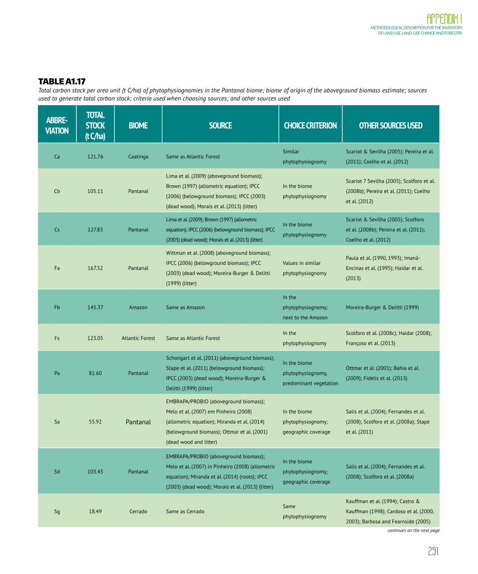
291
APPENDIX I METHODOLOGICAL DESCRIPTION FOR THE INVENTORY
OF LAND USE, LAND-USE CHANGE AND FORESTRY
TABLE A1.17 Total carbon stock per area unit (t C/ha) of phytophysiognomies in the Pantanal biome; biome of origin of the aboveground biomass estimate; sources used to generate total carbon stock; criteria used when choosing sources; and other sources used
ABBRE-VIATION
TOTAL STOCK (t C/ha)
BIOME SOURCE CHOICE CRITERION OTHER SOURCES USED
Ca 121.76 Caatinga Same as Atlantic ForestSimilar
phytophysiognomy
Scariot & Sevilha (2005); Pereira et al.
(2011); Coelho et al. (2012)
Cb 105.11 Pantanal
Lima et al. (2009) (aboveground biomass);
Brown (1997) (allometric equation); IPCC
(2006) (belowground biomass); IPCC (2003)
(dead wood); Morais et al. (2013) (litter)
In the biome
phytophysiognomy
Scariot 7 Sevilha (2005); Scolforo et al.
(2008b); Pereira et al. (2011); Coelho
et al. (2012)
Cs 127.83 Pantanal
Lima et al. (2009); Brown (1997) (allometric
equation); IPCC (2006) (belowground biomass); IPCC
(2003) (dead wood); Morais et al. (2013) (litter)
In the biome
phytophysiognomy
Scariot & Sevilha (2005); Scolforo
et al. (2008b); Pereira et al. (2011);
Coelho et al. (2012)
Fa 167.52 Pantanal
Wittman et al. (2008) (aboveground biomass);
IPCC (2006) (belowground biomass); IPCC
(2003) (dead wood); Moreira-Burger & Delitti
(1999) (litter)
Values in similar
phytophysiognomy
Paula et al. (1990, 1993); Imanã-
Encinas et al. (1995); Haidar et al.
(2013)
Fb 145.37 Amazon Same as Amazon
In the
phytophysiognomy;
next to the Amazon
Moreira-Burger & Delitti (1999)
Fs 123.05 Atlantic Forest Same as Atlantic Forest In the
phytophysiognomy
Scolforo et al. (2008c); Haidar (2008);
Françoso et al. (2013)
Pa 81.60 Pantanal
Schongart et al. (2011) (aboveground biomass);
Stape et al. (2011) (belowground biomass);
IPCC (2003) (dead wood); Moreira-Burger &
Delitti (1999) (litter)
In the biome
phytophysiognomy,
predominant vegetation
Ottmar et al. (2001); Bahia et al.
(2009); Fidelis et al. (2013)
Sa 55.92 Pantanal
EMBRAPA/PROBIO (aboveground biomass);
Melo et al. (2007) em Pinheiro (2008)
(allometric equation); Miranda et al. (2014)
(belowground biomass); Ottmar et al. (2001)
(dead wood and litter)
In the biome
phytophysiognomy;
geographic coverage
Salis et al. (2004); Fernandes et al.
(2008); Scolforo et al. (2008a); Stape
et al. (2011)
Sd 103.45 Pantanal
EMBRAPA/PROBIO (aboveground biomass);
Melo et al. (2007) in Pinheiro (2008) (allometric
equation); Miranda et al. (2014) (roots); IPCC
(2003) (dead wood); Morais et al. (2013) (litter)
In the biome
phytophysiognomy;
geographic coverage
Salis et al. (2004); Fernandes et al.
(2008); Scolforo et al. (2008a)
Sg 18.49 Cerrado Same as CerradoSame
phytophysiognomy
Kauffman et al. (1994); Castro &
Kauffman (1998); Cardoso et al. (2000,
2003); Barbosa and Fearnside (2005)
continues on the next page
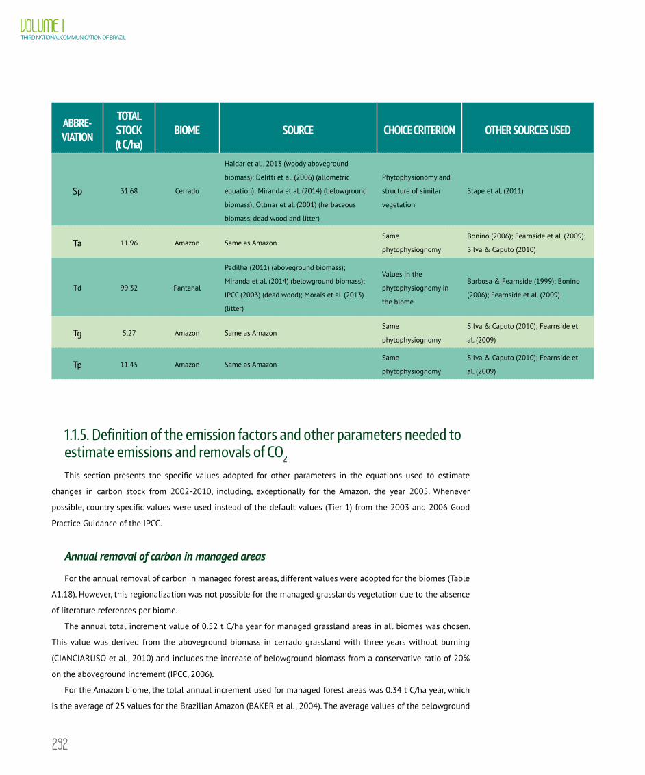
292
VOLUME ITHIRD NATIONAL COMMUNICATION OF BRAZIL
ABBRE-VIATION
TOTAL STOCK (t C/ha)
BIOME SOURCE CHOICE CRITERION OTHER SOURCES USED
Sp 31.68 Cerrado
Haidar et al., 2013 (woody aboveground
biomass); Delitti et al. (2006) (allometric
equation); Miranda et al. (2014) (belowground
biomass); Ottmar et al. (2001) (herbaceous
biomass, dead wood and litter)
Phytophysionomy and
structure of similar
vegetation
Stape et al. (2011)
Ta 11.96 Amazon Same as AmazonSame
phytophysiognomy
Bonino (2006); Fearnside et al. (2009);
Silva & Caputo (2010)
Td 99.32 Pantanal
Padilha (2011) (aboveground biomass);
Miranda et al. (2014) (belowground biomass);
IPCC (2003) (dead wood); Morais et al. (2013)
(litter)
Values in the
phytophysiognomy in
the biome
Barbosa & Fearnside (1999); Bonino
(2006); Fearnside et al. (2009)
Tg 5.27 Amazon Same as Amazon Same
phytophysiognomy
Silva & Caputo (2010); Fearnside et
al. (2009)
Tp 11.45 Amazon Same as AmazonSame
phytophysiognomy
Silva & Caputo (2010); Fearnside et
al. (2009)
1.1.5. Definition of the emission factors and other parameters needed to estimate emissions and removals of CO2
This section presents the specific values adopted for other parameters in the equations used to estimate
changes in carbon stock from 2002-2010, including, exceptionally for the Amazon, the year 2005. Whenever
possible, country specific values were used instead of the default values (Tier 1) from the 2003 and 2006 Good
Practice Guidance of the IPCC.
Annual removal of carbon in managed areas
For the annual removal of carbon in managed forest areas, different values were adopted for the biomes (Table
A1.18). However, this regionalization was not possible for the managed grasslands vegetation due to the absence
of literature references per biome.
The annual total increment value of 0.52 t C/ha year for managed grassland areas in all biomes was chosen.
This value was derived from the aboveground biomass in cerrado grassland with three years without burning
(CIANCIARUSO et al., 2010) and includes the increase of belowground biomass from a conservative ratio of 20%
on the aboveground increment (IPCC, 2006).
For the Amazon biome, the total annual increment used for managed forest areas was 0.34 t C/ha year, which
is the average of 25 values for the Brazilian Amazon (BAKER et al., 2004). The average values of the belowground

293
APPENDIX I METHODOLOGICAL DESCRIPTION FOR THE INVENTORY
OF LAND USE, LAND-USE CHANGE AND FORESTRY
biomass ratio for the dense and open forest in the Amazon for the 25.8% aboveground increment (NOGUEIRA et
al., 2008) were considered. Consequently, the total annual increment used for the managed forest in the Amazon
biome was 0.43 t C/ha.
For the Cerrado biome, the average of the two highest and lowest values was chosen (0.1 to 0.3 t C/ha year) in
a flux tower of CO2 in Forested Savanna for this biome (ROCHA et al., 2002), reaching an incremental value of 0.2
t C/ha year. These towers vary in carbon flux in all the stocks on which this element is part, and it is not necessary
to add a ratio for the belowground biomass in this case.
In the Atlantic Forest, the total annual increment value for aboveground biomass (0.27 t C/ha), found in this
biome (SCARANELLO, 2010), was used. A ratio of 20% of the belowground biomass increment (IPCC, 2006) was
chosen, resulting in a total increment of 0.32 t C/ha for the managed forest areas for this biome.
Annual increment values of primary vegetation to the Caatinga biome were not found. Based on consultation with an
expert researcher (PAREYN, 2014), a minimum value for Cerrado was chosen, that is, an annual increment of 0.1 t C/ha.
For the Pantanal biome, annual increment values of primary forest vegetation were not found. Due to
the proximity and large area occupied by phytophysiognomies that are typical of the Cerrado, an increment
value was chosen. Thus, the increment value of total annual carbon for the managed forest vegetation in the
Pantanal was 0.2 t C/ha.
In the Pampa biome, due to the proximity to the Atlantic Forest biome and the lack of regional information, the
same value adopted for the total increment of the Atlantic Forest was used, resulting in a value of 0.32 t C/ha per year.
A Table A1.18 presents a summary of the values adopted for annual carbon increment of the managed forest
vegetation of the Brazilian biomes and, when necessary, the ratio to add the belowground increment, in addition
to the respective references used.
TABLE A1.18 Annual aboveground and belowground biomass increment (t C/ha) of managed primary forest vegetation per biome, percentage of belowground increment in relation to that of aboveground, and references used
BIOME ABOVEGROUND BIOMASS INCREMENT (t C/ha)
RATIO (%) (BELOWGROUND BIOMASS INCREMENT)
TOTAL INCREMENT (t C/ha) REFERENCE
Amazon 0.34 25.8 0.43 Baker et al. (2004); Nogueira et al. (2008)
Cerrado 0.2 Rocha et al. (2002)
Atlantic Forest 0.30 20 0.32 Scaranello (2010); IPCC (2006)
Caatinga 0.1 Rocha et al. (2002)
Pantanal 0.2 Same as Cerrado
Pampa 0.30 20 0.32 Same as Atlantic Forest
294
VOLUME ITHIRD NATIONAL COMMUNICATION OF BRAZIL
Average annual carbon removal in secondary vegetation areas
A decision was made to regionalize by biome, whenever possible, the values for annual increment of
secondary vegetation. In addition, distinct historical uses that preceded the secondary vegetation formation
(pasture, agriculture and other uses) were also sought. Besides that, the estimates of carbon stock changes
were included for secondary forests with a history of having been forest (primary or secondary forest vegetation
and reforestation.
1) Secondary vegetation developed from previous forest areas
The regionalization was possible only in the secondary forest vegetation (Table A1.19), a single value for
Brazil for the secondary grassland vegetation was adopted. The total annual increment value for the grassland
secondary vegetation was 0.52 t C/ha (CIANCIARUSO et al. , 2010), the same value for managed fields.
For the secondary forest vegetation in the Amazon biome, the aboveground increment value was 3.94 t C/
ha per year (ALVES et al. , 1997), with a correction factor for the belowground biomass of 25.8% (NOGUEIRA et
al. , 2008) over this increment. As a result, the total incremental annual value for the secondary forests in the
Amazon was 4.96 t C/ha.
For the Cerrado biome, the aboveground increment value for the secondary vegetation obtained in this biome
was 1.41 t C/ha per year (DURIGAN, 2004), with a ratio for belowground biomass of 22% over this increment
(MIRANDA et al., 2014) and an application of 47% to convert biomass into carbon stock. As a result, the total
incremental annual value for the secondary forests in Cerrado was 1.72 t C/ha.
For the Atlantic Forest biome, an annual aboveground increment value of 4.46 t C/ha for the secondary
vegetation obtained in this biome (MELO & DURIGAN, 2006) was adopted, with a ratio for the belowground
biomass of 20% over aboveground biomass (IPCC, 2006), resulting in a total incremental value of 5.35 t
C/ha per year.
For the Caatinga biome, the aboveground increment value for the secondary vegetation obtained in this
biome (0.47 t C/ha per year) (PAREYIN, 2014; GARIGLIO et al. , 2010; ISAIA et al. , 1992) was adopted, with a
ratio for the belowground biomass of 27% over native vegetation under regeneration in this same biome,
according to Costa et al. (2014). As a result, the total incremental annual value for the secondary forests in
Caatinga was 0.6 t C/ha.
For the secondary forest vegetation of the Pampa biome, the aboveground increment value of 1.4 t C/ha was
adopted, with a ratio for the belowground biomass of 26% over aboveground biomass, based on a study carried
out in the state of Rio Grande do Sul (BRUN, 2004). As a result, the total incremental annual value for the Pampa
biome was 1.76 t C/ha.
For the Pantanal biome, the aboveground increment value for the secondary vegetation obtained in this biome
was 2.25 t C/ha. This value was calculated based on the secondary vegetation Cambarazal (Vochysia divergens) on
this biome (SCHONGART et al., 2011). The ratio of 23% of this value was used for the belowground biomass, based
on a study of Stape et al. (2011), also on the Cambarazal in Pantanal. As a result, the total incremental annual value
is 2.77 t C/ha for this biome.

295
APPENDIX I METHODOLOGICAL DESCRIPTION FOR THE INVENTORY
OF LAND USE, LAND-USE CHANGE AND FORESTRY
TABLE A1.19 Average annual increment of carbon stocks in living biomass in secondary forest vegetation areas per biome; annual average increment of carbon stock of aboveground biomass; ratio of belowground biomass for the aboveground biomass; and respective literature reference
BIOMEABOVEGROUND
BIOMASS INCREMENTt C/ha
REFERENCE USED FORABOVEGROUND BIOMASS
INCREMENT
RATIOA:B (%)
REFERENCE USED FOR RATIO A:B
TOTAL INCREMENTt C/ha
Amazon 3.94 Alves et al. (1997) 25.8 Nogueira (2008) 4.96
Cerrado 1.41 Durigan (2004) 22 Miranda et al. (2014) 1.72
Atlantic Forest 4.46 Melo and Durigan (2006) 20 IPCC (2006) 5.35
Caatinga 0.47 Gariglio et al. (2010); Isaia et al. (1992) 27 Costa et al. (2014) 0.60
Pantanal 2.25 Schongart et al. (2011) 23 Stape et al. (2011) 2.77
Pampa 1.4 Brun (2004) 26 Brun (2004) 1.76
2) Secondary vegetation developed from planted pasture areas
The value used for the annual increment of secondary vegetation developed from planted pasture areas was
2.85 t C/ha for all the biomes. This value was calculated from an average for secondary vegetation as planted
pasture up to 10 years of age in the Amazon (FELDPAUSCH et al., 2007), and with the addition of 20% for root
increment (IPCC, 2006).
3) Secondary vegetation developed from agricultural areas
The value adopted for the total annual increment of secondary vegetation developed from agricultural areas
was 4.73 t C/ha for all biomes. This value results from an average of secondary vegetation values between 2-to-9-
years of age developed from diversified crops (ALVES et al., 1997), with the addition of 20% for the increment in
belowground biomass (IPCC, 2006).
4) Secondary vegetation with other land-use history
Open-pit mining was considered as other land-use history. The total annual increment to secondary forest
vegetation developed from mining areas was 0.59 t C/ha for all biomes. This value was calculated from the
density of individuals per hectare and the diameter at breast height (DBH) of a mining area under 9-years recovery
(SALOMÃO et al., 2007), with application of the Brown equation (BROWN, 1997), adding 20% to the aboveground
increment based on the ratio for belowground biomass (IPCC, 2006).
Annual carbon removal in forest areas submitted to selective logging
The annual increment value adopted for forest vegetation where selective logging occurred was 0.02% (HUANG
& ASNER, 2010) in relation to the remaining carbon stock after logging. This was only applied to the Amazon biome.

296
VOLUME ITHIRD NATIONAL COMMUNICATION OF BRAZIL
Average carbon stock in secondary vegetation areas
The average carbon stock in secondary vegetation areas was obtained based on the mean values found in
the Amazon (FEARNSIDE & GUIMARAES, 1996; ALVES et al., 1997), Atlantic Forest (MELO & DURIGAN, 2006) and
Pantanal biomes (SCHONGART et al., 2011), for secondary forest vegetation at different ages. This resulted in an
average carbon stock value of 44% of the primary vegetation (managed and unmanaged forest) for the secondary
vegetation in all Brazilian biomes.
Carbon loss in forest area submitted to selective logging
The average carbon loss value of 29% was adopted (HUANG & ASNER, 2010) in relation to the total carbon
stock of the phytophysiognomy when a forest area is submitted to selective logging in the Amazon.
Carbon stock and removal in reforestation area
For the reforestations with Eucalyptus spp. the value of 44 m3/ha/yr for average mean increment was
adopted (BRACELPA, 2014), corresponding to an increment value of living biomass of 14.24 t C/ha/year. The
density of wood and the canopy/trunk and root/trunk ratio were considered to include the carbon contained
in the trunk, canopy and roots of the plants, using an allometric equation (IPCC, 2003). For the calculation of
the average carbon of a reforestation area, a seven-year cycle between the cuts, resulting in the average stock
value of 49.83 t C/ha, was considered.
For the reforestations with Pinus spp. the value of 38 m3/ha/yr was adopted of average increment (BRACELPA,
2014), corresponding to an increment value of 11.60 t C/ha/year. The density of wood and the canopy/trunk
and root/trunk ratios were considered to include the carbon contained in the trunk, canopy and roots of the
plants, using an allometric equation (IPCC, 2003). A 15-year cycle was considered between the cuts for the
calculation of the average carbon, resulting in the average stock value of 87.03 t C/ha.
Average carbon stock in planted pasture areas
The carbon stock in the living biomass of non-shrubby planted pasture was estimated with the IPCC
default values (2003) (Table 3.4.9, page 3.125), adapting them to the different climate zones associated with
the biomes and adopting the value of 0.47 t C/t m.s. For the Pampa biome a value of 6.35 t C/ha was adopted
because it is associated with a humid temperate region. For the Caatinga the adopted value (4.09 t C/ha)
refers to a dry tropical region. For the other biomes, the value of 7.57 t C/ha was adopted, because it is
associated with tropical humid region.
Carbon stock in agricultural areas
For the perennial crops in agricultural areas that remain as agricultural areas, the carbon stock was IPCC’s
default value of table 3.3.2 (IPCC, 2003), with climatic zone differentiations associated with each biome
considered. Except for the Caatinga, all the biomes were attributed the value of tropical wet zones (21 t C/ha).
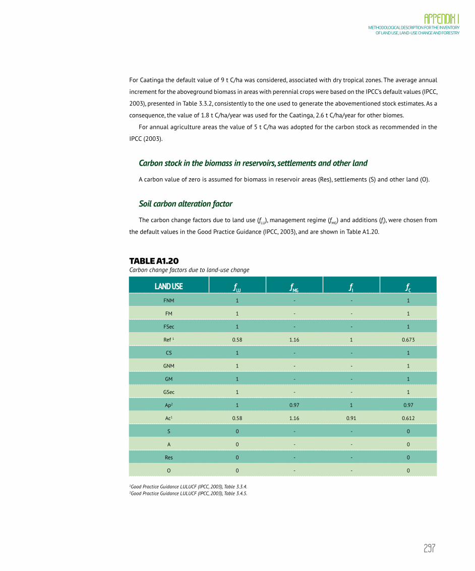
297
APPENDIX I METHODOLOGICAL DESCRIPTION FOR THE INVENTORY
OF LAND USE, LAND-USE CHANGE AND FORESTRY
For Caatinga the default value of 9 t C/ha was considered, associated with dry tropical zones. The average annual
increment for the aboveground biomass in areas with perennial crops were based on the IPCC’s default values (IPCC,
2003), presented in Table 3.3.2, consistently to the one used to generate the abovementioned stock estimates. As a
consequence, the value of 1.8 t C/ha/year was used for the Caatinga, 2.6 t C/ha/year for other biomes.
For annual agriculture areas the value of 5 t C/ha was adopted for the carbon stock as recommended in the
IPCC (2003).
Carbon stock in the biomass in reservoirs, settlements and other land
A carbon value of zero is assumed for biomass in reservoir areas (Res), settlements (S) and other land (O).
Soil carbon alteration factor
The carbon change factors due to land use (fLU), management regime (fMG) and additions (fI), were chosen from
the default values in the Good Practice Guidance (IPCC, 2003), and are shown in Table A1.20.
TABLE A1.20 Carbon change factors due to land-use change
LAND USE fLU fMG fI fC
FNM 1 - - 1
FM 1 - - 1
FSec 1 - - 1
Ref 1 0.58 1.16 1 0.673
CS 1 - - 1
GNM 1 - - 1
GM 1 - - 1
GSec 1 - - 1
Ap2 1 0.97 1 0.97
Ac1 0.58 1.16 0.91 0.612
S 0 - - 0
A 0 - - 0
Res 0 - - 0
O 0 - - 0
1Good Practice Guidance LULUCF (IPCC, 2003), Table 3.3.4.2Good Practice Guidance LULUCF (IPCC, 2003), Table 3.4.5.

APPENDIX II FIRES NOT ASSOCIATED WITH DEFORESTATION

300
APPENDIX II FIRES NOT ASSOCIATED WITH DEFORESTATION
Fire scars for the year 2010 were mapped in the Amazon, Cerrado, and Caatinga biomes with a view to evaluating,
in the next inventories, greenhouse gas emissions from fires not associated with deforestation.
Despite the fact that these fires are not associated with deforestation, proximity with anthropogenic
activities (for example, roads, settlements, selective logging, previous fires) may facilitate the occurrence of
fires (ALENCAR et al. , 2004).
For the purpose of this mapping, the biomes were considered in all their extent. Fires scars from vegetal biomass
combustion were identified by visual interpretation of the same satellite images (mostly TM/Landsat-5 images)
used for the mapping of land use and cover of 2010. Exclusively for the Cerrado biome, heat spots detections by
NOAA satellites (12, 15, 16, 17, 18 and 19), AQUA, TERRA, ERS-2, GOES (10 and 12) and MSG-02, equipped with
different sensors, were used.
Fire scars, or even the active heat spots, were mapped at a 1:125,000 scale. Only natural fires were
considered (FNM, FM, GNM and GM), that is, only those occurring outside previously-mapped polygons with
some anthropogenic use, according to item 6.1.1.2. It is important to point out that burned areas whose formats
are regular and located around areas previously-mapped as anthropogenic (mostly pastures or agriculture)
were considered as fires associated with deforestation, and therefore, have been mapped according to the use
attributed to the region. On the other hand, burned areas with an irregular format, whose location did not
allow a land-use attribution or where the scar showed that fires went out of control (accidental fires) have
been mapped at fires not associated with deforestation.
It is important to highlight that the same satellite images used for the inventory of the LULUCF sector
cover, mostly, the period from June to October 2010 (representing 77% of the images in the Amazon biome,
73% of the images in the Cerrado biome and 43% of the images in the Caatinga). Fires after the day the
images were collected were not taken into account. Other images dating back from 2009 might have been
considered in the 2010 survey.
The final result was a digital map, with representation off ire scars per biome at a 1:250,000 scale. Products may
be checked, by biome, in Figures A2.1, A2.2 and A2.3. Quantifications of burned areas by state and biome are show
in Figure A2.4 and Tables A2.1, A2.2 and A2.3.

301
FIGURE A2.1 Distribution of fire scars mapped in 2010 in the Amazon biome
FIGURE A2.2 Distribution of fire scars mapped in 2010 in the Cerrado biome
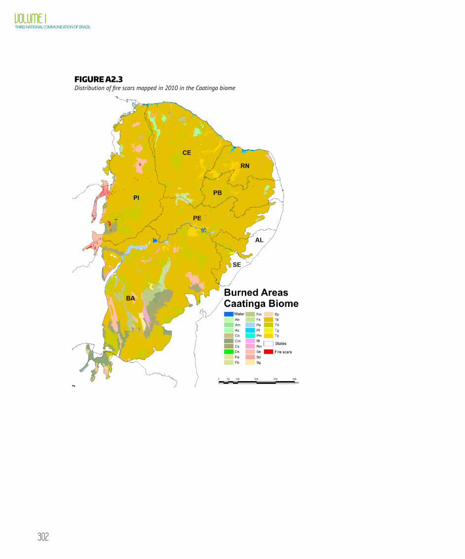
302
VOLUME ITHIRD NATIONAL COMMUNICATION OF BRAZIL
FIGURE A2.3 Distribution of fire scars mapped in 2010 in the Caatinga biome

303
APPENDIX II FIRES NOT ASSOCIATED WITH DEFORESTATION
FIGURE A2.4 Quantification of burned areas by state in the Amazon (a), Cerrado (b) and Caatinga (c) biomes in 2010
Hec
tare
s (1
03 )
500
400
300
20040
30
20
10
0
Fires - Amazon
StateAC AM AP MA MT PA RO RR TO
(a)
Fires - Cerrado
Hec
tare
s (1
03 )
1200
800
400
30
20
10
0
StateBA DF GO MA MT MS MG PI SP TO
(b)
Fires - Caatinga
Hec
tare
s (1
03 )
150,0
120,0
90,0
60,0
30,0
0,2
0,1
0,0
StateBA CE MA MG PB PE PI RN SE
(c)

304
VOLUME ITHIRD NATIONAL COMMUNICATION OF BRAZIL
TABLE A2.1 Quantification of burned areas in the Amazon biome in 2010
FIRES IN THE AMAZON BIOME IN 2010
STATE ABBREVIATIONGRASSLANDS FOREST TOTAL AREA PERCENTAGE OF
BIOME(ha)Acre AC - 2,965.1 2,965.1 0.001%
Amazonas AM 25,862.1 7,823.0 33,685.1 0.008%
Amapá AP 26,003.3 6,585.4 32,588.7 0.008%
Maranhão MA - 1,447.1 1,447.1 0.000%
Mato Grosso MT 67,310.8 158,739.4 226,050.2 0.054%
Pará PA 247,229.0 241,674.1 488,903.1 0.116%
Rondônia RO 13,897.1 18,660.5 32,557.6 0.008%
Roraima RR 2,590.7 2,785.7 5,376.4 0.001%
Tocantins TO - 6,442.5 6,442,. 0.002%
TOTAL 382,893.0 447,122.9 830.015,9 0.197%
TABLE A2.2 Quantification of burned areas in the Cerrado biome in 2010
FIRES IN THE CERRADO BIOME IN 2010
STATE ABBREVIATIONGRASSLAND FOREST TOTAL AREA PERCENTAGE OF THE
BIOME(ha)
Bahia BA 232,734.2 671,010.3 903,744.5 0.443%
Distrito Federal DF 18,509.9 10,888.5 29,398.4 0.014%
Goiás GO 244,576.9 200,090.3 444,667.3 0.218%
Maranhão MA 162,157.5 260,959.9 423,117.4 0.207%
Minas Gerais MG 198.265.9 52,331.6 250,597.5 0.123%
Mato Grosso do Sul MS 2,086.2 2,646.8 4,733.0 0.002%
Mato Grosso MT 294,952.7 527,530.7 822,483.4 0.403%
Piauí PI 1,707.7 526,953.4 528,661.1 0.259%
São Paulo SP 459.1 459.1 0.000%
Tocantins TO 719,574.5 594,109.0 1,313,683.5 0.644%
TOTAL 1,874,565.5 2,846,979.7 4,721,545.2 2.315%

305
APPENDIX II FIRES NOT ASSOCIATED WITH DEFORESTATION
TABLE A2.3 Quantification of burned areas in the Caatinga biome in 2010
FIRES IN THE CAATINGA BIOME IN 2010
STATE ABBREVIATIONGRASSLAND FOREST TOTAL AREA PERCENTAGE OF THE
BIOME(ha)Bahia BA 4,222.3 11,650.3 15,872.5 0.019%
Ceará CE - 209.9 209.9 0.000%
Maranhão MA - 3,049.3 3,049.3 0.004%
Minas Gerais MG - 0.7 0.7 0.000%
Paraíba PB - 1,078.4 1,078.4 0.001%
Pernambuco PE - 141.6 141.6 0.000%
Piauí PI - 147,996.3 147,996.3 0.179%
Rio Grande do Norte RN - 0.0 0.0 0.000%
Sergipe SE - 138.2 138.2 0.000%
TOTAL 4,222.3 164,264.6 168,486.8 0.203%
Values for combustion factors were established by group of phytophysiognomies and biome. After careful
review of literature, priority was given to values calculated in the phytophysiognomies and in the biome, according
to Tables A2.4, A2.5 and A2.6.
TABLE A2.4 Biomass combustion factors per group of phytophysiognomies in the Amazon biome, biome of origin, and respective bibliographic references
GROUP PHYTOPHYSIOGNOMIES COMBUSTION FACTOR (%) BIOME REFERENCES
Dense Humid Forests Da, Db and Ds 32.5 ¹ AmazonWARD et al., 1992; KAUFFMAN et al., 1995; ARAUJO et al., 1999;
FEARNSIDE et al., 1993; 1999; 2001; CARVALHO JR et al., 1995; 1998; 2001
Open Humid Forests Aa, Ab, As 45.0 ¹ Amazon KAUFFMAN et al., 1995; GRAÇA et al., 1999
(Decidual and Semidecidual)
Seasonal ForestsCs, Fa, Fb, Fs 46.4 ² Amazon BALCH et al., 2008
Pioneering vegetation Pa 20.1 ² Amazon ARAUJO et al., 1999
Forested vegetation Sd, Td 33.0 ² Cerrado CASTRO & KAUFFMAN, 1998
Arboreal vegetation Sa, La 43.5 ² Cerrado CASTRO & KAUFFMAN, 1998
Shrubby vegetation and
parksSp, Tp, Lb 53.9 ² Cerrado BARBOSA & FEARNSIDE, 2005
Woody-grass vegetation Sg, Tg, Lg, Rm 77.1 ² Cerrado BARBOSA & FEARNSIDE, 2005
¹ Value calculated from papers describing slash-and-burn.² Value calculated from papers describing only fires.

306
VOLUME ITHIRD NATIONAL COMMUNICATION OF BRAZIL
TABLE A2.5 Biomass combustion factors per group of phytophysiognomies in the Cerrado biome, biome of origin, and respective bibliographic references
GROUP PHYTOPHYSIOGNOMIES COMBUSTION FACTOR (%) BIOME REFERENCES
Dense Humid Forests Dm, Ds 32.5 ¹ AmazonWARD et al., 1992; KAUFFMAN et al., 1995; ARAUJO et al., 1999; FEARNSIDE
et al., 1993; 1999; 2001; CARVALHO JR et al., 1995; 1998; 2001
Open Humid Forests Aa, Ab, As 45.0 ¹ Amazon KAUFFMAN et al., 1995; ALENCASTRO GRAÇA et al., 1999
(Decidual and Semidecidual)
Seasonal Forests Cm, Cs, Fa, Fb, Fs, Fm 46.4 ² Amazon BALCH et al., 2008
Palm swamp Pa 18.3 ² Cerrado CASTRO & KAUFFMAN, 1998
Sandbanks Pm 46.4 ² Amazon BALCH et al., 2008
Forested vegetation Sd, Td 33.0 ² Cerrado CASTRO & KAUFFMAN, 1998
Arboreal vegetation Sa, Ta 43.5 ² Cerrado CASTRO & KAUFFMAN, 1998
Shrubby vegetation and parks Sp, Tp 84.0 ² Cerrado CASTRO & KAUFFMAN, 1998
Woody-grass vegetation Sg, Tg 92.0 ² Cerrado CASTRO & KAUFFMAN, 1998
¹ Value calculated from papers describing slash-and-burn.² Value calculated from papers describing only fires.
TABLE A2.6 Biomass combustion factors per group of phytophysiognomies in the Caatinga biome, biome of origin, and respective bibliographic references
GROUP PHYTOPHYSIOGNOMIES COMBUSTION FACTOR (%) BIOME REFERENCES
Forest formations Cm, Cs, Fm, Fs, Pa, Sd, Td 33.0 ² Cerrado CASTRO & KAUFFMAN, 1998
Arboreal vegetation Sa, Ta 43.5 ² Cerrado CASTRO & KAUFFMAN, 1998
Park vegetation Sp 84.0 ² Cerrado CASTRO & KAUFFMAN, 1998
¹ Value calculated from papers describing slash-and-burn.² Value calculated from papers describing only fires.
Tables A2.7, A2.8 and A2.9 show burned areas in the different phytophysiognomies by structure (grasslands and
forest) and biome (Amazon, Cerrado and Caatinga), respective combustion factors and biomass value (aboveground
with dead organic matter, including dead wood and litter), to which the combustion factor was applied.

307
APPENDIX II FIRES NOT ASSOCIATED WITH DEFORESTATION
TABLE A2.7 Burned areas not associated with deforestation, by phytophysiognomy of the Amazon biome in 2010
STRUCTURE PHYTOPHYSIOGNOMY BURNED AREA (ha)
ABOVEGROUND BIOMASS (t /ha) COMBUSTION FACTOR
Grassland
Lb 108.4 15.91 0.539
Lg 233.4 7.65 0.771
Rm 156.6 3.10 0.771
Sg 80,946.3 3.28 0.771
Sp 300,566.8 8.04 0.539
Tg 18.7 2.83 0.771
Tp 672.2 6.12 0.539
Forest
Aa 720.6 361.91 0.450
Ab 9,325.6 323.96 0.450
As 54,883.1 290.12 0.450
Cs 2,941.5 241.89 0.464
Da 7,736.2 382.70 0.325
Db 98,457.9 337.12 0.325
Ds 103,050.5 336.15 0.325
Fa 4,126.2 236.40 0.464
Fb 384.7 258.00 0.464
Fs 32,696.5 240.99 0.464
La 151.3 17.50 0.435
Pa 72,469.1 264.61 0.201
Pf 0.5 185.97 0.201
Sa 52,590.7 36.78 0.435
Sd 7,279.5 90.30 0.330
Td 183.0 29.00 0.330
TOTAL 829,699.1

308
VOLUME ITHIRD NATIONAL COMMUNICATION OF BRAZIL
TABLE A2.8 Burned areas not associated with deforestation, by phytophysiognomy of the Cerrado biome in 2010
STRUCTURE PHYTOPHYSIOGNOMY BURNED AREA (ha)
ABOVEGROUND BIOMASS (t /ha) COMBUSTION FACTOR
Grassland
Sg 351,533.3 9.83 0.920
Sp 1,520,948.4 19.68 0.840
Tg 1,690.2 2.83 0.920
Tp 393.6 6.12 0.840
Forest
Aa 691.5 361.91 0.450
Ab 1,183.7 323.96 0.450
As 1,528.3 172.46 0.450
Cm 14,670.3 172.11 0.464
Cs 94,157.1 172.11 0.464
Dm 1.7 318.02 0.325
Ds 208.9 198.00 0.325
Fa 82,742.7 188.79 0.464
Fb 3,151.3 206.36 0.464
Fm 6,355.8 193.10 0.464
Fs 66,842.2 127.35 0.464
Pa 4,934.2 61.60 0.183
Pm 1,296.3 216.56 0.464
Sa 1,875,647.4 36.78 0.435
Sd 654.178.1 124.58 0.330
Ta 39,359.2 25.10 0.435
Td 31.0 46.70 0.330
Total 4,786,487.0

309
APPENDIX II FIRES NOT ASSOCIATED WITH DEFORESTATION
TABLE A2.9 Burned areas not associated with deforestation, by phytophysiognomy of the Caatinga biome in 2010
STRUCTURE PHYTOPHYSIOGNOMY BURNED AREA (ha)
ABOVEGROUND BIOMASS (t /ha) COMBUSTION FACTOR
Grassland Sp 4,222.3 10.81 0.840
Forest
Cm 662.5 115.32 0.330
Cs 8,922.3 115.32 0.330
Fm 0.2 99.98 0.330
Fs 2,439.2 99.98 0.330
Pa 33.6 120.96 0.330
Sa 35,483.8 36.78 0.435
Sd 57,062.1 90.30 0.330
Ta 31,467.5 25.10 0.435
Td 28,193.4 46.70 0.330
Total 168,486.8
The burned area, aboveground biomass and combustion factor values allow for the estimation of burned dry
matter in each of the Amazon, Cerrado and Caatinga biomes’ phytophysiognomies. Subsequently, with the emission
factors shown in Table 3.113 of the National Inventory, based on the 2006 IPCC Guidelines, the correspondent
greenhouse gas emissions may be obtained. Table A2.10 shows the estimates of emissions related to fires not
associated with deforestation in 2010.
TABLE A2.10 Emissions related to fires not associated with deforestation in 2010
BIOMECO2 CO CH4 N2O NOX
GgAmazon 67,249 4,426.5 289.4 8.51 68.1
Cerrado 172,632 6,956.6 246.2 22.48 417.4
Caatinga 5,696 229.5 8.1 0.74 13.8
Results related to emissions from fires not associated with deforestation were not incorporated to this inventory,
for the following reasons:
>> Regarding CO2 emissions, biomass recovery after combustion occurs in the years to come, and depends on
the regeneration capacity of different vegetation formations as they are not associated with deforestation.
The monitoring of these areas recovery might determine whether future removals will be equivalent to
emissions from combustion, given that frequent fires may reduce the resilience of the vegetation.
310
VOLUME ITHIRD NATIONAL COMMUNICATION OF BRAZIL
>> Regarding emissions of other gases, the ones that are not removed with the regeneration of vegetation,
it was not possible to consider them since there has not been the same quantification for previous years,
nor has a correlation with an approximate calculation been identified.
>> In addition, it was not possible to evaluate the successional or transition paths in burned areas along a
historical series in order to guarantee the time consistency of the series of national inventories regarding
this type of emission.
The abovementioned aspects demand methodological improvements in order to assess the impacts of fires
not associated with deforestation when accounting for greenhouse gas emissions. This analysis is another step to
understanding the occurrence of fires not associated with deforestation, and the incorporation of the corresponding
non-CO2 gas emissions to the inventory in the coming editions. It is important to bear in mind that emissions from
fires associated with deforestation are incorporated in the inventory (item 3.5.2.8).


APPENDIX III GREENHOUSE GAS
EMISSIONS ESTIMATES BY GAS AND SECTOR,
FROM 1990 TO 2010
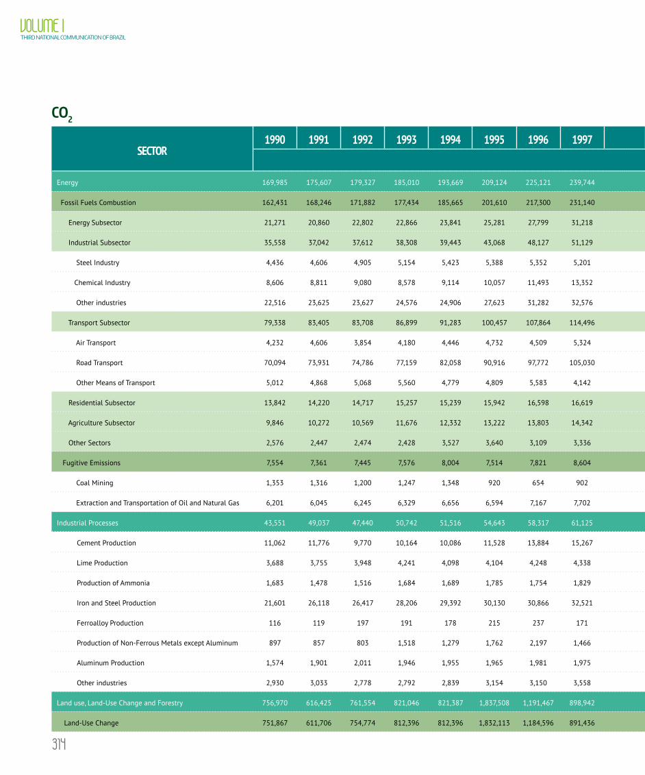
314
VOLUME ITHIRD NATIONAL COMMUNICATION OF BRAZIL
CO2
SECTOR1990 1991 1992 1993 1994 1995 1996 1997 1998 1999 2000 2001 2002 2003 2004 2005 2006 2007 2008 2009 2010
Gg
Energy 169,985 175,607 179,327 185,010 193,669 209,124 225,121 239,744 249,209 260,751 267,646 276,893 273,412 268,111 282,581 290,621 295,611 308,967 327,452 315,649 347,974
Fossil Fuels Combustion 162,431 168,246 171,882 177,434 185,665 201,610 217,300 231,140 239,746 250,628 256,909 265,172 262,194 256,912 271,741 276,744 282,729 295,498 313,245 297,215 332,760
Energy Subsector 21,271 20,860 22,802 22,866 23,841 25,281 27,799 31,218 32,223 39,123 40,484 44,837 39,776 39,449 45,372 47,343 47,967 47,494 58,186 47,616 58,857
Industrial Subsector 35,558 37,042 37,612 38,308 39,443 43,068 48,127 51,129 51,874 55,314 59,008 58,128 58,426 56,218 56,999 60,019 60,817 66,790 66,810 63,657 68,306
Steel Industry 4,436 4,606 4,905 5,154 5,423 5,388 5,352 5,201 4,594 4,302 4,657 4,510 4,759 4,891 4,975 5,526 5,491 6,012 5,811 4,543 5,642
Chemical Industry 8,606 8,811 9,080 8,578 9,114 10,057 11,493 13,352 12,343 13,551 13,942 13,930 14,161 13,508 14,353 14,624 14,880 15,598 14,283 14,446 13,847
Other industries 22,516 23,625 23,627 24,576 24,906 27,623 31,282 32,576 34,937 37,461 40,409 39,688 39,506 37,819 37,671 39,869 40,446 45,180 46,716 44,668 48,817
Transport Subsector 79,338 83,405 83,708 86,899 91,283 100,457 107,864 114,496 121,389 120,217 121,748 124,867 127,290 126,675 134,513 135,182 139,533 145,186 150,798 149,354 168,364
Air Transport 4,232 4,606 3,854 4,180 4,446 4,732 4,509 5,324 5,857 6,017 6,206 6,626 6,677 5,871 6,193 6,316 6,563 7,220 7,325 8,330 9,751
Road Transport 70,094 73,931 74,786 77,159 82,058 90,916 97,772 105,030 111,067 109,634 111,337 113,548 115,889 116,036 123,083 123,519 127,773 131,881 136,931 134,781 151,481
Other Means of Transport 5,012 4,868 5,068 5,560 4,779 4,809 5,583 4,142 4,465 4,566 4,205 4,693 4,724 4,768 5,237 5,347 5,197 6,085 6,542 6,243 7,132
Residential Subsector 13,842 14,220 14,717 15,257 15,239 15,942 16,598 16,619 16,760 17,095 17,179 17,247 16,675 15,532 15,863 15,591 15,616 16,123 16,530 16,738 17,249
Agriculture Subsector 9,846 10,272 10,569 11,676 12,332 13,222 13,803 14,342 13,824 14,496 14,152 15,579 15,207 15,291 15,075 14,964 15,162 16,096 17,473 16,785 17,346
Other Sectors 2,576 2,447 2,474 2,428 3,527 3,640 3,109 3,336 3,676 4,383 4,338 4,514 4,820 3,747 3,919 3,645 3,634 3,809 3,448 3,065 2,638
Fugitive Emissions 7,554 7,361 7,445 7,576 8,004 7,514 7,821 8,604 9,463 10,123 10,737 11,721 11,218 11,199 10,840 13,877 12,882 13,469 14,207 18,434 15,214
Coal Mining 1,353 1,316 1,200 1,247 1,348 920 654 902 1,004 1,150 1,291 1,936 1,151 1,208 1,429 1,381 1,246 1,510 1,658 1,758 1,846
Extraction and Transportation of Oil and Natural Gas 6,201 6,045 6,245 6,329 6,656 6,594 7,167 7,702 8,459 8,973 9,446 9,785 10,067 9,991 9,411 12,496 11,636 11,959 12,549 16,676 13,368
Industrial Processes 43,551 49,037 47,440 50,742 51,516 54,643 58,317 61,125 62,611 61,714 65,991 63,423 66,195 67,056 69,452 68,016 67,476 73,561 75,910 66,738 80,786
Cement Production 11,062 11,776 9,770 10,164 10,086 11,528 13,884 15,267 16,175 16,439 16,047 15,227 14,390 13,096 13,273 14,349 15,440 17,200 18,884 19,031 21,288
Lime Production 3,688 3,755 3,948 4,241 4,098 4,104 4,248 4,338 4,141 4,352 5,008 4,811 4,956 5,064 5,505 5,356 5,410 5,666 5,690 5,060 5,950
Production of Ammonia 1,683 1,478 1,516 1,684 1,689 1,785 1,754 1,829 1,718 1,943 1,663 1,396 1,567 1,690 1,934 1,922 1,968 1,866 1,811 1,576 1,739
Iron and Steel Production 21,601 26,118 26,417 28,206 29,392 30,130 30,866 32,521 33,319 31,680 35,552 34,845 37,516 38,683 39,805 37,509 36,051 39,422 39,825 31,690 38,360
Ferroalloy Production 116 119 197 191 178 215 237 171 562 482 545 608 573 937 938 932 942 1,080 1,142 1,018 1,195
Production of Non-Ferrous Metals except Aluminum 897 857 803 1,518 1,279 1,762 2,197 1,466 1,201 1,319 1,606 1,431 1,582 1,724 1,788 1,855 1,901 2,112 1,813 1,914 4,332
Aluminum Production 1,574 1,901 2,011 1,946 1,955 1,965 1,981 1,975 2,007 2,079 2,116 1,879 2,176 2,198 2,408 2,472 2,646 2,739 2,753 2,544 2,543
Other industries 2,930 3,033 2,778 2,792 2,839 3,154 3,150 3,558 3,488 3,420 3,454 3,226 3,435 3,664 3,801 3,621 3,118 3,476 3,992 3,905 5,379
Land use, Land-Use Change and Forestry 756,970 616,425 761,554 821,046 821,387 1,837,508 1,191,467 898,942 1,145,470 1,137,736 1,197,175 1,192,787 1,401,764 2,311,652 2,501,327 1,797,842 1,399,630 1,193,617 1,294,043 379,257 310,736
Land-Use Change 751,867 611,706 754,774 812,396 812,396 1,832,113 1,184,596 891,436 1,138,370 1,131,002 1,188,458 1,184,833 1,391,958 2,300,008 2,489,746 1,790,368 1,392,216 1,183,866 1,283,495 370,862 300,312

315
APPENDIX III GREENHOUSE GAS EMISSIONS EstimatEs BY GAS AND SECTOR, FROM 1990 TO 2010
CO2
SECTOR1990 1991 1992 1993 1994 1995 1996 1997 1998 1999 2000 2001 2002 2003 2004 2005 2006 2007 2008 2009 2010
Gg
Energy 169,985 175,607 179,327 185,010 193,669 209,124 225,121 239,744 249,209 260,751 267,646 276,893 273,412 268,111 282,581 290,621 295,611 308,967 327,452 315,649 347,974
Fossil Fuels Combustion 162,431 168,246 171,882 177,434 185,665 201,610 217,300 231,140 239,746 250,628 256,909 265,172 262,194 256,912 271,741 276,744 282,729 295,498 313,245 297,215 332,760
Energy Subsector 21,271 20,860 22,802 22,866 23,841 25,281 27,799 31,218 32,223 39,123 40,484 44,837 39,776 39,449 45,372 47,343 47,967 47,494 58,186 47,616 58,857
Industrial Subsector 35,558 37,042 37,612 38,308 39,443 43,068 48,127 51,129 51,874 55,314 59,008 58,128 58,426 56,218 56,999 60,019 60,817 66,790 66,810 63,657 68,306
Steel Industry 4,436 4,606 4,905 5,154 5,423 5,388 5,352 5,201 4,594 4,302 4,657 4,510 4,759 4,891 4,975 5,526 5,491 6,012 5,811 4,543 5,642
Chemical Industry 8,606 8,811 9,080 8,578 9,114 10,057 11,493 13,352 12,343 13,551 13,942 13,930 14,161 13,508 14,353 14,624 14,880 15,598 14,283 14,446 13,847
Other industries 22,516 23,625 23,627 24,576 24,906 27,623 31,282 32,576 34,937 37,461 40,409 39,688 39,506 37,819 37,671 39,869 40,446 45,180 46,716 44,668 48,817
Transport Subsector 79,338 83,405 83,708 86,899 91,283 100,457 107,864 114,496 121,389 120,217 121,748 124,867 127,290 126,675 134,513 135,182 139,533 145,186 150,798 149,354 168,364
Air Transport 4,232 4,606 3,854 4,180 4,446 4,732 4,509 5,324 5,857 6,017 6,206 6,626 6,677 5,871 6,193 6,316 6,563 7,220 7,325 8,330 9,751
Road Transport 70,094 73,931 74,786 77,159 82,058 90,916 97,772 105,030 111,067 109,634 111,337 113,548 115,889 116,036 123,083 123,519 127,773 131,881 136,931 134,781 151,481
Other Means of Transport 5,012 4,868 5,068 5,560 4,779 4,809 5,583 4,142 4,465 4,566 4,205 4,693 4,724 4,768 5,237 5,347 5,197 6,085 6,542 6,243 7,132
Residential Subsector 13,842 14,220 14,717 15,257 15,239 15,942 16,598 16,619 16,760 17,095 17,179 17,247 16,675 15,532 15,863 15,591 15,616 16,123 16,530 16,738 17,249
Agriculture Subsector 9,846 10,272 10,569 11,676 12,332 13,222 13,803 14,342 13,824 14,496 14,152 15,579 15,207 15,291 15,075 14,964 15,162 16,096 17,473 16,785 17,346
Other Sectors 2,576 2,447 2,474 2,428 3,527 3,640 3,109 3,336 3,676 4,383 4,338 4,514 4,820 3,747 3,919 3,645 3,634 3,809 3,448 3,065 2,638
Fugitive Emissions 7,554 7,361 7,445 7,576 8,004 7,514 7,821 8,604 9,463 10,123 10,737 11,721 11,218 11,199 10,840 13,877 12,882 13,469 14,207 18,434 15,214
Coal Mining 1,353 1,316 1,200 1,247 1,348 920 654 902 1,004 1,150 1,291 1,936 1,151 1,208 1,429 1,381 1,246 1,510 1,658 1,758 1,846
Extraction and Transportation of Oil and Natural Gas 6,201 6,045 6,245 6,329 6,656 6,594 7,167 7,702 8,459 8,973 9,446 9,785 10,067 9,991 9,411 12,496 11,636 11,959 12,549 16,676 13,368
Industrial Processes 43,551 49,037 47,440 50,742 51,516 54,643 58,317 61,125 62,611 61,714 65,991 63,423 66,195 67,056 69,452 68,016 67,476 73,561 75,910 66,738 80,786
Cement Production 11,062 11,776 9,770 10,164 10,086 11,528 13,884 15,267 16,175 16,439 16,047 15,227 14,390 13,096 13,273 14,349 15,440 17,200 18,884 19,031 21,288
Lime Production 3,688 3,755 3,948 4,241 4,098 4,104 4,248 4,338 4,141 4,352 5,008 4,811 4,956 5,064 5,505 5,356 5,410 5,666 5,690 5,060 5,950
Production of Ammonia 1,683 1,478 1,516 1,684 1,689 1,785 1,754 1,829 1,718 1,943 1,663 1,396 1,567 1,690 1,934 1,922 1,968 1,866 1,811 1,576 1,739
Iron and Steel Production 21,601 26,118 26,417 28,206 29,392 30,130 30,866 32,521 33,319 31,680 35,552 34,845 37,516 38,683 39,805 37,509 36,051 39,422 39,825 31,690 38,360
Ferroalloy Production 116 119 197 191 178 215 237 171 562 482 545 608 573 937 938 932 942 1,080 1,142 1,018 1,195
Production of Non-Ferrous Metals except Aluminum 897 857 803 1,518 1,279 1,762 2,197 1,466 1,201 1,319 1,606 1,431 1,582 1,724 1,788 1,855 1,901 2,112 1,813 1,914 4,332
Aluminum Production 1,574 1,901 2,011 1,946 1,955 1,965 1,981 1,975 2,007 2,079 2,116 1,879 2,176 2,198 2,408 2,472 2,646 2,739 2,753 2,544 2,543
Other industries 2,930 3,033 2,778 2,792 2,839 3,154 3,150 3,558 3,488 3,420 3,454 3,226 3,435 3,664 3,801 3,621 3,118 3,476 3,992 3,905 5,379
Land use, Land-Use Change and Forestry 756,970 616,425 761,554 821,046 821,387 1,837,508 1,191,467 898,942 1,145,470 1,137,736 1,197,175 1,192,787 1,401,764 2,311,652 2,501,327 1,797,842 1,399,630 1,193,617 1,294,043 379,257 310,736
Land-Use Change 751,867 611,706 754,774 812,396 812,396 1,832,113 1,184,596 891,436 1,138,370 1,131,002 1,188,458 1,184,833 1,391,958 2,300,008 2,489,746 1,790,368 1,392,216 1,183,866 1,283,495 370,862 300,312
continues on the next page

316
VOLUME ITHIRD NATIONAL COMMUNICATION OF BRAZIL
SECTOR1990 1991 1992 1993 1994 1995 1996 1997 1998 1999 2000 2001 2002 2003 2004 2005 2006 2007 2008 2009 2010
Gg
Amazon Biome 437,574 297,413 440,481 498,103 498,103 1,459,071 811,554 518,394 765,328 757,960 815,416 811,791 1,018,916 1,638,185 1,827,923 1,128,545 738,993 530,643 630,272 199,576 162,888
Cerrado Biome 241,511 241,511 241,511 241,511 241,511 212,958 212,958 212,958 212,958 212,958 212,958 212,958 212,958 282,275 282,275 282,275 282,275 282,275 282,275 92,617 58,755
Other Biomes 72,782 72,782 72,782 72,782 72,782 160,084 160,084 160,084 160,084 160,084 160,084 160,084 160,084 379,548 379,548 379,548 370,948 370,948 370,948 78,669 78,669
Application of Limestone in soils 5,103 4,719 6,780 8,650 8,991 5,395 6,871 7,506 7,100 6,734 8,717 7,954 9,806 11,644 11,581 7,474 7,414 9,751 10,548 8,395 10,424
Waste 19,0 31,0 54,0 61,0 66,0 78,0 78,0 78,0 84,0 88,0 95,0 95,0 99,0 117,0 120,0 128,0 136,0 155,0 159,0 168,0 175,0
TOTAL 970,525 841,100 988,375 1,056,859 1,066,638 2,101,353 1,474,983 1,199,889 1,457,374 1,460,289 1,530,907 1,533,198 1,741,470 2,646,936 2,853,480 2,156,607 1,762,853 1,576,300 1,697,564 761,812 739,671
For information purposes only
Bunker fuels 6,086 5,584 6,239 6,914 7,298 8,667 10,077 10,835 12,105 13,881 13,639 15,545 15,823 14,094 14,362 14,766 15,150 16,347 19,998 15,461 18,550
Air Transport 4,366 3,147 3,610 3,619 3,539 4,520 5,541 5,911 6,621 5,397 4,626 5,388 4,381 4,035 4,303 4,707 4,543 4,936 5,675 5,167 5,784
Shipping 1,720 2,437 2,629 3,295 3,759 4,147 4,536 4,924 5,484 8,484 9,013 10,157 11,442 10,059 10,059 10,059 10,607 11,411 14,323 10,294 12,766
CO2 emissions from biomass 165,792 166,171 165,294 163,296 173,888 168,791 171,036 177,229 177,266 180,876 166,435 174,763 190,568 207,531 219,888 228,285 242,166 263,098 285,428 281,666 303,170
CH4
SECTOR1990 1991 1992 1993 1994 1995 1996 1997 1998 1999 2000 2001 2002 2003 2004 2005 2006 2007 2008 2009 2010
GgEnergy 545.8 548.5 535.5 499.2 494.7 473.6 464.3 479.7 488.1 498.6 511.8 542.9 571.9 568.7 605.2 684.8 647.9 634.6 639.4 686.3 629.1
Fossil Fuels Combustion 455.3 454.0 450.5 410.5 408.9 388.1 389.0 393.6 393.9 396.4 392.8 403.7 440.1 460.9 471.4 478.6 478.6 465.4 466.5 446.3 448.2
Energy Subsector 25.5 24.6 23.0 23.3 24.4 23.1 22.5 23.4 21.1 21.4 20.7 20.7 22.2 25.8 28.4 29.2 29.9 32.6 36.7 30.3 34.5
Industrial Subsector 15.7 14.8 15.3 15.5 17.7 18.1 19.2 19.3 20.5 21.9 19.9 22.1 23.9 26.0 28.0 28.4 31.7 33.1 32.9 31.9 34.4
Steel Industry 0.2 0.2 0.2 0.2 0.2 0.2 0.2 0.2 0.1 0.2 0.2 0.2 0.2 0.2 0.2 0.2 0.2 0.2 0.2 0.2 0.3
Other industries 15.5 14.6 15.1 15.3 17.5 17.9 19.0 19.1 20.4 21.7 19.7 21.9 23.7 25.8 27.8 28.2 31.5 32.9 32.7 31.7 34.1
Transport Subsector 72.6 76.3 76.4 76.7 80.3 85.8 91.4 92.2 88.7 81.9 75.6 73.1 73.2 74.6 75.3 74.4 68.5 68.1 67.9 62.3 66.9
Residential Subsector 318.4 316.8 316.9 277.4 269.4 243.7 238.6 241.5 247.2 255.3 261.5 272.8 304.9 316.7 321.1 327.6 329.0 311.1 307.1 300.8 290.1
Other Sectors 23.1 21.5 18.9 17.6 17.1 17.4 17.3 17.2 16.4 15.9 15.1 15.0 15.9 17.8 18.6 19.0 19.5 20.5 21.9 21.0 22.3
Fugitive Emissions 90.5 94.5 85.0 88.7 85.8 85.5 75.3 86.1 94.2 102.2 119.0 139.2 131.8 107.8 133.8 206.2 169.3 169.2 172.9 240.0 180.9
Coal Mining 49.7 54.3 44.2 47.0 42.4 41.1 25.5 32.6 33.0 34.0 43.3 60.0 44.0 41.0 48.0 49.1 48.3 54.9 58.6 52.3 39.2
Extraction and Transportation of Oil and Natural Gas 40.8 40.2 40.8 41.7 43.4 44.4 49.8 53.5 61.2 68.2 75.7 79.2 87.8 66.8 85.8 157.1 121.0 114.3 114.3 187.7 141.7
continues on the next page
(CO2 continuing)
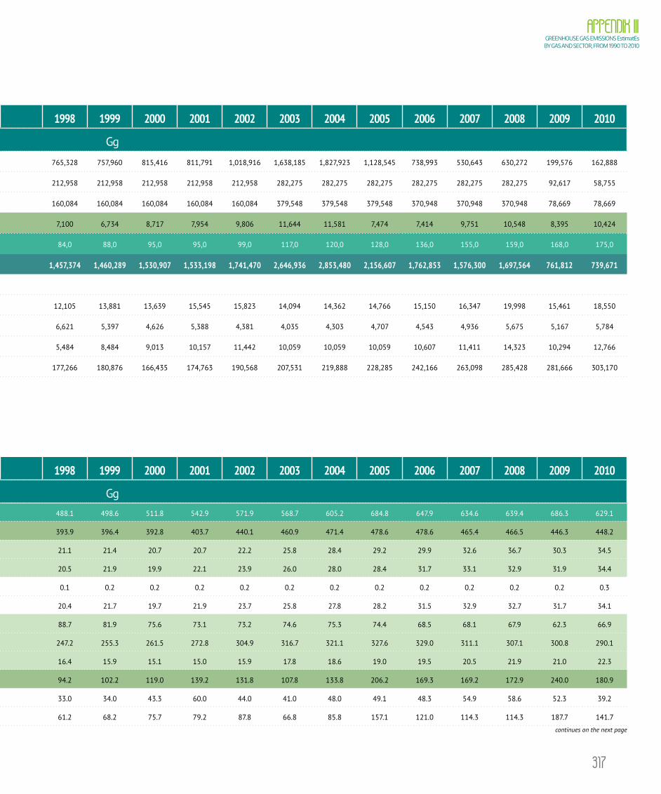
317
APPENDIX III GREENHOUSE GAS EMISSIONS EstimatEs BY GAS AND SECTOR, FROM 1990 TO 2010
SECTOR1990 1991 1992 1993 1994 1995 1996 1997 1998 1999 2000 2001 2002 2003 2004 2005 2006 2007 2008 2009 2010
Gg
Amazon Biome 437,574 297,413 440,481 498,103 498,103 1,459,071 811,554 518,394 765,328 757,960 815,416 811,791 1,018,916 1,638,185 1,827,923 1,128,545 738,993 530,643 630,272 199,576 162,888
Cerrado Biome 241,511 241,511 241,511 241,511 241,511 212,958 212,958 212,958 212,958 212,958 212,958 212,958 212,958 282,275 282,275 282,275 282,275 282,275 282,275 92,617 58,755
Other Biomes 72,782 72,782 72,782 72,782 72,782 160,084 160,084 160,084 160,084 160,084 160,084 160,084 160,084 379,548 379,548 379,548 370,948 370,948 370,948 78,669 78,669
Application of Limestone in soils 5,103 4,719 6,780 8,650 8,991 5,395 6,871 7,506 7,100 6,734 8,717 7,954 9,806 11,644 11,581 7,474 7,414 9,751 10,548 8,395 10,424
Waste 19,0 31,0 54,0 61,0 66,0 78,0 78,0 78,0 84,0 88,0 95,0 95,0 99,0 117,0 120,0 128,0 136,0 155,0 159,0 168,0 175,0
TOTAL 970,525 841,100 988,375 1,056,859 1,066,638 2,101,353 1,474,983 1,199,889 1,457,374 1,460,289 1,530,907 1,533,198 1,741,470 2,646,936 2,853,480 2,156,607 1,762,853 1,576,300 1,697,564 761,812 739,671
For information purposes only
Bunker fuels 6,086 5,584 6,239 6,914 7,298 8,667 10,077 10,835 12,105 13,881 13,639 15,545 15,823 14,094 14,362 14,766 15,150 16,347 19,998 15,461 18,550
Air Transport 4,366 3,147 3,610 3,619 3,539 4,520 5,541 5,911 6,621 5,397 4,626 5,388 4,381 4,035 4,303 4,707 4,543 4,936 5,675 5,167 5,784
Shipping 1,720 2,437 2,629 3,295 3,759 4,147 4,536 4,924 5,484 8,484 9,013 10,157 11,442 10,059 10,059 10,059 10,607 11,411 14,323 10,294 12,766
CO2 emissions from biomass 165,792 166,171 165,294 163,296 173,888 168,791 171,036 177,229 177,266 180,876 166,435 174,763 190,568 207,531 219,888 228,285 242,166 263,098 285,428 281,666 303,170
CH4
SECTOR1990 1991 1992 1993 1994 1995 1996 1997 1998 1999 2000 2001 2002 2003 2004 2005 2006 2007 2008 2009 2010
GgEnergy 545.8 548.5 535.5 499.2 494.7 473.6 464.3 479.7 488.1 498.6 511.8 542.9 571.9 568.7 605.2 684.8 647.9 634.6 639.4 686.3 629.1
Fossil Fuels Combustion 455.3 454.0 450.5 410.5 408.9 388.1 389.0 393.6 393.9 396.4 392.8 403.7 440.1 460.9 471.4 478.6 478.6 465.4 466.5 446.3 448.2
Energy Subsector 25.5 24.6 23.0 23.3 24.4 23.1 22.5 23.4 21.1 21.4 20.7 20.7 22.2 25.8 28.4 29.2 29.9 32.6 36.7 30.3 34.5
Industrial Subsector 15.7 14.8 15.3 15.5 17.7 18.1 19.2 19.3 20.5 21.9 19.9 22.1 23.9 26.0 28.0 28.4 31.7 33.1 32.9 31.9 34.4
Steel Industry 0.2 0.2 0.2 0.2 0.2 0.2 0.2 0.2 0.1 0.2 0.2 0.2 0.2 0.2 0.2 0.2 0.2 0.2 0.2 0.2 0.3
Other industries 15.5 14.6 15.1 15.3 17.5 17.9 19.0 19.1 20.4 21.7 19.7 21.9 23.7 25.8 27.8 28.2 31.5 32.9 32.7 31.7 34.1
Transport Subsector 72.6 76.3 76.4 76.7 80.3 85.8 91.4 92.2 88.7 81.9 75.6 73.1 73.2 74.6 75.3 74.4 68.5 68.1 67.9 62.3 66.9
Residential Subsector 318.4 316.8 316.9 277.4 269.4 243.7 238.6 241.5 247.2 255.3 261.5 272.8 304.9 316.7 321.1 327.6 329.0 311.1 307.1 300.8 290.1
Other Sectors 23.1 21.5 18.9 17.6 17.1 17.4 17.3 17.2 16.4 15.9 15.1 15.0 15.9 17.8 18.6 19.0 19.5 20.5 21.9 21.0 22.3
Fugitive Emissions 90.5 94.5 85.0 88.7 85.8 85.5 75.3 86.1 94.2 102.2 119.0 139.2 131.8 107.8 133.8 206.2 169.3 169.2 172.9 240.0 180.9
Coal Mining 49.7 54.3 44.2 47.0 42.4 41.1 25.5 32.6 33.0 34.0 43.3 60.0 44.0 41.0 48.0 49.1 48.3 54.9 58.6 52.3 39.2
Extraction and Transportation of Oil and Natural Gas 40.8 40.2 40.8 41.7 43.4 44.4 49.8 53.5 61.2 68.2 75.7 79.2 87.8 66.8 85.8 157.1 121.0 114.3 114.3 187.7 141.7
continues on the next page

318
VOLUME ITHIRD NATIONAL COMMUNICATION OF BRAZIL
(CH4 continuing)
SECTOR1990 1991 1992 1993 1994 1995 1996 1997 1998 1999 2000 2001 2002 2003 2004 2005 2006 2007 2008 2009 2010
GgIndustrial Processes 47.1 42.1 39.6 43.0 44.2 41.2 37.9 38.2 36.0 40.0 43.7 40.0 41.4 47.9 55.5 54.9 56.5 58.4 56.5 39.2 45.3
Chemical Industry 5.2 5.2 5.4 6.0 6.6 6.6 6.6 7.4 7.9 8.3 9.0 8.6 8.3 8.9 9.3 9.4 12.4 12.7 11.5 11.9 11.8
Production of Metals 41.9 36.9 34.2 37.0 37.6 34.6 31.3 30.8 28.1 31.7 34.7 31.4 33.1 39.0 46.2 45.5 44.1 45.7 45.0 27.3 33.5
Agriculture 9,185.6 9,474.1 9,639.0 9,681.3 9,865.1 10,058.2 9,742.2 9,887.9 9,963.9 10,111.9 10,382.3 10,757.6 11,121.3 11,666.8 12,195.7 12,357.7 12,293.0 11,707.1 11,955.4 12,166.2 12,415.6
Enteric Fermentation 8,223.9 8,470.3 8,596.8 8,625.8 8,786.7 8,957.1 8,738.7 8,899.2 8,979.5 9,057.6 9,349.5 9,713.3 10,050.1 10,574.9 11049.3 11,213.8 11,162.0 10,573.0 10,730.3 10,908.0 11,158.0
Cattle 7,808.9 8,049.5 8,175.2 8,218.7 8,370.5 8,534.3 8,413.3 8,572.9 8,650.5 8,722.2 9,005.8 9,368.0 9,708.9 10,228.3 10,698.6 10,855.7 10,801.9 10,220.4 10,376.3 10,555.6 10,798.4
Dairy Cattle 1,197.7 1,245.1 1,279.3 1,258.3 1,262.8 1,297.1 1,081.0 1,123.9 1,136.7 1,143.1 1,177.9 1,206.7 1,236.6 1,268.8 1,320.5 1,371.4 1,396.3 1,296.8 1,331.4 1,384.6 1,424.0
Beef Cattle 6,611.2 6,804.4 6,895.9 6,960.4 7,107.7 7,237.2 7,332.3 7,449.0 7,513.8 7,579.1 7,827.9 8,161.3 8,472.3 8,959.5 9,378.1 9,484.3 9,405.6 8,923.6 9,044.9 9,171.0 9,374.4
Other Animals 415.0 420.8 421.6 407.1 416.2 422.8 325.4 326.3 329.0 335.4 343.7 345.3 341.2 346.6 350.7 358.1 360.1 352.6 354.0 352.4 359.6
Manure Management 421.6 435.5 443.0 447.1 457.9 471.6 431.0 442.3 448.8 461.1 479.7 500.5 500.6 519.6 533.0 543.9 545.6 558.0 575.4 593.3 608.1
Cattle 191.2 197.6 200.4 201.2 204.6 208.7 200.3 204.7 207.0 209.0 215.9 224.4 223.6 235.9 248.5 254.0 252.9 245.3 249.0 253.4 258.7
Dairy Cattle 35.9 37.5 38.4 37.7 37.6 38.5 31.1 32.6 33.0 33.2 34.1 34.7 35.5 36.4 38.5 39.7 40.4 40.6 41.5 43.1 44.0
Beef Cattle 155.3 160.1 162.0 163.5 167.0 170.2 169.2 172.1 174.0 175.8 181.8 189.7 188.1 199.5 210.0 214.3 212.5 204.7 207.5 210.3 214.7
Swine 159.5 161.8 161.9 164.4 169.4 173.7 146.4 149.1 152.2 158.6 166.5 174.5 176.7 180.5 178.4 178.7 179.8 188.5 196.0 207.2 214.9
Poultry 48.4 53.3 57.8 59.2 61.3 66.3 65.9 69.9 70.9 74.6 78.1 82.4 81.2 83.8 86.6 91.5 93.2 104.9 111.2 113.7 115.3
Other Animals 22.5 22.8 22.9 22.3 22.6 22.9 18.4 18.6 18.7 18.9 19.2 19.2 19.1 19.4 19.5 19.7 19.7 19.3 19.2 19.0 19.2
Rice Cultivation 433.6 462.9 490.8 511.9 505.8 510.8 456.0 430.3 416.2 479.9 448.1 431.7 451.4 440.6 477.3 463.7 438.8 423.5 474.2 486.0 464.2
Burning of Agricultural Wastes 106.5 105.4 108.4 96.5 114.7 118.7 116.5 116.1 119.4 113.3 105.0 112.1 119.2 131.7 136.1 136.3 146.6 152.6 175.5 178.9 185.3
Land use, Land-Use Change and Forestry 1,041.5 959.3 1,153.3 1,222.4 1,213.2 2,895.7 2,016.2 1,657.1 1,984.3 1,979.1 2,048.8 2,048.4 2,321.9 3,898.7 4,148.9 3,237.9 2,565.3 2,324.4 2,441.7 1,221.3 1135.5
Waste 1,173.7 1,219.9 1,270.4 1,314.2 1,361.2 1,418.7 1,470.6 1,530.0 1,587.1 1,683.8 1,754.2 1,799.4 1,887.2 2,002.2 2,018.4 2,062.0 2,178.8 2,241.7 2,277.4 2,336.0 2,462.7
Solid Wastes 824.4 852.2 882.2 910.2 938.7 965.3 994.4 1,025.4 1,053.3 1,111.9 1,149.4 1,177.4 1,219.5 1,288.5 1,243.3 1,237.1 1,310.3 1,301.0 1,266.4 1,257.8 1,327.0
Effluents 349.3 367.7 388.2 404.0 422.5 453.4 476.2 504.6 533.8 571.9 604.8 622.0 667.7 713.7 775.1 824.9 868.5 940.7 1,011.0 1,078.2 1,135.7
Industrial 82.6 94.0 107.8 116.4 126.9 149.1 162.3 178.0 193.3 216.4 233.1 238.0 271.1 304.2 352.2 388.3 417.8 475.6 530.4 581.7 622.9
Domestic 266.7 273.7 280.4 287.6 295.6 304.3 313.9 326.6 340.5 355.5 371.7 384.0 396.6 409.5 422.9 436.6 450.7 465.1 480.6 496.5 512.8
TOTAL 11,993.7 12,243.9 12,637.8 12,760.1 12,978.4 14,887.4 13,731.2 13,592.9 14,059.4 14,313.4 14,740.8 15,188.3 15,943.7 18,184.3 19,023.7 18,397.3 17,741.5 16,966.2 17,370.4 16,449.0 16,688.2
For information purposes only
Bunker fuels 0.0 0.0 0.0 0.0 0.0 0.0 0.1 0.1 0.1 0.1 0.1 0.1 0.1 0.1 0.1 0.1 0.1 0.1 0.2 0.1 0.2
Air Transport 0.0 0.0 0.0 0.0 0.0 0.0 0.0 0.0 0.0 0.0 0.0 0.0 0.0 0.0 0.0 0.0 0.0 0.0 0.0 0.0 0.0
Shipping 0.0 0.0 0.0 0.0 0.0 0.0 0.1 0.1 0.1 0.1 0.1 0.1 0.1 0.1 0.1 0.1 0.1 0.1 0.2 0.1 0.2

319
APPENDIX III GREENHOUSE GAS EMISSIONS EstimatEs BY GAS AND SECTOR, FROM 1990 TO 2010
SECTOR1990 1991 1992 1993 1994 1995 1996 1997 1998 1999 2000 2001 2002 2003 2004 2005 2006 2007 2008 2009 2010
GgIndustrial Processes 47.1 42.1 39.6 43.0 44.2 41.2 37.9 38.2 36.0 40.0 43.7 40.0 41.4 47.9 55.5 54.9 56.5 58.4 56.5 39.2 45.3
Chemical Industry 5.2 5.2 5.4 6.0 6.6 6.6 6.6 7.4 7.9 8.3 9.0 8.6 8.3 8.9 9.3 9.4 12.4 12.7 11.5 11.9 11.8
Production of Metals 41.9 36.9 34.2 37.0 37.6 34.6 31.3 30.8 28.1 31.7 34.7 31.4 33.1 39.0 46.2 45.5 44.1 45.7 45.0 27.3 33.5
Agriculture 9,185.6 9,474.1 9,639.0 9,681.3 9,865.1 10,058.2 9,742.2 9,887.9 9,963.9 10,111.9 10,382.3 10,757.6 11,121.3 11,666.8 12,195.7 12,357.7 12,293.0 11,707.1 11,955.4 12,166.2 12,415.6
Enteric Fermentation 8,223.9 8,470.3 8,596.8 8,625.8 8,786.7 8,957.1 8,738.7 8,899.2 8,979.5 9,057.6 9,349.5 9,713.3 10,050.1 10,574.9 11049.3 11,213.8 11,162.0 10,573.0 10,730.3 10,908.0 11,158.0
Cattle 7,808.9 8,049.5 8,175.2 8,218.7 8,370.5 8,534.3 8,413.3 8,572.9 8,650.5 8,722.2 9,005.8 9,368.0 9,708.9 10,228.3 10,698.6 10,855.7 10,801.9 10,220.4 10,376.3 10,555.6 10,798.4
Dairy Cattle 1,197.7 1,245.1 1,279.3 1,258.3 1,262.8 1,297.1 1,081.0 1,123.9 1,136.7 1,143.1 1,177.9 1,206.7 1,236.6 1,268.8 1,320.5 1,371.4 1,396.3 1,296.8 1,331.4 1,384.6 1,424.0
Beef Cattle 6,611.2 6,804.4 6,895.9 6,960.4 7,107.7 7,237.2 7,332.3 7,449.0 7,513.8 7,579.1 7,827.9 8,161.3 8,472.3 8,959.5 9,378.1 9,484.3 9,405.6 8,923.6 9,044.9 9,171.0 9,374.4
Other Animals 415.0 420.8 421.6 407.1 416.2 422.8 325.4 326.3 329.0 335.4 343.7 345.3 341.2 346.6 350.7 358.1 360.1 352.6 354.0 352.4 359.6
Manure Management 421.6 435.5 443.0 447.1 457.9 471.6 431.0 442.3 448.8 461.1 479.7 500.5 500.6 519.6 533.0 543.9 545.6 558.0 575.4 593.3 608.1
Cattle 191.2 197.6 200.4 201.2 204.6 208.7 200.3 204.7 207.0 209.0 215.9 224.4 223.6 235.9 248.5 254.0 252.9 245.3 249.0 253.4 258.7
Dairy Cattle 35.9 37.5 38.4 37.7 37.6 38.5 31.1 32.6 33.0 33.2 34.1 34.7 35.5 36.4 38.5 39.7 40.4 40.6 41.5 43.1 44.0
Beef Cattle 155.3 160.1 162.0 163.5 167.0 170.2 169.2 172.1 174.0 175.8 181.8 189.7 188.1 199.5 210.0 214.3 212.5 204.7 207.5 210.3 214.7
Swine 159.5 161.8 161.9 164.4 169.4 173.7 146.4 149.1 152.2 158.6 166.5 174.5 176.7 180.5 178.4 178.7 179.8 188.5 196.0 207.2 214.9
Poultry 48.4 53.3 57.8 59.2 61.3 66.3 65.9 69.9 70.9 74.6 78.1 82.4 81.2 83.8 86.6 91.5 93.2 104.9 111.2 113.7 115.3
Other Animals 22.5 22.8 22.9 22.3 22.6 22.9 18.4 18.6 18.7 18.9 19.2 19.2 19.1 19.4 19.5 19.7 19.7 19.3 19.2 19.0 19.2
Rice Cultivation 433.6 462.9 490.8 511.9 505.8 510.8 456.0 430.3 416.2 479.9 448.1 431.7 451.4 440.6 477.3 463.7 438.8 423.5 474.2 486.0 464.2
Burning of Agricultural Wastes 106.5 105.4 108.4 96.5 114.7 118.7 116.5 116.1 119.4 113.3 105.0 112.1 119.2 131.7 136.1 136.3 146.6 152.6 175.5 178.9 185.3
Land use, Land-Use Change and Forestry 1,041.5 959.3 1,153.3 1,222.4 1,213.2 2,895.7 2,016.2 1,657.1 1,984.3 1,979.1 2,048.8 2,048.4 2,321.9 3,898.7 4,148.9 3,237.9 2,565.3 2,324.4 2,441.7 1,221.3 1135.5
Waste 1,173.7 1,219.9 1,270.4 1,314.2 1,361.2 1,418.7 1,470.6 1,530.0 1,587.1 1,683.8 1,754.2 1,799.4 1,887.2 2,002.2 2,018.4 2,062.0 2,178.8 2,241.7 2,277.4 2,336.0 2,462.7
Solid Wastes 824.4 852.2 882.2 910.2 938.7 965.3 994.4 1,025.4 1,053.3 1,111.9 1,149.4 1,177.4 1,219.5 1,288.5 1,243.3 1,237.1 1,310.3 1,301.0 1,266.4 1,257.8 1,327.0
Effluents 349.3 367.7 388.2 404.0 422.5 453.4 476.2 504.6 533.8 571.9 604.8 622.0 667.7 713.7 775.1 824.9 868.5 940.7 1,011.0 1,078.2 1,135.7
Industrial 82.6 94.0 107.8 116.4 126.9 149.1 162.3 178.0 193.3 216.4 233.1 238.0 271.1 304.2 352.2 388.3 417.8 475.6 530.4 581.7 622.9
Domestic 266.7 273.7 280.4 287.6 295.6 304.3 313.9 326.6 340.5 355.5 371.7 384.0 396.6 409.5 422.9 436.6 450.7 465.1 480.6 496.5 512.8
TOTAL 11,993.7 12,243.9 12,637.8 12,760.1 12,978.4 14,887.4 13,731.2 13,592.9 14,059.4 14,313.4 14,740.8 15,188.3 15,943.7 18,184.3 19,023.7 18,397.3 17,741.5 16,966.2 17,370.4 16,449.0 16,688.2
For information purposes only
Bunker fuels 0.0 0.0 0.0 0.0 0.0 0.0 0.1 0.1 0.1 0.1 0.1 0.1 0.1 0.1 0.1 0.1 0.1 0.1 0.2 0.1 0.2
Air Transport 0.0 0.0 0.0 0.0 0.0 0.0 0.0 0.0 0.0 0.0 0.0 0.0 0.0 0.0 0.0 0.0 0.0 0.0 0.0 0.0 0.0
Shipping 0.0 0.0 0.0 0.0 0.0 0.0 0.1 0.1 0.1 0.1 0.1 0.1 0.1 0.1 0.1 0.1 0.1 0.1 0.2 0.1 0.2

320
VOLUME ITHIRD NATIONAL COMMUNICATION OF BRAZIL
N2O
SECTOR1990 1991 1992 1993 1994 1995 1996 1997 1998 1999 2000 2001 2002 2003 2004 2005 2006 2007 2008 2009 2010
Gg
Energy 14.08 14.11 14.00 13.91 14.53 15.03 15.98 17.31 18.24 18.91 18.99 20.04 21.39 22.74 24.13 24.96 25.53 27.02 28.77 28.29 31.97
Fuels Combustion 14.02 14.06 13.94 13.85 14.47 14.97 15.91 17.24 18.16 18.82 18.88 19.93 21.27 22.62 24.02 24.75 25.37 26.87 28.60 28.00 31.76
Industrial Subsector 2.54 2.53 2.59 2.65 2.97 2.97 3.02 3.16 3.44 3.61 3.34 3.62 3.83 4.08 4.34 4.43 4.91 5.20 5.20 5.28 5.73
Transport Subsector 3.75 3.91 3.93 4.05 4.28 5.14 6.09 7.07 7.98 8.31 8.67 9.23 9.85 10.34 11.02 11.46 11.46 12.42 13.42 13.83 16.47
Other Sectors 7.73 7.62 7.42 7.15 7.22 6.86 6.80 7.01 6.74 6.90 6.87 7.08 7.59 8.20 8.66 8.86 9.00 9.25 9.98 8.89 9.56
Fugitive Emissions 0.06 0.05 0.06 0.06 0.06 0.06 0.07 0.07 0.08 0.09 0.11 0.11 0.12 0.12 0.11 0.21 0.16 0.15 0.17 0.29 0.21
Industrial Processes 11.83 14.56 13.60 17.28 17.47 18.57 14.68 13.20 20.09 20.06 21.14 17.36 21.48 19.95 27.48 24.27 26.17 4.41 3.75 2.01 2.15
Chemical Industry 10.69 13.46 12.55 16.14 16.31 17.45 13.62 12.12 19.07 18.98 19.94 16.25 20.29 18.62 25.99 22.83 24.78 2.94 2.28 1.01 0.93
Nitric Acid Production 1.81 1.93 1.89 2.00 2.01 2.05 2.07 2.12 2.06 2.06 2.09 2.06 2.14 2.14 2.21 2.24 2.20 2.07 1.58 0.79 0.80
Adipic Acid Production 8.63 11.25 10.41 13.84 13.99 15.08 11.22 9.66 16.75 16.62 17.51 13.90 17.80 16.19 23.48 20.29 22.31 0.57 0.37 0.14 0.13
Other Productions 0.25 0.28 0.25 0.30 0.31 0.32 0.33 0.34 0.26 0.30 0.34 0.29 0.35 0.29 0.30 0.30 0.27 0.30 0.33 0.08 0.00
Metals Production 1.14 1.10 1.05 1.14 1.16 1.12 1.06 1.08 1.02 1.08 1.20 1.11 1.19 1.33 1.49 1.44 1.39 1.47 1.47 1.00 1.22
Agriculture 303.54 311.30 320.00 323.49 334.67 340.16 318.98 329.47 337.23 339.71 355.93 366.75 382.26 412.38 419.86 428.97 433.03 445.43 448.06 453.87 472.08
Manure Management 10.03 10.58 10.93 10.92 11.21 11.49 10.62 10.89 10.87 11.16 11.49 11.88 11.80 12.16 11.29 12.82 12.93 13.70 14.31 14.65 14.83
Cattle 2.90 2.96 3.00 3.01 3.04 3.07 2.83 2.89 2.92 2.93 2.98 3.05 3.13 3.22 2.13 3.29 3.29 3.27 3.33 3.40 3.46
Swine 2.43 2.48 2.49 2.43 2.48 2.54 1.95 1.97 1.99 2.04 2.06 2.11 2.03 2.04 2.13 2.17 2.20 2.22 2.24 2.30 2.35
Poultry 4.40 4.83 5.13 5.18 5.39 5.58 5.60 5.79 5.72 5.95 6.20 6.47 6.40 6.65 6.78 7.11 7.19 7.97 8.50 8.71 8.78
Other Animals 0.30 0.31 0.31 0.30 0.30 0.30 0.24 0.24 0.24 0.24 0.25 0.25 0.24 0.25 0.25 0.25 0.25 0.24 0.24 0.24 0.24
Agricultural Soils 290.75 297.99 306.26 310.07 320.49 325.59 305.34 315.57 323.27 325.61 341.72 351.96 367.37 396.81 405.04 412.62 416.30 427.77 429.20 434.58 452.45
Direct Emissions 184.07 188.19 193.71 195.06 201.60 205.28 191.67 198.00 202.19 204.21 213.85 221.03 230.01 247.99 253.43 257.09 259.54 266.16 269.13 271.45 282.31
Animals on Pasture 129.73 133.73 135.65 135.36 137.50 140.20 130.03 132.95 134.44 135.85 140.12 144.62 150.82 158.19 164.86 167.45 166.82 162.37 164.36 166.83 170.24
Synthetic Fertilizers 9.81 9.79 10.94 12.52 14.74 14.27 14.98 16.23 18.06 17.16 21.28 20.70 23.09 27.95 28.31 27.51 28.83 34.64 31.33 32.11 35.74
Animal Manure 14.90 15.31 15.77 15.64 15.87 16.40 14.76 15.30 15.56 15.65 15.88 16.00 16.12 16.64 15.44 17.81 18.14 18.94 20.15 21.30 21.33
Agricultural Waste 15.32 14.99 16.92 17.05 18.94 19.80 17.23 18.79 19.34 20.70 21.66 24.74 24.95 30.12 29.67 29.11 30.48 34.88 37.90 35.76 39.49
Organic Soils 14.31 14.37 14.43 14.49 14.55 14.61 14.67 14.73 14.79 14.85 14.91 14.97 15.03 15.09 15.15 15.21 15.27 15.33 15.39 15.45 15.51
Indirect Emissions 106.68 109.80 112.55 115.01 118.89 120.31 113.67 117.57 121.08 121.40 127.87 130.93 137.36 148.82 151.61 155.53 156.76 161.61 160.07 163.13 170.14
Burning of Agricultural Wastes 2.76 2.73 2.81 2.50 2.97 3.08 3.02 3.01 3.09 2.94 2.72 2.91 3.09 3.41 3.53 3.53 3.80 3.96 4.55 4.64 4.80
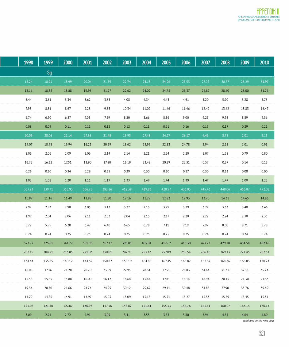
321
APPENDIX III GREENHOUSE GAS EMISSIONS EstimatEs BY GAS AND SECTOR, FROM 1990 TO 2010
N2O
SECTOR1990 1991 1992 1993 1994 1995 1996 1997 1998 1999 2000 2001 2002 2003 2004 2005 2006 2007 2008 2009 2010
Gg
Energy 14.08 14.11 14.00 13.91 14.53 15.03 15.98 17.31 18.24 18.91 18.99 20.04 21.39 22.74 24.13 24.96 25.53 27.02 28.77 28.29 31.97
Fuels Combustion 14.02 14.06 13.94 13.85 14.47 14.97 15.91 17.24 18.16 18.82 18.88 19.93 21.27 22.62 24.02 24.75 25.37 26.87 28.60 28.00 31.76
Industrial Subsector 2.54 2.53 2.59 2.65 2.97 2.97 3.02 3.16 3.44 3.61 3.34 3.62 3.83 4.08 4.34 4.43 4.91 5.20 5.20 5.28 5.73
Transport Subsector 3.75 3.91 3.93 4.05 4.28 5.14 6.09 7.07 7.98 8.31 8.67 9.23 9.85 10.34 11.02 11.46 11.46 12.42 13.42 13.83 16.47
Other Sectors 7.73 7.62 7.42 7.15 7.22 6.86 6.80 7.01 6.74 6.90 6.87 7.08 7.59 8.20 8.66 8.86 9.00 9.25 9.98 8.89 9.56
Fugitive Emissions 0.06 0.05 0.06 0.06 0.06 0.06 0.07 0.07 0.08 0.09 0.11 0.11 0.12 0.12 0.11 0.21 0.16 0.15 0.17 0.29 0.21
Industrial Processes 11.83 14.56 13.60 17.28 17.47 18.57 14.68 13.20 20.09 20.06 21.14 17.36 21.48 19.95 27.48 24.27 26.17 4.41 3.75 2.01 2.15
Chemical Industry 10.69 13.46 12.55 16.14 16.31 17.45 13.62 12.12 19.07 18.98 19.94 16.25 20.29 18.62 25.99 22.83 24.78 2.94 2.28 1.01 0.93
Nitric Acid Production 1.81 1.93 1.89 2.00 2.01 2.05 2.07 2.12 2.06 2.06 2.09 2.06 2.14 2.14 2.21 2.24 2.20 2.07 1.58 0.79 0.80
Adipic Acid Production 8.63 11.25 10.41 13.84 13.99 15.08 11.22 9.66 16.75 16.62 17.51 13.90 17.80 16.19 23.48 20.29 22.31 0.57 0.37 0.14 0.13
Other Productions 0.25 0.28 0.25 0.30 0.31 0.32 0.33 0.34 0.26 0.30 0.34 0.29 0.35 0.29 0.30 0.30 0.27 0.30 0.33 0.08 0.00
Metals Production 1.14 1.10 1.05 1.14 1.16 1.12 1.06 1.08 1.02 1.08 1.20 1.11 1.19 1.33 1.49 1.44 1.39 1.47 1.47 1.00 1.22
Agriculture 303.54 311.30 320.00 323.49 334.67 340.16 318.98 329.47 337.23 339.71 355.93 366.75 382.26 412.38 419.86 428.97 433.03 445.43 448.06 453.87 472.08
Manure Management 10.03 10.58 10.93 10.92 11.21 11.49 10.62 10.89 10.87 11.16 11.49 11.88 11.80 12.16 11.29 12.82 12.93 13.70 14.31 14.65 14.83
Cattle 2.90 2.96 3.00 3.01 3.04 3.07 2.83 2.89 2.92 2.93 2.98 3.05 3.13 3.22 2.13 3.29 3.29 3.27 3.33 3.40 3.46
Swine 2.43 2.48 2.49 2.43 2.48 2.54 1.95 1.97 1.99 2.04 2.06 2.11 2.03 2.04 2.13 2.17 2.20 2.22 2.24 2.30 2.35
Poultry 4.40 4.83 5.13 5.18 5.39 5.58 5.60 5.79 5.72 5.95 6.20 6.47 6.40 6.65 6.78 7.11 7.19 7.97 8.50 8.71 8.78
Other Animals 0.30 0.31 0.31 0.30 0.30 0.30 0.24 0.24 0.24 0.24 0.25 0.25 0.24 0.25 0.25 0.25 0.25 0.24 0.24 0.24 0.24
Agricultural Soils 290.75 297.99 306.26 310.07 320.49 325.59 305.34 315.57 323.27 325.61 341.72 351.96 367.37 396.81 405.04 412.62 416.30 427.77 429.20 434.58 452.45
Direct Emissions 184.07 188.19 193.71 195.06 201.60 205.28 191.67 198.00 202.19 204.21 213.85 221.03 230.01 247.99 253.43 257.09 259.54 266.16 269.13 271.45 282.31
Animals on Pasture 129.73 133.73 135.65 135.36 137.50 140.20 130.03 132.95 134.44 135.85 140.12 144.62 150.82 158.19 164.86 167.45 166.82 162.37 164.36 166.83 170.24
Synthetic Fertilizers 9.81 9.79 10.94 12.52 14.74 14.27 14.98 16.23 18.06 17.16 21.28 20.70 23.09 27.95 28.31 27.51 28.83 34.64 31.33 32.11 35.74
Animal Manure 14.90 15.31 15.77 15.64 15.87 16.40 14.76 15.30 15.56 15.65 15.88 16.00 16.12 16.64 15.44 17.81 18.14 18.94 20.15 21.30 21.33
Agricultural Waste 15.32 14.99 16.92 17.05 18.94 19.80 17.23 18.79 19.34 20.70 21.66 24.74 24.95 30.12 29.67 29.11 30.48 34.88 37.90 35.76 39.49
Organic Soils 14.31 14.37 14.43 14.49 14.55 14.61 14.67 14.73 14.79 14.85 14.91 14.97 15.03 15.09 15.15 15.21 15.27 15.33 15.39 15.45 15.51
Indirect Emissions 106.68 109.80 112.55 115.01 118.89 120.31 113.67 117.57 121.08 121.40 127.87 130.93 137.36 148.82 151.61 155.53 156.76 161.61 160.07 163.13 170.14
Burning of Agricultural Wastes 2.76 2.73 2.81 2.50 2.97 3.08 3.02 3.01 3.09 2.94 2.72 2.91 3.09 3.41 3.53 3.53 3.80 3.96 4.55 4.64 4.80
continues on the next page
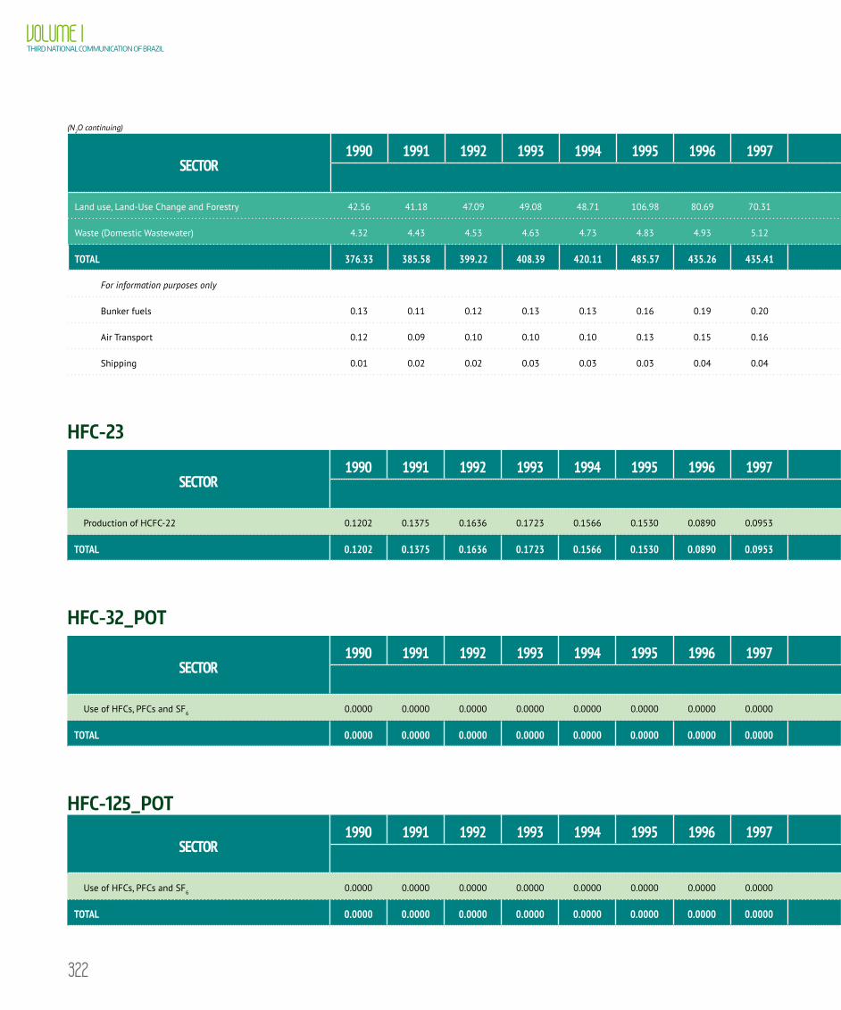
322
VOLUME ITHIRD NATIONAL COMMUNICATION OF BRAZIL
SECTOR1990 1991 1992 1993 1994 1995 1996 1997 1998 1999 2000 2001 2002 2003 2004 2005 2006 2007 2008 2009 2010
Gg
Land use, Land-Use Change and Forestry 42.56 41.18 47.09 49.08 48.71 106.98 80.69 70.31 80.06 79.95 81.96 81.99 90.07 144.95 152.41 125.25 105.16 97.90 101.45 51.66 47.08
Waste (Domestic Wastewater) 4.32 4.43 4.53 4.63 4.73 4.83 4.93 5.12 5.33 5.54 5.68 5.79 6.08 6.38 6.49 6.61 6.72 6.83 6.96 7.08 7.21
TOTAL 376.33 385.58 399.22 408.39 420.11 485.57 435.26 435.41 460.95 464.17 483.70 491.93 521.28 606.40 630.37 610.06 596.61 581.59 588.99 542.91 560.49
For information purposes only
Bunker fuels 0.13 0.11 0.12 0.13 0.13 0.16 0.19 0.20 0.22 0.22 0.20 0.23 0.22 0.20 0.20 0.21 0.21 0.23 0.27 0.23 0.27
Air Transport 0.12 0.09 0.10 0.10 0.10 0.13 0.15 0.16 0.18 0.15 0.13 0.15 0.13 0.12 0.12 0.13 0.13 0.14 0.16 0.15 0.17
Shipping 0.01 0.02 0.02 0.03 0.03 0.03 0.04 0.04 0.04 0.07 0.07 0.08 0.09 0.08 0.08 0.08 0.08 0.09 0.11 0.08 0.10
HFC-23
SECTOR1990 1991 1992 1993 1994 1995 1996 1997 1998 1999 2000 2001 2002 2003 2004 2005 2006 2007 2008 2009 2010
Gg
Production of HCFC-22 0.1202 0.1375 0.1636 0.1723 0.1566 0.1530 0.0890 0.0953 0.0130 0.0972 0.0000 0.0000 0.0000 0.0000 0.0000 0.0000 0.0000 0.0000 0.0000 0.0000 0.0000
TOTAL 0.1202 0.1375 0.1636 0.1723 0.1566 0.1530 0.0890 0.0953 0.0130 0.0972 0.0000 0.0000 0.0000 0.0000 0.0000 0.0000 0.0000 0.0000 0.0000 0.0000 0.0000
HFC-32_POT
SECTOR1990 1991 1992 1993 1994 1995 1996 1997 1998 1999 2000 2001 2002 2003 2004 2005 2006 2007 2008 2009 2010
Gg
Use of HFCs, PFCs and SF6 0.0000 0.0000 0.0000 0.0000 0.0000 0.0000 0.0000 0.0000 0.0000 0.0000 0.0000 0.0000 0.0000 0.0000 0.0000 0.0000 0.0000 0.0718 0.0420 0.0872 0.1059
TOTAL 0.0000 0.0000 0.0000 0.0000 0.0000 0.0000 0.0000 0.0000 0.0000 0.0000 0.0000 0.0000 0.0000 0.0000 0.0000 0.0000 0.0000 0.0718 0.0420 0.0872 0.1059
HFC-125_POT
SECTOR1990 1991 1992 1993 1994 1995 1996 1997 1998 1999 2000 2001 2002 2003 2004 2005 2006 2007 2008 2009 2010
Gg
Use of HFCs, PFCs and SF6 0.0000 0.0000 0.0000 0.0000 0.0000 0.0000 0.0000 0.0000 0.0000 0.0000 0.0071 0.0392 0.0508 0.0548 0.1207 0.1249 0.2517 0.2850 0.3021 0.3587 0.5012
TOTAL 0.0000 0.0000 0.0000 0.0000 0.0000 0.0000 0.0000 0.0000 0.0000 0.0000 0.0071 0.0392 0.0508 0.0548 0.1207 0.1249 0.2517 0.2850 0.3021 0.3587 0.5012
(N2O continuing)

323
APPENDIX III GREENHOUSE GAS EMISSIONS EstimatEs BY GAS AND SECTOR, FROM 1990 TO 2010
SECTOR1990 1991 1992 1993 1994 1995 1996 1997 1998 1999 2000 2001 2002 2003 2004 2005 2006 2007 2008 2009 2010
Gg
Land use, Land-Use Change and Forestry 42.56 41.18 47.09 49.08 48.71 106.98 80.69 70.31 80.06 79.95 81.96 81.99 90.07 144.95 152.41 125.25 105.16 97.90 101.45 51.66 47.08
Waste (Domestic Wastewater) 4.32 4.43 4.53 4.63 4.73 4.83 4.93 5.12 5.33 5.54 5.68 5.79 6.08 6.38 6.49 6.61 6.72 6.83 6.96 7.08 7.21
TOTAL 376.33 385.58 399.22 408.39 420.11 485.57 435.26 435.41 460.95 464.17 483.70 491.93 521.28 606.40 630.37 610.06 596.61 581.59 588.99 542.91 560.49
For information purposes only
Bunker fuels 0.13 0.11 0.12 0.13 0.13 0.16 0.19 0.20 0.22 0.22 0.20 0.23 0.22 0.20 0.20 0.21 0.21 0.23 0.27 0.23 0.27
Air Transport 0.12 0.09 0.10 0.10 0.10 0.13 0.15 0.16 0.18 0.15 0.13 0.15 0.13 0.12 0.12 0.13 0.13 0.14 0.16 0.15 0.17
Shipping 0.01 0.02 0.02 0.03 0.03 0.03 0.04 0.04 0.04 0.07 0.07 0.08 0.09 0.08 0.08 0.08 0.08 0.09 0.11 0.08 0.10
HFC-23
SECTOR1990 1991 1992 1993 1994 1995 1996 1997 1998 1999 2000 2001 2002 2003 2004 2005 2006 2007 2008 2009 2010
Gg
Production of HCFC-22 0.1202 0.1375 0.1636 0.1723 0.1566 0.1530 0.0890 0.0953 0.0130 0.0972 0.0000 0.0000 0.0000 0.0000 0.0000 0.0000 0.0000 0.0000 0.0000 0.0000 0.0000
TOTAL 0.1202 0.1375 0.1636 0.1723 0.1566 0.1530 0.0890 0.0953 0.0130 0.0972 0.0000 0.0000 0.0000 0.0000 0.0000 0.0000 0.0000 0.0000 0.0000 0.0000 0.0000
HFC-32_POT
SECTOR1990 1991 1992 1993 1994 1995 1996 1997 1998 1999 2000 2001 2002 2003 2004 2005 2006 2007 2008 2009 2010
Gg
Use of HFCs, PFCs and SF6 0.0000 0.0000 0.0000 0.0000 0.0000 0.0000 0.0000 0.0000 0.0000 0.0000 0.0000 0.0000 0.0000 0.0000 0.0000 0.0000 0.0000 0.0718 0.0420 0.0872 0.1059
TOTAL 0.0000 0.0000 0.0000 0.0000 0.0000 0.0000 0.0000 0.0000 0.0000 0.0000 0.0000 0.0000 0.0000 0.0000 0.0000 0.0000 0.0000 0.0718 0.0420 0.0872 0.1059
HFC-125_POT
SECTOR1990 1991 1992 1993 1994 1995 1996 1997 1998 1999 2000 2001 2002 2003 2004 2005 2006 2007 2008 2009 2010
Gg
Use of HFCs, PFCs and SF6 0.0000 0.0000 0.0000 0.0000 0.0000 0.0000 0.0000 0.0000 0.0000 0.0000 0.0071 0.0392 0.0508 0.0548 0.1207 0.1249 0.2517 0.2850 0.3021 0.3587 0.5012
TOTAL 0.0000 0.0000 0.0000 0.0000 0.0000 0.0000 0.0000 0.0000 0.0000 0.0000 0.0071 0.0392 0.0508 0.0548 0.1207 0.1249 0.2517 0.2850 0.3021 0.3587 0.5012

324
VOLUME ITHIRD NATIONAL COMMUNICATION OF BRAZIL
HFC-134A
SECTOR1990 1991 1992 1993 1994 1995 1996 1997 1998 1999 2000 2001 2002 2003 2004 2005 2006 2007 2008 2009 2010
Gg
Use of HFCs, PFCs and SF6 0.0004 0.0009 0.0042 0.0080 0.0685 0.0028 0.0471 0.1641 0.2804 0.3803 0.4988 0.6310 0.7691 0.9056 1.0533 1.2279 1.4488 1.7220 2.0187 2.3359 2.7196
TOTAL 0.0004 0.0009 0.0042 0.0080 0.0685 0.0028 0.0471 0.1641 0.2804 0.3803 0.4988 0.6310 0.7691 0.9056 1.0533 1.2279 1.4488 1.7220 2.0187 2.3359 2.7196
HFC-143A_POT
SECTOR1990 1991 1992 1993 1994 1995 1996 1997 1998 1999 2000 2001 2002 2003 2004 2005 2006 2007 2008 2009 2010
Gg
Use of HFCs, PFCs and SF6 0.0000 0.0000 0.0000 0.0000 0.0000 0.0000 0.0000 0.0000 0.0000 0.0000 0.0075 0.0271 0.0398 0.0500 0.1037 0.0929 0.2157 0.2520 0.3074 0.3209 0.4671
TOTAL 0.0000 0.0000 0.0000 0.0000 0.0000 0.0000 0.0000 0.0000 0.0000 0.0000 0.0075 0.0271 0.0398 0.0500 0.1037 0.0929 0.2157 0.2520 0.3074 0.3209 0.4671
HFC-152A_POT
SECTOR1990 1991 1992 1993 1994 1995 1996 1997 1998 1999 2000 2001 2002 2003 2004 2005 2006 2007 2008 2009 2010
Gg
Use of HFCs, PFCs and SF6 0.0000 0.0000 0.0000 0.0000 0.0000 0.0000 0.0000 0.0000 0.0000 0.0000 0.0001 0.0295 0.0081 0.0238 0.0543 0.1748 0.2800 0.0000 0.0000 0.0000 0.0000
TOTAL 0.0000 0.0000 0.0000 0.0000 0.0000 0.0000 0.0000 0.0000 0.0000 0.0000 0.0001 0.0295 0.0081 0.0238 0.0543 0.1748 0.2800 0.0000 0.0000 0.0000 0.0000
CF4
SECTOR1990 1991 1992 1993 1994 1995 1996 1997 1998 1999 2000 2001 2002 2003 2004 2005 2006 2007 2008 2009 2010
Gg
Production of aluminum 0.3022 0.3365 0.3565 0.3348 0.3231 0.3060 0.2976 0.2027 0.2276 0.2013 0.1465 0.1147 0.1351 0.1362 0.1241 0.1239 0.1219 0.1174 0.1145 0.0823 0.0767
TOTAL 0.3022 0.3365 0.3565 0.3348 0.3231 0.3060 0.2976 0.2027 0.2276 0.2013 0.1465 0.1147 0.1351 0.1362 0.1241 0.1239 0.1219 0.1174 0.1145 0.0823 0.0767
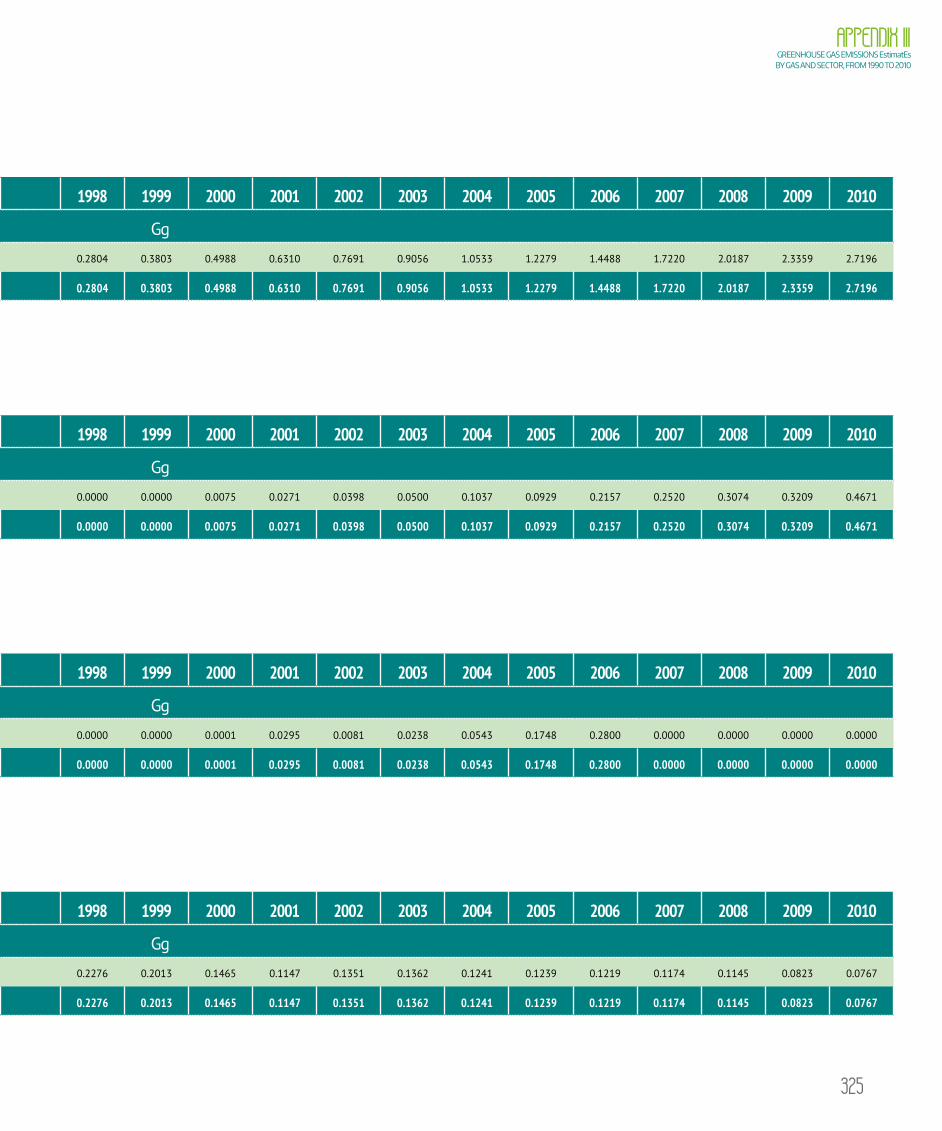
325
APPENDIX III GREENHOUSE GAS EMISSIONS EstimatEs BY GAS AND SECTOR, FROM 1990 TO 2010
HFC-134A
SECTOR1990 1991 1992 1993 1994 1995 1996 1997 1998 1999 2000 2001 2002 2003 2004 2005 2006 2007 2008 2009 2010
Gg
Use of HFCs, PFCs and SF6 0.0004 0.0009 0.0042 0.0080 0.0685 0.0028 0.0471 0.1641 0.2804 0.3803 0.4988 0.6310 0.7691 0.9056 1.0533 1.2279 1.4488 1.7220 2.0187 2.3359 2.7196
TOTAL 0.0004 0.0009 0.0042 0.0080 0.0685 0.0028 0.0471 0.1641 0.2804 0.3803 0.4988 0.6310 0.7691 0.9056 1.0533 1.2279 1.4488 1.7220 2.0187 2.3359 2.7196
HFC-143A_POT
SECTOR1990 1991 1992 1993 1994 1995 1996 1997 1998 1999 2000 2001 2002 2003 2004 2005 2006 2007 2008 2009 2010
Gg
Use of HFCs, PFCs and SF6 0.0000 0.0000 0.0000 0.0000 0.0000 0.0000 0.0000 0.0000 0.0000 0.0000 0.0075 0.0271 0.0398 0.0500 0.1037 0.0929 0.2157 0.2520 0.3074 0.3209 0.4671
TOTAL 0.0000 0.0000 0.0000 0.0000 0.0000 0.0000 0.0000 0.0000 0.0000 0.0000 0.0075 0.0271 0.0398 0.0500 0.1037 0.0929 0.2157 0.2520 0.3074 0.3209 0.4671
HFC-152A_POT
SECTOR1990 1991 1992 1993 1994 1995 1996 1997 1998 1999 2000 2001 2002 2003 2004 2005 2006 2007 2008 2009 2010
Gg
Use of HFCs, PFCs and SF6 0.0000 0.0000 0.0000 0.0000 0.0000 0.0000 0.0000 0.0000 0.0000 0.0000 0.0001 0.0295 0.0081 0.0238 0.0543 0.1748 0.2800 0.0000 0.0000 0.0000 0.0000
TOTAL 0.0000 0.0000 0.0000 0.0000 0.0000 0.0000 0.0000 0.0000 0.0000 0.0000 0.0001 0.0295 0.0081 0.0238 0.0543 0.1748 0.2800 0.0000 0.0000 0.0000 0.0000
CF4
SECTOR1990 1991 1992 1993 1994 1995 1996 1997 1998 1999 2000 2001 2002 2003 2004 2005 2006 2007 2008 2009 2010
Gg
Production of aluminum 0.3022 0.3365 0.3565 0.3348 0.3231 0.3060 0.2976 0.2027 0.2276 0.2013 0.1465 0.1147 0.1351 0.1362 0.1241 0.1239 0.1219 0.1174 0.1145 0.0823 0.0767
TOTAL 0.3022 0.3365 0.3565 0.3348 0.3231 0.3060 0.2976 0.2027 0.2276 0.2013 0.1465 0.1147 0.1351 0.1362 0.1241 0.1239 0.1219 0.1174 0.1145 0.0823 0.0767

326
VOLUME ITHIRD NATIONAL COMMUNICATION OF BRAZIL
C2F6
SECTOR1990 1991 1992 1993 1994 1995 1996 1997 1998 1999 2000 2001 2002 2003 2004 2005 2006 2007 2008 2009 2010
Gg
Production of aluminum 0.0263 0.0290 0.0311 0.0290 0.0279 0.0264 0.0261 0.0157 0.0172 0.0154 0.0117 0.0092 0.0117 0.0115 0.0100 0.0104 0.0104 0.0099 0.0096 0.0064 0.0059
TOTAL 0.0263 0.0290 0.0311 0.0290 0.0279 0.0264 0.0261 0.0157 0.0172 0.0154 0.0117 0.0092 0.0117 0.0115 0.0100 0.0104 0.0104 0.0099 0.0096 0.0064 0.0059
SF6
SECTOR1990 1991 1992 1993 1994 1995 1996 1997 1998 1999 2000 2001 2002 2003 2004 2005 2006 2007 2008 2009 2010
Gg
Production of magnesium 0.0058 0.0058 0.0070 0.0101 0.0099 0.0101 0.0097 0.0127 0.0101 0.0098 0.0103 0.0095 0.0122 0.0147 0.0170 0.0191 0.0216 0.0260 0.0260 0.0130 0.0000
Use of HFCs, PFCs and SF6 0.0042 0.0040 0.0040 0.0040 0.0041 0.0041 0.0041 0.0042 0.0047 0.0049 0.0050 0.0051 0.0053 0.0056 0.0060 0.0061 0.0063 0.0064 0.0081 0.0084 0.0087
TOTAL 0.0100 0.0098 0.0110 0.0141 0.0140 0.0142 0.0138 0.0169 0.0148 0.0147 0.0153 0.0146 0.0175 0.0203 0.0230 0.0252 0.0279 0.0324 0.0341 0.0214 0.0087
CO
SECTOR1990 1991 1992 1993 1994 1995 1996 1997 1998 1999 2000 2001 2002 2003 2004 2005 2006 2007 2008 2009 2010
Gg
Energy 9,592.6 9,695.5 9,470.6 9,380.3 9,632.1 9,636.3 9,784.5 9,423.3 9,166.2 8,745.5 8,181.0 7,825.7 8,176.5 8,110.5 8,270.6 8,194.7 7,841.1 7,815.7 7,893.6 7,212.9 7,695.9
Fossil Fuels Combustion 9,592.6 9,695.5 9,470.6 9,380.3 9,632.1 9,636.3 9,784.5 9,423.3 9,166.2 8,745.5 8,181.0 7,825.7 8,176.5 8,110.5 8,270.6 8,194.7 7,841.1 7,815.7 7,893.6 7,212.9 7,695.9
Energy Subsector 1,398.0 1,303.1 1,214.8 1,250.1 1,292.5 1,208.5 1,148.9 1,171.4 1,065.1 1,098.9 1,104.3 1,083.3 1,148.5 1,347.4 1,498.8 1,528.1 1,536.2 1,653.3 1,778.4 1,418.0 1,617.9
Industrial Subsector 758.1 749.5 735.6 792.2 837.7 815.1 858.4 852.4 916.3 999.0 1,036.8 1,035.1 1,059.6 1,160.2 1,223.3 1,283.5 1,363.5 1,448.6 1,541.2 1,558.8 1,710.3
Steel Industry 2.5 2.7 2.8 4.0 3.2 3.2 4.8 6.4 6.2 7.1 8.2 7.3 8.7 9.8 11.0 11.4 11.5 12.2 12.3 9.5 11.4
Food and Beverage 182.3 185.7 170.6 172.0 178.1 175.8 179.7 179.3 186.7 191.9 187.5 189.8 191.8 192.5 200.3 204.8 214.8 223.8 230.5 236.8 260.9
Other industries 573.3 561.1 562.2 616.2 656.4 636.1 673.9 666.7 723.4 800.0 841.1 838.0 859.1 957.9 1,012.0 1,067.3 1,137.2 1,212.6 1,298.4 1,312.5 1,438.0
Transport Subsector 5,902.9 6,118.9 6,006.1 5,993.7 6,192.3 6,419.3 6,608.8 6,217.0 5,982.6 5,410.1 4,776.2 4,389.7 4,508.1 4,080.0 4,002.7 3,807.3 3,358.9 3,200.3 3,065.2 2,752.8 2,933.7
Road Transport 5,856.4 6,074.7 5,965.7 5,949.0 6,144.5 6,373.4 6,559.5 6,166.6 5,928.4 5,358.1 4,724.6 4,339.0 4,460.7 4,035.0 3,955.1 3,761.8 3,315.5 3,153.5 3,014.6 2,701.5 2,875.0
Other Transports 46.5 44.2 40.4 44.7 47.8 45.9 49.3 50.4 54.2 52.0 51.6 50.7 47.4 45.0 47.6 45.5 43.4 46.8 50.6 51.3 58.7
Residential Subsector 1,443.2 1,433.6 1,427.2 1,254.8 1,218.4 1,098.7 1,072.1 1,084.7 1,107.6 1,142.1 1,172.3 1,221.8 1,361.6 1,418.9 1,439.1 1,468.4 1,472.8 1,397.7 1,382.2 1,361.6 1,306.7
Other Sectors 90.4 90.4 86.9 89.5 91.2 94.7 96.3 97.8 94.6 95.4 91.4 95.8 98.7 104.0 106.7 107.4 109.7 115.8 126.6 121.7 127.3

327
APPENDIX III GREENHOUSE GAS EMISSIONS EstimatEs BY GAS AND SECTOR, FROM 1990 TO 2010
C2F6
SECTOR1990 1991 1992 1993 1994 1995 1996 1997 1998 1999 2000 2001 2002 2003 2004 2005 2006 2007 2008 2009 2010
Gg
Production of aluminum 0.0263 0.0290 0.0311 0.0290 0.0279 0.0264 0.0261 0.0157 0.0172 0.0154 0.0117 0.0092 0.0117 0.0115 0.0100 0.0104 0.0104 0.0099 0.0096 0.0064 0.0059
TOTAL 0.0263 0.0290 0.0311 0.0290 0.0279 0.0264 0.0261 0.0157 0.0172 0.0154 0.0117 0.0092 0.0117 0.0115 0.0100 0.0104 0.0104 0.0099 0.0096 0.0064 0.0059
SF6
SECTOR1990 1991 1992 1993 1994 1995 1996 1997 1998 1999 2000 2001 2002 2003 2004 2005 2006 2007 2008 2009 2010
Gg
Production of magnesium 0.0058 0.0058 0.0070 0.0101 0.0099 0.0101 0.0097 0.0127 0.0101 0.0098 0.0103 0.0095 0.0122 0.0147 0.0170 0.0191 0.0216 0.0260 0.0260 0.0130 0.0000
Use of HFCs, PFCs and SF6 0.0042 0.0040 0.0040 0.0040 0.0041 0.0041 0.0041 0.0042 0.0047 0.0049 0.0050 0.0051 0.0053 0.0056 0.0060 0.0061 0.0063 0.0064 0.0081 0.0084 0.0087
TOTAL 0.0100 0.0098 0.0110 0.0141 0.0140 0.0142 0.0138 0.0169 0.0148 0.0147 0.0153 0.0146 0.0175 0.0203 0.0230 0.0252 0.0279 0.0324 0.0341 0.0214 0.0087
CO
SECTOR1990 1991 1992 1993 1994 1995 1996 1997 1998 1999 2000 2001 2002 2003 2004 2005 2006 2007 2008 2009 2010
Gg
Energy 9,592.6 9,695.5 9,470.6 9,380.3 9,632.1 9,636.3 9,784.5 9,423.3 9,166.2 8,745.5 8,181.0 7,825.7 8,176.5 8,110.5 8,270.6 8,194.7 7,841.1 7,815.7 7,893.6 7,212.9 7,695.9
Fossil Fuels Combustion 9,592.6 9,695.5 9,470.6 9,380.3 9,632.1 9,636.3 9,784.5 9,423.3 9,166.2 8,745.5 8,181.0 7,825.7 8,176.5 8,110.5 8,270.6 8,194.7 7,841.1 7,815.7 7,893.6 7,212.9 7,695.9
Energy Subsector 1,398.0 1,303.1 1,214.8 1,250.1 1,292.5 1,208.5 1,148.9 1,171.4 1,065.1 1,098.9 1,104.3 1,083.3 1,148.5 1,347.4 1,498.8 1,528.1 1,536.2 1,653.3 1,778.4 1,418.0 1,617.9
Industrial Subsector 758.1 749.5 735.6 792.2 837.7 815.1 858.4 852.4 916.3 999.0 1,036.8 1,035.1 1,059.6 1,160.2 1,223.3 1,283.5 1,363.5 1,448.6 1,541.2 1,558.8 1,710.3
Steel Industry 2.5 2.7 2.8 4.0 3.2 3.2 4.8 6.4 6.2 7.1 8.2 7.3 8.7 9.8 11.0 11.4 11.5 12.2 12.3 9.5 11.4
Food and Beverage 182.3 185.7 170.6 172.0 178.1 175.8 179.7 179.3 186.7 191.9 187.5 189.8 191.8 192.5 200.3 204.8 214.8 223.8 230.5 236.8 260.9
Other industries 573.3 561.1 562.2 616.2 656.4 636.1 673.9 666.7 723.4 800.0 841.1 838.0 859.1 957.9 1,012.0 1,067.3 1,137.2 1,212.6 1,298.4 1,312.5 1,438.0
Transport Subsector 5,902.9 6,118.9 6,006.1 5,993.7 6,192.3 6,419.3 6,608.8 6,217.0 5,982.6 5,410.1 4,776.2 4,389.7 4,508.1 4,080.0 4,002.7 3,807.3 3,358.9 3,200.3 3,065.2 2,752.8 2,933.7
Road Transport 5,856.4 6,074.7 5,965.7 5,949.0 6,144.5 6,373.4 6,559.5 6,166.6 5,928.4 5,358.1 4,724.6 4,339.0 4,460.7 4,035.0 3,955.1 3,761.8 3,315.5 3,153.5 3,014.6 2,701.5 2,875.0
Other Transports 46.5 44.2 40.4 44.7 47.8 45.9 49.3 50.4 54.2 52.0 51.6 50.7 47.4 45.0 47.6 45.5 43.4 46.8 50.6 51.3 58.7
Residential Subsector 1,443.2 1,433.6 1,427.2 1,254.8 1,218.4 1,098.7 1,072.1 1,084.7 1,107.6 1,142.1 1,172.3 1,221.8 1,361.6 1,418.9 1,439.1 1,468.4 1,472.8 1,397.7 1,382.2 1,361.6 1,306.7
Other Sectors 90.4 90.4 86.9 89.5 91.2 94.7 96.3 97.8 94.6 95.4 91.4 95.8 98.7 104.0 106.7 107.4 109.7 115.8 126.6 121.7 127.3
continues on the next page

328
VOLUME ITHIRD NATIONAL COMMUNICATION OF BRAZIL
(CO continuing)
SECTOR1990 1991 1992 1993 1994 1995 1996 1997 1998 1999 2000 2001 2002 2003 2004 2005 2006 2007 2008 2009 2010
Gg
Industrial Processes 900.8 810.4 759.8 819.5 834.3 778.0 714.8 707.5 653.4 724.7 790.5 723.4 764.0 886.8 1,037.9 1,022.4 997.3 1,037.7 1,027.7 665.8 809.6
Iron and Steel Production 775.0 669.2 628.1 686.2 708.4 656.2 577.6 603.4 558.3 623.9 676.1 637.4 662.1 745.3 888.3 867.3 836.4 865.4 849.6 508.4 633.2
Ferroalloy Production 60.8 81.9 69.6 84.2 73.6 64.2 97.2 65.2 54.9 60.9 72.5 44.7 56.6 90.2 94.8 96.7 97.6 104.5 106.7 82.5 96.7
Production of Non-Ferrous Metals 44.4 36.1 36.2 21.8 22.8 27.6 8.7 6.8 5.9 2.8 3.7 3.4 4.0 4.3 4.5 4.6 4.9 5.1 4.9 4.7 4.9
Other Productions 20.6 23.2 25.9 27.3 29.5 30.0 31.3 32.1 34.3 37.1 38.2 37.9 41.3 47.0 50.3 53.8 58.4 62.7 66.5 70.2 74.8
Agriculture 3,627.6 3,590.2 3,696.5 3,289.4 3,908.1 4,045.8 3,968.2 3,957.5 4,067.1 3,861.7 3,576.4 3,818.0 4,060.8 4,485.9 4,637.8 4,644.4 4,996.6 5,198.4 5,980.4 6,095.2 6,313.5
Cotton crop residues burning 128.4 114.8 80.0 31.9 16.8 0.0 0.0 0.0 0.0 0.0 0.0 0.0 0.0 0.0 0.0 0.0 0.0 0.0 0.0 0.0 0.0
Sugarcane burning 3,499.2 3,475.4 3,616.5 3,257.5 3,891.3 4,045.8 3,968.2 3,957.5 4,067.1 3,861.7 3,576.4 3,818.0 4,060.8 4.485.9 4,637.8 4,644.4 4,996.6 5,198.4 5,980.4 6,095.2 6,313.5
Land use, Land-Use Change and Forestry 18,429.4 17,390.4 20,397.4 21,446.1 21,286.6 48,855.6 35,319.7 29,864.8 34,894.5 34,821.8 35,879.9 35,881.7 40,075.6 65,971.8 69,818.3 55,810.0 45,459.9 41,737.2 43,552.8 21,977.9 20,231.4
TOTAL 32,550.4 31,486.5 34,324.3 34,935.3 35,661.1 63,315.7 49,787.2 43,953.1 48,781.2 48,153.7 48,427.8 48,248.8 53,076.9 79,455.0 83,764.6 69,671.5 59,294.9 55,789.0 58,454.5 35,951.8 35,050.4
For information purposes only
Bunker fuels 0.9 0.6 0.7 0.7 0.7 0.9 1.1 1.1 1.3 1.1 0.9 1.1 0.9 0.8 1.1 1.2 1.0 0.9 1.2 1.0 1.1
Air Transport 0.9 0.6 0.7 0.7 0.7 0.9 1.1 1.1 1.3 1.1 0.9 1.1 0.9 0.8 1.1 1.2 1.0 0.9 1.2 1.0 1.1
Shipping 0.0 0.0 0.0 0.0 0.0 0.0 0.0 0.0 0.0 0.0 0.0 0.0 0.0 0.0 0.0 0.0 0.0 0.0 0.0 0.0 0.0
NOX
SECTOR1990 1991 1992 1993 1994 1995 1996 1997 1998 1999 2000 2001 2002 2003 2004 2005 2006 2007 2008 2009 2010
Gg
Energy 1,639.8 1,705.7 1,743.9 1,800.7 1,870.0 1,977.5 2,098.4 2,155.0 2,235.5 2,296.3 2,273.3 2,300.7 2,285.2 2,249.1 2,345.6 2,346.4 2,334.3 2,423.6 2,555.9 2,439.0 2,567.1
Fossil Fuels Combustion 1,639.8 1,705.7 1,743.9 1,800.7 1,870.0 1,977.5 2,098.4 2,155.0 2,235.5 2,296.3 2,273.3 2,300.7 2,285.2 2,249.1 2,345.6 2,346.4 2,334.3 2,423.6 2,555.9 2,439.0 2,567.1
Energy Subsector 214.9 226.3 245.3 247.9 256.2 266.6 289.2 332.0 341.0 388.5 395.0 416.3 382.1 415.2 449.8 479.8 491.0 501.9 584.0 557.4 577.5
Industrial Subsector 134.8 138.4 140.9 146.1 159.5 169.9 180.9 193.7 201.5 218.0 222.7 223.2 227.2 229.5 236.3 242.9 255.5 278.2 271.6 270.7 286.6
Steel Industry 10.4 11.1 12.3 12.9 13.3 12.3 10.7 11.5 10.4 10.4 11.1 10.5 10.8 10.6 10.6 12.1 11.8 11.9 11.4 9.8 12.0
Other industries 124.4 127.3 128.6 133.2 146.2 157.6 170.2 182.2 191.1 207.6 211.6 212.7 216.4 218.9 225.7 230.8 243.7 266.3 260.2 260.9 274.6
Transport Subsector 1,138.8 1,184.9 1,198.9 1,236.6 1,274.2 1,352.6 1,435.5 1,429.5 1,497.5 1,485.5 1,457.4 1,447.9 1,462.4 1,391.5 1,447.4 1,414.0 1,375.5 1,420.6 1,456.5 1,373.8 1,459.7
Road Transport 1,021.6 1,070.7 1,080.7 1,105.7 1,159.2 1,237.5 1,300.1 1,327.8 1,387.7 1,373.2 1,355.3 1,334.7 1,348.2 1,279.6 1,323.4 1,287.4 1,252.3 1,274.8 1,298.9 1,222.4 1,290.6
Other Transports 117.2 114.2 118.2 130.9 115.0 115.1 135.4 101.7 109.8 112.3 102.1 113.2 114.2 111.9 124.0 126.6 123.2 145.8 157.6 151.4 169.1

329
APPENDIX III GREENHOUSE GAS EMISSIONS EstimatEs BY GAS AND SECTOR, FROM 1990 TO 2010
SECTOR1990 1991 1992 1993 1994 1995 1996 1997 1998 1999 2000 2001 2002 2003 2004 2005 2006 2007 2008 2009 2010
Gg
Industrial Processes 900.8 810.4 759.8 819.5 834.3 778.0 714.8 707.5 653.4 724.7 790.5 723.4 764.0 886.8 1,037.9 1,022.4 997.3 1,037.7 1,027.7 665.8 809.6
Iron and Steel Production 775.0 669.2 628.1 686.2 708.4 656.2 577.6 603.4 558.3 623.9 676.1 637.4 662.1 745.3 888.3 867.3 836.4 865.4 849.6 508.4 633.2
Ferroalloy Production 60.8 81.9 69.6 84.2 73.6 64.2 97.2 65.2 54.9 60.9 72.5 44.7 56.6 90.2 94.8 96.7 97.6 104.5 106.7 82.5 96.7
Production of Non-Ferrous Metals 44.4 36.1 36.2 21.8 22.8 27.6 8.7 6.8 5.9 2.8 3.7 3.4 4.0 4.3 4.5 4.6 4.9 5.1 4.9 4.7 4.9
Other Productions 20.6 23.2 25.9 27.3 29.5 30.0 31.3 32.1 34.3 37.1 38.2 37.9 41.3 47.0 50.3 53.8 58.4 62.7 66.5 70.2 74.8
Agriculture 3,627.6 3,590.2 3,696.5 3,289.4 3,908.1 4,045.8 3,968.2 3,957.5 4,067.1 3,861.7 3,576.4 3,818.0 4,060.8 4,485.9 4,637.8 4,644.4 4,996.6 5,198.4 5,980.4 6,095.2 6,313.5
Cotton crop residues burning 128.4 114.8 80.0 31.9 16.8 0.0 0.0 0.0 0.0 0.0 0.0 0.0 0.0 0.0 0.0 0.0 0.0 0.0 0.0 0.0 0.0
Sugarcane burning 3,499.2 3,475.4 3,616.5 3,257.5 3,891.3 4,045.8 3,968.2 3,957.5 4,067.1 3,861.7 3,576.4 3,818.0 4,060.8 4.485.9 4,637.8 4,644.4 4,996.6 5,198.4 5,980.4 6,095.2 6,313.5
Land use, Land-Use Change and Forestry 18,429.4 17,390.4 20,397.4 21,446.1 21,286.6 48,855.6 35,319.7 29,864.8 34,894.5 34,821.8 35,879.9 35,881.7 40,075.6 65,971.8 69,818.3 55,810.0 45,459.9 41,737.2 43,552.8 21,977.9 20,231.4
TOTAL 32,550.4 31,486.5 34,324.3 34,935.3 35,661.1 63,315.7 49,787.2 43,953.1 48,781.2 48,153.7 48,427.8 48,248.8 53,076.9 79,455.0 83,764.6 69,671.5 59,294.9 55,789.0 58,454.5 35,951.8 35,050.4
For information purposes only
Bunker fuels 0.9 0.6 0.7 0.7 0.7 0.9 1.1 1.1 1.3 1.1 0.9 1.1 0.9 0.8 1.1 1.2 1.0 0.9 1.2 1.0 1.1
Air Transport 0.9 0.6 0.7 0.7 0.7 0.9 1.1 1.1 1.3 1.1 0.9 1.1 0.9 0.8 1.1 1.2 1.0 0.9 1.2 1.0 1.1
Shipping 0.0 0.0 0.0 0.0 0.0 0.0 0.0 0.0 0.0 0.0 0.0 0.0 0.0 0.0 0.0 0.0 0.0 0.0 0.0 0.0 0.0
NOX
SECTOR1990 1991 1992 1993 1994 1995 1996 1997 1998 1999 2000 2001 2002 2003 2004 2005 2006 2007 2008 2009 2010
Gg
Energy 1,639.8 1,705.7 1,743.9 1,800.7 1,870.0 1,977.5 2,098.4 2,155.0 2,235.5 2,296.3 2,273.3 2,300.7 2,285.2 2,249.1 2,345.6 2,346.4 2,334.3 2,423.6 2,555.9 2,439.0 2,567.1
Fossil Fuels Combustion 1,639.8 1,705.7 1,743.9 1,800.7 1,870.0 1,977.5 2,098.4 2,155.0 2,235.5 2,296.3 2,273.3 2,300.7 2,285.2 2,249.1 2,345.6 2,346.4 2,334.3 2,423.6 2,555.9 2,439.0 2,567.1
Energy Subsector 214.9 226.3 245.3 247.9 256.2 266.6 289.2 332.0 341.0 388.5 395.0 416.3 382.1 415.2 449.8 479.8 491.0 501.9 584.0 557.4 577.5
Industrial Subsector 134.8 138.4 140.9 146.1 159.5 169.9 180.9 193.7 201.5 218.0 222.7 223.2 227.2 229.5 236.3 242.9 255.5 278.2 271.6 270.7 286.6
Steel Industry 10.4 11.1 12.3 12.9 13.3 12.3 10.7 11.5 10.4 10.4 11.1 10.5 10.8 10.6 10.6 12.1 11.8 11.9 11.4 9.8 12.0
Other industries 124.4 127.3 128.6 133.2 146.2 157.6 170.2 182.2 191.1 207.6 211.6 212.7 216.4 218.9 225.7 230.8 243.7 266.3 260.2 260.9 274.6
Transport Subsector 1,138.8 1,184.9 1,198.9 1,236.6 1,274.2 1,352.6 1,435.5 1,429.5 1,497.5 1,485.5 1,457.4 1,447.9 1,462.4 1,391.5 1,447.4 1,414.0 1,375.5 1,420.6 1,456.5 1,373.8 1,459.7
Road Transport 1,021.6 1,070.7 1,080.7 1,105.7 1,159.2 1,237.5 1,300.1 1,327.8 1,387.7 1,373.2 1,355.3 1,334.7 1,348.2 1,279.6 1,323.4 1,287.4 1,252.3 1,274.8 1,298.9 1,222.4 1,290.6
Other Transports 117.2 114.2 118.2 130.9 115.0 115.1 135.4 101.7 109.8 112.3 102.1 113.2 114.2 111.9 124.0 126.6 123.2 145.8 157.6 151.4 169.1
continues on the next page
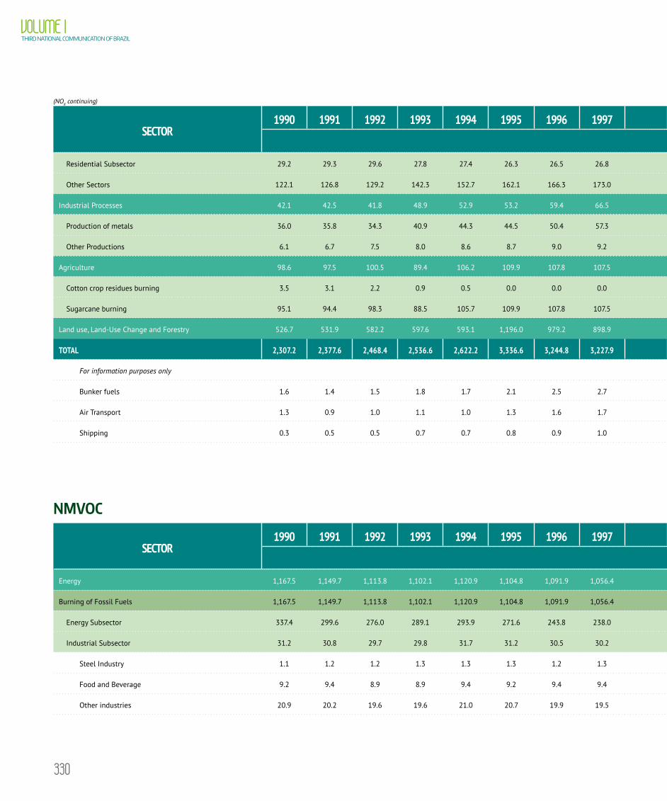
330
VOLUME ITHIRD NATIONAL COMMUNICATION OF BRAZIL
SECTOR1990 1991 1992 1993 1994 1995 1996 1997 1998 1999 2000 2001 2002 2003 2004 2005 2006 2007 2008 2009 2010
Gg
Residential Subsector 29.2 29.3 29.6 27.8 27.4 26.3 26.5 26.8 27.2 27.9 28.5 29.2 30.6 30.6 31.1 31.3 31.3 30.8 31.0 30.9 30.6
Other Sectors 122.1 126.8 129.2 142.3 152.7 162.1 166.3 173.0 168.3 176.4 169.7 184.1 182.9 182.3 181.0 178.4 181.0 192.1 212.8 206.2 212.7
Industrial Processes 42.1 42.5 41.8 48.9 52.9 53.2 59.4 66.5 75.3 86.3 94.9 91.8 102.4 117.0 125.0 125.2 125.3 134.7 136.9 113.5 100.8
Production of metals 36.0 35.8 34.3 40.9 44.3 44.5 50.4 57.3 65.5 75.7 84.0 81.0 90.7 103.8 110.9 110.1 109.0 117.3 118.3 93.9 80.1
Other Productions 6.1 6.7 7.5 8.0 8.6 8.7 9.0 9.2 9.8 10.6 10.9 10.8 11.7 13.2 14.1 15.1 16.3 17.4 18.6 19.6 20.7
Agriculture 98.6 97.5 100.5 89.4 106.2 109.9 107.8 107.5 110.5 104.9 97.2 103.8 110.3 121.9 126.0 126.2 135.8 141.3 162.5 165.6 171.6
Cotton crop residues burning 3.5 3.1 2.2 0.9 0.5 0.0 0.0 0.0 0.0 0.0 0.0 0.0 0.0 0.0 0.0 0.0 0.0 0.0 0.0 0.0 0.0
Sugarcane burning 95.1 94.4 98.3 88.5 105.7 109.9 107.8 107.5 110.5 104.9 97.2 103.8 110.3 121.9 126.0 126.2 135.8 141.3 162.5 165.6 171.6
Land use, Land-Use Change and Forestry 526.7 531.9 582.2 597.6 593.1 1,196.0 979.2 898.9 978.8 978.6 993.8 994.7 1,060.5 1,631.8 1,692.9 1,470.3 1,304.5 1,243.5 1,273.8 659.0 589.9
TOTAL 2,307.2 2,377.6 2,468.4 2,536.6 2,622.2 3,336.6 3,244.8 3,227.9 3,400.1 3,466.1 3,459.2 3,491.0 3,558.4 4,119.8 4,289.5 4,068.1 3,899.9 3,943.1 4,129.1 3,377.1 3,429.4
For information purposes only
Bunker fuels 1.6 1.4 1.5 1.8 1.7 2.1 2.5 2.7 3.0 3.3 3.2 3.6 3.6 3.2 3.3 3.4 3.5 3.8 4.6 3.7 4.3
Air Transport 1.3 0.9 1.0 1.1 1.0 1.3 1.6 1.7 1.9 1.6 1.4 1.6 1.3 1.2 1.3 1.4 1.4 1.5 1.7 1.6 1.8
Shipping 0.3 0.5 0.5 0.7 0.7 0.8 0.9 1.0 1.1 1.7 1.8 2.0 2.3 2.0 2.0 2.0 2.1 2.3 2.9 2.1 2.5
NMVOC
SECTOR1990 1991 1992 1993 1994 1995 1996 1997 1998 1999 2000 2001 2002 2003 2004 2005 2006 2007 2008 2009 2010
Gg
Energy 1,167.5 1,149.7 1,113.8 1,102.1 1,120.9 1,104.8 1,091.9 1,056.4 1,031.0 1,014.6 987.4 955.3 1,003.1 1,025.3 1,072.8 1,061.5 1,020.9 1,017.4 1,019.5 864.4 900.5
Burning of Fossil Fuels 1,167.5 1,149.7 1,113.8 1,102.1 1,120.9 1,104.8 1,091.9 1,056.4 1,031.0 1,014.6 987.4 955.3 1,003.1 1,025.3 1,072.8 1,061.5 1,020.9 1,017.4 1,019.5 864.4 900.5
Energy Subsector 337.4 299.6 276.0 289.1 293.9 271.6 243.8 238.0 216.7 232.7 249.5 234.2 245.1 287.6 330.8 328.9 322.9 332.9 337.7 228.3 251.6
Industrial Subsector 31.2 30.8 29.7 29.8 31.7 31.2 30.5 30.2 33.6 38.8 41.7 43.5 42.9 44.8 46.1 48.6 52.5 56.9 59.7 58.9 67.3
Steel Industry 1.1 1.2 1.2 1.3 1.3 1.3 1.2 1.3 1.3 1.2 1.2 1.2 1.2 1.4 1.4 1.4 1.4 1.4 1.4 1.3 1.6
Food and Beverage 9.2 9.4 8.9 8.9 9.4 9.2 9.4 9.4 9.9 10.2 9.7 10.0 10.3 10.4 10.9 11.1 11.9 12.6 12.8 13.2 14.5
Other industries 20.9 20.2 19.6 19.6 21.0 20.7 19.9 19.5 22.4 27.4 30.8 32.3 31.4 33.0 33.8 36.1 39.2 42.9 45.5 44.4 51.2
(NOX continuing)

331
APPENDIX III GREENHOUSE GAS EMISSIONS EstimatEs BY GAS AND SECTOR, FROM 1990 TO 2010
SECTOR1990 1991 1992 1993 1994 1995 1996 1997 1998 1999 2000 2001 2002 2003 2004 2005 2006 2007 2008 2009 2010
Gg
Residential Subsector 29.2 29.3 29.6 27.8 27.4 26.3 26.5 26.8 27.2 27.9 28.5 29.2 30.6 30.6 31.1 31.3 31.3 30.8 31.0 30.9 30.6
Other Sectors 122.1 126.8 129.2 142.3 152.7 162.1 166.3 173.0 168.3 176.4 169.7 184.1 182.9 182.3 181.0 178.4 181.0 192.1 212.8 206.2 212.7
Industrial Processes 42.1 42.5 41.8 48.9 52.9 53.2 59.4 66.5 75.3 86.3 94.9 91.8 102.4 117.0 125.0 125.2 125.3 134.7 136.9 113.5 100.8
Production of metals 36.0 35.8 34.3 40.9 44.3 44.5 50.4 57.3 65.5 75.7 84.0 81.0 90.7 103.8 110.9 110.1 109.0 117.3 118.3 93.9 80.1
Other Productions 6.1 6.7 7.5 8.0 8.6 8.7 9.0 9.2 9.8 10.6 10.9 10.8 11.7 13.2 14.1 15.1 16.3 17.4 18.6 19.6 20.7
Agriculture 98.6 97.5 100.5 89.4 106.2 109.9 107.8 107.5 110.5 104.9 97.2 103.8 110.3 121.9 126.0 126.2 135.8 141.3 162.5 165.6 171.6
Cotton crop residues burning 3.5 3.1 2.2 0.9 0.5 0.0 0.0 0.0 0.0 0.0 0.0 0.0 0.0 0.0 0.0 0.0 0.0 0.0 0.0 0.0 0.0
Sugarcane burning 95.1 94.4 98.3 88.5 105.7 109.9 107.8 107.5 110.5 104.9 97.2 103.8 110.3 121.9 126.0 126.2 135.8 141.3 162.5 165.6 171.6
Land use, Land-Use Change and Forestry 526.7 531.9 582.2 597.6 593.1 1,196.0 979.2 898.9 978.8 978.6 993.8 994.7 1,060.5 1,631.8 1,692.9 1,470.3 1,304.5 1,243.5 1,273.8 659.0 589.9
TOTAL 2,307.2 2,377.6 2,468.4 2,536.6 2,622.2 3,336.6 3,244.8 3,227.9 3,400.1 3,466.1 3,459.2 3,491.0 3,558.4 4,119.8 4,289.5 4,068.1 3,899.9 3,943.1 4,129.1 3,377.1 3,429.4
For information purposes only
Bunker fuels 1.6 1.4 1.5 1.8 1.7 2.1 2.5 2.7 3.0 3.3 3.2 3.6 3.6 3.2 3.3 3.4 3.5 3.8 4.6 3.7 4.3
Air Transport 1.3 0.9 1.0 1.1 1.0 1.3 1.6 1.7 1.9 1.6 1.4 1.6 1.3 1.2 1.3 1.4 1.4 1.5 1.7 1.6 1.8
Shipping 0.3 0.5 0.5 0.7 0.7 0.8 0.9 1.0 1.1 1.7 1.8 2.0 2.3 2.0 2.0 2.0 2.1 2.3 2.9 2.1 2.5
NMVOC
SECTOR1990 1991 1992 1993 1994 1995 1996 1997 1998 1999 2000 2001 2002 2003 2004 2005 2006 2007 2008 2009 2010
Gg
Energy 1,167.5 1,149.7 1,113.8 1,102.1 1,120.9 1,104.8 1,091.9 1,056.4 1,031.0 1,014.6 987.4 955.3 1,003.1 1,025.3 1,072.8 1,061.5 1,020.9 1,017.4 1,019.5 864.4 900.5
Burning of Fossil Fuels 1,167.5 1,149.7 1,113.8 1,102.1 1,120.9 1,104.8 1,091.9 1,056.4 1,031.0 1,014.6 987.4 955.3 1,003.1 1,025.3 1,072.8 1,061.5 1,020.9 1,017.4 1,019.5 864.4 900.5
Energy Subsector 337.4 299.6 276.0 289.1 293.9 271.6 243.8 238.0 216.7 232.7 249.5 234.2 245.1 287.6 330.8 328.9 322.9 332.9 337.7 228.3 251.6
Industrial Subsector 31.2 30.8 29.7 29.8 31.7 31.2 30.5 30.2 33.6 38.8 41.7 43.5 42.9 44.8 46.1 48.6 52.5 56.9 59.7 58.9 67.3
Steel Industry 1.1 1.2 1.2 1.3 1.3 1.3 1.2 1.3 1.3 1.2 1.2 1.2 1.2 1.4 1.4 1.4 1.4 1.4 1.4 1.3 1.6
Food and Beverage 9.2 9.4 8.9 8.9 9.4 9.2 9.4 9.4 9.9 10.2 9.7 10.0 10.3 10.4 10.9 11.1 11.9 12.6 12.8 13.2 14.5
Other industries 20.9 20.2 19.6 19.6 21.0 20.7 19.9 19.5 22.4 27.4 30.8 32.3 31.4 33.0 33.8 36.1 39.2 42.9 45.5 44.4 51.2
continues on the next page
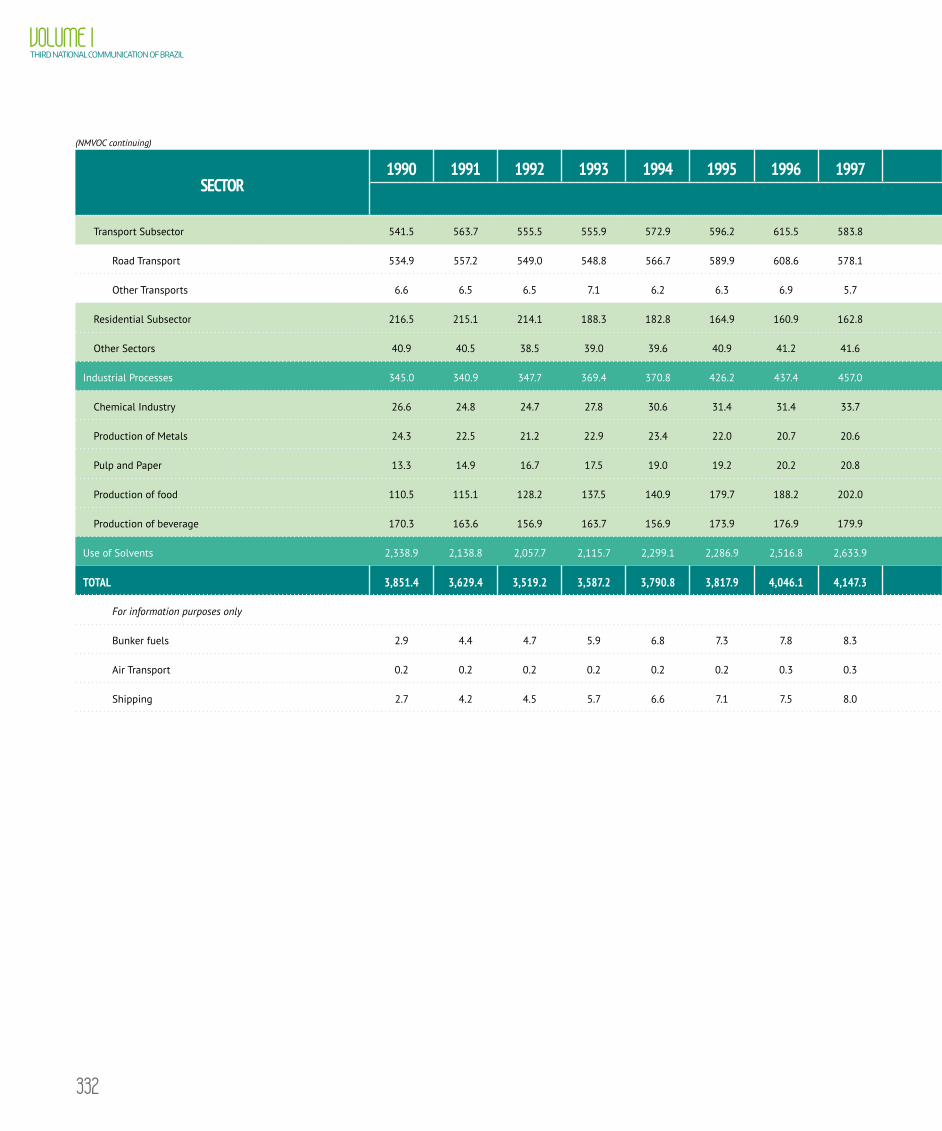
332
VOLUME ITHIRD NATIONAL COMMUNICATION OF BRAZIL
SECTOR1990 1991 1992 1993 1994 1995 1996 1997 1998 1999 2000 2001 2002 2003 2004 2005 2006 2007 2008 2009 2010
Gg
Transport Subsector 541.5 563.7 555.5 555.9 572.9 596.2 615.5 583.8 574.2 531.3 481.5 454.1 469.0 435.7 434.1 417.4 377.2 368.0 360.6 321.1 331.3
Road Transport 534.9 557.2 549.0 548.8 566.7 589.9 608.6 578.1 567.9 525.0 475.3 447.4 462.3 429.0 426.8 410.4 370.4 360.6 352.6 313.4 322.0
Other Transports 6.6 6.5 6.5 7.1 6.2 6.3 6.9 5.7 6.3 6.3 6.2 6.7 6.7 6.7 7.3 7.0 6.8 7.4 8.0 7.7 9.3
Residential Subsector 216.5 215.1 214.1 188.3 182.8 164.9 160.9 162.8 166.2 171.4 175.9 183.3 204.3 212.9 215.9 220.3 221.0 209.7 207.4 204.3 196.1
Other Sectors 40.9 40.5 38.5 39.0 39.6 40.9 41.2 41.6 40.3 40.4 38.8 40.2 41.8 44.3 45.9 46.3 47.3 49.9 54.1 51.8 54.2
Industrial Processes 345.0 340.9 347.7 369.4 370.8 426.2 437.4 457.0 463.4 507.2 532.8 501.8 542.1 590.5 629.5 616.6 745.8 695.3 724.2 717.9 736.8
Chemical Industry 26.6 24.8 24.7 27.8 30.6 31.4 31.4 33.7 35.0 37.5 43.0 40.7 42.3 45.3 49.1 49.1 53.9 56.3 56.6 59.5 61.2
Production of Metals 24.3 22.5 21.2 22.9 23.4 22.0 20.7 20.6 19.4 21.1 23.3 21.5 22.8 25.8 29.8 29.1 28.1 29.5 29.1 18.9 23.0
Pulp and Paper 13.3 14.9 16.7 17.5 19.0 19.2 20.2 20.8 22.0 23.9 24.6 24.5 26.6 30.4 32.3 34.8 37.7 40.5 43.0 45.5 48.5
Production of food 110.5 115.1 128.2 137.5 140.9 179.7 188.2 202.0 204.0 238.8 252.8 223.1 255.5 291.3 317.4 338.8 331.0 374.8 386.6 386.8 407.2
Production of beverage 170.3 163.6 156.9 163.7 156.9 173.9 176.9 179.9 183.0 185.9 189.1 192.0 194.9 197.7 200.9 164.8 295.1 194.2 208.9 207.2 196.9
Use of Solvents 2,338.9 2,138.8 2,057.7 2,115.7 2,299.1 2,286.9 2,516.8 2,633.9 2,879.5 2,976.0 3,154.0 2,899.6 2,958.8 2,657.0 3,032.2 2,982.2 3,722.6 2,475.0 4,135.7 4,317.4 4,749.9
TOTAL 3,851.4 3,629.4 3,519.2 3,587.2 3,790.8 3,817.9 4,046.1 4,147.3 4,373.9 4,497.8 4,674.2 4,356.7 4,504.0 4,272.8 4,734.5 4,660.3 5,489.3 4,187.7 5,879.4 5,899.7 6,387.2
For information purposes only
Bunker fuels 2.9 4.4 4.7 5.9 6.8 7.3 7.8 8.3 9.1 14.4 14.9 17.0 19.2 16.9 16.9 16.9 17.9 19.2 24.2 17.1 21.4
Air Transport 0.2 0.2 0.2 0.2 0.2 0.2 0.3 0.3 0.3 0.3 0.2 0.3 0.2 0.2 0.2 0.2 0.2 0.2 0.2 0.2 0.2
Shipping 2.7 4.2 4.5 5.7 6.6 7.1 7.5 8.0 8.8 14.1 14.7 16.7 19.0 16.7 16.7 16.7 17.7 19.0 24.0 16.9 21.2
(NMVOC continuing)

333
APPENDIX III GREENHOUSE GAS EMISSIONS EstimatEs BY GAS AND SECTOR, FROM 1990 TO 2010
SECTOR1990 1991 1992 1993 1994 1995 1996 1997 1998 1999 2000 2001 2002 2003 2004 2005 2006 2007 2008 2009 2010
Gg
Transport Subsector 541.5 563.7 555.5 555.9 572.9 596.2 615.5 583.8 574.2 531.3 481.5 454.1 469.0 435.7 434.1 417.4 377.2 368.0 360.6 321.1 331.3
Road Transport 534.9 557.2 549.0 548.8 566.7 589.9 608.6 578.1 567.9 525.0 475.3 447.4 462.3 429.0 426.8 410.4 370.4 360.6 352.6 313.4 322.0
Other Transports 6.6 6.5 6.5 7.1 6.2 6.3 6.9 5.7 6.3 6.3 6.2 6.7 6.7 6.7 7.3 7.0 6.8 7.4 8.0 7.7 9.3
Residential Subsector 216.5 215.1 214.1 188.3 182.8 164.9 160.9 162.8 166.2 171.4 175.9 183.3 204.3 212.9 215.9 220.3 221.0 209.7 207.4 204.3 196.1
Other Sectors 40.9 40.5 38.5 39.0 39.6 40.9 41.2 41.6 40.3 40.4 38.8 40.2 41.8 44.3 45.9 46.3 47.3 49.9 54.1 51.8 54.2
Industrial Processes 345.0 340.9 347.7 369.4 370.8 426.2 437.4 457.0 463.4 507.2 532.8 501.8 542.1 590.5 629.5 616.6 745.8 695.3 724.2 717.9 736.8
Chemical Industry 26.6 24.8 24.7 27.8 30.6 31.4 31.4 33.7 35.0 37.5 43.0 40.7 42.3 45.3 49.1 49.1 53.9 56.3 56.6 59.5 61.2
Production of Metals 24.3 22.5 21.2 22.9 23.4 22.0 20.7 20.6 19.4 21.1 23.3 21.5 22.8 25.8 29.8 29.1 28.1 29.5 29.1 18.9 23.0
Pulp and Paper 13.3 14.9 16.7 17.5 19.0 19.2 20.2 20.8 22.0 23.9 24.6 24.5 26.6 30.4 32.3 34.8 37.7 40.5 43.0 45.5 48.5
Production of food 110.5 115.1 128.2 137.5 140.9 179.7 188.2 202.0 204.0 238.8 252.8 223.1 255.5 291.3 317.4 338.8 331.0 374.8 386.6 386.8 407.2
Production of beverage 170.3 163.6 156.9 163.7 156.9 173.9 176.9 179.9 183.0 185.9 189.1 192.0 194.9 197.7 200.9 164.8 295.1 194.2 208.9 207.2 196.9
Use of Solvents 2,338.9 2,138.8 2,057.7 2,115.7 2,299.1 2,286.9 2,516.8 2,633.9 2,879.5 2,976.0 3,154.0 2,899.6 2,958.8 2,657.0 3,032.2 2,982.2 3,722.6 2,475.0 4,135.7 4,317.4 4,749.9
TOTAL 3,851.4 3,629.4 3,519.2 3,587.2 3,790.8 3,817.9 4,046.1 4,147.3 4,373.9 4,497.8 4,674.2 4,356.7 4,504.0 4,272.8 4,734.5 4,660.3 5,489.3 4,187.7 5,879.4 5,899.7 6,387.2
For information purposes only
Bunker fuels 2.9 4.4 4.7 5.9 6.8 7.3 7.8 8.3 9.1 14.4 14.9 17.0 19.2 16.9 16.9 16.9 17.9 19.2 24.2 17.1 21.4
Air Transport 0.2 0.2 0.2 0.2 0.2 0.2 0.3 0.3 0.3 0.3 0.2 0.3 0.2 0.2 0.2 0.2 0.2 0.2 0.2 0.2 0.2
Shipping 2.7 4.2 4.5 5.7 6.6 7.1 7.5 8.0 8.8 14.1 14.7 16.7 19.0 16.7 16.7 16.7 17.7 19.0 24.0 16.9 21.2


Ministry ofScience, Technology and Innovation
Empowered lives.Resilient nations.