This Audubon of Florida publication is Chapter 3 from the final report to the US Army Corps of Engineers, Everglades National Park, and the US Geological Survey for the project entitled, “Development and Testing of Protocols for Sampling Fishes in Forested Wetlands in Southern Florida.” Please cite as:

Liston, S. E., N. Katin and J. J. Lorenz. 2007. Sampling aquatic fauna in cypress forests, Big Cypress National Preserve. In Development and Testing of Protocols

for Sampling Fishes in Forested Wetlands of Southern Florida (S. E. Liston, J. J. Lorenz, C. C. McIvor and W. F. Loftus, eds.). Final Report to the U.S. Army Corps of Engineers, Everglades National Park, and the U.S. Geological Survey. Questions should be addressed to: Dr. Shawn E. Liston Audubon of Florida, Corkscrew Swamp Sanctuary 375 Sanctuary Road West Naples, FL 34120 sliston@audubon.org (239) 354-4469

III-1

III

Sampling Aquatic Fauna in Cypress Forests, Big Cypress National Preserve

Shawn E. Liston Nicole M. Katin Jerome J. Lorenz

SUMMARY South Florida’s cypress forests provide critical habitat for aquatic fauna (fishes,

macroinvertebrates, amphibians), wading birds, and higher vertebrates (alligators, river otters, etc.), but they have been significantly understudied compared to other aquatic habitats in the Greater Everglades ecosystem. Complex habitat structure and dramatic intra-annual hydrologic fluctuations in Big Cypress National Preserve (BCNP) cypress forests present considerable challenges for sampling aquatic fauna using methods traditionally employed in other Everglades habitats. It is imperative, however, to understand community structure, function, and faunal standing stocks in this habitat prior to any hydrologic alteration of the system through CERP projects. In this study, we: (1) tested numerous sampling gears commonly employed in other parts of the Everglades system to develop a robust protocol for sampling cypress forest aquatic fauna, and (2) collected baseline data describing spatial and temporal variation in cypress forest aquatic fauna communities. Sampling was conducted five times annually (corresponding with early-wet, mid-

wet, transition, mid-dry, and late-dry seasons) from 2005-2007 at three sites in BCNP. We evaluated 9-m2 drop traps, 6-m2 bottomless lift nets, 1-m2 throw traps, drift fence arrays and experimental gill nets, many of which were modified in attempts to improve their performance in this system. Estimates of fish density (total fish density and density of most ‘common’ species) were significantly lower in drop traps than throw traps or lift nets. Logistical issues constrained the effectiveness of lift nets and drift fence arrays. Gill nets were only valuable in rare cases when numbers of large fishes moving into sites increased. The primary limitation of all methods except the 1-m2 throw trap, was an inability to quantify macroinvertebrates. We saw no difference in fish density between traps that included large habitat structure (tree trunks, large root masses, large woody debris) and those that excluded it. We conclude that the 1-m2 throw trap is the most effective and practical aquatic fauna sampling method in this system, and provide recommendations for a long-term monitoring program based on power analyses of baseline data.

III-2

Aquatic fauna communities changed significantly throughout each year of this

study in response to dramatic hydrologic variation. All sites re-flooded relatively quickly in June/July of each year and water levels receded much more slowly in the dry season. In general, wet prairies dried in late-November to early-December, shallow zones dried between January and March, and deep zones and refuges dried in mid- to late March. Upon cypress forest re-flooding, macroinvertebrate (primarily crayfish) density increased rapidly and fish density increased more slowly (crayfish constituted a majority of the fauna density and biomass in the early- and mid-wet seasons). Invertebrate density began to decrease with the on-set of the dry season (~December/January) and continued to decrease throughout the dry season. Fish density increased throughout the season, reaching a maximum in deep-water refuges in the late-dry season just prior to marshes drying. Amphibian density was generally quite low throughout the study, showing little variation. Data collected in this study illustrate that community structure, density, and biomass of cypress forest aquatic fauna respond directly to hydrologic variation. Because several CERP projects are expected to impact the hydrology of eastern portions of BCNP, and this system appears to be extremely sensitive to hydrologic change, we feel it is imperative that continued aquatic fauna (prey-base) monitoring efforts include BCNP cypress forests.

INTRODUCTION Freshwater forested wetlands Forested freshwater wetlands provide critical habitat for fish and macroinvertebrate

communities, but they have been poorly studied compared to other freshwater wetlands. These systems are often seasonally inundated, with aquatic fauna moving into the system during periods of flooding and then seeking deeper-water refuges when waters recess. Timing and delivery of water to freshwater forested wetlands is critical to proper ecosystem functioning. Fish in permanent freshwater systems are often so dependent upon forested floodplains for feeding, spawning, and rearing of young that it has been argued the permanently flooded aquatic systems and their neighboring temporarily- or seasonally-flooded forested habitats should be considered as a single system (Lambou 1990). Adjacent, temporarily- or seasonally-flooded forests have been found to provide important habitat for fish in large rivers (Kwak 1988, Turner et al. 1994), streams (Ross & Baker 1983), and coastal wetlands (Poulakis et al. 2002). Fish in these forested systems may actually depend on annual water level fluctuation to limit intra- and interspecific competition for food, space, and spawning grounds (Lambou 1959), although the relative importance of habitat structure and hydrologic variability is likely species-specific (Ross & Baker 1983). Due to the fact that seasonally-flooded forested systems are cut-off from continuously inundated areas as water levels recede,

III-3

competition for food in these systems may become increasingly important as the dry season progresses. Lambou (1959) found that approximately 44% of fish collected in a Mississippi River floodplain forest were predators. Lambou further concluded that predaceous fish must be partially dependent upon some type of forage other than fish, suggesting that swamp crayfish are likely important in their diet. Studies have also suggested strong aquatic-terrestrial food web links in these systems, as terrestrial invertebrates may provide a significant proportion of fish diet, in some cases (Arner et al. 1976, Woodall et al. 1975). Ecological role of cypress forests in the Greater Everglades system Although the Greater Everglades ecosystem contains thousands of hectares of

freshwater forested wetlands, a paucity of information exists on their aquatic faunal communities. The few studies that have previously been conducted in South Florida cypress forests focused primarily on fish and spanned relatively small spatial and temporal scales, leaving large-scale spatial variation, inter- and intra-annual variation, and overall faunal community structure virtually undescribed. Several groups in the 1960s and 1970s made fish collections to describe prey populations for wading birds (Kahl 1964, Kushlan 1974, Browder 1976). More recent studies have described the composition and distribution of native and non-indigenous fishes in southern areas of Big Cypress National Preserve (BCNP) (Loftus & Kushlan 1987) and produced inventories of fishes found in the different habitats of BCNP (Ellis et al. 2003). Limited records of fish collections in the Big Cypress Region (BCR) have also been reported by Loftus (1987, written communication) and Dalrymple (1995). Small quantitative studies describing fish community dynamics in shallow- and deep-water habitats in the Corkscrew region of Big Cypress (Carlson & Duever 1979) and comparing fish communities in natural and restored habitats within the Big Cypress Seminole Indian Reservation (Dunker 2003), have also been reported. Forested wetlands provide critical nesting and foraging habitat for wading birds in

South Florida. In Florida, wood storks (Mycteria americana) nest primarily in the Everglades, most often in the tops of cypress and mangrove trees. Wood stork populations declined from 20,000 nesting pairs in the 1930s to 5,000 nesting pairs in the late 1970s, prompting their addition to the federal register of endangered species in 1984 (US Fish & Wildlife Service 1996). Declines in wood stork populations have been linked to a decline in small fish that serve as their prey-base, due primarily to loss of wetland habitat and detrimental changes in hydrology (US Fish & Wildlife Service 1996). Wood storks feed primarily on fish (mosquitofish, sunfish, killifish) but also commonly consume crayfish and other aquatic prey (Kahl 1964). White ibis (Eudocimus albus), identified as a Species of Special Concern by the State of Florida, feed on fish and crayfish and were the most abundant birds observed during 2005 systematic reconnaissance flights (SRF) (Nelson & Metzger 2005). Ibis were observed to use trees in BCNP for roosting. Reports from 2005 SRF flights indicate that the east-central area

III-4

of BCNP (the L28 gap area) is one of three regions of the Preserve with the highest densities of wading birds, and that the areas with the highest densities were those that tended to be wetter (Nelson & Metzger 2005). Density of wading birds was lower in BCNP than the adjacent Water Conservation Areas (WCAs), also likely due to water levels and period of inundation. Potential impact of CERP activities on the Big Cypress ecosystem Several CERP projects have the potential to impact cypress forests of BCNP, both in

the very near and more distant future. Most immediately, hydrologic restoration of Picayune Strand (Southern Golden Gates Estates) is beginning. While hydrological alteration of BCNP is not expected from this project, comparisons with baseline and concurrent data from aquatic communities in un-impacted portions of the region will be very important in assessing the effect of restoration efforts on this ecosystem. Furthermore, the development of robust, quantitative sampling methods for Southwest Florida’s forested wetlands is essential to the monitoring efforts that will accompany this restoration project. Several other CERP projects will be beginning in the next few years, and it is imperative that baseline data describing the aquatic faunal community are collected prior to these restoration efforts. The WCA 3 Decompartmentalization and Sheetflow Enhancement project, Seminole Big Cypress Plan, Big Cypress/L-28 Interceptor Modifications and Western Tamiami Trail Culverts will all change hydrology in BCNP (particularly in the north-eastern and eastern regions). Furthermore, concerns exist about additional nutrient delivery to the highly-oligotrophic system with the proposed changes in water delivery. Numerous studies in Everglades graminoid marshes have found fish and

macroinvertebrate communities to be quite sensitive to changes in hydrology and nutrient status. Altered hydrology has been seen to correlate with changes in fish community structure (Chick et al. 2004, Trexler et al. 2005, Ruetz et al. 2005) and aquatic macroinvertebrate abundance (Liston et al. in prep). Furthermore, interactions between hydroperiod and eutrophication have been linked to changes in fish and macroinvertebrate community structure (Liston 2006) and food web alterations (Williams & Trexler 2006). Because the systems have similar faunal assemblages, it is likely that fish and macroinvertebrate communities in the Big Cypress system will be equally sensitive to hydrologic and nutrient impacts, but the magnitude of these impacts is unknown. It is thought that flooded forests in Big Cypress may be even more sensitive to hydrological changes than Everglades graminoid marshes, due to a steeper gradient in topography and greater inter-annual variation in water depths.

III-5

Objectives

The objectives of this study were:

(1) To compare the effectiveness and utility of sampling methods (drop trap, bottomless lift net, throw trap, drift fence, gill net) for aquatic fauna in flooded forests of Big Cypress National Preserve

(2) To collect baseline data describing spatial and temporal variation in aquatic faunal communities in flooded forests of Big Cypress National Preserve

(3) To cooperate and coordinate efforts with mangrove forest and stable isotope/food web project components

METHODS Site selection and sampling design We sampled at three sites in BCNP (Figure III-1) that are geographically dispersed

and span the range of mixed swamp and cypress forest habitats found in the Big Cypress Region (BCR). Each site (L-28, Bear Island, and Raccoon Point) consisted of three replicate plots, with ‘shallow’ and ‘deep’ zones within each. Typically, deep zones were in the center of cypress domes and shallow zones were in more peripheral areas of the dome (Figure III-2). Additionally, ‘prairie’ zones were located at one L-28 plot and two Raccoon Point plots that have open cypress prairie immediately adjacent to the forest (only throw-trap samples were collected in wet prairies). Sampling was conducted five times annually during the 2005-2006 and 2006-2007 seasons: early-wet season, mid-wet season, transition, mid-dry season, and late-dry season. We conducted additional sampling, as needed, to correlate with hydrological differences between sites and to obtain additional replicates for the habitat structure portion of the methods comparison. Sample collection Sampling gear employed in this study was selected following a literature review of

published studies conducted in both forested wetlands and Everglades’ graminoid marshes (Appendix 1). A variety of sampling gears that target fish, macroinvertebrates and amphibians were used in order to determine their utility and effectiveness in cypress forests. Sampling gears that were used included 4-m2 and 9-m2 drop traps (Lorenz et al. 1997), 6-m2 bottomless lift nets (Rozas 1992), 1-m2 throw traps (Jordan et al. 1997), drift fence arrays (Loftus et al. 2005), and 38-m experimental gill nets (Hubert 1996). These sampling gears were added throughout the study as water levels and other logistical factors allowed for their installation and proper function (Appendix 2). In some cases use of gear was discontinued when it became clear that it was ineffective.

III-6

During each sampling event we collected two drop trap samples (fixed locations; one in deep zone and one in shallow zone), six throw-trap samples (haphazard; three in deep zone and three in shallow zone), and one lift net sample (deep zone at Bear Island only). Three replicate throw-trap samples were also collected at each plot with a prairie zone (L28-3, RP-2, RP-3). At one plot within each site, one drift fence (fixed location; located between shallow and deep zones) and one gill net were also deployed. Additional efforts included throw-trap sampling in deep-water refuges adjacent to two plots (L28-1 and RP-2) when possible in the mid-late dry season (when water levels were low enough (<80 cm) to allow use of the throw trap). In order to facilitate analyses of the influence of habitat structure within traps on

capture efficiency, we installed an additional deep drop trap (DDTX) at each Bear Island plot in the 2006-2007 hydrologic season. While the existing drop traps were installed so that they enclosed ~20% habitat structure (small pond apple or cypress tree), DDTX traps were installed adjacent to the existing deep drop traps in tree-less areas (no habitat structure). Deep drop traps and deep throw traps at Bear Island were sampled during our routine sampling events (mid-wet, transition and mid-dry seasons), as well as on two additional occasions (early- and mid-December 2006). Gear and methods were adopted from those currently used in Everglades’

graminoid and mangrove habitats, and developed using recommendations from sampling in Big Cypress Swamp made by Ellis et al. (2003) and Dunker (2003). Some modifications were made in response to difficulties encountered with extreme annual hydrologic variation and excessive amounts of habitat structure (trees, tree roots, woody debris; see Figure III-3):

Drop trap - We omitted the substrate raking step described by Lorenz et al. (1997) due to the sensitivity of the cypress forest floor and understory vegetation to disturbance. Additionally, due to extremely low catches on the second day of sampling, we only sampled each trap for one day on several occasions to better utilize time and energy in the field (refer to Results for more details on day 1 versus day 2 catches). Nets were made taller and modified to include a 15-cm weighted skirt to help seal the trap against the uneven forest floor (and small submerged woody debris). We also increased the amount of rotenone 2- to 3-fold due to decreased rotenone effectiveness in this environment (likely due to the presence of large amounts of vegetation and woody debris). While we initially installed 4-m2 drop traps, prior to the October 2005 sampling we replaced them with taller, 9-m2 traps that enclosed ~20% habitat structure (small pond apple or cypress tree) to allow for use in deeper water and to facilitate comparison with data from other systems. See Appendix 3A for the drop trap standard operating procedure (SOP) used in this study.

III-7

Throw trap – Due to difficulties encountered moving the trap through the cypress forest, we developed a collapsible throw trap that is more manageable in this environment. We also added a 15-cm weighted skirt to the bottom of the trap to help seal the trap against the uneven forest floor (and small submerged woody debris). See Appendix 3B for the throw trap SOP used in this study. Lift Net – Bottomless lift nets in mangrove forests were designed to be cleared using tidal fluctuations, but in this study lift nets were cleared using rotenone (fin-clipped fish were also used to estimate trap efficiency, as with drop traps). See Appendix 3C for the lift net SOP used in this study. Drift fence – While the center box (1 m x 1 m) was permanently installed, drift fence wings were attached with Velcro© and removed when not in use. To modify this method for deeper water and limited open-space in cypress forests, drift fences were made taller (4 feet high) and wings were shortened to 6 m. See Appendix 3D for the drift fence array SOP used in this study. Gill Net – The gill nets we deployed were 38-m with five panels: 2.54 cm, 3.81 cm, 5.08 cm, 6.35 cm, and 7.62 cm. Initially we used a 30-m soak time, but we continued to modify this based on catch and by-catch. See Appendix 3E for the gill net SOP used in this study.

Hydrology and physicochemical data collection In April 2006 we installed a Telog© continuous water level recorder at one plot at

each site (BI-1, L28-1, RP-2) and a permanent staff gauge at all other plots. Due to the extreme intra-annual hydrologic fluctuations at our sites, Telog© data were found to be unreliable at the upper and lower extremes of their depth range. In order to obtain hydrologic data at each site throughout the entire year, Telog© data (excluding extreme upper and lower values where data were inaccurate) were correlated with stage data from nearby hydrologic gauging stations (BCA1 for BI, BCA18 for L-28 and BCA3 for RP). Data were highly correlated (BI: R2=0.975; L28: R2=0.987; RP: R2=0.994), and regression equations were used to estimate daily depths ate each site. Data from staff gauges at each plot within a site were also highly correlated (no significant intra-site hydrologic variation; all R2>0.80) which allowed estimation of the daily depth at each plot, and calculations of days-since-dry (DSD) to correspond with each collected sample. We used a YSI-556 or a YSI-85 (with a pH10 pH/temperature pen) to collect water

temperature, dissolved oxygen (percent saturation and concentration), specific conductance, and pH in each sampling location during each sampling event. Water depth was also recorded to correspond with each sample. Beginning in April 2006, we took digital photographs of the canopy at each permanent sampling location (drop

III-8

traps and lift nets) using a Nikon Coolpix 8700 digital camera with a 180º fish-eye converter lens (Nikon model FC-E9) to test the feasibility of obtaining accurate estimates of canopy cover. Sample processing Field samples were kept on ice in the field and frozen for preservation. In the

laboratory, fauna were identified (fish, decapods and adult amphibians to species and other invertebrates to lowest feasible taxonomic level (often family or order)), enumerated, and length (standard length for most fish, total length for Lepisosteus platyrhincus (Florida gar) and Amia calva (bowfin), snout-vent length for sirens and newts, carapace length for crayfish), mass, and sex (when possible) data were recorded. See Appendix 3F for detailed SOP for laboratory processing of aquatic fauna samples. Data analysis Prior to analyses, water depth, water temperature, specific conductance, dissolved

oxygen concentration, and density and biomass of taxa were ln(y+1) transformed and

proportions (relative abundances, percent dissolved oxygen) were arcsine(√y) transformed to fulfill assumptions of normality. All results reported from ANOVA are based on type III sums-of-squares (Shaw & Mitchell-Olds 1993). Methods comparison: We compared densities of common fish species (incidence

≥10%) in the three fixed-area traps (drop trap, lift net, throw trap) across sampling seasons at one site (BI) using analysis of variance (ANOVA). Additionally, we used ANOVA to compare drop traps and throw traps at all sites across seasons and zones (shallow deep). Habitat structure: The influence of habitat structure on the ability of traps to collect fish was determined by Repeated Measures ANOVA of simultaneous sampling efforts using drop traps with habitat structure, drop traps without habitat structure, and throw traps. Baseline data: Analyses of baseline data focused only on data collected in 1-m2 throw traps. We used ANOVA to examine spatial and temporal variation in physicochemical data (water depth, water temperature, specific conductance, and dissolved oxygen). Three-way ANOVA were used to examine variation among sampling sites, seasons, and zones (deep, shallow, prairie). Spatial variation (across sites and zones) in emergent macrophyte community structure was described using a 2-way crossed analysis of similarities (ANOSIM) based on a standardized Bray-Curtis dissimilarity matrix (Clarke 1993, Clarke & Warwick 1994). Variation in the density of common emergent macrophyte species and the percent cover of floating and submerged species was described using 2-way crossed ANOVA (site, zone).

III-9

Fauna communities (fish and macroinvertebrates) were analyzed using a combination of multivariate and univariate techniques. Community analyses

focused on common taxa (incidence≥10%). Temporal and spatial variation in fish and macroinvertebrate community structure (by season, site) were described using 1-way ANOSIM based on both standardized and non-standardized Bray-Curtis dissimilarity matrices. Non-metric multidimensional scaling (nMDS) was used to help visualize observed patterns. We then used factorial ANOVA to describe patterns in density and biomass of taxa between sites (BI, L28, RP), sampling seasons (early-wet, mid-wet, transition, mid-dry, late-dry), and zones (prairie, shallow, deep, refuge).

RESULTS Summary of Sampling Efforts

2005-2006 Season We completed five sampling events in BCNP during the 2005-2006 hydrologic season. We made numerous adjustments to our sampling strategy with each sampling event, adding new sampling gear types and adjusting them for use in cypress forests. Sampling was frequently limited by the dynamic hydrology of BCR cypress forests. July 2005 (Early Wet Season) – Heavy rains from Hurricane Dennis resulted in

extremely high water levels at our sites, and impeded much of our sampling effort. High water levels prevented installation of lift nets at Bear Island. Water levels were too high to sample drop traps in any of our ‘deep’ zones. Shallow drop traps were sampled at all sites and plots. October 2005 (Mid Wet Season) – Deep and shallow drop traps were sampled and we

began the use of the 1-m2 throw trap in deep, shallow, and prairie zones. We were only able to complete our sampling at the L-28 site, however, as BCNP closed on 10/19/05 in anticipation of Hurricane Wilma. Hurricane Wilma – We visited all BCNP sites 11/10/05 to assess damages from Hurricane Wilma (J. Lorenz, S. Liston, W. Loftus, D. Green). While many sites incurred significant damages, our Bear Island site was particularly impacted. Small tree limbs and large debris were removed from many traps that were otherwise in good condition. Drift fences appeared to have incurred significant damage, but they were completely submerged and damage assessments were not possible until water levels receded (March 06). Most repairs were made in the field on 11/10/05; all other repairs were made prior to December sampling.

III-10

December 2005 (Transition) – Drop-trap and throw-trap sampling was completed at all sites. February 2006 (Mid Dry Season) – We began sampling bottomless lift nets at Bear

Island, and continued sampling drop traps and throw traps at all sites. We were unable to sample one shallow drop trap at L-28, as it was dry. April 2006 (Late Dry Season) – Our April sampling effort was significantly reduced due to low water levels in BCNP cypress forests. At Bear Island, we were only able to sample in deep habitat zones (all deep drop traps, 1 lift net, and 9 deep throw traps). At L-28, we were only able to sample 1 deep drop trap, and 5 deep throw traps. While all of our Raccoon Point plots were dry, we were able to collect 4 throw-trap samples in a deep-water refuge in the center of the cypress dome at one plot (RP-2). Although all drift fence locations were dry, we removed the old drift fences at all sites, and replaced them with the newly designed drift fences. Permanent hydrologic monitoring stations were installed at one plot at each site, and staff gauges were installed at all other plots. 2006-2007 Season We completed six regular sampling events in BCNP during the 2006-2007 season (two sampling efforts were made in the early wet season). Two supplemental sampling efforts were made at Bear Island in December 2006 for habitat structure analyses. Additional sampling efforts were also made in deep-water refuges at L-28 and Raccoon Point during the late-dry season. We adjusted the sampling schedule to accommodate a late on-set of the wet season and an early on-set of the dry season. Beginning in December 2006, we focused all methods testing at Bear Island, and discontinued use of drop traps and drift fences at other sites. July 2006 (Pre-Early Wet Season) – With a delayed wet-season, sampling efforts were limited by low water levels. All plots at L-28 were completely dry. At Bear Island, we were able to sample all drop traps, 2 lift nets, and triplicate throw-trap samples in all deep zones. We also installed and sampled a second deep drop trap (DDTX) at each Bear Island plot (enclosing no habitat structure). Only one Bear Island plot (BI-1) had enough water to sample using the drift fence and gill net. We were able to sample all Raccoon Point plots (including prairie zones). We were unable to complete our sampling at one plot (RP-1), however, due to heavy smoke from a controlled burn adjacent to our plot. We sampled the drift fence and gill net at one plot (RP-2). We discovered that the permanently installed drift fence center boxes at several sites had been damaged or destroyed by bears.

III-11

August 2006 (Early Wet Season) – We added an August sampling effort this year in response to a delayed wet season in southwest Florida. Due to time and other resource limitations, we only collected samples using throw traps and gill nets. By the end of August, all sites had re-flooded and triplicate throw trap samples were collected at each sampling location. Gill nets were used to sample large fish at one plot at each site (30-60 min soak time; BI-1, L28-3, RP-2), but no fish were collected using this method. October 2006 (Mid Wet Season) – At the height of the wet season, we were able to sample all sites with all methods except lift nets (water was too deep). DDTX were sampled at two Bear Island plots; DDTX at BI-2 needed to be re-built and was not sampled. December 2006 (Transition) – Drop trap and throw trap sampling was completed

where possible. Shallow zones at all Bear Island plots, one Raccoon Point plot, and one L28 plot were dry (not sampled). We sampled all DDTX, lift nets, and one drift fence at Bear Island, and set a gill net at one plot at each site. In an attempt to identify and begin sampling an additional ‘reference’ site, we established and sampled (throw trap only) two plots at Fire Prairie Trail. Additional Habitat Structure Sampling – Two additional sampling efforts were made at

Bear Island in December 2006 (12/04-05 and 12/19-20) to supplement comparisons of the influence of habitat structure. In each of these efforts, we sampled drop traps (DDT and DDTX) and throw traps (DTT) in the deep zone of each plot. We also sampled with drift fences to continue testing this method. January 2007 (Mid Dry Season) – The relatively quick drying of cypress forests in the BCR prompted an earlier-than-usual sampling effort. All shallow zones at all sites, except one plot at L28, were dry (not sampled). One plot at Raccoon Point was completely dry (deep and shallow). The drift fence at Bear Island was sampled, and one gill net was set at each site. Throw trap sampling was completed at both plots previously established at Fire Prairie Trail, but we were not able to identify a third plot and temporarily abandoned this sampling location (this site was eventually eliminated; data are sparse and not presented in this report). March 2007 (Late Dry Season) – By early March, all sampling locations were dry

except two deep plots at L28 which were sampled with the throw trap. Throw trap samples were also collected from deep-water refuges at L28-1 and RP-2. Additional Dry-Season Refuge Sampling – To describe the dynamics of fauna

communities at our sites as the dry season progressed, we collected additional throw-trap samples in deep-water refuges at L28-1 and RP-2. In February and

III-12

March we sampled the refuge at RP-2 twice and the refuge at L28-1 once, in addition to refuge sampling conducted during our ‘late dry season’ sampling event.

Comparison of Sampling Methods Fixed Area Sampling Devices: drop traps, lift nets and throw traps

Comparisons of 9-m2 drop traps, 6-m2 bottomless lift nets and 1-m2 throw traps

were made by adjusting for enclosure size. Samples collected with 4-m2 drop traps (July 2005) were excluded, as these traps were only sampled once and no other enclosure methods were used simultaneously. Efficiency of drop traps and lift nets was estimated using mark-recapture

techniques. Percent of fish recaptured did not vary by site, sampling season, trap type or zone (all P>0.05). In numerous cases (see Table III-1), efficiency estimates were not made because fish density was extremely low and fish could not be captured to mark and release. Overall, 57% of the 428 marked fish were recaptured. Gambusia holbrooki (Eastern mosquitofish) was the most commonly marked species (n=253) and had the highest recapture rate (69%). Recapture rates of Lepomis marginatus (dollar sunfish; n=88) and Jordanella floridae (flagfish; n=43) were 36% and 58%, respectively. Of the 9 other species used for efficiency estimates, ≤12 individuals of each were marked and recapture rates ranged from 0% to 100% with no clear patterns. Because no recapture rates were estimated for throw traps, efficiency estimates were not used to adjust density estimates. Side-by-side comparisons of drop traps, lift nets, and throw traps were made at

Bear Island from October 2005 to December 2006. ANOVA indicated total fish density varied by season and with trap type (Table III-2). Estimates of total fish density from throw traps and lift nets were similar while density estimates from drop traps were significantly lower (Figure III-4). Densities of 6 common fish species (Cichlasoma urophthalmus (Mayan cichlid), Elassoma evergladei (Everglades pygmy sunfish), Fundulus chrysotus (golden topminnow), G. holbrooki, Heterandria formosa (least killifish), and Lucania goodei (bluefin killifish)) showed patterns similar to those seen in total fish density, although results varied by season (sampling event). Further comparisons of drop traps and throw traps were made in both shallow

and deep zones across all sites from October 2005 to October 2006. In the early wet season, density estimates from the two methods were similar (and extremely low). In all other sampling seasons, estimates of total fish density made with throw traps were significantly higher than those made with drop traps (Table III-3, Figure III-5). ANOVA indicated significant variation in fish density with trap-type in 8 common fish species: C. urophthalmus, E. evergladei, J. floridae, G. holbrooki, H. formosa, Lepomis

III-13

gulosus (warmouth), L. goodei, and L. marginatus. We saw significant variation across sampling seasons, but significant variation among traps (P≤0.05) was attributed to

throw trap density estimates being higher than drop trap density estimates in all cases (Figure III-5).

A note on 2-day sampling: The drop trap protocol outlined by Lorenz et al. (1997)

described a 2-day sampling effort: netting all visible fish within the trap the day rotenone is applied (“set-up day”) and returning the following day when water had cleared (“take-down day”) to remove all remaining fish (also see Appendix 3A). Due to time restrictions, the considerable distance and subsequent travel time between sites, and early indications of the small proportion of fish collected on Day 2, the second day of sampling was omitted for the majority of this study (see Appendix 2). Toward the end of the study, we re-instituted the 2-day sampling protocol to obtain estimates of the efficiency of our single-day sampling. Of the 1180 fish collected in drop traps and lift nets using the 2-day protocol, over 88% were collected on Day 1 (Table III-4). With one possible exception, Day 2 catches were minimal and did not appear to be biased for or against individual species (the only two Hoplosternum littorale (brown hoplo catfish) in these samples were collected on Day 2 in a single trap). Evaluation of Drift Fence Arrays Drift fence arrays were sampled 5 times in the 2006-2007 hydrologic year.

Overall, CPUE was relatively low and fish catch was dominated by G. holbrooki (Table III-5). While the small data set prohibited analysis of directional fish movement, no patterns were evident from observation of the raw data. The decision to discontinue this sampling method was based on both the paucity of data collected and the logistical challenges outlined below. We had to redesign the drift fence arrays several times throughout the study in

response to logistical issues. Due to large amounts of water moving through the forest, and the associated movement of large woody debris, we made array ‘wings’ shorter and removable and we removed them between sampling events. Wings were also made taller in an attempt to accommodate high water levels. Even with these redesigning efforts, this method did not prove to be practical. Drift fences had to be located near the deep zone so they could be sampled several times throughout the season, but due to high water levels we were often unable to sample them during the peak of the wet season. Additionally, it is unclear whether the CPUE obtained in drift fence minnow traps is correlated with the density of fishes in the wetland, and what influence priority effects (which fishes enter the traps first) have on the fish collections. Due to these concerns and the relative success of other methods, efforts with drift fence arrays were abandoned in December 2006.

III-14

Evaluation of Experimental Gill Nets Experimental gill nets were used to sample large fishes at each site 5 times

throughout the 2006-2007 hydrologic year. Target soak time was 1 h, but in many cases soak time was adjusted due to logistical constraints (the amount of time available at a particular sampling location) and other factors. Soak time was extended in several cases where nets were empty after 1 h. In cases where many fish were caught, soak time was decreased in order to minimize stress and handling mortality of large fishes (see Appendix 2 for individual soak times). In total, we collected 106 fish from 5 species (Table III-6). Of the fish collected, 96

(90.6%) were collected from 3 large samples at BI-1 (pre-early wet, transition, and mid-dry seasons). In these cases, large numbers of H. littorale and L. platyrhincus were captured while moving (via a culvert) between a deep pond and the adjacent cypress forest. While gill nets were effective in capturing these large fishes moving through the cypress forest at this site, overall the incidence of large fishes was extremely low in this study. Additionally, since gill net catch is dependent upon fish movement, the application of these data to quantifying fish standing crop or species richness is questionable (we noted several cases that fish were present at this site and not moving around, therefore not becoming entangled in the net).

After evaluating the various sampling methods employed in this study, we concluded 1-m2

throw traps are the most effective method for estimating density and biomass of aquatic fauna in cypress forests. As such, subsequent analyses and descriptions of spatial and temporal variation in macrophyte and aquatic fauna communities are based on data collected in throw traps (except ‘Effect of Habitat Structure’ section). Physiochemical Variation Water depth, temperature, specific conductance, and dissolved oxygen levels generally varied across sampling zones and within the hydrologic season (Table III-7). As expected, water depth increased from the wet prairie to the deep zone (Figure III-6). Water depth rose quickly in the beginning of the wet season, reaching a maximum in the mid-wet season (October) and decreasing through the late-dry season (March/April) (see Hydrology (below) for more detail). Water temperature did not vary significantly among zones, but decreased from the early-wet season to the mid-dry season and then increased in the late-dry season (Figure III-7). Specific conductance increased throughout the season (from early-wet to late-dry) (Figure III-8). Late in the wet season, specific conductance was often higher in the shallow zone than the deep zone (this was most dramatic at Bear Island). Dissolved oxygen (% saturation and concentration) was higher in wet prairies than other zones and

III-15

tended to increase in the late-dry season (Figures III-9, III-10). No significant variation was observed in pH across sites, seasons, or zones (P>0.05).

Canopy Cover - From April 2006 to January 2007, 80 hemispherical canopy photographs were taken at drop traps and lift nets during routine sampling events (Figure III-11). Although these images may be useful in providing a generalized description of canopy openness at each site during each sampling event, a number of logistical issues prevented us from obtaining quantitative estimates of photosynthetically active radiation (PAR) or leaf area index (LAI) using this technique. Hemispherical photography is a common method for obtaining estimates of PAR and LAI to correlate with variation in ecological communities (Weiss et al. 1991, Grether et al. 2001, Skelly et al. 2005). To obtain images that can be used for these analyses, however, photographs must be taken with uniform sky-lighting as appears either early in the day, late in the evening or under overcast skies (Weiss et al. 1991, Roxburgh & Kelly 1995, Robison & McCarthy 1999, Grether et al. 2001, Inoue et al. 2004). Due to the logistics associated with sampling at remote locations in South Florida’s forested wetlands, it is impractical to coordinate sampling events with these ‘ideal’ atmospheric conditions. Additionally, the establishment of a formal protocol for the utilization of digital hemispherical photography as it applies to ecological assessment studies continues to be an issue of debate among researchers, an issue further complicated by the constant evolution of camera technology as well as computer software necessary for analysis (Jonckheere et al. 2004, Zhang et al. 2005, MacFarlane et al. 2007). For these reasons, it is our opinion that the integration of hemispherical photography to quantify canopy cover (PAR and LAI) is not practical for long-term monitoring of aquatic fauna in this ecosystem.

Hydrology

Daily water level data indicated dramatic intra-annual hydrologic variation at our sites (Figures III-12, III-13, III-14) and significant intra-site variation in some cases. In the 2005-2006 season, most sampling locations were inundated in early-June. Several sampling zones, however, failed to dry in the previous season(s) and had been inundated for over one year prior to our first sampling event: 3 zones at Bear Island had been inundated since July 2004, 1 zone at Bear Island had been inundated since June 2001, 3 zones at L-28 had been inundated since prior to December 2000 (hydrologic data were not available prior to this date), and one zone (the refuge at RP-2) had been inundated since May 1999 (Table III-8). With the exception of one location (BI-2, deep zone), all sites dried completely in the 2006 dry season. In general, prairies dried January to March, shallow zones dried March to April, deep zones dried April to May, and refuges dried in early-May.

III-16

In the 2006-2007 season, all sites re-flooded between mid-June and mid-July 2006. All sites dried completely in the winter/spring of 2007, with most sites drying from one to three months earlier than in the previous year. In general, prairies dried late-November to early-December, shallow zones dried January to March, and deep zones and refuges dried in March. The average number of days each sampling zone was inundated was similar among sites, and was greater in 2005-2006 than in 2006-2007 (Table III-9).

Understory Macrophyte Community

We identified 21 emergent and 10 floating and/or submerged macrophyte taxa within throw traps (Table III-10). Community structure of emergents varied with both site (Global R=0.217, P=0.003) and zone (Global R=0.315, P=0.001). Site variation was attributed to differences between L28 and RP (pairwise: Global R=0.236, P=0.006; other pairs P>0.05). Relative abundances of Panicum spp. (panic grass), Pontederia cordata (pickerelweed), Thalia geniculata (alligator flag), and Eleocharis spp. (spikerush) were higher at L28, while relative abundances of Rhynchospora spp. (beakrush), Cladium jamaicense (sawgrass), and Taxodium spp. (bald or pond cypress) were higher at RP (cumulative dissimilarity=95.83%). Significant pairwise variation in community structure was seen across all zones (P<0.05), with the exception of deep and refuge which were similar (P>0.99). The wet prairie zone was characterized by Rhynchospora spp., Eleocharis spp., Stillingia aquatica (water toothleaf), and Panicum spp. (cumulative similarity=93.42%). The shallow zone was characterized by Panicum spp., P. cordata, and C. jamaicense (cumulative dissimilarity=90.95%). The deep zone was characterized by T. geniculata, P. cordata, and T. distichum (cumulative dissimilarity=100.00%) and the refuge was characterized by T. geniculata (cumulative similarity=100.00%). NMDS failed to help visualize this variation. Univariate analyses indicated densities of emergent macrophytes and relative

abundance of floating and submerged vegetation varied with both site and zone (Table III-11). Three of 8 common emergent species and 5 of 7 common floating and submerged species varied significantly across sites. While some species were particularly abundant or absent from specific sites (e.g., Bacopa caroliniana (lemon bacopa) was absent at BI), no consistent patterns were evident. Densities of most macrophyte species (6 of 8 common emergent, total emergents, and 6 of 7 common floating and submerged species) varied across zones, and four distinct patterns were evident in their variation. Total emergent stem density, like densities of Panicum spp., Eleocharis spp., S. aquatica, and floating periphyton, decreased from prairie to refuge (Figure III-15A). Sagittaria graminea (grassy arrowhead), P. cordata, C. jamaicense, and Ludwigia repens (red ludwigia) were most abundant in the shallow zone and less abundant in other zones (Figure III-15B). B. caroliniana and Eleocharis vivipara (sprouting spikerush) had increased densities in shallow and deep zones

III-17

and very low densities elsewhere (Figure III-15C). Salvinia minima (water fern), Utricularia foliosa (leafy bladderwort), and T. geniculata were most abundant in

refuges, and had low densities in all other zones (Figure III-15D).

Aquatic Fauna Community (See Appendix 4 for description of fauna species collected by season, site, zone, and trap type)

We observed dramatic variation in the aquatic fauna community in the two years of this study. Variation in density and biomass were similar (Figures III-16, III-17). Fish and invertebrate density increased with the onset of the wet season, with invertebrates increasing more quickly than fishes early in the season. Fish density reached a maximum in deep-water refuges in the late-dry season, just prior to marshes drying. Invertebrate densities began to decrease with the on-set of the dry season (~December/January) as crayfish began to burrow, and in most cases, continued to decrease throughout the dry season. Amphibian density was generally quite low throughout the study and showed little variation. Multiple regression analyses relating fish and macroinvertebrate densities to estimates of days-since-dry (DSD) were performed, but the amount of variance explained was low (R2<0.3). Linear models incorporating season and zone better described the data and are presented here (results of multiple regressions are not included in this report). Fishes

We collected 12,526 fish from 25 species in throw traps in the two years of this

study (Table III-12A). Fish community structure varied with both site and season in analyses of both standardized (site: Global R=0.183, P=0.001; season: Global R=0.151, P=0.001) and non-standardized data (site: Global R=0.246, P=0.001; season: Global R=0.098, P=0.001). Multivariate analysis of standardized data (relative abundances) indicated a dramatic shift in community structure early in the season (from early-wet to mid-wet or transition), and only small changes through the remainder of the season (Figure III-18). Analysis of non-standardized data indicated consistent shifts in the community throughout the season (Figure III-19). Comparison of the patterns in these two analyses suggests that fish community structure changes dramatically in the beginning/middle of the wet season, as the community is assembling, and changes in the community throughout the remainder of the season are driven by changes in fish density. Results of SIMPER were similar for both analysis methods. In general, variation

among sites was subtle. The community at BI was comprised primarily of G. holbrooki and H. formosa (cumulative similarity=91.5%). While both L28 and RP communities were comprised primarily of G. holbrooki, L. goodei, H. formosa, and J. floridae, L28 was also characterized by Cichlasoma bimaculatum (black acara) and L. gulosus (cumulative similarity=92.88%) and RP was also characterized by L.

III-18

marginatus (cumulative similarity=91.63%). Throughout the hydrologic year, G. holbrooki was consistently the most common species at all sites. Additionally, the early-wet season community was characterized by J. floridae and juvenile Lepomis spp. (cumulative similarity=93.52%), the mid-wet season community was characterized by J. floridae, H. formosa, L. goodei and L. gulosus (cumulative similarity=90.72%), the transition community was characterized by H. formosa, L. goodei, and L. marginatus (cumulative similarity=90.10%), the mid-dry season community was characterized by L. goodei, H. formosa, E. evergladei, and J. floridae (cumulative similarity=92.44%) and the late-dry season community was characterized by H. formosa, L. goodei, J. floridae, and L. gulosus (91.63%). ANOVA of fish density revealed significant site and season effects in most

common species (Table III-13). Total fish density and densities of 7 of 15 common fish species varied across sites. In most cases, density was higher at RP and lower at BI (exceptions: C. bimaculatum density was higher at L28 than other sites, C. urophthalmus density was lower at L28 than other sites, and E. evergladei density was higher at BI and lower at RP). Densities of 10 of 15 common fish species and total fish density varied with sampling season. In all cases, density increased throughout hydrologic year and reached a maximum in the late-dry season, just prior to drying (Figure III-20). Results of analyses of biomass were similar to those of density (Table III-14).

Effect of Habitat Structure: In order to determine the influence of large habitat structure (trees, large woody debris) that is excluded from throw traps and some other enclosure methods, we compared fish data collected in 9-m2 drop traps with habitat structure (Figure III-21A), 9-m2 drop traps without habitat structure (Figure III-21B) and 1-m2 throw traps. Of 8 common fish species, densities of 2 species and total fish density varied among traps (G. holbrooki: F2,28=18.8, P<0.01; L. gulosus: F2,28=4.8, P=0.02; total fish: F2,28=20.5, P<0.01). Variation, however, was driven by higher fish densities in throw traps than drop traps and no significant variation was seen among the two drop trap treatments (Figure III-22). Similar trends were seen in analyses of biomass (G. holbrooki: F2,28=11.6, P<0.01; total fish: F2,28=8.5, P<0.01). Macroinvertebrates We collected 8,773 macroinvertebrates from over 24 taxa in throw traps in the

two years of this study (Table III-12B). Results from analyses of macroinvertebrate community structure were similar for standardized and non-standardized data, indicating that shifts in community structure are less influenced by density than the fish community (Figures III-23, III-24) (results discussed here are from standardized data). Macroinvertebrate community structure varied with both site (Global R=0.153, P=0.001) and season (Global R=0.349, P=0.001). Inter-site variation in community structure was subtle, with only slightly different rankings of the relative

III-19

abundances of the same suite of common taxa. Seasonal variation in community structure was more apparent. The early-wet season macroinvertebrate community was comprised primarily of Procambarus alleni (Everglades crayfish) and juvenile Procambarus spp. (cumulative similarity=91.1%) and the mid-wet season community was characterized by P. alleni, Anisoptera (dragonfly larvae), Procambarus fallax (slough crayfish), juvenile Procambarus spp. and Palaemonetes paludosus (riverine

grass shrimp; cumulative similarity=95.2%). With the onset of the transition season, P. paludosus became the most common taxon and persisted as such throughout the remainder of the hydrologic season. Additionally, the transition season was characterized by Anisoptera, P. fallax, P. alleni, and juvenile Procambarus spp. (cumulative similarity=96.5%) and the mid-dry season was characterized by P. fallax and P. alleni (cumulative similarity=97.0%). The late-dry season macroinvertebrate community was characterized by P. paludosus and Gyrinidae (whirligig beetles) (cumulative similarity=92.9%). Univariate analyses of macroinvertebrate density revealed significant variation

with site, season, and zone (Table III-15A). Total invertebrate density was generally higher in short-hydroperiod zones (prairie, shallow) and was lower in zones with longer periods of inundation (Figure III-25). The density of P. alleni was highest at RP and lowest at BI, while the density of P. fallax showed the opposite pattern (Figure III-26). Following the initial increase in productivity with wetland inundation, total invertebrate density decreased throughout the first half of the hydrologic season (from early-wet to transition) and increased late in the season (mid- to late-dry). The two crayfish species showed marked differences in density variation throughout the hydrologic year. P. alleni and Procambarus spp. (most of which were likely P. alleni) had high densities shortly after wetland inundation at the beginning of the wet season, and their densities decreased throughout the season (Figure III-27A,C). Density of P. fallax increased from early-wet to transition/early-dry season, and was low in the late-dry season (Figure III-27B). Density of Procambarus spp. was higher in the shallow zone, than in prairie or deep zones. Density of P. paludosus increased throughout the season (Figure III-28A). Planorbella spp. (ramshorn snail) density was highest in the prairie and shallow zones, and increased in these zones throughout the season until they dried (Figure III-28B). Similar results were obtained in analyses of biomass (Table III-16A).

Amphibians We collected 107 amphibians in throw traps in the two years of this study (Table

III-12C). Significant seasonal variation was observed in both density and biomass of amphibians (Tables III-15B, III-16B). Tadpole density was at a maximum immediately following inundation and remained low through the remainder of the season (Figure III-28C). Total amphibian density was driven primarily by tadpole density and showed a similar pattern, although it increased slightly at the end of the

III-20

season (mid- to late-dry season) due to an increase in Notophthalmus viridescens (peninsula newt) and Siren spp. (lesser and dwarf sirens) (Figure III-28D).

DISCUSSION

Evaluation of Sampling Methods In the course of this study we encountered significant obstacles to sampling aquatic

fauna in the forested wetlands of BCNP. Excessive habitat structure (trees, submerged vegetation, submerged woody debris) and extreme intra-annual hydrologic variation (>150 cm in some areas) make sampling methods traditionally used in Everglades graminoid marshes and mangrove forests difficult. Numerous modifications were made to traditional sampling methods to adapt them for use in cypress forests, with varying success. By comparing the density and biomass of aquatic fauna collected in fixed-area traps (drop traps, lift nets, and throw traps) and evaluating the logistical constraints associated with all methods, we determined that 1-m2 throw traps were the superior method for quantifying aquatic fauna in South Florida’s cypress forests. Significant modifications were made to most sampling methods in an attempt to

improve their effectiveness in cypress forests. Drop trap support poles were made longer and nets were made taller to accommodate high water levels (> 1 m). Additionally, a 15-cm weighted skirt was added to the bottom of the net in an attempt to seal it against an uneven forest floor, and the ‘substrate raking’ procedure (described in Lorenz et al. (1997)) was eliminated from the protocol to minimize disturbance (we found the cypress forest floor was very sensitive to this disturbance). The amount of rotenone used to clear drop traps and lift nets was doubled (sometimes tripled), in order to increase its effectiveness in this highly vegetated environment. We modified a 1-m2 throw trap for use in cypress forests by making it collapsible (and thus more maneuverable) and adding a 15-cm weighted skirt. We modified drift fence arrays by making them taller and making the ‘wings’ shorter and removable to minimize damage between sampling events. Estimates of fish density (total fish density and density of common species) were

consistently lower in drop traps than lift nets or throw traps. While lift nets and throw traps produced similar estimates of fish density, lift nets could not be used when water depths exceeded 30 cm because they created too much drag to be raised through the water column quickly. It is likely that the low fish density in drop traps resulted from a combination of small fish (Heterandria formosa and juvenile Gambusia holbrooki) escaping through drop traps’ 4-mm mesh (throw trap mesh was 1.6-mm and lift nets were solid nylon) and fish escaping underneath the bottom of the trap (drop traps often didn’t seal completely against the forest floor due to unevenness and/or woody debris). Efficiency estimates for drop traps and lift nets were often low (<50%) due to a combination of fish

III-21

escaping from traps and our failure to recover dead fish in traps following rotenone poisoning (detailed below). Drift fences failed to prove practical or effective in this habitat, and gill nets did not routinely capture large fish. The rotenone-clearing method likely significantly limited the success of drop traps

and lift nets in this study. Rotenone is a commonly used fish toxicant that inhibits mitochondrial respiration which causes fish to surface (seeking air) and causes death in a matter of minutes to hours, in most cases (Ling 2003). While studies have found rotenone to be toxic to other aquatic animals, including crayfish (Billis & Marking 1988), shrimp (Naess et al. 1991), and amphibians (Chandler & Marking 1982), these animals do not surface like fish do and mortality often occurs after longer periods of time. Due to large amounts of tannins often found in cypress forest water (and the resulting poor visibility), most fish captured in drop-traps and lift-nets in this study were observed at the surface of the water or when they became incapacitated and exposed their light-colored ventral sides. Therefore, it appears that in cypress forests the rotenone-clearing method is likely ineffective for dark-colored fauna (most macroinvertebrates, some fishes) and those who fail to surface in response to poisoning. Our data indicate that failure to adequately sample macroinvertebrates is a critical

weakness in sampling methods, as macroinvertebrates (particularly crayfish) are a significant component of the standing stock of aquatic fauna in BCNP cypress forests. Crayfish are known to be a major food source for white ibis (Eudocimus albus) (Kushlan 1979, Kushlan & Kushlan 1979, Frederick & Collopy 1989), little blue herons (Egretta caerulea) (Baynard 1912, Kushlan 1978), and tri-colored herons (Egretta tricolor) (Rhoads 1970, Frederick & Spalding 1994), and are also consumed by wood storks (Mycteria americana), snowy egrets (Egretta thula), and roseate spoonbills (Ajaja ajaja), among others (Kahl 1964, Kushlan 1978). The 1-m2 throw trap has been found to be effective for sampling large macroinvertebrates in other Everglades habitats (crayfish, grass shrimp, dragonfly naiads, etc.) (Jordan et al. 1997), and was the only sampling method we found that captured significant numbers of macroinvertebrates in this study. Due to its proven ability to quantify fish and macroinvertebrates in this study, and our ability to directly compare these data with those collected in other parts of the system (1-m2 throw traps are employed by RECOVER PIs Trexler, Gawlik, and Dorn), we found the 1-m2 throw trap was the preferred method for sampling aquatic fauna in BCNP cypress forests. Prior to this study, the impact of large woody debris, tree trunks, and root masses on

sampling fishes in this habitat was unclear. While we know this habitat structure is utilized as refuge by fishes, it was unclear whether its presence or absence in a trap affects local fish abundance or our ability to capture fishes. In paired sampling efforts, we found no difference in fish density between drop traps containing habitat structure and drop traps without habitat structure. 1-m2 throw traps cannot incorporate large habitat structure due to their relatively small size and their method of deployment. Our

III-22

data suggest that this systematic exclusion of habitat structure does not have a measurable effect on total fish density or the density of any common fish species, and further supports the applicability of the 1-m2 throw trap sampling method in cypress forests.

Spatial and Temporal Variability of Fauna Communities The baseline data that we have collected in the two years of this study can be

directly applied to data needs expressed by RECOVER. Schematic models of ecosystem function emphasize the importance of describing and monitoring prey populations, specifically: aquatic fauna wet season prey populations, extreme peaks in prey abundance, crayfish population dynamics, dry season aquatic refugia and dry season prey concentrations (see MAP Part 2, Figure 9-2-91). Most spatial variation observed in this study can be directly linked to intra- and

inter-site hydrologic variation. Small fish density was higher at RP than other sites. Unlike our other sites that have adjacent sloughs and ponds, RP is a matrix of large, contiguous short-hydroperiod marshes (deep-water refuges are found only in the center of cypress domes). Hydrologic disturbance has been shown to be a significant limiting factor for larger fishes in this system (Loftus et al. 1990, Ruetz et al. 2005, Trexler et al. 2005, Liston 2006). Consequently, Everglades’ short-hydroperiod marshes are often highly productive areas for small fishes and macroinvertebrates due to the reduced predation risk. Similarly, macroinvertebrate density was generally higher in the shallow zone and wet prairies, areas with shorter periods of inundation than the adjacent deep zone and refuges. At RP we saw an increased density of Procambarus alleni, the crayfish species that is more common in short-hydroperiod marshes, while the longer-hydroperiod Procambarus fallax were more abundant at BI (Hendrix & Loftus 2000, Dorn & Trexler 2007). The abundance of macroinvertebrate grazers (e.g., gastropods, Pelocoris femoratus (alligator flea)) was likely also influenced by the attenuation of light into the water column and subsequent increased algal production. Density and biomass of aquatic fauna increased throughout the wet season, reaching

a maximum in the late spring. Immediately following cypress forest inundation, juvenile crayfish and large adult crayfish (P. alleni) were abundant and fish density was low. The early wet-season fish community was comprised primarily of G. holbrooki, juvenile Lepomis spp., and Jordanella floridae. These species have strong dispersal and

colonization abilities and are typical of early-season Everglades marshes (Snodgrass et. al 1996, Jordan et al. 1998, Ruetz et al. 2005, Trexler et al. 2005, Loftus et al. 2006). Small tadpoles were most abundant in cypress forests immediately following inundation but density decreased later in the season, likely a result of increased predation pressure. As the wet season progressed, Heterandria formosa, Lucania goodei, Lepomis gulosus, and

1 http://www.evergladesplan.org/pm/recover_map_part2.aspx

III-23

Lepomis marginatus became abundant and the density of macroinvertebrates decreased while the biomass increased. This seeming discrepancy in the macroinvertebrate community resulted from many juvenile crayfish succumbing to predation, while the others rapidly increased in size. Anisoptera density was also relatively high during the middle and late stages of the wet season. In December and January we saw a transition from both the wet season to the dry

season and from a macroinvertebrate-dominated system to a fish-dominated system. Crayfish density and biomass decreased significantly during this time as water levels began to decrease and crayfish began to burrow, seeking subterranean refuge and avoiding desiccation (Acosta & Perry 2001). Palaemonetes paludosus density increased during this time, however, especially in shallow and prairie zones where a reduced canopy allowed greater grazing opportunity. The structure of the fish community did not change significantly during this time, but density and biomass continued to increase substantially as water receded and fish began to become concentrated. The dry season was characterized by extremely high densities of fauna as prey

became concentrated in depressions at the center of cypress domes, and in sloughs and ponds. In April 2006 we saw extremely high densities of P. paludosus and Gyrinidae in a late-dry season refuge, but we did not observe this in the second year of the study (macroinvertebrate density was low), despite more extensive sampling efforts. Fish density reached a maximum in the mid- to late-dry season. As fish persisted in refuges, predation pressure increased and water quality decreased, causing a decrease in fish density just prior to desiccation. Large non-indigenous cichlids (Cichlasoma urophthalmus, Astronotus ocellatus (oscar), Tilapia mariae (spotted tilapia)) and catfish (Clarias batrachus (walking catfish) and Hoplosternum littorale) were much more abundant and comprised a greater proportion of the overall fish community in dry-season refuges than any other locations throughout the year. Just prior to desiccation, dissolved oxygen levels are quite low in refuges and these non-indigenous species likely either use aquatic surface respiration (ASR) or are well-adapted to hypoxia (e.g., Loftus 1979, Chapman et al. 1995, Schofield et al. 2007). Large cichlids may also exert significant predation pressure on small native fishes (Loftus et al. 2006). In most cases, the density of non-indigenous fishes was relatively low compared to

densities observed in other Everglades habitats (Trexler et al. 2000, Kobza et al. 2004, Loftus et al. 2006) and in BCNP canals (Ellis et al. 2003). Overall, we collected seven non-indigenous fish species, but only three were common: Cichlasoma bimaculatum, C. urophthalmus, and H. littorale. Common non-indigenous species were often only locally abundant, with increased density at a particular site or sites (C. bimaculatum at L28, C. urophthalmus at RP and BI, H. littorale at BI and in refuges). H. littorale were more

common in the second year of our study, and observations (in this study and throughout other parts of the Big Cypress and Corkscrew systems) suggest they are expanding their range and significantly increasing their population in the BCR.

III-24

Data collected in this study emphasize the sensitivity of BCR aquatic communities to

hydrologic variation. Using a 1-m2 throw trap, we were able to quantify the aquatic fauna community through two hydrologic years and establish a baseline description of spatial and temporal variation in this system. Because the BCR provides critical habitat for wading birds, and restoring wading bird nesting depends on the production, concentration, and distribution of prey organisms, we strongly recommend continuing aquatic fauna monitoring efforts through the duration of CERP restoration projects in this region. Specific monitoring plan recommendations are outlined in the following section.

III-25

STATISTICAL POWER AND DESIGN OF NAS SOUTH FLORIDA CYPRESS FOREST FAUNAL SAMPLING PROGRAM Prepared by: Brian G. Ormiston, Ph.D., Ecological Consultant Introduction

I reviewed the current sampling design and data collected for fish, invertebrates and

amphibians in forested (cypress swamp) wetlands in South Florida by Audubon biologists, and performed statistical power analyses for the current sampling program design. All sample data were collected and provided by National Audubon Society (NAS) scientists (Dr. Shawn Liston, Project Coordinator). In addition, the past year’s Annual Report for this research program (Liston et al. 2007) was reviewed. The research program has two primary goals: 1) to compare and identify the most appropriate sampling gear and methods employed routinely in other parts of the Everglades system for utility in monitoring aquatic fauna in forested wetlands, and 2) to collect baseline data to characterize aquatic faunal communities in these swamps. The baseline data should be useful in assessing change (i.e. recovery) in forested portions of the western Everglades (Big Cypress Region) after hydrologic restoration actions are implemented in the future as part of the Comprehensive Everglades Restoration Plan (CERP). To evaluate the statistical power and sample sizes required for the monitoring

program, hypotheses and recovery goal levels for the post-restoration time period need to be specified. The program should contain a sufficient number of replicates at each area of interest and adequate sampling frequency in time to detect ecologically important levels of change, given the observed variability in the baseline data. In order to carry out planned statistical tests with a reasonable probability of detecting changes of a specified magnitude, statistical power analyses were conducted. As part of this task, the most appropriate, commonly used, and powerful statistical test methods were identified and evaluated. Power analyses focused on throw-trap data, because throw-trap sampling has been identified as the most efficient and reliable of various methods tested by Audubon scientists (Liston, pers. comm.). In this report I summarize the statistical power of the sampling program to detect differences in sampled variables over time and provide recommendations for statistical tests and sampling design. The current program monitors fauna in cypress swamps at three “sites” (localities):

Raccoon Point (RP), a natural area considered to serve as a “control” site; Bear Island (BI), a relatively natural area in terms of hydrology but that is apparently somewhat disturbed by water quality impacts from adjacent agricultural areas (Liston, pers. comm.), and the area near the L-28 Canal, an area that is hydrologically disturbed and in which future improvements in hydrology, and in the fauna that depend on natural

III-26

hydrologic conditions, are expected after the CERP is implemented. In Audubon database terminology a site is the general locality being sampled, and three replicate plots (physically separate cypress dome systems) are monitored at each site. Values reported in the database are the mean of three throw-trap samples. Because habitat depth zones were of potential interest to the investigators, deep, shallow, wet prairie and refuge (deep holes) habitats within each swamp system were sampled when possible. Generally, deep and shallow samples were feasible, whereas wet prairie and refuge samples were taken opportunistically. Due to sparse wet prairie and refuge data, the power analyses were restricted to the deep and shallow habitat samples. Because the deep and shallow samples are located in the same wetland (plot), these were considered separately in the statistical design and power analysis instead of pooling the data from the depth zones for analysis. This is because the samples from two zones within the same system would not be truly independent replicate samples meant to represent the population of all cypress domes, but instead would be ‘pseudoreplicates’ (Hurlbert 1984). Balanced (all sites and plots sampled) sampling data spans the period December

2005 to January 2007. Exact months sampled varied but seasons within a hydrologic year that begins in October with the cessation of the rainy season prevalent in South and Central Florida are characterized by NAS in the database as early-wet (August), mid-wet (October), transitional (December), mid-dry (January-February), and late-dry (March-April). Statistical Power Background

Statistical analyses entail the statement of a null and alternative hypothesis as part of

the statistical test process. The null hypothesis is usually of the form that there is no significant difference between (or among) the samples or treatments in their central tendency (means). The alternative hypothesis is that there is a difference or effect at conventional significance levels. Two types of test decision error risk, Type I and II, are present in hypothesis testing. Type I or alpha is the probability of incorrectly rejecting the null hypothesis, that is, rejecting the null hypothesis when the data obtained and used to produce the test result are due to chance. In statistical testing, the most commonly used level for alpha is 0.05, so there is a 5% chance of rejecting the null hypothesis and accepting a false alternative hypothesis if the null hypothesis is correct. However, a Type II error, with a probability known as beta, occurs if the null hypothesis is false but we accept it based on a non-significant test result (i.e. P value > 0.05). Power is given by the quantity 1-beta, and is the probability of correctly rejecting the false null hypothesis, i.e. of finding a true difference or effect. The conventional levels of alpha and beta recommended for the majority of biological studies are 0.05 and 0.20 respectively. Thus, the usual desired power is 80%, i.e. we wish to be 80% certain that our test will accept the alternative hypothesis if it is in fact correct. These conventional levels were employed in conducting the power and sample size analyses

III-27

for this task. Power is influenced by the inherent sample variation present (reduced variance leads to greater power), the value of alpha used in significance testing, and the sample size used (number of replicates per group). In addition, different statistical tests or designs have different degrees of power. For example, simple t-tests on independent samples are less powerful than matched pairs t-tests (appropriate if the same subjects or sites are measured on two occasions), and general ANOVAs are less powerful than repeated measures ANOVA designs where the latter can be applied. There is no simple linear relationship between alpha and beta although increasing alpha to for example 0.10 will reduce the beta. In some cases such as some wildlife management programs it may be appropriate to employ compromise levels with a relaxed alpha of 0.10 and thus a reduced beta (and increased power). Statistical Methods

Statistica 6.0 software and MS Excel were used to import, manipulate, and perform

statistical analyses of the data in order to obtain estimates of sample variation (variance and standard deviations) and means. NAS provided both raw and ln (y+1) transformed data for all study variables, and routinely uses the transformed data in their ANOVAs. Examination of the raw data suggests that the distributions by and large are not normally distributed and that the ln-transformation substantially improves the conditions such that the variates are more or less normally distributed and the variances are more homogeneous (do not increase as the mean increases). Because of the use of ANOVA by both NAS and in our task, we have used the ln-transformed data. However, in setting the desired future “increased” values to be detected by ANOVA we first calculated the increase as a percent in raw units, and then converted this to the transformed values. This required finding the original baseline cell means by back-transformation, applying the increase, and transforming the target variables. In performing the power analyses the terminology and procedures given in the

authoritative work of Cohen (1969) were used. Because power calculations are tedious and subject to error if done manually, and Cohen’s published tables are approximations for a range of effect sizes, the G*POWER3 software developed by Faul et al. (2007) was used to compute power for t-tests and ANOVAs. This software, freely available via the internet at www.psycho.uni-duesseldorf.de/abteilungen/aap/gpower3/, runs on Windows and Mac OS X and provides improvements over previous versions of the former DOS based program, including scope of tests, effect size calculators, graphics, and input and output options. In addition to the ANOVA design analysis, the power to detect an increasing trend over time (by regression of density on year as the independent variable) was determined separately for the BI, L28 and RP sites using a Monte Carlo simulation approach, based on the software MONITOR version 10.0 (Gibbs 2006). The actual replicate plot value means and standard deviation estimates from the baseline data period were used as input. Program MONITOR is freely

III-28

available via the internet at www.esf.edu/efb/gibbs/monitor/monitor.htm. All software and analyses were run on a Dell PC workstation running the Windows 2000 Professional Operating System. The following dependent variables (all ln-transformed) were considered to be key

variables of interest for analysis by ANOVA: total fish density (all species combined), total invertebrate density, and densities of three dominant fish species and two crayfish species. The fish species included Gambusia holbrooki (Eastern mosquitofish—code GAMHOL), Jordanella floridae (flagfish—code JORFLO), and Lucania goodei (bluefin killifish—code LUCGOO). Crayfish included Procambarus alleni (Everglades crayfish—code PROALL) and P. fallax (slough crayfish—code PROFAL). Focal species were selected by the project coordinator (S. Liston, NAS) and based upon preliminary analyses of baseline data collected in this system and results presented by Trexler et al. (2005). Power Analysis of ANOVAs In order to investigate statistical power, univariate ANOVAs were considered. The

first option is a simple t-test (one-way ANOVA with two independent groups). Because site RP is considered to be a control site, the other sites could be compared with it in a pairwise fashion. At any given point in time, samples could be compared. However, because of the small number of replicates (3) per site, power was expected to be very low and substantially more replication than is feasible is likely to be required. This was confirmed by exploratory analyses (presented in results section). Another option is detecting change between two time periods at a single site using the matched-pairs t-test (analogous to a Repeated Measures ANOVA with no grouping factor and two trials). Power would also be limited in this design. The most appropriate and powerful ANOVA design to contrast a control and restoration site would be a two-way (mixed model) repeated measures ANOVA, with site (s=2) as the fixed treatment effect, and time as the repeated measure. In such a model sources of variation would include the site, time and site x time interaction effects, and it is the interaction effect that would be of interest. This is because restoration is expected to increase density of aquatic organisms at the L28 or BI site after hydrology is improved, whereas at RP the same density levels would be expected in the post-restoration period as in the baseline (pre-restoration) period. Therefore, the expectation if restoration sites increase relative to the control is for a significant site x time interaction, although the significance would depend on the effect size for the interaction, and in turn on the sample size, number of samples over time, and magnitude of increase in density at the restoration site. For this design, the null hypothesis of no interaction and expected Mean Square for the interaction term (no recovery, density values do not depend on the time sampled) is easily specified. However, in order to compute the expected power of this test in the future given the existing baseline variance estimates and sampling method of three replicates per site at each time sample, it is necessary to specify the future cell means in

III-29

order to compute the expected mean square value. The latter is needed to compute the effect size to be detected in the power analysis. Based on input from NAS ecologists2, two values of density increase, 17% and 28%,

were selected for exploration in the above 2-way ANOVA power analyses. These values are believed to represent increases in fish and invertebrate prey species density that are biologically significant to the wading bird species populations which feed on them. Although these values of increase would not necessarily occur within the year following a baseline (pre-restoration) period, this was assumed in the test design. For the two increase scenarios the percent increase was based on a linear increase from the last baseline time sample to the final post-restoration sample. The expected cell means for the control site post-restoration were equal to the pre-restoration period. To carry out the analyses, the current data was temporally classified between

December 2005 and October 2006 by four samples taken in seasons called transitional, mid-dry, early-wet and mid-wet. Because of drought (dry) conditions and receding water levels missing data prevented the inclusion of the late-dry season as well as samples in December 2006 and January 2007. However, the samples included were considered representative of one annual hydrologic season. Thus, there were four repeated time samples for each replicate plot. Deep and shallow zones were analyzed separately for each key variable. To obtain the initial cell means and error variance, two-way repeated measures ANOVAs were carried out. These were input into a series of MS Excel worksheets with cell formulas that would compute the expected cell means in the second period (sample times 5 to 8) for 17% and 28% increases at the restoration site, compute the interaction mean square (variance), and the effect size associated with this. Effect size was computed as described in Cohen (1969) where f = sd interaction/ sd within, where the numerator is the square root of the interaction mean square for the planned test, and the denominator is the square root of the expected error variance term (input from the preliminary ANOVA described above). The resulting effect sizes were input to the G*POWER3 program, using the F-test, ANOVA repeated measures within-between interaction test. A priori power analyses were performed to compute required

2 Justification of “17%” and “28%” as biologically meaningful changes in prey density (S. Liston & J. Lorenz): In order to estimate the magnitude of change in prey density that is biologically meaningful in this system, efforts were made estimate the magnitude of changes in fish density that feeding wading birds respond to. We focused on white ibis, snowy egrets, and wood storks, wading bird species that appear most

sensitive to prey density and water depth (Gawlik 2002). Extrapolating data provided by Gawlik (2002), we calculated the relative difference in fish density in shallow, medium, and deep marshes between the day birds arrived at a site and the day they abandoned the site (see Appendix 5 for calculations). The lowest ‘detectable’ difference in fish density was by wood storks in deep water (17%). Because wood

stork data were relatively sporadic (they appear to be responding to factor(s) other than fish density alone) we also selected the second-lowest ‘detectable’ difference in fish density (snowy egrets in deep water, 28%). This range was comparable to data provided in Lorenz (2000) which indicate a 29% decrease in fish density corresponded with roseate spoonbill nest failure.

III-30

sample sizes given alpha (0.05), desired power (0.80), and effect size, with two groups (sites) and eight repetitions (time samples). Graphic and text results from the program were saved and required samples sizes summarized in an excel table. Power Analysis of Long-term Temporal Trend Tests

As an alternative to the ANOVA design as structured, an alternative test was explored in which sites were individually tested, using four samples annually, for the power to detect a positive linear increase in total fish density over a total monitoring period of 10 years, and a shorter period of 5 years, for various percent annual increases. This was accomplished using Monte Carlo methods employed in the Monitor 10.0 power analysis software. The existing baseline data was used to compute and input the standard deviation and mean for each of the three replicate plots at each site using the customized plots option. The procedure evaluates the probability of detecting a given trend by regression trend analysis of density for the region at each site sampled by the replicate plots, given the plot initial means and variances and planned monitoring period, frequency and number of replicate plots. A total of five trends were evaluated. For the 10-yr period power estimates were obtained for annual increases of 1, 5, 10, 15, and 20 percent. For the 5-yr period, power was lower as expected, so the annual increase trends evaluated were 10, 20, 30, 40 and 50 percent. 500 replications (iterations) were used to evaluate each trend. The RP, BI and L28 sites were evaluated separately, for both deep and shallow location data. Results T-tests The t-tests, such as would be applied in pairwise contrasts, have extremely limited

power with the current design of three replicate samples per site per time sample. Table III-17 summarizes the sample sizes per subgroup using the RP site mean and standard deviation for total fish density, and represents the number of plots that would be required in a conventional t-test to find various percent differences between pairs of sites that are statistically significant with 80% power (alpha=0.05, 1-tailed test). Even for a 50% difference, the number of replicates required for such a test would probably be impractical. If a paired comparisons t-test were applied to total fish density at the L28 or BI sites, in which they increased from baseline levels to those of the RP site, the number of replicates would also appear to be extremely large (Table III-18). Power Analysis of 2-way Mixed Model Repeated Measures ANOVAs

Table III-19 summarizes the power that would be obtained and sample sizes required to achieve at least 80 percent power to find the site x time interaction

III-31

significant with 17% and 28% increases in L28 means during a post-restoration year of monitoring for the key variables identified by NAS (also see Figure III-29, Appendix 6). It appears that the current design of three replicates per site per time sample, assuming four samples per year were collected, would be adequate in most cases (variable and depth zone classes) to achieve or exceed 80%. In a few instances 4, 5 or 6 replicate plots are reported. In actuality, the evaluation period would likely be based on an even longer period, so that the number of repeated samples would be greatly increased over the 8 in the current model design. This would further increase the power, suggesting that the current use of 3 replicates per site may be sufficient if adding further replicates would be extremely difficult. Monte Carlo Analysis of Site Trend Tests Table III-20 summarizes the expected power results for detecting various linear

trends in total fish density over longer monitoring periods for the BI, L28 and RP sites, obtained from the Monitor 10.0 program output. For the ten-year monitoring period scenarios, adequate power to detect as small as a 10% annual trend is indicated. For the shorter five-year period, the annual trend would have to be in the range of 20-40% to be detected with 80% power for all site and depth classes. The reduction in power with fewer years of monitoring is as expected, since the sample size upon which the trend tests are based is reduced by 50%. Discussion and Recommendations

From the analyses a few conclusions can be made. The current number of replicates

will result in poor power to detect differences between sites in density for pairwise comparisons tests employing ordinary t-tests or matched-pairs t-tests. However, if a two-way repeated measures ANOVA design is used, then generally adequate power should be achieved to detect increases by an interaction test for annual increases of 17 to 28% in a restoration site. The power of this approach, because it includes the control site profile over time in the test, is apparently greater than if sites are analyzed by linear regression separately for trends, even though the trend tests would involve a greater number of samples over time. These results suggest that the current program design of three replicate plots per site

may provide adequate power to detect future density increases that are expected following hydrologic restoration. However, if resources permit, it would be prudent to increase the number of replicates. Five replicates would be a reasonable goal. Although adding replicates may be difficult and more costly, once restoration is effected there will be no opportunity to collect more replicate plot data from the baseline period.

III-32

PRODUCTS AND PRESENTATIONS

Aug 2005 • Letter Report (Results of Kick-off Meeting, Initial Work Plan)

Sep 2005 • Letter Report (Literature Review, Work Plan, Summary of July 05 Field Sampling)

Oct 2005 • Project Review with USGS, USACE, SFWMD (UF, Davie, FL)

Dec 2005 • Annual Report (Results of Fall 05 Field Sampling, Preliminary Trap Testing, Work Plan)

• 2005 Investigator’s Annual Report (IAR) to National Park Service

Jan 2006 • Attended and provided project status update at GE Trophic Sub-Group Meeting (FIU, Miami, FL)

Mar 2006 • Quarterly Report

Apr 2006 • Attended and provided project status update at GE Trophic Sub-Group Meeting (UF, Davie, FL)

May 2006 • Presented project overview and preliminary results to administration at Corkscrew Swamp Sanctuary (Naples, FL)

Jun 2006 • Liston, SE, BE Dunker, DP Green, WF Loftus, and JJ Lorenz. Distribution, abundance, and seasonal variation of fishes and macroinvertebrates in forested wetlands of Big Cypress National Preserve, Florida. 2006 Greater Everglades Ecosystem Restoration Conference, Orlando, FL (oral presentation)

• Ellis, G, M Zokan, SE Liston, WF Loftus, and JJ Lorenz. Freshwater fishes in Big Cypress National Preserve. 2006 Annual Greater Everglades Ecosystem Restoration Conference, Orlando, FL (poster presentation)

• MAP Status Report (Results of April 06 Field Sampling, Preliminary Trap Testing, Work Plan)

Aug 2006 • Submitted proposal to USACE for 2 years of additional funding (FY07-FY08) for concurrent methods testing (cypress and mangrove forests) and additional proof-of-concept sampling

Sep 2006 • Identified potential budget cuts for FY07, as requested by MAP AT Chairs

• Integrated Annual Report (Executive Summary, Spatial and Temporal Variation in Aquatic Faunal Communities of Forested Wetlands in Big Cypress National Preserve: Year 1, Sampling Fishes in Mangrove Forests of Everglades National Park, Development of Integrated Sampling of Fishes in Forested Wetlands in South Florida with Emphasis on Food-

III-33

Web Structure: Big Cypress and Mangrove Forest Food-Web Diagnosis, Synthesis and Conclusions)

Nov 2006 • Attended and provided project status update at GE Trophic Sub-Group Meeting

Dec 2006 • Quarterly Report

• 2006 Investigator’s Annual Report (IAR) to National Park Service

Jan 2007 • Attended (via conference call) and provided project status update at GE Trophic Sub-Group Meeting

Feb 2007 • Presented “Integrative Trophic Sampling in the Greater Everglades” to the AT, as requested

Mar 2007 • Presented “Fish and Macroinvertebrate Communities in Big Cypress National Preserve Cypress Forests” (SE Liston & JJ Lorenz) at the South Florida and Caribbean Cooperative Ecosystems Studies Unit (SFC CESU) Annual Science Forum, Miami, FL

• Presented “A Comparison of Consumer Dynamics and the Influence of Hydrology Across Multiple Everglades Habitats” (JS Rehage, SE Liston, JJ Lorenz, WF Loftus, and JC Trexler) at the 2007 Florida Coastal Everglades Long-Term Ecological Research (FCE-LTER) All-Scientists Meeting, Miami, FL (poster presentation)

• Quarterly Report

• Completed CERP Project Inventory

• Attended and provided project status update at GE Trophic Sub-Group Meeting

Apr 2007 • Presented “Importance of Cypress Forests to Everglades Fish and Macroinvertebrate Communities” (SE Liston, WF Loftus, JC Trexler & JJ Lorenz) at the National Conference on Ecosystem Restoration, Kansas City, MO

May 2007 • Completed edits of 2007 SSR

Jun 2007 • Quarterly Report

• Completed CERP QA/QC Questionnaire

Jul 2007 • Prepared and submitted SOW and Cost Estimate for 1-year ‘proof-of-concept’ sampling (FY08) to USACE, as requested

Sep 2007 • Quarterly Report

• Prepared and submitted SOW and Cost Estimate for 3 years (1-year proof-of-concept sampling’ and 2-year monitoring; FY08-FY10) with stop/go clause to USACE, as requested

III-34

Nov 2007 • Prepared and submitted two reduced budget scenarios for FY08 to Jana Newman (SFWMD), as requested

Dec 2007 • 2007 Investigator’s Annual Report (IAR) to National Park Service

ACKNOWLEDGEMENTS

We are grateful for support provided by the National Park Service (particularly, Sue

Perry) and the US Geological Survey’s Priority Ecosystem Studies (PES) program. Field sampling was completed with the assistance of Bill Loftus, David Green, Brad Dunker, Krissy Dunker, Noah Silverman, Greg Ellis, Pete Frezza, Luis Canedo, and interns from Audubon’s Corkscrew Swamp Sanctuary. Michelle Robinson provided laboratory assistance and other support. We appreciate logistical support and other assistance provided by Ron Clark, Bob Sobczak, Jim Snyder, and Jim Burch at Big Cypress National Preserve, Ed Carlson and Jason Lauritsen at Audubon’s Corkscrew Swamp Sanctuary, Ann Hodgson at Audubon’s Coastal Islands Sanctuary, and Lucille Canavan and Joe Wolkowsky at Audubon’s Tavernier Science Center. LITERATURE CITED Acosta, CA & SA Perry. 2001. Impact of hydropattern disturbance on crayfish

population dynamics in the seasonal wetlands of Everglades National Park, USA. Aquatic Conservation: Marine and Freshwater Ecosystems 11: 45-57.

Arner, DH, HR Robinette, JE Frasier & MH Gray. 1976. Effects of channelization of the Luxapalila River on fish, aquatic invertebrates, water quality and furbearers. U.S. Fish and Wildlife Services, Office of Biological Services FWS/OBS-76-08.

Baynard, OE. 1912. Food of herons and ibises. The Wilson Bulletin 24(4): 167-169.

Billis, RD & LL Marking. 1988. Control of nuisance populations of crayfish with traps and toxicants. The Progressive Fish-Culturist 50: 103-106.

Browder, JA. 1976. Water, wetlands, and wood storks in southwest Florida. Ph.D. Dissertation, University of Florida, Gainesville, FL.

Carlson, JE & MJ Duever. 1979. Seasonal fish populations in a South Florida swamp. Proceedings of the Annual Conference of the Southeast Association of Fish and Wildlife Agencies 31: 603-611.

Chandler, JHJ & LL Marking. 1982. Toxicity of rotenone to selected aquatic invertebrates and frog larvae. The Progressive Fish-Culturist 44(2) 78-80.

III-35

Chapman, LJ, LS Kaufman, CA Chapman & FE McKenzie. 1995. Hypoxia tolerance in twelve species of East African cichlids: potential for low oxygen refugia in Lake Victoria. Conservation Biology 9(5): 1274-1287.

Chick, JH, CR Ruetz III & JC Trexler. 2004. Spatial scale and abundance patterns of large fish communities in freshwater marshes of the Florida Everglades. Wetlands 24: 652-664.

Clarke, KR. 1993. Non-parametric multivariate analyses of change in community structure. Australian Journal of Ecology 18:117-143.

Clarke KR. & RM Warwick. 1994. Change in Marine Communities: An Approach to Statistical Analyses and Interpretation. Natural Environmental Research Council, Plymouth Marine Laboratory, Plymouth, UK.

Cohen, J. 1969. Statistical Power Analysis for the Behavioral Sciences (1st Edition). Academic Press, New York.

Dalrymple, GH. 1995. Wildlife Inventory for Baseline Studies of the Additional Lands of the Big Cypress National Preserve: Miami, Report prepared for Florida International University.

Dorn, NJ & JC Trexler. 2007. Crayfish assemblage shifts in a large drought-prone wetland: the roles of hydrology and competition. Freshwater Biology 52: 2399-2411.

Dunker, KJ. 2003. Non-indigenous fishes in restored and natural wetlands on the Big Cypress Seminole Indian Reservation. M.S. Thesis, Florida Atlantic University, Boca Raton, FL.

Ellis, G, M Zokan, JJ Lorenz & WF Loftus. 2003. Inventory of the freshwater fishes of the Big Cypress National Preserve, with a proposed plan for a long-term aquatic sampling program. Annual report to the USGS Place-Based Study Program, Homestead, FL.

Faul, F, E Erdfelder, A-G Lang & A Buchner. 2007. G*Power3: A flexible statistical power analysis program for the social, behavioral, and biomedical sciences. Behavioral Research Methods 39: 175-191.

Frederick, PC & MW Collopy. 1989. Nesting success of five Ciconiiform species in relation to water conditions in the Florida Everglades. The Auk 106: 625-634.

Frederick, PC & MG Spalding. 1994. Factors affecting reproductive success of wading birds (Ciconiiformes) in the Everglades ecosystem. In Everglades: The Ecosystem and Its Restoration, pages 659-691 (SM Davis and JC Ogden, eds). St. Lucie Press, Delray Beach, FL.

Gawlik, DE. 2002. The effects of prey availability on the numerical response of wading birds. Ecological Monographs 72(3): 329-346.

III-36

Gibbs, JP & P Ramirez de Arellano. 2007. Program MONITOR: Estimating the Statistical Power of Ecological Monitoring Programs. Version 10.0. URL: www.esf.edu/efb/gibbs/monitor/monitor.htm

Grether, GF, DF Millie, MJ Bryant, DN Reznick & W Mayea. 2001. Rainforest canopy cover, resource availability, and life history evolution in guppies. Ecology 82(6): 1546-159.

Hendrix, AN & WF Loftus. 2000. Distribution and relative abundance of the crayfishes Procambarus alleni (Faxon) and P. fallax (Hagen) in southern Florida. Wetlands 20(1): 194-199.

Hubert, WA. 1996. Passive capture techniques. In Fisheries Techniques (Second Edition), pages 157-192 (BR Murphy and DW Willis, eds). American Fisheries Society, Bethesda, MD.

Hurlbert, SH. 1984. Pseudoreplication and the design of ecological field experiments. Ecological Monographs 54: 187-211.

Inoue, A, K Yamamoto & N Mizoue. 2004. Calibrating view angle and lens distortion of the Nikon fish-eye converter FC-E8. Journal of Forest Research 9: 1777-181.

Jonckheere, I, S Fleck, K Nackaerts, B Muys, P Coppin, M Weiss & F Baret. 2004. Review of methods for in situ leaf area index determination: part I. theories, sensors and hemispherical photography. Agricultural and Forest Meteorology 121: 19-35.

Jordan, F, S Coyne & JC Trexler. 1997. Sampling fishes in vegetated habitats: effects of

habitat structure on sampling characteristics of the 1-m2 throw trap. Transactions

of the American Fisheries Society 126: 1012-1020.

Jordan, F, KJ Babbitt & CC McIvor. 1998. Seasonal variation in habitat use by marsh fishes. Ecology of Freshwater Fish 7: 159-166.

Kahl, MP. 1964. Food ecology of the wood stork (Mycteria americana) in Florida. Ecological Monographs 34: 97-117.

Kobza, RM, JC Trexler, WF Loftus & SA Perry. 2004. Community structure of fishes inhabiting aquatic refuges in a threatened Karstic wetland and its implication for ecosystem management. Biological Conservation 116: 153-165.

Kushlan, JA. 1974. Effects of a natural fish kill on the water quality, plankton, and fish population of a pond in the Big Cypress Swamp, Florida. Transactions of the American Fisheries Society 103: 348-352.

Kushlan, JA. 1978. Nonrigorous foraging by robbing egrets. Ecology 59(4): 649-653.

Kushlan, JA. 1979. Feeding ecology and prey selection in the white ibis. Condor 81(4): 376-389.

Kushlan, JA & MS Kushlan. 1979. Observations on crayfish in the Everglades, Florida, USA. Crustaceana, Supplement 5: 115-120.

III-37

Kwak, TJ. 1988. Lateral movement and use of floodplain habitat by fishes of the Kankakee River, Illinois. American Midland Naturalist 120(2): 241-249.

Lambou, VW. 1959. Fish populations of backwater lakes in Louisiana. Transactions of the American Fisheries Society 88: 7-15.

Lambou, VW. 1990. Importance of bottomland forest zones to fishes and fisheries: a case history. In Ecological processes and cumulative impacts: illustrated by bottomland

hardwood wetland ecosystems, pages 125-194 (JG Gosselink, LC Lee, and TA Muir, eds). Lewis Publishers, Chelsea, MI.

Ling, N. 2003. Rotenone- A review of its toxicity and use for fisheries management. Science for Conservation 211: 1-40.

Liston, SE, AD Hernandez, and JC Trexler. (In prep.) Variation in aquatic animal community structure along a hydrologic gradient in an oligotrophic freshwater wetland.

Liston, SE, JJ Lorenz, WF Loftus, CC McIvor. 2006. Development and testing of protocols for sampling fishes in forested wetlands in southern Florida. Annual Report to the US Army Corps of Engineers and US Geological Survey.

Liston, SE. 2006. Interactions between nutrient availability and hydroperiod shape macroinvertebrate communities in Florida Everglades marshes. Hydrobiologia 569: 343-357.

Loftus, WF. 1979. Synchronous aerial respiration by the walking catfish in Florida. Copeia 1979: 156-158.

Loftus, WF & JA Kushlan. 1987. Freshwater fishes of southern Florida. Bulletin of the Florida State Museum, Biological Sciences 31: 147-344.

Loftus, WF, JD Chapman & R Conrow. 1990. Hydroperiod effects on Everglades marsh food webs, with relation to marsh restoration efforts. In Larson, F & M Soukup

(eds), Proceedings of the Fourth Conference on Research in the National Parks and Equivalent Reserves: Fisheries and Coastal Wetlands Research, 1986. George Wright Society and National Park Service, Fort Collins, CO, USA, 1-22.

Loftus, WF, JC Trexler, JS Rehage, SE Liston & KJ Dunker. 2005. The role of aquatic refuges in the rockland wetland complex of southern Florida, in relation to system restoration. Final report, U.S. Geological Survey, Everglades National Park, Homestead, FL.

Loftus, WF, JC Trexler, K Dunker, SE Liston & JS Rehage. 2006. Introduced fishes in short-hydroperiod wetlands: evaluation of sampling, status and potential effects. Final Project Report from USGS to Everglades NP for Agreement #CESI IA F5284-04-0039. Homestead, FL: US Geological Survey.

III-38

Lorenz, JJ, CC McIvor, GVN Powell & PC Frederick. 1997. A drop net and removable walkway used to quantitatively sample fishes over wetland surfaces in the dwarf mangroves of the southern Everglades. Wetlands 17: 346-359.

Lorenz JJ. 2000. Impacts of water management on roseate spoonbills and their piscine prey in the coastal wetlands of Florida Bay. Ph.D. Dissertation, University of Miami, Coral Gables, FL.

MacFarlane, C, A Grigg & C Evangelista. 2007. Estimating forest leaf area using cover and fullframe fisheye photography: thinking inside the circle. Agricultural and Forest Meteorology 146(1-2): 1-12.

Naess T, KE Naas & OB Samuelsen. 1991. Toxicity of rotenone to some potential predators on marine fish larvae- an experimental study. Aquacultural Engineering 10(3): 149-159.

Nelson, DA & RK Metzger. 2005. Distribution and abundance of wading birds in the Big Cypress National Preserve, 2005. Report to the US Army Corps of Engineers by Lone Star Environmental Studies.

Poulakis, GR, JM Shenker & DS Taylor. 2002. Habitat use by fishes after tidal reconnection of an impounded estuarine wetland in the Indian River Lagoon, Florida (USA). Wetlands Ecology and Management 10: 51-69.

Rhoads, PB. 1970. An interim report on a study of the life history and ecology of the Everglades crayfish Procambarus alleni (Faxon). Unpublished report, University of Miami, Florida, USA.

Robison, S & B McCarthy. 1999. Potential factors affecting the estimation of light availability using hemispherical photography in oak forest understories. Journal of the Torrey Botanical Society 126(4): 344-349.

Ross, ST & JA Baker. 1983. The response of fishes to periodic spring floods in a southeastern stream. American Midland Naturalist 109(1): 1-14.

Roxburgh, J & D Kelly. 1995. Uses and limitations of hemispherical photography for estimating forest light environments. New Zealand Journal of Ecology 19(2): 213-217.

Rozas, LP. 1992. Bottomless lift net for sampling nekton on intertidal marshes. Marine Ecology Progress Series 89: 287-92.

Ruetz, CR, III, JC Trexler, F Jordan, WF Loftus & SA Perry. 2005. Population dynamics of wetland fishes: Spatiotemporal patterns shaped by hydrological disturbance? Journal of Animal Ecology 74: 322-332.

Schofield, PJ, WF Loftus & ME Brown. 2007. Hypoxia tolerance of two centrarchid sunfishes and an introduced cichlid from Karstic Everglades wetlands of southern Florida, U.S.A. Journal of Fish Biology 71(Supplement D): 87-99.

III-39

Shaw, RG & T Mitchell-Olds. 1993. ANOVA for unbalanced data: An overview. Ecology 74:1638-1645.

Skelly, D, M Halverson, L Freidenburg & M Urban. 2005. Canopy closure and amphibian diversity in forested wetlands. Wetlands Ecology and Management 13:261-268.

Snodgrass, JW, AL Bryan, RF Lide & GM Smith. 1996. Factors affecting the occurrence and structure of fish assemblages in isolated wetlands of the upper coastal plan, USA. Canadian Journal of Fisheries and Aquatic Sciences 53: 443-454.

Trexler, JC, WF Loftus, F Jordan, JJ Lorenz, JJ Chick & RM Kobza. 2000. Empirical assessment of fish introductions in a subtropical wetland: an evaluation of contrasting views. Biological Invasions 2: 265-277.

Trexler, JC, WF Loftus & S Perry. 2005. Disturbance frequency and community structure in a twenty-five year intervention study. Oecologia 145: 140-152.

Turner, TF, JC Trexler, GL Miller & KE Toyer. 1994. Temporal and spatial dynamics of larval and juvenile fish abundance in a temperate floodplain river. Copeia 1994(1): 174-183.

US Fish and Wildlife Service. 1996. Revised Recovery Plan for the US Breeding Population of the Wood Stork. US Fish and Wildlife Service, Atlanta, GA. 40 pages.

Weiss, S, P Rich, D Murphy, W Calvert & P Ehrlich. 1991. Forest canopy structure at overwintering monarch butterfly sites: measurements with hemispherical photography. Conservation Biology 5(2): 165-175.

Williams, AJ & JC Trexler. 2006. A preliminary analysis of the correlation of food-web characteristics with hydrology and nutrient gradients in the southern Everglades. Hydrobiologia 569: 493-504.

Woodall, WR, JG Adams & J Heise. 1975. Invertebrates eaten by Altamaha River fish.

39th Meeting Ga. Entomol. Soc., St. Simons Island, March 19-21.

Zhang, Y, J Chen & J Miller. 2005. Determining digital hemispherical photograph exposure for leaf area index estimation. Agricultural and Forest Meteorology 133: 166-181.

III-4

0

Table III-1. Recapture rate (%) of marked fishes in drop traps (SDT, DDT, DDTX) and bottomless lift nets (LN) in each

sampling event throughout the study. “x” indicates trap was not sampled, “-“ indicates no marked fish were released.

2005-2006 Season

2006-2007 Season

Site

Plot

Trap

Mid-Wet

Transition

Mid-Dry

Late-Dry

Early-Wet

Mid-Wet

Habitat

Structure 1

Transition

Habitat

Structure 2

Mid-Dry

SDT

x 60

100

x x

80

x x

x x

DDT

x 80 87.5

0 –

20

40

- -

- DDTX

x x

x x

–

40

60

- -

-

1

LN

x x

85.7 50 –

x x

- x

x SDT

x 50 14.3

x x

- x

x x

x DDT

x 40

100

40 –

- x

83.3

- 100

DDTX

x x

x x

x

x x

80

- 100

2

LN

x x

100

x x

x x

83.3

x x

SDT

x 100

20

x x

0 x

x x

x DDT

x 44.4

– 57.1 –

60

50

- -

- DDTX

x x

x x

–

60

80

- -

-

BI

3

LN

x x

87.5

x –

x x

- x

x

SDT

0 40

x x

x

x x

x x

x 1

DDT

80

70

100

x x

- x

x x

x SDT

100

100

30

x x

90

x x

x x

2 DDT

– 71.4 100

0 x

- x

x x

x SDT

– 0

0 x

x

71.4

x x

x x

L28

3 DDT

– 0

62.5

x x

- x

x x

x

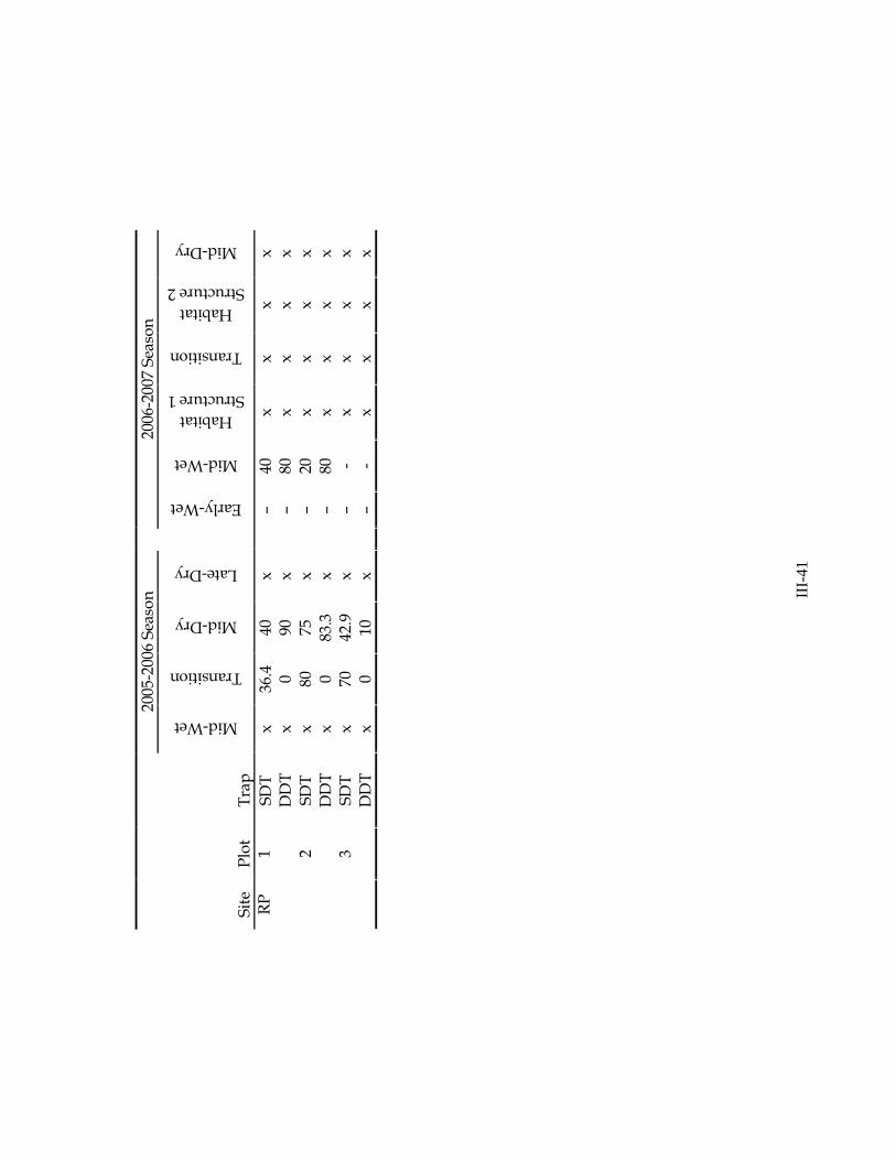
III-4

1

2005-2006 Season

2006-2007 Season

Site

Plot

Trap

Mid-Wet

Transition

Mid-Dry

Late-Dry

Early-Wet

Mid-Wet

Habitat

Structure 1

Transition

Habitat

Structure 2

Mid-Dry

SDT

x 36.4 40

x –

40

x x

x x

1

DDT

x 0

90

x –

80

x x

x x

SDT

x 80

75

x –

20

x x

x x

2 DDT

x 0

83.3

x –

80

x x

x x

SDT

x 70 42.9

x –

- x

x x

x

RP

3 DDT

x 0

10

x –

- x

x x

x

III-4

2

Table III-2. Results from ANOVA of density of fishes collected at BI across seasons (early-wet, mid-wet, transition, mid-

dry, late-dry) and trap types (lift net, drop trap, throw trap).

Season

Trap

Season x

Trap

Species

F4,37

P

F2,37

P

F7,37

P

R2

Cichlasom

a urophthalmus

22.7

<0.01

13.9

<0.01

9.3

<0.01 0.775

Elassom

a evergladei

19.4

<0.01

5.5

0.01

3.4

0.01

0.764

Fundu

lus chrysotus

1.5

0.23 2.0

0.15

2.6

0.03

0.461

Gam

busia holbrooki

8.1

<0.01

8.2

<0.01

2.9

0.02

0.640

Heterandria form

osa

10.7

<0.01

5.3

0.01

2.4

0.04

0.576

Lucania goodei

4.9

<0.01

3.8

0.03

1.5

0.19 0.486

Total Fish

13.2

<0.01

9.4

<0.01

2.1

0.06 0.689

III-4

3

Table III-3. Results from ANOVA of fish density at all sites across seasons (early-wet, mid-wet, transition, mid-dry, late-

dry), trap type (drop trap, throw trap), and zone (shallow, deep).

Season

Trap

Zone

Trap x Season Season x

Zone

Trap x

Zone

Trap x Zone

x Season

Species

F4,136

P

F1,136

P

F1,136

P

F4,136

P

F3,136 P F1,136

P F3,136

P

R2

Cichlasom

a urophthalmus

3.4

0.01

9.7

<0.01 0.2

0.62

3.9

0.01 0.2 0.91 0.4 0.52 0.2 0.87 0.220

Elassom

a evergladei

21.9

<0.01

8.7

<0.01 0.3

0.58

3.9

0.01 0.2 0.87 0.0 0.87 0.4 0.77 0.468

Jordan

ella floridae

4.7

<0.01

12.0

<0.01 1.8

0.18

4.2

<0.01 0.1 0.94 0.1 0.80 0.0 0.99 0.269

Gam

busia holbrooki

19.7

<0.01

25.1

<0.01 0.3

0.59

4.9

<0.01 0.1 0.97 0.1 0.73 0.6 0.62 0.498

Heterandria formosa

17.8

<0.01

3.0

0.09 2.0

0.16 0.3

0.86 0.2 0.91 0.4 0.51 0.1 0.98 0.370

Lepom

is gulosus

2.6

0.04

7.5

0.01 0.8

0.36

2.8

0.03 0.9 0.43 0.2 0.67 0.4 0.73 0.206

Lucania goodei

10.0

<0.01

17.9

<0.01 0.3

0.61

4.0

<0.01 0.2 0.88 0.5 0.47 0.1 0.97 0.363

Lepom

is m

arginatus

5.0

<0.01

5.8

0.02 0.3

0.58 1.7

0.15 0.6 0.64 0.0 0.87 0.3 0.79 0.226

Total Fish

30.2

<0.01

33.1

<0.01 0.6

0.44

2.9

0.03 0.5 0.69 0.1 0.71 0.3 0.84 0.578

III-44

Table III-4. Summary of the total number of fish collected (n) and the percentages collected on Day 1 (“Set-up day”) and Day 2 (“Take-down day”) of the 2-day sampling effort of drop traps and lift nets.

Species n %Captured Day 1

%Captured Day 2

Cichlasoma bimaculatum 26 96.2 3.8 Cichlasoma urophthalmus 6 66.7 33.3 Elassoma evergladei 1 100.0 0.0 Enneacanthus gloriosus 1 100.0 0.0 Etheostoma fusiforme 6 100.0 0.0 Fundulus chrysotus 3 100.0 0.0 Gambusia holbrooki 1040 87.7 12.3 Heterandria formosa 1 100.0 0.0 Hoplosternum littorale 2 0.0 100.0 Jordanella floridae 26 96.2 3.8 Lepomis gulosus 13 100.0 0.0 Lepomis macrochirus 9 88.9 11.1 Lepomis marginatus 6 66.7 33.3 Lepomis microlophus 11 90.9 9.1 Lepomis punctatus 5 80.0 20.0 Lepomis spp. 1 100.0 0.0 Lucania goodei 21 95.2 4.8 Poecilia latipinna 1 100.0 0.0 Tilapia mariae 1 100.0 0.0

Total fish 1180 88.1 11.9

III-45

Table III-5. Total fish and crayfish CPUE (catch per unit effort) during each sampling event. CPUE are included for each trap (corresponding to cardinal directions: N, S, E, W) within the drift fence array.

Total Fish CPUE Total Crayfish CPUE

Season Site* N S E W N S E W

Pre-Early-Wet** BI 3 0 0 1 1 0 0 0 RP 0 0 0 0 0 0 0 0 Mid-Wet BI 0 1 0 0 0 2 2 0 L28 0 23 12 2 0 5 3 1 RP 2 1 0 6 9 12 2 4

Transition BI 0 44 0 11 0 0 0 0

Hab. Structure (12/20/06)

BI 0 35 27 109 0 0 0 0

Mid-Dry BI 206 219 124 127 0 1 0 0

* Drift fences were located at plots BI-1, RP-2, and L28-3 ** Samples collected in July 2006 prior to ‘Early Wet Season’ sampling

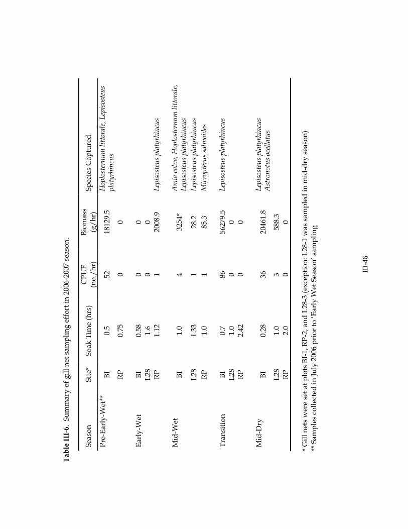
III-4

6

Table III-6. Summary of gill net sampling effort in 2006-2007 season.

Season

Site* Soak Time (hrs)

CPUE

(no./hr)

Biomass

(g/hr)

Species Captured

Pre-Early-Wet**

BI

0.5

52

18129.5

Hoplosternum littorale, Lepisosteus

platyrhincus

RP

0.75

0 0

Early-Wet

BI

0.58

0 0

L28

1.6

0 0

RP

1.12

1 2008.9

Lepisosteus platyrhincus

Mid-Wet

BI

1.0

4 3254*

Amia calva, H

oplosternum littorale,

Lepisosteus platyrhincus

L28

1.33

1 28.2

Lepisosteus platyrhincus

RP

1.0

1 85.3

Micropterus salm

oides

Transition

BI

0.7

86

56279.5

Lepisosteus platyrhincus

L28

1.0

0 0

RP

2.42

0 0

Mid-Dry

BI

0.28

36

20461.8

Lepisosteus platyrhincus

Astronotus ocellatus

L28

1.0

3 588.3

RP

2.0

0 0

* Gill nets were set at plots BI-1, RP-2, and L28-3 (exception: L28-1 was sampled in mid-dry season)

** Samples collected in July 2006 prior to ‘Early Wet Season’ sampling

III-4

7

Table III-7. Results of ANOVA of physicochemical variables across sites (BI, RP, L28), seasons (early-wet, mid-wet,

transition, mid-dry, late-dry) and zones (prairie, shallow, deep, refuge).

Site

Season

Zone

Site x Season Site x Zone Season x

Zone

Site x Zone

x Season

F2,105

P

F4,105

P

F2,105

P

F7,105

P

F3,105

P

F4,105

P

F7,105

P

R2

Depth

1.0

0.36

18.3

<0.01

30.7

<0.01 0.8

0.59 2.3 0.08 0.6 0.68 0.5 0.83 0.562

F2,107

P

F4,107

P

F2,107

P

F7,107

P

F3,107

P

F4,107

P

F7,107

P

R2

Temperature

1.3

0.29

84.9

<0.01 1.0

0.39

2.4

0.02 0.4 0.78

3.3

0.01 0.2 0.97 0.795

F2,107

P

F4,107

P

F2,107

P

F7,107

P

F3,107

P

F4,107 P

F7,107

P

R2

Specific

conductance

1.1

0.34

27.8

<0.01

3.5

0.04 1.1

0.40 0.9 0.46 1.8 0.14 0.5 0.81 0.572

F2,100

P

F4,100

P

F2,100

P

F7,100

P

F3,100

P

F4,100 P

F7,100

P

R2

% DO

16.7

<0.01

7.3

<0.01

15.5

<0.01

2.4

0.03 0.3 0.84 2.2 0.07 0.6 0.76 0.573

F2,101

P

F4,101

P

F2,101

P

F7,101

P

F3,101

P

F4,101

P

F7,101

P

R2

[DO]

23.4

<0.01

7.4

<0.01

13.5

<0.01

2.2

0.04 0.2 0.88 1.4 0.24 0.5 0.82 0.580

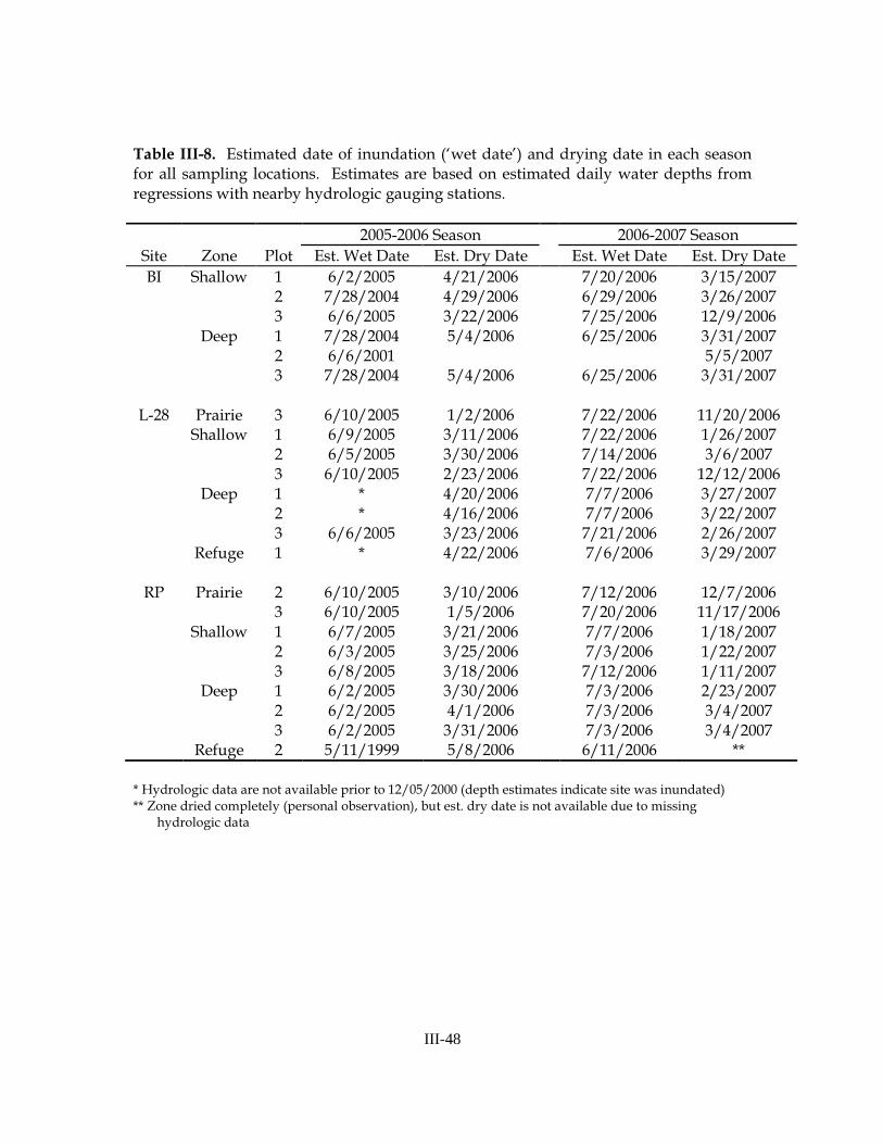
III-48

Table III-8. Estimated date of inundation (‘wet date’) and drying date in each season for all sampling locations. Estimates are based on estimated daily water depths from regressions with nearby hydrologic gauging stations.

2005-2006 Season 2006-2007 Season

Site Zone Plot Est. Wet Date Est. Dry Date Est. Wet Date Est. Dry Date

BI Shallow 1 6/2/2005 4/21/2006 7/20/2006 3/15/2007 2 7/28/2004 4/29/2006 6/29/2006 3/26/2007 3 6/6/2005 3/22/2006 7/25/2006 12/9/2006 Deep 1 7/28/2004 5/4/2006 6/25/2006 3/31/2007 2 6/6/2001 5/5/2007 3 7/28/2004 5/4/2006 6/25/2006 3/31/2007

L-28 Prairie 3 6/10/2005 1/2/2006 7/22/2006 11/20/2006 Shallow 1 6/9/2005 3/11/2006 7/22/2006 1/26/2007 2 6/5/2005 3/30/2006 7/14/2006 3/6/2007 3 6/10/2005 2/23/2006 7/22/2006 12/12/2006 Deep 1 * 4/20/2006 7/7/2006 3/27/2007 2 * 4/16/2006 7/7/2006 3/22/2007 3 6/6/2005 3/23/2006 7/21/2006 2/26/2007 Refuge 1 * 4/22/2006 7/6/2006 3/29/2007 RP Prairie 2 6/10/2005 3/10/2006 7/12/2006 12/7/2006 3 6/10/2005 1/5/2006 7/20/2006 11/17/2006 Shallow 1 6/7/2005 3/21/2006 7/7/2006 1/18/2007 2 6/3/2005 3/25/2006 7/3/2006 1/22/2007 3 6/8/2005 3/18/2006 7/12/2006 1/11/2007 Deep 1 6/2/2005 3/30/2006 7/3/2006 2/23/2007 2 6/2/2005 4/1/2006 7/3/2006 3/4/2007 3 6/2/2005 3/31/2006 7/3/2006 3/4/2007 Refuge 2 5/11/1999 5/8/2006 6/11/2006 **

* Hydrologic data are not available prior to 12/05/2000 (depth estimates indicate site was inundated) ** Zone dried completely (personal observation), but est. dry date is not available due to missing hydrologic data

III-49

Table III-9. Estimate of average (± SE) number of days each sampling location was inundated prior to drying in each season. Only one prairie plot was sampled at L28 (no SE).

Site

BI L28 RP

2005-06 Season Prairie --- 206 241 (± 32)

Shallow 417 (± 112) 277 (± 12) 288 (± 4)

Deep 645* (± 0) > 1403† 302 (± 1)

Refuge --- > 1,963† > 2,411†

2006-07 Season

Prairie --- 121 134 (± 14)

Shallow 215 (± 40) 189 (± 27) 194 (± 6)

Deep 906 (± 627) 247 (± 14) 241 (± 3)

Refuge --- 266 **

† Estimates not possible (hydrologic data unavailable, refer to Table D) * Estimate excludes one plot that failed to dry this season (BI2) ** Zone dried completely (personal observation), but estimated dry date is not available (hydrologic data unavailable)

III-50

Table III-10. Percent incidence (%I), relative abundance (%RA), sample size (n) and abundance range (no./m2 for emergents and percent cover for floating and submerged)of macrophytes sampled with 1-m2 throw traps. Relative abundance and sample size included only for emergent vegetation.

Latin Name Common Name %I %RA n

Abundance Range

EMERGENT VEGETATION Annona glabra Pond apple 0.8 0.0 1 0 - 0.3 Blechnum serrulatum Swamp fern 1.6 0.2 9 0 - 2.3 Cladium jamaicense Sawgrass 5.7 1.7 70 0 - 7.7 Crinum americanum String lily 0.8 0.4 16 0 - 5.3 Eleocharis spp. Spikerush 11.5 6.0 247 0 - 51.7 Eupatorium spp. Dog fennel 0.8 0.0 1 0 - 0.3 Hymenocallis spp. Spider lily 1.6 0.1 4 0 - 1.0 Leersia hexandra Cutgrass 0.8 0.0 2 0 - 0.7 Myrica cerifera Wax myrtle 0.8 0.0 1 0 - 0.3 Nymphoides aquatica Big floating heart 0.8 0.1 6 0 - 2.0 Nymphaea odorata Fragrant water lily 1.6 0.3 12 0 - 2.3 Oxypolis spp. Dropwort 2.5 0.2 8 0 - 1.0 Panicum spp. Panic grass 18.9 5.9 245 0 - 27.3 Paspalidium geminatum Egyptian paspalidium 3.3 0.2 8 0 - 1.3 Pluchea rosea Rosy camphorweed 3.3 0.3 11 0 - 1.0 Polygonum spp. Knotweed 0.8 0.0 2 0 - 0.7 Pontederia cordata Pickerelweed 7.4 1.7 71 0 - 3.7 Rhynchospora spp. Beak sedge 13.9 72.6 2991 0 - 201.0 Stillingia aquatica Water toothleaf 9.1 3.5 146 0 - 26.7

Taxodium distichum Bald cypress 11.5 1.4 56 0 - 3.0 Thalia geniculata Alligator flag 4.1 0.4 16 0 - 3.0 Unidentified 15.6 4.8 197 0 - 10.7 Total emergent stems - - 4120 0 - 225.7 FLOATING & SUBMERGED VEGETATION Bacopa caroliniana Water hyssop 29.5 - - 0 - 93.3 Eleocharis vivipara Sprouting spikerush 4.9 - - 0 - 66.7 Eriocaulon spp. Pipewort 4.1 - - 0 - 33.3

Floating periphyton - - - 4.9 - - 0 - 61.7 Lemna spp. Duckweed 0.8 - - 0 - 0.7 Ludwigia repens Red ludwigia 22.1 - - 0 - 97.5 Pistia stratiotes Water lettuce 0.8 - - 0 - 0.3 Sagittaria graminea Grassy arrowhead 21.3 - - 0 - 50.0 Salvinia minima Common salvinia 16.4 - - 0 - 85.0 Utricularia foliosa Leafy bladderwort 6.6 - - 0 - 25.0 Utricularia purpurea Purple bladderwort 2.5 - - 0 - 17.0 Unidentified 0.8 - - 0 - 20.0

III-51

Table III-11. Results of ANOVA of common macrophyte species abundance across sites (BI, RP, L28) and zones (prairie, shallow, deep, refuge).

Site Zone Site x Zone

F2,112 P F3,112 P F4,112 P R2

Emergent Vegetation Cladium jamaicense 2.5 0.09 2.4 0.07 2.1 0.08 0.191 Eleocharis spp. 0.1 0.89 64.6 <0.01 0.1 0.99 0.668 Panicum spp. 4.7 0.01 24.9 <0.01 6.2 <0.01 0.454 Pontederia cordata 2.2 0.12 3.3 0.02 2.3 0.06 0.216 Rhynchospora spp. 1.1 0.35 82.0 <0.01 0.7 0.59 0.735 Stillingia aquatica 41.3 <0.01 193.5 <0.01 67.7 <0.01 0.864 Taxodium distichum 7.8 <0.01 38.4 <0.01 10.9 <0.01 0.674 Total Stems 1.5 0.23 91.7 <0.01 0.6 0.64 0.740 Floating & Submerged Vegetation Bacopa caroliniana 15.0 <0.01 2.8 0.04 2.5 0.04 0.375 Eleocharis vivipara 6.1 <0.01 0.4 0.77 0.5 0.70 0.155 Floating periphyton 2.1 0.13 9.6 <0.01 4.1 <0.01 0.384 Ludwigia repens 6.8 <0.01 14.8 <0.01 10.5 <0.01 0.489 Sagittaria graminea 0.5 0.62 4.6 0.01 0.3 0.88 0.125 Salvinia minima 8.2 <0.01 6.1 <0.01 4.4 <0.01 0.239 Utricularia foliosa 3.1 0.05 3.5 0.02 4.1 <0.01 0.202

III-5

2

Table III-12. Percent incidence (%I), relative abundance (%RA), sample size (n) and density range of fishes (A),

invertebrates (B), and amphibians (C) collected with 1-m2 throw traps.

Latin Name

Common Name

% I % RA

n

Density Range

A. FISHES

Ameiurus natalis

Yellow bullhead

4.2

1.3

185

0 – 58.5

Belonesox belizan

us

Pike killifish

0.7

< 0.01

3 0 – 1.0

Cichlasoma bimaculatum

Black acara

22.5

0.7

103

0 – 3.7

Cichlasoma urophthalmus

Mayan cichlid

8.5

0.2

26

0 – 2.0

Clarias batrachus

Walking catfish

1.4

0.3

36

0 – 11.0

Elassom

a evergladei

Everglades pygmy sunfish 16.9

0.6

85

0 – 5.0

Enneacanthus gloriosus

Bluespotted sunfish

9.2

0.2

29

0 – 1.7

Etheostom

a fusiform

e Swamp darter

3.5

< 0.01

6 0 – 0.7

Fundulus chrysotus

Golden topminnow

15.5

0.4

53

0 – 3.0

Fundulus confluentus

Marsh killifish

2.1

< 0.01

5 0 – 1.0

Gam

busia holbrooki

Eastern mosquitofish

84.5 56.7

7807

0 – 507.0

Heterandria form

osa

Least killifish

43.7 10.2

1404

0 – 66.0

Hoplosternum littorale

Brown hoplo catfish

7.7

0.2

32

0 – 4.0

Jordan

ella floridae

Flagfish

40.8 20.8

2860

0 – 540.8

Labidesthes sicculus

Brook silverside

15.5

1.6

215

0 – 35.0

Lepisosteus platyrhyn

chus

Florida gar

1.4

< 0.01

6 0 – 1.0

Lepom

is gulosus

Warmouth

30.3

2.1

283

0 – 10.3

Lepom

is m

acrochirus

Bluegill sunfish

2.8

< 0.01

5 0 – 0.7

Lepom

is m

arginatus

Dollar sunfish

29.6

2.8

383

0 – 18.5

Lepom

is punctatus

Spotted sunfish

2.1

0.1

8 0 – 1.0

Lepom

is spp.

Unidentified sunfish

14.8

0.4

50

0 – 2.0

Lucania goodei

Bluefin killifish

46.5

2.6

356

0 – 19.3

Notem

igon

us crysoleucas

Golden shiner

4.2

0.1

14

0 – 2.0

Noturus gyrinus

Tadpole madtom

2.1

< 0.01

6 0 – 1.0

Poecilia latipinna

Sailfin molly

11.3

0.8

116

0 – 17.0

III-5

3

Latin Name

Common Name

% I % RA

n

Density Range

Tilapia m

ariae

Spotted tilapia

4.2

0.1

11

0 – 1.0

---

Unidentified fish

3.5

0.1

14

0 – 1.7

---

Unidentified fish larvae

1.4

0.1

4 0 – 1.0

---

Total fish

91.6

100

13776

0 – 1117.8

B. INVERTEBRATES

Anisoptera

†

Dragonfly†

63.4

3.6

437

0 – 5.7

Belostoma spp.

Giant water bug

7.7

0.1

15

0 – 1.0

Coenagrionidae

†

Damselfly†

14.8

0.7

82

0 – 6.0

Coleoptera

Aquatic beetle

20.4

2.4

291

0 – 39.7

Corixidae

Water boatman

9.2

0.4

48

0 – 3.7

Cybister spp. †

Predaceous diving beetle†

5.6

0.3

39

0 – 9.7

Ephemeroptera

†

Mayfly†

1.4

< 0.01

2 0 – 0.3

Gyrinus spp.

Whirligig water beetle

13.4

4.4

535

0 – 106.0

Heteroptera

True bugs

0.7

< 0.01

2 0 – 0.7

Hirudinea

Leech

4.2

0.1

7 0 – 0.7

Isopoda

Isopod

0.7

< 0.01

1 0 – 0.3

Lethocerus spp.

Toe biter

11.3

0.3

33

0 – 3.0

Pelocoris fem

oratus

Alligator flea

16.2

0.4

49

0 – 2.3

Palaemonetes paludosus

Grass shrimp

62.0 46.2

5623

0 – 355.3

Physella spp.

Physid snail

8.5

0.3

33

0 – 4.7

Planorbella spp.

Planorbid snail

21.8

0.7

91

0 – 5.0

Pom

acea paludosa

Florida apple snail

4.2

< 0.01

6 0 – 0.3

Procambarus alleni

Everglades crayfish

62.7 12.4

1507

0 – 38.7

Procambarus fallax

Slough crayfish

54.9

5.6

686

0 – 22.3

Procambarus spp.

Unidentified crayfish

54.9 23.0

2808

0 – 149.0

Ranatra spp.

Water scorpion

3.5

< 0.01

5 0 – 0.3

Sphaeridae

Fingernail clam

12.7

1.4

169

0 – 16.0

Stratiomyidae

†

Soldier fly†

0.7

< 0.01

1 0 – 0.3

Tipulidae

†

Crane fly†

1.4

< 0.01

2 0 – 0.3

III-5

4

Latin Name

Common Name

% I % RA

n

Density Range

---

Unidentified invertebrate

2.1

< 0.01

4 0 – 0.7

---

Unidentified snail

2.1

< 0.01

5 0 – 0.7

---

Total invertebrates

98.6

100

12183

0 – 355.5

C. AMPHIBIANS

Notophthalmus viridescens

Peninsula newt

12.0 11.3

20

0 – 0.7

Siren spp.

Siren (greater or lesser)

2.1

3.9

7 0 – 1.0

---

Total tadpoles

21.1 85.4

152

0 – 7.7

---

Total amphibians

28.2

100

178

0 – 7.7

† indicates larval life stage

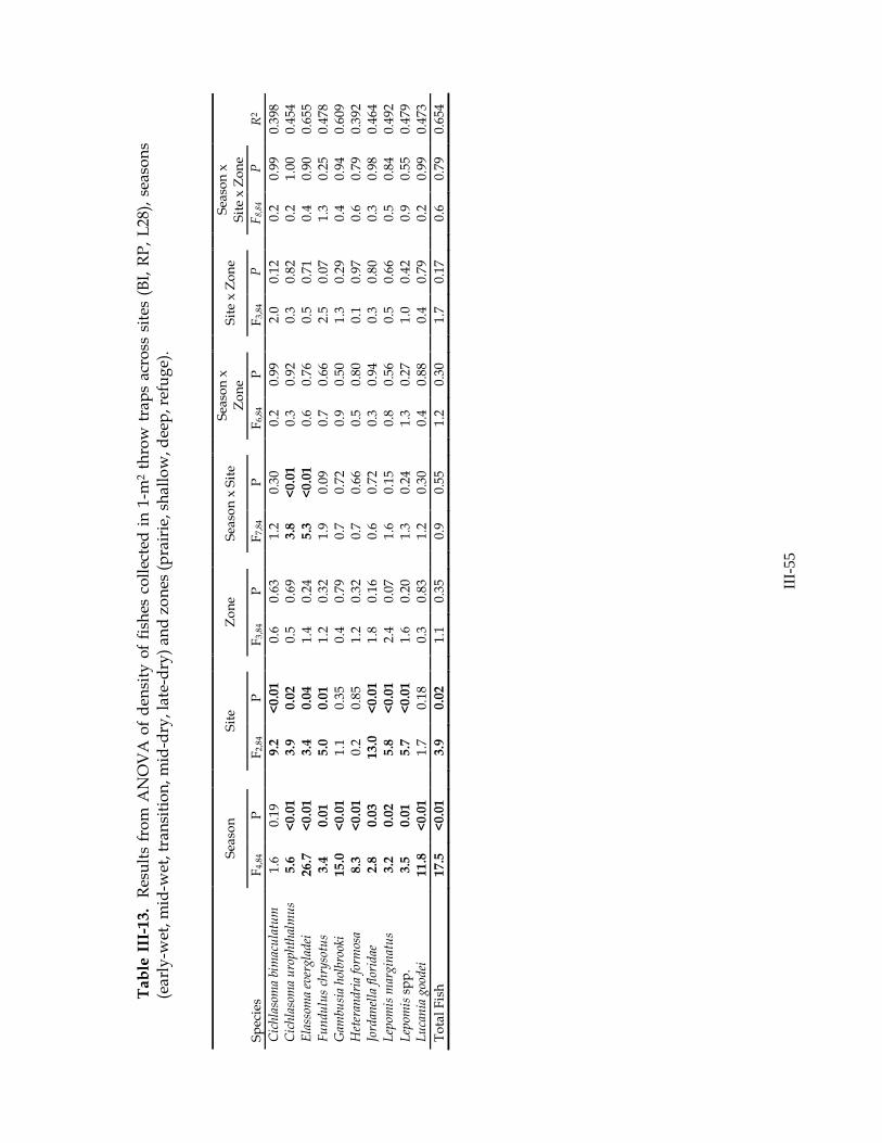
III-5

5

Table III-13. Results from ANOVA of density of fishes collected in 1-m2 throw traps across sites (BI, RP, L28), seasons

(early-wet, mid-wet, transition, mid-dry, late-dry) and zones (prairie, shallow, deep, refuge).

Season

Site

Zone

Season x Site

Season x

Zone

Site x Zone

Season x

Site x Zone

Species

F4,84

P

F2,84

P

F3,84

P

F7,84

P

F6,84

P

F3,84

P

F8,84

P

R2

Cichlasoma bimaculatum

1.6

0.19

9.2

<0.01 0.6 0.63

1.2

0.30 0.2 0.99 2.0 0.12 0.2 0.99

0.398

Cichlasoma urophthalmus

5.6

<0.01

3.9

0.02

0.5 0.69

3.8

<0.01 0.3 0.92 0.3 0.82 0.2 1.00

0.454

Elassom

a evergladei

26.7

<0.01

3.4

0.04

1.4 0.24

5.3

<0.01 0.6 0.76 0.5 0.71 0.4 0.90

0.655

Fundu

lus chrysotus

3.4

0.01

5.0

0.01

1.2 0.32

1.9

0.09 0.7 0.66 2.5 0.07 1.3 0.25

0.478

Gam

busia holbrooki

15.0

<0.01 1.1

0.35

0.4 0.79

0.7

0.72 0.9 0.50 1.3 0.29 0.4 0.94

0.609

Heteran

dria formosa

8.3

<0.01 0.2

0.85

1.2 0.32

0.7

0.66 0.5 0.80 0.1 0.97 0.6 0.79

0.392

Jordanella floridae

2.8

0.03

13.0

<0.01 1.8 0.16

0.6

0.72 0.3 0.94 0.3 0.80 0.3 0.98

0.464

Lepom

is m

arginatus

3.2

0.02

5.8

<0.01 2.4 0.07

1.6

0.15 0.8 0.56 0.5 0.66 0.5 0.84

0.492

Lepom

is spp.

3.5

0.01

5.7

<0.01 1.6 0.20

1.3

0.24 1.3 0.27 1.0 0.42 0.9 0.55

0.479

Lucania goodei

11.8

<0.01 1.7

0.18

0.3 0.83

1.2

0.30 0.4 0.88 0.4 0.79 0.2 0.99

0.473

Total Fish

17.5

<0.01

3.9

0.02

1.1 0.35

0.9

0.55 1.2 0.30 1.7 0.17 0.6 0.79

0.654

III-5

6

Table III-14. Results from ANOVA of biomass of fishes collected in 1-m2 throw traps across sites (BI, RP, L28), seasons

(early-wet, mid-wet, transition, mid-dry, late-dry) and zones (prairie, shallow, deep, refuge).

Season

Site

Zone

Season x

Site

Season x

Zone

Site x Zone

Season x

Site x Zone

Species

F4,84

P

F2,84

P

F3,84

P

F7,84

P

F6,84 P F3,84

P

F8,84

P

R2

Cichlasoma bimaculatum

2.3

0.06

5.4

0.01 0.2

0.92 1.6 0.14 0.2 0.99 0.9 0.45 0.1 1.00 .425

Cichlasoma urophthalmus

9.9

<0.01

2.9

0.06 0.4

0.78

6.0

<0.01 0.5 0.80 0.2 0.89 0.2 0.99 .524

Elassom

a evergladei

21.0

<0.01 1.2

0.31 1.7

0.18

2.1

0.05 0.1 1.00 0.3 0.84 0.1 1.00 .569

Enneacanthus gloriosus

1.3

0.27 1.0

0.37 0.9

0.46

2.2

0.05 1.2 0.34 0.4 0.75 0.3 0.98 .335

Fundu

lus chrysotus

7.3

<0.01

8.9

<0.01 1.6

0.20

3.6

<0.01 0.7 0.65

3.1

0.03 1.3 0.27 .592

Gam

busia holbrooki

16.2

<0.01 2.8

0.07 0.5

0.68 0.3 0.97 0.7 0.69 0.6 0.62 0.4 0.90 .637

Heteran

dria formosa

9.6

<0.01 0.2

0.85 2.1

0.10 0.4 0.91 0.3 0.92 0.2 0.92 0.5 0.82 .399

Jordanella floridae

3.4

0.01

12.2

<0.01 1.8

0.15 0.6 0.76 0.3 0.95 0.2 0.88 0.2 0.99 .514

Lepom

is m

arginatus

8.0

<0.01 1.8

0.17 1.2

0.31 0.9 0.53 0.5 0.82 0.3 0.82 0.3 0.97 .439

Lepom

is gulosus

3.1

0.02 2.3

0.11 1.7

0.17 0.5 0.83 0.5 0.80 0.6 0.59 0.5 0.85 .415

Lepom

is spp.

3.2

0.02

4.7

0.01 1.3

0.29 1.3 0.27 1.2 0.33 0.8 0.53 1.0 0.42 .436

Lucania goodei

28.7

<0.01

3.3

0.04 0.4

0.73

2.8

0.01 0.2 0.97 0.3 0.85 0.2 0.99 .650

Poecilia latipinna

4.9

<0.01 1.3

0.29 0.1

0.99 0.1 1.00 0.0 1.00 0.0 1.00 0.0 1.00 .421

Total Fish

21.7

<0.01

5.6

0.01 1.8

0.16 0.4 0.88 0.8 0.55 1.5 0.23 0.7 0.66 .719

III-5

7

Table III-15. Results from ANOVA of density of invertebrates (A) and amphibians (B) collected in 1-m2 throw traps

across sites (BI, RP, L28), seasons (early-wet, mid-wet, transition, mid-dry, late-dry) and zones (prairie, shallow, deep,

refuge).

Season

Site

Zone

Season x

Site

Season x

Zone

Site x Zone

Season x

Site x Zone

Taxa

F4,84

P

F2,84

P

F3,84

P

F7,84

P

F6,84

P

F3,84

P

F8,84

P

R2

A. Invertebrates

Coleoptera

1.6

0.17 2.9

0.06

3.7

0.01 1.7 0.11 1.6

0.15 0.7

0.56 1.2

0.30 0.398

Gyrinus spp.

26.3

<0.01

8.6

<0.01 0.5

0.70

7.3

<0.01 0.2

0.99 0.8

0.53 0.4

0.93 0.654

Palaemon

etes paludosus

23.0

<0.01 0.2

0.81 2.5

0.07 0.3 0.96 0.6

0.77 0.3

0.79 0.2

0.99 0.618

Pelocoris fem

oratus

7.8

<0.01

4.1

0.02

34.1

<0.01

0.6 0.73 7.6

<0.01

7.9

<0.01

1.3

0.27 0.683

Planorbella spp.

3.9

0.01 2.8

0.07

5.4

<0.01

2.3

0.03 2.0

0.08

4.4

0.01

2.3

0.03 0.435

Procambarus alleni

11.8

<0.01

6.4

<0.01 1.0

0.38 1.7 0.12 0.5

0.83 0.4

0.76 0.5

0.84 0.572

Procambarus fallax

6.0

<0.01

4.7

0.01

3.4

0.02 1.9 0.09 1.2

0.33 1.0

0.39 0.2

0.99 0.480

Procambarus spp.

32.8

<0.01

3.0

0.06

5.2

<0.01

1.6 0.14

2.6

0.02

5.8

<0.01

4.4

<0.01 0.782

Total Invertebrates

12.6

<0.01 0.7

0.48

5.3

<0.01

0.6 0.79 0.3

0.94

2.9

0.04 0.5

0.87 0.511

B. Amphibians

Tadpoles

16.4

<0.01 0.7

0.51 0.5

0.68 0.7 0.71 0.4

0.89

5.4

<0.01

3.4

<0.01 0.629

Total Amphibians

11.9

<0.01 0.6

0.57 0.3

0.83 0.4 0.87 0.6

0.75

5.5

<0.01

2.3

0.03 0.559

III-5

8

Table III-16. Results from ANOVA of biomass of invertebrates (A) and amphibians (B) collected in 1-m2 throw traps

across sites (BI, RP, L28), seasons (early-wet, mid-wet, transition, mid-dry, late-dry) and zones (prairie, shallow, deep,

refuge).

Season

Site

Zone

Season x

Site

Season x

Zone

Site x Zone

Season x

Site x Zone

Species

F4,84

P

F2,84

P

F3,84

P

F7,84

P

F6,84

P

F3,84

P

F8,84

P

R2

A. Invertebrates

Gyrinus spp.

21.4

<0.01

8.0

<0.01 0.1

0.97

9.0

<0.01 0.0

1.00 0.1

0.96

0.0 1.00 0.640

Palaemon

etes paludosus

27.0

<0.01 0.8

0.39 1.6

0.19

0.3 0.93 0.4

0.88 0.1

0.96

0.1 1.00 0.643

Pelocoris fem

oratus

11.2

<0.01

7.3

<0.01

39.7

<0.01 0.6 0.77

10.5

<0.01

11.4

<0.01

1.5 0.16

0.71

Planorbella spp.

3.6

0.01

1.9

0.15

3.8

0.01

2.5

0.02

2.2

0.05

3.2

0.03

2.7

0.01 0.425

Procambarus alleni

4.3

<0.01

7.3

<0.01 1.8

0.16

1.6 0.16 0.4

0.86 0.8

0.50

0.8 0.63 0.464

Procambarus fallax

6.2

<0.01

10.9

<0.01

3.8

0.01

1.8 0.10 1.7

0.13 1.9

0.13

0.8 0.59 0.554

Procambarus spp.

41.7

<0.01

9.5

<0.01

5.5

<0.01

6.8

<0.01

3.7

<0.01

12.8

<0.01

11.1

<0.01 0.855

B. Amphibians

Notophthalmus viridescens

5.0

<0.01

17.5

<0.01

9.2

<0.01

4.1

<0.01 0.2

0.96 0.3

0.83

0.2 0.99 0.657

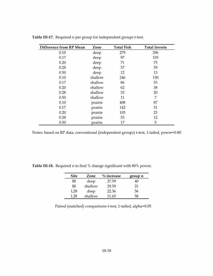
III-59

Table III-17. Required n per group for independent groups t-test.

Difference from RP Mean Zone Total Fish Total Inverts

0.10 deep 279 296

0.17 deep 97 103

0.20 deep 71 75

0.28 deep 37 39

0.50 deep 12 13

0.10 shallow 246 150

0.17 shallow 86 53

0.20 shallow 62 38

0.28 shallow 32 20

0.50 shallow 11 7

0.10 prairie 408 87

0.17 prairie 142 31

0.20 prairie 103 23

0.28 prairie 53 12

0.50 prairie 17 5

Notes: based on RP data, conventional (independent groups) t-test, 1-tailed, power=0.80 Table III-18. Required n to find % change significant with 80% power.

Site Zone % increase group n

BI deep 27.59 40

BI shallow 29.59 21

L28 deep 22.36 56

L28 shallow 11.65 58

Paired (matched) comparisons t-test, 1-tailed, alpha=0.05

III-60

Table III-19. A priori power and n of replicates per site for site x time test.

Dependent Variable Zone % Incr effect size Power N *

DEEP 28 0.562 0.966 3

DEEP 17 0.555 0.962 3

SHALLOW 28 0.531 0.943 3 TOTFISH

SHALLOW 17 0.514 0.926 3

DEEP 28 0.350 0.881 5

DEEP 17 0.337 0.846 5

SHALLOW 28 0.373 0.826 4 GAMHOL

SHALLOW 17 0.362 0.904 5

DEEP 28 0.609 0.819 2

DEEP 17 0.599 0.805 2

SHALLOW 28 0.409 0.899 4 JORFLO

SHALLOW 17 0.404 0.889 4

DEEP 28 0.838 0.986 2

DEEP 17 0.817 0.981 2

SHALLOW 28 0.611 0.821 2 LUCGOO

SHALLOW 17 0.594 0.981 3

DEEP 28 0.822 0.982 2

DEEP 17 0.826 0.983 2

SHALLOW 28 0.704 0.925 2 PROALL

SHALLOW 17 0.695 0.917 2

DEEP 28 0.512 0.924 3

DEEP 17 0.509 0.921 3

SHALLOW 28 0.314 0.878 6 PROFAL

SHALLOW 17 0.311 0.869 6

DEEP 28 0.607 0.815 2

DEEP 17 0.612 0.824 2

SHALLOW 28 0.428 0.927 4 TOTINV

SHALLOW 17 0.428 0.926 4

N * - N is the required number of spatial replicates per site; Planned alpha 0.05, Planned power 0.80; 4 samples/yr, total of 8 repeated samples per replicate.

III-61

Table III-20. Expected power for trend tests of total fish density from current design.

10-Year Monitoring Period

Site and Depth Zone Class BI L28 RP Annual

Trend (%) Deep Shallow Deep Shallow Deep Shallow

1 0.022 0.006 0.056 0.010 0.002 0.062 5 0.414 0.502 0.108 0.134 0.724 0.070 10 0.694 0.856 0.834 0.950 0.960 0.986

15 0.842 0.926 0.832 0.988 0.974 1.000 20 0.936 0.954 0.920 0.998 0.994 1.000

5-Year Monitoring Period

Site and Depth Zone Class BI L28 RP Annual

Trend (%) Deep Shallow Deep Shallow Deep Shallow

10 0.438 0.520 0.170 0.144 0.574 0.098 20 0.514 0.814 0.676 0.768 0.878 0.916 30 0.684 0.874 0.662 0.980 0.940 0.998 40 0.834 0.914 0.802 0.994 0.992 1.000

50 0.834 0.942 0.830 1.000 0.994 1.000

Monitor 10.0 Software used with 500 simulations; alpha=0.05, 1-tailed tests for increasing trend. There are 3 replicates per depth class at each site. A sampling frequency of 4 times per year was assumed. Values in italics meet or exceed goal of 80% power.

III-62

Figure III-1. Location of three study sites (Bear Island, L-28, and Raccoon Point) in Big Cypress National Preserve. Three replicate plots are located within each site.

RaccoonPoint

N

5 0 5 10 Km

BearIsland

HQ

I-75

US 41

L-28

BIG CYPRESS NATIONAL PRESERVE

RaccoonPoint

NN

5 0 5 10 Km

BearIsland

HQ

I-75

US 41

L-28

BIG CYPRESS NATIONAL PRESERVE

III-63

Figure III-2. Aerial views (left) and schematic diagrams (right) of representative study plots at Raccoon Point (A) and L28 (B). Shading of schematic diagrams demonstrates locations of sampling zones (prairie, shallow, deep, refuge) in dome-type plots (e.g., Raccoon Point) and more contiguous strand-type plots (e.g., L28).

Deep

Shallow

250 m

250 m

PrairieShallow

Deep

Refuge

B. L

-28

A. R

acco

on

Po

int

Schematic DiagramAerial View

Deep

Shallow

250 m

250 m

PrairieShallow

Deep

Refuge

B. L

-28

A. R

acco

on

Po

int

Schematic DiagramAerial View

III-64

Figure III-3. Examples of the copious habitat structure (tree trunks, woody debris, etc.) present at many sampling locations in Big Cypress National Preserve cypress forests. Photographs taken at L-28 (plot 3) during the 2006-2007 dry season.

III-65

Figure III-4. Average total fish density (no./m2) collected in deep traps (drop trap, throw trap and bottomless lift net) without habitat structure element from sampling events between October 2005 and February 2007 (error bars represent ± 1 SE).

Date

Oct 05 Feb 06 Jun 06 Oct 06 Feb 07

Ln(T

otal

Fis

h D

ensi

ty (

no./m

2) +

1)

0

1

2

3

4

5

6

Drop trap

Throw trap

Lift net

Date

Oct 05 Feb 06 Jun 06 Oct 06 Feb 07

Ln(T

otal

Fis

h D

ensi

ty (

no./m

2) +

1)

0

1

2

3

4

5

6

Drop trap

Throw trap

Lift net

III-66

Figure III-5. Average density (no./m2) of Cichlasoma urophthalmus (A), Jordanella floridae (B), Lepomis gulosus (C) and total fish (D) collected in drop traps and throw traps at all sites across sampling seasons (error bars represent ±1 SE).

Throw trap

Drop trap

0.0

0.5

1.0

1.5

2.0

0.0

0.2

0.4

0.6

0.8

1.0

1.2

EarlyWet

LateDry

MidDry

MidWet

Transition

Season

0.0

0.5

1.0

1.5

2.0

2.5

EarlyWet

LateDry

MidDry

MidWet

Transition

0

1

2

3

4

5

6

7

A. Cichlosoma urophthalmus B. Jordanella floridae

C. Lepomis gulosus D. Total Fish

Ln(d

ensi

ty (

no./m

2+

1)

Throw trap

Drop trap

0.0

0.5

1.0

1.5

2.0

0.0

0.2

0.4

0.6

0.8

1.0

1.2

EarlyWet

LateDry

MidDry

MidWet

Transition

Season

0.0

0.5

1.0

1.5

2.0

2.5

EarlyWet

LateDry

MidDry

MidWet

Transition

0

1

2

3

4

5

6

7

A. Cichlosoma urophthalmus B. Jordanella floridae

C. Lepomis gulosus D. Total Fish

Ln(d

ensi

ty (

no./m

2+

1)

III-67

Figure III-6. Average water depth (cm) at each site (BI=Bear Island, RP=Raccoon Point) in prairie, shallow and deep habitat zones during each sampling season (error bars represent ± 1 SE).

Ln(a

vera

ge w

ater

dep

th (

cm)

+ 1

)

BI

2.0

2.5

3.0

3.5

4.0

4.5

RP

Early Wet Mid Wet Trans Mid Dry Late Dry2.0

2.5

3.0

3.5

4.0

4.5

L28

2.0

2.5

3.0

3.5

4.0

4.5

Ln(a

vera

ge w

ater

dep

th (

cm)

+ 1)

Ln(a

vera

ge w

ater

dep

th (

cm)

+ 1)

Shallow

Deep

Prairie

Zone

Season

Ln(a

vera

ge w

ater

dep

th (

cm)

+ 1

)

BI

2.0

2.5

3.0

3.5

4.0

4.5

BI

2.0

2.5

3.0

3.5

4.0

4.5

RP

Early Wet Mid Wet Trans Mid Dry Late Dry2.0

2.5

3.0

3.5

4.0

4.5

L28

2.0

2.5

3.0

3.5

4.0

4.5

Ln(a

vera

ge w

ater

dep

th (

cm)

+ 1)

L28

2.0

2.5

3.0

3.5

4.0

4.5

Ln(a

vera

ge w

ater

dep

th (

cm)

+ 1)

Ln(a

vera

ge w

ater

dep

th (

cm)

+ 1)

Shallow

Deep

Prairie

Zone

Shallow

Deep

Prairie

Zone

Season

III-68

Figure III-7. Average water temperature (°C) at each site (BI=Bear Island, RP=Raccoon Point) in prairie, shallow and deep habitat zones during each sampling season (error bars represent ± 1 SE).

BI

Ln(a

vg. w

ater

tem

p (°C

)+

1)

2.6

2.8

3.0

3.2

3.4

3.6

L28

2.6

2.8

3.0

3.2

3.4

3.6

RP

Early Wet Mid Wet Trans Mid Dry Late Dry2.6

2.8

3.0

3.2

3.4

3.6

Ln(a

vg. w

ater

tem

p (°C

)+

1)

Ln(a

vg. w

ater

tem

p (°C

)+

1)

Shallow

Deep

Prairie

Zone

Season

BI

Ln(a

vg. w

ater

tem

p (°C

)+

1)

2.6

2.8

3.0

3.2

3.4

3.6

BI

Ln(a

vg. w

ater

tem

p (°C

)+

1)

2.6

2.8

3.0

3.2

3.4

3.6

L28

2.6

2.8

3.0

3.2

3.4

3.6

RP

Early Wet Mid Wet Trans Mid Dry Late Dry2.6

2.8

3.0

3.2

3.4

3.6

Ln(a

vg. w

ater

tem

p (°C

)+

1)

Ln(a

vg. w

ater

tem

p (°C

)+

1)

Shallow

Deep

Prairie

Zone

Shallow

Deep

Prairie

Zone

Season

III-69

Figure III-8. Average specific conductance (µs/cm) at each site (BI=Bear Island, RP=Raccoon Point) in prairie, shallow and deep habitat zones during each sampling season (error bars represent ± 1 SE).

Ln(s

peci

fic c

ondu

ctan

ce (µ

s/cm

)+

1)

BI

0

1

2

3

4

5

6

7

L28

Ln(s

peci

fic c

ondu

ctan

ce (µ

s/cm

)+

1)

0

1

2

3

4

5

6

7

RP

Early Wet Mid Wet Trans Mid Dry Late Dry

0

1

2

3

4

5

6

7

Ln(s

peci

fic c

ondu

ctan

ce (µ

s/cm

)+

1)

Shallow

Deep

Prairie

Zone

Season

Ln(s

peci

fic c

ondu

ctan

ce (µ

s/cm

)+

1)

BI

0

1

2

3

4

5

6

7

BI

0

1

2

3

4

5

6

7

L28

Ln(s

peci

fic c

ondu

ctan

ce (µ

s/cm

)+

1)

0

1

2

3

4

5

6

7

RP

Early Wet Mid Wet Trans Mid Dry Late Dry

0

1

2

3

4

5

6

7

Ln(s

peci

fic c

ondu

ctan

ce (µ

s/cm

)+

1)

Shallow

Deep

Prairie

Zone

Shallow

Deep

Prairie

Zone

Season

III-70

Figure III-9. Average dissolved oxygen (%) at each site (BI=Bear Island, RP=Raccoon Point) in prairie, shallow and deep habitat zones during each sampling season (error bars represent ± 1 SE).

BI

0.2

0.4

0.6

0.8

1.0

1.2

1.4

L28

0.2

0.4

0.6

0.8

1.0

1.2

1.4

RP

Early Wet Mid Wet Trans Mid Dry Late Dry

Arc

sine

( √

%D

O)

0.2

0.4

0.6

0.8

1.0

1.2

1.4

Arc

sine

( √

%D

O)

Arc

sine

( √

%D

O)

Shallow

Deep

Prairie

Zone

Season

BI

0.2

0.4

0.6

0.8

1.0

1.2

1.4

BI

0.2

0.4

0.6

0.8

1.0

1.2

1.4

L28

0.2

0.4

0.6

0.8

1.0

1.2

1.4

L28

0.2

0.4

0.6

0.8

1.0

1.2

1.4

RP

Early Wet Mid Wet Trans Mid Dry Late Dry

Arc

sine

( √

%D

O)

0.2

0.4

0.6

0.8

1.0

1.2

1.4

RP

Early Wet Mid Wet Trans Mid Dry Late Dry

Arc

sine

( √

%D

O)

0.2

0.4

0.6

0.8

1.0

1.2

1.4

Arc

sine

( √

%D

O)

Arc

sine

( √

%D

O)

Shallow

Deep

Prairie

Zone

Shallow

Deep

Prairie

Zone

Season

III-71

Figure III-10. Average dissolved oxygen concentration (mg/L) at each site (BI=Bear Island, RP=Raccoon Point) in prairie, shallow and deep habitat zones during each sampling season (error bars represent ± 1 SE).

BI

0.4

0.8

1.2

1.6

2.0

2.4

Ln([

DO

] (m

g/L)

+ 1

)

Shallow

Deep

Prairie

Zone

L28

0.4

0.8

1.2

1.6

2.0

2.4

Ln([

DO

] (m

g/L)

+ 1

)

RP

Early Wet Mid Wet Trans Mid Dry Late Dry

0.4

0.8

1.2

1.6

2.0

2.4

Ln([

DO

] (m

g/L)

+ 1

)

BI

0.4

0.8

1.2

1.6

2.0

2.4

Ln([

DO

] (m

g/L)

+ 1

)

BI

0.4

0.8

1.2

1.6

2.0

2.4

Ln([

DO

] (m

g/L)

+ 1

)

Shallow

Deep

Prairie

Zone

Shallow

Deep

Prairie

Zone

L28

0.4

0.8

1.2

1.6

2.0

2.4

Ln([

DO

] (m

g/L)

+ 1

)

L28

0.4

0.8

1.2

1.6

2.0

2.4

Ln([

DO

] (m

g/L)

+ 1

)

RP

Early Wet Mid Wet Trans Mid Dry Late Dry

0.4

0.8

1.2

1.6

2.0

2.4

Ln([

DO

] (m

g/L)

+ 1

)

RP

Early Wet Mid Wet Trans Mid Dry Late Dry

0.4

0.8

1.2

1.6

2.0

2.4

Ln([

DO

] (m

g/L)

+ 1

)

III-72

Figure III-11. Example of the digital 180° fish-eye canopy photographs that were taken at all sites from April 2006 to February 2007 to determine the feasibility of obtaining estimates of PAR and LAI.

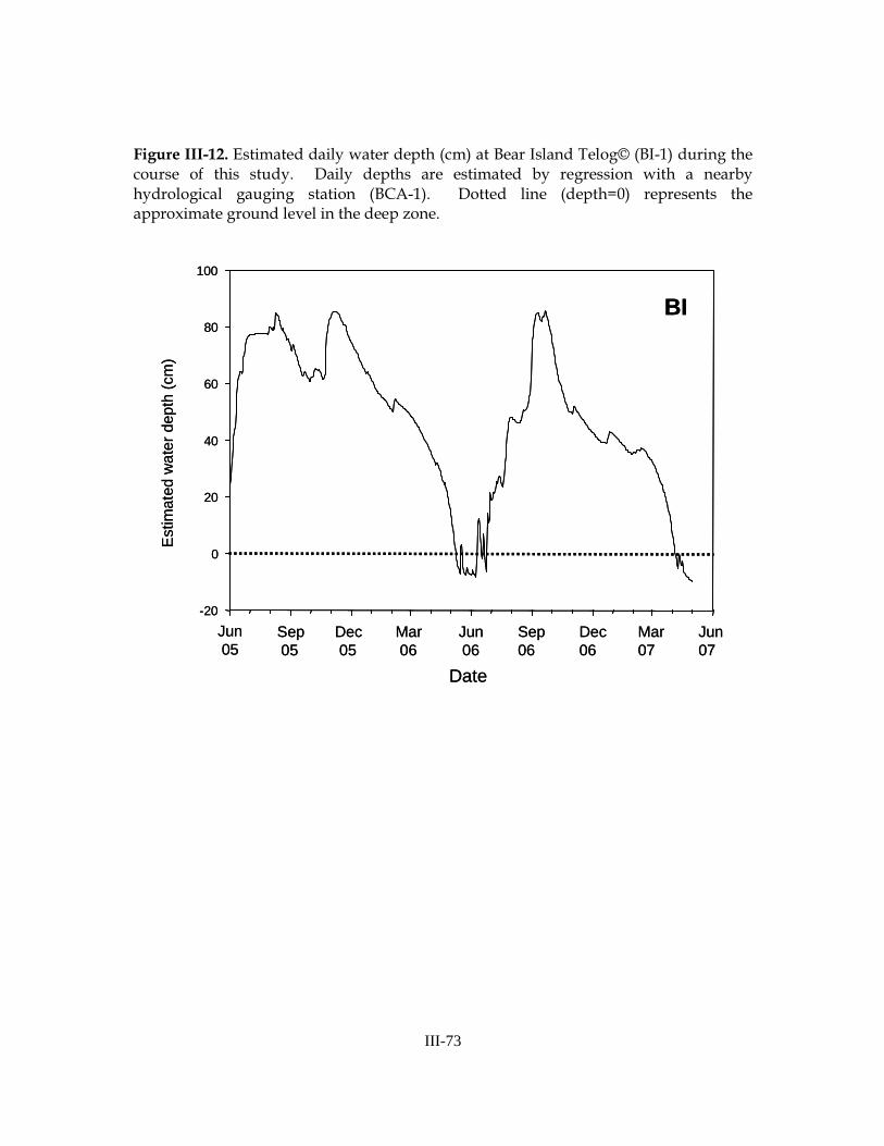
III-73

Figure III-12. Estimated daily water depth (cm) at Bear Island Telog© (BI-1) during the course of this study. Daily depths are estimated by regression with a nearby hydrological gauging station (BCA-1). Dotted line (depth=0) represents the approximate ground level in the deep zone.

BI

Jun05

Sep05

Dec 05

Mar06

Jun06

Sep06

Dec06

Mar07

Jun 07

-20

0

20

40

60

80

100

Est

imat

ed w

ater

dep

th (

cm)

Date

BI

Jun05

Sep05

Dec 05

Mar06

Jun06

Sep06

Dec06

Mar07

Jun 07

-20

0

20

40

60

80

100

Est

imat

ed w

ater

dep

th (

cm)

Date

III-74

Figure III-13. Estimated daily water depth (cm) at L28 Telog© (L28-1) during the course of this study. Daily depths are estimated by regression with a nearby hydrological gauging station (BCA-18).

Date

Est

imat

ed w

ater

dep

th (

cm)

-100

-80

-60

-40

-20

0

20

40

60

80

100

120

L28

Jun05

Sep05

Dec 05

Mar06

Jun06

Sep06

Dec06

Mar07

Jun 07

Date

Est

imat

ed w

ater

dep

th (

cm)

-100

-80

-60

-40

-20

0

20

40

60

80

100

120

L28

Jun05

Sep05

Dec 05

Mar06

Jun06

Sep06

Dec06

Mar07

Jun 07

III-75

Figure III-14. Estimated daily water depth (cm) at Raccoon Point Telog© (RP-2) during the course of this study. Daily depths are estimated by regression with a nearby hydrological gauging station (BCA-5). Dotted line (depth=0) represents the approximate ground level in the deep zone.

Est

imat

ed w

ater

dep

th (

cm)

-40

-20

0

20

40

60

80

100

RP

Date

Jun05

Sep05

Dec 05

Mar06

Jun06

Sep06

Dec06

Mar07

Jun 07

Est

imat

ed w

ater

dep

th (

cm)

-40

-20

0

20

40

60

80

100

RP

Date

Jun05

Sep05

Dec 05

Mar06

Jun06

Sep06

Dec06

Mar07

Jun 07

III-76

Figure III-15. Average abundance of total emergent stems (A), Sagittaria graminea (B), Bacopa caroliniana (C), and Salvinia minima (D) across habitat zones at each site (BI=Bear

Island, RP=Raccoon Point) (error bars represent ± 1 SE).

0

1

2

3

4

5

BI

L28

RP

B. Sagittaria graminea

0.00

0.05

0.10

0.15

0.20

0.25

0.30

Prairie Shallow Deep Refuge

Arc

sin(

√(%

Cov

er))

D. Salvinia minima

0.0

0.1

0.2

0.3

0.4

0.5

0.6

A. Total Stems

0.0

0.2

0.4

0.6

0.8

1.0

1.2C. Bacopa caroliniana

Prairie Shallow Deep Refuge

Zone

Site

Ln(D

ensi

ty (

no./m

2 ) +

1)

0

1

2

3

4

5

BI

L28

RP

B. Sagittaria graminea

0.00

0.05

0.10

0.15

0.20

0.25

0.30

Prairie Shallow Deep Refuge

Arc

sin(

√(%

Cov

er))

D. Salvinia minima

0.0

0.1

0.2

0.3

0.4

0.5

0.6

A. Total Stems

0.0

0.2

0.4

0.6

0.8

1.0

1.2C. Bacopa caroliniana

Prairie Shallow Deep Refuge

Zone

Site

Ln(D

ensi

ty (

no./m

2 ) +

1)

III-77

Figure III-16. Average density (no./m2) of amphibians, fish and invertebrates collected in throw traps during the course of this study (error bars represent ± 1 SE). Dotted line (depth=0) represents the approximate ground level in the deep zone.

Sampling Date

Sep 05 Jan 06 May 06 Sep 06 Jan 07 May 07

Ln(t

otal

den

sity

(no

./m2 )

+ 1

)

0

1

2

3

4

5

6

7

Amphibians

Fish

Invertebrates

Sampling Date

Sep 05 Jan 06 May 06 Sep 06 Jan 07 May 07

Ln(t

otal

den

sity

(no

./m2 )

+ 1

)

0

1

2

3

4

5

6

7

Amphibians

Fish

Invertebrates

III-78

Figure III-17. Average biomass (g/m2) of amphibians, fish and invertebrates collected in throw traps during the course of this study (error bars represent ± 1 SE).

Sampling Date

Sep 05 Jan 06 May 06 Sep 06 Jan 07 May 07

Ln(b

iom

ass

(g/m

2 ) +

1)

0

1

2

3

4

5

6

Amphibians

Fish

Invertebrates

Sampling Date

Sep 05 Jan 06 May 06 Sep 06 Jan 07 May 07

Ln(b

iom

ass

(g/m

2 ) +

1)

0

1

2

3

4

5

6

Amphibians

Fish

Invertebrates

III-79

Figure III-18. NMDS of fish community structure (data are standardized) at each site throughout the hydrologic year. Arrows indicate successive transitions between sampling seasons.

Late-DryMid-DryTransitionMid-WetEarly-Wet

Sampling Season:L-28Raccoon PointBear Island

Site:

Stress = 0.12

Late-DryMid-DryTransitionMid-WetEarly-Wet

Sampling Season:L-28Raccoon PointBear Island

Site:

Stress = 0.12

III-80

Figure III-19. NMDS of fish community structure (data are non-standardized) at each site throughout the hydrologic year. Arrows indicate successive transitions between sampling seasons. Stress = 0.05

Late-DryMid-DryTransitionMid-WetEarly-Wet

Sampling Season:L-28Raccoon PointBear Island

Site:

Stress = 0.05

Late-DryMid-DryTransitionMid-WetEarly-Wet

Sampling Season:L-28Raccoon PointBear Island

Site:

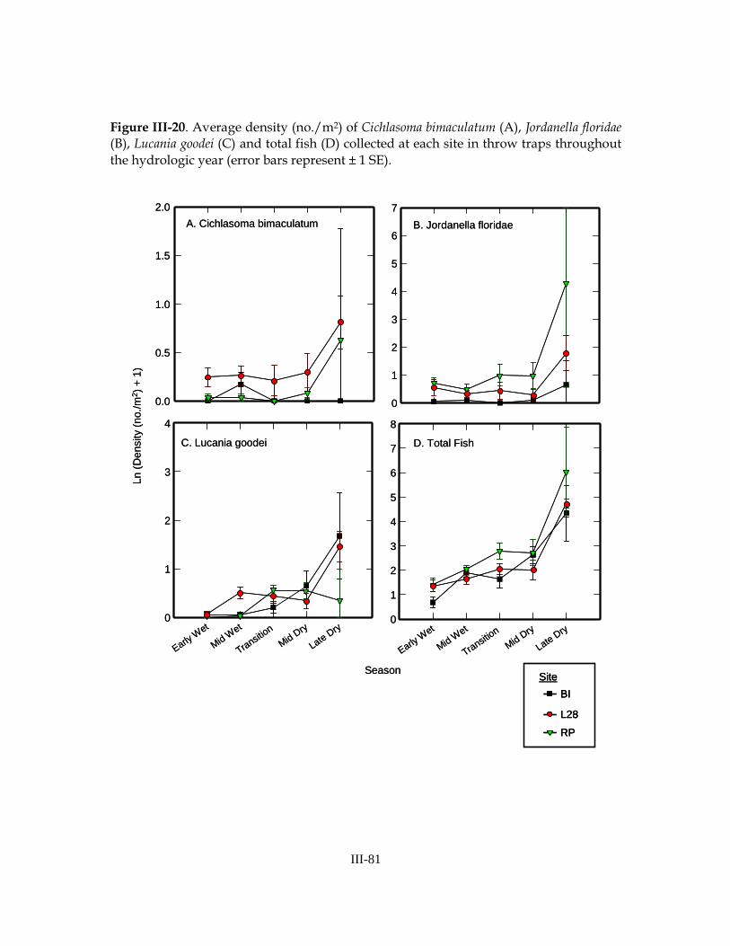
III-81

Figure III-20. Average density (no./m2) of Cichlasoma bimaculatum (A), Jordanella floridae (B), Lucania goodei (C) and total fish (D) collected at each site in throw traps throughout

the hydrologic year (error bars represent ± 1 SE).

0.0

0.5

1.0

1.5

2.0

A. Cichlasoma bimaculatum

0

1

2

3

4

5

6

7

B. Jordanella floridae

EarlyWet

MidWet

Transition

MidDry

LateDry

0

1

2

3

4

C. Lucania goodei

Season

EarlyWet

MidWet

Transition

MidDry

LateDry

0

1

2

3

4

5

6

7

8

D. Total Fish

Ln(D

ensi

ty (

no./m

2 ) +

1)

BI

L28

RP

Site

0.0

0.5

1.0

1.5

2.0

A. Cichlasoma bimaculatum

0

1

2

3

4

5

6

7

B. Jordanella floridae

EarlyWet

MidWet

Transition

MidDry

LateDry

0

1

2

3

4

C. Lucania goodei

Season

EarlyWet

MidWet

Transition

MidDry

LateDry

0

1

2

3

4

5

6

7

8

D. Total Fish

Ln(D

ensi

ty (

no./m

2 ) +

1)

BI

L28

RP

Site

BI

L28

RP

Site

III-82

Figure III-21. Examples of drop traps at Bear Island with (A) and without (B) habitat structure (compared in analysis of the impact of habitat structure on fish sampling).

B. Drop trap without habitat structure

A. Drop trap with habitat structure

B. Drop trap without habitat structure

A. Drop trap with habitat structure

III-83

Figure III-22. Average density (no./m2) of Lepomis gulosus, Gambusia holbrooki and total fish collected in drop traps (with and without habitat structure) and throw traps at Bear Island during habitat structure sampling effort (error bars represent ± 1 SE).

Total Fish

Drop Trap(w/o hab str)

0.0

0.1

0.2

0.3

0.4

ThrowTrap

Drop Trap(w/ hab str)

0.0

0.5

1.0

1.5

2.0

2.5

Lepomis gulosus

Gambusia holbrooki

Drop Trap(w/o hab str)

ThrowTrap

Drop Trap(w/ hab str)

Trap Type

Ln(D

ensi

ty (

no./m

2 ) +

1)

Total Fish

Drop Trap(w/o hab str)

0.0

0.1

0.2

0.3

0.4

ThrowTrap

Drop Trap(w/ hab str)

0.0

0.5

1.0

1.5

2.0

2.5

Lepomis gulosus

Gambusia holbrooki

Drop Trap(w/o hab str)

ThrowTrap

Drop Trap(w/ hab str)

Trap Type

Ln(D

ensi

ty (

no./m

2 ) +

1)

III-84

Figure III-23. NMDS of macroinvertebrate community structure (data are non-standardized) at each site throughout the hydrologic year. Arrows indicate successive transitions between sampling seasons.

Late-DryMid-DryTransitionMid-WetEarly-Wet

Sampling Season:L-28Raccoon PointBear Island

Site:

Stress = 0.07

Late-DryMid-DryTransitionMid-WetEarly-Wet

Sampling Season:L-28Raccoon PointBear Island

Site:

Stress = 0.07

III-85

Figure III-24. NMDS of macroinvertebrate community structure (data are standardized) at each site throughout the hydrologic year. Arrows indicate successive transitions between sampling seasons.

Late-DryMid-DryTransitionMid-WetEarly-Wet

Sampling Season:L-28Raccoon PointBear Island

Site:

Stress = 0.06

Late-DryMid-DryTransitionMid-WetEarly-Wet

Sampling Season:L-28Raccoon PointBear Island

Site:

Stress = 0.06

III-86

Figure III-25. Average total invertebrate density (no./m2) in each sampling zone at each site throughout the hydrologic year (error bars represent ± 1 SE).

Ln(D

ensi

ty (

no./m

2 ) +

1)

0

1

2

3

4

5

6

7

BI

Shallow

Deep

Prairie

Zone

Refuge

0

1

2

3

4

5

6

7

Ln(D

ensi

ty (

no./m

2 ) +

1)

Season

Early Wet Mid Wet Transition Mid Dry Late Dry0

1

2

3

4

5

6

7

Ln(D

ensi

ty (

no./m

2 ) +

1)

L28

RP

Ln(D

ensi

ty (

no./m

2 ) +

1)

0

1

2

3

4

5

6

7

BI

Shallow

Deep

Prairie

Zone

Refuge

Shallow

Deep

Prairie

Zone

Refuge

0

1

2

3

4

5

6

7

Ln(D

ensi

ty (

no./m

2 ) +

1)

Season

Early Wet Mid Wet Transition Mid Dry Late Dry0

1

2

3

4

5

6

7

Ln(D

ensi

ty (

no./m

2 ) +

1)

L28

RP

III-87

Figure III-26. Average density (no./m2) of Procambarus alleni and Procambarus fallax collected at each site throughout the course of the study (error bars represent ± 1 SE).

Site

BI L28 RP

Ln(D

ensi

ty (

no./m

2 ) +

1)

0.2

0.4

0.6

0.8

1.0

1.2

1.4

1.6

1.8

Procambarus alleni

Procambarus fallax

Crayfish species

Site

BI L28 RP

Ln(D

ensi

ty (

no./m

2 ) +

1)

0.2

0.4

0.6

0.8

1.0

1.2

1.4

1.6

1.8

Procambarus alleni

Procambarus fallax

Crayfish species

III-88

Figure III-27. Average density (no./m2) of Procambarus alleni (A), Procambarus fallax (B) and juvenile Procambarus spp. (C) collected in each sampling zone throughout the

hydrologic year (error bars represent ± 1 SE). A. Procambarus alleni

0.0

0.5

1.0

1.5

2.0

2.5

3.0

3.5

Shallow

Deep

Prairie

Zone

Refuge

Ln(D

ensi

ty (

no./m

2 ) +

1)

0.0

0.5

1.0

1.5

2.0

2.5

3.0

3.5

B. Procambarus fallax

Ln(D

ensi

ty (

no./m

2 ) +

1)

Season

Early Wet Mid Wet Transition Mid Dry Late Dry

0.0

0.5

1.0

1.5

2.0

2.5

3.0

3.5

C. Procambarus spp.

Ln(D

ensi

ty (

no./m

2 ) +

1)

A. Procambarus alleni

0.0

0.5

1.0

1.5

2.0

2.5

3.0

3.5

Shallow

Deep

Prairie

Zone

Refuge

Shallow

Deep

Prairie

Zone

Refuge

Ln(D

ensi

ty (

no./m

2 ) +

1)

0.0

0.5

1.0

1.5

2.0

2.5

3.0

3.5

B. Procambarus fallax

Ln(D

ensi

ty (

no./m

2 ) +

1)

Season

Early Wet Mid Wet Transition Mid Dry Late Dry

0.0

0.5

1.0

1.5

2.0

2.5

3.0

3.5

C. Procambarus spp.

Ln(D

ensi

ty (

no./m

2 ) +

1)

III-89

Figure III-28. Average density (no./m2) of Palaemonetes paludosus (A), Planorbella spp. (B), tadpoles (C) and total amphibians (D) collected in each sampling zone throughout the hydrologic year (error bars represent ± 1 SE).

EarlyWet

A. Palaemonetes paludosus

0

1

2

3

4

0.0

0.2

0.4

0.6

0.8

1.0

1.2

1.4B. Planorbella spp.

Ln(D

ensi

ty (

no./m

2 ) +

1)

MidWet

Transition

MidDry

LateDry

0.0

0.2

0.4

0.6

0.8

1.0

Season

EarlyWet

MidWet

Transition

MidDry

LateDry

Shallow

Deep

Prairie

Zone

Refuge

C. Tadpoles D. Total Amphibians

EarlyWet

A. Palaemonetes paludosus

0

1

2

3

4

0.0

0.2

0.4

0.6

0.8

1.0

1.2

1.4B. Planorbella spp.

Ln(D

ensi

ty (

no./m

2 ) +

1)

MidWet

Transition

MidDry

LateDry

0.0

0.2

0.4

0.6

0.8

1.0

Season

EarlyWet

MidWet

Transition

MidDry

LateDry

Shallow

Deep

Prairie

Zone

Refuge

Shallow

Deep

Prairie

Zone

Refuge

C. Tadpoles D. Total Amphibians

III-90

Figure III-29. Sample graphic output from G*POWER3 program, total fish density test, deep habitat, 28% increase in L28 (see Appendix 6 for full graphic output).

Total sample size

Appendix–1

APPENDICES

Appendix–2

Appendix 1

(Original Submission Date: 30 September 2005)

DEVELOPMENT AND TESTING OF PROCEDURES FOR SAMPLING FISHES IN FORESTED WETLANDS

IN SOUTHERN FLORIDA

Sampling Fishes in Cypress and Mangrove Forests: A Literature Review

Prepared by:

Shawn E. Liston Jerome J. Lorenz Carole C. McIvor

National Audubon Society Tavernier Science Center 115 Indian Mound Trail Tavernier, FL 33070

US Geological Survey Center for Coastal & Watershed Studies

600 Fourth Street South St. Petersburg, FL 33701

Appendix–3

INTRODUCTION

The Ecological Importance of Forested Wetlands Forested wetlands are found throughout the world in both estuarine and freshwater

environments. Habitat structure provided by trees in these systems (particularly, above-ground root systems, trunks with complex surfaces, and treefall) is invaluable to resident fishes and macroinvertebrates. These ecosystems appear to be critical for many species of fish and macroinvertebrates for feeding, reproducing, and as nursery grounds for young (Mitsch & Gosselink, 1986). Freshwater forested wetlands may also provide critical habitat for amphibians who seek refuge in root holes and crayfish holes during dry downs, and reproduce in large breeding aggregations in depressional pools, upon re-flooding (Wharton et al., 1982). As with many aquatic systems, hydrology is often an important factor in the functioning of these ecosystems. Mangrove forests experience daily (tidal) variation in water levels (and subsequent nutrient inputs), while freshwater flooded forests typically experience a longer duration hydrologic cycle, resulting in forests that are temporarily to seasonally inundated. Fish in permanent freshwater systems are often so dependent upon forested

floodplains for feeding, spawning, and rearing of young that it has been argued the permanently flooded aquatic systems and their neighboring temporarily- or seasonally-flooded forested habitats should be considered as a single system (Lambou, 1990). Adjacent, temporarily- or seasonally-flooded forests have been found to provide important habitat for fish in large rivers (Kwak, 1988; Turner et al., 1994), streams (Ross & Baker, 1983), and coastal wetlands (Poulakis et al., 2002). Fish in these forested systems may actually depend on annual water level fluctuation to limit intra- and interspecific competition for food, space, and spawning grounds (Lambou, 1959), although the relative importance of habitat structure and hydrologic variability is likely species-specific (Ross & Baker, 1983). Due to the fact that seasonally-flooded forested systems are cut-off from continuously inundated areas as water levels recede, competition for food in these systems may become increasingly important as the dry season progresses. Lambou (1959) found that approximately 44% of fish collected in a Mississippi River floodplain forest were predators. Lambou further concluded that predaceous fish must be partially dependent upon some type of forage other than fish, suggesting that swamp crayfish are likely important in their diet. Studies have also suggested strong aquatic-terrestrial food web links in these systems, as terrestrial invertebrates may provide a significant proportion of fish diet, in some cases (Arner et al., 1976; Woodall et al., 1975). A wide variety of methodologies have been used to sample fishes in mangrove

habitats throughout the world. Sampling methods in mangrove creeks include nets, trawls, visual sampling, and hydroacoustic techniques. In ecotonal regions of the Everglades, previous sampling has primarily consisted of block netting for large fishes

Appendix–4

and drop nets or bottomless lift nets for small fishes. Few studies have utilized electrofishing, due to salinity limitations (sampling is only feasible up to 15 ppt with existing electrofishing units).

Forested Wetlands in Southern Florida Forested wetlands cover hundreds of thousands of hectares of southern Florida. The

mangrove swamps of southern and southwestern Everglades National Park represent one of the largest continuous mangrove forests on earth. The Big Cypress Swamp ecosystem covers a large area of interior southwestern Florida, and is comprised of several types of cypress habitats termed domes, strands, and dwarf cypress (Duever et al., 1986; Ewel, 1990). Both systems are important pieces in the hydrological system of the Greater Everglades region, yet both have been poorly studied compared with the Everglades gramminoid wetlands. Few fish studies have been carried out in the closed-canopy mangrove forests of

southern Florida. The early work of Tabb (1974) looked at the influence of changing water levels on fish distribution. Odum and Heald (1972) elucidated the importance of mangrove detritus to the secondary productivity of fishes in mangrove forests. Neither of these early works used quantitative methods of fish collection, making change analysis difficult. McIvor and Silverman (unpub. manuscript) have improved the sampling characteristics of a quantitative bottomless lift net for use in tidal mangrove forests, but considerable work remains to be done before a widely exportable method is developed. Similarly, few studies of fish communities have been carried out in Big Cypress

Swamp forests, and they have used various sampling techniques. Kushlan (1974) studied the dynamics of a dry-season fish kill in an alligator pond. Carlson and Duever (1979) examined the community dynamics of shallow and deep-water habitats in the Corkscrew region of Big Cypress. Recently, Ellis et al. (2003) inventoried the freshwater fishes of the region, and Dunker (2003) completed a comparison of fish communities in natural and restored habitats within the Big Cypress Seminole Indian Reservation. Those studies provide us with examples of methods that have been effective in some Big Cypress habitats. These methods were qualitative or semi-quantitative, and do not meet the objective of a quantitative, repeatable technique that is useful across habitats. The habitat structure that provides critical refuge for fish presents, in fact, the

greatest obstacle for sampling in these habitats. Traditional fishery methods of towing trawls, pulling seines, or visual censuses, simply do not work. Fixed-location, bottomless enclosure nets that either drop from above or are pulled up from below have shown considerable promise (Lorenz et al., 1997; McIvor & Silverman, unpub. manuscript), but these have never been cross-calibrated for gear bias and recovery

Appendix–5

efficiency in such habitats. In the following, we discuss sampling methods tested and used in other forested aquatic systems, as well as, methods currently used in gramminoid marshes that may be adaptable for forested systems. REVIEW OF SAMPLING METHODS

Fixed-Area Devices Sampling devices that enclose a fixed area, and are then cleared of captured animals

have been used extensively, and for some time, in aquatic systems throughout the world. These devices typically range in area from 0.25 to 10 m2, and provide quantitative surface-area density estimates (no./m2). Additionally, when water depth is taken into account, these devices can produce estimates of volumetric density (no./m3). Fixed-area sampling devices vary considerably, however, in a few key factors that must be weighed during the selection of sampling gear appropriate for each individual study. As with all sampling devices, the size of the sampling devices does present some limitations in the size of the animals captured within them. Additionally, while some of these devices allow critical habitat structure (trees, treefall, submerged vegetation) to be encompassed within the trap, others systematically exclude it. The method with which these traps are cleared (e.g., manually, chemically, tidally) can also lead to the selection or exclusion of particular species, and can cause different types of disturbance to the system. Finally, the portability of the device (i.e., whether they are fixed and sample the same location repeatedly, or are movable) is an important factor to consider, especially when coupled with the composition of the bottom substrate and any disturbance caused by the clearing method. Pull-up traps. Permanently installed pull-up traps were used for some time in open gramminoid marshes in the Florida Everglades. Pull-up traps used by Higer & Kolipinski (1967) and Kushlan (1974, 1980) have a mesh bottom and sides and are quickly pulled upwards through the water column to capture fish. While this trap was effective in water over 1.5 m deep (Kushlan 1974), it involves significant habitat alteration, as submerged vegetation must be cleared in order to install the nets. Loftus & Eklund (1994) demonstrated that in the Everglades these traps significantly degraded sampling sites with vegetation removal and reduced soil elevation, and repeated of foot traffic caused the creation of corridors to and from sample sites. Additionally, the nets became a substrate for algae that made them heavier (nets lifted more slowly, allowing fish to escape) and attracted fish. Drop traps. Drop traps were used in open marshes in the Florida Everglades by Kahl

(1963) and A. Higer (described in Kushlan (1974), and although these traps were relatively effective, they were heavy and difficult to re-set (Kushlan 1974). Gilmore et al. (1978) tested a similar trap in a shallow estuarine habitat, and found the trap was

Appendix–6

biased against schooling fishes or those with a clumped distribution, but was an effective tool for obtaining estimates of fish density and biomass in fish populations with a relatively small adult size. Drop traps constructed from a weighted frame and nylon mesh sides and solid metal traps transported via floats have also been developed, and have been found to be effective and much easier to use (Table 1). Drop traps developed by Lorenz et al. (1997) are large enough to encompass small mangroves (9 m2) which provide habitat structure within the trap, thereby decreasing trap avoidance by fish seeking refuge. While small fish may avoid or be attracted to permanently installed drop-trap frames (Kjelson et al., 1975), little success has been achieved in the development of an effective, portable drop trap that can be manually moved between sampling locations by field personnel (J. C. Trexler, Florida International University and J. Lorenz, Audubon of Florida, personal communications). Table 1. Examples of previous studies utilizing drop traps to capture fish. Portable trap designs are denoted with an asterisk (other traps are in fixed locations).

Study Habitat Size Material

Kahl, 1963

FL Everglades marsh 1 m2 Metal sheeting

A. Higer (described by Kushlan, 1974)

FL Everglades marsh ~4.5 m2 3-mm mesh

Kjelson et al., 1975

Newport River estuary, NC 4 m2 3-mm mesh

Gilmore et al., 1978*

FL estuary 10 m2 3.2-mm mesh

Lorenz et al., 1997

FL Everglades mangroves 9 m2 1.6-mm mesh

Pihl et al., 2000*

Sweedish soft-bottom and rocky-bottom shorelines

1 m2 Solid

Polte et al., 2005* North Sea eelgrass beds 0.5 m2 Aluminum

Bottomless lift nets. Bottomless lift nets (as described by Rozas 1992) have been successfully used to sample fishes in tidal mangrove systems. Ellis & Bell (2004) found the recapture efficiency of Cyprinidon variegatus in 9-m2 (4 mm mesh) bottomless lift net was 92%. Throw traps. Portable throw traps have been tested and used extensively to sample fish in a variety of aquatic habitats worldwide. Trap size has ranged from 0.25-m2 to 2.25-m2 (Table 2). Several studies have tested the efficiency of traps, through mark-recapture, repeated sampling, and statistical modeling. Pelicice et al. (2005) were able to recapture 95% of marked fish in a 1-m2 trap, and Jacobsen & Kushlan (1987) used

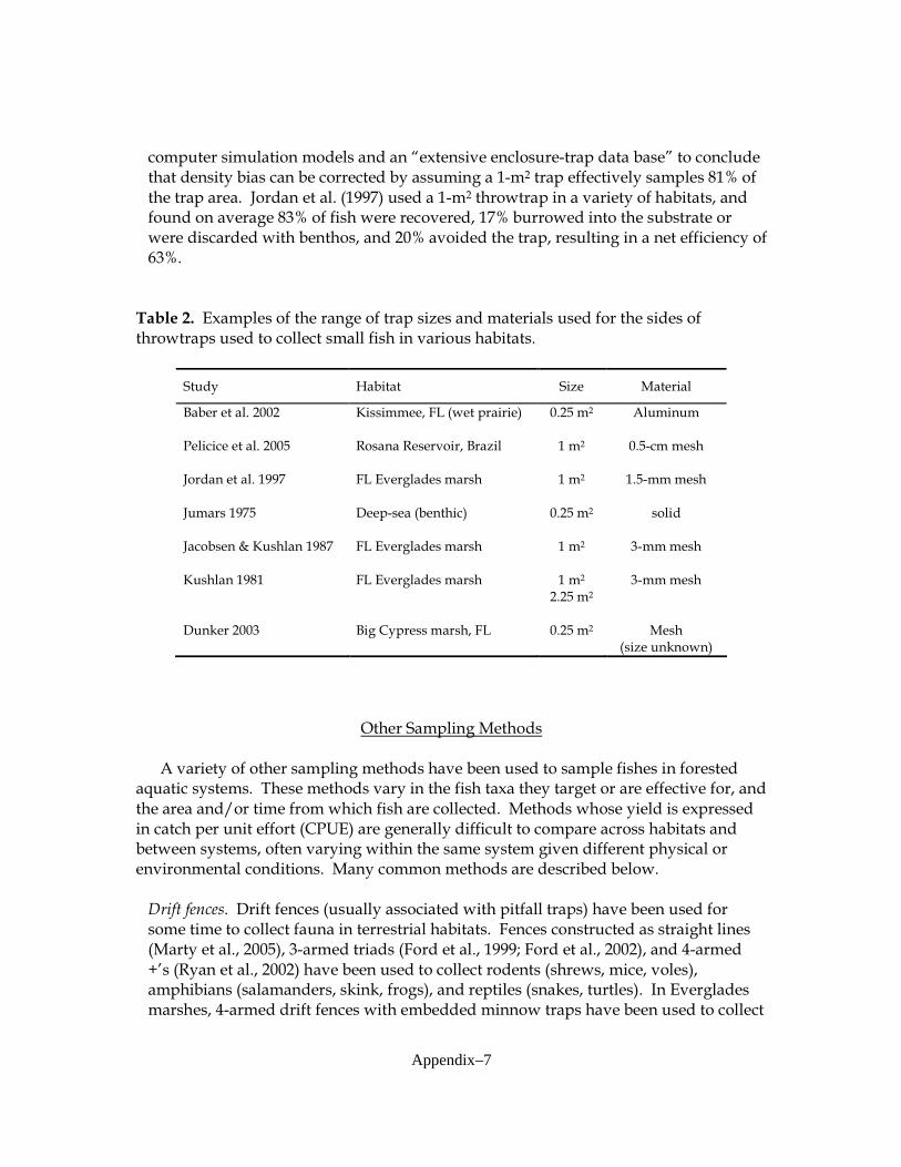
Appendix–7

computer simulation models and an “extensive enclosure-trap data base” to conclude that density bias can be corrected by assuming a 1-m2 trap effectively samples 81% of the trap area. Jordan et al. (1997) used a 1-m2 throwtrap in a variety of habitats, and found on average 83% of fish were recovered, 17% burrowed into the substrate or were discarded with benthos, and 20% avoided the trap, resulting in a net efficiency of 63%.

Table 2. Examples of the range of trap sizes and materials used for the sides of throwtraps used to collect small fish in various habitats.

Study Habitat Size Material

Baber et al. 2002 Kissimmee, FL (wet prairie)

0.25 m2 Aluminum

Pelicice et al. 2005 Rosana Reservoir, Brazil

1 m2 0.5-cm mesh

Jordan et al. 1997

FL Everglades marsh 1 m2 1.5-mm mesh

Jumars 1975

Deep-sea (benthic) 0.25 m2 solid

Jacobsen & Kushlan 1987

FL Everglades marsh 1 m2 3-mm mesh

Kushlan 1981

FL Everglades marsh 1 m2 2.25 m2

3-mm mesh

Dunker 2003 Big Cypress marsh, FL 0.25 m2 Mesh (size unknown)

Other Sampling Methods A variety of other sampling methods have been used to sample fishes in forested

aquatic systems. These methods vary in the fish taxa they target or are effective for, and the area and/or time from which fish are collected. Methods whose yield is expressed in catch per unit effort (CPUE) are generally difficult to compare across habitats and between systems, often varying within the same system given different physical or environmental conditions. Many common methods are described below. Drift fences. Drift fences (usually associated with pitfall traps) have been used for some time to collect fauna in terrestrial habitats. Fences constructed as straight lines (Marty et al., 2005), 3-armed triads (Ford et al., 1999; Ford et al., 2002), and 4-armed +’s (Ryan et al., 2002) have been used to collect rodents (shrews, mice, voles), amphibians (salamanders, skink, frogs), and reptiles (snakes, turtles). In Everglades marshes, 4-armed drift fences with embedded minnow traps have been used to collect

Appendix–8

fish moving through the marsh, and orientation of the arms in each of the cardinal compass directions allows for interpretation of directional fish movement (Loftus et al., 2005; Trexler, 2005; Goss, unpub. thesis). Similarly, Walker (1980) used two-way weir traps on the Creeping Swamp floodplain, and Kwak (1988) used one-way fish traps on a river floodplain to examine seasonal directional fish movement. Minnow traps. Minnow traps have been used extensively to collect small fish in stream, lake, and wetland habitats. Most studies of minnow trap capture efficiency, however, have noted significant limitations and/or catch biases. Minnow traps only capture fish within a certain size range (Blaustein, 1989; Pot et al., 1984; Ritchie & Johnson, 1986), however, some species have also been seen to enter or avoid traps preferentially (Pot et al., 1984; Blaustein, 1989; Layman & Smith, 2001). Several studies have recommended caution in using minnow trap catch to estimate fish abundance, or describe size distributions or community structure (Pot et al., 1984; Blaustein, 1989; Kneib & Craig, 2001; Layman & Smith, 2001). Some success has been achieved estimating fish abundance through depletion with repeated use of baited minnow traps (Bryant 2000). Electrofishing. While electrofishing is a common method to sample fishes in many freshwater systems (Reynolds, 1996), habitat structure associated with forested wetlands presents several problems. Dunker (2003) completed limited sampling in the Big Cypress system with a boat-mounted electroshocker, focusing efforts primarily in open marsh areas. Ellis et al. (2005) sampled fish in canals in Big Cypress National Preserve with a boat-mounted electroshocker, but noted that the size of the vessel restricted its use only to canals. They also used a smaller, barge-mounted electroshocker in other areas of the system, but found that even with its relatively small size, they were unable to penetrate heavily vegetated habitats. Gill nets. Experimental gill nets have been used to capture large fish in Big Cypress National Preserve in two studies. Dunker (2003) used experimental gill nets with 4 panels (1, 2, 3, and 4 cm) with a 6 h soak time. Ellis et al. (2005) used two different 4-panel experimental gill nets (1.2, 2.5, 3.7, 5 cm and 6.2, 7.6, 8.8, 11 cm) with 1-4 h soak times. Both groups noted some difficulties with nets in the flooded forests. Dunker had difficulties with woody debris and herbaceous vegetation becoming tangled in nets (personal communication), and Ellis et al. (2005) noted that reptiles (particularly alligators) were often caught in nets, prompting shorter soak times. Other nets. A variety of other types of nets have been used to sample fishes in mangrove ecosystems (Table 3).

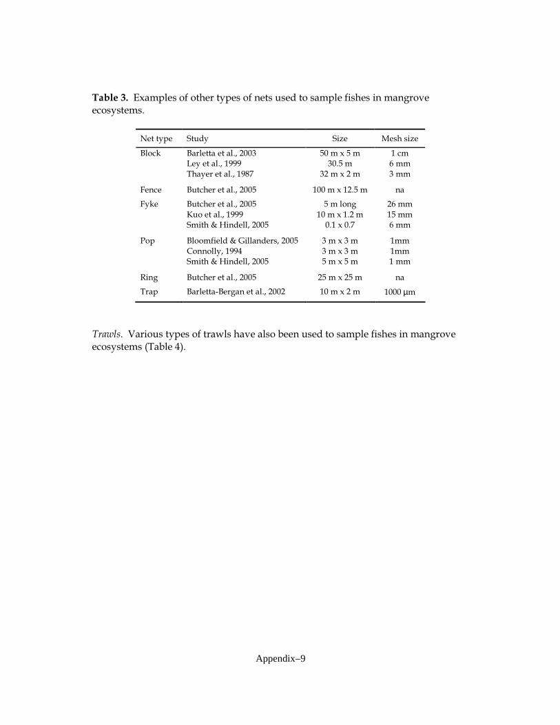
Appendix–9

Table 3. Examples of other types of nets used to sample fishes in mangrove ecosystems.

Net type Study Size Mesh size

Barletta et al., 2003 50 m x 5 m 1 cm Ley et al., 1999 30.5 m 6 mm

Block

Thayer et al., 1987 32 m x 2 m 3 mm

Fence Butcher et al., 2005 100 m x 12.5 m na

Butcher et al., 2005 5 m long 26 mm

Kuo et al., 1999 10 m x 1.2 m 15 mm

Fyke

Smith & Hindell, 2005 0.1 x 0.7 6 mm

Bloomfield & Gillanders, 2005 3 m x 3 m 1mm Connolly, 1994 3 m x 3 m 1mm

Pop

Smith & Hindell, 2005 5 m x 5 m 1 mm

Ring Butcher et al., 2005 25 m x 25 m na

Trap Barletta-Bergan et al., 2002 10 m x 2 m 1000 µm

Trawls. Various types of trawls have also been used to sample fishes in mangrove ecosystems (Table 4).

Appendix–10

Table 4. Examples of types of trawls used to sample fishes in mangrove ecosystems.

Trawl type Study

Barletta et al., 2005 Colby et al., 1985 McPherson, 1970 Petrik & Levin, 2000 Tabb et al., 1962

Otter

Thayer et al., 1987

Beam Butcher et al., 2005

Surface Colby et al., 1985

Roller frame Serafy et al., 1997

Previous Sampling Gear Comparison Studies Many studies have presented comparisons of different types of sampling gear in

marsh and flooded forest habitats. In terms of fixed-area devices, Kushlan (1974) recommends the use of portable traps, as they are not biased by previous habitat alteration. Rozas & Minello (1997) discourage the use of trawls and seines, as they have low, variable catch efficiency, and recommend enclosure samplers (the type of which should be dictated by the specific requirements of the project). Knight & Bain (1996) compared several sampling methods in forested stream floodplains (see Table 5), and concluded that a combination of area electrofishing, gill nets, and light traps provide a thorough and comprehensive description of wetland fish assemblages. Most gear comparison studies, however, conclude that a combination of several sampling methods should be employed, and the choice of these should be dictated by the community being targeted (Knight & Bain, 1996; Jackson & Harvey, 1997; Rozas & Minello, 1997; Petrik, 2000; Lazzari, 2002).

SUMMARY Modifying existing sampling protocols and incorporating local habitat and faunal-

distribution characteristics will help minimize sample variability both locally and across the sampling network. Minimizing intra-site variation is a critical component in the development of this assessment network. Minimizing gear bias by employing a single method across the network is also desirable, but may not be feasible because no one gear is suitable for all habitats. Previous work demonstrates that depth and duration of flooding, water quality characteristics, and structural habitat influence fish and invertebrate species composition in many wetland types. These features vary considerably both seasonally and spatially in south Florida. Developing standard

Appendix–11

techniques and protocols that encompass these variables is crucial to sampling fishes in forested habitats. Due to constraints imposed by copious amounts of habitat structure, many types of sampling gear currently used in Everglades marshes will be inadequate in the mangrove zone and cypress forests. We present a summary (Table 6) of the advantages and disadvantages of five sampling devices that we have selected to evaluate the use of in mangrove and/or cypress forests: 9-m2 drop traps (as described by Lorenz et al. (1997)), 6 m2 lift nets (as described by as described by McIvor & Silverman (unpub. manuscript)), 1-m2 throw traps (as described by as described by Jordan et al. (1997)), drift fences (as described by Loftus et al. (2005)) and experimental gill nets. Unfortunately, we will not be able to coordinate these efforts with the Florida Bay Fisheries Habitat Assessment Program (FHAP) as this program requires the use of portable sampling devices so that sampling locations can be randomly selected prior to each sampling event.

Appendix–12

Table 5. Comparison of various sampling techniques applied in forested floodplain wetlands. Reproduced from Knight & Bain (1996), p. 83.

Sampling gear Advantages Limitations

Quantitative sampling

Area electrofishing Broad species coverage Records a wide size range Sampling can be done quickly and in one day

High catch rates Consistent catch rates in a variety of habitats

Inefficient in highly turbid, deep (>50 cm), and very shallow (<20 cm) water Uses heavy and expensive equipment Safety precautions must be followed May undersample some benthic species

Trap nets High catch rates Effective on benthic species Effective in very shallow (<20 cm), densely structured and highly turbid waters

Species selective Selective for small size fish Susceptible to clogging by debris

Small-mesh gill nets (1.3 and 2-cm bar mesh)

Effective on nocturnal and highly mobile species

Easy to use and transport

Species selective Ineffective on small fish Inefficient in very shallow water Susceptible to clogging by debris

Large-mesh gill nets (2.5 and 5 cm bar mesh)

Effective on large, nocturnal, and highly mobile species

Easy to use and transport

Species selective Ineffective on small to medium size fish Inefficient in very shallow water

Light traps (larval fish)

Broad species coverage High catch rates Easy to deploy

Does not sample non-phototaxic species Efficiency related to water clarity Requires specialized custom equipment

Qualitative sampling

Electrofishing Broad species and size coverage Rapid sampling technique

Uses heavy and expensive equipment May under-sample some benthic species Safety precautions must be followed

Dip nets (larval fish) Broad species coverage Rapid sampling technique

Catch rate can be low Sampling may be highly variable

Appendix–13

Table 6. Summary of advantages and disadvantages of various sampling gear, feasible for use in South Florida flooded forests: 9-m2 drop trap (as described by Lorenz et al. (1997)), 6 m2 lift net (as described by as described by McIvor & Silverman (unpub. manuscript)), 1-m2 throw trap (as described by as described by Jordan et al. (1997)), drift fence (as described by Loftus et al. (2005)) and experimental gill nets.

Sampling Characteristic Drop trap

Lift net

Throw trap

Drift fence

Gill net

Produces density estimates

Yes Yes Yes No No

Allows incorporation of habitat structure (trees, treefall, etc.)

Yes Yes No na na

Portable

No No Yes No Yes

Effective for small fish

Yes Yes Yes Yes No

Effective for large fish

No No No No Yes

Effective for large macroinvertebrates

No No Yes No No

Sampling duration

Single point in

time

Single point in

time

Single point in

time

24 h (cumulative)

soak time undeter-

mined

Species-specific selectivity Low O2* Low O2* Minnow trap preference/

avoidance

Allow interpretation of directional fish movement

No No No Yes No

*rotenone may not be as effective on fish adapted to low oxygen environments (personal observation)

Appendix–14

LITERATURE CITED Arner, D.H., H.R. Robinette, J.E. Frasier, and M.H. Gray. 1976. Effects of channelization

of the Luxapalila River on fish, aquatic invertebrates, water quality and furbearers. U.S. Fish and Wildlife Services, Office of Biological Services FWS/OBS-76-08.

Baber, M.J., D.L. Childers, K.J. Babbitt, and D.H. Anderson. 2002. Controls on fish distribution and abundance in temporary wetlands. Canadian Journal of Fisheries and Aquatic Sciences 59(9): 1441-1450.

Barletta, M., A. Barletta-Bergan, U. Saint-Paul, and G. Hubold. 2003. Seasonal changes in density, biomass and diversity of estuarine fishes in tidal mangrove creeks of the lower Caete Estuary (northern Brazilian coast, east Amazon). Marine Ecology Progress Series 256: 217-228.

Barletta, M., A. Barletta-Bergan, U. Saint-Paul, and G. Hubold. 2005. The role of salinity in structuring the fish assemblages in a tropical estuary. Journal of Fish Biology 66: 45-72.

Barletta-Bergan, A., M. Barletta, and U. Saint-Paul. 2002. Community structure and temporal variability of ichthyoplankton in North Brazilian mangrove creeks. Journal of Fish Biology 61: 33-51.

Blaustein, L. 1989. Effects of various factors on the efficiency of minnow traps to sample mosquitofish (Gambusia affinis) and green sunfish (Lepomis cyanellus)

populations. Journal of the American Mosquito Control Association 5(1): 29-35.

Bloomfield, A.L. and B.M. Gillanders. 2005. Fish and invertebrate assemblages in seagrass, mangrove, saltmarsh, and nonvegetated habitats. Estuaries 28: 63-77.

Bryant, M.D. 2000. Estimating fish populations by removal methods with minnow traps in southeast Alaska streams. North American Journal of Fisheries Management 20: 923-930.

Butcher, A., D. Mayer, D. Smallwood, and M. Johnston. 2005. A comparison of the relative efficiency of ring, fyke, fence nets and beam trawling for estimating key estuarine fishery populations. Fisheries Research 73: 311-321.

Carlson, J.E. and M.J. Duever. 1979. Seasonal fish populations in a South Florida swamp. Proceedings of the Annual Conference of the Southeast Association of Fish and Wildlife Agencies 31: 603-611.

Colby, D.R., G.W. Thayer, W.F. Hettler, and D.S. Peters. 1985. A comparison of forage fish communities in Faka Union Bay, Florida and eight collateral bays during the wet season. Technical Memorandum: NOAA-TM-NMFS-SEFC 162.

Connolly, R.M. 1994. Comparison of fish catches from a buoyant pop net and a beach seine net in a shallow seagrass habitat. Marine Ecology Progress Series 109: 305-309.

Appendix–15

Duever, M.J., J.E. Carlson, J.F. Meeder, L.C. Duever, L.H. Gunderson, L.A. Riopelle, T.R. Alexander, R.L. Myers, and D.P. Spangler. 1986. The Big Cypress National Preserve. National Audubon Society, New York, NY.

Dunker, K.J. 2003. Non-indigenous fishes in restored and natural wetlands on the Big Cypress Seminole Indian Reservation. M.S. Thesis, Florida Atlantic University, Boca Raton, FL.

Ellis, G., M. Zokan, J.J. Lorenz, and W.F. Loftus. 2003. Inventory of the freshwater fishes of the Big Cypress National Preserve, with a proposes plan for a long-term aquatic sampling program. Annual report to the USGS Place-Based Study Program, Homestead, FL.

Ellis, W.L., and S.S. Bell. 2004. Conditional use of mangrove habitats by fishes: depth as a cue to avoid predators. Estuaries 27: 966-76.

Ewel, K.C. 1990. Swamps. In R.L. Myers and J.J. Ewel (eds), Ecosystems of South Florida, pages 281-323. University of Central Florida Press, Gainesville, FL.

Ford, W.M., M.A. Menzel, D.W. McGill, J. Laerm, and T.S. McCay. 1999. Effects of a community restoration fire on small mammals and herpetofauna in the southern Appalachians. Forest Ecology and Management 114: 233-243.

Ford, W.M., B.R. Chapman, M.A. Menzel, and R.H. Odom. 2002. Stand age and habitat influences on salamanders in Appalachian cove hardwood forests. Forest Ecology and Management 155: 131-141.

Gilmore, R.G., J.K. Holt, R.S. Jones, G.R. Kulczycki, L.G. MacDowell, III, and W.C. Magley. 1978. Portable tripod drop net for estuarine fish studies. Fishery Bulletin 76: 285-289.

Goss, C.W. unpub. The effects of hydrological disturbance on fish population dynamics. M.S. Thesis, Florida International University, Miami, FL.

Higer, A.L. and M.C. Kolipinski. 1967. Pull-up trap: a quantitative device for sampling shallow-water animals. Ecology 48(6): 1008-1009.

Jackson, D.A. and H.H. Harvey. 1997. Qualitative and quantitative sampling of lake fish communities. Canadian Journal of Fisheries and Aquatic Sciences 54: 2807-2813.

Jacobsen, T. and J.A. Kushlan. 1987. Sources of sampling bias in enclosure fish trapping: effects on estimates of density and diversity. Fisheries Research 5: 401-412.

Jordan, F., S. Coyne, and J.C. Trexler. 1997. Sampling fishes in vegetated habitats: effects of habitat structure on sampling characteristics of the 1-m2 throw trap. Transactions of the American Fisheries Society 126: 1012-1020.

Jumars, P.A. 1975. Methods for measurement of community structure in deep-sea macrobenthos. Marine Biology 30: 145-252.

Appendix–16

Kahl, M.P., Jr. 1963. Technique for sampling population density of small shallow-water fish. Limnology and Oceanography 8(2): 302-304.

Kneib, R.T. and A.H. Craig. 2001. Efficacy of minnow traps for sampling mummichogs in tidal marshes. Estuaries 24(6A): 884-893.

Kjelson, M.A., W.R. Turner, and G.N. Johnson. 1975. Description of a stationary drop-net for estimating nekton abundance in shallow waters. Transactions of the American Fisheries Society 104: 46-49.

Knight, J.G. and M.B. Bain. 1996. Sampling fish assemblages in forested floodplain wetlands. Ecology of Freshwater Fish 5: 76-85.

Kuo, S.-R., H.-J. Lin, and K.-T. Shao. 1999. Fish assemblages in the mangrove creeks of northern and southern Taiwan. Estuaries 22: 1004-1015.

Kushlan, J.A. 1974. Quantitative sampling of fish populations in shallow, freshwater environments. Transactions of the American Fisheries Society 103(2): 348-352.

Kushlan, J.A. 1980. Population fluctuations of Everglades fishes. Copeia 1980(4): 870-874.

Kushlan, J.A. 1981. Sampling characteristics of enclosure fish traps. Transactions of the American Fisheries Society 110(4): 557-562.

Kwak, T.J. 1988. Lateral movement and use of floodplain habitat by fishes of the Kankakee River, Illinois. American Midland Naturalist 120(2): 241-249.

Lambou, V.W. 1959. Fish populations of backwater lakes in Louisiana. Transactions of the American Fisheries Society 88: 7-15.

Lambou, V.W. 1990. Importance of bottomland forest zones to fishes and fisheries: a case history. In J.G. Gosselink, L.C. Lee, and T.A. Muir (eds), Ecological processes and cumulative impacts: illustrated by bottomland hardwood wetland ecosystems, pages 125-194. Lewis Publishers, Chelsea, MI.

Layman, C.A. and D.E. Smith. 2001. Sampling bias of minnow traps in shallow aquatic habitats on the eastern shore of Virginia. Wetlands 21(1): 145-154.

Lazzari, M.A. 2002. Epibenthic fishes and decapod crustaceans in northern estuaries: a comparison of vegetated and unvegetated habitats in Maine. Estuaries 25(6A): 1210-1218.

Ley, J.A., C.C. McIvor, and C.L. Montague. 1999. Fishes in mangrove prop-root habitats of northeastern Florida Bay: distinct assemblages across an estuarine gradient. Estuarine, Coastal, and Shelf Science 48: 701-723.

Loftus, W.F. and A.M. Eklund. 1994. Long-term dynamics of an Everglades small-fish assemblage. In S. Davis and J. Ogden (eds), Everglades: The Ecosystem and Its Restoration, pages 461-483. St. Lucie Press, Delray Beach, FL.

Appendix–17

Loftus, W.F., J.C. Trexler, J.S. Rehage, S.E. Liston, and K.J. Dunker. 2005. The role of aquatic refuges in the rockland wetland complex of southern Florida, in relation to system restoration. Final report, U.S. Geological Survey, Everglades National Park, Homestead, FL.

Lorenz, J.J., C.C. McIvor, G.V.N. Powell, and P.C. Frederick. 1997. A drop net and removable walkway used to quantitatively sample fishes over wetland surfaces in the dwarf mangroves of the southern Everglades. Wetlands 17: 346-359.

Marty, P., S. Angelibert, N. Giani, and P. Joly. 2005. Directionality of pre- and post-breeding migrations of a marbled newt population (Triturus marmoratus): implications for buffer zone management. Aquatic Conservation: Marine and Freshwater Ecosystems 15: 215-225.

McIvor, C.C. and N. Silverman. unpub. Modifications to the bottomless lift net for use in closed canopy mangrove forests.

McPherson, B.F. 1970. Hydrobiological characteristics of Shark River estuary, Everglades National Park, Florida. Open File Report: US Geological Survey 71002.

Mitsch, W.J. and J.G. Gosselink. 1986. Wetlands. Van Nostrand Reinhold Company, Inc., New York, NY.

Odum, W.E. and E.J. Heald. 1972. Trophic analysis of an estuarine mangrove community. Bulletin of Marine Science 22(3): 671-738.

Pelicice, F.M., A.A. Agostinho, and S.M. Thomaz. 2005. Fish assemblages associated with Egeria in a tropical reservoir: investigating the effects of plant biomass and

diel period. Acta Oecologia 27: 9-16.

Petrik, R. and P.S. Levin. 2000. Estimating relative abundance of seagrass fishes: a quantitative comparison of three methods. Environmental Biology of Fishes 58: 461-466.

Pihl, L., J. Modin, and H. Wennhage. 2000. Spatial distribution patterns of newly settled plaice (Pleuronectes platessa L.) along the Sweedish Skagerrak archipelago. Journal of Sea Research 44: 65-80.

Polte, P., A. Schanz, and H. Asmus. 2005. Effects of current exposure on habitat preference of mobile 0-group epibenthos for intertidal seagrass beds (Zostera noltii) in the northern Wadden Sea. Estuarine, Coastal, and Shelf Science 62: 627-635.

Pot, W., L.G. Noakes, M.M. Ferguson, and G. Coker. 1984. Quantitative sampling of fishes in a simple system: failure of conventional methods. Hydrobiologia 114(3): 249-254.

Poulakis, G.R., J.M. Shenker, and D.S. Taylor. 2002. Habitat use by fishes after tidal reconnection of an impounded estuarine wetland in the Indian River Lagoon, Florida (USA). Wetlands Ecology and Management 10: 51-69.

Appendix–18

Reynolds, J.B. 1996. Electrofishing. In B.R. Murphy and D.W. Willis, Fisheries Techniques, pages 221-253. American Fisheries Society, Bethesda, MD.

Ritchie, S.A. and E.S. Johnson. 1986. Modified Gee’s Improved Wire Minnow TrapR: an excellent surveillance tool for mosquito larvivores. Journal of the Florida Anti-Mosquito Association 57(1): 22-24.

Ross, S.T. and J.A. Baker. 1983. The response of fishes to periodic spring floods in a southeastern stream. American Midland Naturalist 109(1): 1-14.

Rozas, L.P. 1992. Bottomless lift net for sampling nekton on intertidal marshes. Marine Ecology Progress Series 89: 287-92.

Rozas, L.P. and T.J. Minello. 1997. Estimating densities of small fishes and decapod crustaceans in shallow estuarine habitats: a review of sampling design with focus on gear selection. Estuaries 20(1): 199-213.

Ryan, T.J., T. Philippi, Y.A. Leiden, M.E. Dorcas, T.B. Wigley, and J.W. Gibbons. 2002. Monitoring herpetofauna in a managed forest landscape: effects of habitat types and census techniques. Forest Ecology and Management 167: 83-90.

Serafy, J.E., K.C. Lindeman, T.E. Hopkins, and J.S. Ault. 1997. Effects of freshwater canal discharge on fish assemblages in a subtropical bay: field and laboratory observations. Marine Ecology Progress Series 160: 161-172.

Smith, T.M. and J.S. Hindell. 2005. Assessing effects of diel period, gear selectivity and predation on patterns of microhabitat use by fish in a mangrove-dominated system in SE Australia. Marine Ecology Progress Series 294: 257-270.

Tabb, D.C., D.L. Dubrow, and R.B. Manning. 1962. The ecology of northern Florida Bay and adjacent estuaries. Technical Series No. 39. Florida State Board of Conservation, Tallahassee, FL.

Tabb, D.C., B. Drummond, and N. Kenny. 1974. Coastal marshes of southern Florida as habitat for fishes and effects of changes in water supply on these habitats. Final Report to the U.S. Department of the Interior, Bureau of Sport Fisheries and Wildlife, Branch of River Basins, Rosenstiel School of Marine and Atmospheric Sciences, University of Miami, Miami, FL.

Thayer, G.W., D.R. Colby, and W.F. Hettler, Jr. 1987. Utilization of the red mangrove prop root habitat by fishes in southern Florida. Marine Ecology Progress Series 35: 25-38.

Trexler, J.C. 2005. Analyzing the impact of the Intermediate Operating Plan (IOP) in the Eastern Everglades, Everglades National Park. Annual Report.

Turner, T.F., J.C. Trexler, G.L. Miller, and K.E. Toyer. 1994. Temporal and spatial dynamics of larval and juvenile fish abundance in a temperate floodplain river. Copeia 1994(1): 174-183.

Appendix–19

Walker, M. 1980. Utilization by fishes of a blackwater creek floodplain in North Carolina. M.S. Thesis, Eastern Carolina University, Greenville, NC.

Wharton, C.H., W.M. Kitchens, E.C. Pendleton, and T.W. Sipe. 1982. The ecology of bottomland hardwood swamps of the Southeast: a community profile. U.S. Fish and Wildlife Service, Biological Services Program, Washington, D.C. FWS/OBS-81/37. 133pp.

Woodall, W.R., J.G. Adams, and J. Heise. 1975. Invertebrates eaten by Altamaha River fish. 39th Meeting Ga. Enomol. Soc., St. Simons Island, March 19-21.

Ap

pen

dix

–20

Appendix 2

Summary of sampling efforts throughout the study. DT=9-m2 drop trap, TT=1-m2 throw trap, LN=bottomless lift net,

GN=experimental gill net, DF=drift fence array. “P” indicates sampling in prairie, “S” indicates sampling in shallow

zone, “D” indicates sampling in deep zone, “H” indicates sampling DDTX traps (BI only, refer to methods section for

explanation), “X” indicates that LN, GN, and DF were sampled (numbers indicate soak time (in hours) for gill net).

Trap:

DT

TT

LN

GN

DF

Site:

BI

L28

RP

BI

L28

RP

BI

BI

L28

RP BI

L28 RP

Plot: 1

2

3

1

2

3

1 2 3 1 2 3 1 2 3 1 2 3 1 2 3

1

3 2

1

3

2

Early

Wet

5

S

1

S

1

S

1

S

1

S

1

S

1

S

1 S

1 S

1

Mid

Wet

6

6

6

3,6 S D

3,6 S D

3,6 S D

6

6

6

6

6

6

S D

S D

P S D

6

6

6

Tran-

sition

S D

S D

S D

S D

S D

S D

S D

S D

S D

S D

S D

S D

2

D

S D

P S D

S D

P S D

P S D

Mid

Dry

S D

S D

S D

2

D

S D

S D

S D

S D

S D

S D

S D

S D

2

D

S D

2 S D

S D

P S D

2 S D X X X

2005 – 2006 Season

Late

Dry

2

D

2

D

2

D

2

2

D

2

2

2

2

2

D

2

D

2

D

2

D

2

D

2

2

2

2 X

2

2

Early

Wet 1

D

H

D

4

D

H

2

2

2

S

D

S

D

S

D

2 D

2 D

2 D

2

2

2

S

7

P S

D

P S

D

X

2 X

X

0.50

2

X

0.75

X

2

X

Early

Wet 2

S D

S D

S D

8 S D

S D

P S D

S D

P S D

P S D

X

0.58

X

1.60

X

1.12

2006 – 2007 Season

Mid

Wet

S D H

S D

4

S D H

D

S D

S D S D S D S D S D

S D

S D

S D

S D

P S D

S D

P S D

P S D

1

1

1

X

1.00

X

1.33

X

1.00

X

X

X

Ap

pen

dix

–21

Trap:

DT

TT

LN

GN

DF

Site:

BI

L28

RP

BI

L28

RP

BI

BI

L28

RP BI

L28 RP

Plot: 1

2

3

1

2

3

1 2 3 1 2 3 1 2 3 1 2 3 1 2 3

1

3 2

1

3

2

Habitat

Structu

re 1

3

D H

3

4

3

D H

D

4

D

Tran-

sition

3

D H

3

D H

3

D H

2

D

2

D

2

D

2

D

S D

2

D

S D

S D

2

D

3

X

3 X

3 X

X

0.70

X

1.00

X

2.42

X

Habitat

Structu

re 2

3

D H

3

D H

3

D H

2

D

2

D

2

D

X

Mid

Dry

3

D H

3

D H

3

D H

2

D

2

D

2

D

2

D

S

D

2

D

2

D

2

D

2

X

0.28

X

1.00

X

1.00

X

Late

Dry

2

2

2

2

D

2

D

2

2

2

2

2

2

2

2

1 Too wet to sample (too deep)

2 Site too shallow to sample or dry

3 Drop trap sampled two days (D1 & D2)

4 Problem(s) with method/trap – not sampled

5 4-m2 drop trap

6 Hurricane Wilma

7 Sampling cut short due to smoke/fire

8 Sampling cut short due to inclement weather (only 2 TT reps)

ADDITIONAL SAMPLING:

- 10/2005: TT samples collected on ATV road between

L28-1 and L28-2 (3 throws)

- 04/2006: TT samples collected in center of dome

(refuge) at RP-2 (4 throws)

- 12/2006: GN@L28-1 (1.00 hr), ATV trail (2.70 hrs);

DTT@FP1 (3 throws); STT@FP2 (3 throws);

DTT@FP2 (3 throws)

- Jan 07: DTT@FP1 (3 throws), DTT@FP2 (3 throws)

- 2/16/2007: RP2 RefugeTT (5 throws)

- 3/2/2007: RP2 RefugeTT (4 throws)

- Mar 07: RP2 RefugeTT (3 throws), L28-1 RefugeTT (3

throws)

- 3/26/2007: L28-1 RefugeTT (3 throws)

Appendix–22

Appendix 3

Standard Operating Procedures (SOPs) used in this study for:

A: Drop-trap sampling B: Throw-trap sampling C: Bottomless lift net sampling D: Drift fence array sampling E: Experimental gill net sampling F: Laboratory procedures

A. SOP for Drop-Trap Sampling (Adapted from SOP used by Audubon of Florida’s Tavernier Science Center) Trap Design

• Net Frames: 3 m x 3 m frames are constructed from #3 steel reinforcement bar (‘rebar”) with 3.0-cm (outside diameter) PVC pipe uprights at each corner. The cross bars of the rebar frames are bent at each end forming a loop, which encircle the upright PVC support poles. Five 15-cm long V-shaped wire prongs are attached at equal distances along the length of each crossbar. Net frames are stored out of the water by drilling holes in the tops of each of the PVC support poles and using 4 nails (one at each corner) to hold the rebar frame out of the water.

• Net: Nylon parachute material, treated with water-sealing vinyl paint, is sewn to

the lower portion of sampling nets (36m x 1.8 m; 4.0-mm mesh) to ensure containment of the toxicant used to clear the net. The parachute cloth is ~75 cm deep and is attached to the net ~ 10-cm above the leadline. Canvas webbing (2.5-cm wide strips) is used at the seams between the net and the parachute cloth to facilitate sewing. At the lower end of the net, the webbing is perforated every 3 cm along its length by burning small holes with a soldering iron. Five cm wide Velcro strips are sewn at each terminal end of the net so that the ends can be fastened together, thereby forming an enclosure.

• Pull Strings: A stainless steel cotter pin (7 inches in length) is attached to 30 feet of nylon solid-braid rope. This rope is wound around a 6-inch piece of PVC (0.5-inch diameter). Each individual net requires 4 pull strings.

Sampling Procedure

• Set-up Day: Nets are set-up 3 or more hours ahead of the actual sampling. The

float line is attached to the PVC support poles so that it hangs loosely inside the

Appendix–23

frame. To attach the nets to the crossbars, the lower end of the net is lifted from under the crossbar and the holes in the webbing are fitted over the outside arm of each of the V-prongs. The bulk of the net is then furled and cradled into the “V” of the upward turned prongs, thereby preventing it from blowing in the wind or touching the surface of the water. Four pull strings replace the 4 nails in the PVC support poles, thereby keeping the frame and net above the water column. The pull strings are unwound and stretched approximately 10-m from the net, and placed in a PVC holding pole.

• Sample Time: A net is triggered by pulling on the net strings, so that the frame falls into the water and lands in the sediment. The float line stays out of the water column as it is still attached at each corner to the support poles. A quick trip around the net is necessary to push the rebar completely into the sediment and to ensure that the net fell properly. Once all nets have been triggered, 5 to 10 efficiency fish are collected (from minnow traps or dip-netting sweeps), and are identified and caudal fin-clipped for marking. Efficiency fish are recorded and placed into each of the nets at the site. Powdered rotenone is then added to the interior of the enclosure, and fish are collected within 15-20 minutes, as they surface, using a dipnet. Once the net has been cleared of fish, potassium permanganate is added to neutralize the rotenone. Fish are bagged, labeled as “Day 1 Fish” and placed into a cooler with ice. Water depth, rotenone usage and physiochemical data are recorded for each zone. Water depth within the drop trap is also recorded. This process is repeated until all plots and zones have been sampled.

• Take-down Day: Fish are collected from trap enclosure with a dipnet and the sediment is gently raked to uncover fish that are burrowed are tangled in the vegetation. These fish are bagged, tagged as “Day 2 Fish” and placed into a cooler with ice. Once all of the remaining fish have been collected, the frame is lifted out of the water column and the 4 nails are placed in the PVC support poles again. The Velcro is unconnected and the net is removed from the V-prongs and from the PVC support poles. The net is rolled-up and stored for future use. This process is repeated for each plot and zone until the site is completed.

B. SOP for Throw-Trap Sampling Trap Design

• 1- m2 collapsible throw trap: Two 1-m2 frames are constructed with 2.0-cm (outside

diameter) copper pipe connected (soldered) at each corner by 90-degree copper elbow and tee joints. 1.6-mm nylon netting is sewn to adjoin square frames creating a 1 m x 1 m x 80-cm (height) enclosure area with a 28-cm “skirt” hanging below the bottom of the frame. A metal chain is sewn into the bottom of the skirt. 80-cm long removable copper pipe uprights attach at the tees (inside

Appendix–24

the net), allowing the trap to be collapsed and re-assembled in the field for greater portability.

• Bar Seine: A 60 cm x 95 cm rectangular bar seine is constructed with four 1.5-cm (outside diameter) copper pipes soldered together with copper elbow joints. 1.6- mm nylon netting is sewn across the frame.

Sampling Procedure

• Collapsible throw trap is assembled using the 80-cm copper uprights upon arrival to the sampling location.

• Trap is thrown from several feet away (as far as it can be thrown, ensuring that the trap falls on a horizontal plane). As soon as trap lands, immediately assure that all 4 sides are effectively sealed at the bottom. Woody debris is manually removed from the trap, when necessary.

• Measure average water depth within the trap.

• All vegetation inside the trap is identified and counted (floating vegetation is quantified as percent cover and emergent vegetation is quantified as number of stems per trap (m2)).

• With one person on either side of the trap and holding a short side of the bar seine, the bar seine is used to sweep the interior of the trap. Sweeping continues until 3 consecutive sweeps yield no fauna.

• Two dip nets are then used to sweep through the interior of the net (a 1.2-mm mesh net is used to sweep the water column, and a 3.175-mm mesh net is used to sweep across the benthos). Sweeping continues until each net completes 5 consecutive empty sweeps.

• All fauna collected in each trap (bar seine and sweep nets) are placed in a labeled plastic bag and put in a cooler (on ice) in the field, and frozen in the laboratory each evening.

C. SOP for Bottomless Lift-Net Sampling (Trap design adapted from Rozas 1992, clearing method adapted from drop trap method (above)) Trap Design

• Frame: 3 m x 2 m, 10-cm wide (7-cm deep) trenches are dug into the soil. Velcro® tape is glued to the inside of the trench. Aluminum flashing is used to cover trenches between sampling events. One 3.2 m guide post is dug vertically into the sediment just outside of each short end of the rectangular frame.

• Net: 6 m2 nets (2 m x 3 m x 1 m deep) are constructed from nylon parachute

material treated with water-sealing vinyl paint. Velcro® is sewn along the bottom edge of the net. 1” PVC (2 m long) is attached to the top of the short side of the net. On each end of the net, a rope is run through the PVC at the top of the net and tied together. A second rope is then run from the first, across the top of

Appendix–25

the upright pole. Nets are attached to the inside of trenches using Velcro® and stored there between sampling events.

Sampling Procedure

• Prior to sampling, trench covers are removed and ropes are attached to the upright pole/pulley system.

• Net deployment: Net is deployed by 2 individuals (standing on opposite sides of

the net, at some distance) quickly, simultaneously pulling on the ropes at each end and raising the net out of the water. The ropes are tied off to keep the top of the net out of the water throughout the sampling procedure.

• Net clearing: Nets are cleared using the technique used for drop trap sampling (see above).

D. SOP for Drift Fence Array Sampling Drift Fence Array Design

• Design: Drift fence arrays are constructed from 4’ high plastic erosion-control

fencing material supported by 1” x 2” wooden stakes. A 1 m x 1 m center box is constructed and oriented with each side facing a cardinal direction. A small hole is cut in the face of each side of the box so that minnow traps can be embedded. 6 m long ‘wings’ are attached using Velcro® to each corner of the center box and extend out as an X in the NE, NW, SE, and SW directions. Wings are removed between sampling events.

Sampling Procedure

• Set-up: Drift fences are set-up by attaching and setting up the wings (see above)

and embedding one 3-mm wire mesh minnow trap in each side of the center box. The side of the minnow trap facing the inside of the box is plugged using Styrofoam®.

• Sampling: The day following drift fence set-up (~24 h later) all animals are

removed from minnow traps and placed into bags labeled with the proper directional and placed on ice. Minnow traps and wings are removed and stored for future sampling events.

E. SOP for Experimental Gill Net Sampling • Net: 38-m long, monofilament experimental gill net with 5 panels: 2.54 cm, 3.81 cm, 5.08 cm, 6.35 cm, and 7.62 cm.

• Sampling: The gill net is stretched across the sampling site with the leadline along the bottom sediment and the floats across the surface. The net remains

Appendix–26

for 1 hour. All fishes are removed from the net and preserved or field-processed, as appropriate.

F. SOP for Laboratory Processing of Specimens

• Fishes: Fish are identified to species using appropriate identification guides and

dichotomous keys. Each fish is measured using digital calipers (nearest 0.01 mm). Standard length is recorded for all species except Lepisosteus platyrhincus and Amia calva (total length is recorded). Sex is recorded for Gambusia holbrooki, Belonesox belizanus, Poecilia latipinna, Heterandria formosa, Lucania goodei, and Jordanella floridae.

• Aquatic Invertebrates: Aquatic invertebrates are identified to family (insect larvae and most adult insects), genus (gastropods), or species (decapods and some insects). Mass of each individual is determined using a digital balance (nearest 0.01 g). Carapace length is measured (digital calipers to nearest 0.01 mm) and sex is determined for crayfish.

• Amphibians: Amphibians are identified to species (newts, amphiuma) or genus (sirens) (tadpoles are grouped as ‘tadpoles’). Mass of each individual is determined using a digital balance (nearest 0.01 g). Snout-vent length is measured (digital calipers to nearest 0.01 mm) for newts, amphiuma and sirens.

Ap

pen

dix

–27

Appendix 4

Presence/absence of invertebrate, fish and amphibian taxa collected across sampling seasons, sites, zones, and with

different sampling methods (TT=1-m2 throw trap, DT=9-m2 drop trap, LN=bottomless lift net, DF=drift fence array,

GN=experimental gill net) through the course of this study. Non-indigenous fish species are indicated in red.

Season

Site

Zone

Trap Type

Latin Name

Common Name

2005-06

2006-07

BI RP L-28 FP

Deep

Shallow

Prairie

Refuge

TT DT LN DF GN

INVERTEBRATES

Anisoptera

†

Dragonfly

X X X

X

X

X X X X X X

X

Belostoma spp.

Giant water bug

X X X

X

X

X X X

X

X

Coenagrionidae

†

Damselfly

X X X

X

X

X X X X

X

X

Coleoptera

Aquatic beetle

X X X

X

X

X X X X X X

X

Corixidae

Water boatman

X X

X

X

X X X

X

Cybister spp.†

Predaceous diving beetle

X X X

X

X

X X X

X

X

Gyrinus spp.

Whirligig water beetle

X X X

X

X

X X X X X

X

Heteroptera

True bugs

X

X

X

X

Hirudinea

Leech

X X X

X

X

X X X

X

X

Isopoda

Isopod

X X

X

X

Lethocerus spp.

Toe biter

X X X

X

X

X X X X X

Pelocoris fem

oratus

Alligator flea

X X X

X

X

X X X

X

Palaemonetes paludosus

Grass shrimp

X X X

X

X

X X X X X X

X

X

X

Physella spp.

Physid snail

X X X

X

X

X X X X

X

X

X

Planorbella spp.

Planorbid snail

X X X

X

X

X X X X X X

X

Pom

acea paludosa

Florida apple snail

X X X

X

X

X X X X

X

Procambarus alleni

Everglades crayfish

X X X

X

X

X X X X X X

X

Procambarus fallax

Slough crayfish

X X X

X

X

X X X X X X

X

X

Procambarus spp.

Unidentified crayfish

X X X

X

X

X X X X

X

X

X

Ran

atra spp.

Water scorpion

X X X

X

X X

X X

X

X

Sphaeridae

Fingernail clam

X X X

X

X

X X X X

X

X

Unidentified insect

X X

X

X X X

X

Unidentified snail

X

X

X

X X

X

X

Ap

pen

dix

–28

Season

Site

Zone

Trap Type

Latin Name

Common Name

2005-06

2006-07

BI RP L-28 FP

Deep

Shallow

Prairie

Refuge

TT DT LN DF GN

FIS

HES

Ameiurus natalis

Yellow bullhead

X X X

X

X

X

X X X

X

Amia calva

Bowfin

X X

X

Astronotus ocellatus

Oscar

X X

X

Belon

esox belizanus

Pike killifish

X

X

X

X

X

Cichlasoma bimaculatum

Black acara

X X X

X

X

X X X X X X

X

X

X

Cichlasoma urophthalmus

Mayan cichlid

X X X

X

X X

X X

X

X

X

X

Clarias batrachus

Walking catfish

X

X

X X

Cyprinodon variegatus

Sheepshead minnow

X

X

X

X

Elassom

a evergladei

Everglades pygmy

sunfish

X X X

X

X

X X X X

X

X

X

Enneacanthus gloriosus

Bluespotted sunfish

X X X

X

X

X X X

X

X

X

Erimyzon sucetta

Lake chubsucker

X

X

X

Etheostom

a fusiform

e Swamp darter

X X X

X

X

X X

X

X

Fundu

lus chrysotus

Golden topminnow

X X X

X

X

X X X X X X

X

X

X

Fundu

lus confluentus

Marsh killifish

X X X

X

X

X X X X

X

X

X

Gam

busia holbrooki

Eastern mosquitofish

X X X

X

X

X X X X X X

X

X

X

Heteran

dria formosa

Least killifish

X X X

X

X

X X X X X X

X

X

X

Hoplosternum littorale

Brown hoplo catfish

X X X

X

X

X X

X X

X

X

X

X

Jordan

ella floridae

Flagfish

X X X

X

X

X X X X X X

X

X

X

Labidesthes sicculus

Brook silverside

X X X

X

X

X X X

X X

X

Lepisosteus platyrhy

nchus Florida gar

X X X

X

X X

X X

X

X

Lepom

is gulosus

Warmouth

X X X

X

X

X X X

X X

X

X

X

X

Lepom

is m

acrochirus

Bluegill sunfish

X X

X

X

X

X X

X

Lepom

is m

arginatus

Dollar sunfish

X X X

X

X

X X X X X X

X

X

X

Lepom

is m

icroloph

us

Redear sunfish

X X

X

X

Lepom

is punctatus

Spotted sunfish

X X X

X

X

X X X

X

X

X

X

X

Lepom

is spp.

Unidentified sunfish

X X X

X

X

X X X X

X

X

Lucania goodei

Bluefin killifish

X X X

X

X

X X X X X X

X

X

Micropterus salm

oides

Largemouth bass

X

X

X

Ap

pen

dix

–29

Season

Site

Zone

Trap Type

Latin Name

Common Name

2005-06

2006-07

BI RP L-28 FP

Deep

Shallow

Prairie

Refuge

TT DT LN DF GN

Notem

igon

us crysoleucas

Golden shiner

X X X

X

X

X X

Noturus gy

rinus

Tadpole madtom

X

X

X

X X

Poecilia latipinna

Sailfin molly

X X X

X

X

X X X

X X

X

X

X

Tilapia m

ariae

Spotted tilapia

X X X

X

X

X X

X X

X

X

Unidentified fish

X X X

X

X

X X X

X

X

AM

PHIB

IANS

Hyla cinereatp

Green treefrog

X

X

X

X

Notophthalmus viridescens Peninsula newt

X X X

X

X

X X X

X X

Ran

a sphenocephalatp

Southern leopard frog

X

X

X

X

X

X

X

Ran

a gryliotp

Pigfrog

X X X

X

X X X

X

Siren spp.

Siren (Greater or Lesser)

X X X

X

X X

X

X

Unidentified tadpole

X X

X

X

X X X

X

X

† indicates larval life stage

tp indicates tadpole

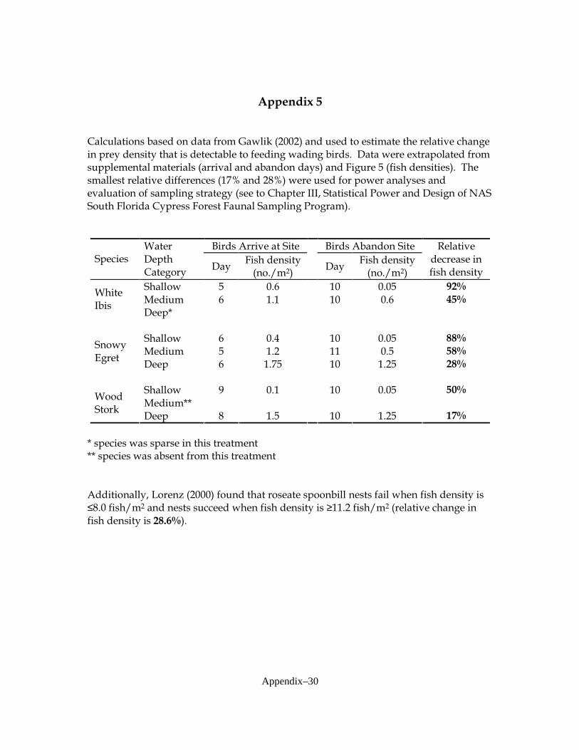
Appendix–30

Appendix 5 Calculations based on data from Gawlik (2002) and used to estimate the relative change in prey density that is detectable to feeding wading birds. Data were extrapolated from supplemental materials (arrival and abandon days) and Figure 5 (fish densities). The smallest relative differences (17% and 28%) were used for power analyses and evaluation of sampling strategy (see to Chapter III, Statistical Power and Design of NAS South Florida Cypress Forest Faunal Sampling Program).

Birds Arrive at Site Birds Abandon Site Species

Water Depth Category

Day Fish density (no./m2)

Day Fish density (no./m2)

Relative decrease in fish density

Shallow 5 0.6 10 0.05 92%

Medium 6 1.1 10 0.6 45% White Ibis

Deep*

Shallow 6 0.4 10 0.05 88%

Medium 5 1.2 11 0.5 58% Snowy Egret

Deep 6 1.75 10 1.25 28%

Shallow 9 0.1 10 0.05 50%

Medium** Wood Stork

Deep 8 1.5 10 1.25 17%

* species was sparse in this treatment ** species was absent from this treatment Additionally, Lorenz (2000) found that roseate spoonbill nests fail when fish density is ≤8.0 fish/m2 and nests succeed when fish density is ≥11.2 fish/m2 (relative change in fish density is 28.6%).

Appendix–31

Appendix 6 Power curve outputs (G*POWER3 program) from analyses of cypress forest data. Analyses conducted by Brian G. Ormiston, Ph.D., Ecological Consultant. A. Gambusia holbrooki density test, shallow habitat, 17% increase

B. Gambusia holbrooki density test, shallow habitat, 28% increase

Appendix–32

C. Gambusia holbrooki density test, deep habitat, 17% increase

D. Gambusia holbrooki density test, deep habitat, 28% increase

Appendix–33

E. Jordanella floridae density test, shallow habitat, 17% increase

F. Jordanella floridae density test, shallow habitat, 28% increase

Appendix–34

G. Jordanella floridae density test, deep habitat, 17% increase

H. Jordanella floridae density test, deep habitat, 28% increase

Appendix–35

I. Lucania goodei density test, shallow habitat, 17% increase

J. Lucania goodei density test, shallow habitat, 28% increase

Appendix–36

K. Lucania goodei density test, deep habitat, 17% increase

L. Lucania goodei density test, deep habitat, 28% increase

Appendix–37

M. Total fish density test, shallow habitat, 17% increase

N. Total fish density test, shallow habitat, 28% increase

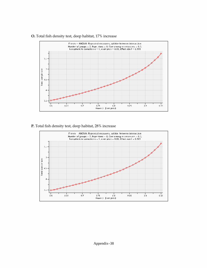
Appendix–38

O. Total fish density test, deep habitat, 17% increase

P. Total fish density test, deep habitat, 28% increase

Appendix–39

Q. Procambarus alleni density test, shallow habitat, 17% increase

R. Procambarus alleni density test, shallow habitat, 28% increase

Appendix–40

S. Procambarus alleni density test, deep habitat, 17% increase

T. Procambarus alleni density test, deep habitat, 28% increase

Appendix–41

U. Procambarus fallax density test, shallow habitat, 17% increase

V. Procambarus fallax density test, shallow habitat, 28% increase

Appendix–42

W. Procambarus fallax density test, deep habitat, 17% increase

X. Procambarus fallax density test, deep habitat, 28% increase

Appendix–43

Y. Total invertebrate density test, shallow habitat, 17% increase

Z. Total invertebrate density test, shallow habitat, 28% increase

Appendix–44

AA. Total invertebrate density test, deep habitat, 17% increase

BB. Total invertebrate density test, deep habitat, 28% increase