This course is about: The statistical analysis of …home.ku.edu.tr/~itunali/econ311/handouts/Week 1 L2 Overview.pdf · ... Introduction to Econometrics Lecture 2 . This course is

Econ 311 – Fall 2017, Week 1: Overview Version: 9/22/2016 4:09 PM Page: 1 /28

Murat DEMİRCİ and İnsan TUNALI 21 September 2017 Econ 311 – Introduction to Econometrics Lecture 2

This course is about:

The statistical analysis of economic (and related) data

The main textbook is: Introduction to Econometrics

Global - Updated 3rd Edition

by

James H. Stock and Mark W. Watson

You must own a copy!


Brief Overview of the Course

Economic theory suggests important relationships, often with policy implications, but rarely suggests numerical magnitudes of causal effects. Some examples of quantifiable causal effects:

• How does another year of education change earnings? (Think about the first lecture.)

• What is the effect on inflation of a 10 percentage point depreciation of the TL?

• What is the price elasticity of cigarettes? … alcoholic beverages? • What is the quantitative effect of reducing class size on student

achievement?


This course is about using data to measure causal effects.

• Ideally, we would like to conduct an experiment… o Think: How would you conduct an experiment to estimate

the effect of class size on standardized test scores? • But typically we only have observational (non-experimental) data.

o Cigarette consumption (Q) vs. prices (P)

Price elasticity = ∆𝑄𝑄 𝑄𝑄⁄∆𝑃𝑃 𝑃𝑃⁄

.

o Inflation rate vs. exchange rate – similar. o Wages vs. years of education

“Returns to education” = “slope” of f(x) in handout: Empirical Relations.


• Most of the course deals with difficulties arising from using observational data to estimate causal effects. o Confounding effects (omitted factors)

How is the “returns to education” affected by our failure to account for other factors that influence wages?

o Simultaneous causality Does an interest rate increase cause inflation to go up? Or does a higher inflation rate cause interest rates to go up?

o Correlation does not imply causation Causality, or spurious relations?


“If you fail to do the assignment, you will do poorly in the quizzes, and exams…”

Quiz total vs. Asg. total Final grade vs. Asg. total

Data are from Fall 2016. Positively sloped lines show the relation discovered by linear regression. Other lines mark the sample means.

020

4060

80Q

uiz

tota

l

0 20 40 60 80 100ASG100

Fitted values QUIZTOT

020

4060

8010

0Fi

nal

0 20 40 60 80 100ASG100

Fitted values FINAL


Here are the STATA regression results. Try to figure out what the numbers mean. . regress quiztot asg100, robust Linear regression Number of obs = 84 F(1, 82) = 239.83 Prob > F = 0.0000 R-squared = 0.6098 Root MSE = 12.432 ------------------------------------------------------------------------------ | Robust quiztot | Coef. Std. Err. t P>|t| [95% Conf. Interval] -------------+---------------------------------------------------------------- asg100 | .5714546 .0369003 15.49 0.000 .4980482 .6448609 _cons | -2.100251 2.579111 -0.81 0.418 -7.230925 3.030423 ------------------------------------------------------------------------------ . regress final asg100, robust Linear regression Number of obs = 84 F(1, 82) = 69.35 Prob > F = 0.0000 R-squared = 0.3648 Root MSE = 15.864 ------------------------------------------------------------------------------ | Robust final | Coef. Std. Err. t P>|t| [95% Conf. Interval] -------------+---------------------------------------------------------------- asg100 | .4420632 .0530828 8.33 0.000 .3364646 .5476619 _cons | 22.86251 3.344904 6.84 0.000 16.20843 29.51659 ------------------------------------------------------------------------------


On the previous page you saw examples of simple regression (SR). Here is a more relevant multiple regression (MR).

What does MR achieve that the SR cannot? .* generate gtotal = 0.1*asg100 + 0.25*(exam1+qx1bonus) + 0.25*(exam1+qx1bonus)+ 0.4*(final + qfxbonus)

. reg gtotal quiztot asg100, r Linear regression Number of obs = 84 F(2, 81) = 187.91 Prob > F = 0.0000 R-squared = 0.8044 Root MSE = 10.087 ------------------------------------------------------------------------------ | Robust gtotal | Coef. Std. Err. t P>|t| [95% Conf. Interval] -------------+---------------------------------------------------------------- quiztot | .8771844 .0784668 11.18 0.000 .7210601 1.033309 asg100 | .1295542 .0556892 2.33 0.022 .0187503 .2403582 _cons | 23.17526 2.566715 9.03 0.000 18.0683 28.28222 ------------------------------------------------------------------------------


In this course you will:

• Learn methods that can be used for statistical analysis of data (these can be used in term projects in advanced courses, in coveted positions at banks, international organizations, etc.);

• Learn methods for estimating causal effects w/observational data; • Learn to evaluate the regression analysis of others (this means

you will be able to read/understand empirical economics papers in other Econ courses);

• Get some hands-on experience with regression analysis using a popular software, STATA.

Focus is on applications – theory is used only as needed to understand why we do what we do.


What, precisely, is a causal effect?

• S&W take a practical approach to defining causality:

A causal effect is defined to be the effect measured in an ideal randomized controlled experiment.

This is the methodology used by experimental sciences.

How tomato yield responds to fertilizer use.

How patients respond to treatment by a particular drug.

Experimental units are broken into two groups: treatment group receives the treatment (fertilizer, drug, etc.), control group does not.


Ideal Randomized Controlled Experiment

• Ideal: subjects all follow the treatment protocol – perfect compliance, no errors in reporting, etc.!

• Randomized: subjects from the population of interest are randomly assigned to a treatment or control group (so there are no confounding factors).

• Controlled: having a control group permits measuring the differential effect of the treatment.

• Experiment: treatment status is assigned as part of the experiment. The subjects have no choice, so there is no “reverse causality” in which subjects choose the treatment they think will work best.


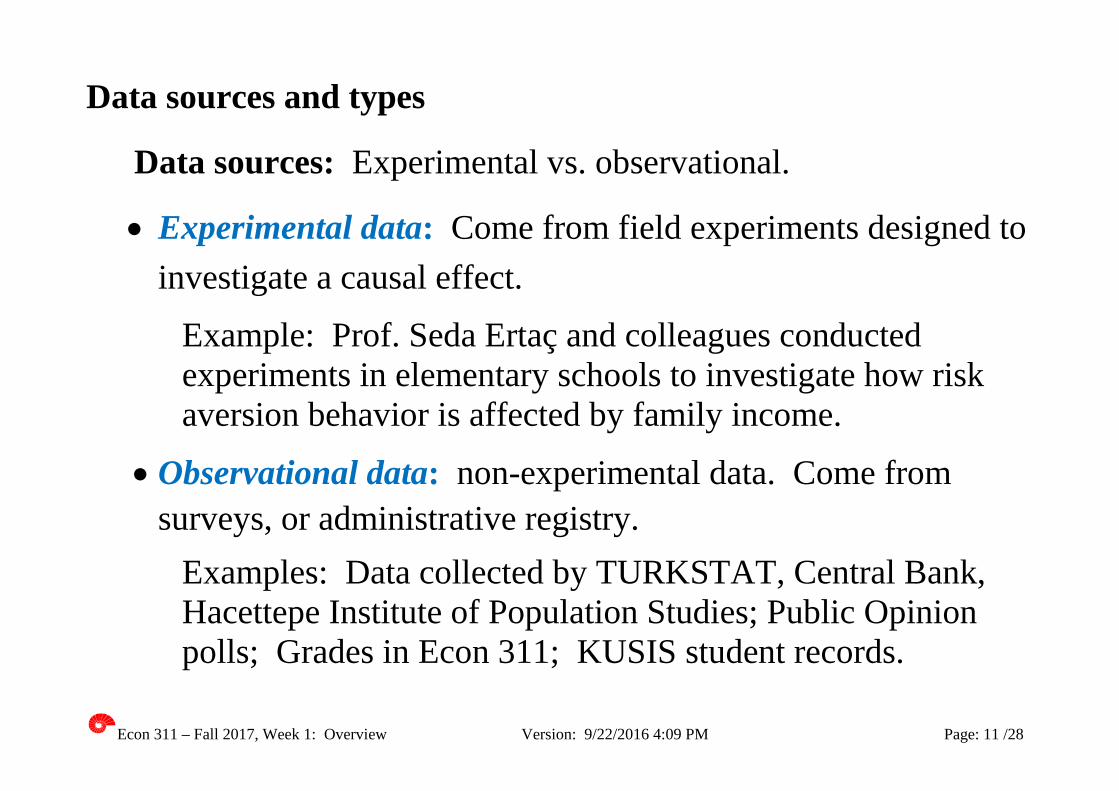
Data sources and types

Data sources: Experimental vs. observational.

• Experimental data: Come from field experiments designed to investigate a causal effect.

Example: Prof. Seda Ertaç and colleagues conducted experiments in elementary schools to investigate how risk aversion behavior is affected by family income.

• Observational data: non-experimental data. Come from surveys, or administrative registry.

Examples: Data collected by TURKSTAT, Central Bank, Hacettepe Institute of Population Studies; Public Opinion polls; Grades in Econ 311; KUSIS student records.


Data types: • Cross-sectional (CS) data

Data collected from many units* at a single point in time. e.g. Household Labor Force Survey (TURKSTAT).

• Time Series (TS) data Data collected on a single unit* at multiple time periods. e.g. Monthly data on monetary variables (inflation rate, interest rates) – see the web page of CB of Turkey.

• Panel (longitudinal) data Data for multiple units in which each unit* is observed at two or more time periods.

*Unit (of analysis): what the data points represent (workers, students, firms, countries…)


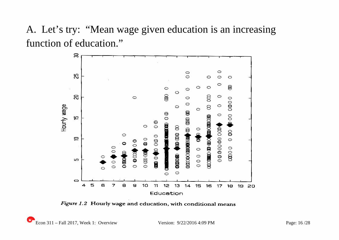
Looking ahead: In Lecture 1, we examined the relationship between wages and education (see handout: Empirical Relations). Human Capital Theory (subject of Econ 320 – Labor Economics) claims wages (y) increase with education (x). That is, y = f(x), where f’ > 0.

What does the empirical evidence look like?

We have a random sample of 528 individual observations included in a survey conducted in the U.S.A. in 1985. There

y = hourly wages,

x = education (years of schooling). Observation: There is a distribution of wages for each level of education. That is, there are multiple y values for each value of x!



In Lecture 1 we answered the following questions:

Q. Why is there a “distribution” of wages at each level of education?

A. Because there are many other factors that influence wages: Gender, labor market experience, quality of schooling, ability…

Q. How do we discover the function that Human Capital Theory refers to? Put differently, what does the theorist mean when s/he says “wage is an increasing function of education”?

Hint: The theorist surely knows that factors other than education affect wages but wants to abstract from them.


A. Let’s try: “Mean wage given education is an increasing function of education.”


The “function” we obtain by calculating the mean wage at each level of education is called the “sample conditional mean function.”

Remark: Sample conditional mean function (cmf) of wage given education appears like a “jumpy” function, but it appears to capture the relation we are after: average wage seems to increase with education.

Q. Can we find simpler representations which serve our aims? A. Yes. We can find the best fitting line using linear regression.

We modify the theory slightly and write:

y = f(x) + u

where f(x) = β0 + β1x and u = all other factors that may be relevant.


Here the unknowns (β0 and β1) have been replaced by Ordinary Least Squares estimates. The slope is positive, as claimed.

Q. How do we find the Ordinary Least Squares estimates?


Tough questions:

Is there a causal relation between • assignment grades and quiz grades? • quiz grades and exam grades? • education and wages?

Or are these spurious relations? Econ 311 is a first step towards answering these questions…

And more: See course objectives and learning outcomes (page 3 of the syllabus)


Secret to success:

Students who read the handouts before coming to class and study regularly will gain a lot from the assignments, do well in the quizzes, and will be able to prepare for the exam without having to cut back on time devoted to other activities.

Road to disaster:

Students who fail to keep up with the pace of the course by skipping classes, and not doing the reading and the homework assignments on a regular basis should not expect to do well in the course.


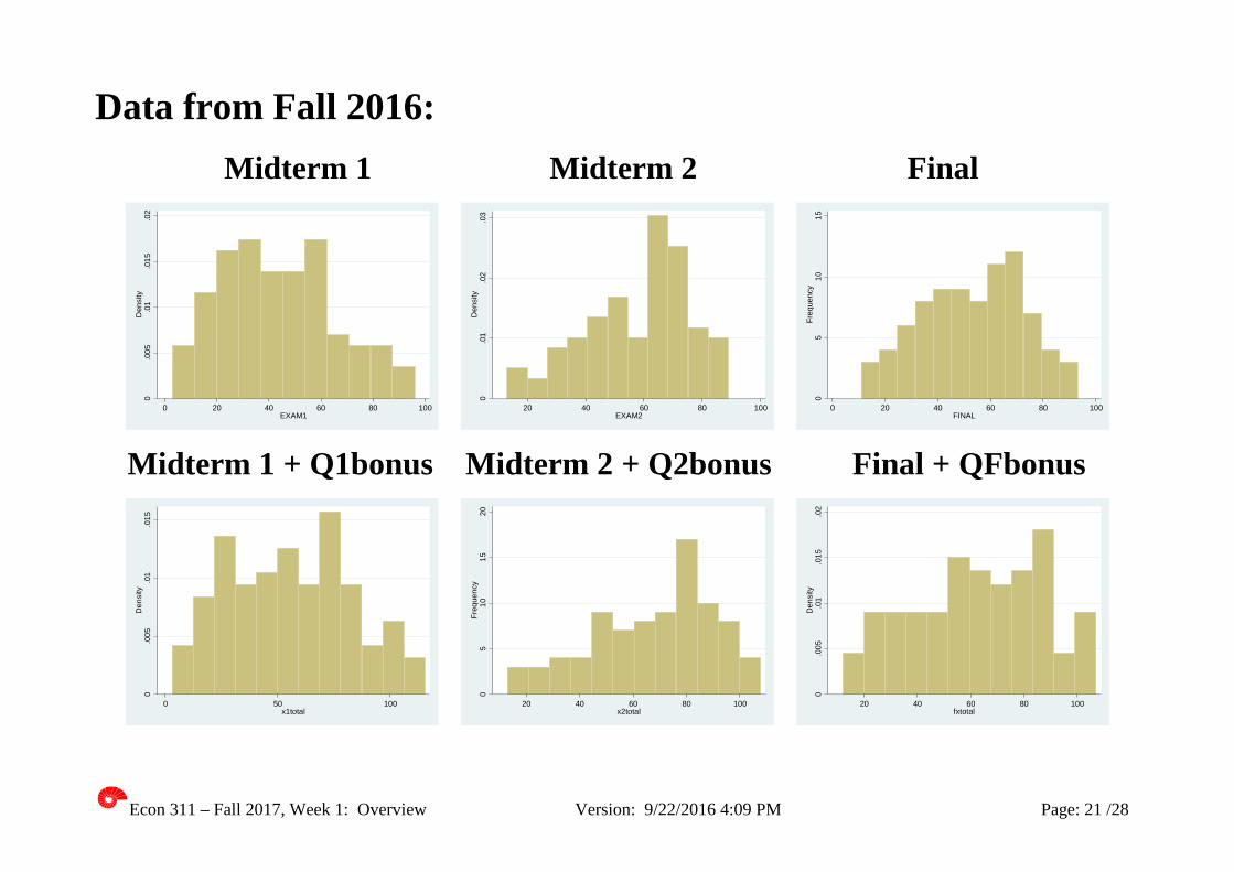
Data from Fall 2016: Midterm 1 Midterm 2 Final

Midterm 1 + Q1bonus Midterm 2 + Q2bonus Final + QFbonus

0.0

05.0

1.0

15.0

2D

ensi

ty

0 20 40 60 80 100EXAM1

0.0

1.0

2.0

3D

ensi

ty

20 40 60 80 100EXAM2

05

1015

Freq

uenc

y

0 20 40 60 80 100FINAL

0.0

05.0

1.0

15D

ensi

ty

0 50 100x1total

05

1015

20Fr

eque

ncy

20 40 60 80 100x2total

0.0

05.0

1.0

15.0

2D

ensi

ty

20 40 60 80 100fxtotal


Data from Fall 2016: • 107 students started the course. • 18 withdrew. • Grades: 20 A’s, 25 B’s, 20 C’s, 14 D’s, 10 F’s.

Grading policy:

Grade will be based on: Weekly assignments (10%), two midterm exams (25% each) and a final exam (40%).

Quiz grades Bonus: Will be added to exam scores! You can earn extra credit – up to 20% of the exam grade!

See last page of the syllabus, or Blackboard/Econ 311.


There will be 12 weekly assignments; 2 will be based on Excel, 5-6 will be based on STATA. All will have analytical problems. STATA is a highly acclaimed, widely used s/w.

☺ It is easier to learn econometrics using STATA! ☺ By learning STATA you will be able to add a line on your CV!

It is very difficult to pass the course if you do not learn STATA!

. tabulate stata, summarize(gtotal)

| Summary of GTOTAL STATA | Mean Std. Dev. Freq. ------------+------------------------------------ 0 | 33.888889 19.218705 9 1 | 50.708333 15.997412 12 2 | 53.8875 22.159708 8 3 | 60.033333 12.770407 3 4 | 74.209091 16.845232 22 5 | 75.62 17.786772 30 ------------+------------------------------------ Total | 64.594047 22.52888 84


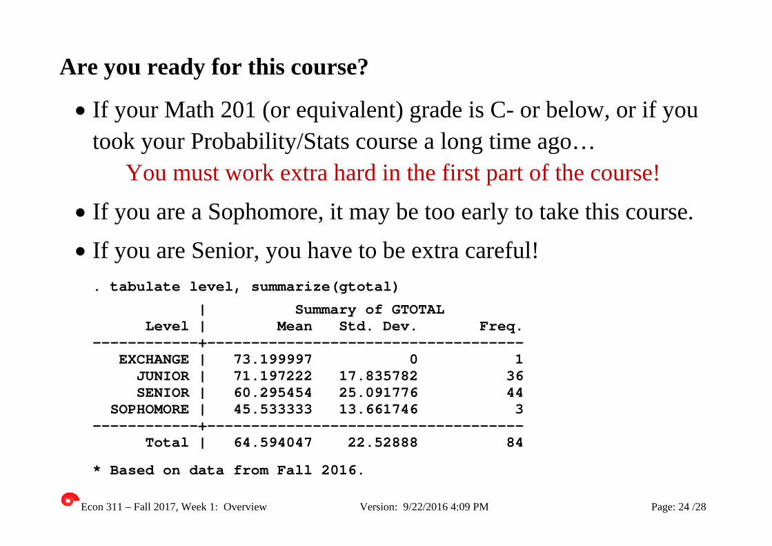
Are you ready for this course?

• If your Math 201 (or equivalent) grade is C- or below, or if you took your Probability/Stats course a long time ago…

You must work extra hard in the first part of the course! • If you are a Sophomore, it may be too early to take this course. • If you are Senior, you have to be extra careful! . tabulate level, summarize(gtotal)

| Summary of GTOTAL Level | Mean Std. Dev. Freq. ------------+------------------------------------ EXCHANGE | 73.199997 0 1 JUNIOR | 71.197222 17.835782 36 SENIOR | 60.295454 25.091776 44 SOPHOMORE | 45.533333 13.661746 3 ------------+------------------------------------ Total | 64.594047 22.52888 84

* Based on data from Fall 2016.


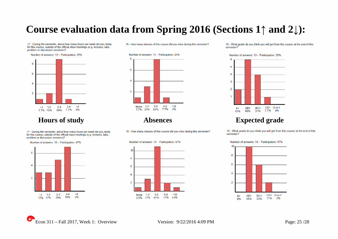
Course evaluation data from Spring 2016 (Sections 1↑ and 2↓):

Hours of study Absences Expected grade


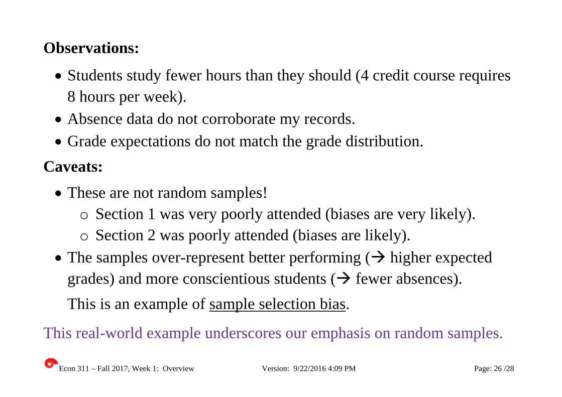
Observations:

• Students study fewer hours than they should (4 credit course requires 8 hours per week).

• Absence data do not corroborate my records. • Grade expectations do not match the grade distribution.

Caveats: • These are not random samples!

o Section 1 was very poorly attended (biases are very likely). o Section 2 was poorly attended (biases are likely).

• The samples over-represent better performing ( higher expected grades) and more conscientious students ( fewer absences). This is an example of sample selection bias.

This real-world example underscores our emphasis on random samples.


Tips for the conscientious (or grade conscious) student:

• Print a copy of the handout (4 slides per page, landscape). o Read it and do the exercises before coming to class.

• During lectures: o Bring the handout to class; take notes on it. o Put your smartphone away. o If you do not understand something, ask.

“Not understanding” is not a normal state! • After the lectures:

o Read the relevant sections in the book. • If you miss a class, try to catch up quickly – borrow a friend’s notes,

go to office hours. • Read the assignment as soon as it is posted.

o Link problems with the handouts and the book. • Go to office hours and problem sessions, earn your bonus!


TENTATIVE SCHEDULE

Part Week Topic Chapters in Stock & Watson [Goldberger] 1 1 Economic questions and data 1 [1] 1 2-5 Statistical foundations 2-3 [3-5] ------------- Exam 1: Oct. 23-28* -------------------------------------------------------------- 2 6-7 Simple regression 4 [6, 8] 2 7-8 Inference in simple regression 5 [7] 2 9-10 Multiple regression 6 [9-10] ------------- Exam 2: Nov. 20-25* ------------------------------------------------------------- 3 11-12 Inference in multiple regression 7 [11-12] 3 13-14 Nonlinear regression 8 [7] ------------- Final Exam (TBA) ----------------------------------------------------------------- *Tentative; date to be determined by the Registrar’s Office.

* Next week, we start our Review of Probability and Statistics. ** Make sure to print the handout, and study it before class!

Documents

This course is about: The statistical analysis of …home.ku.edu.tr/~itunali/econ311/handouts/Week 1 L2 Overview.pdf · ... Introduction to Econometrics Lecture 2 . This course is