This course will describe particular statistical methods ...staff.pubhealth.ku.dk/~kkho/undervisning/family2013/day1-intro-2x2.pdf · Statistical methods for twins and families

UNIVERSITY OF COPENHAGENDEPARTMENT OF BIOSTATISTICS

Statistical methods for twins and families

Klaus K. Holst

Department of BiostatisticsUniversity of Copenhagen

November 10, 2013


Welcome and practicalities

Statistical methods for twins and familiesThis course will describe particular statistical methods and their usefor multivariate data with a focus on how to quantify familialaggregation of specific diseases and quantitative and binomial traits.

- Thomas Scheike [email protected] Klaus Kähler Holst [email protected] Jacob Hjelmborg

http://www.biostat.ku.dk/~kkho/undervisning/family2013

Time plan

915–1030 Lecture & Practicals1045–1200 Lectures & Practicals1200–1300 Lunch1300–1415 Lectures & Practicals1445–1600 Lectures & Practicals

Course outlineNov 11 Continuous traitsNov 12 Binary traitsNov 18 SurvivalNov 19 Competing risks


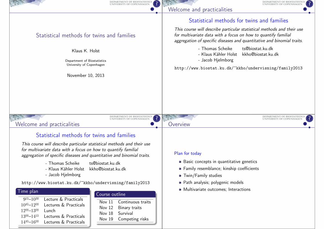
Welcome and practicalities

Statistical methods for twins and familiesThis course will describe particular statistical methods and their usefor multivariate data with a focus on how to quantify familialaggregation of specific diseases and quantitative and binomial traits.

- Thomas Scheike [email protected] Klaus Kähler Holst [email protected] Jacob Hjelmborg

http://www.biostat.ku.dk/~kkho/undervisning/family2013

Time plan

915–1030 Lecture & Practicals1045–1200 Lectures & Practicals1200–1300 Lunch1300–1415 Lectures & Practicals1445–1600 Lectures & Practicals

Course outlineNov 11 Continuous traitsNov 12 Binary traitsNov 18 SurvivalNov 19 Competing risks


Overview

Plan for today

Basic concepts in quantitative geneticsFamily resemblance; kinship coefficientsTwin/Family studiesPath analysis; polygenic modelsMultivariate outcomes; Interactions


Litterature

1 Methodology for Genetic Studies of Twins and Families byMichael C. Neale, Lon R. Cardon and Hermine H.M. Maes.

2 Genetics and Analysis of Quantitative Traits by Michael Lynchand Bruce Walsh. Sinauer Associates 1998.

3 Mathematical and Statistical Methods for Genetic Analysis byKenneth Lange. Springer-Verlag 2003.


LitteratureRijsdijk, F. and Sham, P (2002). Analytic approaches to twindata using structural equation models. Briefings inBioinformatics 3 (2) pp.119-133.

Dongen, J. et al (2012). The continuing value of twin studiesin the omics era. Nature Reviews Genetics 13, 640-653.10.1038/nrg3243

Witte JS, Carlin JB, Hopper JL. (1999). Likelihood-basedapproach to estimating twin concordance for dichotomoustraits. Genet.Epidemiol.16(3):290–304.

Scheike, T and Holst, K and Hjelmborg, J (2013), Estimatingheritability for cause specific mortality based on twin studies.Lifetime Data Analysis. DOI: 10.1007/s10985-013-9244-x.

Scheike, T and Holst, K and Hjelmborg, J (2013). Estimatingtwin concordance for bivariate competing risks twin data.Statistics in Medicine. DOI: 10.1002/sim.6016.


Practicals

Computer practicals with R and the mets package.

R and the package should be installed on your laptops:

1 install.packages("mets",dependencies=TRUE)

1 library(mets)

Loading ’mets’ version 0.2.5

Other popular software for family studies: Mplus, (open)Mx, stataGLLAMM. . . . However, currently much better methods in mets fordealing with time-to-event endpoint (e.g. disease status in a cohortstudy).



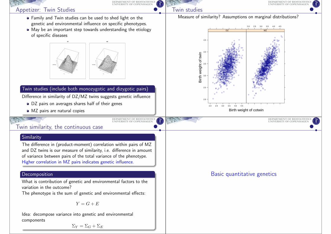
Appetizer: Twin StudiesFamily and Twin studies can be used to shed light on thegenetic and environmental influence on specific phenotypes.May be an important step towards understanding the etiologyof specific diseases

DZ

Y1

Y2

Density

MZ

Y1

Y2

Density

Twin studies (include both monozygotic and dizygotic pairs)Difference in similarity of DZ/MZ twins suggests genetic influence

DZ pairs on averages shares half of their genesMZ pairs are natural copies


Twin studiesMeasure of similarity? Assumptions on marginal distributions?

Birth weight of cotwin

Bir

th w

eigh

t of t

win

2.0

2.5

3.0

3.5

4.0

4.5

2.0 2.5 3.0 3.5 4.0 4.5

DZ

2.0 2.5 3.0 3.5 4.0 4.5

MZ


Twin similarity, the continuous case

SimilarityThe difference in (product-moment) correlation within pairs of MZand DZ twins is our measure of similarity, i.e. difference in amountof variance between pairs of the total variance of the phenotype.Higher correlation in MZ pairs indicates genetic influence.

DecompositionWhat is contribution of genetic and environmental factors to thevariation in the outcome?The phenotype is the sum of genetic and environmental effects:

Y = G+ E

Idea: decompose variance into genetic and environmentalcomponents

ΣY = ΣG + ΣE


Basic quantitative genetics


Basic quantitative-genetics

The phenotype or disease status is a compounding ofgenes (G) and environment (E)

Important step in understanding the phenotype oretiology of disease is to be able to quantify the role ofG and E (both may be unobserved!).

Research questionIs G (or E) present?To what magnitude?Which particular genotypes or environmentaleffects causes the disease or phenotype.


Genetic inference

Two different path-ways to genetic inference:

1 Family-study + Linkage analysis −→ Candidategenes

2 Genome-Wide-Association Studies3 Family-based studies are the gold-standard

(hypothesis-driven) for quantification of familialrisk and heritability.

Idea based on familial resemblance: is trait more similaramong related than unrelated individuals?

Continuous trait: tighter correlation in closerrelatives.Disease: Risk of disease greater in case familiescompared to none-cases of general population


Hierarchical research questions: causes of phenotype

Family aggregation?

Heritability? Environmental effects?

ChromosomesGenesGenotypeProteins/RNA

Identification

interactions?


Basic quantitative-genetics (Vocabulary)

The phenotype is the observable characteristics ofan individual z = G+ E - quantitative trait.Genetic information encoding resides onchromosomes (strands of DNA). Most cellscontains 46 chromosomes (22 homologous pairs -autosomes - and 2 pairs of sex chromosomes XXand XY).Sequences along the chromosomes that encode forparticular proteins/RNAs: genes. Chromosomallocation: loci.Except for sex chromosomes there are two genesat every locus. The various forms of a gene ateach locus are called alleles.Gene loci that exhibit more than one allele arepolymorphic (then one subject to genetics).


Quantitative geneticsCentral goal: quantify association between phenotypic, Z, andgenotypic, G, values.Assume phenotype is sum of the total effects of all loci on the traitand an environmental effect/deviation E

Z = G+ E

In multi-locus trait G may be very complicated function of alleles!Squared correlation

ρ2(G,Z) =Cov(G,Z)2

{Var(G)Var(Z)}Assuming uncorrelated genes and environment we obtain the broadsense heritability:

H2 = ρ2(G,Z) =Var(G)

Var(Z)

OBS: Cov(G,E) 6= 0 may pull ρ(G,Z) in any direction


Quantitative genetics

Key pointsNot all genes are transmitted

At autosomal loci offsprings gets one maternal and onepaternal allele

F A A A a M

O1 A A A a O2

Family resemblance (and clever design) can be used to estimategenotypic effects

Full siblings get one allele from common father and one allelefrom common mother.Monozygotic twins on average shares all genes


Quantitative geneticsProblem: In general only the phenotype Z is directly observable.I.e. we can only directly estimate Var(Z).

Solution: Exploit that related individuals carry copies of many ofthe same alleles.

Example: Single locus with additive effectsFather Zf and mother Zm with offspring Zo.Single locus (autosomal genotype/diploid) with additive effect

Zf = gf + g′f + Ef

Zm = gm + g′m + Em

Zo = gf + gm + Eo

Mid-parent value:

Zmp =Zf + Zm

2


Example: Single locus with additive effectsgm, gf effects of alleles inherited from mother and fatherg′m, g

′f effects of alleles not transmitted from mother and father

Ef , Em, Eo environmental effects

gf gm g′f g′m Ef Em Eo

gf Var(gf )

gm Cov(gm, gf ). . .

g′f...

. . .

g′m...

. . .

Ef...

. . .

Em...

. . .Eo Cov(E0, gf ) · · · · · · · · · · · · · · · Var(Eo)

18 terms in mid-parent-offspring covariance. . .Covariance


Example: Single locus with additive effectsAssumptions

1 Random mating, no selectionNo correlation between gene at specific locus in mother andfather. Genes inherited by offspring not correlated with theones that were not transmitted.

2 No gene-environment correlationIndividuals not assorted into environment based on theirgenetic attributes

3 Parents do not transmit their environmental effects to offspring

Cov(Zmp, Zo) = Cov(1

2(gf + gm), gf + gm) =

Var(gf ) + Var(gm)

2

As we only assume additive genetic effects we define

σ2A = Var(gf ) + Var(gm)


Example: Single locus with additive effectsAssumptions

1 Random mating, no selectionNo correlation between gene at specific locus in mother andfather. Genes inherited by offspring not correlated with theones that were not transmitted.

2 No gene-environment correlationIndividuals not assorted into environment based on theirgenetic attributes

3 Parents do not transmit their environmental effects to offspring

Cov(Zmp, Zo) = Cov(1

2(gf + gm), gf + gm) =

Var(gf ) + Var(gm)

2

As we only assume additive genetic effects we define

σ2A = Var(gf ) + Var(gm)


Example: Single locus with additive effectsKey-point: genetic component can be extracted from phenotypicresemblance between relativesRegression of of one relatives value on values of other familymember.

E(Zo | Zmp) = µ+ βZmp

Under random mating cov(Zm, Zf ) = 0. Assuming same variancein males and females

Var(Zmp) =1

2σ2Z

Least squares estimator gives the narrow-sense heritability

β =Cov(Zo, Zmp)

Var(Zmp)=σ2Aσ2Z

= h2

h2 := efficiency of response to selection (i.e. h2 = 0 means there isno tendency for offspring to resemble their parents - no evolutionarychange)


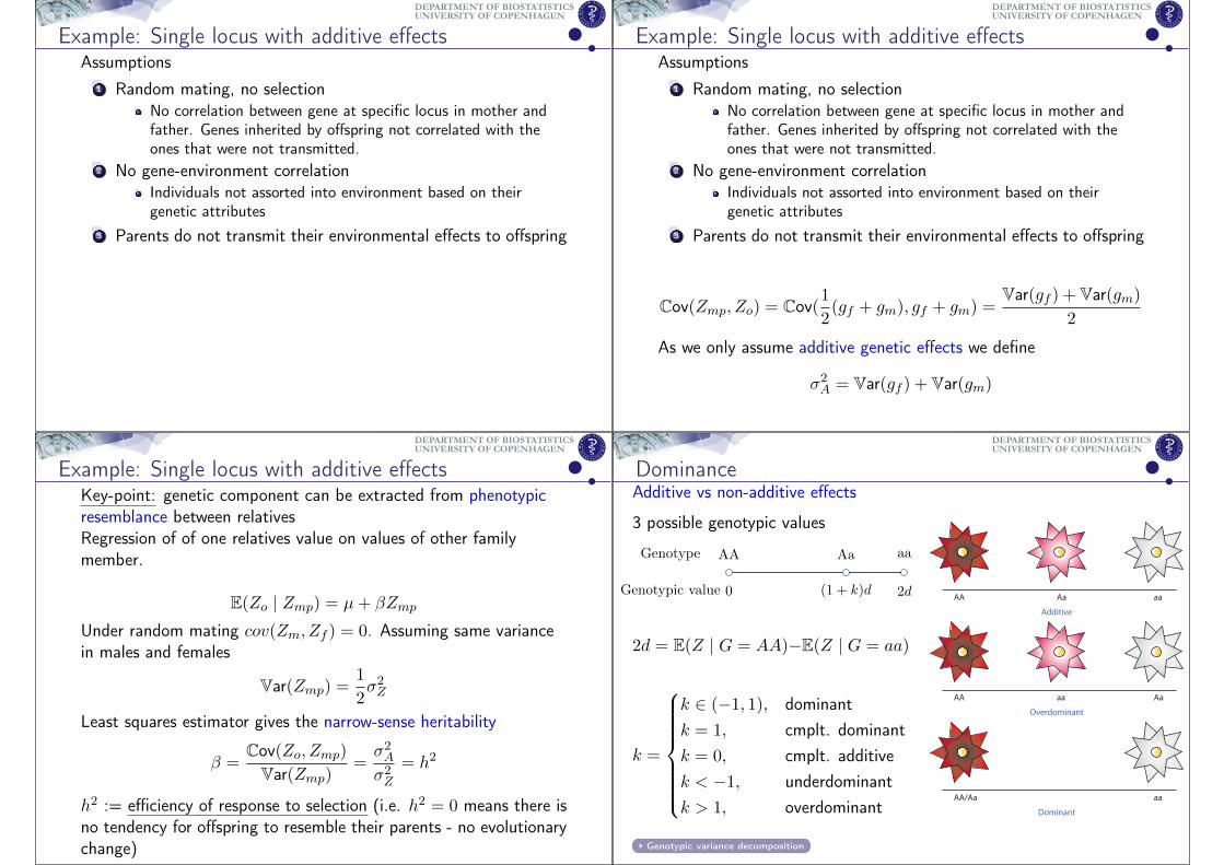
DominanceAdditive vs non-additive effects

3 possible genotypic values

Genotype

Genotypic value

Aa

(1 + k)d

AA

0

aa

2d

2d = E(Z | G = AA)−E(Z | G = aa)

k =

k ∈ (−1, 1), dominantk = 1, cmplt. dominantk = 0, cmplt. additivek < −1, underdominantk > 1, overdominant

Genotypic variance decomposition

AA aa Aa

AA/Aa aa

Additive

Overdominant

Dominant

AA Aa aa


Fishers decomposition of the genotypic value

We consider a phenotype Z genetically determined by a single locus

Let ak denote the kth allele with population frequency pkIn absence of environmental effect an individual with(maternal/paternal) genotype ak/al has constant phenotypevalue (or equivalently, genotypic value) µkl = µlk.We wish to approximate the genotypic value/phenotype valueby additive effect of the alleles

µkl = αk + αl + δkl

Without loss of generality we assume standardized phenotypeE(Z) =

∑k

∑l µklpkpl = 0

Here we assume the locus is in Hardy-Weinberg Equilibrium.


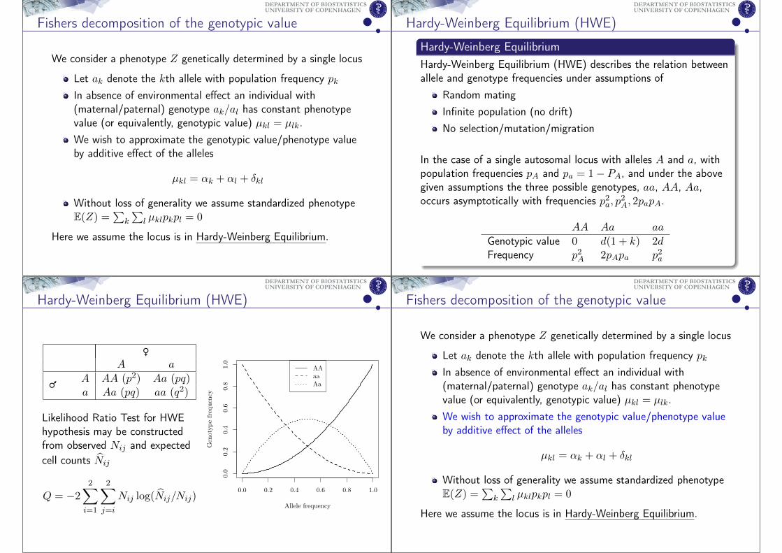
Hardy-Weinberg Equilibrium (HWE)

Hardy-Weinberg EquilibriumHardy-Weinberg Equilibrium (HWE) describes the relation betweenallele and genotype frequencies under assumptions of

Random matingInfinite population (no drift)No selection/mutation/migration

In the case of a single autosomal locus with alleles A and a, withpopulation frequencies pA and pa = 1− PA, and under the abovegiven assumptions the three possible genotypes, aa, AA, Aa,occurs asymptotically with frequencies p2a, p

2A, 2papA.

AA Aa aa

Genotypic value 0 d(1 + k) 2dFrequency p2A 2pApa p2a


Hardy-Weinberg Equilibrium (HWE)

~A a

|A AA (p2) Aa (pq)a Aa (pq) aa (q2)

Likelihood Ratio Test for HWEhypothesis may be constructedfrom observed Nij and expectedcell counts N̂ij

Q = −22∑

i=1

2∑

j=i

Nij log(N̂ij/Nij)0.0 0.2 0.4 0.6 0.8 1.0

0.0

0.2

0.4

0.6

0.8

1.0

Allele frequency

Gen

otypefrequen

cy

AAaaAa



We consider a phenotype Z genetically determined by a single locus

Let ak denote the kth allele with population frequency pkIn absence of environmental effect an individual with(maternal/paternal) genotype ak/al has constant phenotypevalue (or equivalently, genotypic value) µkl = µlk.We wish to approximate the genotypic value/phenotype valueby additive effect of the alleles

µkl = αk + αl + δkl

Without loss of generality we assume standardized phenotypeE(Z) =

∑k

∑l µklpkpl = 0

Here we assume the locus is in Hardy-Weinberg Equilibrium.


Fishers decomposition of the genotypic valueLet X1, X2 be independent random variables (maternal/paternalallele). We wish to determine functions h1, h2 that minimizes

arg minf,g E({Z − f(X1)− g(X2)}2)

under condition E(h1(X1)) = E(h2(X2)) = 0.Now rewriting as

Var(Z − h1(X1)− h2(X2)) = Var(Z) + Var(h1(X1)) + Var(h2(X2))

− 2Cov(Z, h1(X1))− 2Cov(Z, h2(X2))

= Var(Z − h1(X1)) + Var(Z − h2(D2))

− Var(Z)

solution is given by

hi(Xi) = E(Z | Xi)


Fishers decomposition of the genotypic valueWe define the average additive allele effects

αk = E(Z | Xi = ak) =∑

l

µklpl

and orthogonal on that the dominant deviation

δkl = Z − E(Z | X1 = ak)− E(Z | X2 = al)

Genetic variancesAs a consequence a natural definition of additive genetic variance is

σ2A = 2Var[E(Z | Xi)] = 2∑

k

α2kpk

and dominant genetic variance

σ2D = Var[Z − E(Z | X1)]− E(Z | X2)] =∑

k,l

δ2klpkpl


Fishers decomposition of the genotypic valueAlternative derivation, 2 alleles. . .Wish to decompose genotypic value (assume environmental effecthas mean zero) into additive and residual (dominant dev.)component

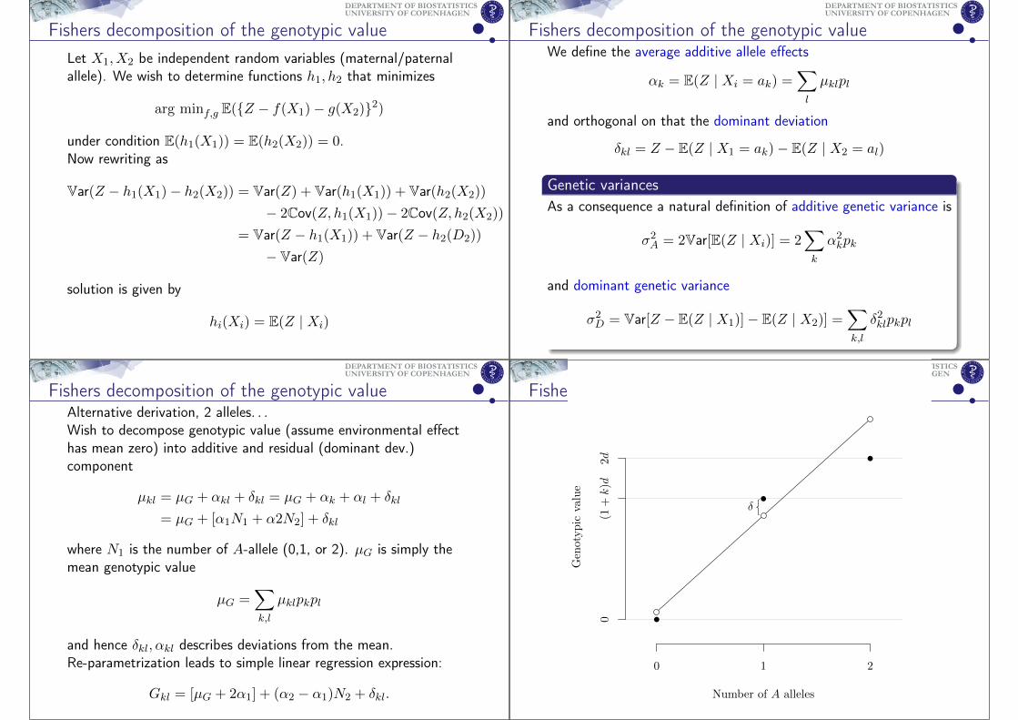
µkl = µG + αkl + δkl = µG + αk + αl + δkl

= µG + [α1N1 + α2N2] + δkl

where N1 is the number of A-allele (0,1, or 2). µG is simply themean genotypic value

µG =∑

k,l

µklpkpl

and hence δkl, αkl describes deviations from the mean.Re-parametrization leads to simple linear regression expression:

Gkl = [µG + 2α1] + (α2 − α1)N2 + δkl.



Number of A alleles

Genotypic

value

0 1 2

0(1

+k)d

2d

δ



Assume N2 ⊥⊥ δij we can use least squares estimator to obtainestimates of intercept and slope β = α2 − α1. The OLS estimator

can be expressed [Lynch&Walsh 98] in gene coefficients Dominance

average effects if allele substitution:

β =Cov(G,N2)

Var(N2)= d[1 + k(p1 − p2)]

Parametrization choice leads to

α1E(N1) + α2E(N2) = 2α1p1 + 2α2p2 = 0 =⇒α2 = p1β and α1 = −p2β

where we have used E(Nk)/2 = pk, p1 + p2 = 1.



Indep. between prediction and residual leads to

σ2G = Var(A1 +A2 +D) = σ2A + σ2D

Ak = α11{Xk=a1} + α21{Xk=a2}, D =∑

k,l

δkl1{Xi=ak}1{Xj=al}

Genetic variances, biallelic case

σ2A = 2(α21p1 + α2

2p2)

= 2β2p1p2(p1 + p2) = 2p1p2d2[1 + k(p1 − p2)]2

σ2D = (2p1p2dk)2


Multiple Loci

If the trait is inherited from n loci in linkage equilibrium andassuming no epistasis, we obtain

Genetic variance n loci

σ2G =

n∑

i=1

σ2Ai+

n∑

i=1

σ2Di


LinkageLinkage causes additional covariance terms, e.g.

σ2A = 2

n∑

k=1

α2kpkpl + 2

n∑

k=1

n∑

l=k+1

αkαkDkl

whereDkl = pkl − pkpl

is the linkage disequilibrium coefficient


EpistasisEpistasisIn the multi-loci case interactions between loci may occur. Variancedecomposition can still be obtained by

σ2G =∑

m,n

σ2AnDm

= σ2A + σ2D + σ2AA + σ2AD + σ2DD

+ σ2AAA + σ2AAD + σ2ADD + σ2DDD + · · ·

n number of additive effects and m the number of dominant effects

Cov(Gi, Gj) =∑

m,n

(2Φij)n∆m

7ijσ2AnDm

= 2Φijσ2A + ∆7ijσ

2D

+ 4Φ2ijσ

2AA + ∆2

7ijσ2DD + 2Φij∆7ijσ

2AD + · · ·

Parent-offspring


Familial resemblance


Familial resemblance

The fundamental property we exploit is that phenotypic dependenceamong relatives can be used to estimate the variances of thecomponents of genotypic effect. Fisher 1918

To further develop this we need to be able to quantify degree ofrelatedness between individuals. . .

“No, but I would to save two brothers or eight cousins.”

Reply from JBS Haldane when asked if he would give his life tosave a drowning brother1

1Mathematical Models of Social Evolution : A Guide for the Perplexed(2007) by Richard McElreath and Robert Boyd, p. 82.


Family resemblanceConcept of relatives should be understood in the framework of agiven pedigree structure

2 1 4 3 6 5

8 7 9 10 7 11 12 14 13

15 16 17 18 19

with independence at base


Familial resemblanceWe define relatedness via concepts of identical alleles. . .

Identical allelesTwo genes are identical by state (i.b.s.) if they represent the sameallele.The genes are identical by descent (i.b.d.) if the alleles are directdescendants of the same gene carried by a common ancestralindividual.

A A A a

A A A a


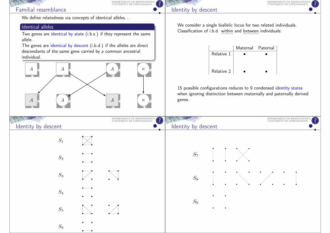
Identity by descent

We consider a single biallelic locus for two related individuals.Classification of i.b.d. within and between individuals:

Maternal PaternalRelative 1 • •

Relative 2 • •

15 possible configurations reduces to 9 condensed identity stateswhen ignoring distinction between maternally and paternally derivedgenes.


Identity by descent

S1

S2

S3

S4

S5

S6


Identity by descent

S7

S8

S9


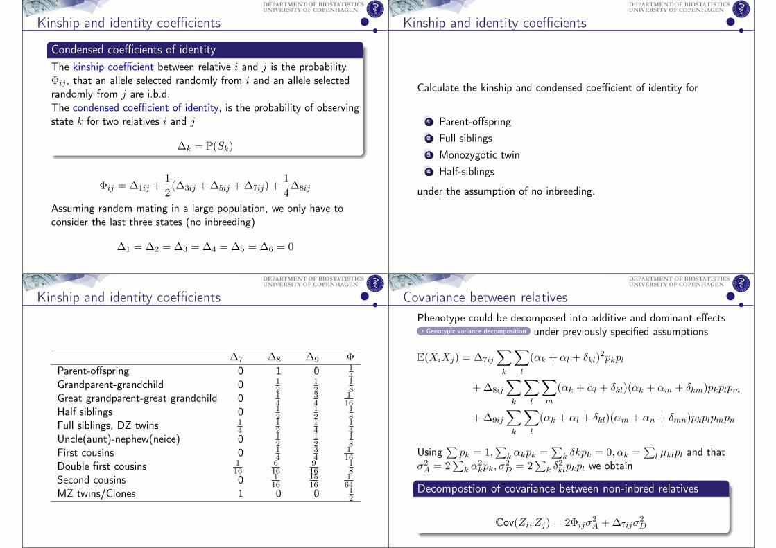
Kinship and identity coefficients

Condensed coefficients of identityThe kinship coefficient between relative i and j is the probability,Φij , that an allele selected randomly from i and an allele selectedrandomly from j are i.b.d.The condensed coefficient of identity, is the probability of observingstate k for two relatives i and j

∆k = P(Sk)

Φij = ∆1ij +1

2(∆3ij + ∆5ij + ∆7ij) +

1

4∆8ij

Assuming random mating in a large population, we only have toconsider the last three states (no inbreeding)

∆1 = ∆2 = ∆3 = ∆4 = ∆5 = ∆6 = 0



Calculate the kinship and condensed coefficient of identity for

1 Parent-offspring2 Full siblings3 Monozygotic twin4 Half-siblings

under the assumption of no inbreeding.



∆7 ∆8 ∆9 Φ

Parent-offspring 0 1 0 14

Grandparent-grandchild 0 12

12

18

Great grandparent-great grandchild 0 14

34

116

Half siblings 0 12

12

18

Full siblings, DZ twins 14

12

14

14

Uncle(aunt)-nephew(neice) 0 12

12

18

First cousins 0 14

34

116

Double first cousins 116

616

916

18

Second cousins 0 116

1516

164

MZ twins/Clones 1 0 0 12


Covariance between relativesPhenotype could be decomposed into additive and dominant effects

Genotypic variance decomposition under previously specified assumptions

E(XiXj) = ∆7ij

∑

k

∑

l

(αk + αl + δkl)2pkpl

+ ∆8ij

∑

k

∑

l

∑

m

(αk + αl + δkl)(αk + αm + δkm)pkplpm

+ ∆9ij

∑

k

∑

l

(αk + αl + δkl)(αm + αn + δmn)pkplpmpn

Using∑pk = 1,

∑k αkpk =

∑k δkpk = 0, αk =

∑l µklpl and that

σ2A = 2∑

k α2kpk, σ

2D = 2

∑k δ

2klpkpl we obtain

Decompostion of covariance between non-inbred relatives

Cov(Zi, Zj) = 2Φijσ2A + ∆7ijσ

2D


Covariance between relativesProof in the biallelic case:

Zi = µG+A1i+A2i+Di, (A1+A2) ⊥⊥ D,E(A1) = E(A2) = E(D) = 0

The two genes may be i.b.d. with probability Φij in which case

E(AkiAkj) = E(A2k) = 0.5σ2A

If not i.b.d. they are independent

E(AkiAkj) = [E(Ak)]2 = 0

same arguments for other combinations leads to

E[(Aki +Ali)(Akj +Alj)] = 4ΦijE(A2k) = 2Φijσ

2A

Similarly,E(DiDj) = E(D2)

when both genes are i.b.d. occurring with probability ∆7ij and zerootherwise.


Heritability

Narrow-sense heritability

h2 =σ2A

Var(Z)

Broad-sense heritability

H2 =σ2G

Var(Z)

assuming no-epistastis and gene-environment effects

H2 =σ2A + σ2DVar(Z)


Dermal Ridges

We will use the mets::dermalridges data set in the practicals

Sarah B. Holt (1952). Genetics of dermal ridges: bilateralasymmetry in finger ridge-counts. Annals of Eugenics 17 (1),pp.211-231. DOI: 10.1111/j.1469-1809.1952.tb02513.x

Data consists of 50 families with ridge counts in left and right handfor mother, father and each child. Additional 18 pairs of MZ twinsare available.

Predominantly additive genetic determined trait

Heritability, gender differences, symmetry. . .

Google Image Search: Dermal Ridges



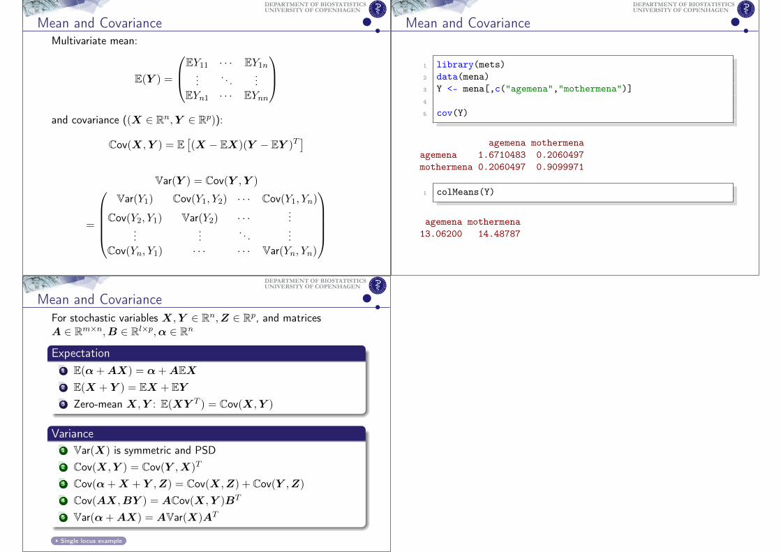
Mean and CovarianceMultivariate mean:

E(Y ) =

EY11 · · · EY1n...

. . ....

EYn1 · · · EYnn

and covariance ((X ∈ Rn,Y ∈ Rp)):

Cov(X,Y ) = E[(X − EX)(Y − EY )T

]

Var(Y ) = Cov(Y ,Y )

=

Var(Y1) Cov(Y1, Y2) · · · Cov(Y1, Yn)

Cov(Y2, Y1) Var(Y2) · · · ......

.... . .

...Cov(Yn, Y1) · · · · · · Var(Yn, Yn)


Mean and Covariance

1 library(mets)2 data(mena)3 Y <- mena[,c("agemena","mothermena")]4

5 cov(Y)

agemena mothermenaagemena 1.6710483 0.2060497mothermena 0.2060497 0.9099971

1 colMeans(Y)

agemena mothermena13.06200 14.48787


Mean and CovarianceFor stochastic variables X,Y ∈ Rn,Z ∈ Rp, and matricesA ∈ Rm×n,B ∈ Rl×p,α ∈ Rn

Expectation1 E(α+AX) = α+AEX2 E(X + Y ) = EX + EY3 Zero-mean X,Y : E(XY T ) = Cov(X,Y )

Variance1 Var(X) is symmetric and PSD2 Cov(X,Y ) = Cov(Y ,X)T

3 Cov(α+X + Y ,Z) = Cov(X,Z) + Cov(Y ,Z)

4 Cov(AX,BY ) = ACov(X,Y )BT

5 Var(α+AX) = AVar(X)AT

Single locus example

Documents

This course will describe particular statistical methods ...staff.pubhealth.ku.dk/~kkho/undervisning/family2013/day1-intro-2x2.pdf · Statistical methods for twins and families