On Introducing Imperfection in theNon-Linear Analysis of Buckling of Thin

Shell Structures

Version of June 13, 2014

Tian Chen

On Introducing Imperfection in theNon-Linear Analysis of Buckling of Thin

Shell Structures

THESIS

submitted in partial fulfillment of therequirements for the degree of

MASTER OF SCIENCE

in

CIVIL ENGINEERING

by

Tian Chen

Department of Structural MechanicsFaculty CEG, Delft University of TechnologyDelft, the Netherlandswww.ceg.tudelft.nl

Swiss Federal Institute of TechnologyWolfgang-Pauli-Strasse 15, Honggerberg

8093, Zurich, Switzerlandwww.ethz.ch

© 2014 Tian Chen.

On Introducing Imperfection in theNon-Linear Analysis of Buckling of Thin

Shell Structures

Author: Tian ChenStudent id: 4240642Email: t.chen-3@student.tudelft.nl

Abstract

This master thesis details the investigation of the effect of geometrical imperfection on thinshell structures using general FEM software packages. The author proposes a finite elementbased method for the analysis and design of thin shell structures, and describes the im-plementation of such a procedure on four FEM packages. The procedure involves assessingstructural imperfection sensitivity, and imposing geometrical imperfection prior to a physicaland geometrical non-linear analysis.

Starting with thin metallic cylinders, by incorporating imperfection to the surface, the au-thor shows that ANSYS is capable of reproducing Koiter’s asymptotic theory as well asexperimental data. The author further demonstrates the robustness of the procedure byimplementing it on four simple yet realistic structures with both symmetric and asymmetricload cases.

For extremely imperfection sensitive structures such as an axially loaded cylinder, the authorintroduces four different types of imperfection that could be imposed instead of the firstbuckling mode, and gauges the effectiveness of each with a modified knock-down factor.By varying the vertical curvature, it is discovered that an axisymmetric imperfection shapegoverns the ultimate buckling capacity of any near-cylindrical shells. Change in Gaussiancurvature is calculated as the end of every load step in the FEM analysis. By plotting thechange in Gaussian curvature, the onset of buckling can be readily defined.

Finally, physical non-linearities are introduced to the FEM models to gauge the effect ofyielding and cracking. It is found that metallic shells buckle within the elastic range, thoughyielding eliminates post-buckling capacity. With concrete cracking, instability occurs soonafter cracks develop at the buckles of the imperfection shape, therefore reducing the capacityby as much as 8 times from that of the elastic model.

Thesis Committee

Committee chair: Prof. Dr. Ir. Jan G. Rots, Faculty CEG, TU DelftCommittee member and supervisor: Dr. Ir. Pierre C.J. Hoogenboom, Faculty CEG, TU DelftCommittee member: Dr. Ir. Frans P. van der Meer, Faculty CEG, TU DelftCommittee member (External): Prof. Dr. Eleni Chatzi, D-BAUG, ETHZ

Preface

First and foremost, I would like to express my sincere gratitude to my advisor Pierre Hoogenboomfor chatting with me about research and life as an academic, and of course, for guiding methrough this thesis. I would like to thank my thesis committee, Jan, Frans, and Eleni for theirencouragement, insightful comments, and hard questions.

While challenging at times, the past 5⁄7 of seven months had been fun and exciting, and deeplyrewarding. Though writing thesis is never about the writer as much as it is about the fruit ofhis or her research. I hope that this thesis paves way for future investigations in the field of thinshell buckling; let’s face facts, there are many questions waiting to be answered.

For the remaining 2⁄7 of the time, I would like to thank Arup Amsterdam and the colleagueswithin for indulging me with interesting and challenging projects.

As I will be leaving this place and embarking on the next phase of my journey, I would like toleave this with you for your reading pleasure.

Tian ChenDelft, the Netherlands

June 13, 2014

iii

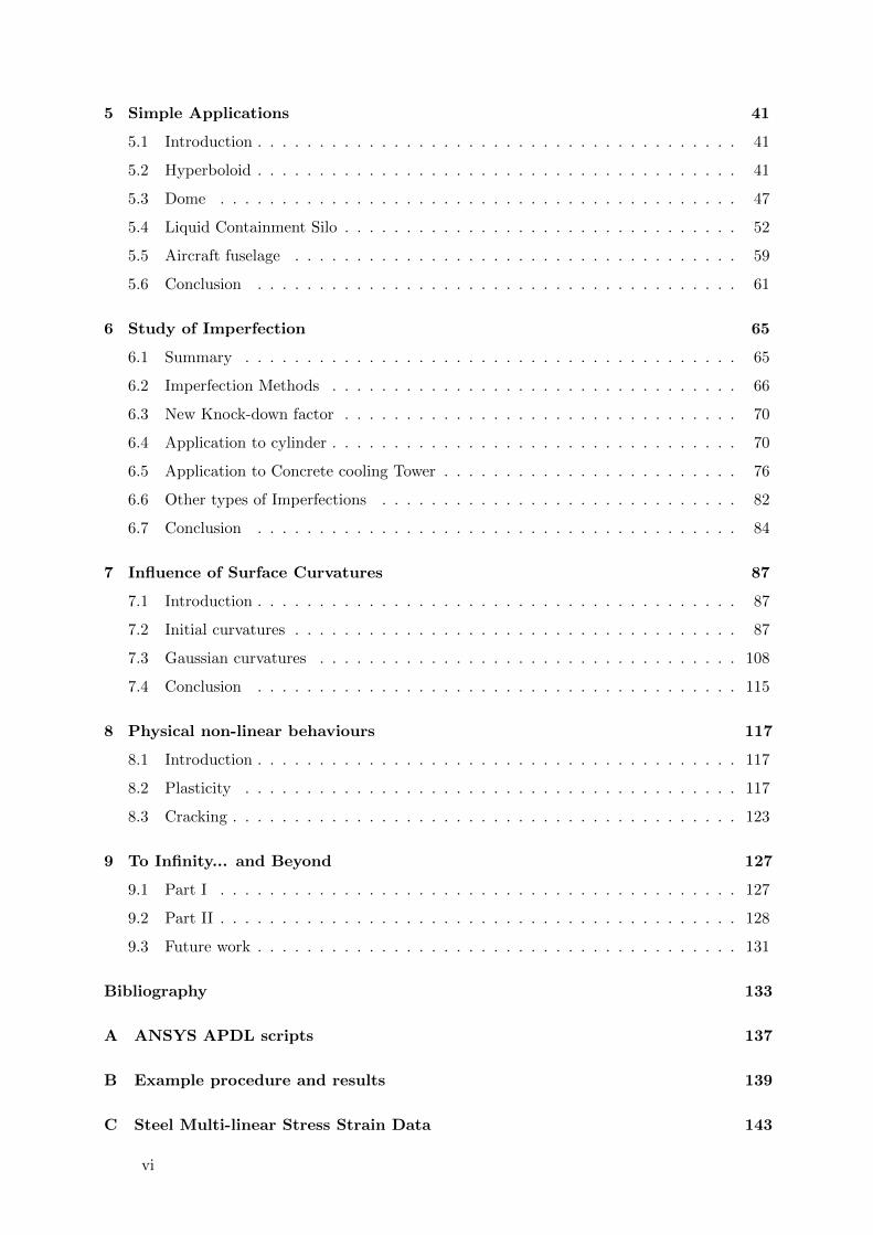
Contents

Preface iii

Contents v

1 Introduction 1

1.1 Objective . . . . . . . . . . . . . . . . . . . . . . . . . . . . . . . . . . . . . . . . 1

1.2 Procedure . . . . . . . . . . . . . . . . . . . . . . . . . . . . . . . . . . . . . . . . 2

1.3 Thesis Summary . . . . . . . . . . . . . . . . . . . . . . . . . . . . . . . . . . . . 4

2 Existing Knowledge 7

2.1 Shell structures . . . . . . . . . . . . . . . . . . . . . . . . . . . . . . . . . . . . . 7

2.2 Failure . . . . . . . . . . . . . . . . . . . . . . . . . . . . . . . . . . . . . . . . . . 8

2.3 Nothing is perfect . . . . . . . . . . . . . . . . . . . . . . . . . . . . . . . . . . . 8

3 Software Comparison 15

3.1 Introduction . . . . . . . . . . . . . . . . . . . . . . . . . . . . . . . . . . . . . . . 15

3.2 Hyperboloid Model . . . . . . . . . . . . . . . . . . . . . . . . . . . . . . . . . . . 16

3.3 GSA - General Structural Analysis . . . . . . . . . . . . . . . . . . . . . . . . . . 18

3.4 ANSYS . . . . . . . . . . . . . . . . . . . . . . . . . . . . . . . . . . . . . . . . . 20

3.5 Diana . . . . . . . . . . . . . . . . . . . . . . . . . . . . . . . . . . . . . . . . . . 24

3.6 Abaqus . . . . . . . . . . . . . . . . . . . . . . . . . . . . . . . . . . . . . . . . . 26

3.7 Comparison with theoretical Solution . . . . . . . . . . . . . . . . . . . . . . . . . 28

3.8 Conclusion . . . . . . . . . . . . . . . . . . . . . . . . . . . . . . . . . . . . . . . 29

4 Study of cylinders 33

4.1 Introduction . . . . . . . . . . . . . . . . . . . . . . . . . . . . . . . . . . . . . . . 33

4.2 Geometry . . . . . . . . . . . . . . . . . . . . . . . . . . . . . . . . . . . . . . . . 33

4.3 Linear Buckling Analysis . . . . . . . . . . . . . . . . . . . . . . . . . . . . . . . . 37

4.4 Comparison to experimental data . . . . . . . . . . . . . . . . . . . . . . . . . . . 38

4.5 Comparison to Koiter’s Law . . . . . . . . . . . . . . . . . . . . . . . . . . . . . . 39

4.6 Conclusion . . . . . . . . . . . . . . . . . . . . . . . . . . . . . . . . . . . . . . . 40

v

5 Simple Applications 41

5.1 Introduction . . . . . . . . . . . . . . . . . . . . . . . . . . . . . . . . . . . . . . . 41

5.2 Hyperboloid . . . . . . . . . . . . . . . . . . . . . . . . . . . . . . . . . . . . . . . 41

5.3 Dome . . . . . . . . . . . . . . . . . . . . . . . . . . . . . . . . . . . . . . . . . . 47

5.4 Liquid Containment Silo . . . . . . . . . . . . . . . . . . . . . . . . . . . . . . . . 52

5.5 Aircraft fuselage . . . . . . . . . . . . . . . . . . . . . . . . . . . . . . . . . . . . 59

5.6 Conclusion . . . . . . . . . . . . . . . . . . . . . . . . . . . . . . . . . . . . . . . 61

6 Study of Imperfection 65

6.1 Summary . . . . . . . . . . . . . . . . . . . . . . . . . . . . . . . . . . . . . . . . 65

6.2 Imperfection Methods . . . . . . . . . . . . . . . . . . . . . . . . . . . . . . . . . 66

6.3 New Knock-down factor . . . . . . . . . . . . . . . . . . . . . . . . . . . . . . . . 70

6.4 Application to cylinder . . . . . . . . . . . . . . . . . . . . . . . . . . . . . . . . . 70

6.5 Application to Concrete cooling Tower . . . . . . . . . . . . . . . . . . . . . . . . 76

6.6 Other types of Imperfections . . . . . . . . . . . . . . . . . . . . . . . . . . . . . 82

6.7 Conclusion . . . . . . . . . . . . . . . . . . . . . . . . . . . . . . . . . . . . . . . 84

7 Influence of Surface Curvatures 87

7.1 Introduction . . . . . . . . . . . . . . . . . . . . . . . . . . . . . . . . . . . . . . . 87

7.2 Initial curvatures . . . . . . . . . . . . . . . . . . . . . . . . . . . . . . . . . . . . 87

7.3 Gaussian curvatures . . . . . . . . . . . . . . . . . . . . . . . . . . . . . . . . . . 108

7.4 Conclusion . . . . . . . . . . . . . . . . . . . . . . . . . . . . . . . . . . . . . . . 115

8 Physical non-linear behaviours 117

8.1 Introduction . . . . . . . . . . . . . . . . . . . . . . . . . . . . . . . . . . . . . . . 117

8.2 Plasticity . . . . . . . . . . . . . . . . . . . . . . . . . . . . . . . . . . . . . . . . 117

8.3 Cracking . . . . . . . . . . . . . . . . . . . . . . . . . . . . . . . . . . . . . . . . . 123

9 To Infinity... and Beyond 127

9.1 Part I . . . . . . . . . . . . . . . . . . . . . . . . . . . . . . . . . . . . . . . . . . 127

9.2 Part II . . . . . . . . . . . . . . . . . . . . . . . . . . . . . . . . . . . . . . . . . . 128

9.3 Future work . . . . . . . . . . . . . . . . . . . . . . . . . . . . . . . . . . . . . . . 131

Bibliography 133

A ANSYS APDL scripts 137

B Example procedure and results 139

C Steel Multi-linear Stress Strain Data 143

vi

D Circumferential displacement of the axisymmetric imperfection 145

E 20 Eigenvalues of each 37 models of different curvatures 147

F Other Types of Imperfections 149

F.1 Initial Conditions Deformation Diagrams . . . . . . . . . . . . . . . . . . . . . . 149

F.2 Loading Imperfection Deformation Diagrams . . . . . . . . . . . . . . . . . . . . 150

vii

Chapter 1

Introduction

1.1 Objective

Thin shells are often the structure of choice when the design is weight critical. They inherentlyhave excellent strength to weight ratio; this attribute allows for much thinner designs than thatof other types of structures. Experienced designers realize that the rigidity of shells preventsthem from giving ample warning before catastrophic failures. Unlike traditional constructionswhere the structure would deform visibly a long time prior to collapse, shells typically exhibitno such behaviour. These failures are often attributed to buckling instabilities [16]. Despite thisblemish, shell structures have been widely adopted in aerospace, civil and offshore industries.Consequently, many experiments have been performed (especially on stiffened and un-stiffenedcylindrical shells) in an attempt to formulate theories that can be used by designers. Theexperimental results, however, displayed a wide scatter (See Fig. 1.1), the average of which wassignificantly less than that of the established linear buckling theory. It has been agreed thatinitial geometric imperfections is the main cause for this scatter and deviation [10].

Figure 1.1: Test results of axially compressed cylinders (From Buckling of Bars, Plates andShells by D. O. Brush and B. O. Almroth).

The current design approach to account for this deviation follows the ”Lower Bound DesignPhilosophy”, where the critical buckling load is multiplied by an empirical knock-down factor to

1

ensure that the resultant is a ”lower bound” of all experimental data obtained. Driven by theneed to reduce weight and cost of developing buckling-resistant aeronautical structures, mostresearch done on this subject have been focusing a few narrowly defined subjects (e.g. axiallycompressed cylindrical shells), where experimental data is abundant and the knock-down factorcan be confidently calculated.

However, from a civil engineer’s point of view where shell structures may take on any form, theauthor noted a general lack in progress in the following areas,

1. Axially loaded cylinders were almost always the only structure studied, scant attentionhas been paid to other elementary shapes, or more complex structures.

2. Aside from cylinders, design codes offer little guideline aside from the ”lower Bound DesignPhilosophy”. The onerous tasks of experimentation are at the hands of the designers aspast data were obtained almost exclusively from cylindrical shells.

3. The Lower Bound design method penalizes efficient and well designed shells by enforcingan uniform, and conservative ”knock-down” factor.

4. Updated correlation between modern software packages, theories, and practice. Compu-tational capability and performance increases daily; yet designers have not been able totake full advantage of these increasingly powerful tools.

5. For thin shells, physical non-linearity is usually neglected since the onset of buckling is inthe elastic range. However, it is necessary for the simulation of post-buckling behaviour.

6. There is no attempt in classifying structures beyond the applied load and support condi-tions. Curvature may be a useful quantity when estimating the imperfection sensitivity ofa structure.

Koiter in his doctoral dissertation proposed the Imperfection Sensitivity Design Philosophywhere initial periodic imperfection is incorporated into the problem formulation. Using thebasics of his theory and many that builds on it, this thesis plans to address these challenges andintroduce to engineers an easy-to-implement method to standardize the analysis of thin-shellstructures that are imperfection sensitive.

1.2 Procedure

There has been a resurgence in thin-shells in the recent decade as architects become more andmore interested in designing free-formed structures. It is the hope of the author that this thesiscan provide design engineers with a relatively simple method to evaluate the robustness of theirshell structure. To expand on the procedure flowchart (Fig 1.2), each item is discussed in detailhere.

Step 1 Construct the Finite Element Method model

Method Build the model consisting of elements and nodes from either a CADmodel, a macro script, and so on.

Step 1a Input physical non-linearity parameters

Method If the design may yield / crack prior to buckling then material data mustbe supplied (e.g. stress-strain curve, concrete cracking, etc).

2

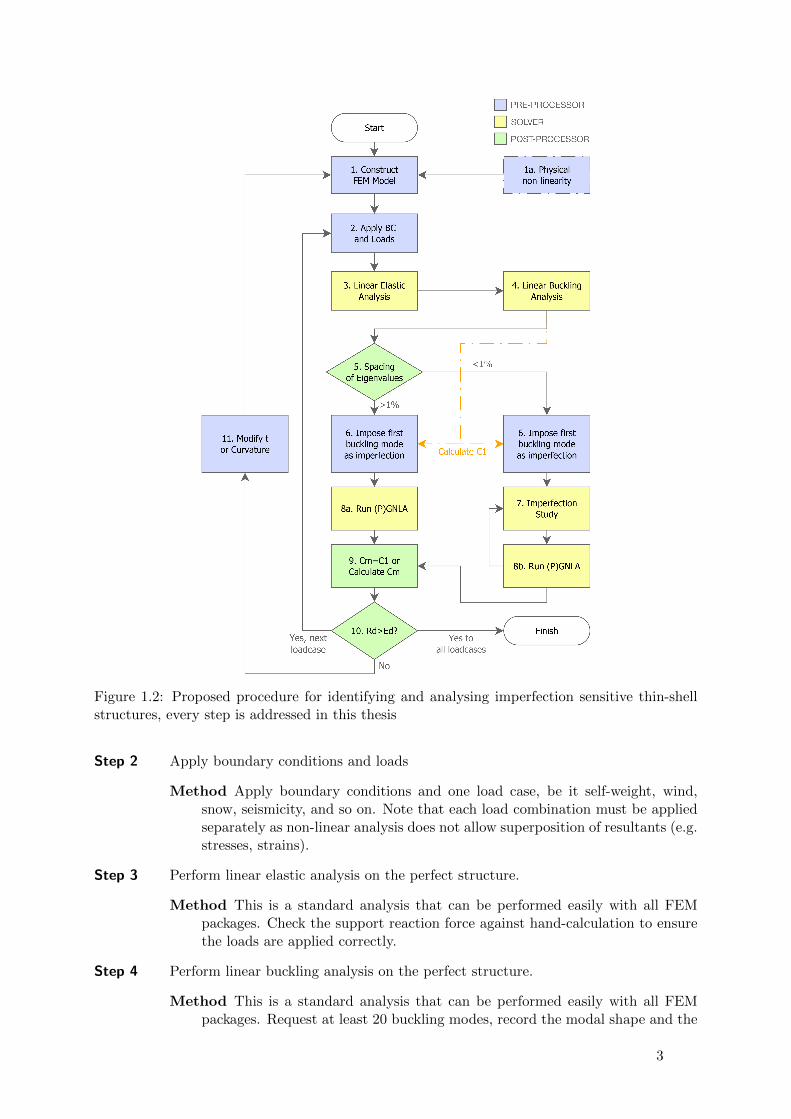
Figure 1.2: Proposed procedure for identifying and analysing imperfection sensitive thin-shellstructures, every step is addressed in this thesis

Step 2 Apply boundary conditions and loads

Method Apply boundary conditions and one load case, be it self-weight, wind,snow, seismicity, and so on. Note that each load combination must be appliedseparately as non-linear analysis does not allow superposition of resultants (e.g.stresses, strains).

Step 3 Perform linear elastic analysis on the perfect structure.

Method This is a standard analysis that can be performed easily with all FEMpackages. Check the support reaction force against hand-calculation to ensurethe loads are applied correctly.

Step 4 Perform linear buckling analysis on the perfect structure.

Method This is a standard analysis that can be performed easily with all FEMpackages. Request at least 20 buckling modes, record the modal shape and the

3

load factor of each mode.

Step 5 Imperfection sensitivity - spacing of eigenvalues

Method Determine whether or not the structure is imperfection sensitive by cal-culating the difference in eigenvalue between the first and the 20th bucklingmode.

Step 6 Impose imperfection in the shape of the first buckling mode

Method This is done based on the capability of the software.

Step 7 Imperfection study

Method Should the eigenvalues be closely spaced, a detailed imperfection studyshould be done to extract the largest reduction factor.

Step 8a Run Geometric Non-linear Analysis on the imperfect model

Method Obtain the ultimate buckling capacity and compare it with the criticaleigenvalue from Step 4.

Step 8b Run Geometric Non-linear Analysis on the imperfect model for each imperfectionshape

Method Obtain the lowest ultimate buckling capacity and compare it with theultimate buckling capacity from Step 8a.

Step 9 Calculate the largest reduction factor

Method This reduction factor should be calculated in reference to the ultimatecapacity resulting from Step 8a.

Step 10 Unity check

Method Whether structural resistance is greater than load. If true then move backto Step 2 and apply the next set of loads. If not, move to Step 11.

Step 11 If the unity check fails

Method Then either the thickness should be increased, or if possible, the geometryof the design should be changed.

1.3 Thesis Summary

Each step of the procedure above is discussed in this thesis. The thesis is divided roughly in twoparts, the first part focuses the practicality of imperfection imposition on thin-shell structures.It discusses software capability, validity of the proposed procedure, and then provides severalcase studies of real design problems. It also includes, as the last step, an discussion on theinfluence of physical non-linearities. The second part is more abstract in its topics. Focusingon variations of the cylindrical structure, different shapes of imperfections are discussed andimplemented, influence of initial curvature, and the change in Gaussian curvature behaviour areanalysed in-depth.

4

1.3.1 Chapter Descriptions

Following this introduction, this thesis starts by giving a concise and easy-to-understand back-ground on shell structures, shell buckling and imperfection sensitivity in Chapter 2. As thisthesis focuses on the FEM implementation of imperfection sensitivity analyses, Chapter 3 sur-veys four popular FEM packages and addresses their strengths and short-comings. The fourpackages are ANSYS, Abaqus, Diana, and GSA.

As cylinder buckling under axial load is one of the most widely studied problem, Chapter 4compares FEM results against both experimental and theoretical results and finds commonground with both, thereby giving confidence in the proposed procedure for future analyses.Following this validation, the purposed method of imperfection imposition is applied to foursimple yet realistic engineering problems, a hyperboloid cooling tower, a liquid containing silo,a monolithic dome, and an airplane fuselage in Chapter 5. In Chapter 8, a multi-linear stressstrain model and a reinforced concrete model is applied to the cylinder and the hyperboloidrespectively to assess the influence of plasticity or cracking on the buckling behaviour. Thisends the first portion of the thesis.

Thus far in this thesis, imperfection in the shape of the first buckling mode has been the onlyshape applied, Chapter 6 studies imperfection in other modes, and other shapes in general. LikeChapter 8, the cylinder, and the hyperboloid are used as trial structures. In this case, theyare chosen for their markedly different imperfection sensitivity levels. Lastly, to understanddifference between the two shapes, a range of different geometries each with a different curvatureare studied in Chapter 7. In addition to the differences in initial curvature, incremental changesin Gaussian curvature are also studied.

5

Chapter 2

Existing Knowledge

2.1 Shell structures

Shells, a derivative of the Latin scalus, describes a broad spectrum of natural objects rangingfrom the shell of a nautilus to the carapace of a turtle. The word has been adapted to describehuman made structures commonly associated with a finite curvature and vanishing thickness,e.g. aircraft fuselages, gas and water pipes, hull of ships, and also many civil constructions.

When designed properly, shell structures exhibit incredible strength. As they carry a largeportion of the load through membrane action, their thickness can be much less than that ofplate structures spanning the same area. Nature has utilized the inherent strength of shellsthrough evolution and produced strong and beautiful structures such as egg shells, sea shells,blood cells and other shapes that surround us.

When the thickness of a shell structure is reduced to a certain level, given by the ratio a/t, wecall it a thin shell. The radius, a, is defined in Eq. (2.1), and t is the thickness of the shell.Figure 2.1 gives definitions to the geometrical variables.

a =1

2s+

1

8

l2

s(2.1)

Figure 2.1: Geometry of a shell [24]

Traditionally, civil shell structures were designed through the hands of masters (Felix Candela,Frei Otto, Vladimir Shukhov, and Heinz Isler to name a few) using the empirical method of formfinding. Form finding can be seen as an extension of the famous revelation of Robert Hooke ”Ashangs a flexible cable, so inverted, stand the touching pieces of an arch”; a shell structure canbe formed by inverting a piece of hanging cloth, see Figure 2.2 for such a model. These physicalmodels can then be loaded to find their real capacities.

1Heinz Isler, Wikipedia, http://en.wikipedia.org/wiki/File:Gartencenter_Wyss_Zuchwil_01_09.jpg

7

Figure 2.2: Shell structure, and its hanging models1

Structural designers and architects favour these thin shells due to their inherent elegant andtheir ability to span a large roof area efficiently. Figure 2.3 shows one example of a successfullyexecuted shell structure. In search for ever lighter and stronger shapes, aerospace engineers havebeen utilizing shell structures almost exclusively.

Figure 2.3: TWA Terminal at J.F.K. International Airport2

2.2 Failure

Designers realize that the rigidity of shells prevents them from giving ample warning beforecatastrophic failures. Unlike traditional constructions where the structure would deform visiblya long time prior to collapse, thin shells typically exhibit no such behaviour. These failures areusually attributed to bifurcation buckling [16]. Buckling is a structural instability and is causedby a bifurcation in equilibrium. Buckling happens when the strain energy initially absorbedin-plane convert to bending. Due to the higher stiffness of membrane action, the correspondingamount of energy causes a large non-linear bending deformation. To complicate the matter, thecapacity of many thin shell structures are imperfection sensitive.

Table 2.1 summarizes the critical load pC, the critical membrane force ncr of simple shell struc-tures. Note that these are the analytical solutions of linear buckling.

2.3 Nothing is perfect

A chicken’s egg is on average 60 mm long and 40 mm wide. The thickness is on average 0.31 mm.This gives an a/t ratio of approximately 1/100, placing it in the category of thin shells. Shells suchas eggs are extremely strong as anyone who tried to squeeze crack an egg will agree. An eggthat is nicked (even imperceptibly) however, would crack at a much lower force. This significant

2Evan P. Cordes, TWA Flight Center, Wikipedia, http://en.wikipedia.org/wiki/TWA_Flight_Center

8

pC nC

N/m2 N m−1

Cylinder, axially loaded - −1√3(1−ν2)

Et2

a

Hyperboloid, axially loaded - 1√3(1−ν2)

Et2

a

Cylinder, external pressure 2√3(1−ν2)

Et2

a21√

3(1−ν2)

Et2

a

Dome base radius > 3.8√at 2√

3(1−ν2)

Et2

a2−1√

3(1−ν2)

Et2

a

Table 2.1: Critical loading and membrane force of shells

reduction in capacity suggests that eggs (with positive Gaussian curvatures) under hydrostaticpressure (from the hand squeezing) are susceptible to imperfections.

2.3.1 imperfection sensitivity

Some man-made thin shells exhibit similar reduction in load carrying capacity, while others donot. Calladine in his 1995 paper on ”Understanding Imperfection-Sensitivity in the Buckling ofThin-Walled Shells” [17] gave an introductory account on the various advances made in thisfield since the 1940s. He stated that imperfection sensitivity in a structure is usually categorizedby three characteristics,

1. buckling capacity is much less than what is predicted by the classical theory. For the caseof an axially compressed cylinder, the predicted bifurcation value is as much as six timeshigher than the actual buckling load [16].

2. experimental buckling capacity is unpredictable and scatters over a wide range, see Fig 1.1.

3. catastrophic failure occurs at on set of buckling.

Graphically speaking, the structure is imperfection sensitive if λS in Fig 2.4 is less than λC andthere is limited post-buckling strength (i.e. point F is always lower than point E).

Karman was the first scientist to formally attempt an theory trying to predict the bucklingcapacity of imperfection sensitive shells. He proposed that unlike real columns, shells behavesimilarly to columns transversely supported by non-linear spring supports, i.e. these springshave a much stiffer tensile response than compressive. Crookedness in these fictitious columnsresulted in the three above behaviours that characterize shells.

Around the same time, Koiter investigated the same problem in his PhD thesis [28]. He concludedthat this discrepancy is predominately due to geometrical sensitivity of these thin shell structures,meaning imperfection in the shape of a shell is the main reason why it may buckle at a lower thanpredicted load. He further showed that square root of the amplitude of geometrical imperfectionsis approximately the reduction factor of the buckling capacity of a shell. Eq. (2.2) shows thegeneral equation of post-buckling load displacement relation,

P/PC = 1 + b(δ/t)2 (2.2)

where PC is the classical critical buckling load from LBA; δ is the normal-to-surface amplitudeof buckling displacement, and t is the thickness. b is a geometrical constant that describes therate of change of load after buckling.

Using perturbation analysis, Koiter expanded equation (2.2) and described the calculation ofload factors in equation (2.3), where λ is the load factor, λC is the critical load factor calculated

9

Figure 2.4: Load-deflection curve showing points of interest, path 0AB presents axisymetricdeformation, 0BD non axisymmetric deformation, 0EF for a real structure (or GNLA withimperfection). Snap through occurs at point E. [16]

using LBA, w is the normalized bifurcation buckling modal amplitude, and a and b are relatedto the geometrical and load characteristics of a given structure.

λ = λC(1 + aw + bw2 + ...) (2.3)

Depending on the constants a and b, Koiter identified three categories of buckling behaviour(Fig. 2.5).

Figure 2.5: Buckling behaviour, left: not susceptible, susceptible, one-sided susceptibility [24]

This classification also defines imperfection insensitive structures as b > 0. Bars, plates andother typical structural elements belong to this first category in 2.5 where there exists a stablepost-buckling path to prevent the structure from progressively collapsing into a heap of brokenpieces.

This is not the case for many shell structures. When the initial part of the post-buckling pathhas a negative slope, buckling occurs violently and the magnitude of the critical load factordepends on the degrading influence of initial imperfection as in the categories II, and III inFigure 2.5. λS is the load factor that an imperfect structure would buckle at, and for categoriesII and III λS is smaller than λC, and structures in those categories are imperfection sensitive.The reduction from λC is indicated in Table 2.2.

10

Category a b λS/λC

I = 0 > 0 Not susceptible to imperfections

II = 0 < 0 = 1− 3(−b/4)1/3(ρwimp)2/3

III > 0 - = 1− 2(−ρawimp)1/2

Table 2.2: Koiter’s knock-down factor equations for the different geometries

Note that the above equations assume there exists a unique buckling mode at the critical load.Koiter hypothesized that this is not the cause for axially loaded cylinders where the lowestmode is associated with several buckling loads, or for hydrostatically pressured domes where thecritical load is followed immediately by a group of bifurcation loads. For these cases, due tomodal interaction, extreme sensitivity is expected and equation (2.3) turns into N asymptoticequations. Note that in equation (2.4) the repeated indices represent summations from one toN .

[λ/λC − 1]wi = Aijkwbjwbk +Bijklwbjwbkwbl + ... (2.4)

This thesis is concerned with shells in the second category where a = 0 as the geometry isaxisymmetric. It is shown that the most negative b is, the greater sensitivity of the critical loadto initial geometric imperfections [15].

2.3.2 Implementation of imperfection

Due to the size and production size and scale (often unique) of shell structures, they are sub-jected to lenient quality control and large construction tolerances. It is impossible to completelyeliminate all imperfections; consequently various methods have been proposed to account for theeffect of imperfections in the finite element calculation of the load capacity of shells.

When designing a shell structure, it is almost never the case that the shape is simple enough(e.g. constant curvature) for there to exist an analytical solution. For complex structures wherethere is no analytical solution, finite element analysis is usually the only viable method forward(aside from physical modelling, for example, by Heinz Isler [19]). To perturb the model geometrywith some imperfection, that imperfection must be made known.

While imperfections are random by nature, there has been efforts to investigate and classifygeometrical imperfections. Koiter in his initial theory imposes imperfection solely in the shapeof buckling modes. The argument was that any imperfection shape may be decomposed into aseries of periodic pattern with Fourier series. In a later paper, he applied his method to a morelocalised, albeit still periodic, imperfection and found the same type of imperfection-sensitivity.

Cederbaum and Arbocz took a probabilistic approach to Koiter’s theory by varying two criticalparameters, initial imperfection amplitude and the allowable load, in an attempt to construct areliability design theory [18]. The idea of constructing an imperfection data bank was proposedby Arbocz [11] in 1979. Majority of the data were gathered from electro-plated stiffened andun-stiffened cylinders. However, this pursuit has not produced an actual accessible database intoday’s definition (i.e. on the internet), rather, the measurements were published in a collectionof research articles.

In the aerospace industry, due to the limited number of contractors, contractor-manufacturing-process specific tolerances and imperfection shapes are recognized by the engineers and utilized asthe first-estimate of imperfection [23]. A similar method has been in use in structural engineering,where imperfections are classified by the fabrication method [11]. Unfortunately, most advancesin this field have been done with axially loaded cylindrical shells as they are easy to test both

11

experimentally and numerically, and more importantly, they are the most relevant shape for theaerospace industry.

It is clear that when the imperfection cannot be measured or otherwise be made known (e.g.the structure has not been built and the contractor does not have accurate tolerance data),the ”worst” imperfection should be assumed and an appropriate knock-down factor be applied.This method may penalize the design unduly and increase the weight and cost enough to over-shadow the benefit of a shell structure all together. To obtain a more accurate imperfectionrepresentation associated with certain geometries, several methods were proposed.

2.3.3 Finite Element Analysis

In Finite Element Method, the software discretizes a structural continuum into finite elements.Governing differential equations are then solved numerically for each element. Different strate-gies are implemented to account for both geometrical and physical non-linearities. In the aca-demic context, a shell is a structure whose structural behaviour can be mathematically describedby shell elements. A generalized shell element is a 2 dimensional element that describe bothin-plane and out-of-plane forces and moments.

Using the previously defined ratio a/t, shell structures can be divided into the following cate-gories [24].

Very thick shells (a/t ≤ 5)3-D effects - use 3-D solid elements

Thick shells (5 ≤ a/t ≤ 15)In-plane membrane forces, out of plane bending and higher order transverse shear included

Moderate shells (15 ≤ a/t ≤ 30)In-plane membrane forces, out of plane bending and linear transverse shear included

Thin shells (30 ≤ a/t ≤ 4000)In-plane membrane forces, out of plane bending moments and shear included, thoughtransverse shear deformation neglected

Membrane (4000 ≤ a/t)In-plane membrane forces only

Element Formulation

This thesis focuses on the structural behaviour of thin shells where 30 ≤ a/t ≤ 1000. There aretypically three approaches to analyse such problems. First is to assume that the geometry ofindividual elements resemble flat plates, and therefore can be solved with plate equations. Theissue with such an approach is that the size of each element must be sufficiently small to notmisrepresent the overall curvature of the surface. The second is to use Sanders-Koiter equationwhich incorporates the curvature of each element into its formulation. For simple geometrieswith constant curvatures (kx, ky, kxy), the differential equation can be simplified to Eq. (2.5).While the Sanders-Koiter equation should be able to converge at the correct solution with muchless DOFs, no surveyed software packages provide such elements.

Et3

12(1− ν2)52 52 52 52uz + EtΓΓuz = 52 52 pz (2.5)

12

The last and the most popular approach is to degenerate a 3-D solid element into a 2-D surfaceelement (Fig. 2.6) [20]. This approach is most commonly implemented in modern FEA softwarepackages and is the one used for this thesis [7]. In Chapter 3, the strategies implemented byvarious popular FEM packages are compared and contrasted.

Figure 2.6: Degenerate of 3-D Solid elements [20]

2.3.4 Analysis of buckling behaviour

Linear buckling analysis (LBA) is typically used to find the critical buckling load of a structure.This type of analysis solves the Eigenvalue problem and produces a set of Eigenvalues andtheir associated vectors. In practical terms, this analysis produces a set of buckling modes eachcontaining a buckling shape, and a load factor. The lowest of these theoretical load factorsshould cause the structure to fail in buckling.

The Lower bound approach is based on this type of analysis. Eurocode 1993-1-6 (2007) providesdetailed and theoretical procedure for the design of thin-shell structures with the focus on thedesign of cylindrical silos and tanks. The code provides several methods to designers. The firstand most often applied method compares resistance stresses from LBA of a perfect shell with thedesign stresses. LBA calculates the buckling modes of a structure along with their associatedload factors λcr. During design, reduction factors, Eq. (2.6), are then applied to the lowest loadfactor λcr to account for geometric imperfections and other non-linear behaviours [12]. It wasnoted that the Eurocode treats the issue of thin shell buckling with more academic rigour andbased on more theoretical ground than other guides (e.g. AISC / ACI) [36].

λa ≤ Cλcr

γm(2.6)

where λa is the allowable applied load factor, λcr is the lowest buckling load of the perfectstructure, C is the empirical ’knockdown’ factor, γm is the traditional partial factor of safety.λcr can be obtained from Table 2.1 for simple shells of revolution.

This approach is appealing to designers as it is similar to the calculation procedure of othertypes of structure, and can be easily performed without special training. It is however up todesigner’s judgement as to what the reduction factors C should be applied for different loadingand support conditions. Many experts in the field of shell structures suggest that to designagainst catastrophic failure, the designer must possess knowledge of the failure mode of thedesign through either experience or experiment. Without those, reduction factors must beset sufficiently low as to negate many advantages of a shell structure [16]. Furthermore, VonKarman and Tsien [27] stated that the classical small deflection theory does not produce therealistic buckling shapes, and that the deformed structure may produce buckling shapes withlower associated eigenvalues.

The second approach and the one used in this thesis involves the evaluation of the structureusing a geometrically non-linear analysis that includes imperfections. This procedure was used

13

by numerous scientists in more recent studies of imperfection sensitive problems [35]. A shell isconsidered imperfection sensitive if the load capacity resulting from a geometrically non-linearanalysis (GNLA) with imperfection is less than that from a LBA, as this means the load carryingcapacity is reduced by the imperfection. Values for the magnitude and patterns of imperfectionsof the most basic shapes (e.g. cylinders, spheres) may be found in Imperfection Databanks [11],but the Eurocode states that various imperfection patterns be studied if the most detrimentalpattern cannot be easily identified. The buckling resistance is calibrated by comparisons betweenit and the known resistances of other real shells or experimental ones [36].

The last approach is applicable only for the simplest of structures, in which analytical equationsbased on Koiter’s asymptotic theory can be applied directly.

2.3.5 Imposition of Modal Shape

Ramm stated that FEM is suited to geometric imperfections of any shape. He suggested thatthe geometrical perturbation of a perfect shell is equivalent to a new independent model thatcan be analysed separately. He further recommended that the imperfection can be based onbuckling modes, post-buckling mode, combination of several modes, or realistic deviations.

Performing non-linear analysis directly on a symmetric structure with a symmetric load mayproduce unrealistic result as buckling is a second order effect that results from either out ofbalance load or displacement, neither of which existed in a perfect structure. Several studiesrecommend either to apply a small out of balance load or displacement to the structure toobtain more accurate results. (Note that in the Chapter 6, the effects of combinations andhigher buckling modes are investigated.)

14

Chapter 3

Software Comparison

3.1 Introduction

Bushnell summarized the technical advances in buckling failure analysis up until 1981 in hislecture on ”Buckling of Shells - Pitfall for Designers”. The aim is always to determine themaximum load-carrying capacity of a structure, and to that end three main approaches weredescribed, one is to adapt Koiter’s asymptotic theories to different classes of structures (plates,shells, etc), two is to simulate these behaviours in general purpose computer programs, and threeis to develop special purpose programs (e.g. BOSOR5) for the analysis of axisymmetric struc-tures [16]. Both method one and three remain applicable only to a limited class of structures,and are used mainly for academic research. This chapter explores the second method and showsthat general purpose programs are capable of accomplishing the eventual goal as the specializedprograms but requires far less specialized training.

The first task of this study is to understand the capability of the different software packagesto impose geometrical imperfection, and to perform GNLA on the imperfect geometry; and thesecond is to compare the accuracy, performance, and user-friendliness of the different packages,and to select one package to use for all future studies in this thesis. The packages in question areGSA (General Structural Analysis), ANSYS, and Diana. Abaqus is included as a fourth packagewhen it was discovered that GSA cannot perform GNLA with 2-D elements. The author usesa hyperboloid shaped wet cooling tower as the benchmark model to perform these analyses onwith all of the above software packages.

The author spent much time in familiarizing himself with the software packages. This reportdetails the findings and observations made as the author progressed. Note that since it is theauthor’s first time using most of these packages, errors are invariably made. Also note thatthese software packages are being actively developed, and thin shell buckling is one of the areaswhere developers are focusing their efforts on. This report only reflects the reality of the timeit is being written, and may contain false information when read at a future time. The authoraims to perform these analyses with the most time-saving methods possible. As a result, most ofthese are done with the geometry being generated by a script or a spreadsheet, and the analysesdone with the GUI of the packages.

3.1.1 Computer System

All analyses in this section are performed on a notebook PC with the specifications listed inTable 3.1. The versions of the different software packages are also listed for reference.

15

Computer Model ASUS K56CAOperating System Windows 8.1 Enterprise 64-bit OS

Processor Intel Core i5-3317U @ 1.70GHz, x64-basedGPU Intel(R) HD Graphics 4000RAM 4.00 GB

# of Cores 2

Software packages VersionOasys General Structural Analysis (GSA) 8.6

Mechanical ANSYS 14.5TNO Diana 9.44

Simulia Abaqus 6.13

Table 3.1: Computer Specifications

3.2 Hyperboloid Model

Cooling towers dissipate waste heat from processes to the atmosphere. Hyperboloid concretetowers are the largest type of cooling towers. They operate on the principle of evaporativecooling, the warm water circulates to the base of the tower and the temperature lowers aswater evaporates. The warm moist air rises to the top of the tower as it is less dense thanits surrounding cold air. Hyperboloid cooling towers are often used for their high structuralstrength verses material ratio. The hyperbolic shape also accelerates the upward convective airflow, increasing the cooling efficiency.

3.2.1 Shape

The geometry of a typical cooling tower is shown in Figure 3.1 [5]. To simplify the geometry andto assist in mesh generation, a single hyperbolic curve is defined using the following parametersobtained from an existing tower,

rThroat = 25.1 m ; rBottom = 39.3 m ; hBottom = 76.8 m (3.1)

The equation of a hyperbolic curve is defined in equation (3.2) by constants a and b. By placingthe center of the coordinate system at the red circle in Figure 3.1, we could solve for a by settingx = rThroat and z = 0. After a is obtained, b is solved by setting x = rBottom and z = ±hBottom.

x2

a2− z2

b2= 1 ; a = 25.1 m ; b = 63.7 m (3.2)

Rearranging the equation, the varying radius x could be found by incrementing the height z.Note that the coordinate system had been shifted to the base of the hyperboloid in equation (3.3).

x = r(z) =

√(z − hBottom)2

a2

b2 + 1; z = 0→ 108 (3.3)

The points above hTotal = 108 m are discarded since 108 m is the height of the cooling tower, seeFigure 3.1. The surface of a cooling tower is formed by revolving this hyperbolic curve aroundthe vertical axis. The shell is assumed to have a uniform thickness of 0.190 m. To find the radiusto thickness ratio, or the slenderness ratio, the radius is first calculated,

c2 = a2 + b2 ; c = 68.5m (3.4)

Therefore the ratio is,c− at

=43.4

0.19= 228.5 (3.5)

16

Figure 3.1: Geometry of a typical cooling tower

3.2.2 Mesh

To perform a finite element analysis, one must divide the geometrical shape into a grid ofelements. Each element is defined by a set of points and their associated coordinates. A grid ofpoints is generated by assuming a constant increment of 1 m long the z axis, and a constant angleof variation of 2° at odd elevation steps and 4° at even ones (see Figure 3.2). This differences inangular division allows for 8 node elements to be created. Following this grid arrangement, 180elements are generated per 2 meters.

8 node curved shell elements are used to accurately represent the doubly curved surface. Thereis no danger of irregular elements in this model as the model could be thought of as a cylinderwith a wider top and bottom. The element aspect ratio is kept as 1 at the neck of the tower,and the maximum ratio of 2 occurred at the base.

Figure 3.2: Geometry of the mesh, and size of a typical shell element

There are 6 degrees of freedom (DOFs) at each of the nodes, three translational, and threerotational. The drilling rotations can be eliminated to reduce the number of equations. Notethat the mesh density is not refined at this stage since all results are relative between thepackages. This mesh results in 4860 elements, 14760 nodes and 88560 DOFs.

3.2.3 Material

A generic reinforced concrete material is defined. Since this thesis is more interested in therelative effect of imperfection, and not the failure modes, the material properties are crudely

17

defined as a weighted average between steel reinforcement and concrete.

Eequiv = 22× 109 Pa ; ν = 0.2 (3.6)

3.2.4 Loads

For the purpose of this study, only the self-weight of the structure is applied. The initial loadfactor is set as 1.

g = 9.81 m/s2 ; ρ = 2400 kg/m3 (3.7)

During GNLA, the gravitational acceleration, g, is linearly incremented.

3.2.5 Supports

The base ring of the shell is pinned against translation in the three axes but allowed to freelyrotate. This simulates the real structure where the shell is supported by a ring beam and aseries of diagonal (∧) shaped struts. In the real structure, there is a ring beam at the base andthe top of the structure. These are summarily neglected.

3.3 GSA - General Structural Analysis

Below is a detailed report on the performance of each FEM packages. GSA is a StructuralAnalysis and Design package produced by Oasys, the software house of Arup. Its aim is toprovide engineers with efficient, reliable and capable FEA tools. Comparing to the other twopackages, GSA is arguably more user friendly and intuitive, though this comes at a cost as it lacksmany of the features that are essential to this project. Its incremental non-linear performancewhen analysing larger models is found lacking when compared with Diana or ANSYS.

3.3.1 Model

GSA allows data to be directly copied and pasted from Excel. This greatly simplifies the nodalcoordinate, and element connectivity inputs. The resulting structure is immediately visible onthe graphical display, and sections can be extracted by dragging a window across. Figure 3.3shows an example of such an interface.

GSA is currently incapable of performing analyses with 8 node curved elements; such an elementdoes exist in the element library, though it is used exclusively for pre-processing at the moment.Therefore 8 node flat elements are implemented by modifying the coordinate of the middlenodes to be the average of their neighbours. Self-weight is added to the structure, and pinnedconnections are assigned to the nodes on the bottom ring through the graphical interface as well.

3.3.2 Linear Elastic Analysis

A maximum deflection occurs at the top of the structure as expected. The magnitude of theZ-directional deflection is −4.5 mm. The sum of the reaction forces Rz is 89.76× 106 N, similarto what is calculated in the theoretical section with a difference of 1.8 %.

18

Figure 3.3: GSA user interface showing node and element input windows, and a graphical display

3.3.3 Linear Buckling Analysis

GSA’s Euler modal buckling analysis produces modal shapes similar to those produced by theother packages as shown in Figure 3.4. The lowest load factor resulted is 19.98. This LF issignificantly higher than what is produced by the other packages. This is attributed to the useof flat shell elements as oppose to curved elements, as an equivalent model in ANSYS usingSOLID181 elements resulted in the same LF as GSA.

Figure 3.4: GSA LBA mode 1

The resulting mode 1, 2, 3 and 4 consists of three layers of buckles with each layer containing14 buckles, 7 outward, and 7 inward. The deflection distribution of mode 1 and 2 are as follows(scaled to a maximum of 1000 mm); top layer: ± 150 mm; middle layer: ± 450 mm; base layer:± 1000 mm.

Similar FEM analysis on a cooling tower was done by Kratzig, et al. to show the functionalityof his proposed finite element [30]. The resulting linear buckling shape is presented in figure 3.5.His model is significantly more complex, and also geometrically much larger, though some com-parisons can be made between his un-stiffened model and Figure 3.4. There are only two layersof buckles in the vertical direction of his model as its height to width ratio is smaller. Thebottom buckles emerge higher up in elevation in his model, suggesting that the boundary layeris stiffer than the model in this study (his boundary conditions possibly included rotational stiff-ness). In the tangential direction, the number of buckles (bow-in and bow-out) however remainidentical to the model in this study (7 buckles in the half shell). The inclusion of stiffeners alsooffer some insights to the buckling behaviour. When lateral deformation is constricted, largestbuckles occur intra-stiffener.

19

Figure 3.5: Buckling modal shape resulting from Kratzig’s analysis

3.3.4 Imperfection

GSA can rather easily impose initial deformations in the shape of buckling modes with userdefined magnitude. 100 mm is imposed as the maximum magnitude of imperfection. 100 mm ison the same magnitude as the thickness of the shell, and is a sufficiently accurate estimate sincewe are more interested in the relative effect of imperfections.

GSA 8.6 Tools H Manipulate Model I Create New Model from Deformed Geometry . . .

From the prompt window, the user can select from which case (Load, or combination) thedeformation originates. The user can also choose between applying a scale factor or using amaximum displacement (with automatic scaling). Rotation can also be accounted for.

Note that since the 8 node flat elements are usually wrapped out of plane by the modal defor-mation, the usage of flat shell elements is necessary but not the most suitable. This becomes amoot point however since no further analyses can be done with GSA.

3.3.5 Geometrically Non-linear Analysis

GSA does not have the ability to perform non-linear buckling analysis on 2-D elements. Thisrestricts the usage of GSA to serve as a checker of the buckling modes and load factors.

3.4 ANSYS

ANSYS is one of the most popular finite element analysis and computer aided engineeringsoftware. It markets two suite of products, Simulation Technology (Structural Mechanics, Mul-tiphysics, etc) and Workflow Technology (Workbench Platform, High-Performance Computing,etc). The Workflow Technology compliments the Simulation Technology by improving produc-tivity, and usability [8].

The author wrote an APDL (ANSYS Parametric Design Language) script to generate the model,the mesh, and the input parameters such as density, thickness, and load. In the interest of savingtime, the model is imported into Workbench for the subsequent analyses. See Figure 3.6 for adetailed sequence description.

3.4.1 Element Type

SHELL281 is an 8-Node Structural Shell element with quadratic interpolation functions, Eq. (3.8) [4].The element has eight nodes with six degrees of freedom at each node: translations in the x,y, and z axes, and rotations about the x, y, and z-axes. It is most accurate for linear, large

20

Figure 3.6: ANSYS Workbench interface; 1. APDL module to run the script, 2. importing theresultant geometry, 3. Static Structural module to run the linear elastic analysis, 4. Using theload from 3, and running the linear buckling analysis, 5. Application of imperfection through aAPDL script, 6. importing the resultant geometry again, 7. Non-linear Analysis

rotation, and large strain non-linear analyses. Initial shell thickness can be specified at eachnode, and change in shell thickness is also accounted for in non-linear analyses. The formulationis based on logarithmic strain and true stress measures. The element kinematics allow for finitemembrane strains (stretching). However, the curvature changes within a time increment areassumed to be small.

u =1

4(uI(1− s)(1− t)(−s− t− 1) + uJ(1 + s)(1− t)(s− t− 1) + uK(1 + s)(1 + t)(s+ t− 1)

+ uL(1− s)(1 + t)(−s+ t− 1)) +1

2(uM (1− s2)(1− t) + uN (1 + s)(1− t2)

+ uO(1− s2)(1 + t) + uP (1− s)(1− t2))(3.8)

3.4.2 Linear Elastic Analysis

ANSYS does not differentiate between linear and non-linear analyses, rather, non-linearity andlarge deformation are provided as options within the static structural analysis.

The geometry is imported as an APDL script, and linked to the static structural module withinWorkbench. A downward acceleration of 9.81 m/s2 is applied to the structure. As a result,a maximum deflection occurs at the top of the structure as expected. The magnitude of theZ-directional deflection is −5.73 mm. The sum of the reaction forces Rz is 89.78× 106 N, similarto what is calculated in the theoretical section with an percentage difference of 1.8 %.

3.4.3 Linear Buckling Analysis

The geometry and load is linked from the static linear module to the buckling module. 20modal shapes are requested. The block Lanczos solver is used as it is currently the only optionavailable. Lanczos alogrithm is an iterative energy method to find eigenvalues and eignvectors

21

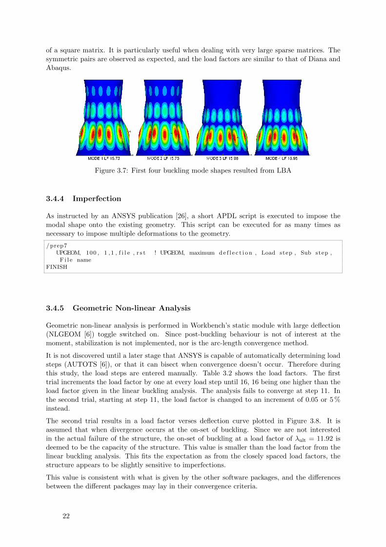
of a square matrix. It is particularly useful when dealing with very large sparse matrices. Thesymmetric pairs are observed as expected, and the load factors are similar to that of Diana andAbaqus.

Figure 3.7: First four buckling mode shapes resulted from LBA

3.4.4 Imperfection

As instructed by an ANSYS publication [26], a short APDL script is executed to impose themodal shape onto the existing geometry. This script can be executed for as many times asnecessary to impose multiple deformations to the geometry.

/ prep7UPGEOM, 100 , 1 ,1 , f i l e , r s t ! UPGEOM, maximum d e f l e c t i o n , Load step , Sub step ,

F i l e nameFINISH

3.4.5 Geometric Non-linear Analysis

Geometric non-linear analysis is performed in Workbench’s static module with large deflection(NLGEOM [6]) toggle switched on. Since post-buckling behaviour is not of interest at themoment, stabilization is not implemented, nor is the arc-length convergence method.

It is not discovered until a later stage that ANSYS is capable of automatically determining loadsteps (AUTOTS [6]), or that it can bisect when convergence doesn’t occur. Therefore duringthis study, the load steps are entered manually. Table 3.2 shows the load factors. The firsttrial increments the load factor by one at every load step until 16, 16 being one higher than theload factor given in the linear buckling analysis. The analysis fails to converge at step 11. Inthe second trial, starting at step 11, the load factor is changed to an increment of 0.05 or 5 %instead.

The second trial results in a load factor verses deflection curve plotted in Figure 3.8. It isassumed that when divergence occurs at the on-set of buckling. Since we are not interestedin the actual failure of the structure, the on-set of buckling at a load factor of λult = 11.92 isdeemed to be the capacity of the structure. This value is smaller than the load factor from thelinear buckling analysis. This fits the expectation as from the closely spaced load factors, thestructure appears to be slightly sensitive to imperfections.

This value is consistent with what is given by the other software packages, and the differencesbetween the different packages may lay in their convergence criteria.

22

LF Trial 1 LF Trial 2m/s2 m/s2

1 9806.6 1 9806.62 19613.2 2 19613.23 29419.8 3 29419.8

...8 78452.8 8 78452.89 88259.4 9 88259.410 98066.0 10 98066.011 107872.6 11.000 107872.612 117679.2 11.005 107921.613 127485.8 11.010 107970.714 137292.4 11.015 108019.7

...12.185 119493.412.190 119542.512.195 119591.513.000 127485.8

Table 3.2: Load Factor Steps

Figure 3.8: ANSYS load factor vs. deflection curve

23

3.5 Diana

3.5.1 Model

Diana itself is a finite element solver, and it relegates pre- and post-processing duties to otherpackages. Either iDiana or FX+ can be used for those purposes. Since the trial model (thehyperboloid) can be easily described analytically, the pre-processing is done via a vba macrothat generates a file in the format of Diana’s input files. This also allows for smaller toleranceerrors, and greater user control. The analyses are done within Diana through its GUI. Dianaprovides 8 node curved shell elements both with (CQ48S) and without (CQ40S) drilling rotationDOFs. Input files can be imported by the following procedure.

DIANA Analysis setup H Input data file H Add .dat file

3.5.2 Linear Elastic Analysis

The following procedure in Diana starts the linear elastic analysis.

DIANA H Select analysis type H Structural linear static

Diana produces similar results in both deflection and support reaction as the other packages.

3.5.3 Linear Buckling Analysis

The modal buckling analysis is called Structural Stability analysis in Diana. The number ofmodes to be solved is set by the user, so is the output format. The user can request Diana tooutput the result in a table or as a model for the post-processor. Both are requested since boththe load factors and the shapes are of interest.

The Diana solver package itself is relatively easy to use and understand. The documentationand the examples are tremendously useful in aiding novices. The iDiana pre- and post-processorhowever proves to be user unfriendly. So far the only commands used are the ones offered by theexamples, in particular, the cylindrical shell example in the stability category. The following isa post-processing script that displays the displacement contour.

# To obta in load f a c t o r sUTILITY TABULATE LOADCASES

# To obta in modal shapesRESULTS LOADCASE MO1# MO1 f o r mode one , MO2 f o r mode two , e t c .RESULTS NODAL DTX . . . . G RESDTX! DisplacementPRESENT SHAPE

# To obta in modal d i sp lacementsCONSTRUCT COORDSYS CYLINDRIC CS1 ZRESULTS TRANSFORM LOCAL CYLINDRIC CS1 RRPRESENT CONTOUR LEVELS

24

3.5.4 Imperfection

Within the buckling analysis, Diana allows for the user to apply imperfections in geometry tothe structure. The imperfections could take one of three shapes: a buckling mode, user defined,and random. Each accepted a maximum deflection as an input. For this study, the first bucklingmode is selected, with a maximum deflection of 100 mm. This imperfection is carried throughinto the subsequent analyses. The feature of including imperfection of a random shape is ofvalue when trying to show that modal shaped deformation always cause the largest reduction incapacity.

S t r u c t u r a l s t a b i l i t yS t r u c t u r a l s t a b i l i t y S e t t i n g s

Eigen SetupNo − Incorpora te i n i t i a l d i sp lacementsYes − Imper f e c t i on

Pattern −> Buckl ing modeMode number 1Maximum value o f impe r f e c t i on 100 mm or 0 .1 m

3.5.5 Geometric Non-linear Analysis

The second type of analysis done in Diana is GNLA. Updated Lagrange is selected as oppose toTotal Lagrange to ensure that the geometry from the previous step’s equilibrium state is usedas the reference geometry for the next iteration. Load steps are then defined. The method ofiteration governs the speed of convergence but not the result. The convergence norm has thesame effect. These are left to their default values.

S t r u c t u r a l Non−l i n e a rS t r u c t u r a l non−l i n e a r S e t t i n g s

TypeGeometr i ca l ly non−l i n e a r

Geometr ical S e t t i n g sType o f geomet r i ca l non− l i n e a r i t y −> Updated Lagrange

ExecuteLoad s t ep s −> S e t t i n g s

Execute load s t ep sSteps

I t e r a t i o n based step s i z e sMaximum step s i z e −> Set t h i s low enough to ensure d ive rgence does

not occur at near f a i l u r e( r e s u l t i n g in i l l −cond i t i oned matrix e r r o r )

Others can be ad jus t by t r i a l and e r r o r

To prove that without imperfection, the model would behave completely linear elastically, bothmodels (perfect and perturbed) are run through the same analysis with the same load steps.From the above deflection plot, we observe that the structure behave linearly until the very lastload step. The last load step shows a structure failing in the modal shape. I hypothesize thatthis is due to a precision issue within the software itself as all other parameters are perfectlysymmetric and no out-of-plane components are observed. Note that the plot would indicatethat the structure behaves non-linearly from the start despite the material being linear elastic.The analysis diverges at a load factor of 11.20. This result follows a very similar load deflectioncurve as ANSYS despite appearing numerically different.

25

Figure 3.9: Diana - displaced shapes, comparison between perfect and imperfection model

3.6 Abaqus

Abaqus is another popular FEA package widely used in academia and industry. It was initiallydesigned to analyse very non-linear behaviours (e.g. deformation of rubber) and that is still itsadvantage over other packages. Its operation sequence is similar to that of the other packages.A model is generated in the pre-processor, analyzed, and displayed in the post-processor. Itsutilization of Object Oriented Python as a scripting language presents a large advantage overother packages that have limited scripting ability.

The author has discovered that the documentation is difficult to navigate through. Thoughsince all actions within the GUI are recorded as input commands in the command file, it is easyto replicate them in the overall input. As with the other packages, the author chose the fastestmethod to generate and analyze this structure. In this case, it was a input file including all loadsteps ran directly through the command interface.

3.6.1 Linear Elastic Analysis

Abaqus produced similar results as the other packages using the following input.

# STEP: SW#∗Step , name=SW, nlgeom=NO#∗ S t a t i c1 . , 1 . , 1e−05, 1 .

# ∗Dload, GRAV, 9 .806 , 0 . , 0 . , −1.∗End Step

3.6.2 Linear Buckling Analysis

Abaqus recommends the use of 9-node elements when analysing the buckling behaviour of doublycurved shell structures. It states that if the middle node is not specified (as in 8-node elements),

26

the internally calculated middle node may not actually be on the curved surface, thus leadingto inaccurate solution. This advise is not heeded since the written script does not generate suchnodes. As the calculated buckling capacity is similar to ANSYS, the geometry generating scriptis not changed.

∗Step , name=Euler , nlgeom=NO, per turbat i on∗Buckle20 , , 28 , 100#∗∗ BOUNDARY CONDITIONS∗Boundary , op=NEW, load case=1M3 , PINNED

#∗∗ LOADS∗Dload, GRAV, 9 . 81 , 0 . , 0 . , −1.∗End Step

The resulting first 2 pairs of eigenvalues are 14.72 and 14.97. Note that Abaqus indicated thatthe buckling load estimate equals to dead loads plus the eigenvalue multiplied by any live loads.Therefore one should be added to the eigenvalues, giving 15.72, and 14.97, which is identical tothat of the other packages.

BUCKLING LOAD ESTIMATE = ( ”DEAD” LOADS) + EIGENVALUE ∗ ( ”LIVE” LOADS) .”DEAD” LOADS = TOTAL LOAD BEFORE ∗BUCKLE STEP.”LIVE” LOADS = INCREMENTAL LOAD IN ∗BUCKLE STEP

3.6.3 Imperfection

Following the documentation and the sample file called ”Buckling of an imperfection-sensitivecylindrical shell” in the following directory,

ABAQUS Example Problems Guide H 1. Static Stress/Displacement Analyses H 1.2 Bucklingand Collapse AnalysesH 1.2.6 Buckling of an imperfection-sensitive cylindrical shell

The *IMPERFECTION command is used to impose the first modal shape to the model.

#∗∗ F i l e name , and load step∗IMPERFECTION, FILE=buckl ing ,STEP=1#∗∗Modal number , and s c a l e f a c t o r1 , 0 . 1

It is noted that additional lines can be appended to the end of the above code to impose additionalbuckling modes onto the structure.

3.6.4 Geometrically Non-linear Analysis

Abaqus provides the option to allow large deformation (NLGEOM), to create automatic ormanual load stepping (*STEP), and arc-length step control.

#∗∗ This i s s tep one o f the non−l i n e a r a n a l y s i s . The load i s s e t to increment by aload f a c t o r o f one . Actual substep increments are determined by Abaqus .

#∗∗ STEP: NL1 # Step 2 would look NL2∗STEP, name=NL1 , nlgeom=YES, s o l v e r=ITERATIVE,AMPLITUDE=RAMP∗STATIC

27

1 . , 1 . , 1e−05, 1 . # Step 2 would look 1 . , 2 . , 1e−05, 1 .∗DLOAD, GRAV, 9 . 81 , 0 . , 0 . , −1. # Step 2 would look , GRAV, 19 ,62 , 0 . , 0 . , −1.

#∗∗ OUTPUT REQUESTS#∗∗ Get r e a c t i o n f o r c e from node s e t M3 , i e . the bottom nodes∗RESTART, write , f r equency=0∗NODE PRINT,NSET= M3 ,SUMMARY=YESRF#∗∗ Get d i sp lacements from node s e t M5 , i e . the top nodes∗NODE PRINT,NSET= M5 ,SUMMARY=YESU∗End Step

The resulting load deflection curve compares well with the other packages, so no further inves-tigation is done.

3.7 Comparison with theoretical Solution

3.7.1 Linear Static

Linear static analysis is performed mainly to ensure that the geometry is properly connected,and that there is no unit inconsistency. The check is done by summing the reaction forces in thevertical direction, and equating that to the theoretical weight of the structure. The theoreticalweight of the structure is calculated as follows,

Rz =

108∑z=0

2πr(z) · ρgh;h = 1000mm (3.9a)

=

108∑z=0

2π

√(z − hBottom)2

a2

b2 + 1· ρgh (3.9b)

= 88.16× 105 N (3.9c)

This load will be increased until the structure fails in buckling. Note that buckling will neverhappen in theory in a perfect structure as the material is linear elastic and the load, the boundaryconditions and the geometry are all axisymmetric. The linear elastic results is in Table 3.3. While

GSA ANSYS DIANA ABAQUS

Reaction Force MN 89.76 89.78 89.81 89.77Deflection mm -4.5 -5.723 -5.723 -5.721

Table 3.3: Linear elastic reaction forces and deflection

all the packages results in similar reaction forces, they are slightly different from the calculation.This is due to the fact that summation is used in the calculation as oppose to integration. Thediscretization resulted in slight difference in the volume of each height layer.

3.7.2 Geometrically Non-linear Analysis

The highest load factors reached in Figure 3.10 are assumed to be where the buckling bifurcationsstart. The values are listed in Table 3.4.

Table 3.5 shows the first twenty load factors generated from each of the packages. Note thatGSA produces results significantly different from the other packages.

28

Package Load Factor Cmm

GSA - -ANSYS 11.92 1.32Diana 11.20 1.40

Abaqus 11.70 1.34

Table 3.4: Load factors from non-linear analyses

0

0.1

0.2

0.3

0.4

0.5

0.6

0.7

0.8

0.9

1

1.1

-90-80-70-60-50-40-30-20-100

Load

Fac

tor

Displacement [mm]

Diana Perfect

Diana Imperfect

Abaqus

ANSYS

Critical Load Factor

Figure 3.10: Force-deflection curves of the different software packages

3.7.3 Computation performance

Several measurements are used to compare the software packages. Table 3.6 lists the computerperformance data generated by the output files of each package. Note that since the majorityof resources are spent on the non-linear portion, GSA data is not realistically comparable andare excluded.

3.8 Conclusion

4 FEA packages are tested for their capability in analysing thin shell structures. A hyperboloidshaped cooling tower is used as a reference structure, with the self-weight as the sole load case.The sequence of analyses performed are as follows. Linear elastic analysis is done to verify thegeometry, linear buckling analysis calculates the load factors and the modal shapes, imperfectionis applied to the structure in the shape of the first buckling mode, and geometrically non-linearanalysis is performed to obtain the realistic capacity. Memory usage, file size and CPU-time arerecorded and compared. The user interfaces are assessed for their intuitiveness.

GSA is a structural analysis program developed by and for engineers. It is concluded that GSAlacks critical capabilities that forces it to be excluded from the selection. The reasons being:it cannot utilize meshes of non-flat shell elements; and it cannot perform non-linear bucklinganalysis on 2-D elements. Though it is worth noting that GSA serves as an excellent geometryviewer and validator, and buckling modal shape checker. Abaqus is substituted in as the thirdviable package for comparison as a result.

With Diana, ANSYS, and Abaqus, it is a general observation that the pre-processor includedare difficult to use and impractical for all but the simplest geometries (GSA does not contain a

29

Mode # Load FactorGSA ANSYS DIANA ABAQUS

1 19.98 15.73 15.70 15.721 19.98 15.73 15.70 15.723 20.29 15.98 15.94 15.984 20.29 15.98 15.94 15.985 20.73 16.32 16.28 16.316 20.73 16.32 16.28 16.317 21.40 16.86 16.83 16.868 21.40 16.86 16.83 16.869 23.00 18.12 18.10 18.1210 23.00 18.12 18.10 18.1211 23.60 18.58 18.53 18.5612 23.60 18.58 18.53 18.5613 24.90 19.62 19.58 19.6114 24.90 19.62 19.58 19.6115 24.92 19.63 19.60 19.6316 24.92 19.63 19.60 19.6417 25.34 19.97 19.93 19.6718 25.34 19.97 19.93 19.6719 25.55 20.12 20.09 20.1120 25.55 20.12 20.09 20.12

Table 3.5: Buckling modes and associated load factors

GSA ANSYS DIANA ABAQUS

Total CPU Time s - 1004 2892 4205Max. total memory MB - 926 2560 486

Folder Size GB - 1.56 9.23 0.493Cost of a License 1 e 1,750 13,000 10,000 to 40,000 ?1With the exception of GSA, all have refused to provide an official general quote

Table 3.6: Analyses performance data of geometrical non-Linear analyses

full pre-processor). This is especially true should the user want to create a model from scratch.It is frequently easier to either generate the model through a script, or import the surface from aCAD program and utilize only the meshing ability of the pre-processor (which can be advancedand excellent).

With the exception of GSA, the three remaining packages successfully performed all the taskswith relative ease. Specifically, all fours packages have the capability of adding geometric im-perfection in the shape of one buckling mode to shell finite element models.

The FEA solvers in the three packages offered similar results from the linear elastic and lin-ear buckling analyses. Results from the geometrically non-linear analyses gave not insignificantdifferences, especially in the stiffness behaviour. This is due to the difference in element formu-lation and other solver parameters, as well as numerical loss-of-precision. The final capacitiesobtained are comparable. This shows that the procedure outlined in Chapter 1 can and shouldbe used when designing thin shell structures in place of the Lower Bound Design method. Thisis particularly true since the mesh geometry needed by the linear buckling analysis can be reused

30

for subsequent non-linear analyses, the additional amount of effort in generating the model isnegligible. The computation time in GNLA is significant though it does not require man-hourinput.

Each package also has its own advantages and disadvantages. DIANA offers a relatively gentlelearning curve; one is able to construct the model, perform the analyses, and obtain reasonableresults without wasting time. Though this comes with a cost; Diana is not as flexible, and itsperformance lags behind the other two packages. At the time of writing, DIANA does not havea scripting language, thus forcing the user to either use its graphical pre-processors (iDIANA orFX+) or to generate the input file externally. The imposition of more than one buckling modeis a challenge as this task is associated with the Structural Stability analysis and not separatelyas its own task. Lastly, DIANA’s result files at ˜10GB are one magnitude larger than that ofANSYS’. This presents a challenge should a sensitivity analysis be required and many modelsmust be analysed.

ANSYS provides a friendlier and more robust user interface, both through Workbench (and thepre-processor within), and through APDL, the scripting language that underlines all of ANSYS.Its imperfection imposition is a separate function, and can be performed at any stage of theanalysis to impose imperfection of any shape. In addition, nodal coordinate change is a separatefunction that can be utilized to achieve the same task. Its disadvantages lie in its complexity.As ANSYS can be used for all types of FEM analyses (e.g. CFD, electromagnetism, thermal-mechanics, etc), its terminology is extremely general, thus leading to confusion when attemptingto find the relevant information. While well documented, ANSYS’ manual is broken into severalbooks, each containing thousands of pages and is difficult to parse through. Through all theavailable commands in APDL, it is difficult to discern the effect of each.

Abaqus is similar to Diana in that an input file can be generated externally and directly imported.However, it also provides the scripting option should the user be familiar with Python. Whileits documentation is also difficult to use, the graphical interface records all user actions and savethem as a input file so trial and error works fairly well. Its capabilities to impose imperfectionand its non-linear solver function similarly to those of ANSYS’. It is noted that the Riks analysis(called arc-length method in ANSYS) is more robust and user-friendlier than ANSYS.

ANSYS is chosen to be used for the remainder of this thesis for its capability and performance,despite being difficult to use initially. From my impression at several design firms, ANSYS ismore well known in the industry. The license fee is potentially cheaper. It has a good balancebetween file size, calculation speed and memory usage. Though the selection is dependent onpersonal preference, availability of licenses, and other facts that are not related to the packages’capabilities.

31

Chapter 4

Study of cylinders

4.1 Introduction

Thin cylindrical shells are widely used in the aerospace industry, most satellites have extremelythin shells as their casing, airplane fuselage is essentially a stiffened cylindrical shell, and so on.The boom in space exploration led to a surge of research initiatives at NASA in the 1960s andonward. Cylinders were widely studied also due to a large discrepancy between the experimentaland the theoretical results. In this thesis, in hindsight, an axially compressed cylinder wouldhave been a better candidate for the software assessment as well, as it is an extensively studiedimperfection sensitive buckling problem.

Civil engineers have long been utilizing the cylindrical shape for storage silos and tanks, thoughsince these structures usually loaded by their content inside, imperfection sensitivity is not anissue. Only in cases when there is a heavy wind load on a near empty tank, or when there isground acceleration do these shells buckle. The investigation of real silo structures is describedin chapter 5.

This chapter is devoted to showing that the general purpose FE program ANSYS is capableof delivering realistic results to the axially compressed cylinder. This is done by comparingthe results from ANSYS to both experimental data, and to Koiter’s theoretical formulation,Eq. (2.3).

4.2 Geometry

The length and width of the cylinder model are chosen to resemble a typical test setup. The a/tratio is set at 500. The applied load also simulates a typical compression test condition wherethe test apparatus press downward onto the top ring of the cylinder. To prevent in-extensionaldeformation, the same ring is restrained laterally. The bottom ring is pin supported.

While appearing simple, many factors influence the behaviour of the cylinder and the analysis.In particular, depending on the mesh size, nonuniformity near the edges may not be presentin the LBA, increasing the predicted critical load by 8-20% [16]. Therefore the surface musthave sufficient mesh density to trigger the buckling modes along the top and bottom edge. Theresulting mesh contains 4860 elements, and 88560 DOFs.

4.2.1 Loading

The compression load is applied first as a uniform downward edge pressure. This force controlledload application resulted in asymmetrical buckling modes along the xy plane, and edge warping

33

as shown in Figure 4.1. Warping of the loaded edge can be eliminated by applying the loadthrough displacement as suggested by Ramm [38]. Therefore to obtain perfectly symmetricalbuckling modes, and thus better simulate the test set-up, displacement controlled method isused where the top ring is simultaneously moved downward by a fixed magnitude of 0.025 m.This loading was referred to as ”end-shortening” by Kroplin in his study of cylinders (a/h = 200)with imperfection, his results are used for comparison in Chapter 6 [31]. The magnitude is setsufficiently small to improve convergence.

Figure 4.1: Asymmetric modes with force control

4.2.2 Comparison between load application methods

Since displacement controlled loading is impossible to apply in almost all real structures, thedifference between force and displacement control is compared here. The procedure remainsidentical in all other respects; first LBA is performed to obtain the critical load factor, thenimperfection is applied to the structure in the shape of the first buckling mode with a maximumamplitude of t/2. GNLA with large deformation enabled then calculates the load displacementbehaviour of the structure. The only difference is in the application of the load. In the firstmodel, uniform edge pressure is incremented at every load step, whereas in the second model,the increments are applied as uniform edge displacements.

(a) (b)

Figure 4.2: (a) Displacement controlled loading (b) Force controlled loading

The eigenvalues resulting from a LBA is calculated from either of the two conditions in Figure 4.2.

ucr = λDcr · uz (4.1)

Fcr = λFcr · Fz (4.2)

34

To show that the critical load factor from displacement controlled loading λDcr can be applied

equally to the force controlled situation, we assume the structure has the stiffness K, and thatthe system is linear elastic. Then the following relationships must be true,

Fcr = Kucr (4.3)

Fz = Kuz (4.4)

Re-arranging Eq (4.1), and substituting it into Eq (4.4),

Fz = K · ucr

λDcr

(4.5)

Moving λDcr to the LHS,

λDcr · Fz = K · ucr (4.6)

Using Eq (4.2) and we get,

λDcr · Fz = Fcr (4.7)

Figure 4.3 shows two load-displacement curves extracted from the same node. While there isslight difference in the displacement, the final load factor obtained is similar. Displacementcontrol allows the post-buckling behaviour to be observed (albeit only in the immediate vicinityof onset of buckling), whereas one can never be certain that the point of divergence in a forcecontrolled simulation is actually the on-set of instability. In a paper on FEM application tothin-walled members [39], Sarawit recommends implementing displacement control to bypasslimiting points when there is no snap back behaviour.

0

0.05

0.1

0.15

0.2

0.25

0.3

0.35

0.4

0.45

0.5

0 0.005 0.01 0.015 0.02 0.025 0.03

F /

Fcr

Displacement [m]

Displacement control

Force control

Figure 4.3: Comparison of force verses displacement controlled loading

35

4.2.3 Post-buckling

The above would suggest that displacement control should be used whenever possible on struc-tures prone to instability. In reality, displacement control is seldom applied since most naturaland human actions are imposed as forces, and it is next to impossible to apply the equivalentdisplacement field at each load step. Other techniques are developed as a result to adequatelyaddress this issue. Nonlinear stabilization, arc-length method, and slow-dynamic analysis arestudied in an attempt to extract more information about the post-buckling path. These threemethods are proposed by ANSYS Structural Analysis Guide to converge unstable structures.

Nonlinear stabilization is a new ANSYS technique that adds an artificial damper or dashpotelement to every node. When there is a large displacement at a node, a large damping forceis generated to reduce that displacement. Since the dashpot force is proportional to velocityand not displacement, a fictitious velocity is calculated as the change in displacement overthe duration of the current time-step. When there is no instability, ANSYS claims that smalldeflection generates negligible restoring force. With many trials, the user should be able tospecify a damping coefficient that is sufficiently large to circumvent divergence but that is notso large as to introduce excessive stiffness. Because the dashpot elements are attached to everynode, this technique is able to circumvent both local and global instability. The disadvantageof this technique is that the slope of the load displacement curve must still remain positivefor Newton-Raphson to function, therefore it is not applicable in cases where stiffness dropssuddenly.

“However, nonlinear stabilization cannot detect the negative-slope portion of a load vs. displace-ment curve problem with global instability.” - ANSYS manual

In the Newton-Raphson (NP) Approach, the solution is found by linear increments of positiveslopes, the arc-length method attempts to converge the Newton-Raphson equilibrium along anarc instead of a line. This allows convergence to occur even when the slope of the load deflectioncurve becomes zero or negative. The figure on the left in Fig. 4.4 shows a situation whereconvergence is impossible with NP irrespective of the size of the increments since decrementsare necessary. This method is only able to circumvent global instability and only when loadsare applied as forces. As shown in the figure on the right, the radius of the arc is an importantparameter, and may be determined through a large number of trial runs. The implementationin ANSYS is an improvement on the Riks method based on the theoretical work by Forde andStiemer [21].

Figure 4.4: Scheme of the arc-length method

Slow dynamic analysis attempts to solve the same structural problem but in a time-dependentmanner. The initial condition is set so that both displacement and velocity start at zero. Thismethod take considerably more effort than the above two as the user must supply the time-integration parameters and the damping factor.

36

Abaqus in its documentation suggested similar methods when dealing with unstable responses.Slow dynamic analysis, dash-pot stabilization, displacement method, and Ritz method werelisted as the possible solutions. Two noticeable differences were mentioned, one, it appears asthough dynamic analysis can be used at the onset of divergence thus speeding up the analysisconsiderably, and two, Ritz method can be used only when the load can be controlled by a singlescalar parameter.

Stabilization did not resulted in better convergence. ANSYS’ arc-length implementation at-tempts to restart the analysis every time divergences occurs, resulting in an infinite loop. It isthe author’s suspicion that the post-buckling behaviour of an axially compressed cylinder is toounstable to be captured unless the arc-length radius is set extremely small, though then driftback may occur. It is noted that many researchers and analysts have experienced difficulty in us-ing ANSYS arc-length method when analysing unstable structures (even for 1-D elements) [33].As a result, ANSYS Inc. appeared to have reformulated the algorithm in its newest release [44].The slow dynamic method show promising signs of convergence. However the results are dif-ficult to interpret as there exist significant discrepancies from the static analyses. Much moretime must be invested to obtain a functional model, therefore in all subsequent analyses in thisthesis where force control is used, the author assumes the peak force represents the onset ofbuckling. This assumption was used by Wunderlich, et al. in the simplified analysis of Elastic-Plastic Buckling of shells where post-peak behaviour is discarded. It was stated that since theinterest is in finding the buckling capacity of a structure, it is sufficient to obtain pre-bucklingbehaviour [46]. It was suggested that incremental and iterative procedure combined with conver-gence acceleration was sufficient for this purpose. Convergence acceleration was necessary dueto the geometrical softening of the structure, and such accelerator is implemented in ANSYS.

4.3 Linear Buckling Analysis

For the thin cylinder modeled in this chapter, LBA produced extremely closely spaced distinctbuckling modes. In fact, the sequence of buckling modes becomes sensitive to many modelingparameters such as mesh density, support loading condition, and so on. This shows that theorder of buckling modes has no real significance. 1 % difference in load factor is observed onlyafter 200 modes. Figure 4.5 shows that these modes are not merely rotations of the first modebut are rather distinct modes.

Figure 4.5: The first four buckling modes, and sample load factors up to the 50th mode

37

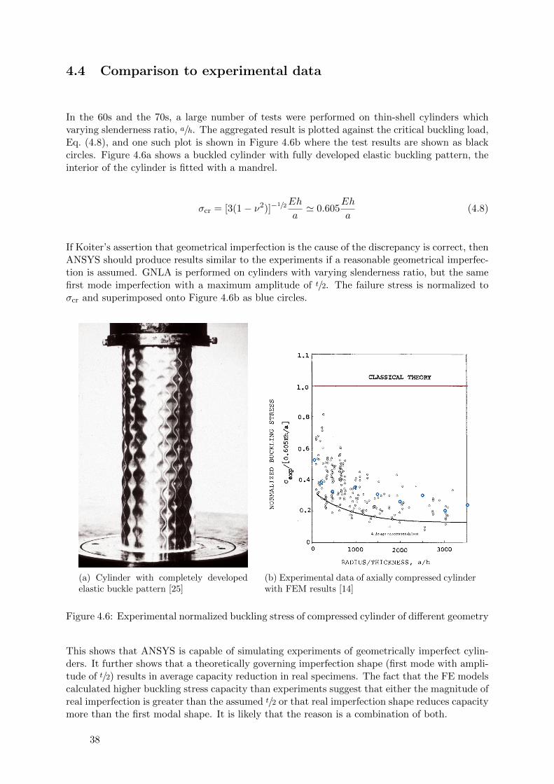
4.4 Comparison to experimental data

In the 60s and the 70s, a large number of tests were performed on thin-shell cylinders whichvarying slenderness ratio, a/h. The aggregated result is plotted against the critical buckling load,Eq. (4.8), and one such plot is shown in Figure 4.6b where the test results are shown as blackcircles. Figure 4.6a shows a buckled cylinder with fully developed elastic buckling pattern, theinterior of the cylinder is fitted with a mandrel.

σcr = [3(1− ν2)]−1/2Eh

a' 0.605

Eh

a(4.8)

If Koiter’s assertion that geometrical imperfection is the cause of the discrepancy is correct, thenANSYS should produce results similar to the experiments if a reasonable geometrical imperfec-tion is assumed. GNLA is performed on cylinders with varying slenderness ratio, but the samefirst mode imperfection with a maximum amplitude of t/2. The failure stress is normalized toσcr and superimposed onto Figure 4.6b as blue circles.

(a) Cylinder with completely developedelastic buckle pattern [25]

(b) Experimental data of axially compressed cylinderwith FEM results [14]

Figure 4.6: Experimental normalized buckling stress of compressed cylinder of different geometry

This shows that ANSYS is capable of simulating experiments of geometrically imperfect cylin-ders. It further shows that a theoretically governing imperfection shape (first mode with ampli-tude of t/2) results in average capacity reduction in real specimens. The fact that the FE modelscalculated higher buckling stress capacity than experiments suggest that either the magnitude ofreal imperfection is greater than the assumed t/2 or that real imperfection shape reduces capacitymore than the first modal shape. It is likely that the reason is a combination of both.

38

4.5 Comparison to Koiter’s Law

The load displacement plots in Figure 4.7b are obtained by varying the values of δ/t in Koiter’sequation, Eq. (4.9). (

1− PS

PC

3/2)

=3(3)1/2

2(−b)1/2

∣∣∣∣ δt∣∣∣∣ (PS

PC

)(4.9)

In this section, the first mode with various maximum amplitude from δ/t = 0.001 to δ/t = 1is used as the geometrical imperfection. This is done to show that there exists an correlationbetween ANSYS model and the theoretical formulation (Figure 4.7a), and that ANSYS is ableto reproduce the theoretical results if imperfection is included in the model.

(a) (b)

Figure 4.7: (a) Theoretical curved compared with ANSYS GNLA [15] (b) Load displacementcurves for all thickness ratios, force controlled increments

Figure 4.7b shows that using the first mode, ANSYS produced results very close to the curveb = −1 for δ/t up to 0.6. The close correlation to the b = −1 curve is expected since no modalcombination is imposed. Budiansky stated that b = −1 imply an imperfection-sensitivity levelas severe as that of a cylinder under axial compression, this statement is proved by ANSYShere. This is a important finding as it shows that ANSYS, a general FE program, withoutimplementing any buckling formulations (such as the ones used in LBA) is able to produceaccurate results. The divergence between the theoretical and ANSYS results past δ/t up to 0.6maybe investigated further. Results from ABAQUS also showed similar divergence in higherimperfection range [47].

Figure 4.7a shows the load displacement curves as well as the upper bound resulting fromGNLA of cylinders of different δ/t. It’s evident that passing a certain threshold, the magnitudeof imperfection reduces only the stiffness of the structure, but not the buckling capacity. Asstated above, this contradicts Koiter’s prediction that capacity continuously decrease, even asthe rate of decrease declines.

Referring to the dotted line in Figure 4.7(a), Koiter’s Law suggests that for the cases of extremelysensitive shells such as an axially loaded cylinder, a combination of buckling modes may interactto produce a lower buckling factor, with the governing equation (2.4). In the next chapter,modal combinations are studied to investigate Koiter’s modal interaction suggestion.

39

4.6 Conclusion

A number of parameters including slenderness, and imperfection magnitude, and the loadingmethod are studied to assess their effects on the buckling capacity of a axially compressed thincylinder. It is first observed that the order of buckling modes is meaningless as they are extremelyclosely spaced, and is sensitive to variations of the FE model (in particular mesh density, andloading method). Furthermore, given the large difference between the load factor resulting fromLBA and from any of the performed GNLA, it is extremely un-conservative to use the criticalbuckling load for design.

Force and displacement controlled loading is compared and found to be equally adequate inpredicting the buckling capacity of the cylinder. However, displacement controlled analysisprovides the assurance that the peak has actually been reached, and calculates post-bucklingbehaviour.

Comparing the results from GNLA and aggregated experimental data, it is shown that by impos-ing geometrical imperfection, GNLA can adequately simulate real test conditions and specimenusing only one maximum amplitude (t/2) and only the first mode as imperfection. GNLA withsingle modal imperfection results corroborates well with Koiter’s asymptotic theory for singlemodal imperfection up to a certain maximum imperfection magnitude. These results demon-strate the viability of the purposed procedure of imperfection imposition, and the capability ofFEM in analysing such problems despite the various simplifications made on the boundary andloading conditions.

40

Chapter 5

Simple Applications

5.1 Introduction

This study analyses four simple yet realistic structures with the proposed procedure. The struc-tures studied are a hyperboloid concrete wet cooling tower, a concrete dome, a steel liquidstorage silo and an airplane fuselage. The dimensions, loads, and support conditions are setto simulate reality. This study demonstrates the capability of ANSYS Mechanics in analysingimperfect structures with multitude of load types and support conditions.

5.2 Hyperboloid

5.2.1 Geometry

The structural model used in chapter two is reused in this study, however the geometry generationscript is changed to polar coordinate (θ and φ) to obtain better element aspect ratios. Afull-length model is used to account for both symmetric and anti-symmetric buckling modes.Figure 5.1 defines the variables used in the following equations. Using the calculated constantsa and b,Eq. (3.2), the focal point (and the distance from it to the z axis) of the hyperbola iscalculated as follows,

c =√a2 + b2 (5.1)

The eccentricity of the hyperbola is then,

e =c

a(5.2)

From the focal point, R2 is calculated based on φ1. Note that φ1 ranges from φbase to φtop. Theangles beneath the focal line are negative.

R2 =a(e2 − 1)

1 + e · cos(φ)(5.3)

From there, the radius of the hyperboloid R1 is calculated using simple trigonometry.

R1 = c−R2cos(φ1) (5.4)

The volume of the hyperboloid is calculated in equation (5.5).

V =

∫ φtop

φbase

∫ 2π

0tr2cos(φ) dθ dφ (5.5)

41

Figure 5.1: Geometry of the hyperboloid

Finite element mesh

As with all structures in this study, single layered curved 8 node elements (SHELL281 [9]) is usedto mesh the surface. Curved elements are able to incorporate initial curvature effects. SHELL281is suited for large strain nonlinear applications. The thickness can vary over individual elements(nodal thickness definitions). It can be layered to simulate composite sandwich materials. Thelocal coordinate system is set so the z axis is normal to the plane.

As oppose to assuming a mesh density as was done in the second Chapter, a mesh sensitivitystudy of the linear eigenvalue problem is done. The mesh density is continuously halved untilthe relative change of the eigenvalues converges. The second requirement is for the mesh to haveseveral elements along each spatial deformation wave.

The three different models shown in Figure 5.2 are generated by initial variations of 50 % and150 % on ∆z and ∆θ from the model in the centre. Variables ∆z and ∆θ are defined in Figure 5.1.The lowest four resulting buckling modes of each model are compared. From the results listed inTable 5.1, it is observed that the coarse mesh exceeds the threshold of 1 % difference. Thereforethe next finest mesh (∆z = 1.0 m ; ∆θ = 4°) is used.

Load cases

In addition to self-weight as was done in Chapter 3, wind pressure is applied as a second loadcase. The wind pressure is assumed to increase linearly in the vertical direction, and variessinusoidally along the tangential direction. The peak pressure is set at 10 000 Pa, and the

42

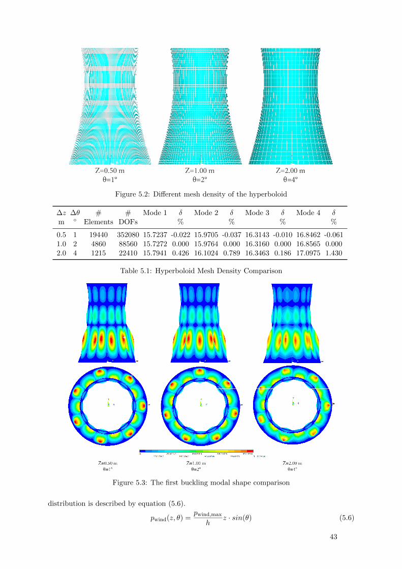
Figure 5.2: Different mesh density of the hyperboloid

∆z ∆θ # # Mode 1 δ Mode 2 δ Mode 3 δ Mode 4 δm ◦ Elements DOFs % % % %

0.5 1 19440 352080 15.7237 -0.022 15.9705 -0.037 16.3143 -0.010 16.8462 -0.0611.0 2 4860 88560 15.7272 0.000 15.9764 0.000 16.3160 0.000 16.8565 0.0002.0 4 1215 22410 15.7941 0.426 16.1024 0.789 16.3463 0.186 17.0975 1.430

Table 5.1: Hyperboloid Mesh Density Comparison

Figure 5.3: The first buckling modal shape comparison

distribution is described by equation (5.6).

pwind(z, θ) =pwind,max

hz · sin(θ) (5.6)

43

The combination of the first two loads is considered as the third load case. The intent is tosimulate a simple load combination of G+ ψQ.

Load case Description pwind,max

1 Self-weight of the structure -2 Wind pressure 10 000 Pa3 Self-weight with wind pressure 10 000 Pa

Table 5.2: Hyperboloid load cases

5.2.2 Analysis

Buckling, yielding, crushing

The proposed method is only valid when the shell buckles elastically since the material is assumedto be linear elastic (see Chapter 8 for discussion on non-linear material behaviour). Therefore,a check is made to ensure that the relative slenderness is greater than one.

λ =

√ncr

np> 1 (5.7)

The critical membrane force is taken from Table 2.1

ncr =1√

3(1− ν2)

Et2

a(5.8)

and the crushing force is simply,

np = f · t (5.9)

Where f is the compressive yield stress of concrete and t is the thickness of the shell. UsingC35 as the typical concrete quality, fc = 35 MPa. Therefore equation (5.7) gives the followingslenderness ratio, and shows that the hyperboloid would buckle before yielding.

λ = 1.62 > 1 (5.10)

Linear elastic, linear buckling analyses, and imperfection imposition

The linear elastic analysis gives a reaction force and a deformation that can be checked againsttheoretical values to ensure that the geometry is proper. This is done in Chapter 3 and thoughthe mesh density of the model is adjusted, the results remain similar. Load factors and bucklingshapes remain similar as well. An imperfection of t/2 = 95 mm is imposed on the geometry inthe shape of the first positive buckling mode in preparation for the next analysis.

The resulting load factors are listed in Table 5.3. Note that the factors are spaced close togetherwith the first and the third mode differing by 1.5 % in the first load case. The negative valuesassociated with LC2 and LC3 are due to the suction force of the wind. Since the eigenvaluesolver starts at 0, half of the eigenvalues of a symmetrically laterally loaded structure wouldalways be negative. In the third case, positive LFs dominate due to the presence of self-weight.

44

Mode number LC1 LC2 LC3

1 15.727 -9.830 -8.0762 15.727 -9.830 -8.0763 15.976 -9.085 -6.7374 15.976 -9.085 -6.7375 16.316 -8.242 5.7606 16.316 -8.242 5.7607 16.856 -7.248 5.9688 16.856 -7.248 5.9689 18.123 -6.602 6.45810 18.123 -6.602 6.45811 18.575 6.602 6.76312 18.575 6.602 6.76313 19.621 7.248 7.32414 19.621 7.248 7.32415 19.634 8.242 7.79916 19.634 8.242 7.79917 19.971 9.085 8.28218 19.971 9.085 8.28219 20.124 9.830 8.75620 20.124 9.830 8.756

Table 5.3: Hyperboloid load factors

Non-linear Analysis

Two different non-linear analyses are run for each load case, one with and the other withoutimperfection. The load displacement curves are shown in Figure 5.4. The imperfect GNLAcurves results in a less stiff structure than that from the Linear Buckling Analysis (LBA) asexpected. However the perfect GNLA curves follow an almost linear curve that attain a muchhigher maximum load factor. For the first load case, this is due to the fact that the given structureand its load condition are both axi-symmetric. Therefore without physical non-linearity, afictional stiffness is introduced by the geometry much in the same way as column crushing. Thedivergence in these linear curves are caused by an accumulation of loss of precision, leading toa type of computational imperfection.

In the second and the third load cases however, the load is asymmetric and the fictitious stiffnesstheory does not explain the excessive capacity. The stepwise GNLA somehow avoids the lowerbuckling modes, and buckles at a buckling mode does not resemble any of the modes generatedby the LBA. Further investigation is necessary to explain this anomaly.

Note that in the third load case, the load factor given by the LBA is lower than that fromthe imperfect GNLA. This is due to the fact that in the case of GNLA, the load increment isapplied only to the wind load, where as in LBA the load factor is calculated considering both theself-weight and the wind load. This issue is documented in APDL command manual 7.5.2. [7].The resulting knock-down factor is listed in Table 5.4.

It is evident that using GNLA without imperfection can be dangerously under-conservative,over-estimation of stiffness and strength is evident even when the load is asymmetrical. Withthe perturbation however, the strength is brought to a level that is lower than the result fromLBA. The reductions of 0.76 and 0 84 are in line with the traditional factor of safety applied toall structure indicating that hyperboloids are not overly imperfection sensitive. This prediction

45

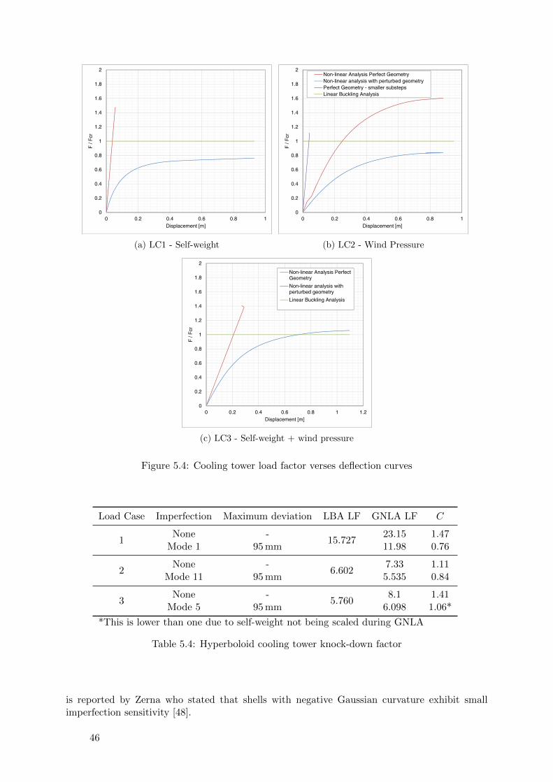
0

0.2

0.4

0.6

0.8

1

1.2

1.4

1.6

1.8

2

0 0.2 0.4 0.6 0.8 1

F /

Fcr

Displacement [m]

(a) LC1 - Self-weight

0

0.2

0.4

0.6

0.8

1

1.2

1.4

1.6

1.8

2

0 0.2 0.4 0.6 0.8 1

F /

Fcr

Displacement [m]

Non-linear Analysis Perfect GeometryNon-linear analysis with perturbed geometryPerfect Geometry - smaller substepsLinear Buckling Analysis

(b) LC2 - Wind Pressure

0

0.2

0.4

0.6

0.8

1

1.2

1.4

1.6

1.8

2

0 0.2 0.4 0.6 0.8 1 1.2

F /

Fcr

Displacement [m]

Non-linear Analysis PerfectGeometry

Non-linear analysis withperturbed geometry

Linear Buckling Analysis

(c) LC3 - Self-weight + wind pressure

Figure 5.4: Cooling tower load factor verses deflection curves

Load Case Imperfection Maximum deviation LBA LF GNLA LF C

1None -

15.72723.15 1.47

Mode 1 95 mm 11.98 0.76

2None -

6.6027.33 1.11

Mode 11 95 mm 5.535 0.84

3None -

5.7608.1 1.41

Mode 5 95 mm 6.098 1.06*

*This is lower than one due to self-weight not being scaled during GNLA

Table 5.4: Hyperboloid cooling tower knock-down factor

is reported by Zerna who stated that shells with negative Gaussian curvature exhibit smallimperfection sensitivity [48].

46

5.3 Dome

Domes and spheres are structures with a positive Gaussian curvature. Monolithic domes areconcrete domes constructed by first casting a ring beam as the foundation, inflating a PVC-coated nylon or polyester fabric, and then casting Shotcrete with the fabric as the formwork.

5.3.1 Geometry

A typical dome situated in a region with heavy wind load is selected for this study [40]. Thebase radius of the dome is RD = 55′ or approximately 16.75 m. The height from the base to thetip of the dome is HD = 37′ or approximately 11.25 m. The thickness of the dome varies from8′′ (203 mm) at the base to 3′′ (76 mm) at the tip. See Figure 5.5 for a graphical representationof the variables. The actual radius of the dome is found with equation (5.11). Note that this is

Figure 5.5: Geometry of a typical dome

a rearrangement of the calculation for sagitta in Eq. (2.1).

R =H2

D +R2D

2HD=

(11.252 + 16.752)

2 · 11.25= 18.09 m (5.11)

The variable thickness is implemented as a function of the vertical angle as shown in equa-tion (5.12).

t(φ) =tT − tBπ/2

φ+ tB; ∀φ ∈ [φbase, π/2] (5.12)

The slenderness ratio of the dome varies proportionally to its thickness. At the base, a/tbottom =89, where as at the top, a/ttop = 237. The Gaussian curvature of the dome is assumed constantover its surface.

κ1 = κ2 =1

R= 0.055 ; K = κ1κ2 = 0.00305 (5.13)

Material

Again, a generic reinforced concrete is used to represent the mixture of Shotcrete and the rein-forcement grid.

ρ = 2400 kg/m3 ; E = 35 GPa (5.14)

47

Loads

Under normal operating conditions, the self-weight would be the dominate load on the structure.However, since these domes are built in areas of heavy wind, it is expected that wind load wouldbecome the principle load condition in extreme circumstances. To simulate a variety of windload conditions, different pressures are applied to the surface of the dome shell. The relationshipbetween wind speed and pressure can be estimated using Equation (5.15) [37].

p = 1/2ρw2ξ (5.15)

Literature [40] suggests that the most critical wind load occurs when half of the dome is subjectedto positive pressure, and the other half to negative pressure (suction). This load combination isimplemented by assuming a wind pressure profile of two sine waves, one circumferential and theother vertical. The peak wind speed is taken from the FEMA specification for the ”Design andConstruction Guidance for Community Safe Rooms” as these structures are frequently used assafe rooms in the event of a hurricane or tornado [1].

The second load case is a uniformly applied external pressure. This is a well studied bucklingimperfection problem and is included as a reference [16]. Table 5.5 lists the three load casestested.

Figure 5.6: Load profiles of dome in elevation and plan view (not to scale)

Load Case Description Wind pressurePa

1 Self-weight -2 Wind pressure and suction 100003 Uniform external pressure 10000

Table 5.5: Dome Load Cases

48

Mesh Comparison

Two different algorithms are used to mesh the dome. The first attempt used a constant heightincrement ∆z along the z axis. However this resulted in very flat elements near the base of thedome, and very elongated ones at the tip. Changing to a spherical coordinate, the author is ableto increment with ∆φ and eliminate the element aspect ratio issue.

The two variables determining the size of a mesh are shown in Figure 5.5, namely the changein the Zenith ∆φ and in the Azimuth ∆θ. These are varied in the same manner, by 50 % and150 %, to assess the relative changes in the buckling load factors of the structure.

φ θ Mode 1 ∆ Mode 3 ∆ Mode 5 ∆ Mode 7 ∆m ◦ % % % %

0.0625 1 9.60144 0.974 10.8384 0.866 11.4960 1.212 12.195 0.7360.1250 2 9.50886 0.000 10.7453 0.000 11.3583 0.000 12.1058 0.0000.2500 4 9.43707 -0.755 10.7912 0.427 11.3761 0.156 12.3431 1.960

Table 5.6: Dome Mesh Density Comparison

As observed in Table 5.6 and Figure 5.8 there are significant differences in both the load factorsand buckling modes between the finer and the coarser meshes, and therefore the model withthe finest mesh is used for future analyses. Note that the mesh can theoretically be made morerefined, however a further refined mesh is computationally not feasible.

It is hypothesised that smaller elements are needed due the load being more concentrated, andtherefore the buckling is more of a local behaviour.

Figure 5.7: Load profile of domes with different mesh density

5.3.2 Analyses

Buckling, yielding and crushing

This section verifies that the dome buckles prior to crushing.

λ =

√ncr

np> 1 (5.16)

The critical membrane force is taken from Table. 2.1

ncr =1√

3(1− ν2)

Et2

a(5.17)

49

Figure 5.8: Comparison of buckling shapes of models with different mesh density, using windload as the test load case

and the crushing force is simply,

np = f · t (5.18)

Where f is the compressive yield stress of concrete and t is the thickness of the shell. UsingC35 as the typical concrete quality, f = 35 MPa. Therefore equation (5.16) gives the followingslenderness ratio, and shows that the hyperboloid would buckle before yielding.

λ = 2.152 > 1 (5.19)

Linear elastic analysis

This analysis is to verify the mass of the structure is indeed correct. Equation (5.20) calculatesthe volume of the dome using the variable thickness equation derived in equation (5.12).

Vdome =

∫ 2π

0

∫ π2

φbase

t(φ)r2cos(φ) dθ dφ (5.20)

This volume is multiplied with the density of typical concrete in equation (5.14).

mdome = V ρ ; mdome = 4.874 21× 105 kg (5.21)

The resulting mass compares well with the mass calculated by ANSYS at 4.874 29× 105 kg.

Linear buckling analysis

LBA is performed on the dome model with each load case. The resulting load factors are listedin Table 5.7. The closely spaced LFs are observed especially for the second load case, whereuniform pressure is applied. The resulting buckling shapes are shown in figure 5.9. The firstmode is an axisymmetric mode with buckles observed at the top of the dome. Higher modesshow progressively lowering of buckles until the whole surface is covered. Each axisymmetricmode is followed by a series of asymmetric ones with buckles starting at the same height.

Imperfection

Assuming the fabric is manufactured with greater precision than the concrete casting procedure,the inner surface must be more uneven than the outer. Therefore, the imperfection is more ofa change in thickness than a change in geometry. However, for ease of comparison, the same

50

Figure 5.9: Sample buckling modes of the uniform pressure load case

Mode LC1 LC2 LC3

1

N/A

-19.307 9.91342 -19.307 10.1193 -18.019 10.1194 -18.019 10.5125 -17.108 10.5126 -17.108 11.1857 -15.957 11.1858 -15.957 12.0079 -14.074 12.00710 -14.074 12.93911 14.074 12.93912 14.074 13.05413 15.957 13.19114 15.957 13.19115 17.108 13.54416 17.108 13.54417 18.019 13.96718 18.019 13.96719 19.307 14.10220 19.307 14.102

Table 5.7: Dome LBA load factors of the different load cases

imperfection imposition method is used. The thickness of the dome averages to 5′ or 130 mm.A maximum imperfection of 65 mm or t/2 is imposed on the structure. Bauer states that theaxisymmetric local (and also regular and random) thickness deviations affect critical load muchless than the corresponding initial imperfections of the surface [13]. The first mode is used asthe imperfection shape, though it is unclear that a higher mode won’t govern.

Non-Linear Analysis

With the same procedure as the above two structures, the dome is analysed taking geometricalnon-linearity into account. It can be seen in figure 5.4 that without imperfection, capacityresulting from GNLA is similar to that from LBA, even though some of the load cases areasymmetric.

51

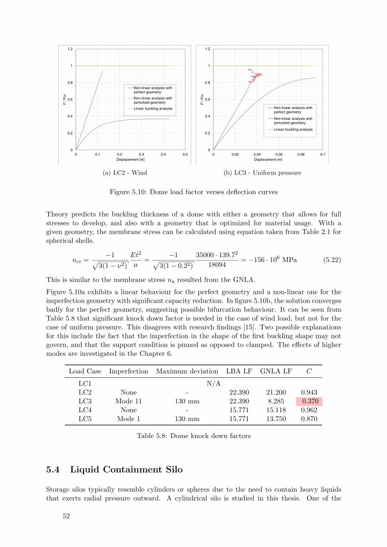
0

0.2

0.4

0.6

0.8

1

1.2

0 0.1 0.2 0.3 0.4 0.5

F /

Fcr

Displacement [m]

Non-linear analysis withperfect geometry

Non-linear analysis withperturbed geometry

Linear buckling analysis

(a) LC2 - Wind

0

0.2

0.4

0.6

0.8

1

1.2

0 0.02 0.04 0.06 0.08 0.1

F /

Fcr

Displacement [m]

Non-linear analysis withperfect geometry

Non-linear analysis withperturbed geometry

Linear buckling analysis

(b) LC3 - Uniform pressure

Figure 5.10: Dome load factor verses deflection curves

Theory predicts the buckling thickness of a dome with either a geometry that allows for fullstresses to develop, and also with a geometry that is optimized for material usage. With agiven geometry, the membrane stress can be calculated using equation taken from Table 2.1 forspherical shells.

ncr =−1√

3(1− ν2)

Et2

a=

−1√3(1− 0.22)

35000 · 139.72

18094= −156 · 106 MPa (5.22)

This is similar to the membrane stress na resulted from the GNLA.

Figure 5.10a exhibits a linear behaviour for the perfect geometry and a non-linear one for theimperfection geometry with significant capacity reduction. In figure 5.10b, the solution convergesbadly for the perfect geometry, suggesting possible bifurcation behaviour. It can be seen fromTable 5.8 that significant knock down factor is needed in the case of wind load, but not for thecase of uniform pressure. This disagrees with research findings [15]. Two possible explanationsfor this include the fact that the imperfection in the shape of the first buckling shape may notgovern, and that the support condition is pinned as opposed to clamped. The effects of highermodes are investigated in the Chapter 6.

Load Case Imperfection Maximum deviation LBA LF GNLA LF C

LC1 N/ALC2 None - 22.390 21.200 0.943LC3 Mode 11 130 mm 22.390 8.285 0.370LC4 None - 15.771 15.118 0.962LC5 Mode 1 130 mm 15.771 13.750 0.870

Table 5.8: Dome knock down factors

5.4 Liquid Containment Silo

Storage silos typically resemble cylinders or spheres due to the need to contain heavy liquidsthat exerts radial pressure outward. A cylindrical silo is studied in this thesis. One of the

52

principle curvatures of a cylinder is zero, and therefore the Gaussian curvature is also zero.As the material properties improve, ever thinner and bigger silos are constructed. Thereforeinstabilities due to various load conditions have become a practical issue.

5.4.1 Geometry

A typical liquid storage silo is used as the test structure (Meridian Manufacturing Inc. 304Stainless Steel Flat Bottom Liquid Fertilizer Tanks Model SS1840) [3]. Its geometry is shownin Figure 5.11. Its height from base to top of the cylinder is h = 42′9′′ or ∼ 13 m. Its radius isr = 8′ or ∼ 4.25 m throughout its height. The thickness is assumed to be t = 25 mm, throughin reality it may vary along the height of the silo. There is a lid atop the silo with a pitch of10° resulting in a lid height of ∼ 0.825 m. Any ring-shaped stiffeners are ignored. Ring-stiffenedcylinders are tested as the next case study.

a

t=

8.5

0.025= 340 (5.23)

Figure 5.11: A Meridian Storage Silo, its geometry, and the different water levels, sloshing anglesand wind pressure

53

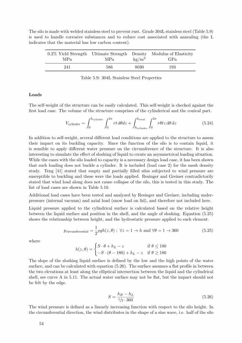
The silo is made with welded stainless steel to prevent rust. Grade 304L stainless steel (Table 5.9)is used to handle corrosive substances and to reduce cost associated with annealing (the Lindicates that the material has low carbon content).

0.2% Yield Strength Ultimate Strength Density Modulus of ElasticityMPa MPa kg/m3 GPa

241 586 8030 193

Table 5.9: 304L Stainless Steel Properties

Loads

The self-weight of the structure can be easily calculated. This self-weight is checked against thefirst load case. The volume of the structure comprises of the cylinderical and the conical part.

Vcylinder =

∫ hcylinder

0

∫ 2π

0rt dθdz +

∫ htotal

hcylinder

∫ 2π

0rθtz dθ dz (5.24)

In addition to self-weight, several different load conditions are applied to the structure to assesstheir impact on its buckling capacity. Since the function of the silo is to contain liquid, itis sensible to apply different water pressure on the circumference of the structure. It is alsointeresting to simulate the effect of sloshing of liquid to create an asymmetrical loading situation.While the cases with the silo loaded to capacity is a necessary design load case, it has been shownthat such loading does not buckle a cylinder. It is included (load case 2) for the mesh densitystudy. Teng [41] stated that empty and partially filled silos subjected to wind pressure aresusceptible to buckling and these were the loads applied. Resinger and Greiner contradictorilystated that wind load along does not cause collapse of the silo, this is tested in this study. Thelist of load cases are shown in Table 5.10.

Additional load cases have been tested and analyzed by Resinger and Greiner, including under-pressure (internal vacuum) and axial load (snow load on lid), and therefore not included here.

Liquid pressure applied to the cylindrical surface is calculated based on the relative heightbetween the liquid surface and position in the shell, and the angle of sloshing. Equation (5.25)shows the relationship between height, and the hydrostatic pressure applied to each element.

pcircumferential =1

2ρgh(z, θ) ; ∀z = 1→ h and ∀θ = 1→ 360 (5.25)

where

h(z, θ) =

{S · θ + hL − z if θ ≤ 180

−S · (θ − 180) + hL − z if θ ≥ 180

The slope of the sloshing liquid surface is defined by the low and the high points of the watersurface, and can be calculated with equation (5.26). The surface assumes a flat profile in betweenthe two elevations at least along the elliptical intersection between the liquid and the cylindricalshell, see curve A in 5.11. The actual water surface may not be flat, but the impact should notbe felt by the edge.

S =hH − hL1/2 · 360

(5.26)

The wind pressure is defined as a linearly increasing function with respect to the silo height. Inthe circumferential direction, the wind distributes in the shape of a sine wave, i.e. half of the silo

54

is subjected to over-pressure, and the other half to under-pressure or suction (see Figure 5.11).Wind pressure acts perpendicularly to the element surface. The maximum amplitude is set topmax = 10 000 Pa.

pwind = sin(θ)p(z) ; ∀z = 1→ h and ∀θ = 1→ 360 (5.27)

wherep(z) =

pmax

hz (5.28)

Load Case Description Height L Height H Wind pressurem m Pa

1 Self-weight 0 0 02 Empty silo 0 0 500003 Half capacity with sloshing 4.25 7.25 500004 Half capacity no sloshing 5.75 5.75 50000

Table 5.10: Silo Load Cases

Mesh Density

A mesh refinement study is performed to determine the size of each element. The relativechange of the eigenvalues in the buckling analysis is recorded as the element size decreases.In addition to the relative change in eigenvalues, each spatial deformation wave must containseveral elements, [2].Once both conditions are satisfied, then the mesh size is found.

The two same variables (as the hyperboloid mesh) determine the mesh density in this model,namely the length of each element in the height direction z and the change in angle in the radialdirection θ. Using the first load case as the reference case, here are the results obtained byvarying z and θ by 50% and 150%. The lowest four buckling modes are used for comparison.Load case two (wind load with no hydrostatic pressure) is used as the test load case.

Figure 5.12: Comparison of mesh density

55

z θ # # Mode 1 ∆ Mode 2 ∆ Mode 3 ∆ Mode 4 ∆m ◦ Elements DOFs 10−3 % 10−3 % 10−3 % 10−3 %

0.05 1 25200 453606 22.527 - 25.885 - 26.288 - 27.018 -0.1 2 6750 121506 22.532 0.211 25.898 0.500 26.307 0.718 27.058 1.4870.25 4 1620 29166 22.562 1.543 26.096 8.149 26.725 16.62 27.970 35.24

Table 5.11: Silo Mesh Density Comparison using wind load as reference

The buckling shapes of the different meshes are shown in Figure 5.13. Note that in the coarsemesh the elements do not have sufficient resolution to capture the peak of the buckle wave. Thismay introduce additional stiffness to the structure, and therefore the next finest mesh is chosen.

Figure 5.13: Mesh density comparison - buckling shape

5.4.2 Analysis

Linear Elastic

The self-weight of the structure calculated in Eq. (5.29) is compared with the ANSYS modelload case one.

Vcylinder · ρ = 43 527.35 kg (5.29)

This is similar to the ANSYS result of 43 529 kg.

Linear Buckling

Similar to what was done previously, a linear buckling analysis is performed with each load caseindividually to obtain the associated load factors. It is worth noting that the asymmetrical loadcauses the load factor to decrease, even though the total pressure applied onto the structureremains constant.

56

Load Case 1 2 3 4Capacity - 0% 50% 50%Sloshing - - Yes No

Wind - No Yes YesHeight 1 m - - 4.25 5.75Height 2 m - - 7.25 5.75

1 - 22.532 22.89 23.312 - 22.532 22.891 23.313 - 25.898 26.218 27.7434 - 25.898 26.616 28.0485 - 26.307 27.671 28.5196 - 26.307 27.676 28.527 - 27.058 27.82 29.1498 - 27.083 28.21 29.6129 - 27.596 28.227 29.62210 - 27.705 28.624 29.897

Table 5.12: Silo Linear Buckling Load Factor

Imperfection

An geometrical imperfection in the shape of the first buckling mode is applied to the structure.The maximum amplitude of the imperfection is 12.5 mm, half of the thickness of the shell.

Non Linear Buckling

It is observed that unlike the hyperboloid, the results from GNLA of the perfect silo does notoverestimate the capacity. This is due to the fact that all load cases have an asymmetrical(i.e. wind load) component. The load displacement plots show linear elastic behaviour untilbifuration for the perfect geometry. With an imperfect geometry however, the behaviour is non-linear from the start and the tangent stiffness decreases as load increases. Table 5.13 lists theresulting load factors and knock-down factors from both LBA and GNLA. It is observed thatwith imperfection, a knock-down factor of 3/4 can be conservatively applied.

57

0

0.2

0.4

0.6

0.8

1

1.2

0 0.05 0.1 0.15 0.2

F /

Fcr

Displacement [m]

Non-linear analysis withperfect geometry

Non-linear analysis withperturbed geometry

Linear buckling analysis

(a) LC2 - wind pressure, empty silo

0

0.2

0.4

0.6

0.8

1

1.2

0 0.05 0.1 0.15 0.2

F /

Fcr

Displacement [m]

Non-linear analysis withperfect geometry

Non-linear analysis withperturbed geometry

Linear buckling analysis

(b) LC3 - wind pressure, silo with sloshing wa-ter table

0

0.2

0.4

0.6

0.8

1

1.2

0 0.05 0.1 0.15 0.2

F /

Fcr

Displacement [m]

Non-linear analysis withperfect geometry

Non-linear analysis withperturbed geometry

Linear buckling analysis

(c) LC4 - wind pressure, silo with flat watertable

Figure 5.14: Silo load factor verses displacement curves

Load Case Imperfection Maximum deviation LBA LF GNLA LF C

LC1 -LC2 None - 22.532 22.700 1.010

Mode 11 12.5 mm 22.532 17.200 0.763LC3 None - 22.890 22.500 0.980

Mode 1 12.5 mm 22.890 17.400 0.757LC4 None - 23.31 22.6 0.971

Mode 1 12.5 mm 23.31 17.304 0.741

Table 5.13: Summary of silo knock-down factors and other results

58

5.5 Aircraft fuselage

Using a grossly over-simplified model of an aircraft, the author intends to analyse the aircraftfuselage air-frame modelled by ring- and stringer- stiffened cylindrical shell. The model of thesilo is recycled here to represent the fuselage thin of the aircraft.

5.5.1 Geometry

The fuselage is a major component of the air-frame of an aircraft. It extends from the nose tothe empennage and holds crews, passengers and cargo. Traditionally, a fuselage is composedof a cylindrical skin supported longitudinally by stringers and radially by stiffening rings. Thestiffening rings (formers or frames) set the shape of the fuselage and reduce the column lengthof stringers to prevent instability. The rings typically have a cross section of a I-beam. Stringers(longerons) are thin strips of material which are connected to the skin of the fuselage. Insome aircraft designs, the stringers are also fastened to the stiffening rings, while in others, thestringers run the whole length of the fuselage uninterrupted.

Width of the fuselage is 5.77 m and height is 5.97 m. For simplicity, an average radius of 6 mis used. The ring stiffeners are 200 mm wide and are spaced 560 mm apart. The trapezoidalstringers are spaced 4° apart in the tangential direction. They are 50 mm, 80 mm and 40 mm inheight, larger width (adjacent to the skin), and smaller width respectively. The thicknesses ofthe skin, the stiffeners, and the stringers are 5 mm,7.5 mm, and 5 mm respectively.

Mesh

The mesh generation is done parametrically to ensure all the above variables can be changed toadapt to different air crafts and possibly to ship hulls as well. In addition to the length and thewidth of the fuselage itself, the number of elements along each ring, the spacing of the rings, thespacing of the stringers are all parametric variables.

To address the fact that the stringers run through the ringed stiffeners without being physicallyattached to them in some aircraft designs, the rings do not share the node with the stringers andthe skin at points of intersection. The stringers are modelled as quadratic Timoshenko beams(BEAM189) that allows for large deformation.

In the refined mesh model, there exists 148 680 elements in total, and 2 548 800 degrees offreedom. This study considers the situation where the aircraft is airborne at cruising altitudewith a constant velocity. As a rigid object, the aircraft has six degrees of freedom. This studyis concerned mainly with the equilibrium in the longitudinal direction, or the direction of flightand the vertical axis z. In the direction of flight (x), the two forces acting are thrust and drag.Drag is felt by all surface area perpendicular to the flow of wind, and thrust is produced by theturbo engines mounted to the wings. Assuming the wind is composed entirely of headwind, itseffect can be calculated from calculating the surface area of the cockpit. In the earth-referencedvertical z direction. A stiff continuous cross-beam span the entire wingspan of the aircraft. Thisis used to transfer the lift generated by the wings to the fuselage and the tail to equilibrate withthe weight of the aircraft.

Loads and Supports

To further simplify the analysis, one segment of the fuselage is considered as an axially loadedcylinder. The load is applied as uniform displacement along one end of the segment, and theother end is pinned.

59

Figure 5.15: Fuselage mesh

Material

Traditionally, the whole fuselage is made entirely of aluminum. It is used due to its excellentstrength to weight ratio and its ability to be extruded into any shape.

E = 205× 109 MPa ; ν = 0.3 (5.30)

Computational Cost

With this large model, the computational performance becomes a significant factor in the methodof analysis. The standard procedure is applied to the fuselage, and the computation times of thedifferent analyses are listed in Table 5.14. It is evident that LBA is an expensive analysis to run.This can be attributed to using zero as the starting point of eigenvalue search. By generating theimperfection shape without the use of LBA, the computation time can be decreased by ∼ 40 %.

Analyses Computation CostType s

Linear Elastic 294Linear Buckling 11406

Imperfection 60Non-Linear (average of 6 steps) 3082

Table 5.14: Computation cost of the different analyses

Linear Buckling Analysis

From LBA, the critical load factor calculated is λcr = 3.96. The buckling shape calculated isnot symmetrical( Figure 5.16b); the asymmetry is attributed to the placement of longitudinalstringers, leading to different stiffnesses around the ring. It is seen that buckles occur in betweenthe stiffeners and stringers, and closer to the supports (due to the pinned boundary layer). Thistype of local buckling is shown not to produce large reduction in capacity in Chapter 6. Therefore

60

(a) Linear Elastic Analysis (b) Linear Buckling Analysis

Figure 5.16: Behaviour of the fuselage

one must obtain sufficient number of buckling modes until the first global buckle occur. Thelinear increase in computation cost makes this infeasible.

5.5.2 Imperfection

The first mode is imposed as the imperfection for the subsequent non-linear analysis. However,as stated above, a global buckling mode would be more desirable as the imperfection shape.This shape can be generated without the use of LBA, but by using the ”superimposed wave”imperfection shape as described in Chapter 6. It remains to be seen whether global imperfectionresults in a larger reduction factor.

Non-Linear

Two non-linear analyses are run, one with imperfection and the other without. The resultingforce verses displacement diagrams are plotted in Figure 5.17. Result of the analysis of theperfect structure vastly over-estimates the critical buckling capacity as is the case with otheraxisymmetric structures and loads. The model with imperfection however results in an ultimatecapacity that is very similar to the critical one, C ∼ 1. This suggests that using the first modeas imperfection, it would appear that the structure is not imperfection sensitive at all. Whileit is reassuring to know that the issue of over estimation is eliminated, it remains to be seenwhether a higher mode or other imperfection shapes would render the structure imperfectionsensitive.

The progressive displacement diagrams are shown in figure 5.18. Note that the buckles arelocalized to boxes bounded by stringers and stiffeners. The amplitude decreases as the bucklesmove toward the middle. This confirms the expectation that local buckling is not imperfectionsensitive as the knock-down factor is 1. One may also observe the buckling of radial stiffeners.As the edge is restrained laterally, the stiffeners buckle inward uniformly.

5.6 Conclusion

Four simple yet realistic structures are studied using the proposed method of imperfection impo-sition. The cooling tower is used as an example of a hyperbolic structure. Self-weight and wind

61

0

0.2

0.4

0.6

0.8

1

1.2

1.4

0 0.002 0.004 0.006 0.008 0.01

F /

Fcr

Displacement [m]

Non-linear analysis withoutimperfection

Non-linear analysis withimperfection

Linear buckling analysis

Figure 5.17: Force displacement plot of the fuselage segment

(a) Initial State (b) Final State

Figure 5.18: Initial and final displacement of the fuselage segment showing local buckles inbetween stringers and stiffeners

load are applied separately and in concert, both with and without geometrical imperfection, toassess the effect of imperfection on symmetric and asymmetric loading conditions. It is foundthat in both load cases, the model without imperfection follows a linear load-deflection curvethat diverges at or above the critical load as calculated with the linear buckling analysis. Thedivergence is attributed to the sudden failure due to bifurcation buckling caused by excessivenumerical imprecision. With geometrical imperfection, a knock-down factor of 0.75 can be ap-plied to the critical load factor. The next structure tested is a monolithic concrete dome. Threeloads are applied, namely the self-weight, wind load, and uniform external pressure. The sameobservation is made when the model is not perturbed by imperfection. When it is however, theknock-down factor is necessary to account for geometrical imperfection. For wind load, a factorof 0.37 is needed, and for the case of uniform pressure, C = 0.87. The spacing of the LBA loadfactors suggest higher modes may govern the behaviour.

The third model studied is the liquid containing silo. The structure is modelled after a com-mercially available aluminum silo. Wind load is applied to both an empty and a half filled silowith flat or sloshing water surface. The largest knock-down factor, C = 0.74, is associated witha half filled silo with flat water surface.

The fourth is also a cylindrical structure. A typical aircraft fuselage is modelled with stiffeners

62

and stringers. From LBA, it is observed that local buckling governs the behaviour. However, itmay be the case that imperfection in the shape of a (much) higher mode with global bucklinggoverns the GNLA result. Due to the computational cost of LBA, it becomes infeasible tocalculate more than a few modes. Therefore, if it would be advantageous to generate theimperfection shape without the need of LBA.

Overall, GNLA of shell structures with geometric imperfections are quite robust and easy toperform. It is evident that the designers of the software provided the tools specifically for thispurpose. Without geometrical imperfections, the analyses becomes much more difficult and theresults much less reliable. This is expected for symmetrical structures loaded by self-weight, butthe inaccuracy was also observed in asymmetric loading as well.

63

Chapter 6

Study of Imperfection

6.1 Summary

Construction tolerances given to contractors offer a wide margin of error, this is done to avoidfuture litigation should disasters happen. It is the author’s intent to integrate this tolerance inthe study of the amplitude of imperfection on structural capacity of thin shells. In chapter 3,the applied imperfection has been in the shape of the first buckling mode with a maximumamplitude of t/2. This is in accordance with the design philosophy that the first mode is theworst since it is by definition the mode with the lowest load factor.

However, as indicated by numerous studies [15] and in Chapter 5, in certain structures undercertain load and support conditions, imperfections in the shape of the higher modes or a com-bination of modes may be more critical. Furthermore, other studies have attempted to imposerandom imperfections in an attempt to extract lower load factors through geometrical non-linearanalyses.

Koiter’s original theory imposes imperfection of global periodic shapes [28], then at a laterstage applied his theory to a localized periodic disturbance and obtained the same imperfectioncharacteristics [29].

Arbocz started by varying the modal imperfection amplitude and also the applied load [18]. Hethen focused on measuring real imperfections, representing them in Fourier series and recordingthe coefficients. With the idea of categorizing imperfection based on the production method,he proposed to combine this characteristic imperfection with statistical analysis when analysingshell structures [11] [12]. The Fourier coefficients are the basis of an ”Imperfection Databank”.Furthermore, Arbocz proposed an improved knock-down factor which rewards manufacturerswho are able to produce at a higher quality. This technique has only been applied to metalliccircular cylindrical shells.

This study proposes four methods of imperfection generation based on the above attempts, andthen applies these methods to both the hyperboloid and the cylinder in an attempt to extractan imperfection shape that produces the lowest load factor.

1. The first method proposed is the single modal method, where one buckling mode is imposedas the imperfection. Two variations are proposed. One introduces a noise on the wholebuckling shape, and the second flattens out a buckle wave in the buckling shape.

2. The second method superimposes multiple modal shapes before imposing it as the imper-fection shape. The superposition is done in two ways. The first assumes equal contributionfrom the constituting modes, the second assumes random contribution.

65

3. The third method generates a Gaussian random imperfection shape based on constructiontolerance as an input.

4. The fourth method generates a periodic buckling wave imperfection.

Measured imperfection field is not used in any of the methods described, as characteristic man-ufacturing imperfection is not available for any shapes other than the cylinder, and it is theauthor’s intent to apply these methods to all shapes. Note that the amplitude of imperfectionis not varied in this study. Its effect was shown in Chapter 4, and is assumed to have similar orless pronounced effect on other types of structures. This study also proposes a new knock-downfactor to measure the effect of the imperfection shapes on the buckling capacity.

Lastly, stress related and loading imperfections are studied.

6.2 Imperfection Methods

6.2.1 kth buckling mode

The buckling mode that has been used thus far is defined here as the kth buckling mode, wherek is the modal number. Therefore the imperfection shape can be defined as follows,

δImp(x, y, z) =C · tδkmax

δk(x, y, z) (6.1)

where C · t is the maximum amplitude of imperfection expressed as a function of the thick-ness, δkmax is the maximum magnitude of the vectorial deflection in the kth buckling mode, andδk(x, y, z) is the component deflection in the kth buckling mode.

With Eq. (6.1), δImpi,j,k is the field of imperfection that is applied to the initial perfection geometry

on a component by component basis. For example, k = 1, C = 0.5 would mean to applyimperfection in the shape of the first mode with the maximum resulting amplitude of half of thethickness.

One weakness to this method is that the boundary layer will remain geometrically perfect if idealpin / fixed support conditions are assumed. To overcome this issue one could either assume swapthe pinned condition to finite stiffness springs or to artificially perturb the boundary layer.

Perturbation

Eq. (6.1) is supplemented with an additional noise term to test the effect of a perturbed bucklingshape.

δImp(x, y, z) =C · tδkmax

δk(x, y, z) + GDIS(µ, σ) (6.2)

where µ is the mean and σ is the standard deviation. For this study the mean is set to zero,µ = 0, and the standard deviation is set to be one tenth of the thickness, σ = t/10. For a detaileddiscussion on using ANSYS GDIS (Random generator using Gaussian Distribution) to generateprobabilistic rough surfaces, see Thompson [42].

With this method of perturbation, the geometry of the boundary layers (top and bottom ring) nolonger remain perfect, therefore the effect of perturbing the boundary condition can be assessedas well.

66

Flattening

The buckling modal imperfection is regionally flattened to eliminate the largest buckle. This isdone to test the effect of significant asymmetry. It is implemented with a recursive algorithmthat starts at the node with the maximum deflection, and propagates depth-first down to thering of nodes with less-than-limit deflection. The limit is set at a value slightly above zero toterminate the recursion before the end of one buckle is reached, and to ensure that the recursionnever reached the neighbouring buckles.

As ANSYS does not allow recursion (or any iteration) past 20 steps, a more restrictive algorithmis developed to eliminate recursion. The algorithm finds the largest nodal displacement, andparses in four directions (up, down, left, right) until the displacements become less than thelimit, and set all imperfections within that rectangular area to zero. Evidently, the algorithmonly works with rectangular buckles.

Reverse Flattening

To simulate Koiter’s theory on ”More-or-less” localized periodic disturbance, the above genera-tion function is modified so that only one buckle is preserved. The imperfection field is set tozero except in the vicinity of the largest buckle as identified by the algorithm above. This issimilar to Kroplin’s local imperfection, though it appears that the localized imperfection usedwas smaller than the size of a buckle.

6.2.2 Combination of n buckling modes

The hypothesis of modal interaction is tested here where nmodal shapes are combined to producean imperfection shape. The first variation of this method assumes equal contribution from allselected modes and creates an imperfection shape with the same total maximum amplitude ofC · t.

δImp(x, y, z) =C · t

max∑n

k=1 δki,j,k

n∑k=1

δk(x, y, z) (6.3)

Perturbation

The second variation generates n random weights to be multiplied to each modal shape. Thisrandomizes the contributions of each mode and produces a different imperfection shape at eachtrial. With this variation, the correlation between modal contribution and relative change inreduction factor can be tested, and the governing modal shape can be identified.

δrand(x, y, z) =n∑k=1

Akδk(x, y, z) (6.4)

where the random weights range from 0 to 1,

Ak = rand(0, 1); k ∈ [1, n] (6.5)

and the sum of these weights is also 1

n∑k=1

Ak = 1 (6.6)

then this random shape is normalized to the same maximum imperfection magnitude of C · t,

δImp(x, y, z) =C · tδrand

max

δrand(x, y, z) (6.7)

67

Sufficient n

There as many buckling modes as there are DOFs in the system and it would be infeasibleto generate combinations of all of them. For a typical shell such as the hyperboloid, one caninclude those modes whose the load factor is within a certain percentage of the first mode. Thisapproach may not work for shells that are very sensitive to imperfection where the modes arespaced closely together, such as the cylinder. In that case, the first ten modes are extracted andused as the basis of imperfection shapes. The rationale being that the first ten modes encompassall the different types of buckling shapes (i.e. axisymmetric, asymmetric, and so on).

6.2.3 Gaussian random

While imposing buckling modes as imperfection is the standard approach to thin shell bucklingproblems, there is no guarantee that the above will produce the worst case scenario. Therefore,random imperfections are generated in an attempt to produce lower load factors.

With the exception of the imperfection data generated by cylinder measurements, the designersoften have no other reliable imperfection data aside from the construction tolerance provided bythe contractor. To simulate geometrical imperfection that may occur at an actual constructionsite, an simple application is written which generates such a random imperfection with the totaldeflection of a buckling mode and a maximum construction tolerance as inputs.

In the purpose of this thesis, to ensure the randomly generated imperfections are comparableto a buckling mode, the maximum displacement is also set as C · t (instead of the construc-tion tolerance). To impose further constraints on the random generation, the total magnitudeof vector imperfection displacement is set to equal to those of a buckling mode. With thesetwo constraints in mind, an optimization problem is set to solve for a random shape of theimperfection.

Constraint 1 states that the maximum amplitude of random imperfection must not be greaterthan that of a modal shape ∣∣δrand

max

∣∣ ≤ ∣∣δmmax

∣∣ (6.8)

Constraint 2 states that the total absolute amplitude of random imperfection must not be greaterthan that of a model shape

n∑i=1

∣∣δrandi

∣∣ ≤ n∑i=1

∣∣δmi ∣∣ (6.9)

Parametrized onto a two dimensional surface, constraint 3 limits the change in deflection (orslope) between neighbouring nodes. ∣∣δrand

u,v − δrandu+i,v+j

∣∣ (6.10)

where

i ∈ [u− 1, u+ 1], j ∈ [v − 1, v + 1] (6.11)

Implementation

The author uses ANSYS’s native GDIS function to generate the imperfection field with a Gaus-sian random function. Two calibration constants, C1, C2 are introduced in order to optimizethe field towards the constraints, though never to satisfy them rigorously. The optimization isdone iteratively where C1 and C2 are continuously adjusted with each generation of imperfectionfield until constraints 1 and 2 are within 95 % of the required values. Constant C1 is introduced

68

to the standard deviation of the Gaussian random function. This is so that the probability ofgenerating an individual value outside of the constraint (6.8) is sufficiently small.

σ = C1 · C · t (6.12)

Constant C2 is introduced to simulate pinching of the distribution of the randomly generatedimperfection field. This pinching is done by multiplying the field by a linear function. Figure 6.1shows one such Gaussian distribution and the linear multiplier function. Note that this linearfunction is applied to the sample values on the x-axis and not the probabilities on the y-axis.The function is set so that the maximum and the minimum values of the imperfection fieldremain the same (multiplied by 1), and the closer the values are to 0, the more they are reduced,with the maximum reduction set at C2. C2 could also be a negative number to effectively widenthe distribution, and increase the total absolute amplitude. A parabolic function could also beimplemented, however since the maximum and the minimum amplitude are not necessarily thesame, the function may not be centred at zero.

δimpi = δrand

i · f(δrandi ) (6.13)

f(δrandi ) =

δrandi

C2(δrandmin

− 1) + 1 δrandi ≤ 0

δrandi

C2(δrandmax− 1) + 1 δrand

i ≥ 0

Figure 6.1: Typical g;aussian distribution and the linear multiplier function

The above is applied to each individual coordinate components (x,y,z) separately. This howevertended to generate ill-shaped elements for extremely refined meshes. In such cases, the normal tothe element surface may be calculated, and the nodes may be perturbed along the normal vector.In all models in this thesis however, no ill-shaped errors occur. Constraint 3 is implemented viathe smoothing function native to ANSYS.

6.2.4 Buckling waves

Seeing that the buckling shapes are essentially different super-positions of periodic waves, afunction is written that generates an imperfection field based on the number of buckles in uand v directions. This function generates periodic buckling wave shaped imperfections over thewhole surface of the structure. Presuming the structure can be parametrized onto a 2-D surface,the algorithm superimposes two sinusoidal functions onto that surface. Kroplin also performedan analysis with sine - imperfection [31].

69

Cu,v = A · sin(mπ

L1xu + φ1) · sin(

nπ

L2xv + φ2) (6.14)

Note that there is no randomness in this method. In this thesis, no phase shift is added, andthe buckling wave parameters are m and n. Should either m or n be zero, then buckles wouldonly exist in one direction. This shape would be similar to a axisymmetric buckling shape.

6.3 New Knock-down factor

The author hypothesizes a new knock-down factor Cm which compares the resulting load factor ofa geometrically non-linear analysis perturbed by mth imperfection to the same model perturbedby the imperfection in the shape of the first mode. This differs from the traditional knock-downfactor (Eq. (2.6)) in that the load factor is no longer compared with the linear buckling loadfactor. This new factor serves to eliminate the uncertainty around the imperfection sensitivityof a geometry.

Cm =λult,1

λult,m(6.15)

With λult,1 the designer would understand both the imperfection sensitivity, and the real bucklingcapacity of the design. Should the first buckling mode always governs, then Cm would be greaterthan 1. As an example, should 0.8 ≤ Cm ≤ 1.2 then for this particular structure with thisparticular load case, 0.8 would be the safety factor applied to the load factor produced by theperturbed GNLA (Eq. (6.16)).

R = Cmλult,1 (6.16)

6.4 Application to cylinder

The methods of imperfection generation proposed above are used on the cylindrical model fromChapter 4. It is hypothesized that these methods cover most of the reasonable imperfectionshapes, and therefore the modified knock-down factor obtained can be used to design such astructure. The cylinder is chosen for its extreme imperfection sensitivity. This study showsthat the first mode does not govern, and modal combinations are more severe, and so are somerandom shapes. As was discussed in Chapter 4, displacement-control is assumed for all analysesof the circular cylinder. The model and analysis set-up remains identical.

6.4.1 Method 1

As with previous analyses, first the LBA is performed to obtain sufficient number of bucklingmodes. Figure 6.2 shows the buckling shape of the first ten modes, and the eigenvalues associatedwith each. As stated in Chapter 4, though the most shapes are distinct, the eigenvalues remainalmost identical. This would suggest that the structure is imperfection sensitive. It is alsoobserved that some modes are axisymmetric in the sense that there are buckling waves primarilyin one (vertical) direction (3, 6, 7, and 10) and the rest are asymmetrical.

The LBA result file is duplicated for each subsequent GNLA to ensure that the starting pointremains identical. Ten GNLA are performed, each assuming the imperfection one of the first

70

Figure 6.2: First 10 buckling modes of a cylinder

(a) Load displacement curves (b) Cm values

Figure 6.3: Behaviour resulting from modal shaped imperfections

ten modes. The maximum imperfection amplitude is set at t/2 for all ten cases. The results aregathered in Figure 6.3a.

Figure 6.3a contains the load displacement curves of all the analyses. The wide scatter of bothstiffness and ultimate strength is evident. As was discussed in Chapter 4 already, all trialsexhibit a major reduction in capacity when compared to the results of LBA or with the resultsof GNLA of a geometrically perfect cylinder.

The previously defined modified knock-down factor Cm is applied to this series of analysis withthe GNLA result from trial 1 as a reference. Trial 1 is the GNLA with first buckling mode asthe imperfection. Figure 6.3b plots the Cm for each trial.

71

It is evident that Cm is not monotonically increasing, proving that the first modal imperfectiondoes not generate the largest reduction factor in capacity. Furthermore, the distribution seemsto be random, with similar factors for different imperfection shapes. Mode 3 (an axisymmetricalmode) seems to have the least reduction factor, while other axisymmetrical modes (6, 7) governthe reduction.

Method 1 Variation 1

Gaussian noise is added to the modal imperfection shapes with a standard deviation of σ =t/10 and a mean of zero. The same ten trials are performed, but each buckling modal shapeis perturbed with Gaussian noise. It is expected that the modal shapes would be the worstimperfection shapes, and any perturbation around the shapes would lessen the effect. This isnot the case for cylinders. Several interesting observations can be made with the above analyses.

(a) Load displacement curves (b) Cm values

(c) Effect of Gaussian noise (d) Original and perturbed boundary

Figure 6.4: Effect of Gaussian noise and perturbing the boundary layer

As Figure 6.4a shows, the post-buckling behaviour is more sustained and ductile. Larger strainis observed for all trial runs.

Figure 6.4b shows the effect of Gaussian noise on Cm. A uniform decrease is observed in all butone trial, where a significant drop is exhibited. The load displacement curves of these two trials

72

are isolated in Figure 6.4c. This observation would imply that axisymmetrical imperfectionsmay introduce an artificial capacity in the hoop direction to the structure, and prevent bucklingin between the ring buckles. By introducing the noise, this artificial capacity is removed. Thisform of buckling is investigated in more detail in chapter 7.

Lastly, Figure 6.4d shows the effect of boundary layer disturbance. Trials involving imperfectionshape 1 and 3 are re-analysed but with the boundary nodes (both top and bottom) unperturbed(by the Gaussian noise). Shape 1 is chosen as a normal case and 3 as an extreme one (in terms ofthe effect of Gaussian noise). An improvement is observed as expected, but the improvement isnot drastic. Therefore, it can be stated that the geometrical perturbation of the boundary layerdoes not have as large of an impact on the buckling capacity as general geometrical imperfection.

Furthermore, referring to Calladine’s initial boundary stress condition [32] where an inducedlocalised initial stress around the support showed a significantly less influence on capacity re-duction, it seems that boundary layer does not play an important role on imperfection sensitivityof a thin cylindric shell.

Method 1 Variation 2

Buckle flattening and reverse flattening is only applicable to asymmetric buckling modes, aswith axisymmetric modes there is already no buckle in the tangential direction. Furthermore,as the buckles are extremely localized in the cylinder, the mesh is not sufficiently refined for thealgorithm to function.

6.4.2 Method 2

6.4.3 Variation 1

Method 2 forms new imperfection shapes by combining the different modal shapes. As withmethod 1, the resulting imperfection field is scaled so that the maximum amplitude equals tot/2. The first attempt is to pair-wise combine neighbouring modes with equal contribution. Theresults are plotted in Figure 6.5a, where for example, combination of mode 1 and 2 is plotted asbuckling mode 1.5. Most combinations result in buckling capacities exactly the average of theresults of their two constituents. The exception is around mode 3 as was the case in the previousmethod. Combination 2 and 3, and combination 3 and 4 resulted in capacities that are moreinline with the result from the Gaussian noise method than with the original. This suggests thatthe modal combination also removes the artificial stiffness introduced by the mode 3 shape.

The buckling shapes of combination 2+3 and 3+4 resulted from GNLA are shown below. Notethat in both cases, buckles occur at the equator of the cylinders, and in both tangential andvertical directions.

It is evident that the third mode produces the largest reduction in capacity, therefore the nextstudy combines the third mode with other modes. Figure 6.5b superimposes the Cm factors ofcombination 3+1 to 3+10 on results from method 1. It is evident that when the third mode (anaxisymmetric mode) combines with another axisymmetric mode (6, 7, 10), the capacity increases,suggesting that the artificial stiffness is not eliminated. Conversely, when it is combined withan asymmetric mode, the capacity lowers.

6.4.4 Variation 2

Going back to the combinations of 2+3 and 3+4, instead of assuming equal contribution, theweights are varied to assess the impact of each constituting modes. 3 random trials are done with

73

(a) Pair-wise combination (b) Combination with BM3

Figure 6.5: Effect of modal combination

(a) Combination BM2 + BM3 (b) Combination BM3 + BM4

Figure 6.6: Final displacement diagrams resulting from different imperfection shapes

each of the two combinations. By observing figure 6.7, it is clear that as long as an asymmetricmode is present, however minutely, the reduction deviates towards the governing value. Indeed,the Gaussian noise may be considered a minute asymmetric perturbation. Beyond that, themore contribution the axisymmetric mode has, the larger the capacity reduction is.

6.4.5 Method 3

This method generates a Gaussian random field as a geometrical imperfection. In the designphase of an actual project, the only parameter needed is the construction tolerance. Thistolerance is used to calculate a standard deviation for the Gaussian distribution. In this thesis,for the sake of comparison, a modal displacement field is used as a reference.

5 GNLA are performed with buckling mode 1 as the reference and 5 more with buckling mode2, towards a total of 10 simulations. In addition, 2 more GNLA are performed for each bucklingmode but doubling the magnitude of total imperfection.

Figures 6.8 compares the Cm resulted from random imperfection with those from modal shapedimperfections. It is immediately evident that modal imperfection governs the capacity for buck-ling mode 1. The magnification lowers the capacity but not by an overwhelming amount. For

74

Figure 6.7: Combination of 2+3 and 3+4 withrandom contribution

BM1 BM2 W1 W2

2 3 0.733593 0.2664072 3 0.499557 0.5004432 3 0.287106 0.7128943 4 0.593494 0.4065063 4 0.469052 0.5309483 4 0.191967 0.808033

Table 6.1: Contributing modes, andassociated weights

Figure 6.8: Gaussian random imperfection trials

buckling mode 3 as reference however, some trials of the randomly generated imperfection gen-erates a lower capacity value than the unperturbed buckling modal imperfection. Magnificationdoes not have a visible effect.

If we consider buckling mode 3 as an outlier, there seems to be little correlation between themaximum imperfection amplitude or the total imperfection amplitude of an imperfection shapeto the structures buckling capacity. Indeed, if the shape is randomly generated, Cm remainsabove 1.2 irrespective of the total displacement amplitude. The shape of the imperfection is theremaining uncertainty that need be investigated.

6.4.6 Method 4

Different permutation of tangential and vertical buckling wave numbers, m and n, are simulatedin separate GNLA trials in attempts to extract the governing buckling capacity of the cylinder.m and n range from 0 (i.e. no waves) to 5, 10, and 20, resulting in 64 separate analyses. Toreduce the computational effort, several combinations are eliminated for being unrealistic or notrepresentative. Table 6.2 lists the permutations of analyses and the resulting Cm.

75

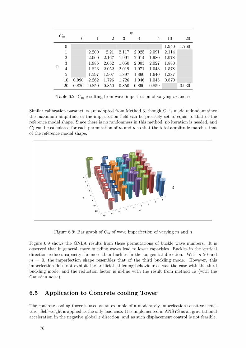
Cmm

0 1 2 3 4 5 10 20

n

0 1.940 1.7601 2.200 2.21 2.117 2.025 2.091 2.1142 2.060 2.167 1.991 2.014 1.980 1.9783 1.986 2.052 1.050 2.003 2.027 1.8804 1.823 2.052 2.019 1.971 1.043 1.5785 1.597 1.907 1.897 1.860 1.640 1.38710 0.990 2.262 1.726 1.726 1.046 1.045 0.87020 0.820 0.850 0.850 0.850 0.890 0.859 0.930

Table 6.2: Cm resulting from wave imperfection of varying m and n

Similar calibration parameters are adopted from Method 3, though C1 is made redundant sincethe maximum amplitude of the imperfection field can be precisely set to equal to that of thereference modal shape. Since there is no randomness in this method, no iteration is needed, andC2 can be calculated for each permutation of m and n so that the total amplitude matches thatof the reference modal shape.

Figure 6.9: Bar graph of Cm of wave imperfection of varying m and n

Figure 6.9 shows the GNLA results from these permutations of buckle wave numbers. It isobserved that in general, more buckling waves lead to lower capacities. Buckles in the verticaldirection reduces capacity far more than buckles in the tangential direction. With n 20 andm = 0, the imperfection shape resembles that of the third buckling mode. However, thisimperfection does not exhibit the artificial stiffening behaviour as was the case with the thirdbuckling mode, and the reduction factor is in-line with the result from method 1a (with theGaussian noise).

6.5 Application to Concrete cooling Tower

The concrete cooling tower is used as an example of a moderately imperfection sensitive struc-ture. Self-weight is applied as the only load case. It is implemented in ANSYS as an gravitationalacceleration in the negative global z direction, and as such displacement control is not feasible.

76

For a detailed description of the geometry and modelling parameters, refer to Chapter 3.

6.5.1 Method 1

The axisymmetrical nature of the structure resulted in mirrored or paired buckling modes fromLBA calculations, therefore only the odd modes are extracted for the subsequent analyses.Modes 1, 3, 5, 7, 9, 11 are imposed separately as imperfection shapes onto the original structure.The maximum imperfection magnitude remains t/2.

(a) Load displacement curves (b) Cms

Figure 6.10: Results of modal shaped imperfections

From Figure 6.10b it is evident that Cm is greater than 1, and monotonically increasing untilmode 11. This would suggest that geometrical imperfection in the first buckling mode governsthe capacity.

Method 1 Variation 1

Gaussian noise is introduced to each of the above buckling modal imperfections. GNLA is thenperformed to obtain the following results.

By combining the modal shapes, figure 6.11a show that the load displacement curves reduce inscatter. Cm while still greater than 1, is no longer monotonically increasing. In fact, significantdivergence is observed for the higher imperfection modes (7 and 9). To verify that it is thechange in geometry due to the noise, and not the slight change in amplitude that is causing thereduction in Cm in imperfection model 9, the standard deviation of the Gaussian noise is reducedby a factor of 2, and then 4. The resulting Cms are plotted in 6.11b near the original model 9value (they should all be aligned vertically in the plot but for clarity, they are shifted slightly tothe right). The data points near mode 9 shows that the change in amplitude of noise does nothave an effect on the capacity reduction. This agrees with the conclusion from Chapter 4.

Method 1 Variation 2

With the hyperboloid, buckles flattening and reverse flattening is more easily accomplishedsince they are large and rectangularly defined. From the figure, it is clear that one of the

77

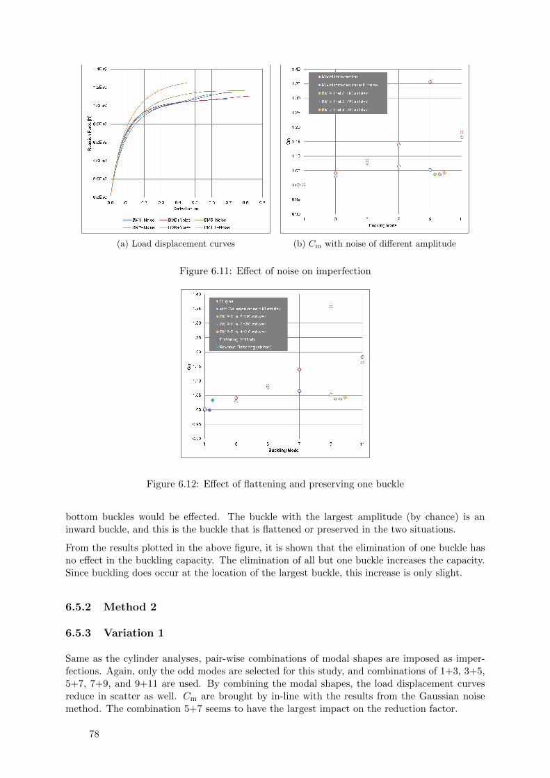
(a) Load displacement curves (b) Cm with noise of different amplitude

Figure 6.11: Effect of noise on imperfection

Figure 6.12: Effect of flattening and preserving one buckle

bottom buckles would be effected. The buckle with the largest amplitude (by chance) is aninward buckle, and this is the buckle that is flattened or preserved in the two situations.

From the results plotted in the above figure, it is shown that the elimination of one buckle hasno effect in the buckling capacity. The elimination of all but one buckle increases the capacity.Since buckling does occur at the location of the largest buckle, this increase is only slight.

6.5.2 Method 2

6.5.3 Variation 1

Same as the cylinder analyses, pair-wise combinations of modal shapes are imposed as imper-fections. Again, only the odd modes are selected for this study, and combinations of 1+3, 3+5,5+7, 7+9, and 9+11 are used. By combining the modal shapes, the load displacement curvesreduce in scatter as well. Cm are brought by in-line with the results from the Gaussian noisemethod. The combination 5+7 seems to have the largest impact on the reduction factor.

78

(a) Load displacement curve (b) Cms

Figure 6.13: Behaviour resulting from imperfection in shapes of combinations of buckling modes

6.5.4 Variation 2

Since combination 5+7 appears to be the most critical, more analyses are run with the contri-bution of its constituents weighed randomly. Figure 6.14 shows the results from 5 trials, eachwith different weights assigned.

Figure 6.14: Cm

BM 5 BM 7 Cm

0.922 0.078 1.0820.765 0.235 1.0770.566 0.434 1.0300.306 0.694 1.0070.488 0.512 1.002

Table 6.3: Contributingmodes, and associatedweights

The above results would suggest that equal contribution actually produces the worst imperfectionshape. Since the reduction factor is still greater than 1, no further analyses are done.

6.5.5 Method 3

Results from the random imperfection trials suggest that neither the maximum imperfectionamplitude, nor the total imperfection amplitude govern the buckling capacity of the hyperboloid.In fact, comparing to the modal shapes with the same maximum and total amplitude, thecapacity resulting from random imperfection is higher by an average of 30 % (Fig. 6.15b). As

79

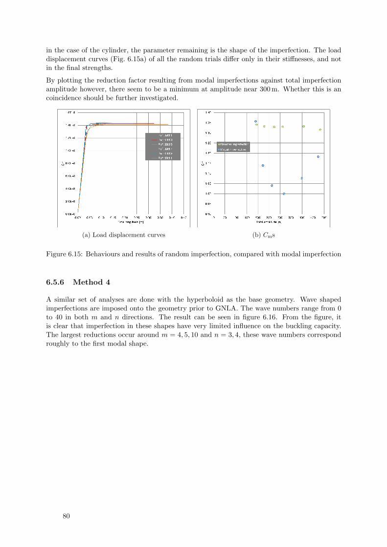
in the case of the cylinder, the parameter remaining is the shape of the imperfection. The loaddisplacement curves (Fig. 6.15a) of all the random trials differ only in their stiffnesses, and notin the final strengths.

By plotting the reduction factor resulting from modal imperfections against total imperfectionamplitude however, there seem to be a minimum at amplitude near 300 m. Whether this is ancoincidence should be further investigated.

(a) Load displacement curves (b) Cms

Figure 6.15: Behaviours and results of random imperfection, compared with modal imperfection

6.5.6 Method 4

A similar set of analyses are done with the hyperboloid as the base geometry. Wave shapedimperfections are imposed onto the geometry prior to GNLA. The wave numbers range from 0to 40 in both m and n directions. The result can be seen in figure 6.16. From the figure, itis clear that imperfection in these shapes have very limited influence on the buckling capacity.The largest reductions occur around m = 4, 5, 10 and n = 3, 4, these wave numbers correspondroughly to the first modal shape.

80

Figure 6.16: Cm resulting from wave imperfection of varing m and n

Cmm

0 1 2 3 4 5 10 20

n

0 N/A 1.343 1.403 1.365 1.346 1.356 1.334 1.3291 1.581 1.357 1.443 1.336 1.365 1.336 1.381 1.3572 1.394 1.400 1.369 1.381 1.351 1.399 1.350 1.3443 1.359 1.368 1.394 1.375 1.332 1.332 1.393 1.3974 1.397 1.355 1.368 1.372 1.335 1.334 1.336 1.3355 1.444 1.398 1.419 1.349 1.366 1.335 1.355 1.57610 1.400 1.700 1.430 1.517 1.358 1.365 1.343 1.35420 1.429 1.575 1.571 1.394 1.366 1.429 1.403 1.420

Table 6.4: Modified knock-down factor resulting from wave imperfection

81

6.6 Other types of Imperfections

6.6.1 Stress Imperfection

Geometrical imperfection has been the main focus of this thesis. However, as pointed out byCalladine [17], it is impossible for a fabrication to remain stress free when deformed in a double-periodic pattern (since this necessitates a change in Gaussian curvature).

Calladine stated that it is unreasonable to assume a stress free surface when change in Gaussiancurvature (by the existence of imperfection) clearly induces stress. Therefore, stress must bepresent in an imperfect surface, and need to be accounted for. To test the effect of this residualstress, the imperfection is imposed not as a change in nodal coordinates, but as a nodal displace-ment. As with previous analyses, the first buckling mode is used as the imperfection shape, andthe maximum amplitude is set at half the thickness.

The scaled displacement is imposed as a displacement boundary condition on each node toinduce an initial stress state directly in GNLA. This displacement load is applied only to thefirst load step, and removed there after. It is found that as soon as the displacement is removed,the structure ”bounces” back to the perfect state, and proceed as if unperturbed. The resultingcapacity is identical to the one from GNLA without imperfection. Therefore a second solution isproposed where the initial stress / strain state is obtained from the above displacement boundaryconditions using LEA. The resulting stress / strain state is then imposed onto the model priorto the eventual GNLA as an initial condition.

ANSYS does not currently support the imposition of initial stress and strain values on nodesof shell elements using the global coordinate system, therefore the imposition is acted on theelements using each element’s local coordinate system. The intent of this section to obtain thegeometrical imperfection ”equivalent” stress / strain state. Therefore, three different attemptsare made, one is to impose only the initial stresses, two, only the initial strains, and three,imposing both stress and strain.

Figure 6.17: Force displacement curves of thedifferent trials with LC3 - geometrical imper-fection as reference

Capacity [N] C

1 73.34× 106 1.0002 75.47× 106 1.0293 29.22× 106 0.3984 72.83× 106 0.9935 77.98× 106 1.0636 66.82× 106 0.9117 63.34× 106 0.864

Table 6.5: Knock-downfactor resulting from othertypes of imperfection

From the analyses, it is apparent that initial conditions, be it stress, strain, or displacement,has negligible influence on the final capacity of a thin cylinder in comparison with geometricalimperfection. The initial irregularity in Figure 6.17 at the beginning of the curves is due to therebeing more upward stress (or displacement) than downward, resulting in a negative reactionforce. Beyond the initial portion of the analyses, these initial conditions all resulted in similar

82

capacity as from the LBA or from the model with no imperfection at all. Furthermore, theforce displacement curves from these different initial conditions remain remarkably similar. Thisproves that the geometrical perturbation has significance beyond the introduction of an initialstress / strain state to the surface. The deformation diagrams are included in Appendix F. Thisresult concurs with Calladine’s experimental study on the effect of initial stress imperfection onaxially loaded cylindrical shell [32] [49], where the result exhibited less reduction in capacity(ie. buckling occurred at the higher end of the scatter shown in Chapter 4), and without thecharacteristic scatter exhibited by geometrically imperfect cylinders.

6.6.2 Boundary Layer Imperfection

For a structurally indeterminant structure, change in boundary (such as settlement) inducessignificant stress. Thus far in this section, the load has always been applied perfectly uniformlyto the top ring of the cylinder. However, it is unreasonable to assume that the experimentalset-up includes a perfectly flat loading plate, and that the specimen has perfectly flat top andbottom rings. To fully investigate the issue of loading imperfection, an imperfect loading plateshould also be included in the FEM model, such that there exists a layer of contact elementsin between the plate and the cylinder. To simplify this procedure for the purpose of this studyhowever, it is assumed that the applied displacement varies sinusoidally along the top ring ofthe cylinder. This loading condition is adapted from DIANA’s example manual.1

To understand the magnitude of this imperfection, it is helpful to visualize the load as a combi-nation of axial displacement and rotation. The axial displacement is set at uz = 0.025 or l/400,and maximum rotation is set to φz = π/3600, this value ensures the magnitude of the eccentricitydoes not dominate the behaviour. The total displacement can then be calculated as follows,

utotz (θ, 0 ≤ LS ≤ 1) = uz + uez · sin(aθ); a ≥ 1 (6.17)

Where a determines the number of waves in the tangential direction. The eccentric componentcan be calculated as follows,

uez = R · tan(φz) = R · tan(

π

3600) = 0.004 36 m (6.18)

This loading imperfection is only implemented in the first load step as it is assumed that localimperfections are flattened out after initial contact due to localized plasticity. For all furtherload steps, the regular loading is specified.

utotz (θ, LS > 1) = uz (6.19)

Four different values of a ranging from 1, 5, 10 to 20 are chosen to assess the effect of initialloading imperfection (Figure 6.19a shows the scheme of the implementation).

From the LBA results (Fig. 6.18), it is observed that the buckling shapes differ greatly. The firstmode exhibits complete asymmetric behaviour as there is one dominate applied moment. Themodes with higher wave numbers become symmetrical, though the buckles are localized at thepoint under the troughs of the sinusoidal load. This agrees with Maiboroda’s assertion that ”anuneven loading leads to localization of the buckling form near the weakest point, the bucklingform decreases as one moves away from this point” [34]. The eigenvalues resulting from LBA isplotted against a in figure 6.19b.

1DIANA manual - https://support.tnodiana.com/manuals/d95/Diana.html

83

(a) a = 1 (b) a = 5 (c) a = 10 (d) a = 25

Figure 6.18: Buckling modes with varying a

From the ”knock-down factor - no imperfection” curve of Figure 6.19b, we can conclude thatGNLA with no geometric imperfection (only load imperfection) shows no imperfection sensitiv-ity. In fact, the resulting capacity is consistently greater than that of the LBA results. Fromdisplacement diagrams it is observed that as the loading increases, the initial loading imperfec-tion becomes insignificant as the displacements ”smooth” out. The structure always reverts backto the uniform downward deflection state when the imperfection is removed (LS ≥ 1). This maybe due to the fact that aside from the assumed local plasticity near the troughs of the sinusoidalload pattern, the global behaviour remains elastic prior to onset of buckling.

(a) Scheme of imperfect loadapplication (b) Resulting knock-down factor

Figure 6.19: Results of variable displacement control

If geometrical imperfections (in the buckling shapes shown in Figure 6.18) are imposed in ad-dition to the loading imperfection however, the behaviour becomes drastically different andsignificant imperfection sensitivity is observed. The resulting capacity is similar to Method oneat the beginning of this chapter. It is observed from the deformation diagrams that the defor-mation caused by the initial load imperfection is still being absorbed, and it is the geometricalimperfection that causes the eventual buckling. The deformation diagrams are included in Ap-pendix F. This shows that as with the previous section, geometrical imperfection has a far largerimpact on the buckling capacity of a thin-shell than other types of imperfections.

6.7 Conclusion

This chapter discusses the methods of imperfection generation and categorization. In the ab-sence of characteristic imperfection measurement, a credible random imperfection field can be

84

generated with the knowledge of tolerance alone. 4 different types of imperfection shapes arediscussed, namely modal shaped, combination of modes, Gaussian random, and sinusoidal waves.

A modified knock-down factor is proposed to replace the traditional knock-down factor, and totake advantage of the modern computational capability. Cm is defined as the quotient of theshell true ultimate load and the shell ultimate load that follows from a geometrical nonlinearanalysis including the first buckling mode imperfection. Should Cm be larger than one, thenthe designer may stop the imperfection analysis after imposing the first buckling mode as theimperfection. The true ultimate load can be computed by a full non-linear analyses includingrandom imperfections. In this project this factor has been determined as 0.8 for axially loadedcylinders and 1 for concrete cooling towers. It is recommended that this factor is determinedfor many types of thin shell structure.

An exhaustive list of imperfection shapes derived from the 4 types are imposed onto boththe cylinder and the cooling tower. It was observed that for a structure with closely spacedeigenvalues, imperfection sensitivity is severe in general. A large knock-down factor can beexpected. Furthermore, for such a structure, imperfection in the shape of the first mode maynot govern the capacity. Cylinder is an extreme example of such a structure, where imperfectionin the shape of higher modes, combinations of mode, or sinusoidal waves may govern.

In particular, attention is applied to the third buckling mode. This mode shows an axisymmetricshape with no buckles in the tangential direction. If it is used as the imperfection shape, adeceptively low knock-down factor is observed. However, should the shape be perturbed by aGaussian noise, or be combined with an asymmetric shape, the knock-down factor increasessignificantly to point of governing the behaviour. Therefore, one recommendation is to alwaysimpose additional noise should axisymmetric mode emerge. In general, for an axially loadedcylinder a modified knock-down factor of Cm = 0.8 should be used.

For a moderately sensitive structure such as the hyperbolic cooling tower, all the above imper-fection shapes are similarly applied. However, after many attempts, the first mode still governsthe buckling behaviour of the structure.

Lastly, other types of imperfections are applied to the cylinder. The axial load is imposed as asinusoidal (as opposed to uniform) displacement for the first load step. The number of periodsin the sine wave is varied. This resulted in completely different buckling modes as bucklesappear localized right underneath the troughs of the wave. However, if load shape constitutesthe sole imperfection, the perturbation is absorbed by the structure before buckling occur. Thebehaviour remains as if there is no imperfection at all. The second attempt involves imposingthe imperfection not geometrically, but rather as a stress, a strain or a displacement. Again, novisible change in capacity is observed in all of the cases.

Overall, it is possible to impose randomly shaped imperfections but this requires much effort ofthe analyst and this is not feasible for engineering design. It is recommended that finite elementsoftware is extended so that random imperfections to shell structures can be inserted effortlessly.

85

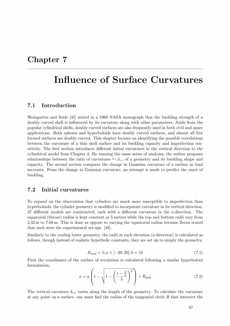
Chapter 7

Influence of Surface Curvatures

7.1 Introduction

Weingarten and Seide [45] stated in a 1969 NASA monograph that the buckling strength of adoubly curved shell is influenced by its curvature along with other parameters. Aside from thepopular cylindrical shells, doubly curved surfaces are also frequently used in both civil and spaceapplications. Both spheres and hyperboloids have doubly curved surfaces, and almost all freeformed surfaces are doubly curved. This chapter focuses on identifying the possible correlationsbetween the curvature of a thin shell surface and its buckling capacity and imperfection sen-sitivity. The first section introduces different initial curvatures in the vertical direction to thecylindrical model from Chapter 4. By running the same series of analyses, the author proposesrelationships between the ratio of curvatures kzz/kxx of a geometry and its buckling shape andcapacity. The second section compares the change in Gaussian curvature of a surface as loadincreases. From the change in Gaussian curvature, an attempt is made to predict the onset ofbuckling.

7.2 Initial curvatures

To expand on the observation that cylinders are much more susceptible to imperfection thanhyperboloids, the cylinder geometry is modified to incorporate curvature in its vertical direction.37 different models are constructed, each with a different curvature in the z-direction. Theequatorial (throat) radius is kept constant at 5 meters while the top and bottom radii vary from2.32 m to 7.68 m. This is done as oppose to varying the equatorial radius because Zerna statedthat such were the experimental set-ups [48].

Similarly to the cooling tower geometry, the radii at each elevation (z-direction) is calculated asfollows, though instead of realistic hyperbolic constants, they are set up to simply the geometry.

Rmid = 5; a ∈ [−20, 20]; b = 10 (7.1)

First the coordinates of the surface of revolution is calculated following a similar hyperboloidformulation,

x = a

1−

√√√√1−

(z − L

2

b

)2+Rmid (7.2)

The vertical curvature kzz varies along the length of the geometry. To calculate the curvatureat any point on a surface, one must find the radius of the tangential circle R that intersect the

87

point. Using the finite element mesh, three adjacent points on a local axis of a element can beused to find one of the principle curvature kzz = 1/Rz along that particular element.

Using point A in figure 5.1 as an example. Rz is calculated by solving a system of three equationswith O(x), O(z), and Rz as the unknowns. O(x), O(z) are the distances from the origin of thecoordinate system to the origin of the particular circle that intersects the three points, and Rzis the radius of that circle.

(x1 −O(x))2 + (z1 −O(z))2 = R2z (7.3a)

(x2 −O(x))2 + (z2 −O(z))2 = R2z (7.3b)

(x3 −O(x))2 + (z3 −O(z))2 = R2z (7.3c)

Instead of solving the above non-linear equations directly, the following simplification involv-ing trigonometry is used. Referring to Figure 7.1, m(A) and m(B) are slopes of lines A andB respectively. Using these slopes, centre of the circle that intersects these three points arecalculated as O(x) and O(z). The radius Rz follows from the Pythagoras theorem. Finally,reciprocate Rz and obtain kzz.

m(A) =z2 − z1

x2 − x1; m(B) =

z3 − z2

x3 − x2(7.4a)

O(x) =m(A)m(B)(z3 − z1) +m(A)(x2 + x3)−m(B)(x1 + x2)

2(m(A)−m(B))(7.4b)

O(z) = − 1

m(A)

(O(x)− x1 + x2

2

)+z1 + z2

2(7.4c)

Rz =√

(O(x)− x2)2 + (O(z)− z2)2 (7.4d)

kzz =1

Rz(7.4e)

The tangential curvature kxx and Rx can be calculated in a similar fashion using three pointsalong the surface tangent, through that is unnecessary as the origin is known to be on the z-axis,and the equatorial radius is set at Rx = 5.

Figure 7.1: Surface and curvature calculation variables

The curvature ratio, kzz/kxx, is calculated at the mid point of the structure. From the change ina, corresponding change occurs in kzz.

a ∈ [−20, 20]; kzz ∈ [+1,−1] (7.5)

88

Increments of ∆kzz/kxx = 0.05 is used over the above range except nearing 0 where increasinglysmaller changes in curvature are used. The list of curvature ratios used are listed in table 7.1.

Trial kzz/kxx RF Load Fcrit Fult CN Factor N N

1 1.00 3729661 9.252 34506000 20893000 0.6052 0.75 5401823 8.457 45684000 26910000 0.5893 0.50 7865679 7.465 58720000 31370000 0.5344 0.45 8480845 7.225 61277000 31325000 0.5115 0.40 9139767 6.971 63715000 31549000 0.4956 0.35 9841189 6.705 65982000 31838000 0.4837 0.30 10581566 6.428 68023000 31426000 0.4628 0.25 11354324 6.146 69784000 30478000 0.4379 0.20 12149094 5.862 71217000 30337000 0.426

10 0.15 12951065 5.581 72279000 29509000 0.40811 0.10 13740617 5.308 72938000 27384000 0.37512 0.05 14493514 5.053 73237000 23902000 0.32613 0.025 14847596 4.937 73300000 22418000 0.30614 0.005 15116772 4.850 73319000 21177000 0.28915 0.0025 15149432 4.838 73291000 35075000 0.47916 0.0005 15175392 4.819 73132000 36707000 0.50217 0.00025 15178627 4.817 73108000 36772000 0.50318 0.00005 15181213 4.814 73087000 36459000 0.49919 0 15181859 4.814 73081000 36419000 0.49820 -0.00005 15182505 4.813 73075000 35225000 0.48221 -0.00025 15185089 4.810 73045000 34277000 0.46922 -0.0005 15188316 4.807 73006000 33014000 0.45223 -0.0025 15214051 4.768 72544000 27870000 0.38424 -0.005 15246003 4.698 71629000 26242000 0.36625 -0.025 15492555 3.637 56346000 33153000 0.58826 -0.05 15775993 2.597 40977000 25200000 0.61527 -0.10 16247255 1.833 29784000 22024000 0.73928 -0.15 16571272 1.399 23188000 19650000 0.84729 -0.20 16731157 1.197 20026000 18871000 0.94230 -0.25 16719867 1.068 17850000 18028000 1.01031 -0.30 16541129 0.982 16246000 19080000 1.17432 -0.35 16208688 0.923 14958000 16284000 1.08933 -0.40 15744123 0.886 13956000 13435000 0.96334 -0.45 15173832 0.873 13246000 12566000 0.94935 -0.50 14525880 0.860 12491000 12132000 0.97136 -0.75 10948374 0.925 10124000 9829000 0.97137 -1.00 7957466 1.088 8655000 8077000 0.933

Table 7.1: Summary of results

89

7.2.1 Linear Elastic and buckling analysis

The mesh density in this study is set to be double of the cylinder model in Chapter 4. This isdone so that the Gaussian curvature (in the second part of this chapter) can be calculated witha higher resolution. The trade off is much longer calculation time (averaging 4 hours comparedto 30 minutes), and much larger hard drive requirement (depending on the number of bisections,each analysis may take up to 20 GB of space).

Following the same procedure laid out in chapter 4, load is applied via displacement controlledsteps to the top ring of the cylinder. To ensure sufficiently refined load steps, the step-wisedownward displacement is set at uz = 0.025 m. The top ring is similarly laterally restrained toprevent in-extensional deformation, and the bottom ring is pinned.

LEA is performed on each of the models to obtain the equivalent reaction forces. This ismultiplied to the eigenvalues produced by the buckling analysis to calculate the critical load.Since the eigenvalues from LBA are calculated based on a displacement-controlled load, it mustbe shown that it can be applied to the reaction force. This was done in Chapter 4. The firstbuckling mode of the different geometries are recorded in figure 7.2.

90

Figure 7.2: First buckling mode of the different geometries (Left then down from 1 to 37)

91

From the figure above, it is observed that when the geometry is in the positive curvature group,axisymmetric buckling mode is always the dominant mode (buckles only in the vertical directionand none in the tangential). This is in-line Tovstik’s assertion that for shells of positive curvature,the deformation occur in lines [43]. As the curvature increases, the ring shaped buckles occurmore towards the edge, and become more localized. As the curvature ratio approaches zero(0 ≤ kzz/kxx ≤ 0.0025) the axisymmetric modes disappear.

When the curvature ratio is sufficiently negative (Kxx/Kzz ≤ −0.005), buckling modes similar tothe ones produced by the hyperbolic cooling tower emerges. A chessboard pattern that spreadalong the entire neutral surface appear as the deformation shape due to the fact that negativeGaussian curved surfaces have two systems of asymptotic lines. The notion of ”sufficientlynegative” was also referenced by Tovstik who stated the chessboard pattern emerges assumingthat the Gaussian curvature is not small.

In the near-zero group, the behaviour cannot be clearly categorized. The shape of buckles iswhat Tovstik predicted, deformation pits stretch along the generatrices (vertical lines) of thecylinder [43]. However, it would appear as though LBA cannot distinguish made between thedifferent near-cylindrical geometries: the resulting buckling shapes are similar if not identical,especially on the slightly positive curvature side (0.0025 > Kxx/Kzz ≥ 0).

More troubling fact is that when compared with the coarse mesh model in Chapter 6, it isobserved that with the refined mesh, the axisymmetric (governing) buckling shape does notoccur within the first 20 modes. It is possible that the mesh is still not refined sufficientlyfor the small difference in curvature to change the buckling behaviour, ie. all geometries inthe near-zero group are considered cylindrical by the software. Mesh density is of importancewith the near-zero models as the buckles are small and numerous, there must be sufficientamount of elements per buckle to represent them accurately. This is not an important issue forhyperboloidal shapes as the buckles are larger, and the influence of mesh density is reduced.

Based on these observations, the analyses are grouped in three categories, negative (kzz/kxx ≥0.005), near-zero (−0.005 ≤ kzz/kxx ≤ 0.0025), and positive (kzz/kxx ≤ −0.0025). Based on thisgrouping, Figure 7.3a shows a plot of reaction forces and buckling load factors, both normalizedto the cylinder geometry. Critical forces are calculated as follows,

Fcrit = λcritFz (7.6)

The behaviour on the positive curvature side is expected. As the contact surface decreases(top and bottom ring diameters shrink), the stiffness lowers and less force is experienced dueto the displacement, and therefore the load factor increases and reaction force decreases. Onthe negative curvature side, the reaction force increases until kzz/kxx = −0.2 where it reachesa maximum. On further increase of the curvature, the structure becomes less stiff and thereaction forces decrease. Both the buckling load factors and the critical buckling force decaysexponentially on the negative curvature side as the curvature increases.

When zoomed into the range around near-zero curvature, it is observed that the transition issmooth for all three variables, implying that the transition from positive to negative curvaturedoes not have an influence on the structural stiffness.

7.2.2 Imperfection

Imperfection in the shape of the first buckling mode ( 7.2) is imposed onto the structure. Themaximum amplitude is scaled to half of the thickness. Should the modal shape be axisymmetric(ie. all models in the positive curvature group, similar to model 14), addition Gaussian noise isimposed. This is done to extract a realistic knock-down factor as suggested in Chapter 6. Only

92

0.0

0.2

0.4

0.6

0.8

1.0

1.2

1.4

1.6

1.8

2.0

-1.0 -0.8 -0.6 -0.4 -0.2 0.0 0.2 0.4 0.6 0.8 1.0

Rat

ios

norm

aliz

ed to

kzz

/kxx

=0

kzz/kxx

Normalized reaction force

Normalized buckling load factor

Normalized critical force

(a) −1.0 ≤ kzz/kxx ≤ 1.0

0.75

0.8

0.85

0.9

0.95

1

1.05

-0.025 -0.015 -0.005 0.005 0.015 0.025

Rat

ios

norm

aliz

ed to

kzz

/kxx

=0

kzz/kxx

(b) −0.005 ≤ kzz/kxx ≤ 0.005

0.998

0.9985

0.999

0.9995

1

1.0005

1.001

1.0015

1.002

-0.0005 -0.0003 -0.0001 0.0001 0.0003 0.0005

Rat

ios

norm

aliz

ed to

kzz

/kxx

=0

kzz/kxx

(c) −0.0005 ≤ kzz/kxx ≤ 0.0005

Figure 7.3: Eigenvalues, reaction force, and critical buckling force, normalized to the values ofthe cylinder

the first mode is used in the trials due to time constraint, but as shown in Chapter 6, the firstmode may not govern the behaviour. The imperfection imposition is done on a node by nodebasis, no ill-conditioned elements resulted.

7.2.3 Non-Linear Analysis

GNLA are performed on each of the 37 perturbed FEA models, and the results are collectedand grouped in the same three categories as above. The resulting capacity is converted toa knock-down factor. These are shown with different scales in figure 7.4. Figure 7.4a plotsFult from GNLA and Fcrit from LBA against the curvature ratio. It is evident that the threegroups of curvatures behave differently. With the positive curvature geometry, both Fult andFcrit follow a predictable pattern. As the stiffness decreases (Fcrit decreases), the imperfectionsensitivity decreases as well (the gap between Fult and Fcrit decreases). This group is also wherethe largest knock-down factor occurs; a factor of ∼ 1/3.5 results from the model with a curvatureratio of 0.005 (model number 14, the first model where axisymmetric buckling mode emerges).This differs from the notion that cylinder is most imperfection sensitive. However, this result is

93

0

10

20

30

40

50

60

70

80

-1.0 -0.8 -0.6 -0.4 -0.2 0.0 0.2 0.4 0.6 0.8 1.0

Rea

ctio

n F

orce

s [M

N]

kzz/kxx

(+) Fult (+) Fcrit

(~0) Fult (~0) Fcrit

(-) Fult (-) Fcrit

(a) −1.0 ≤ kzz/kxx ≤ 1.0

0

10

20

30

40

50

60

70

80

-0.025 -0.015 -0.005 0.005 0.015 0.025

Rea

ctio

n F

orce

s [M

N]

kzz/kxx

(b) −0.025 ≤ kzz/kxx ≤ 0.025

0

10

20

30

40

50

60

70

80

-0.0005 -0.0003 -0.0001 0.0001 0.0003 0.0005

Rea

ctio

n F

orce

s [M

N]

kzz/kxx

(c) −0.0005 ≤ kzz/kxx ≤ 0.0005

Figure 7.4: Fcrit from LBA and Fult from GNLA

remarkably similar to the analysis done on the cylinder with the third mode as the imperfectionin Chapter 6. Similarity exist both in the imperfection shape (axisymmetrical buckles) and inthe knock-down factor (∼ 1/3.4).

This is an important observation in several ways. In chapter 6 (the study on a variety ofimperfection shapes), the cylinder was constructed with a coarser mesh. It is assumed that acoarser mesh is less accurate than the finer mesh used in this chapter. With the finer mesh inthis chapter, the axisymmetric mode does not appear(within the first 20 modes) until there issufficient positive curvature, kzz/kxx ≥ 0.005. The fact that the axisymmetric mode emerged asa buckling mode at all in the coarse model means that the software was not able to distinguishbetween curvatures that are less than 0.005. Conversely, assuming that the finer mesh is moreaccurate, it would be correct to state that coarse meshing adds an additional imperfection termto the FEM model that must be accounted for. However, from chapter 6, two conclusions weredrawn,

1. The axisymmetric mode is not the first, but the third mode

2. The axisymmetric imperfection shape resulted in the largest knock-down factor

94

These conclusions show that the axisymmetric imperfection is desirable, but does not exist ina perfect cylinder if a finer mesh is used. To produce such a shape, either the mesh densitymust be adjusted (made less refined), or the curvature must be changed. Furthermore, it canbe said that mesh density has a large influence on buckling modes, but it is not immediatelyobvious that a finer mesh is better. As the eigenvalues are very close together, and they are notso accurately represented with a coarse mesh, introducing reducing mesh density may actuallybe beneficial in obtaining a real capacity. The axisymmetric mode is studied in detail in thenext sections.

Shifting the attention to the negative curvature part of the plot. Both Fult and Fcrit decaysexponentially, with Fcrit decaying at a faster rate. For curvatures ≤ −0.2, the models arepractically imperfection insensitive as is the case for the hyperboloid cooling towere analysed inchapter 5.

The near-zero portion of the plot is the most intriguing and complex. From figure 7.4b, there is aclear discontinuity in ultimate buckling capacity Fult, but not in the linear buckling Fcrit. Fromfigure 7.4c, there appears to be a local maximum between kzz/kxx = 0 and 0.0005. In immediatevicinity outside of that range, the capacity decreases. This contradict the notion that a perfectcylinder should result in minimal capacity.

This may be explained by realizing that the difference in curvature between these models arepractically invisible to the naked eyes, they may well result from manufacturing imperfections.It is encouraging to see that none of the models in this range produce a worse knock-down factorthan kzz/kxx = +0.005 (model 14 with the first axisymmetric imperfection). This suggest that adesigner may be able to use either a slightly off-perfect cylindrical model or with a coarser meshto design a cylindrical structure.

Figure 7.5 shows the calculated knock-down factor of the various geometries using the followingknock-down factor equation.

C =Fult

Fcrit(7.7)

The discontinuity at near-zero curvature is clearly visible here as well, where C decreased byapproximately 50 % from 0.6 to 0.3, therefore the knock-down factor in the near-zero range isdifficult to predict. Fortunately, the behaviour of positive curvature geometry can be describedas a monotonically increasing function. Using a polynomial fit with bi-square fit, the followingrelationship is obtained with coefficient of determination value of 0.99,

C = −0.342(kzzkxx

)2 + 0.644kzzkxx

+ 0.3 (7.8)

kxx is known in our case as the throat radius remains constant. By substituting it with 1/R = 0.2we obtain,

C = −8.54k2zz + 3.22kzz + 0.3 (7.9)

Since the largest knock-down factor occurs at kzz/kxx = 0.005, it is conservative to assume thatthis equation is valid from 0 ≤ kzz/kxx ≤ 1. In the instance of a perfect cylinder, kzz = 0 andC = 0.3, which is lower and therefore more significant than any results in the near-zero group.Beyond curvature ratio of one, the geometry transforms into a point-loaded sphere and thebehaviour may differ significantly.

Considering the results of the imperfection study in Chapter 6, where imperfection in the shapeof the axisymmetric mode governed the capacity, and the observation from this chapter that theaxisymmetric mode starts to emerge as the first mode at kzz/kxx > 0.025, it can be assumed thatfor curvatures greater than 0.025, the first mode governs the knock-down factor.

The negative side is more complex due to the loss of stiffness as the curvature becomes morenegative. It is reassuring however that C is higher in general, and the geometry becomes

95

0.0

0.2

0.4

0.6

0.8

1.0

1.2

1.4

-1.0 -0.8 -0.6 -0.4 -0.2 0.0 0.2 0.4 0.6 0.8 1.0

Kno

ck-d

own

Fact

or, C

kzz/kxx

(+) (~0) (-)

(a) −1.0 ≤ kzz/kxx ≤ 1.0

0.25

0.3

0.35

0.4

0.45

0.5

0.55

0.6

-0.025 -0.015 -0.005 0.005 0.015 0.025

Kno

ck-d

own

Fact

or, C

kzz/kxx

(b) −0.025 ≤ kzz/kxx ≤ 0.025

0.45

0.47

0.49

0.51

0.53

0.55

-0.0005 -0.0003 -0.0001 0.0001 0.0003 0.0005

Kno

ck-d

own

Fact

or, C

kzz/kxx

(c) −0.0005 ≤ kzz/kxx ≤ 0.0005

Figure 7.5: Knock-down factor of the different geometries

practically imperfection insensitive beyond kzz/kxx < −0.2. It is not helpful to curve-fit the entireresulting knock-down factors aside from noting the emergence of the festoon shapes. However,if we focus solely on the geometries in between curvatures 0 ≤ kzz/kxx < 0, an almost linear fitcan be constructed (Eq.(7.10)).

C = −3.0kzz/kxx + 0.3 (7.10)

The reason for this fit ending at the lower bound of the entire graph will become clear in alater section where it is shown that the slight hyperbolic geometry can also result in a knock-down factor of ≈ 0.3. Combining this with the previous observation that the geometry becomesimperfection insensitive beyond kzz/kxx < −0.2, we obtain the following conclusion,

C =

{−3.0kzz/kxx + 0.3 if −0.2 ≤ kzz/kxx < 0;0.9 if kzz/kxx < −0.2.

(7.11)

From Chapter 6 it can be seen that imperfection in the shape of the first mode of the coolingtower does govern the behaviour. When similar buckling mode starts to emerge in this chapter(ie. kzz/kxx < −0.005), it can be assumed at the first mode governs the ultimate buckling

96

capacity. Therefore, only within the near-zero region does it become ambiguous as to thegoverning imperfection shape. This is investigated further in the following sections.

7.2.4 How cylindrical is cylindrical

As was previously compared, with a finer mesh, the axisymmetric mode does not emerge whenthe geometry sufficiently resembles a perfect cylinder. This section finds the curvature at whichthe axisymmetric starts to emerge, but not yet the dominate mode.

Since the axisymmetric mode emerges as the predominate mode at kzz/kxx = 0.005 and is com-pletely absent at kzz/kxx = 0.0025, a new geometry is created with a curvature ratio that bisectsthe two above, kzz/kxx = 0.00375. By running LBA, results (Figure 7.6a) shows that the predomi-nate model remains the axisymmetric one. Bisection is done again between kzz/kxx = 0.00375 and0.0025 and a new geometry is created at kzz/kxx = 0.003125. Running LBA again, Figure 7.6bshows that while the axisymmetric mode still exists, it is no longer the first mode. Note thatdue to the similarity between these models, the resulting eigenvalues are very similar. It hasbeen mentioned before that the order of the buckling modes is highly dependent on a varietyof factors such as mesh density, therefore all parameters except the vertical curvature are keptconstant to ensure that this study produces valid result.

This trend that the axisymmetric mode moves forward as curvature increases is alarming sinceimperfection in that particular modal shape is shown to govern the buckling behaviour. Itsuggests that the particular mode may move backward (up the modal number) as curvaturebecomes 0 and therefore may be neglected if only the first modes are extracted.

This shows the benefit of using a coarse mesh as the axisymmetric mode is captured with acoarse model of zero curvature. With a coarse mesh such as the one in Chapter 6, the solver isnot able to distinguish it and another geometry with a curvature up to kzz/kxx = 0.00375 as theabove figure 7.6b suggests, as the resulting buckling modes look identical to Figure 6.2.

7.2.5 Numerical and Analytical Analysis of Axisymmetric Mode

Effect of the axisymmetric imperfection

Upon observing the detrimental effect of the axisymmetric imperfection shape on the positivelycurved geometries, one wishes to impose it also on the hyperbolic and cylindrical geometries. Theobstacle lies in the fact that axisymmetric buckling does not occur in negatively or zero curvedsurfaces. Therefore, through trickery, the axisymmetric buckling mode is borrowedfrom the leastpositively curved surface that still produces such a mode within the first 20, kzz/kxx = 0.003125.After performing LBA, the positively curved geometry is modified to a negatively curved one,kzz/kxx = −0.025, and then the axisymmetric mode is imposed as imperfection. Note thatthis hack would only work for geometries with exactly the same number of nodes and nodalarrangements.

After imposing the axisymmetric imperfection, the same GNLA is performed with displacementcontrolled load steps. Figure 7.7a shows that for a slight hyperbolic structure kzz/kxx = −0.025,larger reduction factor can be obtained by imposing an axisymmetric imperfection shape thanwith the 1st buckling mode. This is especially significant as this imperfection shape would neverresult from the buckling analysis of a hyperbolic structure, making it unsafe to use only the firstmode as the imperfection shape.

The traditional knock-down factor can not be used in this case as there is no correspondingcritical force since the imperfection is not a real modal shape. The modified knock-down factor

97

(a) kzz/kxx = 0.00375, axisymmetric mode governs

(b) kzz/kxx = 0.003125, axisymmetric mode does not govern (similar to the cylinder model inchapter 6)

Figure 7.6: First ten buckling modes of the two different curvatures

0

5

10

15

20

25

30

35

40

0 0.01 0.02 0.03 0.04 0.05

For

ce [M

N]

Displacement [m]

With AxisymmetricImperfection

With first ModalImperfection

(a) Hyperboloid, kzz/kxx = −0.025

0

5

10

15

20

25

30

35

40

0 0.01 0.02 0.03 0.04 0.05

For

ce [M

N]

Displacement [m]

With Axisymmetric Imperfection

With first modal imperfection

(b) Cylinder, kzz/kxx = 0

Figure 7.7: Force displacement curves comparison between effect of first modal and axisymmetricimperfections

comes quite handle here as it compares the ultimate capacity with the capacity resulting from

98

GNLA with the first mode as imperfection.

Cm =Fult,axi

Fult,1=

21040479

33153000= 0.635 (7.12)

Fult,1 and the traditional knock-down factor of the hyperboloid retrieved from Figure 7.5 areFult,1 = 33 153 000 N and C = 0.588 respectively.

The same procedure is applied to the perfect cylinder, kzz/kxx = 0. This is done because such abuckling mode is not present in a cylindrical model with a fine mesh density (at least within thefirst 20 modes). The resulting load displacement plot (Fig. 7.7b) shows a significant reductionas well.

Similar knock-down factor can be calculated,

Cm =Fult,i

Fult,1=

21787000

36419000= 0.598 (7.13)

The traditional knock-down factor of the cylinder with the first mode as imperfection is C =0.498.

From these two results, it may be suggested that the initial curvature does not influence thecapacity as much as the initial imperfection, at least for geometries in close proximity to acylinder. With this axisymmetric mode as imperfection, the resulting knock-down factor of thenear-cylindrical hyperboloid, the cylinder, and the previously analysed near-cylindrical barrelbecome remarkably similar.

The failure mode of these two analyses are similar as well (Fig 7.8), both experience three distinctphase of displacement shapes. The axisymmetric shape, the Yoshimura shape (Fig 7.8b, lastingfor a brief time), and then a modified Yoshimura pattern with layers of buckles alternatingbetween flattened out or deepened (i.e. the wave length doubled).

(a) LS170 (b) LS178 (c) LS187

Figure 7.8: Deflected shape near buckling

The same axisymmetric imperfection is applied to another hyperboloid, though with a muchlarger curvature kzz/kxx = −0.5. From the results shown in figure 7.9, it was shown that thisgeometry is not imperfection sensitive if the first buckling mode is applied as the imperfection.The axisymmetric mode is no longer governing as was the case for the near-zero curvatures. Thisis inline with the expectation that sufficiently negatively curved structures are not imperfectionsensitive.

99

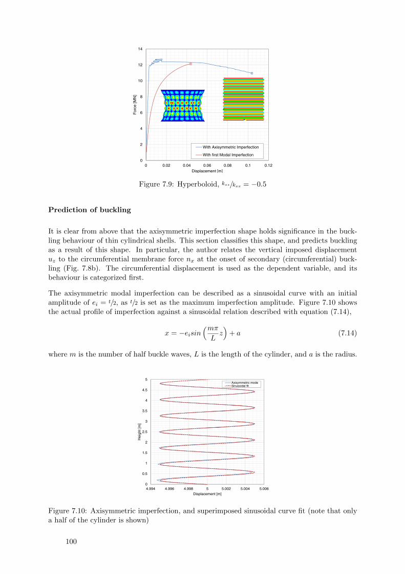
0

2

4

6

8

10

12

14

0 0.02 0.04 0.06 0.08 0.1 0.12

For

ce [M

N]

Displacement [m]

With Axisymmetric Imperfection

With first Modal Imperfection

Figure 7.9: Hyperboloid, kzz/kxx = −0.5

Prediction of buckling

It is clear from above that the axisymmetric imperfection shape holds significance in the buck-ling behaviour of thin cylindrical shells. This section classifies this shape, and predicts bucklingas a result of this shape. In particular, the author relates the vertical imposed displacementuz to the circumferential membrane force nx at the onset of secondary (circumferential) buck-ling (Fig. 7.8b). The circumferential displacement is used as the dependent variable, and itsbehaviour is categorized first.

The axisymmetric modal imperfection can be described as a sinusoidal curve with an initialamplitude of ei = t/2, as t/2 is set as the maximum imperfection amplitude. Figure 7.10 showsthe actual profile of imperfection against a sinusoidal relation described with equation (7.14),

x = −eisin(mπLz)

+ a (7.14)

where m is the number of half buckle waves, L is the length of the cylinder, and a is the radius.

0

0.5

1

1.5

2

2.5

3

3.5

4

4.5

5

4.994 4.996 4.998 5 5.002 5.004 5.006

Hei

ght [

m]

Displacement [m]

Axisymmetric modeSinusoidal fit

Figure 7.10: Axisymmetric imperfection, and superimposed sinusoidal curve fit (note that onlya half of the cylinder is shown)

100

The number of half waves in the axisymmetric mode is 26, and the wavelength is calculated asL/m = 0.385 m. This is verified by Calladine who derived equation (7.15).

L

m= π

(a2h2

12(1− ν2)

) 14

≈ 1.72√ah

= 0.385 m

(7.15)

Like compressing an accordion, the amplitude of the sine wave (the horizontal displacement)increases as the axial load increases. The total displacement in the circumferential direction isdefined by e = ei + ∆e.

ei =t

2= 0.0005 (7.16)

By plotting the horizontal displacement (∆e) of an inward and an outward buckle against theimposed displacement(uz) as it increases, one can obtain an almost linear relationship prior tosecondary (circumferential) buckling (see the average displacement plot on figure 7.11). Notethat in the real system, outward buckles displace more than the inward ones, even thoughthe initial imperfection assumes buckles of equal amplitude. For this study, this asymmetry isignored, and the buckles are assumed to be equal in lateral displacement, and the numericalvalue used is the average of the two. This is assumed to be valid as ∆e at the onset of bucklingis 1/2.5 of ei.

∆e =∆eout + ∆ein

2(7.17)

∆e, being the horizontal displacement at the extremities of buckles, can be estimated by thepre-buckling displacement of a series of vertical columns supported laterally by distributed bysprings (similar to how a wine barrel is constructed). The attempt to construct such a relationis detailed in appendix D, however the end result is asymptotic in shape, and does not matchwith the near-linear relationship (Fig 7.11) given by FEM without an adjustment factor. It isproposed that the initial axisymmetric imperfection has already pre-buckled the structure, andwhat is calculated by FEM is the post-buckling behaviour (of the axisymmetric buckling). Andit is this post-buckling state that leads to the onset of secondary (circumferential) buckling.

0

0.005

0.01

0.015

0.02

0.025

0 0.002 0.004 0.006 0.008 0.01 0.012 0.014 0.016

Circ

umfe

rent

ial D

ispl

acem

ent ,

∆e 

[m]

Vertical displacement, uz [m]

Average displacement

Linear fit of the pre-buckled portion

Inward displacement

Outward displacement

Figure 7.11: Circumferential displacements of an outward, and an inward buckle

An empirical relation between ∆e and the imposed vertical displacement based on figure 7.11 isconstructed instead (Eq. (7.18)).

101

∆e = 0.24uz (7.18)

Now that ∆e can be predicted with a formula, the next step is to relate it to the membraneforce in the hoop direction. To predict the onset of asymmetric buckling in between the rings ofaxisymmetric buckles, the compressive stress in the hoop direction must be calculated. Take asection of an inward buckle, one can construct a free body diagram as in Figure 7.12, where q1

and q2 are the membrane stresses at the top and bottom of the section, and P1 and P2 are thehoop forces at the top and the bottom ring of the section.

e1

1. InitialState

2. DeformedState

(Real)

A

B

C

D

E

A

C

E

F F

R1

R2

2 L/m

q1

q2

p1

p2o

p2

p2

p1

p1

q1 q2

1 23

2

e1 Δe

e=e1+Δe

2. DeformedState

(Simplified)

A

B

C

D

E

F

B

D

1. Initial Imperfection2. Displacement immediately prior to

asymmetric buckling3. Displacement of asymmetric buckling

qm

R2

a

R1

a

l1 lm l2

A (-0.436, -4.976, 5.600)B (-0.437, -4.986, 5.200)C (-0.435, -4.976, 4.800)D (-0.437, -4.986, 4.400)E (-0.436, -4.976, 4.000)

Figure 7.12: Free body diagram of axisymmetric buckling

From equilibrium in the vertical direction,∑Fy = 0 = h(q1l1) = h(q2l2) (7.19a)

nz,1l1 = nz,2l2 (7.19b)

l1 = πR1 (7.19c)

l2 = πR2 (7.19d)

102

From equilibrium in the horizontal direction, it is clear that

∑Fx = 0 (7.20a)

P1 = P2 (7.20b)

From equilibrium in rotation around point ”o”, assuming a clock-wise coordinate system,

∑MA = 0 = −nz,1l1

4R1

3π+ nz,2l2

4R2

3π+ 4P1

L

m(7.21a)

P1 =1

3π

m

Lnz,1l1(R1 −R2) (7.21b)

The centre of gravity of a semicircle is located 4R/3π from the equator, P1 is the hoop force ofone edge, therefore a factor of 2 is applied. The above relations shall always hold true in allload steps, and all except the radii R1 and R2 remain constant as load increases. In particular,the vertical distance L/m remains constant as the transition between axisymmetric and theasymmetric state is brief, and the loading conditions are almost identical. After imposing theimperfection and before loading the eccentricity equals to the initial imperfection amplitude.Going back to finding how the radii change as load increases,

R1 = a+ ei + ∆e (7.22a)

R2 = a− ei −∆e (7.22b)

R1−R2 = 2ei + 2∆e (7.22c)

To convert forces P1 and P2 to membrane forces, one assumes that the stress distributes si-nusoidally over the distance of 2L/m. Therefore, the peak stress is the amplitude of the sinewave.

nx(z) =nx2

[1− cos

(mπLz)]

(7.23)

The area under the stress curve is the force

P =

∫σ dA (7.24a)

=

∫ 2L/m

0nx dz (7.24b)

=1

2nx

[z − L

mπsin(mπLz)]∣∣∣∣2L/m

0

(7.24c)

=L

mnx (7.24d)

To convert q1 to the stress at an undisturbed cross section (Rm = a = 5), one can make referenceto line lm and stress qm in figure 7.12.

nz,1l1 = nz,mlm (7.25a)

nz,1 =lml1nz,m (7.25b)

103

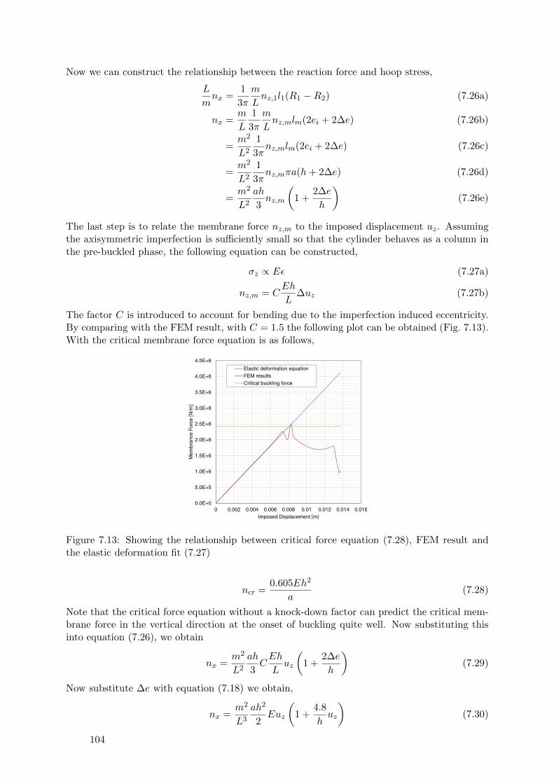
Now we can construct the relationship between the reaction force and hoop stress,

L

mnx =

1

3π

m

Lnz,1l1(R1 −R2) (7.26a)

nx =m

L

1

3π

m

Lnz,mlm(2ei + 2∆e) (7.26b)

=m2

L2

1

3πnz,mlm(2ei + 2∆e) (7.26c)

=m2

L2

1

3πnz,mπa(h+ 2∆e) (7.26d)

=m2

L2

ah

3nz,m

(1 +

2∆e

h

)(7.26e)

The last step is to relate the membrane force nz,m to the imposed displacement uz. Assumingthe axisymmetric imperfection is sufficiently small so that the cylinder behaves as a column inthe pre-buckled phase, the following equation can be constructed,

σz ∝ Eε (7.27a)

nz,m = CEh

L∆uz (7.27b)

The factor C is introduced to account for bending due to the imperfection induced eccentricity.By comparing with the FEM result, with C = 1.5 the following plot can be obtained (Fig. 7.13).With the critical membrane force equation is as follows,

0.0E+0

5.0E+5

1.0E+6

1.5E+6

2.0E+6

2.5E+6

3.0E+6

3.5E+6

4.0E+6

4.5E+6

0 0.002 0.004 0.006 0.008 0.01 0.012 0.014 0.016

Mem

bran

ce F

orce

[N/m

]

Imposed Displacement [m]

Elastic deformation equationFEM resultsCritical buckling force

Figure 7.13: Showing the relationship between critical force equation (7.28), FEM result andthe elastic deformation fit (7.27)

ncr =0.605Eh2

a(7.28)

Note that the critical force equation without a knock-down factor can predict the critical mem-brane force in the vertical direction at the onset of buckling quite well. Now substituting thisinto equation (7.26), we obtain

nx =m2

L2

ah

3CEh

Luz

(1 +

2∆e

h

)(7.29)

Now substitute ∆e with equation (7.18) we obtain,

nx =m2

L3

ah2

2Euz

(1 +

4.8

huz

)(7.30)

104

With this equation and the resulting plot on Figure 7.14, it can be seen that while the valuesbetween the analytical and the numerical result are similar, the behaviour is not. With FEM,the pre-buckling behaviour is linear, whereas with the equation above, the behaviour is quadratic(with the u2

z term).

0.0E+0

5.0E+5

1.0E+6

1.5E+6

2.0E+6

2.5E+6

3.0E+6

0 0.002 0.004 0.006 0.008 0.01 0.012 0.014 0.016

Mem

bran

ce F

orce

[N/m

]

Imposed Displacement [m]

Theoretical equation

FEM results

Critical buckling force

Figure 7.14: Plotting equation (7.30) with FEM results

For reference, the more complete picture of stress development can be observed from the stressplots at the positions of the circumferential buckles (Fig 7.15).

-800

-600

-400

-200

0

200

400

600

800

0 0.0025 0.005 0.0075 0.01 0.0125 0.015

Str

ess

[MP

a]

Vertical displacement [m]

Stress xx at Point AStress zz at Point AStress xx at Point EStress zz at Point E

A

E

D1 

D2 

D3 

D1  D2  D3 

Figure 7.15: Circumferential and vertical stresses verses top displacement load, with differentstages of buckling superimposed

7.2.6 Change in eigenvalue

It has been suggested that closely spaced eigenvalues is an indication of imperfection sensitivity.This hypothesis is tested here with the 37 geometries. The first 20 buckling modes of eachgeometry are calculated (results of LBA is shown in Appendix E) and the difference is defined asthe percentage change between the first and the twentieth eigenvalue as stated in Equation (7.31).The usage of the twentieth mode is arbitrary, one could equally use the tenth, or the fiftiethmodes.

105

∆λcr =λ20

cr − λ1cr

λ1cr

(7.31)

The resulting change in eigenvalues are plotted with the calculated knock-down factors againstthe changing initial curvatures in Figure 7.16.

y = -0.3415x2 + 0.6442x + 0.2994

y = -14.932x2 + 39.172x - 0.3784

0

20

40

60

80

100

0.0

0.2

0.4

0.6

0.8

1.0

1.2

-1.0 -0.8 -0.6 -0.4 -0.2 0.0 0.2 0.4 0.6 0.8 1.0

Eig

enva

lue

Rat

io

Kno

ck-d

own

Fact

or

kzz/kxx

(+) Knock-down Factor

(~0) Knock-down Factor

(-) Knock-down Factor

(+) Eigenvalue Ratio

(~0) Eigenvalue Ratio

(-) Eigenvalue Ratio

(a) −1.0 ≤ kzz/kxx ≤ 1.0

0

1

2

3

4

5

6

7

8

9

10

0.0

0.1

0.2

0.3

0.4

0.5

0.6

0.7

0.8

0.9

1.0

-0.005 -0.003 -0.001 0.001 0.003 0.005

Eig

enva

lue

Rat

io

Kno

ck-d

own

Fact

or

kzz/kxx

Eigenvalue to knock-down factor, (~0)range

(b) −0.005 ≤ kzz/kxx ≤ 0.005

0

1

2

3

4

5

6

7

8

9

10

0.0

0.1

0.2

0.3

0.4

0.5

0.6

0.7

0.8

0.9

1.0

-0.0005 -0.0003 -0.0001 0.0001 0.0003 0.0005

Eig

enva

lue

Rat

io

Kno

ck-d

own

Fact

or

kzz/kxx

Eigenvalue to knock-down factor, (~0)range

(c) −0.0005 ≤ kzz/kxx ≤ 0.0005

Figure 7.16: Change in eigenvalues

The trend is again quite clear for the positive curvature geometries. Graphically speaking it hasa strong correlation with the knock-down factor. By using the same curve fit method, one canobtain the following equation to describe the behaviour of the Gaussian curvature.

∆λcr = −14.932(kzzkxx

)2 + 39.172kzzkxx− 0.3784 (7.32)

For the near-zero curvature range, as with the knock-down factor, the trend cannot be easilydescribed. However, noting that ∆λcr values are similar to the knock-down factors if they wereflipped around C ∼ 0.3, one could construct a rough correlation equation.

C = −∆λcr

10+ c1 (7.33)

106

Where, c1 = 0.6 is the mean value of all the knock-down factors and ∆λcr values within thenear-zero range, plus the knock-down factor at zero curvature. This correlation is plotted inFigure 7.16b and 7.16c.

The shape of negative curvature results also suggests correlations between eigenvalue spacingsand ultimate capacities. The festoon shape is also present in the ∆λcr values. If we visualize the∆λcr plot stretched in the x direction and compressed in the y direction, so that the peak alignwith the knock-down factor at kzz/kxx = −0.3 then the two plots would look remarkably similar.

This result in itself is an unexpected observation as the spacing of eigenvalues has been used onlyas an indication of imperfection sensitivity, and not to calculate the actual knock-down factor.However, the above suggest that we may be able to do exactly that, at least for elementarygeometries. This correlation deserve study in depth to see whether actual relationship exist.

107

7.3 Gaussian curvatures

7.3.1 Introduction

It is hypothesized that the imperfection susceptibility of a shell is influenced by its Gaussiancurvature. Therefore, structures with positive, negative and zero Gaussian curvatures will bestudied in this thesis. From the two principle curvatures, the Gaussian curvature can be calcu-lated using the equation (7.34).

K = k1k2 = kxky − k2xy (7.34)

Figure 7.17 gives a simplistic view of the shapes associated with these curvatures. Note thataside from a few structures, most are designed with a combination of many different curvaturesand therefore are more difficult to analyse.

Figure 7.17: Different Gaussian curvatures, from the left: hyperboloid, cylinder, and sphere1

This study first details a systematic method to extract Gaussian curvatures of a parametricallyrectangular surface mesh. The author then implements this method in ANSYS script as apost-processor to any GNL analyses, so that the change in Gaussian curvature between everyload-step can be observed. This tool is used to further investigate the difference in bucklingbehaviour between the geometry of various curvatures. In particular, attention is paid to thedevelopment of buckles, and its relation with change in Gaussian curvature.

7.3.2 Algorithm

ANSYS does not have the native function to compute Gaussian curvature of a surface, thereforea custom calculation macro is written in APDL to calculate the Gaussian curvature at everyelement. The basis of calculation follows the mathematical theorem which states the Gaussiancurvature of a surface in R3 may be expressed as the quotient of the determinant of the secondfundamental form by the determinant of the first. The mathematical limitation of this algorithmis beyond the scope of this thesis2.

The first fundamental form assumes that the surface is once differentiable and parametrizedwith u, and v. It then calculates the inner (dot) product of the of the two tangent vectors. Ifthe following is true,

K =det[II]

det[I]=LN −M2

EG− F 2(7.35)

1Jhausauer, Gaussian curvature, wikipedia, http://en.wikipedia.org/wiki/Gaussian_curvature2Gray, A. The Definition of a Regular Surface in Rn. 12.4 in Modern Differential Geometry of Curves and

Surfaces with Mathematica, 2nd ed. Boca Raton, FL: CRC Press, pp. 281-286, 1997.

108

then E,F,G are the coefficients of the first fundamental form. In a discrete system, the coeffi-cients can be calculated by taking the dot product of the partial derivatives

E = u · u = x2u + y2

u + z2u

F = u · v = xu · xv + yu · yv + zu · zvG = v · v = x2

v + y2v + z2

v

(7.36)

where

∇x =δx

δu+δx

δv= xu~u+ xv~v

∇y =δy

δu+δy

δv= yu~u+ yv~v

∇z =δz

δu+δz

δv= zu~u+ zv~v

(7.37)

and,

u = xu~i+ yu~j + zu~k

v = xv~i+ yv~j + zv~k(7.38)

Then the normal vector to the surface is determined.

m = u× v

p =√m ·m

n =m

p

(7.39)

Assuming the displacement field is twice differentiable (not a concern when it is a discretesystem), the coefficients of the second fundamental form L,M,N can be calculated as follows.First the second derivatives of the displacement is calculated.

∇xu =δxuδu

+δxuδv

= xuu~u+ xuv~v

∇yu =δyuδu

+δyuδv

= yuu~u+ yuv~v

∇zu =δzuδu

+δzuδv

= zuu~u+ zuv~v

∇xv =δxvδu

+δxvδv

= xvu~u+ xvv~v

∇yv =δyvδu

+δyvδv

= yvu~u+ yvv~v

∇zv =δzvδu

+δzvδv

= zvu~u+ zvv~v

(7.40)

Thenuu = xuu~i+ yuu~j + zuu~k

uv = xuv~i+ yuv~j + zuv~k

vv = xvv~i+ yvv~j + zvv~k

(7.41)

Finally, the coefficients are calculated,

L = uu · nM = uv · nN = vv · n

(7.42)

109

7.3.3 Implementation

Most of the script is a direct adaptation of the above algorithm as common operators such asdot and cross product are a part of the built-in library. The coordinates x, y, z are stored in a2-D matrix with 3 columns which are accepted by the built-in functions. Gradient is calculatedaccording to Matlab’s numerical gradient, gradient, function (eq (7.43)3). The practical (andfurther restrictive) assumption of the algorithm that it can only be applied to a matrix ofcoordinates, with each of the two dimensions being greater than 5.

Ai =1

2

N−1∑i=2

Ai+1 −Ai−1 (7.43)

Along the top and bottom edges, the gradient is calculated single-sided difference between thevalue itself and its neighbour. This ensures the resulting matrix size has the same size. The leftand right edges are physically connected since the geometry is a surface of revolution, thereforegradient is calculated between the element’s adjacent value and the value at the opposite end.

Since it is much easier to refer to neighbouring elements as oppose to neighbouring nodes whenusing quadratic elements, the input to this macro is assumed to be the centroidal coordinate ofeach element. Similarly the output is an array of each element’s respective Gaussian curvature.A different macro loops through each load step, and imposes the calculated displacements on toeach node4. Then the centroidal location of the modified elements are obtained and sent to theGaussian curvature macro. The resultants are imposed as a surface pressure for visualizationpurposes.

The incremental change in Gaussian curvature is also of interest. After computing the Gaussiancurvature for a particular load step, the difference is calculated between it and the Gaussiancurvature of the previous load step. This difference is also displayed as a surface pressure forvisualization.

∆K =Kt −Kt−1

δt(7.44)

7.3.4 Application

Since this algorithm is implemented strictly as a post-processor, it can be used on any of thepreviously analysed models. Four of the above 37 models are chosen, and the resulting Gaussiancurvature visually inspected. Then the numerical values are extracted for the models that exhibitclear buckling behaviour.

Geometry 1 kzz/kxx = −1

Starting from the hyperbolic side, the Gaussian curvature of model kzz/kxx = −1 is calculatedand graphically shown in figure 7.18a. This model is representative in two ways. The top ringis large enough that the cantilever action reduces the stiffness of the structure, and the reactionforce decreases (see previous fig 7.3a). It is slightly imperfection sensitive, with a knock-downfactor of 0.933.

Figure 7.18a shows the effectiveness of plotting the Gaussian curvature and the change in Gaus-sian curvature. The initial imperfection can be seen from A1, where the maximum imperfections

3Gradient, Numerical gradient, MathWorks., http://www.mathworks.nl/help/matlab/ref/gradient.html4This is a problematic step in the procedure, as the displacement must be scaled small enough to not cause

ill-definition, and large enough to distinguish itself from the initial imperfection

110

occur at equator. A2 shows that the largest curvature also exists at the equator, and also thatat t ∼ 0 the global shape determines K, and not the local imperfection. As the imposed dis-placement increases (point B), both K and ∆K decrease the most at the equator still. PositiveK surface starts forming due to the imperfection. At point C and D however, ∆K decreasesthe most at the edges. This is not clearly evident in the displacement plots C3 and C4. Themodel diverges slightly after point E, where from E2, and E3 it is evident that the surface ismost curved around the edge points.

(a) kzz/kxx = −1.0 ; Top - Displacement, middle - K, and bottom - ∆K

0

1

2

3

4

5

6

7

8

9

10

0

50

100

150

200

250

300

350

400

450

500

0 5 10 15 20 25

Rea

ctio

n F

orce

[N] ■

Str

ess

[Pa]

■

Load Step, t

B

C

E

D

A

(b) Stress and force vs. load step

-0.04

-0.03

-0.02

-0.01

0

0.01

0.02

0.03

-0.4

-0.3

-0.2

-0.1

0

0.1

0.2

0.3

0 5 10 15 20 25

Cha

nge

in G

auss

ian

Cur

vatu

re ■■

Gau

ssia

n C

urva

ture

■■

Load Step, t

Min K

Max K

Min K Difference

Max K Difference

A

B

D

E

C

(c) K and ∆K vs. load step

Figure 7.18: Buckling behaviour of geometry with large negative Gaussian curvature

The visual assessment is complimented by plots of K and ∆K vs. load step as show in Fig-ure 7.18b. At t ∼ 0 it is clear that the initial curvature is largely negative. As load increases,the graph shows that for both maximum and minimum K, the behaviour is largely multi-linear.δK furthers shows that the change in curvature occur in discrete steps and not gradually. Fromthis plot, it is clear where attention should be focused on, and where buckling happens.

111

Geometry 2 kzz/kxx = −0.05

The next geometry is also a hyperboloid, but in this case the buckle happens near the equatorof the structure as oppose to at the top and bottom rings. Figure 7.19 shows the same threefigures as for the first geometry. A1 shows the shape and the magnitude of the initial imper-fection. Column B is where the structure reaches is buckling capacity. Note that there is nosignificant K or ∆K, as Figure 7.19c shows a flat line at zero for both. Column C shows thestructure immediately after buckling. Visually inspecting displacement plot B1 and C1, there isno significant difference aside from the colour change. However the difference is clear betweenB2 and C2, and B3 and C3. In fact because the curvature changed dramatically from B to C,∆K at that step is almost equivalent of K (ie. C3 equals to C2), dominating the Gaussiancurvature from previous steps. As the load further increases, the buckles become more localized.As shown in Figure 7.19c, load step D and E, step-wise increase of ∆K can be observed.

(a) kzz/kxx = −0.1 ; Top - Displacement, middle - K, and bottom - ∆K

0

5

10

15

20

25

0

100

200

300

400

500

600

700

800

900

1000

0 .5 .5 2 .5 3

Rea

ctio

n F

orce

[N] ■

Str

ess

[MP

a] ■

Load Step, t

A B C D E

1 1 2

(b) Stress and force vs. load step

-0.6

-0.4

-0.2

0

0.2

0.4

0.6

0 .5 .5 .5 3

Gau

ssia

n C

urva

ture

/ C

hang

e in

Gau

ssia

n C

urva

ture

Load Step, t

B C D EA

1 1 2 2

(c) K and ∆K vs. load step

Figure 7.19: Buckling behaviour of geometry with slight negative Gaussian curvature

112

Geometry 3 kzz/kxx = 0

At zero curvature, it is observed that axisymmetric buckling modes do not emerge. Buckles aredistributed and small in size. At load step D, the emergence of the second layer of buckles isevident in D3, and develops further in E3. Where as in D1, and D2, the second layer of bucklesis scarcely visible. This shows a difference between the initial linear buckling mode and the finalbuckling mode. This difference may suggest that imperfection in the final shape may reduce thecapacity further.

(a) kzz/kxx = +0.1 ; Top - Displacement, middle - K, and bottom - ∆K

0

5

10

15

20

25

30

35

40

0

50

100

150

200

250

300

350

400

0 0.5 1 1.5 2 2.5 3 3.5

Rea

ctio

n F

orce

[N] ■

Str

ess

[Pa]

■

Load Step, t

A B C D E

(b) Stress and force vs. load step

-0.1

-0.05

0

0.05

0.1

0.15

0.2

0 0.5 1 1.5 2 2.5 3 3.5

Gau

ssia

n C

urva

ture

/ C

hang

e in

Gau

ssia

n C

urva

ture

Load Step, t

A B C D E

(c) K and ∆K vs. load step

Figure 7.20: Buckling behaviour of geometry with neutral Gaussian curvature

113

Geometry 4 kzz/kxx = +0.005

Next a positive curvature geometry, kzz/kxx = +0.1, is analysed. This model resulted in thehighest reduction factor out of all the different curvatures analysed in this chapter. Again,Column A of figure 7.21a shows the initial imperfection. Note that the Gaussian noise can beobserved here as random specks of local curvature difference. From load step A to B, there is aconstant ∆K and a linear increase in K, the structures deforms like an accordion due to the axialload. At point B, slight difference in deformation in the tangential direction starts emerging.This is most obvious in the ∆K plot B3 where the incremental change in Gaussian curvature is nolonger symmetrical, but rather wave-like. There appears to be significant asymmetry resultingin a diagonal band. The next load step, C, shows clear buckles forming in C3, at the location ofthe diagonal band. This is not apparent in either C1 or C2. At D, and E, buckles intensify andbecome more apparent and localized around the equator. If we focus on the transition betweenC2 and D2, it is apparent that buckles in the tangential direction form in between the verticalbuckles.

(a) kzz/kxx = +0.1 ; Top - Displacement, middle - K, and bottom - ∆K

0

5

10

15

20

25

30

35

0

100

200

300

400

500

600

700

0 2 4 6 8 10

Rea

ctio

n F

orce

[N] ■

Str

ess

[Pa]

■

Load Step, t

A B C D E

(b) Stress and force vs. load step

-1

-0.8

-0.6

-0.4

-0.2

0

0.2

0.4

0.6

0.8

1

0 2 4 6 8 10

Gau

ssia

n C

urva

ture

/ C

hang

e in

Gau

ssia

n C

urva

ture

Load Step, t

A B C D E

(c) K and ∆K vs. load step

Figure 7.21: Buckling behaviour of geometry with slight positive Gaussian curvature

This observation provides further validation of Koiter’s modal interaction theory, where Koiterboth qualitatively and quantitatively described the physical behaviour of modal interaction by

114

considering an axisymmetric buckling mode in Figure 7.22a as the initial imperfection. As axialload increases, the inward-deflecting (concaved) portion of the shell surface also compresses inthe hoop direction, this destabilises the shell into a asymmetric (doubly-periodic) mode (Fig-ure 7.22b) at a bifurcation point from the nonlinear prebuckled state.

(a) (b)

Figure 7.22: (a) Axisymmetric mode (b) Square mode with matching wavelengths

7.4 Conclusion

The impact of curvature is studied in this chapter. First the cylinder’s initial curvature isvaried to create multiple hyperbolic and elliptical geometries (37 in total, each with a differentcurvature). The buckling shapes are calculated for each of the geometries. From the resultingshapes, they are categorized into three curvature groups. The positive group is defined by agoverning axisymmetric buckling mode. The negative group is defined by the on set of clear twodirectional buckles (chessboard). The curvature range in the middle is grouped as near-zero.The remainder of this chapter makes significant use of the above categorization.

From the results of LBA, the critical load factor is plotted against curvature. A clear changein slope at zero curvature is observed in Figure 7.3a. Next GNLA is performed on each of thedifferent geometries. The ultimate capacity is calculated and shown in Figure 7.4a. There existsa clear discontinuity at zero curvature, showing that the transition is an important indication tostructural behaviour. When zoomed into the near-zero range (Figure 7.4b), it is noted that thisdiscontinuity does not occur exactly at zero curvature but rather at the transition between near-zero to positive curvature (ie. when axisymmetric mode starts to emerge). The emergence ofthe axisymmetric mode also results in the largest reduction in capacity as shown in Figure 7.5a.

The behaviour of knock-down factor in the positive curvature range can be accurately predictedfrom the curvature value alone with a parabolic function. Similarly in the negative curvaturerange, the prediction can be made with an exponential decay function, albeit with less accuracy.The results in the near-zero range is ambiguous and its the author’s recommendation that thefunction for the positive range be used as well.

After identifying the correlation between curvature and knock-down factor, the relationshipbetween the spacing of eigenvalues and knock-down factor is investigated. By finding the per-centage difference in eigenvalue between the 20th and the first mode, equations are proposedthat relate the percentage difference and the knock-down factor in both the positive and thenear-zero curvature range. The relationship is more complex in the negative curvature range.

115

Seeing the significant of the transition between near-zero and positive curvature, two moregeometries are introduced to extract a non-governing axisymmetric buckling mode (i.e. likewhat was discovered in Chapter 6). Such is found with kzz/kxx = 0.003125. This shows that theaxisymmetric mode moves forward as the curvature becomes positive.

Second part of this chapter is devoted to inspecting the change in Gaussian curvature as loadincreases. Again, geometries are picked from each of the three curvature groups and inspectedin detail. In general, buckling can be visualized with the change in Gaussian curvature. As totalGaussian curvature may be dominated by the initial shape, the minute yet significant changemay not be readily observable, however the incremental change, when magnified, can predictthe onset of drastic change. These changes occur in discrete steps, and not continuously asexpected. These discrete steps usually predict the onset of a dramatic change in geometry suchas buckling. For the most critical case (with axisymmetric mode as the imperfection), bucklingcan be predicted by rapid change (spikes) in Gaussian curvature. In that case, buckles in thetangential direction develops in between adjacent rings of buckles in the vertical direction.

116

Chapter 8

Physical non-linear behaviours

8.1 Introduction

To present a more complete picture on the buckling behaviour of thin shells, physical non-linearities are integrated to the FEA models from the onset of analyses. For the metallic shells,a multi-linear stress strain curve is introduced to represent the elastic and plastic behaviour ofsteel. The analysis is performed on a number of structures of different curvature from Chapter 7.For the concrete shells, a different type of element (solid element with reinforcement and crackingmodel) is used to construct the model. This is done on the hyperbolic cooling tower.

This chapter belongs to Part I of the thesis as integrating non-linear material behaviour can beeasily done in ANSYS without any scripting, and should be done by structural designers. Theprocedure is described in detail below. The reason for its placement at the end of Part II is thatthe author intends to compare the change in Gaussian curvature between an elastic model andan elastic-plastic one.

8.2 Plasticity

This chapter starts by describing the proposed material model, and how ANSYS handles non-linear material behaviour. Then this material model is integrated into the analyses of twostructures. For ease of comparison, 2 of the selected geometries in Chapter 7 are reused, theirkzz/kxx ratios are −0.05, and +0.005 respectively. All aspects of the model and of the analysisprocedure remain identical except the introduction of the Multi-linear stress-strain model.

ANSYS provides a large library of plasticity options, out of which the Multilinear IsotropicHardening (MISO) option is utilized1. The stress-strain relationship is defined by 70 line seg-ments starting from (0, 0), the coordinates are listed in Appendix C. The stress-strain curveimplemented follows the typical steel behaviour, including the linear elastic portion, the yieldplateau and strain hardening. Non-linear Isotropic Hardening may also be used to simplify therelationship.

8.2.1 Stresses

To adequately understand the influence of plasticity, it is worth while to discuss how plasticbehaviour is represented in ANSYS. ANSYS conveniently calculates the 3 principal stresses as

1Kinematic Hardening should be used should the loading be cyclic

117

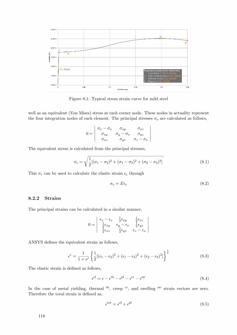
Figure 8.1: Typical stress strain curve for mild steel

well as an equivalent (Von Mises) stress at each corner node. These nodes in actuality representthe four integration nodes of each element. The principal stresses σo are calculated as follows,

0 =

∣∣∣∣∣∣σx − σo σxy σxzσxy σy − σo σyzσxz σyz σz − σo

∣∣∣∣∣∣The equivalent stress is calculated from the principal stresses,

σe =

√1

2[(σ1 − σ2)2 + (σ1 − σ3)2 + (σ2 − σ3)2] (8.1)

This σe can be used to calculate the elastic strain εe through

σe = Eεe (8.2)

8.2.2 Strains

The principal strains can be calculated in a similar manner,

0 =

∣∣∣∣∣∣εx − εo 1

2εxy12εxz

12εxy εy − εo 1

2εyz12εxz

12εyz εz − εo

∣∣∣∣∣∣ANSYS defines the equivalent strain as follows,

εe =1

1 + ν ′

{1

2[(ε1 − ε2)2 + (ε1 − ε3)2 + (ε2 − ε3)2]

} 12

(8.3)

The elastic strain is defined as follows,

εel = ε− εth − εpl − εcr − εsw (8.4)

In the case of metal yielding, thermal th, creep cr, and swelling sw strain vectors are zero.Therefore the total strain is defined as,

εtot = εel + εpl (8.5)

118

8.2.3 Yielding and buckling

It is often unclear whether yielding or buckling happens first. This issue is further complicatedby the fact that yielding almost always happens immediately after buckling. Using the clas-sical buckling equation for axially loaded cylinders, one could construct a simple stress versesslenderness relation where,

σ =

{fy if 0.605Eh

a ≥ fy;0.605Eh

a otherwise.(8.6)

and,

fy = 355 MPa (8.7)

This relationship is plotted in figure 8.2. From the plot, it can be assumed that buckling occursprior to yielding for a/h = 500. However, it is also clear from chapter 4 that the critical bucklingload equation (8.6) does not reflect the ultimate load capacity of a cylinder, the real curve wouldbe somewhere lower than the buckling curve.

0

50

100

150

200

250

300

350

400

450

0 200 400 600 800 1000 1200 1400

ST

RE

SS

[M

Pa]

RADIUS/THICKNESS, a/h

σult

Crushing

Buckling

a/h=500

0.605

Figure 8.2: Yield and buckling curves

8.2.4 Application to metallic hyperboloid

The first structure detailed here is a hyperboloid with a curvature ratio of kzz/kxx = −0.05.The analysis procedure remains identical to that in chapter 7 with the exception of materialproperties. LEA and LBA are performed on the model, and the resulting load factors remainidentical to those from chapter 7. This shows that material non-linearity does not influence linearanalyses. The first buckling mode is imposed as the imperfection with a maximum amplitude oft/2. Finally a step wise displacement controlled non-linear analysis is performed. The step sizeis set to be uz = 0.001 m.

Structural behaviour is categorized in Figure 8.3. With the first diagram, the stress-strain,and reaction force-strain relationships are plotted for the node with the largest combined dis-placement. The onset of plasticity is defined as the start of non-zero plastic strain, εpl. Thestress strain plot shows that the behaviour remains linear until fy = 355× 106 Pa at whichpoint yielding occurs. Structural collapse occurs at a strain of approximately ε ∼ 0.014. To-gether with Figure 8.3b, it is evident that buckling occurs prior to yielding; buckling occurs atε ∼ 3.47× 10−4 where as yielding is at ε ∼ 1.77× 10−3.

With compared with the behaviour of the linear model (the orange curve in Fig. 8.3a), it isobserved that the material non-linearity eliminated any post-buckling capacity, thereby making

119

0

50

100

150

200

250

300

350

400

0

5

10

15

20

25

30

35

40

0 5 10 15 20 25 30

Str

ess

[MP

a]

For

ce [M

N]

Load Step

Von Mises Stress

Reaction Force

(a) Elastic and post yielding forces and stresses

0

50

100

150

200

250

300

350

400

0

5

10

15

20

25

30

35

40

0 0.005 0.01 0.015

Str

ess

[MP

a]

For

ce [M

N]

Strain [m/m]

Elastic Force

Plastic Force

Behaviour of elastic model

Elastic Stress

Plastic Stress

(b) Forces and stresses vs load step

-1

-0.5

0

0.5

1

1.5

2

0 5 10 15 20 25 30

Gau

ssia

n C

urva

ture

Load step

Minimum Gaussian Curvature

Change in Min Gaussian Curvature

Maximum Gaussian Curvature

Change in Max Gaussian Curvature

(c) K and ∆K vs load step

-0.3

-0.2

-0.1

0

0.1

0.2

0.3

2 2.5 3 3.5 4 4.5 5

Gau

ssia

n C

urva

ture

Load step

(d) K and ∆K at critical points

Figure 8.3: PGNLA response of kzz/kxx = −0.05

this structure imperfection sensitive. This shows that while adding plasticity does not changethe buckling behaviour of the structure, it does have a large influence on the post-bucklingbehaviour. The difference in post-buckling behaviour within the elastic range is caused by thechange in the size of sub-steps during loading (the sizes are automatically determined).

Looking at the two lower plots (Fig. 8.3c, 8.3d), the onset of buckling is represented by a spikein ∆K, after which the buckles deepen at discrete intervals. Figure 8.4 visually illustrates thebehaviour of the hyperboloid under displacement load.

8.2.5 Application to metallic truncated ellipsoid (barrel)

The next structure detailed here is a barrel with a curvature ratio of kzz/kxx = +0.005. Asdiscussed in length in Chapter 7, this geometry resulted in the largest reduction in capacity.Again, the procedure remains identical to that in chapter 7.

Structural behaviour is categorized in Figure 8.5. With the first diagram, the stress-strain,and reaction force-strain relationships are plotted for the node with the largest displacement.The onset of plasticity is defined as the start of non-zero plastic strain, εpl. In figure 8.5b, thestress-strain behaviour remains linear until fy = 355× 106 Pa at which point yielding occurs.

120

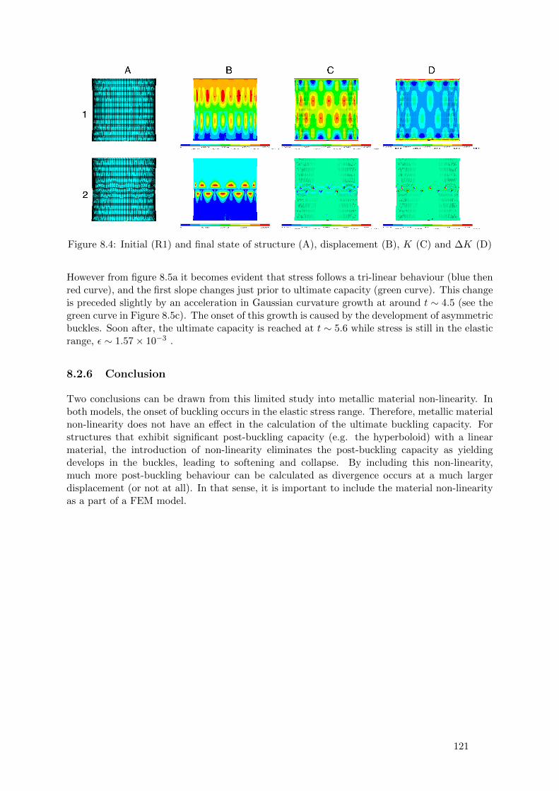
Figure 8.4: Initial (R1) and final state of structure (A), displacement (B), K (C) and ∆K (D)

However from figure 8.5a it becomes evident that stress follows a tri-linear behaviour (blue thenred curve), and the first slope changes just prior to ultimate capacity (green curve). This changeis preceded slightly by an acceleration in Gaussian curvature growth at around t ∼ 4.5 (see thegreen curve in Figure 8.5c). The onset of this growth is caused by the development of asymmetricbuckles. Soon after, the ultimate capacity is reached at t ∼ 5.6 while stress is still in the elasticrange, ε ∼ 1.57× 10−3 .

8.2.6 Conclusion

Two conclusions can be drawn from this limited study into metallic material non-linearity. Inboth models, the onset of buckling occurs in the elastic stress range. Therefore, metallic materialnon-linearity does not have an effect in the calculation of the ultimate buckling capacity. Forstructures that exhibit significant post-buckling capacity (e.g. the hyperboloid) with a linearmaterial, the introduction of non-linearity eliminates the post-buckling capacity as yieldingdevelops in the buckles, leading to softening and collapse. By including this non-linearity,much more post-buckling behaviour can be calculated as divergence occurs at a much largerdisplacement (or not at all). In that sense, it is important to include the material non-linearityas a part of a FEM model.

121

0

50

100

150

200

250

300

350

400

0

5

10

15

20

25

30

35

40

0 1 2 3 4 5 6 7

Str

ess

[MP

a]

For

ce [M

N]

Load Step

Elastic Force

Plastic Force

Elastic Stress

Plastic Stress

(a) Elastic and post yielding forces and stresses

0

50

100

150

200

250

300

350

400

0

5

10

15

20

25

30

35

40

0 0.001 0.002 0.003 0.004 0.005 0.006 0.007

Str

ess

[MP

a]

For

ce [M

N]

Strain [m/m]

(b) Forces and stresses vs load step

-0.1

-0.08

-0.06

-0.04

-0.02

0

0.02

0.04

0.06

0.08

0.1

-0.2

-0.16

-0.12

-0.08

-0.04

0

0.04

0.08

0.12

0.16

0.2

0 1 2 3 4 5 6 7

Cha

nge

in C

urva

ture

[1/m

]

Cur

vatu

re [1

/m]

Load Step

Min K

Max K

Min dK

Max dK

(c) K and ∆K vs load step

-0.1

-0.08

-0.06

-0.04

-0.02

0

0.02

0.04

0.06

0.08

0.1

-0.2

-0.16

-0.12

-0.08

-0.04

0

0.04

0.08

0.12

0.16

0.2

4.5 5 5.5 6 6.5 7

Cha

nge

in C

urva

ture

[1/m

]

Cur

vatu

re [1

/m]

Load Step

(d) K and ∆K at critical points

Figure 8.5: PGNLA response of kzz/kxx = +0.005

122

8.3 Cracking

To simulate cracking, a reinforced concrete model of the hyperboloid is generated. Insteadof using quadratic 2-D elements, linear 3-D elements are used with discrete embedded rein-forcement. ANSYS features both a specialized cracking concrete element (SOLID65), and alsogeneral brick elements (SOLID185 - 8 nodes, SOLID186 - 20 nodes). Since ANSYS plans todeprecate SOLID65 and dissociate base element formulation from reinforcement element, the 8node SOLID185 element is used at first.

ANSYS provides several non-linear material models suitable for concrete, Extended Drucker-Prager (EDP) and Microplane being the two current-technology options. EDP includes threeyield criteria and corresponding flow potentials to account for the material’s internal cohesionand friction. It can be combined with hardening rules (both isotropic and kinematic) to accountfor yielding behaviour.

Figure 8.6: ANSYS SOLID65 3-D Reinforced Concrete Solid

However, after initial trials, the author encountered difficulty in inputting the correct parametersfor either of the two material models. SOLID65 is used instead, with the associated CONCRETEmaterial model. The parameters of this material model are listed in table 8.1.

Constant Value Meaning

1 0.3 Shear transfer coefficients for an open crack.2 1.0 Shear transfer coefficients for a closed crack.3 3 MPa Uniaxial tensile cracking stress.4 25 MPa Uniaxial crushing stress.5 N/A Biaxial crushing stress .6 N/A Ambient hydrostatic stress state for use with constants 7 and 8.7 N/A Biaxial crushing stress under ambient hydrostatic stress state.8 N/A Uniaxial crushing stress under ambient hydrostatic stress state.9 N/A Stiffness multiplier for cracked tensile condition.

Table 8.1: Concrete Material Data

An advantage of SOLID185 is that ANSYS provides the option to automatically impose arbitrarynumber of discreet reinforcement elements (at any angle) within each base element. The initialmodel is constructed with one reinforcement bar (REINF194) in each element’s three local axes.

Since the results through the thickness direction is of no consequence considering the slender-ness ratio, only two layer of solids are used. For SOLID65, the reinforcement must be embedded

123

manually. This is not a difficult issue in this case as the base model is regularly defined. Re-inforcement bars are simulated using linear Timoshenko beam elements, and are placed at theintersection of each brick element. The area of reinforcement is calculated per element. Assum-ing there is one rebar per element surface, the area of those surfaces are as follows,

Ax = lelem · t = 0.095 m2;Az = welem · t = 0.095 m2 (8.8)

Where the subscripts denote the surface normal. LEA calculates the component stresses at eachGauss point, and the area of reinforcement is sized based on these values. It is apparent thatunder self-weight the only tensile stress is the hoop stress at the top of the hyperboloid.

σx = 0.110 MPa;λcr = 15.373;σcr = λcrσx = 1.715 MPa (8.9)

Therefore the total force per element surface is,

Fx = σcr ·Ax = 163 kN (8.10)

Assuming the reinforcement has a strength of frebar = 510 MPa, the cross sectional area can becalculated as follows,

Arebar = Fx/frebar = 320 mm2 (8.11)

Therefore one φ20 bar is used. The reinforcing elements in the z direction cannot be calculatedas the stress is always negative, the minimum reinforcement of one φ10 bar is assumed. Thereinforcing elements in the radial (thickness) direction is not effective in this case. Should crosssectional information be necessary and there are more elements through the thickness, then thesereinforcing elements can represent the stirrups.

The analysis set-up remains identical to those in other chapters of this thesis. LEA and LBA areperformed on the model, and the resulting load factors remain similar to those from chapter 5.The difference in weight is attributed to the added reinforcement. The buckling modes remainidentical in shape; the first mode is imposed as the imperfection.

From PGNLA, it is observed that with the concrete material model, cracking drastically reducesthe buckling capacity of the hyperboloid (Fig. 8.7). The knock-down factor is reduced fromC = 0.76 to 0.092. This extreme reduction suggests that with sufficient cracking, the strengthof the composite material is much less than that of linear concrete.

0

0.2

0.4

0.6

0.8

1

1.2

1.4

1.6

0 0.2 0.4 0.6 0.8 1

F/F

cr

Displacement

Linear buckling analysis

Geometric non-linear analysis without imperfection

Geometric Non-Linear Analysis with Imperfection

Physical and geometric non-linear analysis with imperfection

Figure 8.7: Comparison of different non-linearities

By looking at the crack development in detail (Fig 8.8), it is evident that vertical cracks occurat the outward buckles of the initial imperfection shape. This suggests that as the outward

124

buckle extends in magnitude, the hoop tension causes cracking. At the moment of divergence,the maximum tensile stress in concrete is 3 MPa. The Von Mises stress in the reinforcementis 192 MPa. This further shows that buckling of metallic structures is elastic, and that metalplasticity model is not necessary if the item of interest is the ultimate capacity.

Figure 8.8: Development of cracks, and tangential stress

The crack pattern is very different from the same model without the initial imperfection (Fig 8.9).As both the load and the geometry are axisymmetric, no cracking develops until the top ringdevelops sufficient hoop tension.

Figure 8.9: Crack pattern of GNLA of the perfect model

125

Chapter 9

To Infinity... and Beyond

9.1 Part I

9.1.1 Procedure to analyse thin shell structures

This thesis introduces a design procedure for analysing thin-shell structures using commercialfinite element method packages. The step-wise procedure is detailed in Chapter 1. The first stepis to construct the FEM model and apply the loads and boundary conditions. Linear bucklinganalysis (LBA) is run to obtain the buckling load factors, λcr, and the buckling shapes of thestructure. Depending on the spacing of these factors, the structure’s imperfection sensitivitycan be roughly estimated. For a regularly sensitive structure, the first buckling mode is imposedas the geometrical imperfection shape, with the maximum amplitude equalling to that of theconstruction tolerance (in this thesis, the amplitude is usually set to half of the thickness). Ageometrical and physical non linear analysis is then performed on the imperfect geometry toobtain a realistic ultimate capacity of the structure.

9.1.2 Verification of procedure against theoretical and experimental results

Part I of this thesis serves to demonstrate the validity, robustness and effectiveness of the pro-posed procedure. To that end, the procedure is applied to the well-studied problem of axiallycompressed cylinder. The results are compared to experimental findings and to Koiter’s theoret-ical work. By varying the slenderness ratio, a/h, of the cylinder while keeping the imperfectionshape (i.e. first buckling mode) and amplitude (i.e. t/2) constant, ANSYS is able to producebuckling stresses that are within one standard deviation of the mean experimental values upto a/h = 2500, beyond which the experiments resulted in lower buckling stress than ANSYS.One can conclude two points from this, one is that ANSYS can reliably simulate buckling be-haviour of thin shells, and two, the imperfection shape and amplitude used in these analyses isan adequate representation of real imperfection.

The comparison is made between FEM results and Koiter’s asymptotic equation by varying δ/tfrom 0 (i.e. a perfect cylinder) to 1 (i.e. the amplitude of imperfection equals to its thickness). Itis shown that by using the first mode as imperfection, the FEM results match Koiter’s equation(with b = −1) up to and including δ/t = 0.6, beyond which FEM results over estimates thecapacity. It can be concluded that with single mode as imperfection, FEM can reproducetheoretical findings by Koiter for small amplitude imperfection.

• General purpose FEM packages can simulate experimental set up and obtain realisticresults

127

• FEM result corroborates with Koiter’s asymmetric equation

• The first mode with a maximum amplitude of t/2 can be expected in real cylinders

9.1.3 Four case studies

The proposed procedure is then applied to 4 existing structures with realistic load conditionsin Chapter 5. The standard design procedure is followed, including a mesh refinement studyfor each structure. In the geometric non-linear analysis, the load is incremented until bucklingoccurs. The knock-down factor (Eq. (9.1)) of the various structures and load conditions aresummarized in table 9.1.

C =λult

λcr(9.1)

Structure Load case Load factor Knock-down factorLBA GNLA w/ imp GNLA w/ imp

Cooling TowerSelf weight 15.73 23.15 11.98 1.472 0.761Wind 6.60 7.33 5.54 1.110 0.838Self weight + wind 5.76 8.10 6.10 1.406 1.059

Monolithic domeWind 22.39 21.20 8.29 0.947 0.370Uniform pressure 15.77 15.12 13.75 0.959 0.872

Grain siloWind on empty silo 22.53 22.70 17.20 1.007 0.763Wind + calm water 22.89 22.50 17.40 0.983 0.760Wind + sloshing water 23.31 22.60 17.30 0.970 0.742

Fuselage Axial compression 3.96 4.95 4.01 1.251 1.012

Table 9.1: Summary of results from the four case studies

From the summary table, several important conclusions can be made,

• GNLA analysis without imperfection can result in un-realistic results, this error is morepronounce in axisymmetric structure with axisymmetric loads

• with imperfection, GNLA results do not exceed LBA results (significantly) even for struc-tures that are not sensitive to imperfection, making GNLA with imperfection universallyapplicable

• Dome structures experience the largest reduction in capacity of the bunch due to imper-fections

9.2 Part II

9.2.1 Imperfection shapes

Part II of this thesis focuses on structures with extreme imperfection sensitivity, and the cat-egorization of such structures. A method for extracting the knock-down factor of extremeimperfection sensitive structures is proposed. The method suggests 4 different categories of im-perfection shapes that may be imposed on to the structure. These categories are modal shapes,combinations of modal shapes, random, and superimposed-wave.

128

A modified knock-down factor Cm is proposed to replace the traditional factor when performingan imperfection sensitivity analysis. This new factor is the quotient of the shell true ultimateload and the shell ultimate load that follows from a geometrical non-linear analysis including thefirst buckling mode imperfection, λ1stMode

ult . The true ultimate load can be computed by a fullnon-linear analyses including any imperfection shapes (including the ones mentioned above).

These imperfection shapes are imposed on to the axially loaded cylinder, a classic example ofextreme imperfection sensitivity, and on to the cooling tower. It is found that imperfection inthe axisymmetric shape with additional Gaussian noise governs with Cm = 0.68.

”Random” imperfection does not result in significant reduction in capacity (Cm > 1). ”Com-binations” of modal shapes show that the combination between an axisymmetric mode with anon-axisymmetric one ([m,n] ∈ R) produce a lower reduction factor than combinations betweentwo axisymmetric modes (see Fig. 6.5b).

The cooling tower, being marginally imperfection sensitive, is governed in capacity by imperfec-tion in the shape of the first buckling mode (Cm > 1). This further strengthens the procedureproposed in Part I where only the first mode is needed for analysis.

Initial imperfection in loading is also simulated but found to be ineffective as the initial asym-metry is absorbed soon after the load becomes uniform (see Fig. 6.19). Imperfection imposednot as changes in nodal coordinates, but as in initial stresses, strains and boundary conditionsare also simulated but found to be similarly ineffective.

9.2.2 Influence of curvature

The significant difference in reduction between the cylindrical and the hyperbolic shape is studiedfurther in Chapter 7 where 37 different geometries of varying curvatures ranging from a barrelto a hyperboloid (−1 ≤ kzz/kxx ≤ 1) are generated and analysed. With imperfection in the shapeof the first mode, and maximum amplitude set to t/2, the procedure proposed above is used oneach model.

From linear buckling analyses, it is evident that the models can be categorized into three groupsbased on their initial curvature, kzz/kxx and the shape of the first mode (Fig. 7.2).

The resulting knock-down factor also show three distinct patterns of behaviour, in the positivecurvature group, the imperfection sensitivity decreases parabolically from C = 0.289 with anear-cylindrical geometry (kzz/kxx = 0.005) to 0.605 with a barrel (kzz/kxx = 1). The correlationbetween the curvature and the knock-down factor is detailed in equation (7.8). C = 0.289 alsorepresents the largest knock-down factor of the entire study. This knock-down factor is inducedby an axisymmetric imperfection shape, this corroborate with the findings of chapter 6.

The discontinuity in knock-down factor, C, around the zero curvature geometry preludes simplecorrelations to be constructed, though all Cs in this group are higher than C = 0.289, thereforeequation (7.8) applies in the near-zero curvature range as well.

In the negative curvature group, the reduction sharply decreases and forms festoons that ap-proaches 1 beyond kzz/kxx ≤ −0.2, meaning that the geometries become insensitive to imper-fections. The knock-down factor of negative curvature geometries can also be predicted usingEq. (7.11). Furthermore, post-buckling capacity is observed, making the hyperboloid a class Igeometry.

Upon observing the effect of the axisymmetric imperfection, it is imposed on to both the cylinderand a hyperboloid kzz/kxx = −0.05, and the results can be observed in figure 7.7. It is shown thatthe axisymmetric imperfection results in a larger reduction than the shapes’ 1stbuckling mode(for the cylinder, C = 0.297, and for the hyperboloid C = 0.373). It can be concluded thatthe design of near-zero curvature geometries (cylindrical shapes) should adopt an axisymmetricimperfection shape.

129

• Axisymmetric imperfection shape results in the largest knock-down factor for near-cylindricalstructures, irrespective the linear buckling behaviour

• The knock-down factor of positive, zero and negative curvature geometries can be calcu-lated from the initial curvature alone

• Negative curvature geometries are less sensitive to imperfection, and becomes insensitivewith sufficient curvature

9.2.3 Gaussian curvature

Both cumulative and incremental changes in Gaussian curvature (K and ∆K) are calculatedso that the onset of buckling can be observed. K is calculated as the ratio of the determinantsof the second and first fundamental forms. In a very negatively curved geometry where initialimperfection covers the entire surface in grid pattern, it can be seen that K follows a multi-linearincrease (Fig 7.18b), and points of slope change indicate dramatic changes in the surface, i.e. theformation of buckles. As load increases, the initial imperfection buckles increase in magnitudeuntil the buckles shift and localize to the boundary edges. The shift corresponds to a slopechange in Gaussian curvature, and to the start of non-linearity in the load-displacement curve(Fig 7.18).

In the most critical geometry in the positive curvature range (where axisymmetric mode governs),the change in Gaussian curvature remains constant in both positive and negative extremes (theaxisymmetric shape becomes more compressed and both convex and concave buckles becomemore defined as load increases), until asymmetric buckles occur. The point of occurrence canbe observed in ∆K as a band of sharp curvature change, and in the end of the linear portionof the load displacement curve (Fig. 7.21). After this point, asymmetric buckles spread throughthe meridian of the surface. This suggests that the extreme imperfection sensitive nature ofcylinders is indeed caused by modal interaction as Koiter suggested, where an axisymmetricmode changes to an asymmetric one at the moment of bifurcation.

• Axisymmetric imperfection shape leads to secondary buckling in the circumferential direc-tion as predicted by Koiter’s modal interaction theory

• Incremental change in Gaussian curvature is an accurate indicator of buckling behaviour,though a fine mesh is needed to accurately calculate the numerical values

9.2.4 Physical non-linearities

It has been the assumption that the buckling phenomena above occur within the elastic range.To test the validity of this assumption, a yield model is introduce to the cylindrical imperfectFEM model used in chapter 7. From the result shown in figure 8.3b, it is clear that bucklingindeed occur within elastic stress range, σvm ≈ 250× 106 Pa. However, the yield material modeleliminates the post-buckling capacity exhibited by the elastic model. With the yield model, thepost-buckling behaviour becomes more stable and converges for a larger strain range than withthe elastic model.

A concrete cracking model is applied to the imperfect cooling tower FEM geometry, and theresult is shown in figure 8.7. From chapter 5, it was found that the knock-down factor withoutphysical non-linearity is Celas = 0.76. This is more than eight times higher than the factor withphysical non-linearity, Cconc = 0.092. The circumferential cracks occur at the locations of initialimperfection buckle waves. These cracks are entirely absent if the geometry is perfect.

130

• Elasto-plastic model for metallic structures does not change the ultimate capacity, butdoes reduce the post-buckling capacity

• Cracking model must be applied for thin concrete shells as the resulting capacity reducesdrastically (in combination with initial imperfection)

9.3 Future work

As with all research endeavours, questions are just as frequently generated as answers. This thesisis no exception, several important yet unanswered questions deserve more detailed investigation.

9.3.1 Modal interaction

This thesis has shown that modal interaction does occur in the case of an axisymmetric imper-fection transforming into an asymmetric one. Given that this produced the largest reduction incapacity, it would be beneficial to procedure modal interaction in other structures with otherimperfection shapes. The dome geometry under external pressure would be an ideal candidate.

9.3.2 Case study on complex doubly curved structures

As the name suggests, structures that are significantly more complex than the ones studied inthis thesis may be used as base structures for the proposed procedure. It would be especiallyinteresting to study the imperfection sensitivity of doubly curved structures such as the RolexLearning Center, and relating its curvature to the buckling capacity.

9.3.3 Post-buckling behaviour

As the reader may have noticed, this thesis focused almost exclusively on the pre-buckling andthe buckling behaviour of shells. Koiter himself stated that his post-buckling theory only worksin the immediate vicinity of buckling. With ever more robust solving methods such as Ritzmethod or slow dynamic analysis, it would be interesting to obtain a more complete picture ofbuckling.

9.3.4 Change in Gaussian curvature

On a more fundamental level, it would be useful to relate the incremental change in Gaussiancurvature to the stress state at the element level.

9.3.5 Eigenvalue spacing

It has already been shown that the change in eigenvalue can be correlated to the ultimate capacityof an imperfection sensitive structure (e.g. an axially loaded cylinder). This correlation is doneon a numerical level, it would be interesting to formulate a theory that shows this relationshipfrom first principles.

131

Bibliography

[1] Design Criteria for Tornado and Hurricane Safe Rooms. Technical report, Federal Emer-gency Management Agency, 2008.

[2] Abaqus Documentation 6.13. Technical report, Dassault Systemes, Providence, RhodeIsland, 2013.

[3] stainless steel liquid tanks. Technical report, Meridian Manufacturing, Inc., Storm Lake,Iowa, 2013.

[4] Sohrabuddin Ahmad, Bruce M. Irons, and O.C. Zienkiewicz. Analysis of thick and thinshell structures by curved finite elements. International Journal for Numerical Methods inEngineering, 2(October 1969):419–451, 1970.

[5] AM El Ansary, AA El Damatty, and AO Nassef. Optimum Shape and Design of CoolingTowers. waset.org, 9:4–13, 2011.

[6] ANSYS Inc. Command Reference for the Mechanical APDL. In ANSYS Manual, volume15317, pages 1–1920. Canonsburg, PA, 12.0 edition, 2009.

[7] ANSYS Inc. Theory Reference for the Mechanical APDL and Mechanical Applications. InPeter Kohnke, editor, ANSYS Manual, volume 3304, pages 32–38, 877–879. Canonsburg,PA, 12.1 edition, 2009.

[8] ANSYS Inc. Structural Mechanics. ANSYS Manual, pages 5–12, 2011.

[9] ANSYS Inc. ANSYS Mechanical APDL Element Reference. In ANSYS Manual, volume15317, pages 1377–1390. canonsburg, PA, 14.5 edition, 2012.

[10] J. Arbocz. Past, present and future of shell stability analysis. Technical report, Departmentof Aerospace Engineering, Delft University of Technology, Delft, 1981.

[11] J. Arbocz and H. Abramovich. The initial imperfection data bank at the Delft Universityof Technology: Part I. Technical report, Department of Aerospace Engineering, DelftUniversity of Technology, Delft, 1979.

[12] J. Arbocz and J. Ho. Collapse of axially compressed cylindrical shells with random imper-fections. AIAA journal, 23(December 1991):131–158, 1991.

[13] S.M. Bauer, S.B. Filippov, A.L. Maiboroda, A.L. Smirnov, and I. Yu. Teterin. Bucklingof Thin Cylindrical Shells and Shells of Negative Gaussian Curvature. In Remi Vaillan-court and Andrei L. Smirnov, editors, Asymptotic Methods in Mechanics, pages 153–161,Providence, Rhode Island, 1993. American Mathematical Society.

133

[14] D. O. Brush and B. O. Almroth. Buckling of Bars, Plates and Shells. McGraw-Hill, Inc.,New York, 1975.

[15] B. Budiansky and J.W. Hutchinson. A survey of some buckling problems. AIAA Journal,4(9):1505–1510, 1966.

[16] David Bushnell. Buckling of Shells-Pitfall for Designers. AIAA Journal, 19(9):1183–1226,September 1981.

[17] C.R. Calladine. Understanding imperfection-sensitivity in the buckling of thin-walled shells.Thin-walled structures, 23:215–235, 1995.

[18] G. Cederbaum and J. Arbocz. Reliability of shells via koiter formulas. Thin-Walled Struc-tures, 24(2):173–187, January 1996.

[19] J. Chilton. Heinz Isler’s Infinite Spectrum: Form Finding in Design. Architectural Design,pages 64–71, 2010.

[20] Fehmi Cirak. Finite Element Formulation for Shells Overview of Shell Finite Elements.

[21] Bruce W.R. Forde and Siegfried F. Stiemer. Improved arc length orthogonality methods fornonlinear finite element analysis. Computers & Structures, 27(5):625–630, January 1987.

[22] M.L. Gambhir. Stability Analysis and Design of Structures. Springer, Berlin, 2004.

[23] M.W. Hilburger, M.P. Nemeth, and J.H. Starnes. Shell buckling design criteria based onmanufacturing imperfection signatures. AIAA journal, (May), 2006.

[24] P.C.J. Hoogenboom. CIE4143 Shell Analysis, Theory and Application.

[25] Wilfred H. Horton, Stanley C. Bailey, and Beatrice H. Mcquilkin. An Introduction toStability. Stanford University report version of Paper 219 presented at ASTM AnnualMeeting, Atlantic City, N.J., 115(638), 1966.

[26] Sheldon Imaoka. Analyzing Buckling in ANSYS Workbench Simulation. ANSYS Advantage,II(1):41–43, 2008.

[27] T. Karman and H.S. Tsien. The buckling of thin cylindrical shells under axial compression.Journal of the Aeronautical Sciences, 8(8):303–312, 1941.

[28] Warner Tjardus Koiter. The stability of elastic equilibrium. Dissertation for a degree ofdoctor in the technical sciences, Techishe Hooge School at Delft, Delft, 1970.

[29] Warner Tjardus Koiter. The influence of more-or-less localised short-wave imperfections onthe buckling of circular cylindrical shells under axial compression (in a first approximation).In Complex Analysis and its Applications, pages 242–244, 1978.

[30] W.B. Kratzig, Y. Basar, and U. Wittek. Nonlinear Behavior and Elastic Stability of Shells- Theoretical Concepts - Numerical Computations - Results. In E. Ramm, editor, Bucklingof Shells, pages 19–56, Stuttgart, 1982. Springer.

[31] B.-H. Kroplin. Postbuckling Instability Analysis of Shells Using the Mixed Method. InBuckling of Shells, pages 175–199, 1982.

[32] E.R. Lancaster, C.R. Calladine, and S.C. Palmer. Paradoxical buckling behaviour of a thincylindrical shell under axial compression. International Journal of Mechanical Sciences,42(5):843–865, May 2000.

134

[33] B. Liu and Y. Huang. The Stable Finite Element Method for Minimization Problems.Journal of Computational and Theoretical Nanoscience, 5(7):1251–1254, July 2008.

[34] Aleksandr L. Maiboroda. Buckling of Convex Shells under Nonaxisymmetric Loading. InRemi Vaillancourt and Andrei L. Smirnov, editors, Asymptotic Methods in Mechanics, pages217–225, Providence, Rhode Island, 1993. American Mathematical Society.

[35] P. Mandal and C.R. Calladine. Buckling of thin cylindrical shells under axial compression.International Journal of Solids and Structures, 37(33):4509–4525, August 2000.

[36] C. Maraveas and K. Miamis. Shell buckling evaluation of thin-walled steel tanks filled atlow liquid level according to current design codes. Proceedings of the Annual Stability . . . ,pages 710–724, 2013.

[37] National Institute for Coastal and Marine Management. Wind climate assessment of theNetherlands, 2005.

[38] E. Ramm and H. Stegmuller. The displacement finite element method in nonlinear bucklinganalysis of shells. In E. Ramm, editor, Buckling of Shells, pages 201–235, Stuttgart, 1982.Springer.

[39] A.T. Sarawit, Y. Kim, M.C.M. Bakker, and T. Pekoz. The finite element method for thin-walled members-applications. Thin-Walled Structures, 41(2-3):191–206, February 2003.

[40] David B. South. Monolithic Domes. Technical report, Monolithic, Italy, Texas, 2004.

[41] Jin Guang Teng. Buckling of Thin Shells: Recent Advances and Trends. Applied MechanicsReviews, 49(4):263, 1996.

[42] MK Thompson and JM Thompson. Methods for generating probabilistic rough surfaces inANSYS. . . . of the 20th Korea ANSYS User’s . . . , 2010.

[43] Petr E. Tovstik and Andrei L. Smirnov. Asymptotic Methods in the Buckling Theory ofElastic Shells. World Scientific Publishing Co. Pte. Ltd., Singapore, 1st edition, 2001.

[44] UK Ansys. Structural Mechanics Highlights. Technical report, ANSYS Inc., 2013.

[45] V. I. Wingarten and P. Seide. Buckling of Thin-Walled Doubly Curved Shells. Technicalreport, Langley Research Center, NASA, Hampton, 1969.

[46] W. Wunderlich, H.J. Rensch, and H. Obrecht. Analysis of Elastic-Plastic Buckling andImperfectionaATSensitivity of Shells of Revolution. In E. Ramm, editor, Buckling of shells,pages 137–174, Stuttgart, 1982. Springer.

[47] Hailan Xu. Buckling, Postbuckling and Imperfection Sensitivity Analysis of Different Typeof Cylindrical Shells by Hui’s Postbuckling Method. Doctor of philosophy, University of NewOrleans, 2013.

[48] W. Zerna and I. Mungan. Buckling stresses of shells having negative gaussian curvature.In E. Ramm, editor, Buckling of Shells, pages 467–485, Stuttgart, 1982. Springer.

[49] E. Zhu, P. Mandal, and C.R. Calladine. Buckling of thin cylindrical shells: an attempt toresolve a paradox. International journal of mechanical . . . , 44(202):1583–1601, 2002.

135

Appendix A

ANSYS APDL scripts

All FEM models used in this thesis were generated, analysed, and processed with APDL scripts.The included scripts are tested to function on ANSYS 15.0 Mechanical APDL. They are nottested on Workbench. The author did his best to optimize the performance of some of theslower-running scripts by using built-in APDL commands, however there is room for furtheroptimization.

The scripts are intended for a structure whose surface can be parametrized onto a rectangular2-D plane, no generalization is attempted for irregular surfaces. The scripts are user interactive,i.e. they may ask for user inputs. The unit system used is the SI system (metre, kilogram,Pascal, and second). Refer to the excellent ANSYS APDL Command Reference whenever indoubt.

The scripts are visually grouped in Figure A.1. Each block in the flowchart represents one APDLscript file. The background colour of each block gives indication as to whether it is a pre-, solver,or post-processing script. The arrows indicates the sequence the scripts should be run.

137

Fig

ure

A.1

:M

ech

anic

alA

PD

Lco

de

flow

char

t

138

Appendix B

Example procedure and results

Using the cylinder with zero curvature as an example, this section details the procedure that isfollowed to obtain the results in figure 7.4a. First the geometry of the cylinder if generated. Asthere is no curvature, 0 is specified in the curvature field. In this study, the mesh density is setto fine. This corresponds to an element size of x by y, and approximately # elements per metresquared. Figure B.1a shows the meshed geometry.

Then the boundary conditions are specified on the model. The nodes on the bottom ring areselected, and pinned condition is imposed on each of them. To prevent in-extensional deforma-tion, the nodes on the top ring are constrained in global x and y directions, ie. they are onlyallowed to move up and down, and rotate.

The load is applied as a downward displacement of 0.025 m on each of the nodes on the top ring.LEA is performed to obtain the total reaction force. As expected, the displacement field is apure downward movement, with the top nodes deflection the most. Figure B.1b shows the LEAresult.

(a) (b)

Figure B.1: (a) Mesh geometry (b) LEA result plot

Next, LBA is performed to extract 20 buckling modes, of which the first one is used as theimperfection shape. Figure B.1b shows the first 20 buckling modes of the cylinder with theassociated eigenvalues.

The imperfection is imposed after it is uniformly scaled down so the largest imperfection am-plitude equals to half the thickness. Random or wave imperfections are applied in a similarmanner. A magnified shape of the imperfection can be seen in the following figure.

After applying the imperfection, large displacement is enabled. With the imposed displacementon the top ring of the structure as load, GNLA is performed on the imperfect geometry. The

139

Figure B.2: Buckling modes of the perfect cylinder and their associated load factor

Figure B.3: Imperfect geometry, imperfection magnified 10x

initial load is set to be equal to 0.025 m, and it is doubled in every subsequent load step. Theintra-step load profile is ramped (gradual increase) and not stepped. Once the peak capacityis reached, limited post-buckling behaviour is also captured. The structure usually diverges atthis point.

140

Load Step Dz

mm1 0.0252 0.053 0.0754 0.1

...

Table B.1: Load Steps

Following the analysis, a post-processing script is run. Depending on user input, the script willproduce the following. A series of displacement results, each for one sub-step, an spreadsheetwith stress, strain, displacement and reaction force, and Gaussian curvatures.

Time Stress Elastic Strain Plastic Strain Total Strain Displacement ReactionTime Pa m m−1 m m−1 m m−1 m N

4.E-02 2259760 1.17E-05 0 1.17E-05 7.42E-05 580807.28.E-02 4532071 2.35E-05 0 2.35E-05 1.48E-04 1162057

0.12 6807851 3.53E-05 0 3.53E-05 2.23E-04 1742108...

Table B.2: Spreadsheet output

With the Gaussian curvature, another series of images will be produced, with the calculatedGaussian curvature, and change in Gaussian curvature imposed as a fictitious element-normalpressure. In addition to the images, an additional spreadsheet containing the maximum and theminimum Gaussian curvature and change thereof is produced.

Kmin Kmax ∆Kmin ∆Kmax

-1.876304948E-02 3.78E-02 0 0-1.88521416E-02 3.84E-02 -2.77E-04 6.19E-04

-1.893555015E-02 3.91E-02 -2.84E-04 6.23E-04-1.901400506E-02 3.97E-02 -2.93E-04 6.29E-04-1.908718409E-02 4.03E-02 -3.03E-04 6.36E-04-1.915474832E-02 4.10E-02 -3.14E-04 6.42E-04

...

Table B.3: Spread sheet output of K and ∆K

141

Appendix C

Steel Multi-linear Stress Strain Data

143

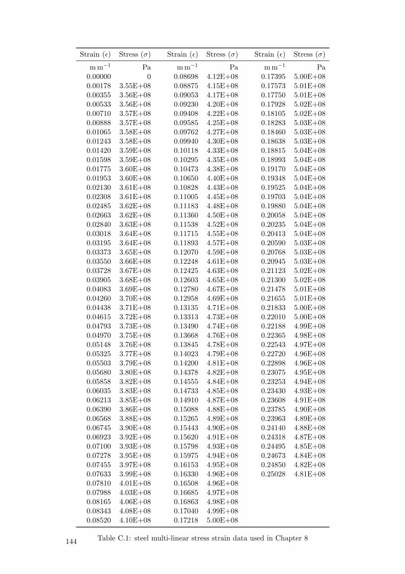
Strain (ε) Stress (σ) Strain (ε) Stress (σ) Strain (ε) Stress (σ)

m m−1 Pa m m−1 Pa m m−1 Pa0.00000 0 0.08698 4.12E+08 0.17395 5.00E+080.00178 3.55E+08 0.08875 4.15E+08 0.17573 5.01E+080.00355 3.56E+08 0.09053 4.17E+08 0.17750 5.01E+080.00533 3.56E+08 0.09230 4.20E+08 0.17928 5.02E+080.00710 3.57E+08 0.09408 4.22E+08 0.18105 5.02E+080.00888 3.57E+08 0.09585 4.25E+08 0.18283 5.03E+080.01065 3.58E+08 0.09762 4.27E+08 0.18460 5.03E+080.01243 3.58E+08 0.09940 4.30E+08 0.18638 5.03E+080.01420 3.59E+08 0.10118 4.33E+08 0.18815 5.04E+080.01598 3.59E+08 0.10295 4.35E+08 0.18993 5.04E+080.01775 3.60E+08 0.10473 4.38E+08 0.19170 5.04E+080.01953 3.60E+08 0.10650 4.40E+08 0.19348 5.04E+080.02130 3.61E+08 0.10828 4.43E+08 0.19525 5.04E+080.02308 3.61E+08 0.11005 4.45E+08 0.19703 5.04E+080.02485 3.62E+08 0.11183 4.48E+08 0.19880 5.04E+080.02663 3.62E+08 0.11360 4.50E+08 0.20058 5.04E+080.02840 3.63E+08 0.11538 4.52E+08 0.20235 5.04E+080.03018 3.64E+08 0.11715 4.55E+08 0.20413 5.04E+080.03195 3.64E+08 0.11893 4.57E+08 0.20590 5.03E+080.03373 3.65E+08 0.12070 4.59E+08 0.20768 5.03E+080.03550 3.66E+08 0.12248 4.61E+08 0.20945 5.03E+080.03728 3.67E+08 0.12425 4.63E+08 0.21123 5.02E+080.03905 3.68E+08 0.12603 4.65E+08 0.21300 5.02E+080.04083 3.69E+08 0.12780 4.67E+08 0.21478 5.01E+080.04260 3.70E+08 0.12958 4.69E+08 0.21655 5.01E+080.04438 3.71E+08 0.13135 4.71E+08 0.21833 5.00E+080.04615 3.72E+08 0.13313 4.73E+08 0.22010 5.00E+080.04793 3.73E+08 0.13490 4.74E+08 0.22188 4.99E+080.04970 3.75E+08 0.13668 4.76E+08 0.22365 4.98E+080.05148 3.76E+08 0.13845 4.78E+08 0.22543 4.97E+080.05325 3.77E+08 0.14023 4.79E+08 0.22720 4.96E+080.05503 3.79E+08 0.14200 4.81E+08 0.22898 4.96E+080.05680 3.80E+08 0.14378 4.82E+08 0.23075 4.95E+080.05858 3.82E+08 0.14555 4.84E+08 0.23253 4.94E+080.06035 3.83E+08 0.14733 4.85E+08 0.23430 4.93E+080.06213 3.85E+08 0.14910 4.87E+08 0.23608 4.91E+080.06390 3.86E+08 0.15088 4.88E+08 0.23785 4.90E+080.06568 3.88E+08 0.15265 4.89E+08 0.23963 4.89E+080.06745 3.90E+08 0.15443 4.90E+08 0.24140 4.88E+080.06923 3.92E+08 0.15620 4.91E+08 0.24318 4.87E+080.07100 3.93E+08 0.15798 4.93E+08 0.24495 4.85E+080.07278 3.95E+08 0.15975 4.94E+08 0.24673 4.84E+080.07455 3.97E+08 0.16153 4.95E+08 0.24850 4.82E+080.07633 3.99E+08 0.16330 4.96E+08 0.25028 4.81E+080.07810 4.01E+08 0.16508 4.96E+080.07988 4.03E+08 0.16685 4.97E+080.08165 4.06E+08 0.16863 4.98E+080.08343 4.08E+08 0.17040 4.99E+080.08520 4.10E+08 0.17218 5.00E+08

Table C.1: steel multi-linear stress strain data used in Chapter 8144

Appendix D

Circumferential displacement of theaxisymmetric imperfection

This appendix section details the formulation that relates the circumferential displacement tothe vertical membrane force of a cylinder with axisymmetric imperfection, the FEM resultsof the same set-up can be found in chapter 7. Assuming the axisymmetric imperfection shapecomprises of a series of hyperboloids and barrels stacked one on top another, one barrel is isolatedas a free body. Further assume that this barrel can be represented by a series of columns, thenpre-buckling displacement due to an initial imperfection can be calculated with equation (D.1).

∆e = ei

(n

n− 1− 1

)(D.1a)

n =Fcr

RF(D.1b)

Figure D.1: Laterally spring support column model

Fcr could be calculated by consider the shell as a series of distributed spring supported columnwith pinned ends as suggested by von Karman (Fig D.1). Solving the differential equation resultsin equation(D.2) [22].

Fcr =π2EI

L2b

[n2 +

(kL4

b

n2π4EI

)](D.2)

Where I is the second moment of area of the rolled out section of the cylinder, lmh3/12, Lb

is the length of a buckle, 2L/m and n is one. The equivalent spring stiffness, k, could be

145

found by substituting Fcr with the maximum reaction force from the FEM analysis. With themaximum reaction force equals to Fcr = 21.79× 106 N, k can be found by solving equation (D.2),k = 217.84 MPa.

k could also be calculated by calculating Fcr using Koiter’s equation (Eq. (D.3)) without aknock-down factor.

Fcr = 0.605Eh

a(D.3)

With these two different Fcrs, the theoretical displacements are plotted in figure D.2. It is

0

0.002

0.004

0.006

0.008

0.01

0 100 200 300 400 500 600 700

Dis

plac

emen

t [m

]

Membrane force [KN / m]

Inward displacementOutward displacementAverage displacementMaximum reaction forceKoiter's equationStiffness k for best fit with average

Figure D.2: Average lateral displacement of the buckles, compared to theoretical values

evident that neither adequately represent the actual displacement. Therefore a best-fit stiffnessk is calculated in the Fcr equation (Eq. (D.2)), k = 1200 MPa. Continuing equation (D.1), wesubstitute the above

Looking at figure D.1, one can construct a moment equilibrium around the bottom of the column,and assuming that the top moment M is zero first.

∑M· = Fcr∆e− Fkl

′= 0 (D.4)

The equivalent spring force can be calculated by integrating individual spring over the wholerange between 0 and l/2. Assuming that the column is deforming parabolically (sinusoidal shapewould also work),

Fk =

∫ l2

0

4∆e

l2z(l − z) dz

Fk =1

3∆e · l

(D.5)

Subtituting Fk back to the equilibrium equation,

0 = Fcr∆e−1

3∆e · l · l′ (D.6)

The ∆e drops out of the equation. This would indicate that the application of force does notchange the displacement which is obviously false. This requires further research.

146

Appendix E

20 Eigenvalues of each 37 models ofdifferent curvatures

147

Curvatu

re1

23

45

67

89

10

11

12

13

14

15

16

17

18

19

20

119.25199.27249.28059.28059.28819.28819.33119.33119.33219.33219.39709.39709.39729.39729.48219.48219.48219.48219.58909.5890

20.758.45728.47758.48058.48058.49048.49048.52398.52398.52618.52618.57938.57938.57978.57978.64958.64958.64968.64968.73648.7364

30.5

7.46547.47977.47977.48067.48887.48887.50917.50917.51207.51207.54687.54687.54757.54757.59417.59417.59427.59427.65227.6522

40.457.22537.23767.23767.23887.24607.24607.26347.26347.26627.26627.29687.29687.29757.29757.33877.33877.33887.33887.39017.3901

50.4

6.97126.98156.98156.98286.98896.98897.00377.00377.00627.00627.03267.03267.03327.03327.06897.06897.06907.06907.11357.1135

60.356.70476.71306.71306.71446.71946.71946.73156.73156.73386.73386.75596.75596.75656.75656.78666.78666.78676.78676.82446.8244

70.3

6.42846.43506.43506.43616.44016.44016.44996.44996.45176.45176.46986.46986.47016.47016.49496.49496.49496.49496.52596.5259

80.256.14606.15096.15096.15186.15486.15486.16246.16246.16376.16376.17796.17796.17816.17816.19766.19766.19776.19776.22226.2222

90.2

5.86195.86535.86535.86615.86825.86825.87375.87375.87475.87475.88515.88515.88535.88535.89995.89995.89995.89995.91815.9181

10

0.155.58095.58325.58325.58465.58615.58615.58865.58865.59045.59045.59635.59635.59775.59775.60635.60635.60775.60775.61885.6188

11

0.1

5.30825.30945.30945.31245.31245.31485.31575.31575.31695.31695.31845.31845.32285.32285.32285.32285.32875.32875.33065.3306

12

0.055.05315.05375.05375.05505.05505.05725.05725.06035.06035.06465.06465.06585.06625.06625.06725.06725.06785.06785.06805.0680

13

0.0254.93684.93714.93714.93794.93794.93924.93924.94114.94114.94404.94404.94504.94504.94554.94554.94574.94574.94694.94694.9478

14

0.0054.85024.85044.85044.85084.85084.85104.85104.85134.85134.85144.85144.85224.85224.85234.85234.85254.85254.85254.85254.8530

15

0.00254.83794.83794.83804.83804.83804.83804.83894.83894.83904.83904.83944.83944.83944.83944.83974.83974.83974.83974.83984.8398

16

0.00054.81914.81914.81964.81964.82064.82064.82084.82084.82084.82084.82244.82244.82274.82274.82424.82424.82564.82564.82644.8264

17

0.00034.81654.81654.81704.81704.81724.81724.81754.81754.81874.81874.82024.82024.82084.82084.82254.82254.82364.82364.82484.8248

18

5E-054.81434.81434.81454.81454.81484.81484.81494.81494.81704.81704.81844.81844.81934.81934.82124.82124.82184.82184.82204.8220

19

04.81374.81374.81384.81384.81414.81414.81444.81444.81654.81654.81804.81804.81894.81894.82084.82084.82094.82094.82124.8212

20

-5E-054.81314.81314.81324.81324.81344.81344.81384.81384.81614.81614.81754.81754.81854.81854.82004.82004.82044.82044.82054.8205

21

-3E-044.81034.81034.81064.81064.81094.81094.81174.81174.81444.81444.81574.81574.81644.81644.81704.81704.81734.81734.81914.8191

22

-5E-044.80674.80674.80714.80714.80794.80794.80904.80904.81194.81194.81224.81224.81344.81344.81354.81354.81514.81514.81684.8168

23

-0.0034.76824.76824.76884.76884.77184.77184.77394.77394.77394.77394.77504.77504.78054.78054.78194.78194.78654.78654.78674.7867

24

-0.0054.69824.69824.69994.69994.70124.70124.70354.70354.70594.70594.70744.70744.72054.72054.72144.72144.72284.72284.72454.7245

25

-0.0253.63703.63703.68703.68703.72963.72963.77533.77533.79963.79963.81103.81103.82343.82343.83463.83463.85553.85553.89193.8919

26

-0.052.59742.59742.67092.67092.73882.73882.78382.78382.78992.78992.80072.80072.82412.82412.83452.83452.84202.84202.90512.9051

27

-0.1

1.83321.83321.85931.85931.86491.86491.88281.88281.94281.94281.96851.96852.03772.03772.07992.07992.09302.09302.15812.1581

28

-0.151.39931.39931.42981.42981.43011.43011.44411.44411.44641.44641.46521.46521.50201.50201.50721.50721.57531.57531.59911.5991

29

-0.2

1.19691.19691.20771.20771.21091.21091.21141.21141.24331.24331.25881.25881.26121.26121.26311.26311.33881.33881.34221.3422

30

-0.251.06761.06761.07361.07361.07571.07571.07591.07591.11181.11181.11391.11391.11841.11841.13181.13181.18061.18061.18521.1852

31

-0.3

0.98210.98210.98600.98600.98760.98760.99360.99361.01971.01971.02651.02651.02741.02741.04511.04511.08381.08381.08541.0854

32

-0.350.92280.92280.92640.92640.93810.93810.93950.93950.96470.96470.96740.96740.97550.97550.97760.97761.01891.01891.02871.0287

33

-0.4

0.88640.88640.89750.89750.89910.89910.90500.90500.92580.92580.92750.92750.93840.93840.94750.94750.98480.98480.99150.9915

34

-0.450.87300.87300.87300.87300.87740.87740.88790.88790.89870.89870.90990.90990.91990.91990.92760.92760.96850.96850.97380.9738

35

-0.5

0.85990.85990.86660.86660.87380.87380.88260.88260.89080.89080.90940.90940.90960.90960.91230.91230.96210.96210.97500.9750

36

-0.750.92470.92470.94320.94320.94920.94920.95310.95310.95990.95990.96590.96590.99860.99861.00731.00731.02581.02581.03821.0382

37

-11.08771.08771.09641.09641.10901.10901.12561.12561.12971.12971.15671.15671.15911.15911.16241.16241.22061.22061.24951.2495

Table

E.1

:M

odel

sof

diff

eren

tcu

rvat

ure

and

thei

ras

soci

ated

20

eige

nva

lues

148

Appendix F

Other Types of Imperfections

F.1 Initial Conditions Deformation Diagrams

(a)

(b)

Figure F.1: (a) Initial stress (b) Initial stress + strain

149

F.2 Loading Imperfection Deformation Diagrams

(a)

(b)

Figure F.2: a=1 (a) Load imperfection (b) Load + geometrical imperfection

(a)

(b)

Figure F.3: a=5 (a) Load imperfection (b) Load + geometrical imperfection

150

(a)

(b)

Figure F.4: a=10 (a) Load imperfection (b) Load + geometrical imperfection

(a)

(b)

Figure F.5: a=25(a) Load imperfection (b) Load + geometrical imperfection

151