econstorMake Your Publications Visible.

A Service of

zbwLeibniz-InformationszentrumWirtschaftLeibniz Information Centrefor Economics

Lutgen, Vanessa; Van der Linden, Bruno

Working Paper

Regional Equilibrium Unemployment Theory at theAge of the Internet

CESifo Working Paper, No. 5326

Provided in Cooperation with:Ifo Institute – Leibniz Institute for Economic Research at the University of Munich

Suggested Citation: Lutgen, Vanessa; Van der Linden, Bruno (2015) : Regional EquilibriumUnemployment Theory at the Age of the Internet, CESifo Working Paper, No. 5326, Center forEconomic Studies and ifo Institute (CESifo), Munich

This Version is available at:http://hdl.handle.net/10419/110814

Standard-Nutzungsbedingungen:

Die Dokumente auf EconStor dürfen zu eigenen wissenschaftlichenZwecken und zum Privatgebrauch gespeichert und kopiert werden.

Sie dürfen die Dokumente nicht für öffentliche oder kommerzielleZwecke vervielfältigen, öffentlich ausstellen, öffentlich zugänglichmachen, vertreiben oder anderweitig nutzen.

Sofern die Verfasser die Dokumente unter Open-Content-Lizenzen(insbesondere CC-Lizenzen) zur Verfügung gestellt haben sollten,gelten abweichend von diesen Nutzungsbedingungen die in der dortgenannten Lizenz gewährten Nutzungsrechte.

Terms of use:

Documents in EconStor may be saved and copied for yourpersonal and scholarly purposes.

You are not to copy documents for public or commercialpurposes, to exhibit the documents publicly, to make thempublicly available on the internet, or to distribute or otherwiseuse the documents in public.

If the documents have been made available under an OpenContent Licence (especially Creative Commons Licences), youmay exercise further usage rights as specified in the indicatedlicence.

www.econstor.eu

Regional Equilibrium Unemployment Theory at the Age of the Internet

Vanessa Lutgen Bruno Van der Linden

CESIFO WORKING PAPER NO. 5326 CATEGORY 4: LABOUR MARKETS

APRIL 2015

An electronic version of the paper may be downloaded • from the SSRN website: www.SSRN.com • from the RePEc website: www.RePEc.org

• from the CESifo website: Twww.CESifo-group.org/wp T

ISSN 2364-1428

CESifo Working Paper No. 5326

Regional Equilibrium Unemployment Theory at the Age of the Internet

Abstract This paper studies equilibrium unemployment in a two-region economy with matching frictions, where workers and jobs are free to move and wages are bargained over. Job-seekers choose between searching locally or searching in both regions. Search-matching externalities are amplified by the latter possibility and by the fact that some workers can simultaneously receive a job offer from each region. The rest of the framework builds upon Moretti (2011). Increasing the matching effectiveness out of the region of residence has an ambiguous impact on unemployment rates. While it reduces the probability of remaining unemployed, it also decreases labor demand because of a lower acceptance rate. We characterize the optimal allocation and conclude that the Hosios condition is not sufficient to restore efficiency. A numerical exercise indicates that the loss in net output is non negligible and rising in the matching effectiveness in the other region.

JEL-Code: J610, J640, R130, R230.

Keywords: matching, non-segmented labor markets, spatial equilibrium, regional economics, unemployment differentials.

Vanessa Lutgen* IRES

Catholic University of Louvain Place Montesquieu 3

Belgium – 1348 Louvain-la-Neuve vanessa.lutgen@uclouvain.be

Bruno Van der Linden FNRS, IRES

Catholic University of Louvain Place Montesquieu 3

Belgium – 1348 Louvain-la-Neuve bruno.vanderlinden@uclouvain.be

*corresponding author April 17, 2015 We thank the editor and two anonymous referees for useful comments and suggestions, which helped us to improve the manuscript. We are grateful to Pierre-Philippe Combes, David de la Croix, Bruno Decreuse, Philipp Kircher, Patrick Kline, Etienne Lehmann, Frank Malherbet, Ioana Marinescu, Enrico Moretti, Olivier Pierrard, Henri Sneessens, Matthias Wrede and Yves Zenou. We also thank participants to various workshops and conferences for their comments on a preliminary version of this paper (The ARC workshop on mobility of factors held in Louvain-la-Neuve, the Search and Matching workshops held in Rouen, in Aix-en-Provence and in Louvain-la-Neuve, the Belgian Day for Labor Economists in Leuven, the 2013 EALE Conference in Turin, the 2014 Search and Matching Conference in Edinburgh and the 2014 EEA-ESEM Conference in Toulouse). The usual disclaimer applies. We acknowledge financial support from the Belgian French-speaking Community (convention ARC 09/14-019 on “Geographical Mobility of Factors”).

1 Introduction

While an abundant literature in urban economics addresses unemployment issues withincities (see Zenou, 2009, for a detailed coverage), less effort has been devoted to analyzethe causes of unemployment at the regional level. “Given the large geographical dif-ferences in the prevalence of unemployment observed in the real world, understandingspatial equilibrium when the labor market does not instantly clear would appear to beof primary importance.” (Kline and Moretti, 2013, p. 239). The main purpose of thispaper is to contribute to this understanding.

The Internet allows both sides of the labor market to find more easily potentialpartners, even faraway, thanks to job boards and meta-search engines.1 Moreover, therecruitment process can now also be conducted online through virtual recruiting tools.2

Marinescu and Rathelot (2014) provide evidence that the distance between the job-seekerand the job vacancy exceeds 100 km (63 miles) in about 10% of the online applicationson CareerBuilder.com. This suggests that a non negligible share of US job-seekers rampup their job search by expanding it over long distances.3

While most of the literature dealing with regional unemployment assumes that peo-ple need to migrate before they can start searching locally, we relax the assumptionof segmented regional labor markets. Our main contribution consists in developing ageneral equilibrium search-matching framework where job-seekers choose whether theysearch in their region of residence only or all over the country. To the best of our knowl-edge, this has not been done yet. In this setting, regions are strongly interdependent andseveral sources of inefficiency explained later are present. A numerical exercise suggestsa non-negligible gap between the efficient and the equilibrium allocations.

As a secondary contribution, our analysis also sheds some light on a puzzle. Expec-tations that the Internet would improve the functioning of the labor market by reducingsearch-matching frictions were great (see e.g. Autor, 2001). A decade later, the evidenceis mixed. Some microeconometric evaluations find that online job search shortens un-employment duration in the US (Kuhn and Mansour, 2014; Choi, 2011). For graduatestudents in Italy, Bagues and Labini (2009) conclude that the use of an online platformreduces the probability of unemployment and raises geographical mobility. However, viaa difference-in-differences approach, Kroft and Pope (2014) find no evidence that therapid expansion of a major online job board (during the years 2005-2007) has affectedcity-level unemployment rates in the US. So, the reasons why improvements at the in-dividual level disappear at a more aggregate level need to be understood. This paperproposes an explanation in a spatial economy.

1 In 2010, 25% of the interviewed Americans who use the Internet declared to do so to find a position(U.S. Census Bureau, 2012, Survey of Income and Program Participation, 2008 Panel). In Europe, in2005, among the unemployed workers, 25% used the Internet to search for a job. This share has increasedto 50% in 2013 (Eurostat, 2014, see http://ec.europa.eu/eurostat/data/database?node_code=isoc_

ci_ac_i).2See e.g. http://variousthingslive.com/virtual-open-house/ and the links on http://hiring.

monster.com/hr/hr-best-practices/recruiting-hiring-advice/acquiring-job-candidates/

virtual-recruitment-strategies.aspx .3The evidence is more mixed for the UK (see Manning and Petrongolo, 2011).

2

We build upon the synthesis of Moretti (2011) who develops a two-region staticspatial equilibrium model a la Rosen (1979)-Roback (1982). Contrary to these authors,Moretti (2011) assumes that the supply of labor is not perfectly elastic. This property isobtained by assuming that economic agents have heterogeneous idiosyncratic preferencesfor regions. The aim of Moretti (2011) is to analyze how local shocks propagate in thelong run to the rest of the economy, with a focus on the labor market. He discussesthe case where agents have different skills, while we keep labor homogeneous. However,regional unemployment disparities are not studied by Moretti. We introduce search-matching frictions and wage bargaining within this framework (Pissarides, 2000) but weabstract from the housing market.

Contrary to most of the search and matching literature, the spatial heterogeneity isexplicit in our framework. In each region, imperfect information and lack of coordinationamong agents create frictions summarized by a constant-returns-to-scale regional-specificmatching function in which the number of job-seekers is a weighted sum of the residentsand of the non-residents who decide to search all over the country, both numbers beingendogenous. We characterize the equilibrium. We show how regional unemploymentdifferentials are affected by the partition of the population between the two regions andbetween the statuses of national and regional job-seekers. We also conclude that a risein matching effectiveness out of the region of residence has an ambiguous effect on theunemployment rates. It decreases the probability of remaining unemployed but it alsoreduces labor demand through a lower acceptance rate of job offers. This ambiguityechoes the main conclusion of Kroft and Pope (2014).

In the standard search-matching literature, frictions generate congestion externalitieswhich are not internalized by decentralized agents unless the Hosios (1990) condition ismet. As soon as some workers search all over the country, new sources of inefficiencyarise. First, when decentralized agents decide whether to search nationally, they lookat their private interest and ignore the consequences of their choices on job creation inall regions. Second, when opening vacancies in a region, firms do not internalize thechanges in the matching probability and hence in net output in the rest of the economy.We show that the Hosios condition is never sufficient to decentralize the constrainedefficient allocation.

We develop a numerical exercise for a very stylized US economy made of two regionsthat are initially symmetric and where the Hosios condition prevails. The decentralizedeconomy appears to be far from efficient. For a very wide range of parameters, efficiencyrequires that nobody searches in the whole country while 10% of the workforce does it inthe decentralized economy. Furthermore, the efficient unemployment rate level is lowerthan the decentralized one. As this exercise assumes symmetric regions, this conclusionis not in contradiction with the recent evidence that geographical mismatch is negligiblein the US (see e.g. Sahin et al., 2014, Marinescu and Rathelot, 2014 and Nenov, 2014).

Although a spatial equilibrium model with genuine unemployment has for long beenmissing, some papers have recently partly filled the gap. Leaving aside the literaturewhere regions are so close that commuting is an alternative to relocation, the literatureabout regional unemployment differentials can be divided in two groups according to the

3

type of search: either one needs to move before starting to seek a job in the region ofresidence or one can search all over the country and then move if needed.

In the first case, some papers extend the island model of Lucas and Prescott (1974)whose economy is populated by a large number of segmented perfectly competitive labormarkets where only labor is mobile (workers being allowed to visit only one island perperiod). Lkhagvasuren (2012) adds search-matching frictions as well as match-locationspecific productivity shocks in an otherwise standard islands model to reproduce thevolatility of unemployment rates in the United States. Focusing also on one (small)region out of many, Wrede (2014) studies the relationships between wages, rents, un-employment and the quality of life in a dynamic framework. He assumes a standardsearch-matching framework and analyzes how regional amenities affect unemploymentand the quality of life. Beaudry et al. (2014) introduce search-matching frictions in aspatial equilibrium setting with wage bargaining, free mobility of jobs, a very stylizedhousing market, and amenities with congestion externalities. In their paper, with someexogenous probability, the jobless population gets the opportunity to move to anothercity in order to seek jobs, while we let agents choose between two strategies: regionaland national search. Furthermore, Beaudry et al. (2014) do not look at efficiency whilewe do. Kline and Moretti (2013) develop a matching model to characterize the optimal(fixed) hiring cost and to look at the rationale for place-based hiring subsidies. Finally,Kline and Moretti (2014) provide a two-region model in which workers have idiosyncraticpreferences for a region and are mobile. They use the model for policy purposes, namelyto show that place-based policies are not always welfare improving for the whole country.This is due to the fact that taxes generate a deadweight loss.

Second, some recent papers assume that workers can seek a job in the whole country.In a setting with many regions, Amior (2012) studies wages’ responses to a housingshock in the presence of skill heterogeneity. He assumes national search in a search-matching framework as well as a random migration cost. Domingues Dos Santos (2011)builds a search-matching dynamic framework with two regions that are each consideredas a line. She finds that increasing search effectiveness is beneficial for unemploymentrates in both regions. However, she keeps wages exogenous. Using a search-matchingdynamic framework with national search and endogenous wages, Antoun (2010) assumestwo types of agents who differ in their preference for a region. He finds that a positiveproductivity shock in one region decreases unemployment locally but raises it in theother region. We extend these models by endogenizing the choice between regional andnational search under wage bargaining.4 Contrary to these papers, we also develop anormative analysis by looking at efficiency. However, we keep our framework static whilethey all assume a dynamic setting.

In the new economic geography literature, Epifani and Gancia (2005) analyze thesimultaneous emergence of both agglomeration economies and unemployment rate dif-

4Molho (2001) develops a partial equilibrium job-search framework with both types of search. Man-ning and Petrongolo (2011) build a partial equilibrium framework where job-seekers choose their searchfield. See also Marinescu and Rathelot (2014). We share a common interest with these papers in ageneral equilibrium model with endogenous wages and vacancies.

4

ferentials. For this purpose, they build a dynamic two-sector two-region model withtransport costs and search-matching frictions. They assume a congestion effect in theutility which could reflect the housing market. They emphasize the role of migrationfollowing a productivity shock, which raises the unemployment rate in the short run butdecreases it in the long run. Francis (2009) extends this framework to endogenous jobdestruction.

Galenianos and Kircher (2009) build a directed-search wage-posting model whereworkers simultaneously apply to a N > 1 jobs. They show that multiple applications leadto an inefficient allocation when a vacancy remains unmatched if the job applicant refusesthe offer (an assumption revisited by Kircher, 2009). We stick to the random matchingassumption with wage bargaining popularized by Pissarides (2000). More importantly,by assumption in our paper, the search for an efficient allocation is constrained by thefree choice of agents when they get two job offers. So, the possibility of unmatchedvacancies is common to both the decentralized equilibrium and the efficient allocation.

The rest of this paper is organized as follows. Section 2 describes the model and itsequilibrium. We first focus on a symmetric equilibrium, to highlight the main mecha-nisms. We then turn to the case of asymmetric regions. Section 3 studies efficiency. Anumerical analysis is conducted in Section 4. Section 5 discusses some extensions to theframework of Section 2. Section 6 concludes.

2 The model

This section develops a model with two distant regions. We first introduce the mainassumptions and the matching process. Then, we develop a simple version of the modelwith symmetric regions and derive the symmetric equilibrium. We allow for differencesacross regions in a last subsection.

We consider a static model of an economy made of two large regions (i ∈ {1, 2}).Each region is a point in space. The distance between the two regions is such thatcommuting is ruled out, while inter-regional migration is allowed. Topel (1986) andKennan and Walker (2011) among others have stressed the importance of migrationcosts. As will soon be clear, idiosyncratic preferences for regions will in our setup playthe role of individual-specific relocation costs. The aggregate national labor force ismade of an exogenous large number N of homogeneous risk-neutral workers. A workerliving in region i supplies one unit of labor if the wage is above the value of time if shestays at home, denoted bi. Firms are free to locate in the region they prefer. They uselabor to produce a unique consumption good which is sold in a competitive market andtaken as the numeraire.

Workers have idiosyncratic preference for regions. Agent j gets utility cij from livingin region i. As Moretti (2011), we assume that the relative preference for region 1over region 2, c1j − c2j , is uniformly distributed on a given support [−v; v] , v > 0.The presence of a distribution of relative preferences implies that the elasticity of inter-regional labor mobility is finite. A higher value of v entails less intense responses toregional differences.

5

The indirect utility V eij of an employed individual j living in region i is, as in Moretti

(2011), assumed to be additive and defined by:

V eij = wij + ai + cij (1)

where wij represents the wage earned by agent j in region i and ai is a measure ofexogenous local consumption amenities in region i, such as the climate. These amenitiesare public goods and are not affected by the number of inhabitants in a region (norivalry).5 Similarly, the indirect utility V u

ij of an unemployed person j residing in regioni is:

V uij = bi + ai + cij . (2)

In each regional labor market, we assume a regional-specific random matching pro-cess. Adopting a one-job-one-firm setting, firms decide in which region they open atmost one vacancy. The cost κi of opening a vacancy is constant, exogenous and regional-specific.6 Throughout the paper, we assume constant returns in the production of theconsumption good.7 If the vacancy is filled, a firm produces yi > bi units of the consump-tion good. So, depending on the origin of the worker, a firm makes a profit Jij = yi−wijon a filled position.

2.1 The timing of decisions

At the beginning of the unique period, everybody is unemployed, chooses in which regionto reside, and decides to search for a job either regionally or nationally (i.e. either oneonly searches for a job in the region where one lives or one searches in both regionsat the same time). The reason why some workers would only search in their region ofresidence rather than nationally is intuitive. If a worker has a sufficiently strong relativeidiosyncratic preference for her region of residence, she will not accept to migrate to takea position. Since, following Decreuse (2008), we assume a small cost of refusing a joboffer, this individual will then not take part in the matching process in the other region.

In a second step, firms open vacancies and possibly meet a worker. This processoccurs simultaneously in both regions. If a vacancy meets a job-seeker, this worker thenaccepts or not the job offer. When a match is formed with a job-seeker who does notlive in the firm’s region, this worker relocates. Allowing unemployed workers to relocateat this stage would complicate the exposition without yielding more insights. After the

5Contrary to what is sometimes done in the literature (see e.g. Wrede, 2014 or Brueckner andNeumark, 2014), amenities ai do not affect the production function either.

6Capital is assumed to move freely across regions through vacancy creation. Ignoring credit marketimperfections, entrepreneurs have no problem financing their vacancy cost κi.

7Although very standard in the search-matching literature, this assumption does not account for anempirical regularity according to which firms are more productive in larger cities. The elasticity is quitesmall, especially when controlling for characteristics such as education, but differences in populationsizes can be substantial. In the US however, Beaudry et al. (2014) find no significant evidence ofagglomeration effects on productivity (over 10-year periods). So, we think that our assumption is nottoo strong a simplification, at least in the US context.

6

relocation step, employed workers and firms bargain over wages. Fourth, productiontakes place and good markets clear.

The moment at which wages are negotiated matters when a relocation of the workeris involved. If this moment occurs before the decision to migrate is taken, throughNash bargaining, the worker will get a partial compensation for the difference in theregional non-wage components of utility ai + cij . To implement this timing, one hasto assume that the employer is aware of the idiosyncratic preferences of the worker forboth regions. One can doubt that this information is available.8 A survey conductedby CareerBuilder.com at the end 2011 indicates that less then a third of employers areready to pay for relocation costs of their new employees.9 This is casual evidence infavor of the timing indicated above: The bargained wage will then not compensate theworker for the difference in ai + cij and hence wij can be written simply as wi. We willreturn to the timing of the wage bargain in Section 3.

Some additional notations have to be introduced. Before the matching process, Ni

agents choose to reside in region i (Ni is called the ex-ante population in region i, withN1 +N2 = N). Population in region i is composed of NN

i agents who search nationallyand NR

i individuals who only search in their region of residence (Ni = NNi +NR

i ). Foragents located in region i, the notation −i will designate the other region.

2.2 The matching process

We allow for distant search, meaning that search in a region can be conducted while livingin the other one. The matching effectiveness of those living in the region where vacanciesare open is normalized to one. For residents of the other region, this effectiveness takesan exogenous value α with 0 ≤ α ≤ 1. The main focus is here on strictly positive valuesof α.10 The number of hirings in each region is given by a regional-specific matchingfunction Mi(·, ·) with:

Mi(Vi, Ni + αNN−i) < min{Vi, Ni + αNN

−i}, i ∈ {1, 2}, (3)

where Vi represents the endogenous number of vacancies opened in region i andNi+αNN−i

is the endogenous number of job-seekers measured in efficiency units. As Molho (2001)and Manning and Petrongolo (2011) do in a partial equilibrium framework, we endog-enize search effort by letting job-seekers choose their search field. Following Pissarides(2000) and a large empirical literature, the matching function has constant returns toscale11 and is increasing and concave in both arguments. Defining tightness in region ias

θi =Vi

Ni + αNN−i,

8Notice that if the framework was dynamic this timing would raise another issue. Under the standardassumption of automatic renegotiation (Pissarides 2000, p. 15), the wage would be revised after therelocation step and would be chosen exactly as proposed in the timing of events we privilege.

9See http://www.careerbuilder.com/share/aboutus/pressreleasesdetail.aspx?id=pr677&sd=

1/18/2012&ed=1/18/2099&siteid=cbpr&sc_cmp1=cb_pr677_.10Subsection 2.3 of Lutgen and Van der Linden (2013) discusses the case α = 0 in detail.11 Manning and Petrongolo (2011) provide recent evidence at the local level for the UK.

7

mi(θi) designates the probability Mi/Vi that a vacancy in region i meets a worker, with0 < mi(θi) < 1 by the inequality in (3) and m′i(θi) < 0 because of search-matchingcongestion externalities. So, unfilled jobs find a partner more easily in a region able toattract more job-seekers. The probability that an unemployed worker living in i meetsa firm located in region i is pi(θi) = θimi(θi), with 0 < pi(θi) < 1. Job-seekers find ajob more easily in a thicker local labor market: [pi(θi)]

′ > 0.12 The probability that anunemployed worker searching nationally and living in −i meets a firm settled in regioni is αpi(θi). In case of national search, for someone living in i, the probability of gettingan offer in i and no offer from the other region is pi(θi)(1− αp−i(θ−i)). The probabilityof the opposite event is αp−i(θ−i)(1 − pi(θi)). The probability of getting an offer fromeach region is αpi(θi)p−i(θ−i). In this case, the worker accepts the position that offersthe highest indirect utility level. Finally, this worker living in i faces a probability(1− pi(θi))(1− αp−i(θ−i)) of remaining unemployed.

2.3 A model with symmetric regions

Before discussing the general case of asymmetric regions, let us consider the case of thesymmetric equilibrium. The main effects of a rise in matching effectiveness out of theregion of residence already appear in this framework (in which, when not necessary, wedrop the region subscript i).

2.3.1 Wage bargaining

Individual Nash bargaining takes place ex-post, once the cost of opening a vacancy issunk. So, when a vacancy and a job-seeker j have met, the wage solves the followingmaximization:

maxwj

(V ej − V u

j )β(J − V )1−β

where V is the value of an unfilled vacancy and β ∈ [0, 1) denotes the bargaining powerof a worker. The first-order condition can be rewritten as:

wj = w = βy + (1− β)b− βV. (4)

Hence, the wage is independent of the worker’s preferences. As w > b, under free-entry,workers always take the position.

2.3.2 Acceptation decision

A worker searching locally always accepts a job offer, as V ej > V u

j in a free-entry equilib-rium with Nash bargaining. Similarly, a worker searching nationally who only gets a joboffer from a firm located in the region where she lives always takes the position. In casethis worker only receives a job offer from a firm settled in the other region, she always

12As is standard, we assume Inada conditions: limθ→0

m(θ) = 1; limθ→0

p(θ) = 0; limθ→+∞

m(θ) =

0; limθ→+∞

p(θ) = 1.

8

accepts the job, as she decided to search for a job there (as shown in Appendix A). Incase a worker gets two job offers, she decides which position to take to maximize herutility in employment (1). When regions are symmetric, the only variables that matterare preferences. One thus gets:

Lemma 1. Acceptance decisions in case of symmetric regions

When receiving two job offers, a worker j

• accepts the position in region 2 if c1j − c2j < 0,

• takes the job in region 1 otherwise.

2.3.3 Opening of vacancies

The expected value of a vacant position V is equal to −κ+πm(θ)(y−w). π correspondsto the probability that meeting a worker leads to a filled vacancy. Firms open vacanciesfreely until this value V is nil. Anticipating correctly the outcome of the wage bargain,the free-entry condition becomes:

κ

(1− β)(y − b)= πm(θ). (5)

The probability of filling a vacancy πm(θ) increases with the (ex-post) surplus of a matchy− b and decreases with the cost of opening a vacancy κ and workers’ bargaining powerβ.

2.3.4 Search and location decisions

Appendix A shows that taking search and location decisions simultaneously or choosingfirst the location and then the searching area is equivalent (the proof is given for thegeneral case of asymmetric regions). Therefore, to ease the exposition, the presentationbelow opts for the second timing.

Search decision When deciding whether to search or not in the other region, aworker maximizes her expected utility as regional or national job-seeker. Let pi be ashort notation for pi(θi). The expected utility if the agent located in i searches nationallyis

pi(1−αp−i)V eij+αp−i(1−pi)V e

−ij+αpip−i(max{V e−ij ;V

eij

}−ε)+(1−pi)(1−αp−i)V u

ij , (6)

where ε stands for the small cost of refusing a job offer.The expected utility of a job-seeker living in region i and searching for a job in this region only is

piVeij + (1− pi)V u

ij . (7)

When the small cost of refusing a job offer ε tends to zero, someone searches nation-ally if her relative preference for region i over region −i, cij − c−ij , is above a threshold

9

z equal to w − b. Otherwise, she decides to look for a job in region i only. Perfectlyanticipating the wage (4), under free-entry, let zβ(y − b). Defining

z1 = −z and z2 = z, (8)

the following lemma applies.

Lemma 2. When α > 0 and the cost of refusing an offer ε → 0. Assuming that bothzi’s lie in (−v, v),

• If c1j − c2j < z1, agent j searches in region 2 only;

• If z1 ≤ c1j − c2j ≤ z2, agent j searches nationally;

• If c1j − c2j > z2, agent j searches in region 1 only.

The number of regional job seekers in each region is given by:

NR =v − z

2vN (9)

By comparing their expected utility in case of regional and national search, unemployedworkers turn out to compare the utility levels when they are actually employed in theother region and when they remain unemployed in their region of residence. These utilitylevels are not in expected terms and so search decisions are independent of probabilities toget a job offer.13 Therefore, the number of workers who search nationally is independentof the matching effectiveness α > 0.14 A higher wage relative to home production yieldsa higher threshold z, implying that a lower number of workers search for a job regionally.

Location choice As an unemployed worker who decides to look for a job regionallyonly locates in her region of search, we have to compare the expected utility of an agentj who searches nationally while being located in region 1 or in region 2. These expectedutility levels are given by (6), for i = {1, 2}. As regions are symmetric, the problemsimplifies to c1j Q c2j . One gets the following result:

Lemma 3. Location choice when regions are symmetric

• If c1j − c2j < 0, then agent j locates in region 2;

• Else, worker j settles in region 1.

The size of the population is therefore equal in both regions.

13If ε was non negligible, these probabilities would however play a role in the definition of the zi’s.14This would still be true if ε was non negligible. When α is nil, searching all over the country cannot

be ruled out but the probability of finding a job in the other region is zero. So, every job-seeker searcheslocally.

10

2.3.5 Acceptance probability, vacancy creation and unemployment rates

A detailed explanation is provided in Appendix C. The number of job-seekers for a firmis v + αz in efficiency units. As we have seen, a worker located in a region alwaysaccepts the position there. The workers located in the other region accepts the positionif they did not get an offer from a firm located in their region of residence (probabilityp). Denoting by π the acceptance rate conditional on the meeting, one gets

π = 1− αpz

v + αz(10)

When workers cannot search out of their region of residence (i.e. α = 0), the acceptancerate is 1. When the probability p of meeting a vacancy increases, the acceptance rateshrinks. The same holds for a rise in α. In both cases, the increase leads to a highernumber of workers that get two job offers. Because these workers have to refuse one ofthe two, the acceptance rate goes down.

Combining (5) with (10) leads to the following free-entry condition:

κ

(1− β)(y − b)=v + α(1− p)z

v + αzm(θ) (11)

Because α affects negatively the acceptance rate, a rise in the matching effectivenessleads to a lower equilibrium tightness. So does a rise in κ.

The unemployment rate in a region can be written as:

u =(1− p)(v − αpz)

v(12)

To construct this rate, one needs to notice that because regions are symmetric, thepopulation leaving ex-post in a region is N/2. Regarding the number of unemployed, itis equal to (1− p)NR + (1− p)(1− αp)NN , with

NN = N/2−NR = (z/v)(N/2) (13)

A higher tightness or a higher matching effectiveness out of the region of residenceα yields, other things equal, lower unemployment rates.

2.3.6 Equilibrium and impact of a shock to the matching effectiveness

Definition 1. An interior equilibrium is a vector {w, θ, u,NR, NN} and a scalar z thatsatisfies equations (4) under free-entry V = 0, (8), (9), (11),(12) and (13).

This equilibrium exists and is unique whenever v > β(y − b) (see Appendix E). Itis determined recursively. Once w and z are computed, tightness θ is determined usingthe free-entry condition (11), which allows to set uniquely u.

Proposition 1. When regions are symmetric, a rise in the matching effectiveness inthe other region α has an ambiguous effect on the equilibrium unemployment rates.

11

1 𝑚(𝜃)

𝜋 𝛼, 𝜃 𝑚(𝜃) 𝜃

𝜋 𝛼, 𝜃 𝑚(𝜃)

𝑢(𝜃, 𝛼)

𝑢(𝜃, 𝛼)

𝑢(𝜃, 0)

1

𝑢0 𝑢1

𝜅

1 − 𝛽 (𝑦 − 𝑏)

𝜃0 𝜃1

Figure 1: The symmetric equilibrium: α = 0 (π = 1; the black curves) versus α > 0(π < 1; the red curves).

The consequences of increasing the matching effectiveness can be shown graphicallyin this simple economy. In the upper part of Figure 1, we draw the left-hand side of(11) when α = 0 (in black) and when 0 < α ≤ 1 (in red). A rise in α induces a leftwardshift of the curve. The equilibrium level of tightness therefore declines because theacceptance rate π shrinks with α. The lower part of the figure draws (12) and illustratesthe favorable partial effect of a rise in α on the unemployment rate conditional ontightness. Depending on the importance of the shifts of the two curves the equilibriumunemployment rate can vary in both directions.

If α = 0 (resp., α > 0) can be interpreted as a world without (resp., with) themodern communication technologies using the Internet, Figure 1 illustrates that theintroduction of these technologies can have ambiguous effects on the regional equilibriumunemployment rates. This is a way of rationalizing the results of Kroft and Pope (2014).

2.4 A model with asymmetric regions

This section highlights the main differences with respect to the symmetric case andshows how the main conclusions from a shock on α are affected. We solve the problemby backwards induction.

12

The generalized Nash bargaining process is now given by

maxwi

(V eij − V u

ij )βi(Ji − Vi)1−βi .

The first-order condition can be rewritten as:

wi = βiyi + (1− βi)bi − βiVi. (14)

The conclusions drawn in the previous subsection still holds: wages are independent ofworker’s preferences and are a positive function of the worker’s bargaining power andproductivity. Wages in region i do not depend on the conditions in the other region.

2.4.1 Acceptance of a job offer

If a worker searching nationally gets two offers, one from each region, she rejects oneof them (incurring an arbitrary small cost ε) and accepts the other one. To take thisdecision, the unemployed worker compares V e

1j with V e2j . The agent whose relative pref-

erence c1j − c2j is above the threshold w2 − w1 + a2 − a1 chooses to work in region 1rather than in region 2. Let ∆ = b2 − b1 + a2 − a1.

Lemma 4. When a job-seeker searching nationally has one job offer from each region,there is a threshold

x = ∆ + β2(y2 − b2)− β1(y1 − b1), (15)

assumed to be in (−v, v), such that she accepts the job offer in region 2 if c1j − c2j < x.Otherwise, she accepts the job offer in region 1.

The higher the worker’s share of the surplus in region 2 or the higher ∆, the morepeople will accept the position in region 2 when getting two job offers.

2.4.2 Vacancy creation

Firms open vacancies in region i until the expected gain Vi is nil (i ∈ {1, 2}). Combining(14) and the free-entry condition yields

κi(1− βi)mi(θi)

= πi(yi − bi), ∀i ∈ {1, 2}, (16)

where πi is the conditional acceptance rate in region i. The rate at which vacancies areon average filled, πimi(θi), varies as in the previous subsection with the parameters in i.

2.4.3 Search decision and location choice

Search decision An individual j living in region 2 decides to search regionally ornationally by comparing the expected utility in both cases (Equations (6) and (7) fori = 2). When the small cost of refusing a job offer ε tends to zero, someone searchesnationally if her relative preference for region 1 over region 2, c1j − c2j , is above a

13

threshold z1 = b2 − w1 + a2 − a1. Otherwise, she decides to look for a job in region 2only. This is shown in Appendix A (the comparison of cases e and f).

A similar development is conducted for a worker settled in region 1. A job-seekerliving in region 1 whose relative preference for region 1 over region 2 is higher than athreshold z2 = w2 − b1 + a2 − a1 searches in region 1 only. Below this threshold, theworker looks for a job in the whole country (see the comparison of cases a and c inAppendix A).

Under perfect anticipation of bargained wages and free-entry, let now the zi thresh-olds become:

z1 = β1(b1 − y1) + ∆ and z2 = β2(y2 − b2) + ∆ (17)

Then, Lemma 2 applies. The shares of these three groups in the total population arev+z12v for regional job-seekers in region 2, z2−z1

2v for national ones and v−z22v for regional

job-seekers in 1. Remembering (15), it is easily seen that z1 ≤ x ≤ z2.A rise in relative amenity levels in region 2, a2−a1, leads to more regional job-seekers

in region 2, less regional job-seekers in region 1 but leaves the number of national onesunchanged. A rise in the expected surplus of a match in region 1 does not affect thedecision to search or not in region 2 (the threshold z2 remains constant)but implies lessregional job-seekers living in 2. Finally, a rise in α still has no impact on the z thresholds.

Location choice The same comparison as in the symmetric case leads to the fol-lowing lemma.

Lemma 5. If relative idiosyncratic preference c1j − c2j < x, agent j chooses to residein region 2, where

x = ∆ +1− α

1− αp1 − αp2 + αp1p2(p2β2(y2 − b2)− p1β1(y1 − b1)) , (18)

with 0 ≤ 1−α1−αp1−αp2+αp1p2 < 1 and, by (17), z1 ≤ x ≤ z2. Otherwise agent j settles in

region 1. The share of the population living ex-ante in region 2 (respectively, 1) is thenv+x2v (respectively v−x

2v ).

Compared to the symmetric case where x was equal to 0, we see that regional dif-ferences matter. Notice that when search is equally efficient wherever one looks for ajob (i.e. α = 1), differences in wages and levels of tightness do not impact the worker’slocation decision. An increase in relative amenities in region 2, a2 − a1, as well as arise (respectively, a drop) in the value of home production in region 2 (resp., 1) inducemore workers to locate in 2 ex-ante. A rise in α attracts more workers in region 1 ifp2β2(y2 − b2) − p1β1(y1 − b1) > 0 and conversely.15 An increase in tightness in region1 has several effects if 0 < α < 1. First, if one lives in region 1, the increase in theprobability of being employed in this region equals the decrease in the probability of

15When this inequality holds, a rise in α augments the chances of benefiting from the better employ-ment prospects in region 2 while staying in the first one.

14

being unemployed. As the individual stays in the same region, the net gain is propor-tional to w1− b1. Second, if one lives in region 2, the increase in the probability of beingemployed in region 1 equals the decrease in the probability of staying unemployed inregion 2. This effect is proportional to V e

1j −V u2j . Third, the decline in the probability of

being employed in 2 is the same wherever one lives. So, this effect cancels out. The firstand the second effects push the difference in idiosyncratic preference of the indifferentagent, x, in opposite directions so that the net effect is ambiguous. This conclusion alsoholds if θ2 increases. However, the first effect described just above dominates if α issufficiently small.16

Proposition 2. When 0 < α < 1, a tighter labor market in region i induces more peopleto reside there under the following sufficient condition:

α < 1− (β1(y1 − b1)− β2(y2 − b2))2

(β1(y1 − b1) + β2(y2 − b2))2. (19)

When α = 1, the levels of tightness do not influence the choice of residence any more.

The proof is provided in Appendix B. Recalling (18), Condition (19) is easy tointerpret: The higher the inter-regional difference in workers’ shares in the surpluses,17

the lower α should be in order to get the intuitive relations between the levels of tightnessand x.

2.4.4 Summary of the acceptance, search and location decisions

Combining Lemmas 2 and 5, the total labor force is made of four groups with distinctbehaviors:

Proposition 3. Partition of the population

• If c1j − c2j < z1, agent j locates in region 2 and searches there only;

• If z1 ≤ c1j − c2j < x, agent j settles in region 2 and searches in the whole country;

• If x ≤ c1j − c2j ≤ z2, agent j locates in region 1 and looks for a job nationally;

• If c1j − c2j > z2, agent j settles in region 1 and looks for a job in region 1 only.

Figure 2 illustrates this partition of the total population if −v < z1, z2 < v.

In general, one cannot rank threshold values x and x since x varies with the levelsof tightness. When α = 1 and regions are asymmetric, the comparison of the thresholdsis obvious since x = ∆ then : x ≶ x⇔ β2(y2 − b2)− β1(y1 − b1) ≶ 0.

16We thank one of the anonymous referees who suggested to study this condition.17Compared to the sum of these shares in the 2 regions.

15

Figure 2: The partition of the population in case of an interior solution.

2.4.5 Acceptance probability and vacancy creation

A detailed explanation is provided in Appendix C. Consider again a vacant position inregion 1. The mass of job-seekers searching for a job in 1 is now [v−x+α(x−z1)][N/2v]in efficiency units. Conditional on meeting one of these unemployed workers, all thosewhose relative preference c1j − c2j lies above x accept for sure an offer from region 1.For those between z1 and x, this is only the case if they get no offer from region 2. So,conditional on a contact between a vacancy in region 1 and a job-seeker, the acceptanceprobability π1 is (with a corresponding expression for π2):

π1 = 1− αp2(x− z1)v − x+ α(x− z1)

(20)

π2 = 1− αp1(z2 − x)

v + x+ α(z2 − x)(21)

It is easily checked that the higher x, the more workers accept job offers in region 2and so the lower the acceptance rate in 1. The same is true for x. The higher thenumber of workers searching in region 2 only (an increasing function of z1), the higherthe acceptance rate in 1. Finally, an increase in the probability of getting a job offerin region 2 decreases the acceptance rate in region 1. Similarly, π2 increases with xand x and decreases with z2 and p1. The impact of the matching effectiveness α shouldbe stressed: A higher α leads to a lower conditional acceptance probability, as theprobability of getting two job offers increases. Conversely, limα→0 πi = 1.

Combining (16) with (20)-(21) leads to the following free-entry conditions:

κ1(1− β1)m1(θ1)

=v − x+ α(x− z1)− αp2(θ2)(x− z1)

v − x+ α(x− z1)(y1 − b1) (22)

κ2(1− β2)m2(θ2)

=v + x+ α(z2 − x)− αp1(θ1)(z2 − x)

v + x+ α(z2 − x)(y2 − b2) (23)

16

Through the endogenous acceptance rate, vacancy creation in any region is now affectedby the level of tightness and the value of parameters in the other region.

2.4.6 Populations and unemployment rates

Since z1 ≤ x ≤ z2, and assuming an interior solution, the sizes NNi of the workforce

searching nationally and NRi of those searching in their region of residence only are

given by:

NR1 =

(v − z2)2v

N NN1 =

(z2 − x)

2vN (24)

NR2 =

(z1 + v)

2vN NN

2 =(x− z1)

2vN (25)

so that the total ex-ante population sizes are N1 = NN1 + NR

1 = v−x2v N and N2 =

NN2 +NR

2 = v+x2v N , with N1 +N2 = N .

The unemployment rates which are the ratio of the number of (ex-post) unemployedworkers over the (ex-post) population, are:

u1 =(1− p1)(v − x− αp2(z2 − x))

v − x− αp2(1− p1)(z2 − x) + αp1(1− p2)(x− z1) + αp1p2(x− x)(26)

u2 =(1− p2)(v + x− αp1(x− z1))

v + x+ αp2(1− p1)(z2 − x)− αp1(1− p2)(x− z1)− αp1p2(x− x)(27)

The number of (ex-post) unemployed workers in, say, region 1 is composed of the agentsliving ex-ante in 1 who did not get a job offer in region 1, (1 − p1)

v−x2v N , to which

we subtract the workers who did not get an offer from region 1 but well from region 2(αp2(1 − p1) z2−x2v N). The denominator corresponds to the population living ex-post inthe region (up to a N/2v term). Ex-post, the number of inhabitants in, say, region 1 isthe sum of 4 terms. The first term represents the population living ex-ante in region1. The second term corresponds to the workers who were living ex-ante in 1 and wholeave region 1 as they only get a position in region 2. The third term is composed of theagents who lived ex-ante in region 2 and who move as they only get an offer from region1. Finally, the fourth term represents the number of workers who get two offers. Thisterm is positive whenever x > x, meaning that some more workers living in 2 ex-anteaccept a position in region 1.

The following lemma provides the signs of the partial derivatives of (26) and (27)with respect to the other endogenous variables and α.18

Lemma 6. When α > 0 and regions are asymmetric, the unemployment rate ui de-creases with the level of tightness θi in the same region. A rise in the matching effec-tiveness α lowers both regional unemployment rates. Furthermore, (i) The sign of thecross-derivatives ∂ui/∂θ−i varies with the sign of p2β2(y2 − b2) − p1β1(y1 − b1) (moreon this below). (ii) A rise in the threshold x (i.e. a bigger workforce N2 living ex-ante

18The proof, which is available upon request, consists in reorganizing these partial derivatives.

17

in region 2) decreases the unemployment rate in region 1 while it increases it in region2. (iii) An increase in the number of regional job-seekers increases the unemploymentrate in both regions. (iv) The unemployment rate in region 1 increases with x, while theopposite holds for the unemployment rate in region 2.

An increase in region i’s labor market tightness θi boosts the probability that aworker living in region i finds a job there and it rises the probability that a workerlocated in the other region gets a position in region i (which increases the labor forceliving in region i). Consequently, the unemployment rate in region i goes down. Turningto Property (i) of Lemma 6, augmenting θ−i rises the probability of leaving region i andthis reduces both the number of unemployed workers and the size of the labor forcein region i. The net effect on the unemployment rate depends on the inter-regionaldifference in the gains piβi(yi − bi). More precisely, Appendix D shows that

p2β2(y2 − b2) < p1β1(y1 − b1)⇒∂u1∂θ2

< 0, limα→0+

∂u2∂θ1

> 0 and limα→1

∂u2∂θ1

< 0, (28)

p2β2(y2 − b2) > p1β1(y1 − b1)⇒∂u2∂θ1

< 0, limα→0+

∂u1∂θ2

> 0 and limα→1

∂u1∂θ2

< 0. (29)

Consequently, the cross-partial derivatives are both negative when α is big enough.When α = 0, the unemployment rate in a region does not depend on tightness in theother. However, for sufficiently small positive values of α, one cross-derivative ∂ui/∂θ−iis positive.

As x goes up (Property (ii)), the number N1 of agents living ex-ante in region 1shrinks while N2 increases. These population sizes are (up to a N/2v term) present inthe numerators and the denominators of (26) and (27). In addition, a rise in x affects thenumbers of national job-seekers who depletes the regional workforces if they are recruitedin the other region. All in all, a rise in x reduces (resp., increases) the unemploymentrate in region 1 (resp., 2). A corollary of Property (iii) is that more workers searchingall over the country reduces the unemployment rates in both regions. These propertiesas well as the favorable role of α on the unemployment rates are conditional on the otherendogenous variables.

In a standard Mortensen-Pissarides setting (where geographical heterogeneities areconcealed in an aggregate matching function), the size of the labor force does not af-fect the equilibrium unemployment rate (as eventually the number of vacancies risesproportionately, leaving the equilibrium level of tightness unaffected). This equilibriumproperty is not different here (N plays no role in (26)-(27)). However,

Proposition 4. If α > 0 and regions are asymmetric, the equilibrium unemploymentrates are affected by the partition of the population between the two regions and betweenthe two statuses of national versus regional job-seekers.

2.4.7 Equilibrium

Definition 2. When 0 < α ≤ 1 and regions are asymmetric, an interior equilibrium isa vector {x, x, z1, z2} assumed to be in (−v, v) and a vector {wi, θi, ui, NN

i , NRi }i∈{1,2},

18

solving (14) under free-entry Vi = 0, (15), (16), (17), (18), (20), (21), (24), (25), (26)and (27).

As we already know that z1 ≤ x, x ≤ z2, an equilibrium is interior if −v < z1 andz2 < v. From the definition of ∆ and Lemma 2, these conditions become:

Condition 1. Necessary and sufficient conditions for an interior solution are

v > β1(y1 − b1)− (b2 − b1 + a2 − a1) and v > β2(y2 − b2) + (b2 − b1 + a2 − a1) (30)

The system of equations characterizing an equilibrium is block recursive. The thresh-olds zi’s and x being explicit functions of the parameters only, the central endogenousvariables are {θ1, θ2, x}. They are determined by the system (18)-(22)-(23). Once thissystem is solved, all other endogenous variables get unique values. Under Condition(19), Definition (18) is an implicit relationship which is decreasing in θ1 and increasingin θ2 (unless α = 1 in which case x is constant). Substituting this relationship into thefree-entry conditions (22)-(23) yields:

κ1(1− β1)m1(θ1)

− π1(θ1≥0, θ2<0

)(y1 − b1) = 0 (31)

κ2(1− β2)m2(θ2)

− π2(θ1<0, θ2≥0

)(y2 − b2) = 0, (32)

where the inequality signs under the θi’s designate those of the partial derivatives. Thefree-entry condition in region 1, (31), can be seen as an implicit reaction function θ1 =Θ1(θ2). Similarly, (32) defines an implicit relationship θ2 = Θ2(θ1). Figure 3 draws thesefunctions for the limit cases, namely α = 0 (the two relationships being then orthogonal)and α = 1 (the dotted curves),19 and for an interior value α. By looking at (20) and(21), it is easily seen that the values of Θi (0) are independent of the magnitude of α.

The net effect of a change in a regional gap yj−bj on the equilibrium levels of tightnessis hard to sign because it affects almost all thresholds present in the acceptance ratesπi, i ∈ {1, 2}. A rise in α has a clear effect on one of the acceptance probabilities but anambiguous one on the other. So, the impact on both equilibrium levels of tightness is hardto sign (this effect was negative in the symmetric case). The cost of opening a vacancy isa determinant of unemployment differentials emphasized in the urban search-matchingliterature (see e.g. Coulson et al., 2001). A rise in the cost of opening a vacancy in, say,region 1 only shifts the Θ1(θ2) function to the left, leading to a lower equilibrium valueof θ1 and, more interestingly, to a rise in θ2 (see the red curve and compare equilibriumE and E′ in Figure 3). According to Lemma 6, the direct implications are a rise (resp.,a decline) in the unemployment rate in region 1 (resp., 2). There are however also

19If α = 1, πi is a function of tightness in the other region only. θ1 = Θ1(θ2) and θ2 = Θ2(θ1) arenegatively sloped. It can easily be checked that +∞ > lim

θ2→0Θ1(θ2) > lim

θ2→+∞Θ1(θ2) > 0 and +∞ >

limθ1→0

Θ2(θ1) > limθ1→+∞

Θ2(θ1) > 0. Furthermore, the Θi (θ−i) functions are convex if the matching function

is a Cobb-Douglas. With more general matching functions, the same conclusions hold if the matchingrates mi(θi) are sufficiently convex.

19

𝜃1

𝜃2 Θ1 𝜃2 , 𝛼 = 0

Θ2 𝜃1 𝛼 = 0

Θ1 𝜃2 𝛼 = 1

Θ2 𝜃1 𝛼 = 1

Θ2 𝜃1 0 < 𝛼 < 1

Θ1 𝜃2 0 < 𝛼 < 1 Θ1 𝜃2

𝑑𝜅1 > 0

E

E’

Figure 3: The equilibrium levels of tightness for various values of α.

induced effects in various directions. Given Proposition 2, more people decide to residein region 2 (x rises). Then, by Result (ii) of Lemma 6, the unemployment rate in region1 (resp., 2) shrinks (resp., increases). In addition the cross-effects ∂ui/∂θ−i can reinforceor not the direct effects (see (28) and (29)). The net effect on the unemployment rates istherefore ambiguous, contrary to the symmetric case where the net effect was negative.

3 Efficiency

This section studies the efficiency of the laissez-faire20 decentralized equilibria introducedin the previous section. We first derive the symmetric optimal allocation and analyzethe differences between this allocation and the decentralized equilibrium characterized inSection 2.3. We explain why the Hosios condition is not sufficient to guarantee efficiencyof the decentralized equilibrium. We next turn to the analysis of the asymmetric economyand show that additional inefficiencies arise.

In a directed search framework with multiple applications, wage posting with com-mitment and no recall of applications, Galenianos and Kircher (2009) conclude that thedecentralized equilibrium is inefficient because firms cannot influence the probability ofretaining applications when they get more than one. By allowing firms to recall all theapplicants they receive, Kircher (2009) shows that efficiency is restored. In our frame-work, firms cannot receive more than one application while some job-seekers can gettwo job opportunities. Consequently, in the decentralized equilibrium, the probabilitythat a vacancy is rejected is not nil. This feature, which is also present in Galenianosand Kircher (2009), is as such a source of efficiency that could be avoided in a dynamicmodel in continuous time. We return to this in Section 5. Here, we show that there are

20This expression is added since there is no public intervention in Section 2.

20

other sources of inefficiency that are specific to our regional model.

3.1 The symmetric case

In our static framework, we will first look at the case where the constrained socialplanner only chooses the levels of tightness. All thresholds are determined as in thedecentralized economy. In this environment, the probability of rejecting an offer will beexactly the same in the decentralized and the efficient economies if the correspondingtightness levels are equal too. Next, we will let the planner choose in addition all thethreshold values but we will impose that the arrival of two offers cannot be avoided bythe planner if it is efficient that some workers search all over the country. If we assumetwo symmetric regions, the efficient allocation is symmetric as well. We can denote thethresholds z2 = −z1 = z ∈ [0, v] and the probability of being recruited p1 = p2 = p. Theplanner’s objective function measures net output adjusted to take account of amenitiesand idiosyncratic preferences for regions:21

2 ((y − b)L− κV) + (b+ a)N + N2v

∫ 0−v c2jdj + N

2v

∫ v0 c1jdj +

−N2vαp(θ)(1− p(θ))

[∫ z0 (c1j − c2j)dj

]+ N

2vαp(θ)(1− p(θ))[∫ 0−z(c1j − c2j)dj

]where employment L = (N/2v) [p(θ)v + αp(θ)(1− p(θ))z] and the number of vacanciesV = θ(N/2v) [v + αz]. Hence, up to a constant term, the objective can be rewritten as:

N

v[(y − b)p(θ)(v + αz(1− p(θ)))− κθ(v + αz)− αp(θ)(1− p(θ))(z2/2)]. (33)

To start with, let z be equal to its decentralized value (8). Then, the optimal tightnessverifies:

κ

(1− η)m(θ)= (y − b)(v + αz(1− 2p(θ)))

v + αz− α(1− 2p(θ))

v + αz

z2

2(34)

In a decentralized equilibrium, tightness solves (5), where the acceptance rate π verifies(10) and hence is similar to but different from the term that multiplies y− b in (34). Inaddition, the last term in the latter expression is not present in (5). So, two sources ofinefficiency arise. First, the planner recognizes that an additional vacancy in region ireduces the chances of a match between residents of region i and vacancies in region −i,while firms in region i have no reason to share the same concern. By subtracting thenonnegative term −(y − b)p(θ)αz/(v + αz),22 the planner internalizes an induced effecton expected output in the other region and this pushes optimal tightness downwards.Second, when choosing the number of vacancies in each region, the planner takes intoaccount the impacts of a rise in the number of vacancies on the value of the idiosyncratic

21In expressions∫ x−v c2jdj and

∫ vxc1jdj, there is a slight abuse of notation since v and x are values

for the difference c1j − c2j . This notation is equivalent to assuming a bijective relationship between theidentifier of workers, j, and their relative preference for region 1, c1j − c2j .

22Merged with the probability of rejecting an offer, it leads to the term 1 − 2p(θ) in (34) while it isonly 1− p(θ) in (11).

21

preferences when a worker has to migrate to take a job offer. This is represented by theterm in z2 on the RHS (34). A detailed interpretation of this term is given when regionscan be asymmetric.

Next, we let the planner also chooses the threshold values. For given numbers ofparticipants to the matching process, the planner divides the population in two equalgroups as far as the choice of residence is concerned. Hence, there is no difference withrespect to the decentralized economy. In addition, to offer them the highest idiosyncraticlevel of preference, the planner puts the regional job-seekers at the extremes of the[−v, v] segment and the national job-seekers, if any, in the middle. The national job-seekers located in region 1 are more likely to stay there than national job-seekers locatedex-ante in region 2 are likely to live in region 1 (if α < 1). So, it is efficient to putthem to the right of the national job-seekers living in region 2. All this implies thatthe planner selects unique thresholds z1, z2 under the constraints −v ≤ z1 ≤ z2 ≤ v.Because regions are symmetric, we can assume that z2 = z = −z1. Therefore, theplanner’s problem consists now in maximizing Objective (33) with respect to {θ, z}.The first-order conditions are given by (34) and:

z = y − b− κ

m(θ)

1

1− p(θ)(35)

As a comparison between (35) and the decentralized value z = β(y−b) shows, workersdo not take their search decision optimally. Two effects are at work. First, because theplanner considers the net gain in output, y − b, while workers only consider the shareβ(y − b) that accrues to them, the decentralized value of z is lower than the efficientone. As Appendix F.6 explains, this source of inefficiency disappears if the wage bargainoccurs before the migration decision, an alternative setting that we henceforth call ex-ante bargaining. The second effect is instead present whenever the wages are set. Amarginal decrease in z reduces the size of the workforce living in a region and searchingalso in the other one. This lowers expected net output by an amount αp(1 − p)(y − b)but reduces the cost of vacancy creation by ακθ. After division by αp(1− p), the loss inexpected output becomes y− b while the gain becomes the product of the expected costof opening a vacancy, κ/m(θ), and of 1/(1− p). This gain is not taken into account bydecentralized decisions but well by the planner (see the last term in (35)). So, throughthis second effect, too many workers search for a job nationally.

22

3.2 The general case

Let us now consider asymmetric regions. The planner solves23:

maxθ1,θ2,x,x,z1,z2

2∑i=1

{(yi − bi)Li − κiVi + (bi + ai)N

Pi

}+N

2v

[∫ x

−vc2jdj

]+N

2v

[∫ v

xc1jdj

]−N

2vαp2(1− p1)

[∫ z2

x(c1j − c2j)dj

]+N

2vαp1(1− p2)

[∫ x

z1

(c1j − c2j)dj]

+N

2vαp1p2

[∫ x

x(c1j − c2j)dj

](36)

subject to:

V1 = θ1N

2v[v − x+ α(x− z1)] V2 = θ2

N

2v[v + x+ α(z2 − x)] ,

L1 =N

2v[p1(v − x) + αp1(1− p2)(x− z1) + αp1p2(x− x)] ,

L2 =N

2v[p2(v + x) + αp2(1− p1)(z2 − x)− αp1p2(x− x)] ,

NP1 =

N

2v[v − x− αp2(1− p1)(z2 − x) + αp1(1− p2)(x− z1) + αp1p2(x− x)] ,

NP2 =

N

2v[v + x+ αp2(1− p1)(z2 − x)− αp1(1− p2)(x− z1)− αp1p2(x− x)] .

An efficient allocation is a vector {θ1, θ2, x, x, x, z1, z2} solving the following first-orderconditions:

κ1(1− η1)m1(θ1)

= π1(y1 − b1)−αp2(z2 − x)

v − x+ α(x− z1)(y2 − b2)

−α(1− p2)(x− z1)v − x+ α(x− z1)

(∆− x+ z1

2

)− αp2(z2 − x)

v − x+ α(x− z1)

(∆− z2 + x

2

)(37)

− αp2(x− x)

v − x+ α(x− z1)

(∆− x+ x

2

)

κ2(1− η2)m2(θ2)

= π2(y2 − b2)−αp1(x− z1)

v + x+ α(z2 − x)(y1 − b1)

+α(1− p1)(z2 − x)

v + x+ α(z2 − x)

(∆− z2 + x

2

)+

αp1(x− z1)v + x+ α(z2 − x)

(∆− x+ z1

2

)(38)

+αp1(x− x)

v + x+ α(z2 − x)

(∆− x+ x

2

)23With the same slight abuse of notation as in the previous subsection.

23

x = ∆ + y2 − b2 − (y1 − b1), (39)

z1 = b1 − y1 + ∆ +κ1

m1(θ1)

1

1− p2, (40)

z2 = y2 − b2 + ∆− κ2m2(θ2)

1

1− p1(41)

x = ∆ +(1− α)

[p2(y2 − b2 − κ2

m2(θ2))− p1(y1 − b1 − κ1

m1(θ1))]

1− αp1 − αp2 + αp1p2. (42)

in which π1 (resp., π2) verifies the same expression as in the decentralized economy,namely (20) (resp., (21)).

The same sources of inefficiency as in the previous subsection arise. First, firms donot set the number of vacancies optimally. The planner recognizes that an additionalvacancy in region i reduces the chances of a match between residents of region i andvacancies in region −i, while firms in region i do not. This planner’s concern is capturedby subtracting [αp2(z2 − x)(y2 − b2)]/[v − x + α(x − z1)] from π1(y1 − b1) in (37). Acorresponding mechanism applies in (38) as well.

Furthermore, when choosing the number of vacancies in each region, the planner takesinto account the impacts of a rise in the number of vacancies on the value of leisure, theamenities and the idiosyncratic preference when a worker has to migrate to take a joboffer (see the second and third lines of (37) and (38)).24 These compensations are notpresent in the decentralized equilibrium. Appendix F verifies that ex-ante bargainingdoes not entirely eliminate these sources of inefficiency. For, as Appendix F.6 explains,the decentralized number of vacancies created in a region does not take into account theinduced effects (in terms of leisure, amenities and idiosyncratic preferences) on workerswho live in this region but are recruited in the other one.

Regarding the search decision, the same sources of inefficiency as in the previoussubsection arise, namely that workers do not take the entire surplus into account anddo not internalize their impact on the opening of vacancies.

Turning to the choice of residence, a comparison between (42) and (18) indicatesone additional source of inefficiency. When fixing x, the planner compares the expected

24Three terms are distinguished in both equations. We now interpret them after multiplication by(1 − ηi)mi(θi). The first part of the second line measures the marginal impact of vacancy creation inregion i on workers who seek a job in region i, live in the other region and get a position in region i.This first part is the product of the change in the share of these workers when an additional vacancyis created in i and an expression between parentheses that recognizes that these workers do not enjoyleisure, amenities and their idiosyncratic preference in region −i since they move to region i. The secondpart of the second line is also the product of two terms. The first one quantifies the change in the shareof workers who live in region i, only get an offer in region −i and migrate there when an additionalvacancy is created in i. The second term captures that these workers do not enjoy leisure, amenitiesand their idiosyncratic preference in region i since they move to region −i. Finally, the sign of the thirdline depends on the sign of x − x. The first term of the line corresponds to the change in the share ofworkers who get two job offers when an additional vacancy is created in i. These workers are locatedex-ante in region 2 (resp. 1) whenever x ≥ x (resp. x < x). The second term takes into account thatthese workers do not (resp. do) enjoy leisure, amenities and their idiosyncratic preference in region 2.All these compensations cannot appear if α = 0 since workers never migrate to take a position.

24

increase in net output in each region, pi(yi − bi − κi/mi(θi)), while job-seekers comparethe expected net increase in income piβi(yi−bi). The Hosios condition does not reconcilethe two perspectives since in any case (37) and (38) do not yield an equality betweenthe expected cost of opening a vacancy and (1− ηi)(yi − bi) when α > 0. This remainstrue under ex-ante bargaining (see Appendix F.6). It should be mentioned that thissource of inefficiency in the choice of x would disappear in the limit case where job-seekers are equally effective in the matching process wherever they search (α = 1). Thedecentralized threshold x would in this case be efficient and equal to ∆. In sum,

Proposition 5. If α > 0, even if the Hosios condition is met in both regions, the decen-tralized laissez-faire equilibrium unemployment rates, regional partition of the workforceand numbers of job-seekers searching in the whole country are inefficient. One cannotrank the optimum and the equilibrium and hence one cannot determine the direction ofchanges in the workers’s bargaining power that could be welfare improving. This propo-sition is robust to changes in the timing of the wage bargain.

4 Numerical exercise

In this section, we consider a stylized symmetric economy. We highlight that nobodysearches nationally in the efficient allocation. This conclusion resists to many changesin the parameters. We also look at the gap between the efficient and the decentralizedallocation when parameter α varies. As a change in α has ambiguous effects on theunemployment rates, we finally show how unemployment rates vary when α rises.

4.1 Parametrization

We consider two symmetric regions in a stylized US economy. We normalize the totalsize of the population N to 1. We assume Cobb-Douglas matching functions Mi =h V0.5i

(Ni + αNN

−i)0.5

with h = 0.7.25 Following common practice, we assume that theHosios condition holds (workers’ bargaining powers βi = 0.5). In the dynamic frameworkof Pissarides (2009), the expected cost of opening a vacancy amounts to 43% of monthlyoutput. Normalizing regional productivity levels yi to 1 in our static framework can beinterpreted as equating monthly output divided by the sum of the discount rate and theseparation rate to 1. So, following Pissarides (2009), monthly output equals the sum ofthe interest rate (0.004) and the separation rate (0.036). Therefore, in our static setting,the expected cost of opening a vacancy, (κi/[πimi(θi)]), is 0.43 × (0.004 + 0.036) =0.0172, i.e. 1.72% of intertemporal output. From the free-entry conditions (16), wethen derive the value of home production: 0.9656. By (14), the wage equals then 0.98.The difference between the wage and home production may look small. However, asPissarides (2009) explains, the permanent income of employed workers is only marginallyabove the permanent income of unemployed workers, even if the difference in a dynamic

25In a static setting, the Cobb-Douglas specification does not guarantee that the hiring rate tends to1 when θi becomes sufficiently big. In the simulations we take care of this difficulty.

25

framework between current wage and current home production is quite large. Pluggingthe above-mentioned values for β, y and b into (17) yields z = 0.0172. On the basis of theevidence provided by Marinescu and Rathelot (2014) for the US, we assume that 10%of the population is looking for a job nationally. This information is then introduced inthe definition of NR

i (24)-(25) and yields v = 0.172. In the absence of evidence aboutα, we arbitrarily set this parameter to 0.12, which means that workers searching out oftheir region of residence are 8 times less efficient than in their own region. However, wedevelop a sensitivity analysis with respect to α. Finally, we calibrate the cost of openinga vacancy κi to match an average unemployment rate in the US in the period 2005-2011,namely 7%. So, κi = 0.0090. In the calibrated economy, p(θ) = 0.93, a value well above0.5.

4.2 The efficient allocation and the efficiency gap

Let us first look at the efficient allocation.26 The central planner chooses higher levels oftightness than in the decentralized equilibrium, so that the efficient unemployment rateis lower than in the decentralized economy (6% versus 7%). As regions are symmetric,this difference is not an indicator of regional mismatch (as measured by e.g. Sahin et al.,2014) but the impact on unemployment of the sources of inefficiency explained afterEquality (35). While 10% of the population searches nationally in the decentralizedeconomy, it is optimal that everyone searches regionally only (z = 0). A high value oftightness implies that m(θ)(1−p(θ)) is low in the RHS of (35) and this explains why theoptimal z is zero. Recall that −κ/ [m(θ)(1− p(θ))] captures the consequences of searchdecisions on the cost of opening vacancies in the region where the job-seeker does notlive.27

The conclusion that workers should only search regionally appears to be very robustto changes in the parameters. Varying the matching effectiveness in the other region, α,from 0.01 to 1 does not modify this conclusion. Let superscript c designate the calibratedvalues. With αc = 0.12, z = 0 is still optimal when we successively consider the followingchanges in the other parameters: κ ∈ [0.95 ∗ κc, 1.85 ∗ κc], v ∈ [0.1 ∗ vc, 30 ∗ vc], y ∈[yc, 1.0025 ∗ yc]28 and h ∈ [0.5 ∗ hc, 1 ∗ hc].

Net output levels at the social optimum and at the decentralized equilibrium differonly by the net gain of firms’ production minus some idiosyncratic preferences. Wecompute an “efficiency gap” as this difference in net output divided by the optimalvalue of net output. Figure 4 draws the evolution of this efficiency gap with α. Asalready mentioned, the efficiency gap is positive whenever α is positive. The gap isincreasing with α and amounts to about 7% when α→ 1.

26To compute the optimal values of −z1 = z2 = z ≥ 0 and of p1 = p2 = p ≥ 0 (from which thecorresponding value of θ is deducted), we discretize z in [0; 0.172] and p in [0, 1] (allowing each to take9000 values), then we evaluate the social objective of the planner for each of the 9000 × 9000 values.Finally, we select the global optimum.

27The value of −κ/ [m(θ)(1− p(θ))] is -0.28 at the optimum, which is 8 times bigger than the differencey − b. This implies that the optimal z is bounded below by x = 0.

28The efficient unemployment rate is already nil when y= 1.0025.

26

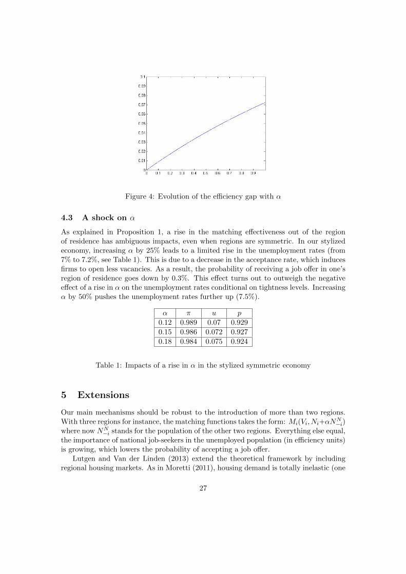
Figure 4: Evolution of the efficiency gap with α

4.3 A shock on α

As explained in Proposition 1, a rise in the matching effectiveness out of the regionof residence has ambiguous impacts, even when regions are symmetric. In our stylizedeconomy, increasing α by 25% leads to a limited rise in the unemployment rates (from7% to 7.2%, see Table 1). This is due to a decrease in the acceptance rate, which inducesfirms to open less vacancies. As a result, the probability of receiving a job offer in one’sregion of residence goes down by 0.3%. This effect turns out to outweigh the negativeeffect of a rise in α on the unemployment rates conditional on tightness levels. Increasingα by 50% pushes the unemployment rates further up (7.5%).

α π u p

0.12 0.989 0.07 0.929

0.15 0.986 0.072 0.927

0.18 0.984 0.075 0.924

Table 1: Impacts of a rise in α in the stylized symmetric economy

5 Extensions

Our main mechanisms should be robust to the introduction of more than two regions.With three regions for instance, the matching functions takes the form: Mi(Vi, Ni+αN

N−i)

where now NN−i stands for the population of the other two regions. Everything else equal,

the importance of national job-seekers in the unemployed population (in efficiency units)is growing, which lowers the probability of accepting a job offer.

Lutgen and Van der Linden (2013) extend the theoretical framework by includingregional housing markets. As in Moretti (2011), housing demand is totally inelastic (one

27

unit of dwelling per resident) and housing supply is increasing in the population size.The introduction of an endogenous housing market complicates the model a lot. Manymore effects become ambiguous since they hinge upon the slope of the housing supply.For example, more valuable amenities in a region has now an ambiguous impact on thesearch and location decisions. At given rents, the size of the population increases inthe better endowed region. When rents are endogenous, their rise in this region is adisincentive to search and locate there. If the housing supply is very inelastic, one couldget that the population shrinks in the better endowed region.

Consider next a dynamic extension with infinitely-lived agents. As in the staticframework, for national job-seekers, the partial effect of a rise in α is an increase in theprobability of finding a job. In a continuous time setting, the probability of receivingtwo offers during a very small interval of time tends to zero. A rise in α now negativelyaffects equilibrium tightness through wages. When α rises, national job-seekers have animproved outside option and hence their bargained wages rise. Then, through the freeentry of vacancies, labor demand shrinks. So, although the mechanism at work differs,the ambiguity remains.

6 Conclusion

This paper studies equilibrium unemployment in a two-region static economy wherewages are endogenous and homogeneous workers and jobs are free to move. We developa tractable search-matching equilibrium in which job-seekers can decide to search for ajob in another region without first migrating there. Current communication technolo-gies motivate this assumption. Since individuals have idiosyncratic and heterogeneouspreferences for regions, part of the population chooses to seek a job all over the countrywhile the rest only searches in the region where they live. These decisions affect the re-gional unemployment rates. Compared to the case where job-seekers can only search intheir region of residence, search-matching externalities are amplified by the opportunityof searching in a region where one does not live and by the fact that some workers cansimultaneously receive a job offer from each region. Hence, some vacant positions remainunfilled, which leads to a waste of resources. By this effect, if it is now much easier tosearch for a job all over the country thanks to the Internet, firms are less inclined toopen vacancies. The shrinking labor demand and the higher probability of finding a jobconditional on tightness are two opposite forces that hold true in a dynamic framework.They can explain the disagreement between Kroft and Pope (2014) at the city level andKuhn and Mansour (2014) and Choi (2011) at the individual level.

We characterize the constrained efficient allocation, where the central planner issubject to the same matching frictions as the decentralized agents. In standard non-spatial search-matching models with wage bargaining, the laissez-faire decentralizedeconomy is efficient if the Hosios condition is verified. This is also true when searcheffort is endogenous. In our model where job-seekers decide over their search field,the Hosios condition is not sufficient to guarantee efficiency when workers can searchnationally. Workers and firms take decisions without internalizing the effect of their

28

choices on net output in both regions. Simulations show that the optimal allocation is acorner solution where no one searches all over the country (this result is very robust tochanges in parameters) and the efficient regional unemployment rates are one percentagepoint lower than in the decentralized equilibrium.

This paper does not claim to have evaluated the general equilibrium impact of theInternet on the matching process. It has only focused on the implications of searchingbefore possibly moving to another region under the standard assumptions of constantreturns to scale in the matching process and in production. Beaudry et al. (2014) find nosignificant effects of agglomeration forces on productivity in the US. So, we feel confidentthat the latter assumption is not too strong a simplification. However, the presence ofnon negligible agglomeration forces would affect our conclusions.

References

Amior, M. (2012). A Labor Market Cushion for Housing Market Shocks, mimeo, Uni-versity College London, London.

Antoun, R. (2010). Why Almost Similar Regions Have Different Unemployment Rates,mimeo, ERMES, Universite Pantheon-Assas, Paris.

Autor, D. H. (2001). Wiring the Labor Market. Journal of Economic Perspectives,15 (1), 25–40.

Bagues, M. F. and Labini, M. S. (2009). Do Online Labor Market IntermediariesMatter? The Impact of AlmaLaurea on the University-to-Work Transition. In Studiesof Labor Market Intermediation, National Bureau of Economic Research, Inc, pp.127–154.

Beaudry, P., Green, D. A. and Sand, B. (2014). Spatial Equilibrium with Unem-ployment and Wage Bargaining: Theory and Estimation. Journal of Urban Economics,79, 2–19.

Brueckner, J. K. and Neumark, D. (2014). Beaches, Sunshine, and Public SectorPay: Theory and Evidence on Amenities and Rent Extraction by Government Work-ers. American Economic Journal: Economic Policy, 6 (2), 198–230.

Choi, E. J. (2011). Does the Internet Help the Unemployed Find Jobs?, mimeo, U.S.Bureau of Labor Statistics.

Coulson, N. E., Laing, D. and Wang, P. (2001). Spatial Mismatch in Search Equi-librium. Journal of Labor Economics, 19 (4), pp. 949–972.

Decreuse, B. (2008). Choosy Search And The Mismatch Of Talents. InternationalEconomic Review, 49 (3), 1067–1089.

Domingues Dos Santos, M. (2011). Immigration policy, spatial job search and un-employment, mimeo, ERUDITE, Universite Paris-Est, Paris.

29

Epifani, P. and Gancia, G. A. (2005). Trade, Migration and Regional Unemployment.Regional Science and Urban Economics, 35 (6), 625–644.

Francis, J. (2009). Agglomeration, job flows and unemployment. The Annals of Re-gional Science, 43 (1), 181–198.

Galenianos, M. and Kircher, P. (2009). Directed search with multiple job applica-tions. Journal of Economic Theory, 144 (2), 445–471.

Hosios, A. (1990). On the efficiency of matching and related models of search andunemployment. Review of Economic Studies, 57, 279–298.

Kennan, J. and Walker, J. (2011). The Effect of Expected Income on IndividualMigration Decisions. Econometrica, 79, 211–251.

Kircher, P. (2009). Efficiency of Simultaneous Search. Journal of Political Economy,117 (5), 861–913.

Kline, P. and Moretti, E. (2013). Place Based Policies with Unemployment. Amer-ican Economic Review, Papers and Proceedings, 103 (3), 238–43.

— and — (2014). People, Places, and Public Policy: Some Simple Welfare Economics ofLocal Economic Development Programs. Annual Review of Economics, 6 (1), 629–662.

Kroft, K. and Pope, D. G. (2014). Does Online Search Crowd Out Traditional Searchand Improve Matching Efficiency? Evidence from Craigslist. Journal of Labor Eco-nomics, 32 (2), 259 – 303.

Kuhn, P. and Mansour, H. (2014). Is Internet Job Search Still Ineffective? TheEconomic Journal, 124 (581), 1213–1233.

Lkhagvasuren, D. (2012). Big Locational Unemployment Differences Despite HighLabor Mobility. Journal of Monetary Economics, 59 (8), 798–814.

Lucas, R. E. and Prescott, E. C. (1974). Equilibrium search and unemployment.Journal of Economic Theory, 7 (2), 188 – 209.

Lutgen, V. and Van der Linden, B. (2013). Regional Equilibrium UnemploymentTheory at the Age of the Internet. IZA Discussion Papers 7763, Institute for the Studyof Labor (IZA).

Manning, A. and Petrongolo, B. (2011). How Local Are Labor Markets? Evidencefrom a Spatial Job Search Model. IZA Discussion Papers 6178, Institute for the Studyof Labor (IZA).

Marinescu, I. and Rathelot, R. (2014). The Geography of Job Search and MismatchUnemployment, mimeo.

30

Molho, I. (2001). Spatial Search, Migration and Regional Unemployment. Economica,68 (270), pp. 269–283.

Moretti, E. (2011). Local Labor Markets. In O. Ashenfelter and D. Card (eds.), Hand-book of Labor Economics, vol. 4, chapter 14, Elsevier, pp. 1237–1313.

Nenov, P. (2014). Regional Reallocation and Housing Markets in a Model of FrictionalMigration, mimeo.

Pissarides, C. A. (2000). Equilibrium Unemployment Theory, 2nd Edition. The MITPress.

— (2009). The Unemployment Volatility Puzzle: Is Wage Stickiness the Answer? Econo-metrica, 77 (5), 1339–1369.

Roback, J. (1982). Wages, Rents, and the Quality of Life. Journal of Political Economy,90 (6), 1257–78.

Rosen, H. S. (1979). Wage based indexes of urban quality of life. In P. N. Miezkowskiand M. R. Straszheim (eds.), Current Issues in Urban Economics, Johns HopkinsUniversity Press, pp. 74–104.

Sahin, A., Song, J., Topa, G. and Violante, G. L. (2014). Mismatch unemploy-ment. American Economic Review, 104 (11), 3529–64.

Topel, R. H. (1986). Local Labor Markets. Journal of Political Economy, 94 (3),S111–43.

Wrede, M. (2014). Wages, Rents, Unemployment, and the Quality of Life: A Constis-tent Theory-Based Measure. Journal of Regional Science, forthcoming.

Zenou, Y. (2009). Urban Labor Economics. Cambridge University Press.

Appendices

A Search and location decisions are taken simultaneously

The following table summarizes the different cases an agent faces when α > 0:

Where to search

Where to live Region 1 Region 2 Region 1 and region 2Region 1 case a case b case cRegion 2 case d case e case f

31

We will proceed by first computing the expected utility of an individual in each case.By doing so, we will be able to drop cases b and d. In a second step, we will define 3thresholds out of the 6 that could be computed from the 4 remaining cases. By rankingthese thresholds and comparing the expected utility levels, we will be able to rank theexpected utility levels and show that these thresholds are those we get if we assume thatagents take the location and search decisions sequentially.

1. Expected utility in each case

Case a: The utility if the individual lives in 1 and searches in 1 only

p1Ve1j + (1− p1)V u

1j

Case b: The utility if the individual lives in 1 and searches in 2 only

αp2Ve2j + (1− αp2)V u

1j

Case c: The utility if the individual lives in 1 and searches in both regions

p1(1−αp2)V e1j+αp2(1−p1)V e

2j+(1−p1)(1−αp2)V u1j+αp1p2

[max

{V e1j ;V

e2j

}− ε]

Case d: The utility if the individual lives in 2 and searches in 1 only

αp1Ve1j + (1− αp1)V u

2j

Case e: The utility if the individual lives in 2 and searches in 2 only

p2Ve2j + (1− p2)V u

2j

Case f: The utility if the individual lives in 2 and searches in both regions

p2(1−αp1)V e2j+αp1(1−p2)V e

1j+(1−p2)(1−αp1)V u2j+αp1p2

[max

{V e1j ;V

e2j

}− ε]

We assume that the cost ε of refusing a job offer tends to zero.

2. Case b is dominated by case c if

αp2Ve2j + (1− αp2)V u

1j

< p1(1− αp2)V e1j + αp2(1− p1)V e

2j + (1− p1)(1− αp2)V u1j + αp1p2 max

{V e1j ;V

e2j

}⇔ 0 < (1− αp1p2)V u

1j + p1(Ve1j − V u

1j) + αp1p2[max

{V e1j ;V

e2j

}− V e

1j − V e2j + V u

1j

]Two sub-cases should be considered:

• If max{V e1j ;V

e2j

}= V e

2j , then the comparison becomes:

0 < (1− αp1p2)V u1j + p1(V

e1j − V u

1j) + αp1p2(Vu1j − V e

1j)

0 < (1− αp1p2)V u1j + (1− αp2)p1(V e

1j − V u1j)

This always holds. Similarly,

• If max{V e1j ;V

e2j

}= V e

1j , then the comparison becomes:

0 < (1− αp1p2)V u1j + p1(V

e1j − V u

1j) + αp1p2(Vu1j − V e

2j)

0 < (1− αp1p2)V u1j + (1− αp2)p1(V e

1j − V u1j) + αp1p2(V

e1j − V e

2j)

32

This always holds since V e1j ≥ V e

2j . As a result, case b will never be optimal foragent j.

3. Case d is dominated by case f if

αp1Ve1j + (1− αp1)V u

2j

< p2(1− αp1)V e2j + αp1(1− p2)V e

1j + (1− p2)(1− αp1)V u2j + αp1p2 max

{V e1j ;V

e2j

}⇔ 0 < (1− αp1p2)V u

2j + p2(Ve2j − V u

2j) + αp1p2[max

{V e1j ;V

e2j

}− V e

1j − V e2j + V u

2j

]Two sub-cases should be considered:

• If max{V e1j ;V

e2j

}= V e

1j , then the comparison becomes:

0 < (1− αp1p2)V u2j + p2(V

e2j − V u

2j) + αp1p2(Vu2j − V e

2j)

0 < (1− αp1p2)V u2j + (1− αp1)p2(V e

2j − V u2j)

This always holds. Similarly,

• If max{V e1j ;V

e2j

}= V e

2j , then the comparison becomes:

0 < (1− αp1p2)V u2j + p2(V

e2j − V u

2j) + αp1p2(Vu2j − V e

1j)

0 < (1− αp1p2)V u2j + (1− αp1)p2(V e

2j − V u2j) + αp1p2(V

e2j − V e

1j)

This always holds since V e2j ≥ V e

1j . As a result, case d will never be optimal foragent j.

4. Defining the thresholds

With the 4 remaining cases, we define 3 threshold values and show that this issufficient to get a dominant case for each value of c1j − c2j :

Definition of the threshold between case c and case f

p1(1− αp2)V e1j + αp2(1− p1)V e

2j + (1− p1)(1− αp2)V u1j + αp1p2 max

{V e1j ;V

e2j

}= p2(1− αp1)V e

2j + αp1(1− p2)V e1j + (1− p2)(1− αp1)V u

2j + αp1p2 max{V e1j ;V

e2j

}⇔ (1− α)p1V

e1j − (1− α)p2V

e2j + (1− p1)(1− αp2)V u

1j − (1− p2)(1− αp1)V u2j = 0

⇔ (1− α)p2(Ve2j − V u

2j)− (1− α)p1(Ve1j − V u

1j)

= (1− αp1 − αp2 + αp1p2)(Vu1j − V u

2j) = 0

Using the definitions of utilities, we get equation (18):

x = b2 − b1 + a2 − a1 + (1− α)p2(w2 − b2)− p1(w1 − b1)

1− αp1 − αp2 + αp1p2

33

Definition of the threshold between case e and case f

p2Ve2j + (1− p2)V u

2j = p2(1− αp1)V e2j + αp1(1− p2)V e

1j

+(1− p2)(1− αp1)V u2j + αp1p2 max

{V e1j ;V

e2j

}⇔ αp1(V

e1j − V u

2j) + αp1p2[max

{V e1j ;V

e2j

}− V e

1j − V e2j + V u

2j

]= 0

Two sub-cases should be considered:

• If max{V e1j ;V

e2j

}= V e

2j ,

αp1(1− p2)(V e1j − V u

2j) = 0

⇔ V e1j = V u

2j as 0 < pi < 1 and α > 0

⇔ z1 = b1 − w1 + b2 − b1 + a2 − a1

• If max{V e1j ;V

e2j

}= V e

1j ,

αp1(1− p2)(V e1j − V u

2j) + αp1p2(Ve1j − V e

2j) = 0

⇔ z1 = b1 − w1 + b2 − b1 + a2 − a1 + p2(w2 − b2) as 0 < pi < 1 and α > 0

However, the assumption of the sub-cases, V e1j ≥ V e

2j , implies that in this caserelative preference are such that:

c1j − c2j ≥ b1 − w1 + b2 − b1 + a2 − a1 + w2 − b2 > z1

which leads a contradiction as we assume in the definition of z1 that V e1j ≥ V e

2j .Therefore, the only possible threshold value between case e and case f is z1.

Definition of the threshold between case a and case c

p1Ve1j + (1− p1)V u

1j = p1(1− αp2)V e1j + αp2(1− p1)V e

2j

+(1− p1)(1− αp2)V u1j + αp1p2 max

{V e1j ;V

e2j

}⇔ αp2(V

e2j − V u

1j) + αp1p2[max

{V e1j ;V

e2j

}− V e

1j − V e2j + V u

1j

]= 0

Two sub-cases should be considered:

• If max{V e1j ;V

e2j

}= V e

1j ,

αp2(1− p1)(V e2j − V u

1j) = 0

⇔ V e2j = V u

1j as 0 < pi < 1 and α > 0

⇔ z2 = w2 − b2 + b2 − b1 + a2 − a1

34

• If max{V e1j ;V

e2j

}= V e

2j ,

αp2(1− p1)(V e2j − V u

1j) + αp1p2(Ve2j − V e

1j) = 0

⇔ z2 = w2 − b2 + b2 − b1 + a2 − a1 − p1(w1 − b1) as 0 < pi < 1 and α > 0

However, the assumption of the sub-case, V e2j ≥ V e

1j , implies that in this caserelative preference are such that:

c1j − c2j ≤ w2 − b2 + b2 − b1 + a2 − a1 + b1 − w1 < z1

which leads to a contradiction as we assume in the definition of z2 that V e2j ≥ V e

1j .Therefore, the only possible threshold value between case a and case c is z2.

5. Ranking the thresholds

It is easily seen that z1 ≤ x ≤ z2.

6. Dominant strategies

Figure 5: Dominant strategies

• the individual whose relative preference is x is indifferent between living in 1and searching in both regions (case c) and living in 2 and searching in bothregions (case f );

• the individual whose relative preference is z1 is indifferent between living in 2and searching in 2 only (case e) and living in 2 and searching in both regions(case f );

• the individual whose relative preference is z2 is indifferent between living in1 and searching in 1 only (case a) and living in 1 and searching in both (casec);

We conclude from Figure 5 that the three threshold values we chose at first are sufficientto get a dominant strategy for each value of the relative preference c1j − c2j . Thesevalues are equivalent to those obtained when location and search decisions are takensequentially.

35

B Proof of Proposition 2

When α = 1, Proposition 2 is obvious.When 0 < α < 1, we first provide conditions guaranteeing that ∂x/∂p2 > 0 and

∂x/∂p1 < 0 . These conditions depend on endogenous variables. We finally derive aunique sufficient condition on α.

∂x

∂p2=

1− α(1− αp1 − αp2 + αp1p2)2

((1− αp1)β2(y2 − b2)− αp1(1− p1)β1(y1 − b1))

which has a positive sign if:

α <β2(y2 − b2)

p1(β2(y2 − b2) + (1− p1)β1(y1 − b1))(43)

To obtain a sufficient condition depending on parameters only, we should now minimizethe RHS of (43) by maximizing the denominator with respect to p1 ∈ (0, 1). The uniquemaximum is

p∗1 = min

(β1(y1 − b1) + β2(y2 − b2)

2β1(y1 − b1), 1

)If β2(y2 − b2) < β1(y1 − b1), p∗1 < 1 and a sufficient condition for (43) is

α <4β1(y1 − b1)β2(y2 − b2)

(β1(y1 − b1) + β2(y2 − b2))2(44)

Otherwise, a sufficient condition is α < 1.Similarly ∂x/∂p1 < 0 if

α <β1(y1 − b1)

p2(β1(y1 − b1) + (1− p2)β2(y2 − b2))(45)

Minimizing this ratio with respect to p2 ∈ (0, 1) yields

p∗2 = min

(β1(y1 − b1) + β2(y2 − b2)

2β2(y2 − b2), 1

)If β2(y2 − b2) > β1(y1 − b1), p∗2 < 1 and a sufficient condition for (45) is (44) Otherwise,a sufficient condition is α < 1. To guarantee that both ∂x/∂p2 > 0 and ∂x/∂p1 < 0, weconclude that (44), i.e. (19) in Proposition 2, is the unique sufficient condition, its RHSbeing in any case lower than one.

C Conditional acceptance rates

In this appendix, we show formulas (20) and (21). In the first part, we focus on theconditional acceptance rate when the vacancy is located in region 1. We then turn tothe opposite case.

36

C.1 Conditional acceptance rate in region 1

A vacant position located in region 1 faces v−x+α(x−z1)2v N possible workers in efficiency

units. These workers always accept a job offer from the firm if their relative preferencefor region 1 over region 2, c1j − c2j , is higher than x. If their relative preference is belowx, job-seekers only accept the offer if they have not received one from a firm located inregion 2.

We thus compute the conditional acceptance rate as :

2v

v − x+ α(x− z1){P(c1j − c2j ≥ x)1 + P(c1j − c2j < x) P(no offer from 2)}

There are two sub-cases: Whether x is lower or greater than x.Whenever x < x,

Relative Proba to have Proba to acceptpreference this preference a position in 1

v > c1j − c2j > x v−x2v 1

x > c1j − c2j > x x−x2v 1− αp2

x > c1j − c2j > z1α(x−z1)

2v 1− p2

The conditional acceptance rate is thus:

2v

v − x+ α(x− z1)

{v − x

2v+x− x

2v(1− αp2) + α

x− z12v

(1− p2)}

which leads to equation (20).Whenever x > x,

Relative Proba to have Proba to acceptpreference this preference a position in 1

v > c1j − c2j > x v−x2v 1

x > c1j − c2j > x α(x−x)2v 1

x > c1j − c2j > z1α(x−z1)

2v 1− p2

The condition acceptance rate is thus:

2v

v − x+ α(x− z1)

{v − x

2v+α(x− x)

2v1 + α

x− z12v

(1− p2)}

which leads to equation (20) as well.

C.2 Conditional acceptance rate in region 2

A vacant position located in region 2 faces v+x+α(z2−x)2v N possible workers in efficiency

units. These workers always accept a job offer from the firm if their relative preferencefor region 1 over region 2, c1j − c2j , is lower than x. If their relative preference is higher

37

x, job-seekers only accept the offer if they have not received one from a firm located inregion 1.

We thus compute the conditional acceptance rate as :

2v

v + x+ α(z2 − x){P(c1j − c2j < x)1 + P(c1j − c2j ≥ x) P(no offer from 1)}

Here again there are two sub-cases: Whether x is lower or greater than x.Whenever x < x,

Relative Proba to have Proba to acceptpreference this preference a position in 2

−v < c1j − c2j < x v+x2v 1

x < c1j − c2j < x α(x−x)2v 1

x < c1j − c2j < z2α(z2−x)

2v 1− p1

The condition acceptance rate is thus:

2v

v + x+ α(z2 − x)

{v + x

2v+α(x− x)

2v1 + α

z2 − x2v

(1− p1)}

which leads to equation (21).Whenever x > x,

Relative Proba to have Proba to acceptpreference this preference a position in 2

−v < c1j − c2j < x v+x2v 1

x < c1j − c2j < x x−x2v 1− αp1

x < c1j − c2j < z2α(z2−x)

2v 1− p1

The condition acceptance rate is thus:

2v

v + x+ α(z2 − x)

{v + x

2v+x− x

2v(1− αp1) + α

z2 − x2v

(1− p1)}

which leads again to equation (21).

D Cross partial derivative of unemployment rates

The cross-partial derivatives of the unemployment rates with respect to tightness in theother region are respectively:

sign

{∂u1∂θ2

}= sign {αp1 [(v − x)(x−∆)− α(z2 − x)(x− z1)]} (46)

sign

{∂u2∂θ1

}= sign {αp2 [(v + x)(∆− x)− α(z2 − x)(x− z1)]} (47)

38

We directly notice that one of these two derivatives is always negative:

x−∆ < 0 i.e. p2β2(y2 − b2) < p1β1(y1 − b1)⇒∂u2∂θ1

T 0 and∂u1∂θ2

< 0,

x−∆ > 0 i.e. p2β2(y2 − b2) > p1β1(y1 − b1)⇒∂u1∂θ2

T 0 and∂u2∂θ1

< 0.

To limit the extent of these ambiguities, we first compute the limits when α tendsto 0 and to 1. We then check how the functions could behave between these two limits.¿From (46), (47) and (18), the following limit values are obvious:

limα→0

∂u1∂θ2

= limα→0

∂u2∂θ1

= 0;

limα→1

sign

{∂u1∂θ2

}= lim

α→1sign

{∂u2∂θ1

}= sign {−(z2 − x)(x− z1)} < 0.

It can furthermore be shown29 that:

limα→0+

sign

{∂u1∂θ2

}= sign {(x−∆)(v − x)} ,

limα→0+

sign

{∂u2∂θ1

}= sign {(∆− x)(v + x)} .

Between the two extremes, we cannot go further in the analysis. Because of the limitwhen α→ 1, we however can conclude that:

• When x−∆ > 0, ∂u2∂θ1

< 0 ∀α > 0 and ∂u1∂θ2

< 0 if α is large enough;

• When x−∆ < 0, ∂u1∂θ2

< 0 ∀α > 0 and ∂u2∂θ1

< 0 if α is large enough;

• When x−∆ = 0, both partial derivatives are always negative.

29A proof is available upon request. It can actually be shown that the partial derivatives (46) and (47)have the same sign as a polynomial of degree four in α, whose constant term is respectively (v−x)(x−∆)and (v + x)(∆− x).

39

E Existence of a symmetric equilibrium

When both regions have the same exogenous characteristics, a free-entry symmetricequilibrium is characterized by the following conditions:

x = x = 0

z2 = β(y − b) = −z1πm(θ) =

κ

(1− β)(y − b)(48)

π = 1− αp(θ)z2v + αz2

(49)

u =(1− p(θ))(v − αp(θ)z2)

v

NP1 = NP

2 = 1/2

and (24) and (25). This system of equations can be solved recursively. First, the z1 andz2 thresholds are functions of parameters only. Second, combining equations (48) and(49) leads to the following implicit relationship in equilibrium tightness:

v + α(1− p(θ))β(y − b)v + αβ(y − b)

=1

m(θ)

κ

(1− β)(y − b)

The left-hand side is a negative function of tightness, while the right-hand side dependspositively on tightness. So, there is at most one equilibrium. To show the existence ofthe equilibrium, consider the limit of each side of the last equality when θ tends to 0:

limθ→0

v + α(1− p(θ))β(y − b)v + αβ(y − b)

= 1

limθ→0

1

m(θ)

κ

(1− β)(y − b)= 0, by the Inada conditions.

So, a unique symmetric equilibrium tightness exists. The other endogenous variablesare then determined uniquely as well.

F Ex-ante bargaining

The aim of this appendix is to check whether the ex-ante bargaining process leads toan efficient allocation under the Hosios condition. In the five following subsections, wederive and briefly explain the key equations that are modified compared to the modeldescribed in the paper. In the last subsection, we compare the decentralized equilibriumfree-entry conditions with the efficient allocation, and show that the Hosios condition isnever sufficient to restore efficiency.

When bargaining ex-ante, the timing is defined as follows30:

30An alternative timing would be that workers who get two job offers bargain with the firms beforerefusing one of the job offers. This would lead to Bertrand competition between the two firms for thisworker. It has however been checked that this lead to further sources of inefficiency.

40

1. Workers decide where to locate and where to search.

2. Firms open vacancies and the matching process takes place.

3. In case a worker gets two offers, she chooses one of them.

4. Workers bargain with the firm.

5. Workers relocate if the accepted position is in the other region.

6. Production takes place and both the housing and the good markets clear.

F.1 Wage bargaining

Since there are, for each worker, two potential fall-back positions when bargaining (beingunemployed in region 1 or in region 2), there will be four wages in the economy, whichmay depend on the worker’s relative idiosyncratic preference. Let wikj denote the wageof individual j living in region k ex-ante and who works for a firm located in i and V e

ikj

the utility she gets in this case. The wage wikj verifies:

maxwikj

(V eikj − V u

kj)βi(Jij)

1−βi

whereV eikj − V u

kj = wikj − bk + ai − ak + cij − ckjThis leads to the following wages:

wikj = βiyi + (1− βi)bi − (1− βi)(bi − bk + ai − ak + (cij − ckj)) (50)

or

w11j = w11 = β1y1 + (1− β1)b1w12j = β1y1 + (1− β1)b1 + (1− β1)(∆− (c1j − c2j)) (51)

w22j = w22 = β2y2 + (1− β2)b2w21j = β2y2 + (1− β2)b2 − (1− β2)(∆− (c1j − c2j)) (52)

It is worth mentioning that ex-ante bargaining allows workers coming from the otherregion to be compensated for the difference in leisure, amenities and idiosyncratic pref-erences (see the term ∆− (c1j − c2j) in (51) and (52)).

F.2 Acceptance decisions

Acceptance decisions are conditional on the region of residence, as wages in the otherregion depend on it. Workers located in region 1 decide whether they prefer working inregion 1 by comparing V e

11j and V e21j . This leads to the following threshold:

x2 = ∆ + y2 − b2 −β1β2

(y1 − b1)

41

Considering now workers located in region 2 ex-ante, one gets:

x1 = ∆ +β2β1

(y2 − b2)− (y1 − b1)

When regions are asymmetric, these two thresholds are equal if and only if β1 =β2. As we aim at checking whether an ex-ante bargaining process leads to an efficientallocation under Hosios, we make the assumption that β1 = β2, so that we get a uniquethreshold x. This assumption is made as the central planner would always choose aunique x threshold. For, assume that β1 6= β2, so that there exist two threshold valuesx1 and x2 . The only possibility that these two thresholds are simultaneously meaningfulis when we have x1 < x < x2.

31 This case is represented by Figure 6 and is neveroptimal. For, take a first worker whose relative preference for region 1 over region 2lies between x1 and x. This worker would choose to work in region 1. Take then asecond worker whose relative preference lies between x and x2. She chooses to worker inregion 2. As assumed in the paper, workers are homogenous in productivity in a givenregion. Thus, interchanging these 2 workers (the first worker would then work in region2 and the second one in region 1) does not modify the total levels of production nor theex-post population sizes. However, this will change the levels of workers’ idiosyncraticpreferences. In this regard, interchanging the first worker and the second worker wouldlead to a higher level of preferences (as workers having a relative preference between xand x2 value more region 1 relative to region 2 than workers with a relative preferencebetween x1 and x), without modifying the level of production nor the population sizes.The central planner thus prefer this situation than the initial one. This induces thathaving two distinct thresholds x is never optimal. Therefore, for the rest of this appendix,we assume that β1 = β2 = β, so that we do not face a multi-thresholds equilibrium forthe acceptance decision.

F.3 Opening of vacancies

We assume free-entry of firms. Firms open vacancies until the expected profit is nil:πimi(θi)(yi − wei ) − κi = 0, where wei is the wage a firm located in region i is expectedto pay. This can be rewritten as:

κimi(θi)

= πi(yi − wei )

F.4 Location and search decisions

The location and search decisions are taken simultaneously. With the assumption onthe β’s, it is easily shown that taking the decision simultaneously of choosing first whereto locate and then where to search is equivalent (one needs to proceed as in AppendixA). To ease the exposition, we focus on the second procedure.

31This situation assumes that the threshold x is unique. This unicity is verified with the assumptionwe make regarding the β’s.

42

𝑐1𝑗 − 𝑐2𝑗

𝑓(𝑐1𝑗 − 𝑐2𝑗)

𝑥 1 𝑥 2

Choose region 2

−𝑣 𝑣

Choose region 1

Choose region 2

Choose region 2

𝑥

Locate in region 2

Locate in region 1

Figure 6: Case of two different x thresholds

F.4.1 Search decision

A worker located in region 2 searches regionally when:

0 > −αp1p2V e22j + αp1p2

[max

{V e22j ;V

e12j

}− ε]

+ αp1(1− p2)(V e12j − V u

2j)

Assuming that ε tends to 0, one gets the following threshold value whenever V e22j ≥ V e

12j :

z1 = ∆− (y1 − b1) (53)

When V e22j < V e

12j , one gets:

z1 = ∆− (y1 − b1) + p2(y2 − b2)

However, V e22j < V e

12j implies that:

c1j − c2j = ∆− (y1 − b1) + y2 − b2 > z1

which leads to a contradiction, as we assume in the definition of z1 that V e22j < V e

12j . Wethus get a unique threshold value, z1, for the search decision of agents located in region2.

Similarly, we get the following threshold for workers located in region 1:

z2 = ∆ + y2 − b2 (54)

F.4.2 Location choice

The marginal worker that decides where to locate is a national job-seeker. One thusneeds to compare the expected utility of a national job-seeker in both regions. One getsas threshold value:

x = ∆2 +(1− α)(p2β(y2 − b2)− p1β(y1 − b1))

1− αβp1 − αβp2 + αβp1p2(55)

43

F.5 Population, acceptance rates and expected wages

Populations can be described as in the paper, using the new threshold definitions. Accep-tance rates are given, as in the ex-post bargaining case, by equations (20)-(21). Knowinghow workers locate and search, one can compute the expected wage of a firm. In region1, the wage bill can be rewritten as:

N

2v(βy1 + (1− β)b1) [p1(v − x) + αp1(1− p2)(x− z1) + αp1p2(x− x)]

+N

2v(1− β)αp1(1− p2)

∫ x

z1

(∆− (c1j − c2j))dj

+max {x− x; 0}

x− xN

2v(1− β)αp1p2

∫ x

x(∆− (c1j − c2j))dj

As the number of employed workers in region 1 is given by

L1 =N

2v[p1(v − x) + αp1(1− p2)(x− z1) + αp1p2(x− x)] ,

we can write the expected wage in region 1 as:

we1 = βy1 + (1− β)b1 +(1− β)(1− p2)α(x− z1)(∆− x+z1

2 )

v − x+ α(x− z1)− αp2(x− x)

+(1− β)αp2 max {x− x; 0} (∆− x+x

2 )

v − x+ α(x− z1)− αp2(x− z1)

So, plugging this equation in the free-entry condition yields:

κ1(1− β)m1(θ1)

= π1(y1 − b1)−α(1− p2)(x− z1)v − x+ α(x− z1)

(∆− x+ z1

2

)−αp2 max {x− x; 0}v − x+ α(x− z1)

(∆− x+ x

2

) (56)

Similarly, one gets for the expected wage in region 2:

we2 = βy2 + (1− β)b2 −(1− β)(1− p1)α(z2 − x)(∆− x+z2

2 )

v + x+ α(z2 − x) + αp1(x− x)

−(1− β)αp1 max {x− x; 0} (∆− x+x

2 )

v − x+ α(z2 − x)− αp1(z2 − x)

so that the free-entry condition in region 2 writes:

κ2(1− β)m2(θ2)

= π2(y2 − b2) +α(1− p1)(z2 − x)

v + x+ α(z2 − x)

(∆− z2 + x

2

)+αp1(max {x− x; 0})v + x+ α(z2 − x)

(∆− x+ x

2

) (57)

44

F.6 Efficiency

Comparing (56)-(57) with (37)-(38), one directly sees that the ex-ante bargaining helpsrestoring efficiency, but is not sufficient.

First, regarding the search thresholds definitions (equations (40)-(41) and (53)-(54)),we notice that it partially corrects the search decisions, by taking the whole surplusformed rather than a share β. Workers however still do not take into account the impactof their search decision on the opening of vacancies in the other region.

Second, even if thresholds were set optimally, firms do not open the optimal numberof vacancies. This is due to the fact that workers get compensated for leisure, amenities,rents and idiosyncratic preferences by a firm if they are currently working in it, whilethe central planner compensate all workers. For example, for a firm settled in region 1,the third term on the RHS of (37) is equivalent to the second term on the RHS of (56).Furthermore, if x > x, then the fifth term in (37) corresponds to the third term of (56).As workers, when getting two job offers and being located in region 2, prefer to work inregion 1, firms located in region 1 compensate them for not living in region 2 anymore.However, when deciding how many vacancies they open in region 1, firms do not takeinto account the implications of their decisions on the workers who live in region 1 butaccept a job offer in region 2. Such an event is of course influenced among other thingsby the number of vacancies created in region 1.

Furthermore, ex-ante bargaining does not allow to internalize the loss in output inthe other region (in (56)-(57) there is no expression corresponding to the second termon the RHS of (37)-(38) because when they bargain over wages agents have no reason tointernalize the induced effect of the wage via vacancy creation on the net output createdin the other region).

45