Embed Size (px)
Citation preview
This PDF is a selection from an out-of-print volume from the National Bureauof Economic Research
Volume Title: Economic Adjustment and Exchange Rates in Developing Countries
Volume Author/Editor: Sebastian Edwards and Liaquat Ahamed, eds.
Volume Publisher: University of Chicago Press
Volume ISBN: 0-226-18469-2
Volume URL: http://www.nber.org/books/edwa86-1
Publication Date: 1986
Chapter Title: Wage Indexation, Supply Shocks, and Monetary Policy in aSmall, Open Economy
Chapter Author: Joshua Aizenman, Jacob Frenkel
Chapter URL: http://www.nber.org/chapters/c7671
Chapter pages in book: (p. 89 - 142)
3 Wage Indexation, Supply Shocks, and Monetary Policy in a Small, Open Economy Joshua Aizenman and Jacob A. Frenkel
3.1 Introduction
The energy crises of the 1970s stimulated a renewed interest in ques- tions concerning the proper adjustment to external supply shocks. In general, restoring equilibrium in response to shocks necessitates the adjustment of both quantities and prices. When applied to labor mar- kets, various proposals for policy rules attempting to restore labor market equilibrium may be classified in terms of their impact on the division of adjustment between quantities (the level of employment) and prices (the real wage). The design of optimal policies provides for the appropriate division of this adjustment.
This paper develops a unified framework for the analysis of wage indexation and monetary policy. The analytical framework is then ap- plied to determine the optimal policy rules in the presence of supply shocks, as well as to evaluate the welfare consequences and ranking of alternative (suboptimal) policy rules. To set the stage for an evalu- ation of the welfare implications of alternative policy rules, we first analyze two extreme cases: a rule that stabilizes employment, and a rule that stabilizes the real wage. The analysis of these two extreme cases provides the ingredients for evaluating various rules for wage indexation and monetary targeting. We examine the implications of indexing wages to the nominal gross national product (GNP), the con- sumer price index (CPI), and the value-added price index. The dis-
Joshua Aizenman is an associate professor of business economics at the Graduate School of Business, University of Chicago, and a faculty research fellow of the National Bureau of Economic Research. Jacob A. Frenkel is the David Rockefeller Professor of International Economics at the Department of Economics, University of Chicago and a research associate of the National Bureau of Economic Research.
89
90 Joshua AizenmanlJacob A. Frenkel
tinction between the CPI and the value-added price index is of special importance in the study of supply shocks. We also look at the impli- cations of targeting the money supply to these three alternative indicators.
Our analysis demonstrates that, on the formal level, the various indexation rules bear a dual relationship to the various monetary tar- geting rules. We show that the welfare ranking of the various rules depends on whether the elasticity of the demand for labor exceeds or falls short of the elasticity of labor supply. Specifically, if the demand for labor is more elastic than the supply of labor, policy rules that stabilize employment are preferable to those that stabilize the real wage, and vice-versa. Accordingly, using this principle we demonstrate that if the elasticity of labor demand exceeds the elasticity of labor supply, indexing wages to the nominal GNP is preferable to indexing to the value-added price index, which in turn is preferable to indexing to the CPI. Likewise, because of the dual relationship between mon- etary policy and wage indexation, it follows that under the same cir- cumstances, monetary policy that targets the nominal GNP is prefer- able to policy that targets the value-added price index, which in turn is preferable to the policy that targets the CPI. This ranking is reversed when the elasticity of labor supply exceeds the elasticity of labor demand.
Our analysis has implications for both theoretical and policy debates over wage indexation and monetary rules. Specifically, great attention has been given to the question whether the monetary authority, when faced with a higher price of imported energy, should follow an accom- modative policy and expand the money supply to “finance” the higher energy price or whether it should be unaccommodating and contract the money supply to lower inflation. The key question has been whether, in the absence of an active monetary response, labor markets can adjust without costly deviations from full employment (see, for example, Gor- don 1975; 1984; Phelps 1978; Blinder 1981; Rasche and Tatom 1981; and Fischer 1985). Our analysis deals with these questions as part of the more general analytical framework.
Section 3.2 describes the building blocks of the model, including a specification of the stochastic shocks and a determination of output and employment. Section 3 . 3 introduces the objective function that is designed to minimize the expected value of labor market distortions. In our model, as in Gray (1976) and Fischer (1977a; 1977c), the need for wage indexation and monetary policy arises from the existence of labor market contracts according to which wages are set in advance of the realization of the stochastic shocks. This labor market convention results in some stickiness of wages. Wage indexation and monetary policies are designed to reduce the undesirable consequences of this stickiness. With the aid of the objective function, we derive the optimal
91 Wage Indexation, Supply Shocks, and Monetary Policy
wage indexation rule that eliminates the welfare cost. The key char- acteristic of the optimal indexation rule is that it distinguishes between the effects of monetary shocks and the effects of real shocks on the wage.
In section 3.4 we examine the implications of departures from the optimal indexation rule. In this context we develop a general criterion for comparing rules that stabilize employment and rules that stabilize real wages. We then apply this criterion to determine the welfare rank- ing of alternative proposals for wage indexation rules.
The question of monetary accommodation is addressed in section 3.5. We start by specifying the conditions for monetary equilibrium. We then determine the optimal money-supply rule and analyze its de- pendence on the nature of the stochastic shocks, on the parameters of the demand for money, on the elasticities of the demand for and supply of labor, and on the degree of wage indexation. The section concludes with an analysis of various targeting rules for monetary policies. Anal- ogously to the comparisons of the wage indexation rules, the monetary rules are analyzed in terms of their relative impact on stabilizing quan- tities (employment) versus stabilizing prices (the real wage).
In section 3.6 we apply the analytical framework to investigate the welfare implications of other departures from the optimal wage index- ation rule. For this purpose we examine two alternative simple formulas representing different degrees of departure from the optimal rule, and we modify the money-supply process to allow for exchange rate in- tervention. We thus are able to determine the optimal managed float in conjunction with the optimal wage indexation coefficients. These (second-best) solutions are determined subject to the constraints lim- iting the form of the money-supply process and the constraints limiting the variables that govern the wage indexation formulas. Finally, section 3.7 offers our concluding remarks.
Before turning to the formal analysis a word of caution is in order, especially to the casual reader. This paper develops a theoretical frame- work, and its arguments are therefore based on the formal logic of economic theorizing. Our purpose is to formulate in what we hope is a useful and revealing way a complex structure of a small, open econ- omy that is subject to a variety of stochastic shocks. Since the analysis is formal (containing some algebra), we anticipate that the more prac- tically inclined reader might wonder where the algebra leads. This question cannot, of course, be answered in the abstract. Rather, it should be examined in the context of the insights yielded by the the- oretical model. We believe that the analytical framework developed in this paper is sufficiently robust to accommodate some changes in spec- ifications. We illustrate this point in a brief discussion in the final section of the paper.
92 Joshua AizenmanIJacob A. Frenkel
3.2 The Model
In this section we outline the structure of the model, which includes a specification of the productive technology and a determination of the levels of output, employment, and wages.
3.2.1 Output and Employment Output is assumed to be produced by a Cobb-Douglas production
function using labor and imported energy as variable inputs. Thus, for period t :
(1) O S p < l , O S A < l ,
where Y, denotes the level of output; L, and V , denote, respectively, the inputs of labor and energy; B denotes a parameter including all fixed factors of production; and p, denotes a productivity shock. The productivity shock is assumed to be distributed independently and normally with a zero mean and a known variance of a:. In competitive equilibrium the parameters p and A denote, respectively, the relative shares of labor income and the energy bill in the GNP. Throughout the analysis we assume that current information is complete; thus, pro- ducers and others in the economy know the realized values of the stochastic shocks.'
Producers, who are assumed to maximize profits, demand labor and energy so as to equate the real wage and the relative price of energy to the marginal products of labor and energy. Expressed logarithmi- cally, these equalities are:
log Y, = log B + plog L, + A log V , + k,,
(3) log(>) = log AB + plog L, - (1 - A)log V, + p,,
where W denotes the nominal wage; P,, denotes the nominal price of energy; and P denotes the price level.
Equations (1) through ( 3 ) characterize the levels of output and factor inputs for a given realization of the stochastic productivity shock pr. In the absence of stochastic shocks, the corresponding levels of output and factor inputs are denoted by Yo, Lo, and V,, and the corresponding real factor prices are (W/P), and (PJP),. For subsequent use we denote by lowercase letters the percentage discrepancy of a variable from the value obtained in the absence of shocks. Thus, x = log X - log X,. Accordingly, the percentage deviation of output from its nonstochastic level is:
(1') y = p/ + Av + p,
I
93 Wage Indexation, Supply Shocks, and Monetary Policy
where y = log Y, - log YO, 1 = log L, - log Lo, and v = log V, - log Vn. Analogously, subtracting from equations ( 2 ) and (3) the corresponding equations for the nonstochastic equilibrium yields:
(2 ' ) w - p = - ( I - p)1 + AV + p
(3') p,, - p = p l - ( 1 - A)v + p,
where, for simplicity, the time subscript has been omitted. From equa- tions (2') and (3') the demands for labor and energy (or, more precisely, the percentage discrepancy of the demands for labor and energy from their nonstochastic levels) are:
(4) 1 = ~ [ ( l - A)@ - W ) - A@, - P ) + PI ( 5 )
where (T =
Assuming that producers are always able to satisfy their demands for labor and energy inputs, we substitute equations (4) and ( 5 ) into ( 1 ' ) and obtain:
(6)
Equation (6), which may be viewed as the aggregate supply function, shows that the percentage deviation of output from its deterministic level depends on the percentage deviations of the real wage and of the relative price of energy from their deterministic levels, as well as on the real productivity shock p. Higher values of the real wage and of the real energy price operate like negative supply shocks and result in lower output, whereas a positive productivity shock raises output.
We assume that the economy is small in the world energy market and that it faces an exogenously given energy price that is distributed normally around a given mean. To simplify the notations we define an efiective real shock, u , as the sum of the positive supply shocks arising from shocks to productivity and to the price of imported energy. Thus, u = p - X(p,. - p ) . With this definition of the effective real shock, the demand for labor in equation (4) and the supply of output in equation (6) can be written as:
(4')
(6')
where -q = a(l - A) denotes the (absolute value of the) elasticity of the demand for labor with respect to the real wage. This specification of employment and output (or, more precisely, the percentage discrep- ancy of employment and output from their nonstochastic levels) reflects the assumption that 1 and y are determined exclusively by the demand
v = a@ - HI) - (1 - P>@,, - P ) + PI,
1 I - p - A '
Y = U[P@ - w ) - A@,. - P ) + PI.
1 = q(p - w ) + (Tu
Y = a@ - w ) + ul,
94 Joshua AizenmadJacob A. Frenkel
for labor rather than by the interaction between the labor demand and labor supply.* The resultant disequilibrium in the labor market induces a welfare cost, which can be minimized in ways outlined in our sub- sequent analysis. To obtain a benchmark for assessing the implications of distortions in the labor market, we turn first to an analysis of the equilibrium that would exist in the absence of distortions.
3.2.2 The Undistorted Equilibrium
labor supply. Let the supply of labor be: Under the condition of undistorted equilibrium, labor demand equals
(7)
where E denotes the elasticity of labor supply. As before, using low- ercase letters to denote the percentage deviation of labor supply from the nonstochastic level, we obtain:
(7’)
Equating the demand for labor, equation (4’), with the supply of labor, equation (7‘), yields the undistorted equilibrium employment, and the
I ” = E(W - p ) .
,I,. undistorted equilibrium real wages, (w - p ) ,
(9) __j U (w - p ) = - U .
E + r )
such that:
Using equation (9) in (6’) yields the undistorted equilibrium ourput $:
(1 + €)U
E + r ) $ = U .
When this equilibrium exists, the demand for labor equals the supply of labor, and, in the absence of other distortions, efficiency is maximized.
3.3 The Measure of Welfare Loss and Optimal Indexation
The foregoing analysis determined the undistorted equilibrium levels of output, employment, and real wages. It was assumed that the flex- ibility of wages and prices yielded an undistorted labor market equi- librium. The values of the key variables in the undistorted equilibrium serve as benchmarks against which the actual levels of output, em- ployment, and real wages can be compared. These comparisons provide the basis for computing the welfare loss caused by labor market dis-
95 Wage Indexation, Supply Shocks, and Monetary Policy
tortions. In this section we outline a measure of the welfare loss and discuss the optimal policies to eliminate this loss. A more formal der- ivation of the measure of welfare loss is presented in the appendix.
3.3.1 The Welfare Loss
We assume that, because of contract negotiation costs, nominal wages are set in advance at their expected market-clearing level and that em- ployment is determined by the demand for labor. For a given realization of the effective real shock, u, the resulting level of employment is 1, as given by equation (4'). The corresponding equilibrium level of employ- ment is I , as given by equation ( 4 ) below, which is obtained by substi- tuting into (4') the equilibrium real wage (w - p ) for the actual real wage.
( 4 )
The discrepancy between That discrepancy is:
(1 1)
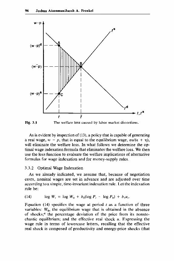
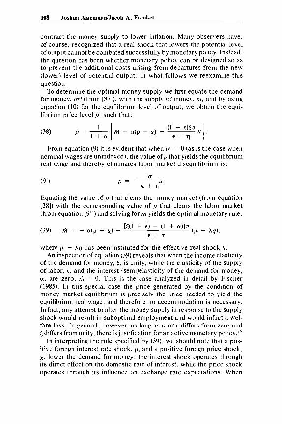
To compute the welfare loss associated with this discrepancy, we need to multiply the discrepancy by one-half of the difference between the demand and the supply prices at the actual level of employment. As illustrated in figure 3.1, i and ('iF$) designate the equilibrium values of employment and real wages, whereas 1 designates actual employ- ment. At the actual employment level, 1, the demand price for labor, (w - p)d , exceeds the corresponding supply price, ( w - p)". The wel- fare loss is represented by A, which measures the area of the triangle ABC. This triangle expresses the welfare loss in terms of consumer and producer surpluses. Thus:
-,,
-._ 1 1 = q(p - w ) + uu.
and 1 is responsible for the welfare loss.
-.- I - 1 = q [ - ( w - p ) + (w - p ) ] .
1 2
A = - [ (w - P ) ~ - (W - p)"] ( I - I ) . (12)
By using the definitions of the elasticities of labor demand and labor
supply, we note that ( w - P ) ~ - ( w - p)" = (k + i) ( I - 0. Sub-
stituting this into equation (12) and recalling that the equilibrium real wage, ( w - p ) , is specified by equation (9), we find that: __j
A = h ( + ) ( - w + p + - 2
Equation (13) measures the area of the triangle ABC in figure 3.1. In what follows we assume that the objective of policy is to minimize the expected value of the welfare loss, and we denote the loss function by H, where H = E(A).3
96 Joshua AizenmadJacob A. Frenkel
w-P
(w - PId
W-P)
(W - P)*
Fig. 3.1
P, PS
The welfare loss caused by labor market distortions.
As is evident by inspection of (13), a policy that is capable of generating a real wage, w - p, that is equal to the equilibrium wage, (TU/(E + q), will eliminate the welfare loss. In what follows we determine the op- timal wage indexation formula that eliminates the welfare loss. We then use the loss function to evaluate the welfare implications of alternative formulas for wage indexation and for money-supply rules.
3.3.2 Optimal Wage Indexation As we already indicated, we assume that, because of negotiation
costs, nominal wages are set in advance and are adjusted over time according to a simple, time-invariant indexation rule. Let the indexation rule be:
(14)
Equation (14) specifies the wage at period r as a function of three variables: W,, the equilibrium wage that is obtained in the absence of shock^;^ the percentage deviation of the price from its nonsto- chastic equilibrium; and the effective real shock u. Expressing the wage rule in terms of lowercase letters, recalling that the effective real shock is composed of productivity and energy-price shocks (that
log w, = log w, + b,(log P, - log Po) + b$,.

97 Wage Indexation, Supply Shocks, and Monetary Policy
is, u = p - Xq), and allowing for different coefficients of indexation to p and q, we find that:
(15)
Equation (15) specifies an indexation rule by which the nominal wage adjusts in response to the price, p ; to the productivity shock, p; and to the energy-price shock, q. The optimal values of bo, b,, and b, are chosen so as to eliminate the discrepancy between actual and equilib- rium real wages. Inspection of the last parenthetical term in equation (13) reveals that the nominal wage that eliminates the welfare loss is:
w = bop + b , p + b*q.
U Au l i j = p + -
E + q k - - E + p where p - Xq has been substituted for the effective real shock u. Thus, the optimal values of the coefficients in the indexation rule of equation (15) are:
U bo = 1;b , = - * , and 6, = -X6,.
E + T )
This formulation of the indexation rule is analogous to that of Karni (1983), who showed (in the context of a closed economy without an energy input) that at the optimum, the nominal wage must adjust to the price level by an indexation coefficient of unity, whereas, in general, its adjustment to the productivity shock differs from unity.5
The magnitude of the indexation coefficient 6, depends on the struc- ture of the economy as reflected by the elasticities of labor demand and labor supply. For example, a lower elasticity of labor supply raises the absolute values of the optimal coefficients of indexation to the real shocks (that is, to productivity and energy-price shocks). When the elasticity of labor supply approaches zero, approaches [l/(l - A)] > 1 , and b2 approaches - X / ( l - A). Likewise, the magnitude of the coef- ficients of indexation to real shocks depends on the relative share of the energy cost in output. As shown in equation (16), a higher share of the energy cost raises 6, as well as the absolute values of 6,. In general, 6, will be positive and 6, will be negative.
The key point to emphasize here is that by altering the nominal wage, the optimal indexation rule eliminates the welfare loss associated with the distortion to the real wage. The equilibrium that is obtained with optimal indexation replicates the equilibrium that would have been obtained if the labor market cleared after realizing the stochastic shocks. The optimal indexation formula thus serves to nullify the distortions arising from the assumption that, because of labor contracts, nominal wages are predetermined.6 Further, if economic policy was only con-
98 Joshua AizenmanlJacob A. Frenkel
cerned with the efficiency of resource allocation, then, in the absence of other distortions, there would be no need to undertake additional macroeconomic policies once the optimal indexation formula was adopted .
The essence of the optimal indexation rule lies in the distinction between the coefficients of indexation to nominal shocks and those to real shocks. In the specification of equation (14), nominal shocks were represented by p and real shocks were represented by u. It was shown that with optimal indexation, wages should be indexed to p with a coefficient of unity, whereas the magnitude of the optimal indexation to u would depend on the elasticities of labor demand and labor supply. Since the real shocks are ultimately manifested in the realized level of output, we may also include the level of output directly in the indexation rule and thereby obtain an alternative formulation. The alternative expresses the wage indexation rule in terms of the response of nominal wages to the price and to the level of output. such that:
(17) w = p + h g ,
where b, denotes the coefficient of indexation of nominal wages to real output. Substituting b,.y for ( w - p ) in equation (6') yields the realized value of y ; and equating this realization with the equilibrium value 9 from equation (10) yields the optimal indexation coefficient:
I I + €
b , = - .
Thus, the optimal indexation rule expressed in terms of prices and output is:
(17') 1
I + € w = p + -y.7
The advantage of this alternative (but equivalent) formulation is its simplicity. Here the wage rule is specified in terms of the observable variables p and y , about which data are readily available.
3.4 Alternative Wage Indexation Rules
In the previous section we specified the optimal wage indexation formula. In this section we apply the analytical framework to evaluate specific proposals for indexation rules, including the indexation of nom- inal wages to nominal income, to the CPI, and to the domestic value- added price index.8 In general, restoring labor market equilibrium in response to a shock necessitates some adjustment of employment and some adjustment of real wages. The optimal indexation formula pro-
99 Wage Indexation, Supply Shocks, and Monetary Policy
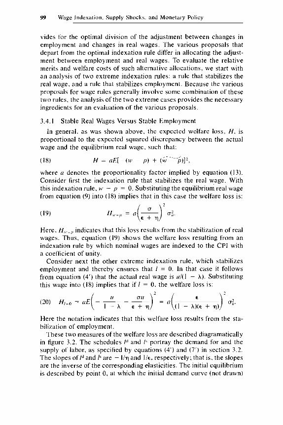
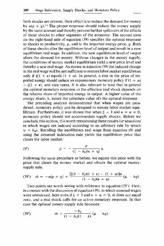
vides for the optimal division of the adjustment between changes in employment and changes in real wages. The various proposals that depart from the optimal indexation rule differ in allocating the adjust- ment between employment and real wages. To evaluate the relative merits and welfare costs of such alternative allocations, we start with an analysis of two extreme indexation rules: a rule that stabilizes the real wage, and a rule that stabilizes employment. Because the various proposals for wage rules generally involve some combination of these two rules, the analysis of the two extreme cases provides the necessary ingredients for an evaluation of the various proposals.
3.4. I Stable Real Wages Versus Stable Employment In general, as was shown above, the expected welfare loss, H , is
proportional to the expected squared discrepancy between the actual wage and the equilibrium real wage, such that:
where a denotes the proportionality factor implied by equation ( 13). Consider first the indexation rule that stabilizes the real wage. With this indexation rule, 11: - p = 0. Substituting the equilibrium real wage from equation (9) into (18) implies that in this case the welfare loss is:
/ \ 2
Here, H,,.=r, indicates that this loss results from the stabilization of real wages. Thus, equation (19) shows the welfare loss resulting from an indexation rule by which nominal wages are indexed to the CPI with a coefficient of unity.
Consider next the other extreme indexation rule, which stabilizes employment and thereby ensures that I = 0. In that case it follows from equation (4') that the actual real wage is ul(1 - A). Substituting this wage into (18) implies that if 1 = 0, the welfare loss is:
- - _ _ - / 14 u11 \2 / E \ ? - - - A)(€ + q)) (20) H,=" =
Here the notation indicates that this welfare loss results from the sta- bilization of employment.
These two measures of the welfare loss are described diagramatically in figure 3.2. The schedules Id and Is portray the demand for and the supply of labor, as specified by equations (4') and (7') in section 3.2. The slopes of Id and Pare - 117 and l k . respectively; that is, the slopes are the inverse of the corresponding elasticities. The initial equilibrium is described by point 0, at which the initial demand curve (not drawn)
100 Joshua AizenmadJacob A. Frenkel
-d intersected with the supply. Thus, initially, (w - p ) = 0. The demand schedule shown here corresponds to a situation in which there was a positive realization of the effective real shock, u. As indicated by equa- tion (4'), this shock induces an upward displacement of the demand schedule by u/(l - A) and results in a new equilibrium real wage, ad (E + q), and correspondingly in a new equilibrium level of employment.
When the indexation rule stipulates that real wages must not change, the real wage remains at point 0 and employment increases to I , at point C . In that case the welfare loss is proportional to the area of the triangle CEB, and its expected value is H,, = p , as specified by equation (19). In the other extreme, when the indexation rule stipulates that employment must not change, the level of employment remains at point 0 and the real wage rises to ul(1 - A) at point A . In that case the welfare loss is proportional to the area of the triangle OAB, and its expected value is H,=", as specified by equation (20). Since the various expressions illustrate percentage deviations from the nonstochastic
Fig. 3.2 The welfare losses caused by indexation rules that stabilize the real wage and by indexation rules that stabilize employ- ment.
101 Wage Indexation, Supply Shocks, and Monetary Policy
equilibrium, the actual welfare loss expressed in units of output is obtained by multiplying (19) and (20) by the equilibrium nonstochastic wage bill.
To determine the relationship between the extent of the welfare losses in the two cases, we need to compare the areas of the two triangles CEB (denoted by A , ) and OAB (denoted by A2). We first note from the geometry that the two triangles are similar in shape and that the ratio ADIDO (where point D indicates the equilibrium real wage) equals the ratio ABIBC. It follows, therefore, that the ratio of the two areas A2/A, equals (ADIDO)2. As can been seen in figure 3.2:
and
therefore:
Thus, if the elasticity of labor supply, E, is smaller than the elasticity of labor demand, q, an indexation rule that fixes employment induces a lower welfare loss than that induced by an indexation rule that fixes the real wage. This is the case i lh t ra ted in figure 3.2. On the other hand, if the elasticity of the labor supply exceeds the elasticity of labor demand, A2 > A , . Under these circumstances rules that stabilize em- ployment inflict a higher welfare loss than that inflicted by rules that stabilize the real wage.
Now that we have analyzed the two extreme indexation rules in preparation for evaluating the various proposals that combine elements of the two rules, we turn next to examine the properties of the proposal of linking the nominal wage to nominal income.
3.4.2 Indexation to Nominal Income When the nominal wage is indexed to nominal income with a unit
coefficient, w = p + y. In this case the coefficients of indexation to the price and to real output are both unity. We should first note with reference to equation (17') that as long as the elasticity of labor supply, E, differs from zero, full indexation to nominal income entails a welfare loss. Only when E = 0 does the optimal indexation rule require that wages be indexed to nominal income with a coefficient of unity.
102 Joshua AizenmanIJacoh A. Frenkel
To evaluate the welfare loss induced by a departure from the optimal indexation rule, we must stipulate that with indexation to nominal income. w - p = y . Substituting U’ - p for y in equation ( 6 ‘ ) and solving for the realized real wage yields:
(22) ( w - P )
Here the notation indicates that this wage is obtained under the rule by which nominal wages are indexed to nominal income with a coef- ficient of unity. With this real wage the level of employment can be read from equation (4’). Substituting (22) for the real wage in (4’) shows that in this case I = 0. Thus, an indexation rule that links the nominal wage to nominal income through an indexation coefficient of unity results in stable employment. The resulting welfare loss corresponds to the area of the triangle OAB in figure 3.2 and is expressed by equation (20). Thus, it follows that:
14. I
I - A -- -
U’ = p + y
(23) H,, - p i , = Hl-0.
3.4.3 An alternative proposal that received especially wide attention fol-
lowing the energy shocks of the 1970s links wages to the domestic value-added price index. This proposal was analyzed recently by Mar- ston and Turnovsky (1983. In what follows we explore further the implications of this indexation rule.
Let the price of final output, p , be a weighted average of the domestic value-added price index, p d , and the price of imported energy input, p , ; and let the weights correspond to the relative shares of value added and energy in output. Thus:
Indexation to the Value-Added Price Index
P = (1 - Alp,/ + AP, .
It follows that the domestic value-added price index is:
An indexation rule that links the nominal wage to this index through a coefficient of unity sets M’ equal to p d . By the definition of p I I from (24), the implied real wage is:
where the notation indicates that this wage is obtained under the rule by which nominal wages are indexed to pL/ with a coefficient of unity.
103 Wage Indexation, Supply Shocks, and Monetary Policy
A comparison of equations (25) and ( 2 2 ) reveals that in the special case in which = 0 (so that shocks to the imported energy price constitute the only component of the effective real shock), LI = - A 4 and the indexation of wages to the domestic value-added price index is equiv- alent to the indexation of wages to nominal income. Furthermore, as was shown above, in this case such indexation results in stable em- ployment, and the corresponding welfare loss is also represented by equations (20).
In the more general case, however, with nonzero productivity shocks the indexation to pd does not stabilize employment, and the welfare loss differs from the one represented by equations (20). The expression for the welfare loss in that case is obtained by substituting the equilib- rium real wage from (9) and the actual real wage from (25) into (IS), such that: /
Here the notation indicates that this welfare loss results from adopting the rule by which nominal wages are indexed to p d with a coefficient of unity.
3.4.4 Ranking the Indexation Rules The preceding discussion implies that, in general, the choice between
indexing to nominal income and indexing to the domestic value-added price index depends on the difference between the expressions mea- suring the losses H,, =/,<, in (26) and H,-,, in (20). To facilitate this com- parison we can usefully rewrite equation (20) somewhat differently by decomposing the effective real shock into its two components. Thus:
Since the terms involving the variance of q are identical in both of the expressions in (26) and (20’), differences in the welfare losses arise only from the terms involving the variance of k. Subtracting (20’) from (26) and denoting the difference by D yields:
(27)
Thus, the sign of L> depends on whether the elasticity of the demand for labor exceeds or falls short of the corresponding elasticity of supply. Since q = ( I - A)u exceeds unity (in practice, with typical relative shares the magnitude of q is likely to be around 3 ) , and since estimates of the elasticity of labor supply are typically small, indexation to nom-
104 Joshua AizenmanIJacob A. Frenkel
inal income is likely to be preferable to indexation to the domestic value-added price index. The opposite holds, however, for cases in which the elasticity of supply exceeds the elasticity of demand.
A comparison of (20’) and (26) shows that when E = 0, indexation to nominal income is optimal, since in that case the value of the loss function in (20’) is zero. In contrast, as shown in equation (26), the welfare loss associated with indexation to the domestic value-added price index is positive, even though E = 0. In this case the expression in (26) is reduced to a[l/(l - A)]*at. As argued above, only when the variance of the productivity shock, p, is zero do the two indexation rules yield identical outcome^.^
To gain a broader perspective over the issues raised by comparing the two forms of indexation, we observe that the condition determining the sign of D in (27) is the same as the condition determining whether the cost of indexation rules that stabilize the real wage exceeds or falls short of the cost of indexation rules that stabilize employment. These relative costs are reflected in the relative sizes of the triangles in figure 3.2. As shown in equation (21), when the elasticity of labor demand exceeds the elasticity of labor supply, indexation rules that stabilize employment are preferable to those that stabilize real wages. These are also the circumstances under which the indexation of wages to nominal income is preferable to indexation to the domestic value-added price index.
The equivalence between the condition under which stable employ- ment is preferable is stable real wages and the condition under which indexation to nominal income is preferable to indexation to the value- added price index is interpreted by reference to equations (22) and (25). When wages are indexed to the value-added price index, then, as shown in equation (25), any given realization of the productivity shock, p, does not alter the real wage. Thus, when the effective real shock con- sists only of productivity shocks, this rule stabilizes the real wage. On the other hand, when wages are indexed to nominal income, then, as shown in equation (22), any given realization of the productivity shock alters the real wage by p/(I - A). This change in the real wage cor- responds precisely to the vertical displacement of the demand for labor arising from the productivity shock and therefore results in stable em- ployment. Finally, as indicated above, when the effective real shock consists only of shocks to the price of imported energy, then, as can be seen from equations (22) and (25), the two rules yield identical outcomes in terms of real wages, employment, and welfare.
The following analysis of the various wage indexation rules is sum- marized in table 3.1 , which reports the coefficients of indexation to the price (bJ , to the productivity shock (b,) , and to the energy-price shock (b2) that are implied by the alternative indexation rules. For example, as indicated by the second line of the table, indexing wages to p d implies

105 Wage Indexation, Supply Shocks, and Monetary Policy
an indexation to p with a coefficient bo = 1 and an indexation to 4 with a coefficient b2 = -A/ ( l - A). This rule follows from equation (25). Likewise, the third line of the table specifies the coefficients im- plied by an indexation rule by which nominal wages are indexed to nominal income with a coefficient of unity. These coefficients follow from equation (22). The optimal indexation formula corresponds to the fourth line in the table, which follows from equation (16). It is a weighted average of the first and the third lines with weights E/(E + q) and q / ( ~ + q), respectively.
Our analysis also determines the welfare cost associated with the various indexation rules. Accordingly, as shown in table 3.1, if the elasticity of the labor supply is smaller than the elasticity of the labor demand, the welfare ranking of the alternative rules is:
where the symbol x > y indicates that x is preferred to y . Thus, it follows that under this assumption, full indexation to nominal income is preferred to full indexation to the domestic value-added price index, which in turn is preferred to full indexation to the CPI. Of course, the optimal indexation rule, b, is preferred to all of the other alternatives. On the other hand, in cases in which the elasticity of the labor supply exceeds the elasticity of the labor demand, the welfare ordering of the suboptimal rules is reversed. In that case:
3.5 Monetary Equilibrium and Optimal Accommodation
Up to this point the monetary sector has played no explicit role in our analysis of the wage indexation rules. Detailed considerations of
Table 3.1 Alternative Wage Rules, where w = bop + blp + bzq
Indexation Coefficients
Wages Indexed to C W P ) 1 Value-added deflator ( p d ) 1
0 0
Nominal income ( p + y ) I I
Optimal indexation (b) 1 U
- I - A
- E f 9
0 A
I - A A
I - A
--
--
- AU
Conclusion: If < q, the welfare ranking of the alternative rules is 6 > p + y > pd > p ; and if E > q, the welfare ranking is b t p > pd t ( p + y) .
106 Joshua AizenmanNacob A. Frenkel
the money market could be left in the background, since in all the rules we have examined, the wages were indexed to the CPI with a coefficient of unity. Furthermore, as shown in Aizenman and Frenkel(1985a), the specification of the model implies that there is a redundancy of policy instruments. Thus, in the absence of other distortions, once the optimal indexation rule is adopted there is no need to undertake additional macroeconomic policies. On the other hand, it also follows that if wages are not indexed optimally, there may be room for other policies de- signed to restore labor market equilibrium. In this section we introduce the monetary sector and analyze the optimal money-supply rule.
3.5.1 The Monetary Sector To determine the equilibrium levels of the nominal quantities such
as the price level, we need to introduce the conditions of money market equilibrium. Let the demand for money be:
(29) log M;' = log k + log P, + 51og Y, - ai,,
where M denotes nominal balances; i denotes the nominal rate of in- terest; a denotes the (semi)elasticity of the demand for money with respect to the rate of interest; and 5 denotes the income elasticity of the demand. The domestic price level is assumed to be linked to the foreign price through purchasing power parity. Thus:
(30)
where S , denotes the exchange rate (the price of foreign currency in terms of domestic currency); and P: denotes the foreign price. Let the foreign price be:
(31)
where a prime (') denotes a foreign variable, and a bar over a variable denotes the value of its fixed component. In equation (31) X , denotes the stochastic component of the foreign price, which is assumed to be distributed normally with a mean of zero and a fixed known variance. Using (31) for log P: yields:
(32)
In principle, the random component of P, may also include stochastic deviations from the purchasing power parity relation of equation (32). When all shocks are zero, the domestic price is:
(32')
and subtracting (32') from (32) yields:
(33) p = s + x ,
log P, = log S , + log P:,
log P: = log p' + X , ,
log P , = log s, + log p' + x,.
log P" = log S" + log B';
where, as before, we suppress the time subscripts.
107 Wage Indexation, Supply Shocks, and Monetary Policy
The nominal rate of interest is linked to the foreign rate of interest, i’. Arbitrage by investors, who are assumed to be risk neutral, assures that uncovered interest parity holds, such that:
(34) i, = ii + &(log Sr+l - log S,),
where E, log S, + denotes the expected exchange rate for period t + 1 based on the information available at period t . The foreign rate of interest is also subject to a random shock, p, which is distributed normally with a mean of zero and a fixed known variance. Thus:
(35) i: = i’ + p,.
The specification of the stochastic shocks implies that the expected exchange rate for period I + 1 is So (the level obtained in the absence of shocks) and therefore E,(log S, +, - log S,) = - s,. Thus, from equa- tions (34) and (35), it follows that:
(36)
In the absence of stochastic shocks, i = I‘ and therefore:
(29‘)
Subtracting (29‘) from (29), omitting the time subscript, and recalling that, from (33), s = p - x yields:
(37)
The supply of money (or, more precisely, the percentage deviation of the supply of money from its nonstochastic level) is denoted by m. Monetary equilibrium is obtained when the demand for money equals the supply of money. We turn next to an analysis of the optimal money
j , - j ’ = p - s.10
log M;f = log K + log Po + <log Y, - a?.
md = (1 + ..)P + sy - 4 P + X I .
supply.
3.5.2 Optimal Monetary Policy The analysis of section 3.3 derived the optimal wage indexation rule.
In this section we focus on the determinants of a money-supply rule that is designed to achieve the same goal of eliminating labor market disequilibrium. To determine the optimal money supply and to contrast the results with those of the previous sections, we assume that wages are completely unindexed, so that w = 0. The question that is being addressed concerns the optimal response of monetary policy in the face of exogeneously given shocks. This question is not new. It has been addressed by various authors in the context of the energy-supply shocks of the 1 9 7 0 ~ . ~ ’ The key question has been whether monetary policy should be accommodative and expend the money supply to “finance” the higher energy price or whether it should be nonaccommodative and
108 Joshua AizenmanIJacob A. Frenkel
contract the money supply to lower inflation. Many observers have, of course, recognized that a real shock that lowers the potential level of output cannot be combated successfully by monetary policy. Instead, the question has been whether monetary policy can be designed so as to prevent the additional costs arising from departures from the new (lower) level of potential output. In what follows we reexamine this question.
To determine the optimal money supply we first equate the demand for money, md (from [37]), with the supply of money, m, and by using equation (10) for the equilibrium level of output, we obtain the equi- librium price level p , such that:
From equation (9) it is evident that when w = 0 (as is the case when nominal wages are unindexed), the value o fp that yields the equilibrium real wage and thereby eliminates labor market disequilibrium is:
(9') U
P = - - U. E f r l
Equating the value of p that clears the money market (from equation [381) with the corresponding value of p that clears the labor market (from equation [9']) and solving for m yields the optimal monetary rule:
where p - Xq has been instituted for the effective real shock u. An inspection of equation (39) reveals that when the income elasticity
of the demand for money, (, is unity, while the elasticity of the supply of labor, E , and the interest (semi)elasticity of the demand for money, a, are zero, f i = 0. This is the case analyzed in detail by Fischer (1985). In this special case the price generated by the condition of money market equilibrium is precisely the price needed to yield the equilibrium real wage, and therefore no accommodation is necessary. In fact, any attempt to alter the money supply in response to the supply shock would result in suboptimal employment and would inflict a wel- fare loss. In general, however, as long as a or E differs from zero and 5 differs from unity, there is justification for an active monetary policy. I z
In interpreting the rule specified by (39), we should note that a pos- itive foreign interest rate shock, p, and a positive foreign price shock, x, lower the demand for money; the interest shock operates through its direct effect on the domestic rate of interest, while the price shock operates through its influence on exchange rate expectations. When
109 Wage Indexation, Supply Shocks, and Monetary Policy
both shocks are present, their effect is to reduce the demand for money by a(p + x ) . I 3 The proper response should reduce the money supply by the same amount and thereby prevent further spillovers of the effects of these shocks to other segments of the economy. The second term on the right-hand side of equation (39) specifies the optimal response to shocks to productivity, p, and to the imported energy price, q . Both of these shocks alter the equilibrium level of output and result in a new equilibrium real wage. In addition, the new equilibrium level of output alters the demand for money. Without changes in the money supply, the conditions of money market equilibrium yield a new price level and thereby a new real wage. As shown in equation (39) the induced change in the real wage will be just sufficient to restore labor market equilibrium only if t(1 + E) equals (1 + a) . In general, a rise in the price of im- ported energy should induce an expansionary monetary policy if ( 1 + a) > ((1 + E), and vice versa. I t is also relevant to note that in general the optimal monetary response to the effective real shock depends on the relative share of imported energy in output. A higher value of the energy share, A , raises the (absolute value of) the optimal response.
The preceding analysis demonstrated that when wages are unin- dexed, monetary policy can be designed to ensure labor market equi- librium. Furthermore, it was shown that when = 1 and E = a = 0, monetary policy should not accommodate supply shocks. Before we conclude this section, it is worth reexamining these results for situations in which wages are indexed according to an arbitrary rule by which w = bop. Recalling the equilibrium real wage from equation (9) and using the assumed indexation rule yields the equilibrium price that clears the labor market:
Following the same procedure as before, we equate this price with the price that clears the money market and obtain the optimal money- supply rule:
Two points are worth noting with reference to equation (39’). First, in contrast with the discussion of equation (39), in which nominal wages were unindexed, here even if = I and E = a = 0, m does not equal zero, and a real shock calls for an active monetary response. In that case the optimal money-supply rule becomes:
( 3 9 )
110 Joshua AizenmanJJacob A. Frenkel
Thus, with a partial wage indexation, a rise in the price of energy and a negative productivity shock require an expansionary monetary policy.
Second, with one important exception, the welfare loss induced by the choice of a suboptimal value of bo could be eliminated through the monetary rule prescribed by equation (39’). The important exception occurs when bo is arbitrarily set to equal unity. In that case the index- ation rule prevents changes in the real wage and results in an absolute real wage rigidity. Any real shock that alters the equilibrium real wage therefore results in labor market disequilibrium and induces a welfare loss. And monetary policy cannot reduce that loss.
Equation (9”) specified the value of the equilibrium price f i that is obtained when monetary policy adopts the optimal rule m. It follows that the variance of the equilibrium price is:
r 7 2
Further, since at the optimum the domestic price is independent of the foreign price shock, x, it follows that:
(41)
Thus, when monetary policy follows an optimal rule, the variance of the exchange rate exceeds the variance of domestic prices.
Finally, from the specification of m in equation (39’), we can note that the variance of the optimal money supply is:
u; = u$ + a:.
Thus, in general, the variance of the optimal money supply depends positively on the variance of the foreign interest and price shocks (p and x), as well as on the variance of the effective real shock, u. Using equation (40) we can also express the variance of m as:
(42’) ~5 = a2 (T:,~ + [((l - bo)(l + E) - ( 1 + c-w)]’ u$.
Equation (42’) shows that at the optimum the relative magnitude of the variances of money and prices depends on whether [5(1 - bo)(l + E)
- (1 + 4 3 ’ exceeds or falls short of unity. In general, if this quantity is larger than unity, the variance of money will exceed that of prices, whereas if it is smaller than unity, the relationship between the vari- ances will depend on the magnitude of o ~ ~ a ~ + ~ . ~ ~
3.5.3 Alternative Monetary Rules The preceding discussion specified the optimal money-supply rule.
In practice, various alternative rules for monetary targets have been
111 Wage Indexation, Supply Shocks, and Monetary Policy
proposed, with special attention given recently to the proposal that monetary policy target nominal income.I5 In this section we apply the analytical framework to the evaluation of alternative proposals. For this purpose we substitute equation (6’) for y into the demand-for- money equation (37); and recalling that with zero wage indexation (w = 0), the demand for money can be written as:
(37‘) md = (1 + a + [ap)p + t a u - a ( p + x). Consider first a monetary rule that targets the CPI. With such a rule,
p = 0 in equation (37’), and the resulting money supply is:
(43)
This monetary rule assures that p = 0 and that, in the absence of wage indexation, the real wage is stabilized. The welfare loss associated with CPI targeting is the same as the loss resulting from a full indexation of wages to the CPI, since both stabilize the real wage. This loss is specified in equation (19).
Consider next the monetary rule that targets nominal income, such that p + y = 0. In this case, from equation (6’), the value of output is y =ad( 1 + pa). If we substitute this into equation (37’) and recall that p = - y , the resulting money supply is:
= tau - a ( p + x). = 0
To evaluate the welfare loss associated with this monetary rule, we observe that in this case, with w = 0, the real wage (w - p ) equals y ; and from equation (6’), y = [l/(l - A)]u. With this real wage the level of employment remains unchanged (as can be seen from equation [4’]), and, therefore, the resulting welfare loss is specified in equation (23).
Consider next a third monetary rule that targets the domestic value- added price index. With this rule, pd = 0; and from the definition of P d in (24), it follows that p = [A/(l - A)]q. Substituting this into (37‘) yields a money supply of
With this targeting rule and with unindexed wages, w = P d = 0 and the resulting welfare loss is specified by equation (26).
The equivalence between the measures of the welfare losses asso- ciated with the different targeting rules for monetary policy and with the indexation rules for nominal wages implies that the welfare rankings
112 Joshua AizenmanIJacob A. Frenkel
of the various rules is also the same as those in equations (28) and (28’). It follows that if E < q, the welfare ranking is:
(46)
and if E > q, the welfare ranking is:
(46‘)
m > m / p + y = 0 >
m > m l p = O > m l p d = o Z m l p + y = 0’
= 0 > = 0
It is interesting to note that the ranking provided by (46) is also con- sistent with that in Tobin (1983), where the targeting of nominal income (with annual revisions) is supported and the targeting of price indexes is criticized. In discussing the choice between targeting p and targeting Pd Tobin concluded, however, that “if any price index were to be a policy target, it should surely not be the CPI, subject as that index is to fluctuations from specific commodity prices, taxes, exchange rates, import costs, interest rates, and other idiosyncracies. It should be some index of domestic value added at factor cost” (Tobin 1983, 119). Our analysis shows that this ranking is not robust. As revealed by the comparison of (46) and (46’), the ranking of the various alternatives depends on the relative magnitudes of the elasticities of the demand for and the supply of labor.
In this section we have considered three specific targeting rules. A similar analysis can be applied to the evaluation of other rules, such as targeting the exchange rate (settings equal to 0), targeting the interest rate (setting i - i’ equal to 0), targeting the money supply (setting m equal to 0), or Hall’s (1984) “elastic price rule.” Each of these alter- natives inflicts a welfare loss, but in general, the welfare ranking of the various rules depends on the values of the parameters. It can be shown, however, that:
(47)
Thus, in the present model, a monetary rule that targets the CPI is preferable to a rule that targets the exchange rate, which in turn is preferable to a rule that targets the rate of interest. Furthermore, in the special case in which E = 0, the targeting of the nominal GNP is optimal, and it therefore is the most preferred of all the policy rules, including the rule specifying a constant money growth.
Finally, we should note that when there are no real shocks (so that = q = y = O), p + y = p = p d . In this special case all of the tar-
geting rules (including the optimal rule, m) yield identical money-supply responses. Those responses ensure that the real wage remains intact,
m l p = OZm/s = OZmJi - 7 = 0’
113 Wage Indexation, Supply Shocks, and Monetary Policy
that changes in the money supply exactly offset shock-induced changes in the money demand, and that the welfare loss is eliminated.
3.6 Other Departures from Optimal Indexation Rules
In section 3.4 we analyze the welfare implications of alternative rules for wage indexation. The rules we considered ensured that either the level of employment or the real wage was kept constant. In this section we examine the welfare implications of other departures from the op- timal wage indexation rule. For this purpose suppose that instead of the sophisticated wage indexation rule specified in equation ( 1 3 , the actual rule adjusts the nominal wage according to simpler formulas. We consider in this section two alternative simple formulas representing different degrees of departure from the optimal rule. To allow for ex- change rate intervention, we let the money supply be:
(48) log M: = log M + 6 , - YS,,
where M denotes the mean value of the nominal money stock; 6, de- notes a random money-supply shock that is assumed to be distributed with a mean of zero and a fixed known variance; and the parameter y denotes the elasticity of the money supply with respect to s-the per- centage deviation of the exchange rate from its deterministic value. As is evident, when y = 0, the supply of money does not respond to s and the exchange rate is fully flexible; on the other hand, when y = ~0
the exchange rate is fixed. Between these two extremes there is a wide range of intermediate exchange rate regimes. Expressing equation (48) in terms of lowercase letters and suppressing the time subscripts yields:
(48”) m = 6 - ys.
3.6.1 Suppose that wages are indexed only to the observed price level.
Also suppose that the coefficients b, and b2 in equation (15) are set equal to zero. Thus:
Indexation to the Price Level
(15’) w = b,p.
In addition, suppose that the monetary authority can adjust the money supply in response to the information conveyed by the exchange rate according to equation (48‘). What should be the optimal values of bo and y?
To find these values, we incorporate the constraints on the forms of the wage indexation and the money-supply rules into the measure of the welfare loss. With the indexation rule the real wage, w - p , is (1 - bo)p. To compute the value of p , we equate the supply of money
114 Joshua AizenmanIJacob A. Frenkel
from equation (48”) with the demand for money from equation (37); and to simplify, we assume for the rest of this section (without sacri- ficing any great insights) that the income elasticity of the demand for money, 6 , is unity. Recalling that s = p - x and that from equation (6’) y = u[P@ - w) + u ] , we find that the value of p that clears the money market is:
’ = 1 + ( 1 - b o ) p o + a + y ‘ (49)
Using equation (49), we can write the negative of the real wage, -(w - p) , as:
6 + a p + (a + y)x - uu
(50) ( 1 - bok = $05
1 - bo 1 + (1 - b,)@ + (Y + y
where $ = and 0 = [?I + a p + (a + y)x - uu]. Substituting equation (50) for the real wage into the measure of the welfare loss, A, in equation (13) yields:
(13’)
and computing the expected value of the loss yields the loss function H:
where ui = u: + + u2ut. To find the optimal value of the indexation coefficient, we should note that in (13’) and in the loss function (51), b, appears only in $; therefore, minimization of A in (13’) or of H in (51) with respect to b, is equivalent to minimization with respect to $ (holding y constant). This procedure yields the optimal value of $ , 1 6 such that:
+ (a + y)2
Equating $* with the definition of $ in (50) yields the optimal value of the indexation coefficient b,;
115 Wage Indexation, Supply Shocks, and Monetary Policy
where the notation on the left-hand side indicates that the optimization is performed under the constraints that the coefficients b, and b2 in the general indexation rule of equation (15) are set equal to zero.
Equation (53) suggests that the optimal indexation coefficient b; de- pends on three groups of parameters. The first contains the structural parameters of the economy, such as the interest (semi)elasticity of the demand for money (a); the elasticity of the supply of labor (6); and the elasticity of the demand for labor (q), which also embodies the elas- ticities of output with respect to labor and energy (p and A). The second group contains the stochastic structure of the various shocks (6 , p, x, p, and 9); and the third contains parameters of other prevailing policies, such as the degree of foreign exchange intervention represented by y. In general, the dependence of b; on the various parameters is:
3 > 0, A< ab* 0, -< ab; 0 a€ ap ax
Equation (53) specifies the optimal value of the indexation coefficient under the assumption that the value of y is set at an arbitrary level. Later on, we will also set y at its optimal level, but before we do so, it might be instructive to examine the implications of two extreme exchange rate regimes. First, we observe that when y = 03, that is, when the exchange rate is completely fixed, the optimal indexation coefficient is unity. This can be verified by noting that in the measure of the welfare loss (13r), when y = 00 the negative of the real wage $0 is (1 - h , ) ~ . Thus, to minimize the value of the last term in parentheses on the right-hand side of (13r), we need to set b; equal to unity. On the other hand, when y = 0, that is, when the exchange rate is completely flexible, the optimal indexation coefficient is given in equation (53) after setting y equal to zero. As can be seen, in that case, when the ratio of ui + a 2 ( u ~ + uf) to a’, approaches infinity, as would be the case in the absence of supply shocks, the optimal indexation coefficient approaches unity. On the other hand, when this ratio approaches zero, as would be the case when supply shocks constitute the only distur- bances, the optimal indexation coefficient approaches (E - a)/(l + E). (Recall that in deriving this expression we have assumed a unit income elasticity of the demand for money.)
To compute the welfare implications of the departures from the op- timal wage indexation rule of section 3.3, we substitute (52) for 4 into the loss function (51) and obtain:
116 Joshua AizenrnanNacob A. Frenkel
(54)
H(b;,;y) I u: + a%; + (a + y)%; 6 , = 0 = I[ 2 c(c u2qut + q) I[ uz + + (a + ?)*a; + u2(rZ '
b2 = 0
where the notation on the left-hand side indicates that the loss is eval- uated under the condition that only bo is set optimally, while the coef- ficients bl and b2 in the wage indexation rule (15) are zero and the coefficient y in the money-supply rule (48) is set at an arbitrary level. As can be seen, in general (except for the special cases in which the variance of the effective real shock is zero or the second bracketed term in (54) is zero), the indexation to the price level alone cannot eliminate the welfare loss.
It is also of some interest to examine the welfare implications of alternative magnitudes of the production elasticities, A and p, which are embodied in u, where u = 1/(1 - p - A). It can be shown that
aH(b';y) > 0. Thus, if wages are m y ) > and when 6 , = b2 = 0, ap ah
constrained to be indexed only to the price level, then, for a given configuration of the stochastic shocks, the optimal welfare loss is higher in economies in which the relative shares of labor and energy in the GNP are higher. Equation (54) reveals the channels through which these shares affect the welfare loss. The size of the labor share, p, affects the loss function through its direct impact on u. On the other hand, the size of the energy share, A, affects the loss function through its direct effect on u, as well as through its impact on the stochastic structureitself. Sinceu = p, - Aqandut = + A*u$ahighervalue of A will increase the variance of the effective real shock.
Equation (54) can also be used to assess the welfare implications of adopting two extreme exchange rate regimes. When the exchange rate is completely fixed, y = ~0 and (54) becomes:
(54')
b2 = 0 / Y = O C i
In that case, the welfare loss depends only on the productive tech- nology, on the elasticity of labor supply, and on the effective real shock. The adoption of the optimal value of bo eliminates the welfare impli- cations of the money-supply shock, 6 ; the foreign interest shock, p; and the foreign price shock, x. In that case, the value of a therefore does not influence the measure of the welfare cost. On the other hand,
117 Wage Indexation, Supply Shocks, and Monetary Policy
(55) H ( b h ) 2 H ( b h ) 6 , = 0 b2 = 0 y = w
when the exchange rate is completely flexible, y = 0 and the loss function becomes:
6 , = 0 b2 = 0 y = o

118 Joshua AizenmanIJacob A. Frenkel
an optimal exchange rate policy eliminates the effects of the variance of foreign price shocks, a:.
Equation (53') indicates that, in general, as the ratio of u: + a'$ to at approaches infinity, as would be the case when there are no real shocks, the optimal indexation coefficient approaches unity. On the other hand, when this ratio approaches zero, as would be the case when there are only real shocks, the optimal indexation coefficient approaches the fraction ~ / ( 1 + E).
Substituting -a for y in the loss function (54) yields:
Ib, = 0
where the left-hand side indicates that the loss is evaluated under the conditions that both b, and y are set optimally and that 6 , and b2 are constrained to equal zero.
3.6.2 Indexation to the Price Level and to the Relative Price of Imported Energy
Consider now an alternative indexation rule that comes closer to the general rule of equation (15). Suppose that only the coefficient 6 , in equation (15) is constrained to be zero. Thus, wages are assumed to be indexed to the price, p , and to the relative price of energy, 4, according to the following:
( 15") w = bop + b24.
With this indexation rule the measure of the welfare loss is:
and the policy problem is to determine the optimal values of bo and b2 so as to minimize the expected value of the welfare loss. As is evident, minimizing the loss function is equivalent to minimizing the expected value of the last (squared) term in (13"), which measures the difference between the actual real wage and the equilibrium real wage. In what follows we focus on this term.
Proceeding along similar lines as in section 3.5.1, we find that the equilibrium price that clears the money market is:
119 Wage Indexation, Supply Shocks, and Monetary Policy
After substituting this expression forp into (13”) and collecting terms, we can write the loss function (or, more precisely, the expected value of the squared difference between the actual and the equilibrium real wage) as:
where = 6 + a p + (a + y)x - a~ = 8 - aAq, and 8 and + are as defined in equation (50).
In minimizing the loss function we first equate the coefficient of q to zero and substitute the optimal value of + (analogous to equation [52]) into (57). This yields the optimal value of b2, such that:
Thus, a higher relative price of imported energy must lower the wage. The dependence of b; on the various parameters is:
Furthermore, it is noteworthy that the elasticity of - b; with respect to the size of the energy share, A , exceeds unity.
Once b2 has been set at its optimal level, the coefficient of q in the loss function vanishes and the expression in (57) reduces to the following:
, \ 2
(57’)
Since the optimal value of b2 serves to eliminate the impact of imported energy-price shocks on labor market disequilibrium, it is evident that from now on the formal structure of the optimization problem is in- dentical to that in section 3.6.1. The only difference between the two is that the expression in (57’) does not include terms involving q. Thus, (57’) contains O 1 and p, whereas the expression in (51) contains 0 and u . It follows that the optimal value of bo is the same as in equations (53) and (53’) except for the substitution of a: for a:.
A comparison of the optimal value of b ; in (58) and the corresponding value of b: shows that the two components of the wage indexation rule are related to each other through a simple link. For example, when y is set at its optimal value, b: is described by equation (53’) (modified to include a:, instead of at), and the two indexation coefficients are related to each other according to the following:
120 Joshua AizenmanIJacob A. Frenkel
(59)
Thus, the ratio b;l(hG - 1 ) is higher, the higher the relative share of imported energy in output. Likewise, this ratio is higher, the higher the variances of the monetary shock, 6, and the foreign interest shock, p, and the lower the variance of the productivity shock, k.
The formal similarity between the structure of the optimization prob- lem in equation (57') and that of section 3.6.1 also implies that all the expressions developed in that section for the purpose of measuring the welfare loss resulting from alternative second-best situations continue to apply. The only modification requires the substitution of the variance of the productivity shock, u:, for the variance of the effective real shock, uf,. Furthermore, since a: is smaller than u; (which also contains the variance of the imported energy price), it follows from ( 5 3 ) that the optimal value of h,, is higher when the indexation rule allows for the application of an optimal response to y than when it does not.
The foregoing discussion, together with the results obtained in sec- tion 3.3, implies that:
(60) b,l d hG1 =z b;l = I . 6 , = 0 b , = 0 b , = b; h2 = 0 b2 = bl h, = 6;
This chain of inequalities demonstrates that the optimal degree to which wages should be indexed to the price level depends critically on the precise form of the constraints that are imposed on the indexation rule. In the absence of constraints on the degree of sophistication of the wage rule, the optimal coefficient of indexation to the price level is unity. This ensures that monetary shocks, which should not affect the equilibrium real wage, are prevented from inducing changes in the real wage. At the optimum, real shocks are allowed to alter the real wage through separate indexation coefficients. Once such a separation is not allowed, successive departures from the sophisticated indexation rule result in successive reductions in the degree to which wages ought to be indexed to prices.'*
3.7 Concluding Remarks
In this paper we analyzed the interactions among supply shocks, wage indexation, and monetary policy. We developed an analytical framework for determining the optimal wage indexation and monetary policy. This framework was then applied to analyze the implications
121 Wage Indexation, Supply Shocks, and Monetary Policy
of suboptimal policy rules. The welfare ranking of those rules was based on the relative magnitudes of the deadweight losses associated with the various policies. The main results of our analysis are summarized in the introduction to this paper. In this section we outline some of the limitations of the study and possible further extensions of this line of research.
In our framework labor market contracts stipulate the nominal wage rule for the length of the contract period. Those contracts reflect the cost of negotiations. Since the wage rule is set in advance of the re- alization of the stochastic shocks, it may give rise to deadweight losses associated with disequilibrium real wages. Our analysis employs this specific form of wage contracts as a stylized description of conventional labor market arrangements. Implicit in our formulation is the assump- tion that workers and employers are risk neutral. A useful extension would allow for risk aversion that would rationalize contracts in terms of the insurance function (see, for example, Azariadis 1978).
Further, in our specification the welfare loss arises only from a sub- optimal employment level. Implicit in this specification is the assump- tion that all other markets are undistorted. An extension would allow for other distortions. In that case the welfare loss caused by suboptimal money holdings would be added to the loss associated with labor market distortions and would depend on both the level and the variance of inflation.
Although we have assumed in the main analysis that the stochastic shocks are identically and independently distributed with a mean of zero and a fixed variance, we have outlined the way by which one could allow for more general time-series properties of the stochastic shocks. An explicit elaboration of such an extension would highlight the important distinction between permanent and transitory shocks and would generate a profile of wage dynamics. In addition to the distinction between permanent (long-lived) and transitory (short-lived) shocks, one could also allow for lags in the implementation of the indexation rules. With such lags, as indicated by Fischer in his accompanying comment, optimal policies would index wages to the long-lived shocks but would not index wages to the short-lived shocks. To clarify the above pre- scription, we should note that “long-lived” shocks are those that are in effect during the period in which indexation can be implemented but that have not yet been incorporated into the determination of the con- tractual base wage. On the other hand, “short-lived” shocks are those that are in effect for a length of time shorter than the indexation lag. With this distinction, our formulas for optimal wage indexation rules are fully applicable. They may be interpreted as providing a guide for the necessary adjustment of the nominal wage in the presence of long-
122 Joshua AizenmanlJacob A. Frenkel
lived shocks. Richer and more complicated dynamics could also be induced by staggered contracts and by capital accumulation (see, for example, Fischer 1977~; 1985) and Taylor 1980).
Our analysis assumed that there is one composite good that is traded internationally at a (stochastically) given world price. With this level of aggregation we demonstrated that wage indexation rules bear an exact dual relationship to monetary targeting rules. This duality implied that there was no fundamental difference between the outcomes of various wage indexation rules and the outcomes of the corresponding monetary targeting rules. Thus, when there is a single composite com- modity, the choice between wage indexation and monetary policy is governed by additional considerations such as the relative costs and complexities associated with the implementation of the two alternatives rules. In the more general case, however, when there are many sectors producing a variety of goods, the exact duality between wage index- ation and monetary policy breaks down. Specifically, as shown by Blinder and Mankiw (1984), it is clear that monetary policy, being an aggregative policy, is not a suitable response to sector-specific shocks. Under such circumstances it is evident that optimal sector-specific policies are called for instead. A natural extension of our analysis would be to apply the analytical framework to determine the optimal sector- specific wage indexation formulas that would eliminate the welfare loss resulting from labor market distortions (for a sketch of such a frame- work, see Aizenman and Frenkel 1986b).
Appendix: The Computation of the Welfare Loss
In this appendix we provide a formal derivation of the welfare loss that is used in the text.
Consider a two-period model and let the present value of utility U be:
(All
where designates the subjective discount factor; Ci and Li (i = 1, 2) denote the levels of consumption and labor in period i; and the sub- scripts 1 and 2 designate periods 1 and 2, respectively. The value of assets not consumed in period 1 is A l , and their value in period 2 is (1 + r)Al, where r designates the exogenously given (stochastic) world rate of interest on internationally traded bonds. Profits are denoted by R and are assumed to be redistributed as lump-sum transfers. The value
u = 4c1, Ll) + P U ( C 2 , L2),
123 Wage Indexation, Supply Shocks, and Monetary Policy
of profits in each period is the corresponding value of output, Y,, minus payments to labor and energy inputs, such that:
where W, P,, and P denote the nominal wage, the price of energy, and the price of output, respectively. Producers are assumed to maximize profits subject to the given real wage and the given relative price of energy. In equilibrium the real wage and the relative price of energy are equated to the marginal products of labor and energy, respectively, such that:
These conditions yield the demands for labor and energy inputs. The equilibrium real wage that clears the labor market is defined by ( WiP), and L and V denote the corresponding equilibrium levels of employment and energy utilization. At this general equilibrium all markets clear.
We turn now to the formal maximization problem, starting with the maximization of second-period utility. Denoting by RIT (i = 1, 2) the solution to the producers' profit maximization problem in period i , as implied by the solutions to (A3) and (A4), we can write the maximi- zation problem in period 2 as:
The solution to this problem yields C; and L; as the optimal values of consumption and labor supply in period 2. These optimal values are conditional, of course, on the historically given value of A , . Thus, we can define a function u*(A,) , which denotes the expected value of op- timal utility in the second period. Thus, u*(A,) = E[u(C;, L;)]. The maximization problem for period 1 can then be presented as:
where Q denotes the given initial endowment. The solution to (A6) yields the optimal values C,, L, , and A,. For subsequent use we note
124 Joshua AizenmadJacob A. Frenkel
that the optimal value of A , is chosen so as to satisfy the first-order condition requiring that:
(A71 6 au*(Al)/aA, = au(c, , L l ) /ac l .
The value of utility in the general equilibrium is denoted by U(LJ , where it is understood that this level of utility is obtained when C , , L , and A l are set at their unconstrained optimal values, C,, Ll and A,. In practice, because of the existence of contracts, the level of employment might be constrained to L , . The resulting level of utility would be U(L,) , where it is understood that C , and A , are still chosen optimally subject to the constraint that the maximization of profits and the given nominal wage yield labor demand (and therefore employment) at the level L I . The welfare loss caused by the constrained employment (L , ) in terms of first-period consumption is:
AU U(L1) - U(L1) _ - - 8 a&, L,)/aC, '
where AU = U ( i l ) - U(L,) , and 8 = du(C,, i l ) / aCl denotes the marginal utility of consumption during the first period evaluated around the general equilibrium.
To obtain an expression measuring the welfare loss, we first compute the change in welfare associated with a marginal change in employment around an initial arbitrary level L. In what follows we compute the welfare loss for period 1, and we suppress the corresponding time subscript. Using equation (A6), the first-order approximation of the change in welfare resulting from a marginal change in employment is:
(A9) U(L + AL) - U(L) = [au(C, L)/dC]AC + [au(C, L)/dL)AL + fi[au'(A)/aA]AA.
Using equation (A7) and expressing (A9) in terms of first-period con- sumption yields:
where (W/P). = - au(C, L)/aL denotes the real wage as measured along the supply of labor. From the definition of profits in (A2) and the budget constraint in (A6) we can see that:
and therefore:
(Al l ) ay dY p , aL av P
AC + AA = PAL + -AV - -AV.
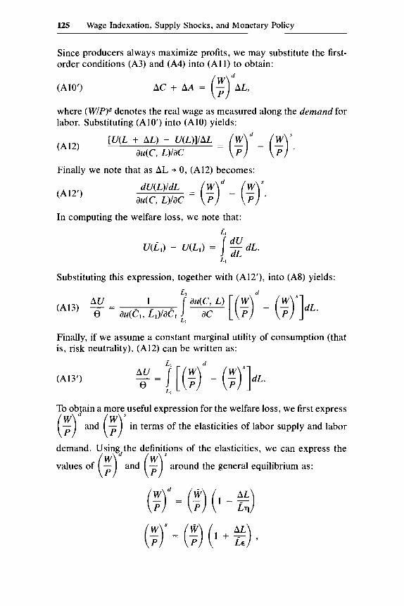
125 Wage Indexation, Supply Shocks, and Monetary Policy
Since producers always maximize profits, we may substitute the first- order conditions (A3) and (A4) into (A1 1) to obtain:
(A10’) d
AC + AA = (T) AL,
where ( W/P)d denotes the real wage as measured along the demand for labor. Substituting (AlO’) into (A10) yields:
(A 12)
Finally we note that as AL + 0, (A12) becomes:
[U(L + AL) - U(L)]/AL = (!!)d - (q. au(c, L)/dC
(A12’) dU(L)/dL
au(c, ~yac In computing the welfare loss, we note that:
L
LI
Substituting this expression, together with (A12’), into (A8) yields:
Finally, if we assume a constant marginal utility of consumption (that is, risk neutrality), (A12) can be written as:
(A13’)
To objain a more useful expression for the welfare loss, we first express
(T) and (F)‘ in terms of the elasticities of labor supply and labor
demand. Usingdthe definitions of the elasticities, we can express the
values of (F) and (;) ’ around the general equilibrium as:
(;)d = (;) ( 1 - g) (;y = (;) ( 1 + 2) ,
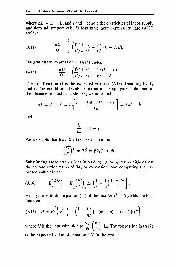
126 Joshua AizenmanIJacob A. Frenkel
where AL = L - L , and E and -q denote the elasticities of labor supply and demand, respectively. Substituting these expressions into (A13’) yields:
Integrating the expression in (A14) yields:
AU W 1 1 1 ( L - L)*
- e = (-)- P L (- E + ;) 2 ,
The loss function H is the expected value of (A15). Denoting by Yo and Lo the equilibrium levels of output and employment obtained in the absence of stochastic shocks, we note that:
and
We also note that from the
_ - - (1 - i). LO
first-order condition:
(;)L = p Y = pYO(1 + f ) ,
Substituting these expressions into (A15), ignoring terms higher than the second-order terms of Taylor expansion, and computing the ex- pected value yields:
(A16) E - ( y ) = E [ ( F ) o L o (: + !-) v] .
Finally, substituting equation ( I 1) of the text for (1 - I) yields the loss function:
(A17) H = E { $ - q y (: + i) [-(w - p ) + (w - p) ]* , ’- I
where His the approximation to -/ - Lo. The expression in (A17)
is the expected value of equation (13) in the text.
127 Wage Indexation, Supply Shocks, and Monetary Policy
Notes
I . This assumption is relaxed in Aizenman and Frenkel (1985a), where it is assumed (in the context of a model without energy) that the value of the stochastic shock is not known at each point in time. In that case behavior is governed by the conditional expectations of the shocks based on the available information.
2. The question concerning the efficiency of the assumed wage contract is addressed in section 3.3.2, note 6.
3. This expression corresponds to equation (A17) in the appendix. To obtain the welfare loss in units of output, we need to multiply equation (13) by the equilibrium (nonstochastic) wage bill, (W/P)&. For a useful discussion of welfare loss measurement, see Harberger (1971).
4. We assume that the initial contractual nominal wage is set at W-the level that would have prevailed in equilibrium in the absence of shocks. Any other initial wage would not minimize the expected value of the welfare loss. In making this statement we use the approximation log E,_I(eut) = El- , (u,). This approximation is valid for small values of the variance and of the realization of the stochastic shock u.
5 . For an analysis of optimal indexation rules, see Fischer (1977a; 1977b). 6. The assumption that employment is determined by the demand for labor was chal-
lenged by Cukierman (1980), who examined alternative specifications of employment. As is evident with optimal policies, these issues become inconsequential since, at the optimum, labor demand and labor supply are equal. Likewise, at the optimum, the conceptual difficulties raised by Barro (1977) concerning the existence of suboptimal contracts are also inconsequential, since with optimal policies these contracts are in fact optimal. For a further discussion and rationalization of labor contracts, see Hall and Lazear (1984) and Fischer (1977b).
7. The specification in equation (17) constrained the coefficient o f p to be unity. More formally, let the coefficient of p in (17) be bp; in that case the real wage is w - p = (bp ~ I)p + b,y, and the level of output (using 6') is y = [ - (bp - I)p + uu]/ (1 + Pub,). Substituting this expression into the real wage equation and using equation (13) reveals that to equate the realized real wage with the equilibrium real wage, the coefficient o f p must be unity and the coefficient o fy must be 1/(1 + E ) . It is also relevant to note that equation (17') corresponds to equation (15) in Karni (1983, 286). The precise analogy may not be apparent because there is a typographical error in Karni's equation (IS). Using Karni's notations his coefficient of indexation to real output should read q/
8. For analyses of alternative proposals, see Fischer (1977a), Eden (1979), Marston and Turnovsky (1989, and Marston (1984). For an analysis of alternative compensation systems and for a related discussion of employment versus real wage stabilization, see Weitzman (1983).
9. It is relevant to note that with a Cobb-Douglas production function, indexing nom- inal wages to nominal income is equivalent to indexing real wages to the real value of value added in terms of units of final output. To verify, define the real value added by
(q + v). From the Y - (Pv/P)V and the percentage change thereof by - - - first-order conditions, AYIV = P,/P and therefore y = q + v. It thus follows that
y = y . Marston and Turnovsky (1985) argued that the rule according to
which nominal wages are indexed to the value-added price index produces equivalent results to those produced by the rule by which real wages are indexed to the real GNP. Our analysis shows that this equivalence holds only as long as there are no productivity shocks. Further, if the two rules are equivalent, they will be optimal only if, in addition, E = 0.
10. The implicit assumption underlying this formulation is that all variables are sta- tionary, that is, that there are no trends and that E, log SI+I is not influenced by the observed price. Thus, in the absence of shocks, i = i'. Our assumption about the absence of trend allows us to focus on the properties of the stationary equilibrium for which the
(w + q + Swq).
A Y I - A I - A
A Y I - A 1 - A
128 Joshua AizenmanIJacob A. Frenkel
current values of the stochastic shocks d o not affect expectations about future values of the variables. In general, the stochastic shocks need not be identically and indepen- dently distributed with a mean of zero and a fixed variance. Allowing for a more general specification requires a modification of the definition of the benchmark equilibrium that is obtained in the absence of shocks. With a more general specification of the stochastic shocks we let lowercase letters denote an innovution of a given variable. Thus, x, = log X , - log X , , instead of the specification adopted in the text according to which x, = log X , - log X,. Obviously, in the special case discussed in the text, the assumed properties of the stochastic shocks imply that El.] log XI = log X,. With this interpre- tation of xl (as the innovation of log X , ) + the analysis can allow for trends in the various series, and the various shocks may include permanent and transitory components. It is also relevant to note that the specification of equation (36) also embodies the assumption that the equilibrium is unique. The choice of the unique equilibrium is consistent with the criterion suggested by McCallum (1983). On the issue of uniqueness, see Calvo (1979) and Turnovsky (1983b).
11 . Relevant early references are Gordon (1975) and Phelps (1978). The focus on the question of accommodation in the presence of supply shocks is contained in Blinder (1981). Gordon (1984). and Fischer (198.5); and various structural issues concerning adjustment to external shocks in an international setting are found in Bruno (1984). Bruno and Sachs (1982), Findlay and Rodriguez (I977), and Marion and Svensson (1982).
12. Phelps (1978) emphasized the implications of an income elasticity differing from unity.
13. In the more general specification of the stochastic shocks (which are described in note lo), the term (p + x ) in equation (37) would be replaced by the innovation in i, + log P,, which can also be expressed as i; + E, log S,,, + log P;. Thus, the innovation of this term is (i; - E,-,i;) + E,s ,+ , + p ; , where E,s,+l = El log S,+I - 4-1 log &+I, and p; = log P; - E,. I log P;. To obtain this expression for the innovation we first substitute equation (34) into the demand for money (in equation 1291) and replace i’ (in equation [29’]) with E,-]i;. Subtracting the resulting two equations from each other yields the more general expression corresponding to equation (37).
14. We should note that the formulation of the objective function in terms of the minimization of the welfare loss from labor market distortions presumes that other markets are undistorted. Within this framework the variances of prices and of the money supply are reported in equations (40) and (42) only as informative statistics. A more general formulation would recognize that the productivity (or the utility yield) of money depends on these variances. Optimal policies would then minimize the welfare loss from labor market distortions along with the loss from suboptimal inflation and price variability.
15. For analyses of nominal income targeting, see, for example. Meade (1978). Poole (1980), Tobin (1980; 1983), Hall (1983). Bean (1983), Taylor (198.5). and Aizenman and Frenkel (1986a). For discussions of a close variant of nominal income targeting see McCallum (1984) and Mishkin (1984); and for other rules see Phelps and Taylor (1977).
16. Minimizing the expected value of (13’) with respect to t$ amounts to computing the ordinary-least-squares estimate of a regression of U U / ( E + q) on -8. It follows that the optimal value of +B is:
COV(U, 8)[UN€ + $1 , +* = - Ui
and when the stochastic shocks are independent of each other, this expression reduces to equation (52) in the text.
17. For a related analysis of the relationship between optimal wage indexation and optimal foreign exchange intervention, see Aizenman and Frenkel (1985a), Bhandari (1982), Marston (1982), and Turnovsky (1983a).
18. It can be shown that if the constraint on the indexation rule sets b2 = 0 but allows for the optimal determination of ho and h , , then:
6Ib2 = 61 as u; i~ &,. bl = by 6 , = 0
b? = hi
129 Wage Indexation, Supply Shocks, and Monetary Policy
References
Aizenman, Joshua, and Frenkel, Jabob A. 1985. Optimal wage index- ation, foreign exchange intervention and monetary policy. American Economic Review 75, no. 3 (June): 402-23.
. 1986a. Targeting rules for monetary policy. Economics Letters 21.
. 1986b. Sectorial wages and the real exchange rate. NBER Working Paper Series, no. 18 (January). Forthcoming in Journal of International Economics.
Azariadis, Costas. 1978. Escalator clauses and the allocation of cyclical risks. Journal ofEconomic Theory 18, no. 1 (June): 119-55.
Barro, Robert J. 1977. Long-term contracting, sticky prices, and mon- etary policy. Journal of Monetary Economics 3, no. 3 (July): 305- 16.
Bean, Charles R. 1983. Targeting nominal income: An appraisal. Eco- nomic Journal 93, no. 4 (December): 806-19.
Bhandari, Jagdeep S. 1982. Staggered wage setting and exchange rate policy in an economy with capital assets. Journal of International Money and Finance I , no. 3 (December): 275-92.
Blinder, Alan S. 1981. Monetary accommodation of supply shocks un- der rational expectations. Journal of Money, Credit and Banking 13, no. 4 (November): 425-38.
Blinder, Alan S., and Mankiw, Gregory N. 1984. Aggregation and sta- bilization policy in a multi-contract economy. Journal of Monetary Economics 13, no. 1 (January): 67-86.
Bruno, Michael. 1984. Raw materials, profits, and the productivity slow- down. Quarterly Journal of Economics 99, no. 1 (February): 1-30.
Bruno, Michael, and Sachs, Jeffrey. 1982. Input price shocks and the slowdown in economic growth: The case of U. K. Manufacturing. Review of Economic Studies 5 (special issue): 679-706.
Calvo, Guillermo A. 1979. On models of money and perfect foresight, International Economic Review 20, no. 1 (February): 83- 102.
Cukierman, Alex. 1980. The effects of wage indexation on macroeco- nomic fluctuations: A generalization. Journal of Monetary Econom- ics 6, no. 2 (April): 147-70.
Eden, Benjamin. 1979. The nominal system: Linkage to the quantity of money or to nominal income. Revue Economique 30, no. 1 (Jan- uary): 121-43.
Findlay, Ronald, and Rodriguez, Carlos A. 1977. Intermediate imports and macroeconomic policy under flexible exchange rates. Canadian Journal of Economics 10 (May): 208-17.
Fischer, Stanley. 1977a. Wage indexation and macroeconomic stability. In Stabilization of domestic and international economy, ed. Karl Brunner and Allan Meltzer. Carnegie-Rochester Conference Series
130 Joshua Aizenman/Jacob A. Frenkel
on Public Policy, vol. 5, a supplementary series to the Journal of Monetary Economics 3: 107-47.
. 1977b. Long term contracting, sticky prices and monetary pol- icy: A comment. Journal of Monetary Economics 3, no. 3 (July): 3 17-23.
. 1977c. Long-term contracts, rational expectations, and the op- timal money supply rule. Journal of Political Economy 85, no. 1 (February): 19 1 -205.
. 1985. Supply shocks, wage stickiness, and accommodation. Journal of Money, Credit and Banking, 17, no. 1 (February): 1 - 15.
Flood, Robert P., and Marion, Nancy P. 1982. The transmission of disturbance under alternative exchange-rate regimes with optimal indexation. Quarterly Journal of Economics 97, no. 1 (February):
Gordon, Robert J . 1975. Alternative responses of policy to external supply shocks. Brookings Papers on Economic Activity (no. 1) : 183- 206.
. 1984. Supply shocks and monetary policy revisited. American Economic Review 74, no. 2 (May): 38-43.
Gray, Jo Anna. 1976. Wage indexation: A macroeconomic approach. Journal of Monetary Economics 2, no. 2 (April): 221-35.
Hall, Robert E. 1983. Macroeconomic policy under structural change. In Zndustrial change and public policy, 85- 1 11. Federal Reserve Bank of Kansas City.
. 1984. Monetary Strategy with an Elastic Price Standard. In Price stability and public policy, 137-59. Federal Reserve Bank of Kansas City.
Hall, Robert E., and Lazear, Edward P. 1984. The excess sensitivity of quits and layoffs to demand. Journal of Labor Economics 2, no. 2 (April): 233-57.
Harberger, Arnold C. 1971. Three basic postulates for applied welfare economics: An interpretive essay. Journal of Economic Literature 9, no. 3 (September): 785-97.
Karni, Edi. 1983. On optimal wage indexation. Journal of Political Economy 91, no. 2 (April): 282-92.
Marion, Nancy P., and Svensson, Lars E. 0. 1982. Adjustment to ex- pected and unexpected oil price increases. NBEK Working Paper no. 997. Cambridge, Mass.: National Bureau of Economic Research, October.
Marston, Richard C. 1982. Wages, relative prices and the choice be- tween fixed and flexible exchange rates. Canadian Journal of Eco- nomics 15, no. 1 (February): 87-103.
. 1984. Real wages and the terms of trade: Alternative indexation rules for an open economy. Journal qf Money, Credit und Bunking 16, no. 3 (August): 285-301.
43-66.
131 Wage Indexation, Supply Shocks, and Monetary Policy
Marston, Richard C., and Turnovsky, Stephen J. 1985. Imported ma- terial prices, wage policy and macroeconomic stabilization. Cana- dian Journal of Economics 19, no. 2 (May): 273-84.
McCallum, Bennett T. 1983. On non-uniqueness in rational expecta- tions models: An attempt at perspective. Journal of Monetary Eco- nomics 1 1 , no. 2 (March): 139-68.
. 1984. Monetarist rules in the light of recent experiences. Arner- ican Economic Review 74, no. 2 (May): 388-91.
Meade, James E. 1978. The meaning of internal balance. Economic Journal 88, no. 3 (September): 423-35.
Mishkin, Frederic S. 1984. The causes of inflation. In Price stability and public policy, 1-24. Federal Reserve Bank of Kansas City.
Phelps, Edmund S. 1978. Commodity-supply shock and full-employment monetary policy. Journal of Money, Credit and Bunking 10, no. 2 (May): 206-21.
Phelps, Edmund S. , and Taylor, John B. 1977. Stabilizing powers of monetary policy under rational expectations. Journal of Political Economy 85, no. 1 (February): 163-90.
Poole, William. 1980. Comments on paper by Tobin. Brookings Papers on Economic Activity (no. I): 79-85.
Rasche, Robert H., and Tatom, John A. 1981. Energy price shocks, aggregate supply and monetary policy: The theory and the interna- tional evidence. In Supply shocks, incentives and national wealth, ed. Karl Brunner and Allan Meltzer, 9- 13. Carnegie-Rochester Conference Series on Public Policy, vol. 14, Amsterdam: North- Holland.
Taylor, John B . 1980. Aggregate dynamics and staggered contracts. Journal of Political Economy 88, no. 1 (February): 1-23.
. 1985. What would nominal GNP targeting do to the business cycle? In Understanding Monetary Regimes, ed. Karl Brunner an3 Allan Meltzer, 61 -84. Carnegie-Rochester Conference Series on Public Policy, vol. 22. Amsterdam: North-Holland.
Tobin, James. 1980. Stabilization policy ten years after. Brookings Pa- pers on Economic Activity (no. l ) : 19-71.
. 1983. Commentary. In Industrial change and public policy, 113-22. Federal Reserve Bank of Kansas City.
Turnovsky, Stephen J. 1983a. Wage indexation and exchange market intervention in a small open economy. Canadian Journal of Eco- nomics 16, no. 4 (November): 574-92.
. 1983b. Exchange market intervention policies in a small open economy. In Economic interdependence andJlexible exchange rates, ed. J. Bhandari and B. Putnam, 286-311.
Weitzman, Martin L. 1983. Some macroeconomic implications of al- ternative compensation systems. Economic Journal 93, no. 4 (De- cember): 763-83.
132 Joshua AizenmanJJacob A. Frenkel
Comment Stanley Fischer
My comments on this useful paper start with an alternative graphic presentation of the model, continue by highlighting the main results, and end by noting the limitations and potential extensions of the analysis.
The paper derives optimal and some second-best wage-indexing formulas and their implications for the macro economy. Wages or the wage indexation formulas are fixed one period in advance of the shock to the economy, and firms determine the level of employment ac- cording to their demand functions for labor. The optimality criterion is the minimization of the welfare-triangle loss in the labor market that results from the difference between the actual real wage and the real wage that would clear the labor market. Because Aizenman and Frenkel's welfare criterion does not include the behavior of the price level, they are unable to discuss analytically the trade-off between inflation and unemployment that is the essence of the accommodation issue.
The most valuable section of the paper, 3.4, examines the well-known proposals that wages be indexed to the domestic value-added deflator or to the nominal GNP. The interest in this section comes both from the fact that the proposed indexation formulas have attracted much support and from the fact that this section examines indexation for- mulas that tie wages to directly observable macro aggregates such as the price level and the GNP, as they have to be tied in practice, rather than to disturbances.' The authors' general conclusion is that indexing to nominal income is likely to be better than indexing to the domestic value-added deflator or to the price level.
The Model
Aizenman and Frenkel (A & F) concentrate their graphic presen- tation on the labor market. This makes it easy to see labor market welfare triangles. An alternative exposition of the same model focuses on the goods market, drawing aggregate supply and demand curves as in figure C3.1.
The aggregate supply curve (AS) is derived from A & F's equation (4 ' ) . It is:
1 U p = w + -
apY - p' Stanley Fischer is a professor of economics at the Massachusetts Institute of Tech-
I am grateful to Joshua Aizenrnan and Jacob Frenkel for their comments on this paper. nology and a research associate of the National Bureau of Economic Research.
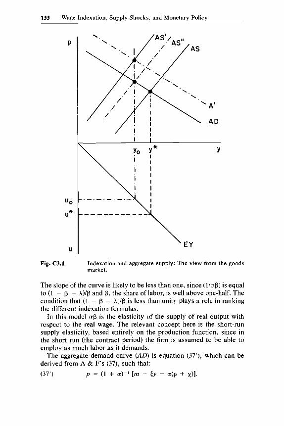
133 Wage Indexation, Supply Shocks, and Monetary Policy
P
" 0
U*
U
Fig. C3.1 Indexation and aggregate supply: The view from the goods market.
The slope of the curve is likely to be less than one, since (l/up) is equal to (1 - p - h) /p and p, the share of labor, is well above one-half. The condition that (1 - p - X)/p is less than unity plays a role in ranking the different indexation formulas.
In this model crp is the elasticity of the supply of real output with respect to the real wage. The relevant concept here is the short-run supply elasticity, based entirely on the production function, since in the short run (the contract period) the firm is assumed to be able to employ as much labor as it demands.
The aggregate demand curve (AD) is equation (37'), which can be derived from A & F's (37), such that:
(37') p = (1 + a)-' [rn - 5y - a ( p + x)].
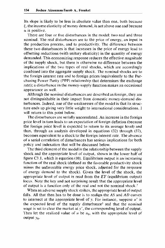
134 Joshua AizenmanIJacob A. Frenkel
Its slope is likely to be less in absolute value than one, both because 5, the income elasticity of money demand, is not above one and because a is positive.
There are four or five disturbances in the model: two real and three nominal. The real disturbances are to the price of energy, an input in the production process, and to productivity. The difference between these two disturbances is that increases in the price of energy lead to offsetting reductions (with unitary elasticity) in the quantity of energy demanded. This economizing response reduces the effective magnitude of the supply shock, but there is otherwise no difference between the implications of the two types of real shocks, which are accordingly combined into the aggregate supply shock. The nominal shocks are to the foreign interest rate and to foreign prices (equivalently to the Pur- chasing Power Parity (PPP) relationship that determines the exchange rate); a disturbance in the money-supply function makes an occasional appearance as well.
Although the nominal disturbances are described as foreign, they are not distinguishable in their impact from domestic money-demand dis- turbances. Indeed, one of the weaknesses of the model is that its struc- ture ends up giving very little weight to international considerations. I will return to this point below.
The disturbances are serially uncorrelated. An increase in the foreign price level in turn leads to an expectation of foreign deflation (because the foreign price level is expected to return to its average level) and thus, through an analysis developed in equations ( 3 2 ) through (37) , becomes equivalent to a shock to the foreign interest rate. The absence of a serial correlation of disturbances has serious implications for both policy and indexation that will be discussed below.
The third element of the model is the relationship between the supply shock and the appropriate level of output, shown in the lower half of figure C3.1, which is equation (10). Equilibrium output is an increasing function of the real shock (defined as the favorable productivity shock minus the unfavorable energy price shock, adjusted for the response of energy demand to the shock). Given the level of the shock, the appropriate level of output is read from the EY (equilibrium output) locus. Note the key and not surprising result that the appropriate level of output is a function only of the real and not the nominal shock.’
When an adverse supply shock strikes, the appropriate level of output falls. All that then has to be done is to realign the AS and AD curves to intersect at the appropriate level of y. For instance, suppose u* is the expected level of the supply disturbance3 and that the nominal wage is set to clear the market at y * , the corresponding level of output. Then let the realized value of u be uo, with the appropriate level of output yo.
135 Wage Indexation, Supply Shocks, and Monetary Policy
The economy can attain yo through shifts in either the AS or the A D curves. There is an automatic upward shift of the aggregate supply curve in response to an adverse supply shock, but the shift appears a priori unlikely to take the intersection precisely to the correct level of output without either indexation or a change in the money stock.
One of the contributions of A & F's analysis is to clarify the con- ditions under which the automatic shift of the AS curve, with nominal wage fixity and without an accommodating monetary policy, leads to the optimal level of output. In their model that happens only if the coefficient of the supply shock in (39) is zero, that is, if
((1 + E) = 1 + a. 5 is the income elasticity of money demand; E, the labor-supply elas- ticity; and a, the interest elasticity of money demand. With 5 = 1, E = 0, and a = 0, the condition is ~a t i s f i ed .~ But it is, of course, a singular event for the condition to be satisfied, and it is unlikely that it would ever be met exactly in practice.
It has frequently been argued on a priori grounds by equilibrium business cycle theorists that the elasticity of labor supply in response to transitory real wage increases is large. If it were, so that k(1 + E) > 1 + a, an adverse supply shock would be followed by overemploy- ment unless the money stock were reduced. With E large, the EY locus would be relatively flat, implying that the intersection of the new AS schedule following a supply shock and A D would be to the right of yo. Since the problem of supply shocks seems instead to be one of un- employment, we assume that the full employment level of output falls by less than the reduction implied by the intersection of A D and the new AS curve and that the maintenance of full employment requires an expansion and not a contraction of aggregate demand. The demand curve should therefore shift to AD'.
Of course, shifting the curves to ensure that a supply shock creates a recession does not explain why in fact adverse supply shocks are associated with high unemployment. More careful modeling of the em- ployment decision, of the links between output and employment, and of the reallocation of labor would be needed to go more deeply into this issue.
Optimal monetary policy when wages are fixed in nominal terms is described by equation (39). The money stock should respond not only to the real shock, but also to nominal shocks. Nominal shocks should be just offset so that the aggregate demand curve remains unaffected.
The maintenance of full employment can also be achieved by wage flexibility, which shifts the AS curve appropriately. The ideal indexing formula is given by (16), which shows there should be full indexing to the price level provided there is also indexing to the real shock. The
136 Joshua AizenmanIJacob A. Frenkel
nominal wage rises automatically with the price level and falls with the supply shock. In the face of a supply shock, the ideally indexed wage would shift AS to AS”. Indexing and monetary policy are equally ef- ficient, and either can maintain equilibrium employment. An obvious implication, shown in equation (39’), is that the appropriate monetary policy is not independent of the existence of indexation.
Highlights
One of the highlights of A & F’s paper has already been reviewed: the analysis of optimal monetary policy (optimal in the sense of main- taining equilibrium employment) in the face of supply shocks. Another comes in the analysis of suboptimal indexation rules. The result ob- tained here is that indexation to the price level should be lower, the fewer the contingencies other than nominal shocks taken into account in the indexation formula.
This result can be understood in terms of the general principle that price indexation is optimal for nominal shocks and not for real shocks. In this model indexation to one component of the real shock means, in an expected value sense, partial indexing to the entire shock. Ac- cordingly, the greater the degree of indexing to the real shock, the more indexing can be permitted to the nominal shock (provided, of course, that there is not overindexing to the real shock-and that is ensured by A & F’s studying optimal-suboptimal indexation rules).
The results for indexation to the value-added price deflator and to the nominal GNP also deserve attention. The key equation here is:
Y w = p + - 1 + € ’ (17’)
which shows optimal indexation to the price level and real output separately. If there is no elasticity of labor supply, indexation to the nominal GNP is optimal. In general, there is no reason to index to anything beyond the price level and the real GNP. If a choice has to be made between indexation to the nominal GNP and to the domestic value-added deflator, indexation to the latter is optimal only in the unlikely circumstance the elasticity of labor supply is extremely high. I will discuss below the sensitivity of this result to the structure of the model.
Other special indices have also been proposed. One suggestion is to index to the nominal money stock. This is appropriate only if all shocks are money supply shocks. If indexation had been invested by the pri- vate sector as a defense against an errant monetary authority, this formula might have something to recommend it.
137 Wage Indexation, Supply Shocks, and Monetary Policy
General Comments and Suggestions
The open economy aspects of the A & F model are not well devel- oped. Indeed, aside from the description of the energy price shock as imported, their analysis of indexation is no different from an analysis of a closed economy. There is no interaction at all between the energy price shock and the balance of payments or the real exchange rate, except to the extent that the price increase affects the price of domestic output. The terms of trade do not enter into the A & F’s model.
The basic difficulty here is that neither the current account nor the capital account are analyzed explicitly. The country has free access to foreign capital at the world interest rate. There is no balance-of-payments problem for this country following an oil price shock because it can borrow as much as it wants. But in practice many of the problems facing developing countries in the wake of the oil shock related to the balance of payments, and it is hard indeed to believe that the optimal indexing formula can be independent of that aspect of the problem.
Taking account of the balance of payments would likely increase the attractiveness of indexation to a domestic value-added index rather than to the nominal GNP. This argument is strengthened by the fact that the short-run elasticity of substitution between energy and other inputs is small. Adjustment in the short run to an oil price increase while maintaining full employment would then require a large reduction in the real wage if external balance (defined relative to optimal bor- rowing in the face of the supply shock) were to be maintained. The absence of a complete model of the balance of payments may thus seriously bias the conclusions of the paper.
The absence of dynamics from the paper certainly also affects the conclusions. Much of the dimness of the view of indexation taken by its critics arises from the possibility that it prolongs rather than speeds up the response of the economy to shocks. Wage indexation works with a lag, and it is therefore in practice always adjusting to yesterday’s (or last year’s) shocks. In the A & F paper, any lag in the implemen- tation of indexation would make nonindexation the optimal response. That is because all disturbances are serially uncorrelated. A disturbance today says nothing about tomorrow’s disturbances, and indexation to yesterday’s shocks would merely increase variance in the model.
The serial correlation of disturbances is as crucial a determinant of the optimal indexing formula as the relative variances of shocks. The general rule in the presence of indexing lags would be to index to adjust for effectively long-lived disturbances but not for the short- lived ones. It is not necessarily the disturbances themselves that have to be long-lived, just their effects. For instance, overlapping long-term labor contracts could transform transitory disturbances into longer-
138 Joshua AizenmaniJacob A. Frenkel
lived effects on prices, which would perhaps be adjusted for in the indexing formulas.
The discussion of dynamics raises the question of the accuracy of the conventional view that differences in indexing arrangements are responsible for the differential responses of economies to supply shocks. Labor contracts do not last forever, and a new base wage can be negotiated in new contracts. I am therefore skeptical of the standard view. This skepticism is reinforced by the absence of a strong corre- lation between the presence of indexation and measures of the rigidity of real wages across countries.' For example, Great Britain has rigid real wages but has had only sporadic indexing.
A & F clearly have in mind that inflation, or at least price variability, is undesirable, for they generally present an expression for the variance of the price level. But their theoretical consciences, which have already been violated-for the social good-by predetermining wages and al- lowing firms to choose the level of output, prevent their writing down a loss function that includes price-level variability. Although their model does not explain why price variability matters, we can assume that it does, and then discuss the choice between indexing and active mon- etary policy in the light of a criterion that weighs price-level stability against full employment.
Price-level stability requires that monetary policy stabilize against nominal shocks. We saw in figure C3.1 that leaving it to monetary policy to handle real shocks results in greater price-level variability than oc- curs when indexation undertakes that task. Accordingly, an allocation of tasks in which monetary policy deals with nominal shocks and the labor market deals with real shocks is better than the converse. But when indexation deals with real shocks, there is still some variability in the aggregate price level. The extent to which it is desirable to reduce that variability, by reducing the money stock and causing unemploy- ment in the face of a supply shock that has already resulted in a re- duction in the nominal wage, cannot be analyzed without a more de- tailed model.
By that stage, however, we are in a context in which more difficult questions about monetary policy and inflation arise. For instance, if labor contracts are written in the knowledge that the money stock will be reduced when there is a real shock, and if that monetary policy is followed, perfect price-level stabilization with full employment can be attained. This points to the need for a more complete analysis of the interactions between indexation and monetary policy-which might reveal that when the monetary authority and the private sector have different objective functions, indexation is a defense against, and not a harmonious partner of, monetary policy. That kind of analysis would have to be carried out with an explicitly game-theoretic model. But that would be the topic of another paper.
139 Wage Indexation, Supply Shocks, and Monetary Policy
Notes
1. In A & F's paper, as in several other papers studying indexing, all disturbances can be identified from the level of observables, so that there is no difficulty in moving from formulas that index to disturbances to formulas that index to observables. But it is entirely possible that the disturbances to which there should be indexation are not identifiable: for instance, if there are lags in the implementation of indexing, only the serially correlated part of disturbances should be reflected in the indexing formula. But if disturbances are a mixture of permanent and transitory components, the permanent component cannot be identified and it is necessary to calculate the optimal formula that indexes to obscrvables.
2. Figure C3.1 is not quite in accord with the A & F text in that the analysis in the text sets the expected levels of p . y. Oli - p ) . and u all equal to zero, since these are deviations from means. It is graphically more convenient to show p , y and II all a s positive, as in figure C3.1. This causes no errors.
3. See note 2. 4. Precisely these assumptions were made in Fischer (1985). 5. See Branson and Rotemberg (1980). Bruno and Sachs (1985). and Grubb, Jackman,
and Layard (1983). In Fischer (1983) I found no correlation between the extent of the inflationary shock suffered by economies after the first oil shock and the presence of wage indexation.
References
Branson, William H., and Rotemberg, J. J . 1980. International adjust- ment with wage rigidity. European Economic Review 13, no. 3: 309- 32.
Bruno, Michael, and Sachs, Jeffrey. 1985. Economics of worldwide staKfEation. Cambridge: Harvard University Press.
Fischer, Stanley. 1983. Indexing and inflation. Journal of Monetary Economics 12, (no. 4): 519-42.
. 1985. Supply shocks, wage stickiness, and accommodation. Journal of Money, Credit and Banking 1 (February): 1 - 15.
Grubb, Dennis; Jackman, Richard; Layard, Richard. 1983. Wage rigid- ity and unemployment in OECD countries. European Economic Re- view 21, no. 1-2: 11-40.
Comment Constantino Lluch
This is a very long paper, full of algebra. Practical people must ask themselves where does the algebra lead. What are the results, and how useful are they'? I want to answer these questions by summarizing how the results are obtained and by placing them in the context of the real world.
The authors obtain their results by using the following strategy. First, determine the optimal money supply and the rules for the optimal
Constantino Lluch is chief of the Labor Economics Division of the Development Research Department of the World Bank.
140 Joshua AizenmanJJacob A. Frenkel
indexing of nominal wages in an economy in which nominal wages are sticky; there is some degree of exchange rate flexibility; there are four possible stochastic shocks; and there is equilibrium in three markets: output, money, and labor. Optimality is defined by the adjustment to nominal wages for the quantity of money that would yield the equilib- rium real wage in the “shocked” economy.
Second, suppose that indexing is constrained in the sense that the indexation formula does not include real shocks to the economy (either a shock to productivity or a pseudo shock brought about by a change in the relative price of raw materials’); or that the degree of flexibility of the exchange rate is not chosen optimally; or that the pseudo shock appears in the adjustment formula but the productivity shock does not. What then are the constrained adjustment coefficients and the asso- ciated welfare loss?
Third, examine what all this implies for indexation proposals ad- vanced in practice, such as indexing to nominal incomes or to the value- added price index. Also examine whether there is a link between these proposals and indexing designed to achieve stable employment versus stable real wages.
This strategy produces many results. They can be grouped into two categories: one comprising the results concerning the optimal indexing coefficients: and the other, those concerning the optimal indexing pro- posals. The first result in the first category says that with a “sophis- ticated” indexing formula for nominal wages, there is a 100 percent adjustment to a change in prices: either more or less than a 100 percent adjustment to a productivity shock; and less than a hundred percent adjustment to the pseudo shock caused by a change in the relative price of raw materials. The coefficient of the adjustment to the productivity shock is a ratio whose numerator is unity and whose denominator is E/U + (1 - X), where E is the elasticity of labor supply, u is the share of capital, and X is the share of raw materials. If the supply of labor is completely inelastic ( E = O), a productivity shock therefore leads to a more than proportional adjustment in nominal wages of the same sign as that of the shock. The coefficient of adjustment to the pseudo shock (the change in the relative price of raw materials) is always negative and proportional to the productivity-shock coefficient. The factor of proportionality is the share of raw materials.
The equilibrium real wage in the “shocked” economy can be reached through an entirely different device if nominal wages are, and remain, fixed. Obviously enough, there is a new price level that would produce such an equilibrium real wage. The money supply that achieves that new price level is called “optimal.”
Two remarks can be made in passing here. First, how nice algebra is! One can determine the desired real wage one way or another, or by
141 Wage Indexation, Supply Shocks, and Monetary Policy
any linear combination. Second, only one shock, the productivity shock, is included in the “sophisticated” wage-indexing formula. Two others, though, are recognized as relevant in setting the optimal money supply. Can it be shown that, were those other two shocks included in the wage- indexing formula, their corresponding adjustment coefficient would be zero? The answer is no, because the wage-indexing formula is quite arbitrary, whereas the loss function is not. When prices are fully flexible, this is not a very interesting observation, however. One would substitute out the price change in the wage-indexing formula, using instead the equilibrium condition in the market for money. Adjustment to the price change would still be 100 percent, and this price change would be broken down into changes in the money supply and in all shocks.
I am not advocating to complicate the wage-indexing formula in this fashion. The formulas used in practice do not contain the productivity shock, or any other, because practical people are unable to recognize shocks, alone or in combination, when they see them. It is therefore more relevant to ask what the coefficient of the adjustment to prices is, in the wage-indexing formula, when shocks are not present. This question leads to all the other results in the first category. Of particular interest are those relating to the adjustment in wages and the adjustment in the exchange rate.
I say this advisedly, because the relationship between both adjust- ments is quite peculiar. The optimal degree of flexibility of the exchange rate is independent of everything else. It is simply equal to the absolute value of the (semi)elasticity of the demand for money with respect to the rate of interest. Substituting this number into the relevant expres- sions for the loss function yields the basic results about the relative size of the coefficients of the adjustment of wages to prices: they are smaller in magnitude, the more restrictive the indexing formula is.
The fact that there is very little relationship between the optimal exchange rate and the optimal wage is one aspect of how little this economy is actually open-a point made by Fischer in the preceding comment. In general, the ratio of the two variables is an approximation to the real exchange rate; and problems of adjustment to shocks are usually problems of how to shift from excess demand to excess supply of tradables by increasing the real exchange rate, in other words, prob- lems of how elastic the supply of tradable goods is. Wage indexation does affect such elasticity, and of course, it also affects the increase in the real exchange rate. What is the loss function associated with this way of looking at indexation issues?
The results in the second category are very neat and very easily summarized. The elasticity of demand for labor is around 3, consid- erably higher than the available estimates of the elasticity of labor supply. It then follows that indexation to nominal income is preferable
142 Joshua AizenmanIJacob A. Frenkel
to indexation to the price index of domestic value added, which in turn is equivalent to a preference for indexation rules that stabilize em- ployment rather than the real wage.
So what does all this mean to the practical person who hopes to understand the “real world”? This question may be unfair or ill put. Nevertheless, some attempt to come to grips with it is important, I think, to determine both what research to pursue next and how much enthusiasm one should have for policy proposals that might flow from the paper (such as “adjust wages less than 100 percent” or “index to nominal incomes’ ’).
A different way to put this general question is to consider some of the historical experiences with indexation, say in Brazil or Israel, and ask: What does one learn from this paper about mistakes made in those cases? I think the most telling criticism on this point is that made above by Fischer. Indexation has never been instantaneous, but the model employed by Aizenman and Frenkel is instantaneous. How many of their results would apply if there were lags in indexation? My own sense is that none would, because a shock would then be an event that takes place after inflation has already eroded the real wage. By how much depends on the inflation rate and the period of adjustment. The loss function would be quite different in that case.
In any event, practical observers can always make these points. The paper is nonetheless still quite interesting.
Note
1. 1 call this a pseudo shock because there is no stochastic element to it