This short manual was created by extracting pages from The ...web4.uwindsor.ca/.../$FILE/ISC-AERMOD_View_UsersGuide_Short1.pdf · Contents ISC-AERMOD View • Lakes Environmental

This short manual was created by extracting pages from The User’s Guide, both the short manual and The User’s Guide is copyright of Lakes Environmental Software. This short manual is posted on this site under permission of Lakes Environmental Software.

ISC-AERMOD View 1996-2006 Lakes Environmental Software. All rights reserved. Windows, Windows 95, Windows 98, Windows Me, Windows NT, Windows 2000, Windows XP and WordPad are trademarks of Microsoft Corporation in the USA and other countries. AutoCAD is a registered trademark of Autodesk, Inc. Published by Lakes Environmental Software 419 Phillip Street, Unit 3 Waterloo, Ontario N2L 3X2 Canada Tel.: (519) 746-5995 Fax: (519) 746-0793 Web Site: http://www.weblakes.com e-mail: [email protected] ISCAER5.3UG

DISCLAIMER

This document and accompanying software follow the U.S. EPA models and documentation (ISCST3, ISC-PRIME, AERMOD, AERMAP, BPIP, PCRAMMET, and AERMET) to the best of our understanding. The user is responsible for checking the input data and the results for consistency.

Contents

ISC-AERMOD View • Lakes Environmental Software i

Contents

Chapter 1 - ISC-AERMOD View Basics ..........................................................1-1 About ISC-AERMOD View........................................................................... 1-1 The ISCST3 Model....................................................................................... 1-2 The ISC-PRIME Model................................................................................. 1-3 The AERMOD Model ................................................................................... 1-3 Installing ISC-AERMOD View ...................................................................... 1-4

System Requirements ........................................................................... 1-4 Installation Instructions .......................................................................... 1-5

Chapter 2 - ISC-AERMOD View Interface .......................................................2-1 ISC-AERMOD View Interface Overview ...................................................... 2-1 Menu Options............................................................................................... 2-3 Menu Toolbar Buttons................................................................................ 2-13 Annotation Toolbar..................................................................................... 2-14

Select Tool........................................................................................... 2-14 Zoom In Tool ....................................................................................... 2-15 Zoom Out Tool..................................................................................... 2-16 Pan Tool .............................................................................................. 2-16 View Min. Extents Tool ........................................................................ 2-16 View Max. Extents Tool ....................................................................... 2-16 Delete Objects ..................................................................................... 2-17 Rectangle Annotation .......................................................................... 2-17 Circle Annotation ................................................................................. 2-18 Text Annotation ................................................................................... 2-19 Marker Annotation ............................................................................... 2-19 Arrow Annotation ................................................................................. 2-20 Web Annotation ................................................................................... 2-21 North Arrow Annotation ....................................................................... 2-21 Overlay Control.................................................................................... 2-22 Measure Distances and Areas Tool .................................................... 2-24 Map Import .......................................................................................... 2-24 Site Domain ......................................................................................... 2-25 Graphical Options................................................................................ 2-27 Impact Tool.......................................................................................... 2-28 Identify Tool ......................................................................................... 2-29 Eagle Watch View Tool ....................................................................... 2-30

Application Toolbar .................................................................................... 2-31 Point Source Tool ................................................................................ 2-31 Flare Source Tool ................................................................................ 2-32 Area Source Tool................................................................................. 2-32 Open Pit Source Tool .......................................................................... 2-33 Volume Source Tool ............................................................................ 2-33 Circular Area Source Tool ................................................................... 2-34 Polygon Area Source Tool................................................................... 2-34

Contents

ii ISC-AERMOD View • Lakes Environmental Software

Line Source Tool ................................................................................. 2-35 Discrete Cartesian Receptor Tool ....................................................... 2-35 Discrete Polar Receptor Tool .............................................................. 2-36 Discrete Cartesian Receptor (ARC) Tool ............................................ 2-36 Uniform Cartesian Grid Tool................................................................ 2-37 Non-Uniform Cartesian Grid Tool........................................................ 2-37 Uniform Polar Grid Tool....................................................................... 2-38 Non-Uniform Polar Grid Tool ............................................................... 2-38 Plant Boundary Tool ............................................................................ 2-39 Elevations/Flagpole Heights Tool........................................................ 2-39 Rectangular Building Tool ................................................................... 2-40 Angled Rectangular Building Tool ....................................................... 2-40 Circular Building Tool .......................................................................... 2-41 Polygonal Building Tool ....................................................................... 2-41 Show/Hide Structure Influence Zone Tool........................................... 2-42 Show/Hide GEP 5L Area of Influence Tool ......................................... 2-42

Chapter 3 - Control Pathway...........................................................................3-1 Control Pathway........................................................................................... 3-1

Dispersion Options ................................................................................ 3-2 Pollutant/Averaging ............................................................................... 3-7 Terrain Options.................................................................................... 3-10 NOx to NO2 ......................................................................................... 3-12 Re-Start/Multi-Year Files ..................................................................... 3-13 Event/Error Files.................................................................................. 3-16 Debug Files ......................................................................................... 3-17 Gas Dry Deposition ............................................................................. 3-18 Seasonal Categories ........................................................................... 3-21 Land Use Categories........................................................................... 3-22

Chapter 4 - Source Pathway............................................................................4-1 Source Pathway ........................................................................................... 4-1

Source Summary................................................................................... 4-2 Source Inputs ........................................................................................ 4-3 Building Downwash ............................................................................. 4-18 Gas & Particle Data ............................................................................. 4-21 Source Groups .................................................................................... 4-27 Urban Sources..................................................................................... 4-28 Emission Output Unit........................................................................... 4-30 Hourly Emission File............................................................................ 4-31 Variable Emission Rates by Season ................................................... 4-32 Variable Emission Rates by Month ..................................................... 4-33 Variable Emission Rates by Hour-of-Day............................................ 4-34 Variable Emission Rates by Wind Speed/Stability Class .................... 4-35 Variable Emission Rates by Wind Speed............................................ 4-36 Variable Emission Rates by Season/Hour .......................................... 4-37 Variable Emission Rates by Season/Hour/Day................................... 4-38

Contents

ISC-AERMOD View • Lakes Environmental Software iii

Variable Emission Rates by Season/Hour/7-Days.............................. 4-39

Chapter 5 - Receptor Pathway ........................................................................5-1 Receptor Pathway........................................................................................ 5-1

Receptor Summary................................................................................ 5-2 Terrain Options...................................................................................... 5-3 Uniform Cartesian Grid.......................................................................... 5-5 Non-Uniform Cartesian Grid.................................................................. 5-7 Uniform Polar Grid................................................................................. 5-9 Non-Uniform Polar Grid ....................................................................... 5-11 Multi-Tier Grid...................................................................................... 5-13 Discrete Cartesian Receptors ............................................................. 5-15 Discrete Polar Receptors..................................................................... 5-16 Discrete ARC Receptors ..................................................................... 5-17 Cartesian Plant Boundary.................................................................... 5-19 Polar Plant Boundary........................................................................... 5-22 Fenceline Grid ..................................................................................... 5-23

Chapter 6 - Terrain Grid Pathway ...................................................................6-1 Terrain Grid Options..................................................................................... 6-1

TG Grid Settings.................................................................................... 6-3 Terrain Grid Data File Format................................................................ 6-4

Chapter 7 - Meteorology Pathway ..................................................................7-1 Meteorology Pathway................................................................................... 7-1

Met Data Input ....................................................................................... 7-2 Data Period............................................................................................ 7-7 Wind Speed Categories......................................................................... 7-8 Wind Profile Exponents ......................................................................... 7-9 Vertical Temperature Gradients .......................................................... 7-10 SCIM Sampling.................................................................................... 7-11

Chapter 8 - Output Pathway............................................................................8-1 Output Pathway............................................................................................ 8-1

Tabular Outputs..................................................................................... 8-2 Contour Plot Files .................................................................................. 8-4 Threshold Violation Files ....................................................................... 8-6 Post-Processing Files............................................................................ 8-8 TOXX Files .......................................................................................... 8-10 Season Hour Files ............................................................................... 8-12 Rank Files............................................................................................ 8-13 Evaluation Files ................................................................................... 8-15 Percentiles/Rolling Ave. Settings ........................................................ 8-16 Percentiles/Rolling Ave. Contour Plot Files......................................... 8-18

Contents

iv ISC-AERMOD View • Lakes Environmental Software

Chapter 9 - Terrain Options.............................................................................9-1 Terrain Processor......................................................................................... 9-1 Terrain Processor - Terrain.......................................................................... 9-2

How to Import USGS DEM Files ........................................................... 9-3 How to Import GTOPO30 Files ............................................................. 9-5 How to Import UK DTM and UK NTF Files............................................ 9-6 How to Import XYZ Files........................................................................ 9-7 How to Import AUTOCAD DXF Files..................................................... 9-8

Terrain Processor – Region to Import........................................................ 9-11 Terrain Processor – Import Elevations....................................................... 9-14 Terrain Processor – Advanced Options ..................................................... 9-15

Chapter 10 - Building Options ......................................................................10-1 Building Inputs............................................................................................ 10-1

Rectangular Building Inputs................................................................. 10-3 Polygonal Building Inputs .................................................................... 10-5 Circular Building Inputs........................................................................ 10-7

Running the EPA BPIP Model ................................................................... 10-9

Chapter 11 - Multi-Chemical Run Utility.......................................................11-1 About the Multi-Chemical Run Utility ......................................................... 11-1 Setting Up a Multi-Chemical Run............................................................... 11-2 Chemical Setup tab.................................................................................... 11-4 Output Options tab ..................................................................................... 11-6 Warnings tab .............................................................................................. 11-7 Information tab ........................................................................................... 11-7

Chapter 12 - Running the U.S. EPA Model...................................................12-1 Project Status............................................................................................. 12-1 Details ........................................................................................................ 12-2 Running the U.S. EPA Model..................................................................... 12-3 Running the U.S. EPA EVENT Model........................................................ 12-4

Chapter 13 – Plot file and Graphical Options ..............................................13-1 Contouring in ISC-AERMOD View............................................................. 13-1 Graphical Options ...................................................................................... 13-3

Levels .................................................................................................. 13-4 Smoothing ........................................................................................... 13-5 Labeling ............................................................................................... 13-7 Color Ramp ......................................................................................... 13-8 Posting................................................................................................. 13-9 Ruler Options..................................................................................... 13-12 Color Mappings ................................................................................. 13-13

Contents

ISC-AERMOD View • Lakes Environmental Software v

Labels ................................................................................................ 13-14 Graphical Output Toolbar......................................................................... 13-15 Concentration Converter .......................................................................... 13-17

Chapter 14 - Printing & Preferences.............................................................14-1 Print Preview .............................................................................................. 14-1 Preferences................................................................................................ 14-3

Preferences - General ......................................................................... 14-4 Preferences - Appearance................................................................... 14-5 Preferences - EPA Models/Limits - ISCST3........................................ 14-5 Preferences - EPA Models/Limits - ISC-PRIME.................................. 14-6 Preferences - EPA Models/Limits - AERMOD..................................... 14-7 Preferences - EPA Models/Limits - AERMAP ..................................... 14-8 Preferences - EPA Models/Limits - BPIP ............................................ 14-9 Preferences - Page Layout................................................................ 14-10 Preferences - Labeling ...................................................................... 14-11 Preferences - Font Options ............................................................... 14-12 Preferences - Logo ............................................................................ 14-13 Preferences - Default Settings .......................................................... 14-14 Preferences - Default Palette ............................................................ 14-16 Preferences - Terrain Processor ....................................................... 14-17

References......................................................................................................15-1

Chapter 1 – ISC-AERMOD View Basics

ISC-AERMOD View • Lakes Environmental Software 1-1

CHAPTER 1

ISC-AERMOD View Basics

In this Chapter:

About ISC-AERMOD View The ISCST3 Model The ISC-PRIME Model The AERMOD Model Installing ISC-AERMOD View

About ISC-AERMOD View ISC-AERMOD View is a complete and powerful air dispersion modeling package which seamlessly incorporates the popular U.S. EPA models, ISCST3, ISC-PRIME and AERMOD into one interface without any modifications to the models. These models are used extensively to assess pollution concentration and deposition from a wide variety of sources. ISC-AERMOD View is a true, native Microsoft Windows application and runs in Windows 2000/XP and NT4 (Service Pack 6).

Some Features: ♦ Easy and intuitive graphical interface of ISC-AERMOD View can help you create impressive

presentations of your model results. You can customize your project using display options such as transparent contour shading, annotation tools, various font options, and specify compass directions.

♦ Ability to specify model objects such as sources, receptors and buildings graphically. After

defining an object graphically you automatically have access to the related text mode window in which you can further modify parameters.

♦ Automatically eliminate receptors within the facility property line. ♦ ISC-AERMOD View can import base maps in a variety of formats for easy visualization and

source identification.


1-2 ISC-AERMOD View • Lakes Environmental Software

♦ Supports the major digital elevation terrain formats - USGS DEM, GTOPO30 DEM, UK DTM, UK NTF, XYZ Files, CDED 1-degree, AutoCAD DXF.

♦ Powerful 3D visualization built right into the interface allows you to understand the effects

of topography by displaying your model results with 3D terrain. ♦ ISC-AERMOD View provides all the necessary tools to effectively and quickly complete your

building downwash analysis. ♦ Meteorological pre-processing guides you through the steps to prepare your meteorological

data. ♦ ISC-AERMOD View features integrated post-processing with automatic contouring of results,

automatic gridding, blanking, shaded contour plotting and posting of your results. ♦ Report-ready formats allow you to summarize your modeling input in professionally

designed reports. ♦ Context-sensitive “Help that really helps” provides you with a clear explanation of the

modeling requirements to assist in quickly applying ISC-AERMOD View to your best advantage.

The ISCST3 Model The ISCST3 (Industrial Source Complex - Short Term version 3) dispersion model is a steady-state Gaussian plume model which can be used to assess pollutant concentrations and/or deposition fluxes from a wide variety of sources associated with an industrial source complex. The ISCST3 dispersion model from the U. S. Environmental Protection Agency, was designed to support the EPA’s regulatory modeling options, as specified in the Guidelines on Air Quality Models (Revised). Some of the ISCST3 modeling capabilities are: ♦ ISCST3 model may be used to model primary pollutants and continuous releases of toxic

and hazardous waste pollutants. ♦ ISCST3 model can handle multiple sources, including point, volume, area, and open pit

source types. Line sources may also be modeled as a string of volume sources or as elongated area sources.

♦ Source emission rates can be treated as constant or may be varied by month, season,

hour-of-day, or other optional periods of variation, for a single source or for a group of sources.

♦ The model can account for the effects aerodynamic downwash due to nearby buildings on

point source emissions. ♦ The model contains algorithms for modeling the effects of settling and removal (through dry

deposition) of large particulates and for modeling the effects of precipitation scavenging for gases or particulates.

♦ Receptor locations can be specified as gridded and/or discrete receptors in a Cartesian or

polar coordinate system. ♦ ISCST3 incorporates the COMPLEX1 screening model dispersion algorithms for receptors in

complex terrain. ♦ ISCST3 model uses real-time meteorological data to account for the atmospheric conditions

that affect the distribution of air pollution impacts on the modeling area. ♦ Output results for concentration, total deposition, dry deposition, and/or wet deposition

flux.



The ISC-PRIME Model The Plume Rise Model Enhancements (PRIME) model was designed to incorporate the two fundamental features associated with building downwash: ♦ Enhanced plume dispersion coefficients due to the turbulent wake ♦ Reduced plume rise caused by a combination of the descending streamlines in the lee of the

building and the increased entrainment in the wake. The PRIME algorithms have been integrated into the ISCST model and called the ISC-PRIME model which contains the same basic options as the ISCST3 model but with enhanced building downwash analysis. ISC-PRIME uses the standard ISCST3 input file with few modifications. These modifications allow the specification of three new inputs used to describe the building/stack configuration. These new inputs are as follows: ♦ BUILDLEN: Projected length of the building along the flow ♦ XBADJ: Along-flow distance from the stack to the center of the upwind face of the

projected building. ♦ YBADJ: Across-flow distance from the stack to the center of the upwind face of the

projected building. To be able to run the ISC-PRIME model, you must first run the BPIP-PRIME model. The BPIP-PRIME building downwash output results are then used by the ISC-PRIME model. All the remaining options for the ISC-PRIME model are the same as for the ISCST3 model. However, some enhancements of the ISCST3 model are currently not being supported in ISC-PRIME such as: ♦ Post-97 PM10 Processing ♦ Memory Allocation ♦ INCLUDED Option ♦ TOXICS Option ♦ Sampled Chronological Input Model (SCIM) Option ♦ Optimized Area Source and Dry Depletion Algorithms ♦ Gas Dry Deposition Algorithm ♦ Season by Hour-of-Day Output Option (SEASONHR)

Note: See a detailed description on these options on the ADDENDUM for the User’s Guide for the Industrial Source Complex (ISC3) Dispersion Models - Volume 1 – User Instructions (U.S. EPA, 1997).

The AERMOD Model The AMS/EPA Regulatory Model (AERMOD) was specially designed to support the EPA’s regulatory modeling programs. AERMOD is a regulatory steady-state plume modeling system with three separate components: AERMOD (AERMIC Dispersion Model), AERMAP (AERMOD Terrain Preprocessor), and AERMET (AERMOD Meteorological Preprocessor). The AERMOD model includes a wide range of options for modeling air quality impacts of pollution sources, making it a popular choice among the modeling community for a variety of applications. AERMOD contains basically the same options as the ISCST3 model: ♦ AERMOD requires two types of meteorological data files, a file containing surface scalar

parameters and a file containing vertical profiles. These two files are provided by the U.S. EPA AERMET meteorological preprocessor program.

♦ PRIME building downwash algorithms based on the ISC-PRIME model have been added to

the AERMOD model; ♦ Use of allocatable arrays for data storage;



♦ Incorporation of EVENT processing for analyzing short-term source culpability; ♦ Post-1997 PM10 processing; ♦ A non-regulatory default TOXICS option that includes optimizations for area sources and the

Sampled Chronological Input Model (SCIM) option; ♦ Explicit treatment of multiple-year meteorological data files and the ANNUAL average; ♦ Options to specify emissions that vary by season, hour-of-day and day-of- week. ♦ For applications involving elevated terrain, the user must also input a hill height scale along

with the receptor elevation. The U.S. EPA AERMAP terrain preprocessing program can be used to generate hill height scales as well as terrain elevations for all receptor locations.

♦ Deposition algorithms have been implemented in the AERMOD model - results can be

output for concentration, total deposition flux, dry deposition flux, and/or wet deposition flux.

♦ The model contains algorithms for modeling the effects of settling and removal (through dry

deposition) of large particulates and for modeling the effects of precipitation scavenging for gases or particulates.

♦ Two types of files of intermediate results for debugging purposes can be requested. One

containing information related to the model results and the other containing gridded profiles of meteorological variables.

♦ AERMOD does not make any distinction between elevated terrain below release height

(simple terrain) and terrain above release height (complex terrain). ♦ AERMOD does not support the Open Pit type source. ♦ The Polar Plant Boundary receptor type is not available in AERMOD. A new type of receptor

was included, the discrete Cartesian receptors that allows for grouping of receptors, e.g., along arcs. This receptor option was designed to be used with the EVALFILE option which is described below.

♦ Two additional output file options were included in AERMOD. One type of file lists

concentrations by rank (RANKFILE). The other type of output file (EVALFILE) provides arc maxima results along with detailed information about the plume characteristics associated with the arc maximum.

Installing ISC-AERMOD View Before you install ISC-AERMOD View, make sure you have the following minimum requirements:

System Requirements

♦ An IBM or IBM-compatible machine ♦ A Pentium III processor or higher ♦ At least 500 MB of available hard disk space ♦ At least 512 MB of memory (RAM) ♦ Windows 2000 or XP Professional ♦ CD-ROM drive (for installation)

Chapter 2 – ISC-AERMOD View Interface


CHAPTER 2

ISC-AERMOD View Interface

In this Chapter:

ISC-AERMOD View Interface Overview Menu Options Menu Toolbar Buttons Annotation Toolbar Application Toolbar Graphical Output Toolbar

ISC-AERMOD View Interface Overview ISC-AERMOD View features a friendly, intuitive interface which provides easy access to all modeling tools and simultaneous visualization of your project. The components of the ISC-AERMOD View window are briefly described below:

♦ Control Menu: The Control Menu displays options for sizing, switching to another

application, or closing the ISC-AERMOD View program. ♦ Menu Bar: Displays menu names. To open a menu, move the mouse over the menu

name and then click the left mouse button. A drop-down menu appears displaying a list of related commands.

♦ Toolbar Buttons: These are a series of buttons that provide a fast method of selecting



Menu Toolbar Buttons The Menu Toolbar Buttons are shortcuts to some of the menu commands. The function of each one of these buttons is explained below and the equivalent menu bar command is indicated.

File | New Project: Lets you create a new ISC-AERMOD View project (*.isc).

File | Open Project: Opens an existing ISC-AERMOD View project (*.isc).

File | Print: Displays the Print Preview dialog, where you can preview what will be sent to the printer.

Run | Run Model: Displays the Project Status dialog from where you can check the status of your project and run the model.

Data | Control Pathway: Displays the Control Pathway dialog.

Data | Source Pathway: Displays the Source Pathway dialog.

Data | Receptor Pathway: Displays the Receptor Pathway dialog.

Data | Meteorology Pathway: Displays the Meteorology Pathway dialog.

Data | Output Pathway: Displays the Output Pathway dialog.

Data | Building Inputs: Displays the Building Inputs dialog.

Data | Terrain Processor: Displays the Terrain Processor dialog.

File | Reports: Displays the Reports dialog where you can view reports.

View | 3D View: Displays the 3D View window, where you can see your project in 3D.

Help | Contents: Displays the Help Contents, from where you can select topics.



Site Domain In the Site Domain dialog you define the domain extents of your modeling area. Your domain extents are automatically setup but you can change the size of the initial domain at any time. You have access to the Site Domain dialog by selecting View | Site Domain... from the menu

or by clicking the Site Domain tool ( ) located on the Annotation Toolbar. In the Site Domain dialog, you can redefine the domain extents of your project area. The Site Domain dialog contains the following options: ♦ Site Domain tab: Specify the X and Y coordinates for the southwest (SW) corner and the

northeast (NE) corner of your domain and/or enter the width and height of your domain.

Site Domain tab

♦ Layer Diagnostics tab: This tab is available to help you identify potential problems with

the locations of your modeling objects. All objects that are used in the modeling are assigned a layer in the domain. For example, a project containing sources and buildings will contain two layers in the Layer Diagnostics tab.

Layer Diagnostics tab If one of the layers contains objects that are located far away from the rest of the modeling objects, it will be highlighted in blue in the table. This could result from one set of objects being entered in UTM coordinates while another set is entered in Cartesian coordinates. If the extents of a particular layer seems too large it will be highlighted in red. You can zoom

to a layer by selecting a layer and then clicking on the Zoom to Layer ( ) button.



Application Toolbar The tools available in the Application Toolbar allow you to graphically define the location project objects such as of your sources, buildings, grids, and coastal lines. If you have imported a base map into the drawing area, the digitization of objects will be very easy. You can turn on and off the display of the Application Toolbar in the View Menu. See the following sections for a description of each of these tools:

Point Source Tool Flare Source Tool Area Source Tool Open Pit Source Tool Volume Source Tool Circular Area Source Tool Polygon Area Source Tool Line Source Tool Discrete Cartesian Receptor Tool Discrete Polar Receptor Tool Discrete Cartesian Receptor (ARC) Tool Uniform Cartesian Grid Tool Non-Uniform Cartesian Grid Tool Uniform Polar Grid Tool Non-Uniform Polar Grid Tool Plant Boundary Tool Elevations/Flagpole Heights Tool Rectangular Building Tool Angled Rectangular Building Tool Circular Building Tool Polygonal Building Tool Show/Hide Structure of Influence Zone (SIZ) Tool Show/Hide GEP 5L Area of Influence Tool

Point Source Tool The Point Source tool allows you to graphically define the location of a point source on the drawing area.

How to Graphically Define a Point Source:

Step 1: Press the Point Source tool ( ) located on the Application Toolbar. Step 2: Left-click, with the mouse pointer on the drawing area, the desired location of the

point source. Note that as you move the mouse the current coordinates are displayed on the status bar.

Step 3: The Source Inputs dialog is displayed to allow you to adjust the coordinates, if

necessary, and define additional point source information. Step 4: When you finish entering all the required information, press the Close button. A

marker ( ) will be placed at the selected location for the point source.



Uniform Cartesian Grid Tool The Uniform Cartesian Grid tool allows you to graphically define the location of a uniform Cartesian receptor grid on the drawing area.

How to Graphically Define a Uniform Cartesian Grid:

Step 1: Select the Uniform Cartesian Grid tool ( ) located on the Application Toolbar. Step 2: Left-click, with the mouse pointer on the drawing area, the desired location for one of

the grid corners. Holding down the left mouse button drag the mouse pointer diagonally until you reach the desired grid size. Release the left mouse button.

Step 3: The Uniform Cartesian Grid dialog is displayed to allow you to adjust if necessary

the origin coordinates, number of X and Y points, and spacing. Step 4: When you finish entering all the required information, press the Close button. A

representation of the uniform Cartesian grid ( ) will be displayed on the drawing area at the specified location.

Non-Uniform Cartesian Grid Tool The Non-Uniform Cartesian Grid tool allows you to graphically define the location of a non-uniform Cartesian receptor grid on the drawing area.

How to Graphically Define a Non-Uniform Cartesian Grid:

Step 1: Select the Non-Uniform Cartesian Grid tool ( ) located on the Application Toolbar.

Step 2: Left-click, with the mouse pointer on the drawing area, the desired location for one of

the grid corners. Holding down the left mouse button drag the mouse pointer diagonally until you reach the desired grid size. Release the left mouse button.

Step 3: The Non-Uniform Cartesian Grid dialog is displayed to allow you to adjust if

necessary the origin coordinates, number of X and Y points, and spacing. Step 4: When you finish entering all the required information, press the Close button. A

representation of the non-uniform Cartesian receptor grid ( ) will be displayed on the drawing area at the specified location.

Chapter 7 – Meteorology Pathway


CHAPTER 7

Meteorology Pathway

In this Chapter:

Met Input Data Data Period Wind Speed Categories Wind Profile Exponents Vertical Temperature Gradients SCIM Sampling

Meteorology Pathway The Meteorology Pathway allows you to specify the input meteorological data file and other meteorological variables, including the period to process for the meteorological files. You have access to the Meteorology Pathway dialog by selecting Data | Meteorology Pathway... from the menu or by clicking on the Met menu toolbar button.

The Meteorology Pathway dialog uses a two-pane view. The tree located on the left side of the dialog is used for navigation and item selection. Select an item (marked as ) in the tree to display the available options on the right panel.

Meteorology Pathway dialog See the following sections for a description of each window found in the Meteorology Pathway:

Chapter 7 – Meteorology Pathway


Met Data Input The Met Input Data page allows you to specify the meteorological data file and information on the meteorological stations. Meteorology Pathway - Met Input Data from the tree located on the left side of the Meteorology Pathway dialog, to display the available met input options.

Meteorology Pathway dialog - Met Input Data The inputs specified in the Met Input Data window differ slightly depending on the model being used. See below the required inputs for each model -

ISCST3 & ISC-PRIME The ISCST3 & ISC-PRIME models require the following met inputs to be specified - Meteorological Input Data File and Format ISCST3 & ISC-PRIME uses hourly meteorological data as one of the basic model inputs. The meteorological data is read into the models from a separate data file. In this panel you must specify the met data file you will be using for your project.

♦ File Name: Press the button to specify the name and location of the meteorological data file to be used. The full path of the specified met data file will be displayed on the panel. If the specified met data file is located in the same path as the project, then only the file name will be displayed.

♦ Format: Select from the drop-down list the format of the meteorological data file specified.

The following formats are available for selection -

Default ASCII format: This is the default ASCII format for a sequential hourly file.

Specify FORTRAN ASCII read format: If this option is selected than the FORTRAN read format for an ASCII sequential hourly file should be specified in the User Format field. The user specified ASCII format can be up to 60 characters long and may be used to specify the READ format for files that differ from the default format.

FREE-formatted reads: This is the free-formatted reads for an ASCII sequential

hourly file.

UNFORMatted file (RAMMET or MPRM): Unformatted file generated by the RAMMET or MPRM preprocessors. The UNFORMatted file format is no longer supported by ISCST3 (dated 00101) but is still currently provided in ISC-PRIME. The Bintoasc utility in Rammet View can convert your binary preprocessed met data to the ASCII format.

Chapter 8 – Output Pathway


Step 5: All evaluation files will be saved to the default location project directory\projectname.AD\. If you wish to specify an alternate location for the

evaluation files, click on the button in the Specify Path for EVALFILES panel and select the location to save the files. If you wish to return to the default

location, click on the button. There are a number of buttons available in this window. Their functions are described below:

Click on this button to display the EVALFILE Data dialog.

Press this button to view the contents of the selected file. Please note that you can preview the evaluation file only after running the model.

Click on this button to clear all the files from the List of Output Files window.

Click on this button to remove the selected file from the List of Output Files window.

Click on this button to replace the selected file in the List of Output Files with the alternate parameters specified.

Click on this button to add the specified file parameters to the List of Output Files window.

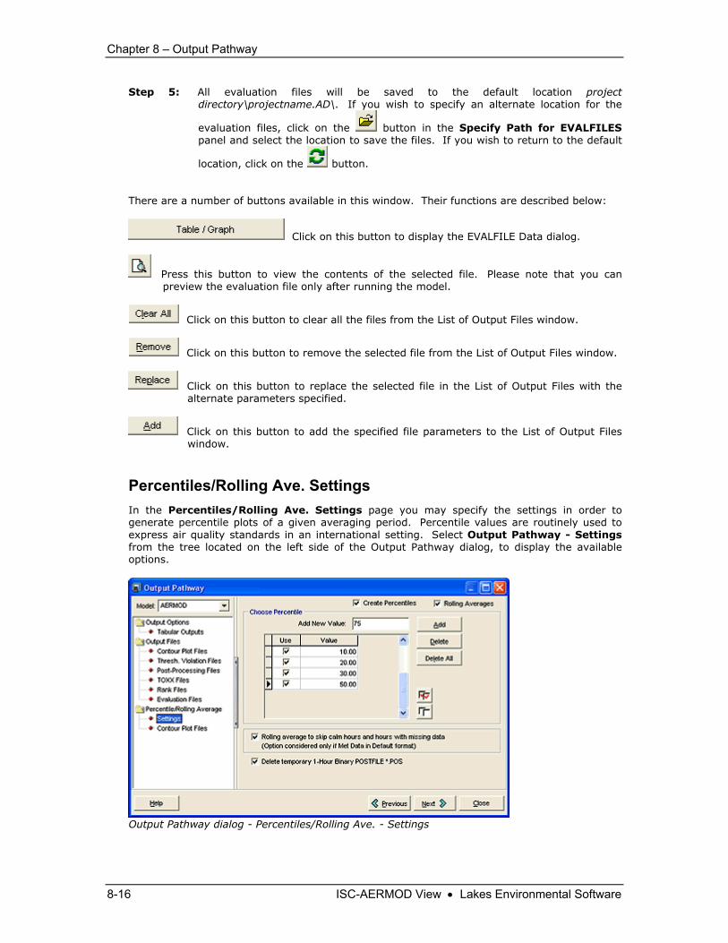
Percentiles/Rolling Ave. Settings In the Percentiles/Rolling Ave. Settings page you may specify the settings in order to generate percentile plots of a given averaging period. Percentile values are routinely used to express air quality standards in an international setting. Select Output Pathway - Settings from the tree located on the left side of the Output Pathway dialog, to display the available options.

Output Pathway dialog - Percentiles/Rolling Ave. - Settings

Chapter 8 – Output Pathway


How to Specify the Percentile/Rolling Averages Settings: Step 1: At the top of the window you may check either one or both of the following options -

♦ Create Percentiles: Check this box if you wish to generate percentile plots for each combination of averaging period and percentile value.

♦ Rolling Averages: Check this box to generate rolling or running averages. This

type of average differs from the U.S. EPA averaging calculations, also known as block averages.

Step 2: If the Create Percentiles option was checked, then you need to specify for which

percentiles plotfiles should be created. Type in the percentile value in the Add New

Value field and then press the button to add this value to the table. You may repeat this for as many percentiles as you wish to add. Only percentile values added to the table and checked will be considered when plotfiles are generated.

Step 3: When creating the percentile plot files a temporary post file (*.POS) is generated. You

have the option to delete this temporary file by checking the Delete temporary 1-Hour Binary POSTFILE (*.POS) box.

Step 4: If the Rolling Averages option was checked, you can specify that calm hours and

hours with missing data should not be considered when calculating the rolling averages. As long as your met data is in the default format, then ISC-AERMOD View will can calculate rolling averages by skipping calm hours and hours with missing data. Check the Rolling average to skip calm hours and hours with missing data check box to use this option.

Step 5: Once you have specified your settings continue to the Percentiles/Rolling Ave. -

Contour Plot Files window to preview the list of the percentiles/rolling averages plot files to be generated when you run the model.

The following buttons are available for use in this window:

Adds percentile values to the table

Deletes the selected percentile value from the table.

Deletes all the percentile values from the table.

Press this button to check the Use column box for all the percentile entries in the table. Only the percentile values that are checked will be considered when generating the plotfiles.

Press this button to uncheck the Use column box for all the percentile entries in the table. Any percentile value that is not checked will not be considered when generating the plotfiles.

Chapter 13 – Plot file and Graphical Options


Format ♦ Angle: If you would like your label placed at an angle relative to the marker, enter the

angle value here. ♦ Offset X: This is the X distance between the marker and the label. The default is 5, but

you can change this anytime. ♦ Offset Y: This is the Y distance between the marker and the label. The default is 5, but

you can change this anytime. ♦ Background Color: Check the Background Color box if you would like to change the

background color just around the label. Click on the color bar to open the Color dialog from where you can select a background color.

Anchor ♦ Origin Point: Select this option if you would like the label anchored around the origin

point. The origin point is the SW corner of the object, such as a building or grid.

♦ Center Point: Select this option if you would like the label anchored around the center

point of the object.

Sample As you make selections for color, font, size, and style for your labels, the sample is updated to reflect the changes.

Graphical Output Toolbar The Graphical Output Toolbar allow you to easily turn on and off contouring, posting of results, and acts as a quick reference to the to the maximum result value. This toolbar also allows you to select the desired plotfiles and output type to be displayed. As you select different output types, the drawing area is refreshed and results are displayed for the new option.

♦ Show Contours tool ( ): With this tool, you have the option of turning on or off the display of the contours.

♦ Show Concentrations tool ( ): With this tool, you have the option of turning on or off the display of the result values at each receptor location.

Chapter 13 – Plot file and Graphical Options


♦ Show Terrain tool ( ): With this tool, you have the option of turning on or off the display of the terrain contours, if you have elevated terrain.

♦ Plot file List: This drop-down list contains all the plotfiles generated for the current run.

Select from this list the plot file you wish to be displayed. ♦ Output Type: The Output Type drop-down list displays the output types available for the

current ISC-AERMOD Plot file. This depends on what output options you selected in the Dispersion Options window in the Control Pathway. The possible output types for each plot file are:

CONC: Select this option to show concentration results for the current plot file. DEPOS: Select this option to show deposition results for the current plot file. DDEP: Select this option to show dry deposition results for the current plot file. WDEP: Select this option to show wet deposition results for the current plot file.

Select the desired output type from the drop-down list. The plot file for the selected output will be displayed in the drawing area.

♦ Max: ISC-AERMOD View reads the plot file, which gives the calculated concentration

and/or deposition values at each receptor location, and then displays in the Max panel the maximum concentration or deposition value along with the X and Y coordinates for the position of receptor where this maximum value occurs.

Note: Plotfiles from Lakes Environmental ISC-AERMOD View version 5 and up contain information regarding units for concentration and deposition values, either the default output units or the units specified in the Emission Output Unit window. If you have imported a plot file from a version earlier than Lakes Environmental ISC-AERMOD View version 5 or from another source, the default output unit of ug/m3 (micrograms per cubic meter) for concentration values and the default output unit g/m2 (grams per square meter) for deposition values will be used. You are responsible for specifying the appropriate units, if different than the default, in the Color Ramp window of the Graphical Options dialog.

Documents

This short manual was created by extracting pages from The ...web4.uwindsor.ca/.../$FILE/ISC-AERMOD_View_UsersGuide_Short1.pdf · Contents ISC-AERMOD View • Lakes Environmental