1

This talk is structured as a semi-chronological walk through the development of some common rendering pipelines, with particular emphasis placed on the problems that motivated the development of different algorithms.

2

Simple forward shading can be summarized as doing everything that is required to shade a pixel and outputting the result.

Typically this requires looping over a bunch of lights, evaluating their contributions and accumulating the results.

The lights can be handled separately in a multi-pass setup but it scales poorly as each lighting pass requires resubmitting the scene geometry.

3

While simple, forward shading has a number of disadvantages.

The first is that it’s hard to cull lights efficiently.

Culling in object space before submitting geometry is the best you can do in practice and that is often suboptimal.

Since lighting and shading are coupled in a single pixel shader, variations in these cause a combinatoral explosion of shader permutations which in turn affects the ability to efficiently batch work together.

The light culling problems are particularly unfortunate as we ideally want hundreds or thousands of dynamic lights for global illumination approximations like instant radiosity (VPLs).

Another problem is that since we have a single program to “do everything”, all input data has to be resident in memory and available to that program at the same time.

That means all shadow maps for all lights, all reflection maps and so on need to be allocated storage in memory which is simply infeasible as rendering becomes more complex.

Finally forward shading couples the scheduling of shader execution to the rasterizeroutput, which wastes resources at triangle boundaries.

Small or skinny triangles in particular are fairly inefficient to shade on current architectures.

Kayvon discussed this problem in detail earlier in this course.

I highly recommend checking out the slides on the course web page if you missed it.

4

Conventional deferred shading avoids a number of these problems by restructuring the rendering pipeline.

In particular, it decouples lighting from surface shading so that lights can be evaluated independently and their contributions built up in image space.

To accomplish this, an initial geometry pass stores surface information such as position, normal, alebdo in a fat “geometry buffer” (G-buffer).

Then for each light the rasterizer is used to scatter and cull light volumes which executes the light shader only where it has a non-zero contribution.

The light shader reads the G-buffer, evaluates the contribution of the current light and accumulates it using additive blending.

This reordering effectively captures the coherence in accumulating the contribution from lights and schedules it efficiently.

5

Modern implementations of deferred shading typically forgo full light meshes in favour of screen-aligned quads that bound the light’s maximum extents.

Similarly it is usually faster overall to use a single-direction depth test rather than full stencil updates and clears for each light.

Depth bounds tests can be used on some hardware but they are not particularly friendly to drawing multiple lights in a single batch since the bounds must be set for each light from the CPU.

6

This image shows a scene lit with deferred shading using 256 coloured points lights of small to moderate size.

7

This visualization demonstrates the effect of light culling.

Here the whiter a pixel the more lights are being evaluated there.

You can see the screen-aligned quads used to bound the extents of the point lights in screen space.

You can also see that the single-directional depth culling is removing lights that are entirely occluded, but missing ones that are entirely in front of visible geometry (i.e. “floating in the air”).

8

Despite its advantages deferred shading is not without its own problems, the largest of which is high bandwidth usage when lights overlap.

Recall the light loop from earlier.

Reconstructing the G-buffer and accumulating lighting with additive blending both represent overhead compared to the actual lighting computation.

Unfortunately when many lights overlap we end up duplicating this overhead and it starts to dominate the actual work being done.

9

There are several approaches to improving the bandwidth usage of deferred shading.

The first is to simply reduce the overhead by minimizing the data that we read and write inside the light loop.

This is precisely the reasoning behind deferred lighting and light pre-pass rendering which I will discuss in a moment.

Another approach is to try and amortize the overhead better by grouping up multiple lights and processing them together.

Tile-based deferred shading uses this approach to great effect as I will demonstrate later.

10

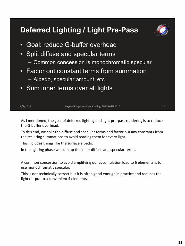
As I mentioned, the goal of deferred lighting and light pre-pass rendering is to reduce the G-buffer overhead.

To this end, we split the diffuse and specular terms and factor out any constants from the resulting summations to avoid reading them for every light.

This includes things like the surface albedo.

In the lighting phase we sum up the inner diffuse and specular terms.

A common concession to avoid amplifying our accumulation load to 6 elements is to use monochromatic specular.

This is not technically correct but it is often good enough in practice and reduces the light output to a convenient 4 elements.

11

In a final resolve step we reconstruct the factored terms and combine them with our summed diffuse and specular values.

The remaining terms can be reconstructed by rendering the scene again but moving forward it’s probably best to store them up front in the G-buffer and read them from there in a screen-space resolve phase.

This will be cheaper than transforming and rasterizing the scene again which involves significant CPU and GPU overhead.

As an added bonus recall that image-space passes have better scheduling efficiency for shading than pixel shaders driven by triangle rasterization.

Thus deferred lighting is an incremental improvement for some hardware, however it isn’t without its downsides.

In particular, we sacrifice some flexibility by having to pre-factor lighting equations into diffuse and specular parts.

While it may seem like there’s a flexibility advantage by being able to combine diffuse and specular differently in the resolve pass, this flexibility is not particularly useful in practice because interesting lighting variations occur mostly in the diffuse and specular terms themselves.

I’m being intentionally brief in the interest of covering more material, so for more details on this I highly recommend checking out Naty Hoffman and Adrian Stone’s excellent blog posts that I have linked at the end of this presentation.

12

Tile-based deferred shading takes a different approach, namely amortizing bandwidth overhead by doing more work for each byte read.

A good way to accomplish this is by grouping overlapping lights and evaluating them all at once with a single read of the G-buffer.

To that end we split the screen into tiles and construct tile frusta that tightly bounds the geometry in each time.

We use these tile frusta to cull lights that cannot affect the given tile.

This greatly reduces the number of lights that we have to consider in each tile.

Finally we read the G-buffer and evaluate all of the lights that we didn’t cull.

This greatly reduces the bandwidth used compared to classical deferred shading.

Again this is a pretty brief overview but see Johan Andersson’s Beyond Programmable Shading talk from SIGGRAPH 2009 for more information.

13

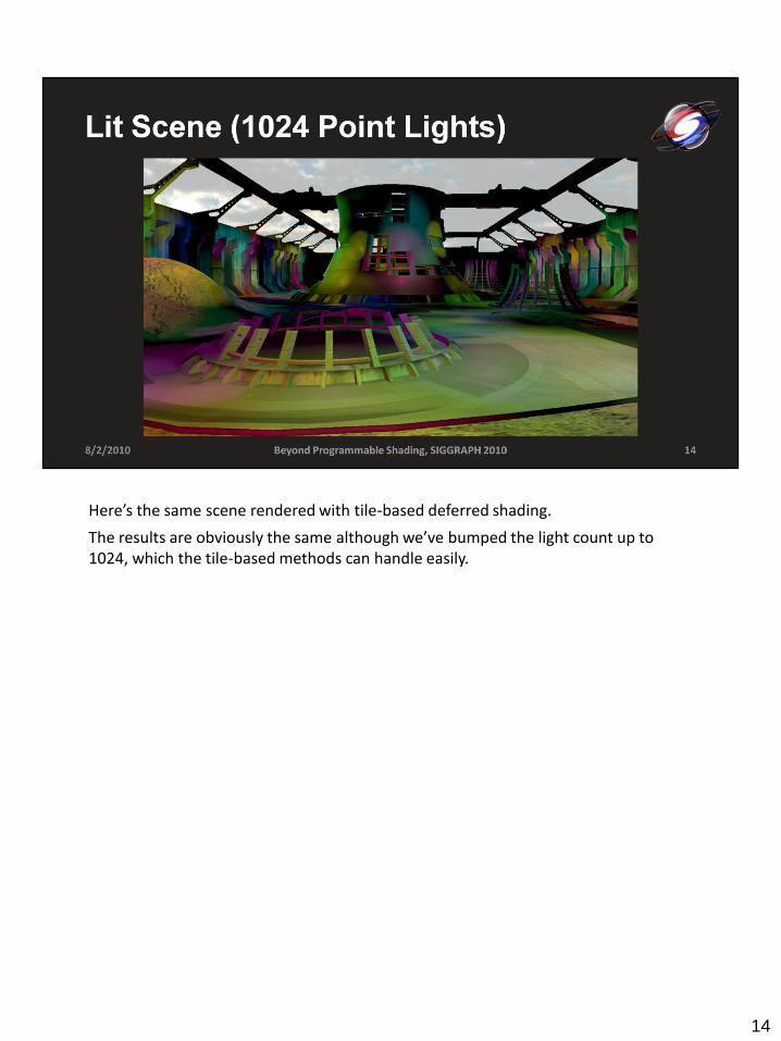
Here’s the same scene rendered with tile-based deferred shading.

The results are obviously the same although we’ve bumped the light count up to 1024, which the tile-based methods can handle easily.

14

Here is the same visualization as earlier but for tile-based culling.

Note the quantization of the culling results to the tiles (16x16 pixels in this case).

Also note that since the tile-based culling employs a two-directional depth test (compares to both min and max Z of the tile) it is able to cull lights more aggressively.

You can also see that at depth discontinuities (object edges) the light lists tend to be long since the Z range of the tile is large.

More sophisticated culling could be applied if desired, with the usual trade-off being struck between the cost of culling and the cost of the culled work.

15

For comparison, this is the result of quad-based culling for the same scene.

There’s no spatial quantization, but the culling is less efficient overall.

16

Since all of these techniques produce identical results (except for the monochromatic specular approximation of deferred lighting) the only relevant comparison metric is performance.

This graph compares just the culling performance of the various techniques in frame rendering times without any light shading.

Since the G-buffer rendering cost is constant, the difference here are related only to light culling efficiency.

Note the use of Log-base-2 on both axes to better demonstrate scaling.

We’ll use this on most of our performance graphs.

As the graph demonstrates for small light counts the overhead of tiling (computing min/max Z and frusta) dominates.

For larger light counts tile-based culling scales much better since culling is evaluated for entire tiles rather than for every pixel.

Thus the difference in the trending slope of these techniques is quite pronounced.

17

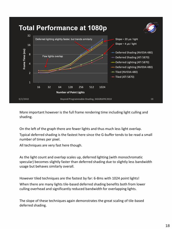
More important however is the full frame rendering time including light culling and shading.

On the left of the graph there are fewer lights and thus much less light overlap.

Typical deferred shading is the fastest here since the G-buffer tends to be read a small number of times per pixel.

All techniques are very fast here though.

As the light count and overlap scales up, deferred lighting (with monochromatic specular) becomes slightly faster than deferred shading due to slightly less bandwidth usage but behaves similarly overall.

However tiled techniques are the fastest by far: 6-8ms with 1024 point lights!

When there are many lights tile-based deferred shading benefits both from lower culling overhead and significantly reduced bandwidth for overlapping lights.

The slope of these techniques again demonstrates the great scaling of tile-based deferred shading.

18

One large disadvantage of all of these deferred shading techniques is that multi-sample anti-aliasing does not work as naturally as it does with forward rendering.

The problem is that storing the G-buffer at sample frequency loses the decoupling of shading frequencies that MSAA normally achieves.

We can choose to accept this and shade at sample frequency (i.e. super-sampling) but the performance hit of super-sampling is very high.

Alternatively we can do some work to decouple shading from the G-buffer data structure and only apply per-sample shading where it is required.

This is generally a more attractive option and implementing it in user space actually offers some additional flexibility over forward rendering.

19

One advantage of identifying edge pixels for per-sampling shading in user space is that we can clever.

Forward shaded MSAA applies anti-aliasing to every triangle edge, even ones that form a smooth, tessellated surface where AA is not required.

We really only want to apply per-sample shading at surface discontinuities.

To detect these we compare the sample depths over a pixel to the depth derivatives.

Using depth derivatives (equivalent to face normals) is a very robust method for comparing sample depths.

It does require that these derivatives be stored in the G-buffer, but they are highly useful in other applications.

For instance, they allow reconstructing light space texture coordinate derivatives for proper filtering of shadow maps in deferred passes.

Surfaces that are nearly aligned with the view direction or surfaces with high curvature cannot be reliable differentiated from actual edges using just depth though.

Thus we also compare the shading normal deviation over the samples and use per-sample shading if it deviates too much.

These two tests are suitable for the majority of applications but since all this is in user space different applications can use tailored edge detection kernels if desired. 20

Here’s a visualization of the edge detection step.

Red pixels here are the ones identified as requiring per-sample shading.

Note that unlike forward MSAA we don’t wastefully apply additional shading to triangle edges that form a smooth surface.

21

With the quad-based deferred shading algorithms we use this edge detection kernel to mark pixels for per-pixel shading.

Per-pixel vs per-sample shading can then be done using either branching or stencil.

Stencil still seems to be faster on current hardware, probably due to pixels that pass the stencil test being better scheduled to the hardware SIMD lanes.

Once we’ve generated a stencil mask we simply apply the two shading frequencies in two passes.

Unfortunately, this means that we end up duplicating the light culling work as we have to re-render the bounding volumes for the second pass.

Furthermore scheduling is still fairly inefficient.

22

Pixels that require per-sample shading tend to follow edges and thus do not exhibit strong spatial locality.

This is problematic for most hardware implementations which tend to schedule and pack SIMD lanes based on spatial locality.

The result is inefficient execution and wasted performance.

23

Tile-based methods give us an opportunity to avoid some of these weaknesses.

In particular, we can handle both frequencies of shading in a single pass to avoid duplicating culling work.

We could use branching to handle these cases but as we discussed, this is fairly inefficient in terms of work scheduling.

Instead, we repack the pixels that require per-sample shading and redistribute our computer shader threads to efficiently evaluate them.

24

As these performance results demonstrate, this user-space scheduling is a huge win here making tile-based deferred MSAA practical.

The performance hit for enabling 4x MSAA with packing is around 2.0x on ATI and 1.4x on NVIDIA.

Without packing, the hit is approximately 3.0x on both GPUs.

25

Looking at the total performance for the various methods with MSAA, the tile-basedmethods take a much smaller hit from enabling MSAA than the conventional deferred algorithms due to the advantages that we discussed.

It’s also worth nothing that deferred lighting is even less compelling when using MSAA since the resolve pass(es) are relatively more expensive.

26

So to summarize, deferred shading is a useful rendering tool and tile-based deferred shading is likely to be the best method in the future.

It has many benefits in terms of performance and flexibility and enables and efficiently-scheduled implementation of MSAA.

27

There are a number of interesting research directions for future work.

Hierarchical clustering is interesting as it scales better than the simple regular grid of tiles.

However given how fast the simple tiled implementation runs, you would need a huge set of small lights for the culling to become a significant bottleneck.

Another really important topic is the memory and bandwidth usage of deferred MSAA, which is really quite excessive.

Perhaps there is an efficient way to take advantage of the MSAA compression that already exists in hardware.

It also might be worth revisiting binning pipelines since they have some huge advantages in terms of MSAA and memory usage.

A practical option in the short term is to simply accept lower resolutions when using MSAA to keep the memory usage reasonable.

28

29

30

31

32

33

34