Embed Size (px)
Citation preview
This Week’s Objectives
• Establish Dynamic Models of System to be Controlled– Second Order Systems
• Obtain Solutions using LaPlace Transforms
• Create Simulink Model and Generate Simulated Results
Modeling of a Spring-Mass-Damper System
(Modeling of a Second Order System)
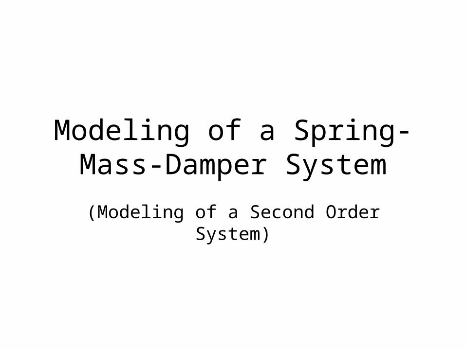
• let’s start with a one car system– suppose we know:
• m1 mass of the car
• k1, L01 spring constant and free length
• c damping coefficient
m1
k1,L01
c
f(t)
x1
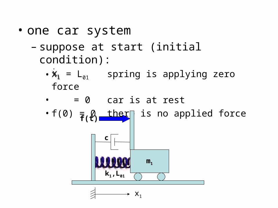
• one car system– suppose at start (initial condition):
• x1 = L01 spring is applying zero force
• = 0 car is at rest• f(0) = 0 there is no applied force
m1
k1,L01
c
f(t)
x1
1x
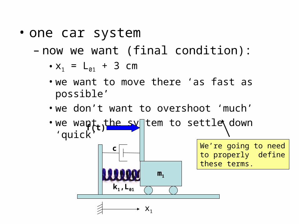
• one car system– now we want (final condition):
• x1 = L01 + 3 cm
• we want to move there ‘as fast as possible’• we don’t want to overshoot ‘much’• we want the system to settle down ‘quick’
m1
k1,L01
c
f(t)
x1
We’re going to need to properly define these terms.
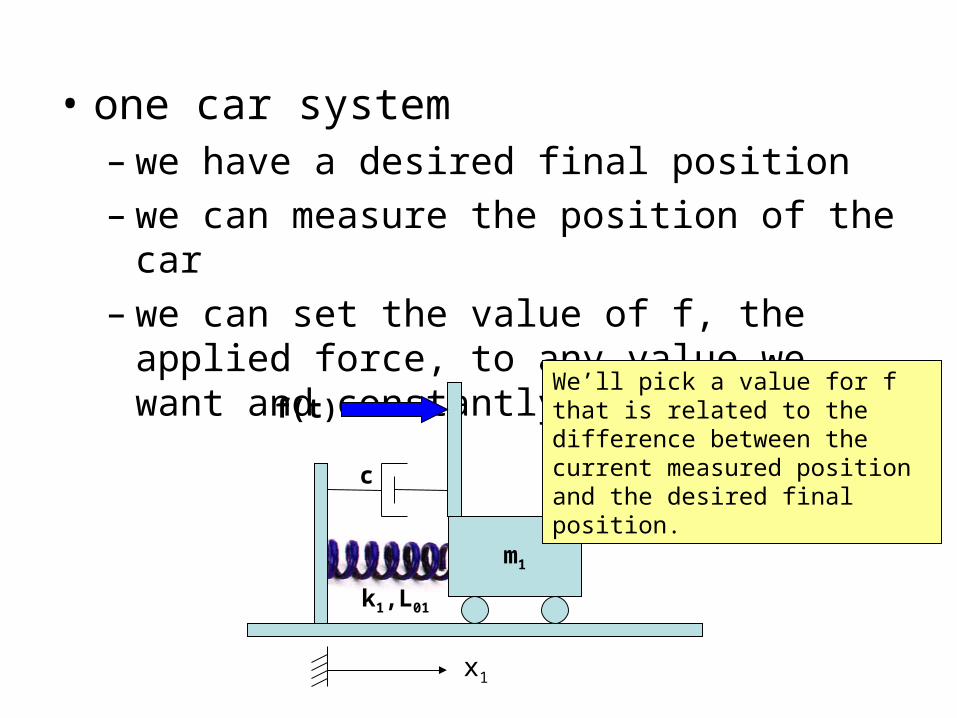
• one car system– we have a desired final position– we can measure the position of the car– we can set the value of f, the applied force, to
any value we want and constantly adjust it
m1
k1,L01
c
f(t)
x1
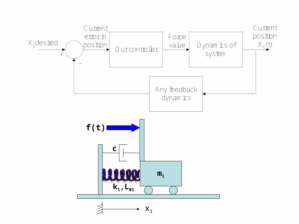
We’ll pick a value for f that is related to the difference between the current measured position and the desired final position.
m1
k1,L01
c
f(t)
x1
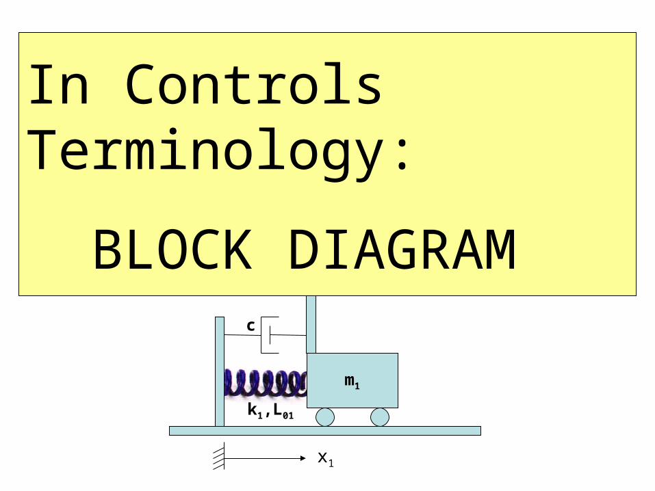
Our controllerDynamics of
system
Any feedbackdynamics
Currentposition
X1(t)X1desired
+-
Currenterror inposition
ForcevalueIn Controls Terminology:
BLOCK DIAGRAM
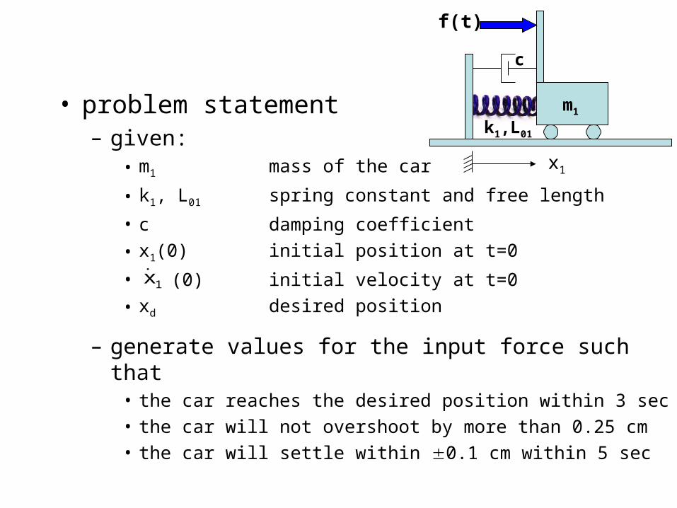
• problem statement– given:
• m1 mass of the car
• k1, L01 spring constant and free length
• c damping coefficient
• x1(0) initial position at t=0
• (0) initial velocity at t=0
• xd desired position
– generate values for the input force such that• the car reaches the desired position within 3 sec• the car will not overshoot by more than 0.25 cm• the car will settle within 0.1 cm within 5 sec
m1
k1,L01
c
f(t)
x1
1x
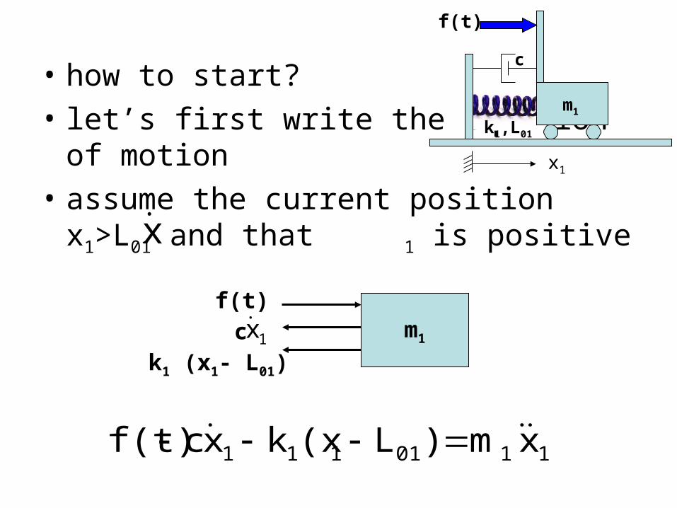
• how to start?
• let’s first write the equationof motion
• assume the current position x1>L01 and that 1 is positive
m1
k1,L01
c
f(t)
x1
x
m1ck1 (x1- L01)
f(t)
1x
1101111 xm)L(xkxcf(t)
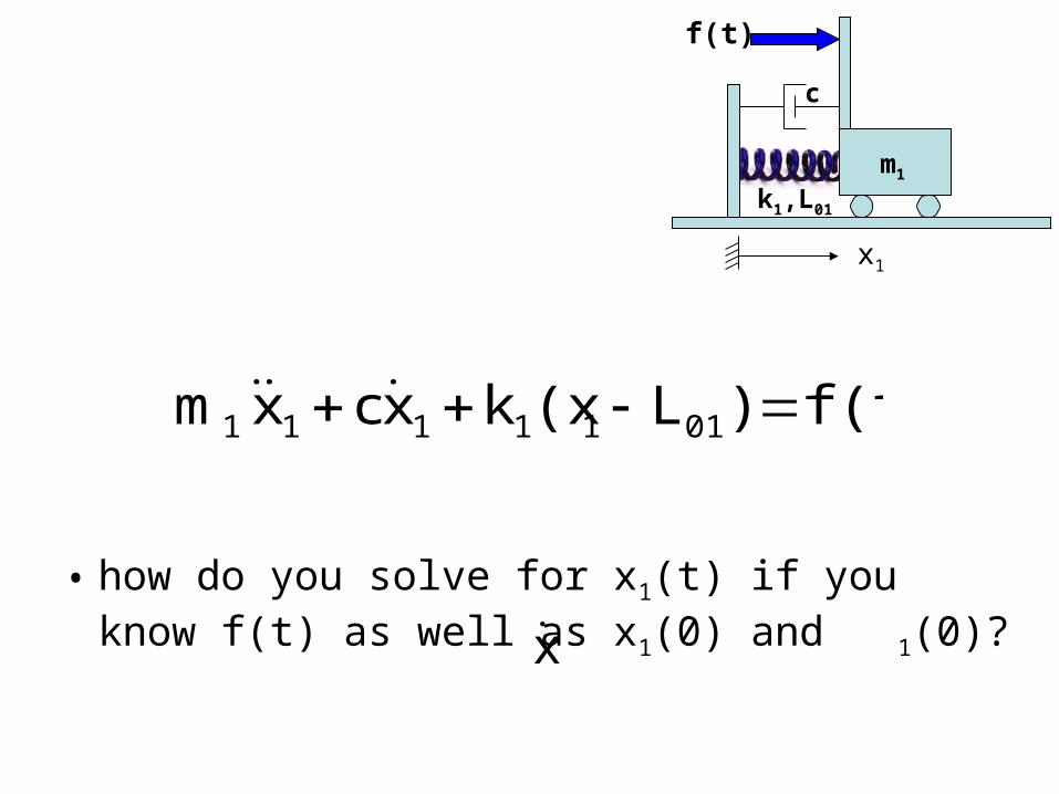
• how do you solve for x1(t) if you know f(t) as well as x1(0) and 1(0)?
m1
k1,L01
c
f(t)
x1
f(t))L(xkxcxm 0111111
x
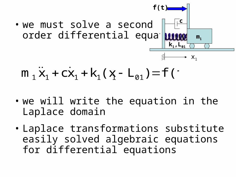
• we must solve a secondorder differential equation
• we will write the equation in the Laplace domain
• Laplace transformations substitute easily solved algebraic equations for differential equations
m1
k1,L01
c
f(t)
x1
f(t))L(xkxcxm 0111111
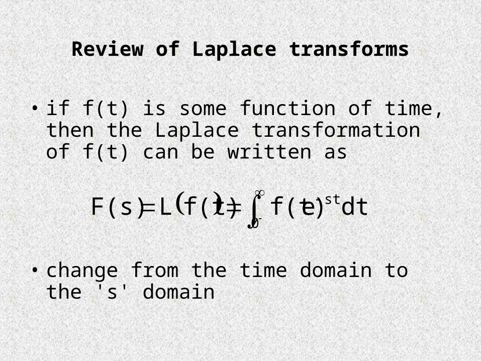
Review of Laplace transforms
• if f(t) is some function of time, then the Laplace transformation of f(t) can be written as
• change from the time domain to the 's' domain
0
dtef(t)f(t)F(s) stL
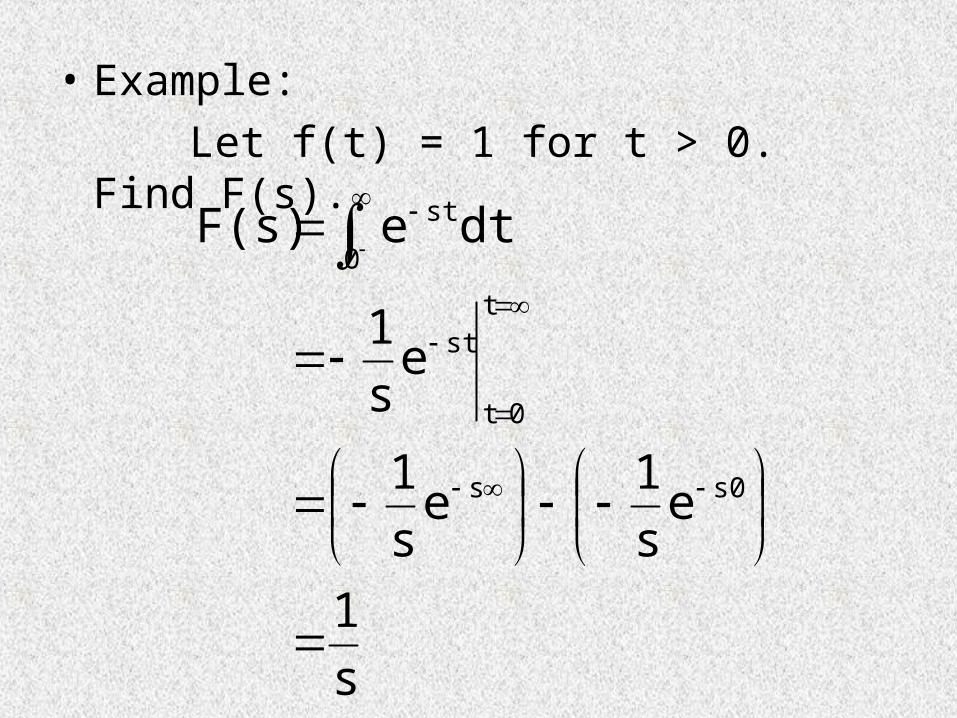
• Example:
Let f(t) = 1 for t > 0. Find F(s).
s
1
es
1e
s
1
es
1
dteF(s)
s0s
t
0t
st
st
0
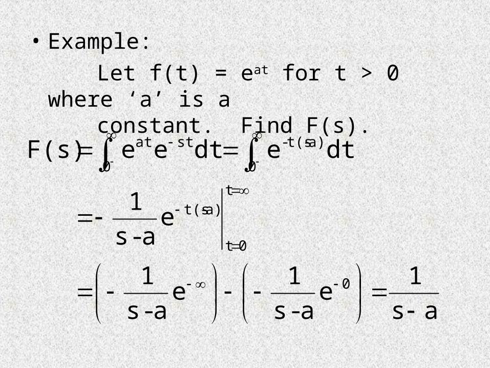
• Example:
Let f(t) = eat for t > 0 where ‘a’ is aconstant. Find F(s).
as
1e
a-s
1e
a-s
1
ea-s
1
dtedteeF(s)
0
t
0t
a)-t(s
a)-t(s-stat
00
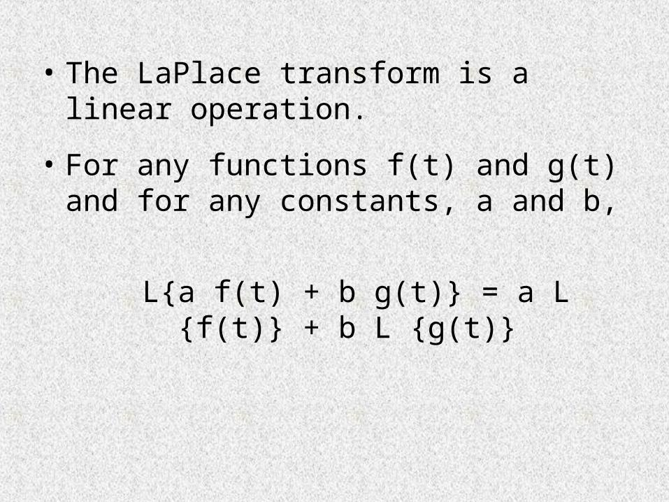
• The LaPlace transform is a linear operation.
• For any functions f(t) and g(t) and for any constants, a and b,
L{a f(t) + b g(t)} = a L {f(t)} + b L {g(t)}
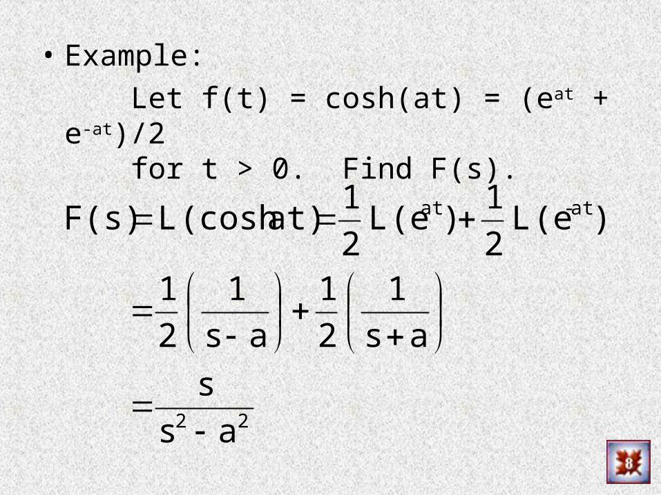
• Example:
Let f(t) = cosh(at) = (eat + e-at)/2for t > 0. Find F(s).
22
at-at
as
s
as
1
2
1
as
1
2
1
)(e2
1)(e
2
1 at)(coshF(s)
LLL
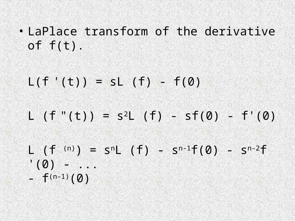
• LaPlace transform of the derivative of f(t).
L(f '(t)) = sL (f) - f(0)
L (f "(t)) = s2L (f) - sf(0) - f'(0)
L (f (n)) = snL (f) - sn-1f(0) - sn-2f '(0) - ... - f(n-1)(0)
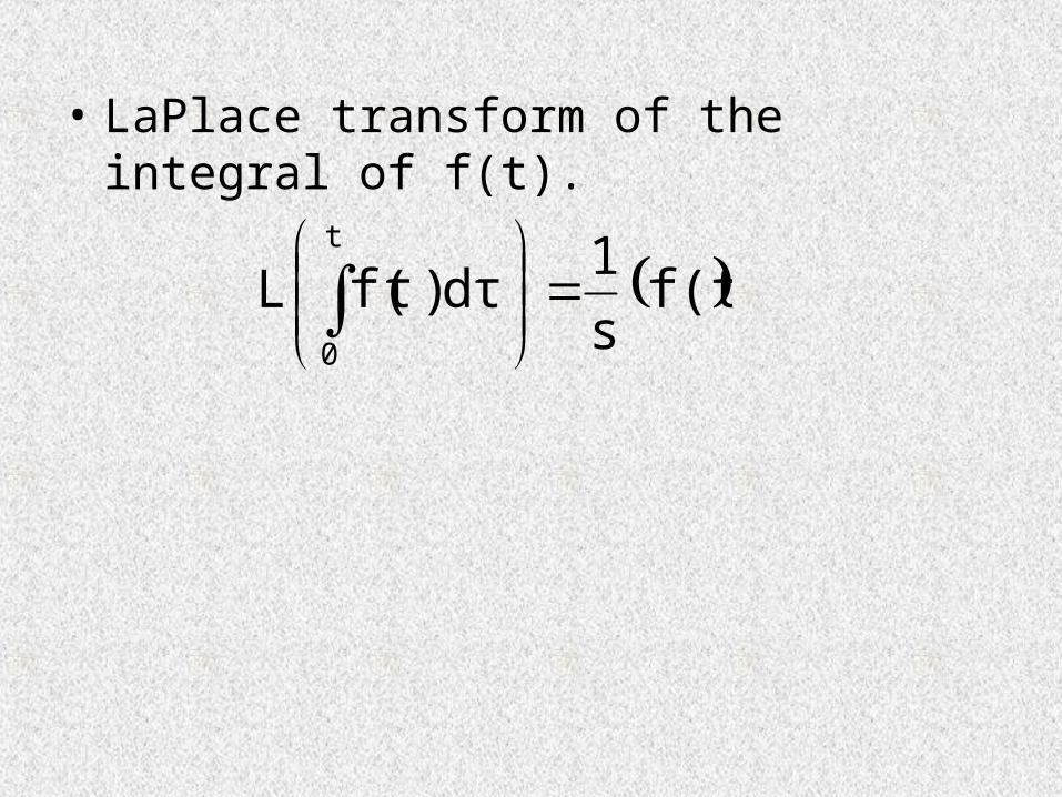
• LaPlace transform of the integral of f(t).
f(t)s
1d)f(
t
0
ττL
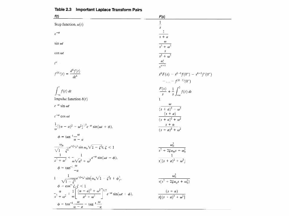
• Laplace transforms have been calculated for a large variety of functions. Sampling of these are listed in Table 2.3 of the text – Modern Control Systems, 9th ed., R.C. Dorf
and R.H. Bishop, Prentice Hall, 2001.
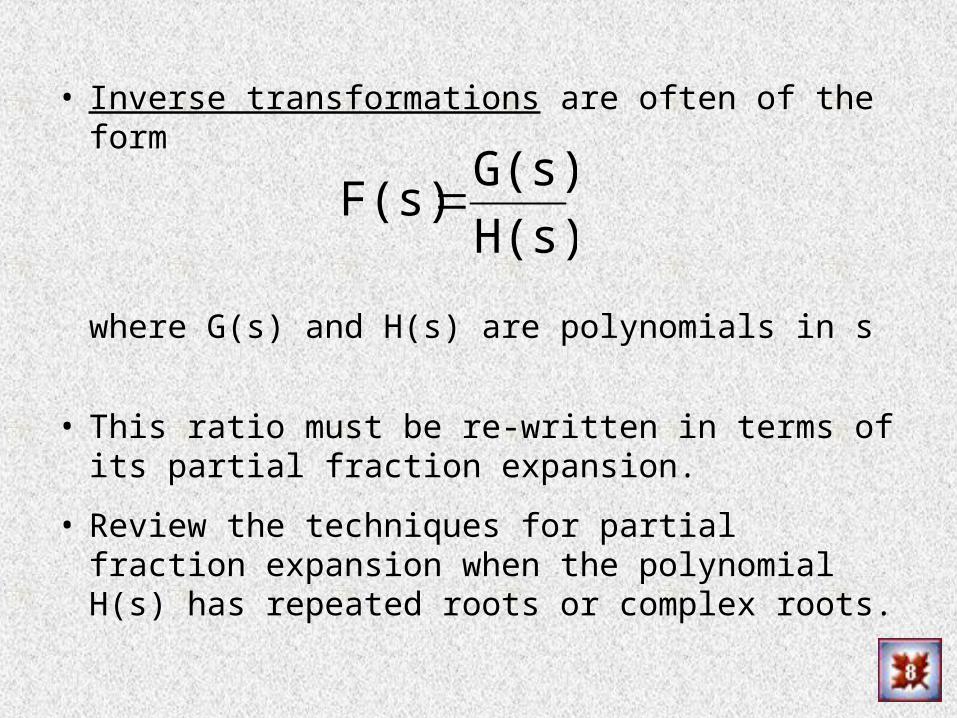
• Inverse transformations are often of the form
where G(s) and H(s) are polynomials in s
• This ratio must be re-written in terms of its partial fraction expansion.
• Review the techniques for partial fraction expansion when the polynomial H(s) has repeated roots or complex roots.
H(s)
G(s)F(s)
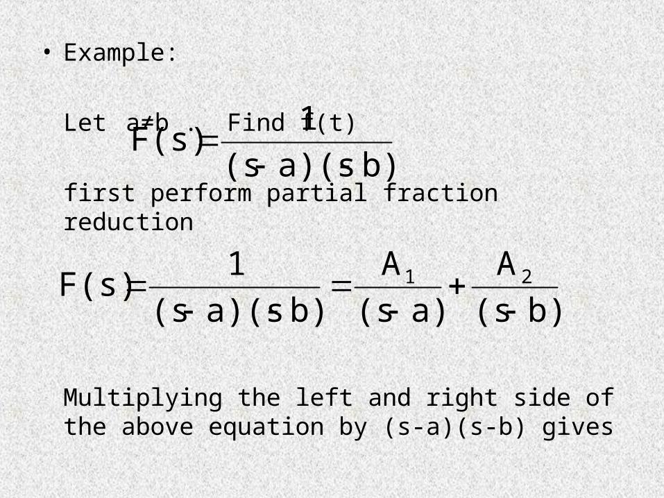
• Example:
Let a≠b . Find f(t)
first perform partial fraction reduction
Multiplying the left and right side of the above equation by (s-a)(s-b) gives
b)a)(s(s
1F(s)
b)(s
A
a)(s
A
b)a)(s(s
1F(s) 21
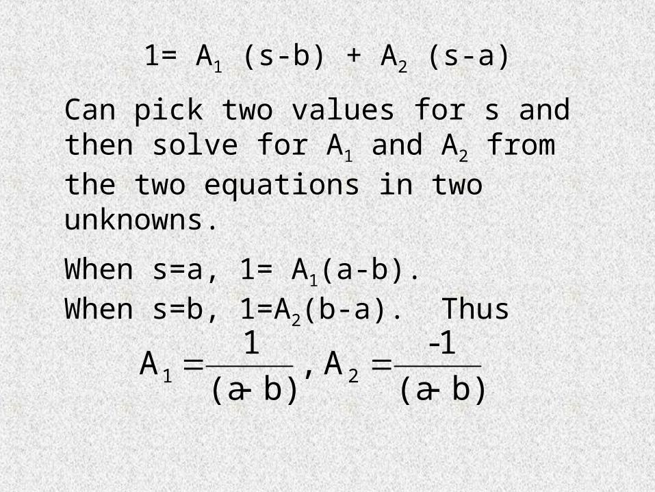
1= A1 (s-b) + A2 (s-a)
Can pick two values for s and then solve for A1 and A2 from the two equations in two unknowns.
When s=a, 1= A1(a-b). When s=b, 1=A2(b-a). Thus
b)(a
1-A,
b)(a
1A 21
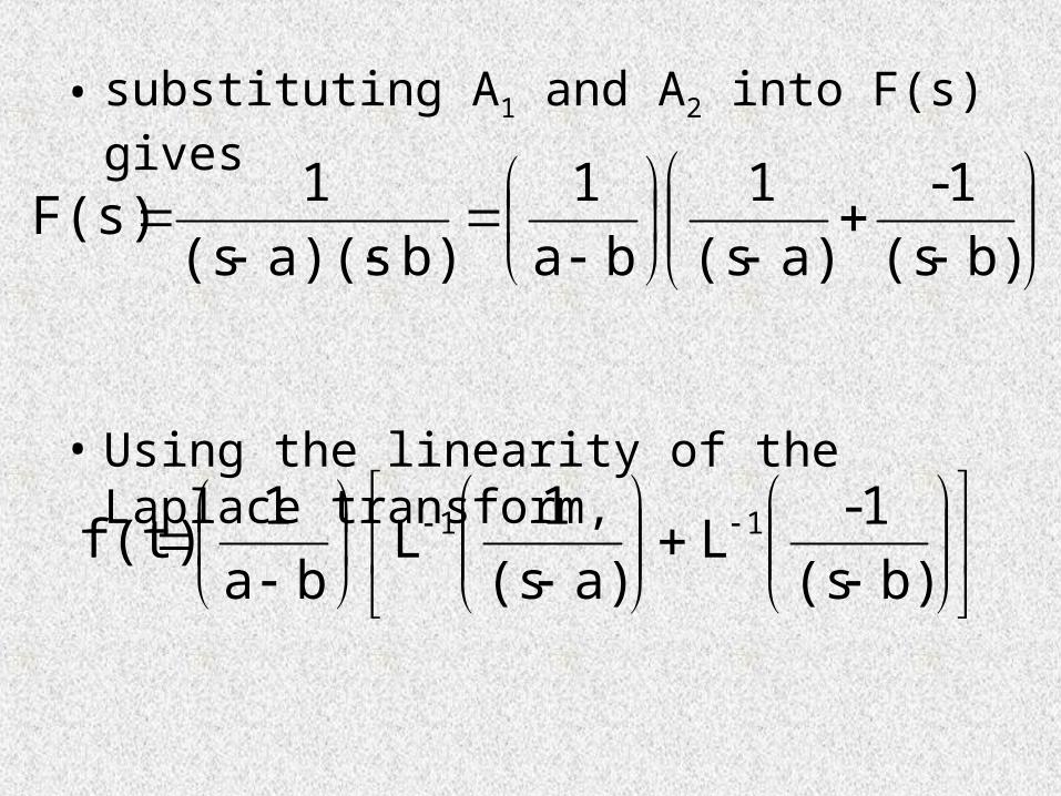
• substituting A1 and A2 into F(s) gives
• Using the linearity of the Laplace transform,
b)(s
1-
a)(s
1
ba
1
b)a)(s(s
1F(s)
b)(s
1-
a)(s
1
ba
1f(t) 11 LL
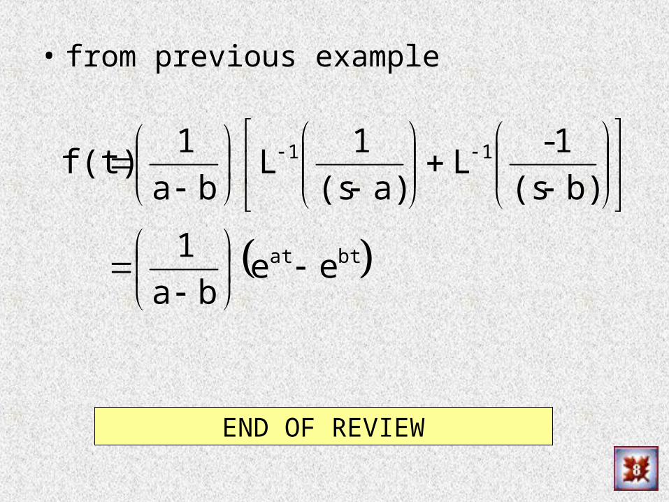
• from previous example
btat eeba
1
b)(s
1-
a)(s
1
ba
1f(t)
11 LL
END OF REVIEW
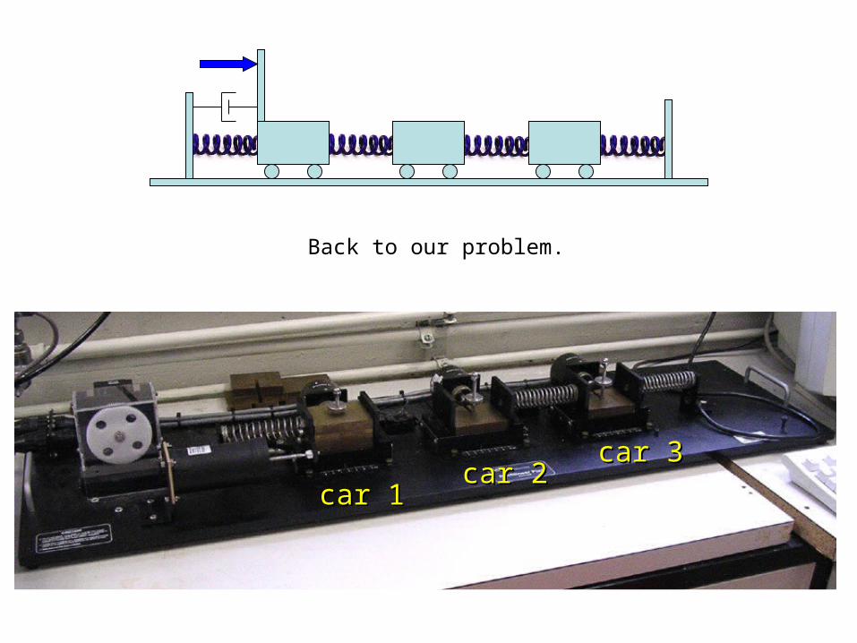
car 1car 1car 2car 2
car 3car 3
Back to our problem.
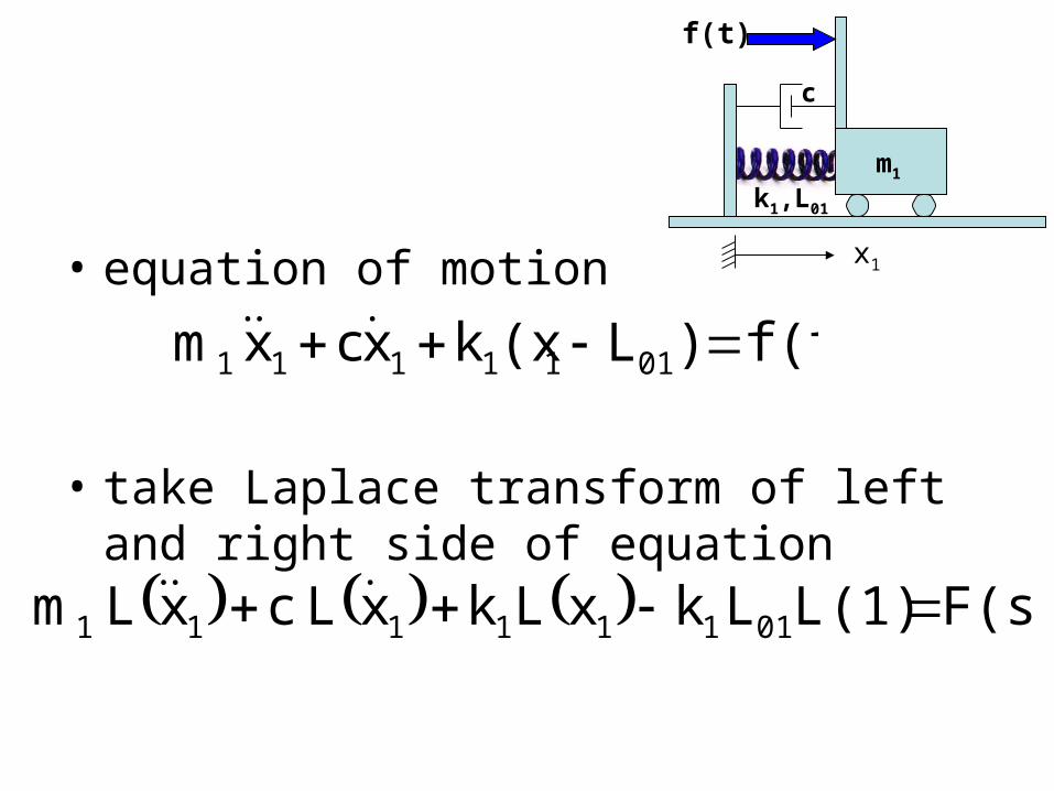
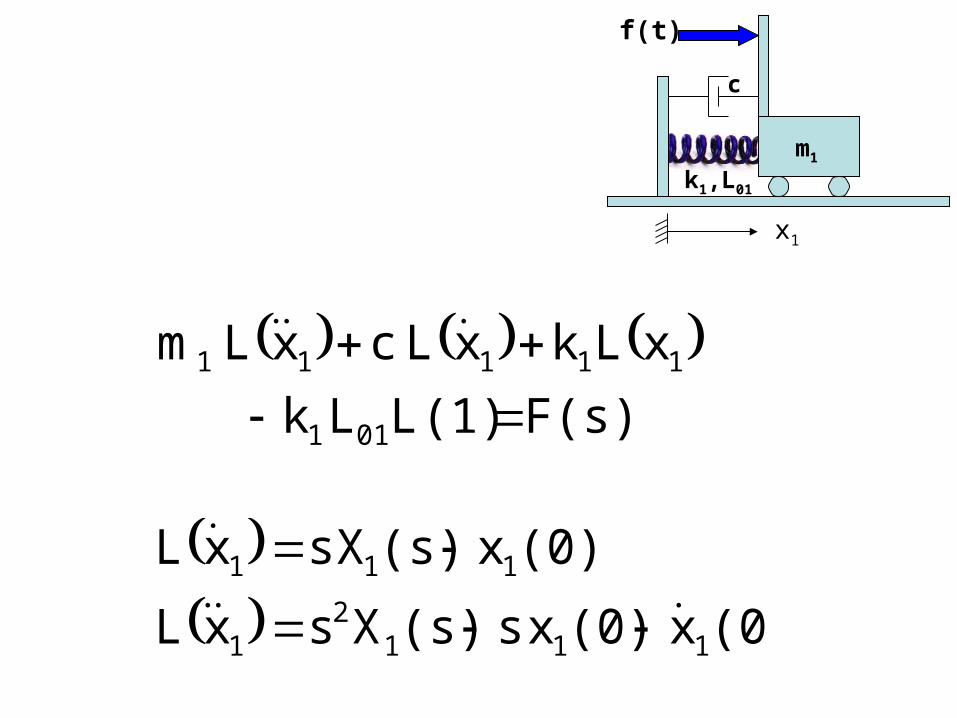
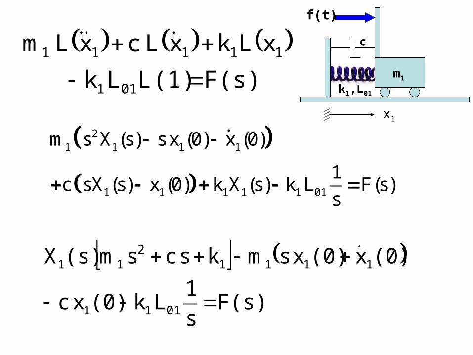
• equation of motion
• take Laplace transform of left and right side of equation
m1
k1,L01
c
f(t)
x1
f(t))L(xkxcxm 0111111
F(s)(1)Lkxkxcxm 01111111 LLLL
m1
k1,L01
c
f(t)
x1
F(s)(1)Lk
xkxcxm
011
11111
L
LLL
(0)x(0)xs(s)Xsx
(0)x(s)sXx
1112
1
111
L
L
m1
k1,L01
c
f(t)
x1
21 1 1 1
1 1 1 1 1 01
m s X (s) s x (0) x (0)
1c sX (s) x (0) k X (s) k L F(s)
s
F(s)(1)Lk
xkxcxm
011
11111
L
LLL
F(s)s
1Lk(0)xc
(0)x(0)xsmkscsm(s)X
0111
11112
11
m1
k1,L01
c
f(t)
x1
1x
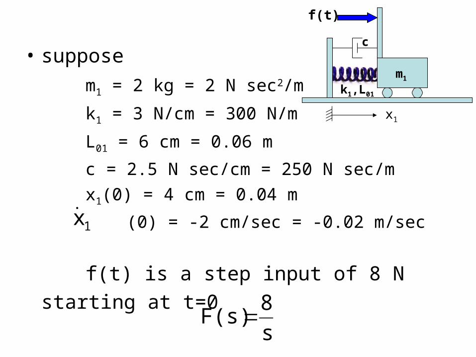
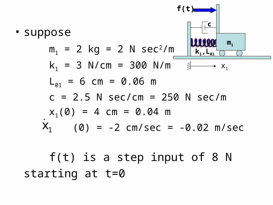
• suppose
m1 = 2 kg = 2 N sec2/m
k1 = 3 N/cm = 300 N/m
L01 = 6 cm = 0.06 m
c = 2.5 N sec/cm = 250 N sec/m
x1(0) = 4 cm = 0.04 m
(0) = -2 cm/sec = -0.02 m/sec
f(t) is a step input of 8 N starting at t=0
s
8F(s)
m1
k1,L01
c
f(t)
x1
s
N8
s
1m0.06
m
N300m)(0.04
m
secN250
)sec
m(-0.02m)(0.04s
m
secN2
m
N300s
m
secN250s
m
secN2(s)X
2
22
1
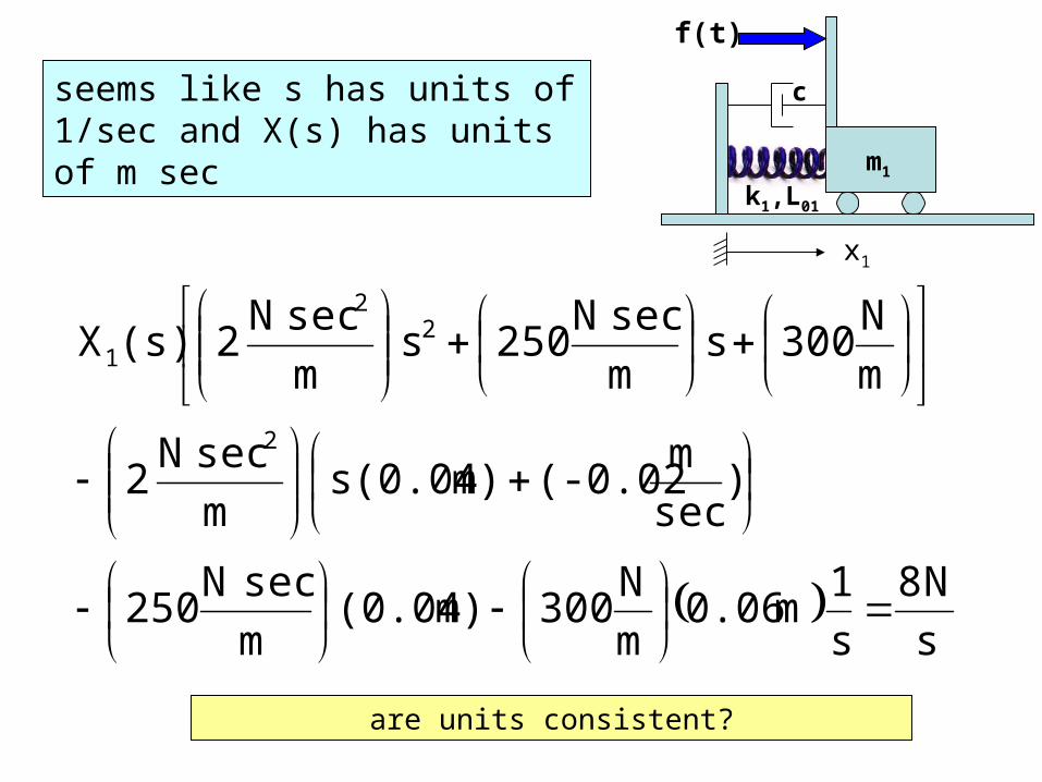
are units consistent?
seems like s has units of 1/sec and X(s) has units of m sec
s
10.06300(0.04)250
0.02s0.042s
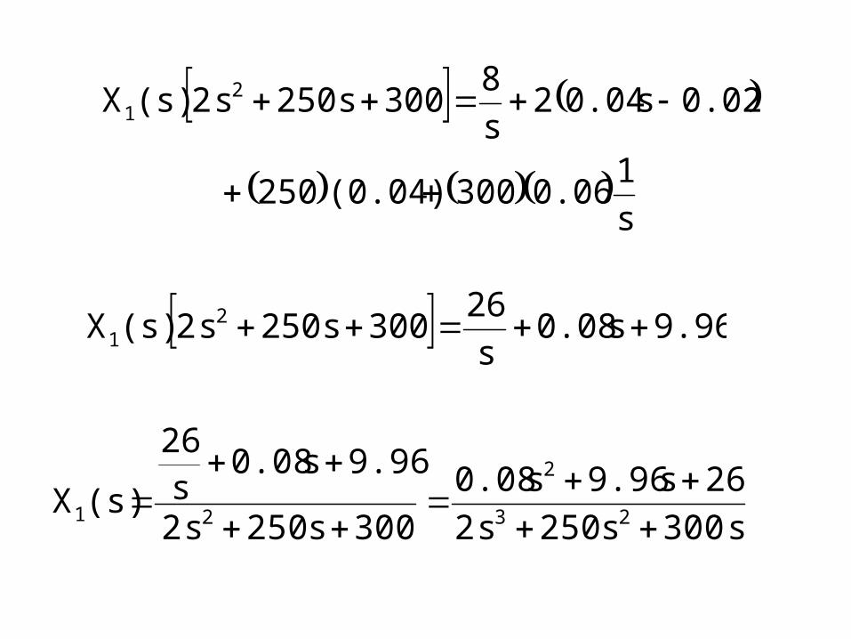
8300s250s2(s)X 2
1
9.96s0.08s
26300s250s2(s)X 2
1
s300s250s2
26s9.96s0.08
300s250s2
9.96s0.08s
26
(s)X23
2
21
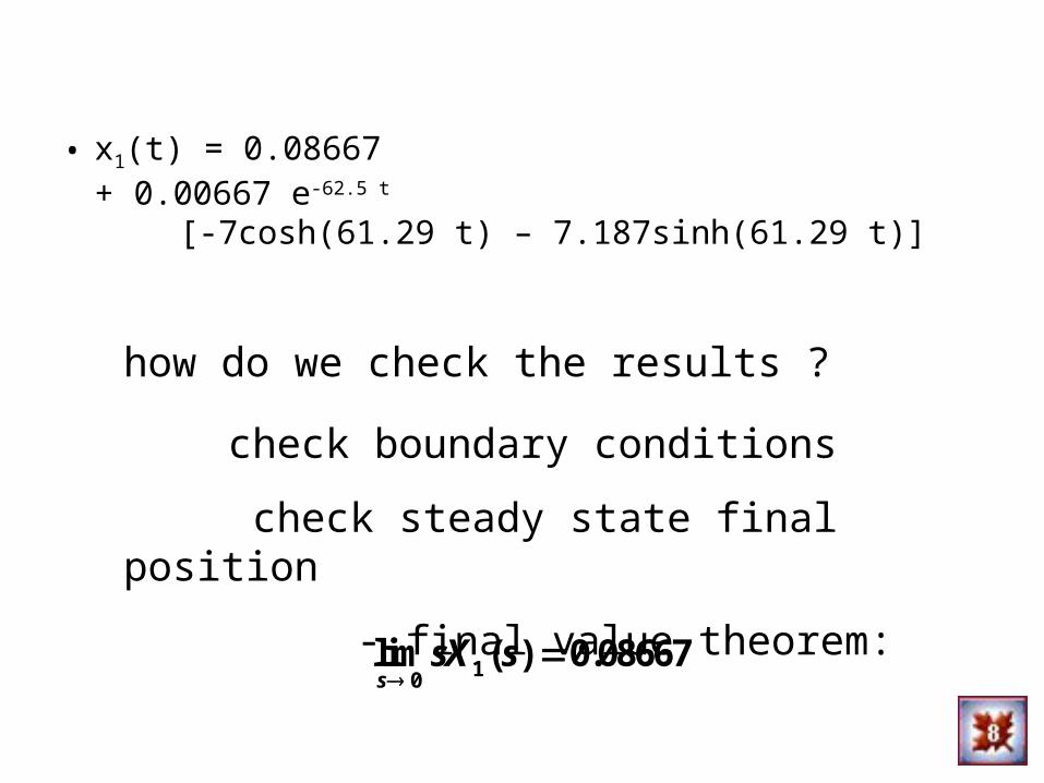
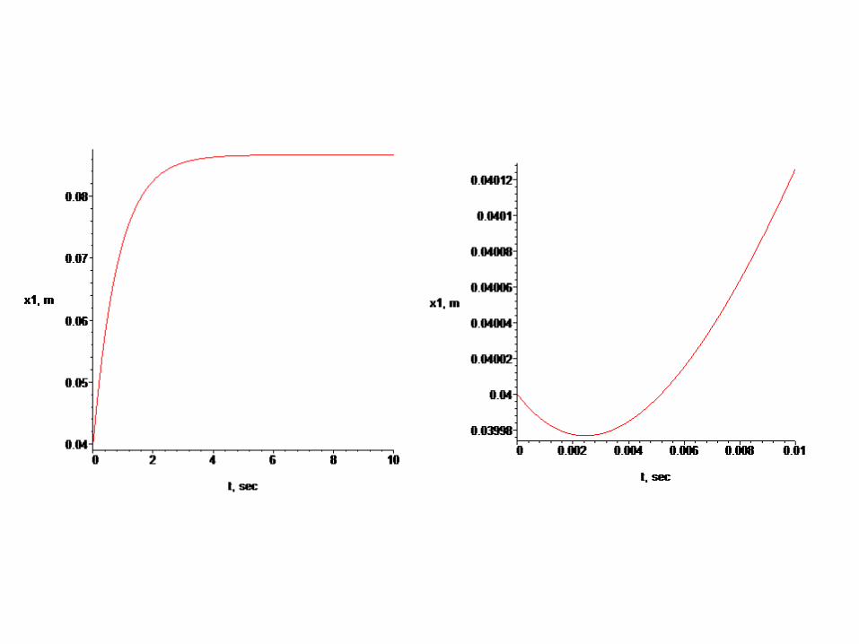
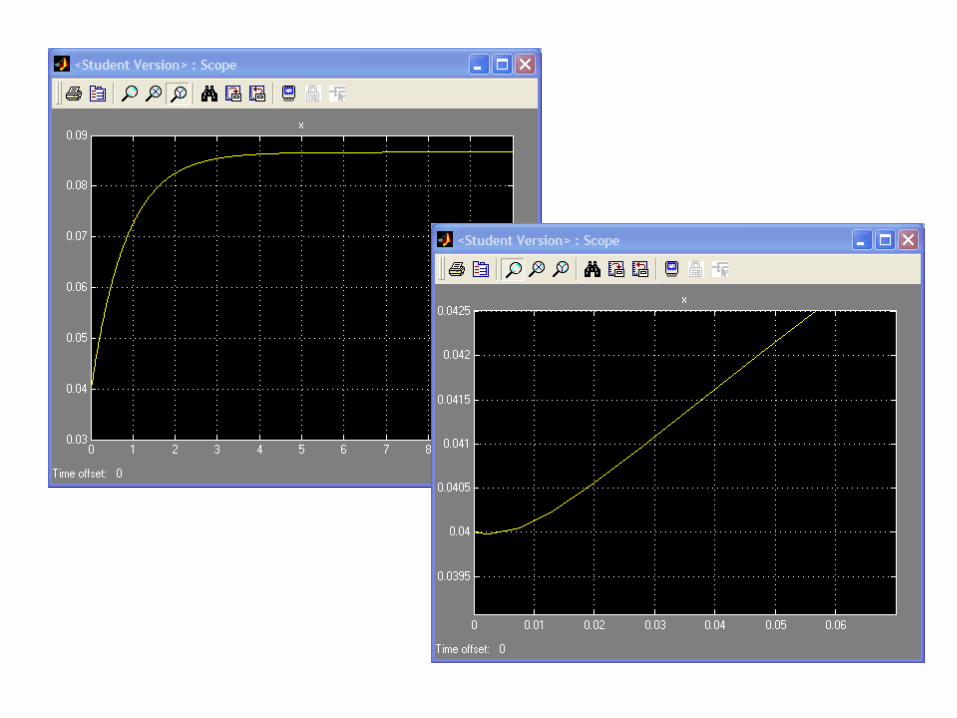
• x1(t) = 0.08667+ 0.00667 e-62.5 t
[-7cosh(61.29 t) – 7.187sinh(61.29 t)]
how do we check the results ?
10lim ( ) 0.08667ssX s
check boundary conditions
check steady state final position
- final value theorem:
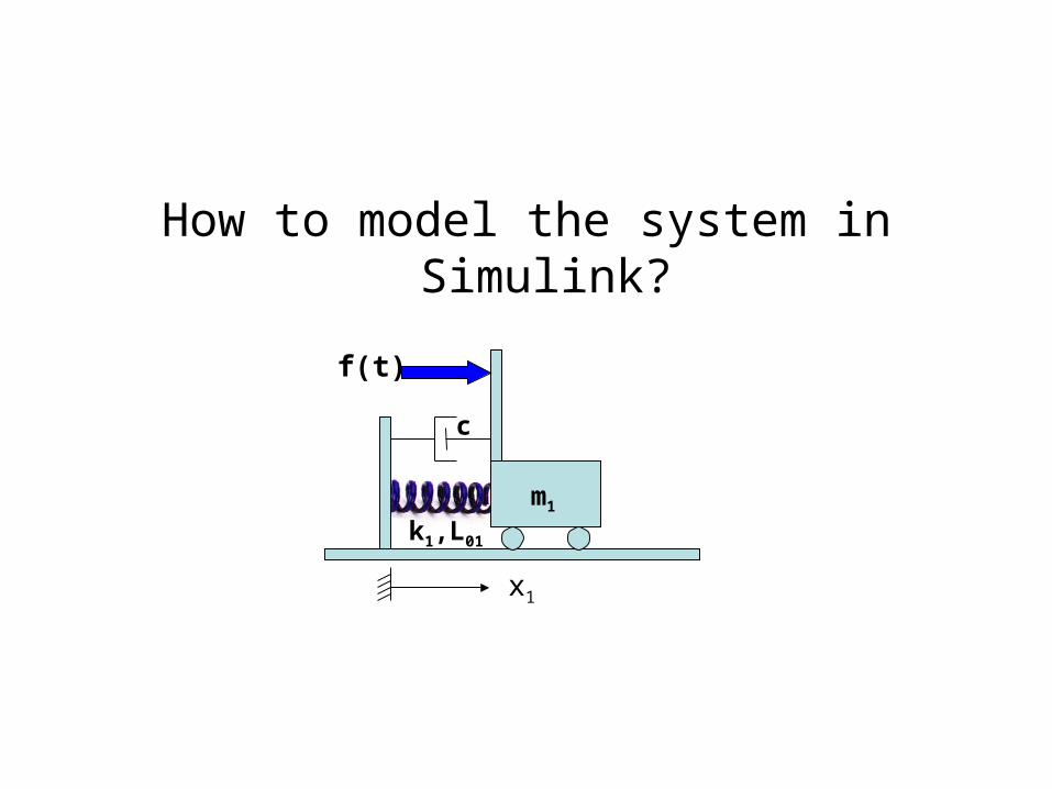
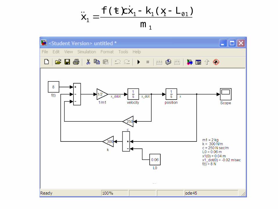
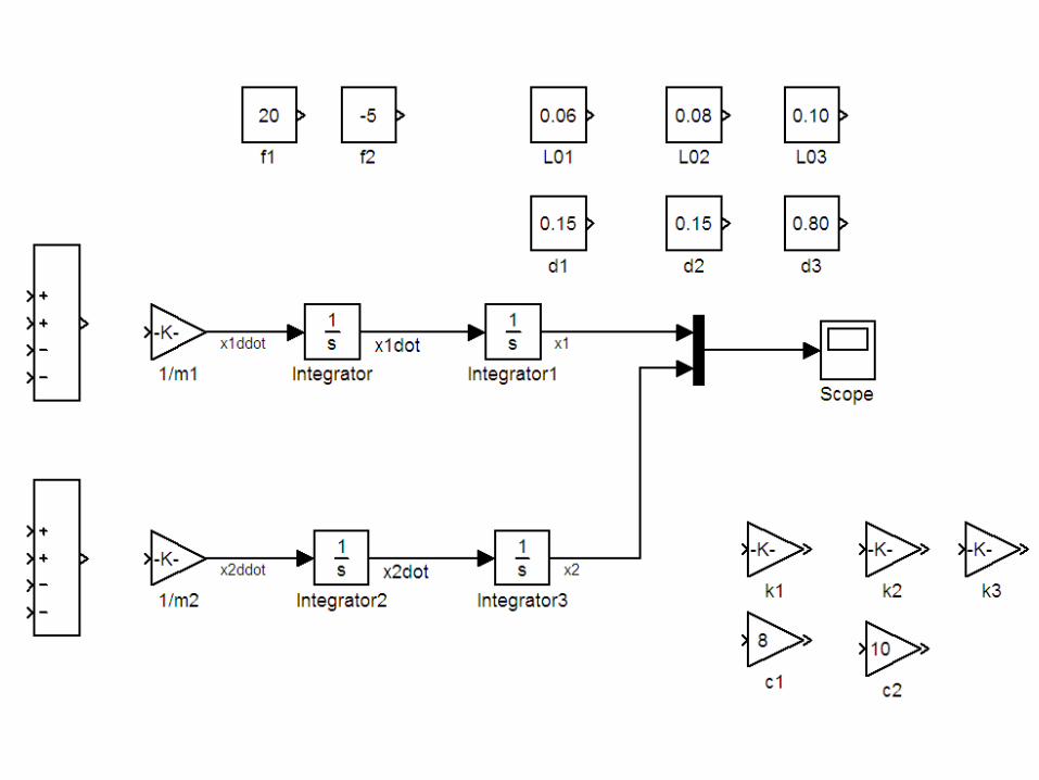
How to model the system in Simulink?
m1
k1,L01
c
f(t)
x1
m1
k1,L01
c
f(t)
x1
1x
• suppose
m1 = 2 kg = 2 N sec2/m
k1 = 3 N/cm = 300 N/m
L01 = 6 cm = 0.06 m
c = 2.5 N sec/cm = 250 N sec/m
x1(0) = 4 cm = 0.04 m
(0) = -2 cm/sec = -0.02 m/sec
f(t) is a step input of 8 N starting at t=0
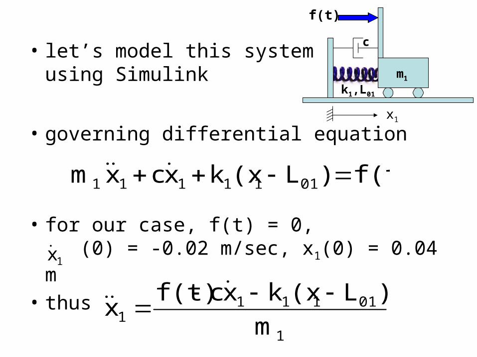
• let’s model this systemusing Simulink
• governing differential equation
• for our case, f(t) = 0, (0) = -0.02 m/sec, x1(0) = 0.04 m
• thus
f(t))L(xkxcxm 0111111
1x
1
011111 m
)L(xkxcf(t)x
m1
k1,L01
c
f(t)
x1
1
011111 m
)L(xkxcf(t)x
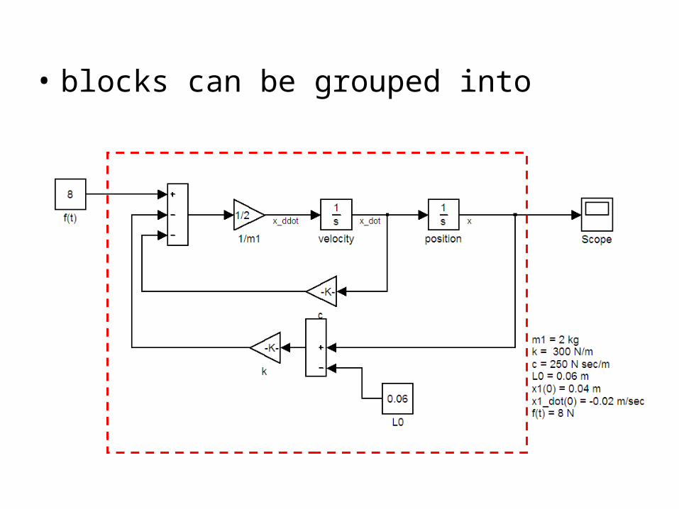
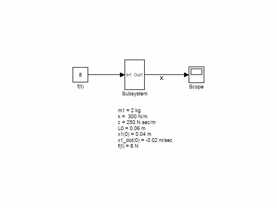
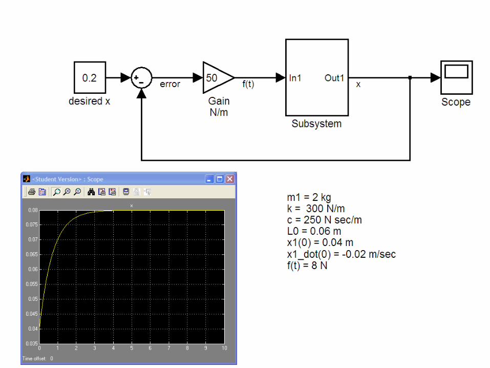
• blocks can be grouped into subsystems
x
m1
k1,L01
c
f(t)
x1
Our controllerDynamics of
system
Any feedbackdynamics
Currentposition
X1(t)X1desired
+-
Currenterror inposition
Forcevalue
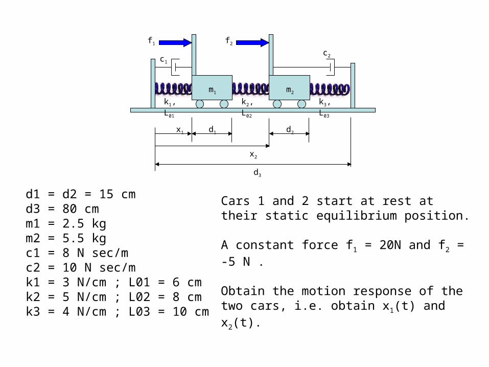
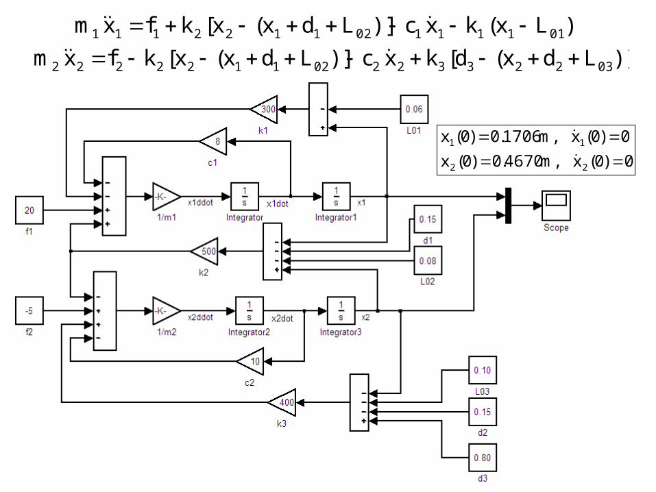
d1 = d2 = 15 cmd3 = 80 cmm1 = 2.5 kgm2 = 5.5 kgc1 = 8 N sec/mc2 = 10 N sec/mk1 = 3 N/cm ; L01 = 6 cmk2 = 5 N/cm ; L02 = 8 cmk3 = 4 N/cm ; L03 = 10 cm
Cars 1 and 2 start at rest at their static equilibrium position.
A constant force f1 = 20N and f2 = -5 N .
Obtain the motion response of the two cars, i.e. obtain x1(t) and x2(t).
x1
x2
d1
f1 f2
d2
d3
c2c1
m2m1
k2, L02k1, L01 k3, L03
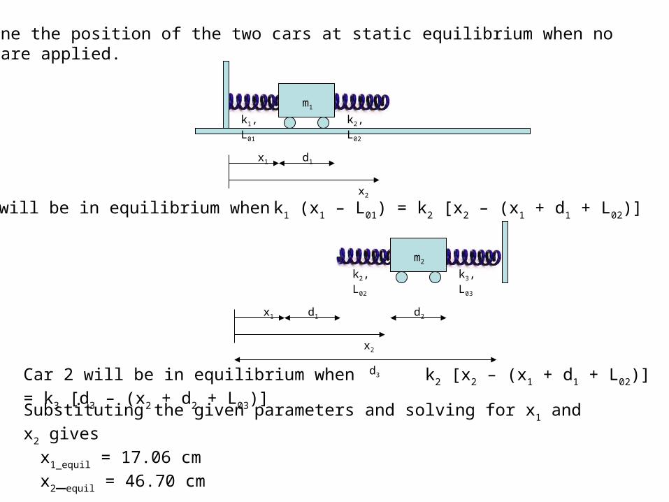
Determine the position of the two cars at static equilibrium when noforces are applied.
x1
x2
d1
m1
k2, L02k1, L01
Car 1 will be in equilibrium when k1 (x1 – L01) = k2 [x2 – (x1 + d1 + L02)]
x1
x2
d1 d2
d3
m2
k2, L02 k3, L03
Car 2 will be in equilibrium when k2 [x2 – (x1 + d1 + L02)] = k3 [d3 – (x2 + d2 + L03)]
Substituting the given parameters and solving for x1 and x2 gives
x1_equil = 17.06 cm
x2_equil = 46.70 cm
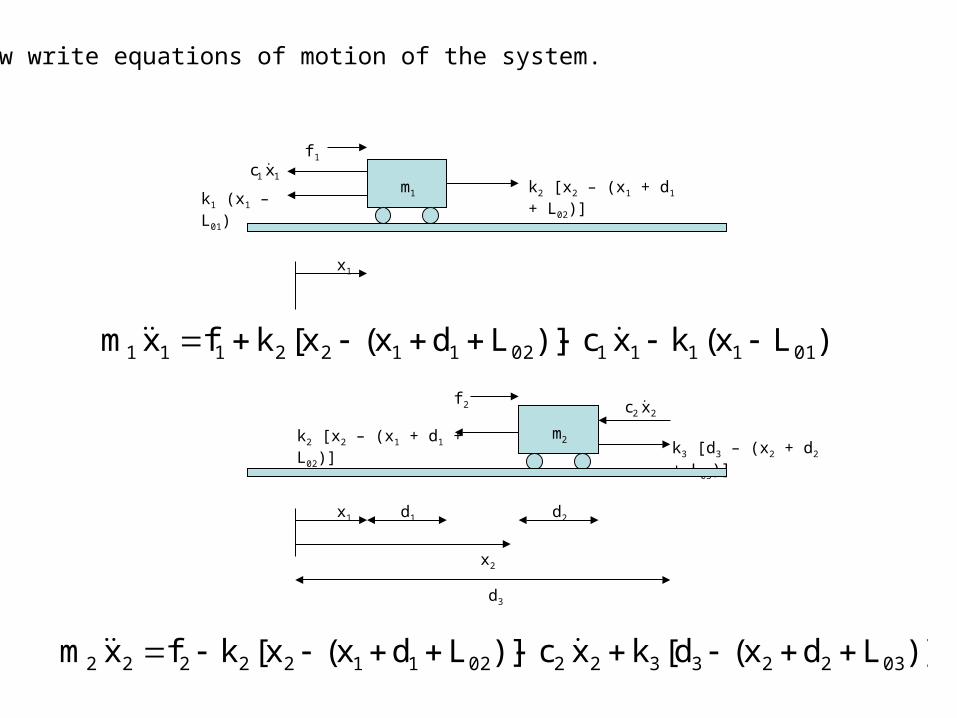
Now write equations of motion of the system.
x1
m1 k2 [x2 – (x1 + d1 + L02)]k1 (x1 – L01)
11 xc f1
)Lx(kxc)]Ldx(x[kfxm 011111021122111
x1
x2
d1 d2
d3
m2k3 [d3 – (x2 + d2 + L03)]
k2 [x2 – (x1 + d1 + L02)]
22 xc f2
)]Ldx(d[kxc)]Ldx(x[kfxm 03223322021122222
)Lx(kxc)]Ldx(x[kfxm 011111021122111
)]Ldx(d[kxc)]Ldx(x[kfxm 03223322021122222
0)0(x,m4670.0)0(x
0)0(x,m1706.0)0(x
22
11
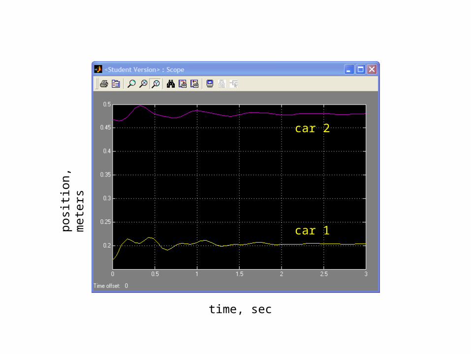
time, sec
posi
tion,
m
eter
s
car 2
car 1

This Week’s Objectives
• Establish Dynamic Models of System to be Controlled– Second Order Systems
• Obtain Solutions using LaPlace Transforms
• Create Simulink Model and Generate Simulated Results