Three-Dimensional Cloud-System Modeling of GATE Convection

15 JUNE 1999 1885D O N N E R E T A L .

Three-Dimensional Cloud-System Modeling of GATE Convection

LEO J. DONNER, CHARLES J. SEMAN, AND RICHARD S. HEMLER

Geophysical Fluid Dynamics Laboratory, NOAA, Princeton University, Princeton, New Jersey

(Manuscript received 3 November 1997, in final form 22 July 1998)

ABSTRACT

Deep convection and its associated mesoscale circulations are modeled using a three-dimensional elastic modelwith bulk microphysics and interactive radiation for a composite easterly wave from the Global AtmosphericResearch Program Atlantic Tropical Experiment. The energy and moisture budgets, large-scale heat sources andmoisture sinks, microphysics, and radiation are examined.

The modeled cloud system undergoes a life cycle dominated by deep convection in its early stages, followedby an upper-tropospheric mesoscale circulation. The large-scale heat sources and moisture sinks associated withthe convective system agree broadly with diagnoses from field observations. The modeled upper-troposphericmoisture exceeds observed values. Strong radiative cooling at the top of the mesoscale circulation can produceoverturning there. Qualitative features of observed changes in large-scale convective available potential energyand convective inhibition are found in the model integrations, although quantitative magnitudes can differ,especially for convective inhibition.

Radiation exerts a strong influence on the microphysical properties of the cloud system. The three-dimensionalintegrations exhibit considerably less sporadic temporal behavior than corresponding two-dimensional integra-tions. While the third dimension is less important over timescales longer than the duration of a phase of aneasterly wave in the lower and middle troposphere, it enables stronger interactions between radiation and dynamicsin the upper-tropospheric mesoscale circulation over a substantial fraction of the life cycle of the convectivesystem.

1. Introduction

Deep convection and its associated mesoscale cir-culations represent dominant components in the hy-drology and radiation of the tropical atmosphere. Thesecloud systems transport and remove large amounts ofwater and are thereby important in controlling upper-tropospheric water vapor, which in turn exerts a stronggreenhouse effect (Soden and Fu 1995). The spatiallyextensive, optically thick upper-tropospheric ice cloudsin these systems can exert large longwave and shortwavecloud radiative forcing (e.g., Harrison et al. 1990). Thus,these cloud systems are crucial elements in global cli-mate. Significant large-scale heating is associated withthese systems, and general circulation models (GCMs)have suggested that modes of large-scale tropical var-iability depend on the frequency and spatial distributionof deep convection (Slingo et al. 1994). The mass trans-ports associated with these cloud systems lead to re-distribution of chemical species and probably play im-

Corresponding author address: Dr. Leo J. Donner, GeophysicalFluid Dynamics Laboratory, NOAA, Princeton University, P.O. Box308, Princeton, NJ 08542.E-mail: [email protected]

portant roles in atmospheric chemistry (e.g., Lelieveldand Crutzen 1994; Stenchikov et al. 1996).

The parameterization of the effects of deep convec-tion in GCMs remains a complex, challenging problemin atmospheric science with many uncertain aspects. Theclimate in GCMs is sensitive to the details of cumulusparameterization (e.g., Donner et al. 1982; Hack 1994).Most cumulus parameterizations currently used inGCMs have been designed to treat heat and moistureinteractions between deep convection and large-scaleflows, with little attention to microphysical and radiativeaspects or the mesoscale circulations associated withdeep convection. Donner (1993) treats mesoscale cir-culations associated with deep convection but is limitedby both current lack of knowledge of the basic processesinvolved in convective systems and absence of somecritical observations of these systems, for example, icecontents in the mesoscale circulations and simultaneouscharacterization of both the large-scale dynamic envi-ronment and microphysical and radiative properties.

High-resolution models that can explicitly resolve in-dividual deep convective elements are a valuable toolfor studying the processes associated with these systemsand for evaluating cumulus parameterizations for large-scale models. The characteristics of convective cloudsystems (including radiation and associated interactions)have been studied with these models (e.g., Tao et al.

1886 VOLUME 56J O U R N A L O F T H E A T M O S P H E R I C S C I E N C E S

1993; Fu et al. 1995; Chin et al. 1995; Guichard et al.1996; Grabowski et al. 1996b). They have also beenused to evaluate cloud parameterizations (e.g., Gregoryand Miller 1989; Xu and Krueger 1991). The equilib-rium climates of these models in the absence (Held etal. 1993) and presence (Sui et al. 1994; Grabowski etal. 1996a) of imposed dynamic forcing have been in-vestigated. Until recently, cloud-system models havebeen two-dimensional, with a few small-domain (sev-eral tens of kilometers per side) three-dimensional ex-ceptions (Lipps and Hemler 1986; Redelsperger andSommeria 1986; Tao and Soong 1986; Dudhia and Mon-crieff 1987).

Currently, efforts are underway at several laboratoriesand universities to study convective systems with larger-domain (several hundreds of kilometers per side) three-dimensional cloud-resolving models. These modelshave domains significantly larger than those of the in-dividually resolved cumulus elements and are also com-parable in size to the resolution of GCMs typically usedfor climate studies. The purpose of this paper is to ex-amine a three-dimensional large-domain integration ofa cloud system for conditions associated with a com-posite easterly wave from the Global Atmospheric Re-search Program (GARP) Atlantic Tropical Experiment(GATE). The model is described in section 2. Dynamicsand energetics (section 3), microphysics and radiation(section 4), and the role of the third dimension (section5) are highlighted. In focusing on these issues, the paperaims to evaluate the behavior of the model in a typicalcase, especially regarding properties that are importantfor the interaction between convection and larger scales.If models of this nature can capture these features re-alistically, they have great potential for evaluating cu-mulus parameterizations and the hypotheses on whichparameterizations are based. The results to be presentedare generally promising in this regard, although theyindicate that some aspects of the models require furtherdevelopment. General questions regarding the basis forparameterization will also require use of models in moresynoptic environments than the GATE case consideredhere.

2. Model description and integration design

The model used for these integrations is a three-di-mensional version of that employed by Held et al.(1993). The model uses elastic dynamics, bulk micro-physics, and interactive radiation. In addition to addingthe third dimension, other modifications include the fol-lowing. 1) In the bulk aerodynamic formulations forsurface sensible- and latent-heat fluxes, atmospherictemperatures and mixing ratios extrapolated to 10-mheights are used. By doing so, observed sensible-heatfluxes (which used atmospheric measurements at 10 m)can be compared more readily with the model. No min-imum value is imposed on the horizontal wind speed inthe bulk aerodynamic formulation here. 2) An autocon-

version threshold for ice of 1.5 g kg21 [instead of zeroand similar to the threshold of 1.0 g m23 in Lipps andHemler (1988)] is used in the bulk microphysics. Themodel includes two classes of ice: cloud ice and snow.3) The sponge layer near the model top has a strengthk0(z 2 z0). The damping is linear above z0 5 13.875km with a damping time of 235 s at the model top at16 km. For potential temperature, the model is dampedto observations, instead of the model horizontal meansin Held et al. (1993), where the sponge is applied abovez0. The sponge layer is fairly thin, and the model topis only somewhat above the heights to which GATEconvection penetrates, following Lipps and Hemler(1986). This offers an obvious advantage in limitingcomputational demands, but the sponge layer is thinnerthan in many studies of deep convection (e.g., Held etal. 1993), and active microphysical and radiative pro-cesses will be seen to extend through the full verticalextent of the model domain at some times during theintegrations. Although some details of the integrationsmay be artifacts of these limitations, the fundamentalcharacter of the modeled convective systems does notappear to have been altered significantly by the use ofa fairly thin sponge layer or limited vertical domain.

The horizontal model domain for these integrationsis 220 3 220 km. The horizontal and vertical gridlengths are 2 km and 500 m, respectively. The horizontaldomain is similar to that of the GATE B-scale array,from which observations used to force and evaluate theintegrations are obtained. It is also typical of resolutionsof many climate GCMs in which convective processesare parameterized. A series of test calculations with themodel using resolutions from 500 m to 5 km indicatedthat some basic features of the integrations (e.g., patternof vertical velocity) began to change noticeably as theresolution was degraded beyond 2 km, motivating thechoice of horizontal resolution in the face of the greatcomputational demands of the three-dimensional inte-grations. Also, note that Golding (1993) successfullymodeled intense convection near Darwin (Australia) us-ing 3-km resolution. The model employs periodic lateralboundary conditions. The model time step is 2 s. Themodel domain moves with the time-dependent, verti-cally averaged wind, obtained from Thompson et al.(1979). These winds have not been mass weighted, andthis movement of the domain will be used only in an-alyzing the surface precipitation field.

The integrations are performed over a composite east-erly wave from GATE. Advantages of this procedureinclude the presence of well-documented observationsand the typical character of the synoptic situation as-sociated with the composite. Disadvantages, relative tointegrating for specific cases, arise from the nonlinearrelationships between atmospheric structures, forcing,and convection, which limit the extent to which con-vection arising from composite states in the integrationcan be compared with composite observations. Anotherdisadvantage is that a diurnal cycle of radiation is not

15 JUNE 1999 1887D O N N E R E T A L .

implemented; instead, radiation calculations are per-formed with a solar zenith angle of 538, representing atropical diurnal average. The radiative-transfer modelused here is described in Held et al. (1993).

Large-scale forcing for potential temperature and vapormixing ratio are imposed as terms added to the ther-modynamic and vapor mixing-ratio equations. This large-scale forcing, which depends on height and time, rep-resents the effects of both horizontal and vertical large-scale advection of temperature and vapor mixing ratio.Feedbacks by convection on the easterly wave and itslarge-scale forcing (Paradis et al. 1995) are excluded bythis procedure. Height-dependent observations fromGATE (Thompson et al. 1979) for temperature, mixingratio, apparent heat source, apparent moisture sink, andduration of GATE wave phases are used. The large-scaleforcings (representing total advection) for potential tem-perature ]LSu and mixing ratio ]LSq are given by

]u Q p1] u 5 2 , (1)LS ]t cp

]q Q2] q 5 1 . (2)LS ]t L1

Potential temperature is denoted by u, vapor mixing ratioby q, specific heat capacity at constant pressure by cp,and latent heat of vaporization by L1. The reciprocal Ex-ner function p is , where p is pressure, p0 isR /cd p(p / p )0

a reference pressure (100 hPa), and Rd is the gas constantfor dry air. The apparent heat source Q1 is given by

]s ]Q 5 1 = · (v s) 1 (v s), (3)1 ]t ]p

where s 5 cpT 1 gz is the dry static energy, v is thehorizontal velocity vector, and v is the (pressure) verticalvelocity (T and g denote temperature and the gravityconstant, respectively). A large-scale average is indicatedby an overbar. The apparent moisture sink Q2 is givenby

]q ]Q 5 2L 1 = · (v q) 1 (v q) . (4)2 1 [ ]]t ]p

The model integrations are initialized with height-dependent temperature and mixing-ratio soundings fromGATE phase 1 in Thompson et al. (1979). Perturbationsare imposed on the initial mixing ratio to initiate con-vection. The perturbations vary in the horizontal but areconstant throughout the lowest 1.5 km in each columnof the model. The perturbations are horizontally random,generated from a uniform distribution between 62 gkg21. These perturbations are similar to those employedby Lipps and Hemler (1986). The perturbations are cho-sen to be random so as not to impose organized structureon the convection when it develops, and Lipps and Hem-ler (1986) found that perturbations of this magnitudewere sufficient to initiate convection. However, further

research as to the most appropriate magnitude and struc-ture of these initial perturbations is warranted. The in-tegrations extend from phase 1 through phase 7 ofGATE. (Phase numbers refer to particular synoptic fea-tures of the composite easterly wave. For example,phase 4 refers to the trough and phase 8, to the ridge,while phases 2 and 6 indicate maximum north and southwinds, respectively. Intermediate numbers indicate in-termediate synoptic phases.) Phase 8, with little ob-served deep convection, is not used in the integration.Phase 1, also with limited deep convection, is used inthe integration to allow the model to spin up. UsingTable 1 of Thompson et al. (1979), the durations ofphases 1–7 are taken as 10, 14, 9, 10, 8, 13, and 9 h,respectively. The local tendencies of potential temper-ature and mixing ratio in (1) and (2) are evaluated bydifferencing the potential temperatures and mixing ra-tios at the beginning of each wave phase in Thompsonet al. (1979) and dividing by the duration of the wavephase. Apparent heat sources and moisture sinks areinterpolated linearly between their Thompson et al.(1979) values at the beginning of each wave phase.Zonal and meridional velocity components are inter-polated from Thompson et al. (1979) to hourly fre-quency; these values are used to update the base-statevelocity each hour. This approach differs from that used,for example, by Grabowski et al. (1996b), who relaxthe base-state wind toward imposed large-scale winds.No difficulties have been noted with the direct impo-sition of observed wind profiles at hourly frequency inthe present integrations.

Time-dependent surface temperatures are imposed.These temperatures yield the surface sensible-heat flux-es in Thompson et al. (1979), when their formulationsfor heat flux and temperature profiles are used.

Three integrations are considered. The three-dimen-sional integration is referred to as ‘‘3D.’’ To evaluatethe effect of the third dimension, a parallel two-dimen-sional integration (‘‘2D’’) is performed. The 2D inte-gration uses only zonal-wind components and is con-fined to a height–longitude plane with no meridionaldimension. In both 3D and 2D, radiative heating andcooling are large relative to other diabatic and dynamicprocesses. The effect of radiation is isolated by per-forming a third integration, ‘‘2D No Radiation,’’ whichis identical to 2D but with no solar or longwave radi-ation.

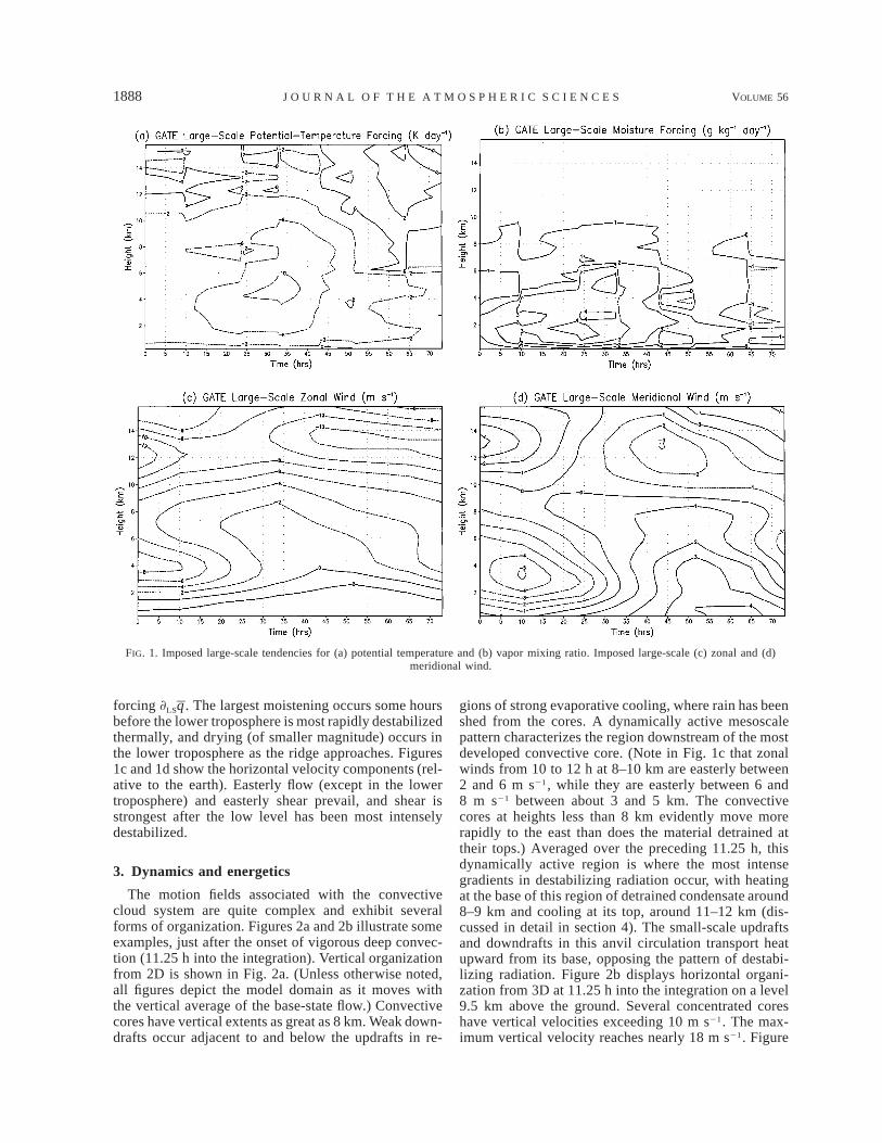
Large-scale potential-temperature forcing ]LSu isshown in Fig. 1a. Large-scale forcing destabilizes thelower and middle troposphere appreciably from about25 to 45 h, the transition from maximum low-level northwinds through the trough axis in the easterly wave. Theupper troposphere is stabilized as low-level southerlyflow is established in advance of the approach of theridge axis. The magnitude of this stabilization is lessthan the magnitude of the destabilization of the lowerand middle troposphere during the earlier stages of theeasterly wave. Figure 1b shows the large-scale moisture


FIG. 1. Imposed large-scale tendencies for (a) potential temperature and (b) vapor mixing ratio. Imposed large-scale (c) zonal and (d)meridional wind.

forcing ]LSq . The largest moistening occurs some hoursbefore the lower troposphere is most rapidly destabilizedthermally, and drying (of smaller magnitude) occurs inthe lower troposphere as the ridge approaches. Figures1c and 1d show the horizontal velocity components (rel-ative to the earth). Easterly flow (except in the lowertroposphere) and easterly shear prevail, and shear isstrongest after the low level has been most intenselydestabilized.

3. Dynamics and energetics

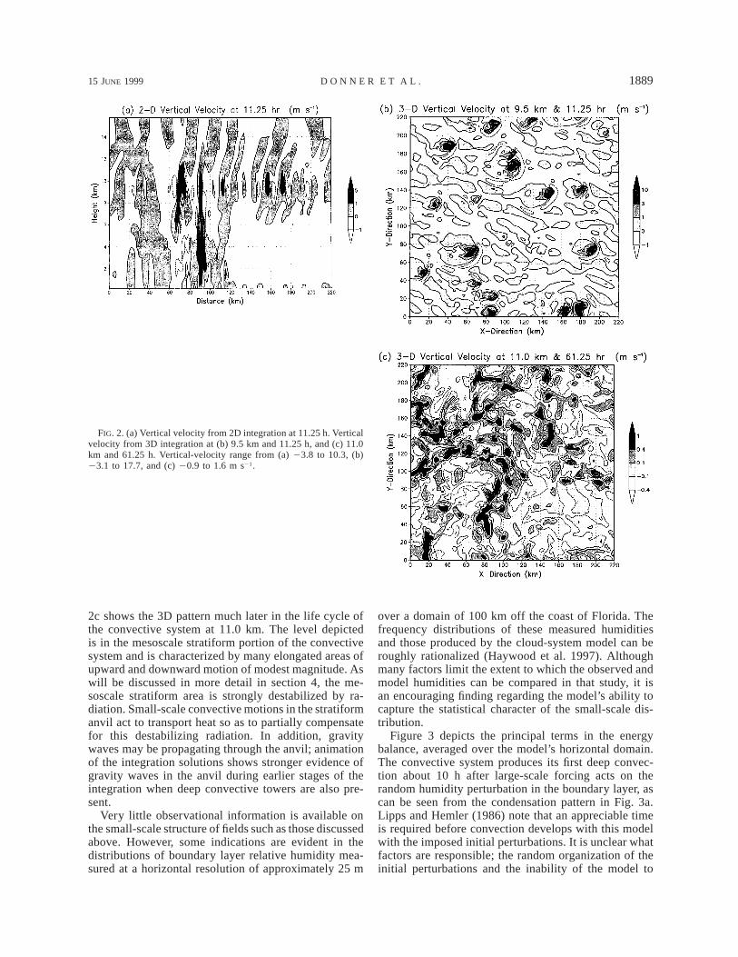
The motion fields associated with the convectivecloud system are quite complex and exhibit severalforms of organization. Figures 2a and 2b illustrate someexamples, just after the onset of vigorous deep convec-tion (11.25 h into the integration). Vertical organizationfrom 2D is shown in Fig. 2a. (Unless otherwise noted,all figures depict the model domain as it moves withthe vertical average of the base-state flow.) Convectivecores have vertical extents as great as 8 km. Weak down-drafts occur adjacent to and below the updrafts in re-

gions of strong evaporative cooling, where rain has beenshed from the cores. A dynamically active mesoscalepattern characterizes the region downstream of the mostdeveloped convective core. (Note in Fig. 1c that zonalwinds from 10 to 12 h at 8–10 km are easterly between2 and 6 m s21, while they are easterly between 6 and8 m s21 between about 3 and 5 km. The convectivecores at heights less than 8 km evidently move morerapidly to the east than does the material detrained attheir tops.) Averaged over the preceding 11.25 h, thisdynamically active region is where the most intensegradients in destabilizing radiation occur, with heatingat the base of this region of detrained condensate around8–9 km and cooling at its top, around 11–12 km (dis-cussed in detail in section 4). The small-scale updraftsand downdrafts in this anvil circulation transport heatupward from its base, opposing the pattern of destabi-lizing radiation. Figure 2b displays horizontal organi-zation from 3D at 11.25 h into the integration on a level9.5 km above the ground. Several concentrated coreshave vertical velocities exceeding 10 m s21. The max-imum vertical velocity reaches nearly 18 m s21. Figure

15 JUNE 1999 1889D O N N E R E T A L .

FIG. 2. (a) Vertical velocity from 2D integration at 11.25 h. Verticalvelocity from 3D integration at (b) 9.5 km and 11.25 h, and (c) 11.0km and 61.25 h. Vertical-velocity range from (a) 23.8 to 10.3, (b)23.1 to 17.7, and (c) 20.9 to 1.6 m s21.

2c shows the 3D pattern much later in the life cycle ofthe convective system at 11.0 km. The level depictedis in the mesoscale stratiform portion of the convectivesystem and is characterized by many elongated areas ofupward and downward motion of modest magnitude. Aswill be discussed in more detail in section 4, the me-soscale stratiform area is strongly destabilized by ra-diation. Small-scale convective motions in the stratiformanvil act to transport heat so as to partially compensatefor this destabilizing radiation. In addition, gravitywaves may be propagating through the anvil; animationof the integration solutions shows stronger evidence ofgravity waves in the anvil during earlier stages of theintegration when deep convective towers are also pre-sent.

Very little observational information is available onthe small-scale structure of fields such as those discussedabove. However, some indications are evident in thedistributions of boundary layer relative humidity mea-sured at a horizontal resolution of approximately 25 m

over a domain of 100 km off the coast of Florida. Thefrequency distributions of these measured humiditiesand those produced by the cloud-system model can beroughly rationalized (Haywood et al. 1997). Althoughmany factors limit the extent to which the observed andmodel humidities can be compared in that study, it isan encouraging finding regarding the model’s ability tocapture the statistical character of the small-scale dis-tribution.

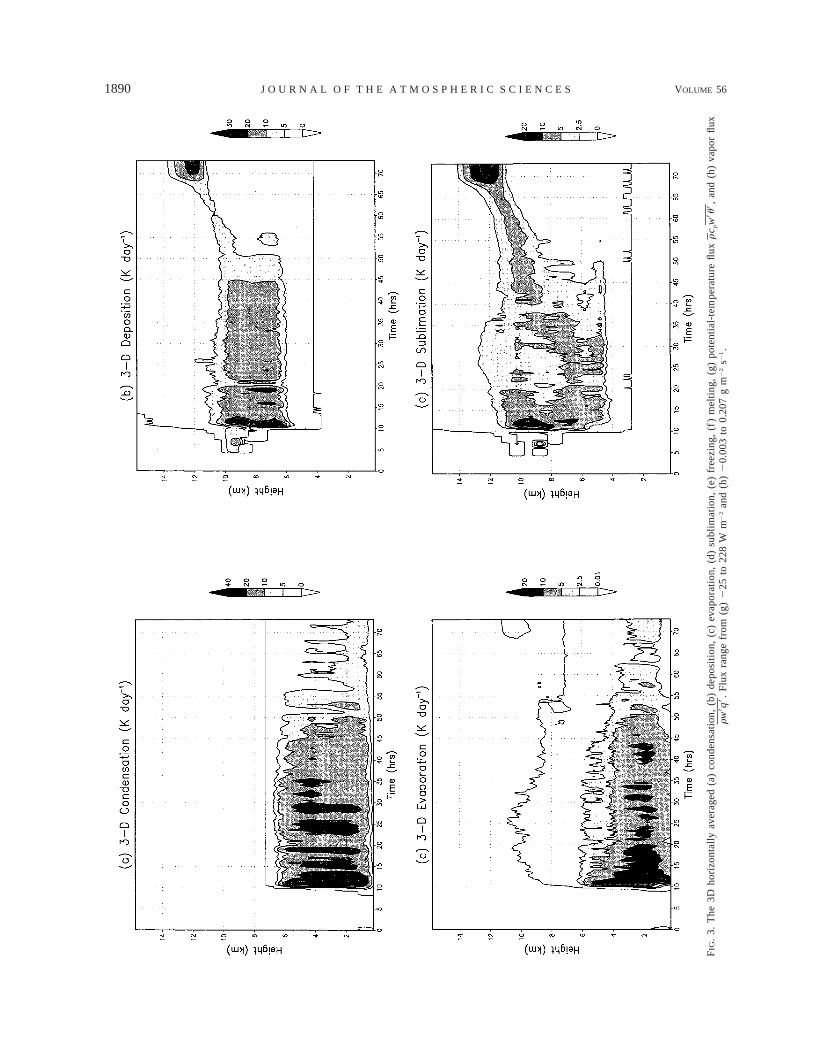
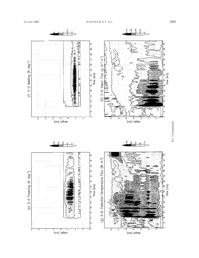
Figure 3 depicts the principal terms in the energybalance, averaged over the model’s horizontal domain.The convective system produces its first deep convec-tion about 10 h after large-scale forcing acts on therandom humidity perturbation in the boundary layer, ascan be seen from the condensation pattern in Fig. 3a.Lipps and Hemler (1986) note that an appreciable timeis required before convection develops with this modelwith the imposed initial perturbations. It is unclear whatfactors are responsible; the random organization of theinitial perturbations and the inability of the model to


FIG

.3.

The

3Dho

rizo

ntal

lyav

erag

ed(a

)co

nden

sati

on,

(b)

depo

siti

on,

(c)

evap

orat

ion,

(d)

subl

imat

ion,

(e)

free

zing

,(f

)m

elti

ng,

(g)

pote

ntia

l-te

mpe

ratu

refl

ux,

and

(h)

vapo

rfl

uxr

cw

9u9

p

rw9q

9.F

lux

rang

efr

om(g

)2

25to

228

Wm

22

and

(h)

20.

003

to0.

207

gm

22

s21.

15 JUNE 1999 1891D O N N E R E T A L .

FIG

.3

(Con

tinu

ed)


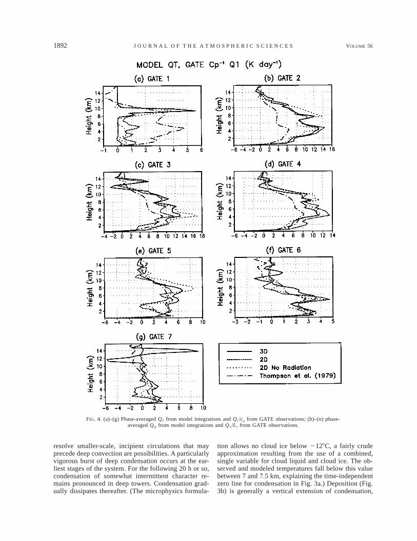
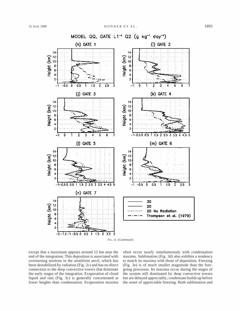
FIG. 4. (a)–(g) Phase-averaged QT from model integrations and Q1/cp from GATE observations; (h)–(n) phase-averaged QQ from model integrations and Q2/L1 from GATE observations.

resolve smaller-scale, incipient circulations that mayprecede deep convection are possibilities. A particularlyvigorous burst of deep condensation occurs at the ear-liest stages of the system. For the following 20 h or so,condensation of somewhat intermittent character re-mains pronounced in deep towers. Condensation grad-ually dissipates thereafter. (The microphysics formula-

tion allows no cloud ice below 2128C, a fairly crudeapproximation resulting from the use of a combined,single variable for cloud liquid and cloud ice. The ob-served and modeled temperatures fall below this valuebetween 7 and 7.5 km, explaining the time-independentzero line for condensation in Fig. 3a.) Deposition (Fig.3b) is generally a vertical extension of condensation,

15 JUNE 1999 1893D O N N E R E T A L .

FIG. 4. (Continued )

except that a maximum appears around 12 km near theend of the integration. This deposition is associated withoverturning motions in the stratiform anvil, which hasbeen destabilized by radiation (Fig. 2c) and has no directconnection to the deep convective towers that dominatethe early stages of the integration. Evaporation of cloudliquid and rain (Fig. 3c) is generally concentrated atlower heights than condensation. Evaporation maxima

often occur nearly simultaneously with condensationmaxima. Sublimation (Fig. 3d) also exhibits a tendencyto match its maxima with those of deposition. Freezing(Fig. 3e) is of much smaller magnitude than the fore-going processes. Its maxima occur during the stages ofthe system still dominated by deep convective towersbut are delayed appreciably; condensate builds up beforethe onset of appreciable freezing. Both sublimation and


freezing persist slightly where temperatures are some-what above 08, a result of the presence of snow fallingfrom colder areas. The conversion of snow to vapor(before it melts) in these warm areas is sublimation.When snow accretes cloud liquid in these warm areas,freezing of the cloud liquid occurs. Considerations sim-ilar to those for freezing also apply for melting (Fig.3f), except that it is concentrated in a thinner layer whereit is locally of greater magnitude than freezing. In ad-dition to phase changes, significant fluxes of heat andmoisture are produced by the motions in the convectivesystem. The potential temperature flux (Fig. 3g)c rw9u9p

exhibits maxima around 4 km in deep convective towersand also around 10 km. Examination of profiles of ver-tical velocity (not shown) indicates that large upwardvertical velocities around 10 km occur in individual con-vective towers. There are also smaller-scale updrafts anddowndrafts in the mesoscale stratiform region. Bothconvective-scale and stratiform vertical motions cancontribute to the heat flux. Toward the end of the in-tegration, small-scale, shallow convection in the radia-tively destabilized anvil produces moderate heat fluxes.Convergence (divergence) of these heat fluxes opposesradiative cooling (heating) in the anvil; radiation in thiscloud system will be discussed in section 4. Water vaporfluxes (Fig. 3h) are broadly in phase with lower-tro-posphere heat fluxes. (Temperatures are too cold forappreciable vapor fluxes where strong upper-tropo-sphere heat fluxes develop.) The lower-troposphere wa-ter vapor fluxes provide a strong signal of deep con-vection in the first half of the integration.

The aggregate effects of phase changes and conver-gence of fluxes act to force the temperature and water-vapor fields of large-scale flows in which convectivesystems develop. Cumulus parameterizations for large-scale models attempt to infer these forcings from theproperties of large-scale flows. The ability of cloud-system models to match large-scale heat sources andmoisture sinks diagnosed from observations provides ameasure of their skill in representing processes that areimportant in the interaction between cloud systems andlarge-scale flows. The usefulness of cloud-system mod-els in evaluating and developing cumulus parameteri-zations obviously depends on the ability of these modelsto represent these interactions.

Figures 4a–g illustrate the sums of heating by phasechanges and flux convergence for the cloud-systemmodel integrations, defined as

6

L gO i i 1 ]i51Q 5 2 rw9u9 , (5)1 2T c rp ]zp

where gi is the rate of the ith phase transformation, wis vertical velocity, and r is density. The subscripts irun from 1 to 6 and refer to condensation, evaporation,deposition, sublimation, freezing, and melting, respec-

tively. The latent heats of vaporization, sublimation, andfusion are indicated by L1, L3, and L5, respectively. (Themodel has one set of levels for w and another set oflevels for u. Vertical derivatives of fluxes are obtainedby first interpolating u to the w levels and evaluatingthe fluxes on those levels. The derivatives are then ver-tical finite differences centered at the u levels. An anal-ogous procedure is employed to evaluate moisture flux-es.) All phase changes are defined as positive semide-finite, so

L2 5 2L1, L4 5 2L3, L6 5 2L5.

Overbars refer to averages over the horizontal domainof the model, and primes refer to departures therefrom.Also illustrated in Figs. 4a–g are related quantities di-agnosed from observations by Thompson et al. (1979),Q1/cp, following the definition [(3)]. Note that QT doesnot include radiation, which, along with subgrid dif-fusion (including convergence of surface heat flux),would render QT and Q1/cp consistent. Radiation hasbeen omitted from QT to focus on the effects of phasechanges and flux convergence. With a few exceptions,the magnitude of radiative heating and cooling between1 and 6 km is less than 2 K day21. As will be discussedin section 4, radiative effects are much greater above 6km, where their addition to QT produces appreciablechanges in the total large-scale forcing by the convectivesystem relative to the profiles in Figs. 4a–g.

Once convection begins, the sum of the model phasechanges and flux convergence generally captures suc-cessfully key features in the shapes of the profiles ofthe apparent heat source below approximately 7 km.The temporal evolution of the amplitude of the modelheat source differs from the evolution of the model heat-ing through the trough, with the model amplitude toosmall initially and then too large. This may be a resultof the procedure used to initiate the convection, whichstarts later in the model than in the observations. Aswill be discussed shortly, the delayed onset of deepconvection allows more convective available potentialenergy to build up than is observed, so, once convectionis established, it is more vigorous than observed. By thetrough exit (phase 5), the magnitudes of the model anddiagnosed apparent heat sources are comparable in thelower and middle troposphere. Above 7 km or so, QT

exhibits more vertical structure than the diagnosed heatsources. Comparing the modeled heating from phasechanges and flux convergence in Fig. 4 directly withthe diagnosed heat source is not very meaningful atthese heights, since radiative heating and cooling, them-selves having characteristic vertical structures, becomelarge in magnitude relative to the phase changes andflux convergence. Especially in the later stages of theintegration, differences between 3D and the other in-tegrations emerge in the upper troposphere. These dif-ferences will be discussed in more detail later and areof particular interest in the context of the effects ofradiation, which heat the lower portions of the meso-

15 JUNE 1999 1895D O N N E R E T A L .

scale stratiform circulation (at approximately 10 km)and cool its upper portions (at approximately 14 km).

Figures 4h–n show the sums of moisture sinks byphase changes and moisture-flux convergence for thecloud-system model. These sums QQ are defined as

4 |L | 1 ]iQ 5 g 1 rw9q9 . (6)O 1 2Q iL r ]zi51 i

(As with QT, subgrid diffusion is not included in QQ,which is defined to be a measure of the direct moisturesink produced by the resolved effects of convection ondomain-scale flows.) The corresponding quantities di-agnosed from observations by Thompson et al. (1979),Q2/L1, are also shown. Since the moisture budget lacksa radiative component, QQ and Q2 are more directlycomparable. As was also the case for the heat budget,the modeled moisture sink is too weak during phase 1and then too strong in phase 2, when the initial stagesof convection are stronger than observed. In phases 5–7, the modeled moisture sinks agree reasonably in broadfeatures with observations, especially for 3D; an ex-ception is 2D in phase 7 from 2–4 km, where QQ isappreciably less than Q2/L1. Another exception is nearthe surface, where the effects of the modeled surfacemoisture flux are not included in QQ; analogous ob-served effects are included in Q2. The convergence ofmodeled surface moisture fluxes in the lowest layer pro-duces vapor tendencies of about 3–9 g kg21 day21 andwould generally decrease QQ values at least to those ofQ2/L1. (Similar behavior characterizes the heating inFigs. 4a–g, where convergence of surface fluxes notincluded in QT would add around 1–4 K day21 near thesurface, bringing these values closer to diagnosed Q1/cp

there.) The Q2 and QQ profiles both exhibit maxima inthe lower troposphere; both also are fairly consistent inshowing a secondary maximum in the middle tropo-sphere during some of the phases.

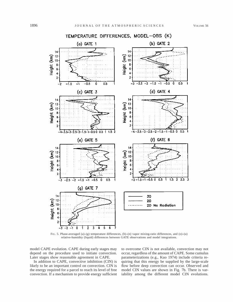
Figures 5a–g show the evolution of the domain-av-eraged temperature, relative to observations. In the low-er troposphere, the differences between the modeled andobserved temperatures show a relatively small cool biasin the model. Above 7 km, effects of radiation and di-mensionality are apparent. Particularly evident towardthe end of the integration is the effect of radiative heat-ing of the base of the mesoscale stratiform circulation,which produces warmer temperatures in the model thanin the observations from about 7 to 14 km. The mag-nitude of the temperature differences is similar to thatobtained by Grabowski et al. (1996b) in their two-di-mensional model, although the patterns differ, with thelatter obtaining temperatures about 5 K colder than ob-served above 16 km toward the end of their integration.(Recall that the present integration damps to observedtemperatures above about 14 km.)

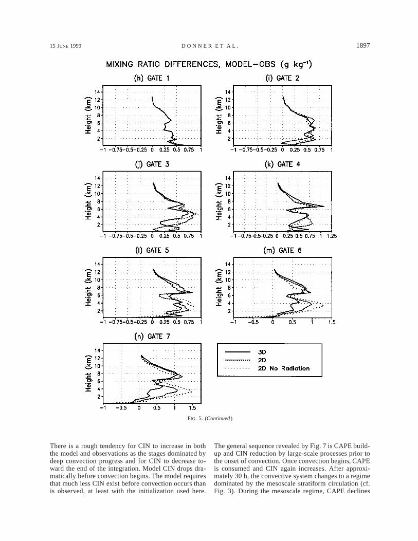
Relative to observations, the model mixing ratios aregenerally somewhat high, although the 3D integrationis drier than the others below 4–5 km after the trough

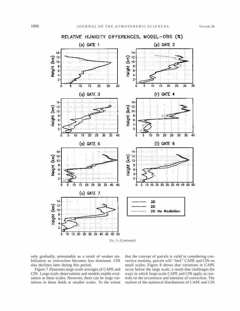
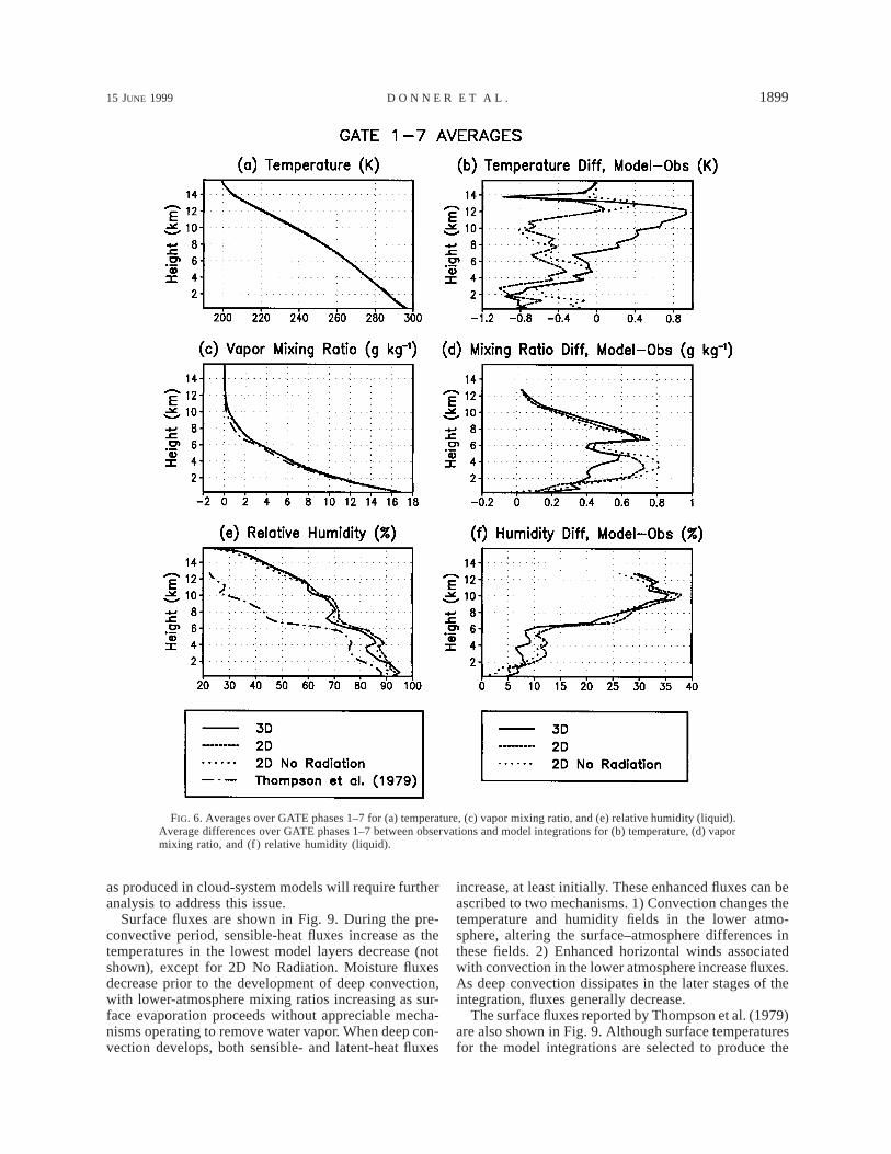
axis (Figs. 5h–n). Grabowski et al. (1996b) find that thelargest moist biases in their integrations are around 1 gkg21 at heights of 6 km, a somewhat higher height thanhere in most cases. The relative humidity (with respectto liquid, Figs. 5o–u) is too high in the model, especiallyin the stratiform region. This pattern is also obtainedby Grabowski et al. (1996b); their maximum bias isaround 30%. The model and observed fields integratedover phases 1–7 (with weighting corresponding to theobserved composite lengths of these phases) are shownin Fig. 6. Model temperatures are slightly cooler thanobserved below approximately 12 km in the two-di-mensional calculations and below approximately 7 kmin the three-dimensional calculations. Between 7 and 12km, the three-dimensional calculations are warmer thanobserved (Figs. 6a,b). Consistent with the individualphases, the model is too moist through much of middleand upper troposphere (Figs. 6c–f). The sharp reductionin the observed relative humidity around 6 km does notoccur in the model, as also seen in Grabowski et al.(1996b). Lateral periodic boundary conditions and un-certainties in ice removal by sedimentation could beresponsible, but note also that upper-tropospheric hu-midity is difficult to measure.

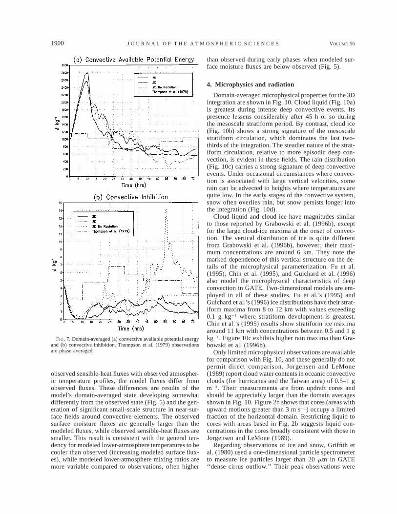
Simple, conceptual models of deep convection oftenrelate intensity to convective available potential energy(CAPE), and cumulus parameterizations often are castin terms of quantities related to CAPE (Emanuel 1994,chap. 6; Arakawa and Schubert 1974; Fritsch and Chap-pell 1980). [CAPE is defined here as the energy releasedby a parcel between the level of free convection andthe level of zero buoyancy, as in Donner (1996).] Mod-eled and observed CAPE are displayed in Fig. 7a. (Mod-el CAPE calculations initiate parcel ascent at the sur-face, and observations at 1000 hPa. CAPE values aresensitive to the level from which the parcel is assumedto ascend. Observations are available and plotted as av-erages over each phase.) Prior to the onset of convectionin the model, CAPE builds up to values appreciablygreater than observed. This buildup is a result of thecontinuing action of large-scale forcing as convectionfails to develop; the onset of convection is evidentlydelayed in the model relative to the atmosphere. Onceconvection begins, CAPE is consumed very rapidly. Ob-served CAPE values also decline through the convec-tively dominated stages of the integration, although notnearly so dramatically. From about 25 h onward, ob-served CAPE values change only slightly. Two-dimen-sional and observed CAPE values tend upward towardthe end of the period, albeit later in the model than inobservations, with model CAPE generally somewhatless than observed. The development of large CAPEbefore convective onset in the model is consistent withthe QT pattern in Fig. 4, with model values too low priorto convection and too large in the early stage of con-vection. If cloud-system models are to be used to eval-uate closure hypotheses for cumulus parameterization,significant attention must be given to the realism of


FIG. 5. Phase-averaged (a)–(g) temperature differences, (h)–(n) vapor mixing-ratio differences, and (o)–(u)relative-humidity (liquid) differences between GATE observations and model integrations.

model CAPE evolution. CAPE during early stages maydepend on the procedure used to initiate convection.Later stages show reasonable agreement in CAPE.

In addition to CAPE, convective inhibition (CIN) islikely to be an important control on convection. CIN isthe energy required for a parcel to reach its level of freeconvection. If a mechanism to provide energy sufficient

to overcome CIN is not available, convection may notoccur, regardless of the amount of CAPE. Some cumulusparameterizations (e.g., Kuo 1974) include criteria re-quiring that this energy be supplied by the large-scaleflow before deep convection can occur. Observed andmodel CIN values are shown in Fig. 7b. There is var-iability among the different model CIN evolutions.

15 JUNE 1999 1897D O N N E R E T A L .


There is a rough tendency for CIN to increase in boththe model and observations as the stages dominated bydeep convection progress and for CIN to decrease to-ward the end of the integration. Model CIN drops dra-matically before convection begins. The model requiresthat much less CIN exist before convection occurs thanis observed, at least with the initialization used here.

The general sequence revealed by Fig. 7 is CAPE build-up and CIN reduction by large-scale processes prior tothe onset of convection. Once convection begins, CAPEis consumed and CIN again increases. After approxi-mately 30 h, the convective system changes to a regimedominated by the mesoscale stratiform circulation (cf.Fig. 3). During the mesoscale regime, CAPE declines



only gradually, presumably as a result of weaker sta-bilization as convection becomes less dominant. CINalso declines later during this period.

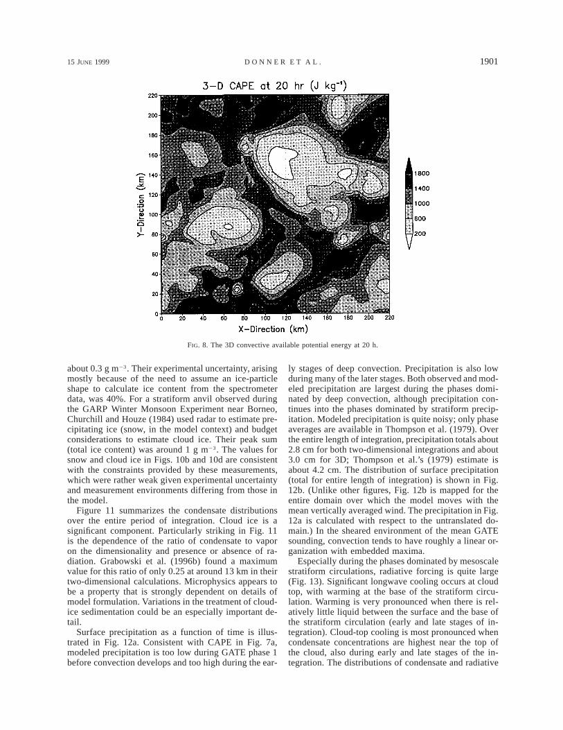
Figure 7 illustrates large-scale averages of CAPE andCIN. Large-scale observations and models enable eval-uation at these scales. However, there can be large var-iations in these fields at smaller scales. To the extent

that the concept of parcels is valid in considering con-vective motions, parcels will ‘‘feel’’ CAPE and CIN onsmall scales. Figure 8 shows that variations in CAPEoccur below the large scale, a result that challenges theways in which large-scale CAPE and CIN apply as con-trols on the occurrence and intensity of convection. Therealism of the statistical distributions of CAPE and CIN

15 JUNE 1999 1899D O N N E R E T A L .

FIG. 6. Averages over GATE phases 1–7 for (a) temperature, (c) vapor mixing ratio, and (e) relative humidity (liquid).Average differences over GATE phases 1–7 between observations and model integrations for (b) temperature, (d) vapormixing ratio, and (f ) relative humidity (liquid).

as produced in cloud-system models will require furtheranalysis to address this issue.

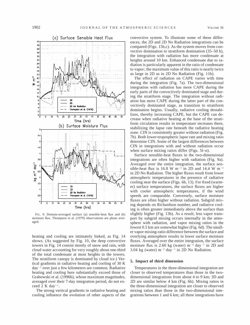
Surface fluxes are shown in Fig. 9. During the pre-convective period, sensible-heat fluxes increase as thetemperatures in the lowest model layers decrease (notshown), except for 2D No Radiation. Moisture fluxesdecrease prior to the development of deep convection,with lower-atmosphere mixing ratios increasing as sur-face evaporation proceeds without appreciable mecha-nisms operating to remove water vapor. When deep con-vection develops, both sensible- and latent-heat fluxes

increase, at least initially. These enhanced fluxes can beascribed to two mechanisms. 1) Convection changes thetemperature and humidity fields in the lower atmo-sphere, altering the surface–atmosphere differences inthese fields. 2) Enhanced horizontal winds associatedwith convection in the lower atmosphere increase fluxes.As deep convection dissipates in the later stages of theintegration, fluxes generally decrease.

The surface fluxes reported by Thompson et al. (1979)are also shown in Fig. 9. Although surface temperaturesfor the model integrations are selected to produce the


FIG. 7. Domain-averaged (a) convective available potential energyand (b) convective inhibition. Thompson et al. (1979) observationsare phase averaged.

observed sensible-heat fluxes with observed atmospher-ic temperature profiles, the model fluxes differ fromobserved fluxes. These differences are results of themodel’s domain-averaged state developing somewhatdifferently from the observed state (Fig. 5) and the gen-eration of significant small-scale structure in near-sur-face fields around convective elements. The observedsurface moisture fluxes are generally larger than themodeled fluxes, while observed sensible-heat fluxes aresmaller. This result is consistent with the general ten-dency for modeled lower-atmosphere temperatures to becooler than observed (increasing modeled surface flux-es), while modeled lower-atmosphere mixing ratios aremore variable compared to observations, often higher

than observed during early phases when modeled sur-face moisture fluxes are below observed (Fig. 5).

4. Microphysics and radiation

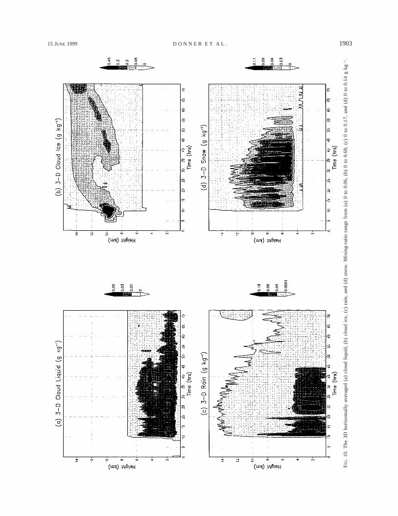
Domain-averaged microphysical properties for the 3Dintegration are shown in Fig. 10. Cloud liquid (Fig. 10a)is greatest during intense deep convective events. Itspresence lessens considerably after 45 h or so duringthe mesoscale stratiform period. By contrast, cloud ice(Fig. 10b) shows a strong signature of the mesoscalestratiform circulation, which dominates the last two-thirds of the integration. The steadier nature of the strat-iform circulation, relative to more episodic deep con-vection, is evident in these fields. The rain distribution(Fig. 10c) carries a strong signature of deep convectiveevents. Under occasional circumstances where convec-tion is associated with large vertical velocities, somerain can be advected to heights where temperatures arequite low. In the early stages of the convective system,snow often overlies rain, but snow persists longer intothe integration (Fig. 10d).

Cloud liquid and cloud ice have magnitudes similarto those reported by Grabowski et al. (1996b), exceptfor the large cloud-ice maxima at the onset of convec-tion. The vertical distribution of ice is quite differentfrom Grabowski et al. (1996b), however; their maxi-mum concentrations are around 6 km. They note themarked dependence of this vertical structure on the de-tails of the microphysical parameterization. Fu et al.(1995), Chin et al. (1995), and Guichard et al. (1996)also model the microphysical characteristics of deepconvection in GATE. Two-dimensional models are em-ployed in all of these studies. Fu et al.’s (1995) andGuichard et al.’s (1996) ice distributions have their strat-iform maxima from 8 to 12 km with values exceeding0.1 g kg21 where stratiform development is greatest.Chin et al.’s (1995) results show stratiform ice maximaaround 11 km with concentrations between 0.5 and 1 gkg21. Figure 10c exhibits higher rain maxima than Gra-bowski et al. (1996b).

Only limited microphysical observations are availablefor comparison with Fig. 10, and these generally do notpermit direct comparison. Jorgensen and LeMone(1989) report cloud water contents in oceanic convectiveclouds (for hurricanes and the Taiwan area) of 0.5–1 gm23. Their measurements are from updraft cores andshould be appreciably larger than the domain averagesshown in Fig. 10. Figure 2b shows that cores (areas withupward motions greater than 3 m s21) occupy a limitedfraction of the horizontal domain. Restricting liquid tocores with areas based in Fig. 2b suggests liquid con-centrations in the cores broadly consistent with those inJorgensen and LeMone (1989).

Regarding observations of ice and snow, Griffith etal. (1980) used a one-dimensional particle spectrometerto measure ice particles larger than 20 mm in GATE‘‘dense cirrus outflow.’’ Their peak observations were

15 JUNE 1999 1901D O N N E R E T A L .

FIG. 8. The 3D convective available potential energy at 20 h.

about 0.3 g m23. Their experimental uncertainty, arisingmostly because of the need to assume an ice-particleshape to calculate ice content from the spectrometerdata, was 40%. For a stratiform anvil observed duringthe GARP Winter Monsoon Experiment near Borneo,Churchill and Houze (1984) used radar to estimate pre-cipitating ice (snow, in the model context) and budgetconsiderations to estimate cloud ice. Their peak sum(total ice content) was around 1 g m23. The values forsnow and cloud ice in Figs. 10b and 10d are consistentwith the constraints provided by these measurements,which were rather weak given experimental uncertaintyand measurement environments differing from those inthe model.

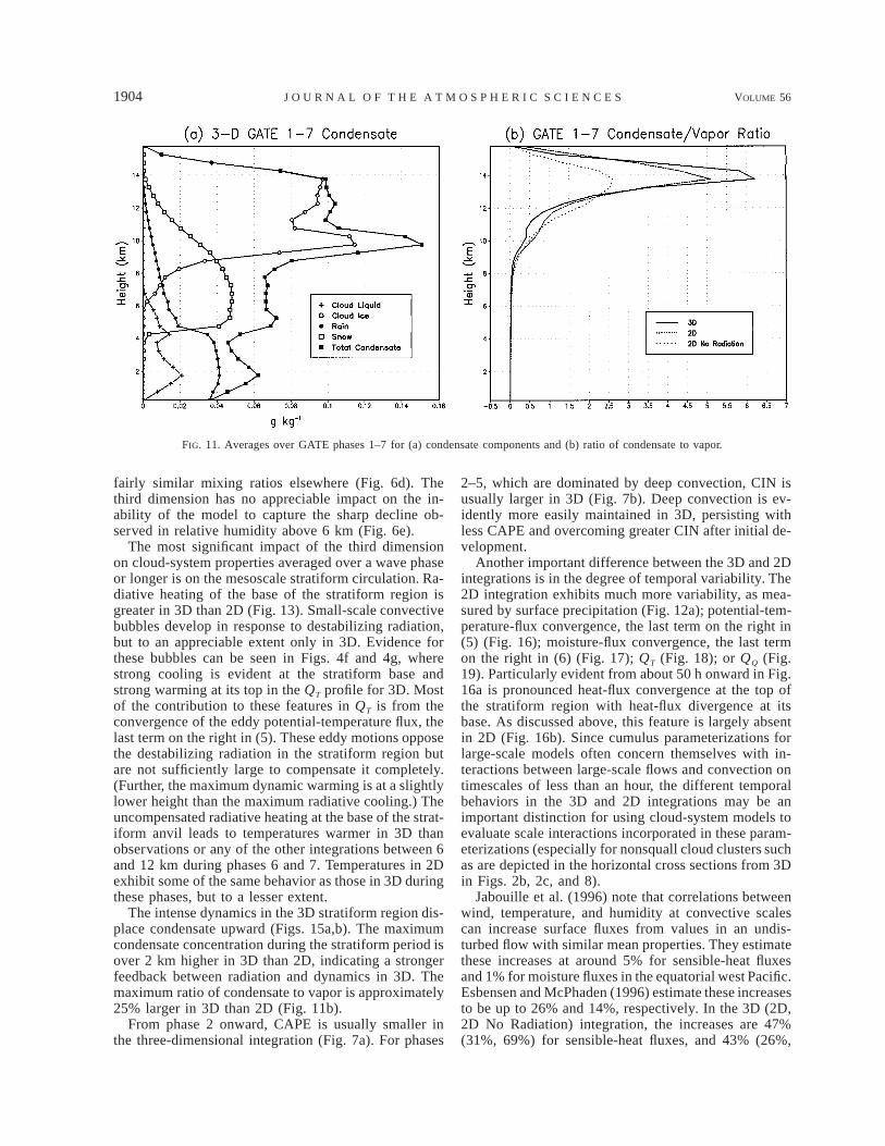
Figure 11 summarizes the condensate distributionsover the entire period of integration. Cloud ice is asignificant component. Particularly striking in Fig. 11is the dependence of the ratio of condensate to vaporon the dimensionality and presence or absence of ra-diation. Grabowski et al. (1996b) found a maximumvalue for this ratio of only 0.25 at around 13 km in theirtwo-dimensional calculations. Microphysics appears tobe a property that is strongly dependent on details ofmodel formulation. Variations in the treatment of cloud-ice sedimentation could be an especially important de-tail.

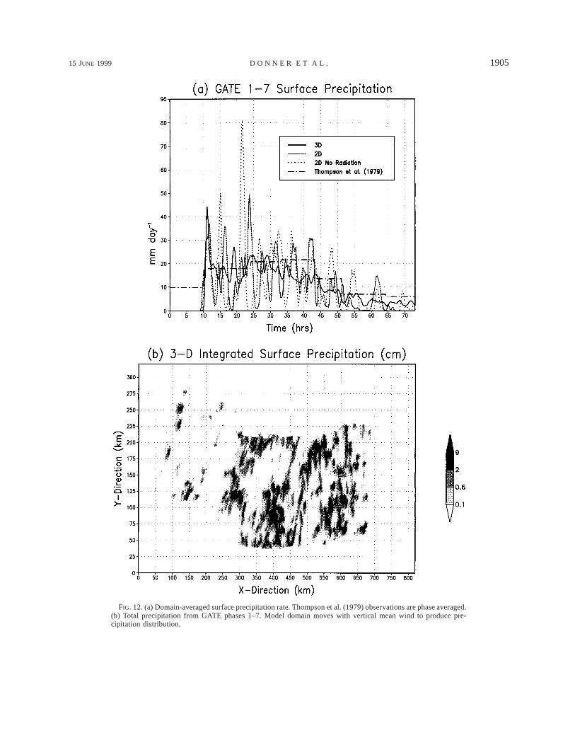
Surface precipitation as a function of time is illus-trated in Fig. 12a. Consistent with CAPE in Fig. 7a,modeled precipitation is too low during GATE phase 1before convection develops and too high during the ear-

ly stages of deep convection. Precipitation is also lowduring many of the later stages. Both observed and mod-eled precipitation are largest during the phases domi-nated by deep convection, although precipitation con-tinues into the phases dominated by stratiform precip-itation. Modeled precipitation is quite noisy; only phaseaverages are available in Thompson et al. (1979). Overthe entire length of integration, precipitation totals about2.8 cm for both two-dimensional integrations and about3.0 cm for 3D; Thompson et al.’s (1979) estimate isabout 4.2 cm. The distribution of surface precipitation(total for entire length of integration) is shown in Fig.12b. (Unlike other figures, Fig. 12b is mapped for theentire domain over which the model moves with themean vertically averaged wind. The precipitation in Fig.12a is calculated with respect to the untranslated do-main.) In the sheared environment of the mean GATEsounding, convection tends to have roughly a linear or-ganization with embedded maxima.

Especially during the phases dominated by mesoscalestratiform circulations, radiative forcing is quite large(Fig. 13). Significant longwave cooling occurs at cloudtop, with warming at the base of the stratiform circu-lation. Warming is very pronounced when there is rel-atively little liquid between the surface and the base ofthe stratiform circulation (early and late stages of in-tegration). Cloud-top cooling is most pronounced whencondensate concentrations are highest near the top ofthe cloud, also during early and late stages of the in-tegration. The distributions of condensate and radiative


FIG. 9. Domain-averaged surface (a) sensible-heat flux and (b)moisture flux. Thompson et al. (1979) observations are phase aver-aged.

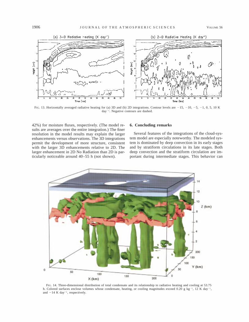
heating and cooling are intimately linked, as Fig. 14shows. (As suggested by Fig. 10, the deep convectivetowers in Fig. 14 consist mostly of snow and rain, withcloud water accounting for very roughly about one-thirdof the total condensate at most heights in the towers.The stratiform canopy is dominated by cloud ice.) Ver-tical gradients in radiative heating and cooling of 30 Kday21 over just a few kilometers are common. Radiativeheating and cooling here substantially exceed those ofGrabowski et al. (1996b), whose maximum magnitudes,averaged over their 7-day integration period, do not ex-ceed 2 K day21.

The strong vertical gradients in radiative heating andcooling influence the evolution of other aspects of the

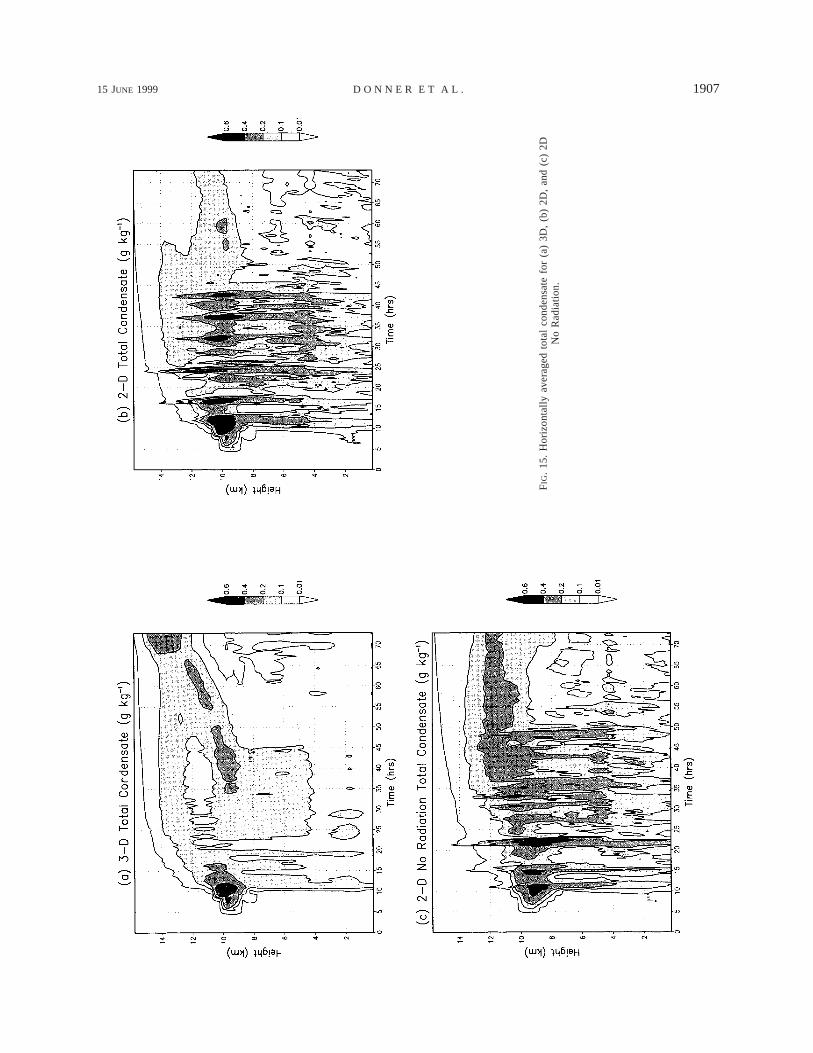
convective system. To illustrate some of these differ-ences, the 2D and 2D No Radiation integrations can becompared (Figs. 15b,c). As the system moves from con-vective domination to stratiform domination (35–50 h),the integration with radiation has more condensate atheights around 10 km. Enhanced condensate due to ra-diation is particularly apparent in the ratio of condensateto vapor; the maximum value of this ratio is nearly twiceas large in 2D as in 2D No Radiation (Fig. 11b).

The effect of radiation on CAPE varies with timeduring the integration (Fig. 7a). The two-dimensionalintegration with radiation has more CAPE during theearly parts of the convectively dominated stage and dur-ing the stratiform stage. The integration without radi-ation has more CAPE during the latter part of the con-vectively dominated stage, as transition to stratiformdomination begins. Usually, radiative cooling destabi-lizes, thereby increasing CAPE, but the CAPE can de-crease when radiative heating at the base of the strati-form circulation results in temperature increases there,stabilizing the lapse rate beneath the radiative heatingzone. CIN is consistently greater without radiation (Fig.7b). Both lower-tropospheric lapse rate and mixing ratiodetermine CIN. Some of the largest differences betweenCIN in integrations with and without radiation occurwhen surface mixing ratios differ (Figs. 5l–n).

Surface sensible-heat fluxes in the two-dimensionalintegrations are often higher with radiation (Fig. 9a).Averaged over the entire integration, the surface sen-sible-heat flux is 16.8 W m22 in 2D and 14.4 W m22

in 2D No Radiation. The higher fluxes result from loweratmospheric temperatures in the presence of radiativecooling near the surface (Figs. 6b, 13). For fixed (warm-er) surface temperatures, the surface fluxes are higherwith cooler atmospheric temperatures, if the windspeeds are comparable. Conversely, surface moisturefluxes are often higher without radiation. Subgrid mix-ing depends on Richardson number, and radiative cool-ing is often greater immediately above the surface thanslightly higher (Fig. 13b). As a result, less vapor trans-port by subgrid mixing occurs internally in the atmo-sphere with radiation, and vapor mixing ratios in thelowest 0.5 km are somewhat higher (Fig. 6d). The small-er vapor mixing-ratio difference between the surface andoverlying atmosphere results in lower surface moisturefluxes. Averaged over the entire integration, the surfacemoisture flux is 2.60 kg (water) m22 day21 in 2D and3.04 kg (water) m22 day21 in 2D No Radiation.

5. Impact of third dimension

Temperatures in the three-dimensional integration arecloser to observed temperatures than those in the two-dimensional integrations from about 4 to 9 km; 3D and2D are similar below 4 km (Fig. 6b). Mixing ratios inthe three-dimensional integration are closer to observedmixing ratios than those in the two-dimensional inte-grations between 1 and 6 km; all three integrations have

15 JUNE 1999 1903D O N N E R E T A L .

FIG

.10

.T

he3D

hori

zont

ally

aver

aged

(a)

clou

dli

quid

,(b

)cl

oud

ice,

(c)

rain

,an

d(d

)sn

ow.

Mix

ing-

rati

ora

nge

from

(a)

0to

0.06

,(b

)0

to0.

68,

(c)

0to

0.1

7,an

d(d

)0

to0.

14g

kg2

1.


FIG. 11. Averages over GATE phases 1–7 for (a) condensate components and (b) ratio of condensate to vapor.

fairly similar mixing ratios elsewhere (Fig. 6d). Thethird dimension has no appreciable impact on the in-ability of the model to capture the sharp decline ob-served in relative humidity above 6 km (Fig. 6e).

The most significant impact of the third dimensionon cloud-system properties averaged over a wave phaseor longer is on the mesoscale stratiform circulation. Ra-diative heating of the base of the stratiform region isgreater in 3D than 2D (Fig. 13). Small-scale convectivebubbles develop in response to destabilizing radiation,but to an appreciable extent only in 3D. Evidence forthese bubbles can be seen in Figs. 4f and 4g, wherestrong cooling is evident at the stratiform base andstrong warming at its top in the QT profile for 3D. Mostof the contribution to these features in QT is from theconvergence of the eddy potential-temperature flux, thelast term on the right in (5). These eddy motions opposethe destabilizing radiation in the stratiform region butare not sufficiently large to compensate it completely.(Further, the maximum dynamic warming is at a slightlylower height than the maximum radiative cooling.) Theuncompensated radiative heating at the base of the strat-iform anvil leads to temperatures warmer in 3D thanobservations or any of the other integrations between 6and 12 km during phases 6 and 7. Temperatures in 2Dexhibit some of the same behavior as those in 3D duringthese phases, but to a lesser extent.

The intense dynamics in the 3D stratiform region dis-place condensate upward (Figs. 15a,b). The maximumcondensate concentration during the stratiform period isover 2 km higher in 3D than 2D, indicating a strongerfeedback between radiation and dynamics in 3D. Themaximum ratio of condensate to vapor is approximately25% larger in 3D than 2D (Fig. 11b).

From phase 2 onward, CAPE is usually smaller inthe three-dimensional integration (Fig. 7a). For phases

2–5, which are dominated by deep convection, CIN isusually larger in 3D (Fig. 7b). Deep convection is ev-idently more easily maintained in 3D, persisting withless CAPE and overcoming greater CIN after initial de-velopment.

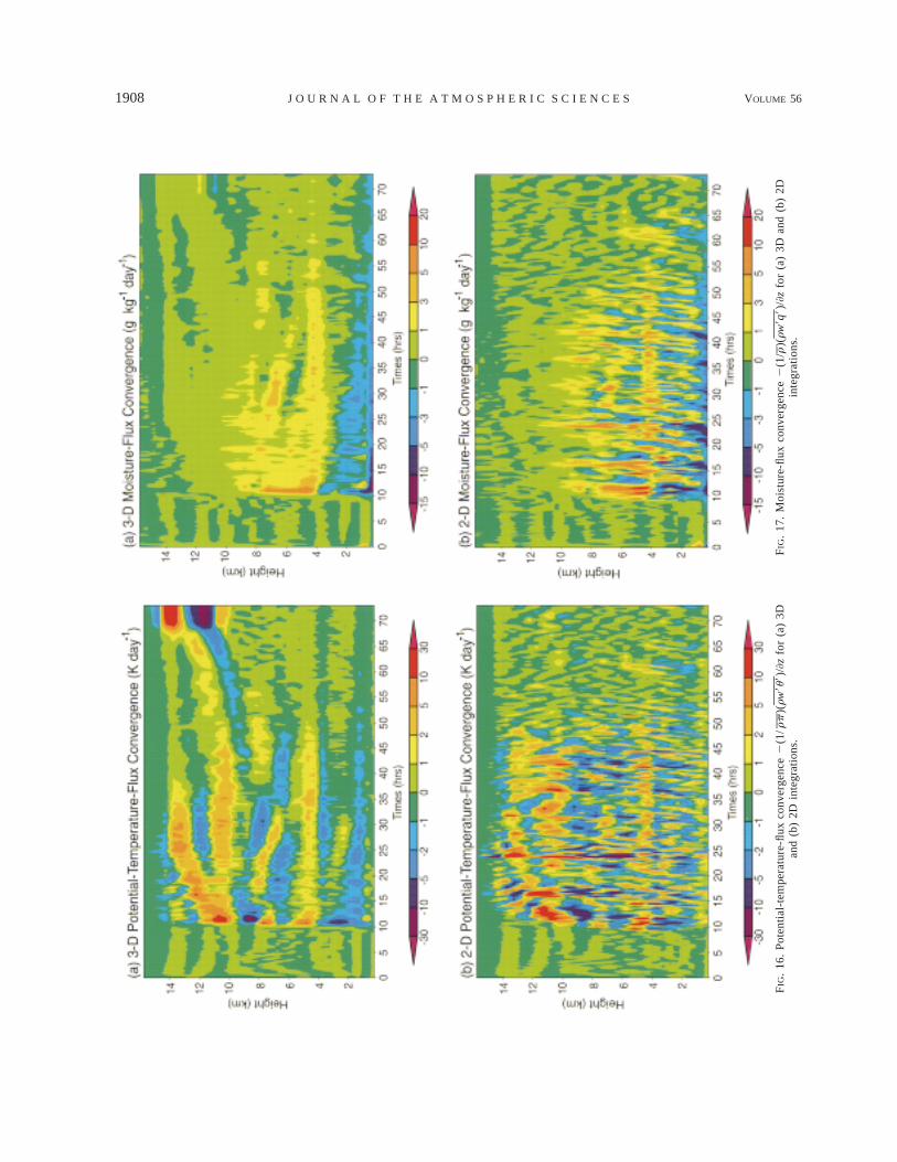
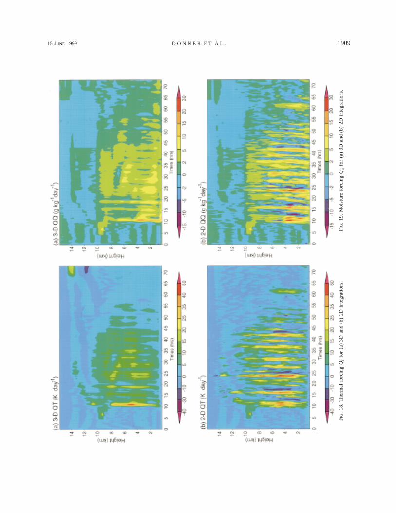
Another important difference between the 3D and 2Dintegrations is in the degree of temporal variability. The2D integration exhibits much more variability, as mea-sured by surface precipitation (Fig. 12a); potential-tem-perature-flux convergence, the last term on the right in(5) (Fig. 16); moisture-flux convergence, the last termon the right in (6) (Fig. 17); QT (Fig. 18); or QQ (Fig.19). Particularly evident from about 50 h onward in Fig.16a is pronounced heat-flux convergence at the top ofthe stratiform region with heat-flux divergence at itsbase. As discussed above, this feature is largely absentin 2D (Fig. 16b). Since cumulus parameterizations forlarge-scale models often concern themselves with in-teractions between large-scale flows and convection ontimescales of less than an hour, the different temporalbehaviors in the 3D and 2D integrations may be animportant distinction for using cloud-system models toevaluate scale interactions incorporated in these param-eterizations (especially for nonsquall cloud clusters suchas are depicted in the horizontal cross sections from 3Din Figs. 2b, 2c, and 8).

Jabouille et al. (1996) note that correlations betweenwind, temperature, and humidity at convective scalescan increase surface fluxes from values in an undis-turbed flow with similar mean properties. They estimatethese increases at around 5% for sensible-heat fluxesand 1% for moisture fluxes in the equatorial west Pacific.Esbensen and McPhaden (1996) estimate these increasesto be up to 26% and 14%, respectively. In the 3D (2D,2D No Radiation) integration, the increases are 47%(31%, 69%) for sensible-heat fluxes, and 43% (26%,

15 JUNE 1999 1905D O N N E R E T A L .

FIG. 12. (a) Domain-averaged surface precipitation rate. Thompson et al. (1979) observations are phase averaged.(b) Total precipitation from GATE phases 1–7. Model domain moves with vertical mean wind to produce pre-cipitation distribution.


FIG. 13. Horizontally averaged radiative heating for (a) 3D and (b) 2D integrations. Contour levels are 215, 210, 25, 21, 0, 5, 10 Kday21. Negative contours are dashed.

FIG. 14. Three-dimensional distribution of total condensate and its relationship to radiative heating and cooling at 53.75h. Colored surfaces enclose volumes whose condensate, heating, or cooling magnitudes exceed 0.20 g kg21, 12 K day21,and 214 K day21, respectively.

42%) for moisture fluxes, respectively. (The model re-sults are averages over the entire integration.) The finerresolution in the model results may explain the largerenhancements versus observations. The 3D integrationspermit the development of more structure, consistentwith the larger 3D enhancements relative to 2D. Thelarger enhancement in 2D No Radiation than 2D is par-ticularly noticeable around 40–55 h (not shown).

6. Concluding remarks

Several features of the integrations of the cloud-sys-tem model are especially noteworthy. The modeled sys-tem is dominated by deep convection in its early stagesand by stratiform circulations in its late stages. Bothdeep convection and the stratiform circulation are im-portant during intermediate stages. This behavior can

15 JUNE 1999 1907D O N N E R E T A L .

FIG

.15

.H

oriz

onta

lly

aver

aged

tota

lco

nden

sate

for

(a)

3D,

(b)

2D,

and

(c)

2DN

oR

adia

tion

.


FIG

.16

.P

oten

tial

-tem

pera

ture

-flux

conv

erge

nce

2(1

/rp

)(rw

9u9)

/]z

for

(a)

3Dan

d(b

)2D

inte

grat

ions

.F

IG.

17.

Moi

stur

e-fl

uxco

nver

genc

e2

(1/r

)(rw

9q9)

/]z

for

(a)

3Dan

d(b

)2D

inte

grat

ions

.

15 JUNE 1999 1909D O N N E R E T A L .

FIG

.18

.T

herm

alfo

rcin

gQ

Tfo

r(a

)3D

and

(b)

2Din

tegr

atio

ns.

FIG

.19

.M

oist

ure

forc

ing

QQ

for

(a)

3Dan

d(b

)2D

inte

grat

ions

.


be seen by examining the condensate patterns in Fig.10. The nature of the convective system in the presentintegrations is associated closely with the time evolutionof the large-scale forcing, with deep convection asso-ciated most closely with periods when the middle tro-posphere is destabilized (Fig. 1a). Note here that ‘‘largescale’’ simply defines an averaging operation. It doesnot in any way characterize the motions that composethe average; that is, convective motions may contributesubstantially to this average. This average is extremelyuseful, since it is resolved by models with the resolutionof general circulation models and (to an appreciabledegree) by atmospheric observing systems.

Leary and Houze (1980) observe a GATE convectivesystem to undergo a similar evolution. However, thelifetime of their system is about 24 h, in contrast to the3-day integration here. Leary and Houze’s (1980) com-posite system is drawn mostly from 5 September 1974.Thompson et al. (1979) indicate their system was inphase 2 for 12 h (6 h on 5 September), phase 3 for 12h, and phase 4 for 15 h (6 h on 5 September). Phases3 and 4 are both longer than the composite values usedin these integrations. The integration phases correspond-ing to those on 5 September extend from approximately16 to 36 h. There is some evidence in these integrationsof individual systems evolving like that of Leary andHouze (1980), even while they are parts of the moregeneral pattern associated with large-scale forcing.Around 20 h in 3D, surface precipitation increases (Fig.12a) and maxima in cloud liquid and rain in the lowerpart of convective towers develop (Figs. 10a,c). Strat-iform cloud ice is then at a minimum (Fig. 10b), cor-responding to the deep convective stage of Leary andHouze (1980). At 25–30 h, significant snow develops(Figs. 10d), and cloud ice in the stratiform region in-creases, corresponding to Leary and Houze’s (1980)stage with both convective and stratiform activity. At40 h, rain and snow associated with deep convectionhave decreased, but a maximum develops in cloud ice,corresponding to Leary and Houze’s (1980) stratiformstage. The absence of a diurnal radiation cycle in thesecomposite easterly wave integrations probably alters theintensity and duration of these individual embedded cy-cles.

Although cumulus parameterizations for large-scalemodels relate the intensity of convection to large-scaleproperties in a variety of ways, the nature of the subgriddisturbances that initiate convection is not among theseproperties. Further, the design of cloud-system modelexperiments for parameterization evaluation assumesthat properties averaged over the large scale are closelylinked to the properties of convection. The results ob-tained here are broadly in support of this approach butdo suggest limits, especially in the early stages of con-vection. In these integrations, the onset of convectionis delayed relative to observations, resulting in exces-sive CAPE buildup, followed by convection of too greatintensity. Apparent heat sources and moisture sinks,

which are products of parameterizations to be evaluatedby cloud-system models, clearly manifest this behavior.Dependence on the details of initialization is indicated.This dependence requires further study.

A striking result from these integrations is the dif-ference in temporal variability, even over the entire do-main, between the two- and three-dimensional versionsof the cloud-system model. Larger variability in the two-dimensional integrations is probably partly related tothe different behavior of the CAPE and CIN in two andthree dimensions. Most of the fields associated with theconvective ensemble show more variability in two di-mensions. The three-dimensional integration has moregrid points over which motions may be realized, so someof the reduced variability in the three-dimensional in-tegration may reflect sampling from a larger set of gridcolumns. The restriction of motions to a plane in thetwo-dimensional integrations may also be important,since the possible forms of organization of motions arelimited. Some behaviors, such as the low CIN in thetwo-dimensional integrations with radiation, could beresults of this limitation. Some inferences regarding therelative roles of these distinctions between two- andthree-dimensions could be drawn by comparing ensem-ble integrations under varying initial perturbations intwo dimensions with a three-dimensional integration.

Another prominent result of these integrations is thestrong interaction between radiation and the dynamicsof the mesoscale stratiform circulation in the three-di-mensional integration. The possibility of an equilibriumin which large radiative heating and cooling are bal-anced by small-scale convective bubbles in the strati-form clouds is suggested. The model results remainsomewhat inconclusive due to several model numericaland physical issues. The dynamic heating and coolingdo not fully balance the radiative cooling and heating,as indicated by temperature trends relative to observa-tions in the stratiform region.

Other than initialization details, model issues that re-quire further study include 1) use of periodic lateralboundary conditions, (2) sedimentation of cloud ice, (3)vertical and horizontal resolution in the mesoscale strat-iform region, and (4) radiative properties of ice. Periodicboundary conditions do not permit ice flowing out ofthe model domain to leave it; rather, it simply appearsat the opposite boundary. Excessive ice concentrations,that exaggerate ice-radiative feedbacks, could result.Cloud ice in these integrations does not settle, despiteexperimental evidence that ice at concentrations belowthat at which autoconversion to snow begins does settle(Petch et al. 1997; Heymsfield and Donner 1990; Cottonet al. 1982). Neglecting this mechanism could also leadto excessive ice contents. The failure of the cloud-sys-tem model to produce observed decreases with heightin middle-troposphere relative humidities strongly sug-gests inadequate moisture removal, and boundary con-ditions and ice sedimentation are both plausible culprits.

15 JUNE 1999 1911D O N N E R E T A L .

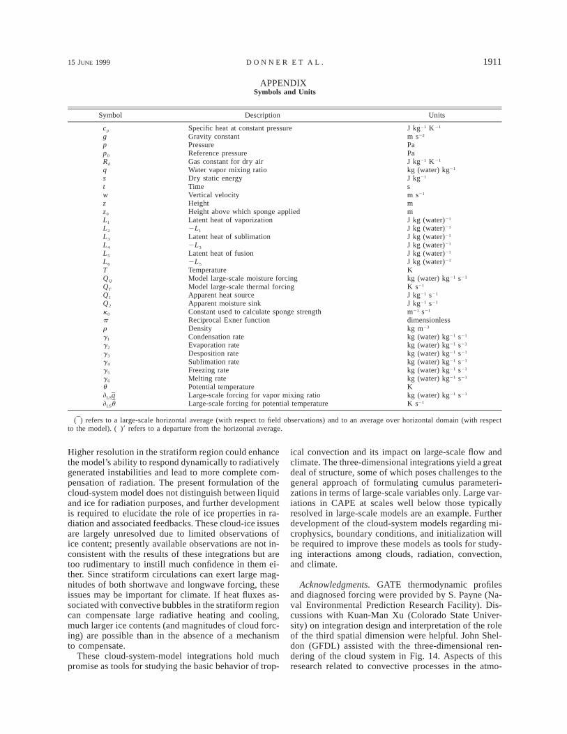
APPENDIXSymbols and Units

Symbol Description Units

cp

gpp0

Rd

qstwzz0

L1

L2

L3

L4

L5

L6

TQQ

Specific heat at constant pressureGravity constantPressureReference pressureGas constant for dry airWater vapor mixing ratioDry static energyTimeVertical velocityHeightHeight above which sponge appliedLatent heat of vaporization2L1

Latent heat of sublimation2L3

Latent heat of fusion2L5

TemperatureModel large-scale moisture forcing

J kg21 K21

m s22

PaPaJ kg21 K21

kg (water) kg21

J kg21

sm s21

mmJ kg (water)21

J kg (water)21

J kg (water)21

J kg (water)21

J kg (water)21

J kg (water)21

Kkg (water) kg21 s21

QT

Q1

Q2

k0

prg1

g2

g3

g4

g5

g6

u]LSq]LSu

Model large-scale thermal forcingApparent heat sourceApparent moisture sinkConstant used to calculate sponge strengthReciprocal Exner functionDensityCondensation rateEvaporation rateDesposition rateSublimation rateFreezing rateMelting ratePotential temperatureLarge-scale forcing for vapor mixing ratioLarge-scale forcing for potential temperature

K s21

J kg21 s21

J kg21 s21

m21 s21

dimensionlesskg m23

kg (water) kg21 s21

kg (water) kg21 s21

kg (water) kg21 s21

kg (water) kg21 s21

kg (water) kg21 s21

kg (water) kg21 s21

Kkg (water) kg21 s21

K s21

( ) refers to a large-scale horizontal average (with respect to field observations) and to an average over horizontal domain (with respectto the model). ( )9 refers to a departure from the horizontal average.

Higher resolution in the stratiform region could enhancethe model’s ability to respond dynamically to radiativelygenerated instabilities and lead to more complete com-pensation of radiation. The present formulation of thecloud-system model does not distinguish between liquidand ice for radiation purposes, and further developmentis required to elucidate the role of ice properties in ra-diation and associated feedbacks. These cloud-ice issuesare largely unresolved due to limited observations ofice content; presently available observations are not in-consistent with the results of these integrations but aretoo rudimentary to instill much confidence in them ei-ther. Since stratiform circulations can exert large mag-nitudes of both shortwave and longwave forcing, theseissues may be important for climate. If heat fluxes as-sociated with convective bubbles in the stratiform regioncan compensate large radiative heating and cooling,much larger ice contents (and magnitudes of cloud forc-ing) are possible than in the absence of a mechanismto compensate.

These cloud-system-model integrations hold muchpromise as tools for studying the basic behavior of trop-

ical convection and its impact on large-scale flow andclimate. The three-dimensional integrations yield a greatdeal of structure, some of which poses challenges to thegeneral approach of formulating cumulus parameteri-zations in terms of large-scale variables only. Large var-iations in CAPE at scales well below those typicallyresolved in large-scale models are an example. Furtherdevelopment of the cloud-system models regarding mi-crophysics, boundary conditions, and initialization willbe required to improve these models as tools for study-ing interactions among clouds, radiation, convection,and climate.

Acknowledgments. GATE thermodynamic profilesand diagnosed forcing were provided by S. Payne (Na-val Environmental Prediction Research Facility). Dis-cussions with Kuan-Man Xu (Colorado State Univer-sity) on integration design and interpretation of the roleof the third spatial dimension were helpful. John Shel-don (GFDL) assisted with the three-dimensional ren-dering of the cloud system in Fig. 14. Aspects of thisresearch related to convective processes in the atmo-


spheric general circulation were supported by NASALangley (CERES) Grant 97-1239. Comments on thestudy by C. Andronache and V. Balaji were appreciated.

REFERENCES

Arakawa, A., and W. H. Schubert, 1974: Interaction of a cumuluscloud ensemble with the large-scale environment, Part 1. J. At-mos. Sci., 31, 674–701.

Chin, H.-N. S., Q. Fu, M. M. Bradley, and C. R. Molenkamp, 1995:Modeling of a tropical squall line in two dimensions: Sensitivityto radiation and comparison with a midlatitude case. J. Atmos.Sci., 52, 3172–3193.

Churchill, D. D., and R. A. Houze Jr., 1984: Mesoscale updraft mag-nitude and cloud-ice content deduced from the ice budget of thestratiform region of a tropical cloud cluster. J. Atmos. Sci., 41,1717–1725.

Cotton, W. R., M. A. Stephens, T. Nehrkorn, and G. J. Tripoli, 1982:The Colorado State University three-dimensional cloud/meso-scale model-1982. Part II. An ice phase parameterization. J.Rech. Atmos., 16, 295–320.

Donner, L., 1993: A cumulus parameterization including mass fluxes,vertical momentum dynamics, and mesoscale effects. J. Atmos.Sci., 50, 889–906., 1996: Conditional and convective instability. Encyclopedia ofWeather and Climate, S. H. Schneider, Ed., Vol. 1, Oxford Uni-versity Press, 186–191., H. L. Kuo, and E. J. Pitcher, 1982: The significance of ther-modynamic forcing by cumulus convection in a general circu-lation model. J. Atmos. Sci., 39, 2159–2181.

Dudhia, J., and M. W. Moncrieff, 1987: A numerical simulation ofquasi-stationary tropical convective bands. Quart. J. Roy. Me-teor. Soc., 113, 929–967.

Emanuel, K. A., 1994: Atmospheric Convection. Oxford UniversityPress, 580 pp.

Esbensen, S. K., and M. J. McPhaden, 1996: Enhancement of tropicalocean evaporation and sensible heat flux by atmospheric me-soscale systems. J. Climate, 9, 2307–2325.

Fritsch, J. M., and C. F. Chappell, 1980: Numerical prediction ofconvectively driven mesoscale pressure systems. Part I: Con-vective parameterization. J. Atmos. Sci., 37, 1722–1733.

Fu, Q., S. K. Krueger, and K.-N. Liou, 1995: Interactions of radiationand convection in simulated tropical cloud clusters. J. Atmos.Sci., 52, 1310–1328.

Golding, B. W., 1993: A numerical investigation of tropical islandthunderstorms. Mon. Wea. Rev., 121, 1417–1433.

Grabowski, W. W., M. W. Moncrieff, and J. T. Kiehl, 1996a: Long-term behaviour of precipitating tropical cloud systems: A nu-merical study. Quart. J. Roy. Meteor. Soc., 122, 1019–1042., X. Wu, and M. W. Moncrieff, 1996b: Cloud-resolving modelingof tropical cloud systems during Phase III of GATE. Part I: Two-dimensional experiments. J. Atmos. Sci., 53, 3684–3709.

Gregory, D., and M. J. Miller, 1989: A numerical study of the pa-rameterization of deep tropical convection. Quart. J. Roy. Me-teor. Soc., 115, 1209–1241.

Griffith, K. T., S. K. Cox, and R. G. Knollenberg, 1980: Infraredradiative properties of tropical cirrus clouds inferred from air-craft measurements. J. Atmos. Sci., 37, 1077–1087.

Guichard, F., J.-L. Redelsperger, and J.-P. LaFore, 1996: The behav-iour of a cloud ensemble in response to external forcings. Quart.J. Roy. Meteor. Soc., 122, 1043–1073.

Hack, J. J., 1994: Parameterization of moist convection in the Na-tional Center for Atmospheric Research community climatemodel (CCM2). J. Geophys. Res., 99, 5551–5568.

Harrison, E. F., P. Minnis, B. R. Barkstrom, V. Ramanathan, R. D.

Cess, and G. G. Gibson, 1990: Seasonal variation of cloud ra-diative forcing derived from the Earth Radiation Budget Ex-periment. J. Geophys. Res., 95, 18 687–18 703.

Haywood, J. M., V. Ramaswamy, and L. J. Donner, 1997: A limited-area-model case study of the effects of sub-grid scale variationsin relative humidity and cloud upon the direct radiative forcingof sulfate aerosol. Geophys. Res. Lett., 24, 143–146.

Held, I. M., R. S. Hemler, and V. Ramaswamy, 1993: Radiative–convective equilibrium with explicit two-dimensional moist con-vection. J. Atmos. Sci., 50, 3909–3927.

Heymsfield, A. J., and L. J. Donner, 1990: A scheme for parameter-izing ice-cloud water content in general circulation models. J.Atmos. Sci., 47, 1865–1877.

Jabouille, P., J. L. Redelsperger, and J. P. Lafore, 1996: Modificationof surface fluxes by atmospheric convection in the TOGACOARE region. Mon. Wea. Rev., 124, 816–837.

Jorgensen, D. P., and M. A. LeMone, 1989: Vertical velocity char-acteristics of oceanic convection. J. Atmos. Sci., 46, 621–640.

Kuo, H.-L., 1974: Further studies of the parameterization of the in-fluence of cumulus convection on large-scale flow. J. Atmos.Sci., 31, 1232–1240.

Leary, C. A., and R. A. Houze Jr., 1980: The contribution of me-soscale motions to the mass and heat fluxes of an intense tropicalconvective system. J. Atmos. Sci., 37, 784–796.

Lelieveld, J., and P. J. Crutzen, 1994: Role of deep convection in theozone budget of the troposphere. Science, 264, 1759–1761.

Lipps, F. B., and R. S. Hemler, 1986: Numerical simulation of deeptropical convection associated with large-scale convergence. J.Atmos. Sci., 43, 1796–1816., and , 1988: Numerical modeling of a line of toweringcumulus on day 226 of GATE. J. Atmos. Sci., 45, 2428–2444.

Paradis, D., J. P. Lafore, J. L. Redelsperger, and V. Balaji, 1995:African easterly waves and convection. Part I: Linear simula-tions. J. Atmos. Sci., 52, 1657–1679.

Petch, J. C., G. C. Craig, and K. P. Shine, 1997: A comparison oftwo bulk microphysical schemes and their effects on radiativetransfer using a single-column model. Quart. J. Roy. Meteor.Soc., 123, 1561–1580.

Redelsperger, J. L., and G. Sommeria, 1986: Three-dimensional simu-lation of a convective storm: Sensitivity studies on subgrid param-eterization and spatial resolution. J. Atmos. Sci., 43, 2619–2635.

Slingo, J. M., and Coauthors, 1994: Mean climate and transience inthe tropics of the UGAMP GCM: Sensitivity to convective pa-rameterization. Quart. J. Roy. Meteor. Soc., 120, 881–922.

Soden, B. J., and R. Fu, 1995: A satellite analysis of deep convection,upper-tropospheric humidity, and the greenhouse effect. J. Cli-mate, 8, 2233–2351.

Stenchikov, G., R. Dickerson, K. Pickering, W. Ellis Jr., B. Doddridge,S. Kondragunta, and O. Poulida, 1996: Stratosphere–troposphereexchange in a midlatitude mesoscale convective complex. 2.Numerical simulations. J. Geophys. Res., 101, 6837–6851.

Sui, C. H., K. M. Lau, W. K. Tao, and J. Simpson, 1994: The tropicalwater and energy cycles in a cumulus ensemble model. Part. I:Equilibrium climate. J. Atmos. Sci., 51, 711–728.

Tao, W.-K., and S.-T. Soong, 1986: A study of the response of deeptropical clouds to mesoscale processes: Three-dimensional nu-merical experiments. J. Atmos. Sci., 43, 2653–2676., J. Simpson, C.-H. Sui, B. Ferrier, S. Lang, J. Scala, M.-D. Chou,and K. Pickering, 1993: Heating, moisture, and water budgets oftropical and midlatitude squall lines: Comparisons and sensitivityto longwave radiation. J. Atmos. Sci., 50, 673–690.

Thompson, R. M., S. W. Payne, E. E. Recker, and R. J. Reed, 1979:Structure and properties of synoptic-scale wave disturbances inthe intertropical convergence zone of the eastern Atlantic. J.Atmos. Sci., 36, 53–72.

Xu, K.-M., and S. K. Krueger, 1991: Evaluation of cloudiness pa-rameterization using a cumulus ensemble model. Mon. Wea.Rev., 119, 342–367.

Documents

Three-Dimensional Cloud-System Modeling of GATE Convection