Embed Size (px)
Citation preview
Three-Dimensional Dynamical Models, 2
Paul J. KushnerUniversity of Toronto
GCC Summer SchoolBanff 2005
QuickTime™ and aTIFF (Uncompressed) decompressor
are needed to see this picture.QuickTime™ and a
TIFF (Uncompressed) decompressorare needed to see this picture.
QuickTime™ and aTIFF (Uncompressed) decompressor
are needed to see this picture.
QuickTime™ and aTIFF (Uncompressed) decompressor
are needed to see this picture.QuickTime™ and a
TIFF (Uncompressed) decompressorare needed to see this picture.
QuickTime™ and aTIFF (Uncompressed) decompressor
are needed to see this picture.QuickTime™ and a
TIFF (Uncompressed) decompressorare needed to see this picture.

Outline
• Review
• Using a simple dry AGCM to studyThe tropospheric general circulation.The distribution of relative humidity in the
troposphere.The connections between the stratosphere
and the troposphere.
• Strengths and weaknesses of simple models
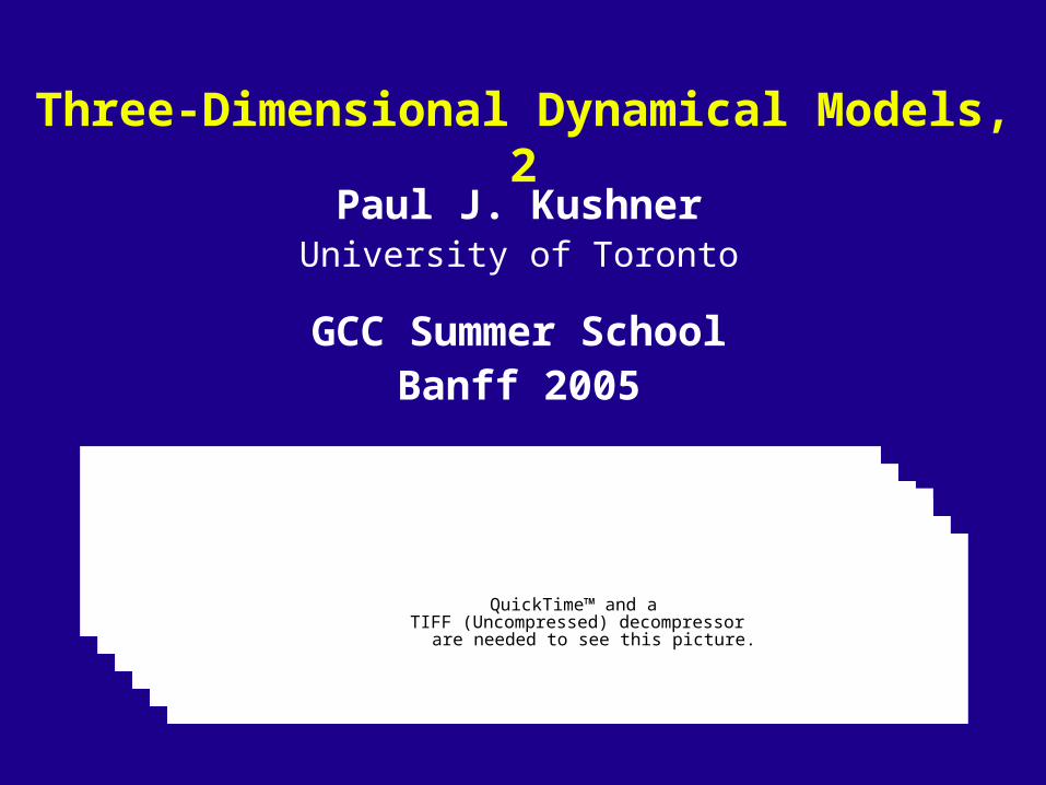
Terms and Concepts
• Quasigeostrophic Scaling:
• Potential vorticity definition:
An Adjustment Problem: Homework! (Sort of)
air
water
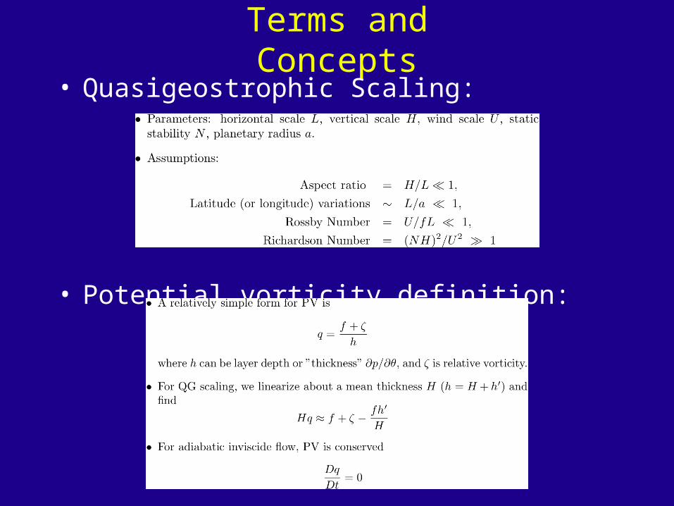
• This example illustrates the impact of rotation (and some subtleties).
• The diagram below represents the cross section of a channel going into the screen.
• Initially, the fluid is sloped (gently) and is at rest. (Imagine holding it in place with a sheet of plexiglass.)
• 1. Non-rotating case (f = 0): estimate the cross channel transport of mass and cross-channel speed you would obtain afterwards, in terms of the slope, of g, and of the mean layer depth.
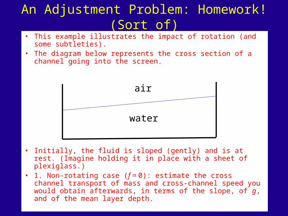
An Adjustment Problem: Homework! (Sort of)
air
water
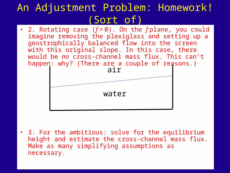
• 2. Rotating case (f > 0). On the f plane, you could imagine removing the plexiglass and setting up a geostrophically balanced flow into the screen with this original slope. In this case, there would be no cross-channel mass flux. This can’t happen: why? (There are a couple of reasons.)
• 3. For the ambitious: solve for the equilibrium height and estimate the cross-channel mass flux. Make as many simplifying assumptions as necessary.
Review - 1
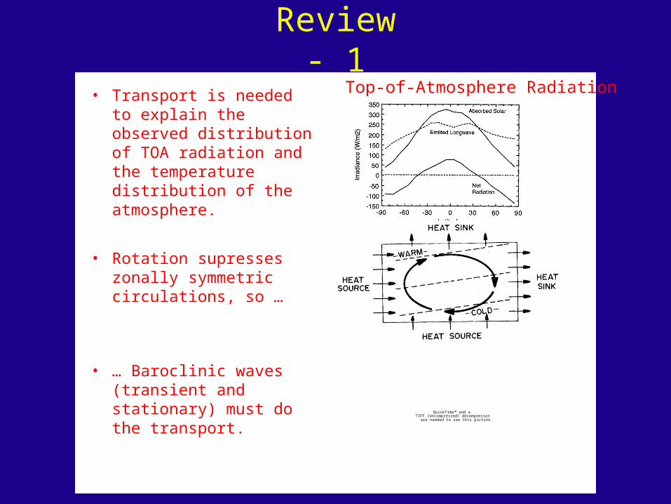
Top-of-Atmosphere Radiation
Hartmann 1994
• Transport is needed to explain the observed distribution of TOA radiation and the temperature distribution of the atmosphere.
• Rotation supresses zonally symmetric circulations, so …
• … Baroclinic waves (transient and stationary) must do the transport.
QuickTime™ and aTIFF (Uncompressed) decompressor
are needed to see this picture.
Review – 2
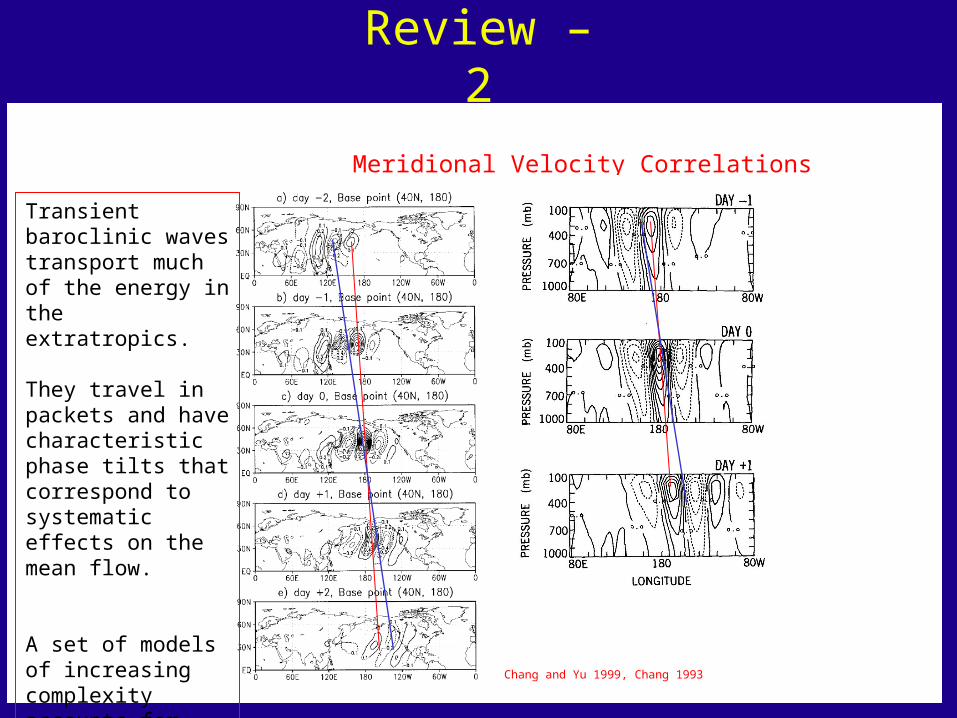
Meridional Velocity Correlations
Chang and Yu 1999, Chang 1993
Transient baroclinic waves transport much of the energy in the extratropics.
They travel in packets and have characteristic phase tilts that correspond to systematic effects on the mean flow.
A set of models of increasing complexity accounts for these structures.

Review – 3
Phillips (Holton)
• We described a sequence of linear models of baroclinic waves.
Eady (Gill) Charney (Gill)
Simmons and Hoskins
Review – 4
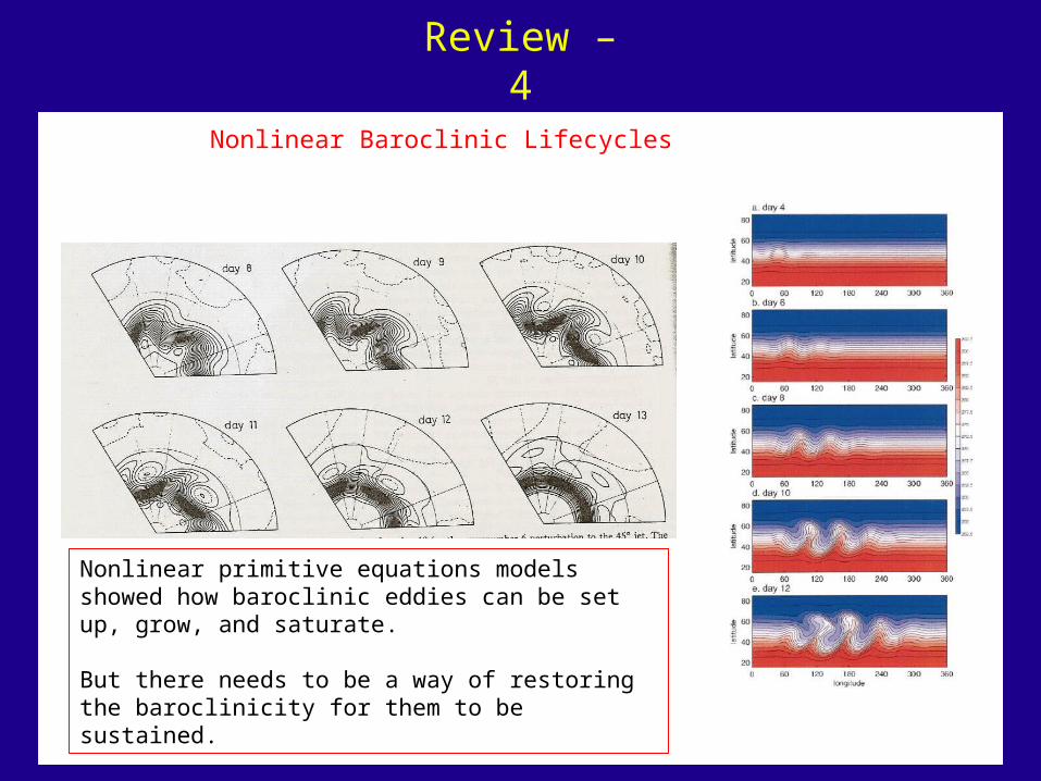
Nonlinear Baroclinic Lifecycles
Nonlinear primitive equations models showed how baroclinic eddies can be set up, grow, and saturate.
But there needs to be a way of restoring the baroclinicity for them to be sustained.
Transient Eddies in Climate Models
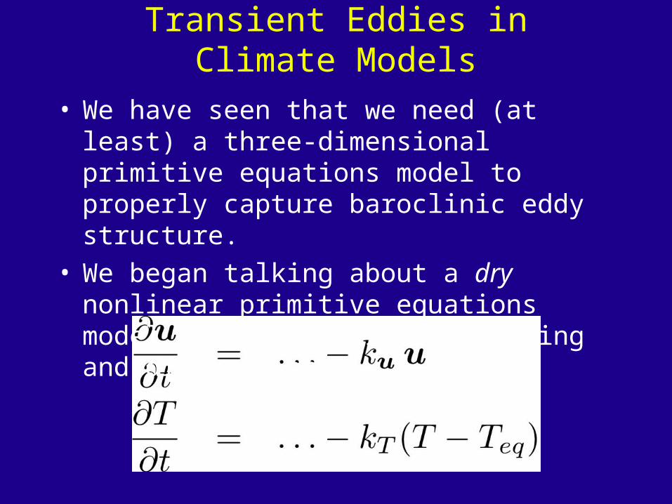
• We have seen that we need (at least) a three-dimensional primitive equations model to properly capture baroclinic eddy structure.
• We began talking about a dry nonlinear primitive equations model with the following forcing and dissipation:
Baroclinic Turbulence Models: T. Schneider
Schneider 2004
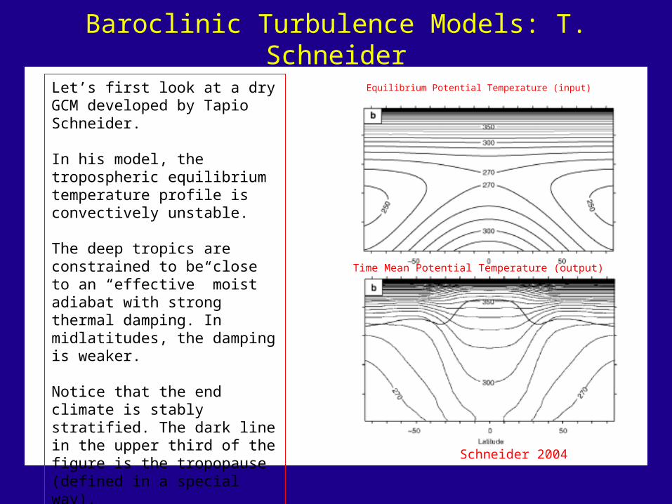
Let’s first look at a dry GCM developed by Tapio Schneider.
In his model, the tropospheric equilibrium temperature profile is convectively unstable.
The deep tropics are constrained to be close to an “effective” moist adiabat with strong thermal damping. In midlatitudes, the damping is weaker.
Notice that the end climate is stably stratified. The dark line in the upper third of the figure is the tropopause (defined in a special way).
Equilibrium Potential Temperature (input)
Time Mean Potential Temperature (output)
Baroclinic Turbulence Models: T. Schneider
Schneider 2004
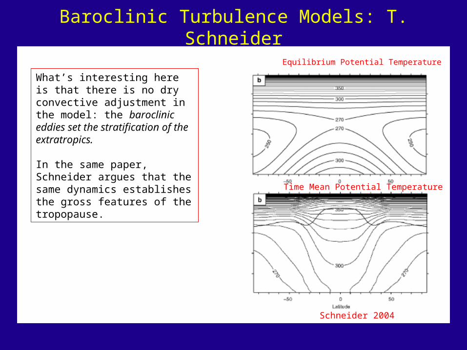
What’s interesting here is that there is no dry convective adjustment in the model: the baroclinic eddies set the stratification of the extratropics.
In the same paper, Schneider argues that the same dynamics establishes the gross features of the tropopause.
Equilibrium Potential Temperature
Time Mean Potential Temperature
Baroclinic Turbulence Models: T. Schneider
Schneider 2004
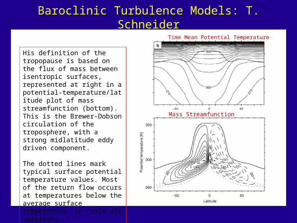
His definition of the tropopause is based on the flux of mass between isentropic surfaces, represented at right in a potential-temperature/latitude plot of mass streamfunction (bottom). This is the Brewer-Dobson circulation of the troposphere, with a strong midlatitude eddy driven component.
The dotted lines mark typical surface potential temperature values. Most of the return flow occurs at temperatures below the average surface temperature, in “cold air outbreaks. “
Time Mean Potential Temperature
Mass Streamfunction
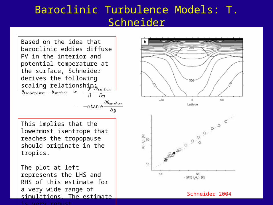
Baroclinic Turbulence Models: T. Schneider
Schneider 2004
Based on the idea that baroclinic eddies diffuse PV in the interior and potential temperature at the surface, Schneider derives the following scaling relationship:
This implies that the lowermost isentrope that reaches the tropopause should originate in the tropics.
The plot at left represents the LHS and RHS of this estimate for a very wide range of simulations. The estimate is very robust.
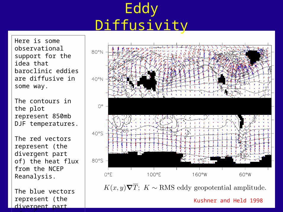
Eddy Diffusivity
Here is some observational support for the idea that baroclinic eddies are diffusive in some way.
The contours in the plot represent 850mb DJF temperatures.
The red vectors represent (the divergent part of) the heat flux from the NCEP Reanalysis.
The blue vectors represent (the divergent part of) the downgradient flux using the formula at right. Kushner and Held 1998
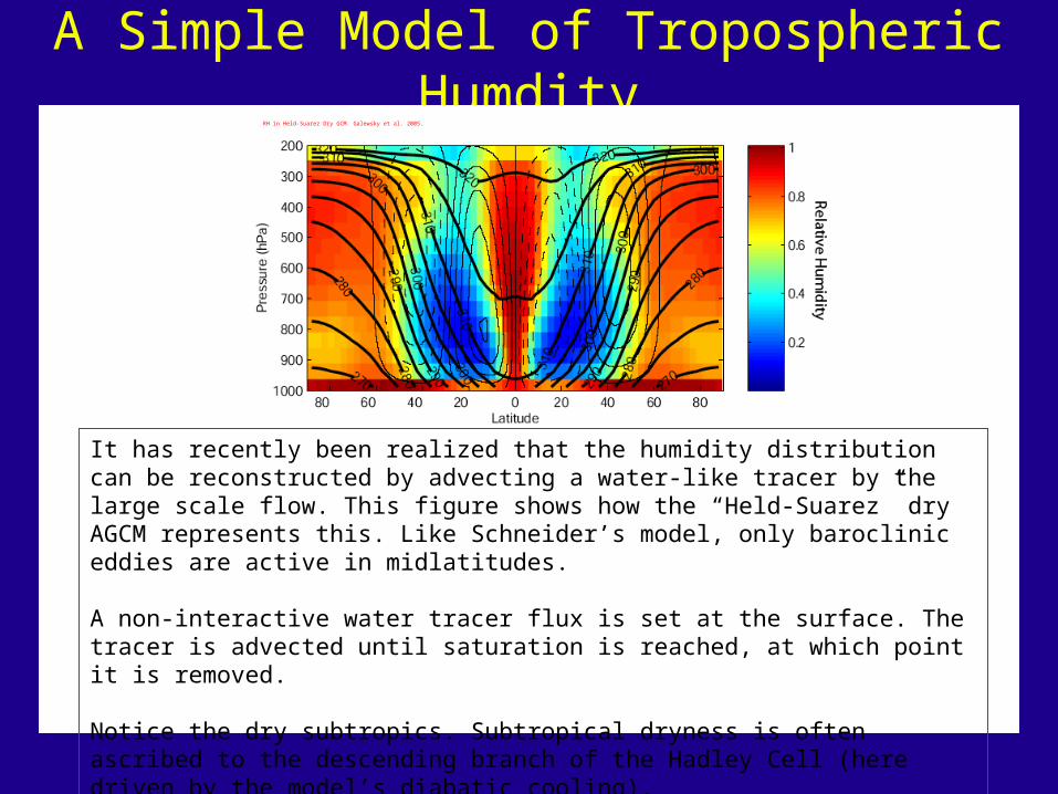
A Simple Model of Tropospheric Humdity
It has recently been realized that the humidity distribution can be reconstructed by advecting a water-like tracer by the large scale flow. This figure shows how the “Held-Suarez” dry AGCM represents this. Like Schneider’s model, only baroclinic eddies are active in midlatitudes.
A non-interactive water tracer flux is set at the surface. The tracer is advected until saturation is reached, at which point it is removed.
Notice the dry subtropics. Subtropical dryness is often ascribed to the descending branch of the Hadley Cell (here driven by the model’s diabatic cooling).
RH in Held-Suarez Dry GCM. Galewsky et al. 2005.
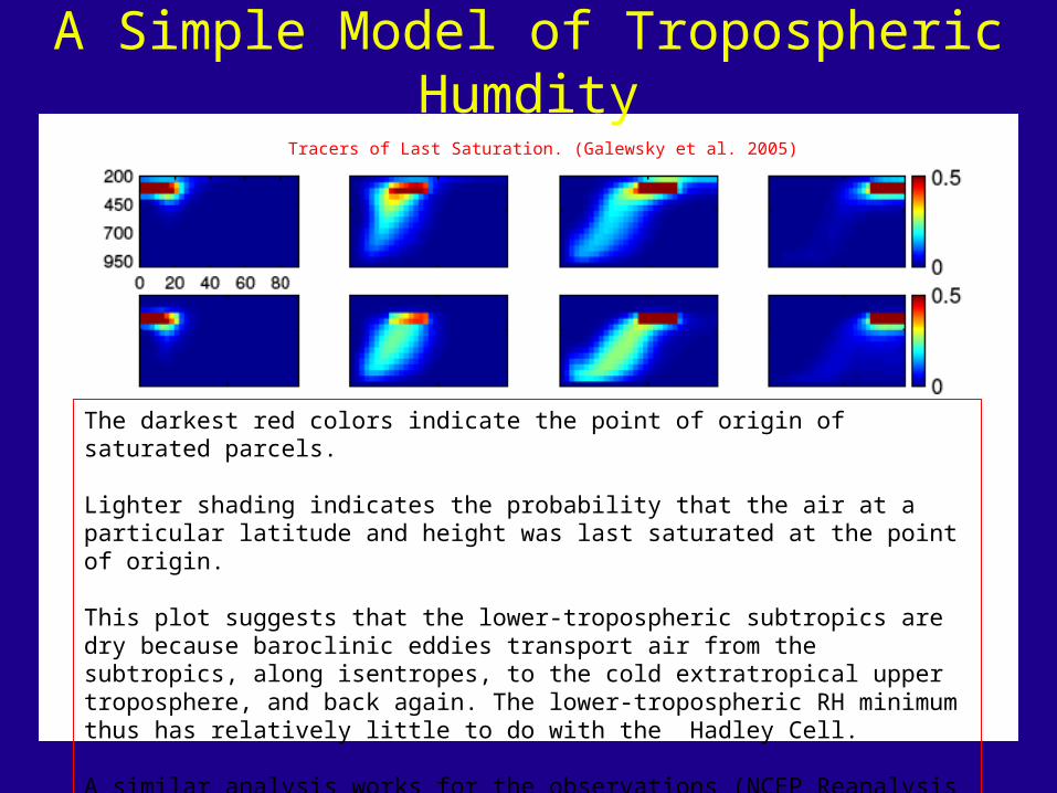
A Simple Model of Tropospheric Humdity
The darkest red colors indicate the point of origin of saturated parcels.
Lighter shading indicates the probability that the air at a particular latitude and height was last saturated at the point of origin.
This plot suggests that the lower-tropospheric subtropics are dry because baroclinic eddies transport air from the subtropics, along isentropes, to the cold extratropical upper troposphere, and back again. The lower-tropospheric RH minimum thus has relatively little to do with the Hadley Cell.
A similar analysis works for the observations (NCEP Reanalysis + MATCH).
Tracers of Last Saturation. (Galewsky et al. 2005)
Simple Models of Stratosphere-Troposphere Coupling
Scinocca and Haynes 1998
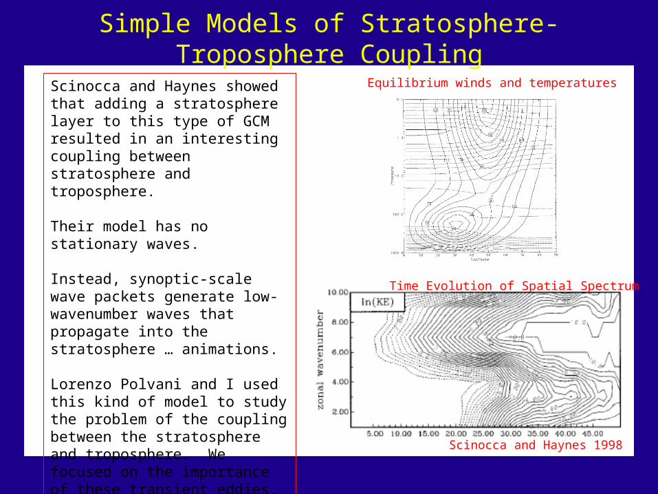
Scinocca and Haynes showed that adding a stratosphere layer to this type of GCM resulted in an interesting coupling between stratosphere and troposphere.
Their model has no stationary waves.
Instead, synoptic-scale wave packets generate low-wavenumber waves that propagate into the stratosphere … animations.
Lorenzo Polvani and I used this kind of model to study the problem of the coupling between the stratosphere and troposphere. We focused on the importance of these transient eddies.
Equilibrium winds and temperatures
Time Evolution of Spatial Spectrum
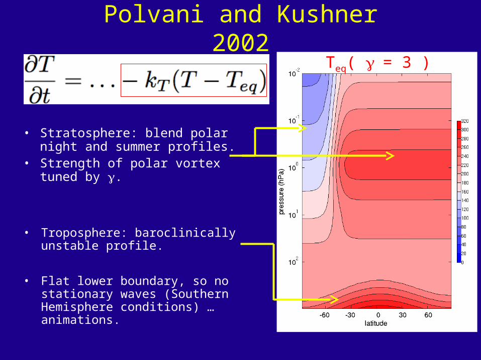
Teq( = 3 )
Polvani and Kushner 2002
• Troposphere: baroclinically unstable profile.
• Flat lower boundary, so no stationary waves (Southern Hemisphere conditions) … animations.
• Stratosphere: blend polar night and summer profiles.
• Strength of polar vortex tuned by .
A Spontaneous Sudden Warming
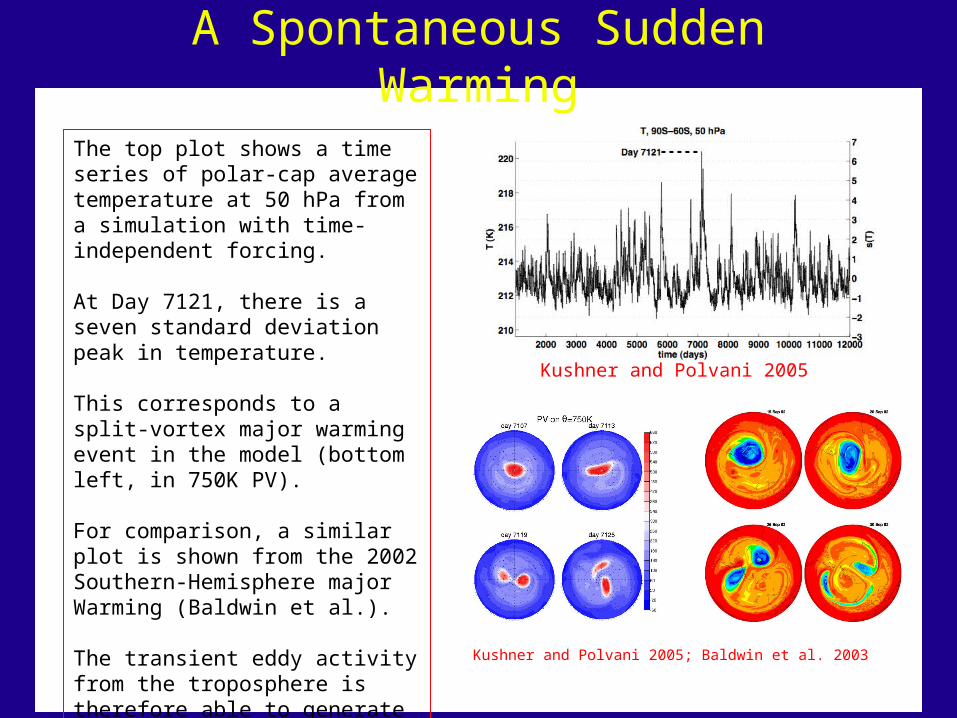
The top plot shows a time series of polar-cap average temperature at 50 hPa from a simulation with time-independent forcing.
At Day 7121, there is a seven standard deviation peak in temperature.
This corresponds to a split-vortex major warming event in the model (bottom left, in 750K PV).
For comparison, a similar plot is shown from the 2002 Southern-Hemisphere major Warming (Baldwin et al.).
The transient eddy activity from the troposphere is therefore able to generate a
Kushner and Polvani 2005
Kushner and Polvani 2005; Baldwin et al. 2003
Stratosphere-Troposphere Coupling
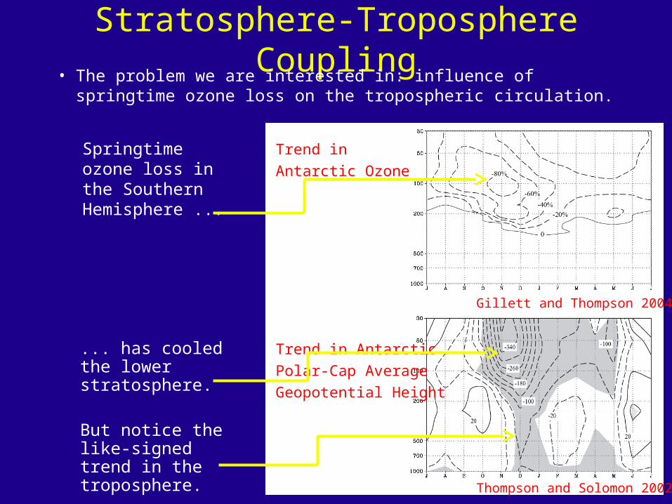
Springtime ozone loss in the Southern Hemisphere ...
Trend in
Antarctic Ozone
Trend in Antarctic
Polar-Cap Average
Geopotential Height
Gillett and Thompson 2004
Thompson and Solomon 2002
... has cooled the lower stratosphere.
But notice the like-signed trend in the troposphere.
• The problem we are interested in: influence of springtime ozone loss on the tropospheric circulation.
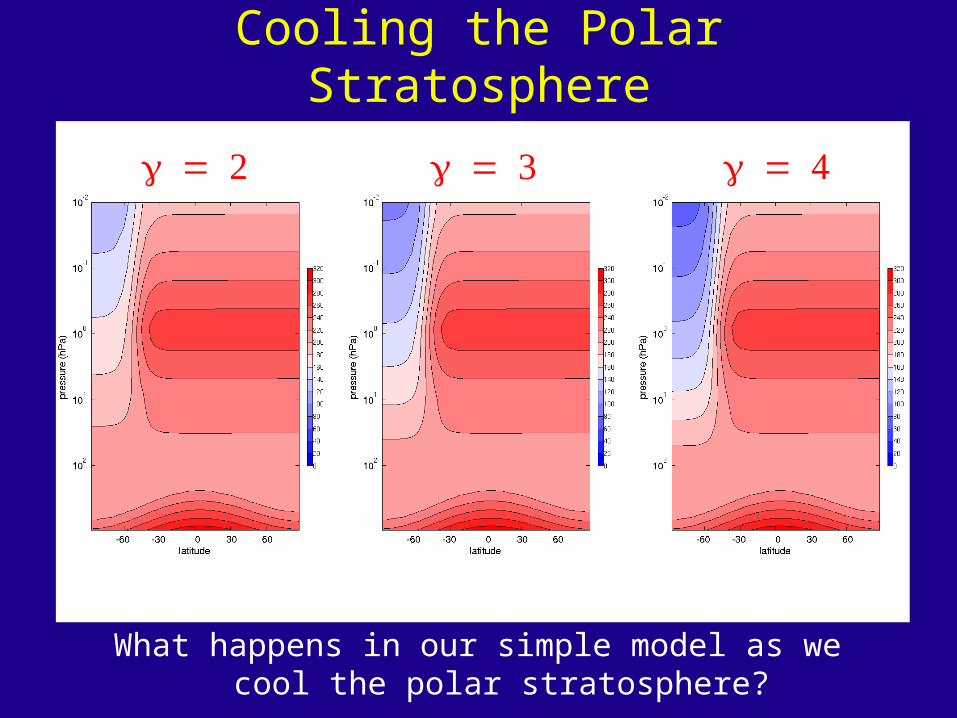
Cooling the Polar Stratosphere
What happens in our simple model as we cool the polar stratosphere?
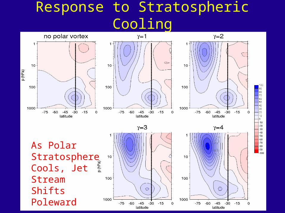
Response to Stratospheric Cooling
As Polar Stratosphere Cools, Jet Stream Shifts Poleward
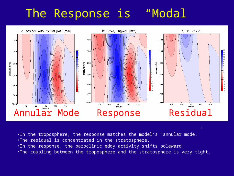
The Response is “Modal”
•In the troposphere, the response matches the model’s “annular mode.” •The residual is concentrated in the stratosphere.•In the response, the baroclinic eddy activity shifts poleward.•The coupling between the troposphere and the stratosphere is very tight.
Annular Mode Response Residual
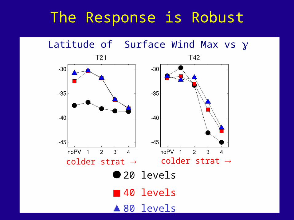
The Response is Robust
Latitude of Surface Wind Max vs
colder strat colder strat
20 levels
40 levels
80 levels
The World of General Circulation Models
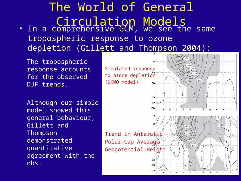
The tropospheric response accounts for the observed DJF trends.
Although our simple model showed this general behaviour, Gillett and Thompson demonstrated quantitative agreement with the obs.
• In a comprehensive GCM, we see the same tropospheric response to ozone depletion (Gillett and Thompson 2004):
Simulated response
to ozone depletion
(UKMO model)
Trend in Antarctic
Polar-Cap Average
Geopotential Height
Strengths of these Simple Models
• We have seen several examples of how baroclinic eddies and their associated circulations influence the climate system.The residual circulation seems to set or at least
influence tropopause structure.The eddies seem to dry out the extratropical
troposphere.The eddies drive planetary waves and are
implicated strat-trop coupling.• We use the model to get a handle on the
mechanisms.• But we must bear in mind their limitations.
Weaknesses of these Simple Models
• These models are highly tunable and so can be “forced” to agree with observations.
• They are thus difficult to compare directly with observations, which is the main theme of this workshop.
• Even though they are simple, they are not simple to understand.
• We will have to move into the world of GCMs – this will be tomorrow’s story.