Three-dimensional Radar Imaging of a Building

by Traian Dogaru, DaHan Liao, and Calvin Le

ARL-TR-6295 December 2012

Approved for public release; distribution unlimited

NOTICES

Disclaimers

The findings in this report are not to be construed as an official Department of the Army position

unless so designated by other authorized documents.

Citation of manufacturer’s or trade names does not constitute an official endorsement or

approval of the use thereof.

Destroy this report when it is no longer needed. Do not return it to the originator.

Army Research Laboratory Adelphi, MD 20783-1197

ARL-TR-6295 December 2012

Three-dimensional Radar Imaging of a Building

Traian Dogaru, DaHan Liao, and Calvin Le Sensors and Electron Devices Directorate, ARL

Approved for public release; distribution unlimited.

ii

REPORT DOCUMENTATION PAGE Form Approved

OMB No. 0704-0188 Public reporting burden for this collection of information is estimated to average 1 hour per response, including the time for reviewing instructions, searching existing data sources, gathering and maintaining the

data needed, and completing and reviewing the collection information. Send comments regarding this burden estimate or any other aspect of this collection of information, including suggestions for reducing the

burden, to Department of Defense, Washington Headquarters Services, Directorate for Information Operations and Reports (0704-0188), 1215 Jefferson Davis Highway, Suite 1204, Arlington, VA 22202-4302.

Respondents should be aware that notwithstanding any other provision of law, no person shall be subject to any penalty for failing to comply with a collection of information if it does not display a currently

valid OMB control number.

PLEASE DO NOT RETURN YOUR FORM TO THE ABOVE ADDRESS.

1. REPORT DATE (DD-MM-YYYY)

December 2012

2. REPORT TYPE

Final

3. DATES COVERED (From - To)

October 2011 to September 2012

4. TITLE AND SUBTITLE

Three-dimensional Radar Imaging of a Building

5a. CONTRACT NUMBER

5b. GRANT NUMBER

5c. PROGRAM ELEMENT NUMBER

6. AUTHOR(S)

Traian Dogaru, DaHan Liao, and Calvin Le

5d. PROJECT NUMBER

5e. TASK NUMBER

5f. WORK UNIT NUMBER

7. PERFORMING ORGANIZATION NAME(S) AND ADDRESS(ES)

U.S. Army Research Laboratory

ATTN: RDRL-SER-U

2800 Powder Mill Road

Adelphi, MD 20783-1197

8. PERFORMING ORGANIZATION REPORT NUMBER

ARL-TR-6295

9. SPONSORING/MONITORING AGENCY NAME(S) AND ADDRESS(ES)

10. SPONSOR/MONITOR'S ACRONYM(S)

11. SPONSOR/MONITOR'S REPORT NUMBER(S)

12. DISTRIBUTION/AVAILABILITY STATEMENT

Approved for public release; distribution unlimited.

13. SUPPLEMENTARY NOTES

14. ABSTRACT

This report describes the study of a through-the-wall radar system for three-dimensional (3-D) building imaging, based on

computer simulations. Two possible configurations are considered, corresponding to an airborne spotlight and a ground-based

strip-map geometry. The report details all the steps involved in this analysis: creating the computational meshes, calculating

the radar signals scattered by the target, forming the radar images, and processing the images for visualization and

interpretation. Particular attention is given to the scattering phenomenology and its dependence on the system geometry. The

images are created via the time-reversal technique and further processed using a constant false-alarm rate (CFAR) detector.

We discuss methods of 3-D image visualization and interpretation of the results and point the way to possible future

improvements.

15. SUBJECT TERMS

Sensing through the wall radar, synthetic aperture radar

16. SECURITY CLASSIFICATION OF:

17. LIMITATION OF

ABSTRACT

UU

18. NUMBER OF

PAGES

52

19a. NAME OF RESPONSIBLE PERSON

Traian Dogaru

a. REPORT

Unclassified

b. ABSTRACT

Unclassified

c. THIS PAGE

Unclassified

19b. TELEPHONE NUMBER (Include area code)

(301) 394-1482

Standard Form 298 (Rev. 8/98)

Prescribed by ANSI Std. Z39.18

iii

Contents

List of Figures iv

List of Tables v

1. Introduction 1

2. Modeling Methods and Algorithms 2

2.1 Meshes and Radar Imaging Geometries ..........................................................................2

2.2 EM Radar Scattering Models ..........................................................................................5

2.3 SAR Imaging Algorithms ................................................................................................6

2.4 Image Analysis and Visualization .................................................................................13

3. Phenomenological Discussion and Numerical Results 20

3.1 Phenomenology of Airborne Radar Imaging of a Building ..........................................20

3.2 3-D Images Obtained by Airborne Radar......................................................................25

3.3 Phenomenology of Ground-based Radar Imaging of a Building ..................................29

3.4 3-D Images Obtained by Ground-based Radar .............................................................32

3.5 Further Comments on the Numerical Results ...............................................................35

4. Conclusions and Future Work 38

5. References 40

List of Symbols, Abbreviations, and Acronyms 43

Distribution List 44

iv

List of Figures

Figure 1. The “complex room” computational mesh used in the radar imaging study in this report, showing (a) perspective view and (b) top view. .............................................................3

Figure 2. Schematic representations of the airborne spotlight radar imaging system, showing (a) the radar platform moving in a circular pattern around the building and (b) the synthetic aperture positions (marked as yellow dots) placed on a sphere. ................................4

Figure 3. Two representations of the ground-based strip-map radar imaging system, showing the moving radar platform, as well as the vertical antenna array. Each orange balloon-like feature represents one antenna beam. ........................................................................................5

Figure 4. Drawing illustrating the shrinking of the separation distance between two points as they get projected from the ground plane onto the slant plane. ...............................................11

Figure 5. Difference between azimuth and elevation integration strategies in the strip-map imaging configuration: (a) top view and (b) side view. ...........................................................13

Figure 6. CFAR detector sliding windows for point-like targets, showing (a) 2-D and (b) 3-D version. .....................................................................................................................................15

Figure 7. Sliding windows for the CFAR detection of walls, showing (a) 2-D version (line detector), (b) 3-D version for the airborne case (line detector), and (c) 3-D version for the ground-based case (wall detector). ..........................................................................................18

Figure 8. A 2-D slice in the ground plane through the 3-D image of the building showing (a) the raw image, (b) the test ratio map for the point detector, (c) the test ratio map for the line (wall) detector, and (d) the detection map. .................................................................20

Figure 9. Schematic ray-tracing representation of the major radar scattering mechanisms for the airborne spotlight configuration, with the far-field geometry assumption. .......................21

Figure 10. The 2-D slant-plane SAR images of the building obtained by the airborne radar in spotlight mode with fixed-elevation aperture at = 20°, showing (a) V-V polarization and (b) H-V polarization. .........................................................................................................22

Figure 11. The 2-D representations of the 3-D building radar image collapsed onto (a) the x-y plane and (b) the y-z plane. ...................................................................................................23

Figure 12. The 3-D building image for the airborne spotlight configuration and V-V polarization, with SNR = 40 dB, as seen from two different aspect angles. The feature colors correspond to their brightness levels in the raw 3-D image. ........................................26

Figure 13. The 3-D building image for the airborne spotlight configuration and V-V polarization, with SNR = 40 dB, as seen from two different aspect angles, showing positive point detections in blue and positive line detections in red........................................27

Figure 14. The 3-D building image for the airborne spotlight configuration and H-V (cross) polarization as seen from two different aspect angles. The feature colors correspond to their brightness levels in the raw 3-D image. ..........................................................................28

v

Figure 15. The 3-D building image for the airborne spotlight configuration and V-V polarization, with SNR = 30 dB. The pink ellipses highlight missing features as compared to figure 12. ..............................................................................................................................29

Figure 16. Schematic ray-tracing representation of the major radar scattering mechanisms for the ground-based strip-map configuration, with the near-field geometry assumption. .....30

Figure 17. The 2-D horizontal-plane slices through the 3-D image of the building obtained by the ground-based radar in strip-map mode, showing the plane at (a) z = 1.25 m and (b) z = 0.25 m. ..........................................................................................................................31

Figure 18. The 2-D slices through the 3-D image of the building obtained by the ground-based radar in strip-map mode, in the horizontal plane z = 1.25 m, showing an image (a) without windowing in azimuth and elevation and (b) with windowing in both azimuth and elevation. ...........................................................................................................................32

Figure 19. The 3-D building image for the ground-based strip-map configuration as seen from two different aspect angles. The feature colors correspond to their brightness levels in the raw 3-D image................................................................................................................33

Figure 20. The 3-D building image for the ground-based strip-map configuration, with SNR = 30 dB. The pink ellipses highlight missing features as compared to figure 19. ...................35

Figure 21. The 3-D building image obtained by fusing the airborne (red features) and ground-based (blue features) images presented in sections 3.2 and 3.4 (SNR = 40 dB). ........37

List of Tables

Table 1. Dielectric constant and conductivity of the materials involved in the building model in figure 1. .......................................................................................................................3

vi

INTENTIONALLY LEFT BLANK.

1

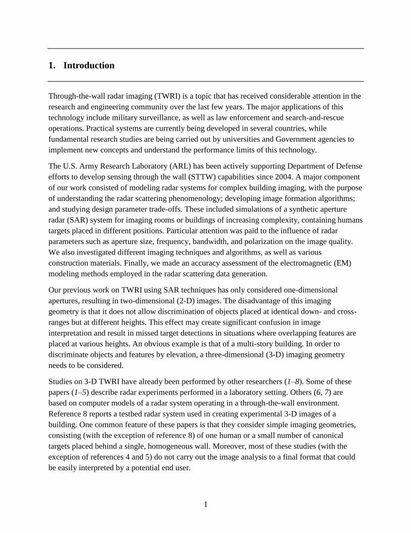
1. Introduction

Through-the-wall radar imaging (TWRI) is a topic that has received considerable attention in the

research and engineering community over the last few years. The major applications of this

technology include military surveillance, as well as law enforcement and search-and-rescue

operations. Practical systems are currently being developed in several countries, while

fundamental research studies are being carried out by universities and Government agencies to

implement new concepts and understand the performance limits of this technology.

The U.S. Army Research Laboratory (ARL) has been actively supporting Department of Defense

efforts to develop sensing through the wall (STTW) capabilities since 2004. A major component

of our work consisted of modeling radar systems for complex building imaging, with the purpose

of understanding the radar scattering phenomenology; developing image formation algorithms;

and studying design parameter trade-offs. These included simulations of a synthetic aperture

radar (SAR) system for imaging rooms or buildings of increasing complexity, containing humans

targets placed in different positions. Particular attention was paid to the influence of radar

parameters such as aperture size, frequency, bandwidth, and polarization on the image quality.

We also investigated different imaging techniques and algorithms, as well as various

construction materials. Finally, we made an accuracy assessment of the electromagnetic (EM)

modeling methods employed in the radar scattering data generation.

Our previous work on TWRI using SAR techniques has only considered one-dimensional

apertures, resulting in two-dimensional (2-D) images. The disadvantage of this imaging

geometry is that it does not allow discrimination of objects placed at identical down- and cross-

ranges but at different heights. This effect may create significant confusion in image

interpretation and result in missed target detections in situations where overlapping features are

placed at various heights. An obvious example is that of a multi-story building. In order to

discriminate objects and features by elevation, a three-dimensional (3-D) imaging geometry

needs to be considered.

Studies on 3-D TWRI have already been performed by other researchers (1–8). Some of these

papers (1–5) describe radar experiments performed in a laboratory setting. Others (6, 7) are

based on computer models of a radar system operating in a through-the-wall environment.

Reference 8 reports a testbed radar system used in creating experimental 3-D images of a

building. One common feature of these papers is that they consider simple imaging geometries,

consisting (with the exception of reference 8) of one human or a small number of canonical

targets placed behind a single, homogeneous wall. Moreover, most of these studies (with the

exception of references 4 and 5) do not carry out the image analysis to a final format that could

be easily interpreted by a potential end user.

2

Our approach in this study is based on computer simulations of a 3-D SAR imaging system for a

one-story building of moderate complexity, containing several human targets as well as furniture

objects. We analyze two possible synthetic aperture configurations: an airborne system operating

in circular spotlight mode and a ground-based system operating in linear strip-map mode. The

ultra-wideband (UWB) radar signature of the target is obtained via simulations over a 2-D

aperture. After creating the 3-D images, we develop image segmentation and visualization

techniques based primarily on a constant false alarm rate (CFAR) detection framework. We

emphasize the phenomenological aspects of the radar imaging process, and compare the

advantages and drawbacks of the two possible SAR configurations. We also suggest further

improvements that could be made in designing the SAR system configuration, the imaging

algorithms, and the visualization techniques.

Section 2 of this report describes the methodology in modeling the SAR system and EM

scattering phenomena, as well as the imaging and visualization algorithms. Section 3 presents

numerical results, with an emphasis on the radar phenomenology of the two SAR configurations.

We finish with conclusions and suggestions for future work in section 4.

2. Modeling Methods and Algorithms

2.1 Meshes and Radar Imaging Geometries

The building we consider in our computer models in this study is the “complex room,” which has

already been introduced in some of our previous work (9). A representation of the computational

mesh is shown in figure 1. It consists of a one-story building, with exterior 20-cm-thick brick

walls equipped with doors and windows, and an interior area that includes four humans, pieces

of furniture (made of wood and fabric), and an interior drywall. The overall building dimensions

are 10 m by 7 m by 2.2 m. Although not shown in figure 1, the mesh includes a 5-cm-thick

concrete ceiling and an infinite dielectric ground plane. The dielectric properties of all materials

are listed in table 1. The four humans in this mesh are placed at different azimuth orientation

angles. Using the numbering system in figure 1b, the orientation angles are as following:

1 = 45°, 2 = 0°, 3 = –20°, and 4 = 10° (Note: The = 0° angle corresponds to the human

facing along the positive x direction; the positive angles correspond to a counterclockwise

rotation in the horizontal plane). The human meshes represent the “fit man,” as described in

references 9 and 10, made of uniform dielectric material.

3

(a) (b)

Figure 1. The “complex room” computational mesh used in the radar imaging study in this report, showing

(a) perspective view and (b) top view.

Table 1. Dielectric constant and conductivity of the materials involved

in the building model in figure 1.

Material r

(S/m) "

Brick 3.8 0.02 0.24

Concrete 6.8 0.1 1.2

Glass 6.4 0 0

Wood 2.5 0.004 0.05

Sheetrock 2.0 0 0

Fabric 1.4 0 0

Human body 50 1.0 12

Ground 10 0.005 0.06

For the 3-D radar imaging geometry, we study two different configurations: one involves an

airborne platform (such as a helicopter) and operates in the spotlight mode, whereas the other

involves a ground-based platform (such as a small truck) and operates in the strip-map mode. In

both cases, the radar is assumed to transmit UWB waveforms, at typical frequencies for this

application (0.3 to 2.5 GHz).

A conceptual description of the airborne configuration is shown in figure 2. The platform moves

on circular trajectories around the building, at various elevations, with the antenna beam always

pointed towards the target (hence the spotlight mode). Figure 2b describes the 2-D aperture

where the radar data is monostatically collected for image formation (yellow dots). This aperture

4

spans an angle in azimuth and an angle in elevation, with the radar positions moving on a

sphere (the distance to the coordinate system origin, where the building is centered, is constant).

Essential to this configuration is the assumption that the target is placed in the far-field region of

the radar antennas, meaning that the transmitted waves that reach the target, as well as the

scattered waves that reach the radar receiver, can be approximated by plane waves.

(a) (b)

Figure 2. Schematic representations of the airborne spotlight radar imaging system, showing (a) the radar platform

moving in a circular pattern around the building and (b) the synthetic aperture positions (marked as yellow

dots) placed on a sphere.

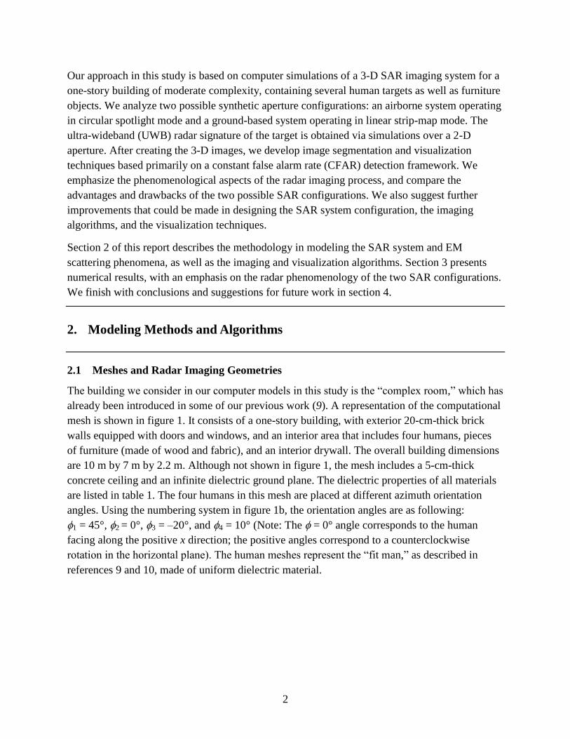
The ground-based radar imaging scenario is schematically described in figure 3 and resembles

the system described in reference 5. The radar is equipped with a vertical antenna array that is

assumed to transmit and receive monostatically, one element at a time. The vehicle moves on a

linear trajectory in the y direction at constant velocity, creating the synthetic aperture in the

horizontal direction. The spacing between the synthetic aperture and the front wall is d = 4 m.

For a large-size target such as a building, this represents a near-field configuration, requiring

both EM models and image formation algorithms compatible with this scenario.

5

Figure 3. Two representations of the ground-based strip-map radar imaging system, showing the moving radar

platform, as well as the vertical antenna array. Each orange balloon-like feature represents one antenna

beam.

2.2 EM Radar Scattering Models

The EM radar scattering models performed in this report are based on two different programs:

AFDTD (11), which implements the finite-difference time-domain (FDTD) technique, and

Xpatch (12), which is a combination of ray tracing and physical optics (PO). These codes were

introduced in some of our previous EM modeling work (10).

AFDTD was developed at ARL and implements an “exact” computational electromagnetic

(CEM) method. A comprehensive description of the FDTD computational method can be found

in reference 13. Although AFDTD provides accurate models of complex radar scattering

problems, it is a very computationally intensive code both in terms of central processing unit

(CPU) time and memory. Additionally, AFDTD is designed to work only with far-field EM

configurations; therefore, we only use is to model the airborne spotlight scenario in figure 2.

Xpatch was developed by Science Applications International Corporation (SAIC) under a grant

from the U.S. Air Force and implements an “approximate” EM solver. Although it has certain

limitations in terms of accuracy (especially at low microwave frequencies), Xpatch is much more

efficient than AFDTD both in terms of CPU time and memory resources. In previous studies

(including references 9 and 10), we performed an extensive validation of the Xpatch models as

applied to STTW radar problems. In this report, we employ Xpatch to simulate the ground-based

strip-map radar scenario described in figure 3. Notice that for this application, we use a near-

6

field version of Xpatch which was introduced in reference 14. A brief description of this code

and its usage to STTW imaging radar problems was also given in reference 10.

The 3-D imaging of the building involves acquiring its radar signature over a band of frequencies

and a 2-D spatial aperture. The frequency band is typical for STTW radar applications and

extends from 0.3 to 2.5 GHz in 6.7-MHz increments for the spotlight configuration and 3.9-MHz

increments for the strip-map configuration. The aperture geometry depends on the radar system

configuration, as described in section 2.1. Thus, for the airborne spotlight configuration, we carry

out the computations for azimuth angles from –15° to 15° ( = 30°) in 0.25° increments and

elevation angles from 10° to 50° ( = 40°) in 1° increments. We call the direction of the plane

waves emanating from the aperture center ( = 0° and = 30°) the radar middle line of sight

(LOS). For the ground-based strip-map system, the vertical antenna array has 16 elements,

spanning a 1.5-m height (from 0.5 to 2 m above the ground plane) in 10-cm increments. The

horizontal synthetic aperture has a length of approximately 23 m and is sampled every 5 cm. For

the near-field configuration, the antennas are assumed to have a beam width of 60° in both

azimuth and elevation, centered along the x axis.

All the models (performed with both AFDTD and Xpatch) calculate the monostatic radar

signature in vertical-vertical (V-V) polarization (for the airborne scenario we also computed the

horizontal-vertical [H-V] combination). The AFDTD computational grid is made of

approximately 1.68 billion cubic cells of 5-mm size. The parallel version of this code was run at

the ARL and U.S. Air Force Research Laboratory (AFRL) Defense Supercomputing Resource

Centers (DSRC) (15, 16) on high performance computing (HPC) systems, such as JVN, Harold,

Hawk, and Raptor. A typical AFDTD run used 64 cores. Since the simulations were performed

over a long period of time on computing platforms with different speeds, it is difficult to estimate

the total CPU time used in this project. However, if all simulations were run on Harold (the

fastest of the systems previously listed), the AFDTD models would have used approximately

2 million CPU hours (the actual figure was certainly higher). At the same time, the Xpatch

simulations were entirely run on Harold and used about 60,000 CPU hours.

The post-processing algorithms (image formation and visualization) were developed in-house at

ARL using the MATLAB software (17). The 3-D image formation algorithm uses the Message

Passing Interface (MPI) framework and was run at ARL DSRC on the Harold system. The idea

behind this code was to distribute the task to multiple cores, each one creating a 2-D image in

one horizontal plane. The 3-D image is then obtained by aggregating all the 2-D slices into one

3-D array. Compared to the EM simulations performed for this study, the image formation

algorithm used a very small amount of CPU time (between 200 CPU hours per image for the

spotlight mode and 400 CPU hours per image for the strip-map mode).

2.3 SAR Imaging Algorithms

To create a 3-D image of the building based on the simulated radar data we apply the time-

reversal imaging (TRI) technique (18, 19). The image formation algorithm used in this study was

7

described in references 20 and 21. If the frequency domain signal starting at transmitter T and

ending at receiver R is ,, TRS rr , where rR and rT represent the position vectors of the receiver

and transmitter, respectively, and f 2 with f representing the frequency, then the (complex)

image at the point r is described by the equation:

R T

RTTRTRI GGSI ,,,,,, rrrrrrr , (1)

where ,',rrG is the Green’s function that characterizes the propagation medium. The

summation in equation 1 is performed over all frequencies of interest, as well as all the

transmitter and receiver combinations for which multi-static scattering data are available. In

references 20 and 21, we applied this algorithm to obtain 2-D radar images of a scene in both

near- and far-field configurations. In the current study, we extend the method to a 3-D imaging

scenario. Notice that the formulation in equation 1 is valid for any sensor position geometry in

the physical space.

In the most general case, the Green’s function for EM fields is a dyadic (22), while the received

signal S may be represented by a vector in the case of polarimetric radar. To simplify the

analysis, here we consider only one component of the Green’s function dyadic, which links the

vertically polarized fields at the receiver to the z-directed induced currents on the target and

reciprocally, the z-directed induced current on the target to the vertically polarized transmitted

fields. Consequently, both S and G are scalars, with S representing the vertically polarized

electric field and G representing the free-space Green’s function (22):

'4

,',

'

rrrr

rr

cj

eG , (2)

where c is the speed of light.

As described in section 2.1, in this work, we only consider monostatic radar scenarios, which

allow us to further simplify the TRI algorithm formulation. Thus, instead of rR and rT (which

now coincide), we use the vector rA (where the subscript A stands for aperture) and obtain

2

2

4,

A

cj

A

ATRI

A

eSI

rrrr

rr

, (3)

A refinement of the algorithm consists of using a tapered window that extends in both the

frequency and spatial domains, in order to reduce the image sidelobes. By calling the real-valued

window function ,AW r , we obtain the following expression:

2

2

4,,

A

cj

A

AATRI

A

eSWI

rrrrr

rr

. (4)

8

For the far-field configuration, a common assumption is that 2

Arr in the denominator of

equation 4 is constant across the image space. In that case, the denominator simply becomes a

scaling factor and its omission from the equation amounts to an image re-normalization. The TRI

equation for the far-field case becomes

A

cj

A

AAFFTRI eSWIrr

rrr

2

,, . (5)

Moreover, by choosing the coordinate system origin within the image area, we can write the

approximate far-field expression:

AAAAAAA zyxr sincossincoscos0 rr , (6)

where zyx ,,r in Cartesian coordinates and AAAA r ,,0r in spherical coordinates. Since

in the far-field spotlight mode the aperture is placed on a sphere, r0A is constant and can be taken

out of the double sum as a phase factor that has no impact on the image magnitude. Therefore,

we obtain the final image point expression for the far-field TRI algorithm:

AAAAA zyx

cj

A

AAAAFFTRI eSWzyxI

sincossincoscos

2

,,,,,,

. (7)

For the near-field configuration, 2

Arr (in the denominator of equation 4) may vary by large

amounts within the image area. Moreover, the radar scattered signal ,AS r has a magnitude

that generally varies inverse proportionally with 2

Arr . The effect is a strong reduction in the

voxel magnitude for image points placed far from the aperture as compared to those placed

closer. In order to produce image voxels with equal magnitude weights, we need to perform a

range compensation procedure by modifying the imaging algorithm. Typically, this consists of

multiplying each term in the sum over A in equation 4 by 4

Arr :

A

cj

A

A

AANFTRI eSWIrr

rrrrr

2

2,, . (8)

Using Cartesian coordinates, the near-field TRI equation can be written as

2222

222

,,,,,,,,

AAA zzyyxxc

j

AAA

A

AAAAAANFTRI

e

zzyyxxzyxSzyxWzyxI

. (9)

Since the target in our scenario is placed on top of an infinite dielectric ground plane, a rigorous

application of equation 1 would require calculating the half-space Green’s function (20, 21).

While asymptotic formulations could simplify this calculation in the far-field case, the near-field

half-space Green’s function evaluation is much more complicated. At the time of this writing,

9

our imaging algorithm did not incorporate the half-space Green’s functions, so the free-space

version had to be used. The impact of this choice on the building images is discussed in

section 3.

Although the TRI algorithm offers a general and elegant solution to the radar imaging problem,

other SAR imaging techniques can be employed for the same purpose. For example, the back-

projection algorithm (BPA) (23) can also handle arbitrary sensor position geometries to create 2-

or 3-D images of a scene where the propagation medium is free-space. In the following, we show

that the TRI and BPA algorithms are related to each other, at least under certain simplifying

assumptions.

In the most basic form of the BPA (also known as “delay-and-sum”), the image function at point

r can be calculated using the time-domain radar returns ts A ,r as (23)

A

AABPA sI rrrr ,, , (10)

where is the time delay characterizing the propagation from transmitter to image voxel and

back to the receiver c

A

A

rrrr

2, and the summation is performed over all aperture

positions. We can write the delayed expression of ts A ,r as a discrete Fourier sum as follows:

AA

cj

At

tjcj

At

A

A eSeeSc

tsrrrr

rrrr

r

2

0

2

0 ,,2

, , (11)

where ,AS r is the Fourier transform of ts A ,r . By replacing equation 11 in equation 10 we

obtain

A

cj

A

ABPA eSIrr

rr

2

, . (12)

After applying a window ,AW r in the spatial and frequency domains, the equation becomes

A

cj

A

AABPA eSWIrr

rrr

2

,, (13)

(in the case of an impulse UWB radar signal, the frequency-domain window is already included

in ,AS r , so the window function simply becomes AW r ).

Notice that we obtain exactly the same expressions for the free-space far-field version of TRI

and the BPA, with the exception of a complex conjugation, which has no impact on the image

voxel magnitude. Furthermore, the BPA can be easily extended to a multistatic transmitter-

receiver configuration, leading again to the same formulation as the TRI method.

10

To adapt the BPA to near-field configurations, a range correction factor can be added in a

manner similar to TRI:

A

cj

A

AAANFBPA eSWIrr

rrrrr

2

2,, . (14)

To make the simulation more realistic, we add noise directly to the radar image as a post-

processing step. In the complex image domain, both the real and imaginary parts of the noise are

uncorrelated, identically distributed, zero-mean Gaussian random sequences, with a standard

deviation dictated by the desired signal-to-noise ratio (SNR). If one considers the image

magnitude, the noise becomes Rayleigh-distributed, which is a common model for the

background noise statistics in many radar problems (24).

Notice that we could have added the noise sequences to the raw radar return data prior to the

image formation process. Even if this path were followed, according to the central limit theorem,

the complex-valued voxel noise at the output of the SAR image formation algorithm would still

exhibit the Gaussian distribution described above. The relationship between the SNR of the raw

radar data and the SAR image’s SNR would depend on the way these ratios are defined. An

additional complication, particularly for the far-field case, consists of evaluating the absolute

power of the received radar signal based on the simulated data, since the computational model

does not include important radar system parameters, such as transmitted power, range, and

antenna gain. To avoid the uncertainties related to these calculations, we choose to add an

arbitrary amount of complex-valued white Gaussian noise directly to the SAR image. The effects

of various SNR levels on the 3-D building images are discussed in section 3.

An important part of the radar image analysis is the evaluation of its resolution. We start by

determining the image resolution for the airborne spotlight configuration in figure 2. Notice that

the aperture extends over a range of azimuth angles ( centered at = 0°) and elevation angles

( centered at 0), creating cross-range and height resolution, while the down-range resolution

is related to the signal bandwidth B, centered at f0. More specifically, we are interested in finding

expressions for the image resolution in the x, y and z directions, corresponding to down-range,

cross-range, and elevation, respectively. These are

0cos2 B

cx (15a)

00 cos2

sin4

f

cy (15b)

00 cos2

sin4

f

cz (15c)

11

It is interesting to notice the cos0 factor that appears in the denominator of the expressions in

equation 15. An intuitive justification for its presence in the equations 15a and 15b goes as

follows. Consider a circular aperture at constant elevation that is used to create a 2-D image in

the slant plane (figure 4). Two points separated by a distance in a horizontal plane (such as

the ground plane) appear in the slant plane as separated by a distance cos (the separation

distance shrinks by a cos factor), regardless of the points orientation with respect to the x and y

axes. Since the separation distance shrinks, the image resolution degrades by the same factor

(meaning x and y increase by a factor of cos

1). With the 3-D image being obtained from

circular apertures over a range of elevation angles, it is reasonable to infer that, on the average,

the resolution in the horizontal directions (x and y) will degrade by a factor of cos0, where 0 is

the center of the aperture in elevation. A more rigorous proof of this effect is presented in

reference 23, based on the support region of the image data in the zyx kkk ,, domain.

Figure 4. Drawing illustrating the shrinking of the separation distance between

two points as they get projected from the ground plane onto the slant plane.

With regards to the presence of the cos0 factor in the denominator of equation 15c, this can be

explained by the fact that the image data support region is squinted by an angle 0 in any vertical

plane of the zyx kkk ,, space that goes through the origin. If the targets were placed in free-

space, this issue could be eliminated for a spotlight configuration by rotating the entire

coordinate system (including the targets) such that the aperture is centered at = 0° in elevation.

However, given the fact that our geometry contains a ground plane and the definition of the

elevation angle is referenced to this plane, the rotation procedure cannot be applied to this

configuration. Consequently, the image data support region in the elevation direction is reduced

by a cos0 factor, resulting in a similar degradation of the elevation resolution.

One direct conclusion that we derive from this analysis is that the elevation angle in the middle

of the aperture should not be too large in order to minimize its impact on the image resolution. In

our case, we have = 30°, which degrades the resolution by about 15% as compared to the

hypothetical case where = 0°.

12

Another interesting conclusion is that, if we keep a constant azimuth integration angle regardless

of the elevation, the contribution of each constant-elevation circular aperture to the 3-D image

will have variable resolution (we can intuitively see this in figure 2b, where each horizontal

circle on the sphere seems to shrink as we go higher in elevation, although the azimuth angular

span within the aperture is the same). In order to keep a constant down- and cross-range

resolution for all constant-elevation apertures, both the bandwidth B and the azimuth integration

angle should be adjusted by a factor of cos

1(that is, increasing with the elevation angle).

This can easily be performed in the image formation algorithm by choosing a window ,AW r

with the appropriate dependence on While we did not pursue this approach in the current

study, future work will investigate whether the procedure can improve the quality of the radar

images.

For the strip-map configuration in figure 3, the resolution analysis is more straightforward, since

the elevation aperture is centered at = 0°. In this case, we employ a constant angle integration

procedure in azimuth (meaning that for each image voxel, we integrate aperture data that spans a

fixed angle centered at 0° in azimuth), while in elevation we use a fixed aperture length (h)

for all image voxels (figure 5). This strategy is dictated by the physical constraints of the strip-

map imaging geometry, where the antenna array has a fixed (and limited) vertical dimension,

while the synthetic aperture can be extended as much as desired in the horizontal dimension. The

expressions for the down-range, cross-range, and elevation resolutions are, respectively,

B

cx

2 (16a)

2sin4 0

f

cy (16b)

hf

xxcz

A

02

(16c)

13

(a) (b)

Figure 5. Difference between azimuth and elevation integration strategies in the strip-map imaging configuration:

(a) top view and (b) side view.

Notice that, while the down- and cross-range resolutions are independent of the voxel position,

the elevation resolution depends on the voxel x coordinate (down-range). The effect is that

regions in the image placed farther apart from the aperture display poorer elevation resolution

than those at closer range. Equation 16c should also contain a factor to account for the elevation

squint angle of the image voxel with respect to the middle of the antenna array (in vertical

direction), but, since that angle is generally small, we choose to neglect its effect.

In equations 15 and 16, we did not take into account the effect of windowing the data on image

resolution. The images shown in section 3 use Hanning windows in all three dimensions

(frequency and angles or Cartesian coordinates), with the exception of the z direction for the

ground-based case. Following the analysis outlined in reference 10, we conclude that, after

windowing, the resolution in all three directions degrades by about a factor of 2 (meaning that

x, y, and z increase by a factor of 2) as compared to the numbers obtained from equations 15

and 16. The images obtained in section 3 have the following resolutions: for the airborne

spotlight case x = 16 cm, y = 48 cm, and z = 36 cm; for the ground-based strip-map case

x = 14 cm, y = 22 cm, and z between 29 and 79 cm. The voxel size is 5 cm in all three

Cartesian directions.

2.4 Image Analysis and Visualization

Once the 3-D image of the building is created, the next step consists of extracting the relevant

information and displaying that information in a format intelligible to the end user. The “relevant

information” contained in an image depends on the specific application. If we are interested in

extracting the building layout, we may only be concerned with the location of the walls. If we are

trying to detect human targets, we may want to reject everything else in the image (including the

walls) as clutter. In this study, we assume that we are interested in displaying all the image

features (walls, humans, and possibly, furniture objects) that stand out of the background. The

14

problem of classifying the image objects into categories such as human targets, walls, or clutter

is beyond the scope of this work.

Displaying 3-D SAR images on a 2-D medium support (such as a computer screen or a page) is a

significantly more difficult problem than its 2-D counterpart. Notice that all the images

considered here are “monochromatic,” meaning that each pixel (or voxel in 3-D) is described by

a single real number (its magnitude). As such, the images can simply be represented in a

grayscale, although using a pseudo-color scale typically enhances the image contrast and makes

for an easier interpretation. In our previous work (9, 10), most of the 2-D SAR images use

pseudo-color scales, representing the true pixel magnitudes above a certain threshold dictated by

the desired dynamic range. However, this procedure cannot be directly applied to visualize 3-D

images, which represent scalar functions of three variables.

The approach we follow in this report is to perform a background removal procedure prior to

visualization, meaning that we only display voxels that stand out of the background. More

specifically, we process the image through a CFAR detector (24–26), which, in essence,

compares each voxel in the image with a threshold that depends on the surrounding background

level, such that the detection scheme preserves a constant false alarm probability. Once the

voxels indicating target detection have been identified (and assuming they are clustered together

around the outstanding features in the image), all voxels within a “target” volume (or more

exactly, voxel cluster) are assigned a constant magnitude (equal to the maximum voxel

magnitude within the cluster), while the background, consisting of voxels rejected by the

detector, is assigned an arbitrarily low magnitude, at the bottom of the dynamic range. Finally,

the visualization is performed by displaying the isosurfaces (2-D surfaces of constant magnitude

in the 3-D space) representing each target within the 3-D image volume. While only projections

of this 3-D image can be rendered on a 2-D support, changing the viewing angle can offer a more

complete interpretation for the end user.

Notice that, throughout this work, we use the term “target” to designate any image object that

stands out of the background, including humans, walls, and other possible clutter objects in the

scene. Since the focus of our study is on EM scattering phenomenology (“what the radar sees”)

rather than on image processing, interpretation, and classification, the final 3-D images displayed

in section 3 contain all these image features regardless of their physical nature. In this context,

the CFAR detector’s function is not to detect specific targets inside a building, but to serve as a

pre-screening tool for background noise removal that facilitates the 3-D image visualization. An

essential role of the CFAR detector is to reject the sidelobes created by image objects, which can

potentially create significant confusion in interpreting the SAR images of buildings.

The specific CFAR detection algorithm employed in this study is a 3-D extension of the

procedure outlined in references 27 and 28, which consists of a refinement of the cell-average

CFAR detector (24–26). For the 2-D version of this algorithm, we apply a sliding window

(figure 6a) centered at each image pixel, computing a test ratio and comparing it to a threshold.

15

Notice in figure 6a that the overall window has three components: an inner (or test) window, a

guard window around it, and an outer (or background) window. Although these window

dimensions can be chosen independently in the two Cartesian directions, we did not find any

particular advantage in setting different sizes along the x and y axes (therefore the windows in

figure 6a have square shapes). The 3-D extension to this sliding window is shown in figure 6b,

where all window sizes are equal in the x, y, and z directions.

(a) (b)

Figure 6. CFAR detector sliding windows for point-like targets, showing (a) 2-D and (b) 3-D version.

In the original form of this CFAR detector, the test window contains only one pixel (27).

Choosing a test window size larger than one has a spatial averaging effect, with the image

resolution reduced accordingly. However, in our 3-D images, the voxel size is typically only a

fraction of the resolution cell. Therefore, setting a test window size larger than one (in our case

we set Ni = 3) has no impact on the image resolution. Moreover, this choice may have a

beneficial effect by smoothing out any possible spikes in image magnitude caused by the small

voxel size.

The background window is the area where the clutter level is locally estimated. This area must

be large enough to allow for a good estimate of the clutter statistics, but not too large as to span

image areas with different statistics (24). For images of a scene with relatively widely spaced

objects, such as the one shown in figure 1, a simple rule is to choose an outer window

dimensions comparable to the separation distance between objects. In our case, we set No = 19,

which gives an overall window dimension of 95 cm.

The guard window contains pixels that are excluded from the background statistics estimation.

This procedure is required by the fact that most targets in the scene have a spatial extent

16

significantly larger than the test window size. Consequently, when we test a target voxel, the

adjacent target voxels could “spill over” inside the background estimation area and end up

skewing the clutter statistics significantly. In order to avoid this effect, the guard window must

have an extent comparable to the targets of interest. In our algorithm we set Ng = 13, giving a

guard window size of 65 cm.

As mentioned in section 2.3, a small level of background noise is added to the noise-free image

data. The image noise has Rayleigh statistics for the voxel magnitude I, or exponential statistics

for the voxel power (magnitude square) 2IP (25). A benefit of this procedure is that it forces

the background voxel magnitude statistics to conform to the Rayleigh model, as compared to the

“noise-free” case, where the background voxel statistics are dominated by peculiar biases such as

round-off errors at the level of the least significant digit. The noise power (more exactly, the

standard deviation of the complex-valued additive white Gaussian noise) is computed as a

function of the desired SNR and the average signal power contained in the 3-D SAR image. To

evaluate the average signal power, the noise-free 3-D SAR image is first created and processed

through the CFAR detector. Subsequently, only the voxels passing the detection test (the “target”

voxels) are taken into account for the average signal power computation.

The detection problem can be formulated in terms of the Neyman-Pearson test (29), where the

likelihood ratio is compared to an appropriately set threshold, with the outcome deciding

between hypotheses: H0, no target present at the test voxel, or H1, target present at the test voxel.

A well-known result in detection theory establishes the fact that this procedure maximizes the

probability of detection for a given probability of false alarm (29). The voxel power statistics can

be written as exponential probability density functions both for target and background regions

(25):

00

0 exp1

PHPp (17)

11

1 exp1

PHPp . (18)

For the cell-average CFAR detector, the decision is made according to references 25–28:

. (19)

The test ratio in equation 19 involves the average power of the voxels within the background

window (which represents an estimate of 0):

bgN

n

n

bg

bg PN

P1

1, (20)

17

where Nbg = No3 – Ng

3 is the number of voxels included in the background window, as well as the

average power within the test window:

testN

n

n

test

test PN

P1

1. (21)

Notice that the average background power is estimated locally (depending on the detection

window position), meaning that the detector can adapt to inhomogeneous clutter conditions. One

could argue that, in our case, the background noise is constant by design throughout the 3-D

image; therefore, a flat threshold would work in eliminating the image noise as well. However,

the adaptive feature of the CFAR detector is essential in rejecting the sidelobes associated with

various objects in the scene, whose levels strongly depend on the main radar response of those

objects and thus may vary within a wide dynamic range. The threshold can be calculated by the

formula (25)

1/1

bgN

FAbg PNT , (22)

where PFA is the desired probability of false alarm.

Since this study only analyzes one image that contains several targets, we cannot make statistical

inferences about the probability of detection and probability of false alarm from this data set

alone. Instead of using equation 22 to set the detection threshold based on a given PFA, we use

empirical threshold values that produce satisfactory image quality, in the sense that only the

important image features (walls and humans) are retained, while the background clutter is

rejected. For the record, in the numerical examples in section 3, the PFA computed according to

22 is usually on the order of 10–5

.

An additional complication is introduced by the fact that not all targets in our TWRI scene have

equal extent in all directions. In particular, as we show in section 3, the walls appear in the

images as features to much larger extent in cross-range (and, in the strip-map mode, in height as

well) than in down-range. The application of the algorithm outlined so far to wall images could

result in missed detections, since the target image would certainly “spill over” inside the

background window. Therefore, the sliding window shown in figure 6, which is specifically

designed to detect mostly isotropic targets, must be modified to accommodate the particular

shapes of the wall features (with the additional information that, in our imaging geometries, these

features always run parallel to the y and the z axes).

The design of the CFAR window for wall detection follows well-known algorithms for edge and

line detection in image processing (30). Although in the image processing literature the sliding

windows are known as masks, the detection principles are the same: the mask is run over the

entire image and a certain mask-dependent metric computed for each pixel is compared to a

threshold to decide whether the feature is present or absent at that location. The 2-D version of

the wall detection sliding window employed in this work is shown in figure 7a. This is

18

reminiscent of the line detection masks presented in reference 30, with the major difference that

we add a guard window, as explain earlier in this section. The window in figure 7a is designed to

work for walls parallel to the y axis.

(a) (b) (c)

Figure 7. Sliding windows for the CFAR detection of walls, showing (a) 2-D version (line detector), (b) 3-D version

for the airborne case (line detector), and (c) 3-D version for the ground-based case (wall detector).

The 3-D extension to this CFAR detection window depends on the radar imaging geometry.

Thus, as shown in section 3, for the airborne spotlight configuration, only the top and bottom

edges of the wall appear in the image; hence, a 3-D line detector is the most appropriate for this

case. This is shown in figure 7b, where the guard window extends to the limits of the overall

window in the y direction only. For the ground-based strip-map configuration, where the entire

wall volume appears in the image, a window design as in figure 7c is required. The test ratio for

the wall detection problem is the same as in equation 19, with the difference that, in this case,

22

goobg NNNN for the airborne images and gobg NNNN 2

0 for the ground-based

images.

The final form of the CFAR detection algorithm can be summarized as follows:

• Run the sliding windows in figures 6b, 7b, and 7c over the entire image separately and

compute the average power ratio in equation 19 for each voxel and each window type.

• Compare the pixel average power ratios to preset thresholds (there are different thresholds

for each different type of feature).

• Decide that a target voxel has been detected if any of the tests is positive.

To gain a better understanding of how the CFAR detection algorithm works on building images,

we present several possible visualizations for a 2-D slice of the 3-D image. Particularly, we

display the image in the ground plane (z = 0) obtained from the airborne spotlight 3-D imaging

geometry. As is shown in section 3.1, this plane is particularly interesting for the airborne case,

since it is expected to contain the projections of all objects in the scene.

19

Figure 8a contains the raw image as obtained by the algorithm described in section 2.3, after

adding image noise with SNR = 40 dB. Note that the image magnitude is given in dB and uses a

pseudo-color scale representation, with a dynamic range of 40 dB. For this limited dynamic

range, the noise does not show up in the image (remember that the noise level is referenced to

the average target voxel power). Next, we apply the window in figure 6a and display a map of

the test ratios as computed by equation 19 in figure 8b. The test ratio is represented in dB

(computed as bg

test

P

P10log10 ) on a 15-dB dynamic range scale. It is interesting to see that the

humans appear as some of the “brightest” targets to this CFAR detector. Figure 8c represents the

test ratio map after we apply the window in figure 7a (for wall detection), with the same dynamic

range. As expected, the “brightest” targets in this case are the walls (particularly the front wall).

Finally, in figure 8d, we present a map of all positive detections. In this case, we chose a

threshold Tpoint = 5 (or 7 dB) for “point” targets and Tline = 100 (or 20 dB) for “line” targets. The

color of each detected target corresponds to the maximum pixel magnitude within that target

area. The pixels that fail the detection test are set to a dB level at the bottom of the dynamic

range. The notable image features that can be distinguished in this detection map are the front

wall, the interior wall, part of the back wall, the human targets, the front edge of the dresser, and

the front edge of the sofa.

20

(a) (b)

(c) (d)

Figure 8. A 2-D slice in the ground plane through the 3-D image of the building showing (a) the raw image, (b) the

test ratio map for the point detector, (c) the test ratio map for the line (wall) detector, and (d) the detection

map.

Note: The pink circles highlight the human targets. The mesh contours were overlaid on the images as gray lines.

3. Phenomenological Discussion and Numerical Results

3.1 Phenomenology of Airborne Radar Imaging of a Building

Before we present the building images, we discuss some preliminary phenomenological aspects

of the radar imaging process. The purpose of understanding the phenomenology is to help with

the 3-D image interpretation. Interestingly, there are some significant differences in the EM

21

scattering mechanisms between the airborne spotlight and ground-based strip-map

configurations. In this section, we discuss the phenomenology of radar scattering for the airborne

spotlight mode.

First, we analyze the major scattering mechanisms and their impact on the SAR image. Two

essential aspects of the EM propagation and scattering in the airborne configuration are the

presence of the infinite ground plane and the fact that the target is in the far-field region. The

latter condition means that we can represent the plane waves emitted and received in the

backscatter direction by the radar by parallel rays with the same tilt angle (figure 9). The drawing

in figure 9 suggests that the major scattering centers of a building wall are its top and bottom

edges. We expect the bottom edge to appear very bright in a SAR image, since the ground

bounce creates a corner effect between the wall and the ground plane. At the same time, the top

edge scatters the waves via a single-bounce diffraction mechanism, which is usually much

weaker than backscattering from a corner.

Figure 9. Schematic ray-tracing representation of the major radar scattering mechanisms for the airborne

spotlight configuration, with the far-field geometry assumption.

Similarly, the ground bounce creates a relatively bright footprint in the ground plane for any

target in the scene (e.g., the humans) that makes a 90° angle with this plane. Notice that the

ground-bounced rays always back-project to the same point in the image (that is, the target’s

projection onto the ground plane), regardless of the radar elevation angle. This means that

apertures placed at various elevations will reinforce those image points, which will appear as

particularly bright in the 3-D image. Other features in the image will usually represent single-

bounce scattering centers (such as the human torso). However, these centers typically exhibit

22

lower brightness than the corners since the strength of their back-scattering response may vary

significantly with the elevation angle.

Figure 10a presents a 2-D SAR noise-free image of the building obtained with a circular aperture

placed at a fixed elevation angle ( = 20°), and centered at = 0°, for V-V polarization. The

image is formed in the slant plane. The main features that we notice are the top and bottom of the

walls perpendicular to the radar middle LOS, showing at different down-ranges in the image. (As

a side note, since the elevation angle is close to the Brewster angle [22], the ground bounce is

weak in this case; however, the 3-D image is formed by combining radar data obtained over a

large range of elevation angles, including those where the ground bounce is much stronger).

(a) (b)

Figure 10. The 2-D slant-plane SAR images of the building obtained by the airborne radar in spotlight mode with

fixed-elevation aperture at = 20°, showing (a) V-V polarization and (b) H-V polarization.

Note: The mesh contours were overlaid on the images as gray lines.

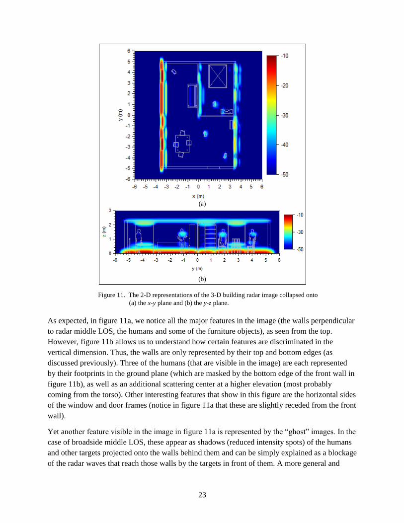
As mentioned in section 2.4, a direct representation of the 3-D building image on a 2-D medium

support is not possible. One way to visualize the image data is by displaying 2-D slices through

the 3-D image. An example, showing the ground plane image slice, was presented in figure 8a.

Another possible 2-D representation that conveys additional information on the full image is to

collapse the 3-D image onto one of the principal Cartesian planes (x-y, x-z, or y-z) and display

the voxel of maximum intensity (taken across the entire image) at each pair of 2-D coordinates.

In figure 11, we show the images obtained by this procedure in the x-y and y-z planes.

23

(a)

(b)

Figure 11. The 2-D representations of the 3-D building radar image collapsed onto

(a) the x-y plane and (b) the y-z plane.

As expected, in figure 11a, we notice all the major features in the image (the walls perpendicular

to radar middle LOS, the humans and some of the furniture objects), as seen from the top.

However, figure 11b allows us to understand how certain features are discriminated in the

vertical dimension. Thus, the walls are only represented by their top and bottom edges (as

discussed previously). Three of the humans (that are visible in the image) are each represented

by their footprints in the ground plane (which are masked by the bottom edge of the front wall in

figure 11b), as well as an additional scattering center at a higher elevation (most probably

coming from the torso). Other interesting features that show in this figure are the horizontal sides

of the window and door frames (notice in figure 11a that these are slightly receded from the front

wall).

Yet another feature visible in the image in figure 11a is represented by the “ghost” images. In the

case of broadside middle LOS, these appear as shadows (reduced intensity spots) of the humans

and other targets projected onto the walls behind them and can be simply explained as a blockage

of the radar waves that reach those walls by the targets in front of them. A more general and

24

rigorous explanation of this effect (which is essentially produced by multipath propagation and

scattering) is given in reference 10. Notice that the analysis in reference 10, which was

performed for a 2-D geometry, is valid for the 3-D case as well.

An image artifact that is apparent in figure 11a is the relatively large down-range extent of the

targets placed behind the front wall. This effect is the result of the fact that the radar waves incur

time delays of various magnitudes when transmitted through the walls at different elevation

angles. Importantly, our image formation algorithm does not try to compensate for the wall

delays, meaning that a target is focused at slightly different ranges for radar apertures placed at

different elevations. As figure 11a suggests, the image distortions created in the absence of the

wall delay compensation are more severe in the 3-D than in the 2-D case. The wall delay

compensation procedure, explained in reference 1 for known wall parameters, is a complex

research topic discussed extensively in the literature. However, most studies on this topic treat

the simple case of a single homogeneous wall. It is not clear how these techniques can be

extrapolated to inhomogeneous walls (containing doors, windows, and interior gaps) or multiple

walls at unknown ranges. Moreover, since the displacements in the target images are typically

smaller than the image resolution, the impact on the final building images (processed through the

CFAR detector) is probably not very significant.

For the airborne radar configuration, noticeable timing and magnitude differences may arise

between radar waves that reach the targets through the side walls of the building or the ceiling,

since these structures may have vastly different transmission characteristics (dictated by

construction material and thickness). The type of transmission mechanism depends on the

elevation angle in the 3-D imaging system and the target location. Notice that, for the building

considered in this study, these differences are not very large. However, we see an important

effect on the image intensity of targets placed directly behind doors or windows, where the radar

waves suffer less attenuation than through wall or ceiling materials. While these issues are not

very critical for the 3-D imaging of a single-story building, they may become much more

important in the case of a multi-story building, where, at high elevation angles, the radar waves

must penetrate through multiple structures to reach the lower floors.

Finally, we discuss the impact of radar polarization on the building images. The differences

between V-V and horizontal-horizontal (H-H) polarizations for an airborne slant-plane 2-D

imaging system were discussed in reference 9 and are mainly dictated by the fact that the

Brewster angle effect only exists for the V-V case (22). As a consequence, the H-H images

obtained around this angle display a much stronger ground bounce than their V-V counterparts.

In order to detect targets inside a building in the H-H mode from an airborne radar, a larger

dynamic range is usually required. Notice that our data sets for 3-D building imaging do not

include the H-H polarization.

A slant-plane 2-D image obtained from an airborne radar in cross-polarization (H-V) is shown in

figure 10b ( = 20°). Notice that, in this case, most of the wall three-way corners appear as bright

25

features in the image, along with the humans. Since these features may be difficult to

discriminate by the target type, we think that the cross-polarization mode does not offer any

particular advantage over co-polarization in the airborne SAR configuration.

3.2 3-D Images Obtained by Airborne Radar

In this section we present the 3-D images of the building obtained from the airborne radar

simulations, after processing the images through the CFAR detector as outlined in section 2.4.

To ease the image interpretation, we overlay the 3-D computational mesh (figure 1) onto the

radar image. In the final representation, the mesh is always shown in shades of gray, whereas the

objects detected in the radar image appear colored, using a pseudo-color scale (in dB) attached to

each figure. Notice that, unless otherwise specified, these colors indicate the intensity level of the

corresponding feature in the raw 3-D image, as explained in section 2.4. The images have a

dynamic range of 40 dB, meaning that the voxels whose intensities fall below this threshold are

not even considered in the CFAR detection scheme. All the images are generally displayed from

two viewing angles ( = 20°, = –70° and = 60°, = 50°), such that all the important

image features can be clearly distinguished.

The images obtained for this configuration and V-V polarization are shown in figure 12. In this

case, the SNR is 40 dB and we do not expect the noise to have a significant impact on the major

image features. The sliding window parameters (figure 6) are Ni = 3, Ng = 13, and No = 19, while

the thresholds are set to Tpoint = 10 (or 10 dB) and Tline = 300 (or 25 dB). The main features

detected in the image are the top and bottom edges of the walls perpendicular to the radar middle

LOS, the humans, the front-bottom edges of the dresser and sofa, as well as small pieces of two

chairs. Notice that the wall edges (particularly the ones at the bottom) appear with some

interruptions. While it is difficult to explain the gap in the bottom edge of the front wall, the gaps

in the interior and back walls clearly correspond to shadows (or “ghosts”) of the humans or other

objects projected onto those walls. The human images also appear fragmented, with two major

scattering centers corresponding to the ground plane footprint (multiple scattering due to the

ground bounce) and the torso (single scattering).

It is interesting to discriminate the image features that are produced by the point CFAR detector

from those produced by the line detector. Figure 13 accomplishes this task, by showing the

positive point detections in blue and the positive line detections in red (these are represented in

flat colors, regardless of the image intensity of those voxels). As expected, most of the line

detections occur along the wall edges, while the other targets are picked up primarily by the

point detector. However, it is important to emphasize that the line detector threshold is set much

higher than for the point detector in order to avoid positive line detections in targets other than

the walls. (As a side note, the line detector sliding window operates with a smaller number of

background samples Nbg, which would lead to a larger probability of false alarm if we kept a

constant threshold, according to equation 22; in order to keep the false alarm probability at low

levels in this case, we compensate by increasing the threshold). Interestingly, most of the interior

26

and back wall edges are picked up by the point detector, while the bottom of the front wall (the

brightest feature in the entire image) fails the point detection test.

Figure 12. The 3-D building image for the airborne spotlight configuration and V-V polarization,

with SNR = 40 dB, as seen from two different aspect angles. The feature colors

correspond to their brightness levels in the raw 3-D image.

27

Figure 13. The 3-D building image for the airborne spotlight configuration and V-V polarization,

with SNR = 40 dB, as seen from two different aspect angles, showing positive point

detections in blue and positive line detections in red.

In figure 14, we present the images obtained for cross-polarization (H-V), using the same

detector parameters as above and a 40-dB dynamic range. As discussed in the previous section,

most of the three-way corners in the building geometry appear as bright spots in the image.

Although the humans also appear in the image, the amount of clutter is probably too large to

allow their reliable discrimination as targets of interest.

28

Figure 14. The 3-D building image for the airborne spotlight configuration and H-V (cross)

polarization as seen from two different aspect angles. The feature colors correspond to

their brightness levels in the raw 3-D image.

Figure 15 shows the effect of increasing the noise level in the image. In this case we consider

SNR = 30 dB (V-V polarization). Notice that, after processing the image through the CFAR

detector, some weak targets disappear, since their radar response is now below the noise level.

Such is the case for the human closest to the front wall, as well as the top edge of the interior

wall (these are displayed in dark blue color in figure 12, while in figure 15 their absence is

highlighted by pink ellipses). This result clearly emphasizes the difficulty of detecting behind-

29

the-wall targets, whose radar response is strongly attenuated by transmission through walls. To

obtain a response above the noise level from these targets, high transmitted power and/or short

ranges are typical operational requirements for the radar system.

Figure 15. The 3-D building image for the airborne spotlight configuration and V-V polarization, with

SNR = 30 dB. The pink ellipses highlight missing features as compared to figure 12.

3.3 Phenomenology of Ground-based Radar Imaging of a Building

The ground-based imaging radar phenomenology differs significantly from that of an airborne

system. A major difference consists (as explained in section 2.2) of the fact that the ground-

based radar operates in the near-field region. This means that, from a ray-tracing point of view,

the rays emanating from the radar transmitter antenna diverge and propagate at various azimuth

and elevation angles (an analogous process takes places at the receiver). This is illustrated in

figure 16. It turns out that, in this case, the rays that incur direct specular reflection from targets

usually have the largest contribution to the image. These are the rays perpendicular to targets

such as the walls and the humans.

30

Figure 16. Schematic ray-tracing representation of the major radar scattering mechanisms for the ground-

based strip-map configuration, with the near-field geometry assumption.

Although the EM scattering model for this configuration contains an infinite ground plane, the

effect of the radar wave ground bounces on the SAR images is not as pronounced as in the far-

field case. The reason for this effect was discussed in reference 10 and it amounts to the fact that

the path length of the rays describing ground-bounced backscattering contributions from a given

target point depend on the elevation angle. Consequently these contributions do not back-project

coherently to the same point in the image. Nevertheless, the ground-bounced waves scattered by

the targets do appear in the SAR images as relatively faint replicas of the main scattering center,

displaced by a distance that increases with the antenna elevation.

A major difference in terms of the 3-D images of a building obtained by airborne and ground-

based systems is that, in the latter case, the walls appear as solid vertical features (as opposed to

only the lower and upper edges in the airborne case). An analogous effect is obtained for the

human targets, as is shown in section 3.4.

An additional complication is introduced by the fact that the vertical antenna array does not

extend all the way to the ground (although its upper element height is close to the top of the

building). Therefore, there are points on the lower part of the walls that do not create specular

reflection for the radar waves. Although these points do contribute to the image by other

(weaker) scattering mechanisms, such as ground bounces and diffraction, they appear less well

defined than the specular points. This is clearly illustrated in figure 17, where we show 2-D

horizontal slices through the 3-D image at different heights (z = 1.25 m in figure 17a and

z = 0.25 m in figure 17b). Notice the bright, clearly resolved front wall image in figure 17a, as

compared to the less bright, double-image front wall in figure 17b (as a reminder, the lower

elevation limit of the antenna array is 0.5 m). Most likely, a significant contribution to the front

wall image in figure 17b is provided by the vertical sidelobe spillover from specular points

located at higher elevations. Other features in the figure 17b image also appear weaker than in

31

the figure 17a image. Notice that all the images in this section are noise-free and have a dynamic

range of 50 dB.

(a) (b)

Figure 17. The 2-D horizontal-plane slices through the 3-D image of the building obtained by the ground-based

radar in strip-map mode, showing the plane at (a) z = 1.25 m and (b) z = 0.25 m.

On the topic of image sidelobes, particularly those created by large scatterers such as walls, we

should mention that, in TWRI applications, their effect on image quality is very important.

Therefore, sidelobe mitigation through aperture windowing constitutes a critical part of the

image formation algorithm. To illustrate the point, in figure 18, we present the same 2-D slice

through the 3-D image as in figure 17a (z = 1.25 m), with the following modifications: the image

in figure 18a is obtained without windowing in both azimuth and elevation. The image in

figure 18b is obtained with windowing in both azimuth and elevation (as a reminder, the image

in figure 17a uses a window only in azimuth, not in elevation). The differences between

figures 17a and 18a are obvious and underscore the importance of azimuth windowing.

However, the differences between figures 17a and 18b are not significant, suggesting that, for

this imaging geometry, windowing in elevation is not necessary. Moreover, by foregoing the

elevation window, we increase the image resolution in this direction.

32

(a) (b)

Figure 18. The 2-D slices through the 3-D image of the building obtained by the ground-based radar in strip-map

mode, in the horizontal plane z = 1.25 m, showing an image (a) without windowing in azimuth and

elevation and (b) with windowing in both azimuth and elevation.

Other effects, such as image defocusing in the absence of wall delay compensation, and “ghost”

images are also present in the ground-base strip-map configuration; although, the “ghost” images

are less pronounced than in the far-field case (the analysis in reference 10 is only valid for far-

field geometry). Since most of the bright image features come from single-bounce scattering of

rays at = 0°, we do not expect significant differences between the V-V and H-H images in the

ground-based strip-map case. However, this type of imaging geometry may produce interesting

results for cross-polarization (emphasizing the human targets over the walls and furniture

objects). Unfortunately, since Xpatch does not produce reliable radar signature results for cross-

polarization, this data set was unavailable to us for the current study.

3.4 3-D Images Obtained by Ground-based Radar

This section presents the 3-D images obtained from the ground-based radar simulations. The

image format is similar to that used in the section 3.2 images. For the images in figure 19, we use

a 40-dB dynamic range. A major difference from the airborne spotlight images is that, instead of

a line-detecting sliding window (figure 7b), we use a wall-detecting sliding window (figure 7c).

The thresholds are set to Tpoint = 5 (or 7 dB) and Twall = 30 (or 15 dB). As expected, the wall

detector picks up the front wall and part of the interior wall, but few other features in the image.

The bulk of the positive detections for the ground-based system are performed by the point

detector.

33

Figure 19. The 3-D building image for the ground-based strip-map configuration as seen

from two different aspect angles. The feature colors correspond to their brightness

levels in the raw 3-D image.

The full volume of the front wall appears now in the images in figure 19, because most radar

positions on the aperture correspond to specular reflection points on the wall. Notice that the

bottom of the wall (below 0.5 m height) is less well defined in the image, since the aperture does

34

not extend all the way to the ground level; therefore, those points on the wall are not specular

reflection centers. On the other hand, the interior wall and especially the back wall are only

partially represented in the image. One explanation of this effect comes from the shadows cast on

these walls by the humans and other interior objects. Another explanation is that the waves that

hit the farther-range walls propagate through a highly inhomogeneous medium producing

fragmented wall images (see figure 17a), as opposed to the straight-lined walls in figure 11a.

Note that the humans (as well as their shadows) show up in their full vertical extent in figure 19.

Other interesting features in the image include the window frame on one side of the building. As

compared to the airborne case, where the image displays the horizontal sides of the receding

frames (see figure 11b), this time we notice the vertical frame sides. The explanation consists of

different mechanisms creating major back-scattering centers in the two cases, depending of the

radar wave incidence angle—oblique incidence (with respect to the ground plane) in the airborne

case versus horizontal incidence direction in the ground-based case.

In figure 20, we increase the image noise level to an SNR of 30 dB. Similarly to the airborne

scenario, some weak targets disappear (these are mainly the dark blue color features in figure 19

images): two humans, part of the couch, part of the interior wall, the side of the dresser, and the

window frame on the building’s side (we emphasized the missing targets by pink ellipses in

figure 20). It seems that the noise effect is more pronounced in this case than for the airborne

radar, since now all the scattering propagation paths from behind-the-wall targets involve

transmissions through the brick walls, whereas in the airborne case some propagation takes place

through the lower-attenuation ceiling.

We should mention that a more careful design of the CFAR detector sliding window may

produce better results for the ground-based strip-map radar images. Particularly, one could use

windows with different sizes in the three Cartesian directions, and different sizes between the

point and wall detector. However, some limitations on the image quality are simply dictated by

the physics of the radar scattering problem, particularly the height of the vertical antenna array.

35

Figure 20. The 3-D building image for the ground-based strip-map configuration, with

SNR = 30 dB. The pink ellipses highlight missing features as compared to figure 19.

3.5 Further Comments on the Numerical Results

While the 3-D images of the building presented in this report could make sense to the radar

engineer, they are still very difficult to interpret by the non-expert user. Ultimately, it is not the

radar images that the end user is interested in, but information on the presence and location of the

targets of interest, or the building layout. From this perspective, once we detect the salient image

features and classify them into appropriate target types, we can simply replace them with

pictograms representing humans, walls, or other objects placed at the corresponding locations in

space and show them as such on the radar display.

In general, the image analysis consists of segmentation, representation, and identification (or

classification) (30). The segmentation process subdivides an image into its constituent parts or

objects. The detection (or, more appropriately, background removal) algorithm that we presented

in this study represents a simple form of image segmentation. Since the targets detected in high-

resolution SAR images can sometime comprise pixels (or voxels) that are isolated or non-

contiguous, post-detection processing such as pixel clustering (31) or morphological filtering (8)

is introduced to mitigate this issue. Notice that we did not encounter this problem in our 3-D

building images, since the voxel power averaging within the test cells effectively smoothed out

the image intensity spikes. Another possible image segmentation approach is based on region

growing by pixel/voxel aggregation (30) and was applied in reference 5.

36

The classification of image objects can be based on the size and shape of the objects present in

the detection maps. More generally, one can use the statistical spatial distribution of voxel

intensity in the 3-D images for target classification purposes. Most likely, the classification

algorithm would include prior information regarding the building structure (especially the size,

location and orientation of the walls) that can be combined with the SAR image features to

produce a building layout. An example of building layout extraction based on radar images is

presented in reference 32. However, these topics are beyond the scope of our current study.

A direct improvement of the 3-D building images based on the data already presented in this

work is to fuse the images obtained by the airborne and ground-based radar systems together.

The fused 3-D image is shown in figure 21 (for SNR = 40 dB), where the features detected in the

airborne image appear in red, while those detected in the ground-based image appear in blue.

Interestingly, the two types of images complement each other, since the airborne radar detects

mostly horizontal features, whereas the ground-based radar detects mostly vertical features. The

fusion performed in figure 21 is non-coherent and consists of a simple voxel-wise logical OR

operation between the positive detection map for the airborne radar and the positive detection

map for the ground-based radar.

Yet another possible way to obtain more information on the building layout and interior is to

combine multiple images created from synthetic apertures on different sides of the building (1,

7–9). At least two orthogonal sides of the building must be involved in this process in order to

image the walls perpendicular to the middle LOS in each case. If we consider synthetic apertures

on all four sides of the building, then targets behind the walls will appear at different ranges in

images taken from two opposing sides (because the wall transmission delays produce image

spatial shifts in opposite directions). Absent a wall delay compensation procedure, one way to

mitigate this issue is to use only half of the building image obtained from each side (the nearest

to the aperture) when fusing all four side contributions.

37

Figure 21. The 3-D building image obtained by fusing the airborne (red features)

and ground-based (blue features) images presented in sections 3.2 and

3.4 (SNR = 40 dB).

38

4. Conclusions and Future Work

This report demonstrated a 3-D radar system for through-the-wall building imaging based on

computer models of the EM radar scattering. We considered a single-story building containing

humans and furniture objects, as well as two possible radar system configurations: airborne

spotlight and ground-based strip-map. Our study contained a detailed phenomenological

discussion on the differences between the two configurations, as well as the different modeling

techniques and image formation algorithms required by the two. The 3-D images were created

using a free-space version of the time-reversal method, and further processed using a CFAR

detector for background removal. The final representation included only the positive outcome

voxels in the detection process.

The airborne spotlight SAR system produces images that contain only the top and bottom edges

of the walls, while targets such as the human also appear fragmented, with a prominent footprint

in the ground plane. The ground-based strip-map system produces full-volume images of the

front wall and human targets, but suffers from relatively poor elevation resolution (especially at

farther ranges) because of practical constraints on the physical antenna array height. The image

misalignments produced by the propagation of the radar waves through a highly inhomogeneous

medium make it difficult to detect the interior and back walls to their full extent. Reducing the

sidelobes via aperture windowing is a critical part of the image formation algorithm. Other

imaging artifacts were described in detail in section 3, for both configurations. One should

remember that the images presented here were obtained via computer modeling of the radar

signature for a relatively simple building geometry, with well-separated targets and a relatively

small amount of noise added to the data. It is very likely that images based on experimental radar

data collected in the field, on a complex building configuration, would be much more difficult to

interpret. As already shown in figures 15 and 20, increasing the amount of noise in the image

makes the weaker targets “disappear” within the background.

In section 3.5, we discussed ways to improve the image interpretation by advanced image

processing techniques. An obvious method to obtain more complete information about a building

is to fuse radar images obtained from different configurations and aspect angles. One could apply

more sophisticated algorithms for image segmentation and classification that would attempt to

discriminate the human targets from other objects in the scene. Another important application

consists of locating the walls inside the building for layout reconstruction. A suggestion briefly

mentioned in section 2.3 was that using the half-space Green’s functions in the image formation

algorithm could reduce the effect of the ground bounces in the image (this will be the topic of

future research).

39

In a follow-up study, we plan to create 3-D images of a multi-story building, based on similar

EM radar scattering models. We expect this problem to be significantly more challenging than

the single-story building. From an airborne radar perspective, the bottom floors are difficult to

image because the radar waves must penetrate through multiple structures. On the other hand,

from a ground-based radar perspective, the top floors are difficult to image because of practical

restrictions on the vertical antenna array height. A possible operational scenario for this radar

imaging problem is to jointly use an airborne and ground-based system and fuse together the

images obtained from the two sensors.

40

5. References

1. Ahmad, F.; Amin, M. G. Multi-location Wideband Synthetic Aperture Imaging for Urban

Sensing Applications. Journal of the Franklin Institute September 2008, 345, 618–639.

2. Solimene, R.; Soldovieri, F.; Prisco, G.; Pierri, R. Three-Dimensional Through-Wall

Imaging under Ambiguous Wall Parameters. IEEE Transactions on Geoscience and Remote

Sensing May 2009, 47, 1310–1317.

3. Soldovieri, F.; Ahmad, F.; Solimene, R. Validation of Microwave Tomographic Inverse

Scattering Approach via Through-the-Wall Experiments in Semicontrolled Conditions. IEEE

Geoscience and Remote Sensing Letters January 2011, 8, 123–127.

4. Wang, Z.; Fathy, A. Advanced System Level Simulation Platform for Three-Dimensional

UWB Through-Wall Imaging SAR Using Time-Domain Approach. IEEE Transactions on

Geoscience and Remote Sensing May 2012, 50, 1986–2000.

5. Sevigny, P.; DiFilippo, D.; Laneve, T.; Fournier, J. Indoor Imagery with a 3-D Through-

Wall Synthetic Aperture Radar. Proceedings of SPIE 2012, 8361.

6. Schechter, R.; Chun, S. High Resolution 3-D Imaging of Objects through Walls. Optical

Engineering November 2010, 49 (11).

7. Debes, C.; Amin, M.; Zoubir, A. Target Detection in Single and Multiple-View Through-

the-Wall Radar Imaging. IEEE Transactions on Geoscience and Remote Sensing May 2009,

47, 1349–1361.

8. Debes, C.; Riedler, J.; Zoubir, A.; Amin, M. Adaptive Target Detection with Application to

Through-the-Wall Radar Imaging. IEEE Transactions on Signal Processing November

2010, 58, 5572–5583.

9. Dogaru, T.; Le, C.; Nguyen, L. Through the Wall Radar Simulations for Complex Room

Imaging; ARL-TR-5205; U.S. Army Research Laboratory: Adelphi, MD, May 2010.

10. Dogaru, T.; Le, C.; Nguyen, L. Synthetic Aperture Radar Images of a Simple Room Based

on Computer Models; ARL-TR-5193; U.S. Army Research Laboratory: Adelphi, MD, May

2010.

11. Dogaru, T. AFDTD User’s Manual; ARL-TR-5145; U.S. Army Research Laboratory:

Adelphi, MD, March 2010.

12. SAIC Web page. http://www.saic.com/products/software/xpatch (accessed December 2011).

41

13. Taflove, A.; Hagness, S. Computational Electrodynamics: The Finite-Difference Time-

Domain Method; Artech: Norwood, MA, 2000.

14. Jeng, S. Near-field Scattering by Physical Theory of Diffraction And Shooting and

Bouncing Rays. IEEE Transactions on Antennas and Propagation April 1998, 46, 551–558.

15. ARL DSRC Web page. http://www.arl.hpc.mil (accessed June 2012).

16. AFRL DSRC Web page. http://www.afrl.hpc.mil (accessed June 2012).

17. Mathworks Web page. http://www.mathworks.com (accessed September 2012).

18. Fink, M. Time Reversal of Ultrasonic Fields – Part I: Basic Principles. IEEE Transactions

on Ultrasonics, Ferroelectrics and Frequency Control September 1992, 39 (5), 555–566.

19. Borcea, L.; Papanicolaou, G.; Tsogka, C. A Resolution Study for Imaging and Time

Reversal in Random Media. Contemporary Mathematics 2003, 313, 63–67.

20. Liao, D.; Dogaru, T. Full-Wave Characterization of Rough Terrain Surface Scattering for

Forward-Looking Radar Applications. IEEE Transactions on Antenna and Propagation

August 2012, 60, 3853–3866.

21. Liao, D.; Dogaru, T.; Sullivan, A. Emulation of Forward-Looking Radar Technology for

Threat Detection in Rough Terrain Environments: A Scattering and Imaging Study. To

appear in ITEA Journal, 2012.

22. Balanis, C. Advanced Engineering Electromagnetics; Wiley: New York, 1989.

23. Soumekh, M. Synthetic Aperture Radar Signal Processing; Wiley: New York, 1999.

24. Skolnik, M. I. Introduction to Radar Systems; McGraw Hill: New York, 2001.

25. Gandhi, P. P.; Kassam, S. A. Analysis of CFAR Processors in Homogeneous Background.

IEEE Transactions on Aerospace and Electronic Systems July 1988, 24 (4), 427–445.

26. Kuttikkad, S.; Chellappa, R. Statistical Modeling and Analysis of High-Resolution Synthetic

Aperture Radar Images. Statistics and Computing October 2000, 10, 133–145.

27. Novak, L.; Owirka, G.; Netishen, C. Performance of a High-Resolution Polarimetric SAR

Automatic Target Recognition System. The Lincoln Laboratory Journal 1993, 6 (1), 11–24.

28. Martone, A.; Innocenti, R.; Ranney, K. Moving Target Indication for Transparent Urban

Structures; ARL-TR-4809; U.S. Army Research Laboratory: Adelphi, MD, May 2009.

29. Kay, S. M. Fundamentals of Statistical Signal Processing: Detection Theory; Prentice Hall:

Upper Saddle River, NJ, 1998.

30. Gonzales, R.; Woods, R. Digital Image Processing; Addison-Wesley: Reading, MA, 1992.

42

31. Wilpon, J.; Rabiner, L. A Modified K-means Clustering Algorithm for use in Isolated Work

Recognition. IEEE Transactions on Acoustics, Speech and Signal Processing July 1985, 33

(3), 587–594.

32. Lavely, E.; Zhang, Y.; Hill, E.; Lai, Y.-S.; Weichman, P.; Chapman, A. Theoretical and

Experimental Study of Through-Wall Microwave Tomography Inverse Problem. Journal of

the Franklin Institute September 2008, 345, 592–617.

43

List of Symbols, Abbreviations, and Acronyms

2-D two-dimensional

3-D three-dimensional

AFRL U.S. Air Force Research Laboratory

ARL U.S. Army Research Laboratory

BPA back-projection algorithm

CEM computational electromagnetics

CFAR constant false alarm rate

CPU central processing unit

DSRC Defense Supercomputing Resource Center

EM electromagnetic

FDTD Finite Difference Time Domain

H-H horizontal-horizontal

HPC High Performance Computing

H-V horizontal-vertical

LOS line of sight

MPI message passing interface

PO physical optics

SAIC Scientific Applications International Corporation

SAR synthetic aperture radar

SNR signal-to-noise ratio

STTW sensing through the wall

TRI time-reversal imaging

TWRI through-wall radar imaging

UWB ultra-wideband

V-V vertical-vertical

44

No. of

Copies Organization

1 DEFENSE TECHNICAL

(PDF INFORMATION CTR

only) DTIC OCA

8725 JOHN J KINGMAN RD

STE 0944

FORT BELVOIR VA 22060-6218

1 US ARMY RDECOM CERDEC

INTELLIGENCE & INFO WARFARE

DIRECTORATE (I2WD)

ATTN RDER IWR RS S BRODERICK

ABERDEEN PROVING GROUND MD 21005

6 HCS US ARMY RSRCH LAB

4 PDF ATTN IMAL HRA

MAIL & RECORDS MGMT

ATTN RDRL CIO LL TECHL LIB

ATTN RDRL SER U

A SULLIVAN (1 HC)

C LE (1 HC)

K RANNEY (1 PDF)

A MARTONE (1 PDF)

L NGUYEN (1 PDF)

D LIAO (1 HC)

K KAPPRA (1 PDF)

T DOGARU (1 HC)

ADELPHI MD 20783-1197

TOTAL: 12 (5 ELEC, 7 HCS)